arX

iv:a

stro

-ph/

0608

632v

2 3

0 O

ct 2

006

Cosmological Constraints from the SDSS Luminous Red Galaxies

Max Tegmark1, Daniel J. Eisenstein2, Michael A. Strauss3, David H. Weinberg4, Michael R. Blanton5, Joshua A.

Frieman6,7, Masataka Fukugita8, James E. Gunn3, Andrew J. S. Hamilton9, Gillian R. Knapp3, Robert C. Nichol10,

Jeremiah P. Ostriker3, Nikhil Padmanabhan11, Will J. Percival10, David J. Schlegel12, Donald P. Schneider13,

Roman Scoccimarro5, Uros Seljak14,11, Hee-Jong Seo2, Molly Swanson1, Alexander S. Szalay15, MichaelS. Vogeley16, Jaiyul Yoo4, Idit Zehavi17, Kevork Abazajian18, Scott F. Anderson19, James Annis7, Neta

A. Bahcall3, Bruce Bassett20,21, Andreas Berlind5, Jon Brinkmann22, Tamas Budavari15, Francisco Castander23,

Andrew Connolly24, Istvan Csabai15, Mamoru Doi25, Douglas P. Finkbeiner3,26, Bruce Gillespie22, Karl

Glazebrook15, Gregory S. Hennessy27, David W. Hogg5, Zeljko Ivezic19,3, Bhuvnesh Jain28, David Johnston29,30,Stephen Kent7, Donald Q. Lamb6,31, Brian C. Lee32,12, Huan Lin7, Jon Loveday33, Robert H. Lupton3,

Jeffrey A. Munn27, Kaike Pan22, Changbom Park34, John Peoples7, Jeffrey R. Pier27, Adrian Pope15, Michael

Richmond35, Constance Rockosi6, Ryan Scranton24, Ravi K. Sheth28, Albert Stebbins7, Christopher Stoughton7,

Istvan Szapudi36, Douglas L. Tucker7, Daniel E. Vanden Berk24, Brian Yanny7, Donald G. York6,31

1Dept. of Physics, Massachusetts Institute of Technology, Cambridge, MA 02139, USA; 2Department of Astronomy,University of Arizona, Tucson, AZ 85721, USA; 3Princeton University Observatory, Princeton, NJ 08544, USA; 4Dept. of Astronomy,

Ohio State University, Columbus, OH 43210, USA; 5Center for Cosmology and Particle Physics, Dept. of Physics, New York University,4 Washington Pl., New York, NY 10003, USA; 6Center for Cosmological Physics and Department of Astronomy & Astrophysics,

Univ. of Chicago, Chicago, IL 60637, USA; 7Fermi National Accelerator Laboratory, P.O. Box 500,Batavia, IL 60510, USA; 8Inst. for Cosmic Ray Research, Univ. of Tokyo, 5-1-5, Kashiwanoha, Kashiwa,Chiba, 277-8582, Japan; 9JILA and Dept. of Astrophysical and Planetary Sciences, Univ. of Colorado,

Boulder, CO 80309, USA; 10Inst. of Cosmology & Gravitation, Univ. of Portsmouth, Portsmouth,P01 2EG, United Kingdom; 11Dept. of Physics, Princeton University, Princeton, NJ 08544,

USA; 12Lawrence Berkeley National Laboratory, Berkeley, CA 94720, USA; 13Dept. of Astronomy and Astrophysics,Pennsylvania State University, University Park, PA 16802, USA; 14International Center for Theoretical Physics,Strada Costiera 11, 34014 Trieste, Italy; 15Department of Physics and Astronomy, The Johns Hopkins University,

3701 San Martin Drive, Baltimore, MD 21218, USA; 16Dept. of Physics, Drexel University, Philadelphia,PA 19104, USA; 17Dept. of Astronomy, Case Western Reserve University, 10900 Euclid Avenue, Cleveland,

OH 44106-7215; 18Theoretical Division, Los Alamos National Laboratory, Los Alamos, NM 87545,USA; 19Dept. of Astronomy, Univ. of Washington, Box 351580, Seattle, WA 98195; 20South African Astronomical Observatory,

Cape Town, South Africa; 21Applied Mathematics Dept., Univ. of Cape Town, Cape Town,South Africa; 22Apache Point Observatory, 2001 Apache Point Rd, Sunspot, NM 88349-0059,

USA; 23Institut d’Estudis Espacials de Catalunya/CSIC, Campus UAB, 08034 Barcelona,Spain; 24University of Pittsburgh, Department of Physics and Astronomy, 3941 O’Hara Street,

Pittsburgh, PA 15260, USA; 25Inst. of Astronomy, Univ. of Tokyo, Osawa 2-21-1, Mitaka, Tokyo,181-0015, Japan; 26Harvard-Smithsonian Center for Astrophysics, 60 Garden Street, MS46, Cambridge,

MA 02138; 27U.S. Naval Observatory, Flagstaff Station, 10391 W. Naval Obs. Rd., Flagstaff,AZ 86001-8521, USA; 28Department of Physics, University of Pennsylvania, Philadelphia, PA 19104,

USA; 29Jet Propulsion Laboratory, 4800 Oak Grove Dr., Pasadena CA, 91109, USA; 30California Inst. of Technology,1200 East California Blvd., Pasadena, CA 91125, USA; 31Enrico Fermi Institute, University of Chicago,

Chicago, IL 60637, USA; 32Gatan Inc., Pleasanton, CA 94588; 33Sussex Astronomy Centre, University of Sussex,Falmer, Brighton BN1 9QJ, UK; 34Department of Astronomy, Seoul National University, 151-742,

Korea; 35Physics Dept., Rochester Inst. of Technology, 1 Lomb Memorial Dr, Rochester, NY 14623,USA; 36Institute for Astronomy, University of Hawaii, 2680, Woodlawn Drive, Honolulu, HI 96822, USA;

(Dated: Submitted to Phys. Rev. D. August 22 2006, revised October 10, accepted October 26)

2

We measure the large-scale real-space power spectrum P (k) using luminous red galaxies (LRGs)in the Sloan Digital Sky Survey (SDSS) and use this measurement to sharpen constraints on cos-mological parameters from the Wilkinson Microwave Anisotropy Probe (WMAP). We employ amatrix-based power spectrum estimation method using Pseudo-Karhunen-Loeve eigenmodes, pro-ducing uncorrelated minimum-variance measurements in 20 k-bands of both the clustering powerand its anisotropy due to redshift-space distortions, with narrow and well-behaved window functionsin the range 0.01 h/Mpc < k < 0.2 h/Mpc. Results from the LRG and main galaxy samples are con-sistent, with the former providing higher signal-to-noise. Our results are robust to omitting angularand radial density fluctuations and are consistent between different parts of the sky. They providea striking confirmation of the predicted large-scale ΛCDM power spectrum. Combining only SDSSLRG and WMAP data places robust constraints on many cosmological parameters that complementprior analyses of multiple data sets. The LRGs provide independent cross-checks on Ωm and thebaryon fraction in good agreement with WMAP. Within the context of flat ΛCDM models, our LRGmeasurements complement WMAP by sharpening the constraints on the matter density, the neutrinodensity and the tensor amplitude by about a factor of two, giving Ωm = 0.24±0.02 (1σ),

∑mν ∼

< 0.9eV (95%) and r < 0.3 (95%). Baryon oscillations are clearly detected and provide a robust measure-ment of the comoving distance to the median survey redshift z = 0.35 independent of curvature anddark energy properties. Within the ΛCDM framework, our power spectrum measurement improvesthe evidence for spatial flatness, sharpening the curvature constraint Ωtot = 1.05±0.05 from WMAPalone to Ωtot = 1.003± 0.010. Assuming Ωtot = 1, the equation of state parameter is constrained tow = −0.94±0.09, indicating the potential for more ambitious future LRG measurements to provideprecision tests of the nature of dark energy. All these constraints are essentially independent ofscales k > 0.1h/Mpc and associated nonlinear complications, yet agree well with more aggressivepublished analyses where nonlinear modeling is crucial.

I. INTRODUCTION

The dramatic recent progress by the Wilkinson Mi-crowave Anisotropy Probe (WMAP) and other experi-ments [1–4] measuring the cosmic microwave background(CMB) has made non-CMB experiments even more im-portant in the quest to constrain cosmological models andtheir free parameters. These non-CMB constraints arecrucially needed for breaking CMB degeneracies [5, 6];for instance, WMAP alone is consistent with a closeduniverse with Hubble parameter h = 0.3 and no cosmo-logical constant [7]. As long as the non-CMB constraintsare less reliable and precise than the CMB, they will bethe limiting factor and weakest link in the precision cos-mology endeavor. Much of the near-term progress in cos-mology will therefore be driven by reductions in statisti-cal and systematic uncertainties of non-CMB probes ofthe cosmic expansion history (e.g., SN Ia) and the matterpower spectrum (e.g., Lyman α Forest, galaxy clusteringand motions, gravitational lensing, cluster studies and 21cm tomography).

The cosmological constraining power of three-dimensional maps of the Universe provided by galaxyredshift surveys has motivated ever more ambitious ob-servational efforts such as the CfA/UZC [8, 9], LCRS[10], PSCz [11], DEEP [12], 2dFGRS [13] and SDSS [14]projects, resulting in progressively more accurate mea-surements of the galaxy power spectrum P (k) [15–30].Constraints on cosmological models from these data setshave been most robust when the galaxy clustering couldbe measured on large scales where one has confidence inthe modeling of nonlinear clustering and biasing (e.g.,[7, 31–42]).

Our goal in this paper therefore is to measure P (k)

on large scales using the SDSS galaxy redshift survey ina way that is maximally useful for cosmological param-eter estimation, and to explore the resulting constraintson cosmological models. The emphasis of our cosmo-logical analysis will be on elucidating the links betweencosmological parameters and observable features of theWMAP and SDSS power spectra, and on how these twodata sets alone provide tight and robust constraints onmany parameters that complement more aggressive butmore systematics-prone analyses of multiple data sets.

In a parallel paper, Percival et al. [43] present a powerspectrum analysis of the Main Galaxy and LRG samplesfrom the SDSS DR5 data set [44], which is a superset ofthe data used here. There are a number of differencesin the analysis methods. Percival et al. use an FFT-based method to estimate the angle-averaged (monopole)redshift-space galaxy power spectrum. We use a Pseudo-Karhunen-Loeve method [45, 46] (see further discussionand references below) to estimate the real space (as op-posed to redshift space) galaxy power spectrum, usingfinger-of-god compression and linear theory to removeredshift-space distortion effects. In addition, the manytechnical decisions that go into these analyses, regardingcompleteness corrections, angular masks, K-correctionsand so forth, were made independently for the two pa-pers, and they present different tests for systematic un-certainties. Despite these many differences of detail, ourconclusions agree to the extent that they overlap (as dis-cussed in Section III F and Appendix A1), a reassuringindication of the robustness of the results.

3

A. Relation between different samples

The amount of information in a galaxy redshift surveyabout the galaxy power spectrum Pg(k) and cosmologicalparameters depends not on the number of galaxies per se,but on the effective volume of the survey, defined by [47]as

Veff(k) ≡∫ [

n(r)Pg(k)

1 + n(r)Pg(k)

]2

d3r, (1)

where n(r) is the expected number density of galaxies inthe survey in the absence of clustering, and the FKP ap-proximation of [19] has been used. The power spectrumerror bars scale approximately as ∆Pg(k) ∝ Veff(k)−1/2,which for a fixed power Pg is minimized if a fixed to-tal number of galaxies are spaced with density n ∼ P−1

g

[48]. The SDSS Luminous Red Galaxy (LRG) samplewas designed [49, 50] to contain such “Goldilocks” galax-ies with a just-right number density for probing the poweraround the baryon wiggle scale k ∼ (0.05 − 0.1)h/Mpc.For comparison, the SDSS main galaxy sample [50] ismuch denser and is dominated by sample variance onthese scales, whereas the SDSS quasar sample [51] ismuch sparser and is dominated by Poisson shot noise.As shown in [36], the effective volume of the LRG sam-ple is about six times larger than that of the SDSS maingalaxies even though the number of LRGs is an order ofmagnitude lower, and the LRG volume is over ten timeslarger than that of the 2dFGRS. These scalings are con-firmed by our results below, which show that (∆Pg/Pg)

2

on large scales is about six times smaller for the SDSSLRGs than for the main sample galaxies. This gain re-sults both from sampling a larger volume, and from thefact that the LRG are more strongly clustered (biased)than are ordinary galaxies; Pg for LRGs is about 3 timeslarger than for the main galaxy sample.

We will therefore focus our analysis on the SDSS LRGsample. Although we also measure the SDSS main sam-ple power spectrum, it adds very little in terms of sta-tistical constraining power; increasing the effective vol-ume by 15% cuts the error bar ∆P by only about(1 + 0.15)1/2 − 1 ∼ 7%. This tiny improvement is eas-ily outweighed by the gain in simplicity from analyzingLRGs alone, where (as we will see) complications such asredshift-dependence of clustering properties are substan-tially smaller.

A complementary approach implemented by [41, 42]is to measure the angular clustering of SDSS LRGs withphotometric redshifts, compensating for the loss of radialinformation with an order of magnitude more galaxiesextending out to higher redshift. We will see that thisgives comparable or slightly smaller error bars on verylarge scales k ∼< 0.02, but slightly larger error bars onthe smaller scales that dominate our cosmological con-straints; this is because the number of modes down to agiven scale k grows as k3 for our three-dimensional spec-troscopic analysis, whereas they grow only as k2 for a2-dimensional angular analysis.

B. Relation between different methods

In the recent literature, two-point galaxy clusteringhas been quantified using a variety of estimators of bothpower spectra and correlation functions. The most re-cent power spectrum measurements for both the 2dFGRS[26, 29] and the SDSS [30, 38, 43] have all interpolatedthe galaxy density field onto a cubic grid and measuredP (k) using a Fast Fourier Transform (FFT).

Appendix A1 shows that as long as discretization er-rors from the FFT gridding are negligible, this procedureis mathematically equivalent to measuring the correlationfunction with a weighted version of the standard “DD-2DR+RR” method [52, 53], multiplying by “RR” andthen Fourier transforming. Thus the only advantage ofthe FFT approach is numerical speedup, and comparingthe results with recent correlation function analyses suchas [36, 54–56] will provide useful consistency checks.

Another approach, pioneered by [45], has been to con-struct “lossless” estimators of the power spectrum withthe smallest error bars that are possible based on infor-mation theory [23, 24, 27, 28, 34, 45, 46, 57, 58]. Wewill travel this complementary route in the present pa-per, following the matrix-based Pseudo Karhunen-Loeve(PKL) eigenmode method described in [28], as it has thefollowing advantages:

1. It produces power spectrum measurements withuncorrelated error bars.

2. It produces narrow and well-behaved window func-tions.

3. It is lossless in the information theory sense.

4. It treats redshift distortions without the small-angle approximation.

5. It readily incorporates the so-called integral con-straint [16, 59], which can otherwise artificially sup-press large-scale power.

6. It allows testing for systematics that produce excesspower in angular or radial modes.

These properties make the results of the PKL-methodvery easy to interpret and use. The main disadvantageis that the PKL-method is numerically painful to im-plement and execute; our PKL analysis described belowrequired about a terabyte of disk space for matrix stor-age and about a year of CPU time, which contributed tothe long gestation period of this paper.

The rest of this paper is organized as follows. We de-scribe our galaxy samples and our modeling of them inSection II and measure their power spectra in Section III.We explore what this does and does not reveal about cos-mological parameters in Section IV. We summarize ourconclusions and place them in context in Section V. Fur-ther details about analysis techniques are given in Ap-pendix A.

4

FIG. 1: The redshift distribution of the luminous red galaxies usedis shown as a histogram and compared with the expected distribu-tion in the absence of clustering, ln 10×

∫n(r)r3dΩ (solid curve) in

comoving coordinates assuming a flat ΩΛ = 0.75 cosmology. Thebottom panel shows the ratio of observed and expected distribu-tions. The four vertical lines delimit the NEAR, MID and FARsamples.

II. GALAXY DATA

The SDSS [14, 60] uses a mosaic CCD camera [61] ona dedicated telescope [62] to image the sky in five pho-tometric bandpasses denoted u, g, r, i and z [63]. Af-ter astrometric calibration [64], photometric data reduc-tion [65, 66] and photometric calibration [67–70], galax-ies are selected for spectroscopic observations [50]. To agood approximation, the main galaxy sample consists ofall galaxies with r-band apparent Petrosian magnituder < 17.77 after correction for reddening as per [71]; thereare about 90 such galaxies per square degree, with a me-dian redshift of 0.1 and a tail out to z ∼ 0.25. Galaxyspectra are also measured for the LRG sample [49], tar-geting an additional ∼ 12 galaxies per square degree,enforcing r < 19.5 and color-magnitude cuts describedin [36, 49] that select mainly luminous elliptical/earlytype galaxies at redshifts up to ∼ 0.5. These targetsare assigned to spectroscopic plates of diameter 2.98

into which 640 optical fibers are plugged by an adap-tive tiling algorithm [72], feeding a pair of CCD spectro-graphs [73], after which the spectroscopic data reductionand redshift determination are performed by automatedpipelines. The rms galaxy redshift errors are of order 30km/s for main galaxies and 50 km/s for LRGs [49], hencenegligible for the purposes of the present paper.

Our analysis is based on 58, 360 LRGs and 285, 804main galaxies (the “safe13” cut) from the 390, 288 galax-ies in the 4th SDSS data release (“DR4”) [74], processedvia the SDSS data repository at New York University[75]. The details of how these samples were processedand modeled are given in Appendix A of [28] and in [36].The bottom line is that each sample is completely speci-fied by three entities:

1. The galaxy positions (RA, Dec and comoving red-shift space distance r for each galaxy),

2. The radial selection function n(r), which gives theexpected number density of galaxies as a functionof distance,

3. The angular selection function n(r), which gives thecompleteness as a function of direction in the sky,specified in a set of spherical polygons [76].

Our samples are constructed so that their three-dimensional selection function is separable, i.e., simplythe product n(r) = n(r)n(r) of an angular and a radialpart; here r ≡ |r| and r ≡ r/r are the comoving radial dis-tance and the unit vector corresponding to the positionr. The effective sky area covered is Ω ≡

∫n(r)dΩ ≈ 4259

square degrees, and the typical completeness n(r) exceeds90%. The radial selection function n(r) for the LRGs isthe one constructed and described in detail in [36, 56],based on integrating an empirical model of the luminosityfunction and color distribution of the LRGs against theluminosity-color selection boundaries of the sample. Fig-ure 1 shows that it agrees well with the observed galaxydistribution. The conversion from redshift z to comovingdistance was made for a flat ΛCDM cosmological modelwith Ωm = 0.25. If a different cosmological model isused for this conversion, then our measured dimensionlesspower spectrum k3P (k) is dilated very slightly (by ∼< 1%for models consistent with our measurements) along thek-axis; we include this dilation effect in our cosmologicalparameter analysis as described in Appendix A4.

For systematics testing and numerical purposes, wealso analyze a variety of sub-volumes in the LRG sam-ple. We split the sample into three radial slices, labeledNEAR (0.155 < z < 0.300), MID (0.300 < z < 0.380)and FAR (0.380 < z < 0.474), containing roughlyequal numbers of galaxies, as illustrated in Figure 2.Their galaxy-weighted mean redshifts are 0.235, 0.342and 0.421, respectively. We also split the sample into theseven angular regions illustrated in Figure 3, each againcontaining roughly the same number of galaxies.

It is worth emphasizing that the LRGs constitute aremarkably clean and uniform galaxy sample, contain-ing the same type of galaxy (luminous early-types) at allredshifts. Not only is it nearly complete (n(r) ∼ 1 asmentioned above), but it is close to volume-limited forz ∼< 0.38 [36, 49], i.e., for our NEAR and MID slices.

5

-1000 -500 0 500 1000

-1000

-500

0

500

1000

FIG. 2: The distribution of the 6,476 LRGs (black) and 32,417 main galaxies (green/grey) that are within 1.25 of the Equatorial plane.The solid circles indicate the boundaries of our NEAR, MID and FAR subsamples. The “safe13” main galaxy sample analyzed here andin [28] is more local, extending out only to 600h−1 Mpc (dashed circle).

III. POWER SPECTRUM MEASUREMENTS

We measure the power spectrum of our various samplesusing the PKL method described in [28]. We follow theprocedure of [28] exactly, with some additional numeri-cal improvements described in Appendix A, so we merelysummarize the process very briefly here. The first stepis to adjust the galaxy redshifts slightly to compress so-

called fingers-of-god (FOGs), virialized galaxy clustersthat appear elongated along the line-of-sight in redshiftspace; we do this with several different thresholds andreturn to how this affects the results in Section IV F2.The LRGs are not just brightest cluster galaxies; about20% of them appear to reside in a dark matter halo withone or more other LRG’s. The second step is to expandthe three-dimensional galaxy density field in N three-

6

FIG. 3: The angular distribution of our LRGs is shown in Hammer-Aitoff projection in celestial coordinates, with the seven colors/greysindicating the seven angular subsamples that we analyze.

dimensional functions termed PKL-eigenmodes, whosevariance and covariance retain essentially all the informa-tion about the k < 0.2h/Mpc power spectrum from thegalaxy catalog. We use N = 42,000 modes for the LRGsample and 4000 modes for the main sample, reflectingtheir very different effective volumes. The third step isestimating the power spectrum from quadratic combina-tions of these PKL mode coefficients by a matrix-basedprocess analogous to the standard procedure for mea-suring CMB power spectra from pixelized CMB maps.The second and third steps are mathematically straight-forward but, as mentioned, numerically demanding forlarge N .

A. Basic results

The measured real-space power spectra are shown inFigure 4 for the LRG and MAIN samples and are listedin Table 1. When interpreting them, two points shouldbe borne in mind:

1. The data points (a.k.a. band power measurements)probe a weighted average of the true power spec-trum P (k) defined by the window functions shownin Figure 5. Each point is plotted at the mediank-value of its window with a horizontal bar rangingfrom the 20th to the 80th percentile.

2. The errors on the points, indicated by the verticalbars, are uncorrelated, even though the horizon-tal bars overlap. Other power spectrum estimationmethods (see Appendix A1) effectively produce asmoothed version of what we are plotting, with er-ror bars that are smaller but highly correlated.

Table 1 – The real-space galaxy power spectrum Pg(k) in unitsof (h−1Mpc)3 measured from the LRG sample. The errors on Pg

are 1σ, uncorrelated between bands. The k-column gives themedian of the window function and its 20th and 80th percentiles;

the exact window functions fromhttp://space.mit.edu/home/tegmark/sdss.html (see Figure 5)should be used for any quantitative analysis. Nonlinear modeling

is definitely required if the six measurements on the smallestscales (below the line) are used for model fitting. These error bars

do not include an overall calibration uncertainty of 3% (1σ)related to redshift space distortions (see Appendix A3).

k [h/Mpc] Power Pg

0.012+0.005−0.004 124884 ± 18775

0.015+0.003−0.002 118814 ± 29400

0.018+0.004−0.002 134291 ± 21638

0.021+0.004−0.003 58644 ± 16647

0.024+0.004−0.003 105253 ± 12736

0.028+0.005−0.003 77699 ± 9666

0.032+0.005−0.003 57870 ± 7264

0.037+0.006−0.004 56516 ± 5466

0.043+0.008−0.006 50125 ± 3991

0.049+0.008−0.007 45076 ± 2956

0.057+0.009−0.007 39339 ± 2214

0.065+0.010−0.008 39609 ± 1679

0.075+0.011−0.009 31566 ± 1284

0.087+0.012−0.011 24837 ± 991

0.100+0.013−0.012 21390 ± 778

0.115+0.013−0.014 17507 ± 629

0.133+0.012−0.015 15421 ± 516

0.153+0.012−0.017 12399 ± 430

0.177+0.013−0.018 11237 ± 382

0.203+0.015−0.022 9345 ± 384

7

FIG. 4: Measured power spectra for the full LRG and main galaxy samples. Errors are uncorrelated and full window functions are shownin Figure 5. The solid curves correspond to the linear theory ΛCDM fits to WMAP3 alone from Table 5 of [7], normalized to galaxy biasb = 1.9 (top) and b = 1.1 (bottom) relative to the z = 0 matter power. The dashed curves include the nonlinear correction of [29] forA = 1.4, with Qnl = 30 for the LRGs and Qnl = 4.6 for the main galaxies; see equation (4). The onset of nonlinear corrections is clearlyvisible for k ∼

> 0.09h/Mpc (vertical line).

Our Fourier convention is such that the dimensionlesspower ∆2 of [77] is given by ∆2(k) = 4π(k/2π)3P (k).

Before using these measurements to constrain cosmo-logical models, one faces important issues regarding theirinterpretation, related to evolution, nonlinearities andsystematics.

B. Clustering evolution

The standard theoretical expectation is for matterclustering to grow over time and for bias (the rela-tive clustering of galaxies and matter) to decrease overtime [78–80] for a given class of galaxies. Bias is also

8

FIG. 5: The window functions corresponding to the LRG bandpowers in Figure 4 are plotted, normalized to have unit peak height.Each window function typically peaks at the scale k that the cor-responding band power estimator was designed to probe.

luminosity-dependent, which would be expected to af-fect the FAR sample but not the MID and NEAR sam-ples (which are effectively volume limited with a z-independent mix of galaxy luminosities [49]). Since thegalaxy clustering amplitude is the product of these twofactors, matter clustering and bias, it could therefore inprinciple either increase or decrease across the redshiftrange 0.155 < z < 0.474 of the LRG sample. We quan-tify this empirically by measuring the power spectra ofthe NEAR, MID and FAR LRG subsamples. The resultsare plotted in Figure 6 and show no evidence for evolutionof the large-scale galaxy (k ∼< 0.1h/Mpc) power spectrumin either shape or amplitude. To better quantify this, wefit the WMAP-only best-fit ΛCDM model from Table 5of [7] (solid line in Figure 6) to our power spectra, by scal-ing its predicted z = 0 matter power spectrum by b2 for aconstant bias factor b, using only the 14 data points thatare essentially in the linear regime, leftward of the dottedvertical line k = 0.09h/Mpc. For the NEAR, MID andFAR subsamples, this gives best fit bias factors b ≈ 1.95,1.91 and 2.02, respectively. The fits are all good, givingχ2 ≈ 10.3, 11.2 and 15.9 for the three cases, in agree-ment with the expectation χ2 = 13 ±

√2 × 13 ≈ 13 ± 5

and consistent with the linear-theory prediction that thelarge-scale LRG power spectrum should not change itsshape over time, merely (perhaps) its amplitude.

The overall amplitude of the LRG power spectrum isconstant within the errors over this redshift range, ingood agreement with the results of [41, 56] at the corre-sponding mean redshifts. Relative to the NEAR sample,the clustering amplitude is 2.4%± 3% lower in MID and3.5% ± 3% higher in FAR. In other words, in what ap-pears to be a numerical coincidence, the growth over time

FIG. 6: Same as Figure 4, but showing the NEAR (circles), MID(squares) and FAR (triangles) LRG subsamples. On linear scales,they are all well fit by the WMAP3 model with the same clusteringamplitude, and there is no sign of clustering evolution.

in the matter power spectrum is approximately canceledby a drop in the bias factor to within our measurementuncertainty. For a flat Ωm = 0.25 ΛCDM model, thematter clustering grows by about 10% from the FARto NEAR sample mean redshifts, so this suggests thatthe bias drops by a similar factor. For a galaxy popu-lation evolving passively, under the influence of gravityalone [78, 79], b would be expected to drop by about 5%over this redshift range; a slight additional drop couldbe caused by luminosity-dependent bias coupling to theslight change in the luminosity function for the FAR sam-ple, which is not volume limited.

This cancellation of LRG clustering evolution is a for-tuitous coincidence that simplifies our analysis: we canpool all our LRGs and measure a single power spectrumfor this single sample. It is not a particularly surprisingresult: many authors have found that the galaxy cluster-ing strength is essentially independent of redshift, evento redshifts z > 3 [81], and even the effect that is partlycanceled (the expected 10% growth in matter clustering)is small, because of the limited redshift range probed.

C. Redshift space distortions

As described in detail in [28], an intermediate step inour PKL-method is measuring three separate power spec-tra, Pgg(k), Pgv(k) and Pvv(k), which encode clustering

9

FIG. 7: Same as Figure 4, but multiplied by k and plotted witha linear vertical axis to more clearly illustrate departures from asimple power law.

FIG. 8: Constraints on the redshift space distortion parametersβ and rgv . The contours show the 1, 2 and 3σ constraints fromthe observed LRG clustering anisotropy, with the circular dot in-dicating the best fit values. The diamond shows the completelyindependent β-estimate inferred from our analysis of the WMAP3and LRG power spectra (it puts no constraints on rgv, but hasbeen plotted at rgv = 1).

anisotropies due to redshift space distortions. Here “ve-locity” refers to the negative of the peculiar velocity di-vergence. Specifically, Pgg(k) and Pvv(k) are the powerspectra of the galaxy density and velocity fields, respec-tively, whereas Pgv(k) is the cross-power between galaxiesand velocity, all defined in real space rather than redshiftspace.

In linear perturbation theory, these three power spec-tra are related by [82]

Pgv(k) = βrgvPgg(k), (2)

Pvv(k) = β2Pgg(k), (3)

where β ≡ f/b, b is the bias factor, rgv is the dimen-sionless correlation coefficient between the galaxy andmatter density fields [79, 83, 84], and f ≈ Ω0.6

m is thedimensionless linear growth rate for linear density fluc-tuations. (When computing f below, we use the moreaccurate approximation of [85].)

The LRG power spectrum P (k) tabulated and plottedabove is a minimum-variance estimator of Pgg(k) thatlinearly combines the Pgg(k), Pgv(k) and Pvv(k) estima-tors as described in [28] and Appendix A 3, effectivelymarginalizing over the redshift space distortion param-eters β and rgv. As shown in Appendix A3, this lin-ear combination is roughly proportional to the angle-averaged (monopole) redshift-space galaxy power spec-trum, so for the purposes of the nonlinear modelingin the next section, the reader may think of our mea-sured P (k) as essentially a rescaled version of the red-shift space power spectrum. However, unlike the redshiftspace power spectrum measured with the FKP and FFTmethods (Appendix A1), our measured P (k) is unbiasedon large scales. This is because linear redshift distortionsare treated exactly, without resorting to the small-angleapproximation, and account is taken of the fact that theanisotropic survey geometry can skew the relative abun-dance of galaxy pairs around a single point as a functionof angle to the line of sight.

The information about anisotropic clustering that isdiscarded in our estimation of P (k) allows us to mea-sure β and perform a powerful consistency test. Figure 8shows the joint constraints on β and rgv from fitting equa-tions (2) and (3) to the 0.01h/Mpc ≤ k ≤ 0.09h/MpcLRG data, using the best fit WMAP3 model from Fig-ure 4 for Pgg(k) and marginalizing over its amplitude.The data are seen to favor rgv ≈ 1 in good agree-ment with prior work [86, 87]. Assuming rgv = 1 (thatgalaxy density linearly traces matter density on theselarge scales) gives the measurement β = 0.309 ± 0.035(1σ). This measurement is rather robust to changing theFOG compression threshold by a notch (Section IVF2)or slightly altering the maximum k-band included, bothof which affect the central value by of order 0.01. As across-check, we can compute β = f(Ωm, ΩΛ)/b at the me-dian survey redshift based on our multi-parameter anal-ysis presented in Section IV, which for our vanilla classof models gives β = 0.280 ± 0.014 (marked with a di-

10

FIG. 9: Power spectrum modeling. The best-fit WMAP3 modelfrom Table 5 of [7] is shown with a linear bias b = 1.89 (dottedcurve), after applying the nonlinear bias correction with Q = 31(the more wiggly solid curve), and after also applying the wigglesuppression of [88] (the less wiggly solid curve), which has no effecton very large scales and asymptotes to the “no wiggle” spectrumof [89] (dashed curve) on very small scales. The data points arethe LRG measurements from Figure 7.

amond in Figure 8)1. That these two β-measurementsagree within 1σ is highly non-trivial, since the second β-measurement makes no use whatsoever of redshift spacedistortions, but rather extracts b from the ratio of LRGpower to CMB power, and determines Ωm from CMBand LRG power spectrum shapes.

D. Nonlinear modeling

Above we saw that our k < 0.09h/Mpc measurementsof the LRG power spectrum were well fit by the lineartheory matter power spectrum predicted by WMAP3. Incontrast, Figures 4, 6 and 7 show clear departures fromthe linear theory prediction on smaller scales. There areseveral reasons for this that have been extensively studiedin the literature:

1. Nonlinear evolution alters the broad shape of the

1 Here β = f(Ωm,ΩΛ)/b is computed with Ωm, ΩΛ and b evaluatedat the median redshift z = 0.35, when b = 2.25 ± 0.08, takinginto account linear growth of matter clustering between then andnow.

matter power spectrum on small scales.

2. Nonlinear evolution washes out baryon wiggles onsmall scales.

3. The power spectrum of the dark matter halos inwhich the galaxies reside differs from that of theunderlying matter power spectrum in both ampli-tude and shape, causing bias.

4. Multiple galaxies can share the same dark matterhalo, enhancing small-scale bias.

We fit these complications using a model involving thethree “nuisance parameters” (b, Qnl, k∗) as illustrated inFigure 9. Following [29, 88], we model our measuredgalaxy power spectrum as

Pg(k) = Pdewiggled(k)b2 1 + Qnlk2

1 + 1.4k, (4)

where the first factor on the right hand side accountsfor the non-linear suppression of baryon wiggles and thelast factor accounts for a combination of the non-linearchange of the global matter power spectrum shape andscale-dependent bias of the galaxies relative to the darkmatter. For Pdewiggled(k) we adopt the prescription [88]

Pdewiggled(k) = W (k)P (k) + [1−W (k)]Pnowiggle(k), (5)

where W (k) ≡ e−(k/k∗)2/2 and Pnowiggle(k) denotes the“no wiggle” power spectrum defined in [89] and illus-trated in Figure 9. In other words, Pdewiggled(k) is simplya weighted average of the linear power spectrum and thewiggle-free version thereof. Since the k-dependent weightW (k) transitions from 1 for k ≪ k∗ to 0 for k ≫ k∗, equa-tion (5) retains wiggles on large scales and gradually fadesthem out beginning around k = k∗. Inspired by [88],we define the wiggle suppression scale k∗ ≡ 1/σ, where

σ ≡ σ2/3⊥ σ

1/3‖ (As/0.6841)1/2 and σ⊥ and σ‖ are given by

equations (12) and (13) in [88] based on fits to cosmolog-ical N-body simulations. The expression in parenthesisis an amplitude scaling factor that equals unity for thebest fit WMAP3 normalization As = 0.6841 of [7]. Es-sentially, σ is the characteristic peculiar-velocity-induceddisplacement of galaxies that causes the wiggle suppres-sion; [88] define it for a fixed power spectrum normal-ization, and it scales linearly with fluctuation amplitude,

i.e., ∝ A1/2s . For the cosmological parameter range al-

lowed by WMAP3, we find that k∗ ∼ 0.1h/Mpc, with arather rather weak dependence on cosmological parame-ters (mainly Ωm and As).

The simulations and analytic modeling described by[29] suggest that the Qnl-prescription given by equa-tion (4) accurately captures the scale-dependent bias ofgalaxy populations on the scales that we are interestedin, though they examined samples less strongly biasedthan the LRGs considered here. To verify the applica-bility of this prescription for LRGs in combination with

11

FIG. 10: The points in the bottom panel show the ratio of the real-space power spectrum from 51 averaged n-body simulations (seetext) to the linear power spectrum dewiggled with k∗ = 0.1h/Mpc.Here LRGs were operationally defined as halos with mass exceeding8 × 1012M⊙, corresponding to at least ten simulation particles.The solid curve shows the prediction from equation (4) with b =2.02, Qnl = 27, seen to be an excellent fit for k ∼

< 0.4h/Mpc.The top panel shows the ratio of the simulation result to this fit.Although the simulation specifications and the LRG identificationprescription can clearly be improved, they constitute the first andonly that we tried, and were in no way adjusted to try to fit ourQnl = 30 ± 4 measurement from Table 2. This agreement suggeststhat our use of equations (4) and (5) to model nonlinearities isreasonable and that our measured Qnl-value is plausible.

our dewiggling model, we reanalyze the 51 n-body sim-ulations described in [90], each of which uses a 512h−1

Mpc box with 2563 particles and WMAP1 parameters.Figure 10 compares these simulation results with ournonlinear modeling prediction defined by equations (4)and (5) for b = 2.02, Qnl = 27.0, showing excellent agree-ment (at the 1% level) for k ∼< 0.4h/Mpc. Choosinga k∗ very different from 0.1h/Mpc causes 5% wigglesto appear in the residuals because of a over- or under-suppression of the baryon oscillations. These simulationsare likely to be underresolved and the LRG halo prescrip-tion used (one LRG for each halo above a threshold massof 8 × 1012M⊙) is clearly overly simplistic, so the truevalue of Qnl that best describes LRGs could be somewhatdifferent. Nonetheless, this test provides encouraging ev-idence that equation (4) is accurate in combination withequation (5) and that our Q = 30± 4 measurement fromTable 2 is plausible. Further corroboration is provided bythe results in [41] using the Millennium Simulation [91].Here LRG type galaxies were simulated and selected in

an arguably more realistic way, yet giving results nicelyconsistent with Figure 10, with a best-fit value Qnl ≈ 24.(We will see in Section IVF that FOG-compression canreadily account for these slight differences in Qnl-value.)A caveat to both of these simulation tests is that theywere performed in real space, and our procedure for mea-suring Pg(k) reconstructs the real space power spectrumexactly only in the linear regime [28]. Thus, these re-sults should be viewed as encouraging but preliminary,and more work is needed to establish the validity of thenonlinear modeling beyond k ∼> 0.1h/Mpc; for up-to-datediscussions and a variety of ideas for paths forward, see,e.g., [92–95].

In addition to this simulation-based theoretical evi-dence that our nonlinear modeling method is accurate,we have encouraging empirical evidence: Figure 9 showsan excellent fit to our measurements. Fitting the best-fit WMAP3 model from [32] to our first 20 data points(which extend out to k = 0.2h/Mpc) by varying (b, Qnl)gives χ2 = 19.2 for 20−2 = 18 degrees of freedom, wherethe expected 1σ range is χ2 = 18±(2×18)1/2 = 18±6, sothe fit is excellent. Moreover, Figures 7 and 9 show thatthat main outliers are on large and highly linear scales,not on the smaller scales where our nonlinear modelinghas an effect.

The signature of baryons is clearly seen in the mea-sured power spectrum. If we repeat this fit with baryonsreplaced by dark matter, χ2 increases by 8.8, correspond-ing to a baryon detection at 3.0σ (99.7% significance).Much of this signature lies in the acoustic oscillations: ifwe instead repeat the fit with k∗ = 0, corresponding tofully removing the wiggles, χ2 increases by an amountcorresponding to a detection of wiggles at 2.3σ (98%significance). The data are not yet sensitive enough todistinguish between the wiggled and dewiggled spectra;dewiggling reduces χ2 by merely 0.04.

In summary, the fact that LRGs tend to live in high-mass dark matter halos is a double-edged sword: it helpsby giving high bias b ∼ 2 and luminous galaxies observ-able at great distance, but it also gives a stronger non-linear correction (higher Qnl) that becomes importanton larger scales than for typical galaxies. Although Fig-ure 10 suggests that our nonlinear modeling is highlyaccurate out to k = 0.4h/Mpc, we retain only measure-ments with k ∼< 0.2h/Mpc for our cosmological parame-ter analysis to be conservative, and plan further workto test the validity of various nonlinear modeling ap-proaches. In Section IVF2, we will see that our data with0.09h/Mpc< k ∼< 0.2h/Mpc, where nonlinear effects areclearly visible, allow us to constrain the nuisance param-eter Qnl without significantly improving our constraintson cosmological parameters. In other words, the cosmo-logical constraints that we will report below are quiteinsensitive to our nonlinear modeling and come mainlyfrom the linear power spectrum at k < 0.09h/Mpc. Moresophisticated treatments of galaxy bias in which Qnl iseffectively computed from theoretical models constrainedby small scale clustering may eventually obviate the need

12

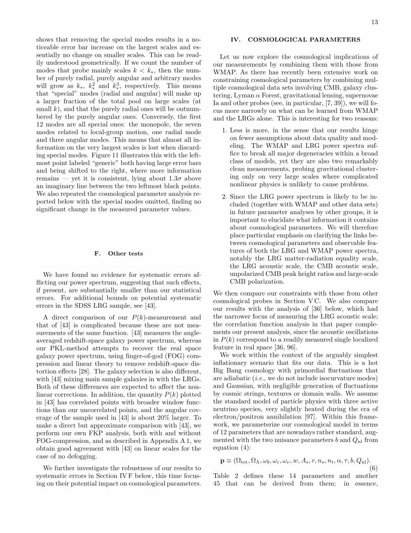
FIG. 11: Same as Figure 7, but showing the effect of discardingspecial modes on the large-scale power. The circles with associatederror bars correspond to our measured power spectrum using all4000 full-sample PKL modes. The other points show the effectof removing the 332 purely angular modes (crosses), the 18 purelyradial modes (triangles), and all special modes combined (squares),including seven associated with the motion of the local group asdescribed in [28]. Any systematic errors adding power to thesespecial modes would cause the black circles to lie systematicallyabove the other points. These special modes are seen to have lessimpact at larger k because they are outnumbered: the number ofradial, angular, and generic modes below a given k-value scales ask, k2 and k3, respectively.

to marginalize over this nuisance parameter, increasingthe leverage of our measurements for constraining thelinear power spectrum shape [93].

E. Robustness to systematic errors

Let us now consider potential systematic errors in theLRG data that could affect our results. Examples of sucheffects include radial modulations (due to mis-estimatesof the radial selection function) and angular modulations(due to effects such as uncorrected dust extinction, vari-able observing conditions, photometric calibration errorsand fiber collisions) of the density field. As long as sucheffects are uncorrelated with the cosmic density field,they will tend to add rather than subtract power.

1. Analysis of subsets of galaxies

To test for effects that would be expected to vary acrossthe sky (depending on, say, reddening, seasonally variablephotometric calibration errors, or observing conditionssuch as seeing and sky brightness), we repeat our entireanalysis for the seven different angular subsets of the skyshown in Figure 3 in search of inconsistencies. To searchfor potential zero-point offsets and other systematic ef-fects associated with the southern Galactic stripes, theyare defined as one of these seven angular subsets (see Fig-ure 3). To test for effects that depend on redshift, we usethe measurements for our three redshift slices, plotted inFigure 6.

To test the null hypothesis that all these subsamplesare consistent with having the same power spectrum, wefit them all to our WMAP+LRG best-fit vanilla modeldescribed in Section IV, including our nonlinear cor-rection (this P (k) curve is quite similar to the best-fitWMAP3 model plotted above in, e.g., Figure 4). Weinclude the 20 band-powers with k ∼< 0.2 in our fit, soif the null hypothesis is correct, we expect a mean χ2

of 20 with a standard deviation of√

2 × 20 ≈ 6.3. Ourseven angular subsamples give a mean 〈χ2〉 ≈ 22.6 anda scatter 〈(χ2 − 20)2〉1/2 ≈ 6.9. Our three radial sub-samples give 〈χ2〉 ≈ 18.6 and 〈(χ2 − 20)2〉1/2 ≈ 2.4. Allof the ten χ2-values are statistically consistent with thenull hypothesis at the 95% level. We also repeated thecosmological parameter analysis reported below with thesouthern stripes omitted, finding no significant change inthe measured parameter values. In other words, all ourangular and radial subsamples are consistent with hav-ing the same power spectrum, so these tests reveal noevidence for systematic errors causing radial or angularpower spectrum variations.

2. Analysis of subsets of modes

Because of their angular or radial nature, all poten-tial systematic errors discussed above create excess powermainly in the radial and angular modes. As mentionedabove, one of the advantages of the PKL method is thatit allows these modes to be excluded from the analysis,in analogy to the way potentially contaminated pixels ina CMB map can be excluded from a CMB power spec-trum analysis. To quantify any such excess, we thereforerepeat our full-sample analysis with radial and/or angu-lar modes deleted. The results of this test are shown inFigure 11 and are very encouraging; the differences aretiny. Any systematic errors adding power to these specialmodes would cause the black circles to lie systematicallyabove the other points, but no such trend is seen, so thereis no indication of excess radial or angular power in thedata.

The slight shifts seen in the power on the largest scalesare expected, since a non-negligible fraction of the infor-mation has been discarded on those scales. Figure 11

13

shows that removing the special modes results in a no-ticeable error bar increase on the largest scales and es-sentially no change on smaller scales. This can be read-ily understood geometrically. If we count the number ofmodes that probe mainly scales k < k∗, then the num-ber of purely radial, purely angular and arbitrary modeswill grow as k∗, k2

∗ and k3∗, respectively. This means

that “special” modes (radial and angular) will make upa larger fraction of the total pool on large scales (atsmall k), and that the purely radial ones will be outnum-bered by the purely angular ones. Conversely, the first12 modes are all special ones: the monopole, the sevenmodes related to local-group motion, one radial modeand three angular modes. This means that almost all in-formation on the very largest scales is lost when discard-ing special modes. Figure 11 illustrates this with the left-most point labeled “generic” both having large error barsand being shifted to the right, where more informationremains — yet it is consistent, lying about 1.3σ abovean imaginary line between the two leftmost black points.We also repeated the cosmological parameter analysis re-ported below with the special modes omitted, finding nosignificant change in the measured parameter values.

F. Other tests

We have found no evidence for systematic errors af-flicting our power spectrum, suggesting that such effects,if present, are substantially smaller than our statisticalerrors. For additional bounds on potential systematicerrors in the SDSS LRG sample, see [43].

A direct comparison of our P (k)-measurement andthat of [43] is complicated because these are not mea-surements of the same function. [43] measures the angle-averaged redshift-space galaxy power spectrum, whereasour PKL-method attempts to recover the real spacegalaxy power spectrum, using finger-of-god (FOG) com-pression and linear theory to remove redshift-space dis-tortion effects [28]. The galaxy selection is also different,with [43] mixing main sample galaxies in with the LRGs.Both of these differences are expected to affect the non-linear corrections. In addition, the quantity P (k) plottedin [43] has correlated points with broader window func-tions than our uncorrelated points, and the angular cov-erage of the sample used in [43] is about 20% larger. Tomake a direct but approximate comparison with [43], weperform our own FKP analysis, both with and withoutFOG-compression, and as described in Appendix A1, weobtain good agreement with [43] on linear scales for thecase of no defogging.

We further investigate the robustness of our results tosystematic errors in Section IVF below, this time focus-ing on their potential impact on cosmological parameters.

IV. COSMOLOGICAL PARAMETERS

Let us now explore the cosmological implications ofour measurements by combining them with those fromWMAP. As there has recently been extensive work onconstraining cosmological parameters by combining mul-tiple cosmological data sets involving CMB, galaxy clus-tering, Lyman α Forest, gravitational lensing, supernovaeIa and other probes (see, in particular, [7, 39]), we will fo-cus more narrowly on what can be learned from WMAPand the LRGs alone. This is interesting for two reasons:

1. Less is more, in the sense that our results hingeon fewer assumptions about data quality and mod-eling. The WMAP and LRG power spectra suf-fice to break all major degeneracies within a broadclass of models, yet they are also two remarkablyclean measurements, probing gravitational cluster-ing only on very large scales where complicatednonlinear physics is unlikely to cause problems.

2. Since the LRG power spectrum is likely to be in-cluded (together with WMAP and other data sets)in future parameter analyses by other groups, it isimportant to elucidate what information it containsabout cosmological parameters. We will thereforeplace particular emphasis on clarifying the links be-tween cosmological parameters and observable fea-tures of both the LRG and WMAP power spectra,notably the LRG matter-radiation equality scale,the LRG acoustic scale, the CMB acoustic scale,unpolarized CMB peak height ratios and large-scaleCMB polarization.

We then compare our constraints with those from othercosmological probes in Section VC. We also compareour results with the analysis of [36] below, which hadthe narrower focus of measuring the LRG acoustic scale;the correlation function analysis in that paper comple-ments our present analysis, since the acoustic oscillationsin P (k) correspond to a readily measured single localizedfeature in real space [36, 96].

We work within the context of the arguably simplestinflationary scenario that fits our data. This is a hotBig Bang cosmology with primordial fluctuations thatare adiabatic (i.e., we do not include isocurvature modes)and Gaussian, with negligible generation of fluctuationsby cosmic strings, textures or domain walls. We assumethe standard model of particle physics with three activeneutrino species, very slightly heated during the era ofelectron/positron annihilation [97]. Within this frame-work, we parameterize our cosmological model in termsof 12 parameters that are nowadays rather standard, aug-mented with the two nuisance parameters b and Qnl fromequation (4):

p ≡ (Ωtot, ΩΛ, ωb, ωc, ων , w, As, r, ns, nt, α, τ, b, Qnl).(6)

Table 2 defines these 14 parameters and another45 that can be derived from them; in essence,

14

(Ωtot, ΩΛ, ωb, ωc, ων , w) define the cosmic matter bud-get, (As, ns, α, r, nt) specify the seed fluctuations and(τ, b, Qnl) are nuisance parameters. We will frequentlyuse the term “vanilla” to refer to the minimal modelspace parametrized by (ΩΛ, ωb, ωc, As, ns, τ, b, Qnl), set-ting ων = α = r = nt = 0, Ωtot = 1 and w = −1; thisis the smallest subset of our parameters that provides agood fit to our data. Since current nt-constraints are tooweak to be interesting, we make the slow-roll assumptionnt = −r/8 throughout this paper rather than treat nt asa free parameter.

All our parameter constraints were computed using thenow standard Monte Carlo Markov Chain (MCMC) ap-proach [98–104] as implemented in [33] 2.

A. Basic results

Our constraints on individual cosmological parametersare given in Tables 2 and 3 and illustrated in Figure 12,both for WMAP alone and when including our SDSSLRG information. Table 2 and Figure 12 take the Oc-cam’s razor approach of marginalizing only over “vanilla”parameters (ΩΛ, ωb, ωc, As, ns, τ, b, Qnl), whereas Table 3shows how key results depend on assumptions about thenon-vanilla parameters (Ωtot, ων , w, r, α) introduced oneat a time. In other words, Table 2 and Figure 12 use thevanilla assumptions by default; for example, models withων 6= 0 are used only for the constraints on ων and otherneutrino parameters (Ων , ξν , fν and Mν).

The parameter measurements and error bars quotedin the tables correspond to the median and the cen-tral 68% of the probability distributions, indicated bythree vertical lines in Figure 12. When a distributionpeaks near zero, we instead quote an upper limit atthe 95th percentile. Note that the tabulated medianvalues are near but not identical to those of the maxi-mum likelihood model. Our best fit vanilla model has

2 To mitigate numerically deleterious degeneracies, the in-dependent MCMC variables are chosen to be the param-eters (Θs,ΩΛ, ωb, ωd, fν , w, Apeak, ns, α, r, nt, Aτ , b, Qnl) fromTable 2, where ωd ≡ ωc + ων , i.e., (Ωtot, ωc, ων , As, τ) are re-placed by (Θs, ωd, fν , Apeak, e−2τ ) as in [33, 105]. When impos-ing a flatness prior Ωtot = 1, we retained Θs as a free parameterand dropped ΩΛ. The WMAP3 log-likelihoods are computedwith the software provided by the WMAP team or taken fromWMAP team chains on the LAMBDA archive (including all un-polarized and polarized information) and fit by a multivariate4th order polynomial [106] for more rapid MCMC-runs involvinggalaxies. The SDSS likelihood uses the LRG sample alone andis computed with the software available at http://space.mit.

edu/home/tegmark/sdss/ and described in Appendix A4, em-ploying only the measurements with k ≤ 0.2h/Mpc unless oth-erwise specified. Our WMAP3+SDSS chains have 3 × 106 stepseach and are thinned by a factor of 10. To be conservative, wedo not use our SDSS measurement of the redshift space distor-tion parameter β, nor do we use any other information (“priors”)whatsoever unless explicitly stated.

ΩΛ = 0.763, ωb = 0.0223, ωc = 0.105, As = 0.685,ns = 0.954, τ = 0.0842, b = 1.90, Qnl = 31.0. As cus-tomary, the 2σ contours in the numerous two-parameterfigures below are drawn where the likelihood has droppedto 0.0455 of its maximum value, which corresponds to∆χ2 ≈ 6.18 and 95.45% ≈ 95% enclosed probability fora two-dimensional Gaussian distribution.

We will spend most of the remainder of this paper di-gesting this information one step at a time, focusing onwhat WMAP and SDSS do and don’t tell us about theunderlying physics, and on how robust the constraintsare to assumptions about physics and data sets. Theone-dimensional constraints in the tables and Figure 12fail to reveal important information hidden in param-eter correlations and degeneracies, so we will study thejoint constraints on key 2-parameter pairs. We will beginwith the vanilla 6-parameter space of models, then intro-duce additional parameters (starting in Section IVB) toquantify both how accurately we can measure them andto what extent they weaken the constraints on the otherparameters.

First, however, some of the parameters in Table 2 de-serve comment. The additional parameters below thedouble line in Table 2 are all determined by those abovethe double line by simple functional relationships, andfall into several groups.

Together with the usual suspects under the heading“other popular parameters”, we have included alterna-tive fluctuation amplitude parameters: to facilitate com-parison with other work, we quote the seed fluctuationamplitudes not only at the scale k = 0.05/Mpc employedby CMBfast [113], CAMB [114] and CosmoMC [102] (de-noted As and r), but also at the scale k = 0.002/Mpcemployed by the WMAP team in [7] (denoted A.002 andr.002).

The “cosmic history parameters” specify when our uni-verse became matter-dominated, recombined, reionized,started accelerating (a > 0), and produced us.

Those labeled “fundamental parameters” are intrinsicproperties of our universe that are independent of ourobserving epoch tnow. (In contrast, most other parame-ters would have different numerical values if we were tomeasure them, say, 10 Gyr from now. For example, tnow

would be about 24 Gyr, zeq and ΩΛ would be larger, andh, Ωm and ωm would all be smaller. Such parametersare therefore not properties of our universe, but merelyalternative time variables.)

The Q-parameter (not to be confused with Qnl!) isthe primordial density fluctuation amplitude ∼ 10−5.The curvature parameter κ is the curvature that theUniverse would have had at the Planck time if therewas no inflationary epoch, and its small numerical value∼ 10−61 constitutes the flatness problem that infla-tion solves. (ξ, ξb, ξc, ξν) are the fundamental parame-ters corresponding to the cosmologically popular quar-tet (Ωm, Ωb, Ωc, Ων), giving the densities per CMB pho-ton. The current densities are ρi = ρhωi, where i =m, b, c, ν and ρh denotes the constant reference density

15

Table 2: Cosmological parameters measured from WMAP and SDSS LRG data with the Occam’s razor approach described in the text: the constraint on each quantity ismarginalized over all other parameters in the vanilla set (ωb, ωc, ΩΛ, As, ns, τ, b, Qnl). Error bars are 1σ.

Parameter Value Meaning Definition

Matter budget parameters:

Ωtot 1.003+0.010−0.009

Total density/critical density Ωtot = Ωm + ΩΛ = 1 − Ωk

ΩΛ 0.761+0.017−0.018

Dark energy density parameter ΩΛ ≈ h−2ρΛ(1.88 × 10−26kg/m3)

ωb 0.0222+0.0007−0.0007

Baryon density ωb = Ωbh2 ≈ ρb/(1.88 × 10−26kg/m3)

ωc 0.1050+0.0041−0.0040

Cold dark matter density ωc = Ωch2 ≈ ρc/(1.88 × 10−26kg/m3)

ων < 0.010 (95%) Massive neutrino density ων = Ωνh2 ≈ ρν /(1.88 × 10−26kg/m3)

w −0.941+0.087−0.101

Dark energy equation of state pΛ/ρΛ (approximated as constant)

Seed fluctuation parameters:

As 0.690+0.045−0.044

Scalar fluctuation amplitude Primordial scalar power at k = 0.05/Mpc

r < 0.30 (95%) Tensor-to-scalar ratio Tensor-to-scalar power ratio at k = 0.05/Mpc

ns 0.953+0.016−0.016

Scalar spectral index Primordial spectral index at k = 0.05/Mpc

nt + 1 0.9861+0.0096−0.0142

Tensor spectral index nt = −r/8 assumed

α −0.040+0.027−0.027

Running of spectral index α = dns/d ln k (approximated as constant)

Nuisance parameters:

τ 0.087+0.028−0.030

Reionization optical depth

b 1.896+0.074−0.069

Galaxy bias factor b = [Pgalaxy(k)/P (k)]1/2 on large scales, where P (k) refers to today.

Qnl 30.3+4.4−4.1

Nonlinear correction parameter [29] Pg(k) = Pdewiggled(k)b2(1 + Qnlk2)/(1 + 1.7k)

Other popular parameters (determined by those above):

h 0.730+0.019−0.019

Hubble parameter h =√

(ωb + ωc + ων)/(Ωtot − ΩΛ)

Ωm 0.239+0.018−0.017

Matter density/critical density Ωm = Ωtot − ΩΛ

Ωb 0.0416+0.0019−0.0018

Baryon density/critical density Ωb = ωb/h2

Ωc 0.197+0.016−0.015

CDM density/critical density Ωc = ωc/h2

Ων < 0.024 (95%) Neutrino density/critical density Ων = ων/h2

Ωk −0.0030+0.0095−0.0102

Spatial curvature Ωk = 1 − Ωtot

ωm 0.1272+0.0044−0.0043

Matter density ωm = ωb + ωc + ων = Ωmh2

fν < 0.090 (95%) Dark matter neutrino fraction fν = ρν /ρd

At < 0.21 (95%) Tensor fluctuation amplitude At = rAs

Mν < 0.94 (95%) eV Sum of neutrino masses Mν ≈ (94.4 eV) × ων [107]

A.002 0.801+0.042−0.043

WMAP3 normalization parameter As scaled to k = 0.002/Mpc: A.002 = 251−ns As if α = 0

r.002 < 0.33 (95%) Tensor-to-scalar ratio (WMAP3) Tensor-to-scalar power ratio at k = 0.002/Mpc

σ8 0.756+0.035−0.035

Density fluctuation amplitude σ8 = 4π∫ ∞0 [ 3

x3 (sin x − x cos x)]2P (k) k2dk(2π)3

1/2, x ≡ k × 8h−1Mpc

σ8Ω0.6m 0.320

+0.024−0.023

Velocity fluctuation amplitude

Cosmic history parameters:

zeq 3057+105−102

Matter-radiation Equality redshift zeq ≈ 24074ωm − 1

zrec 1090.25+0.93−0.91

Recombination redshift zrec(ωm, ωb) given by eq. (18) of [108]

zion 11.1+2.2−2.7

Reionization redshift (abrupt) zion ≈ 92(0.03hτ/ωb)2/3Ω1/3m (assuming abrupt reionization; [109])

zacc 0.855+0.059−0.059

Acceleration redshift zacc = [(−3w − 1)ΩΛ/Ωm]−1/3w − 1 if w < −1/3

teq 0.0634+0.0045−0.0041

Myr Matter-radiation Equality time teq ≈(9.778 Gyr)×h−1 ∫ ∞zeq

[H0/H(z)(1 + z)]dz [107]

trec 0.3856+0.0040−0.0040

Myr Recombination time treq ≈(9.778 Gyr)×h−1 ∫ ∞zrec

[H0/H(z)(1 + z)]dz [107]

tion 0.43+0.20−0.10

Gyr Reionization time tion ≈(9.778 Gyr)×h−1 ∫ ∞zion

[H0/H(z)(1 + z)]dz [107]

tacc 6.74+0.25−0.24

Gyr Acceleration time tacc ≈(9.778 Gyr)×h−1 ∫ ∞zacc

[H0/H(z)(1 + z)]dz [107]

tnow 13.76+0.15−0.15

Gyr Age of Universe now tnow ≈(9.778 Gyr)×h−1 ∫ ∞0 [H0/H(z)(1 + z)]dz [107]

Fundamental parameters (independent of observing epoch):

Q 1.945+0.051−0.053

×10−5 Primordial fluctuation amplitude Q = δh ≈ A1/2.002

× 59.2384µK/TCMB

κ 1.3+3.7−4.3

×10−61 Dimensionless spatial curvature [110] κ = (hc/kBTCMBa)2k

ρΛ 1.48+0.11−0.11

×10−123ρPl Dark energy density ρΛ ≈ h2ΩΛ × (1.88 × 10−26kg/m3)

ρhalo 6.6+1.2−1.0

×10−123ρPl Halo formation density ρhalo = 18π2Q3ξ4

ξ 3.26+0.11−0.11

eV Matter mass per photon ξ = ρm/nγ

ξb 0.569+0.018−0.018

eV Baryon mass per photon ξb = ρb/nγ

ξc 2.69+0.11−0.10

eV CDM mass per photon ξc = ρc/nγ

ξν < 0.26 (95%) eV Neutrino mass per photon ξν = ρν/nγ

η 6.06+0.20−0.19

×10−10 Baryon/photon ratio η = nb/ng = ξb/mp

AΛ 2077+135−125

Expansion during matter domination (1 + zeq)(Ωm/ΩΛ)1/3 [111]

σ∗gal 0.561

+0.024−0.023

×10−3 Seed amplitude on galaxy scale Like σ8 but on galactic (M = 1012M⊙) scale early on

CMB phenomenology parameters:

Apeak 0.579+0.013−0.013

Amplitude on CMB peak scales Apeak = Ase−2τ

Apivot 0.595+0.012−0.011

Amplitude at pivot point Apeak scaled to k = 0.028/Mpc: Apivot = 0.56ns−1Apeak if α = 0

H1 4.88+0.37−0.34

1st CMB peak ratio H1(Ωtot, ΩΛ, ωb, ωm, w, ns, τ) given by [112]

H2 0.4543+0.0051−0.0051

2nd to 1st CMB peak ratio H2 = (0.925ω0.18m 2.4ns−1)/[1 + (ωb/0.0164)

12ω0.52m )]0.2 [112]

H3 0.4226+0.0088−0.0086

3rd to 1st CMB peak ratio H3 = 2.17[1 + (ωb/0.044)2]−1ω0.59m 3.6ns−1/[1 + 1.63(1 − ωb/0.071)ωm]

dA(zrec) 14.30+0.17−0.17

Gpc Comoving angular diameter distance to CMB dA(zrec) = cH0

sinh

[Ω

1/2k

∫ zrec0 [H0/H(z)]dz

]/Ω

1/2k

[107]

rs(zrec) 0.1486+0.0014−0.0014

Gpc Comoving sound horizon scale rs(ωm, ωb) given by eq. (22) of [108]

rdamp 0.0672+0.0009−0.0008

Gpc Comoving acoustic damping scale rdamp(ωm, ωb) given by eq. (26) of [108]

Θs 0.5918+0.0020−0.0020

CMB acoustic angular scale fit (degrees) Θs(Ωtot, ΩΛ, w, ωb, ωm) given by [112]

ℓA 302.2+1.0−1.0

CMB acoustic angular scale ℓA = πdA(zrec)/rs(zrec)

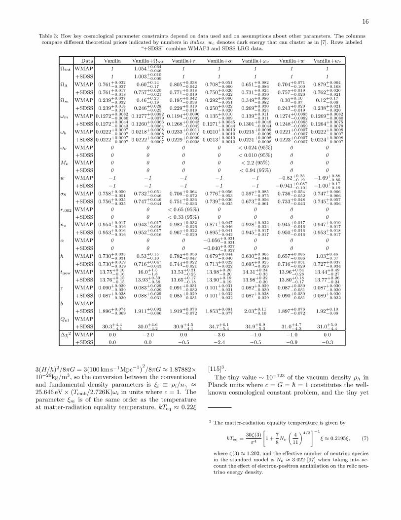
16

Table 3: How key cosmological parameter constraints depend on data used and on assumptions about other parameters. The columnscompare different theoretical priors indicated by numbers in italics. wc denotes dark energy that can cluster as in [7]. Rows labeled

“+SDSS” combine WMAP3 and SDSS LRG data.

Data Vanilla Vanilla+Ωtot Vanilla+r Vanilla+α Vanilla+ων Vanilla+w Vanilla+wc

Ωtot WMAP 1 1.054+0.064−0.046 1 1 1 1 1

+SDSS 1 1.003+0.010−0.009 1 1 1 1 1

ΩΛ WMAP 0.761+0.032−0.037 0.60+0.14

−0.17 0.805+0.038−0.042 0.708+0.051

−0.060 0.651+0.082−0.086 0.704+0.071

−0.100 0.879+0.064−0.168

+SDSS 0.761+0.017−0.018 0.757+0.020

−0.021 0.771+0.018−0.019 0.750+0.020

−0.022 0.731+0.024−0.030 0.757+0.019

−0.020 0.762+0.020−0.021

Ωm WMAP 0.239+0.037−0.032 0.46+0.23

−0.19 0.195+0.042−0.038 0.292+0.060

−0.051 0.349+0.086−0.082 0.30+0.10

−0.07 0.12+0.17−0.06

+SDSS 0.239+0.018−0.017 0.246+0.028

−0.025 0.229+0.019−0.018 0.250+0.022

−0.020 0.269+0.030−0.024 0.243+0.020

−0.019 0.238+0.021−0.020

ωm WMAP 0.1272+0.0082−0.0080 0.1277+0.0082

−0.0079 0.1194+0.0096−0.0092 0.135+0.010

−0.009 0.139+0.011−0.011 0.1274+0.0083

−0.0082 0.1269+0.0082−0.0080

+SDSS 0.1272+0.0044−0.0043 0.1260+0.0066

−0.0064 0.1268+0.0043−0.0042 0.1271+0.0045

−0.0044 0.1301+0.0048−0.0044 0.1248+0.0063

−0.0059 0.1264+0.0075−0.0079

ωb WMAP 0.0222+0.0007−0.0007 0.0218+0.0008

−0.0008 0.0233+0.0011−0.0010 0.0210+0.0010

−0.0010 0.0215+0.0009−0.0009 0.0221+0.0007

−0.0007 0.0222+0.0008−0.0007

+SDSS 0.0222+0.0007−0.0007 0.0222+0.0007

−0.0007 0.0229+0.0009−0.0008 0.0213+0.0010

−0.0010 0.0221+0.0008−0.0008 0.0223+0.0007

−0.0007 0.0224+0.0008−0.0007

ων WMAP 0 0 0 0 < 0.024 (95%) 0 0

+SDSS 0 0 0 0 < 0.010 (95%) 0 0

Mν WMAP 0 0 0 0 < 2.2 (95%) 0 0

+SDSS 0 0 0 0 < 0.94 (95%) 0 0

w WMAP −1 −1 −1 −1 −1 −0.82+0.23−0.19 −1.69+0.88

−0.85

+SDSS −1 −1 −1 −1 −1 −0.941+0.087−0.101 −1.00+0.17

−0.19

σ8 WMAP 0.758+0.050−0.051 0.732+0.051

−0.046 0.706+0.064−0.072 0.776+0.056

−0.053 0.597+0.085−0.075 0.736+0.054

−0.052 0.747+0.066−0.066

+SDSS 0.756+0.035−0.035 0.747+0.046

−0.044 0.751+0.036−0.036 0.739+0.036

−0.035 0.673+0.056−0.061 0.733+0.048

−0.043 0.745+0.057−0.056

r.002 WMAP 0 0 < 0.65 (95%) 0 0 0 0

+SDSS 0 0 < 0.33 (95%) 0 0 0 0

ns WMAP 0.954+0.017−0.016 0.943+0.017

−0.016 0.982+0.032−0.026 0.871+0.047

−0.046 0.928+0.022−0.024 0.945+0.017

−0.016 0.947+0.019−0.017

+SDSS 0.953+0.016−0.016 0.952+0.017

−0.016 0.967+0.022−0.020 0.895+0.041

−0.042 0.945+0.017−0.017 0.950+0.016

−0.016 0.953+0.018−0.017

α WMAP 0 0 0 −0.056+0.031−0.031 0 0 0

+SDSS 0 0 0 −0.040+0.027−0.027 0 0 0

h WMAP 0.730+0.033−0.031 0.53+0.15

−0.10 0.782+0.058−0.047 0.679+0.044

−0.040 0.630+0.065−0.044 0.657+0.085

−0.086 1.03+0.46−0.37

+SDSS 0.730+0.019−0.019 0.716+0.047

−0.043 0.744+0.022−0.021 0.713+0.022

−0.022 0.695+0.025−0.028 0.716+0.031

−0.029 0.727+0.037−0.034

tnow WMAP 13.75+0.16−0.16 16.0+1.5

−1.8 13.53+0.21−0.25 13.98+0.20

−0.20 14.31+0.24−0.33 13.96+0.34

−0.28 13.44+0.49−0.27

+SDSS 13.76+0.15−0.15 13.93+0.59

−0.58 13.65+0.17−0.18 13.90+0.19

−0.19 13.98+0.22−0.20 13.80+0.18

−0.17 13.77+0.26−0.24

τ WMAP 0.090+0.029−0.029 0.083+0.029

−0.029 0.091+0.031−0.032 0.101+0.031

−0.031 0.082+0.029−0.030 0.087+0.030

−0.031 0.087+0.030−0.030

+SDSS 0.087+0.028−0.030 0.088+0.029

−0.031 0.085+0.029−0.031 0.101+0.032

−0.032 0.087+0.028−0.029 0.090+0.030

−0.031 0.089+0.030−0.032

b WMAP

+SDSS 1.896+0.074−0.069 1.911+0.092

−0.086 1.919+0.078−0.072 1.853+0.081

−0.077 2.03+0.11−0.10 1.897+0.076

−0.072 1.92+0.10−0.08

Qnl WMAP

+SDSS 30.3+4.4−4.1 30.0+4.6

−4.2 30.9+4.5−4.1 34.7+6.1

−5.4 34.9+6.9−5.3 31.0+4.7

−4.3 31.0+5.0−4.4

∆χ2 WMAP 0.0 −2.0 0.0 −3.6 −1.0 −1.0 0.0

+SDSS 0.0 0.0 −0.5 −2.4 −0.5 −0.9 −0.3

3(H/h)2/8πG = 3(100 kms−1Mpc−1)2/8πG ≈ 1.87882×

10−26kg/m3, so the conversion between the conventionaland fundamental density parameters is ξi ≡ ρi/nγ ≈25.646 eV × (Tcmb/2.726K)ωi in units where c = 1. Theparameter ξm is of the same order as the temperatureat matter-radiation equality temperature, kTeq ≈ 0.22ξ

[115]3.

The tiny value ∼ 10−123 of the vacuum density ρΛ inPlanck units where c = G = h = 1 constitutes the well-known cosmological constant problem, and the tiny yet

3 The matter-radiation equality temperature is given by

kTeq =30ζ(3)

π4

[1 +

7

8Nν

(4

11

)4/3]−1

ξ ≈ 0.2195ξ, (7)

where ζ(3) ≈ 1.202, and the effective number of neutrino speciesin the standard model is Nν ≈ 3.022 [97] when taking into ac-count the effect of electron-positron annihilation on the relic neu-trino energy density.

17

FIG. 12: Constraints on key individual cosmological quantities using WMAP1 (yellow/light grey distributions), WMAP3 (narrowerorange/grey distributions) and including SDSS LRG information (red/dark grey distributions). If the orange/grey is completely hiddenbehind the red/dark grey, the LRGs thus add no information. Each distribution shown has been marginalized over all other quantitiesin the “vanilla” class of models parametrized by (ΩΛ, ωb, ωc, As, ns, τ, b, Qnl). The parameter measurements and error bars quoted in thetables correspond to the median and the central 68% of the distributions, indicated by three vertical lines for the WMAP3+SDSS caseabove. When the distribution peaks near zero (like for r), we instead quote an upper limit at the 95th percentile (single short vertical

line). The horizontal dashed lines indicate e−x2/2 for x = 1 and 2, respectively, so if the distribution were Gaussian, its intersections withthese lines would correspond to 1σ and 2σ limits, respectively.

similar value of the parameter combination Q3ξ4 explainsthe origin of attempts to explain this value anthropically[116–123]: Q3ξ4 is roughly the density of the universeat the time when the first nonlinear dark matter halos

would form if ρΛ = 0 [115], so if ρΛ ≫ Q3ξ4, dark energyfreezes fluctuation growth before then and no nonlinearstructures ever form.

The parameters (AΛ, σ∗gal) are useful for anthropic

18

buffs, since they directly determine the density fluctua-tion history on galaxy scales through equation (5) in [111](where σ∗

gal is denoted σM (0)). Roughly, fluctuationsgrow from the initial level σ∗

gal by a factor AΛ. Marginal-

izing over the neutrino fraction gives AΛ = 2279+240−182,

σ∗gal = 0.538+0.024

−0.022 × 10−3.The group labeled “CMB phenomenology parameters”

contains parameters that correspond rather closely tothe quantities most accurately measured by the CMB,such as heights and locations of power spectrum peaks.Many are seen to be measured at the percent level orbetter. These parameters are useful for both numeri-cal and intuition-building purposes [105, 106, 112, 124–126]. Whereas CMB constraints suffer from severe de-generacies involving physical parameters further up inthe table (involving, e.g., Ωtot and ΩΛ as discussed be-low), these phenomenological parameters are all con-strained with small and fairly uncorrelated measure-ment errors. By transforming the multidimensionalWMAP3 log-likelihood function into the space spannedby (H2, ωm, fν , ΩΛ, w, Θs, Apivot, H3, α, r, nt, Aτ , b, Qnl),it becomes better approximated by our quartic polyno-mial fit described in Footnote 2 and [106]: for example,the rms error is a negligible ∆ lnL ≈ 0.03 for the vanillacase. Roughly speaking, this transformation replaces thecurvature parameter Ωtot by the characteristic peak scaleΘs, the baryon fraction by the ratio H2 of the first twopeak heights, the spectral index ns by the ratio H3 ofthe third to first peak heights, and the overall peak am-plitude Apeak by the amplitude Apivot at the pivot scalewhere it is uncorrelated with ns. Aside from this nu-merical utility, these parameters also help demystify the“black box” aspect of CMB parameter constraints, elu-cidating their origin in terms of features in the data andin the physics [112].

B. Vanilla parameters

Figure 12 compares the constraints on key parametersfrom the 1-year WMAP data (“WMAP1”), the 3-yearWMAP data (“WMAP3”) and WMAP3 combined withour SDSS LRG measurements (“WMAP+LRG”). We in-clude the WMAP1 case because it constitutes a well-tested baseline and illustrates both the dramatic progressin the field and what the key new WMAP3 informationis, particularly from E-polarization.

1. What WMAP3 adds

The first thing to note is the dramatic improvementfrom WMAP1 to WMAP3 emphasized in [7]. (PlottedWMAP1 constraints are from [33].) As shown in [127],this stems almost entirely from the new measurement ofthe low-ℓ E power spectrum, which detects the reion-ization signature at about 3σ and determines the corre-sponding optical depth τ = 0.09 ± 0.03. This measure-

ment breaks the severe vanilla degeneracy in the WMAP1data [32, 33] (see Figure 13) and causes the dramatictightening of the constraints on (ωb, ωc, ΩΛ, As, ns) seenin the figures; essentially, with τ well constrained, the ra-tio of large scale power to the acoustic peaks determinesns, and the relative heights of the acoustic peaks thendetermine ωb and ωc without residual uncertainty dueto ns. Indeed, [127] has shown that discarding all theWMAP3 polarization data (both TE and EE) and re-placing it with a Gaussian prior τ = 0.09± 0.03 recoversparameter constraints essentially identical to those fromthe full WMAP3 data set. In Section IVF1, we will re-turn to the issue of what happens if this τ -measurementis compromised by polarized foreground contamination.

The second important change from WMAP1 toWMAP3 is that the central values of some parametershave shifted noticeably [7]. Improved modeling of noisecorrelations and polarized foregrounds have lowered thelow-ℓ TE power and thus eliminated the WMAP1 ev-idence for τ ∼ 0.17. Since the fluctuation amplitudescales as eτ times the CMB peak amplitude, this τ dropof 0.08 would push σ8 down by about 8%. In addi-tion, better measurements around the 3rd peak and achange in analysis procedure (marginalizing over the SZ-contribution) have lowered ωm by about 13%, causingfluctuation growth to start later (zeq decreases) and endearlier (zacc increases), reducing σ8 by another 8%. Theseeffects combine to lower σ8 by about 21% when also tak-ing into account the slight lowering of ns.

2. What SDSS LRGs add

A key reason that non-CMB datasets such as the2dFGRS and the SDSS improved WMAP1 constraintsso dramatically was that they helped break the vanillabanana degeneracy seen in Figure 13, so the factthat WMAP3 now mitigates this internally with its E-polarization measurement of τ clearly reduces the valueadded by other datasets. However, Table 3 shows thatour LRG measurements nonetheless give substantial im-provements, cutting error bars on Ωm, ωm and h by abouta factor of two for vanilla models and by up to almost anorder of magnitude when curvature, tensors, neutrinos orw are allowed.

The physics underlying these improvements is illus-trated in Figure 14. The cosmological information inthe CMB splits naturally into two parts, one “vertical”and one “horizontal”, corresponding to the vertical andhorizontal positions of the power spectrum peaks.

19

FIG. 13: 95% constraints in the (Ωm, h) plane. For 6-parameter“vanilla” models, the shaded red/grey region is ruled out byWMAP1 and the shaded orange/grey region by WMAP3; the mainsource of the dramatic improvement is the measurement of E-polarization breaking the degeneracy involving τ . Adding SDSSLRG information further constrains the parameters to the whiteregion marked “Allowed”. The horizontal hatched band is re-quired by the HST key project [137]. The dotted line shows the fith = 0.72(Ωm/0.25)−0.32 , explaining the origin of the percent-levelconstraint h(Ωm/0.25)0.32 = 0.719 ± 0.008 (1σ).

FIG. 14: Illustration of the physics underlying the previous figure.Using only WMAP CMB peak height ratios constrains (ωm, ωb, ns)independently of As, τ , curvature and late-time dark energy prop-erties. This excludes all but the white band ωm ≡ h2Ωm =0.127 ± 0.017 (2σ). If we assume Ωtot = 1 and vanilla dark en-ergy, we can supplement this with independent “standard ruler”information from either WMAP CMB (thin yellow/light grey el-lipse) giving Ωm = 0.239 ± 0.034 (1σ), or SDSS galaxies (thickerblue/grey ellipse) giving Ωm = 0.239±0.027 (1σ). These two rulersare not only beautifully consistent, but also complementary, withthe joint constraints (small ellipse marked “allowed”) being tighterthan those from using either separately, giving Ωm = 0.238±0.017(1σ). The plotted 2-dimensional constraints are all 2σ. The threeblack curves correspond to constant “horizontal” observables: con-stant angular scales for the acoustic peaks in the CMB power (dot-ted, h ∼

∝ Ω−0.3m ), for the acoustic peaks in the galaxy power (solid,

h ∼∝ Ω0.37

m ) and for the turnover in the galaxy power spectrum

(dashed, h ∼∝ Ω−0.93

m ). This illustrates why the galaxy acousticscale is even more helpful than that of the CMB for measuring Ωm:although it is currently less accurately measured, its degeneracy di-rection is more perpendicular to the CMB peak ratio measurementof h2Ωm.

20

By vertical information, we mean the relative heightsof the acoustic peaks, which depend only on the physicalmatter densities (ωm, ωb, ων) and the scalar primordialpower spectrum shape (ns, α). They are independent ofcurvature and dark energy, since ΩΛ(z) ≈ Ωk(z) ≈ 0 atz ∼> 103. They are independent of h, since the physics atthose early times depended only on the expansion rateas a function of temperature back then, which is simplyξ1/2T 3/2 times a known numerical constant, where ξ isgiven by ωm and the current CMB temperature (see Ta-ble 3 in [115]). They are also conveniently independentof τ and r, which change the power spectrum shape onlyat ℓ ≪ 102.

By horizontal (a.k.a. “standard ruler”) information, wemean the acoustic angular scale ℓA ≡ πdA(zrec)/rs(zrec)defined in Table 2. The ℓ-values of CMB power spectrumpeaks and troughs are all equal to ℓA times constants de-pending on (ωm, ωb), so changing ℓA by some factor by al-tering (Ωk, ΩΛ, w) simply shifts the CMB peaks horizon-tally by that factor and alters the late integrated SachsWolfe effect at ℓ ≪ 102. Although this single number ℓA

is now measured to great precision (∼ 0.3%), it dependson multiple parameters, and it is popular to break thisdegeneracy with assumptions rather than measurements.The sound horizon at recombination rs(zrec) in the de-nominator depends only weakly on (ωm, ωb), which arewell constrained from the vertical information, and Ta-ble 2 shows that it is now known to about 1%. In con-trast, the comoving angular diameter distance to recom-bination dA(zrec) depends sensitively on both the spa-tial curvature Ωk and the cosmic expansion history H(z),which in turn depends on the history of the dark energydensity:

H(z)

H0=

[X(z)ΩΛ + (1 + z)2Ωk + (1 + z)3Ωm + (1 + z)4Ωr)

]1/2.

(8)Here X(z) is defined as the dark energy density relative toits present value [128], with vanilla dark energy (a cosmo-logical constant) corresponding to X(z) = 1. The mostcommon (although physically unmotivated) parametriza-tion of this function in the literature has been a simplepower law X(z) = (1+z)3(1+w), although it has also beenconstrained with a variety of other parametric and non-parametric approaches (see [129] and references therein).The parameter Ωr refers to the radiation contributionfrom photons and massless neutrinos, which is given byh2Ωr ≈ 0.0000416(Tcmb/2.726K)4 and makes a negligiblecontribution at low redshift.

Using the vertical WMAP information alone gives atight constraint on ωm ≡ h2Ωm, corresponding to thewhite band in Figure 14, independent of assumptionsabout curvature or dark energy.4 To this robust measure-

4 To obtain this ωm-constraint, we marginalized over ℓA bymarginalizing over either Ωk or w; Table 3 shows that these twoapproaches give essentially identical answers.

FIG. 15: 95% constraints in the (Ωm, ΩΛ) plane. The large shadedregions are ruled out by WMAP1 (red/dark grey) and WMAP3 (or-ange/grey) when spatial curvature is added to the 6 vanilla param-eters, illustrating the well-known geometric degeneracy betweenmodels that all give the same acoustic peak locations in the CMBpower spectrum. The yellow/light grey region is ruled out whenadding SDSS LRG information, breaking the degeneracy mainlyby measuring the acoustic peak locations in the galaxy power spec-trum. Models on the diagonal dotted line are flat, those below areopen and those above are closed. Here the yellow banana has beencut off from below by an h ∼

> 0.4 prior in the CosmoMC software.

ment, we can now add two independent pieces of infor-mation if we are willing to make the vanilla assumptionsthat curvature vanishes and dark energy is a cosmologicalconstant: If we add the WMAP horizontal information,the allowed region shrinks to the thin ellipse hugging theh ∼∝ Ω−0.3

m line of constant ℓA (dotted). If we insteadadd the LRG information (which constrains hΩ0.93

m viathe P (k) turnover scale and hΩ−0.37

m via the acoustic os-cillation scale5), the allowed region shrinks to the thick

5 The origin of these scalings can be understood as follows.The matter-radiation equality horizon scale req ∝ ω−1

m . The

sound horizon scales as rs(zeq) ∝ ω−0.25m with a weak depen-

dence on ωb that is negligible in this context [108]. For theLRG mean redshift z = 0.35, the power law fit dA(z, Ωm) =0.3253(Ωm/0.25)−0.065cH−1

0 ∝ h−1Ω−0.065m is quite good within

our range of interest, accurate to within about 0.1% for 0.2 <Ωm < 0.3. For z = 1100, the power law fit dA(z, Ωm) ≈

3.4374(Ωm/0.25)−0.4cH−10 ∝ h−1Ω−0.4

m retains 0.1% accuracyfor for 0.19 < Ωm < 0.35. The P (k) turnover angle ∝

req/dA(0.35) ∝ (h2Ωm)−1/h−1Ω−0.065m is therefore constant

for h ∝ Ω−0.93m , the P (k) acoustic angle ∝ rs/dA(0.35) ∝

21

FIG. 16: 95% constraints in the (Ωtot, h) plane for 7-parametercurved models. The shaded red/dark grey region was ruled outby WMAP1 alone, and WMAP3 tightened these constraints (or-ange/grey region), illustrating that CMB fluctuations alone do notsimultaneously show space to be flat and measure the Hubble pa-rameter. The yellow/light grey region is ruled out when addingSDSS LRG information. Here the yellow banana has been artifi-cially cut off for h ∼

> 0.4 by a hardwired prior in the CosmoMCsoftware.

ellipse.These two independent pieces of horizontal informa-

tion are seen to be not only beautifully consistent, butalso complementary: the joint constraints are signifi-cantly tighter than those from using either separately.When going beyond vanilla models below, the thin CMB-only ellipse is of course no longer relevant, making theLRG constraints even more valuable.

C. Spacetime geometry

To zeroth order (ignoring perturbations), the space-time geometry is simply the Friedmann-Robertson-Walker metric determined by the curvature Ωk and thecosmic expansion history H(z). The vanilla assumptionsimply the special case of no curvature (Ωk = 0) andconstant dark energy (H(z) given by equation (8) withX(z) = 1).

(h2Ωm)−0.25/h−1Ω−0.065m is constant for h ∝ Ω0.37

m , and theCℓ acoustic angle ∝ rs/dA(zrec) ∝ (h2Ωm)−0.25/h−1Ω−0.4

m isconstant for h ∝ Ω−0.3

m .

FIG. 17: 95% constraints in the (Ωtot, tnow) plane for 7-parametercurved models. The shaded red/dark grey region is ruled outby WMAP1 alone, and WMAP3 tightened these constraints (or-ange/grey region), illustrating that CMB fluctuations do not si-multaneously show space to be flat and measure the age of theUniverse. The yellow/light grey region is ruled out when addingSDSS LRG information. The age limit tnow > 12 Gyr shown isthe 95% lower limit from white dwarf ages by [132]; for a review ofrecent age determinations, see [7].

Let us now spice up the vanilla model space by in-cluding spatial curvature Ωk and a constant dark energyequation of state w as free parameters, both to constrainthem and to quantify how other constraints get weakenedwhen dropping these vanilla assumptions.

1. LRGs as a standard ruler at z = 0.35

Before constraining specific spacetime geometry pa-rameters, let us review the relevant physics to intuitivelyunderstand what CMB and LRGs do and do not teachus about geometry. As discussed in the previous sec-tion, current CMB data accurately measure only a singlenumber that is sensitive to the spacetime geometry infor-mation in Ωk and H(z). This number is the peak angularscale ℓA, and it in turn depends on the four independentparameters (Ωm, Ωk, w, h). (ΩΛ is of course not indepen-dent, fixed by the identity ΩΛ = 1−Ωk −Ωm.) Since thesound horizon size rs is now accurately known indepen-dently of spacetime geometry from CMB peak ratios, theCMB ℓA-measurement provides a precise determinationof the comoving angular diameter distance to the lastscattering surface, dA(zrec), thus allowing one function

22

of (Ωm, Ωk, w, h) to be accurately measured.As emphasized in [36, 128, 130, 131], measuring the

acoustic angular scale at low redshift in galaxy cluster-ing similarly constrains a second independent combina-tion of (Ωm, Ωk, w, h), and measuring dA(z) at multipleredshifts with future redshift surveys and current andfuture SN Ia data can break all degeneracies and allowrobust recovery of both Ωk and the dark energy historyX(z). For the galaxy approach, the point is that leav-ing the early universe physics (ωb, ωm, ns, etc.) fixed,changing the spacetime geometry merely scales the hori-zontal axis of the angular power spectrum of galaxies ata given redshift z as dA(z). More generally, as describedin detail in [36], the main effect of changing the space-time geometry is to shift our measured three-dimensionalpower spectrum horizontally by rescaling the k-axis. Thek-scale for angular modes dilates as the comoving an-gular diameter distance dA(z) to the mean survey red-shift z ≈ 0.35, whereas that for radial modes dilates asd(dA)/dz = c/H(z) for the flat case. For small varia-tions around our best fit model, the change in H(0.35)is about half that of the angular diameter distance. Tomodel this, [36] treats the net dilation as the cube rootof the product of the radial dilation times the square ofthe transverse dilation, defining the distance parameter

dV (z) ≡[dA(z)2

cz

H(z)

]1/3

. (9)

Using only the vertical WMAP peak height informationas a prior on (ωb, ωd, ns), our LRG power spectrum givesthe measurement dV (0.35) = 1.300 ± 0.088 Gpc, whichagrees well with the value measured in [36] using the LRGcorrelation function. It is this geometric LRG informa-tion that explains most of the degeneracy breaking seenin the Figures 15, 16, 17 and 18 below.

As more LRG data become available and strengthenthe baryon bump detection from a few σ to > 5σ, thismeasurement should become even more robust, not re-quiring any ωm-prior from WMAP peak heights.

2. Spatial curvature

Although it has been argued that closed inflation mod-els require particularly ugly fine-tuning [133], a numberof recent papers have considered nearly-flat models ei-ther to explain the low CMB quadrupole [134], in stringtheory landscape-inspired short inflation models, or foranthropic reasons [110, 135, 136], so it is clearly interest-ing and worthwhile to continue sharpening observationaltests of the flatness assumption. In the same spirit, mea-suring the Hubble parameter h independently of theo-retical assumptions about curvature and measurementsof galaxy distances at low redshift provides a powerfulconsistency check on our whole framework.

Figures 15, 16 and 17 illustrate the well-known CMBdegeneracies between the curvature Ωk ≡ 1 − Ωtot and

dark energy ΩΛ, the Hubble parameter h, and the age ofthe universe tnow; without further information or priors,one cannot simultaneously demonstrate spatial flatnessand accurately measure ΩΛ, h or tnow, since the CMBaccurately constrains only the single combination ℓA. In-deed, the WMAP3 degeneracy banana extends towardseven larger Ωtot than these figures indicate; the plottedbanana has been artificially truncated by a hardwiredlower limit on h in the CosmoMC software used to com-pute this particular MCMC.

Including our LRG information is seen to reduce thecurvature uncertainty by about a factor of five, providinga striking vindication of the standard inflationary pre-diction Ωtot = 1. The physical reason for this LRG im-provement is obvious from the thick ellipse in Figure 14:WMAP vertical peak height information combined withLRG standard ruler information on dV (0.35) measuresΩm rather independently of curvature.

Yet even with WMAP+LRG information, the figuresshow that a strong degeneracy persists between curvatureand h, and curvature and tnow, leaving the measurementuncertainty on h comparable with that from the HSTkey project [137]. If we add the additional assumptionthat space is exactly flat, then uncertainties shrink byfactors around 4 and 10 for h and tnow, respectively, stillin beautiful agreement with other measurements.

In conclusion, within the class of almost flat models,the WMAP-only constraints on h, tnow, ΩΛ and Ωtot re-main weak, and including our LRG measurements pro-vides a huge improvement in precision.

3. Dark energy

Although we now know its present density fairly accu-rately, we still know precious little else about dark energy,and much interest is focused on understanding its nature.Assuming flat space1, Table 3 and Figure 18 show ourconstraints on constant w for two cases: assuming thatdark energy is homogeneous (does not cluster) and thatit allows spatial perturbations (does cluster) as modeledin [7]. We see that adding w as a free parameter does notsignificantly improve χ2 for the best fit, and all data areconsistent with the vanilla case w = −1, with 1σ uncer-tainties in w in the 10% - 30% range, depending on darkenergy clustering assumptions.

As described above, the physical basis of these con-straints is similar to those for curvature, since (aside fromlow-ℓ corrections from the late ISW effect and dark en-ergy clustering), the only readily observable effect of thedark energy density history X(z) is to alter dA(zrec) anddA(0.35), and hence the CMB and LRG acoustic angularscales. (The dark energy history also affects fluctuationgrowth and hence the power spectrum amplitude, butwe do not measure this because our analysis marginal-izes over the galaxy bias parameter b.)

It has been argued (see, e.g., [138]) that it is inappro-priate to assume Ωk = 0 when constraining w, since there

23

FIG. 18: 95% constraints in the (Ωm, w) plane. The shadedred/grey region is ruled out by WMAP1 alone when the darkenergy equation of state w is added to the 6 vanilla parameters.The shaded orange/grey region is ruled out by WMAP3. The yel-low/light grey region is ruled out when adding SDSS LRG infor-mation. The region not between the two black curves is ruled outby WMAP3 when dark energy is assumed to cluster.

is currently no experimental evidence for spatial flatnessunless w = −1 is assumed. We agree with this critique,and merely note that no interesting joint constraints cancurrently be placed on as many as four spacetime geome-try parameters (Ωm, Ωk, w, h) from WMAP and our LRGmeasurements alone, since they accurately constrain onlythe two combinations dA(zrec) and dV (0.35). Other datasuch as SN Ia need to be included for this; [7] do this andobtain w = −1.06+0.13

−0.08.One can also argue, in the spirit of Occam’s razor, that

the fact that vanilla works so well can be taken as evi-dence against both Ωk 6= 0 and w 6= −1, since it wouldrequire a fluke coincidence for them to both have signifi-cantly non-vanilla values that conspire to lie on the samedV (0.35) and dA(zrec) degeneracy tracks as the vanillamodel.

D. Inflation

Inflation [139–143] remains the leading paradigm forwhat happened in the early universe because it can solvethe flatness, horizon and monopole problems (see, e.g.,[144]) and has, modulo minor caveats, successfully pre-dicted that Ωtot ≈ 1, ns ≈ 1, |α| ≪ 1 and r ∼< 1 as wellas the facts that the seed fluctuations are mainly Gaus-

FIG. 19: 95% constraints in the (ns, r.002) plane for 7-parametertensor models (the vanilla parameters plus r). The large shadedregions are ruled out by WMAP1 (red/dark grey) and WMAP3 (or-ange/grey). The yellow/light grey region is ruled out when addingSDSS LRG information, pushing the upper limit on r.002 down bya factor of two to r.002 < 0.33 (95%). The solid black curve with-out shading shows the 68% limit. The two dotted lines delimit thethree classes of inflation models known as small-field, large-fieldand hybrid models. Some single-field inflation models make highlyspecific predictions in this plane as indicated. From top to bottom,the figure shows the predictions for V (φ) ∝ φ6 (line segment; ruledout by CMB alone), V (φ) ∝ φ4 (star; a textbook inflation model;on verge of exclusion) and V (φ) ∝ φ2 (line segment; the eternalstochastic inflation model; still allowed). These predictions assumethat the number of e-foldings between horizon exit of the observedfluctuations and the end of inflation is 64 for the φ4 model andbetween 50 and 60 for the others as per [150].

sian and adiabatic. For the ekpyrotic universe alternative[145], controversy remains about whether it can survive a“bounce” and whether it predicts ns ≈ 1 [146] or ns ≈ 3[147].

In the quest to measure the five parameters (Q, ns −1, α, r, nt) characterizing inflationary seed fluctuations,the first breakthrough was the 1992 COBE discovery thatQ ∼ 10−5 and that the other four quantities were con-sistent with zero [149]. The second breakthrough is cur-rently in progress, with WMAP3 suggesting 1 − ns > 0at almost the 3σ level (1 − ns = 0.049+0.019

−0.015) [7]. Thiscentral value is in good agreement with classic (singleslow-rolling scalar field) inflation models, which generi-cally predict non-scale invariance in the ballpark 1−ns ∼2/N ∼ 0.04, assuming that the number of e-foldings be-tween the time horizon the observed fluctuations exit thehorizon and the end of inflation is 50 < N < 60 as per[150]. This central value of ns agrees well with numerous

24

measurements in the recent literature (e.g., [151]); it ismerely the error bars that have changed.

As illustrated in Figure 19 and discussed in [7], ns = 1becomes allowed if the tensor fluctuation parameter r isincluded (as it clearly should be when constraining in-flation models), but the “vanilla lite” Harrison-Zeldovichmodel (ns = 1, r = 0) remains ruled out. In contrast, thearguably simplest of all inflation models, a single slow-rolling scalar field with potential V (φ) ∝ φ2, remains vi-able: it predicts (ns, r) = (1 − 2/N, 8/N) ≈ (0.96, 0.15).The string-inspired “N-flation” model makes a similarprediction [152, 153].

Our constraints on the inflation parameters(Q, ns, α, r, nt) in Table 3 and Figure 19 are seento confirm those reported in [7] — the main addition ofour LRG analysis is simply to provide a clean way oftightening the WMAP-only constraints on both Ωtot andr (by factors of 5 and 2, respectively). Lyman α Forest(LyαF) constraints provide valuable complementaryinformation on smaller scales, constraining the runningof the spectral index to vanish at the percent level[39, 40].

Since the WMAP3 announcement, there has been sub-stantial discussion of how strong the evidence againstHarrison-Zeldovch (ns = 1, r = 0) really is [39, 127, 154–160]. For example, the WMAP team marginalized overthe SZ-amplitude on small scales, which lowered the ns-estimate by about 0.01, but did not model the CMB lens-ing effect, which would raise the ns-estimate by a com-parable amount [127]. It has also been argued that im-proved modeling of point source contamination increasesthe ns-estimate [158]. Inclusion of smaller-scale CMBdata and LyαF information clearly affects the signifi-cance as well. The bottom line is therefore that evenmodest improvements in measurement accuracy over thenext few years can significantly improve our confidence indistinguishing between competing early-universe models— even without detecting r > 0.

E. Neutrinos

It has long been known [161] that galaxy surveys aresensitive probes of neutrino mass, since they can detectthe suppression of small-scale power caused by neutrinosstreaming out of dark matter overdensities. For detaileddiscussion of post-WMAP3 astrophysical neutrino con-straints, see [7, 39, 162–167].

Our neutrino mass constraints are shown in Figure 20and in the Mν-panel of Figure 12, where we allow ourstandard 6 vanilla parameters and fν to be free6. As-suming three active neutrinos with standard freezeout

6 It has been claimed that the true limits on neutrino masses fromthe WMAP1 (but not WMAP3) CMB maps are tighter thanrepresented in these figures [37, 163, 164].

FIG. 20: 95% constraints in the (ωd, fν) plane. The large shadedregions are ruled out by WMAP1 (red/dark grey) and WMAP3(orange/grey) when neutrino mass is added to the 6 vanilla param-eters. The yellow/light grey region is ruled out when adding SDSSLRG information. The five curves correspond to Mν , the sum ofthe neutrino masses, equaling 1, 2, 3, 4 and 5 eV, respectively —barring sterile neutrinos, no neutrino can have a mass exceeding∼ Mν/3 ≈ 0.3 eV (95%).

abundance, we obtain a 95% upper limit Mν < 0.9 eV,so combining this with the atmospheric and solar neu-trino oscillation results [168, 169], which indicate smallmass differences between the neutrino types, implies thatnone of the three masses can exceed Mν/3 ≈ 0.3 eV. Inother words, the heaviest neutrino (presumably in a hi-erarchical model mostly a linear combination of νµ andντ ) would have a mass in the range 0.04 − 0.3 eV.

If one is willing to make stronger assumptions aboutthe ability to model smaller-scale physics, notably involv-ing the LyαF, one can obtain the substantially sharperupper bound Mν < 0.17 eV [39]. However, it should benoted that [39] also find that these same assumptionsrule out the standard model with three active neutrinospecies at 2.5σ, preferring more than three species.

F. Robustness to data details

Above, we explored in detail how our cosmologi-cal parameter constraints depend on assumptions aboutphysics in the form of parameter priors (Ωk = 0, w = −1,etc.). Let us now discuss how sensitive they are to detailsrelated to data modeling.

25

1. CMB modeling issues

With any data set, it is prudent to be extra cautiousregarding the most recent additions and the parts withthe lowest signal-to-noise ratio. In the WMAP case, thissuggests focusing on the T power spectrum around thethird peak and the large-scale E-polarization data, whichas discussed in Section IVB 1 were responsible for tight-ening and lowering the constraints on ωm and τ , respec-tively.

The large-scale E-polarization data appear to be themost important area for further investigation, becausethey are single-handedly responsible for most of the dra-matic WMAP3 error bar reductions, yet constitute onlya 3σ detection after foregrounds an order of magnitudelarger have been subtracted from the observed polar-ized CMB maps [2]. As discussed in [127] and Sec-tion IVB1, all the WMAP3 polarization information iseffectively compressed into the probability distributionfor τ , since using the prior τ = 0.09 ± 0.03 instead ofthe polarized data leaves the parameter constraints es-sentially unchanged. This error bar ∆τ = 0.03 foundin [7] and Table 2 reflects only noise and sample vari-ance and does not include foreground uncertainties. Iffuture foreground modeling increases this error bar sub-stantially, it will reopen the vanilla banana degeneracydescribed in [33]: Increasing τ and As in such a waythat Apeak ≡ Ase

−2τ stays constant, the peak heights re-main unchanged and the only effect is to increase poweron the largest scales. The large-scale power relative tothe first peak can then be brought back down to theobserved value by increasing ns, after which the secondpeak can be brought back down by increasing ωb. Sincequasar observations of the Gunn-Peterson effect allow τto drop by no more than about 1σ (0.03) [170, 171], themain change possible from revised foreground modelingis therefore that (τ, ΩΛ, ωd, ωb, As, ns, h) all increase to-gether [33]. For a more detailed treatment of these issues,see [172].

A separate issue is that, as discussed in Section IVD,reasonable changes in the CMB data modeling can easilyincrease ns by of order 0.01 [39, 127, 154–156, 158], weak-ening the significance with which the Harrison-Zeldovichmodel (ns = 1, r = 0) can be ruled out.

With the above-mentioned exceptions, parameter mea-surements now appear rather robust to WMAP modelingdetails. We computed parameter constraints using theWMAP team chains available on the LAMBDA archive.We created our own chains using the CosmoMC pack-age [102] for the vanilla case (of length 310,817) as across-check and for the case with curvature (of length226,456) since this was unavailable on LAMBDA. The pa-rameter constraints were in excellent agreement betweenthese two vanilla chains. For a fair comparison betweenWMAP team and CosmoMC-based chains, the best-fitχ2 values listed in Table 3 have been offset-calibrated sothat they all give the same value for our best fit vanillamodel.

FIG. 21: The key information that our LRG measurements addto WMAP comes from the power spectrum shape. Parametrizingthis shape by Ωm and the baryon fraction Ωb/Ωm for vanilla mod-els with ns = 1, h = 0.72, the 95% constraints above are seen tobe nicely consistent between the various radial subsamples. More-over, the WMAP+LRG joint constraints from our full 6-parameteranalysis are seen to be essentially the intersection of the WMAPand “ALL LRG” allowed regions, indicating that these two shapeparameters carry the bulk of the cosmologically useful LRG infor-mation.

2. LRG modeling issues

Since we marginalize over the overall amplitude ofLRG clustering via the bias parameter b, the LRG powerspectrum adds cosmological information only throughits shape. Let us now explore how sensitive this shapeis to details of the data treatment. A popular way toparametrize the power spectrum shape in the literaturehas been in terms of the two parameters (Ωm, fb) shownin Figure 21, where fb ≡ Ωb/Ωm is the baryon fraction.Since we wish to use (Ωm, fb) merely to characterize thisshape here, not for constraining cosmology, we will ig-nore all CMB data and restrict ourselves to vanilla mod-els with ns = 1, h = 0.72 and As = 1, varying only thefour parameters (Ωm, fb, b, Qnl). Figure 21 suggest thatfor vanilla models, the two parameters (Ωm, fb) do infact capture the bulk of this shape information, since theWMAP+LRG joint constraints from our full 6-parameteranalysis are seen to be essentially the intersection of theWMAP and “ALL LRG” allowed regions in the (Ωm, fb)-plane.

a. Sensitivity to defogging Figure 21 shows goodconsistency between the power spectrum shapes recov-

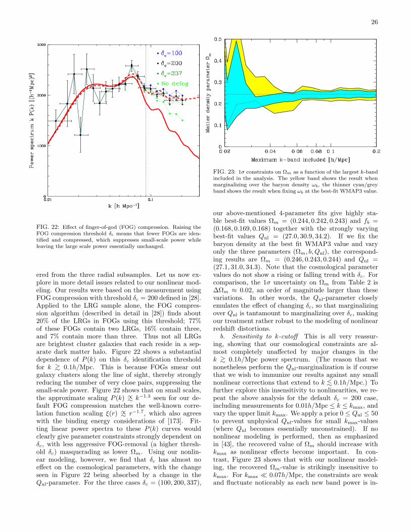
26

FIG. 22: Effect of finger-of-god (FOG) compression. Raising theFOG compression threshold δc means that fewer FOGs are iden-tified and compressed, which suppresses small-scale power whileleaving the large scale power essentially unchanged.

ered from the three radial subsamples. Let us now ex-plore in more detail issues related to our nonlinear mod-eling. Our results were based on the measurement usingFOG compression with threshold δc = 200 defined in [28].Applied to the LRG sample alone, the FOG compres-sion algorithm (described in detail in [28]) finds about20% of the LRGs in FOGs using this threshold; 77%of these FOGs contain two LRGs, 16% contain three,and 7% contain more than three. Thus not all LRGsare brightest cluster galaxies that each reside in a sep-arate dark matter halo. Figure 22 shows a substantialdependence of P (k) on this δc identification thresholdfor k ∼> 0.1h/Mpc. This is because FOGs smear outgalaxy clusters along the line of sight, thereby stronglyreducing the number of very close pairs, suppressing thesmall-scale power. Figure 22 shows that on small scales,the approximate scaling P (k) ∼∝ k−1.3 seen for our de-fault FOG compression matches the well-known corre-lation function scaling ξ(r) ∼∝ r−1.7, which also agreeswith the binding energy considerations of [173]. Fit-ting linear power spectra to these P (k) curves wouldclearly give parameter constraints strongly dependent onδc, with less aggressive FOG-removal (a higher thresh-old δc) masquerading as lower Ωm. Using our nonlin-ear modeling, however, we find that δc has almost noeffect on the cosmological parameters, with the changeseen in Figure 22 being absorbed by a change in theQnl-parameter. For the three cases δc = (100, 200, 337),

FIG. 23: 1σ constraints on Ωm as a function of the largest k-bandincluded in the analysis. The yellow band shows the result whenmarginalizing over the baryon density ωb, the thinner cyan/greyband shows the result when fixing ωb at the best-fit WMAP3 value.

our above-mentioned 4-parameter fits give highly sta-ble best-fit values Ωm = (0.244, 0.242, 0.243) and fb =(0.168, 0.169, 0.168) together with the strongly varyingbest-fit values Qnl = (27.0, 30.9, 34.2). If we fix thebaryon density at the best fit WMAP3 value and varyonly the three parameters (Ωm, b, Qnl), the correspond-ing results are Ωm = (0.246, 0.243, 0.244) and Qnl =(27.1, 31.0, 34.3). Note that the cosmological parametervalues do not show a rising or falling trend with δc. Forcomparison, the 1σ uncertainty on Ωm from Table 2 is∆Ωm ≈ 0.02, an order of magnitude larger than thesevariations. In other words, the Qnl-parameter closelyemulates the effect of changing δc, so that marginalizingover Qnl is tantamount to marginalizing over δc, makingour treatment rather robust to the modeling of nonlinearredshift distortions.

b. Sensitivity to k-cutoff This is all very reassur-ing, showing that our cosmological constraints are al-most completely unaffected by major changes in thek ∼> 0.1h/Mpc power spectrum. (The reason that wenonetheless perform the Qnl-marginalization is if coursethat we wish to immunize our results against any smallnonlinear corrections that extend to k ∼< 0.1h/Mpc.) Tofurther explore this insensitivity to nonlinearities, we re-peat the above analysis for the default δc = 200 case,including measurements for 0.01h/Mpc ≤ k ≤ kmax, andvary the upper limit kmax. We apply a prior 0 ≤ Qnl ≤ 50to prevent unphysical Qnl-values for small kmax-values(where Qnl becomes essentially unconstrained). If nononlinear modeling is performed, then as emphasizedin [43], the recovered value of Ωm should increase withkmax as nonlinear effects become important. In con-trast, Figure 23 shows that with our nonlinear model-ing, the recovered Ωm-value is strikingly insensitive tokmax. For kmax ≪ 0.07h/Mpc, the constraints are weakand fluctuate noticeably as each new band power is in-

27

cluded, but for kmax beyond the first baryon bump atk ∼ 0.07h/Mpc, both the central value and the measure-ment uncertainty remain essentially constant all the wayout to kmax = 0.2h/Mpc.

The above results tells us that, to a decent approxima-tion, our k ∼> 0.1/Mpc data are not contributing informa-tion about cosmological parameters, merely informationabout Qnl. Indeed, the error bar ∆Ωm is larger whenusing k < 0.2h/Mpc data and marginalizing over Qnl

then when using merely k < 0.09h/Mpc data and fixingQnl. In other words, our cosmological constraints comealmost entirely from the LRG power spectrum shape atk ∼< 0.1h/Mpc.

c. Comparison with other galaxy P (k)-measurements

Let us conclude this section by briefly comparing withΩm-values obtained from other recent galaxy clusteringanalyses.

Our WMAP3+LRG measurement Ωm = 0.24 ± 0.02has the same central as that from WMAP3 alone [7],merely with a smaller error bar, and the most recent2dFGRS team analysis also prefers Ωm ≈ 0.24 [37]. Thiscentral value is 1.5σ below the result Ωm = 0.30 ± 0.04reported from WMAP1 + SDSS main sample galaxies in[33]; part of the shift comes from the lower third peakin WMAP3 as discussed in Section IVB. Post-WMAP3results are also consistent with ours. Analysis of an in-dependent SDSS LRG sample with photometric redshiftsgave best-fit Ωm-values between 0.26 and 0.29 dependingon binning [41], while an independent analysis includ-ing acoustic oscillations in SDSS LRGs and main samplegalaxies preferred Ωm ≈ 0.256 [148].

The galaxy power spectra measured from the above-mentioned data sets are likely to be reanalysed as nonlin-ear modeling methods improve. This makes it interestingto compare their statistical constraining power. [41] doso by comparing the error bar ∆Ωm from fitting two pa-rameter (Ωm, b)-models to all k ≤ 0.2h/Mpc data, withall other parameters, including Qnl or other nonlinearmodeling parameters, fixed at canonical best fit values.This gives ∆Ωm ≈ 0.020 for 2dFGRS and ∆Ωm ≈ 0.012for for the SDSS LRG sample with photometric redshifts[41]. Applying the same procedure to our LRGs yields∆Ωm = 0.007. This demonstrates both the statisticalpower of our sample, and that our cosmological analysishas been quite conservative in the sense of marginalizingaway much of the power spectrum information (marginal-izing over Qnl doubles the error bar to ∆Ωm = 0.014).

3. Other issues

A fortunate side effect of improved cosmological preci-sion is that priors now matter less. Monte Carlo MarkovChain generators usually assume a uniform Bayesianprior in the space of its “work parameters”. For ex-ample, if two different papers parametrize the fluctua-tion amplitude with As and lnAs, respectively, they im-plicitly assign As-priors that are constant and ∝ 1/As,

respectively (the new prior picks up a factor from theJacobian of the parameter transformation). Such priordifferences could lead to substantial (∼ 1σ) discrepancieson parameter constraints a few years ago, when some pa-rameters were still only known to a factor of order unity.In contrast, Table 2 shows that most parameters are nowmeasured with relative errors in the range 1% − 10%.As long as these relative measurement errors are ≪ 1,such priors become unimportant: Since the popular re-parametrizations in the literature and in Table 2 involvesmooth functions that do not blow up except perhapswhere parameters vanish or take unphysical values, therelative variation of their Jacobian across the allowed pa-rameter range will be of the same order as the relativevariation of the parameters (≪ 1), i.e., approximatelyconstant. Chosing a uniform prior across the allowed re-gion in one parameter space is thus essentially equivalentto choosing a uniform prior across the allowed region ofanybody else’s favorite parameter space.

V. CONCLUSIONS

We have measured the large-scale real-space powerspectrum P (k) using luminous red galaxies in the SloanDigital Sky Survey (SDSS) with narrow well-behavedwindow functions and uncorrelated minimum-varianceerrors. The results are publicly available in an easy-to-use form at http://space.mit.edu/home/tegmark/sdss.html.

This is an ideal sample for measuring the large-scalepower spectrum, since its effective volume exceeds that ofthe SDSS main galaxy sample by a factor of six and thatof the 2dFGRS by an order of magnitude. Our resultsare robust to omitting purely angular and purely radialdensity fluctuations and are consistent between differ-ent parts of the sky. They provide a striking model-independent confirmation of the predicted large-scaleΛCDM power spectrum. The baryon signature is clearlydetected (at 3σ), and the acoustic oscillation scale pro-vides a robust measurement of the distance to z = 0.35independent of curvature and dark energy assumptions.

Although our measured power spectrum provides inde-pendent cross-checks on Ωm and the baryon fraction, ingood agreement with WMAP, its main utility for cosmo-logical parameter estimation lies in complementing CMBmeasurements by breaking their degeneracies; for exam-ple, Table 3 shows that it cuts error bars on Ωm, ωm

and h by about a factor of two for vanilla models (oneswith a cosmological constant and negligible curvature,tensor modes, neutrinos and running spectral index) andby up to almost an order of magnitude when curvature,tensors, neutrinos or w are allowed. We find that allthese constraints are essentially independent of scalesk > 0.1h/Mpc and associated nonlinear complications.

Since the profusion of tables and figures in Section IVcan be daunting to digest, let us briefly summarize themand discuss both where we currently stand regarding cos-

28

mological parameters and some outstanding issues.

A. The success of vanilla

The first obvious conclusion is that “vanilla rules OK”.We have seen several surprising claims about cosmologi-cal parameters come and go recently, such as a runningspectral index, very early reionization and cosmologicallydetected neutrino mass — yet the last two rows of Table 3show that there is no strong evidence in the data for anynon-vanilla behavior: none of the non-vanilla parametersreduces χ2 significantly relative to the vanilla case. TheWMAP team made the same comparison for the CMB-only case and came to the same conclusion [7]. Adding ageneric new parameter would be expected to reduce χ2 byabout unity by fitting random scatter. Although WMAPalone very slightly favor spatial curvature, this preferencedisappears when SDSS is included. The only non-vanillabehavior that is marginally favored is running spectralindex α < 0, although only at 1.6σ. This persistent suc-cess of the vanilla model may evoke disturbing parallelswith the enduring success of the standard model of par-ticle physics, which has frustrated widespread hopes forsurprises. However, the recent evidence for ns < 1 rep-resents a departure from the ns = 1 “vanilla lite” modelthat had been an excellent fit ever since COBE [149], andas we discuss below, there are good reasons to expect fur-ther qualitative progress soon.

B. Which assumptions matter?

When quoting parameter constraints, it is important toknow how sensitive they are to assumptions about bothdata sets and priors. The most important data assump-tions discussed in Section IVF are probably those aboutpolarized CMB foreground modeling for constraining τand those about nonlinear galaxy clustering modeling forconstraining the power spectrum shape. The effect of pri-ors on other parameters is seen by comparing the sevencolumns of Table 3, and the effect of including SDSS isseen by comparing odd and even rows.

WMAP alone has robustly nailed certain parametersso well that that neither adding SDSS information norchanging priors have any significant effect. Clearly in thiscamp are the baryon density ωb (constrained by WMAPeven-odd peak ratios) and the reionization optical depthτ (constrained by WMAP low-ℓ E-polarization); indeed,Table 1 in [39] shows that adding LyαF and other CMBand LSS data does not help here either. The spectral in-dex ns is also in this nailed-by-WMAP category as longas we assume that α is negligible; generic slow-roll infla-tion models predict |α| ∼< 10−3, well below the limits ofdetectability with current data sets.

For many other parameters, e.g., Ωm, h and tnow, theWMAP-only constraints are extremely sensitive to pri-ors, with the inclusion of SDSS information tightening

them by factors 2 - 10. The prior assumptions of thevanilla model (Ωk = r = fν = α = 0, w = −1) matter alot with WMAP alone, and when one of them is dropped,the best fit values of Ωm and h are typically very different,with much larger errors. These assumptions no longermatter much when SDSS is included, greatly simplify-ing the caveat list that the cautious cosmologist needs tokeep in mind. This is quite different from the recent past,when the joint constraints from older WMAP and SDSSdata were sensitive to prior assumptions such as spatialflatness [33]; a major reason for this change is clearlythe SDSS measurement of the baryon acoustic scale. In-deed, one of the most interesting results of our analysisis the strengthened evidence for a flat universe, with theconstraint on Ωtot tightening from 1.054+0.064

−0.046 (WMAP3

only) to 1.003+0.010−0.009 (WMAP3+SDSS).

In other words, large-scale cosmic clustering data nowrobustly constrain all the vanilla parameters, even whenany one of (fν , Ωk, r, fν , w) are included as in Table 3.If w is varied jointly with Ωk (as it arguably shouldbe [138]), one expects dramatically weakened constraintson the two (since two standard rulers cannot determinethe three parameters (w, Ωk, Ωm)), but rather unaffecteddegradation for the rest.

C. Other data

Our cosmological parameter analysis has been veryconservative, using the bare minimum number of datasets (two) needed to break all major degeneracies, andusing measurements which mainly probe the large-scalelinear regime. It is therefore interesting to compare ourresults with the complementary approach of [39] of push-ing the envelope by using essentially all available data(including LyαF, supernovae Ia and smaller-scale CMBexperiments), which gives tighter constraints at the costof more caveats. Comparing with the error bars in Ta-ble 1 of [39] shows that the additional data give merelymodest improvements for (ωb, ωd, ns, r, h), a halving ofthe error bars on Ωtot (still consistent with flatness),and great gains for α and Mν. These last two param-eters are strongly constrained by the small-scale LyαFinformation, with [39] reporting α = −0.015± 0.012 andMν/3 < 0.06 eV (95%), a factor of six below our con-straint and bumping right up against the atmosphericlower bound ∼ 0.04 eV. On the other hand, the sameanalysis also rules out the standard model with three ac-tive neutrino species at 2.5σ [39]; one can always worryabout pushing the envelope too far by underestimatingmodeling uncertainties and systematics. [39] also high-light interesting tension at the 2σ-level between the LyαFand WMAP3 data regarding the fluctuation amplitudeσ8, and weak gravitational lensing may emerge as the de-cisive arbiter here, by directly pinning down the matterfluctuation amplitude independently of bias [174, 175].

29

FIG. 24: 95% constraints in the (Ωm, Qnl) plane for vanilla mod-els. The shaded regions are ruled out by WMAP1 (red/dark grey),WMAP3 (orange/grey) and when adding SDSS LRG information.

D. Future challenges

The impressive improvement of cosmological measure-ments is likely to continue in coming years. For example,the SDSS should allow substantially better cosmologi-cal constraints from LRGs for several reasons. Whenthe SDSS-II legacy survey is complete, the sky area cov-ered should be about 50% larger than the DR4 samplewe have analyzed here, providing not only smaller er-ror bars, but also narrower window functions as the gapsin Figure 3 are filled in. Global photometric calibrationwill be improved [176]. Various approaches may allow di-rect measurements of the bias parameter b, e.g., galaxylensing [178], higher-order correlations [177], halo lumi-nosity modeling [179] and reionization physics [180]. Abias measurement substantially more accurate than our11% constraint from redshift space distortions would bea powerful degeneracy breaker. Figure 24 shows that ourother galaxy nuisance parameter, Qnl, is somewhat de-generate with Ωm, so improved nonlinear modeling thatreliably predicts the slight departure from linear theoryin the quasilinear regime from smaller scale data wouldsubstantially tighten our cosmological parameter con-straints. More generally, any improved modeling thatallows inclusion of higher k will help.

As a result of such data progress in many areas, pa-rameter constraints will clearly keep improving. Howgood is good enough? The baryon density ωb is a pa-rameter over which it is tempting to declare victory andmove on: The constraints on it from cosmic clusteringare in good agreement, and are now substantially tighterthan those from the most accurate competing techniqueagainst which it can be cross-checked (namely Big Bangnucleosynthesis), and further error bar reduction appearsunlikely to lead to qualitatively new insights. In con-trast, there are a number of parameters where cosmic

clustering constraints are only now beginning to bumpup against theory and other measurements, so that fur-ther sensitivity gains give great discovery potential. Wehave (ns, r, α, Ωk) to test inflation, Mν to cosmologicallydetect neutrino mass, w and more generally X(z) to con-strain dark energy, and σ8 to resolve tension betweendifferent cosmological probes.

Cosmology has now evolved from Alan Sandage’s“search for two numbers” (h, Ωm) to Alan AlexanderMilne’s “Now we are six” (h, Ωb, Ωc, σ8, ns, τ). Each timea non-trivial value was measured for a new parameter,nature gave up a valuable clue. For example, Ωc > 0revealed the existence of dark matter, ΩΛ > 0 revealedthe existence of dark energy and the recent evidence forns < 1 may sharpen into a powerful constraint on infla-tion. Milestones clearly within reach during the next fewyears include a measurement of ns < 1 at high signifi-cance and Mν > 0 from cosmology to help uncover theneutrino mass hierarchy. If we are lucky and r ∼ 0.1 (assuggested by classic inflation and models such as [152]),an r > 0 detection will push the frontier of our ignoranceback to 10−35s and the GUT scale. Then there is alwaysthe possibility of a wild surprise such as Ωtot 6= 1, large|α|, X(z) 6= 1, demonstrable non-Gaussianity, isocurva-ture contributions, or something totally unexpected. Ourresults have helped demonstrate that challenges relatedto survey geometry, bias and potential systematic errorscan be overcome, giving galaxy clustering a valuable roleto play in this ongoing quest for greater precision mea-surements of the properties of our universe.

Acknowledgments:

We thank Angelica de Oliveira-Costa, Kirsten Hub-bard, Oliver Zahn and Matias Zaldarriaga for helpfulcomments, and Dulce Goncalves de Oliveira-Costa forground support. We thank the WMAP team for mak-ing data and Monte Carlo Markov Chains public via theLegacy Archive for Microwave Background Data Analy-sis (LAMBDA) at http://lambda.gsfc.nasa.gov, andAnthony Lewis & Sarah Bridle for making their Cos-moMC software [102] available at http://cosmologist.info/cosmomc. Support for LAMBDA is provided by theNASA Office of Space Science.

MT was supported by NASA grants NAG5-11099 andNNG06GC55G, NSF grants AST-0134999 and 0607597,the Kavli Foundation, and fellowships from the Davidand Lucile Packard Foundation and the Research Corpo-ration. DJE was supported by NSF grant AST-0407200and by an Alfred P. Sloan Foundation fellowship.

Funding for the SDSS has been provided by the Al-fred P. Sloan Foundation, the Participating Institutions,the National Science Foundation, the U.S. Departmentof Energy, the National Aeronautics and Space Adminis-tration, the Japanese Monbukagakusho, the Max PlanckSociety, and the Higher Education Funding Council forEngland. The SDSS Web Site is http://www.sdss.org.

The SDSS is managed by the Astrophysical ResearchConsortium for the Participating Institutions. The Par-

30

ticipating Institutions are the American Museum of Nat-ural History, Astrophysical Institute Potsdam, Univer-sity of Basel, Cambridge University, Case Western Re-serve University, University of Chicago, Drexel Univer-sity, Fermilab, the Institute for Advanced Study, theJapan Participation Group, Johns Hopkins University,the Joint Institute for Nuclear Astrophysics, the KavliInstitute for Particle Astrophysics and Cosmology, theKorean Scientist Group, the Chinese Academy of Sci-ences (LAMOST), Los Alamos National Laboratory, theMax-Planck-Institute for Astronomy (MPIA), the Max-Planck-Institute for Astrophysics (MPA), New MexicoState University, Ohio State University, University ofPittsburgh, University of Portsmouth, Princeton Univer-sity, the United States Naval Observatory, and the Uni-versity of Washington.

APPENDIX A: POWER SPECTRUM

ESTIMATION DETAILS

1. Relation between methods for measuring the

power spectrum and correlation function

In this section, we clarify the relationship between dif-ferent popular techniques for quantifying galaxy cluster-ing with pair-based statistics, including correlation func-tion estimation with the “DD-2DR+RR” method [52, 53]and power spectrum estimation with the FKP [19], FFT[26, 29, 30, 38, 43] and PKL [23, 24, 27, 28, 34, 58] meth-ods.

Suppose we have Nd data points giving the comovingredshift space position vectors ri of galaxies numberedi = 1, Nd, and Nr random points si from a mock catalogwhich has the same selection function n(r) as the realdata. The number densities of data points and randompoints are then sums of Dirac δ-functions:

nd(r) =

Nd∑

i=1

δ(r − ri), (A1)

nr(r) =

Nr∑

i=1

δ(r − si). (A2)

By definition of the selection function n(r), the quantity

δ(r) ≡ nd(r) − αnr(r)

n(r), (A3)

where α ≡ Nd/Nr, is then an unbiased estimator of theunderlying density fluctuation field δ(r) in the sense that

〈δ〉 = δ, where the averaging is over Poisson fluctua-tions as customary. Except for the PKL method, alltechniques we will discuss take the same general form,weighting galaxy pairs in a form that depends only onthe position of each galaxy and on the distance betweenthe two, so we will now describe them all with a uni-fied notation. (For an even more general pair-weighting

formalism that also incorporates the PKL method, see[181].) As long as one uses Nr ≫ Nd random points,they will contribute negligible Poisson noise; their roleis in effect to evaluate certain cumbersome integrals byMonte Carlo integration.

Let us define the quantity

ξ[f ] ≡∫ ∫

w(r)δ(r)w(r′)δ(r′)f(|r − r′|)d3rd3r′. (A4)

Here w(r) and f(d) are the above-mentioned weight func-tions that depend on position and distance, respectively.As we will see, the “DD-2DR+RR”, FKP and FFT meth-ods simply correspond to different choices of w and f .Substituting equations (A1)-(A3) into equation (A4), wefind that

ξ[f ] = ξdd[f ] − 2ξdr[f ] + ξrr[f ], (A5)

where we have defined

ξdd[f ] ≡Nd∑

i=1

Nd∑

j=1

w(ri)w(rj)

n(ri)n(rj)f(|ri − rj |), (A6)

ξdr[f ] ≡ α

Nd∑

i=1

Nr∑

j=1

w(ri)w(sj)

n(ri)n(sj)f(|ri − sj |), (A7)

ξrr[f ] ≡ α2Nr∑

i=1

Nr∑

j=1

w(si)w(sj)

n(si)n(sj)f(|si − sj |), (A8)

As a first example, let us consider the FKP method[19]. This corresponds to [181]

f(d) = j0(kd), (A9)

w(r) ∝ n(r)

1 + n(r)P (k), (A10)

and turns ξ into the FKP estimator of the window-convolved power spectrum P (k). Here j0(x) ≡ sin(x)/x,w is normalized so that

∫w(r)2d3r = 1 and P is an a pri-

ori guess as to what the galaxy power spectrum is. Fordetails, see [181] around equations (25) and (56). The

main point is that Fourier transforming δ and averaging

|δ(k)|2 over a spherical shell in k-space gives the factor∫e−ik·|r−r

′|dΩk/4π = j0(k|r − r′|) = f . We apply thismethod to our LRG data and compare the results withthose of [43] in Figure 25, finding good agreement.

The FFT method [26, 29, 30, 38, 43] is identical tothe FKP method except for two simplifications: P inequation (A10) is taken to be a k-independent constantand the density field is binned onto a three-dimensionalgrid to replace the time-consuming double sums abovewith a fast Fourier transform.

The “DD-2DR+RR” method [52, 53] estimates thecorrelation function ξ(r) by the Landy-Szalay estimator

ξLS =ξdd − 2ξdr + ξrr

ξrr

, (A11)

31

FIG. 25: Comparison of power spectrum estimation techniques.Our FKP measurement without defogging is seen to agree quitewell with the measurement of [43] considering that the latter in-cludes also main sample galaxies with different β and small-scaleclustering properties. These curves cannot be directly comparedwith the PKL measurements or theoretical models, because theyare not corrected for the effects of redshift distortions, window func-tions and the integral constraint; the qualitative agreement that isnonetheless seen is as good as one could expect given these caveats.

which is often written informally as (DD − 2DR +RR)/RR. Here two common weighting choices in the lit-erature are w(r) = n(r) [52] and w(r) = n(r)/[1+ n(r)J ][53], where J ≡

∫ r

0 ξ(r′)d3r′ tends to be of the same orderof magnitude as P (k). To measure the binned correla-tion function using equations (A6)-(A8), one thus setsf(d) = 1 when d is inside the bin and f(d) = 0 other-wise.

These close relationships between the FKP, FFT and“DD-2DR+RR” methods lead to interesting conclusionsregarding all three methods.

First, it can be interesting for some applications to re-place J by P when measuring the correlation function,using w(r) = n(r)/[1+ n(r)P ], as was done for the analy-sis of the QDOT survey in [19] and for the LRG analysisin [36]. For instance, one could use a constant P evalu-ated at the baryon wiggle scale if the goal is to measurethe baryon bump in the correlation function.

Second, there is an interesting equivalence between themethods. For reasons that will become clear below, let us

refer to the numerator of equation (A11), ξdd−2ξdr + ξrr,as the “convolved” correlation function estimator and fullexpression ξLS as the “deconvolved” estimator. The in-formation content in the convolved and decovolved es-

timators is clearly the same, since dividing by ξrr inequation (A11) is a reversible operation. Moreover, it isstraightforward to show that the FKP estimator of P (k)is simply the 3D Fourier transform of the convolved cor-relation function estimator as long as the same weight-ing function w(r) is used for both. [182] also commenton this. (Note that this is a quite different statementfrom the well-known fact that P (k) is the 3D Fouriertransform of the correlation function ξ(r).) This im-plies that the measured FKP power spectrum and themeasured correlation function contain exactly the sameinformation. In particular, it means that cosmologicalconstraints from one are no better than cosmological con-straints from the other, since they should be identicalas long as window functions, covariance matrices, etc.,are handled correctly. (An analogous correspondence forpurely angular data is discussed in [183].) In contrast,the information content in the PKL measurement of thepower spectrum is not identical; it uses a more generalpair weighting than equation (A4) and by constructioncontains more cosmological information; a more detaileddiscussion of this point is given in Appendix A.3 in [184].

Third, this Fourier equivalence between the convolvedcorrelation function estimator and the FKP power spec-trum estimator sheds light on the fact that the decon-

volved correlation function estimator ξLS is unbiased

(〈ξ〉LS(d) = ξ(d), the true correlation function), whereasthe expectation value of the FKP estimator is merely thetrue power spectrum convolved with a so-called window

function. This difference stems from the division by ξrr

in equation (A11): Multiplication by ξrr in real space cor-

responds to convolution with the Fourier transform of ξrr

(the window function) in Fourier space. The reason thatone cannot deconvolve this windowing in Fourier space

is that one cannot Fourier transform ξLS , as it is com-pletely unknown for large d-values that exceed all pairseparations in the survey.

Fourth, this equivalence implies that gridding errors inthe 3D FFT method (which become important at large k[30]) can be completely eliminated by simply computingthe correlation function with w(r) = n(r)/[1 + n(r)P ]by summation over pairs and then transforming the con-volved correlation function with the kernel j0(kr).

Figure 25 compares the LRG power spectra measuredwith the different techniques discussed above. A directcomparison between our PKL P (k)-measurement andthat of [43] is complicated both by window function ef-fects and by the fact that the latter was performed in red-shift space without FOG compression, with SDSS MAINgalaxies mixed in with the LRG sample. To facilitatecomparison, we performed our own FKP analysis usingthe direct summation method as described above, withconstant P = 30000(h−1Mpc)3 and α ≈ 0.06. This isseen to agree with the measurement of [43] to within afew percent for 0.04h/Mpc < k < 0.2h/Mpc for the caseof no defogging, with the remaining differences presum-ably due mainly to the inclusion of main-sample galaxies,

32

particularly on small scales where nonlinear behavior be-comes important. Figure 25 also shows that our defoggedFKP measurements agree qualitatively between the PKLand FKP techniques, and that the FKP power spectrumcontinues to track our nonlinear WMAP model beauti-fully all the way out to k = 1h/Mpc even though Qnl wasonly fit to the k < 0.2h/Mpc PKL data.

An important caveat must be borne in mind when in-terpreting Figure 25: The PKL points are constructed insuch a way as to allow direct visual comparison with amodel power spectrum [28], but the FKP and [43] curvesare not, and should not be expected to fall right on topthe PKL points or the best-fit cosmological model be-cause they are not corrected for the effects of redshiftdistortions, window functions and the integral constraint.Redshift distortions should boost the FKP LRG curvesslightly above the true real space power spectrum (seeSection A3), and should boost the curve from Figure 25slightly more because the main sample galaxies have ahigher β than the LRGs. The FKP window functions arebroader than their PKL counterparts, and the steeper thepower spectrum is, the more power leaks in from largerscales, causing the plotted measurements to lie abovethe true power spectrum. Finally, the integral constraintsuppresses the plotted FKP power on the largest scales.In conclusion, the agreement seen in Figure 25 is as goodas one could expect given these many caveats.

2. Numerical acceleration of the PKL method

In this section, we describe a numerical improvementover the PKL power spectrum estimation method de-scribed in [28] that enables us to increase the number ofmodes from 4000 to 42,000.

The cosmological information content in a galaxy red-shift survey, quantified by the Fisher information matrix[46, 47, 57], scales approximately as the effective volumeVeff defined in equation (1), with error bars on cosmo-logical parameters optimally measured from the survey

scaling as V−1/2eff . However, actually extracting all this in-

formation in a numerically feasible way is far from trivial,contributing to the extensive literature on power spec-trum estimation methods.

Our PKL method expands the galaxy density field in Nfunctions (“PKL modes”) that probe successively smallerscales, and the number of modes needed to retain all in-formation down to some length scale λ = 2π/k is clearlyof order Veff/λ3. In [28], N = 4000 modes were used,and it was empirically determined that this retained es-sentially all information for k ∼< 0.1h/Mpc with a gradualtapering off towards smaller scales. This was a convenientcoincidence, since using N ≫ 4000 becomes numericallypainful: because of the many N × N matrix operationsinvolved in the analysis, the disk usage is about 80 GBtimes (N/4000)2 and the CPU time required on a currentworkstation is about 20 days times (N/4000)3.

The effective volume of our LRG sample is about

ten times larger than that of the above-mentioned maingalaxy analysis because the sky area covered has in-creased and because the sample is significantly deeper.To extract all the k ∼< 0.1h/Mpc information, we wouldtherefore like to use about ten times more modes, butwithout the analysis taking 103 times longer (∼ 50 years).

We therefore combine the method of [33] with a divide-and-conquer approach, performing a separate 2000-modeanalysis on each of the 21 sub-volumes described in Sec-tion II (3 radial × 7 angular subsets) and combining theresults with minimum-variance weighting (which, follow-ing the notation of [28], corresponds to simply summingboth the F-matrices and the q-vectors). Although thiscombined analysis with its 21×2000 = 42,000 modes be-comes lossless in the information theory sense on scalessubstantially smaller than each of the 21 sub-volumes,it destroys most of the information on scales compara-ble to these volumes, because the mean density in eachvolume is projected out (effectively marginalized over)[28]. It also becomes suboptimal on these largest scalesbecause it neglects correlations between different sub-volumes when optimizing the pair weighting. We there-fore complement the combined analysis with a 4000-modeglobal analysis of the entire volume, which is optimal onthe largest scales.

Both of these analyses produce uncorrelated bandpower estimators, and we use the first 8 (with k <0.04h/Mpc) from the global analysis and the remain-ing ones from the combined analysis. This splice pointwas chosen because the Fisher matrices show that theglobal analysis contains the most information (gives thesmallest power spectrum error bars) for smaller k, andthe combined analysis contains the most information forlarger k. For the radial subsamples, the correspondingsplice points are after bands 11 (NEAR), 10 (MID) and8 (FAR). We confirm that, as the above scaling argu-ments suggest, the two analyses give essentially identicalresults in the intermediate k-range where they both re-tain virtually all the information. For example, the twoanalyses agree for band number 9 to about 0.7% in power,a difference which is completely negligible compared tothe statistical error bars.

3. Redshift space distortion details

As described in detail in [28], our PKL method

produces three estimators (Pgg(k), Pgv(k), Pvv(k)) ofthe galaxy-galaxy, galaxy-velocity and velocity-velocitypower spectra (Pgg(k), Pgv(k), Pvv(k)). These estimatorsare uncorrelated, both with each other and between dif-ferent k-bands, but not unbiased: the expectation value

of Pgg(k), say, includes contributions from all three powerspectra. As explained in [28], we therefore construct our

final power spectrum estimator Pg as a linear combina-

tion of Pgg(k), Pgv(k) and Pvv(k) that makes it an anunbiased estimator of the real-space galaxy power spec-

33

trum Pgg(k). This linear combination corresponds tothe process of marginalizing over the relative amplitudesof Pgv(k) and Pvv(k), which according to equations (2)and (3) are βrgv and β2, respectively, so it can also bethought of as a marginalization over β and rgv.

Two ways of forming this linear combination were ex-plored in [28], referred to as the modeling method and thedisentanglement method, respectively. The former corre-sponds to marginalizing over β and rgv globally, treatingthem as scale-independent constants, whereas the lat-ter corresponds to treating them as arbitrary functionsof k and marginalizing over them separately for each k-band. We used the former approach for the “official”P (k)-measurement in [28] that was used for cosmologi-cal parameter estimation, and we make the same choicein the present paper, using only k < 0.09h/Mpc data tofind the best-fitting values (β, rgv) ≈ (0.3, 1). The latterapproach is more conservative, at the price of producingmuch larger error bars.

To facilitate the interpretation of our thus-measured

power spectrum Pg(k), it is helpful to re-express it interms of multipoles of the redshift space power spec-trum. In the small-angle (distant observer) approxima-tion where all galaxy pairs subtend a small angle relativeto the line of sight, (Pgg, Pgv, Pvv) reduce to simple linearcombinations of the monopole, quadrupole and hexade-capole power spectra in redshift space [185, 186]:

Pgg(k)

Pgv(k)

Pvv(k)

=

1 − 12

38

0 34 − 15

8

0 0 358

P s0(k)

P s2(k)

P s4(k)

. (A12)

Inverting equation (A12) gives

P s0(k)

P s2(k)

P s4(k)

=

1 23

15

0 43

47

0 0 835

Pgg(k)

Pgv(k)

Pvv(k)

. (A13)

Equation (A12) tells us that, in the small angle approxi-mation, the disentanglement method would correspond

to measuring 〈Pg(k)〉 = P s0(k) − 1

2P s2 (k) + 3

8P s4(k) =

Pgg(k). The corresponding weights for the modelingmethod are found by minimizing the variance amongthe class of all unbiased estimators, and thus depend onthe detailed survey geometry, the shot noise level, etc.

Empirically, we find 〈Pg(k)〉 ≈ 0.8P s0(k) − 0.07P s

2(k) +0.006P s

4(k), with the weights roughly independent of k.This can be intuitively understood from the fact thatthe estimators of P s

2 and P s4 are much noisier than that

for P s0 , and thus get assigned low statistical weight.

If P s2 and P s

4 were so noisy that they were discardedaltogether, only the estimator of P s

0 would be used.The relation P s

0 (k) =(1 + 2

3rgvβ + 15β2

)Pgg(k) follow-

ing from equation (A13) would then give the simple es-

timator Pg(k) = P s0(k)/

(1 + 2

3rgvβ + 15β2

)≈ 0.8P s

0(k)for β = 0.3, rgv = 1, i.e., weights close to those we find

empirically. Our measured uncertainty in this normaliza-tion factor

(1 + 2

3rgvβ + 15β2

)is about 3% (see Figure 8),

in good agreement with the exact numerical calculationdescribed in [28], and this translates into an overall 3%calibration uncertainty of our measured power spectrumwhich is perfectly correlated between all k-bands.

The fact that the quantity measured by our power

spectrum estimator Pg(k) is so similar to the rescaledredshift space monopole spectrum is convenient, since itimplies that nonlinear simulations of the redshift spacepower spectrum (as discussed in Section III D) should ap-ply rather well to our results. However, it is important to

keep in mind that our measurement Pg(k) is a more accu-rate estimator of Pgg(k) than the rescaled redshift spacepower spectrum would be, for several reasons. First, itnever resorts to the small-angle approximation. Second,full account is taken of the fact that anisotropic surveygeometry can skew the relative abundance of galaxy pairsaround a single point that are aligned along or perpen-dicularly to the line-of-sight. These two caveats mat-ter because P s

2(k) and P s4(k) are undefined except in the

small angle limit, which could cause the correction fac-tor

(1 + 2

3rgvβ + 15β2

)to be inaccurate on large scales.

Finally, our estimator Pg(k) by construction has smallererror bars than a standard FKP estimator of the redshiftspace power spectrum, and one expects this advantage tobe most important on the largest scales, comparable toand exceeding the thickness of the slices seen in Figure 3.

4. How spacetime geometry affects the power

spectrum measurement

We performed our power spectrum analysis in comov-ing three-dimensional space, with the conversion of red-shifts into comoving distances performed for a fiducialflat ΛCDM model with Ωm = 0.25. As described inSection IVC 1, the conversion between redshift and co-moving distance (measured in h−1Mpc) depends on thecosmological parameters (Ωm, Ωtot, w), so if a differentfiducial model had been used for the conversion, then theinferred three-dimensional galaxy distribution in comov-ing coordinates would be radially dilated. As discussedin [36] and Section IVC 1, this would approximately di-late the dimensionless power spectrum k3P (k) by scalingthe k-axis by a factor

a ≡ dV (z)

dfiducialV (z)

, (A14)

where dV (z) is given by equation (9) and z = 0.35 is themedian survey redshift. For the parameter range allowedby WMAP3 and our LRG data,

a ≈(

Ωm

0.25

)−0.087

(−wΩtot)0.19. (A15)

This means that the typical correction is very small: therms scatter in the scaling factor a is 0.7% for vanilla

34

models, 1% for curved models and 3% for w-models. Forexample, increasing the fiducial Ωm-value by 25%, from0.24 to 0.30, alters the scaling factor by 2% and, sincethe power spectrum turnover scale ∝ Ωm, ignoring thiscorrection could potentially bias the measured Ωm-valuefrom 0.240 to 0.245.

To be conservative, we nonetheless correct for thisscaling effect in our likelihood software. Reanalyzingthe galaxy data with the fiducial model replaced bythe one to be tested would shift the measured P (k)curve up to the left on a log-log plot if a > 1, withk 7→ k/a and P 7→ Pa3. We therefore apply the op-posite scaling (k 7→ ka and P 7→ P/a3) to the the-

oretically predicted power spectrum P (k) before com-puting its χ2 against our measurement power spectrumfrom Table 1. We repeated our entire power spectrumanalysis for Ωm = 0.30 and confirmed that this scalingis accurate. Our likelihood software, which is availableat http://space.mit.edu/home/tegmark/sdss/, eval-uates a exactly instead of using equation (A15).

In summary, the correction discussed in this sectionis quite small, especially since marginalizing over biaserases the effect of the a3 amplitude shift, but we includeit anyway to ensure that there is no bias on cosmologicalparameter estimates.

[1] G. Hinshaw et al., astro-ph/0603451 (2006)[2] L. Page et al., astro-ph/0603450 (2006)[3] S. Masi, astro-ph/0507509 (2005)[4] J. Sievers et al., astro-ph/0509203 (2005)[5] D. J. Eisenstein, W. Hu, and M. Tegmark, ApJ, 518, 2

(1999)[6] G. Efstathiou and J. R. Bond, MNRAS, 304, 75 (1999)[7] D. N. Spergel et al., astro-ph/0603449 (2006)[8] J. P. Huchra, M. J. Geller, V. de Lapparent, and II. G.

Jr Corwin, ApJS, 72, 433 (1990)[9] E. E. Falco et al., PASP, 111, 438 (1999)

[10] S. A. Shectman et al., ApJ, 470, 172 (1996)[11] W. Saunders et al., MNRAS, 317, 55 (2000)[12] M. C. Cooper et al., astro-ph/0607512 (2006)[13] M. Colless et al., astro-ph/0306581 (2003)[14] D. G. York et al., Astron.J., 120, 1579 (2000)[15] M.. S. Vogeley, C. Park, M. J. Geller, and J. P. Huchra,

ApJ, 391, L5 (1992)[16] K. B. Fisher, M. Davis, M. A. Strauss, A. Yahil, and J.

P. Huchra, ApJ, 402, 42 (1993)[17] C. Park, M. S. Vogeley, M. J. Geller, and J. P. Huchra,

ApJ, 431, 569 (1994)[18] L. N. da Costa, M. S. Vogeley, M. J. Geller, J. P. Huchra,

and C. Park, ApJ, 437, L1 (1994)[19] H. A. Feldman, N. Kaiser, and J. A. Peacock, ApJ, 426,

23 (1994)[20] H. Tadros and Efstathiou G, MNRAS, 276, L45 (1995)[21] H. Tadros and Efstathiou G, MNRAS, 282, 1381 (1996)[22] H. Lin et al., ApJ, 471, 617 (1996)[23] N. Padmanabhan, M. Tegmark, and Hamilton A J S,

ApJ, 550, 52 (2001)[24] A. J. S Hamilton, M. Tegmark, and N. Padmanabhan,

MNRAS, 317, L23 (2000)[25] A. J. S Hamilton M. Tegmark, MNRAS;330;506-530

(2002)[26] W. J. Percival et al., MNRAS, 327, 1297 (2001)[27] M. Tegmark, A. J. S Hamilton, and Y. Xu, MNRAS,

335, 887 (2002)[28] M. Tegmark et al., ApJ, 606, 702 (2004)[29] S. Cole et al., MNRAS, 362, 505 (2005)[30] G. Hutsi, A&A, 449, 891 (2006)[31] X. Wang, M. Tegmark, and M. Zaldarriaga, Phys. Rev.

D, 65, 123001 (2002)[32] D. N. Spergel et al., ApJS, 148, 175 (2003)[33] M. Tegmark et al., PRD, 69, 103501 (2004)

[34] A. C. Pope et al., ApJ, 607, 655-660 (2004)[35] U. Seljak et al., PRD;71;103515 (2005)[36] D. J. Eisenstein et al., ApJ, 633, 560 (2005)[37] A. G. Sanchez, C. M. Bauch, W. J. Percival, N. D.

Padilla, S. Cole, C. S. Frenk, and P. Norberg, MNRAS,366, 189 (2006)

[38] G. Hutsi, astro-ph/0604129 (2006)[39] U. Seljak, A. Slosar, and P. McDonald, astro-

ph/0604335 (2006)[40] M. Viel, M. G. Haehnelt, and A. Lewis, MNRAS, 370,

L51 (2006)[41] N. Padmanabhan et al., astro-ph/0605302 (2006)[42] C. Blake, A. Collister, S. Bridle, and O. Lahav, astro-

ph/0605303 (2006)[43] W. J. Percival et al., astro-ph/0608636 (2006)[44] J. Adelman-McCarthy et al. 2006, in preparation[45] M. S. Vogeley and A. S. Szalay, ApJ, 465, 34 (1996)[46] M. Tegmark, A. N. Taylor, and A. F. Heavens, ApJ,

480, 22 (1997)[47] M. Tegmark, Phys. Rev. Lett., 79, 3806 (1997)[48] N. Kaiser, MNRAS, 219, 785 (1986)[49] D. J. Eisenstein et al., AJ, 122, 2267 (2001)[50] M. A. Strauss et al., AJ, 124, 1810 (2002)[51] G. Richards et al., AJ, 123, 2945 (2002)[52] S. D. Landy and A. S. Szalay, ApJ, 412, 64 (1993)[53] A. J. S Hamilton, ApJ, 417, 19 (1993)[54] E. Hawkins et al., MNRAS, 346, 78 (2003)[55] D. J. Eisenstein et al., ApJ, 619, 178 (2005)[56] I. Zehavi et al., ApJ, 621, 22 (2005)

[57] K. Karhunen, Uber lineare Methoden in derWahrscheinlichkeitsrechnung (Kirjapaino oy. sana,Helsinki, 1947).

[58] A. J. S Hamilton, astro-ph/0503604 (2005)[59] J. A. Peacock and D. Nicholson, MNRAS, 253, 307

(1991)[60] C. Stoughton et al., AJ, 123, 485 (2002)[61] J. E. Gunn, M. A. Carr, C. M. Rockosi, M. Sekiguchi

et al., Astron. J., 116, 3040 (1998)[62] J. E. Gunn, W. A. Siegmund, E. J. Mannery, E. J. Owen

et al., AJ, 131, 2332 (2006)[63] M. Fukugita, T. Ichikawa, J. E. Gunn, M. Doi, K. Shi-

masaku , and D. P. Schneider, Astron. J., 111, 1748(1996)

[64] J. R. Pier et al., AJ, 125, 1559 (2003)[65] R. H. Lupton, J. E. Gunn, Z. Ivezic, G. R. Knapp, S.

35

Kent, and N. Yasuda 2001, in ASP Conf. Ser. 238,Astronomical Data Analysis Software and Systems X,ed. F. R. Harnden, Jr., F. A. Primini, and H. E. Payne(Astron. Soc. Pac.: San Francisco;269)

[66] R. H. Lupton et al. 2006, Astron J., submitted[67] D. W. Hogg, D. P. Finkbeiner, D. J. Schlegel, and J. E.

Gunn, AJ, 122, 2129 (2001)[68] J. A. Smith et al., AJ, 123, 2121 (2002)[69] Z. Ivezic, R. H. Lupton, D. Schlegel et al., As-

tron. Nachrichten, 325, 583 (2004)[70] D. Tucker, S. Kent, M. S. Richmond et al., As-

tron. Nachrichten, in press (2006)[71] D. J. Schlegel, D. P. Finkbeiner, and M. Davis, ApJ,

500, 525 (1998)[72] M. R. Blanton, R. H. Lupton, F. M. Maley, N. Young,

I. Zehavi, and J. Loveday, AJ, 125, 2276 (2003)[73] A. Uomoto et al., SPIE, 5492, 1411 (2004)[74] J. Adelman-McCarthy et al., ApJS, 162, 38 (2006)[75] M. R. Blanton et al., AJ, 129, 2562 (2005)[76] A. J. S Hamilton and M. Tegmark, MNRAS, 349, 115

(2004)[77] J. A. Peacock and S. J. Dodds, MNRAS, 267, 1020

(1994)[78] J. N. Fry, ApJ, 461, L65 (1996)[79] M. Tegmark and P. J. E Peebles, ApJL, 500, 79 (1998)[80] H. J. Mo and S. D. M White, MNRAS, 282, 347 (1996)[81] M. Giavalisco et al., ApJ, 503, 543 (1998)[82] N. Kaiser, MNRAS, 227, 1 (1987)[83] A. Dekel and O. Lahav, ApJ, 520, 24 (1999)[84] U. Pen, ApJ, 504, 601 (1998)[85] A. J. S Hamilton, MNRAS, 322, 419 (2001)[86] M. Blanton R, R. Cen, J. P. Ostriker, M. A. Strauss,

and M. Tegmark, ApJ, 531, 1 (2000)[87] V. Wild et al., MNRAS, 356, 247 (2005)[88] D. J. Eisenstein, H. Seo, and M. White, astro-

ph/0604361 (2006)[89] D. J. Eisenstein and W. Hu, ApJ, 511, 5 (1999)[90] H. Seo and D. J. Eisenstein, ApJ, 633, 575 (2005)[91] V. Springel, C. S. Frenk, and S. D. M White, 2006, 440,

1137 (Nature)[92] E. Huff, A. E. Schultz, M. White, D. J. Schlegel, and M.

S. Warren, astro-ph/0607061 (2006)[93] J. Yoo et al., in preparation (2006)[94] P. McDonald, astro-ph/0609413 (2005)[95] R. E. Smith, R. Scoccimarro, and R. K. Sheth, astro-

ph/0609547 (2006)[96] S. Bashinsky and E. Bertschinger, PRD, 65, 123008

(2002)[97] N. Y. Gnedin and O. Y. Gnedin, ApJ, 509, 11 (1998)[98] N. Metropolis, A. W. Rosenbluth, M. N. Rosenbluth, A.

H. Teller, and E. Teller, J.Chem.Phys., 21, 1087 (1953)[99] W. K. Hastings, Biometrika, 57, 97 (1970)

[100] W. R. Gilks, S. Richardson, and D. J. Spiegelhalter,Markov Chain Monte Carlo in Practice (Chapman &Hall: London, 1996)

[101] N. Christensen, R. Meyer, L. Knox, and B. Luey, Class.Quant. Grav., 18, 2677 (2001)

[102] A. Lewis and S. Bridle, PRD, 66, 103511 (2002)[103] A. Slosar and M. Hobson, astro-ph/0307219 (2003)[104] L. Verde et al., ApJS, 148, 195 (2003)[105] M. Chu, M. Kaplinghat, and L. Knox, ApJ, 596, 725

(2003)[106] H. Sandvik, M. Tegmark, X. Wang, and M. Zaldarriaga,

PRD, 69, 063005 (2004)

[107] E. W. Kolb and M. S. Turner, The Early Universe (Ad-dison Wesley: New York, 1990)

[108] W. Hu, astro-ph/0407158 (2005)[109] M. Tegmark, J. Silk, and A. Blanchard, ApJ, 420, 484

(1994)[110] M. Tegmark and M. J. Rees, ApJ, 499, 526 (1998)[111] M. Tegmark, A. Vilenkin, and L. Pogosian, PRD, 71,

103523 (2005)[112] W. Hu, M. Fukugita, M. Zaldarriaga, and M. Tegmark,

ApJ, 549, 669 (2001)[113] U. Seljak, and M. Zaldarriaga, ApJ, 469, 437 (1996)[114] A. Lewis and A. Challinor, PRD, 66, 023531 (2002)[115] M. Tegmark, A. Aguirre, M. J. Rees, and F. Wilczek,

Phys. Rev. D, 73, 023505 (2006)[116] J. D. Barrow and F. J. Tipler, The Anthropic Cosmo-

logical Principle (Clarendon Press: Oxford, 1986)[117] A. D. Linde 1987, in 300 Years of Gravitation, ed. S.

Hawking and W. Israel (Cambridge University Press:Cambridge)

[118] S. Weinberg, PRL, 59, 2607 (1987)[119] G. Efstathiou, MNRAS, 274, L73 (1995)[120] A. Vilenkin, PRL, 74, 846 (1995)[121] H. Martel, P. R. Shapiro, and S. Weinberg, ApJ, 492,

29 (1998)[122] J. Garriga and A. Vilenkin, PRD, 67, 43503 (2003)[123] M. Tegmark, JCAP, 2005-4, 1 (2005)[124] A. Kosowsky, M. Milosavljevic, and Jimenez R, PRD,

66, 73007 (2002)[125] R. Jimenez, L. Verde, H. Peiris, and A. Kosowsky, PRD,

70, 023005 (2004)[126] W. A. Fendt and B. Wandelt D, astro-ph/0606709

(2006)[127] A. Lewis, astro-ph/0603753 (2006)[128] Y. Wang and M. Tegmark, PRL, 92, 241302 (2004)[129] Y. Wang and P. Mukherjee, astro-ph/0604051 (2006)[130] D. J. Eisenstein, W. Hu, and M. Tegmark, ApJL, 504,

L57 (1998)[131] C. Blake and K. Glazebrook, ApJ, 594, 665 (2003)[132] B. M. S Hansen et al., ApJ, 574, L155 (2002)[133] A. Linde, JCAP, 305, 2 (2003)[134] G. Efstathiou, MNRAS, 343, L95 (2003)[135] A. D. Linde, Phys. Lett. B, 351, 99 (1995)[136] A. Vilenkin and S. Winitzki, Phys. Rev. D, 55, 548

(1997)[137] W. L. Freedman et al., ApJ, 553, 47 (2001)[138] E. L. Wright, astro-ph/0603750 (2006)[139] A. Guth, PRD, 23, 347 (1981)[140] A. A. Starobinsky, Phys. Lett. B, 91, 99 (1980)[141] A. D. Linde, Phys. Lett. B, 108, 389 (1982)[142] A. Albrecht and P. J. Steinhardt, Phys. Rev. Lett., 48,

1220 (1982)[143] A. D. Linde, Phys. Lett. B, 129, 177 (1983)[144] J. Bock et al., astro-ph/0604101 (2006)[145] J. Khoury, B,. OvrutSteinhardt. P. . J, and N. Turok,

PRD, 64, 123522 (2001)[146] J. Khoury, P. J. Steinhardt, and N. Turok, PRL, 91,

161301 (2003)[147] P. Creminelli, A. Nicolis, and M. Zaldarriaga, PRD, 71,

063505 (2005)[148] W. J. Percival et al. 2006, astro-ph/0608635, submitted

to ApJL[149] G. F. Smoot et al., ApJ, 396, L1 (1992)[150] A. R. Liddle and S. M. Leach, PRD, 68, 103503 (2003)[151] C. McTavish et al., astro-ph/0507503 (2005)

36

[152] S. Dimopoulos, S. Kachru, J. McGreevy, and J. Wacker,hep-th/0507205 (2005)

[153] R. Easther and L. McAllister, JCAP, 0605, 018 (2006)[154] H. Peiris and R. Easther, JCAP, 07, 002 (2006)[155] W. H. Kinney, E. W. Kolb, A. Melchiorri, and A. Ri-

otto, astro-ph/0605338 (2006)[156] J. Martin and R. Ringeval, astro-ph/0605367 (2006)[157] H. K. Erikssen et al., astro-ph/0606088 (2006)[158] K. M. Huffenberger, H. K. Eriksen, and F. K. Hansen,

astro-ph/0606538 (2006)[159] A. R. Liddle, P. Mukherjee, and D. Parkinson, astro-

ph/0608184 (2006)[160] B. Feng, J. Xia, and J. Yokohama, astro-ph/0608365

(2006)[161] W. Hu, D. J. Eisenstein, and M. Tegmark, PRL, 79,

3806 (1998)[162] A. Goobar, S. Hannestad, E. Mortsell, and H. Tu,

JCAP, 06, 019 (2006)[163] J. Lesgourges and S. Pastor, Phys.Rep., 429, 307 (2006)[164] M. Fukugita, K. Ichikawa, M. Kawasaki, and O. Lahav,

PRD, 74, 027302 (2006)[165] M. Cirelli and A. Strumia, astro-ph/0607086 (2006)[166] S. Hannestad and G. Raffelt, astro-ph/0607101 (2006)[167][168] S. King, hep-ph/0310204 (2003)[169] Y. Ashie et al., PRD, 71, 112005 (2005)

[170] W. A. Chiu, X. Fan, and J. P. Ostriker, ApJ, 599, 759(2003)

[171] X. Fan et al., AJ, 132, 117 (2006)[172] Zahn, O. et al., in preparation (2006)[173] M. Fukugita and P. J. E Peebles, ApJ, 616, 643 (2004)[174] M. Jarvis, B. Jain, G. Bernstein, and D. Dolney, ApJ,

644, 71 (2006)[175] A. F. Heavens, T. B. Kitching, and A. N. Taylor, astro-

ph/0606568 (2006)[176] N. Padmanabhan et al. 2006, in preparation[177] L. Verde et al., MNRAS, 335, 432 (2002)[178] U. Seljak et al., PRD, 71, 3511 (2005)[179] J. P. Ostriker and A. Vale, astro-ph/0511816 (2005)[180] W. A. Chiu, X. Fan, and J. P. Ostriker, ApJ, 599, 759

(2003)[181] M. Tegmark, A. J. S Hamilton, M. A. Strauss, M. S.

Vogeley, and A. S. Szalay, ApJ, 499, 555 (1998)[182] I. Szapudi and A. S. Szalay, ApJL, 494, L41 (1998)[183] I. Szapudi, S. Prunet, D. Pogosyan, A. S. Szalay, and J.

R. Bond, ApJ, 548, L115 (2001)[184] M. Tegmark et al., ApJ, 571, 191 (2002)[185] S. Cole, K. B. Fisher, and D. H. Weinberg, MNRAS,

267, 785 (1994)[186] A. J. S Hamilton 1998, in The Evolving Universe, ed.

D. Hamilton (Dordrecht: Kluwer), p185