arX

iv:a

stro

-ph/

0307

371v

1 2

1 Ju

l 200

3

SDSS J0903+5028: A New Gravitational Lens

David E. Johnston,1,2 Gordon T. Richards,3 Joshua A. Frieman,1,2,4 Charles R. Keeton,1,5

Michael A. Strauss,3 Robert H. Becker,6,7 Richard L. White ,8 Eric T. Johnson,2 Zhaoming Ma,1

Mark SubbaRao,1,9 Neta A. Bahcall ,3 Mariangela Bernardi ,18 Jon Brinkmann, 10 Daniel J.

Eisenstein, 11 Masataka Fukugita, 12 Patrick B. Hall,3,13 Naohisa Inada,14 Gillian R. Knapp,3

Bartosz Pindor,3 David J. Schlegel 3 Ryan Scranton,15 Erin S. Sheldon,1,2 Donald P. Schneider ,16 Alexander S. Szalay, 17 and Donald G. York 1

ABSTRACT

We report the discovery of a new gravitationally lensed quasar from the Sloan Dig-

ital Sky Survey, SDSS J090334.92+502819.2. This object was targeted for SDSS spec-

troscopy as a Luminous Red Galaxy (LRG), but manual examination of the spectrum

showed the presence of a quasar at z ≃ 3.6 in addition to a red galaxy at z = 0.388, and

1Department of Astronomy and Astrophysics, The University of Chicago, 5640 South Ellis Avenue, Chicago, IL

60637.

2Center for Cosmological Physics, The University of Chicago, 5640 South Ellis Avenue, Chicago, IL 60637.

3Princeton University Observatory, Peyton Hall, Princeton, NJ 08544.

4Fermi National Accelerator Laboratory, P.O. Box 500, Batavia, IL 60510.

5Hubble Fellow.

6Physics Department, University of California, Davis, CA 95616.

7IGPP-LLNL, L-413, 7000 East Avenue, Livermore, CA 94550.

8Space Telescope Science Institute, 3700 San Martin Drive, Baltimore, MD 21218.

9Adler Planetarium & Astronomy Museum, Chicago, IL 60605.

10Apache Point Observatory, 2001 Apache Point Road, P.O Box 59,Sunspot, NM, 88349

11Steward Observatory, University of Arizona, 933 North Cherry Avenue, Tucson, AZ 85721.

12Institute for Cosmic Ray Research, University of Tokyo, 5-1-5 Kashiwa, Kashiwa City, Chiba 277-8582.

13Departamento de Astronomia y Astrofisica, Facultad de Fisica, Pontificia Universidad Catolica de Chile, Casilla

306, Santiago 22, Chile.

14Department of Physics, University of Tokyo, Hongo 7-3-1, Bunkyo-ku, Tokyo, 113-0033, Japan.

15Department of Physics & Astronomy, University of Pittsburgh, 3941 O’Hara St., Pittsburgh, PA 15260.

16Department of Astronomy and Astrophysics, The Pennsylvania State University, 525 Davey Laboratory, Univer-

sity Park, PA 16802

17Department of Physics and Astronomy, The Johns Hopkins University, Baltimore, MD 21218

18Department of Physics, Carnegie Mellon University, Pittsburgh, PA 15213

– 2 –

the SDSS image showed a second possible QSO image nearby. Follow-up imaging and

spectroscopy confirmed the lensing hypothesis. In images taken at the ARC 3.5-meter

telescope, two quasars are separated by 2.′′8; the lensing galaxy is clearly seen and is

blended with one of the quasar images. Spectroscopy taken at the Keck II telescope

shows that the quasars have identical redshifts of z ≃ 3.6 and both show the presence

of the same broad absorption line-like troughs. We present simple lens models which

account for the geometry and magnifications. The lens galaxy lies near two groups of

galaxies and may be a part of them. The models suggest that the groups may contribute

considerable shear and may have a strong effect on the lens configuration.

Subject headings: gravitational lensing—quasars: individual (SDSS J090334.92+502819.2)

1. Introduction

Gravitational lenses have become important astrophysical and cosmological tools in several

ways. The frequency of lensing is in principle sensitive to the dark energy density (Fukugita et al.

1990, Turner 1990, Fukugita & Turner 1991, Kochanek 1995, but see Keeton 2002) and the mat-

ter density of the Universe (Mortlock & Webster 2000a). Lens statistics also probe the properties

of the lensing galaxy systems, such as their mass distribution, potential well depth and extinc-

tion (Chen et al. 1995; Chae et al. 1998; Keeton et al. 1998; Malhotra et al. 1997; Keeton 2001a;

Keeton & Madau 2001). In addition, measurement of the time delay between images in individual

lensed quasars can be used to measure the Hubble parameter (Refsdal 1964).

Since the discovery of the first double quasar Q0957+561 (Walsh et al. 1979; Schild & Thompson 1997),

about 80 lensed quasars have been discovered19. In this paper, we report the discovery of another

lensed quasar, SDSS J090334.92+502819.2 (hereafter SDSS J0903+5028), discovered in the Sloan

Digital Sky Survey data (SDSS; (York et al. 2000)). There have been several gravitational lenses

discovered previously in the SDSS data (Inada et al. 2003a; Inada et al. 2003b; Burles et al. 2003;

Pindor et al. 2003b; Morgan et al. 2003), but this one is unusual in the way it was found. The stan-

dard algorithm for selecting lens candidates in the SDSS involves looking for deviations from PSF

profiles for spectroscopically confirmed quasars (Inada et al. 2003a; Pindor et al. 2003a). By con-

trast, SDSS J0903+5028 was selected for follow-up based on the presence of z ≃ 3.6 quasar features

superimposed on the SDSS fiber spectrum of a z = 0.388 luminous red galaxy (LRG). Moreover,

the SDSS image showed another source about 2.′′5 from the spectroscopically targeted galaxy as

well as the presence of surrounding galaxies with colors similar to the LRG. While this system

may be unusual, it is not unprecedented: the well-known lens 2237+0305 (Huchra et al. 1985) was

discovered serendipitously in a galaxy redshift survey, and such cases are expected (Kochanek 1992;

Mortlock & Webster 2000b).

19see http://cfa-www.harvard.edu/castles/

– 3 –

Follow-up spectroscopy at the ARC 3.5-meter telescope showed that both main image compo-

nents contain flux from a z ≃ 3.6 quasar with strong BAL-like associated absorption (Foltz et al. 1986),

strongly suggesting that this is a lensed system. Subsequent r and i band imaging at the ARC

3.5-meter telescope in better seeing revealed the lens geometry more clearly, as shown in Figure 1,

and enabled us to model the lens system. Finally, higher signal-to-noise ratio, higher-resolution

spectra were taken at the Keck II telescope. Taken together, these data make a firm case that

SDSS J0903+5028 comprises two images of a high-redshift quasar lensed by a massive, red, fore-

ground galaxy in a group.

This paper is organized as follows. In Section 2 we describe the SDSS data on this object,

discuss how it was selected for follow-up, and describe the spectroscopic and imaging data from the

ARC 3.5m telescope and spectroscopic data from the Keck telescope. In Section 3, we fit a simple

two-quasar + galaxy model to the ARC 3.5m images and extract positions and magnitudes for the

three components. With this information, we fit a lens model, estimate the velocity dispersion of

the lens galaxy, and study the quadrupole moment of the lensing potential. We also decompose

the SDSS and Keck spectra into quasar and galaxy components and find flux ratios consistent with

the imaging data. We conclude in Section 4.

2. Observations

The data on SDSS J0903+5028 consist of the following. The object was observed in routine

SDSS imaging in January 2001. Based on its colors and brightness, it was targeted for SDSS

spectroscopy as a luminous red galaxy (LRG) and spectroscopic observations were taken in March

2001. Due to the presence of both quasar and galaxy features in the SDSS spectrum, the object

was included in a list of promising lens candidates for follow-up observations. Spectroscopy of the

two main components on the ARC 3.5m telescope in October 2002 revealed that they both contain

very similar quasar features in addition to galaxy spectral features. This observation was followed

by higher quality spectroscopy with the Keck II telescope and deeper, better seeing-quality imaging

data with the ARC 3.5m telescope. In the following, we describe each of these data sets in detail.

2.1. SDSS Data

The Sloan Digital Sky Survey is a wide-field photometric and spectroscopic survey being carried

out by the Astrophysical Research Consortium (ARC) at the Apache Point Observatory in New

Mexico (York et al. 2000). The SDSS multi-CCD camera (Gunn et al. 1998) will produce images

for ∼ 5× 108 objects in five optical bands u, g, r, i, z to a detection limit of approximately r = 22.2.

The photometric pipeline software is described in Lupton et al. (2001). The photometric calibration

is described in Fukugita et al. (1996) and Smith et al. (2002) and the astrometric calibration in Pier

et al. (2003). Galaxies, quasars, stars, and other sources identified in SDSS imaging are targeted

– 4 –

for SDSS spectroscopy based on several selection criteria (Stoughton et al. 2002); for a description

of the selection algorithm for luminous red galaxies (LRGs), see Eisenstein et al. (2001).

SDSS J0903+5028 was imaged on 2001 January 26 with SDSS identifiers: run 2074, cam-

era column 2, field 113. This field is included in the recently released SDSS Data Release 1 20

(Abazajian et al. 2003). SDSS J0903+5028 is the close pair of objects near the center of the r

band image shown in Figure 1. The Western member of the pair is a blend of galaxy and quasar

light and corresponds to the combined object(s) labeled G, B in Figure 1. In the photometric

reduction used for spectroscopic targeting (rerun 0), this object was assigned SDSS identification

number id 229 in this field. In the current ‘best’ reduction (rerun 21), using an improved version

of the photometric pipeline, the object has id 186. The Eastern member of the pair—component A

in Figure 1—was also identified by the photometric pipeline (id 228 in rerun 0 and id 185 in rerun

21, with the same run, camcol, and field numbers as above). It was identified as a faint galaxy, not

a point source, most likely because of its close proximity to the B/G component.

In Table 1 we provide SDSS photometric (Hogg et al. 2001; Smith et al. 2002) and astrometric

(Pier et al. 2003) parameters for both components from the ‘best’ rerun 21. Since the seeing

measured in bands u, g, r, i, z was 1.′′83, 1.′′73, 1.′′50, 1.′′40, 1.′′50, respectively, comparable to the

separation of the two images, the A and G/B components were not fully deblended from each other

by the SDSS photometric pipeline. As a result, one should be cautious about interpreting the SDSS

photometric parameters for this object. More accurate astrometric and photometric information

for the different components, based on subsequent ARC 3.5m imaging in better conditions, is given

in Table 2.

The G/B component was targeted for SDSS spectroscopy as a ‘cut II’ luminous red galaxy

(LRG) (Eisenstein et al. 2001; see Blanton, et al. 2003 for a description of the spectroscopic tiling

algorithm) and was likely boosted above the flux limit of the LRG sample by the addition of the

blended quasar light. Its spectrum was taken on 2001 March 24 with SDSS identifiers: Plate 552,

Fiber 221, MJD 51992. This plate was observed for 8 × 15-minute exposures, yielding combined

spectra of somewhat higher S/N than is typical for the survey. The 3′′ spectroscopic fiber was

centered on 09h03m34s.92 + 5028′19.′′2 (J2000); in Figure 1, this corresponds approximately to

centering on the G component. The SDSS spectrum, shown in Figure 2, clearly shows absorption

features of an early-type galaxy at redshift z = 0.388 (e.g., the Ca H and K lines at 5463 and 5510

A), along with strong quasar emission lines with a peak C IV redshift of z = 3.584.

The surrounding field in Figure 1 shows several fainter galaxies with colors similar to those

of the G/B component of SDSS J0903+5028, suggesting the presence of a small galaxy group as-

sociated with the LRG. We have applied a group finding algorithm which looks for a red-sequence in

color-magnitude space for over-dense regions, the maxBCG algorithm (Annis et al. 2003; Bahcall et al. 2003).

The algorithm does not find a cluster or group centered at the lens galaxy since it is not a local

20also see http://www.sdss.org/dr1/

– 5 –

maximum of the galaxy density on cluster length scales. However it does find two small nearby

clusters, both about 5.′7 away and both with photometric redshifts of z=0.44 ± 0.03. The lens

galaxy sits right between these two clusters and they are aligned north and south of the lens. The

properties of these photometric clusters are summarized in Table 3. The actual physics of these

two clusters will require a detailed spectroscopic study: they may be part of one bigger cluster or

set of merging clusters that span the entire region including the compact group of galaxies sur-

rounding the lens galaxy shown in Figure 1, but the precision of photometric redshifts does not

allow definitive answers to these kind of questions.

2.2. Selection for Follow-up

SDSS J0903+5028 was recognized as a possible gravitational lens during routine testing of the

spectroscopic outputs of the SDSS. There are two independent SDSS software pipelines developed

for classifying spectra and assigning redshifts: spectro1d (briefly described by Stoughton et al. 2002;

for more detail, see SubbaRao et al. 2003), which uses both cross-correlation via Fourier transforms

with a family of templates and emission line identification, and specBS (Schlegel 2003), which uses

χ2 template fits in wavelength space. Significant discrepancies in redshifts and/or classifications

between the two were examined by eye21. One common type of discrepancy arises when light from

superposed objects falls within the 3′′ spectroscopic fiber, and the two pipelines make different

choices about which object’s redshift to report. In DR1, there were half a dozen galaxy-quasar

superpositions at very different redshifts identified in this way, including SDSS J0903+5028. None of

the others appear to be lenses. In the case of SDSS J0903+5028, spectro1d returned a classification

of Galaxy with a redshift of z = 0.388 at 94% confidence, while specBS returned a classification of

Quasar with a redshift (albeit incorrect) of z = 1.788.

In addition to comparison of the two pipelines, the spectro1d pipeline also flags spectra which

cross-correlate with two templates at substantially different redshifts at high confidence level. Such

was the case with SDSS J0903+5028: spectro1d reported a significant (80% confidence) z = 3.6

cross-correlation peak for this spectrum with a quasar template. The relative confidence levels of

the galaxy and quasar peaks are in line with expectation, given that the galaxy flux through the

3′′ fiber is about twice that of the quasar (see below).

One of the unusual features of this lens is the fact that the target was identified as a luminous

red galaxy, not as a quasar: the lensing galaxy is brighter than the lensed quasar images (see

Table 2). This system would therefore not be included in many optical searches for lensed quasars,

because the brighter component has galaxy rather than quasar colors and because it was identified

as an extended rather than a point source. On the other hand, in surveys that extend to faint

21This totaled only 1.7% of all spectra in SDSS Data Release 1, of which roughly half were of too low S/N to yield

a meaningful redshift, usually correctly classified as “unknown” by both pipelines.

– 6 –

magnitudes, it is not completely surprising to find such objects. For example, for UV-excess selected

quasars at z < 2.5, Kochanek (1991) estimated that in a few percent of three-image lenses, the lens

galaxy flux will exceed that of the combined quasar light for surveys to m = 21; presumably this

percentage is higher for multi-band surveys that include quasars to higher redshifts. Alternatively,

the typical r-band flux for a spectroscopically targeted z = 3.6 quasar in the SDSS is r ∼ 19.4 (PSF

mag), while the typical r-band flux from a targeted z = 0.38 LRG is r ∼ 18.8 (model mag). While

this comparison is obviously biased by our target selection criteria, it is nevertheless suggestive.

2.3. ARC Spectrum

We conducted follow-up spectroscopy of SDSS J0903+5028 and other interesting lens can-

didates on 2002 October 9 with the Astrophysical Research Consortium (ARC) 3.5m telescope

at Apache Point, New Mexico using the Double Imaging Spectrograph22. This instrument has a

dichroic at 5550A; the red and blue spectra combined have a usable wavelength coverage of about

3700A to 10000A. We took a 22 minute spectrum with the slit aligned along the direction con-

necting the two primary image (A and B/G) components. Although the two spectra were partially

blended and of relatively low signal-to-noise ratio, it was clear after reduction that both spectra

contained flux from high redshift quasars at the same redshift of z ∼ 3.6. Both spectra also showed

absorption features from the galaxy. Because the DIS data established a strong case for lensing but

were not definitive, we subsequently re-observed this lens candidate at the W. M. Keck Observatory.

2.4. Keck Spectrum

We obtained a high-dispersion spectrum of both image components of SDSS J0903+5028 using

the echelle spectrograph and imager (ESI; Epps & Miller 1998) on the Keck II telescope on the

night of 2002 December 5; see Figure 3. Three slit orientations were used; here we report only

the pair of spectra taken with the slit perpendicular to the axis separating the image pair, since

these observations yielded the cleanest reductions. The night was clear, with 0.′′8 seeing. A 900s

high-resolution spectrum was taken for each member of the pair through a 1′′ slit in the echellette

mode of ESI. In this mode, the spectral range of 3900A to 11000A is covered in 10 spectral orders

with a nearly constant dispersion of 11.4 km s−1 pixel−1. Wavelength calibrations were performed

with observations of a CuAr lamp. The spectrophotometric standard BD+28 4211 was observed for

flux calibration. The data were reduced using a tailored set of IRAF23 and IDL routines developed

specifically for ESI data. The smoothed spectra are shown in Figure 3. The signal-to-noise ratio is

22DIS II see http://www.apo.nmsu.edu/Instruments/DIS/

23IRAF is distributed by the National Optical Astronomy Observatories, which are operated by the Association of

Universities for Research in Astronomy, Inc., under cooperative agreement with the National Science Foundation.

– 7 –

∼ 5 pixel−1 in the raw spectra at 1450A in the rest-frame and ∼ 29 pixel−1 in the smoothed spectra.

As with the SDSS spectrum, the peak C IV redshift is z = 3.584. However, given that there is

associated absorption long-ward of the emission peak, this redshift is likely to be an underestimate.

Using templates from Richards et al. (2002), which allow for the possibility that C IV emission

is blueshifted with respect to systemic and also allowing for reddening of the spectrum, we find

a best-fit redshift of z = 3.605 for the less contaminated ’A’ component, which would place the

associated C IV absorption at roughly the systemic redshift (instead of being infalling). Figure 3

shows that the two components have remarkably similar spectra and consistent redshifts. Scaling

the fainter Eastern (‘A’) component by a factor 1.3 leads to a good match with the brighter Western

(‘G/B’) spectrum. Furthermore the spectrum is by no means a typical quasar spectrum since it

has irregular BAL-like troughs. The fact that both components have these same rare BAL troughs

makes the lensing case very solid; the fact that there is clearly a galaxy between them makes the

case practically certain.

2.5. ARC Imaging

From the SDSS imaging data, it was apparent that SDSS J0903+5028 does not simply comprise

two point sources: the G/B source is extended and was tentatively interpreted as a possible super-

position of the lens galaxy with a quasar point source. To further test the lensing hypothesis and to

determine source positions and magnitudes for lens modeling, we obtained follow-up imaging data

on 2002 November 13 with the ARC 3.5m telescope using SPIcam. SPIcam is a backside-illuminated

SITe 2048× 2048 CCD camera with 24µm pixels and a plate scale of 0.′′14 pixel−1, giving a field of

view of 4.′78. Because of the small pixels, this camera can take advantage of very good seeing. As

it turned out, the seeing was 1.′′1, a significant improvement over the SDSS 1.′′5. Also, the longer

exposure, co-added SPIcam images are about 1.8 magnitudes deeper in r than the corresponding

SDSS image. We obtained four dithers in each of the SDSS r and i bands for a total exposure time

of 20 minutes in each band. These images were de-biased, overscan-corrected, and flat-fielded in

the usual manner with IRAF. Figure 1 shows a 35′′ by 35′′ region around SDSS J0903+5028 from

the co-added r band SPIcam image. The small group of galaxies is evident. Based on modeling (see

below), the objects labeled A and B were identified as the quasar images, while the object labeled

G is the galaxy image, blended with quasar image B. We used SExtractor (Bertin & Arnouts 1996)

to find objects in the co-added r and i images and matched these to the SDSS imaging catalog to

obtain photometric zero-points and an accurate astrometric solution.

– 8 –

3. Analysis

3.1. Modeling the Image

In order to fit a lens model to the data we proceed to determine the positions and relative

fluxes of the quasar and galaxy images. While ideally one would like higher resolution images for

this purpose, we can in fact determine the configuration of this system quite confidently with just

arc-second imaging. The co-added ARC 3.5m images in both SDSS r and i filters are used to fit

for an image model.

The top left panels in Figures 4 and 5 show the r and i band co-added SPIcam images of

the 8′′ by 5′′ area around the lens. The object on the left (East, component A) is unresolved and

is one of the quasar images. The object on the right (West) is resolved and it is evident from

visual inspection that this is in fact bimodal, with a point source, the quasar, to the lower right

(southwest) of the blended object centroid.

This hypothesis can be tested by fitting the image to a simple parametric model and looking at

the residuals. The simplest model consists of a two-image lens with the galaxy in between the two

quasar images. There are some conditions that must be met for this image to be consistent with

gravitational lensing. The quasars should have identical shapes, consistent with the local point-

spread function (PSF), while the galaxy may be more extended. The three objects should have

positions in the two bands that are statistically consistent, and the quasars should have nearly

identical flux ratios. There are other conditions that relate the flux ratios and the three image

positions that arise from the gravitational lens model; we address those additional constraints in

the Section 3.3.

We fit the surface brightness of all three objects as two-dimensional t-distributions, also known

as Moffat profiles. A normalized, 2D t-distribution is given by

φ(x) =1

2π|Σ|−1/2(1 + δ/ν)−(ν+2)/2 ,

where δ = (x−µ)T Σ−1(x−µ), the vector µ is the image centroid, and Σ is the 2×2 symmetric matrix

of moments which determines the shape of the elliptical isophotes. The free parameter ν determines

the logarithmic slope of the asymptotic profile. In the limit ν → ∞, the surface brightness becomes

a Gaussian, φ(x) → (2π)−1|Σ|−1/2 exp(−δ/2); even for finite ν, φ is approximately Gaussian near

the centroid.

Our PSFs are well fit by ν = 2, so we fix ν to this value for the two point sources. The galaxy

is also reasonably well fit by a ν = 2 profile (but with different moments), but it is better fit by a

ν = 1 profile, so we use the latter. We further require that the quasars have the same moments.

This leaves 15 free parameters: 3 pairs of centroid coordinates, 3 fluxes, 3 PSF moments, and 3

galaxy moments. The fits are done independently in each band. The best fit values are presented

in Table 2.

– 9 –

The best fit dereddened magnitudes for the lens galaxy are r = 19.59±0.06 and i = 18.86±0.07,

where we have included all errors from shot noise, calibration, and model degeneracy. We can use

the measured redshift of 0.388 to calculate absolute magnitudes in both bands and then use the

L − σ relation (Faber & Jackson 1976) to estimate the galaxy velocity dispersion in each band.

We use K-corrections from Bruzual & Charlot (1993) and correct for luminosity evolution using

Bernardi et al. (2003) to arrive at Mr = −22.26 and Mi = −22.74. The galaxy is therefore very

luminous ;about 3L∗ in both bands. Using the L−σ relations and the L−σ scatter from Bernardi

et al. (2003), we estimate the velocity dispersion as σr = 206 ± 53 km/s and σi = 213 ± 54 km/s.

Typical lens galaxy velocity dispersions are 200-300 km/s, so these values are not unusual; they are

also consistent with the velocity dispersion inferred from the lens model below.

The top two panels of Figures 4 and 5 show the SPIcam data along with the best fit model.

The middle panels show the best fit model separated into the quasars and galaxy. The lower panels

show the residual image (image−model) and a contour plot with the relative positions and fluxes

of the three components. One can see that the r and i data give visually consistent results. The

best fit models have reduced χ2 of 0.99 in r and 1.00 in i, indicating that the model is a good fit to

both bands. The inferred quasar flux ratios (B/A) in r and i are 0.483 ± 0.012 and 0.461 ± 0.021,

consistent at the 1.3 σ level. The quasar separations are 2.′′83 ± 0.′′02 in r and 2.′′80 ± 0.′′03 in i,

consistent at about the 1 σ level.

The image model also yields a measurement of the ellipticity of the galaxy light. The uncor-

rected model galaxy ellipticity is ǫ ≡ (1 − r2)/(1 + r2) = 0.12 in the r image and 0.19 in i, with

position angles of 12.0 and 18.2 deg (East of the North-South axis) in the two bands; here, r = b/a

is the ratio of semi-minor to semi-major axis of the surface brightness distribution. However, these

numbers do not take into account the extent and anisotropy of the image PSF. We correct the

galaxy shape measurement by subtracting the second moments of the local PSF from the second

moments of the G model image. Using these deconvolved moments, the estimated corrected galaxy

ellipticity is ǫ = 0.27 in r and 0.32 in i; the corresponding position angles are 24.8 and 30.8 deg.

The estimated error on the inferred ellipticity is about 0.1.

While the image modeling above does not rule out more complicated lens configurations, it does

show that this image is consistent with the simplest configuration of a two-image lens. We also note

that we have applied this image fitting procedure to the lower signal-to-noise ratio SDSS images

and to subsequent CFHT images (taken in better seeing but with more complex PSF structure)

with very similar results.

3.2. Modeling the Spectrum

As with the imaging, we have also attempted to model the various spectra of SDSS J0903+5028

as a sum of quasar and galaxy components, using Principle Component Analysis (PCA). A large

number of redshifted SDSS quasar spectra are used to construct eigenspectra ei(λ), which form

– 10 –

an orthonormal basis in terms of which any other quasar spectrum can be expanded, fQSO(λ) =

ΣNi ciei(λ). Similarly, a set of galaxy eigenspectra are constructed from many SDSS galaxy spectra.

Spectra can be usefully classified by their coefficients ci, provided they can be accurately recon-

structed when the series is truncated at relatively small N . Three eigenspectra span the range of

most galaxy types; for quasars, more components are needed. Here, we used 10 quasar and 10

galaxy eigenspectra, constructed from samples of several thousand SDSS quasar spectra and about

100,000 SDSS galaxy spectra (Yip et al. 2003). (The same galaxy eigenspectra are used in the

SDSS spectro1d spectroscopic pipeline to classify galaxies.)

To decompose a spectrum containing both quasar and galaxy components, for which the two

redshifts are known, we simply assume it can be modeled as a weighted sum of the galaxy and

quasar eigenspectra, where the coefficients are determined by minimizing the χ2 of the reconstructed

spectrum fit to the true spectrum. An example of this 20-parameter fit (hereafter called Model

I) is shown in the top panel of Figure 6, which shows the best fit to the SDSS spectrum of the

G/B component; for this fit, the quasar flux is about 25% of the galaxy flux summed over this

wavelength range. Unfortunately, given the nature of this procedure, it is difficult to assign an

error to this value.

In addition to the model above, we experimented with two other models with fewer parameters.

In Model II, instead of using 10 galaxy eigenspectra, we fixed the galaxy spectrum to have the shape

of the average Luminous Red Galaxy spectrum constructed by co-adding a large number of LRG

spectra (Eisenstein et al. 2003). This makes use of the information that LRG spectra are quite

homogeneous and that the G component has colors typical of an LRG. An example is shown in

the lower panel of Figure 6, which shows a decomposition of the Keck Western (G/B) spectrum

using this model. As with the SDSS spectrum, the reconstructed quasar spectrum is a reasonable

first approximation to the observed spectrum; not surprisingly, this procedure does not capture

the BAL-like features, since the parent sample of SDSS quasar spectra used to produce the quasar

eigenspectra did not include quasars with BAL features. The ratio of quasar to galaxy flux for this

model is 42%; for comparison, Model I for this spectrum yields a quasar/galaxy flux ratio of 48%

and yields a galaxy spectrum with the general spectral shape of an LRG. The differences between

this spectral decomposition and that for the SDSS spectrum are not particularly troubling: the

Keck spectrum has higher signal-to-noise ratio, and it is based on a narrow slit with rather different

aperture from the SDSS fiber spectrum. On the other hand, the quasar/galaxy flux ratio for the

Keck West spectrum model is in good agreement with that inferred from the r and i band imaging

given in Table 2.

In Model III, on the assumption that the Keck East spectrum has little contamination by the

lensing galaxy, we fit the Keck West spectrum to a sum of Keck East and the LRG template or to

Keck East plus 10 galaxy eigenspectra. This model generally gave poor or unphysical fits, consistent

with the fact that Figure 3 appears to indicate that the Western component is somewhat bluer

than the Eastern component. The latter result is somewhat surprising: given the lens geometry

shown in Figure 4 and the results in Table 2, one would naively expect the Eastern component to

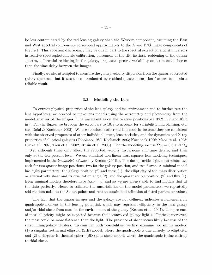
– 11 –

be less contaminated by the red lensing galaxy than the Western component, assuming the East

and West spectral components correspond approximately to the A and B/G image components of

Figure 1. This apparent discrepancy may be due in part to the spectral extraction algorithm, errors

in relative spectrophotometric calibration, placement of the slit, intrinsic reddening of the quasar

spectra, differential reddening in the galaxy, or quasar spectral variability on a timescale shorter

than the time delay between the images.

Finally, we also attempted to measure the galaxy velocity dispersion from the quasar-subtracted

galaxy spectrum, but it was too contaminated by residual quasar absorption features to obtain a

reliable result.

3.3. Modeling the Lens

To extract physical properties of the lens galaxy and its environment and to further test the

lens hypothesis, we proceed to make lens models using the astrometry and photometry from the

model analysis of the images. The uncertainties on the relative positions are 0.′′02 in r and 0.′′03

in i. For the fluxes, we broaden the error bars to 10% to account for variability, microlensing, etc.

(see Dalal & Kochanek 2002). We use standard isothermal lens models, because they are consistent

with the observed properties of other individual lenses, lens statistics, and the dynamics and X-ray

properties of elliptical galaxies (Fabbiano 1989; Kochanek 1993; Kochanek 1996; Maoz et al. 1993;

Rix et al. 1997; Treu et al. 2002; Rusin et al. 2003). For the modeling we use Ωm = 0.3 and ΩΛ

= 0.7, although these only affect the reported velocity dispersions and time delays, and then

only at the few percent level. We use standard non-linear least-squares lens modeling techniques,

implemented in the lensmodel software by Keeton (2001b). The data provide eight constraints: two

each for two quasar image positions, two for the galaxy position, and two fluxes. A minimal model

has eight parameters: the galaxy position (2) and mass (1), the ellipticity of the mass distribution

or alternatively shear and its orientation angle (2), and the quasar source position (2) and flux (1).

Even minimal models therefore have Ndof = 0, and so we are always able to find models that fit

the data perfectly. Hence to estimate the uncertainties on the model parameters, we repeatedly

add random noise to the 8 data points and refit to obtain a distribution of fitted parameter values.

The fact that the quasar images and the galaxy are not collinear indicates a non-negligible

quadrupole moment in the lensing potential, which may represent ellipticity in the lens galaxy

and/or tidal shear from mass in the environment of the galaxy (Keeton et al. 1997). The presence

of mass ellipticity might be expected because the deconvolved galaxy light is elliptical; moreover,

the mass could be more flattened than the light. The presence of shear seems likely because of the

surrounding galaxy clusters. To consider both possibilities, we first examine two simple models:

(1) a singular isothermal ellipsoid (SIE) model, where the quadrupole is due entirely to ellipticity,

and (2) a singular isothermal sphere (SIS) plus shear model, where the quadrupole is due entirely

to tidal shear.

– 12 –

Both SIE and SIS+shear models can fit the lens exactly, with the parameters given in Ta-

ble 4. Both sets of models seem reasonable: SIE models require a mass ellipticity ǫ = 0.5–0.6,

slightly larger than the ellipticity of the light (∼ 0.3), while SIE+shear models require a shear

strength γ = 0.15–0.18, typical of lenses in group or cluster environments (Keeton et al. 1997;

Kundic et al. 1997; Kneib, Cohen, & Hjorth 2000). There are small differences between the r-

band and i-band models due to differences in the deconvolved positions of quasar B and the galaxy

in the r and i-band data, but the differences are only at the 1σ level.

The models yield an Einstein radius of 1.′′4, corresponding to a velocity dispersion of 250 ± 4

km s−1 for the lens galaxy. This number is consistent with the velocity dispersion estimates made

with the L− σ relations in Section 3.1; the estimate from the lens model may be higher due to the

surrounding group slightly enhancing the image angular separation. The implied total magnification

of the system is a moderate factor of 3–4. The models also predict that the time delay between the

images should be in the range 57–72 h−1 days. Because the predicted delay depends on the relative

amounts of ellipticity and shear (Witt et al. 2000), the usefulness of this lens for Hubble parameter

analyses will depend on how well the ellipticity and shear can be determined independently.

It is interesting to note that in both SIE and SIS+shear models the quadrupole moment of

the lensing potential is oriented almost exactly north–south, while the corrected galaxy light is

inclined at ∼30. A misalignment of more than ∼10 usually indicates that the lensing potential

has both ellipticity and shear with different orientations (Keeton et al. 1998; Kochanek 2002). It

is pointless to fit models with unconstrained ellipticity and shear to SDSS J0903+5028, because

such models are under-constrained. However, analyses of other lenses suggest that it is reasonable

to constrain the shape of the model mass distribution using the observed shape of the light distri-

bution. The orientation angles of the mass and light are strongly correlated and typically aligned

to within ∼ 10, even if there is no clear relationship between the ellipticities of the mass and

light (Keeton et al. 1998; Kochanek 2002). Figure 7 shows results for SIE+shear models where we

either fix the shape of the model mass distribution to that of the light (panel a) or just require that

the mass distribution match the light within assumed uncertainties of 10 in orientation and 0.1 in

ellipticity (panel b). In both cases, the constraint on the mass orientation provides an important

lower limit on the shear strength. In other words, under the reasonable assumption that the mass

distribution is aligned with the light distribution, the misalignment between the galaxy and the

quadrupole moment of the lensing potential directly implies the presence of shear from the lens

environment (the group or nearby clusters). Adopting a constraint on the mass ellipticity would

then yield an upper limit on the shear, but this result is less reliable because there is no strong

evidence that the mass ellipticity should match that of the light (Keeton et al. 1998). We also

note that if the two nearby clusters found by the maxBCG algorithm are indeed separate spherical

clusters, they would produce a shear with the requisite north–south orientation; however, given

their relatively large angular separation from the lens galaxy, one would expect them to produce a

combined shear of only a few percent.

Thus, the lens models suggest but do not conclusively reveal that the group or clusters around

– 13 –

the lens galaxy play an important role in the lensing potential. The best way to test this hypothesis

would be to obtain spectroscopy for galaxies in the field of the lens, to confirm the cluster(s) and

identify members, and to measure the centroid and velocity dispersion of the cluster(s). Those

quantities could be used to estimate the shear from the environment, and compared with the

predicted shear strength γ ∼ 0.1–0.2 and orientation θγ = 136–174 to test and further constrain

the lens models.

4. Conclusions

We have identified a lensed quasar candidate, SDSS J0903+5028, based on the superposition

of a z = 3.605 quasar and a z = 0.388 luminous red galaxy in an SDSS spectrum. Follow-up

observations with the ARC 3.5-m and the Keck II telescope have confirmed that this is a two-

image gravitational lens system, with image angular separation of 2.′′8. The lens model is consistent

with a massive galaxy with a velocity dispersion of 250 km sec−1. The lens geometry indicates

a quadrupolar lensing potential which can be generated by an elliptical galaxy mass distribution

and/or tidal shear from what appears to be a group of galaxies surrounding the lens. The misalign-

ment between the quadrupole and the galaxy light suggests that there is indeed significant shear

from the environment.

5. Acknowledgments

We thank Paul Schechter and Scott Burles for useful discussions. Funding for the creation and

distribution of the SDSS Archive has been provided by the Alfred P. Sloan Foundation, the Par-

ticipating Institutions, the National Aeronautics and Space Administration, the National Science

Foundation, the U.S. Department of Energy, the Japanese Monbukagakusho, and the Max Planck

Society. The SDSS Web site is http://www.sdss.org/. The SDSS is managed by the Astrophysical

Research Consortium (ARC) for the Participating Institutions. The Participating Institutions are

The University of Chicago, Fermilab, the Institute for Advanced Study, the Japan Participation

Group, The Johns Hopkins University, Los Alamos National Laboratory, the Max-Planck-Institute

for Astronomy (MPIA), the Max-Planck-Institute for Astrophysics (MPA), New Mexico State Uni-

versity, Princeton University, the United States Naval Observatory, the University of Pittsburgh,

and the University of Washington. JF and DJ acknowledge support from the NSF Center for

Cosmological Physics and NSF grant PHY-0079251, from the DOE, and from NASA grant NAG5-

10842. GTR acknowledges support from HST-GO-09472.01-A. Part of the work reported here was

done at LLNL under the auspices of the U.S. Department of Energy under contract W-7405-Eng-48.

This work is based in part on observations obtained with the Apache Point Observatory 3.5-meter

telescope, which is owned and operated by the Astrophysical Research Consortium. Some of the

data presented herein were obtained at the W.M. Keck Observatory, which is operated as a sci-

entific partnership among the California Institute of Technology, the University of California, and

– 14 –

the National Aeronautics and Space Administration. The Observatory was made possible by the

generous financial support of the W.M. Keck Foundation. We thank the staffs of the Keck and

Apache Point Observatories, and C. Ryan at CFHT, for their assistance.

– 15 –

REFERENCES

Abazajian, K., et al. 2003 astro-ph/0305492, AJ submitted

Annis, J., et al. 2003, in preparation

Bahcall, N., et al. 2003, ApJ, 585, 182

Bernardi, M., et al. 2003, AJ, 125, 1849

Bertin, E. & Arnouts, S. 1996, A&A Supp., 117, 393

Blanton, M.R., Lupton, R.H., Maley, F.M., Young, N., Zehavi, I., & Loveday, J. 2003, AJ, 125,

2276

Bruzual, G., & Charlot, S. 2003, MNRAS, in press

Burles, S., et al. 2003, in preparation

Chae, K.H., Turnshek, D.A., Khersonsky, V.K. 1998 ApJ, 495, 609

Chen, G.H., Kochanek C.S., Hewitt, J.N. ApJ, 447, 62

Dalal, N., & Kochanek, C. S. 2002, ApJ, 572, 25

Eisenstein, D. J., Annis, J., Gunn, J. E., Szalay, A. S., Connolly, A. J., Nichol, R. C., et al., 2001,

AJ, 122, 2267

Eisenstein, D. J., Hogg, D. W., Fukugita, M., Nakamura, O., Bernardi, M., Finkbeiner, D., Schlegel,

D. et al. 2003, ApJ, 585, 694

Epps, H. W. & Miller, J. S. 1998, Proc. SPIE, 3355, 48

Fabbiano, G. 1989, ARA&A, 27, 87

Faber, S. M., Jackson, R. 1976, ApJ, 204, 668

Foltz, C.B., Weymann, R.J., Peterson, B.M., Sun, L., Malkan, M.A., & Chaffee, F.H. 1986, ApJ,

307, 504

Fukugita, M., Futamase, T., Kasai, M. 1990 MNRAS 246, 24P

Fukugita, M., Ichikawa, T., Gunn, J. E., Doi, M., Shimasaku, K., & Schneider, D. P. 1996, AJ,

111, 1748

Fukugita, M., Turner, E.L. 1991, MNRAS, 253, 99

Gunn, J. E., Carr, M., Rockosi, C., Sekiguchi, M., Berry, K., Elms, B., de Haas, E., Ivezic , Z., et

al. 1998, AJ, 116, 3040

– 16 –

Hogg, D.W., Finkbeiner, D.P., Schlegel, D.J., & Gunn, J.E. 2001, AJ, 122, 2129

Huchra, J., Gorenstein, M., Kent, S., Shapiro, I., Smith, G., Horine, E., & Perley, R. 1985, AJ, 90,

691

Inada, N. et al. 2003a, AJ submitted

Inada, N. et al. 2003b, preprint (astro-ph/0304377), AJ, in press

Keeton, C. R. 2001a, ApJ, 561, 46

Keeton, C. R. 2001b, preprint (astro-ph/0102340)

Keeton, C. R. 2002, ApJ, 575, L1

Keeton, C. R., Kochanek, C.S., Falco, E.E. 1998 ApJ, 495, 609

Keeton, C. R., Kochanek, C. S., & Seljak, U. 1997, ApJ, 482, 604

Keeton, C. R. , Madau, P. 2001 ApJ, 549, 25

Kneib, J. P., Cohen, J. G., & Hjorth, J. 2000, ApJ, 544, L35

Kochanek, C. S. 1991, ApJ, 379, 517

Kochanek, C. S. 1992, ApJ, 397, 381

Kochanek, C. S. 1993, ApJ, 419, 12

Kochanek, C. S., 1995, ApJ, 453, 545

Kochanek, C. S. 1996, ApJ, 466, 638

Kochanek, C. S. 2002, in Proc. Yale Cosmology Workshop “The Shapes of Galaxies and Their Dark

Matter Halos,” ed. P. Natarajan (Singapore: World Scientific), 62

Lupton, R. H., Gunn, J. E., & Szalay, A. S. 1999, AJ, 118, 1406

Lupton, R. H., Gunn, J. E., Ivezic , Z., Knapp, G.R., Kent, S.M. & Yasuda, N. 2001, ADASS X,

ed. F.R. Harnden, Jr., F.A. Primini and H. E. Payne, ASP Conf. Proc. 238,269

Kundic, T., Hogg, D. W., Blandford, R. D., Cohen, J. G., Lubin, L. M., & Larkin, J. E. 1997, AJ,

114, 2276

Malhotra S., Rhoads, J.E., Turner, E.L., 1997 MNRAS, 247, 1P

Maoz, D., & Rix, H.-W. 1993, ApJ, 416, 425

Morgan, N.D., Snyder, J.A., Reens, L.H., astro-ph/0305036

– 17 –

Mortlock, D.J., Webster, R.L. 2000, MNRAS, 319, 872

Mortlock, D.J., Webster, R.L. 2000, MNRAS, 319, 879

Petrosian, V. 1976, ApJ, 209, L1

Pier, J.R., Munn, J.A., Hindsley, R.B., Hennessy, G.S., Kent, S.M., Lupton, R.H., & Ivezic , Z.

2003, AJ, 125, 1559

Pindor, B., Turner, E. L., Lupton, R. H., & Brinkmann, J. 2003, AJ, 125, 2325

Pindor, B., et al. 2003 in preparation

Refsdal, S. 1964, MNRAS, 128, 307

Richards, G. T., Vanden Berk, D. E., Reichard, T. A., Hall, P. B., Schneider, D. P., SubbaRao,

M., Thakar, A. R., & York, D. G. 2002, AJ, 124, 1

Rix, H.-W., de Zeeuw, P. T., Carollo, C. M., Cretton, N., & van der Marel, R. P. 1997, ApJ, 488,

702

Rusin, D., Kochanek, C. S., & Keeton, C. R. 2003, ApJ, submitted

Schild,R. & Thompson, D. J. 1997, AJ, 113, 130

Schlegel, D. J. 2003, unpublished

Schlegel, D. J., Finkbeiner, D. P., & Davis, M. 1998, ApJ, 500, 525

Smith, J.A., Tucker, D. L., Kent, S., et al. 2002, AJ, 123, 2121

Stoughton, C. et al. 2002, AJ, 123, 485

SubbaRao, M., Frieman, J., Bernardi, M., Burles, S., Castander, F., Connolly, A., Loveday, J.,

Meiksin, A., Nichol, R. et al. 2003, in preparation

Treu, T., & Koopmans, L. V. E. 2002, ApJ, 575, 87

Turner, E.L., 1990, ApJ, 365, L43

Walsh, D., Carswell, R.F.,Weymann, R.J. 1979, Nature, 279, 381

Witt, H. J., Mao, S., & Keeton, C. R. 2000, ApJ, 544, 98

Yip, C.-W., Connolly, A. J., Szalay, A., Budavari, T., SubbaRao, M., Frieman, J., Nichol, R., et

al. 2003, submitted to AJ

York, D. G., Adelman, J., Anderson, J. E., Anderson, S. F., Annis, J., Bahcall, N. A., Bakken,

J. A., Barkhouser, R., et al. 2000, AJ, 120, 1579

This preprint was prepared with the AAS LATEX macros v5.0.

– 18 –

Fig. 1.— SPIcam r-band image of area around SDSS J0903+5028. North is up and East is to the

left. The scale of the image is 35′′ across, the pixel scale is 0.′′14/pixel and the seeing is 1.′′1. The

objects labeled A and B are the quasar images; the galaxy is labeled G and is blended with quasar

B. These other galaxies may be a small group or part of two nearby clusters.

– 19 –

Fig. 2.— SDSS spectrum of SDSS J0903+5028 (smoothed by 9 pixels). The error spectrum (also

smoothed by 9 pixels) is given by the dashed line. Dotted lines mark the centers of Lyα and CIV

emission for z = 3.584. The flux units are 10−17 ergs/s/cm2/A.

– 20 –

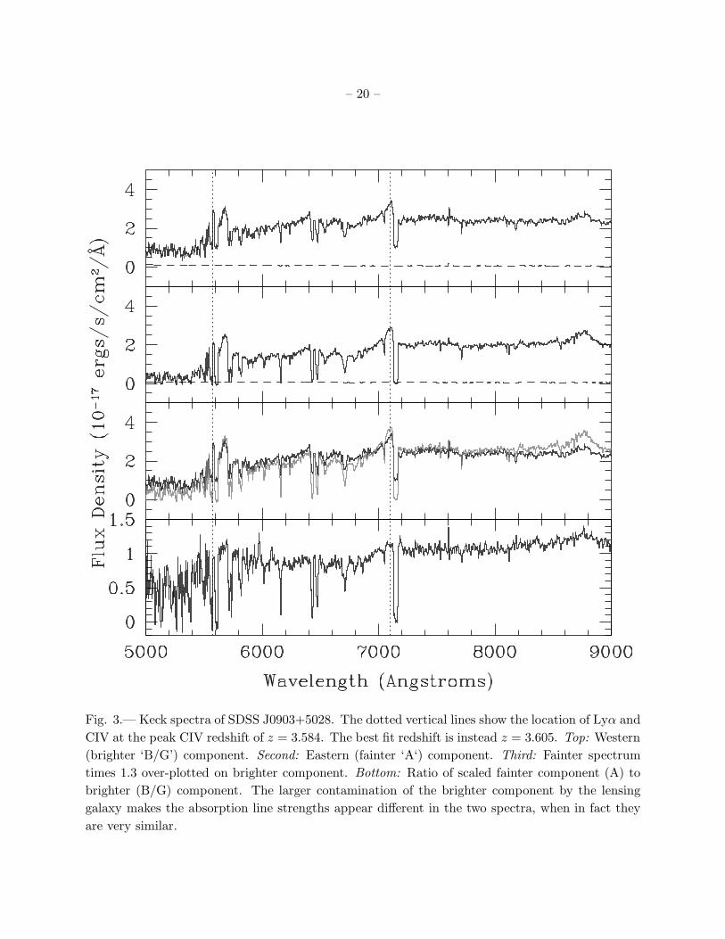
Fig. 3.— Keck spectra of SDSS J0903+5028. The dotted vertical lines show the location of Lyα and

CIV at the peak CIV redshift of z = 3.584. The best fit redshift is instead z = 3.605. Top: Western

(brighter ‘B/G’) component. Second: Eastern (fainter ‘A‘) component. Third: Fainter spectrum

times 1.3 over-plotted on brighter component. Bottom: Ratio of scaled fainter component (A) to

brighter (B/G) component. The larger contamination of the brighter component by the lensing

galaxy makes the absorption line strengths appear different in the two spectra, when in fact they

are very similar.

– 21 –

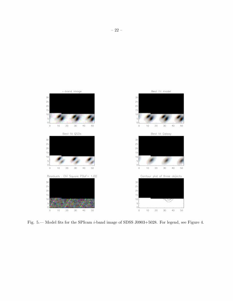
Fig. 4.— Model fits for the SPIcam r-band image of SDSS J0903+5028. Top left: Image. Top right:

best fit model to two point sources and one extended source. Middle: Best fit model quasar and

galaxy surface brightnesses. Lower left: Residuals between best fit model and the image. Lower

right: Surface brightness contours for the 3 model components.

– 22 –

Fig. 5.— Model fits for the SPIcam i-band image of SDSS J0903+5028. For legend, see Figure 4.

– 23 –

SDSS

5000 6000 7000 8000 9000Wavelength (A)

0

2

4

6

8

10

12Fl

ux (

10^

-17

ergs

/s/c

m^2

/A)

KECK

5000 6000 7000 8000 9000Wavelength (A)

-1

0

1

2

3

4

Flux

(10

^ -1

7 er

gs/s

/cm

^2/A

)

Fig. 6.— Top: SDSS spectrum of SDSS J0903+5028, decomposed into galaxy and quasar compo-

nents: Spectrum (black), Galaxy (blue), quasar (green), sum of Galaxy and quasar components

(red). Bottom: Keck Western spectrum of SDSS J0903+5028, decomposed into LRG and quasar

components.

– 24 –

Fig. 7.— Results from SIE+shear lens models. The solid curves show models in which the position

angle (PA) of the mass is constrained to match that of the light, while the dotted curves show

models for which both the position angle and ellipticity of the mass are constrained to match those

of the light. There are separate curves for models of the r and i-band data. (a) The mass, PA, and

ellipticity are fixed. (b) The mass, PA, and ellipticity are free parameters but constrained by the

light, with assumed uncertainties of 10 and 0.1, respectively. Note that the χ2min = 0 only because

Ndof = 0.

– 25 –

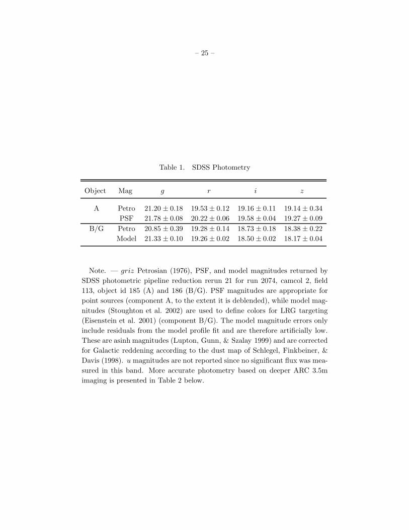
Table 1. SDSS Photometry

Object Mag g r i z

A Petro 21.20 ± 0.18 19.53 ± 0.12 19.16 ± 0.11 19.14 ± 0.34

PSF 21.78 ± 0.08 20.22 ± 0.06 19.58 ± 0.04 19.27 ± 0.09

B/G Petro 20.85 ± 0.39 19.28 ± 0.14 18.73 ± 0.18 18.38 ± 0.22

Model 21.33 ± 0.10 19.26 ± 0.02 18.50 ± 0.02 18.17 ± 0.04

Note. — griz Petrosian (1976), PSF, and model magnitudes returned by

SDSS photometric pipeline reduction rerun 21 for run 2074, camcol 2, field

113, object id 185 (A) and 186 (B/G). PSF magnitudes are appropriate for

point sources (component A, to the extent it is deblended), while model mag-

nitudes (Stoughton et al. 2002) are used to define colors for LRG targeting

(Eisenstein et al. 2001) (component B/G). The model magnitude errors only

include residuals from the model profile fit and are therefore artificially low.

These are asinh magnitudes (Lupton, Gunn, & Szalay 1999) and are corrected

for Galactic reddening according to the dust map of Schlegel, Finkbeiner, &

Davis (1998). u magnitudes are not reported since no significant flux was mea-

sured in this band. More accurate photometry based on deeper ARC 3.5m

imaging is presented in Table 2 below.

– 26 –

Table 2. ARC Photometry: Model Results

Object (J2000) r i r − i

QSO A 09h03m35s.132 + 5028′20.′′21 19.99 ± 0.01 19.43 ± 0.01 0.56 ± 0.02

QSO B 09h03m34s.877 + 5028′18.′′75 20.78 ± 0.03 20.27 ± 0.05 0.51 ± 0.06

Galaxy 09h03m34s.925 + 5028′19.′′53 19.59 ± 0.02 18.86 ± 0.04 0.73 ± 0.05

Note. — Dereddened magnitudes. The astrometry is well calibrated to the SDSS

astrometry and so the dominant errors simply come from the fitting routine and

this error is about 0.′′07. The photometry is also calibrated to the SDSS and has a

systematic error in the zero points estimated at 0.06 in both bands. The relative

photometry could in principle be better but, due to the degeneracy between QSO B

and the galaxy, the error on the relative magnitudes are at about the same level. We

conclude that the color difference between the two quasars is consistent with zero.

Table 3. MaxBCG Clusters

(J2000) angle Distance z Ngal

09h03m43s + 5032′58′′ 5.′7 1.36 0.44 12

09h03m47s + 5024′54′′ 5.′8 1.39 0.44 14

Note. — The two clusters near the lens galaxy. The

first column gives the cluster center J2000 coordinates as

reported by the maxBCG algorithm. The second column

is the separation in arc-minutes of the cluster center from

the lens galaxy. The third is the separation in Mpc at the

indicated redshift. The fourth column is the photometric

redshift as reported by maxBCG. The estimated errors on

the maxBCG redshift estimates are typically 0.02 for low

redshift and about 0.05 for these higher redshift clusters.

The fifth column is Ngal, a richness measure returned by

maxBCG, the estimated number of L∗ and brighter galaxies

in the cluster.

– 27 –

Table 4. Lens Model Results

Type Band RE (′′) ǫ or γ θǫ or θγ () µtot ∆t (h−1 days)

SIE r 1.42 ± 0.03 0.47 ± 0.04 4.6 ± 2.8 3.62 ± 0.19 67.4 ± 2.8

i 1.38 ± 0.04 0.57 ± 0.06 2.0 ± 3.0 3.19 ± 0.23 72.0 ± 4.2

SIS+shear r 1.44 ± 0.03 0.15 ± 0.01 3.1 ± 3.0 4.13 ± 0.21 57.0 ± 2.2

i 1.43 ± 0.04 0.18 ± 0.02 1.0 ± 3.2 3.76 ± 0.26 57.8 ± 3.1

Note. — Col. 3 gives the Einstein radius. Col. 4–5 give the ellipticity ǫ and position angle

θǫ for SIE models, or the shear γ and position angle θγ for SIS+shear models. Col. 6 gives the

total magnification. Col. 7 gives the predicted time delay (for a cosmology with ΩM = 0.3 and

ΩΛ = 0.7).