WEAK GRAVITATIONAL LENSING STUDIES USING RADIO ...
156
WEAK GRAVITATIONAL LENSING STUDIES USING RADIO INFORMATION A THESIS SUBMITTED TO THE UNIVERSITY OF MANCHESTER FOR THE DEGREE OF DOCTOR OF P HILOSOPHY IN THE FACULTY OF ENGINEERING AND P HYSICAL S CIENCES 2016 By Constantinos Demetroullas School of Physics and Astronomy
-
Upload
khangminh22 -
Category
Documents
-
view
3 -
download
0
Transcript of WEAK GRAVITATIONAL LENSING STUDIES USING RADIO ...

WEAK GRAVITATIONAL LENSINGSTUDIES USING RADIO
INFORMATION
A THESIS SUBMITTED TO THE UNIVERSITY OF MANCHESTER
FOR THE DEGREE OF DOCTOR OF PHILOSOPHY
IN THE FACULTY OF ENGINEERING AND PHYSICAL SCIENCES
2016
ByConstantinos Demetroullas
School of Physics and Astronomy

Contents
Abstract 11
Acknowledgements 14
Nomenclature 18
1 Cosmological Background 201.1 Dark Matter . . . . . . . . . . . . . . . . . . . . . . . . . . . . . . . 26
1.2 Dark Energy . . . . . . . . . . . . . . . . . . . . . . . . . . . . . . . 28
1.3 Standard model of Cosmology . . . . . . . . . . . . . . . . . . . . . 29
2 Weak Gravitational Lensing 332.1 Light Deflection and Lens Equation . . . . . . . . . . . . . . . . . . 34
2.2 Weak lensing by galaxies and galaxy clusters . . . . . . . . . . . . . 35
2.3 Lensing by the Large Scale Structure . . . . . . . . . . . . . . . . . . 38
2.4 Radio Weak Lensing and Interferometry . . . . . . . . . . . . . . . . 40
Interferometry . . . . . . . . . . . . . . . . . . . . . . . . . 42
Complications of Using Interferometric Data for Weak Lens-ing Studies . . . . . . . . . . . . . . . . . . . . . . 45
Polarisation Information in Interferometric Data . . . . . . . 46
Calibrating the Data . . . . . . . . . . . . . . . . . . . . . . 46
Shape Reconstruction from Interferometric Data . . . . . . . 47
2.5 Measuring Weak Lensing Shear . . . . . . . . . . . . . . . . . . . . 49
Galaxy Shape Measurements . . . . . . . . . . . . . . . . . . 51
Weak Lensing Measurement Errors . . . . . . . . . . . . . . 51
The necessity for simulations . . . . . . . . . . . . . . . . . . 54
2.6 Conclusions . . . . . . . . . . . . . . . . . . . . . . . . . . . . . . . 54
2

3 Cross correlation shear with the SDSS and VLA FIRST surveys 563.1 Cosmic Shear in Fourier Space . . . . . . . . . . . . . . . . . . . . . 57
Weak Lensing in Spherical Harmonic Space . . . . . . . . . . 58Power Spectrum Estimation on a Cut Sky: . . . . . . . . . . . 60
3.2 The Surveys . . . . . . . . . . . . . . . . . . . . . . . . . . . . . . . 623.2.1 FIRST Data . . . . . . . . . . . . . . . . . . . . . . . . . . . 623.2.2 SDSS Data . . . . . . . . . . . . . . . . . . . . . . . . . . . 64
3.3 Shear Maps and Tests for Systematics . . . . . . . . . . . . . . . . . 653.3.1 FIRST Analysis . . . . . . . . . . . . . . . . . . . . . . . . . 65
Source Selection . . . . . . . . . . . . . . . . . . . . . . . . 65Residual Systematics in FIRST Ellipticities . . . . . . . . . . 66FIRST Shear Maps . . . . . . . . . . . . . . . . . . . . . . . 67
3.3.2 SDSS Analysis . . . . . . . . . . . . . . . . . . . . . . . . . 69Shape Measurements and Initial Source Selection . . . . . . . 69Shear Systematics and Additional Source Selection . . . . . . 71
3.4 Simulations . . . . . . . . . . . . . . . . . . . . . . . . . . . . . . . 733.4.1 Signal Simulations . . . . . . . . . . . . . . . . . . . . . . . 743.4.2 Noise Simulations . . . . . . . . . . . . . . . . . . . . . . . 763.4.3 Modelling Small-Scale Systematic Effects . . . . . . . . . . . 763.4.4 Power Spectra from Simulations . . . . . . . . . . . . . . . . 773.4.5 Recovery in the Presence of Large-Scale Systematics . . . . . 79
3.5 Real Data Measurements . . . . . . . . . . . . . . . . . . . . . . . . 813.5.1 The SDSS-FIRST Cross-power Spectra . . . . . . . . . . . . 813.5.2 Null Tests . . . . . . . . . . . . . . . . . . . . . . . . . . . . 833.5.3 Constraints on the FIRST and SDSS Median Redshifts, σ8 and
Ωm . . . . . . . . . . . . . . . . . . . . . . . . . . . . . . . 863.6 Conclusions . . . . . . . . . . . . . . . . . . . . . . . . . . . . . . . 90
4 Weak Lensing by Galaxies and Galaxy Clusters 934.1 Weak Lensing Background . . . . . . . . . . . . . . . . . . . . . . . 944.2 Dark Matter Halo Models . . . . . . . . . . . . . . . . . . . . . . . . 96
4.2.1 SIS Model . . . . . . . . . . . . . . . . . . . . . . . . . . . 964.2.2 NFW Model . . . . . . . . . . . . . . . . . . . . . . . . . . 98
4.3 The Data . . . . . . . . . . . . . . . . . . . . . . . . . . . . . . . . . 1004.3.1 Brightest Cluster Galaxy Data . . . . . . . . . . . . . . . . . 1004.3.2 SDSS-FIRST Matched Objects . . . . . . . . . . . . . . . . 101
3

4.4 FIRST Shape Corrections . . . . . . . . . . . . . . . . . . . . . . . . 1014.5 Simulations . . . . . . . . . . . . . . . . . . . . . . . . . . . . . . . 104
4.5.1 Simulated Source Shape Corrections . . . . . . . . . . . . . . 1054.5.2 Galaxy-Galaxy Lensing Signal from Simulations . . . . . . . 105
4.6 Real Data Measurements . . . . . . . . . . . . . . . . . . . . . . . . 1094.7 Residual Systematics Test Measurements . . . . . . . . . . . . . . . 1104.8 Constrains on the Properties of the Lensing Sources . . . . . . . . . . 1134.9 Conclusions . . . . . . . . . . . . . . . . . . . . . . . . . . . . . . . 116
5 The SuperCLuster Assisted Shear Survey 1195.1 Scientific Objectives . . . . . . . . . . . . . . . . . . . . . . . . . . 1205.2 The Data . . . . . . . . . . . . . . . . . . . . . . . . . . . . . . . . . 122
5.2.1 e-MERLIN Data . . . . . . . . . . . . . . . . . . . . . . . . 1225.2.2 Complementary Data . . . . . . . . . . . . . . . . . . . . . . 124
5.3 The SuperCLASS e-MERLIN Data Reduction and Imaging . . . . . . 1245.4 Conclusions . . . . . . . . . . . . . . . . . . . . . . . . . . . . . . . 144
6 Summary 145
Word Count: ∼35,746
4

List of Tables
1.1 Parameters of the ΛCDM cosmology computed from the temperatureand polarisation spectra at multiples 2< l <2500 (Planck Collabora-tion et al., 2015). . . . . . . . . . . . . . . . . . . . . . . . . . . . . 30
2.1 Current and future radio and optical surveys information. Asky, ngal,zm, m and c denote the covered by the survey sky area, the sourcenumber density, the survey’s median redshift and the multiplicativeand additive biases respectively. . . . . . . . . . . . . . . . . . . . . 42
3.1 PTE values from the the χ2 null tests described in Section 3.5.2. . . . 86
4.1 The lens and background objects redshifts and concentration factorsvalues used to fit the data. . . . . . . . . . . . . . . . . . . . . . . . . 114
4.2 Model fitting extracted parameters . . . . . . . . . . . . . . . . . . . 117
5.1 Properties of galaxy clusters in the observed SuperCLASS field. . . . 1215.2 Acquired data-set contained files . . . . . . . . . . . . . . . . . . . . 1255.3 Position, peak and integrated flux density, convolved and deconvolved
size and position angle information for the sources in the field that havebeen detected at the 5-10σ level. . . . . . . . . . . . . . . . . . . . . 140
5.4 Position, peak and integrated flux density, convolved and deconvolvedsize and position angle information for the sources in the field that havebeen detected at the >10σ level. . . . . . . . . . . . . . . . . . . . . 143
5

List of Figures
1.1 The matter power spectrum measurements and predictions at z=0. . . 26
1.2 Schematic representation of a galaxy surrounded by a Dark Matter halo. 27
1.3 Planck 2015 CMB TT, TE and EE spectra . . . . . . . . . . . . . . . 29
1.4 Joint constrains on the matter density Ωm and power spectrum nor-malisation σ8 (left) and the Dark Energy state equation of state w
and §8 = σ8(Ωm/0.3)0.5 (right) placed by the DES survey, Planck andCFHTlenS. . . . . . . . . . . . . . . . . . . . . . . . . . . . . . . . 31
1.5 Effect of Λ and K on the expansion rate of the Universe . . . . . . . . 32
2.1 Schematic representation of a GL effect . . . . . . . . . . . . . . . . 36
2.2 Schematic representation of the effects of the convergence κ and theshear γ on a source shape . . . . . . . . . . . . . . . . . . . . . . . . 38
2.3 Schematic representation of decomposing a shear field into its E-modeand B-mode component . . . . . . . . . . . . . . . . . . . . . . . . . 39
2.4 Schematic of WGL due to large scale structure . . . . . . . . . . . . 40
2.5 Schematic of u-v visibility points . . . . . . . . . . . . . . . . . . . . 44
3.1 Results of the test for residual beam systematics in the FIRST galaxyshapes . . . . . . . . . . . . . . . . . . . . . . . . . . . . . . . . . . 66
3.2 Maps of the tangential shear (γt) and rotated shear (γr) as a function ofthe separation in RA and δ from the central stacking positions. . . . . 67
3.3 Maps of the γ1 and γ2 shear components, constructed by simple aver-aging of the FIRST galaxy ellipticities within each pixel. . . . . . . . 68
3.4 The galaxy number density map (normalised with the maximum num-ber of galaxies laying at any given pixel of the map) used to weight theFIRST shear field (Fig. 3.3) in the power spectrum analysis. . . . . . . 69
6

3.5 Maps of the γ1 and γ2 shear components, constructed by simple aver-aging of the SDSS galaxy ellipticities within each pixel. These mapswere constructed from the∼25 million galaxies remaining in the SDSSshear catalogue immediately after the PSF correction and source selec-tion steps described in Section 3.3.2 were implemented. . . . . . . . . 70
3.6 Maps of the γ1 and γ2 shear components, constructed by simple aver-aging of the SDSS galaxy ellipticities within each pixel. These mapswere constructed from the ∼9 million galaxies remaining in the SDSSshear catalogue immediately after the additional source selection basedon the strength of the PSF, described in Section 3.3.2, was implemented. 72
3.7 The galaxy number density map (normalised with the maximum num-ber of galaxies laying at any given pixel of the map) used to weight theSDSS shear field (Fig. 3.6) in the power spectrum analysis. . . . . . . 73
3.8 Normalised galaxy redshift distributions adopted for the SDSS popu-lation and for the FIRST population . . . . . . . . . . . . . . . . . . 75
3.9 The γt component of the contamination template used to model theFIRST residual beam systematic discussed in Section 3.3.1, and dis-played in Fig. 3.2. The γr component of the contamination was as-sumed to be zero. . . . . . . . . . . . . . . . . . . . . . . . . . . . . 77
3.11 The recovered mean SDSS auto power spectra and SDSS-FIRST cross-power spectra from 100 simulations in the presence of large-scale sys-tematic effects in the real SDSS shear maps. . . . . . . . . . . . . . . 80
3.12 The recovered mean FIRST auto power spectra and SDSS-FIRST cross-power spectra from 100 simulations in the presence of large-scale sys-tematic effects in the real FIRST shear maps. . . . . . . . . . . . . . 80
3.13 The cosmic shear cross-power spectrum measured from the SDSS andFIRST datasets. . . . . . . . . . . . . . . . . . . . . . . . . . . . . . 83
3.14 Histograms showing the χ2 and χ values for the Cκκ` , Cββ
` and Cκβ
`
power spectra as measured from the simulations. Over-plotted as thevertical blue line is the equivalent value for the real data measurements. 84
3.15 The Cκκ` , Cββ
` and Cκβ
` power spectra measurements for the null testsdescribed in Section 3.5.2. . . . . . . . . . . . . . . . . . . . . . . . 86
7

3.16 Histograms showing the distribution of χ2 values measured from thesimulations for the suite of null tests described in Section 3.5.2. Theresults are shown for the Cκκ
` , Cββ
` and Cκβ
` power spectra. Over-plottedas the vertical blue line is the equivalent value for the real data mea-surement. . . . . . . . . . . . . . . . . . . . . . . . . . . . . . . . . 87
3.17 Histograms showing the distribution of χ values measured from thesimulations for the suite of null tests described in Section 3.5.2. Theresults are shown for the Cκκ
` , Cββ
` and Cκβ
` power spectra. Over-plottedas the vertical blue line is the equivalent value for the real data mea-surement. . . . . . . . . . . . . . . . . . . . . . . . . . . . . . . . . 88
3.18 Joint constraints on the median redshifts of the SDSS and FIRST sur-veys obtained from fitting theoretical models to my Cκκ
` cross-powerspectrum measurements. Cosmological parameters were kept fixed atthe concordance values reported in Planck Collaboration et al. (2014). 89
3.19 Joint constraints on the matter density, Ωm and power spectrum nor-malisation, σ8 from fitting theoretical models to my Cκκ
` cross-powerspectrum measurements. The median redshifts were fixed at zSDSS
m =
0.53 and zFIRSTm = 1.2. . . . . . . . . . . . . . . . . . . . . . . . . . . 91
4.1 The tests for residual contamination in the FIRST shapes using all theFIRST positions, randomly selecting 25 % and 10 % of those positionsrespectively. The residual tangential and rotated shear signal are plot-ted as blue squares and red circles. Over-plotted is the measured con-tamination in the tangential direction before any corrections were ap-plied to the data (cyan Xs). . . . . . . . . . . . . . . . . . . . . . . . 103
4.2 Maps of the residual tangential shear (γt) and rotated shear (γr) as afunction of the separation in RA and δ from the central stacking posi-tions after the FIRST shapes were corrected. . . . . . . . . . . . . . . 104
4.3 The measured contamination from a random simulation. The black,orange and red solid lines represent the measured tangential signal be-fore (black line) and after (orange line) the simulated FIRST sourcesshapes were corrected and the measured rotated shear after the shapecorrection (red line). . . . . . . . . . . . . . . . . . . . . . . . . . . 106
8

4.4 The tangential shear signal measured from 100 simulations in the ab-sence and presence of systematics and after the FIRST simulated shapeswere corrected. Over-plotted (red line) is the input tangential signalcalculated using the derived CGκ
` spectrum and eq. 4.8 . . . . . . . . . 107
4.5 The measured tangential shear signal for the TRAINING and SIG-NAL data-sets before (black line) and after (blue line) shape correc-tions were performed to the data. . . . . . . . . . . . . . . . . . . . . 109
4.6 The measured tangential (blue squares) and rotated (red circles) shearusing as lenses the SDSS complete catalogue, the BCG sample and theFIRST-SDSS matched objects. Over-plotted on the left hand panel isthe normalised theoretical tangential shear signal from a set of fore-ground and background sources lying at redshifts of zSDSS
median=0.53 andzFIRST
median=1.2 respectively. . . . . . . . . . . . . . . . . . . . . . . . . . 110
4.7 The null tests conducted using the full SDSS sample, the BCGs andthe SDSS-FIRST matched objects. . . . . . . . . . . . . . . . . . . . 112
4.8 The tangential shear signal measured using the FIRST selected sourcesas background objects and the SDSS-FIRST matched objects with zLow<1(blue squares) and zHigh>1 (red circles) as lenses. . . . . . . . . . . . 113
4.9 Galaxy-galaxy lensing measurements using the SDSS-FIRST matchedobjects as lenses and the selected FIRST sources as background objects. 114
4.10 The measured tangential (blue squares) shear for the SDSS completecatalogue, the BCG sample and the FIRST-SDSS matched objects.Over-plotted are the best fitted NFW with a fixed c f (red continuousline), NFW with a variable c f (blue dashed line) and SIS (black dot-dashed line) models. . . . . . . . . . . . . . . . . . . . . . . . . . . 115
5.1 The proposed field of observations, containing the four Abell clustersA968, A981, A998 and A1005 (box bounded by the solid lines and thedashed line to the south) covering a ∼1.0 deg2 (Source: SuperCLASSproposal document) . . . . . . . . . . . . . . . . . . . . . . . . . . . 120
5.2 Mosaic e-MERLIN scheme. . . . . . . . . . . . . . . . . . . . . . . 123
5.3 SPFLG interface showing the recorded amplitude of 1407+284 for IFs1-4 in grayscale as a function of frequency (x-axis) and time intervalsof 10s (y-axis) before and after a SERPENT auto-flagging run. . . . . . 127
9

5.4 IBLED interface showing the recorded amplitude of the target field(1024+6806) for the Lovell-Knocking baseline (1-5) and IF1 as a func-tion of time before and after short period spurious amplitude spikeswere removed. . . . . . . . . . . . . . . . . . . . . . . . . . . . . . . 129
5.5 POSSM interface showing the amplitude and phase of the phase calibra-tor (1034+6832) as a function of frequency for a number of baselinesand for both the LL and RR polarisations. . . . . . . . . . . . . . . . 130
5.6 SPFLG interface showing the amplitude of the combined dataset for theLovell-Knockin baseline (1-5), RR polarisation and IFs 2 to 8. . . . . 131
5.7 Left panel: Phase gains for the whole duration of the observationsof IF4 and LL polarisation across all telescopes. Right panel: Phasegains for the bandpass calibrator for all Lovell baselines and RR polar-isation. . . . . . . . . . . . . . . . . . . . . . . . . . . . . . . . . . . 132
5.8 Derived absolute flux scale values for the bandpass calibrator. Over-plotted (continuous line) is the expected theoretical flux density valuesfor the source. . . . . . . . . . . . . . . . . . . . . . . . . . . . . . 133
5.9 The image of the phase calibrator source before any self calibrationwas applied and after one and two iterations of the process. . . . . . . 133
5.10 The final images of the flux calibrator (left), and bandpass calibrator(right). . . . . . . . . . . . . . . . . . . . . . . . . . . . . . . . . . . 134
5.11 The noise and source distribution in the target field. RMS noise wasfound to be at ∼40 µJy/beam. 153 sources were detected at >5σ level. 134
5.12 The size (major axis) and integrated flux density distributions of the 99sources that were at least partially resolved in the observations. . . . . 141
5.13 Starting from the top left corner are: The bright source detected north-east of the target field and the 7 sources designated as Demetroullas1-7. . . . . . . . . . . . . . . . . . . . . . . . . . . . . . . . . . . . 142
10

ABSTRACT OF THESIS submitted by Constantinos Demetroullasfor the Degree of Doctor of Philosophy
November 2015.
Weak gravitational lensing has developed to be one of the most powerful tools for studying
the (dark) matter distribution in the Universe. Most weak lensing studies thus far were con-
ducted in the optical and near infrared. Measuring weak lensing in the radio though, provided
it is feasible, can be very advantageous. One can exploit the well known and deterministic
beam pattern of a radio telescope and the polarisation information in radio data to reduce shape
biases and intrinsic alignment effects respectively. Combining the information from an optical
and a radio survey can also help remove systematics from both datasets. This has motivated
this study that uses archival radio and optical data to treat telescope systematics and measure
an unbiased weak lensing signal using shape information derived from radio observations.
Using simulations I have shown that an unbiased convergence cross power spectrum can be
measured in the presence of the large scale (θ>1) systematics detected in FIRST and SDSS.
The method however amplifies the uncertainties by a factor ∼2.5 compared to the errors due
to cosmic variance and noise due to galaxy intrinsic shape alone. Using the shape information
from the two surveys I measure a Cκκ` spectrum signal that is inconsistent with zero at the 2.7σ.
The placed constraints are consistent with the expected signal in the concordance cosmological
model assuming recent estimates of the cosmological parameters from the Planck satellite and
literature values for the median redshifts of SDSS and FIRST.
Through simulations I also show that I can successfully remove position based small scale
systematics (θ<200′′) detected in FIRST. Correlating the positions of the SDSS data release
10, Brightest cluster galaxy (BCG) and the FIRST sources that match a position of a galaxy in
SDSS with the shapes of the FIRST selected sources, I measure a tangential shear signal that
is inconsistent with zero at 10σ, 3.8σ and 9σ respectively. Using an NFW and an SIS mass
profile I extract the Virial mass for the three lensing samples. The masses for the SDSS and
BCG groups are in good agreement (1σ) with values quoted in the literature. No previous work
had been performed on the third sample.
SuperCLASS is an experiment that aims to show the feasibility of measuring weak lens-
ing in the radio on a range of angular scales. I was tasked with editing and imaging the first
e-MERLIN observations of the SuperCLASS field around the Abell cluster A0981. The ob-
servations yield an RMS noise of ∼40µJy/beam. A performed source extraction revealed 153
sources at a signal-to-ratio of >5. Using the deconvolved information for the resolved sources
I calculate a FWHM median size and flux density of 0.5′′ and 300µJy respectively. Comparing
the source number density and RMS noise of the study with those of FIRST, I extrapolate to
predict that the number density of sources at >5σ will be ∼5arcmin−2, assuming the target
noise threshold for the survey is reached.
11

Declaration
I declare that no portion of the work referred to in the thesis has been submitted insupport of an application for an other degree or qualification of this or any other
university or other institute of learning
12

Copyright Statement
The author of this dissertation (including any appendices and/or schedules to thisdissertation) owns any copyright in it (the “Copyright”) and s/he has given TheUniversity of Manchester the right to use such Copyright for any administrative,
promotional, educational and/or teaching purposes.
Copies of this dissertation, either in full or in extracts, may be made only inaccordance with the regulations of the John Rylands University Library of
Manchester. Details of these regulations may be obtained from the Librarian. Thispage must form part of any such copies made.
The ownership of any patents, designs, trade marks and any and all other intellectualproperty rights except for the Copyright (the “Intellectual Property Rights”) and anyreproductions of copyright works, for example graphs and tables (“Reproductions”),
which may be described in this dissertation, may not be owned by the author and maybe owned by third parties. Such Intellectual Property Rights and Reproductions
cannot and must not be made available for use without the prior written permission ofthe owner(s) of the relevant Intellectual Property Rights and/or Reproductions.
Further information on the conditions under which disclosure, publication andexploitation of this dissertation, the Copyright and any Intellectual Property Rightsand/or Reproductions described in it may take place is available from the Head of
School of Physics and Astronomy.
13

Acknowledgements
Completing my doctoral studies was not easy. The project was challenging and I
found myself free falling quite often, but I knew that with hard work things would
turn around. What I never accounted for, and took a toll on me, were the personal
issues I had to face, the ones I had no control over. Looking back I can see my self
turning to the dark side and back more than a few times.
First and foremost I would like to thank the people that stood next to me throughout
this difficult journey; my parents, two sisters and brother-in-law. Although separated
by thousands of miles, I always knew that they were by my side feeling my struggle,
agonising with my troubles. Even if I tried to hide what I was feeling I knew they
could see right through me. Their kind words, and knowing that me getting my PhD
was almost as important to them as it was to me, is what kept me going.
Secondly I would like to express my deepest gratitude to my supervisor. His guid-
ance is what kept me from stranding somewhere in this vast unknown world of science.
Although his patience I am sure was tested in many cases, his door was always open
for me, and with his comments and kind words he always got me back on track.
It would be an omission of me not to also thank my colleagues for always being
friendly eager to chat. I also would like to thank everyone for the great times I had to
the parties and other activities they organised throughout these past few years. Spe-
cial thanks to Nicholas Wrigley, Stuart Harper, Philippa Hartley and Fiona Healy for
helping when needed it the most, by proofreading my thesis and finding an enormous
14

amount of mistakes that I would had never found by myself.
I would also like to thank my flatmate Christos for putting up with me during my
worst times, I know I would not. To the rest of my friends in Manchester, thank you
for the good and the bad times, but most of all thank you for the lessons in life that you
taught me.
Finally to those whose actions made it clear that I was not welcome in their lives
any more, we had a good run and I wish you well, but now that I think about it, it was
not really worth getting too much upset over it.
15

I dedicate this work to my family.

Original text
“Η Ιθάκη σ᾿ έδωσε τ᾿ ωραίο ταξίδι.Χωρίςv αυτήν δεν θάβγαινεςv στον δρόμο.΄Αλλα δεν έχει να σε δώσει πια.
Κι αν πτωχική την βρειςv, η Ιθάκη δεν σε γέλασε.΄Ετσι σοφόςv που έγινεςv, με τόση πείρα,ήδη θα το κατάλαβεςv οι Ιθάκεςv τι σημαίνουν.”
—Κωνσταντίνοςv Καβαφήςv, Ιθάκη.
English translation
“Ithaka gave you the marvelous journey.Without her you would not have set out.She has nothing left to give you now.
And if you find her poor, Ithaka won’t have fooled you.Wise as you will have become, so full of experience,you will have understood by then what these Ithakas mean. ”
—Constantinos Kavafis, Ithaka.

Nomenclature
AGN Active Galactic Nuclei
AIPS Astronomical Processing and Imaging System
APO Apachi Point Observatory
ASKAP Australian Square Kilometre Array Pathfinder
BCG Brightest Cluster Galaxy
BOOMERANG Balloon Observations Of Millimetric Extragalactic Radiation ANd Geophysics
BOSS Baryon Oscillation Spectroscopic Survey
CFHT Canada France Hawaii Telescope
CFHTLenS Canada France Hawaii Telescope Lensing Survey
CMB Cosmic Microwave Background
CMBR Cosmic Microwave Background Radiation
COBE Cosmic Background Explorer
COSMOS Cosmological Evolution Survey
COSMOSOMAS COSMOlogical Structures On Medium Angular Scales
CS Cosmic Shear
DASI Degree Angular Scale Interferometer
DES Dark Energy Survey
DLS Deep Lens Survey
EVN European VLBI Network
FIR Far InfraRed
FIRST Faint Images of the Radio Sky at Twenty-Centimeters
FLRW Friedmann-Lemaître-Robertson-Walker
FWHM Full Width Half Maximum
GMRT Giant Metrewave Radio Telescope
GL Gravitational Lensing
GR General Relativity
HEALPix Hierarchical Equal Area isoLatitude Pixelization of a sphere
HDFN Hubble Deep Field North
HSC Hyper Suprime-Cam
18

19
HST Hubble Space Telescope
ISM InterStellar Medium
IGM InterGalactic Medium
JVLA Jansky Very Large Array
NFW Navarro Frenk White
QUaD QUEST (Q and U Extragalactic Survey Telescope) at DASI
RFI Radio Frequency interference
RMS Root Mean Square
RWL Radio Weak Lensing
SCUBA-2 Submillimetre Common-User Bolometer Array
SDSS Sloan Digital Sky Survey
SED Spectral Energy Distribution
SERPENT Scripted E-merlin Rfi-mitigation PipelinE for iNTerferometry
SIS Singular Isothermal Sphere
SKA Square Kilometer Array
SuperCLASS SuperCLuster Assisted Shear Survey
KiDS Kilo Degree Survey
LOFAR LOw Frequency ARrray
LRG Large Red Galaxies
LSST Large Synoptic Survey Telescope
MAXIMA Millimeter Anisotropy eXperiment IMaging Array
MC Monte Carlo
MeerKAT More of Karoo Array Telescope
MERLIN Multi-Element Radio Interferometer Network
NVSS NRAO VLA Sky Survey
PSF Point Spread Function
VSA Very Small Array
VLBI Very Long Baseline Interferometry
VLBA Very Long Baseline Array
WGL Weak Gravitational Lensing
WFIRST-AFTA Wide-Field InfraRed Survey Telescope-Astrophysics Focused Telescope Assets
WMAP Wilkinson Microwave Anisotropy Probe
WSRT Westerbork Synthesis Radio Telescope
ΛCDM Λ Cold Dark Matter
2DF 2 Degree Field
2MASS 2 Micron All-Sky Survey

Chapter 1
Cosmological Background
Cosmology is currently going through a revolutionary era as numerous experimentsare conducted, with ever increasing accuracy, transforming it into a high precision areaof science.
The story begins in the mid 1960s with Penzias and Wilson accidentally glimpsingthe Cosmic Microwave Background (CMB, Penzias & Wilson 1965), the relic radi-ation imprinted on the sky when the Universe was only ∼380,000 years old. Thediscovery seemed to agree with the prediction made more than two decades earlierby George Gamow, that the Universe had began from a very hot and dense state, inwhich light and matter were coupled, forming a radiation fluid in thermal equilibrium(Gamow, 1946). It was only when the Universe had expanded and therefore cooledsufficiently enough, that photons decoupled from the matter particles and started prop-agating freely in the Universe, forming what we now observe as the CMB radiation(CMBR). Gamow’s scenario also predicted that this primordial radiation should fol-low a black body spectrum peaking in current times at a temperature of a few degreesKelvin.
It was more than two decades later, in a modern version of the Penzias and Wilsonexperiment, that data gathered by the Cosmic Background Explorer (COBE, Smootet al. 1992) confirmed the Big Bang theory. The COBE team showed for the first timethat the CMB spectrum is that of a nearly perfect blackbody with a temperature of2.725±0.002K. The experiment also showed that the Universe was isotropic at a levelof a part in 100000. These tiny variations (10−5) in the intensity of the CMB over thesky, also imprinted in the matter distribution, developed to the structure in the Universethat we observe today (stars, galaxies, clusters, etc.).
The results of the COBE team kickstarted the high precision experimental era in
20

21
cosmology. During the years that followed a number of cosmological studies tookplace like BOOMERANG (Netterfield et al., 2002), MAXIMA (Hanany et al., 2000),WMAP (Hinshaw et al., 2013), Planck (Planck Collaboration et al., 2014), the two de-gree field (2DF, Cole et al. 2005) and the Sloan Digital Sky Survey (SDSS, Kessleret al. 2009). Incorporating the observational evidence of these surveys, like the Cos-mic Microwave Background Radiation, but also the large scale structure, the chemistryof the Universe, the baryon acoustic oscilations and finally its accelerating expansion,guided scientists into creating our model of the Universe; also known as the Λ ColdDark Matter (ΛCDM) model. The theory is a combination of a solution of the fieldequations of General Relativity and of a theory for the formation of structure. Ad-ditionally the cosmological principle is enforced, in which observers on earth do notoccupy an unusual or privileged location in the Universe and that the laws of physicsare universal.
In General Relativity time and space are interrelated, and gravity is merely a geo-metric property of the space-time manifold. The distance ds between two events takingplace in this 4-dimensional space-time is given by
ds2 = gαβdxαdxβ , (1.1)
where dxα is the coordinate difference between the two events, gαβ is the metric tensorrelated to the stress-energy tensor of the matter contained in the space-time, and theindices α and β can have values between 0 and 3. It should be noted that throughoutthis thesis proper distance roughly corresponds to the distance between two objects (orevents) at a specific moment of cosmological time, which can change over time due tothe expansion of the universe. Comoving distance incorporates the expansion of theUniverse therefore giving a distance that does not change in time due to the expansionof space.
The proper time taken by an observer to travel a distance ds is equal to dτ = c−1ds.By demanding that the proper time of fundamental observers is equal to the cosmictime, the term g00 is equal to c2. Therefore by splitting eq. 1.1 into its components andsubstituting g00=c2 one gets
ds2 = c2dt2 +2g0idxidt +gi jdxidx j , (1.2)
where the indices i and j represent the spatial coordinates, hence running between 1and 3.

22 CHAPTER 1. COSMOLOGICAL BACKGROUND
The cosmological principle states that the Universe is both spatially isotropic andhomogenous on sufficiently large scales (of the order of ∼100Mpc). Isotropy meansthat when averaged over sufficiently large scales, the density of radiation and matter inthe Universe is approximately constant in any direction. Homogeneity states that allobservers in the Universe will perceive this isotropy regardless of their position.
Enforcing isotropy on eq. 1.2 implies that the term g0i should vanish. This is be-cause the components of g0i identify one particular direction in space-time, thus vio-lating the postulate. It also means that the metric of spatial hyper-spaces gi j can onlyisotropically expand or contract. Finally gi j can only have a time dependence, other-wise the expansion will be at a different point in different parts of the Universe, henceviolating homogeneity.
Therefore in our current cosmological model, eq. 1.2 simplifies to (Bartelmann &Schneider, 2001)
ds2 = c2dt2−a2(t)dl2 , (1.3)
where the metric of hyper-spaces is reduced to a time dependant scale function, a(t),and dl is the line element of the three dimensional space, spherically symmetric topreserve the isotropy of the Universe.
Exploiting homogeneity, one is allowed to choose an arbitrary point in the Universeto form a new coordinate origins. I can then introduce the angles θ and φ and the radialcoordinate w to form a sphere around that point. The most general form of the spatialline described by the aforementioned quantities is (Bartelmann & Schneider, 2001)
dl2 = dw2 + f 2K(w)(dφ
2 + sin2θdθ
2) = dw2 + f 2K(w)dω
2 , (1.4)
where the subscript K denotes a dependance on the curvature of space-time.
Homogeneity requires that the radial function f 2K(w) is a trigonometric, linear, or
hyperbolic function of w, depending on the value of the curvature K. More precisely
fK(w) =
K−1/2 sin(K1/2w) (K > 0) ,w (K = 0) ,(−K)−1/2 sinh[(−K)1/2w] (K < 0) .
(1.5)
It is worth noting that fK(w) and thus |K|−1/2 have the dimension of length. Finally by

23
defining fK(w)≡ r, the metric dl2 takes the form
dl2 =dr2
1−Kr2 + r2dω2 . (1.6)
To complete the description of space-time one also needs to understand how the scalefunction a(t) depends on time and how the curvature K is related to the matter that fillsthe Universe. To do that I use Einstein’s field equations relating the Einstein tensorGαβ to the stress-energy tensor of matter Tαβ,
Gαβ =8πGc2 Tαβ +Λgαβ , (1.7)
where Λ is called the cosmological constant and G is the gravitational constant. Thesecond term has been added by Einstein in his attempt to achieve a stationary Uni-verse. In the light of new observational evidence the term is required to allow for anaccelerating expansion of the Universe.
For the highly symmetrical metric illustrated in eq. 1.2 and eq. 1.4, Tαβ must de-scribe a homogeneous perfect fluid, which is characterised only by its density ρ(t)
and pressure p(t). Both density and pressure can only be time dependent because ofthe homogeneous axiom. The field equations then simplify to the two independentequations (
aa
)2
=8πG
3ρ− Kc2
a2 +Λ
3, (1.8)
andaa=−4
3πG(
ρ+3pc2
)+
Λ
3. (1.9)
The scale factor a(t) is determined relative to an arbitrary value set to it for oneinstant of time. I choose a=1 at the present. By combining eq. 1.8 and eq. 1.9 One gets
ddt
[a3(t)ρ(t)c2]+ p(t)
da3(t)dt
= 0 . (1.10)
The term a3ρ is proportional to the energy contained inside a fixed volume. eq. 1.10therefore can be interpreted as the first law of thermodynamics in the cosmologicalcontext.
A metric of the form given by eq. 1.3 and eq. 1.4, where the conditions in eq. 1.8and eq. 1.10 are met, is known as the Friedman-Lemaître-Robertson-Walker (FLRW)metric. This is the solution of Einstein’s field equations used to described the Universe

24 CHAPTER 1. COSMOLOGICAL BACKGROUND
at large.
I can now rearrange eq. 1.8 in the form
ΩΛ +Ωm +ΩR +ΩK = 1 , (1.11)
where Ωm = 8πGρm3H2 , ΩR ' 1−5 (at present) are the matter and radiation parts, while
ΩΛ = Λ
3H2 and ΩK = −KaH2 are the cosmological constant and curvature terms.
Therefore different values for the matter and cosmological constant density param-eters will impose different values on the curvature term. If ΩΛ +Ωm > 1 then K mustalso be greater than zero, corresponding to a closed Universe. Now if ΩΛ +Ωm < 1then the value for K must be smaller than zero, satisfying the conditions for an openUniverse. A critical value is obtained for ΩΛ +Ωm = 1 in which case K=0 and theUniverse is flat. Planck latest data release (Planck Collaboration et al., 2015) revealedthat the sum of ΩΛ +Ωm is equal to one with an uncertainty σΩ = 0.0087, suggestingthat we live in a Universe with zero curvature.
Using Friedman’s equation (eq. 1.8) where at present a=1, and moving backwardsin time, we can see that there are a number of combinations for which a is alwaysgreater than zero. Such models do not describe a Universe that started with the BigBang. The necessity of choosing those combinations that allow the Big Bang to havehappened is inferred by the discovery of its imprints on the CMBR (Bartelmann &Schneider, 2001).
In the expanding Universe, the density fluctuations which scientists observed to beimprinted on the CMB evolved into the structure we observe today (galaxies, clustersof galaxies, filaments). The currently favoured theory (known as "inflation") is thatthe fluctuations originated from quantum fluctuations in the very early Universe. Atthis point there was slightly more matter than anti-matter in the Universe. In the firstfew minutes after the end of inflation matter and antimatter particles collided to pro-duce light leaving the Universe dominated by particles. A few minutes after the BigBang, protons and neutrons had combined to form the nuclei of hydrogen and helium.Due to the high density and temperature of particles in the early Universe, matter wastightly coupled with photons. Around 380000 years after the big bang the Universe hadexpanded and therefore cooled to about 3000 K. At this point, protons and electronscombined to form atoms and photons were left to propagate freely in the Universe,creating the CMBR. From this point on ordinary matter particles, under the influenceof gravity, started moving to the centre of the gravitational potential of over-dense re-gions. A few hundred million years later and matter collapsed to form the filaments

25
that make up the cosmic web, also known as the large scale structure. At the inter-sections of these filaments the density of ordinary matter was so high that the force ofgravity ignited the first stars. These massive first stars were formed almost entirely onhydrogen and helium. Due to their massive size though, these stars lived very shortlives, exploding soon after their formation, providing in this way the environmentalconditions for the formation of more massive elements. Several star generations laterthe Universe was enriched with heavier particles that planets could also be formed. Inthe mean time, under the gravitational influence, stars grouped to form galaxies andgalaxies formed clusters of galaxies, generating the image of the Universe we observetoday. For most of the evolution of the Universe these density fluctuations were suf-ficiently small that they could be treated using linear perturbation theory. Once thesefluctuations grow to become non linear other approaches are needed to describe them,for example higher order perturbation theory, analytical models for gravitational col-lapse or N-body simulations.
As described above, cosmic structure results from the gravitational instability ofprimordial density fluctuations. The power spectrum of matter therefore, is a key cos-mological observable. The matter power spectrum can be estimated in galaxy surveysassuming that the fractional fluctuations in the number of galaxies traces the fractionalfluctuations in the matter. Fig.1.1 compares the predictions of the ΛCDM model at z=0to the measurements of various surveys conducted at different scales (Tegmark et al.,2004). The predicted matter power spectrum on large scales grows as a function ofk, it peaks at k∼0.01Mpc−1, corresponding to the horizon at matter-radiation equal-ity, while beyond that its power should drop as k−3. The measurements seem to bein very good agreement with theoretical predictions which gives us confidence in thecorrectness of the concordance model.
Now given that the laws governing the evolution of the Universe are accuratelydescribed by General Relatively (GR) and our theories of structure formation, obser-vational evidence accumulated over the last few decades reveal something astonishing;the Universe we can observe is but the tip of an iceberg. It turns out that if we addup all the luminous-baryonic matter across the Universe (planets, stars, the interstellarmedium1 and the intergalactic medium2) it only accounts for ∼5 % of its total ener-gy/mass density Ω. ∼20 % of its total density is due to a non-luminous non-baryonicform of matter commonly known as Dark Matter. These two forms of matter make up
1ISM: The matter that exists in the space between the star systems in a galaxy.2IGM: The matter that exists in the space between galaxies.

26 CHAPTER 1. COSMOLOGICAL BACKGROUND
2/26/2016 figure2.jpg (654×600)
https://ned.ipac.caltech.edu/level5/Sept11/Norman/Figures/figure2.jpg 1/1
Figure 1.1: Linear matter power spectrum versus wavenumber extrapolated to z=0, from var-ious measurements of cosmological structure. The best fit ΛCDM model is shown as a solidline.
the term Ωm in eq. 1.11. Finally the remaining∼75 % of the energy density in the Uni-verse, incorporated under the term ΩΛ, is ascribed to Dark Energy and is what governsthe expansion of the Cosmos on large scales.
1.1 Dark Matter
Although the “standard model" of particle physics can be described sufficiently wellby quarks, leptons and bosons, it completely neglects to address the building blocks ofthe most common form of matter in the Universe. The first evidence for the existenceof this beyond the standard model substance came from observations of the Coma andVirgo clusters. By measuring the velocities of galaxies within these clusters, Zwicky(1933), Smith (1936) and Zwicky (1937) concluded that the total mass of each clustermust be of about an order of magnitude larger than the sum of the luminous massesobserved within the galaxies themselves. The same effect was detected in individualgalaxies too. It was discovered that stars in the Andromeda (Babcock, 1939; Rubin& Ford, 1970; Roberts & Whitehurst, 1975) and NGC 3114 galaxies (Oort, 1940)were rotating too rapidly to be gravitationally bounded only by the baryonic matter oftheir host galaxy. “Ordinary" matter in these galaxies is concentrated in their centre,

1.1. DARK MATTER 27
Figure 1.2: Schematic representation of a galaxy surrounded by a Dark Matter halo (Picturetaken from http://www.physast.uga.edu).
therefore the angular velocities of the stars were expected to decrease at large radii.What was discovered instead was that the stars in the outskirts were rotating at thesame rate as the ones near the centre. To prevent the galaxies from ripping themselvesapart, an additional type of non luminous matter is required to be placed around themin a form of a halo (see Fig. 1.2).
Additional evidence for the existence of Dark Matter came from observations ofthe coherent distortions in the images of background galaxies due to the deflectionof light by mass inhomogeneities in the Universe. This effect is called gravitationallensing and it has become one of the best ways to study this ubiquitous form of matter.The method will be described in more detail in Chapter 2. Our current cosmologicalmodels require the additional gravitational force generated by (cold) Dark Matter toslow down the expansion of the Universe after the Big Bang, otherwise the contents ofthe Universe would have become un-inhabitably thin by now. Finally observations ofthe CMB have proven that the density perturbations in ordinary matter at the time oflast scattering were only one part in 105 (Smoot et al., 1992; Efstathiou et al., 1992).Current density perturbation theories, assuming that the Universe is 13.7 billion yearsold, predict that there was not enough time for matter to collapse into the structureswe observe today (planets, stars, galaxies, etc.). Hence an additional form of matter isrequired which started collapsing under its own gravity at an earlier stage than baryonicmatter. This form of matter should have the additional property of not interacting withthe electroweak force, otherwise its effects would be incorporated on the CMB. Such

28 CHAPTER 1. COSMOLOGICAL BACKGROUND
characteristics are met once again by Dark Matter.Determining the nature of this peculiar form of matter has become an outstanding
problem for physicists. Studies on gravitational lensing though (see Chapter 2) pro-vided us with a wealth of information which leads to to the following deductions (formore details see Massey et al. 2010):
• The ratio of Dark Matter to luminous matter in the Universe is 5:1.
• Dark and luminous matter interact with gravity approximately in the same way.
• Dark Matter has a very small electroweak and self-interaction cross section.
• Dark Matter is not found in the form of dense, planet-size objects.
• Dark Matter is dynamically cold.
1.2 Dark Energy
Although observational evidence for Dark Energy emerged in the last 15 years, thetheoretical considerations started almost a century ago with Einstein’s attempt to intro-duce static cosmological solutions to his field equations (see eq. 1.7), by introducingthe cosmological constant Λ. Soon after that (1920s) Pauli realised that the quantumzero point energy or vacuum energy is too large to gravitate, around 55 orders of mag-nitude larger than anticipated (Rugh & Zinkernagel, 2000; Li et al., 2012). Also aroundthat time (1920s) Edwin Hubble showed that our Universe was not static, but expand-ing. Einstein subsequently revoked his idea of the cosmological constant, calling it“His greatest mistake". Around 50 years later, Zel’dovich (1968) attempted to resolvethe cosmological constant problem by trying to fine-tune the value of Λ. Since thena lot of scientists tried to eliminate this large cosmological constant, as reviewed inWeinberg (1989). This is considered one of the worst fine tuning problems in physics.
In 1998, observations of type Ia supernovae at high redshifts shed light on thismystery at an unexpected way (Riess et al., 1998; Perlmutter et al., 1999). The Uni-verse not only expands but it does so at an accelerated rate. Assuming the validity ofEinstein’s GR, the cosmological constant is needed not to keep the Universe static, butto force it instead to expand in an accelerating rate. Although lacking a theoreticalinterpretation, the results were quickly accepted by the scientific community. This wasbecause indirect evidence in favour of the cosmological constant already existed fromstudies of the large scale structure and the CMB anisotropies (Efstathiou et al., 1990;

1.3. STANDARD MODEL OF COSMOLOGY 29
Krauss & Turner, 1995; Ostriker & Steinhardt, 1995). This extra factor in Einstein’sfield equations must therefore be attributed to this bizarre substance with negative pres-sure that all our theories fail to comprehend. Dark Energy acts as a repulsing gravityforce and it must be the dominant form of mass-energy in the Universe. But then thecoincidence problem arises. Why is the Dark Energy density comparable to the matterdensity today, when most models predict that this was not the case in the past nor itwill be in the future? The alternative explanation is that GR is not accurate enough toexplain gravity at large scales.
1.3 Standard model of Cosmology
We have come a long way from the COBE mission (Smoot et al., 1992) and the firstdiscovery of the CMB anisotropies. A number of ground based experiments includingamong others the CBI (Padin et al., 2002), the VSA (Dickinson et al., 2004), COS-MOSOMAS (Gallegos et al., 2001) and QUAD (Brown et al., 2009), sub-orbital mis-sions like the BOOMERANG (Netterfield et al., 2002) and MAXIMA (Hanany et al.,2000) and the WMAP satellite (Hinshaw et al., 2013) measured the CMB with an in-creasing level of accuracy on a variety of angular scales. With the latest release ofthe Planck data (Planck Collaboration et al., 2015) however, the CMB was measuredwith immense accuracy both in temperature and in polarisation between multipoles of2 < l < 2500 (see Fig. 1.3). The data show a staggering agreement with predictionsfrom the ΛCDM model allowing little to no room for new physics. The parameters forthe best fit ΛCDM cosmology on the Planck data are shown in Table 1.1.
Planck Collaboration: Cosmological parameters
0
1000
2000
3000
4000
5000
6000
DT
T
[µK
2]
30 500 1000 1500 2000 2500
-60-3003060
D
TT
2 10-600-300
0300600
Fig. 1. The Planck 2015 temperature power spectrum. At multipoles ` 30 we show the maximum likelihood frequency averagedtemperature spectrum computed from the Plik cross-half-mission likelihood with foreground and other nuisance parameters deter-mined from the MCMC analysis of the base CDM cosmology. In the multipole range 2 ` 29, we plot the power spectrumestimates from the Commander component-separation algorithm computed over 94% of the sky. The best-fit base CDM theoreticalspectrum fitted to the Planck TT+lowP likelihood is plotted in the upper panel. Residuals with respect to this model are shown inthe lower panel. The error bars show ±1 uncertainties.
sults to the likelihood methodology by developing several in-dependent analysis pipelines. Some of these are described inPlanck Collaboration XI (2015). The most highly developed ofthese are the CamSpec and revised Plik pipelines. For the2015 Planck papers, the Plik pipeline was chosen as the base-line. Column 6 of Table 1 lists the cosmological parameters forbase CDM determined from the Plik cross-half-mission like-lihood, together with the lowP likelihood, applied to the 2015full-mission data. The sky coverage used in this likelihood isidentical to that used for the CamSpec 2015F(CHM) likelihood.However, the two likelihoods di↵er in the modelling of instru-mental noise, Galactic dust, treatment of relative calibrations andmultipole limits applied to each spectrum.
As summarized in column 8 of Table 1, the Plik andCamSpec parameters agree to within 0.2, except for ns, whichdi↵ers by nearly 0.5. The di↵erence in ns is perhaps not sur-prising, since this parameter is sensitive to small di↵erences inthe foreground modelling. Di↵erences in ns between Plik andCamSpec are systematic and persist throughout the grid of ex-tended CDM models discussed in Sect. 6. We emphasise thatthe CamSpec and Plik likelihoods have been written indepen-dently, though they are based on the same theoretical framework.None of the conclusions in this paper (including those based on
the full “TT,TE,EE” likelihoods) would di↵er in any substantiveway had we chosen to use the CamSpec likelihood in place ofPlik. The overall shifts of parameters between the Plik 2015likelihood and the published 2013 nominal mission parametersare summarized in column 7 of Table 1. These shifts are within0.71 except for the parameters and Ase2 which are sen-sitive to the low multipole polarization likelihood and absolutecalibration.
In summary, the Planck 2013 cosmological parameters werepulled slightly towards lower H0 and ns by the ` 1800 4-K linesystematic in the 217 217 cross-spectrum, but the net e↵ect ofthis systematic is relatively small, leading to shifts of 0.5 orless in cosmological parameters. Changes to the low level dataprocessing, beams, sky coverage, etc. and likelihood code alsoproduce shifts of typically 0.5 or less. The combined e↵ect ofthese changes is to introduce parameter shifts relative to PCP13of less than 0.71, with the exception of and Ase2. The mainscientific conclusions of PCP13 are therefore consistent with the2015 Planck analysis.
Parameters for the base CDM cosmology derived fromfull-mission DetSet, cross-year, or cross-half-mission spectra arein extremely good agreement, demonstrating that residual (i.e.uncorrected) cotemporal systematics are at low levels. This is
8
Planck Collaboration: Cosmological parameters
-140
-70
0
70
140
DT
E`
[µK
2]
30 500 1000 1500 2000
`
-100
10
D
TE
`
0
20
40
60
80
100
CE
E
[10
5µK
2]
30 500 1000 1500 2000
-404
C
EE
Fig. 3. Frequency-averaged T E and EE spectra (without fitting for T -P leakage). The theoretical T E and EE spectra plotted in theupper panel of each plot are computed from the Planck TT+lowP best-fit model of Fig. 1. Residuals with respect to this theoreticalmodel are shown in the lower panel in each plot. The error bars show ±1 errors. The green lines in the lower panels show thebest-fit temperature-to-polarization leakage model of Eqs. (11a) and (11b), fitted separately to the T E and EE spectra.
13
Figure 1.3: From left to right are the Planck 2015 CMB TT (left), TE (centre) and EE (right)spectra. The best-fit ΛCDM theoretical spectrum is plotted in the upper panel of each figure.Residuals in respect to the model are shown in the lower panels. Uncertainties are plotted atthe 1σ level. Source: Planck Collaboration et al. (2015)
A milestone for cosmic shear was set with the release of the CFHTLenS data.The study covered 154 deg2 in five optical bands. The survey resolved the shapes and

30 CHAPTER 1. COSMOLOGICAL BACKGROUND
Ωbh2 0.02225 ± 0.00016 Baryon density todayΩch2 0.1198 ± 0.0015 Cold Dark Matter density today
τ 0.079 ± 0.017 Thomson scattering optical depth due to reionisationln(1010As) 3.094 ± 0.034 Log power of the primordial density fluctuations
ns 0.9645 ± 0.0049 Scalar spectrum power law indexH0 67.27 ± 0.66 Current expansion rate in Km s−1 Mpc−1
Ωm 0.3156 ± 0.0091 Matter density today divided by the critical densityσ8 0.831 ± 0.013 RMS matter fluctuations today in linear theory
109Ase−2τ 1.882 ± 0.012 109× dimensionless curvature power spectrum at k0=0.05Mpc−1
Table 1.1: Parameters of the ΛCDM cosmology computed from the temperature and polarisa-tion spectra at multiples 2< l <2500 (Planck Collaboration et al., 2015).
measured the redshifts3 of ∼10 million galaxies. The data were used in a number ofcosmology studies, for example the measurement of two-dimensional cosmic shear(CS) correlation functions by Kilbinger et al. (2013) and the tomographic analysis byKitching et al. (2014). The same tomographic data were later used to place constrainson modified gravity models. Other significant contributors to the field were the COS-MOS, DLS and SDSS.
The Dark Energy survey (DES) is another cosmic survey whose goal is to un-derstand the driving force behind the accelerating expansion of the Universe and thegrowth of large scale structure. DES probes for Dark Energy are type IA supernovae,baryon acoustic oscillations, galaxy clusters and weak gravitational lensing. The studyhas completed 2 out of 5 image taking cycles. When observations are complete a 5000deg2 area of the southern sky will be observed in 5 optical filters to record the infor-mation of ∼300 million galaxies. The study recently released its first CS results andplaced constrains on the amplitude of fluctuations σ8, the matter density Ωm and theDark Matter equation of state w (see Fig. 1.4). The results are already comparable tothe ones released by the CFHTlenS collaboration. When more data are accumulatedthe study will eventually shed light on the discrepancy detected between the findingsof CFHTlenS and Planck.
The incorporation of the observational data and theories about our Universe gath-ered since the creation of General Relativity by Albert Einstein almost a century agoled to the creation of the standard model of cosmology called the Big Bang model or
3Redshift occurs when light or other electromagnetic radiation from an object is perceived by theobserver to have a higher wavelength than what has been emitted. This happens whenever a light sourcemoves away from an observer. Cosmological redshift results from the expansion of space itself and notfrom the motion of an individual body though.

1.3. STANDARD MODEL OF COSMOLOGY 316 The Dark Energy Survey Collaboration
Figure 2. Constraints on the amplitude of fluctuations 8 andthe matter density m from DES SV cosmic shear (purple filled
contours) compared with constraints from Planck (red filled con-tours) and CFHTLenS (orange filled, using the correlation func-
tions and covariances presented in Heymans et al. (2013), and the
‘original conservative scale cuts’ described in Section 6.1.1). DESSV and CFHTLenS are marginalised over the same astrophysical
systematics parameters and DES SV is additionally marginalised
over uncertainties in photometric redshifts and shear calibration.Planck is marginalised over the 6 parameters of CDM (the 5 we
vary in our fiducial analysis plus ). The DES SV and CFHTLenS
constraints are marginalised over wide flat priors on ns, b andh (see text), assuming a flat universe. For each dataset, we show
contours which encapsulate 68% and 95% of the probability, as is
the case for subsequent contour plots.
The fiducial data vector is the real-space shear–shearangular correlation function ±() measured in three red-shift bins (hereafter bins 1, 2, 3, with ranges of 0.3 < z <0.55, 0.55 < z < 0.83 and 0.83 < z < 1.3, and galaxiesassigned to bins according the mean of their photometricredshift probability distribution function) including cross-correlations, as shown in Figure 1. The data vector initiallyincludes galaxy pairs with separations between 2 and 300 ar-cmin (although many of these pairs are excluded by the scalecuts described in Section 4.2). We focus mostly on placingconstraints on the matter density of the Universe, m, and8, defined as the rms mass density fluctuations in 8 Mpc/hspheres at the present day, as predicted by linear theory.
We marginalise over wide flat priors 0.2 < h < 1, 0.01 <b < 0.07 and 0.7 < ns < 1.3, assuming a flat Universe, andthus we vary 5 cosmological parameters in total. The priorswere chosen to be wider than the constraints in a varietyof existing Planck chains.. In practice the results are verysimilar to those with these parameters fixed, due to the weakdependence of cosmic shear on these other parameters. Weuse a fixed neutrino mass of 0.06 eV.
We summarise our systematics treatments below:(i) Shear calibration: For each redshift bin, wemarginalise over a single free parameter to account forshear measurement uncertainties: the predicted data vectoris modified to account for a potential unaccounted multi-plicative bias ij ! (1+mi)(1+mj)
ij . We place a separateGaussian prior on each of the three mi parameters. Each is
centred on 0 and of width 0.05, as advocated by J15. SeeSection 5.1 for more details.(ii) Photometric redshift calibration: Similarly, wemarginalise over one free parameter per redshift bin to de-scribe photometric redshift calibration uncertainties. We al-low for an independent shift of the estimated photomet-ric redshift distribution ni(z) in redshift bin i i.e. ni(z) !ni(z zi). We use independent Gaussian priors on each ofthe three zi values of width 0.05 as recommended by Bo15.See Section 5.2 for more details.(iii) Intrinsic alignments: We assume an unknown ampli-tude of the intrinsic alignment signal and marginalise overthis single parameter, assuming the non-linear alignmentmodel of Bridle & King (2007). See Section 5.3 for moredetails of our implementation and tests on the sensitivity ofour results to intrinsic alignment model choice.(iv) Matter power spectrum: We use halofit (Smithet al. 2003a), with updates from Takahashi et al. (2012) tomodel the non-linear matter power spectrum, and refer tothis prescription simply as ‘halofit’ henceforth. The rangeof scales for the fiducial data vector is chosen to reduce thebias from theoretical uncertainties in the non-linear matterpower spectrum to a level which is not significant given ourstatistical uncertainties (see Sections 4.2 and 5.4, and Table2 for the minimum angular scale for each bin combination).We thus marginalise over 3 + 3 + 1 = 7 nuisance parame-ters characterising potential biases in the shear calibration,photometric redshift estimates and intrinsic alignments re-spectively.
Figure 2 shows our main DES SV cosmological con-straints in the m 8 plane, from the fiducial data vec-tor and systematics treatment, compared to those fromCFHTLenS and Planck. For the CFHTLenS constraints, weuse the same six redshift bin data vector and covariance asH13, but apply the conservative cuts to small scales usedas a consistency test in that work (for + we exclude an-gles < 30 for redshift bin combinations involving the lowesttwo redshift bins, and for , we exclude angles < 300 forbin combinations involving the lowest four redshift bins, andangles < 160 for bin combinations involving the highest tworedshift bins). We see that in this plane, our results are mid-way between the two datasets and are compatible with both.We discuss this further in Section 6.1.
Using the MCMC chains generated for Figure 2 we findthe best fit power law 8(m/0.3)↵ to describe the degen-eracy direction in the 8, m plane (we estimate ↵ usingthe covariance of the samples in the chain in log8 logm
space). We find ↵ = 0.478 and so use a fiducial value for ↵of 0.5 for the remainder of the paper 9 We find a constraintperpendicular to the degeneracy direction of
S8 8(m/0.3)0.5 = 0.81 ± 0.06 (68%). (1)
Because of the strong degeneracy, the marginalised 1d con-straints on either m or 8 alone are weaker; we findm = 0.36+0.09
0.21 and 8 = 0.81+0.160.26. In Table 1 we also show
other results which are discussed in the later sections, includ-
9 We would advise caution when using S8 to characterise the DES
SV constraints instead of a full likelihood analysis - S8 is sensi-tive to the tails of the probability distribution, and also weakly
depends on the priors used on the other cosmological parameters.
MNRAS 000, 1–20 (2015)
16 The Dark Energy Survey Collaboration
Figure 11. Non-tomographic DES SV (blue circles), CFHTLenSK13 (orange squares) and Planck (red) data points projected
onto the matter power spectrum (black line). This projection is
cosmology-dependent and assumes the Planck best fit cosmologyin CDM. The Planck error bars change size abruptly because
the C`s are binned in larger ` bins above ` = 50.
of the point is the median of the window function of theP (k) integral used to predict the observable (+ or C`). Theheight of the point is given by the ratio of the observed topredicted observable, multiplied by the theory power spec-trum at that wavenumber. For simplicity we use the no-tomography results from each of DES SV and CFHTLenS(K13). The results are therefore cosmology dependent, andwe use the Planck best fit cosmology for the version shownhere. The CFHTLenS results are below the Planck best fitat almost all scales (see also discussion in MacCrann et al.2014). The DES results agree relatively well with Planck upto the maximum wavenumber probed by Planck, and thendrop towards the CFHTLenS results.
6.2 Dark Energy
The DES SV data is only 3% of the total area of the fullDES survey, so we do not expect to be able to significantlyconstrain dark energy with this data. Nonetheless, we haverecomputed the fiducial DES SV constraints for the secondsimplest dark energy model, wCDM, which has a free (butconstant with redshift) equation of state parameter w, inaddition to the other cosmological and fiducial nuisance pa-rameters (see Section 3). The purple contours in Figure 12show constraints on w versus the main cosmic shear param-eter S8; we find DES SV has a slight preference for lowervalues of w, with w < 0.68 at 95% confidence. There is asmall positive correlation between w and S8, but our con-straints on S8 are generally robust to variation in w.
The Planck constraints (the red contours in Figure 12)agree well with the DES SV constraints: combining DES SVwith Planck gives negligibly di↵erent results to Planck alone.This is also the case when combining with the Planck+extresults shown in grey. Planck Collaboration et al. (2015b)
Figure 12. Constraints on the dark energy equation of state w
and S8 8(m/0.3)0.5, from DES SV (purple), Planck (red),
CFHTLenS (orange), and Planck+ext (grey). DES SV is consis-tent with Planck at w = 1. The constraints on S8 from DES SV
alone are also generally robust to variation in w.
discuss that while Planck CMB temperature data alone donot strongly constrain w, they do appear to show close to a2 preference for w < 1. However, they attribute it partlyto a parameter volume e↵ect, and note that the values ofother cosmological parameters in much of the w < 1 regionare ruled out by other datasets (such as those used in the‘ext’ combination).
Planck CMB data combined with CFHTLenS also showa preference for w < 1 (Planck Collaboration et al. 2015b).The CFHTLenS constraints (orange contours) in Figure 12show a similar degeneracy direction to the DES SV results,although with a preference for slightly higher values of wand lower S8. The tension between Planck and CFHTLenSin CDM is visible at w = 1, and interestingly, is not fullyresolved at any value of w in Figure 12. This casts doubt onthe validity of combining the two datasets in wCDM.
7 CONCLUSIONS
We have presented the first constraints on cosmology fromthe Dark Energy Survey. Using 139 square degrees of ScienceVerification data we have constrained the matter density ofthe Universe m and the amplitude of fluctuations 8, andfind that the tightest constraints are placed on the degener-ate combination S8 8(m/0.3)0.5, which we measure to7% accuracy to be S8 = 0.81 ± 0.06.
DES SV alone places weak constraints on the darkenergy equation of state: w < 0.68 (95%). These donot significantly change constraints on w compared toPlanck alone, and the cosmological constant remains withinmarginalised DES SV+Planck contours.
The state of the art in cosmic shear, CFHTLenS, givesrise to some tension when compared with the most powerfuldataset in cosmology, Planck (Planck Collaboration et al.
MNRAS 000, 1–20 (2015)
Figure 1.4: Joint constrains on the matter density Ωm and power spectrum normalisation σ8(left) and the Dark Energy state equation of state w and §8 = σ8(Ωm/0.3)0.5 (right) placedby the DES survey (purple contours), Planck (red and grey contours) and CFHTlenS (orangecontours,The Dark Energy Survey Collaboration et al. 2015).
ΛCDM (Λ Cold Dark Matter) model. According to this model the Universe at its earlystages was small, hot and dense. The cosmological background is flat (K=0), homoge-neous and isotropic and is described by the solution of the field equations of GR knownas the Friedmann-Lemaître-Robertson-Walker metric. The expansion of the Universeis currently accelerating and is governed by Dark Energy which manifested in the fieldequations of GR as the cosmological constant Λ. Fig. 1.5 illustrates expansion ratesfor the Universe for different values of Λ and K. The structure formation process inthe Universe is driven by the gravitational collapse of dark and luminous matter intooverdense regions and by their scattering from underdence sectors. Finally out of thetotal mass-energy in the Universe ∼ 5% is luminous baryonic matter,∼ 20% is nonbaryonic Dark Matter and ∼ 75% is Dark Energy.
But our theory of the cosmos on large scales is far from complete, as a lot of ques-tions are yet to be answered; is GR the correct theory for gravity on these scales, whatis Dark Matter made of? Finally, is there Dark Energy and if so what is its effect onthe expansion of the Universe and the formation of structure? All these questions canbe tackled by studying the tiny perturbations in the propagation of light from distantsources due to mass inhomogeneities in the Universe caused by galaxies or clusters inthe line of sight or by the large scale structure, a phenomenon commonly known asweak gravitational lensing. Studies of this phenomenon will form the majority of thework in this thesis.

32 CHAPTER 1. COSMOLOGICAL BACKGROUND
Figure 1.5: Effect of Λ and K on the expansion rate of the Universe. Models one and fourcorrespond to an open Universe where its size will increase indefinitely. Plots two and fiveillustrate a flat Universe where the gravitational force will bring its expansion to a halt in aninfinitely long time. Finally plots three, six, seven and eight show a closed Universe wheregravity will reverse the expansion at a finite time, resulting to the what is called called BigCrunch. The ΛCDM model is shown on the top left corner of the figure (Picture taken fromabyss.uoregon.edu).

Chapter 2
Weak Gravitational Lensing
The term Gravitational Lensing (GL) is used to describe the deflection of light, as ittravels from a distant source to an observer, by the tidal gravitational field of inter-vening matter. Although several researchers, among them Newton and Laplace, hadspeculated about about the probability of GL, it was Einstein’s theory of General Rel-ativity (GR) in 1916 that accurately predicted it. The confirmation came 3 years laterin an expedition led by Arthur Eddington, which measured for the first time the de-flection of starlight by the Sun during a total eclipse (Eddington, 1920). The first everextra-galactic gravitational lensing measurement was obtained in 1979, with the detec-tion of a double-imaged quasar lensed by a galaxy (Walsh et al., 1979). Lensing shapedistortions were first detected in 1987 when scientists observed the images of galaxieslying behind massive clusters being stretched to look like arcs (Soucail et al., 1987).Only three years later statistical tangential alignments of galaxies lying behind mas-sive clusters were detected (Tyson et al., 1990) giving birth what is now known as weakgravitational lensing. A further 10 years past until coherent galaxy distortions were de-tected across large distances on the sky, revealing the existence of weak gravitationallensing by the large scale structure also known as cosmic shear (CS, Bacon et al. 2000;Kaiser et al. 2000; Van Waerbeke et al. 2000; Wittman et al. 2000). For a review onconstrains placed by cosmic weak gravitational lensing see Kilbinger (2015).
Weak gravitational lensing (WGL) is now frequently used to probe the matter dis-tribution in the Universe. It is one of the phenomena that drove scientists to accept theexistence of a non luminous non baryonic matter in the Universe (see Chapter 1). Asgravitational lensing is sensitive to the geometry of the Universe, it can also be used asa means for studying Dark Energy (Huterer, 2002), and for testing GR on large scales.
33

34 CHAPTER 2. WEAK GRAVITATIONAL LENSING
2.1 Light Deflection and Lens Equation
To quantify gravitational lensing one needs to quantify light propagation in an inhomo-geneous universe. There are multiple ways of deriving the equations for the deflectionof light in the presence of massive objects. One way is to use the field equations ofGeneral Relativity and Fermat’s principle as in geometrical optics.
For a general metric that describes an expanding universe including first order per-turbations the line element ds is given by
ds2 =
(1+
2Ψ
c2
)c2dt2−α
2(
1− 2Φ
c2
)dl2 . (2.1)
In GR and in the absence of anisotropic stress the potentials Φ and Ψ are equal. For thecase of photons traveling on null geodesics, the line element ds vanishes. The light-raytravel time there is given by
t =1c
∫ (1− 2Φ
c2
)dr , (2.2)
where I have set α to be equal to 1.
Now analogous to geometrical optics, the potential acts as a medium with a variablerefractive index n = 1− 2Φ
c2 .
Now by applying Fermat’s principle which states that the light travelling betweentwo points will follow the path that minimises travel time I get the Euler-Lagrangeequations for the refractive index (Meneghetti, 1997)
∂L∂x
=∂n∂x|x| , (2.3)
∂L∂x
= nx|x| . (2.4)
Integrating these equations along the light path results in the deflection angle α, definedas the difference between the direction of emitted and received light rays,
ααα =− 2c2
∫∇⊥ΦΦΦdr , (2.5)
where the gradient of the potential is taken perpendicular to the light path. The de-flection angle is twice the Newtonian mechanics prediction where photons are massiveparticles.

2.2. WEAK LENSING BY GALAXIES AND GALAXY CLUSTERS 35
2.2 Weak lensing by galaxies and galaxy clusters
Consider the deflection of light from a point source with mass M in the WGL regime.In this case the potential Φ takes the form
Φ =−GMR
, (2.6)
Substituting that in eq. 2.5 I get
|ααα|=−4GMc2b
. (2.7)
The equation relates the deflection angle α to the mass of the lensing source, M andthe impact parameter b (see Fig. 2.1).
Let us consider a three-dimensional mass distribution with a density ρ(r). I candivide the mass distribution into cells of size dV and mass dM=ρ(r)dV . I now examinethe propagation of a light ray through this mass distribution. Its trajectory is given by(b1,b2,r3) where the coordinates are chosen such that the light away from the deflectingmass distribution propagates across r3 and the angle of deflection is small. The impactvector of the light ray, relative to a mass element dm at r = (b′1,b
′2,r′3) is then b−b′,
and the total deflection angle is
ααα(b) =4Gc2
∫d2b′Σ(b′)
b−b′
|b−b′|2 , (2.8)
where Σ(b) is the mass density projected onto a plane perpendicular to the incominglight ray and is equal to
Σ(b)≡∫
dr3ρ(b1,b2,r3) . (2.9)
The expression is valid for as long as the deviation of the light’s path from a straightline is small within the mass distribution, compared to the scale at which the massdistribution changes significantly. The condition stands in virtually all astrophysicalcases.
I now need to relate the true position of the source to its observed position on thesky. As shown in Fig. 2.1, for a geometrically thin matter distribution, source and lenslay on a plane perpendicular to the line connecting the observer, the lens and the sourceplane respectively. The parameters DL, DLS, DS are the radial distances of observer-lens, lens-source and observer-source respectively. ΘIΘIΘI, ΘSΘSΘS and b are the angle of theapparent position of the source on the source plane, the angle of true position of the

36 CHAPTER 2. WEAK GRAVITATIONAL LENSING
η"
Figure 2.1: Schematic representation of a GL effect (Peacock, 1999).
source on the source plane and the two dimensional impact factor respectively.
Let ηηη denote the two-dimensional position of the source on the source plane. I canthen read from Fig. 2.1
bDL
=ηηη
DS, (2.10)
which is equivalent to
θθθs = θθθI−ααα(b)DLS
DS= θθθI−ααα(θθθ) (2.11)
Now using eq. 2.8 and eq. 2.11 I get
ααα(θθθ) =1π
∫R2
d2θθθ′κ(θθθ′)
θθθ−θ′θ′θ′
|θθθ−θ′θ′θ′|2 , (2.12)
where κ is the dimensionless surface mass density
κ(θθθ) =Σ(b)Σcr
, (2.13)
and Σcr is defined as the critical mass surface density and is equal to
Σcr ≡c2
4πGDS
DLDLS. (2.14)
Σcr is a characteristic value for the surface mass density that distinguishes betweenweak (Σ > Σcr) and strong (Σ < Σcr) gravitational lensing. Eq. 2.12 implies that thedeflection angle α can be written as the gradient of the deflection potential ψ, α=∇ψ,

2.2. WEAK LENSING BY GALAXIES AND GALAXY CLUSTERS 37
where (Bartelmann & Schneider, 2001)
ψ(θθθ) =1π
∫R2
κ(θθθ′) ln |θθθ−θθθ′|d2
θθθ′ . (2.15)
ψ acts as the 2-D analogue of the Newtonian gravitational potential and satisfies thePoisson equation ∇2ψ(θ) = 2κ(θ).
One can now relate the mass distribution of a lensing source to observables. Thesolution θθθ for the lens equation reveals the position of the image of a source on thesky. The apparent shape of the source will differ from its intrinsic one because eachlight-ray in a beam will be deflected differently. If a source is much smaller than theangular scale on which the lens properties change, then the lens mapping can locallybe linearised. In this case the distortion of the images can be described by the Jacobianmatrix
A(θθθ) =∂θθθS
∂θθθ= δi j−
∂2ψ(θθθ)
∂θi∂θ j=
(1−κ− γ1 −γ2
−γ2 1−κ+ γ1
). (2.16)
This defines the convergence κ = 12(∂1∂1 + ∂2∂2)ψ, and the two components of the
shear γ, γ1 =12(∂1∂1−∂2∂2)ψ and γ2 = ∂1∂2ψ.
The Jacobian matrix can also be written in the form
A = (1−κ)
(1 00 1
)− γ
(cos2φ sin2φ
sin2φ −cos2φ
), (2.17)
where γ1=γcos(2φ), γ2=γsin(2φ), φ is the angle that the shear forms relative to an arbi-trary axis. The extra factor “2” is due to the shear being a spin-two quantity, meaninga rotation about π is the identity transformation of an ellipse. Throughout the analysisI choose to define φ as the angle formed Eastward from North. This equation revealsthe meaning of both the convergence and the shear. For simplicity at this point I willassume that galaxies prior to lensing have perfectly circular shapes and are all the samesize. The distortion induced by the convergence is an isotropic expansion or contrac-tion of the sources shape. The shear on the other hand stretches the intrinsic shape ofthe source along a privileged direction. The effects of the convergence κ and the shearγ are illustrated in Fig. 2.2.
Note that the shear fields of eq. 2.17 are defined with respect to an arbitrarily de-fined reference axis. In the case where one is interested in the weak lensing distortionin a population of background sources due to the presence of a known foregroundobject (or “lens”), it is more natural to consider the tangential and rotated shear (or

38 CHAPTER 2. WEAK GRAVITATIONAL LENSING
κ < 0
κ > 0 Source
W
S
φ=0 γ1=γ γ2==0
φ=π/2 γ1=0 γ2==γ
φ=π γ1=-‐γ γ2=0
φ=3π/2 γ1=0 γ2==-‐γ
Source
Figure 2.2: Schematic representation of the effects of the convergence κ and the shear γ on asource shape.
ellipticity), defined by
γt = γ1 cos(2θ)+ γ2 sin(2θ), (2.18)
γr = −γ1 sin(2θ)+ γ2 cos(2θ), (2.19)
where θ is the position angle formed by moving counter clockwise from the refer-ence axis to the great circle connecting each source-lens pair. The tangential shear,γt, describes distortions in a tangential and/or radial direction with respect to the lensposition. The rotated shear, γr, describes distortions in the orthogonal direction, at anangle ±π/4 to the vector pointing to the lens position.
The decomposition of the shear field γ into its E-mode or gradient shear field γt andthe B-mode or curl shear filed γr components (see Fig. 2.3) is similar to the electric andmagnetic terms in the theory of electromagnetism.
2.3 Lensing by the Large Scale Structure
Considering now the light deflection on cosmological scales (see Fig. 2.4 for a schematicrepresentation). In a homogenous FLRW Universe, the separation x0 between two lightrays as a function of comoving distance from the observer χ is proportional to the co-moving angular distance
x0(χ) = fκ(χ)θ , (2.20)

2.3. LENSING BY THE LARGE SCALE STRUCTURE 39
E > 0
E < 0 B < 0
B > 0
Figure 2.3: Schematic representation of decomposing a shear field into its E-mode and B-modecomponents.
where the separation vector x0 is seen by the observer under the small angle θ (Schnei-der et al., 1992; Seitz et al., 1994).
The separation between the two light rays x0 will be modified in the presence ofdensity pertubations. Using eq. 2.5 and eq. 2.11 which are still valid, one can show that
x(χ) = fK(χ)θ−2c2
∫χ
0dχ′ fK(χ−χ
′)[∇⊥Φ(x,χ′)−∇⊥Φ0(χ′)] . (2.21)
Note that the equation is now being expressed in a comoving frame. From eq. 2.21 Iget
ααα =2c2
∫χ
0dχ′ fK(χ−χ′)
fK(χ)[∇⊥Φ(x,χ′)−∇⊥Φ
0(χ′)] . (2.22)
The distortions can once again be approximated by the Jacobian matrix (analogousequations to eq. 2.16) where the convergence κ and shear γ are defined as before whilethe deflection potential ψ now takes the form
ψ(θθθ,χ) =2c2
∫χ
0dχ′ fK(χ−χ′)fK(χ) fK(χ′)
Φ( fK(χ′)θ,χ′) . (2.23)

40 CHAPTER 2. WEAK GRAVITATIONAL LENSING
3 WEAK COSMOLOGICAL LENSING FORMALISM 8
0
~
~x()
d~x()r?(
0 )d~↵
~
0
Figure 1. Propagation of two light rays (red solid lines), converging on the observer on the left.
The light rays are separated by the transverse comoving distance x, which varies with distance
from the observer. An exemplary deflector at distance 0 perturbes the geodescics proportional to
the transverse gradient r? of the potential. The dashed lines indicate the apparent direction of
the light rays, converging on the observer under the angle . The dotted lines show the unperturbed
geodesics, defining the angle under which the unperturbed transverse comoving separation x is
seen.
modify the path of both light rays, and we denote with the superscript (0) the potential along the
second, fiducial ray. The result is
x() = fK() 2
c2
Z
0
d0fK( 0)r?(x,0),0) r?
(0)(0). (12)
In the absence of lensing the separation vector x would be seen by the observer under an angle
= x()/fK(). The di↵erence between the apparent angle and is the total, scaled deflection
angle ↵, defining the lens equation
= ↵, (13)
with
↵ =2
c2
Z
0
d0fK( 0)
fK()
r?(x,0),0) r?(0)(0)
. (14)
Equation (13) is analogous to the standard lens equation in the case of a single, thin lens, in which
case is the source position.
3.3. Linearized lensing quantities
The integral equation (12) can be approximated by substituting the separation vector x in the integral
by the 0th-order solution x0() = fK() (11). This corresponds to integrating the potential gradient
along the unperturbed ray, which is called the Born approximation (see Sect. 3.14 for higher-order
corrections). Further, we linearise the lens equation (13) and define the (inverse) amplification matrix
as the Jacobian A = @/@, which describes a linear mapping from lensed (image) coordinates to
unlensed (source) coordinates ,
Aij =@i
@j
= ij @↵i
@j
= ij 2
c2
Z
0
d0fK( 0)fK(0)
fK()
@2
@xi@xj
(fK(0),0). (15)
Figure 2.4: Schematic of WGL due to the large scale structure (Kilbinger, 2015). The redsolid lines illustrate the propagation of light rays converting on the observer to the left. Thedashed lines indicate the apparent direction of the light rays while the dotted lines show theunperturbed geodesics.
2.4 Radio Weak Lensing and Interferometry
Nearly all weak lensing studies to date have been performed in the optical and nearinfrared (NIR). The only comparable study in the radio band is the analysis of theVLA FIRST1 survey described in Chang et al. (2004). An attempt to measure a shearsignal was also applied to data of the Hubble Deep Field-North (HDFN) acquired withthe VLA and MERLIN telescopes (Patel et al., 2010). Weak lensing in the radio is stillat an early stage compared to lensing at optical/NIR wavelengths. The primary reasonfor this is the relatively small number of sources in the radio sky at current telescopesensitivities. Current radio surveys can deliver source counts of ∼100 deg−2, of which∼25% can be used in weak lensing studies (Becker et al., 1995; Chang et al., 2004).This can be compared to optical surveys which can reach source number density of∼10 arcmin−2 over a similar area of sky (e.g. Ahn et al. 2014). This, together withthe inability of radio surveys to deliver redshifts for the detected galaxies, means thatWL studies in the radio cannot currently compete with state-of-the-art optical/NIR WLexperiments.
This situation is expected to change in the foreseeable future. The number counts of
1Very Large Array; Faint Images of the Radio Sky at Twenty centimetres

2.4. RADIO WEAK LENSING AND INTERFEROMETRY 41
radio sources will increase dramatically when radio telescopes reach the 1–10µJy sen-sitivity level, at which point radio and optical galaxy counts will be comparable. Ongo-ing and future surveys with the JVLA2 and e-MERLIN3 facilities, the SKA pathfindersMeerKAT4 and ASKAP5, and finally the SKA itself, will achieve and ultimately sur-pass this sensitivity level. Additionally with the advent of the SKA, the detection ofradio galaxies will also be accompanied by estimates of their redshifts from measuringtheir HI emission.
Where galaxy numbers are comparable, radio WL studies provide potential advan-tages over their optical/NIR counterparts. Radio interferometers have well-known anddeterministic beam patterns. Therefore the instrumental point spread function (PSF)can be estimated, at any position on the sky, to very high accuracy. This is in contrastto optical studies where the PSF is typically mapped across the sky using point sources(stars) and is then extrapolated to the positions of the galaxies (see Section 2.5).
Future radio surveys are also expected to be sensitive to star-forming galaxy pop-ulations that are at a higher redshift than is typically probed with optical surveys (seeBrown et al. 2013, 2015 and Table 2.1). Radio WL surveys are therefore expected toprobe the Universe at earlier times. Additionally, Brown & Battye (2011) demonstratedthe potential use of polarisation information (which comes relatively easy with radioobservations) for estimating the orientations of galaxies prior to lensing. This tech-nique can be used to suppress the impact of intrinsic galaxy alignments (IA, see Sec-tion 2.5)), a key astrophysical systematic effect that contaminates weak lensing studiesat all wavelengths (see Joachimi et al. 2015, Kiessling et al. 2015 and Kirk et al. 2015for a recent overview).
Radio polarization measurements can potentially also be used to significantly re-duce the number of galaxies required for a weak lensing study. Looking to even higherredshifts, Pourtsidou & Metcalf (2014) have shown that one can exploit 21cm SKAsurveys to perform weak lensing studies without having to resolve or even identify in-dividual galaxies. For more details on the SKA WL prospects in general see Brownet al. (2015).
Another key advantage, which I aim to exploit in this thesis, arises when radioand optical/NIR data are combined. WL analyses rely on extremely accurate (and,to a lesser extent, precise) measurements of galaxy shapes. However instrumental
2Jansky VLA, https://science.nrao.edu/facilities/vla3http://www.e-merlin.ac.uk4http://www.ska.ac.za/meerkat/5http://www.atnf.csiro.au/projects/askap/index.html

42 CHAPTER 2. WEAK GRAVITATIONAL LENSING
Experiment Asky ngal zm m < c < YearDES 5000 12 0.8 0.004 0.0006 2014+Euclid 20000 35 0.9 0.001 0.0005 2020SuperCLASS 1.75 1.5 1.0 0.67 0.0082 2015+VLASS-DEEP 10 1.5 1.1 0.191 0.0038 2016+SKA1-early 5000 1.2 0.8 0.012 0.0011 2018SKA1-early 30940 0.35 0.5 0.011 0.0011SKA1 5000 2.7 1.0 0.0067 0.00082 2024SKA1 30940 0.9 0.7 0.0058 0.00076SKA2 5000 23 1.4 0.0019 0.00043 2030SKA2 30940 10 1.3 0.0012 0.00035
Table 2.1: Current and future radio and optical surveys information. Asky, ngal, zm, m and cdenote the covered by the survey sky area, the source number density, the survey’s medianredshift and the multiplicative and additive biases respectively.
systematic effects can introduce correlated errors in the measurements. Since it is pri-marily correlations in the galaxy shapes that one wishes to measure for cosmology,such instrumental systematics represent a significant problem for WL surveys. Thesource of systematic effects in optical/NIR telescopes and radio interferometers areof a very different origin and nature, and are therefore not expected to correlate. Bycross-correlating the shape information from two such experiments, one therefore ex-pects to cancel out any instrumental systematics and obtain an unbiased cosmic shearmeasurement (Jarvis & Jain, 2008; Patel et al., 2010).
Interferometry
The angular resolution of a single-dish telescope is approximately θ1/2 ' λ/D, whereλ is the observed wavelength and D is the dish diameter. As stated earlier, weak lensingstudies require data obtained at resolutions of θ1/2 . 1′′. For a radio telescope operat-ing at a central frequency of ν = 1.5GHz, to achieve such a high resolution its dish sizeshould have a diameter of D ' 40km. Such a construction is clearly unfeasible withtodays technology, so what is used instead is widely spaced telescopes whose signalsare combined to produce a complex interference pattern. Correlating the phases andamplitudes of the signal received by the telescopes allows an image to be created.
Consider for simplicity an interferometer array consisting of 2 antenna elements(one baseline). Both telescopes receive wavefronts from a source. By multiplying thevoltage output of the 2 telescopes the waves interfere constructively or destructivelydepending on the position of the source on the sky. Introducing a delay time on one of

2.4. RADIO WEAK LENSING AND INTERFEROMETRY 43
the two telescopes so that the constructive interference is maximum, allows to identifythe location of the source relatively to the baseline. If an additional element is addedto the array the location of the source can be pin-pointed in both directions (l,b) on thesky.
The interference measurements from a set of two antenna elements are known asvisibilities (V ) and they are cosine and sine functions of the position on the sky andfrequency. The total correlation of an interferometer across the sky expressed in unitsof wavelength can therefore be expressed as (Taylor et al., 1999)
V (u,v) =∫ ∫
A(l,m) · I(l,m)e−2πi(ul+vm)dldm , (2.24)
where u,v are the new coordinates of visibility V (u,v) expressed in units of number ofwavefronts, I is the sky brightness distribution and A is the primary beam or normalisedresponse of the interferometer. A sky distribution consisting of only point sourcescan therefore be recovered by taking the inverse Fourier transform of eq. 2.24. Theapproach though has implications for spatially extended sources as they have narrowcomponents in the ‘u-v’ plane and unless the plane is sampled sufficiently enough,information about the sources is lost.
To acquire images of extended sources one needs to measure multiple Fourier com-ponents of the sky brightness distribution. To do that one needs to
• Add more elements to the interferometer array. Each combination of two anten-nas will add another visibility point on the Fourier plane (see Fig. 2.5).
• Use the rotation of the earth to project different baseline length and orientationson the sky. This methods assumes that the intensity of the sources is constantthroughout the observation. The visibility measurements associated with a givenbaseline as the earth rotates, is projected on the ‘u-v’ plane as an arc-like trajec-tory.
• As stated earlier visibilities are functions of the observed frequency. By increas-ing therefore the allowed bandwidth of the telescope’s receiver one increases thenumber of Fourier components of the sky brightness distribution, although notall of them have the exact same frequency. The increased bandwidth translatesto wider arcs on the ‘u-v’ plane. This of course will complicate the removal ofany beam effects from the sources.

44 CHAPTER 2. WEAK GRAVITATIONAL LENSING
0.0 -‐1.0 -‐0.5 1.0 0.5
0.0
-‐1.0
1.0
0.5
-‐0.5
Visibility points Visibility points allowing the earth to rotate and a wider bandwidth
Visibility points allowing the earth to rotate
Mega Wavelength
Mega Wavelen
gth
Figure 2.5: u-v coverage of an interferometer array. Each baseline generates one point on theu-v space. Allowing the earth to rotate for 24 hours each points turns into an ellipse. Finally ifone increases the receivers bandwidth the thickness of the ellipse increases.
The angular resolution of an interferometer, unlike a single-dish telescope, is pro-portional to the baseline separation; a longer baseline length L translates to better an-gular resolution although at the cost of losing extended source information
θint1/2 ' λ/L. (2.25)
Fourier transforming eq. 2.24 results in the so called “dirty image”
ID(l,m) =∫
∞
−∞
∫∞
−∞
S(u,v)V (u,v)e2πi(ul+vm)dudv , (2.26)
where S is the sampling function showing the amount of baseline coverage and V ′ isthe noise corrupted visibility measurement.
Using the convolution theorem which states that the Fourier Transform (F.T.) of aproduct of functions is the convolution of the F.T. of those functions, eq. 2.26 takes the

2.4. RADIO WEAK LENSING AND INTERFEROMETRY 45
formID(l,m) = FV ′ ∗FS , (2.27)
where F denotes the F.T. operator and FS is the point spread function (PSF) or dirtybeam.
This means that the observed dirty image is the product of the sky image convolvedwith the PSF. Therefore by applying deconvolution on the dirty image with the dirtybeam one can recover the true intensity distribution of the sky or clean image.
Complications of Using Interferometric Data for Weak Lensing Studies
Maximising the number of sources that can be used in a weak lensing study is cru-cial, therefore imaging up to the FWHM of the telescope is essential. Reaching thenecessary resolution that will allow to resolve the faint distance galaxies is equallyimportant.
Meeting these prerequisites create a number of complications when using interfer-ometric data, such as:
• The light detected is not monochromatic but has a finite bandwidth. At thephase centre of the array the interference pattern is constructive regardless ofthe recorded light beam frequency. Away from the phase centre the superposi-tion of slightly different frequencies becomes destructive and fringes begin tosmear together. The effect is called “bandwidth smearing".
• The integration time per data point is non zero leading to a phase offset due tothe rotation of the Earth, an effect known as “time smearing".
• Eq. 2.26 assumes that the sky is two dimensional (l,m). Although this is a goodapproximation for sources near the phase centre of the array, this breaks down atgreater angles as the incoming waves are no longer parallel due to the curvatureof the sky. The result is that the phase references as we move towards the edgeof the field, become increasingly invalid for those at the centre. This is knownas the w-projection effect.
• The noise of an interferometer is given by
σ(Jy) =
√2kTsys
Aeff√
N(N−1)∆ν× τ, (2.28)

46 CHAPTER 2. WEAK GRAVITATIONAL LENSING
where, τ is the integration time required, ∆ν is the observed bandwidth, Tsys
is the system temperature, Aeff is the effective collecting area of each antenna,N is the number of elements in the array and k is Boltzmann’s constant. Byincreasing the antenna separation of the array one also increases the resolutionof the instrument. Assuming that the telescope set up remains as it was, thenoise/beam will also remain constant. As the beam size decreases though thistranslates to a higher noise/area.
Polarisation Information in Interferometric Data
Polarisation is a property of waves that can oscillate in more than one direction. Electro-magnetic (EM) waves oscillate on the plane that is perpendicular to the direction ofpropagation. The axis of rotation therefore might be stationary (linearly polarised)or it may rotate (circularly polarised). Stokes parameters are a set of values that candescribe the polarisation state of an EM wave.
There are two ways that the polarisation information can be measured using a radiotelescope:
• Two orthogonal feeds are present recording the amplitude of the EM wave alongthe x and y axes (Ex or X and Ey or Y).
• A circular feed horn design records the left circular polarisation (El or L) andthe right circular polarisation (Er or R) components of the signal.
In both cases the four Stokes parameters can be calculated from combinations of theamplitudes recorded on the Cartesian or the rotational basis. Interferometers generatethe four different polarisation correlations RR, LL, RL, LR and XX, YY, XY, YX bycombining the polarisation information from two telescopes i.e by calculating R1R2,L1L2, R1L2, L1R2 and X1X2, Y1Y2, X1Y2, Y1X1.
Calibrating the Data
Prior to inverse Fourier transforming the observed visibilities the raw u-v data includeseveral errors, some introduced by the telescope and others by the atmosphere. Watervapour in the troposphere and charged particles in the ionosphere cause signal debili-tation and a phase rotation. These effects are not generally the same for each antennaand they vary on timescales of minutes to hours. Also the response of the telescopechanges on timescales of hours. All these effects can be calibrated out by regularly
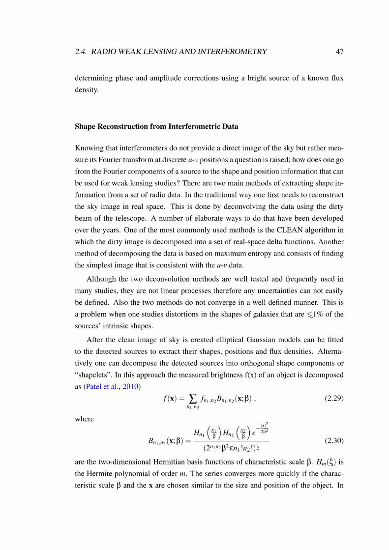
2.4. RADIO WEAK LENSING AND INTERFEROMETRY 47
determining phase and amplitude corrections using a bright source of a known fluxdensity.
Shape Reconstruction from Interferometric Data
Knowing that interferometers do not provide a direct image of the sky but rather mea-sure its Fourier transform at discrete u-v positions a question is raised; how does one gofrom the Fourier components of a source to the shape and position information that canbe used for weak lensing studies? There are two main methods of extracting shape in-formation from a set of radio data. In the traditional way one first needs to reconstructthe sky image in real space. This is done by deconvolving the data using the dirtybeam of the telescope. A number of elaborate ways to do that have been developedover the years. One of the most commonly used methods is the CLEAN algorithm inwhich the dirty image is decomposed into a set of real-space delta functions. Anothermethod of decomposing the data is based on maximum entropy and consists of findingthe simplest image that is consistent with the u-v data.
Although the two deconvolution methods are well tested and frequently used inmany studies, they are not linear processes therefore any uncertainties can not easilybe defined. Also the two methods do not converge in a well defined manner. This isa problem when one studies distortions in the shapes of galaxies that are ∼<1% of thesources’ intrinsic shapes.
After the clean image of sky is created elliptical Gaussian models can be fittedto the detected sources to extract their shapes, positions and flux densities. Alterna-tively one can decompose the detected sources into orthogonal shape components or“shapelets”. In this approach the measured brightness f(x) of an object is decomposedas (Patel et al., 2010)
f (x) = ∑n1,n2
fn1,n2Bn1,n2(x;β) , (2.29)
where
Bn1,n2(x;β) =Hn1
(x1β
)Hn2
(x2β
)e− |x|
2
2β2
(2n1n2β2πn1!n2!)12
(2.30)
are the two-dimensional Hermitian basis functions of characteristic scale β. Hm(ξ) isthe Hermite polynomial of order m. The series converges more quickly if the charac-teristic scale β and the x are chosen similar to the size and position of the object. In

48 CHAPTER 2. WEAK GRAVITATIONAL LENSING
principle one can use polynomials of up to any order to decompose a source. In prac-tice though the series has to be truncated at some order (n1,n2) = (nmax
1 ,nmax2 ) in which
a sufficiently good model of the galaxy is recovered but at the same time the process iscomputationally efficient, as the computation of each object’s decomposition is ∝n4
max.
Using the orthonormality one can calculate the shapelet coefficients of a galaxy asfollows
fn1,n2 =∫
f (x)Bn1,n2(x;β)d2x. (2.31)
Patel et al. (2010) found that in order for the shapelets method to fit the data using a rea-sonable low nmax both x and β had to be fixed to the detected positions and 0.4×FWHMof each source respectively. To remove any beam effects from the sources the shapeletsare convolved with the PSF model and the resulting functions are used to fit the data.
An alternative way of reconstructing the images from interferometric observationsis to use shapelets to fit the data directly into the ‘u-v’ plane. This can be done due tothe property of Hermite basis functions of being invariant under a Fourier transform(up to a rescaling factor, Chang & Refregier 2002).
Lets consider the Fourier transform of the intensity of an object
f (k) = (2π)1/2∫
∞
−∞
d2x f (x)eik·x. (2.32)
The intensity can then be decomposed as
f (k) = ∑n1,n2
fn1,n2Bn1,n2(k;β) , (2.33)
where Bn1,n2(k;β) are the Fourier transforms of the basis functions obeying the prop-erty
Bn1,n2(k;β) = in1+n2Bn1,n2(k;β−1) . (2.34)
Once again, using the orthonormality of the basis functions, the coefficients are calcu-lated as
fn1,n2 =∫
f (k)Bn1,n2(k;β)d2k. (2.35)
The advantage of this approach is that the non-linear decomposition of the image canbe omitted. Instead one can reconstruct the sky distribution by applying a linear fitto the u-v data using the shapelets coefficients as free parameters. An additional ad-vantage of the method is that since the u,v,w coordinates are entirely determined by

2.5. MEASURING WEAK LENSING SHEAR 49
the antenna positions and orientation on the sky, any primary beam attenuation, time-average, bandwidth smearing and non-coplanarity issues can be treated very easily.
A limitation of the method, due to having to fit the shapelet coefficients of all thesources simultaneously, is computing power, memory and time. Chang & Refregier(2002) reported that to calculate 177 shapelet coefficients for 23 sources, using 10 coreson the UK COSMOS SGI supercomputer and 700MB of running memory, required26s.
2.5 Measuring Weak Lensing Shear
The assumption made in Section 2.2 that sources prior to lensing are spheres of con-stant radius is now dropped, as galaxies come in different sizes and shapes. Thereforethe convergence κ and shear γ affects the galaxy sizes and ellipticities as follows
§obs = κ∗§int +§noise , (2.36)
εobs = ε
int + γ+ εnoise , (2.37)
where ε = ε1 + iε2 and γ = γ1 + iγ2 are the complex ellipticity and shear and § is thegalaxy size. The superscripts “obs" and “int" designate the observed and intrinsicellipticity (and size), respectively. The superscript “noise" corresponds to the noiseinduced to the galaxy ellipticity during the measurement stage.
Galaxy ellipticity can be described in terms of a semi-major axis (a), a semi-minoraxis (b), and a position angle (φ) as
ε1 = ε× cos(2φ), (2.38)
ε2 = ε× sin(2φ). (2.39)
Here, ε = (a−b)/(a+b) is the modulus of the galaxy’s ellipticity and φ is the positionangle of the galaxy with respect to the reference axis of the chosen coordinate system.
Looking at eq. 2.36 and eq. 2.37 an issue arises. How does one acquire the intrinsicshapes and ellipticities of the lensed sources? Currently there are no known methodsfor acquiring the intrinsic sizes of the sources prior to lensing. Although assumptionscan be made about the ensemble size distribution at a given redshift, this limitationseverely hinders any weak lensing studies that make use of the convergence κ. Ways

50 CHAPTER 2. WEAK GRAVITATIONAL LENSING
to extract information about the galaxy ellipticities prior to lensing have been devel-oped over the last few years (see Chapter 2.4) but they have not been properly testedyet. Further more in the weak gravitational lensing regime any additional “stretching”induced by gravity is 100 −10000 times weaker than the intrinsic shape of the galaxy,making in impossible to detect by looking at individual sources. But assuming thatin the absence of the lensing mass the background objects are randomly orientatedthough and that the noise during the measuring process is Gaussian random, then thenet alignment induced by the mass distribution can be recovered statistically:
〈εi j〉= γi j ≡(
γ1 γ2
γ2 −γ1
), (2.40)
where the angled brackets denote an ensemble average.
The lensed galaxies’ alignment is so small that any weak gravitational lensing studyhas the following prerequisites:
1. The observation of large and deep sky areas at sub-arcsec resolution is needed, toacquire large samples of foreground and background sources up to high redshiftsand to faint fluxes.
2. During the imaging stage galaxy, shapes are corrupted by the point-spread func-tion (PSF) of the telescope. This artificial contamination might be originatingfrom the optics and detector of the telescope, or from inhomogeneities in theatmosphere. The anisotropic part of the PSF creates spurious correlations be-tween galaxy shapes that, if not treated properly, can generate a signal that islarger than the one we are trying to measure. It is also essential therefore thatsystematic contamination is kept minimal, is properly quantified and accountedfor.
3. Sophisticated image analysis methods are needed to extract the galaxy shapeinformation from the images.
4. Large sets of realistic image simulations to ensure that the measurement biasesare small enough compared to the statistical errors. The simulations should in-corporate survey and observed galaxy populations properties.
5. Accurate redshift information for the observed galaxy populations, as the correctinterpretation of the detected shear signal depends critically on it.

2.5. MEASURING WEAK LENSING SHEAR 51
Galaxy Shape Measurements
One of the greatest challenges for WGL studies is extracting the galaxy shape infor-mation from the images. Most of the signal is carried by high-redshift lensed galaxies.These are usually faint objects with sizes of the order arcsec. These galaxies during theobservation stage are convolved with a spatially and in many cases time varying PSF.To perform weak lensing studies though one first needs to remove the PSF effects fromthe galaxy shapes. It is not required that an individual galaxy shape is measured withhigh precision; what is more important is that the ensemble galaxy shape distributionis unbiased. The galaxy shape measurement bias must decrease with increasing sensi-tivity of the study. Currently surveys measure galaxy ellipticity to ∼ 1% accuracy, butwith the next generation experiments this needs to be improved by at least one orderof magnitude (see the values for the m and c terms in Table 2.1).
There are two main families of methods to measure the ellipticity ε of a galaxyimage with a light distribution I(θ) (For more details on how this is achieved withinterferometric radio data see Section 2.4). With the first method the ellipticity is esti-mated from the data by measuring the second moments of the surface brightness I or bydecomposing I into basis functions and extracting the ellipticity from the correspond-ing coefficients. In the second approach a model is generated, assuming ellipticityparameters and is then fitted to the observed image. The first family of methods aremore sensitive to the pixel noise compared to the second but they also require fewerassumptions about I. The advantage of the model fitting methods is a straightforwardtreatment of the PSF. For more information about the methods please refer to Kilbinger(2015)
Weak Lensing Measurement Errors
Errors in the shape measurement stage can arise from several sources. The first cat-egory is related to the PSF of the telescope. The model of the PSF in optical groundbased instruments (for example SDSS) is affected by atmospheric turbulence. Addi-tionally the shape of the PSF for optical single dish telescopes is not known and itshould be modelled across the sky using point sources (i.e stars). It should then beextrapolated to the positions of the galaxies, inevitably limiting its accurate recon-struction. The point spread function of a telescope varies with frequency. Furthermoreatmospheric refraction is chromatic. For optical surveys therefore in which stars andgalaxies have a different spectral energy distribution (SED), the PSF used to correct the

52 CHAPTER 2. WEAK GRAVITATIONAL LENSING
shapes of the latter might not be the one they were convolved with, introducing biases.The bias depends on the SED variation within the filter, which is larger the broader thefilter is. For space-based optical instruments (for example Hubble) the number of starsper field of view is much smaller, but due to the lack of atmospheric disturbances andtherefore the high stability of the system a global PSF model can be created.
Radio interferometers on the other hand have more stable and deterministic beampattern across the sky. Radio multi-element telescopes though suffer from an incom-plete ‘u-v’ coverage which can lead to sub-optimal deconvolution/CLEANing of thesources (see Section 2.4). The PSF of radio telescopes, similar to optical instrumentsalso depend on frequency. Current radio interferometers have wide bands to increasetheir sensitivity and “u-v” coverage (once again I refer to Section 2.4). This generateslarge number of data. To increase processing speed, a PSF is usually generated at themean frequency of the band. If the observed source has an SED that significantly varieswithin that frequency range, then the PSF used to correct the shape of the source willnot match perfectly the one that was used to convolve it in the first place.
The second class of errors proceeds during the measurement stage. Pixel noise biasarises from the fact that galaxy ellipticities are not a linear function of pixel intensitiesin the presence of noise and PSF. This effect is strongly correlated to the signal-to-noise detection of each source. The effects of noise can cause biases of the order of1-10% on measured shear and affect both moment and model fitting methods. Formore information on the subject please see Kacprzak et al. (2012).
A further source of measurement biases, called “ellipticity gradients”, occurs whenthe galaxy ellipticity varies with radius. This bias, as most types of shear biases, can becharacterised to first approximation by a multiplicative component m and an additiveterm c.
εobsi = (1+mi)ε
truei + ci; i = 1,2 (2.41)
The shear biases m and c are generally functions of galaxy properties and redshift.Current measurement methods provide shear estimates with m at the 1 to 10 percentlevel and c between 10−3 and 10−2. Both pixel noise and ellipticity bias are usuallycorrected during the simulation stage (see next Section). Future surveys require theaccuracy of calibrated shapes to be on the order of 0.1% (see Table 2.1).
Weak gravitational lensing observables, require knowledge of the galaxy redshiftdistribution, in order to be interpreted cosmologically. Acquiring spectroscopic red-shifts for all faint galaxies used in a typical weak-lensing study is too resource and

2.5. MEASURING WEAK LENSING SHEAR 53
time costly. Therefore redshifts have to be estimated from broad-band photometry, us-ing a technique of photometric redshifts or photo-zs. There are various methods formeasuring photo-zs. Template-based approaches perform χ2-type fits of (redshifted)template SEDs to the flux density in the observed bands. Empirical approaches on theother hand make use of a training set with acquired spectroscopic redshifts to estimatethe redshifts for the rest of the sources. For more information about photometric red-shifts refer to Kilbinger (2015) and references thereafter. The dispersion of currentphotometric redshifts is of the order of σz/(1+ z) = 0.03–0.06, for a typical multi-band optical survey. The rate of galaxies whose estimated redshift is off from the trueredshift by more than a few standard deviations is on the order of a few percent. Thethird source of errors therefore is associated with inaccuracies in estimating the red-shifts of galaxies. In a weak lensing study by galaxies or galaxy clusters, inaccuratelyestimating the redshifts of galaxies could lead to a failure in distinguishing foregroundto background objects. It would also mean that the extracted information about thelensing sources will be biased. On a cosmic shear tomography study, in which thelarge scale lensing signal is calculated at different redshift bins, inaccurate redshift es-timation could mean that galaxies might end up in the wrong tomographic bin, thusproviding us with the false picture for the evolution of the Universe.
The fourth type of errors in a weak lensing study is of cosmological origins. Con-trary to the assumption made earlier in the thesis, galaxy shapes can be correlated in theabsence of gravitational lensing, due to the gravitational forces between them and theirsurrounding environment. The intrinsic alignment (IA) of the shapes of galaxies thatare close in redshift can introduce spurious power into estimates of autocorrelationsof the shear field (the so-called intrinsic-intrinsic or ’II’ term). Moreover, intrinsiccorrelations can introduce anti-correlations of the shapes of galaxies that are widelyseparated in redshift (the what is known as lensing-intrinsic or ’GI’ term). IA biasesare difficult to account for as they can not be removed simply by galaxy selection, norcan be easily predicted theoretically since they depend on details about galaxy forma-tion.
The first IA studies came around the time the first detections of cosmic shear weremade. A variety of methods were implemented to study this effect such as analyticalcalculations (Crittenden et al., 2001; Catelan et al., 2001; Mackey et al., 2002) andN-body dark matter simulations, in which they would either measure alignments fromdark matter halos alone (Croft & Metzler, 2000; Heavens et al., 2000) or populate ha-los with galaxies using simple, semi-analytic prescriptions for their shape correlations

54 CHAPTER 2. WEAK GRAVITATIONAL LENSING
(Heavens et al., 2000). Unfortunately the predictions from these methods did not seemto agree. Only recently have hydro-dynamical simulations with high enough resolutionto form galaxies with realistic morphologies, allowed a direct measurement of galaxyalignments (Hahn et al., 2010; Dubois et al., 2014; Tenneti et al., 2014; Codis et al.,2015). The studies have shown that IA effects if not properly accounted for can biasthe results of a measurement by tens of percent.
One of the aims of this thesis is to develop ways to make unbiased weak lensingmeasurements in the presence of errors due to the telescopes’ beam and the measure-ment stage.
The necessity for simulations
Realistic, large volume simulations are crucial for the interpretation of shear data for avariety of reasons.
1. The scales on which shear measurements are taking place extend deep into thehighly non-linear regime. To construct analytical predictions on those scales isnot always feasible. N-body simulations offer an alternative way to obtain theinformation in this non-linear regime.
2. Baryonic effects have to be taken into account with increasing necessity for cur-rent and future studies. By using hydro-dynamical simulations baryons can betaken into account for cosmological predictions.
3. Simulations are an important tool for estimating and correcting potential astro-physical and observational systematics. Alignments caused by the PSF pattern ofa telescope can create non-zero shape correlations between galaxies (see Chap-ter 3). To assess data quality and validity of the measuring methods simulatedsystematic free samples need to be generated.
4. Simulations can be used to test the mathematical approximations used to deriveweak lensing estimators, like the linearisation of the propagation equation (Bornapproximation).
2.6 Conclusions
Weak lensing offers great potential for constraining the (dark) matter and dark energydistribution in the Universe. The coherent deformation of the sources though, due to

2.6. CONCLUSIONS 55
the matter inhomogeneities along the line of side, can be biased by telescope inducedsystematics. The artificial origins of shape correlations in many cases generate a signalthat can be of orders of magnitude greater than the cosmological one of interest (seeChapter 3 and Chapter 4). This thesis has focussed on applying novel approaches ondealing with such systematics, detected both in the radio and in the optical, across anumber of angular scales. Simulations are employed both to confirm the removal ofthe artificial origins generated signal and to calculate the uncertainties in the measure-ments. Then using archival optical and radio data, non zero weak lensing signals aresuccessfully detected across scales of 20′′ ∼< θ ∼< 20. Finally the data are fitted and anumber of cosmological parameters are extracted.

Chapter 3
Cross correlation shear with the SDSSand VLA FIRST surveys
Gravitational lensing is the apparent distortion in the shapes of distant backgroundgalaxies due to the path of their light rays being altered by the gravitational field of aforeground object. In the weak lensing (WL) regime these distortions are so slight thatthey cannot be measured using only one background source; hence WL is an intrinsi-cally statistical measurement. WL is considered today to be a uniquely powerful toolin astronomy. This is because it can be used to estimate the total mass of a foregroundlens regardless of the constituent matter’s fundamental nature.
The tiny coherent WL distortions of background galaxy shapes caused by the large-scale structure in the Universe is termed cosmic shear. The theoretical basis for cosmicshear was pioneered by Gunn (1967), but due to its challenging observational nature itwas only detected around three decades later (Villumsen, 1995; Schneider, 1998; Ba-con et al., 2000; Kaiser et al., 2000; Van Waerbeke et al., 2000; Wittman et al., 2000).The field has since flourished with numerous experiments delivering results with in-creasing accuracy (Van Waerbeke et al., 2001; Brown et al., 2003; Bacon et al., 2003;Fu et al., 2008; Heymans et al., 2012; Jee et al., 2013). Measuring these gravitationallyinduced distortions at different scales provides a wealth of cosmological information.In particular cosmic shear studies can constrain the clustering amplitude σ8 and thematter density Ωm (Hoekstra et al., 2006; Schrabback et al., 2010; Kilbinger et al.,
56

3.1. COSMIC SHEAR IN FOURIER SPACE 57
2013). Furthermore with forthcoming and future large surveys containing redshift in-formation (e.g. DES1, KIDS2, HSC3 LSST4, WFIRST-AFTA5, Euclid6 and SKA7),it will be possible to measure the evolution of the large-scale matter distribution andhence place constraints on the dark energy equation of state w.
Cosmic shear studies require extremely accurate galaxy shape measurements. Tele-scope induced systematics though can alter these shapes in such a way that will biascosmological studies of this sort. The source of systematics for an optical/NIR tele-scope and a radio interferometer are of a very different origins and therefore are notexpected to be correlated.
The cross-power spectrum approach described in this Chapter represents a power-ful technique for mitigating shear systematics and will be ideal for extracting robustresults, with the exquisite control of systematics required, from future cosmic shearsurveys with the SKA, LSST, Euclid and WFIRST-AFTA.
3.1 Cosmic Shear in Fourier Space
Refering back to Sections 2.2-2.3 the shear at angular position Ω can be related to alensing potential (ψ) as
γi j(Ω) =
(δiδ j−
12
δKi jδ
2)
ψ(Ω), (3.1)
where δi ≡ r(δi j− rir j∇i) is a dimensionless, transverse differential operator, and δ2 =
δiδj is the transverse Laplacian. The lensing potential can in turn be related to the 3-D
gravitational potential, Φ(r) by (e.g. Kaiser 1998)
ψ(Ω) =2c2
∫ r
0dr′(
r− r′
rr′
)Φ(r′), (3.2)
where r is the comoving distance to the sources.
As indicated by eq. 2.40, the shear components can be estimated by averaging overa set of observed background galaxy ellipticities. The shear field can be related to the
1Dark Energy Survey, http://www.darkenergysurvey.org2KIlo Degree Survey, http://kids.strw.leidenuniv.nl3Hyper Suprime-Cam, http://www.naoj.org/Projects/HSC4Large Synoptic Survey Telescope, http://www.lsst.org5Wide-Field IR Survey Telescope, http://wfirst.gsfc.nasa.gov6Euclid satellite, http://sci.esa.int/euclid7Square Kilometre Array, http://www.skatelescope.org

58CHAPTER 3. CROSS CORRELATION SHEAR WITH THE SDSS AND VLA FIRST SURVEYS
lensing convergence field by (Kaiser & Squires, 1993)
κ = ∂−2
∂i∂ jγi j, (3.3)
where ∂−2 is the inverse 2-D Laplacian operator defined by
∂−2 ≡ 1
2π
∫d2r′ ln
∣∣r− r′∣∣ . (3.4)
A second decomposition of the shear yields the odd-parity divergence field,
β = ∂−2
εni ∂ j∂nγi j, (3.5)
where εni is the Levi-Civita symbol in two dimensions,
εni =
(0 -11 0
). (3.6)
It is worth noting at this point that κ and β of eq. 3.3 and eq. 3.5 are the same asthe E- and B- modes described in Section 2.2. The standard lore is that due to thehomogeneity and isotropy in the Universe, gravitational lensing produces no β-modes,at least to first order, therefore the divergence field is a useful quantity for testingsystematic effects in weak lensing studies.
Weak Lensing in Spherical Harmonic Space
As mentioned above, lensing shear is a spin-2 field, i.e. it transforms as γ→ γei2φ
under rotation by φ (where, for convenience I have defined the complex shear γ =
γ1 + iγ2). One may thus expand γ and its complex conjugate in terms of the spin-weighted spherical harmonics, sY`m (Newman & Penrose, 1966) as
γ(Ω) = γ1(Ω)+ iγ2(Ω)
= ∑`m(κ`m + iβ`m)2Y`m(Ω), (3.7)
γ∗(Ω) = γ1(Ω)− iγ2(Ω)
= ∑`m(κ`m− iβ`m)−2Y`m(Ω), (3.8)
where s denotes the spin and the summation in m is over −` ≤ m ≤ `. κ`m and β`m
are the spin-2 harmonic modes of the so-called electric (i.e. “gradient” or “E-mode”)

3.1. COSMIC SHEAR IN FOURIER SPACE 59
and magnetic (i.e. “curl” or “B-mode”) components of the shear field respectively,which I further identify as the harmonic space versions of the lensing convergence anddivergence fields mentioned in the previous section. Using the orthogonality of thespin-s spherical harmonics over the whole sphere,∫
dΩ sY`m(Ω) sY ∗`′m′(Ω) = δ``′δmm′, (3.9)
where the spin states must be equal, the harmonic modes of the κ and β fields can befound directly from the shear field, γ;
κ`m =12
∫dΩ [γ(Ω)2Y ∗`m(Ω)+ γ
∗(Ω)−2Y ∗`m(Ω)], (3.10)
β`m =−i2
∫dΩ [γ(Ω)2Y ∗`m(Ω)− γ
∗(Ω)−2Y ∗`m(Ω)]. (3.11)
Taking the average values over the sphere of products of the harmonic coefficients ofthe κ and β fields, one can construct three possible power spectra:
Cκκ` =
12`+1 ∑
mκ`m κ
∗`m, (3.12)
Cββ
` =1
2`+1 ∑m
β`m β∗`m, (3.13)
Cκβ
` =1
2`+1 ∑m
κ`m β∗`m. (3.14)
The parity invariance of weak lensing suggests that Cββ
` and Cκβ
` should be equal tozero in the absence of systematics. However, systematic effects (both instrumental andastrophysical) can give rise to a non-zero Cββ
` . Finite fields and boundary effects canalso lead to leakage of power between the three spectra.
In the limit of weak lensing, the two-point statistical properties of the shear andconvergence fields are the same (Blandford et al., 1991) so that Cγγ
` = Cκκ` . Finally, I
can relate the convergence power spectrum to the 3-D matter power spectrum Pδ(k,r)
through (e.g. Bartelmann & Schneider 2001)
Cκ(i)κ( j)` =
94
(H0
c
)4
Ω2m
∫ rH
0dr Pδ
(lr,r)(
W i(r)W j(r)a(r)2
), (3.15)
where I have assumed a flat Universe, and I have now considered the more general casewhere one measures the cross-correlation signal between two different surveys, here

60CHAPTER 3. CROSS CORRELATION SHEAR WITH THE SDSS AND VLA FIRST SURVEYS
denoted with indices i and j. In eq. 3.15, H0 is the Hubble constant, a is the scale factorof the Universe, r is comoving distance, rH is the comoving distance to the horizon andΩm is the matter density. The weighting, W i(r), is given in terms of the normalisedsource distribution for each survey, Gi(r)dr = pi(z)dz:
W i(r)≡∫ rH
rdr′Gi(r′)
r′− rr′
. (3.16)
Power Spectrum Estimation on a Cut Sky:
The power spectrum estimators of eqs. 3.12–3.14 are only unbiased in the case of fullsky coverage and in the absence of noise. However, in the analysis of chapter 3 I shallbe estimating these power spectra from noisy data covering only a fraction of the sky.In order to correct for the effects of limited sky coverage and noise, I adopt a “pseudo-C`” analysis, originally developed in the context of CMB polarization observations.I provide a brief summary of the technique here and refer the reader to Brown et al.(2005) for further details.
In the presence of finite sky coverage and/or a mask that excludes certain regionsof the sky, one can estimate the so-called pseudo-C`’s directly from a set of shear maps(using fast spherical harmonic transforms from e.g. the HEALPIX software8, Górskiet al. 2005) as:
CA(i)B( j)` =
12`+1 ∑
mA`m(i)B∗`m( j), (3.17)
where A,B are any of the three possible combinations of κ and β and i, j denotethe two different surveys. In the following chapter, I will mostly be interested in takingthe cross-power spectra of the FIRST and SDSS datasets (see section 3.2), i.e. where i
denotes the FIRST dataset and j denotes SDSS. When cross-correlating two datasets,there are then in principle two possible Cκβ
` power spectra. For simplicity, I will takethe average of these and present a single Cκβ
` cross-power spectrum. In eq. 3.17, A`m
and B`m denote the spin-2 spherical harmonic modes (found using eq. 3.10 and eq. 3.11of weighted versions of the lensing shear field,
γ(Ω) =W (Ω)γ(Ω), (3.18)
where W (Ω) is an arbitrary weighting function which can be used to exclude certainregions of the sky and/or downweight noisier sky pixels.
8Software for pixelisation, hierarchical indexation, synthesis, analysis and visualisation of data onthe sphere. For more details see http://healpix.sourceforge.net.

3.1. COSMIC SHEAR IN FOURIER SPACE 61
Grouping all three power spectra into a single vector, C` = Cκκ` ,Cββ
` ,Cκβ
` , onecan show that the pseudo-C`’s measured from the weighted shear fields are related tothe true power spectra on the full sky via
C` = ∑`′
M``′C`′ , (3.19)
where I have introduced the coupling matrix, M``′ . This coupling matrix fully en-codes how the survey geometries and masks (described via the function, W (Ω)) mixmodes, both within a single spectrum (e.g. Cκκ
` →Cκκ
`′ ), and also between spectra (e.g.Cκκ` →Cββ
`′ ), and it can be calculated exactly for any given set of weighting functions,W (Ω). Specifically, in my case where I am estimating the cross-power spectra betweentwo datasets, I can calculate the M``′ matrix exactly from the pseudo-C` cross-powerspectra (estimated using eq. 3.17) of the weighting functions used for the two differentsurveys, Wi(Ω) and Wj(Ω). Further details and explicit formulae for calculating M``′
are provided in Brown et al. (2005).
Recovering an estimate of the power spectra on the full sky is then only a matterof inverting eq. 3.19. When calculating auto-power spectra (from a single survey), onealso needs to include a correction for the noise bias arising from the intrinsic disper-sion in galaxy shapes and measurement errors. For practical reasons, it is often alsoconvenient to estimate the power spectrum in terms of “band powers” which recoverthe average power across a range of multipoles, ∆`. Including these features, the powerspectrum estimator becomes
Pb = ∑b′
K−1bb′ ∑
`
Ob′`(C`−〈N`〉MC), (3.20)
where Pb denotes the debiased combined estimator for band powers of the Cκκ` , Cκβ
`
and Cββ
` power spectra. In eq. 3.20, C` are the pseudo-C`’s measured from the data and〈N`〉 are the noise-only pseudo-Cl’s estimated from a suite of 100 Monte Carlo (MC)simulations which contain realisations of the noise, and also incorporate the effects ofthe survey masks. Note that, for the cross-power spectrum analysis of chapter 3, thenoise is uncorrelated and so the noise subtraction step (subtraction of the 〈N`〉MC term)is not required, although I will nevertheless implemented it in my analysis pipeline forcompleteness. We have found that this number of noise realisations is computationallyefficient to generate with the resources we had in our possession. At the same time,given the level of the signal we are trying to measure, any uncertainties associated in

62CHAPTER 3. CROSS CORRELATION SHEAR WITH THE SDSS AND VLA FIRST SURVEYS
estimating the ensemble noise component are sufficiently small that can be neglected.
Kbb′ is the binned coupling matrix, constructed from M``′ as
Kbb′ = ∑`
Ob`∑`′
M``′F ′Q`′b′, (3.21)
where Ob` is a binning operator that bins the C`’s into band powers and Q`b is theinverse operator which “unfolds” the band powers into individual C`’s. The function,F describes the smoothing effect on the underlying shear fields due to the fact that thesky maps are pixelized. This function is provided by the HEALPIX software that I useto pixelize the sky and perform the spin spherical harmonic transforms.
The binning operator I choose to use is
Ob` =
12π
`(`+1)
`(b+1)low −`(b)low
, if 2≤ `(b)low ≤ ` < `
(b+1)low
0 , otherwise ,(3.22)
where `(b)low denotes the lower edge of band b. With this choice, the quantity `(`+
1)C`/2π is approximated as constant within each band power.
3.2 The Surveys
3.2.1 FIRST Data
The VLA FIRST survey (Becker et al., 1995) is a 10,575 deg2 survey of the sky inthe declination range −10 ≤ δ≤ 70, and right ascension range 8hrs≤ RA≤ 17hrs.Of the survey’s total sky coverage, 8,444 deg2 are in the north galactic cap and 2,131deg2 are in the south. The data were gathered using the VLA at L-band (1.4 GHz),in B-configuration (maximum baseline length of 11.1 km) and in snapshot mode (<5minutes per observation). The observations were conducted between 1993 and 2011.The coverage for the southern cap is discontinuous due to poor weather and systemfailures during the 2011 observations.
The beam of the telescope at δ >+433′ can be approximated by a circular Gaus-sian with a full width at half maximum (FWHM) of 5.4′′. Below δ = +433′ thebeam is elliptical with a FWHM of 6.4′′×5.4′′, with the major axis running north-south. For 21hrs < RA < 3hrs and δ < −230′ the ellipticity of the beam increasesfurther to 6.8′′×5.4′′. The survey achieved an RMS noise level of ∼0.15 mJy, and

3.2. THE SURVEYS 63
delivered positions, flux densities and shape information for ∼1 million radio sources,of which ∼40% are resolved. Shape information was extracted by fitting an ellipticalGaussian model to each source. The FIRST catalogue provides this shape informationvia a major and minor axis and a position angle (PA) for each object. Note that theFIRST analysis pipeline includes a deconvolution step to remove blurring due to thetelescope’s PSF.
Mainly due to the relatively sparse coverage in visibility (or u-v) space – an un-avoidable result of the observation strategy – the deconvolution/CLEANing9 of theFIRST sources was imperfect. The catalogue therefore contains information about thepossibility of a detected source being a residual sidelobe of a nearby brighter source.Of the total number of FIRST sources, 76.4% had a probability of being spurious, P(S),less than 5%. For 17% of the sources the probability was between 5 and 50%. Theremaining 6.5% had more than a 50% chance of being a sidelobe of a nearby brightgalaxy. Additional information about the sources was generated by cross-correlatingtheir positions with positions of optical sources from the SDSS and 2-micron All-SkySurvey (2MASS, Skrutskie et al. 2006) catalogues. More information regarding thecontents of the FIRST catalogue and how it was generated is available from the FIRSTwebsite10. The data are edited, self-calibrated, mapped and CLEANed using an auto-mated pipeline based largely on routines in the Astronomical Image Processing System(AIPS). According to their webpage, both the images and the catalogues constructedfrom the FIRST observations are only made publicly available if they successfully passa set of quality-controls tests designed by the VLA FIRST team.
The FIRST data have previously been used to make a detection of cosmic shearin the radio band by extracting source shape information directly from the u-v plane(Chang et al., 2004). Those authors measured the 2-point correlation function (2PCF)on angular scales, 1 < θ < 40. On scales 1 < θ < 4 the measured β-modes whereconsistent with zero while a significant signal was detected in the κ-modes at the ∼3σ
level. From their results, Chang et al. (2004) placed a joint constraint on the clusteringamplitude, σ8 and the median redshift of the FIRST sources without an optical coun-terpart, zm of σ8(zm/2)0.6' 1.0±0.2. Adopting a prior of σ8 = 0.9±0.1 they obtainedthe constraint zm = 2.2±0.9 (68% CL). This value is consistent with existing models
9The CLEAN algorithm (Högbom, 1974) is a standard technique commonly used in radio astron-omy to deconvolve images for the effects of a finite PSF. The algorithm models the data as a collectionof point sources and, starting with the brightest source, iteratively subtracts (from the u-v-data) the fluxassociated with each source in order to detect and characterise fainter objects.
10FIRST website: http://sundog.stsci.edu/index.html

64CHAPTER 3. CROSS CORRELATION SHEAR WITH THE SDSS AND VLA FIRST SURVEYS
of the radio source luminosity function. The results are encouraging as they show thatalthough radio surveys lack the sensitivity at the moment to compete with optical lens-ing surveys, they can deliver shape information which, with the proper processing, canbe used for weak lensing studies.
For the purposes of this study I acquired the 13JUN05 version of the FIRST cata-logue. The Chang et al. (2004) study estimated the median redshift of the entire FIRSTsample to be between 0.9 and 1.4 (depending on the model of the radio source lumi-nosity function used). Using the SKA simulated skies (S3,Wilman et al. 2008) – acomputer simulation based on more recent data, and designed to model the radio andsubmillimetre Universe – I estimate the median redshift of the entire FIRST sample.This was done by supplying the online S3 platform with the relevant information aboutFIRST (survey size, rms noise etc.) Using the redshift information of the sources con-tained in the generated mock catalogue, I estimate the median redshift of the survey tobe zm ∼1.2.
3.2.2 SDSS Data
The SDSS is an ongoing (since 2000) optical survey of the north and south galacticcaps north of declination -15, covering ∼14,500 deg2 of the sky. The survey usesa 2.5 metre telescope located at Apache Point Observatory (APO) in the Sacramentomountains in south New Mexico (Abazajian et al., 2003; Ahn et al., 2014). In 2008the experiment entered a new phase called SDSS-III in which new instruments cameinto operation (Eisenstein et al., 2011). One of the SDSS-III surveys, the Baryon Os-cillation Spectroscopic Survey (BOSS; Dawson et al. 2013), obtained spectra of ∼1.4million luminous red galaxies (LRGs) and ∼0.3 million quasars which have subse-quently been used to place stringent constraints on cosmological models (Aubourget al., 2014).
The SDSS data have been used in numerous weak lensing experiments probingdifferent angular scales on the sky. The data have proved particularly useful for galaxy-galaxy lensing (e.g. Fischer et al. 2000; Mandelbaum et al. 2006b) and cluster lensing(e.g. Mandelbaum et al. 2008; Sheldon et al. 2009; Rozo et al. 2010). In terms ofcosmic shear measurements, Lin et al. (2012) and Huff et al. (2014) have both exploitedthe deep observations of SDSS “Stripe 82” to perform cosmic shear analyses. Both ofthese latter studies detected a significant κ-mode signal on degree scales with β-modesfound to be consistent with zero. Derived constraints on Ωm and σ8 were also found tobe consistent between these two independent studies.
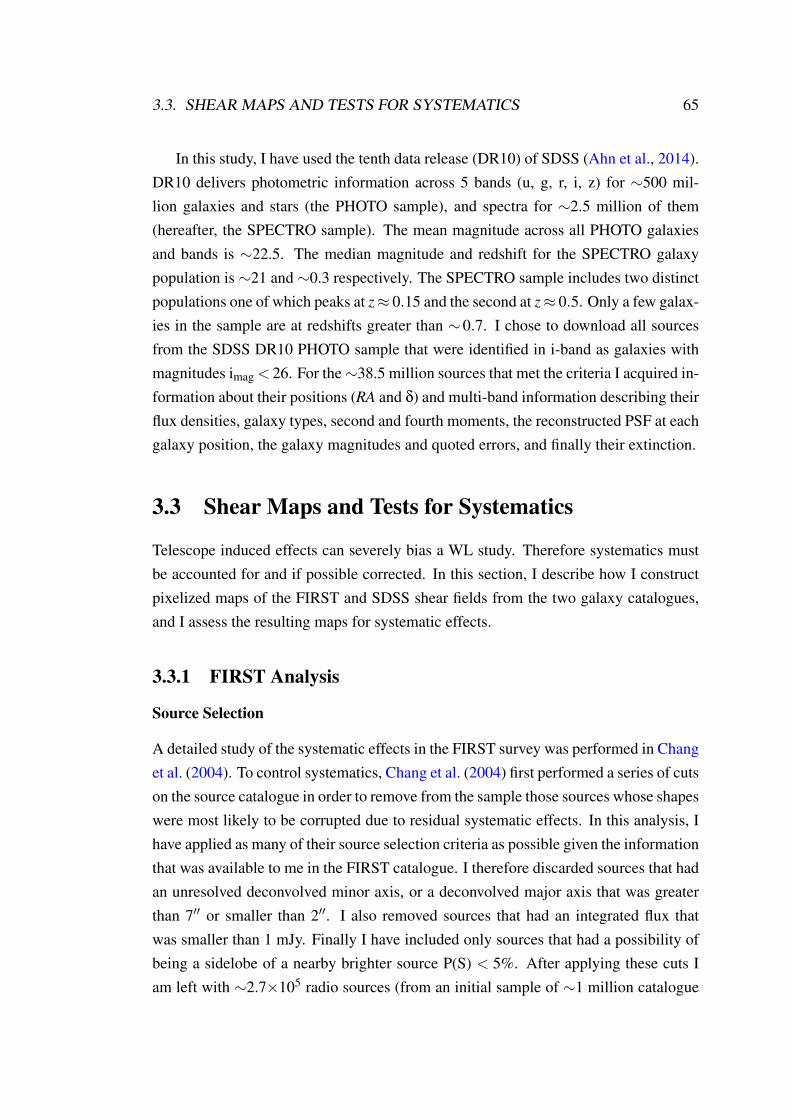
3.3. SHEAR MAPS AND TESTS FOR SYSTEMATICS 65
In this study, I have used the tenth data release (DR10) of SDSS (Ahn et al., 2014).DR10 delivers photometric information across 5 bands (u, g, r, i, z) for ∼500 mil-lion galaxies and stars (the PHOTO sample), and spectra for ∼2.5 million of them(hereafter, the SPECTRO sample). The mean magnitude across all PHOTO galaxiesand bands is ∼22.5. The median magnitude and redshift for the SPECTRO galaxypopulation is ∼21 and ∼0.3 respectively. The SPECTRO sample includes two distinctpopulations one of which peaks at z≈ 0.15 and the second at z≈ 0.5. Only a few galax-ies in the sample are at redshifts greater than ∼0.7. I chose to download all sourcesfrom the SDSS DR10 PHOTO sample that were identified in i-band as galaxies withmagnitudes imag < 26. For the∼38.5 million sources that met the criteria I acquired in-formation about their positions (RA and δ) and multi-band information describing theirflux densities, galaxy types, second and fourth moments, the reconstructed PSF at eachgalaxy position, the galaxy magnitudes and quoted errors, and finally their extinction.
3.3 Shear Maps and Tests for Systematics
Telescope induced effects can severely bias a WL study. Therefore systematics mustbe accounted for and if possible corrected. In this section, I describe how I constructpixelized maps of the FIRST and SDSS shear fields from the two galaxy catalogues,and I assess the resulting maps for systematic effects.
3.3.1 FIRST Analysis
Source Selection
A detailed study of the systematic effects in the FIRST survey was performed in Changet al. (2004). To control systematics, Chang et al. (2004) first performed a series of cutson the source catalogue in order to remove from the sample those sources whose shapeswere most likely to be corrupted due to residual systematic effects. In this analysis, Ihave applied as many of their source selection criteria as possible given the informationthat was available to me in the FIRST catalogue. I therefore discarded sources that hadan unresolved deconvolved minor axis, or a deconvolved major axis that was greaterthan 7′′ or smaller than 2′′. I also removed sources that had an integrated flux thatwas smaller than 1 mJy. Finally I have included only sources that had a possibility ofbeing a sidelobe of a nearby brighter source P(S) < 5%. After applying these cuts Iam left with ∼2.7×10⁵ radio sources (from an initial sample of ∼1 million catalogue

66CHAPTER 3. CROSS CORRELATION SHEAR WITH THE SDSS AND VLA FIRST SURVEYS
Figure 3.1: Results of the test for residual beam systematics in the FIRST galaxy shapes, asdescribed in Section 3.3.1. A large radial (negative γt , black triangles) distortion, decreasingas a function of angular scale, θ, is found in the FIRST galaxy ellipticities when their shapesare stacked around the FIRST galaxy positions. The rotated shear (γr, red circles) is consistentwith zero.
entries). For all remaining sources, I formed the ε1 and ε2 ellipticity estimates fromthe catalogued major and minor axes, and position angle, according to eq. 2.38 andeq. 2.39.
Residual Systematics in FIRST Ellipticities
I have performed a number of quality checks on the data immediately after applyingthe cuts described above. By far the most informative of these was a test for corruptionof the galaxy ellipticities due to residual sidelobe contamination resulting from an im-perfect deconvolution and/or CLEANing procedure. To perform this test, I have madeuse of the g-g lensing tangential and rotated shear constructions (γt and γr; eq. 2.18 &eq. 2.19 and have stacked the shapes of the selected FIRST galaxies around the posi-tions of all of the sources in the original FIRST catalogue (including both resolved andunresolved objects). The results of this test are shown in Fig. 3.1 where I see a strongdistortion in the FIRST galaxy shapes oriented radially from the central stacking po-sition. This signal persists when I randomly choose a sub-set of the FIRST sources’shapes and/or positions. Moreover, the signal shows no obvious dependency on theflux of the stacked and/or central sources.
To further investigate the origin of this signal I repeated the stacking analysis in(∆RA,∆δ) space (i.e. where the positions of all of the central sources are re-mappedto ∆RA = 0;∆δ = 0). The resulting maps of tangential and rotated shear are shown in

3.3. SHEAR MAPS AND TESTS FOR SYSTEMATICS 67
Figure 3.2: Maps of the tangential shear (γt , left panel) and rotated shear (γr, right panel) as afunction of the separation in RA and δ from the central stacking positions. The tangential shearmap reveals a negative amplitude 6-arm star pattern which closely resembles the structure inthe synthesised beam (PSF) of the VLA snapshot observations.
Fig. 3.2.
The 6-arm star pattern apparent in the γt map, displayed in the left panel of Fig. 3.2,closely matches the synthesised beam (or PSF) of the VLA in “snapshot mode” whichwas the observation mode employed during collection of the FIRST survey data. Theresults of this test clearly indicate the presence of residual systematics in the FIRSTgalaxy ellipticities, which are strongly correlated with the known PSF of the VLA-FIRST observations. These residuals are clearly spurious, and are almost certainlythe result of an imperfect deconvolution and/or CLEANing of the FIRST data duringthe imaging step in the FIRST data reduction. In the analysis which follows, I willattempt to include the effects of these residual ellipticity correlations by incorporatinga model of the systematic in my MC simulations. However, I also expect my cross-power spectrum approach – whereby I cross-correlate the FIRST and SDSS galaxyshapes – to be robust to the presence of this FIRST-specific systematic effect.
FIRST Shear Maps
The pseudo-C` power spectrum analysis outlined in Section 3.1 requires as input pix-elized maps of the shear components. I create these maps by simple averaging ofthe ellipticities of the FIRST sources which fall within each sky pixel and I use theHEALPIX scheme (Górski et al., 2005) to define the sky pixelisation. I choose thepixel size according to the density of sources in the FIRST survey: with ∼ 2.7×10⁵

68CHAPTER 3. CROSS CORRELATION SHEAR WITH THE SDSS AND VLA FIRST SURVEYS
Figure 3.3: Maps of the γ1 (left panel) and γ2 (right panel) shear components, constructed bysimple averaging of the FIRST galaxy ellipticities within each pixel.
sources surviving the cuts described in Section 3.3.1, a pixel size of ∼1 deg2 results ina mean pixel occupation number of ∼20 galaxies. This choice ensures that my mapsare contiguous over the survey area and are mostly free from unoccupied pixels withinthe survey boundaries. I therefore set the HEALPIX resolution parameter, Nside = 64,which corresponds to a pixel size of ∼0.85 deg2.
Fig. 3.3 shows maps of the shear components, γ1 and γ2, as reconstructed from theFIRST galaxy ellipticities. These maps are dominated by random noise due to theintrinsic dispersion in galaxy shapes and measurement errors. Visual inspection of thefigure does also suggest a weak dependence of the γ1 amplitudes on declination thoughsome of this may simply reflect the varying galaxy number density, which also showssome dependence on declination. (Later in Section 3.5, I perform a suite of null-testson my cross-power spectrum results, one of which is to split the datasets according todeclination. This test should highlight any significant problems associated with anydeclination-dependent systematic effects that persist in the FIRST shear maps.)
In addition to the shear maps, I construct a weight map (the W (Ω) of eq. 3.18)as simply the number of galaxies that lie within each pixel. In the case of uniformmeasurement errors on the ellipticities, setting W (Ω) to be equal to the galaxy numberdensity is equivalent to an inverse-variance weighting scheme, which, for the noise-dominated régime in which I am working, is the optimal weighting scheme to use.To limit the sensitivity to individual outliers in the galaxy ellipticity distribution, I setW (Ω) = 0 for pixels that contain less than 5 galaxies. Fig. 3.4 shows the weight mapthat results from this process. I use this map to weight the FIRST shear data in thesubsequent power spectrum analysis.

3.3. SHEAR MAPS AND TESTS FOR SYSTEMATICS 69
Figure 3.4: The galaxy number density map (normalised with the maximum number of galax-ies laying at any given pixel of the map) used to weight the FIRST shear field (Fig. 3.3) in thepower spectrum analysis.
3.3.2 SDSS Analysis
Shape Measurements and Initial Source Selection
The SDSS catalogue provides shape information for each detected source as ellipticitycomponents derived from second moments,
ε1 =Qxx−Qyy
Qxx +Qyy, (3.23)
ε2 =2Qxy
Qxx +Qyy, (3.24)
where the adaptive moments are measured directly from the SDSS images accordingto
Qi j =∫
dΩI(Ω)w(Ω)ΩiΩ j. (3.25)
Here, I(Ω) is the object intensity at position Ω = (Ωx,Ωy) and i, j can take valuesx,x, y,y or x,y. Ideally, adaptive moments are measured using a radial weightfunction, w(Ω), which is iteratively adapted to the object’s size. In practice, the SDSSpipeline used a Gaussian weighting function with a size matched to that of the objectbeing fitted. Such an approach has been shown to be nearly optimal (Bernstein &Jarvis, 2002) and is much quicker.
As stated above the SDSS ellipticity estimators used in this study were drawn fromthe SDSS DR10 publicly available database. We chose not to use the calibrated el-lipticity estimators of previous SDSS shear studies. This cause of action was selectedas previous full sky SDSS shear studies made use of the survey’s DR7 (or earlier)data (Mandelbaum et al., 2008). The 8th and onwards data releases though contain an

70CHAPTER 3. CROSS CORRELATION SHEAR WITH THE SDSS AND VLA FIRST SURVEYS
Figure 3.5: Maps of the γ1 (left panel) and γ2 (right panel) shear components, constructed bysimple averaging of the SDSS galaxy ellipticities within each pixel. These maps were con-structed from the∼25 million galaxies remaining in the SDSS shear catalogue immediately af-ter the PSF correction and source selection steps described in Section 3.3.2 were implemented.Significant large-scale systematic effects are clearly evident in these maps.
∼2400 deg2 more sky coverage and an additional ∼120 million unique object entries.Furthermore for the DR8 (and more recent data releases) the SDSS team used newimproved reduction and calibration algorithms improving the quality of all ellipticityestimators. More recent SDSS shear studies, utilising the new improved quality data,mainly focussed on the sky area known as Stripe 82.
The SDSS catalogue’s galaxy ellipticities need to be corrected for PSF smearingand atmospheric seeing. To facilitate this, the catalogue also provides moment infor-mation that describes the PSF reconstructed at each galaxy’s position. I follow theprocedure advocated by the SDSS team which corrects the catalogue ellipticities forthe effects of seeing and PSF anisotropy according to
εcorr1 = (εmeas
1 −Rεpsf1 )/(1−R) ,
εcorr2 = (εmeas
2 −Rεpsf2 )/(1−R) , (3.26)
where εmeasi are the galaxy ellipticity components, ε
psfi are the PSF ellipticity compo-
nents reconstructed at each galaxy position and R is a parameter formed from a com-bination of the second and fourth-order moments of the galaxy and PSF shapes. (Forfurther details, and an explicit formula for R, see the description on the SDSS DR10catalogue webpage11). Comparing the above equations to eq. 2.41, we can see thatthe SDSS data are both affected by an additive and a multiplicative bias. This biasesas illustrated in the next Section are strongly correlated to the shape and size of thereconstructed PSF. As mentioned in the SDSS catalogue description, the correction of
11http://www.sdss3.org/dr10/algorithms/classify.php

3.3. SHEAR MAPS AND TESTS FOR SYSTEMATICS 71
eq. 3.26 is not exact and results in a small bias (Bernstein & Jarvis, 2002; Hirata & Sel-jak, 2003). Additionally, the distribution of the SDSS ellipticities in the pixels of themaps in Fig.3.5 is somewhat wider when compared to a map that was generated usingthe same number of sources but whose ellipticity components were randomised. Thissuggest that the SDSS data suffer from a small multiplicative bias. However, ratherthan implementing a more sophisticated correction algorithm, I will mostly appeal tothe cross-correlation approach of Section 2.4 to limit the sensitivity to any residual bi-ases that remain in the shear catalogue after source selection and implementing thePSF correction of eq. 3.26 (although see below for an additional source selection cutthat I have applied based on the strength of the reconstructed PSF anisotropy, prior toconstruction of my final shear maps).
To limit the impact of very poorly measured and/or noisy shape estimates, I performan initial source selection on the SDSS galaxy sample. To select galaxies, I follow theworks of Bernstein & Jarvis (2002) and Mandelbaum et al. (2008). I thus excludesources for which the modulus of the corrected ellipticity ε = (ε2
1 + ε22)
1/2 > 4 or ifthe uncertainty in the corrected modulus, σε > 0.4. I also only retain sources thathave an i-band extinction that is less than 0.2. In addition, I retain only sources thathave both a PSF and DeVaucouleur r-band magnitude greater than 22, and both a PSFand DeVaucouleur i-band magnitude greater than 21.6. Finally, to exclude very smallgalaxies, I only include sources with R f > 1/3 where the resolution factor, R f is givenby,
R f = 1− Qpsfxx +Qpsf
yy
Qxx +Qyy. (3.27)
With these selection criteria applied, ∼25 million SDSS sources remain in the cata-logue.
Shear Systematics and Additional Source Selection
Using the shape information of the remaining SDSS sources I construct maps of theshear components γ1 and γ2 on a Nside = 64 HEALPIX grid using simple averaging,the same as was used in the previous section for the FIRST maps. The resulting mapsare shown in Fig. 3.5. Note that, because of the large increase in galaxy numbers, thenoise is much lower in the SDSS maps than in the FIRST maps of Fig. 3.3. Visualexamination of Fig. 3.5 shows that these initial SDSS shear maps are clearly contam-inated with large-scale spurious arcs. Comparing the structure and morphology ofthese large-scale systematics with a map of the reconstructed PSF anisotropy reveals a

72CHAPTER 3. CROSS CORRELATION SHEAR WITH THE SDSS AND VLA FIRST SURVEYS
Figure 3.6: Maps of the γ1 (left panel) and γ2 (right panel) shear components, constructedby simple averaging of the SDSS galaxy ellipticities within each pixel. These maps were con-structed from the∼9 million galaxies remaining in the SDSS shear catalogue immediately afterthe additional source selection based on the strength of the PSF, described in Section 3.3.2, wasimplemented. The large-scale systematic effects apparent in Fig. 3.5 have been substantiallyreduced with this additional cut on the galaxy catalogue.
strong correlation, indicating that the observed systematics are residual biases that theapproximate correction scheme of eq. 3.26 has failed to account for.
In order to limit the impact of this residual bias, I have implemented an additionalcut on the galaxy catalogue based on the strength of the PSF anisotropy at each galaxyposition. I discard all remaining SDSS sources for which the reconstructed PSF ellip-ticity modulus is ε > 0.08. (I have experimented with this threshold value and havefound 0.08 to be the minimum value which still suppresses the systematics to approxi-mately the level of the random noise.) Implementing this additional cut, I am left with∼9 million SDSS sources. The SDSS shear maps constructed from this revised cat-alogue are shown in Fig. 3.6. Visual inspection of the new maps demonstrate a largereduction in the amplitude of large-scale systematics, which now appear to be at orbelow the level of the random noise (amplitude of systematics now at . 0.02). Ad-ditionally when comparing the distribution of ellipticities in the pixels of the maps inFig. 3.6 to maps generated using the same number of sources with the same coordinatesbut whose ellipticity components were randomised, the distributions seem to be in avery good agreement suggesting that the multiplicative bias detected at earlier stagesof the analysis, has been removed from the data. If there is residual multiplicative biasin the SDSS data it will cause the measured SDSS-FIRST band power measurementsto shift upwards, making them inconsistent with the theoretical expectations.
This additional cut on the galaxy catalogue increased the noise in the SDSS shearmaps by a factor ∼
√3. However, the measured SDSS auto shear power spectrum and
the uncertainties associated with the large-scale systematics were reduced by a factorof ∼10. Although the FIRST-SDSS cross-power spectrum analysis will be robust to

3.4. SIMULATIONS 73
Figure 3.7: The galaxy number density map (normalised with the maximum number of galax-ies laying at any given pixel of the map) used to weight the SDSS shear field (Fig. 3.6) in thepower spectrum analysis.
this SDSS-specific systematic effect, suppressing the PSF systematic to the level of thenoise at this stage in the analysis is still beneficial in terms of the error performanceof the cross-power spectrum analysis: without this additional selection based on thePSF anisotropy amplitude, the uncertainties in the cross-power spectrum increase by afactor of ∼ 5 (see Section 3.5 for more details).
Finally, I generate a weight map for the SDSS survey using the same method as wasused in the previous section for the FIRST data. The resulting weight map is shownin Fig. 3.7 and shows a non-uniform distribution of SDSS source number density. Inparticular, the very deep coverage of Stripe 82 is clearly visible as an excess of galaxiesnear the Galactic anti-centre, at declinations δ∼ 0.
3.4 Simulations
In this section, I describe my approach to creating simulations of the SDSS and FIRSTshear datasets. My simulations serve several purposes. Firstly, the pseudo-C` powerspectrum estimator (eq. 3.20) includes a noise-subtraction step which debiases a mea-surement of the shear power spectrum for the effects of random shape noise (due toboth intrinsic galaxy shape noise and measurement errors). For this purpose, I estimatethe noise bias, 〈N`〉MC as the average pseudo-C` power spectra measured from a suiteof simulations containing realisations of the random shape noise in each survey.
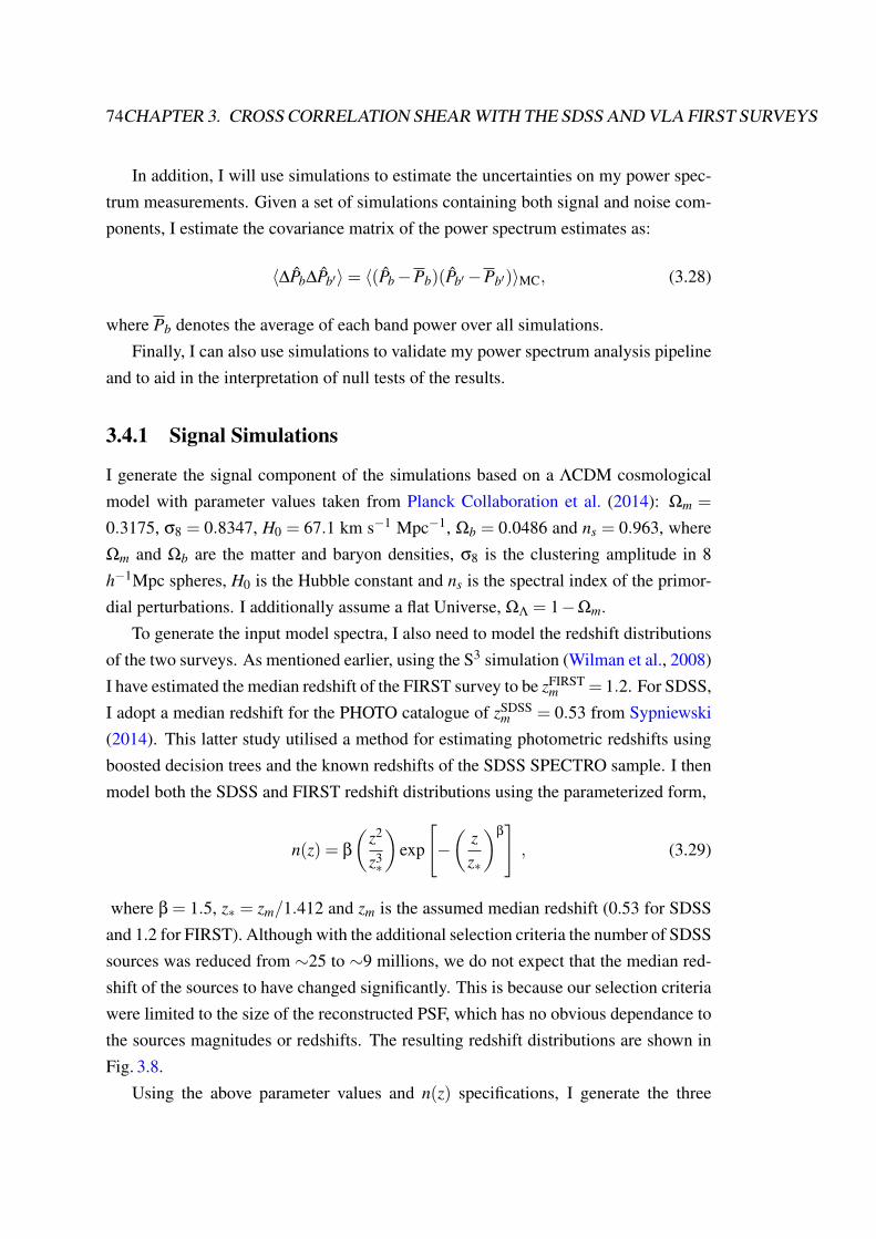
74CHAPTER 3. CROSS CORRELATION SHEAR WITH THE SDSS AND VLA FIRST SURVEYS
In addition, I will use simulations to estimate the uncertainties on my power spec-trum measurements. Given a set of simulations containing both signal and noise com-ponents, I estimate the covariance matrix of the power spectrum estimates as:
〈∆Pb∆Pb′〉= 〈(Pb−Pb)(Pb′−Pb′)〉MC, (3.28)
where Pb denotes the average of each band power over all simulations.Finally, I can also use simulations to validate my power spectrum analysis pipeline
and to aid in the interpretation of null tests of the results.
3.4.1 Signal Simulations
I generate the signal component of the simulations based on a ΛCDM cosmologicalmodel with parameter values taken from Planck Collaboration et al. (2014): Ωm =
0.3175, σ8 = 0.8347, H0 = 67.1 km s−1 Mpc−1, Ωb = 0.0486 and ns = 0.963, whereΩm and Ωb are the matter and baryon densities, σ8 is the clustering amplitude in 8h−1Mpc spheres, H0 is the Hubble constant and ns is the spectral index of the primor-dial perturbations. I additionally assume a flat Universe, ΩΛ = 1−Ωm.
To generate the input model spectra, I also need to model the redshift distributionsof the two surveys. As mentioned earlier, using the S3 simulation (Wilman et al., 2008)I have estimated the median redshift of the FIRST survey to be zFIRST
m = 1.2. For SDSS,I adopt a median redshift for the PHOTO catalogue of zSDSS
m = 0.53 from Sypniewski(2014). This latter study utilised a method for estimating photometric redshifts usingboosted decision trees and the known redshifts of the SDSS SPECTRO sample. I thenmodel both the SDSS and FIRST redshift distributions using the parameterized form,
n(z) = β
(z2
z3∗
)exp
[−(
zz∗
)β], (3.29)
where β = 1.5, z∗ = zm/1.412 and zm is the assumed median redshift (0.53 for SDSSand 1.2 for FIRST). Although with the additional selection criteria the number of SDSSsources was reduced from ∼25 to ∼9 millions, we do not expect that the median red-shift of the sources to have changed significantly. This is because our selection criteriawere limited to the size of the reconstructed PSF, which has no obvious dependance tothe sources magnitudes or redshifts. The resulting redshift distributions are shown inFig. 3.8.
Using the above parameter values and n(z) specifications, I generate the three

3.4. SIMULATIONS 75
Figure 3.8: Normalised galaxy redshift distributions adopted for the SDSS population (solidline) and for the FIRST population (dashed line). I use these distributions to generate the modelshear power spectra for my simulations.
model shear power spectra (the auto power spectra for the two surveys and the cross-power) according to eq. 3.15. For the 3-D matter power spectrum, I use the Bond &Efstathiou (1984) CDM transfer function. I also use the Halofit formula (Smith et al.,2003) to predict the non-linear Pδ(k,r), although for the scales of interest here, thenon-linear contribution is negligible.
I use these power spectra to generate correlated Gaussian realisations of the shearfields in the two surveys. To create the correlated fields, at each multipole, `, I constructthe 2×2 power spectrum matrix, Cκ(i)κ( j)
` where i, j denote the two surveys. Takingthe Cholesky decomposition of this matrix at each multipole, Li j
` , defined by
Cκ(i)κ( j)` = ∑
kLik` L jk
` , (3.30)
I generate random Gaussian realisations of the spin-2 spherical harmonic coefficientsof the two shear fields as
ai`0 = ∑
jLi j` G j
`0,
ai`m =
√12 ∑
jLi j` G j
`m, (3.31)
where Gi`m is an array of unit norm complex Gaussian random deviates. The resulting
fields transformed to real space via a spin-2 transform will then be correctly correlatedaccording to the input auto and cross-power spectra. When generating the real-space
76CHAPTER 3. CROSS CORRELATION SHEAR WITH THE SDSS AND VLA FIRST SURVEYS
shear fields, I use the same spatial resolution as was used in constructing the shearmaps from the real data (HEALPIX Nside = 64, corresponding to 0.85 deg2 pixels).
For each survey, I then create mock galaxy shape catalogues as follows. Foreach object in the real catalogues, I replace its measured ellipticity components withthe components of the simulated shear signal at the appropriate sky location in theHEALPIX-generated maps. Note that I do not randomise the galaxy positions. Ichoose to keep these fixed as I wish to mimic the real data as closely as possible in thesimulations. One aspect of this is that I require the structure in the simulated galaxynumber density maps to be the same as that for the real data (see Figs. 3.4 and 3.7).The observed large-scale structure in the number density maps is clearly dominated byobservational selection effects rather than being due to intrinsic galaxy clustering. Itis therefore appropriate to use the exact same number density fluctuations in the sim-ulations in order to capture the impact of these selection effects. Using the unalteredgalaxy positions from the real catalogues in all of the simulations ensures that this isthe case.
3.4.2 Noise Simulations
To create realisations of the random noise, I assign to each simulated galaxy the mea-sured ellipticity components of a real galaxy, sampled at random from the real galaxycatalogues.
This procedure should model the random noise properties of the data (due to boththe intrinsic dispersion in galaxy shapes and measurement errors in the shape estima-tion step) and facilitate the estimation of the noise bias term, 〈N`〉MC. In principle, myprocedure may slightly over-estimate the uncertainties in the measurements since thedispersion in the simulated galaxy shapes will be enhanced slightly due to any lensingsignal present in the real data. However, I expect this effect to have a negligible ef-fect on my analysis – the ellipticity variance due to the combination of intrinsic shapedispersion and measurement errors will greatly dominate over the lensing contributionfor any plausible cosmological signal. In any case, my cross-power spectrum measure-ments are not affected by the noise bias term, 〈N`〉MC.
3.4.3 Modelling Small-Scale Systematic Effects
In my FIRST simulations, I also include a model of the spurious shear systematic,induced by the FIRST beam residuals, described in Section 3.3.1, and illustrated in

3.4. SIMULATIONS 77
Figure 3.9: The γt component of the contamination template used to model the FIRST residualbeam systematic discussed in Section 3.3.1, and displayed in Fig. 3.2. The γr component of thecontamination was assumed to be zero.
Figs. 3.1 & 3.2. To model this effect, I first created a template of the observed spuriousshear signal. This template is shown in Fig. 3.9 and has been normalised such thatits azimuthally averaged tangential shear profile matches that measured from the realFIRST survey, shown in Fig. 3.1.
I then use this template to model the contaminating influence of each source de-tected in the FIRST survey on all other FIRST sources. The spurious signal inducedon one source A, due to another source B, is modelled as
εspur1 = γ
Bt (∆RA,∆δ)cos(2θ),
εspur2 = γ
Bt (∆RA,∆δ)sin(2θ), (3.32)
where γBt (∆RA,∆δ) is the tangential shear extracted from the template at the position
(in ∆RA,∆δ-space) of source A relative to source B. In eq. 3.32, θ describes theorientation of the great circle connecting the two sources with respect to the chosenreference axis of the γ1/2 coordinate system.
3.4.4 Power Spectra from Simulations
I create 100 signal and noise simulated datasets as described in Section 3.4.1, eachcontaining a known cosmic shear signal, appropriately correlated between the FIRST

78CHAPTER 3. CROSS CORRELATION SHEAR WITH THE SDSS AND VLA FIRST SURVEYS
Figure 3.10: The recovered mean SDSS-SDSS (left), SDSS-FIRST (centre) and FIRST-FIRST(right) Cκκ
` (blue squares), Cββ
` (red circles) and Cκβ
` (green diamonds) power spectra. The solidgreen curve shows the input Cκκ
` power spectra. The input Cββ
` and Cκβ
` power spectra were setto zero. Continuous and dashed line error bars show the error in the mean recovered values,and the uncertainty associated with a single realisation or measurement, respectively.
and SDSS realisations. Each realisation set also contains a noise-only simulation (Sec-tion 3.4.2) which is uncorrelated between datasets, and a model of the residual FIRSTbeam systematic which is the same for each realisation (Section 3.4.3). For each reali-sation, the sum of all three of these components produces a full mock realisation of theFIRST and SDSS shear catalogues.
I process each simulated catalogue in exactly the same way as I do for the real data.First, maps of the shear components are created from the simulated FIRST and SDSSellipticities using simple averaging within Nside = 64 HEALPIX pixels. These mapsare then multiplied by the appropriate weight maps (Figs. 3.4 & 3.7) before they arepassed through the power spectrum estimation pipeline described in Section 3.1.
Fig. 3.10 shows the mean recovered power spectra from the 100 simulations. Iestimate the three possible shear power spectra: the SDSS auto power, the FIRST auto-power and the cross-power between the two surveys. For each of these, in additionto the Cκκ
` (or E-mode) power spectra, I have also measured the Cββ
` (or B-mode)power and the cross-correlation, Cκβ
` (or EB). I measure the power spectra in four bandpowers (1 < ` < 32; 33 < ` < 64; 65 < ` < 96; 97 < ` < 128). For each band power Idisplay two error bars: the larger (dashed) errors show the uncertainty associated witha single realisation or measurement (calculated as σPb
= 〈P2b 〉1/2 where 〈P2
b 〉 are thediagonal elements of the covariance matrix, eq. 3.28) while the smaller errors show theerror in the mean recovered band powers, σPb
= σPb/√
NMC.
Inspecting the results, I see an unbiased recovery of the input Cκκ` signal in all cases
while the recovered Cββ
` and Cκβ
` are consistent with zero, as required. The 4th bandpower (97 < `< 128) measurement in the SDSS auto Cκκ
` spectrum is∼2 standard de-viations away from the expected theoretical value. Assuming each band power across

3.4. SIMULATIONS 79
all possible spectra shown in Fig. 3.10 is an independent measurement (resulting in36 measurements), then this is to be expected as the random Gaussian noise that isinserted to the simulated data will result in one out of every ∼20 measurements to beshifted t the 2σ level away from its expected value. The dashed error bars suggeststhat SDSS has the raw precision to detect the cosmic shear signal on these scales, thecross-power could potentially make a marginal detection while the FIRST dataset istoo noisy on its own to detect the signal. Note that, on the relatively large scales ofinterest here, there is no noticeable effect from the residual beam systematic that I haveincluded in my FIRST simulations. However, I have confirmed with higher resolutionsimulations that this systematic does bias the recovery of the FIRST auto-power spec-trum, and increases the uncertainties on the FIRST-SDSS cross-power spectrum, onsmaller angular scales (at higher `).
3.4.5 Recovery in the Presence of Large-Scale Systematics
The results of the previous section demonstrate that my power spectrum analysis canrecover a known input signal in the presence of both random noise and the small-scaleFIRST systematic. Those results also show that my analysis correctly accounts for theeffects of the finite sky coverage and masking of the data.
However, visual inspection of Figs. 3.3 & 3.6 suggests that there are additionallarge-scale systematics present in the data that are not modelled by my simulations.My approach to dealing with these systematics is a central theme of this Chapter: bymeasuring the FIRST–SDSS cross-power spectrum, these systematics should drop outof the analysis, provided that the FIRST and SDSS systematic effects are uncorrelated.To quantify the advantages of this approach, here I demonstrate the unbiased recoveryof a simulated cross-power spectrum signal in the presence of either the real SDSS orthe real FIRST large-scale systematic effects.
To demonstrate unbiased recovery of the cross-power spectrum in the presence ofthe SDSS systematics, I superimpose the SDSS signal-only simulations onto the realSDSS map. Along with any signals present in the real data (cosmic shear, noise andsystematics), the resulting coadded maps will now also contain a simulated signal thatis correlated with that present in the FIRST simulations.
I have passed these coadded “real + simulated” maps through my power spectrumestimation pipeline and the results are shown in Fig. 3.11. These recovered powerspectra have undergone noise-bias subtraction and correction of the mask in exactlythe same way as before. Fig. 3.11 shows that the recovery of the SDSS auto power

80CHAPTER 3. CROSS CORRELATION SHEAR WITH THE SDSS AND VLA FIRST SURVEYS
Figure 3.11: The recovered mean SDSS auto power spectra (left panel) and SDSS-FIRSTcross-power spectra (right panel) from 100 simulations in the presence of large-scale system-atic effects in the real SDSS shear maps. For a definition of the symbols see Fig. 3.10. Sys-tematic effects in the SDSS data severely bias the recovery of the auto power spectrum, shownas the solid curve in the left hand panel. The cross-power spectrum recovery is unbiased in thepresence of the same systematics, though the errors are amplified.
Figure 3.12: The recovered mean FIRST auto power spectra (left panel) and SDSS-FIRSTcross-power spectra (right panel) from 100 simulations in the presence of large-scale system-atic effects in the real FIRST shear maps. For a definition of the symbols see Fig. 3.10. Sys-tematic effects in the FIRST data severely bias the recovery of the auto power spectrum, shownas the solid curve in the left hand panel. As in Fig. 3.11, the systematics contribute additionalerrrors into the cross-power spectrum measurement though it remains unbiased.
spectrum is very heavily biased by the presence of unaccounted-for large-scale system-atics in the data.12 However, the right hand panel of Fig. 3.11 shows that the recoveryof the SDSS-FIRST cross-power spectrum remains unbiased, despite the presence of
12 The alternative explanation – that the power observed in the left hand panel of Fig. 3.11 is ofcosmological origin – is ruled out given current CMB and large-scale structure observations, and in anycase is incompatible with the FIRST-SDSS cross-power spectrum that I measure later. The very largeCββ
` signal observed is a further strong indicator that the observed Cκκ` signal in the SDSS auto power
spectrum is due to large-scale systematics.

3.5. REAL DATA MEASUREMENTS 81
the SDSS systematics. Note that, although it is unbiased, the cross-power spectrumis not completely unaffected by the presence of the SDSS systematics: their presenceresults in a significant increase in the error bars of the cross-power spectrum recovery(compare the right-hand panel of Fig. 3.11 and the central panel of Fig. 3.10), due tochance correlations between the noise in the FIRST simulations and the SDSS system-atic effects. I will account for these additional contributions to the errors in my finalanalysis.
To assess the impact of the large-scale systematics in the FIRST shear maps, I haveperformed an equivalent analysis to what is described above but now I superimposethe FIRST signal-only simulations onto the real FIRST maps and cross-correlate thesewith the SDSS simulations. The results of this test are displayed in Fig. 3.12 where Iobserve similar effects to what is described above – the FIRST auto-power spectrumis heavily biased by large-scale systematics while the cross-power spectrum remainsunbiased.
3.5 Real Data Measurements
In the previous section, I have demonstrated, using simulations, that I can extract anunbiased cosmic shear signal by cross-correlating the two datasets even in the presenceof significant systematic effects in both surveys, provided that the SDSS and FIRSTsystematics are not correlated with one another. I now apply the analysis to the realdatasets.
3.5.1 The SDSS-FIRST Cross-power Spectra
To extract the cross-power spectrum from the real data, I apply the exact same pro-cedure as was followed for measuring the power spectrum from the simulations inthe previous section. Explicitly, I apply the power spectrum estimator of eq. 3.20 tothe real data maps, including both the noise debiasing step (based on the mean noisebias, 〈NMC〉, measured from noise only simulations) and the correction for the surveygeometries and masks.
To estimate errors, I once again use the scatter in the MC simulations (eq. 3.28).However, in addition to the normal cosmic variance and noise terms, I now also wishto include the enhanced uncertainties due to chance correlations between random noiseand large-scale systematics discussed in Section 3.4.5. To facilitate this, I generate the

82CHAPTER 3. CROSS CORRELATION SHEAR WITH THE SDSS AND VLA FIRST SURVEYS
total mock cross-power spectrum for the each simulation realisation as
Pib = Pb(simi
F × simiS)+ Pb(simi
F × realS)+ Pb(realF × simiS), (3.33)
where Pb(simiF × simi
S) is the cross-power spectrum measured from the ith simulationset containing both signal and noise, Pb(simi
F × realS) is the power spectrum mea-sured by cross-correlating the ith signal+noise FIRST simulation with the real SDSSmap, and Pb(realF × simi
S) is the power spectrum measured by cross-correlating theith SDSS simulation with the real FIRST map. The covariance matrix of the measure-ments can then be calculated from the scatter amongst the total mock power spectraof eq. 3.33, and will now include uncertainites due to cosmic variance, random noiseand the enhanced uncertainties due to the systematic effects. This is shown in eq. 3.33which summarises that the covariance matrix for the vectors Xi = [signal, noise, syst],where i = FIRST, SDSS, now includes all diagonal and off diagonal terms, exceptthe term systFIRST× systSDSS. This diagonal term is not included because we only useone realisation of the SDSS and FIRST systematics and therefore its covariance willbe equal to zero.
The cross-spectrum measured from the real FIRST and SDSS datasets is shownin Fig. 3.13. Comparing the real data measurement to the distribution of measuredpower spectra from simulations that include only noise and systematics, I find mymeasurement equates to a marginal detection of the Cκκ
` power spectrum at the 99%confidence level (a “∼2.7σ detection”). The measured signal is in agreement (within∼1σ) with the model theory power spectrum where the median redshifts for the SDSSand FIRST populations are assumed to be 0.53 and 1.2 respectively. The B-modepower spectrum (Cββ
` ) and the EB cross-correlation (Cκβ
` ) are both consistent with zero(within ∼1σ).
To further assess the significance of my measurement and the degree to which itis consistent with the expected signal in the concordance cosmological model, I havecalculated a χ2 statistic from my suite of total simulated power spectra (eq. 3.33) as:
χ2 = ∑
b(Pb−Pth
b )2/σ2Pb, (3.34)
where Pthb is the expected value of the band power in the concordance model. I then
compare the χ2 value measured from the real data to the distribution of values fromthe simulated data sets. I have calculated this statistic for the three power spectra (Cκκ
` ,Cββ
` and Cκβ
` ) separately and note that, for the latter two spectra, Pthb = 0. The results of

3.5. REAL DATA MEASUREMENTS 83
Figure 3.13: The cosmic shear cross-power spectrum measured from the SDSS and FIRSTdatasets. The blue squares show the measured E-mode signal (Cκκ
` ), the red circles show themeasured B-mode (Cββ
` ) and the green diamonds show the measured EB correlation Cκβ
` . Thegreen solid curve is the expected Cκκ
` power spectrum for two populations with median redshiftsof 0.53 and 1.2 respectively.
this test are shown in the top panels of Fig. 3.14. I see that the measurement from thereal data is consistent with the simulation distribution, and hence with the expectationbased on the concordance cosmology.
The χ2 statistic tests for a particular type of discrepancy between model and data.However, it does not test for all possible deviations. In particular, it is insensitive to thesign of Pb−Pth
b . I have therefore also performed a consistency test using the followingstatistic (which I loosely call χ):
χ = ∑b(Pb−Pth
b )/σPb. (3.35)
The results from this test are shown in the lower panels of Fig. 3.14 and once again, re-veal no inconsistencies between my measurements and the concordance cosmologicalmodel.
3.5.2 Null Tests
I further assess the credibility of the data and results through a set of measurementsdesigned to reveal any residual systematics that, for whatever reason, might not bemitigated using my cross-power spectrum approach. For each of these null tests, I haveprocessed each of my simulated datasets in exactly the same way in order to assignappropriate error bars to the null test measurements. The tests that I have performed

84CHAPTER 3. CROSS CORRELATION SHEAR WITH THE SDSS AND VLA FIRST SURVEYS
Figure 3.14: Histograms showing the χ2 values (eq. 3.34; upper panels) and χ values (eq. 3.35;lower panels) for the Cκκ
` (left), Cββ
` (centre) and Cκβ
` (right) power spectra as measured fromthe simulations. Over-plotted as the vertical blue line is the equivalent value for the real datameasurements.
are the following:
1. North-South: I split both the SDSS and FIRST data into North and South sam-ples, with roughly the same number of sources in each sample. The split takesplace at DEC=14.5 with ∼135000 FIRST and ∼12.5 million SDSS sourcescontained for each survey North and South samples. I then measure the powerspectra for the two samples separately. Finally I subtract the signal between thetwo sets of spectra.
2. East-West: This is the same as test (i) but splitting the data into East and Westcomponents. The split takes place at RA=12H0m0s.
3. FIRST random: I randomly split the FIRST data into two subsets with the samenumber of galaxies. For each subset, a set of γ1 and γ2 maps is then created. I takethe difference of the shear maps for the two FIRST subsets and then estimate thecross-power spectrum of the resulting residual map with the SDSS shear map.
4. SDSS random: The same as test (iii) but randomly splitting the SDSS data.
5. FIRST PSF: This test is designed to test whether the measured signal is an arte-fact of the FIRST PSF. In addition to deconvolved shape estimates, the FIRST

3.5. REAL DATA MEASUREMENTS 85
catalogue also includes estimates of source shapes before PSF deconvolution. Ireplace the FIRST galaxy ellipticity catalogue with an ellipticity catalogue basedon these uncorrected shape measurements for only those sources that are flaggedas point sources (unresolved) in FIRST. The shear maps constructed from thiscatalogue should then trace the FIRST PSF accurately. I then estimate the cross-power spectrum of the FIRST PSF map and SDSS shear catalogue.
6. SDSS PSF: To test for artefacts associated with the SDSS PSF, I construct SDSSPSF maps using the quoted values in the SDSS survey for the reconstructed PSFat the location of each galaxy. The resulting PSF ellipticity maps are then cross-correlated with the FIRST shear catalogue.
7. FIRST P(S) > 0.05: This final test is not strictly a null test. However, I im-plement it to test for any dependence of my measurement on the likelihood ofthe FIRST sources being sidelobe residuals. To perform this test, I create analternate FIRST shape catalogue based on only those sources that have a higherchance of being a sidelobe, P(S) > 0.05. (Recall my main analysis is basedon only sources with P(S) < 0.05.) I then repeat the FIRST-SDSS cross-powerspectrum analysis using the P(S)> 0.5 alternative FIRST catalogue.
The Cκκ` , Cββ
` and Cκβ
` power spectra measured for all of these tests are shownin Fig. 3.15. In order to interpret these null tests, in Fig. 3.16, I once again plot theχ2 measurement from the real data alongside the χ2 histograms from the simulations.When calculating the χ2 values for the null tests, I set Pth
b = 0 in eq. 3.34. Examinationof Figs. 3.15 and 3.16 show that the data passes most of these null tests in the sensethat the χ2 values from the real data are usually consistent with being a random sampleof the simulation χ2 distribution. Potential problem cases are the East-West Cββ
` andSDSS PSF Cκβ
` null tests. However, taken as a population, these tests do not reveal anymajor outstanding problems in the cross-power spectrum results since in every casethere is at least one simulated realisation that exceeds the values calculated using thereal data. To summarise the results of these tests, in Table 3.1, I list the probability toexceed (PTE) values for each test, which gives the probability that the χ2 value mea-sured from the real data is consistent with being a random sampling of the simulationdistribution. Low values of these PTE numbers indicate potential residual systemat-ics. For completeness, in Fig. 3.17, I also present the measurements of χ (eq. 3.35 withPth
b = 0) from the real data along with the simulation histograms. These tests reveal noobvious problems with the analysis.

86CHAPTER 3. CROSS CORRELATION SHEAR WITH THE SDSS AND VLA FIRST SURVEYS
Figure 3.15: The Cκκ` (left), Cββ
` (centre) and Cκβ
` (right) power spectra measurements forthe null tests described in Section 3.5.2. The displayed results are as follows: North-South:blue squares; East-West: red circles; FIRST random: green face up triangles; SDSS random:magenta horizontal lines; FIRST PSF: orange face left triangles; SDSS PSF: brown rectangles;FIRST P(S)>0.05: black crosses.
Table 3.1: PTE values from the the χ2 null tests described in Section 3.5.2.
Null test Cκκ` Cββ
` Cκβ
`North-South: 0.64 0.10 0.10East-West: 0.81 0.01 0.12
FIRST random: 0.41 0.53 0.52SDSS random: 0.35 0.10 0.19FIRST PSF: 0.96 0.85 0.87SDSS PSF: 0.18 0.67 0.02
FIRST P(S)>0.05: 0.35 0.31 0.99
Fig. 3.16 compares the χ2 statistic (eq. 3.34) for the data with the distribution ofχ2 measured from the simulations for the suite of null tests described in Section 3.5.2.Fig. 3.17 shows the same comparison for the χ statistic of eq. 3.35.
3.5.3 Constraints on the FIRST and SDSS Median Redshifts, σ8
and Ωm
Having demonstrated the validity of my results using null tests, I now use my cross-power spectrum measurement to constrain the median redshifts of the two populations,and the power spectrum normalisation, σ8 and matter density, Ωm.
To constrain the median redshifts of FIRST and SDSS I perform a grid-basedlikelihood analysis and generate the Cκκ
` spectrum for two populations with medianredshifts in the range 0.05 < zSDSS
m < 5.05 and 0.5 < zFIRSTm < 5.5. The grid reso-
lution in both directions is ∆z = 0.01. I fix the cosmological parameters values at

3.5. REAL DATA MEASUREMENTS 87
Figure 3.16: Histograms showing the distribution of χ2 values (eq. 3.34) measured from thesimulations for the suite of null tests described in Section 3.5.2. The results are shown for theCκκ` (left column), Cββ
` (centre column) and Cκβ
` (right column) power spectra. Over-plotted asthe vertiocal blue line is the equivalent value for the real data measurement.

88CHAPTER 3. CROSS CORRELATION SHEAR WITH THE SDSS AND VLA FIRST SURVEYS
Figure 3.17: Histograms showing the distribution of χ values (eq. 3.35) measured from thesimulations for the suite of null tests described in Section 3.5.2. The results are shown for theCκκ` (left column), Cββ
` (centre column) and Cκβ
` (right column) power spectra. Over-plotted asthe vertiocal blue line is the equivalent value for the real data measurement.

3.5. REAL DATA MEASUREMENTS 89
Figure 3.18: Joint constraints on the median redshifts of the SDSS and FIRST surveys obtainedfrom fitting theoretical models to my Cκκ
` cross-power spectrum measurements. Cosmologicalparameters were kept fixed at the concordance values reported in Planck Collaboration et al.(2014).
σ8 = 0.8347 and Ωm = 0.3175 (Planck Collaboration et al., 2014). The model FIRST-SDSS cross-power spectrum is generated using eq. 3.15 and is then averaged in bandpowers (1 < ` < 32; 33 < ` < 64; 65 < ` < 96; 97 < ` < 128) similarly to what wasdone during the power spectrum estimation. These four band power values for eachgenerated model are compared against their equivalent real SDSS-FIRST measuredPκκ
b illustrated in Fig. 3.13.
For each point in parameter space, I construct the χ2 misfit statistic (eq 3.34) whichI then convert to likelihood values for a model with two degrees of freedom. The re-sults are shown in Fig. 3.18. I immediately see that the constraints are symmetric aboutthe zSDSS
m = zFIRSTm line. However, for the purposes of this study I will make the rea-
sonable assumption that zSDSSm < zFIRST
m . With this prior in place, the best fitting valuesfor the median redshifts are zSDSS
m = 1.5 and zFIRSTm = 1.75. However, the data are also
entirely consistent (within 1 σ) with the median redshifts derived from the literatureof zSDSS
m = 0.53 (Sypniewski, 2014) and zFIRSTm = 1.2 (Wilman et al., 2008). Although
our results might suggest that the data are suffering from multiplicative bias, this mightnot be the case as 3 out of 4 band power measurements are fully consistent with the-oretical expectations and only 1 of them deviates by more 1 standard deviation fromthe expected theoretical value. I now fix the median redshifts for SDSS and FIRSTto the literature values (zSDSS
m =0.53 and zFIRSTm =1.2) and use my Cκκ
` measurements toplace constraints on the cosmological parameters, σ8 and Ωm. The results are shown

90CHAPTER 3. CROSS CORRELATION SHEAR WITH THE SDSS AND VLA FIRST SURVEYS
in Fig. 3.19. The best fitting values for the two parameters are σ8 = 1.5+0.6−0.8 (68%) and
Ωm = 0.3+0.3−0.2 (68%). My results are in agreement with the values in Planck Collabo-
ration et al. (2014) at the 1σ level. My results are also in good agreement with the σ8
constraint obtained from the FIRST cosmic shear analysis of Chang et al. (2004).
3.6 Conclusions
I have presented a cosmic shear cross-power spectrum analysis of the SDSS and FIRSTsurveys, a pair of optical and radio sky surveys with approximately 10,000 deg2 ofoverlapping sky coverage.
The motivation for my study has been to demonstrate the power of optical-radiocross-correlation analyses for mitigating systematic effects in cosmic shear analyses.The shear maps that I have constructed from both the SDSS and the FIRST cataloguesare severely affected by systematic effects. Measuring the auto-shear power spectrumfrom either of the datasets results in a heavily biased measurement – in both cases,the measured convergence power spectrum, Cκκ
` is more than an order of magnitudelarger than that expected in the concordance cosmological model. The presence of alarge B-mode signal (Cββ
` ) in both the SDSS and FIRST auto power spectra is furtherevidence that the shear maps are contaminated by large-scale systematic effects. Formy SDSS maps, these large-scale systematics dominate over the random noise on thescales of interest here ( ` < 120). For FIRST, the spurious power due to the large-scalesystematics is approximately the same as the noise power spectrum. Note however thatthe random noise component in the FIRST shear maps is much larger than in the SDSSmaps due to the much small galaxy number density in FIRST. Despite these very largeshear systematics, I have demonstrated using simulations that one can still recover acosmic shear signal using the FIRST-SDSS cross-power spectrum. Although the cross-power spectrum is not affected by uncorrelated systematics in the mean, the associateduncertainties on the cross-power spectrum measurements are amplified by the presenceof the FIRST and SDSS systematic effects. In my final analysis, the total errors onCκκ` have increased by a factor of ∼2.5 compared to those due to cosmic variance
and random noise alone. Although not the focus of this Chapter, it is likely that thisenhancement in the cross-power spectrum errors could be significantly reduced byapplying more sophisticated techniques for correcting the galaxy shapes measurementsfor the effects of PSF anisotropy in both surveys, prior to construction of the final shearmaps.

3.6. CONCLUSIONS 91
Figure 3.19: Joint constraints on the matter density, Ωm and power spectrum normalisation, σ8from fitting theoretical models to my Cκκ
` cross-power spectrum measurements. The medianredshifts were fixed at zSDSS
m = 0.53 and zFIRSTm = 1.2.
By cross-correlating the SDSS and the FIRST data, I tentatively detect a signalin the Cκκ
` power spectrum that is inconsistent with zero at the 99% confidence level.In contrast to almost all cosmic shear analyses to date (which primarily probe theshear signal on sub-degree scales), my measurements constrain the weak lensing powerspectrum on large angular scales. My measurements probe the power spectrum in thefully linear régime, in the multipole range 10 ∼< ` ∼< 100, corresponding to angularscales 2 ∼< θ ∼< 20.
My results are consistent (within∼1σ) with the expected signal in the concordancecosmological model, assuming median redshifts of zSDSS
m = 0.53 and zFIRSTm = 1.2 for
the SDSS and FIRST surveys respectively. The measurements of the odd-parity (Cββ
` )and parity-violating (Cκβ
` ) cross-power spectra are fully consistent with zero, whichdemonstrates the success of the cross-power spectrum approach in mitigating system-atic effects. I have also validated my analysis and results by performing a range of nulltests on the data.
I have used my Cκκ` measurement to jointly constrain the median redshifts of the
two surveys. With cosmological parameters fixed at their concordance values and as-suming zSDSS
m < zFIRSTm , I find best fitting value of zSDSS
m = 1.5 and zFIRSTm = 1.75.
However, the constraints are weak and the measurements are also consistent with theliterature values of zSDSS
m = 0.53 and zFIRSTm = 1.2. Fixing the median redshifts to these
literature values, I have used my measurements to constrain the cosmological param-eters Ωm and σ8, where I find best fitting values of Ωm = 0.30+0.3
−0.2 and σ8 = 1.5+0.6−0.8

92CHAPTER 3. CROSS CORRELATION SHEAR WITH THE SDSS AND VLA FIRST SURVEYS
(68% confidence levels), which are consistent with values quoted in Planck Collabora-tion et al. (2014) at the 1σ level.
Although the detection of Cκκ` presented here is tentative and lacks the precision
acheived by state-of-the-art optical weak lensing surveys, I believe the analysis tech-niques developed in this Chapter will prove extremely useful for future high precisioncosmic shear analyses. In particular, I have successfully demonstrated that one can ex-tract an unbiased cosmic shear signal even in the presence of severe shear systematicsusing the cross-power spectrum approach. This type of analysis will be well suited forperforming cross-correlation studies of future overlapping optical and radio surveys(e.g. with SKA, LSST and Euclid). Cosmic shear analyses of these future surveys willrequire exquisite control of systematic effects if they are to meet their science goalsof per cent level constraints on dark energy and modified gravity theories. The cross-power spectrum approach that I have demonstrated for the first time in this Chapterrepresents a very promising tool for achieving the required control of systematic ef-fects.

Chapter 4
Weak Lensing by Galaxies and GalaxyClusters
Observational and theoretical evidence point to the importance of environment condi-tions on the properties of galaxies. Early type galaxies for example are usually foundin less dense areas compared to late type galaxies (Dressler, 1980). Blanton et al.(2005) concluded that colour and luminosity correlate to the galaxy’s density. Further,star-formation is strongly associated with the density on small <1Mpc scales (Baloghet al., 2004; Blanton et al., 2006). Finally, dark matter profiles can provide us withinformation related to the galaxies’ merging history (Mandelbaum et al., 2006a).
Clusters of galaxies, on the other hand, are among the most promising probes ofcosmology and the physics of structure formation. Theoretical predictions (Gunn &Gott, 1972; Press & Schechter, 1974) followed by numerical simulations (Navarroet al., 1997; Evrard et al., 2002) have shown that rich clusters are associated with themost massive collapsed haloes. N-body simulations have predicted that dark matterhalos should follow a Universal density profile (Navarro et al. 1996, 1997; Moore et al.1999; Fukushige & Makino 2001, see also Chapter 1). The simulations have shownthat cluster-size halos should have a relatively shallow and low-concentration massprofile with a density that decreases with increasing radius. Moreover, studies haveshown that the evolution of cluster abundance with redshift is a function of a numberof cosmological parameters like σ8, the normalisation of the power spectrum, and thedark energy equation of state w (White et al., 1993; Viana & Liddle, 1999; Newman &Davis, 2002; Bahcall et al., 2003).
A key difficulty in understanding the properties of such objects is to constrain thetidal potential in which they are enveloped. The visible component may be extracted
93

94 CHAPTER 4. WEAK LENSING BY GALAXIES AND GALAXY CLUSTERS
using galaxy properties such as luminosities or stellar mass. The dark matter on theother hand can not be directly observed, but has to be probed indirectly by its gravi-tational influence on its surroundings. Weak gravitational lensing provides a powerfultechnique for studying the dark matter distribution in the Universe across a wide rangeof scales.
Recent years have seen tremendous progress in the detection of weak lensing bygalaxies (hereafter galaxy-galaxy lensing) and by galaxy clusters (Brainerd et al., 1996;McKay et al., 2001; Hoekstra et al., 2003; Sheldon et al., 2004; Heymans et al., 2008;Sheldon et al., 2009; Velander et al., 2013). All these experiments though were con-ducted in the optical/NIR; The reason for which and the advantages of radio weaklensing have already been discussed in previous sections.
Galaxy-galaxy lensing depends on the lens-background object configuration, withthe signal strength weakened when such pairs are close in redshift. One advantageof combining optical and radio data for weak lensing studies by galaxies or galaxyclusters lies in the fact that the two surveys trace source populations that are clearlyseparated in redshift. This configuration will therefore help boost the measured signal.Another advantage of such optical-radio set-up, also mentioned in the previous chapter,is that it helps mitigate position correlated shape systematics in the background sourcesample. Finally, by using the galaxies that are bright in both these frequencies as lensesone can probe the environment that triggers such a phenomenon and therefore betterunderstand galaxy formation and evolution.
In this chapter, by cross correlating position and shape information from opticaland radio data, I study the ensemble mass profiles of a sample of galaxies, a sampleof galaxy clusters and a group of galaxies that have been found to be bright in bothwavelengths.
4.1 Weak Lensing Background
As illustrated in previous sections, the galaxy over-density G is directly related to theconvergence κ and therefore the shear γ (see eq. 2.9, eq. 2.13, eq. 2.15 and eq. 3.1)while the shear field can be extracted directly from galaxy shapes (see eq. 2.40). For aderivation of the relation between the shear and the 3-D power spectrum Pδ(k,r) pleaserefer to Section 3.1. Similarly, one can expand the galaxy over-density G, at an angular

4.1. WEAK LENSING BACKGROUND 95
position Ω, in terms of the spherical harmonics Y`m as (Brown et al., 2005)
G(Ω) = ∑`m
G`mY`m(Ω) , (4.1)
where the inverse form isG`m =
∫dΩG(Ω)Y ?
`m . (4.2)
By correlating the values in an over-density map with the values in an other over-density map or a set of shear maps one can construct the power spectra
CGG` =
12`+1 ∑
mG`mG?
`m , (4.3)
CGκ
` =1
2`+1 ∑m
G`mκ?`m , (4.4)
CGβ
` =1
2`+1 ∑m
G`mβ?`m , (4.5)
where κ and β are the lensing convergence and odd-parity divergence fields, respec-tively (see eq. 3.3 and eq. 3.5) ,
The matter auto spectrum can be related to the 3-D matter power spectrum through(Joachimi & Bridle, 2010)
CGG` =
∫ rH
0drPδ
(`r,r)(Gi(r)G j(r)
r2
)b2
g(`
r,r), (4.6)
while the matter convergence cross spectrum can be related to the 3-D matter powerspectrum through (Joachimi & Bridle, 2010)
CGκ
` =32(H0
c)2
Ωm
∫ rH
0drPδ
(`r,r)(Wi(r)G j
α(r)r
)bg(`
r,r)rg(`
r,r), (4.7)
where G j is the probability source distribution of each survey, α is the scale factorof the Universe, bg is the bias due to the galaxy clustering deviating from the darkmatter clustering and rg is the cross-correlation coefficient between matter and galaxyclustering.
Finally, the cross power spectrum CGκ
l can be related to the tangential shear γt
through (Hu & Jain, 2004)
γt(θ) =1
2π
∫`d`CGκ
` J2(`θ) , (4.8)

96 CHAPTER 4. WEAK LENSING BY GALAXIES AND GALAXY CLUSTERS
where J2 denotes a Bessel function.
Once again, due to parity invariance of weak lensing, one expects the CGβ
l spectrumin the absence of systematics to be equal to zero. Therefore
γr(θ) =1
2π
∫`d`CGβ
` J2(`θ) , (4.9)
should also be consistent with zero and hence can be used to trace systematics in thedata.
The tangential shear statistic of eq. 4.8, contrary to the shear measurements de-scribed in the previous chapter, does not need to be corrected for the limited sky cov-erage.
4.2 Dark Matter Halo Models
The equations of the previous section can only account for the linear evolution of thedensity-perturbations in the Universe. This assumption breaks down on galaxy andgalaxy cluster scales. On these scales and under the assumption that the lenses have asurface density that is independent of the position angle with respect to the lens centre,their density profiles can be predicted using axially symmetric density profile models.
4.2.1 SIS Model
One of the most widely used axially symmetric dark matter halo models is the singularisothermal sphere (hereafter SIS). The model can be derived assuming that the mattercontent is an ideal gas in equilibrium confined in a spherically symmetric gravitationalpotential.
For an isothermal equation of state the gravitational potential is given by (Meneghetti,1997)
Φ =−σ2u ln(
ρ
ρo) =−σ
2u ln(ρ′) , (4.10)
where σu is the velocity dispersion of the gas, ρ is the density of the source, ρo is themean density of the Universe and ρ′ is the fractional density equal to ρ′ = ρ
ρo.
For a given velocity dispersion σu, by applying the Virial theorem one can calculatethe radius R200 and mass M200 of the dark matter halo at which its density is equal to200 times the critical density of the Universe ρc =
3H2
8πG .

4.2. DARK MATTER HALO MODELS 97
Rearranging eq. 4.10 with respect to the matter density ρ′ I get (Meneghetti, 1997)
ρ′ = exp
(−Φ
σ2u
). (4.11)
Inserting this in the Poisson equation ∇2Φ =−4πGρ I get
−σ2u
1r2
ddr
r2 ddr
(lnρ′)= 4πGρ
′ , (4.12)
where G is the gravitational constant and r is the radial component of the sphericalcoordinates. When I integrate eq. 4.12 I get
ρ′(r) =
ρ
ρo=
σ2u
2πGr2 . (4.13)
Using eq. 4.13, and by projecting the three-dimensional density along the line of sightI obtain the corresponding surface mass density:
Σ(b) = 2σ2
u2πG
∫∞
0
dzb2 + z2 =
σ2u
2Gb. (4.14)
The model has two pathological properties: It predicts a total source mass that is infi-nite and a surface mass density that goes to infinity as we move close to the centre ofthe object (b = 0). Nevertheless it has been used in many studies as it has shown to bea good fit to data for angular scales θ < 3′ (van Uitert et al., 2011).
The corresponding dimensionless surface mass density is
κ(θ) =θE
2θ, (4.15)
where the Einstein radius θE is equal to
θE = 4π
(σu
c
)2 DLS
DS. (4.16)
From eq. 2.12 I can show that the scaled deflection angle is constant for the SIS massprofile, |−→α |= θE and the deflection potential is ψ = θE|
−→θ |. From that is easy to show
that Bartelmann & Schneider (2001)
γ(θ) =− θE
2|θ|e2iα , (4.17)

98 CHAPTER 4. WEAK LENSING BY GALAXIES AND GALAXY CLUSTERS
where α is the polar angle of the galaxy position relative to the lens centre. The angle α
throughout this analysis is measured Northward from West. Eq. 4.17 shows that for anaxially-symmetric mass distribution, the shear is always tangentially aligned relativeto the direction towards the mass centre. The factor “2” on the exponential shows thatthe shear transforms as a spin-two quantity (see also Section 2.2).
At this point, therefore, I need to perform the coordinate system transformationintroduced in Section 2.2 and express γ in respect of its tangential (E-mode) and rotated(B-mode) components. Due to the circularly-symmetric model that is being used Iexpect, at least to first order, that the detected shear field should only include E-modes.The B-mode shear field can be used to test for systematics in the data.
Eq. 4.17 can now be expanded to
γt(θ) =θE
2θand γr(θ)' 0 . (4.18)
I can now use either eq. 4.15 or eq. 4.18 to relate either the observed convergence orshear to extract information about the lensing source such as its velocity dispersion, itsviral radius R200 and its virial mass M200.
4.2.2 NFW Model
Navarro et al. (1996) (hereafter NFW) found using simulations in the frame of CDMcosmology that the density profile of dark matter halos for objects with a mass rangingbetween 1012 .M/h−1M . 1015 can be accurately represented by the radial function
ρ(r) =ρcδc
(r/rs)(1+ r/rs)2 , (4.19)
where ρc=3H2(z)/(8πG) is the critical density of the Universe at the halo redshift z,H(z) is the Hubble parameter at that same redshift and G is Newton’s constant. Thescale radius rs = r200/c is the characteristic radius of the object, r200 is the radius ofthe object where its density is equal to 200 times the critical density of the Universeρs, c is a dimensionless number known as the concentration parameter and
δ =200
3c3
ln(1+ c)− c/(1+ c). (4.20)

4.2. DARK MATTER HALO MODELS 99
The mass of an NFW halo contained within a radius r200 is therefore
M200 ≡M(r200) =800π
3ρcr3
c =800π
3ρ(z)Ω(z)
r3c , (4.21)
where ρ(z) and Ω(z) are the mean density and the density parameter of the Universeat given z.
Several algorithms have been developed to estimate the concentration of dark mat-ter halos. All are based on the assumption that the density of the halos reflects the meancosmic density at the time the halo had formed. This is justified with simulations ofstructure formation which showed that halos were more concentrated the earlier theywere formed. As expected, all models predict that the concentration factor depends oncosmology. Additionally, all models estimate that the concentration increases towardslower masses a direct result of less massive systems collapsing at higher redshifts. Formore details on the various algorithms for calculating the concentration factors refer toMeneghetti (1997) and references therein.
The logarithmic slope of the NFW density profile changes from -1 at the centre ofthe object to -3 at large radii. The model therefore predicts a mass density that is flatterthan the SIS for the inner part of the halo and steeper on the outskirts. Additionally,contrary to the SIS, the NFW model has no points were the mass density ρ becomesinfinite, making it more realistic.
The NFW surface mass density is obtained by integrating the NFW mass densityprofile (see eq. 4.19) along the line of sight (Wright & Brainerd, 2000). Since the NFWis a spherically symmetric profile (like the SIS) the radial dependence of the shear canbe written as
γNFWt (x) =
ΣNFW(x)−ΣNFW(x)Σc
, (4.22)
where I adopt the dimensionless radial distance x = r/rs and the mean surface massdensity ΣNFW(x) is equal to
ΣNFW(x) =
2x2
∫ x
0x′ΣNFW(x′)dx′ (4.23)

100 CHAPTER 4. WEAK LENSING BY GALAXIES AND GALAXY CLUSTERS
The radial dependence of the shear is therefore (Wright & Brainerd, 2000)
γNFWt (x) =
rsδcρcΣc
g<(x), x < 1rsδcρc
Σc
[103 +4ln
(12
)], x = 1
rsδcρcΣc
g>(x), x > 1 ,
(4.24)
and the functions g<(x) and g>(x) are equal to
g<(x) =8arctanh
√(1−x)/(1+x)
x2√
x2−1+ 4
x2 ln( x
2
)− 2
(x2−1) +4arctanh
√(1−x)/(1+x)
(x2−1)√
1−x2 ,
g>(x) =8arctan
√(x−1)/(1+x)
x2√
1−x2 + 4x2 ln
( x2
)− 2
(x2−1) +4arctan
√(x−1)/(1+x)
(x2−1)3/2 .
(4.25)The value for the concentration factor c adopted in this thesis is not fitted from the
data but instead is extracted from Bullock et al. (2001), based on the median redshiftof the lensing sources and on previous studies estimates of their mass.
I have once again related the measured shear as a function of angular separation toinformation about the lensing source like its Virial mass and radius, M200 and R200.
4.3 The Data
The background objects used in this study are extracted from the VLA FIRST cat-alogue described in Section 3.2.1. The sample contains information for ∼1 millionsources out of which ∼270000 are resolved and can be used for galaxy-galaxy lensingstudies. Using the S3 simulation I have calculated the median redshift of the study tobe∼1.2. The study is performed using three different lens samples. The first one is theSDSS DR10 sample described in Section 3.2.2. The catalogue contains ∼38 millionentries and has a median redshift of ∼0.53 (Sypniewski, 2014). The remaining lenssamples are described in the following sub-sections.
4.3.1 Brightest Cluster Galaxy Data
As shown earlier in this thesis, GL directly traces the matter distribution of a lensingsource. It is therefore expected that the phenomenon will be more apparent aroundmassive objects like galaxy clusters. Brightest Cluster Galaxies (BCGs) are luminouselliptical galaxies located at the potential centres of clusters. By using the positions of

4.4. FIRST SHAPE CORRECTIONS 101
such objects therefore one can examine weak lensing by galaxy clusters. I draw thepositions for a number of these objects from the galaxy cluster catalogue of Wen et al.(2012).
Wen et al. (2012) uses the SDSS data release 8 (dr8) to identify 132684 BCGpositions in the redshift range of 0.05< z <0.8. To identify a cluster, the survey usesthe following criteria:
• The richness RL? = Ltotal/L? ≥ 12.
• The number of galaxy candidates within a photometric redshift bin of z±0.04(1+z) and a radius r200 should be N200 ≥ 8. Here, Ltotal is the total luminosity of themember galaxies in r band and the characteristic luminosity of galaxies in thatband, L?(z) = L?(z = 0)100.648z (Blanton et al., 2003). The brightest memberwithin a radius of 0.5 Mpc from where the number density peaks is consideredas the BCG.
The catalogue contains information about the cluster position, the assigned pho-tometric redshift Zph and the r band magnitude rmag. It also contains the radius andrichness of the cluster within the area in which its density is ρ≥ 200ρcrit. The medianredshift for the sources in the catalogue was calculated to be zBCG
median=0.37. Previousweak lensing studies showed that the mass of a cluster should be somewhere on theorder of 1013M (Heymans et al., 2008).
4.3.2 SDSS-FIRST Matched Objects
The third sample is defined to be those galaxies that are both bright in the radio andin the optical. I create a catalogue with SDSS objects whose position matches theposition of a FIRST source within a 5′′ radius (beam of the VLA FIRST survey). Thecatalogue contains the combined information from the FIRST and SDSS surveys for∼78000 galaxies. The source population has a median redshift similar to the completeSDSS DR10 sample of zSDSS−FIRST
median =0.57.
4.4 FIRST Shape Corrections
I now turn my attention to the small scale systematics detected earlier in FIRST (seeChapter 3 and Fig. 3.1 therein). I found that a lot of BCG positions match the posi-tion of a FIRST source. I also aim to measure a galaxy-galaxy lensing signal from all

102 CHAPTER 4. WEAK LENSING BY GALAXIES AND GALAXY CLUSTERS
FIRST sources that are also bright in the optical. For these two cases therefore and forscales θ<200′′ it is clear that, unless treated, this spurious signal will severely contam-inate the measurement. My earlier approach to remove the systematics in FIRST reliedon cross correlating the data with information from SDSS. This time I follow a differ-ent route in which I model the systematics as a function of FIRST sources separation(see Fig. 3.1) and remove it from the FIRST shapes.
I choose to use the azimuthally averaged model for the contamination (Fig. 3.1)and not the one that also takes into consideration the relative orientations between thesources (see Fig. 3.2) as the latter, due to the small number of FIRST sources, is verynoisy.
The model for the contamination that I use predicts that the FIRST sources’ shapesare altered in such a way that a spurious negative tangential shear is measured whenstacking FIRST shapes around FIRST positions. The spurious signal is a functionof angular separation between the sources. The corresponding spurious rotated shearis consistent with zero. Working backwards I can predict this extra component inthe ellipticities of each galaxy using the template for the spurious signal, the relativeangular separation and the relative orientation between the pairs of FIRST sources.I start by solving the equations that were used in the creation of the contaminationtemplate (eq. 2.18 and eq. 2.19) in respect of ε1 and ε2 assuming that γt = γ
spurt and
γr = γspurr = 0.
εspur1 = γ
spurt × cos(2θ) , (4.26)
εspur2 = γ
spurt × sin(2θ) , (4.27)
The position and relative angle information of each galaxy and its surrounding sources(up to a ∆ωmax = 250′′) is extracted from the FIRST catalogue. The angular separationin turn is translated to a spurious signal through the template shown in Fig. 3.1. Finally,using eq. 4.26 and eq. 4.27 I calculate and subtract the additional ε1 and ε2 componentsinflicted in each FIRST source by its neighbours. The task is repeated for all FIRSTsources.
To test the residual contamination in the data after the correction is applied, I stackthe corrected shapes of the selected FIRST sources around the positions of all galaxiesin the FIRST catalogue. Both the residual tangential and rotated signals (shown asblue squares and red circles in the left hand side of Fig 4.1) are now consistent withzero. The spurious radial signal before correcting the data is over-plotted (cyan Xs) forcomparison.

4.4. FIRST SHAPE CORRECTIONS 103
Figure 4.1: From left to right are the tests for residual contamination in the FIRST shapes usingall the FIRST positions (left), randomly selecting 25 % (middle) and 10 % of those positionsrespectively. The residual tangential and rotated shear signal are plotted as blue squares and redcircles (right). Over-plotted is the measured contamination in the tangential direction beforeany corrections were applied to the data (cyan Xs).
Two sub-sets of the FIRST catalogue positions are generated by randomly selecting1 out of 4 and 1 out of 10 sources from the sample respectively. I now repeat the testand stack the shape of the FIRST galaxies around the positions of the sources in eachsub-set. The results of these tests are also shown in Fig. 4.1. The residual tangentialand rotated contamination, although noisier, are still consisted with zero. Using thecontaminated shapes of the FIRST sources I also measure the spurious tangential signalpresent in each of the two samples. Once again, within statistical errors, the signal isconsistent with the one measured using the complete FIRST catalogue.
The stacking analysis using the FIRST corrected shapes and complete FIRST cat-alogue is remapped so that the central object’s position is ∆RA=0; ∆δ=0 (similar toFig 3.2). The resulting maps shown in Fig. 4.2 reveal that the spurious star-shape sig-nal in the tangential direction has been removed while the signal in the rotated direc-tion remains consistent with zero. These tests confirm that the contamination removalmethod that was applied to the data was successful.
The contamination modelling approach that was followed is believed to be sensitiveto a small extent to the real galaxy-galaxy lensing signal as well. This is because theFIRST source population does extends in the redshift space, therefore a number ofthe sources are being lensed by others in the sample. This drawback can easily bedealt with if redshift information about the sources is made available. In such casefor every pair of FIRST sources used to create the contamination template, only theshape information from the foreground galaxy would be used. Even so, as GL optimalconfiguration is obtained when the lensing source is halfway between the observer andthe lensed source and since most the FIRST sources lay close in redshift, the signalthat has leaked into the model for the contamination is expected to be very small.Also simulations described in the next Sections have shown that this dilution factor is

104 CHAPTER 4. WEAK LENSING BY GALAXIES AND GALAXY CLUSTERS
Figure 4.2: Maps of the residual tangential shear (γt , left panel) and rotated shear (γr) as afunction of the separation in RA and δ from the central stacking positions after the FIRSTshapes were corrected.
insignificant.
Since no SDSS shape information was used in this analysis any multiplicative biascorrupting this dataset will not affect the results. No treatment for multiplicative biaswas performed for the radio data. If a significant multiplicative bias affects the FIRSTdata it will manifest as a constant offset between any measured tangential shear signalbetween the 3 lensing samples and theoretical estimations.
4.5 Simulations
This section describes the simulations that were conducted to assess the extent of bi-asing in a galaxy-galaxy lensing study probing scales on which the FIRST shape con-tamination has been detected. The simulations are also used to further examine thecontamination removal method that was applied to the FIRST data and to estimate theuncertainties in the measurement due to random shape noise in the FIRST galaxies.
The signal component of the simulations is generated based on a ΛCDM cosmol-ogy according to Section 4.1 and to Section 3.1. Once again the input spectra are pro-duced for two surveys at a median redshift of zSDSS
median = 0.53 and zFIRSTmedian = 1.2 respec-
tively (for the generated redshift distributions see Fig. 3.8). I first generate the over-density auto power spectra for each survey according to eq. 4.6 and the over-densityshear cross spectrum according to eq. 4.7. Throughout these simulations we assumethat the galaxy distribution traces the dark matter distribution perfectly (rg=bg=1). It

4.5. SIMULATIONS 105
should also be noted that these simulations do not include any position correlationsbetween the two surveys. The generated spectra are used to produce realisations of theshear and over-density maps for the two surveys similar to Section 3.4.1. To access thescales on which the contamination due to the VLA beam has been detected, the real-isations of the shear and over-density maps are generated at the HEALPIX maximumresolution (Nside of 8192, pixel side length α' 25′′). The over-density cross spectrumis also translated to a tangential shear γt through eq. 4.8.
The produced over-density fields for the two surveys are used to assign positionsto 38.5 million SDSS and 270000 FIRST sources. This analysis, contrary to the one inChapter 3, makes use of only the positions of the SDSS sources and not their shapes;therefore all available entries were included. The information is stored into a cata-logue. Additionally, for the FIRST survey I generate a mock shear catalogue as fol-lows. Each FIRST simulated source is assigned ellipticity components based on valuesat the appropriate sky location of the corresponding shear map. The intrinsic shape ofthe FIRST sources is approximated by randomly selecting real FIRST ellipticities. Thesystematic errors in FIRST induced by the VLA beam residuals are modelled similarto Section 3.3.1. Finally, the simulated FIRST sources undergo a shape correction stepsimilar to that applied to the real data.
4.5.1 Simulated Source Shape Corrections
I create 100 simulated data-sets as described above, each one containing a knowngalaxy-galaxy lensing signal and noise due to the intrinsic shapes of the FIRST sources.In each case I choose to store the information on the FIRST shapes prior and after con-tamination and finally after their shapes were corrected.
Now, using the information on the FIRST sources positions and shapes, I test thecontamination removal method that was applied to the data. The results (see Fig. 4.3)validate that the contamination was initially present in the FIRST shapes and that itwas successfully removed afterwards.
4.5.2 Galaxy-Galaxy Lensing Signal from Simulations
Having processed the simulated data in the exact same way as we did for the real data,we proceed to measure the galaxy-galaxy lensing signal by correlating the positionsof the SDSS objects with the shapes of the FIRST sources in the mock catalogues.Before doing so though we should note that, by imprinting a signal onto a pixelised

106 CHAPTER 4. WEAK LENSING BY GALAXIES AND GALAXY CLUSTERS
0 50 100 150 200 250θ (arcsec)
-0.05
-0.04
-0.03
-0.02
-0.01
0.00
γ t
Figure 4.3: The measured contamination from a random simulation. The black, orange andred solid lines represent the measured tangential signal before (black line) and after (orangeline) the simulated FIRST sources shapes were corrected and the measured rotated shear afterthe shape correction (red line).
map its shape is altered. To incorporate this in the analysis the theoretical tangentialshear signal introduced in eq. 4.28 is instead calculated as follows
γt(θ) =1
2π
∫ lmax
0`d`F2
` CGκ
` J2(`θ) , (4.28)
where F describes the smoothing effects due to the pixelisation of the HEALPIX maps.
Additionally, as stated earlier in the study, the tangential shear signal is directly re-lated to the over-density field (see eq. 4.7 and eq. 4.8). It should also be noted therefore,that the tangential shear signal measurements made using the over-density and shearHEALPIX maps, will be offsetted when compared to the equivalent values measuredusing the generated mock catalogue information.
To understand this discrepancy one needs to consider the construction of an over-density map from discrete galaxy counts (information included in the catalogue)
δ′ =
N− NN
, (4.29)
where N is the number of galaxies in a map pixel and N is the mean galaxy numberacross all pixels.
Due to the way the simulations were designed, the over-density map created fromdiscrete galaxy counts will therefore always have values between −1<δ′<1, meaningthat it carries no information about the absolute scale of the over-densities. This means

4.5. SIMULATIONS 107
Figure 4.4: From left to right are the tangential shear signal measured from 100 simulations inthe absence (left) and presence of systematics (middle) and after the FIRST simulated shapeswere corrected (left). Over-plotted (red line) is the input tangential signal calculated using thederived CGκ
` spectrum for the SDSS and FIRST populations at zSDSSmedian = 0.53 and zFIRST
median = 1.2respectively and eq. 4.8.
that a tangential shear measurement made using the discrete positions of galaxies, willnot contain any information about the absolute scale of the over-densities either. Tocorrect this discrepancy we normalise the over-density HEAPIX maps so that they willalso have values between −1<δ<1.
This normalisation step though results in the loss of the information about the ab-solute scale value of the expected tangential shear. This will not affect the results ofthe simulations but without any additional information about the absolute scale of thedensity fluctuations in the real data one can only compare the shape of the measuredtangential shear signal to the one calculated from the simulations and not its absolutescale. In future work we will investigate whether this normalisation procedure is ab-solutely necessary or if there is a way to usefully recover amplitude information fromour tangential shear analysis as well.
Fig. 4.4 shows the normalised tangential weak lensing signal recovered in the ab-sence (left panel) and the presence (middle panel) of FIRST systematics and aftershape corrections were applied (right panel). The three panels show a very similarpicture. The measured tangential shear in all three cases is consistent with the inputsignal, while the rotated shear is consistent with zero. The contamination (and there-fore the corrections) does not seem to affect the measurement because the SDSS andFIRST positions are not correlated. The noise levels in all three cases are also verysimilar. This is because at this point the results are dominated by statistical errors dueto the FIRST sources intrinsic shapes. Further investigation on the matter has shownthat by increasing the number of FIRST or SDSS sources (and therefore decrease thestatistical uncertainties), the additional scatter due to the contamination in the data isno longer negligible (the error bars increase by a few percent).
In a galaxy-galaxy measurement containing SDSS- and FIRST-like data, in which

108 CHAPTER 4. WEAK LENSING BY GALAXIES AND GALAXY CLUSTERS
the positions of the sources in the two data sets do not correlate, the contaminationdoes not seem to affect the results. This would change if the positions of the lensingand lensed sources start correlating. Examples of such cases include using the BCGsas lensing sources, of which a significant portion have positions that match the posi-tion of a FIRST source, or when studying the properties of the sources that are bothbright in the radio and in the optical (SDSS-FIRST matched objects) in conjunctionwith the FIRST shapes. In such cases one can expect a dilution of the measured tan-gential shear signal. The dilution of the shear signal around the SDSS-FIRST matchedobjects, due to the FIRST shape contamination, is shown in Fig. 4.9. In this case themeasured tangential signal before shape corrections are applied is negative but afterFIRST ellipticities are rectified it becomes positive. The rotated shear is unaffected bythe contamination. Designing a realistic simulation aiming to examine these two casesis very difficult as it is not really obvious what the theoretical signal should be, nor theexact numbers of the sources and strength of the position correlations.
I therefore design a simpler simulation in which the entries of two galaxy cata-logues (designated as TRAINING and SIGNAL sets), each with no intrinsic shapeinformation and random positions, are contaminated with position based systematicssuch that a negative tangential shear γt =−0.2, constant across all scales, will be mea-sured when correlating the positions and shapes of the sources in each dataset. Inaddition to the galaxies in the SIGNAL dataset, position shape correlations are addedthat will result in a constant tangential shear signal equal to γt = 0.25. I measure thetangential shear signal in each dataset by stacking the shapes of the sources around thepositions of the remaining sources in the group across two bins. The results illustratedas black lines in Fig. 4.5, show a constant negative tangential shear γt = −0.2 for theTRAINING group and a diluted γt = 0.05 for the SIGNAL group, as expected. Us-ing the measurements from the TRAINING set as a template, I correct the shapes ofthe sources in both groups similar to what was performed with the real data. I repeatthe measurement using the corrected shapes of the sources. The measured tangentialshear signal for the TRAINING set (blue line) is now consistent with zero and for theSIGNAL set (blue line) is consistent with the expected input signal at γt = 0.25.
The test validates the contamination removal method. However due to the arbitrarylevels of the contamination and the signal, and the lack of noise due to the galaxiesintrinsic shapes, I can not use the results to assess the uncertainties in the real datameasurement. It has already been established though that for the number of lensesand background sources that I have at my disposal the results would be dominated

4.6. REAL DATA MEASUREMENTS 109
Figure 4.5: The measured tangential shear signal for the TRAINING (left) and SIGNAL (right)data-sets before (black line) and after (blue line) shape corrections were performed to the data.
by statistical uncertainties due to the FIRST shapes. Therefore, to calculate the errorbars in a study using the FIRST selected objects as background sources and the BCGsor SDSS-FIRST matched galaxies as lenses, all I need to do is repeat the simulationsdescribed in Section 4.5, substituting in each case the SDSS source numbers with thenumbers of galaxies in each of the other two lensing samples.
4.6 Real Data Measurements
In the previous section I have shown using simulations that I can successfully correctthe shapes of the FIRST sources that were contaminated by the systematics due to theVLA beam. Using the corrected FIRST shapes I then recover the simulated galaxy-galaxy lensing signal in an unbiased manner. I now apply the same analysis to the realdata. To estimate the uncertainties in the measurements I once again use the scatter inthe MC simulations.
The galaxy-galaxy lensing signal measured from the real SDSS and FIRST data isshown in the left panel of Fig. 4.6. I find that the tangential shear in the measurementis inconsistent with zero at the∼10σ level. To assess the degree at which the measuredsignal is in agreement with the cosmological model I calculate the χ2 misfit statistic(eq. 3.33) for scales θ ∼> 200′′ (points 3 to 8) which I then convert to likelihood valuesfor a model with two degrees of freedom, the median redshift of the FIRST and SDSSsurveys. It should be noted that as I do not currently make any use of additionalinformation about the absolute scale of the density fluctuations in the SDSS sample,and therefore use the normalised theoretical tangential signal, I can only really probethe shape of the curve.

110 CHAPTER 4. WEAK LENSING BY GALAXIES AND GALAXY CLUSTERS
Figure 4.6: The measured tangential (blue squares) and rotated (red circles) shear using aslenses the SDSS complete catalogue (left), the BCG sample (middle) and the FIRST-SDSSmatched objects (right). Over-plotted on the left hand side panel is the theoretical tangen-tial signal calculated using the derived CGκ
` spectrum for the SDSS and FIRST populations atzSDSS
median = 0.53 and zFIRSTmedian = 1.2 respectively and eq. 4.8.
I find that the measured signal on scales greater than θ = 200′′ is in agreement withthe theoretical predictions for a Planck cosmology and two populations with medianredshifts at zSDSS
median = 0.53 and zFIRSTmedian = 1.2 at the 2σ level. The first two points are
omitted from the analysis as the Gaussianity of the over-density field that is assumedto generate the template maps, is not valid for θ < 200′′, hence the model can not becompared to the data on these scales. The measured rotated shear signal is consistentwith zero.
When substituting the SDSS sources with the BCGs or the SDSS-FIRST matchobjects I also measure a tangential shear signal that is inconsistent with zero at 3.8σ
and 9σ respectively (middle and right hand panel of Fig. 4.6). The rotated shear signalfor the FIRST-SDSS sources is consistent with zero. The measured rotated shear forthe BCG population, although lower than the measured tangential shear, is inconsistentwith zero. As expected, the tangential shear signal measured using the BCG sampleas lensing sources is ∼1 order of magnitude higher than the one measured using theSDSS DR10 catalogue. Unexpectedly though, the shear signal from the SDSS-FIRSTmatched objects is even higher than the one measured from the BCGs. It also looks likeit has the steepest slope out of the three as it becomes consistent with zero for scales θ&
150′′. These scales, assuming median redshift for the lens sample of zSDSS−FIRSTmedian =0.53,
correspond to a radius of R'1Mpc.
4.7 Residual Systematics Test Measurements
To evaluate the validity of the results I conduct a set of measurements that are designedto reveal any residual systematics in the data that might have have not been accounted

4.7. RESIDUAL SYSTEMATICS TEST MEASUREMENTS 111
for during the shape correction and thereafter simulations stages. These measurementsare assigned the appropriate error bars by processing the simulated datasets in exactlythe same way as the real data have been for each test.
I have performed the following null tests for each one the three lens samples I haveused:
1. North-South: I split the lens sample and the FIRST data into roughly equalNorth and South samples. I then measure the galaxy-galaxy lensing signal fromeach sample separately. Finally, I subtract the signal between the two measure-ments.
2. East-West: Same as test (1) but splitting the data into a West and an East com-ponent.
3. Random lens: Randomly splitting the lens samples into two equal subsets. Foreach subset the galaxy-galaxy lensing signal is measured. Finally I subtract thetwo measurements.
4. Random lens position: I randomly select positions on the sky to match the num-ber of lenses in each lens group. I then use those positions as centres and measurea stacked galaxy-galaxy lensing signal.
The results of these tests are shown in Fig. 4.7. In all cases the results, both in thetangential and the rotated direction, are consistent with zero. The scatter of the pointsboth for the tangential and the rotated shear signal for the North-South test conductedon the SDSS full sample seems to be larger compared to the rest of the tests, but still noobvious coherent signal could be detected. The tests therefore reveal no major issueswith the analysis that was followed.
In addition to these null tests I have also looked into the redshift dependence ofthe signal that has been measured using the SDSS-FIRST matched objects and theFIRST shapes. In this test I look into the scales at which there is a significant non-zero tangential shear signal (θ<150′′). I compare the measured tangential shear signalfor the SDSS-FIRST sources that have redshifts zLow<1 and zHigh>1. The results(see Fig. 4.8) although noisy, show that the signal decreases when one moves from thesample with zLow<1 to the sub-set with zHigh>1. This is consistent with the expectedbehaviour from a real signal in which its strength decreases as a function of redshift.
Finally, I look at the signal dependence as a function of angular distance θ be-fore and after shape corrections for when the SDSS-FIRST matched objects are used

112 CHAPTER 4. WEAK LENSING BY GALAXIES AND GALAXY CLUSTERS
Figure 4.7: Form left to right are the null tests conducted using the full SDSS sample (left),the BCGs (middle) and the SDSS-FIRST matched objects (right). From top to bottom are theNorth-South, West-East, Random lens and Random lens position test respectively. Blue squaresand red circles indicate the measured tangential and rotated shear respectively.

4.8. CONSTRAINS ON THE PROPERTIES OF THE LENSING SOURCES 113
Figure 4.8: The tangential shear signal measured using the FIRST selected sources as back-ground objects and the SDSS-FIRST matched objects with zLow<1 (blue squares) and zHigh>1(red circles) as lenses.
as lenses. I primarily focus on this sample as a galaxy-galaxy lensing measurement,made by stacking the FIRST ellipticities around the positions of this group, will morelikely be biased if the shape correction algorithm was not successful. As expected, thetangential shear signal for this lens group prior to shape correcting the FIRST sources isnegative for θ≤ 200′′. The signal, although negative in absolute values, is smaller thanthe signal detected when the complete FIRST catalogue was used as central objects(see left panel of Fig. 4.1). This suggests that a strong positive cosmological tangentialshear is also present competing with the spurious negative one. The measured gradientcomponent of the shear after shape corrections are applied is positive but has a steepslope as it becomes consistent with zero for θ ∼> 150′′. The two tangential shear signalsalso have a different dependence on angular separation θ with the spurious one havinga steeper slope in absolute terms. This a further validation that the two tangential shearsignals do not share the same origins. The measured rotated shear signals for the twocases are consistent with each other and they are also consistent with zero (see rightpanel of Fig. 4.9).
All these tests show no evidence of residual systematics in the data after the shapecorrection stage was performed.
4.8 Constrains on the Properties of the Lensing Sources
Having demonstrated the credibility of my results I now fit the two dark matter halomodels to the measured tangential shear to constrain the ensemble mass M200, the

114 CHAPTER 4. WEAK LENSING BY GALAXIES AND GALAXY CLUSTERS
Figure 4.9: Galaxy-galaxy lensing measurements using the SDSS-FIRST matched objects aslenses and the selected FIRST sources as background objects. The tangential shear prior (cyancircles) and after shape corrections (blue squares) is shown in the left panel and the rotatedshear prior (orange circles) and after shape corrections (red squares) shown in the right panel.
Table 4.1: The lens and background objects redshifts and concentration factors values used tofit the data.
SDSS BCGs SDSS-FIRSTzlens 0.53 0.37 0.57
zBGsources 1.2 1.2 1.2c f 10 7 7
radius R200, the velocity dispersion σu and the Einstein radius θE for each one of thethree lens samples that were used. To fit the data both models should be provided withthe median redshifts of the lens and background source populations. Additionally,for the NFW model, the lens concentration factor can either be supplied or left to beconstrained by the data. Initially I choose to adopt the value for this parameter drawnfrom Bullock et al. (2001). Subsequently I allow the concentration factor to vary andI compare the returned χ2 and parameter values. The values for the sources’ redshiftsand concentration factors that were extracted from the literature to fit the three detectedshear signals are summarised in Table 4.1.
The tangential shear signal measured using the FIRST sources as background ob-jects and the three lensing samples are shown in Fig. 4.10. Over-plotted are the bestSIS and NFW models in which the parameters that were used are drawn from the liter-ature. Also over-plotted is the NFW model in which the concentration factor is fittedfrom the data. The best fitted parameters to the data are illustrated in Table 4.2.
For the SDSS DR10 sample (left panel of Fig. 4.10) it is obvious that the SIS model

4.8. CONSTRAINS ON THE PROPERTIES OF THE LENSING SOURCES 115
Figure 4.10: The measured tangential (blue squares) shear for the SDSS complete catalogue(left), the BCG sample (middle) and the FIRST-SDSS matched objects (right). Over-plottedare the best fitted NFW with a fixed c f (red continuous line), NFW with a variable c f (bluedashed line) and SIS (black dot-dashed line) models.
is more consistent with the data than the NFW model in which archival values for theconcentration factor were used. Instead, when the parameter is allowed to vary, the χ2
value for the fit decreases by∼25. This indicates that although the NFW model can beused to constrain the halo mass of galaxies, it predicts a shallower profile than is quotedin the literature. Both models though seem to predict broadly the same values for theenclosed mass of the sample M200. The extracted values on the SDSS DR10 sampleare consistent (within 1σ) with results from the Canada France Hawaii Lensing Survey(CFHTLenS). Velander et al. (2013) measured using the complete CFHTLenS lenssample with mean redshift zCFHTLenS
mean =0.3, an Einstein radius and a velocity dispersionof θE=0.136±0.03 and σu=97.9±1.0 Kms−1. Also Parker et al. (2007) using a sub-setof that CFHTLenS sample measured an M200 value of M200=1.1±0.2M. This resultsconfirm that the FIRST data do not suffer from any multiplicative bias and thereforecan be used in shear studies with out any further calibrations.
Both the SIS and the NFW profile, in which the concentration factor was drawnfrom the literature, are in good agreement with the shear signal measured from theBCGs (middle panel of Fig. 4.10). Additionally, the best fit value for the concentra-tion factor is roughly the same with the one drawn from Bullock et al. (2001). Thisis expected as the NFW profile is primarily used to predict the matter halos of galaxyclusters in which the dark matter is the predominant component. The extracted val-ues for the BCG population are in good agreement with the Hubble Space Telescope(HST) STAGES study on the Abell 901/902 superclaster in which they measured clus-ter masses ranging from 3.5-6.5×10¹³Mh−1 (Heymans et al., 2008).
Using parameter values from the literature neither the SIS nor the NFW best fitmodels can accurately predict the tangential lensing signal that is generated from theSDSS-FIRST matched objects sample. When allowing the concentration factor to vary,the NFW model fits to a better degree the data (∆χ2=2) for the maximum allowed

116 CHAPTER 4. WEAK LENSING BY GALAXIES AND GALAXY CLUSTERS
value for the parameter c f = 12. The predicted mass for these galaxies M200 is of theorder 1013M. No similar work has been conducted on the SDSS-FIRST sample. Myfindings suggest that galaxies that are embedded in very dense environments on scalesR ∼< 1Mpc (θ ∼< 150′′) are both bright in the optical and in the radio, a result that is ingood agreement with the work of Balogh et al. (2004); Blanton et al. (2005, 2006).
Masters et al. (2010) showed that the parameter FracDev (which illustrates thefraction of light that is fitted by a de Vaucouleurs profile) can be used to separate earlyand late type galaxies. This is the case as early type elliptical and spirals with bigbulges are traditionally better characterised by a de Vaucouleur’s profile and thereforehave a FracDec>0.5. Using the FracDev information in the SDSS data we discoveredthat the SDSS DR10 sample contains 60% of early type galaxies and 40% of late typegalaxies. Contrary in the SDSS-FIRST matched objects sample ∼85% of the galaxiesare early type ones and only ∼15% are late type ones. Courteau et al. (2014) showedby combining the results of a weak lensing, a strong lensing and a dynamic analysisstudy that early type SLACS galaxies in the redshift range of z=0.1-0.8 have an averagemass of M ' 2×10¹³ M. The results are in good agreement with the findings of thisstudy (within 2σ).
4.9 Conclusions
Using realistic simulations I have shown that I can correct the shapes of galaxiescontaminated by beam modelling/deconvolution imperfections. Additionally, I haveshown that for the number of lenses and background objects in my possession, andassuming Planck cosmology and median redshifts for the two samples at zSDSS
median=0.53and zFIRST
median=1.2, a non zero galaxy-galaxy lensing signal can be detected at a high sig-nificance. Using the SDSS and FIRST data I detect a tangential shear signal that isinconsistent with zero at ∼10σ but is consistent with theoretical predictions at the 2σ
level. At the same time the rotated shear signal that was measured is consistent withzero.
Substituting the lens sample to the BCG positions detected by Wen et al. (2012) andthe FIRST-SDSS matched objects I detect a tangential shear signal that is inconsistentwith zero at 3.8σ and 9σ respectively.
The detected tangential shear signal of the three samples is fitted using an NFW andan SIS model. The extracted parameters for the SDSS and BCG samples are in goodagreement with values found in the literature. No previous studies were conducted on

4.9. CONCLUSIONS 117
Tabl
e4.
2:M
odel
fittin
gex
trac
ted
para
met
ers
SDSS
DR
10B
CG
sSD
SS-F
IRST
NFW
c ffix
ed/fi
tted
byth
eda
ta10
17
67
12χ
240
155.
25.
027
25r 2
00[M
pc]
0.31±
0.04
0.22±
0.03
0.51±
0.19
0.50±
0.18
0.90±
0.16
0.90±
0.16
M20
0[×
1012
M
]3.
2±1.
31.
2±0.
415±
1414±
1379±
4380±
42SI
Sχ
215
.54.
531
θE
[arc
sec]
0.17±
0.02
0.92±
0.25
1.89±
0.32
σu
[KM
/h]
102±
3329
4±15
433
9±14
0M
200
[×10
12M
]1.
3±0.
232±
1348±
12

118 CHAPTER 4. WEAK LENSING BY GALAXIES AND GALAXY CLUSTERS
the FIRST-SDSS sources, the results of which have shown that the environment theyare embedded in is very dense on angular scales of R ∼< 1Mpc.
The study has shown that systematic contamination of radio data is deterministicand can be modelled and removed, and that radio data have the necessary quality to beused for precision studies like weak lensing. It has also been found that weak lensingstudies that combine the information from optical and radio data, can produce newexciting results that either of the two surveys can deliver separately.

Chapter 5
The SuperCLuster Assisted ShearSurvey
Until the commission of the SKA optical weak lensing experiments will always achievea higher absolute source count compared to similar studies conducted in the radio.The studies that the author of this thesis was involved in are under the grand schemeof proving to the scientific community that radio weak lensing is feasible and cancompete or be used complementary, with similar studies conducted in the optical/NIR.This will in turn allow steering in the design of the SKA so that the data gatheredby the telescope array will meet the requirements needed for precision weak lensingstudies. Additionally, between now and the commission of the telescope, a race ison for developing the right methods and techniques for extracting the shear from theshapes of the detected sources and to gain information about the source populationsthat the telescope will be sensitive to.
The SuperCLuster Assisted Shear Survey (SuperCLASS) will play an importantrole in the development stage of the SKA as it is currently the only study in the radiodesign to have the necessary sensitivity and resolution to detect the ellipticity of indi-vidual sources assuming that they have a similar extent to that detected in the optical(Muxlow et al., 2005). The project is lead by the Jodrell Bank Centre for Astrophysicsin Manchester with collaborators from 9 more universities from across the world.
The study will perform a deep survey of a∼1 deg2 area spanning between∼154.24and 158.00 degrees in RA and 66.30 and 68.30 degrees in δ (see Fig. 5.1), at∼1.5 GHzand 0.2′′ resolution to measure cosmic shear over a wide range of scales. The surveyaims to reach an RMS noise of∼4 µJy/beam and have a galaxy source density detectedat the 10σ level, of 1 arcmin−2 and at the 5σ level, of 2-6 arcmin−2. Out of the >10000
119

120 CHAPTER 5. THE SUPERCLUSTER ASSISTED SHEAR SURVEY
DECL
INAT
ION
(J20
00)
RIGHT ASCENSION (J2000)10 40 35 30 25 20 15 10
69 30
00
68 30
00
67 30
00
66 30
00
ABELL0968
ABELL1006
ABELL0981
ABELL0998
ABELL1005
Nominal 1.77 Sq deg field
DECL
INAT
ION
(J20
00)
RIGHT ASCENSION (J2000)10 40 35 30 25 20 15 10
69 30
00
68 30
00
67 30
00
66 30
00
DECL
INAT
ION
(J20
00)
RIGHT ASCENSION (J2000)10 40 35 30 25 20 15 10
69 30
00
68 30
00
67 30
00
66 30
00
Red = sources >500mJyPink = sources >250mJyBlue = source >100mJyBlack = source >50mJy
DECL
INAT
ION
(J20
00)
RIGHT ASCENSION (J2000)10 40 35 30 25 20 15 10
69 30
00
68 30
00
67 30
00
66 30
00
Figure 1: The presently proposed field of observation contains 5 Abell clusters: A968, A981, A998, A1005,A1006 which have z ≈ 0.2. The box covers the 1.75 deg2 field which we plan to observe. As explained belowwe plan a more sophisticated mosaicing strategy, including the Lovell Telescope, which should allow us toachieve a uniform sensitivity across the same region. The coloured dots are the known radio sources fromNVSS.
Figure 2: (a) Sensitivity pattern for a single e-MERLIN pointing with an inner sensitive region set by thesize of the 76m-25m interferometer beam together with an outer less sensitive annulus set by the size of the25m-25m interferometer beam. The outer circle is ≈ 30 arcmin and the inner is ≈ 11 arcmin. (b) A simplehexagonal mosaic based on the central 76m-25m beam size which can be used to image out to the edge ofthe outer annulus as set by the 25m-25m interferometer beam.
6
Figure 5.1: The proposed field of observations, containing the four Abell clusters A968, A981,A998 and A1005 (box bounded by the solid lines and the dashed line to the south) coveringa ∼1.0 deg2 (Source: SuperCLASS proposal document). Initially the proposed field also in-cluded the Abell cluster A1006 (box bounded by the four solid lines) and covered a∼1.77 deg2
area. The proposal was later revised and it was decided that it would be better to reduce thearea by a factor of ∼2 so that the study will achieve an RMS noise that is ∼
√2 lower.
sources detected in the study 2/3 are expected to be star-forming galaxies and 1/3 to beradio active galactic nuclei (AGN).
The target field was chosen as it is known to contain the four Abell clusters A968,A981, A998, and A1005 (Abell et al., 1989). Observational properties of these clus-ters are listed in Table 5.1. This supercluster environment will help increase the shearsignal so that it will be detected at a higher significance. It is also sufficiently high indeclination to allow observations with the e-MERLIN telescope array.
5.1 Scientific Objectives
The main scientific driver of SuperCLASS is to detect weak lensing in the radio at highangular resolution and sensitivity as a pathfinder for the SKA. In doing so the projectaims to develop methods for analysing radio data and for extracting shear from galaxyshapes. The results will in turn be used as guidelines for the development of the SKApipeline so that the acquired data could be used for weak lensing studies. Additional

5.1. SCIENTIFIC OBJECTIVES 121
Table 5.1: Properties of galaxy clusters in the observed SuperCLASS field.
NAME RA (J2000) δ (J2000) zAbell 968 10h21m09.5s 6815′53′′ 0.195Abell 981 10h24m24.8s 6806′47′′ 0.202Abell 998 10h26m17.0s 6757′44′′ 0.203
Abell 1005 10h27m29.1s 6813′42′′ 0.200
objectives targeted by the study are:
1. Use polarisation information in radio data as a means of mitigating the contami-nation in the shear signal due to the galaxy intrinsic alignment (IA) effects (seeSection 2.5).
2. Explore the properties of the radio source population at sub-mJy flux densitylevels. Emission from weak radio sources is usually AGN or supernova drivenas a result of recent star-formation. By studying these faint radio sources onecan therefore examine the star-formation history of the Universe and how feed-back from the active nucleus might regulate both star formation and black holegrowth.
3. Investigate the polarisation properties of AGNs and star-forming galaxies atthese flux densities.
4. Study cosmic magnetism in clusters and superclusters. Polarisation informationfrom galaxies and of cosmological origins will provide powerful observationalconstraints on the origins of cosmic magnetism and therefore the large scalestructure in the universe and it will significantly impact the design of CosmicMagnetism studies with the SKA.
5. Using complementary optical data investigate the alignment properties of galax-ies detected both in the optical and in the radio. This can provide us with awealth of information about the processes that are in operation within galaxiesdepending on the environment they are embedded in.
6. Perform strong gravitational lensing studies. Detecting new strong gravitationallenses is very likely with SuperCLASS due to the selected field containing anumber of massive objects and due to the survey’s high resolution and sensitivity.

122 CHAPTER 5. THE SUPERCLUSTER ASSISTED SHEAR SURVEY
Once found, such sources can help study the mass distribution in distant galaxiesand their statistics as a function of redshift, and therefore provide informationabout the galaxy mass evolution.
5.2 The Data
5.2.1 e-MERLIN Data
The main driver in the study are radio data collected by the e-MERLIN array. Theproject is considered as one of e-MERLIN legacy programmes and was awarded∼832hours with the telescope out of which ∼200 have already been observed.
The Array
The Multi-Element Radio Interferometer Network (MERLIN) is an array of telescopesspread across England. The array consists of the Lovell (d=76m), Mark II (d=25m),Cambridge (d=32m), Defford (d=25m), Knockin (d=25m), Durham (d=25m), andPickmere (previously known as Tabley, d=25m) telescopes.
The e-MERLIN upgrade was designed to increase the sensitivity of MERLIN bymore than an order of magnitude and increase u-v coverage. This was achieved bychanging the receivers to allow wide band reception and by using a dedicated opticalfibre network connecting all telescopes at a bandwidth of 30 Gb/s to a new correlatorin the Jodrell Bank Observatory (JBO).
The array is designed to observe at L-band (1.25-1.8 GHz), C-band (4-8 GHz), andK-band (22-24 GHz). With baselines up to 217 Km the array has a resolution of 10 to150 mas. The interferometer can achieve noise levels of ∼1µJy making it one of themost sensitive radio telescopes for observing high redshift galaxies to date. Both itssensitivity (µJy level) and its angular resolution render e-MERLIN as one of the mostwell-suited radio telescopes for weak lensing studies.
The array’s unique combination of resolution and sensitivity are being used to ad-dress a number of scientific questions. Amongst others e-MERLIN data were used instudies of the star-formation history of the Universe (Seymour et al., 2008) and to bet-ter understand the properties of steep-spectrum radio sources (CSSs, Fanti et al. 1990).The e-MERLIN high resolution capabilities were utilised to resolve and therefore un-derstand the spatial properties of radio galaxies (Pedlar et al., 1990) and of supernovaeremnants (SNRs, Muxlow et al. 1994). The array is also regularly used to study the

5.2. THE DATA 123
DECL
INAT
ION
(J20
00)
RIGHT ASCENSION (J2000)10 40 35 30 25 20 15 10
69 30
00
68 30
00
67 30
00
66 30
00
ABELL0968
ABELL1006
ABELL0981
ABELL0998
ABELL1005
Nominal 1.77 Sq deg field
DECL
INAT
ION
(J20
00)
RIGHT ASCENSION (J2000)10 40 35 30 25 20 15 10
69 30
00
68 30
00
67 30
00
66 30
00
DECL
INAT
ION
(J20
00)
RIGHT ASCENSION (J2000)10 40 35 30 25 20 15 10
69 30
00
68 30
00
67 30
00
66 30
00
Red = sources >500mJyPink = sources >250mJyBlue = source >100mJyBlack = source >50mJy
DECL
INAT
ION
(J20
00)
RIGHT ASCENSION (J2000)10 40 35 30 25 20 15 10
69 30
00
68 30
00
67 30
00
66 30
00
Figure 1: The presently proposed field of observation contains 5 Abell clusters: A968, A981, A998, A1005,A1006 which have z ≈ 0.2. The box covers the 1.75 deg2 field which we plan to observe. As explained belowwe plan a more sophisticated mosaicing strategy, including the Lovell Telescope, which should allow us toachieve a uniform sensitivity across the same region. The coloured dots are the known radio sources fromNVSS.
Figure 2: (a) Sensitivity pattern for a single e-MERLIN pointing with an inner sensitive region set by thesize of the 76m-25m interferometer beam together with an outer less sensitive annulus set by the size of the25m-25m interferometer beam. The outer circle is ≈ 30 arcmin and the inner is ≈ 11 arcmin. (b) A simplehexagonal mosaic based on the central 76m-25m beam size which can be used to image out to the edge ofthe outer annulus as set by the 25m-25m interferometer beam.
6
11.4 arcmin
Figure 5.2: Left hand side plot illustrates the inner and outer less sensitive region of an e-MERLIN single pointing. Right hand side is the 7 point mosaic scheme employed for thee-MERLIN SuperCLASS observations (Source: SuperCLASS proposal document).
solar wind and coronal mass ejections and to test the laws of physics in extreme con-ditions, for example near a black hole or a neutron star. The array will also be used ingalaxy evolution investigations (e-MERGE) and for strong gravitational lensing stud-ies. For more details on the current scientific programs that the e-MERLIN array ispart of, please refer to the e-MERLIN webpage1.
Observing Strategy
The observing strategy, when a large area of the sky needs to be mapped, is to mosaican image of the region out of individual pointings. The mosaicing scheme that isemployed with SuperCLASS is of a hexagonal mosaic pattern with a positional step of0.5 HPBW of the primary beam response (right hand panel in Fig. 5.2). This method isbetter suited for homogeneous array observations, but including the Lovell telescopecan result in significant saving in the total observing time.
Observations of a single pointing centre in which the Lovell telescope is includedresult in an inner sensitive area and an outer shell which has a sensitivity that is about afactor of two lower (left hand panel in Fig. 5.2). At 1750 MHz the 76m-32m-25m beamwill have a FWHM diameter of 11.4′ . In order to fully cover the SuperCLASS fieldone will need a total of ∼128 pointing centres. To achieve the necessary sensitivitylevels each pointing should be observed approximately for 6 hours (including phase-referencing overheads). The total observing time, including ∼2 hours per day foradditional calibrations sums to ∼800 hours.
1e-MERLIN webpage: http://www.e-merlin.ac.uk/legacy/projects/

124 CHAPTER 5. THE SUPERCLUSTER ASSISTED SHEAR SURVEY
5.2.2 Complementary Data
Given the limitations of the instrument and the nature of the region which allows forsupplementary science projects to be undertaken, additional data are also being gath-ered from a number of sources:
• Jansky Very Large Array (JVLA) data, that are currently being processed, will becombined to the ones collected with the e-MERLIN. The combined dataset willhave a better u-v coverage, thus enabling us to more accurately recover the mor-phology of the detected sources, and lower noise levels, which will potentiallyallow us to detect fainter sources in the field.
• Y-band (λ'1000 nm) and Z-band (λ'900 nm) Subaru Hyper-Surprime-Cam data(the survey has been partially completed) combined with Canada France HawaiiTelescope (CFHT) MegaCAM K-band (λ'2200 nm) data will provide us withphotometric redshifts for the detected sources.
• Submillimetre Common-User Bolometer Array (SCUBA-2) observations of theregion, that have already been conducted, will allow us to probe the propertiesof these radio sources in the FIR/Sub-mm.
• Giant Metrewave Radio Telescope (GMRT) and LOw Frequency ARrray (LO-FAR) data (also have been collected and processed) will allow us to probe thesegalaxy populations at different radio frequencies. They will also enable us toperform cosmic magnetism studies and look for strong lenses in the field.
5.3 The SuperCLASS e-MERLIN Data Reduction andImaging
The author as part of the collaboration was tasked with imaging the SuperCLASSe-MERLIN pilot observations and subsequently with providing feedback that couldassist in the development of the reduction and imaging pipeline for the project.
The first observations of the SuperCLASS field using the e-MERLIN array wereconducted on 11/12/2012. These ∼18 hour (12 hours on target) long single pointingtest observations mainly focussed on the area around the cluster A0981 (see Fig. 5.1).The observations were conducted in L-band (1.25–1.80 GHz) and the data were dividedinto 8 spectral windows (also known as intermediate frequencies or IFs), each one

5.3. THE SUPERCLASS E-MERLIN DATA REDUCTION AND IMAGING 125
Table 5.2: Acquired data-set contained files
Field Source RA (J2000) δ (J2000)Target source 1024+6806 10h24m25.0s 6814′06′′
Flux calibrator 1407+284 or OQ2O8 14h07m00.4s 2827′15′′
Phase calibrator 1034+6832 10h34m01.1s 6832′27′′
Bandpass calibrator 0555+398 05h55m30.8s 3948′49′′
containing 512 frequency channels (to ensure quasi monochromatic observations, seeSection 2.4). The acquired data contained separate files for
The phase calibrator is a point source near the field of observations that is used toderive the phase solutions for the telescope. The flux calibrator is a bright source withknown flux density levels used for acquiring the absolute flux levels of the observa-tions. Finally the bandpass calibrator is a source with a known spectral index, that isused to derive the flux level for each individual channel within each IF.
The antennas in each dataset are numbered as:
1. Lovell
2. Mark II
3. Knockin
4. Defford
5. Pickmere
6. Darnhall
7. Cambridge
Unfortunately throughout the observations Defford was not online therefore anydata from the telescope had to be removed. Data editing was performed using theAstronomical Processing and Imaging System (AIPS), a software that was originallydeveloped by NRAO to analyse VLA data. It is now used for imaging data obtainedby a number of radio interferometers such as the JVLA, e-MERLIN, WSRT, VLBA,EVN and VLBI. The data reduction and imaging process that was followed can besummarised as follows.

126 CHAPTER 5. THE SUPERCLUSTER ASSISTED SHEAR SURVEY
The data are loaded into AIPS, corrected for any u,v,w phase errors followed byprinting out information regarding the observing periods for each source and the num-ber of gathered visibility points. It was at this point that it became obvious to theauthor that during the observation of the flux calibrator the array failed to collect anydata. Luckily 1407+284 observations were conducted earlier on that day within thetime period that the system is considered to be stable. The additional flux calibratordata were added to the dataset while the old file containing no visibilities was removed.
The next step involves removing (or flagging) the data that are severely contam-inated by radio frequency interference (RFI). This task as part of the SuperCLASSpipeline was performed by the python like interface used to control AIPS (Parsel-Tongue) Scripted E-merlin Rfi-mitigation PipelinE for iNTerferometry (SERPENT) auto-flagger. The SERPENT version that was used (version 2012) takes a significant time torun (processing periods of 2-5 days) and by setting the parameters to the default val-ues the script is in many cases too aggressive, removing >60% of the data. In othercases the program ended up flagging good data but neglected to remove the RFI con-taminated ones. In most cases though the program would "underflag" meaning that itwould remove some of the RFI contaminated data but not to a satisfactory level. Suchan example is illustrated using the AIPS task SPFLG in which one can plot the ampli-tude of the data as a function of frequency (x-axis) and time (usually averaged, y-axis,see Fig. 5.3). The plot reveals that residual contamination is present in the data afterthe 5-day SERPENT auto-flagging run. It is clear that with the version of SERPENT thatwas used additional manual flagging should be performed by the user. Experimentingwith the values for the parameters in the SERPENT script didn’t improve the results sig-nificantly. What became obvious to the author though is the parameter values dependon the brightness of the sources in the field. Therefore a different set of values whereneeded when flagging the calibrators and the source field. It was decided that it wouldboth save time and improve the outcome if the remaining RFI were flagged manually.It is worth noting that subsequent SERPENT versions deliver significantly better resultsand the script is currently being implemented to the e-MERLIN pipeline.
The AIPS tasks that were predominantly used for editing the data are:
• The task SPFLG, also discussed earlier, allows for an interactive data editing.Display options include plotting in grayscale the phase, amplitude or RMS asa function of time and frequency. Among other flagging options are to removebad channels, time periods or data that do not meet amplitude of phase criteria.More task options are shown on the top left corner of each panel in Fig. 5.3.

5.3. THE SUPERCLASS E-MERLIN DATA REDUCTION AND IMAGING 127
Figure 5.3: SPFLG interface showing the recorded amplitude of 1407+284 for IFs 1-4 ingrayscale as a function of frequency (x-axis) and time intervals of 10s (y-axis) before (toppanel) and after (bottom panel) a SERPENT auto-flagging run.

128 CHAPTER 5. THE SUPERCLUSTER ASSISTED SHEAR SURVEY
It was found that just by making use of the FLAG INTERACTIVE option withinSPFLG, which allows for flagging the data that have an amplitude that is greaterfrom a certain value, the results were comparable to the output of SERPENT butwith the process completed at a much shorter timescale.
• Another interactive editing task, complementary to SPFLG, is IBLED. This taskallows to plot the amplitude and phase of the data as a function of time, while thefrequency domain collapses. Such an interface showing all available plotting andflagging options is shown in Fig. 5.4. The advantage of plotting the data usingIBLED, which ensures that they are not averaged in time, is that the process ismore sensitive to time-dependent contamination and to telescope malfunctionsthat are short in period, compared to the plotting scheme of SPFLG. This isshown in the top panel of Fig. 5.4 where for short periods of time the recordeddata have spurious high amplitude values. These periodic spikes usually arise atthe beginning and/or end of each scan of an individual field while the telescopeit is still rotating and therefore it is not in its equilibrium state. The data areflagged (bottom panel of Fig. 5.4) using the inbuilt functions within the task.
• Using POSSM, the amplitude and phase of the data is plotted as a function offrequency averaged across a range of time. POSSM plots using the calibratorsources should reveal coherent behaviours across all baselines as the sources arebright. Where this is not the case there are instrumental problems and the data forall sources should be removed. In the example shown in Fig. 5.5, POSSM plots of1034+6832 show a loss in the phase coherence for IF1, in both polarisations, forthe Knockin-Cambridge baseline (5-9). Also the spikes in amplitude detected inIF4 for the Knockin-Pickmere baseline (5-7) should be investigated and if notpresent in multiple baselines, they should be removed. This task does not allowfor any data editing, therefore any bad data should be recorded and removedusing UVFLG.
The contamination on this particular dataset was particularly severe such that by theend ∼30% of the data were flagged. After flagging is complete the data are combinedinto a single file and are sorted by time and baseline. An SPFLG interface showing theamplitude for the RR polarisation of the combined dataset across the whole durationof the observations for the Lovell-Knockin (1-5) baseline (see Fig. 5.6) reveals no ob-vious residual contamination. Manually editing the data requires approximately thesame time as a SERPENT auto-flagging run. Additionally the plot shows dark grey thin

5.3. THE SUPERCLASS E-MERLIN DATA REDUCTION AND IMAGING 129
Figure 5.4: IBLED interface showing the recorded amplitude of the target field (1024+6806)for the Lovell-Knocking baseline (1-5) and IF1 as a function of time before (top) and after(bottom) short period spurious amplitude spikes were removed.

130 CHAPTER 5. THE SUPERCLUSTER ASSISTED SHEAR SURVEY
Figure 5.5: POSSM interface showing the amplitude and phase of the phase calibrator(1034+6832) as a function of frequency for a number of baselines and for both the LL andRR polarisations.
lines bracketed with thicker light grey stripes confirming that the observations werescheduled to alternate between source and phase reference fields. Finally the observa-tions of the flux and bandpass calibrators shown as black thick stripes at the bottomand middle section of the plot confirm that the two sources are much brighter than thephase calibrator and any galaxies in the source field.
The RFI removal stage follows the calibration for instrumental and atmosphericeffects. Using all calibrator sources the correction factors for instrumental generatedsignal delays are calculated and examined. Delay offsets should be continuous andshould not exceed∼100 ns. Data generating bad solutions must be removed and a newset of delay corrections must be created. Inspecting the solutions for the Mark 2 (Ant2) across all IFs, RR polarisation and for all sources (left hand side plot in Fig. 5.7)shows no significant delay offsets for the data. The process is deemed successful andthe solutions are stored. The relative flux and phase correction factors (or gains) arethen generated and inspected for bad sections of phase solutions and/or outliers. Thephase gains for IF4 and LL polarisation across all telescopes is shown on the righthand side panel of Fig. 5.7. Pickmere (Ant 7) phase solutions are set to zero since it

5.3. THE SUPERCLASS E-MERLIN DATA REDUCTION AND IMAGING 131
Figure 5.6: SPFLG interface showing the amplitude of the combined dataset for the Lovell-Knockin baseline (1-5), RR polarisation and IFs 2 to 8.
used as the reference antenna. For the remaining telescopes no obvious bad sections arevisible and phase solutions are mostly continuous. The phase calibration step thereforeis considered to be successful and the solutions are stored.
The absolute flux scale is set to the data by supplying AIPS with the flux densityand spectral index values for the flux calibrator. The solutions are examined by com-paring the calculated spectral index and absolute flux scale of the bandpass calibratorto values from the literature (see Fig. 5.8). The results indicate that data editing andcalibrating were successful across IFs 2-8. IF1 was found to deviate significantly fromthe expected theoretical values and was removed. Flagging IF1 is common practiceduring L-Band observations as it has been found to be severely contaminated by RFI.The bandpass calibrator is then used to derive flux density correction factors for eachchannel of the remaining IFs.
Self-calibration is a process in which telescope gains are calculated by comparingthe observed data with a model of the sky. The model that is used is merely constructedby the data image, hence the term “self". The gains are used to correct the data andhence provide us with a new corrected image of the sky. The strategy is to performthis iterative procedure on the phase calibrator until a convergence is reached between

132 CHAPTER 5. THE SUPERCLUSTER ASSISTED SHEAR SURVEY
Delay vs UTC time for ALLDATAFL.FLGCOM.1CL 14 Rpol IF 1 - 8
Plot file version 9 created 24-OCT-2015 11:36:58
2R Mk2IF 1
11001000900800700
2R Mk2IF 2
11001000900800700
2R Mk2IF 3
11001000900800700
2R Mk2IF 4
11001000900800700
2R Mk2IF 5
Pico
Sec
onds
11001000900800700
2R Mk2IF 6
11001000900800700
2R Mk2IF 7
11001000900800700
2R Mk2IF 8
Time (hours)12 14 16 18 20 22 1/00 1/02 1/04 1/06 1/08 1/10
11001000900800700
Gain phs vs UTC time for ALLDATAFL.FLGCOM.1CL 14 Lpol IF 4
Plot file version 3 created 07-OCT-2015 16:26:53
1L200100
0-100-200
2L Mk2300200100
05L Kn300
200100
07L Pi
Deg
rees
0.00100.00050.0000
-0.0005-0.0010
8L Da200100
0-100-200
9L Cm
Time (hours)16 18 20 22 1/00 1/02 1/04 1/06 1/08 1/10
200100
0-100-200
Figure 5.7: Left panel: Phase gains for the whole duration of the observations of IF4 and LLpolarisation across all telescopes. Right panel: Phase gains for the bandpass calibrator for allLovell baselines and RR polarisation.
the model and the new image of the source. The accumulated corrections are thentransferred to the rest of the sources. Fig. 5.9 shows the result for this process. On eachiteration the telescope induced artefacts are less prominent and the peak/noise ratioimproves. I have found that after 3 iterations the process converges.
The generated images of the flux and bandpass calibrators shown in Fig. 5.10 val-idate that the data reduction and calibration processes applied to the data were suc-cessful. The bandpass calibrator as expected is an unresolved source at the e-MERLINresolution. This is not what I observe when looking at the image of the flux calibratorthough where one can see extended structure on the north-south orientation. The struc-ture that is visible is not real but it is rather due to the source being convolved with apoorly sampled PSF, as the observations of OQ2O8 are short in duration. It could alsoindicate that small low level residual systematics are present in the data.
The noise and source distribution in the ∼18×18 arcmin2 target field are shownin the left and right panels of Fig. 5.11 respectively. The noise map shows that thenoise levels increase as we move from the centre to edge of the field, as expected, asthe sensitivity of the instrument decreases away from the phase centre of the beam.The field has an RMS noise level of ∼40 µJy/beam. The noise levels considering thatDefford was out of commission during this observation, the Lovell was not weightedmore than the rest of the telescopes, IF1 was removed and that 30% of the remainingdata were flagged is still ∼1.3 times higher than the expected theoretical estimations.

5.3. THE SUPERCLASS E-MERLIN DATA REDUCTION AND IMAGING 133
Spectral index lin-lin plot for 0555+398 ALLDATAFL.FLGCOM.1PLot file version 2 created 07-OCT-2015 15:04:49
FLU
X Jy
FREQUENCY GHz1.30 1.35 1.40 1.45 1.50 1.55 1.60 1.65 1.70
3.0
2.8
2.6
2.4
2.2
2.0
1.8
1.6
1.4
F@1 1.1995SpI 1.7375
Figure 5.8: Derived absolute flux scale values for the bandpass calibrator. Over-plotted (con-tinuous line) is the expected theoretical flux density values for the source.
CONT: 1034+683 IPOL 1543.790 MHz ALLDATAFL.ICL001.7PLot file version 1 created 07-OCT-2015 14:58:56
Cont peak flux = 2.0413E-01 JY/BEAM
Dec
linat
ion
(J20
00)
Right Ascension (J2000)10 34 01.6 01.4 01.2 01.0 00.8 00.6
68 32 29
28
27
26
25
24
CONT: 1034+683 IPOL 1543.834 MHz ALLDATAFL.ICL001.9PLot file version 2 created 07-OCT-2015 15:00:02
Cont peak flux = 2.0788E-01 JY/BEAM
Dec
linat
ion
(J20
00)
Right Ascension (J2000)10 34 01.6 01.4 01.2 01.0 00.8 00.6
68 32 29
28
27
26
25
24
CONT: 1034+683 IPOL 1543.834 MHz ALLDATAFL.ICL001.23PLot file version 2 created 07-OCT-2015 14:56:34
Cont peak flux = 1.8251E-01 JY/BEAM
Dec
linat
ion
(J20
00)
Right Ascension (J2000)10 34 01.6 01.4 01.2 01.0 00.8 00.6
68 32 29
28
27
26
25
24
Figure 5.9: The image of the phase calibrator source before any self calibration was applied(left) and after one (middle) and two (right) iterations of the process.
Therefore further data editing and calibration can potentially improve the results. Thehigher noise levels can also be attributed to the∼100 µJy source that has been detectednorth-east of the field (for an image of the source see top left panel of Fig. 5.13). Thesource is not properly subtracted from the data at this point. Therefore side-lobescaused by it could potentially contaminate the source field increasing its noise levels.The source it is so bright that, although it is detected down to the FWHM of the Lovell,it is still much brighter than any other source in the target field. Increased noise levelsare also visible where a bright source has been detected within the field.
The distribution of sources that are >5 times brighter than the RMS noise in thefield looks to be more or less uniform with the exception of a slightly increased source

134 CHAPTER 5. THE SUPERCLUSTER ASSISTED SHEAR SURVEY
CONT: 1407+284 IPOL 1542.791 MHz FLUXIM.UVDATA.1PLot file version 3 created 07-OCT-2015 15:39:43
Cont peak flux = 3.0603E-01 JY/BEAM
Dec
linat
ion
(J20
00)
Right Ascension (J2000)14 07 00.6 00.5 00.4 00.3 00.2
28 27 18
17
16
15
14
13
12
CONT: 0555+398 IPOL 1545.151 MHz BPASSIM.UVDATA.1PLot file version 1 created 07-OCT-2015 15:29:18
Cont peak flux = 2.1108E+00 JY/BEAM
Dec
linat
ion
(J20
00)
Right Ascension (J2000)05 55 31.05 31.00 30.95 30.90 30.85 30.80 30.75 30.70 30.65 30.60
39 48 51.5
51.0
50.5
50.0
49.5
49.0
48.5
48.0
47.5
47.0
46.5
Figure 5.10: The final images of the flux calibrator (left), and bandpass calibrator (right).
CONT: 1024+680 IPOL 1349.400 MHz SOURCEUP2.ICL001.1
Cont peak flux = 3.5712E-03 JY/BEAM
Decl
inat
ion
(J20
00)
Right Ascension (J2000)10 26 00 25 30 00 24 30 00 23 30 00
68 14
12
10
08
06
04
02
00
67 58
CONT: 1024+680 IPOL 1349.400 MHz SOURCEUP2.ICL001.1
Cont peak flux = 3.5712E-03 JY/BEAM
Dec
linat
ion
(J20
00)
Right Ascension (J2000)10 26 00 25 30 00 24 30 00 23 30 00
68 14
12
10
08
06
04
02
00
67 58
Figure 5.11: The noise (left) and source (right) distribution in the target field. RMS noise wasfound to be at ∼40 µJy/beam. 153 sources were detected at >5σ level.
counts at the edge of the field (see Fig. 5.11). Source extraction is performed usingAIPS inbuilt tasks. I first create a noise map with pixel values equal to the average fluxdensity across a 500×500 pixel2 box centred on the corresponding pixel position onthe source field. In this way I take into consideration the increased noise levels aroundbright sources and towards the edge of the field. Using the AIPS source extractor taskSAD I identify the sources in the target field that are >5 times brighter than the cor-responding noise levels in the noise map. I have identified 7 sources at the 10σ leveland another 146 at the 5σ level. Information regarding the positions, flux densities,

5.3. THE SUPERCLASS E-MERLIN DATA REDUCTION AND IMAGING 135
convolved and deconvolved major axis, minor axis and position angle of the sourcesdetected at the 5σ level is summarised in Table 5.3. Out of the 146 sources 99 wereat least partially resolved. The remaining 47 are point sources at this resolution. Dueto the low signal-to-noise detection deconvolution uncertainties for these sources werequite large. Out of the 99 sources that were partially resolved, 68 are also consistentwith a point source within error bars. Using the information from the 99 partially un-resolved sources I measure their size (major axis) and integrated flux densities; theirmedian values are 0.5′′ and 300 µJy respectively. The distributions of these quanti-ties are shown in Fig. 5.12. If the shape distribution shown in Fig. 5.12 extents to thefaintest sources in the field as well, then e-MERLIN will be able to resolve the shapesof most of the galaxies and therefore one will be able to conduct weak lensing studieswith the data.

136 CHAPTER 5. THE SUPERCLUSTER ASSISTED SHEAR SURVEYN
oPe
ak(µ
Jy)
Flux
(µJy
)R
A—
SIN
DE
C–S
INM
aj(a
rcse
c)M
in(a
rcse
c)PA
(deg
)D
Maj
(arc
sec)
DM
in(a
rcse
c)D
PA(d
eg)
132
6.64±
70.2
943
0.45±
146.
9710
2245
.41±
0.05
6815
11.9
7±0.
070.
78±
0.17
0.44±
0.09
152±
150.
50+
0.34
−0.
500.
00+
0.40
−0.
0017
2+13
7−−−
240
3.35±
70.2
230
5.25±
101.
4310
2245
.54±
0.04
6813
22.4
9±0.
040.
77±
0.14
0.25±
0.04
133±
50.
43+
0.27
−0.
430.
00+
0.00
−0.
0013
6+13−−−
343
2.28±
69.8
831
0.02±
97.5
410
2245
.67±
0.04
6813
34.1
8±0.
030.
68±
0.11
0.28±
0.05
119±
60.
25+
0.29
−0.
250.
00+
0.00
−0.
0010
2+15−−−
434
2.88±
68.4
742
5.03±
137.
2110
2245
.73±
0.08
6812
05.1
0±0.
061.
14±
0.23
0.28±
0.06
127±
40.
95+
0.34
−0.
400.
00+
0.00
−0.
0012
6+11−
8
538
3.23±
68.7
134
9.93±
112.
0710
2245
.83±
0.06
6811
29.0
6±0.
030.
81±
0.14
0.29±
0.05
109±
60.
53+
0.27
−0.
480.
00+
0.00
−0.
0097
+26−
15
644
4.12±
70.2
825
0.73±
84.5
710
2245
.98±
0.03
6812
47.7
2±0.
030.
49±
0.08
0.30±
0.05
138±
130.
00+
0.22
−0.
000.
00+
0.00
−0.
00—
+14−−−
744
3.08±
69.7
724
8.35±
83.5
810
2246
.48±
0.03
6802
35.9
8±0.
020.
53±
0.08
0.27±
0.04
110±
90.
00+
0.35
−0.
000.
00+
0.00
−0.
00—
+10
5−−−
839
0.61±
70.2
026
3.33±
94.2
610
2246
.61±
0.04
6808
17.0
1±0.
040.
61±
0.11
0.28±
0.05
136±
90.
00+
0.44
−0.
000.
00+
0.00
−0.
00—
+17
8−−−
941
1.76±
69.4
440
6.10±
119.
1610
2246
.62±
0.05
6806
32.4
0±0.
030.
78±
0.13
0.33±
0.05
118±
70.
47+
0.27
−0.
470.
00+
0.18
−0.
0010
7+38−−−
1054
9.80±
72.4
767
9.45±
144.
9210
2246
.73±
0.05
6757
22.1
1±0.
030.
90±
0.12
0.35±
0.05
111±
50.
66+
0.21
−0.
250.
00+
0.00
−0.
0010
2+18−
11
1142
3.12±
69.4
119
3.30±
73.5
310
2246
.79±
0.03
6806
33.0
6±0.
020.
50±
0.08
0.24±
0.04
114±
80.
00+
0.23
−0.
000.
00+
0.00
−0.
00—
+81−−−
1239
4.62±
69.9
831
3.77±
104.
3210
2246
.80±
0.04
6809
10.9
1±0.
040.
64±
0.11
0.32±
0.06
126±
100.
00+
0.49
−0.
000.
00+
0.00
−0.
00—
+16
9−−−
1339
7.23±
68.8
123
5.28±
85.2
610
2246
.82±
0.03
6800
34.3
3±0.
040.
57±
0.10
0.27±
0.05
144±
80.
00+
0.40
−0.
000.
00+
0.00
−0.
00—
+17
7−−−
1439
0.73±
69.1
622
5.08±
84.2
510
2246
.89±
0.03
6814
25.0
5±0.
030.
50±
0.09
0.30±
0.05
138±
140.
00+
0.27
−0.
000.
00+
0.00
−0.
00—
+16
3−−−
1542
4.77±
68.8
820
6.62±
75.7
510
2246
.92±
0.03
6800
37.3
8±0.
030.
51±
0.08
0.25±
0.04
134±
80.
00+
0.12
−0.
000.
00+
0.00
−0.
00—
+17
6−−−
1640
6.32±
73.2
825
1.01±
93.1
910
2246
.93±
0.04
6815
46.0
2±0.
030.
56±
0.10
0.28±
0.05
131±
100.
00+
0.31
−0.
000.
00+
0.00
−0.
00—
+16
5−−−
1741
5.66±
72.9
445
4.79±
134.
2010
2247
.04±
0.05
6757
22.7
0±0.
030.
74±
0.13
0.38±
0.07
82±
100.
56+
0.23
−0.
300.
00+
0.00
−0.
0067
+18−
17
1837
3.48±
68.7
223
0.72±
87.3
910
2247
.17±
0.04
6759
46.5
4±0.
030.
53±
0.10
0.31±
0.06
125±
130.
00+
0.31
−0.
000.
00+
0.00
−0.
00—
+17
5−−−
1941
4.24±
68.7
328
2.32±
92.9
210
2247
.54±
0.04
6803
45.9
1±0.
020.
66±
0.11
0.27±
0.05
109±
70.
29+
0.27
−0.
290.
00+
0.00
−0.
0087
+26−−−
2036
4.48±
67.4
545
4.08±
135.
6410
2247
.74±
0.05
6758
47.9
8±0.
040.
67±
0.12
0.48±
0.09
128±
220.
27+
0.36
−0.
270.
18+
0.43
−0.
1852
+38−−−
2132
5.82±
63.9
664
7.44±
180.
0410
2249
.20±
0.06
6759
52.3
2±0.
060.
75±
0.15
0.69±
0.14
173±
109
0.60
+0.
24−
0.60
0.31
+0.
46−
0.31
33+
27−−−
2236
6.55±
66.7
625
2.00±
90.7
510
2252
.80±
0.04
6808
47.2
3±0.
030.
49±
0.09
0.36±
0.07
120±
250.
00+
0.38
−0.
000.
00+
0.00
−0.
00—
+16
3−−−
2337
1.08±
66.0
326
2.26±
91.3
310
2253
.29±
0.05
6801
27.2
5±0.
020.
67±
0.12
0.28±
0.05
103±
70.
35+
0.26
−0.
350.
00+
0.00
−0.
0081
+23−−−
2443
0.88±
65.3
024
5.92±
79.1
010
2254
.99±
0.03
6809
21.1
0±0.
020.
51±
0.08
0.29±
0.04
117±
100.
00+
0.27
−0.
000.
00+
0.00
−0.
00—
+14
7−−−
2547
3.00±
68.8
220
9.82±
71.6
510
2255
.30±
0.03
6757
22.8
0±0.
010.
55±
0.08
0.21±
0.03
95±
50.
18+
0.23
−0.
180.
00+
0.00
−0.
0068
+5−−−
2638
5.86±
64.9
921
0.36±
76.5
510
2256
.38±
0.03
6759
04.8
3±0.
030.
46±
0.08
0.31±
0.05
124±
160.
00+
0.21
−0.
000.
00+
0.00
−0.
00—
+11
1−−−
2736
8.02±
69.3
032
2.51±
110.
0210
2256
.68±
0.04
6815
42.5
2±0.
040.
64±
0.12
0.36±
0.07
131±
120.
00+
0.50
−0.
000.
00+
0.19
−0.
00—
+17
2−−−
2840
6.32±
69.4
442
3.53±
123.
6510
2257
.61±
0.05
6815
45.2
6±0.
030.
70±
0.12
0.39±
0.07
116±
110.
33+
0.30
−0.
330.
00+
0.29
−0.
0093
+44−−−
2936
3.66±
64.3
532
0.17±
102.
4810
2301
.52±
0.05
6800
46.1
3±0.
030.
79±
0.14
0.29±
0.05
116±
60.
49+
0.27
−0.
490.
00+
0.00
−0.
0010
5+32−−−
3038
3.43±
67.5
625
7.12±
90.4
110
2304
.77±
0.03
6757
24.5
4±0.
040.
59±
0.10
0.30±
0.05
136±
100.
00+
0.39
−0.
000.
00+
0.00
−0.
00—
+16
9−−−
3135
9.63±
64.4
633
9.63±
107.
4910
2305
.87±
0.05
6810
49.3
7±0.
040.
83±
0.15
0.29±
0.05
121±
60.
53+
0.28
−0.
530.
00+
0.00
−0.
0011
5+34−−−
3240
1.42±
68.1
137
7.70±
113.
3010
2307
.39±
0.05
6815
45.8
7±0.
040.
74±
0.12
0.33±
0.06
121±
80.
37+
0.29
−0.
370.
00+.0
50−
0.00
110+
39−−−
3340
6.14±
67.1
925
0.11±
85.2
810
2308
.76±
0.03
6757
23.1
5±0.
020.
49±
0.08
0.32±
0.05
96±
160.
08+
0.31
−0.
080.
00+
0.17
−0.
0057
+9−−−

5.3. THE SUPERCLASS E-MERLIN DATA REDUCTION AND IMAGING 137
3443
2.79±
67.2
635
5.57±
102.
4110
2310
.12±
0.05
6757
22.7
9±0.
020.
69±
0.11
0.31±
0.05
100±
71.
15+
0.11
−0.
120.
67+
0.11
−.1
3015
+10−
11
3537
4.73±
63.3
823
3.89±
81.1
210
2318
.96±
0.04
6758
59.7
2±0.
020.
60±
0.10
0.27±
0.05
108±
80.
41+
0.23
−0.
410.
00+
0.14
−0.
0080
+21−−−
3637
7.87±
67.2
732
3.27±
105.
1510
2321
.66±
0.05
6815
42.4
4±0.
030.
72±
0.13
0.31±
0.05
108±
80.
16+
0.31
−0.
160.
00+
0.00
−0.
0078
+9−−−
3734
9.44±
63.0
233
7.70±
106.
7010
2323
.16±
0.06
6758
54.5
0±0.
030.
76±
0.14
0.33±
0.06
96±
80.
41+
0.27
−0.
410.
00+
0.17
−0.
0090
+32−−−
3838
1.24±
67.4
621
3.45±
80.7
610
2326
.40±
0.04
6815
45.4
9±0.
020.
56±
0.10
0.26±
0.05
111±
90.
53+
0.25
−0.
380.
00+
0.00
−0.
0080
+22−
18
3933
7.30±
65.2
046
5.72±
140.
8710
2331
.59±
0.08
6815
30.6
3±0.
040.
97±
0.19
0.37±
0.07
109±
70.
00+
0.40
−0.
000.
00+
0.00
−0.
00—
+11
2−−−
4035
4.11±
63.9
019
6.02±
75.9
710
2332
.70±
0.03
6812
20.0
3±0.
030.
51±
0.09
0.28±
0.05
136±
120.
75+
0.31
−0.
390.
00+
0.20
−0.
0010
2+26−
14
4134
1.25±
63.6
827
3.01±
95.3
110
2335
.21±
0.05
6810
52.9
6±0.
030.
62±
0.12
0.34±
0.06
113±
120.
00+
0.25
−0.
000.
00+
0.00
−0.
00—
+18
0−−−
4238
3.04±
63.3
018
3.42±
68.9
710
2341
.94±
0.03
6813
13.8
1±0.
030.
49±
0.08
0.25±
0.04
130±
90.
20+
0.34
−0.
200.
00+
0.42
−0.
0079
+43−−−
4341
8.21±
67.1
531
5.49±
96.8
010
2345
.05±
0.05
6757
28.0
4±0.
020.
69±
0.11
0.29±
0.05
106±
71.
64+
0.24
−0.
240.
85+
0.17
−.1
902+
10−
168
4429
9.64±
61.9
941
0.31±
133.
1510
2348
.03±
0.07
6806
37.6
7±0.
050.
92±
0.19
0.39±
0.08
119±
90.
000.
00—
-45
337.
71±
62.6
924
0.29±
87.0
810
2348
.36±
0.04
6800
22.0
7±0.
040.
59±
0.11
0.31±
0.06
136±
110.
37+
0.24
−0.
370.
00+
0.00
−0.
0086
+24−−−
4637
9.48±
67.3
024
5.90±
88.1
610
2350
.34±
0.04
6757
24.3
8±0.
030.
58±
0.10
0.29±
0.05
132±
100.
66+
0.33
−0.
660.
00+
0.39
−0.
0011
3+33−−−
4730
6.60±
59.8
766
3.98±
179.
8110
2358
.19±
0.06
6807
42.9
4±0.
060.
92±
0.18
0.61±
0.12
133±
190.
00+
0.42
−0.
000.
00+
0.00
−0.
00—
+17
1−−−
4830
7.37±
62.7
925
5.28±
96.2
710
2400
.60±
0.06
6758
26.3
7±0.
030.
76±
0.16
0.28±
0.06
103±
70.
00+
0.35
−0.
000.
00+
0.00
−0.
00—
+16
6−−−
4939
2.67±
67.9
523
1.72±
84.0
010
2401
.99±
0.04
6815
47.2
0±0.
030.
63±
0.11
0.24±
0.04
127±
60.
65+
0.34
−0.
650.
46+
0.28
−0.
4613
6+13
5−−−
5037
3.81±
63.4
327
4.21±
89.8
210
2404
.63±
0.04
6813
47.4
2±0.
030.
56±
0.09
0.34±
0.06
102±
140.
49+
0.30
−0.
490.
00+.0
90−
0.00
88+
26−−−
5135
7.56±
63.1
623
9.37±
84.4
310
2404
.94±
0.04
6812
52.4
4±0.
030.
54±
0.09
0.32±
0.06
118±
140.
00+
0.45
−0.
000.
00+
0.00
−0.
00—
+13
9−−−
5232
6.33±
62.4
030
5.14±
103.
3810
2405
.92±
0.05
6759
08.2
9±0.
050.
76±
0.14
0.32±
0.06
131±
80.
19+
0.29
−0.
190.
00+
0.25
−0.
0064
+22−−−
5350
2.35±
62.4
962
5.16±
125.
5710
2408
.78±
0.03
6809
17.4
5±0.
040.
73±
0.09
0.44±
0.05
155±
100.
00+
0.37
−0.
000.
00+
0.00
−0.
00—
+17
1−−−
5430
6.60±
61.5
167
5.78±
187.
2410
2411
.30±
0.10
6803
03.7
7±0.
061.
26±
0.25
0.45±
0.09
116±
70.
39+
0.31
−0.
390.
00+
0.00
−0.
0013
2+42−−−
5530
7.16±
60.3
393
1.70±
235.
7410
2411
.51±
0.06
6803
05.4
9±0.
091.
05±
0.21
0.75±
0.15
174±
230.
45+
0.20
−0.
450.
00+
0.36
−0.
000+
29−−−
5634
1.85±
66.4
839
6.45±
127.
2610
2412
.60±
0.06
6757
27.1
6±0.
050.
88±
0.17
0.34±
0.07
124±
71.
09+
0.38
−0.
410.
15+
0.25
−.1
5011
3+19−
11
5738
7.65±
67.8
130
0.76±
99.5
110
2415
.78±
0.04
6815
40.6
7±0.
040.
70±
0.12
0.29±
0.05
136±
70.
50+.0
40−.0
500.
38+.0
60−
0600
8+22−
160
5835
8.67±
63.2
223
8.56±
84.1
810
2417
.77±
0.04
6810
34.7
4±0.
040.
62±
0.11
0.28±
0.05
137±
80.
92+
0.33
−0.
430.
50+
0.34
−.5
007+
39−
139
5930
6.08±
59.6
464
2.62±
174.
9810
2419
.47±
0.07
6804
53.5
8±0.
071.
05±
0.20
0.52±
0.10
134±
100.
60+
0.31
−0.
600.
00+
0.22
−0.
0012
1+44−−−
6039
1.98±
63.3
614
9.37±
60.3
610
2422
.74±
0.03
6811
49.8
7±0.
020.
43±
0.07
0.23±
0.04
116±
100.
28+
0.31
−0.
280.
00+
0.00
−0.
0014
4+26−−−
6131
9.50±
64.4
231
6.94±
110.
9910
2424
.17±
0.05
6814
58.4
5±0.
050.
75±
0.15
0.34±
0.07
137±
100.
00+
0.45
−0.
000.
00+
0.00
−0.
00—
+17
7−−−
6236
5.87±
68.2
531
2.11±
106.
4710
2424
.62±
0.05
6757
24.6
5±0.
050.
83±
0.15
0.27±
0.05
137±
51.
18+
0.41
−0.
540.
74+
0.25
−.4
0014
8+13
6−
35
6337
9.39±
67.5
646
5.48±
134.
4310
2425
.88±
0.05
6757
23.6
5±0.
050.
90±
0.16
0.35±
0.06
140±
70.
83+
0.33
−0.
430.
33+
0.22
−.3
3013
6+34−
35
6436
4.93±
62.9
421
1.18±
76.8
810
2425
.99±
0.04
6809
43.7
8±0.
030.
62±
0.11
0.24±
0.04
131±
60.
000.
00—
-65
359.
63±
64.5
220
7.15±
78.6
010
2426
.08±
0.04
6803
27.9
1±0.
030.
53±
0.10
0.28±
0.05
127±
100.
38+
0.33
−0.
380.
00+
0.16
−0.
0014
6+14
3−−−
6639
7.16±
62.6
930
8.93±
92.1
410
2428
.19±
0.04
6801
23.7
0±0.
020.
66±
0.10
0.31±
0.05
102±
80.
52+
0.29
−0.
520.
00+
0.00
−0.
0014
2+12−−−
6734
2.93±
63.7
119
4.39±
76.8
510
2431
.09±
0.04
6814
27.0
0±0.
030.
52±
0.10
0.28±
0.05
121±
120.
64+
0.28
−0.
390.
00+
0.17
−0.
0014
6+13−
34

138 CHAPTER 5. THE SUPERCLUSTER ASSISTED SHEAR SURVEY68
387.
69±
63.2
117
1.00±
65.5
910
2432
.69±
0.03
6800
26.7
9±0.
020.
40±
0.06
0.29±
0.05
112±
210.
00+
0.41
−0.
000.
00+
0.00
−0.
00—
+14
8−−−
6938
3.40±
68.2
424
3.87±
88.3
710
2437
.80±
0.04
6757
23.7
0±0.
030.
55±
0.10
0.30±
0.05
115±
110.
00+
0.28
−0.
000.
00+
0.00
−0.
00—
+16
7−−−
7036
2.30±
63.6
939
1.26±
116.
1610
2441
.34±
0.05
6811
35.6
0±0.
050.
90±
0.16
0.31±
0.05
137±
60.
35+
0.24
−0.
350.
00+.0
40−
0.00
79+
22−−−
7135
4.16±
63.4
723
7.89±
85.0
210
2443
.08±
0.04
6759
58.4
2±0.
030.
56±
0.10
0.31±
0.05
126±
110.
00+
0.32
−0.
000.
00+
0.00
−0.
00—
+16
0−−−
7234
8.23±
62.3
930
4.99±
99.0
210
2443
.47±
0.05
6809
54.9
9±0.
030.
67±
0.12
0.34±
0.06
107±
100.
00+
0.17
−0.
000.
00+
0.00
−0.
00—
+58−−−
7350
4.52±
61.4
573
8.10±
138.
3110
2444
.04±
0.03
6803
02.7
9±0.
040.
84±
0.10
0.45±
0.05
138±
70.
00+
0.39
−0.
000.
00+
0.00
−0.
00—
+14
9−−−
7437
0.46±
67.2
422
3.28±
84.2
110
2445
.39±
0.04
6757
32.6
5±0.
030.
52±
0.09
0.30±
0.05
121±
130.
63+
0.28
−0.
380.
00+
0.00
−0.
0014
1+14−
27
7539
5.56±
64.2
023
6.66±
80.0
410
2448
.20±
0.03
6758
26.4
0±0.
030.
53±
0.09
0.29±
0.05
123±
100.
00+
0.37
−0.
000.
00+
0.00
−0.
00—
+16
2−−−
7636
9.11±
63.0
821
9.31±
78.3
210
2449
.93±
0.03
6806
33.2
4±0.
030.
44±
0.08
0.35±
0.06
96±
290.
34+
0.28
−0.
340.
00+
0.19
−0.
0082
+35−−−
7738
9.41±
66.6
431
2.29±
99.8
910
2450
.21±
0.04
6815
47.5
0±0.
040.
60±
0.10
0.35±
0.06
133±
120.
55+
0.20
−0.
300.
18+
0.18
−.1
8014
6+13
6−
44
7831
2.33±
63.7
332
9.16±
114.
3310
2451
.95±
0.06
6758
42.3
6±0.
060.
97±
0.20
0.28±
0.06
137±
50.
00+
0.33
−0.
000.
00+
0.00
−0.
00—
+17
2−−−
7937
7.51±
63.2
626
4.55±
87.0
410
2453
.12±
0.04
6801
34.3
1±0.
030.
65±
0.11
0.28±
0.05
112±
70.
00+
0.28
−0.
000.
00+
0.00
−0.
00—
+16
3−−−
8037
4.21±
62.3
030
8.08±
94.9
810
2453
.83±
0.04
6809
43.6
3±0.
030.
55±
0.09
0.39±
0.06
129±
190.
00+
0.35
−0.
000.
00+
0.00
−0.
00—
+13
3−−−
8131
0.86±
61.7
942
3.41±
132.
2310
2454
.76±
0.07
6800
55.2
1±0.
050.
96±
0.19
0.37±
0.07
120±
70.
00+
0.41
−0.
000.
00+
0.14
−0.
00—
+17
3−−−
8230
3.74±
63.0
752
7.79±
160.
7310
2456
.62±
0.07
6815
34.6
5±0.
081.
11±
0.23
0.41±
0.09
137±
70.
73+
0.32
−0.
430.
00+
0.00
−0.
0014
0+10−
22
8335
0.64±
62.5
622
7.45±
82.0
010
2500
.15±
0.04
6810
52.5
2±0.
030.
52±
0.09
0.32±
0.06
121±
140.
70+
0.14
−0.
150.
54+
0.12
−.1
8089
+44−
34
8435
8.88±
64.0
325
5.95±
89.0
610
2500
.92±
0.05
6759
26.5
4±0.
030.
73±
0.13
0.25±
0.05
121±
60.
25+
0.29
−0.
250.
00+.0
70−
0.00
88+
30−−−
8533
7.08±
63.7
634
5.49±
112.
2610
2501
.09±
0.05
6814
57.2
5±0.
040.
70±
0.13
0.38±
0.07
118±
120.
00+
0.39
−0.
000.
00+
0.15
−0.
00—
+17
8−−−
8638
9.19±
62.7
025
0.16±
81.7
110
2503
.40±
0.03
6801
57.1
7±0.
030.
52±
0.08
0.32±
0.05
121±
130.
72+
0.32
−0.
430.
00+
0.23
−0.
0011
6+35−
14
8737
2.22±
63.2
828
0.37±
91.1
310
2504
.14±
0.04
6803
05.5
1±0.
030.
58±
0.10
0.34±
0.06
113±
120.
90+
0.36
−0.
410.
04+
0.29
−04
0013
9+17−
26
8839
0.96±
67.1
725
3.23±
87.9
610
2506
.35±
0.04
6815
44.0
3±0.
030.
54±
0.09
0.31±
0.05
117±
120.
00+
0.35
−0.
000.
00+
0.00
−0.
00—
+16
5−−−
8938
5.84±
63.2
519
5.29±
71.2
310
2509
.89±
0.03
6813
09.8
8±0.
030.
45±
0.07
0.29±
0.05
127±
150.
35+
0.29
−0.
350.
00+
0.00
−0.
0011
0+20−−−
9036
9.17±
63.7
724
5.39±
84.8
710
2511
.26±
0.04
6803
22.4
8±0.
030.
61±
0.11
0.28±
0.05
117±
80.
33+
0.33
−0.
330.
00+
0.28
−0.
0096
+38−−−
9136
4.61±
62.9
825
6.70±
86.9
010
2511
.88±
0.04
6812
05.3
0±0.
030.
64±
0.11
0.29±
0.05
127±
80.
00+
0.31
−0.
000.
00+
0.00
−0.
00—
+14
6−−−
9233
9.17±
63.8
124
3.95±
89.2
510
2512
.50±
0.05
6804
17.0
6±0.
030.
64±
0.12
0.29±
0.05
110±
90.
67+
0.18
−0.
190.
27+
0.20
−.2
7017
9+15
8−
25
9339
2.81±
67.4
531
6.78±
101.
4710
2513
.53±
0.04
6815
47.3
1±0.
030.
64±
0.11
0.33±
0.06
114±
90.
10+
0.36
−0.
100.
00+
0.29
−0.
0071
+37−−−
9435
6.28±
63.5
329
3.37±
96.8
610
2515
.30±
0.04
6758
44.9
3±0.
040.
62±
0.11
0.34±
0.06
136±
110.
00+
0.37
−0.
000.
00+
0.00
−0.
00—
+14
2−−−
9534
8.36±
63.5
838
2.83±
117.
3410
2515
.34±
0.05
6812
54.2
4±0.
040.
75±
0.14
0.38±
0.07
113±
100.
00+
0.13
−0.
000.
00+
0.00
−0.
00—
+15
2−−−
9635
4.22±
64.1
133
5.06±
107.
0210
2516
.81±
0.05
6806
29.7
0±0.
040.
81±
0.15
0.30±
0.05
127±
60.
09+
0.38
−0.
090.
00+
0.00
−0.
0088
+13−−−
9741
7.60±
60.6
093
0.17±
185.
9710
2520
.87±
0.04
6808
08.4
7±0.
060.
99±
0.14
0.58±
0.09
0±11
0.00
+0.
47−
0.00
0.00
+0.
00−
0.00
—+
167
−−−
9834
3.89±
63.0
827
4.13±
94.2
010
2521
.92±
0.05
6810
18.9
4±0.
030.
76±
0.14
0.27±
0.05
115±
60.
27+
0.30
−0.
270.
00+
0.10
−0.
0085
+31−−−
9938
3.41±
64.5
335
2.89±
105.
7910
2523
.91±
0.04
6800
45.2
0±0.
030.
60±
0.10
0.40±
0.07
81±
160.
23+
0.31
−0.
230.
00+
0.16
−0.
0086
+37−−−
100
274.
42±
63.6
461
1.33±
195.
3110
2526
.31±
0.08
6815
47.1
3±0.
081.
00±
0.23
0.58±
0.14
135±
170.
00+
0.48
−0.
000.
00+
0.11
−0.
00—
+17
8−−−
101
357.
92±
64.9
939
2.12±
119.
6810
2526
.33±
0.04
6803
08.1
4±0.
040.
64±
0.12
0.44±
0.08
135±
200.
43+
0.30
−0.
430.
00+
0.32
−0.
0094
+43−−−

5.3. THE SUPERCLASS E-MERLIN DATA REDUCTION AND IMAGING 139
102
379.
11±
63.6
517
3.98±
67.6
110
2529
.14±
0.03
6806
44.1
7±0.
020.
45±
0.08
0.27±
0.05
103±
120.
49+
0.28
−0.
490.
00+
0.16
−0.
0012
4+35−−−
103
391.
82±
65.0
319
6.79±
72.9
110
2530
.17±
0.03
6804
05.9
8±0.
020.
47±
0.08
0.28±
0.05
119±
130.
86+
0.23
−0.
270.
10+
0.37
−.1
0011
+17−
159
104
356.
23±
63.5
328
8.43±
95.8
210
2531
.93±
0.05
6810
56.5
2±0.
040.
73±
0.13
0.29±
0.05
124±
70.
44+
0.28
−0.
440.
00+
0.00
−0.
0010
3+33−−−
105
318.
13±
63.9
833
8.64±
115.
5610
2533
.57±
0.06
6800
06.4
7±0.
040.
82±
0.16
0.34±
0.07
118±
80.
39+
0.21
−0.
390.
00+
0.34
−0.
0059
+18−−−
106
417.
36±
68.9
430
5.29±
97.4
510
2534
.53±
0.04
6757
23.1
1±0.
030.
65±
0.11
0.29±
0.05
112±
70.
76+
0.39
−0.
760.
42+
0.22
−0.
4213
7+13
5−−−
107
313.
15±
61.9
363
6.12±
177.
2210
2534
.60±
0.07
6805
17.9
6±0.
060.
89±
0.18
0.59±
0.12
124±
190.
21+
0.32
−0.
210.
00+
0.57
−0.
0011
6+36−−−
108
380.
15±
63.7
419
6.22±
72.6
310
2537
.78±
0.03
6811
27.2
6±0.
030.
43±
0.07
0.31±
0.05
130±
200.
00+
0.26
−0.
000.
00+
0.00
−0.
00—
+72−−−
109
357.
93±
63.3
241
6.00±
121.
3910
2538
.03±
0.06
6801
41.0
3±0.
050.
98±
0.17
0.31±
0.05
126±
50.
00+
0.20
−0.
000.
00+
0.00
−0.
00—
+74−−−
110
399.
20±
71.3
842
9.77±
129.
9110
2538
.52±
0.06
6804
21.6
7±0.
051.
00±
0.18
0.28±
0.05
125±
40.
34+
0.30
−0.
340.
00+
0.00
−0.
0011
5+24−−−
111
467.
28±
70.8
155
8.88±
138.
4510
2538
.78±
0.05
6804
23.8
6±0.
040.
99±
0.15
0.31±
0.05
130±
40.
52+
0.31
−0.
520.
00+
0.28
−0.
0010
9+35−−−
112
402.
32±
71.4
344
4.32±
132.
2710
2538
.81±
0.06
6804
20.7
8±0.
040.
83±
0.15
0.35±
0.06
119±
70.
27+
0.28
−0.
270.
00+
0.00
−0.
0088
+29−−−
113
411.
40±
71.6
742
9.99±
127.
8710
2539
.48±
0.05
6804
17.9
8±0.
050.
93±
0.16
0.29±
0.05
134±
50.
62+
0.34
−0.
620.
43+
0.29
−0.
4311
6+42−−−
114
418.
00±
71.6
745
7.51±
131.
9010
2539
.53±
0.05
6804
18.5
5±0.
050.
92±
0.16
0.31±
0.05
129±
50.
00+
0.16
−0.
000.
00+
0.00
−0.
00—
+14
7−−−
115
521.
38±
72.0
530
5.61±
88.7
010
2540
.34±
0.02
6804
16.9
3±0.
020.
43±
0.06
0.35±
0.05
131±
280.
73+
0.29
−0.
350.
00+
0.00
−0.
0012
4+19−
10
116
422.
75±
63.9
746
6.67±
118.
4110
2545
.43±
0.03
6813
21.5
6±0.
040.
63±
0.09
0.46±
0.07
28±
190.
77+
0.29
−0.
350.
00+
0.00
−0.
0012
3+15−
8
117
467.
14±
63.9
639
9.03±
99.8
710
2545
.52±
0.04
6813
20.7
7±0.
020.
70±
0.10
0.31±
0.04
115±
60.
75+
0.24
−0.
290.
00+
0.00
−0.
0013
0+12−
11
118
255.
01±
59.4
275
5.52±
227.
8410
2546
.11±
0.09
6801
49.1
3±0.
080.
96±
0.22
0.80±
0.19
64±
500.
54+
0.28
−0.
540.
00+
0.24
−0.
0011
1+39−−−
119
349.
91±
63.4
921
0.90±
79.5
210
2546
.72±
0.04
6808
27.9
7±0.
030.
50±
0.09
0.31±
0.06
122±
150.
67+
0.28
−0.
350.
00+
0.00
−0.
0013
6+14−
19
120
386.
92±
68.9
332
4.04±
106.
2610
2547
.46±
0.04
6804
41.6
7±0.
030.
60±
0.11
0.36±
0.06
113±
140.
65+
0.27
−0.
350.
00+
0.00
−0.
0012
8+22−
17
121
442.
39±
68.2
453
7.73±
134.
9110
2548
.39±
0.04
6804
34.4
5±0.
040.
72±
0.11
0.44±
0.07
142±
120.
92+
0.21
−0.
230.
16+
0.21
−.1
6016
5+10−
14
122
372.
01±
65.3
536
0.34±
110.
8210
2552
.81±
0.04
6803
07.0
6±0.
040.
69±
0.12
0.36±
0.06
130±
100.
00+
0.22
−0.
000.
00+
0.00
−0.
00—
+13
3−−−
123
319.
54±
65.3
834
2.89±
118.
7310
2552
.82±
0.05
6802
49.4
7±0.
060.
90±
0.18
0.31±
0.06
141±
70.
48+
0.15
−0.
230.
00+
0.00
−0.
0036
+18−
12
124
393.
58±
66.9
228
0.07±
92.9
610
2552
.82±
0.04
6815
36.1
8±0.
030.
58±
0.10
0.32±
0.05
117±
110.
35+
0.23
−0.
350.
00+
0.13
−0.
0096
+29−−−
125
360.
91±
66.2
024
4.27±
89.1
110
2554
.27±
0.04
6804
06.2
6±0.
030.
51±
0.09
0.34±
0.06
132±
190.
86+
0.32
−0.
860.
49+
0.65
−0.
4954
+43−−−
126
471.
46±
69.6
726
0.56±
82.7
510
2555
.27±
0.03
6757
22.1
0±0.
020.
52±
0.08
0.28±
0.04
105±
90.
00+
0.31
−0.
000.
00+
0.00
−0.
00—
+17
2−−−
127
395.
07±
71.5
831
6.55±
107.
2410
2559
.85±
0.03
6815
46.4
3±0.
040.
56±
0.10
0.37±
0.07
152±
180.
17+
0.34
−0.
170.
00+
0.35
−0.
0071
+30−−−
128
405.
43±
67.4
220
5.24±
75.9
410
2601
.14±
0.03
6800
02.1
7±0.
030.
48±
0.08
0.27±
0.05
129±
111.
71+
0.16
−0.
161.
21+
0.12
−.1
4016
7+11−
14
129
404.
69±
67.1
323
5.10±
82.2
010
2601
.94±
0.04
6813
07.9
0±0.
020.
59±
0.10
0.25±
0.04
111±
70.
37+
0.28
−0.
370.
01+
0.35
−0.
0116
5+13
7−−−
130
450.
23±
72.6
936
4.65±
109.
6510
2602
.45±
0.04
6757
34.8
8±0.
030.
70±
0.11
0.30±
0.05
119±
70.
25+
0.33
−0.
250.
00+
0.33
−0.
0012
6+41−−−
131
394.
20±
68.4
429
5.84±
98.3
310
2602
.57±
0.04
6806
11.4
3±0.
030.
65±
0.11
0.30±
0.05
118±
80.
63+
0.32
−0.
510.
00+
0.00
−0.
0014
7+13−
35
132
392.
06±
68.0
251
7.73±
142.
4310
2602
.83±
0.06
6809
22.2
7±0.
040.
88±
0.15
0.39±
0.07
121±
80.
00+
0.43
−0.
000.
00+
0.00
−0.
00—
+15
3−−−
133
400.
18±
68.0
730
3.43±
98.4
410
2602
.95±
0.05
6804
50.7
9±0.
030.
75±
0.13
0.26±
0.04
116±
50.
00+
0.32
−0.
000.
00+
0.00
−0.
00—
+13
9−−−
134
422.
42±
67.8
322
1.15±
77.9
710
2603
.09±
0.04
6808
41.2
6±0.
020.
54±
0.09
0.25±
0.04
97±
80.
00+
0.35
−0.
000.
00+
0.00
−0.
00—
+92−−−
135
444.
27±
68.8
926
0.14±
84.7
710
2603
.11±
0.03
6800
43.3
2±0.
020.
48±
0.08
0.31±
0.05
116±
140.
15+
0.11
−0.
150.
00+
0.49
−0.
0011
1+27−−−

140 CHAPTER 5. THE SUPERCLUSTER ASSISTED SHEAR SURVEY13
637
9.16±
68.5
636
4.36±
115.
6510
2603
.12±
0.05
6804
25.2
2±0.
050.
86±
0.16
0.29±
0.05
130±
60.
00+
0.09
−0.
000.
00+
0.00
−0.
00—
+74−−−
137
385.
90±
68.5
222
2.23±
83.4
510
2603
.18±
0.04
6800
12.1
1±0.
030.
56±
0.10
0.26±
0.05
123±
90.
13+
0.32
−0.
130.
00+
0.00
−0.
0080
+9−−−
138
445.
26±
68.3
620
8.12±
73.4
110
2603
.19±
0.03
6807
10.9
7±0.
020.
48±
0.07
0.25±
0.04
110±
90.
32+
0.27
−0.
320.
00+
0.13
−0.
0010
3+40−−−
139
358.
62±
67.4
240
4.30±
126.
5910
2603
.21±
0.06
6808
14.7
5±0.
030.
77±
0.14
0.38±
0.07
104±
100.
22+
0.32
−0.
220.
00+.0
60−
0.00
95+
39−−−
140
409.
43±
68.4
034
9.28±
106.
7110
2603
.58±
0.04
6808
47.0
6±0.
040.
63±
0.10
0.35±
0.06
137±
110.
61+
0.28
−0.
390.
00+
0.26
−0.
0011
5+40−
22
141
437.
14±
69.3
344
6.11±
121.
7210
2603
.59±
0.06
6809
32.2
0±0.
030.
89±
0.14
0.30±
0.05
109±
50.
43+
0.26
−0.
430.
00+
0.00
−0.
0010
3+30−−−
142
373.
39±
68.6
131
7.48±
106.
8210
2603
.73±
0.05
6814
12.0
2±0.
040.
77±
0.14
0.28±
0.05
119±
60.
17+
0.26
−0.
170.
00+
0.00
−0.
0067
+6−−−
143
435.
08±
69.5
634
3.23±
103.
1710
2603
.74±
0.04
6810
57.5
3±0.
030.
67±
0.11
0.31±
0.05
123±
70.
00+
0.28
−0.
000.
00+
0.00
−0.
00—
+15
5−−−
144
436.
43±
72.3
922
9.74±
83.4
810
2603
.78±
0.03
6815
21.7
2±0.
030.
55±
0.09
0.25±
0.04
124±
80.
57+
0.28
−0.
440.
00+
0.00
−0.
0012
9+31−
29
145
391.
51±
69.2
527
8.13±
96.0
910
2603
.82±
0.06
6811
41.5
7±0.
020.
78±
0.14
0.24±
0.04
99±
50.
00+
0.36
−0.
000.
00+
0.00
−0.
00—
+14
0−−−
146
370.
64±
68.4
727
0.30±
96.6
010
2604
.01±
0.05
6813
54.9
0±0.
030.
63±
0.12
0.30±
0.05
120±
90.
00+
0.24
−0.
000.
00+
0.00
−0.
00—
+78−−−
Tabl
e5.
3:Po
sitio
n,pe
akan
din
tegr
ated
flux
dens
ity,c
onvo
lved
and
deco
nvol
ved
size
and
posi
tion
angl
ein
form
atio
nfo
rth
eso
urce
sin
the
field
that
have
been
dete
cted
atth
e5-
10σ
leve
l.

5.3. THE SUPERCLASS E-MERLIN DATA REDUCTION AND IMAGING 141
Figure 5.12: The size (major axis, left) and integrated flux density (right) distributions of the99 sources that were at least partially resolved in the observations.
To remove any non co-planar effects the 7 sources detected at the 10σ level, desig-nated as Demetroullas 1-7, are re-imaged after applying a phase rotation placing themat the centre of the image. The images of these sources are shown in Fig. 5.13, whilethe information about their position, flux density, convolved and deconvolved majoraxis, minor axis and position angle are summarised in Table 5.4. Searching in the liter-ature, using the online VizieR service I find that Demetroullas 1, 2, 3, 4 and the brightsource northern of the field have also been detected in NVSS (Condon et al., 1998). Inall cases the sources were unresolved. Demetroullas 2, 3, 4, 5 and 6 were also detectedin a number of optical surveys (Monet et al., 2003; Cutri et al., 2013; Smart, 2013).The source detected at the position of Demetroullas 6 was identified as a star though.Demetroullas 7 was not detected in any archival data set. No archival redshift informa-tion could be recovered for any of these sources in the literature. These milli-Janskysources will need to be carefully removed before any weak lensing studies are to beundertaken as they are at least one order of magnitude brighter than the rest of thegalaxies and therefore are a source of confusion for the rest of the data.
Within the 18×18 arcmin2 field I have detected 7 resolved milli-Jansky sources.This corresponds to a milli-Jansky source count of ∼80 deg−2. This is ∼4 timeshigher than what FIRST has achieved over the ∼10000 deg2 sky it has surveyed. Theincreased source count is expected as the region was selected for being a dense su-percluster region. Also at the ∼40 µJy/beam sensitivity level the survey achieved agalaxy source count at the 5σ level of both resolved and unresolved sources of ∼0.5arcmin−2 (∼1800 deg−2). This source count is∼18× higher than FIRST has achieved(∼100 deg−2 of both resolved and unresolved sources), while the noise level is ∼25times lower. Using the information about the source number density and RMS noise in

142 CHAPTER 5. THE SUPERCLUSTER ASSISTED SHEAR SURVEY
CONT: 1024+680 IPOL 1349.400 MHz BRIGHTSOU.ICL001.5
Cont peak flux = 2.1171E-03 JY/BEAM
Decl
inat
ion
(J20
00)
Right Ascension (J2000)10 26 28.6 28.4 28.2 28.0 27.8 27.6 27.4 27.2
68 19 17
16
15
14
13
12
11
10
09
CONT: 1024+680 IPOL 1349.400 MHz SOURCE4.ICL001.1
Cont peak flux = 1.1998E-03 JY/BEAM
Decl
inat
ion
(J20
00)
Right Ascension (J2000)10 23 10.10 10.05 10.00 09.95 09.90 09.85 09.80 09.75
68 06 29.2
29.0
28.8
28.6
28.4
28.2
28.0
27.8
27.6
27.4
CONT: 1024+680 IPOL 1349.400 MHz SOURCE6.ICL001.1
Cont peak flux = 6.5164E-04 JY/BEAM
Decl
inat
ion
(J20
00)
Right Ascension (J2000)10 23 37.60 37.55 37.50 37.45 37.40 37.35 37.30 37.25
68 13 45.2
45.0
44.8
44.6
44.4
44.2
44.0
43.8
43.6
43.4
CONT: 1024+680 IPOL 1349.400 MHz SOURCE3.ICL001.1
Cont peak flux = 1.5905E-03 JY/BEAM
Decl
inat
ion
(J20
00)
Right Ascension (J2000)10 24 11.6 11.5 11.4 11.3 11.2 11.1
68 03 06.0
05.5
05.0
04.5
04.0
03.5
CONT: 1024+680 IPOL 1349.400 MHz SOURCE4.ICL001.2
Cont peak flux = 5.8616E-04 JY/BEAM
Decl
inat
ion
(J20
00)
Right Ascension (J2000)10 24 52.65 52.60 52.55 52.50 52.45 52.40
68 03 36.0
35.8
35.6
35.4
35.2
35.0
34.8
34.6
CONT: 1024+680 IPOL 1349.400 MHz SOURCE7-8-9.ICL001.1
Cont peak flux = 6.0859E-04 JY/BEAM
Decl
inat
ion
(J20
00)
Right Ascension (J2000)10 25 04.20 04.15 04.10 04.05 04.00 03.95 03.90 03.85 03.80
68 03 06.6
06.4
06.2
06.0
05.8
05.6
05.4
05.2
05.0
04.8
04.6
CONT: 1024+680 IPOL 1349.400 MHz SOURCE12.ICL001.1
Cont peak flux = 3.2884E-03 JY/BEAM
Decl
inat
ion
(J20
00)
Right Ascension (J2000)10 25 40.3 40.2 40.1 40.0 39.9 39.8 39.7
68 04 18.5
18.0
17.5
17.0
16.5
16.0
15.5
15.0
14.5
CONT: 1024+680 IPOL 1349.400 MHz SOURCE2.ICL001.1
Cont peak flux = 1.6786E-03 JY/BEAM
Decl
inat
ion
(J20
00)
Right Ascension (J2000)10 25 48.3 48.2 48.1 48.0 47.9 47.8
68 04 40.5
40.0
39.5
39.0
38.5
38.0
37.5
Figure 5.13: Starting from the top left corner are: The bright source detected north-east of thetarget field and the 7 sources designated as Demetroullas 1-7.

5.3. THE SUPERCLASS E-MERLIN DATA REDUCTION AND IMAGING 143
Tabl
e5.
4:Po
sitio
n,pe
akan
din
tegr
ated
flux
dens
ity,c
onvo
lved
and
deco
nvol
ved
size
and
posi
tion
angl
ein
form
atio
nfo
rth
eso
urce
sin
the
field
that
have
been
dete
cted
atth
e>
10σ
leve
l.
No
Peak
(µJy
)Fl
ux(µ
Jy)
RA
—SI
ND
EC
–SIN
Maj
(arc
sec)
Min
(arc
sec)
PA(d
eg)
DM
aj(a
rcse
c)D
Min
(arc
sec)
DPA
(deg
)1
1180±
5934
67±
205
1023
09.9
1±0.
0268
0628
.48±
0.03
0.30±
0.01
0.18±
0.01
94±
40.
27±
0.03
0.09±
0.03
95±
42
667±
6412
95±
139
1023
37.4
3±0.
0468
1344
.41±
0.02
0.19±
0.10
0.19±
0.03
44±
900.
14±
0.02
0.10±
0.02
107±
383
1351±
5037
67±
201
1024
11.3
5±0.
0168
0304
.60±
0.01
0.30±
0.01
0.17±
0.01
14±
30.
25±
0.02
0.13±
0.02
12±
54
493±
5213
61±
186
1024
52.5
4±0.
0268
0335
.37±
0.02
0.27±
0.03
0.18±
0.02
26±
100.
22±
0.05
0.14±
0.05
24±
405
487±
5110
37±
151
1025
04.0
0±0.
0168
0305
.90±
0.02
0.44±
0.05
0.20±
0.02
167±
40.
26±
0.20
0.14±
0.10
150±
506
3330±
6110
141±
240
1025
40.0
1±0.
0168
0417
.02±
0.02
0.31±
0.01
0.18±
0.01
101±
20.
29±
0.02
0.09±
0.02
102±
27
1642±
5655
30±
237
1025
48.0
5±0.
0168
0438
.02±
0.03
0.31±
0.01
0.20±
0.02
95±
30.
28±
0.02
0.13±
0.02
97±
4

144 CHAPTER 5. THE SUPERCLUSTER ASSISTED SHEAR SURVEY
FIRST and in this SuperCLASS field observations, linearly extrapolating to the targetsensitivity of the survey level of 4 µJy/beam we can expect a galaxy source count of∼5arcmin−2. This number is in good agreement with the expected source count of 2-6arcmin−2 targeted by experiment.
5.4 Conclusions
In this chapter I have described the data reduction, imaging and source extraction forthe pilot SuperCLASS observations of a 18×18 arcmin2 area around the Abell clusterA0981. ∼30% of the data had to be flagged due to being severely contaminated byRFI, one telescope antenna was out of commission and IF1 had to be removed as it wasnot calibrated properly. The observations reached a sensitivity level of ∼40 µJy/beam.The noise level is higher than expected probably due to side-lobe contamination from abright source detected north-east of the field. The area revealed 153 sources at a signal-to-noise ratio of at least 5. The seven brightest sources designated as Demetroullas1-7, all reaching the mJy level, were detected at the 10σ level. Demetroullas 1-6 werealso detected in a number of other optical and radio sources. No redshift informationwas available for any of these sources. Out of the remaining 146 sources 99 weresuccessfully devonvolved. The mean integrated flux density and major axis values forthese 99 sources is 300 µJy and 0.5′′ respectively. The observations indicate that whenthe set noise level of 4 µJy/beam level is met the targeted source number density of∼5 arcmin−2 at the 5σ level will be reached.
Radio weak lensing is entering a make or break period. Over the next few yearstherefore SuperCLASS will reveal the feasibility of these studies and it will act as apathfinder for similar experiments with the SKA. Additionally, new exciting problemswill be tacked with the survey like for example if the polarisation information can beused to remove IA effects from shear measurements. Finally, the magnetic propertiesof µJy sources and of the large scale structure will be examined opening a new windowin our understanding of galactic and cosmic magnetism. SuperCLASS is already inan advanced stage with its first scientific breakthroughs just around the corner (GMRTSuperCLASS paper soon to be published), stay tuned.

Chapter 6
Summary
This thesis focusses on measuring weak lensing, using shape information from radiosources, on scales of 20′′ ≤ θ ≤ 20. For doing so I acquired the archival FIRST cat-alogue of radio galaxies. FIRST is the largest to-date publicly available radio survey.I additionally utilise archival SDSS data. The survey, conducted in the optical, hasbeen selected as it has a ∼10000 deg2 overlap with FIRST, thus increasing the shearstatistics. Also the galaxy populations in the two surveys are well separated in redshiftwhich potentially can help boost the weak lensing signal. Finally, telescope system-atics in FIRST and SDSS are of very different origins. This makes it easier, by crosscorrelating the information from the two studies, to remove them.
Using the acquired galaxy shape information from FIRST and SDSS, I found thatboth surveys contain large scale systematics which, unless treated carefully, will bias acosmic shear auto power spectrum measurement. The systematics are obvious in boththe SDSS and FIRST shear maps generated using the HEALPIX software package.
Using simulations I have shown that the position-shape correlations induced bythe systematics generate a convergence auto power spectrum signal that is 1-2 ordersof magnitude higher than the cosmological one that is of interest. The presence of anon zero B-mode signal (Cββ
` ) in the auto spectra is further evidence that the data areheavily biased by telescope induced systematics. However by cross correlating theshape information from FIRST and SDSS one can measure an unbiased convergencesignal, while at the same time revealing that the divergence signal is consistent withzero. The caveat of this method is that the uncertainties in the measurement increasecompared to those due to random noise and cosmic variance alone.
By cross correlating the SDSS and FIRST data I detect a Cκκ` cross spectrum signal
that is inconsistent with zero at 2.7σ (99% confidence levels) in the multipole rangeof 10 ≤ ` ≤ 100, corresponding to angular scales of 2 ≤ θ ≤ 20. The results are
145

146 CHAPTER 6. SUMMARY
consistent (within 1σ) with a ΛCDM cosmology, assuming median redshifts for theSDSS and FIRST source populations of ZSDSS
median=0.53 and ZFIRSTmedian=1.2 respectively.
The measurements of the Cββ
` and Cκβ
` are both consistent with zero, validating that themethod has successfully removed any systematic effects. The cross correlation signalis further assessed by performing a number of null tests on the data.
Using the measured Cκκ` I calculate that the best fitting values for the redshifts of
the two surveys are ZSDSSmedian=1.5 and ZFIRST
median=1.75. The constraints are so weak thoughdue to the tentative detection of the signal, that the values are also consistent within1σ with the literature values of ZSDSS
median=0.53 and ZFIRSTmedian=1.2. By fixing the redshifts
of the two surveys on the archival values I measure the cosmological parameters Ωm
and σ8 and find them to be equal to Ωm = 0.3+0.3−0.2 and σ8 = 1.5+0.6
−0.8. The results areconsistent at the 1σ level with the quoted values in Planck Collaboration et al. (2014).
Although the detection of the convergence signal using SDSS and FIRST data istentative, the method that was used has proven to be very powerful in measuring anunbiased power spectrum in the presence of systematics. The analysis therefore willbe very useful for future high precision cosmic shear analysis of overlapping radio andoptical surveys like the SKA, LSST and Euclid.
This work also revealed the presence of position based small scale systematicsθ ≤ 200′′ in the FIRST data, probably originating from the sub-optimal modelling ofthe VLA beam and/or CLEANing of the detected sources. This type of systematicerror, unless accounted for, will most likely bias a galaxy-galaxy lensing measurementin which the shape information from FIRST is being used.
Using simulations, I have shown that the FIRST systematics bias a galaxy-galaxylensing measurement if the positions of the lensing sources correlates with the posi-tions of the FIRST objects. In such cases the tangential shear signal is reduced, whilethe rotated shear signal remains unaffected. Using a model of the contamination I cor-rect the shapes of both the real and simulated FIRST data. Additional simulations showthat after the shape corrections are applied the contamination is no longer present inthe data and a non-biased tangential shear can be recovered. The rotated shear remainsconsistent with zero.
Applying these techniques to the SDSS dr10 and FIRST data, I detect a tangentialshear signal that is inconsistent with zero at the 10σ level. At the same time the B-modesignal, used as a tracer for systematics in the data, is consistent with zero. The shape ofthe signal in the tangential direction is consistent with theoretical estimations derivedusing ΛCDM cosmology with source populations at median redshifts of ZSDSS
median=0.53

147
and ZFIRSTmedian=1.2, at the 2σ level. Using the BCG positions, detected using the SDSS
dr8, and FIRST shapes and then the positions of the FIRST galaxies, that match aposition in SDSS and the remaining FIRST sources shapes, I detect a tangential shearsignal that is inconsistent with zero at the 3.8σ and 9σ respectively. In both cases thereis no significant presence of a rotated shear signal. The results are further validated byrunning a set of tests designed to reveal any residual biasing in the measurement.
The three tangential shear signals are then fitted using an NFW and an SIS massprofile, assuming a median redshift for the SDSS dr10, BCGs, SDSS-FIRST matchedobjects and FIRST of ZSDSS
median=0.53, ZBCGsmedian=0.37, ZSDSS−FIRST
median =0.57 and ZFIRSTmedian=1.2
respectively. The mean extracted values for the Virial mass, from the two mass profilesfor the SDSS dr10, BCGs and SDSS-FIRST samples are MSDSSdr10
200 =(1.2±0.4)×1012M,MBCGs
200 =(2.3±1.8)×1013M and MSDSS−FIRST200 =(5.4±4.3)×1012M respectively. The
concentration factor for the SDSS dr10 group however was found to be much lowerthan the theoretical predictions for objects on the mass range of M200∼1012M. Theextracted Virial mass values for the SDSS dr10 and BCG samples are in good agree-ment with the findings of Velander et al. (2013) and Heymans et al. (2008) respectively.No previous work has been conducted on the third group. The results of the analysisfor the SDSS-FIRST matched objects sample though have shown that for the objectsto be bright both in the optical and in the radio the galaxy must be embedded in a verydense environment on scales R . 1.5Mpc (θ . 150′′).
The results therefore demonstrate that radio information can be used to make mea-surements of weak lensing at high significance. It has also shown that when radiosurveys are combined with optical data, they yield information that neither of the twostudies independently can deliver.
The SuperCLuster Assisted Shear Survey (SuperCLASS) is an experiment thataims to measure weak lensing on a wide range of scales using radio information asa pathfinder for the SKA. The project will allow the development of the necessarytechniques for extracting the shear signal from interferometric data. The project willalso test the polarisation information as a means of mitigating IA effects (Brown &Battye, 2011). Such a survey will also yield significance other science. Among oth-ers it will investigate the polarisation properties of faint sub-milliJansky sources as ameans for constraining the origins of cosmic magnetism. It will also investigate thealignment properties of galaxies detected both in the optical and in the radio. Finallythe study will search for new strong gravitational lensing sources in order to betterunderstand galaxy mass evolution.

148 CHAPTER 6. SUMMARY
The project utilises data from a number of sources like the e-MERLIN, JVLA,LOFAR, GMRT, SCUBA-2, Subaru HyperSurprimeCAM and the CFHT MegaCAMtelescopes. The author of this thesis was assigned the task of editing and imaging the e-MERLIN pilot observations of the SuperCLASS field. This 18 hour long observations(12 hours on target) of the area around the Abell cluster A0981 where conducted on11/12/2012.
Data editing, calibrations, and imaging was performed using the software packageAIPS. During the observations one the seven telescopes was offline. Also due to RFIcontamination ∼30% of the data had to be flagged. Finally IF1 had to be removed asit was found that it had not been calibrated properly.
The noise level in the 18×18 arcmin2 source field was measured to be∼40µJy/beam.This value is ∼30% higher than the theoretical estimations. The origins for this in-crease in the noise levels of the map might be traced at the bright source detectedjust outside the field towards the north-west direction. As it was not deconvolved, thesource’s side-lobes might be contaminating the field thus increasing its noise levels.
Using an AIPS inbuilt source extraction task, 147 sources were identified with asignal-to-noise ratio between 5 and 10 and 7 more at the >10σ level. 6 out of the 7sources were also detected in other radio and/or optical surveys. No redshift informa-tion was available in the literature for any of these sources.
Extracting the deconvolution shape and flux density values for the sources detectedat the 5-10σ level was successful for 99 out of the 147 sources. Using this informationI calculate the median size (major axis) and flux density for the detected resolvedpopulation in the field to be 0.5′′ and 300µJy respectively. Finally by comparing thenumber density and RMS values of this study to FIRST, I extrapolate to find that whenthe target survey noise level is reached the number density of sources detected at >5σ
will be ∼5 arcmin−2.Radio weak lensing is entering a critical and exciting period. The work conducted
for the completion of this doctoral thesis has confirmed the feasibility of such studiesin the radio and has shown how beneficial it is for weak lensing to combine opticaland radio data. If additionally SuperCLASS proves successful in showing that weaklensing can be detected at high significance using radio information, then radio weaklensing with its unique properties and advantages will most likely play an importantrole in the advancement of science and, similar to optical weak lensing, it will berecognised as one of astronomers’ most power tools for cosmology. I feel honouredand fortunate to be given the opportunity of being part of this process.

Bibliography
Abazajian K. et al., 2003, AJ, 126, 2081
Abell G. O., Corwin H. G., Jr., Olowin R. P., 1989, ApJS, 70, 1
Ahn C. P. et al., 2014, ApJS, 211, 17
Aubourg É. et al., 2014, ArXiv e-prints
Babcock H. W., 1939, Lick Observatory Bulletin, 19, 41
Bacon D. J., Massey R. J., Refregier A. R., Ellis R. S., 2003, MNRAS, 344, 673
Bacon D. J., Refregier A. R., Ellis R. S., 2000, MNRAS, 318, 625
Bahcall N. A. et al., 2003, ApJ, 585, 182
Balogh M. et al., 2004, MNRAS, 348, 1355
Bartelmann M., Schneider P., 2001, Phys. Rep., 340, 291
Becker R. H., White R. L., Helfand D. J., 1995, ApJ, 450, 559
Bernstein G. M., Jarvis M., 2002, AJ, 123, 583
Blandford R. D., Saust A. B., Brainerd T. G., Villumsen J. V., 1991, MNRAS, 251,600
Blanton M. R., Eisenstein D., Hogg D. W., Schlegel D. J., Brinkmann J., 2005, ApJ,629, 143
Blanton M. R., Eisenstein D., Hogg D. W., Zehavi I., 2006, ApJ, 645, 977
Blanton M. R. et al., 2003, ApJ, 592, 819
Bond J. R., Efstathiou G., 1984, ApJ, 285, L45
149

150 BIBLIOGRAPHY
Brainerd T. G., Blandford R. D., Smail I., 1996, ApJ, 466, 623
Brown M. L. et al., 2013, ArXiv e-prints
Brown M. L. et al., 2009, ApJ, 705, 978
Brown M. L. et al., 2015, ArXiv e-prints
Brown M. L., Battye R. A., 2011, MNRAS, 410, 2057
Brown M. L., Castro P. G., Taylor A. N., 2005, MNRAS, 360, 1262
Brown M. L., Taylor A. N., Bacon D. J., Gray M. E., Dye S., Meisenheimer K., WolfC., 2003, MNRAS, 341, 100
Bullock J. S., Kolatt T. S., Sigad Y., Somerville R. S., Kravtsov A. V., Klypin A. A.,Primack J. R., Dekel A., 2001, MNRAS, 321, 559
Catelan P., Kamionkowski M., Blandford R. D., 2001, MNRAS, 320, L7
Chang T.-C., Refregier A., 2002, ApJ, 570, 447
Chang T.-C., Refregier A., Helfand D. J., 2004, ApJ, 617, 794
Codis S. et al., 2015, MNRAS, 448, 3391
Cole S. et al., 2005, MNRAS, 362, 505
Condon J. J., Cotton W. D., Greisen E. W., Yin Q. F., Perley R. A., Taylor G. B.,Broderick J. J., 1998, AJ, 115, 1693
Courteau S. et al., 2014, Reviews of Modern Physics, 86, 47
Crittenden R. G., Natarajan P., Pen U.-L., Theuns T., 2001, ApJ, 559, 552
Croft R. A. C., Metzler C. A., 2000, ApJ, 545, 561
Cutri R. M. et al., 2013, Explanatory Supplement to the AllWISE Data Release Prod-ucts, Technical report
Dawson K. S. et al., 2013, AJ, 145, 10
Dickinson C. et al., 2004, MNRAS, 353, 732
Dressler A., 1980, ApJ, 236, 351

BIBLIOGRAPHY 151
Dubois Y. et al., 2014, MNRAS, 444, 1453
Eddington A. S., 1920, Space, time and gravitation. an outline of the general relativitytheory
Efstathiou G., Bond J. R., White S. D. M., 1992, MNRAS, 258, 1P
Efstathiou G., Sutherland W. J., Maddox S. J., 1990, Nature, 348, 705
Eisenstein D. J. et al., 2011, AJ, 142, 72
Evrard A. E. et al., 2002, ApJ, 573, 7
Fanti R., Fanti C., Schilizzi R. T., Spencer R. E., Nan Rendong , Parma P., van BreugelW. J. M., Venturi T., 1990, A&A, 231, 333
Fischer P. et al., 2000, AJ, 120, 1198
Fu L. et al., 2008, A&A, 479, 9
Fukushige T., Makino J., 2001, ApJ, 557, 533
Gallegos J. E., Macías-Pérez J. F., Gutiérrez C. M., Rebolo R., Watson R. A., HoylandR. J., Fernández-Cerezo S., 2001, MNRAS, 327, 1178
Gamow G., 1946, Physical Review, 70, 572
Górski K. M., Hivon E., Banday A. J., Wandelt B. D., Hansen F. K., Reinecke M.,Bartelmann M., 2005, ApJ, 622, 759
Gunn J. E., 1967, ApJ, 150, 737
Gunn J. E., Gott J. R., III, 1972, ApJ, 176, 1
Hahn O., Teyssier R., Carollo C. M., 2010, MNRAS, 405, 274
Hanany S. et al., 2000, ApJ, 545, L5
Heavens A., Refregier A., Heymans C., 2000, MNRAS, 319, 649
Heymans C. et al., 2008, MNRAS, 385, 1431
Heymans C. et al., 2012, MNRAS, 427, 146
Hinshaw G. et al., 2013, ApJS, 208, 19

152 BIBLIOGRAPHY
Hirata C., Seljak U., 2003, MNRAS, 343, 459
Hoekstra H., Franx M., Kuijken K., Carlberg R. G., Yee H. K. C., 2003, MNRAS, 340,609
Hoekstra H. et al., 2006, ApJ, 647, 116
Högbom J. A., 1974, A&AS, 15, 417
Hu W., Jain B., 2004, Phys. Rev. D, 70, 043009
Huff E. M., Eifler T., Hirata C. M., Mandelbaum R., Schlegel D., Seljak U., 2014,MNRAS, 440, 1322
Huterer D., 2002, Phys. Rev. D, 65, 063001
Jarvis M., Jain B., 2008, JCAP, 1, 3
Jee M. J., Tyson J. A., Schneider M. D., Wittman D., Schmidt S., Hilbert S., 2013,ApJ, 765, 74
Joachimi B., Bridle S. L., 2010, A&A, 523, A1
Joachimi B. et al., 2015, ArXiv e-prints
Kacprzak T., Zuntz J., Rowe B., Bridle S., Refregier A., Amara A., Voigt L., HirschM., 2012, MNRAS, 427, 2711
Kaiser N., 1998, ApJ, 498, 26
Kaiser N., Squires G., 1993, ApJ, 404, 441
Kaiser N., Wilson G., Luppino G. A., 2000, ArXiv Astrophysics e-prints
Kessler R. et al., 2009, ApJS, 185, 32
Kiessling A. et al., 2015, ArXiv e-prints
Kilbinger M., 2015, Reports on Progress in Physics, 78, 086901
Kilbinger M. et al., 2013, MNRAS, 430, 2200
Kirk D. et al., 2015, ArXiv e-prints
Kitching T. D. et al., 2014, MNRAS, 442, 1326
BIBLIOGRAPHY 153
Krauss L. M., Turner M. S., 1995, General Relativity and Gravitation, 27, 1137
Li M., Li X.-D., Wang S., Wang Y., 2012, ArXiv e-prints
Lin H. et al., 2012, ApJ, 761, 15
Mackey J., White M., Kamionkowski M., 2002, MNRAS, 332, 788
Mandelbaum R., Seljak U., Cool R. J., Blanton M., Hirata C. M., Brinkmann J., 2006a,MNRAS, 372, 758
Mandelbaum R., Seljak U., Hirata C. M., 2008, JCAP, 8, 6
Mandelbaum R., Seljak U., Kauffmann G., Hirata C. M., Brinkmann J., 2006b, MN-RAS, 368, 715
Massey R., Kitching T., Richard J., 2010, Reports on Progress in Physics, 73, 086901
Masters K. L. et al., 2010, MNRAS, 404, 792
McKay T. A. et al., 2001, ArXiv Astrophysics e-prints
Meneghetti M., 1997, Introduction to Gravitational Lensing, Lecture scripts
Monet D. G. et al., 2003, AJ, 125, 984
Moore B., Ghigna S., Governato F., Lake G., Quinn T., Stadel J., Tozzi P., 1999, ApJ,524, L19
Muxlow T. W. B., Pedlar A., Wilkinson P. N., Axon D. J., Sanders E. M., de BruynA. G., 1994, MNRAS, 266, 455
Muxlow T. W. B. et al., 2005, MNRAS, 358, 1159
Navarro J. F., Frenk C. S., White S. D. M., 1996, ApJ, 462, 563
Navarro J. F., Frenk C. S., White S. D. M., 1997, ApJ, 490, 493
Netterfield C. B. et al., 2002, ApJ, 571, 604
Newman E. T., Penrose R., 1966, Journal of Mathematical Physics, 7, 863
Newman J. A., Davis M., 2002, ApJ, 564, 567
Oort J. H., 1940, ApJ, 91, 273

154 BIBLIOGRAPHY
Ostriker J. P., Steinhardt P. J., 1995, Nature, 377, 600
Padin S. et al., 2002, PASP, 114, 83
Parker L. C., Hoekstra H., Hudson M. J., van Waerbeke L., Mellier Y., 2007, ApJ, 669,21
Patel P., Bacon D. J., Beswick R. J., Muxlow T. W. B., Hoyle B., 2010, MNRAS, 401,2572
Peacock J. A., 1999, Cosmological Physics
Pedlar A., Ghataure H. S., Davies R. D., Harrison B. A., Perley R., Crane P. C., UngerS. W., 1990, MNRAS, 246, 477
Penzias A. A., Wilson R. W., 1965, ApJ, 142, 419
Perlmutter S. et al., 1999, ApJ, 517, 565
Planck Collaboration et al., 2014, A&A, 571, A16
Planck Collaboration et al., 2015, ArXiv e-prints
Pourtsidou A., Metcalf R. B., 2014, MNRAS, 439, L36
Press W. H., Schechter P., 1974, ApJ, 187, 425
Riess A. G. et al., 1998, AJ, 116, 1009
Roberts M. S., Whitehurst R. N., 1975, ApJ, 201, 327
Rozo E. et al., 2010, ApJ, 708, 645
Rubin V. C., Ford W. K., Jr., 1970, ApJ, 159, 379
Rugh S. E., Zinkernagel H., 2000, ArXiv High Energy Physics - Theory e-prints
Schneider P., 1998, ApJ, 498, 43
Schneider P., Ehlers J., Falco E. E., 1992, Gravitational Lenses
Schrabback T. et al., 2010, A&A, 516, A63
Seitz S., Schneider P., Ehlers J., 1994, Classical and Quantum Gravity, 11, 2345

BIBLIOGRAPHY 155
Seymour N. et al., 2008, MNRAS, 386, 1695
Sheldon E. S. et al., 2004, AJ, 127, 2544
Sheldon E. S. et al., 2009, ApJ, 703, 2217
Skrutskie M. F. et al., 2006, AJ, 131, 1163
Smart R. L., 2013, VizieR Online Data Catalog, 1324, 0
Smith R. E. et al., 2003, MNRAS, 341, 1311
Smith S., 1936, ApJ, 83, 23
Smoot G. F. et al., 1992, ApJ, 396, L1
Soucail G., Fort B., Mellier Y., Picat J. P., 1987, A&A, 172, L14
Sypniewski A. J., 2014, Optimizing Photometric Redshift Estimation for Large Astro-nomical Surveys Using Boosted Decision Trees
Taylor G. B., Carilli C. L., Perley R. A., ed, 1999, Astronomical Society of the PacificConference Series, Vol. 180, Synthesis Imaging in Radio Astronomy II
Tegmark M. et al., 2004, Phys. Rev. D, 69, 103501
Tenneti A., Mandelbaum R., Di Matteo T., Feng Y., Khandai N., 2014, MNRAS, 441,470
The Dark Energy Survey Collaboration et al., 2015, ArXiv e-prints
Tyson J. A., Wenk R. A., Valdes F., 1990, ApJ, 349, L1
van Uitert E., Hoekstra H., Velander M., Gilbank D. G., Gladders M. D., Yee H. K. C.,2011, A&A, 534, A14
Van Waerbeke L. et al., 2000, A&A, 358, 30
Van Waerbeke L. et al., 2001, A&A, 374, 757
Velander M. et al., 2013, ArXiv e-prints
Viana P. T. P., Liddle A. R., 1999, ArXiv Astrophysics e-prints
Villumsen J. V., 1995, ArXiv Astrophysics e-prints

156 BIBLIOGRAPHY
Walsh D., Carswell R. F., Weymann R. J., 1979, Nature, 279, 381
Weinberg S., 1989, Reviews of Modern Physics, 61, 1
Wen Z. L., Han J. L., Liu F. S., 2012, ApJS, 199, 34
White S. D. M., Efstathiou G., Frenk C. S., 1993, MNRAS, 262, 1023
Wilman R. J. et al., 2008, MNRAS, 388, 1335
Wittman D. M., Tyson J. A., Kirkman D., Dell’Antonio I., Bernstein G., 2000, Nature,405, 143
Wright C. O., Brainerd T. G., 2000, ApJ, 534, 34
Zel’dovich Y. B., 1968, Soviet Physics Uspekhi, 11, 381
Zwicky F., 1933, Helvetica Physica Acta, 6, 110
Zwicky F., 1937, ApJ, 86, 217