MEASURING CONSENSUS IN WEAKORDERS

Jose Luis Garcıa-Lapresta and David Perez-Roman

Abstract In this chapter we focus our attention in how to measure consensus ingroups of voters when they show their preferences over a fixed set of alternativesor candidates by means of weak orders (complete preorders). We have introduced anew class of consensus measures on weak orders based on distances, and we haveanalyzed some of their properties paying special attention to seven well-known dis-tances.

1 Introduction

Consensus has different meanings. One of them is related to iterative procedureswhere voters must change their preferences to improve agreement. Usually, a mod-erator advise voters to modify some opinions (see, for instance, Eklund, Rusinowskaand de Swart [12]). However, in this chapter consensus is related to the degree ofagreement in a committee, and voters do not need to change their preferences. Foran overview about consensus, see Martınez-Panero [22].

From a technical point of view, it is interesting to note that the problem of mea-suring the concordance or discordance between two linear orders has been widelyexplored in the literature. In this way, different rank correlation indices have beenconsidered for assigning grades of agreement between two rankings (see Kendalland Gibbons [21]). Some of the most important indices in this context are Spear-man’s rho [31], Kendall’s tau [20], and Gini’s cograduation index [16]. On the otherhand, some natural extensions of the above mentioned indices have been considered

Jose Luis Garcıa-LaprestaPRESAD Research Group, Dep. de Economıa Aplicada, Universidad de Valladolid, Spain, e-mail:lapresta@eco.uva.es

David Perez-RomanPRESAD Research Group, Dep. de Organizacion de Empresas y Comercializacion e Investigacionde Mercados, Universidad de Valladolid, Spain, e-mail: david@emp.uva.es

1

2 Jose Luis Garcıa-Lapresta and David Perez-Roman

for measuring the concordance or discordance among more than two linear orders(see Hays [17] and Alcalde-Unzu and Vorsatz [1, 2]). For details and references, seefor instance Borroni and Zenga [6] and Alcalde-Unzu and Vorsatz [1, 2].

In the field of Social Choice, Bosch [7] introduced the notion of consensus mea-sure as a mapping that assigns a number between 0 and 1 to every profile of linearorders, satisfying three properties: unanimity (in every subgroup of voters, the high-est degree of consensus is only reached whenever all individuals have the sameranking), anonymity (the degree of consensus is not affected by any permutation ofvoters) and neutrality (the degree of consensus is not affected by any permutationof alternatives).

Recently, Alcalde-Unzu and Vorsatz [1] have introduced some consensus mea-sures in the context of linear orders –related to some of the above mentioned rankcorrelation indices– and they provide some axiomatic characterizations (see alsoAlcalde-Unzu and Vorsatz [2]).

In this chapter1 we extend Bosch’s notion of consensus measure to the context ofweak orders (indifference among different alternatives is allowed)2, and we considersome additional properties that such measures could fulfill: maximum dissension (ineach subset of two voters, the minimum consensus is only reached whenever prefer-ences of voters are linear orders and each one is the inverse of the other), reciprocity(if all individual weak orders are reversed, then the consensus does not change) andhomogeneity (if we replicate a subset of voters, then the consensus in that groupdoes not change). After that, we introduce a class of consensus measures basedon the distances among individual weak orders. We pay special attention to sevenspecific metrics: discrete, Manhattan, Euclidean, Chebyshev, cosine, Hellinger, andKemeny.

The chapter is organized as follows. Section 2 is devoted to introduce basic ter-minology and distances used along the chapter. In Section 3 we introduce consensusmeasures and we analyze their properties. An Appendix contains the most technicalproofs.

2 Preliminaries

Consider a set of voters V = {v1, . . . ,vm} (m ≥ 3) who show their preferences on aset of alternatives X = {x1, . . . ,xn} (n ≥ 3). With L(X) we denote the set of linearorders on X , and with W (X) the set of weak orders (or complete preorders) on X .Given R ∈ W (X), the inverse of R is the weak order R−1 defined by xi R−1 x j ⇔x j Rxi, for all xi,x j ∈ X .

1 A preliminary study can be found in Garcıa-Lapresta and Perez-Roman [15].2 Recently, Garcıa-Lapresta [14] has introduced a class of agreement measures in the context ofweak orders when voters classify alternatives within a finite scale defined by linguistic categorieswith associated scores. These measures are based on distances among individual and collectivescores generated by an aggregation operator.

MEASURING CONSENSUS IN WEAK ORDERS 3

A profile is a vector R= (R1, . . . ,Rm) of weak or linear orders, where Ri containsthe preferences of the voter vi, with i = 1, . . . ,m. Given a profile R = (R1, . . . ,Rm),we denote R−1 = (R−1

1 , . . . ,R−1m ).

Given a permutation π on {1, . . . ,m} and /0 = I ⊆V , we denoteRπ = (Rπ(1), . . . ,Rπ(m)) and Iπ = {vπ−1(i) | vi ∈ I}, i.e., v j ∈ Iπ ⇔ vπ( j) ∈ I.

Given a permutation σ on {1, . . . ,n}, we denote by Rσ = (Rσ1 , . . . ,R

σm) the pro-

file obtained from R by relabeling the alternatives according to σ , i.e., xi Rk x j ⇔xσ(i) Rσ

k xσ( j) for all i, j ∈ {1, . . . ,n} and k ∈ {1, . . . ,m}.The cardinal of any subset I is denoted by |I|. With P(V ) we denote the power

set of V , i.e., I ∈P(V ) ⇔ I ⊆V ; and we also use P2(V ) = {I ∈P(V ) | |I | ≥ 2}.Notice that |P2(V )|= |P(V )|− |V |−1 = 2m −m−1.

2.1 Codification of weak orders

We now introduce a system for codifying linear and weak orders by means of vectorsthat represent the relative position of each alternative in the corresponding order.

Given R ∈ L(X), the position of each alternative in R is defined by the mappingoR : X −→{1, . . . ,n}. Notice that the vector oR = (oR(x1), . . . ,oR(xn))∈ {1, . . . ,n}n

determines R and viceversa (oR is a bijection).There does not exist a unique system for codifying weak orders. We propose one

based on linearizing the weak order and to assign each alternative the average ofthe positions of the alternatives within the same equivalence class3. As an example,consider R ∈W ({x1, . . . ,x7}):

Rx2 x3 x5

x1x4 x7

x6

Then, oR(x2) = oR(x3) = oR(x5) =1+2+3

3 = 2, oR(x1) = 4, oR(x4) = oR(x7) =5+6

2 = 5.5 and oR(x6) = 7. Consequently, R is codified by (4, 2, 2, 5.5, 2, 7, 5.5).Taking into account this idea, given R ∈ W (X), we may consider the mapping

oR : X −→ R that assigns the relative position of each alternative in R. We denoteoR = (oR(x1), . . . ,oR(xn)) and, depending on the context, R ≡ oR or oR ≡ R.

Remark 1. If (a1, . . . ,an)≡ R ∈W (X), then R−1 ≡ (n+1−a1, . . . ,n+1−an).

Remark 2. For every R ∈W (X), it holds

1. oR(x j) ∈ {1, 1.5, 2, 2.5, . . . , n−0.5, n} for every j ∈ {1, . . . ,n}.

3 Similar procedures have been considered in the generalization of scoring rules from linear ordersto weak orders (see Smith [30], Black [5] and Cook and Seiford [9], among others).

4 Jose Luis Garcıa-Lapresta and David Perez-Roman

2.n

∑j=1

oR(x j) = 1+2+ · · ·+n =n(n+1)

2.

In Proposition 1, we provide a complete characterization of the vectors that cod-ify weak orders.

Given (a1, . . . ,an)≡ R ∈W (X), we denote Mi(R) = {m ∈ {1, . . . ,n} | am = ai},for i= 1, . . . ,n. Given a permutation σ on {1, . . . ,n}, we denote Rσ ≡ (aσ

1 , . . . ,aσn ),

with aσi = aσ(i).

Proposition 1. Given (a1, . . . ,an)∈Rn, (a1, . . . ,an)≡R∈W (X) if and only if thereexists a permutation σ on {1, . . . ,n} such that Rσ satisfies the following conditions:

1. aσ1 ≤ ·· · ≤ aσ

n .

2. aσ1 + · · ·+aσ

n =n(n+1)

2.

3. For all i ∈ {1, . . . ,n} and m ∈ Mi(Rσ ) it holds

aσm =

k−1

∑l=0

j+ lk

= j+k−1

2,

where j = min Mi(Rσ ) and k = |Mi(Rσ )|.

Proof. See the Appendix. ⊓⊔

Remark 3. Notice that if |Mi(R)|= 1 for every i ∈ {1, . . . ,n}, then R ∈ L(X). More-over, if R ∈ L(X), then there exists a unique permutation σ such that aσ

i = i forevery i ∈ {1, . . . ,n}.

Definition 1. We denote by AW the set of vectors that codify weak orders, i.e.,

AW = {(a1, . . . ,an) ∈ Rn | (a1, . . . ,an)≡ R for some R ∈W (X)}.

Remark 4. For every R∈W (X), the mapping oR : X −→AW that assigns the relativeposition of each alternative in R is a bijection. Thus, we can identify W (X) and AW .

Remark 5. AW is stable under permutations, i.e., for every permutation σ on {1, . . . ,n},if (a1, . . . ,an) ∈ AW , then (aσ

1 , . . . ,aσn ) ∈ AW .

Example 1. Consider R ∈W ({x1, . . . ,x8}):

Rx3

x1 x6x4

x5 x7 x8x2

Then, R ≡ (2.5,8,1,4,6,2.5,6,6).

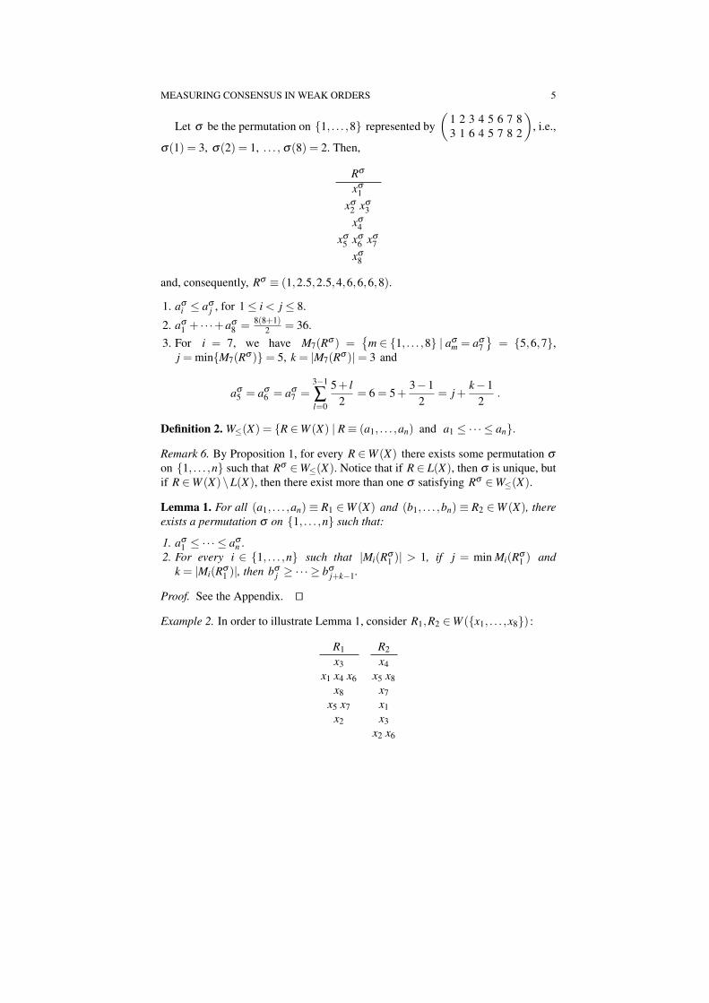
MEASURING CONSENSUS IN WEAK ORDERS 5

Let σ be the permutation on {1, . . . ,8} represented by(

1 2 3 4 5 6 7 83 1 6 4 5 7 8 2

), i.e.,

σ(1) = 3, σ(2) = 1, . . . , σ(8) = 2. Then,

Rσ

xσ1

xσ2 xσ

3

xσ4

xσ5 xσ

6 xσ7

xσ8

and, consequently, Rσ ≡ (1,2.5,2.5,4,6,6,6,8).

1. aσi ≤ aσ

j , for 1 ≤ i < j ≤ 8.

2. aσ1 + · · ·+aσ

8 = 8(8+1)2 = 36.

3. For i = 7, we have M7(Rσ ) ={

m ∈ {1, . . . ,8} | aσm = aσ

7

}= {5,6,7},

j = min{M7(Rσ )}= 5, k = |M7(Rσ )|= 3 and

aσ5 = aσ

6 = aσ7 =

3−1

∑l=0

5+ l2

= 6 = 5+3−1

2= j+

k−12

.

Definition 2. W≤(X) = {R ∈W (X) | R ≡ (a1, . . . ,an) and a1 ≤ ·· · ≤ an}.

Remark 6. By Proposition 1, for every R ∈W (X) there exists some permutation σon {1, . . . ,n} such that Rσ ∈W≤(X). Notice that if R ∈ L(X), then σ is unique, butif R ∈W (X)\L(X), then there exist more than one σ satisfying Rσ ∈W≤(X).

Lemma 1. For all (a1, . . . ,an) ≡ R1 ∈ W (X) and (b1, . . . ,bn) ≡ R2 ∈ W (X), thereexists a permutation σ on {1, . . . ,n} such that:

1. aσ1 ≤ ·· · ≤ aσ

n .2. For every i ∈ {1, . . . ,n} such that |Mi(Rσ

1 )| > 1, if j = min Mi(Rσ1 ) and

k = |Mi(Rσ1 )|, then bσ

j ≥ ·· · ≥ bσj+k−1.

Proof. See the Appendix. ⊓⊔

Example 2. In order to illustrate Lemma 1, consider R1,R2 ∈W ({x1, . . . ,x8}) :

R1x3

x1 x4 x6x8

x5 x7x2

R2x4

x5 x8x7x1x3

x2 x6

6 Jose Luis Garcıa-Lapresta and David Perez-Roman

Then, R1 ≡ (3,8,1,3,6.5,3,6.5,5) and R2 ≡ (5,7.5,6,1,2.5,7.5,4,2.5). Let σ ′ be

the permutation on {1, . . . ,n} represented by(

1 2 3 4 5 6 7 83 1 6 4 8 5 7 2

). Then,

Rσ ′1 ≡ (1, 3, 3, 3, 5, 6.5, 6.5, 8),

Rσ ′2 ≡ (6, 5, 1, 7.5, 2.5, 2.5, 4, 6).

Let σ ′′ be the permutation on {1, . . . ,n} represented by(

1 2 3 4 5 6 7 81 4 2 3 5 7 6 8

). It

is clear that Rσ ′1 = (Rσ ′

1 )σ ′′. Thus, if σ = σ ′ ·σ ′′, i.e., σ(i) = σ ′(σ ′′(i)), then σ is

represented by(

1 2 3 4 5 6 7 83 4 1 6 8 7 5 2

). Therefore,

Rσ1 ≡ (1, 3, 3, 3, 5, 6.5, 6.5, 8) ,

Rσ2 ≡ (6, 7.5, 5, 1, 2.5, 4, 2.5, 6) .

2.2 Distances

The use of distances for designing and analyzing voting system has been widely con-sidered in the literature. On this, see Kemeny [18], Slater [29], Nitzan [26], Baigent[3, 4], Nurmi [27, 28], Meskanen and Nurmi [23, 24], Monjardet [25], Gaertner [13,6.3] and Eckert and Klamler [11], among others. A general and complete survey ondistances can be found in Deza and Deza [10].

The consensus measures introduced in this chapter are based on distances onweak orders. After presenting the general notion, we show the distances on Rn usedfor inducing the distances on weak orders. We pay special attention to the Kemenydistance.

Definition 3. A distance (or metric) on a set A = /0 is a mapping d : A×A −→ Rsatisfying the following conditions for all a,b,c ∈ A:

1. d(a,b)≥ 0.2. d(a,b) = 0 ⇔ a = b.3. d(a,b) = d(b,a).4. d(a,b)≤ d(a,c)+d(c,b).

2.2.1 Distances on Rn

Example 3. Typical examples of distances on Rn or [0,∞)n are the following:

1. The discrete distance d′ : Rn ×Rn −→ R ,

d′((a1, . . . ,an),(b1, . . . ,bn)) =

{1, if (a1, . . . ,an) = (b1, . . . ,bn) ,0, if (a1, . . . ,an) = (b1, . . . ,bn) .

MEASURING CONSENSUS IN WEAK ORDERS 7

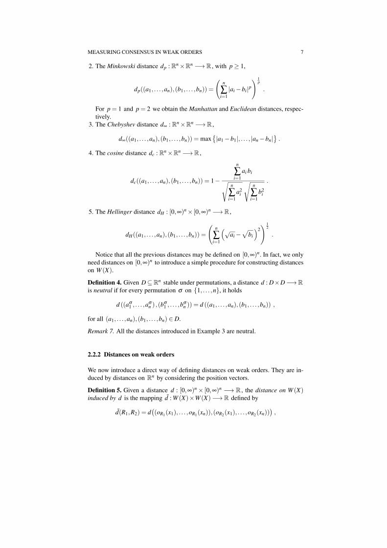
2. The Minkowski distance dp : Rn ×Rn −→ R , with p ≥ 1,

dp((a1, . . . ,an),(b1, . . . ,bn)) =

(n

∑i=1

|ai −bi|p) 1

p

.

For p = 1 and p = 2 we obtain the Manhattan and Euclidean distances, respec-tively.

3. The Chebyshev distance d∞ : Rn ×Rn −→ R ,

d∞((a1, . . . ,an),(b1, . . . ,bn)) = max{|a1 −b1|, . . . , |an −bn|

}.

4. The cosine distance dc : Rn ×Rn −→ R ,

dc((a1, . . . ,an),(b1, . . . ,bn)) = 1−

n

∑i=1

ai bi√n

∑i=1

a2i

√n

∑i=1

b2i

.

5. The Hellinger distance dH : [0,∞)n × [0,∞)n −→ R ,

dH((a1, . . . ,an),(b1, . . . ,bn)) =

(n

∑i=1

(√ai −

√bi

)2) 1

2

.

Notice that all the previous distances may be defined on [0,∞)n. In fact, we onlyneed distances on [0,∞)n to introduce a simple procedure for constructing distanceson W (X).

Definition 4. Given D ⊆Rn stable under permutations, a distance d : D×D −→Ris neutral if for every permutation σ on {1, . . . ,n}, it holds

d ((aσ1 , . . . ,a

σn ) ,(b

σ1 , . . . ,b

σn )) = d ((a1, . . . ,an),(b1, . . . ,bn)) ,

for all (a1, . . . ,an),(b1, . . . ,bn) ∈ D.

Remark 7. All the distances introduced in Example 3 are neutral.

2.2.2 Distances on weak orders

We now introduce a direct way of defining distances on weak orders. They are in-duced by distances on Rn by considering the position vectors.

Definition 5. Given a distance d : [0,∞)n × [0,∞)n −→ R , the distance on W (X)induced by d is the mapping d : W (X)×W (X)−→ R defined by

d(R1,R2) = d((oR1(x1), . . . ,oR1(xn)),(oR2(x1), . . . ,oR2(xn))

),

8 Jose Luis Garcıa-Lapresta and David Perez-Roman

for all R1,R2 ∈W (X).

Given a distance d− on [0,∞)n, we use d− to denote the distance on W (X)induced by d−.

2.2.3 The Kemeny distance

The Kemeny distance was initially defined on linear orders by Kemeny [18], as thesum of pairs where the orders’ preferences disagree. However, it has been gener-alized to the framework of weak orders (see and Eckert and Klamler [11], amongothers).

The Kemeny distance on weak orders dK : W (X)×W (X) −→ R is usually de-fined as one half4 of the cardinal of the symmetric difference between the weakorders, i.e.,

dK(R1,R2) =|(R1 ∪R2)\ (R1 ∩R2)|

2.

We now consider dK : AW ×AW −→ R , given by

dK((a1, . . . ,an),(b1, . . . ,bn)

)=

n

∑i, j=1i< j

|sgn (ai −a j)− sgn (bi −b j)| ,

where sgn is the sign function:

sgn (a) =

1, if a > 0 ,0, if a = 0 ,

−1, if a < 0 .

Notice that dK is a neutral distance on AW .Taking into account Kemeny and Snell [19, p. 18], it is easy to see that dK

coincides with the distance on W (X) induced by dK , i.e.,

dK(R1,R2) = dK(R1,R2) = dK((a1, . . . ,an),(b1, . . . ,bn)

)=

=12

n

∑i, j=1

|sgn (ai −a j)− sgn (bi −b j)|=

=n

∑i, j=1i< j

|sgn (ai −a j)− sgn (bi −b j)| ,

where R1 ≡ (a1, . . . ,an) and R2 ≡ (b1, . . . ,bn).

4 Sometimes “one half” is removed.

MEASURING CONSENSUS IN WEAK ORDERS 9

3 Consensus measures

Consensus measures have been introduced and analyzed by Bosch [7] in the contextof linear orders. We now extend this concept to the framework of weak orders.

Definition 6. A consensus measure on W (X)m is a mapping

M : W (X)m ×P2(V )−→ [0,1]

that satisfies the following conditions:

1. Unanimity. For all R ∈W (X)m and I ∈ P2(V ), it holds

M (R, I) = 1 ⇔ Ri = R j for all vi,v j ∈ I.

2. Anonymity. For all permutation π on {1, . . . ,m}, R ∈ W (X)m and I ∈ P2(V ),it holds

M (Rπ , Iπ) = M (R, I) .

3. Neutrality. For all permutation σ on {1, . . . ,n}, R ∈W (X)m and I ∈ P2(V ), itholds

M (Rσ , I) = M (R, I) .

Unanimity means that the maximum consensus in every subset of decision mak-ers is only achieved when all opinions are the same. Anonymity requires symmetrywith respect to decision makers, and neutrality means symmetry with respect toalternatives.

We now introduce other properties that a consensus measure may satisfy.

Definition 7. Let M : W (X)m ×P2(V )−→ [0,1] be a consensus measure.

1. M satisfies maximum dissension if for all R ∈W (X)m and vi,v j ∈V such thati = j, it holds

M (R,{vi,v j}) = 0 ⇔ Ri,R j ∈ L(X) and R j = R−1i .

2. M is reciprocal if for all R ∈W (X)m and I ∈ P2(V ), it holds

M (R−1, I) = M (R, I) .

3. M is homogeneous if for all R ∈W (X)m, I ∈ P2(V ) and t ∈ N, it holds

M t(t R, t I) = M (R, I) ,

where M t : W (X)tm ×P2(t V )−→ [0,1], tR = (R, t. . .,R) ∈W (X)tm is the pro-file defined by t copies of R and t I = I⊎ t· · · ⊎ I is the multiset of voters5 definedby t copies of I.

5 List of voters where each voter occurs as many times as the multiplicity. For instance, 2{v1,v2}={v1,v2}⊎{v1,v2}= {v1,v2,v1,v2}.

10 Jose Luis Garcıa-Lapresta and David Perez-Roman

Maximum dissension means that in each subset of two voters6, the minimumconsensus is only reached whenever preferences of voters are linear orders and eachone is the inverse of the other. Reciprocity means that if all individual weak ordersare reversed, then the consensus does not change. And homogeneity means that ifwe replicate a subset of voters, then the consensus in that group does not change.

We now introduce our proposal for measuring consensus in sets of weak orders.

Definition 8. Given a distance d : W (X)×W (X)−→ R , the mapping

Md : W (X)m ×P2(V )−→ [0,1]

is defined by

Md (R, I) = 1−

∑vi,v j∈I

i< j

d(Ri,R j)

(|I|2

)·∆n

,

where∆n = max

{d(Ri,R j) | Ri,R j ∈W (X)

}.

Notice that the numerator of the quotient appearing in the above expression is thesum of all the distances between the weak orders of the profile, and the denominatoris the number of terms in the numerator’s sum multiplied by the maximum distancebetween weak orders. Consequently, that quotient belongs to the unit interval and itmeasures the disagreement in the profile.

Proposition 2. For every distance d : W (X)×W (X)−→R , Md satisfies unanimityand anonymity.

Proof. Let R ∈W (X)m and I ∈ P2(V ).

1. Unanimity.

Md(R, I) = 1 ⇔ ∑vi,v j∈I

i< j

d(Ri,R j) = 0 ⇔

∀vi,v j ∈ I d(Ri,R j) = 0 ⇔ ∀vi,v j ∈ I Ri = R j .

2. Anonymity. Let π be a permutation on {1, . . . ,m}.

∑vi,v j∈Iπ

i< j

d(Rπ(i),Rπ( j)) = ∑vπ(i),vπ( j)∈I

π(i)<π( j)

d(Rπ(i),Rπ( j)) = ∑vi,v j∈I

i< j

d(Ri,R j) .

Thus, Md(Rπ , Iπ) = Md(R, I). ⊓⊔

6 It is clear that a society reach maximum consensus when all the opinions are the same. However,in a society with more than two members it is not an obvious issue to determine when there isminimum consensus (maximum disagreement).

MEASURING CONSENSUS IN WEAK ORDERS 11

If Md is neutral, then we say that Md is the consensus measure associated withd.

Proposition 3. If d : [0,∞)n × [0,∞)n −→ R is a neutral distance, then Md is aconsensus measure.

Proof. By Proposition 2, Md satisfies unanimity and anonymity. Obviously, if d isneutral, then Md is neutral and thus Md is a consensus measure. ⊓⊔

Proposition 4. If d is the distance on W (X) induced by d′, d1, d2, d∞, dc or dK ,then Md is a reciprocal consensus measure.

Proof. See the Appendix. ⊓⊔

Remark 8. MdHis not a reciprocal consensus measure.

Let us consider R1,R2 ∈W ({x1,x2,x3}):

R1x1

x2 x3

R2x1 x2 x3

R−11

x2 x3x1

R−12

x1 x2 x3

The above weak orders are codified by R1 ≡ (1,2.5,2.5), R−11 ≡ (3,1.5,1.5) and

R2 = R−12 ≡ (2,2,2) . We have

dH(R1,R2) =

=

((√1−

√2)2

+(√

2.5−√

2)2

+(√

2.5−√

2)2) 1

2= 0.476761 =

= 0.415713 =

((√3−

√2)2

+(√

1.5−√

2)2

+(√

1.5−√

2)2) 1

2=

= dH(R−11 ,R−1

2 ) .

In order to prove that the maximum dissension property is satisfied for some ofthe consensus measures introduced above, we need two lemmas.

Lemma 2. Let R1 ∈W (X)\L(X) and R2 ∈W (X). If d− is the distance induced byd2, dc, dH or dK , then there exists R3 ∈W (X) such that d−(R1,R2)< d−(R1,R3).

Proof. See the Appendix. ⊓⊔

Lemma 3. Let R1,R2 ∈ L(X) such that R2 = R−11 . If d− is the distance induced by

d2, dc, dH or dK , then there exists R3 ∈W (X) such that d−(R1,R2)< d−(R1,R3).

Proof. See the Appendix. ⊓⊔

Proposition 5. If d− is the distance induced by d2, dc, dH or dK , then Md− satis-fies the maximum dissension property.

12 Jose Luis Garcıa-Lapresta and David Perez-Roman

Proof. First of all, notice that Md− (R,{vi,v j}) = 0 if and only if d−(Ri,R j) = ∆n.By Lemma 2 and Lemma 3, d−(R1,R2) = ∆n if and only if R2 = R−1

1 . ⊓⊔

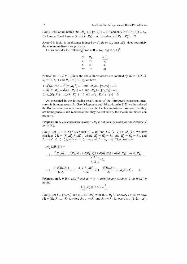
Remark 9. If d− is the distance induced by d′, d1 or d∞, then Md− does not satisfythe maximum dissension property.

Let us consider the following profile R = (R1,R2) ∈ L(X)2:

R1x1x2x3

R2x3x1x2

R−11x3x2x1

Notice that R2 = R−11 . Since the above linear orders are codified by R1 ≡ (1,2,3),

R2 ≡ (2,3,1) and R−11 ≡ (3,2,1), we have

1. d′(R1,R2) = d′(R1,R−11 ) = 1 and Md′(R,{v1,v2}) = 0.

2. d1(R1,R2) = d1(R1,R−11 ) = 4 and Md1

(R,{v1,v2}) = 0.3. d∞(R1,R2) = d∞(R1,R−1

1 ) = 2 and Md∞(R,{v1,v2}) = 0.

As presented in the following result, none of the introduced consensus mea-sures is homogeneous. In Garcıa-Lapresta and Perez-Roman [15] we introducedthe Borda consensus measures, based on the Euclidean distance. We note that theyare homogeneous and reciprocal, but they do not satisfy the maximum dissensionproperty.

Proposition 6. The consensus measure Md is not homogeneous for any distance don W (X).

Proof. Let R ∈ W (X)m such that R1 = R2 and I = {v1,v2} ∈ P2(V ). We nowconsider 2R = (R′

1,R′2,R

′3,R

′4), where R′

1 = R′3 = R1 and R′

2 = R′4 = R2, and

2 I = {v′1,v′2,v

′3,v

′4}, with v′1 = v′3 = v1 and v′2 = v′4 = v2. Then, we have

M 2d (2R,2 I) =

= 1−d(R′

1,R′2)+d(R′

1,R′3)+d(R′

1,R′4)+d(R′

2,R′3)+d(R′

2,R′4)+d(R′

3,R′4)(

|2 I|2

)·∆n

=

= 1− 4 · d(R1,R2)

6 ·∆n= 1− 2 · d(R1,R2)

3 ·∆n= 1− d(R1,R2)

∆n= Md (R, I) . ⊓⊔

Proposition 7. If R ∈ L(X)2 and R2 = R−11 , then for any distance d on W (X) it

holds:limt→∞

M td (t R, t I) =

12.

Proof. Let I = {v1,v2} and R = (R1,R2) with R2 = R−11 . For every t ∈N, we have

t R = (R1,R2, . . . ,R2t), where R2k−1 = R1 and R2k = R2 for every k ∈ {1,2, . . . , t}.

MEASURING CONSENSUS IN WEAK ORDERS 13

We should calculate the limit of the following expression:

M td (t R, t I) = 1−

∑vi,v j∈tI

i< j

d(Ri,R j)

(|tI|2

)·∆n

.

Since

d(Ri,R j) =

0, if i, j are both even ,

0, if i, j are both odd ,

∆n, otherwise ,

we obtain

∑vi,v j∈tI

i< j

d(Ri,R j) =2t−1

∑i=1

2t

∑j=i+1

d(Ri,R j) =

(t

∑i=1

i+t−1

∑j=1

j

)·∆n = t2 ·∆n .

On the other hand, we have (|tI|2

)=

(2t2

)= 2t2 − t .

Consequently,

limt→∞

M td (t R, t I) = 1− lim

t→∞

t2 ·∆n

(2t2 − t) ·∆n=

12. ⊓⊔

Remark 10. Homogeneity ensures that a society has no consensus at all when it isdivided into two groups each one ranks order the alternatives just in the oppositeway to the other group. According to Proposition 6, our consensus measures are nothomogeneous. Thus, they perceive some consensus in polarized societies and, byProposition 7, consensus tends to 0.5 when the number of voters tends to infinity,regardless of the distance used. Notice that this result holds even when the distanceused does not verify the maximum dissension property, which guaranteed that theconsensus between two profiles is zero if and only if they are opposites.

We summarize the properties of the analyzed consensus measures in Table 1.

Appendix

Proof of Proposition 1. Consider (a1, . . . an)≡ R ∈W (X).

1. Obvious.2. By Remark 2.

14 Jose Luis Garcıa-Lapresta and David Perez-Roman

Table 1 Summary

Max. diss. Reciproc. Homogen.Md′ No Yes NoMd1

No Yes NoMd2

Yes Yes NoMd∞ No Yes NoMdc

Yes Yes NoMdH

Yes No NoMdK

Yes Yes No

3. Consider i ∈ {1, . . . ,n} with |Mi(Rσ )| = k > 1, and j = min Mi(Rσ ) . Then,Mi(Rσ ) = { j, j+1, . . . , j+(k−1)} and aσ

j = aσj+1 = · · ·= aσ

j+(k−1) = aσi .

Since we assign each alternative the average of the positions of the alternativeswithin the same equivalence class, then we have

aσi =

∑m∈Mi(Rσ )

m

k=

j+( j+1)+ · · ·+( j+(k−1))k

= j+k−1

2.

Reciprocally, given (a1, . . . ,an) ∈ Rn and a permutation σ verifying conditions1, 2 and 3, then we can consider that aσ

i is the relative position of the alternative xiin R ∈W (X). Then, R ≡ (a1, . . . ,an). ⊓⊔

Proof of Lemma 1. By Proposition 1, there exists a permutation σ ′ on {1, . . . ,n}such that Rσ ′

1 satisfies 1. We consider Rσ ′2 . Let σ ′′ be a permutation on {1, . . . ,n}

such that:

1. If∣∣∣Mi

(Rσ ′

1

)∣∣∣= 1, then σ ′′(i) = i.

2. If∣∣∣Mi

(Rσ ′

1

)∣∣∣ = k > 1 and j = min Mi

(Rσ ′

1

), then let σ ′′ be a permutation on

{1, . . . ,n} such that bσ ′σ ′′( j) ≥ bσ ′

σ ′′( j+1) ≥ ·· · ≥ bσ ′σ ′′( j+k−1). Obviously, aσ ′

σ ′′( j) =

· · ·= aσ ′σ ′′( j+k−1) = aσ ′

i .

Therefore, σ = σ ′ ·σ ′′. ⊓⊔

Proof of Proposition 4. By Remark 7 and Proposition 3, we only need to prove thatthe corresponding distances are reciprocal.

1. Case d′.

Since Ri = R j ⇔ R−1i = R−1

j , we have d′(Ri,R j) = d′(R−1i ,R−1

j ). Consequently,Md′(R−1, I) = Md′(R, I).

MEASURING CONSENSUS IN WEAK ORDERS 15

2. Cases dp (p ∈ {1,2}).

By Remark 1, we have

dp(R−1i ,R−1

j ) =

(n

∑k=1

|(n+1−oRi(xk))− (n+1−oR j(xk))|p) 1

p

=

=

(n

∑k=1

|oRi(xk)−oR j(xk)|p) 1

p

= dp(Ri,R j) .

Thus, Mdp(R−1, I) = Mdp

(R, I).

3. Case d∞.

By Remark 1, we have

d∞(R−1i ,R−1

j ) =

= max{|(n+1−oRi(xk))− (n+1−oR j(xk))| | k ∈ {1, . . . ,n}

}=

= max{|oRi(xk)−oR j(xk)| | k ∈ {1, . . . ,n}

}= d∞(Ri,R j) .

Thus, Md∞(R−1, I) = Md∞(R, I).

4. Case dc.

dc(R−1i ,R−1

j ) = 1−

n

∑k=1

(n+1−oRi(xk))(n+1−oR j(xk))√n

∑k=1

(n+1−oRi(xk))2

√n

∑k=1

(n+1−oR j(xk))2

.

By Remark 2, we haven

∑k=1

((n+1)− (oRi(xk)+oR j(xk))

)= 0. Thus,

n

∑k=1

(n+1−oRi(xk))(n+1−oR j(xk)) =

= (n+1)

[n

∑k=1

((n+1)− (oRi(xk)+oR j(xk))

)]+

n

∑k=1

oRi(xk)oR j(xk) =

=n

∑k=1

oRi(xk)oR j(xk) .

By Remark 2, we also haven

∑k=1

((n+1)−2oRi(xk)) =n

∑k=1

((n+1)−2oR j(xk)) = 0.

Thus,

16 Jose Luis Garcıa-Lapresta and David Perez-Roman

n

∑k=1

(n+1−oRi(xk))2 = (n+1)

n

∑k=1

((n+1)−2oRi(xk))+n

∑k=1

oRi(xk)2 =

n

∑k=1

oRi(xk)2 ,

and

n

∑k=1

(n+1−oR j(xk))2 = (n+1)

n

∑k=1

((n+1)−2oR j(xk))+n

∑k=1

oR j(xk)2 =

n

∑k=1

oR j(xk)2 .

Consequently,

dc(R−1i ,R−1

j ) = 1−

n

∑k=1

oRi(xk)oR j(xk)√n

∑k=1

(oRi(xk))2

√n

∑k=1

(oR j(xk))2

= dc(Ri,R j) .

Thus, Mdc(R−1, I) = Mdc

(R, I).

5. Case dK .

dK(R−11 ,R−1

2 ) =

=n

∑i, j=1i< j

∣∣sgn(n+1−oR1(xi)− (n+1−oR1(x j))

)−

− sgn(n+1−oR2(xi)− (n+1−oR2(x j))

)∣∣==

n

∑i, j=1i< j

∣∣sgn(oR1(x j)−oR1(xi)

)− sgn

(oR2(x j)−oR2(xi)

)∣∣==

n

∑i, j=1i< j

∣∣sgn(oR1(xi)−oR1(x j)

)− sgn

(oR2(xi)−oR2(x j)

)∣∣= dK(R1,R2) .

Thus, MdK(R−1, I) = MdK

(R, I). ⊓⊔

Proof of Lemma 2. Let (a1, . . . ,an)≡R1 ∈W (X)\L(X), (b1, . . . ,bn)≡R2 ∈W (X)and (a′1, . . . ,a

′n) ≡ R′ ∈ W (X). By Proposition 1 and Lemma 1, and taking into

account that all the considered distances are neutral (Remark 7), we can assumewithout loss of generality:

• R1 ≡ (a1, . . . ,a j, . . . ,a j+k−1, . . . ,an) ∈ W≤(X) with j = min{i | |Mi(R1)| > 0},|M j(R1)|= k and a j = · · ·= a j+k−1 = j+ k−1

2 .• R2 ≡ (b1, . . . ,b j, . . . ,b j+k−1, . . . ,bn) ∈W (X) with b j ≥ ·· · ≥ b j+k−1.

Let now (a′1, . . . ,a′n) = (a1, . . . ,a j−1, j, . . . , j+k−1,a j+k, . . . ,an)≡ R3 ∈W (X) and

MEASURING CONSENSUS IN WEAK ORDERS 17

m =

{k−1

2 −1, if k is odd,k−1

2 − 12 , if k is even.

1. Case d2 .

d2(R1,R2)< d2(R3,R2) ⇔ 0 <(d2(R3,R2)

)2 −(d2(R1,R2)

)2 ⇔

⇔ 0 <n

∑i=1

(a′i −bi)2 − (ai −bi)

2 =k−1

∑l=0

( j+ l −b j+l)2 −(

j+k−1

2−b j+l

)2

=

=m

∑l=0

( j+ l −b j+l)2 −(

j+k−1

2−b j+l

)2

+(( j+ k−1)− l −b j+k−1−l)2 −

−(

j+k−1

2−b j+k−1−l

)2

=

=m

∑l=0

2(

l − k−12

)2

+(( j−b j+k−1−l)− ( j−b j+l)

)((k−1)−2l)

).

Since 0 < l < k−12 and 0 < b j+k−1−l ≤ b j+l , we have d2(R1,R2)< d2(R3,R2).

2. Case dc . Consider ∥R∥=√

a21 + · · ·+a2

n whenever R ≡ (a1, . . . ,an).

∥R3∥2 −∥R1∥2 =n

∑i=1

((a′i)

2 − (ai)2)=

=m

∑l=0

( j+ l)2 −(

j+k−1

2

)2

+( j+(k−1)− l)2 −(

j− k−12

)2

=

= 2(

k−12

− l)2

> 0. (1)

Thus, ∥R3∥> ∥R1∥.

18 Jose Luis Garcıa-Lapresta and David Perez-Roman

dc(R3,R2)− dc(R1,R2) =∑n

i=1(ai bi)

∥R1∥ ∥R2∥− ∑n

i=1(a′i bi)

∥R3∥ ∥R2∥by (1)>

>1

∥R1∥ ∥R2∥

(n

∑i=0

(ai bi −a′i bi

))=

=1

∥R1∥ ∥R2∥

(m

∑l=0

((j+

k−12

)b j+l − ( j+ l)b j+l +

+

(j+

k−12

)b j+k−1−l − ( j+ k−1+ l)b j+k−1−l

))=

=1

∥R1∥ ∥R2∥

(m

∑l=0

(b j+l

(k−1

2+ l)+b j+k−1−l

(l − k−1

2

)))≥

≥ 1∥R1∥ ∥R2∥

(m

∑l=0

b j+k−1−l 2l

)≥ 0.

Thus, dc(R1,R2)< dc(R3,R2).

3. Case dH .

dH(R1,R2)< dH(R3,R2) ⇔ 0 <(dH(R3,R2)

)2 −(dH(R1,R2)

)2 ⇔

⇔ 0 <n

∑i=1

(√a′i −

√bi

)2

−(√

ai −√

bi

)2=

m

∑l=0

(√j+ l −

√b j+l

)2−

−

(√j+

k−12

−√

b j+l

)2

+(√

( j+ k−1)− l −√

b j+k−1−l

)2−

−

(√j+

k−12

−√

b j+k−1−l

)2

=

= 2m

∑l=0

√b j+l

(√j+

k−12

−√

j+ l

)+

+√

b j+k−1−l

(√j+ k−1−

√j+ k−1− l

).

Since 0 < l < k−12 , we have dH(R1,R2)< dH(R3,R2).

4. Case dK .

dK(R1,R2) =n

∑i,h=1i<h

|sgn (ai −ah)− sgn (bi −bh)| .

MEASURING CONSENSUS IN WEAK ORDERS 19

dK(R3,R2) =n

∑i,h=1i<h

|sgn (a′i −a′h)− sgn (bi −bh)| .

|sgn (ai −ah)− sgn (bi −bh)| =

=

{ |sgn (a′i −a′h)− sgn (bi −bh)| , if {i,h} ⊆ a j(R),

|− sgn (bi −bh)| < |sgn (a′i −a′h)− sgn (bi −bh)| , if {i,h} ⊆ a j(R).

Thus, dK(R1,R2)< dK(R3,R2). ⊓⊔

Proof of Lemma 3. Consider R1,R2,R3 ∈ L(X), R1 ≡ (a1, . . . an), R2 ≡ (b1, . . . bn)and R′ ≡ (a′1, . . . a′n). By Proposition 1 and Lemma 1, and taking into account thatall the considered distances are neutral (Remark 7), we can assume without loss ofgenerality that R1 ≡ (1,2, . . . ,n) .

If R2 = R−11 , then we consider j = min{i | bi = n− i+1} and k = j+ l such that

bk = n− j + 1. Let now R3 ≡ (b′1, . . . ,b′n) such that b′i = b j for every i /∈ { j,k},

b′j = bk = n− j+1 and b′k = b j < n− j+1.

1. Case d2 .

d2(R1,R3)2 − d2(R1,R2)

2 = | j−b′j|2 + |k−b′k|2 −(| j−b j|2 + |k−bk|2

).

| j−b′j|2 + |k−b′k|2 = ( j+ l −bk − l)2 +( j−b j + l)2 =

= (k−bk)2 +( j−b j)

2 +2l(l +( j−b j)− (k−bk)) =

= ( j−b j)2 +(k−bk)

2 +2l(bk −b j)> | j−b j|2 + |k−bk|2.

Thus, d2(R1,R2)< d2(R1,R3).

2. Case dc .

It is clear that ∥R2∥= ∥R3∥.

dc(R1,R3)− dc(R1,R2) =∑n

i=1 ibi

∥R1∥ ∥R2∥− ∑n

i=1 ib′i∥R1∥ ∥R3∥

=

=j b j + k bk − ( j b′j + k b′k)

∥R1∥ ∥R2∥=

j b j + k bk − ( j bk + k b j)

∥R1∥ ∥R2∥=

=(bk −b j)(k− j)

∥R1∥ ∥R2∥> 0.

Thus, dc(R1,R2)< dc(R1,R3).

20 Jose Luis Garcıa-Lapresta and David Perez-Roman

3. Case dH .

dH(R1,R3)2 − dH(R1,R2)

2 =

=(√

j−√

b′j)2

+(√

k−√

b′k)2

−(√

j−√

b j

)2+(√

k−√

bk

)2=

=(√

j−√

bk

)2+(√

k−√

b j

)2−(√

j−√

b j

)2+(√

k−√

bk

)2=

= 2(√

jb j +√

kbk −√

jbk −√

kb j

)=

= 2((√

k−√

j)−(√

bk −√

b j

))> 0.

Thus, dH(R1,R2)< dH(R1,R3).

4. Case dK .

dK(R1,R3)− dK(R1,R2) =

= |sgn ( j− k)− sgn (b′j −b′k)|− |sgn ( j− k)− sgn (b j −bk)|== |sgn ( j− k)− sgn (bk −b j)|− |sgn ( j− k)− sgn (b j −bk)|== |−1−1|− |−1− (−1)|= 2 > 0.

Thus, dK(R1,R2)< dK(R1,R3). ⊓⊔

Acknowledgements

This research has been partially supported by the Spanish Ministerio de Cien-cia e Innovacion (Project ECO2009–07332), ERDF and Junta de Castilla y Leon(Consejerıa de Educacion, Projects VA092A08 and GR99). The authors are grate-ful to Jorge Alcalde-Unzu, Miguel Angel Ballester, Christian Klamler and MiguelMartınez-Panero for their suggestions and comments.

References

1. Alcalde-Unzu, J., Vorsatz, M. (2010): Do we agree? Measuring the cohesiveness of prefer-ences. Mimeo.

2. Alcalde-Unzu, J., Vorsatz, M. (2010): Measuring Consensus: Concepts, Comparisons, andProperties. This book.

3. Baigent, N. (1987): Preference proximity and anonymous social choice. The Quarterly Jour-nal of Economics 102, pp. 161–169.

4. Baigent, N. (1987): Metric rationalisation of social choice functions according to principlesof social choice. Mathematical Social Sciences 13, pp. 59–65.

5. Black, D. (1976): Partial justification of the Borda count. Public Choice 28, pp. 1–15.6. Borroni, C.G., Zenga, M. (2007): A test of concordance based on Gini’s mean difference.

Statistical Methods and Applications 16, pp. 289–308.

MEASURING CONSENSUS IN WEAK ORDERS 21

7. Bosch, R. (2005): Characterizations of Voging Rules and Consensus Measures. Ph. D. Disser-tation, Tilburg University.

8. Cook, W.D., Kress, M., Seiford, L.M. (1996): A general framework for distance-based con-sensus in ordinal ranking models. European Journal of Operational Research 96, pp. 392–397.

9. Cook, W.D., Seiford, L.M. (1982): On the Borda-Kendall consensus method for priority rank-ing problems. Management Science 28, pp. 621–637.

10. Deza, M.M., Deza, E. (2009): Encyclopedia of Distances. Springer-Verlag, Berlin.11. Eckert, D., Klamler, C. (2010): Distance-Based Aggregation Theory. This book.12. Eklund, P., Rusinowska, A., de Swart, H. (2007): Consensus reaching in committees. Euro-

pean Journal of Operational Research 178, pp. 185–193.13. Gaertner, W. (2009): A Primer in Social Choice Theory. Revised Edition. Oxford University

Press, Oxford.14. Garcıa-Lapresta, J.L. (2008): Favoring consensus and penalizing disagreement in group deci-

sion making. Journal of Advanced Computational Intelligence and Intelligent Informatics 12(5), pp. 416–421.

15. Garcıa-Lapresta, J.L., Perez-Roman, D. (2008): Some consensus measures and their applica-tions in group decision making. In: Computational Intelligence in Decision and Control (eds.D. Ruan, J. Montero, J. Lu, L. Martınez, P. D’hondt, E.E. Kerre). World Scientific, Singapore,pp. 611–616.

16. Gini, C. (1954): Corso di Statistica. Veschi, Rome.17. Hays, W.L. (1960): A note on average tau as a measure of concordance. Journal of the Amer-

ican Statistical Association 55, pp. 331–341.18. Kemeny, J.G. (1959): Mathematics without numbers. Daedalus 88, pp. 571–591.19. Kemeny, J.G., Snell, J.C. (1961): Mathematical Models in the Social Sciences. Ginand Com-

pany, New York.20. Kendall, M.G. (1962): Rank Correlation Methods. Griffin, London.21. Kendall, M., Gibbons, J.D. (1990): Rank Correlation Methods. Oxford University Press, New

York.22. Martınez-Panero, M., Consensus Perspectives: Glimpses into Theoretical Advances and Ap-

plications. This book.23. Meskanen, T., Nurmi, H. (2006): Analyzing political disagreement. JASM Working Papers 2,

University of Turku, Finland.24. Meskanen, T., Nurmi, H. (2007): Distance from consensus: A theme and variations. In Math-

ematics and Democracy. Recent Advances in Voting Systems and Collective Choice (eds.:Simeone, B., Pukelsheim, F.). Springer, pp. 117–132.

25. Monjardet, B.: “Mathematique Sociale” and Mathematics. A case study: Condorcet’s effectand medians. Electronic Journal for History of Probability and Statistics 4, 2008.

26. Nitzan, S. (1981): Some measures of closeness to unanimity and their implications. Theoryand Decision 13, pp. 129-138.

27. Nurmi, H. (2004): A comparison of some distance-based choice rules in ranking environments.Theory and Decision 57, pp. 5–24.

28. Nurmi, H. (2010): Settings of Consensual Processes: Candidates, Verdicts, Policies. This book.29. Slater, P. (1961): Inconsistencies in a schedule of paired comparisons. Biometrika 48, pp. 303–

312.30. Smith, J. (1973): Aggregation of preferences with variable electorate. Econometrica 41, pp.

1027–1041.31. Spearman, C. (1904): The proof and measurement of association between two things. Ameri-

can Journal of Psychology 15, pp. 72–101.