arX

iv:a

stro

-ph/

0607

629v

1 2

7 Ju

l 200

6

Mon. Not. R. Astron. Soc. 000, 1–13 (2002) Printed 5 February 2008 (MN LATEX style file v2.2)

The 2dF-SDSS LRG and QSO survey: Evolution of the

Luminosity Function of Luminous Red Galaxies to z = 0.6

David A. Wake1,2, Robert C. Nichol1, Daniel J. Eisenstein3, Jon Loveday4, Alastair

C. Edge2, Russell Cannon5, Ian Smail6, Donald P. Schneider7, Ryan Scranton15,

Daniel Carson1, Nicholas P. Ross2, Robert J. Brunner8, Matthew Colless5, War-

rwick J. Couch9, Scott M. Croom5, Simon P. Driver10, Jose da Angela2, Sebastian

Jester14, Roberto de Propris11, Michael J. Drinkwater12, Joss Bland-Hawthorn5,

Kevin A. Pimbblet12, Isaac G. Roseboom12, Tom Shanks2, Robert G. Sharp5, Jon

Brinkmann13

1Institute of Cosmology and Gravitation (ICG), Mercantile House, University of Portsmouth, Portsmouth, PO1 2EG, UK2Dept. of Physics, Durham University, South Road, Durham, DH1 3LE, UK3Steward Observatory, University of Arizona, 933 N. Cherry Ave., Tucson AZ85721, USA4Astronomy Center, University of Sussex, Falmer, Brighton, BN1 9QH, UK5Anglo–Australian Observatory, PO Box 296, NSW 1710, Australia6Institute of Computational Cosmology, Durham University, South Road, Durham, DH1 3LE, UK7Department of Astronomy and Astrophysics, Pennsylvania State University, 525 Davey Laboratory, University Park, PA 16802, USA8National Center for Supercomputing Applications, University of Illinois at Urbana-Champaign, 1205 W. Clark St., Urbana, IL 61801, USA9School of Physics, University of New South Wales, Sydney, Australia10School of Physics & Astronomy, University of St Andrews, North Haugh, St Andrews, KY16 9SS, UK11Cerro Tololo Inter-American Observatory, Casilla 603, La Serena, Chile12Dept. of Physics, University of Queensland, Brisbane, QLD 4072, Australia13Apache Point Observatory, 2001 Apache Point Road, P.O. Box 59, Sunspot, NM 88349, USA14 School of Physics & Astronomy, University of Southampton Southampton, SO17 1BJ, UK15Dept. of Physics and Astronomy, University of Pittsburgh, 3941 O’Hara Street, Pittsburgh, PA 15260, USA

5 February 2008

ABSTRACT

We present new measurements of the luminosity function (LF) of Luminous RedGalaxies (LRGs) from the Sloan Digital Sky Survey (SDSS) and the 2dF–SDSS LRGand Quasar (2SLAQ) survey. We have carefully quantified, and corrected for, un-certainties in the K and evolutionary corrections, differences in the colour selectionmethods, and the effects of photometric errors, thus ensuring we are studying the samegalaxy population in both surveys. Using a limited subset of 6326 SDSS LRGs (with0.17 < z < 0.24) and 1725 2SLAQ LRGs (with 0.5 < z < 0.6), for which the matchingcolour selection is most reliable, we find no evidence for any additional evolution inthe LRG LF, over this redshift range, beyond that expected from a simple passiveevolution model. This lack of additional evolution is quantified using the comoving lu-minosity density of SDSS and 2SLAQ LRGs, brighter than M0.2

r− 5logh0.7 = −22.5,

which are 2.51 ± 0.03 × 10−7 L⊙ Mpc−3 and 2.44 ± 0.15 × 10−7 L⊙ Mpc−3 respec-tively (< 10% uncertainty). We compare our LFs to the COMBO-17 data and findexcellent agreement over the same redshift range. Together, these surveys show noevidence for additional evolution (beyond passive) in the LF of LRGs brighter thanM0.2

r− 5logh0.7 = −21 (or brighter than ∼ L⋆). We test our SDSS and 2SLAQ LFs

against a simple “dry merger” model for the evolution of massive red galaxies andfind that at least half of the LRGs at z ≃ 0.2 must already have been well-assembled(with more than half their stellar mass) by z ≃ 0.6. This limit is barely consistentwith recent results from semi-analytical models of galaxy evolution.

Key words: cosmology: observations – galaxies: abundances – galaxies: ellipticalsand lenticular, cD – galaxies: evolution – galaxies: fundamental parameters

2 Wake et al.

1 INTRODUCTION

The formation of massive elliptical galaxies is a majorconundrum in modern cosmology. Observationally, it isclear that such galaxies formed the bulk of their stars atredshifts greater than two, with evidence coming from avariety of studies, including observations of clusters andgroups of galaxies (Bower et al. 1992; Ellis et al. 1997;Kodama et al. 1998; de Propris et al. 1999; Brough et al.2002; Wake et al. 2005; Holden et al. 2005; Pimbblet et al.2006), optical/NIR galaxy count and colour studies(Metcalfe et al. 1996, 2001, 2005) and spectroscopic surveysof field galaxies over a range of redshifts (Bernardi et al.1998; Trager et al. 2000; Bernardi et al. 2003a,b,c,d;Hogg et al. 2002; Kuntschner & Davies 1998; Baldry et al.2004; Glazebrook et al. 2004; McCarthy et al. 2004;Cimatti et al. 2004; Thomas et al. 2005; Papovich et al.2005; Bernardi et al. 2006).

These studies also suggest that the evolution of amajority of these massive ellipticals is consistent with asimple passive model of stellar evolution. For example,Bernardi et al. (2003c,d) have used the Sloan Digital SkySurvey (SDSS; York et al. 2000) to study the evolution ofluminous early–type galaxies (out to z ≃ 0.3) and findthat, for a fixed velocity dispersion, older ellipticals are red-der and fainter in luminosity, fully consistent with the ex-pected fading of their stellar populations with time. Theyalso find that the environment (as measured by local den-sity) of luminous ellipticals has only a weak effect upontheir properties, e.g., the Fundamental Plane fades by only0.075 mags/arcsec2 from the field to the cores of clus-ters (consistent with cluster galaxies forming at a slightlyearlier epoch than field ellipticals). Several other studieshave also found very similar results (Kuntschner et al. 2002;Clemens et al. 2006; Bernardi et al. 2006). However, sev-eral authors have found evidence for recent and/or on-going star-formation in a fraction of local massive ellipticals(Trager et al. 2000; Goto et al. 2003; Fukugita et al. 2004;Balogh et al. 2005). This fraction appears to increase withredshift (Le Borgne et al. 2005; Roseboom et al. 2006) anddecrease with mass (Caldwell et al. 2003; Nelan et al. 2005;Clemens et al. 2006).

One potential problem for studies of massiveelliptical/early-type galaxies, particularly those track-ing the evolution with redshift, is that of progenitor bias(van Dokkum & Franx 1996; van Dokkum et al. 2000). Bystudying only galaxies that look like massive early-typesystems at high redshift, some of the progenitors of thelow redshift massive early-type galaxies may be missed.An effective way to counter this problem is to study theevolution in the number density, or luminosity function(LF), of massive early-type galaxies with redshift. If thesegalaxies did indeed form at high redshift, then there will belittle evidence for the evolution of their LF with redshift.Such studies have only just begun, e.g., the COMBO–17(C17) survey, which reported on the evolution of ≃ 5000 red(and thus implied early-type) galaxies and found at mosta factor of two evolution out to z ≃ 1 (corresponding to 9Gyrs in look–back time; Bell et al. 2004). This is consistentwith earlier (but smaller in number) studies of high redshiftred (early–type) galaxies from the CFRS (Lilly et al. 1995;Schade et al. 1999), CNOC2 (Lin et al. 1999) and K20

(Pozzetti et al. 2003) surveys. At higher redshifts (z > 1),recent spectroscopic surveys suggest that a significantfraction of massive galaxies are already in place at theseearly epochs (Glazebrook et al. 2004; Cimatti et al. 2004).

Theoretically, the existence of massive, passively–evolved ellipticals has been a major challenge for some mod-els of galaxy evolution. For example, in the favoured hier-archical Cold Dark Matter (CDM) model of structure for-mation, such massive galaxies are expected to reside inthe largest dark matter haloes, that form at late timesthrough the merger of smaller mass haloes (see Kauffmann(1996) for early predictions). In recent years, there havebeen a number of prescriptions proposed to solve the “anti–hierarchical” nature of the formation and evolution of mas-sive ellipticals and thus better match the observations dis-cussed above, including: i) The reduction of the gas coolingrate (Benson et al. 2003); ii) Super-winds that eject the gasonce it has cooled, but before it can form stars (Benson et al.2003; Baugh et al. 2005); iii) Shock heating of infalling gasand -PdV work of the gas (Naab et al. 2005); iv) Feedbackfrom Active Galactic Nuclei (AGN; Kawata & Gibson 2005;Scannapieco et al. 2005).

The latter of these proposed effects (AGN feedback)is appealing because of the observed empirical relationshipbetween the luminosity, central concentration and mass ofgalactic bulges and the mass of their central super-massiveblack holes (Ferrarese & Merritt 2000; Tremaine et al. 2002;Novak et al. 2006). AGN feedback comes in two flavors:i) The merger of gas–rich galaxies causing an initial star-burst, followed by the growth of the central black holeand a “quasar wind” which quenches further star–formation(Hopkins et al. 2005); ii) Radio feedback from low lumi-nosity AGN that suppresses the cooling of gas in mas-sive halos resulting in the termination of late–time star-formation (Bower et al. 2005; Croton et al. 2006). Detailedsimulations of these AGN feedback models on the evolu-tion of ellipticals has helped resolve the discrepancy betweenpresent observations and the naive hierarchical expectationsof the CDM model (Springel et al. 2005; De Lucia et al.2005; Bower et al. 2005; Hopkins et al. 2005; Croton et al.2006). For example, De Lucia et al. (2005) predict that forgalaxies more massive than 1011M⊙, over 50% of their starshave formed by a median redshift of z = 2.6, while the typ-ical assembly redshift of these galaxies (when these starsreside in a single object) is only z ≃ 0.8. This requires “drymergers” of the smaller galaxies (i.e. without gas) to avoidcausing bursts of new star–formation. Several authors havefound evidence for such dry mergers (see van Dokkum 2005;Bell et al. 2005).

In this paper, we present an accurate measurementof the evolution of the luminosity function (LF) of Lumi-nous Red Galaxies (LRGs; Eisenstein et al. 2001), that arepredominantly massive elliptical galaxies and thus providestrong constraints on the physical mechanisms that havebeen suggested to produce anti-hierarchical galaxy forma-tion in a CDM universe. We utilise two samples of LRGs,one from the SDSS (0.15 < z < 0.37), and a new survey ofhigher redshift LRGs (0.45 < z < 0.8) selected from themulti–colour SDSS photometry, but spectroscopically ob-served using the 2dF spectrograph on the Anglo–AustralianTelescope (AAT). This new survey is known as the 2dF-SDSS LRG and QSO (2SLAQ) survey.

The 2SLAQ survey: Evolution of LF to z = 0.6 3

The LRG component of the 2SLAQ survey is a signif-icant advance over previous surveys of massive early-typegalaxies due to an increase in both the volume surveyed(∼ 107 h−3 Mpc3), thus reducing the problem of cosmic vari-ance, and the number of galaxy redshifts obtained, thusgreatly increasing the statistical accuracy of the LF at brightmagnitudes. In Section 2, we describe the 2SLAQ survey,while in Section 3 we present a detailed discussion of the Kand evolutionary corrections, photometric errors and consis-tent colour selections for the SDSS and 2SLAQ samples. InSection 4.2 we present the luminosity functions of the SDSSand 2SLAQ surveys. In Section 5, we discuss our results interms of models of galaxy evolution and conclude. Through-out, we adopt a cosmology of ΩM = 0.3, ΩΛ = 0.7 and H0

= 70 km s−1 Mpc−1.

2 LRGS IN THE SDSS AND 2SLAQ SURVEYS

We present in this paper an analysis of LRGs taken fromboth the SDSS survey and the 2dF–SDSS LRG and QSO(2SLAQ) survey. For the SDSS data, we only use the LRGCut I photometric selection (using the g − r and r − i

colours of galaxies) as defined and discussed in Eisensteinet al. (2001; E01). This provides us with a pseudo volume–limited sample of LRGs, with Mr 6 −21.8 and 0.15 <

z < 0.35, selected from the SDSS Data Release (DR3,Adelman-McCarthy et al. 2005) dataset. Below z = 0.15,the space density of SDSS LRGs increases by nearly 50% be-cause of contamination by low redshift star–forming galax-ies in the colour selection, while above z > 0.35, the spacedensity of SDSS LRGs begins to decrease because of the fluxlimit and the degeneracy between the colours and redshift ofLRGs close to z ≃ 0.37 where the 4000Abreak feature passesout of the SDSS g–band into the r–band (Fukugita et al.1996). Within the range 0.15 < z < 0.35, the space densityof SDSS Cut I LRGs is approximately constant with redshift(see E01).

In 2003, the 2SLAQ survey began with the goal of pro-ducing a pseudo volume–limited sample of 10,000 LRGs,with a median redshift of z = 0.55, and 10,000 faint z < 3quasars, both selected from the SDSS multi–colour imagingdata. In this paper, we focus on the 2SLAQ LRGs which areselected using similar criteria as the Cut II SDSS LRGs inE01. The key differences are: (i) The apparent magnitudelimit has been lowered to mi(model) < 19.8, thus extend-ing the volume–limited LRG samples to z ≃ 0.6; (ii) Theeffective rest–frame colour cut (c⊥ in E01) has been shiftedslightly bluer than in the SDSS LRG selection to accom-modate the density of 2dF fibres available. This provides aless conservative colour cut, at these higher redshifts, whichis essential for studying potentially small changes in theircolour.

The details of the 2SLAQ LRG selection and observa-tions are presented elsewhere (Cannon et al. 2006). How-ever, we have measured over 11000 LRG redshifts, covering180deg2 of SDSS imaging data, from 87 allocated nights ofAAT time. Over 90% of these galaxies are within the range0.45 < z < 0.7. The targeted LRGs where split into threesubsamples as detailed in Cannon et al. (2006), with the pri-mary sample (Sample 8) accounting for two thirds of these.We only focus on Sample 8 in this paper due to its high com-

pleteness and uniform selection. The overall success rate ofobtaining redshifts from the 2dF spectra for Sample 8 LRGsis 95%, while the centers of the 2dF fields were spaced by1.2, resulting in an overall redshift completeness of sam-ple 8 LRG targets of ∼75% across the whole survey area(see section 4.1). These data have recently been used tocalibrate LRG photometric redshifts (Padmanabhan et al.2005; Collister et al. 2006).

Although the SDSS magnitude system was designedto be on the AB scale (Fukugita et al. 1996), the finalcalibration has differences from the proposed values bya few percent. We have applied the corrections mAB =mSDSS + [−0.036, 0.012, 0.010, 0.028, 0.040] for u, g, r, i, z

respectively (Eisenstein, priv. comm.). All magnitudes andcolours presented throughout this paper are corrected forGalactic extinction (Schlegel et al. 1998).

3 SAMPLE SELECTION

The galaxy samples discussed in this paper were originallyselected under the assumption that LRGs are old, passively–evolving galaxies. Here, we continue this fundamental as-sumption when investigating the evolution of the LRG lu-minosity function by applying the same passively–evolvingmodels to our data when computing K and evolutionary(e) corrections, luminosity functions and colour selectionboundaries. If this assumption is correct, then our K+e cor-rected luminosity functions will be identical over the wholeredshift range studied here, with any additional evolution inthe LRG population (beyond the simple passive model) be-ing displayed as a change in the LF with redshift. However,as we are using two slightly different selections of LRGs togenerate our total LRG sample, it is vital that we select thesame galaxy population at all redshifts.

3.1 K+e corrections

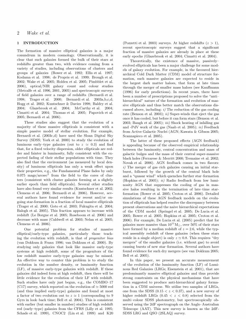
In order to make a fair comparison between the SDSS and2SLAQ LRG samples (at different redshifts), we must cor-rect the properties of our observed galaxies (magnitude,colours etc.) into rest–frame quantities by applying K–corrections. In addition, we can also correct these rest–framequantities for the expected evolutionary changes over theredshift range studied. These e–corrections are usually per-formed assuming a model for the galaxy spectral energy dis-tribution (SED) and its evolution with redshift. In this pa-per, we therefore generate our K+e corrections using theBruzual & Charlot (2003) stellar population synthesis code.In detail, we generate two stellar population models the firstof which forms all its stars in a single instantaneous burst atz = 9.84 (solar metallicity) and then evolves passively withno further star formation. The second model forms the bulkof its stars in a similar burst, but includes a small amount ofcontinuous star formation throughout the rest of its evolu-tion, accounting for 5% of its final mass. These two modelsare shown in Figure 1 and are labelled “Passive” and “Pas-sive+SF” respectively.

Figure 1 shows the colour evolution as a function of red-shift for these two models along with the actual measuredcolours of the SDSS and 2SLAQ LRGs. Some differences be-tween the models and data are evident, e.g., the models are

4 Wake et al.

Figure 1. The g − r and r − i colours of the SDSS and 2SLAQLRGs as a function of redshift (points). The solid black line showsthe median of the fits with the coloured lines showing the modeltracks described in the text with (solid) and without (dashed)evolution applied.

too red in g − r and too blue in r − i for the lowest redshiftLRGs, with the opposite effect for the highest redshift LRGs.This offset between models and data in the lower redshiftLRGs was noted in E01 and a correction to the g−r coloursof 0.08 magnitudes was applied. However, with the additionof the higher redshift sample, it is clear that a simple offsetis an inadequate correction over our entire redshift range.Such differences between the models and observed coloursof early-type galaxies has been seen before, e.g., Wake et al.(2005) were unable to match the red sequence colours ingalaxy clusters at similar redshifts, while a similar offsetis seen in the colour–redshift plots of Ferreras et al. (2005)from the GOODS/CDFS fields. Simple changes to the mod-els, such as the formation redshift, metallicity and IMF ofthe models, are unable to improve the model fits to the data.We also note that using the PEGASE stellar populationsynthesis model (Fioc & Rocca-Volmerange 1997) producedvery similar results. It appears that the models are not accu-rately reproducing the shape of the spectrum between 4000Aand 5000A causing an offset in g − r and r − i as the r fil-ter passes through this (rest–frame) wavelength region. Theg − i colours of LRGs are well reproduced by the models.

In order to minimise the systematic uncertainties in themodels, and thus uncertainties in our K+e corrections, we

2000 3000 4000 5000 6000 7000

00.

20.

40.

6

0.2u,0.2g,0.2r,0.2i0.55g,0.55r,0.55i,0.55z

Wavelength

Flux

den

sity

/Tra

nsm

isio

n

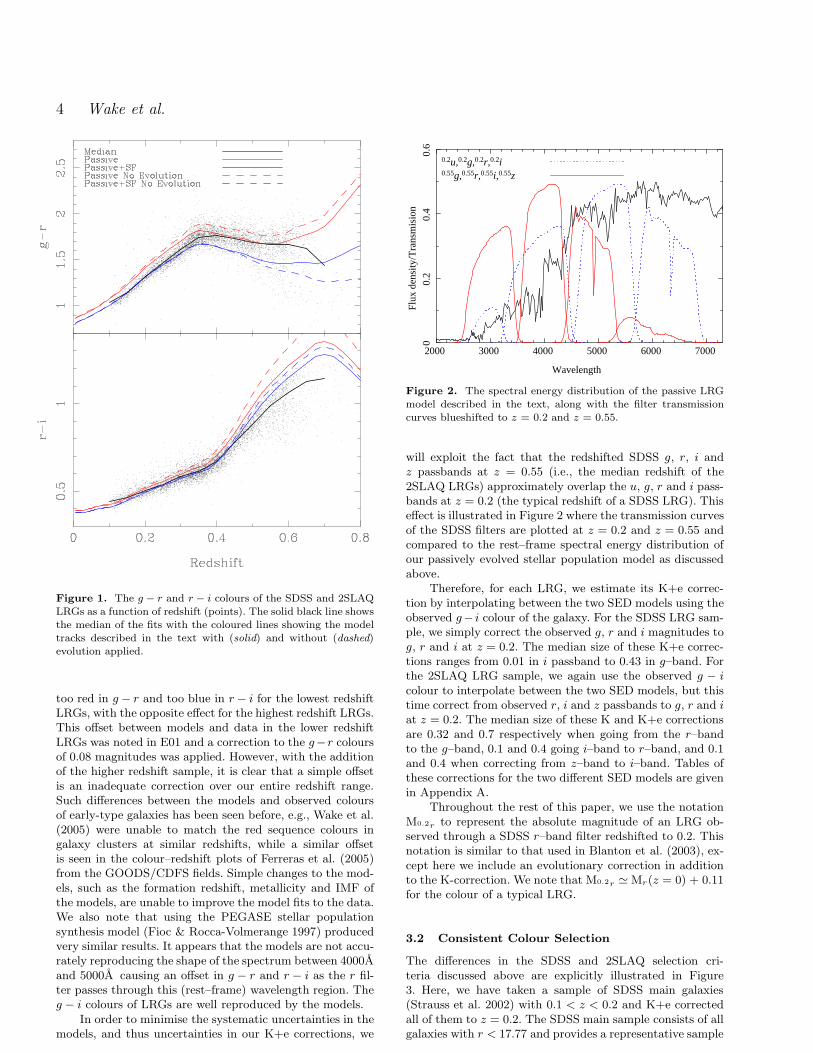
Figure 2. The spectral energy distribution of the passive LRGmodel described in the text, along with the filter transmissioncurves blueshifted to z = 0.2 and z = 0.55.

will exploit the fact that the redshifted SDSS g, r, i andz passbands at z = 0.55 (i.e., the median redshift of the2SLAQ LRGs) approximately overlap the u, g, r and i pass-bands at z = 0.2 (the typical redshift of a SDSS LRG). Thiseffect is illustrated in Figure 2 where the transmission curvesof the SDSS filters are plotted at z = 0.2 and z = 0.55 andcompared to the rest–frame spectral energy distribution ofour passively evolved stellar population model as discussedabove.

Therefore, for each LRG, we estimate its K+e correc-tion by interpolating between the two SED models using theobserved g− i colour of the galaxy. For the SDSS LRG sam-ple, we simply correct the observed g, r and i magnitudes tog, r and i at z = 0.2. The median size of these K+e correc-tions ranges from 0.01 in i passband to 0.43 in g–band. Forthe 2SLAQ LRG sample, we again use the observed g − i

colour to interpolate between the two SED models, but thistime correct from observed r, i and z passbands to g, r and i

at z = 0.2. The median size of these K and K+e correctionsare 0.32 and 0.7 respectively when going from the r–bandto the g–band, 0.1 and 0.4 going i–band to r–band, and 0.1and 0.4 when correcting from z–band to i–band. Tables ofthese corrections for the two different SED models are givenin Appendix A.

Throughout the rest of this paper, we use the notationM0.2r to represent the absolute magnitude of an LRG ob-served through a SDSS r–band filter redshifted to 0.2. Thisnotation is similar to that used in Blanton et al. (2003), ex-cept here we include an evolutionary correction in additionto the K-correction. We note that M0.2r ≃ Mr(z = 0) + 0.11for the colour of a typical LRG.

3.2 Consistent Colour Selection

The differences in the SDSS and 2SLAQ selection cri-teria discussed above are explicitly illustrated in Figure3. Here, we have taken a sample of SDSS main galaxies(Strauss et al. 2002) with 0.1 < z < 0.2 and K+e correctedall of them to z = 0.2. The SDSS main sample consists of allgalaxies with r < 17.77 and provides a representative sample

The 2SLAQ survey: Evolution of LF to z = 0.6 5

Figure 3. The 0.2(g − i) versus M0.2r colour magnitude relationfor SDSS main galaxies with 0.1 < z < 0.2 all K+e correctedto z = 0.2. The small black points in each panel show the wholesample. The second panel shows those galaxies that would havebeen selected by the 2SLAQ selection criteria when K+e correctedto z = 0.55 (large points). The third panel shows those galaxiesthat would be selected by the SDSS LRG Cut I selection criteriawhen K+e corrected to z = 0.2 (large points). The final panelshows the galaxies that satisfy both the SDSS and 2SLAQ LRGselection criteria at both z = 0.2 and 0.55 respectively (largepoints).

of the whole galaxy population. For this sample, we gener-ate the K+e corrections by interpolating between a passivemodel and one with continuous star formation based on theobserved g − i colour of the galaxy. We then applied theSDSS and 2SLAQ LRG selection criteria at the two redshiftsrespectively. We plot in Figure 3 the colour–magnitude re-lation (0.2(g− i) versus M0.2r) for these galaxies, where 0.2g

is the g filter at z = 0.2, illustrating which galaxies wouldbe selected by each criteria and their combination. This fig-ure clearly illustrates the bluer 2SLAQ selection as well asthe magnitude dependence of the SDSS LRG colour selec-tion (E01) as the selection cuts through the red sequencestarting at M0.2r > -22.8.

Although the detailed colour evolution of LRGs remainsunknown, we will proceed by assuming a simple passivemodel for LRGs evolution and thus make a self–consistentcolour selection at both z = 0.2 and z = 0.55. We can thencheck whether the observed LF evolution is consistent withthis simple hypothesis and whether any further evolution(beyond passive) is required to explain our observations. Todo this, we first use the K+e corrections described above tocorrect all the LRGs in both samples to the redshift of theother sample i.e. we correct the 2SLAQ LRGs to z = 0.2and the SDSS LRGs to z = 0.55. We then require that forany individual LRG to be included in our analysis of theLRG LF it must satisfy both the SDSS criteria (at z = 0.2)and the 2SLAQ criteria (at z = 0.55). As might be expected,considering the broader colour and magnitude ranges of the2SLAQ selection criteria, most of the SDSS LRGs (≃90%)would still be selected as LRGs at z = 0.55. The oppositeis not true with only ≃30% of the 2SLAQ LRGs satisfyingthe stricter SDSS Cut I LRG criteria.

Figure 4 shows the colour distributions of all the 2SLAQLRGs (red) and all the SDSS LRGs (blue) convolved withthe typical photometric errors of the 2SLAQ LRGs, K+ecorrected to z = 0.2. The left–hand panel shows the colourdistributions of the full sample of SDSS and 2SLAQ LRGsconsidered in this paper (i.e., the raw data), while the middlepanel shows only those galaxies which satisfy both the SDSSand 2SLAQ LRG selection criteria at z = 0.2 and z = 0.55 re-spectively. As mentioned previously, the 2SLAQ LRGs in theleft–hand panel have bluer colour distributions compared tothe SDSS LRGs, reflecting their bluer and fainter selectioncriteria. When the joint SDSS and 2SLAQ selection criteriaare applied, the colour distributions of this restricted set of2SLAQ LRGs now become redder and much closer to theSDSS LRG colour distributions. However, an offset betweenthe 2SLAQ and SDSS LRG colour distributions is still evi-dent (in the middle panel), i.e., 0.05 magnitudes in the meang − r colour of LRGs. We believe this offset is due to resid-ual inaccuracies in the models used for our K-corrections,although we have tried to reduce this problem by correctingbetween overlapping filters. The wide redshift range of oursamples (particularly in the SDSS) results in the errors inour K-corrections still being significant and detectable.

To improve the agreement between the 2SLAQ andSDSS LRG samples, we restrict the redshift ranges of thesetwo samples to be closer to the redshifts where the SDSSfilters have their greatest overlap (Figure 2). We restrictthe SDSS LRG sample to 0.17 < z < 0.24 and 2SLAQLRG sample to 0.5 < z < 0.6, which reduces the ampli-tude of the K-corrections at z = 0.2 for the SDSS LRGsto a range of 0.005 to 0.06, compared to 0.01 to 0.11 with-out this restricted redshift range. Likewise, the amplitude ofthe 2SLAQ LRG K-corrections reduce to a range of 0.08 to0.30, compared to 0.11 to 0.36 without the restricted red-shift range. The right–hand panel of Figure 4 shows thecolour distributions of LRGs that satisfy both the SDSSand 2SLAQ selection criteria within the restricted redshift

6 Wake et al.

Table 1. The median photometric errors for the SDSS and2SLAQ LRGs from the single–epoch SDSS photometry and themulti-epoch SDSS photometry described in the text.

u g r i z

SDSS single-epoch 0.56 0.04 0.01 0.01

2SLAQ single-epoch 0.15 0.05 0.03 0.092SLAQ multi-epoch 0.05 0.02 0.01 0.03

ranges discussed above. This results in the colour distribu-tions of the two LRG samples being almost identical; themedian colour difference is now less than 0.01 magnitudes.These restricted redshift LRG samples give us greater con-fidence that, under the assumption of passive evolution, weare now selecting the same type of galaxy in both the SDSSand 2SLAQ surveys. It also suggests that the discrepancybetween the observed and model colours is only affecting theK-corrections and not the evolution corrections. The finalredshift–restricted samples contain 6326 SDSS LRGs, with0.17 < z < 0.24, and 1725 2SLAQ LRGs, with 0.5 < z < 0.6.Clearly making such tight redshift cuts has resulted in a sig-nificant reduction in the size of our samples. However, webelieve that minimising the errors in the K+e corrections isvital to ensure that the LRG samples from the SDSS and2SLAQ are as close as possible.

3.3 Photometric errors

Another potential bias that could affect the sample selec-tion is the larger photometric errors on the 2SLAQ LRGscompared to the SDSS LRGs (because they are intrinsicallyfainter and from the same imaging dataset). This could sys-tematically change the selection, as a function of redshift,as more 2SLAQ LRGs could be scattered both in and outof the sample as the photometric error increases.

We attempt to measure this effect by utilising the multi-epoch SDSS imaging data available over a subsample of the2SLAQ survey area (see Baldry et al. 2005; Scranton et al.2005). This multi-epoch data covers a total of ≃190 deg2

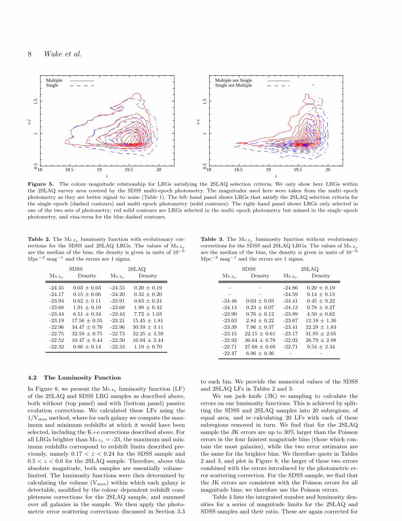
of the southern part of the 2SLAQ survey, and providesbetter signal–to–noise photometry for LRGs in this area asdemonstrated by Table 1. We begin by comparing the num-ber of LRGs that satisfy the 2SLAQ selection criteria usingboth the single and multi-epoch photometry. We find that10059 2SLAQ LRG targets were selected from the single-epoch photometry compared to 10265 2SLAQ LRG targetsselected using the multi-epoch data. However, 25% of thesetargets are different between the two samples and have beenscattered across the selection boundaries in almost equalnumbers. In Figure 5, we show the colour–magnitude rela-tionship for LRGs both in common between the multi andsingle-epoch photometry as well as the LRGs only selected inone of the two data sets. As expected, LRGs selected only inthe single–epoch data (i.e., missed by the 2SLAQ selectionusing the multi–epoch photometry) are fainter and bluerthan 2SLAQ LRGs scattered out of the single–epoch selec-tion but selected using the multi–epoch photometry (theright-hand panel of Figure 5). We note however that thecolour–magnitude relationship of LRGs for both the multiand single-epoch photometry is nearly identical for i < 19.3.

This magnitude corresponds to M0.2r = -23.0 at z = 0.6, theupper redshift limit used herein to calculate the luminosityfunction.

As a further test, we can limit this comparison, to onlyLRGs with measured redshifts. This is possible because asubset of the 2dF fibres (∼ 30%) were allocated to galaxytargets that lie slightly beyond the original 2SLAQ colourselection boundaries for the highest priority “Sample 8” se-lection (for details see Cannon et al. 2006). These extra LRGredshifts allow us to investigate the effect of photometric er-rors on the completeness of “Sample 8”, although we arelimited by the small size of the colour region beyond sample8 when considering those galaxies that weren’t selected butshould have been. In Figure 6 (top), we show the multi-epochcolour and magnitude distributions for 2SLAQ LRGs, in theredshift range 0.5 < z < 0.6, all K+e corrected to z = 0.2as before. As above, 22% of the 2SLAQ LRGs are scatteredinto the sample because of photometric errors, i.e., they sat-isfy the selection criteria in the single–epoch photometry,but fail the criteria for the multi–epoch photometry. Again,these LRGs are bluer and fainter (in absolute magnitude)as shown by the dotted blue line in Figure 6 (top). How-ever, brighter than M0.2r < = -22.65 the magnitude dis-tributions of those selected by the single and multi-epochdata are almost identical. We are therefore confident thatthe photometric errors have minimal effect on the 2SLAQsample function brighter than this limit.

A more significant effect of the photometric errors oc-curs when we apply the additional selection criteria we useto match the samples as discussed in Section 3.2. We canagain try to quantify this effect using the multi-epoch dataand again show in Figure 6 (centre) the magnitude distribu-tions of the single and multi-epoch selected 2SLAQ LRGs.However, here we only show those LRGs in the redshift range0.5 < z < 0.6 that pass both both the SDSS and 2SLAQ se-lection criteria. Unlike previously, where we had a limitedset of spectra for galaxies beyond the selection boundaries,in this instance we have many galaxies far beyond the selec-tion boundaries due to the much bluer and fainter 2SLAQselection. This is clearly visible when comparing the secondand fourth panels of Figure 3. On inspection of the magni-tude distributions in Figure 6 it is clear that a significantfraction of galaxies are being scattered across the selectionboundaries even for LRGs as bright as M0.2r = -23.3. Thisis more clearly illustrated by the bottom panel of Figure6 where we plot the ratio of the number of LRGs selectedusing the multi-epoch data to the number selected usingthe single-epoch data as a function of absolute magnitude.Since we are confident that we have fully sampled the colour-magnitude space beyond the selection boundaries we can usethis ratio to correct the luminosity function and integratednumber and luminosity densities presented in the Section4.2. We note that the only place that we are not samplingbeyond the boundary is for the faintest and reddest objectsand we are thus not confident of the correction and any re-sulting quantities for M0.2r > -22.4. In order to generateaccurate errors on this correction, we take the multi-epochselected sample and add random Gaussian errors typical ofthe 2SLAQ photometric errors to each magnitude. We thencalculate how many LRGs would be selected in our finalsample. We repeat this procedure 10000 times and measure

The 2SLAQ survey: Evolution of LF to z = 0.6 7

0.2

0.4

0.6

0.8 SDSS

2SLAQ

0.2 (

r-i)

All LRGs, All Redshifts

0 0.1 0.2Fraction

1.2 1.4

00.

10.

2Fr

actio

n

0.2(g-r)

0.2

0.4

0.6

0.8 SDSS

2SLAQ

0.2 (

r-i)

Selection Matched LRGs, All Redshifts

0 0.1 0.2Fraction

1.2 1.4

00.

10.

2Fr

actio

n

0.2(g-r)

0.2

0.4

0.6

0.8 SDSS

2SLAQ

0.2 (

r-i)

Selection Matched LRGs, Restricted Redshifts

0 0.1 0.2Fraction

1.2 1.4

00.

10.

20.

3Fr

actio

n

0.2(g-r)

Figure 4. The g − r and r − i colours of all the SDSS and 2SLAQ LRGs K+e corrected to z = 0.2. The SDSS distributions have beenconvolved with the typical 2SLAQ photometric errors. The left–hand plot shows all the LRGs in these two samples, while the middleplot shows only those LRGs (in both samples) that match both the SDSS and 2SLAQ LRG selection criteria (described in the text).The right–hand plot shows those LRGs that match both the SDSS and 2SLAQ LRG selection criteria and have an additional redshiftrestriction; 0.17 < z < 0.24 for the SDSS LRGs and 0.5 < z < 0.6 for the 2SLAQ LRGs.

the standard deviations in each bin which are shown as theerrors in Figure 6 (bottom).

So far we have only discussed the effect of the photo-metric errors on the 2SLAQ LRGs. It is also worth brieflydiscussing any potential effect on the SDSS LRGs. As listedin Table 1 the typical photometric errors on the SDSS LRGsare much smaller than those of 2SLAQ and comparable tothe multi-epoch errors on the 2SLAQ LRGs, except in thecase of the u band. However, the u band data are only usedwhen applying the 2SLAQ selection criteria to the SDSSLRGs and since the 2SLAQ criteria are typically signifi-cantly bluer and fainter than the SDSS criteria one wouldexpect a small effect. In fact only 5% of the SDSS LRGsare removed when the 2SLAQ criteria are applied to themand most of these (3%) are as a result of the 2SLAQ mag-nitude limits where the r band magnitude is used. We aretherefore confident that the photometric errors on the SDSSLRGs result in an insignificant amount of scattering acrossthe selection boundaries.

4 LUMINOSITY FUNCTIONS

4.1 Redshift Completeness

The 2SLAQ survey is not spectroscopically complete unlikethe SDSS LRG sample which is > 99% complete for inputtarget redshifts. Therefore, we must correct the 2SLAQ sur-vey for this redshift incompleteness, taking into account anydependence on magnitude and/or colour. The redshift com-pleteness is defined as the ratio of the number of Sample 82SLAQ LRGs with a reliable redshift to the number of Sam-ple 8 target LRGs selected from the SDSS imaging in eachobserved 2dF field. To calculate this, we need to define theexact survey area covered by the 2SLAQ survey in order todetermine the number of possible LRG targets. To achievethis, we repeatedly ran the 2dF configuration software onrandom positions until we had configured over 5 million ran-dom points in a single 2dF field. This exercise provides a

detailed map of all possible positions available to the 2dFfibres within the field of view. We then built a random cata-logue for the whole 2SLAQ survey area by placing this singlerandomised 2dF field at every observed field centre (see Can-non et al. 2006). Finally, we remove any regions not in theoriginal target input catalogue, i.e., edges of the 2dF fields,that extended beyond the SDSS photometry, and holes inthe SDSS coverage. This produced a random catalogue ofapproximately 400 million positions, covering every possibleposition a 2dF fibre could have been placed throughout thewhole 2SLAQ survey. We then pixelised these random posi-tions (into 30 by 30 arcsecond pixels) to generate a surveymask and positively flagged all pixels that contain at leastone random position.

The survey mask was used in two ways. First, we calcu-lated the area of the survey by summing all positive pixels,giving an area of 180.03 deg2. Secondly, we used the maskto define those LRGs in the input catalogue that could havebeen included in the 2SLAQ survey in order to calculate theredshift completeness. We also restrict the observed LRGsin the same manner resulting in about 0.5% of the observedLRGs (with redshifts) being excluded. This is caused byslight changes made to the 2dF configuration software dur-ing the 2SLAQ survey which we are unable to account forwhen constructing our mask. Figure 7 shows the redshiftcompleteness of the 2SLAQ survey as a function of mag-nitude and colour. There are no significant dependence ofthe redshift completeness on the r − i colour, and i magni-tude only shows any significant dependence fainter than i

= 19.7. However, we do witness a dependency on the g − r

colour of the LRGs. We correct for this dependence by fit-ting a 3rd order polynomial to the data (as shown in Figure7) and use this function to calculate the completeness foreach LRG depending on its observed g− r colour. Includingthis correction changes the 2SLAQ LRG LF by < 1% com-pared to assuming an overall redshift completeness of 76.5%regardless of its g − r colour.

8 Wake et al.

18 18.5 19 19.5 200.5

11.

5

MultipleSingle

i

r-i

18 18.5 19 19.5 200.5

11.

5

Multiple not SingleSingle not Multiple

i

r-i

Figure 5. The colour–magnitude relationship for LRGs satisfying the 2SLAQ selection criteria. We only show here LRGs withinthe 2SLAQ survey area covered by the SDSS multi-epoch photometry. The magnitudes used here were taken from the multi–epochphotometry as they are better signal–to–noise (Table 1). The left–hand panel shows LRGs that satisfy the 2SLAQ selection criteria forthe single–epoch (dashed contours) and multi–epoch photometry (solid contours). The right–hand panel shows LRGs only selected inone of the two sets of photometry; red solid contours are LRGs selected in the multi–epoch photometry but missed in the single–epochphotometry, and visa-versa for the blue dashed contours.

Table 2. The M0.2rluminosity function with evolutionary cor-

rections for the SDSS and 2SLAQ LRGs. The values of M0.2r

are the median of the bins, the density is given in units of 10−6

Mpc−3 mag−1 and the errors are 1 sigma.

SDSS 2SLAQM0.2r Density M0.2r Density

-24.45 0.03 ± 0.03 -24.55 0.20 ± 0.19-24.17 0.15 ± 0.06 -24.20 0.32 ± 0.20-23.94 0.62 ± 0.11 -23.91 0.63 ± 0.24-23.68 1.91 ± 0.19 -23.68 1.99 ± 0.42-23.44 6.51 ± 0.34 -23.43 7.72 ± 1.03-23.19 17.56 ± 0.55 -23.21 15.45 ± 1.81-22.96 34.47 ± 0.76 -22.96 30.59 ± 3.11-22.75 32.59 ± 0.75 -22.73 32.25 ± 3.59-22.52 10.47 ± 0.44 -22.50 16.94 ± 2.44-22.32 0.86 ± 0.14 -22.33 1.19 ± 0.70

4.2 The Luminosity Function

In Figure 8, we present the M0.2r luminosity function (LF)of the 2SLAQ and SDSS LRG samples as described above,both without (top panel) and with (bottom panel) passiveevolution corrections. We calculated these LFs using the1/Vmax method, where for each galaxy we compute the max-imum and minimum redshifts at which it would have beenselected, including the K+e corrections described above. Forall LRGs brighter than M0.2r = -23, the maximum and min-imum redshifts correspond to redshift limits described pre-viously, namely 0.17 < z < 0.24 for the SDSS sample and0.5 < z < 0.6 for the 2SLAQ sample. Therefore, above thisabsolute magnitude, both samples are essentially volume–limited. The luminosity functions were then determined bycalculating the volume (Vmax) within which each galaxy isdetectable, modified by the colour–dependent redshift com-pleteness corrections for the 2SLAQ sample, and summedover all galaxies in the sample. We then apply the photo-metric error scattering corrections discussed in Section 3.3

Table 3. The M0.2rluminosity function without evolutionary

corrections for the SDSS and 2SLAQ LRGs. The values of M0.2r

are the median of the bins, the density is given in units of 10−6

Mpc−3 mag−1 and the errors are 1 sigma.

SDSS 2SLAQM0.2r Density M0.2r Density

– – -24.86 0.20 ± 0.19– – -24.59 0.14 ± 0.13

-24.46 0.03 ± 0.03 -24.41 0.45 ± 0.22-24.14 0.23 ± 0.07 -24.13 0.78 ± 0.27-23.90 0.76 ± 0.12 -23.89 4.50 ± 0.62-23.63 2.84 ± 0.22 -23.67 12.18 ± 1.30-23.39 7.96 ± 0.37 -23.41 22.29 ± 1.83-23.15 22.15 ± 0.61 -23.17 31.95 ± 2.05-22.92 36.64 ± 0.78 -22.92 26.79 ± 2.88-22.71 27.68 ± 0.69 -22.71 9.54 ± 2.34-22.47 6.96 ± 0.36 – –

to each bin. We provide the numerical values of the SDSSand 2SLAQ LFs in Tables 2 and 3.

We use jack–knife (JK) re–sampling to calculate theerrors on our luminosity functions. This is achieved by split-ting the SDSS and 2SLAQ samples into 20 subregions, ofequal area, and re–calculating 20 LFs with each of thesesubregions removed in turn. We find that for the 2SLAQsample the JK errors are up to 30% larger than the Poissonerrors in the four faintest magnitude bins (those which con-tain the most galaxies), while the two error estimates arethe same for the brighter bins. We therefore quote in Tables2 and 3, and plot in Figure 8, the larger of these two errorscombined with the errors introduced by the photometric er-ror scattering correction. For the SDSS sample, we find thatthe JK errors are consistent with the Poisson errors for allmagnitude bins; we therefore use the Poisson errors.

Table 4 lists the integrated number and luminosity den-sities for a series of magnitude limits for the 2SLAQ andSDSS samples and their ratio. These are again corrected for

The 2SLAQ survey: Evolution of LF to z = 0.6 9

Table 4. The integrated number and luminosity density of the evolution corrected SDSS and 2SLAQ samples and the ratio of these twomeasurements.

Sample Density (×10−6 Mpc−3) Luminosity Density (×106 L⊙ Mpc−3)M0.2r < -22.5 M0.2r < -23.0 M0.2r < -23.5 M0.2r < -22.5 M0.2r < -23.0 M0.2r < -23.5

SDSS 25.09 ± 0.33 9.77 ± 0.20 1.12 ± 0.07 3.62 ± 0.05 1.79 ± 0.04 0.31 ± 0.022SLAQ 24.36 ± 1.47 9.33 ± 0.68 1.24 ± 0.16 3.53 ± 0.21 1.78 ± 0.12 0.36 ± 0.05

Ratio 1.03 ± 0.06 1.05 ± 0.08 0.91 ± 0.13 1.03 ± 0.06 1.01 ± 0.08 0.86 ± 0.13

the effect of the photometric errors scattering galaxies intoand out of the sample. However, in this instance we use thefit to the relation shown in Figure 6 as we need to make acorrection to each individual galaxy. The errors are again acombination of the JK errors and those from the photomet-ric scattering.

5 DISCUSSION

As seen in Figure 8, the SDSS and 2SLAQ LFs brighter thanM0.2r = -22.6 are in excellent agreement when the passiveevolution corrections are included. Fainter than this limit weare not confident of the photometric scattering correctionwe have made, although we note that the LFs are still inreasonable agreement. The agreement of these luminosityfunctions is further confirmed by calculating the integratednumber and luminosity density of LRGs as given in Table 4.Brighter than M0.2r = -22.5, both the integrated luminosityand number density of the 2SLAQ and SDSS samples agreeto within their one sigma errors, and are measured to betterthan 10% out to z = 0.6.

Throughout the analysis presented herein, we have con-sistently used the same simple passive evolution model forpredicting and correcting the colours and luminosities ofLRGs as a function of redshift, and this agreement demon-strates the lack of any extra evolution, beyond the passivefading of old stars, out to z ≃ 0.6. This result confirmsthe underlying assumptions of Eisenstein et al. (2001), andCannon et al. (2006), that the majority of LRGs out toz ≃ 0.6 can be selected via straightforward colour cuts,in multicolour data, assuming simple passive evolution oftheir stellar populations. The result also confirms the workof Bernardi et al. (2003c,d) for lower redshift massive ellip-ticals in the SDSS.

It may appear that our lack of extra evolution beyondpassive (out to z ∼ 0.6) is in conflict with recent resultsfrom the C17, DEEP2, and SXDS surveys (Bell et al. 2004;Faber et al. 2005; Yamada et al. 2005). These smaller–area,but deeper (in magnitude limit and redshift), surveys findevidence for a change in the density of red galaxies out toz ∼ 1 beyond that expected from passive fading of the stel-lar populations. For example, Faber et al. (2005) report aquadrupling of φ∗ for red galaxies since z = 1, althoughthis result is strongest in their highest redshift bin, wherethey admit their data are weakest. A direct comparison withthese deeper surveys is difficult because of the differences incolour selections used for the surveys, as well as the rela-tive luminosity ranges probed by the different surveys, i.e.,the 2SLAQ survey is designed to probe galaxies brighterthan a few L∗, while the DEEP2, SXDS and C17 surveys

effectively probe galaxies below L∗ at z ∼ 0.6 (due to theirsmaller areal coverage and fainter magnitude limits).

However, to facilitate such a comparison, we show inFigure 9, the LFs from Figure 8, and the C17 red galaxy LFs(Bell et al. 2004, Figure 3) for the same redshift range andK+e corrected to M0.2r. We only plot our LFs to M0.2r <

-22.9 as we do not include all the red galaxies fainter thanthis due to the SDSS LRG selection criteria. Figure 9 demon-strates that when one restricts the data to the same red-shift range, there is excellent qualitative agreement betweenthe 2SLAQ and C17 luminosity functions. We are unableto make a quantitative comparison due to the difficultyin exactly matching the selection criteria of the two sur-veys. Taken together, the surveys shown in Figure 9 ex-tend the evidence for no evolution in the LF of LRGs toM0.2r < −21, which is close to L⋆ in the LF. Figure 9 alsodemonstrates that these two surveys are probing differentluminosity regimes at z < 0.6 as there is at most only 0.5magnitudes of overlap in their LFs in which the C17 surveyis becoming seriously affected by small number statistics dueto its smaller areal coverage.

The C17 data presented in Figure 9 agrees with ourfindings that for the brightest galaxies there appears to beno evidence for density evolution out to z ∼ 0.6. This re-sult is not necessarily in conflict with the work of Bell et al.(2004); Faber et al. (2005); Yamada et al. (2005), as we arestill probing different redshift and luminosity ranges thanthese other studies. Taken together, these results could in-dicate the existence of different evolutionary scenarios aboveand below L∗ in the luminosity function, i.e., above L∗,galaxies have only evolved passively (since z = 0.6), whilebelow this luminosity, the red galaxy population is experi-encing significant evolution. Kodama et al. (2004) sees sim-ilar evidence for differential evolutionary trends with lu-minosity at z ∼ 1, and claim this supports the idea of“down-sizing” i.e., the galaxy evolutionary processes (likestar–formation and assembly) decrease with increased lumi-nosity as a function of redshift. These higher redshift obser-vations are also consistent with the observed transition, atMr ∼ −20.5, in the local colour–magnitude relationship be-tween a dominant “red” population of galaxies (above thisluminosity), compared to “blue” population below. Likewise,Kauffmann et al. (2003) find a significant change in the dis-tribution of stellar masses of local galaxies at the same lu-minosity. A more detailed joint analysis of the 2SLAQ anddeeper surveys will be presented in a forthcoming paper.

The luminosity functions given in Figure 8 place tightconstraints on models of massive galaxy formation and evo-lution. Our results appear to favour little, or no, densityevolution, as we only require the expected passive evolutionof the luminosities of these LRGs to explain the observed

10 Wake et al.

-24 -23.5 -23 -22.5 -22 -21.5

00.

10.

20.

30.

4

M0.2r

frac

tion

Multiple (430)Single (518)Multiple not Single (27)Single not Multiple (115)

-24 -23.5 -23 -22.5 -22 -21.5

00.

10.

20.

30.

4

M0.2r

frac

tion

Multiple (190)Single (210)Multiple not Single (62)Single not Multiple (82)

-23.5 -23 -22.5 -22

00.

51

1.5

M0.2r

Nm

ulti

/ Nsi

ngle

Figure 6. Top and Middle - The magnitude distributions for all2SLAQ LRGs in the redshift range 0.5 < z < 0.6 with multi-epoch photometry. This subsample is further split into LRGsselected from the multi-epoch data (dot-dashed line), from thesingle-epoch data (solid line), and those LRGs selected only frommulti–epoch data but not the single epoch data (dashed line) andvisa-versa (dotted line). The distributions are normalised to thenumber in the single-epoch subsample. The number of LRGS ineach of these subsamples is given in parentheses in the top panel.The top panel shows those passing the original 2SLAQ selectioncriteria, the middle those passing the additional selection criteriadiscussed in Section 3.2. Bottom - The ratio of number selectedusing the multi-epoch data to the number selected using the sin-

gle epoch data using the additional selection criteria discussed inSection 3.2. The solid line shows a polynomial fit and the dashedlines the 1 sigma errors on the fit.

18.5 19 19.5 20

0.7

0.8

i

com

plet

enes

s

0.8 1 1.2 1.4

0.7

0.8

r-i

com

plet

enes

s

1 1.5 2

0.6

0.7

0.8

g-r

com

plet

enes

s

Figure 7. The redshift completeness of 2SLAQ LRGs as a func-tion of apparent i magnitude (top panel), r − i colour (middlepanel) and g− r colour (bottom panel). The solid line in the bot-tom panel shows the 3rd order polynomial fit to the data andused to correct the sample for this incompleteness as a functionof g − r colour. The bins, chosen to contain 800 LRGs each, areplotted at the mean magnitude of the bin with the one sigmaerror bars.

differences in their LFs as a function of redshift. In otherwords, there are already enough LRGs per unit volume atz ≃ 0.6 to account for the density of LRGs measured atz ≃ 0.2. To study this further, we must compare our re-sults with the latest predictions for massive galaxy evolu-tion. For example, De Lucia et al. (2005) have used the ef-fects of AGN feedback to regulate new star–formation inmassive ellipticals within their semi–analytical Cold DarkMatter (CDM) model of galaxy formation. As shown in Fig-ures 4 & 5 of De Lucia et al. (2005), they find that 50% ofstars in z = 0 massive ellipticals are already formed by a

The 2SLAQ survey: Evolution of LF to z = 0.6 11

-25 -24 -23

-8-6

-4

With evolutionary correction

M0.2r

log

10de

nsity

(M

pc-3

mag

-1)

-8-6

-4

SDSS 0.17 < z < 0.242SLAQ 0.5 < z < 0.6

Without evolutionary correction

Figure 8. The M0.2r luminosity function without (top panel)and with (bottom panel) passive evolution corrections for boththe SDSS (open data points) and 2SLAQ (solid data points) LRGsamples. The points are plotted with their one sigma error barsas described in the text.

-24 -23 -22 -21

-8-6

-4

M0.2r

log

10de

nsity

(M

pc-3

mag

-1)

COMBO-17 z = 0.25COMBO-17 z = 0.55SDSS LRG z = 0.22SLAQ LRG z = 0.55

Figure 9. The M0.2r luminosity function with passive evolutioncorrections for the SDSS (blue open data points), 2SLAQ (redsolid data points) LRG samples, and the COMBO-17 red galaxiesat z = 0.25 (black open stars) and z = 0.55 (green solid stars)(Bell et al. 2004). The dashed lines show the Schechter functionfit to the COMBO-17 points. The points are plotted with theirone sigma errors.

-24.5 -24 -23.5 -23 -22.5

-8-7

-6-5

-4

z = 0.2z = 0.55 10% mergez = 0.55 25% mergez = 0.55 50% mergez = 0.55 75% merge

M0.2r

log 10

dens

ity (

Mpc

-3 m

ag-1

)

Figure 10. The M0.2r luminosity function with passive evolutioncorrections for the 2SLAQ LRGs (solid data points) and fit tothe SDSS LRGs black line. The lines show the effect of splittingvarying fractions of the 2SLAQ LRGs in two, simulating majormergers between z = 0.6 and z = 0.2.

Table 5. The chi–squared values for fitting difference merger frac-tions

Fraction M0.2r < -22.75 M0.2r < -23.25Merging Reduced χ2 Prob Reduced χ2 Prob

0 0.68 0.70 0.53 0.760.10 0.64 0.74 0.90 0.470.25 1.66 0.10 2.00 0.070.50 4.54 < 0.0001 3.52 0.0030.75 6.07 < 0.0001 6.08 < 0.0001

median redshift of z = 2.6, yet 50% of the stellar mass ofz = 0 massive ellipticals is not in place until a median red-shift of z = 0.8. In Figure 9 of their paper, they show thatgalaxies more massive than ≃ 1011M⊙ are built up through∼ 5 major mergers, that must be “dry” (without gas) toprevent new star-formation (van Dokkum 2005). Using theBruzual & Charlot (2003) models described earlier, we es-timate that our LRGs have stellar masses > 5 × 1011M⊙,consistent with the massive galaxy sample discussed byDe Lucia et al. (2005).

We investigate a simple model, motivated by the idea of“dry mergers” and the results of De Lucia et al. (2005), tosimulate the effect on the luminosity function of the hierar-chical build–up of these LRGs through major merger events.To achieve this, we fit the SDSS LRG LF predict the higherredshift (at z = 0.55) 2SLAQ LRG LF under the assumptionthat a given fraction of the SDSS LRGs were formed froma major merger of two equal mass progenitors, i.e., we as-sume that two 2SLAQ LRGs have merged between z = 0.55and z = 0.2 to form a more massive SDSS LRG. We then

12 Wake et al.

determine the likely fraction of z = 0.2 LRGs that couldhave been formed this way by fitting (via χ2) this model tothe observed z = 0.55 2SLAQ LRG luminosity function. Wecould have performed this test using the actual data, ratherthan fitting the z = 0.2 SDSS LRG LF, but unfortunatelysuch a method would suffer from small number statistics atthe bright end of the LF, resulting in the brightest bin dis-appearing as there are no brighter LRGs being split to refillthe bin. However, the χ2 values are almost identical for theother bins.

The results are presented in Figure 10 and listed in Ta-ble 5. They reveal that the 2SLAQ and SDSS LFs are con-sistent with each other without any need for merging. At the3σ level, we can exclude merger rates of > 50%, i.e., morethan half the LRGs at z = 0.2 are already well-assembled,with more than half their stellar mass in place, by z ≃ 0.6.This observation is consistent with Masjedi et al. (2005) whofind that LRG-LRG mergers can not be responsible for themass growth of LRGs at z < 0.36 based on the small–scaleclustering amplitude of SDSS LRG correlation function.

Our limit is barely consistent with the predictions inFigure 5 of De Lucia et al. (2005), where they show that∼ 50% of z = 0 massive ellipticals have accreted 50% of theirstellar mass since z ≃ 0.8. We note that our simple modeldoes not constrain the rate of minor mergers; the results ofRoseboom et al. (2006) on the spectral analysis of 2SLAQLRGs suggests the ≃ 1% of our LRGs have experienced asmall burst of star–formation in the last Gigayear (based onthe observed Hδ line), which affects less than 10% of theirstellar mass.

Our results are a challenge for models of hierarchicalgalaxy formation. More detailed comparisons with semi–analytical CDM models are required and will be investi-gated in other papers. For example, Bower et al. (2005) alsoinclude AGN feedback in their semi-analytic simulations,but follow the model suggested by Binney (2004) wherebythe AGN heating and the gas cooling form a self–regulatingfeedback loop if the gas is in the hydrostatic cooling regime(found in groups and cluster) and the central black hole issuitably massive. Initial results suggest that the Bower et al.(2005) prescription provides a better fit to the LRG evo-lution discussed here (Bower, priv. comm.). We also havesignificantly more data than used in this paper, i.e., if wecould precisely model the K+e corrections of these LRGsover the joint redshift range of the SDSS & 2SLAQ surveys,we would gain a factor of 2 increase in the number of LRGsused to compute their luminosity functions. In future work,we will investigate the use of other stellar synthesis modelsfor such corrections (Maraston 2005).

ACKNOWLEDGEMENTS

The authors are very grateful to Carlton Baugh, RichardBower, Darren Croton, Yeong Loh, Claudia Maraston,Daniel Thomas, and Russell Smith for advice and commentson this work. The authors thank the AAO staff for theirassistance during the collection of these data. We are alsograteful to PPARC TAC and ATAC for their generous al-location of telescope time to this project. DAW thanks theICG Portsmouth for their financial support during this work.RCN acknowledges the EU Marie Curie program for their

support. IRS and ACE acknowledge support from the RoyalSociety.

Funding for the SDSS and SDSS-II has been providedby the Alfred P. Sloan Foundation, the Participating In-stitutions, the National Science Foundation, the U.S. De-partment of Energy, the National Aeronautics and SpaceAdministration, the Japanese Monbukagakusho, the MaxPlanck Society, and the Higher Education Funding Councilfor England. The SDSS Web Site is http://www.sdss.org/.

The SDSS is managed by the Astrophysical ResearchConsortium for the Participating Institutions. The Partic-ipating Institutions are the American Museum of Natu-ral History, Astrophysical Institute Potsdam, University ofBasel, Cambridge University, Case Western Reserve Uni-versity, University of Chicago, Drexel University, Fermilab,the Institute for Advanced Study, the Japan ParticipationGroup, Johns Hopkins University, the Joint Institute forNuclear Astrophysics, the Kavli Institute for Particle As-trophysics and Cosmology, the Korean Scientist Group, theChinese Academy of Sciences (LAMOST), Los Alamos Na-tional Laboratory, the Max-Planck-Institute for Astronomy(MPIA), the Max-Planck-Institute for Astrophysics (MPA),New Mexico State University, Ohio State University, Uni-versity of Pittsburgh, University of Portsmouth, PrincetonUniversity, the United States Naval Observatory, and theUniversity of Washington.

REFERENCES

Adelman-McCarthy, J. K., et al. 2005, astro-ph/0507711Baldry, I. K., Glazebrook, K., Brinkmann, J., Ivezic, Z.,Lupton, R. H., Nichol, R. C., & Szalay, A. S. 2004, ApJ,600, 681

Baldry, I. K., et al. 2005, MNRAS, 358, 441Balogh, M. L., Miller, C., Nichol, R., Zabludoff, A., & Goto,T. 2005, MNRAS, 360, 587

Baugh, C. M., Lacey, C. G., Frenk, C. S., Granato, G. L.,Silva, L., Bressan, A., Benson, A. J., & Cole, S. 2005,MNRAS, 356, 1191

Bell, E. F., et al. 2004, ApJ, 608, 752Bell, E. F., et al. 2005, ApJ, 625, 23Benson, A. J., Bower, R. G., Frenk, C. S., Lacey, C. G.,Baugh, C. M., & Cole, S. 2003, ApJ, 599, 38

Bernardi, M., Renzini, A., da Costa, L. N., Wegner, G.,Alonso, M. V., Pellegrini, P. S., Rite, C., & Willmer,C. N. A. 1998, ApJL, 508, L143

Bernardi, M., et al. 2003a, AJ, 125, 1817Bernardi, M., et al. 2003b, AJ, 125, 1849Bernardi, M., et al. 2003c, AJ, 125, 1866Bernardi, M., et al. 2003d, AJ, 125, 1882Bernardi, M., Nichol, R. C., Sheth, R. K., Miller, C. J., &Brinkmann, J. 2006, AJ, 131, 1288

Binney, J. 2004, MNRAS, 347, 1093Blanton, M. R., et al. 2003, ApJ, 592, 819Bower, R. G., Lucey, J. R., & Ellis, R. S. 1992, MNRAS,254, 601

Bower, R., et al. 2005, astro-ph/0511338Brough, S., Collins, C. A., Burke, D. J., Mann, R. G., &Lynam, P. D. 2002, MNRAS, 329, L53

Bruzual, G., & Charlot, S. 2003, MNRAS, 344, 1000Cannon, R., et al. 2006, submitted

The 2SLAQ survey: Evolution of LF to z = 0.6 13

Clemens, M. S., Bressan, A., Nikolic, B., Alexander, P.,Annibali, F., & Rampazzo, R. 2006, ArXiv Astrophysicse-prints, arXiv:astro-ph/0603714

Caldwell, N., Rose, J. A., & Concannon, K. D. 2003, AJ,125, 2891

Cimatti, A., et al. 2004, Nature, 430, 184Collister, A., et al. 2006, MNRAS, submittedCroton, D. J., et al. 2006, MNRAS, 365, 11De Lucia, G., et al. 2005, astro-ph/0509725De Propris, R., Stanford, S. A., Eisenhardt, P. R., Dickin-son, M., & Elston, R. 1999, AJ, 118, 719

Eisenstein, D. J., et al. 2001, AJ, 122, 2267Ellis, R. S., Smail, I., Dressler, A., Couch, W. J., Oemler,A. J., Butcher, H., & Sharples, R. M. 1997, ApJ, 483, 582

Faber, S., et al., 2005, astro-ph/0506044Ferrarese, L., & Merritt, D. 2000, ApJL, 539, L9Ferreras, I., Lisker, T., Carollo, C. M., Lilly, S. J., &Mobasher, B. 2005, ApJ, 635, 243

Fioc, M., & Rocca-Volmerange, B. 1997, AA, 326, 950Fukugita, M., Ichikawa, T., Gunn, J. E., Doi, M., Shi-masaku, K., & Schneider, D. P. 1996, AJ, 111, 1748

Fukugita, M., Nakamura, O., Turner, E. L., Helmboldt, J.,& Nichol, R. C. 2004, ApJL, 601, L127

Glazebrook, K., et al. 2004, Nature, 430, 181Goto, T., et al. 2003, PASJ, 55, 771Hogg, D. W., et al. 2002, AJ, 124, 646Holden, B. P., et al. 2005, ApJL, 620, L83Hopkins, P. F., et al., astro-ph/0508167Kauffmann, G. 1996, MNRAS, 281, 487Kauffmann, G., et al. 2003, MNRAS, 341, 54Kawata, D., & Gibson, B. K. 2005, MNRAS, 358, L16Kodama, T., Arimoto, N., Barger, A. J., & Arag’on-Salamanca, A. 1998, AA, 334, 99

Kodama, T., et al. 2004, MNRAS, 350, 1005Kuntschner, H., & Davies, R. L. 1998, MNRAS, 295, L29Kuntschner, H., Smith, R. J., Colless, M., Davies, R. L.,Kaldare, R., & Vazdekis, A. 2002, MNRAS, 337, 172

Le Borgne, D., et al. 2005, ApJ, astro-ph/0503401Lilly, S. J., Tresse, L., Hammer, F., Crampton, D., & LeFevre, O. 1995, ApJ, 455, 108

Lin, H., Yee, H. K. C., Carlberg, R. G., Morris, S. L., Saw-icki, M., Patton, D. R., Wirth, G., & Shepherd, C. W.1999, ApJ, 518, 533

McCarthy, P. J., et al. 2004, ApJL, 614, L9Maraston, C. 2005, MNRAS, 362, 799Masjedi, M., et al., 2005, astro-ph/0512166Metcalfe, N., et al., 1996, Nature, 383, 236Metcalfe, N., et al., 2001, MNRAS, 323, 795Metcalfe, N., et al., 2005, MNRAS, submitted (as-troph/0509540)

Naab, T., et al. 2005, astro-ph/0512235Nelan, J. E., Smith, R. J., Hudson, M. J., Wegner, G. A.,Lucey, J. R., Moore, S. A. W., Quinney, S. J., & Suntzeff,N. B. 2005, ApJ, 632, 137

Novak, G. S., Faber, S. M., & Dekel, A. 2006, ApJ, 637, 96Padmanabhan, N., et al. 2005, MNRAS, 359, 237Papovich, C., Dickinson, M., Giavalisco, M., Conselice,C. J., & Ferguson, H. C. 2005, ApJ, 631, 101

Pimbblet, K. A., Smail, I., Edge, A. C., O’Hely, E., Couch,W. J., & Zabludoff, A. I. 2006, MNRAS, 366, 645

Pozzetti, L., et al. 2003, A&A, 402, 837Roseboom, I., et al. 2005, in prep.

Scannapieco, E., Silk, J., & Bouwens, R. 2005, ApJL, 635,L13

Schade, D., et al. 1999, ApJ, 525, 31Schlegel, D. J., Finkbeiner, D. P., & Davis, M. 1998, ApJ,500, 525

Scranton, R., et al. 1005, astro-ph/0508564Springel, V., Di Matteo, T., & Hernquist, L. 2005, ApJL,620, L79

Strauss, M. A., et al. 2002, AJ, 124, 1810Trager, S. C., Faber, S. M., Worthey, G., & Gonzalez, J. J.2000, AJ, 120, 165

Tremaine, S., et al. 2002, ApJ, 574, 740Thomas, D., Maraston, C., Bender, R., & de Oliveira, C. M.2005, ApJ, 621, 673

van Dokkum, P. G., & Franx, M. 1996, MNRAS, 281, 985van Dokkum, P. G., Franx, M., Fabricant, D., Illingworth,G. D., & Kelson, D. D. 2000, ApJ, 541, 95

Van Dokkum, P. G. 2005, AJ, 130, 2647Wake, D. A., Collins, C. A., Nichol, R. C., Jones, L. R., &Burke, D. J. 2005, ApJ, 627, 186

Yamada, T., et al. 2005, ApJ, 634, 861York, D. G., et al. 2000, AJ, 120, 1579

APPENDIX A: K AND EVOLUTIONARY

CORRECTIONS

We present here tables of the g − i colours, K and K+e cor-rections derived from the Bruzual & Charlot (2003) modelsdescribed in Section 3.1.

14 Wake et al.

Table A1. K and K+e corrections for the SDSS LRGs to z = 0.2 assuming the passive model discussed in the text

K K+ez g − i u g r i u g r i

0.150 1.697 -0.398 -0.280 -0.086 -0.035 -0.312 -0.214 -0.030 0.0170.175 1.813 -0.207 -0.141 -0.043 -0.018 -0.162 -0.108 -0.015 0.0080.200 1.929 0.000 0.000 0.000 0.000 0.000 0.000 0.000 0.0000.225 2.034 0.202 0.132 0.042 0.017 0.159 0.098 0.015 -0.0080.250 2.121 0.422 0.254 0.088 0.043 0.336 0.185 0.032 -0.0080.275 2.208 0.647 0.376 0.140 0.069 0.523 0.272 0.056 -0.0070.300 2.300 0.879 0.506 0.190 0.097 0.726 0.367 0.079 -0.0050.325 2.393 1.116 0.644 0.242 0.128 0.934 0.466 0.104 0.0010.350 2.450 1.333 0.753 0.303 0.168 1.125 0.537 0.137 0.015

Table A2. K and K+e corrections for SDSS LRGs to z = 0.2 assuming the passive plus star–forming model discussed in the text

K K+ez g − i u g r i u g r i

0.150 1.597 -0.217 -0.244 -0.078 -0.032 -0.189 -0.195 -0.029 0.0160.175 1.703 -0.107 -0.123 -0.039 -0.016 -0.095 -0.098 -0.014 0.0070.200 1.808 0.000 0.000 0.000 0.000 0.000 0.000 0.000 0.0000.225 1.903 0.094 0.113 0.038 0.016 0.086 0.088 0.014 -0.0070.250 1.982 0.186 0.217 0.079 0.039 0.174 0.167 0.030 -0.0070.275 2.060 0.268 0.321 0.126 0.064 0.261 0.246 0.053 -0.0060.300 2.143 0.340 0.429 0.170 0.089 0.343 0.332 0.074 -0.003

0.325 2.225 0.402 0.542 0.217 0.118 0.417 0.420 0.097 0.0030.350 2.275 0.444 0.631 0.271 0.155 0.472 0.484 0.128 0.017

Table A3. K and K+e corrections for 2SLAQ LRGs to z = 0.55 assuming the passive model discussed in the text

K K+ez g − i g r i z g r i z

0.450 2.574 -0.402 -0.470 -0.140 -0.086 -0.256 -0.328 -0.042 0.0000.475 2.635 -0.298 -0.351 -0.111 -0.066 -0.190 -0.244 -0.037 -0.0010.500 2.682 -0.204 -0.227 -0.075 -0.049 -0.131 -0.157 -0.025 -0.0060.525 2.735 -0.105 -0.110 -0.041 -0.027 -0.069 -0.074 -0.016 -0.0050.550 2.788 0.000 0.000 0.000 0.000 0.000 0.000 0.000 0.0000.575 2.850 0.115 0.103 0.040 0.027 0.078 0.068 0.016 0.0050.600 2.921 0.245 0.203 0.084 0.058 0.169 0.136 0.036 0.0140.625 3.001 0.394 0.306 0.137 0.093 0.278 0.208 0.064 0.0270.650 3.077 0.546 0.414 0.200 0.126 0.389 0.284 0.101 0.037

Table A4. K and K+e corrections for 2SLAQ LRGs to z = 0.55 assuming the passive plus star-forming model discussed in the text.

K K+ez g − i g r i z g r i z

0.450 2.376 -0.244 -0.412 -0.126 -0.080 -0.189 -0.308 -0.039 -0.0010.475 2.422 -0.177 -0.308 -0.100 -0.061 -0.139 -0.230 -0.035 -0.0020.500 2.455 -0.118 -0.199 -0.067 -0.045 -0.095 -0.148 -0.024 -0.006

0.525 2.491 -0.060 -0.096 -0.037 -0.025 -0.049 -0.070 -0.015 -0.0050.550 2.526 0.000 0.000 0.000 0.000 0.000 0.000 0.000 0.0000.575 2.566 0.063 0.090 0.036 0.025 0.055 0.065 0.015 0.0050.600 2.609 0.130 0.177 0.076 0.053 0.118 0.129 0.034 0.0140.625 2.655 0.202 0.268 0.123 0.086 0.191 0.198 0.061 0.0260.650 2.693 0.269 0.361 0.178 0.117 0.263 0.270 0.095 0.036

The 2SLAQ survey: Evolution of LF to z = 0.6 15

Table A5. K and K+e corrections for SDSS LRGs to z = 0.55

Passive Star-formingK K+e K K+e

z g − i u → g g → r r → i u → g g → r r → i g − i u → g g → r r → i u → g g → r r → i

0.150 1.697 0.200 0.031 -0.012 0.727 0.501 0.386 1.597 0.381 0.067 -0.004 0.850 0.520 0.3870.175 1.813 0.391 0.170 0.031 0.877 0.607 0.401 1.703 0.491 0.188 0.035 0.944 0.617 0.4020.200 1.929 0.598 0.311 0.074 1.039 0.715 0.416 1.808 0.598 0.311 0.074 1.039 0.715 0.4160.225 2.034 0.800 0.443 0.116 1.198 0.813 0.431 1.903 0.703 0.434 0.118 1.113 0.802 0.4290.250 2.121 1.020 0.565 0.162 1.375 0.900 0.448 1.982 0.830 0.573 0.176 1.159 0.876 0.4410.275 2.208 1.245 0.687 0.214 1.562 0.987 0.472 2.060 0.920 0.685 0.227 1.237 0.954 0.4630.300 2.300 1.477 0.817 0.264 1.765 1.082 0.495 2.143 0.992 0.793 0.271 1.319 1.040 0.4840.325 2.393 1.714 0.955 0.316 1.973 1.181 0.520 2.225 1.054 0.906 0.318 1.393 1.128 0.5070.350 2.450 1.931 1.064 0.377 2.164 1.252 0.553 2.275 1.096 0.995 0.372 1.448 1.192 0.538

Table A6. K and K+e corrections for 2SLAQ LRGs to z = 0.2

Passive Star-forming

K K+e K K+ez g − i r → g i → r z → i r → g i → r z → i g − i r → g i → r z → i r → g i → r z → i

0.450 2.574 -0.781 -0.214 -0.183 -1.043 -0.458 -0.408 2.376 -0.776 -0.227 -0.192 -1.016 -0.449 -0.4020.475 2.635 -0.662 -0.185 -0.163 -0.959 -0.453 -0.409 2.422 -0.672 -0.201 -0.173 -0.938 -0.445 -0.4030.500 2.682 -0.538 -0.149 -0.146 -0.872 -0.441 -0.414 2.455 -0.563 -0.168 -0.157 -0.856 -0.434 -0.4070.525 2.735 -0.421 -0.115 -0.124 -0.789 -0.432 -0.413 2.491 -0.460 -0.138 -0.137 -0.778 -0.425 -0.4060.550 2.788 -0.311 -0.074 -0.097 -0.715 -0.416 -0.408 2.526 -0.364 -0.101 -0.112 -0.708 -0.410 -0.4010.575 2.850 -0.208 -0.034 -0.070 -0.647 -0.400 -0.403 2.566 -0.274 -0.065 -0.087 -0.643 -0.395 -0.3960.600 2.921 -0.108 0.010 -0.039 -0.579 -0.380 -0.394 2.609 -0.187 -0.025 -0.059 -0.579 -0.376 -0.3870.625 3.001 -0.005 0.063 -0.004 -0.507 -0.352 -0.381 2.655 -0.096 0.022 -0.026 -0.510 -0.349 -0.3750.650 3.077 0.103 0.126 0.029 -0.431 -0.315 -0.371 2.693 -0.003 0.077 0.005 -0.438 -0.315 -0.365