arX

iv:a

stro

-ph/

0106

498v

3 1

0 D

ec 2

001

Mon. Not. R. Astron. Soc. 000, 000–000 (0000) Printed 1 February 2008 (MN LATEX style file v2.2)

The 2dF Galaxy Redshift Survey: Spectra and redshifts

Matthew Colless1, Gavin Dalton2, Steve Maddox3, Will Sutherland4, PederNorberg5, Shaun Cole5, Joss Bland-Hawthorn6, Terry Bridges6, Russell Cannon6,Chris Collins7, Warrick Couch8, Nicholas Cross4, Kathryn Deeley8, Roberto DePropris8, Simon P. Driver4, George Efstathiou9, Richard S. Ellis10, Carlos S. Frenk5,Karl Glazebrook11, Carole Jackson1, Ofer Lahav9, Ian Lewis6, Stuart Lumsden12,Darren Madgwick9, John A. Peacock13, Bruce A. Peterson1, Ian Price1, MarkSeaborne2, Keith Taylor6,10 (the 2dFGRS team)1Research School of Astronomy & Astrophysics, The Australian National University, Weston Creek, ACT 2611, Australia2Department of Physics, University of Oxford, Keble Road, Oxford OX1 3RH, UK3School of Physics & Astronomy, University of Nottingham, Nottingham NG7 2RD, UK4School of Physics and Astronomy, University of St Andrews, North Haugh, St Andrews, Fife, KY6 9SS, UK5Department of Physics, University of Durham, South Road, Durham DH1 3LE, UK6Anglo-Australian Observatory, P.O. Box 296, Epping, NSW 2121, Australia7Astrophysics Research Institute, Liverpool John Moores University, Twelve Quays House, Birkenhead, L14 1LD, UK8Department of Astrophysics, University of New South Wales, Sydney, NSW 2052, Australia9Institute of Astronomy, University of Cambridge, Madingley Road, Cambridge CB3 0HA, UK10Department of Astronomy, California Institute of Technology, Pasadena, CA 91125, USA11Department of Physics & Astronomy, Johns Hopkins University, Baltimore, MD 21218-2686, USA12Department of Physics, University of Leeds, Woodhouse Lane, Leeds, LS2 9JT, UK13Institute for Astronomy, University of Edinburgh, Royal Observatory, Blackford Hill, Edinburgh EH9 3HJ, UK

Accepted —. Received —; in original form —.

ABSTRACT

The 2dF Galaxy Redshift Survey (2dFGRS) is designed to measure redshifts for ap-proximately 250 000 galaxies. This paper describes the survey design, the spectroscopicobservations, the redshift measurements and the survey database. The 2dFGRS usesthe 2dF multi-fibre spectrograph on the Anglo-Australian Telescope, which is capableof observing 400 objects simultaneously over a 2 diameter field. The source cataloguefor the survey is a revised and extended version of the APM galaxy catalogue, and thetargets are galaxies with extinction-corrected magnitudes brighter than bJ=19.45. Themain survey regions are two declination strips, one in the southern Galactic hemispherespanning 80×15 around the SGP, and the other in the northern Galactic hemispherespanning 75×10 along the celestial equator; in addition, there are 99 fields spreadover the southern Galactic cap. The survey covers 2000deg2 and has a median depthof z=0.11. Adaptive tiling is used to give a highly uniform sampling rate of 93% overthe whole survey region. Redshifts are measured from spectra covering 3600–8000A ata two-pixel resolution of 9.0A and a median S/N of 13 pixel−1. All redshift identifica-tions are visually checked and assigned a quality parameter Q in the range 1–5; Q≥3redshifts are 98.4% reliable and have an rms uncertainty of 85 km s−1. The overallredshift completeness for Q≥3 redshifts is 91.8%, but this varies with magnitude from99% for the brightest galaxies to 90% for objects at the survey limit. The 2dFGRSdatabase is available on the WWW at http://www.mso.anu.edu.au/2dFGRS.

Key words: surveys — galaxies: clustering — galaxies: distances and redshifts —cosmology: observations — cosmology: large scale structure of universe

2 Colless et al.

1 INTRODUCTION

The 2dF Galaxy Redshift Survey is designed to measure red-shifts for approximately 250 000 galaxies in order to achievean order of magnitude improvement on previous redshift sur-veys, and provide a detailed and representative picture of thegalaxy population and its large-scale structure in the nearbyuniverse. The main goals of the 2dFGRS are:

1. To measure the galaxy power spectrum P (k) on scalesup to a few hundred Mpc, filling the gap between the smallscales where P (k) is known from previous galaxy redshiftsurveys and the largest scales where P (k) is well-determinedby observations of the cosmic microwave background (CMB)anisotropies. Particular goals are to determine the scale ofthe turnover in the power spectrum and to observe in thegalaxy distribution the acoustic peaks detected in the CMBpower spectrum (Percival et al. 2001).

2. To measure the redshift-space distortion of the large-scale clustering that results from the peculiar velocity fieldproduced by the mass distribution (Peacock et al. 2001).This distortion depends on both the mass density parame-ter Ω and the bias factor b of the galaxy distribution withrespect to the mass distribution, constraining the combina-tion β = Ω0.6/b.

3. To measure higher-order clustering statistics of thegalaxy distribution in order to: (a) determine the bias pa-rameter b, revealing the relationship between the distribu-tions of mass and light and yielding a direct measure ofΩ; (b) establish whether the galaxy distribution on largescales is a Gaussian random field, as predicted by most in-flationary models of the early universe; and (c) investigatethe non-linear growth of clustering in the small-scale galaxydistribution.

4. To fully and precisely characterise the galaxy pop-ulation in terms of the distributions of fundamental prop-erties such as luminosity, surface brightness, spectral typeand star-formation rate (Folkes et al. 1999; Cole et al. 2001;Madgwick et al. 2001a; Cross et al. 2001).

5. To quantify the relationships between the internalproperties of galaxies (such as luminosity, spectral type andstar-formation rate) and their external environment (the lo-cal density of galaxies and the surrounding large-scale struc-ture) in order to constrain models of galaxy formation andevolution (Norberg et al. 2001a).

6. To investigate the properties of galaxy groups andclusters, not just from existing cluster catalogues (De Pro-pris et al. 2001), but by defining a large, homogeneous sam-ple of groups and clusters in redshift space, avoiding theproblems of cluster catalogues defined in projection and al-lowing detailed study of the mass distributions and dynam-ical evolution in the most massive bound structures in theuniverse.

7. To provide a massive spectroscopic database for usein conjunction with other surveys, for finding rare and inter-esting types of object, and as a source for a wide variety offollow-up observations (Cole et al. 2001; Sadler et al. 2001,Magliocchetti et al. 2001).

This paper provides an overview of the survey and de-tailed description of the survey observations. The layout ofthe papers is as follows: §2 summarises the main capabilitiesof the 2dF multi-fibre spectrograph; §3 describes the inputsource catalogue for the survey; §4 discusses the survey de-

sign, including the areas of sky covered by the survey andthe tiling of the survey fields; §5 outlines the algorithm usedto assign fibres to targets, and its uniformity and complete-ness; §6 describes the spectroscopic data obtained for thesurvey and the data reduction methods; §7 deals with theestimation of the redshifts and various internal and exter-nal checks on their reliability and precision; §8 describes thesurvey masks, which encapsulate the coverage, magnitudelimits and redshift completeness of the survey; §9 outlinesthe main components and features of the survey database;§10 summarises some of the main results emerging from thesurvey; and §11 provides conclusions.

2 THE 2DF SPECTROGRAPH

The survey is designed around the Two-degree Field (2dF)multi-fibre spectrograph on the Anglo-Australian Telescope,which is capable of observing up to 400 objects simultane-ously over a 2 diameter field of view. Here we summarisethe aspects of the instrument relevant to the 2dFGRS; a fulldescription is provided by Lewis et al. (2001) and the 2dFUser Manual (http://www.aao.gov.au/2df). The four maincomponents of 2dF are the corrector optics, the fibre posi-tioner, the fibres and the spectrographs.

The 2dF corrector optics are a four-element lens assem-bly which gives 1′′ images over a 2.1 diameter flat field ofview at the prime focus of the AAT. The corrector incorpo-rates an atmospheric dispersion compensator (ADC) whichcorrects for atmospheric dispersion at zenith distances lessthan about 70. The most significant remaining image degra-dation is a chromatic variation in distortion, which has theeffect of dispersing images in the radial direction. This effectis largest halfway out from the field centre, where the wave-length range 0.35–1.0µm is dispersed over 2′′ radially. Theradial distortion introduced by the corrector gives an imagescale that varies over the field of view, from 15.5′′/mm at thecentre to 14.2′′/mm at the edge; the corresponding changein focal ratio is from f/3.4 to f/3.7.

The 2dF fibre positioner X-Y robot takes about 6–7 sec-onds on average to position one fibre. Since approximately550–580 fibre moves are required to re-configure a typical400-fibre field, this means that a full re-configuration takesabout 60–65 minutes. The actual configuration time variesdepending on the number of fibres used and the complexityof the field. To avoid dead-time there are two field plates,each with 400 fibres. While one field plate is placed at thefocal plane for observing, the other is being re-configuredby the fibre positioner. The positions of the field plates arereversed by tumbling them about their horizontal axis.

The fibres are have 140µm diameter cores, correspond-ing to 2.16′′ at the field centre and 1.99′′ at the field edge.There are 400 fibres on each field plate. The internal preci-sion with which the fibres are positioned is 11µm (0.16′′) onaverage, with no fibres outside 20µm (0.3′′). The fibres ter-minate in magnetic ‘buttons’ that attach to the steel fieldplates. Each button has a right-angle prism which directsthe light from the focal plane into the fibre. To prevent fibrebuttons coming into direct contact and protect the fragileprisms, the fibres cannot be placed too close together. Theabsolute minimum fibre separation is 800µm (approximately12′′), and the required separation is generally larger (approx-

2dFGRS: Spectra and redshifts 3

imately 30′′), as it depends on the detailed geometry of thebuttons and their relative orientations.

Half the fibres on each field plate go to one of the twoidentical spectrographs. Each spectrograph has an f/3.15 off-axis Maksutov collimator feeding a 150mm collimated beamto the grating and then, at an angle of 40, to an f/1.2 wide-field Schmidt camera. The detectors are Tektronix CCDswith 1024×1024 24µm pixels. The 200 fibre spectra imagedonto each CCD are separated by approximately 5 pixels.The 2dFGRS used the 300B gratings, which are blazed at4200A and give a dispersion of 178.8A/mm (4.3A/pixel). Fora typical spectrograph focus of 2.1 pixels (FWHM), this cor-responds to a FWHM spectral resolution of 9.0A. The 2dF-GRS observations used a central wavelength around 5800A,and covered the approximate range 3600–8000A. Flexure isless than 0.2 pixel/hour (i.e. less than 40 kms−1 over a typ-ical integration time).

The overall system efficiency (source to detector) of2dF with the 300B gratings used in the 2dFGRS is 2.8%at 4400A, 4.3% at 5500A and 4.7% at 7000A. These figureswere obtained from measurements of photometric standardstars, corrected to nominal 1′′ seeing.

3 SOURCE CATALOGUE

The source catalogue for the survey (Maddox et al. 2001,in preparation) is a revised and extended version of theAPM galaxy catalogue (Maddox et al. 1990a,b,c;1996). Thiscatalogue is based on Automated Plate Measuring machine(APM) scans of 390 plates from the UK Schmidt Telescope(UKST) Southern Sky Survey. The extended version of theAPM catalogue includes over 5 million galaxies down tobJ=20.5 in both north and south Galactic hemispheres overa region of almost 104 deg2 (bounded approximately by dec-lination δ≤+3 and Galactic latitude b≥30). Small regionsaround bright stars, satellite trails and plate flaws are ex-cluded; these are accounted for by the survey mask (see§8.1).

The bJ magnitude system for the Southern Sky Surveyis defined by the response of Kodak IIIaJ emulsion in combi-nation with a GG395 filter. It is zeropointed to Vega—i.e. bJ

is equal to Johnson B for an object with zero colour in theJohnson–Cousins system. The colour equation is normallytaken to be

bJ = B − 0.28(B − V ) , (1)

following Blair & Gilmore (1982). A larger coefficient(−0.35) has been suggested by Metcalfe et al. (1995), butwe measure −0.27±0.02 in comparison with the ESO Imag-ing Survey (Arnouts et al. 2001), and we therefore retainthe usual value of −0.28. The photometry of the catalogueis calibrated with numerous CCD sequences and, for galax-ies with bJ=17–19.45, has a 68% spread of approximately0.15 mag, but with a non-Gaussian tail to the error distri-bution. We emphasise that the calibration is to total CCDphotometry, which absorbs any remaining correction to thethresholded APM magnitudes.

The star-galaxy separation is as described in Maddoxet al. (1990b), and the locus dividing stars and galaxies waschosen to exclude as few compact galaxies as possible whilekeeping the contamination of the galaxy sample by stars to

about 5%. Spectroscopic identifications of the survey objects(see §7), show that the stellar contamination is in fact 6%.

The source catalogue is incomplete at all magnitudesdue to various effects, including the explicit exclusion of ob-jects classified by the APM as merged images, the misclas-sification of some galaxies as stars, and the non-detection(or misclassification as noise) of some low surface brightnessobjects. This incompleteness has been studied in compar-isons with deeper wide-area CCD photometry by Pimbbletet al. (2001) and Cross & Driver (2001, in preparation). Theoverall level of incompleteness is 10–15% and varies slightlywith apparent magnitude, being largest for the brightestand faintest objects. The main classes of objects that areexcluded are: (i) merged galaxy images that are explicitlyexcluded from the 2dFGRS source catalogue (about 60% ofthe missing objects); (ii) large galaxies that are resolved intocomponents that are classified as stellar, merged or noise ob-jects (20%); (iii) compact normal galaxies that are detectedbut classified as stars (15%); and (iv) low surface brightnessgalaxies that are either not detected or classified as noiseobjects (5%). Thus the main cause of incompleteness is mis-classification of objects rather than their non-detection.

The target galaxies for the 2dFGRS were selectedto have extinction-corrected magnitudes brighter thanbJ=19.45. Since the targets were selected, improvements tothe photometric calibrations and revised extinction correc-tions have resulted in slight variations to the magnitude limitover the survey regions—this is precisely quantified by themagnitude limit mask for the survey (see §8.1). The bJ ex-tinction is taken to be AbJ

==4.035E(B−V ), where the co-efficient, and the reddening E(B−V ) as a function of posi-tion, come from Schlegel et al. (1998). The limit of bJ=19.45was chosen because: (i) The surface density of galaxies atbJ=19.45 (approximately 165 deg−2) is sufficiently largerthan the surface density of 2dF fibres on the sky (127 deg−2)to allow efficient use of all fibres—few fibres are unused evenin low-density fields. (ii) The time taken to configure a typ-ical field (60–65 min) allows, with overheads, a sufficientlylong exposure time to reach the desired signal-to-noise levelof S/N>10 pixel−1 for galaxies with bJ=19.45 even in ratherpoor conditions. This limiting magnitude corresponds to amedian redshift for the survey of about z=0.1, so that the2dFGRS is essentially a survey of the local universe.

4 SURVEY DESIGN

4.1 Survey areas

The areas of the sky covered by the survey were chosen soas to satisfy a number of different requirements. The firstgoal was to cover as large a volume as possible, in order toclosely approach a statistically representative sample of theuniverse on the largest possible scales. The second was toobtain near-complete sampling down to the survey limit inorder to have the finest possible resolution of structure onsmall scales. The third requirement was to match the sampleto the observational capabilities of the 2dF instrument inorder to achieve high efficiency. The adopted geometry is aneffective compromise between these requirements.

The survey consists of two separate declination stripsof overlapping 2 fields plus 99 scattered ‘random’ 2 fields.

4 Colless et al.

Figure 1. The 2dFGRS regions shown in an Aitoff projection of R.A. and Dec., with individual 2dF fields marked as small circles. Alsoshown are the lines of Galactic latitude |b|=0, 30, 45. The numbers of survey galaxies in these regions are: 193 550 in the 643 fields ofthe 80×15 SGP strip, 139 144 in the 450 fields of the 75×10 NGP strip, and 57 019 in the 99 fields scattered around the SGP strip.

Figure 2. The survey fields in the NGP (left) and SGP (right) on maps of the extinction AbJderived from Schlegel et al. (1998).

One strip (the SGP strip) is in the southern Galactic hemi-sphere and covers approximately 80×15 centred close tothe South Galactic Pole (21h40m < α < 03h40m, −37.5 <δ < −22.5). The other strip (the NGP strip) is in the north-ern Galactic hemisphere and covers 75×10 (09h50m < α <14h50m, −7.5 < δ < +2.5). The 99 ‘random’ fields are cho-sen from the low-extinction region of the APM catalogue in

the southern Galactic hemisphere outside the survey strip(the mean extinction over each field is required to be lessthan 0.2 mag—see Figure 2 of Efstathiou & Moody (2001)).The fields are chosen pseudo-randomly within this region,except that the field centres are at least 3 apart. A mapof the survey fields on the sky is shown in Figure 1; thelocations of the fields with respect to the extinction map

2dFGRS: Spectra and redshifts 5

Figure 3. The distribution of extinction corrections AbJwith

Galactic latitude b (dots and left axis) and the fraction of correc-tions larger than a given value (line and right axis).

derived from Schlegel et al. (1998) are shown in Figure 2.All the survey fields lie at Galactic latitudes greater than|b|=30, and the whole of the SGP strip and most of theNGP strip and the random fields lie at Galactic latitudesgreater than |b|=45.

The distribution of extinction corrections as a func-tion of Galactic latitude, and the fraction of correctionslarger than a given value, are shown in Figure 3. Over-all, the median correction is 0.07 mag, 90% are less than0.16 mag, and 99% are less than 0.26 mag; the corre-sponding quantiles in the NGP are (0.12,0.19,0.28) mag,in the SGP (0.05,0.07,0.11) mag and in the random fields(0.07,0.13,0.30) mag.

The 2dFGRS target sample of galaxies contains 193 550galaxies in the SGP strip, 139 144 galaxies in the NGP strip,and 57 019 galaxies in the random fields. This gives a totalof 389 713 possible targets, significantly more than the sur-vey goal of 250 000 galaxies. Survey observations of the NGPand SGP strips are proceeding outwards in declination fromthe centre of each strip towards this goal. Note that the to-tal number of galaxies listed in the survey source catalogue(and the survey database) is 467 214, which is larger thanthe number of possible survey targets because the sourcecatalogues for the NGP and SGP strips conservatively in-cludes galaxies fainter than the spectroscopic survey magni-tude limit, down to bJ=19.6.

At the median redshift of the survey (z=0.11) theSGP strip extends over 400 h−1 Mpc×75 h−1 Mpc, and theNGP strip over 375 h−1 Mpc×50h−1 Mpc. Out to the effec-tive limit of the survey at z≈0.3, the strips contain a vol-ume of 1.2×108 h−3 Mpc3(for Ωm=0.3, ΩΛ=0.7); the volumesparsely sampled including the random fields is between twoand three times larger.

4.2 Tiling the survey

The survey limit of bJ=19.45 was chosen, in part, becauseit gives a good match between the surface density of galax-ies and the surface density of 2dF fibres. Due to clustering,however, the number of galaxies in a given field varies con-siderably. The rms variation in the number of galaxies perrandomly-placed 2 field is 140 at bJ=19.5, and is largelyindependent of the choice of magnitude limit over the rangeconsidered here. To make efficient use of 2dF we thereforerequire an algorithm for tiling the sky with 2 fields thatallows us to cover the survey area at a high, and nearlyuniform, sampling rate with the minimum number of 2dFfields.

So long as the sampling of the source catalogue is notbiased in any way that depends on the photometric or spec-troscopic properties of the galaxies, we can always use thesource catalogue to accurately determine the sampling rateas a function of position (see §8). The sampling can then beaccounted for in any analysis. However to keep such correc-tions to a minimum, considerable effort has been invested inmaking the sampling as complete and uniform as possible.

There are a number of possible approaches to layingdown target field centres. The simplest is to adopt a uniformgrid of equally spaced centres and then either randomly sam-ple each field with the number of available fibres or observeeach field several times until all the galaxies have been ob-served. The second of these options is clearly inefficient, as itwill give rise to a large number of fields being observed withsignificantly less than the full complement of fibres, whilethe first is undesirable as it gives a different sampling factorfor each field. A more efficient solution is to use an adaptivetiling strategy, where we allow each field centre to drift fromthe regular grid so that we maximise the number of targetsthat are assigned to each field, subject to the constraint thatthe number of targets assigned to any one field should notexceed the number of available fibres, Nf .

We begin with a uniform grid with field centres equallyspaced by s =

√3 in right ascension along rows 1.5 apart

in declination. For each galaxy in the survey we then deter-mine how many fields it lies within, and assign each field aweight wi, where

wi = 0 if Ni ≥ Nf (2)

= 1 − Ni

Nfif Ni < Nf

and Ni is the number of galaxies in this field. These weightsare normalised such that

∑Nt

1wi = 1, where Nt is the num-

ber of fields that this galaxy could be assigned to. The galaxyin question is then randomly assigned to one of the fieldsusing these weights, unless all the fields are already filled,in which case it is assigned to the first field in which itwas found. Once all the field occupancies have been deter-mined in this way we move each field in right ascension byan amount

δαi = ∆α + 0.05s Ni

Nfif (Ni ≥ Nf ) (3)

= ∆α − s′(

1 − Ni

Nf

)

if (Ni < Nf )

where s is the maximum allowed separation between adja-cent fields, s′ is the current distance to the neighbouringfield centre, and ∆α is the cumulative shift that has cur-rently been applied to this row. New fields are added at

6 Colless et al.

the end of each row if the total length of the row has con-tracted enough to exclude any galaxies at the trailing edge.We found that using a fixed separation of 1.5 in declina-tion, and adjusting the tile positions in right ascension only,provided sufficient flexibility to achieve uniform high com-pleteness without a large increase in the total number offields and without leaving gaps in the sky coverage.

In practice, it is found that the above prescription re-quires a further modification to account for the position ofeach object within the field. This additional constraint arisesbecause of the physical restrictions on the positioning of in-dividual fibres, both in terms of their deviation from theradial angle and their extension from the parked position atthe edge of the field. We apply this constraint by dividingeach field into 36 sub-fields and restricting the number oftargets that can be assigned to each sub-field to 16. This islarger than the number of fibres whose park positions fallwithin the arc of the sector, but allows for the fact that thearea of the field that can be reached by each fibre is increas-ing with the fibre extension. Without this extra constraintthe algorithm tends to place large clusters in the overlappingareas of neighbouring fields where, although there are moreavailable fibres because of the overlap, it rapidly becomesimpossible to use these fibres because of the high density oftargets close to the edge of each field. Limiting the number oftargets within each sector effectively removes this problem,and so increases the uniformity of the survey completeness.

The adaptive tiling algorithm also needed to cope withthe requirement that the galaxy redshift survey be mergedwith the concurrent survey of QSO candidates (the 2dF QSORedshift Survey: Boyle et al. 2000; Croom et al. 2001). Thisresults in a higher surface density of targets in the region ofoverlap, for which we compensate by reducing the separationin declination of the tiling strips in the QSO survey regionsto 75% of the original value (i.e. to 1.125). As the QSO sur-vey occupies the central declination strip of our SGP surveyregion this results in a 3-4-3 arrangement of tiling strips overthe three rows of UKST fields used in the SGP survey. Asimilar consideration applied to the NGP survey region givesa 3-4 arrangement if we consider the full areas of the tworows of UKST fields used.

With these additional modifications, our tiling algo-rithm was able to achieve an overall sampling rate of 99.8%,dropping to 93% after the assignment of fibres to targets hasbeen made (see §5.3). On average, fewer than 5% of the fibresin each field were unused. For comparison, the mean sam-pling rate that would be achieved for randomly distributedfields is 68%, with an rms variation of 15%.

5 FIBRE ASSIGNMENT

The tiling procedure described above fixes the location ofthe 2dF target fields on the sky and provides a first passpriority scheme (based on the random field assignments) foruse in assigning targets to fibres. However, the mechanicalconstraints of 2dF imply that we cannot usually allocatefibres to all the targets assigned to a particular field, and sowe consider all targets that lie within each field boundary.Our tiling scheme implies that many of the survey targetsare found on more than one field, so we adopt a priorityscheme as follows: targets which are unique to the field in

question are assigned the highest priority, then targets whichare assigned to the field, but which can also be reached fromneighbouring fields, then targets which fall within the field,but which are assigned to a different, overlapping field. Thepriorities of the QSO targets are increased one step to ensurethat we do not imprint the strong clustering pattern of thegalaxy distribution on the weak clustering expected fromthe QSO sample.

5.1 Single-field assignments

The allocation procedure for a single field can be dividedinto two distinct steps: an initial allocation pass and a fibreswapping pass. These two steps are repeated for each rangeof decreasing priorities for targets that have been assigned tothis field. An attempt is then made to reduce the complexityof the configuration by identifying pairs of allocated fibreswhich are crossed, and which can safely be exchanged. Theallocation and uncrossing steps are then repeated to allowconsideration of the lower priority targets which were notassigned to this field. The details of these steps are as follows:

(1) Initial allocation pass. For each target, t, of a givenpriority we determine the set, Ft, of all fibres that could beallocated to that target in the absence of any other alloca-tions. We then determine the set, Tt, of all targets which fallwithin the sector defined by the target and the two most ex-treme fibres in Ft. We then use the difference N(Tt)−N(Ft)between the number of targets in Tt and the number of fibresin Ft to determine which targets are hardest to access andhence should be given the highest priority: targets withinthe sector defined by the target with the largest value ofN(Tt) − N(Ft) are allocated first. This procedure is thenrepeated for targets of successively lower priorities.

(2) Fibre-swapping pass. For each remaining unallo-cated target, u, we now consider each fibre in Tu. For eachfibre in this set that could still be allocated to u given thecurrent configuration we make a tentative re-allocation ofthis fibre from its initial assignment, i, to target u and checkto see if any unallocated fibres can be assigned to i. If nounallocated fibres can be assigned we repeat this processrecursively until one of the following conditions have beensatisfied: either (i) a previously unallocated fibre is allocated(implying that u has been allocated and that all previouslyallocated targets remain allocated); or (ii) the search exceedsa depth of 10 iterations. In the latter case, if at any point inthe search a fibre has been moved from a low-priority tar-get such that a target of higher priority has been allocatedthen the search is unpacked to this point; if no such trade-off was found then the search is unpacked to the originalconfiguration.

(3) Fibre-uncrossing pass. Each pair of fibres in the con-figuration is tested to see if the fibres cross. For each crossedpair an attempt is made to swap the allocations of fibres totargets. This process is iterated until no further swaps canbe made. The net effect of this procedure is that the fi-nal configuration supplied to the positioner is simplified sothat the transition to the following configuration will requirefewer fibres to be moved twice. This simplification effectivelyreduces the time required for each re-configuration, and isachieved without constraint on the allocation.

2dFGRS: Spectra and redshifts 7

Figure 4. The distribution of the 7% of objects in the sample that are not allocated to fibres (NGP strip at top, SGP strip at bottom).

5.2 Field-overlap assignments

While the above procedure provides an optimised methodof allocating as many fibres as possible to a given individualfield, it does not make optimal use of the flexibility providedby the overlapping fields. We therefore ran a second pass ofthe configuration algorithm which considered each pair ofoverlapping fields as an 800 fibre problem in which all objectsfound within the overlap area are matched up, so that anobject which is allocated in one field can be allocated tothe second field to allow acquisition of unallocated targetsin the first field. Compared to the results of treating thetwo overlapping fields as separate configuration problems,this procedure proves more effective at reducing the overallincompleteness due to the instrumental constraints. Sincethe tiling algorithm tends to place local over-densities closeto the edges of tiles, this procedure also serves to homogenisethe distribution of incompleteness as a function of positionwithin a field.

A significant fraction of this incompleteness arises dueto close pairs of objects which lie within the unique regionsof individual fields. The separation at which this occurs isa strong function of the relative orientation of the two fibrebuttons (see Lewis et al. 2001). The upper limit on the valueof this separation is 11mm in the focal plane (correspondingto 2.2′), while the mean separation of close pairs of objectsfor which one target cannot be assigned is ∼30′′.

5.3 Fibre assignment completeness

The results of this procedure are that we are able to al-locate fibres to 93% of the source catalogue objects. Thedistribution of the unallocated objects on the sky are shown

in Figure 4. The most prominent features visible in thesedistributions are occasional localised clusters of unallocatedobjects. These are due to over-dense regions where the ge-ometrical packing constraints imposed by the fibre buttondimensions mean that it has not been possible to assign ev-ery fibre to a target, even though there are enough fibresavailable as a result of the tiling algorithm. This effect is en-hanced by the relative increase in the number of close pairsin strongly clustered regions.

The distribution of these unallocated objects is alsoshown as a function of position within the 2dF field in Fig-ure 5. This plot shows a slight overall gradient in the R.A.direction, which is due to the order in which the field over-laps are processed (see §5.2). This apparent gradient is mis-leading, since the missed objects are plotted according tothe field plate coordinates on the plate to which they wereassigned, whereas the majority of objects which contributeto this effect are actually missed on more than one 2dF field.The next most prominent feature of Figure 5 is the imprintof the four fibres which are used for field acquisition andguiding. These fibres must be allocated with a higher prior-ity than the targets if the field is to be observed successfully.They prevent the subsequent allocation of target objects ly-ing along their length, and so produce a slight increase inthe numbers of unallocated objects along the four cardinalaxes of the field, in the regions of the plate where they canbe placed.

It should be noted that these figures do not representthe final incompleteness in the survey, since individual targetallocations are adjusted immediately prior to observation toaccount for the actual number of fibres available to 2dF onany given night (typically, about 1% of the fibres are broken

8 Colless et al.

Figure 5. The distribution of the unallocated objects within thestacked 2dF fields.

at any given time, though they are continually replaced).The overall incompleteness at this stage, before any obser-vations have been made, is 7%. The level of this incomplete-ness is such that the pattern is dominated by residuals due toclustering within individual two-degree fields, implying thatan attempt to correct for this effect would effectively imprintthe observed pattern onto the data. We therefore concludethat we have achieved our goal of reducing the mean in-completeness to an acceptably low level, comparable to thelevel of incompleteness due to the individual uncertainties ingalaxy magnitudes and the incompleteness due to not mea-suring redshifts because of inadequate signal-to-noise. Weemphasise that neither the tiling nor the fibre allocation de-pend on the photometric or spectroscopic properties of theobjects, so that we can use the source catalogue to accu-rately determine the sampling of the survey, as discussed in§8).

5.4 Visual inspection

Postage stamp images of each target galaxy and each can-didate fiducial star were generated from the Digitized SkySurvey1 (DSS; Lasker et al. 1998). These DSS images wereused to examine the target galaxies for merged images andto remove unsuitable fiducial star candidates.

The APM image classification parameter k (see Mad-dox et al. 1990b) was used to find target galaxies whichmight possibly be merged images. Objects with k>1.15 inthe SGP and k>1.2 in the NGP were analysed by a sim-ple routine which attempts to relocate the fibre onto the

1 The Digitized Sky Survey was produced at the Space TelescopeScience Institute, and is based on photographic data obtainedusing the Oschin Schmidt Telescope on Palomar Mountain andthe UK Schmidt Telescope.

local maximum of surface brightness closest to the nomi-nal target position. This is achieved by starting from thecentral pixel of the DSS image and allowing the positionto move in a direction of increasing intensity until a localmaximum is found. The position corresponding to this lo-cal maximum is then inserted into the 2dF configuration fileprior to observation. All objects which are tested in this wayare flagged as merged images by changing the second char-acter of the object’s OBSNAME parameter from G to M, evenif the final position of the fibre is unchanged. The surveydatabase records both the original source catalogue position(database parameters RA and DEC; see §9.2)and the actualobserved position (database parameters OBSRA and OBSDEC);the parameter MATCH DR gives the offset (in arcsec) betweenthese two positions, and may be non-zero for objects flaggedas mergers.

The DSS images of candidate fiducial stars are in-spected visually to allow removal of the following types ofobject, which would compromise field acquisition: (i) starswhich are merged with another object; (ii) stars which areclose to other stars of comparable brightness; (iii) brightstars which are strongly saturated on the sky survey plates;(iv) spurious objects that are fragments of the diffractionspikes or halos of bright stars, or bright regions withinlarge galaxies; (v) asteroids and portions of satellite trails;(vi) spurious objects due to noise.

5.5 Final adjustments

The configuration procedure described above determines theoptimal assignment of fibres to targets over the whole sur-vey. This procedure assumes a fixed set of parameters forthe transformation of sky-coordinates to plate-coordinates,whereas in practice a slightly different transform is deter-mined each time the instrument is mounted on the telescope.The above procedure also assumes a full complement of fi-bres, and does not allow for the small but significant attri-tion rate as fibres are disabled due to optical or mechanicalfailures. Fibres which are disabled in this way are repairedon a regular basis, but operational constraints require thatdisabled fibres are replaced in batches, and so there is gen-erally some delay before a particular fibre is replaced.

We account for both the fibre attrition and the effectsof changes to the coordinate transform by re-examining eachconfiguration the day before that field is to be observed. Allbroken or inoperative fibres which had been allocated aredeallocated and the targets to which they were assigned areflagged. An attempt is then made to recover each flaggedtarget using the current list of available fibres, according tothe same algorithm used for the original allocation. Again,low-priority targets may be lost at this stage in favour ofhigh-priority targets. In practice, we usually find that themajority of the high-priority targets which were flagged caneither be recovered or replaced.

A similar check is then made to allow for a furtherchange to the coordinate transform due to the hour angle atwhich the field is to be observed. This correction is a com-bination of the effects of atmospheric refraction and flexureand misalignment of the telescope itself. Each configurationis checked for hour angles of ±4 hours, and adjustments aremade to ensure that no fibre conflicts will occur within this

2dFGRS: Spectra and redshifts 9

range. Again, we usually find that all such conflicts can berecovered without loss of target allocations.

After this correction to the configuration, a number ofunallocated fibres (at least 10 for each spectrograph) are al-located to blank sky positions. This is done initially using anazimuthally symmetrical grid of positions around the field,but if insufficient fibres can be allocated to this grid, moreare allocated to other blank sky regions manually. The posi-tion of each allocated sky position is then checked to ensurethat it is genuinely blank by examining the surrounding areausing the Digitized Sky Survey. Any sky fibres likely to becontaminated by objects visible on the DSS are reallocatedto other blank sky regions.

6 SPECTROSCOPIC DATA

6.1 Observational procedure

A target field is acquired using the four guide fibres, each ofwhich consists of 6 fibres in a hexagonal pattern surround-ing a central fibre. The individual fibres are 95µm (1.4′′)in diameter and have centre-to-centre separations of 1.8′′.These guide fibres are positioned on 14<V <15 stars withpositions measured from the same UKST plates as the tar-get galaxies. As the blue sky survey plates are often 20–25years old, we use the more recent red sky survey plates tocheck for any proper motion, and we also apply a colour cutto reduce the number of nearby stars. On some fields, wherered plates are not available, we have used fiducial stars fromthe USNO A1.0 astrometric catalogue (Monet et al. 1996).

The guide fibres are viewed by the AAT’s standard ac-quisition and guiding TV system. The position for optimumacquisition of the fiducial stars, and subsequent guiding cor-rections, are determined by visual inspection of the locationsof the stars in the guide fibres on the TV image. Acquisitionof a new field typically requires less than 5 minutes.

For each field we first take a multi-fibre flat-field ex-posure using the quartz lamp in the calibration unit. Thisflat-field is used to trace the positions of the fibres on theimage, to fit the spatial profile of each fibre as a functionof wavelength, and to apply a 1-dimensional pixel-to-pixelflat-field correction to the extracted spectra. We next take awavelength calibration exposure of helium and copper-argonarc lamps. We then typically take three 1100s exposures ofthe target objects. However the exposure time is varied tosuit the conditions: for galaxy-only fields in good conditions,three 900s exposures are sufficient; in poor conditions, espe-cially for fields including targets from the QSO survey, alonger total integration time is used. With the CCD read-out time of 60s, the whole series of exposures typically takesjust over an hour, so that the observations of one field arefinished just as the configuration for the next field is com-pleted.

6.2 Data reduction

The data are reduced using the 2dF data reduction pipelinesoftware, 2dfdr, a full description of which is given by Baileyet al. (2001; see also http://www.aao.gov.au/2df). The mainsteps in the process are as follows:

1. Basic image processing. Each image undergoes the

same initial processing, which consists of flagging bad pixels(both saturated pixels and those specified in the bad-pixelmask for each CCD). The bias level is computed as the me-dian of the CCD overscan region and subtracted from theimage. The image is then trimmed to remove the overscanregion. Finally, a variance array is computed based on thepixel data values and the known properties of the CCDs.The variances are propagated through all subsequent reduc-tion steps.

2. Mapping the spectra. The next step is to map thelocations and shapes of the spectra on the detector. Thecentroids of the fibre spectra along the slit are determinedusing the fibre flat field image, and the fibre identificationschecked visually. This is necessary because the positioningof the slit block is not precisely reproducible, so that thelocations of the fibres on the CCD can change by a fewpixels, and occasionally the first or last fibre may fall off theedge of the detector. Visual checking ensures that spectra arecorrectly identified with fibres and thus with the objects thatwere observed. Given this starting location, 2dfdr finds thecentroids of each fibre spectrum as a function of wavelengthand fits a model based on the known optical properties ofthe spectrograph. For each subsequent frame, this model isadjusted (to account for flexure) by fitting an overall shiftand rotation to the positions of the spectra on the detector.

3. Subtracting the background. The background of scat-tered light is fitted with an empirically-determined modelusing the unilluminated portions of the detector. Fibres areso closely packed on the detector that the light level be-tween transmitting fibres does not drop to the backgroundlevel. Hence the only unilluminated areas are at the edgesof the detector and at the positions of dead (broken, non-transmitting) fibres. A small number of fibres are broken atany one time and are continually being replaced. Occasion-ally the number of broken fibres becomes sufficiently smallthat it is not possible to reliably fit the background, and thisstep must be omitted.

4. Fitting the spatial profiles. The close packing of thefibres on the detector means that their spatial profiles over-lap, producing cross-talk between neighbouring spectra. Inorder to correct for this, it is necessary to know the spatialprofile of each fibre spectrum as a function of wavelength.These profiles are determined from the fibre flat field imageby performing simultaneous fits of 200 Gaussians to the fibreprofiles at each of 20 wavelength ranges. These fits are theninterpolated in the wavelength direction with cubic splinesto give the spatial profile for each fibre at every wavelengthon the detector.

5. Spectrum extraction. Given the location and shape ofeach fibre’s spatial profile, optimal extraction consists of aweighted fit of the profiles to recover the amplitude of thespectrum at each wavelength. Because the spectra overlap,a simultaneous fit of the profile amplitudes of each fibrespectrum and its nearest neighbour on either side is carriedout. The fit is performed using least-squares with varianceweighting.

6. Flat-fielding. The extracted spectra are then ‘flat-fielded’ by dividing by the pixel-to-pixel variations in theextracted spectra from the fibre flat field image. This one-dimensional flat-fielding is used because there is presently nomeans of generating a full two-dimensional flat-field image.

7. Wavelength calibration and linearisation. A predicted

10 Colless et al.

wavelength for each pixel, based on the nominal centralwavelength and the optical model for the spectrograph, isfirst calculated. Lines in the helium/argon arc spectra areautomatically identified by a peak-finding algorithm, thenmatched to a list of known lines, discarding both unidenti-fied peaks and unmatched lines, as as well as known blends.The relation between the measured line positions and theirtrue wavelengths is fit by a third-order polynomial. This fititerated up to four times, with the most discrepant line ex-cluded at each iteration. The final fits usually include 21–22lines over the 4400A spectral range, and have typical rmsresiduals of 0.3A (0.07 pixels). Once the wavelength calibra-tion is determined, the spectrum is re-binned onto a linearwavelength scale using quadratic interpolation.

8. Fibre throughput calibration. The spectrum of the skybackground is measured with at least 8 fibres (and usuallymore) on each of the two spectrographs. The spectra fromthe sky fibres are normalised by their mean fluxes and amedian sky spectrum is calculated. The relative through-puts of the fibres are then derived from the relative fluxesin the strong sky lines as follows. All object and sky fibresand the median sky are continuum-subtracted using a con-tinuum derived by median smoothing with a 201-pixel box.This removes the continuum leaving only the strong lines inthe residual spectrum. A robust least-squares fit to the con-stant of proportionality between the counts in each pixel ofthe residual object+sky spectrum and the residual mediansky spectrum then yields the relative throughput for eachfibre (the sky lines in common to both spectra contributeto the fit, but strong emission lines found only in the objectspectrum do not). The individual object and sky spectra arethen normalised by dividing by their relative throughputs.

9. Sky subtraction. The median sky spectrum is re-calculated from the individual normalised sky spectra, andsubtracted from each normalised object and sky spectrum.The sky-subtraction precision, measured as the ratio of thetotal flux in the sky fibres before and after sky-subtraction,is typically 2–3% and rarely worse than 6%. Precise sky-subtraction is dependent on effective scattered light subtrac-tion, wavelength calibration and throughput calibration.

10. Combining spectra. The fully-reduced spectra fromeach of the multiple exposures on the target objects (typ-ically three) are optimally combined in a final step. Thecombination algorithm accounts for overall flux variationsbetween exposures (due to different integration times or ob-serving conditions) and rejects cosmic ray events. The rel-ative weighting of the exposures is computed from the to-tal fluxes in the brightest 5% of the spectra (after they aremedian-smoothed over a 201-pixel box to eliminate cosmicrays and normalised to the first exposure). The maximumflux weight is unity, and the weights are applied to the in-dividual exposures before they compared for cosmic rays.The cosmic ray rejection algorithm is similar to that of theIRAF crreject package. It flags likely cosmic ray events,which are taken to be those pixels that are more than 5σdeviations from the median (over the set of flux-weightedexposures) together with some neighbouring pixels. The fi-nal pixel value in the combined spectrum is computed as thevariance-weighted mean over the flux-weighted exposures ofthe unflagged pixels.

The final result of the reduction is a pair of data files(one for each CCD), both of which contain a multi-spectrum

image (200 fibres × 1024 spectral pixels), the associatedvariance array (which is correctly propagated throughoutthe reduction process), and a copy of the median sky spec-trum used in the background subtraction. The data files alsocontain the identifications of the spectra obtained from thefibre configuration file and detailed information about theinstrument and observation.

The spectra are not flux-calibrated. Flux calibration offibre spectra is very difficult to achieve for a number of rea-sons. Chief among these are: (i) astrometric/positioning er-rors, which, combined with the small fibre aperture, preventreproducible sampling of each galaxy’s light distribution;(ii) chromatic variations in distortion (see §2) and resid-ual errors in the atmospheric dispersion correction, whichproduce variations in the flux calibration dependent on theattitude of the telescope and the position of the object in thefield. These effects can produce significant variations in thecontinuum slope of the spectra, and are discussed in quanti-tative detail in Madgwick et al. (2001b) and Madgwick et al.(2001c, in preparation).

Various problems are exhibited by some of the spectra:(i) Poor sky-subtraction. A small but significant fraction offields suffered sky-subtraction errors of more than 5%. Thestrong oxygen sky lines at 5577A, 6300A, 6363A and theOH bands to the red of 6000A leave significant residuals inthe spectra. (ii) Fringing. Damaged fibres sometimes pro-duce a fringing effect that results in a strong oscillation inthe throughput with wavelength. (iii) Halation. Sometimeshalation due to condensation on the field flattener lens justin front of the CCD results in a high level of scattered lightwhich fills in absorption features; when present, this effectwas worse in CCD camera #2. (iv) ADC error. A soft-ware error meant that the atmospheric dispersion corrector(ADC) was incorrectly positioned for observations prior to31 August 1999; some of the spectra obtained before thisdate suffer from significant atmospheric dispersion losses.

7 REDSHIFTS

7.1 Redshift estimation

The main parameter to be determined from the spectra wasthe redshift of each object. A sophisticated and highly-tunedredshift code was developed in order to achieve a high levelof precision, reliability and automation in the measurementof redshifts from the 2dFGRS spectral data.

The redshift code (version 990505) uses two quasi-independent automated methods: ‘absorption’ redshifts areobtained by cross-correlation with template spectra (afterclipping emission lines) and ‘emission’ redshifts are obtainedby finding and fitting emission lines. These automated red-shift estimates are followed by a visual check and (occasion-ally, where necessary) a ‘manual’ redshift obtained by fittingidentified spectral features.

Before these redshift estimates are made, however, thespectra are pre-processed in a number of ways. Residual fea-tures from the strong atmospheric emission lines at 5577A,5893A, 6300A and 7244A are masked by interpolating overa small wavelength range (20–30A) centred on the sky line.The atmospheric absorption bands around 6870A (B-band)and 7600A (A-band), and the fibre absorption band around

2dFGRS: Spectra and redshifts 11

Figure 6. The eight template spectra against which the 2dFGRSgalaxy spectra were cross-correlated.

7190A, are removed by dividing by an approximate bandcorrection. This correction is obtained by fitting a low-orderpolynomial to the mean of all the spectra in the reduced im-age, dividing the mean spectrum by this smooth fit, findingthe region about each band centre where this ratio is lessthan unity, and setting the band correction to the value ofthis ratio in these regions and to unity elsewhere. The spec-tra, which are not flux-calibrated, are finally multiplied by asimple quadratic approximation to the mean flux calibrationcorrection in order to give appropriate weighting across thewhole spectral range.

An ‘absorption’ redshift is obtained by cross-correlatingthe galaxy spectrum against a suite of 8 template spec-tra following the general method of Tonry & Davis (1979).The templates that are used cover a broad range of spec-tral types, and include 5 galaxies and 3 stars. The galax-ies (and their morphological types) are: 1. NGC3379 (E),2. NGC4889 (cD), 3. NGC5248 (Sbc), 4. NGC2276 (Sc)and 5. NGC4485 (Sm/Im); the stars (and their spectraltypes) are: 6. HD116608 (A1V), 7. HD23524 (K0V) and8. BD 05 1668 (M5V). The galaxy spectra come from spec-trophotometric atlas of Kennicutt (1992); the stellar spectracome from the library of Jacoby et al. (1984). The full setof template spectra are shown in Figure 6.

The galaxy and template spectra are prepared forcross-correlation using the following steps: (1) continuum-subtraction using a sixth-order polynomial fit to the con-tinuum; (2) removal of strong emission lines by patching

out all points more than 5 times the rms variation abovethe mean; (3) re-binning to a logarithmic wavelength scalewith 2048 pixels; (4) apodising (tapering the ends of thespectrum to zero) by multiplying the first and last 5% ofthe spectrum with a cosine bell; (5) Fourier transformation;and, finally, (6) multiplication by an exponential filter of theform e−k/kh −e−k/kl , where k is wavenumber in inverse pix-els, kh=300 pixel−1 and kl=15 pixel−1, in order to reduce theeffects of both the residual continuum at low wavenumberand the noise at high wavenumber.

The cross-correlation function is then computed as theinverse Fourier transform of the complex product of the fil-ter Fourier transforms of the processed galaxy and templatespectra. The highest peak in cross-correlation function isfitted with a quadratic in order to obtain the position andheight of the peak. The significance of the peak is measuredin terms of the ratio, R, of the height of the peak to the noisein the cross-correlation function, which is estimated fromits anti-symmetric part. The absorption redshift is taken tobe the cross-correlation redshift obtained with the templategiving the highest value of R. An estimate of the qualityof the absorption redshift, Qa, is based on the value of R,with Qa=1,2,3,4 for R>3.5,4.0,4.5,5.0 and Qa=0 otherwise(with the additional requirement that Qa=3 and Qa=4 alsorequire, respectively, at least 4 and 6 of the 8 templates givethe same redshift to within 600 km s−1).

An ‘emission’ redshift is obtained by fitting Gaussiansto significant spectral features and searching for a multi-linematch. The galaxy spectrum is first continuum-subtractedusing a sixth-order polynomial fit to the continuum andlightly smoothed with a Gaussian kernel having a disper-sion of 0.8 pixels. Peaks in the smoothed spectrum above athreshold (set at 3.3 times the robustly-estimated rms vari-ation) are flagged as candidate emission lines. For each ofthese, in descending order of strength, a Gaussian is then fit-ted to the unsmoothed data, using the peak in the smoothedspectrum as the initial guess for the line centre. The Gaus-sian fits to the stronger lines are subtracted in turn beforethe weaker lines are fitted (to minimize blending effects inthe Hα/NII pair). Then lines with fitted FWHM between 0.7and 7 pixels, and total ‘significance’ of the whole line above3.5σ are marked as ‘good’; this rejects unclipped cosmic raysand low-significance features.

The ‘good’ lines are then sorted by strength, and thethree strongest tested to see if at least two can be iden-tified as common emission lines ([OII] 3727A, Hβ 4861A,[OIII] 5007A, Hα 6563A or [NII] 6584A) at a single redshift(the two out of three criterion is used to allow for one spuri-ous feature, such as a residual sky line or cosmic ray). If so,then all the other lines in this set (plus [OIII] 4959A) thatmatch this redshift to better than 600 kms−1 are found andthe mean redshift from these matching lines is adopted asthe emission redshift. If not, then up to two possible single-line redshifts are kept for comparison with the absorptionredshift, assuming the single line is either [OII] or Hα in therange 0<z<0.4, as appropriate. An estimate of the qual-ity of the emission redshift, Qe, is based on the number andstrength of the lines from which it is determined, with Qe=0if there are no lines, Qe=1 for one weak line, Qe=2 for anytwo lines or one strong line, and Qe=4 for three or morelines.

The penultimate step is the choice of the best auto-

12 Colless et al.

mated redshift estimate, given the absorption and emissionredshifts and their quality parameters. The best redshift istaken to be whichever of the absorption and emission red-shifts has the higher quality parameter (with the absorptionredshift preferred if Qa=Qe). The best estimate of the red-shift quality is Qb =max(Qa,Qe), with two exceptions: (i) ifthe difference between the absorption and emission redshiftsis less than 600 kms−1 then Qb =max(Qa,Qe,3); and (ii) ifQa≥2 and Qe≥2 and the difference between the absorptionand emission redshifts is greater than 600 km s−1, then thisdiscrepancy is flagged and we set Qb=1.

The final step in measuring the redshift is a visual checkof the best automatic redshift. The redshift code displays forthe user both the cross-correlation function and the galaxyspectrum with all the common spectral features superposedat the best automatic redshift. The spectrum displayed isthe version actually used for the redshift estimate, with badpixels and the strongest night sky lines patched out, andwith an approximate correction applied for the instrumen-tal response. To assist in identifying spurious features thecode also displays the mean sky spectrum (to show the posi-tions of the sky features), the atmospheric absorption bandsand the variance array associated with the spectrum. Theuser is given the emission and/or absorption line redshifts,the best-estimate redshift, whether this is an emission orabsorption redshift (or both), and whether (if both are ob-tained) the emission and absorption redshifts agree or not.If neither of the automated estimates are correct, the usercan manually estimate a redshift by identifying a particularspectral feature and fitting Gaussians at the positions of allthe common features. These fits can be to emission or ab-sorption features and are rejected if there is no detectablefeature near the nominal position. The manual redshift istaken to be the mean of the redshifts estimated from eachof the well-fitted features. Given all this information, theobserver can visually inspect the spectrum, try alternativeredshifts (absorption, emission and manual) and determinethe best redshift estimate.

Once the final redshift estimate has been decided, theuser assigns a quality, Q, to this redshift on a five-pointscale, with the nominal interpretation (see below for fur-ther discussion): Q=1 means no redshift could be estimated;Q=2 means a possible, but doubtful, redshift estimate; Q=3means a ‘probable’ redshift (notionally 90% confidence);Q=4 means a reliable redshift (notionally 99% confidence);Q=5 means a reliable redshift and a high-quality spectrum.Note that this quality parameter is determined entirely bythe subjective judgement of the user, and is independent ofthe automatic quality parameter Qb. Quality classes 1 and2 are considered failures, so the redshift completeness is thenumber of Q=3,4,5 redshifts divided by the total number ofgalaxies in the field. The standard redshift sample comprisesobjects with Q≥3, but (for applications where redshift relia-bility is more important than completeness) one may preferto use the set of objects with Q≥4.

For the objects ending up with ‘acceptable’ (Q=3,4,5)redshifts, the best automated redshift is the same as the bestvisual redshift about 93% of the time; about 5% of the timeeither the absorption or the emission redshift agrees with thebest visual redshift but the code has preferred the other one;and about 2% of the time neither of the estimates matches

the best visual redshift, and a manual redshift estimate isrequired.

While there is some element of subjectivity in decid-ing whether a redshift estimate is ‘acceptable’ or not, thisvisual assessment is found to improve the reliability of thefinal sample, since the observer can assess a number of fac-tors that are hard to fully automate, such as the overallshape of the spectrum, line ratios, the general quality of skysubtraction, and the proximity of features to sky lines or ab-sorption bands. For 15,000 spectra, two or more users havemeasured redshifts independently using the same redshiftcode on the same spectra; the pair-wise ‘blunder’ rate (seebelow) is 0.4%, which is several times smaller than that fordifferent observations of the same object. The rms differencein redshift completeness (fraction of objects per field withQ≥3) between two users for the same data is less than halfof that between the same observer measuring redshifts formany different fields. The human variation is therefore sub-stantially smaller than the unavoidable variation betweenfields due to weather and other effects, and will to first or-der be corrected by the completeness factors.

7.2 Quality of spectra

A quantitative overall measure of spectral quality is the me-dian signal-to-noise ratio (S/N) per pixel computed overall pixels in the wavelength range 4000–7500A with fluxesgreater than zero. This is computed directly from the spec-trum and it associated variance array, and can be comparedto the quality class Q assigned to the redshift identification.The distribution of S/N over the 5 quality classes for thebest spectrum of each object (i.e. the spectrum on whichthe adopted redshift is based) is shown in Figure 7. Thefraction of objects in each quality class and the median S/Nfor each quality class are given in the figure legend. Objectswith reliable redshifts (Q=3,4,5) make up 91.8% of the sam-ple and have a median S/N of 13.1 pixel−1 (6.3 A−1).

Example 2dFGRS spectra for quality classes Q=3, Q=4and Q=5 are shown in Figure 8; for each quality class, oneobject with an absorption redshift and one object with anemission redshift are shown. In order to be representative,the spectra are chosen to have a S/N per pixel close to themedian of their quality class. Residuals from the strong nightsky lines at 5577A and 6300A have been interpolated over.

7.3 Repeat observations

Amongst the first 150 000 galaxies in the survey with red-shifts, there are 8480 repeat redshift measurements; i.e. asecond, or even a third, reliable (Q=3,4,5) redshift measure-ment for an object. These repeat measurements are eitherobjects that lie in the overlaps between fields (7444 cases)or are in fields which were observed more than once, usuallybecause the first observation was of poor quality and lowcompleteness (1036 cases). For these objects we can com-pare their best redshift measurement with the repeat mea-surements to estimate both the rate of incorrect redshiftidentifications in the survey and the uncertainties on thecorrect redshift identifications.

The top panel of Figure 9 shows the distribution ofthe redshift differences (w.r.t. the best redshift measure-ment for the object) for all the repeat observations. The rms

2dFGRS: Spectra and redshifts 13

Figure 7. The distribution of the median S/N per pixel for ob-jects in each of the 5 quality classes.

redshift difference (robustly estimated here and throughoutas the half-width of the central 68% of the distribution) is120 kms−1, implying an overall single-measurement rms un-certainty of 85 km s−1.

The lower panels of the figure show the trends in theredshift uncertainty as a function of redshift, magnitude,S/N and quality class Q. As expected, the uncertaintiesincrease at higher redshifts (from 95 kms−1 for z<0.05 to150 kms−1 at z>0.15), fainter magnitudes (from 100 km s−1

for bJ<18.5 to 140 kms−1 for bJ>19.3) and lower S/N(from 95 kms−1 for S/N>25 to 145 kms−1 for S/N<5).The strongest trends are with redshift quality class and themethod of estimating the redshift. Table 1 gives the rms pre-cision of single measurements as function of redshift qualityclass or measurement method (ABS = cross-correlation ofabsorption features; EMI = automatic fit to emission lines;MAN = manual fit to features). The fact that manual red-shift estimation has the largest uncertainties mainly reflectsthe fact that it is only employed when the automatic meth-ods have failed, usually in cases of low S/N.

We divide the repeat measurements into two categories:correct identifications, where the redshift difference is lessthan 600 kms−1, and ‘blunders’, where it is greater than600 kms−1. The division at 600 kms−1 corresponds to 5times the rms error in the redshift differences. It should benoted that these blunders are not necessarily due to incor-rect redshift measurements for one (or both) of the observedspectra. They may also be due to two observations of a closepair of objects with slight offsets in the fibre position, result-ing in a different member of the pair dominating the spectralflux in each observation.

There are 263 blunders, so that the pair-wise blunderrate amongst the Q=3,4,5 repeat measurements is 3.1%.This implies a single-measurement blunder rate of just 1.6%.Figure 10 shows plots of the redshift differences for the blun-ders with respect to redshift, magnitude, S/N and quality

Figure 8. Example 2dFGRS spectra, showing objects with qual-ity classes Q=3, Q=4 and Q=5, and both absorption (ABS) and

emission (EMI) redshifts. The most common spectral features aremarked at the wavelengths corresponding to the measured red-shift of each object.

14 Colless et al.

Figure 9. The distribution of redshift differences between repeatmeasurements with Q≥3 is shown in the top panel, along with theGaussian having the same median and rms. The dependence ofthe redshift differences on redshift, apparent magnitude, signal-to-noise ratio and quality class for the best observation, is shownin the lower panels (note that the quality classes have small ran-dom offsets added to make the distribution of redshift differencesclear). The lines in the lower panels are the running median andthe ±2σ ranges.

Table 1. Summary statistics by quality class and method.

Quality Fraction RMS error Blunderclass of sample ( km s−1) rate

Q=1 2.5% — —Q=2 4.8% 143 69.5%Q=3 11.9% 123 10.2%Q=4 57.3% 89 0.9%Q=5 23.5% 64 0.2%

Redshift Fraction RMS error Blundermethod of sample ( km s−1) rate

Q=1,2 7.3% — —ABS 72.0% 87 0.7%EMI 18.3% 61 0.9%MAN 2.4% 159 9.3%

class; it also shows the pair-wise fraction of blunders as afunction of each of these quantities.

There is no increase in the blunder rate with redshift,but a significant increase at fainter magnitudes, lower S/Nand lower quality class. The single-measurement blunderrates as functions of quality class and measurement method

Figure 10. The distribution of the redshift differences for theblunders (repeat observations with |∆cz| > 600 km s−1) againstredshift, magnitude, S/N and quality class. The circles are absorp-tion redshifts, the squares are emission redshifts and the crossesare manual redshifts. The histograms at the foot of each panel

show the fraction of blunders as a function of redshift, magni-tude, S/N and quality class.

are given in Table 1. We find that Q=3 corresponds to indi-vidual redshifts having 90% reliability, and that Q=4 and 5correspond to better than 99% reliability, as intended. Theblunder rate for Q=2 redshifts is 70%, consistent with thedefinition of Q=2 as ‘possible but doubtful’. The blunderrates for the absorption and emission redshifts are less than1%, but the blunder rate for manual redshifts is 9% (due tothe fact that manual redshifts are only used in the 2.4% ofcases where the automatic methods fail).

The distribution of blunders shows a slight peak aroundzero redshift difference, suggesting that the tail of the errordistribution for correct redshift identifications is more ex-tended than a Gaussian. Some of the blunders may thus becorrect identifications with larger than normal errors, im-plying that we may be slightly over-estimating the blunderrate. However, the most notable feature in the distributionof blunders is the large number of instances (22% of the to-tal) where one or other of the redshifts in the comparisonis approximately zero. The redshift difference is defined as(other redshift − best redshift), so the upper envelope cor-responds to objects where the best redshift is zero and thelower envelope corresponds to the other redshift being zero.In the former case the best redshift indicates that the ob-jects are stars and the other (non-zero) redshift is due to ablunder based on a poor-quality spectrum; in the latter casewe have the reverse of this situation. There are 3 times as

2dFGRS: Spectra and redshifts 15

Table 2. Comparisons of redshifts with external sources.

Source Ncomp N600 〈∆cz〉 σ(∆cz)km s−1 km s−1

CfA2 87 1 −22 93SAPM 228 10 +11 123PSCz 172 7 −11 120LCRS 3135 11 −1 109ZCAT 1593 103 −33 127

many objects in the upper envelope as the lower, so starsbeing mistaken for galaxies is a much more common errorthan galaxies being mistaken for stars—which is remarkablegiven that galaxies are 20 times more common than stars inour sample.

We have repeated the above analyses after separatingthe repeat observations into those cases where the repeat isdue to re-observing a field (12%) and those where it is due toobserving an object in overlapping fields (88%). We find nosignificant difference in either the single-measurement rmsprecision or the blunder rate for these two subsets of repeatmeasurements.

Examination of the individual object spectra in thecases where there is a blunder shows that in general thebest redshift appears to be quite reliable and that the mainreason for the discrepancy is that the other redshift mea-surement has been obtained from a poor-quality (low-Q)spectrum.

7.4 External comparisons

In order to compare our redshift measurements with thosefrom other sources, we have matched our catalogue tothe redshift catalogues from the second Center for As-trophysics redshift survey (CfA2; Huchra et al. 1999), theStromlo-APM redshift survey (SAPM; Loveday et al. 1996),the PSCz survey (PSCz; Saunders et al. 2000), the LasCampanas redshift survey (LCRS; Shectman et al. 1996),and also to the heterogeneous redshift compilation of theZCAT catalogue (version November 13, 2000; J.P. Huchra,priv.comm.). Objects in these catalogues were matched toobjects in the 2dFGRS by position; positions separated by4 arcsec or less were assumed to belong to the same object.This criterion was chosen to include most genuine matchesand exclude most false matches between close but unrelatedobjects.

Table 2 and Figure 11 summarise the results of thesecomparisons. The table lists, for each external source cat-alogue: the number of matched objects in the comparison,Ncomp; the number of cases, N600, where the redshift dif-ference between the 2dFGRS and the other source indicatesa blunder (|∆cz| > 600 kms−1); the median redshift differ-ence, 〈∆cz〉; and the rms scatter of ∆cz about this median,σ(∆cz). The median and rms scatter are estimated exclud-ing the blunders.

In interpreting these comparisons we need to keep inmind the magnitude range of the objects that are in com-mon. Figure 12 shows the magnitude distributions of thecomparison samples, all of which are significantly brighterthan the 2dFGRS itself. The CfA2, SAPM and PSCz cat-alogues only overlap with the bright tail, while the medianmagnitude of the LCRS is a magnitude brighter than that

Figure 11. Comparisons of the 2dFGRS redshifts with thosefrom the CfA2, SAPM, LCRS and ZCAT catalogues. The leftpanels shown the correlations between the redshift measurements,with each comparison shown as a dot. Most dots lie along the1-to-1 line; the relatively few blunders (|∆cz| > 600 km s−1) are

circled. The right panels show the histogram of redshift differencesoverlaid with a Gaussian having the same median and rms.

of the 2dFGRS. ZCAT has a broader magnitude range, butis also heavily weighted towards brighter objects.

The best comparison is with the LCRS: the compari-son sample is the largest, the magnitude range most simi-lar, and the catalogue is homogeneous (unlike ZCAT). Therms redshift difference of 109 kms−1 is consistent with thesingle-measurement uncertainty of 76 kms−1 for objects inthe 2dFGRS brighter than bJ=18.5 and the typical uncer-tainty of 67 kms−1 on the LCRS redshifts (Shectman et al.1996). The pair-wise blunder rate in the comparison sampleis 11/3135 = 0.4%, which in fact is rather lower than mightbe expected from the pair-wise blunder rate of 46/2920 =1.6% for repeat measurements of objects in the 2dFGRSbrighter than bJ=18.5; this may be due to the high surfacebrightness selection criterion of the LCRS.

The worst comparison is with ZCAT: the rms redshiftdifference is 127 kms−1 and the pair-wise blunder rate is103/1593 = 6.5%, which is more than twice the pair-wiseblunder rate for the 2dFGRS repeats. Given the single-measurement blunder rate for the 2dFGRS is 1.6%, the im-plied single-measurement blunder rate for ZCAT is 5.0%,which is presumably due to the heterogeneous nature of itssource catalogues.

Although the samples in common with CfA2, SAPMand PSCz are relatively small, they give results that are

16 Colless et al.

Figure 12. The magnitude distributions of the 2dFGRS sample,the repeat observations in the 2dFGRS sample, and the five sam-ples of objects in common with other redshift catalogues: CfA2,SAPM, PSCz, LCRS and ZCAT.

consistent with the rms redshift errors and pair-wise blunderrate obtained from the 2dFGRS repeat observations.

Checking the 2dFGRS spectra of the objects that haveredshift blunders, we find that 0/1 cases in the compari-son with CfA2, 1/10 for SAPM, 1/7 for PSCz and 4/11 forLCRS might possibly be attributed to errors in the 2dFGRSredshift estimates. Examining the DSS images of these ob-jects, we find that 2 of the discrepancies with SAPM, 1 ofthose with PSCz, and 6 of those with LCRS, occur in caseswhere there is a close companion to the target object andhence some potential for confusion.

8 SURVEY MASKS

For accurate statistical analysis of the 2dFGRS it is essen-tial to fully understand the criteria that define its parentphotometric catalogue and also the spatial and magnitude-dependent completeness of the redshift catalogue. For thispurpose we have defined three maps or masks characterizingthis information as a function of position on the sky:

(1) The magnitude limit mask gives the extinction-corrected magnitude limit of the survey at each position.

(2) The redshift completeness mask gives the fractionof measured redshifts at each position.

(3) The magnitude completeness mask gives a parame-ter defining how the redshift success rate depends on appar-ent magnitude.

Each mask has its own use, but for some analyses it isnecessary to make use of two or even all three masks. Wenow describe in more detail how each one of these masks isdefined and briefly outline some of their uses.

8.1 Magnitude limit mask

Although the 2dFGRS sample was originally selected to havea uniform extinction-corrected magnitude limit of bJ=19.45,in fact the survey magnitude limit varies slightly with po-sition on the sky. There are two reasons for this. First, thephotometric calibrations now available are much more ex-tensive than when the parent 2dFGRS catalogue was origi-nally defined. This has enabled us to recalibrate the whole2dFGRS parent catalogue (Maddox et al. 2001, in prepa-ration), and results in new zero-point offsets and linearitycorrections for each of the UKST photographic plates. Sec-ond, the extinction corrections have been changed to use thefinal published version of the Schlegel et al. (1998) extinc-tion maps; the original extinction corrections came from apreliminary version of those maps.

The magnitude limit mask is therefore defined by thechange in the photometric calibration of each UKST pho-tographic plate and the change in the dust extinction cor-rection at each position on the sky. The magnitude limitmasks for the NGP and SGP strips are shown in Figure 13;note that the mask also accounts for the holes in the sourcecatalogue around bright stars and plate flaws.

In the SGP, which is a subset of the APM galaxy sur-vey (Maddox et al. 1990a,b,c), the rms change in plate zero-point is only 0.03 mag. However, in the NGP region the orig-inal calibration was less accurate and the change in zero-points have an rms of 0.08 mag. The change in the dustcorrections are also less in the SGP, as the extinction is gen-erally lower in this region. In the SGP the rms magnitudechange due to improved dust corrections is 0.01 mag whilein the NGP it is 0.02 mag.

The magnitude limit distribution over the NGP andSGP strips is shown in Figure 14. In the SGP the medianlimiting magnitude is bJ=19.40 with an rms about this valueof 0.05 mag; in the NGP the median limiting magnitude isbJ=19.35 with an rms of 0.11 mag.

For accurate statistical analysis of the 2dF survey themagnitude limits defined by this mask should be used. Itis always possible to analyse the data with a fixed magni-tude limit if one is prepared to omit both the areas of thesurvey that have magnitude limits brighter than the chosen

2dFGRS: Spectra and redshifts 17

Figure 13. The magnitude limit masks for the NGP strip (top) and the SGP strip (bottom), plotted in a zenithal equal area projection.

Figure 14. The fraction of the sky in the NGP and SGP surveystrips where the survey limit is fainter than a given bJ magnitude.

limit and also all the galaxies in the remaining areas withmagnitudes fainter than the chosen limit.

8.2 Simple redshift completeness mask

The best way to define a redshift completeness mask is tomake use of the geometry defined by the complete set of 2

fields that were used to tile the survey region for spectro-scopic observations. Each region of the sky inside the surveyboundary is covered by at least one 2 field, but more oftenby several overlapping fields. We define a sector as the regiondelimited by a unique set of overlapping 2 fields. This is themost natural way of partitioning the sky, as it takes accountof the geometry imposed by the pattern of 2 fields and theway in which the galaxies were targeted for spectroscopicobservation. Within each sector, θ, we define the redshiftcompleteness, R(θ), as the ratio of the number of galaxiesfor which redshifts have been obtained, Nz(θ), to the totalnumber of objects contained in the parent catalogue, Np(θ):

R(θ) = Nz(θ)/Np(θ). (4)

The redshift completeness of a given sector, R(θ), shouldbe clearly distinguished from the redshift completeness ofa given field, cF, since multiple overlapping fields can con-tribute to a single sector.

This simple redshift completeness mask, shown in Fig-ure 15, can be used to locate regions in which the redshiftcompleteness is high. It can also be used as a first step in

18 Colless et al.

Figure 15. The redshift completeness, R(θ) ≡ Nz(θ)/Np(θ) as a function of position for the 100k public release dataset (2dFGRS data

from October 1997 to January 2000). The top panel is for the NGP, bottom panel for the SGP, plotted in a zenithal equal area projection.

either applying weights to statistically correct for incom-pleteness or to construct a random unclustered catalogue(for use in estimating correlation functions) that have thesame angular pattern of incompleteness as the redshift sam-ple. For this latter purpose one should also take account ofhow the redshift completeness depends on position withina sector as a result of constraints on fibre positioning andother considerations. This is best done by using the parentcatalogue to derive weights for each galaxy with a measuredredshift (Norberg et al. 2001b, in preparation). Also, as dis-cussed in the next section, one should take account of howthe redshift completeness depends on apparent magnitude.

8.3 Magnitude completeness mask

The success rate of measuring redshifts is generally veryhigh. Fields for which the field completeness, cF, is less than70% are re-observed, while of the remainder just over 76%have a completeness greater than 90%. As one approachesthe magnitude limit of the survey it becomes increasinglydifficult to obtain good-quality spectra from which reliableredshifts can be measured. Hence the success of measuringredshifts (the redshift completeness) is a function of appar-ent magnitude.

In Figure 16 we show the redshift completeness as afunction of apparent magnitude for four different intervals offield completeness, cF. We see that in all cases the complete-ness is a function of apparent magnitude, and that the mag-

nitude at which the completeness begins to drop is brightestin the fields with lowest cF, which are generally those takenin marginal observing conditions. Overall, the magnitude-dependent incompleteness is well modelled by a function ofthe form

cz(m,µ) = γ(1 − exp(m − µ)) (5)

with γ = 0.99 and the parameter µ depending on cF. Foreach field we have chosen to fix µ by combining equa-tion (5) with a simple power-law model for the galaxy num-ber counts, N(m) ∝ exp(αm), so that cF and µ are relatedby

cF(µ) =

∫ m2

m1

N(m)cz(m,µ) dm∫ m2

m1

N(m) dm, (6)

where m1 and m2 are the bright and faint magnitude limits.This integral can be evaluated to give

cF(µ) = γ (1 − g(α) exp(m1 − µ)), (7)

where

g(α) =α

α + 1

exp [(α + 1)(m2 − m1)] − 1

exp [α(m2 − m1)] − 1(8)

and we take α=0.5 as appropriate for the galaxy numbercounts around bJ=19. This equation can be inverted, yield-ing

2dFGRS: Spectra and redshifts 19

Figure 16. Redshift completeness as a function of apparentmagnitude. The different panels are for fields of different over-all field completeness: top left, fields with completeness in therange 95% < cF ≤ 100%; top right, fields with 90% < cF ≤ 95%;

bottom left, fields with 85% < cF ≤ 90%; and bottom right, fieldswith 80% < cF ≤ 85%. Note that over 76% of the observed fieldsfall in the first two bins, with cF > 90%. The dashed curves areone-parameter model fits (see text).

µ = ln

[

g(α) exp(m1)

(1 − cF/γ)

]

, (9)

which enables µ to be computed for each observed field.Our goal is to define the value of µ characterising the

magnitude-dependent completeness for each position in thesky. Since the 2 fields overlap it again makes sense to de-fine µ(θ) for each sector θ. The value of µ(θ) is defined by anappropriately-weighted average of the µ values of the NF(θ)overlapping observed fields comprising the sector. Specifi-cally we take

µ(θ) = − ln

[

NF(θ)∑

i=1

fi exp(−µi)

]

, (10)

where fi is the fraction of the observed galaxies in this sectorthat were targeted in field i.

Finally, it is straightforward to combine the magnitudecompleteness given by µ(θ) with the redshift completenessR(θ) to define an estimate of redshift completeness that de-pends on both position (sector) and magnitude:

S(θ, m) =Np(θ)

Ne(θ)R(θ) cz(m, µ(θ)). (11)

In the first factor, Np(θ) is again the number of parent cat-alogue galaxies in this sector while

Ne(θ) =

Np(θ)∑

i=1

cz(mi, µ(θ)) (12)

is an estimate of the number of galaxies one would expectto have measured redshifts for given the value of µ that has

been assigned to this sector. For ease in calculating equa-tion (11) we tabulate Np(θ)/Ne(θ) as well as µ(θ) and R(θ),using, for convenience, a pixellated mask rather than theexact sectors.

9 SURVEY DATABASE

The 2dFGRS database consists of three main components:(i) a collection of FITS files, one per object in the sourcecatalogue, that contains every piece of information abouteach object from the source catalogue, spectroscopic ob-servations and subsequent analysis; (ii) an mSQL database(Jepson & Hughes 1998), that contains all of the parametersfor each object and allows complex searching and subsettingof the survey objects and the retrieval of selected subsets ofspectra and images; and (iii) a WWW interface, that pro-vides a number of different modes for querying the mSQLdatabase and a variety of ways for returning the results ofsuch queries. The next three subsections describe these threedatabase components.

9.1 Object FITS files

There are 467 214 target objects in the FITS database, eachwith its own FITS file. This number is much larger thanthe number of objects surveyed, since it includes objectsdown to bJ=19.6 in the NGP and SGP strips. Each object inthe survey source catalogue has been given a serial number(SEQNUM), and the name of the FITS file for that object isthis serial number. The serial numbers for objects in theSGP strip are 1–193550 and 416694–467214 for objects inthe NGP strip 193551–332694 and 389714–416693, and forobjects in the random fields 332695–389713.

Each FITS file has a primary part which contains all thesource catalogue data about the object (as FITS keywords)and a DSS postage stamp image of the object. Spectra areappended as additional FITS extensions. Each spectrum ex-tension contains the spectrum of the object, the variance(error) array for the object spectrum, the spectrum of themean sky that was subtracted from the object spectrum,and FITS keyword data giving information about the spec-troscopic observation and derived parameters such as theredshift and spectral quality. Many targets contain multiplespectrum extensions corresponding to multiple observations.

Table 3 lists all the FITS keywords present in the pri-mary part (extension 0) of the FITS files; Table 4 lists all thekeywords present in the spectrum extensions (1. . .spectra).The tables give the names of the keywords, example values,and the keyword definitions.

9.2 mSQL parameter database

The mSQL database can be thought of as a table. The rowsof the table are labelled by the unique object serial number(SEQNUM) and the extension number (extnum), with multi-ple rows for each target object corresponding to each ex-tension in the object’s FITS file. The columns of the tablecorrespond to the object parameters, and are labelled bythe name of the corresponding keyword. The object serialnumbers (SEQNUM) provide the primary database key, butthe objects are also indexed by their unique survey name

20 Colless et al.

Table 3. FITS keywords for the primary image (extension 0)

Keyword Example Definition

SIMPLE T file does conform to FITS standard

BITPIX 16 number of bits per data pixel

NAXIS 2 number of data axes

NAXIS1 49 length of data axis 1

NAXIS2 49 length of data axis 2

EXTEND T FITS dataset may contain extensions

BSCALE 1.0000 REAL = (FITS × BSCALE) + BZERO

BZERO 0.0000 zeropoint of conversion to REAL

SEQNUM 100100 Serial number : database primary key

NAME ’TGS469Z164’ 2dFGRS assigned name

IMAGE ’SKYCHART’ Existence of postage stamp image

RA 0.7943429758 RA (B1950) in radians : 3 2 3.00

DEC -0.5475286941 DEC (B1950) in radians : -31 22 15.9

EQUINOX 1950.00 equinox of RA and DEC

BJSEL 18.93 final bJ mag used in the object selection

PROB 2335.4 psi star-galaxy classification parameter

PARK 0.910 k star-galaxy classification parameter

PARMU 0.187 mu star-galaxy classification parameter

IGAL 1 final classification flag (1 for a galaxy)

JON -1 eyeball classification flag

ORIENT 91.0 orientation in degrees clockwise from E-W

ECCENT 0.270 eccentricity

AREA 308.0 isophotal area in pixels

X BJ 2918.7 plate xbJ in 8 micron pixels

Y BJ 9123.1 plate ybJ in 8 micron pixels

DX 43.0 corrected difference 100(xbJ − xR)

DY 49.0 corrected difference 100(ybJ − yR)

BJG 18.99 bJ without extinction correction

RMAG 10.35 unmatched APM ‘total’ mag

PMAG 10.53 unmatched raw APM profile integrated mag

FMAG 8.72 unmatched raw APM 2′′ ‘fibre’ mag

SMAG 10.74 unmatched raw stellar mag (from APMCAL)

IFIELD 417 UKST field

IGFIELD 2007 galaxy number in UKST field

REGION ’S417 ’ GSSS region name

OBJEQNX 2000.00 equinox of the plate reference frame

OBJRA 0.8034094522 RA (J2000) in radians : 03 04 07.673

OBJDEC -0.5441390223 DEC (J2000) in radians : -31 10 36.73

PLTSCALE 67.2000 Plate scale in arcsec per mm

XPIXELSZ 25.2844500 X pixel size in microns

YPIXELSZ 25.2844500 Y pixel size in microns

OBJPLTX 7970.86 object X on plate (pixels)

OBJPLTY 4148.11 object Y on plate (pixels)

DATAMAX 14431 Maximum data value

DATAMIN 4011 Minimum data value

BJSELOLD 18.96 original bJ mag used in the object selection

BJG OLD 19.01 original bJ without extinction correction

END End of FITS header

(NAME), which has the format TGhfffZnnn, where h is thehemisphere (N for the NGP strip and S for the SGP stripand random fields), fff is the number of the primary fieldto which the object is assigned and nnn is the number of thegalaxy within that field. Note that the observed name of theobject (parameter OBSNAME in each spectrum extension) isthe same as NAME except that: (i) if the field in which theobject is observed (given by OBSFLD) is an overlapping fieldrather than its primary field (given by fff), then the firstcharacter of the name is changed from T to X; and (ii) ifthe object has been flagged as a possible merger, then thesecond character of the name is changed from G to M.

The first row for each object (extnum=0) contains thesource catalogue data and the basic spectroscopic informa-

Table 4. FITS keywords for the spectra (extensions 1. . .spectra)

Keyword Example DefinitionXTENSION ’IMAGE ’ IMAGE extension

BITPIX -32 number of bits per data pixel

NAXIS 2 number of data axes

NAXIS1 1024 length of data axis 1

NAXIS2 3 length of data axis 2

PCOUNT 0 required keyword; must = 0

GCOUNT 1 required keyword; must = 1

CRVAL1 5802.8979492 coordinate value of axis 1

CDELT1 4.3103027344 coordinate increment on axis 1

CRPIX1 512.0000000000 reference pixel on axis 1

CUNIT1 ’Angstroms’ units for axis 1

EXTNAME ’SPECTRUM’ 2dFGRS spectrum

OBSNAME ’TGS469Z164’ observed object name

OBSRA 0.7943429758 observed RA (B1950) in radians

OBSDEC -0.5475286940 observed DEC (B1950) in radians

MATCH DR 0.0000 position match error in arcsec

Z 0.178876 raw measured redshift

Z HELIO 0.178860 heliocentric redshift

QUALITY 5 redshift measurement quality

ABEMMA 1 redshift type: abs=1,emi=2,man=3

NMBEST 0 # emission lines for emission z

NGOOD 0 number of good emission lines

Z EMI -9.9990 emission redshift

Q Z EMI 0 emission redshift quality

KBESTR 2 cross-correlation template

R CRCOR 15.5600 cross-correlation peak

Z ABS 0.1789 cross-correlation redshift

Q Z ABS 3 cross-correlation quality

Q FINAL 3 suggested quality for redshift

IALTER 0 IALTER=1 if automatic z altered

Z COMM ’ ’ observer’s comment

THPUT 0.96613 fibre throughput

SPFILE ’sgp469 991104 1z.fits’ 2dF reduced data file

PLATE 1 2dF plate number

PIVOT 302 2dF pivot number

FIBRE 58 2dF fibre number

OBSRUN ’99OCT ’ observation run

GRS DATE ’991104 ’ 2dF YYMMDD observed date

UTDATE ’1999:11:04’ UT date of observation

SPECTID ’A ’ 2dF spectrograph ID

GRATID ’300B ’ 2dF grating ID

GRATLPMM 300 2dF grating line per mm

GRATBLAZ ’COLLIMATOR’ 2dF grating blaze direction

GRATANGL 25.30000 2dF grating angle

LAMBDAC 5782.700 central wavelength

CCD ’TEKTRONIX 5’ CCD ID

CCDGAIN 2.790 CCD inverse gain (e per ADU)

CCDNOISE 5.200 CCD read noise (electrons)

OBJX 196833 2dF object X position

OBJY 10401 2dF object Y position

OBJXERR 6 2dF object X position error

OBJYERR 14 2dF object Y position error

OBJMAG 18.96 2dF object magnitude

THETA 4.526 2dF fibre angle

PTRTYPE ’P ’ 2dF ptrtype

PID 0 2dF pid

OBSFLD ’sgp469 ’ 2dF observed field number

NCOMB 3 number of frames combined

REFRUN 31 AAT run number of reference

UTSTART ’16:37:59.48’ UT start of reference exposure

UTEND ’16:57:59’ UT end of reference exposure

REFEXP 1200.0 reference run exposure (secs)

REFHASTA ’36.07264’ HA start of reference exposure

REFHAEND ’41.08119’ HA end of reference exposure

ETA TYPE -2.5934501E+00 eta spectral type parameter

SNR 2.0299999E+01 median S/N per pixel

2dFGRS: Spectra and redshifts 21

Table 5. Additional mSQL database keywords

(i) Keywords in all extensions

Keyword Example Definition

serial 100100 2dFGRS serial number

name TGS469Z164 2dFGRS name

UKST 417 UKST sky survey field number

spectra 1 number of spectra for this object

extnum 1 extension number

obsrun 99OCT observing run year and month

TDFgg -469 2dFGRS field number (+NGP, -SGP)

pivot 302 2dF pivot

plate 1 2dF plate

fiber 58 2dF fibre

z 0.178876 observed redshift

z helio 0.178860 heliocentric redshift

abemma 1 redshift type (abs=1,emi=2,man=3)

quality 5 redshift quality parameter

(i) Keywords in extension 0 only

Keyword Example Definition

alpha 0.7943429758 RA (B1950) in radians

delta -0.5475286941 DEC (B1950) in radians

ra 3 2 3.00 RA (B1950) in HH MM SS.SS

dec -31 22 15.9 DEC (B1950) in DD MM SS.S

ra2000 03 04 07.68 RA (J2000) in HH MM SS.SS

dec2000 -31 10 36.8 DEC (J2000) in DD MM SS.S

l2 228.9258834424 Galactic longitude

b2 -60.8572447739 Galactic latitude

tion from the best spectrum of that object. The keywordsfor that row are the FITS parameters for the primary image(Table 3) plus all the additional keywords listed in Table 5.The best spectrum is the one with the highest redshift qual-ity parameter; if there is more than one spectrum of the samequality, then the most recent of these spectra is used. Subse-quent rows for the same object (extnum=1. . .spectra, wherespectra is the number of spectra obtained for that object)contain the FITS parameters pertaining to each spectro-scopic observation (Table 4) plus the additional keywordsin section (i) of Table 5. If there is no spectrum for theobject then spectra=0 and only the row corresponding toextnum=0 will exist. Note that some information is dupli-cated between rows and that not all parameters are definedfor all rows; undefined parameters return a NULL value.

Searches of the database use the mSQL query format(Jepson & Hughes 1998), which has the basic formatSELECT list of parameters FROM database name WHERE

list of conditions

and list of conditions is a series of equalities andinequalities linked by Boolean relations.

An example isSELECT name, extnum, ra, dec, BJSEL, Z, QUALITY,

z, quality FROM public WHERE name=’TGS469Z164’

which selects the listed parameters for the object with 2dF-GRS name TGS469Z164 (note the single quotes around thecharacter string) from both the summary row (extnum=0)and for each spectrum (extnum=1. . .spectra). Note thatthe parameters with the same name in lower case and uppercase are distinct: the former are generally from extnum=0,the latter from extnum>0 (parameters are returned as NULL

in rows where they are not defined).

An example with a more complex list of conditions isSELECT name FROM public WHERE extnum=0 AND

((BJSEL<15.5 AND quality>=3) OR quality>4)

which lists just the names of the objects which are eitherbrighter than bJ=15.5 with redshift quality at least 3, orhave quality greater than 4, or both; the search is restrictedjust to the summary row by requiring extnum=0.

Simple searches on the two indexed parameters,serial and name), are quick—e.g. WHERE serial=69656

or WHERE name=’TGS203Z081’; more complex searches takeabout 5 minutes. Further information about the mSQLdatabase software and its structured query language isgiven in Yarger et al. (1999) and on the WWW athttp://www.hughes.com.au.

9.3 WWW interface

The 2dFGRS mSQL database can be searched via theWWW interface in a number of ways: (i) search via a stan-dard mSQL query as described above—this is the most gen-eral method; (ii) perform a standard mSQL query restrictedto a list of named objects; (iii) perform a standard mSQLquery restricted to objects within a specified radius of agiven position on the sky; (iv) match objects to a suppliedcatalogue of positions.

The results of a query can be returned in several forms:as an HTML table, as an ASCII table, as a gzipped ASCIIfile, as an email giving the URL of a gzipped ASCII filecreated with a background job, or as a tar file containingthe FITS files for the selected objects. The HTML table hasbuttons allowing you to select a particular object and viewthe postage stamp DSS image and all the observed spectrafor the object; if the spectra have measured redshifts, thenthe positions of prominent spectral features are indicated atthe redshift associated with each individual spectrum. TheFITS files for the objects in the HTML table can also bebundled up into a compressed tar file which can then bedown loaded by anonymous ftp.

Full instructions for accessing the database are given onthe survey website at http://www.mso.anu.edu.au/2dFGRSand at mirror sites given there.

10 RESULTS

The redshift distribution of the galaxies in the survey isshown in Figure 17. Also shown is a simple analytic approx-imation to the redshift distribution, following Efstathiou &Moody (2001), with the form

dN ∝ z2 exp

[

−(

1.36z

z

)1.55]

dz (13)

where z=0.11 is the median redshift of the survey.The spatial distribution of the galaxies in the survey

strips is shown in Figure 18. This figure is the projectionof the full width of the strips (10 in the NGP and 15 inthe SGP). As not all fields have yet been observed, thereare variations in the effective thicknesses of the strips in thedirections of the missing fields that produce correspondingvariations in the galaxy density. The clustering of galaxiesrevealed in this figure has been investigated by Peacock et al.(2001), Percival et al. (2001) and Norberg et al. (2001a).

22 Colless et al.

Figure 17. The redshift distribution of the 2dFGRS (histogram)and a simple smooth analytic approximation (curve).

The 2dFGRS has provided the first clear detection ofthe redshift-space clustering anisotropy on large scales thatis a key prediction of the gravitational instability paradigmfor the growth of structure in the universe (Peacock et al.2001). Measurements of this distortion yield a precise esti-mate of the parameter β = Ω0.6/b = 0.43 ± 0.07, where Ωis the total mass density of the universe and b is the lin-ear bias of the galaxies with respect to the mass. Combinedwith recent measurements of the anisotropies in the cosmicmicrowave background (Jaffe et al. 2001), this result favoursa low-density universe, with Ω≈0.3.

The power spectrum of the galaxy distribution has beendetermined from the survey using a direct FFT-based tech-nique (Percival et al. 2001). Over the range in wavenum-ber 0.02<k<0.15 h Mpc−1, the shape of the observed powerspectrum will be close to that of the linear density perturba-tions convolved with the window function of the survey. Fit-ting convolved power spectrum models constrains the shapeparameter Γ = Ωh to be 0.20 ± 0.03 (68% confidence level)and shows that models containing baryon oscillations arepreferred over models without baryons at the 95% confidencelevel. This is the first detection of baryon oscillations in thegalaxy distribution, and yields an estimate for the baryonfraction Ωb/Ωm = 0.15 ± 0.07, assuming scale-invariant pri-mordial fluctuations.

The size of the 2dFGRS sample has allowed investiga-tion of the variation in the strength of galaxy clustering withluminosity, using the projected two-point correlation func-tion of galaxies in a series of volume-limited samples (Nor-berg et al. 2001a). The clustering of L∗ (M∗

bJ− 5 log h =

−19.7) galaxies in real space is well fitted by a power-lawrelation with exponent γ = 1.71 ± 0.06 and a correlationlength r∗0 = (4.9 ± 0.3) h−1 Mpc. The exponent shows verylittle variation for galaxy samples with luminosities differ-ing by a factor of 40. The clustering amplitude, however,increases with luminosity: slowly for galaxies fainter thanM∗, but more strongly at brighter absolute magnitudes.

This dependence of the correlation length on luminosity isin good agreement with the predictions of the hierarchicalgalaxy formation models of Benson et al. (2001). In termsof the bias parameter, the relation is well-represented byδb/b∗ = 0.15δL/L∗, where δb = b− b∗, δL = L−L∗ and therelative bias is given by b/b∗ = (r0/r∗0)γ/2.

The 2dFGRS has also been used to characterise theinternal properties of the galaxy population. Folkes et al.(1999) and Madgwick et al. (2001a) have determined theluminosity function for galaxies, both overall and as a func-tion of spectral type. Principal Component Analysis hasbeen applied to the 2dFGRS spectra, and a linear combina-tion of the first two principal components, η, has been usedto parametrise the spectral type. Going from early typesto late types, the luminosity functions appear to exhibit asystematic decrease in the characteristic luminosity (fromM∗

bJ− 5 log h = −19.6 to −19.0) and a steepening of the

faint-end slope (from α = −0.52 to −1.43). However there isalso evidence that, at the precision afforded by the 2dFGRSsample, the standard Schechter fitting function is no longeran adequate representation of the luminosity function.

Figure 19 shows the redshift slices for each of the fourspectral types defined in terms of the η parameter by Madg-wick et al. (2001a): type 1 are the earliest types and type 4the latest types. The association of earlier types with clus-ters and local density enhancements is apparent, as is thetendency for later types to be associated with lower-densityregions. A quantitative study of the clustering of differentspectral types will be the subject of a subsequent paper.

The large 2dFGRS sample also allows the generalisa-tion of the luminosity function into the bivariate bright-ness distribution (BBD) over both luminosity and surfacebrightness (Cross et al. 2001). The BBD derived from the2dFGRS shows a strong surface brightness–luminosity rela-tion, MbJ

∝ (2.4±1.50.5)µe. The luminosity density is domi-

nated by normal giant galaxies and the peak of the BBDlies away from the survey selection boundaries, implyingthat the 2dFGRS is complete and that luminous low sur-face brightness galaxies are rare. By integrating over theBBD, the local luminosity density is estimated to be jB =(2.5 ± 0.2) × 108 h L⊙ Mpc−3.

Cole et al. (2001) have combined the 2dFGRS with the2MASS extended source catalogue to produce an infrared-selected sample of over 17 000 galaxies with redshifts. Thissample has been used to determine the J and KS-bandgalaxy luminosity functions. The luminosity functions (in2MASS Kron magnitudes) are fairly well fit by Schechterfunctions: in J with M∗

J − 5 log h = −22.36 ± 0.02, αJ =−0.93 ± 0.04, Φ∗

J = 0.0104 ± 0.0016 h3 Mpc−3, and in KS

by M∗K − 5 log h = −23.44 ± 0.03, αK = −0.96 ± 0.05,

Φ∗K = 0.0108 ± 0.0016 h3 Mpc−3. From the distributions of

B−K and J−K colours with absolute magnitude and mod-els of the stellar populations, the galaxy stellar-mass func-tion can be estimated. Integrated over all galaxy masses, ityields a total mass fraction in stars (in units of the criticaldensity) of Ωstarsh = (1.6±0.2)×10−3 for a Kennicutt IMF,and Ωstarsh = (2.9 ± 0.4) × 10−3 for a Salpeter IMF. Thesevalues are consistent with estimates based on the time inte-gral of the observed star formation history of the universeonly if dust extinction corrections at high redshift are mod-est.

2dFGRS: Spectra and redshifts 23

Figure 18. The projected distribution of the galaxies in the NGP (top) and SGP (bottom) strips, as a function of redshift and R.A.;the variations in the galaxy density with R.A. are due to variations in the effective widths of the strips.

24 Colless et al.

Figure 19. Redshift slices for different spectral types: type 1 corresponds to E/S0, type 2 to Sa/Sb, type 3 to Sc/Sd and type 4 to Irr.

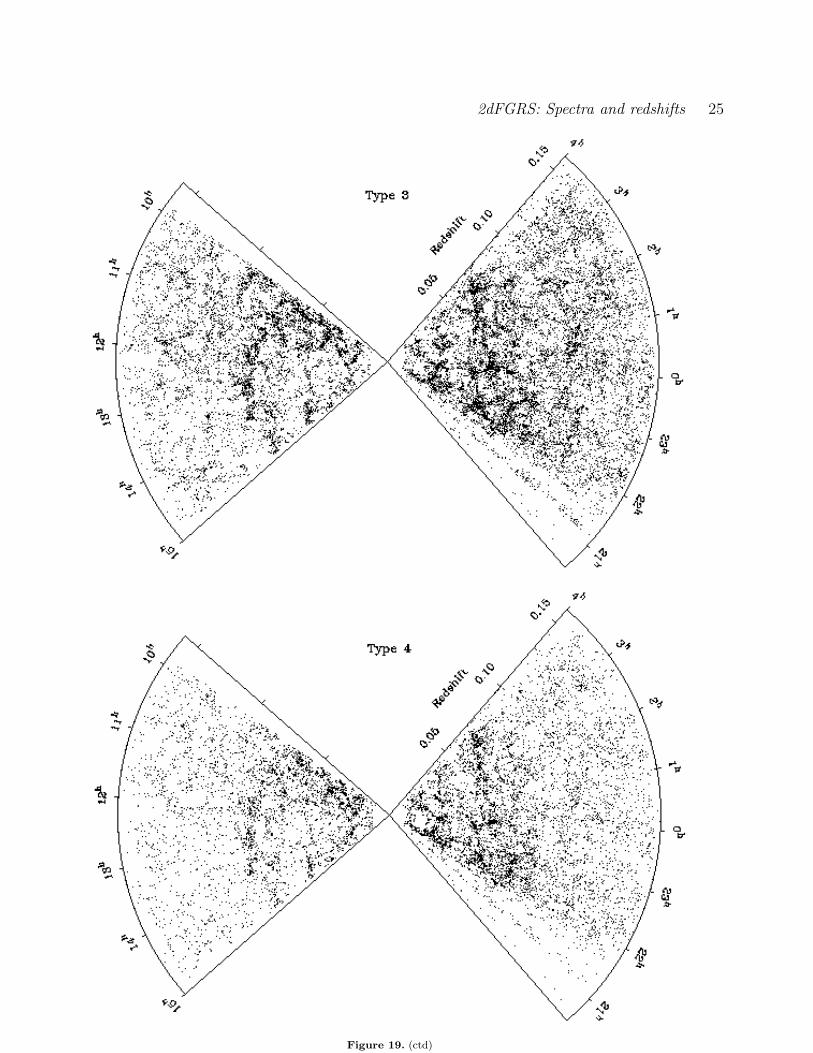
2dFGRS: Spectra and redshifts 25

Figure 19. (ctd)

26 Colless et al.

The 2dFGRS can add significant value to all-sky imag-ing surveys at all wavelengths, as in the studies of the radiogalaxy population combining redshifts and optical spectrafrom the 2dFGRS with the NVSS radio survey (Sadler et al.2001) and the FIRST radio survey (Magliocchetti et al.2001). Using 20% of the full 2dFGRS area, Sadler et al.(2001) find 757 optical counterparts for NVSS sources—thelargest and most homogeneous set of radio-source spectra todate. These sources range from z=0.005 to z=0.438, and area mixture of active galaxies (60%) and star-forming galax-ies (40%). The local radio luminosity function at 1.4 GHzis determined for both active and star-forming galaxies, andyields an estimate for the local star-formation density of(2.8 ± 0.5) × 10−3 M⊙ yr−1 h3 Mpc−3.

11 CONCLUSIONS

The 2dF Galaxy Redshift Survey (2dFGRS) is designed tomeasure redshifts for approximately 250 000 galaxies. Thesurvey uses the 2dF multi-fibre spectrograph on the Anglo-Australian Telescope, which is capable of observing up to400 objects simultaneously over a 2 diameter field of view.The source catalogue for the survey is a revised and ex-tended version of the APM galaxy catalogue, which is basedon Automated Plate Measuring machine (APM) scans of 390plates from the UK Schmidt Telescope (UKST) SouthernSky Survey. The target galaxies have extinction-correctedmagnitudes brighter than bJ=19.45, with extinctions de-rived from the maps of Schlegel et al. (1998).

The main survey regions are two contiguous declina-tion strips, one in the southern Galactic hemisphere (theSGP strip) covering 80×15 centred close to the SGP, andthe other in the northern Galactic hemisphere (the NGPstrip) covering 75×10. In addition, there are 99 randomfields are spread uniformly over the entire region of theAPM catalogue in the southern Galactic hemisphere outsidethe SGP strip. In total the survey covers some 2000 deg2

and has a median depth of z=0.11. Out to the effectivelimit of the survey at z≈0.3, the strips contain a volume of1.2×108 h−3 Mpc3; the volume sparsely sampled includingthe random fields is two to three times larger. An adaptivetiling algorithm is used to give a highly uniform samplingrate of 93% over the whole survey region.

Spectra are obtained over the wavelength range 3600–8000A at two-pixel resolution of 9.0A. The median S/N is13 pixel−1 over 4000–7500A. Redshifts are measured bothby cross-correlation with a range of template spectra andby fitting strong spectral features. All redshift identifica-tions are visually checked and assigned a quality parameterQ in the range 1–5. From repeat measurements and compar-isons with other redshift catalogues, we find that redshiftswith Q=3 have a blunder rate (fraction of incorrect identi-fications) of just under 10% and Q=4 and 5 redshifts haveblunder rates less than 1%—the overall blunder rate for re-liable (Q≥3) redshifts is 3%. The overall rms uncertaintyin the Q≥3 redshifts is 85 kms−1. The completeness of thesurvey is computed as a function of both field and appar-ent magnitude. The overall redshift completeness is 91.8%,but this varies with magnitude from 99% for the brightestgalaxies to 90% for objects at the survey limit.

The survey database has two components: a collection

of FITS files, one per object, which contain all the param-eters and spectra for each object, and a mSQL parame-ter database which can be used for sophisticated search-ing, matching and sorting of the survey data. The 2dF-GRS database is available through the survey WWW siteat http://www.mso.anu.edu.au/2dFGRS.

ACKNOWLEDGEMENTS

The 2dF Galaxy Redshift Survey was made possible throughthe dedicated efforts of the staff of the Anglo-AustralianObservatory, both in creating the 2dF instrument and insupporting the survey observations.

REFERENCES

Arnouts S., et al., 2001, A&A, submitted

Bailey J.A., Glazebrook K., Offer A., Taylor K., 2001, MNRAS,submitted

Benson A.J., Frenk C.S., Baugh C.M., Cole S., Lacey C.G., 2001,MNRAS, submitted

Blair M., Gilmore G., 1982, PASP, 94, 741

Boyle B.J., Shanks T., Croom S.M., Smith R.J., Miller L., LoaringN., Heymans C., 2000, MNRAS, 317, 1014

Cole S., et al. (2dFGRS team), 2001, MNRAS, in press

Colless M.M., 1999, Phil. Trans. Roy. Soc. Lond. A, 357, 105Croom S.M., Smith R.J., Boyle B.J., Shanks T., Loaring N.S.,

Miller L., Lewis I.J., 2001, MNRAS, 322, 29Cross N. et al. (2dFGRS team), 2001, MNRAS, 324, 825

De Propris R., et al. (2dFGRS team), 2001, MNRAS, submittedEfstathiou G., Moody S.J., 2001, MNRAS, in press

Folkes S. et al. (2dFGRS team), 1999, MNRAS, 308, 459Huchra J.P., Vogeley M.S., Geller M.J., 1999, ApJS, 121, 287Jacoby G.H., Hunter D.A., Christian C.A., 1984, ApJS, 56, 257

Jaffe A.H., et al., 2001, Phys. Rev. Lett., 86, 3475Jepson B., Hughes D.J., 1998, The Official Guide to miniSQL 2.0,

John Wiley & Sons

Kennicutt R.C., 1992, ApJS, 79, 255Lasker B.M. et al., 1998, BAAS, 192, 6403Lewis I.J., et al., 2001, submitted

Loveday J., 1996, MNRAS, 278, 1025Loveday J., Maddox S.J., Efstathiou G., Peterson B.A., 1996,

ApJS, 107, 201Maddox S.J., Efstathiou G., Sutherland W.J., Loveday J., 1990a,

MNRAS, 242, 43P

Maddox S.J., Efstathiou G., Sutherland W.J., Loveday J., 1990b,MNRAS, 243, 692

Maddox S.J., Efstathiou G., Sutherland W.J., 1990c, MNRAS,246, 433

Maddox S.J., Efstathiou G., Sutherland W.J., 1996, MNRAS,283, 1227

Madgwick D.S., et al. (2dFGRS team), 2001a, MNRAS, submit-ted

Madgwick D.S., et al. (2dFGRS team), 2001b, ‘Mining the Sky’,

eds Banday A. et al., ESO Astrophysics Symposia, Springer-Verlag, in press

Magliochhetti M., et al. (2dFGRS team), 2001, MNRAS, submit-ted

Metcalfe N., Fong R., Shanks T., 1995, MNRAS, 274, 769

Monet D., et al., 1996, USNO-A1.0: A Catalog of AstrometricStandards (Washington: US Nav. Obs.)

Norberg P., et al. (2dFGRS team), 2001a, MNRAS, submittedPeacock J.A., et al. (2dFGRS team), 2001, Nature, 410, 169

Percival W.J., et al. (2dFGRS team), 2001, MNRAS, submitted

2dFGRS: Spectra and redshifts 27

Pimbblet K.A., Smail I., Edge A.C., Couch W.J., O’Hely E.,

Zabludoff A.I., 2001, MNRAS, submittedSadler E.M., et al. (2dFGRS team), 2001, MNRAS, submittedSaunders W., et al., 2000, MNRAS, 317, 55Schlegel D.J., Finkbeiner D.P., Davis M., 1998, ApJ, 500, 525Shectman S.A., Landy S.D., Oemler A., Tucker D.L., Lin H.,

Kirshner R.P., Schechter P.L., 1996, ApJ, 470, 172Taylor K., Cannon R.D., Watson F.G., 1997, Proc. SPIE, 2871,

145Tonry J.L., Davis M., 1979, AJ, 84, 1511Yarger R.J., Reese G., King T., 1999, MySQL and mSQL,

O’Reilly & Associates