Galaxy Clustering in Early SDSS Redshift Data

Idit Zehavi1, Michael R. Blanton1, Joshua A. Frieman1,2, David H. Weinberg3, Houjun J. Mo4,Michael A. Strauss5, Scott F. Anderson6, James Annis1, Neta A. Bahcall5, Mariangela Bernardi2,John W. Briggs7, Jon Brinkmann8, Scott Burles1, Larry Carey6, Francisco J. Castander2, AndrewJ. Connolly9, Istvan Csabai10,11, Julianne J. Dalcanton6, Scott Dodelson1,2, Daniel Eisenstein12,Michael L. Evans6, Douglas P. Finkbeiner5, Scott Friedman11, Masataka Fukugita13, James E.Gunn5, Greg S. Hennessy14, Robert B. Hindsley15, Zeljko Ivezic5, Stephen Kent1,2, Gillian R.Knapp5, Richard Kron1,2, Don Q. Lamb2, R. French Leger1, Daniel C. Long8, Jon Loveday16,

Robert H. Lupton5, Timothy McKay17, Avery Meiksin18, Aronne Merrelli19, Jeffrey A. Munn14,Vijay Narayanan5, Matt Newcomb20, Robert C. Nichol20, Russell Owen6, John Peoples1, AdrianPope20,11, Constance M. Rockosi2, David Schlegel5, Donald P. Schneider21, Roman Scoccimarro22,

Ravi K. Sheth1, Walter Siegmund6, Stephen Smee23, Yehuda Snir20, Albert Stebbins1,Christopher Stoughton1, Mark SubbaRao2, Alexander S. Szalay11, Istvan Szapudi24, Max

Tegmark25, Douglas L. Tucker1, Alan Uomoto11, Dan Vanden Berk1, Michael S. Vogeley26,Patrick Waddell6, Brian Yanny1, and Donald G. York2, for the SDSS Collaboration

1Fermi National Accelerator Laboratory, P.O. Box 500, Batavia, IL 60510, USA2Astronomy and Astrophysics Department, University of Chicago, Chicago, IL 60637, USA3Department of Astronomy, Ohio State University, Columbus, OH 43210, USA4Max-Planck-Institute for Astrophysics, Karl-Schwarzschild-Strasse 1, D-85741 Garching, Germany5Princeton University Observatory, Peyton Hall, Princeton, NJ 08544, USA6Department of Astronomy, University of Washington, Box 351580, Seattle, WA 98195, USA7Yerkes Observatory, University of Chicago, 373 West Geneva Street, Williams Bay, WI 53191, USA8Apache Point Observatory, P.O. Box 59, Sunspot, NM 88349, USA9University of Pittsburgh, Department of Physics and Astronomy, 3941 O’Hara Street, Pittsburgh, PA 15260,USA

10Department of Physcis, Eotvos University, Budapest, Pf. 32, Hungary, H-151811Department of Physics and Astronomy, The Johns Hopkins University, 3701 San Martin Drive, Baltimore, MD

21218, USA12Steward Observatory, University of Arizona, 933 N. Cherry Ave., Tucson, AZ 85721, USA13Institute for Cosmic Ray Research, University of Tokyo, Kashiwa 277-8582, Japan14U.S. Naval Observatory, 3450 Massachusetts Ave., NW, Washington, DC, 20392, USA15Remote Sensing Division, Code 7210, Naval Research Laboratory, 4555 Overlook Ave., SW, Washington, DC

20375, USA16Sussex Astronomy Centre, University of Sussex, Falmer, Brighton BN1 9QJ, UK17Department on Physics, University of Michigan, Ann Arbor, MI 48109, USA18Department of Physics & Astronomy, The University of Edinburgh, James Clerk Maxwell Building, The King’s

Buildings, Mayfield Road, Edinburgh, EH9 3JZ, UK19Department of Astronomy, California Institute of Technology, Pasadena, CA 91125, USA20Department of Physics, 5000 Forbes Avenue, Carnegie Mellon University, Pittsburgh, PA 15213, USA21Department of Astronomy and Astrophysics, The Pennsylvania State University, University Park, PA 16802,USA22Department of Physics, New York University, 4 Washington Place, New York, NY 10003, USA23Department of Astronomy, University of Maryland, College Park, MD 20742, USA24Institute for Astronomy, University of Hawaii, 2680 Woodlawn Drive, Honolulu, HI 96822, USA25Department of Physics, University of Pennsylvania, Philadelphia, PA 19101, USA26Department of Physics, Drexel University, Philadelphia, PA 19104, USA

– 2 –

ABSTRACT

We present the first measurements of clustering in the Sloan Digital Sky Survey(SDSS) galaxy redshift survey. Our sample consists of 29, 300 galaxies with redshifts5, 700 km s−1 ≤ cz ≤ 39, 000 km s−1, distributed in several long but narrow (2.5 − 5)segments, covering 690 square degrees. For the full, flux-limited sample, the redshift-space correlation length is approximately 8h−1Mpc. The two-dimensional correlationfunction ξ(rp, π) shows clear signatures of both the small-scale, “fingers-of-God” distor-tion caused by velocity dispersions in collapsed objects and the large-scale compressioncaused by coherent flows, though the latter cannot be measured with high precision inthe present sample. The inferred real-space correlation function is well described by apower law, ξ(r) = (r/6.1 ± 0.2h−1Mpc)−1.75±0.03, for 0.1h−1Mpc ≤ r ≤ 16h−1Mpc.The galaxy pairwise velocity dispersion is σ12 ≈ 600 ± 100 km s−1 for projected sepa-rations 0.15h−1Mpc ≤ rp ≤ 5h−1Mpc. When we divide the sample by color, the redgalaxies exhibit a stronger and steeper real-space correlation function and a higher pair-wise velocity dispersion than do the blue galaxies. The relative behavior of subsamplesdefined by high/low profile concentration or high/low surface brightness is qualitativelysimilar to that of the red/blue subsamples. Our most striking result is a clear measure-ment of scale-independent luminosity bias at r . 10h−1Mpc: subsamples with absolutemagnitude ranges centered on M∗ − 1.5, M∗, and M∗ + 1.5 have real-space correla-tion functions that are parallel power laws of slope ≈ −1.8 with correlation lengths ofapproximately 7.4h−1Mpc, 6.3h−1Mpc, and 4.7h−1Mpc, respectively.

Subject headings: Cosmology: observations — cosmology: theory — dark matter —galaxies: clustering — galaxies: distances and redshifts — large-scale structure of uni-verse

1. Introduction

The primary observational goals of the Sloan Digital Sky Survey (SDSS) are to image 10,000square degrees of the North Galactic Cap in five passbands, with an r′ limiting magnitude of 22.5,to obtain spectroscopic redshifts of 106 galaxies and 105 quasars, and to obtain similar data forthree ∼ 200 square degree stripes in the South Galactic Cap, with repeated imaging to enableco-addition and variability studies in one of these stripes (York et al. 2000). One of the principalscientific objectives is to map the large-scale structure traced by optical galaxies with unprece-dented precision over a wide range of scales. These measurements of large-scale structure will allowcritical tests of cosmological models and theories of galaxy formation. This paper presents the firstmeasurements of galaxy clustering from the SDSS redshift survey, based on a sample of ∼ 30, 000galaxies observed during commissioning operations and during the first few months of the surveyproper. Complementary studies of the angular clustering of galaxies in the SDSS imaging survey

– 3 –

appear in Connolly et al. (2001) and Tegmark et al. (2001), and the implications of these measure-ments for the 3-D galaxy power spectrum are discussed by Dodelson et al. (2001) and Szalay et al.(2001). Scranton et al. (2001) examine many possible systematic effects on the angular clusteringmeasurements and conclude that they are small; these tests and conclusions are also relevant tothe analyses of the redshift survey carried out here.

The redshift-space clustering of galaxies has been a central concern of observational cosmologysince the early studies of Gregory & Thompson (1978) and Joeveer & Einasto (1978). Milestones inthis effort include: the first CfA redshift survey (Huchra et al. 1983), which mapped ∼ 2400 galaxiesselected from the Zwicky et al. (1968) catalog over 2.7 sr of sky to a magnitude limit of mZw = 14.5;redshift surveys to similar depth in other areas of sky such as the Southern Sky Redshift Survey(da Costa et al. 1991) and the Optical Redshift Survey (Santiago et al. 1995); sparsely sampledsurveys of optically selected galaxies to B ≈ 17 (the Stromlo-APM Redshift Survey, Loveday et al.1996; the Durham/UKST Redshift Survey, Ratcliffe et al. 1998); the second CfA redshift survey (deLapparent, Geller, & Huchra 1986; Geller & Huchra 1989), with a magnitude limit of mZw = 15.5and an eventual total of ∼ 13, 000 galaxies in the “Updated Zwicky Catalog” (Falco et al. 1999);a similar extension of the Southern Sky Redshift Survey (da Costa et al. 1998); redshift surveysof IRAS-selected galaxies to successively deeper flux limits of 2 Jy (Strauss et al. 1992), 1.2 Jy(Fisher et al. 1995), and 0.6 Jy (the sparsely sampled QDOT survey, Lawrence et al. 1999; thePSCz survey of ∼ 15, 000 galaxies, Saunders et al. 2001); the deep slice surveys of Vettolani etal. (1998; ∼ 3300 galaxies to bJ = 19.4) and Geller et al. (1997; ∼ 1800 galaxies to R = 16.13);and the Las Campanas Redshift Survey (LCRS; Shectman et al. 1996), which mapped ∼ 24, 000galaxies in six thin (1.5×90) slices at a depth R ≈ 18. The current state-of-the-art is representedby Peacock et al. (2001) and Percival et al.’s (2001) studies of redshift-space clustering in a sampleof ∼ 140, 000 galaxies from the ongoing 2dF Galaxy Redshift Survey. The sample that we analyzehere is most similar to the LCRS, with slightly more galaxies but a comparable depth and thin-slicegeometry.

Two factors that complicate and enrich the interpretation of galaxy clustering in redshift sur-veys are the distortions of structure induced by peculiar velocities and the possibility that galaxiesare “biased” tracers of the underlying matter distribution. On small scales, velocity dispersions incollapsed objects (a.k.a. “fingers-of-God”) smear out structures along the line of sight, effectivelyconvolving the real-space correlation function with the galaxy pairwise velocity distribution (see,e.g., Davis & Peebles 1983). On large scales, coherent flows into high density regions and out fromlow density regions enhance structures along the line of sight (Sargent & Turner 1977; Kaiser 1987;Hamilton 1998). Because the underlying clustering pattern should be statistically isotropic, theapparent anisotropy induced by redshift-space distortions yields constraints on the distribution ofpeculiar velocities, which can in turn yield constraints on the matter density parameter Ωm. Withour current galaxy sample, we clearly detect the signature of both the small-scale, “fingers-of-God”suppression and the large-scale, coherent flow amplification. However, we are not yet able to mea-sure the latter effect with high precision, so we defer a detailed examination of Ωm constraints (and

– 4 –

comparison to Peacock et al. 2001) to a future analysis of a larger sample.

The notion that the optical galaxy population might give a systematically “biased” picture ofmatter clustering came to the fore in the mid-1980s, largely in an effort to reconcile the predictionsof Ωm = 1 inflationary models with observations (Davis et al. 1985; Bardeen et al. 1986; Melott& Fry 1986; Bahcall & Soneira 1983; Kaiser 1984). There are now numerous arguments in favorof a low-Ωm universe, but theoretical models of galaxy formation, the well known dependence ofobserved galaxy clustering on morphological type (e.g., Hubble 1936; Zwicky 1937; Abell 1958;Davis & Geller 1976; Dressler 1980; Guzzo et al. 1997), and more recent evidence for dependence ofclustering on luminosity (e.g., Hamilton 1988; White, Tully, & Davis 1988; Park et al. 1994; Lovedayet al. 1995; Benoist et al. 1998; Willmer, da Costa, & Pellegrini 1998) all imply that galaxies cannotbe perfect tracers of the underlying matter distribution. Advances in hydrodynamic cosmologicalsimulations, high-resolution N-body simulations, and semi-analytic methods now allow detailed apriori predictions of bias for physically motivated models of galaxy formation (e.g., Cen & Ostriker1992; Katz, Hernquist, & Weinberg 1992; Benson et al. 1999; Blanton et al. 1999; Colın et al. 1999;Kauffman et al. 1999; Pearce et al. 1999; White, Hernquist, & Springel 2001; Yoshikawa et al. 2001).Empirical constraints on bias can therefore provide tests of galaxy formation theories and guidanceto physical ingredients that may be missing from current models. The SDSS is ideally suited tothe empirical study of bias because of the high sampling density and the detailed photometric andspectroscopic information available for every galaxy. We begin the effort here, by examining thedependence of the real-space correlation function and redshift-space distortions on galaxy color,luminosity, surface brightness, and light profile concentration.

The next Section describes the data sample used for the clustering analysis. Section 3 describesour methods for estimating the correlation function, including technical issues such as samplingcorrections and the effects of the minimum fiber spacing in the spectroscopic observations. Section4 presents the clustering results for the full, flux-limited galaxy sample. Section 5 examines theclustering of subsamples defined by color, luminosity, and other galaxy properties. We summarizeour results in Section 6. A discussion of our jackknife error estimation procedure, and comparisonof this procedure to results from mock redshift catalogs, appears in Appendix A. About half of thegalaxies in our sample are in the SDSS Early Data Release.27 To aid researchers attempting toreproduce and extend our results, we present the redshift-space correlation function for this subsetof the data in Appendix B. Throughout the paper, absolute magnitudes quoted for galaxies assumeH0 = 100 km s−1 Mpc−1.

27See http://archive.stsci.edu/sdss/ and the technical description in Stoughton et al. (2001).

– 5 –

2. Data

2.1. Description of the Survey

The SDSS (York et al. 2000) is producing an imaging and spectroscopic survey over π steradiansin the Northern Galactic Cap. A dedicated 2.5m telescope (Siegmund et al. 2001) at Apache PointObservatory, Sunspot, New Mexico, images the sky in five bands between 3,000 and 10,000 A(u′,g′, r′, i′, z′; Fukugita et al. 1996) using a drift-scanning, mosaic CCD camera (Gunn et al. 1998),detecting objects to a flux limit of r′ ≈ 22.5. Approximately 900,000 galaxies (down to r′lim ≈ 17.77;Strauss et al. 2001), 100,000 Luminous Red Galaxies (LRGs; Eisenstein et al. 2001), and 100,000quasars (Richards et al. 2001) are targeted for spectroscopic follow up using two double fiber-fedspectrographs on the same telescope. Most of the essential technical details are summarized in apaper that accompanies the SDSS Early Data Release (Stoughton et al. 2001).

As of June 2001, the SDSS has imaged around 2,500 square degrees of sky and taken spectraof approximately 140,000 objects. We use a subset of these data here to calculate the correlationfunction of galaxies, confining our attention to regions where the data reductions and calibrationhave been carefully checked and the spectroscopic completeness is well understood.

2.2. Imaging and Spectroscopic Pipelines

As described by Stoughton et al. (2001), the imaging data are processed by astrometric (Pieret al. 2001) and photometric (Lupton et al. 2001ab) pipelines and calibrated relative to a set ofstandard stars (Tucker et al. 2001). Targets are selected by a target selection pipeline (VandenBerk et al. 2001), and plates for spectroscopic observations are drilled based on the results of atiling pipeline (Blanton et al. 2001b). After the spectra are observed, the spectroscopic pipelinethen reduces, calibrates, and classifies the spectra and determines redshifts.

The photometric pipeline (Lupton et al. 2001b) detects objects and measures their propertiesin all five bands. Most relevant here are the Petrosian magnitude mP , the radius r50 containing50% of the Petrosian flux, and the radius r90 containing 90% of the Petrosian flux. The details ofSDSS Petrosian magnitudes, a modified form of those introduced by Petrosian (1976), are describedin a number of references and will not be repeated here, except to say that they are designed tomeasure a constant (and large) fraction of a galaxy’s total light, independent of redshift or centralsurface brightness but (slightly) dependent on light-profile shape (Blanton et al. 2001a; Lupton etal. 2001b; Strauss et al. 2001; Stoughton et al. 2001; Yasuda et al. 2001). The radii r50 and r90,which we use below to quantify galaxies’ surface brightnesses and morphologies, are not correctedfor seeing. However, such corrections would be small since most of the galaxies in this sample arerelatively large (r50 > 2′′; Blanton et al. 2001a), and the seeing conditions for the imaging aregenerally good (FWHM. 1.5′′).

The calibration is performed relative to standard stars as described in York et al. (2000), Tucker

– 6 –

et al. (2001) and Stoughton et al. (2001). Calibration is a three-tiered system in which “secondarystandards” that are not saturated in the 2.5m imaging camera are used to calibrate the imagingdata. These secondary standards are themselves calibrated relative to a set of “primary standards”using a 0.5m photometric telescope (PT; Uomoto et al. 2001). These primary standards havebeen calibrated relative to the fundamental standard BD +174708 by the United States NavalObservatory 1m telescope. The calibrations used here are not fully validated, though they arethought to be accurate to within 5%. Because of this remaining uncertainty, object magnitudes arereferred to in this paper and others based on early SDSS data as u∗, g∗, r∗, i∗, and z∗.

The target selection pipeline (Vanden Berk et al. 2001) determines which objects from theimaging survey are spectroscopic targets. We concentrate here on the “Main Sample” galaxies inthe SDSS, which are selected using the criteria detailed by Strauss et al. (2001). The essentialselection criteria for this sample are the star/galaxy separator, the surface-brightness limit, andthe flux limit. The star/galaxy separation is based on a comparison of the flux fPSF of the objectmeasured through a PSF aperture to the flux fmodel estimated using a best-fit model to the galaxyprofile (choosing the better of pure exponential and de Vaucouleurs profiles). This method isknown to be an extremely efficient and reliable separator at the magnitudes appropriate for thespectroscopic sample (Lupton et al. 2001b). We find that 98% of objects targeted as main samplegalaxies indeed turn out to be galaxies. The major contaminant is double stars with separationsless than 2′′.

The surface-brightness limit is based on the Petrosian half-light surface brightness in r∗. Forsome parts of the sample used here, obtained during commissioning observations, the surface-brightness limit is µ1/2 = 23.5 mag arcsec−2, but for most of the sample it is µ1/2 = 24.5 magarcsec−2. Because we will use relatively luminous galaxies to trace the density field here, thepositive correlation between surface brightness and luminosity (Blanton et al. 2001a) guaranteesthat the surface-brightness limit will be unimportant.

The flux limit of the spectroscopic survey is approximately r∗ = 17.77, after correction forGalactic reddening using the maps of Schlegel, Finkbeiner & Davis (1998). The limit varies some-what over the area of our sample, as the target selection criteria changed during the commissioningphase of the survey, when much of these data were taken. We will cut back to a uniform flux limitof r∗ = 17.6 for our current analysis. In addition, there is a bright limit imposed on the flux ina 3-arcsecond diameter aperture (the entrance aperture of a spectroscopic fiber) of mfiber > 15 ing∗, r∗ and mfiber > 14.5 in i∗, in order to avoid saturation and cross-talk between fibers in thespectrograph.

The reliability of the galaxy target selection is very high; galaxy target selection results fortwo imaging runs over the same patch of sky agree for 95% of the objects; the differences areattributable to small, random magnitude errors shifting objects across the flux limit (Strauss et al.2001).

The tiling pipeline (Blanton et al. 2001b) positions spectroscopic tiles and assigns fibers to

– 7 –

targets. The most important constraint is imposed by the size of the fiber plugs, which dictatesthat two fibers cannot be placed closer than 55′′ to each other. If the spectroscopic tiles did notoverlap, this would mean that about 10% of the objects would be unobservable. We define themaximal subset of objects that do not collide with each other this way as the “decollided” setof objects. It is this set of objects for which we desire high completeness. Because the tiles arecircular, about 30% of the sky is actually covered by more than a single tile; in these regions, manyof the objects lost due to collisions (hereafter known as “collided” objects) can be recovered. Note,however, that the tiles are positioned such that there are more tiles in dense areas of sky; thus, theregions covered by tile overlaps tend to be 5–10% overdense compared to average. We will describein Section 3 how we handle objects whose redshifts are missing due to fiber collisions.

Finally, the spectroscopic pipeline extracts, analyzes, and classifies the spectra, determiningthe spectral type, redshift, and other spectral information for each target. The success rate forclassifying spectra and determining redshifts correctly is very high (> 99%) for main sample galaxytargets, based on a subsample of ∼ 20, 000 spectra examined by eye. The spectroscopic pipelineassigns an empirically calibrated confidence level to the redshift determination for each object;cutting out main sample galaxy redshifts with low confidence (CL< 75%) removes only 0.7% of theobjects from the sample, with a negligible effect on the clustering results below.

2.3. Determining Positions, Luminosities, and Rest-frame Colors

The redshift of a galaxy is not a linear measure of an object’s distance at the moderateredshifts probed here (median z ∼ 0.1), and the comoving distance of an object depends somewhaton the cosmology assumed. Throughout this paper, we assume a Friedmann-Lemaıtre metric withΩm = 0.3 and ΩΛ = 0.7. When we plot correlation functions versus separation, we are alwaysreferring to the comoving separation, transformed from km s−1 separations using the standardformulas as tabulated in, for example, Hogg (1999).

We also must account for cosmological effects when calculating the absolute magnitudes fromthe apparent magnitude and the redshift using the formula

M = m−DM(z)−K(z) + 5 log10 h, (1)

where DM(z) is the bolometric distance modulus for the cosmology in question (again, see Hogg1999), K(z) is the K-correction, and the Hubble constant is H0 = 100h km s−1 Mpc−1. Throughoutthis paper, we use h = 1 to compute absolute magnitudes, and we quote distances in h−1Mpc.

The K-correction is necessary to account for the fact that the system response in the observedframe corresponds to a narrower, bluer rest-frame passband, depending on the redshift of theobserved object. In order to make an estimate of the K-correction, it is therefore necessary tohave an estimate of the spectral energy distribution (SED) of each object. We can make a goodestimate based on the five-band photometry provided by SDSS. For each object, we find the linear

– 8 –

combination of the four SED templates of Coleman, Wu, & Weedman (1980), as extended in thered and blue by Bolzonella, Miralles & Pello (2000), which best fits the photometry. We use theresulting SED to estimate the K-corrections, assuming no evolution of the SED. This methodis similar to simply interpolating between passbands to infer a rest-frame flux, while also takingadvantage of what astronomers know already about galaxy SEDs. These K-corrections are alsouseful to determine the rest-frame colors of objects from their observed colors. The details of ourprocedure, which are based on the photometric redshift methods of Csabai et al. (2000), will bedescribed in a forthcoming paper.

2.4. Description of the Sample

Figure 1 shows the angular distribution of the resulting sample in Galactic coordinates. Thearea covered is approximately 690 square degrees (comparable to the sky coverage of the LCRSsurvey), or about 7% of the area that will eventually be covered by the survey; in this area, we haveselected ≈ 30, 000 galaxies for our sample, as explained in the following paragraphs. Figure 2 showsthe distribution in right ascension and redshift of galaxies near the Celestial Equator (|δ| < 5).

Even though some regions of the survey are currently complete to r∗ < 17.77 (dereddened,using Schlegel et al. 1998), others are complete only to r∗ < 17.6, and for simplicity we havepared back our sample to this constant flux limit. In addition, we have imposed a bright limitof r∗ > 14.5 because at the bright end we are limited by the bright spectroscopic limits (the 3-arcsecond aperture magnitude limit of r∗ > 15 imposed to prevent saturation and cross-talk offibers in the spectrograph) and by the quality of deblending of large galaxies in the version ofthe photometric pipelines used for targeting many of these galaxies. These flux limits reduce thenumber of targets we consider by about 10%.

We limit this work to a fairly small range in redshift, 5, 700 km s−1 < cz < 39, 000 km s−1, eventhough the sample includes additional galaxies at higher redshift. We do so primarily because it isclear that galaxy evolution within the full range of redshifts (which extends to about 80, 000 km s−1)is important, and at the time of this work there was not yet an adequate model of this evolution toallow proper calculation of the radial selection function. Working at low redshift primarily limits ourestimate of the large-scale clustering; however, the thrust of this work is the small-scale clusteringof galaxies. Much larger-area samples of SDSS galaxies will soon be available, as well as goodmodels of the evolution of the luminosity function, and much better estimates of the large-scaleclustering will come from these samples. The outer redshift cut is the most costly of our imposedlimits, eliminating 30% of the objects available after the above flux limits have been imposed.

We wish to study the clustering of relatively luminous galaxies near the exponential cutoff inthe luminosity function at M∗. For most of the work below, we therefore impose absolute magnitudelimits of −22 < Mr∗ − 5 log10 h < −19, which roughly brackets the value M∗ = −20.8 determinedfor the SDSS (Blanton et al. 2001a). These absolute magnitude limits exclude another 15% of the

– 9 –

0 180 360

Fig. 1.— Aitoff projection of our galaxy sample in Galactic coordinates.

– 10 –

Fig. 2.— Pie-diagram distribution for the equatorial part of our sample. The plot includes 16, 300galaxies that lie within |δ| < 5 of the Celestial Equator.

– 11 –

objects (after the redshift and flux cuts are imposed), leaving us with our canonical sample of 29,300galaxies. We will use slightly different cuts to define volume limited samples of different luminosityranges below. Finally, we will compare below the clustering of several different types of galaxies,defined by color, surface brightness, and morphology, describing in the appropriate sections howthose subsamples of the canonical sample are defined.

3. Measuring the Correlation Function

Before measuring the correlation function, we need to determine how to treat the fiber collisionsand how to properly correct for angular and radial selection effects. We first detail how we accountfor these issues, then describe our estimators for the correlation function and its errors.

3.1. Accounting for Fiber Collisions

One of the important observational constraints in the SDSS is that no two fibers on the sameplate can be closer than 55′′. Thus, redshifts for both members of a close galaxy pair can only beobtained in regions where tiles overlap.

If we took no account of fiber collisions at all, then we would systematically underestimatecorrelations even on large scales because collisions occur more often in overdense regions such asclusters, which have enhanced large-scale clustering for the reasons discussed by, e.g., Kaiser (1984).A simple way to correct this bias is to double-weight the member of each pair that was observed,since its a priori selection probability was 50%. Here we adopt a variant of the double-weightingprocedure, assigning each galaxy whose redshift was not obtained because of a fiber collision thesame redshift as its closest (angular) neighbor. On large scales, where both members of the paircontribute to the same separation bin, the effect is the same as double weighting, but our procedureshould perform somewhat better on small scales because it retains information about the knownangular positions of the collided galaxies. Some of the galaxy targets are not assigned fibers dueto collisions with QSOs or LRGs; in these cases, no redshift is assigned, and the galaxy is treatedas if the fiber simply did not measure a redshift successfully, as described in the next subsection.

At cz = 39, 000 km s−1, the outer edge of our sample, 55′′ corresponds to a comoving transverseseparation of 0.1h−1Mpc. Fiber collisions will have a significant effect on correlation functionestimates below this scale, and in this paper we will restrict our measurements to separations> 0.1h−1Mpc, so as to avoid the artificial increase of pairs with very small separations. Becausetwo collided galaxies also have a line-of-sight separation, the collisions can in principle affect ourestimate of the correlation function out to somewhat larger scales, but we show below that theseeffects are probably smaller than our statistical uncertainties for this sample. The spectroscopicobservations obtain redshifts for the ∼ 30% of collided galaxies that lie in tile overlap regions.We find that roughly half of these galaxies in fact have a redshift within 5h−1Mpc of their closest

– 12 –

angular neighbor, while the other half are chance projections. In the chance projection cases, eithergalaxy has equal a priori chance of being selected, so double weighting does not statistically biasthe correlations with more distant galaxies.

Figure 3 demonstrates the effectiveness of our correction procedure. For the standard analysesin this paper, we use the true redshifts of collided galaxies whenever we have them and the closestneighbor redshifts when we do not. The long-dashed line shows what happens if we instead useclosest neighbor redshifts for all collided galaxies. The correlation function ξ(s) is virtually identicalto that of the standard case, with differences in individual bins that are usually much smaller thanthe statistical error bar (as they should be in the absence of systematic bias, since the samplescontain mostly the same galaxies). The short-dashed line shows the effect of ignoring fiber collisionsentirely, i.e., dropping the collided galaxies out of the sample and applying no special weights totheir neighbors. (In this case, we still account for the missing collided galaxies in the local samplingrate as described in the next subsection, treating these objects as though they were assigned fibersbut did not yield a redshift measurement.) The resulting change in the correlation function is stillsmaller than the statistical errors of individual bins, but it is now systematic, with a ∼ 2% bias forseparations s ∼ 1− 10h−1Mpc.

A detailed examination of fiber collision effects will require tests on artificial catalogs withrealistic galaxy clustering and geometry. Preliminary tests with N-body simulations suggest thatour adopted correction procedure should work extremely well (Berlind, private communication),and the agreement between the long-dashed and solid lines in Figure 3 supports this conclusion.We therefore expect that any residual systematic biases in our correlation function estimates dueto fiber collisions are smaller than our current statistical errors.

3.2. Angular Selection Function

A small fraction of the galaxy targets in our sample were not assigned fibers in the observedplates. There are also some galaxy targets whose redshifts are not successfully measured, for themost part because of broken fibers in the spectrograph, but sometimes because of a low signal-to-noise ratio in the spectra. The completeness of the redshift sample, denoted here f , thus variesacross the survey, and it is necessary to incorporate these variations into the window function ofthe survey. We evaluate the completeness in the following way. We break up the survey geometryinto “sectors” defined by areas of sky covered by unique sets of tiles, as described by Blanton et al.(2001b). For example, if the survey consisted of two tiles, there would be three sectors: the areacovered by only the first tile, the area covered by only the second tile, and the area covered byboth tiles. These sectors are the natural units in which to divide the survey, and we calculate thecompleteness f for each sector. The completeness is simply the fraction of objects that were selectedas galaxy targets for which a spectral classification was obtained (whether the object turned outto be a galaxy or not), or a redshift was assigned because the object was lost in a collision.

– 13 –

Fig. 3.— Comparison of alternative ways of treating fiber collisions. In the “standard” case, galaxieswith missing redshift due to collisions are assigned their own angular position and the redshift oftheir companion (“col. correc.”, solid line). Alternatively, we assign the companion’s redshift to allcollided galaxies, even when a collided galaxy’s redshift was obtained due to an overlapping plate(“all col. correc.”, long-dashed line). The short-dashed line shows the effect of simply discardingthe galaxies with missing redshifts from the sample (“no col. correc.”); this approach is obviouslyincorrect, and it introduces a systematic bias at large scales, but the impact is still small. The ratioof the redshift-space correlation function ξ(s) for these cases to our “standard” ξ(s) is shown. Thepoints and errorbars for the latter two cases are shifted slightly to the left and the right for clarity.

– 14 –

In this sample, the average completeness is about 94%. There are two contributions to theincompleteness. First, only 97% percent of the available galaxy targets in the regions covered byplates actually are assigned fibers or have a neighbor that can provide a collision correction. Thisis partly because some galaxies are eliminated due to collisions with QSOs, LRGs, quality holes, orlight traps (which have higher priority when fibers are assigned), and thus cannot be given collisioncorrections. In addition, we have included some regions that are covered by two plates, only oneof which has so far been observed; the targets in such a region that are assigned to fibers on theunobserved plate contribute to the incompleteness. Second, the fraction of fibers assigned to maingalaxy targets that successfully receive classifications is about 97% in this sample. The successrate for obtaining main sample galaxy redshifts during normal survey operations is over 99% .However, some of the data in this sample come from plates that have low signal-to-noise ratio (andwill therefore be reobserved later in the survey) or were reduced using older, less efficient versionsof the spectroscopic pipeline. In addition, some of these targets are imaging defects that weremistakenly classified as galaxies by early versions of the galaxy target selection algorithm, such asghost images due to reflections of bright stars inside the camera or satellite trails. Though theselatter cases, in fact, do not contribute to galaxy incompleteness, they are included in our estimateof f , but this makes a negligible difference to our results.

We apply several masks for regions of particularly bad seeing and where an early version of thetiling algorithm (now replaced) accidentally produced artificial gaps in the sampling. We excludeany objects in our data or random catalog that lie inside these masks. The masks cover less than1% of the total area. We have not applied masks around bright stars; if we did, they would excludeabout 1% of the total area (Scranton et al. 2001). It will be necessary to include these masks whenstudying clustering at the largest scales, because at large scales the clustering amplitude of starsbecomes large (due to the variation with Galactic latitude) and the clustering amplitude of galaxiesbecomes small.

Because the completeness of the redshift sample is high to begin with, and because we accountfor the incompleteness in each individual sector, the effects of completeness variations on our currentclustering measurements are negligible.

3.3. Radial Selection Function

As noted above, our sample is limited at bright and faint apparent magnitudes: 14.5 < r∗ <

17.6. Thus, at any given redshift we can only observe galaxies in a given absolute magnitude range.Furthermore, we restrict our analysis here to galaxies with absolute magnitudes −22 < Mr∗ < −19.At any redshift, the fraction of objects in this absolute magnitude range that are in the sample is

φ(z) =

∫ Mmax(z)Mmin(z) dMΦ(M)∫ −19−22 dMΦ(M)

, (2)

– 15 –

where Φ(M) is the luminosity function (number density of objects per unit magnitude) and

Mmin(z) = max(−22, 14.5 −DM(z)−K(z)),Mmax(z) = min(−19, 17.6 −DM(z) −K(z)), (3)

and DM(z) = m−M is the distance modulus as described in Section 2.3. In this context, K(z) isdetermined using the mean galaxy SED in the sample. Equations (2) and (3) simply express thefact that a galaxy must lie in our apparent magnitude range and in our absolute magnitude rangeto be included in the sample.

The luminosity function for our sample is determined in the manner described by Blanton et al.(2001a). It is necessary to perform this calculation separately for each of the subsamples describedin Section 5 because the luminosity functions of, for example, blue galaxies and red galaxies differsubstantially. The luminosity function for our full sample is consistent with that of Blanton et al.(2001a) when determined using the same redshift limits as that paper. However, we note here thatit appears from preliminary results (to be described in detail elsewhere) that the galaxy luminosityfunction evolves measurably within the redshift range of our spectroscopic sample. At the timethe calculations presented here were performed, we had not yet accounted for this effect in ourcalculation of the selection function. This is our main motivation for limiting the current sampleto cz < 39, 000 km s−1. More recently, we have fit a pure luminosity evolution model to the data.The resulting change in the selection function below cz = 39, 000 km s−1 is less than 5%, and theresulting differences in the measured correlation functions are negligible. Thus we are confidentthat our radial selection function calculated without accounting for evolution is sufficient to studythe small-scale clustering of interest here.

When the random sample is created for the calculation of the correlation function (see below),this selection function φ(z) and the local completeness f must be taken into account. In practice,we first distribute points uniformly in comoving space; we then include each such point in therandom sample with a probability fφ(z). Figure 4 compares the expected redshift distributionof this uniform sample (smooth line) to the actual redshift histogram of galaxies, including thegalaxies whose redshifts were assigned by our collision correction method. The differences betweenthe expected redshift distribution and the actual one reflect the large-scale structure which we arehere attempting to measure.

3.4. Estimator

To account for the survey geometry, we generate random catalogs of galaxies with the samesurvey geometry as the real sample, applying both the radial and angular selection functions. Wetypically use in each random catalog 10 times the number of galaxies in the real sample, and wehave verified that increasing the number of random points makes negligible difference to the results.

– 16 –

Fig. 4.— Histogram of the redshift distribution of the SDSS galaxies in our sample. The solid lineis the average distribution expected given the luminosity function, the flux limits, and the angularselection function.

– 17 –

We calculate the correlation function using the Landy & Szalay (1993) estimator,

ξ(s) =1

NRR(s)

[NDD(s)

nR(nR − 1)nD(nD − 1)

− 2NDR(s)nR

nD+ NRR(s)

], (4)

where NDD, NDR, and NRR are the weighted data-data, data-random, and random-random paircounts, respectively, with redshift-space separations in a bin centered on s, and nD and nR are themean number densities of galaxies in the data and random samples. Bins in s are logarithmicallyspaced with width of 0.2 in log(s/ h−1Mpc) starting from s = 0.1h−1Mpc. Other statistics arecalculated in an analogous way. We also tried the alternative estimators of Davis & Peebles (1983)and Hamilton (1993) and found no significant difference in the results.

For the pair weighting we follow Hamilton (1993) and use a minimum variance weighting (seealso Davis & Huchra 1982; Feldman, Kaiser & Peacock 1994). For a galaxy pair with redshiftseparation s, we weight each galaxy by

wi =1

1 + 4π nDφ(zi)J3(s), (5)

where J3(s) ≡∫ s0 s′2ξ(s′)ds′. For this integral, we approximate ξ by a power-law with slope −1.2

and correlation length 8h−1Mpc (resembling the result for the correlation function in redshift spacethat we get below, see § 4.1), but the results are robust to reasonable choices. Alternatively, we alsoweighted each galaxy simply by the inverse of the selection function φ and obtained comparableresults.

The full covariance error matrices are obtained by a jackknife error estimate (see, e.g., Lupton1993). We divide our sample into ten separate regions on the sky of approximately equal area. Weperform the analysis ten times, each time leaving a different region out. The estimated statisticalcovariance of ξi in redshift separation bin i and ξj in bin j is then

Covar(ξi, ξj) =N − 1

N

N∑l=1

(ξil − ξl

i)(ξjl − ξl

j), (6)

where N = 10 in our case, and ξi is the mean value of ξi measured in the samples. Furtherdiscussion regarding the robustness of the jackknife error estimate and comparison to alternativeerror estimates can be found in Appendix A. Note that if the number of regions is increased(N > 10), then each term in the sum decreases (because the N − 1 regions in each jackknifesubsample are a larger fraction of the total sample), but the number of terms increases, so theestimated covariance converges to a stable answer.

In what follows, we present results for the Landy-Szalay estimator, with minimum varianceweighting for the galaxies, and errors obtained by jackknife resampling. Galaxies with missingredshifts due to fiber collisions are accounted for as described above in Section 3.1.

– 18 –

4. Clustering of the Full Sample

In this Section we present the results for our full galaxy sample. Summarizing the details de-scribed in the previous sections, the sample consists of 29, 300 galaxies with redshift 5, 700 km s−1 <

cz < 39, 000 km s−1, apparent magnitude (corrected for Galactic absorption) 14.5 < r∗ < 17.6, andabsolute magnitude −22 < Mr∗ < −19.

4.1. Redshift-Space Clustering

Figure 5 shows the redshift-space correlation function ξ(s) of the full sample. For separations2h−1Mpc < s < 10h−1Mpc, the observed correlation function can be crudely approximated bya power-law, ξ(s) = (s/s0)−γ , with γ = 1.2 and s0 = 8.0h−1Mpc. Our results are in quitegood agreement with those from Tucker et al.’s (1997) analysis of the LCRS (open squares inFigure 5), though the SDSS correlation function has a slightly higher amplitude. We have assumedan Ωm = 0.3, ΩΛ = 0.7 model to compute comoving separations, but adopting an Einstein-deSitter model (as Tucker et al. do) yields a nearly indistinguishable result. The SDSS ξ(s) remainsmeasurably non-zero out to s = 30h−1Mpc and is consistent with zero at larger separations.

The redshift-space correlation function ξ(s) differs from the real-space correlation functionξr(r) because of peculiar velocities. Following standard practice, we separate the effects of redshift-space distortions from spatial correlations by separating the vector between two galaxies into aline-of-sight component π and a projected component rp, and measuring ξ(rp, π). More specifically,following the notation of Fisher et al. (1994), for a pair of galaxies with redshift positions v1 andv2, we define the redshift separation vector s ≡ v1−v2 and the line-of-sight vector l ≡ 1

2 (v1 +v2).This allows us to define the parallel and perpendicular separations

π ≡ s · l/|l| , rp2 ≡ s · s− π2 . (7)

In real space, the contours of equal ξ should be circular (by isotropy, ξ depends only on the scalarseparation), but in redshift space the contours are distorted by peculiar velocities.

Figure 6 shows ξ(rp, π) for our sample, where we bin rp and π in linear bins of 2h−1Mpc. Onsmall scales, the contours are elongated along the line of sight direction, exhibiting the expected“fingers-of-God” distortion caused by velocity dispersion in collapsed objects. On larger scales,ξ(rp, π) shows compression in the π direction, caused by coherent large-scale streaming. Thequalitative appearance of Figure 6 is similar to that of, e.g., figure 1 of Fisher et al. (1994) orfigure 2 of Peacock et al. (2001).

– 19 –

Fig. 5.— The redshift-space correlation function ξ(s) (solid points and line). The error bars plottedhere, and in all subsequent figures, correspond to the 1σ uncertainty estimated from jackkniferesampling. A fiducial power-law fit for the range 2h−1Mpc < s < 10h−1Mpc is plotted as adot-dashed line. Open squares show ξ(s) obtained from the LCRS (Tucker et al. 1997).

– 20 –

Fig. 6.— Contours of ξ(rp, π), the correlation function as a function of separation perpendicular(rp) and parallel (π) to the line of sight. The heavy solid contour corresponds to ξ = 1; for largervalues of ξ contours are logarithmically spaced, with ∆ log10 ξ = 0.1; below ξ = 1 they are linearlyspaced, with ∆ξ = 0.1; the heavy dashed contour corresponds to ξ = 0. The concentric dottedlines are the angle-averaged redshift-space correlation function, ξ(s), at ξ(s) = 1.0, 0.5 and 0.25.

– 21 –

4.2. Real-Space Clustering

The effects of redshift-space distortions are only radial, so projection onto the rp axis gives in-formation about the real-space correlation function. We compute the projected correlation functionwp(rp) by integrating ξ(rp, π) over π,

wp(rp) ≡ 2∫ ∞

0dπ ξ(rp, π) = 2

∫ ∞

0dy ξr

(√r2p + y2

), (8)

where ξr is the desired real-space correlation function (Davis & Peebles 1983). In practice we inte-grate up to πmax = 40h−1Mpc, which is large enough to include most correlated pairs and to givea stable result. The second equation above allows us to relate wp to the real-space correlation func-tion. In particular, for a power-law ξr(r) = (r/r0)−γ , the second integral can be done analytically,yielding

wp(rp) = Ar1−γp with A = rγ

0Γ(0.5)Γ[0.5(γ − 1)]/Γ(0.5γ), (9)

where Γ is the Gamma function.

Figure 7 shows wp(rp) for the full galaxy sample and the best-fit power-law model, whichcorresponds to ξr(r) = (r/r0)−γ with r0 = 6.14 ± 0.18h−1Mpc, γ = 1.75 ± 0.03. This fit to theslope and amplitude of the correlation function is obtained using points in the range 0.1h−1Mpc <

rp < 16h−1Mpc; the correlation coefficient between r0 and γ, measuring the normalized covarianceof the two estimates, is ∼ −0.5, implying that the measures are anti-correlated to a degree. Sincethe jackknife estimates of the off-diagonal terms in the covariance matrix are noisy and lead to anunstable matrix inversion in the χ2 minimization (unless we confine the fit to only a few bins),the best-fit r0 and γ values were obtained from the diagonal terms only. As a result, we are notguaranteed to have unbiased estimates of these parameters, but the visually evident goodness-of-fitsuggests that any such bias is negligible. The errors on r0 and γ were obtained from the variancein the estimates of these quantities among the jackknife subsamples, again using only the diagonalterms in the covariance matrix, as described in Appendix A.

The real-space correlation function is characterized much more accurately by a power-law thanthe redshift-space correlation function. Our value of γ agrees well with results from previous redshiftsurveys and angular clustering studies (e.g., Davis & Peebles 1983; Loveday et al. 1995; Hermit et al.1996) and with the slope derived from the SDSS angular correlation function (Connolly et al. 2001).The value of r0 is also similar to that obtained from other optically selected galaxy samples, thoughslightly on the high side; for example, Jing, Mo, & Borner (1998) find r0 = 5.06± 0.12h−1Mpc forthe LCRS. If we adopt an Einstein-de Sitter cosmology, as they do, instead of a flat-Λ cosmology,then our inferred value of r0 drops slightly, to r0 = 5.7± 0.2h−1Mpc.

– 22 –

Fig. 7.— Projected correlation function wp(rp) (solid points). The solid line is the best-fit power-law for wp, which implies the denoted power-law for the real-space correlation function ξr(r). Thefit is performed for rp < 16h−1Mpc.

– 23 –

4.3. Angular Moments

The redshift-space correlation function ξ(s) in Figure 5 differs from the real-space correlationfunction ξr(r) inferred from wp(rp) in the expected sense: ξ(s) is depressed on small scales byvelocity dispersions and enhanced on large scales by coherent flows, so the slope of ξ(s) is shallowerand s0 > r0. The anisotropy of ξ(rp, π) encodes more complete information about the amplitudeof galaxy peculiar velocities. In principle, the anisotropy on large scales can be used to constrainβ ≡ Ω0.6

m /b, where the bias parameter b is the ratio of galaxy fluctuations to mass fluctuations(Kaiser 1987; Hamilton 1992). For this application, it is helpful to decompose ξ(rp, π) into a sumof Legendre polynomials,

ξ(rp, π) =∑

l

ξl(s)Pl(µ), (10)

where Pl is the lth Legendre polynomial and µ is the cosine of the angle between the line of sightand the redshift separation vector. The angular moments are found by integration

ξl(s) =2l + 1

2

∫ 1

−1ξ(rp, π)Pl(µ)dµ. (11)

In linear perturbation theory, only the monopole, ξ0(s), quadrupole, ξ2(s), and hexadecapole, ξ4(s)are non-zero, and the ratio

Q(s) ≡ ξ2(s)3s2

∫ s0 ξ0(s′)s′2ds′ − ξ0(s)

= G(β) ≡43β + 4

7β2

1 + 23β + 1

5β2(12)

(Hamilton 1992). Thus, the ratio Q provides an estimate of β (similar estimates can be constructedusing ξ4(s), but they are noisier). However, while linear theory distortions produce a negativequadrupole term, finger-of-God distortions produce a positive quadrupole, and their signaturepersists out to large separations (Cole, Fisher & Weinberg 1994, Fisher et al. 1994).

Figure 8 shows the quadrupole ratio Q(s) for the full sample. The error bars are obtained, asbefore, from the scatter in the jackknife subsamples. This Figure quantifies the visual impression ofthe contours in Figure 6, showing positive (finger-of-God) quadrupole distortion at s . 10h−1Mpcand negative (coherent flow) quadrupole distortion at larger scales. Q(s) should approach a constantvalue in the linear regime, and the measured results are consistent with this prediction. However,the error bars on these scales are large and highly correlated, whereas high precision over a range ofscales is needed to separate the influence of coherent flows from that of small-scale dispersions (see,e.g., Hatton & Cole 1998). The effective volume of our current sample is ∼ 4×106(h−1Mpc)3. Ourmeasurement of large-scale redshift-space distortions is limited by finite volume effects, as a smallnumber of elongated superclusters and filaments in the data can give rise to anisotropy in ξ(rp, π)on large scales. In this respect, the thin-slice geometry of our present sample works against us,since it provides relatively few pairs at large transverse separations. We therefore defer an estimateof β to a future study based on a larger, more nearly 3-dimensional sample of SDSS data, and focusinstead on the amplitude of small-scale, incoherent velocities.

– 24 –

Fig. 8.— Modified quadrupole to monopole ratio, Q = ξ2/(ξ0 − ξ0). In linear theory this ratiois determined by the parameter β ≡ Ω0.6

m /b. Dotted lines show the linear theory expectation forβ = 0.3 and β = 1.0.

– 25 –

4.4. Pairwise Velocity Dispersion

In the non-linear regime, where density and velocity fields are weakly coupled, the correla-tion function ξ(rp, π) can be modeled as a convolution of ξr(r) with the galaxy pairwise velocitydistribution F (V ) (Peebles 1980, §76; Davis & Peebles 1983; see Fisher 1995 for an illuminatingdiscussion of the assumptions implicit in this approach). If F varies only slowly with r, one canwrite

1 + ξ(rp, π) = H0

∫ ∞

−∞

[1 + ξr

(√r2p + y2

)]F (V ) dy , (13)

whereV ≡ π −H0y + v12(r) (14)

and v12(r) is the mean radial pairwise velocity of galaxies at separation r. The real-space correlationfunction ξr(r) can be inferred from wp(rp) as described in §4.2. Unfortunately, the forms of v12(r)and F (V ) are not known a priori for galaxies. Following Davis & Peebles (1983), we assume thatv12(r) in the above equation takes the form

v12(r) =H0y

1 + (r/r0)2. (15)

This model is based on the similarity solution of the pair conservation equation (Davis & Peebles1977). Using the formulae given in Mo, Jing & Borner (1997), it can be shown that equation (15)with r0 ∼ 5h−1Mpc matches reasonably well the mean streaming velocities of dark matter particlesin the ΛCDM model with Ωm = 0.3 and σ8 ∼ 1. The similarity solution may therefore be areasonable approximation for the underlying density field over limited ranges of length and timescales. If galaxies are biased relative to the mass with a constant bias factor independent of time,the mean streaming velocities for galaxies should have a similar form (see Fisher et al. 1994). Ourfollowing presentation is based on equation (15), but we will test the sensitivity of our results tothis assumed infall model.

Based on observational (Davis & Peebles 1983; Fisher et al. 1994) and theoretical (e.g., Peebles1976; Sheth 1996; Juszkiewicz, Fisher, & Szapudi 1998) considerations, we adopt an exponentialform for F ,

F (V ) = C exp(−21/2|V |/σ12

), (16)

where C is a normalization factor and σ12(r) is the pairwise velocity dispersion (PVD). Under theseassumptions, we can estimate σ12(r) by performing a χ2 minimization of the difference between theobserved ξ(rp, π) and the prediction given by equation (13). In practice, we minimize the followingquantity ∑

i

[ξobs(rp, πi)− ξpred(rp, πi;σ12)

σobsξ (rp, πi)

]2

, (17)

where the summation is done over π bins up to 15h−1Mpc for a fixed rp, so generally σ12 is afunction of rp. Here σobs

ξ (rp, π) is the error on ξ(rp, π) estimated from the jackknife samples. Thefit for σ12 is robust to changing the limiting π in the range 10− 20h−1Mpc.

– 26 –

Figure 9 shows the result of this calculation, the PVD of the full sample for projected sepa-rations 0.1h−1Mpc < rp < 20h−1Mpc. The error bars are obtained by fitting σ12 separately fromeach of the jackknife samples and computing the associated jackknife error (analogous to the waywe obtain errors on the power-law fit for wp). This provides a realistic estimate of the errors, whichare dominated by variations in the number of rare, high-dispersion structures in the sample (seediscussions by Mo, Jing & Borner 1993; Zurek et al. 1994; Somerville, Davis, & Primack 1997).Figure 10 compares the function ξ(rp, π) predicted by the best fit model to the measured values forseveral different choices of rp.

As a test of the sensitivity of our results to the assumed form of v12, we have repeated theanalysis where v12 is assumed to be the same as that for dark matter particles in the ΛCDMmodel (calculated using the formulae in Mo, Jing & Borner 1997). This assumption would bevalid if the mean streaming velocity of galaxy pairs at a given separation is the same as that ofmass particles at the same separation. We find that for rp . 3h−1Mpc, the PVD is quite similarto that obtained assuming the similarity model (eq. 15), while at larger separations it changessignificantly. Without knowing how galaxies are biased relative to the mass, it is unclear whichinfall model is more realistic. The test we describe here, however, indicates that estimates of thePVD at rp . 3h−1Mpc are robust to uncertainties in the infall model.

The measured PVD is roughly constant in this range, with σ12(r) ' 550 − 675 km s−1. If weadopt an Einstein-de Sitter cosmology, σ12 decreases by ≈ 50 − 100 km s−1. Our estimate is closeto the values found by Jing et al. (1998) for the LCRS (σ12 = 570 km s−1 at rp = 1h−1Mpc) and byMarzke et al. (1995) for CfA2+SSRS2 (σ12 = 540 km s−1), but it is substantially higher than thevalues found in the early 1980s from much smaller redshift surveys (250 km s−1 by Bean et al. 1983;340 km s−1 by Davis & Peebles 1983). The SDSS result thus confirms that the galaxy velocity field,while colder than predicted by unbiased Ωm = 1 models (e.g., Davis et al. 1985), is not so cold thatit demands an extremely low value of Ωm or a highly biased galaxy distribution. While σ12(r) hasbeen the most widely used characterization of small-scale velocity dispersions, other statistics havebeen proposed that are less sensitive to rare objects that contribute many pairs (Davis, Miller, &White 1997; Landy, Szalay, & Broadhurst 1998) or that quantify the dispersion as a function oflocal density (Strauss, Ostriker & Cen 1998). Future measurements that examine the dispersion asa function of both environment and type may prove a valuable diagnostic for the relation betweengalaxies and dark matter halos (Sheth et al. 2001b).

5. Dependence on Galaxy Properties

The SDSS is ideal for investigating the dependence of clustering on galaxy properties becausea wealth of photometric data is available for each galaxy in the spectroscopic sample. Here weexamine the dependence of the real-space correlation function and redshift-space anisotropy ongalaxy color, then calculate the real-space correlation function for subsamples defined by luminosity,surface brightness, and light-profile concentration. The spirit of our investigation is similar to that of

– 27 –

Fig. 9.— The pairwise velocity dispersion σ12(rp), inferred by fitting ξ(rp, π). Error bars areobtained from the values of σ12 in different jackknife subsamples. The value of σ12 for rp > 3h−1Mpcdepends significantly on the assumed mean streaming model.

– 28 –

Fig. 10.— Examples of the model fits for ξ(rp, π) for four different values of rp. The histogramshows the observed values, and the dashed line is the model fit of eq. (13).

– 29 –

Guzzo et al.’s (1997) study of galaxy clustering as a function of morphological type and luminosity,but the higher quality of our imaging data allows us to consider a broader set of photometricparameters, and the larger size of our redshift sample allows us to measure differences in clusteringwith higher precision.

5.1. Color

We divide our full sample into two subsamples based on the rest-frame u∗ − r∗ colors of thegalaxies. Strateva et al. (2001) find that the u∗ − r∗ color distribution of galaxies is bimodal,and thus galaxies can be naturally divided into “blue” and “red” classes. They also show (usingindependent morphological classification schemes) that the blue class contains mainly late (spiral)morphological types while the red class consists mainly of bulge-dominated galaxies, as one wouldexpect. After K-corrections are accounted for, we find that the color distribution is still bimodalbut that the division at u∗ − r∗ = 2.2 in observed bands is closer to u∗ − r∗ = 1.8 in rest-framebands. We therefore divide the sample into galaxies bluer and redder than a rest-frame color ofu∗−r∗ = 1.8, resulting in a red subsample that includes ∼ 20, 000 galaxies and a blue subsample of∼ 10, 000 galaxies. In the full absolute magnitude range considered here (−19 < Mr∗ < −22), thetwo subsamples have similar space densities, but the red galaxies are systematically more luminous(Blanton et al. 2001a) and therefore sample a larger volume. We list some relevant properties ofthe full sample and the color subsamples in the first lines of Table 1. Space densities n are theinferred mean density for the indicated class of galaxies over the full absolute magnitude range.We also repeated our clustering analysis defining the blue and red samples based on the rest-frameg∗ − r∗ color (making the division at g∗ − r∗ = 0.6), and found very similar results.

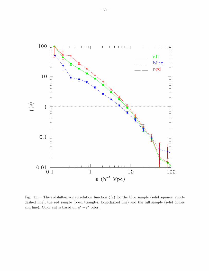
Figure 11 compares the redshift-space correlation functions of the red and blue subsamplesto that of the full galaxy sample. The red galaxies have a substantially higher amplitude andsteeper ξ(s) than the blue galaxies, with a correlation length s0 ≈ 9h−1Mpc compared to s0 ≈5.5h−1Mpc for the blue galaxies. This difference is expected from the well known morphology-density relation, since redder, early-type galaxies preferentially inhabit high density regions. Thedifference in anisotropy of ξ(rp, π) is equally striking (Figure 12), with red galaxies exhibiting muchstronger finger-of-God distortions on small scales. The compression of contours along the π axis atlarge scales is also much more obvious for the red galaxies, though this may be just a consequence ofthe smaller number and weaker clustering of the blue galaxies, which makes ξ(rp, π) much noisier.

Because the peculiar velocity distortions are very different for the two subsamples, it is im-portant to remove them in order to assess their relative spatial clustering. Figure 13 compares theprojected correlation functions wp(rp), with the red galaxies again exhibiting a steeper and higheramplitude correlation function. Power-law model fits in the range 0.1h−1Mpc < rp < 16h−1Mpcyield r0 = 6.78 ± 0.23h−1Mpc, γ = 1.86 ± 0.03 for the red galaxies and r0 = 4.02 ± 0.25h−1Mpc,γ = 1.41 ± 0.04 for the blue galaxies. The blue galaxies show hints of a departure from power-lawbehavior at the smallest separations, a possible signature of their tendency to cluster in lower mass

– 30 –

Fig. 11.— The redshift-space correlation function ξ(s) for the blue sample (solid squares, short-dashed line), the red sample (open triangles, long-dashed line) and the full sample (solid circlesand line). Color cut is based on u∗ − r∗ color.

– 31 –

Fig. 12.— ξ(rp, π) for the blue sample (left panel) and red sample (right panel). Contours are asin Fig. 5.

– 32 –

Fig. 13.— Projected correlation functions wp(rp) for the blue (squares) red (triangles), and full(circles) samples. The straight lines are the best-fit power-laws for wp, obtained for 0.1h−1Mpc <

rp < 16h−1Mpc. The short-dashed, long-dashed and solid lines correspond to the blue, red, andfull samples, respectively.

– 33 –

halos with smaller virial radii (see, e.g., Seljak 2000), but the statistical significance of this depar-ture is not high. At large scales, the two correlation functions approach each other, with wp(rp) forthe red galaxies having a slightly higher amplitude but similar shape. The behavior in Figure 13 isqualitatively consistent with expectations based on the morphology-density relation (Narayanan,Berlind, & Weinberg 2000, figure 2), though the data at large scales are too noisy to test whetherthe relative bias becomes constant in the linear regime, as “local” bias models predict (Coles 1993;Fry & Gaztanaga 1993; Mann, Peacock, & Heavens 1998; Scherrer & Weinberg 1998; Narayananet al. 2000).

Figure 14, the quadrupole ratio Q(s), confirms the much stronger finger-of-God distortion ofthe red galaxies evident in Figure 12, with a large positive Q at small scales. At large scales, thered galaxies have a more negative Q(s) than the blue galaxies, which is contrary to expectationgiven their higher relative bias, but the difference is marginal at best; for s > 15h−1Mpc, bothsubsamples generally have Q(s) within the 1σ error bar of the full sample Q(s). With future,larger samples, comparison of real-space clustering amplitudes and redshift-space distortions onlarge scales will allow interesting new tests of bias models.

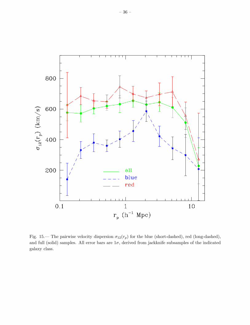
Figure 15 shows the pairwise velocity dispersions of the two subsamples, demonstrating veryclearly the preference of red galaxies for denser, hotter environments. For rp ∼ 0.2 − 8h−1Mpc,the PVD of the red sample is σ12 ≈ 650 − 750 km s−1, while the blue galaxy PVD is only σ12 ≈300 − 450 km s−1. This latter range is in fact similar to that obtained by Fisher et al. (1994) forIRAS galaxies. The two subsamples have similar σ12 at rp = 15h−1Mpc; partial convergence ofσ12 at large scales is expected in theoretical models (Sheth et al. 2001a), though the assumptionsused to infer σ12 from ξ(rp, π) may also be breaking down at this point (see §4.4 and Fisher 1995).Calculations where v12 is assumed to be the same as that for dark matter particles in the ΛCDMmodel show again that the PVD at rp . 3h−1Mpc are quite robust against the change of infallmodel.

5.2. Luminosity

We study the dependence of clustering on luminosity using three volume-limited subsamples,each with different absolute magnitude and redshift limits, as summarized in Table 2. The absolutemagnitude ranges of the three subsamples are centered approximately on M∗+1.5, M∗, and M∗−1.5,where M∗ = −20.8 is the characteristic luminosity in a Schechter (1976) function fit to the SDSSluminosity function (Blanton et al. 2001a). The space density of the lowest luminosity subsampleis 27 times that of the highest luminosity subsample. The redshift ranges are chosen to ensure thatthe selection function φ(z) = 1 for each subsample (i.e., they are volume-limited), accounting forK−corrections and the bright and faint apparent magnitude limits of the full sample. Because thewidth of the absolute magnitude bins is half the range of apparent magnitudes in the full sample,the three redshift ranges are actually disjoint, so our comparison of clustering properties relies oneach subsample volume being large enough to fairly represent the cosmic mean.

– 34 –

Table 1. Flux-limited Correlation Function Samples

Description Additional limits Ngal n r0 γ rr0γ

Full — 29,300 1.85 6.14 ±0.18 1.75 ± 0.03 -0.51Red u− r > 1.8 19,603 1.05 6.78 ± 0.23 1.86 ± 0.03 -0.15Blue u− r < 1.8 9,532 0.87 4.02 ± 0.25 1.41 ± 0.04 -0.24High SB µ1/2,r∗ < 20.5 17,859 0.94 6.48 ± 0.21 1.84 ± 0.03 -0.14Low SB µ1/2,r∗ > 20.5 11,439 0.98 5.55 ± 0.21 1.55 ± 0.04 -0.47High Concen. c = r90/r50 > 2.7 11,883 0.55 6.74 ± 0.24 1.88 ± 0.02 -0.29Low Concen. c = r90/r50 < 2.7 17,417 1.41 5.64 ± 0.22 1.63 ± 0.03 -0.01

Note. — All samples use 14.5 < mr∗ < 17.6, 5, 700 km s−1 < cz < 39, 000 km s−1,and −22 < Mr∗ < −19. n is measured in units of 10−2 h3 Mpc−3. r0 and γ are obtainedfrom a fit for wp(rp). rr0γ ≡ σr0γ/

√σr0σγ is the correlation coefficient between r0 and

γ.

Table 2. Volume-limited Correlation Function Samples

Absolute Mag. Limits Redshift Limits Ngal n r0 γ rr0γ

−23.0 < Mr∗ < −21.5 0.100 < z < 0.174 3,674 0.06 7.42 ± 0.33 1.76 ± 0.04 -0.85−21.5 < Mr∗ < −20.0 0.052 < z < 0.097 9,067 0.73 6.28 ± 0.77 1.80 ± 0.09 -0.77−20.0 < Mr∗ < −18.5 0.027 < z < 0.051 3,130 1.64 4.72 ± 0.44 1.86 ± 0.06 -0.83

Note. — All samples use 14.5 < mr∗ < 17.6. n is measured in units of 10−2 h3 Mpc−3. r0

and γ are obtained from a fit for wp(rp). rr0γ is the normalized correlation coefficient betweenr0 and γ.

– 35 –

Fig. 14.— Q(s) for the blue (short-dashed), red (long-dashed) and full (solid) samples. For clarity,error bars are drawn only for the full sample.

– 36 –

Fig. 15.— The pairwise velocity dispersion σ12(rp) for the blue (short-dashed), red (long-dashed),and full (solid) samples. All error bars are 1σ, derived from jackknife subsamples of the indicatedgalaxy class.

– 37 –

Figure 16 shows the projected correlation functions wp(rp) for the three absolute magnitudesubsamples. Table 2 lists the parameters r0 and γ of power-law ξr(r) models determined by fittingwp(rp) in the range 0.4h−1Mpc < rp < 16h−1Mpc for the highest luminosity subsample and0.1h−1Mpc < rp < 16h−1Mpc for the other two subsamples. The correlation length and slope ofthe middle sample is similar to that of the full sample analyzed in §4, which is not surprising sincemost of the galaxies in a flux-limited sample have absolute magnitudes in the neighborhood of M∗.The low luminosity subsample has a clustering amplitude that is lower by ∼ 40%, and the highluminosity subsample has a clustering amplitude higher by ∼ 35%.

The general trend of Figure 16, stronger clustering for more luminous galaxies, is similar to thatfound in a number of earlier studies (Davis et al. 1988; Hamilton 1988; White, Tully, & Davis 1988;Park et al. 1994; Loveday et al. 1995; Guzzo et al. 1997; Benoist et al. 1998; Willmer, da Costa, &Pellegrini 1998). However, while some of these studies found that luminosity dependence becamestrong only for galaxies brighter than M∗, we find a steady trend from M∗ + 1.5 to M∗− 1.5. Mostof the earlier studies were based on B-band luminosities, while we have used r∗-band luminosities,so this difference in selection may contribute to the different trend. As the SDSS sample grows, wewill be able to examine luminosity dependence of clustering in greater detail over a wider dynamicrange.

Perhaps the most remarkable aspect of Figure 16 is the nearly identical shape of the threecorrelation functions; at the 1σ level each is consistent with a power-law ξr(r) of slope γ = 1.8 (seeTable 2). A “halo occupation” analysis of galaxy clustering (see, e.g., Benson et al. 1999; Ma &Fry 2000; Peacock & Smith 2000; Seljak 2000; Scoccimarro et al. 2001) implies that the correlationfunction at sub-Mpc scales is dominated by pairs of galaxies that reside in the same virializeddark halo, while the correlation function at scales & 2h−1Mpc comes from pairs in separate halos.Maintaining the constant slope seen in Figure 16 requires maintaining the relative strength of thesetwo contributions in galaxy populations that differ by a factor of 27 in space density and a factorof 2.3 in correlation amplitude, a delicate balancing act. This empirical result should prove ademanding constraint for theoretical models of galaxy formation.

As we were completing this paper, a study of luminosity-dependent clustering in the 2dFGalaxy Redshift Survey became available in preprint form (Norberg et al. 2001). The 2dF resultsalso show nearly identical power-law forms of wp(rp) in different luminosity ranges, and they showa strong dependence of clustering amplitude on luminosity for L > L∗. However, Norberg et al.(2001) find little luminosity dependence for L < L∗. Given the strong color dependence of clustering(§5.1; see also Shepherd et al. 2001) and of the luminosity function itself (Blanton et al. 2001a), itis not too surprising that bJ -selection (2dF) and r∗-selection (SDSS) lead to different luminositydependence. The complex interplay between color, luminosity, and clustering offers yet anothertarget for galaxy formation theories.

– 38 –

Fig. 16.— Projected correlation function wp(rp) for three volume-limited samples, with absolutemagnitude and redshift ranges as indicated. Squares, circles, and triangles show results for faint(sub-M∗), intermediate (M∗), and luminous (super-M∗) galaxies, respectively. Short-dashed, solid,and long-dashed lines show the best fit power-law models in the range they were fitted; parametersof the corresponding real-space ξr(r) appear in Table 2.

– 39 –

5.3. Dependence on Surface Brightness and Morphology

The SDSS photometric pipeline (Lupton et al. 2001ab) measures many other properties thatcan be used to define galaxy classes. Here we consider two of these properties, surface bright-ness and light-profile concentration. Table 1 summarizes the thresholds that we use to definesurface-brightness and concentration subsamples, along with sample sizes, mean space densities,and correlation function parameters.

The surface-brightness subsamples are divided at the threshold µ1/2 = 20.5 mag arcsec−2,where µ1/2 = m + 2.5 log10(2πr2

50) is the mean r∗ surface brightness within the Petrosian half-lightradius r50, K-corrected and corrected for cosmological surface-brightness dimming. The low surface-brightness sample contains around 11,400 objects and the high surface-brightness sample containsaround 17,900 objects. The left panel of Figure 17 shows the projected correlation functions wp(rp)of the two subsamples and of the full sample. The high surface-brightness galaxies have a steeperwp(rp) and a higher clustering amplitude at rp . 3h−1Mpc. Fits of a power-law ξr(r) to pointswith rp < 16h−1Mpc yield r0 = 5.55± 0.21h−1Mpc, γ = 1.55± 0.04 for the low surface-brightnesssample and r0 = 6.48± 0.21h−1Mpc, γ = 1.84 ± 0.03 for the high surface-brightness sample. Thistrend of clustering strength with surface brightness is consistent with some earlier results based onsmaller samples (Bothun et al. 1993, Mo, McGaugh & Bothun 1994). The two correlation functionsactually cross at large scales, contrary to the expectation from simple bias models (see Narayananet al. 2000), but the wp(rp) amplitudes on these scales are consistent with each other at the 1σlevel. We also note that since wp(rp) is an integral in the π direction out to 40h−1Mpc, its valueat rp in fact probes clustering out to considerably larger scales.

The profile concentration subsamples are defined using the concentration parameter c ≡r90/r50, which serves as a proxy for the traditional division of galaxies into early and late mor-phological types. For example, a pure de Vaucouleurs profile has c ≈ 3.3 (given our definition ofPetrosian magnitudes; see Blanton et al. 2001a), while a pure exponential profile has c ≈ 2.3. Wedivide our full galaxy sample at c = 2.7, yielding about 11,900 galaxies with high concentrationand 17,400 galaxies with low concentration. The right panel of Figure 17 shows the projected cor-relation functions of these subsamples. As expected from earlier studies of morphology-dependentclustering (Guzzo et al. 1997 and references therein), high-c (early type) galaxies have a steeper,higher amplitude correlation function. Fits of a power-law ξr(r) yield r0 = 6.74 ± 0.24h−1Mpc,γ = 1.88± 0.02 for the high concentration subsample and r0 = 5.64± 0.22h−1Mpc, γ = 1.63± 0.03for the low concentration subsample.

Qualitatively, our results for galaxy subsamples defined by surface brightness or profile concen-tration parallel our results for color subsamples described in §5.1. We have focused on wp(rp) andξr(r), but the same characterization extends to redshift-space anisotropy: like red galaxies, highsurface-brightness and high concentration galaxies show strong finger-of-God distortions, which inturn imply high pairwise velocity dispersions. Given the well known correlations between galaxymorphology, color, and surface brightness, these similarities are not surprising. As the SDSS pro-

– 40 –

Fig. 17.— Projected correlation function wp(rp) for samples cut according to surface brightness µ

(left panel) and concentration parameter c ≡ r90/r50 (right panel). The straight lines correspondto the power-law fits of wp(rp), for rp < 16h−1Mpc.

– 41 –

gresses, it will be possible to extend this type of analysis to a much finer level; for example, seeingif surface-brightness effects can be separated from color effects, isolating extreme classes of lowsurface-brightness or compact galaxies, comparing the clustering of galaxies with high and lowprofile concentration at fixed half-light surface brightness, or even comparing the clustering ofbarred and unbarred spirals or “disky” and “boxy” ellipticals. Detailed clustering studies of thissort should help disentangle the roles of early formation history and late-time transformation indetermining galaxy properties.

6. Conclusions

We have presented the first measurements of galaxy clustering from early SDSS spectroscopicdata, based on a sample of 29, 300 galaxies. Since this sample covers a limited volume, spanningonly ∼ 7% of the total projected survey area of the SDSS, our analysis has focused mainly onsmall-scale clustering. The sample used for this analysis has been chosen with care: in additionto a uniform flux limit imposed at bright and faint magnitudes, 14.5 < r∗ < 17.6, the sample islimited in radial velocity, 5, 700 km s−1 < cz < 39, 000 km s−1, to avoid uncertainties introducedby evolution of the luminosity function, and in absolute magnitude, −22 < Mr∗ − 5log10h < 19, sothat it is dominated by galaxies with r∗-band luminosities around M∗. While these cuts reduce thenumber of galaxies included in the sample by nearly a factor of two, they allow robust conclusions tobe drawn from the measurements. We have checked, for example, that our results are insensitive todetails of the correlation function estimation, to uncertainties in the sample selection function, andto the effects of the 55-arcsecond minimum fiber separation. As discussed in Appendix A below,we have also tested our jackknife error estimation method using a large number of mock redshiftcatalogs drawn from N-body simulations of Cold Dark Matter models. These tests indicate that thejackknife errors used herein provide an accurate representation of the true statistical uncertaintiesover the scales of interest, at least in the context of these models.

For our full, flux-limited galaxy sample, we have measured the angle-averaged redshift-spacecorrelation function ξ(s) and the two-dimensional correlation function ξ(rp, π), projected the latteralong the π axis to infer the real-space correlation function ξr(r), measured angular moments toquantify the anisotropy induced by peculiar motions, and modeled the small-scale anisotropy toinfer the galaxy pairwise velocity dispersion σ12(r). Approximating the redshift-space correlationfunction by a power law, ξ(s) = (s/s0)−γ , yields a correlation length s0 ≈ 8h−1Mpc and a slopeγ ≈ 1.2, but this representation is not accurate over a large range of scales. At small projectedseparations, contours of ξ(rp, π) show the characteristic “fingers-of-God” elongation along the lineof sight caused by velocity dispersions in collapsed structures. At large separations, they showcompression along the line of sight produced by coherent flows into high density regions. Theprojected correlation function wp(rp) can be well fit by a power-law real-space correlation functionξr(r) = (r/r0)−γ , with r0 = 6.14±0.18h−1Mpc and γ = 1.75±0.03, for projected separations from0.1h−1Mpc to 30h−1Mpc. The ratio Q(s) of the quadrupole and monopole moments of ξ(rp, π)

– 42 –

is positive for s . 10h−1Mpc, where “finger-of-God” distortions dominate, and negative at largerscales, where coherent flow distortions dominate. A future analysis using a larger sample thatextends to large scales in all three dimensions will enable us to extract an estimate of β ≡ Ω0.6

m /b

from the large-scale anisotropy. From the elongation of ξ(rp, π) at small scales, we estimate apairwise velocity dispersion σ12(r) ≈ 600 km s−1 that is roughly constant in the range 0.1h−1Mpc <

r < 10h−1Mpc.

Our results for the full galaxy sample are in fairly good agreement with those obtained fromearlier optically selected galaxy redshift surveys, in particular from clustering analyses of the LCRS(Tucker et al. 1997; Jing et al. 1998). The fact that our first analysis of early data from the SDSSreproduces these results and yields comparable or better statistical precision demonstrates theencouraging prospects for future galaxy clustering studies with the SDSS redshift survey.

Taking advantage of our large sample and the high quality of SDSS imaging data, we havecarried out a detailed examination of the dependence of real-space correlations and redshift-spacedistortions on galaxy photometric properties. Red and blue galaxies display markedly different clus-tering statistics, with the red galaxies exhibiting a higher amplitude and steeper real-space correla-tion function and much stronger finger-of-God distortions than the blue galaxies; at rp = 1h−1Mpc,the pairwise velocity dispersion is ∼ 750 km s−1 for our red galaxy subsample and ∼ 350 km s−1

for our blue galaxy subsample. Subsamples of high/low surface brightness and high/low profileconcentration display qualitative behavior similar to that of the red/blue subsamples. Perhaps ourmost striking result is a measurement of luminosity bias of the real-space correlation function thatis approximately scale-independent at r . 10h−1Mpc. Using three volume-limited subsamples, wefind a ∼ 40% decrease in clustering amplitude as we go from a median absolute magnitude of M∗to M∗ + 1.5 and a similar increase when going from M∗ to M∗ − 1.5, implying a relative biasingparameter b/b∗ ≡ (ξ/ξ∗)0.5 of 0.8 and 1.2, respectively, for the faintest and brightest samples. Thesethree samples differ by a factor of 27 in galaxy number density, but in each case ξr(r) is consistentwith a power law of slope γ ≈ 1.8.

Studies of galaxy clustering and redshift-space distortions in the local universe have two mainscientific objectives: (a) to test cosmological models and determine their parameters, and (b) to inferthe relation between the galaxy and dark matter distributions, partly to sharpen cosmological tests,but mostly to constrain and guide the emerging theory of galaxy formation. Cosmological modeltests usually focus on large scales, where the effects of non-linear gravitational evolution and biasedgalaxy formation are relatively simple. These tests typically employ Fourier methods or statisticaltechniques that can isolate large-scale information and produce approximately uncorrelated errorestimates even in the presence of a complicated survey geometry (Vogeley & Szalay 1996; Tegmark,Taylor, & Heavens 1997; Tegmark et al. 1998). Several of these methods have been applied toSDSS angular clustering data (Connolly et al. 2001; Scranton et al. 2001; Tegmark et al. 2001;Dodelson et al. 2001; Szalay et al. 2001), and they will be applied to the increasing sample of SDSSredshift data in the near future. The best constraints on galaxy bias will probably come fromsmall and intermediate scales, where clustering statistics are most sensitive to the relation between

– 43 –

galaxies and dark matter and where precise measurements can be obtained for many differentclasses of galaxies. Our results on the color and luminosity dependence of real-space clustering andon pairwise velocities already provide a challenging target for theories of galaxy formation. In thenear future, these will be complemented by measurements of higher-order clustering, which canbreak degeneracies among bias models that match two-point correlations (Scoccimarro et al. 2001).Studies of galaxy-galaxy weak lensing in the SDSS offer an entirely new route to determiningthe relation between galaxies and dark matter (Fischer et al. 2000; McKay et al. 2001). Thesemeasurements and other characterizations of galaxy clustering will improve in precision and detailas the SDSS progresses, yielding a wealth of new information with which to understand galaxyformation.

IZ, MRB and JAF are supported by the DOE and NASA grants NAG 5-7092 and NAG 5-10842at Fermilab.

The Sloan Digital Sky Survey (SDSS) is a joint project of the University of Chicago, Fermilab,the Institute for Advanced Study, the Japan Participation Group, the Johns Hopkins University, theMax-Planck-Institute for Astronomy (MPIA), the Max-Planck-Institute for Astrophysics (MPA),New Mexico State University, Princeton University, the United States Naval Observatory, and theUniversity of Washington. Apache Point Observatory, site of the SDSS telescopes, is operated bythe Astrophysical Research Consortium (ARC).

Funding for the project has been provided by the Alfred P. Sloan Foundation, the SDSSmember institutions, the National Aeronautics and Space Administration, the National ScienceFoundation, the U. S. Department of Energy, the Japanese Monbukagakusho, and the Max PlanckSociety. The SDSS Web site is http://www.sdss.org/.

A. Reliability of Error Estimates

A complete model of galaxy clustering predicts, in addition to mean values, the distributionand covariance of statistical measurement errors for any specified sample geometry and selectionfunction. These predicted statistical errors can be used to assess the consistency of the model withthe data. However, such error estimates can be cumbersome to compute, and they depend on theassumed clustering model itself. For some purposes, therefore, it is desirable to have estimates ofstatistical errors and their covariances that depend only on the data set itself.

One common approach to this task is to estimate errors from disjoint subsamples of the fulldata set, each occupying a separate sub-volume. One calculates the statistic of interest — e.g.,ξ(si) for a number of separations si — in each sub-volume, and the estimated error of ξ(si) isthe error on the mean determined from the N sub-volumes. The same approach can be usedto estimate covariance of errors. The disadvantage of this technique is that estimates of ξ(si)from individual sub-volumes may become noisy or biased, especially on scales comparable to the

– 44 –

sub-volume size. A related but more robust way to estimate errors from the sample itself is thejackknife method described in Section 3.4 (see specifically eq. 6). In this approach, each jackknifesubsample is obtained by excluding one of the sub-volumes from the full sample, and one “sumsup” the variances of the jackknife subsamples rather than taking the error of the mean. Sinceeach jackknife subsample is similar in size to the full sample, this method performs better on largescales, though the two approaches should give equivalent results in the limit where each sub-volumeis representative of the whole data set (i.e., when fractional variances are small).

Our error bars on plotted data points and on parameter estimates (r0, γ, σ12) are all computedusing the jackknife method. Here we compare this approach to the model-based approach using themock SDSS catalogs of Cole et al. (1998). Cole et al. (1998) ran a series of high resolution N-bodysimulations, using an Adaptive P3M code (Couchman 1991), for a suite of cosmological models andbiasing schemes. They created catalogs with the survey geometry and anticipated selection functionof the SDSS. We use two of their catalogs: a COBE-normalized flat ΛCDM universe (with Ωm = 0.3and h = 0.65) and a structure-normalized τCDM model (with Ωm = 1.0, h = 0.5 and Γ = 0.25).From each of these we extract 75 galaxy samples, each of which resembles the observed stripesin our sample. For computational convenience, we used artificial samples that are smaller thanour current data set, with only ∼ 6, 000 galaxies per sample, but we expect that our conclusionsabout the relative behavior of jackknife and mock catalog error estimates would also hold for largersamples.

For each artificial galaxy sample we calculate the redshift-space ξ(s) and the error estimates(including the full covariance matrix) using the jackknife method and the sub-volume method.Figure 18 compares these estimated errors to the “true” errors of this model, defined as the scatterof the 75 ξ(s) estimates from different samples. Points and error bars show the mean and 1σ scatterof the “internal” error estimates (jackknife or sub-volume) in units of the true, “external” error atthe same separation s.

The jackknife estimates recover the true errors reasonably well (with 1σ scatter . 50%),and they are robust on all scales, without any gross systematics. The sub-volume estimates docomparably well on the intermediate scales, but on large scales they overestimate the errors. Thesub-volume estimates are also more numerically unstable on small scales, where a single sub-volumemay contain few galaxy pairs.

The jackknife method produces unbiased estimates of the true errors for both cosmologicalmodels. These models are both designed to match the observed APM correlation function, so theirpredicted errors are also comparable, but they do differ by ∼ 20% on some scales, and the jackknifeestimates seem to track these variations. We also performed this analysis for the off-diagonalelements of the covariance matrices. The covariance estimates do fairly well at intermediate scalesbut less well at small and large separations. The scatter in the estimates progressively increases forelements farther away from the diagonal. We are therefore less confident in the usefulness of thejackknife method for estimating a full covariance matrix; estimates of off-diagonal terms may be

– 45 –

Fig. 18.— Comparison of jackknife and sub-volume “internal” error estimates to “external” esti-mates derived from variation among artificial samples, using the N-body mock catalogs of Cole etal. (1998). Points and error bars show the mean and 1σ scatter of the error estimates derived from75 artificial samples, in units of the true (external) error. Top panels show results for the jackknifeestimator and bottom panels for the sub-volume estimator. Left and right panels show ΛCDM andτCDM models, respectively.

– 46 –

noisy and inter-dependent, making inversion of the covariance matrix unstable. When estimatingparameters like r0, γ, and σ12, therefore, we fitted values for each jackknife subsample using onlydiagonal terms, then estimated the error on the parameter by summing the variance of the estimatesin the jackknife subsamples (see §4.2 and 4.4). This approach seems more reliable than using thefull jackknife covariance matrix itself.

For a specified clustering model, the mock catalog approach is probably the best way to as-sess the consistency of the model with the data, provided that one has an efficient way to createlarge numbers of mock catalogs of the necessary size. (Scoccimarro & Sheth 2001 present a novelmethod that should improve the computational practicality of this approach for large-scale sur-veys.) However, the tests presented here give us confidence that our jackknife error estimatesshould be representative of the true statistical error bars for models that have clustering similar tothat observed. The jackknife approach is especially convenient when one breaks up the full sampleinto subsets that have different clustering properties, as we have done in §5, since it will automati-cally account for the influence of these clustering differences on the statistical errors. Scranton etal. (2001) have compared jackknife and mock catalog errors in the context of angular clusteringmeasurements and reached similar conclusions.

B. Early Data Release Sample

In June 2001, the SDSS released a large number of objects to the astronomical community in an“Early Data Release” (EDR). In order to facilitate the comparison of the results people find usingthat data with ours, we have run our code on a subsample of the data approximately correspondingto the EDR, which covers the North and South Equatorial regions as well as a high declinationregion that overlaps part of the SIRTF First Look region. The area of the spectroscopic sample isabout 330 square degrees, and it contains 15,279 main sample galaxies within our adopted rangesof apparent magnitude, absolute magnitude, and redshift. The EDR sample is thus about half thesize of the sample analyzed in this paper.

Our “EDR” sample differs slightly from that which one would create directly from the publicdata set. In particular, we use somewhat older photometric reductions and calibrations (though thechanges since the ones we used have been small), and a more inclusive set of spectroscopic platesto make our sample. However, we do not believe that these small differences will have a significanteffect on our results.

Figure 19 shows the result for the redshift-space correlation function ξ(s) obtained for theEDR sample (solid line). The result for our full sample, presented in Section 4.1, is plotted as wellfor comparison (dashed line). It is apparent that the results from the EDR sample closely resemblethose of our bigger sample, with only slight deviations consistent within the errors. As expected,the errors associated with the EDR results are somewhat larger than the ones obtained for oursample, mainly on the smallest and largest scales. The results for comparing the other statisticsare qualitatively similar.

– 47 –

Fig. 19.— The redshift-space correlation function ξ(s) for the spectroscopic sample included inthe Early Data Release (solid symbols and line). The results from our larger sample are shown forcomparison (open symbols and dashed line).

– 48 –

REFERENCES

Abell, G. O. 1958, ApJS, 50, 241

Bahcall, N., & Soneira, R. 1983, ApJ, 270, 20

Bardeen, J., Bond, J. R., Kaiser, N., & Szalay, A. 1986, ApJ, 304, 15

Bean, A. J., Ellis, R. S., Shanks, T., Efstathiou, G., & Peterson, B. A. 1983, MNRAS, 205, 605

Benoist, C., Cappi, A., da Costa, L. N., Maurogordato, S., Bouchet, F. R., & Schaeffer, R. 1998,ApJ, 514, 563

Benson, A. J., Cole, S., Frenk, C. S., Baugh, C. M., & Lacey, C. G. 2000, MNRAS, 311, 793

Blanton, M., Cen, R., Ostriker, J. P., & Strauss, M. 1999, ApJ, 522, 590

Blanton, M. R., et al. 2001a, AJ, 121, 2358

Blanton, M. R., Lupton, R. H., Maley, F. M., Zehavi, I., & Loveday, J. 2001b, AJ, submitted,astro-ph/0105535

Bolzonella, M., Miralles, J.-M., Pello, R. 2000, A & A, 363,476

Bothun G. D., Schombert J. M., Impey C. D., Sprayberry D., McGaugh S. S. 1993, AJ, 106, 548

Cen, R., & Ostriker, J. P. 1992, ApJ, 399, L113

Cole, S., Fisher, K., & Weinberg, D. H. 1994, MNRAS, 267, 785

Cole, S., Hatton, S., Weinberg, D., & Frenk C. 1998, 1998, 300, 945

Coleman, G. D., Wu, C.-C., & Weedman, D. W. 1980, ApJS, 43, 393

Coles, P., 1993, MNRAS, 262, 1065

Colın, P., Klypin, A. A., Kravtsov, A. V., & Khokhlov, A. M. 1999, ApJ, 523, 32

Connolly, A. J., et al. 2001, ApJ, to be submitted

Couchman, H. M. P. 1991, ApJ, 368, 23

Csabai, I., Connolly, A. J., Szalay, A. S., & Budavari. T. 2000, AJ, 119, 69

da Costa, L. N., Pellegrini, P. S., Davis, M., Meiksin, A., Sargent, W. L. W., & Tonry, J. L. 1991,ApJS, 75, 935

da Costa, L. N. et al. 1998, AJ, 116, 1

Davis, M., Efstathiou, G., Frenk, C. S., & White, S. D. M. 1985, ApJ, 292, 371

– 49 –

Davis, M., & Geller, M. 1976, ApJ, 208, 13

Davis, M., & Huchra, J. 1982, ApJ, 254, 437

Davis, M., Meiksin, A., Strauss, M. A., da Costa, L. N., & Yahil, A. 1988, ApJ, 333, L9

Davis, M., Miller, A., & White, S. D. M. 1997, ApJ, 490, 63

Davis, M., & Peebles, P. J. E. 1977, ApJS, 34, 425

Davis, M., & Peebles, P. J. E. 1983, ApJ, 267, 465

de Lapparent, V., Geller, M., & Huchra, J. P. 1986, ApJ, 302, L1

Dodelson, S., et al. 2001, ApJ, to be submitted

Dressler, A. 1980, ApJ, 236, 351

Eisenstein, D., et al. 2001, AJ, submitted

Falco, E. E., Kurtz, M. J., Geller, M. J., Huchra, J. P., Peters, J., Berlind, P., Mink, D. J., Tokarz,S. P., & Elwell, B. 1999, PASP, 111, 438

Feldman, H., Kaiser, N., & Peacock, J. 1994, ApJ, 426, 23

Fischer, P., et al. 2000, AJ, 120, 1198

Fisher, K. B. 1995, ApJ, 448, 494

Fisher, K. B., Davis, M., Strauss, M. A., Yahil, A., & Huchra, J. P. 1994, MNRAS, 267, 927

Fisher, K. B., Huchra, J. P., Strauss, M. A., Davis, M., Yahil, A., & Schlegel, D. 1995, ApJS, 100,69

Fry, J. N., & Gaztanaga, E. 1993, ApJ, 413, 447

Fukugita, M., Ichikawa, T., Gunn, J. E., Doi, M., Shimasaku, K., & Schneider, D. P. 1996, AJ,111, 1748

Geller, M. J. et al. 1997, AJ, 114, 2205

Geller, M. J., & Huchra, J. P. 1989, Science, 246, 897

Gregory, S. A. & Thompson, L. A. 1978, ApJ, 222, 784

Gunn, J. E., Carr, M. A., Rockosi, C. M., Sekiguchi, M., et al. 1998, AJ, 116, 3040

Guzzo, L., Strauss, M. A., Fisher, K. B., Giovanelli, R., & Haynes, M. P. 1997, ApJ, 489, 37

Hamilton, A. J. S. 1988, ApJ, 331, L59

– 50 –

Hamilton, A. J. S. 1992, ApJ, 385, L5

Hamilton, A. J. S. 1993, ApJ, 417, 19

Hamilton, A. J. S. 1998, ASSL Vol. 231: The Evolving Universe, 185

Hatton, S., & Cole, S. 1998, MNRAS, 296, 10

Hogg, D. 1999, astro-ph/9905116

Hubble, E.P. 1936, The Realm of the Nebulae (Oxford University Press: Oxford), 79

Huchra, J., Davis, M., Latham, D., & Tonry, J. 1983, ApJS, 52, 89

Jing, Y. P., Mo. H. J., & Borner, G. 1998, ApJ, 494, 1

Joeveer, M. & Einasto, J. 1978, IAU Symp. 79: Large Scale Structures in the Universe, 79, 241

Juszkiewicz, R., Fisher, K. B., & Szapudi, I. 1998, ApJ, 504, L1

Kaiser, N. 1984, ApJ, 294, L9

Kaiser, N. 1987, MNRAS, 227, 1

Hermit, S., Santiago, B. X., Lahav, O., Strauss, M. A., Davis, M., Dressler, A., & Huchra, J. P.1996, MNRAS, 283, 709

Katz, N., Hernquist, L., & Weinberg, D. H. 1992, ApJ, 399, L109

Kauffmann, G., Colberg, J. M., Diaferio, A., & White, S. D. M. 1999, MNRAS, 303, 188

Landy, S. D., Szalay, A. S., & Broadhurst, T. J. 1998, ApJ, 494, L133

Landy, S. D., & Szalay, A. S. 1993, ApJ, 412, 64

Lawrence, A., Rowan-Robinson, M., Ellis, R. S., Frenk, C. S., Efstathiou, G., Kaiser, N., Saunders,W., Parry, I. R., Xiaoyang, X., & Crawford, J. 1999, MNRAS, 308, 897

Loveday, J., Maddox, S. J., Efstathiou, G., & Peterson, B. A. 1995, ApJ, 442, 457

Loveday, J., Peterson, B. A., Maddox, S. J., & Efstathiou, G. 1996, ApJS, 107, 201

Lupton, R. H. 1993, Statistics in Theory and Practice (Princeton: Princeton University Press)

Lupton, R., Gunn, J. E., Ivezic, Z., Knapp, G. R., Kent, S., & Yasuda, N. 2001a, in ASP Conf.Ser. 238, Astronomical Data Analysis Software and Systems X, ed. F. R. Harnden, Jr.,F. A. Primini, and H. E. Payne (San Francisco: Astr. Soc. Pac.), in press, astro-ph/0101420

Lupton, R. H., et al. 2001b, in preparation

– 51 –

Ma, C., & Fry, J. N. 2000, ApJ, 543, 503

Mann, R. G., Peacock, J. A., & Heavens, A. F. 1998, MNRAS, 293, 209

Marzke, R.O, Geller, M.J., da Costa, L.N. & Huchra, J.P. 1995, AJ, 110, 477

McKay, T., et al. 2001, AJ, submitted

Melott, A. L., & Fry, J. N. 1986, ApJ, 305, 1

Mo, H. J., Jing, Y. P., & Borner, G. 1993, MNRAS, 264, 825

Mo, H. J., Jing, Y. P., & Borner, G. 1997, MNRAS, 286, 979

Mo, H. J., McGaugh, S. S., & Bothun G. D. 1994, MNRAS, 267, 129

Narayanan, V. K., Berlind, A. A., & Weinberg, D. H. 2000, ApJ, 528, 1

Norberg, P., et al. 2001, MNRAS, submitted, astro-ph/0105500

Park, C., Vogeley, M. S., Geller, M. J., & Huchra, J. P. 1994, ApJ, 431, 569

Peacock, J. A. et al. 2001, Nature, 410, 169

Peacock, J. A., & Smith, R. E. 2000, MNRAS, 318, 1144

Pearce, F. R., Jenkins, A., Frenk, C. S., Colberg, J. M., White, S. D. M., Thomas, P. A., Couchman,H. M. P., Peacock, J. A., & Efstathiou, G. 1999, ApJ, 521, L99

Peebles, P.J.E. 1976, Ap&SS, 45, 3

Peebles, P. J. E. 1980, The Large Scale Structure of the Universe (Princeton: Princeton UniversityPress)

Percival, W. J., et al. 2001, MNRAS, in press, astro-ph/0105252

Petrosian, V. 1976, ApJ, 209, L1

Pier, J. R., et al. 2001, in preparation

Ratcliffe, A., Shanks, T., Parker, Q. A., Broadbent, A., Watson, F. G., Oates, A. P., Collins, C.A., & Fong, R. 1998, MNRAS, 300, 417

Richards, G. T., et al. 2001, in preparation

Santiago, B. X., Strauss, M. A., Lahav, O., Davis, M., Dressler, A., & Huchra, J. P. 1995, ApJ,446, 457

Sargent, W. W., & Turner, E. L. 1977, ApJ, 212, L3

– 52 –

Saunders, W., et al. 2001, MNRAS, 317, 55

Schechter, P. 1976, ApJ, 203, 297

Scherrer, R. J., & Weinberg, D. H. 1998, ApJ, 504, 607

Schlegel, D. J., Finkbeiner, D. P., & Davis, M. 1998, ApJ, 500, 525

Scoccimarro, R., & Sheth, R. 2001, preprint, astro-ph/0106120

Scoccimarro, R., Sheth, R. K., Hui, L., & Jain, B. 2001, ApJ, 546, 20

Scranton, R., et al. 2001, ApJ, submitted

Seljak, U. 2000, MNRAS, 318, 203

Shectman, S. A., Landy, S. D., Oemler, A., Tucker, D. L., Lin, H., Kirshner, R. P., & Schechter,P. L. 1996, ApJ, 470, 172

Shepherd, C. W., Carlberg, R. G., Yee, H. K. C., Morris, S. L., Lin, H., Sawicki, M., Hall, P. B.,& Patton, D. R. 2001, ApJ, in press, astro-ph/0106250

Sheth, R. 1996, MNRAS, 279, 1310

Sheth, R. K., Diaferio, A., Hui, L., & Scoccimarro, R. 2001, MNRAS, submitted, astro-ph/0010137

Sheth, R. K., Hui, L., Diaferio, A., & Scoccimarro, R. 2001, MNRAS, submitted, astro-ph/0009167

Siegmund, W., et al. 2001, in preparation

Somerville, R. S., Davis, M., & Primack, J. R. 1997, ApJ, 479, 616

Stoughton, C., et al. 2001, in preparation

Strateva, I., et al. 2001, AJ, submitted

Strauss, M. A., Huchra, J. P., Davis, M., Yahil, A., Fisher, K. B., & Tonry, J. 1992, ApJS, 83, 29

Strauss, M. A, Ostriker, J., & Cen, R. 1998, ApJ, 494, 20

Strauss, M. A., et al. 2001, in preparation

Szalay, A. S., et al. 2001, ApJ, to be submitted

Tegmark, M., Hamilton, A., Strauss, M., Vogeley, M., & Szalay, A. 1998, ApJ, 499, 555

Tegmark, M., Taylor, A. N., & Heavens, A. F. 1997, ApJ, 480, 22

Tegmark, M., et al. 2001, ApJ, to be submitted

– 53 –

Tucker, D. L., Oemler, A., Jr, Kirshner, R. P., Lin, H., Shechtman, S. A., Landy, S. D., Schechter,P. L., Muller, V., Gottlober, S., & Einasto, J. 1997, MNRAS, 285, L5

Tucker, D. L., et al. 2001, in preparation

Uomoto, A., et al. 2001, in preparation

Vanden Berk, D. E., et al. 2001, in preparation

Vettolani, G., et al. 1998, A&AS, 130, 323

Vogeley, M. S. & Szalay, A. S. 1996, ApJ, 465, 34

White, M., Hernquist, L., & Springel, V. 2001, ApJ, 550, L129

White, S. D. M., Tully, R. B., & Davis, M. 1988, ApJ, 333, L45

Willmer, C. N. A., da Costa, L. N., & Pellegrini, P. S. 1998, AJ, 115, 869

Yasuda, N., et al. 2001, AJ, in press, astro-ph/0105545

York, D. G. et al. 2000, AJ, 120, 1579

Yoshikawa, K., Taruya, A., Jing, Y. P., Suto, Y. 2001, ApJ, in press, astro-ph/0104361

Zurek, W. H., Quinn, P.J., Salmon, J.K., & Warren, M.S. 1994, ApJ, 431, 559

Zwicky, F. 1937, ApJ, 86, 217

Zwicky, F., Herzog, E., Wild, P., Karpowicz, M., & Kowal, C., 1961-1968, Catalog of Galaxies andof Clusters of Galaxies, Vols. 1-6, (Pasadena: California Institute of Technology)

AAS LATEX macros v5.0.