BINARY QUASARS IN THE SLOAN DIGITAL SKY SURVEY

BINARY QUASARS IN THE SLOAN DIGITAL SKY SURVEY: EVIDENCE FOR EXCESSCLUSTERING ON SMALL SCALES

Joseph F. Hennawi,1,2,3

Michael A. Strauss,3Masamune Oguri,

3,4Naohisa Inada,

5Gordon T. Richards,

3

Bartosz Pindor,6,7

Donald P. Schneider,8Robert H. Becker,

9,10Michael D. Gregg,

9,10Patrick B. Hall,

11

David E. Johnston,3Xiaohui Fan,

12Scott Burles,

13David J. Schlegel,

14James E. Gunn,

3

Robert H. Lupton,3Neta A. Bahcall,

3Robert J. Brunner,

15and Jon Brinkmann

16

Received 2005 April 25; accepted 2005 August 3

ABSTRACT

We present a sample of 221 new quasar pairs with proper transverse separations Rprop < 1 h�1 Mpc over theredshift range 0:5< z < 3:0, discovered from an extensive follow-up campaign to find companions around the SloanDigital Sky Survey and 2dF QSO Redshift Survey quasars. This sample includes 26 new binary quasars with sep-arations Rprop < 50 h�1 kpc (� < 1000), more than doubling the number of such systems known. We define a statisti-cal sample of binaries selected with homogeneous criteria and compute its selection function, taking into accountsources of incompleteness. The first measurement of the quasar correlation function on scales 10 h�1 kpc < Rprop <400 h�1 kpc is presented. For RpropP 40 h�1 kpc, we detect an order of magnitude excess clustering over theexpectation from the large-scale (Rpropk 3 h�1 Mpc) quasar correlation function, extrapolated down as a power law(� ¼ 1:53) to the separations probed by our binaries. The excess grows to �30 at Rprop �10 h�1 kpc and providescompelling evidence that the quasar autocorrelation function gets progressively steeper on submegaparsec scales.This small-scale excess can likely be attributed to dissipative interaction events that trigger quasar activity in richenvironments. Recent small-scale measurements of galaxy clustering and quasar-galaxy clustering are reviewed anddiscussed in relation to our measurement of small-scale quasar clustering.

Key words: cosmology: observations — large-scale structure of universe — quasars: general — surveys

Online material: color figures, machine-readable tables

1. INTRODUCTION

A fundamental problem for cosmologists is to understand howquasars are embedded in the galaxy formation hierarchy and torelate them to the gravitational evolution of the structure of theunderlying dark matter. In the current paradigm, every massivespheroidal galaxy is thought to have undergone a luminous qua-sar phase, and quasars at high redshift are the progenitors of thelocal dormant supermassive black hole population found in the

centers of nearly all nearby bulge-dominated galaxies (e.g., Small&Blandford 1992; Yu&Tremaine 2002). This fundamental con-nection is supported by the tight correlations between the massesof central black holes and the velocity dispersions of their oldstellar populations (Magorrian et al. 1998; Ferrarese & Merritt2000; Gebhardt et al. 2000; Tremaine et al. 2002) and by compar-ing the number density of black holes in the local universe to theluminosity density produced by quasars at high redshift (Small &Blandford 1992; Yu & Tremaine 2002).

Quasars are likely to reside in massive hosts (Turner 1991),and it has been suggested that they occupy the rarest peaks in theinitial Gaussian density fluctuation distribution (Efstathiou&Rees1988; Cole &Kaiser 1989; Nusser & Silk 1993; Djorgovski et al.1999, 2003; Djorgovski 1999; Stiavelli et al. 2005). It is alsothought that quasar activity is triggered by the frequent merg-ers that are a generic consequence of bottom-up structure for-mation models (Bahcall et al. 1997; Carlberg 1990; Haehnelt &Rees 1993; Wyithe & Loeb 2002b). Both of these hypothesesimply that quasars should be highly biased tracers of the darkmatter distribution: rare peaks in the density field are intrin-sically strongly clustered (Kaiser 1984), and the frequency ofmergers is higher in dense environments (Lacey & Cole1993).Measurements of quasar clustering can thus teach us about theenvironments of quasars, as well as give clues to the dynamicalprocesses that trigger quasar activity. Furthermore, a compari-son of quasar clustering with the quasar luminosity function canbe used to constrain the mean quasar lifetime (Haiman & Hui2001; Martini &Weinberg 2001), as well as the relationship be-tween the masses of central black holes and the circular veloc-ities of their host dark halos (Wyithe & Loeb 2005).

There have been many attempts to measure quasar clustering,beginning with the pioneering work of Osmer (1981). Shaver(1984) first detected quasar clustering using a clever technique to

1 Hubble Fellow.2 Department of Astronomy, University of California at Berkeley, 601

Campbell Hall, Berkeley, CA 94720-3411.3 Princeton University Observatory, Peyton Hall, Princeton, NJ 08544.4 Department of Physics, University of Tokyo, Hongo 7-3-1, Bunkyo-ku,

Tokyo 113-0033, Japan.5 Institute of Astronomy, University of Tokyo, 2-21-1 Osawa, Mitaka, Tokyo

181-8588, Japan.6 Department of Astronomy, University of Toronto, 60 St. George Street,

Toronto, ON M5S 3H8, Canada.7 CFHT Legacy Survey Postdoctoral Fellow.8 Department of Astronomy and Astrophysics, Pennsylvania State Univer-

sity, 525 Davey Laboratory, University Park, PA 16802.9 Department of Physics, University of California at Davis, 1 Shields Ave-

nue, Davis, CA 95616.10 Institute of Geophysics and Planetary Physics, Lawrence Livermore

National Laboratory, L-413, 7000 East Avenue, Livermore, CA 94550.11 Department of Physics and Astronomy, York University, 4700 Keele

Street, Toronto, ON M3J 1P3, Canada.12 Steward Observatory, University of Arizona, 933 North Cherry Avenue,

Tucson, AZ 85721.13 PhysicsDepartment,Massachusetts Institute of Technology, 77Massachusetts

Avenue, Cambridge, MA 02139.14 Lawrence Berkeley National Laboratory, One Cyclotron Road, Mail Stop

50-R232, Berkeley, CA 94720.15 Department of Astronomy and National Center for Supercomputer Ap-

plications, University of Illinois, 1002 West Green Street, Urbana, IL 61801.16 Apache Point Observatory, P.O. Box 59, Sunspot, NM 88349-0059.

A

1

The Astronomical Journal, 131:1–23, 2006 January

# 2006. The American Astronomical Society. All rights reserved. Printed in U.S.A.

measure correlations from inhomogeneous catalogs and discov-ered that quasars were clustered similarly to galaxies in the localuniverse, a result later confirmed by Kruszewski (1988). Mostrecently, Croom et al. (2001, 2005) and Porciani et al. (2004,hereafter PMN04) measured the clustering of quasars in the red-shift range z ¼ 0:3 2:2 from the �15,000 quasars in the 2dFQSO Redshift Survey (2QZ; Croom et al. 2004a). They findgood agreement with a power-law correlation function �(r) ¼(r /r0)

�� on scales r ¼ 1 35 h�1 Mpc, with correlation lengthr0 � 5 h�1 Mpc (comoving) and slope � � 1:5, with only aweakdependence on redshift and luminosity (Croom et al. 2002). Thisagrees with previous measurements ( Iovino & Shaver 1988;Andreani & Cristiani 1992; Mo & Fang 1993; Shanks & Boyle1994; Croom & Shanks 1996; La Franca et al. 1998) and is sim-ilar to the clustering of nearby galaxies.

At redshift z > 2:5, quasars are rarer, and thus quasar clus-tering has been much more difficult to measure. However, themere existence of a few high-redshift quasar pairs provides cir-cumstantial evidence that quasars may have been much morehighly clustered in the past. In the Palomar Transit Grism Surveyof Schneider et al. (1994), three quasar pairs with zk 3 andcomoving separations 5–10 h�1 Mpc were found in a completesample of 90 quasars covering 61.5 deg2. Analysis of clusteringin this high-redshift sample by Kundic (1997) and Stephens et al.(1997) detected a statistically significant clustering signal, dom-inated by the three pairs, which implied a comoving correlationlength r0 � 50 h�1 Mpc. This is much larger than the correlationlength of present-day galaxies or z � 1:5 quasars. The only sub-arcminute high-redshift quasar pair known is a 3300 pair of qua-sars at z ¼ 4:25 discovered serendipitously by Schneider et al.(2000). Based on the discovery of this one object with a propertransverse separation of 162 h�1 kpc, they estimated the corre-lation length could be as large as�30 h�1 Mpc. Djorgovski et al.(2003) discovered a companion at z ¼ 5:02 separated by 19600

from the high-redshift quasar at z ¼ 4:96 discovered by Fanet al. (1999), corresponding to a proper transverse separation of896 h�1 kpc. This is the highest redshift pair of quasars known.

Even in the large quasar sample studied by Croom et al. (2001,2005) and PMN04, the smallest scale at which the correlationfunction can be measured is �1 h�1 Mpc. The reason for this istwofold. First, close quasar pairs with angular separationsP6000,corresponding to �1 h�1 Mpc at z � 1:5, are extremely rare,simply because at small separations, the correlation function doesnot increase as fast as the volume decreases. Second, because ofthe finite size of the optical fibers of the Two Degree Field (2dF)multiobject spectrograph, only one quasar in a close pair withseparation <3000 can be observed. This limitation, referred to asa ‘‘fiber collision,’’ is also a problem for the Sloan Digital SkySurvey (SDSS; York et al. 2000), for which this angular scale is5500 (Blanton et al. 2003).

A significant motivation for studying small-scale quasar clus-tering is the existence of a controversial population of quasarpairs discovered in the search for gravitationally lensed quasars(Kochanek et al. 1999; Mortlock et al. 1999). These close pairshave similar optical spectra and small velocity differences, andtypically have separations in the range 200P��P1000 character-istic of group- or cluster-scale lenses. However, deep imagingshows no identifiable lenses in the foreground. Although ahandful of wide-separation (�� > 300) gravitational lenses havebeen discovered (see, e.g., Inada et al. 2003b; Oguri et al. 2005),the expected number of quasars lensed by groups and clustersis too small to account for all the controversial pairs (Oguri &Keeton 2004; Hennawi et al. 2005). The poster child example isQ2345+007 (Weedman et al. 1982), the famous pair of z ¼ 2:16

quasars with 7B1 separation, for which a plethora of papers canbe found in the literature arguing for (Weedman et al. 1982;Turner et al. 1982; Steidel & Sargent 1991; Bonnet et al. 1993;Fischer et al. 1994; Pello et al. 1996; Small et al. 1997) or against(Phinney & Blandford 1986; Djorgovski 1991; Schneider 1993;Kochanek et al. 1999; Mortlock et al. 1999; Green et al. 2002)the lensing hypothesis.This population has thus led to much speculation about exotic

mass concentrations that could be responsible for the apparentmultiple imaging. It has been suggested that the lenses in thesesystems are ‘‘dark’’ galaxies or galaxy clusters (Subramanianet al. 1987; Duncan 1991; Hawkins et al. 1997; Malhotra et al.1997; Peng et al. 1999; Koopmans et al. 2000), that they could belensed by free-floating �1014 M� black holes (Turner 1991), orthat they might be instances of gravitational lensing by cosmicstrings (Vilenkin 1984; Paczynski 1986; Hogan&Narayan 1984).A much more plausible explanation is that these controversial

pairs are binaries rather than lenses (Phinney & Blandford 1986;Djorgovski 1991; Schneider 1993; Kochanek et al. 1999;Mortlocket al. 1999) and hence just amanifestation of quasar clustering onsmall scales. Djorgovski (1991) first pointed out that this interpre-tation implies a factor of �100 more binary quasars over whatis naively expected from extrapolating the quasar correlationfunction power law down to comoving scalesP100 h�1 kpc, andhe proposed that this was due to the enhancement of quasar ac-tivity during merger events. Based on two close pairs found inthe Large Bright Quasar Survey, Hewett et al. (1998) similarlyclaimed an excess of�100 over the expectation from quasar clus-tering. Kochanek et al. (1999) compared the optical and radioproperties of the controversial quasar pairs and argued that theywere all binary quasars, and similarly claimed that the excessbinaries could be explained in a merger scenario.The study of binary quasars and small-scale quasar clustering

has been hindered by the small number of known examples andthe heterogeneous mix of detection methods. In this paper weconduct a systematic search for binary quasars in the SDSS and2QZ quasar samples. We present a sample of 221 new binaryquasars with proper transverse separations Rprop< 1 h�1 Mpc,24 of which have angular separations P1000 corresponding totransverse proper separations RpropP 50 h�1 kpc, more than dou-bling the number of such systems known. A subsample of pairsselected with well-defined criteria is constructed, and we quan-tify its selection function. Based on this sample, we present thefirst measurement of the correlation function of quasars on thesmall scales 10 h�1 kpcP RpropP1 h�1 Mpc. We detect excesssmall-scale clustering compared to the expectation froman extrap-olation of the larger scale two-point correlation function power-law slope.The outline of this paper is as follows: In x 3 we discuss the

color-selection criteria used to find binary quasars, and we de-scribe the follow-up observations required to confirm quasar paircandidates in x 4. Our binary quasar sample is presented in x 5.We show that the number of binary quasars discovered thus far inthe SDSS implies an excess of small-scale quasar clustering inx 6, and we compare this result to small-scale galaxy and quasar-galaxy clustering in x 7. We summarize and conclude in x 8. Inthe Appendix we present tables summarizing the results of allour follow-up observations, as well as a catalog of projectedquasar pairs from the SDSS.Throughout this paper we use the best-fit Wilkinson Micro-

wave Anisotropy Probe (only) cosmological model of Spergelet al. (2003), with �m ¼ 0:270, �� ¼ 0:73, and h ¼ 0:72. Be-cause both proper and comoving distances are used, we alwaysindicate the former as Rprop. It is helpful to remember that in the

HENNAWI ET AL.2 Vol. 131

chosen cosmology, for a typical quasar redshift of z ¼ 1:5, anangular separation of�� ¼ 100 corresponds to a proper (comoving)transverse separation of Rprop ¼ 6 h�1 kpc (R ¼ 15 h�1 kpc),and a velocity difference of 1000 km s�1 at this redshift cor-responds to a proper radial redshift space distance of sprop ¼4:4 h�1 Mpc (comoving s ¼ 11 h�1 Mpc).

2. QUASAR SAMPLES

In this section we present a variety of techniques used to selectquasar pair candidates. First, we describe the quasar catalogs thatserved as the parent samples for our quasar pair search. Then weintroduce a statistic that quantifies the color similarity of twoquasars. Finally, we discuss each selection method in detail anddescribe our follow-up observations.

2.1. The SDSS Spectroscopic Quasar Sample

The SDSS uses a dedicated 2.5 m telescope and a large-formatCCD camera (Gunn et al. 1998) at the Apache Point Observatory(APO) in New Mexico to obtain images in five broad bands (u,g, r, i, and z, centered at 3551, 4686, 6166, 7480, and 8932 8,respectively; Fukugita et al. 1996; Stoughton et al. 2002) of highGalactic latitude sky in the northern Galactic cap. The imagingdata are processed by the astrometric pipeline (Pier et al. 2003)and photometric pipeline (Lupton et al. 2001) and are photomet-rically calibrated to a standard star network (Smith et al. 2002;Hogg et al. 2001). Additional details on the SDSS data productscan be found in Abazajian et al. (2003, 2004, 2005).

Based on this imaging data, spectroscopic targets chosen byvarious selection algorithms (i.e., quasars, galaxies, stars, andserendipity) are observed with two double spectrographs pro-ducing spectra covering 3800–92008, with a spectral resolutionranging from 1800 to 2100. Details of the spectroscopic observa-tions can be found in York et al. (2000), Castander et al. (2001),and Stoughton et al. (2002). A discussion of quasar target se-lection can be found in Richards et al. (2002b). The Third DataRelease (DR3) quasar catalog contains 46,420 quasars (Schneideret al. 2005). Here we use a larger sample of quasars, as we includenonpublic data: our parent sample includes 67,385 quasars withz > 0:3, of which 52,279 lie in the redshift range 0:7< z < 3:0.Note also that we have used the Princeton/Massachusetts Insti-tute of Technology spectroscopic reductions,17which differ slightlyfrom the official SDSS data release.

Most quasar candidates are selected based on their locationin multidimensional SDSS color space. All magnitudes are red-dening corrected following the prescription in Schlegel et al.(1998). Objects with colors that place them outside of the stellarlocus that do not inhabit specific ‘‘exclusion’’ regions (e.g., placesdominated by white dwarfs, A stars, and M star–white dwarfpairs) are identified as primary quasar candidates. An i magni-tude limit of 19.1 is imposed for candidates whose colors indi-cate a probable redshift of less than�3; high-redshift candidatesare accepted if i < 20:2. Over 90% of SDSS-selected quasarsfollow a remarkably tight color-redshift relation in the SDSScolor system (Richards et al. 2001a). In addition to the multi-color selection, unresolved objects brighter than i ¼ 19:1 that liewithin 1B5 of a FIRST radio source (Becker et al. 1995) are alsoidentified as primary quasar candidates.

Supplementing the primary quasar sample described aboveare quasars targeted by other SDSS target-selection packages:Galaxy (the SDSS main and extended galaxy samples; Eisenstein

et al. 2001; Strauss et al. 2002), X-ray (objects near the positionof a ROSATAll-Sky Survey source; Anderson et al. 2003), Star(point sources with unusual color), or Serendipity (unusual coloror FIRST matches). No attempt at completeness is made for thelast three categories; objects selected by these algorithms areobserved if a given spectroscopic plate has fibers remaining afterall the high-priority classes (galaxies, quasars, and sky and spec-trophotometric calibrations) in the field have been assigned fi-bers (see Blanton et al. 2003). Most of the quasars that fall belowthe magnitude limits of the quasar survey were selected by theserendipity algorithm.

As we described in x 1, the spectroscopic SDSS selects againstclose pairs of quasars because of fiber collisions. The finite sizeof optical fibers implies that only one quasar in a pair with sep-aration<5500 can receive a fiber. Follow-up spectroscopy is thusrequired to discover quasar pairs. An exception to this rule existsfor a fraction (�30%) of the area of the spectroscopic surveycovered by overlapping plates. For these plates the same area ofsky was observed spectroscopically on more than one occasion,so that there is no fiber collision limitation.

2.2. The SDSS Faint Photometric Quasar Sample

Richards et al. (2004) have demonstrated that faint (i P 21)photometric samples of quasars can be constructed from theSDSS photometry by separating quasars from stars using knowl-edge of their relative densities in color space. Each member ofthis catalog is assigned a probability of being a quasar, a pho-tometric redshift, and a probability that the photometric redshiftis correct (see Richards et al. 2004 for details). We searched for(and found) quasar pairs in a photometric sample of 273,287quasar candidates. Note that the faint photometric quasar usedhere is based on the larger SDSSDR3 area (Abazajian et al. 2005),whereas that published in Richards et al. (2004) covers the smallerSDSS DR1 area (Abazajian et al. 2003).

2.3. The SDSS + 2QZ Quasar Sample

The 2QZ is a homogeneous spectroscopic catalog of 44,576stellar objects with 18:25� bJ � 20:85 (Croom et al. 2004a). Ofthese, 23,338 are quasars spanning the redshift range 0:3P z P2:9. Selection of quasar candidates is based on broadband colors(ubJr) from automated platemeasurements of theUnitedKingdomSchmidt Telescope photographic plates. Spectroscopic observa-tions were carried out with the 2dF instrument, which is a multi-object spectrograph at the Anglo-Australian Telescope. The 2QZcovers a total area of 721.6 deg2 arranged in two 75� ; 5� stripsacross the southern Galactic cap (south Galactic pole strip), cen-tered on � ¼ �30

�, and the northern Galactic cap (north Ga-

lactic pole [NGP] strip, or equatorial strip), centered at � ¼ 0�.The NGP overlaps the SDSS footprint, corresponding to roughlyhalf of the 2QZ area.

By combining the SDSS quasar catalog with 2QZ quasars inthe NGP that have matching SDSS photometry, we arrive at acombined sample of 75,579 quasars with z>0:3, ofwhich 67,385are from the SDSS and 8194 from the 2QZ. For the clusteringanalysis in x 6 we restrict attention to the redshift range 0:7<z < 3:0, for which we define a combined SDSS + 2QZ sampleof 59,608 quasars, of which 52,279 are from the SDSS and 6879from the 2QZ.

3. QUASAR PAIR SELECTION

Several different techniques are used to find binary quasars.For small-separation pairs, �� 300, characteristic of the ma-jority of gravitational lenses, binary quasars were discovered in17 Available at http://spectro.princeton.edu.

BINARY QUASARS 3No. 1, 2006

the SDSS search for gravitationally lensed quasars (e.g., Oguriet al. 2005). For wider separations, both components are resolvedand we can exploit the precise digital photometry of the SDSS tocolor-select quasar pair candidates. Finally, quasar pairs can befound directly from the spectroscopy; the SDSS contains a fairnumber of overlapping spectroscopic plates for which fiber col-lision does not limit the pair separation, and quasar pairs can befound by searching the SDSS + 2QZ quasar catalog over regionswhere the survey areas overlap.

3.1. Lens Selection

For small-separation pairs �� 300, the two images are un-resolved or marginally resolved, as the SDSS imaging has amedian seeing of 1B4. Candidates are selected by fitting a multi-component point-spread function (PSF) model to atlas imagesof each of the SDSS quasars as described in Pindor et al. (2003)and Inada et al. (2003a). We restricted attention to candidates inthe redshift range 0:7 < z < 3:0. Quasars with z < 0:7 are un-likely to be gravitational lenses, and the PSF fitting is compli-cated by the presence of resolved host galaxy emission. TheSDSS is biased against gravitational lenses with z > 3:0 becausethe target selection algorithm for high-z quasars does not targetobjects classified as extended by the photometric pipeline, andmost candidate lenses and binaries appear extended. See the dis-cussion in Pindor et al. (2003) for more details. The number ofquasars in this redshift range searched with our lens algorithmwas 39,142, which makes up the parent sample of our lens search.This is a subset of the total number (52,279) of SDSS quasars inthis range, as the lens algorithm was run on a sample of quasarsdefined at an earlier date. We refer to objects selected by thisalgorithm as the ‘‘lens’’ sample.

Follow-up observations are required to confirm that the com-panion object is indeed a quasar at the same redshift. The lim-iting magnitude for the companion objects is i < 21:0 (here andthroughout we always quote reddening-corrected asinh magni-tudes; Lupton et al. 1999), as fainter objects are too difficult toobserve from the 3.5 m telescope at APO, where most of thefollow-up observations were conducted, even in the best condi-tions (see x 4).

3.2. �2 Color Selection

Although quasars have a wide range of luminosities, the ma-jority have similar optical/ultraviolet spectral energy distributions.Richards et al. (2001a) demonstrated that most quasars followa relatively tight color-redshift relation in the SDSS filter system,a property that has been exploited to calculate photometric red-shifts of quasars (Richards et al. 2001b; Budavari et al. 2001;Weinstein et al. 2004). It is thus possible to efficiently select pairsof quasars at the same redshift by searching for pairs of objectswith similar, quasar-like colors.

To this end, we define a statistic that quantifies the likelihoodthat two astronomical objects have the same color. Recall that acolor u� g is a statement about flux ratios, f u/f g. Thus, if twoobjects have the same color, then their fluxes should be pro-portional. Given the fluxes f m1 of the first, we can ask whether thefluxes of the second are consistent with the proportionality

f m2 ¼ A f m1 ; ð1Þ

where f m is a five-dimensional vector of fluxes (one for eachSDSS band), m designates the filter, and this relationship holdswith the same proportionality constant A in all bands.

The maximum likelihood value of the parameter A, given thefluxes of both objects, can be determined by minimizing the �2:

�2(A) ¼Xugriz

f m2 � A f m1

� �2�m2

� �2 þ A2 �m1

� �2 ; ð2Þ

where we have dropped a term corresponding to the normali-zation of the likelihood because of its slow variation with theparameter A. The �m are the photometric measurement errorsbut do not include the intrinsic scatter about the mean color–redshift relation (see the discussion below). We thus arrive atthe implicit equation for A:

A ¼

Pugriz f

m2 f m1 = �m

2

� �2 þ A2 �m1

� �2� �P

ugriz f m2� �2

= �m2

� �2 þ A2 �m1

� �2� � ; ð3Þ

which can be solved in a few iterations. This value is insertedinto equation (2), reducing the number of degrees of freedom in�2 to 4, i.e., the number of independent colors one could haveformed from the five magnitudes.If the fluxes of the two objects are proportional and if the

photometric errors are distributed normally, this statistic followsthe �2 distribution with 4 degrees of freedom, and the typicalvalue is �2 � 4. However, the colors of two quasars at the sameredshift, although similar, will in general not be exactly pro-portional. Fluctuations about the median color–redshift relationof quasars (Richards et al. 2001a) will result in an additionalsource of ‘‘dispersion’’ in our color similarity statistic. This leadsto a much broader distribution of �2 than expected fromGaussianstatistical errors. Figure 1 shows the distribution of �2 for the64,621 unique pair combinations of 359 quasars in the redshiftinterval 2:4 < z < 2:45. The median value of this distributionis 33.1, so that a quasar pair survey that aims to achieve 50%completeness in this redshift interval would have to observe allquasar pair candidates with �2 < 33:1. Also notice that a longtail in this distribution extends even beyond �2 � 100 becauseof outliers from the median color–redshift relation of quasars(Richards et al. 2001a), caused by broad absorption line features(Richards et al. 2003) or reddening (Hopkins et al. 2004).Our survey for close pairs of quasars thus involves a trade-

off between completeness and efficiency, since tolerating largervalues of �2 will increase the number of false pair candidates.Our follow-up observations targeted quasar pair candidates with�2 < 20. This threshold implies a certain level of completenessfor our survey, which varies with redshift, as the dispersion in thecolor-redshift relation of quasars depends on redshift (Richardset al. 2001a). We quantify this incompleteness by dividing theSDSS quasar sample into redshift bins of �z ¼ 0:043 and com-puting the fraction of all the unique combinations of pairs in eachbin with �2 < 20. Figure 2 shows the completeness of our qua-sar pair survey as a function of redshift. For the redshift range0:70< z< 3:0, wheremost of our binary quasars lie, the�2 < 20cut results in �35% completeness.Finally, note that the statistic defined by equation (2) uses an

isotropic ‘‘metric’’ in color space. This would not be the case hadwe included the variance of the color-redshift relation �m(z) inour errors �m

total, similar to the procedure used by Richards et al.(2001b) and Weinstein et al. (2004) to determine photometricredshifts of quasars. In retrospect, this would be a more suitableprocedure for finding binary quasars. However, we were also


conducting a search for wide-separation gravitational lenses, andfor lenses there is no color-redshift scatter. (After all, it is the samequasar observed twice!)

We applied our color similarity statistic to all objects withinthe annulus 300 < ��< 6000 around the 59,608 quasars (0:7<z < 3:0) in the combined SDSS + 2QZ catalog. We refer to thebinaries selected by searching around the SDSS + 2QZ quasarsas members of our ‘‘�2’’ sample. To be considered for follow-upobservations, a quasar pair had to meet the following criteria:

�2 < 20:0; 0:70 < z < 3:0; i < 21:0; �i < 0:2: ð4Þ

The minimum redshift was imposed because of our desireto find wide-separation gravitational lenses ( Inada et al. 2003b;Oguri et al. 2004). The �i < 0:2 requirement gets rid of objectswith very large photometric errors due to problemswith deblend-ing or very poor image quality. In addition, we required that thecompanion objects be optically unresolved in the SDSS imag-ing to avoid contamination from galaxies. Nearly all quasars atz > 0:70 should be unresolved in the SDSS imaging, with the ex-ception of very small separation pairs, <300; however, these paircandidates are selected by our algorithm described in x 3.1.

We also used the criteria in equation (4) to search for paircandidates in the catalog of 273,287 faint photometric quasars.We restricted attention to members of the catalog only and didnot consider other nearby photometric objects. We refer to bina-ries discovered in this catalog as our ‘‘photometric’’ sample. Thesame criteria as in equation (4) were used, but there were nolower or upper limits on redshift since spectroscopic redshiftswere not available for this sample.

3.3. Overlap and Spectroscopic Selection

As mentioned previously, the SDSS contains a fair number ofoverlapping spectroscopic plates for which fiber collision doesnot limit the pair separation. Furthermore, quasar pairs can be foundbelow the fiber collision limits by searching the SDSS + 2QZquasar catalog over regions where the survey areas overlap.Finally, for separations � � 6000, larger than the SDSS fibercollision scale,18 quasar pairs can be found in the entire SDSS

area. We refer to pairs found in the spectroscopic catalog with� � 6000 as our ‘‘overlap’’ sample, and we refer to those with� > 6000 as our ‘‘spectroscopic’’ sample. No color similarity cri-teria were applied to these objects, and the only magnitude orerror limits are those imposed by the SDSS target selection(Richards et al. 2002b).

3.4. Previously Known Binaries

It is instructive to ask whether previously known binary qua-sars are selected by our selection techniques. In Table 1 we listthe nine previously known binary quasars with 0:7 P z P 3:0 thatare in the SDSS footprint, of which seven were recovered. Thecolumn labeled ‘‘Sample’’ indicates the sample for which eachbinary was selected as a candidate. Six of these binaries are listedin the compilation of binary quasars on the CASTLES Website.19 The others are SDSS J2336�0107 (Gregg et al. 2002) andSDSS J1120+6711 (Pindor et al. 2006), discovered recently inthe SDSS search for gravitational lenses, and 2QZ J1435+0008,the 3300 pair of quasars discovered in the 2QZ by Miller et al.(2004).

Of the nine binaries listed in the table, all but Q1343+2650,Q1635+267, and 2QZ J1435+0008 had at least one member ofthe pair in the SDSS spectroscopic sample. Neither member ofthe pairs Q1343+2650 and 2QZ J1435+0008 was targeted forspectroscopy, because these quasars are below the flux limit ofthe SDSS quasar catalog (i < 19:1 for quasars in this region ofcolor space). The brighter member of Q1635+267 is above theflux limit, but this area of sky has only been imaged and has yetto be spectroscopically observed. However, both members ofthis pair are members of the faint photometric catalog, and in-deed, this pair was selected as a candidate by our photometricselection. Both members of the binary HS 1216+5032 (Hagenet al. 1996) received SDSS fibers, so this binary is a memberof our overlap sample. The brighter of the two members of thefamous double quasar Q2345+007 received an SDSS fiber, andthis pair was selected as a pair candidate by our �2 algorithm. Ofthe two binaries that were not recovered, Q1343+2650wasmissed

Fig. 2.—Completeness of the �2 color similarity statistic (see eq. [2]) as afunction of redshift for a quasar pair survey that observes all quasar pair can-didates with �2 < 20. The dispersion in the color-redshift relation of quasars(Richards et al. 2001a) gives rise to a broad distribution of �2 for pairs of qua-sars at the same redshift (see Fig. 1). As the amount of color dispersion varies withredshift, so does the fraction of quasar pairs recovered for �2 < 20. Restrictingthe observations of pair candidates to those with �2 < 20 results in�35% com-pleteness in the redshift range 0:70 < z < 3:0.

Fig. 1.—Histogram of the �2 color similarity statistic (see eq. [2]) values for64,621 unique pair combinations of 359 quasars in the SDSS sample in thenarrow redshift interval 2:4 < z < 2:45. Although the quasars are all at nearlythe same redshift, z ’ 2:4, the dispersion in the color-redshift relation of quasars(Richards et al. 2001a) results in a broad distribution. The median value is 33.1,so that a quasar pair survey that aims to achieve 50% completeness for z ’2:4 quasars would have to observe all quasar pair candidates with �2 < 33:1.

18 Although the fiber collision limit is 5500, for operational purposes we take itto be 6000 to give a small buffer from the actual limit, where the fiber tiling maystill be imperfect. 19 Available at http://cfa-www.harvard.edu /castles.


because it was below the SDSS flux limits, and the quasar pairQ1120+0195 (Meylan & Djorgovski 1989) was missed becauseits �2 of 20.6 is just above the cutoff �2 < 20 of the ‘‘�2’’ se-lection algorithm.

4. SPECTROSCOPIC OBSERVATIONS

Candidates in our lens, �2, and photometric samples requirefollow-up spectroscopy to confirm the quasar pair hypothesis,which we describe in this section. The SDSS images of the can-didate quasar pairs and the spectrum of the quasar with an SDSSor 2QZ spectrum were visually inspected to reject bad imagingdata and possible spectroscopic misidentifications. Color-colordiagrams for each candidate were also visually inspected, andpairs for which the companion object overlaps the stellar locus(see, e.g., Richards et al. 2001a) were given a lower priority.

The result of a successful follow-up observation of a qua-sar pair candidate falls into one of four categories: (1) a quasar-quasar pair at the same redshift, (2) a projected pair of quasarsat different redshifts, (3) a quasar-star pair, or (4) a star-starpair (for the photometric catalog). As an operational definition,we consider quasar pairs with velocity differences of j�vj �2000 km s�1 to be at the same redshift, since this brackets therange of velocity differences caused by both peculiar velocities,which could be as large as �500 km s�1 if the binary quasarsreside in rich environments, and redshift uncertainties caused byblueshifted broad lines (�1500 km s�1; Richards et al. 2002a).

Spectra of the vast majority of our quasar pair candidates wereobtained with the Astrophysical Research Consortium (ARC)3.5 m telescope at the APO, during a number of nights between2003 March and 2005 January. In addition, two of the binaryquasars in our sample were confirmed at other telescopes: SDSSJ1600+0000 was confirmed at the ESO 3.58 mNew TechnologyTelescope, and SDSS J1028+3929was discovered at the Hobby-Eberly Telescope. Higher signal-to-noise ratio spectra of fiveof the binary quasars in our sample were obtained at the 10 mKeck I and Keck II telescopes.

For the ARC 3.5 m observations, we used the Double ImagingSpectrograph, a double spectrograph with a transition wave-length of 5350 8 between the blue and red side. The observa-tions were taken with low-resolution gratings, with a dispersionof 2.48 pixel�1 in the blue side and 2.38 pixel�1 on the red side,and a resolution of roughly 2 pixels. A 1B5 slit was used, and we

oriented the slit at the position angle between the two quasarsso that both members of the pair could be observed simulta-neously. The final spectrum covered the wavelength range of3800–100008. Observations of a variety of optical spectropho-tometric standards (Oke & Gunn 1983) provided flux calibra-tion; however, most of the candidates were not observed underphotometric conditions, nor were they observed with the slitoriented at the parallactic angle. Exposure times ranged from1200 s for candidates with i � 18 to 2400 s for the faintest can-didates, i � 20:8.Higher signal-to-noise ratio spectra were obtained on theKeck I

and Keck II telescopes. Both components of the quasar pairsSDSS J0955+6045, SDSS J1010+0416, and SDSS J1719+2549were obtained onUT 2003 February 5–6 using the Echelle Spec-trograph and Imager (ESI; Epps & Miller 1998) on the Keck IItelescope. Spectra of the pair SDSS J0248+0009 were obtainedon UT 1999 October 17 using the Low Resolution Imaging Spec-trograph (LRIS) on Keck II (Oke et al. 1995) (before LRIS wascommissioned as a double spectrograph), and SDSS J0048�1051was observed onUT 2003 September 27 using the LRISDoubleSpectrograph on the Keck I telescope.All the data were reduced using standard procedures in the

IRAF20 package, supplemented by IDL routines borrowed fromthe SDSS spectroscopic reduction software and adapted to thedifferent instruments. Quasar redshifts were determined by cross-correlating the quasar spectra with the first four eigenspectra of aprincipal component decomposition of the SDSS quasar sample(D. J. Schlegel et al. 2006, in preparation).

5. BINARY QUASAR SAMPLE

In this section we present a sample of 221 new quasar pairswith transverse separations Rprop < 1 h�1 Mpc over the redshiftrange 0:5 � z � 3:0. Of these, 65 have angular separations ��6000, i.e., below the SDSS fiber collision scale. Our 26 newbinaries with transverse proper separations Rprop < 50 h�1 kpc(� < 1000) more than double the number of known binary quasarswith separations this small. Table 2 lists the relevant quan-tities for 33 binaries with 300 < � � 6000 discovered from our �2

20 IRAF is distributed by the National Optical Astronomy Observatory,which is operated by the Association of Universities for Research in Astronomy,Inc., under cooperative agreement with the National Science Foundation.

TABLE 1

Previously Known Binary Quasars in the SDSS Footprint

Name z �� Rprop |�v | i1 i2 �2 Sample Notes

SDSS J1120+6711 ................. 1.49 1.5 9.0 <100 18.49 19.57 . . . Lens 1

Q1120+0195........................... 1.47 6.5 39.6 630 15.61 20.26 20.6 . . . 2

HS 1216+5032....................... 1.46 9.1 55.1 50 16.76 18.31 534.1 Overlap 3

Q1343+2650 .......................... 2.03 9.2 55.4 200 19.14 19.97 113.7 . . . 4

LBQS 1429�008................... 2.08 5.1 30.8 260 17.40 20.74 4.3 �2 5

2QZ J1435+0008 ................... 2.38 33.2 194.8 760 19.90 20.56 7.0 �2 6

Q1635+267 ............................ 1.96 3.9 23.2 30 19.04 20.26 7.7 Photo 7

SDSS J2336�0107 ................ 1.29 1.7 10.0 240 19.26 18.94 . . . Lens 8

Q2345+007 ............................ 2.16 7.1 42.4 480 18.68 20.45 0.3 �2 9

Notes.—The redshift of the binary quasar is z, �� is the angular separation, R is the proper transverse separation, |�v | is the velocity differencebetween the two quasars in km s�1, i1 and i2 are extinction-corrected i-band magnitudes of the brighter and fainter quasar, respectively, and �2 is thevalue of our color similarity statistic, computed only for pairs with �� > 300. The column labeled ‘‘Sample’’ indicates which of our selectionalgorithms recovered the binary. (1) SDSS binary quasar (Pindor et al. 2006). (2) Q1120+0195 is also named PHL 1222 and UM 144 (Meylan &Djorgovski 1989). (3) Spectra of both quasars are in the SDSS sample (Hagen et al. 1996). (4) Both quasars are below the flux limit of the quasar SDSS(Crampton et al. 1988). (5) Hewett et al. (1989). (6) Miller et al. (2004). (7) This region of sky has been imaged by the SDSS but not yet spec-troscopically observed. Both quasars are members of the faint photometric quasar sample (Sramek&Weedman 1978). (8) SDSS binary quasar (Gregget al. 2002). (9) Weedman et al. (1982).

HENNAWI ET AL.6

TABLE 2

Binary Quasars with Separations 300 < �� < 6000 Discovered from Follow-Up Observations

Name

R.A.

(J2000.0)

Decl.

(J2000.0) u g r i z �� z �v Rprop �2 Sample

SDSS J0048�1051A ........................... 00 48 00.77 �10 51 48.6 20.99 20.52 20.18 19.94 19.91 3.6 1.56 <200 22.1 5.8 �2

SDSS J0048�1051B ........................... 00 48 00.96 �10 51 46.2 20.39 20.04 19.70 19.30 19.28

SDSS J0054�0946A ........................... 00 54 08.47 �09 46 38.3 18.17 17.90 17.71 17.51 17.31 14.1 2.13 �1600 84.5 17.5 �2

SDSS J0054�0946B ........................... 00 54 08.04 �09 46 25.7 20.87 20.70 20.37 20.11 19.74

SDSS J0117+3153Aa........................... 01 17 08.39 +31 53 38.7 21.20 20.42 20.32 20.39 20.10 11.3 2.13 1170 65.3 2.7 �2

SDSS J0117+3153Ba ........................... 01 17 07.52 +31 53 41.2 20.41 19.77 19.66 19.66 19.43

SDSS J0201+0032A............................ 02 01 43.49 +00 32 22.7 19.99 19.39 19.47 19.41 19.19 19.0 2.30 �520 112.4 10.8 �2

SDSS J0201+0032B ............................ 02 01 42.25 +00 32 18.5 20.80 20.30 20.14 20.12 19.92

SDSS J0248+0009A............................ 02 48 20.80 +00 09 56.7 19.44 19.24 19.23 18.98 19.00 6.9 1.64 <200 41.9 8.8 �2

SDSS J0248+0009B ............................ 02 48 21.26 +00 09 57.3 20.77 20.71 20.74 20.57 20.39

SDSS J0332�0722A ........................... 03 32 38.38 �07 22 15.9 20.24 20.29 20.00 19.78 19.63 18.1 2.10 960 108.4 5.0 Photo

SDSS J0332�0722B ........................... 03 32 37.19 �07 22 19.6 20.63 20.57 20.22 19.96 19.70

SDSS J0846+2749A............................ 08 46 31.77 +27 49 21.9 19.55 19.57 19.66 19.49 19.26 18.8 2.12 �490 112.4 14.3 �2

SDSS J0846+2749B ............................ 08 46 30.38 +27 49 18.1 19.82 19.88 19.82 19.71 19.55

SDSS J0939+5953A............................ 09 39 48.78 +59 53 48.7 20.40 19.85 19.80 19.79 19.45 32.6 2.53 290 189.4 9.3 �2

SDSS J0939+5953B ............................ 09 39 46.56 +59 53 20.7 19.31 18.67 18.57 18.56 18.42

SDSS J0955+6045A............................ 09 55 24.37 +60 45 51.0 20.84 20.37 20.29 20.25 20.34 18.6 0.72 460 95.5 10.8 �2

SDSS J0955+6045B ............................ 09 55 25.37 +60 45 33.8 20.68 20.65 20.62 20.72 20.30

SDSS J0959+5449A............................ 09 59 07.46 +54 49 06.7 20.26 20.06 19.95 19.76 19.73 3.9 1.95 200 23.8 18.9 Photo

SDSS J0959+5449B ............................ 09 59 07.05 +54 49 08.4 20.48 20.61 20.43 20.28 19.82

SDSS J1010+0416A............................ 10 10 04.98 +04 16 36.2 20.18 20.08 20.00 19.87 20.08 17.2 1.51 <200 104.3 6.5 �2

SDSS J1010+0416B ............................ 10 10 04.37 +04 16 21.6 20.29 20.19 20.03 19.87 19.94

SDSS J1014+0920A............................ 10 14 11.43 +09 20 47.7 19.95 19.14 19.12 18.92 18.73 22.0 2.29 <200 129.8 11.7 �2

SDSS J1014+0921B ............................ 10 14 10.29 +09 21 01.7 20.81 20.27 20.25 20.13 19.79

SDSS J1028+3929A............................ 10 28 43.67 +39 29 36.9 19.96 19.90 19.95 19.57 19.49 7.5 1.89 �1030 45.6 6.4 Photo

SDSS J1028+3929B ............................ 10 28 44.30 +39 29 34.8 20.92 20.81 20.91 20.60 20.66

SDSS J1034+0701A............................ 10 34 51.47 +07 01 21.2 19.86 19.47 18.94 19.04 19.08 3.1 1.25 850 18.7 9.7 �2

SDSS J1034+0701B ............................ 10 34 51.38 +07 01 24.0 21.20 21.26 21.08 20.89 20.99

2QZ J1056�0059A ............................. 10 56 44.89 �00 59 33.4 20.16 19.92 19.89 19.80 19.59 7.2 2.13 �350 43.1 6.7 �2

SDSS J1056�0059B ........................... 10 56 45.25 �00 59 38.1 20.76 20.78 20.59 20.58 20.33

SDSS J1123+0037A ............................ 11 23 10.96 +00 37 45.2 19.02 19.03 18.90 18.98 19.08 56.3 1.17 �330 332.1 6.0 �2

SDSS J1123+0037B ............................ 11 23 07.21 +00 37 45.7 20.26 20.29 20.10 20.12 20.22

SDSS J1225+5644A............................ 12 25 45.73 +56 44 40.7 20.05 19.28 19.44 19.35 19.07 6.0 2.38 970 35.4 20.7 Photo

SDSS J1225+5644B ............................ 12 25 45.24 +56 44 45.1 21.08 20.52 20.50 20.35 19.80

SDSS J1254+6104A............................ 12 54 21.98 +61 04 22.0 19.24 19.06 19.01 18.92 18.74 17.6 2.05 �1010 105.6 11.4 �2

SDSS J1254+6104B ............................ 12 54 20.52 +61 04 36.0 19.67 19.56 19.47 19.28 19.14

SDSS J1259+1241A............................ 12 59 55.62 +12 41 53.8 20.33 19.99 19.93 19.74 19.53 3.6 2.19 �840 21.2 6.0 Photo

SDSS J1259+1241B ............................ 12 59 55.46 +12 41 51.0 20.22 19.90 19.87 19.79 19.56

SDSS J1303+5100A............................ 13 03 26.17 +51 00 47.5 20.46 20.33 20.28 20.05 20.03 3.8 1.68 220 23.0 4.0 Photo

SDSS J1303+5100B ............................ 13 03 26.13 +51 00 51.3 20.87 20.60 20.66 20.38 20.59

SDSS J1310+6208A............................ 13 10 37.89 +62 08 21.6 18.87 18.77 18.63 18.57 18.35 46.9 2.06 �1850 281.7 10.8 �2

SDSS J1310+6208B ............................ 13 10 31.96 +62 08 43.5 20.65 20.49 20.35 20.15 20.12

SDSS J1337+6012A............................ 13 37 13.13 +60 12 06.7 18.68 18.57 18.56 18.34 18.42 3.1 1.73 �610 18.9 0.6 �2

SDSS J1337+6012B ............................ 13 37 13.08 +60 12 09.8 20.15 20.01 20.03 19.66 19.80

SDSS J1349+1227A............................ 13 49 29.84 +12 27 07.0 17.92 17.76 17.71 17.46 17.45 3.0 1.72 <200 18.3 12.9 �2

SDSS J1349+1227B ............................ 13 49 30.00 +12 27 08.8 19.50 19.26 19.10 18.74 18.60

SDSS J1400+1232A............................ 14 00 52.07 +12 32 35.2 20.41 20.28 20.27 20.13 19.88 14.6 2.05 1470 87.7 0.6 Photo

SDSS J1400+1232B ............................ 14 00 52.56 +12 32 48.0 20.54 20.42 20.45 20.27 19.99

SDSS J1405+4447A............................ 14 05 01.94 +44 47 59.9 18.68 18.14 17.93 17.86 17.66 7.4 2.23 1870 44.2 3.2 �2

SDSS J1405+4447B ............................ 14 05 02.41 +44 47 54.4 20.61 20.12 19.96 19.89 19.60

SDSS J1409+3919A............................ 14 09 53.74 +39 19 60.0 20.31 20.24 20.14 20.06 19.78 6.8 2.08 480 40.7 3.9 Photo

SDSS J1409+3919B ............................ 14 09 53.88 +39 19 53.4 20.89 20.92 20.87 20.67 20.31

SDSS J1530+5304A............................ 15 30 38.56 +53 04 04.2 20.86 20.54 20.42 20.13 20.06 4.1 1.53 230 25.0 8.8 Photo

SDSS J1530+5304B ............................ 15 30 38.82 +53 04 00.8 20.67 20.66 20.53 20.31 20.21

SDSS J1546+5134A............................ 15 46 10.55 +51 34 29.5 22.34 20.57 20.31 20.20 20.29 42.2 2.95 �1450 236.0 12.4 �2

SDSS J1546+5134B ............................ 15 46 14.24 +51 34 05.0 20.64 19.43 19.10 18.91 18.88

SDSS J1629+3724A............................ 16 29 02.59 +37 24 30.8 19.47 19.26 19.10 19.16 19.06 4.4 0.92 <200 24.5 15.9 �2

SDSS J1629+3724B ............................ 16 29 02.63 +37 24 35.2 19.50 19.41 19.28 19.38 19.31

SDSS J1719+2549A............................ 17 19 46.66 +25 49 41.2 20.17 19.93 19.90 19.85 19.61 14.7 2.17 �220 87.5 6.4 �2

SDSS J1719+2549B ............................ 17 19 45.87 +25 49 51.3 20.08 19.74 19.65 19.65 19.46

SDSS J1723+5904A............................ 17 23 17.42 +59 04 46.8 19.40 19.04 18.95 18.69 18.76 3.7 1.60 �830 22.7 3.0 �2

SDSS J1723+5904B ............................ 17 23 17.30 +59 04 43.2 21.24 20.43 20.46 20.18 20.20

and photometric samples. The last column indicates the algo-rithm that was used to select the binary. The binaries with �� 300

discovered from our lens sample are shown in Table 3, and theoverlap and spectroscopic binaries found by searching for pairsin the SDSS + 2QZ quasar catalog are shown in Table 4. Table 5gives a summary of the number of binary quasars selected byeach algorithm described in x 3. For completeness, the Appendixincludes tables of projected pairs of quasars at different redshifts,as well as projected quasar-star pairs.

The distribution of redshifts and proper transverse separationsprobed by these binary quasars is illustrated by the scatter plot inFigure 3. The upside-down triangles show members of the lenssample, the squares show members of the photometric sample,and the upright triangles show the �2 sample. The open circlesshow members of the overlap sample, and the smaller dots showpairs in the spectroscopic sample. The dashed curve shows theproper transverse distance corresponding to � ¼ 300, which di-vides the lens sample from the other samples, and the dotted lineindicates the distance corresponding to � ¼ 6000, above the fibercollision limit so that pairs can be found in the spectroscopic

quasar catalog. It should be noted that the distribution of sym-bols in Figure 3 reflects some biases in our observational pro-gram. In particular, we tended to observe small-separation pairsfirst, and we were much more likely to observe candidates withz > 2, because quasar pairs at these redshifts are of interest forstudying the Ly� forest (Lidz et al. 2003; Hennawi 2005).We next discuss the possibility that some of the quasar pairs

in this sample are strong gravitational lenses rather than binaries.After showing spectra of some of the more notable binaries, wedefine a subsample of binaries selected homogeneously that weuse in our analysis of small-scale quasar clustering in x 6.

5.1. Contamination by Gravitational Lenses

It is possible that some of the quasar pairs with image split-tings P1500 in our sample could be wide-separation strong grav-itational lenses rather than binary quasars. Indeed, the recentlydiscovered quadruply imaged lensed quasar SDSS J1004+4112(Inada et al. 2003b; Oguri et al. 2004), with a maximum imageseparation of 14B6, was discovered as part of our follow-up cam-paign to discover quasar pairs, as were two new gravitational

TABLE 2—Continued

Name

R.A.

(J2000.0)

Decl.

(J2000.0) u g r i z �� z �v Rprop �2 Sample

SDSS J2128�0617A ............................. 21 28 57.38 �06 17 50.9 19.84 19.66 19.87 19.80 19.68 8.3 2.07 �290 49.7 15.7 Photo

SDSS J2128�0617B ............................. 21 28 57.74 �06 17 57.2 20.03 19.74 20.12 19.92 19.63

SDSS J2214+1326A.............................. 22 14 27.03 +13 26 57.0 20.39 20.19 20.19 19.96 19.60 5.8 2.00 �690 35.2 19.4 Photo

SDSS J2214+1326B .............................. 22 14 26.79 +13 26 52.3 20.65 20.41 20.26 19.98 19.82

SDSS J2220+1247A.............................. 22 20 30.26 +12 47 33.5 20.11 20.03 20.00 19.88 19.78 15.9 1.99 1600 95.5 43.0 Photo

SDSS J2220+1247B .............................. 22 20 29.53 +12 47 45.1 20.92 20.85 20.72 20.34 20.21

Notes.—Units of right ascension are hours, minutes, and seconds, and units of declination are degrees, arcminutes, and arcseconds. Quasars labeled ‘‘A’’ are themembers of the SDSS or 2QZ spectroscopic quasar catalog. Quasars discovered from follow-up spectroscopy are designated as ‘‘B.’’ For pairs discovered from thephotometric catalog, ‘‘A’’ designates the brighter of the two quasars. Extinction-corrected SDSS five-band PSF photometry is given in the columns u, g, r, i, and z.The redshift of quasar A is indicated by the second ‘‘z’’ column,�� is the angular separation in arcseconds,�v is the velocity of quasar B relative to quasar A in km s�1,Rprop is the transverse proper separation in h

�1 kpc, and�2 is the value of our color similarity statistic. The column labeled ‘‘Sample’’ indicates the selection algorithm usedto find the binary. Table 2 is also available in machine-readable form in the electronic edition of the Astronomical Journal.

a The binary quasar SDSS J0117+3153 was discovered after this paper was submitted for publication. It is published here for completeness; however, it is notused in the clustering analyses discussed in the text.

TABLE 3

Binary Quasars with �� < 300 Discovered from Lens Selection

Name

R.A.

(J2000.0)

Decl.

(J2000.0) u g r i z �� z �v Rprop

SDSS J0740+2926A............................ 07 40 13.45 +29 26 48.4 18.61 18.46 18.30 18.42 18.48 2.6 0.98 230 15.0

SDSS J0740+2926B ............................ 07 40 13.43 +29 26 45.7 19.98 19.67 19.50 19.68 20.03

SDSS J1035+0752A............................ 10 35 19.37 +07 52 58.0 19.17 19.13 18.97 19.03 19.14 2.7 1.22 270 15.8

SDSS J1035+0752B ............................ 10 35 19.23 +07 52 56.4 20.62 20.42 19.98 19.84 19.84

SDSS J1124+5710A ............................ 11 24 55.24 +57 10 57.0 19.34 18.66 18.83 18.65 18.44 2.2 2.31 �540 12.7

SDSS J1124+5710B ............................ 11 24 55.44 +57 10 58.4 20.31 19.83 19.52 19.52 19.42

SDSS J1138+6807A ............................ 11 38 09.21 +68 07 38.8 18.28 17.98 17.87 17.89 17.78 2.6 0.77 840 13.7

SDSS J1138+6807B ............................ 11 38 08.89 +68 07 36.9 20.31 19.74 19.76 19.72 19.58

SDSS J1508+3328A............................ 15 08 42.21 +33 28 02.6 17.88 17.78 17.81 17.97 17.86 2.9 0.88 <200 16.0

SDSS J1508+3328B ............................ 15 08 42.22 +33 28 05.5 20.56 20.36 20.15 20.56 19.71

SDSS J1600+0000Aa........................... 16 00 15.50 +00 00 45.5 19.23 19.11 18.84 18.95 19.08 1.9 1.01 �660 10.6

SDSS J1600+0000Ba........................... 16 00 15.59 +00 00 46.9 . . . . . . �21 �21 . . .

Notes.—Units of right ascension are hours, minutes, and seconds, and units of declination are degrees, arcminutes, and arcseconds. Quasars labeled ‘‘A’’ are themembers of the SDSS spectroscopic quasar catalog. Quasars discovered from follow-up spectroscopy are designated as ‘‘B.’’ Extinction-corrected SDSS five-bandPSF photometry is given in the columns u, g, r, i, and z. These magnitudes are estimated from the deblending algorithm of the main SDSS photometric pipeline(Stoughton et al. 2002) (except for SDSS J1600+0000; see below in this note). The redshift of the SDSS quasar is given by the second ‘‘z’’ column, �� is theangular separation in arcseconds, �v is the velocity of quasar B relative to quasar A in km s�1, and Rprop is the transverse proper separation in h�1 kpc. Table 3 isalso available in machine-readable form in the electronic edition of the Astronomical Journal.

a The pair SDSS J1600+0000A and SDSS J1600+0000B was not deblended by the photometric pipeline because the separation is too small. The magnitudes ofSDSS J1600+0000A have contributions from both members of the pair, and the approximate r- and i-band magnitudes of NTT J1600+0000B were measured fromfollow-up NTT imaging of this system.

HENNAWI ET AL.8

TABLE 4

Binary Quasars Discovered in Overlapping Plates and the SDSS + 2QZ Catalog

Name

R.A.

(J2000.0)

Decl.

(J2000.0) u g r i z �� z �v Rprop �2

SDSS J0012+0052A.............................. 00 12 01.88 +00 52 59.7 21.53 20.82 20.33 19.83 19.63 16.0 1.63 1590 97.3 59.8

SDSS J0012+0053B .............................. 00 12 02.35 +00 53 14.1 21.03 20.82 20.51 20.22 20.10

SDSS J0117+0020A .............................. 01 17 58.84 +00 20 21.5 17.96 17.67 17.82 17.79 17.99 44.5 0.61 �260 212.9 34.1

SDSS J0117+0021B .............................. 01 17 58.00 +00 21 04.1 20.26 20.01 20.13 19.86 19.89

SDSS J0141+0031A.............................. 01 41 11.63 +00 31 45.9 20.23 20.19 20.11 19.87 19.96 42.9 1.89 1140 259.2 2.9

SDSS J0141+0031B .............................. 01 41 10.41 +00 31 07.1 20.76 20.59 20.50 20.29 20.20

SDSS J0245�0113A ............................. 02 45 12.08 �01 13 14.0 20.56 19.85 19.56 19.47 19.33 4.5 2.46 �190 26.3 17.0

SDSS J0245�0113B ............................. 02 45 11.90 �01 13 17.6 21.14 20.57 20.45 20.38 20.11

SDSS J0258�0003A ............................. 02 58 15.55 �00 03 34.2 18.93 18.93 18.66 18.66 18.74 29.4 1.32 240 176.6 32.9

SDSS J0258�0003B ............................. 02 58 13.66 �00 03 26.5 19.67 19.89 19.66 19.75 19.71

SDSS J0259+0048A.............................. 02 59 59.69 +00 48 13.7 19.63 19.26 19.22 19.33 19.10 19.6 0.89 830 108.1 1914.2

SDSS J0300+0048B� ............................. 03 00 00.57 +00 48 28.0 19.47 19.01 16.51 16.37 16.05

SDSS J0350�0031A ............................. 03 50 53.29 �00 31 14.7 20.35 20.17 19.45 18.99 18.62 45.5 2.00 �920 273.8 492.9

SDSS J0350�0032B ............................. 03 50 53.05 �00 32 00.1 19.66 19.40 19.32 19.29 19.16

SDSS J0743+2054A.............................. 07 43 37.29 +20 54 37.1 20.06 19.86 19.77 19.51 19.43 35.5 1.56 640 215.5 15.9

SDSS J0743+2055B .............................. 07 43 36.85 +20 55 12.1 20.36 20.08 20.04 19.90 19.94

SDSS J0747+4318A.............................. 07 47 59.02 +43 18 05.4 19.52 19.24 19.21 18.89 18.75 9.2 0.50 150 39.9 6.3

SDSS J0747+4318B .............................. 07 47 59.66 +43 18 11.5 19.79 19.45 19.36 19.11 18.99

SDSS J0824+2357A.............................. 08 24 40.61 +23 57 09.9 18.72 18.51 18.69 18.58 18.59 14.9 0.54 �170 67.0 13.2

SDSS J0824+2357B .............................. 08 24 39.83 +23 57 20.3 19.00 18.67 18.88 18.70 18.72

SDSS J0856+5111A .............................. 08 56 25.63 +51 11 37.4 18.90 18.52 18.64 18.45 18.51 21.8 0.54 60 98.2 138.9

SDSS J0856+5111B .............................. 08 56 26.71 +51 11 18.2 20.03 19.55 19.42 19.17 19.19

SDSS J0909+0002A.............................. 09 09 24.01 +00 02 11.0 16.65 16.68 16.61 16.39 16.34 15.0 1.87 1700 90.6 28.0

SDSS J0909+0002B .............................. 09 09 23.13 +00 02 04.0 20.08 20.06 20.11 19.97 19.82

SDSS J0955+0616A.............................. 09 55 56.38 +06 16 42.5 17.79 18.07 17.84 17.81 17.86 44.0 1.28 �1040 263.3 38.6

SDSS J0955+0617B .............................. 09 55 59.03 +06 17 01.9 20.35 20.29 20.11 20.21 20.29

SDSS J1032+0140A.............................. 10 32 44.65 +01 40 20.5 18.93 18.86 18.84 18.76 18.86 55.1 1.46 �1580 333.5 16.0

2QZ J1032+0139B ................................ 10 32 43.17 +01 39 30.0 20.50 20.46 20.27 20.15 20.21

SDSS J1103+0318A .............................. 11 03 57.72 +03 18 08.3 18.35 18.36 18.30 18.10 17.96 57.3 1.94 �1730 345.7 41.5

SDSS J1104+0318B .............................. 11 04 01.49 +03 18 17.5 19.08 19.04 19.12 19.02 18.97

SDSS J1107+0033A .............................. 11 07 25.70 +00 33 53.9 18.98 18.94 18.84 18.51 18.42 24.8 1.88 280 150.1 22.9

2QZ J1107+0034B................................. 11 07 27.08 +00 34 07.6 20.01 20.04 20.05 19.84 19.80

SDSS J1116+4118A .............................. 11 16 11.74 +41 18 21.5 20.35 18.53 18.16 17.94 17.96 13.8 2.99 890 76.8 28.4

SDSS J1116+4118B............................... 11 16 10.69 +41 18 14.4 21.33 19.44 19.17 19.03 19.03

SDSS J1134+0849A .............................. 11 34 57.74 +08 49 35.3 19.30 19.10 19.01 18.83 18.85 27.1 1.53 �390 164.4 6.4

SDSS J1134+0849B .............................. 11 34 59.38 +08 49 23.3 19.65 19.50 19.34 19.11 19.13

2QZ J1146�0124A ............................... 11 46 52.97 �01 24 46.4 20.54 20.23 20.17 19.93 19.65 28.5 1.98 �490 172.0 26.0

2QZ J1146�0124B................................ 11 46 51.19 �01 24 56.3 20.53 20.46 20.52 20.35 20.24

SDSS J1152�0030A ............................. 11 52 40.53 �00 30 04.3 18.95 18.80 18.93 18.86 18.80 29.3 0.55 740 132.8 23.1

2QZ J1152�0030B................................ 11 52 40.10 �00 30 32.9 20.32 20.12 20.16 19.99 20.16

SDSS J1207+0115A .............................. 12 07 00.97 +01 15 39.4 19.03 18.94 18.84 18.87 18.85 35.4 0.97 �260 200.1 3.5

2QZ J1207+0115B................................. 12 07 01.40 +01 15 04.7 20.62 20.40 20.30 20.37 20.36

2QZ J1217+0006A ................................ 12 17 36.18 +00 06 57.4 19.96 19.93 20.06 19.76 19.62 51.8 1.78 �200 314.0 13.5

2QZ J1217+0006B ................................ 12 17 35.03 +00 06 08.6 19.17 19.30 19.32 19.05 19.17

2QZ J1217+0055A ................................ 12 17 36.95 +00 55 22.7 20.33 20.24 20.12 20.23 19.84 40.5 0.90 �60 224.7 18.3

2QZ J1217+0055B ................................ 12 17 34.25 +00 55 22.2 20.25 19.92 19.78 19.82 19.98

SDSS J1226�0112A ............................. 12 26 24.09 �01 12 34.5 17.47 17.39 17.23 17.27 17.28 50.6 0.92 100 282.4 22.8

2QZ J1226�0113B................................ 12 26 25.58 �01 13 19.9 19.74 19.82 19.75 19.79 19.53

SDSS J1300�0156A ............................. 13 00 45.56 �01 56 31.8 18.26 18.26 18.14 17.88 17.90 44.5 1.62 480 270.7 37.6

2QZ J1300�0157B................................ 13 00 44.52 �01 57 13.5 19.81 19.72 19.73 19.59 19.70

2QZ J1328�0157A ............................... 13 28 30.14 �01 57 32.8 19.86 19.49 19.52 19.55 19.42 52.6 2.37 �890 309.2 26.8

2QZ J1328�0157B................................ 13 28 33.64 �01 57 27.9 20.46 19.92 19.78 19.77 19.75

2QZ J1354�0108A ............................... 13 54 40.40 �01 08 45.4 19.48 19.54 19.46 19.29 19.21 55.5 1.99 740 334.2 37.1

2QZ J1354�0107B................................ 13 54 39.97 �01 07 50.3 20.40 20.13 19.99 19.85 19.64

Notes.—Units of right ascension are hours, minutes, and seconds, and units of declination are degrees, arcminutes, and arcseconds. The brighter of the twoquasars is designated ‘‘A,’’ except for SDSS-2QZ pairs, for which the SDSS quasar is designated ‘‘A.’’ Extinction-corrected SDSS five-band PSF photometry isgiven in the columns u, g, r, i, and z. The redshift of quasar A is indicated by the second ‘‘z’’ column, �� is the angular separation in arcseconds, �v is the velocityof quasar B relative to quasar A in km s�1, Rprop is the transverse proper separation in h�1 kpc, and �2 is the value of our color similarity statistic. We publish allquasars with proper transverse separations Rprop < 1 h�1 Mpc; however, only those with � < 6000 are listed in this table. The asterisk indicates that quasar SDSSJ0300+0048B has a large broad absorption line trough, which explains the very large �2 ¼ 1914:2 for this pair. Table 4 is published in its entirety in the electronicedition of the Astronomical Journal. A portion is shown here for guidance regarding its form and content.

lenses with separationsk300 (Oguri et al. 2005). We thus reviewthe set of objective criteria that must be satisfied for a quasarpair to be classified as a binary or lens (Kochanek et al. 1999;Mortlock et al. 1999) and briefly discuss whywe have concludedthat the binary hypothesis is correct for our pairs.

A quasar pair can be positively confirmed as a binary if thespectra of the images are vastly different (see Gregg et al. 2002),if only one of the images is radio-loud (an O2R pair, in the no-tation of Kochanek et al. [1999]), or if the quasars’ hosts aredetected and they are not clearly lensed. The sufficient condi-tions for a pair to be identified as a lens are the presence of morethan two images in a lensing configuration, the measurement ofa time delay between images, the detection of a plausible deflector,or the detection of lensed host galaxy emission.

For the majority of pairs in our sample, the APO discoveryspectra have too low a signal-to-noise ratio to make convincingarguments for or against the lensing hypothesis based on spectraldissimilarity. The exceptions are the five binaries for which wehave high signal-to-noise ratio Keck spectra (three from ESI andtwo from LRIS). We comment on the spectral similarity of thesebinaries below.

Although the absence of a deflector in images of a quasar pairdoes not, strictly speaking, confirm the binary hypothesis, it cer-tainly makes it more plausible. For small-separation (�� P 300)gravitational lenses, the lens galaxies are rarely detected in therelatively shallow SDSS imaging. However, for the wider separa-tion lenses with ��k 300, such as SDSS J1004+4112 (��max ¼14B62, zlens ¼ 0:68) or Q0957+561 (�� ¼ 6B2, zlens ¼ 0:36;Walsh et al. 1979), where the lens is a bright galaxy in a clusteror group, the lens galaxies are detected in the SDSS imaging,although it is quite possible that fainter high-redshift lens gal-axies or clusters in other wide-separation lens systems would goundetected.

Using the University of Hawaii 2.2 m telescope, we have takendeeper optical (i P24, z P 22) or near-infrared images (J P22,H P 22) of all the binaries in our sample with separations � � 400

and of a subset of those with wider separations. None of theimages showed lens galaxies in the foreground. For the wider� > 400 pairs, the lensing hypothesis would require a very brightmassive galaxy in a group or cluster. In particular, because thetypical redshift range of our binaries is z ¼ 1:5 2, the most prob-able lens redshifts would be in the range z ¼ 0:3 0:7, whichwould likely have been detected in the SDSS imaging. Further-more, these wide-separation, multiply imaged quasars are ex-tremely rare (Hennawi et al. 2005); thus, we are confident thatthe pairs in our sample are all binaries.

5.2. Sample Spectra of Binaries

Keck ESI spectra of the three binaries SDSS J0955+6045,SDSS J1010+0416, and SDSS J1719+2549 are shown in Figure 4.

The signal-to-noise ratios of these spectra are high enough thatwe can make arguments against the lensing hypothesis based onspectral dissimilarity. In particular, for SDSS J0955+6045 the nar-row [O iii] emission lines are significantly stronger in one of thequasars than the other. In SDSS J1010+0416, the C iii] emissionlines have a velocity offset of�2000 km s�1, although this offsetis less apparent in Mg ii, which tends to be a better tracer of thesystemic redshifts of quasars (Richards et al. 2002a). Finally, forSDSS J1719+2549 the peak-to-continuum flux ratios of the Mg iibroad line differ by a factor of �1.5 between the two quasars.Figure 5 shows Keck LRIS spectra of SDSS J0048�1051

(moderate resolution) and SDSS J0248+0009 ( low resolution).For SDSS J0048�1051 the profiles of all the emission linesdiffer significantly, especially Mg ii. For SDSS J0248+0009, thepeak-to-continuum flux ratios differ significantly for C iv, C iii],and Mg ii. Figures 6 and 7 show SDSS and APO spectra of sixother binaries in our sample.

5.3. Clustering Subsample

In this section we define a statistical subsample of binary qua-sars that we use to measure the quasar correlation function in x 6.In x 3 the various samples used to identify the binary quasars inTables 2–4 were described. These various selection algorithmsselected quasar pairs over different angular scales, with differentlimiting magnitudes and varying degrees of completeness. Herewe combine these samples in a coherent way, which allows us toquantify their selection function. We pay special attention to thecompleteness of each sample used and the parent sample of qua-sars searched to define each sample.For the clustering analysis we restrict attention to quasars in

the redshift range 0:7 � z � 3:0 with velocity differences j�vj<2000 km s�1. We use the lens, �2, overlap, and spectroscopic

TABLE 5

Summary of Binary Quasar Sample

Algorithm Number of Binaries

Lens........................................... 6

�2............................................... 21

Photometric ............................... 12

Overlap...................................... 26

Spectroscopic ............................ 153

Notes.—The right column is the number of binary qua-sars with Rprop < 1 h�1 Mpc, selected by the various algo-rithms discussed in x 3 and plotted in Fig. 3.

Fig. 3.—Range of redshifts and proper transverse separations probed by thebinary quasars published in this work (see Tables 2–5). The dots show binaryquasars identified in the SDSS spectroscopic sample. The region to the left of thedotted curve is excluded because of fiber collisions (� < 6000), with the ex-ception of the binaries discovered from overlapping plates, which are indicatedby the larger open circles. The upside-down triangles show members of the lenssample, the upright triangles are from the �2 sample, and the squares showbinaries from the photometric sample. Because of the fiber collisions, the vastmajority of small-separation (RP300 h�1 kpc) pairs were discovered from ourfollow-up observations. The dashed curve indicates the transverse separationcorresponding to � ¼ 300 below which binaries are found with our lens algo-rithm. Although we publish only pairs with separations Rprop < 1 h�1 Mpc inthis work, Fig. 3 shows all pairs in the SDSS + 2QZ catalog out to 3 h�1 Mpc forthe sake of illustration. [See the electronic edition of the Journal for a colorversion of this figure.]


samples. Our approach is to stitch the samples together as a func-tion of angle. The photometric quasar pairs are not in the SDSS +2QZ catalog, so the selection function and completeness of thesebinaries are more difficult to quantify.

All pairs with � � 300 come from the lens sample. The parentsample of quasars for this angular range is the 39,142 SDSS qua-sars to which we applied the lens algorithm. The completeness isthe product of the intrinsic completeness of the lens algorithm(Pindor et al. 2003; Inada et al. 2003a) and the fraction of candidatesthat have had spectroscopic confirmation thus far in the survey.

For pairs in the range 300 < � � 6000 we use the �2 sample.Quasar pairs from the overlap sample that also meet the �2 se-lection criteria in equation (4) are included and can be thoughtof as follow-up observations that came for ‘‘free’’ from the over-lapping plates. Of the 21 binaries with 0:7� z� 3:0 in the over-lap sample, eight satisfy�2 < 20 (see Table 4) and are included inthe clustering subsample. The completeness of binary quasars inthe range 300 < � � 6000 is the product of completeness of the �2

selection, C(zj�2 < 20), and the fraction of candidates observedthus far. The parent sample aroundwhich we searchedwith the �2

algorithm is the combined SDSS + 2QZ quasar sample of 59,608quasars in the range 0:7� z � 3:0.

For separations � > 6000 we use pairs found in the SDSS spec-troscopic catalog of 52,279 quasars. We restrict attention to theSDSS (rather than SDSS + 2QZ), because the completeness fordetecting quasar companions is very high if we restrict atten-tion to companions above the SDSS flux limit for low-redshiftquasars. Vanden Berk et al. (2005) measured a completeness of�95% for quasars in the range 0:3 < z < 3:0with i < 19:1. Thus,we only include quasar pairs � > 6000 in our clustering sampleprovided that at least one member of the pair is brighter thanthis flux limit.

Finally, any of the previously known binaries listed in Table 1that satisfied any of the criteria for the clustering subsample arealso included. Thus, we include the binaries SDSS J1120+6711and SDSS J2336�0107 as part of the lens sample, and LBQS1429�0008, Q2345+007, and 2QZ J1435+0008 are included aspart of our �2 sample.

Of the 65 quasar pairs with angular separations � � 6000 thatwe publish in this work, 35 are included in our clustering sub-sample along with five previously known binaries for a total of40 subarcminute pairs. The distribution of redshifts and propertransverse separations of our clustering sample is illustrated bythe scatter plot in Figure 8. The horizontal long-dashed lines

Fig. 4.—Keck ESI spectra of both members of three binary quasars. The top panel shows the binary SDSS J0955+6045 (z ¼ 0:72,�� ¼ 18B6, Rprop ¼ 95:5 h�1 kpc),the middle panel shows SDSS J1010+0416 (z ¼ 1:51, �� ¼ 17B2, Rprop ¼ 104:3 h�1 kpc), and the bottom panel shows SDSS J1719+2549 (z ¼ 2:17, �� ¼ 14B7,Rprop ¼ 87:5 h�1 kpc). The discontinuity in the spectra at 4500 8 is an artifact of a gap in the echelle orders. The ESI has a dispersion of 0.15–0.3 8 pixel�1 over awavelength range of 4000–10500 8. [See the electronic edition of the Journal for a color version of this figure.]


indicate the redshift limits 0:7� z � 3:0 of the sample, and thesymbols and dotted and short-dashed curves are the same as inFigure 3.

6. CLUSTERING ANALYSIS

Ameasurement of quasar clustering on the small scales probedby our binary sample, 10 h�1 kpc P RpropP 1 h�1 Mpc, is un-precedented. Our strategy has been to overcome the fiber colli-sion limitation and high level of shot noise by following up closepairs of quasars to magnitudes i < 21, fainter than the flux limitof the quasar SDSS.

As our pairs have a fainter flux limit than the underlying par-ent quasar catalog, and the mean density at this limit cannot bedetermined from the brighter sample, we cannot use the conven-tional technique of Monte Carlo integration of a random catalog

to compute the correlation function. However, the mean numberdensity of quasars as a function of magnitude and redshift is wellknown (Croomet al. 2004b; Richards et al. 2005) and can be com-puted from the quasar luminosity function. Below, we explainhow wemodel the quasar luminosity function. We then introducean estimator for the quasar correlation function that takes the in-completeness of our pair survey into account. After determiningthe selection function of our clustering subsample, we compute itscorrelation function and compare it to previous clustering mea-surements extrapolated down to the scales RpropP1 h�1 Mpcprobed by our binaries.

6.1. Modeling the Luminosity Function

At low redshift z < 2:3, the quasar luminosity function hasbeenmeasured by several groups (Boyle et al. 2000; Croom et al.

Fig. 5.—Keck spectra of two binary quasars. Spectral dissimilarity and the absence of a lensing galaxy in optical and near-IR follow-up imaging provide strongevidence that these are both binary quasars rather than gravitational lenses. Top: Keck LRIS moderate-resolution spectra of both members of the binary quasar SDSSJ0048�1051 (z ¼ 1:56, �� ¼ 3B6, R ¼ 22:1 h�1 kpc). The resolution is 0.63 8 pixel�1 for k < 5600 8 and 1.86 8 pixel�1 for k > 5600 8. The absorption featureat 7600 8 is telluric. Bottom: Keck LRIS low-resolution (2.55 8 pixel�1) spectra of both members of SDSS J0248+0009 (z ¼ 1:64, �� ¼ 6B8, R ¼ 41:9 h�1 kpc).[See the electronic edition of the Journal for a color version of this figure.]


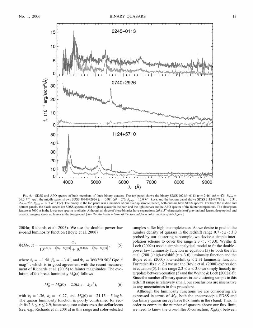
2004a; Richards et al. 2005). We use the double–power lawB-band luminosity function (Boyle et al. 2000)

� MB; zð Þ ¼ ��

100:4(�lþ1) MB�M�B(z)½ þ 100:4(�hþ1) MB�M�

B(z)½ ; ð5Þ

where �l ¼ �1:58, �h ¼ �3:41, and �� ¼ 360(h/0:50)3 Gpc�3

mag�1, which is in good agreement with the recent measure-ment of Richards et al. (2005) to fainter magnitudes. The evo-lution of the break luminosity M �

B(z) follows

M �B ¼ M�

B(0)� 2:5(k1zþ k2z2); ð6Þ

with k1 ¼ 1:36, k2 ¼ �0:27, and M �B(0) ¼ �21:15þ 5 log h.

The quasar luminosity function is poorly constrained for red-shifts 2:6� z � 2:9, because quasar colors cross the stellar locus(see, e.g., Richards et al. 2001a) in this range and color-selected

samples suffer high incompleteness. As we desire to predict thenumber density of quasars in the redshift range 0:7< z < 3:0probed by our clustering subsample, we devise a simple inter-polation scheme to cover the range 2:3< z < 3:0: Wyithe &Loeb (2002a) used a simple analytical model to fit the double–power law luminosity function in equation (5) to both the Fanet al. (2001) high-redshift (z > 3:6) luminosity function and theBoyle et al. (2000) low-redshift (z < 2:3) luminosity function.For redshifts z < 2:3 we use the Boyle et al. (2000) expressionin equation (5). In the range 2:3< z < 3:0 we simply linearly in-terpolate between equation (5) and theWyithe &Loeb (2002a) fit.Since the number of binary quasars in our clustering sample in thisredshift range is relatively small, our conclusions are insensitiveto any uncertainties in this procedure.

Although the luminosity functions we are considering areexpressed in terms of MB, both the spectroscopic SDSS andour binary quasar survey have flux limits in the i band. Thus, inorder to compute the number of quasars above our flux limit,we need to know the cross-filter K-correction, KBi (z), between

Fig. 6.—SDSS and APO spectra of both members of three binary quasars. The top panel shows the binary SDSS J0245�0113 (z ¼ 2:46, �� ¼ 4B5, Rprop ¼26:3 h�1 kpc), the middle panel shows SDSS J0740+2926 (z ¼ 0:98, �� ¼ 2B6, Rprop ¼ 15:0 h�1 kpc), and the bottom panel shows SDSS J1124+5710 (z ¼ 2:31,�� ¼ 2B2, Rprop ¼ 12:7 h�1 kpc). The binary in the top panel was a member of our overlap sample; hence, both quasars have SDSS spectra. For both the middle andbottom panels, the black curves are SDSS spectra of the brighter quasar in the pair, and the light curves are the APO spectra of the fainter companions. The absorptionfeature at 76008 in the lower two spectra is telluric. Although all three of these binaries have separations��P500 characteristic of gravitational lenses, deep optical andnear-IR imaging show no lenses in the foreground. [See the electronic edition of the Journal for a color version of this figure.]


apparent magnitude i and absolute magnitude B (see, e.g.,Hogg et al. 2002):

MB ¼ i� DM (z)� KBi(z); ð7Þ

where DM(z) is the distance modulus. We compute KBi (z) fromthe SDSS composite quasar spectrum of Vanden Berk et al.(2001) and the Johnson B and SDSS i filter curves.

The number density of quasars brighter than the flux limit i0 isan integral over the luminosity function,

n z; i < i0ð Þ ¼Z Mi 0

B

Mbright

B

dMB � MB; zð Þ; ð8Þ

where MbrightB (z) and Mi 0

B (z) are the absolute magnitudes corre-sponding to the bright- and faint-end apparent magnitude limitsas per equation (7).

To check ourmodel, we compute the cumulative numbermag-nitude counts n(<i) for the redshift range 0:3< z < 3:0 and

compare to the measurement over the same redshift interval byVanden Berk et al. (2005). We find that our model slightly over-estimates the number counts of quasars. Specifically, Vanden Berket al. (2005) measured n (<18:5) ¼ 3:74 deg�2, whereas ourmodel predicts n (<18:5) ¼ 4:63 deg�2.We thus scale our modelluminosity function down by this ratio so as to give the correctnumber counts for i < 18:5.

6.2. Estimating the Correlation Function

If it is true that quasars depart from the gravitational clusteringhierarchy because of dissipative encounters, thiswould be expectedto occur for separations smaller than some length scale characteris-tic of tidal effects or mergers. Proper rather than comoving coordi-nates are appropriate for such an investigation. However, clusteringmeasurements are typically carried out in comoving coordinates, asthese are most intuitive in the linear regime where objects are stillmovingwith theHubble flow.We compute the correlation functionin both proper and comoving units, but for definiteness we usecomoving units in the equations that follow.

Fig. 7.—SDSS and APO spectra of both members of three binary quasars. The top panel shows the binary SDSS J1405+4447 (z ¼ 2:23,�� ¼ 7B4, R ¼ 142:8 h�1 kpc),the middle panel shows SDSS J1530+5304 (z ¼ 1:53, �� ¼ 4B1, R ¼ 63:3 h�1 kpc), and the bottom panel shows SDSS J1723+5904 (z ¼ 1:60, �� ¼ 3B7, R ¼59:0 h�1 kpc). The binary in the middle panel is a member of the photometric sample, and both spectra were taken at APO. In the other two panels, the black curves areSDSS spectra of the brighter quasar in the pair, and the light curves are the APO spectra of the fainter companion. Deep imaging of SDSS J1405+4447 and SDSS J1723+5904shows no lens in the foreground. The absorption features at 7600 8 are telluric. [See the electronic edition of the Journal for a color version of this figure.]


We consider quasars with a maximum velocity difference ofj�vj < 2000 km s�1; thus, we measure the redshift space cor-relation function projected over this velocity interval:

wp(R; z) ¼Z vmax=aH(z)

�vmax=aH (z)

�s(R; s; z) ds; ð9Þ

where �s is the quasar correlation function in redshift space,vmax ¼ 2000 km s�1, H(z) is the expansion rate at redshift z,and the factor of a ¼ 1/(1þ z) converts the redshift distance tocomoving units.

The redshift space correlation function �s(R, s, z) is the con-volution of the velocity distribution in the redshift direction,Fv(vz),with the real space correlation function �(r, z):

�s(R; s; z) ¼Z 1

�1�

ffiffiffiffiffiffiffiffiffiffiffiffiffiffiffiR2 þ x2

p; z

� �fv(H(z)(x� s)) dx: ð10Þ

The radial velocity distribution Fv(vz) has contributions fromboth peculiar velocities and uncertainties in the systemic red-shifts of the quasars. Provided that the distance in redshift spaceover which we project contains most of the area under Fv, it is agood approximation to replace the redshift space correlationfunction �s under the integral in equation (9) with the real spacecorrelation function �, since radial velocities will simply movepairs of points within the volume.

The small number of close pairs will limit the number of binsin R for which we can measure the correlation function. Sincewp may change significantly over these large bins, we choose tomeasure the volume-averaged projected correlation function inte-grated over each radial bin.We denote this dimensionless quantityby Wp. Within a comoving bin [Rmin, Rmax] it can be written as

Wp Rmin; Rmax; zð Þ

R vmax=aH(z)�vmax=aH(z)

R Rmax

Rmin�(R; s; z)2R dR ds

Vshell

;

ð11Þ

where Vshell is the volume of the cylindrical shell in redshift space:

Vshell ¼ R2max � R2

min

� � 2vmax

aH(z)

� : ð12Þ

The correlation function of a point process is computed by com-paring the number of pairs detected to the number expected in theabsence of clustering, taking into account the sample limits. Wechoose the estimator

1þ Wp(Rmin; Rmax) ¼hQQihQRi : ð13Þ

Usually, random catalogs are constructed to determine the av-erage number of data-random pairs hQRi. However, a subtletyarises in the current context, because for�� < 6000 we have tar-geted the companion quasars (i.e., the quasars discovered fromfollow-up observations) to fainter magnitudes than the quasarsfrom the parent spectroscopic sample. Rather than estimate thecorrelation function from the number of pairs, we use the num-ber of companions. Specifically, hQQi is defined to be the num-ber of companions about quasars in the parent sample in a givencomoving transverse radial bin [Rmin, Rmax], and hQRi is theaverage number of random companions in this radial bin in theabsence of clustering. In the case in which the parent and com-panion samples are distinct (as is the case for the lens and �2

samples), then hQQi is just the number of binaries in the bin inquestion. However, if the parent and companion samples are iden-tical (as is the case for the overlap and spectroscopic samples),then hQQi is twice the number of pairs, since each of the two qua-sars in the parent sample has a companion.

Our model of the luminosity function in x 6.1 is used to com-pute the average number of random companions R about thequasars Q in each parent quasar sample, taking into account theflux limits and various sources of incompleteness. We separatelycompute the quasar-random contribution for each selection algo-rithm used to define our clustering sample, and we then add the re-sults. Specifically, for a comoving transverse radial bin [Rmin,Rmax]centered on R, we can write

hQRi ¼XNQSO

j

n zj; i < i0� �

VshellS zj; �j� �

; ð14Þ

where n(zj; i < i0 ) is the number density of quasars above theflux limit i 0, Vshell is the volume of each bin in equation (12), andthe sum is over all quasars in the parent sample. The quantityS(zj, �j) is the selection probability of detecting a companionabout the jth quasar. It is a function of angle and redshift, sincethese quantities parameterize our various selection algorithms,as discussed in x 3. Here �j ¼ R /D(z) is the angle onto which the( logarithmic) center of the bin projects for a quasar at redshift z,and D(z) is the comoving distance.

In what follows we compare our measured correlation func-tion to previous larger scale (1–30 h�1 Mpc) clustering measure-ments extrapolated as a power law down to the scales probed byour binaries. Since Wp in equation (11) is a function of redshift,we must average it over the redshift distribution of our quasarsample before a comparison can be made to the measurementfrom equation (13),

Wp Rmin; Rmaxð Þ ¼ 1

NQSO

XNQSO

j

Wp Rmin; Rmax; zj� �

: ð15Þ

Fig. 8.—Range of redshifts and proper transverse separations probed by thebinary quasars in our clustering subsample. The dots show binary quasarsidentified in the SDSS spectroscopic sample (� > 6000). The dotted line in-dicates the transverse separation corresponding to � ¼ 6000. The open circlesindicate pairs from the overlapping plates. These pairs are required to also meetthe �2 selection criteria (eq. [4]). The upside-down and upright triangles showmembers of the lens and �2 samples, respectively. The short-dashed curveindicates the transverse separation corresponding to � ¼ 300, below which bi-naries are found with our lens algorithm. The horizontal long-dashed curves atz ¼ 0:7 and 3.0 indicate the redshift limits of the clustering subsample. [See theelectronic edition of the Journal for a color version of this figure.]


In Figure 9 we show the prediction for the number of com-panions in the bin 5 h�1 kpc< Rprop < 50 h�1 kpc with j�vj<2000 km s�1 as a function of redshift:

Nc ¼ n (z; i < 21)Vshell 1þ Wp(5; 50; z)� �

: ð16Þ

For only this figure, we ignore the redshift evolution of thecorrelation length and set r0 ¼ 4:8 h�1 Mpc. The expectedmean number of companions per quasar with 5 h�1 kpc < R <50 h�1 kpc is �2 3 ; 10�5, so that for a perfect pair survey of�50,000 quasars, we expect to find roughly one quasar pair inthis interval. However, our clustering sample already contains20 quasars with transverse separations this small. Although ourpair survey is far from complete, there is already evidence forexcess clustering over what is expected from extrapolating thecorrelation function power law. In the next two sections wemake this argument more precise.

6.3. Computing the Selection Function

To estimate the correlation function, we compute the totalnumber of random pairs expected from equation (14) by sum-ming over the redshifts of the quasars in each parent samplearound which we searched for candidate companions. How-ever, we must first consider several sources of incompleteness.For the �2-selected sample, our �2 < 20 cut results in thecompleteness fraction C(z; �2 < 20) shown in Figure 2. Inaddition, only a fraction of the pair candidates that satisfy thecriteria for our lens and �2 selection algorithms have been ob-served to date, and the fraction of candidates observed varieswith angular separation because of our tendency to observesmall-separation pairs first. Finally, for the � > 6000 pairs thatwe find in the SDSS spectroscopic sample, the completenessfraction is just that of the quasar SDSS and does not vary with

angle. The selection probability in equation (14) can therefore bewritten as

S(z; � ) ¼Flens �ð Þ; � � 300;

F�2 (�)C zj�2 < 20ð Þ; 300 < � � 6000;

Fspec; � > 6000;

8><>: ð17Þ

where Flens(� ), F�2 (� ), and Fspec are the completeness fractionsof the lens, �2, and spectroscopic samples, respectively.We take Fspec ¼ 0:95 following Vanden Berk et al. (2005).

The angular selection functions, Flens(� ) and F�2 (� ), of the lensand �2 selection algorithms are computed by comparing, in bins,the number of pair candidates that have been observed to date tothe total number of candidates.For � < 1500 we choose the bin spacing such that each bin

contains at least six objects. For 1500 < � < 6000 we use 10 loga-rithmically spaced angular bins. The selection probability forthe angular bin ½�k ; �kþ1 is

Fk ¼Nobs

Nobs þ Nrem

; ð18Þ

where Nobs is the number of objects observed and Nrem is thenumber of objects remaining. There is an uncertainty in the num-ber of remaining candidates for the lens selection, which is basedon the goodness of fit of a multicomponent PSF to the images ofSDSS quasars (Pindor et al. 2003; Inada et al. 2003a). Becauseour observations were heavily biased toward those candidatesthat were likely to be quasar pairs, we bracket the angular selec-tion function Flens(� ) with upper and lower limits correspond-ing to pessimistic and optimistic assessments of the number ofremaining candidates that are likely to be confirmed as binaries.The lens candidates are given a grade of A, B, or C determinedby the goodness of fit of the multicomponent PSF. For the lowerlimit on Flens(� ), Nrem is taken to be all candidates, whereas forthe upper limit Nrem is restricted to only the candidates that re-ceived a grade of A. Note that to be conservative, we ignore theintrinsic incompleteness of the lens selection algorithm, which isa function of separation, magnitude, and flux ratio (Pindor et al.

Fig. 9.—Expected mean number of companions per quasar with propertransverse separation 5 h�1 kpc < Rprop < 50 h�1 kpc and velocity differencej�vj < 2000 km s�1, as a function of redshift calculated from eq. [16], whichassumes that the large-scale quasar correlation function can be extrapolatedas a power law to small scales. We used the correlation function parameters� ¼ 1:53 and r0 ¼ 4:8 h�1 Mpc measured by PMN04 from the 2dF quasarsurvey. A perfect survey, with no sources of incompleteness, is assumed. In asample of�50,000 quasars, the predicted number of binaries with 5 h�1 kpc <R < 50 h�1 kpc is �1. However, our clustering sample already contains20 quasars with transverse separations this small, which is compelling evidencefor excess clustering over what is expected from extrapolating the correlationfunction.

Fig. 10.—Angular selection function of binary quasars with � < 6000. Wehave pasted Flens(� ) and F�2 (� ) together at � ¼ 300. For � � 300, the dark and lighthistograms represent the upper and lower limits on the fraction of lens paircandidates observed to date, respectively. The histogram for � > 300 shows thefraction of �2 pair candidates observed so far. [See the electronic edition of theJournal for a color version of this figure.]


2003) of the pair, and focus only on the incompleteness of ourobservations of the candidates.

The color-color diagrams of the candidates identified by �2

selectionwere visually inspected prior to observations, and thosewhose colors overlapped the stellar locus were given a lowerpriority. However, some interlopers were observed depending ona variety of criteria. For instance, we were more likely to observepairs with particularly small angular separations, redshifts z > 2(because of their use for Ly� forest studies), or particularly brightmagnitudes. Including the stellar locus interlopers identified bythe �2 statistic as part of Nrem in equation (18) would overesti-mate the number of candidates likely to be quasar pairs and henceunderestimate our selection function. To this end, we apply ad-ditional criteria to these remaining candidates to filter out colormatches that are likely to be quasar-star pairs. However, all quasar-

star pairs we confirmed spectroscopically are included as part ofNobs in equation (18). In this way, we conservatively err on the sideof overestimating our selection completeness, or underestimatingthe correlation function.

In addition to using the criteria in equation (4), we only in-clude �2 candidates that either (1) have colors consistent with theUV-excess region of color space (u� g < 0:6) but outside the re-gion populated bywhite dwarfs (Richards et al. 2002b), (2) matchamember of the faint photometric catalog of Richards et al. (2004)(extended to the DR3 region), or (3) are optically unresolved andmatch a FIRST radio source. Objects that satisfy these criteriahave a k90% probability of being a quasar. For the UV-excesscriteria, we conservatively require that the candidates’ 1 �photometric errors leave them inside the UV-excess region andoutside the white dwarf region. The angular selection function ofour binary quasar survey is shown in Figure 10.

6.4. Excess Clustering

The individual quasar-random contributions for each selectionalgorithmwere computed by carrying out the sum in equation (14)over the respective parent samples. Specifically, we summed overthe 39,142 quasars thatwere the parent sample for the lens sample,the 59,608 (SDSS + 2QZ quasars) that were the parent sampleof the �2 algorithm, and the 52,279 (SDSS only) quasars thatmade up the parent sample of the spectroscopic sample.

For the proper (comoving) projected correlation functions, webinnedour clustering sample into 15 logarithmically spacedbins in

Fig. 11.—Small-scale quasar clustering in proper coordinates.Top: Comparisonof the projected correlation function Wp(Rmin; Rmax; z) (see eq. [11]) measuredfrom our clustering sample with the prediction of the large-scale measurement ofPMN04, extrapolated as a power law down to the scales probed by our binaries.Error bars are 1 � Poisson counting errors. The light circles show the measurementof the projected correlation function if we use the lower limit (optimistic) for theselection function of our lens algorithm (Fig. 10, light histogram for � � 300) topredict the number of quasar-random pairs, rather than the upper limit, which isshown by the black circles. The light circles are offset slightly to the right for thesake of illustration. Dark and light rectangles indicate the predictions based on thelarge-scale measurements of PMN04 for � ¼ 1:53 and 1.8, respectively, wherethe heights of the rectangles indicate the range of predictions based on 1 � errorsin the correlation length measurements, and the widths indicate the bin used foreachmeasurement.Bottom: Ratio of the projected correlation function to the (best-fit � ¼ 1:53) prediction of PMN04. [See the electronic edition of the Journal for acolor version of this figure.]

Fig. 12.—Same as Fig. 11, but in comoving units. [See the electronic editionof the Journal for a color version of this figure.]


the range 9 h�1 kpc< Rprop < 3 h�1 Mpc (20 h�1 kpc < R <7 h�1 Mpc), which are shown in the top panels of Figures 11and 12. The error bars are 1 � Poisson counting errors, where weused the fitting formula in Gehrels (1986) for N < 30. The lightcircles show the measurement of the projected correlation func-tion if we use the lower limit (optimistic) for the selection func-tion of our lens algorithm (Fig. 10, light histogram for � � 300)to predict the number of quasar-random pairs, while the blackcircles use the upper limit. Uncertainty in our selection functionchanges only the innermost few bins, because our lens algorithm

is restricted to angular separations � < 300. These light circles areoffset slightly to the right for the sake of illustration.These projected correlation functions are compared to an ex-

trapolation of the large-scale power laws measured by PMN04,which are indicated by the dark and light rectangles.21 Taking allredshifts together, PMN04 measured a best-fit slope of � ¼ 1:53

TABLE 6

Projected Correlation Function in Proper Coordinates

Rmin Rmax hQQi hQRi hQRiperfect Wp W PMNp Ratio

9.00 13.26 4 0.02014 (0.01136) 0.03147 197.60 (350.98) 7.89 25.0 (44.5)

13.26 19.53 7 0.06694 (0.05749) 0.06922 103.57 (120.76) 6.40 16.2 (18.9)

19.53 28.76 5 0.04506 0.2240 109.96 5.17 21.3

28.76 42.37 2 0.09635 0.4860 19.76 4.18 4.73

42.37 62.40 3 0.11784 1.055 24.46 3.37 7.26

62.40 91.92 2 0.1654 2.288 11.09 2.71 4.09

91.92 135.39 6 0.6090 4.964 8.85 2.17 4.07

135.39 199.42 7 0.5938 10.77 10.79 1.74 6.22

199.42 293.74 8 1.142 23.37 6.01 1.38 4.36

293.74 432.67 20 3.305 37.30 5.05 1.09 4.64

432.67 637.31 23 12.59 13.25 0.83 0.85 0.97

637.31 938.74 49 27.31 28.75 0.79 0.66 1.20

938.74 1382.73 71 59.26 62.38 0.20 0.50 0.39

1382.73 2036.71 195 128.6 135.3 0.52 0.38 1.37

2036.71 3000.00 316 279.0 293.6 0.13 0.27 0.48

Notes.—Given are the data for the clustering measurements shown in Fig. 11. The 15 logarithmically spaced bins of proper transverseseparation are given byRmin andRmax in h

�1 kpc. The number of observed pairs in our clustering subsample for each bin is given by hQQi. Ourcalculation of the number of randompairs in each bin is hQRi (eq. [14]), and hQRiperfect is the expected number of randompairs for a ‘‘perfect’’survey with no sources of incompleteness. Our measurement of the projected correlation function is given by Wp(Rmin; Rmax). The quantityW PMN

p (Rmin; Rmax) is the prediction from the larger scale clustering measurements of PMN04 (� ¼ 1:53), extrapolated as a power law downto the scale probed by our binaries and averaged over the redshift distribution of our parent quasar sample (see eq. [15]). The ratio of ourmeasurement to the prediction from PMN04 (� ¼ 1:53) is given in the last column. The quantities in parentheses are the measurements if weuse the lower limit for the selection function of the lens algorithm (Fig. 10, light histogram for � � 300) to predict hQRi, which corresponds tothe light circles in Fig. 11.

TABLE 7

Projected Correlation Function in Comoving Coordinates

Rmin Rmax hQQi hQRi hQRiperfect Wp W PMNp Ratio

20.00 29.56 4 0.01251 (0.007935) 0.02452 318.69 (503.12) 8.73 36.5 (57.6)

29.56 43.68 5 0.03213 (0.02595) 0.06007 154.61 (191.66) 7.06 21.9 (27.1)

43.68 64.54 5 0.05895 (0.05623) 0.1674 83.81 (87.92) 5.71 14.7 (15.4)

64.54 95.38 3 0.07226 0.3886 40.52 4.61 8.80

95.38 140.95 3 0.1127 0.8487 25.63 3.71 6.91

140.95 208.28 2 0.1907 1.853 9.49 2.98 3.18

208.28 307.80 3 0.4731 4.047 5.34 2.39 2.24

307.80 454.85 10 0.6467 8.839 14.46 1.91 7.58

454.85 672.16 5 1.032 18.75 3.85 1.52 2.54

672.16 993.29 21 3.160 29.00 5.65 1.20 4.71

993.29 1467.84 20 10.80 13.29 0.85 0.94 0.91

1467.84 2169.12 42 23.71 24.96 0.77 0.73 1.06

2169.12 3205.45 70 51.78 54.51 0.35 0.56 0.63

3205.45 4736.89 166 113.1 119.0 0.47 0.42 1.11

4736.89 7000.00 317 246.9 259.9 0.28 0.31 0.92

Notes.—Given are the data for the clustering measurements shown in Fig. 12. The 15 logarithmically spaced bins of proper transverseseparation are given by Rmin and Rmax in h

�1 kpc. The number of observed pairs in our clustering subsample for each bin is given by hQQi.Our calculation of the number of random pairs in each bin is hQRi (eq. [14]), and hQRiperfect is the expected number of random pairs for a‘‘perfect’’ survey with no sources of incompleteness. Our measurement of the projected correlation function is given by Wp(Rmin; Rmax). Thequantity W PMN

p (Rmin; Rmax) is the prediction from the larger scale clustering measurements of PMN04 (� ¼ 1:53), extrapolated as a powerlaw down to the scale probed by our binaries and averaged over the redshift distribution of our parent quasar sample (see eq. [15]). The ratioof our measurement to the prediction from PMN04 (� ¼ 1:53) is given in the last column. The quantities in parentheses are the measurementsif we use the lower limit for the selection function of the lens algorithm (Fig. 10, light histogram for � � 300) to predict hQRi, whichcorresponds to the light circles in Fig. 12.

21 The PMN04 correlation function is in comoving coordinates. For the propercorrelation function, we translated the correlation lengths to proper coordinates ineach element of the average in eq. (15).


and r0 ¼ 4:8 h�1 Mpc, consistent with the measurement byCroom et al. (2001, 2005). They also detected evolution of thecorrelation length r0 with look-back time by splitting the sampleinto three redshift bins (0:8 < z < 1:3, 1:3 < z < 1:7, and 1:7 <z < 2:1). As there is significant covariance between the slopeand amplitude, they quoted correlation lengths (and errors) inthese bins at two slopes: the best-fit value � ¼ 1:53 and a steepervalue of � ¼ 1:8. The dark rectangles indicate the prediction forthe projected correlation function based on an extrapolation ofthe � ¼ 1:53 large-scale power law, whereas the light rectanglesare for � ¼ 1:8. The heights of the rectangles are the range ofpredictions based on the 1 � errors on the correlation lengths (foreach redshift interval ) published by PMN04, and the widths ofthe rectangles indicate the bin used for each measurement. Notethat we include the evolution of the correlation length (from thevalues of Table 2 in PMN04) in the average in equation (15).The ratios of the measured projected correlation functions tothe extrapolation of the best-fit � ¼ 1:53 predictions of PMN04are shown in the bottom panels of Figures 11 and 12.

A summary of the data plotted in these figures is given inTables 6 and 7. In the tables we compare our calculation for thenumber of random pairs in each bin hQRi (eq. [14]) for our sur-vey to hQRiperfect, which is the expected number of random pairsfor a ‘‘perfect’’ survey with no sources of incompleteness. A com-parison of these two quantities is a measure of our incompletenessin each bin.

Our clustering measurement agrees with the measurementsof PMN04 for large proper (comoving) separations Rpropk400 h�1 kpc (Rk 1 h�1 Mpc), where the PMN04 measure-ments are valid. However, we detect a significant excess overthe expectation from extrapolating the power law of the corre-lation function to smaller scales. The uncertainties are large be-cause of shot noise, our uncertain selection function for � < 300,and the range of permitted large-scale correlation function slopes.For the best-fit large-scale slope � ¼ 1:53, the excess is an order ofmagnitude for proper (comoving) separations RpropP 40 h�1 kpc(RP100 h�1 kpc) and is largest (�30) on the smallest scalesRprop �15 h�1 kpc (R �30 h�1 kpc). For the steeper slope � ¼1:8, the excess is smaller by a factor of 4–5.

Our clustering statistic Wp(Rmin, Rmax) is the average over acylinder shell with velocity extent 4000 km s�1, correspondingto a typical extent rprop � 18 h�1 Mpc (r � 44 h�1 Mpc). For apower-law correlation function �(r) ¼ (r/r0)

�� , Wp(Rmin, Rmax)progressively flattens toward small scales, as is seen in the darkrectangles in the top panels of Figures 11 and 12. In contrast, ourmeasuredWp(Rmin, Rmax) does not flatten but rather resembles apower law in projection. This necessarily implies that the truethree-dimensional correlation function of quasars is not a powerlaw �(r) but rather gets progressively steeper on small scales.

7. DISCUSSION

On large proper comoving scales k1 h�1 Mpc, quasars atz �1:5, similar to high-redshift galaxies, are strongly biased andhave nearly the same correlation length that galaxies do in thelocal universe. In x 6 we argued that the correlation function ofquasars becomes significantly steeper on submegaparsec scales.Does small-scale galaxy clustering (or quasar-galaxy clustering)show a similar trend? As we compare to previous clusteringmeasurements in this section, all distances quoted are comoving.

At low redshift, Zehavi et al. (2004) measured the projectedcorrelation function of the nearby (z P 0:2) SDSS main galaxysample down to �100 h�1 kpc and found only small deviationsfrom a power law �� 1:9. At intermediate redshift (0:2Pz P 0:3), Masjedi et al. (2005) recently measured the small-scale

clustering of the SDSS luminous red galaxies, using a novel sta-tistical technique to overcome the incompleteness caused by fibercollisions. They found that the correlation function is surprisinglyclose to an r�2 power law over 5 orders ofmagnitude in comovingseparation, down to scales as small as 10 h�1 kpc.

Another complementary set of low-redshift observations thatprobe clustering on small scales (10 h�1 kpc to 1 h�1 Mpc) isthe SDSS galaxy-galaxy lensing studies (Guzik & Seljak 2002;Sheldon et al. 2004), whichmeasure the galaxy–darkmatter cross-correlation function.No excess small-scale clustering over a powerlaw was detected in these studies either.

A comparison with small-scale galaxy clustering at high red-shift is clearly more relevant to our purposes. Adelberger et al.(2003) and Coil et al. (2004) have measured the correlation func-tion of galaxies at z � 3 and z �1, respectively, down to scales assmall as�100–200 h�1 kpc, and no small-scale excess clusteringwas found. As the redshift ranges of these measurements bracketthe redshift range probed by our sample of binary quasars, weexpect that galaxies in the redshift desert, z �1:4 2:5, coevalwith the bulk of our binary quasars (see Fig. 3), alsowill not showany enhancement in small-scale clustering.

Thus, as first suggested by Djorgovski (1991), quasars atz �1:5 depart from the power-law clustering hierarchy followedby galaxies, both in the local universe and at high redshift. Galaxyinteractions are often implicated as a means of triggering, fueling,or forming active galactic nuclei (AGNs; Toomre&Toomre1972;Barnes & Hernquist 1996; Bahcall et al. 1997), and it has beenclaimed by several authors that excess quasar clustering is the hall-mark of these dissipative interactions (Djorgovski 1991;Kochaneket al. 1999; Mortlock et al. 1999). However, if this is the case, asimilar small-scale enhancement is to be expected in the quasar-galaxy correlation function, as follows.

If the quasar-quasar correlation function is �QQ and quasarstrace galaxy overdensities with a linear relative bias bQ definedby �Q ¼ bQ�G, then the ratio of the quasar-quasar correlation tothe galaxy-galaxy correlation is �QQ/�GG ¼ b2Q, and the ratio ofthe quasar-galaxy cross-correlation function to galaxy-galaxy clus-tering is �QG/�GG ¼ bQ. Since we have argued that small-scalequasar clustering is enhanced relative to galaxy clustering at thesame redshift, we expect to see the square root of that enhance-ment in the quasar-galaxy cross-correlation.

It has long been known that quasars are associated with en-hancements in the distribution of galaxies (Bahcall et al. 1969;Yee & Green 1984, 1987; Bahcall & Chokshi 1991; Laurikainen& Salo 1995; Smith et al. 1995, 2000; Hall et al. 1998; Hall &Green 1998), and the foregoing argument has led us to ask ifthere is a small-scale excess of galaxy pairs around quasars.22

However, nearly all studies of quasar-galaxy correlations havebeen restricted to low redshifts (z P 0:6) and therefore low lu-minosity. Recently, Adelberger & Steidel (2005) measured thecross-correlation of high-redshift (1:8 P z P3:5) Lyman breakgalaxies (LBGs) with AGNs. A best-fit correlation length ofr0 ¼ 4:7 h�1 Mpc (at a fixed slope of � ¼ 1:6) was measuredfor bright AGNs in the luminosity range considered here, whichis very close to the autocorrelation length of LBGs (Adelbergeret al. 2003). This measurement does not probe small scales be-cause it was limited to quasar-galaxy pairs with separations>6000, corresponding to k1 h�1 Mpc. However, the small-scale

22 We note that the disagreement in the literature on whether radio-loudquasars are located in richer environments (Yee & Green 1984, 1987; Ellingsonet al. 1991) or not (Fisher et al. 1996; McLure & Dunlop 2001; Finn et al. 2001;Wold et al. 2001) is not an issue in the current context, since only one close binaryin our clustering subsample, LBQS 1429�008, has a radio-loud member.


<6000 clustering of LBGs around quasars seems to be consistentwith this result (K. Adelberger 2005, private communication).While it is puzzling that the quasar-LBG cross-correlation doesnot seem to show a small-scale enhancement, it is conceivablethat fainter galaxies below the flux limit (RAB � 25:5 or�0.4L�)of the LBG survey (Steidel et al. 2003) could still show a small-scale clustering excess.

Historically, there has been significant scatter in the low-redshift measurements of quasar-galaxy correlations (see Brownet al. 2001, Table 1, for a compilation of recent studies) caused byheterogeneous quasar samples, methodology, and imaging depths.Furthermore, the measurement of a factor of �4 enhancement ofthe number of companion galaxies around quasars compared tothe mean number around galaxies, measured by theHubble SpaceTelescope studies of�40 nearbyAGNs by Fisher et al. (1996) andMcLure & Dunlop (2001), has been called into question by Finnet al. (2001) as being the result of sample biases. We thus focuson the most recent determinations of quasar-galaxy correlations,albeit at low redshifts zP0:3, by the 2dF survey and SDSS;these surveys have samples of �10,000 AGNs surrounded by�100,000 galaxies at their disposal.

Croom et al. (2004b) andWake et al. (2004) measured the ratio�QG/�GG ¼ bQ, in the 2dF survey and SDSS, respectively, findingit to be consistent with unity on small and large scales. The Croomet al. (2004b) measurement extends down to �900 h�1 kpc,whereas the Wake et al. (2004) measurement probes down toscales of �400 h�1 kpc. Both of these studies cross-correlatedspectroscopic samples of galaxies with spectroscopic samples ofAGNs; hence, they are limited to low redshift zP 0:3, becausethe spectroscopic galaxy samples are shallow, and large scales,because offiber collisions. At z � 0:2 the fiber collision limit cor-responds to �160 h�1 kpc in the SDSS and �80 h�1 kpc in the2dF. What is needed is a clustering study using photometricgalaxies around spectroscopic quasars that could extend to red-shift z � 0:5 and resolve the scales R � 10 h�1 kpc of most in-terest to us for the excess quasar clustering (see Serber et al. 2005).

8. SUMMARY AND CONCLUSIONS

We have presented a sample of 221 new quasar pairs withtransverse separations Rprop < 1 h�1 Mpc over the redshift range0:5 � z � 3:0. Of these, 65 have angular separations � < 6000 be-low the SDSS fiber collision scale. Our 26 new pairs with properseparations Rprop < 50 h�1 kpc (� < 1000) more than double thenumber of binaries known with splittings this small. Althoughthese binaries were discovered with a variety of selection algo-rithms, we defined a statistical subsample selected with homo-geneous criteria and computed its selection function taking intoaccount sources of incompleteness. We presented the first mea-surement of the quasar correlation function on the small proper(comoving) scales of 10–400 h�1 kpc (20 h�1 kpc to 1 h�1 Mpc).For a large-scale correlation function slope of � ¼ 1:53, we detectan order of magnitude excess clustering for proper (comoving)separations RpropP 40 h�1 kpc (R P 100 h�1 kpc), which growsto �30 on the smallest scale probed by our sample, Rprop �15 h�1 kpc (R � 30 h�1 kpc). This excess is smaller by a factorof 4–5 if the large-scale correlation function has a steeper slope� ¼ 1:8.

We reviewed recent small-scale measurements of galaxy clus-tering and quasar-galaxy clustering and discussed the results inrelation to the excess small-scale quasar clustering that we mea-sured. The quasar-galaxy correlation function of redshift z �1:5quasars should show a small-scale clustering enhancement withamplitude roughly the square root of the enhancement detected

here. However, existing studies of the environments of quasars atz �1:5 have been plagued by small sample sizes and lack thestatistics to address the clustering strength on the �100 h�1 kpcscales of interest.Deep imaging of the binaries published here will provide valu-

able information about their environments. The detection of sig-nificant overdensities of galaxies coeval with the binary wouldsupport the idea that enhanced quasar activity is triggered by gal-axy interactions, and it might suggest that quasars at high redshifttrace the biased peaks that are the progenitors of the rich clusterswesee today (Efstathiou & Rees 1988; Cole & Kaiser 1989; Nusser& Silk 1993; Djorgovski et al. 1999, 2003; Djorgovski 1999).Intriguingly, Fukugita et al. (2004) took deep Subaru images ofthe z ¼ 4:25 quasar discovered by Schneider et al. (2000) andfound no evidence for an overdensity of galaxies. Similar deepimaging studies of high-redshift quasar environments (for singlequasars) have been conducted by Infante et al. (2003) at z � 3,by Djorgovski and collaborators at zk 4 (Djorgovski et al. 1999,2003; Djorgovski 1999; Stiavelli et al. 2005), and byWillott et al.(2005) at z � 6. The binaries in our sample offer an opportu-nity to conduct analogous studies over a range of lower andmore accessible redshifts, with the added bonus that one ex-pects these extremely rare binary systems to trace even richerenvironments.Measurements of the shape of the quasar-quasar and quasar-

galaxy correlation function on the small scales probed by ourbinaries will yield valuable insights into the physical processesthat trigger quasar activity and will help explain how quasarsare embedded in the structure formation hierarchy. Reproducingthe excess clustering with semianalytical models (Kauffmann& Haehnelt 2002) and halo models (see, e.g., PMN04) wouldprovide constraints on the distribution of quasars in dark matterhalos. Another interesting question is whether the quasars inthese binaries have significantly longer lifetimes than ‘‘field’’ qua-sars (Haiman & Hui 2001; Martini & Weinberg 2001), whichwould have interesting implications for the masses of super-massive black holes (Wyithe & Loeb 2005) in the richest re-gions of the universe.We close with the reminder that our survey for quasar pairs is

ongoing and less than 50% complete. We expect to find a com-parable number of binaries in the current SDSS quasar sample.Furthermore, the faint photometric quasar selection techniques ofRichards et al. (2004) aim to construct a sample of �106 quasars.Extrapolating from the number of pairs published here, we wouldexpect to find �1000 new binaries in a sample of this size, whichwould allow a much more precise measurement of the correlationfunction on small scales.

J. F. H. wishes to thank his thesis advisor David Spergel foradvice, guidance, and helpful discussions over the course of thiswork during his time in Princeton. For part of this study, J. F. H.was supported by the Proctor Graduate Fellowship at PrincetonUniversity and by a generous gift from the Paul and Daisy SorosFellowship for New Americans. The program is not responsiblefor the views expressed. J. F. H. is currently supported by NASAthrough Hubble Fellowship grant 01172.01-A awarded by theSpace Telescope Science Institute, which is operated by theAssociation of Universities for Research in Astronomy, Inc., forNASA, under contract NAS5-26555. Thanks to Bob Nichol andAlex Gray for help with the faint photometric quasar catalog. Weare grateful to the observing specialists at Apache Point Obser-vatory, Russet MacMillan, John Barentine, Bill Ketzeback, and


Jack Dembicky, for many nights of hard work. D. P. S. acknowl-edges support from NSF grant AST 03-07582, and M. A. S.acknowledges the support of NSF grant AST 03-07409. Fi-nally, we wish to thank the anonymous referee for constructivecomments.

Funding for the creation and distribution of the SDSS Archivehas been provided by the Alfred P. Sloan Foundation, the Partic-ipating Institutions, the National Aeronautics and Space Admin-istration, the National Science Foundation, the US Departmentof Energy, the Japanese Monbukagakusho, and the Max PlanckSociety. The SDSSWeb site is at http://www.sdss.org. The SDSSismanaged by theAstrophysical ResearchConsortium for the Par-ticipating Institutions. The Participating Institutions are the Uni-versity of Chicago, Fermilab, the Institute for Advanced Study,the Japan Participation Group, The Johns Hopkins University,theKorean Scientist Group, LosAlamosNational Laboratory, theMax Planck Institute for Astronomy, the Max Planck Institutefor Astrophysics, New Mexico State University, the Universityof Pittsburgh, the University of Portsmouth, Princeton Univer-sity, the United States Naval Observatory, and the University ofWashington.

This paper is based in part on data collected at theW.M. KeckObservatory, the Apache Point Observatory 3.5 m telescope, theHobby-Eberly Telescope, and the European Southern Observa-tory, Chile (proposal 67.A-0544). The Apache Point Observa-tory 3.5 m telescope is owned and operated by the AstrophysicalResearch Consortium. The W. M. Keck Observatory is operatedas a scientific partnership among the California Institute of Tech-nology, the University of California, and NASA. The Hobby-

Eberly Telescope is a joint project of the University of Texas atAustin, the Pennsylvania State University, Stanford University,Ludwig-Maximillians-Universitat Munchen, andGeorg-August-Universitat Gottingen. The Hobby-Eberly Telescope is named inhonor of its principal benefactors, William P. Hobby and RobertE. Eberly. The Marcario Low-Resolution Spectrograph is namedforMikeMarcario ofHigh LonesomeOptics, who fabricated sev-eral optics for the instrument but died before its completion; it isa joint project of the Hobby-Eberly Telescope partnership and theInstituto de Astronomıa de la Universidad Nacional Autonoma deMexico.

APPENDIX

In this appendix we present the results of all our follow-upobservations not included above, as well as the list of projectedpairs of quasars in the SDSS quasar sample that have similarredshifts. These tables will facilitate future studies of close qua-sar pairs and prevent the duplicate observations of candidatesalready observed by the SDSS or our follow-up observationprogram.

In Table 8 we list all projected pairs of quasars in the com-bined SDSS + 2QZ spectroscopic catalog with angular sepa-rations � < 9000 and redshift difference�z < 0:5. All projectedpairs of quasars discovered from our follow-up spectroscopicobservations are listed in Table 9. Finally, Table 10 lists all thequasar-star pairs identified from our follow-up observations.The full versions of these tables are published in the electronicversion of this article.

TABLE 8

Projected Pairs of Quasars Discovered in Overlapping Plates

Name R.A. (J2000.0) Decl. (J2000.0) u g r i z z �� Rprop

SDSS J0005+0102A............. 00 05 00.84 +01 03 03.3 19.50 19.26 19.20 18.93 18.81 1.63 42.7 259.7

SDSS J0005+0102B ............. 00 05 00.54 +01 02 20.8 18.67 18.45 18.33 18.27 18.10 2.12

SDSS J0008�0039A ............ 00 08 04.23 �00 39 23.0 20.79 20.41 20.25 19.97 19.72 1.61 27.7 168.6

SDSS J0008�0039B ............ 00 08 05.18 �00 39 46.8 20.53 20.53 20.56 20.16 20.11 1.94

Notes.—Units of right ascension are hours, minutes, and seconds, and units of declination are degrees, arcminutes, and arcseconds. Quasars labeled ‘‘SDSS’’ or‘‘2QZ’’ are members of the SDSS or 2QZ spectroscopic quasar catalog. The redshift of each quasar is indicated by the second ‘‘z’’ column, and the foreground quasar isalways designated ‘‘A.’’ The column labeled Rprop is the transverse proper separation (in h�1 kpc), evaluated at the foreground quasar redshift, and �� is the angularseparation in arcseconds. Extinction-corrected SDSS five-band PSF photometry is given in the columns u, g, r, i, and z. Table 8 is published in its entirety in theelectronic edition of the Astronomical Journal. A portion is shown here for guidance regarding its form and content.

TABLE 9

Projected Pairs of Quasars Discovered from Follow-Up Spectroscopy

Name R.A. (J2000.0) Decl. (J2000.0) u g r i z z �� R �2

SDSS J0002�0053A .................... 00 02 12.53 �00 53 11.7 20.72 20.59 20.34 20.12 20.17 1.54 7.3 44.5 20.9

SDSS J0002�0053B .................... 00 02 12.53 �00 53 11.7 20.10 19.64 19.52 19.41 19.23 2.21

SDSS J0036�1109A .................... 00 36 49.63 �11 09 29.8 19.08 18.85 18.67 18.45 18.67 1.51 4.7 28.5 19.0

SDSS J0036�1109B .................... 00 36 49.63 �11 09 29.8 20.92 20.64 20.46 20.52 20.24 2.18

Notes.—Units of right ascension are hours, minutes, and seconds, and units of declination are degrees, arcminutes, and arcseconds. Quasars labeled ‘‘A’’ aremembers of the SDSS or 2QZ spectroscopic quasar catalogs. Quasars discovered from follow-up spectroscopy are designated by ‘‘B.’’ For projected pairs discovered fromthe photometric catalog, ‘‘A’’ designates the brighter of the two quasars. The redshift of each quasar is indicated by the second ‘‘z’’ column. The column labeledRprop is thetransverse proper separation (in h�1 kpc), evaluated at the foreground quasar redshift, and�� is the angular separation in arcseconds. Extinction-corrected SDSS five-bandPSF photometry is given in the columns u, g, r, i, and z, and �2 is the value of our color similarity statistic. Table 9 is published in its entirety in the electronic edition of theAstronomical Journal. A portion is shown here for guidance regarding its form and content.


REFERENCES

Abazajian, K., et al. 2003, AJ, 126, 2081———. 2004, AJ, 128, 502———. 2005, AJ, 129, 1755Adelberger, K. L., & Steidel, C. C. 2005, ApJ, 630, 50Adelberger, K. L., Steidel, C. C., Shapley, A. E., & Pettini,M. 2003, ApJ, 584, 45Anderson, S. F., et al. 2003, AJ, 126, 2209Andreani, P., & Cristiani, S. 1992, ApJ, 398, L13Bahcall, J. N., Kirhakos, S., Saxe, D. H., & Schneider, D. P. 1997, ApJ, 479, 642Bahcall, J. N., Schmidt, M., & Gunn, J. E. 1969, ApJ, 157, L77Bahcall, N. A., & Chokshi, A. 1991, ApJ, 380, L9Barnes, J. E., & Hernquist, L. 1996, ApJ, 471, 115Becker, R. H., White, R. L., & Helfand, D. J. 1995, ApJ, 450, 559Blanton, M. R., Lin, H., Lupton, R. H., Maley, F. M., Young, N., Zehavi, I., &Loveday, J. 2003, AJ, 125, 2276

Bonnet, H., Fort, B., Kneib, J.-P., Mellier, Y., & Soucail, G. 1993, A&A, 280, L7Boyle, B. J., Shanks, T., Croom, S. M., Smith, R. J., Miller, L., Loaring, N., &Heymans, C. 2000, MNRAS, 317, 1014

Brown, M. J. I., Boyle, B. J., & Webster, R. L. 2001, AJ, 122, 26Budavari, T., et al. 2001, AJ, 122, 1163Carlberg, R. G. 1990, ApJ, 350, 505Castander, F. J., et al. 2001, AJ, 121, 2331Coil, A. L., et al. 2004, ApJ, 609, 525Cole, S., & Kaiser, N. 1989, MNRAS, 237, 1127Crampton, D., Cowley, A. P., Hickson, P., Kindl, E., Wagner, R. M., Tyson, J. A.,& Gullixson, C. 1988, ApJ, 330, 184

Croom, S. M., Boyle, B. J., Loaring, N. S., Miller, L., Outram, P. J., Shanks, T.,& Smith, R. J. 2002, MNRAS, 335, 459

Croom, S. M., & Shanks, T. 1996, MNRAS, 281, 893Croom, S. M., Shanks, T., Boyle, B. J., Smith, R. J., Miller, L., Loaring, N. S.,& Hoyle, F. 2001, MNRAS, 325, 483

Croom, S. M., Smith, R. J., Boyle, B. J., Shanks, T., Miller, L., Outram, P. J., &Loaring, N. S. 2004a, MNRAS, 349, 1397

Croom, S., et al. 2004b, in ASP Conf. Ser. 311, AGN Physics with the SloanDigital Sky Survey, ed. G. T. Richards & P. B. Hall (San Francisco: ASP), 457

———. 2005, MNRAS, 356, 415Djorgovski, S. 1991, in ASP Conf. Ser. 21, The Space Distribution of Quasars,ed. D. Crampton (San Francisco: ASP), 349

Djorgovski, S. G. 1999, in ASP Conf. Ser. 193, The Hy-Redshift Universe:Galaxy Formation and Evolution at High Redshift, ed. A. J. Bunker &W. J. M. van Breugel (San Francisco: ASP), 397

Djorgovski, S.G., Odewahn, S. C.,Gal, R. R., Brunner, R. J.,& deCarvalho, R. R.1999, in ASP Conf. Ser. 191, Photometric Redshifts and High-Redshift Gal-axies, ed. R. J. Weymann et al. (San Francisco: ASP), 179

Djorgovski, S. G., Stern, D., Mahabal, A. A., & Brunner, R. 2003, ApJ, 596, 67Duncan, R. C. 1991, ApJ, 375, L41Efstathiou, G., & Rees, M. J. 1988, MNRAS, 230, 5PEisenstein, D. J., et al. 2001, AJ, 122, 2267Ellingson, E., Yee, H. K. C., & Green, R. F. 1991, ApJ, 371, 49Epps, H. W., & Miller, J. S. 1998, Proc. SPIE, 3355, 48Fan, X., et al. 1999, AJ, 118, 1———. 2001, AJ, 121, 54Ferrarese, L., & Merritt, D. 2000, ApJ, 539, L9Finn, R. A., Impey, C. D., & Hooper, E. J. 2001, ApJ, 557, 578Fischer, P., Tyson, J. A., Bernstein, G. M., & Guhathakurta, P. 1994, ApJ, 431,L71

Fisher, K. B., Bahcall, J. N., Kirhakos, S., & Schneider, D. P. 1996, ApJ, 468,469

Fukugita,M., Ichikawa, T., Gunn, J. E., Doi,M., Shimasaku,K.,&Schneider, D. P.1996, AJ, 111, 1748

Fukugita, M., Nakamura, O., Schneider, D. P., Doi, M., & Kashikawa, N. 2004,ApJ, 603, L65

Gebhardt, K., et al. 2000, ApJ, 539, L13Gehrels, N. 1986, ApJ, 303, 336Green, P. J., et al. 2002, ApJ, 571, 721Gregg, M. D., Becker, R. H., White, R. L., Richards, G. T., Chaffee, F. H., &Fan, X. 2002, ApJ, 573, L85

Gunn, J. E., et al. 1998, AJ, 116, 3040Guzik, J., & Seljak, U. 2002, MNRAS, 335, 311Haehnelt, M. G., & Rees, M. J. 1993, MNRAS, 263, 168Hagen, H.-J., Hopp, U., Engels, D., & Reimers, D. 1996, A&A, 308, L25Haiman, Z., & Hui, L. 2001, ApJ, 547, 27Hall, P. B., & Green, R. F. 1998, ApJ, 507, 558Hall, P. B., Green, R. F., & Cohen, M. 1998, ApJS, 119, 1Hawkins,M.R. S.,Clements,D., Fried, J.W.,Heavens,A.F.,Veron, P.,Minty,E.M.,& van der Werf, P. 1997, MNRAS, 291, 811

Hennawi, J. F. 2005, Ph.D. thesis, Princeton Univ.Hennawi, J. F., Dalal, N., & Bode, P. 2005, ApJ, submitted (astro-ph /0506175)Hewett, P. C., Foltz, C. B., Harding, M. E., & Lewis, G. F. 1998, AJ, 115, 383Hewett, P. C., Webster, R. L., Harding, M. E., Jedrzejewski, R. J., Foltz, C. B.,Chaffee, F. H., Irwin, M. J., & Le Fevre, O. 1989, ApJ, 346, L61

Hogan, C., & Narayan, R. 1984, MNRAS, 211, 575Hogg, D. W., Baldry, I. K., Blanton, M. R., & Eisenstein, D. J. 2002, preprint(astro-ph /0210394)

Hogg,D.W., Finkbeiner, D. P., Schlegel, D. J., &Gunn, J. E. 2001, AJ, 122, 2129Hopkins, P. F., et al. 2004, AJ, 128, 1112Inada, N., et al. 2003a, AJ, 126, 666———. 2003b, Nature, 426, 810Infante, L., Varela, J., Moles, M., Hertling, G., Garcıa, A., & Menanteau, F.2003, ApJ, 588, 90

Iovino, A., & Shaver, P. A. 1988, ApJ, 330, L13Kaiser, N. 1984, ApJ, 284, L9Kauffmann, G., & Haehnelt, M. G. 2002, MNRAS, 332, 529Kochanek, C. S., Falco, E. E., & Munoz, J. A. 1999, ApJ, 510, 590Koopmans, L. V. E., et al. 2000, A&A, 361, 815Kruszewski, A. 1988, Acta Astron., 38, 155Kundic, T. 1997, ApJ, 482, 631Lacey, C., & Cole, S. 1993, MNRAS, 262, 627La Franca, F., Andreani, P., & Cristiani, S. 1998, ApJ, 497, 529Laurikainen, E., & Salo, H. 1995, A&A, 293, 683Lidz, A., Hui, L., Crotts, A. P. S., & Zaldarriaga, M. 2003, ApJ, submitted(astro-ph /0309204)

Lupton, R. H., Gunn, J. E., Ivezic, Z., Knapp, G. R., Kent, S., & Yasuda, N.2001, in ASP Conf. Ser. 238, Astronomical Data Analysis Software and Sys-tems X, ed. F. R. Harnden, Jr., F. A. Primini, & H. E. Payne (San Francisco:ASP), 269

Lupton, R. H., Gunn, J. E., & Szalay, A. S. 1999, AJ, 118, 1406Magorrian, J., et al. 1998, AJ, 115, 2285Malhotra, S., Rhoads, J. E., & Turner, E. L. 1997, MNRAS, 288, 138Martini, P., & Weinberg, D. H. 2001, ApJ, 547, 12Masjedi, M., et al. 2005, ApJ, submittedMcLure, R. J., & Dunlop, J. S. 2001, MNRAS, 321, 515Meylan, G., & Djorgovski, S. 1989, ApJ, 338, L1Miller, L., Lopes, A. M., Smith, R. J., Croom, S. M., Boyle, B. J., Shanks, T., &Outram, P. 2004, MNRAS, 348, 395

Mo, H. J., & Fang, L. Z. 1993, ApJ, 410, 493Mortlock, D. J., Webster, R. L., & Francis, P. J. 1999, MNRAS, 309, 836Nusser, A., & Silk, J. 1993, ApJ, 411, L1Oguri, M., & Keeton, C. R. 2004, ApJ, 610, 663

TABLE 10

Quasar-Star Pairs Discovered from Follow-Up Spectroscopy

Name R.A. (J2000.0) Decl. (J2000.0) u g r i z z �� 2

SDSS J0006+0026A............... 00 06 14.00 +00 26 05.0 20.85 20.09 19.98 19.95 19.81 2.51 28.0 42.4

SDSS J0006+0026B ............... 00 06 14.00 +00 26 05.0 21.04 20.16 19.83 19.70 19.78

SDSS J0015+0048A............... 00 15 57.08 +00 48 22.4 20.74 19.95 19.63 19.57 19.29 2.31 53.5 5.4

SDSS J0015+0048B ............... 00 15 57.08 +00 48 22.4 21.12 20.38 20.08 19.96 19.87

Notes.—Units of right ascension are hours, minutes, and seconds, and units of declination are degrees, arcminutes, and arcseconds. Quasars labeled ‘‘A’’ aremembers of the SDSS or 2QZ spectroscopic quasar catalog. Stars discovered from follow-up spectroscopy are designated by ‘‘B.’’ The redshift of the quasar is indicatedby the second ‘‘z’’ column, extinction-corrected SDSS five-band PSF photometry is given in the columns u, g, r, i, and z,�� is the angular separation in arcseconds, and� 2 is the value of our color similarity statistic. Table 10 is published in its entirety in the electronic edition of the Astronomical Journal. A portion is shown here forguidance regarding its form and content.


Oguri, M., et al. 2004, ApJ, 605, 78———. 2005, ApJ, 622, 106Oke, J. B., & Gunn, J. E. 1983, ApJ, 266, 713Oke, J. B., et al. 1995, PASP, 107, 375Osmer, P. S. 1981, ApJ, 247, 762Paczynski, B. 1986, Nature, 319, 567Pello, R., Miralles, J. M., Le Borgne, J.-F., Picat, J.-P., Soucail, G., & Bruzual, G.1996, A&A, 314, 73

Peng, C. Y., et al. 1999, ApJ, 524, 572Phinney, E. S., & Blandford, R. D. 1986, Nature, 321, 569Pier, J. R.,Munn, J.A., Hindsley, R.B.,Hennessy,G. S., Kent, S.M., Lupton, R.H.,& Ivezic, Z. 2003, AJ, 125, 1559

Pindor, B., Turner, E. L., Lupton, R. H., & Brinkmann, J. 2003, AJ, 125, 2325Pindor, B., et al. 2006, AJ, 131, 41Porciani, C.,Magliocchetti,M.,&Norberg, P. 2004,MNRAS, 355, 1010 (PMN04)Richards, G. T., Vanden Berk, D. E., Reichard, T. A., Hall, P. B., Schneider, D. P.,SubbaRao, M., Thakar, A. R., & York, D. G. 2002a, AJ, 124, 1

Richards, G. T., et al. 2001a, AJ, 121, 2308———. 2001b, AJ, 122, 1151———. 2002b, AJ, 123, 2945———. 2003, AJ, 126, 1131———. 2004, ApJS, 155, 257———. 2005, MNRAS, 360, 839Schlegel, D. J., Finkbeiner, D. P., & Davis, M. 1998, ApJ, 500, 525Schneider, D. P., Schmidt, M., & Gunn, J. E. 1994, AJ, 107, 1245Schneider, D. P., et al. 2000, AJ, 120, 2183———. 2005, AJ, 130, 367Schneider, P. 1993, in Gravitational Lenses in the Universe, ed. J. Surdej et al.(Liege: Univ. Liege), 41

Serber, W., et al. 2005, ApJ, submittedShanks, T., & Boyle, B. J. 1994, MNRAS, 271, 753Shaver, P. A. 1984, A&A, 136, L9Sheldon, E. S., et al. 2004, AJ, 127, 2544Small, T. A., & Blandford, R. D. 1992, MNRAS, 259, 725Small, T. A., Sargent, W. L. W., & Steidel, C. C. 1997, AJ, 114, 2254Smith, J. A., et al. 2002, AJ, 123, 2121

Smith, R. J., Boyle, B. J., & Maddox, S. J. 1995, MNRAS, 277, 270———. 2000, MNRAS, 313, 252Spergel, D. N., et al. 2003, ApJS, 148, 175Sramek, R. A., & Weedman, D. W. 1978, ApJ, 221, 468Steidel, C. C., Adelberger, K. L., Shapley, A. E., Pettini, M., Dickinson, M., &Giavalisco, M. 2003, ApJ, 592, 728

Steidel, C. C., & Sargent, W. L. W. 1991, AJ, 102, 1610Stephens, A. W., Schneider, D. P., Schmidt, M., Gunn, J. E., & Weinberg, D. H.1997, AJ, 114, 41

Stiavelli, M., et al. 2005, ApJ, 622, L1Stoughton, C., et al. 2002, AJ, 123, 485Strauss, M. A., et al. 2002, AJ, 124, 1810Subramanian, K., Rees, M. J., & Chitre, S. M. 1987, MNRAS, 224, 283Toomre, A., & Toomre, J. 1972, ApJ, 178, 623Tremaine, S., et al. 2002, ApJ, 574, 740Turner, E. L. 1991, AJ, 101, 5Turner, E. L., Goldberg, R. E., & Gunn, J. E. 1982, BAAS, 14, 974Vanden Berk, D. E., et al. 2001, AJ, 122, 549———. 2005, AJ, 129, 2047Vilenkin, A. 1984, ApJ, 282, L51Wake, D. A., et al. 2004, ApJ, 610, L85Walsh, D., Carswell, R. F., & Weymann, R. J. 1979, Nature, 279, 381Weedman, D. W., Weymann, R. J., Green, R. F., & Heckman, T. M. 1982, ApJ,255, L5

Weinstein, M. A., et al. 2004, ApJS, 155, 243Willott, C. J., Percival, W. J., McLure, R. J., Crampton, D., Hutchings, J. B.,Jarvis, M. J., Sawicki, M., & Simard, L. 2005, ApJ, 626, 657

Wold, M., Lacy, M., Lilje, P. B., & Serjeant, S. 2001, MNRAS, 323, 231Wyithe, J. S. B., & Loeb, A. 2002a, ApJ, 577, 57———. 2002b, ApJ, 581, 886———. 2005, ApJ, 621, 95Yee, H. K. C., & Green, R. F. 1984, ApJ, 280, 79———. 1987, ApJ, 319, 28York, D. G., et al. 2000, AJ, 120, 1579Yu, Q., & Tremaine, S. 2002, MNRAS, 335, 965Zehavi, I., et al. 2004, ApJ, 608, 16


BINARY QUASARS IN THE SLOAN DIGITAL SKY SURVEY

Documents

Transcript of BINARY QUASARS IN THE SLOAN DIGITAL SKY SURVEY