arX

iv:1

004.

0299

v1 [

astr

o-ph

.CO

] 2

Apr

201

0

Low-z Mg II Broad Absorption-Line Quasars from the Sloan Digital Sky Survey

Shaohua Zhang1,2, Ting-Gui Wang1,2, Huiyuan Wang1,2, Hongyan Zhou1,2, Xiao-Bo Dong1,2,

Jian-Guo Wang3,4,5

ABSTRACT

We present a sample of 68 low-z Mg II low-ionization broad absorption-line (loBAL)

quasars. The sample is uniformly selected from the Sloan Digital Sky Survey Data

Release 5 according to the following criteria: (1) redshift 0.4 < z ≤ 0.8, (2) median

spectral S/N > 7 pixel−1, and (3) Mg II absorption-line width ∆vc ≥ 1600 km s−1.

The last criterion is a trade-off between the completeness and consistency with respect

to the canonical definition of BAL quasars that have the ‘balnicity index’ BI > 0

in C IV BAL. We adopted such a criterion to ensure that ∼ 90% of our sample are

classical BAL quasars and the completeness is ∼ 80%, based on extensive tests using

high-z quasar samples with measurements of both C IV and Mg II BALs. We found

(1) Mg II BAL is more frequently detected in quasars with narrower Hβ emission-line,

weaker [O III] emission-line, stronger optical Fe II multiplets and higher luminosity.

In term of fundamental physical parameters of a black hole accretion system, loBAL

fraction is significantly higher in quasars with a higher Eddington ratio than those with

a lower Eddington ratio. The fraction is not dependent on the black hole mass in the

range concerned. The overall fraction distribution is broad, suggesting a large range of

covering factor of the absorption material. (2) [O III]-weak loBAL quasars averagely

show undetected [Ne V] emission line and a very small line ratio of [Ne V] to [O III].

However, the line ratio in non-BAL quasars, which is much larger than that in [O III]-

weak loBAL quasars, is independent of the strength of the [O III] line. (3) loBAL and

non-loBAL quasars have similar colors in near-infrared to optical band but different

colors in ultraviolet. (4) Quasars with Mg II absorption lines of intermediate width

are indistinguishable from the non-loBAL quasars in optical emission line properties

but their colors are similar to loBAL quasars, redder than non-BAL quasars. We also

discuss the implication of these results.

1Key Laboratory for Research in Galaxies and Cosmology, The University of Sciences and Technology of China,

Chinese Academy of Sciences, Hefei, Anhui 230026, China; zsh, whywang@mail.ustc.edu.cn, twang@ustc.edu.cn

2Department of Astronomy, University of Science and Technology of China, Hefei, Anhui 230026, China

3National Astronomical Observatories/Yunnan Observatory, Chinese Academy of Sciences, P.O. Box 110, Kun-

ming, Yunnan 650011, China

4Graduate School of the Chinese Academy of Sciences, 19A Yuquan Road, P.O. Box 3908, Beijing 100039, China

5Laboratory for the Structure and Evolution of Celestial Bodies, Chinese Academy of Sciences, PO Box 110,

650011 Kunming, China

– 2 –

Subject headings: galaxies: active — quasars: absorption lines — quasars: emission

lines — quasars: general

1. Introduction

About 15% of quasars show broad absorption lines (BALs) of high ionization ions such as N V,

C IV, Si IV, Lyα, O VI, up to a velocity of v ∼ 0.1 c. BALs are detected occasionally (another

∼15%) also in low ionization species such as Mg II, Al III. Two very different scenarios have been

proposed to explain the BAL phenomenon. The first scenario, namely ‘unification model’, suggests

that BAL and non-BAL quasars are physically the same, and attributes their different appearance

solely to different line of sight. According to the unification model, every quasar has a BAL region

(BALR) with a covering factor of 10%-20%, and our line of sight passes through BALR only in BAL

quasars, plausibly at low inclination angles (Tolea et al. 2002; Hewett & Foltz 2003; Reichard et al.

2003b; Trump et al. 2006; Gibson et al. 2009, hereafter G09). The second, so called evolutionary

scenario, suggests that BAL quasars are in the early stage of quasar evolution with a gas/dust

richer nuclear environment(Sanders et al. 1988; Hamann & Ferland 1993; Voit et al. 1993; Egami

et al. 1996; Becker et al. 2000; Trump et al. 2006).

On the one hand, there are many pieces of observational evidence for the unification of BAL

and non-BAL quasars, including the similarity of emission line spectrum between the two classes

of quasars (Weymann et al. 1991), a small covering factor of BALR inferred from emission line

profiles (Korista et al. 1993), spectropolarimetric observations of BAL quasars (e.g., Goodrich &

Miller 1995; Cohen et al. 1995; Hines & Wills 1995; Ogle et al. 1999; Schmidt & Hines 1999), and

the great similarity of the spectral energy distribution (SED) between BAL and non-BAL quasars

in the infrared to millimeter waveband (e.g., Willott et al. 2003; Gallagher et al. 2007). The

notoriously weak X-ray emission from BAL quasars is often ascribed to strong absorption in the

BAL direction, which is also supported by X-ray spectroscopy (e.g., Green et al. 1995; Brinkmann

et al. 1999; Wang et al. 1999; Brandt et al. 2000; Gallagher et al. 2002, 2006; Fan et al. 2009). On

the other hand, there are observations that cannot be understood in the simple unification scenario.

First, radio morphology and radio variability study showed that BAL quasars are not observed at

any preferred direction with respect to the radio axis (Jiang & Wang 2003; Brotherton et al. 2006;

Zhou et al. 2006b; Ghosh & Punsly 2007; Wang et al. 2008a). Second, Boroson (2002) found that

BAL quasars on average have higher Eddington ratios than non-BAL quasars in a small sample

of BAL QSOs. A similar conclusion has been reached by Ganguly et al. (2007). It has also been

suggested that BAL quasars are redder and more luminous than other quasars (Reichard et al.

2003b, Trump et al. 2006, cf., G09). The latter results indicate that BAL and non-BAL quasars

can be unified, but the covering factor of BALR depends on their nuclear parameters. A wide

range of covering factor of BALR has also been implied by comparison of the optical polarization

between BAL and non-BAL quasars (Wang et al. 2005).

Significant differences between low-ionization BAL (loBAL) and high-ionization BAL (HiBAL)/non-

– 3 –

BAL quasars are also seen in dust extinction and far-infrared emission. loBAL quasars show a

redder spectrum than HiBAL and non-BAL quasars on average, consistent with a reddening of

E(B − V ) ∼0.1 for a SMC-like dust extinction curve (Weymann et al. 1991; Richards et al. 2003).

Dai et al. (2008) showed that BAL fraction among Two Micron All Sky Survey(2MASS) selected

quasars are as high as ∼ 44% (cf. Ganguly & Brotherton 2008). Surprisingly, when going down

to a low flux limit in near infrared, Maddox & Hewett (2008) found a similar 30% fraction of

BAL quasars. This indicates that BAL quasars on average are heavily reddened and thus many

red BAL quasars have been overlooked in optical spectroscopic surveys. This can be interpreted

physically in two very different scenarios: either BAL quasars are a distinct population with the

nuclei preferring a gas and dust rich environment; or dust is preferably distributed in the outflow

direction as suggested by the dusty disk wind models for BALR (Konigl & Kartje 1994), and overall

covering factor is 30%. Isotropic properties, such as far-infrared emission, are of great importance

to distinguish between the two. Boroson & Meyers (1992) found that the fraction of loBAL quasars

in a small far infrared selected sample is much higher than that in optically selected samples. They

also found that these quasars show weak [O III] and strong optical Fe II emission lines. A large

sample of low-z loBAL quasars are needed to confirm these findings.

Low-z BAL quasars are of great interest also because a number of important spectral diagnos-

tics can be accessed via the ground optical spectroscopic observations, such as narrow emission-lines

(NELs), Balmer and Fe II broad emission lines (BELs). We can also inspect the properties of the

host galaxies much easier at low-z. However, previous studies mainly focused on high-z BAL or

HiBAL quasars due to the rarity of loBAL quasars. With the advent of large area spectroscopic

surveys, such as the Sloan Digital Sky Survey (SDSS; York et al. 2000), it is possible to perform a

systematic study of low-z BAL quasars based on a large sample.

In this paper, we present a sample of 68 Mg II BAL quasars at 0.4 < z ≤ 0.8 uniformly selected

from the quasar sample of SDSS Data Release 5 (Schneider et al. 2007), and make a comparison

study with non-BAL quasars. This paper is oraganized as follows. We analyze the SDSS spectra

and compile the sample in §2. Various definition criteria have been adopted in previous studies,

and different criteria result in different fractions of BAL quasars. We have made extensive tests

for different criteria in order to obtain a more objective definition of loBAL quasars. The tests

are described in detail in this section, together with the definition criterion that is used in our

sample. In §3, we compare the properties between loBAL and non-BAL quasars. The implication

of our findings is discussed in §4. Throughout this paper, we assume a Λ-dominated cosmology

with H0 = 72km s−1 Mpc−1, ΩM = 0.28, and ΩΛ = 0.72.

2. Sample Compilation and Data Analysis

We start from the SDSS DR5 quasar catalog (Schneider et al. 2007), and select 34037 quasars

with redshifts of 0.4 < z < 1.97 and a median signal-to-noise ratio of S/N > 7pixel−1 as the

parent sample of Mg II BAL quasars. The S/N ratio threshold is introduced to ensure reliable

– 4 –

measurements of continua and absorption and emission lines. The redshift cutoffs are so chosen

that Mg II falls in the wavelength coverage of the SDSS spectrograph (∼ 3800− 9200 A). We split

the parent sample into ‘low-z (N = 7229)’, ‘moderate (N = 16621)’ and ‘high-z (N = 10187)

samples with 0.4 < z 6 0.8, 0.8 < z 6 1.53, and 1.53 < z < 1.97, respectively. We will focus

on the low-z sample and cull our low-z Mg II BAL quasars according to an objective criterion

obtained from extensive tests using the high-z sample with both Mg II and C IV measured. The

SDSS spectra are corrected for the Galactic extinction using the extinction map of Schlegel et al.

(1998) and the reddening curve of Fitzpatrick (1999), and transformed into the rest frame using

the redshifts in Schneider et al. (2007) before further analysis.

2.1. Fitting of Mg II Spectral Regime

We fit the spectrum of Mg II regime in the following three steps.

(1) Determination of continuum and UV Fe II multiplets. We fit the SDSS spectra in the

rest-frame wavelength range of 2100 − 3100A with a combination of a single power-law and

an Fe II template. The initial values of the normalization and power-law slope are estimated

from continuum windows ([1790, 1830]A, [2225, 2250]A and [4020, 4050]A) that are not

seriously contaminated by emission-lines (e.g., Forster et al. 2001). We adopt the Fe II

template derived by Vestergaard & Wilkes (2001) and convolve it with a Gaussian kernel in

velocity space to match the width of Fe II multiplets in the observed spectra. Prominent

emission-lines other than Fe II are masked during the fit.

(2) Modeling Mg II emission line. After subtracting the modeled power-law continuum and

Fe II multiplets, we fit the residual spectrum around Mg II with one or two Gaussians. We

find that two Gaussians are sufficient to reproduce Mg II line profile in most cases, and

adding more component does not significantly improve the fit. The weights of Mg II blue

wing are reduced to half of that of the red wing in order to lessen the effect of potential Mg II

absorption troughs.

(3) Remodeling of the spectra. We mask the spectral regions where the observed data are

lower than 90% of the sum of the continuum and emission line models, and refit the spectra.

The deficit may result from absorption-lines.

We do not include other UV emission lines, such as Fe III, [Ne IV], and [C II], which do not

fall in the SDSS wavelength coverage for many quasars in the low-z sample. This does not affect

the measurement of Mg II absorption line. The fit is performed by minimizing χ2. The final model

consists of a single power law for the continuum, the empirical template for UV Fe II multiplets,

and one or two Gaussian for Mg II emission line. It is worthy noting that our final model does not

include intrinsic dust extinction. We have tried to fit spectra with reddening as a free parameter,

and found that the reddening and spectral continuum slope are degenerate. A similar result has

– 5 –

been found in Reichard et al. (2003a). As can be seen in Fig. 1 (see also Fig. 3), this simple

model can reproduce the observed data very well for most quasars. We normalize the observed

spectra using the best-fit models, and measure Mg II absorption line, if present, in the normalized

spectra. We will validate in §2.3 the reliability of our Mg II absorption line measurements by a

careful comparison with previous independent measurements that appeared in the literature.

2.2. Criteria for Mg II BAL Quasars

Both of absorption-line width and depth vary from object to object, and their distribution

is broad and smooth. Upon that the fraction of BAL quasars depends strongly on the definition.

Mg II is more subtle than C IV because (1) loBALs are usually narrower than HiBALs and (2)

Mg II is actually a doublet with a velocity offset of 768 km s−1. In this subsection, we will compare

different definitions that have appeared in the literature and obtain a more objective criterion of

Mg II BAL.

Weymann et al. (1991) proposed the first quantitative definition of BAL by introducing the

‘balnicity index’ (or BI for short) to describe BAL strength, which is defined as

BI =

∫ vu=25,000

vl=3,000[1−

f(−v)

0.9]Cdv, (1)

where f(−v) is the normalized spectrum, and the velocity v in units of km s−1 with respect

to the quasar emission-lines (negative value indicates blueshift). The weight C is set to 1 when

the observed spectrum falls at least 10% below the model of continuum plus emission lines in a

contiguous velocity interval (∆vc) of at least 2000 km s−1, and C = 0, otherwise. The conservative

value of 10% is chosen to ensure that the deficit is not caused by the uncertainty in the model of

continuum and emission lines. BAL quasars are defined as objects with BI > 0 in at least one

absorption line.

Mg II BAL troughs are generally weaker and narrower than those found in C IV, and they

usually show smaller blueshift than C IV (Voit et al. 1993; Trump et al. 2006; G09). Some bona fide

BAL quasars would be lost if the same ‘BI’ definition is adopted for Mg II. With this consideration

in mind, a few authors suggested to modify BIs by changing the starting velocity and/or the

interval of contiguous absorption in the Eq.1. Hall et al. (2002) redefined the starting velocity vl= 0 km s−1 and a minimum contiguous interval of 450 km s−1 to give the ‘absorption index’

(AI for short), and selected loBAL quasars according to the criterion of AI > 0 km s−1. Trump

et al. (2006) modified this definition slightly so that AI is a true equivalent width, measuring all

absorption within the limits of every absorption trough. Their AI is defined as

AI =

∫ vu=29,000

vl=0[1− f(−v)]C ′dv, (2)

where C ′ = 1 when ∆vc >1000 km s−1at a depth of >10% continuum; otherwise, C ′ = 0.

– 6 –

Tolea et al. (2002) found that BI distribution is very broad, and there is no bimodality for BAL

quasars in the SDSS early data release. They pointed out that the definition is subjected to certain

arbitrariness (see also Weymann 2002). However, Knigge et al. (2008) claimed that logarithmic

AI shows a bimodal distribution and argued that BI works fairly well. Similarly, G09 introduced

a modified BI, namely BI0 by expanding the integral from vl=0 km s−1, and they calculated both

BI and BI0 for each ion (Si IV, C IV, Al III, and Mg II). We set a maximum integration velocity of

Mg II BALs to 20,000 km s−1 to avoid confusion of Fe II resonant absorption lines because Mg II

BALs rarely extend to such a large velocity. So, in this work the upper and lower limits on velocity

for AI integral are 20,000 km s−1 and 0 km s−1. The definitions for BAL quasar are summarized

in Table 1.

Since all known loBAL quasars show HiBALs, we can check consistency of different definition

of loBAL with that of HiBAL quasars based on the presence of C IV BAL. With both Mg II and

C IV measurable, the high-z quasar sample is well suited for this purpose. We compare the fraction

of C IV HiBAL, which is defined as BI0 > 0 (G09) among the loBAL quasar candidates with

various ∆vc cutoff in Mg II AI definition. We search for Mg II BAL using different ∆vc, from 800

to 2000 km s−1with an interval of δv= 200 km s−1. The numbers of Mg II BAL quasar candidates

are 395, 152, 119, 93, 73, 49 and 40, for ∆vc ≥ 800, 1000, 1200, 1400, 1600, 1800 and 2000 km s−1,

respectively. We cross-match these candidates with the HiBAL quasar catalog of G09, and find

that the fraction of HiBAL quasars in each bin between two successive widths, p(∆vi,∆vi + δv),

increases with increasing ∆vi. Specifically, all but three loBAL quasar candidates with ∆vc ≥ 1800

km s−1 show C IV BALs, and about 79% of the candidates do for 1600 ≤ ∆vc < 1800 km s−1.

The percentage drops quickly as the velocity cutoff decreases, for example p(1200, 1400) ∼ 42%

and p(1000, 1200) ∼ 27%. For 800 ≤ ∆vc < 1000 km s−1 , only p ∼ 15% of the Mg II BAL quasar

candidates show C IV BAL, which is similar to the fraction of HiBAL quasars found in optically

selected samples.

Assuming an average C IV BAL fraction of 15% for optically-selected quasars, we can estimate

the true fraction of Mg II BAL quasars in each bin approximately as follows:

x(∆v0 + iδv,∆v0 + (i+ 1)δv) =p(∆v0 + iδv,∆v0 + (i+ 1)δv) − 0.15

1− 0.15,

for i = 0, 1, 2, 3... (3)

where ∆v0 = 800 km s−1.

The ‘correctness’ c1 and ’completeness’ c2 as a function of Mg II absorption-line width cutoff

∆vc can be estimated as follows,

c1(∆vc ≥ ∆vi) =

∑

∞

j=0 x(∆vi + jδv,∆vi + (j + 1)δv) ×N(∆vi + jδv,∆vi + (j + 1)δv))

N(∆vc ≥ ∆vi), (4)

– 7 –

c2(∆vc ≥ ∆vi) =

∑

∞

j=0 x(∆vi + jδv,∆vi + (j + 1)δv) ×N(∆vi + jδv,∆vi + (j + 1)δv)∑

∞

j=0 x(∆v0 + jδv,∆v0 + (j + 1)δv) ×N(∆v0 + jδv,∆v0 + (j + 1)δv)(5)

where N is the number of Mg II BALs in the width bin between two neighbor width cutoffs and a

reasonable criterion should be well balanced between ‘correctness’ and ‘completeness’. The cutoff

∆vi ≈ 1600 km s−1 serves as a good trade-off between the ’correctness’ and ’completeness’ (see Fig.

2). Using such a definition criterion, we have a correctness of c1(∆vc ≥ 1600 km s−1) ≈ 87.10%

and a completeness of c2(∆vc ≥ 1600 km s−1) ≈ 78.30%. We have visually examined the Mg II

absorption-line profile, and found that it very often splits into doublet for ∆vc < 1600 km s−1, while

it generally shows a smooth profile for ∆vc ≥ 1600 km s−1. This also suggests that ∆vc ≥ 1600

km s−1 is a natural choice for defining loBAL quasars.

2.3. Reliability of Mg II Absorption-Line Measurements and BAL Classifications

Adopting above criterion, we culled 68 low-z Mg II BAL quasars. The observed spectra and

fits are displayed in Fig. 3, and the properties of absorption and emission lines are summarized in

Table 2. In this subsection, we examine the reliability of our Mg II absorption-line measurements

and BAL classifications by comparing with G09.

In the low-z sample, 49 quasars are classified as Mg II BAL quasars by G09 according to the

criterion of BI0,Mg II > 0. Forty-one of them also fulfill our new criterion (marked with ”B” in

Fig. 3). In Fig. 4, we compare our measurements of EWabsor, Vmin and Vmax with those of G09.

For most quasars, our measurements are the same as G09. Large discrepancies in the minimum

velocity are found for three quasars (J1012+4921, J1044+3656 & J1321+0202). Those quasars

show two absorption troughs, and G09 measured the larger velocity one, while we consider both

troughs (Fig 3). Significant difference in Vmax is found in three quasars J1259+1213, J2107-0620

and J1321+0202. In the former two, Mg II BALs are potentially affected by Fe II absorption lines,

and our AI integral is up to 20,000 km s−1 only, so the measured Vmax are less than these of

G09. The third one is likely caused by different continuum modeling: G09 did not include UV Fe II

model, while we do.

We also find that eight Mg II BAL quasars in G09’s sample do not fulfill our new criterion. Fig.

3 shows the observed spectra and our best-fit models for these ’lost’ Mg II BAL quasars (marked

with ”L”). We divide them into three cases: (1) no absorption line. We do not detect absorption

troughs at the level at least 10% below the best fitted continuum and emission line model in three

objects. Mg II falls near the edge of SDSS spectral coverage for two of them (J1015+3915 and

1018+5726), while the third object (J1142+0709) show strong Fe II emission lines. G09 did not

include UV Fe II in their mod3el and Mg II emission line is fitted with Voigt profile; while we

properly take into account UV Fe II and adopt two Gaussian for Mg II emission line. Different

model should account for the difference in the BAL classification in the last case. (2) narrow

absorption line. We measure only narrow absorption troughs in other four objects (J0848+0345,

– 8 –

J1051+5250, J1400+3539 and J1426+4112). The difference is attributed to different approach of

continuum and emission line modeling. (3) J0802+5513. This object displays a redshifted Mg II

BAL, relative to the systematic redshift (z = 0.663 ± 0.001) measured from NELs, such as [O II]

and [O III], thus main part of Mg II BAL falls out the integration range of absorption line index.

With Vmin=19,935 km s−1 and Vmax=24,466 km s−1, G09 probably took the Fe II absorption

trough as the Mg II BAL.

In our loBAL quasar sample, there are 27 objects which are not included in G09’s sample, we

also show their spectra marked with ”A” in Fig. 3. More than half of them (15) have absorption line

width 1600 ≤ ∆vc < 2000 km s−1, while nearly a half sources have ∆vc ≥ 2000 km s−1 including

five quasars (J0911+4035, J1133+1112, J1250+4021, J1632+4204 and J1652+2158) ∆vc >> 2000

km s−1. Thus the difference between our sample and G09 is caused by the continuum and emission

line modeling, as well as the different definition of Mg II BAL. Noting that most loBAL quasars

with 1600 ≤ ∆vc < 2000 km s−1 show smooth, broad and deep absorption troughs, just like

loBAL quasars selected by ∆vc ≥ 2000 km s−1, except for two sources, 1129+4228 and 1339+1119.

Therefore most of them should be Mg II BAL quasars, and our measurements should be as reliable

as G09.

2.4. Measurement of Emission Line and Continuum Parameters

Our low-z sample of Mg II BAL quasars enable us to explore the properties of many optical

emission lines. We measured in the SDSS spectra the parameters of broad and narrow optical

emission lines, including Hγ, Hβ, Fe II, [Ne V]λ 3425, [O II]λ 3728, [Ne III]λ 3869, [O III] λλ 4959,

5007 as well as the continuum slope and normalization. The procedure of the fitting is described in

detail in Dong et al. (2008), and we will only briefly outline it here. The optical continuum from

3600A to 5300 A is approximated by a single power-law. Fe II multiplets, both broad and narrow,

are modeled using the I Zw 1 templates provided by Veron-Cetty et al. (2004). Emission lines are

modeled as multiple Gaussians: at most four Gaussians for broad Hβ, one or two Gaussians for

[O III]6, and one Gaussian for each of the other NELs. We assume that the [O III] doublet have

the same redshift and profile, and fix their doublet ratio [O III]4959/5007 to its theoretical value.

The equivalent widths of broad and narrow optical Fe II multiplets in the composite spectra are

calculated as follows: EWOptFeII =∫ 5800A

4200AfOptFeII(λ)/fcon(λ)dλ, where, fOptFeII is the flux of

broad or narrow optical Fe II emission, fcon is the continuum flux.

We measure the continuum slope β[3K,4K] (Fλ ∝ λβ[3K,4K]) between ∼ 3000 A and ∼ 4000

A for all quasars in the low-z sample. The two continuum windows, [3010, 3040]A and [4210,

6The [O III]λ5007 profile often shows an extended blue wing and a sharp red falloff (Heckman et al 1981). We

fit each of the [O III] doublets with two Gaussians when the blue wing is significant. We set upper-limits of 400

km s−1 and 500 km s−1 to the line shift and the σ of the broad Gaussian, respectively.

– 9 –

4332]A, are so chosen to avoid strong Fe II multiplets shortward of 3000 A, and possible star-light

contribution longward of 5000 A in some quasars. It is worthy to mention that these bands are still

affected by the Balmer continuum, and significant Fe II emission, though small. The slope thus

may not represent correctly the underlying intrinsic continuum in individual quasar. However, it

can be used as an indicator of continuum reddening in a statistical way.

Using the measured continuum and emission line parameters, we estimate black hole mass

MBH , using empirical relation between black hole mass and the continuum luminosity and broad

line width, and Eddington ratio Lbol/LEdd for all quasars. The presence of Hβ emission line is

important for the black hole mass estimate because BAL associated with Mg II often introduces a

large uncertainty in the measurement of Mg II line width. The black hole mass is estimated using

the following prescription (Vestergaard & Peterson 2006):

log MBH(Hβ) = log

[

(

FWHM(Hβ)

1000 km s−1

)2 (

λLλ(5100 A)

1044erg s−1

)0.50]

+ (6.91 ± 0.02). (6)

where, FWHM(Hβ) is the full width at half-maximum of Hβ, after subtracting the narrow compo-

nent. The bolometric luminosity Lbol is estimated from the monochromatic luminosity at 5100A,

λLλ(5100A), with a bolometric correction of 9 (Kaspi et al. 2000).

3. RESULT AND ANALYSIS

3.1. Dust Extinction in Mg II BAL Quasars

It is known that that BAL quasars in general have redder continua than non-BAL quasars, and

loBAL quasars are even redder than HiBAL quasars (Weymann et al. 1991; Brotherton et al. 2001;

Reichard et al. 2003b; Trump et al. 2006; G09). The red color of BAL quasars is usually ascribed

to the dust reddening in the BAL direction. We plot the probability distributions of β[3K,4K] in

Fig. 5 panel (a) for both of Mg II BAL quasars and non-Mg II BAL quasars. Their distributions

are both skewed to the red. The skewness in the non-BAL quasars is likely due to dust reddening

(Richards et al. 2003). Although the width of the distributions for BAL and non-BAL quasars are

quite similar, BAL quasars are much redder than non-BAL quasars. In fact, all but two Mg II BAL

quasars have β[3K,4K] > −2.2, which is the median value for non-BAL quasars. The larger β[3K,4K]

values of Mg II BAL quasars are very likely due to excess dust reddening in loBAL quasars as

will be discussed in the next section. Interestingly,seven Mg II BAL quasars have very red color of

β[3K,4K] > −0.2, which form the red peak in Fig. 5 panel (a). We visually inspected their observed

spectra and found that this results from significant contribution of starlight of their host galaxies.

Follow-up optical spectroscopy with a high S/N ratio will be able to reveal the properties of their

host galaxies.

We further compare the broad band SED between Mg II BAL and non-Mg II BAL quasars,

from ultraviolet through optical to near-infrared in quasar rest-frame. We cross-correlate our low-z

– 10 –

quasar sample against the 2MASS point source catalog (Skrutskie et al. 2006), and found 1993

matches within 1′′offset between the optical and near-infrared positions. Among them, 33 (or

1.7%) objects are Mg II BAL quasars. As can be seen in Fig. 6, the rest-frame near-infrared to

optical colors of Mg II BAL and non-BAL quasars are essentially the same, while the former are

significantly redder than the latter in the ultraviolet. This result is consistent with the interpretation

of the red color of loBAL quasars as dust reddening.

3.2. Composite Spectra of Mg II BAL Quasars

To compare the average properties of non-Mg II BAL quasars and Mg II BAL quasars, we

created a geometric mean (composite) spectrum for each class, following Vanden Berk et al. (2001).

For each quasar, we measure its redshift from NELs and deredshift the spectrum using the measured

redshift. The spectrum is then normalized at 3000 A, rebinned into the same wavelength grids,

and geometrically averaged bin by bin. The composite spectra are created from the low-z quasar

sample, and are shown in Fig. 7(a). Mg II BAL quasars are redder than the non-BAL quasars.

The redness of Mg II BAL composite spectrum is due to the overall red SED instead of the BAL

absorption troughs. To the first order approximation, the composite spectrum of Mg II BAL quasars

is similar to the non-Mg II BAL quasars on both ultraviolet Fe II around Mg II, Hβ, [O II]λ3727,

[Ne III]λ3869, and the red side of Mg II line profile, after de-reddening with an E(B − V ) = 0.078

for the SMC-like extinction curve (blue curve in the panel (a) of Fig. 7). This extinction value is

similar to that obtained by Reichard et al. (2003b). However, there are subtle differences between

the two composite spectra. The Mg II BAL composite spectrum shows stronger optical Fe II, but

weaker [Ne V]λ3425 in comparison with non-Mg II BAL composite spectrum. A deficit of the Mg II

flux in the Mg II BAL composite spectrum starts well from the redside of the Mg II line centroid.

There is also excess emission in the Hβ wings in the Mg II BAL composite spectrum.

In order to look into more detail the spectrum of Mg II BAL quasars with different properties,

we divide the sample into different bins according to their location on the continuum spectral-index

versus [O III] equivalent width diagram (Fig. 5 panel (b)). A total six bins are adopted, each with

a combination of blue (β[3K,4K] ≤ −2.2), flat (−2.2 < β[3K,4K] ≤ −1.0), red (β[3K,4K] > −1.0)

in the spectral slope and [O III]-strong (EW[O III] ≥ 20A) and [O III]-weak (EW[O III] < 20A).

Composite spectra have been constructed separately for Mg II BAL and non-Mg II BAL quasars

in each bin with proper number of sources. Because there are only two Mg II BAL quasars with

β[3K,4K] ≤ −2.2 in our sample, we will not show the result for Mg II BAL quasars in the blue

bin. Similarly, only three Mg II BAL quasars fall in the bin with red and [O III]-strong spectrum,

thus we will not consider this bin. As a result, only three composite BAL spectra are built. These

composite spectra are shown in Fig. 7, while emission line parameters are measured and listed in

Table 3.

By comparing the composite spectra of Mg II BAL quasars with different spectral indices

and [O III] equivalent widths, we find: (1) [O III]-weak Mg II BAL quasars show a deficit in the

– 11 –

Mg II flux much larger and also extending to more redward than [O III]-strong Mg II BAL quasars.

(2) Other NELs are also much weaker in the [O III]-weak Mg II BAL quasars. In particular,

[Ne V]λ3424 is almost completely absent. However, when normalized to [O III], the narrow optical

Fe II emission is much stronger. (3) The overall spectra of red and flat Mg II BAL quasars are very

similar except for the continuum slope and some narrow line strength, which can be ascribed to a

combination of the dust extinction plus a star-light contribution in the long-wavelength.

The non-Mg II BAL composite spectra have higher S/N ratios than their correspondent Mg II

BAL composite spectra due to a large number of available spectra in each group. As in Mg II

BAL quasars, the other NELs of [O III]-weak non-Mg II BAL quasars are weak as well, suggesting

an overall weakness in narrow lines. Indeed, when normalized to [O III], the equivalent widths

of narrow lines are similar for [O III]-weak and [O III]-strong objects, except for narrow Fe II

lines. The former also displays stronger broad optical Fe II emission as already noticed in many

previous works (e.g., Boroson & Green 1992, hereafter BG92). The equivalent widths of narrow

lines increase from red to blue composite spectra for both [O III]-strong and [O III]-weak groups.

Stellar absorption lines are visible in the composite of red quasars. The presence of prominent

high order Balmer absorption lines suggests a recent starburst in the host galaxies. The differences

in the red to blue sequences can be explained by increasing dust extinction from the red to blue

sequences. As extinction to the nucleus increases, the continuum and broad lines dim more than

narrow lines, resulting in an apparent increase in the equivalent width of NELs. Because both

extinction and star-light contamination makes the spectrum redder, the equivalent width of [O II]

increases more relative to [O III]. This is verified with the composite spectra (see also Table 3).

The Mg II BAL and non-Mg II BAL quasars in the [O III]-weak group have similar equivalent

widths of [O III] and of broad Hβ. In the flat spectrum group, Mg II BAL quasars have stronger

Balmer narrow lines and narrow optical Fe II component, weaker [Ne III], and much weaker [Ne V]

than non-Mg II BAL quasars, but have a similar [O II] equivalent width. We find a similar behavior

for the red spectrum group as well, in comparison with non-Mg II BAL quasars.

3.3. The Fraction of Mg II BAL Quasars

There are 68 Mg II BAL quasars in the low-z quasar sample, which constitute 0.96% of the

sample. After correcting for the missing and mis-classified BAL quasars introduced by ∆vc cut in

AI discussed in §2.2, we find that the fraction of Mg II BAL quasars is FMg II BAL = 1.17% in the

SDSS quasars. This fraction may still under-estimate the true value slightly because Mg II BAL

trough may fall outside of SDSS spectral coverage for some quasars with z ∼ 0.4. This number is

consistent with previous studies, which all yield a fraction of about 1% for Mg II BAL quasars

based on the visual examination of C IV BAL quasars for the presence of strong Mg II absorption

lines (Weymann et al. 1991; Boroson & Meyers 1992; Turnshek et al. 1997). More recently, Trump

et al. (2006) found a fraction of 1.31% for broad Mg II BAL quasars in the SDSS DR3 quasars in

the redshift range 0.5 < z < 2.15 that satisfied an AI definition of ∆vc = 1000 km s−1. With their

– 12 –

definition, we found a slightly high value of 2.05%.

As we have shown, Mg II BAL quasars are usually redder than non-Mg II BAL quasars as a

whole and this can be attributed to dust reddening in Mg II BAL quasars. Dust reddening will

introduce two additional selection effects for Mg II BAL quasars. First, dust extinction will dim

Mg II BAL quasars, and hence they tend to be missed in a magnitude limit quasar sample. Using

the average extinction of 0.078 mag of SMC-like dust derived by the comparison of the composite

spectra of Mg II BAL quasar and non-Mg II BAL quasars, we find that the average extinction

correction to the i-band magnitude for loBAL quasars in the observed frame is between 0.25 and

0.33 mag for redshifts from 0.4 to 0.8. Because the quasar luminosity is fairly steep with a slope

of -3.1 (Richards et al. 2003), this correction will introduce a factor of around 2. However, the

fraction of Mg II BAL quasars missed due to extinction is sensitive not only to the average excess

extinction, but also the extinction distribution. Using the average extinction will under-estimate

the true fraction. Second, because most SDSS quasars in the redshift range of z ∼ 0.4 − 0.8

are selected via their colors and point-like morphologies, the reddening would move some quasars

outside of color locus for quasar candidates, and the extinction to the nucleus also make the galaxy

contribution more prominent, as such they might be missed due to their extend morphologies. Thus

the corrected fraction of Mg II BAL quasars should be > 2%.

Recent surveys in other bands have suggested that the number of optically-selected quasars

will miss half of the total quasar population (Martinez-Sansigre et al. 2005; Alonso-Herrero et al.

2006; Stern et al. 2007), but most of the missed quasars may be type-2 rather than type-1, thus

may not significant affect the fraction of Mg II BAL quasars. Dust-reddened quasars missed in

optical surveys have been found in other non-optical surveys, such as hard X-ray surveys (Polletta

et al. 2007), infrared surveys (Cutri et al. 2001; Lacy et al. 2004; Glikman et al. 2004, 2007) and

radio surveys (White et al. 2003). It has been suggested that the fraction of loBAL quasars are

much higher among those dust reddened quasars, e.g., 32% (Urrutia et al. 2008). A pilot study of

near-infrared bright quasar candidates from UKDISS suggests that the reddening quasars missed

by SDSS probably accounts no more than 30% (Maddox et al., 2008; cf Glikman et al. 2007). From

these multiband observation, the upper limit of the Mg II BAL fraction is estimated to be < 7%.

To summarize, the fraction of Mg II BAL quasars is from 2% to 7%.

It was suggested that BAL quasar fraction increases with continuum luminosity (Ganguly et

al. 2007). However, G09 pointed out that S/N and luminosity are degenerate, and it is unclear if

BAL quasars are truly more luminous or are simply identified at higher S/N . To examine whether

such a luminosity dependent trend is also seen in loBAL quasars, and break the degeneracy of the

S/N -luminosity dependence, we split our sample into low and high luminosity groups. The division

line is so chosen that the two group has the same size. The average luminosities for the low and

high groups are λLλ(5100A) = 2.8 × 1044 and λLλ(5100A) = 8.8 × 1044 erg s−1, respectively. We

further divide the sample into three equal size S/N bins, and calculate the loBAL fraction in each

bin. The results are shown in the left panel of Fig. 8. For comparison, we also show the result of

the whole sample. As one can see, the fraction of Mg II BAL quasars decreases with decreasing

– 13 –

median spectral S/N ratios, from 1.7% for S/N ∼ 25 to 0.8% for S/N ∼ 15 for the whole sample.

A similar trend is also seen in the high luminosity group. However, the increase can be solely

due to luminosity effect because quasars in the highest S/N ratio bin are a factor of two more

luminous than its neigbor bin even for the high luminosity group. The constancy of BAL fraction

7 < S/N < 15 is an indication that S/N ratio does not actually matter. For a given S/N ratio, the

BAL fraction in high luminosity group is twice of that in low luminosity group.

However, in each S/N bin, there is still a variation of S/N . In order to break the degeneracy,

we try to use logistic regression (e.g., Fox 1997) to assess how the likelihood of a quasar being

classified as BAL or non-BAL quasars depends on the luminosity at 5100A and/or S/N . Logistic

regression solves for the natural logarithm of the odd ratio in terms of the variables as follows:

lnPr(G = 1|L,S/N)

Pr(G = 2|L,S/N)= β0 + β1 ln(S/N) + β2 ln(λLλ(5100A)/10

44) (7)

where G = 1 when a quasar is classified as BAL and G = 2 as non-BAL. The logit as the logarithm

of the ratio of the probabilities, is just the logarithm of the BAL to non-BAL ratio. The coefficients

are calculated using the Newton-Raphson method, and errors are estimated by bootstrapping. We

calculated the standard deviation of the coefficients with 1000 random subsets of the true data. In

the Monte-Carlo simulation, we simulate the continuum subtracted spectrum around Mg II regime

using the error array provided by the SDSS pipeline, and remeasure the absorption line parameters

as for the real spectrum, i.e., reclassify as BAL or non-BAL quasars, for each object. The continuum

luminosity is generated using the model parameters and their uncertainties. The uncertainty in the

S/N ratio is very small and is not considered. We obtain β0 = −4.42±0.74, β1 = −0.78±0.48 and

β3 = 1.37±0.32. In other words, the fraction of Mg II BAL decreases with S/N at 1.6σ significance

and increases with luminosity at 4.3σ significance. Therefore, the analysis supports that luminosity

is a far more important factor in determining the BAL fraction while it is far less affected by the

S/N ratio. We show in the right panel of Fig. 8 FMg II BAL as a function of the luminosity. Our

results strongly suggest that Mg II BAL quasars are averagely more luminous than non-Mg II BAL

quasars, consistent with Ganguly et al. (2007). G09 did not find such trend in their sample. The

difference may be due to a relatively larger luminosity range of our sample than G09 or that Mg II

BAL quasars depend more strongly on quasar luminosity than HiBAL quasars.

Fig. 9 shows FMg II BAL as a function of EW[O III], the equivalent width of [O III] λ5007. The

fraction decreases from 1.65% at EW[O III] = 8.6 A to 0.51% at EW[O III] = 34.3A. Because both

FMg II BAL and EW[O III] are correlated with optical luminosity (Dietrich et al. 2002), there is a

concern that such a dependence is caused by luminosity effect. In order to break the degeneracy,

we split the sample into two luminosity bins. Both the high and low luminosity bins show the same

trend with a higher overall fraction and steep slope for high luminosity bin, thus dependence of

Mg II BAL fraction on [O III]-strength is not a secondary effect of luminosity.

Boroson (2002) argued that BAL quasars occupy the high Eddington ratio and the black hole

mass locus on the Eddington ratio versus black hole mass diagram. Ganguly et al. (2007) found

that the frequency and properties of BALs depend on both black hole mass and Eddington ratio

– 14 –

for their sample of HiBAL quasars. We also investigate the possible dependence of FMg II BAL on

MBH and L/LEdd. We divided our quasars into three bins in either Eddington ratio or black hole

mass, and calculate FMg II BAL in each bin. We find that FMg II BAL in the highest Eddington

ratio bin (L/LEdd ≥ 0.24) is significantly higher (two times) than that in rest of the two bins, the

difference is more than 2.6σ (Fig. 10). However, we do not find any significant correlation between

FMg II BAL and MBH , in the range from a few 107 to 109 M⊙ in our sample. In passing, we note

that using other formalisms of black hole mass estimate based on broad Hβ line (e.g., Kaspi et al.

2000; Green & Ho 2005; Wang et al. 2009) yields the same conclusion.

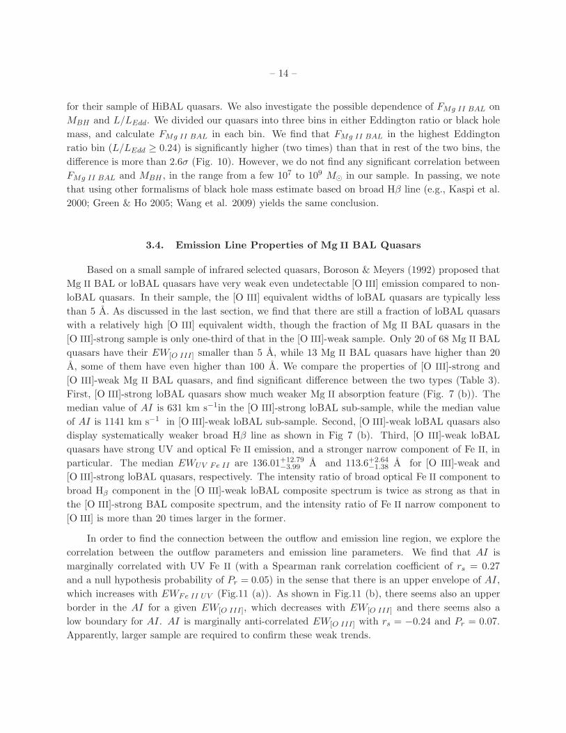
3.4. Emission Line Properties of Mg II BAL Quasars

Based on a small sample of infrared selected quasars, Boroson & Meyers (1992) proposed that

Mg II BAL or loBAL quasars have very weak even undetectable [O III] emission compared to non-

loBAL quasars. In their sample, the [O III] equivalent widths of loBAL quasars are typically less

than 5 A. As discussed in the last section, we find that there are still a fraction of loBAL quasars

with a relatively high [O III] equivalent width, though the fraction of Mg II BAL quasars in the

[O III]-strong sample is only one-third of that in the [O III]-weak sample. Only 20 of 68 Mg II BAL

quasars have their EW[O III] smaller than 5 A, while 13 Mg II BAL quasars have higher than 20

A, some of them have even higher than 100 A. We compare the properties of [O III]-strong and

[O III]-weak Mg II BAL quasars, and find significant difference between the two types (Table 3).

First, [O III]-strong loBAL quasars show much weaker Mg II absorption feature (Fig. 7 (b)). The

median value of AI is 631 km s−1in the [O III]-strong loBAL sub-sample, while the median value

of AI is 1141 km s−1 in [O III]-weak loBAL sub-sample. Second, [O III]-weak loBAL quasars also

display systematically weaker broad Hβ line as shown in Fig 7 (b). Third, [O III]-weak loBAL

quasars have strong UV and optical Fe II emission, and a stronger narrow component of Fe II, in

particular. The median EWUV Fe II are 136.01+12.79−3.99 A and 113.6+2.64

−1.38 A for [O III]-weak and

[O III]-strong loBAL quasars, respectively. The intensity ratio of broad optical Fe II component to

broad Hβ component in the [O III]-weak loBAL composite spectrum is twice as strong as that in

the [O III]-strong BAL composite spectrum, and the intensity ratio of Fe II narrow component to

[O III] is more than 20 times larger in the former.

In order to find the connection between the outflow and emission line region, we explore the

correlation between the outflow parameters and emission line parameters. We find that AI is

marginally correlated with UV Fe II (with a Spearman rank correlation coefficient of rs = 0.27

and a null hypothesis probability of Pr = 0.05) in the sense that there is an upper envelope of AI,

which increases with EWFe II UV (Fig.11 (a)). As shown in Fig.11 (b), there seems also an upper

border in the AI for a given EW[O III], which decreases with EW[O III] and there seems also a

low boundary for AI. AI is marginally anti-correlated EW[O III] with rs = −0.24 and Pr = 0.07.

Apparently, larger sample are required to confirm these weak trends.

– 15 –

3.5. Properties of Intermediate Width Mg II Absorption Line Quasars

In §2.2, we defined our criteria of Mg II BAL quasars by comparing the frequency of C IV

BAL with AI(∆vc ≥ 2000) > 0 at different cuts in ∆vc of Mg II absorption lines. We finally

choose a contiguous absorption with a minimum depth of 10% of the intrinsic emission spectrum

over a width ∆vc = 1600 km s−1. With this definition, we can identify BAL quasars with Mg II

absorption lines that are associated with BALs. Note that Trump et al. (2006) and some other

previous works have used 1000 km s−1 as the selection criteria for loBAL quasars. If quasars with

absorption width between 1000 km s−1 and 1600 km s−1 are true Mg II BAL, they should have

similar properties in the emission lines and continuum as these selected with ∆vc = 1600 km s−1.

In the following, we will check whether there is a clear distinction in the Mg II absorbers with a

width above and below 1600 km s−1.

In our low-z quasar sample, there are 68 Mg II BAL quasars with ∆vc ≥ 1600 km s−1, and

76 quasars with 1000 ≤ ∆vc < 1600km s−1 (hereafter lowV group). We compare continuum and

emission line properties of these two groups with non-Mg II BAL quasars as well as between the two

groups either statistically or using their composite spectra. Table 3 summarizes the emission line

parameters measured from the composite spectrum of lowV quasars. We find that the emission line

properties, including Fe II, [Ne V] and [O III] of lowV quasars are similar to non-Mg II BAL quasars,

but different from BAL quasars. However, the composite spectrum of lowV group is significantly

redder than that of non-Mg II BAL quasars.

We also measure the parameters of broad and narrow optical emission lines and continuum,

including Hβ profile, the equivalent width of UV Fe II and [Ne V], FWHM of [O III] and [O II],

λLλ(5100A) and β[3K,4K] for each quasar. Fig. 12 shows the distributions of line and continuum

parameters for the two samples of Mg II absorbers as well as that of non-Mg II BAL quasars.

Significant difference between lowV quasars and Mg II BAL quasars is found in distributions of

following parameters: the equivalent width of UV Fe II, [Ne V] and λLλ(5100A), as shown in

Fig.12. Kolmogorov-Smirnov (KS) test gives null probabilities of 9× 10−3, 6× 10−3 and 6× 10−5,

respectively, for UV Fe II, [Ne V] and λLλ(5100A), that their distributions are drawn from the

same parent population for lowV and Mg II BAL quasars. Mg II BAL quasars have weaker [Ne V]

and [O II], stronger optical Fe II and higher observed optical luminosity than lowV quasars. The

two groups have almost the same distributions in continuum slope. The lowV quasars show the

similar distributions of all emission line parameters as non-Mg II BAL quasars, except for a redder

continuum and lower observed optical luminosities.

4. Summary and Discussion

We have selected 68 Mg II BAL quasars from the SDSS spectroscopic quasar sample with a

redshift of 0.4 < z ≤ 0.8 and a median S/N ≥ 7 using criteria of a continuous absorption over a

velocity interval greater than 1600 km s−1 for a depth of at least 10%. The BAL-selected criterion

– 16 –

is a trade-off between the completeness and consistency with respect to the canonical definition of

BAL quasars that have the ’balnicity index’ BI > 0 in C IV BAL. We adopted such a criterion to

ensure that ∼ 90% of our sample are classical BAL quasars and the completeness is ∼ 80%, based

on extensive tests using high-z quasar samples with measurements of both C IV and Mg II BALs.

The low-z sample is used to define the fraction of Mg II BAL quasars and its dependence on the

continuum and emission line properties, the difference between Mg II and non-Mg II BAL quasars.

We find that, (1) the fraction of Mg II BAL quasars in the optical survey is around 1.2%. The

fraction does not include correction for internal dust extinction of BAL quasars and the color bias

against reddened loBAL quasars. After correcting these factors, the true Mg II BAL fraction is

likely in between 2% and 7%. (2) Mg II BAL quasars are more frequently found in quasars with

low [O III] equivalent width and high continuum luminosity although they show a wide range of

[O III] equivalent width. loBAL quasars display stronger narrow optical Fe II emission lines and

UV Fe II emission, weaker even absent [Ne V] lines. (3) The fraction of quasars with Mg II BAL

increases strongly with the Eddington ratio but does not correlate with the black hole mass. (4)

There is an excess of intrinsic reddening in Mg II BAL quasars and quasars with intermediate width

Mg II absorption lines with an average of 0.08 mag for SMC-like dust grain. In this section, we will

discuss the implication of our results.

It is generally believed that NELs are nearly isotropic in quasars because they are produced

in an extended region. In contrast the BEL region and continuum are thought to be much more

compact and can be blocked on some lines of sight by obscuration (e.g., Antonucci 1993). The

excess extinction in Mg II BAL quasars with respect to non-Mg II BAL quasars will enhance the

conclusion that [O III] equivalent width is lower in loBAL quasars. The conclusion will be further

strengthened if we consider the anisotropic emission of optical continuum from the accretion disk

because it is generally believed that BAL quasars are seen nearly edge-on. The large range of

observed EW[O III] among Mg II BAL quasars suggests that loBAL occurs in both [O III]-weak and

[O III]-strong emission quasars, but the covering factor decreases strongly as the [O III] strength

increases.

If [O III] is considered as an indicator of overall strength of NELs, the strength of other lines

relative to [O III] should connect more to the physical state of narrow-line region (NLR) or ionizing

continuum. The absence of [Ne V] in [O III]-weak Mg II BAL turns out to be a rather surprise.

Previous studies have suggested that [Ne V] is produced in the high density, inner NLR (e.g.,

Heckman et al. 1981; De Robertis & Osterbrock 1984; Whittle 1985a, 1985b). Lack of [Ne V]

emission indicates that there is no such region or the inner NLR does not expose to a hard ionizing

continuum. Interaction of BAL outflow with inner NLR may destroy dense clouds in the inner NLR.

However, the presence of strong narrow optical Fe II emission would suggest such dense inner NLR

does exist but with low ionization parameters (see Veron-Cetty et al. 2004; also Wang, Dai & Zhou

2008). Then we look at the option that the NLR only sees a soft ionizing continuum. BAL quasars,

loBAL quasars in particular, are weak in soft X-rays (Green et al. 1995; Brinkmann et al. 1999),

which are required to produce Ne4+ (ionization potential 97 eV). If NLR sees a continuum similar

– 17 –

to the observed one, the absence of [Ne V] can be naturally explained. Because the weakness of

soft X-rays in BAL quasars is usually attributed to X-ray absorption rather than intrinsic weakness

(Wang et al. 1999; Gallagher et al. 1999, 2002), this requires that the [Ne V] emission region is

behind the X-ray absorber. There are two possibilities for this, the outflow has a large covering

factor or [Ne V] emission region located coincidently behind the outflow. Nagao et al. (2001)

proposed that [Ne V] emission region is the inner region of the dust torus, and use the hypothesis

to explain the unification of two type Seyfert galaxies. In their scenarios, [Ne V] emission region

lies on the equatorial plane, which is coincident with the region shielded by disk wind.

In order to check this, we select 250 non-Mg II BAL quasars with S/N > 20, β[3K,4K] > −2.2

and EW[O III] < 20, out of which 119 quasars do not show detectable [Ne V] emission line in the

spectra. Fig. 13 shows the two composite spectra of these non-Mg II BAL quasars with/without

[Ne V] emission, the emission parameters are shown in Table 3. The composite spectrum of the

119 non-BAL quasars without [Ne V] is similar to that of Mg II BAL quasars, showing stronger

optical narrow Fe II emission, weak [O III] strength and strong UV Fe II but with a blue continuum.

These quasars are probably from the same parent population of loBAL quasars but our line of sight

does not intersect the outflow. The high fraction of non-BAL quasars without [Ne V] emission line

indicates that the covering factor of loBALR is not large.

Several observed trends may be explained by the strong correlation between the frequency of

loBAL and Eddington ratio, and the correlations of the Eddington ratio with the other parameters

concerned. It was reported that narrow optical Fe II strength is fairly well correlated with the

Eddington ratio for low redshift quasars (Dong et al. 2009b). Dietrich et al. (2002) demonstrated

that [O III] strength is inversely correlated with the Eddington ratio for quasars. Weakness of

Mg II in the red-side of Mg II line profile is difficult to be ascribed to the absorption, and can be

understood in this context as well via a fairly strong anti-correlation between EW of Mg II and the

Eddington ratio (Dong et al. 2009a). Thus, the Eddington ratio can be an underlying driver for the

different covering factor of low ionization BALR. We note that even in the highest Eddington ratio

bin, the fraction of loBAL quasars is only a factor of 2 of the value in the rest two low Eddington

ratio bins. There is no correlation between the fraction of loBAL with black hole mass for this

sub-sample. Narrow line Seyfert 1 galaxies (NLS1s) are believed to be the low mass counter-parts

of high accretion rate quasars. Zhou et al. (2006a; 2006b) found that several NLS1s also show Mg II

BALs. Twelve of our low-z Mg II BAL quasars can be formally classified as NLS1s according to

the formal criterion of Hβ < 2000 km s−1, which account for 1.6% of NLS1s in this redshift range.

Therefore, NLS1s do not appear to show significantly different properties from other quasars with

similar optical luminosity. The black hole mass range of these loBAL-NLS1s is very narrow with

[2.1, 7.8] ×107 M⊙. It is possible that black hole mass does not matter once it is above certain

threshold.

Finally, most quasars with Mg II BALs or intermediate width Mg II absorption lines show red-

dened colors. We already noticed that the two group quasars show significantly different properties

of emission lines, and the BAL fraction among the latter group is less than 25% (refer §2.2). Thus,

– 18 –

it is unlikely due to mixing of un-identified BAL quasars. The ubiquity of dust in intermediate

and LoBAL outflows may be naturally explained as both absorbers are large scale outflows (e.g.,

Dunn et al. 2010). The presence of dust will significantly boost the radiative force and thus it

allow gas in a relative large distance from the nucleus to be accelerated by the quasar radiation.

In other word, gas free from dust will not be accelerated to high velocity by radiation pressure. In

this case, dust reddening would be preferably observed in the outflow direction. As we have argued

that [Ne V]-weak quasars may be Mg II BAL quasars seen from an off-BALR direction, and their

color can be fairly blue, thus dust may not present in other direction. This is consistent with above

argument. Certainly, critical test for this can be done with a comparative study of broad band

infrared SED of BAL and non-BAL quasars.

Dust reddening is ubiquitous in broad (∆vc ≥ 1000 km s−1) Mg II absorbers, regardless of

whether they are BAL or non-BAL quasars. The average excess reddening is E(B-V) ∼ 0.08 mag for

SMC-type dust for both groups. However, we think that the intermediate width Mg II absorption

quasars might have somewhat lower reddening than Mg II BAL quasars. Because quasars with large

extinction, more likely BAL quasars, are missed in the SDSS quasar sample due to color selection

criteria of quasar target, this sample explores only the relative low extinction end of quasars. Thus

the similar color distribution for quasars with Mg II BAL and with intermediate width Mg II

absorption lines may be caused by the color selection effect that introduces a truncation in the

severely reddened quasars. Indeed, radio and infrared-selected Mg II BAL quasars show much

larger extinction with E(B-V) up to 1.5 mag (Urrutia et al. 2008), while there is no good statistical

work for intermediate width Mg II. So it is not conclusive whether Mg II BAL quasars and quasars

with intermediate width Mg II absorption lines have similar dust extinctions.

This work has made use of the data obtained by SDSS. Funding for the SDSS and SDSS-II

has been provided by the Alfred P. Sloan Foundation, the Participatings Institutions, the National

Science Foundation, the U.S. Department of Energy, the National Aeronautics and Space Adminis-

tration, the Japanese Monbukagakusho, the Max Planck Society, and the Higher Education Funding

Council for England. The SDSS Web Site is http://www.sdss.org/.

The SDSS is managed by the Astrophysical Research Consortium for the Participating Institu-

tions. The Participating Institutions are the American Museum of Natural History, Astrophysical

Institute Potsdam, University of Basel, University of Cambridge, Case Western Reserve University,

University of Chicago, Drexel University, Fermilab, the Institute for Advanced Study, the Japan

Participation Group, Johns Hopkins University, the Joint Institute for Nuclear Astrophysics, the

Kavli Institute for Particle Astrophysics and Cosmology, the Korean Scientist Group, the Chinese

Academy of Sciences (LAMOST), Los Alamos National Laboratory, the Max-Planck-Institute for

Astronomy (MPIA), the Max-Planck-Institute for Astrophysics (MPA), New Mexico State Univer-

sity, Ohio State University, University of Pittsburgh, University of Portsmouth, Princeton Univer-

sity, the United States Naval Observatory, and the University of Washington.

– 19 –

REFERENCES

Alonso-Herrero, A., et al. 2006, ApJ, 640, 167

Antonucci, R. 1993, ARA&A, 31, 473

Becker, R. H., White, R. L., Gregg, M. D., Brotherton, M. S., Laurent-Muehleisen, S. A., & Arav,

N. 2000, ApJ, 538, 72

Boroson, T. A. 2002, ApJ, 565, 78

Boroson, T. A., & Green, R. F. 1992, ApJS, 80, 109

Boroson, T. A., & Meyers, K. A. 1992, ApJ, 397, 442

Brandt, W. N., Laor, A., & Wills, B. J. 2000, ApJ, 528, 637

Brinkmann, W., Wang, T., Matsuoka, M., & Yuan, W. 1999, A&A, 345, 43

Brotherton, M. S., Tran, H. D., Becker, R. H., Gregg, M. D., Laurent-Muehleisen, S. A., & White,

R. L. 2001, ApJ, 546, 775

Brotherton, M. S., De Breuck, C., & Schaefer, J. J. 2006, MNRAS, 372, L58

Cohen, M. H., Ogle, P. M., Tran, H. D., Vermeulen, R. C., Miller, J. S., Goodrich, R. W., & Martel,

A. R. 1995, ApJ, 448, L77

Cutri, R. M., Nelson, B. O., Kirkpatrick, J. D., Huchra, J. P., & Smith, P. S. 2001, Bulletin of the

American Astronomical Society, 33, 829

Dai, X., Shankar, F., & Sivakoff, G. R. 2008, ApJ, 672, 108

De Robertis, M. M., & Osterbrock, D. E. 1984, ApJ, 286, 171

Dietrich, M., Hamann, F., Shields, J. C., Constantin, A., Vestergaard, M., Chaffee, F., Foltz, C. B.,

& Junkkarinen, V. T. 2002, ApJ, 581, 912

Dong, X.-B., Wang, T.-G., Wang, J.-G., Fan, X., Wang, H., Zhou, H., & Yuan, W. 2009a, ApJ,

703, L1

Dong, X., Wang, J., Wang, T., Wang, H., Fan, X., Zhou, H., & Yuan, W. 2009b, arXiv:0903.5020

Dong, X., Wang, T., Wang, J., Yuan, W., Zhou, H., Dai, H., & Zhang, K. 2008, MNRAS, 383, 581

Dunn, J. P., et al. 2010, ApJ, 709, 611

Egami, E., Iwamuro, F., Maihara, T., Oya, S., & Cowie, L. L. 1996, AJ, 112, 73

Fan, L. L., Wang, H. Y., Wang, T., Wang, J., Dong, X., Zhang, K., & Cheng, F. 2009, ApJ, 690,

1006

– 20 –

Fitzpatrick, E. L. 1999, PASP, 111, 63

Forster, K., Green, P. J., Aldcroft, T. L., Vestergaard, M., Foltz, C. B., & Hewett, P. C. 2001,

ApJS, 134, 35

Fox, J. 1997, Applied Regression Analysis, Linear Models, and Related Methods (Thousand Oaks,

CA: Sage Publications), 438

Gallagher, S. C., Brandt, W. N., Chartas, G., & Garmire, G. P. 2002, ApJ, 567, 37

Gallagher, S. C., Brandt, W. N., Chartas, G., Priddey, R., Garmire, G. P., & Sambruna, R. M.

2006, ApJ, 644, 709

Gallagher, S. C., Brandt, W. N., Sambruna, R. M., Mathur, S., & Yamasaki, N. 1999, ApJ, 519,

549

Gallagher, S. C., Hines, D. C., Blaylock, M., Priddey, R. S., Brandt, W. N., & Egami, E. E. 2007,

ApJ, 665, 157

Ganguly, R., & Brotherton, M. S. 2008, ApJ, 672, 102

Ganguly, R., Brotherton, M. S., Cales, S., Scoggins, B., Shang, Z., & Vestergaard, M. 2007, ApJ,

665, 990

Ghosh, K. K., & Punsly, B. 2007, ApJ, 661, L139

Gibson, R. R., et al. 2009, ApJ, 692, 758

Glikman, E., Gregg, M. D., Lacy, M., Helfand, D. J., Becker, R. H., & White, R. L. 2004, ApJ,

607, 60

Glikman, E., Helfand, D. J., White, R. L., Becker, R. H., Gregg, M. D., & Lacy, M. 2007, ApJ,

667, 673

Goodrich, R. W., & Miller, J. S. 1995, ApJ, 448, L73

Green, P. J., et al. 1995, ApJ, 450, 51

Greene, J. E., & Ho, L. C. 2005, ApJ, 630, 122

Hall, P. B., et al. 2002, ApJS, 141, 267

Hamann, F., & Ferland, G. 1993, ApJ, 418, 11

Hewett, P. C., & Foltz, C. B. 2003, AJ, 125, 1784

Hines, D. C., & Wills, B. J. 1995, ApJ, 448, L69

Jiang, D. R., & Wang, T. G. 2003, A&A, 397, L13

– 21 –

Kaspi, S., Smith, P. S., Netzer, H., Maoz, D., Jannuzi, B. T., & Giveon, U. 2000, ApJ, 533, 631

Knigge, C., Scaringi, S., Goad, M. R., & Cottis, C. E. 2008, MNRAS, 386, 1426

Konigl, A., & Kartje, J. F. 1994, ApJ, 434, 446

Korista, K. T., et al. 1993, ApJ, 413, 445

Lacy, M., et al. 2004, ApJS, 154, 166

Maddox, N., & Hewett, P. C. 2008, Memorie della Societa Astronomica Italiana, 79, 1117

Maddox, N., Hewett, P. C., Warren, S. J., & Croom, S. M. 2008, MNRAS, 386, 1605

Martınez-Sansigre, A., Rawlings, S., Lacy, M., Fadda, D., Marleau, F. R., Simpson, C., Willott,

C. J., & Jarvis, M. J. 2005, Nature, 436, 666

Nagao, T., Murayama, T., & Taniguchi, Y. 2001, PASJ, 53, 629

Ogle, P. M., Cohen, M. H., Miller, J. S., Tran, H. D., Goodrich, R. W., & Martel, A. R. 1999,

ApJS, 125, 1

Polletta, M., et al. 2007, ApJ, 663, 81

Reichard, T. A., et al. 2003a, AJ, 125, 1711

Reichard, T. A., et al. 2003b, AJ, 126, 2594

Richards, G. T., et al. 2003, AJ, 126, 1131

Sanders, D. B., Soifer, B. T., Elias, J. H., Neugebauer, G., & Matthews, K. 1988, ApJ, 328, L35

Schlegel, D. J., Finkbeiner, D. P., & Davis, M. 1998, ApJ, 500, 525

Schmidt, G. D., & Hines, D. C. 1999, ApJ, 512, 125

Schneider, D. P., et al. 2007, AJ, 134, 102

Skrutskie, M. F., et al. 2006, AJ, 131, 1163

Stern, D., et al. 2007, ApJ, 663, 677

Tolea, A., Krolik, J. H., & Tsvetanov, Z. 2002, ApJ, 578, L31

Trump, J. R., et al. 2006, ApJS, 165, 1

Turnshek, D. A., Monier, E. M., Sirola, C. J., & Espey, B. R. 1997, ApJ, 476, 40

Urrutia, T., Lacy, M., & Becker, R. H. 2008, ApJ, 674, 80

– 22 –

Vanden Berk, D. E., et al. 2001, AJ, 122, 549

Veron-Cetty, M.-P., Joly, M., & Veron, P. 2004, A&A, 417, 515

Vestergaard, M., & Peterson, B. M. 2006, ApJ, 641, 689

Vestergaard, M., & Wilkes, B. J. 2001, ApJS, 134, 1

Voit, G. M., Weymann, R. J., & Korista, K. T. 1993, ApJ, 413, 95

Wang, J., Jiang, P., Zhou, H., Wang, T., Dong, X., & Wang, H. 2008a, ApJ, 676, L97

Wang, T., Dai, H., & Zhou, H. 2008b, ApJ, 674, 668

Wang, T. G., Wang, J. X., Brinkmann, W., & Matsuoka, M. 1999, ApJ, 519, L35

Wang, H.-Y., Wang, T.-G., & Wang, J.-X. 2005, ApJ, 634, 149

Wang, J.-G., et al. 2009, ApJ, 707, 1334

Weymann, R. J. 2002, Mass Outflow in Active Galactic Nuclei: New Perspectives, 255, 329

Weymann, R. J., Morris, S. L., Foltz, C. B., & Hewett, P. C. 1991, ApJ, 373, 23

White, R. L., Helfand, D. J., Becker, R. H., Gregg, M. D., Postman, M., Lauer, T. R., & Oegerle,

W. 2003, AJ, 126, 706

Whittle, M. 1985a, MNRAS, 213, 1

Whittle, M. 1985b, MNRAS, 216, 817

Willott, C. J., Rawlings, S., & Grimes, J. A. 2003, ApJ, 598, 909

York, D. G., et al. 2000, AJ, 120, 1579

Zhou, H., Wang, T., Wang, H., Wang, J., Yuan, W., & Lu, Y. 2006a, ApJ, 639, 716

Zhou, H., Wang, T., Yuan, W., Lu, H., Dong, X., Wang, J., & Lu, Y. 2006b, ApJS, 166, 128

This preprint was prepared with the AAS LATEX macros v5.0.

– 23 –

Table 1. Different Definition for the BAL Quasars

vl vu ∆vc Reference

BI 3,000 25,000 2,000 Weymann et al. 1991

Tolea et al. 2002

Reichard et al. 2003a

Trump et al. 2006

G09

BI 0 25,000 1,000 Reichard et al. 2003a

BI0 0 25,000 2,000 G09

AI 0 25,000 450 Hall et al. 2002

AI 0 29,000 1,000 Trump et al. 2006

AI 0 20,000 1,600 This work

–24

–

Table 2. Low-z Mg II BAL Quasars Catalog in SDSS DR5

Namea R.A. Decl. Redshift AI deepthbmax V c

max V dmin V e

ave λLλ(5100A) β[3K,4K] EW[O III] EW[Ne V ] MBH L/LEDD

J2000 J2000 km s−1 km s−1 km s−1 km s−1 1044 erg s−1 A A 108 M⊙

010352.46+003739.7 15.968604 0.627704 0.7031 480± 1 0.73 11500 9100 10280 22. -1.21 15.1 0.6 16. 0.097

023102.49-083141.2 37.760410 -8.528133 0.5868 303± 2 0.72 3750 2100 2966 3.5 -2.04 18.5 0.9 2.1 0.12

025026.66+000903.4 42.611093 0.150945 0.5963 1032± 8 0.32 3400 750 2066 5.4 0.99 24.2 3.6 37. 0.010

080934.64+254837.9 122.394340 25.810552 0.5454 519± 1 0.49 1600 0 665 9.2 -2.11 13.4 0.4 18. 0.036

081655.34+074311.5 124.230604 7.719886 0.6442 312± 2 0.75 5500 3750 4703 5.7 -1.52 18.1 3.9 2.6 0.15

082231.53+231152.0 125.631381 23.197803 0.6530 677± 1 0.42 2350 450 1346 18. -1.62 51.0 2.2 50. 0.027

083525.98+435211.2 128.858253 43.869796 0.5678 781± 2 0.66 20000 16250 18120 13. -1.58 4.3 0.0 6.0 0.16

083613.23+280512.1† 129.055150 28.086698 0.7412 4105± 11 0.30 17050 5800 10546 5.3 -1.51 7.0 0.0 0.73 0.52

084716.04+373218.0 131.816838 37.538359 0.4539 347± 2 0.73 4100 2400 3265 3.5 -2.22 156.6 4.5 0.98 0.26

085215.66+492040.8 133.065270 49.344685 0.5664 1143± 4 0.14 2250 0 1202 4.3 -1.50 10.7 0.7 4.1 0.076

085357.87+463350.6 133.491147 46.564063 0.5497 418± 1 0.62 4400 2800 3642 8.2 -1.47 3.5 0.2 6.2 0.095

091146.06+403501.1† 137.941942 40.583652 0.4412 1053± 7 0.33 6100 3150 4082 2.9 -0.09 21.2 2.4 0.41 0.51

092157.62+103539.0† 140.490091 10.594188 0.5476 1730± 8 0.49 8950 3250 6068 2.7 -1.61 7.4 0.5 0.33 0.58

092928.63+324129.9 142.369302 32.691639 0.7748 279 ± 2 0.79 9900 8050 8997 1.3 -1.78 9.3 0.2 5.3 0.18

093034.79+570520.7 142.644964 57.089097 0.6374 314 ± 2 0.72 10350 8750 9493 6.8 -2.00 7.1 0.0 1.7 0.29

094443.13+062507.4 146.179709 6.418734 0.6951 1532± 1 0.48 9300 4300 7245 69. -1.42 2.9 0.0 18. 0.28

101203.31+492148.2 153.013803 49.363391 0.7389 1030± 3 0.56 7650 700 4029 8.5 -1.73 1.1 0.0 15. 0.041

102021.21+121909.1 155.088391 12.319199 0.4793 3320± 17 0.31 18350 0 11309 4.0 -0.05 2.4 0.0 1.0 0.28

102802.32+592906.6 157.009676 59.485190 0.5349 995± 3 0.36 2650 300 1421 2.5 -2.11 7.1 0.9 2.5 0.072

102839.11+450009.4 157.162961 45.002620 0.5826 773± 1 0.41 2450 100 1204 24. -1.41 11.8 0.0 8.9 0.20

103621.60+393701.6 159.090011 39.617129 0.7997 777± 1 0.48 3100 200 1488 40. -1.31 5.0 0.0 48. 0.059

104210.43+501609.2 160.543497 50.269224 0.7873 1384± 1 0.13 3650 1050 2503 20. -2.23 1.1 1.8 21. 0.070

104459.60+365605.1 161.248363 36.934775 0.7015 3578± 2 0.02 17650 800 6311 42. -1.34 1.7 0.0 9.1 0.33

105259.99+065358.1† 163.249983 6.899474 0.7224 2508± 7 0.53 12900 4600 8792 8.9 -1.27 9.8 0.0 0.69 0.92

112632.81+430938.6 171.636726 43.160726 0.4356 886± 3 0.24 1800 0 874 6.2 -0.05 5.2 0.7 3.9 0.11

112730.71+423039.0 171.877963 42.510858 0.5310 391± 4 0.52 19050 17300 18079 3.3 -1.81 67.3 4.9 0.75 0.31

112822.41+482309.9 172.093398 48.386109 0.5428 370± 1 0.57 4450 2850 3565 16. -0.83 2.7 0.0 15. 0.077

112912.27+422853.9† 172.301146 42.481651 0.5805 308± 3 0.74 6250 4500 5362 4.6 -1.16 15.4 0.0 0.57 0.58

113355.22+111208.8 173.480118 11.202465 0.7612 706± 4 0.65 10250 5400 7829 6.4 -1.91 4.5 0.0 0.98 0.46

113807.83+531231.7 174.532647 53.208815 0.7899 843± 3 0.36 4700 2750 3790 1.1 -1.38 5.8 0.0 3.5 0.23

114043.62+532439.0 175.181765 53.410835 0.5304 886± 4 0.37 3650 1350 2612 4.5 -1.69 17.9 3.3 8.4 0.039

114915.30+393325.4† 177.313775 39.557076 0.6284 1291± 7 0.46 5050 1600 3326 4.2 -1.25 23.9 1.2 0.33 0.90

115816.72+132624.1† 179.569678 13.440048 0.4389 949± 2 0.60 8650 4750 6484 7.7 -1.62 18.2 0.1 0.65 0.85

121113.38+121937.3 182.805763 12.327049 0.4641 1441± 4 0.18 3950 600 2076 3.1 -0.78 24.4 0.0 2.1 0.11

121303.40-014450.9 183.264183 -1.747485 0.6123 684± 3 0.37 4200 2350 3250 7.8 -1.27 11.6 0.0 1.9 0.29

122043.21-013215.3 185.180046 -1.537600 0.4478 915± 6 0.33 2100 100 990 1.8 -1.41 160.5 6.5 12. 0.011

124300.87+153510.6 190.753663 15.586296 0.5609 1173± 2 0.16 1700 0 856 5.5 -1.56 37.5 0.7 9.2 0.043

125057.57+402100.3 192.739909 40.350086 0.6070 1789± 8 0.05 8350 2550 4427 3.9 -1.25 3.0 1.2 1.2 0.24

125942.80+121312.6† 194.928337 12.220168 0.7487 2716± 10 0.49 13400 2250 7892 12. -0.57 14.7 0.0 0.93 0.94

130741.12+503106.5 196.921364 50.518476 0.6987 1714± 3 0.09 6250 2500 4127 13. -0.81 0.61 0.0 22. 0.042

131823.73+123812.6 199.598896 12.636836 0.5848 1804± 5 0.07 4150 700 2384 3.2 -1.51 4.9 4.9 7.1 0.033

132114.42+020225.0 200.310112 2.040294 0.5813 445± 4 0.58 5050 3200 4059 3.2 -0.56 17.6 0.0 0.95 0.24

133936.69+111949.2 204.902879 11.330361 0.6489 382± 4 0.65 7050 5300 6199 4.9 -1.34 9.1 0.6 0.91 0.39

134415.75+331719.1†‡ 206.065639 33.288650 0.6856 771± 2 0.30 1800 0 901 7.7 -1.28 112.4 5.2 0.82 0.68

135418.26+585935.9 208.576089 58.993326 0.7907 827± 5 0.38 3850 1750 2893 6.3 -0.81 33.1 1.7 1.1 0.40

140025.53-012957.0 210.106416 -1.499180 0.5839 1013± 5 0.38 20000 17400 18844 6.5 -0.98 4.0 0.0 3.3 0.14

142649.24+032517.7 216.705181 3.421588 0.5295 480± 3 0.63 3450 1600 2637 5.3 -1.25 5.9 0.0 4.4 0.086

142927.28+523849.5 217.363680 52.647085 0.5939 1009± 2 0.63 5900 2050 3957 15. -1.25 8.2 0.0 2.9 0.38

143303.27+403105.1 218.263643 40.518104 0.4452 680± 4 0.38 3350 1200 2324 2.4 -1.80 15.9 1.2 1.9 0.089

143828.63+452108.6 219.619318 45.352395 0.4268 324± 3 0.74 8250 6500 7367 3.2 -1.95 18.8 0.3 0.67 0.34

–25

–

Table 2—Continued

Namea R.A. Decl. Redshift AI deepthbmax V c

max V dmin V e

ave λLλ(5100A) β[3K,4K] EW[O III] EW[Ne V ] MBH L/LEDD

J2000 J2000 km s−1 km s−1 km s−1 km s−1 1044 erg s−1 A A 108 M⊙

144642.26+454631.0 221.676097 45.775287 0.7364 675± 4 0.58 5450 2950 4198 12. -1.09 0.0 0.9 4.2 0.20

145724.01+452157.7† 224.350045 45.366055 0.7175 1691± 5 0.62 14200 6800 10259 8.6 -1.45 2.8 0.0 0.95 0.65

145736.70+523454.6 224.402944 52.581834 0.6376 1194± 4 0.68 9150 3600 6041 11. -1.74 8.7 0.2 2.4 0.34

145836.73+433015.5 224.653068 43.504323 0.7595 615± 5 0.62 6500 3850 5122 9.7 -1.58 4.7 0.5 6.5 0.11

150847.41+340437.7 227.197577 34.077147 0.7880 722± 1 0.52 2850 200 1573 34. -1.48 134.1 5.8 30. 0.083

152350.42+391405.2 230.960111 39.234787 0.6612 3227± 2 0.43 20000 11500 16458 38. -1.14 4.8 0.1 39. 0.069

153036.82+370439.1 232.653452 37.077543 0.4170 1911± 5 0.44 8100 2000 4657 7.0 -1.20 13.5 0.3 1.2 0.44

160329.72+502722.2 240.873867 50.456176 0.6389 762± 5 0.49 5300 2800 4133 4.5 -1.61 23.3 2.3 2.4 0.13

160628.06+290333.8 241.616939 29.059398 0.4347 489± 3 0.63 3650 1500 2696 9.1 -0.14 8.3 4.3 1.3 0.49

160721.27+515510.6 241.838665 51.919619 0.7739 404± 3 0.63 6800 5200 5909 6.9 -2.19 4.7 2.3 0.88 0.57

163255.46+420407.7 248.231106 42.068816 0.7263 1152± 4 0.56 8650 750 3985 7.8 -1.53 18.2 4.7 39 0.014

163513.51+213859.6† 248.806315 21.649900 0.6835 573± 5 0.69 6950 4300 5620 4.9 -1.57 6.3 0.3 0.61 0.58

165225.39+215830.7 253.105807 21.975220 0.4468 1155 ± 12 0.42 7850 4450 6170 3.6 -0.26 18.8 0.0 0.68 0.38

170010.83+395545.8† 255.045127 39.929392 0.5766 462 ± 6 0.67 5550 3750 4594 3.7 -0.69 12.5 1.2 0.51 0.52

170341.82+383944.7 255.924255 38.662439 0.5539 785 ± 7 0.43 5000 2750 3949 5.9 0.01 8.1 1.9 5.0 0.084

204333.20-001104.2 310.888342 -0.184524 0.5449 2074 ± 4 0.16 8250 2750 5061 8.9 -1.12 7.7 0.0 2.0 0.31

210757.67-062010.6 316.990293 -6.336294 0.6456 2344 ± 1 0.21 8250 0 3709 27. 0.01 18.5 1.9 76. 0.026

224028.14-003813.1 340.117275 -0.636989 0.6591 1364 ± 2 0.23 3650 750 1994 9.9 -1.19 8.2 0.0 8.1 0.087

aSDSS DR5 designation, hhmmss.ss+ddmmss.s (J2000.0)

bDeepest part of any BAL trough

cMaximum velocity of the BAL troughs from the emission line

dMinimum velocity of the BAL troughs from the emission line

eWeighted average velocity of the BAL troughs

†narrow-line Seyfert 1

‡double-peaked narrow lines

–26

–

Table 3. Parameters of Emission Lines from Composite Spectra

N-B-Ha N-B-L M-F-H N-F-H M-F-L N-F-L N-R-H M-R-L N-R-L no[Ne V]b [Ne V]c nonBAL LowVd BALe

EW[O III] (A) 38.0 12.4 58.0 36.8 8.7 10.7 38.4 5.8 10.7 8.1 19.5 18.4 21.9 14.2

[O III] 1 1 1 1 1 1 1 1 1 1 1 1 1 1

HβN 0.051 0.035 0.060 0.068 0.098 0.16 0.071 0.11 0.098 0.26 0.19 0.084 0.058 0.19

HγN 0.030 0.035 0.041 0.039 0.083 0.079 0.032 0.046 0.036 0.11 0.12 0.048 0.0792 0.097

OptFeIIN 0.16 0.24 0.088 0.057 3.4 1.8 0.13 1.7 0.67 4.8 0.52 0.41 0.45 2.0

[Ne V] 0.065 0.091 0.070 0.077 0.017 0.089 0.081 0.0092 0.14 0.00070 0.089 0.083 0.084 0.051

[O II] 0.070 0.051 0.083 0.097 0.14 0.11 0.15 0.29 0.18 0.083 0.078 0.14 0.11 0.15

[Ne III] 0.086 0.12 0.067 0.099 0.098 0.16 0.12 0.29 0.21 0.18 0.11 0.15 0.15 0.10

EWHβB (A) 117.7 75.7 89.9 74.9 68.4 61.1 60.3 57.5 50.6 66.5 78.4 76.9 71.6 69.5

HβB 1 1 1 1 1 1 1 1 1 1 1 1 1 1

HγB 0.28 0.23 0.24 0.24 0.25 0.24 0.26 0.29 0.21 0.26 0.21 0.25 0.23 0.24

OptFeIIB 0.77 2.2 0.79 1.4 3.5 3.6 1.4 3.3 3.2 3.7 2.4 2.2 2.2 2.7

aNames of the composite spectra: X-Y-Z

X: N– non-Mg II BAL quasar; M– Mg II BAL quasar

Y: B– β[3K,4K] ≤ −2.2; F– −2.2 < β[3K,4K] ≤ −1; R– β[3K,4K] > −1

Z: H– EW[O III] ≥ 20 A; L– EW[O III] < 20 A

bThe composite spectrum of non-Mg II BAL quasars with S/N > 20 and undetectable [Ne V] emission

cThe composite spectrum of non-Mg II BAL quasars with S/N > 20 and detectable [Ne V] emission

dThe composite spectrum of 1000 km s−1≤ ∆vc < 1600 km s−1selected quasars in low-z quasar sub-sample

eThe composite spectrum of ∆vc > 1600 km s−1selected Mg II BAL quasars in low-z quasar sub-sample

– 27 –

Fig. 1.— Observed spectra overplayed with the best-fit models for the six quasars in the high-z

sample. The models are described in detail in §2.1. In each panel, we plot the observed spectrum

in black curves, power-law continuum in pink, broadened Fe II template in blue, Gaussian Mg II

emission line in green, and the model sum in red.

800 1000 1200 1400 1600 1800 2000∆ vc (km s-1)

0

20

40

60

80

100

com

plet

enes

s c2

(%

)

0

20

40

60

80

100

corr

ectn

ess

c1 (

%)

Fig. 2.— Correctness c1 (black filled circles) and completeness c2 (red filled squares) of BAL

quasars as a function of Mg II absorption-line width cutoff ∆vc.

– 28 –

Fig. 3.— Observed spectra and our best-fit models of the low-z sample of 68 Mg II BAL quasars,

including 41 classified as such by both of us and G09 (marked with ”B”), and 27 in this work but

not in G09 (marked with ”A”). Also shown here are eight objects that are not classified as Mg II

BAL quasars according to our new criterion, but are classified as such in G09 (marked with ”L”).

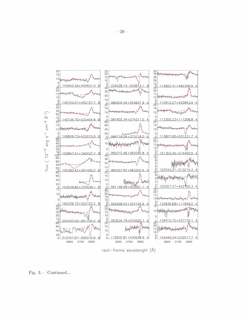
– 29 –

Fig. 3.— Continued...

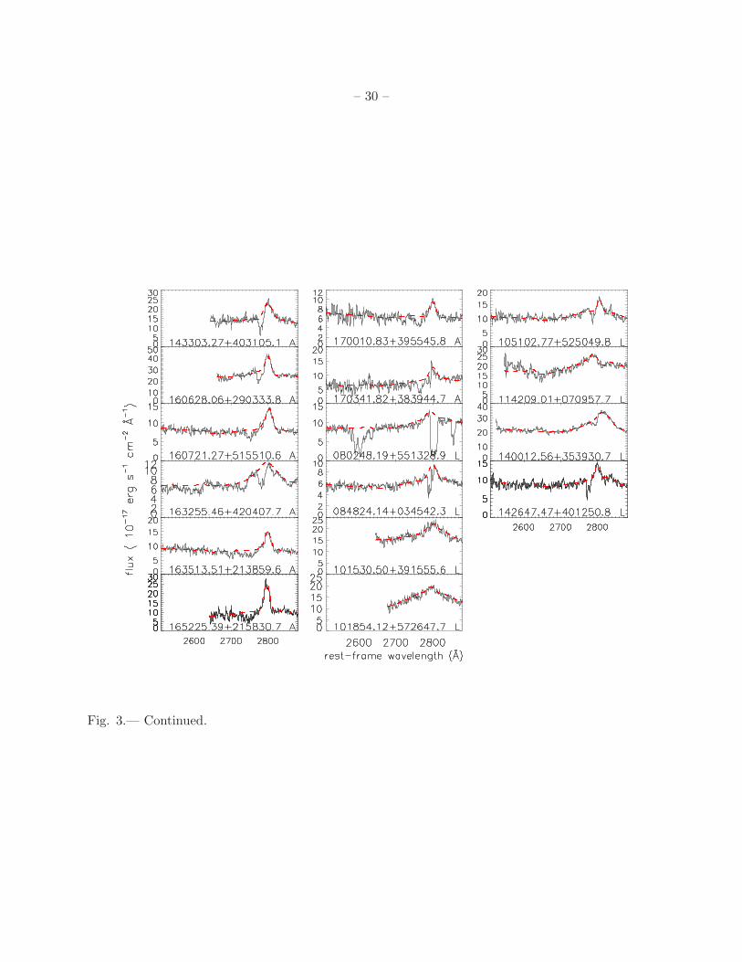
– 30 –

Fig. 3.— Continued.

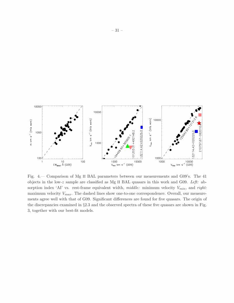
– 31 –

Fig. 4.— Comparison of Mg II BAL parameters between our measurements and G09’s. The 41

objects in the low-z sample are classified as Mg II BAL quasars in this work and G09. Left: ab-

sorption index ‘AI’ vs. rest-frame equivalent width, middle: minimum velocity Vmin, and right:

maximum velocity Vmax. The dashed lines show one-to-one correspondence. Overall, our measure-

ments agree well with that of G09. Significant differences are found for five quasars. The origin of

the discrepancies examined in §2.3 and the observed spectra of these five quasars are shown in Fig.

3, together with our best-fit models.

– 32 –

0.0

0.1

0.2

0.3 (a)

-3 -2 -1 0β[3K,4K]

EW

[O II

I]

10-1

1

10

102

(b)

Fig. 5.— Panel (a): Comparison of the distribution of continuum slope β[3K,4K] between Mg II

BAL quasars (red dash line) and non-loBAL quasars (black thick line). It is obvious that Mg II

BAL quasars are much redder than non-loBAL quasars. The β[3K,4K] distribution of non-Mg II

BAL quasars peaks at -2.2, much less than the value of -1.7 for Mg II BAL quasars. The median

value of β[3K,4K] is -2.08 for non-Mg II BAL quasars, and it is -1.41 for Mg II BAL quasars. Panel

(b): Equivalent width of O III NEL EW[O III] plotted against continuum slope β[3K,4K] for the

low-z sample. Mg II loBAL quasars are shown in filled red squares, and non-loBAL quasars in

filled black circles.

– 33 –

Fig. 6.— Comparison of the UV-optical-NIR SED of Mg II BAL and non-loBAL quasars. All the

data are normalized at the SDSS i-band. The different bands of Mg II BAL quasars are shown by

filled circle in different colors. The black filled circles show the mean SED of non-loBAL quasars,

with the upper and lower quartile denoted by error bars.

– 34 –

Fig. 7.— Panel (a)–Composite spectra of the full non-Mg II BAL quasars sample(black), Mg II

BAL quasars sample(gray) and the blue curve is the de-reddened composite spectra of Mg II BAL

quasars; Panel (b)–Composite spectra of the Mg II BAL quasars with different continuum color

and intensity of [O III] emission line, black for the flat and [O III]-weak sources, red means red and

[O III]-weak and blue curve shows the Mg II BAL composite with flat and [O III]-strong; Panel

(c) and (d)–Composite spectra of the quasars without Mg II broad absorption troughs. The three

colors (black, blue and red) means that continuum slopes are blue, flat and red. (see the text §3.2)

– 35 –

Fig. 8.— Fraction of Mg II BAL quasars in the low-z sample as a function of the median S/N ratio

of the SDSS spectra (left panel) and the luminosity at 5100A(right panel). The median S/N ratios

are calculated in the rest-frame wavelength range of 2820−3200 A. The whole sample are shown in

black, and the high and low luminosity sub-samples are shown in red and blue, respectively. The

two luminosity sub-samples are so carved that they have the same number of quasars.

– 36 –

10 20 30 40EW[O III]

0

1

2

3

4

FM

g II

BA

L (%

)

Fig. 9.— Fraction of Mg II BAL quasars observed in low-z sample as a function of the equivalent

width of [O III] λ5007 NEL (black). Each point in the plot represents the fraction of Mg II BAL

quasars in a bin of 2522 quasars arranged in order of increasing EW[O III]. The x-coordinate of each

point represents the median value of the bin. The ”error bars” represent 1σ limits on the fractions

calculated using a binomial distribution. We also show the connection in the two λLλ(5100A)

quasar bins, the red and blue lines correspond to the high and low λLλ(5100A) bins.

– 37 –

7.5 8.0 8.5 9.0 9.5log MBH

0.0

0.5

1.0

1.5

FM

g II

BA

L (%

)

0.1L / LEDD

0.0

0.5

1.0

1.5

2.0

FM

g II

BA

L (%

)

Fig. 10.— Fraction of Mg II BAL quasars in the low-z sample as a function of black hole mass (left

panel) and Eddington ratio (right panel).

– 38 –

EW[O III]

102

10-1 1 10 102

103

104

(a)

AI

EWFeII UV

(b)

102 103

Fig. 11.— Plots of Mg II absorption index against the equivalent width of [O III] (left panel) and

UV Fe II (right panel) emission lines.

– 39 –

Fig. 12.— Statistical properties of lowV group(green) and Mg II BAL quasar sample (red). The

black line are non-loBAL quasars as the comparison sample.

– 40 –

Fig. 13.— Composite spectrum of non-loBAL quasars with/without detectable [Ne V] emission.