arX

iv:0

709.

2190

v1 [

astr

o-ph

] 1

4 Se

p 20

07

White Dwarf Luminosity and Mass Functions from Sloan Digital

Sky Survey Spectra

Steven DeGennaro1, Ted von Hippel1, D. E. Winget1, S. O. Kepler2, Atsuko Nitta3, Detlev

Koester4, Leandro Althaus5,6

ABSTRACT

We present the first phase in our ongoing work to use Sloan Digital Sky Survey

(SDSS) data to create separate white dwarf (WD) luminosity functions for two or

more different mass ranges. In this paper, we determine the completeness of the

SDSS spectroscopic white dwarf sample by comparing a proper-motion selected

sample of WDs from SDSS imaging data with a large catalog of spectroscopically

determined WDs. We derive a selection probability as a function of a single color

(g− i) and apparent magnitude (g) that covers the range −1.0 < g− i < 0.2 and

15 < g < 19.5. We address the observed upturn in log g for white dwarfs with

Teff . 12,000K and offer arguments that the problem is limited to the line profiles

and is not present in the continuum. We offer an empirical method of removing

the upturn, recovering a reasonable mass function for white dwarfs with Teff <

12,000K. Finally, we present a white dwarf luminosity function with nearly an

order of magnitude (3,358) more spectroscopically confirmed white dwarfs than

any previous work.

Subject headings: white dwarfs — stars: luminosity function — stars: mass

function

1The University of Texas at Austin, Department of Astronomy, 1 University Station C1400, Austin, TX

78712-0259

2Instituto de Fısica, Universidade Federal do Rio Grande do Sul, 91501-900 Porto-Alegre,RS,Brazil

3Gemini Observatory, Hilo, HI 96720, USA

4Institut fur Theoretische Physik und Astrophysik, Universitat Kiel, 24098 Kiel, Germany

5Facultad de Ciencias Astronomicas y Geofısicas, Universidad Nacional de La Plata, Paseo del Bosque

S/N, 1900, La Plata, Argentina

6Instituto de Astrofısica La Plata, IALP, CONICET

– 2 –

1. Introduction

Because white dwarfs cannot replenish the energy they radiate away—any residual nu-

clear burning is negligible and gravitational contraction is severely impeded by electron

degeneracy—their luminosity decreases monotonically with time. A thorough knowledge

of the rate at which WDs cool can provide a valuable “cosmic clock” to determine the

ages of many Galactic populations, including the disk (Winget et al. 1987; Liebert et al.

1988; Leggett et al. 1998; Knox et al. 1999), and open and globular clusters (Claver 1995;

von Hippel et al. 1995; Richer et al. 1998; Claver et al. 2001; Hansen et al. 2002, 2004; von Hippel et al.

2006; Hansen et al. 2007; Jeffery et al. 2007). With more accurate models of the cooling

physics of white dwarfs, heavily constrained by empirical evidence, it may be possible to

determine absolute ages with greater precision than using main-sequence evolution theory.

In addition to applications in astronomy, white dwarfs allow us to probe the physics of

degenerate matter at temperatures and densities no terrestrial laboratory can duplicate.

Attempts at an empirical luminosity function (LF) for white dwarfs date as far back

as Luyten (1958) and Weidemann (1967). The low-luminosity shortfall, discovered by

Liebert et al. (1979), and attributed by Winget et al. (1987) to the finite age of the Galactic

disk, was confirmed and explored more fully when a greater volume of reliable data on low-

luminosity WDs became available (Liebert et al. 1988; Wood 1992). More recently, Sloan

Digital Sky Survey (SDSS) photometric data have been used to provide a much more detailed

luminosity function with more than an order of magnitude more white dwarfs than previ-

ously attempted (Harris et al. 2006), as well a new LF of a large sample of spectroscopically

confirmed WDs (Hu et al. 2007). However, to date no one has published a well-populated

luminosity function that does not include a wide range of masses and spectral types. Thus,

much of the important physics of white dwarf cooling remains buried in the data.

Until recently, empirical WD luminosity functions, especially those derived from stars

with spectra, have been hampered by a limited volume of reliable data. This has forced a

trade-off between the number of stars included in a sample, and their homogeneity; either

a broad range of temperatures, masses, and spectral types must be used, or else the sample

population of stars would be so small as to render reliable conclusions difficult. Recently, the

situation has changed dramatically. Data from SDSS DR4 have yielded nearly 10,000 white

dwarf spectra. All of these spectra have been fitted with model atmospheres to determine

their effective temperatures and surface gravities (Kleinman et al. 2004; Krzesinski et al.

2004; Eisenstein et al. 2006; Hugelmeyer et al. 2006; Kepler et al. 2007).

In a companion paper to be published shortly, we intend to focus on how the WD

cooling rate changes with WD mass. Theoretical work has been done in this area (Wood

1992; Fontaine et al. 2001), but to date, attempts at creating an empirical LF to explore

– 3 –

the effects of mass have relied on limited sample sizes (Liebert et al. 2005). In order to

further isolate the effect of mass, we have chosen to study only the DA white dwarfs—white

dwarfs which show only lines of hydrogen in their spectra—which comprise ∼86% of all white

dwarfs.

In addition to helping unlock the physics of white dwarfs, creating luminosity functions

for several mass bins can also help to disentangle the effects of changes in cooling rates

from changes in star formation rates. A burst or dip in star formation at a given instant in

Galactic history should be recorded in all of the luminosity functions, regardless of mass, and

could be confirmed by its position across the various mass bins. For example, a short burst

of increased star formation would be seen as a bump in each luminosity function, occurring

at cooler temperatures in the higher mass LF (these stars, with shorter MS lifetimes, have

had longer to cool). On the other hand, features intrinsic to the cooling physics of the white

dwarfs themselves should be seen in places that correspond with the underlying physics,

which may be earlier, later, or nearly concurrent across mass bins. These effects include

neutrino cooling, crystallization, the onset of convective coupling (Fontaine et al. 2001), and

Debye cooling (Althaus et al. 2007).

The current paper lays the groundwork for this analysis. In Section 2, we introduce

the data, examining the methods used to classify spectra and derive quantities of interest

(dominant atmospheric element, Teff , and log g). We also address the observed upturn in

log g for DAs below Teff ∼ 12,000K. We present several lines of reasoning that the upturn is

an artifact of the line fitting procedure, and propose an empirical method for correcting the

problem. Section 3 outlines the methods used to construct the luminosity and mass function

and determine error bars.

In Section 4, we present an analysis of the completeness of our data sample. We use

a well-defined sample of proper-motion selected, photometrically determined white dwarfs

in SDSS (Harris et al. 2006) to determine our completeness and derive a correction as a

function of g− i color and g magnitude. Finally, in Section 5, we present our best luminosity

and mass functions for the entire DA spectroscopic sample and discuss the impact of both

our empirical log g correction and our completeness correction.

2. The Data

Our white dwarf data comes mainly from Eisenstein et al. (2006), a catalog of spectro-

scopically identified white dwarfs from the Fourth Data Release (DR4) of the Sloan Digital

Sky Survey (York et al. 2000). The SDSS is a survey of ∼8,000 square degrees of sky at

– 4 –

high Galactic latitudes. It is, first and foremost, a redshift survey of galaxies and quasars.

Large “stripes” of sky are imaged in 5 bands (u,g,r,i,z) and objects are selected, on the

basis of color and morphology, to be followed up with spectroscopy, accomplished by means

of twin fiber-fed spectrographs, each with separate red and blue channels with a combined

wavelength coverage of about 3800 to 9200A and a resolution of 1800. Objects are assigned

fibers based on their priority in accomplishing SDSS science objectives, with high redshift

galaxies, “bright red galaxies” and quasars receiving the highest priority. Stars are assigned

fibers for spectrophotometric calibration, and other classes of objects are only assigned fibers

that are left over on each plate. More detailed descriptions of the target selection and tiling

algorithms can be found in Stoughton et al. (2002) and Blanton et al. (2003).

Though white dwarfs are given their own (low priority) category in the spectroscopic

selection algorithms, very few white dwarfs are targeted in this way. Rather, most of the

white dwarfs in SDSS obtain spectra only through the “back door,” most often when the

imaging pipeline mistakes them for quasars. Kleinman et al. (2004) list the various algo-

rithms that target objects ultimately determined to be white dwarfs in DR1 (their Table 1).

White dwarfs are most commonly targeted by the QSO and SERENDIPITY BLUE algo-

rithms, with significant contributions also from HOT STANDARD (standard stars targeted

for spectrophotometric calibration) and SERENDIPITY DISTANT. Of the significant con-

tributors, the STAR WHITE DWARF category contributes the least to the population of

WD spectra.

The SDSS Data Release 4 contains nearly 850,000 spectra. Several groups have al-

ready attempted to sort through them to find white dwarfs: Harris et al. (2003) for the

Early Data Release, Kleinman et al. (2004) for Data Release 1 (DR1), and most recently,

Eisenstein et al. (2006) for the DR4, from which the majority of our data sample derives,

though a handful of stars from DR1 omitted by Eisenstein have been re-included from

Kleinman et al. (2004). Most recently, Kepler et al. (2007) have refit the DA and DB stars

from Eisenstein et al. (2006) with an expanded grid of models. A complete analysis of the

methods by which candidate objects are chosen, spectra fitted, and quantities of interest are

calculated can be found in Kleinman et al. (2004), Eisenstein et al. (2006), and Kepler et al.

(2007). We put forth a brief outline here, with special attention paid to those aspects

important to our own analysis.

Objects in the SDSS spectroscopic database are put through several cuts in color de-

signed to separate the WDs from the main stellar locus. Figure 1 in Eisenstein et al. (2006)

shows the location of these cuts. The chief failing of their particular choices of cuts, as

noted by the authors, is that WDs with temperatures below ∼8,000K begin to overlap in

color-color space with the far more numerous A and F stars, and they have not attempted to

– 5 –

dig these stars out. The SDSS spectroscopic pipeline calculates a redshift for each object by

looking for prominent lines in the spectrum. Objects with redshifts higher than z=0.003 are

eliminated, unless the object has a proper motion from USNO-A greater than 0.3” per year.

Because the spectroscopic pipeline is fully automated, occasionally DC white dwarfs show

weak noise features that can be misinterpreted as low-confidence redshifts. Other types of

WD, particularly magnetic WDs, can fool the pipeline as well. In the present paper we are

concerned chiefly with DA white dwarfs, so this incompleteness is of importance only insofar

as we use the entire set of white dwarf spectral types to derive our completeness correction,

as outlined in Section 4. We explore the implications of this more fully in that section.

Eisenstein et al. (2006) then use a χ2 minimization technique to fit the spectra and

photometry of the candidate objects with separate model atmospheres of pure hydrogen and

pure helium (Finley et al. 1997; Koester et al. 2001) to determine the dominant element,

effective temperature, surface gravity, and associated errors. As their Figure 2 demonstrates,

they recover a remarkably complete and uncontaminated sample of the candidate stars. They

believe that they have recovered nearly all of the DA white dwarfs hotter than 10,000K with

SDSS spectra.

These stars form the core of our data sample. Their final table lists data on 10,088 white

dwarfs. Of these, 7,755 are classified as single, non-magnetic DAs. Kepler et al. (2007) re-fit

the spectra for these stars using the same autofit method and Koester model atmospheres,

but with a denser grid which also included models up to log g of 10.0. Where they differ from

Eisenstein’s, we use these newer fits in our analysis. Of these 7,755 entries, ∼600 are actually

duplicate spectra of the same star. For our analysis we take an average of the values derived

from each individual spectra weighted by the quoted errors. Our final sample contains 7,128

single, non-magnetic DA white dwarfs.

As noted by Kleinman et al. (2004) and others, the surface gravities determined from

Sloan spectra show a suspicious upturn below temperatures of about 12,000K which increases

at cooler temperatures, as shown in our Figure 1.

A number of separate pieces of evidence argue that this upturn in log g—and thus

mass—is an artifact of the models and not a real effect. Not least among these is that no

one has yet provided any satisfactory mechanism by which WDs could gain enough mass or

shrink enough in radius as they cool to account for the magnitude of the effect. We do expect

a slight increase in mass at cooler temperatures because in a galaxy of finite age, the cooler

white dwarfs must come from higher mass progenitors. This is the reason for the upward

slope of the blue dashed line in Figure 1. However, this effect is clearly small compared to

the upturn observed in the actual data.

– 6 –

Furthermore, Engelbrecht & Koester (2007), and Kepler et al. (2007) demonstrated that

the masses derived solely from the colors do not show an increase in mass for cooler stars,

which indicates that the problem is not physical, but a result of either the line fitting pro-

cedure or the line profiles themselves.

Figure 3 further illustrates the above point. The upper panel shows the colors derived

from the synthetic spectra at the values of Teff and log g quoted by Kepler et al. (2007)

(i.e., the values in Figure 1), overlaid on the actual SDSS photometry for the same objects.

Contrast this with the lower panel, which instead shows the colors derived from the synthetic

spectra when the excess log g has been removed (in a manner described below; the resulting

values are shown in Figure 2). The colors in the latter figure agree much better with the

measured color of the object.

Furthermore, Kepler et al. (2007) found a similar increase in mean mass for the SDSS

DB white dwarfs below Teff ∼ 16,000K. They conclude that since a) the problem only shows

up in the line profiles and not the continuum, and b) the onset of the effect in both hydrogen

(DA) and helium (DB) atmosphere WDs occurs at just the effective temperature where the

neutral species of the atmospheric element begins to dominate, then the problem lies in the

treatment of line broadening by neutral particles. This is supported further by the fact that

as the species continues to become more neutral (i.e., as the temperature drops), the problem

grows worse.

However, more recent model calculations indicate that neutral broadening is not impor-

tant in the DA white dwarfs at temperatures down to at least than 8,500K. Other possible

mechanisms to explain the observed upturn in log g include a flawed or incomplete treat-

ment of convection, leading to errors in the temperature structure of the outer layers of

the WD models, or the convective mixing of helium from a lower layer in the atmosphere

(Bergeron et al. 1990, 1995a). The latter would require a hydrogen layer much thinner than

any seismologically determined in a DA so far (Bradley 1998, 2001, 2006).

Until the problem with the model atmospheres is resolved, the best we can do is to

empirically remove the log g upturn. For a given Teff , we subtract the excess in the measured

mean value (as fit by the red solid lines in Figure 1) over the theoretically expected mean

(blue dashed line). Figure 2 shows the resulting values used. In fitting out the upturn this

way, we make two implicit assumptions. First, that the excess log g is a function only of

Teff ; if the problem is indeed due to the treatment of neutral particles, we would expect

only a small dependence on log g. Second, we assume that the problem affects only the

log g determination and not Teff . This latter assumption is unlikely to be true, as the two

parameters are correlated. In Section 5 we explore more fully the impact of this fitting

procedure on the luminosity and mass functions.

– 7 –

3. Constructing The Luminosity And Mass Functions

Since we are dealing with a magnitude-limited sample, the most luminous stars in our

sample can be seen to much further distances than the intrinsically fainter stars. We thus

expect more of them, proportionally, than we would in a purely volume-limited sample, and

must make a correction for the different observing volumes. As shown by Wood & Oswalt

(1998) and Geijo et al. (2006), the 1/Vmax method of Schmidt (1968) (described more fully

in, e.g. Green 1980; Fleming et al. 1986) provides an unbiased and reliable characterization

of the WDLF.

In the 1/Vmax method, each star’s contribution to the total space density is weighted in

inverse proportion to the total volume over which it would still be included in the magnitude

limited sample. Since the stars are not spherically distributed, but lie preferentially in the

plane of the Galaxy, an additional correction for the scale height of the Galactic disk must

be included. For the purposes of comparison with previous work, we adopt a scale height of

250pc.

To determine the absolute magnitude of each WD, we use the effective temperatures

and log g values provided by Kepler et al. (2007)—as corrected in Section 2—and fit each

WD with an evolutionary model to determine the mass and radius. For 7.0 < log g < 9.0,

we use the mixed C/O models of Wood (1995) and Fontaine et al. (2001), as calculated by

Bergeron et al. (1995b). For 9.0 < log g < 10.0, we use the models of Althaus et al. (2005)

with O/Ne cores, including additional sequences for masses larger than 1.3 M⊙ calculated

specifically for Kepler et al. (2007). Once we know the radius, we can calculate the absolute

magnitude in each Sloan band by convolving the synthetic WD atmospheres of Koester

(Finley et al. 1997; Koester et al. 2001) with the Sloan filter curves. We apply bolometric

corrections from Bergeron et al. (1995b) to determine the bolometric magnitude. For the

handful of stars (∼80-100) with log g values outside the range covered by Bergeron’s tables,

we use a simple linear extrapolation.

We then determine photometric distances to each star from the observed SDSS g magni-

tude. SDSS, being concerned mostly with extragalactic objects, reports the total interstellar

absorption along each line of sight from the reddening maps of Schlegel et al. (1998). Since

the objects in our sample lie within the Galaxy, and most of them within a few hundred

parsecs, they are affected by only a fraction of this reddening. Following Harris et al. (2006),

we therefore assume: 1) that objects within 100pc are not affected by reddening, 2) objects

with Galactic height |z| > 250pc are reddened by the full amount, and 3) that the reddening

varies linearly between these two values. The distances and reddening are then fit itera-

tively from the observed and calculated absolute g magnitude. In practice, the reddening

correction makes very little difference to the final LF (typical Ag values range from 0.01 to

– 8 –

0.05).

We calculate error bars on the luminosity function using a Monte-Carlo simulation,

drawing random deviates in Teff , log g, and each band of photometry from gaussian dis-

tributions centered around the measured value. The standard deviations in Teff and log g

we use for this scattering are 1.2 times the formal errors quoted in Eisenstein et al. (2006)

(their own analysis, based on repeated autofit measurements on duplicate spectra of the

same stars, suggests that the formal errors derived by their method are ∼20% too small).

The photometry errors come directly from the SDSS database. After scattering the param-

eters in this way, we recalculate the LF. We then add in quadrature the standard deviation

of each LF bin after 200 iterations and the counting error for each bin (the errors for each

individual star—taken to be of the order of the star’s 1/Vmax statistical weight—summed in

quadrature).

At a S/N of 16—the mean for the stars in our sample brighter than g = 19.5—formal

errors in Teff and log g are of order 1.5%. When propagated through our code, the mean

errors in Mbol and mass are 0.35 dex and 9% (0.05 M⊙) respectively. For the stars brighter

than g = 19.0 used to compile our mass functions the average S/N is 19.5, leading to errors

in Mbol and mass of 0.35 dex and 7% (0.04 M⊙).

4. Completeness Corrections

The chief difficulty we have encountered in deriving our luminosity functions is un-

raveling the complicated way in which SDSS objects are assigned spectral fibers. SDSS is

foremost a survey of extragalactic objects and rarely targets white dwarfs for follow up spec-

troscopy explicitly. Most of the objects in our sample are targeted by some other algorithm.

In particular, there is considerable overlap in color between white dwarfs and many QSOs.

A completeness correction could, in theory, be built from “first principles.” We know,

for each object in the SDSS spectroscopic database, by which algorithm(s) it was targeted (or

rejected) for spectroscopy, and by which algorithm it was ultimately assigned a fiber. And

for each algorithm, we know which objects were targeted, which were ultimately assigned

a fiber, and which, of the targeted objects, turned out to be WDs. However, the selection

process is a multi-variate function of 5 apparent magnitudes, and colors in spaces of as

many as 4 dimensions (which vary based on the algorithm), as well as the complex tiling

algorithm. We believe such an undertaking to be unnecessary. Instead we have chosen to

compare our sample with the stars used to derive the WDLF of Harris et al. (2006). Given

certain assumptions about completeness and contamination in both data sets, we derive a

– 9 –

completeness correction as a function of a single color index (g − i) and g magnitude.

The Harris et al. (2006) sample comes from photometric data in the SDSS Data Release

3. They selected objects by using the reduced proper motion diagram to separate WDs from

more luminous subdwarfs of the same color. Briefly, they used color and proper motion

(from USNO-B Munn et al. 2004) to determine WD candidates from SDSS imaging data.

They then fit candidates with WD model atmosphere colors to determine temperatures and

absolute magnitudes, from which they derived photometric distances and—together with

proper motion—tangential velocities. In order to minimize contamination, they adopted a

tangential velocity cutoff of 30 km/s and rejected all stars below this limit. The remaining

6,000 objects are, with a high and well-defined degree of certainty (∼ 98 − 99%), likely to

be white dwarfs.

If the database of SDSS spectra were complete, all of these objects would (eventually)

have spectra, and all but the 1-2% of contaminating objects would be confirmed to be WDs.

Furthermore, all of the WDs that did not make it into the Harris et al. sample—because they

were either missing from the Munn et al. (2004) proper motion catalog, or had a tangential

velocity below 30 km/s—would also all have spectra. In such a perfect world, of course,

no completeness correction would be necessary. However, since SDSS does not obtain a

spectrum of every object in its photometric database, a significant percentage of the objects

in Harris et al. will not have spectra, or else will be dropped at some later point by Eisenstein

et al. and thus not make it into our spectroscopic sample. Our goal, then, is to look at all

of the WDs in the Harris et al. sample that potentially could have made it into our sample,

and determine which ones in fact did. If we assume that the WDs not in Harris et al. follow

the same distribution (an assumption we discuss more fully below), then we can take this as

a measure of the overall detection probability and invert it to get a completeness correction.

The imaging area of the DR3, from which Harris et al. derive their sample, is not the

same as the spectroscopic area in the DR4. Therefore, for the purposes of this comparison,

we removed all stars not found in the area of sky common to the two data sets from their

respective samples. This left 5,340 objects classified as white dwarfs by Harris et al. that

could potentially have been recovered by Eisenstein et al. Of these, 2,572 were assigned

spectral fibers in DR4, and 2,346 were ultimately confirmed by Eisenstein et al. to be white

dwarfs.

Since we wish to restrict our analysis to single (i.e., non-binary) DA white dwarfs, we

removed all stars classified as DA+M stars in either catalog. Unfortunately, given that the

Harris catalog contains no further information as to the type of WD, we were unable to

remove the non DA stars and simply compare what remains with the Eisenstein sample.

Instead, we compute the completeness for all of the WDs, under the assumption—explored

– 10 –

more fully below—that DAs, as the largest component of the WD population, dominate the

selection function.

Figure 4 shows a comparison of the two samples. The open symbols are the complete

Harris et al. sample (excluding those, as mentioned above, with Vtan < 30 km/s, those not

in the region of sky covered by spectroscopy, and the DA+M stars). The gray squares lie

outside the cuts in color-color space imposed by Eisenstein et al. They may have spectra in

SDSS, but they were not fit by Eisenstein et al., and therefore will not have made it into our

sample. The filled green circles are the stars that are in Eisenstein et al. In other words, if

the SDSS spectral coverage of WDs were complete, and Eisenstein et al. recovered every WD

spectra in SDSS, then all of the open circles would be filled. The inside of the blue box is

the exclusion region for SDSS’s QSO targeting algorithm (Richards et al. 2002), specifically

implemented to eliminate WDs from their sample. Note that our sample is more complete

for the stars outside this region.

Figure 5 shows the discovery probability as a function of g − i color and g magnitude.

Darker areas mean a higher probability of discovery, with black indicating that all the WDs

in the Harris et al. sample in that area of color-magnitude space made it into our sample.

We have performed a box smoothing to eliminate small scale fluctuations.

There is a drop off in discovery probability for stars bluer than g − i ∼ −0.2 at all ap-

parent magnitudes. This corresponds to the red edge of the exclusion region of the QSO

targeting algorithm, as noted above. The QSO algorithm is also itself a function of apparent

magnitude, which accounts for the general decrease at fainter magnitudes in the red half

of the diagram, and the much steeper drop off between g ≃ 19 and g ≃ 19.5. The bluer

stars (g − i . −0.2), most of which are targeted by the HOT STANDARD or SERENDIP-

ITY BLUE algorithms, show the opposite: a slight increase at fainter magnitudes.

To give a better sense of the order of magnitude of our completeness, Figure 6 shows a

histogram of the values in Figure 5. For most of the cells that end up in the bins for 0, 1,

and 0.5, the Harris et al. sample contains only one or two stars. The mean completeness for

the whole sample is ∼ 51%.

To derive our final completeness correction, we must further consider the incompleteness

and contamination in the Harris et al. sample itself. Assuming that the SDSS photometric

database is essentially complete down to g = 19.5, then the incompleteness in Harris et

al. comes mainly from two sources: 1) the incompleteness in the Munn et al. (2004) proper

motion catalog, and 2) the tangential velocity limit of 30 km/s imposed, which results in

some low tangential velocity WDs being dropped from the sample. However, with one

negligible exception, none of the criteria used to target objects for spectroscopy in SDSS,

– 11 –

nor those used by Eisenstein et al. to select white dwarf candidates, depends explicitly on

proper motion or tangential velocity. Thus we assume that the low-velocity stars—dropped

from the Harris et al. sample—will be recovered by Eisenstein with the same probability as

the high-velocity stars—i.e., the stars in Figure 4.

Contamination poses a bit more challenging problem. At first glance, it would seem

that the reverse of the above process could be applied, whereby those objects in Harris et

al. which did get spectral fibers—but were ultimately rejected as WDs by Eisenstein et al.—

could be removed from the sample, and those that did not get spectra could be assumed to

follow the same distribution. This latter assumption, however, is unlikely to be true. SDSS

gives very low priority to targeting white dwarfs specifically, and we would thus expect a

larger fraction of the objects that get spectral fibers to turn out to be contaminating objects

(in particular QSOs, of which we found 13 in the Harris et al. sample) than if the fibers

were assigned purely randomly. Furthermore, many of the 225 objects which have spectra

in DR4 but are not included in the Eisenstein catalog may actually be white dwarfs which

Eisenstein’s algorithms dropped for some other reason, e.g. they lie outside the color and

magnitude ranges used for initial candidate selection, or there is a problem (low S/N, bad

pixels) with the spectrum. Approximately 100 appear to be DC white dwarfs to which the

SDSS spectroscopic pipeline assigned erroneous redhifts on the basis of weak noise features.

Ultimately, we have chosen to adopt the contamination fraction of Harris et al. (2%) for the

whole sample, and have reduced our final completeness correction accordingly. This choice

has a negligible effect on the small scale structure of the WDLF in which we are interested.

Finally, we note that the Harris et al. sample has an apparent magnitude limit of

g = 19.5, whereas the spectroscopic sample contains objects down to g ≃ 20.5. Given that

the SDSS targeting algorithms are themselves functions of apparent magnitude, our com-

pleteness correction is as well. An extrapolation of our discovery probability is problematic

in this area, though, because this is just the apparent magnitude where the QSO targeting

algorithm drops off rapidly. We have decided to impose a magnitude cutoff of g = 19.5 in our

sample. This reduces our sample by nearly a half, with a corresponding increase in counting

error. However, because SDSS spectra have a small range of exposure times (45-60min),

fainter apparent magnitude usually translates directly into lower S/N and larger errors in

derived parameters.

Figure 7 shows the luminosity functions we derive for different choices of limiting mag-

nitude. We take the generally good agreement between the curves to indicate that our

completeness correction is doing its job correctly in the g magnitude direction.

Figure 8 similarly shows the mass functions we derive for different choices of limiting

magnitude. In the case of the mass function, the S/N of the spectra becomes a much bigger

– 12 –

factor. As a consequence of the essentially constant exposure times of SDSS spectra, the

parameters (Teff and log g) determined from the spectra of fainter objects have larger errors,

which causes a larger error in mass. Thus, the MF is broadened when stars with g > 19.0

are included. For this reason, Kepler et al. (2007) limited their mass functions to stars with

g ≤ 19.0, and we follow their lead for the remaining MFs in the current paper.

5. Luminosity Functions And Discussion

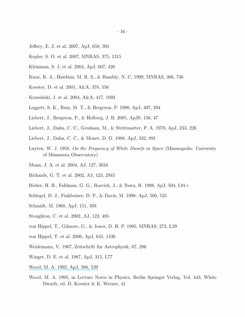
Figure 9 shows the WD mass function we derive for all stars with Teff > 12, 000K and

g < 19.0. The red dashed line is the MF corrected only by 1/Vmax —i.e., before we apply

our completeness correction. It generally shows good agreement with the MF derived in

Kepler et al. (2007) (blue points), not surprising considering we use nearly the same data

set and very similar WD models. The small differences are due to our use of slightly different

sets of data and models, as well as differing treatment of duplicate spectra, and can largely

be considered statistical fluctuations. We refer the interested reader to their paper for a

more in depth analysis of the WDMF.

The solid black line in the upper panel shows our MF after correcting for the complete-

ness of the spectroscopic sample. This curve represents the true local space density of WDs

per cubic parsec per M⊙ interval. The bottom panel shows the total weight of each bin

above the uncorrected MF—essentially the final completeness correction for each bin. There

is little small scale variation from bin to bin, and our completeness correction mainly has

the effect of raising the normalization of the whole MF by a factor of ∼ 2.2. In other words,

the shape of the MF is not strongly affected by the completeness correction.

Figure 10 is the WDMF for all stars down to 8,000K. The dashed red line is for the

data as reported by Kepler et al. (2007), the dotted blue line is after our correction for the

upturn in log g. The solid black line is the WDMF for only those stars above 12,000K (i.e.,

the same as Figure 9) renormalized to the same scale for comparison purposes. There are

more high mass stars in general, and one spurriously large bin, but on the whole, our log g

correction recovers a reasonable mass distribution for stars cooler than 12,000K.

Figure 11 shows the luminosity function we derive for all of the DA stars in our sample

down to 7,000K for all stars with g < 19.5. In red is the LF for the data as reported; in

black is the LF for the data with the increase in log g at low temperature removed. The

process of removing the excess log g pushes stars to lower masses, making them larger and

therefore brighter for the same Teff . In the range plotted, the black curve contains a total of

3,358 WDs, while the red contains 2,940.

– 13 –

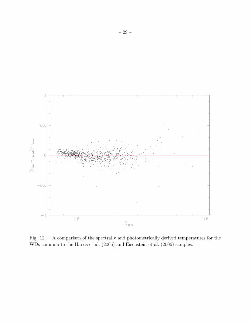
The lack of agreement between our best LF (black) and the Harris et al. (2006) lumi-

nosity function (blue) can be attributed, at least in part, to the differing assumptions used

in creating the two LFs. Harris et al. derived their temperatures by fitting Bergeron models

to the photometry assuming a log g of 8.0 for every star, a poor assumption for more than

30% of WDs (Liebert et al. 2005; Kepler et al. 2007). The temperatures they derive are

systematically different from the spectroscopic temperatures; Figure 12 shows the fractional

difference between the spectroscopically and photometrically derived effective temperatures.

When we use the photometrically derived temperatures and set log g = 8.0, we recover the

Harris et al. LF fairly well.

It should also be noted that the Harris et al. luminosity function is for WDs of all types,

whereas ours is comprised only of the DAs. For each bin in the Harris et al. LF, we have

used the full Eisenstein et al. (2006) catalog to determine a rough DA fraction, and reduced

the LF reported of Harris et al. accordingly. This DA fraction—shown in Table 1—is in

generally good agreement with previous works (Fleming et al. 1986), but we have made no

attempt to address selection biases in the Eisenstein et al. catalog.

One other source of the discrepancy between our results and Harris et al. is due to our

assumption that whatever causes the observed upturn in log g in the cooler stars affects

only the log g determination and does not alter the spectroscopically derived Teff . As the

effects of the two parameters on the line profiles are interdependent, this assumption is

probably not valid. The curves in Figure 11 suggest that in addition to the excess log

g, the temperatures determined by line fitting for the cooler stars are probably too high.

Ultimately, this area of the spectroscopic WDLF will remain uncertain until the problems

with the model atmospheres have been resolved.

The LF of Liebert et al. (2005) shown in green in figure 11 was compiled from a small

dataset (348 DA white dwarfs) based on a survey done on photographic plates over 20 years

ago on a 0.5m telescope. In addition to low number statistics, the dataset suffers from a

very difficult-to-quantify incompleteness on the faint end, which is probably responsible for

the lack of agreement below Mbol ∼ 9.5.

6. Conclusions

Our eventual goal is to take advantage of the tremendous number of WDs spectroscopi-

cally observed by SDSS and studied by Eisenstein et al. (2006) and others to create separate

WD luminosity functions for two or more different ranges of mass. This will effectively add

a third dimension, currently unexplored, to observational WD luminosity functions.

– 14 –

In order to carry out this analysis, we must fully understand the manner in which white

dwarfs were selected to receive spectra in SDSS. By comparing the proper-motion selected

sample of Harris et al. (2006) with the spectroscopically determined WDs of Kleinman et al.

(2004) and Eisenstein et al. (2006), we have derived a WD selection probability over a range

of parameters that includes nearly the entire useful range of g − i color (−1.0 < g − i < 0.2)

and apparent g magnitude (15 < g < 19.5).

We have also presented additional arguments that the observed upturn in log g is an

artifact of the model atmosphere line-fitting procedure, or—more likely—a problem with the

line profiles themselves. Since it may be some time before this problem is fully understood

and addressed, we have implemented a procedure to remove the excess log g empirically and

shown that the mass function recovered for the stars cooler than 12,000K reasonably agrees

with the MF for the hotter stars, which in turn agrees well with previous work.

Finally, we have presented the first WDLF for spectroscopically determined WDs in the

Fourth Data Release of the SDSS. In addition to addressing the issues of completeness and

the observed log g upturn in a more systematic manner than previously attempted, our LF

contains the largest sample of spectroscopically determined WDs to date (3,358), more than

six times the 531 presented in Hu et al. (2007), and more than an order of magnitude more

than the 298 stars included in the LF of Liebert et al. (2005).

We would like to thank Scot Kleinman for providing unpublished fits of the DA white

dwarfs; Hugh Harris and Mukremin Kilic for access to the data and code used to derive the

Harris et al. (2006) luminosity function, as well as much helpful advice; Barbara Canstan-

heira, Elizabeth Jeffery, Agnes Kim, Mike Montgomery, Fergal Mullally, and Kurtis Williams

for many interesing and insightful discussions.

This material is based on work supported by the National Science Foundation under

grants AST 03-07315 and AST 06-07480. This material is partially based upon work sup-

ported by the National Aeronautics and Space Administration under Grant No. NAG5-13070

issued through the Office of Space Science.

REFERENCES

Althaus, L. G., Garcıa-Berro, E., Isern, J., & Corsico, A. H. 2005, A&A, 441, 689

Althaus, L. G., Garcıa-Berro, E., Isern, J., Corsico, A. H., & Rohrmann, R. D. 2007, A&A,

465, 249

– 15 –

Bergeron, P., Liebert, J., & Fulbright, M. S. 1995a, ApJ, 444, 810

Bergeron, P., Wesemael, F., & Beauchamp, A. 1995b, PASP, 107, 1047

Bergeron, P., Wesemael, F., Fontaine, G., & Liebert, J. 1990, ApJ, 351, L21

Blanton, M. R. et al. 2003, AJ, 125, 2276

Bradley, P. A. 1998, ApJS, 116, 307

—. 2001, ApJ, 552, 326

—. 2006, Memorie della Societa Astronomica Italiana, 77, 437

Claver, C. F. 1995, PhD thesis, AA(THE UNIVERSITY OF TEXAS AT AUSTIN.)

Claver, C. F., Liebert, J., Bergeron, P., & Koester, D. 2001, ApJ, 563, 987

Eisenstein, D. J. et al. 2006, ApJS, 167, 40

Engelbrecht, A. & Koester, D. 2007, in press, Proceedings of the 15th European Workshop

on White Dwarfs, Leicester 2006

Finley, D. S., Koester, D., & Basri, G. 1997, ApJ, 488, 375

Fleming, T. A., Liebert, J., & Green, R. F. 1986, ApJ, 308, 176

Fontaine, G., Brassard, P., & Bergeron, P. 2001, PASP, 113, 409

Geijo, E. M., Torres, S., Isern, J., & Garcıa-Berro, E. 2006, MNRAS, 369, 1654

Green, R. F. 1980, ApJ, 238, 685

Hansen, B. M. S. et al. 2002, ApJ, 574, L155

—. 2004, ApJS, 155, 551

—. 2007, ArXiv Astrophysics e-prints

Harris, H. C. et al. 2003, AJ, 126, 1023

—. 2006, AJ, 131, 571

Hu, Q., Wu, C., & Wu, X.-B. 2007, A&A, 466, 627

Hugelmeyer, S. D. et al. 2006, A&A, 454, 617

– 16 –

Jeffery, E. J. et al. 2007, ApJ, 658, 391

Kepler, S. O. et al. 2007, MNRAS, 375, 1315

Kleinman, S. J. et al. 2004, ApJ, 607, 426

Knox, R. A., Hawkins, M. R. S., & Hambly, N. C. 1999, MNRAS, 306, 736

Koester, D. et al. 2001, A&A, 378, 556

Krzesinski, J. et al. 2004, A&A, 417, 1093

Leggett, S. K., Ruiz, M. T., & Bergeron, P. 1998, ApJ, 497, 294

Liebert, J., Bergeron, P., & Holberg, J. B. 2005, ApJS, 156, 47

Liebert, J., Dahn, C. C., Gresham, M., & Strittmatter, P. A. 1979, ApJ, 233, 226

Liebert, J., Dahn, C. C., & Monet, D. G. 1988, ApJ, 332, 891

Luyten, W. J. 1958, On the Frequency of White Dwarfs in Space (Minneapolis: University

of Minnesota Observatory)

Munn, J. A. et al. 2004, AJ, 127, 3034

Richards, G. T. et al. 2002, AJ, 123, 2945

Richer, H. B., Fahlman, G. G., Rosvick, J., & Ibata, R. 1998, ApJ, 504, L91+

Schlegel, D. J., Finkbeiner, D. P., & Davis, M. 1998, ApJ, 500, 525

Schmidt, M. 1968, ApJ, 151, 393

Stoughton, C. et al. 2002, AJ, 123, 485

von Hippel, T., Gilmore, G., & Jones, D. H. P. 1995, MNRAS, 273, L39

von Hippel, T. et al. 2006, ApJ, 645, 1436

Weidemann, V. 1967, Zeitschrift fur Astrophysik, 67, 286

Winget, D. E. et al. 1987, ApJ, 315, L77

Wood, M. A. 1992, ApJ, 386, 539

Wood, M. A. 1995, in Lecture Notes in Physics, Berlin Springer Verlag, Vol. 443, White

Dwarfs, ed. D. Koester & K. Werner, 41

– 17 –

Wood, M. A. & Oswalt, T. D. 1998, ApJ, 497, 870

York, D. G. et al. 2000, AJ, 120, 1579

This preprint was prepared with the AAS LATEX macros v5.2.

– 18 –

Fig. 1.— log g v. log Teff for the white dwarfs in our sample. At temperatures below

∼12,500K, the log g values begin to rise to an extent unexplained by current theory. The

solid line is a function empirically fit to the real data. The dashed line is the modest rise

predicted by theory. The excess at a given Teff is subtracted from the measured log g value

for some of our luminosity functions.

– 19 –

Fig. 2.— log g v. log Teff with the upturn in log g removed.

– 20 –

Fig. 3.— A comparison of the theoretical colors of the SDSS WDs, derived from the atmo-

spheric fits (black triangles), with the observed colors, as measured by the SDSS photometry

(open blue circles). In the upper panel, the colors of the model atmospheres do not agree

with the observed colors at low temperatures, indicating a problem with the line fitting for

stars cooler than ∼ 12,500K. In the lower panel, where the excess log g has been removed,

the colors agree much better.

– 21 –

Fig. 4.— Color-color plot of the white dwarfs in the two samples used to derive our complete-

ness correction. Open symbols are WDs from the Harris et al. (2006) sample that a) were

in the area of sky covered by spectroscopy in DR4, b) had Vtan ≥ 30km/s, and c) were not

determined by i- and z-band excess to be WD + main-sequence binaries. The filled circles

are the stars for which SDSS obtained spectra and Eisenstein et al. (2006) confirmed to be

WDs. The dashed box shows a two-dimensional projection of the QSO targeting algorithm’s

exclusion region. The open gray squares are the WDs from Harris et al. that lie outside

Eisenstein et al.’s color-color cuts. For clarity, only half of the points have been plotted.

– 22 –

−1.0 −0.8 −0.6 −0.4 −0.2 0.0 0.2

1516

1718

19

g − i

g

Fig. 5.— A map of our completeness correction. Darker areas indicate more complete regions

of the figure, with black being 100% complete. The overall completeness is of order ∼50%.

– 23 –

Fig. 6.— A histogram of the completeness values in Figure 5. Most of the 0, 1, and 0.5

values come from color-magnitude regions in which there are only one or two stars in the

Harris et al. sample available for comparison.

– 24 –

Fig. 7.— Luminosity functions for three different limiting magnitudes. We take the good

agreement between the curves to indicate that our completeness correction (and the 1/Vmax

correction) are working properly.

– 25 –

Fig. 8.— Mass functions for three different limiting magnitudes. Because of the essentially

fixed integration time for SDSS spectra, objects with fainter apparent magnitudes generally

have lower signal to noise, which translates directly into larger uncertainties in the derived

parameters (Teff , log g, and mass). Hence, as we include stars with fainter apparent magni-

tudes, more stars scatter out of the peak, broadening the mass function.

– 26 –

Fig. 9.— The white dwarf mass function for all WDs with Teff > 12,000K and g < 19.0. The

dashed line in the upper panel is the MF corrected only for 1/Vmax, without our completeness

correction applied. It agrees very well with Kepler et al. (2007—dots). The solid line is with

our completeness correction applied, and represents the true local space density of white

dwarfs. The bottom panel shows the ratio of our two mass functions—i.e., the cumulative

completeness correction for each bin. The small variation indicates that the completeness

correction, while changing the overall normalization by roughly a factor of 2.2, has little

effect on the shape of the MF.

– 27 –

Fig. 10.— White dwarf mass functions for WDs with Teff > 8,000K and g < 19.0 both with

and without the upturn in log g for cooler stars removed. The solid line is the MF from

Figure 9 renormalized for comparison purposes.

– 28 –

Fig. 11.— LFs derived in this paper. Removing the log g upturn makes each affected star

less massive, and therefore larger and brighter, pushing it to a more leftward Mbol bin. The

results of Harris et al. (2006) and Liebert et al. (2005) are shown for comparison.

– 29 –

Fig. 12.— A comparison of the spectrally and photometrically derived temperatures for the

WDs common to the Harris et al. (2006) and Eisenstein et al. (2006) samples.

– 30 –

Table 1: The fraction of stars in

Eisenstein et al. (2006) listed as DA or

DA auto. Though they generally agree

with previous results, they should be used

with much caution, as they were calculated

crudely and we have taken no care to correct

for biases in the sample. We have employed

them here simply to compare our DA-only

luminosity function to previous work.

Mbol DA Fraction

7.25 0.9338

7.75 0.9243

8.25 0.9246

8.75 0.8980

9.25 0.8433

9.75 0.8146

10.25 0.7958

10.75 0.8158

11.25 0.7957

11.75 0.7721

12.25 0.7985

12.75 0.7976

13.25 0.8173

13.75 0.8009