DRAFT VERSIONJULY 18, 2008Preprint typeset using LATEX style emulateapj v. 08/13/06

HUNDREDS OF MILKY WAY SATELLITES? LUMINOSITY BIAS IN THE SATELLITE LUMINOSITY FUNCTION

ERIK J. TOLLERUD1, JAMES S. BULLOCK1, LOUIS E. STRIGARI1, BETH WILLMAN 2

Draft version July 18, 2008

ABSTRACTWe correct the observed Milky Way satellite luminosity function for luminosity bias using published com-

pleteness limits for the Sloan Digital Sky Survey DR5. Assuming that the spatial distribution of Milky Waysatellites tracks the subhalos found in theVia Lactea ΛCDM N-body simulation, we show that there shouldbe between∼ 300 and∼ 600 satellites within 400 kpc of the Sun that are brighter than the faintest knowndwarf galaxies, and that there may be as many as∼ 1000, depending on assumptions. By taking into ac-count completeness limits, we show that the radial distribution of known Milky Way dwarfs is consistent withour assumption that the full satellite population tracks that of subhalos. These results alleviate the primaryworries associated with the so-called “Missing SatellitesProblem” in CDM. We show that future, deep wide-field surveys like SkyMapper, the Dark Energy Survey (DES), PanSTARRS, and the Large Synoptic SurveyTelescope (LSST) will deliver a complete census of ultra-faint dwarf satellites out to the Milky Way virialradius, offer new limits on the free-streaming scale of darkmatter, and provide unprecedented constraints onthe low-luminosity threshold of galaxy formation.Subject headings: cosmology: observation — surveys — galaxies: halos — galaxies:dwarfs — galaxies: Local

Group

1. INTRODUCTION

It is well-established from simulations in theΛCDM con-cordance cosmology that galaxy halos are formed by themerging of smaller halos (e.g. Stewart et al. 2007, and ref-erences therein). As a result of their high formation redshifts,and correspondingly high densities, a large number of self-bound dark matter subhalos should survive the merging pro-cess and exist within the dark matter halos ofL∗ galaxies likethe Milky Way (Klypin et al. 1999; Moore et al. 1999; Zentner& Bullock 2003). A direct confirmation of this prediction hasyet to occur. Surveys of the halos of the Milky Way (e.g. Will-man et al. 2005; Belokurov et al. 2006; Walsh et al. 2007a;Belokurov et al. 2008) and Andromeda (e.g. Martin et al.2006; Majewski et al. 2007; Irwin et al. 2008; McConnachieet al. 2008) have revealed only∼ 20 luminous dwarf satellitesaround each galaxy – approximately one order of magnitudefewer than the expected number of subhalos that are thoughtto be massive enough to form stars (Klypin et al. 1999; Mooreet al. 1999; Diemand et al. 2007b; Strigari et al. 2007b). Ofcourse, the mismatch is much more extreme (larger than afactor of∼ 1010) when compared to the full mass functionof CDM subhalos, which is expected to rise as∼ 1/M downto the small-scale clustering cutoff for the dark matter parti-cle,Mcut ≪ 1M⊙ (Hofmann et al. 2001; Bertschinger 2006;Profumo et al. 2006; Johnson & Kamionkowski 2008)

Astrophysical solutions to this “Missing Satellites Prob-lem” (MSP) include a reduction in the ability of small ha-los to accrete gas after reionization (Bullock et al. 2000;Somerville 2002; Benson et al. 2002), and tidal stripping,which shrinks the mass of halosafter they have formed stars(Kravtsov et al. 2004). Although there are some promisingnew techniques in development for studying the formationof low-mass galaxies within a CDM context (Robertson &Kravtsov 2007; Kaufmann et al. 2007; Orban et al. 2008), cur-

1 Center for Cosmology, Department of Physics and Astronomy, TheUni-versity of California at Irvine, Irvine, CA, 92697, USA

2 Harvard-Smithsonian Center for Astrophysics, 60 Garden St., Cam-bridge, MA, 02138

rent models have trouble explaining many details, particularlyregarding the lowest luminosity dwarfs (see below). Othermore exotic solutions rely on dark matter particles that arenotcold (Hogan & Dalcanton 2000; Kaplinghat 2005; Cembranoset al. 2005; Strigari et al. 2007c) or non-standard models ofin-flation (Zentner & Bullock 2003), which produce small-scalepower-spectrum cutoffs atMcut ∼ 106−8M⊙, well above thecutoff scale in standardΛCDM. In principle, each of thesescenarios leaves its mark on the properties of satellite galax-ies, although multiple scenarios fit the current data. Hence,precisely determining the shape and normalization of the low-est end of the luminosity function is critical to understandinghow faint galaxies form and how the efficiency of star forma-tion is suppressed in the smallest dark matter halos.

The Sloan Digital Sky Survey (Adelman-McCarthy et al.2007) has revolutionized our view of the Milky Way and itsenvironment, doubling the number of known dwarf spheroidal(dSph) galaxies over the last several years (e.g. Willman etal.2005; Zucker et al. 2006b,a; Belokurov et al. 2006; Grillmair2006; Walsh et al. 2007a; Irwin et al. 2007). Many of thesenew dSph galaxies are ultra-faint, with luminosities as lowas∼ 1000L⊙, faint enough to evade detection in surveys withlimits sufficient for detecting most previously known LocalGroup dwarfs (Whiting et al. 2007). In addition to provid-ing fainter detections, the homogeneous form of the SDSSallows for a much better understanding of the statistics ofdetection. Unfortunately, given the inherent faintness ofthenewly-discovered dSphs and the magnitude-limited nature ofSDSS for such objects, a derivation of the full luminosityfunction of satellites within the Milky Way halo must includea substantial correction for more distant undetectable satel-lites. Koposov et al. (2007) provided an important step inthis process by performing simulations in order to quantifythe detection limits of the SDSS and estimated the luminos-ity function by applying these limits to some simple radialdistribution functions, finding∼ 70 satellites and a satelliteluminosity function consistent with a single power law of theform dN/dLV ∼ L−1.25.

Our aim is to take the detection limits for SDSS Data Re-

2

lease 5 (DR5) as determined by Koposov et al. (2007) andcombine them with a CDM-motivated satellite distribution.In order to provide a theoretically-motivated estimate forthetotal number of Milky Way satellite galaxies, we adopt thedistributions of subhalos in theVia Lactea simulation (Die-mand et al. 2007a), and assume these to be hosts of satellitegalaxies. Note that for the purposes of this paper, we define a“galaxy” as a stellar system that is embedded in a dark matterhalo.

The organization of this paper is as follows: In§2 we de-scribe the overall strategy and sources of data used for thiscorrection, as well as discussing the validity of the assump-tions underlying this data.§3 describes in detail how thecorrection is performed and presents the resulting luminosityfunctions for a number of possible scenarios, while§4 dis-cusses the prospects for detecting the as-yet unseen satellitesthe correction predicts.§5 discusses some of the caveats as-sociated with the technique used for this correction, as wellas the cosmological implications of the presence of this manysatellite galaxies. In§6 we draw some final conclusions.

2. APPROACH & DATA SOURCES

2.1. Strategy

The luminosity bias within the SDSS survey can be approx-imated by a characteristic heliocentric completeness radius,Rcomp(MV), beyond which a dwarf galaxy of absolute mag-nitudeMV cannot be observed. This radial incompleteness isaccompanied by a more obvious angular incompleteness – theSDSS DR5 covers only a fractionfDR5 = 0.194 of the sky,or a solid angleΩDR5 = 8000 square degrees. For the cor-rections presented in§3, we will assume that magnitudeMV

satellites with helio-centric distancesr > Rcomp(MV) havenot been observed, while satellites withr ≤ Rcomp(MV)have been observed, provided that they sit within the areaof the sky covered by the SDSS footprint. Given an ob-served number of satellites brighter thanMV within the sur-vey areaΩDR5 and within a radiusr = Rcomp(MV), weaim to determine a correction factor,c, which gives the to-tal number of satellites brighter thanMV within a spheri-cal volume associated with the larger outer radiusRouter:Ntot = c(r,Ω)Nobs(< r,< Ω). For our main results wecount galaxies withinRouter = 417 kpc, corresponding tothe distance to the outermost Milky Way satellite (Leo T), al-though we do consider otherRouter values in§3.

It is useful (though not precisely correct) to think of the cor-rection factor as a multiplicative combination of a radial cor-rection factor and an angular correction factor,c = crcΩ. Thefirst correction,cr, will depend on the radial distribution ofsatellites. If there is no systematic angular bias in the satellitedistribution, and if the experiment is performed many times,then the second correction factor should have an average value< cΩ >= 1/fDR5 = 5.15. However, if the satellite distribu-tion is anisotropic on the sky, the value ofcΩ for any particularsurvey pointing may be significantly different from the aver-age. An estimate of this anisotropy is essential in any attemptto provide a correction with meaningful errors. Below, we usethe satellite halo distribution inVia Lactea to provide an es-timate for the overall correction (see§2.3). Note that in ourfinal corrections presented in§3, we do not force the radialand angular corrections to be separable, but rather use a seriesof mock survey pointings within the simulation to calculatean effective correction,c = c(r,Ω), satellite by satellite.

2.2. SDSS Detection Limits

0246810121416MV

0

200

400

600

800

1000

1200

1400

1600

Rcomp [

kp

c]

SDSS SatellitesClassical SatsLG Galaxies

102

103

104

105

106

107

108

L [L]

FIG. 1.— The completeness radius for dwarf satellites. The threerisinglines show the helio-centric distance,Rcomp, out to which dwarf satellitesof a given absolute magnitude are complete within the SDSS DR5 survey.The solid is for the published detection limits in Koposov et al. (2007) andthe other lines are the other two detection limits described in §2.2. The dot-ted black line at 417 kpc corresponds to our fiducial adopted outer edge ofthe Milky Way halo satellite population (Router). The data points are ob-served satellites of the Milky Way and the Local Group. The red circles arethe SDSS-detected satellites, the only galaxies for which the detection lim-its actually apply, although the detection limits nevertheless also delineatethe detection zone for more distant Local Group galaxies (yellow diamonds).Purple squares indicate classical Milky Way satellites. The faintest object(red triangle) is Segue 1, which is outside the DR5 footprint.

Koposov et al. (2007) constructed an automated pipeline toextract the locations of Milky Way satellites from the DR5stellar catalog. They then constructed artificial dSph galaxystellar populations (assuming a Plummer distribution), addedthem to the catalog, and ran their pipeline. The detections ofgalaxies were used to construct detection thresholds as a func-tion of distance (Koposov et al. 2007, Figure 8). These thresh-olds are mostly constant as a function of surface brightnessforµ . 30 and linear with the log of distance. Hence, their de-tection threshold is well approximated as a log-linear relation-ship between the absolute magnitude of a dSph galaxy,MV,and the volume,Vcomp(MV), out to which the DR5 could de-tect it. Specifically, Figure 13 of Koposov et al. (2007) implies

Vcomp = 10(−aMV−b) Mpc−3, (1)

such that the completeness volume followsVcomp ∝ L5a/2V .

We will adopt this form as the dwarf galaxy detection limit ofDR5. This volume may be related to a spherical completenessradius,Rcomp, beyond which a dSph of a particular magni-tude will go undetected:

Rcomp(MV) =

(

3

4πfDR5

)1/3

10(−aMV−b)/3Mpc, (2)

wherefDR5 = 0.194 is the fraction of the sky covered byDR5. For our fiducial relation, we use the result presented inKoposov et al. (2007, Figure 13), which is fit bya = 0.60and b = 5.23. We note that for this value ofa, we haveRcomp ≈ 66 kpc(L/1000L⊙)1/2, and the SDSS is completedown to a fixedapparent luminosity. The implied relationshipbetween galaxy luminosity and corresponding helio-centriccompleteness radius is shown by the solid line in Figure 1.We also consider two alternative possibilities. One is obtainedby fitting the data in Koposov et al. (2007) Table 3, whichgivesa = 0.684 andb = 5.667 (black dotted), and the otheris a line that passes through the new SDSS satellites, on the

Hundreds of Milky Way Satellites? 3

5 7 10 20 30 50 90v [km/s]

100

101

102

103

N(>v)

vpeakvmax

FIG. 2.— The cumulative count ofVia Lactea subhalos as a function ofthe (current) maximum circular velocity of the subhalo (vmax, solid), andas a function of the largest maximum circular ever obtained by the subhalo(vpeak, dashed).

assumption that some of them are of marginal detectability(a = 0.666 andb = 6.10; cyan dashed).

It is important to recognize that, in principle, the detectabil-ity of satellites at a particular radius is not a step-functionbetween detection and non-detection. It also should not bespherically symmetric (independent of latitude with respectto the disk plane), nor should it be independent of other vari-ables (such as satellite color or background galaxy density).However, Koposov et al. (2007) found that a simple radial de-pendence provided a good description of their simulation re-sults, and we will adopt it for our corrections here. They did,however, find that galaxies within this “completeness” bound-ary were not always detected at 100% efficiency (dependingon their distance and luminosity) and published detection ef-ficiencies for the known SDSS dwarfs (their Table 3). We willuse these published detection efficiencies in our fiducial cor-rections to the luminosity function below. We also investigatehow our results change when we assume 100% efficiency inthe correction.

For reference, the horizontal dotted line in Figure 1 marksour fiducial adoptedRouter radius for the Milky Way halo(slightly larger than the virial radius, in order to includeLeoT). According to this estimate, only satellites brighter thanMV ≃ −7 are observable out to this radius. The fact thatthe faintest dwarf satellite galaxies known are more than4magnitudes fainter than this limit (see Table 1) immediatelysuggests that there are many more faint satellite galaxies yetto be discovered.

2.3. Via Lactea

Diemand, Kuhlen, & Madau (2007a) describe theViaLactea simulation, which is among the highest resolutionΛCDM N-body simulation of a Milky Way-like dark mat-ter halo yet published. The mass of Via Lactea isM200 ≃1.8×1012 M⊙ with a corresponding virial radiusR200 = 389kpc, whereM200 and R200 are defined by the volume thatcontains 200 times the mean matter density. It resolves a largeamount of substructure, recording 6553 subhalos with peakcircular velocities larger than5 km s−1 at some point in theirhistory, of which 2686 are within our adoptedRouter = 417

0 50 100 150 200 250 300 350 400r[kpc]

100

101

102

1/f(<r)

All Satellitesvpeak>10 km/s

vmax>7 km/s

25 35 45 55r[kpc]

101

102

1/f(<r)

FIG. 3.— Inverse of cumulative subhalo counts within the specified radius.Here f(< r) is the fraction of subhalos that exist within a given radius,normalized to unity atRouter = 417 kpc. The radius is “heliocentric”,defined relative to the (8,0,0) kpc position of theVia Lactea simulation. Weinclude three populations of subhalos, as identified in the key. The insetfocuses on the radial range where most of the new ultra-faint SDSS satelliteshave been detected.

kpc atz = 0. We use the public data release kindly providedby Diemand et al. (2007a) in what follows3.

Figure 2 presents the cumulative maximum circular veloc-ity function,N(> vmax), for Via Lactea subhalos with halo-centric radiusR < 417 kpc atz = 0 (solid) along with thecumulative “peak” circular velocity function (dashed) forthesame halosN(> vpeak). Here,vpeak is the maximum circu-lar velocity that the subhalosever had over their history. Asemphasized by Kravtsov et al. (2004), many subhalos havelost considerable mass over their history, and thereforevpeak

may be a more reasonable variable to associate with satellitevisibility than the (current) subhalovmax. The informationcontained within this figure is presented elsewhere in the lit-erature (Diemand et al. 2007a), though we include it here forthe sake of completeness.

An important ingredient in the luminosity bias correction isthe assumed underlying radial distribution of satellites.Wedetermine this distribution directly fromVia Lactea. We areinterested in determining the total number of satellites,Ntot,given an observed number within a radius,Nobs(< r). Thecorrection will depend on the cumulative fraction of objectswithin a radiusr compared to the total count within somefiducial outer radius:f(< r) = N(< r)/Ntot. The associ-ated radial correction factor is then the inverse of the cumula-tive fraction,cr = f−1(< r), such thatNtot = crNobs(< r).This correction factor is shown in Figure 3 for three differ-ent choices of subhalo populations:vpeak > 10 km s−1 ,vmax > 7 km s−1 , andvpeak > 5 km s−1 ( i.e. all subhalosin theVia Lactea catalog).

In order to mimic a heliocentric radial distribution, in Fig-ure 3 we have placed the observer at a radius of8 kpc withina fictional disk centered onVia Lactea. The orientation ofthe “disk” was chosen to be in theVia Lactea xy plane forall figures that show subhalo distributions, but we allow fora range of disk orientations for the full correction presentedin §3. We do this for completeness, but stress that our results

3 http://www.ucolick.org/˜diemand/vl/data.html

4

are extremely insensitive to the choice of solar location, andare virtually identical if we simply adopt a vantage point fromthe center ofVia Lactea. The total count is defined within ourfiducial Router, such thatf(< 417 kpc) = 1.0. An impor-tant result of this is that our correction doesnot depend on thenumber of subhalos in Via Lactea – only the shape of the dis-tribution. Still, the shape varies among some sub-populationsof subhalo. As noted in Kravtsov et al. (2004), Diemand et al.(2007a) and Madau et al. (2008), subhalos chosen to have alargevpeak tend to be more centrally concentrated. However,the correction we apply is fairly insensitive to the differencesbetween these choices of subhalo populations.

The most important corrections will be those for the faintestgalaxies, which are just observable at local distancesr . 50kpc. It is thus clear that the radial correction factors associ-ated with the three different subhalo populations show verylittle differences at the radii of relevance (see inset in Figure3). Motivated by this result, we will use the fullVia Lacteasubhalo catalog in our fiducial model because it provides alarger statistical sample of subhalos. However, for the sakeof completeness, we present the final corrected counts for ourcorrections using thevpeak > 10 km s−1 andvmax > 7 kms−1 samples in Table 3 below.

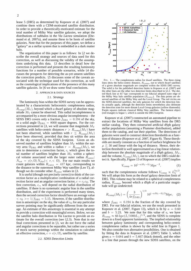
Via Lactea can also be used to extract the angular distribu-tion of subhalos. This will be important for determining theerrors on the overall satellite abundance that may arise fromlimited sky coverage. The SDSS DR5 footprint covers 8000square degrees, or a fractionfDR5 = 0.194 of the sky. Whilethis is sizable fraction of the sky, the upper image in Figure4shows that the subhalo distribution (projected out to the virialradius, in this case) is quite anisotropic even on this scale.The color of each pixel is set by the fraction of all the sub-halos,f(< Ω), that exist within an area ofΩDR5 = 8000square degrees, centered on this pixel. We see clearly thatthe fraction of satellites within a DR5-size region can varyconsiderably (from0.12 to 0.28) depending on the pointingorientation. The same information is shown as a histogram inthe lower panel, now presented as the implied multiplicative“sky coverage” correction factor,cΩ = 1/f(< Ω). Each ofthe 3096 pixels in the sky map is included as a single count inthe histogram. Note that while the average correction factoris cΩ = 1/fDR5 = 5.15 (as expected) the correction can varyfrom just∼ 3.5 up to∼ 8.3 depending on the mock survey’sorientation.

Before moving on, we note that the expected anisotropymay contain a possible solution to the “missing inner satellitesproblem” described in Diemand et al. (2007a), which notesthat there are∼ 20 subhalos inVia Lactea within the inner-most parts of the halo, while only a few galaxies are actuallyobserved. While numerical effects may become important forthese subhalos given their sizes and how close they are to thecenter of the host, it may also simply be an observational cov-erage effect. If only subhalos within 23 kpc (the distance toSegue 1) are considered,∼ 15% of the sky has one or zerosubhalos visible in a survey the size of SDSS. This means thateven if all of the subhalos host galaxies, there is a 15% chancethat we will at most see a galaxy like Segue 1. The fact thatSegue 1 was only recently discovered shows that there is eas-ily room for a significant number of inner satellites that havegone as yet undetected simply because a survey like SDSSis necessary to uncover such objects, but over the entire skyinstead of just a fifth.

2.4. Observed Satellite Galaxies

0.12 0.14 0.16 0.18 0.19 0.21 0.23 0.25 0.27 0.28

3 4 5 6 7 8 9Correction Factor

0

50

100

150

200

250

Nu

mb

er

of

Poin

tin

gs

FIG. 4.— Example of subhalo angular anisotropy. Upper: Hammer projec-tion map of the angular anisotropy inVia Lactea subhalos withvpeak > 5 kms−1 . Colors at each point indicate the fraction of subhalos,f(< Ω), within417 kpc that are contained within an angular cone ofΩDR5 = 8000 squaredegrees, in order to match the area of SDSS DR5. Lower: Distribution of theangular correction factors,cΩ = 1/f(< Ω), which must be applied to thecount within 8000 square degrees in order to return the full number of sub-halos within417 kpc. The histogram includes 1000 pointings, evenly spacedover the sky. For reference, the sky coverage of DR5 isfDR5 = 0.194,which implies an angular correction factor of1/fDR5 = 5.15. As it must,c = 5.15 matches the mean of the distribution, but not the median, which isc = 5.27. Note that these correction factors do not yet include the effects ofradial incompleteness/luminosity bias.

A variety of authors have identified dSphs in the DR5 foot-print, including some that straddle the traditional boundariesbetween globular clusters and dSphs. For example, Willman 1was originally of unclear classification (Willman et al. 2005),but is now generally recognized as being a dark matter dom-inated dSph (Martin et al. 2007; Strigari et al. 2008). Table1lists the complete set of dwarf galaxies from DR5 used in thisanalysis. For the SDSS dwarfs, we use the luminosities fromMartin et al. (2008), which presents a homogeneous analysisfor all of the SDSS dwarfs, as well as de Jong et al. (2008)for Leo T, which is based on much deeper photometry. Wenote that these results are in generally good agreement withpre-existing analyses (Willman et al. 2005; Belokurov et al.2006; Simon & Geha 2007; Walsh et al. 2007a,b). Here, wealso list the “classical” dwarfs, which were discovered beforethe SDSS, along with Segue 1, which was discovered fromdata for the SDSS-II SEGUE survey (Belokurov et al. 2007).All of the objects we list in this table have large mass-to-lightratios (Martin et al. 2007; Simon & Geha 2007; Strigari et al.2008).

Hundreds of Milky Way Satellites? 5

TABLE 1PROPERTIES OF KNOWNM ILKY WAY SATELLITE GALAXIES . DATA AREFROM BOTHUN & T HOMPSON(1988); MATEO (1998); GREBEL ET AL.

(2003); SIMON & GEHA (2007); MARTIN ET AL . (2008);DE JONG ET AL.(2008).

Satellite MV LV [L⊙] dsun[kpc] Rhalf [pc] a ǫ b

SDSS-discovered Satellites⋆Bootes I -6.3 2.83 × 104 60 242 1.0⋆Bootes II -2.7 1.03 × 103 43 72 0.2

⋆Canes Venatici I -8.6 2.36 × 105 224 565 0.99⋆Canes Venatici II -4.9 7.80 × 103 151 74 0.47

⋆Coma -4.1 3.73 × 103 44 77 0.97⋆Hercules -6.6 3.73 × 104 138 330 0.72⋆Leo IV -5.0 8.55 × 103 158 116 0.79⋆Leo T -8.0 5.92 × 104 417 170 0.76†Segue 1 -1.5 3.40 × 102 23 29 1.0

⋆Ursa Major I -5.5 1.36 × 104 106 318 0.56⋆Ursa Major II -4.2 4.09 × 103 32 140 0.78

⋆Willman 1 -2.7 1.03 × 103 38 25 0.99

Classical (Pre-SDSS) Satellites

Carina -9.4 4.92 × 105 94 210 -⋆Draco -9.4 4.92 × 105 79 180 1.0Fornax -13.1 1.49 × 107 138 460 -LMC -18.5 2.15 × 109 49 2591 -Leo I -11.9 4.92 × 106 270 215 1.0

⋆ Leo II -10.1 9.38 × 105 205 160 1.0Ursa Minor -8.9 1.49 × 105 69 200 -

SMC -17.1 5.92 × 108 63 1088 -Sculptor -9.8 7.11 × 105 88 110 -Sextans -9.5 5.40 × 105 86 335 -

Sagittarius -15 8.55 × 107 28 125 -

aSatellite projected half light radius.bDetection efficiency from Koposov et al. (2007).⋆Galaxy sits within the SDSS DR5 footprint.†Satellite is not used in fiducial LF correction.

For our fiducial corrections, following the convention ofKoposov et al. (2007), we have not included Segue 1, as itdoes not lie inside the DR5 footprint and hence the publishedDR5 detection limits are not applicable. We do include Segue1 in an alternative correction scenario below (see Table 3).We do not correct the classical dwarf satellite galaxies forlu-minosity bias or sky coverage, because appropriate detectionlimits for these classical dwarf satellites are unclear given thatthey are not part of a homogeneous survey like SDSS. Weassume that all satellites within those magnitude bins wouldhave been discovered anywhere in the sky, with the possibleexception of objects at low galactic latitudes, where MilkyWay extinction and contamination becomes significant (Will-man et al. 2004a). This assumption is conservative in thesense that it will bias our total numerical estimate low, butis only a minor effect, as our correction described in§3 isdominated by low luminosity satellites.

Before we use the radial distribution ofVia Lactea subha-los to correct the observed luminosity function, it is impor-tant to investigate whether this assumption is even self consis-tent with the data we have on the radial distribution of knownsatellites. The relevant comparison is shown in Figure 5. Wehave normalized to an outer radiusRouter = 417 kpc (slightlylarger than theVia Lactea virial radius) in order to allow acomparison that includes the DR5 dwarf Leo T – this exten-sion is useful because the known dwarf satellite count is solow that even adding one satellite to the distribution increases

the statistics significantly.The radial distribution of all 23 known Milky Way satel-

lites is shown by the magenta dot-dash line in Figure 5. Thefour solid lines show radial distributions for four choicesofsubhalo populations: the 65 largestvpeak(upper) subhalos (65LBA) as discussed in Madau et al. (2008),vpeak > 10 kms−1 (upper-middle),vpeak > 5 km s−1 (lower-middle), andvmax > 7 km s−1 (lower). We note that the all-observed pro-file is clearly more centrally concentrated than any of the the-oretical subhalo distributions. However, as shown in Figure1, our limited ability to detect faint satellite galaxies almostcertainly biases the observed satellite population to be morecentrally concentrated than the full population.

If we include only the 11 satellites (excluding SMC andLMC) that are bright enough to be detected within417 kpc(MV . −7), we obtain the thick blue dashed line. This dis-tribution is significantly closer to all of the theoretical sub-halo distributions, and matches quite well withinr ∼ 50 kpc,where the incompleteness correction to the luminosity func-tion will matter most. It is still more centrally concentratedthen the distribution of all subhalos, however, as has beennoted in the past (at least for the classical satellites – e.g. Will-man et al. 2004b; Diemand et al. 2004; Kravtsov et al. 2004).In order to more rigorously determine whether the theoreti-cal distribution is consistent with that of the 11 “complete”satellites, we have randomly determined the radial distribu-tion of vpeak > 5 km s−1 subhalos using 1000 subsamples of

6

11 subhalos each. The error bars reflect 98 % c.l. ranges fromthese subsamples, although they are correlated and hence onlyrepresent a guide to the possible scatter about the points inthedistribution. From this exercise, we can roughly conclude thatthe complete observed distribution is consistent with being arandom subsample of thevpeak > 5 km s−1 population. Wealso note that thevpeak > 10 km s−1 distribution fits evenmore closely, well within their 68% distribution (errors onthis theory distribution are not shown for figure clarity, butthey are similar in magnitude to those on the central line).

To further investigate the issue of consistency between thevarious radial distributions, we determine the KS-probabilityfor various distributions. The results are shown in Table 2,where in each case thep-value gives the probability that thenull hypothesis is correct (i.e. that the two distributionsaredrawn from the same underlying distribution). While the dis-tribution of all satellites is clearly inconsistent with the sub-halo distributions, choosing only the complete satellitesim-proves the situation, giving a reasonable probability of thecomplete distribution matching thevpeak > 5 km s−1 dis-tribution, and an even better match for the distributions thatare cut onvpeak, as expected from the error bars.

Finally, we note that our definition of “complete” is con-servative, since no satellites fainter thanMV = −8.8 wereknown before the SDSS survey. If we include only the (five)satellites bright enough to be detectable toRouter that existwithin the well-understood area of the DR5 footprint, we ob-tain the radial profile shown by the dotted black line (“DR5Complete”), which is even less centrally concentrated thanany of the theory lines. While this distribution is marginallyconsistent with the other distributions based on the KS-testp-values, caution is noted given the small number of datapoints (5). We conclude that while more data (from deeperand wider surveys) is absolutely necessary in order to deter-mine the radial distribution of Milky Way satellites and tocompare it with theoretical models, the assumption that theunderlying distribution of satellites tracks that predicted forsubhalos is currently consistent with the data. We will adoptthis assumption for our corrections below – specifically, weuse thevpeak > 5 km s−1 distribution for our fiducial case.While thevpeak > 10 km s−1 distribution fits the observedsatellites more closely, we show in§3 that the various subhalodistributions only affect the final satellite counts by a factorof at most∼ 1.4. We chose to use allVia Lactea subhalos(corresponding tovpeak > 5 km s−1 ) as our fiducial case inorder to reduce statistical noise from the smaller number ofsatellites in thevpeak > 10 population – note that numericaleffects will generally produce an under-correction (giving asmaller number of satellites), as described in§3.

Previous studies have pointed to discrepancies betweensimulations and observations of other galaxies’ satellitedis-tributions (e.g. Diemand et al. 2004; Chen et al. 2006). Whilethis is of concern, much of this data is around clusters or otherenvironments very different from that of the Local Group.Furthermore, the detection prospects for faint satellitesaroundthe Milky Way are of course far better than can be achievedfor other galaxies, and the region of the luminosity functionthat is of importance for this correction (e.g.MV > −7) hasnever been studied outside the Local Group.

3. LUMINOSITY FUNCTION CORRECTIONS

The cumulative number of known Milky Way satellitesbrighter than a given magnitude is shown by the lower (red)dashed line with solid circles in Figure 6. This luminosity

0 50 100 150 200 250 300 350 417

r[kpc]

0.0

0.2

0.4

0.6

0.8

1.0

f(<r)

65 LBAvpeak>10

All Subhalosvmax>7

All ObservedComplete

DR5 CompleteVL Host DM

FIG. 5.— Radial distributions for various populations of observed satel-lites as compared to several sample subhalo distributions inVia Lactea. Solidlines are four populations ofVia Lactea subhalos within 417 kpc: from topto bottom, 65 largest before accretion (see Madau et al. 2008,Figure 7),vpeak > 10 km s−1 , All ( i.e. vpeak > 5 km s−1 ), andvmax > 7

km s−1 . The dashed lines are observed satellite distributions. From top tobottom, we have the“All Observed”(magenta), which consists of all knownMilky Way dSph satellites; the “Complete” (blue) distribution correspondsto only those with magnitudes corresponding toRcomp ≥ 417 kpc; “DR5Complete” (cyan) corresponds to satellites brighter than the completenessmagnitude, and also in the DR5 footprint – these are the only observationallycomplete and homogeneous sample. The dotted line is the global dark matterdistribution for theVia Lactea host halo. Error bars (98 % c.l. ) are de-rived by randomly sampling from theVia Lactea subhalos the same numberof satellites as in the “Complete” sample (11). Note that this means the errorbars only apply for comparing the solid lines to the dashed line, and that theyare correlated, but still represent the scatter of individual bins in any possibleobserved sample of 11 satellites fromV ia Lactea.

TABLE 2KS TEST RESULTS FOR RADIAL

DISTRIBUTIONS SHOWN INFIGURE 5.

Distribution 1 Distribution 2 p-value

All Observed 65 LBA 57.6%All Observed vpeak > 10 10.3%All Observed All Subhalos 0.4%All Observed vmax > 7 0.1%

Complete 65 LBA 95.1%Complete vpeak > 10 38.2%Complete All Subhalos 12.1%Complete vmax > 7 8.2%

DR5 Complete 65 LBA 8.6%DR5 Complete vpeak > 10 14.4%DR5 Complete All Subhalos 48.2%DR5 Complete vmax > 7 63.1%All Observed Complete 87.6%All Observed DR5 Complete 6.6%

Complete DR5 Complete 41.1%

function includes both the classical dwarf satellites and thefainter, more recently-discovered SDSS satellites (excludingSegue 1 for reasons discussed above). By simply multiplyingthe SDSS satellite count by the inverse of the DR5 sky frac-tion (1/fDR5) and adding this to the classical dwarf satellitecount, we produce the (green) long-dashed line. This first-order correction provides an extremely conservative loweres-timate on the total Milky Way satellite count by ignoring thedetails of luminosity bias in the SDSS.

We use the following series of mock surveys of theVia

Hundreds of Milky Way Satellites? 7

Lactea subhalo population in order to provide a more real-istic correction. First, an observer is positioned at distance of8 kpc from the center ofVia Lactea. We then define an angu-lar point on the sky from this location and use it to center amock survey of solid angleΩDR5 = 8000 square degrees.We allow this central survey position to vary over the fullsky using 3096 pointings that evenly sample the sky. Thoughwe find that the absolute position of the observer does notaffect our results significantly, we also allow the observer’sposition to vary over six specific locations, at(x, y, z) =(±8, 0, 0), (0,±8, 0), and(0, 0,±8) on theVia Lactea grid.We acknowledge that there are (contradictory) claims in theliterature concerning whether satellite galaxies are preferen-tially oriented (either parallel or perpendicular) with respectto galaxy disks (Kroupa et al. 2005; Metz et al. 2007; Kuhlenet al. 2007; Wang et al. 2008; Faltenbacher et al. 2008), andequally contradictory claims regarding how disks are orientedin halos (Zentner et al. 2005; Bailin et al. 2005; Dutton et al.2007). If there were a preferential orientation, then the appro-priate sky-coverage correction factors would need to be biasedaccordingly, but for our correction, we make no assumptionsabout the orientation of the “disk”. Therefore, any uncertaintyin the correct orientation of the disk is contained within the er-rors we quote on our counts. In the end, we produce 18576equally-likely mock surveys each with their own correctionfactors, and use these to correct the Milky Way satellite lumi-nosity function for angular and radial incompleteness.

For each of the mock surveys, we consider every DR5 satel-lite (i = 1, ..., 11, sometimes 12 ) with a helio-centric distancewithin Router = 417 kpc and determine the total number ofobjects of its luminosity that should be detectable. Specifi-cally, if satellitei has a magnitudeM i

V that is too faint to bedetected atRouter (i.e. if M i

V & −7), then we determine thenumber ofVia Lactea subhalos,N(r < Rcomp,Ω < ΩDR5),that sit within an angular cone of sizeΩDR5 and within ahelio-centric radiusRcomp(Mi). We then divide the totalnumber ofVia Lactea subhalos,Ntot by this “observed” countand obtain a corrected estimate for the total number satellitesof magnitudeM i

V:

ci =Ntot

N(r < Rcomp(M iV),Ω < ΩDR5)

. (3)

If the SDSS satellitei is bright enough to be seen atRouter,thenRcomp is replaced byRouter in the above equation. Inthis case, the correction factor only accounts for angular in-completeness. This method allows us to produce distribu-tions of correction factors for eachMV of relevance. Notealso that because the correction factor is the fraction of sub-halos in the cone, it only depends on the distributions ofViaLactea subhalos, rather than directly depending on the totalnumber, rendering it insensitive to the overall subhalo countin Via Lactea. Furthermore, any subhalo distributions that donot have enough subhalos to fully accommodate all possiblepointings are simply given a correction factor1/Ntot, mean-ing that numerical effects tend toundercorrect, producing aconservative satellite estimate.

Three example distributions of number-count correctionfactors are shown in Figure 7 for hypothetical objects of lu-minosityMV = −3,−5,−7 and corresponding completenessradii Rcomp = 77, 494, 486 kpc. We see that while the bright-est objects typically have correction factors of order the in-verse of the sky coverage fraction,∼ 5, the faintest objectscan be under-counted by a factor of∼ 100 or more. Note thatto produce helio-centric sky coverage maps, we must assume

161412108642MV

100

101

102

103

N(<MV)

Combined CorrectionFixed Coverage CorrectionUncorrected/Observed

103

104

105

106

107

108

109

L [L]

FIG. 6.— Luminosity function as observed (lower), corrected foronlySDSS sky coverage (middle), and with all corrections included (upper). Notethat the classical (pre-SDSS) satellites are uncorrected,while new satelliteshave the correction applied. The shaded error region corresponds to the 98%spread over our mock observation realizations. Segue 1 is notincluded in thiscorrection.

a plane inVia Lactea in which we consider the Sun to lie – forFigure 7, this is thexy plane, but for our final corrections weconsider all possible orientations (described above).

We construct corrected luminosity functions based on eachof the 18576 mock surveys by generating a cumulative countof the observed satellites. We weigh each satellitei by itsassociated correction factorci and (in our fiducial case) itsdetection efficiencyǫi. For each of the new satellites we usethe quoted detection efficiencies from Koposov et al. (2007,Table 3). We reproduce those efficiencies in our Table 1, andwe assumeǫ = 1 for all of the classical satellites that are notwithin the DR5 footprint. Explicitly, the cumulative luminos-ity function for a given pointing is:

n(< MV) =

<MV∑

i

c(M iV)

ǫi. (4)

For a given scenario (subhalo population, completeness lim-its, and detection efficiencies for each satellite) we determinethe luminosity function for each pointing and disk orientation.We are then able to calculate a median luminosity functionand scatter for each scenario.

Our fiducial corrected luminosity function shown by the up-per blue solid line in Figure 6, and the shaded band spansthe 49% tails of the distribution. Note that the errors van-ish aroundMV = −9 because all satellites brighter thanthat are “classical” pre-SDSS satellites and are left com-pletely uncorrected on the conservative assumption that anyobjects brighter than this would have been detected previ-ously. Our fiducial scenario counts galaxies within a radiusRouter = 417 kpc and excludes Segue 1 from the list of cor-rected satellites because it is not within the DR5 footprint.In addition, this scenario uses quoted detection efficienciesǫfrom Koposov et al. (2007) and the completeness radius re-lation in Equation 2 witha = .6 and b = 5.23. With thisfiducial scenario, we find that there are398+178

−94 (98% c.l.)satellites brighter than Boo II within417 kpc of the Sun.

We have performed the same exercise for a number of dif-ferent scenarios as described in Table 3 and summarized in

8

c(MV=3)31

35

40

44

48

30 32 34 36 38 40 42 44 46 48LF correction factor

0

20

40

60

80

100

120

Nu

mb

er

of

poin

tin

gs

MV=3.0Rcomp=77 kpc

c(MV=5)7

9

11

13

14

7 8 9 10 11 12 13 14 15LF correction factor

0

10

20

30

40

50

60

Nu

mb

er

of

poin

tin

gs

MV=5.0Rcomp=194 kpc

c(MV=7)4

5

6

7

8

3.5 4.0 4.5 5.0 5.5 6.0 6.5 7.0 7.5 8.0LF correction factor

0

10

20

30

40

50

60

Nu

mb

er

of

poin

tin

gs

MV=7.0Rcomp=486 kpc

FIG. 7.— Sky anisotropy maps and corresponding distributions for 3 samplelimiting magnitudes. The sky projections are the corresponding correctionfactor (i.e. inverse of the enclosed fraction of total satellites) for a DR5-sizedsurvey pointing in a given direction corresponding to a satellite of a particularmagnitude. The histograms show the distribution of correction factors fromevenly sampling the sky maps. From top to bottom, limiting magnitudes areMV = −3,−5,−7 corresponding toRcomp = 46, 128, 358 kpc.

Figure 8. Table 3 assigns each of these scenarios a number(Column 1) based on different assumptions that go into thecorrection. Scenario 1 is our fiducial case and counts all satel-lites brighter than Boo II (MV > −2.7) within Router = 417kpc. Scenario 2 counts the total number of satellites brighterthan Segue 1 (MV > −1.5) if we consider Segue 1 as in-cluded in the DR5 sample (Column 5). Scenarios 3-4 excludeBoo II or Willman 1 (the faintest satellites) along with Segue1, considering the possibility that these satellites are low lu-minosity owing to strong environmental effects, or are noteven truly dwarf galaxies at all. Alternatively, scenario 4maybe considered the total number brighter than Coma (the 4thfaintest). Scenarios 5-10 allow for different choices withintheVia Lactea subhalo population (Column 7), and 11-14 re-flect changes in outer Milky Way radius,Router (Column 4).Scenarios 16-17 allow different values fora andb in Equa-tion 2 (specified in Columns 2 and 3) for theRcomp(MV )relation, and 15 assumes that the detection efficiency for allsatellites isǫ = 1. Finally, Scenario 18 makes the extremeassumption that there is no luminosity bias and includes onlya sky-coverage correction factor. In columns 8-10,Nsats isthe number of satellites expected for a given scenario, whileNupper andNlower are the upper limits and lower limits forthe 98% distribution. The final column gives the faint-end(i.e. −2 & MV & −7) slope if the luminosity function isapproximated by the formdN/dLV ∼ Lα. Note that someof these luminosity functions arenot consistent with a powerlaw within the anisotropy error bars, but we include the bestfits for completeness (see§6 for further discussion).

From Figure 8 , for all of the cases that adopt the fidu-cial detection limits (1-15), we may expect as many as∼ 500satellites within∼ 400 kpc. Even the most conservative com-pleteness scenarios (4,10,11,14) suggest that∼ 300 satellitesmay exist within the Milky Way’s virial radius. Scenario 17,which relies on a less conservative but not unreasonable de-tection limit, suggests that there may be more than∼ 1000Milky Way satellites waiting to be discovered. We now turnto a discussion of the prospects for this exciting possibility.

4. PROSPECTS FOR DISCOVERY

Upcoming large-area sky surveys such as LSST, DES,PanSTARRS, and SkyMapper (Ivezic et al. 2008; The DarkEnergy Survey Collaboration 2005; Kaiser et al. 2002; Kelleret al. 2007) will survey more sky and provide deeper mapsof the Galactic environment than ever before possible. Inthis section we provide a first rough estimate for the num-ber and type of satellite galaxies that may expect to discoverwith these surveys.

While it is impossible to truly ascertain the detection limitswithout detailed modelling and consideration of the sourcesof contamination for the magnitudes and colors these surveyswill probe, the simplest approximation is to assume all thecharacteristics of detectability are the same as those for SDSSaside from a deeper limiting magnitude. If we do this, wecan estimate the corresponding completeness radius for eachsurvey by the difference between the limiting5 − σ r-bandpoint source magnitude for Sloan (MSDSS = 22.2) and thecorresponding limit for the new survey:

Rlimcomp

RSDSScomp

= 10(Mlim−MSDSS)/5. (5)

Figure 9 shows the results of this exercise for several plannedsurveys. According to this estimate, LSST, with a co-added

Hundreds of Milky Way Satellites? 9

TABLE 3THE LAST FOUR COLUMNS PROVIDE MEDIAN, UPPER, AND LOWER ESTIMATES (98 % RANGE) FOR THEM ILKY WAY SATELLITE COUNT WITHINRouter , AS WELL AS THE FAINT-END SLOPE(AS THE SCHECHTERα, I .E. dN/dLV ∝ Lα

V) FOR SEVERAL DIFFERENT SCENARIOS. SEE TEXT FOR

A DESCRIPTION.

Scenario a b Router [kpc] Excluded Satellites Detection Eff. Subhalos Nsats Nupper Nlower Faint-end slope(α)

1 -0.600 -0.719 417 Seg1 Yes All 398 576 304 −1.87 ± 0.192 -0.600 -0.719 417 None Yes All 558 881 420 −1.78 ± 0.203 -0.600 -0.719 417 Seg1, BooII Yes All 328 561 235 −1.47 ± 0.184 -0.600 -0.719 417 Seg1, BooII, Wil1 Yes All 280 505 194 −1.66 ± 0.175 -0.600 -0.719 417 Seg1 Yes vmax > 5 464 749 316 −1.92 ± 0.236 -0.600 -0.719 417 Seg1 Yes vmax > 7 427 942 258 −1.90 ± 0.327 -0.600 -0.719 417 Seg1 Yes vpeak > 9 302 508 198 −1.90 ± 0.428 -0.600 -0.719 417 Seg1 Yes vpeak > 10 289 521 191 −1.76 ± 0.299 -0.600 -0.719 417 Seg1 Yes vpeak > 14 260 531 167 −1.72 ± 0.3210 -0.600 -0.719 417 Seg1 Yes 65 LBA 224 752 128 −1.67 ± 0.4411 -0.600 -0.719 200 Seg1 Yes All 229 330 176 −1.70 ± 0.1812 -0.600 -0.719 300 Seg1 Yes All 322 466 246 −1.80 ± 0.1913 -0.600 -0.719 389 Seg1 Yes All 382 554 292 −1.87 ± 0.1914 -0.600 -0.719 500 Seg1 Yes All 439 637 335 −1.89 ± 0.2015 -0.600 -0.719 417 Seg1 No All 184 259 142 −1.65 ± 0.1916 -0.684 -0.753 417 Seg1 Yes All 509 758 381 −1.95 ± 0.2017 -0.667 -0.785 417 Seg1 Yes All 1093 2261 746 −2.15 ± 0.2618 N/A N/A 417 Seg1 N/A All 69 100 50 −1.16 ± 0.21

1 2 3 4 5 6 7 8 9 101112131415161718Scenario

0

200

400

600

800

1000

1200

Sate

llit

e C

ou

nts

(9

8 \

% c

.l.)

FIG. 8.— Number of Milky Way satellites for several different scenarios asdescribed in Table 3. Error bars reflect 98% ranges about the median values(points). Scenario 1 (black circle) is our fiducial case and counts all satellitesbrighter than Boo II (MV > −2.7) within Router = 417kpc. Scenario 2-4(blue triangles) consider inclusion or exclusion of different satellites. Sce-narios 5-10 (green squares) allow for different choices within theVia Lacteasubhalo population, 11-14 (red diamonds) reflect changes inRouter, 15 (cyanhexagon) corresponds to no detection efficiency correction, and 16 and 17(magenta pentagons) are for different completeness limit assumptions. Sce-nario 18 (yellow cross) includes only the angular (sky coverage) correctionfactor, i.e. no luminosity bias correction.

limit of MLSST = 27.5, should be able to detect objects asfaint as the faintest known galaxies out to the Milky Way virialradius. Moreover, LSST will be able to detect objects as faintasL ∼ 100L⊙ (if they exist) out to distances of∼ 200 kpc.

Examining the prospects for dwarf satellite detection withLSST in more detail, in Figure 10 we plot the number of satel-lites that LSST would detect in4π sterradians assuming thatthe true satellite distribution follows that expected fromourfiducial correction presented above. Remarkably, even withsingle-exposure coverage (to 24.5), LSST will be able to dis-cover a sizable fraction of the satellites in the Southern sky,> 100 galaxies by this estimate. Moreover, the co-added datawould reveal all∼ 180 dwarf galaxies brighter than Boo II

TABLE 4PREDICTED NUMBER OF DETECTABLE SATELLITES IN A SERIES

OF UPCOMING SURVEYS(IGNORING CROWDING/CONFUSIONEFFECTS, WHICH WILL REDUCE THE NUMBER OF DETECTIONS

OF FAINT OBJECTS).

Survey Name Area (deg2) Limiting r [mag] Nsats

RCS-2 1000 24.8 3-6DES 5000 24 19-37

Skymapper 20000 22.6 42-79PanSTARRS 1 30000 22.7 61-118LSST 1-exp 20000 24.5 93-179

LSST combined 20000 27.5 145-283

(and perhaps even more if they exist at lower luminosities).Asurvey such as this will be quite important for testing galaxyformation models, as even the shape of the satellite luminos-ity function is quite poorly constrained. In Figure 10, theSkymapper line appears close to a power law over the rangeshown, while the “actual” luminosity function is certainlynot.

Finally, in Table 4, we present predictions for the numberof satellites that will be found in each of a series of upcominglarge-area surveys, as well an example smaller-scale survey,RCS-2 (Yee et al. 2007). Given their limiting magnitudes,their fractional sky coverage and assuming the fiducial sce-nario outlined above, we can essentially perform the inverseof the correction described in Section 3, and determine thenumber of satellites the survey will detect (as done in Figure10 for LSST). Note that this is still ignoring more compli-cated issues such as background galaxy contamination andproblems with stellar crowding, which are potentially seri-ous complications, particularly for the faintest of satellites.Hence, these estimates are upper limits, but to first order theyare a representative number of the possibly detectable satel-lites given the magnitude limits and sky coverage. Some ofthe footprints of these surveys will overlap, however, whichwill improve the odds of detection, but reduce the likely num-ber of new detections for later surveys (this effect is not in-cluded in the counts in Table 4).

5. DISCUSSION

5.1. Caveats

10

While our general expectation that there should be manymore satellites seems to be quite solid, there are several im-portant caveats that limit our ability to firmly quote a numberor to discuss the expected overall shape of the LuminosityFunction.

1. Detection Limits. The simplifying approximation thatEquation 1 describes the complexities of satellite de-tection cannot be correct in detail – we expect a depen-dence on properties such as Galactic latitude and color.However, we are leaving these issues aside for this first-order correction. Moreover, the detection limits fromKoposov et al. (2007) apply only for objects with sur-face brightnessµV . 30 - if dSphs exist that are morediffuse than this, they will have been missed by SDSS.In this sense, our results are conservative, as even morevery low surface brightness dwarf galaxies may be dis-covered by new, deeper surveys.

2. Input Assumption. The assumption that the satellitepopulation tracks the full underlying subhalo popula-tion is a major assumption of this correction. As Figure5 shows, this assumption is consistent with the currentdata, and modest cuts onvpeak improve the situationfurther. Given the size of the error bars, the existenceof a discrepancy simply cannot be resolved without sur-veys that have better completeness limits. There arecertainly reasons to expect that the satellite populationwill not track the subhalo population in an unbiasedway – for example, if tidal forces play a role in mak-ing ultra-faint dSph galaxies. However, there are alsoreasons to suspect that there is no such bias. The darkmatter subhalo masses of the known Milky Way dwarfsare approximately the same over a∼ 4 order of magni-tude spread in luminosity (Strigari et al. 2008, in prep.;Strigari et al. 2008), suggesting that the luminosity thatany subhalo obtains is quite stochastic. Whether or notour input assumption about galaxies tracing subhalos iscorrect, future surveys will provide a means to test it,and thereby provide an important constraint on the for-mation processes of these extreme galaxies.

3. Subhalo Distribution. Our correction relies on theViaLactea subhalo population and its distribution with ra-dius and angle. While this provides a well-motivatedstarting point for this correction,Via Lactea is only asingle realization of a particular mass halo and of aparticular set of cosmological parameters (WMAP-3),and hence cannot necessarily be considered representa-tive of a typical halo inΛCDM. Semi-analytic modelssuggest that the cosmic variance in radial distributionsshould not be very large as long as we consider ha-los that are small enough that the mass-function is wellpopulated (Zentner & Bullock 2003). However, a suiteof Via Lactea-type simulations will be necessary to pro-duce a distribution of corrections to statistically averageover before this correction can be considered fully nu-merically robust. As discussed in§1, the uncertaintyin the properties of the Milky Way halo also mean thatusing Via Lactea to accurately model the Milky Wayis subject to those same uncertainties. This uncertaintyis alleviated in this correction because only the fractiondistribution matters – the absolute normalization is de-termined by theobserved satellites rather than the sub-halo counts. But if it is true that the radial distribution

of subhalos tracks the global dark matter distribution,as suggested by Diemand et al. (2007b) and Figure 3,this uncertainty could be important if the inner portionsof the radial distribution change substantially with cos-mological parameters or halo properties.

Note that while the mass ofVia Lactea is quite closeto that obtained fromΛCDM-based mass models of theMilky Way (e.g. Klypin et al. 2002; Madau et al. 2008),the mass of the Milky Way halo is constrained by ob-servations only at the factor of∼ 2 level. The mostrelevant uncertainty associated with the possible massdifference between the Milky Way andVia Lactea isthe difference associated with the uncertain radial scal-ing. SinceR200 ∝ M

1/3200 , a factor of∼ 2 mass uncer-

tainty corresponds to a∼ ±25% uncertainty in virialradius. Fortunately, our corrections depend primarilyon the relative radial distribution of satellites, and noton their absolute masses, and the choice of exactly whatradius within which galaxies are considered “satellites”is somewhat arbitrary, anyway. Moreover, the expectedsubhalo angular anisotropy (see§3) is more importantfor our corrections than the uncertainty associated in theMilky Way halo mass or precisely how the outer radiusis defined.

4. Input Luminosities/Satellites. Most of our correctionscome from the faintest, nearby satellites, as they havevery smallRcomp values compared toRouter. Errors inthe magnitudes of these faintest of satellites will resultin significant changes in the derived luminosity func-tion. These errors are not propagated for this correction,but revisions to faint satellite magnitudes have the po-tential to significantly alter our estimates. Furthermore,the final count is highly sensitive to Poisson statistics inthe innermost regions of the Milky Way, as well as anyphysical effect that biases the radial distribution of thefaintest of the satellites (as discussed above).

5.2. Implications

Keeping in mind the caveats discussed above, it is worthconsidering the potential implications of a Milky Way halofilled with hundreds of satellite galaxies. For the sake of dis-cussion, we will adoptNsat ≃ 400, as obtained in our fiducialestimate.

First,Nsat ≃ 400 can be used to determine a potential char-acteristic velocity scale in the subhalo distribution. Under the(extreme) assumption that only halos larger than a given ve-locity host satellites, Figure 2 implies thatN ≃ 400 corre-sponds to a circular velocityvmax & 7 km s−1 or a historicalmaximum ofvpeak & 12 km s−1 . We note that these cutoffscorrespond closely to those adopted in our corrections (Table3) and that there was no reason that they had to match. If weiteratively apply the correction in order to obtain perfectself-consistently between the corrected count and the input total,we findvpeak > 14 km s−1 . Interestingly, this scale is quiteclose to the threshold where gas may be boiled out of halos viaphotoevaporation (Barkana & Loeb 1999). We note howeverthat the subhalo abundance at fixed mass orvmax may varyperhaps at as much as the factor of∼ 2 level from halo to halo(Zentner & Bullock 2003). Therefore the “cosmic varianceerror” will affect our ability to determine a characteristic sub-halo mass based on counts (but does not affect the correctionitself, which depends only on the radial distribution, and notthe total counts of subhalos). Recently, Diemand et al. (2008)

Hundreds of Milky Way Satellites? 11

have published results from theVia Lactea II halo, which hasa factor of∼ 1.7 times more subhalos at fixedvmax than theVia Lactea halo we analyze here. If we take the velocity func-tion in Diemand et al. (2008) Figure 3,Nsat would correspondto vmax & 9 km s−1 .

While the maximum circular velocity of a subhalo is a use-ful measure of its potential well depth, it is very difficult tomeasurevmax directly from dwarf satellite stellar velocities(Strigari et al. 2007b). The best-determined dark halo observ-able is the integrated mass within a fixed radius within thestellar distribution (Strigari et al. 2007a). While the observedhalf-light radii vary from tens to hundreds of parsecs for thedwarf satellites, all dwarf satellites are found to have a com-mon mass scale of∼ 107M⊙ within a fixed radius of 300 pcwithin their respective centers (Strigari et al 2008 in prep.),and to a similar extent a common mass of106 within 100 pc(Strigari et al 2008). Although the mass within these scalesare difficult to resolve with theV ia Lactea simulation we con-sider in this paper, this mass scale will be well-resolved inViaLactea II (Diemand et al. 2008) and forthcoming simulations.In the future, a statistical sample of highly resolved subhaloswill allow for a robust comparison between the dwarf satel-lite mass function and the subhalo population. This in turnwill allow corrections of the sort presented in this paper onvarious sub-populations of subhalos and galaxies, providinga much more stringent consistency check between the massfunction and luminosity function inΛCDM-based models. Itis important to note, however, that the observed stellar kine-matics of the satellites does set stringent limits on their hosthalovmax values. These limits are consistent with the resultspresented here in that any of the reasonable sub-populationsdiscussed above (e.g.vmax & 7 − 10 km s−1 ) are not ex-cluded by the current data (Strigari et al. 2007b, 2008). Wenote that strong CDM priors suggest somewhatlarger vmax

values (& 15km s−1 – Strigari et al. 2007b, 2008; Penarrubiaet al. 2008), which would (if anything)underpredict the ob-served visible satellite counts, according to our estimates.

As we have shown, we expect the discovery of manymore dwarfs to occur with planned surveys like LSST, DES,PanSTARRS, and SkyMapper. If so, it will provide importantconstraints on galaxy formation models, which, at present,areonly poorly constrained by the present data. The ability to de-tect galaxies as faint asL ∼ 100L⊙ provides an opportunityto discover if there is a low-luminosity threshold in galaxyfor-mation, and to use these faint galaxies as laboratories to studygalaxy formation in the extreme. The planned surveys willalso provide an important measurement of the radial distribu-tion of faint satellites. This will help test our predictions, butmore importantly provide constraints on more rigorous mod-els aimed at understanding why and how low-mass galaxiesare so inefficient at converting their baryons into stars.

Another important direction to consider is searches for sim-ilar satellites around M31. New satellites are rapidly beingdiscovered in deep surveys of its environs (e.g. McConnachieet al. 2008). While there are indications of substantial differ-ences in the M31 satellites and their distributions compared tothe Milky Way (McConnachie & Irwin 2006), such compar-isons are complicated by the fact that it is impossible to detectthe ultra-faint satellites that comprise most of our correctedsatellite counts at the distance of M31. with the much largerdata samples that will be available with future deep surveys,it may be easier to compare the true luminosity function anddistributions of Milky Way satellites to M31 and hence betterunderstand the histories of both the galaxies, as well as better

1210864202MV

0

200

400

600

800

Rcomp

Co-a

dded L

SS

T

Sin

gle

LS

ST

DES

Skym

apper

SD

SS

102

103

104

105

106

L [L]

FIG. 9.— Maximum radius for detection of dSphs as a function of galaxyabsolute magnitude for DR5 (assumed limiting r-band magnitude of 22.2)compared to a single exposure of LSST (24.5), co-added full LSST lifetimeexposures (27.5), DES or one exposure from PanSTARRS (both 24), and theSkyMapper and associated Missing Satellites Survey (22.6). The data pointsare SDSS and classical satellites, as well as Local Group field galaxies.

constrain how dSphs form in a widerΛCDM context.Finally, if LSST and other surveys do discover the (full-sky)

equivalent of∼ 400 or even∼ 1000 satellites, and appropri-ate kinematic follow-up with 30m-class telescopes like TMTconfirmed that these objects were indeed dark-matter domi-nated, then it will provide a unique and powerful means toconstrain the particle nature of dark matter. As discussed inthe introduction, the mass function of dark matter subhalosisexpected to rise steadily to small masses as∼ 1/M (Klypinet al. 1999; Diemand et al. 2007a) and the only scale that isexpected to break this rise is the cutoff scale in the cluster-ing of dark matter. When the MSP was originally formulated,scenarios like Warm Dark Matter (WDM) were suggested as ameans of “erasing” all but the∼ 10 most massive subhalos pergalaxy by truncating the power at∼ 108M⊙ scales. If∼ 1000satellites were discovered, then the same idea could be usedto provide a limit on the small-scale clustering characteris-tics of the dark matter particle. As a rough approximation,N ≃ 1000 subhalos corresponds to a minimum mass sub-halo in Via Lactea of M ≃ 107M⊙ (Diemand et al. 2007a),or an original mass (before infall) ofMi ≃ 3 × 107M⊙

(Diemand et al. 2007b). If we associate thisz = 0 sub-halo mass with a limiting free-streaming mass, then we ob-tain a boundmν & 10 keV on the sterile neutrino (Abaza-jian & Koushiappas 2006). This limit is competitive with thebest constraints possible with the Lyα forest and is not sub-ject to the uncertainties of baryon physics. Of course, WDMsimulations will be required in order to convincingly makea link between satellite counts and the small-scale power-spectrum, but these simulations are certainly viable within thetime frame of LSST.

6. CONCLUSIONS

The goal of this paper has been to provide reasonable,cosmologically-motivated corrections to the observed lumi-nosity function. Our primary aim is to motivate futuresearches for faint dwarf galaxies and to explore the status ofthe Missing Satellites Problem in light of the most recent dis-coveries. By combing completeness limits for the SDSS (Ko-

12

1098765432MV

101

102

N(<MV)

True/ActualLSST Co-addedLSST Single

Skymapper

103

104

105

L [L ]

FIG. 10.— Expected luminosity functions for LSST per4π sterradians.For the single exposure, the adopted limiting magnitude isrlim = 24.5,while for the co-added case,rlim = 27.5 The Skymapper curve assumesa hypothetical full sky coverage survey of the same limiting magnitude asSkymapper (rlim = 22.6).

posov et al. 2007) with the spatial distribution of subhalosin Via Lactea, we have shown that there are likely between∼ 300 and∼ 600 satellites brighter than Boo II within theMilky Way virial radius (Figure 6), and that the total countmay be as large as∼ 2000, depending on assumptions (Table3, Figure 8). We also showed that the observed satellites areindeed consistent with tracing the radial distribution of subha-los, provided completeness limits are taken into account (Fig-ure 5 and Table 2). Moreover, we argued that future largesky surveys like LSST, DES, PanSTARRS, and SkyMappershould be able to see these satellites if they do exist, andthereby provide unprecedented constraints on the nature ofgalaxy formation in tiny halos.

While this correction predicts that nearly all of the unde-tected satellite are faint (MV > −7) and consequently lowsurface brightness, it is important to note that it is not clearhow this maps onto satellites’vmax. While a possible test ofthis correction’s result lies in selecting sub-samples of the ob-served satellite population,vmax is difficult to constrain in theknown satellites (Strigari et al. 2007b), and hence this exerciseis suspect until simulations can resolve subhalos well enoughto compare to observables such as the integrated mass within300 pc (see§5.2).

There are two major points to take away from this correc-tion:

• As it was first formulated, the MSP referred to the mis-match between the then∼ 10 known dwarf satellitegalaxies of the Milky Way and Andromeda, and the ex-pected count of∼ 100 − 500 subhalos withvmax ≥ 10km s−1 (Klypin et al. 1999; Moore et al. 1999). Ourresults suggest that the recent discoveries of ultra-faint

dwarfs about the Milky Way are consistent with a to-tal population of∼ 500 satellites, once we take intoaccount the completeness limits of the SDSS. In thissense, the primary worries associated with the MSPin CDM are alleviated. Nonetheless, it is critical thatsearches for these faint galaxies be undertaken, as theassumptions of this correction must be tested.

• The shape of the faint end of the satellite luminosityfunction is not yet constrained well enough to deeplyunderstand the theoretical implications. There existsyet a large parameter space in galaxy formation theorythat will fall inside the error bars of Figure 6, and aneven larger parameter space of models that are viableif our caveats and scenario possibilities are considered.Our results strongly suggest that the luminosity func-tion continues to rise to the faint end, with a faint endslope in our fiducial scenario given bydN/dMV =10(0.35±0.08)MV +3.42±0.35, or dN/dLV ∝ Lα, withα = −1.9 ± 0.2. This is substantially steeper thanthe result of Koposov et al. (2007), possibly the resultof the use of aΛCDM-motivated subhalo distributioninstead of the analytic profiles used in that paper. Butcaution is advised in reading anything into the details ofthe shape, as nearly anything could be hiding within thefaintest few bins when all the scenarios are considered.This is apparent from Figure 10, where the Skymapperline appears as a power law over the range shown, whilethe actual luminosity function is certainly not. Further-more, depending on which scenario is used, the slope(α) can vary anywhere from -1.16 to -2.15 (see last col-umn of Table 3).

Fortunately, future deep large sky surveys will detect veryfaint satellites out to much larger distances and hence firmlyobserve the complete luminosity function out beyond theMilky Way virial radius (see Section 4). With these data, itwill be possible to provide stringent limits both on cosmologyand galaxy formation scenarios (see Section 5.2). Nonethe-less, the current data are not deep enough, and until the newsurvey data are available, there will be no way to put the spec-tre of the MSP completely to rest.

7. ACKNOWLEDGEMENTS

We wish to acknowledge the creators of theViaLactea Simulation and the public data release thereof(http://www.ucolick.org/˜diemand/vl/data.html). We thankManoj Kaplinghat, Betsy Barton, Anatoly Klypin, Jurg Die-mand, Piero Madau, Ben Moore, Andrew Zentner, NicolasMartin, and Alan McConnachie for helpful conversations andsuggestions, as well as Brant Robertson for conversations andbringing the RCS-2 survey to our attention. We would alsolike to thank the anonymous referee for helpful comments andsuggestions. This work was supported by the Center for Cos-mology at UC Irvine.

REFERENCES

Abazajian, K., & Koushiappas, S. M. 2006, Phys. Rev. D, 74, 023527,arXiv:astro-ph/0605271

Adelman-McCarthy, J. K. et al. 2007, ApJS, 172, 634, arXiv:0707.3380Bailin, J. et al. 2005, ApJ, 627, L17, arXiv:astro-ph/0505523Barkana, R., & Loeb, A. 1999, ApJ, 523, 54, arXiv:astro-ph/9901114Belokurov, V. et al. 2008, ArXiv e-prints, 807, 0807.2831——. 2006, ApJ, 642, L137, arXiv:astro-ph/0605025

——. 2007, ApJ, 654, 897, arXiv:astro-ph/0608448Benson, A. J., Frenk, C. S., Lacey, C. G., Baugh, C. M., & Cole,S. 2002,

MNRAS, 333, 177, arXiv:astro-ph/0108218Bertschinger, E. 2006, Phys. Rev. D, 74, 063509, arXiv:astro-ph/0607319Bothun, G. D., & Thompson, I. B. 1988, AJ, 96, 877Bullock, J. S., Kravtsov, A. V., & Weinberg, D. H. 2000, ApJ, 539, 517,

arXiv:astro-ph/0002214

Hundreds of Milky Way Satellites? 13

Cembranos, J. A. R., Feng, J. L., Rajaraman, A., & Takayama, F. 2005, Phys.Rev. Lett., 95, 181301, hep-ph/0507150

Chen, J., Kravtsov, A. V., Prada, F., Sheldon, E. S., Klypin,A. A., Blanton,M. R., Brinkmann, J., & Thakar, A. R. 2006, ApJ, 647, 86, arXiv:astro-ph/0512376

de Jong, J. T. A. et al. 2008, ApJ, 680, 1112, arXiv:0801.4027Diemand, J., Kuhlen, M., & Madau, P. 2007a, ApJ, 657, 262——. 2007b, ApJ, 667, 859, arXiv:astro-ph/0703337Diemand, J., Kuhlen, M., Madau, P., Zemp, M., Moore, B., Potter, D., &

Stadel, J. 2008, ArXiv e-prints, 805, 0805.1244Diemand, J., Moore, B., & Stadel, J. 2004, MNRAS, 352, 535, arXiv:astro-

ph/0402160Dutton, A. A., van den Bosch, F. C., Dekel, A., & Courteau, S. 2007, ApJ,

654, 27, arXiv:astro-ph/0604553Faltenbacher, A., Jing, Y. P., Li, C., Mao, S., Mo, H. J., Pasquali, A., & van

den Bosch, F. C. 2008, ApJ, 675, 146, arXiv:0706.0262Grebel, E. K., Gallagher, III, J. S., & Harbeck, D. 2003, AJ, 125, 1926,

arXiv:astro-ph/0301025Grillmair, C. J. 2006, ApJ, 645, L37, arXiv:astro-ph/0605396Hofmann, S., Schwarz, D. J., & Stoecker, H. 2001, Phys. Rev., D64, 083507,

astro-ph/0104173Hogan, C. J., & Dalcanton, J. J. 2000, Phys. Rev. D, 62, 063511, arXiv:astro-

ph/0002330Irwin, M. J. et al. 2007, ApJ, 656, L13, arXiv:astro-ph/0701154Irwin, M. J., Ferguson, A. M. N., Huxor, A. P., Tanvir, N. R., Ibata, R. A., &

Lewis, G. F. 2008, ApJ, 676, L17, arXiv:0802.0698Ivezic, Z., Tyson, J. A., Allsman, R., Andrew, J., Angel, R., &for the LSST

Collaboration. 2008, ArXiv e-prints, 805, 0805.2366Johnson, M. C., & Kamionkowski, M. 2008, ArXiv e-prints, 805,0805.1748Kaiser, N. et al. 2002, in Presented at the Society of Photo-Optical

Instrumentation Engineers (SPIE) Conference, Vol. 4836, Survey andOther Telescope Technologies and Discoveries. Edited by Tyson, J.Anthony; Wolff, Sidney. Proceedings of the SPIE, Volume 4836, pp. 154-164 (2002)., ed. J. A. Tyson & S. Wolff, 154–164

Kaplinghat, M. 2005, Phys. Rev. D, 72, 063510, arXiv:astro-ph/0507300Kaufmann, T., Wheeler, C., & Bullock, J. S. 2007, MNRAS, 382, 1187,

arXiv:0706.0210Keller, S. C. et al. 2007, Publications of the Astronomical Society of

Australia, 24, 1, arXiv:astro-ph/0702511Klypin, A., Kravtsov, A. V., Valenzuela, O., & Prada, F. 1999, ApJ, 522, 82,

arXiv:astro-ph/9901240Klypin, A., Zhao, H., & Somerville, R. S. 2002, ApJ, 573, 597, arXiv:astro-

ph/0110390Koposov, S. et al. 2007, The Luminosity Function of the Milky Way SatellitesKravtsov, A. V., Gnedin, O. Y., & Klypin, A. A. 2004, ApJ, 609,482,

arXiv:astro-ph/0401088Kroupa, P., Theis, C., & Boily, C. M. 2005, A&A, 431, 517, arXiv:astro-

ph/0410421Kuhlen, M., Diemand, J., & Madau, P. 2007, ApJ, 671, 1135,

arXiv:0705.2037Madau, P., Diemand, J., & Kuhlen, M. 2008, ArXiv e-prints, 802, 0802.2265Majewski, S. R. et al. 2007, ApJ, 670, L9, arXiv:astro-ph/0702635Martin, N. F., de Jong, J. T. A., & Rix, H.-W. 2008, ArXiv e-prints, 805,

0805.2945Martin, N. F., Ibata, R. A., Chapman, S. C., Irwin, M., & Lewis,G. F. 2007,

MNRAS, 380, 281, arXiv:0705.4622

Martin, N. F., Ibata, R. A., Irwin, M. J., Chapman, S., Lewis, G. F., Ferguson,A. M. N., Tanvir, N., & McConnachie, A. W. 2006, MNRAS, 371, 1983,arXiv:astro-ph/0607472

Mateo, M. L. 1998, ARA&A, 36, 435, arXiv:astro-ph/9810070McConnachie, A. et al. 2008, ArXiv e-prints, 806, 0806.3988McConnachie, A. W., & Irwin, M. J. 2006, MNRAS, 365, 1263, arXiv:astro-

ph/0511004Metz, M., Kroupa, P., & Jerjen, H. 2007, MNRAS, 374, 1125, arXiv:astro-

ph/0610933Moore, B., Ghigna, S., Governato, F., Lake, G., Quinn, T., Stadel, J., & Tozzi,

P. 1999, ApJ, 524, L19, arXiv:astro-ph/9907411Orban, C., Gnedin, O. Y., Weisz, D. R., Skillman, E. D., Dolphin, A. E., &

Holtzman, J. A. 2008, ArXiv e-prints, 805, 0805.1058Penarrubia, J., McConnachie, A. W., & Navarro, J. F. 2008, ApJ,672, 904,

arXiv:astro-ph/0701780Profumo, S., Sigurdson, K., & Kamionkowski, M. 2006, PhysicalReview

Letters, 97, 031301, arXiv:astro-ph/0603373Robertson, B., & Kravtsov, A. 2007, ArXiv e-prints, 710, 0710.2102Simon, J. D., & Geha, M. 2007, ApJ, 670, 313, arXiv:0706.0516Somerville, R. S. 2002, ApJ, 572, L23, arXiv:astro-ph/0107507Stewart, K. R., Bullock, J. S., Wechsler, R. H., Maller, A. H., & Zentner,

A. R. 2007, ApJ, Accepted, 711, 0711.5027Strigari, L. E., Bullock, J. S., & Kaplinghat, M. 2007a, ApJ,657, L1,

arXiv:astro-ph/0701581Strigari, L. E., Bullock, J. S., Kaplinghat, M., Diemand, J.,Kuhlen, M., &

Madau, P. 2007b, ApJ, 669, 676, arXiv:0704.1817Strigari, L. E., Kaplinghat, M., & Bullock, J. S. 2007c, Phys. Rev. D, 75,

061303, arXiv:astro-ph/0606281Strigari, L. E., Koushiappas, S. M., Bullock, J. S., Kaplinghat, M., Simon,

J. D., Geha, M., & Willman, B. 2008, ApJ, 678, 614, arXiv:0709.1510The Dark Energy Survey Collaboration. 2005, ArXiv Astrophysics e-prints,

astro-ph/0510346Walsh, S. M., Jerjen, H., & Willman, B. 2007a, ApJ, 662, L83,

arXiv:0705.1378Walsh, S. M., Willman, B., Sand, D., Harris, J., Seth, A., Zaritsky, D., &

Jerjen, H. 2007b, ArXiv e-prints, 712, 0712.3054Wang, Y., Yang, X., Mo, H. J., Li, C., van den Bosch, F. C., Fan,Z., & Chen,

X. 2008, MNRAS, 385, 1511, arXiv:0710.2618Whiting, A. B., Hau, G. K. T., Irwin, M., & Verdugo, M. 2007, AJ,133, 715,

arXiv:astro-ph/0610551Willman, B. et al. 2005, AJ, 129, 2692, arXiv:astro-ph/0410416Willman, B., Governato, F., Dalcanton, J. J., Reed, D., & Quinn, T. 2004a,

MNRAS, 353, 639, arXiv:astro-ph/0403001——. 2004b, MNRAS, 353, 639, arXiv:astro-ph/0403001Yee, H. K. C., Gladders, M. D., Gilbank, D. G., Majumdar, S., Hoekstra,

H., Ellingson, E., & the RCS-2 Collaboration. 2007, ArXiv Astrophysicse-prints, astro-ph/0701839

Zentner, A. R., & Bullock, J. S. 2003, ApJ, 598, 49, arXiv:astro-ph/0304292Zentner, A. R., Kravtsov, A. V., Gnedin, O. Y., & Klypin, A. A.2005, ApJ,

629, 219, arXiv:astro-ph/0502496Zucker, D. B. et al. 2006a, ApJ, 650, L41, arXiv:astro-ph/0606633——. 2006b, ApJ, 643, L103, arXiv:astro-ph/0604354