arX

iv:a

stro

-ph/

0407

537v

2 8

Feb

200

5

Mon. Not. R. Astron. Soc. 000, 000–000 (2003) Printed 2 February 2008 (MN LATEX style file v2.2)

The 2dF Galaxy Redshift Survey: luminosity functions by

density environment and galaxy type

Darren J. Croton1, Glennys R. Farrar2, Peder Norberg3, Matthew Colless4, JohnA. Peacock5, I. K. Baldry6, C. M. Baugh7, J. Bland-Hawthorn4, T. Bridges8, R.Cannon4, S. Cole7, C. Collins9, W. Couch10, G. Dalton11,12, R. De Propris13,14,S. P. Driver13, G. Efstathiou15, R. S. Ellis16, C. S. Frenk7, K. Glazebrook6, C.Jackson17, O. Lahav18, I. Lewis11, S. Lumsden19, S. Maddox20, D. Madgwick21, B.A. Peterson13, W. Sutherland5, K. Taylor16 (The 2dFGRS Team)1Max-Planck-Institut fur Astrophysik, D-85740 Garching, Germany2Center for Cosmology and Particle Physics, Department of Physics, New York University, New York NY 100033ETHZ Institut fur Astronomie, HPF G3.1, ETH Honggerberg, CH-8093 Zurich, Switzerland4Anglo-Australian Observatory, P.O. Box 296, Epping, NSW 2111, Australia5Institute for Astronomy, University of Edinburgh, Royal Observatory, Blackford Hill, Edinburgh EH9 3HJ, UK.6Department of Physics & Astronomy, Johns Hopkins University, Baltimore, MD 21118-2686, USA7Department of Physics, University of Durham, South Road, Durham DH1 3LE, UK8Department of Physics, Queen’s University, Kingston, Ontario K7L 3N6, Canada9Astrophysics Research Institute, Liverpool John Moores University, Twelve Quays House, Birkenhead, L14 1LD, UK10Department of Astrophysics, University of New South Wales, Sydney, NSW 2052, Australia11Department of Physics, University of Oxford, Keble Road, Oxford OX1 3RH, UK12Space Science & Technology Division, Rutherford Appleton Laboratory, Chilton OX11 0QX, UK13Research School of Astronomy & Astrophysics, The Australian National University, Weston Creek, ACT 2611, Australia14Astrophysics Group, Department of Physics, Bristol University, Tyndall Avenue, Bristol, BS8 1TL, UK15Institute of Astronomy, University of Cambridge, Madingley Road, Cambridge CB3 0HA, UK16Department of Astronomy, California Institute of Technology, Pasadena, CA 91025, USA17CSIRO Australia Telescope National Facility, PO Box 76, Epping, NSW 1710, Australia18Department of Physics and Astronomy, University College London, Gower Street, London WC1E 6BT, UK19Department of Physics, University of Leeds, Woodhouse Lane, Leeds, LS2 9JT, UK20School of Physics & Astronomy, University of Nottingham, Nottingham NG7 2RD, UK21Department of Astronomy, University of California, Berkeley, CA 94720, USA

Accepted —. Received —;in original form —

ABSTRACT

We use the 2dF Galaxy Redshift Survey to measure the dependence of the bJ-bandgalaxy luminosity function on large-scale environment, defined by density contrast inspheres of radius 8h−1Mpc, and on spectral type, determined from principal compo-nent analysis. We find that the galaxy populations at both extremes of density differsignificantly from that at the mean density. The population in voids is dominatedby late types and shows, relative to the mean, a deficit of galaxies that becomes in-creasingly pronounced at magnitudes brighter than MbJ

− 5 log10 h <∼

− 18.5. In con-trast, cluster regions have a relative excess of very bright early-type galaxies withMbJ

− 5 log10 h <∼

− 21. Differences in the mid to faint-end population between envi-ronments are significant: at MbJ

− 5 log10 h = −18 early and late-type cluster galaxiesshow comparable abundances, whereas in voids the late types dominate by almostan order of magnitude. We find that the luminosity functions measured in all den-sity environments, from voids to clusters, can be approximated by Schechter functionswith parameters that vary smoothly with local density, but in a fashion which differsstrikingly for early and late-type galaxies. These observed variations, combined withour finding that the faint-end slope of the overall luminosity function depends at mostweakly on density environment, may prove to be a significant challenge for models ofgalaxy formation.

Key words: galaxies: statistics, luminosity function—cosmology: large-scale struc-ture.

2 Croton et al.

1 INTRODUCTION

The galaxy luminosity function has played a central role inthe development of modern observational and theoretical as-trophysics, and is a well established and fundamental toolfor measuring the large-scale distribution of galaxies in theuniverse (Efstathiou, Ellis & Peterson 1988; Loveday et al.1992; Marzke, Huchra & Geller 1994; Lin et al. 1996; Zuccaet al. 1997; Ratcliffe et al. 1998; Norberg et al. 2002a; Blan-ton et al. 2003a;). The galaxy luminosity function of the 2dFGalaxy Redshift Survey (2dFGRS) has been characterisedin several papers: Norberg et al. (2002a) consider the surveyas a whole; Folkes et al. (1999) and Madgwick et al. (2002)split the galaxy population by spectral type; De Propris etal. (2003) measure the galaxy luminosity function of clus-ters in the 2dFGRS; Eke et al. (2004) estimate the galaxyluminosity function for groups of different mass. Such tar-geted studies are invaluable if one wishes to understand howgalaxy properties are influenced by external factors such aslocal density environment (e.g. the differences between clus-ter and field galaxies).

A natural extension of such work is to examine a widerrange of galaxy environments and how specific galaxy prop-erties transform as one moves between them, from the veryunder-dense ‘void’ regions, to mean density regions, to themost over-dense ‘cluster’ regions. In order to ‘connect thedots’ between galaxy populations of different type and withdifferent local density a more comprehensive analysis needsto be undertaken. Although progress has been made in thisregard on both the observational front (Bromley et al. 1998;Christlein 2000; Hutsi et al. 2002) and theoretical front (Pee-bles 2001; Mathis & White 2002; Benson et al. 2003; Moet al. 2004), past galaxy redshift surveys have been severelylimited in both their small galaxy numbers and small sur-vey volumes. Only with the recent emergence of large galaxyredshift surveys such as the 2dFGRS and also the Sloan Dig-ital Sky Survey (SDSS) can such a study be undertaken withany reasonable kind of precision (for the SDSS, see recentwork by Hogg et al. 2003, Hoyle et al. 2003, and Kauffmannet al. 2004).

In this paper we use the 2dFGRS galaxy catalogue toprovide an extensive description of the luminosity distribu-tion of galaxies in the local universe for all density envi-ronments within the 2dFGRS survey volume. In addition,the extreme under-dense and over-dense regions of the sur-vey are further dissected as a function of 2dFGRS galaxyspectral type, η, which can approximately be cast as earlyand late-type galaxy populations (Madgwick et al. 2002, seeSection 2). The void galaxy population is especially inter-esting as it is only with these very large survey samplesand volumes possible to measure it with any degree of accu-racy. Questions have been raised (e.g., Peebles 2001) as towhether the standard ΛCDM cosmology correctly describesvoids, most notably in relation to reionisation and the sig-nificance of the dwarf galaxy population in such under-denseregions.

This paper is organised as follows. In Section 2 we pro-vide a brief description of the 2dFGRS and the way in whichwe measure the galaxy luminosity function from it. The lu-minosity function results are presented in Section 3, andthen compared with past results in Section 4. We discussthe implications for models of galaxy formation in Section 5.

Throughout we assume a ΛCDM cosmology with parame-ters Ωm = 0.3, ΩΛ = 0.7, and H0 = 100h−1kms−1Mpc−1.

2 METHOD

2.1 The 2dFGRS survey

We use the completed 2dFGRS as our starting point (Collesset al. 2003), giving a total of 221,414 high quality redshifts.The median depth of the full survey, to a nominal magni-tude limit of bJ ≈ 19.45, is z ≈ 0.11. We consider the twolarge contiguous survey regions, one in the south Galacticpole and one towards the north Galactic pole. To improvethe accuracy of our measurement our attention is restrictedto the parts of the survey with high redshift completeness(> 70%) and galaxies with apparent magnitude bJ < 19.0,well within the above survey limit (see also Appendix C).Our conclusions remain unchanged for reasonable choices ofboth these restrictions. Full details of the 2dFGRS and theconstruction and use of the mask quantifying the complete-ness of the survey can be found in Colless et al. (2001, 2003)and Norberg et al. (2002a).

Where possible, galaxy spectral types are determinedusing the principal component analysis (PCA) of Madgwicket al. (2002) and the classification quantified by a spectralparameter, η. This allows us to divide the galaxy sampleinto two broad classes, conventionally called late and earlytypes for brevity. The late types are those with η ≥ −1.4that have active star formation and the early types are themore quiescent galaxy population with η < −1.4. Approxi-mately 90% of the galaxy catalogue can be classified in thisway. This division at η = −1.4 corresponds to an obviousdip in the η distribution (Section 2.4; see also Madgwicket al. 2002) and a similar feature in the bJ− rF colour distri-bution, and therefore provides a fairly natural partition be-tween early and late types. When calculating each galaxy’sabsolute magnitude we apply the spectral type dependentk + e corrections of Norberg et al. (2002a); when no typecan be measured we use their mean k + e correction. In thisway all galaxy magnitudes have been corrected to zero red-shift.

2.2 Local density measurement

The 2dFGRS galaxy catalogue is magnitude limited; it has afixed apparent magnitude limit which corresponds to a faintabsolute magnitude limit that becomes brighter at higherredshifts. Over any given range of redshift there is a cer-tain range of absolute magnitudes within which all galaxiescan be seen by the survey and are thus included in the cat-alogue (apart from a modest incompleteness in obtainingthe galaxies’ redshifts). Selecting galaxies within these red-shift and absolute magnitude limits defines a volume-limited

sub-sample of galaxies from the magnitude-limited catalogue(see e.g. Norberg et al. 2001, 2002b; Croton et al. 2004); thissub-sample is complete over the specified redshift and abso-lute magnitude ranges.

To estimate the local density for each galaxy we firstneed to establish a volume-limited density defining popu-

lation (DDP) of galaxies. This population is used to fix

2dFGRS: luminosity functions by density environment and galaxy type 3

the density contours in the redshift space volume contain-ing the magnitude-limited galaxy catalogue. We restrict themagnitude-limited survey to the redshift range 0.05 < z <0.13, giving an effective sampling volume of approximately7×106h−3Mpc3. Such a restriction guarantees that all galax-ies in the magnitude range −19 > MbJ

−5 log10 h > −22 (i.e.effectively brighter than M∗ + 0.7) are volume limited, andallows us to use this sub-population as the DDP. The meannumber density of DDP galaxies is 8.6 × 10−3h3Mpc−3. InAppendix B we consider the effect of changing the magni-tude range of the DDP and find only a very small differencein our final results.

The local density contrast for each magnitude-limitedgalaxy is determined by counting the number of DDP neigh-bours within an 8h−1Mpc radius, Ng , and comparing thiswith the expected number, Ng , obtained by integrating un-der the published luminosity 2dFGRS function of Norberget al. (2002a) over the same magnitude range that definesthe DDP:

δ8 ≡δρg

ρg

=Ng − Ng

Ng

∣

∣

∣

∣

∣

R=8h−1Mpc

. (1)

In Appendix B we explore the effect of changing this smooth-ing scale from between 4h−1Mpc to 12h−1Mpc. We find thatour conclusions remain unchanged, although, not surpris-ingly, smaller scale spheres tend to sample the under denseregions differently. Spheres of 8h−1Mpc are found to be thebest probe of both the under and over-dense regions of thesurvey.

With the above restrictions, the magnitude-limitedgalaxy sample considered in our analysis contains a totalof 81, 387 (51, 596) galaxies brighter than MbJ

− 5 log10 h =−17 (−19), with 30, 354 (23, 043) classified as early typesand 42, 772 (23, 815) classified as late types. Approximately70% of all galaxies in this sample are sufficiently within thesurvey boundaries to be given a local density. Details of thedifferent sub-samples binned by local density and type aregiven in Table 1.

2.3 Measuring the luminosity function

The luminosity function, giving the number density of galax-ies as a function of luminosity, is conveniently approximatedby the Schechter function (Schechter 1976, see also Norberget al. 2002a):

dφ = φ∗(L/L∗)α

exp(−L/L∗) d(L/L∗) , (2)

dependent on three parameters: L∗ (or equivalently M∗),providing a characteristic luminosity (magnitude) for thegalaxy population; α, governing the faint-end slope of theluminosity function; and φ∗, giving the overall normalisa-tion. Our method, which we describe below, will be to usethe magnitude-limited catalogue binned by density and typeto calculate the shape of each luminosity function, draw onrestricted volume-limited sub-samples of each to fix the cor-rect luminosity function normalisation, then determine themaximum likelihood Schechter function parameters for eachin order to quantify the changing behaviour between differ-ent environments.

The luminosity function shape is determined in thestandard way using the step-wise maximum likelihood

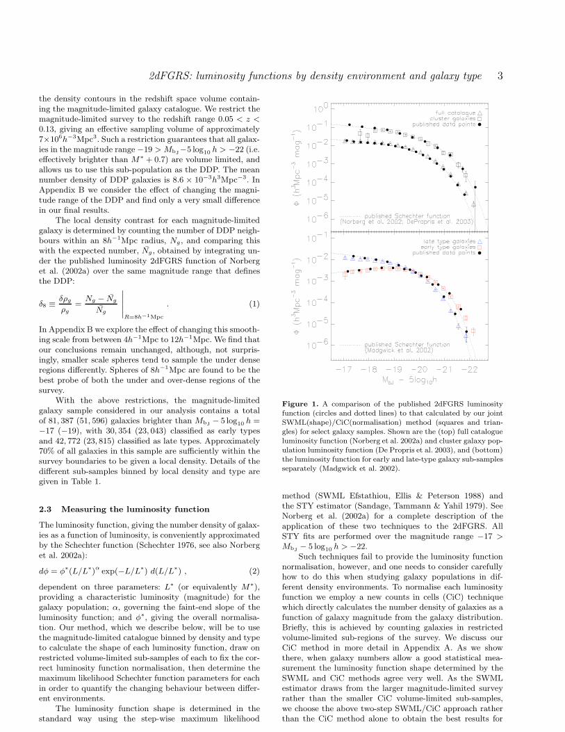
Figure 1. A comparison of the published 2dFGRS luminosityfunction (circles and dotted lines) to that calculated by our jointSWML(shape)/CiC(normalisation) method (squares and trian-gles) for select galaxy samples. Shown are the (top) full catalogueluminosity function (Norberg et al. 2002a) and cluster galaxy pop-ulation luminosity function (De Propris et al. 2003), and (bottom)the luminosity function for early and late-type galaxy sub-samplesseparately (Madgwick et al. 2002).

method (SWML Efstathiou, Ellis & Peterson 1988) andthe STY estimator (Sandage, Tammann & Yahil 1979). SeeNorberg et al. (2002a) for a complete description of theapplication of these two techniques to the 2dFGRS. AllSTY fits are performed over the magnitude range −17 >MbJ

− 5 log10 h > −22.Such techniques fail to provide the luminosity function

normalisation, however, and one needs to consider carefullyhow to do this when studying galaxy populations in dif-ferent density environments. To normalise each luminosityfunction we employ a new counts in cells (CiC) techniquewhich directly calculates the number density of galaxies as afunction of galaxy magnitude from the galaxy distribution.Briefly, this is achieved by counting galaxies in restrictedvolume-limited sub-regions of the survey. We discuss ourCiC method in more detail in Appendix A. As we showthere, when galaxy numbers allow a good statistical mea-surement the luminosity function shape determined by theSWML and CiC methods agree very well. As the SWMLestimator draws from the larger magnitude-limited surveyrather than the smaller CiC volume-limited sub-samples,we choose the above two-step SWML/CiC approach ratherthan the CiC method alone to obtain the best results for

4 Croton et al.

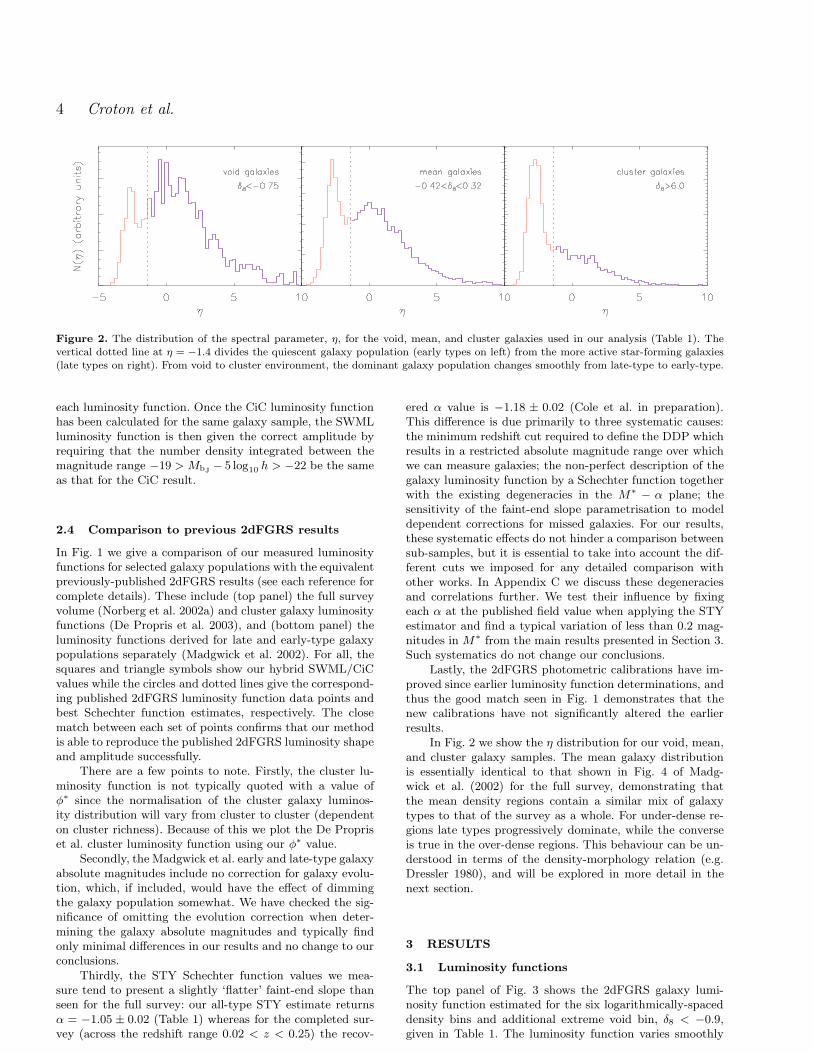
Figure 2. The distribution of the spectral parameter, η, for the void, mean, and cluster galaxies used in our analysis (Table 1). Thevertical dotted line at η = −1.4 divides the quiescent galaxy population (early types on left) from the more active star-forming galaxies(late types on right). From void to cluster environment, the dominant galaxy population changes smoothly from late-type to early-type.

each luminosity function. Once the CiC luminosity functionhas been calculated for the same galaxy sample, the SWMLluminosity function is then given the correct amplitude byrequiring that the number density integrated between themagnitude range −19 > MbJ

− 5 log10 h > −22 be the sameas that for the CiC result.

2.4 Comparison to previous 2dFGRS results

In Fig. 1 we give a comparison of our measured luminosityfunctions for selected galaxy populations with the equivalentpreviously-published 2dFGRS results (see each reference forcomplete details). These include (top panel) the full surveyvolume (Norberg et al. 2002a) and cluster galaxy luminosityfunctions (De Propris et al. 2003), and (bottom panel) theluminosity functions derived for late and early-type galaxypopulations separately (Madgwick et al. 2002). For all, thesquares and triangle symbols show our hybrid SWML/CiCvalues while the circles and dotted lines give the correspond-ing published 2dFGRS luminosity function data points andbest Schechter function estimates, respectively. The closematch between each set of points confirms that our methodis able to reproduce the published 2dFGRS luminosity shapeand amplitude successfully.

There are a few points to note. Firstly, the cluster lu-minosity function is not typically quoted with a value ofφ∗ since the normalisation of the cluster galaxy luminos-ity distribution will vary from cluster to cluster (dependenton cluster richness). Because of this we plot the De Propriset al. cluster luminosity function using our φ∗ value.

Secondly, the Madgwick et al. early and late-type galaxyabsolute magnitudes include no correction for galaxy evolu-tion, which, if included, would have the effect of dimmingthe galaxy population somewhat. We have checked the sig-nificance of omitting the evolution correction when deter-mining the galaxy absolute magnitudes and typically findonly minimal differences in our results and no change to ourconclusions.

Thirdly, the STY Schechter function values we mea-sure tend to present a slightly ‘flatter’ faint-end slope thanseen for the full survey: our all-type STY estimate returnsα = −1.05 ± 0.02 (Table 1) whereas for the completed sur-vey (across the redshift range 0.02 < z < 0.25) the recov-

ered α value is −1.18 ± 0.02 (Cole et al. in preparation).This difference is due primarily to three systematic causes:the minimum redshift cut required to define the DDP whichresults in a restricted absolute magnitude range over whichwe can measure galaxies; the non-perfect description of thegalaxy luminosity function by a Schechter function togetherwith the existing degeneracies in the M∗ − α plane; thesensitivity of the faint-end slope parametrisation to modeldependent corrections for missed galaxies. For our results,these systematic effects do not hinder a comparison betweensub-samples, but it is essential to take into account the dif-ferent cuts we imposed for any detailed comparison withother works. In Appendix C we discuss these degeneraciesand correlations further. We test their influence by fixingeach α at the published field value when applying the STYestimator and find a typical variation of less than 0.2 mag-nitudes in M∗ from the main results presented in Section 3.Such systematics do not change our conclusions.

Lastly, the 2dFGRS photometric calibrations have im-proved since earlier luminosity function determinations, andthus the good match seen in Fig. 1 demonstrates that thenew calibrations have not significantly altered the earlierresults.

In Fig. 2 we show the η distribution for our void, mean,and cluster galaxy samples. The mean galaxy distributionis essentially identical to that shown in Fig. 4 of Madg-wick et al. (2002) for the full survey, demonstrating thatthe mean density regions contain a similar mix of galaxytypes to that of the survey as a whole. For under-dense re-gions late types progressively dominate, while the converseis true in the over-dense regions. This behaviour can be un-derstood in terms of the density-morphology relation (e.g.Dressler 1980), and will be explored in more detail in thenext section.

3 RESULTS

3.1 Luminosity functions

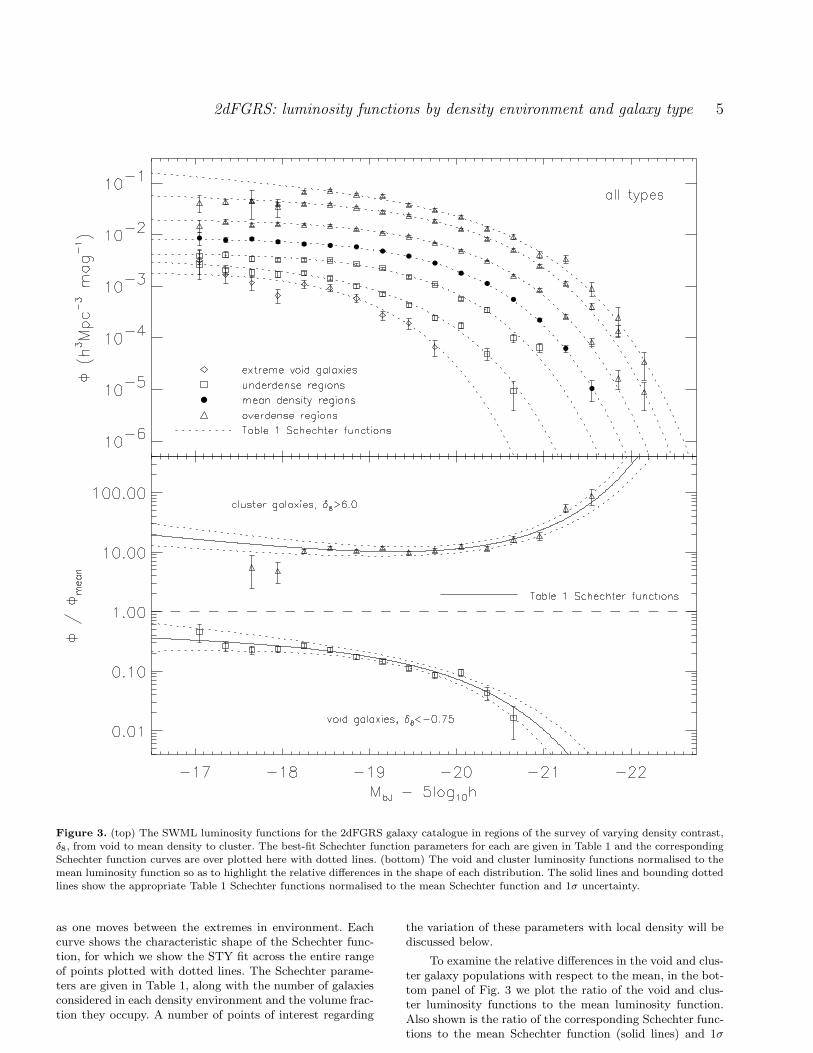
The top panel of Fig. 3 shows the 2dFGRS galaxy lumi-nosity function estimated for the six logarithmically-spaceddensity bins and additional extreme void bin, δ8 < −0.9,given in Table 1. The luminosity function varies smoothly

2dFGRS: luminosity functions by density environment and galaxy type 5

Figure 3. (top) The SWML luminosity functions for the 2dFGRS galaxy catalogue in regions of the survey of varying density contrast,δ8, from void to mean density to cluster. The best-fit Schechter function parameters for each are given in Table 1 and the correspondingSchechter function curves are over plotted here with dotted lines. (bottom) The void and cluster luminosity functions normalised to themean luminosity function so as to highlight the relative differences in the shape of each distribution. The solid lines and bounding dottedlines show the appropriate Table 1 Schechter functions normalised to the mean Schechter function and 1σ uncertainty.

as one moves between the extremes in environment. Eachcurve shows the characteristic shape of the Schechter func-tion, for which we show the STY fit across the entire rangeof points plotted with dotted lines. The Schechter parame-ters are given in Table 1, along with the number of galaxiesconsidered in each density environment and the volume frac-tion they occupy. A number of points of interest regarding

the variation of these parameters with local density will bediscussed below.

To examine the relative differences in the void and clus-ter galaxy populations with respect to the mean, in the bot-tom panel of Fig. 3 we plot the ratio of the void and clus-ter luminosity functions to the mean luminosity function.Also shown is the ratio of the corresponding Schechter func-tions to the mean Schechter function (solid lines) and 1σ

6 Croton et al.

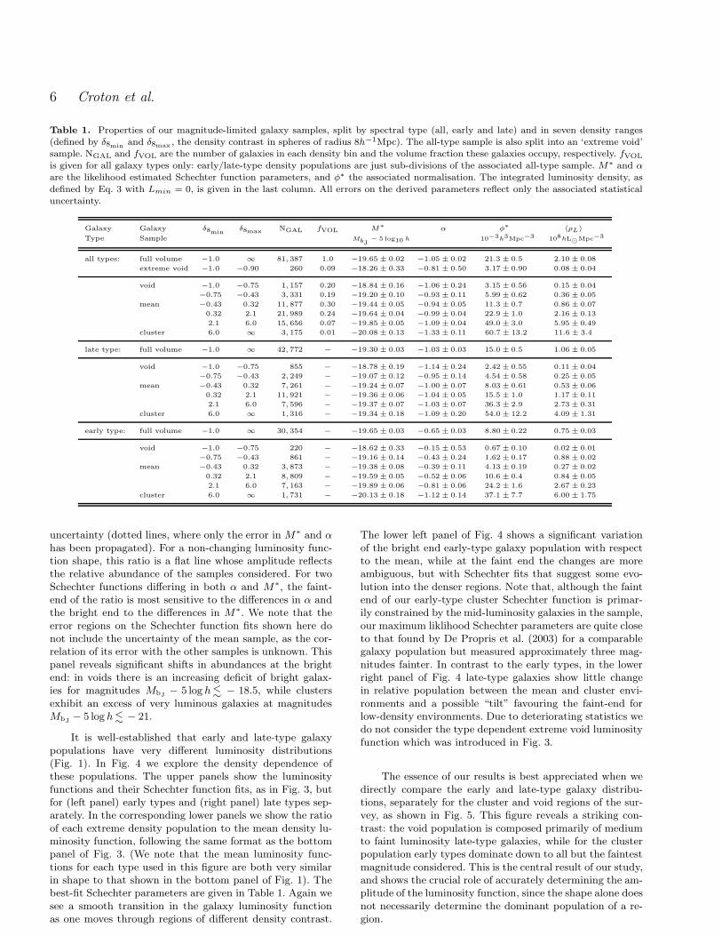
Table 1. Properties of our magnitude-limited galaxy samples, split by spectral type (all, early and late) and in seven density ranges(defined by δ8min

and δ8max , the density contrast in spheres of radius 8h−1Mpc). The all-type sample is also split into an ‘extreme void’sample. NGAL and fVOL are the number of galaxies in each density bin and the volume fraction these galaxies occupy, respectively. fVOL

is given for all galaxy types only: early/late-type density populations are just sub-divisions of the associated all-type sample. M∗ and α

are the likelihood estimated Schechter function parameters, and φ∗ the associated normalisation. The integrated luminosity density, as

defined by Eq. 3 with Lmin = 0, is given in the last column. All errors on the derived parameters reflect only the associated statisticaluncertainty.

Galaxy Galaxy δ8minδ8max NGAL fVOL M∗ α φ∗ 〈ρL〉

Type Sample MbJ

− 5 log10 h 10−3h3Mpc−3 108hL⊙Mpc−3

all types: full volume −1.0 ∞ 81, 387 1.0 −19.65 ± 0.02 −1.05 ± 0.02 21.3 ± 0.5 2.10 ± 0.08

extreme void −1.0 −0.90 260 0.09 −18.26 ± 0.33 −0.81 ± 0.50 3.17 ± 0.90 0.08 ± 0.04

void −1.0 −0.75 1, 157 0.20 −18.84 ± 0.16 −1.06 ± 0.24 3.15 ± 0.56 0.15 ± 0.04

−0.75 −0.43 3, 331 0.19 −19.20 ± 0.10 −0.93 ± 0.11 5.99 ± 0.62 0.36 ± 0.05

mean −0.43 0.32 11, 877 0.30 −19.44 ± 0.05 −0.94 ± 0.05 11.3 ± 0.7 0.86 ± 0.07

0.32 2.1 21, 989 0.24 −19.64 ± 0.04 −0.99 ± 0.04 22.9 ± 1.0 2.16 ± 0.13

2.1 6.0 15, 656 0.07 −19.85 ± 0.05 −1.09 ± 0.04 49.0 ± 3.0 5.95 ± 0.49

cluster 6.0 ∞ 3, 175 0.01 −20.08 ± 0.13 −1.33 ± 0.11 60.7 ± 13.2 11.6 ± 3.4

late type: full volume −1.0 ∞ 42, 772 − −19.30 ± 0.03 −1.03 ± 0.03 15.0 ± 0.5 1.06 ± 0.05

void −1.0 −0.75 855 − −18.78 ± 0.19 −1.14 ± 0.24 2.42 ± 0.55 0.11 ± 0.04

−0.75 −0.43 2, 249 − −19.07 ± 0.12 −0.95 ± 0.14 4.54 ± 0.58 0.25 ± 0.05

mean −0.43 0.32 7, 261 − −19.24 ± 0.07 −1.00 ± 0.07 8.03 ± 0.61 0.53 ± 0.06

0.32 2.1 11, 921 − −19.36 ± 0.06 −1.04 ± 0.05 15.5 ± 1.0 1.17 ± 0.11

2.1 6.0 7, 596 − −19.37 ± 0.07 −1.03 ± 0.07 36.3 ± 2.9 2.73 ± 0.31

cluster 6.0 ∞ 1, 316 − −19.34 ± 0.18 −1.09 ± 0.20 54.0 ± 12.2 4.09 ± 1.31

early type: full volume −1.0 ∞ 30, 354 − −19.65 ± 0.03 −0.65 ± 0.03 8.80 ± 0.22 0.75 ± 0.03

void −1.0 −0.75 220 − −18.62 ± 0.33 −0.15 ± 0.53 0.67 ± 0.10 0.02 ± 0.01

−0.75 −0.43 861 − −19.16 ± 0.14 −0.43 ± 0.24 1.62 ± 0.17 0.88 ± 0.02

mean −0.43 0.32 3, 873 − −19.38 ± 0.08 −0.39 ± 0.11 4.13 ± 0.19 0.27 ± 0.02

0.32 2.1 8, 809 − −19.59 ± 0.05 −0.52 ± 0.06 10.6 ± 0.4 0.84 ± 0.05

2.1 6.0 7, 163 − −19.89 ± 0.06 −0.81 ± 0.06 24.2 ± 1.6 2.67 ± 0.23

cluster 6.0 ∞ 1, 731 − −20.13 ± 0.18 −1.12 ± 0.14 37.1 ± 7.7 6.00 ± 1.75

uncertainty (dotted lines, where only the error in M∗ and αhas been propagated). For a non-changing luminosity func-tion shape, this ratio is a flat line whose amplitude reflectsthe relative abundance of the samples considered. For twoSchechter functions differing in both α and M∗, the faint-end of the ratio is most sensitive to the differences in α andthe bright end to the differences in M∗. We note that theerror regions on the Schechter function fits shown here donot include the uncertainty of the mean sample, as the cor-relation of its error with the other samples is unknown. Thispanel reveals significant shifts in abundances at the brightend: in voids there is an increasing deficit of bright galax-ies for magnitudes MbJ

− 5 log h <∼ − 18.5, while clusters

exhibit an excess of very luminous galaxies at magnitudesMbJ

− 5 log h <∼ − 21.

It is well-established that early and late-type galaxypopulations have very different luminosity distributions(Fig. 1). In Fig. 4 we explore the density dependence ofthese populations. The upper panels show the luminosityfunctions and their Schechter function fits, as in Fig. 3, butfor (left panel) early types and (right panel) late types sep-arately. In the corresponding lower panels we show the ratioof each extreme density population to the mean density lu-minosity function, following the same format as the bottompanel of Fig. 3. (We note that the mean luminosity func-tions for each type used in this figure are both very similarin shape to that shown in the bottom panel of Fig. 1). Thebest-fit Schechter parameters are given in Table 1. Again wesee a smooth transition in the galaxy luminosity functionas one moves through regions of different density contrast.

The lower left panel of Fig. 4 shows a significant variationof the bright end early-type galaxy population with respectto the mean, while at the faint end the changes are moreambiguous, but with Schechter fits that suggest some evo-lution into the denser regions. Note that, although the faintend of our early-type cluster Schechter function is primar-ily constrained by the mid-luminosity galaxies in the sample,our maximum liklihood Schechter parameters are quite closeto that found by De Propris et al. (2003) for a comparablegalaxy population but measured approximately three mag-nitudes fainter. In contrast to the early types, in the lowerright panel of Fig. 4 late-type galaxies show little changein relative population between the mean and cluster envi-ronments and a possible “tilt” favouring the faint-end forlow-density environments. Due to deteriorating statistics wedo not consider the type dependent extreme void luminosityfunction which was introduced in Fig. 3.

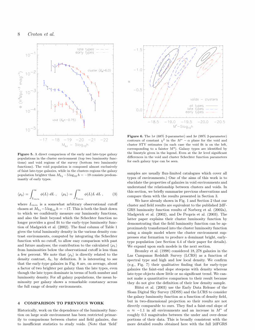
The essence of our results is best appreciated when wedirectly compare the early and late-type galaxy distribu-tions, separately for the cluster and void regions of the sur-vey, as shown in Fig. 5. This figure reveals a striking con-trast: the void population is composed primarily of mediumto faint luminosity late-type galaxies, while for the clusterpopulation early types dominate down to all but the faintestmagnitude considered. This is the central result of our study,and shows the crucial role of accurately determining the am-plitude of the luminosity function, since the shape alone doesnot necessarily determine the dominant population of a re-gion.

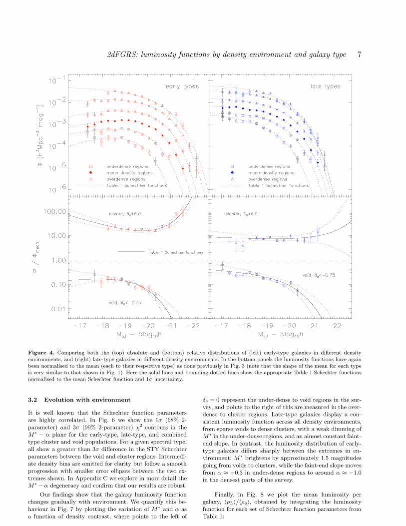
2dFGRS: luminosity functions by density environment and galaxy type 7

Figure 4. Comparing both the (top) absolute and (bottom) relative distributions of (left) early-type galaxies in different densityenvironments, and (right) late-type galaxies in different density environments. In the bottom panels the luminosity functions have againbeen normalised to the mean (each to their respective type) as done previously in Fig. 3 (note that the shape of the mean for each typeis very similar to that shown in Fig. 1). Here the solid lines and bounding dotted lines show the appropriate Table 1 Schechter functionsnormalised to the mean Schechter function and 1σ uncertainty.

3.2 Evolution with environment

It is well known that the Schechter function parametersare highly correlated. In Fig. 6 we show the 1σ (68% 2-parameter) and 3σ (99% 2-parameter) χ2 contours in theM∗ − α plane for the early-type, late-type, and combinedtype cluster and void populations. For a given spectral type,all show a greater than 3σ difference in the STY Schechterparameters between the void and cluster regions. Intermedi-ate density bins are omitted for clarity but follow a smoothprogression with smaller error ellipses between the two ex-tremes shown. In Appendix C we explore in more detail theM∗ −α degeneracy and confirm that our results are robust.

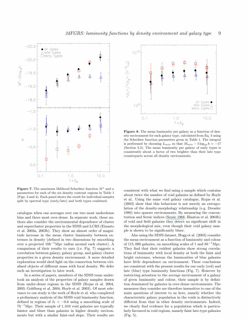
Our findings show that the galaxy luminosity functionchanges gradually with environment. We quantify this be-haviour in Fig. 7 by plotting the variation of M∗ and α asa function of density contrast, where points to the left of

δ8 = 0 represent the under-dense to void regions in the sur-vey, and points to the right of this are measured in the over-dense to cluster regions. Late-type galaxies display a con-sistent luminosity function across all density environments,from sparse voids to dense clusters, with a weak dimming ofM∗ in the under-dense regions, and an almost constant faint-end slope. In contrast, the luminosity distribution of early-type galaxies differs sharply between the extremes in en-vironment: M∗ brightens by approximately 1.5 magnitudesgoing from voids to clusters, while the faint-end slope movesfrom α ≈ −0.3 in under-dense regions to around α ≈ −1.0in the densest parts of the survey.

Finally, in Fig. 8 we plot the mean luminosity pergalaxy, 〈ρL〉/〈ρg〉, obtained by integrating the luminosityfunction for each set of Schechter function parameters fromTable 1:

8 Croton et al.

Figure 5. A direct comparison of the early and late-type galaxypopulations in the cluster environment (top two luminosity func-tions) and void regions of the survey (bottom two luminosityfunctions). The void population is composed almost exclusivelyof faint late-type galaxies, while in the clusters regions the galaxypopulation brighter than MbJ

−5 log10 h = −19 consists predom-inantly of early types.

〈ρg〉 =

∫ ∞

Lmin

φ(L) dL , 〈ρL〉 =

∫ ∞

Lmin

φ(L)L dL , (3)

where Lmin is a somewhat arbitrary observational cutoffchosen at MbJ

−5 log10 h = −17. This is both the limit downto which we confidently measure our luminosity functions,and also the limit beyond which the Schechter function nolonger provides a good fit to the early-type luminosity func-tion of Madgwick et al. (2002). The final column of Table 1gives the total luminosity density in the various density con-trast environments, computed by integrating the Schechterfunction with no cutoff, to allow easy comparison with pastand future analyses; the contribution to the calculated 〈ρL〉from luminosities below the observational cutoff is less thana few percent. We note that 〈ρg〉 is directly related to thedensity contrast, δ8, by definition. It is interesting to seethat the early-type galaxies in Fig. 8 are, on average, abouta factor of two brighter per galaxy than the late types, eventhough the late types dominate in terms of both number andluminosity density. For all galaxy populations, the mean lu-minosity per galaxy shows a remarkable constancy acrossthe full range of density environments.

4 COMPARISON TO PREVIOUS WORK

Historically, work on the dependence of the luminosity func-tion on large scale environment has been restricted primar-ily to comparisons between cluster and field galaxies, dueto insufficient statistics to study voids. (Note that ‘field’

Figure 6. The 1σ (68% 2-parameter) and 3σ (99% 2-parameter)contours of constant χ2 in the M∗

− α plane for the void andcluster STY estimates (in each case the void fit is on the left,corresponding to a fainter M*). Galaxy types are identified bythe linestyle given in the legend. Even at the 3σ level significantdifferences in the void and cluster Schechter function parametersfor each galaxy type can be seen.

samples are usually flux-limited catalogues which cover alltypes of environments.) One of the aims of this work is toelucidate the properties of galaxies in void environments andunderstand the relationship between clusters and voids. Inthis section, we briefly summarise previous observations andcompare them with the results presented in Section 3.

We have already shown in Fig. 1 and Section 2 that ourcluster and field results are equivalent to the published 2dF-GRS luminosity function results of Norberg et al. (2002a),Madgwick et al. (2002), and De Propris et al. (2003). Thelatter paper explains their cluster luminosity function bydemonstrating that the field luminosity function can be ap-proximately transformed into the cluster luminosity functionusing a simple model where the cluster environment sup-presses star formation to produce a dominant bright, early-type population (see Section 4.4 of their paper for details).We expand upon such models in the next section.

Bromley et al. (1998) considered 18, 278 galaxies in theLas Campanas Redshift Survey (LCRS) as a function ofspectral type and high and low local density. We confirm(e.g., Fig. 7) their qualitative finding that for early-typegalaxies the faint-end slope steepens with density whereaslate-type objects show little or no significant trend. We can-not make a quantitative comparison to their result becausethey do not give the definition of their low density sample.

Hutsi et al. (2003) use the Early Data Release of theSloan Digital Sky Survey (SDSS) and the LCRS to considerthe galaxy luminosity function as a function of density field,but in two-dimensional projection so their results are notdirectly comparable to ours. They find a faint-end slope ofα ≈ −1.1 in all environments and an increase in M∗ ofroughly 0.3 magnitudes between the under and over-denseportions of their data. This is broadly consistent with themore detailed results obtained here with the full 2dFGRS

2dFGRS: luminosity functions by density environment and galaxy type 9

Figure 7. The maximum liklihood Schechter function M∗ and α

parameters for each of the six density contrast regions in Table 1(Figs. 3 and 4). Each panel shows the result for individual samplessplit by spectral type (early/late) and both types combined.

catalogue when one averages over our two most underdensebins and three most over-dense. In separate work, these au-thors also consider the environmental dependence of clusterand supercluster properties in the SDSS and LCRS (Einastoet al. 2003a, 2003b). They show an almost order of magni-tude increase in the mean cluster luminosity between ex-tremes in density (defined in two dimensions by smoothingover a projected 10h−1Mpc radius around each cluster). Acomparison of their results to ours (i.e. Fig. 7) suggests acorrelation between galaxy, galaxy group, and galaxy clusterproperties in a given density environment. A more detailedexploration would shed light on the connection between viri-alised objects of different mass with local density. We defersuch an investigation to later work.

In a series of papers, members of the SDSS team under-took an analysis of the properties of galaxy samples drawnfrom under-dense regions in the SDSS (Rojas et al. 2004,2003; Goldberg et al. 2004; Hoyle et al. 2003). Of most rele-vance to our study is the work of Hoyle et al. who completeda preliminary analysis of the SDSS void luminosity function,defined in regions of δ7 < −0.6 using a smoothing scale of7h−1Mpc. Their sample of 1, 010 void galaxies are typicallyfainter and bluer than galaxies in higher density environ-ments but with a similar faint-end slope. Their results are

Figure 8. The mean luminosity per galaxy as a function of den-sity environment for each galaxy type, calculated from Eq. 3 usingthe Schechter function parameters given in Table 1. The integralis performed by choosing Lmin so that Mmin − 5 log10 h = −17(Section 3.2). The mean luminosity per galaxy of early types isconsistently about a factor of two brighter than their late typecounterparts across all density environments.

consistent with what we find using a sample which containsabout twice the number of void galaxies as defined by Hoyleet al.. Using the same void galaxy catalogue, Rojas et al.(2003) show that this behaviour is not merely an extrapo-lation of the density-morphology relationship (e.g. Dressler1980) into sparser environments. By measuring the concen-tration and Sersic indices (Sersic 1968, Blanton et al. 2003b)of void and field galaxies they detect no significant shift inthe morphological mix, even though their void galaxy sam-ple is shown to be significantly bluer.

Also using the SDSS dataset, Hogg et al. (2003) considerthe mean environment as a function of luminosity and colourof 115, 000 galaxies, on smoothing scales of 1 and 8h−1Mpc.They find that their reddest galaxies show strong correla-tions of luminosity with local density at both the faint andbright extremes, whereas the luminosities of blue galaxieshave little dependence on environment. These conclusionsare consistent with the present results for our early (red) andlate (blue) type luminosity functions (Fig. 7). However byrestricting attention to the average environment of a galaxyof given luminosity and colour, their sample is by defini-tion dominated by galaxies in over-dense environments. Themeasures they consider are therefore insensitive to one of themain questions of interest to us here, namely whether thecharacteristic galaxy population in the voids is distinctivelydifferent from that in other density environments. Indeed,we clearly find evidence for a population which is particu-larly favoured in void regions, namely faint late-type galaxies(Fig. 5).

10 Croton et al.

Table 2. A mnemonic summary of our main results, drawing on the work of De Propris et al. (2003) and Mo et al. (2004) to interpretthe observed behaviour in Figs. 5 and 7 in terms of physical processes which govern the void and cluster galaxy populations.

Region Observation Process

Voids 1. galaxies typically reside at the centrefaint, late type of low mass dark halos (⇒ faint)

galaxies dominate 2. gas is available for star formation (⇒ blue)3. merger rate is low (⇒ spirals)

Clusters 1. typically satellite and central galaxies ofmid-bright, early-type massive dark halos (⇒ mid-bright)

galaxies dominate 2. gas is unavailable for star formation (⇒ red)3. merger rate is high (⇒ ellipticals)

5 DISCUSSION

As clusters are comparatively well-studied objects, and havealready been addressed using the 2dFGRS by De Propris etal. (2003), we focus here primarily on a discussion of thevoids.

A detailed analysis of void population properties hasrecently become possible due to significant improvementsin the quality of both theoretical modelling and observa-tional data, as summarised by Benson et al. (2003). Pee-bles (2001) has argued that, visually, observed voids do notmatch simulated ones and discussed several statistical mea-sures for quantifying a comparison, primarily the distance tothe nearest neighbour in a reference sample. However the cu-mulative distributions of nearest neighbour distances shownin Figs. 4–6 of Peebles (2001) show very little difference be-tween the reference–reference and test–reference distribu-tions. It is not surprising that these statistical measures areinsensitive to a void effect, since they are dominated by clus-ter galaxies. Our method is designed to overcome this diffi-culty by explicitly isolating the void population of galaxiesso that their properties can be studied.

Motivated by the claims of discrepancies in Peebles(2001), Mathis & White (2002) investigated the nature ofvoid galaxies using N-body simulations with semi-analyticrecipes for galaxy formation. They call into question the as-sertion of Peebles (2001) that ΛCDM predicts a populationof small haloes in the voids, concluding that “the popula-tion of faint galaxies...does not constitute a void popula-tion”. More specifically, they find that all types of galaxiestend to avoid the void regions of their simulation, down totheir resolution limit of MB = −16.27 in luminosity andMB = −18.46 in morphology.

The abundance of faint galaxies we find in the void re-gions of the 2dFGRS seems to be at odds with the Mathis &White predictions. However their results rely on the Peebles(2001) cumulative distribution of galaxies as a function ofover density (their Fig. 3) which, like cumulative distribu-tions in general, are rather insensitive to numerically-minorcomponents of the galaxy population. Note that Mathis &White define density contrast using the dark matter massdistribution smoothed over a 5 h−1Mpc sphere, whereas wemeasure the density contrast by galaxy counts. Another pos-sible source of discrepancy is the uncertainties in their semi-analytic recipes, such as the implementation of supernovafeedback, which can strongly effect the faint-end luminositydistribution.

There has been recent discussion in the literature aboutthe nature of the faint-end galaxy population and its depen-dence on group and cluster richness. Most notably, Tully etal. (2002) show a significant steepening in the faint-end pop-ulation as one considers nearby galaxy groups of increasingrichness, from the Local Group to Coma. On the surface ofit, this might seem at variance with our results, which arerather better described by a faint-end slope which is approx-imately constant with changing density environment for thefull 2dFGRS galaxy sample (Fig. 7). However the steepeningof the faint-end slope they find primarily occurs at magni-tudes fainter than MB = −17, which is beyond the limitwe can study with our sample. Also, their analysis focuseson individual groups of galaxies, while we have chosen towork with a much bigger galaxy sample and have smoothedit over a scale much larger than the typical cluster. Indeed,as discussed in Appendix B, when the smoothing scale issignificantly larger than the characteristic size of the struc-tures being probed it is possible that the Schechter functionparameters may become insensitive to the small scale shiftsin population. This effect, of course, would be less significantfor survey regions which host clusters of clusters (i.e. super-clusters), and which are prominently seen in the 2dFGRS(Baugh et al. 2004, Croton et al. 2004). When sampling the2dFGRS volume the trend with density that one sees using4h−1 Mpc spheres in Fig. B1 is consistent with the Tullyet al. result, although one needs to additionally understandthe influences of Poisson noise.

Tully et al. attribute their results to a process of pho-toionisation of the IGM which suppresses dwarf galaxy for-mation. Over-dense regions, which at later times becomemassive clusters, typically collapse early and thus have timeto form a dwarf galaxy population before the epoch of reion-isation. Under-dense regions, on the other hand, begin theircollapse at much later times and are thus subject to thephotoionisation suppression of cooling baryons. This, theyargue, explains the significant increase between the dwarfpopulations of the Local Group (low density environment)and Coma (over-dense environment). Although suggestive,a deeper understanding of what is happening will require amuch more statistically significant sample.

Recently Mo et al. (2004) have considered the depen-dence of the galaxy luminosity function on large scale envi-ronment in their halo occupation model. In this model, themass of a dark matter halo alone determines the proper-ties of the galaxies. They create mock catalogues built with

2dFGRS: luminosity functions by density environment and galaxy type 11

a halo-conditional luminosity function (Yang et al. 2003)which is constrained to reproduce the overall 2dFGRS lu-minosity function and correlation length for both luminos-ity and type. They analyse their data by smoothing overspheres of radius 8 h−1Mpc in their mock catalogue, andmeasure the luminosity function as a function of densitycontrast. Their work is performed in real space while weare restricted to work in redshift space. Nonetheless, theirpredictions qualitatively match our density-dependent lu-minosity functions; a quantitative comparison is deferred tosubsequent work.

In the framework of the Mo et al. model, the reasonthe faint-end slope α has such a strong dependence on lo-cal density for early types (Fig. 7) is that faint ellipticalstend to reside predominantly in cluster-sized halos. The αdependence is weaker for late types because faint later-typegalaxies tend to live primarily in less massive haloes, whichare present in all density environments. The correlations be-tween dark halo mass and the properties of the associatedgalaxies are not a fundamental prediction of their model,but are input through phenomenological functions adjustedto give agreement with the 2dFGRS overall luminosity func-tions by galaxy type. However it would be a non-trivial resultif the correlations are the same independently of whether thedark matter halo is in a void or in a cluster. For instance,this property would not apply in models for which reionisa-tion more efficiently prevented star formation in under-denseenvironments than in over-dense environments, as discussedabove.

An interesting consequence of the Mo et al. (2004)model is that the luminous galaxy distribution (which is easyto observe but hard to model) correlates well with the darkhalo mass distribution (which is hard to observe but easy tomodel). If their predictions prove to give a good descriptionof the present data it will lend credence to the underlyingassumption of their model—that the environmental depen-dence of many fundamental galaxy properties are entirelydue to the dependence of the dark halo mass function onenvironment. Exactly why this is would still need to be ex-plained, however such a demonstration may facilitate moredetailed comparisons between theory and observation thanpreviously possible.

An important result of our work is presented in Fig. 5,where a significant shift in the dominant population betweenvoids and clusters is seen. Such a result points to substan-tial differences in the evolutionary tracks of cluster and voidearly-type galaxies. Cluster galaxies have been historicallywell studied: they are more numerous and much brighteron average, with an evolution dominated by galaxy-galaxyinteractions and mergers. In voids, however, the picture isnot so clear. A reasonable expectation would be that thedynamical evolution of void galaxies should be much slowerdue to their relative isolation, with passively evolved stellarpopulations and morphologies similar to that obtained dur-ing their formation. Targeted observational studies of voidearly-type galaxies may reveal much about the high redshiftformation processes that go into making such rare objects.

Table 2 summarises our main results and provides aqualitative or mnemonic interpretation based on our obser-vations and the work of Mo et al. (2004) and De Propris et al.(2003) (and references therein). Our primary result is thestriking change in population types between voids and clus-

ters shown in Fig. 5: faint, late-type galaxies are overwhelm-ingly the dominant galaxy population in voids, completelythe contrary of the situation in clusters. The existence ofsuch a population in the voids, and more generally the waypopulations of different type are seen to change between dif-ferent density environments, place important constraints oncurrent and future models of galaxy formation.

ACKNOWLEDGEMENTS

The 2dFGRS was undertaken using the two-degree fieldspectrograph on the Anglo-Australian Telescope. We ac-knowledge the efforts of all those responsible for the smoothrunning of this facility during the course of the survey, andalso the indulgence of the time allocation committees. Manythanks go to Simon White, Frank van den Bosch, Guine-vere Kauffmann, and Jim Peebles for useful discussions. Wealso wish to thank the referee, Jaan Einasto, for swift andconstructive comments which improved the content of thepaper. DJC wishes to thank the NYU Center for Cosmol-ogy and Particle Physics for its hospitality during part ofthis research, and acknowledges the financial support of theInternational Max Planck Research School in AstrophysicsPh.D. fellowship, under which this work was carried out.GRF acknowledges the hospitality of the Max Planck Insti-tute for Astronomy during the inception of this work andthe support of the Departments of Physics and Astronomy,Princeton University; her research is also supported in partby NSF-PHY-0101738. PN acknowledges financial supportthrough a Zwicky Fellowship at ETH, Zurich.

REFERENCES

Baugh C. M., et al. (2dFGRS team), 2004, MNRAS, 351, L44Benson A. J., Hoyle F., Torres F., Vogeley M. S., 2003, MNRAS,

340, 160Blanton M. R., et al. (SDSS team), 2003a, ApJ, 592, 819

Blanton M. R., et al. (SDSS team), 2003b, ApJ, 594, 186Bromley B. C., Press W. H., Lin H., Kirshner R. P., 1998, ApJ,

505, 25Christlein D., 2000, ApJ, 545, 145Colless M. et al. (2dFGRS team), 2001, MNRAS, 328, 1039Colless M. et al. (2dFGRS team), 2003, astro-ph/0306581

Croton D. J., et al. (2dFGRS team), 2004, MNRAS, 352, 1232De Propris R. et al. (2dFGRS team), 2003, MNRAS, 342, 725Dressler A., 1980, ApJ, 236, 351Efstathiou G., Ellis R. S., Peterson B. A., 1988, MNRAS, 232,

431Einasto J., Hutsi G., Einasto M., Saar E., Tucker D. L., Muller

V., Heinamaki P., & Allam S. S. 2003a, AAP, 405, 425Einasto J., et al. 2003b, AAP, 410, 425

Eke V. R. et al. (2dFGRS team), 2004, MNRAS, submitted(astro-ph/0402566)

Folkes S. et al. (2dFGRS team), 1999, MNRAS, 308, 459Goldberg D. M., Jones T. D, Hoyle F., Rojas R. R., Vogeley M. S.,

Blanton M. R., 2004, ApJ, submitted (astro-ph/0406527)Hogg D. W. et al. (SDSS team), 2003, ApJL, 585, L5Hoyle F., Rojas R. R., Vogeley M. S., Brinkmann J., 2003, ApJ,

submitted (astro-ph/0309728)

Hoyle, F. & Vogeley, M. S. 2004, ApJ, 607, 751Hutsi G., Einasto J., Tucker D. L., Saar E., Einasto M.,

Muller V., Heinamaki P., Allam S. S., 2003, A&A, submit-ted (astro-ph/0212327)

12 Croton et al.

Kauffmann G. et al. (SDSS team), 2004, MNRAS, submitted

(astro-ph/0402030)Lin H., Yee H. K. C., Carlberg R. G., Ellingson E., 1996, BAAS,

28, 1412Loveday J., Peterson B. A., Efstathiou G., Maddox S. J., 1992,

ApJ, 390, 338Madgwick D. S. et al. (2dFGRS team), 2002, MNRAS, 333, 133Marzke R. O., Huchra J. P., Geller M. J., 1994, ApJ, 428, 43Mathis H., White S. D. M., 2002, MNRAS, 337, 1193Mo H. J., Yang X., van den Bosch F. C., Jing Y. P., 2004, MN-

RAS, 349, 205Norberg P. et al. (2dFGRS team), 2001, MNRAS, 328, 64Norberg P. et al. (2dFGRS team), 2002a, MNRAS, 336, 907Norberg P. et al. (2dFGRS team), 2002b, MNRAS, 332, 827Peebles P. J. E., 2001, ApJ, 557, 495Ratcliffe A., Shanks T., Parker Q. A., Fong R., 1998, MNRAS,

293, 197Rojas R. R., Vogeley M. S., Hoyle F., Brinkmann J., 2004, ApJ,

submitted (astro-ph/0409074)Rojas R. R., Vogeley M. S., Hoyle F., Brinkmann J., 2003, ApJ,

submitted (astro-ph/0307274)Sandage A., Tammann G. A., Yahil A., 1979, ApJ, 232, 352Schechter P., 1976, ApJ, 203, 297Sersic J. L., 1968, Atlas de Galaxias Australes. Observatorio As-

tronomico, Cordoba.Tully R. B., Somerville R. S., Trentham, N., Verheijen M. A. W.,

2002, ApJ, 569, 573Yang, X., Mo, H. J., & van den Bosch, F. C. 2003, MNRAS, 339,

1057Zucca E. et al. (ESP team), 1997, A&A, 326, 477

APPENDIX A: THE COUNTS IN CELLS

LUMINOSITY FUNCTION ESTIMATOR AND

COMPARISON TO THE SWML RESULTS

Our counts-in-cells (CiC) method to measure the densitydependent luminosity function and obtain its amplitude issimple and will be illustrated with the example of a mockgalaxy sample in a cubical volume of side-length L. The fullluminosity function for such a sample is trivial. By defini-tion it is simply the number of galaxies in each magnitudeinterval divided by the volume of the box:

Φ(M) = N(M) / L3 . (A1)

To determine the luminosity function as a function oflocal galaxy density we require two additional pieces of in-formation. Firstly we sub-divide the galaxy population intodensity bins. The local density for each galaxy is calculatedwithin an 8h−1Mpc radius as described in Section 2.2. Thisgives us the number of galaxies in each density bin belongingto each magnitude range, Nδ8(M).

Secondly we determine the volume which should be at-tributed to the various density bins. We do this by findingthe fraction of the volume in which the galaxies of eachdensity bin reside, fδ8 . This fraction is measured by mas-sively oversampling the box with randomly placed 8h−1Mpcspheres, in each of which we estimate a local density in thesame way as before. Once all spheres have been placed wecount the number which have a local density in each densityrange. The volume fraction of each bin is then just the frac-tion of spheres found in each bin. Since the total volume ofthe box is known, the volume of each density bin is now alsoknown. The density dependent luminosity function is thencalculated as:

Figure A1. A comparison of the raw counts in cells luminosityfunction with the normalised SWML luminosity function, as de-scribed in the text (Section 2.3 and Appendix A). Shown are thecluster, mean, and void populations consisting of all galaxy typesonly, although all luminosity functions used in this paper behaveequally as well. The shapes estimated by the two very differentmethods are in very good agreement over the magnitude rangesconsidered.

φδ8(M) = Nδ8(M) / fδ8L3 . (A2)

The situation becomes more complicated when dealingwith a magnitude limited redshift survey instead of a sim-ple simulated box. Galaxy counting and volume estimationmust now be restricted to regions of the survey in which themagnitude range being considered is volume limited. Thisrange of course changes for each magnitude bin in whichthe luminosity function is measured. In addition, small cor-rections (< 10%) are required when counting galaxies toaccount for the spectroscopic incompleteness of the survey(see Croton et al. 2004). In all other respects, however, thecalculation of Φδ8(M) is the same as in the “box” examplegiven above.

In Fig. A1 we show a comparison of the 2dFGRS CiCand SWML luminosity functions calculated from the samevoid, mean, and cluster galaxy samples. The SWML lumi-nosity function has been normalised to the CiC measurementas described in Section 2.2. We see that both methods pro-duce almost identical luminosity distribution shapes. Thisgives us confidence that the CiC luminosity function canbe used to normalise the SWML luminosity function in anunbiased way.

Because of the volume-limited restriction of the CiCmethod, the number of galaxies used to calculate the lu-minosity function is smaller than for the SWML method,which draws from the larger magnitude-limited catalogue.However the benefit of the CiC method is that it gives a di-rect measurement of the number density of galaxies rather

2dFGRS: luminosity functions by density environment and galaxy type 13

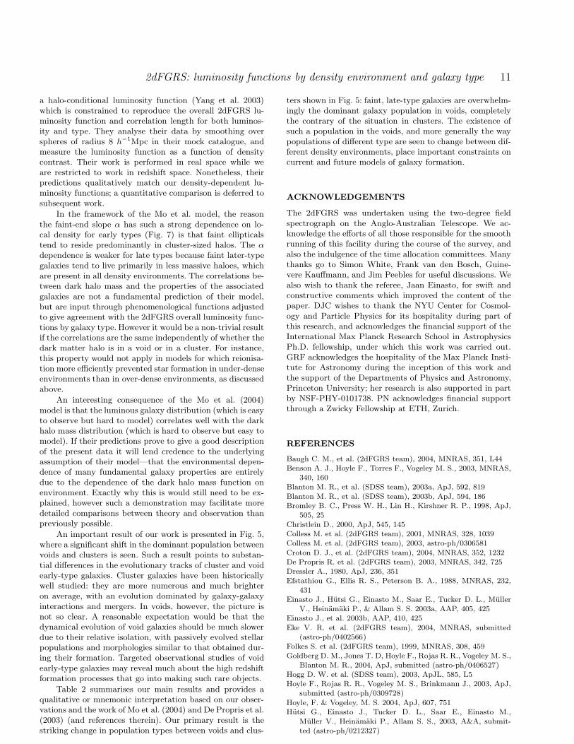
Figure B1. The difference in the STY Schechter function pa-rameters when the local density is calculated with an increasinglyfainter density defining population (DDP): Mmin − 5 log10 h =−20, −19, and −18. Such a change also changes the redshift rangeof the included volume as described in the text. For clarity onlyresults for all galaxy types are shown. The reference sample is theMmin − 5 log10 h = −19 DDP used throughout this paper, andthe other DDP results are shown relative to this.

than just the shape of the distribution as the SWML estima-tor does. In addition, the CiC method is very easy to applyto mock catalogues, as described above. By combining theCiC and SWML methods we capture the best features ofboth.

APPENDIX B: THE EFFECTS OF CHANGING

THE DENSITY DEFINING POPULATION AND

SMOOTHING SCALE

In our analysis we are required to make two importantchoices before beginning. The first is to find the widest pos-sible absolute magnitude range for the density defining pop-ulation (DDP, see Section 2.2) while maximising the amountof the 2dFGRS survey volume sampled. The second is thescale over which we smooth the DDP galaxy distribution todetermine the density contours within this volume. We willnow consider the effect of changing each of these choices inturn.

The density defining population

The DDP is important in that it not only sets the meandensity of galaxies used to define the density contours, butalso determines the redshift range of the full magnitude-limited catalogue to be included in the analysis. Clearlyone would like as high-statistics a sample as possible in aslarge a volume as possible for the best results. In a vol-ume limited galaxy sample such as the DDP, the maxi-mum galaxy redshift available is constrained by the spec-ified faint absolute magnitude limit: galaxies beyond this

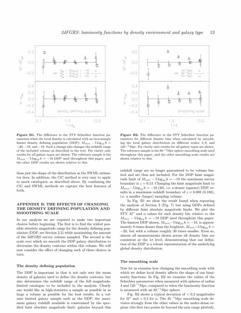
Figure B2. The difference in the STY Schechter function pa-rameters for different density bins when calculated by smooth-ing the local galaxy distribution on different scales: 4, 8, and12h−1Mpc. For clarity only results for all galaxy types are shown.The reference sample is the 8h−1Mpc sphere smoothing scale usedthroughout this paper, and the other smoothing scale results areshown relative to this.

redshift range are no longer guaranteed to be volume lim-ited and are thus not included. For the DDP faint magni-tude limit of Mmin − 5 log10 h = −19 the maximum surveyboundary is z = 0.13. Changing the faint magnitude limit toMmin−5 log10 h = −18 (20), i.e. a denser (sparser) DDP, re-sults in a maximum redshift boundary of z = 0.088 (0.188),i.e. a smaller (larger) sampling volume.

In Fig. B1 we show the result found when repeatingthe analysis of Section 3 (Fig. 7) but using DDPs definedby different faint absolute magnitude limits. We plot theSTY M∗ and α values for each density bin relative to theMmin − 5 log10 h = −19 DDP used throughout this paper.The faintest DDP shown, Mmin−5 log10 h = −18, is approx-imately 8 times denser than the brightest, Mmin−5 log10 h =−20, but with a volume roughly 30 times smaller. Even so,almost all measurements shown across all density bins areconsistent at the 1σ level, demonstrating that our defini-tion of the DDP is a robust representation of the underlyingglobal density distribution.

The smoothing scale

Now let us examine how changing the smoothing scale withwhich we define local density affects the shape of our lumi-nosity functions. In Fig. B2 we examine the values of theSchechter parameters when measured with spheres of radius4 and 12h−1Mpc, compared to when the luminosity functionis measured with an 8h−1Mpc sphere.

Fig. B2 shows a typical deviation of < 0.2 magnitudesfor M∗ and < 0.2 for α. The 4h−1Mpc smoothing scale de-viates strongly from the other values in the under-dense re-gions (the first two points lie beyond the axis range plotted),

14 Croton et al.

however in these environments such a smoothing scale givesa poor estimate of the local galaxy density due to Poissonnoise in small number counts. Indeed, Hoyle et al. (2004)have shown that in the extreme under-dense 2dFGRS sur-vey regions the characteristic scale of voids is approximately15h−1Mpc. For cluster regions 4h−1Mpc spheres can be em-ployed and would give a higher resolution discriminationof the structure. The 8h−1Mpc smoothing scale we haveadopted captures the essential aspects of voids while roughlyoptimising the statistical signal, and is thus a good probe ofboth the under and over-dense regions of the survey volume.

APPENDIX C: SYSTEMATIC EFFECTS WHEN

ESTIMATING THE SCHECHTER FUNCTION

PARAMETERS

One may ask to what degree the trends seen in Fig. 7 andTable 1 are influenced by the systematics discussed in Sec-tion 2.4. We note there that our STY measurements recovera flatter faint end than the current published 2dFGRS lu-minosity function for the completed catalogue. We identifythree systematic effects which contribute to this behaviour:the absolute magnitude range considered when applying theSTY estimator, the fact that the luminosity function is notperfectly described by a Schechter function, and the sen-sitivity of the faint-end slope parameterisation to model-dependent corrections included to account for missed galax-ies.

We find that the first two of these effects have thestrongest influence on the measured STY faint-end slope.Indeed, testing the first reveals that any STY estimate ofthe 2dFGRS luminosity function over a restricted absolutemagnitude range displays a systematic shift in the recov-ered STY parameters along a line in the M∗ − α plane.The brighter the faint magnitude restriction, the flatter thefaint-end slope is and the fainter the characteristic mag-nitude becomes. Such behaviour is a consequence of smallbut important deviations in the galaxy luminosity functionshape from the pure Schechter function assumed by the STYestimator. In addition, Fig. 11 of Norberg et al. (2002) re-veals a dip in the luminosity function between the magni-tude range −17 > MbJ

− 5 log10 h > −18 and a steepeningfaintward of this. In our analysis only galaxies brighter thanMbJ

−5 log10 h = −17 are considered due to the restriction ofthe DDP. This limitation adds extra weight to the influenceof the dip on the STY fit contributing further to a flatterestimation of α. When mock galaxy catalogues constructedto have a perfect Schechter function luminosity distributionare analysed in an identical way to the 2dFGRS samples,we find that the above systematics all but disappear andthe “true” M∗ and α values are recovered for any reason-able choice of STY fitting range.

Finally, we note that the sensitivity of the faint-endslope parametrisation to systematic corrections for spectro-scopically missed galaxies is minimised by restricting ouranalysis to galaxies with bJ < 19, for which the spectro-scopic incompleteness is typically less than ∼ 8% (see Fig. 16of Colless et al. 2001).

Given that a full correction of the above systematic ef-fects is not possible in our analysis, the next best thing wecan do is try to quantify to what degree they influence our

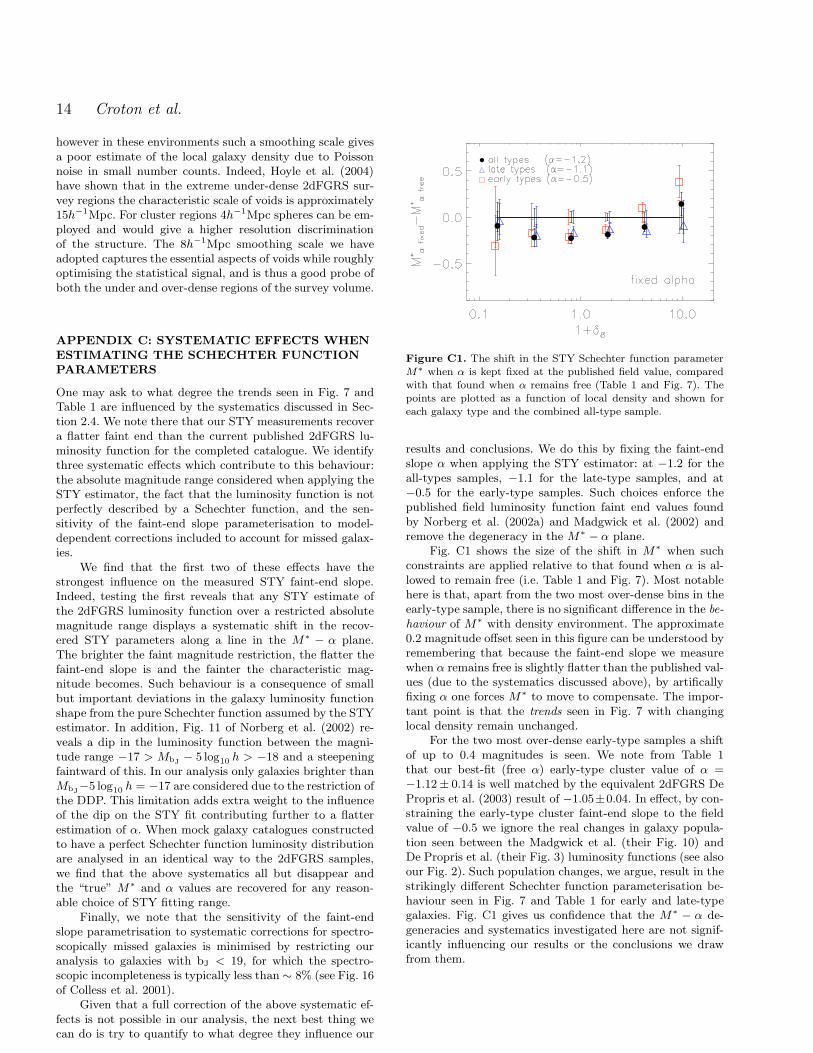
Figure C1. The shift in the STY Schechter function parameterM∗ when α is kept fixed at the published field value, comparedwith that found when α remains free (Table 1 and Fig. 7). Thepoints are plotted as a function of local density and shown foreach galaxy type and the combined all-type sample.

results and conclusions. We do this by fixing the faint-endslope α when applying the STY estimator: at −1.2 for theall-types samples, −1.1 for the late-type samples, and at−0.5 for the early-type samples. Such choices enforce thepublished field luminosity function faint end values foundby Norberg et al. (2002a) and Madgwick et al. (2002) andremove the degeneracy in the M∗ − α plane.

Fig. C1 shows the size of the shift in M∗ when suchconstraints are applied relative to that found when α is al-lowed to remain free (i.e. Table 1 and Fig. 7). Most notablehere is that, apart from the two most over-dense bins in theearly-type sample, there is no significant difference in the be-

haviour of M∗ with density environment. The approximate0.2 magnitude offset seen in this figure can be understood byremembering that because the faint-end slope we measurewhen α remains free is slightly flatter than the published val-ues (due to the systematics discussed above), by artificallyfixing α one forces M∗ to move to compensate. The impor-tant point is that the trends seen in Fig. 7 with changinglocal density remain unchanged.

For the two most over-dense early-type samples a shiftof up to 0.4 magnitudes is seen. We note from Table 1that our best-fit (free α) early-type cluster value of α =−1.12± 0.14 is well matched by the equivalent 2dFGRS DePropris et al. (2003) result of −1.05±0.04. In effect, by con-straining the early-type cluster faint-end slope to the fieldvalue of −0.5 we ignore the real changes in galaxy popula-tion seen between the Madgwick et al. (their Fig. 10) andDe Propris et al. (their Fig. 3) luminosity functions (see alsoour Fig. 2). Such population changes, we argue, result in thestrikingly different Schechter function parameterisation be-haviour seen in Fig. 7 and Table 1 for early and late-typegalaxies. Fig. C1 gives us confidence that the M∗ − α de-generacies and systematics investigated here are not signif-icantly influencing our results or the conclusions we drawfrom them.