arX

iv:a

stro

-ph/

0402

577v

2 1

2 Ju

l 200

4Mon. Not. R. Astron. Soc. 000, 000–000 (0000) Printed 2 February 2008 (MN LATEX style file v1.4)

The 2dF Galaxy Redshift Survey: The clustering of galaxy

groups

Nelson D. Padilla1, Carlton M. Baugh1, Vincent R. Eke1, Peder Norberg2,

Shaun Cole1, Carlos S. Frenk1, Darren J. Croton3, Ivan K. Baldry4, Joss Bland-

Hawthorn5, Terry Bridges5,6, Russell Cannon5, Matthew Colless5,7, Chris Collins8,

Warrick Couch9, Gavin Dalton10,11, Roberto De Propris7, Simon P. Driver7, George

Efstathiou12, Richard S. Ellis13, Karl Glazebrook4, Carole Jackson7, Ofer Lahav14,

Ian Lewis10, Stuart Lumsden15, Steve Maddox16, Darren Madgwick17, John A.

Peacock18, Bruce A. Peterson7, Will Sutherland18,12, Keith Taylor13

1Department of Physics, University of Durham, South Road, Durham DH1 3LE, UK.2ETHZ Institut fur Astronomie, HPF G3.1, ETH Honggerberg, CH-8093 Zurich, Switzerland.3Max-Planck-Institut fur Astrophysik, D-85740 Garching, Germany.4Department of Physics & Astronomy, Johns Hopkins University, Baltimore, MD 21118-2686, USA.5Anglo-Australian Observatory, P.O. Box 296, Epping, NSW 2111, Australia.6Department of Physics, Queen’s University, Kingston, Ontario, K7L 3N6, Canada.7Research School of Astronomy & Astrophysics, The Australian National University, Weston Creek, ACT 2611, Australia.8Astrophysics Research Institute, Liverpool John Moores University, Twelve Quays House, Birkenhead, L14 1LD, UK.9Department of Astrophysics, University of New South Wales, Sydney, NSW 2052, Australia.10Department of Physics, University of Oxford, Keble Road, Oxford OX1 3RH, UK.11Space Science and Technology Department, CCLRC Rutherford Appleton Laboratory, Chilton, Didcot, Oxfordshire, OX11 0QX, UK.12Institute of Astronomy, University of Cambridge, Madingley Road, Cambridge CB3 0HA, UK.13Department of Astronomy, California Institute of Technology, Pasadena, CA 91025, USA.14Department of Physics and Astronomy, University College London, Gower Street, London, WC1E 6BT, UK.15Department of Physics, University of Leeds, Woodhouse Lane, Leeds, LS2 9JT, UK.16School of Physics & Astronomy, University of Nottingham, Nottingham NG7 2RD, UK.17Department of Astronomy, University of California, Berkeley, CA 92720, USA.18Institute for Astronomy, University of Edinburgh, Royal Observatory, Blackford Hill, Edinburgh EH9 3HJ, UK.

2 February 2008

ABSTRACT

We measure the clustering of galaxy groups in the 2dFGRS Percolation-InferredGalaxy Group (2PIGG) catalogue. The 2PIGG sample has 28 877 groups with atleast two members. The clustering amplitude of the full 2PIGG catalogue is weakerthan that of 2dFGRS galaxies, in agreement with theoretical predictions. We have sub-divided the 2PIGG catalogue into samples that span a factor of ≈ 25 in median totalluminosity. Our correlation function measurements span an unprecedented range ofclustering strengths, connecting the regimes probed by groups fainter than L∗ galaxiesand rich clusters. There is a steady increase in clustering strength with group lumi-nosity; the most luminous groups are ten times more strongly clustered than the full2PIGG catalogue. We demonstrate that the 2PIGG results are in very good agreementwith the clustering of groups expected in the ΛCDM model.

Key words: galaxies: haloes, galaxies: clusters: general, large-scale structure of Uni-verse

1 INTRODUCTION

Galaxy groups are important tracers of the matter distri-bution in the Universe, offering a powerful alternative to

c© 0000 RAS

2 Padilla et al.

individual galaxies. Part of the appeal of galaxy groups liesin the simplicity of their relation to the dark matter. The-oretically, each dark matter halo yields a single group ofgalaxies. This is a clear advantage over the use of galaxiesto trace mass, as the occupation of haloes by galaxies de-pends upon halo mass (e.g. Benson et al. 2000; Berlind et al.2003). Typical groups are less elitist than the richest clus-ters which only account for a few percent of the mass of theuniverse (e.g. Jenkins et al. 2001). The measurement of theclustering amplitude of groups as a function of their mass isan important probe of hierarchical clustering (Governato etal. 1999; Colberg et al. 2000; Padilla & Baugh 2002).

Previous attempts to measure the clustering of groupshave been hampered by the small size of the samples. For ex-ample, Jing & Zang (1988) measured the redshift space cor-relation function of a sample of 135 groups extracted fromthe CfA survey by Geller & Huchra (1983). By the end ofthe 1990s, this situation had only improved slightly withan analysis of ∼ 500 groups in the Updated Zwicky Cata-logue by Merchan, Maia & Lambas (2000). Perhaps unsur-prisingly, these early studies were inconclusive. One disputeconcerned the relative strength of the auto-correlation func-tion of groups and of galaxies. Kashlinsky (1987) producedan analytic argument suggesting that a sample of groups cor-responding to haloes less massive than a characteristic massM∗ (see Section 2.3 for a definition of M∗) should display aweaker clustering signal than that of their constituent galax-ies. Similar conclusions can be reached from the calculationof the bias of dark matter haloes first carried out by Cole &Kaiser (1989), and subsequently by Mo & White (1996) andSheth, Mo & Tormen (2001). However, the first results com-paring the clustering of groups and galaxies both confirmed(Jing & Zang 1988; Maia & da Costa 1990) and contra-dicted (Ramella, Geller & Huchra 1990; Girardi, Boschin &da Costa 2000) this theoretical prediction.

An accurate measurement of the clustering of groups isnow particularly timely as theoretical models have advancedto the point where detailed predictions can be made for theclustering of galactic systems. Techniques have been devel-oped recently that allow high resolution N-body simulationsof hierarchical clustering to be populated with galaxies usingsemi-analytic models (Kauffmann et al. 1999; Benson et al.2000; Helly et al. 2003). The models make firm predictionsfor how the luminous baryonic component of the universe ispartitioned between dark matter haloes.

A significant advance in statistical studies of groupproperties was made possible by the two-degree FieldGalaxy Redshift Survey (2dFGRS; Colless et al. 2001; 2003).Merchan & Zandivarez (2002) used the 2dFGRS 100k datarelease to construct a group catalogue, the 2dFGGC, con-sisting of 2198 groups with at least four members. The cor-relation function of the 2dFGGC in redshift space can bedescribed by a power law with correlation length s0 = 8.9±0.3h−1Mpc and slope γ = −1.6 ± 0.1 (Zandivarez, Merchan& Padilla 2003). The clustering amplitude of 2dFGGCgroups is significantly higher than that measured for 2dF-GRS galaxies, for which s0 = 6.82 ± 0.28h−1Mpc (Hawkinset al. 2003).

The completion of the 2dFGRS has made it possibleto construct a much larger group catalogue, the 2dFGRSPercolation Inferred Galaxy Group catalogue (hereafter the2PIGG catalogue; Eke et al. 2004a). The gain is bigger than

the simple factor of just over 2 increase in the number ofgalaxy redshifts; the improved homogeneity and higher spec-troscopic completeness means that group finding is far moreefficient in the final 2dFGRS catalogue. To quantify this im-provement, the number of groups with a minimum of fourmembers in the 2PIGG catalogue is 7200, over three timesthe number of comparable groups detected by Merchan &Zandivarez (2002). Moreover, Eke et al. demonstrate thatthe group finding algorithm can be pushed further still to ex-tract groups containing two or more members, which greatlyincreases the number of groups.

In this paper, we study the clustering of groups in the2PIGG catalogue. The properties of the catalogue are sum-marized in Section 2, along with an explanation of how weconstruct subsamples of groups defined by mass. The keyrole played by mock catalogues of groups is also outlinedin Section 2. The estimation of the correlation function ofgroups is set out in Section 3. A number of assumptions needto be made in order to measure the clustering of groups andthese issues are dealt with in Section 4, in which we usemock catalogues extensively to quantify the likely randomand systematic errors on our measurements. The clusteringmeasurements for 2dFGRS groups are presented in Section5. A summary of our conclusions is given in Section 6.

2 THE DATA AND SAMPLE CONSTRUCTION

In this Section we describe the catalogue from which mea-surements of the clustering of groups are made, the roleplayed by mock datasets in our analysis and the definitionof subsamples of groups.

We use the 2PIGG catalogue constructed by Eke et al.(2004a). The 2PIGG sample is the largest and most ho-mogenous group catalogue currently available and thereforeprovides a unique tool with which to study the clusteringof galactic systems. The properties of the 2PIGG are out-lined in Section 2.1. An important and novel feature of theEke et al. analysis is the extensive use of realistic, physicallymotivated mock catalogues to calibrate the performance ofthe group finding algorithm and to understand how the re-covered groups relate to the underlying distribution of darkmatter. We utilize these catalogues to assess possible sys-tematic effects in the measurement of clustering from the2PIGG sample and to estimate the errors on our results; abrief outline of the mocks is given in Section 2.2. We presentthe rationale behind our definition of subsamples extractedfrom the 2PIGG in Section 2.3. Finally, the choice of rela-tion between an observed group property and the underlyinggroup mass is justified in Section 2.4.

2.1 The 2PIGG Catalogue

The 2PIGG catalogue was constructed from the completed2dFGRS as described by Eke et al. (2004a). The group find-ing algorithm requires a small number of parameters to beset. The motivation for the adopted parameter values andthe consequences of these choices for the accuracy and com-pleteness of the catalogue are discussed at length by Eke etal. (2004a). Eke et al. find that after applying the identifi-cation algorithm to the 2dFGRS (which contains ∼ 190000galaxies in the two large contiguous regions), 56 percent of

c© 0000 RAS, MNRAS 000, 000–000

The 2dFGRS: The clustering of galaxy groups 3

Table 1. The properties of the 2PIGG samples used. A maximum redshift of z = 0.12 is adopted and there are a minimum of twogalaxies per group. The first column gives the sample label (0 denotes the full group sample), the second gives the lower luminositylimit that defines each sample, the third column gives the median luminosity of groups in the sample, the fourth column gives the meannumber of galaxies per group (the value in brackets gives the median number of group members), the fifth column gives the medianvelocity dispersion along with half the interval containing 68% of the groups, the sixth column gives the median mass of the groups(group mass is obtained using eq. 4.7 from Eke et al. 2004a), the seventh column gives the combined number of groups in the NGP andSGP regions, the eighth column gives the mean separation of groups and column nine gives the redshift space correlation length.

Sample luminosity cut median lum. Nmember < σg > median mass Number dc s0

ID log10(L/h−2L⊙) (1010h−2L⊙) mean [median] (kms−1) (1012h−1M⊙) of groups (h−1Mpc) (h−1Mpc)

0 all 1.8 4.0 [2] 149 ± 187 5.0 15938 4.0 5.5 ± 0.11 > 10.2 3.0 5.3 [3] 181 ± 184 9.4 8914 7.5 6.0 ± 0.22 > 10.6 5.5 9.0 [5] 229 ± 175 22 3530 10.1 7.8 ± 0.33 > 10.9 12 19 [12] 318 ± 166 64 1020 16.2 11.1 ± 0.94 > 11.1 19 29 [20] 378 ± 196 110 467 23.4 12.6 ± 1.05 > 11.3 30 45 [32] 460 ± 200 200 211 32.9 16.0 ± 1.76 > 11.5 42 60 [47] 539 ± 161 310 119 46.0 19.4 ± 2.9

the galaxies are grouped into 28 877 groups containing atleast two members. These groups have a median velocity dis-persion of 190kms−1; if groups of four or more members areconsidered, this value changes to 260kms−1. In both cases,the median redshift is z = 0.11. The 2PIGG catalogue issufficiently large that it may be divided into subsamples inorder to measure trends in clustering strength with groupproperties; the construction of subsamples from the 2PIGGcatalogue is set out in Section 2.3.

2.2 Mock 2PIGG catalogues

Two types of mock catalogue are used in this paper: semi-analytic mocks and Hubble Volume mocks. These mockshave different underlying physics and play different roles inour analysis.

(i) Semi-analytic mocks. We use the mock 2PIGG cata-logues constructed by Eke et al. (2004a). These mocks areproduced from a high resolution N-body simulation whichis populated with galaxies using the semi-analytic model,GALFORM (Cole et al. 2000; Benson et al. 2002, 2003). Thesimulation uses standard ΛCDM parameters, with the nor-malization of the density fluctuations given by σ8 = 0.80and a primordial spectral index of n = 0.97, in line with theconstraints from the first year of data from WMAP (Spergelet al. 2003). The N-body simulation box is 250h−1Mpc ona side and contains 1.25 × 108 dark matter particles eachof mass 1.04 × 1010h−1M⊙. We use the z = 0.117 simu-lation output, which is close to the median redshift of the2dFGRS. Dark matter haloes are identified using a friends-of-friends algorithm with a linking length of 0.2 times themean interparticle separation (Davis et al. 1985).

The halo resolution limit is taken to be 1.04×1011h−1M⊙.The GALFORM code is run for each halo and galaxies are as-signed to a subset of dark matter particles in the halo follow-ing the technique described by Benson et al. (2000). Around90% of central galaxies brighter than MbJ − 5 log10 h =−17.5 are expected to be in haloes resolved by the simu-lation. The effective limit of the catalogue is extended toMbJ − 5 log10 h = −16 using a separate GALFORM calculationfor a grid of halo masses below the resolution limit of theN-body simulation. These galaxies are assigned to particles

that are not identified as part of a resolved dark matter halo;such particles account for approximately 50% of the darkmatter in the z = 0.117 simulation output. The luminos-ity function predicted by the semi-analytic model is close tothat estimated for the 2dFGRS (Norberg et al. 2002b): how-ever, we force the luminosity function of the model galaxiesto agree with the 2dFGRS luminosity function by rescal-ing the luminosity of the model galaxies. A mock 2dFGRSis then extracted by placing an observer at a random loca-tion within the simulation cube and applying the radial andangular selection function of the 2dFGRS (Norberg et al.2002b). The simulation box needs to be replicated severaltimes to cover the full 2dFGRS volume and geometry. Forour absolute magnitude limit, the mock 2dFGRS is com-plete above z = 0.04. The mock 2dFGRS is then degradedby applying the redshift completeness mask, and the mag-nitude and velocity errors of the 2dFGRS (Norberg et al.2002b). The Eke et al. group finding algorithm is applied tothe mock 2dFGRS catalogue in exactly the same way andwith the same parameter values as for the real data. We willhenceforth refer to the resulting mock 2PIGG catalogue asthe GALFORM mock.

The GALFORM mock has three roles to play in our analy-sis: (1) To determine which of the observed characteristicsof 2PIGG systems provides the most reliable estimate ofthe true mass of the underlying dark matter halo in whichthe group resides. (2) To assess the systematic errors in ourclustering estimates, by comparing measurements from a2PIGG mock with the measurement for an equivalent sam-ple of galaxy groups extracted from the simulation cube (i.e.before applying the 2dFGRS selection criteria and mask).This allows us to quantify how well our clustering estima-tor compensates for the selection function of the survey andits redshift incompleteness. The results of these comparisonsare used to define sample selection criteria that, when ap-plied to the 2PIGG catalogue, will yield the most robustand reliable clustering measurements. The construction ofthe equivalent samples is outlined below. (3) To cast thepredictions of the ΛCDM model for the clustering of galac-tic systems in a form that can be confronted directly withthe observations.

Finally, we explain the criteria used to construct sam-

c© 0000 RAS, MNRAS 000, 000–000

4 Padilla et al.

ples of groups from the N-body simulation cube that can becompared directly with the groups taken from the GALFORM

mock; these samples will be denoted as equivalent samples.We will employ two approaches to construct equivalent sam-ples. In the first approach, the spatial abundance of groupsidentified in the GALFORM mock is reproduced in the simula-tion cube by selecting an appropriate fraction of the groupsat each mass. The second method is in two stages. First,an effective bias is computed for the groups in the GALFORM

mock, using Eq. 1 below, and the true mass of each group.Second, groups more massive than some lower mass limitin the simulation cube are selected, such that the effectivebias of these groups matches that computed for the mock2PIGG sample in the first stage. The correlation functionsmeasured from these equivalent samples are compared withdirect measurements from the GALFORM mock in Section 4.2.

(ii) Hubble Volume mocks. Eke et al. (2004a) also madeuse of mock 2dFGRS catalogues extracted from the ΛCDMHubble Volume simulation (Jenkins et al. 2001; Evrard etal. 2002). In this case, the “galaxies” are dark matter parti-cles that are selected in order to have a clustering strengthsimilar to that measured for galaxies in the flux limited 2dF-GRS (Hawkins et al. 2003). The selection is based upon thesmoothed density of the dark matter distribution (Cole etal. 1998; see also Norberg et al. 2002b). The large volumeof the Hubble Volume simulation (27Gpc3) allows a highnumber of independent mock versions of the 2dFGRS to beextracted; the ensemble that we consider contains 22 2dF-GRS mocks. The 2PIGG group finding algorithm is run onthese Hubble Volume mocks to produce a set of groups ineach mock. The primary aim of these mocks is to providean estimate of the error on measured clustering statistics;these errors naturally include the contribution from samplevariance due to large-scale structure. We compute the rms

scatter over the ensemble of 22 mocks in the manner de-scribed by Norberg et al. (2001). To recap, the correlationfunction measured from one of the mocks is considered as the“mean” and the scatter of the remaining mocks around thismean is computed. This process is repeated for each mockin turn. The rms scatter is the resulting mean scatter. Thisprocedure gives an rms scatter that is larger than the formalvariance over the ensemble of mocks, since, to some extent,it takes into account the covariance between the correlationfunction measurements in different bins. The fractional rms

scatter obtained from the mocks is taken as an estimate ofthe statistical error and is applied to the measured correla-tion functions.

2.3 Subsample definition

One could consider dividing the 2PIGG catalogue into ei-ther cumulative or differential bins in a property relatedto group mass. Naively, one might anticipate that a divi-sion into differential mass bins would give a cleaner trend ofclustering amplitude varying with increasing sample mass,since the clustering signal from cumulative samples might bedominated by the most massive objects. To investigate thisprejudice, we use theoretical models of the clustering of darkmatter haloes and ascertain which of these two alternativesis the best way to split up the 2PIGG catalogue.

The theoretical predictions for halo clustering are based

Figure 1. Theoretical predictions for the effective bias factor,beff , of a sample of dark matter haloes, as defined by Eq. 1. Thecurves show the expectations for samples of haloes defined usingeither differential (dashed) or cumulative mass bins (solid), com-puted using the formalism developed by Sheth, Mo & Tormen(2001; SMT). The horizontal line indicates a bias of unity. Thethin lines that intersect the curves and run parallel and perpen-dicular to the axes indicate the dynamic range of effective biasesfor the samples we use in this paper. The effective bias is com-puted from the GALFORM mock and the calculation is describedfully in Section 2.4. The thin dashed lines show the predictionsfor 2 or more members per group and the thin solid lines showthe results for a minimum of 4 members per group.

upon the formalism developed by Cole & Kaiser (1989) andMo & White (1996; hereafter MW). These authors com-puted an asymptotic bias for dark matter haloes, using ex-tended Press & Schechter (1974) theory and the sphericalcollapse model. Sheth, Mo & Tormen (2001; hereafter SMT)improved upon this calculation by incorporating an ellip-soidal collapse model. Both approaches have been tested ex-tensively against direct predictions from N-body simulations(Governato et al. 1999; Colberg et al. 2000; SMT; Padilla &Baugh 2002).

The effective bias for a sample of dark matter haloes iscomputed by weighting the bias factor associated with eachindividual halo, b(M), by its abundance in the sample (e.g.Baugh et al. 1999; Padilla & Baugh 2002):

beff =

∫ M2

M1

b(M) (dn(M)/dM) dM∫ M2

M1

(dn(M)/dM) dM, (1)

where dn(M)/dM is the space density of haloes in the massinterval M to M + δM . In the case of cumulative mass bins,the lower mass limit, M1, defines the sample, as M2 → ∞.

Fig. 1 shows the theoretical predictions for the effectivebias as a function of the median mass of the sample. Fordifferential mass samples, an interval of one decade in massis assumed. To make these predictions, we have adopted thelinear theory power spectrum used in the N-body simulationdescribed in Section 2.2. The clustering amplitude of the

c© 0000 RAS, MNRAS 000, 000–000

The 2dFGRS: The clustering of galaxy groups 5

Figure 2. The corrected total group luminosity plotted as a func-tion of true mass for groups extracted from the GALFORM mock withz < 0.12. The grey scale indicates the number of groups, with adarker shading indicating a higher number of groups. The solid

line shows the median, and the dashed lines enclose the intervalwithin which 68% of the groups lie.

overall dark matter distribution corresponds to b = 1. TheMW theory predicts that haloes with mass below a charac-teristic value M∗ (defined as the mass contained within asphere for which the linear theory variance is equal to thethreshold for collapse) will display a weaker clustering signalthan the overall mass distribution, i.e. these haloes will haveb(M) < 1.

The dynamic range in mass of the 2PIGG samples thatwe consider is ≈ 1012h−1M⊙ to 1014h−1M⊙. Over this in-terval, the theoretical predictions for cumulative and differ-ential mass bins have similar shapes, so there is no clearadvantage in using differential mass bins. Moreover, the cu-mulative samples benefit from better statistics. For thesereasons, we will subdivide the 2PIGG sample using cumu-lative bins in a group property related to mass (see Section2.4).

2.4 Indicator of group mass

Our goal in this paper is to estimate the clustering of sub-samples of the 2PIGG catalogue, defined by group mass. Wetherefore need to find an observed property of the 2PIGGsthat displays a tight correlation with the underlying or“true” group mass. Following Eke et al. (2004a), we haveconsidered two possibilities: (i) A dynamical mass estimatethat depends upon the rms radius of the group and its esti-mated velocity dispersion. (ii) An indirect estimate in whichthe corrected total group luminosity is used to infer a massfrom the estimated median mass to light ratio of 2PIGGs.

From the GALFORM mock catalogue, it is possible to findthe “true” mass of any group by associating it with a darkmatter halo in the simulation box. The group’s “true” massis simply the mass of the halo, as computed by summing

Figure 3. The distribution of true mass for subsamples of mock2PIGG groups with at least 2 galaxy members. The upper panelshows the mass distributions for subsamples selected by cumu-lative total luminosity and the lower panel shows the results forsamples selected by cumulative bins in dynamical mass; the binsare given by the key in each panel. The points with error barsshow the median and the 10-80 percentile range in true mass foreach bin.

the particles identified as members of the halo by a friends-of-friends group finding algorithm. Fig. 2 shows the relationbetween corrected total group luminosity and the true groupmass for the GALFORM mock. The total group luminosity isobtained by summing the luminosity of the galaxies identi-fied as members of each group, and then applying a correc-tion to account for missing galaxies that are fainter than theapparent magnitude limit of the 2dFGRS. This correctionfactor is redshift dependent and reaches a factor of ∼ 2 atz ∼ 0.12. In Fig. 2, we only show groups with z < 0.12. Theshading represents the abundance of groups for a given to-tal luminosity and true mass; the darker shading indicatesa higher number density of groups. The solid line showsthe median true mass to total luminosity relation, and thedashed lines enclose 68% of the groups in each mass bin. Thisrelation is reasonably tight over more than two decades intrue mass. The equivalent comparison between the dynam-ical mass estimate and the true mass exhibits much morescatter (see Eke et al. 2004b). The dynamical mass estima-tor is a particularly poor indicator of true mass for objectsless massive than 1013h−1M⊙. We therefore choose to em-ploy the corrected total group luminosity as the indicatorof the true group mass. However, caution is advisable whendealing with very massive groups, since, as is apparent inFig. 2, the interval containing 68% of the groups with massesM > 1014h−1M⊙ broadens considerably. This is due to thefact that such large groups, because of their rarity, are morelikely to be found at higher redshifts, and therefore requirea larger correction to be applied to the observed group lu-minosity to infer the total group luminosity.

Further evidence supporting our choice of the totalgroup luminosity as a mass indicator is given in Fig. 3. Here,

c© 0000 RAS, MNRAS 000, 000–000

6 Padilla et al.

we show the “true” mass distributions of samples from theGALFORM mock selected according to two criteria: (i) cumula-tive bins in total luminosity (top panel), and (ii) cumulativebins in dynamical mass (lower panel). The sample defini-tions are given by the key in each panel. These distributionsare for groups with at least 2 members. The different linesin each panel show the corresponding distributions of truegroup mass for each subsample. The points with error barsshow the median and the range containing 60% of the groupsfor the true mass distributions. It is clear from this plot thatthe distribution of true mass for samples selected by totalgroup luminosity spans a larger dynamic range in mass, andthe distributions have tighter percentile intervals. We haveperformed the same exercise for groups with a minimum offour members and reach similar conclusions. However, wenote that in the case of groups with 4 or more members,there are fewer low mass groups as expected.

We now investigate how the clustering signal from groupsamples varies with the minimum number of group mem-bers, nmin, looking at the cases where nmin = 2 or 4. Wecompute an effective bias for each sample using Eq. 1. InFig. 1, the effective bias is plotted at a representative massfor each sample (indicated by the lines which intersect thebias curves and run parallel and perpendicular to the massaxis). This mass is obtained using the GALFORM mocks byfinding the halo mass above which the effective bias of haloesin the simulation cube matches that of the haloes recov-ered from the mock group catalogue. We show the effectivebias for the brightest and faintest cumulative luminosity binsto illustrate the dynamic range of our clustering measure-ments. The dashed lines show the results of this calcula-tion for nmin = 2 and the solid lines show the case wherenmin = 4. The range of effective masses (x-axis) and clus-tering strengths (y-axis) probed by the different samples iswidest when considering groups with nmin = 2.

3 MEASURING THE CLUSTERING OF

GROUPS

We now outline the method followed to measure the cluster-ing of the 2PIGG samples. In a sample of groups extractedfrom a flux limited galaxy redshift survey, the space den-sity of groups is a function of radial distance. An accurateestimate of the radial selection function of the sample is re-quired to make a robust measurement of the clustering ofgroups. The procedure that we follow to obtain the selectionfunction from the redshift distribution of groups is set outin Section 3.1. The weighting scheme used to approximatea minimum variance estimate is given in Section 3.2, alongwith the estimator used to infer the correlation function.

3.1 The radial selection function

An accurate estimate of the selection function of groups inthe 2PIGG samples is required to permit an analysis of theclustering signal of the groups.

The most straightforward way of doing this is to use theluminosity function of groups to obtain an estimate of theselection function which is unaffected by large scale struc-ture. However, Eke et al. (2004c) show, using the GALFORM

mock, that estimates of the group luminosity function are

affected by errors in the determination of total group lumi-nosity and by contamination, leading to systematic errors inthe number density of groups of up to a factor of 4.

The alternative is to estimate the selection function di-rectly from the observed redshift distribution. The concernin this case is that the redshift distribution displays featuresthat are due to large scale structure (see the histogram inFig. 4). Care must be taken when fitting a parametric formto the observed redshift distribution to avoid ‘over-fitting’the peaks and troughs, thereby inadvertently removing someof the clustering signal from the estimated correlation func-tion.

With this concern in mind, we explore two proceduresto describe the shape of the observed redshift distribution:fitting parametric forms or smoothing the observed redshiftdistribution. We will explore the influence on the measuredcorrelation function of these different ways of fitting the red-shift distribution in Section 4.1.

We adopt a fit to Nobs(z), the observed 2PIGG redshiftdistribution, of the form

Nfit(z)dz = za−1× exp

(

z

b

)a

dz, (2)

where a and b are parameters set by minimising the quantity

χ2N(z) =

nbins∑

i=1

(Nobs(zi) − Nfit(zi))2

N2obs(zi)

. (3)

Alternatively, we have experimented with including a weightproportional to the volume of each redshift bin of width ∆z,

χ2v,N(z) =

nbins∑

i=1

(Nobs(zi) − Nfit(zi))2

N2obs(zi)

z2i ∆zi. (4)

The effect on the best fit parameter values of weightingby volume is small. From now on, best fit parameter val-ues a and b obtained using Eq. 3 (and the redshift distri-bution constructed using them) will be referred to as un-weighted fits, while those found using Eq. 4 will be referredto as volume-weighted fits. The resulting best fits for the full2PIGG catalogues are shown in Fig. 4, as indicated by thekey in the upper panel.

The parametric form adopted for the fit is particularlyattractive since it can be integrated analytically to give thecumulative redshift distribution∫ z

0

Nfit(z)dz/

∫

∞

0

Nfit(z)dz = 1 − exp(

z

b

)a

. (5)

The smoothed redshift distribution is obtained bysmoothing the observed redshift distribution, which is tab-ulated in bins of width ∆z = 0.0025, with a top-hat win-dow in redshift. The smoothed redshift distribution in Fig. 4was produced by smoothing the observed distribution witha top-hat of width ∆z = 0.01.

3.2 Estimating the correlation function

To obtain a minimum variance estimate of the correlationfunction, each group is assigned a weight given by (Efs-tathiou 1988):

wi =1

1 + 4πn(zi)J3(s)c, (6)

c© 0000 RAS, MNRAS 000, 000–000

The 2dFGRS: The clustering of galaxy groups 7

Figure 4. The redshift distributions of the 2PIGG catalogue (his-tograms); the upper panel corresponds to the NGP region and the

lower to the SGP region. The redshift distribution after smooth-ing is shown by the dotted line (see text for details). The dot-dashed lines show volume weighted fits (Eqs. 2 and 4), and thedashed lines show unweighted fits (Eqs. 2 and 3).

where we assume J3(s) = 1200h−3Mpc3, c is the angularcompleteness of the 2dFGRS and n(zi) is the space densityof groups at redshift zi. In Section 4.1 we explore the im-pact of the choice of J3 on the measured correlation function.The space density of groups, n(z), is obtained by integrat-ing over the product of the cosmological volume elementand the adopted description of the redshift distribution; asexplained above, this could be a smoothed version of theredshift distribution or a parametric fit. A catalogue of un-clustered points is produced with the same radial and angu-lar selection functions as the data. The number of randompoints is set to be 10 times the number of data points, witha lower limit of 100000. In the case of the unclustered cat-alogue, the weights are scaled in order to ensure that theirsum matches that of the weights of the observed groups:

wR,i =wR,i

∑

jwR,j

∑

j

wD,j , (7)

where R and D indicate unclustered points and data groupsrespectively.

We adopt the Landy & Szalay (1993) estimator for cal-culating the redshift-space correlation function,

ξ(s) = (DD(s) − 2DR(s) + RR(s))/RR(s), (8)

where

XY (s) =∑

ij

wX,iwY,j ,

with X and Y representing the actual groups (D) and/orpoints in the random catalogue (R); i and j are the indicesfor each individual group/random point, and w correspondsto the weight defined above.

We use the same estimator to obtain the correlationfunction as a function of pair separation perpendicular (σ)and parallel (π) to the line-of-sight, ξ(σ, π). From this cor-relation function, we can define the projected correlationfunction

Ξ(σ)

σ=

2

σ

∫

∞

0

ξ(σ, π)dσ. (9)

This quantity is free from redshift-space effects arising frompeculiar motions and can be related directly to the real spacecorrelation function (e.g. Norberg et al. 2001).

4 TESTING THE ESTIMATION OF THE

CORRELATION FUNCTION

The measurement of the clustering of groups requires a num-ber of choices to be made that can have an impact upon theestimated correlation function. In this section, we carry outa careful examination of our method for measuring the clus-tering of the mock groups, with the goal of determining acorrelation function that is accurate, i.e. with minimal sys-tematic errors, and with random measurement errors thatare as small as possible. The mock catalogues described inSection 2.2 play a key role in this exercise. The GALFORM

mock is used to assess systematic errors by comparing thecorrelation functions measured from the semi-analytic mockgroup catalogue with the correlation function of an equiva-lent sample in the simulation cube (the construction of sucha catalogue is described in Section 2.2). We stress that thegoal of quantifying the systematic errors is to devise a clus-tering measurement algorithm that minimizes these errorsrather than to correct for them. The Hubble Volume mocksare used to estimate the random measurement errors, whichautomatically include the contribution of sample variancefrom large scale structure.

An important test for systematic errors in our clusteringmeasurement is to compare the correlation function recov-ered from a mock group catalogue with that of a comparable,equivalent sample drawn from the distribution of groups inthe simulation cube.

The rest of this section is split into two parts. In thefirst, we present a systematic study of how various assump-tions and approximations affect the recovered correlationfunction. We focus attention on the size of the random mea-surement errors and on minimizing systematic errors in theestimated correlation function. In the second part of thissection, we build on the conclusions of the first part andapply an optimal method to measure the clustering of mock2PIGGs to determine how well we can recover trends in clus-tering amplitude for different subsamples of groups.

4.1 An optimal measurement of clustering

The main results of this subsection are presented in Fig. 5.Each plot in this figure is divided into two panels. The toppanel in all cases compares the correlation function recov-ered from a GALFORM mock group catalogue with the cor-

c© 0000 RAS, MNRAS 000, 000–000

8 Padilla et al.

Figure 5. The accuracy with which the correlation function can be measured from the GALFORM mock catalogue for different assumptionsand approximations. In each plot, the upper panel shows the systematic error on the measured correlation function, expressed as theratio of the correlation function measured from a mock 2PIGG sample to that measured from an idealized, comparable sample. Theerrors on this ratio come from the rms scatter over the ensemble of Hubble Volume mocks; these are used to plot the logarithm of therelative errors in the lower panel of each plot. The different plots show how well the correlation function can be measured when thefollowing are varied: (a) The sample definition, as given in the text: the solid lines shows results for a sample of groups brighter than aminimum luminosity, the dotted line shows a sample of groups more massive than a minimum dynamical mass limit and the dashed lineshows the case of groups within a differential luminosity bin. (b) The minimum group membership. The thinner lines show results fora brighter sample of groups (L > 1010.9h−2 L⊙. (c) The description of the redshift distribution used to model the selection function ofgroups. (d) The maximum redshift used to define the catalogue; again the thinner lines show results for a brighter sample.

c© 0000 RAS, MNRAS 000, 000–000

The 2dFGRS: The clustering of galaxy groups 9

relation function of an equivalent sample, drawn from thesimulation cube, of groups generated by GALFORM. The er-rors on this ratio are the rms scatter over the ensemble of22 Hubble Volume group mocks. Note that this estimateof errors includes cosmic variance, and therefore overesti-mates the error bars in a comparison between results fromthe mock and the simulation cube, since both come from thesame simulated volume. In the absence of systematic errorsin the clustering measurement, this ratio would be consis-tent with unity, indicated by the horizontal line. The lowerpanel in each plot shows the logarithm of the relative erroron the measured correlation function, as deduced from therms scatter over the Hubble Volume mocks. The horizontalline indicates an error of 100%. To improve the clarity of thepresentation, we have used a power law fit to the correlationfunction for separations larger than 8h−1Mpc in the defi-nition of the relative error, which avoids dividing by smallor negative numbers. The correlation function of the equiva-lent sample of groups falls below a power law on large scales,typically s

∼> 15h−1Mpc, so the plotted error is a lower limit

to the true relative error on these scales. We now go throughthe set of choices or assumptions that needs to be made inour clustering measurement method, directing the reader toFig. 5 where appropriate.

(i) Choice of 2dFGRS region. The differences betweenthe correlation functions measured in the NGP and SGPregions provide a crude estimate of the errors; these differ-ences are comparable to the errors inferred from the HubbleVolume mocks. We find that the correlation functions mea-sured in mock NGP and SGP 2dFGRS regions are consistentwithin the errors. Combining the pair counts of groups in thetwo regions reduces the Poisson noise and sample variancein the clustering measurement. Henceforth, our results willbe for combined NGP and SGP samples.

(ii) Choice of J3 in the radial weight. The weight as-signed to each group to compensate for the radial selectionfunction requires a value for the integral of the two-pointcorrelation function, J3(s) (Eq. 6). We have explored usingconstant values in the range 400 < J3/h

−3Mpc3 < 2400, andfind that the changes in the estimated correlation functionare small and within the statistical errors. We adopt J3 =1200h−3Mpc3, which corresponds to the typical asymptoticvalue of J3(s) for separations s > 10h−1Mpc in the HubbleVolume mocks.

(iii) Sample definition. Fig. 5(a) compares the corre-lation function measured for samples defined in differentways: by setting (i) a lower limit on total group luminosity,L > 1010.2h−2L⊙ (solid line), (ii) a lower limit on dynami-cal mass, Mdyn > 1012.4h−1M⊙ (dotted line), which, for themedian mass-to-light ratio of the 2PIGGs (Eke et al. 2004b),corresponds to the luminosity cut in (i), and (iii) a differ-ential luminosity sample defined by 1010.25 < L/h−2L⊙ <1010.55 (dashed line). The correlation function measured forthe sample of groups brighter than the luminosity thresholdin (i) has the smallest systematic and random errors. Thisadds further weight to the preference arrived at for cumula-tive bins in luminosity in Section 2.4. The three remainingpanels, Fig. 5(b),(c) and (d) show the errors on ξ(s) forsamples of mock groups with L > 1010.2h−2L⊙ (shown bysolid lines), and, in some cases for a brighter sample withL > 1010.9h−1M⊙ (indicated by dashed lines).

(iv) Minimum number of group members. We compare

Figure 6. The relative errors on our measurement of ξ(s), ob-tained by dividing the rms scatter in ξ(s) from the Hubble Volumemocks by the mean value of ξ(s) for s < 8h−1Mpc, and a fit tothe mean ξ(s) (over 8 < s/(h−1Mpc) < 15) for s > 8h−1Mpc.The horizontal black line shows the 100% error limit. Differentline types correspond to different subsamples as indicated by thekey.

the accuracy of the correlation function for groups with aminimum number of members of nmin = 2 (solid lines) andnmin = 4 (dashed lines) in Fig. 5(b). The systematic errorson the correlation functions recovered from the mocks areroughly comparable in the two cases. The random errors,however, are smaller for the case of nmin = 2. This is ex-pected since this sample contains more groups. We recallthat samples of groups with nmin = 2 span a wider range inmass (see Fig 3 in Section 2.4). The dashed lines in Fig. 5(b)show the results for a brighter sample of groups, as explainedat the end of (iii) above. This sample contains fewer groupsand so the random errors are somewhat larger than before,particularly at small separations. The systematic errors inthe correlation function recovered from the mock 2PIGGalso become significant below s ≈ 2h−1Mpc for the brightersample.

(v) Selection function model. The impact on the corre-lation function of using different approximations to the formof the redshift distribution of groups to model their selectionfunction is shown in Fig. 5(c). The solid line shows how wellthe correlation function can be measured using a paramet-ric fit to the redshift distribution of groups in the mock, asdescribed in Section 3.1; the dotted line shows the resultswhen a volume weighting is applied to determine the best fitparameters. On small scales, s < 3h−1Mpc, the systematicand random errors are very similar in these two cases. Onlarger scales however, the unweighted fit results in a morefaithful and less noisy measurement of the correlation func-tion. The evidence in this panel shows that the approach ofusing the smoothed redshift distribution of groups to modeltheir selection function (dashed line) is clearly flawed, lead-ing to a significantly discrepant estimate of the correlationfunction for separations s > 1h−1Mpc.

c© 0000 RAS, MNRAS 000, 000–000

10 Padilla et al.

Figure 7. The correlation functions measured in the GALFORM 2PIGG mock for samples defined by lower group luminosity limits(symbols with error bars). In the left hand column, results are shown for nmin = 2 and in the right for nmin = 4. These measurements arecompared with the correlation functions of equivalent samples of groups taken from the simulation cube (lines). Two different methodsof constructing these equivalent samples have been used. In the top row, the equivalent samples have the same mass function as thegroups in the sample from the mock 2PIGG catalogue. In the bottom row, the equivalent samples are complete above some halo mass,chosen so that the groups have the same effective bias as those recovered from the mock 2PIGG catalogue.

(vi) Sample redshift limit. An increase in the redshiftlimit of the sample leads to a larger volume and the associ-ated increase in the size of the sample. However, these addi-tional groups come at the expense of requiring a larger cor-rection to the observed group luminosity to deduce the totalgroup luminosity. The consequences of varying the maxi-mum redshift limit of the sample are presented in Fig. 5(d),where the cases zmax = 0.12 (light lines) and zmax = 0.15(dark lines) are considered. There is a negligible differencein the random measurement errors for these redshift limits.The correlation function is more accurately recovered forzmax = 0.12.

The conclusions of this subsection are that an optimal

measurement of the clustering of the 2PIGG catalogue willbe obtained under the following conditions: (i) The paircounts in the NGP and SGP regions of the 2dFGRS arecombined. (ii) The value of J3 is taken to be 1200h−3Mpc3,though the results are fairly insensitive to the exact value.(iii) Cumulative bins in luminosity are used to define sub-samples of groups from the 2PIGG catalogue. (iv) nmin = 2is used, which leads to the most reliable measurements. (v)The most accurate model of the selection function is ob-tained by a simple parametric fit to the observed group red-shift distribution. (vi) A conservative redshift of zmax = 0.12is used.

c© 0000 RAS, MNRAS 000, 000–000

The 2dFGRS: The clustering of galaxy groups 11

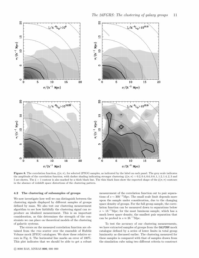
Figure 8. The correlation function, ξ(σ, π), for selected 2PIGG samples, as indicated by the label on each panel. The grey scale indicatesthe amplitude of the correlation function, with darker shading indicating stronger clustering: ξ(σ, π) = 0.2, 0.4, 0.6, 0.8, 1, 1.2, 1.4, 2, 3 and5 are shown. The ξ = 1 contour is also marked by a thick black line. The thin black lines show the expected shape of the ξ(σ, π) contoursin the absence of redshift space distortions of the clustering pattern.

4.2 The clustering of subsamples of groups

We now investigate how well we can distinguish between theclustering signals displayed by different samples of groupsdefined by mass. We also test our clustering measurementalgorithm to see how faithfully the clustering signal can re-produce an idealized measurement. This is an importantconsideration, as this determines the strength of the con-straints we can place on theoretical models of the clusteringof galactic systems.

The errors on the measured correlation function are ob-tained from the rms scatter over the ensemble of HubbleVolume mock 2PIGG catalogues. We show these relative er-rors in Fig. 6. The horizontal line marks an error of 100%.This plot indicates that we should be able to get a robust

measurement of the correlation function out to pair separa-tions of s ∼ 30h−1Mpc. The small scale limit depends moreupon the sample under consideration, due to the changingspace density of groups. For the full group sample, the corre-lation function can be measured down to separations belows ∼ 1h−1Mpc; for the most luminous sample, which has amuch lower space density, the smallest pair separation thatcan be probed is s ≈ 3h−1Mpc.

To test the accuracy of our clustering measurements,we have extracted samples of groups from the GALFORM mockcatalogue defined by a series of lower limits in total groupluminosity as discussed earlier. The clustering measured forthese samples is compared with that of samples drawn fromthe simulation cube using two different criteria to construct

c© 0000 RAS, MNRAS 000, 000–000

12 Padilla et al.

equivalent samples as discussed earlier. The samples drawnfrom the simulation cube are idealized in the sense that theydo not have a radial or angular selection function imposedupon them as is the case for the mock 2PIGG catalogue.Moreover, the groups occupy dark matter haloes identifiedby a friends-of-friends group finder. The mass of a group inthe simulation cube is known very accurately: it is simplythe sum of the mass of the dark matter particles connectedby the group finder.

The correlation functions measured for mock group sub-samples defined by a lower limit on total group luminosityare compared with the results for the equivalent samplesdrawn from the simulation cube in Fig. 7. The top row ofthis figure shows the comparison when the equivalent sam-ples are set up to reproduce the mass function of groupsrecovered from the mock group catalogue for each luminos-ity subsample. The bottom row shows the comparison forequivalent samples constructed to match the effective biasestimated from the mock subsamples. The left hand columnshows the results for groups with a minimum membershipnmin = 2, and the right hand column for nmin = 4. Theclustering measurements from the mock subsamples are inimpressively good agreement with the results obtained forthe equivalent samples in the simulation cube, particularlyfor the case of nmin = 2. The equivalent samples constructedto reproduce the effective bias of mock group subsamples arein somewhat better agreement with the measurements fromthe mocks for the brighter group samples.

The agreement in clustering amplitude between samplesof groups taken from a mock and those extracted from anidealized simulation is significant; it means that we fullyunderstand the impact of making a mock group catalogueon the measurement of the clustering of groups and can usethe clustering of 2PIGG samples to constrain theoreticalmodels of structure formation.

5 2PIGG RESULTS

In this section we measure the clustering amplitude of thereal 2PIGGs for samples defined by total group luminosity.Some basic properties of the samples are given in Table 1.We apply the optimal clustering measurement algorithm setout at the end of Section 4.1. We combine the pair counts inthese regions to estimate the correlation function. We havechecked that the measurements for the individual regionsagree within the errors.

An important test of the integrity of a group catalogueis the form of the correlation function measured in bins ofpair separation parallel (π) and perpendicular (σ) to theline of sight, ξ(σ, π). Padilla & Lambas (2003a,b) exploreddifferent techniques used in the construction of group andcluster catalogues. They found that the shape of ξ(σ, π) is apowerful way to reveal spurious agglomerations of galaxies.A tell-tale sign of problems with the composition of galaxygroups is a significant enhancement of the correlation func-tion, ξ(σ, π), in the π direction, as seen in the early analysesof Abell catalogue clusters (e.g. Bahcall & Soneira 1983;Sutherland 1988). Such a distortion of the clustering pat-tern is seen for 2dFGRS galaxies, due to the large peculiarmotions inside massive virialised structures (Peacock et al.2001; Hawkins et al. 2003). However, for the case of groups

Figure 9. The projected correlation function of selected 2PIGGsamples. The samples are indicated by the key; error bars areplotted on the measurements for selected samples for clarity. Thesolid line shows a fit to the projected correlation function of 2dF-GRS galaxies taken from Hawkins et al. (2003).

and clusters, such virialised structures are not predicted inviable models of structure formation (Kaiser 1987; Padilla etal. 2001; Padilla & Baugh 2002). The correlation function,ξ(σ, π), for samples of 2PIGGs is shown in Fig. 8. There isno enhancement of the clustering signal in the π direction.The contours of constant clustering amplitude are, however,affected by peculiar motions, showing the flattening due tothe infall motions expected in the gravitational instabilityparadigm (Padilla et al. 2001; Peacock et al. 2001). Thereis also a clear increase in clustering amplitude with sampleluminosity.

The projected correlation function, Ξ(σ)/σ, is the in-tegral of ξ(σ, π) over the π direction (e.g. Norberg et al.2001). This statistic is unaffected by peculiar motions. InFig. 9, we show the projected correlation functions for se-lected samples of 2PIGGs. The black line shows the best fitto the projected correlation function of galaxies in the 2dF-GRS for comparison (Hawkins et al. 2003). We find that thelowest luminosity sample plotted is less strongly clusteredthan the galaxy distribution, a point to which we returnlater on in this section. The brightest sample of groups dis-plays a clustering amplitude that is an order of magnitudestronger than that measured for 2dFGRS galaxies.

The projected correlation function, due to the way itis calculated, can be unreliable if the correlation functionis noisy on large scales. A more robust quantity in suchcases is the redshift space correlation function, ξ(s). Thisquantity is the average of ξ(σ, π) within annuli centred on

s =(

σ2 + π2)1/2

. The redshift space correlation functionmeasured for 2PIGG samples with membership nmin ≥ 2 isplotted in the left-hand panel of Fig. 10. For reference, wealso plot the redshift space correlation function of 2dFGRSgalaxies measured by Hawkins et al. (2003). The correlationfunction of the group samples has a similar shape to that ob-

c© 0000 RAS, MNRAS 000, 000–000

The 2dFGRS: The clustering of galaxy groups 13

Figure 10. Left panel: The redshift space correlation function, ξ(s), measured for samples of 2PIGGs. The samples are shown by thekey. Error bars are plotted for selected samples for clarity. The solid line shows ξ(s) for 2dFGRS galaxies, measured by Hawkins et al.(2003). Right panel: The ratio of the group correlation function to the galaxy correlation function, plotted on a logarithmic scale.

tained for galaxies, on scales where a comparison is reliable.There is, however, a dramatic change in clustering amplitudewith group luminosity, mirroring that seen for the projectedcorrelation function in Fig. 9. These points are emphasizedin the right hand panel of Fig. 10, in which we plot the groupcorrelation function divided by the galaxy correlation func-tion. There is a relative bias between the spatial distributionof groups and galaxies. For the full 2PIGG sample, and alsofor the next faintest luminosity sample, this relative bias isactually an anti-bias; these groups are more weakly clus-tered than the galaxies. The brightest groups, on the otherhand, are almost ten times more strongly clustered than thegalaxy distribution.

A useful summary of the clustering measurements canbe made by plotting the correlation length, s0, as a functionof the mean group separation, dc, which is related to thespace density of groups, n, by dc = 1/n1/3. The space den-sity of groups is estimated using the cumulative bJ−bandluminosity function of 2PIGGs out to z = 0.12 (Eke et al.2004b). The space density of each subsample is simply theluminosity function evaluated at the appropriate lower limitin luminosity. We estimate the correlation length (definedby ξ(s0) = 1) by fitting a power law to the measured red-shift space correlation function for pair separations in therange 0.4 < log10(s/h

−1Mpc) < 1.3. Our results are fairlyinsensitive to perturbations to this range.

The clustering strength of 2PIGG samples versus meangroup separation is plotted in Fig. 11. There is an increasein clustering strength with the mean separation of groupsin each sample; the clustering strength increases slightlyless rapidly than the change in group separation. Thereis very good agreement between the results for nmin = 2and nmin = 4 for group separations for which a compari-son is possible. Fig. 11 also shows the s0-dc relation in the

GALFORM mock 2PIGG catalogue with nmin = 2, which is invery close agreement with the results from the real 2PIGGsamples. The solid and dotted lines show the measurementsfor equivalent samples of groups drawn from the simulationcube. The solid line gives the s0-dc relation in redshift spaceand the dotted line shows the real space results. The clus-tering amplitude is typically 10%-20% weaker in real spacethan in redshift space.

The 2PIGG results are compared with a selection ofmeasurements taken from the literature in Fig. 12. This com-parison between datasets should be treated with caution dueto a number of differences in the way the various sampleshave been defined and analysed: namely, in decreasing orderof seriousness: (i) the technique used to identify groups andclusters, (ii) the derivation of a value for the mean inter-group separation and (iii) the calculation of the correlationlength.

Zandivarez et al. (2003) measured the clustering ofgroups in a catalogue constructed from the 100k release of2dFGRS data by Merchan & Zandivarez (2002). The twomost abundant samples of groups analysed by Zandivarez etal. have a significantly higher clustering amplitude than werecover for 2PIGG groups of comparable abundance. Zandi-varez et al. estimated dc from a dynamical estimate of thegroup mass which they translated into a spatial abundanceusing the measured mass function of groups (Martinez etal. 2002). Moreover, Zandivarez et al. only consider groupswith nmin = 4; such groups are probably only associatedwith low mass systems through errors in the dynamical massestimates. The abundance of groups in the Updated ZwickyCatalogue was estimated in a similar way by Merchan etal. (2000). Bahcall et al. (2003) have applied a photometrictechnique (Annis et al. 2004) to a subset of the Sloan surveydata to obtain a sample of clusters that overlaps with the

c© 0000 RAS, MNRAS 000, 000–000

14 Padilla et al.

Figure 11. The correlation length in redshift space, s0, plottedas a function of the mean group separation, dc. The 2PIGG re-sults are shown by filled squares for nmin = 2. Also shown forcomparison are measurements from the GALFORM mock plottedwith triangles. The solid line shows the s0 − dc relation obtainedfrom the simulation cube for equivalent samples of groups (seetext). The dotted line shows how these results change when thecorrelation length is measured in real space.

Figure 12. A comparison of the s0−dc relation for different sam-ples. The squares show the results from the 2PIGGs for nmin = 2.The other symbols show a selection of data taken from the liter-ature, as indicated by the key. The lines show fits to subsets ofthe data, with sources indicated by the key.

Figure 13. A comparison of the s0−dc relation for 2PIGG groups(squares) and for 2dFGRS galaxies (stars, taken from Norberg etal. 2002a). The solid line is a fit to the 2PIGG clustering data,excluding the lowest luminosity sample; the dotted line is a fit tothe 2PIGG results including the faintest sample. The dashed lineshows the fit to the clustering strength-luminosity relation fittedto 2dFGRS data by Norberg et al. (2001).

most luminous 2PIGG groups and with APM Survey clus-ters (Croft et al. 1997; Dalton et al. 1997). The Sloan mea-surements are in reasonable agreement with the results fromAPM clusters and are marginally lower than the 2PIGG val-ues at comparable abundances. However, both the SDSS andAPM clusters are identified in projection. The trend of clus-tering strength versus abundance found for 2PIGGs agreesquite well with the measurements from X-ray selected clus-ter samples (Abadi, Muriel & Lambas 1998; Collins et al.2000; Lee & Park 2002).

The dotted line in Fig. 12 shows the s0-dc relation advo-cated by Bahcall & West (1992), whereas the dot-dashed lineis the relation proposed by Bahcall et al. (2003); the dashedline is the fit of Zandivarez et al. (2003) to their data. Theanalogous fit to the 2PIGG results is plotted in Fig. 13 forclarity. If the faintest groups are ignored, the 2PIGG resultsare described by the relation s0 = 1.67d0.65

c . This is some-what steeper than the fit of Bahcall et al. (2003).

We compare the clustering of 2PIGG groups with 2dF-GRS galaxies in Fig. 13. The clustering amplitude of 2dF-GRS galaxies is taken from Norberg et al. (2002a), who anal-ysed volume limited samples defined by galaxy luminosity.The curve plotted over the galaxy clustering measurementsshows the predictions of the simple relation between relativeclustering strength and luminosity deduced by Norberg etal. (2001). The full sample of 2PIGGs is more weakly clus-tered than L∗ and brighter galaxies. On the other hand, thetrend of clustering strength with pair separation is strongerfor groups than it is for galaxies.

c© 0000 RAS, MNRAS 000, 000–000

The 2dFGRS: The clustering of galaxy groups 15

6 CONCLUSIONS

We have measured the clustering of groups in the 2PIGGsample constructed from the 2dFGRS by Eke et al. (2004a).The group catalogue, made up of galactic systems with aminimum of two members, contains ∼29,000 groups, out ofwhich ∼16,000 are at z < 0.12. The sample is sufficientlylarge and homogenous that a robust measurement of cluster-ing is possible for subsamples of groups defined by their cor-rected total luminosity. Our analysis has relied extensivelyon the use of various mock group catalogues constructedusing high resolution N-body simulations populated withgalaxies using the GALFORM semi-analytic model (Cole et al.2000; Benson et al. 2000, 2003).

In summary, the main conclusions we have reached arethe following:

(i) The main goals of this paper were to make a robustmeasurement of the clustering of galaxy groups with the aimof exploring the dependence of the clustering amplitude on aproperty related to group mass (for example the total groupluminosity) and to compare the results with theoretical pre-dictions. We have tested our algorithm for estimating thecorrelation function by comparing results obtained from amock 2PIGG catalogue with those derived from equivalentsamples drawn from the N-body simulation cube. The suc-cess of this comparison is significant for two reasons. Firstly,in order to make a robust measurement of the clustering ofgroups from a flux limited galaxy survey, it is necessary tomake a number of approximations and to choose certainparameter values (see Section 4.1). We have tuned the al-gorithm for measuring the clustering of 2PIGG groups byrequiring a close match between the correlation functionsestimated from the mocks and the original results from thesimulation cube. Secondly, the ability to extract equivalentsamples of groups from a simulation volume with the sameclustering as samples taken from mock 2PIGG cataloguesmakes it possible to interpret the 2PIGG clustering resultsin the context of structure formation models.

(ii) We find that clustering amplitude increases substan-tially with total group luminosity. The 2PIGG catalogue al-lows clustering measurements to be made for samples span-ning a factor of 25 in median total luminosity. The correla-tion function increases in amplitude by an order of magni-tude over this luminosity interval. Another way of expressingthis is that the redshift space correlation length changes bya factor ≈ 3.5 from the faintest to the brightest sample. Themost luminous groups we consider have a mean pair separa-tion that is ≈ 5.5 times greater than that of the full groupsample. There is little change in the shape of the correlationfunction with group luminosity.

(iii) The shape of the redshift space correlation functionof groups is very similar to that measured for 2dFGRS galax-ies on the scales for which a comparison is possible. The full2PIGG sample has a weaker clustering amplitude than ismeasured for 2dFGRS galaxies; the correlation length of the2PIGG sample with nmin = 2 is s0 = 5.5±0.1h−1Mpc, whilstthat of 2dFGRS galaxies is 6.82 ± 0.28h−1Mpc (Hawkins etal. 2003). However, the clustering amplitude of brighter sam-ples of groups is much greater than that of 2dFGRS galaxies.

(iv) The correlation functions measured for 2PIGG sam-ples are in very good agreement with the predictions of asemi-analytic model of galaxy formation, the GALFORM model

(Cole et al. 2000; Benson et al. 2003), in a cold dark mat-ter universe with a cosmological constant (ΛCDM). Previouswork has compared the predictions of the ΛCDM model withmeasurements of the correlation length versus abundance re-lation for rich clusters (Governato et al. 1999; Colberg et al.2000). To extend the theoretical calculations down to group-sized systems, it is essential to extend the predictions of thespatial distribution of dark matter haloes in the ΛCDM cos-mology with a model for galaxy formation. The galaxy for-mation model predicts how the dark matter haloes shouldbe populated with galaxies. For this reason, the clustering ofgroups provides a more stringent test of theories of galaxiesformation than the clustering of the richest clusters.

(v) The trend of correlation length (measured in redshiftspace) against mean inter-group separation can be quan-tified as: s0 = 1.67d0.65

c . The 2PIGG catalogue has madepossible a robust measurement of the clustering of galacticsystems, ranging from poor groups to rich clusters, from onesample for the first time. Our results are in general agree-ment with those obtained previously for rich groups andclusters.

Galaxies and groups of galaxies trace the underlyingdistribution of dark matter haloes in different ways. Galax-ies trace the halo distribution in a complex way. The halooccupation distribution (HOD), which depends strongly onhalo mass, has been used extensively to constrain theoreti-cal models (e.g. Benson et al. 2000; Peacock & Smith 2000;Seljak 2000; Berlind et al. 2003). In principle, the groupsample should trace the halo distribution in a simple fash-ion, with every halo above some mass spawning one galaxygroup. However, in practice, the identification of groups inreal surveys is complicated, making this ideal difficult toattain. Because of this it is essential to devise a scheme toquantify the fidelity of a group catalogue and to uncover anybiases in comparisons with theoretical models by applyingthe group finder to mock catalogues (Eke et al. 2004a).

The difference between the clustering amplitude mea-sured for the full 2PIGG and the full 2dFGRS galaxy sam-ples can be readily understood in terms of the HOD. Ideally,the groups have a one-to-one correspondence with the un-derlying dark matter haloes within some mass interval. Thegalaxies obviously sample haloes in the same mass range, butwith a weight that increases with halo mass, since the mostmassive haloes host more than one galaxy. Thus, the moremassive haloes, which are the more strongly clustered, makea larger contribution to the correlation function of 2dFGRSgalaxies than they do in the case of the full 2PIGG sample.The clustering of galaxy groups as a function of group lumi-nosity therefore provides an important new test of theoriesof galaxy formation.

ACKNOWLEDGMENTS

This work was supported by a PPARC rolling grant atthe University of Durham. NDP acknowledges receipt of aBritish Council-Fundacion Antorchas fellowship. CMB wassupported by a Royal Society University Research Fellow-ship.

c© 0000 RAS, MNRAS 000, 000–000

16 Padilla et al.

REFERENCES

Abadi M.G., Lambas D.G., Muriel H., 1998, ApJ, 507, 526.

Annis J., et al., 2004, in preparation

Bahcall N.A., Soneira R.M., 1983, ApJ, 270, 20.

Bahcall N.A., West M.J., 1992, ApJ, 392, 419.

Bahcall N.A., Dong F., Hao L., Bode P., Annis J., Gunn J. E.,Schneider D. P., 2003, ApJ, 599, 814.

Baugh C. M., Benson A.J., Cole S., Frenk C.S., Lacey C.G., 1999,MNRAS, 305, L21.

Benson A.J., Cole S., Frenk C.S., Baugh C.M., Lacey C.G., 2000,MNRAS, 311, 793.

Benson A.J., Lacey C.G., Baugh C.M., Cole S., Frenk C.S., 2002,MNRAS, 333, 156.

Benson A.J., Bower R.G., Frenk C.S., Lacey C.G., Baugh C.M.,Cole S., 2003, ApJ, 599, 38.

Berlind A.A., Weinberg D.H., Benson A.J., Baugh C.M., Cole S.,Dave R., Frenk C.S., Jenkins A., Katz N., Lacey C.G., 2003,

ApJ, 593, 1.

Colberg J. M., et al., 2000, MNRAS, 319, 209.

Cole S., Kaiser N., 1989, MNRAS, 237, 1127.

Cole S., Hatton S., Weinberg D.H., Frenk C.S., 1998, MNRAS,300, 945.

Cole S., Lacey C.G., Baugh C.M., Frenk C.S., 2000, MNRAS,319, 168.

Colless M. et al. (the 2dFGRS team), 2001, MNRAS, 328, 1039

Colless M. et al. (the 2dFGRS team), 2003, astro-ph/0306581

Collins C. A., et al., 2000, MNRAS, 319, 939.

Croft R.A.C., Dalton G.B., Efstathiou G., Sutherland W.J., Mad-dox S.J., 1997, MNRAS, 291, 305.

Dalton G.B., Maddox S.J., Sutherland W.J., Efstathiou G., 1997,MNRAS, 289, 263.

Davis M., Efstathiou G., Frenk C.S., White S.D.M., 1985, ApJ,292, 371.

Efstathiou G., 1988, in Comets to cosmology, ed A. Lawrence,Proc 3rd IRAS Conference, Springer-Verlag, Berlin.

Eke V.R. et al. (the 2dFGRS Team), 2004a, MNRAS, 348, 866.(astro-ph/0402567).

Eke V.R. et al. (the 2dFGRS Team), 2004b, MNRAS, submitted,astro-ph/0402566.

Eke V.R. et al. (the 2dFGRS Team), 2004c, in preparation.

Evrard, A.E., MacFarland, T.J., Couchman, H.M.P., Colberg,J.M., Yoshida, N., White, S.D.M., Jenkins, A., Frenk, C.S.,Pearce, F.R., Peacock, J.A., Thomas, P.A., 2002, ApJ, 573,7.

Geller M.J., Huchra J.P., 1983, ApJS, 52, 61.

Girardi M., Boschin W., da Costa L.N., 2000, A&A, 353, 57.

Governato F., Babul A., Quinn T., Tozzi P., Baugh C.M., KatzN., Lake G., 1999, MNRAS, 307, 949.

Hawkins E., et al. (the 2dFGRS Team), 2003, MNRAS, 346, 78.

Helly, J.C., Cole, S., Frenk, C.S., Baugh, C.M., Benson, A., Lacey,C., 2003, MNRAS, 338, 903.

Jenkins A., Frenk C.S., White S.D.M., Colberg J.M., Cole S.,Evrard A.E., Couchman H.M.P., Yoshida N., 2001, MNRAS,321, 372.

Jing Y., Zhang, J., 1988, A&A, 190, L21.

Kaiser N., 1987, MNRAS, 227, 1.

Kashlinsky A., 1987, ApJ, 317, 19.

Kauffmann G., Colberg J.M., Diaferio A., White S.D.M., 1999,MNRAS, 303, 188.

Landy S.D., Szalay A.S., 1993, ApJ, 412, 64.

Lee S., Park C., 2002, J. Korean Astron. Soc., 35, 111.

Maia M.A.G., da Costa L.N., 1990, ApJ, 352, 457.

Martinez H.J., Zandivarez A., Merchan M.E., Dominguez M.J.L.,2002, MNRAS, 337, 1441.

Merchan M.E., Maia M.A.G., Lambas D.G., 2000, ApJ, 545, 26.

Merchan M., Zandivarez A., 2002, MNRAS, 335, 216.

Mo H.J., White S.D.M., 1996, MNRAS, 282, 347.

Norberg P., et al., (the 2dFGRS Team), 2001, MNRAS, 328, 64.

Norberg P., et al., (the 2dFGRS Team), 2002a, MNRAS, 332,827.

Norberg P., et al., (the 2dFGRS Team), 2002b, MNRAS, 336,907.

Padilla N.D., Merchan M.E., Valotto C.A., Lambas D.G., MaiaM.A.G., 2001, ApJ, 554, 873.

Padilla N.D., Baugh C.M., 2002, MNRAS, 329, 431.Padilla N.D., Lambas D.G., 2003a, MNRAS, 342, 519.Padilla N.D., Lambas D.G., 2003b, MNRAS, 342, 532.Peacock J.A., Smith R.E., 2000, MNRAS, 318, 1144.Peacock J.A., et al. (the 2dFGRS Team), 2001, Nature, 410, 169.Press W.H., Schechter P., 1974, ApJ, 187, 425.Ramella M., Geller M.J., Huchra J.P., 1990, ApJ, 353, 51.Seljak U., 2000, MNRAS, 318, 203.Sheth R.K., Mo H.J., Tormen, G., 2001, MNRAS, 323, 1.Spergel D.N., et al. (the WMAP Team), 2003, ApJS, 148, 175.Sutherland W., 1988, MNRAS, 234, 159.Zandivarez A., Merchan M.E., Padilla N.D., 2003, MNRAS, 344,

247.

c© 0000 RAS, MNRAS 000, 000–000