arX

iv:1

404.

2626

v1 [

astr

o-ph

.IM]

9 A

pr 2

014

Mon. Not. R. Astron. Soc.000, 1–13 (2014) Printed 11 April 2014 (MN LATEX style file v2.2)

Galaxy And Mass Assembly (GAMA): AUTOZ spectral redshiftmeasurements, confidence and errors.

I. K. Baldry,1 M. Alpaslan,2,3 A. E. Bauer,4 J. Bland-Hawthorn,5 S. Brough,4

M. E. Cluver,6 S. M. Croom,5 L. J. M. Davies,2 S. P. Driver,2,3 M. L. P. Gunawardhana,7

B. W. Holwerda,8 A. M. Hopkins,4 L. S. Kelvin,9 J. Liske,10 A. R. Lopez-Sanchez,4,11

J. Loveday,12 P. Norberg,7 J. Peacock,13 A. S. G. Robotham,2 E. N. Taylor14

1Astrophysics Research Institute, Liverpool John Moores University, IC2, Liverpool Science Park, 146 Brownlow Hill, Liverpool L3 5RF2International Centre for Radio Astronomy Research, University of Western Australia, 35 Stirling Highway, Crawley, WA6009, Australia3School of Physics and Astronomy, University of St Andrews, North Haugh, St Andrews KY16 9SS4Australian Astronomical Observatory, PO Box 915, North Ryde, NSW 1670, Australia5Sydney Institute for Astronomy, School of Physics A28, University of Sydney, NSW 2006, Australia6Department of Astronomy, University of Cape Town, Private Bag X3, Rondebosch, 7701, South Africa7ICC, Department of Physics, Durham University, South Road,Durham DH1 3LE8University of Leiden, Sterrenwacht Leiden, Niels Bohrweg 2, NL-2333 CA Leiden, Netherlands9Institut fur Astro- und Teilchenphysik, Universitat Innsbruck, Technikerstraße 25, 6020 Innsbruck, Austria10European Southern Observatory, Karl-Schwarzschild-Str.2, 85748 Garching, Germany11Department of Physics and Astronomy, Macquarie University, NSW 2109, Australia12Astronomy Centre, University of Sussex, Falmer, Brighton BN1 9QH13Institute for Astronomy, University of Edinburgh, Royal Observatory, Blackford Hill, Edinburgh EH9 3HJ14School of Physics, University of Melbourne, Parkville, VIC3010, Australia

Paper submitted to MNRAS on 2014 February 26th; revised following referee comments, 2014 April 8th.

ABSTRACTThe Galaxy And Mass Assembly (GAMA) survey has obtained spectra of over 230 000 tar-gets using the Anglo-Australian Telescope. To homogenise the redshift measurements andimprove the reliability, a fully automatic redshift code was developed (AUTOZ). The measure-ments were made using a cross-correlation method for both absorption-line and emission-linespectra. Large deviations in the high-pass filtered spectraare partially clipped in order to berobust against uncorrected artefacts and to reduce the weight given to single-line matches.A single figure of merit (FOM) was developed that puts all template matches onto a similarconfidence scale. The redshift confidence as a function of theFOM was fitted with a tanhfunction using a maximum likelihood method applied to repeat observations of targets. Themethod could be adapted to provide robust automatic redshifts for other large galaxy red-shift surveys. For the GAMA survey, there was a substantial improvement in the reliability ofassigned redshifts and in the lowering of redshift uncertainties with a median velocity uncer-tainty of 33 km/s.

Key words: methods: data analysis — techniques: spectroscopic — surveys — galaxies:redshifts

1 INTRODUCTION

Spectroscopic redshift measurements of large galaxy samples formthe backbone of many extragalactic and cosmological analyses.They are key for testing cosmological models, e.g. using red-shift space distortions (Kaiser 1987), and for providing distancesfor galaxy population studies when the cosmology is assumed.Redshifts from spectroscopy (spec-z) generally have significantlyfewer outliers, compared to the true redshift, than from photometricestimates (photo-z; Dahlen et al. 2013). In addition, spec-z mea-

surements are essential for accurate low-redshift luminosity esti-mates (0.002 . z . 0.2), where the photo-z fractional error is toolarge, and for dynamical measurements within groups of galaxies(Beers, Flynn, & Gebhardt 1990, Robotham et al. 2011).

Redshift surveys of large numbers of galaxies have been un-dertaken in recent years using multi-object spectrographssuch asthe Two Degree Field (2dF, Lewis et al. 2002), Sloan Digital SkySurvey (SDSS, Smee et al. 2013), Visible Multi-Object Spectro-graph (VIMOS, Le Fevre et al. 2003), and Deep Imaging Multi-Object Spectrograph (DEIMOS, Faber et al. 2003). For unifor-

c© 2014 RAS

2 I. K. Baldry et al.

mity of a survey product over a large sample, redshift measure-ment codes have been developed that are either fully automatic(SubbaRao et al. 2002; Garilli et al. 2010; Bolton et al. 2012) orpartially automatic with some user interaction (Colless etal. 2001;Newman et al. 2013).

The main techniques for spectroscopic redshift measurementsare: the identification and fitting of spectral features (Mink & Wyatt1995); cross-correlation of observed spectra with template spec-tra (Tonry & Davis 1979; Kurtz et al. 1992); andχ2 fitting usinglinear combinations of eigenspectra (Glazebrook, Offer, &Deeley1998). A widely used code isRVSAO that allows for cross-correlation with absorption-line and emission-line templates sep-arately (Kurtz & Mink 1998). The 2dF Galaxy Redshift Survey(2dFGRS) and SDSS have used a dual method with fitting ofemission line features and cross-correlation with templates afterclipping the identified emission lines from the observed spectra(Colless et al. 2001; Stoughton et al. 2002). The large VIMOSsur-veys have used theEZ software (Garilli et al. 2010), which pro-vides a number of options including emission-line finding, cross-correlation andχ2 fitting. From SDSS Data Release 8 (DR8) on-wards (Aihara et al. 2011), including the Baryon Oscillation Spec-troscopic Survey (BOSS) targets, the measurements have used χ2

fitting at trial redshifts with sets of eigenspectra for galaxies andquasars (Bolton et al. 2012).

The Galaxy And Mass Assembly (GAMA) survey is basedaround a redshift survey that was designed, in large part, forfinding and characterising groups of galaxies (Driver et al.2009;Robotham et al. 2011). The survey has obtained over 200 000redshifts using spectra from the AAOmega spectrograph of theAnglo-Australian Telescope (AAT) fed by the 2dF fibre positioner.AAOmega is a bench-mounted spectrograph with light comingfrom a 392-fibre slit, split into two beams, each dispersed with avolume-phase holographic grating and focused onto CCDs using aSchmidt camera. See Sharp et al. (2006) for details.

Up until 2013, all the AAOmega redshifts had been obtainedusing RUNZ (Saunders, Cannon, & Sutherland 2004), which is anupdate to the code used by the 2dFGRS (Colless et al. 2001). Theuser assigns a redshift quality for each spectrum from 1–4, whichcan later be changed or normalised during a quality control pro-cess (Driver et al. 2011). By comparing the redshifts assigned torepeated AAOmega observations of the same target, the typicalredshift uncertainty was estimated to be∼ 100 km/s. In addition,the blunder rate was∼ 5 per cent even when the redshifts wereassigned a reliable redshift quality of 4. In order to improve theredshift reliability and uncertainties, and thus the groupcataloguemeasurements, a fully automatic code was developed calledAU-TOZ.

Here we describe theAUTOZ algorithm, which uses a cross-correlation method that works equally well with absorptionoremission line templates, and that is robust to additive/subtractiveresiduals and other uncertainties in the reduction pipeline that out-puts the spectra. This has substantially improved the GAMA red-shift reliability and velocity errors (Liske et al. in preparation). Adescription of the GAMA data is given in§ 2. The method for find-ing the best redshift estimate is outlined in§ 3, the quantitativeassessment of the confidence is described in§ 4, and the redshiftuncertainty estimate is described in§ 5. A summary is given in§ 6.

2 DATA

The GAMA survey is based around a highly complete galaxy red-shift survey and multi-wavelength database (Driver et al. 2011).Since the initial spectroscopic target selection over 144deg2 de-scribed in Baldry et al. (2010), the survey has been expandedto 280deg2 with a main survey limit of r < 19.8 in allfive regions: equatorial fields G09, G12 and G15 and Southernfields G02 and G23. The spectra were obtained from the Anglo-Australian Telescope with the Two-degree Field (2dF) robotic po-sitioner fibre feed to the AAOmega spectrograph. In total, 286 705spectra of 237 822 unique targets were taken over six years, inall weather conditions. The spectra were reduced using 2DFDR

(Croom, Saunders, & Heald 2004). The GAMA setup and data pro-cessing details are described in Hopkins et al. (2013).

In order to obtain high completeness, both in targeting andredshift success, the same region of the sky was observed multi-ple times with different AAOmega configurations (Robotham et al.2010). The spectra were reduced using 2DFDR and redshifts weremeasured usingRUNZ typically within 24 hours of the observations.In between observing seasons, the spectra were usually re-reducedusing the most recent update to the 2DFDR pipeline processing. Inaddition, a significant fraction of spectra were looked at bymulti-ple users in order to quantify the reliability of theRUNZ redshiftassignments (Liske et al. in preparation). The tiling catalogue wasupdated during an observing season, or in between observingsea-sons, using the latest assigned redshift qualities. If a target was notassigned a sufficient redshift quality and had not been observedtwice by AAOmega, then it remained at high priority in the tilingcatalogue. In most cases, a target received a higher-quality redshifton its second attempt.

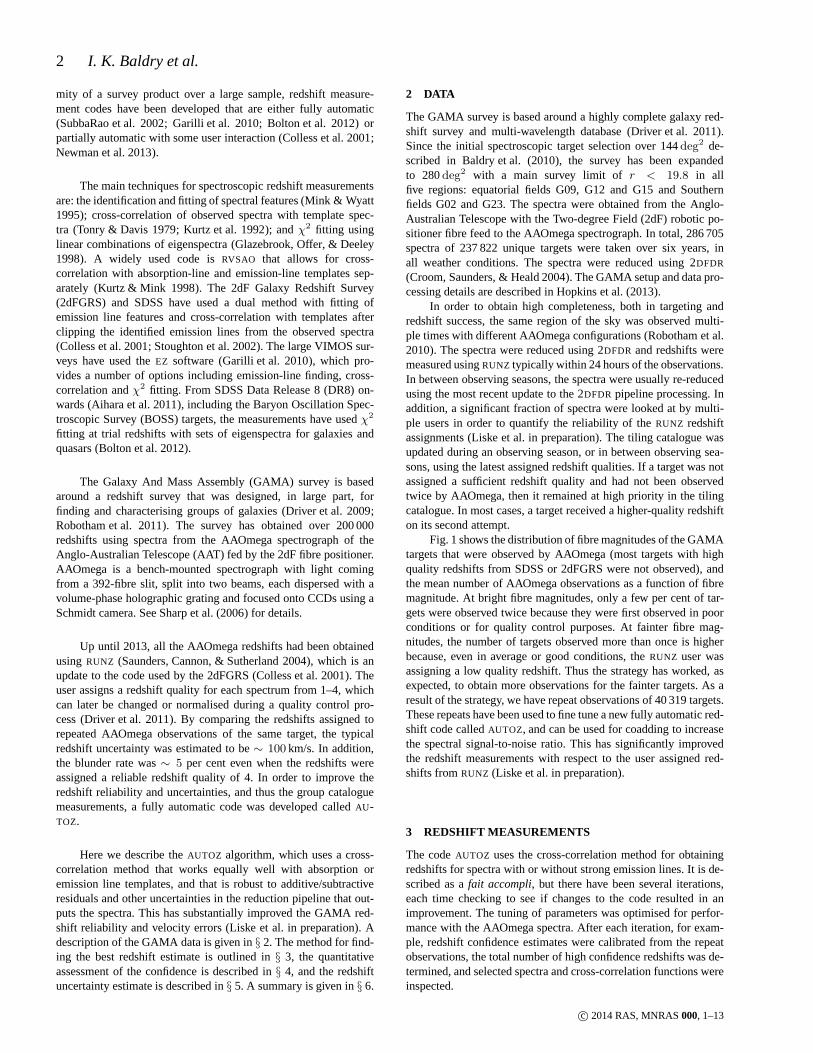
Fig. 1 shows the distribution of fibre magnitudes of the GAMAtargets that were observed by AAOmega (most targets with highquality redshifts from SDSS or 2dFGRS were not observed), andthe mean number of AAOmega observations as a function of fibremagnitude. At bright fibre magnitudes, only a few per cent of tar-gets were observed twice because they were first observed in poorconditions or for quality control purposes. At fainter fibremag-nitudes, the number of targets observed more than once is higherbecause, even in average or good conditions, theRUNZ user wasassigning a low quality redshift. Thus the strategy has worked, asexpected, to obtain more observations for the fainter targets. As aresult of the strategy, we have repeat observations of 40 319targets.These repeats have been used to fine tune a new fully automaticred-shift code calledAUTOZ, and can be used for coadding to increasethe spectral signal-to-noise ratio. This has significantlyimprovedthe redshift measurements with respect to the user assignedred-shifts fromRUNZ (Liske et al. in preparation).

3 REDSHIFT MEASUREMENTS

The codeAUTOZ uses the cross-correlation method for obtainingredshifts for spectra with or without strong emission lines. It is de-scribed as afait accompli, but there have been several iterations,each time checking to see if changes to the code resulted in animprovement. The tuning of parameters was optimised for perfor-mance with the AAOmega spectra. After each iteration, for exam-ple, redshift confidence estimates were calibrated from therepeatobservations, the total number of high confidence redshiftswas de-termined, and selected spectra and cross-correlation functions wereinspected.

c© 2014 RAS, MNRAS000, 1–13

GAMA: AUTOZ redshift measurements 3

Figure 1. The distribution in the fibre magnitude of targets observed as partof the GAMA-AAOmega campaign (solid line), and the mean number ofobservations as a function of fibre magnitude (dashed line),for the equato-rial fields. The fibre magnitudes were obtained from the SDSS catalogue.

3.1 Spectral templates

The SDSS has set a high standard for automatic redshift deter-mination. ForAUTOZ, we used their templates for spectral cross-correlation. These are a high S/N set of coadded spectra given ina similar format to the SDSS spectra for scientific targets. Table 1lists the templates used for this paper. Twenty stellar spectra wereused. Early versions ofAUTOZ used the six SDSS DR2 galaxytemplates (SubbaRao et al. 2002), while later versions usedeightgalaxy templates that were created from the SDSS-BOSS galaxyeigenspectra (Bolton et al. 2012). Six of these templates were cho-sen to closely match the DR2 templates where there was commonwavelength coverage, with an additional two selected to representa post-starburst spectrum (Wild et al. 2007) and a typical SDSS-BOSS spectrum.

The spectra were available rebinned onto a vacuum wave-length scale separated by 0.0001 inlog10 λ. This corresponds toa pixel size of 0.92A at 4000A and 1.84A at 8000A.

The spectral templates were high-pass filtered using a two steprobust procedure:

(i) A 4th-order polynomial was fitted to the spectrum iteratively,with a maximum of 15 iterations. After each iteration, points morethan 3.5σ away from the best-fit curve were rejected. The final 4th-order polynomial was then subtracted from the spectrum.

(ii) A median kernel filter of width 51 was applied to the re-sult of the 1st step. On each end, the 25 edge points were givenamedian value of those points. This median filtered spectrum wassmoothed using a trapezium filter, by applying two boxcar smoothsof width 121 and 21. This low-pass spectrum was then subtractedfrom the result of the 1st step to obtain the high-pass filtered (HPF)spectrum.

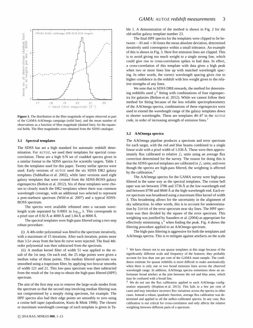
The aim of the first step was to remove the large-scale modes fromthe spectrum so that the second step involving median filtering wasnot compromised by a steeply rising spectrum, for example. TheHPF spectra also had their edge points set smoothly to zero usinga cosine bell taper (apodization, Kurtz & Mink 1998). The chosenor maximum wavelength coverage of each template is given in Ta-

ble 1. A demonstration of the method is shown in Fig. 2 for theold-stellar galaxy template number 23.

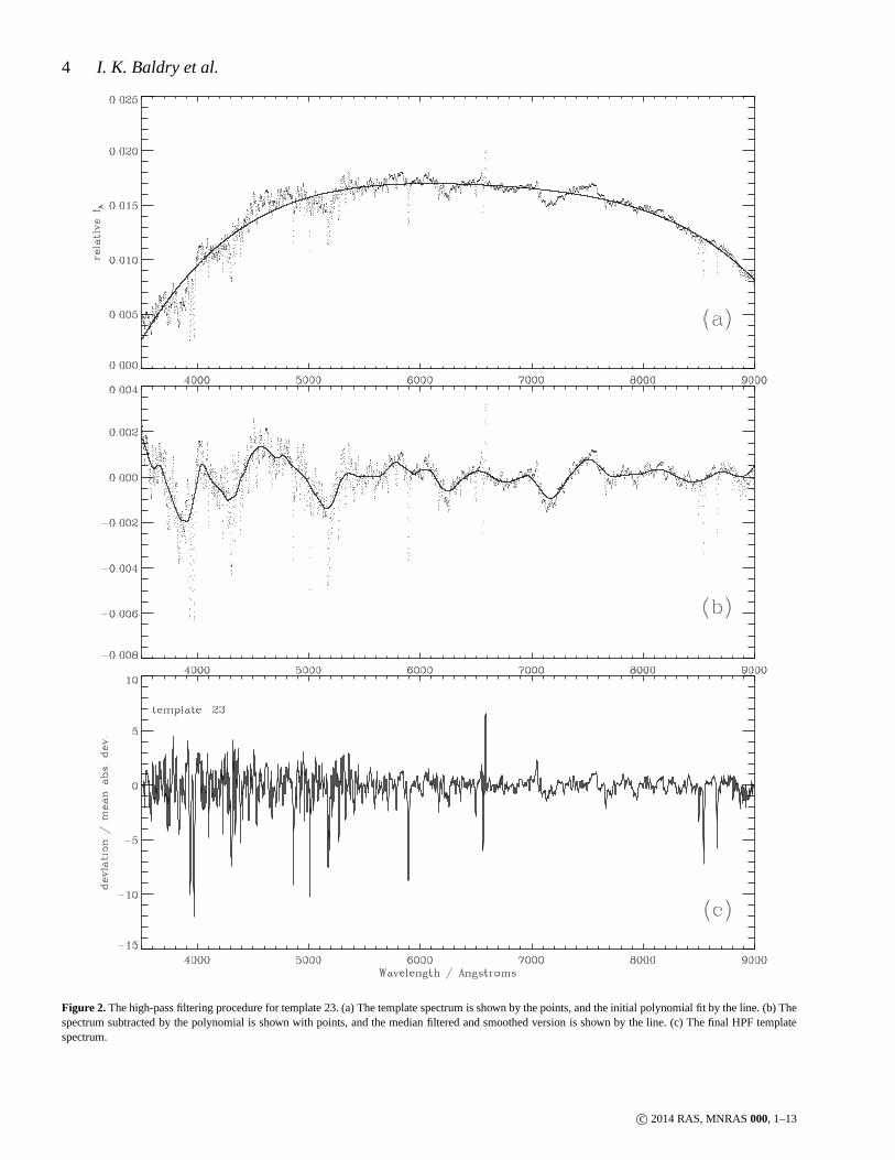
The final HPF spectra for the templates were clipped to lie be-tween−30 and+30 times the mean absolute deviation, determinediteratively until convergence within a small tolerance. Anexampleof this is shown in Fig. 3. Here five emission lines are clipped. Thisis to avoid giving too much weight to a single strong line, whichcould give rise to cross-correlation spikes in bad data. In effect,a cross-correlation of this template with data gives a high peakwhen two or more lines line up with matched wavelength spac-ing. In other words, the correct wavelength spacing gives rise tohigher confidence in the redshift with less weight given to the rela-tive strengths of any lines.

We note that in SDSS DR8 onwards, the method for determin-ing redshifts usedχ2 fitting with combinations of four eigenspec-tra for galaxies (Bolton et al. 2012). While we cannot followtheirmethod for fitting because of the less reliable spectrophotometryof the AAOmega spectra, combinations of these eigenspectrawereused to extend the wavelength range of the galaxy templates downto shorter wavelengths. These are templates 40–47 in theAUTOZ

code, in order of increasing strength of emission lines.1

3.2 AAOmega spectra

The AAOmega pipeline produces a spectrum and error spectrumfor each target, with the red and blue beams combined to a singlelinear scale with a pixel width of 1.036A. These were then approx-imately flux calibrated to relativefλ units using an average fluxcorrection determined for the survey. The reason for doing this isthat the SDSS spectral templates are calibrated infλ units; and eventhough the spectra are high-pass filtered, the weighting is affectedby the calibration.2

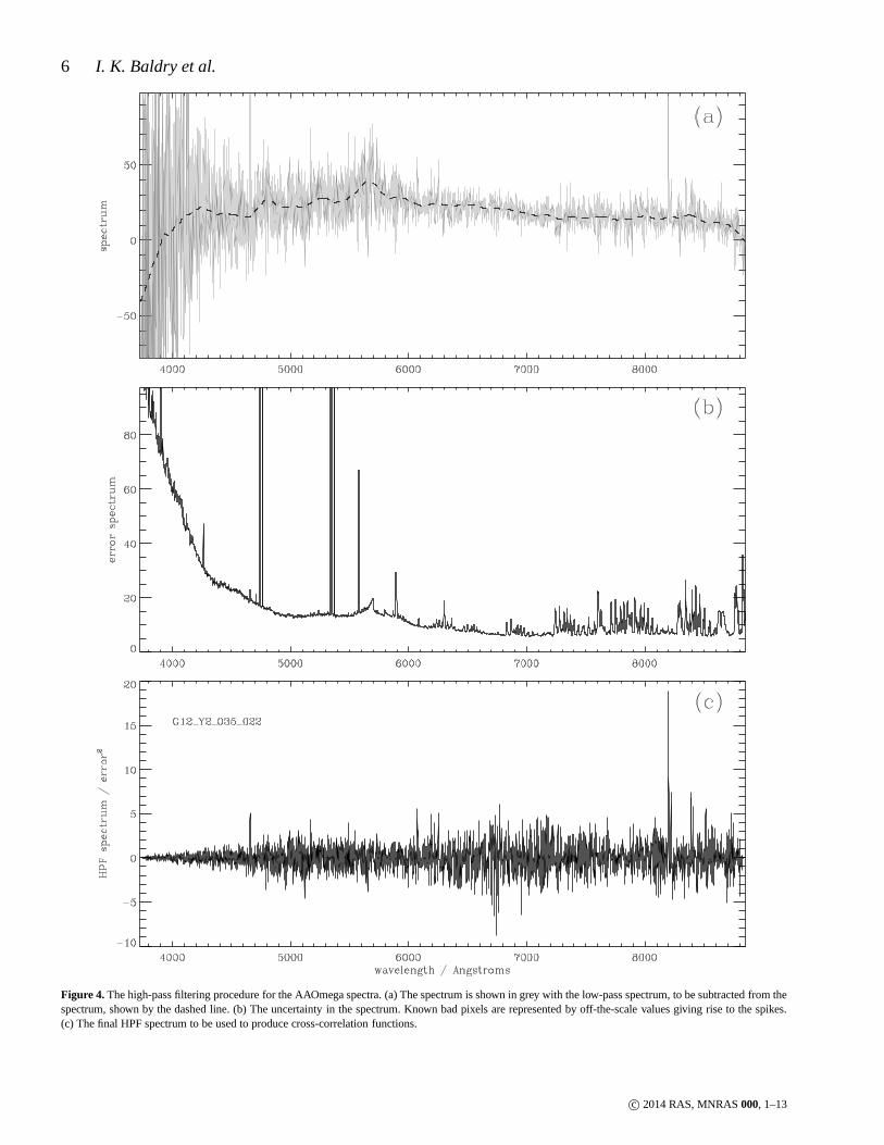
The AAOmega spectra for the GAMA survey were high-passfiltered in the same way as the spectral templates. The cosinebelltaper was set between 3786 and 3736A at the low-wavelength endand between 8790 and 8840A at the high-wavelength end. Each er-ror spectrum was broadened using a maximum filter kernel of width3. This broadening allows for the uncertainty in the alignment ofsky subtraction. In other words, this is to account for underestima-tion by 2DFDR of the error spectrum near sky lines. The HPF spec-trum was then divided by the square of the error spectrum. Thisweighting was justified by Saunders et al. (2004) as appropriate foreffectively minimisingχ2 when finding the peak. Fig. 4 shows thefiltering procedure applied to an AAOmega spectrum.

The high-pass filtering is aggressive for both the templatesandAAOmega spectra. This is to mitigate against artefacts on the scale

1 We have chosen not to use quasar templates at this stage because of thesignificantly different scale and frequency of the features; they probablyaccount for less than one per cent of the GAMA main sample. Theconfi-dence estimate for quasar redshifts is more difficult to makeautomaticallywhen there is only one or two broad emission lines across the observedwavelength range. In addition, AAOmega spectra sometimes show an un-fortunate broad artefact at the join between the red and bluearms, whichmay be confused with a broad line.2 We do not use the flux calibration applied to each AAOmega config-uration separately (Hopkins et al. 2013). This fails in a fewper cent ofcases and may introduce incorrect flux variations across thespectra in othercases. Instead a robust, quadratic function, average flux calibration was de-termined and applied to all the unflux-calibrated spectra. In any case, fluxcalibration is not critical for cross-correlation and onlyaffects the relativeweighting between different parts of a spectrum.

c© 2014 RAS, MNRAS000, 1–13

4 I. K. Baldry et al.

Figure 2.The high-pass filtering procedure for template 23. (a) The template spectrum is shown by the points, and the initial polynomial fit by the line. (b) Thespectrum subtracted by the polynomial is shown with points,and the median filtered and smoothed version is shown by the line. (c) The final HPF templatespectrum.

c© 2014 RAS, MNRAS000, 1–13

GAMA: AUTOZ redshift measurements 5

Table 1. Spectral templates used for cross correlation. The O-star and L1-star stellar templates were not included because theyhave negligible chance ofgenuine matches with our GAMA sample. For theAUTOZ redshifts used by the GAMA team, the initial database versions (SpecCat v20, v21) used 20 stellarand 6 galaxy templates (23–28), while later versions used 20stellar and 8 galaxy templates (40–47). In either case, the galaxy templates cover a range ofemission-line strengths relative to the absorption lines.

template numbers file spectral types rest-frameλ/A searchz range noise-estimatez range

02–10 spDR2-... B to K stars 3800–9150 −0.002 to 0.002 −0.1 to 0.511–14, 17, 19, 22 spDR2-... late-type stars 3800–9150 −0.002 to 0.002 −0.2 to 0.416, 18, 20, 21 spDR2-... other stars 3800–9150 −0.002 to 0.002 −0.1 to 0.523–27 spDR2-... galaxies 3500–9000 −0.005 to 0.8 −0.1 to 0.828 spDR2-028 luminous red galaxy 3000–6800 −0.005 to 0.8 −0.1 to 0.840–47 spEigenGal-55740 galaxies 2500–9000 −0.005 to 0.9 −0.1 to 0.9

Figure 3. The high-pass filtered spectrum for template 26. The emission lines are clipped to 30 times the mean absolute deviation.

of around 200A and longer, for example, ‘fringing’ caused by aseparation between the prism and optical fibre at the 2dF plate, andan imperfect join between the spectra from the red and blue armsof the spectrograph (see Hopkins et al. 2013 for details). Itis morestraightforward to define a reliable automatic confidence estimateusing HPF spectra where these scales have been removed.

The HPF spectra were then clipped to lie between−25 and25 times the mean absolute deviation.3 This was chosen so that, ingeneral, only high S/N spectra had genuine lines clipped. Inthesecases, the clipping does not compromise the cross-correlation peakposition significantly because there is more than sufficientsignal inless extreme deviations in any case. The clipping of the templatesand AAOmega HPF spectra means that no single emission line,or apparent emission line, can result in a high confidence redshift.This approach is therefore more robust to bad data: uncorrected hotpixels, cosmic rays, or misaligned sky subtraction. Bad pixels thathad been accounted for were set to zero in the HPF spectra.

3 The clipping limits were initially±30, which were the same as thoseused for the templates. They were changed to±25 to alleviate some redshiftdisagreements between matched spectra at high figure-of-merit values (§ 4).

3.3 Cross-correlation functions

The template and target HPF spectra were linearly rebinned onto alogarithmic vacuum wavelength4 scale from 3.3 to 4.0 (with zeropadding, Kurtz & Mink 1998) with a pixel width of2 × 10−5,which corresponds to13.8 km/s. For each target HPF spectrum,the cross-correlation function was determined for all the templatesusing the usual procedure involving fast Fourier transforms (Simkin1974). The cross-correlation values were associated with heliocen-tric redshifts given by

zccf,i = 10(2×10−5 δpix,i) (1 + zt)(

1 +vsun,cc

)

− 1 (1)

whereδpix,i is the shift in pixels corresponding to positioni; zt isthe redshift of the template spectrum, usually zero; andvsun,c iscomponent of the velocity of the Earth in the heliocentric frame to-

4 When converting the AAOmega spectra to a vacuum wavelength scale,the formula on the SDSS web pages was used:λair = λv/(1.0 +2.735182×10−4 +131.4182/λ2

v +2.76249×108/λ4v). A lookup table

was created for the conversion factor as a function ofλair, and the valuesdetermined for the AAOmega wavelengths by interpolation. The conversionfactor varies between 1.000275 and 1.000285.

c© 2014 RAS, MNRAS000, 1–13

6 I. K. Baldry et al.

Figure 4.The high-pass filtering procedure for the AAOmega spectra. (a) The spectrum is shown in grey with the low-pass spectrum, to be subtracted from thespectrum, shown by the dashed line. (b) The uncertainty in the spectrum. Known bad pixels are represented by off-the-scale values giving rise to the spikes.(c) The final HPF spectrum to be used to produce cross-correlation functions.

c© 2014 RAS, MNRAS000, 1–13

GAMA: AUTOZ redshift measurements 7

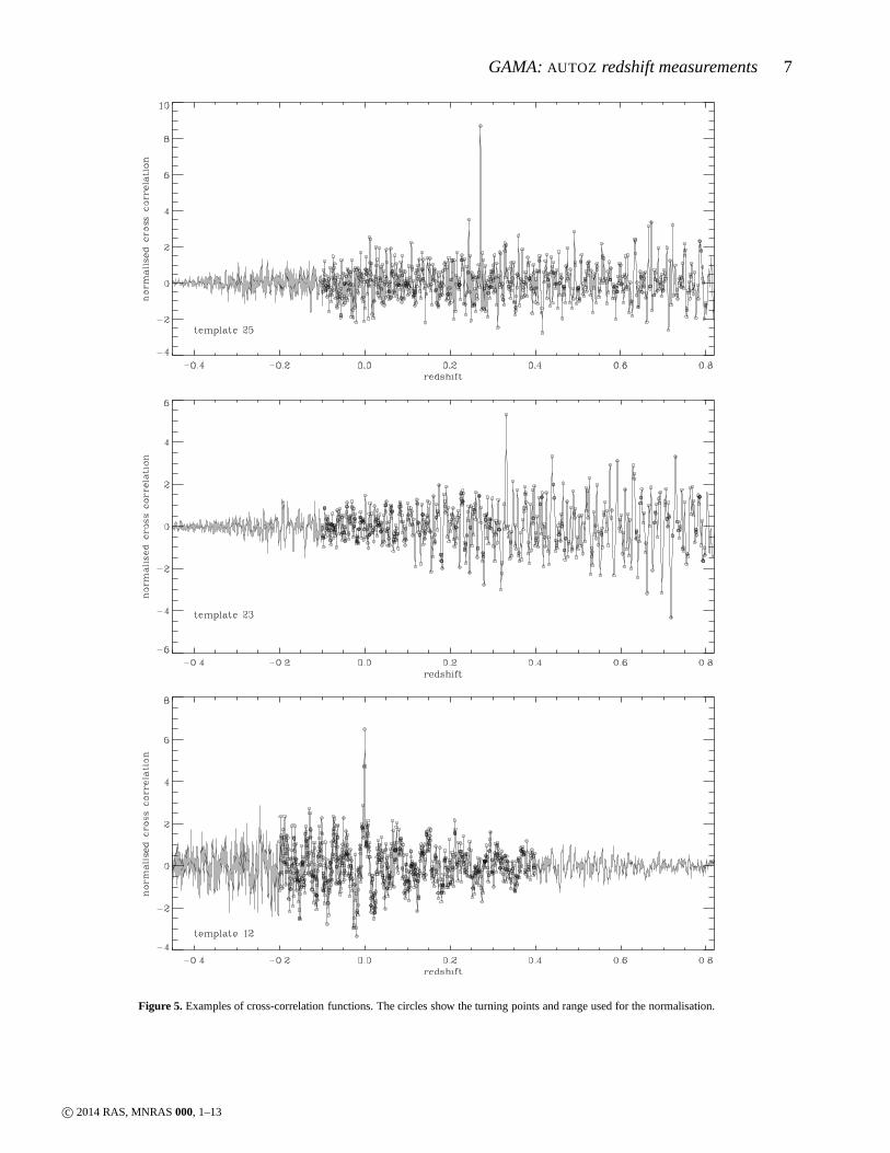
Figure 5. Examples of cross-correlation functions. The circles showthe turning points and range used for the normalisation.

c© 2014 RAS, MNRAS000, 1–13

8 I. K. Baldry et al.

ward the target (if the target spectrum was not put on a heliocentricwavelength scale).

For each template, a search range for finding redshifts and anoise-estimate redshift range for the normalisation procedure weredefined. The ranges for each template are given in Table 1. Thecross-correlation functions were normalised by subtracting a trun-cated mean computed over the noise-estimate range, which resultsin a small adjustment, and dividing by the root mean square (RMS)of the turning points computed over the same range. Typically thecross-correlation functions had between 350 and 850 turning pointsover the noise-estimate range. Fig. 5 shows three examples of nor-malised cross-correlation functions.

For each target spectrum, all the normalised cross-correlationfunctions were determined corresponding to each template beingused (26 or 28 templates; see Table 1). First, the highest cross-correlation peak, within the search ranges, was taken to be the bestestimate of the redshift. The next three best redshifts weredeter-mined after excluding peaks within 600 km/s of the better redshiftestimates, considering all templates, at each stage. The values of thepeaks are calledrx (following the nomenclature of Cannon et al.2006),rx,2, rx,3 andrx,4 each with a corresponding redshift andtemplate number. In order to avoid discretisation at the rebinnedresolution, the redshifts were fine tuned by fitting a quadratic toseven points centred on each peak. Note that the highest redshiftallowed was set at 0.9, which is appropriate for the GAMA magni-tude limit and the fact that theAUTOZ code has not been adapted tosearch for quasar redshifts.

3.3.1 Note on the redshift range used for the normalisation

In order that the normalised cross-correlation functions,rx val-ues, can be compared between different templates, it is impor-tant that the noise-estimate ranges are set appropriately.The cross-correlation function computed using fast Fourier transforms givesvalues forzccf,i from 10−0.35 − 1 to 100.35 − 1 (about−0.55 to1.24) because of the rebinned logarithmic scale from 3.3 to 4.0.Zero padding is necessary because of the wrap-around assumptionof this cross-correlation method. As a result, the amplitude of across-correlation function can drop significantly when theoverlapbetween the rest-frame wavelength range of the template (Table 1)and the observed wavelength range of the target decreases. Thusa more useful estimate of the noise is obtained by computing theRMS over a reduced redshift range, here called the noise-estimaterange. The noise-estimate range for the galaxy templates ischo-sen to encompass the search redshift range with additional negativeredshifts. The noise-estimate range for the stellar templates cov-ers a shorter range because of the reduced rest-frame wavelengthcoverage. For late-type stars, the noise estimate uses morenegativeredshifts because there are larger deviations at the red-end of thetemplate spectra. As a final test of the normalisation procedure, us-ing repeated observations or otherwise, it can be apparent if certaintemplates give rise to numerous false redshift peaks (§ 4).

4 REDSHIFT CONFIDENCE ESTIMATION

In this section, we discuss the process for estimating the likelihoodthat the highest normalised cross-correlation peak corresponds tothe correct redshift. In cases where the distribution of thecross-correlation function values of the turning points is close enough toGaussian, then the value ofrx can be used to give an estimate ofthe redshift confidence (e.g. Cannon et al. 2006; see Heavens1993

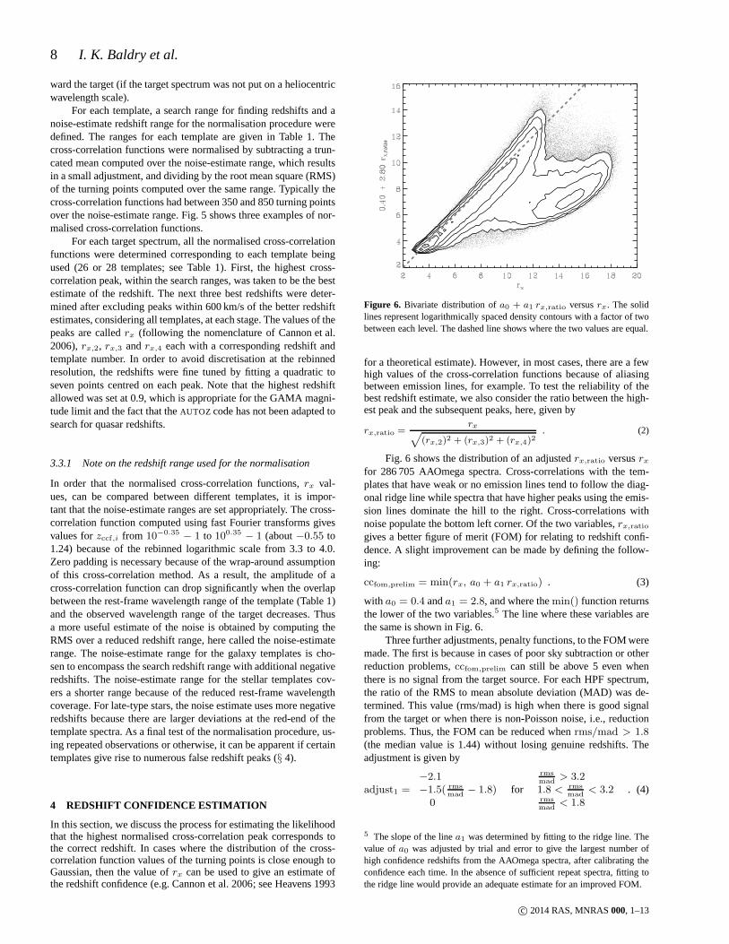
Figure 6. Bivariate distribution ofa0 + a1 rx,ratio versusrx. The solidlines represent logarithmically spaced density contours with a factor of twobetween each level. The dashed line shows where the two values are equal.

for a theoretical estimate). However, in most cases, there are a fewhigh values of the cross-correlation functions because of aliasingbetween emission lines, for example. To test the reliability of thebest redshift estimate, we also consider the ratio between the high-est peak and the subsequent peaks, here, given by

rx,ratio =rx

√

(rx,2)2 + (rx,3)2 + (rx,4)2. (2)

Fig. 6 shows the distribution of an adjustedrx,ratio versusrxfor 286 705 AAOmega spectra. Cross-correlations with the tem-plates that have weak or no emission lines tend to follow the diag-onal ridge line while spectra that have higher peaks using the emis-sion lines dominate the hill to the right. Cross-correlations withnoise populate the bottom left corner. Of the two variables,rx,ratiogives a better figure of merit (FOM) for relating to redshift confi-dence. A slight improvement can be made by defining the follow-ing:

ccfom,prelim = min(rx, a0 + a1 rx,ratio) . (3)

with a0 = 0.4 anda1 = 2.8, and where themin() function returnsthe lower of the two variables.5 The line where these variables arethe same is shown in Fig. 6.

Three further adjustments, penalty functions, to the FOM weremade. The first is because in cases of poor sky subtraction or otherreduction problems,ccfom,prelim can still be above 5 even whenthere is no signal from the target source. For each HPF spectrum,the ratio of the RMS to mean absolute deviation (MAD) was de-termined. This value (rms/mad) is high when there is good signalfrom the target or when there is non-Poisson noise, i.e., reductionproblems. Thus, the FOM can be reduced whenrms/mad > 1.8(the median value is 1.44) without losing genuine redshifts. Theadjustment is given by

adjust1 =−2.1−1.5( rms

mad− 1.8)

0for

rmsmad

> 3.21.8 < rms

mad< 3.2

rmsmad

< 1.8. (4)

5 The slope of the linea1 was determined by fitting to the ridge line. Thevalue ofa0 was adjusted by trial and error to give the largest number ofhigh confidence redshifts from the AAOmega spectra, after calibrating theconfidence each time. In the absence of sufficient repeat spectra, fitting tothe ridge line would provide an adequate estimate for an improved FOM.

c© 2014 RAS, MNRAS000, 1–13

GAMA: AUTOZ redshift measurements 9

The second adjustment is particular to the sample targeted.Sofar only a flat prior has been set for the allowed redshifts; this isgiven by the search ranges. However, there are far fewer galaxies atz > 0.5 than at lower redshifts in the GAMA survey. This adjust-ment is given by

adjust2 =−0.8−4.0(z − 0.45)0

forz > 0.650.45 < z < 0.65z < 0.45

, (5)

and thus

ccfom = ccfom,prelim + adjust1 + adjust2 . (6)

Finally, contamination by solar-system light was checked on atile by tile basis,6 by looking for an excessive number of G-startemplate matches. The number of stars observed as part of ourmain survey is about two per cent (Baldry et al. 2010). When therewas a clustering of ten or more matches to templates 7–10 (bestor second-best redshift estimate), the tile was checked forsolar-system contamination. This was caused by moonlight, under condi-tions where scattering had significant structure on the sub-tile scale,with one notable exception. A cluster of about twenty matches wasfound to be centred on the location of Saturn at the time of theobservation. The spectrum of Saturn can be seen clearly in a few fi-bres;AUTOZ does not have this template but picks up the reflectedsolar absorption lines. In total, 20 tiles were flagged as having pos-sible solar contamination, and any best redshift match to templates7–10 was given accfom value of 2.5. This was applied to about300 spectra and these were not included in the redshift confidenceestimation. In most cases, the targets were re-observed.

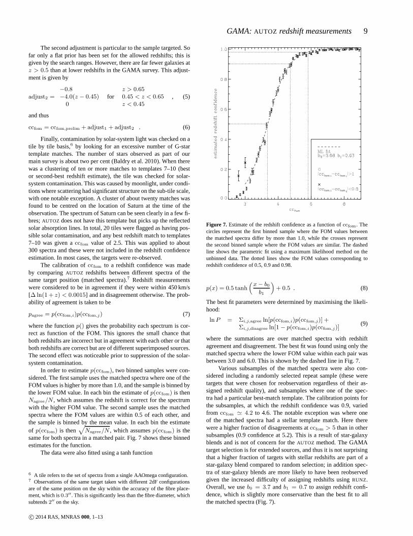
The calibration ofccfom to a redshift confidence was madeby comparingAUTOZ redshifts between different spectra of thesame target position (matched spectra).7 Redshift measurementswere considered to be in agreement if they were within 450 km/s[∆ ln(1 + z) < 0.0015] and in disagreement otherwise. The prob-ability of agreement is taken to be

pagree = p(ccfom,i)p(ccfom,j) (7)

where the functionp() gives the probability each spectrum is cor-rect as function of the FOM. This ignores the small chance thatboth redshifts are incorrect but in agreement with each other or thatboth redshifts are correct but are of different superimposed sources.The second effect was noticeable prior to suppression of thesolar-system contamination.

In order to estimatep(ccfom), two binned samples were con-sidered. The first sample uses the matched spectra where one of theFOM values is higher by more than 1.0, and the sample is binnedbythe lower FOM value. In each bin the estimate ofp(ccfom) is thenNagree/N , which assumes the redshift is correct for the spectrumwith the higher FOM value. The second sample uses the matchedspectra where the FOM values are within 0.5 of each other, andthe sample is binned by the mean value. In each bin the estimateof p(ccfom) is then

√

Nagree/N , which assumesp(ccfom) is thesame for both spectra in a matched pair. Fig. 7 shows these binnedestimates for the function.

The data were also fitted using a tanh function

6 A tile refers to the set of spectra from a single AAOmega configuration.7 Observations of the same target taken with different 2dF configurationsare of the same position on the sky within the accuracy of the fibre place-ment, which is0.3′′. This is significantly less than the fibre diameter, whichsubtends2′′ on the sky.

Figure 7. Estimate of the redshift confidence as a function ofccfom . Thecircles represent the first binned sample where the FOM values betweenthe matched spectra differ by more than 1.0, while the crosses representthe second binned sample where the FOM values are similar. The dashedline shows the parametric fit using a maximum likelihood method on theunbinned data. The dotted lines show the FOM values corresponding toredshift confidence of 0.5, 0.9 and 0.98.

p(x) = 0.5 tanh(

x− b0b1

)

+ 0.5 . (8)

The best fit parameters were determined by maximising the likeli-hood:

lnP = Σi,j,agree ln[p(ccfom,i)p(ccfom,j)] +Σi,j,disagree ln[1− p(ccfom,i)p(ccfom,j)]

(9)

where the summations are over matched spectra with redshiftagreement and disagreement. The best fit was found using onlythematched spectra where the lower FOM value within each pair wasbetween 3.0 and 6.0. This is shown by the dashed line in Fig. 7.

Various subsamples of the matched spectra were also con-sidered including a randomly selected repeat sample (theseweretargets that were chosen for reobservation regardless of their as-signed redshift quality), and subsamples where one of the spec-tra had a particular best-match template. The calibration points forthe subsamples, at which the redshift confidence was 0.9, variedfrom ccfom ≃ 4.2 to 4.6. The notable exception was where oneof the matched spectra had a stellar template match. Here therewere a higher fraction of disagreements atccfom > 5 than in othersubsamples (0.9 confidence at 5.2). This is a result of star-galaxyblends and is not of concern for theAUTOZ method. The GAMAtarget selection is for extended sources, and thus it is not surprisingthat a higher fraction of targets with stellar redshifts arepart of astar-galaxy blend compared to random selection; in addition spec-tra of star-galaxy blends are more likely to have been reobservedgiven the increased difficulty of assigning redshifts usingRUNZ.Overall, we useb0 = 3.7 andb1 = 0.7 to assign redshift confi-dence, which is slightly more conservative than the best fit to allthe matched spectra (Fig. 7).

c© 2014 RAS, MNRAS000, 1–13

10 I. K. Baldry et al.

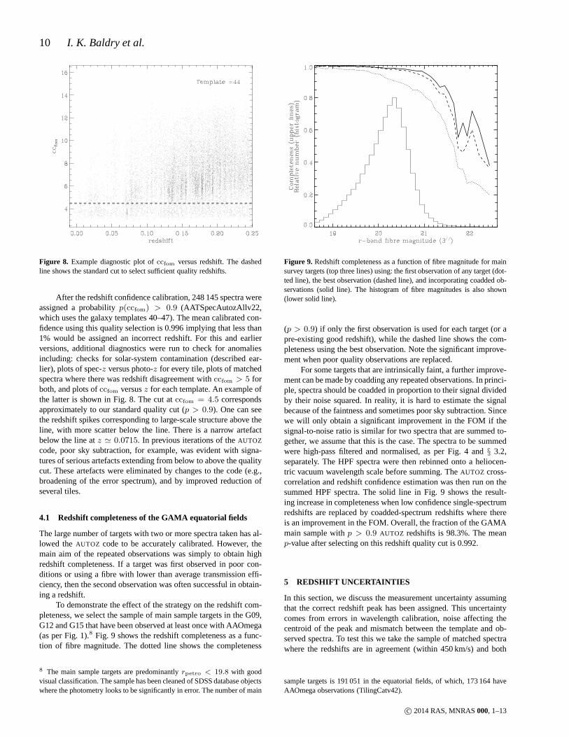
Figure 8. Example diagnostic plot ofccfom versus redshift. The dashedline shows the standard cut to select sufficient quality redshifts.

After the redshift confidence calibration, 248 145 spectra wereassigned a probabilityp(ccfom) > 0.9 (AATSpecAutozAllv22,which uses the galaxy templates 40–47). The mean calibratedcon-fidence using this quality selection is 0.996 implying that less than1% would be assigned an incorrect redshift. For this and earlierversions, additional diagnostics were run to check for anomaliesincluding: checks for solar-system contamination (described ear-lier), plots of spec-z versus photo-z for every tile, plots of matchedspectra where there was redshift disagreement withccfom > 5 forboth, and plots ofccfom versusz for each template. An example ofthe latter is shown in Fig. 8. The cut atccfom = 4.5 correspondsapproximately to our standard quality cut (p > 0.9). One can seethe redshift spikes corresponding to large-scale structure above theline, with more scatter below the line. There is a narrow artefactbelow the line atz ≃ 0.0715. In previous iterations of theAUTOZ

code, poor sky subtraction, for example, was evident with signa-tures of serious artefacts extending from below to above thequalitycut. These artefacts were eliminated by changes to the code (e.g.,broadening of the error spectrum), and by improved reduction ofseveral tiles.

4.1 Redshift completeness of the GAMA equatorial fields

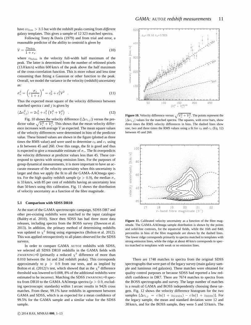
The large number of targets with two or more spectra taken hasal-lowed theAUTOZ code to be accurately calibrated. However, themain aim of the repeated observations was simply to obtain highredshift completeness. If a target was first observed in poorcon-ditions or using a fibre with lower than average transmissioneffi-ciency, then the second observation was often successful inobtain-ing a redshift.

To demonstrate the effect of the strategy on the redshift com-pleteness, we select the sample of main sample targets in theG09,G12 and G15 that have been observed at least once with AAOmega(as per Fig. 1).8 Fig. 9 shows the redshift completeness as a func-tion of fibre magnitude. The dotted line shows the completeness

8 The main sample targets are predominantlyrpetro < 19.8 with goodvisual classification. The sample has been cleaned of SDSS database objectswhere the photometry looks to be significantly in error. The number of main

Figure 9. Redshift completeness as a function of fibre magnitude for mainsurvey targets (top three lines) using: the first observation of any target (dot-ted line), the best observation (dashed line), and incorporating coadded ob-servations (solid line). The histogram of fibre magnitudes is also shown(lower solid line).

(p > 0.9) if only the first observation is used for each target (or apre-existing good redshift), while the dashed line shows the com-pleteness using the best observation. Note the significant improve-ment when poor quality observations are replaced.

For some targets that are intrinsically faint, a further improve-ment can be made by coadding any repeated observations. In princi-ple, spectra should be coadded in proportion to their signaldividedby their noise squared. In reality, it is hard to estimate thesignalbecause of the faintness and sometimes poor sky subtraction. Sincewe will only obtain a significant improvement in the FOM if thesignal-to-noise ratio is similar for two spectra that are summed to-gether, we assume that this is the case. The spectra to be summedwere high-pass filtered and normalised, as per Fig. 4 and§ 3.2,separately. The HPF spectra were then rebinned onto a heliocen-tric vacuum wavelength scale before summing. TheAUTOZ cross-correlation and redshift confidence estimation was then runon thesummed HPF spectra. The solid line in Fig. 9 shows the result-ing increase in completeness when low confidence single-spectrumredshifts are replaced by coadded-spectrum redshifts where thereis an improvement in the FOM. Overall, the fraction of the GAMAmain sample withp > 0.9 AUTOZ redshifts is 98.3%. The meanp-value after selecting on this redshift quality cut is 0.992.

5 REDSHIFT UNCERTAINTIES

In this section, we discuss the measurement uncertainty assumingthat the correct redshift peak has been assigned. This uncertaintycomes from errors in wavelength calibration, noise affecting thecentroid of the peak and mismatch between the template and ob-served spectra. To test this we take the sample of matched spectrawhere the redshifts are in agreement (within 450 km/s) and both

sample targets is 191 051 in the equatorial fields, of which, 173 164 haveAAOmega observations (TilingCatv42).

c© 2014 RAS, MNRAS000, 1–13

GAMA: AUTOZ redshift measurements 11

haveccfom > 3.5 but with the redshift peaks coming fromdifferentgalaxy templates. This gives a sample of 12 323 matched spectra.

Following Tonry & Davis (1979) and from trial and error, areasonable predictor of the ability to centroid is given by

V =vfwhm

1 + rx(10)

where vfwhm is the velocity full-width half maximum of thepeak. The latter is determined from the number of rebinned pixels(13.8 km/s) within 600 km/s of the peak above the half maximumof the cross-correlation function. This is more robust and less timeconsuming than fitting a Gaussian or other function to the peak.Overall, we model the variance in the velocity (redshift) uncertaintyas:

σ2v =

(

cσz

1 + z

)2

= c20 + c21V2 . (11)

Thus the expected mean square of the velocity difference betweenmatched spectrai andj is given by

〈∆v2i,j〉 = 2c20 + c21(

V2i + V2

j

)

. (12)

Fig. 10 shows the velocity difference (|∆vi,j |) versus the pre-dictor value

√

V2i + V2

j . This shows that the mean velocity differ-ence increases with averageV as expected. The mean square valuesof the velocity differences were determined in bins of the predictorvalue. These binned values are shown in the figure (plotted asthreetimes the RMS value) and were used to determinec0 andc1 usinga fit between 45 and 260. Over this range, the fit is good and thusis expected to give a reasonable estimate ofσv. The fit overpredictsthe velocity difference at predictor values less than 45. These cor-respond to spectra with strong emission lines. For the purposes ofgroup dynamical measurements, it is more important to have an ac-curate measure of the velocity uncertainty when this uncertainty islarger and thus we apply the fit to all the GAMA-AAOmega spec-tra. For the high quality redshift sample (p > 0.9), the medianσv

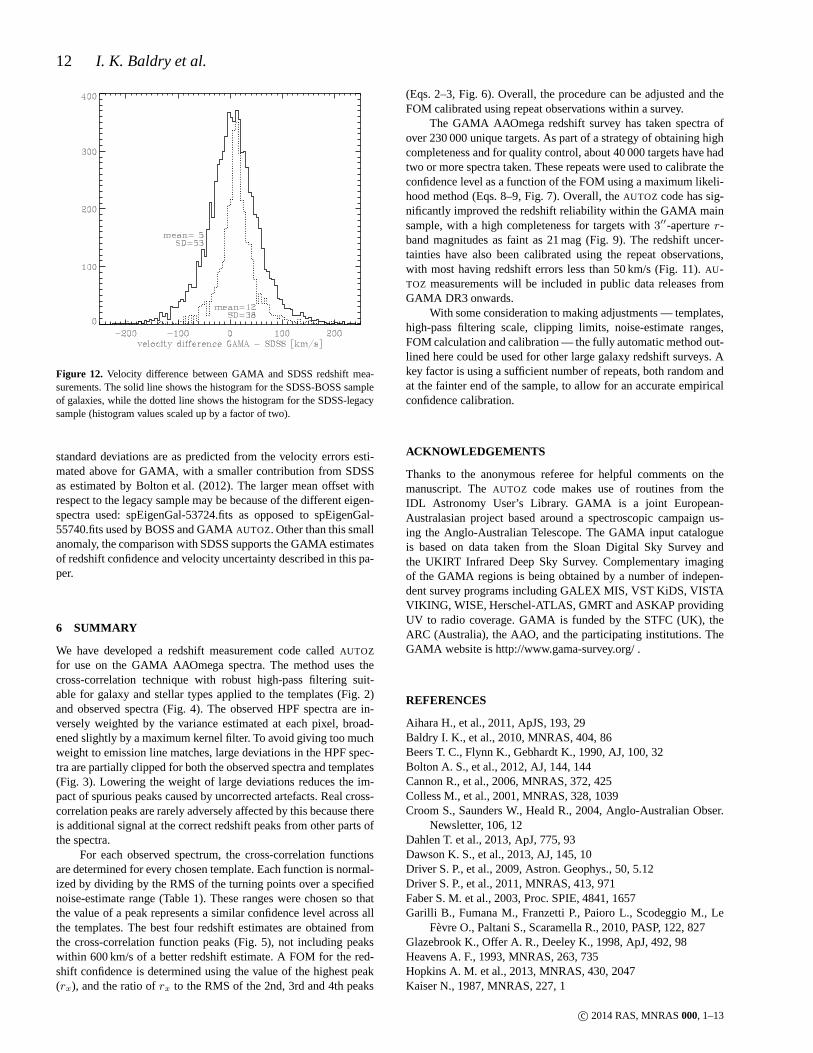
is 33 km/s, with 85 per cent of redshifts having an uncertainty lessthan 50 km/s using this calibration. Fig. 11 shows the distributionof velocity uncertainty as a function of the fibre magnitude.

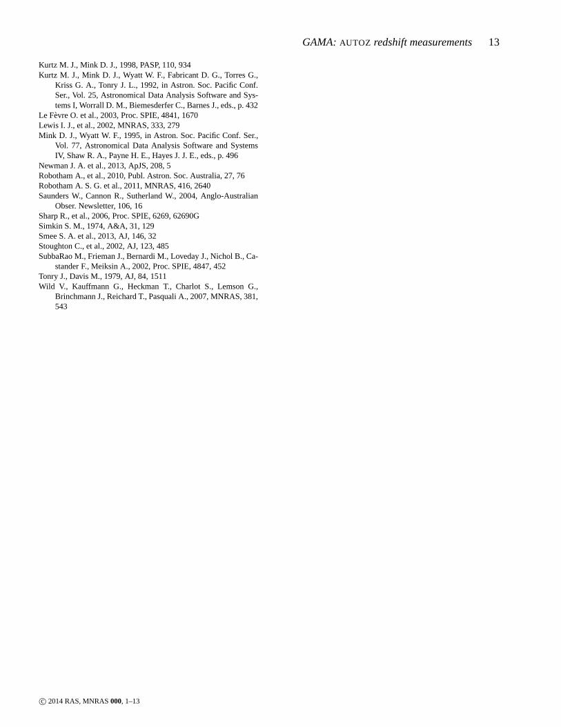
5.1 Comparison with SDSS DR10

At the start of the GAMA spectroscopic campaign, SDSS DR7 andother pre-existing redshifts were matched to the input catalogue(Baldry et al. 2010). Since then SDSS has had three more datareleases, including spectra from the BOSS survey (Dawson etal.2013). In addition, the primary method of determining redshiftswas updated toχ2 fitting using eigenspectra (Bolton et al. 2012).This was applied retrospectively to all plates observed forthe SDSSsurveys.

In order to compare GAMAAUTOZ redshifts with SDSS,we selected all SDSS DR10 redshifts in the GAMA fields withZWARNING=0 (primarily a reducedχ2 difference of more than0.010 between the 1st and 2nd redshift peaks). This correspondsapproximately top > 0.9 from our tests, and as implied byBolton et al. (2012)’s test, which showed that as theχ2 differencethreshold was lowered to 0.008, 8% of the additional redshifts wereestimated to be incorrect. Matching the SDSSZWARNING=0 spec-tra from DR10 to the GAMA AAOmega spectra (p > 0.9, exclud-ing spectroscopic standards) within 1 arcsec results in 9426 crossmatches. From these, 99.1% have redshifts in agreement betweenGAMA and SDSS, which is as expected for a mean confidence of99.5% for the GAMA sample and a similar value for the SDSSsample.

Figure 10.Velocity difference versus√

V2i+ V2

j. The points represent the

|∆vi,j | values for the matched spectra. The squares, with error bars, showthree timesthe RMS velocity differences in bins. The dashed lines showone, two and three times the RMS values using a fit forc0 andc1 (Eq. 12)between 45 and 260.

Figure 11. Calibrated velocity uncertainty as a function of the fibre mag-nitude. The GAMA-AAOmega sample distribution is shown by the pointsand solid-line contours, for the equatorial fields, while the 16th and 84thpercentiles in bins of the fibre magnitude are shown by the dashed lines.The lower ridge corresponds primarily to spectra matched totemplates withstrong emission lines, while the ridge at about 40 km/s corresponds to spec-tra matched to templates with weak or no emission lines.

There are 1748 matches to spectra from the original SDSSspectrographs that were part of the legacy survey (main galaxy sam-ple and luminous red galaxies). These matches were obtainedforquality control purposes or because SDSS had reported a low red-shift confidence in DR7. There are 7674 matches to spectra fromthe BOSS spectrographs and survey. The large number of matchesis a result of GAMA and BOSS independently choosing these tar-gets. Fig. 12 shows the velocity difference histogram for the twosamples [∆vi,j = c ln(1 + zGAMA) − c ln(1 + zSDSS)]. Forthe legacy sample, the mean and standard deviation were 12 and38 km/s, and for the BOSS sample, they were 5 and 53 km/s. The

c© 2014 RAS, MNRAS000, 1–13

12 I. K. Baldry et al.

Figure 12. Velocity difference between GAMA and SDSS redshift mea-surements. The solid line shows the histogram for the SDSS-BOSS sampleof galaxies, while the dotted line shows the histogram for the SDSS-legacysample (histogram values scaled up by a factor of two).

standard deviations are as predicted from the velocity errors esti-mated above for GAMA, with a smaller contribution from SDSSas estimated by Bolton et al. (2012). The larger mean offset withrespect to the legacy sample may be because of the different eigen-spectra used: spEigenGal-53724.fits as opposed to spEigenGal-55740.fits used by BOSS and GAMAAUTOZ. Other than this smallanomaly, the comparison with SDSS supports the GAMA estimatesof redshift confidence and velocity uncertainty described in this pa-per.

6 SUMMARY

We have developed a redshift measurement code calledAUTOZ

for use on the GAMA AAOmega spectra. The method uses thecross-correlation technique with robust high-pass filtering suit-able for galaxy and stellar types applied to the templates (Fig. 2)and observed spectra (Fig. 4). The observed HPF spectra are in-versely weighted by the variance estimated at each pixel, broad-ened slightly by a maximum kernel filter. To avoid giving too muchweight to emission line matches, large deviations in the HPFspec-tra are partially clipped for both the observed spectra and templates(Fig. 3). Lowering the weight of large deviations reduces the im-pact of spurious peaks caused by uncorrected artefacts. Real cross-correlation peaks are rarely adversely affected by this because thereis additional signal at the correct redshift peaks from other parts ofthe spectra.

For each observed spectrum, the cross-correlation functionsare determined for every chosen template. Each function is normal-ized by dividing by the RMS of the turning points over a specifiednoise-estimate range (Table 1). These ranges were chosen sothatthe value of a peak represents a similar confidence level across allthe templates. The best four redshift estimates are obtained fromthe cross-correlation function peaks (Fig. 5), not including peakswithin 600 km/s of a better redshift estimate. A FOM for the red-shift confidence is determined using the value of the highestpeak(rx), and the ratio ofrx to the RMS of the 2nd, 3rd and 4th peaks

(Eqs. 2–3, Fig. 6). Overall, the procedure can be adjusted and theFOM calibrated using repeat observations within a survey.

The GAMA AAOmega redshift survey has taken spectra ofover 230 000 unique targets. As part of a strategy of obtaining highcompleteness and for quality control, about 40 000 targets have hadtwo or more spectra taken. These repeats were used to calibrate theconfidence level as a function of the FOM using a maximum likeli-hood method (Eqs. 8–9, Fig. 7). Overall, theAUTOZ code has sig-nificantly improved the redshift reliability within the GAMA mainsample, with a high completeness for targets with3′′-aperturer-band magnitudes as faint as 21 mag (Fig. 9). The redshift uncer-tainties have also been calibrated using the repeat observations,with most having redshift errors less than 50 km/s (Fig. 11).AU-TOZ measurements will be included in public data releases fromGAMA DR3 onwards.

With some consideration to making adjustments — templates,high-pass filtering scale, clipping limits, noise-estimate ranges,FOM calculation and calibration — the fully automatic method out-lined here could be used for other large galaxy redshift surveys. Akey factor is using a sufficient number of repeats, both random andat the fainter end of the sample, to allow for an accurate empiricalconfidence calibration.

ACKNOWLEDGEMENTS

Thanks to the anonymous referee for helpful comments on themanuscript. TheAUTOZ code makes use of routines from theIDL Astronomy User’s Library. GAMA is a joint European-Australasian project based around a spectroscopic campaign us-ing the Anglo-Australian Telescope. The GAMA input catalogueis based on data taken from the Sloan Digital Sky Survey andthe UKIRT Infrared Deep Sky Survey. Complementary imagingof the GAMA regions is being obtained by a number of indepen-dent survey programs including GALEX MIS, VST KiDS, VISTAVIKING, WISE, Herschel-ATLAS, GMRT and ASKAP providingUV to radio coverage. GAMA is funded by the STFC (UK), theARC (Australia), the AAO, and the participating institutions. TheGAMA website is http://www.gama-survey.org/ .

REFERENCES

Aihara H., et al., 2011, ApJS, 193, 29Baldry I. K., et al., 2010, MNRAS, 404, 86Beers T. C., Flynn K., Gebhardt K., 1990, AJ, 100, 32Bolton A. S., et al., 2012, AJ, 144, 144Cannon R., et al., 2006, MNRAS, 372, 425Colless M., et al., 2001, MNRAS, 328, 1039Croom S., Saunders W., Heald R., 2004, Anglo-Australian Obser.

Newsletter, 106, 12Dahlen T. et al., 2013, ApJ, 775, 93Dawson K. S., et al., 2013, AJ, 145, 10Driver S. P., et al., 2009, Astron. Geophys., 50, 5.12Driver S. P., et al., 2011, MNRAS, 413, 971Faber S. M. et al., 2003, Proc. SPIE, 4841, 1657Garilli B., Fumana M., Franzetti P., Paioro L., Scodeggio M., Le

Fevre O., Paltani S., Scaramella R., 2010, PASP, 122, 827Glazebrook K., Offer A. R., Deeley K., 1998, ApJ, 492, 98Heavens A. F., 1993, MNRAS, 263, 735Hopkins A. M. et al., 2013, MNRAS, 430, 2047Kaiser N., 1987, MNRAS, 227, 1

c© 2014 RAS, MNRAS000, 1–13

GAMA: AUTOZ redshift measurements 13

Kurtz M. J., Mink D. J., 1998, PASP, 110, 934Kurtz M. J., Mink D. J., Wyatt W. F., Fabricant D. G., Torres G.,

Kriss G. A., Tonry J. L., 1992, in Astron. Soc. Pacific Conf.Ser., Vol. 25, Astronomical Data Analysis Software and Sys-tems I, Worrall D. M., Biemesderfer C., Barnes J., eds., p. 432

Le Fevre O. et al., 2003, Proc. SPIE, 4841, 1670Lewis I. J., et al., 2002, MNRAS, 333, 279Mink D. J., Wyatt W. F., 1995, in Astron. Soc. Pacific Conf. Ser.,

Vol. 77, Astronomical Data Analysis Software and SystemsIV, Shaw R. A., Payne H. E., Hayes J. J. E., eds., p. 496

Newman J. A. et al., 2013, ApJS, 208, 5Robotham A., et al., 2010, Publ. Astron. Soc. Australia, 27,76Robotham A. S. G. et al., 2011, MNRAS, 416, 2640Saunders W., Cannon R., Sutherland W., 2004, Anglo-Australian

Obser. Newsletter, 106, 16Sharp R., et al., 2006, Proc. SPIE, 6269, 62690GSimkin S. M., 1974, A&A, 31, 129Smee S. A. et al., 2013, AJ, 146, 32Stoughton C., et al., 2002, AJ, 123, 485SubbaRao M., Frieman J., Bernardi M., Loveday J., Nichol B.,Ca-

stander F., Meiksin A., 2002, Proc. SPIE, 4847, 452Tonry J., Davis M., 1979, AJ, 84, 1511Wild V., Kauffmann G., Heckman T., Charlot S., Lemson G.,

Brinchmann J., Reichard T., Pasquali A., 2007, MNRAS, 381,543

c© 2014 RAS, MNRAS000, 1–13