arX

iv:a

stro

-ph/

0503

249v

1 1

0 M

ar 2

005

The Bolocam Lockman Hole Millimeter-Wave Galaxy Survey:

Galaxy Candidates and Number Counts

G. T. Laurent1,5, J. E. Aguirre1, J. Glenn1, P. A. R. Ade2, J. J. Bock3,4, S. F. Edgington4,

A. Goldin3, S. R. Golwala4, D. Haig2, A. E. Lange4, P. R. Maloney1, P. D. Mauskopf2, H.

Nguyen3, P. Rossinot4, J. Sayers4, & P. Stover1

ABSTRACT

We present results of a new deep 1.1 mm survey using Bolocam, a millimeter-

wavelength bolometer array camera designed for mapping large fields at fast

scan rates, without chopping. A map, galaxy candidate list, and derived number

counts are presented. This survey encompasses 324 arcmin2 to an rms noise level

(filtered for point sources) of σ1.1mm ≃ 1.4 mJy beam−1 and includes the entire

regions surveyed by the published 8 mJy 850 µm JCMT SCUBA and 1.2 mm

IRAM MAMBO surveys. We reduced the data using a custom software pipeline

to remove correlated sky and instrument noise via a principal component analysis.

Extensive simulations and jackknife tests were performed to confirm the robust-

ness of our source candidates and estimate the effects of false detections, bias,

and completeness. In total, 17 source candidates were detected at a significance

≥ 3.0 σ, with six expected false detections. Nine candidates are new detections,

while eight candidates have coincident SCUBA 850 µm and/or MAMBO 1.2 mm

detections. From our observed number counts, we estimate the underlying dif-

ferential number count distribution of submillimeter galaxies and find it to be in

general agreement with previous surveys. Modeling the spectral energy distribu-

tions of these submillimeter galaxies after observations of dusty nearby galaxies

suggests extreme luminosities of L = (1.0 − 1.6) × 1013 L⊙ and, if powered by

star formation, star formation rates of 500− 800 M⊙yr−1.

Subject headings: galaxies: high-redshift — galaxies: starburst — submillimeter

1Center for Astrophysics and Space Astronomy & Department of Astrophysical and Planetary Sciences,

University of Colorado, 593 UCB, Boulder, CO 80309-0593

2Physics and Astronomy, Cardiff University, 5 The Parade, P.O. Box 913, Cardiff CF24 3YB, Wales, UK

3Jet Propulsion Laboratory, California Institute of Technology, 4800 Oak Grove Drive, Pasadena, CA

91109

4California Institute of Technology, 1200 E. California Boulevard, MC 59-33, Pasadena, CA 91125

5glaurent@colorado.edu

– 2 –

1. Introduction

Submillimeter galaxies are extremely luminous (L > 1012L⊙), high-redshift (z > 1),

dust-obscured galaxies detected by their thermal dust emission (for a review see Blain et al.

2002). The dust is heated by the ultraviolet and optical flux from young stars associated with

prodigious inferred star formation rates (SFRs) of ∼ 100−1000 M⊙ yr−1 (Blain et al. 2002).

Although ∼ 13

of sources appear to contain an active galactic nucleus (AGN; Alexander et al.

2003; Ivison et al. 2004), in nearly all cases the AGNs are not bolometrically important (<

20%; Alexander et al. 2004). Given these SFRs, a burst of duration 108 yr would be sufficient

to form all the stars in an elliptical galaxy, making it plausible that submillimeter galaxies

are the progenitors of elliptical galaxies and spiral bulges (Smail et al. 2002; Swinbank

et al. 2004). Deep (sub)millimeter surveys with SCUBA (Holland et al. 1999) and MAMBO

(Bertoldi et al. 2000) have now resolved 10%−40% of the cosmic far-infrared background

(Puget et al. 1996; Hauser et al. 1998; Fixsen et al. 1998) into submillimeter galaxies in blank-

field surveys (e.g., Greve et al. 2004; Borys et al. 2003; Scott et al. 2002) and 40%−100%

using lensing galaxy clusters (Blain et al. 1999; Cowie et al. 2002). Photometric redshifts

constrain most of the submillimeter galaxies found so far to lie at z > 1 (e.g., Carilli & Yun

1999; Yun & Carilli 2002; Aretxaga et al. 2003).

Recent observations of submillimeter galaxies with the Keck Low-Resolution Imaging

Spectrograph (LRIS; Chapman et al. 2003a, 2003b, 2005) have shown that redshifts can

be obtained for ∼70% of bright submillimeter galaxies (S850µm > 5 mJy) with bright radio

counterparts (S1.4GHz > 30 µJy; Blain et al. 2004) (the fraction of submillimeter galaxies with

radio counterparts appears to be ∼65%; Ivison et al. 2002). This sample of submillimeter

galaxies lies in a distribution peaking at z = 2.4 with ∆z = 0.65 (Ivison et al. 2002; Chapman

et al. 2003b, 2005). Six of these galaxies have had their optical spectroscopic redshifts

confirmed by millimeter CO line measurements (Frayer et al. 1998, 1999; Neri et al. 2003;

Sheth et al. 2004). This redshift distribution may be biased with respect to the overall

submillimeter galaxy population owing to a number of selection effects: the requirement of

precise radio positions prior to spectroscopy, which introduces a bias against cooler galaxies,

especially at higher redshifts (z > 2.5); limited completeness (∼ 30%) of the spectroscopic

observations, which biases the sample against galaxies with weak emission lines; and the

redshift gap at z = 1.2−1.8 due to the “spectroscopic desert,” in which no strong rest-frame

ultraviolet lines are redshifted into the optical.

Bolocam is a new millimeter-wave bolometer camera for the Caltech Submillimeter

Observatory (CSO).1 Bolocam’s large field of view (8′), 31′′ beams (FWHM at λ = 1.1 mm),

1See http://www.cso.caltech.edu/bolocam.

– 3 –

and AC biasing scheme make it particularly well-suited to finding rare, bright submillimeter

galaxies and for probing large-scale structure. We have used Bolocam to conduct a survey

toward the Lockman Hole for submillimeter galaxies. The Lockman Hole is a region in

UMa in which absorbing material, such as dust and galactic hydrogen, is highly rarefied

(HI column density of NH ≈ 4.5 x 1019 cm−2; Jahoda et al. 1990), providing a transparent

window for sensitive extragalactic surveys over a wide spectral range, from the infrared

and millimeter wavebands to UV and X-ray observations. Submillimeter (Scott et al. 2002;

Fox et al. 2002; Ivison et al. 2002; Eales et al. 2003) and millimeter-wave (Greve et al.

2004) surveys for submillimeter galaxies have already been done toward the Lockman Hole.

It is one of the one-quarter square degree fields of the SCUBA SHADES,2 the focus of

a deep extragalactic survey with XMM-Newton (Hasinger et al. 2001), and a target field

for Spitzer guaranteed time observations. The coverage of the Lockman Hole region by

several surveys therefore makes it an excellent field for intercomparison of galaxy candidate

lists and measuring spectral energy distributions (SEDs), which will ultimately enable dust

temperatures and redshifts to be constrained.

This paper is arranged as follows. In § 2 Bolocam and the observations are described.

In § 3 the data reduction pipeline, including pointing and flux calibration, cleaning and sky

subtraction, and mapping, is described. In § 4 the source candidate list and tests of the

robustness of the candidates are presented. We devote § 5 to the extraction of the number

counts versus flux density relation using simulations designed to characterize the systematic

effects in the data reduction and the false detections, completeness, and bias in the survey.

In § 6 we discuss the implications of the survey, in § 7 we describe future work for this

program, and in § 8 we give conclusions.

2. Observations

2.1. Instrument Description

The heart of Bolocam is an array of 144 silicon nitride micromesh (“spider-web”)

bolometers cooled to 260 mK by a three-stage (4He/3He/3He) sorption refrigerator. An

array of close-packed (1.5fλ), straight-walled conical feed horns terminating in cylindrical

waveguides and integrating cavities formed by a planar backshort couples the bolometers

to cryogenic and room-temperature optics. The illumination on the 10.4 m diameter CSO

primary mirror is controlled by the combination of the feed horns and a cold (6 K) Lyot stop,

2See http://www.roe.ac.uk/ifa/shades/links.html.

– 4 –

resulting in 31′′ beams (FWHM). A stack of resonant metal-mesh filters form the passband

in conjunction with the waveguides. A λ = 2.1 mm configuration is also available, which

is used for observations of the Sunyaev-Zel’dovich effect and secondary anisotropies in the

cosmic microwave background radiation. Technical details of Bolocam are given in Glenn

et al. (1998, 2003) and Haig et al. (2004); numerical simulations of the integrating cavities

are described in Glenn et al. (2002).

A key element of Bolocam is the bolometer bias and readout electronics: an AC biasing

scheme (130 Hz) with readout by lock-in amplifiers enables the detectors to be biased well

above the 1/f knee of the electronics. The electronic readout stability, in conjunction with

Bolocam’s rigorous sky noise subtraction algorithm, eliminates the need to nutate the CSO

subreflector. Another advantage of this AC biasing scheme is that it is easy to monitor the

bolometer operating voltage; these voltages are determined by the total atmospheric emission

in the telescope beam and the responsivity of the bolometers. Thus, a voltage that is a

monotonic function of the in-band atmospheric optical depth and bolometer responsivity is

continually measured. Sky subtraction is implemented by either a subtraction of the average

bolometer voltages or a principal component analysis (PCA) technique, which is described

below.

2.2. Scan Strategy

Two sets of observations of the Lockman Hole East (R.A. = 10h 52m 08s.82, decl. =

+57 21′ 33′′.80, J2000.0) were made with Bolocam: 2003 January, when the data were taken

with a fast raster scan without chopping (hereafter referred to as raster scan observations),

and 2003 May, when the data were acquired with a slow raster scan with chopping as a

test of this observing mode (referred to as chopped observations). Approximately 82 hr of

integration time over 17 nights were obtained on the field during 2003 January, resulting in

259 separate observations, and 41 hr over 19 nights were obtained in 2003 May, resulting in

64 separate observations. The weather was generally good during the 2003 January run and

mediocre to poor during the 2003 May run, where we characterize the weather quality by

the sky noise variability (rapid variability of the optical depth).3 One hundred and nineteen

bolometer channels were operational during 2003 May; however, only 89 bolometer channels

were used in the analysis of the 2003 January data. (The remaining bolometers were not

3Another weather measurement influencing the Bolocam mapping speed is the CSO 225 GHz heterodyne,

narrowband, “tipper tau” monitor, which measures the zenith atmospheric attenuation. The 2003 January

and May Lockman Hole observations yielded τ225GHz ranges and 75th percentiles of τ225GHz = 0.028−0.129,

τ75% = 0.083 and τ225GHz = 0.014 − 0.307, τ75% = 0.200, respectively.

– 5 –

included in making the final Lockman Hole map because of excess noise and/or electronics

failures.) Nominally one feed horn per hextant is blocked to enable these dark bolometers to

be used for bias and noise monitoring. The 2003 May chopped observations were not deep

enough to detect galaxies individually at > 3 σ and were used only for pointing verification

by cross-correlation with the raster scan observations.

During 2003 January, observations were made by scanning the telescope at 60′′ s−1

in right ascension and stepping in declination by 162′′ (∼ 13

of a field of view) between

subscans (defined as a single raster scan across the sky at a fixed declination) to build up the

map. Subsequent scans (which we define as the set of subscans needed to cover the entire

declination range of the field) were taken with a ±11′′ jitter for each 162′′ step to minimize

coverage variations. Combined with a 5 tilt of the bolometer array relative to azimuth and a

fixed Dewar angle, such that the rotation relative to scan direction varies over the night, this

yielded even coverage and sub-Nyquist sampling in the cross-scan direction (declination).

Sub-Nyquist sampling was automatically achieved in the in-scan direction (right ascension)

with 50 Hz sampling of the lock-in amplifiers. In 2003 May, the chopped observations were

made with raster scans in azimuth and steps in elevation, but with a scan rate of 5′′ s−1 and

a symmetric chopper throw of ±45′′ in azimuth, with frequencies of 1 and 2 Hz.

A coverage map of the Bolocam Lockman Hole East field from 2003 January is shown in

Figure 1, where the integration time per 10′′×10′′ pixel is shown. Bolocam’s 8′ field of view

is not small compared to the map size; thus, there is a large border around the map where

the coverage is reduced and nonuniform compared to the central region. Hence, we define

a “uniform coverage region” of 324 arcmin2 in the center where the rms in the integration

time per pixel is 12%. Because rms noise varies as the square root of the integration time,

the noise dispersion is approximately 6% in the uniform coverage region (2% after the map

has been optimally filtered as discussed in § 3.5). Our analysis is confined to the uniform

coverage region. The observational parameters are summarized in Table 1.

3. Data Reduction

3.1. Basic Pipeline

The Lockman Hole observations were reduced with a custom IDL-based software pipe-

line. The raw files were cleaned with a PCA sky subtraction, where an atmospheric and

instrumental noise template was generated through an eigenvector decomposition of the

time stream data (§ 3.2). In the case of the chopped observations, which are characterized

by both positive and negative beams, the time streams were first demodulated followed by

– 6 –

a convolution with the expected source crossing structure (first the positive beam, then the

negative beam). This results in a positive net peak at the nominal source position with the

full source amplitude and symmetric negative beams with half the source amplitude.

Once the cleaned time streams were obtained, a map was generated by co-adding in-

dividual time streams, weighted by their power spectral densities (PSDs) integrated over

the spectral response to a point source. Pointing offsets were applied to individual observa-

tions from the global pointing model generated from observations of submillimeter pointing

sources (§ 3.3). Time streams were calibrated from lock-in amplifier voltages to millijanskys

using observations of primary and secondary flux calibrators (§ 3.4). The final map was

generated in right ascension and declination using sub-beam-sized pixelization (§ 3.5) and

Wiener filtered to maximize signal-to-noise ratio (S/N) for detections of point sources.

3.2. Cleaning and Sky Subtraction

To facilitate removal of fluctuating atmospheric water vapor emission (sky noise) from

the bolometer signals, Bolocam was designed such that the feed horn beams overlap maxi-

mally on the primary mirror of the telescope and therefore sample very similar columns of

atmosphere. Thus, the sky noise, which dominates the fundamental instrument noise by a

factor of ∼100, is a nearly common-mode signal. To remove this correlated 1/f noise with

maximum effectiveness, a PCA technique was developed. The formalism of the PCA analysis

is standard (see, e.g., Murtagh & Heck 1987). Here the covariance matrix is built from the

n bolometers by m time elements matrix for each subscan. Eigenfunctions of the orthogonal

decomposition that have “large” eigenvalues, corresponding to large contributions to the

correlated noise, are nulled and the resulting functions are transformed back into individual

bolometer time streams. This technique is applicable for the dim (.10 mJy) submillime-

ter galaxies of the Lockman Hole (and other blank-field surveys) because the source signal

contributes negligibly to the sky templates and is largely uncorrelated from bolometer to

bolometer. The PCA technique is not appropriate for extended sources, however, in which

case the bolometers see correlated astrophysical signals, which are then attenuated. The

PCA decomposition was applied to raster scan and chopped data, after chop demodula-

tion in the latter case. Cosmic-ray strikes (spikes in the time streams) are flagged and not

included in constructing the eigenfunctions.

The precise level of the cut on the large eigenvalues is somewhat arbitrary. The greater

the number of eigenfunctions that are nulled, the lower the resulting noise in the cleaned

time stream, but the correspondingly greater source flux density removed. Empirically,

an iterative cut with the nulling of eigenfunctions with eigenvalues > 3 σ from the mean of

– 7 –

the eigenvalue distribution produced a balance between sky emission removal and source flux

density reduction in simulated observations by maximizing the S/N. Because the distribution

of eigenvalues for each observation is characterized by a few outliers (typically 4−7) at large

σ-values, the overall variance of the time stream is largely dominated by these eigenvalues,

resulting in a S/N that is insensitive to the cut threshold for 2 − 5 σ. Furthermore, the

distribution of source candidates in the combined Lockman Hole map was invariant under

variations in the cut threshold in this range.

The PCA sky subtraction attenuates the signal from point sources in addition to the

atmospheric signal because it removes low-frequency power from the time streams. The

amount of flux density attenuation is determined by the number of PCA components that

are removed from the raw time streams, which is controlled by the cut on the eigenvalues:

a more aggressive cut results in greater attenuation. Monte Carlo simulations were done

to determine the amount by which the flux density of galaxy candidates was reduced by

the cleaning. The simulations were done in the following manner: A fake source (Gaussian,

31′′ FWHM) was injected into a blank Lockman Hole map. A simulated bolometer time

stream was generated from the map of the fake source and was added to the raw bolometer

time streams of an individual Lockman Hole observation. The time stream data were then

cleaned with PCA and mapped in the ordinary manner. The resulting source was fitted by

a two-dimensional Gaussian to determine the attenuation of the injected source flux density.

This simulation was repeated 1014 times with fake sources injected into random observations

at random positions and ranging in flux density from 0.1 to above 1000 mJy (Fig. 2). The

average reduction in flux density is 0.19 with an rms dispersion of 0.04, independent of flux

density to 1 Jy.

Above 1 Jy, typical for bright pointing and flux calibrators, the amount of attenuation

by PCA was found to depend on the brightness of the fake source. Thus, a different clean-

ing technique was used for these sources. An atmospheric noise template was generated by

simply taking an average of all n bolometers for each time element. The mean-subtracted

sky template was then correlated to each of the individual bolometer time streams and the

correlated component was subtracted. To prevent the correlation coefficient from being con-

taminated by the calibrators, multiple scans (including telescope turnaround time between

scans) were concatenated and used together to correlate the average sky template to each

individual bolometer signal, thus ensuring a small contribution from the point source. A

similar analysis to that for PCA flux reduction was performed for the simple average sky

subtraction technique, yielding an average flux density reduction of 0.07, independent of

source flux, with an rms dispersion of 0.02.

– 8 –

3.3. Pointing

Observations of planets, quasars, protostellar sources, HII regions, and evolved stars

were used to construct separate pointing models for the 2003 January and May observing

runs. Observations of the pointing sources were taken at the same scanning speeds as the

Lockman Hole observations. The pointing fields were generally small (scan areas of ∼ 4′x4′),

although several larger maps (10′x10′) were made of Mars so that the source would pass over

the entire bolometer array for measuring relative responsivities and beam maps. Pointing

observations are generally small because source crossings are only needed in a small subset

(15 or so) of bolometers to determine the pointing offsets. These observations were used

to map and correct the distortion over the field of view, which is in broad agreement with

the distortion predicted by a Zemaxr ray-tracing model. The residual rms in the raster-

scanned pointing model for the ensemble of all 2003 January sources is 9.1′′, although the

local pointing registered to a nearby pointing source is superior.4 This random pointing error

results in an 18% flux density reduction of the Lockman Hole galaxy candidates (analytically

derived from a convolution of the 31′′ Bolocam beam with a 9.1′′ Gaussian random pointing

error), which is corrected for in the reported flux densities (and uncertainties in these fluxes)

of Table 2.

While the 2003 January pointing observations were used to construct a pointing model

that was applied to the entire sky, the region of the celestial sphere near the Lockman Hole

was not well sampled. A pointing correction derived from sources far away (> 30) from

the Lockman Hole is therefore susceptible to a systematic offset. Pointing observations were

made much more frequently (once per hour) during the 2003 May run and sources near the

Lockman Hole were emphasized to create an improved local pointing model; consequently,

the 2003 May pointing model near the Lockman Hole was superior to the 2003 January

pointing model. No galaxy candidates were detected at ≥ 3 σ significance in the 2003 May

chopped Lockman Hole map owing to poor weather; however, it was cross-correlated with

the 2003 January map to compare the pointing models. The cross-correlation yielded a shift

of 25′′ in right ascension of the 2003 January data with respect to the 2003 May data (Fig.

3). Because the pointing on the sky near the Lockman Hole was substantially better and

more frequently sampled for the 2003 May run, we attribute this shift to a systematic offset

in the 2003 January pointing model. Thus, a systematic 25′′ shift in right ascension was

applied to the 2003 January Lockman Hole map. The need for the shift is also apparent in

a comparison between the Bolocam map and the 8 mJy SCUBA 850 µm and MAMBO 1.2

mm surveys, as several of the Bolocam galaxy candidates become coincident with SCUBA

4A subsequent pointing model for a localized region of sky yields an rms of 4.5′′.

– 9 –

and MAMBO sources in the overlap region of the surveys.

Because no pointing observations were taken near the Lockman Hole, it is difficult to

quantify the uncertainty in the 9.1′′ pointing rms. An independent measurement of our

pointing uncertainty was performed by examining both 10 VLA5 radio positions coincident

with Bolocam Lockman Hole galaxy candidates and the subset of 5 sources with additional

SCUBA and/or MAMBO counterparts (see § 4.3). The rms errors between the Bolocam and

radio positions are 10.2+3.1−2.4 and 9.3+4.4

−3.0 arcsec for the entire 10-source sample and 5-source

subset, respectively. The quoted uncertainties are the minimum length 90% confidence

intervals for 10 and 5 degrees of freedom (for both δR.A. and δdecl., each of which independently

determines the pointing error), respectively.

3.4. Flux Calibration

Observations of primary calibrators (planets) and secondary calibrators (protostellar

sources, HII regions, and evolved stars) were used for flux calibration. Reference planetary

flux densities were obtained from the James Clerk Maxwell Telescope (JCMT) calibration

Web site,6 and flux densities of secondary calibrators were obtained from JCMT calibrators

(Sandell 1994; Jenness et al. 2002). The flux density of IRC +10216 is periodic; the flux

density was adjusted to the epoch of observation using the 850 µm SCUBA phase. The

reference flux densities were corrected for the Bolocam bandpass, which is centered at 265

GHz (the flux densities in the Bolocam band are 5% larger than the those quoted by the

JCMT for the SCUBA 1.1 mm band). During 2003 January, Saturn had a semidiameter

of 10′′; this is not small compared to the 31′′ Bolocam beam, so corrections for the angular

extent of Saturn were required.

The standard technique for flux calibration is to calibrate a given science observation

using the flux calibrator observations taken nearest in time, which were presumably taken

at similar atmospheric opacity and air mass. With Bolocam, we are able to use a more

sophisticated technique via continuous monitoring of the bolometer operating resistance

using the DC level of the lock-in amplifier output signal. The technique uses the following

logic. The atmospheric optical loading increases as the atmospheric optical transmission

decreases, which may occur because of changes in zenith opacity (i.e., weather) or intentional

changes in telescope elevation. The bolometer resistance decreases monotonically as the

5The National Radio Astronomy Observatory is a facility of the National Science Foundation operated

under cooperative agreement by Associated Universities, Inc.

6See http://www.jach.hawaii.edu/jac-bin/planetflux.pl.

– 10 –

atmospheric optical loading increases. Simultaneously, the bolometer responsivity decreases

monotonically as the bolometer resistance decreases. Thus, the flux calibration (in nV

Jy−1, where the voltage drop across the bolometer is proportional to its resistance), which

is proportional to the product of atmospheric transmission and bolometer responsivity, is

expected to be a monotonic function of the bolometer resistance. This relation is measured

empirically, as shown in Figure 4, by plotting the flux calibration (voltage at the bolometer

in nV Jy−1 of source flux) from each of the ensemble of calibrator observations against the

median DC lock-in amplifier voltage measured during the observation. This relation is then

combined with the continuously monitored DC lock-in signal to apply the appropriate flux

calibration value during science observations. Note that the curve is measured only using

sources dim enough to ensure linear bolometer response; Jupiter was dropped for this reason.

The flux density calibration derived from Figure 4 is biased relative to the blank-field

sources by the combination of three effects: reduction in the flux density of calibration

sources due to average cleaning, reduction in the flux density of blank-field sources due to

PCA cleaning, and reduction in the flux density of blank-field sources due to pointing errors.

The first two effects cause the calibration curve of Figure 4 to be shifted up by the factor

ǫavg/ǫPCA, where the flux reduction factors ǫavg and ǫPCA are as determined in § 3.2. The

effect of Gaussian random pointing errors of rms σp on the peak flux density of a source

observed with a Gaussian beam of width σb is equivalent to a convolution of the beam with

a Gaussian of rms σp. The resulting reduction in peak height can be analytically calculated

as

ǫp =σb

√

σ2b + σ2

p

= 0.82+0.09−0.12

for a 31′′ FWHM beam and a random pointing error of 9.1′′. The uncertainty quoted for

ǫp is the minimum length 90% confidence interval obtained from the rms pointing error

between the Bolocam galaxy candidates and coincident radio sources (see § 4.3). (While the

local pointing observations around a specific altitude and azimuth are clustered, each with a

smaller pointing error rms, the Lockman Hole observations were taken over a large range of

zenith and azimuthal angles and thus have an overall pointing error defined by the ensemble

of pointing observations.)

Thus, the final bias in flux density is

ǫ =ǫpǫPCA

ǫavg= 0.71+0.08

−0.10.

All flux densities (as well as uncertainties in these fluxes) quoted in this paper, including the

simulations of § 5, have been corrected for this flux bias. The uncertainty in the flux bias is

a systematic effect that produces a correlated shift in all source fluxes.

– 11 –

3.5. Mapping and Optimal Filtering

Bolocam maps are built up by co-adding subscans weighted by their time stream PSDs

integrated over the spectral (temporal frequency) band of a point source at the raster scan

speed. Data points were binned into 10′′× 10′′ pixels, with approximately 30,000 hits per

pixel. Each hit represents a 20 ms integration per bolometer channel. Four maps were

created: a coverage map with the number of hits per pixel (Fig. 1); the PCA-cleaned,

optimally filtered astrophysical map; a coverage-normalized map; and a within-pixel rms

map. In the coverage-normalized map, each pixel was multiplied by the square root of the

number of hits (effectively the integration time) in that pixel to account for the nonuniform

coverage in the map when comparing pixels. The dispersion of the bolometer voltages (from

each of the hits) within each pixel was recorded in the within-pixel rms map.

Because the signal band of interest (point sources) does not fall throughout the entire

temporal (or spatial) frequency range of the PSD of the data, we filter the co-added map with

an optimal (Wiener) filter, g(q), to attenuate 1/f noise at low frequencies and high-frequency

noise above the signal frequency:

g(q) =s∗(q)/J(q)

∫

|s(q)|2/J(q)d2q, (1)

where J(q) is the average PSD, s(q) is the Fourier transform of the Bolocam beam shape

from map space to spatial frequency (1/x) space, q, and the asterisk indicates complex

conjugation. The factor in the denominator is the appropriate normalization factor so that

when convolved with a map, peak heights of beam-shaped sources are preserved. J(q) is

obtained by transforming the time stream PSDs (averaged over all of the Lockman Hole

observations) to a spatial PSD assuming azimuthal symmetry. A two-dimensional map of

equation (1) was thus convolved with the co-added map to maximize S/N for detections of

point sources. An analogous filter was applied directly to the demodulated time streams of

the chopped observations, with s(t) represented by a positive and negative beam separated

by the chop throw (90′′).

The cleaned, co-added, optimally filtered map is presented in Figure 5. There is a

perimeter a few arcminutes wide around the map that does not lie within the uniform

coverage region (cf. Fig. 1). There are 17 galaxy candidates at > 3 σ, apparent as unresolved

bright spots, numbered in order of decreasing brightness. Six false detections are expected

from simulations (discussed in detail in § 5). There are no negative sidelobes associated with

the source candidates because the observations are not chopped. The 850 µm SCUBA 8

mJy (Scott et al. 2002) and 1.2 mm MAMBO (Greve et al. 2004) surveys cover patches with

radii of ∼ 5′ and ∼ 7′ in the center of the map (central 122 and 197 arcmin2, respectively).

A comparison of the maps is given in § 4.

– 12 –

4. Source List

4.1. Source Extraction

Source extraction was performed on the PCA-cleaned, optimally filtered, coverage-

normalized map consisting of all the raster scan observations co-added together. The al-

gorithm was begun by doing a cut on the uniform coverage region, defined as the set of those

pixels for which (1) the coverage is ≥ 70% of the maximum per pixel coverage and (2) the

within-pixel rms is less than 2 σ from the mean within-pixel rms. The uniform coverage

region is a contiguous region in the center of the map.

Next, an rms in sensitivity units (the flux density of each pixel times the square root

of the integration time for that pixel in units of mJy s1/2) was computed in the uniform

coverage region. This rms is valid for the entire uniform coverage region since variations in

coverage have been accounted for by the t1/2i coverage normalization, where ti is the total

integration time for pixel i. All pixels with coverage-normalized flux densities exceeding

3 σ (“hot pixels”) were flagged as potential sources. Then hot pixels were grouped into

multi-pixel sources by making the maximal group of adjacent hot pixels, including those

within√

2 pixels (i.e., diagonally adjacent). The right ascension and declination of the

source candidates were computed by centroiding two-dimensional Gaussians on the groups.

Because convolution of the map with the Wiener filter properly weights the flux contribution

from each pixel, the best estimate of the source flux density in the optimally filtered map is

given by the peak value in the group.

A histogram of the pixel values in the uniform coverage region is shown in Figure 6.

The quantity that is plotted is the pixel sensitivity, with the scaling by t1/2i accounting for

the nonuniform coverage in the map. Note that the sensitivity histogram should not be

interpreted as instrument sensitivity as the histogram uses an optimally filtered (smoothed)

map but scales by sub-beam-sized integration times. The negative side of the histogram,

plotted logarithmically, is extremely Gaussian. A Gaussian fit to the Bolocam noise-only

(jackknife) distribution is overplotted by a solid line (see § 4.2), indicating a clear excess

on the positive side with respect to the Gaussian. The galaxy candidates make up this

excess. Since the pixels are 10′′×10′′ in size and the beam size is 0.30 arcmin2, there are

approximately 11 pixels per source candidate.

The source candidate list is presented in Table 2, where the flux densities are listed in

order of decreasing brightness in the fifth column. Seventeen galaxy candidates were detected

at > 3 σ significance, with the brightest being 6.8 mJy. Seven of the candidates were detected

at > 3.5 σ significance. The flux densities of the source candidates were attenuated by the

PCA cleaning; their corrected flux densities are listed (see § 3.2). The source candidate list

– 13 –

is compared to the 850 µm SCUBA 8 mJy and 1.1 mm MAMBO surveys in § 4.3.

4.2. Tests for Robustness of Galaxy Candidates

Two tests were carried out to check the robustness of the galaxy candidates. The first

test was a jackknife test in which 50% of the observations were randomly chosen and co-

added together into a map and the remaining 50% of the observations were co-added into

a second map. If the source candidates are real and coherent over multiple observations,

then the positive-side excess of the histogram in Figure 6 should disappear when the two

maps are differenced. Conversely, if the source candidates arise from spurious events in

individual observations, such as cosmic-ray strikes, then the excess would not disappear

when the two maps are differenced. This algorithm was repeated 21 times with the first 50%

of the observations randomly selected independently each time, and the histograms were

averaged. For such an algorithm, one expects the noise realizations to be approximately

independent; the actual correlation was measured to be ∼4%. The result is shown in Figure

7. A Gaussian distribution fits the jackknife histogram extremely well. The absence of

a positive-side excess indicates that the source candidates in the Wiener-filtered map are

common to all observations. The negative side of the real map histogram (cf. Fig. 6) is

slightly broader because confusion noise from sources below our threshold is absent in the

jackknife histogram. Similar histograms result from jackknife tests of scan direction (+R.A.

vs. -R.A.), intranight variations (cuts on local sidereal time), and night-to-night variations,

indicating that the galaxy candidates are not caused by systematic effects, such as scan-

synchronous or elevation-dependent noise. This strong statistical test indicates that the

Bolocam source candidates are real.

A second test was performed to verify that the source candidates arise from the co-

addition of many observations rather than from spurious events. In this test, individual

maps were made from each of the 259 observations. These maps were then co-added with

fixed-amplitude offsets with random directions (phases). The expectation of this null test is

that sources coherent over multiple observations are smeared out onto rings of a fixed radius,

resulting in the disappearance of the positive-side excess. (The positive-side excess will be

distributed over many pixels and therefore spread over many bins of the histogram.) Source

candidates arising from isolated spurious events or characterized by length scales much larger

than the Bolocam beam will merely be moved or negligibly broadened, leaving the histogram

unchanged. Sixteen iterations were performed at each jitter amplitude ranging from 15′′

to 70′′ (Fig. 8). The rms of the jittered histograms in excess of the rms of the jackknife

distribution of Figure 7 continues to decline out to a random jitter of 70′′. The excess does

– 14 –

not go to zero at large amplitudes because the sources are spread out onto annuli with finite

radii and will still be present at a low level. Since the area of the annulus increases as r,

the excess should drop as r−1 (at large jitter amplitudes where the beams do not overlap),

as indicated by Figure 8. This null test confirms that the excess variance (the positive-side

excess in the histogram of Fig. 6 from source candidates) is contributed to by the ensemble

of observations and has a small characteristic length scale (corresponding to point sources).

4.3. Comparison With Other Submillimeter and Millimeter-Wave Surveys

The Bolocam galaxy survey provides a unique contribution to the current state of sub-

millimeter galaxy surveys. The 850 µm JCMT SCUBA 8 mJy survey (Scott et al. 2002;

hereafter SCUBA survey), with a 14′′ beam, implemented a jiggle map strategy with a 30′′

chop throw over 122 arcmin2 to an rms of 2.5 mJy beam−1. The 1.2 mm IRAM MAMBO

survey (Greve et al. 2004; hereafter MAMBO survey), with a 10.7′′ beam, scanned at 5′′ s−1

with a chop throw of 36′′−45′′ and a chop frequency of 2 Hz over 197 arcmin2 to an rms of

0.6−1.5 mJy beam−1. Bolocam’s 60′′ s−1 raster scan strategy (without chopping) facilitated

a large 324 arcmin2 survey to a uniform rms of 1.4 mJy beam−1 (Wiener filtered for detec-

tion of point sources). Using a model SED based on nearby, dusty, star-forming galaxies

(see § 6.3) gives relative flux densities of 1 : 2.0 : 0.8 and relative rms of 1 : 0.9 : 0.6−1.4 for

the Bolocam, SCUBA, and MAMBO surveys, respectively, for a galaxy redshift of z = 2.4

(with the range given for MAMBO due to nonuniform noise).

Figure 9 provides a cumulative overview of recent far-infrared, submillimeter, and radio

observations of the Lockman Hole. The circles of Bolocam, SCUBA, and MAMBO observa-

tions correspond to 2 σ confidence regions of position, including both beam sizes and stated

pointing errors. The 6 cm VLA radio sources of Ciliegi et al. (2003) and unpublished 21 cm

VLA sources of M. Yun (2004, private communication), with average noise levels of 11 and

10−15 µJy beam−1, respectively, are identified. The M. Yun (2004, private communication)

radio field covers the entire Bolocam good coverage region, while the center of Ciliegi et al.

(2003) observations is offset to the northwest, with an overlap of approximately 130 arcmin2.

Also shown are the 20 published radio sources from deep 21 cm VLA observations (average

noise level of 4.8 µJy beam−1) from Ivison et al. (2002) that are coincident with SCUBA

sources, as well as an additional 21 cm VLA source discovered by Egami et al. (2004) from the

reexamination of the Ivison et al. (2002) map. Infrared detections from a recent wide-field

95 µm ISOPHOT survey (Rodighiero & Franceschini 2004) and recent Spitzer detections of

SCUBA sources (Egami et al. 2004) are also identified. Five SCUBA sources from the Scott

et al. (2002) catalog (LE850.9, 10, 11, 15, 20) were retracted by Ivison et al. (2002) on the

– 15 –

basis of large σ850µm values (and lack of radio identifications) and are depicted by crosses

through them.

Examination of Figure 9 shows discrepancies in detections between the surveys. Table 3

summarizes the coincident detections between Bolocam 1.1 mm, SCUBA 850 µm, MAMBO

1.2 mm, and VLA radio observations. Each row in the table corresponds to the fractional

number of counterparts detected by each survey. The five SCUBA sources retracted by

Ivison et al. (2002) are not included in this comparison. The coverage of each survey was

taken into account, with only the overlapping uniform coverage regions considered. The

surveys have a wide range of agreement, ranging from 23% (7 of 31 SCUBA sources detected

by Bolocam) to 75% (6 of 8 Bolocam sources detected by SCUBA). Six of the 17 Bolocam

detections are galaxies previously detected by the SCUBA 8 mJy survey. Of the remaining

11 Bolocam sources, 9 of them lie outside the SCUBA 8 mJy survey region. Similarly, 7 of

the 11 Bolocam sources present within the MAMBO good coverage region were detected with

MAMBO at 1.2 mm. Two of the 4 Bolocam source candidates not detected by MAMBO

have expected 1.2 mm flux densities (from the model SED of § 6.3) below the MAMBO

detection threshold for z = 2.4. The large fraction of Bolocam sources detected by SCUBA

and MAMBO suggests that these submillimeter galaxy candidates are real. The impact of

the converse of this statement is less clear: The majority of SCUBA and MAMBO sources

were not detected by Bolocam, although 17 out of 24 nondetected SCUBA sources and

7 out of 15 nondetected MAMBO sources have expected 1.1 mm flux densities (from the

aforementioned model SED) below the Bolocam detection threshold, nor is there a strong

correlation between SCUBA and MAMBO sources. Some of these sources may not be real or

may not be modeled well by the assumed SED. Furthermore, the majority (65%) of Bolocam

source candidates have at least one radio coincidence (Ivison et al. 2002; Ciliegi et al. 2003;

M. Yun 2004, private communication), although a 34% accidental detection rate is expected.

(This accidental detection rate is the Poisson likelihood that one or more of these known

radio sources, randomly distributed, fall within the 2 σ confidence region of the Bolocam

beam.) To help verify the 9.1′′ pointing rms of § 3.3, the rms positional error of the Bolocam

galaxy candidates compared to the VLA radio positions was calculated for both all Bolocam

sources with radio counterparts and the subset of sources (1, 5, 8, 16, and 17) with additional

SCUBA and/or MAMBO detections. (Bolocam galaxy candidate 14 was excluded owing to

source confusion.)

Five of the Bolocam source candidates show no counterparts in the other surveys. These

may be false detections, although four of these candidates are near the edge or outside of

the SCUBA and MAMBO good coverage regions, which may explain the lack of additional

submillimeter detections. It is possible that one or more of these four Bolocam source

candidates without radio counterparts may instead be sources at high redshift (z > 3),

– 16 –

where the positive K-correction (sharp drop in flux density with increasing redshift) causes

dim radio counterparts. Four SCUBA detections that have at least two detections from

MAMBO, Spitzer, and VLA were not detected by Bolocam, although the corresponding

pixels in the Bolocam map have flux values just below the 4.2 mJy detection threshold for two

of these nondetections. A description of each Bolocam detection (as well as nondetections)

follows in the next section. A follow-up paper is in preparation that will include a more

detailed discussion on individual sources, including redshift/temperature constraints.

The Bolocam 1.1 mm beam solid angle is 0.30 arcmin2 and the uniform coverage region

of the map is 324 arcmin2. There are thus approximately 1000 beams in the map. With

17 source candidates, or ∼ 50 beams per source, source confusion is not a serious issue.

We define “source confusion” here as a high spatial density of detected sources that makes

it difficult to distinguish individual sources. This should not be confused with “confusion

noise” from sources below the detection threshold (discussed in detail in § 5.4). Nevertheless,

source confusion exists at some level because several Bolocam sources are either closely

spaced or near multiple SCUBA detections. While the clustering properties of submillimeter

galaxies remain uncertain, there exists tentative evidence from both two-dimensional angular

correlation functions (Greve et al. 2004; Scott et al. 2002; Borys et al. 2003) and clustering

analyzed with spectroscopic redshift distributions (Blain et al. 2004) that suggests strong

clustering with large correlation lengths (as well as correlation to other classes of high-redshift

galaxies, including Lyman break galaxies and X-ray loud AGNs; Almaini et al. 2003). We

do not attempt to quantify source confusion here but address it in a paper in preparation.

There are 24 8 mJy SCUBA 850 µm and 15 MAMBO 1.2 mm sources within our survey

region that we did not detect. Statistically, however, we detect the aggregate average of

these at significances of 3.3 and 4.0 σ, respectively, at λ = 1.1 mm. This was done by

measuring the distribution of “sensitivity” values (scaled by t1/2i ) for the Wiener-filtered

map pixels that coincide with SCUBA or MAMBO sources for which we found no excursion

above our detection threshold. If no subthreshold “counterparts” are present in these pixels,

the sensitivity values should follow the noise distribution of the map (albeit truncated at 3

σ). Such a distribution has a mean value of -0.004 σ. In the data, we find that the sensitivity

values for these map pixels have mean values of 1.0±0.3 and 0.8±0.2 σ for the SCUBA and

MAMBO nondetections, respectively. Assuming that uncertainties are Gaussian distributed,

the probabilities of such large nonzero means to have arisen from pure noise are very low,

1.7 × 10−4 and 2.5 × 10−4, respectively. Thus, we have statistically detected the ensemble

of SCUBA and MAMBO sources below our threshold at the 3.3 and 4.0 σ confidence levels,

respectively.

– 17 –

4.4. Bolocam Detections

The Bolocam detections are as follows:

Bolocam.LE1100.1.—This 6.8 mJy galaxy candidate has Bolocam and MAMBO detections

but falls outside of region covered by SCUBA observations. A strong 20 cm VLA radio

observation (M. Yun 2004, private communication) exists within both the Bolocam and

MAMBO confidence regions.

Bolocam.LE1100.2.—This 6.5 mJy Bolocam detection has a coincident 20 cm radio (M. Yun

2004, private communication) detection. The source lies outside good coverage regions of

the SCUBA, MAMBO, and Ciliegi et al. (2003) VLA observations.

Bolocam.LE1100.3.—This source has a 6.0 mJy Bolocam detection with two 20 cm radio (M.

Yun 2004, private communication) plausible counterparts but lacks a MAMBO detection.

The source lies outside the good coverage regions of the SCUBA and Ciliegi et al. (2003)

VLA observations.

Bolocam.LE1100.4.—This 5.2 mJy galaxy candidate has Bolocam and MAMBO detections

with no SCUBA or radio detections. Several SCUBA sources (with radio counterparts) are in

close proximity to this source; however, the coincident MAMBO source (with a comparatively

small 10.7” beam FWHM) confirms the Bolocam detection at this location.

Bolocam.LE1100.5.—This 5.1 mJy galaxy candidate has Bolocam, SCUBA, and VLA (Ivison

et al. 2002) detections with two coincident MAMBO and M. Yun (2004, private communi-

cation) detections.

Bolocam.LE1100.6.—Bolocam detection 6 (5.0 mJy) has three potential 20 cm VLA radio

counterparts (M. Yun 2004, private communication), and a 95 µm ISOPHOT (Rodighiero &

Franceschini 2004) detection within the Bolocam confidence region. No SCUBA or MAMBO

coverage (or Ciliegi et al. [2003] VLA coverage) exists for this detection.

Bolocam.LE1100.7, 10, 11, 12, 15.—These five sources (4.9, 4.7, 4.6, 4.6, and 4.4 mJy,

respectively) are Bolocam galaxy candidates with no other coincident detections (including

radio counterparts), although sources 7, 11, 12, and 15 fall near the edge or outside of the

SCUBA, MAMBO, and VLA (Ciliegi et al. 2003) good coverage regions. These sources may

be false detections, since six are statistically expected from simulations (see § 5), or possibly

galaxies at high redshift (z > 3). The likelihood of sources 10, 11, 12, and 15 being false

detections is enhanced by the fact that their flux densities are near the 4.2 mJy threshold.

Bolocam.LE1100.8, 16.—These submillimeter galaxies have Bolocam (4.8 and 4.1 mJy, re-

spectively), SCUBA, MAMBO, and VLA (8, 16, Ivison et al. 2002; 8, Ciliegi et al. 2003; 8,

– 18 –

M. Yun 2004, private communication) detections.

Bolocam.LE1100.9.—This galaxy candidate has a 4.8 mJy Bolocam detection with three 20

cm radio detections (M. Yun 2004, private communication) within the Bolocam confidence

region. There is no SCUBA, MAMBO, or Ciliegi et al. (2003) VLA coverage in this region.

Bolocam.LE1100.13.—This 4.5 mJy Bolocam detection has SCUBA and VLA radio (M. Yun

2004, private communication) counterparts, but no Ivison et al. (2002) or Ciliegi et al. (2003)

VLA detections.

Bolocam.LE1100.14, 17.—These two closely spaced Bolocam detections (4.4 and 4.0 mJy,

respectively) have numerous other detections, including three SCUBA sources, two MAMBO

sources, and multiple VLA radio sources (S1, S4, S8, Ivison et al. 2002; S1, S4, S8, M. Yun

2004, private communication). Spitzer detections with IRAC at 3.6, 4.5, 5.8, and 8.0 µm

exist for all three SCUBA sources, as well as 24 µm detections with MIPS for SCUBA sources

1 and 8. (Three IRAC and MIPS sources are seen within a radius of 8′′ of SCUBA source 8.)

Because of the 31′′ size of the Bolocam beam, we are likely influenced by source confusion.

4.5. Bolocam Nondetections

The Bolocam nondetections are as follows:

SCUBA.LE850.14, 18.—These galaxy candidates have SCUBA and MAMBO detections,

with Spitzer IRAC and MIPS and VLA (Ivison et al. 2002, M. Yun 2004, private commu-

nication) counterparts. SCUBA source 14 is discernible in the Bolocam observations at 3.9

mJy, just below the 4.2 mJy, 3 σ detection threshold. The Bolocam pixel coincident with

SCUBA source 18 has a flux density of 1.6 mJy, well below the detection threshold.

SCUBA.LE850.7, 35.—These sources are detected by SCUBA, Spitzer IRAC and MIPS,

and VLA (7, Ivison et al. 2002; 7, 35 M. Yun 2004, private communication; 7, Ciliegi et al.

2003; 35, Egami et al. 2004). The flux density in the Bolocam map coinciding with SCUBA

source 7 is 3.4 mJy, below the 3 σ detection threshold. At a Bolocam flux density of 0.9

mJy, SCUBA source 35 is well into the Bolocam noise.

5. Number Counts

In this section we discuss the extraction of the number (per unit flux density per unit

solid angle) versus flux density relation (“number counts”) from the observed sources. Be-

cause of the presence of noise (due to the instrument, the atmosphere, and confused back-

– 19 –

ground sources), there is a bias in both the observed flux densities and the observed histogram

of number of sources versus flux density. This bias, first noted by Eddington (1913, 1940), is

quite generic when attempting to measure a statistical distribution in the presence of noise.

Further, because our S/N with respect to these noise sources is not large, this bias is an

effect comparable in size to the statistical Poisson errors in determining the number counts.

There are two broad approaches to extracting the number counts in the regime where

bias is significant. The first is to directly correct the observed number versus flux histogram

using some knowledge of the statistics of the survey. The other approach is to assume a

model and attempt to match its parameters to the data using a fit, aided by simulation.

The direct correction approach does not appear promising for this survey. Eddington (1940)

showed that, in the presence of Gaussian measurement noise, one could apply an asymptotic

series correction to the observed distribution to obtain a better estimate of the underlying

distribution. This correction involves even-numbered derivatives of the observed distribution,

and so, with our observed distribution containing only 17 sources, this method is impractical.

Another approach might be to individually correct each source by its expected bias, but

Eddington (1940) also showed that using the distribution of corrected fluxes as a measure of

the underlying distribution is fundamentally incorrect. Thus, we have elected to fit a model

to the data.

The formalism for relating a given underlying number count distribution to the observed

number counts is given in § 5.1. This provides the definition of the survey bias, completeness,

and false detection rate. The simulations used to determine these quantities are described

in § 5.2, and their actual calculation is given in § 5.3. The effect of confusion noise on the

survey is discussed in § 5.4. The method of extracting the underlying counts is given in § 5.5.

Caveats and difficulties in extracting the underlying number counts, as well as suggestions

for improvements in a future analysis, are discussed in § 5.6.

5.1. Formalism

For a given observing frequency band, we denote the differential number count (DNC)

distribution of galaxies per unit flux density interval per solid angle as N ′(S). The cumulative

number count (CNC) distribution will be denoted N(S), with units of number per solid

angle. The relation between the true N ′ and the observed distribution n′ must account for

the effects of random noise, the presence of a detection threshold, and confusion noise (i.e.,

a contribution to the variance of the map due to sources below the detection threshold). As

a result of all forms of noise, a source having flux density S is in general observed with a

different flux density s. Let B(s, S; N ′) be the probability density that a source with true

– 20 –

flux density S is observed at a flux density s; the implicit dependence on the confusion noise

is included by the parametric dependence on N ′. B(s, S; N ′) is normalized such that

∫

∞

−∞

B(s, S; N ′) ds = 1 (2)

for all values of S. The quantity B(s, S; N ′) will be referred to as the “survey bias”. By

normalizing according to equation (2), one assumes that a source of true flux S will be found

at some flux s with probability unity. In the presence of a detection threshold, however,

sources whose observed flux fluctuates below the threshold will not be included in n′. In

this case, the integral in equation (2) is not 1, but C(S; N ′), the “survey completeness,”

namely, the probability that the source is found at all. Note that this also depends on the

confusion noise through N ′. In addition, there may be false detections of noise fluctuations,

F (s), which contribute to the observed number counts. Thus, the expression for the observed

DNC distribution is

n′(s) = F (s) +

∫

∞

0

B(s, S; N ′)C(S; N ′)N ′ dS. (3)

In the following, the dependence of B and C on N ′ will not be written explicitly.

Under the assumptions of uniform Gaussian noise with rms σ, negligible contribution

from confusion noise, and a fixed detection threshold nσ, analytical expressions for C(S),

B(s, S), and F (s) can be derived. For future reference, these are

C(S) =1√2πσ

∫

∞

mσ

exp

[−(s − S)2

2σ2

]

ds, (4)

B(s, S) =1

C(S)

1√2πσ

exp

[−(s − S)2

2σ2

]

Θ(s − mσ), (5)

F (s) =N√2πσ

exp

[−s2

2σ2

]

Θ(s − mσ), (6)

where Θ(x) is the unit step function (Θ = 1 for x > 0, Θ = 0 for x < 0) and N is a

normalization factor for N independent noise elements.

5.2. Simulation of Noise Maps

Two types of simulations were done to determine the survey bias, completeness, and

false detection rate. Both methods simulate only the instrument and atmospheric noise (the

“random noise”) and do not include the effect of confusion noise. This is appropriate for the

– 21 –

case in which the random noise dominates. The validity of this assumption is discussed in §5.4.

In the first suite of simulations, the observational data were used to generate 100

fake maps (noise realizations) by jittering the individual time streams 60′′ in right ascen-

sion/declination coordinates with a random phase before they were co-added to make maps.

This had the effect of washing out the point sources as discussed in § 4.2. Note that re-

alizations of these jittered maps are not fully independent because the noise is somewhat

correlated between realizations; the average correlation coefficient between maps is 4%. Sta-

tistical error bars on the completeness and bias determined from this simulation method

include the contribution from the correlation. The pointing jitter dilutes the variance of

sources present in the jittered map to 20% or less of its value in the unjittered map (see Fig.

8), effectively removing confusion noise.

Because of the large amount of time required to generate many realizations of maps

from real time stream data (as in the case of the jittered maps) and the difficulties of fully

simulating time stream realizations of instrument and atmospheric noise, a second simulation

method was developed. In this method, the noise properties are derived from the jackknife

maps, which represent realizations of signal-free instrument noise. The noise model for the

map (before optimal filtering) assumes that the noise map, n(x), can be described as an

independent noise per pixel that scales as 1/√

ti, where ti is the integration time in pixel i,

combined with a mild pixel-to-pixel correlation. This correlation is assumed to be stationary

over the map and can thus be described by the two-dimensional PSD of the noise map ξ2(k),

normalized so that its integral has unit variance. These assumptions are justified because,

as shown in § 4, the coverage variation accounts for most of the point-to-point variation in

the noise, and examination of the jackknife map PSD shows that the 1/k contribution to

the PSD is small compared to the white term, leading to largely uncorrelated pixels. The

noise model for the map after Wiener filtering is straightforwardly obtained by convolving

the noise map with the Wiener filter.

The assumptions above are equivalent to writing the covariance matrix C for the unfil-

tered map as

C = D1/2F−1ξ2FD1/2,

where D is diagonal in pixel space and describes the coverage variations, ξ is diagonal in

k-space and describes the pixel noise correlations, and F is the discrete Fourier transform.

The elements of D can be written as

D1/2ij =

√

A

tiσδij .

where σ2 is the sample variance of the noise and A is a normalization that ensures that the

– 22 –

sum of the pixel variances∑

i Aσ2/ti is equal to (N − 1)σ2, the total noise variance in the

map. The noise map should satisfy < nnT >= C; a given realization is

n = D1/2F−1ξFw,

where w is a realization of uncorrelated, Gaussian, mean zero, unit variance noise. Deter-

mining the noise model then reduces to determining the form of ξ(k) and the value of σ. The

PSD ξ2 is computed directly from the uniform coverage region of the unfiltered jackknife

maps using the discrete Fourier transform; multiple jackknife realizations (which are nearly

independent) and adjacent k-space bins are averaged to reduce the noise on the measurement

of the PSD. The overall noise normalization σ is determined by requiring that the variance

of n(x), when considered in the good coverage region, Wiener filtered, and multiplied by√ti, is equal to the variance similarly determined from the jackknife maps (§ 4.2 and Fig.

7). One thousand noise realizations were generated in this way.

5.3. Calculations of False Detection Rate, Bias, and Completeness

The false detections were determined by simply running the source detection algorithm

on each of the simulated maps for both types of simulations and recording the number and

recovered flux density of the detections. Figure 10 shows the results for both methods. Also

plotted is the theoretical prediction, assuming that the normalization N is either Nbeams

or Npixels, which should bracket the possibilities. It is seen that neither Gaussian model

describes the simulated false detection rate well, although both methods of simulation agree

well with each other. The Gaussian model does not describe the simulation data well in either

amplitude or shape. The amplitude discrepancy occurs because N is the number of effective

independent noise elements, which depends on both the correlations in the noise and the

detection algorithm, which does not count all pixels above threshold as source candidates

but considers all pixels within a merged group to be a single source. The shape of the

Gaussian model fits poorly owing to three effects: First, because of the coverage variation,

the threshold is not sharply defined in flux density units, causing some false detections below

the threshold. Second, the grouping algorithm merges closely spaced false detections in the

Wiener-filtered map and assigns a single flux density to the brightest pixel, a conditional

probability that is flux dependent. Finally, the pixels are not independent, since both 1/f

noise and the Wiener filter correlate them. Because of the difficulty in deriving an analytic

expression for all these effects, the false detection rate as determined by simulation is used

in further analysis (see § 5.5) instead of the Gaussian prediction. The mean number of

false detections in the Lockman Hole map as determined from simulation is 6 (Poisson

distributed).

– 23 –

To find the completeness and bias, sources of known flux density were injected into the

noise maps. First, a source-only map was created by adding 30 31′′ FWHM two-dimensional

Gaussians at a specified flux density level to a blank map. The sources were injected at

random into the uniform coverage region but were spaced far enough apart that the source

detection algorithm could distinguish each of them; this circumvented potential complica-

tions involving source confusion. Then, the source-only map was added to a noise map to

simulate a sky map post cleaning and mapping. Next, this map was Wiener filtered and

run through the source extraction algorithm, which enabled us to determine which sources

were detected and their resulting flux densities. Each extracted detection was centroided to

determine its position, and then its position was compared with the position of the nearest

injected source. If the positions were within 15′′ (roughly the distance between two adjacent,

diagonal pixels), the extracted detection was considered real. The flux density was deter-

mined by the maximum value of detected pixels, as is appropriate for the Wiener-filtering

algorithm.

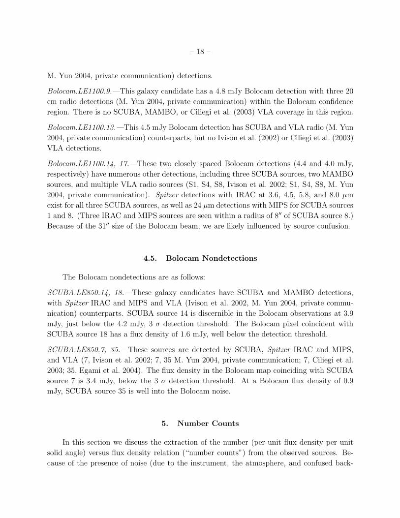
With these mechanics in place, the completeness was calculated by computing the ratio

of the number of detections at a given flux to the number of injected sources. This was

repeated for source flux densities ranging from 2.8 to 9.8 mJy for simulations from map

statistics and from 1.4 to 9.8 mJy for jittered data simulations in 0.7 mJy intervals, with

the results plotted in Figure 11. The two types of simulations agree well. The survey

completeness is 50% at the 3 σ detection threshold, as expected, because half of the sources

at the threshold will be bumped upward by noise and half will be bumped downward. The

simulations also agree with the theoretical prediction for Gaussian noise.

The bias was computed by determining the distribution of measured flux densities as

a function of injected flux densities. At relatively large flux densities, the bias distribution

should approach a Gaussian distribution centered at the injected flux density, with σ equal

to the map rms. This is seen to be the case in Figure 12 for injected flux densities ≥ 7

mJy. The figure gives the distribution of the expected observed flux densities (probability

density per flux bin, normalized to an integral of unity) for a range of injected flux densities.

For low injected flux densities approaching the detection threshold, the distributions become

increasingly asymmetric owing to the presence of the threshold. The distributions do not

drop abruptly to zero below the threshold because there are variations in the map coverage.

Note that sources with true flux below the detection threshold may be detected. The average

bias for a source is shown in Figure 12; this rises steeply for sources with fluxes near or below

the detection threshold.

The preceding discussion (in particular the agreement of the simulated bias and com-

pleteness with the Gaussian theoretical prediction) indicates that, in spite of coverage varia-

– 24 –

tions and correlated noise, the noise in this survey behaves substantially like uniform Gaus-

sian noise. Comparison of the results of the map simulation method with the jitter technique

also shows good agreement, indicating that the assumptions that went into the map simu-

lation method are justified and that we have a reasonable model for the survey noise. This

gives added confidence to the determination of the false detection rate, which depends only

on the noise properties.

5.4. Effects of Confusion Noise on the Bias and Completeness Functions

The completeness and bias function estimates as determined in §§ 5.2 and 5.3 do not in-

clude the effects of confusion noise. The effect of confusion noise is illustrated by considering

two extremes: instrument noise dominant over confusion noise and vice versa. When instru-

ment noise is dominant, the bias function for this survey is correctly described by equation

(5). In the confusion-dominated limit, the bias function takes on the shape of the source

count distribution, reflecting the fact that it is the underlying distribution of sources that

may bias the flux of a given source. In between these two extremes, the Gaussian bias func-

tion acquires additional width and a long positive tail from the source counts distribution.

This tail increases the probability that a low flux source will fluctuate above the detection

threshold. Consequently, the completeness at low flux densities is increased over the case

of Gaussian noise. Note that small changes in the bias tail can cause large changes in the

subthreshold completeness. The case at hand falls in this in-between regime. Understanding

the modification to the bias function by confusion noise is necessary for accurately estimating

how confusion transforms a model source count distribution to an observed one, as in equa-

tion (3). It is difficult to precisely model the effects of confusion on bias and completeness

because they depend on the source count distribution that one is trying to measure.

We can estimate the size of the confusion noise present in our maps by finding the

relative contributions of the noise and signal variances. The sample (per pixel) variance of

the optimally filtered Lockman map in the good coverage region is found to be 2.37 mJy2.

The variance of the optimally filtered jackknife maps in the same region is 1.81 mJy2, leav-

ing 0.56 mJy2 due to sources. The variance contributed by all the sources in Table 2 is

approximately 0.33 mJy2, of which 0.10 mJy2 is expected to be due to false detections of

random noise peaks. This leaves 0.33 mJy2 due to undetected sources. This represents an

S/N per pixel of 0.37 in rms units; considered in quadrature with the 1.81 mJy2 of the noise,

it increases the noise estimates and the rms of the bias function by about 9%.

To estimate the effect of confusion noise on the survey completeness and bias, particu-

larly in the tail, sources were injected one at a time into the real map and extracted using the

– 25 –

source extraction algorithm, with the completeness and bias calculated as in the noise-only

case. This has the effect of making only a small change in the observed distribution of pixel

values, effectively preserving that distribution. No effort was taken to avoid the positions of

source candidates, as this would bias the procedure by failing to take into account the tail of

the distribution. This test showed that the bias acquired a high flux density tail, as expected,

and the completeness was increased above its Gaussian noise value. It should be emphasized,

however, that this method provides an upper limit because it effectively “double-counts” con-

fusion: the map into which the sources are injected is already confused. Positions of high

flux in the true map may already consist of two coincident lower flux sources, and so the

probability of a third source lying on top of them is not truly as high as the probability we

would calculate by this procedure. The determination of the completeness and bias in this

way is also limited by the statistics of only having one realization of the confusion noise.

Applying these new bias and completeness functions, as well as the Gaussian noise-only bias

and completeness (eqs. [4] and [5]), to a power-law model of the number counts (the best-fit

model of § 5.5), the change in the observed counts is of order the size of the 68% confidence

interval for Poisson errors in the observed counts. Thus, confusion noise is not wholly negli-

gible nor does it dominate. In extracting the number counts, we ignore the confusion noise

but discuss how to treat it correctly in § 5.6.

5.5. Fitting a Model to the Differential Number Counts

To extract number counts from this data set, we use equation (3) with the simulation-

derived false detections and the completeness and bias of equations (4) and (5). A model

for N ′ is also required. Because of the small number of detections, the model must have

as few free parameters as possible so that the data will be able to constrain the model

parameters. This pushes us away from detailed, physically motivated models and toward

a simple model in combination with several, somewhat arbitrary, constraints. We use a

two-parameter power-law model for N ′ given by

N ′(S;p) = A

(

S0

S

)δ

, (7)

where p = [A, δ] and S0 is a fixed constant (not a parameter of the model). The choice

of this form for S0 6= 1 reduces the degeneracy between A and δ that prevails over narrow

ranges of S, such as in this survey. We have set S0 = 4 mJy.

The unaltered model of equation (7) is unsatisfactory at both high and low flux values.

At low fluxes, the model diverges, requiring a cutoff on which the result depends. The issue

of the low-flux cutoff is discussed further in § 5.6. For now, we simply impose a low-flux

– 26 –

cutoff Sl = 1 mJy in the integral over S in equation (3). In addition, if the model is extended

indefinitely to high fluxes, it may produce too many sources to be consistent with the lack

of observed sources. This constraint nevertheless does not determine the shape of number

counts above the highest flux observed. Thus, one must either implement a high-flux cutoff

or assume something about the shape of the number counts beyond the region where they

are measured. To address this, a single bin of the same width as the other bins has been

added to the data at high fluxes, where the data are zero and the model nonzero; beyond

Sh = 7.4 mJy, the model is zero. Fixing the upper cutoff as above and allowing the lower to

float to its best-fit value produces Sl = 1.3 mJy. Two additional possibilities were also tried

for a high-flux cutoff: (1) setting the model to zero beyond the highest filled bin resulted in

a very shallow index (δ < 2), and (2) allowing the highest bin to extend to infinity produced

a very steep power law (δ > 10). While both of these cases are unphysical, they illustrate

the sensitivity of the power-law model on the high-flux cutoff. Thus, the constraints that

have been adopted, while arbitrary, serve to restrict the range of possible models sufficiently

to extract reasonable values of [A, δ]. However, in light of this arbitrariness, the resulting

constraint on the parameters of the power-law model must be treated with skepticism.

To fit to the model, the data are first binned. The number of sources with observed

flux between sk and sk+1 is denoted by nk. We assume that the number of sources counted

in any interval ds follows an approximate Poisson process and therefore that each nk is a

Poisson-distributed random variable that is independent of nj for k 6= j. The same would

not be true of the cumulative counts, and so the differential counts are preferred for this

analysis. The likelihood of observing the data nk if the model is Nk is then

L =∏

k

Nnk

k exp [−Nk]

nk!(8)

because it is assumed that the bins are independent. The value of the model in a given

observed bin is defined as

Nk(p) =1

∆s

∫ sk+1

sk

(

F (s) +

∫

∞

0

B(s, S)C(S)N ′(S;p) dS

)

ds. (9)

The function − lnL is minimized with respect to p to find the maximum likelihood value of

p.

Two modifications of the likelihood equation (8) were made for this analysis. The first

is that a prior was applied to constrain δ > 2, so that both the integral of the number counts

and the integral of the total flux density remained finite for S > 0. Thus,

L′ = LΘ(δ − 2).

– 27 –

Second, to extract confidence regions for the fitted parameters, it was necessary to normalize

L′, such that

∫

L′(p) dp = 1.

This normalization was done by numerical evaluation of the likelihood and its integral over

the region where it is appreciably nonzero (see Fig. 14 below).

The various components of this fit are shown in Figure 13. The data are shown with 68%

confidence interval error bars, based on the observed number of sources in each bin, scaled

to an area of a square degree. The error bars were computed according to the prescription of

Feldman & Cousins (1998) for small number Poisson statistics (which unifies the treatment

of upper confidence limits and two-sided confidence intervals). The error bar on the highest

flux density bin is an upper limit. The model is clearly consistent with the data given

the error bars. (All six model bins falling within the 68% confidence interval error bars

of the data may imply that the errors have been overestimated, although this has a 10%

probability of occurring.) Examining the fit in stages, one finds that the product of the

survey completeness and the best-fit number counts shows that the survey incompleteness

reduces the number of sources observed at low flux densities as expected; above ∼7 mJy, the

survey is essentially complete. The effect of the bias, however, combined with the steepness

of the number counts, increases the number of sources observed in all bins substantially

above that of the underlying source distribution and contributes to the observed number of

sources in all bins. In fact, based on the best-fit DNC and computing over the range of fluxes

observed, 67% of real sources will have a true flux density below the detection threshold. Note

that the best-fit number counts lie below the Poisson errors for the raw counts, demonstrating

again that the survey bias is a nonnegligible effect. Given the maximum likelihood values of

A and δ (52.0 and 3.16, respectively), the cumulative source count at S1.1mm > 2.75 mJy is

192+108−88 deg−2. This is consistent with the 1.2 mm MAMBO number count result (378+136

−113

deg−2) for the combined Lockman Hole and European Large-Area ISO Survey (ELAIS) N2

regions (Greve at al. 2004).

Contours of the likelihood function for this fit are shown in Figure 14. In calculating

the likelihood, the upper and lower flux limits were assumed to be a correct model, and as

such, the likelihood does not account for violations of this assumption. The shaded region

was obtained by integrating the normalized likelihood L′ for values L′ > Lthresh, such that

the integral was equal to 0.68. These are Bayesian errors that incorporate the prior belief

that δ > 2.

– 28 –

5.6. Difficulties and Caveats

As the above discussion indicates, the extraction of number counts from this data set

is subject to a number of difficulties and caveats. In addition to the small-number statistics

and the difficulty in modeling the dependence of the survey bias and completeness on the

confusion noise that have already been discussed, a separate discussion of the principal

limitations of the preceding analysis is in order. These are the low S/N of the detections and

the sensitivity of the result to the lowest flux objects assumed to contribute to the observed

counts. These limitations may be overcome with a more sophisticated future analysis, as we

discuss.

The survey bias, combined with an underlying number counts distribution rising at

low fluxes, has a strong effect on the fluxes of sources observed at low S/N. This problem

is exacerbated in the presence of confusion noise, but it is present in surveys in which

random noise dominates over the confusion noise as well. This point has been appreciated

in the historical confusion literature. Crawford et al. (1970) showed how to use a maximum

likelihood method to extract a power-law slope from observed flux densities, and Murdoch

et al. (1973) extended this to the case of sources observed with Gaussian noise. Because

of the divergence at low fluxes of a power law, a lower limit in flux must be imposed in

order to obtain finite answers. The principal conclusion of Murdoch et al. (1973) was that

the power-law slope of the number counts determined by the maximum likelihood method

depends sensitively on this lower cutoff if the S/N of the sources used in the survey is less

than 5, whereas above this point the slope determination, while biased, is not dependent on

the lower cutoff. This sensitivity to the lower flux cutoff also applies to the amplitude of

the power law as well, a point that is clearly described by Marshall (1985). Although the

Murdoch et al. (1973) result is for the rather unphysical case of a power law with an abrupt

cutoff, the general result that derived number counts based on low-S/N sources will depend

sensitively on the assumed behavior of the underlying number counts far below threshold is

more general. This may be seen by considering the behavior of C(S)N ′ as S → 0. As long

as this function is increasing, the bias will continue to push some sources of low intrinsic

flux up above the detection threshold, and so the low-S/N regime will contain sources from

well below threshold. [Note that this is consistent with the behavior of B(s, S), since for s

greater than threshold, B is positive for all values of S.] One can see from Figure 11 that the

completeness drops off rather slowly for Gaussian noise (and even more slowly when confusion

noise is added) and never vanishes. In fact, the product of the Gaussian completeness times

any S−δ, δ > 0, diverges as S → 0, so for many otherwise reasonable number counts models,

this problem will occur. Thus, in the presence of any sort of bias, whether due to confusion or

noise, deriving accurate counts above threshold requires a nontrivial amount of information

about the counts well below threshold if the S/N of the detections is low. Since all of our

– 29 –

sources have S/N ≤ 5, any constraint placed on the power-law amplitude and slope will

likely depend sensitively on the lower cutoff chosen.

An analysis technique that overcomes all of the shortcomings mentioned above is the

so-called fluctuation or “P (D)” analysis (Scheuer 1957, 1974; Condon 1974). This analysis

matches the shape of the observed pixel value distribution (Fig. 6) against the prediction for

a model distribution combined with the instrument noise. It overcomes the small-number

statistics by using the full map instead of only the above-threshold detections. It addresses

the nonlinear aspects of equation (3) by directly including the confusion noise. Low S/N

is no longer an issue, since individual sources are no longer considered, and the lowest flux

considered is naturally at the confusion limit where additional sources contribute only a mean

to the observed histogram. The unchopped scan strategy of the Lockman Hole data simplifies

such an analysis because of the simplicity of the effective beam. Additional effects such as

the attenuation of large angular scale structure by the atmospheric cleaning or the angular

correlation of sources may also be straightforwardly included. A paper on this analysis is in

preparation.

6. Discussion

6.1. Comparison with Previous Number Count Results

A number of other groups have previously published number counts of submillimeter

galaxies. Figure 15 shows selected recent results. These include surveys of blank-fields

by SCUBA on the JCMT at 850 µm (Barger et al. 1999; Borys et al. 2003; Scott et al.

2002), observations of galaxies lensed by clusters, also using SCUBA at 850 µm (Blain et al.

1999; Chapman et al. 2002; Cowie et al. 2002; Smail et al. 2002), and blank-field surveys

by MAMBO on the IRAM telescope (Greve et al. 2004). The Bolocam result is plotted as

the maximum likelihood cumulative number counts (computed from the DNC described in

§ 5.5), evaluated from 1 mJy to the maximum observed flux density (6.8 mJy). The number

counts in the figure are not adjusted for the wavelength differences of the surveys.

The Bolocam result is in broad agreement with previous measurements; the maximum

likelihood cumulative number counts are consistent with the 1200 µm measurement and

below the 850 µm measurements, as expected if the same population of objects is being

measured. The region of 68% probability in parameter space has been translated to cumula-

tive number counts and is shown by the region between the dashed curves. This region does

not correspond to the naive expectation of Poisson errors based on the number of detected

sources. This is due to both the strong effect of the bias and the flux cutoffs imposed on

– 30 –

the model. Because of the bias, it is inappropriate to assume that the number of observed

sources in a bin can be used as a measure of the uncertainty in the underlying number counts

in that bin. The effect of assuming an upper flux cutoff is particularly evident in the figure

in the rapid drop of the cumulative counts as the cutoff is approached. This causes the

error bars to be artificially small, as any model is constrained to be zero beyond this point.

The maximum likelihood number count model presented here, as well as its errors, depends

strongly on the exact low- and high-flux cutoffs assumed for the underlying distribution and

consequently cannot be treated as definitive.

In addition to the caveats above, it should be borne in mind that the uncertainty of

the flux bias discussed in § 3.4 (derived from the rms pointing error between the Bolocam

galaxy candidates and coincident radio sources) introduces a systematic shift in the simple

model of equation (7): the parameter A changes by an amount (1 ± σǫ/ǫ)−δ. This gives a

steep dependence of the amplitude of the number counts on the calibration error and the

presumed power-law index.

At high flux densities, where the survey is nearly complete and the effect of the bias

is smallest, model-independent constraints may be obtained. In particular, the lack of any

observed sources with flux density greater than 8 mJy has been used to place a 90% upper

confidence limit on the cumulative number counts above 8 mJy; this is shown by the dashed

horizontal line in the figure. This constraint depends only linearly on the calibration error.

Bolocam appears to be measuring near the region where the number counts, based on both

the 850 and 1200 µm measurements, would be expected to turn over, but because of the

limited survey area, we do not strongly constrain the number counts at the bright end of the

luminosity function.

6.2. Integrated Flux Density

The fraction of the FIRAS integrated far-infrared background light (Fixsen et al. 1998)

measured by this survey can be computed in several ways. Summing the flux densities of

all observed sources gives 85 mJy, or 3.9% of the FIRAS background over the survey area

at 1.1 mm (8.0 × 10−22 W m−2 sr−1 Hz−1). Subtracting out the expected mean flux of

false detections gives 58 mJy, or 2.7% of the FIRAS background. Integrating the maximum

likelihood DNC between 1 and 6.8 mJy (the maximum observed) gives 276 mJy, or ∼ 13% of

the FIRAS background. Since it seems plausible that the number counts do in fact steepen

beyond the upper range of our observations, we conclude that at least ∼95% of the light from

submillimeter sources lies below the detection threshold of this survey and ∼ 87% below the

minimum flux derived from our number counts model.

– 31 –

6.3. Implied Luminosities and Star Formation Rates

The flux density of a galaxy at an observed frequency, ν, is related to its intrinsic

luminosity, L, by (Blain et al. 2002)

Sν =1 + z

4πD2L

Lfν(1+z)

∫

fν′ dν ′, (10)

where DL is the luminosity distance to redshift z, fν(1+z) is the redshifted SED of the galaxy,

and∫

fν′ dν ′ is the integrated rest SED. For a flat (Ωk = 0) cosmology, it can be shown (e.g.,

Peebles 1993) that the luminosity distance is given by

DL =c (1 + z)

H0

∫ z

0

1

ΩM(1 + z′)3 + ΩΛ

dz′.

To estimate the bolometric luminosities of the submillimeter galaxies detected by Bolo-

cam, a template SED was constructed that assumes a blackbody emission spectrum modified

by a dust emissivity term:

fν ∝ ǫνBν(T ) ∝ [1 − exp (−τν)]Bν(T ), (11)

where Bν(T ) is the Planck function evaluated at dust temperature, T , and frequency, ν, and

τν is the optical depth of the dust:

τν =

(

ν

ν0

)β

.

The dust emissivity index, β, is believed to lie between 1 and 2 (Dunne et al. 2000).

The form of equation (11) is commonly assumed in the literature for dusty nearby galaxies

and high-redshift AGNs, including Benford et al. (1999), Omont et al. (2001), Priddey &

McMahon (2001), and Isaac et al. (2002). This equation reduces to a simple optically

thin emission spectrum, ǫνBν(T ) ∼ ν2+β , in the Rayleigh-Jeans limit and ν ≪ ν0, and

it asymptotes to Bν(T ) at high frequencies (because an emissivity of > 1 is unphysical).

Observations of luminous low-redshift galaxies (Arp 220 and Mrk 231) and high-redshift

galaxies detected by deep submillimeter surveys furthermore suggest that a power law, fν ∝να, is appropriate to model the hotter components of dust on the Wien side of the spectrum

(Blain et al. 1999). We implement such a power law at high frequencies, matched to equation

(11) at 1.2ν0.

Creating a composite SED of nearby dusty IRAS galaxies, high-redshift submillimeter

galaxies, gravitationally lensed high-redshift galaxies, and high-redshift AGNs (Blain et al.

– 32 –

2002, and references therein), we find that parameters of T = 40 K, ν0 = 3700 GHz, β = 1.6,

and α = -1.7 provide a reasonable fit. Assuming a cosmology of Ωλ = 0.7, ΩM = 0.3, and

h0 = 0.73 and a galaxy redshift of z = 2.4 (the median redshift that Chapman et al. [2003b]

derive for their sample of 10 submillimeter galaxies identified using high-resolution radio

observations), equation (10) gives extreme bolometric luminosities of L = (1.0−1.6)×1013 L⊙

for the range of flux densities detected by Bolocam. The derived luminosities are insensitive

to redshift, varying by less than 25% for 0.6 < z < 12. Assuming dust temperatures of 30

and 50 K implies luminosities of (3.5−5.9)×1012 L⊙ and (1.8−3.0)×1013 L⊙, respectively.

If these galaxies are lensed, their intrinsic luminosities will be lower.

Observations of nearby star-forming galaxies suggest the following relation between the

SFR present in a galaxy and its far-infrared luminosity:

SFR = ǫ × 10−10L60µm

L⊙

M⊙yr−1,

where L60µm is the 60 µm luminosity. The value of ǫ varies in the literature from 2.1

to 6.5 (Scoville & Young 1983; Thronson & Telesco 1986; Rowan-Robinson et al. 1997)

because of different assumptions about the duration of the starburst, different initial mass

functions (IMFs), and lower mass limits. In this paper we adopt a value of ǫ = 2.1 from

a ”cirrus” model that combines very small grains and polycyclic aromatic hydrocarbons

(PAHs) with a Salpeter IMF in a starburst of OBA stars over 2 × 106 yr (Thronson &

Telesco 1986). Obtaining L60µm from our model SED yields large SFRs of 480−810 M⊙yr−1.

While these calculated luminosities and SFRs are sensitive to the SED model parameters,

particularly T and β, most recent models of local star-forming galaxies nevertheless result in

dust temperatures and emissivities that imply extreme luminosities and SFRs. It is possible,

however, that these extremely luminous galaxies derive some of their power from AGNs (e.g.,

Alexander et al. 2003), in which case the SFRs have been overestimated. Observations of

ultraluminous infrared galaxies (ULIRGs) in the local universe (z . 0.1) with luminosities

> 1013 L⊙ show that nearly all of these galaxies possess luminous AGNs and that the

dominant power source in the majority of nearby ULIRGs may be AGNs rather than star

formation (Sanders 1999). Recent X-ray observations and optical spectroscopic data of

z > 1 ultraluminous galaxies, however, indicate that in almost all cases the AGNs account

for < 20% of the total bolometric output of higher-redshift galaxies (Alexander et al. 2004).

Spitzer observations will prove useful in investigating the incidence of AGNs versus star

formation in submillimeter galaxies from the shape of the mid-infrared continuum emission;

initial results confirm the high-redshift X-ray results and show a mixture of infrared-warm

AGNs and cooler starburst-dominated sources (Egami et al. 2004; Frayer et al. 2004), with

a smaller fraction (∼25%) of energetically important AGNs (Ivison et al. 2004).

– 33 –

7. Future Work

Observations at shorter submillimeter wavelengths are vital to both confirm the Bolo-

cam galaxy candidate detections and make photometric redshift and temperature estimates.

Follow-up 350 µm photometry of the Bolocam-detected submillimeter galaxies with SHARC-

II is planned to fill in the SEDs of these galaxies. Precise astrometry afforded by the radio

identifications (as well as the 10′′ beam size of SHARC-II) will allow optical and infrared

counterparts to be identified. Furthermore, Spitzer far-infrared observations combined with

the Bolocam 1.1 mm galaxy survey will provide a flux density ratio that is strongly dependent

on redshift for a given temperature. This is because the rest wavelength corresponding to

the observed Spitzer wavelength of 70 µm is on the rapidly falling Wien side of the greybody

spectrum (for a z ∼ 2 galaxy at 40 K), and Bolocam’s 1.1 mm observations are on the steep

ν2+β (β ≈1.5) modified Rayleigh-Jeans side of the SED. The ratio of S1.1mm/S70µm is thus

highly dependent on redshift, growing by a factor of 250 from z = 1 to 5. Spitzer IRAC ob-

servations will also provide independent photometric redshift determinations from the SEDs

of stellar populations of submillimeter galaxies redshifted into the near-IR. These combined

observations, in conjunction with the radio-to-far-infrared correlation (Yun & Carilli 2002),

will thus allow the temperature and redshift distributions of these submillimeter galaxies to

be constrained. A detailed discussion of the SEDs and photometric redshift/temperature

estimates of the Lockman Hole galaxies will follow in a companion paper (in preparation).

As discussed in § 6.1, this survey does not constrain the number counts at flux densities

above 7 mJy, at approximately the break point where the number counts are expected to

drop sharply (based on the 850 µm observations in Fig. 15). This can be addressed with

a survey covering a larger area to shallower depth. Such a survey has been started with

Bolocam in the COSMOS field,7 which currently covers ∼ 1000 arcmin2. This survey should

allow either determination or a strong upper limit on the 1.1 mm number counts beyond

7 mJy, as well as uncover extremely bright, interesting sources, perhaps with strong AGN

components that should be easy to follow up at other wavelengths. In addition to the

wide area, the COSMOS observations have extremely uniform coverage (<3% rms) and a

highly cross linked scan strategy that aids in rejecting atmospheric 1/f noise better than

the Lockman Hole observations.

7See http://www.astro.caltech.edu/cosmos.

– 34 –

8. Conclusions

Bolocam is a new bolometer camera with a large field of view and a rapid mapping

speed optimized for surveys, including surveys for rare, bright submillimeter galaxies. We

have used Bolocam on the Caltech Submillimeter Observatory at a wavelength of 1.1 mm

to conduct a survey of 324 arcmin2 toward the Lockman Hole for submillimeter galaxies.

Unlike previous submillimeter surveys, the observations were made without chopping, at a

fast scan rate of 60′′ s−1. The Bolocam survey encompasses the entire 850 µm 8 mJy JCMT

SCUBA and 1.2 mm IRAM MAMBO surveys to a comparable depth under the assumption

of a model SED for a galaxy at z = 2.4, with relative rms of 1 : 0.9 : 0.6−1.4, respectively. We

have reduced the resulting data set using a custom IDL-based software pipeline, in which

correlated atmospheric and instrument noise is rigorously removed via a PCA sky subtraction

technique. We detect 17 galaxies at a significance of ≥ 3 σ, where the map rms is ∼1.4 mJy.

A series of simulations have allowed us to verify the robustness of the galaxy candidates.

Extensive jackknife and pointing jitter tests reveal that the sources detected in this survey

have a small characteristic length scale (point sources) and are contributed to by the ensemble

of observations, strongly indicating that the galaxy candidates are real. Simulations of

the observations using both synthetic maps and observational data indicate that six false

detections should be expected.

Comparing our detections to those of other surveys (including SCUBA 850 µm, MAMBO

1.2 mm, and VLA radio observations) indicates that the majority of Bolocam sources have

coincident detections in at least two other wavebands; we conclude that a majority of the

Bolocam detections are real. Six of the detections are galaxies previously detected by the

SCUBA 8 mJy survey. Of the remaining 11 Bolocam detections, 9 of them lie outside

the SCUBA survey region, and we cannot search for counterparts for them. Seven of the

17 Bolocam detections have been detected by the MAMBO 1.2 mm survey, with 6 of the

remaining 10 sources lying outside the MAMBO good coverage region. While both the

SCUBA and MAMBO surveys detect most of the Bolocam sources in the overlap region,

neither Bolocam nor SCUBA/MAMBO detect the majority of the remaining SCUBA and

MAMBO sources. A total of 65% of the 17 Bolocam source candidates have at least one radio

coincidence, although the accidental radio detection rate is high (34%) owing to the size (31′′

FWHM) of the Bolocam beam. Furthermore, we statistically detect the aggregate average

of the SCUBA and MAMBO sources below our 3 σ detection threshold at significances of

3.3 and 4.0 σ, respectively.

Further simulations enabled us to estimate the completeness and bias of this survey,

which were subsequently used with the false detection rate to fit a simple power-law model

of the underlying parent distribution to match the observed number count distribution. This

– 35 –

model constrains the submillimeter counts over the flux density range S1.1mm = 1−7 mJy.

While the validity of this model is significantly limited by both the effects of confusion noise

and the flux density cutoffs assumed for the underlying number count distribution, we find

this modeled number count distribution to be consistent with previously published sub-

millimeter galaxy number counts. Integrating the maximum likelihood differential number

counts distribution between 1 and 6.8 mJy (the maximum observed flux density) yields 276

mJy in the map, or ∼13% of the FIRAS integrated far-infrared background light.

If the Bolocam galaxy candidates lie at redshifts z > 1, then their inferred luminosities

are L = (1.0 − 1.6) × 1013 L⊙ (assuming a dust temperature of 40 K). Further assuming

that they are powered by star formation, large SFRs of 480 − 810 M⊙yr−1 are implied.

Multiwavelength follow-up observations of the Lockman Hole field are underway with Spitzer

and SHARC-II in order to constrain the temperature/redshift distributions of these sources.

With alacrity, we acknowledge the support of the CSO director and staff, the support

of Kathy Deniston, and helpful conversations with Andrew Blain, Steven Eales, and Min

Yun. This work was supported in part by NSF grants AST-0098737, AST-9980846, and

AST-0206158 and PPARC grants PPA/Y/S/2000/00101 and PPA/G/O/2002/00015. D. H.

acknowledges the support of a PPARC Ph.D. Fellowship, S. R. G. acknowledges Caltech

for the R. A. Millikan Fellowship, and G. T. L. acknowledges NASA for GSRP Fellowship

NGT5-50384.

– 36 –

REFERENCES

Alexander, D. M., Bauer, F. E., Chapman, S. C., Smail, I., Blain, A. W., Brandt, W. N., &

Ivison, R. J. 2004, preprint (astro-ph/0401129)

Alexander, D. M., Bauer, F. E., Brandt, W. N., Hornschemeier, A. E., Vignali, C., Garmire,

G. P., Schneider, D. P., Chartas, G., & Gallagher, S. C. 2003, AJ, 125, 383

Almaini, O., Scott, S. E., Dunlop, J. S., Manners, J. C., Willott, C. J., Lawrence, A., Ivison,

R. J., Johnson, O., Blain, A. W., Peacock, J. A., Oliver, S. J., Fox, M. J., Mann,

R. G., Perez-Fournon, I., Gonzalez-Solares, E., Rowan-Robinson, M., Serjeant, S.,

Cabrera-Guerra, F., & Hughes, D. H. 2003, MNRAS, 338, 303

Aretxaga, I., Hughes, D. H., Chapin, E. L., Gaztanaga, E., Dunlop, J. S., & Ivison, R. J.

2003, MNRAS, 342, 759

Barger, A. J., Cowie, L. L., & Sanders, D. B. 1999, ApJ, 518, L5

Benford, D. J., Cox, P., Omont, A., Phillips, T. G., & McMahon, R. G. 1999, ApJ, 518, L65

Bertoldi, F., Carilli, C. L., Menten, K. M., Owen, F., Dey, A., Gueth, F., Graham, J. R.,

Kreysa, E., Ledlow, M., Liu M. C., Motte, F., Reichertz, L., Schilke, P., & Zylka, R.

2000, A&A, 360, 92

Blain, A. W., Chapman, S. C., Smail, I., & Ivison, R. 2004, ApJ, 611, 725

Blain, A. W., Kneib, J.-P., Ivison, R. J., & Smail, I. 1999, ApJ, 512, L87

Blain, A., Smail, I., Ivison, R. J., Kneib, J.-P., & Frayer, D. T. 2002, Phys. Rept.369, 111

Borys, C., Chapman, S., Halpern, M., & Scott, D. 2003, MNRAS, 344, 385

Carilli, C. L., & Yun, M. S. 1999, ApJ, 513, L13

Chapman, S. C., Blain, A., Ivison, R., & Smail, I. 2003a, in ASP Conf. Ser. 297, Star

Formation through Time, ed. E. Perez, R. M. Gonzales Delgado, & G. Tenorio-Tagle

(San Francisco: ASP), 289

Chapman, S. C., Blain, A. W., Ivison, R. J., & Smail, I. R. 2003b, Nature, 422, 695

Chapman, S. C., Blain, A. W., Smail, I., & Ivison, R. J. 2005, ApJ, in press (astro-

ph/0412573)

Chapman, S. C., Scott, D., Borys, C., & Fahlman, G. G. 2002, MNRAS, 330, 92

– 37 –

Ciliegi, P., Zamorani, G., Hasinger, G., Lehmann, I., Szokoly, G., & Wilson, G. 2003, A&A,

398, 901

Condon, J. J. 1974, ApJ, 188, 729

Cowie, L. L., Barger, A. J., & Kneib, J.-P. 2002, AJ, 123, 2197

Crawford, D. F., Jauncey, D. L., & Murdoch, H. S. 1970, ApJ, 162, 405

Dunne, L., Eales, S., Edmunds, M., Ivison, R, Alexander, P., & Clements, D. L. 2000,

MNRAS, 315, 115

Eales, S., Bertoldi, F., Ivison, R., Carilli, C., Dunne, L., & Owen, F. 2003, MNRAS, 344,

169

Eddington, A. S. 1913, MNRAS, 73, 359

Eddington, A. S. 1940, MNRAS, 100, 354

Egami, E., Dole, H., Huang, J.-S., Perez-Gonzalez, P., Floc’h, E. Le, Papovich, C., Barmby,

P., Ivison, R. J., Serjeant, S., Mortier, A., Frayer, D. T., Rigopoulou, D., Lagache, G.,

Rieke, G. H., Willner, S. P., Alonso-Herrero, A., Bai L., Engelbracht, C. W., Fazio,

G. G., Gordon, K. D., Hines, D. C., Misselt, K. A., Miyazaki, S., Morrison, J. E.,

Rieke, M. J., Rigby, J. R., & Wilson, G. 2004, ApJ, 154, 130

Feldman, G. J., & Cousins, R. D. 1998, Phys. Rev. D, 57, 3873

Fixsen, D. J., Dwek, E., Mather, J. C., Bennett, C. L., & Shafer, R. A. 1998, ApJ, 508, 123

Fox, M. J., Efstathiou, A., Rowan-Robinson, M., Dunlop, J. S., Scott, S., Serjeant, S., Mann,

R. G., Oliver, S., Ivison, R. J., Blain, A., Almaini, O., Hughes, D., Wilcott, C. J.,

Longair, M., Lawrence, A., & Peacock, J. A. 2002, MNRAS, 331, 839

Frayer, D. T., Ivison, R. J., Scoville, N. Z., Yun, M., Evans, A. S., Smail, I., Blain, A. W.,

& Kneib, J.-P. 1998, ApJ, 506, L7

Frayer, D. T., Ivison, R. J., Scoville, N. Z., Evans, A. S., Yun, M. S., Smail, I., Barger, A. J.,

Blain, A. W., & Kneib, J.-P. 1999, ApJ, 514, L13

Frayer, D. T., Chapman, S. C., Yan, L., Armus, L., Helou, G., Fadda, D., Morganti, R.,

Garrett, M. A., Appleton, P., Choi, P., Fang, F., Heinrichsen, I., Im, M., Lacy,

M., Marleau, F., Amsci, F. J., Shupe, D. L., Soifer, B. T., Squires, G. K., Storrie-

Lombardi, L. J., Surace, J. A., Teplitz, H. I., & Wilson, G. 2004, ApJS, 154, 137

– 38 –

Glenn, J., Bock, J. J., Chattopadhyay, G., Edgington, S. F., Lange, A. E., Zmuidzinas, J.,

Mauskopf, P. D., Rownd, B., Yuen, L., & Ade, P. A. R. 1998, in Proc. of the SPIE,

Advanced Technology MMW, Radio, and Terahertz Telescopes, ed. T.G. Phillips,

3357, 326

Glenn, J., Chattopadhyay, G., Edgington, S. F., Lange, A. E., Bock, J. J., Mauskopf, P. D.,

& Lee, A. T. 2002, Appl. Opt., 41, 136

Glenn, J., Ade, P. A. R., Amarie, M., Bock, J. J., Edgington, S. F., Goldin, A., Golwala,

S., Haig, D., Lange, A. E., Laurent, G., Mauskopf, P. D., Yun, M., & Nguyen, H.

2003, in Proc. of the SPIE, Millimeter and Submillimeter Detectors for Astronomy,

eds. T.G. Phillips & J. Zmuidzinas, 4855, 30

Greve, T. R., Ivison, R. J., Bertoldi, F., Stevens, J. A., Dunlop, J. S., Lutz, D., & Carilli,

C. L. 2004, MNRAS, 354, 779

Haig, D. J., Ade, P. A. R., Aguirre, J. E., Bock, J. J., Enoch, M. L., Glenn, J., Goldin, A.,

Golwala, S., Laurent, G. T., Maloney, P. R., Mauskopf, P. D., Rossinot, P., Sayers,

J., & Stover, P. 2004, Proc. SPIE, 5498, 78

Hasinger, G., Altieri, B., Arnaud, M., Barcons, X., Bergeron, J., Brunner, H., Dadina, M.,

Dennerl, K., Ferrando, P., Finoguenov, A., Griffiths, R. E., Hashimoto, Y., Jansen,

F. A., Lumb, D. H., Mason, F. O., Mateos, S., McMahon, R. G., Miyaji, T., Paerels,

F., Page, M. J., Ptak, A. F., Sasseen, T. P., Schartel, N., Szokoly, G. P., Trumper,

J., Turner, M., Warwick, R. S., & Watson, M. G. 2001, A&A, 365, L45

Hauser, M. G., Arendt, R. G., Kelsall, T., Dwek, E., Odegard, N., Weiland, J. L., Freuden-

reich, H. T., Reach, W. T., Silverberg, R. F., Moseley, S. H., Pei, Y. C., Lubin, P.,

Mather, J. C., Shafer, R. A., Smoot, G. F., Weiss, R., Wilkinson, D. T., & Wright,

E. L. 1998, ApJ, 508, 25

Holland, W. S., Robson, E. I., Gear, W. K., Cunningham, C. R., Lightfoot, J. F., Jenness,

T., Ivison, R. J., Stevens, J. A., Ade, P. A. R., Griffin, M. J., Duncan, W. D., Murphy,

J. A., & Naylor, D. A. 1999, MNRAS, 303, 659

Isaak, K. G., Priddey, R. S., McMahon, R. G., Omont, A., Peroux, C., Sharp, R. G., &

Withington, S. 2002, MNRAS, 329, 149

Ivison, R. J., Greve, T. R., Smail, I., Dunlop, J. S., Roche, N. D., Scott, S. E., Page, M. J.,

Stevens, J. A., Almaini, O., Blain, A. W., Wilcott, C. J., Fox, M. J., Gilbank, D. G.,

Serjeant, S., & Hughes, D. H. 2002, MNRAS, 337, 1

– 39 –

Ivison, R. J., Greve, T. R., Serjeant, S., Bertoldi, F., Egami, E., Mortier, A. M. J., Alonzo-

Herrero, A., Barmby, P., Bei, L., Dole, H., Engelbracht, C. W., Fazio, G. G., Frayer,

D. T., Gordon, K. D., Hines, D. C., Huang, J.-S., Le Floc’h, E., Misselt, K. A.,

Miyazaki, S., Morrison, J. E., Papovich, C., Perez-Gonzalez, P. G., Rieke, M. R.,

Rieke, G. H., Rigby, J., Rigopoulou D., Smail, I., Wilson, G., & Willner, S. P. 2004,

ApJS, 154, 124

Jahoda, K., Lockman, F. J., & McCammon, D. 1990, ApJ, 354, 184

Jenness, T., Stevens, J. A., Archibald, E. N., Economou, F., Jessop, N. E. & Robson, E. I.

2002, MNRAS, 336, 14

Marshall, H. L. 1985, ApJ, 289, 457

Murdoch, H. S., Crawford, D. F., & Jauncey, D. L. 1973, ApJ, 183, 1

Murtagh, F. & Heck, A. 1987 Multivariate Data Analysis, Kluwer Academic Publishers,

Boston

Neri, R., Genzel, R., Ivison, R. J., Bertoldi, F., Blain, A. W., Chapman, S. C., Cox, P.,

Greve, T. R., Omont, A., & Frayer, D. T. 2003, ApJ, 597, L113

Omont, A., Cox, P., Bertoldi, F., McMahon, R. G., Carilli, C., & Isaak, K. G. 2001, A&A,

374, 371

Peebles, P.J.E., 1993 Principles of Physical Cosmology, Princeton University Press, New

Jersey

Priddey, R. S., & McMahon, R. G. 2001, MNRAS, 324, L17

Puget, J.-L., Abergel, A., Bernard, J.-P., Boulanger, F., Burton, W. B., Desert, F.-X., &

Hartmann, D. 1996, A&A, 308, L5

Rodighiero, G., & Franceschini, A. 2004, A&A, 419, L55

Rowan-Robinson, M., Mann, R. G., Oliver, S. J., Efstathiou, A., Eaton, N., Goldschmidt, P.,

Mobasher, B., Serjeant, S. B. G., Sumner, T. J., Danese, L., Elbaz, D., Franceschini,

A., Egami, E., Knotizas, M., Lawrence, A., McMahon, R., Norgaard-Nielsen, H. U.,

Perez-Fournon, I., & Gonzalez-Serrano, J. I. 1997, MNRAS, 289, 490

Sandell, G. 1994, MNRAS, 271, 75

Sanders, D. B. 1999, Ap&SS, 266, 331

– 40 –

Scheuer, P. A. G. 1957, Proc. Cambridge Philos. Soc., 53, 764

Scheuer, P. A. G. 1974, MNRAS, 166, 329

Scott, S. E., Fox, M. J., Dunlop, J. S., Serjeant, S., Peacock, J. A., Ivison, R. J., Oliver,

S., Mann, R. G., Lawrence, A., Efstathiou, A., Rowan-Robinson, M., Hughes, D. H.,

Archibald, E. N., Blain, A., & Longair, M. 2002, MNRAS, 331, 817

Scoville, N. Z., & Young, J. S. 1983, ApJ, 265, 148

Sheth, K., Blain, A. W., Kneib, J., Frayer, D. T., van der Werf, P. P., & Knudsen, K. K.

2004, ApJ, 614, L5

Smail, I., Ivison, R. J., Blain, A. W., & Kneib, J.-P. 2002, MNRAS, 331, 495

Swinbank, A. M., Smail, I., Chapman, S. C., Blain, A. W., Ivison, R.J., & Keel, W. C. 2004,

ApJ, 617, 64

Thronson, H., & Telesco, C. 1986, ApJ, 311, 98

Yun, M. S., & Carilli, C. L. 2002, ApJ, 568, 88

This preprint was prepared with the AAS LATEX macros v5.2.

– 41 –

Fig. 1.— Coverage map of the Lockman Hole East, pixelized at 10′′ resolution. White

corresponds to the highest level of coverage and black to the lowest level of coverage; the

contours are 193, 257, 322, 386, 450, 515, and 579 s of integration time per pixel. The

“uniform coverage region” corresponds to the thick contour at 450 s pixel−1.

– 42 –

Fig. 2.— Source attenuation by PCA cleaning as a function of injected flux density (left)

and histogram with Gaussian fit (right). Sources were injected into the raw time streams,

which were then cleaned using the PCA. The resulting source amplitudes were compared to

the injected source amplitudes (their ratio is the fractional reduction in source flux density).

The attenuation of sources by PCA is 19% with a dispersion of 4%, independent of flux

density from 0.1 mJy to 1 Jy.

– 43 –

Fig. 3.— Cross-correlation of the 2003 January and May Lockman Hole maps, pixelized at

10′′ resolution. While the weather was too poor during the 2003 May observations to yield

any > 3 σ detections, the local pointing near the Lockman Hole was sampled substantially

better than for the 2003 January run. The 25′′ pointing offset corresponding to the peak in

the cross-correlation map was subsequently applied to the 2003 January data.

– 44 –

Fig. 4.— Calibration in nV Jy−1 (nV at the bolometer) as a function of the demodulated

lock-in voltage at the AC bias frequency, which is approximately inversely proportional to

the bolometer loading. The quadratic fit is a minimization of the fractional error between

observed and expected flux densities. The rms of the residual dispersion in flux density is

9.7%.

– 45 –

Fig. 5.— Bolocam map of the Lockman Hole East. The field is centered on R.A. =

10h52m08s.82, decl. = +5721′33′′.80 (J2000.0). The map pixels are 10′′×10′′ and the map

rms is 1.4 mJy. The uniform, high-coverage region of the map is the inner 324 arcmin2.

This map has been cleaned and optimally filtered for point sources. The 17 Bolocam sources

detected at > 3 σ are indicated by thick circles. The bright spot at +8’, -8’ is not listed as

a detection because it falls outside of the uniform coverage region (black contour).

– 46 –

Fig. 6.— Histogram of the pixel sensitivities, defined as the pixel flux density, Sν , times the

integration time per pixel, t1/2int . The solid line is a Gaussian fit to the jackknifed histogram

of Fig. 7. The shaded area indicates the emission due to galaxy candidates in excess of that

expected from map noise. The negative side of the histogram is slightly broader than the fit

to the jackknifed histogram owing to the presence of the galaxies (confusion noise) on both

the positive and negative side. The small negative offset of the peak of the distribution is

expected, as the mean of the entire map (and therefore the histogram) is constrained to have

mean zero from both the high-pass filter in the Bolocam electronics and sky subtraction.

– 47 –

Fig. 7.— Jackknife histogram. In the jackknife test, 50% of the observations were randomly

chosen and co-added together, while the remaining 50% of the observations were co-added

into a second map. The two maps were then differenced. This was repeated 21 times with the

observations randomly selected independently each time, and the histograms were averaged.

The thick solid line corresponds to a Gaussian fit to the jackknifed histogram. The shaded

region indicates the positive excess, which is insignificant.

– 48 –

Fig. 8.— Left: Pointing-jittered histogram. In the pointing jitter test, individual maps

were made from each observation, then co-added with 60′′ amplitude offsets with random

directions (phases). The solid line is a Gaussian fit to the negative side of the histogram and

mirror imaged to the right side of the histogram, indicating that the galaxy candidates have

disappeared. The dashed line corresponds to a Gaussian fit to the jackknifed histogram of

Fig. 7. Right: Decreasing positive-side excess as a function of random jitter amplitude. In

this case, the amplitude of the jitter was varied from 15′′ to 70′′. The excess is defined as the

fractional increase in the rms of the jittered histogram compared to the rms of the jackknife

distribution of Fig. 7. Sixteen iterations were performed at each jitter amplitude with the

average plotted in the figure. The statistical uncertainty in each mean excess is smaller than

the size of the plotted point.

– 49 –

Fig. 9.— Galaxy surveys in the Lockman Hole East region. The 17 Bolocam submillimeter

galaxy candidates have been labeled in order of brightness. The circle radii of Bolocam,

SCUBA (Scott et al. 2002), and MAMBO (Greve et al. 2004) detections correspond to twice

the beam sizes and stated pointing errors added in quadrature to indicate an approximate

region of astrometric uncertainty and source confusion. The good coverage regions of Bolo-

cam, SCUBA and MAMBO are shown. VLA radio sources of Ciliegi et al. (2003), M. Yun

(2004, private communication), and Ivison et al. (2002) are identified by filled diamonds,

open squares, and filled squares, respectively. The five crossed-out SCUBA sources are those

retracted by Ivison et al. (2002). Open diamonds correspond to 95 µm ISOPHOT detections

of Rodighiero & Franceschini (2004). Plus signs correspond to SCUBA sources detected by

Spitzer IRAC and/or MIPS observations (Egami et al. 2004). Reexamination of the 20 cm

Ivison et al. (2002) VLA radio map by the Spitzer group (Egami et al. 2004) reveals a source

(triangle) coincident with SCUBA source LE850.35.

– 50 –

Fig. 10.— False detection rate plotted vs. flux density. Diamonds are simulations from the

map statistics, and asterisks are simulations from the data, shown with error bars for the

finite number of simulation realizations. The two solid curves show the theoretical bounds on

this quantity, the lower curve assuming that the number of independent statistical elements

is the number of beams in the map, and the upper assuming that it is the number of pixels

in the map.

– 51 –

Fig. 11.— The survey completeness as a function of flux density. Diamonds are simulations

from the map statistics, and asterisks are simulations from the jittered data, shown with

error bars for the finite number of simulation realizations. The dashed curve shows the

theoretical prediction for the Gaussian case with σ = 1.4 mJy (the mean noise level of the

cleaned Lockman Hole map). The error bars are statistical only and do not reflect systematic

differences in the two simulation methods.

– 52 –

Fig. 12.— Survey bias as a function of observed flux density for a variety of input flux

densities. The bias is normalized as a probability density as a function of observed flux

density. The flux densities of the sources injected in the simulation are shown in the upper

right of each panel. The solid histograms are simulations from the jittered data, the dashed

curves are simulations from the map statistics, and the solid curves (which lie nearly on top

of the map statistics simulation) are the Gaussian predictions for σ = 1.4 mJy (the mean

noise level of the cleaned Lockman Hole map). The bottom right panel shows the mean

fractional bias as a function of input flux density for the simulations from the map statistics.

The solid curve is the Gaussian prediction for σ = 1.4 mJy.

– 53 –

Fig. 13.— Model of the submillimeter number count distribution as a function of flux density

(results of finding the maximum likelihood value of the model eq. [7]). The functions N ′

and C(S)N ′ are shown as continuous functions of true flux density, S, and the data, false

detection rate,∫

B(s, S)C(S)(N ′) dS, and model are shown binned in the coarse bins of

observed flux density, s, used for the raw data. (Note that the abscissa is used for two

different flux densities, S and s.) The ordinate was scaled from the 324 arcmin2 of the

survey to 1 deg2. The error bars on the data are Poisson errors as described in the text.

– 54 –

Fig. 14.— Contours of the likelihood function (eq. [8]) in the [A, δ]-plane. Contours are

shown for 10%, 20%, . . . , 90% of the peak height. The location of the peak is shown by a

cross, and the hatched area indicates the 68% confidence region. The maximum likelihood

values are A = 52.0 and δ = 3.16.

– 55 –

Fig. 15.— Previous measurements of the number counts of submillimeter galaxies, along

with the new measurement with Bolocam. Previous surveys that used lensing by clusters

are indicated by filled symbols; all other symbols indicate blank-field surveys. The solid

line shows the integral of the Bolocam maximum likelihood differential number counts; the

region between the dashed curves is the 68% confidence region of Fig. 14 translated into the

range of possible cumulative number counts. The thick horizontal dashed line is the 90%

upper confidence limit for sources brighter than 8 mJy for this survey. All surveys are at

850 µm, except for Bolocam at 1100 µm and Greve et al. (2004) (IRAM MAMBO) at 1200

µm. See §§ 5.5 and 5.6 for a description of the limitations of this model.

– 56 –

Table 1. Observational Parameters

Quantity Value

Field of View 8′

Beam Size (FWHM) 31′′

1.1 mm Band Center 265 GHz

Bandwidth 42 GHz

Raster Scan Speeda 60′′ s−1

Chopped Observation Scan Speedb 5′′ s−1

Chopper Throwc 90′′

Subscan Step Size 162′′

Subscan Substep Size ±11′′

aRaster scans were scanned in right ascension

with steps between subscans in declination.

bChopped observations were scanned in az-

imuth with steps between subscans in elevation.

cFor chopped observations only.

– 57 –

Table 2. Galaxy Candidates

Source R.A. (J2000.0) decl. (J2000.0) S/N Corrected Sν Corrected σ

1 10:52:55.5 57:21:03 5.0 6.8 1.4

2 10:51:16.7 57:16:33 4.8 6.5 1.4

3 10:52:12.2 57:15:53 4.5 6.0 1.4

4 10:52:03.6 57:18:23 4.0 5.2 1.4

5 10:52:29.5 57:22:03 3.9 5.1 1.3

6 10:51:15.6 57:14:23 3.5 5.0 1.5

7 10:51:30.0 57:31:03 3.4 4.9 1.5

8 10:52:37.0 57:24:33 3.7 4.8 1.3

9 10:53:05.2 57:15:23 3.1 4.8 1.5

10 10:51:31.4 57:23:13 3.5 4.7 1.4

11 10:52:48.0 57:12:43 3.2 4.6 1.5

12 10:51:15.5 57:15:23 3.2 4.6 1.4

13 10:52:35.7 57:17:53 3.3 4.5 1.4

14 10:52:01.1 57:25:03 3.3 4.4 1.3

15 10:51:47.4 57:28:33 3.2 4.4 1.4

16 10:52:27.1 57:25:13 3.1 4.1 1.4

17 10:51:59.9 57:24:23 3.1 4.0 1.3

Note. — Units of right ascension are hours, minutes, and seconds, and units of

declination are degrees, arcminutes, and arcseconds.

– 58 –

Table 3. Summary of Coincident Detections

Fraction of Galaxy Candidates Detected

Survey Bolocam SCUBA MAMBO Radio Accidental Radio

Bolocam/CSO - 6/8 7/11 12/17 6

SCUBA/JCMT 7/31 - 8/31 15/31 3

MAMBO/IRAM 8/23 8/17 - 11/23 1

Note. — Each row corresponds to the fraction of sources detected by each survey

(i.e. 6 of 8 Bolocam galaxy candidates in the overlap region were detected by SCUBA,

whereas Bolocam detected 7 of 31 SCUBA sources). Column of radio detections include

detections by Ivison et al. (2002), Ciliegi et al. (2003) and/or M. Yun (private commu-

nication). The accidental detection rate is that expected from a random distribution

of these known radio sources within the 2 σ confidence regions of Fig. 9.