Robust traffic and intersection monitoring using millimeter ...
13
Robust traffic and intersection monitoring using millimeter wave sensors Keegan Garcia Marketing Manager Radar & Analytics Processors Mingjian Yan Senior System Engineer Radar & Analytics Processors Alek Purkovic Senior System Engineer Radar & Analytics Processors Texas Instruments
-
Upload
khangminh22 -
Category
Documents
-
view
0 -
download
0
Transcript of Robust traffic and intersection monitoring using millimeter ...
Robust traffic and intersection monitoring using millimeter wave sensors
Keegan GarciaMarketing ManagerRadar & Analytics Processors
Mingjian YanSenior System EngineerRadar & Analytics Processors
Alek PurkovicSenior System EngineerRadar & Analytics Processors
Texas Instruments
Robust traffic and intersection monitoring 2 May 2018using millimeter-wave sensors
Abstract
Numerous sensing technologies tackle the challenging problems of traffic-monitoring
infrastructure, including intersection control, speed tracking, vehicle counting
and collision prevention. TI’s 77-GHz millimeter-wave (mmWave) radio-frequency
complementary metal-oxide semiconductor (RF-CMOS) technology and resulting
mmWave sensors have inherent advantages with respect to environmental insensitivity/
robustness, range and velocity accuracy and system integration. TI’s simplified
hardware and software offerings—including evaluation module (EVM) references,
reference designs in the TI Designs reference design library, software libraries and code
examples—make mmWave sensing technology truly accessible and enable you to
quickly evaluate and demonstrate its capability in an application.
Introduction
Transportation systems are an important component
of the infrastructure necessary to move individuals
and freight quickly, efficiently and safely around
the world. These pieces of infrastructure focus on
sensing conditions around trafficked areas and
collecting data that can help the infrastructure
react to changes. Traffic engineers use the data to
build statistics and help target future infrastructure
investments, while drivers use the data to help
manage their routes. The value of this information
is obvious, since the intelligent transportation
systems market is forecasted to reach more
than US $63.6 billion by 2022.
mmWave sensing technology detects vehicles such
as cars, motorcycles and bicycles, at extended
ranges regardless of environmental conditions
such as rain, fog or dust. TI’s mmWave-sensing
devices integrate a 76–81 GHz mmWave radar
front end with ARM® microcontroller (MCU) and
TI digital signal processor (DSP) cores for single-
chip systems. These integrated devices enable a
system to measure the range, velocity and angle
of objects while incorporating advanced algorithms
for object tracking, classification or application-
specific functions.
Traffic-monitoring applications
Traffic congestion is generally focused around choke
points or high-volume areas, and so a large portion
of traffic-monitoring systems are dedicated to
monitoring vehicle behavior and traffic flow around
intersections and highways.
Around intersections, traffic engineers look to
understand specific information and telemetry about
vehicles in order to react to intersection conditions
and collect traffic statistics. Vehicle information
can include its range from an intersection stop
bar, speed, occupied lane and type (size). A
variety of applications can use this vehicle
information,including:
• Dynamic green-light control—real-time
adjustment of green-light timing to enable more
traffic to flow in certain directions across the
intersection, depending on traffic density.
• Statistics collection—constant monitoring of
traffic flow rate and traffic type over time. When
Robust traffic and intersection monitoring 3 May 2018using millimeter-wave sensors
collected over many intersections, statistics
can help unveil the need for improvements or
changes to an infrastructure.
• Yellow-light timing (dilemma zone
prevention)—real-time adjustment of yellow-
light timing based on traffic speed and type.
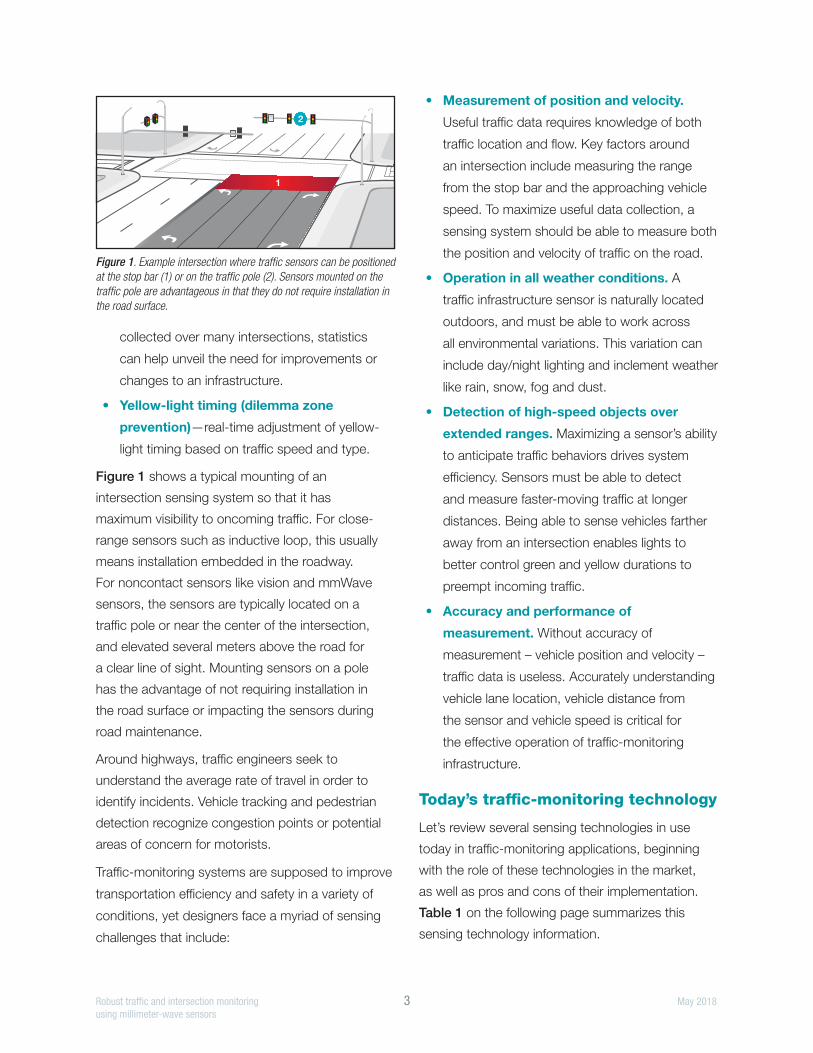
Figure 1 shows a typical mounting of an
intersection sensing system so that it has
maximum visibility to oncoming traffic. For close-
range sensors such as inductive loop, this usually
means installation embedded in the roadway.
For noncontact sensors like vision and mmWave
sensors, the sensors are typically located on a
traffic pole or near the center of the intersection,
and elevated several meters above the road for
a clear line of sight. Mounting sensors on a pole
has the advantage of not requiring installation in
the road surface or impacting the sensors during
road maintenance.
Around highways, traffic engineers seek to
understand the average rate of travel in order to
identify incidents. Vehicle tracking and pedestrian
detection recognize congestion points or potential
areas of concern for motorists.
Traffic-monitoring systems are supposed to improve
transportation efficiency and safety in a variety of
conditions, yet designers face a myriad of sensing
challenges that include:
• Measurement of position and velocity.
Useful traffic data requires knowledge of both
traffic location and flow. Key factors around
an intersection include measuring the range
from the stop bar and the approaching vehicle
speed. To maximize useful data collection, a
sensing system should be able to measure both
the position and velocity of traffic on the road.
• Operation in all weather conditions. A
traffic infrastructure sensor is naturally located
outdoors, and must be able to work across
all environmental variations. This variation can
include day/night lighting and inclement weather
like rain, snow, fog and dust.
• Detection of high-speed objects over
extended ranges. Maximizing a sensor’s ability
to anticipate traffic behaviors drives system
efficiency. Sensors must be able to detect
and measure faster-moving traffic at longer
distances. Being able to sense vehicles farther
away from an intersection enables lights to
better control green and yellow durations to
preempt incoming traffic.
• Accuracy and performance of
measurement. Without accuracy of
measurement – vehicle position and velocity –
traffic data is useless. Accurately understanding
vehicle lane location, vehicle distance from
the sensor and vehicle speed is critical for
the effective operation of traffic-monitoring
infrastructure.
Today’s traffic-monitoring technology
Let’s review several sensing technologies in use
today in traffic-monitoring applications, beginning
with the role of these technologies in the market,
as well as pros and cons of their implementation.
Table 1 on the following page summarizes this
sensing technology information.
2
1
Figure 1. Example intersection where traffic sensors can be positioned at the stop bar (1) or on the traffic pole (2). Sensors mounted on the traffic pole are advantageous in that they do not require installation in the road surface.
Robust traffic and intersection monitoring 4 May 2018using millimeter-wave sensors
Inductive loop sensors
Inductive loop sensors use insulated, electrically
conductive wire passed through cuts in the
roadway. Electrical pulses are sent through the
wire, and when a metal vehicle passes over the
loop, the vehicle body causes Eddy currents to
form that change the inductance of the loop. An
electronic sensing system can measure this change
in inductance, and indicate when a vehicle occupies
a space or passes by.
Inductive loop sensing is a simple technology
that has been used for many years in traffic
infrastructure. It is very well understood, but has
several shortcomings. Detection is limited to a
“presence” around wherever the loop is installed,
and the scale of the system requires that each
zone and lane have its own loop at an intersection.
Perhaps the biggest negative is the fact that
installing or repairing these systems requires digging
up the road surface. This maintenance requires
special personnel and equipment, and can close
down roads. Combine that with the often-short
maintenance cycles of inductive loop systems (one
to two years), and the overall cost of an inductive
loop system compounds quickly.
Cameras and vision-based sensors
Cameras and vision-based sensors use a video
image processor to capture image data from a
complementary metal-oxide semiconductor (CMOS)
camera sensor and analyze the imagery in order to
determine traffic behavior. These systems can be
powerful tools to not only measure traffic behavior at
intersections and highways, but also to transmit live
video to operators.
Despite the power and flexibility of vision-based
systems, the technology can be challenging to work
with. Vision systems are prone to false detection
as changing environmental conditions—day/night
cycles, shadows and weather—directly impact
the ability of these systems to “see.” These vision
challenges require advanced signal processing and
algorithms.
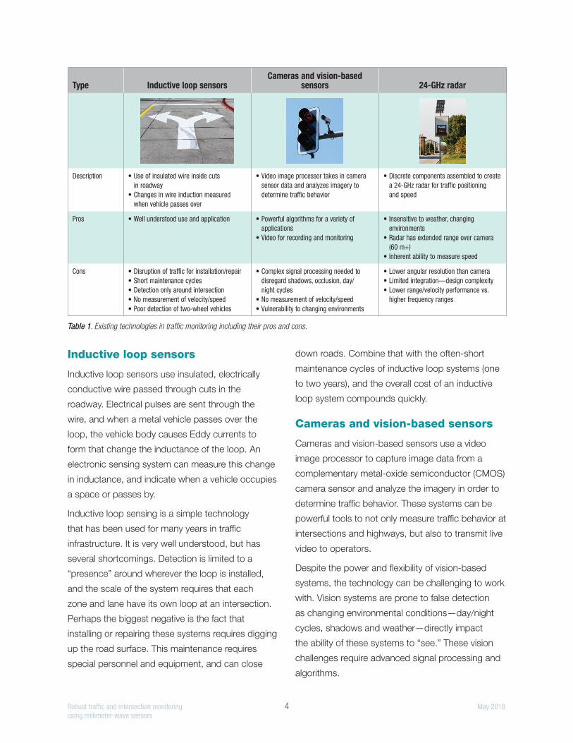
Type Inductive loop sensorsCameras and vision-based
sensors 24-GHz radar
Description • Use of insulated wire inside cuts in roadway
• Changes in wire induction measured when vehicle passes over
• Video image processor takes in camera sensor data and analyzes imagery to determine traffic behavior
• Discrete components assembled to create a 24-GHz radar for traffic positioning and speed
Pros • Well understood use and application • Powerful algorithms for a variety of applications
• Video for recording and monitoring
• Insensitive to weather, changing environments
• Radar has extended range over camera (60 m+)
• Inherent ability to measure speed
Cons • Disruption of traffic for installation/repair• Short maintenance cycles• Detection only around intersection• No measurement of velocity/speed• Poor detection of two-wheel vehicles
• Complex signal processing needed to disregard shadows, occlusion, day/night cycles
• No measurement of velocity/speed• Vulnerability to changing environments
• Lower angular resolution than camera• Limited integration—design complexity• Lower range/velocity performance vs.
higher frequency ranges
Table 1. Existing technologies in traffic monitoring including their pros and cons.
Robust traffic and intersection monitoring 5 May 2018using millimeter-wave sensors
24-GHz radar
One technology that’s getting traction in the traffic-
monitoring market is 24-GHz radar. Radar has
unique advantages in the sensing space that play
well into traffic-monitoring applications. Radar has
the ability to inherently measure the position and
velocity of objects in its view, which opens up new
applications in traffic monitoring such as speed
sensing and vehicle positioning. As a noncontact
technology, radar has an extended range over
vision-based systems, 50 m or more. Radar is
also insensitive to lighting and changing weather
conditions, making it suitable for outdoor sensing
and detection.
There are certain challenges to implementing a radar
solution, however. Today’s radar solutions require
multiple discrete components to create a complete
solution. This lack of integration increases design
complexity and comes at the expense of system
size, cost and power consumption.
76 GHz–81 GHz mmWave radar
Texas Instruments has created a portfolio of
innovative sensors based on millimeter-wave
(mmWave) radar operating in the 76 GHz–81 GHz
frequency band. These sensors integrate radio-
frequency (RF) radar technology with powerful
ARM MCUs and TI DSPs on to a single monolithic
CMOS die, and wrapped in a 10.4-mm-by-10.4-
mm package. This enables small form-factor
applications to accurately measure the range,
velocity and angle of objects in view as well as to
integrate real-time intelligence through advanced
algorithms that can detect, track and classify
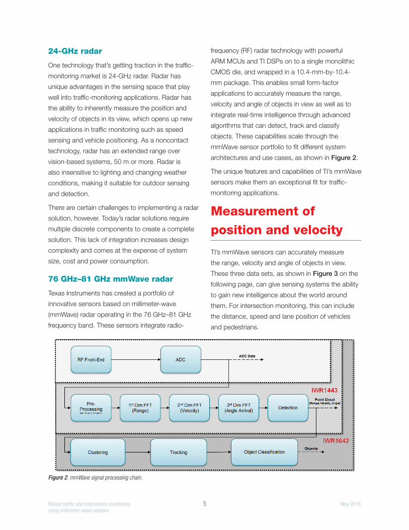
objects. These capabilities scale through the
mmWave sensor portfolio to fit different system
architectures and use cases, as shown in Figure 2.
The unique features and capabilities of TI’s mmWave
sensors make them an exceptional fit for traffic-
monitoring applications.
Measurement of position and velocity
TI’s mmWave sensors can accurately measure
the range, velocity and angle of objects in view.
These three data sets, as shown in Figure 3 on the
following page, can give sensing systems the ability
to gain new intelligence about the world around
them. For intersection monitoring, this can include
the distance, speed and lane position of vehicles
and pedestrians.
Figure 2. mmWave signal processing chain.
Robust traffic and intersection monitoring 6 May 2018using millimeter-wave sensors
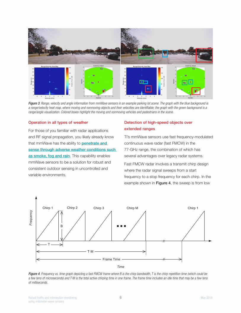
Figure 3. Range, velocity and angle information from mmWave sensors in an example parking lot scene. The graph with the blue background is a range/velocity heat map, where moving and nonmoving objects and their velocities are identifiable; the graph with the green background is a range/angle visualization. Colored boxes highlight the moving and nonmoving vehicles and pedestrians in the scene.
Operation in all types of weather
For those of you familiar with radar applications
and RF signal propagation, you likely already know
that mmWave has the ability to penetrate and
sense through adverse weather conditions such
as smoke, fog and rain. This capability enables
mmWave sensors to be a solution for robust and
consistent outdoor sensing in uncontrolled and
variable environments.
Detection of high-speed objects over
extended ranges
TI’s mmWave sensors use fast frequency-modulated
continuous wave radar (fast FMCW) in the
77-GHz range, the combination of which has
several advantages over legacy radar systems.
Fast FMCW radar involves a transmit chirp design
where the radar signal sweeps from a start
frequency to a stop frequency for each chirp. In the
example shown in Figure 4, the sweep is from low
TI Confidential – NDA Restrictions
Fast FMCW chirp and frame configuration• Illustration for white paper on Fast FMCW chirp and frame configuration
Freq
uenc
y
Time
B
T
T·M
Frame Time
Chirp 1 Chirp 2 Chirp 3 Chirp M
//
//
Chirp 1
Figure 4. Frequency vs. time graph depicting a fast FMCW frame where B is the chirp bandwidth, T is the chirp repetition time (which could be a few tens of microseconds) and T·M is the total active chirping time in one frame. The frame time includes an idle time that may be a few tens of milliseconds.
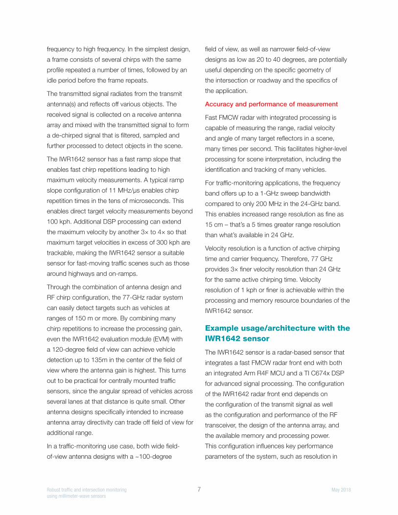
Robust traffic and intersection monitoring 7 May 2018using millimeter-wave sensors
frequency to high frequency. In the simplest design,
a frame consists of several chirps with the same
profile repeated a number of times, followed by an
idle period before the frame repeats.
The transmitted signal radiates from the transmit
antenna(s) and reflects off various objects. The
received signal is collected on a receive antenna
array and mixed with the transmitted signal to form
a de-chirped signal that is filtered, sampled and
further processed to detect objects in the scene.
The IWR1642 sensor has a fast ramp slope that
enables fast chirp repetitions leading to high
maximum velocity measurements. A typical ramp
slope configuration of 11 MHz/µs enables chirp
repetition times in the tens of microseconds. This
enables direct target velocity measurements beyond
100 kph. Additional DSP processing can extend
the maximum velocity by another 3× to 4× so that
maximum target velocities in excess of 300 kph are
trackable, making the IWR1642 sensor a suitable
sensor for fast-moving traffic scenes such as those
around highways and on-ramps.
Through the combination of antenna design and
RF chirp configuration, the 77-GHz radar system
can easily detect targets such as vehicles at
ranges of 150 m or more. By combining many
chirp repetitions to increase the processing gain,
even the IWR1642 evaluation module (EVM) with
a 120-degree field of view can achieve vehicle
detection up to 135m in the center of the field of
view where the antenna gain is highest. This turns
out to be practical for centrally mounted traffic
sensors, since the angular spread of vehicles across
several lanes at that distance is quite small. Other
antenna designs specifically intended to increase
antenna array directivity can trade off field of view for
additional range.
In a traffic-monitoring use case, both wide field-
of-view antenna designs with a ~100-degree
field of view, as well as narrower field-of-view
designs as low as 20 to 40 degrees, are potentially
useful depending on the specific geometry of
the intersection or roadway and the specifics of
the application.
Accuracy and performance of measurement
Fast FMCW radar with integrated processing is
capable of measuring the range, radial velocity
and angle of many target reflectors in a scene,
many times per second. This facilitates higher-level
processing for scene interpretation, including the
identification and tracking of many vehicles.
For traffic-monitoring applications, the frequency
band offers up to a 1-GHz sweep bandwidth
compared to only 200 MHz in the 24-GHz band.
This enables increased range resolution as fine as
15 cm – that’s a 5 times greater range resolution
than what’s available in 24 GHz.
Velocity resolution is a function of active chirping
time and carrier frequency. Therefore, 77 GHz
provides 3× finer velocity resolution than 24 GHz
for the same active chirping time. Velocity
resolution of 1 kph or finer is achievable within the
processing and memory resource boundaries of the
IWR1642 sensor.
Example usage/architecture with the IWR1642 sensor
The IWR1642 sensor is a radar-based sensor that
integrates a fast FMCW radar front end with both
an integrated Arm R4F MCU and a TI C674x DSP
for advanced signal processing. The configuration
of the IWR1642 radar front end depends on
the configuration of the transmit signal as well
as the configuration and performance of the RF
transceiver, the design of the antenna array, and
the available memory and processing power.
This configuration influences key performance
parameters of the system, such as resolution in
Robust traffic and intersection monitoring 8 May 2018using millimeter-wave sensors
range and velocity, maximum range and velocity,
and angular resolution.
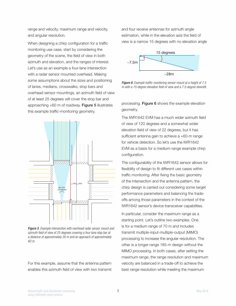
When designing a chirp configuration for a traffic
monitoring use case, start by considering the
geometry of the scene, the field of view in both
azimuth and elevation, and the ranges of interest.
Let’s use as an example a four-lane intersection
with a radar sensor mounted overhead. Making
some assumptions about the sizes and positioning
of lanes, medians, crosswalks, stop bars and
overhead sensor mountings, an azimuth field of view
of at least 25 degrees will cover the stop bar and
approaching +60 m of roadway. Figure 5 illustrates
this example traffic-monitoring geometry.
For this example, assume that the antenna pattern
enables this azimuth field of view with two transmit
and four receive antennas for azimuth angle
estimation, while in the elevation axis the field of
view is a narrow 15 degrees with no elevation angle
processing. Figure 6 shows the example elevation
geometry.
The IWR1642 EVM has a much wider azimuth field
of view of 120 degrees and a somewhat wider
elevation field of view of 22 degrees, but it has
sufficient antenna gain to achieve a +60-m range
for vehicle detection. So let’s use the IWR1642
EVM as a basis for a medium-range example chirp
configuration.
The configurability of the IWR1642 sensor allows for
flexibility of design to fit different use cases within
traffic monitoring. After fixing the basic geometry
of the intersection and the antenna pattern, the
chirp design is carried out considering some target
performance parameters and balancing the trade-
offs among those parameters in the context of the
IWR1642 sensor’s device transceiver capabilities.
In particular, consider the maximum range as a
starting point. Let’s outline two examples. One
is for a medium range of 70 m and includes
transmit multiple-input-multiple-output (MIMO)
processing to increase the angular resolution. The
other is a longer-range 185-m design without the
MIMO processing. In both cases, after setting the
maximum range, the range resolution and maximum
velocity are balanced in a trade-off to achieve the
best range resolution while meeting the maximum
~30m ~60m
Min FOV ~25 degrees
Figure 5. Example intersection with overhead radar sensor mount and azimuth field of view of 25 degrees covering a four-lane stop bar at a distance of approximately 30 m and an approach of approximately 60 m.
25 degrees
~53ft
~25ft
15 degrees
~28m
~7.5m
Vertical FOV and downtilt, 7.5m ~25ft pole mount, 15 and 25 degree antenna opening,
Figure 6. Example traffic-monitoring sensor mount at a height of 7.5 m with a 15-degree elevation field of view and a 7.5-degree downtilt.
Robust traffic and intersection monitoring 9 May 2018using millimeter-wave sensors
velocity requirements. Increasing the velocity
resolution to the practical limit of the internal radar
cube memory also increases the effective range of
the transceiver. It’s possible to further extend the
maximum chirp velocity with additional processing
to an effective velocity estimation four or more
times the maximum chirp velocity. This additional
processing enables tracking and velocity estimation
well above vehicular highway speeds.
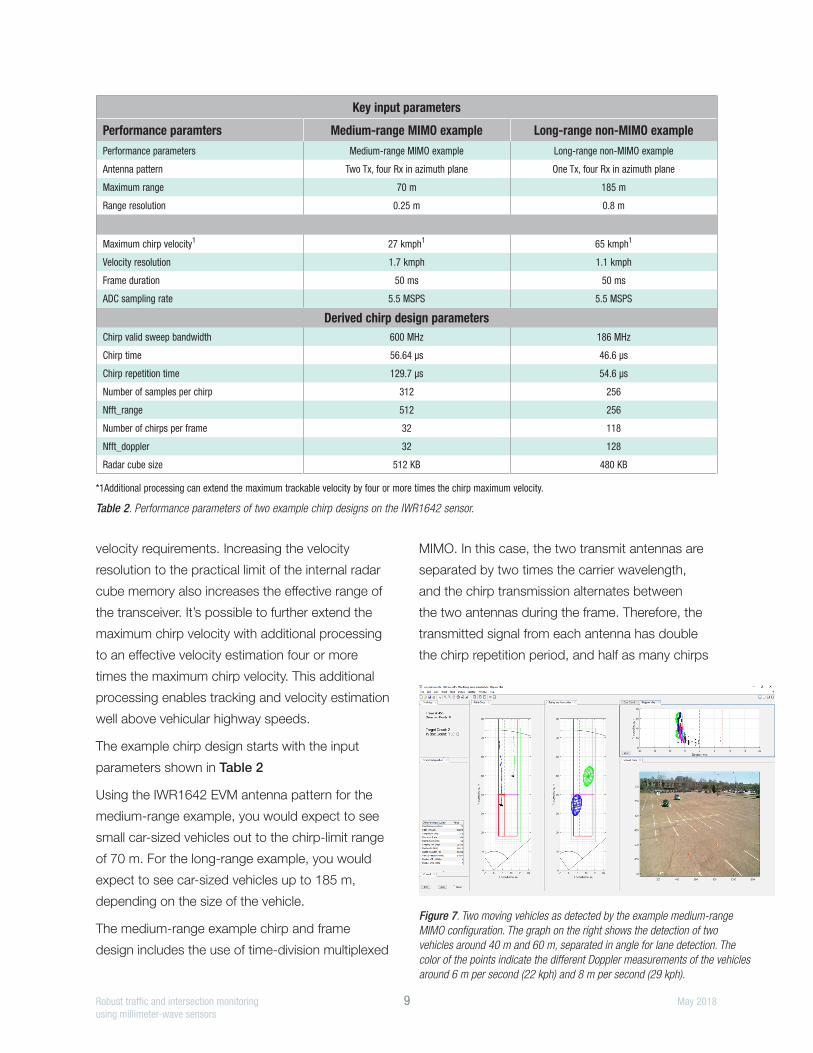
The example chirp design starts with the input
parameters shown in Table 2
Using the IWR1642 EVM antenna pattern for the
medium-range example, you would expect to see
small car-sized vehicles out to the chirp-limit range
of 70 m. For the long-range example, you would
expect to see car-sized vehicles up to 185 m,
depending on the size of the vehicle.
The medium-range example chirp and frame
design includes the use of time-division multiplexed
MIMO. In this case, the two transmit antennas are
separated by two times the carrier wavelength,
and the chirp transmission alternates between
the two antennas during the frame. Therefore, the
transmitted signal from each antenna has double
the chirp repetition period, and half as many chirps
Key input parameters
Performance paramters Medium-range MIMO example Long-range non-MIMO examplePerformance parameters Medium-range MIMO example Long-range non-MIMO example
Antenna pattern Two Tx, four Rx in azimuth plane One Tx, four Rx in azimuth plane
Maximum range 70 m 185 m
Range resolution 0.25 m 0.8 m
Maximum chirp velocity1 27 kmph1 65 kmph1
Velocity resolution 1.7 kmph 1.1 kmph
Frame duration 50 ms 50 ms
ADC sampling rate 5.5 MSPS 5.5 MSPS
Derived chirp design parametersChirp valid sweep bandwidth 600 MHz 186 MHz
Chirp time 56.64 µs 46.6 µs
Chirp repetition time 129.7 µs 54.6 µs
Number of samples per chirp 312 256
Nfft_range 512 256
Number of chirps per frame 32 118
Nfft_doppler 32 128
Radar cube size 512 KB 480 KB
*1Additional processing can extend the maximum trackable velocity by four or more times the chirp maximum velocity.
Table 2. Performance parameters of two example chirp designs on the IWR1642 sensor.
Figure 7. Two moving vehicles as detected by the example medium-range MIMO configuration. The graph on the right shows the detection of two vehicles around 40 m and 60 m, separated in angle for lane detection. The color of the points indicate the different Doppler measurements of the vehicles around 6 m per second (22 kph) and 8 m per second (29 kph).
Robust traffic and intersection monitoring 10 May 2018using millimeter-wave sensors
as in a non-MIMO case. This effectively doubles the
angular resolution of the detector at the expense of
halving the directly measurable maximum velocity.
As mentioned before, the maximum velocity is
extendable through additional signal processing.
Figure 7 shows a data snapshot for the medium-
range example configuration where two vehicles
approach the sensor at just over 40 m and just
over 60 m, respectively. The two vehicles are
easily detected.
The IWR1642 EVM implements an example
processing chain for traffic monitoring using this
chirp and frame design.
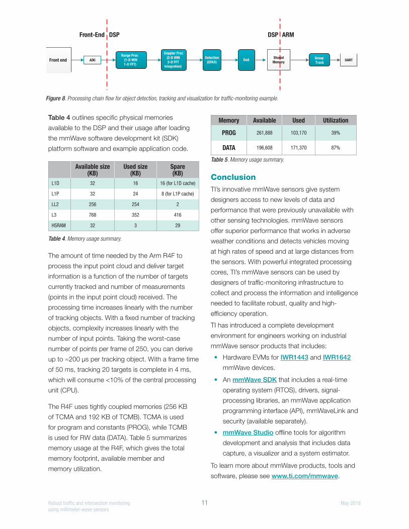
As described in Figure 8, the traffic-monitoring
example implementation signal-processing chain
consists of the following blocks implemented as
DSP code executing on the C674x DSP core in the
IWR1642 sensor:
• Range processing: for each antenna, 1-D
windowing and 1-D fast Fourier transform (FFT).
Range processing is interleaved with the active
chirp time of the frame.
• Doppler processing: for each antenna, 2-D
windowing and 2-D FFT, then noncoherent
combining of received power across antennas
in floating-point precision.
• Range-Doppler detection algorithm: cell
averaging smallest of constant false-alarm
rate (CASO-CFAR) plus CFAR-cell averaging
(CFARCA) detection algorithms run on the
range-Doppler power mapping to find detection
points in range and Doppler space.
• Angle estimation: For each detected point
in range and Doppler space, reconstruct the
2-D FFT output with Doppler compensation. A
beamforming algorithm returns one angle based
on the angle correction for Vmax extension.
After the DSP finishes frame processing, the results
consisting of range, Doppler, angle and detection
signal-to-noise range (SNR) are formatted and
written in shared memory (L3RAM) for the R4F to
perform high-level processing.
Input from the low-level processing layer (point-
cloud data) is copied from the shared memory and
adapted to the tracker interface. The group tracker
is implemented with two sublayers: module layer
and unit layer. One instance module manages
multiple units. At the module layer, you should first
attempt to associate each point from the input
cloud with a tracking unit. Nonassociated points
will undergo an allocation procedure. At the unit
level, each track uses extended Kalman filter (EKF)
process to predict and estimate the properties of
the group. The R4F then sends all the results to
the host through a universal asynchronous receiver
transmitter (UART) for visualization.
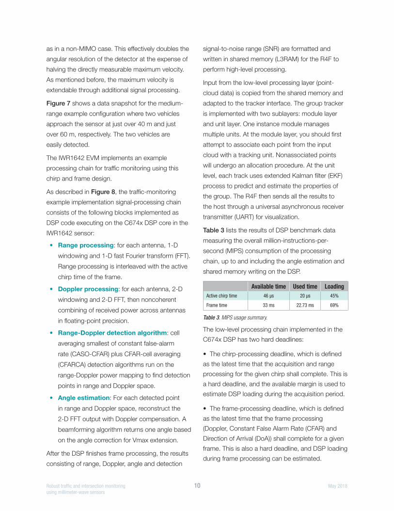
Table 3 lists the results of DSP benchmark data
measuring the overall million-instructions-per-
second (MIPS) consumption of the processing
chain, up to and including the angle estimation and
shared memory writing on the DSP.
Available time Used time LoadingActive chirp time 46 µs 20 µs 45%
Frame time 33 ms 22.73 ms 69%
Table 3. MIPS usage summary.
The low-level processing chain implemented in the
C674x DSP has two hard deadlines:
• The chirp-processing deadline, which is defined
as the latest time that the acquisition and range
processing for the given chirp shall complete. This is
a hard deadline, and the available margin is used to
estimate DSP loading during the acquisition period.
• The frame-processing deadline, which is defined
as the latest time that the frame processing
(Doppler, Constant False Alarm Rate (CFAR) and
Direction of Arrival (DoA)) shall complete for a given
frame. This is also a hard deadline, and DSP loading
during frame processing can be estimated.
Robust traffic and intersection monitoring 11 May 2018using millimeter-wave sensors
Table 4 outlines specific physical memories
available to the DSP and their usage after loading
the mmWave software development kit (SDK)
platform software and example application code.
Available size (KB)
Used size (KB)
Spare (KB)
L1D 32 16 16 (for L1D cache)
L1P 32 24 8 (for L1P cache)
LL2 256 254 2
L3 768 352 416
HSRAM 32 3 29
Table 4. Memory usage summary.
The amount of time needed by the Arm R4F to
process the input point cloud and deliver target
information is a function of the number of targets
currently tracked and number of measurements
(points in the input point cloud) received. The
processing time increases linearly with the number
of tracking objects. With a fixed number of tracking
objects, complexity increases linearly with the
number of input points. Taking the worst-case
number of points per frame of 250, you can derive
up to ≈200 µs per tracking object. With a frame time
of 50 ms, tracking 20 targets is complete in 4 ms,
which will consume <10% of the central processing
unit (CPU).
The R4F uses tightly coupled memories (256 KB
of TCMA and 192 KB of TCMB). TCMA is used
for program and constants (PROG), while TCMB
is used for RW data (DATA). Table 5 summarizes
memory usage at the R4F, which gives the total
memory footprint, available member and
memory utilization.
Memory Available Used Utilization
PROG 261,888 103,170 39%
DATA 196,608 171,370 87%
Table 5. Memory usage summary.
ConclusionTI’s innovative mmWave sensors give system
designers access to new levels of data and
performance that were previously unavailable with
other sensing technologies. mmWave sensors
offer superior performance that works in adverse
weather conditions and detects vehicles moving
at high rates of speed and at large distances from
the sensors. With powerful integrated processing
cores, TI’s mmWave sensors can be used by
designers of traffic-monitoring infrastructure to
collect and process the information and intelligence
needed to facilitate robust, quality and high-
efficiency operation.
TI has introduced a complete development
environment for engineers working on industrial
mmWave sensor products that includes:
• Hardware EVMs for IWR1443 and IWR1642
mmWave devices.
• An mmWave SDK that includes a real-time
operating system (RTOS), drivers, signal-
processing libraries, an mmWave application
programming interface (API), mmWaveLink and
security (available separately).
• mmWave Studio offline tools for algorithm
development and analysis that includes data
capture, a visualizer and a system estimator.
To learn more about mmWave products, tools and
software, please see www.ti.com/mmwave.
Front end ADCRange Proc
(1-D WIN1-D FFT)
UART
DSP ARM
Doppler Proc(2-D WIN2-D FFT
Integration)
Detection Group Track(CFAR)
DoA
DSPFront-End
SharedMemory
Figure 8. Processing chain flow for object detection, tracking and visualization for traffic-monitoring example.

SPYY002B© 2018 Texas Instruments Incorporated
Important Notice: The products and services of Texas Instruments Incorporated and its subsidiaries described herein are sold subject to TI’s standard terms and conditions of sale. Customers are advised to obtain the most current and complete information about TI products and services before placing orders. TI assumes no liability for applications assistance, customer’s applications or product designs, software performance, or infringement of patents. The publication of information regarding any other company’s products or services does not constitute TI’s approval, warranty or endorsement thereof.
The platform bar is a trademark of Texas Instruments. All other trademarks are the property of their respective owners.
IMPORTANT NOTICE FOR TI DESIGN INFORMATION AND RESOURCES
Texas Instruments Incorporated (‘TI”) technical, application or other design advice, services or information, including, but not limited to,reference designs and materials relating to evaluation modules, (collectively, “TI Resources”) are intended to assist designers who aredeveloping applications that incorporate TI products; by downloading, accessing or using any particular TI Resource in any way, you(individually or, if you are acting on behalf of a company, your company) agree to use it solely for this purpose and subject to the terms ofthis Notice.TI’s provision of TI Resources does not expand or otherwise alter TI’s applicable published warranties or warranty disclaimers for TIproducts, and no additional obligations or liabilities arise from TI providing such TI Resources. TI reserves the right to make corrections,enhancements, improvements and other changes to its TI Resources.You understand and agree that you remain responsible for using your independent analysis, evaluation and judgment in designing yourapplications and that you have full and exclusive responsibility to assure the safety of your applications and compliance of your applications(and of all TI products used in or for your applications) with all applicable regulations, laws and other applicable requirements. Yourepresent that, with respect to your applications, you have all the necessary expertise to create and implement safeguards that (1)anticipate dangerous consequences of failures, (2) monitor failures and their consequences, and (3) lessen the likelihood of failures thatmight cause harm and take appropriate actions. You agree that prior to using or distributing any applications that include TI products, youwill thoroughly test such applications and the functionality of such TI products as used in such applications. TI has not conducted anytesting other than that specifically described in the published documentation for a particular TI Resource.You are authorized to use, copy and modify any individual TI Resource only in connection with the development of applications that includethe TI product(s) identified in such TI Resource. NO OTHER LICENSE, EXPRESS OR IMPLIED, BY ESTOPPEL OR OTHERWISE TOANY OTHER TI INTELLECTUAL PROPERTY RIGHT, AND NO LICENSE TO ANY TECHNOLOGY OR INTELLECTUAL PROPERTYRIGHT OF TI OR ANY THIRD PARTY IS GRANTED HEREIN, including but not limited to any patent right, copyright, mask work right, orother intellectual property right relating to any combination, machine, or process in which TI products or services are used. Informationregarding or referencing third-party products or services does not constitute a license to use such products or services, or a warranty orendorsement thereof. Use of TI Resources may require a license from a third party under the patents or other intellectual property of thethird party, or a license from TI under the patents or other intellectual property of TI.TI RESOURCES ARE PROVIDED “AS IS” AND WITH ALL FAULTS. TI DISCLAIMS ALL OTHER WARRANTIES ORREPRESENTATIONS, EXPRESS OR IMPLIED, REGARDING TI RESOURCES OR USE THEREOF, INCLUDING BUT NOT LIMITED TOACCURACY OR COMPLETENESS, TITLE, ANY EPIDEMIC FAILURE WARRANTY AND ANY IMPLIED WARRANTIES OFMERCHANTABILITY, FITNESS FOR A PARTICULAR PURPOSE, AND NON-INFRINGEMENT OF ANY THIRD PARTY INTELLECTUALPROPERTY RIGHTS.TI SHALL NOT BE LIABLE FOR AND SHALL NOT DEFEND OR INDEMNIFY YOU AGAINST ANY CLAIM, INCLUDING BUT NOTLIMITED TO ANY INFRINGEMENT CLAIM THAT RELATES TO OR IS BASED ON ANY COMBINATION OF PRODUCTS EVEN IFDESCRIBED IN TI RESOURCES OR OTHERWISE. IN NO EVENT SHALL TI BE LIABLE FOR ANY ACTUAL, DIRECT, SPECIAL,COLLATERAL, INDIRECT, PUNITIVE, INCIDENTAL, CONSEQUENTIAL OR EXEMPLARY DAMAGES IN CONNECTION WITH ORARISING OUT OF TI RESOURCES OR USE THEREOF, AND REGARDLESS OF WHETHER TI HAS BEEN ADVISED OF THEPOSSIBILITY OF SUCH DAMAGES.You agree to fully indemnify TI and its representatives against any damages, costs, losses, and/or liabilities arising out of your non-compliance with the terms and provisions of this Notice.This Notice applies to TI Resources. Additional terms apply to the use and purchase of certain types of materials, TI products and services.These include; without limitation, TI’s standard terms for semiconductor products http://www.ti.com/sc/docs/stdterms.htm), evaluationmodules, and samples (http://www.ti.com/sc/docs/sampterms.htm).
Mailing Address: Texas Instruments, Post Office Box 655303, Dallas, Texas 75265Copyright © 2018, Texas Instruments Incorporated