Fluid Surface Velocity Measurement using Millimeter-Wave ...

FLUID SURFACE VELOCITYMEASUREMENT USINGMILLIMETER-WAVE RADARSENSOR

GUSTAV BROMAN,LEO GHATNEKAR NILSSON

Master’s thesis2022:E46

Faculty of EngineeringCentre for Mathematical SciencesMathematical Statistics

CENTRU

MSCIEN

TIARU

MM

ATH

EMA

TICARU

M

Master’s Theses in Mathematical Sciences 2022:E46ISSN 1404-6342

LUTFMS-3449-2022

Mathematical StatisticsCentre for Mathematical Sciences

Lund UniversityBox 118, SE-221 00 Lund, Sweden

http://www.maths.lu.se/

Fluid Surface Velocity Measurement usingMillimeter-Wave Radar Sensor

Gustav Broman

[email protected]

Leo Ghatnekar Nilsson

[email protected]

June ��, ��

Master’s thesis work carried out at Acconeer AB.

Supervisors: Andreas Jakobsson, [email protected] Buhl, [email protected]

Examiner: Dragi Anevski, [email protected]

Abstract

Contactless �uid surface velocity measurements with radar technology presentsnovel ways of determining �uid �ow. The Acconeer A�� sensor is used, whichis a pulsed coherent �� GHz millimeter-wave radar, with high accuracy and lowenergy consumption. Fluid�ow data is obtained from three di�erent sites; in theAcconeer lab, a lab in the UK, and in three sewage pipes of VA SYD. Initially,data from the Acconeer lab is analysed and used to implement the algorithmwhich later is run and tested on the other data. The basics of the algorithm iscreating periodograms by FFT in fast-time and averaging in slow-time dimen-sion. The frequency components are converted to velocities by knowledge of thewave speci�cs.

The results show that forward and backward �ow is easy to measure anddistinguish. From Acconeer and UK lab the velocity spectra cohere with thereference velocity data. For the VA SYD sites, the �� mm pipe show somepeak close to Nivus reference, but the signal strength is weak due to small surfaceripples. For the pipe of �� mm the spectra cohere well with Nivus. The non-stationary�ow of the ��mmpipe seem to cause some error in themeasurement.

Keywords: Fluid �ow surface measurement, velocity estimation, FFT, fast-time phasechange, radar

Acknowledgements

We wish to express our gratitude to Acconeer AB for an interesting project, and especiallyour supervisor Anders Buhl, who guided us through the process. We are also grateful to oursupervisor at LTH, Andreas Jakobsson. Without your guidance, the goal of this project couldnot have been realised.

We would also like to thank Tomas Wolf, our contact at VA SYD who helped us collectuseful data in the sewage environments. Finally, we would like to thank Magnus Larson atthe division of Water Resources Engineering for providing us with information about �uiddynamics.

Finally, a sincere thank you to everyone else who helped us during this project, not leastour fellow course mates. If you feel that you have contributed to this project, thank you.

iii

Popular Science Summary

Hastighetsuppskattning av vattenytor med 60 GHz radar

Det �nns ett stort behov av att förbättra infrastrukturen i vatten- och avloppsnäten glob-alt. Belastningen på dessa nätverk måste övervakas för att förutspå och undvika skador,översvämningar samt minimera serviceavbrott. Nuvarande lösningar är dyra, vilket öppnarmarknadsmöjligheter för mer kostnadse�ektiva lösningar.

Traditionellt sett har radar använts i sammanhang för att identi�era större objekt somraketer eller�ygplan. Dagens teknikutveckling harmöjliggjort för snabba ochmillimeternog-granna radarsystem som till följd av energisnålheten gör den lämplig för, och används i allt�er batteridrivna produkter inom konsumentelektronik. Kontaktlös mätning av vätske�ö-den är en radartillämpning som enkelt skulle kunna ersätta dagens dyra mätningsutrustningmed en mindre batteridriven radar. Eftersom den dyra mätutrustningen ofta kräver kontaktmed vattnet skulle en övergång till radarövervakade system medföra en förenklad installa-tionsprocess såväl som ett minskat behov av underhåll. Att dagens dyrare mätutrustning är ibehov av rengöring märktes i denna studie då det uppmätta �ödet i ett dagvattenrör ökademed över ��% efter rengöring till följd av smuts som ansamlas på mätutrustningen, medvärden från �.�� till �.�� m/s under � minuter. Även detta ökar incitamenten ytterligareför en övergång till kontaktlös �ödesmätning.

I denna studie används Acconeers A��-radar, en sensor med hög precision och låg en-ergiförbrukning. Flödets ythastighet bestäms med hjälp av den re�ekterade signalen ochfrån fasförändringarna kan en hastighet beräknas. Hastighetsuppskattningen görs via de småvågorna/ojämnheterna på ytan som betraktas som små objekt i rörelse. Tekniken fungerarsåledes inte om vattenytan är spegelblank vilket resulterar i en mycket liten eller ingen re-�ekterad signal tillbaka till sensorn. Implementeringen av en generell algoritm för det totala�uid-�ödet är komplicerad då sambandet mellan vattenytans hastighet och det totala �ödetvarierar och beror bland annat på rörets dimensioner såväl som �ödets dynamik. Den al-goritm vi utvecklat resulterar i ett spektrum av hastighetskomponenter på ytan, och det ärmöjligt att uppskatta hur snabbt�uidens yta rör sig. Det här projektet visar på att ythastighetsmät-ningmedAcconeers pulsade radarA�� är genomförbartmed den framtagna implementerin-

v

gen, och är ett kostnadse�ektivt system som kan användas i framtiden.

vi

Abbreviations

• ADC - Analog to Digital Converter

• CR - Cross Range

• FFT - Fast Fourier Transform

• DFT - Discrete Fourier Transform

• DR - Down Range

• EM - Electromagnetic

• HWAAS - Hardware Accelerated Average Samples

• IQ - In-phase and quadrature components

• PRF - Pulse Repetition Frequency

• PRI - Pulse Repetition Interval

• PSD - Power Spectral Density

vii

Contents

� Introduction �

� Theory ��.� Radar . . . . . . . . . . . . . . . . . . . . . . . . . . . . . . . . . . . . . . . �

�.�.� Pulsed coherent radar (PCR) . . . . . . . . . . . . . . . . . . . . . ��.� Acconeer Radar Sensor . . . . . . . . . . . . . . . . . . . . . . . . . . . . . �

�.�.� Con�guring the sensor . . . . . . . . . . . . . . . . . . . . . . . . . ��.�.� The sparse IQ service . . . . . . . . . . . . . . . . . . . . . . . . . ��.�.� Mounting of the A��-sensor . . . . . . . . . . . . . . . . . . . . . �

�.� Fourier transforms and power spectral density (PSD) . . . . . . . . . . . . . ��.� Velocity estimation . . . . . . . . . . . . . . . . . . . . . . . . . . . . . . . ��.� Surface velocity pro�les . . . . . . . . . . . . . . . . . . . . . . . . . . . . . ��

� Methodology ��.� Sensor Setup . . . . . . . . . . . . . . . . . . . . . . . . . . . . . . . . . . . ��.� Data collection . . . . . . . . . . . . . . . . . . . . . . . . . . . . . . . . . . ��

�.�.� Acconeer lab environment . . . . . . . . . . . . . . . . . . . . . . . ��.�.� UK lab environment . . . . . . . . . . . . . . . . . . . . . . . . . . ��.�.� VA SYD site . . . . . . . . . . . . . . . . . . . . . . . . . . . . . . ��

�.� Signal processing . . . . . . . . . . . . . . . . . . . . . . . . . . . . . . . . ��.�.� Mean surface velocity . . . . . . . . . . . . . . . . . . . . . . . . . ��

� Results and discussion ��.� Acconeer lab environment . . . . . . . . . . . . . . . . . . . . . . . . . . . ��.� UK lab environment . . . . . . . . . . . . . . . . . . . . . . . . . . . . . . . ��.� VA SYD site . . . . . . . . . . . . . . . . . . . . . . . . . . . . . . . . . . . ��

�.�.� �� mm . . . . . . . . . . . . . . . . . . . . . . . . . . . . . . . . ��.�.� �� mm . . . . . . . . . . . . . . . . . . . . . . . . . . . . . . . . . ��.�.� �� mm . . . . . . . . . . . . . . . . . . . . . . . . . . . . . . . . . ��

ix

CONTENTS

� Conclusions ��.� Summary . . . . . . . . . . . . . . . . . . . . . . . . . . . . . . . . . . . . . ��.� Topical future research . . . . . . . . . . . . . . . . . . . . . . . . . . . . . ��

References ��

Appendix A Electromagnetic Waves ��A.� Basics . . . . . . . . . . . . . . . . . . . . . . . . . . . . . . . . . . . . . . . ��A.� Re�ections and intensity . . . . . . . . . . . . . . . . . . . . . . . . . . . . ��

Appendix B Tables and images ��

x

Chapter �

Introduction

The current methods of contactless �uid velocity and �ow measurements are expensive andoften require di�erent speci�cs of the�uid, such as particles for the signal to re�ect on. In theglobal perspective of improving the infrastructure of sewage systems and mitigating damagesand service maintenance, it is desirable to supervise di�erent �uid �ows. Combining ane�cient way of contactless�uid velocitymeasurementwith this infrastructural improvementhas a big market potential.

The publicly-traded company of Acconeer provides the pulsed coherent radar sensorA��, a sensor with high accuracy and low energy consumption. The energy e�ciency is espe-cially useful for battery driven electronics. Using the �� GHz band-width, i.e., a millimetre-wave pulse, the sensor returns data as complex numbers packaged in the fast-/slow time(sweep-/frame) dimension.

It is the purpose of this project to implement a �uid surface velocity algorithm for theAcconeer A�� sensor. The implementation is based on fast-time phase change of the waveand requires surface waves/ripples structure for re�ection of the signal. These small surfaceirregularities are seen as moving objects, from which we determine a phase shift of the wave,i.e., a velocity.

The measurements and data collection of this project are done in three settings; the Ac-coneer lab, a lab of a company in the UK, and on three sites of VA SYD which are calledGYGK_K1500, TULK_750, and TUAS_800. The number describes the diameter of the sewagepipe in mm. For GYGK_K1500, the amplitude of the return signal is weak which results in aless protruding peak in relation to the background noise. This is referred to as a low signal-to-noise ratio, SNR. The peak that is obtained however matches the reference velocity of theNivus measurement, a reference that is provided on site by VA SYD. The TULK_750 pipeshows good spectra for the �uid �ows with Nivus reference slightly higher than the centre ofthe spectrum peak. This is expected since Nivus measures just below the surface where thevelocity is higher than the surface. For TUAS_800 the �ow is non-stationary which for somemeasurements are problematic. In the Acconeer lab and the UK lab the spectra are ideal with

�

�. I��

reference value matching. In the Acconeer lab forward and backward �ows are measured andfrom the spectra it is easy to determine which �ow is in what direction.

The algorithm of the signal processing is to construct the power spectral density (PSD)estimation by the squared absolute value of the fast Fourier transform (FFT) in the sweepdimension, averaged in slow-time (mean over frames). This is done for the complex valuedsignal data returned by the A�� sensor. The frequency bins are then converted to velocitiesby knowledge of the pulse speci�cs.

The structure of this report is as follows. Chapter � introduces relevant theory regardinggeneral-/the Acconeer radar, periodogram estimation, the velocity estimation, and di�erentsurface velocity pro�les. In appendix A, some basics on electromagnetic waves are found.In chapter �, the methodology of sensor setup, data collection and signal processing is de-scribed. The results of the measurements are found and discussed in chapter �. Finally, someconclusions of the project measurements are found in section �.�.

�

Chapter �

Theory

For basic electromagnetic wave theory the reader is referred to the appendix A.

2.1 Radar

Radar is an acronym for Radio Detection and Ranging. Modern radars however can detectboth the relative distance as well as velocities or classifying objects. It is an electrical systemthat transmits electromagnetic waves and detects the re�ected signals from a certain region.Figure �.� shows an example of the major elements involved in a radar following the signalfrom the transmitter all the way to the signal processor.

Figure �.�: The �gure represent a schematic example view of a radarsystem (�).

�

�. T��

Although this is just an example of a radar system, all radars must at least include a trans-mitter, receiving antenna, and a signal processor (�).

The part that generates the EM-wave is the transmitter, this signal is generated and sentout through an antenna. In �gure �.�, there is a T/R switch connected to the antenna thatmakes sure it can be attached to both the transmitter and receiver preventing them from anydirect interaction. Another common way is to skip the T/R switch and have two separateantennas for transmitting and receiving. The received signal from any re�ecting target isthen input to the receiver circuits marked with a dashed rectangle in �gure �.�. In this part,the radio signal is ampli�ed and converted to an intermediate frequency and then it goesthrough an analog-to-digital converter (ADC) before it reaches the signal processor (�).

When operating with radars there are often two spatial dimensions of interest. Cross-Range (CR) and Down-Range (DR) demonstrated in �gure �.�.

Figure �.�: The �gure illustrates the CR- and DR-directions for aradar.

DR is the dimension in which the radar signal propagates in through time whereas theCR is the directions normal to DR and makes out the ’wave-front’ of the signal. A ’time of�ight’ radar system can therefore only detect movements in the DR direction.

2.1.1 Pulsed coherent radar (PCR)

A pulsed radar transmit short pulses of EM-waves through the transmitting antenna duringa short period. At this time the receiving antenna is isolated and no re�ected signals can bedetected during this time. In between the transmitted pulses the receiver connected to theantenna detects possible re�ected signals. The interval between two pulses is often referred toas pulse repetition interval (PRI) and the number of cycles per unit time is called pulse repetitionfrequency (PRF) and is simply the inverse of the PRI. The passage of time for a pulsed radaris represented in �gure �.�.

EM-waves are said to be coherent if the phase relationship is constant between pulses.One way to accomplish this is to have a coherence oscillator used as a reference. The pulsesthen consist of partial sections of this continuous oscillation so that every pulse is in phasewith the reference (�). This can be visualized in �gure �.�.

The top signal is a stable continuous oscillation used as the reference and the middlesignal is the coherent since pulses are made based on the phase of the reference oscillation.

�

�.� A�� R�� S��

Figure �.�: A block schema over the pulsed radar over time (�).

Reference

Coherrent

Random

Figure �.�: The �gure illustrates how a pulsed coherent signal (mid-dle) can be made using a reference (top) and a random pulsed signal(bottom). The green pulses are in phase with the reference signal.

Pulsing with random phase like in the last signal is therefore a non-coherent pulsed signal.

2.2 Acconeer Radar Sensor

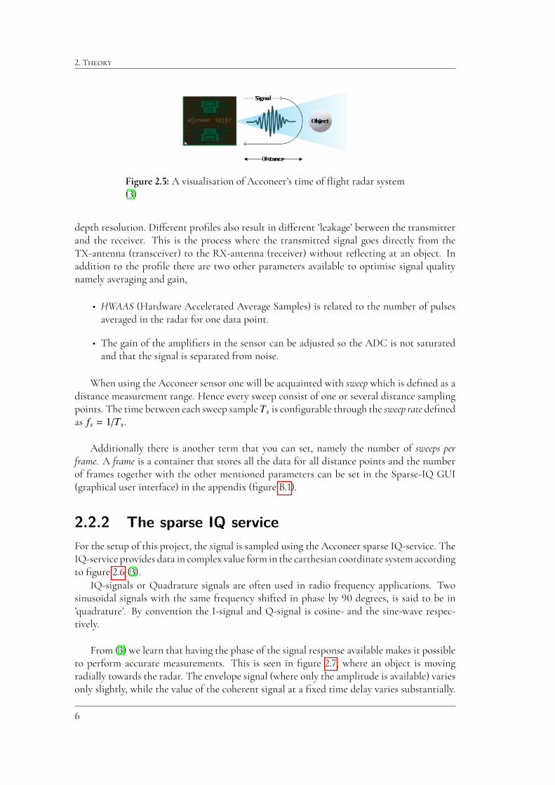
This project is based on the Acconeer A�� sensor which is a pulsed coherent radar operat-ing at �� GHz, resulting in a wavelength of � mm in free space which gives a resolution ofapproximately �.� mm. The radar system is a ’time of �ight’ system meaning that the timebetween the transmitted signal and received signal is measured and used to calculate the DRdistance to objects.

2.2.1 Configuring the sensor

There are multiple settings that can be tuned in order to optimize the sensor performancefor speci�c use cases and requirements. First of all the pulse length profile (Pro�le) speci�esthe transmitted pulse lengths. Shorter pulses provides higher distance resolution and longerpulses reduced the depth resolution. On the other hand short pulses results in a reduced SNR(signal-to-noise ratio) compared to longer pulses so there is a trade-o� between SNR and

�

�. T��

Figure �.�: A visualisation of Acconeer’s time of �ight radar system(�)

depth resolution. Di�erent pro�les also result in di�erent ’leakage’ between the transmitterand the receiver. This is the process where the transmitted signal goes directly from theTX-antenna (transceiver) to the RX-antenna (receiver) without re�ecting at an object. Inaddition to the pro�le there are two other parameters available to optimise signal qualitynamely averaging and gain,

• HWAAS (Hardware Accelerated Average Samples) is related to the number of pulsesaveraged in the radar for one data point.

• The gain of the ampli�ers in the sensor can be adjusted so the ADC is not saturatedand that the signal is separated from noise.

When using the Acconeer sensor one will be acquainted with sweep which is de�ned as adistance measurement range. Hence every sweep consist of one or several distance samplingpoints. The time between each sweep sample Ts is con�gurable through the sweep rate de�nedas fs = 1/Ts.

Additionally there is another term that you can set, namely the number of sweeps perframe. A frame is a container that stores all the data for all distance points and the numberof frames together with the other mentioned parameters can be set in the Sparse-IQ GUI(graphical user interface) in the appendix (�gure B.�).

2.2.2 The sparse IQ service

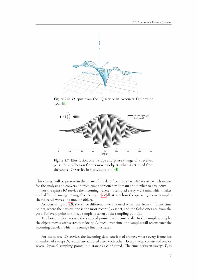
For the setup of this project, the signal is sampled using the Acconeer sparse IQ-service. TheIQ-service provides data in complex value form in the carthesian coordinate system accordingto �gure �.� (�).

IQ-signals or Quadrature signals are often used in radio frequency applications. Twosinusoidal signals with the same frequency shifted in phase by �� degrees, is said to be in’quadrature’. By convention the I-signal and Q-signal is cosine- and the sine-wave respec-tively.

From (�) we learn that having the phase of the signal response available makes it possibleto perform accurate measurements. This is seen in �gure �.�, where an object is movingradially towards the radar. The envelope signal (where only the amplitude is available) variesonly slightly, while the value of the coherent signal at a �xed time delay varies substantially.

�

�.� A�� R�� S��

Figure �.�: Output from the IQ service in Acconeer ExplorationTool (�).

Figure �.�: Illustration of envelope and phase change of a receivedpulse for a re�ection from a moving object, what is returned fromthe sparse IQ Service in Cartesian form. (�)

This change will be present in the phase of the data from the sparse IQ service which we usefor the analysis and conversion from time to frequency domain and further to a velocity.

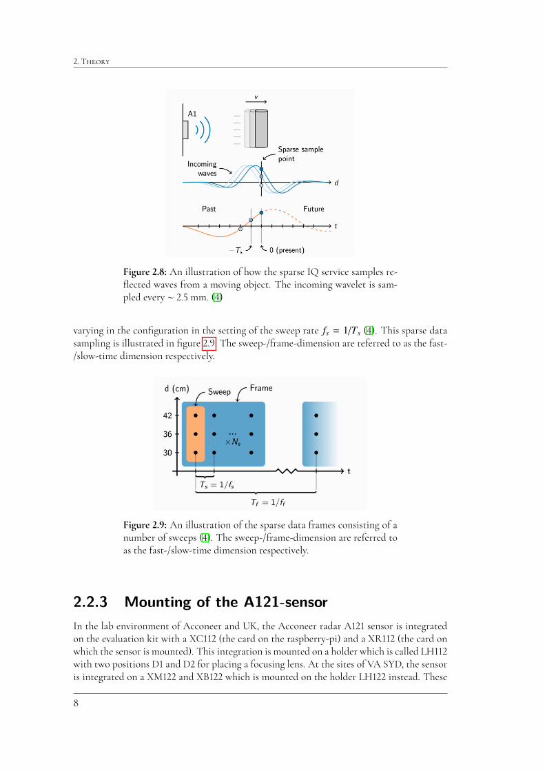
For the sparse IQ service the incoming wavelet is sampled every ⇠ �.� mm, which makesit ideal for measuring moving objects. Figure �.� illustrates how the sparse IQ service samplesthe re�ected waves of a moving object.

As seen in �gure �.�, the three di�erent blue coloured waves are from di�erent timepoints, where the darkest one is the most recent (present), and the faded ones are from thepast. For every point in time, a sample is taken at the sampling point(s).

The bottom plot lays out the sampled points over a time scale. In this simple example,the object moves with a steady velocity. As such, over time, the samples will reconstruct theincoming wavelet, which the orange line illustrates.

For the sparse IQ service, the incoming data consists of frames, where every frame hasa number of sweeps Ns which are sampled after each other. Every sweep consists of one orseveral (sparse) sampling points in distance as con�gured. The time between sweeps Ts is

�

�. T��

Figure �.�: An illustration of how the sparse IQ service samples re-�ected waves from a moving object. The incoming wavelet is sam-pled every ⇠ �.� mm. (�)

varying in the con�guration in the setting of the sweep rate fs = 1/Ts (�). This sparse datasampling is illustrated in �gure �.�. The sweep-/frame-dimension are referred to as the fast-/slow-time dimension respectively.

Figure �.�: An illustration of the sparse data frames consisting of anumber of sweeps (�). The sweep-/frame-dimension are referred toas the fast-/slow-time dimension respectively.

2.2.3 Mounting of the A121-sensor

In the lab environment of Acconeer and UK, the Acconeer radar A�� sensor is integratedon the evaluation kit with a XC�� (the card on the raspberry-pi) and a XR�� (the card onwhich the sensor is mounted). This integration is mounted on a holder which is called LH��with two positions D� and D� for placing a focusing lens. At the sites of VA SYD, the sensoris integrated on a XM�� and XB�� which is mounted on the holder LH�� instead. These

�

�.� A�� R�� S��

evaluation kits are not further described in this report.

The two lenses used in this project are the HBL (hyperbolic lens) and the FZP (Fresnelzone plate). Pictures of these two lenses are seen in �gure �.�� (number � is HBL, and FZPnumber �). These two lenses focus the transmitted signal from the A�� sensor.

Figure �.��: The two focusing lenses used in this project, the HBL-lens (number �) and the FZP-lens (number �) (�).

The di�erent lens mounting positions D� and D� on the LH�� holder are seen in �g-ure �.��. These positions are the same on the LH�� holder (�). The focusing speci�cs ofthese two lenses mounted on the LH�� and LH�� respectively, are described in �gure B.�and �gure B.� in appendix B (�). The numbers are not measured in this project, but are doneby Acconeer in lab environment.

Figure �.��: Picture of the two lens-mounting positions D� and D�on the LH�� holder. The position settings are identical on theLH�� holder. The di�erent positions cause di�erent speci�cationson the transmitted signal. (�).

The sensor signal dispersion angular dependence is shown in �gure �.��. The notation ofE-plane and H-plane angles is used. For this image the default dispersion is shown, i.e., nolens focusing. That makes the E-/H-plane angle to be �� and �� respectively. This is forthe half power beam width which is the angle in which relative power is more than ��% ofthe peak power, in the e�ective radiated �eld of the antenna.

�

�. T��

Figure �.��: The sensor signal dispersion angular dependence in de-fault mode, i.e., with no lens used. That makes the E-/H-plane angleto be �� and �� respectively (�).

2.3 Fourier transforms and power spectral

density (PSD)

From the received signal one can analyze the phase shift and identify the power located at aspeci�c frequency by Fourier transforming the data. This method gives how much spectralcontent that is located at a certain frequency and this frequency can later on be transformedinto a velocity.

The Fourier transform of a continuous function y(t) is de�ned as (�)

F (y(t))( f ) ⌘Z 1

�1e�2⇡ j f ty(t) dt. (�.�)

For a function y(t) only de�ned on t 2 [0, T ], the equation above is transformed into

Y ( f ) =Z T

0e�2⇡ j f ty(t) dt. (�.�)

For discrete values of N samples of the function at t = k TN , k = 0, ...N � 1 the integral is

approximated to the sum of

Y ( f ) ⇡N�1X

k=0e�2⇡ j f kT /Ny(kT /N)(T /N). (�.�)

Specializing the relevant frequencies to f = m/T , m = 0, ...N � 1, we �nd that

Y (m/T ) ⇡ TN

N�1X

k=0e�2⇡ jmk/Ny(kT /N), yk = y(kT /N). (�.�)

This makes the discrete Fourier transform (DFT) of a sequence yk to be

Ym = DFT({yk})(m) ⌘N�1X

k=0e�2⇡ jmk/N yk, (�.�)

��

�.� V��

up to the normalizing constant TN . The data processing algorithm of this DFT operation is

called fast Fourier transform (FFT).

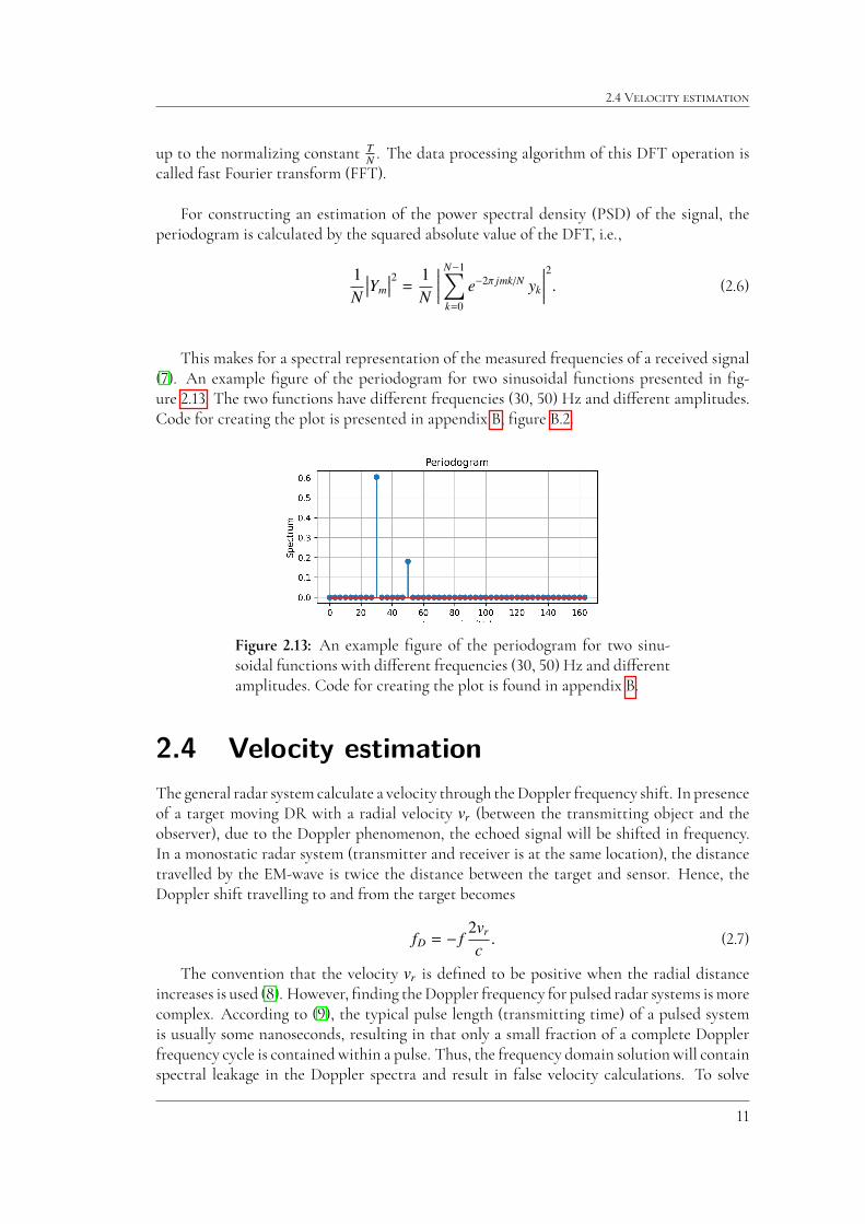
For constructing an estimation of the power spectral density (PSD) of the signal, theperiodogram is calculated by the squared absolute value of the DFT, i.e.,

1N��Ym��2 =

1N

��N�1X

k=0e�2⇡ jmk/N yk

��2. (�.�)

This makes for a spectral representation of the measured frequencies of a received signal(�). An example �gure of the periodogram for two sinusoidal functions presented in �g-ure �.��. The two functions have di�erent frequencies (��, ��) Hz and di�erent amplitudes.Code for creating the plot is presented in appendix B, �gure B.�.

Figure �.��: An example �gure of the periodogram for two sinu-soidal functions with di�erent frequencies (��, ��) Hz and di�erentamplitudes. Code for creating the plot is found in appendix B.

2.4 Velocity estimation

The general radar system calculate a velocity through theDoppler frequency shift. In presenceof a target moving DR with a radial velocity vr (between the transmitting object and theobserver), due to the Doppler phenomenon, the echoed signal will be shifted in frequency.In a monostatic radar system (transmitter and receiver is at the same location), the distancetravelled by the EM-wave is twice the distance between the target and sensor. Hence, theDoppler shift travelling to and from the target becomes

fD = � f 2vr

c . (�.�)

The convention that the velocity vr is de�ned to be positive when the radial distanceincreases is used (�). However, �nding theDoppler frequency for pulsed radar systems ismorecomplex. According to (�), the typical pulse length (transmitting time) of a pulsed systemis usually some nanoseconds, resulting in that only a small fraction of a complete Dopplerfrequency cycle is contained within a pulse. Thus, the frequency domain solution will containspectral leakage in the Doppler spectra and result in false velocity calculations. To solve

��

�. T��

this, one popular technique often used is to collect consecutive pulses and reconstructing theDoppler frequency (�).

However, measuring a �uid surface velocity is not possible with the Acconeer �� GHzradar since the the frequency is to way to high compared to the expected �ow velocities. Thesolution for this project is instead to use an easier version of the pulsed Doppler using onlythe phase di�erence between sweeps. We refer to this as the fast-time phase change.

A received signal has to be sampled with a frequency at least twice the frequency of thesampled signal according to Nyquist criterion to avoid aliasing, i.e.,

f = fs2 .

This makes for a theoretical maximum velocity that can be determined based on thesweep rate,

vmax =c · ( fs/2)

2 · f =c · fs4 · f ⇡ 0.00125 · fs [m/s] (�.�)

where f is the frequency of the radar wavelets and fs is the sweep rate. Note that this is themaximum velocity to/from the sensor in the DR direction.

2.5 Surface velocity profiles

In this report only free surface �uid �ows are measured which are also referred to as open-channel �ows. Additionally, the measurements are done in circular or rectangular pipes.

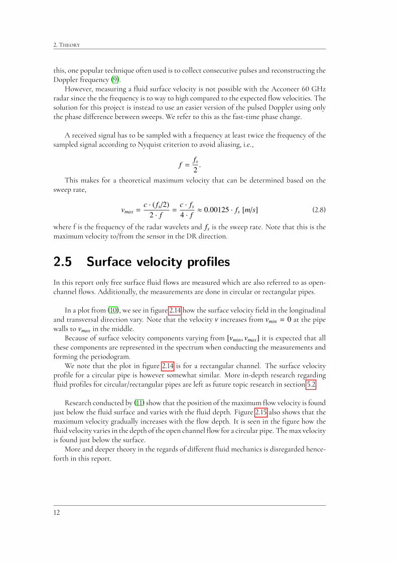
In a plot from (��), we see in �gure �.�� how the surface velocity �eld in the longitudinaland transversal direction vary. Note that the velocity v increases from vmin = 0 at the pipewalls to vmax in the middle.

Because of surface velocity components varying from [vmin, vmax] it is expected that allthese components are represented in the spectrum when conducting the measurements andforming the periodogram.

We note that the plot in �gure �.�� is for a rectangular channel. The surface velocitypro�le for a circular pipe is however somewhat similar. More in-depth research regarding�uid pro�les for circular/rectangular pipes are left as future topic research in section �.�.

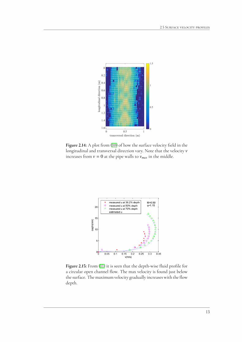
Research conducted by (��) show that the position of the maximum �ow velocity is foundjust below the �uid surface and varies with the �uid depth. Figure �.�� also shows that themaximum velocity gradually increases with the �ow depth. It is seen in the �gure how the�uid velocity varies in the depth of the open channel�ow for a circular pipe. Themax velocityis found just below the surface.

More and deeper theory in the regards of di�erent �uid mechanics is disregarded hence-forth in this report.

��

�.� S��

Figure �.��: A plot from (��) of how the surface velocity �eld in thelongitudinal and transversal direction vary. Note that the velocity vincreases from v = 0 at the pipe walls to vmax in the middle.

Figure �.��: From (��) it is seen that the depth-wise �uid pro�le fora circular open channel �ow. The max velocity is found just belowthe surface. Themaximum velocity gradually increases with the �owdepth.

��

�. T��

��

Chapter �

Methodology

3.1 Sensor Setup

In this project, the �uid surface velocity is measured with a set up demonstrated in �gure �.�.

Figure �.�: The �gure represents the desired setup of the sensorabove a open channel �ow �uid surface, measuring the ’backward’�ow.

��

�. M��

The sensor is placed above the �uid surface with an angle chosen to be �� since it isa trade-o� between receiving re�ections and measuring the horizontal velocity component.We de�ne the direction of �uid �ow as ’backward’ when measuring against the �ow as in�gure �.� and ’forward’ when the �ow is in the opposite direction (�uid moving away fromthe sensor).

Knowledge about the distance dv vertically down from sensor to �uid surface makes itpossible to calculate the angle of incident for di�erent distance points by

' = arcsin(dv

dx). (�.�)

Assuming that the �uid level is stationary compared to the frame rate we can neglect thevertical velocities of the surface since they cancel out each other. Hence the resulting velocitymeasured will be the radial component of the horizontal �uid velocity resulting in a velocityas,

Vf luid = Vmeasured1

cos(') . (�.�)

The di�erent con�guration parameters of the sparse IQ-service are dependant on which�ow you are about to measure. The motivation of the parameters is as follows. Pulse lengthpro�le is selected so that the SNR ismaximisedwithout including direct leakage in the sweep.The number of sweeps within a frame determines the frequency resolution (which is laterconverted to a velocity) and is therefore selected to be large (in our case maximum of ��).The sweep rate is set according to equation �.� so that the maximum measurable velocityis not exceeded and �nally, in order to reduce noise, the HWAAS is set to be fairly high toaverage over more pulses for each data point.

3.2 Data collection

Data are obtained and analyzed from three di�erent settings; in Acconeer lab environment,in a lab environment at a UK-site (similar to our lab setup), and at three sites of VA SYD.For simplicity and structure, results will be presented in this segmentation.

3.2.1 Acconeer lab environment

The initial process of this project was to obtain �uid �ow data to identify relevant charac-teristics and to initiate the analysis of the data. In our lab environment we established a �owdevice consisting of a PVC-tube through which a water could �ow via a garden hose. Thewhole �ow-device could be tilted with some styrofoam discs to achieve di�erent �ow veloc-ities and �uid levels in the pipe. In �gure �.�, the setup in the lab environment is shown. Inthe middle of the PVC-tube a window was cut at which we measure the signal with the A��radar which is connected with some evaluation kit on a Raspberry Pi. The data is transferredvia Wi-�.

��

�.� D��

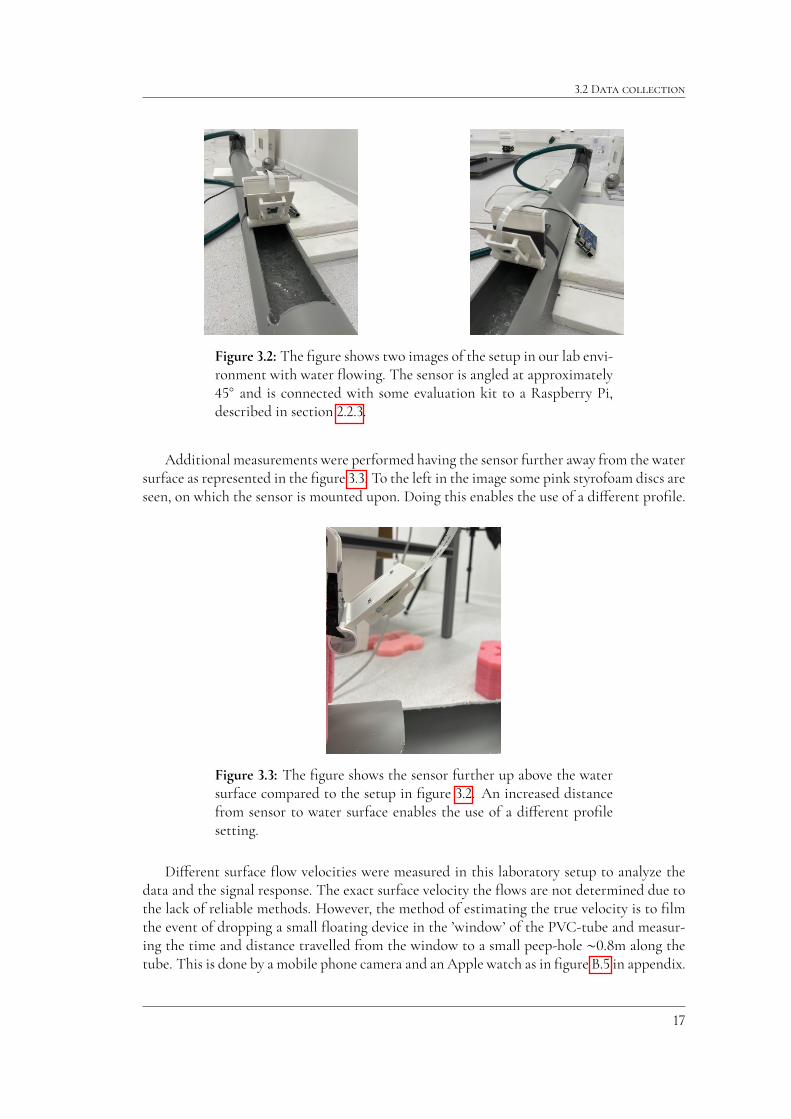
Figure �.�: The �gure shows two images of the setup in our lab envi-ronment with water �owing. The sensor is angled at approximately�� and is connected with some evaluation kit to a Raspberry Pi,described in section �.�.�.

Additional measurements were performed having the sensor further away from the watersurface as represented in the �gure �.�. To the left in the image some pink styrofoam discs areseen, on which the sensor is mounted upon. Doing this enables the use of a di�erent pro�le.

Figure �.�: The �gure shows the sensor further up above the watersurface compared to the setup in �gure �.�. An increased distancefrom sensor to water surface enables the use of a di�erent pro�lesetting.

Di�erent surface �ow velocities were measured in this laboratory setup to analyze thedata and the signal response. The exact surface velocity the �ows are not determined due tothe lack of reliable methods. However, the method of estimating the true velocity is to �lmthe event of dropping a small �oating device in the ’window’ of the PVC-tube and measur-ing the time and distance travelled from the window to a small peep-hole ⇠�.�m along thetube. This is done by a mobile phone camera and an Apple watch as in �gure B.� in appendix.

��

�. M��

The measurement of forward and backward �ow was also conducted, having the samewater �ow through the pipe, but turning the sensor around.

3.2.2 UK lab environment

From a company based in the UK we receive �ow data from their lab environment similarto our own. With exact water dimension measurements and water volume, the average waterspeed can be determined. The setup is shown in �gure �.�. As in our lab environment, thesensor is mounted on some evaluation kit connected to a Raspberry Pi.

Figure �.�: The �gure shows the setup of the lab environment at theUK site used to collect �ow data with reference velocity data.

For the initial measurements from their setup a rectangular open channel pipe was used.If required a circular pipe could be inserted into the channel for circular open channel �ows.The setup for the rectangular open channel pipe is shown in �gure �.�.

Figure �.�: Water �ow in the rectangular open channel on UK labsite.

The sensor casing was angled at ⇠�� towards the water surface, the same as in Acconeerlab environment. The reference �ow rate was measured with a magnetic �ow meter in the

��

�.� D��

return pipe beneath the �ow rig. Note that it is therefore a velocity for the entire �uid �ow,not just the surface velocity.

3.2.3 VA SYD site

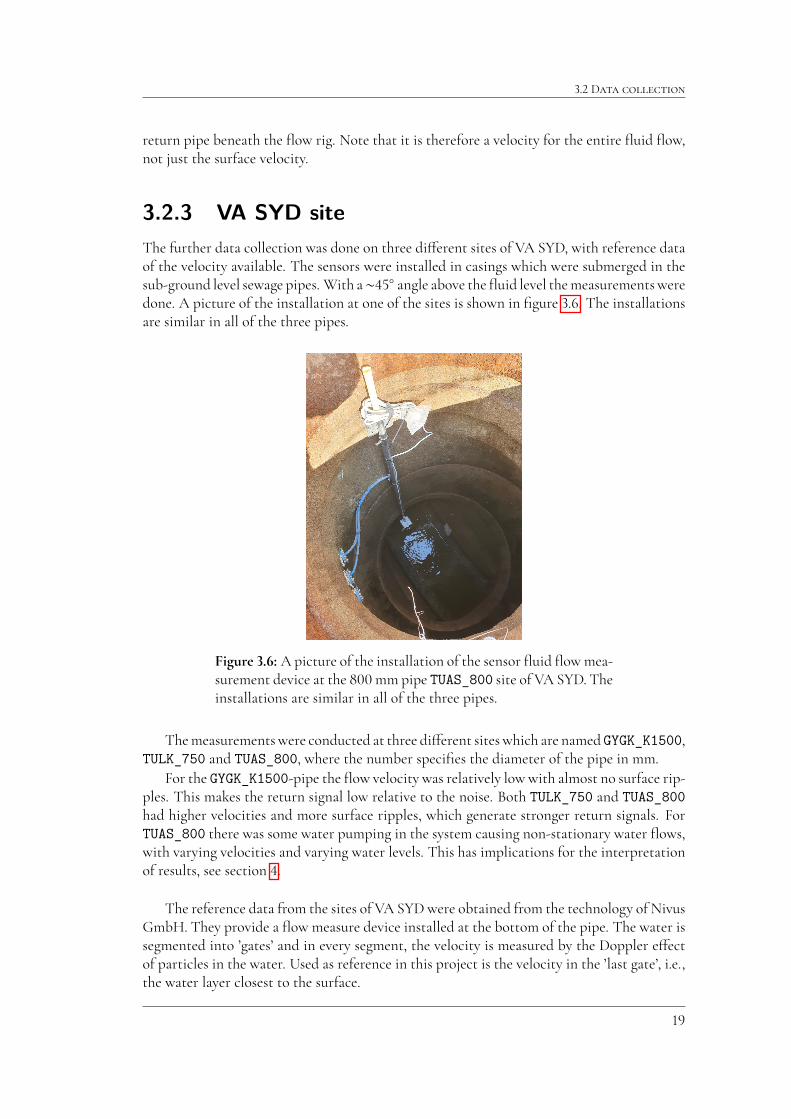
The further data collection was done on three di�erent sites of VA SYD, with reference dataof the velocity available. The sensors were installed in casings which were submerged in thesub-ground level sewage pipes. With a⇠�� angle above the�uid level themeasurements weredone. A picture of the installation at one of the sites is shown in �gure �.�. The installationsare similar in all of the three pipes.

Figure �.�: A picture of the installation of the sensor �uid �owmea-surement device at the ��mmpipe TUAS_800 site of VA SYD. Theinstallations are similar in all of the three pipes.

Themeasurements were conducted at three di�erent sites which are named GYGK_K1500,TULK_750 and TUAS_800, where the number speci�es the diameter of the pipe in mm.

For the GYGK_K1500-pipe the �ow velocity was relatively low with almost no surface rip-ples. This makes the return signal low relative to the noise. Both TULK_750 and TUAS_800had higher velocities and more surface ripples, which generate stronger return signals. ForTUAS_800 there was some water pumping in the system causing non-stationary water �ows,with varying velocities and varying water levels. This has implications for the interpretationof results, see section �.

The reference data from the sites of VA SYDwere obtained from the technology of NivusGmbH. They provide a �ow measure device installed at the bottom of the pipe. The water issegmented into ’gates’ and in every segment, the velocity is measured by the Doppler e�ectof particles in the water. Used as reference in this project is the velocity in the ’last gate’, i.e.,the water layer closest to the surface.

��

�. M��

3.3 Signal processing

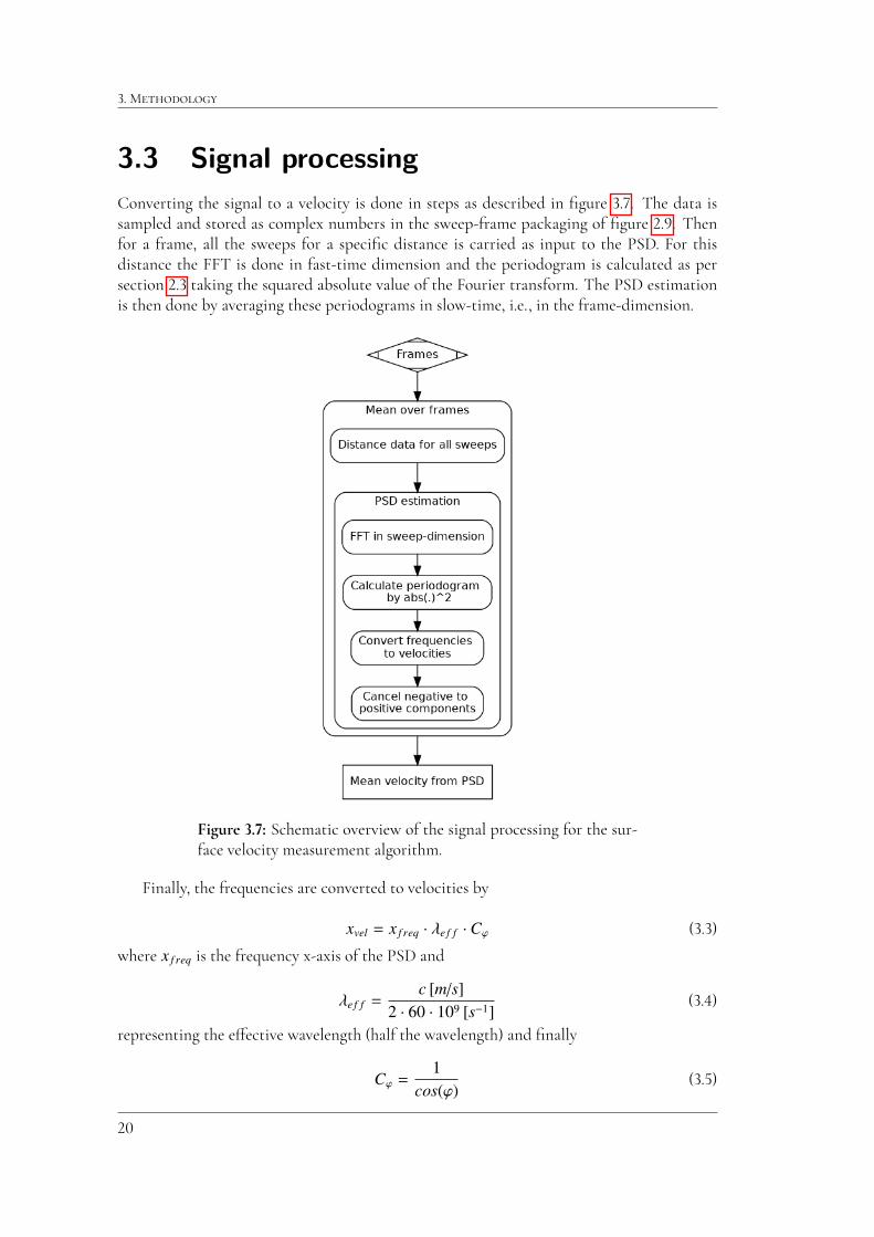
Converting the signal to a velocity is done in steps as described in �gure �.�. The data issampled and stored as complex numbers in the sweep-frame packaging of �gure �.�. Thenfor a frame, all the sweeps for a speci�c distance is carried as input to the PSD. For thisdistance the FFT is done in fast-time dimension and the periodogram is calculated as persection �.� taking the squared absolute value of the Fourier transform. The PSD estimationis then done by averaging these periodograms in slow-time, i.e., in the frame-dimension.

Figure �.�: Schematic overview of the signal processing for the sur-face velocity measurement algorithm.

Finally, the frequencies are converted to velocities by

xvel = x f req · �e f f ·C' (�.�)

where x f req is the frequency x-axis of the PSD and

�e f f =c [m/s]

2 · 60 · 109 [s�1] (�.�)

representing the e�ective wavelength (half the wavelength) and �nally

C' =1

cos(') (�.�)

��

�.� S��

is the compensation for the angle of incident for the re�ected wave. Converting the PSD to amean velocity is a bit tricky since the spectrum will contain low-frequency components thatis considered ’fake’ since they correspond to slow phase-shifts or static re�ections. Possiblythese are due to small movements vertically or leakage in sensor which are cancelled outyielding a more understandable spectrum (to be shown in �gure �.�). Since the x-axis of thespectrum is symmetric the negative and positive side can be cancelled out component-wiseby removing the lowest value (out of the positive and corresponding negative) from both ofthem. Finally the zero-component is set to zero since this would correspond to re�ections ofstatic objects. From this modi�ed spectrum the surface mean velocity is calculated throughmean averaging, as described in section �.�.� and in equation �.�.

This algorithm is done for multiple distance points of the signal. Since the vertical dis-tance from the sensor to the �uid surface dv is known, the angle of incident for the distanced in the trajectory of the sensor is known and we can use multiple distance in the velocityestimation.

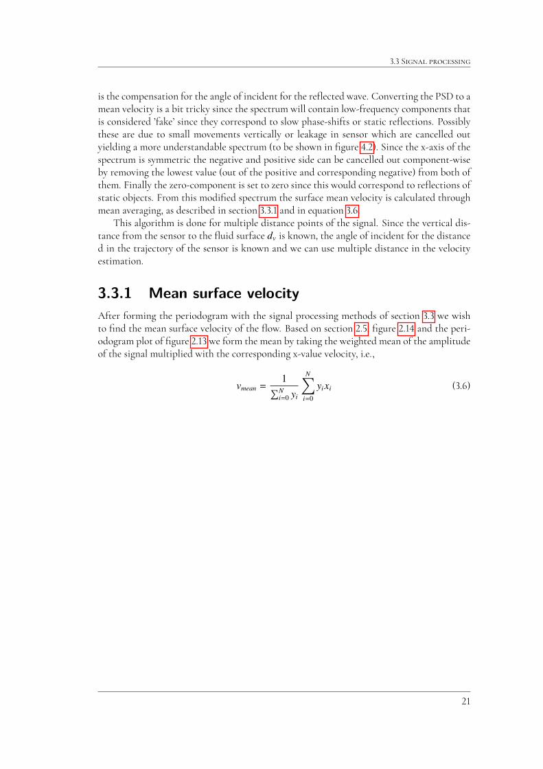
3.3.1 Mean surface velocity

After forming the periodogram with the signal processing methods of section �.� we wishto �nd the mean surface velocity of the �ow. Based on section �.�, �gure �.�� and the peri-odogram plot of �gure �.�� we form the mean by taking the weighted mean of the amplitudeof the signal multiplied with the corresponding x-value velocity, i.e.,

vmean =1

PNi=0 yi

NX

i=0yixi (�.�)

��

�. M��

��

Chapter �

Results and discussion

The measurements of this project are done in three di�erent settings as described earlier. Forclarity and transparency the results will be presented in the same sectioning as before, i.e.,the Acconeer lab, UK lab, and site of VA SYD.

First some results are presented for the step-wise signal processing part of this project.The data is from a measurement in the Acconeer lab. The left hand side plot in �gure �.�show the �rst �� sweeps for some frame in complex value form. To the right is the FFT ofthe same data, with a clear peak at the zero Hz frequency.

Figure �.�: The left plot shows the �rst �� sweeps for some frame,represented in complex value form. The right plot shows the FFT ofthe same data, with a clear peak at the � Hz frequency.

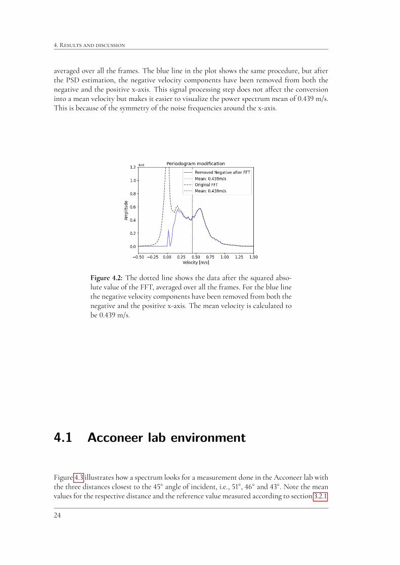
Figure �.� is an example of processing for a measurement. The dotted line shows thePSD estimation of the data, i.e., the squared absolute value of the FFT (the periodogram)

��

�. R��

averaged over all the frames. The blue line in the plot shows the same procedure, but afterthe PSD estimation, the negative velocity components have been removed from both thenegative and the positive x-axis. This signal processing step does not a�ect the conversioninto a mean velocity but makes it easier to visualize the power spectrum mean of �.�� m/s.This is because of the symmetry of the noise frequencies around the x-axis.

Figure �.�: The dotted line shows the data after the squared abso-lute value of the FFT, averaged over all the frames. For the blue linethe negative velocity components have been removed from both thenegative and the positive x-axis. The mean velocity is calculated tobe �.�� m/s.

4.1 Acconeer lab environment

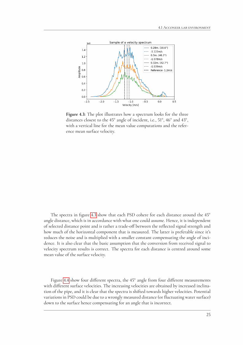
Figure �.� illustrates how a spectrum looks for a measurement done in the Acconeer lab withthe three distances closest to the �� angle of incident, i.e., ��, �� and ��. Note the meanvalues for the respective distance and the reference value measured according to section �.�.�.

��

�.� A��

Figure �.�: The plot illustrates how a spectrum looks for the threedistances closest to the �� angle of incident, i.e., ��, �� and ��,with a vertical line for the mean value computations and the refer-ence mean surface velocity.

The spectra in �gure �.� show that each PSD cohere for each distance around the ��angle distance, which is in accordance with what one could assume. Hence, it is independentof selected distance point and is rather a trade-o� between the re�ected signal strength andhow much of the horizontal component that is measured. The latter is preferable since it’sreduces the noise and is multiplied with a smaller constant compensating the angle of inci-dence. It is also clear that the basic assumption that the conversion from received signal tovelocity spectrum results is correct. The spectra for each distance is centred around somemean value of the surface velocity.

Figure �.� show four di�erent spectra, the �� angle from four di�erent measurementswith di�erent surface velocities. The increasing velocities are obtained by increased inclina-tion of the pipe, and it is clear that the spectra is shifted towards higher velocities. Potentialvariations in PSD could be due to a wrongly measured distance (or �uctuating water surface)down to the surface hence compensating for an angle that is incorrect.

��

�. R��

Figure �.�: Plot of the measurement for the �� angle for four di�er-ent water �ow velocities. The dashed lines are the calculated meansurface velocity of the respective measurement.

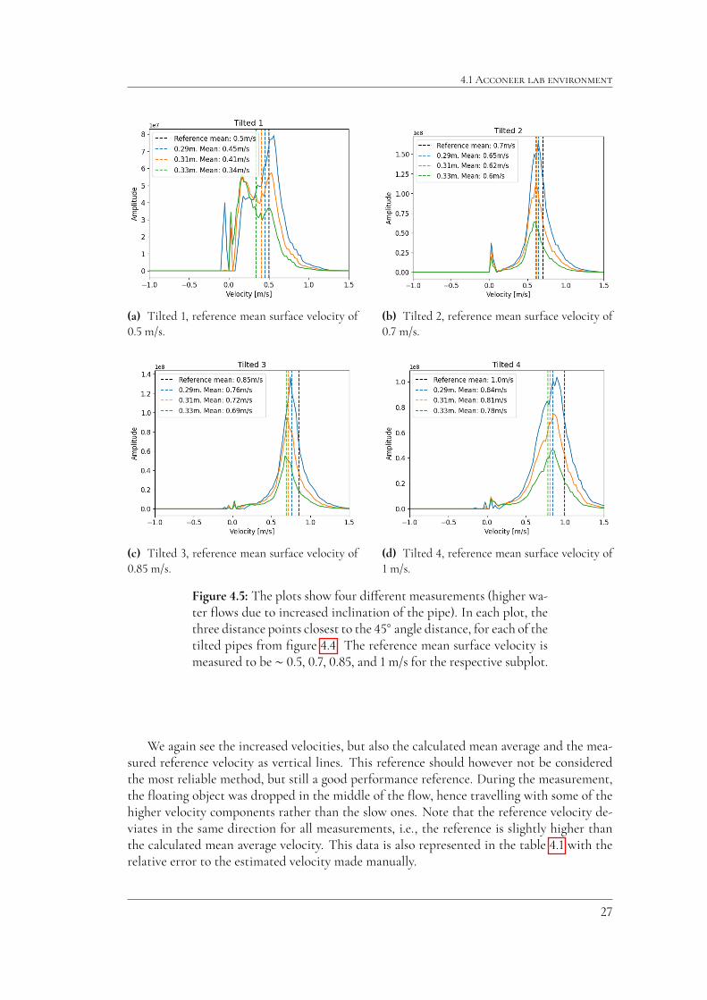
Furthermore the subplots presented in �gure �.� are the same tilted measurements asin �gure �.�, but with the three distance points closest to the �� angle. An approximatemeasurement of the reference surface velocity is done and represented in the plot.

��

�.� A��

(a) Tilted �, reference mean surface velocity of�.� m/s.

(b) Tilted �, reference mean surface velocity of�.� m/s.

(c) Tilted �, reference mean surface velocity of�.�� m/s.

(d) Tilted �, reference mean surface velocity of� m/s.

Figure �.�: The plots show four di�erent measurements (higher wa-ter �ows due to increased inclination of the pipe). In each plot, thethree distance points closest to the �� angle distance, for each of thetilted pipes from �gure �.�. The reference mean surface velocity ismeasured to be ⇠ �.�, �.�, �.��, and �m/s for the respective subplot.

We again see the increased velocities, but also the calculated mean average and the mea-sured reference velocity as vertical lines. This reference should however not be consideredthe most reliable method, but still a good performance reference. During the measurement,the �oating object was dropped in the middle of the �ow, hence travelling with some of thehigher velocity components rather than the slow ones. Note that the reference velocity de-viates in the same direction for all measurements, i.e., the reference is slightly higher thanthe calculated mean average velocity. This data is also represented in the table �.� with therelative error to the estimated velocity made manually.

��

�. R��

Table �.�: A table over the estimated and obtained velocities in [m/s]together with a percentage of error in parenthesis for the data in�gure �.�.

Ref velocity d� d� d�Tilted � �.� �.�� (-��%) �.�� (-��%) �.�� (-��%)Tilted � �.� �.�� (-�%) �.�� (-��%) �.� (-��%)Tilted � �.�� .�� (-��%) �.�� (-��%) �.�� (-��%)Tilted � �.� �.�� (-��%) �.�� (-��%) �.�� (-��%)

Figure �.� shows the measurement done for the same �ow and settings, only havingturned the sensor around, i.e., measuring the forward and backward �ow. By Acconeer con-vention the forward �ow is ’positive’. Figure �.�a is the original result and in �gure �.�b thebackward �ow is mirrored in the y-axis centred around zero.

(a) Original data (b) Mirroring the backward �ow

Figure �.�: The signal for the distance closest to the �� angle formeasurement forward and backward to the �ow. The spectra aresimilar. The reference mean water surface velocity is measured to be⇠ �.� m/s as shown in the vertical line.

The two measurements show similar spectra which are both centred around approxi-mately the same mean velocity and has the same amplitude. The reference mean water sur-face velocity is measured to be ⇠ �.� m/s. From this, we see that the �owing direction iseasy to determine. When mirroring these spectra in the x-axis as in �gure �.�b the PSD’s areoverlapping with approximately the same mean surface velocity. Assuming that the �ow wasconstant and distributed in the same way within the pipe during the two measurements thisis a satisfactory result. These results gives proof-of-concept in the area of measuring di�erent�ow directions. This is important for future further development. All of the results regardingcorrelation between �ow velocity and �owing direction is important, and give the necessarybasis for further implementation of the surface velocity algorithm for the A�� sensor.

��

�.� UK ��

4.2 UK lab environment

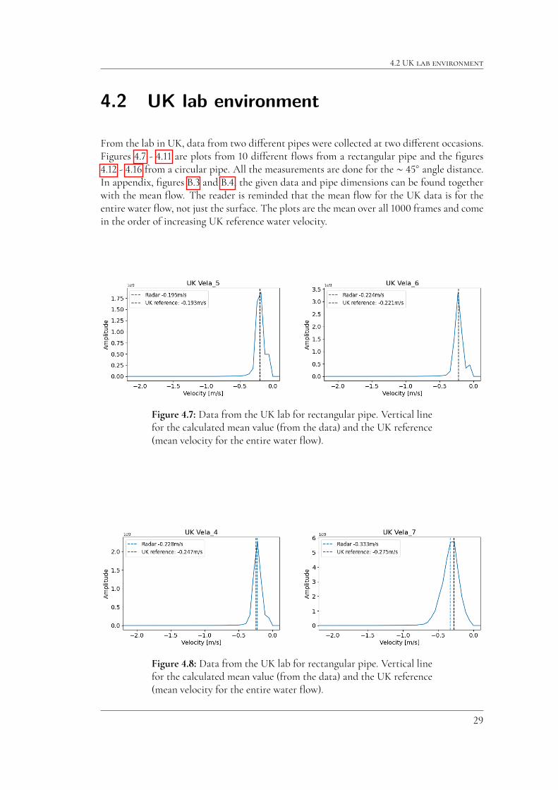
From the lab in UK, data from two di�erent pipes were collected at two di�erent occasions.Figures �.� - �.�� are plots from �� di�erent �ows from a rectangular pipe and the �gures�.�� - �.�� from a circular pipe. All the measurements are done for the ⇠ �� angle distance.In appendix, �gures B.� and B.�, the given data and pipe dimensions can be found togetherwith the mean �ow. The reader is reminded that the mean �ow for the UK data is for theentire water �ow, not just the surface. The plots are the mean over all �� frames and comein the order of increasing UK reference water velocity.

Figure �.�: Data from the UK lab for rectangular pipe. Vertical linefor the calculated mean value (from the data) and the UK reference(mean velocity for the entire water �ow).


��

�. R��


Figure �.��: Data from the UK lab for rectangular pipe. Vertical linefor the calculated mean value (from the data) and the UK reference(mean velocity for the entire water �ow).

Figure �.��: Data from the UK lab for rectangular pipe. Vertical linefor the calculated mean value (from the data) and the UK reference(mean velocity for the entire water �ow).

��

�.� UK ��

Figure �.��: Data from the UK lab for circular pipe. Vertical linefor the calculated mean value (from the data) and the UK reference(mean velocity for the entire water �ow).



��

�. R��



For the rectangular pipe measurements of �gure �.� - �.��, the radar generally predicts ahigher mean surface velocity than the calculated average mean velocity. The spectra of theseplots contain only one peak which is in accordance with the plots of �gure �.�a - �.�d insection �.�. For the circular pipe measurements of �gure �.�� - �.��, the predictions of themean surface velocity is signi�cantly lower than the UK reference velocity and now multiplepeaks are seen in the spectra. The results from the UK lab can be visualised in table �.� andtable �.� respectively. The tables shows the mean velocity in [m/s] together with the error incomparison to the reference mean velocity.

��

�.� UK ��

Table �.�: The table displays the mean reference velocity for all mea-surements from the rectangular pipe together with the calculatedmean velocity from the sensor. All values are in [m/s] and in ad-dition to the velocity the error to the reference is calculated in theparenthesis.

Name Reference mean All framesVela� �.�� .�� (+��%)Vela� �.�� .�� (+��%)Vela� �.�� .�� (+��%)Vela� �.�� .�� (-�%)Vela� �.�� .�� (+�%)Vela� �.�� .�� (+�%)Vela� �.�� .�� (+��%)Vela� �.�� .�� (+��%)Vela�� .�� .�� (+��%)Vela�� .�� .�� (-��%)

Table �.�: The table displays the mean reference velocity for all mea-surements from the circular pipe together with the calculated meanvelocity from the sensor. All values are in [m/s] and in addition tothe velocity the error to the reference is calculated in the parenthe-sis.

Name Reference mean All framesVelb� �.�� .�� (-��%)Velb� �.�� .�� (-��%)Velb� �.�� .�� (-��%)Velb� �.�� .�� (-��%)Velb� �.�� .�� (-��%)Velb� �.�� .�� (-��%)Velb� �.�� .�� (-��%)Velb� �.�� .�� (-��%)Velb� �.�� .�� (-��%)Velb�� .�� .�� (-��%)

Hence the rectangular pipe have a mean percentage error of +��% and the circular pipehave a mean error of -��% using all frames from the measurement.

Since the data presented in table �.� and �.� is the mean of all �� frames it is interestingto investigate any possible variation within these frames. Figures �.�� - �.�� show the varia-tions for the slowest and fastest UK lab measurements for both the rectangular- and circularpipe. Each plot for � di�erent ’frame windows’ of �� consecutive frames together with theirmean velocity. Additionally, the mean velocity over frames (over time) is represented belowthe power spectra. Here, two dashed lines in green represents the ��% error to the referenceto facilitate interpretation of the velocity results.

��

�. R��

Figure �.��: The frame variation of UK Vela � data (rectangularpipe). Both the power spectra and the mean velocity over frames.

Figure �.��: The frame variation of UK Vela �� data (rectangularpipe). Both the power spectra and the mean velocity over frames.

The mean velocity of Vela_� is alternating around the reference mean within the ��% er-ror except for the for the last �� frames. During this time the amplitude of the spectrumsuddenly decreases causing the mean to go to zero which also can be seen in �gure �.��. Ac-cording to �gure �.��, the �ow velocity appears to be stationary with overlapping PSD’s. Thevariations between the frame windows is small and the velocity is lower than the referencethroughout the measurement.

��

�.� UK ��

Figure �.��: The frame variation of UK Velb � data (circular pipe).Both the power spectra and the mean velocity over frames.

Figure �.��: The frame variation of UK Velb � data (circular pipe).Both the power spectra and the mean velocity over frames.

Figure �.�� show that the mean surface velocity is constantly lower than the referencemean and there is basically one frame window that di�ers signi�cantly from the others(frames ��-��) with a PSD peak at⇠�.�m/s. Similarly, �gure �.�� show similar PSDwith amean velocity signi�cantly lower than the reference mean. The PSD and hence the mean sur-face velocity may vary over time. There is a possibility that the water pump �ow rate (whichis set to a constant rate on the UK-pipe) vary over time or that the water level is not station-ary which results in this time variation over di�erent frames. For the rectangular pipe themean surface velocity of the radar sensor increases as the reference increases. For the circularpipe it occurs multiple peaks. This is an odd phenomenon but since these measurements aredone o�-site it is hard to identify any speci�c sources of error. They may however arise dueto some �uid dynamical ’fringe-formation’. We have higher velocities for the circular pipethan for the rectangular, seen in �gures �.� - �.��, which may cause a much more turbulent�ow and hence irregularities in the surface ripples.

��

�. R��

4.3 VA SYD site

The results of this segment are partitioned into the di�erent sites where we have measured,namely GYGK_K1500 (�� mm), TULK_750 (�� mm), and TUAS_800 (�� mm). Data wascollected on site at three di�erent dates and is therefore named as measurement �-�. Forall results in this part there is an associated timestamp to all plots and the data is collectedover one whole minute (corresponding to approximately �� frames in this setting) beforethe timestamp. For example, ��:�� means that data is collected from ��:��:��-��:��:��. Thereference velocity data of Nivus is for the last gate of the water layers, i.e., closest to thesurface.

4.3.1 1500 mm

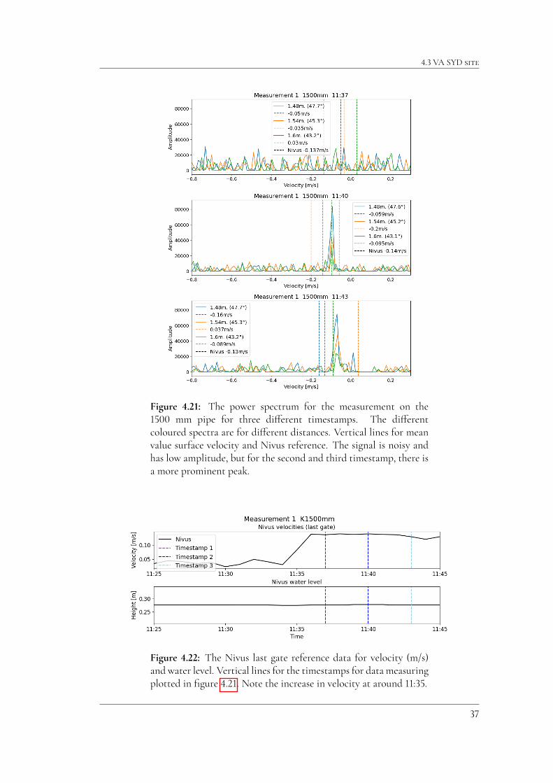
For the ��mmpipe, measurements were only conducted at one occasion. Figure �.�� showsthe power spectrum for three di�erent timestamps and distances. In �gure �.��, the Nivusreference data is plotted for the same period and timestamps.

��

�.� VA SYD ��

Figure �.��: The power spectrum for the measurement on the�� mm pipe for three di�erent timestamps. The di�erentcoloured spectra are for di�erent distances. Vertical lines for meanvalue surface velocity and Nivus reference. The signal is noisy andhas low amplitude, but for the second and third timestamp, there isa more prominent peak.

Figure �.��: The Nivus last gate reference data for velocity (m/s)and water level. Vertical lines for the timestamps for data measuringplotted in �gure �.��. Note the increase in velocity at around ��:��.

��

�. R��

As can be seen in �gure �.�� the re�ected signal amplitude was low and the signal becamenoisy. This was caused by a smooth water �ow with almost no ripples on the water surface.There is however somemore protruding peaks for timestamps ��:�� and ��:�� around �.��m/swhich indicates that there is actually some surface velocity that is detected by the sensor. Forfurther investigations it would be interesting to tilt the sensor down even further to receivestronger re�ections. Looking at the velocities of �gure �.�� there is a sudden jump from⇠�.�� m/s to ⇠�.�� m/s from ��:�� to ��:�� while constant water level. This was due to amanual cleaning of the sensor. The conclusion is that the Nivus reference system is in needof cleaning before measurement which was not done in all of the second measurements.

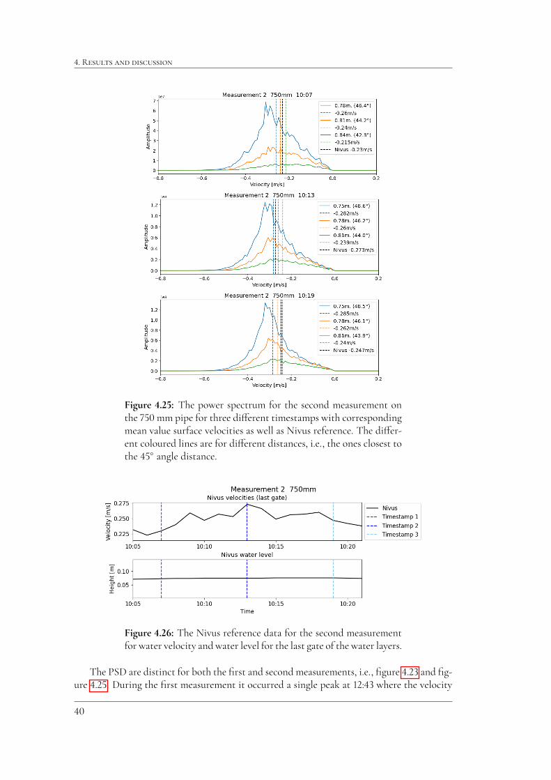
4.3.2 750 mm

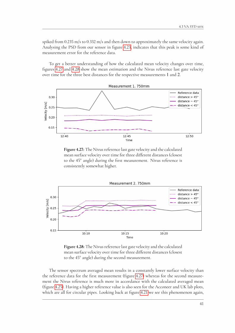
Figure �.�� and �.�� shows the power spectrum for the �rst and second measurement onthe �� mm pipe for three di�erent timestamps. The plots show spectra for three distancesclosest to the �� angle distance with corresponding mean surface velocities as well as Nivusreference. Figure �.�� and �.�� shows the Nivus reference data for water velocity and waterlevel in the ’last gate’ for the three timestamps in �gure �.�� and �.��, respectively.

��

�.� VA SYD ��

Figure �.��: The power spectra for the �rst measurement on the�� mm pipe for three di�erent timestamps with correspondingmean value surface velocities as well as Nivus reference. The dif-ferent coloured lines are for di�erent distances, i.e., the ones closestto the �� angle distance.

Figure �.��: The Nivus reference data for water velocity and waterlevel for the last gate of the water layers. The water level is somewhatconstant, while the last gate velocity has a spike for timestamp �.

��

�. R��

Figure �.��: The power spectrum for the second measurement onthe ��mm pipe for three di�erent timestamps with correspondingmean value surface velocities as well as Nivus reference. The di�er-ent coloured lines are for di�erent distances, i.e., the ones closest tothe �� angle distance.

Figure �.��: The Nivus reference data for the second measurementfor water velocity and water level for the last gate of the water layers.

The PSD are distinct for both the �rst and second measurements, i.e., �gure �.�� and �g-ure �.��. During the �rst measurement it occurred a single peak at ��:�� where the velocity

��

�.� VA SYD ��

spiked from �.��m/s to �.��m/s and then down to approximately the same velocity again.Analysing the PSD from our sensor in �gure �.��, indicates that this peak is some kind ofmeasurement error for the reference data.

To get a better understanding of how the calculated mean velocity changes over time,�gures �.�� and �.�� show the mean estimation and the Nivus reference last gate velocityover time for the three best distances for the respective measurements 1 and 2.

Figure �.��: TheNivus reference last gate velocity and the calculatedmean surface velocity over time for three di�erent distances (closestto the �� angle) during the �rst measurement. Nivus reference isconsistently somewhat higher.

Figure �.��: TheNivus reference last gate velocity and the calculatedmean surface velocity over time for three di�erent distances (closestto the �� angle) during the second measurement.

The sensor spectrum averaged mean results in a constantly lower surface velocity thanthe reference data for the �rst measurement (�gure �.��) whereas for the second measure-ment the Nivus reference is much more in accordance with the calculated averaged mean(�gure �.��). Having a higher reference value is also seen for the Acconeer and UK lab plots,which are all for circular pipes. Looking back at �gure �.�� we see this phenomenon again,

��

�. R��

the reference is slightly higher. However, for the secondmeasurement of the ��mmpipe theNivus sensor was not cleaned, which may have caused a lower value of the velocity. The factthat we get a lower velocity is interesting and for the VA SYD measurements it is somewhatreasonable. The Nivus reference does not measure the surface but the last gate velocity, whichshould be slightly higher, in accordance to �gure �.��. However, for the Acconeer and UKlab environment it is fascinating and may be caused by some �uid dynamics of circular pipes.This e�ect could a�ect and potentially accentuate the o�-set of VA SYD measurements.

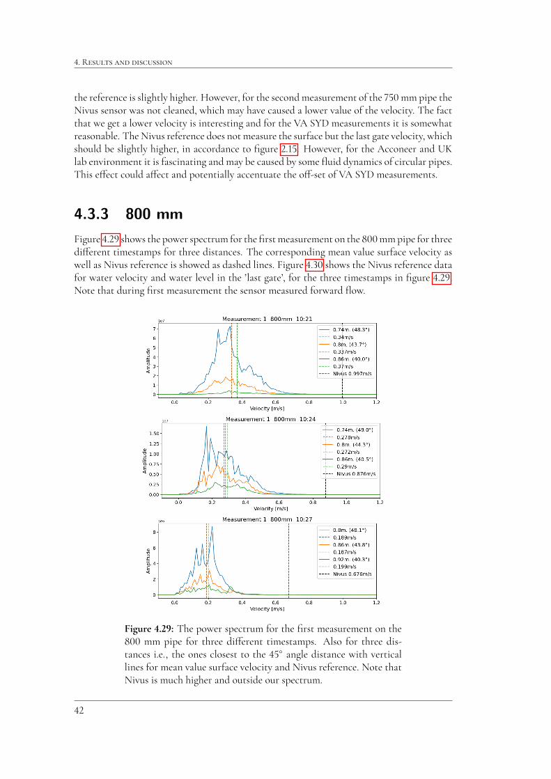
4.3.3 800 mm

Figure �.�� shows the power spectrum for the�rstmeasurement on the ��mmpipe for threedi�erent timestamps for three distances. The corresponding mean value surface velocity aswell as Nivus reference is showed as dashed lines. Figure �.�� shows the Nivus reference datafor water velocity and water level in the ’last gate’, for the three timestamps in �gure �.��.Note that during �rst measurement the sensor measured forward �ow.

Figure �.��: The power spectrum for the �rst measurement on the�� mm pipe for three di�erent timestamps. Also for three dis-tances i.e., the ones closest to the �� angle distance with verticallines for mean value surface velocity and Nivus reference. Note thatNivus is much higher and outside our spectrum.

��

�.� VA SYD ��

Figure �.��: The Nivus reference data for the �rst measurement ofthe ��mmpipe forwater velocity andwater level for the last gate ofthe water layers with dashed vertical lines for the three timestampsrepresented in �gure �.��.

Figure �.�� and �gure �.�� show the power spectrum for the second measurement on the��mm pipe for di�erent timestamps with vertical lines for the mean value surface velocityas well as Nivus reference. Figure �.�� shows the Nivus reference data for water velocityand water level in the ’last gate’ for the the timestamps of �gures �.�� and �.��. The secondmeasurement was conducted measuring backward �ow as seen in the plots.

��

�. R��

Figure �.��: The power spectrum for the �rst second measurementon the �� mm pipe for three di�erent timestamps. The di�erentcoloured lines are for di�erent distances, i.e., the ones closest to the�� angle distance.

Figure �.��: TheNivus reference data for the secondmeasurement ofthe ��mmpipe forwater velocity andwater level for the last gate ofthe water layers. The dashed vertical lines represent the timestampsrepresented in �gures �.�� - �.��.

��

�.� VA SYD ��

Figure �.��: Power spectrum for the second measurement on the��mmpipe for three di�erent timestamps. The di�erent colouredlines are for di�erent distances, i.e., the ones closest to the �� angledistance. The vertical lines represent the mean value surface velocityand Nivus reference.

Due to the non-stationary �ow of the TUAS_800, the sensor cleaned itself, hence missingthe cleaning during the second measurement had less impact on the reference data. Dur-ing measurement �, i.e., �gure �.��, we get a relatively strong return signal and nice spectra.However, the Nivus reference is way o�. During measurement �, �gure �.�� and �gure �.��,only ��:�� has an ’acceptable’ PSD peak that includes the reference velocity and ��:�� havinga reasonable peak but outside the mean velocity. The other selected timestamps during thismeasurement results in a mean velocity close to zero since there is no signal strength withfrequency content. For the timestamps during measurement � the signal strength was betterthan the �rst two times. With the timestamps in mind there seem to be some correlationbetween the water level and the received frequency content, sometimes there is no signal andsuddenly there is a ’good’ signal.

Measurements were made for a third time from this pipe as well, measuring backward�ow. For �gure �.�� data were collected as before but for �gure �.�� the sensor was replacedwith another sensor. Figure �.�� represents the reference data with vertical lines for the Nivusreference data.

��

�. R��

Figure �.��: First third measurement (the old sensor) for three dif-ferent timestamps. The signal strength is not that high. The di�er-ent coloured spectra are for di�erent distances, i.e., the ones closestto the �� angle distance. Vertical lines represent mean value sur-face velocity andNivus reference. Note that Nivus reference is muchhigher than calculated mean and outside spectrum.

Figure �.��: TheNivus reference data for last gate velocity andwaterlevel for the timestamps of �gures �.�� and �.��.

��

�.� VA SYD ��

Figure �.��: Second third measurement, i.e., with a new sensor, forthree di�erent timestamps. Again, the coloured spectra are for dif-ferent distances, i.e., the ones closest to the �� angle distance. Ver-tical lines represent mean value surface velocity andNivus reference.The signal strength seems somewhat higher than in �gure �.��.

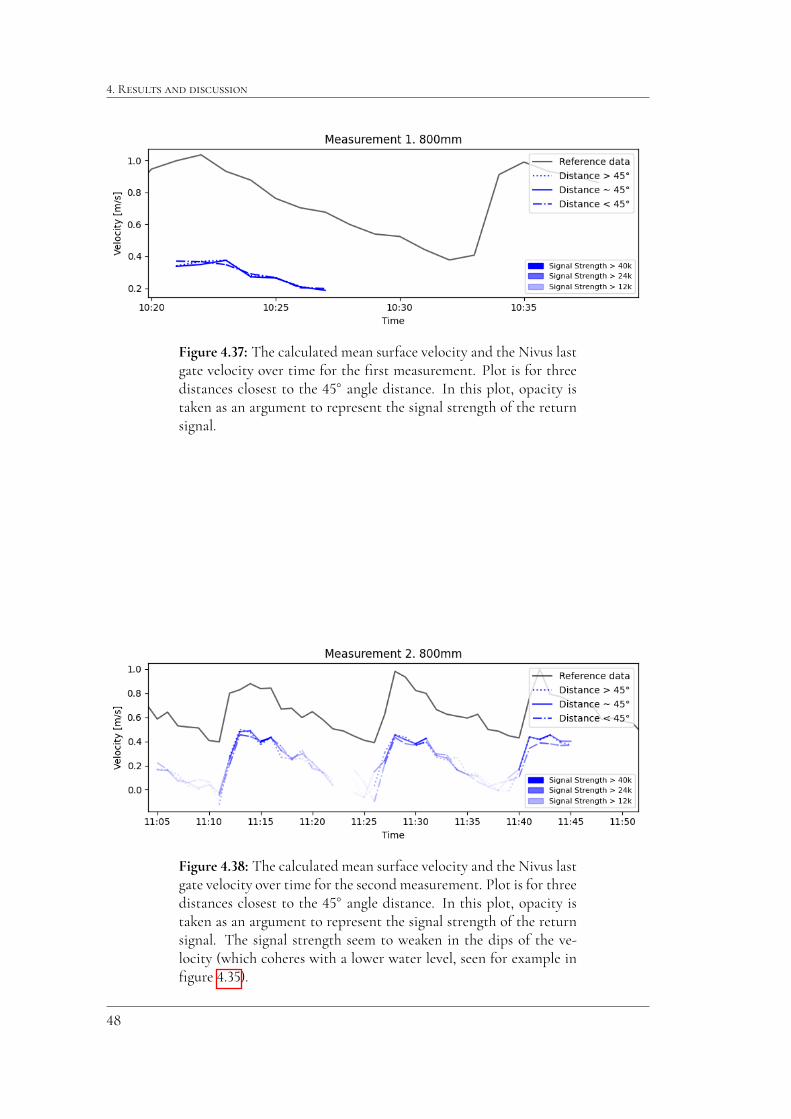
To get a better understanding of how the mean velocity changed over time, �gures �.�� -�.�� show the calculated mean surface velocity and the Nivus last gate reference over time forthe three best distances, i.e., closes to the �� distance. For these plots the signal strength isalso represented in di�erent opacities (the signal strength refers to the the mean amplitudeof the spectrum). As reference the PSD spectrum at ��:�� in �gure �.�� is set to be relativelygood and therefore have a signal strength of ��% yielding that an amplitude mean of morethan ��k counts as full signal strength. Note that the signal strength seem to weaken in thedips of the Nivus reference velocity. Looking at e.g. �gure �.�� we see that the last gatevelocity periodically varies in sync with the water level.

��

�. R��

Figure �.��: The calculated mean surface velocity and the Nivus lastgate velocity over time for the �rst measurement. Plot is for threedistances closest to the �� angle distance. In this plot, opacity istaken as an argument to represent the signal strength of the returnsignal.

Figure �.��: The calculated mean surface velocity and the Nivus lastgate velocity over time for the second measurement. Plot is for threedistances closest to the �� angle distance. In this plot, opacity istaken as an argument to represent the signal strength of the returnsignal. The signal strength seem to weaken in the dips of the ve-locity (which coheres with a lower water level, seen for example in�gure �.��).

��

�.� VA SYD ��

Figure �.��: The calculated mean surface velocity and the Nivus lastgate velocity over time for the third measurement. Plot is for threedistances closest to the �� angle distance. In this plot, opacity istaken as an argument to represent the signal strength of the returnsignal. The signal strength seem to weaken in the dips of the ve-locity (which coheres with a lower water level, seen for example in�gure �.��).

The change in return signal in relation to the non-stationary water levels are investigatedin �gures �.�� - �.��. The signal strength is best at the beginning of and during the peaksand decreasing during the ’slowdown’ which eventually becomes noisy in the dips. Note thatmeasurement � in �gure �.�� has a stronger return signal than then other measurements. Thismeasurement was done with the forward �ow. Looking at �gure �.�� after ��:�� we have astronger return signal than before. These measurements were done with a new sensor whichwas installed. There is a possibility that the sensor angle was di�erent at these times andpossibly resulting in more signal received by the sensor compared to the other ��mmmea-surements. For a di�erent angle, the spectra should also be compensated with a di�erentfactor, possibly generating measurements more in accordance with Nivus reference, espe-cially for the measurement � in �gure �.��. However, since the exact operation of the Nivusreference gauge is unknown, it is of course possible that Nivus measure way too high values.Another source of error could be the �uid dynamics of non-stationary water �ows. Sincemeasurement � has the best return signal and i.e., PSD it is also the possibility of some faultysensor behaviour.

��

�. R��

��

Chapter �

Conclusions

This project set out to measure the surface velocity of a �uid using the Acconeer A�� pulsedcoherent sensor with fast-time phase change of the pulsed wave. The complex valued data ofthe returned signal data is converted to the frequency domain. The results of the measure-ments are presented and discussed in section � above.

5.1 Summary

In this project, we implement an algorithm for converting the returned signal of the Ac-coneer A�� pulsed coherent radar sensor from a �uid surface into a mean velocity. Themain goal is to determine proof-of-concept for measuring �uid �ow surface velocities. Asthe result shows, a forward �ow can easily be distinguished from a backward �ow. This re-sult is of great importance in the aspect of developing better infrastructure and supervisionof e.g. sewage systems. If the vertical distance from sensor to surface is known, the result isindependent of selected distance point and the PSD’s are overlapping. Furthermore, thereis a clear di�erence between �ow velocities, as higher velocities shifts the velocity spectratowards higher velocities.

There seem to be a di�erence (estimated vs reference mean) between the circular andrectangular pipe, where the reference is higher for almost all measurements for the circularpipes and that the reference is lower for the rectangular pipe. This is interesting and a po-tential future topic research, in combination with deeper knowledge of �uid dynamics andapplication-speci�c implementation.

In order to detect surface velocities, the surface needs to have ripple-/wave formationsin order to receive re�ected signals. E.g. for the �� mm pipe, the return signal is weak incomparison to the noise. There is however some protruding peak which cohere with Nivusreference. For a pipe like this, speci�c algorithm and signal processing may be suitable.

��

�. C��

5.2 Topical future research

Since the relation between the surface velocity and the mean velocity is both dependant onthe pipe’s shape and �uid level it would be interesting to combine the measured spectrumdata with �uid dynamics of certain pipes. With deeper knowledge about �uid dynamics,one could �nd precise methods to convert the surface velocity measurement to �uid meanvelocity.

For further investigations in this subject it would be interesting to see how the sensorangle a�ects the measurements. The angle-parameter is the trade-o� between signal strengthand measuring the horizontal component and maybe a steeper angle than ��, especially forsmooth �ows like our �� mm pipe, would be bene�cial.

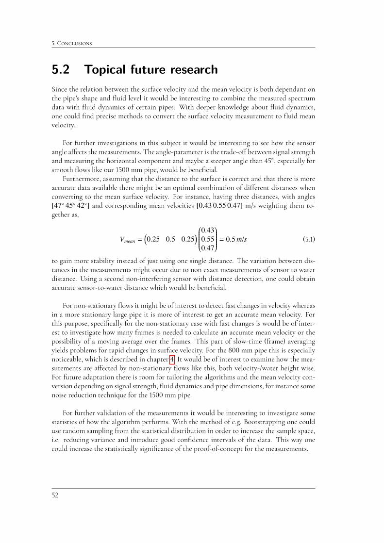
Furthermore, assuming that the distance to the surface is correct and that there is moreaccurate data available there might be an optimal combination of di�erent distances whenconverting to the mean surface velocity. For instance, having three distances, with angles[47� 45� 42�] and corresponding mean velocities [0.43 0.55 0.47] m/s weighting them to-gether as,

Vmean =⇣0.25 0.5 0.25

⌘0BBBBBBBB@

0.430.550.47

1CCCCCCCCA = 0.5 m/s (�.�)

to gain more stability instead of just using one single distance. The variation between dis-tances in the measurements might occur due to non exact measurements of sensor to waterdistance. Using a second non-interfering sensor with distance detection, one could obtainaccurate sensor-to-water distance which would be bene�cial.

For non-stationary �ows it might be of interest to detect fast changes in velocity whereasin a more stationary large pipe it is more of interest to get an accurate mean velocity. Forthis purpose, speci�cally for the non-stationary case with fast changes is would be of inter-est to investigate how many frames is needed to calculate an accurate mean velocity or thepossibility of a moving average over the frames. This part of slow-time (frame) averagingyields problems for rapid changes in surface velocity. For the �� mm pipe this is especiallynoticeable, which is described in chapter �. It would be of interest to examine how the mea-surements are a�ected by non-stationary �ows like this, both velocity-/water height wise.For future adaptation there is room for tailoring the algorithms and the mean velocity con-version depending on signal strength, �uid dynamics and pipe dimensions, for instance somenoise reduction technique for the �� mm pipe.

For further validation of the measurements it would be interesting to investigate somestatistics of how the algorithm performs. With the method of e.g. Bootstrapping one coulduse random sampling from the statistical distribution in order to increase the sample space,i.e. reducing variance and introduce good con�dence intervals of the data. This way onecould increase the statistically signi�cance of the proof-of-concept for the measurements.

��

References

[�] M. A. R. et al., Principles of modern radar: Basic principles, Volume �. Institution of Engi-neering Technology, ��.

[�] C. Wol�, Coherence in Radar. Available at https://www.radartutorial.eu/11.coherent/co05.en.html, accessed ��-��-��.

[�] A. AB, Introduction to Acconeer’s sensor technology. Avail-able at https://developer.acconeer.com/download/introduction-to-acconeers-sensor-technology-pdf, accessed ��-��-��.

[�] A. AB, Acconeer Sparse service. Available at https://docs.acconeer.com/en/latest/services/sparse.html, accessed ��-��-��.

[�] A. AB, Getting Started Guide Lens Evaluation Kit LH��/��/��.Available at https://developer.acconeer.com/download/getting-started-guide-lenses-pdf/, accessed ��-��-��.

[�] S. Engelberg, Digital Signal Processing. Springer-Verlag London Limited, ��.

[�] M. N. S. S. K. Deergha Rao, Digital Signal Processing; Theory and practice. Springer Singa-pore, ��.

[�] V. C. Chen, The Micro-Doppler E�ect in Radar. ARTECH HOUSE, ��.

[�] P. Anju, A. Bazil Raj, and C. Shekhar, “Pulse doppler processing - a novel digital tech-nique,” in �� th International Conference on Intelligent Computing and Control Systems(ICICCS), pp. ��–��, ��.

[��] D. D. Ludovic Cassan, Héléne Roux, Velocity distribution in open channel flow with spatiallydistributed roughness.

[��] Y. J. et al., Analysis of the Velocity Distribution in Partially-Filled Circular PipeEmploying the Principle of Maximum Entropy. PLoS ONE ��(�): e��.doi:��.��/journal.pone.��, March ��, ��.

��

REFERENCES

[��] W. D. Kimura, Electromagnetic Waves and Lasers (Second Edition). IOP Publishing, ��.

[��] D. Gri�ths, Introduction to Electrodynamics, ch. �, p.��-��. Upper Saddle River, N.J:Prentice Hall, ��, �th edition.

[��] R. Fitzpatrick, Reflection at a dielectric boundary. Available at https://farside.ph.utexas.edu/teaching/em/lectures/node104.html, accessed ��-��-��.

[��] A. S. Maths and Physics, The Inverse Square Law for Electromagnetic Waves.Available at https://astarmathsandphysics.com/o-level-physics-notes/254-the-inverse-square-law-for-electromagnetic-waves.html, accessed��-��-��.

��

Appendices

��

Appendix A

Electromagnetic Waves

A.1 Basics

Electromagnetic waves are composed of oscillating magnetic- (B) and electric �elds (E)which are orthogonal to the propagating direction (often called k-vector) and is visualized in�gure A.� (��).

x

y

z k

E

B

Figure A.�: The �gure shows the EM wave where the magnetic �eldand electric�eld is orthogonal to both each other and to the k-vectorrespectively.

The most common wave equation is

f (z, t) = A cos⇥k(z � vt) + �⇤ (A.�)where t represents time, z the distance in the propagating direction, A the amplitude of thewave. The argument of the cosine is called the phase and � represents the phase shift (��).

The parameter k in equation A.� is the wave number and can be expressed with the wavelength � as,

k = 2⇡�. (A.�)

��

A. E��W��

A

�

vz

f (z; 0)

Figure A.�: The �gure is an illustration of the simple cosine wave.

For a given point, letting the wave complete a full cycle is de�ned as a period,

T = 2⇡kv =

�

v (A.�)

with a corresponding frequency

f = 1T =

v�

(A.�)

which represents the number of oscillations per unit time (��).

Using the complex notation of a + b j (for j =p�1 beeing the imaginary number) and

Eulers formula, ej✓ = cos✓ + jsin✓, where ✓ denotes the argument, one can reformulate thewave from equation A.� as

f (z, t) = Re⇥Aej(kz�kvt)+�)⇤ (A.�)

where Re denotes the real part of the complex wave.

A.2 Reflections and intensity

As mentioned before the EM-waves with a real frequency f can be written,

E(r, t) = E0ej(kr� f t),

B(r, t) = B0ej(kr� f t) (A.�)

with amplitudes E0 and B0. Using the Maxwell equation,

r ⇥ E = �@B@t (A.�)

and knowledge about that the wave is transverse (meaning that E0 · k = B0 · k = 0) leads tothe following relation between E0 and B0:

B0 =k ⇥ E0

v (A.�)

��

A.� R��

where k denotes the unit vector pointing in the k (wave propagation) direction (��).

Figure A.�: The �gure shows a schematic view over an electromag-netic wave perpendicular to a dielectric medium surface.

For a re�ection of an incident wave perpendicular to a dielectric media we can expressthe waves as follows. Assuming that the incident wave is polarized in the x-direction it canbe expressed as,

E(z, t) = Eiej(k1z� f t) x,

B(z, t) = Ei

v1ej(k1z� f t) y

(A.�)

where v1 =cn1denotes the phase-velocity of the �rst medium and k1 =

fv1. n1 is the refractive

index and v1 is the propagating speed of medium one. The re�ected wave then becomes,

E(z, t) = Erej(�k1z� f t) x,

B(z, t) = �Er

v1ej(�k1z� f t) y

(A.��)

and the transmitted wave takes the form,

E(z, t) = Etej(k2z� f t) x,

B(z, t) = �Et

v2ej(k2z� f t) y

(A.��)

with v2 =cn2and k2 =

fv2for the second medium.

Having a normal incident like in�gure (A.�) (assuming that bothmedias are non-magnetic)result in that both components of all the three waves are parallel yielding boundary condi-tions at z=� which result in

Ei + Er = Et (A.��)

for the electric components and

��

A. E��W��

Ei � Er

v1=

Et

v2, Ei � Er =

v1

v2Et (A.��)

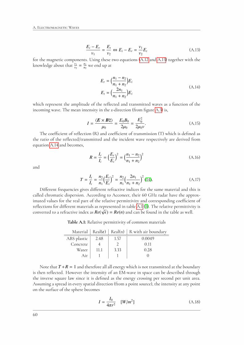
for the magnetic components. Using these two equations (A.�� and A.��) together with theknowledge about that v1

v2= n1

n2we end up at

Er =⇣n1 � n2

n1 + n2

⌘Ei

Et =⇣ 2n1

n1 + n2

⌘Ei

(A.��)

which represent the amplitude of the re�ected and transmitted waves as a function of theincoming wave. The mean intensity in the z-direction (from �gure A.�) is,

I = hE ⇥ Bziµ0

=E0B0

2µ0=

E20

2µ0v. (A.��)

The coe�cient of re�ection (R) and coe�cient of transmission (T) which is de�ned asthe ratio of the re�ected/transmitted and the incident wave respectively are derived fromequation A.�� and becomes,

R = Ir

Ii=⇣Er

Ei

⌘2=⇣n1 � n2

n1 + n2

⌘2(A.��)

and

T = It

Ii=

n2

n1

⇣Et

Ei

⌘2=

n2

n1

⇣ 2n1

n1 + n2

⌘2(��). (A.��)

Di�erent frequencies gives di�erent refractive indices for the same material and this iscalled chromatic dispersion. According to Acconeer, their �� GHz radar have the approx-imated values for the real part of the relative permittivity and corresponding coe�cient ofre�ections for di�erent materials as represented in table A.� (�). The relative permittivity isconverted to a refractive index as Re(

p✏ ) = Re(n) and can be found in the table as well.

Table A.�: Relative permittivity of common materials

Material Real(✏ ) Real(n) R with air boundaryABS plastic �.�� .�� .��Concrete � � �.��

Water ��.� �.�� .��Air � � �

Note that T +R = 1 and therefore all all energy which is not transmitted at the boundaryis then re�ected. However the intensity of an EM-wave in space can be described throughthe inverse square law since it is de�ned as the energy crossing per second per unit area.Assuming a spread in every spatial direction (from a point source), the intensity at any pointon the surface of the sphere becomes

I = I0

4⇡r2 [W /m2] (A.��)

��

A.� R��

where r is the distance from the source to the sphere surface (��). The intensity of the wavethus decreases with / 1/r2.

��

A. E��W��

��

Appendix B

Tables and images

As seen in �gures B.� and B.� the HBL and FZP lens limits the signal more in the angularE-plane and H-plane as well as increases the max gain [dBFS]. The D� lens setting, i.e., whenplacing the lens further away from the sensor, increases the gain and focuses the signal morethan D�.

��

B. T��

Figure B.�: The �gure shows a Screenshot of the Sparse IQ GUIwhere all parameters can be set together with a visualization overthe received signal.

��

Figure B.�: The Python code used to generate the simple peri-odogram plot of �gure �.��.

Figure B.�: The received reference velocity data from UK for therectangular pipe.

��

B. T��

Figure B.�: The received reference data from UK for the circularpipe.

Figure B.�: The setup while measuring the surface �ow velocity withslow motion camera and the Apple Watch in the Acconeer lab en-vironment.

Figure B.�: The performance table of the LH�� mount holder andHBL/FZP lens (�).

��

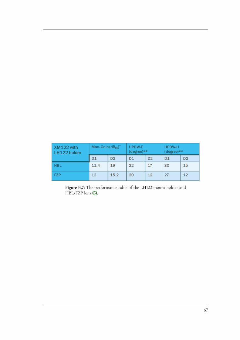
Figure B.�: The performance table of the LH�� mount holder andHBL/FZP lens (�).

��

Fluid Surface Velocity Measurement using Millimeter-Wave ...

Documents

Transcript of Fluid Surface Velocity Measurement using Millimeter-Wave ...