An ultraviolet-selected galaxy redshift survey - II. The physical nature of star formation in an...
27
arXiv:astro-ph/9910104v1 6 Oct 1999 An Ultraviolet-Selected Galaxy Redshift Survey – II: The Physical Nature of Star Formation in an Enlarged Sample Mark Sullivan, 1⋆ Marie A. Treyer, 2 Richard S. Ellis, 1 Terry J. Bridges, 3 Bruno Milliard 2 & Jos´ e Donas 2 1 Institute of Astronomy, Madingley Road, Cambridge CB3 OHA, UK 2 Laboratoire d’Astronomie Spatiale, Traverse du Siphon, 13376 Marseille, France 3 Anglo-Australian Observatory, PO Box 296, Epping NSW 2121, Australia Accepted —. Received —; in original form —. ABSTRACT We present further spectroscopic observations for a sample of galaxies selected in the vacuum ultraviolet (UV) at 2000 ˚ A from the FOCA balloon-borne imaging camera of Milliard et al. (1992). This work represents an extension of the initial study of Treyer et al. (1998). Our enlarged catalogue contains 433 sources (≃ 3 times as many as in our earlier study) across two FOCA fields. 273 of these are galaxies, nearly all with redshifts z ≃ 0−0.4. Nebular emission line measurements are available for 216 galaxies, allowing us to address issues of excitation, reddening and metallicity. The UV and Hα luminosity functions strengthen our earlier assertions that the local volume-averaged star formation rate is higher than indicated from earlier surveys. Moreover, internally within our sample, we do not find a steep rise in the UV luminosity density with redshift over 0 <z< 0.4. Our data is more consistent with a modest evolutionary trend as suggested by recent redshift survey results. Investigating the emission line properties, we find no evidence for a significant number of AGN in our sample; most UV-selected sources to z ≃ 0.4 are intense star-forming galaxies. We find the UV flux indicates a consistently higher mean star formation rate than that implied by the Hα luminosity for typical constant or declining star formation histories. Following Glazebrook et al. (1999), we interpret this discrepancy in terms of a starburst model for our UV-luminous sources. We develop a simple algorithm which explores the scatter in the UV flux-Hα relation in the context of various burst scenarios. Whilst we can explain most of our observations in this way, there remains a small population with extreme UV-optical colours which cannot be understood. Key words: surveys – galaxies: evolution – galaxies: luminosity function, mass func- tion – galaxies: starburst – cosmology: observations – ultraviolet: galaxies 1 INTRODUCTION There has been considerable progress in recent years in de- termining observational constraints on the cosmic history of star formation, and the way this relates to the far infrared background light and present density of stars and metals (see Madau (1999) for a recent summary). Inevitably, most at- tention has focused on the contribution to the global history from the most distant sources, presumably seen at a time close to their formation. Controversial issues at the time of writing include the interpretation of faint sub-mm sources as young, star-forming galaxies (Blain et al. 1999), the ef- ⋆ E-mail: [email protected] fect of dust on measures derived from rest-frame ultraviolet luminosities (Meurer et al. 1997; Steidel et al. 1996), cosmic variance in the limited datasets currently available (Steidel 1999) and uncertain non-thermal components within the far- infrared background (Madau 1999). At more modest redshifts (z < 1), it might be as- sumed that the cosmic star formation history is fairly well- determined. Madau et al.’s (1996) original analysis in this redshift range was based on rest frame near ultraviolet lumi- nosities derived from the I -selected Canada France Redshift Survey (CFRS, Lilly et al. 1995) and local Hα measures taken from Gallego et al.’s (1995) objective prism survey. This combination of data implied a dramatic decline in the c 0000 RAS
Transcript of An ultraviolet-selected galaxy redshift survey - II. The physical nature of star formation in an...

arX
iv:a
stro
-ph/
9910
104v
1 6
Oct
199
9
An Ultraviolet-Selected Galaxy Redshift Survey – II: The
Physical Nature of Star Formation in an Enlarged Sample
Mark Sullivan,1⋆ Marie A. Treyer,2 Richard S. Ellis,1 Terry J. Bridges,3
Bruno Milliard2 & Jose Donas2
1 Institute of Astronomy, Madingley Road, Cambridge CB3 OHA, UK2 Laboratoire d’Astronomie Spatiale, Traverse du Siphon, 13376 Marseille, France3 Anglo-Australian Observatory, PO Box 296, Epping NSW 2121, Australia
Accepted —. Received —; in original form —.
ABSTRACTWe present further spectroscopic observations for a sample of galaxies selected in thevacuum ultraviolet (UV) at 2000 A from the FOCA balloon-borne imaging camera ofMilliard et al. (1992). This work represents an extension of the initial study of Treyeret al. (1998). Our enlarged catalogue contains 433 sources (≃ 3 times as many as inour earlier study) across two FOCA fields. 273 of these are galaxies, nearly all withredshifts z ≃ 0−0.4. Nebular emission line measurements are available for 216 galaxies,allowing us to address issues of excitation, reddening and metallicity. The UV and Hα
luminosity functions strengthen our earlier assertions that the local volume-averagedstar formation rate is higher than indicated from earlier surveys. Moreover, internallywithin our sample, we do not find a steep rise in the UV luminosity density withredshift over 0 < z < 0.4. Our data is more consistent with a modest evolutionarytrend as suggested by recent redshift survey results. Investigating the emission lineproperties, we find no evidence for a significant number of AGN in our sample; mostUV-selected sources to z ≃ 0.4 are intense star-forming galaxies. We find the UVflux indicates a consistently higher mean star formation rate than that implied bythe Hα luminosity for typical constant or declining star formation histories. FollowingGlazebrook et al. (1999), we interpret this discrepancy in terms of a starburst modelfor our UV-luminous sources. We develop a simple algorithm which explores the scatterin the UV flux-Hα relation in the context of various burst scenarios. Whilst we canexplain most of our observations in this way, there remains a small population withextreme UV-optical colours which cannot be understood.
Key words: surveys – galaxies: evolution – galaxies: luminosity function, mass func-tion – galaxies: starburst – cosmology: observations – ultraviolet: galaxies
1 INTRODUCTION
There has been considerable progress in recent years in de-termining observational constraints on the cosmic history ofstar formation, and the way this relates to the far infraredbackground light and present density of stars and metals (seeMadau (1999) for a recent summary). Inevitably, most at-tention has focused on the contribution to the global historyfrom the most distant sources, presumably seen at a timeclose to their formation. Controversial issues at the time ofwriting include the interpretation of faint sub-mm sourcesas young, star-forming galaxies (Blain et al. 1999), the ef-
⋆ E-mail: [email protected]
fect of dust on measures derived from rest-frame ultravioletluminosities (Meurer et al. 1997; Steidel et al. 1996), cosmicvariance in the limited datasets currently available (Steidel1999) and uncertain non-thermal components within the far-infrared background (Madau 1999).
At more modest redshifts (z < 1), it might be as-sumed that the cosmic star formation history is fairly well-determined. Madau et al.’s (1996) original analysis in thisredshift range was based on rest frame near ultraviolet lumi-nosities derived from the I-selected Canada France RedshiftSurvey (CFRS, Lilly et al. 1995) and local Hα measurestaken from Gallego et al.’s (1995) objective prism survey.This combination of data implied a dramatic decline in the
c© 0000 RAS

2 M. Sullivan et al.
comoving density of star formation (by a factor of ≃ 10)which is difficult to match theoretically (Baugh et al. 1998).
The addition of further data to the low redshift compo-nent of the cosmic star formation history has confused ratherthan clarified the situation. The bJ -selected Autofib/LDSSredshift survey (Ellis et al. 1996) satisfactorily probes theevolutionary trends from 0.25 < z < 0.75 and, whilst sup-porting an increase in luminosity density over this inter-val, the survey illustrated the difficulty of connecting faintsurvey data with similar local luminosity functions (LFs)whose absolute normalisations remain uncertain, as well asa fundamental difference in the luminosity dependence ofthe evolution seen (Ellis 1997). The CFRS data indicate lu-minosity evolution of ≃ 1 mag to z ≃ 1 at the bright endof the galaxy LF consistent with a decline in the star for-mation rate of a well-established population. In contrast,the Autofib/LDSS results suggests that most of the changesin luminosity density occurred via a rapid decline in abun-dance of lower luminosity (sub-L∗) systems. Morphologicaldata for both surveys from Hubble Space Telescope (HST)(Brinchmann et al. 1998) has since shown a substantial frac-tion of the rise in luminosity density arises from galaxies ofirregular morphology.
In an earlier paper in this series (Treyer et al. 1998,hereafter Paper I), we presented the first ultraviolet (UV)-selected constraints on the local density of cosmic star for-mation. Using a flux-limited sample of 105 spectroscopically-confirmed sources selected at 2000 A from a balloon-borneUV imaging camera, a local integrated luminosity densitywell above optically-derived estimates was found, suggest-ing claims for strong evolution in the range 0 < z < 1 hadbeen overstated. Corrections for dust extinction would onlystrengthen this conclusion.
A revision of the evolutionary trends for z < 1 is sup-ported by a recent re-evaluation of the field galaxy redshiftsurvey results by Cowie, Songaila & Barger (1999). By se-lecting faint galaxies in the U and B bands rather than theI band (c.f. CFRS), a more modest increase with redshiftin the UV luminosity density is found. Cowie et al. proposethe discrepancy with the CFRS may arise from the extrap-olation necessary in the CFRS at intermediate redshifts todetermine 2800 A luminosities from the available I-bandmagnitudes.
More generally, it is becoming increasingly apparentthat different diagnostics (UV flux, Hα luminosities, 1.4 GHzluminosities) may lead to different star formation rates, evenfor the same galaxies. Glazebrook et al. (1999) have showna consistent discrepancy exists between star formation den-sities derived using UV continua and nebular Hα measures,and interpreted this in terms of both dust extinction and anerratic star formation history for the most active sources. Asimilar trend is seen by Yan et al. (1999).
The above developments serve to emphasize that the in-tegrated comoving star formation density is a poor guide tothe physical processes occurring in the various samples and,moreover, that the evolutionary trends in the (presumed)well-studied 0 < z < 1 range remain uncertain. In this sec-ond paper in the series, we return to the key question ofthe physical nature of the star formation observed in the lo-cal samples and particularly those of the kind discussed inPaper I. We have extended our UV sample and obtained uni-form diagnostic spectroscopy over a wider wavelength range
so that we can compare star formation rates from nebularand UV continuum measures.
A plan of the paper follows. In §2 we discuss theenlarged spectroscopic sample. Using the William Her-schel Telescope (WHT) we have conducted systematic spec-troscopy of a further 305 sources within Selected Area 57(SA57) and Abell 1367, and this allows us to update theanalysis of the UV LF and SF density presented in PaperI, and discuss the implications of possible reddening. In §3we extend our analysis, for the first time, to include a care-ful discussion of the emission line properties of our sample.A puzzling aspect revealed in Paper I was the abnormally-strong UV fluxes and colours of a proportion of our sources.We examine this effect in some detail and discuss constraintson both the metallicity and AGN contamination of our sam-ple. In §4, we interpret our various star formation diagnosticsin terms of duty-cycles exploring quantitatively the sugges-tions of Glazebrook et al. (1999) that the star formation iserratic for a significant proportion of sources. We discussthe implication of our results in §5 and summarise our basicconclusions in §6. Throughout this paper, all calculationsassume an Ω = 1, H0 = 100 h km s−1 Mpc−1 cosmology.
2 THE ENLARGED SAMPLE
This paper presents the spectroscopic extension to the UV-selected redshift survey, conducted on a sample selected us-ing the balloon-borne FOCA2000 camera, preliminary re-sults of which were presented in Paper I. A full descrip-tion of the details of the FOCA experiment can be foundin Milliard et al. (1992). In brief, the telescope is a 40cmCassegrain mounted on a stratospheric gondola, stabilisedto within a radius of 2′′ rms. The spectral response of thefilter used on the telescope approximates a Gaussian cen-tred at 2015 A, FWHM 188 A. The camera was operatedin two modes – the FOCA 1000 (f/2.56, 2.3) and FOCA1500 (f/3.85, 1.55) – with the large field-of-view (FOV) wellsuited to survey work. The limiting depth of the exposuresis mUV = 18.5, which, for a late-type galaxy, corresponds tomB = 20 − 21.5.
The extended dataset presented here is based on twoFOCA fields. The first, SA57, was partially covered inPaper I, and is centred at RA = 13h03m53s, Dec. =+2920′30′′ (1950 epoch). The second field is centred onRA = 11h42m46s, Dec. = +2010′03′′, and contains thecluster Abell 1367. The fields were imaged in both the FOCA1000 and FOCA 1500 modes. The astrometric accuracy ofthe FOCA-1500 catalogue (around 3′′ rms, see Milliard etal (1992)) is insufficient for creating a spectroscopic targetlist, so the FOCA catalogues were therefore matched withAPM scans of the POSS optical plates. Two problems wereencountered. For some UV detections, there was more thanone possible optical counterpart on the POSS plates withinthe search radius used – in these cases, the nearest opti-cal counterpart to the UV detection was selected. Secondly,some of the UV sources have no obvious counterpart onthe APM plates, indicating that either some of the detec-tions are spurious, or that the counterpart lies at a fainter Bmagnitude than the limiting magnitude of the POSS plates(mB ≃ 21).
Paper I presented preliminary results from an optical
c© 0000 RAS, MNRAS 000, 000–000

An Ultraviolet-Selected Galaxy Redshift Survey 3
spectroscopic follow-up to the SA57 UV detections. Afterbasic star/galaxy separation, two instruments – the Hydrainstrument on the 3.5-m WIYN telescope (λλ 3500–6600 A,3.1′′ diameter fibres), and WYFFOS on the 4.2-m WilliamHerschel Telescope (WHT) (λλ 3500–9000 A, 2.7′′ diameterfibres, see Bridges (1997) for more details) – were used toobtain 142 reliable spectra, though 14 of these came from aweather affected exposure in which the incompleteness wasvery large. After further star removal and elimination ofsources with poor UV fluxes, a complete sample of 105 galax-ies with confirmed redshift remained. A further 3 galaxieshave since been found to have unreliable optical (B) magni-tudes.
The new data sample was observed on the WHT toensure that Hα emission would be visible to a redshift ofz = 0.4. The targets for the new survey were chosen so thatno identified galaxy with a redshift from Paper I was re-observed. All the new UV sources are taken from the deeperFOCA 1500 catalogue, which also has the advantage of ahigher imaging resolution (3′′ as opposed to 4.5′′ rms). Thisreduces the problem of multiple optical counterparts for UVsources, as a smaller search radius on the optical plates canbe used, but still leaves around 9 per cent of sources withan uncertain identification.
Six exposures were performed of different fields withinSA57, and one was taken of Abell 1367. Each exposure isbroken into several shorter 1800s exposures to help improvecosmic ray rejection, and median spectra produced for eachfield. Several sources within SA57 were observed on morethan one exposure, allowing a comparison of results betweenexposures. The spectra were reduced as in Paper I, but ad-ditional flux-calibration was performed on the new spectralsample. Details of all observing runs can be found in Table 1.
The spectra were analysed using the splot facility iniraf and the figaro package gauss. Redshifts were mea-sured by visual inspection, and the equivalent widths (EWs)and fluxes of [O ii] (3727 A), [O iii] (4959 A and 5007 A), Hβ(4861 A) and Hα (6562 A) determined using both spectralanalysis programs. 1σ errors were also provided by splot
using an estimate of the noise in the individual spectra. Thecontinuum level can be fitted interactively using polynomialfitting within the gauss program, and compared with thelinear fitting from the splot program. In most cases, espe-cially in the spectra with a high S/N, the two flux measure-ments show an excellent agreement within the 1σ errors pro-vided by splot – the average discrepancy is ≃ 13 per cent.This provides a good reliability check on the effects of contin-uum fitting on the spectra, which differ in the two routines.Additionally, the Hα and [O ii] EWs were measured indepen-dently by two of the authors (MS and MAT) as a check thatthere were no measurement biases. The average discrepancywas ≃ 14 per cent, indicating a good agreement. Thoughthe spectral resolution (10 A) is good enough to resolve theseparate [O iii] lines, in many cases the Hα line (6562 A) wasblended with the nearby [N ii] lines at 6583 A and 6548 A,so a deblending routine was run from within splot to allowdetermination of the fluxes of these individual lines.
The integration error estimates are derived by errorpropagation assuming a Poisson statistics model of the pixelsigmas, generated by measuring the noise in the spectra onan individual basis. It is assumed that the linear continuumhas no errors. The splot errors in the deblending routines
are derived using a Monte-Carlo simulation as follows. Themodel is fit to the data – using the pixel sigmas from thenoise model – and is used as a noise-free spectrum. 100 sim-ulations were run, adding random Gaussian noise to this‘noise-free’ spectrum using the noise model. The deviation ofeach new fitted parameter to model parameter was recorded,and the error estimate for each parameter is then the devi-ation containing 68.3 per cent of the parameter estimates –this corresponds to 1σ if the distribution of the parameterestimates is Gaussian. This allows calculation of the errorsin cases where individual lines are blended together.
The errors are thus random measurement errors only,i.e. they arise from the S/N of the spectrum in question. Afurther source of uncertainty will be introduced during fluxcalibration, as each fibre on the spectrograph may have aslightly different throughput. Ideally, standard stars shouldbe observed through each fibre, but this is not possible inpractice. Note, however, that this uncertainty will only applyto the line fluxes, and not to the EWs. Additionally, noaperture corrections are applied at this stage (see Section 4.2for a discussion of this).
A summary of the new sample is given in Table 2, to-gether with the statistics for that obtained by combiningwith the data discussed in Paper I. From this enlarged sam-ple, 48 objects have two optical counterparts and 1 has three.Additionally, of the galaxies with a redshift, 15 were deter-mined to be unreliable UV detections, and 10 have unreliableB-magnitude information from the POSS plates – these areshown as missing mags in the table. This leaves 234 galaxiesin the spectroscopic sample, and 224 galaxies in a restrictedsample with full colour information, where there is an un-ambiguous optical identification. The total area surveyed inthe enlarged sample is 1.88 deg2 in SA57 and 0.35 deg2 inAbell 1367, giving ∼ 2.2 deg2 in total.
For the new data set, 4 of the unidentified spectra suf-fered from technical difficulties in extraction unrelated tothe S/N ratio, so the formal incompleteness is 48/301, or≃ 16 per cent. Of the 68 unidentified spectra in the en-larged sample, 10 suffered from technical difficulties, so theformal incompleteness within all the well-exposed fields –i.e. excluding the shortened WHT exposure from Paper I –is therefore 52/423, or ≃ 12 per cent.
In summary, therefore, the combined catalogue repre-sents a three-fold increase in sample size c.f. Paper I, withthe added benefit of emission line measurements for a sig-nificant fraction of the total.
2.1 Photometry
The FOCA team adopted a photometric system discussedin detail by Milliard et al. (1992) and in Paper I, which isclose to the ST system. The apparent UV magnitude to fluxconversion is given by:
mλ = −2.5 log fλ − 21.175 (1)
where the flux (fλ) is in erg/cm2/s/A. The zero-point is ac-curate to ≤ 0.2 mag. Close to the limiting magnitude ofthis survey however, the uncertainty in the relative photom-etry may reach ≃ 0.5 mag (Donas et al. 1987) due to non-linearities in the FOCA camera. Conservatively, we estimatethe errors in the UV magnitudes (mλ, hereafter muv) to be0.2 for muv < 17, and 0.5 for muv > 17.
c© 0000 RAS, MNRAS 000, 000–000

4 M. Sullivan et al.
Date Field R.A. (1950) DEC. (1950) Telescope/ Exposure Flux(h m s) ( ′ ′′) instrument time (s) calibration?
Paper I28-02-96 SA57 - 1 13:05:48 29:17:49 WIYN/Hydra 3x1800 No29-02-96 SA57 - 2 13:05:48 29:17:49 WIYN/Hydra 3x1800 No02-04-97 SA57 - 3 13:04:11 29:21:04 WHT/WYFFOS 4x1800 No
SA57 - 4 13:00:59 29:36:28 WHT/WYFFOS 2x1800 No
New24-04-98 SA57 - 5 13:04:01 28:59:48 WHT/WYFFOS 5x1800 Yes
SA57 - 6 13:02:53 29:09:26 WHT/WYFFOS 4x1800 Yes25-04-98 SA57 - 7 13:02:53 29:28:27 WHT/WYFFOS 3x1800 Yes
SA57 - 8 13:04:02 29:37:53 WHT/WYFFOS 3x1800 YesA1367 - 1 11:41:31 20:20:18 WHT/WYFFOS 5x1800 Yes
26-04-98 SA57 - 9 13:05:24 29:28:19 WHT/WYFFOS 4x1800 YesSA57 - 10 13:05:24 29:09:25 WHT/WYFFOS 5x1800 Yes
Table 1. Details of all the observing runs that contribute to the enlarged sample. Standards were not available for the Paper I sample,hence these data is not flux-calibrated.
Field Number Stars QSOs Missing mags Galaxies Emission lines Hα Unidentified OC > 1
New SA57 241 37 14 9 130 97 88 51 32ABELL 1367 64 5 4 3 51 38 37 1 3
Old SA57 128 8 5 13 92 81 34 10 14
Total 433 50 23 25 273 216 159 62 49
Table 2. The breakdown of spectroscopic objects in the new, old (Paper I) and combined sample, giving the number of each objecttype. Missing mags indicates that either UV or B magnitudes were not available.
As in Paper I, the B-photometry was taken from thePOSS database, including saturation and isophotal loss cor-rections. Again, there will be non-linearity effects near thelimiting magnitude of the plates, and also at the brighterend. The error in the B-photometry was taken to be ≃ ±0.2.However, the B photometric scale has to be corrected bymcorr
B ≡ mAPMB − 0.546 in order to align it with the FOCA
system (Paper I, Donas et al. (1987))†.
2.2 Extinction corrections
Extinction arising along the line-of-sight to a target galaxymakes the observed ratio of the fluxes of two emission linesdiffer from their ratio as emitted in the galaxy. The extinc-tion, C, can be derived using the Balmer lines Hα and Hβ:
F (Hα)
F (Hβ)= D10−C[S(Hα)−S(Hβ)] (2)
where F (Hα) and F (Hβ) are the measured integrated linefluxes, and D is the ratio of the fluxes as emitted in thenebula. Assuming case B recombination, with a density of100 cm−3 and a temperature of 10,000 K, the predictedratio of Hα to Hβ is D = 2.86 (Osterbrock 1989). Us-ing the standard interstellar extinction law from Table 3
† This correction differs from that adopted in Paper I; we foundthe correction had been slightly underestimated.
in Seaton (1979), S(Hα) − S(Hβ) = −0.323, and C can bereadily determined from Eqn. 2. Any corrected emission lineflux, F0(λ), can then be estimated using:
F0(λ) = F (λ)10C[1+(S(λ)−S(Hβ))] (3)
where the values of S(λ) − S(Hβ) were taken fromSeaton (1979), with values of -0.323, -0.034, 0 and 0.255for Hα, [O iii] Hβ and [O ii] respectively. 1σ errors for thereddened fluxes have been calculated from the 1σ errors inthe unreddened fluxes and in C in the standard way. Forcomparison with other emission line surveys, the extinctionparameter AV has also been calculated using:
AV = E(B − V )R =CR
1.47mag (4)
where the relation E(B − V ) = C/1.47, and R is the meanratio R = AV /E(B − V ), with a value R = 3.2, both fromSeaton (1979).
A correction must also be made for stellar absorptionunderlying the Hα and Hβ lines. Though most of the galax-ies in the sample have strong emission lines, the reddeningcorrections are very sensitive to the amount of absorption onthe Balmer lines. Two methods were used to analyse the con-tribution of stellar absorption. Firstly, each galaxy spectrumwas checked for higher order Balmer lines (Hγ, Hδ etc.) and,if these lines appeared in absorption, the EW of each wasmeasured, and the average of these values then applied as acorrection to both the Hα and Hβ lines. Where the higher-
c© 0000 RAS, MNRAS 000, 000–000

An Ultraviolet-Selected Galaxy Redshift Survey 5
Figure 1. The distribution of the reddening parameter AV forthe galaxies with both Hα and Hβ in emission, after correctionfor underlying stellar absorption, The average value (0.97) is thesolid line.
order lines were not visible, or appeared in emission, a cor-rection of 2 A was applied, typical of such spectra (Tresse etal. 1996). The second method was to use the program dipso
to fit the stellar absorption line underneath the Hβ emis-sion, then use this fit as the continuum and subtract fromthe spectrum. The flux of the Hβ line should then containno absorption contribution if the fitting is done carefully.The two methods gave similar results. The distribution ofAV after the corrections can be seen in Fig. 1.
From the spectra containing both strong Hα and strongHβ, the mean value for AV without any absorption correc-tion is 1.78, and after correction is 0.97. These compare wellwith values of 1.52 for a selection of CFRS galaxies (Tresseet al. 1996), which made no allowance for stellar absorption,and studies of individual H ii regions in local spiral galaxies(≃ 0.6 (Oey & Kennicutt 1993) and ≃ 1 (Kennicutt et al.1989) ), both corrected for absorption. In spectra where itwas not possible to measure both Hα and Hβ, either dueto a low S/N, or, more commonly, due to the Hβ line beingbadly affected by stellar absorption, a value of AV = 0.97was assumed (i.e. C = 0.45) – these galaxies are not shownin Fig. 1.
It is important to realise one source of possible bias thismay introduce into our corrections. The Balmer-derived cor-rections applied here require the presence of both Hα and Hβin the galaxy spectra. However, as the extinction increases,if the limiting factor on determining a line flux were purelythe S/N of the spectra, the Hβ would become undetectablebefore Hα, implying the average correction used here to bea lower limit. The presence of significant Hβ absorption inmany spectra prevents an accurate calculation of the size ofthis effect.
This complication aside, the Balmer decrement remainsthe best way to estimate extinction in our sample. The prob-lem now arises of how to convert these emission line redden-
ing corrections to those appropriate for our UV (and optical)magnitudes. Though the different extinction laws (e.g. MW,SMC, LMC) are similar at optical emission line wavelengths,and the Balmer extinction results are relatively insensitiveto the choice of extinction law used, this is not the case inthe UV. There is a wide choice of methods available in theliterature, and it is clear that for the unresolved galaxiesunder study here, the reddening of the UV continuum willdepend upon details of the dust-star-gas geometry. The red-dening of the stellar continuum may be different from theobscuration of the ionised gas, as the stars and the gas mayoccupy different areas within the galaxy. Indeed, it has beenshown that the continuum emission from stars is often lessobscured than line emission from the gas (Fanelli, O’Connell& Thuan 1988; Calzetti, Kinney & Storchi-Bergmann 1994;Mas-Hesse & Kunth 1999). From studies of the central re-gions of starburst galaxies, Calzetti (1997b) derived the fol-lowing empirical, and geometry-independent, prescription tocorrect fluxes as a function of wavelength. Using the stan-dard form,
F0(λ) = Fobs(λ)100.4E(B−V )sµ(λ) (5)
where the colour excess of the stellar continuum, E(B−V )s,is related to that for the ionised gas, E(B − V )g, and henceC, by:
E(B − V )s = 0.44E(B − V )g =0.44C
1.47(6)
The function µ(λ) and Equation 6 are empirical relationstaken from Calzetti (1997b), who derived these results usinga sample of star-forming galaxies. The function µ(λ) has thevalue 9.70 at 2000 A, and 6.17 at ≃ 4100 A – the centralwavelength of the POSS B filter. In terms of magnitudes,the corrections are then:
mcorrUV = mobs
UV − 0.3Cµ(2000 A/(1 + z)) (7)
mcorrB = mobs
B − 0.3Cµ(4100 A/(1 + z)) (8)
The effect of the reddening corrections on the absolute mag-nitudes is shown in Fig. 2, and the relation between both theuncorrected and corrected UV and Hα fluxes and E(B−V )g
are shown in Fig. 3. This is shown for the most completesample of our survey, the SA57 field galaxies, excluding theComa cluster galaxies, which may experience different dustenvironments.
The 0.44 factor in Eqn. 6 takes into account the fact thatthe stars and gas may occupy distinct regions with differingamounts of dust and different dust covering factors. TheHα luminosity arises purely from very young, short-livedionising stars, which must remain close to the (dusty) regionsin which they were born. By contrast, the UV continuum at2000 A contains a significant contribution from older non-ionising stars, which may no longer be associated with theregions in which they were formed, and hence will suffer lessfrom dust extinction.
If this simple interpretation is correct, then the redden-ing of the stellar continuum and of the ionising gas shouldnot be strongly correlated; indeed the correlation found(left-hand plot of Fig. 3) is weaker than in previous stud-ies (Calzetti, Kinney & Storchi-Bergmann 1994; Calzetti1997a). This may not be an entirely unexpected result. Asthis survey is selected in the UV at 2000 A, it is likely tobe biased against those objects which are intrinsically dusty
c© 0000 RAS, MNRAS 000, 000–000

6 M. Sullivan et al.
Figure 3. The relationship between the ratio of Hα to UV luminosities and the ionised gas colour excess (from Section 2.2). The leftplot is for the fluxes uncorrected for dust extinction (but corrected for stellar absorption), the right plot for fluxes corrected as explainedin the text. Only single optical counterpart, field galaxies from SA57 are shown.
-25 -24 -23 -22 -21 -20 -19 -18 -17 -16 -15-4
-3.5
-3
-2.5
-2
-1.5
-1
-0.5
0
0.5
-26 -25 -24 -23 -22 -21 -20 -19 -18 -17 -16 -15 -14 -13-3
-2.5
-2
-1.5
-1
-0.5
0
0.5
Figure 2. Dust extinction correction as a function of uncor-rected absolute magnitude using Calzetti (1997b)’s ‘recipe’. Notethat the small scatter arises only because an average AV = 0.97,C = 0.45 was applied for those galaxies without direct Hα / Hβ
extinction measurements.
and hence have lower measured UV fluxes. Therefore weshould not be surprised to see an absence of galaxies with alarge Hα to UV ratio. Additionally, if the Hβ is suppressedrelative to the Hα by a significant amount, it will not be mea-sured reliably in the optical spectra, so galaxies with a largeE(B − V )g will not be shown in Fig. 3. The trend is similarto that noted by Meurer, Heckman & Calzetti (1999), whoplotted the ratio of line flux to F(1600A) against UV spec-tral slope, β, (their Fig. 7), for a sample of local UV-selectedstarbursts and a sample of 7 U -band ‘dropouts’ observed byvarious authors. These are corrected for Galactic extinctiononly, and, for the ‘dropout’ galaxies, show only a weak cor-relation between the line/UV ratios and extinction, similarto that found here.
For the mean correction (C = 0.45) used above tocorrect the emission lines, the Calzetti law gives correc-tions at 2000 A of A2000 = 1.33. Other studies are inbroad agreement with this value, for example Buat & Bur-garella (1998) derive A2000 ≃ 1.2 using radiation transfermodels to estimate extinction. Using the parameterizationof Seaton (1979), which uses a simple foreground dust screenmodel, we derive values of A2000 = 2.70 for the averagevalue C = 0.45. This last correction introduces several com-plexities. We already have uncomfortably blue colours fora sub-sample of our galaxies; as we shall see in Section 4,there is considerable difficulty in reproducing these usingconventional starburst models. The UV luminosities wouldalso become difficult to explain (Section 4). For this reason,we adopt the Calzetti law throughout this paper, noting thatalthough this will result in the smallest corrections to ourUV luminosites, due to the nature of the selection criteriafor this survey, the UV continuum is not likely to suffer froma larger degree of extinction.
2.3 UV redshift/colour distribution
Table 7 lists the catalogue for the new observations and theold data. The overall redshift distribution of the new samplecan be seen in Fig. 4, together with the distribution of theenlarged sample. The distribution in the new sample has alarge peak at z = 0.02 due to the presence of both the Comacluster in SA57, and the cluster Abell 1367.
Absolute magnitudes, MUV and MB , were derived foreach galaxy as follows. The redshift was used to calculate aluminosity distance, and the dust corrected observed colour,(uv − b), to assign a spectral class and hence k -correction.As in Paper I, the spectral classes were allocated accord-ing to the (E/S0, Sa, Sb, Scd, SB) scheme using spectralenergy distributions (SEDs) from Poggianti (1997). The ab-solute UV magnitude MUV of a galaxy with dust-correctedUV magnitude m, redshift z, and inferred type i, is thencomputed as:
MUV = mUV − 5 log dL(z) − 25 − ki(z) (9)
(and a similar relationship for MB) where dL(z) is the lu-
c© 0000 RAS, MNRAS 000, 000–000

An Ultraviolet-Selected Galaxy Redshift Survey 7
Figure 4. The redshift distribution for the new sample (left) and the combined sample (right). LEFT: The hatched area is the newSA57 data, while the superimposed heavy shading refers to objects from the Abell 1367 FOCA field. RIGHT: The hatched area is theentire sample, while the heavy shading refers to the restricted sample of galaxies with only one optical counterpart.
minosity distance at redshift z (we assume Ω = 1 andH0 = 100 h km s−1 Mpc−1). This allows calculation of therest-frame colours, (UV − B)0.
Fig. 5 shows the distribution of the (UV − B)0 colourswith redshift, with the colours both uncorrected and cor-rected for dust. Multiple counterpart cases are not shown.Superimposed on these distributions are various model SEDsfor different galaxy types as a function of redshift from Pog-gianti (1997). The bluer models (labelled SB, as in Paper I)show the colours generated by a starburst superimposed ona passively evolving system. The redder (upper) case, SB1,assumes a 100 Myr burst prior to observation involving 30per cent of the galaxy mass. The bluer SB2 burst is a shorter(10 Myr) but more massive (80 per cent galaxy mass) burst.
As with previous studies using the FOCA catalogues,including Paper I, there is a significant fraction of galax-ies which have extreme (UV − B)0 colours – in this case 12per cent of the uncorrected colours are bluer than the bluestburst model SED plotted; this increases to 17 per cent af-ter our dust correction. The extreme colours are typicallygalaxies with strong UV detections, and previous analysishas shown that a systematic offset between the UV and op-tical photometric systems could not produce effects of thesize seen in Fig. 5 (Paper I). An intriguing possibility is thatwe do not see all of the UV galaxies on the APM plates,which are limited to b ≃ 21. This would suggest that we arenot seeing the most extreme objects in the colour plots, asthere are no optical counterparts to some of the UV detec-tions. Only deeper optical images of our studied fields cansettle this issue. Possible explanations for the objects in oursample with these extreme UV colours will be examined inSections 3 and 4.
2.4 The UV, Hα and OII luminosity functionsrevisited
We now update the results of Paper I. The availability ofemission line measurements allows us to extend our lumi-nosity functions to those based on Hα and [O ii] luminosi-ties as well as the UV flux. With our enlarged sample whichreaches z ≃ 0.4, we can also test for the presence of evolutioninternally within our own sample.
We adopt the traditional Vmax method for the luminos-ity function (LF) derivation (e.g. Felten 1977), corrected forincompleteness in the number-magnitude distribution usingthe average number counts of Milliard et al. (1992). Theincompleteness function p(m) is defined as the ratio of thenumber of galaxies with measured spectra to the total num-ber of UV sources per magnitude bin per square degree onthe sky.
As in Paper I, we removed sources lying in the red-shift range of the intervening Coma and Abell 1367 clus-ters, which we conservatively take to occupy 0.020 < z <0.027. We also discarded those with insecure optical coun-terparts. The incompleteness function was computed afterthese subtractions, as the galaxy number counts of Mil-liard et al. (1992) are averaged over several fields andtherefore we expect the cluster contamination to be suffi-ciently diluted. The least complete magnitude bin is thefaintest (18 ≤ m ≤ 18.5), as expected, with p(m) =65%. All other magnitude bins are over 85 per cent com-plete. The mean incompleteness-corrected < V/Vmax > is0.48, i.e. the galaxy distribution can be considered uniform.The volume Vmax = p(m)V (zmax) is then defined as theincompleteness-corrected comoving volume at redshift zmax,out to which the galaxy could have been observed, i.e. sat-isfying m(M, z ≤ zmax) ≤ 18.5.
For the Hα and [O ii] LFs, the incompleteness functionwas computed using the new data only, as emission line flux
c© 0000 RAS, MNRAS 000, 000–000

8 M. Sullivan et al.
Figure 5. The colour-redshift distribution for the full spectroscopic sample of confirmed galaxies. The photometric system is describedin the text. The lines show the model predictions of galaxy colours as a function of redshift for a set of SEDs from Poggianti (1997).These are the same models as in Paper I; see text for full details of these SED models. Multiple counterparts are not shown. The lefthand plot shows the colours uncorrected for dust extinction, on the right the colours have been corrected using the Calzetti law.
calibration was not available for the old sample. Line widthswere measured for ≃ 74 per cent of the galaxies in this newsample. However, most of the ‘missing’ lines probably cannotsimply be attributed to a low S/N, and we must considerthem as truly being absent. For this reason, we do not applyany correction for missing lines to the LFs. Those lines whichare unmeasured due to a low S/N, rather than being absentfrom the spectrum, are, by definition, weak, and thereforeignoring them only adds to the uncertainty at the faint end.
For Hα, we also account for the fact that the line couldnot be observed at z > 0.4, i.e. z′
max = min(zmax, 0.4). The[O ii] and Hα luminosities have been corrected for extinctionas described in Section 2.2. For the UV LF, we considerboth the uncorrected and extinction-corrected magnitudesfollowing Calzetti’s prescription as described in Section 2.3.
Fig. 5 shows the effect of the reddening corrections onthe colours. After correction, the (UV−B)0 colours are bluerand therefore the galaxy types and k-corrections, as inferredfrom the redshift-colour diagram, will alter slightly. zmax
will also be slightly lower, as the extinction increases withthe emission frequency (Calzetti 1997b) and therefore withredshift. This has a negligible effect on the emission line LFs.
We fit each luminosity function with a Schechter (1976)function in the usual way:
φ(L)dL = φ⋆(
L
L⋆
)α
exp(
−L
L⋆
)
dL
L⋆
. (10)
The best fit parameters – φ⋆, α, M⋆ for the UV and log L⋆
for the emission lines – are listed in Table 3, as well as theresulting luminosity densities in each case. These are definedas:
L =
∫
∞
0
Lφ(L)dL = φ⋆L⋆Γ(α + 2) (11)
Figure 6. The UV luminosity function derived from thefull sample, with (dotted line) and without (solid line anddots) dust extinction correction. The dust correction assumes aCalzetti (1997b) law as described in the text. The long-dashedline is the best fit derived from the old sample (Paper I). The his-togram shows the number of galaxies contributing to each mag-nitude bin in the uncorrected case.
The error bars are Poissonian. The four LFs are shown inFigs. 6,7 and 8; we defer discussion of these to §2.5.
Fig. 9 shows the dust uncorrected 2000 A luminositydensity – L(2000 A) – as a function of redshift. The highredshift points are from Cowie, Songaila & Barger (1999),although, unlike the authors, we do not assume a faint mag-
c© 0000 RAS, MNRAS 000, 000–000

An Ultraviolet-Selected Galaxy Redshift Survey 9
Parameter UV uncorrected UV dust corrected Hα [O ii]
α −1.51 ± 0.10 −1.55 ± 0.11 −1.62 ± 0.10 −1.59 ± 0.12M⋆/log L⋆ (cgs) −20.59 ± 0.13 −22.14 ± 0.20 42.05 ± 0.14 41.96 ± 0.09log φ⋆ (Mpc−3) −2.02 ± 0.11 −2.15 ± 0.14 −2.92 ± 0.20 −2.82 ± 0.18log L (cgs Mpc−3) 38.08 ± 0.05 38.61 ± 0.05 39.49 ± 0.06 39.46 ± 0.06
SFR (PEGASE f = 1) −1.52,−1.69,−1.74 ± 0.05 −0.99,−1.16,−1.21 ± 0.05 −1.56 ± 0.06 −1.62 ± 0.05SFR (PEGASE f = 0.7) −1.51,−1.68,−1.74 ± 0.05 −0.98,−1.15,−1.21 ± 0.05 −1.43 ± 0.06 −1.47 ± 0.05
Table 3. Parameters of the best fit Schechter functions for the various luminosity functions. L is the corresponding luminosity densityintegrated to infinitely faint magnitude. The cgs units are erg/s/A for the UV luminosity at 2000 A and erg/s for the Hα and [O ii]luminosities. The star-formation rates (SFRs) are derived assuming a Salpeter IMF and the PEGASE code (see section 4 for details). Weconsider two cases for the fraction of Lyman continuum photons reprocessed into recombination lines (f = 1 and f = 0.7 respectively).The three SFRs listed for the UV light densities are taken at 3 different ages of a constant SFH stellar population; the conversion factorsare listed Table 4 (first two lines).
Figure 7. The dust corrected Hα luminosity function derivedfrom the present sample. Our best fit is shown by the solid line.The short-dashed line is the Hα LF derived by Tresse & Mad-dox (1998) in a similar redshift range, while the long-dashed lineshows the z ≃ 0 estimate of Gallego et al. (1995).
nitude cutoff. For consistency, we integrated the Cowie et al.LFs to infinity (Eqn. 11) assuming a faint end slope of -1.5similar to the present low redshift estimate. The dashed lineshows the (1 + z)1.7 luminosity evolution derived by Cowieet al., normalised at our new UV estimate. As thoroughlydiscussed by these authors, this evolution is much less rad-ical than the one derived from the CFRS analysis of Lillyet al. (1996) (dotted line, similarly normalised), implyingmuch more star-formation has occured in recent times thanpreviously suspected. In particular, the strong peak in SFRat z ∼ 1 − 2 may have been overestimated.
We looked for traces of evolution in the present sampleby computing the UV LF in two redshift bins: [0−0.15] and[0.15 − 0.4]. Vmax is then defined as min(V (0.15), V (zmax))for the low redshift galaxies, and as V (min(0.4, zmax)) −
V (0.15) for the higher redshift bin. The mean redshifts ineach bin are 0.078 and 0.22 respectively. The low and highredshift LFs overlap around M⋆ and both are consistent with
Figure 8. The dust corrected [O ii] luminosity function derivedfrom the present sample (dots). Our best fit is shown by the solidline.
the best fit derived for the full sample. Therefore no statis-tically significant evolution can be seen in the present data.However, the increase in light density between the meanredshifts of the two samples expected from a (1 + z)1.7 evo-lution law, as derived by Cowie et al., is only a factor of 1.2– within the error bars of the present estimate. By contrast,the (1 + z)4 evolution law based on the CFRS by Lilly etal. (1996) predicts a 60 per cent increase in UV light densitybetween the two redshift bins, which is difficult to reconcilewith our statistics, assuming the Poisson fluctuations are thedominant source of uncertainty. Although the present datado not allow a very reliable conclusion on this point, a weakrate of evolution for the UV light density seems more likely.
2.5 The low-redshift star-formation rate
The uncorrected UV LF is in good agreement with the esti-mate of Paper I, although the latter was based on a third ofthe present number of redshifts. The steep faint end sloperemains a significant feature, in contrast with local optically-
c© 0000 RAS, MNRAS 000, 000–000

10 M. Sullivan et al.
Figure 9. The 2000 A luminosity density as a function of redshift.Empty dots are from Cowie, Songaila & Barger (1999) extrapo-lated assuming a faint end slope of -1.5 similar to the present lowredshift estimate. The dashed line shows the (1 + z)1.7 evolutionlaw derived by Cowie et al. The dotted line is a (1+z)4 evolution
law based on CFRS (Lilly et al. 1996). Both analytic trends arenormalised at our new UV estimate; none of the data points aredust corrected.
selected surveys. It is also apparent in the Hα and [O ii] LFs,although the faintest data points were excluded in both casesand the fits are relatively poor. A steep faint end slope isalso found in the 1.4 GHz LF derived from faint radio galax-ies (Mobasher et al. 1999; Serjeant et al. 1998) confirmingthe preponderance of star-forming galaxies among this pop-ulation. The shape of our Hα LF is in poor agreement withprevious low-redshift determinations (Gallego et al. 1995,Tresse & Maddox 1998), although given the large uncertain-ties in emission line measurements, the fact that the threeestimates derive from very different selection criteria, andthat they probe different redshift ranges, the discrepancy isprobably acceptable. Our integrated Hα luminosity densityis ∼ 43 per cent lower than the Tresse & Maddox (1998)value derived from a sample of I-band selected galaxies atz < 0.3 from the CFRS. The mean redshift of this sampleis 0.2. Truncating the present UV-selected sample at red-shift 0.3 leaves the best fit Hα LF practically unchanged,while slightly reducing the mean redshift to 0.12. The dis-crepancy still cannot be reasonably attributed to evolutionwithin such a short redshift range, rather to poor statistics,differing selection effects and possibly k-correction models(used in computing Vmax). Our Hα luminosity density isalso ∼ 27 per cent higher than the estimate of Gallego etal. (1995), which probes a more local (z = 0), and also proba-bly more comparable (Hα selected), galaxy population. Therate of evolution resulting from the latter discrepancy (fromz = 0 to 0.15) is actually in very good agreement with thatderived by Cowie et al. (1999) from the 2000 A light density.
The conversion from UV, Hα or [O ii] luminosity densi-ties into SFRs is very model dependent (see Section 4 for adetailed discussion). As an illustration, we use the PEGASE
stellar population synthesis code (Fioc & Rocca-Volmerange1997) with which we were able to derive the conversionrates for all three diagnostics self-consistently. We assume aSalpeter IMF with stellar masses ranging from 0.1 – 120 M⊙,and consider two cases for the fraction of Lyman continuumphotons reprocessed into recombination lines (f = 1 andf = 0.7 respectively). These models are described in detailin Section 4. The conversion factors are listed in Table 4(first two lines).
The Hα and [O ii] luminosity densities thus convertedinto SFRs give very consistent results. The conversion fac-tors we use here yield SFRs ∼ 30 to 40 per cent higher thanthose derived from Madau (1998)’s fiducial model based onthe stellar population synthesis code of Bruzual & Char-lot (1993) (for a similar IMF). As our Hα luminosity den-sity falls between the values of Gallego et al. (1995) and ofTresse & Maddox (1998), so does the resulting SFR for agiven stellar population synthesis model.
Converting UV light into an instantaneous SFR is lessstraightforward as it involves an uncertain contribution fromlonger-lived stars, adding to the already large uncertainty inthe dust corrections. We consider three different ages (in aconstant star-formation history) to derive the UV conversionfactors; 10, 100 and 1000 Myr (see Section 4 for details –the conversion factors are as listed in Table 4). The range ofSFRs thus derived from the 2000 A light density is shown inFig. 10, along with the present (dust-corrected) and previousHα and [O ii] estimates. The left and right panels assumef = 1 and f = 0.7 respectively. Also shown is the local SFRestimate recently derived from 1.4 GHz data (Serjeant et al.1998; Mobasher et al. 1999).
The SFR derived from the UV continuum uncorrectedfor dust extinction is in good agreement with the correctedHα and [O ii] estimates for the case f = 1, and slightlylower than these values for f = 0.7. Taking the emissionline estimates at face value, this suggests that local UV-selected galaxies are not significantly affected by dust andthat Calzetti’s extinction law in the UV is significantly over-estimated for this population. There are many caveats how-ever, not least of which is the model-dependency of the con-version factors from line/UV luminosities to SFRs (see, forexample, Schaerer (1999)). The Hα extinction correctionsmay be underestimated, as argued by Serjeant et al. (1998)based on their estimate of the local SFR from radio emission,which is dust insensitive. Our Balmer-derived dust correc-tions to the Hα and [O ii] lines are certainly likely to belower limits, as discussed in Section 2.2. It is also possiblethat the Hα and UV luminosities are measured over differ-ent effective apertures, though we consider this unlikely (seeSection 4.2 for a discussion of this point).
The large uncertainties involved in determining the lowredshift SFR are readily apparent from the large scatter bothin the data and in the models. These uncertainties tend to in-crease with redshift, making interpretations about the SFRevolution quite unreliable at this point. Understanding thedetailed physical mechanisms of star-formation is thereforea crucial task towards reconciling the various SF diagnos-tics and finally drawing conclusions about the nature of starformation in the nearby Universe.
c© 0000 RAS, MNRAS 000, 000–000

An Ultraviolet-Selected Galaxy Redshift Survey 11
0 0.1 0.2 0.3-2
-1.9
-1.8
-1.7
-1.6
-1.5
-1.4
-1.3
-1.2
-1.1
-1
-0.9
-0.8
-0.7
0 0.1 0.2 0.3
Figure 10. The local star-formation rate derived from the presentand other local surveys, assuming the conversion factors describedin the text (previous Hα estimates are rescaled according to thesefactors). All the emission line estimates are dust-corrected as de-scribed in the text. The triangle represents the Hα estimate of
Gallego et al. (1995) and the diamond that of Tresse & Mad-dox (1998). The present estimates are indicated by error bars.The lower cross shows the range of SFRs estimated from theuncorrected UV continuum light (assuming the range of mod-els described in the text), while the upper dotted one shows thedust-corrected values. The Hα and [O ii] estimates are where indi-cated on the plot. The z = 0 dot shows the SFR from the 1.4 GHzanalysis of Serjeant et al. (1998).
3 EMISSION LINE PROPERTIES
A significant advance over the spectra presented in Paper Iis that we now have reliable line measurements for a sub-stantial fraction of the UV-selected sample. For the high-est S/N spectra, EWs and fluxes for up to 5 emission lineshave been measured (6 including the deblended [N ii] line).Our analysis now proceeds in two parts. This section willcover the emission line properties and correlations, togetherwith diagnostic diagrams, whilst the next section will covercomparisons of emission lines with the UV fluxes and thesubsequent star-formation modelling.
One of the possible explanations for the abundance ofextreme (UV−B)0 colour objects seen in this survey is thatthe UV light produced in these galaxies comes from a non-thermal source, such as an QSO/AGN. The mean (not dust-corrected) UV−B colour of the 23 such objects in our sampleis -1.41, though there is large scatter, with some as blue as≃ −4. Clearly, care must be taken to remove such objectsfrom our ‘star-forming’ galaxy sample. Those galaxies withobvious AGN characteristics have been removed from thesample; however, there remains the possibility that AGNswith strong star-forming components have remained in thesample, giving over-abundant UV fluxes. While the best wayto assess the size of the effect is to image the galaxies in theUV and look at the distribution of the UV light, an indirect
method of identifying AGN from starburst galaxies is to useemission line diagnostic diagrams.
Diagnostic diagrams can be used to separate and dis-tinguish between different ionisation sources in the hostgalaxies. Considering the lines measured in this survey, the[O iii]/Hβ versus [O ii]/Hβ diagram is the most appropriateto use. Though not an ideal choice, as the ratio of [O ii]/Hβdepends significantly on reddening, this diagram allows usto look at what proportion of our sources may have ioni-sation sources other than hot OB-type stars, which is vitalgiven the star-formation modelling attempted in Section 4.Fig. 11 shows this diagnostic diagram for both the reddenedand unreddened fluxes. The line on the diagram is takenfrom Tresse et al. (1996), and shows the approximate em-pirical limit between H ii galaxies and ‘active’ galaxies.
It is interesting to note that a significant fraction of thesources lie to the right of the line in Fig. 11, i.e. away fromthe region that is normally associated with H ii galaxies. Theimportant point however is the size of the uncertainties onthe plot, particularly in the corrected fluxes. Though notshown on the diagram, the points to the right of the linetypically have larger errors – up to 2 times as high – so itis difficult to conclude that a large fraction of the sourceshave a strong AGN component. Additionally, the effect ofstellar absorption on the Hβ line has a large effect on thisplot, adding to the uncertainty involved. Although the Hβfluxes include some allowance for the Hβ absorption dueto the way in which they were measured, some individualpoints may still contain significant errors associated withthem. Any further correction will increase the measured Hβflux, moving the galaxy down and to the left on the diagram,back into the H ii galaxy region.
If galaxies that lie away from the H ii region are respon-sible for the extreme (UV − B)0 colours seen in this survey,then we expect a correlation between the [O ii]/Hβ ratio andUV-B colour; none is found. This suggests that an explana-tion of the (UV − B)0 colours cannot be found purely inthe source of ionisation of the galaxies, at least not with thecurrent quality of data.
Another possible explanation for the anomalous UVcolours compared to the model predictions could be unusu-ally low metallicities in the galaxies concerned. To investi-gate this, we examined the metallicity using the R23 emis-sion line index (Pagel et al. 1979) following the prescriptionfrom Poggianti et al. (1999). This is defined in terms of cor-rected fluxes as:
R23 =([O ii]3727 + [O iii]4959,5007)
Hβ
(12)
and is calibrated using:
12 + log(O
H) = 9.265− 0.33x− 0.20x2
− 0.21x3− 0.33x4(13)
where x = log(R23). Full details of this calibration can befound in Zaritsky, Kennicutt & Huchra (1994); in brief, theabsolute R23 index calibration is accurate only to ≃ 0.2 dex,so this estimator is most useful for calculating relative metal-licities.
Only the SA57 galaxies – the more complete spectro-scopic sample – were used in this analysis, creating a sub-sample of 35 galaxies that have the complete line informa-tion required to estimate the metallicity. An added compli-
c© 0000 RAS, MNRAS 000, 000–000

12 M. Sullivan et al.
Figure 11. The diagnostic diagrams as described in the text, for both the corrected and uncorrected fluxes. Typical 1σ error bars areshown in the top right. Note how the reddening corrections move many more galaxies away from the H ii region, though the error barsare larger.
Figure 12. Plot of the metallicity derived from the R23 indexagainst (UV−B)0 and Hα luminosity for the SA57 galaxies whichhave the complete line information. Coma galaxies are plotted assquares, field galaxies are stars.
cation is the effect of stellar absorption on the Hβ line, asthe metallicity estimates are very sensitive to this; however,due to the emission line nature of our survey galaxies, andthey way in which the Hβ fluxes were measured, the effectof stellar absorption should not be a large one.
Fig. 12 shows the relationship between galaxy colour,Hα luminosity and metallicity. Those galaxies which aremembers of the Coma cluster are plotted as empty squares,the field galaxies are shown as stars. There is a slight sug-
gestion in the left hand plot that the bluer galaxies havea higher metallicity (a counter-intuitive result). There is noapparent correlation with Hα luminosity. Unfortunately, dueto the significant errors on the points (not shown) it is dif-ficult to conclude a great deal about metallicity being re-sponsible for the extreme (UV−B)0 colours seen in some ofour galaxies.
To conclude, there is still no single convincing explana-tion for the abnormal colours that we see in this survey onthe basis of the emission line information that we have atour disposal. While it is difficult to completely rule out thepossibility of significant AGN contamination, or metallicityeffects, the evidence is not strong. Improved S/N ratios mustbe obtained on the relevant lines to finally settle the issue.
4 STAR FORMATION MODELLING
4.1 Discussion of spectral evolution models
Our UV selected galaxy survey allows us to compare two dif-ferent tracers of star-formation activity which should, whenconverted, produce similar SFRs. The follow-up optical spec-tra have provided Hα emission line measurements, and theFOCA experiment has provided a measurement of the UVcontinuum at 2000 A. This UV continuum light is domi-nated by short-lived, massive main-sequence stars, with thenumber of these stars proportional to the SFR. Hα emissionlines are generated from re-processed ionising UV radiationat wavelengths of less than 912 A. This radiation is onlyproduced by the most massive stars, which have short life-times of ≃ 20 Myr. To convert these two tracers into actualSFRs for each galaxy requires constructing the spectral en-ergy distribution (SED) of a model galaxy over time, andthe following method is used.
The spectral characteristics of an instantaneous burst
c© 0000 RAS, MNRAS 000, 000–000
An Ultraviolet-Selected Galaxy Redshift Survey 13
of star-formation for a given IMF and set of evolutionarystellar tracks are calculated, and, using a time-dependentSFR, then used to build synthetic spectra over the courseof a galaxy’s history. This time-varying SED is convertedinto time-varying UV magnitudes and Hα luminosities (orEWs). For the UV magnitudes, the response (or transmis-sion) of the FOCA-2000 A filter is included. For Hα, theemission line flux can be calculated from the number of ion-ising Lyman continuum photons, assuming that a certainfraction of these photons are absorbed by the hydrogen gasin the galaxy. This gas is assumed to be optically thick tothe Lyman photons (according to case B recombination).
The number of ionising photons is assumed to be a frac-tion f of the number of Lyman continuum photons, and twovalues will be assumed here. The first is f = 0.7, as proposedby DeGioia-Eastwood (1992), who studied H ii regions in theLMC. However, when the galaxy as a whole is studied, thefraction absorbed is much higher (see Kennicutt (1998) fora discussion). Leitherer et al. (1995) studied the redshiftedLyman continuum in a sample of 4 starburst galaxies withthe Hopkins UV telescope, and reports that < 3 per cent arenot absorbed, i.e. f = 1. These absorbed ionising photonsare then re-processed into recombination lines; for Hα weadopt a conversion of 0.45 Hα photons per ionising Lymanphoton.
There are several galaxy spectral synthesis models avail-able in the literature (see Leitherer et al. (1996) for arecent review). Different models predict slightly differenttime-varying SEDs, and therefore different conversion fac-tors. For Hα, produced only by the most massive stars, aconstant star-formation history (SFH) will have little time-dependence in Hα luminosity – for the published models, theHα luminosity reaches a constant level after ≃ 20− 30 Myr,and varies little thereafter. However, the conversion factoris very sensitive to the form of the IMF, as it depends criti-cally on the number of high-mass stars. The conversion fromUV continuum luminosity to a star-formation rate (SFR) ismore difficult, as the UV continuum at 2000 A also containsa contribution from stars with a longer lifetime, and, un-like Hα, will not settle at a constant level but will increaseslowly with time. Three different conversion factors will beused here, for ages of 10, 100 and 1000 Myr.
There are many Hα conversion factors given in the liter-ature (e.g. Glazebrook et al. (1999), Kennicutt et al. (1998)and Madau et al. (1998) for discussions). The modellingin this paper makes use of two spectral synthesis codes:PEGASE (see Fioc and Rocca-Volmerange (1997) for fur-ther details), and Starburst 99, developed by Leitherer etal. (1999). The PEGASE code uses the evolutionary tracksof Bressan et al. (1993), together with the stellar spectrallibraries assembled by Fioc and Rocca-Volmerange, and islimited to solar metallicity. These libraries cover the wave-length range of 200 A to 10µm with a resolution of 10 A.Full details of the tracks used in the Starburst 99 code canbe found in Leitherer et al. (1999). This code has a choiceof 5 metallicities (Z = 0.040, 0.020 (= Z⊙), 0.008, 0.004 and0.001).
The Hα and UV conversion values used are taken fromMadau et al. (1998), Kennicutt (1998) and directly fromthe PEGASE and Starburst 99 spectral synthesis codes,and tabulated in Table 4 for a SFR of 1M⊙yr−1 and aSalpeter (1955) IMF. The table also lists various [O ii] con-
version factors used in Section 2.4. While the UV contin-uum is relatively insensitive to the fraction of Lyman ionis-ing photons absorbed by the nebular gas, the Hα fluxes arecritically sensitive to this poorly known number; values off = 0.7 and f = 1 were used to produce the two PEGASEvalues. The SB99 UV conversion factors do not increase withdecreasing metallicity for the 10 Myr case (as would be ex-pected) due to red supergiant (RSG) features appearing inthe population; this metallicity dependent feature is due tothe inability of most evolutionary models to predict correctlyRSG properties on this time-scale (see Leitherer et al. (1999)for a full discussion).
4.2 The star-formation diagnostic plots
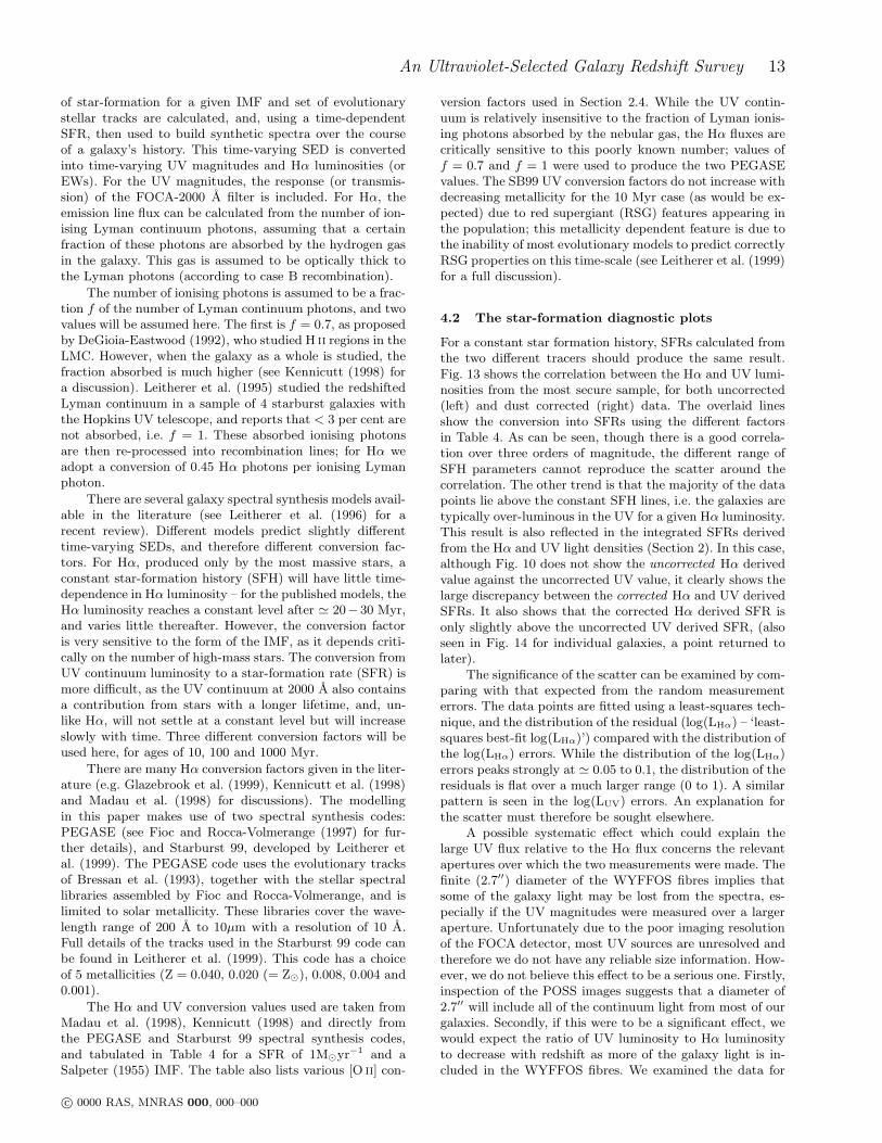
For a constant star formation history, SFRs calculated fromthe two different tracers should produce the same result.Fig. 13 shows the correlation between the Hα and UV lumi-nosities from the most secure sample, for both uncorrected(left) and dust corrected (right) data. The overlaid linesshow the conversion into SFRs using the different factorsin Table 4. As can be seen, though there is a good correla-tion over three orders of magnitude, the different range ofSFH parameters cannot reproduce the scatter around thecorrelation. The other trend is that the majority of the datapoints lie above the constant SFH lines, i.e. the galaxies aretypically over-luminous in the UV for a given Hα luminosity.This result is also reflected in the integrated SFRs derivedfrom the Hα and UV light densities (Section 2). In this case,although Fig. 10 does not show the uncorrected Hα derivedvalue against the uncorrected UV value, it clearly shows thelarge discrepancy between the corrected Hα and UV derivedSFRs. It also shows that the corrected Hα derived SFR isonly slightly above the uncorrected UV derived SFR, (alsoseen in Fig. 14 for individual galaxies, a point returned tolater).
The significance of the scatter can be examined by com-paring with that expected from the random measurementerrors. The data points are fitted using a least-squares tech-nique, and the distribution of the residual (log(LHα) – ‘least-squares best-fit log(LHα)’) compared with the distribution ofthe log(LHα) errors. While the distribution of the log(LHα)errors peaks strongly at ≃ 0.05 to 0.1, the distribution of theresiduals is flat over a much larger range (0 to 1). A similarpattern is seen in the log(LUV) errors. An explanation forthe scatter must therefore be sought elsewhere.
A possible systematic effect which could explain thelarge UV flux relative to the Hα flux concerns the relevantapertures over which the two measurements were made. Thefinite (2.7′′) diameter of the WYFFOS fibres implies thatsome of the galaxy light may be lost from the spectra, es-pecially if the UV magnitudes were measured over a largeraperture. Unfortunately due to the poor imaging resolutionof the FOCA detector, most UV sources are unresolved andtherefore we do not have any reliable size information. How-ever, we do not believe this effect to be a serious one. Firstly,inspection of the POSS images suggests that a diameter of2.7′′ will include all of the continuum light from most of ourgalaxies. Secondly, if this were to be a significant effect, wewould expect the ratio of UV luminosity to Hα luminosityto decrease with redshift as more of the galaxy light is in-cluded in the WYFFOS fibres. We examined the data for
c© 0000 RAS, MNRAS 000, 000–000

14 M. Sullivan et al.
Source Assumed Salpeter IMF L(Hα) L([O ii]) L(UV2000)lower/upper mass limits (1041erg s−1) (1041erg s−1) (1039erg s−1A−1)
(M⊙) 10 Myr 100 Myr 1000 Myr
PEGASE (f = 1.0) 0.1/120 1.15 1.25 4.01 5.90 6.69PEGASE (f = 0.7) 0.1/120 0.85 0.88 3.94 5.84 6.63
SB99 (Z=0.040) 0.1/120 1.23 3.53 5.01SB99 (Z=0.020) 0.1/120 1.53 3.44 5.17SB99 (Z=0.004) 0.1/120 1.79 3.55 5.69SB99 (Z=0.001) 0.1/120 2.01 3.46 5.85
M98 0.1/125 1.58 6.00K98 0.1/100 1.27 0.71
Table 4. The conversion rates used to transform Hα [O ii] and FOCA UV2000 luminosities into SFRs (in the sense L = SFR ×
conversion factor). Values from Madau et al. (1998), Kennicutt (1998), and the PEGASE and Starburst 99 spectral synthesis models.
Figure 13. The correlation between the Hα and FOCA-UV luminosities, for the most secure sample. Only field galaxies are shown. Left:
Both luminosities uncorrected, right: both luminosities corrected. Errors are 1σ. The lines show the position of galaxies with a constantSFR. The lines are (from left to right) SOLID:PEGASE f = 0.7 and f = 1.0, SHORT DASHED: Starburst 99, metallicities 0.04, 0.02,0.004, 0.001, LONG DASHED: M98 Hα with PEGASE UV f = 1.0. UV conversion factors taken at 100 Myr. The markers refer to SFRsof 0.1, 1.0, 10 and 100 M⊙ yr−1 respectively for the PEGASE f = 0.7 and Z = 0.001 Starburst 99 models. See text for further details.
such a trend, but found no significant trend from z = 0 toz = 0.3. From this, we conclude there to be no evidence forsignificant aperture mismatches internally within our sam-ple.
The over-luminosity in the UV and the scatter cannotbe explained in terms of simple foreground screen dust cor-rections, as these will increase the discrepancy, not reduceit. Other dust geometries are also unlikely to be the cause.To move the observed positions of the galaxies so that theyagree with the constant SFH predictions requires large dustcorrections to the Hα luminosities, but almost negligible cor-rections for the UV luminosities. Though the C = 0.45 cor-rection derived in Section 2.2 applied solely to the Hα fluxesproduces a better agreement between the two SFR tracers,to remove the scatter completely would require correctionsof up to C = 1.4, corresponding to AV ≃ 3 (see Section2.2), whilst simultaneously having no effect on the UV lu-
minosities. Such corrections are not seen from the Balmerdecrement measurements, and would require extreme dustgeometries.
This trend initially appears to contradict that of Glaze-brook et al. (1999), who find that their Hα derived SFRslie above that derived from the UV continuum at 2800 A.As a comparison, Fig. 14 shows both our sample and that ofGlazebrook et al. converted to SFRs on an individual galaxybasis using the appropriate PEGASE conversion factor at2800 A (taken from Table 3, Glazebrook et al. (1999)). Thedust corrections applied to the Hα and the 2800 A UV areas given in Glazebrook et al. It is clear that only the brightend of our galaxy population is sampled by Glazebrook etal., and that in this range there is a good agreement betweenthe two samples. The dashed line shows a perfect agreementbetween Hα and UV derived SFRs, and it is clear that cor-recting just the Hα luminosities for dust reduces the offset
c© 0000 RAS, MNRAS 000, 000–000

An Ultraviolet-Selected Galaxy Redshift Survey 15
-3 -2 -1 0 1 2-3
-2
-1
0
1
2
-3 -2 -1 0 1 2-3
-2
-1
0
1
2
Figure 14. A comparison of SFRs derived from our sample (opensquares) and that of Glazebrook et al. 1999 (stars). SFR conver-sions are taken from the PEGASE program. The dashed linesshows a perfect agreement between Hα and UV SFRs. TOP:Only Hα fluxes are corrected for dust, BOTTOM: Both UV and
Hα corrected. There is a good agreement between the samples,though the Glazebrook et al. sample only covers the bright endof our distribution.
apparent in Fig. 13, indicating that our UV corrections maybe upper limits and possibly overestimated, though the scat-ter is more difficult to explain.
However, both the offset and the scatter in Fig. 13 andthe lower (dust corrected) half of Fig. 14 can also be ex-plained by a series of starbursts superimposed on underly-ing galactic SFHs. During a starburst, a galaxy moves upand to the right on the UV-Hα plane, increasing luminosityin both quantities. As the burst decays, the Hα rapidly de-creases due to the short lifetimes of ionising stars, but theUV luminosity is temporarily retained, moving the galaxyto the left. Subsequently, the galaxy returns to its pre-burst(quiescent) position, describing a loop on the plot.
This scenario can also reconcile the difference betweenbright galaxies, including the Glazebrook et al. sample,where the Hα SFR > UV SFR, and the fainter sample inthe lower half of Fig. 14, where the opposite is seen. Thebright galaxies are (likely) at the peak of a particular burst,and, in a Calzetti-like dust scenario, the UV will contain acontribution from young massive (and hence dust obscuredstars) as well as older (less obscured) stars; hence our UVcorrections are probably underestimated in this range andthe Hα SFR will be larger then UV derived measures. Asthe burst dies away, the contribution to the UV luminos-ity from the obscured massive stars decreases and the UVSFR will become larger than the (more rapidly decaying)Hα SFR. The next section attempts to quantify the burstparameters in this picture.
At this point it is relevant to return to the vexing ques-tion of the origin of the extreme (UV−B)0 colours. Fig. 15plots the Hα EW against (UV − B)0 for the galaxies in theUV photometric system (see Section 2.2 for details). Only
Figure 15. Plot of Hα EW against (UV − B)0 colours for fieldand cluster galaxies in SA57 (COMA) and Abell 1367, overlaidwith various SFHs using different IMFs. Field galaxies shown ascrosses, cluster galaxies as open squares. Colours have been dustcorrected. The solid line is the Rana-Basu IMF (also circle mark-
ers), short dash Scalo IMF (also triangles) and long dash SalpeterIMF (squares). The markers refer to different galaxy ages (0.5, 6and 12 Gyr).
those galaxies for which errors in the Hα EWs are availablewith an unambiguous optical identification are shown. Thisremoves some galaxies with extreme (UV−B)0 ≃ −4 colourswhere the UV fluxes were possibly the sum of two galaxies,and were therefore anomalously bright when compared tothe B magnitudes. The advantage of this diagnostic plot isthat it has no complications due to uncertainties in the fluxcalibration of the WHT optical spectra.
The galaxies plotted in Fig. 15 represent two differ-ent environments – cluster members in Abell 1367 or Coma(squares), and field galaxies (crosses). The plot shows a cleartrend – the strongest Hα emission systems are the bluestsystems. Most of the galaxies tend to cluster at aroundHα ≃ 20 − 60, (UV − B)0 ≃ 0, but there are two otherareas on this plot of interest. One consists of those galaxieswith very blue (UV−B)0 colours of ≃ −2 to − 4, the otherare those with a significant Hα EW (≃ 50 − 100) but muchredder colours.
In order to distinguish between the cluster SFH andfield SFH, Fig. 15 also shows various predictions accordingto the PEGASE spectral synthesis program. The historiesare for exponential bursts of the form:
SFR = τ−1 exp(
−t
τ
)
(14)
where τ is the characteristic time of the SFH, and is equal to1.25 Gyr. Altering this value does not change the trajectory,only the speed at which a galaxy travels along it. The plotshows that the cluster galaxies are solely responsible for thegroup of galaxies that have redder colours and a significantHα emission.
The effect of varying the IMFs on the colours is also
c© 0000 RAS, MNRAS 000, 000–000

16 M. Sullivan et al.
explored. A wide range of IMFs are available, and three areshown in Fig. 15; these are the Scalo (1986), Salpeter (1955)and Rana-Basu (1992) IMFs. As in Fig. 13, it is clear thatthese SFHs are incapable of reproducing the scatter in theobserved points of Fig. 15, even when variations in the IMFare considered, and certainly cannot reproduce the (UV −
B)0 colours seen here.In summary, smoothly declining SFHs cannot a) repro-
duce the UV colours and luminosities seen in the field galax-ies, b) produce the strong Hα emission seen in the relativelyred cluster galaxies, or c) generate the scatter seen in bothFigs. 13 & 15.
4.3 Modelling the luminosities and colours
In this section, we aim to understand the scatter in Fig. 13by examining the duty cycle of star formation in thesurvey galaxies. We adopt throughout this section theSalpeter (1955) IMF with mass cut-offs at 0.1 M⊙ and120 M⊙. The modelling techniques discussed here were alsoattempted using other IMFs – those also used in Section 4.2– as well as varying the mass-cutoffs used; however, noappreciable difference was obtained using these ‘standard’IMFs.
In a method similar to that adopted by Glazebrook etal. (1999), who suggested that the SF in a sample of 13CFRS z ≃ 1 galaxies is erratic, we will examine the effect ofsuperimposing a set of bursts on a smoothly declining starformation history. We ask what range in the strength andduration of the bursts is required to reproduce the scatterobserved.
In order to check the bursting hypothesis as a solutionfor the scatter in Fig. 13 (and Fig. 15), the positions ofnon-bursting galaxies should ideally be plotted as a ‘realitycheck’ on the model predictions. In the absence of UV datafor a large sample of normal galaxies, this test cannot yetbe done. Meanwhile it must be assumed that the absolutepositions of galaxies predicted by the synthesis codes are cor-rect, and that there is no systematic offset when comparingmodel and observations.
To model the properties of a galaxy, a series of burstsof varying mass (M) and burst decay time (τ ) were super-imposed on gradual declining or constant SFHs. This givesthree free fitting parameters: M, τ , and the number of bursts,Nb, as well as the form of the declining SFH. Several versionsof the latter were tried; two are introduced here, which differin the resulting present-day colour. Their characteristics aresummarised in Table 5.
The models are compared to the observed data pointsstatistically. We first examined a maximum likelihoodmethod. The likelihood, L, of the observed galaxy points be-ing drawn from a particular model is given by (Glazebrooket al. (1999)):
L =∏
i
∫ ∫ P (h, u) exp(− (hi−h)2
2∆h2
i
−(ui−u)2
2∆u2
i
)
2π∆hi∆ui
dudh (15)
where the observational Hα and UV luminosities are repre-sented by ui and hi respectively for each galaxy i, ∆ui and∆hi are the observational uncertainties in these points mea-sured from the individual spectra (∆hi) or based on the UV
Test SFH Burst τ Burst Mass Nb
(Myr) (% galaxy mass)
1 Red 130 25-30 201 Blue 50 10-15 20
2 Red 50 3-7 202 Blue 70 15-20 20
Table 6. The parameters for the ‘best-fit’ bursts for the twogalaxy SFHs. The top parameters are those generated by maxi-mum likelihood, the bottom are those from the second statisticaltest, which concentrates on reproducing the scatter seen in theobserved points.
magnitudes (∆ui, Section 2.1), u and h represent the pa-rameterization of the PEGASE model points, and P (h, u) isthe probability density of a particular model point in Hα /UV space.
The bursts were added at random times from a galacticage of 4 to 12 Gyr, and were fitted to the data points for theperiod 8 to 12 Gyr. We then calculated the likelihood of aSFH matching the observed data points. This was repeated100 times, and the mean likelihood obtained.
Two types of burst were considered; the first was a burstof constant strength over its duration, the other was an ex-ponentially declining burst similar in form to Equation 14.Constant strength bursts generally gave lower likelihoods asthey tend to generate stationary points in Hα / UV space;exponential bursts generate more scatter. The ‘most likely’burst parameters for each galaxy type are listed in Table 6.A typical likelihood contour plot is shown in Fig. 17. Littleimprovement was obtained by varying the number of bursts;a value of 20 was used throughout, equivalent to a burstevery ≃ 400 Myr. The best-fitting bursts are also demon-strated graphically in Fig. 16, where the path of the modelgalaxy in Hα /UV space is superimposed on the data. Ascan be seen, these bursts reproduce many of the observeddata points but do not reproduce the scatter.
A second, simpler statistical approach was adopted. Theaim is to assess the number of observed points that couldbe reproduced by the maximum likelihood fits. This simplycounted the number of data points reproduced by a partic-ular SFH. Fig. 17 shows an example contour plot from thismethod, Table 6 lists the parameters of the ‘best-fitting’histories as before, and Fig. 16 shows these histories graph-ically.
Although the burst parameters for the two methods aresimilar for the blue galaxy, they are very different for the first(redder) galaxy. The maximum likelihood method favourslonger bursts. With a short burst the galaxy spends much ofits lifetime away from the position of the observed points; theunderlying component is red and the galaxies were selectedin the UV.
It can also be seen that the histories do not reproducethe highest UV luminosity galaxies; these are the galaxiesthat have the strongest (UV−B)0 colours. In Section 3, weconcluded that there was no conclusive evidence that theanomalously bright (UV − B)0 colours could be explainedby AGN contamination or metallicity effects. We find thatthe best-fit histories from above could neither generate the
c© 0000 RAS, MNRAS 000, 000–000

An Ultraviolet-Selected Galaxy Redshift Survey 17
SFH τ (Gyr) (UV − B)0 Hα EW L(Hα) L(UV2000)1040erg s−1 1039erg s−1A−1
1 (Red) 2.00 1.37 1.6 0.0105 0.1492 (Blue) 5.00 -0.58 17.1 0.1540 2.018
Table 5. The two exponential SFHs on which the bursts were superimposed. Superpositions were made between galactic ages of 4 to12 Gyr; the characteristics above are taken at 12 Gyr.
Figure 16. Two distributions of UV-Hα measures for the sample (crosses) compared to that for model galaxies, found by superimposinga series of bursts on the SFHs described in Table 5 using the best-fit parameters of Table 6 (only the ‘redder’ galaxy is shown). Theopen squares show the track made by a global exponentially declining SFR, forming a total mass of 1010 M⊙, as described in the text.The lines show the paths described by a ‘model’ galaxy during its evolution. LEFT: Maximum likelihood ‘best-fit’. Much of the observedscatter is not reproduced by this model. RIGHT: The second statistical test, with the emphasis on matching the scatter in the plot,rather than maximising the likelihood.
Figure 17. Examples of the burst mass/duration contour plots. LEFT: A maximum likelihood contour plot. The peak is at τ = 130 Myr,M≃ 30%. RIGHT: The contours generated by the alternative statistical test, which reproduces more of the scatter in the points. Thepeak is at τ = 50 Myr, M≃ 5%. Both plots are for the redder SFH from Table 5.
c© 0000 RAS, MNRAS 000, 000–000

18 M. Sullivan et al.
Figure 18. As Fig. 16, but attempting to reproduce the high UVluminosity points. This shows τ = 10 Myr, 15% mass bursts. TheUV luminosity points can be reproduced, but even these historiesare not capable of reproducing the extreme (UV − B)0 coloursfound in this survey.
scatter nor the bluest colours seen in the data. Though thehighest UV luminosity bursts are reproducible via short, in-tense bursts (Fig. 18), the extreme (UV − B)0 colours arestill not attained.
5 DISCUSSION
We have seen that the scatter in the UV-Hα plane is consis-tent with a star formation history that is complex and er-ratic. The fundamental observation is that most of our UV-selected galaxies show excess UV luminosities when com-pared to their Hα fluxes on the assumption of a simple starformation history. Moreover, dust extinction would serve toenhance the difference, not reduce it unless, perhaps, thespatial distribution of dust is particularly complex. In Sec-tion 4, we considered more complex star formation historiesinvoking a regular pattern of bursts on top of more generalexponentially-declining histories and found that the differ-ent time-dependencies of the stars that produce UV flux andexcite nebular emission can reproduce the scatter observed.
It is interesting to compare this result with those (veryfew) surveys for which two star formation diagnostics areavailable. Using different selection criteria, Glazebrook etal. (1999) (13 targets colour selected from the I-limitedCFRS) and Yan et al. (1999) (slitless HST NICMOS spec-troscopy of 33 targets) both find Hα derived SFRs in excessof those from UV measurements (at 2800 A) - the oppositeeffect to that seen here. They attribute their discrepancyprimarily to dust extinction (Yan et al. 1999; Glazebrook etal. 1999) but also discuss an erratic SFH (Glazebrook et al.1999). The effect of dust extinction in these different samplesis very difficult to quantify; however both of these surveyssample only the bright end of our galaxy sample, and we
have shown there is actually good agreement between thesesurveys and ours in this range. The other major difference ofsignificance is the size of the samples available for analysisand the quality of spectral data involved; clearly both arebetter for our low z sample than in the z > 1 analyses.
The nature of our UV selected galaxies can also be as-sessed by considering comparisons with 1.4 GHz radio con-tinuum detections. This radiation, caused by synchrotronradiation from relativistic electrons, is thought to be gen-erated by electrons accelerated by supernovae from massive(M > 5M⊙) short-lived stars, and therefore should be a fur-ther tracer of the SFR in galaxies (Condon 1992). A liter-ature search revealed three radio surveys which cover someor all of SA57 – the FIRST catalogue (White et al. 1997),the NVSS (Condon et al. 1998) – both using the VLA –and Windhorst, Heerde & Katgert (1984), which uses theWesterbork Synthesis Radio Telescope. The correlations be-tween these surveys and the FOCA detections are shown inFig. 19.
Though the radio catalogues correlate well, there is asurprisingly poor correlation with the FOCA sources. Only 3FIRST sources and 1 NVSS source have FOCA counterpartswithin 20′′ – a generous search radius – and Hα was detectedin only one of these. However, converting 1.4 GHz luminosityto SFR for our adopted IMF (Cram et al. 1998; Serjeant etal. 1998):
SFR1.4(M ≥ 0.1M⊙) =L1.4
7.45 × 10²⁰ W Hz−1M⊙yr−1 (16)
we find that the largest SFRs in our UV-selected sample(≃ 15M⊙yr−1) would give expected 1.4 GHz luminosities atz = 0.1 of only ≃ 2mJy, i.e. close to the detection thresh-old of the FIRST survey (≃ 1mJy). None the less, as manysources should lie closer than z = 0.1, we might have ex-pected more 1.4 GHz detections. As previous studies (Ser-jeant et al. 1998) have shown that even dust corrected Hαluminosity underestimates local SFRs when compared with1.4 GHz observations, this lack of correlation may indicatethat the Hα derived SFRs are marginally overestimated.Deeper 1.4 GHz surveys are required to explore this further.
Although we have shown that the excess UV luminosi-ties can be reproduced by considering bursting SFHs, wehave generally failed to reproduce the full range of (UV−B)0colours for our sample; in general, colours smaller than(UV − B)0 ≃ −2 are problematic to generate, and we can-not easily explain a number of intense UV sources which areoptically faint. In Paper I we eliminated trivial explanationsfor this category of sources including photometric discrep-ancies between the FOCA and POSS (B) magnitude sys-tems. It is certainly possible to generate UV-optical coloursmore extreme than the Poggianti starburst SEDs. For ex-ample, using the Starburst 99 code (Leitherer et al. 1999),(UV − B)0 ≃ −2.5 – −3 can be generated (but only ona very short time-scales) using standard IMFs and smaller(104 Myr) timesteps then the Poggianti SEDs (107 Myr).The number of such sources found then can only be under-stood in the context of more detailed modelling of the SFduty cycle. On the whole, however, it is becoming apparentthat we do not understand the SEDs of these systems well.
The burst duty cycle produces results consistent withthat of earlier workers. The original analysis of Glazebrooket al. (1999) adopted slightly longer and more massive
c© 0000 RAS, MNRAS 000, 000–000

An Ultraviolet-Selected Galaxy Redshift Survey 19
Figure 19. The correlations between FIRST, NVSS and Wind-horst et al. (1984) 1.4 GHz radio surveys and the FOCA 2000 Adetections. FOCA sources are shown as open squares, FIRST assquare crosses, NVSS as diagonal crosses and Windhorst as opencircles. A poor correlation between FOCA sources and radio de-
tections is observed.
bursts. Marlowe, Meurer & Heckman (1999) examined thenature of starbursts in dwarf galaxies and found similarburst parameters. They find such bursts typically accountfor only a few per cent of the stellar mass. Theoretical studies(Babul & Ferguson 1996) suggest that the burst durationsmay be shorter than those found here, as well as being moreintense in terms of stellar mass. A comprehensive study ofbursts in irregular galaxies has also been undertaken by Mas-Hesse & Kunth (1999). They also find that star-formationepisodes are essentially short, with a mean age of around4 Myr. Though this is much shorter than the ‘best-fit’ dutycycles found in this survey, it does correlate well with thebursts that we require in order to reproduce the full rangeof UV luminosities (≃ 10 Myr).
There remain many avenues for further investigationinto the nature of star-formation in local samples of fieldgalaxies. There is an urgent need for resolved images so thatthe morphological details and physical location of the starforming regions can be determined. Ultimately, only suchimages can rule out significant AGN components in the mostextreme UV sources in our sample. Secondly, more accurateUV photometry is needed over more bandpasses to checkfor dust and SED differences. Finally, we comment in ouranalysis of the importance of verifying and constraining thevarious stellar synthesis models in the UV against a controlsample of quiescent objects with well-behaved star forma-tion histories. The absence of such a body of data simplyhighlights our surprising ignorance of the UV properties ofnormal galaxies.
6 CONCLUSIONS
We sought, in this paper, to illustrate very simply how lit-tle is known about the star formation properties of the bulkpopulation of field galaxies with z < 0.4. For a well-definedpopulation of UV-selected sources, for which detailed spec-troscopic analyses have been carried out, we have found:
(i) A volume-density of star formation well in excess ofprevious estimates both when using the UV and Hα lumi-nosity functions. The UV luminosity function has a remark-ably steep faint end slope making optical redshift surveysprone to underestimating the luminosity density at modestredshift.
(ii) No evidence, internally within our sample, for a strongincrease in UV luminosity density with redshift, such aswould be expected on the basis of earlier work based onthe CFRS (Lilly et al. 1996).
(iii) A significant fraction of UV sources have UV-opticalcolours at the extreme limit of those reproducible in star-burst models, and some are beyond this limit. From detailedemission line studies, we find no evidence for AGN contam-ination or anomalous metallicities in these sources.
(iv) The star formation rates derived from UV flux andextinction-corrected Hα line measurements are not consis-tent in the framework of model galaxies with smoothly-declining star formation histories. We find the UV luminosi-ties are consistently higher than expected and dust effectswould only exacerbate this discrepancy.
(v) We also find a significant scatter in the UV-Hα planeand can reproduce this (and the offset discussed above) interms of a duty cycle of starbursts superimposed upon longerterm histories. We discuss ways of physically constrainingsuch a model and produce illustrative examples where 5–20% of the galactic mass is involved in bursts with decaytime τ ≃ 50 Myr and a frequency of one every ≃ 400 Myr.
ACKNOWLEDGEMENTS
We thank the anonymous referee for his detailed commentswhich improved this manuscript. We also wish to thankChris Blake, Veronique Buat, Lawrence Cram, GerhardtMeurer, Bianca Poggianti, and especially Max Pettini fortheir many helpful discussions in preparing this paper. Weare also grateful for the assistance provided by the La Palmasupport staff in securing the optical spectra. The WIYN Ob-servatory is a joint facility of the University of Wisconsin-Madison, Indiana University, Yale University, and the Na-tional Optical Astronomy Observatories. The William Her-schel Telescope is operated on the island of La Palma by theIsaac Newton Group in the Spanish Observatorio del Roquede los Muchachos of the Instituto de Astrofisica de Canarias.
REFERENCES
Babul A., Ferguson H.C., 1996, ApJ, 458, 100Baugh C., Cole S., Frenk C.S., Lacey C.G., 1998, ApJ, 498, 504Blain A.W., Smail I., Ivison R.J., Kneib J.-P., 1999, MNRAS,
302, 632
Bressan A., Fagotto F., Bertelli G., Chiosi C., 1993, A&AS, 100,647
c© 0000 RAS, MNRAS 000, 000–000

20 M. Sullivan et al.
Bridges T.J., 1998, in “Fiber Optics in Astronomy III”, ASP
Conf. Series 152, 104Brinchmann J., et al., 1998, ApJ, 499, 112
Bruzual A.G., & Charlot S., 1993, ApJ, 405 538Buat V., Burgarella D., 1998, A&A, 334, 772
Calzetti D., 1997a, AJ, 113, 162Calzetti D., 1997b, AIP Conf. Proc., 408, 403
Calzetti D., Kinney A.L., Storchi-Bergmann T., 1994, ApJ, 429,582
Condon J.J., 1992, ARA&A, 30, 575Condon J.J., Cotton W.D., Greisen E.W., Yin Q.F., Perley R.A.,
Taylor G.B., Broderick J.J., 1998, AJ, 115, 1693
Cowie L.L., Songaila A., Barger A.J., 1999, AJ in press, astro-ph/9904345
Cram L., Hopkins A., Mobasher B., Rowan-Robinson M., 1998,ApJ, 507, 155
DeGioia-Eastwood K., 1992, ApJ, 397, 542
Donas J., Deharveng J.M., Laget M., Milliard B., Huguenin D.,1987, A&A, 180, 12
Ellis R.S., 1997, ARA&A, 35, 289
Ellis R.S., Colless M., Broadhurst T., Heyl J., Glazebrook K.,1996, MNRAS, 280, 235
Fanelli M.N., O’Connell W.O., Thuan T.X., 1988, ApJ, 334, 665
Felten J.E., 1977, AJ, 82, 861
Fioc M., Rocca-Volmerange B., 1997, A&A, 326, 950Gallego J., Zamarano J., Aragon-Salamanca A., Rego M., 1995,
ApJ, 455, L1-L4
Glazebrook K., Blake C., Economou F., Lilly S., Colless M., 1999,MNRAS, 306, 843
Kennicutt R. C., 1998, ARA&A, 36, 189
Kennicutt R. C., Keel W. C., Blaha C. A., 1989, AJ, 97, 1022
Leitherer C., Ferguson H.C., Heckman T.M., Lowenthal J.D.,1995, ApJ, 454, L19
Leitherer C., et al., 1996, PASP, 108, 996
Leitherer C., et al., 1999, ApJS, 123, 3Lilly S.J., Le Fevre O., Crampton D., Hammer F., Tresse L., 1995,
ApJ, 455, 108
Lilly S.J., Le Fevre O., Hammer F., Crampton D., 1996, ApJ,460, L1
Madau P., 1999, in Holt S., Smith E., eds, Proc. of the 9th An-nual October Astrophysics Conference in Maryland “After theDark Ages: When Galaxies were Young”, American Instituteof Physics Press, 299
Madau P., Ferguson H.C., Dickinson M.E., Giavalisco M., SteidelC.C., Fruchter A., 1996, MNRAS, 283, 1388
Madau P., Pozzetti L., Dickinson M.E.,, 1998, ApJ, 498, 106Marlowe A.T., Meurer G.R., Heckman T.M., 1999, ApJ, 522, 183
Mas-Hesse J.M., Kunth D., 1999, A&A accepted, astro-ph/9812072
Meurer G.R., Heckman T.M., Lehnert M.D., Leitherer C., Lowen-thal J., 1997, AJ, 114, 54
Meurer G.R., Heckman T.M., Calzetti D., 1999, ApJ, 521, 64
Milliard B., Donas J., Laget M., Armand C., Vuillemin A., 1992A&A, 257, 24
Mobasher B., Cram L., Georgakakis A., Hopkins A., 1999, MN-
RAS, 308, 45Oey M.S., Kennicutt R.C., 1993, ApJ, 411, 137
Osterbrock D.E., 1989, Astrophysics of Gaseous Nebulae and Ac-tive Galactic Nuclei, Univ. Sci. Books
Pagel B. E. J., Edmunds M. G., Blackwell D. E., Chun M. S.,Smith G., 1979, MNRAS, 189, 95
Poggianti B., 1997, A&AS, 122, 399Poggianti B., Smail I., Dressler A., Couch W.J., Barger A.J.,
Butcher H., Ellis R.S., Oemler A. Jr, 1999, ApJ, 518, 576Rana N., Basu S., 1992, A&A, 265, 299
Salpeter E. E., 1955, ApJ, 121, 161Scalo J.N., Fundam. Cosmic Phys., 11, 1
Schaerer D., 1999, astro-ph/9906014
Schechter P., 1976, ApJ, 203, 297
Seaton M. J., 1979, MNRAS, 187, 73Serjeant S., Gruppioni C., Oliver S., 1998, MNRAS submitted,
astro-ph/9808259Steidel C., Adelberger K.L., Giavalisco M., Dickinson M., Pettini
M., 1999, ApJ, 519, 1Steidel C., Giavalisco M., Dickinson M., Adelberger K.L., 1996,
ApJ, 462, L17Tresse L., Maddox S.J., 1998, ApJ, 495, 691Tresse L., Rola C., Hammer F., Stasinska G., Le Fevre O., Lilly
S. J., Crampton D., 1996, MNRAS, 281, 847Treyer M.A., Ellis R.S., Milliard B., Donas J., Bridges T.J., 1998,
MNRAS, 300, 303White R. L., Becker R. H., Helfand D. J., Gregg M. D., 1997,
ApJ, 475, 479Windhorst R.A., van Heerde G.M., Katgert P., 1984, A&AS, 58,
1Yan L., McCarthy P.J., Freudling W., Teplitz H.I., Malmumuth
E.M., Weymann R.J., Malkan M.A., 1999, ApJ, 519, L47Zaritsky D., Kennicutt R. C., Huchra J. P., 1994, ApJ, 420 87
c© 0000 RAS, MNRAS 000, 000–000
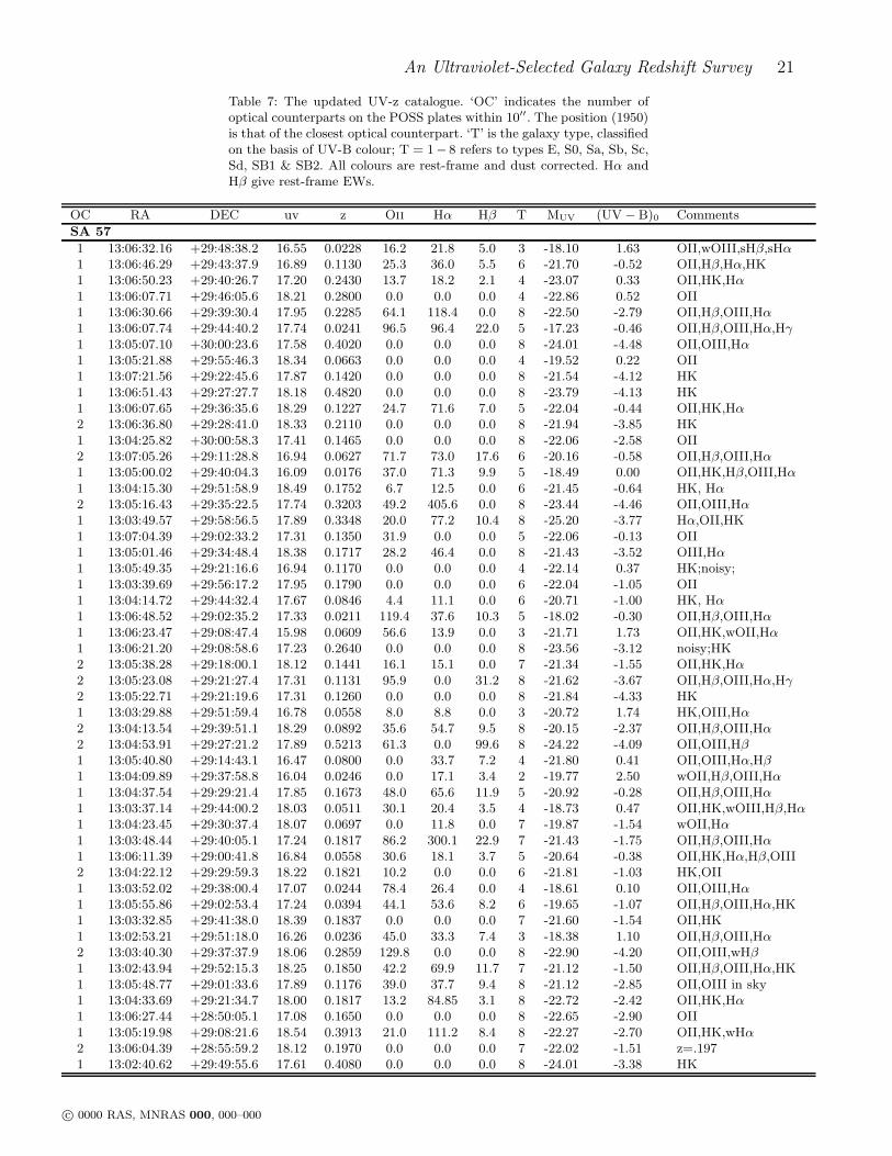
An Ultraviolet-Selected Galaxy Redshift Survey 21
Table 7: The updated UV-z catalogue. ‘OC’ indicates the number ofoptical counterparts on the POSS plates within 10′′. The position (1950)is that of the closest optical counterpart. ‘T’ is the galaxy type, classifiedon the basis of UV-B colour; T = 1− 8 refers to types E, S0, Sa, Sb, Sc,Sd, SB1 & SB2. All colours are rest-frame and dust corrected. Hα andHβ give rest-frame EWs.
OC RA DEC uv z Oii Hα Hβ T MUV (UV − B)0 Comments
SA 57
1 13:06:32.16 +29:48:38.2 16.55 0.0228 16.2 21.8 5.0 3 -18.10 1.63 OII,wOIII,sHβ,sHα1 13:06:46.29 +29:43:37.9 16.89 0.1130 25.3 36.0 5.5 6 -21.70 -0.52 OII,Hβ,Hα,HK1 13:06:50.23 +29:40:26.7 17.20 0.2430 13.7 18.2 2.1 4 -23.07 0.33 OII,HK,Hα1 13:06:07.71 +29:46:05.6 18.21 0.2800 0.0 0.0 0.0 4 -22.86 0.52 OII1 13:06:30.66 +29:39:30.4 17.95 0.2285 64.1 118.4 0.0 8 -22.50 -2.79 OII,Hβ,OIII,Hα1 13:06:07.74 +29:44:40.2 17.74 0.0241 96.5 96.4 22.0 5 -17.23 -0.46 OII,Hβ,OIII,Hα,Hγ1 13:05:07.10 +30:00:23.6 17.58 0.4020 0.0 0.0 0.0 8 -24.01 -4.48 OII,OIII,Hα1 13:05:21.88 +29:55:46.3 18.34 0.0663 0.0 0.0 0.0 4 -19.52 0.22 OII1 13:07:21.56 +29:22:45.6 17.87 0.1420 0.0 0.0 0.0 8 -21.54 -4.12 HK1 13:06:51.43 +29:27:27.7 18.18 0.4820 0.0 0.0 0.0 8 -23.79 -4.13 HK1 13:06:07.65 +29:36:35.6 18.29 0.1227 24.7 71.6 7.0 5 -22.04 -0.44 OII,HK,Hα2 13:06:36.80 +29:28:41.0 18.33 0.2110 0.0 0.0 0.0 8 -21.94 -3.85 HK1 13:04:25.82 +30:00:58.3 17.41 0.1465 0.0 0.0 0.0 8 -22.06 -2.58 OII2 13:07:05.26 +29:11:28.8 16.94 0.0627 71.7 73.0 17.6 6 -20.16 -0.58 OII,Hβ,OIII,Hα1 13:05:00.02 +29:40:04.3 16.09 0.0176 37.0 71.3 9.9 5 -18.49 0.00 OII,HK,Hβ,OIII,Hα1 13:04:15.30 +29:51:58.9 18.49 0.1752 6.7 12.5 0.0 6 -21.45 -0.64 HK, Hα2 13:05:16.43 +29:35:22.5 17.74 0.3203 49.2 405.6 0.0 8 -23.44 -4.46 OII,OIII,Hα1 13:03:49.57 +29:58:56.5 17.89 0.3348 20.0 77.2 10.4 8 -25.20 -3.77 Hα,OII,HK1 13:07:04.39 +29:02:33.2 17.31 0.1350 31.9 0.0 0.0 5 -22.06 -0.13 OII1 13:05:01.46 +29:34:48.4 18.38 0.1717 28.2 46.4 0.0 8 -21.43 -3.52 OIII,Hα1 13:05:49.35 +29:21:16.6 16.94 0.1170 0.0 0.0 0.0 4 -22.14 0.37 HK;noisy;1 13:03:39.69 +29:56:17.2 17.95 0.1790 0.0 0.0 0.0 6 -22.04 -1.05 OII1 13:04:14.72 +29:44:32.4 17.67 0.0846 4.4 11.1 0.0 6 -20.71 -1.00 HK, Hα1 13:06:48.52 +29:02:35.2 17.33 0.0211 119.4 37.6 10.3 5 -18.02 -0.30 OII,Hβ,OIII,Hα1 13:06:23.47 +29:08:47.4 15.98 0.0609 56.6 13.9 0.0 3 -21.71 1.73 OII,HK,wOII,Hα1 13:06:21.20 +29:08:58.6 17.23 0.2640 0.0 0.0 0.0 8 -23.56 -3.12 noisy;HK2 13:05:38.28 +29:18:00.1 18.12 0.1441 16.1 15.1 0.0 7 -21.34 -1.55 OII,HK,Hα2 13:05:23.08 +29:21:27.4 17.31 0.1131 95.9 0.0 31.2 8 -21.62 -3.67 OII,Hβ,OIII,Hα,Hγ2 13:05:22.71 +29:21:19.6 17.31 0.1260 0.0 0.0 0.0 8 -21.84 -4.33 HK1 13:03:29.88 +29:51:59.4 16.78 0.0558 8.0 8.8 0.0 3 -20.72 1.74 HK,OIII,Hα2 13:04:13.54 +29:39:51.1 18.29 0.0892 35.6 54.7 9.5 8 -20.15 -2.37 OII,Hβ,OIII,Hα2 13:04:53.91 +29:27:21.2 17.89 0.5213 61.3 0.0 99.6 8 -24.22 -4.09 OII,OIII,Hβ1 13:05:40.80 +29:14:43.1 16.47 0.0800 0.0 33.7 7.2 4 -21.80 0.41 OII,OIII,Hα,Hβ1 13:04:09.89 +29:37:58.8 16.04 0.0246 0.0 17.1 3.4 2 -19.77 2.50 wOII,Hβ,OIII,Hα1 13:04:37.54 +29:29:21.4 17.85 0.1673 48.0 65.6 11.9 5 -20.92 -0.28 OII,Hβ,OIII,Hα1 13:03:37.14 +29:44:00.2 18.03 0.0511 30.1 20.4 3.5 4 -18.73 0.47 OII,HK,wOIII,Hβ,Hα1 13:04:23.45 +29:30:37.4 18.07 0.0697 0.0 11.8 0.0 7 -19.87 -1.54 wOII,Hα1 13:03:48.44 +29:40:05.1 17.24 0.1817 86.2 300.1 22.9 7 -21.43 -1.75 OII,Hβ,OIII,Hα1 13:06:11.39 +29:00:41.8 16.84 0.0558 30.6 18.1 3.7 5 -20.64 -0.38 OII,HK,Hα,Hβ,OIII2 13:04:22.12 +29:29:59.3 18.22 0.1821 10.2 0.0 0.0 6 -21.81 -1.03 HK,OII1 13:03:52.02 +29:38:00.4 17.07 0.0244 78.4 26.4 0.0 4 -18.61 0.10 OII,OIII,Hα1 13:05:55.86 +29:02:53.4 17.24 0.0394 44.1 53.6 8.2 6 -19.65 -1.07 OII,Hβ,OIII,Hα,HK1 13:03:32.85 +29:41:38.0 18.39 0.1837 0.0 0.0 0.0 7 -21.60 -1.54 OII,HK1 13:02:53.21 +29:51:18.0 16.26 0.0236 45.0 33.3 7.4 3 -18.38 1.10 OII,Hβ,OIII,Hα2 13:03:40.30 +29:37:37.9 18.06 0.2859 129.8 0.0 0.0 8 -22.90 -4.20 OII,OIII,wHβ1 13:02:43.94 +29:52:15.3 18.25 0.1850 42.2 69.9 11.7 7 -21.12 -1.50 OII,Hβ,OIII,Hα,HK1 13:05:48.77 +29:01:33.6 17.89 0.1176 39.0 37.7 9.4 8 -21.12 -2.85 OII,OIII in sky1 13:04:33.69 +29:21:34.7 18.00 0.1817 13.2 84.85 3.1 8 -22.72 -2.42 OII,HK,Hα1 13:06:27.44 +28:50:05.1 17.08 0.1650 0.0 0.0 0.0 8 -22.65 -2.90 OII1 13:05:19.98 +29:08:21.6 18.54 0.3913 21.0 111.2 8.4 8 -22.27 -2.70 OII,HK,wHα2 13:06:04.39 +28:55:59.2 18.12 0.1970 0.0 0.0 0.0 7 -22.02 -1.51 z=.1971 13:02:40.62 +29:49:55.6 17.61 0.4080 0.0 0.0 0.0 8 -24.01 -3.38 HK
c© 0000 RAS, MNRAS 000, 000–000
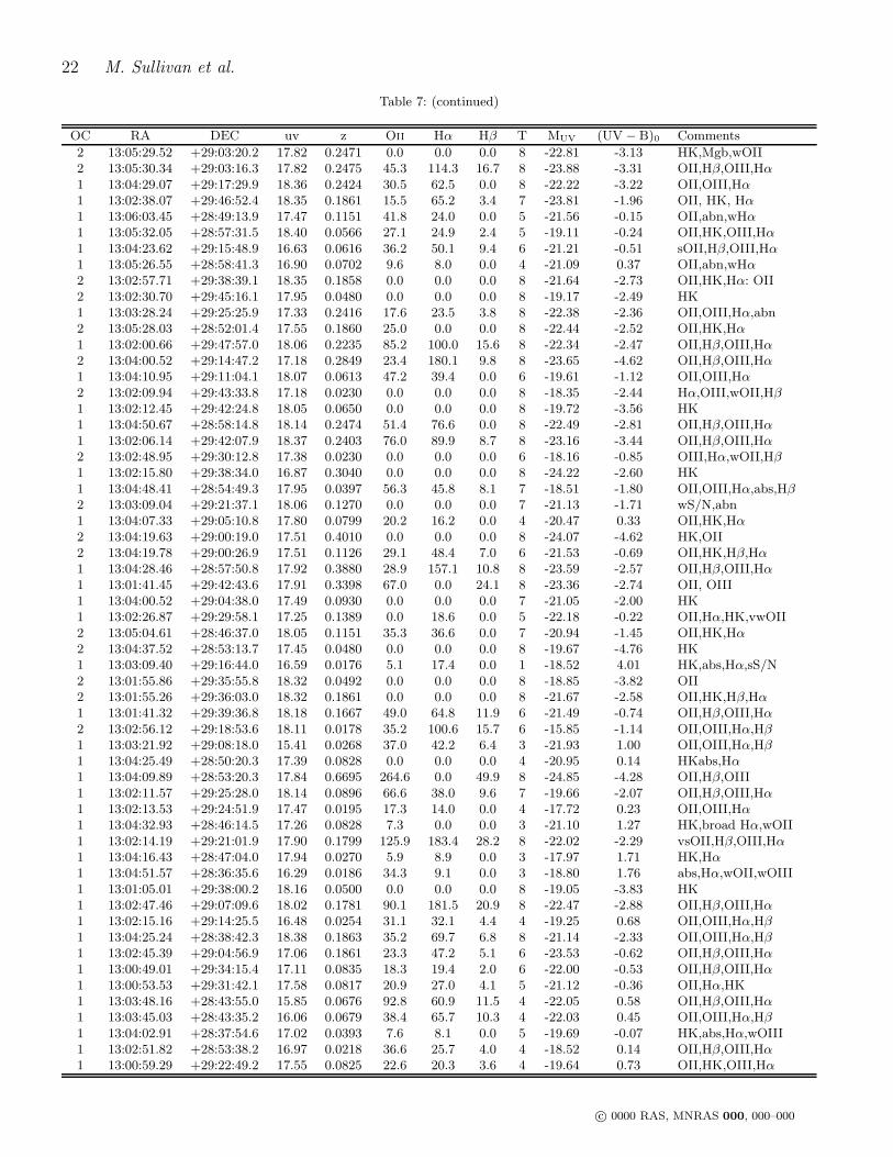
22 M. Sullivan et al.
Table 7: (continued)
OC RA DEC uv z Oii Hα Hβ T MUV (UV − B)0 Comments
2 13:05:29.52 +29:03:20.2 17.82 0.2471 0.0 0.0 0.0 8 -22.81 -3.13 HK,Mgb,wOII2 13:05:30.34 +29:03:16.3 17.82 0.2475 45.3 114.3 16.7 8 -23.88 -3.31 OII,Hβ,OIII,Hα1 13:04:29.07 +29:17:29.9 18.36 0.2424 30.5 62.5 0.0 8 -22.22 -3.22 OII,OIII,Hα1 13:02:38.07 +29:46:52.4 18.35 0.1861 15.5 65.2 3.4 7 -23.81 -1.96 OII, HK, Hα1 13:06:03.45 +28:49:13.9 17.47 0.1151 41.8 24.0 0.0 5 -21.56 -0.15 OII,abn,wHα1 13:05:32.05 +28:57:31.5 18.40 0.0566 27.1 24.9 2.4 5 -19.11 -0.24 OII,HK,OIII,Hα1 13:04:23.62 +29:15:48.9 16.63 0.0616 36.2 50.1 9.4 6 -21.21 -0.51 sOII,Hβ,OIII,Hα1 13:05:26.55 +28:58:41.3 16.90 0.0702 9.6 8.0 0.0 4 -21.09 0.37 OII,abn,wHα2 13:02:57.71 +29:38:39.1 18.35 0.1858 0.0 0.0 0.0 8 -21.64 -2.73 OII,HK,Hα: OII2 13:02:30.70 +29:45:16.1 17.95 0.0480 0.0 0.0 0.0 8 -19.17 -2.49 HK1 13:03:28.24 +29:25:25.9 17.33 0.2416 17.6 23.5 3.8 8 -22.38 -2.36 OII,OIII,Hα,abn2 13:05:28.03 +28:52:01.4 17.55 0.1860 25.0 0.0 0.0 8 -22.44 -2.52 OII,HK,Hα1 13:02:00.66 +29:47:57.0 18.06 0.2235 85.2 100.0 15.6 8 -22.34 -2.47 OII,Hβ,OIII,Hα2 13:04:00.52 +29:14:47.2 17.18 0.2849 23.4 180.1 9.8 8 -23.65 -4.62 OII,Hβ,OIII,Hα1 13:04:10.95 +29:11:04.1 18.07 0.0613 47.2 39.4 0.0 6 -19.61 -1.12 OII,OIII,Hα2 13:02:09.94 +29:43:33.8 17.18 0.0230 0.0 0.0 0.0 8 -18.35 -2.44 Hα,OIII,wOII,Hβ1 13:02:12.45 +29:42:24.8 18.05 0.0650 0.0 0.0 0.0 8 -19.72 -3.56 HK1 13:04:50.67 +28:58:14.8 18.14 0.2474 51.4 76.6 0.0 8 -22.49 -2.81 OII,Hβ,OIII,Hα1 13:02:06.14 +29:42:07.9 18.37 0.2403 76.0 89.9 8.7 8 -23.16 -3.44 OII,Hβ,OIII,Hα2 13:02:48.95 +29:30:12.8 17.38 0.0230 0.0 0.0 0.0 6 -18.16 -0.85 OIII,Hα,wOII,Hβ1 13:02:15.80 +29:38:34.0 16.87 0.3040 0.0 0.0 0.0 8 -24.22 -2.60 HK1 13:04:48.41 +28:54:49.3 17.95 0.0397 56.3 45.8 8.1 7 -18.51 -1.80 OII,OIII,Hα,abs,Hβ2 13:03:09.04 +29:21:37.1 18.06 0.1270 0.0 0.0 0.0 7 -21.13 -1.71 wS/N,abn1 13:04:07.33 +29:05:10.8 17.80 0.0799 20.2 16.2 0.0 4 -20.47 0.33 OII,HK,Hα2 13:04:19.63 +29:00:19.0 17.51 0.4010 0.0 0.0 0.0 8 -24.07 -4.62 HK,OII2 13:04:19.78 +29:00:26.9 17.51 0.1126 29.1 48.4 7.0 6 -21.53 -0.69 OII,HK,Hβ,Hα1 13:04:28.46 +28:57:50.8 17.92 0.3880 28.9 157.1 10.8 8 -23.59 -2.57 OII,Hβ,OIII,Hα1 13:01:41.45 +29:42:43.6 17.91 0.3398 67.0 0.0 24.1 8 -23.36 -2.74 OII, OIII1 13:04:00.52 +29:04:38.0 17.49 0.0930 0.0 0.0 0.0 7 -21.05 -2.00 HK1 13:02:26.87 +29:29:58.1 17.25 0.1389 0.0 18.6 0.0 5 -22.18 -0.22 OII,Hα,HK,vwOII2 13:05:04.61 +28:46:37.0 18.05 0.1151 35.3 36.6 0.0 7 -20.94 -1.45 OII,HK,Hα2 13:04:37.52 +28:53:13.7 17.45 0.0480 0.0 0.0 0.0 8 -19.67 -4.76 HK1 13:03:09.40 +29:16:44.0 16.59 0.0176 5.1 17.4 0.0 1 -18.52 4.01 HK,abs,Hα,sS/N2 13:01:55.86 +29:35:55.8 18.32 0.0492 0.0 0.0 0.0 8 -18.85 -3.82 OII2 13:01:55.26 +29:36:03.0 18.32 0.1861 0.0 0.0 0.0 8 -21.67 -2.58 OII,HK,Hβ,Hα1 13:01:41.32 +29:39:36.8 18.18 0.1667 49.0 64.8 11.9 6 -21.49 -0.74 OII,Hβ,OIII,Hα2 13:02:56.12 +29:18:53.6 18.11 0.0178 35.2 100.6 15.7 6 -15.85 -1.14 OII,OIII,Hα,Hβ1 13:03:21.92 +29:08:18.0 15.41 0.0268 37.0 42.2 6.4 3 -21.93 1.00 OII,OIII,Hα,Hβ1 13:04:25.49 +28:50:20.3 17.39 0.0828 0.0 0.0 0.0 4 -20.95 0.14 HKabs,Hα1 13:04:09.89 +28:53:20.3 17.84 0.6695 264.6 0.0 49.9 8 -24.85 -4.28 OII,Hβ,OIII1 13:02:11.57 +29:25:28.0 18.14 0.0896 66.6 38.0 9.6 7 -19.66 -2.07 OII,Hβ,OIII,Hα1 13:02:13.53 +29:24:51.9 17.47 0.0195 17.3 14.0 0.0 4 -17.72 0.23 OII,OIII,Hα1 13:04:32.93 +28:46:14.5 17.26 0.0828 7.3 0.0 0.0 3 -21.10 1.27 HK,broad Hα,wOII1 13:02:14.19 +29:21:01.9 17.90 0.1799 125.9 183.4 28.2 8 -22.02 -2.29 vsOII,Hβ,OIII,Hα1 13:04:16.43 +28:47:04.0 17.94 0.0270 5.9 8.9 0.0 3 -17.97 1.71 HK,Hα1 13:04:51.57 +28:36:35.6 16.29 0.0186 34.3 9.1 0.0 3 -18.80 1.76 abs,Hα,wOII,wOIII1 13:01:05.01 +29:38:00.2 18.16 0.0500 0.0 0.0 0.0 8 -19.05 -3.83 HK1 13:02:47.46 +29:07:09.6 18.02 0.1781 90.1 181.5 20.9 8 -22.47 -2.88 OII,Hβ,OIII,Hα1 13:02:15.16 +29:14:25.5 16.48 0.0254 31.1 32.1 4.4 4 -19.25 0.68 OII,OIII,Hα,Hβ1 13:04:25.24 +28:38:42.3 18.38 0.1863 35.2 69.7 6.8 8 -21.14 -2.33 OII,OIII,Hα,Hβ1 13:02:45.39 +29:04:56.9 17.06 0.1861 23.3 47.2 5.1 6 -23.53 -0.62 OII,Hβ,OIII,Hα1 13:00:49.01 +29:34:15.4 17.11 0.0835 18.3 19.4 2.0 6 -22.00 -0.53 OII,Hβ,OIII,Hα1 13:00:53.53 +29:31:42.1 17.58 0.0817 20.9 27.0 4.1 5 -21.12 -0.36 OII,Hα,HK1 13:03:48.16 +28:43:55.0 15.85 0.0676 92.8 60.9 11.5 4 -22.05 0.58 OII,Hβ,OIII,Hα1 13:03:45.03 +28:43:35.2 16.06 0.0679 38.4 65.7 10.3 4 -22.03 0.45 OII,OIII,Hα,Hβ1 13:04:02.91 +28:37:54.6 17.02 0.0393 7.6 8.1 0.0 5 -19.69 -0.07 HK,abs,Hα,wOIII1 13:02:51.82 +28:53:38.2 16.97 0.0218 36.6 25.7 4.0 4 -18.52 0.14 OII,Hβ,OIII,Hα1 13:00:59.29 +29:22:49.2 17.55 0.0825 22.6 20.3 3.6 4 -19.64 0.73 OII,HK,OIII,Hα
c© 0000 RAS, MNRAS 000, 000–000

An Ultraviolet-Selected Galaxy Redshift Survey 23
Table 7: (continued)
OC RA DEC uv z Oii Hα Hβ T MUV (UV − B)0 Comments
1 13:02:42.78 +28:54:32.0 17.75 0.0184 49.8 54.5 7.8 4 -17.43 0.69 OII,OIII,Hα,Hβ1 13:01:53.07 +29:07:07.0 17.52 0.0254 74.1 104.3 22.8 6 -18.47 -0.93 OII,OIII,Hα,Hβ1 13:03:01.48 +28:48:32.0 18.33 0.1170 30.0 33.6 0.0 5 -20.73 -0.04 OII,Hα,HK1 13:01:59.06 +29:04:42.8 14.25 0.0267 40.3 47.1 6.9 2 -21.99 3.20 OII,OIII,Hα,Hβ2 13:01:33.44 +29:10:37.6 18.03 0.1978 11.8 23.6 0.0 6 -22.19 -0.81 wOII, HK, Hα2 13:01:32.86 +29:10:34.5 18.03 0.0760 0.0 0.0 0.0 8 -20.07 -3.90 Hα only1 13:02:05.41 +29:01:54.8 18.20 0.0268 26.9 24.1 4.1 7 -17.67 -1.54 OII,OIII,Hα2 13:02:55.68 +28:48:03.4 18.25 0.1645 25.0 0.0 0.0 8 -21.47 -2.72 OII,vwHβ,OIII,Hα1 13:03:31.77 +28:36:53.0 18.09 0.1759 0.0 160.1 0.0 8 -21.78 -2.63 OIIwOIII, Hα2 13:01:58.51 +29:01:55.0 17.48 0.0184 0.0 79.7 21.5 7 -17.51 -1.44 wOII,Hβ,OIII,Hα1 13:01:05.21 +29:15:22.6 17.80 0.0830 0.0 0.0 0.0 3 -20.57 1.99 HK,Hα1 13:02:25.99 +28:51:14.9 18.16 0.2532 78.0 113.8 16.9 6 -21.67 -0.95 OII,Hβ,OIII,Hα1 13:02:15.28 +28:53:47.1 15.48 0.0570 4.1 6.3 0.0 2 -22.28 3.17 HK,vwOII,Hα1 13:02:11.95 +28:53:43.2 15.95 0.0224 27.0 38.3 4.2 3 -20.02 1.87 OII,abs,OIII,Hα,Hβ1 13:01:58.98 +28:55:49.6 18.46 0.2798 0.0 27.6 0.0 8 -22.46 -2.29 HK,abs1 13:02:41.80 +28:42:17.0 18.73 0.2187 14.9 50.1 0.0 4 -21.74 0.38 OII,abs,Hα,Hβ, OIII1 13:02:33.29 +28:43:05.3 17.60 0.0696 28.5 27.4 5.8 5 -20.24 -0.32 OII,OIII,Hα,Hβ2 13:02:08.38 +28:46:55.4 18.53 0.0370 0.0 0.0 0.0 8 -18.03 -3.68 z:,HK1 13:01:49.26 +28:48:37.7 16.00 0.0273 59.6 47.0 17.9 5 -19.92 -0.32 OII,Hβ,OIII,Hα1 13:01:07.18 +28:57:30.8 16.83 0.0224 15.1 35.3 5.1 6 -17.36 -0.80 wOII,Hβ,OIII,Hα
Abell 1367
1 11:41:52.98 +20:47:39.8 17.48 0.0965 0.0 0.0 0.0 6 -21.18 -0.93 OII,HK, OIII1 11:42:30.43 +20:42:57.5 16.49 0.0231 0.0 23.1 0.0 1 -19.24 5.86 Hα,HK,Hβabn1 11:41:28.99 +20:45:35.4 18.19 0.0669 26.4 21.2 0.0 6 -19.68 -1.17 OII,HK,Hβ,OII,Hα1 11:40:59.21 +20:46:04.6 16.91 0.1687 30.9 95.67 11.5 4 -22.96 0.36 OII,Hβ,OIII,Hα1 11:42:53.69 +20:40:01.9 17.91 0.0821 14.8 17.1 0.0 4 -20.41 0.31 wOII,HK,OIII,Hα1 11:42:58.57 +20:39:27.8 17.48 0.1129 10.6 33.1 3.1 3 -21.55 1.31 OII,HK,Hβ,Hα1 11:42:02.60 +20:42:14.0 16.53 0.0391 27.6 10.5 0.0 2 -20.34 2.52 wOII,HK,Hα2 11:42:57.11 +20:36:32.9 17.26 0.0480 0.0 0.0 0.0 3 -19.91 1.56 HK,z:1 11:41:26.28 +20:39:30.9 16.76 0.0399 77.1 82.9 14.5 3 -20.00 1.32 OII,Hβ,OIII,Hα1 11:41:12.18 +20:38:27.7 17.30 0.0222 0.0 0.0 0.0 1 -18.34 3.90 HK,Hα+b in abn1 11:40:54.03 +20:38:39.9 18.22 0.2084 7.2 49.0 0.0 5 -22.12 -0.15 OII,HK,Hα1 11:43:21.82 +20:27:28.1 16.93 0.0815 7.1 16.6 1.0 4 -21.38 0.75 wOII,HK,sHα1 11:40:40.45 +20:34:40.5 17.22 0.1770 0.0 0.0 0.0 3 -22.79 1.87 HK,z:1 11:41:02.34 +20:32:20.4 17.02 0.0413 36.7 37.6 0.0 7 -19.79 -1.47 OII,HK,OIII,Hα1 11:41:13.29 +20:31:34.6 16.51 0.0205 89.2 199.2 40.4 3 -18.79 1.81 OII,Hγ,Hβ,OIII,Hα1 11:40:22.05 +20:34:08.2 17.45 0.0700 0.0 0.0 0.0 4 -20.53 0.09 Hβ,Hα1 11:42:16.91 +20:27:56.5 18.38 0.0243 0.0 0.0 0.0 4 -17.29 0.26 HK,Hγ,Hα,Hβe+a1 11:41:41.45 +20:29:54.4 15.91 0.0216 0.0 10.2 0.0 1 -19.67 5.53 Hα,HK,Hβ(abn)1 11:43:04.16 +20:22:49.6 18.52 0.3826 22.4 49.4 10.4 8 -22.96 -3.78 OII,Hβ,OIII,Hα1 11:41:22.60 +20:27:44.9 15.63 0.0220 16.2 64.1 5.3 1 -19.99 3.83 OII,HK,Hβ,OIII,Hα1 11:42:11.59 +20:24:09.7 15.39 0.0214 13.9 0.0 0.0 1 -20.16 5.13 Hβabn,HK,wOII,Hα2 11:40:24.84 +20:29:35.5 18.07 0.0706 65.3 24.6 0.0 8 -19.87 -2.25 OII,OIII,Hα1 11:41:56.61 +20:23:02.9 18.08 0.0240 26.9 92.5 14.6 2 -17.68 2.83 OII,Hβ,OIII,sHα1 11:40:48.41 +20:25:49.3 17.45 0.0707 53.9 73.6 13.6 6 -20.54 -1.14 OII,Hβ,OIII,Hγ,Hα1 11:42:07.45 +20:21:20.2 17.80 0.0885 15.0 15.8 0.0 7 -20.64 -1.76 OII,HK,OIII,Hα1 11:41:23.40 +20:21:16.6 14.97 0.0250 5.1 12.0 0.0 1 -20.94 4.30 wOII,HK,Hα1 11:41:01.40 +20:21:04.4 17.48 0.0684 44.4 61.8 13.0 7 -20.42 -1.71 OII,Hγ,Hβ,OIII,Hα1 11:41:08.38 +20:19:19.9 18.15 0.0692 7.4 15.5 0.0 6 -19.79 -0.52 OII,HK,Hα1 11:41:18.49 +20:16:31.8 17.36 0.0966 4.2 3.5 0.0 6 -21.30 -0.90 OIII,HK,Hα1 11:40:09.47 +20:18:35.4 15.65 0.0289 0.0 0.0 0.0 1 -20.60 4.81 HK,Hα,Hβabs1 11:39:39.87 +20:19:34.2 16.26 0.0204 16.7 17.5 1.3 2 -19.13 2.33 OII,HK,OIII,Hα1 11:42:40.08 +20:09:19.8 17.62 0.0814 0.0 0.0 0.0 5 -20.68 -0.12 abn:HK,Hβ,wHα1 11:42:19.65 +20:09:28.8 17.63 0.0818 11.4 22.1 23.7 5 -20.68 -0.29 OII,HK,OIII,Hα1 11:41:51.04 +20:10:44.6 18.48 0.2460 0.0 0.0 0.0 8 -22.14 -3.35 HK,z:1 11:40:20.70 +20:14:37.2 15.02 0.0244 28.8 38.1 4.6 2 -20.78 2.91 OII,HK,Hβ,OIII,Hα1 11:40:03.61 +20:14:47.5 17.01 0.0245 98.4 53.7 8.7 5 -18.67 -0.02 OII,Hβ,OIII,Hα1 11:41:20.91 +20:10:20.7 16.87 0.0214 0.0 0.0 0.0 1 -18.68 5.15 abn:HK,G,Hβ,others
c© 0000 RAS, MNRAS 000, 000–000

24 M. Sullivan et al.
Table 7: (continued)
OC RA DEC uv z Oii Hα Hβ T MUV (UV − B)0 Comments
1 11:39:38.39 +20:15:09.9 15.53 0.0261 21.2 16.8 0.0 2 -20.42 3.73 OII,wHK,OIII,Hα1 11:40:18.41 +20:13:05.5 18.11 0.1318 44.8 121.6 11.3 8 -21.14 -3.20 OII,Hβ,OIII,Hα2 11:42:25.90 +20:05:34.0 18.34 0.0812 0.0 14.0 0.0 7 -19.92 -1.38 OII,HK,wOIII,Hα1 11:40:52.95 +20:10:16.2 17.02 0.1126 6.1 10.4 0.0 4 -21.98 0.68 OII,HK,Hβ,Hα1 11:43:10.71 +20:03:06.0 17.24 0.0183 0.0 0.0 0.0 1 -17.96 5.89 abn:HK,Hβ,Hα,others1 11:42:13.44 +20:05:08.6 17.09 0.0677 7.0 13.3 0.0 3 -20.84 1.46 wOII,HK,Hα1 11:40:52.30 +20:08:05.2 18.12 0.0713 15.0 9.9 0.0 6 -19.89 -1.07 OII,HK,Hα1 11:42:27.23 +20:02:00.1 16.87 0.0688 17.8 33.6 4.5 5 -21.06 -0.01 OII,HK,Hβ,OIII,Hα1 11:41:26.36 +20:03:43.3 15.04 0.0165 79.0 63.7 10.9 2 -19.87 2.72 OII,Hβ,OIII,vsHα1 11:40:09.70 +20:07:20.9 18.05 0.0708 34.1 54.2 4.8 8 -19.90 -2.59 OII,Hβ,OIII,Hα1 11:39:42.36 +20:06:54.9 16.79 0.0216 9.1 14.6 0.0 3 -18.63 1.72 wOII,HK,Hα1 11:42:10.07 +19:58:29.9 16.50 0.0821 0.0 8.0 0.0 3 -21.85 1.70 HK,Hα1 11:40:55.61 +19:54:19.7 15.51 0.0437 0.0 0.0 0.0 1 -21.72 3.82 abn:HK,G,Hβ,others1 11:40:26.50 +19:55:38.8 16.56 0.0233 0.0 0.0 0.0 1 -19.19 4.99 abn:HK,Hα,Hβ,Mgb
Paper I
2 13:03:58.95 28:52:21.8 18.02 0.2531 12.0 9.0 0.0 8 -22.64 -3.25 OII1 13:04:24.07 29:06:57.9 17.33 0.0160 0.0 7.0 0.0 5 -17.39 -0.35 Balmer, Hα1 13:04:44.85 28:54:00.4 16.41 0.0393 25.0 26.0 0.0 4 -20.28 0.71 OII, OIII, Hα1 13:06:00.96 29:10:29.5 18.35 0.2702 49.0 -9.0 0.0 8 -22.46 -3.51 OII, OIII2 13:05:55.61 29:12:27.8 17.38 0.1959 41.0 32.0 0.0 8 -22.69 -3.79 OII, OIII, Hα:1 13:05:59.62 29:13:10.1 18.08 0.1757 8.0 13.0 0.0 6 -21.83 -0.76 OII, Hα1 13:06:01.98 29:15:06.0 17.42 0.0256 32.0 86.0 0.0 7 -18.32 -1.79 0II, Hα1 13:05:32.99 29:16:56.8 18.17 0.1377 5.0 4.0 0.0 7 -21.16 -1.47 OII, HK1 13:04:29.55 29:22:03.1 17.86 0.0224 6.0 48.0 0.0 8 -17.58 -2.41 OII, OIII:, Hα2 13:05:38.86 29:32:23.6 18.22 0.0493 6.0 1.0 0.0 8 -18.93 -3.59 OII, OIII, Hα:1 13:05:19.19 29:32:52.8 18.15 0.0848 5.0 6.0 0.0 4 -20.21 0.07 OII, HK, Hα2 13:05:27.53 29:35:30.0 18.28 0.2525 15.0 12.0 0.0 8 -22.37 -2.84 OII, Balmer, Hα1 13:04:35.77 29:25:56.9 17.44 0.0607 27.0 29.0 0.0 5 -20.19 -0.23 OII, OIII, Hα1 13:05:10.07 29:35:40.6 18.04 0.1275 0.0 0.0 0.0 4 -21.19 0.48 Balmer only!1 13:04:27.19 29:26:58.7 17.65 0.1382 3.0 7.0 0.0 5 -21.74 0.00 OII, HK, Hα1 13:04:31.61 29:31:20.9 17.79 0.1379 9.0 35.0 0.0 4 -21.61 0.18 OII, HK, Hα1 13:04:40.52 29:41:16.2 17.44 0.2677 16.0 0.0 0.0 8 -23.35 -4.61 OII1 13:04:30.97 29:35:33.5 17.63 0.2256 13.0 25.0 0.0 6 -22.86 -0.84 OII, HK2 13:04:09.94 29:27:03.8 16.65 0.0312 0.0 13.0 0.0 2 -19.67 2.50 HK, Hα1 13:03:54.86 29:33:35.6 18.20 0.2736 54.0 70.0 0.0 8 -22.64 -2.77 OII, Hβ, OIII, Hα1 13:04:16.07 29:27:03.2 18.19 0.1850 32.0 0.0 0.0 8 -21.76 -3.78 OII1 13:03:20.22 29:41:43.9 17.91 0.0894 50.0 49.0 0.0 7 -20.52 -1.92 OII, OIII, Hα1 13:03:36.41 29:32:45.2 18.13 0.0266 0.0 0.0 0.0 1 -17.90 6.60 Balmer only!1 13:03:15.26 29:37:02.5 16.85 0.0238 11.0 6.0 0.0 5 -18.74 0.03 OII, HK1 13:03:11.64 29:22:44.9 17.98 0.0819 0.0 13.0 0.0 3 -20.33 1.35 HK, Hα1 13:03:13.39 29:35:00.4 18.05 0.0897 28.0 33.0 0.0 7 -20.39 -1.44 OII, OIII, Hα1 13:03:23.02 29:31:13.0 18.23 0.2897 125.0 250.0 0.0 8 -22.73 -2.92 OII, OIII, Hα1 13:03:15.09 29:29:57.6 17.78 0.1390 2.0 4.0 0.0 4 -21.63 0.16 OII, HK, Hα1 13:03:50.38 29:24:30.5 16.57 0.0235 0.0 4.0 0.0 4 -18.99 0.12 OIII, Hα1 13:02:34.52 29:32:08.1 17.49 0.1682 -9.0 -9.0 0.0 8 -22.25 -3.72 OII, Hα(poor ex)2 13:02:57.34 29:18:58.1 18.32 0.0176 0.0 28.0 0.0 7 -16.61 -1.30 Hα, Hβ, OIII, SII2 13:02:52.59 29:16:59.9 18.49 0.0332 0.0 0.0 0.0 8 -17.80 -3.60 HK, abs1 13:02:32.35 29:12:59.0 18.09 0.2427 11.0 30.0 0.0 7 -22.51 -1.84 OII, Balmer, Hα2 13:02:53.91 29:08:50.9 18.39 0.3229 10.0 -9.0 0.0 6 -22.90 -0.89 OII, OIII, Hα1 13:00:19.80 29:42:12.0 17.23 0.0900 8.0 27.0 0.0 4 -21.26 0.27 OII, H1 12:59:17.64 29:38:59.6 16.12 0.0590 48.0 77.0 0.0 4 -21.46 0.48 OII, OIII, Hα1 12:59:40.35 29:31:19.2 17.59 0.0250 0.0 0.0 0.0 1 -18.29 6.22 HK, abn2 12:59:22.62 29:20:41.6 16.16 0.0620 21.0 20.0 0.0 5 -21.52 -0.03 OII, Hα1 12:59:33.16 29:19:06.8 17.44 0.0240 90.0 49.0 0.0 8 -18.15 -2.14 OII, Hα3 13:00:17.07 29:17:06.6 17.52 0.0380 17.0 18.0 0.0 6 -19.09 -1.08 OII, OIII, Hα1 13:02:06.03 29:11:51.5 17.32 0.0830 0.0 65.0 0.0 4 -21.00 0.41 OIII, Hα1 13:02:03.66 29:18:39.3 18.06 0.0840 0.0 49.0 0.0 4 -20.28 0.42 HK, Hα1 13:01:59.75 29:24:29.1 17.89 0.1890 12.0 21.0 0.0 6 -22.19 -0.68 OII, HK, Hα
c© 0000 RAS, MNRAS 000, 000–000

An Ultraviolet-Selected Galaxy Redshift Survey 25
Table 7: (continued)
OC RA DEC uv z Oii Hα Hβ T MUV (UV − B)0 Comments
1 13:00:00.88 30:00:51.0 17.67 0.1570 10.0 13.0 0.0 6 -21.99 -0.84 OII, Hα1 13:06:01.14 29:21:14.7 18.53 0.2407 0.0 0.0 0.0 5 -22.12 -0.23 HK,Hd1 13:04:31.58 28:48:55.0 17.68 0.0206 0.0 0.0 0.0 1 -17.76 6.78 HK,abs1 13:05:01.02 29:03:43.2 17.75 0.1146 3.0 0.0 0.0 6 -21.24 -0.62 OII, HK1 13:06:27.79 29:09:09.3 16.77 0.0800 4.0 0.0 0.0 3 -21.49 2.15 OII,HK1 13:06:08.41 29:16:38.7 18.19 0.0249 16.0 0.0 0.0 6 -17.50 -0.55 OII, OIII1 13:07:29.10 28:38:54.5 15.23 0.0231 0.0 0.0 0.0 1 -20.47 4.04 HK, abs1 13:06:13.24 28:56:47.1 18.20 0.1222 15.0 0.0 0.0 4 -20.94 0.20 OII,HK,abn1 13:05:13.62 28:44:45.9 18.15 0.0686 22.0 0.0 0.0 5 -19.75 -0.42 OII,Hβ,OIII2 13:06:29.96 28:50:03.5 18.27 0.1849 6.0 0.0 0.0 7 -21.70 -1.72 OII,HK,abn1 13:06:26.18 28:50:23.5 17.22 0.0886 41.0 0.0 0.0 4 -21.24 0.10 OII,Hβ,OIII1 13:05:50.11 29:06:51.2 16.36 0.0544 0.0 0.0 0.0 2 -21.26 2.95 HK, abn1 13:05:08.45 28:44:10.1 17.32 0.0685 11.0 0.0 0.0 4 -20.58 0.52 OII, abn2 13:03:57.96 28:52:18.3 18.04 0.1865 47.0 0.0 0.0 8 -21.92 -3.03 OII, OIII1 13:05:13.02 28:41:19.4 18.51 0.0770 42.0 0.0 0.0 7 -19.61 -1.38 OII, Hβ, OIII1 13:03:47.89 29:02:28.4 17.49 0.0836 42.0 0.0 0.0 7 -20.80 -1.84 OII, OIII1 13:07:03.27 28:59:17.8 17.99 0.0376 23.0 0.0 0.0 6 -18.59 -1.07 OII, Hβ1 13:06:04.40 28:36:59.0 17.53 0.0237 25.0 0.0 0.0 3 -18.06 0.90 OII, Hβ, OIII1 13:07:40.56 28:56:33.1 18.21 0.1220 11.0 0.0 0.0 6 -20.91 -1.05 OII, HK, abs1 13:06:20.66 29:09:25.9 16.93 0.0612 35.0 0.0 0.0 5 -20.72 -0.02 OII,Hβ,OIII1 13:06:14.98 29:10:25.8 16.59 0.0395 28.0 0.0 0.0 6 -20.10 -0.98 OII,Hβ,OIII1 13:04:52.46 28:41:20.3 17.71 0.0698 17.0 0.0 0.0 7 -20.20 -1.54 OII,Hβ,OIII2 13:04:45.12 28:41:37.3 18.04 0.0346 19.0 0.0 0.0 6 -18.36 -0.58 OII1 13:03:55.90 28:44:11.1 17.40 0.2379 30.0 0.0 0.0 7 -23.15 -1.59 OII,Balmer,Hβ,OIII1 13:05:45.10 29:18:35.4 16.59 0.0587 21.0 0.0 0.0 6 -20.97 -0.52 OII,HK,Hβ,OIII1 13:04:06.93 28:53:34.4 17.84 0.1866 5.0 0.0 0.0 4 -22.23 0.22 OII,HK,Hβ,OIII1 13:05:54.39 28:57:38.7 16.57 0.0804 13.0 0.0 0.0 8 -21.62 -2.81 OII,OIII1 13:06:03.73 28:50:27.4 16.41 0.0700 25.0 0.0 0.0 4 -21.54 0.23 OII,Balmer,Hβ,OIII1 13:06:49.06 28:43:19.2 17.91 0.0789 26.0 0.0 0.0 6 -20.29 -0.60 OII, OIII1 13:06:23.77 29:05:09.9 17.19 0.1384 31.0 0.0 0.0 8 -22.13 -3.66 OII,Hβ,OIII1 13:07:26.48 29:14:32.2 16.79 0.1222 12.0 0.0 0.0 8 -22.27 -3.23 OII1 13:04:48.14 28:41:26.5 17.95 0.0179 30.0 0.0 0.0 6 -17.02 -1.03 OII, OIII1 13:04:33.35 28:48:11.3 18.23 0.1589 0.0 0.0 0.0 7 -21.41 -1.87 HK1 13:05:52.13 29:17:22.0 16.82 0.0206 25.0 0.0 0.0 5 -18.45 -0.13 OII,Hβ,OIII1 13:05:41.78 28:58:41.9 16.51 0.0800 4.0 0.0 0.0 3 -21.75 1.02 OII,HK,abn1 13:05:16.20 29:17:05.5 18.04 0.1235 4.0 0.0 0.0 3 -21.15 1.21 OII,HK,abn1 13:06:32.30 28:51:22.4 18.27 0.0696 33.0 0.0 0.0 7 -19.63 -1.81 OII,Hβ,OIII2 13:08:00.21 28:54:33.6 17.61 0.1223 11.0 0.0 0.0 6 -21.52 -0.79 OII,HK1 13:07:39.47 29:07:24.7 18.06 0.2348 14.0 0.0 0.0 8 -22.42 -2.45 OII,HK1 13:04:05.73 28:41:24.0 17.89 0.0695 23.0 0.0 0.0 6 -20.03 -1.14 OII,HK1 13:05:58.96 28:47:52.5 18.25 0.1993 8.0 0.0 0.0 7 -21.89 -1.68 OII,HK1 13:05:40.90 29:15:52.3 16.20 0.0242 23.0 0.0 0.0 3 -19.44 1.68 OII,Hβ,OIII1 13:04:57.97 29:15:45.5 17.81 0.1894 26.0 0.0 0.0 7 -22.21 -1.45 OII,OIII1 13:06:34.50 28:59:59.0 17.60 0.0560 0.0 0.0 0.0 1 -20.21 5.17 HK, abn1 13:06:28.46 28:53:45.1 16.16 0.0227 17.0 0.0 0.0 2 -19.44 2.39 OII,Balmer,OIII1 13:06:24.43 28:53:25.3 16.66 0.1893 79.0 0.0 0.0 5 -23.42 -0.21 OII,Hβ,OIII1 13:04:25.09 28:59:31.8 18.09 0.0565 5.0 0.0 0.0 4 -19.39 0.32 OII,HK1 13:06:32.05 29:07:04.6 17.66 0.0794 4.0 0.0 0.0 5 -20.55 -0.01 OII,HK, abn1 13:04:14.22 28:51:15.7 17.26 0.1225 0.0 0.0 0.0 4 -21.88 0.75 HK,abn
QSO / AGN
1 13:05:45.71 +29:50:48.6 18.23 1.1760 QSO2 13:05:42.92 +29:22:52.9 17.49 0.4020 QSO1 13:05:30.13 +29:17:38.2 18.44 0.6750 QSO1 13:04:27.11 +29:25:29.8 16.98 1.3370 QSO2 13:04:27.70 +29:15:50.9 16.76 0.1836 AGN1 13:05:15.88 +28:52:26.6 17.06 0.5789 QSO2 13:03:45.69 +29:06:30.7 16.94 0.0790 QSO2 13:02:56.66 +29:18:51.3 18.11 0.0760 QSO
c© 0000 RAS, MNRAS 000, 000–000

26 M. Sullivan et al.
Table 7: (continued)
OC RA DEC uv z Oii Hα Hβ T MUV (UV − B)0 Comments
1 13:04:41.25 +28:48:41.1 19.08 1.5628 QSO:CIV,CIII1 13:02:06.39 +29:29:13.4 17.42 1.0160 QSO2 13:01:05.74 +29:42:15.0 18.58 1.7590 QSO:CIV,CIII1 13:04:14.14 +28:38:10.2 18.36 1.3625 CIV,CIII,MgI QSO1 13:03:07.94 +28:55:03.4 16.61 0.1840 OII,Balmer,AGN1 13:02:45.26 +28:53:19.3 17.99 1.6700 QSO:CIV,CIII1 11:39:52.35 +20:26:34.2 18.03 1.4150 QSO:CIV,CIII1 11:41:07.70 +20:22:36.4 17.21 1.0580 QSO1 11:42:32.69 +19:55:58.8 17.68 1.0320 QSO1 11:40:20.54 +19:56:54.1 18.03 1.1610 QSO1 13:04:12.79 29:35:29.7 18.30 1.0195 QSO:CIII,MgII1 13:06:36.24 29:21:56.4 17.80 0.7460 QSO:MgII1 13:07:21.82 28:43:32.7 16.41 0.7370 QSO:MgII1 13:04:41.44 29:17:32.8 17.69 1.5866 QSO:CIV,CIII1 13:04:23.17 28:39:55.6 17.17 0.9186 QSO:MgII
Stars
2 13:06:25.11 +29:42:09.2 16.17 * STAR1 13:07:04.67 +29:31:10.5 17.30 * STAR1 13:06:46.99 +29:29:54.3 18.21 * STAR1 13:07:20.12 +29:20:31.2 15.59 * STAR1 13:06:19.31 +29:29:14.2 18.32 * STAR2 13:05:17.21 +29:44:18.9 0.00 * STAR1 13:03:54.71 +29:59:38.9 16.83 * STAR1 13:04:07.05 +29:51:24.9 18.61 * STAR1 13:05:36.36 +29:26:50.8 18.09 * STAR1 13:03:44.60 +29:57:14.7 17.39 * STAR1 13:03:47.43 +29:54:37.7 18.44 * STAR1 13:03:12.29 +30:01:45.1 17.48 * STAR1 13:06:23.62 +29:02:51.5 16.57 * STAR1 13:02:44.74 +29:55:03.3 17.34 * STAR1 13:05:39.76 +29:06:32.0 15.76 * STAR1 13:04:11.26 +29:26:54.5 16.68 * STAR1 13:04:27.83 +29:19:52.0 17.20 * STAR1 13:05:47.53 +28:57:23.2 18.17 * STAR1 13:02:42.36 +29:46:19.1 17.96 * STAR1 13:03:58.77 +29:24:08.3 17.96 * STAR1 13:05:33.64 +28:57:10.0 17.21 * STAR1 13:03:20.26 +29:26:26.6 18.14 * STAR2 13:03:59.68 +29:14:38.8 17.18 * STAR1 13:05:07.25 +28:55:37.9 18.11 * STAR1 13:02:52.40 +29:29:02.4 17.79 * STAR1 13:03:48.62 +29:13:43.6 16.41 * STAR1 13:02:44.35 +29:27:59.6 18.11 * STAR2 13:02:25.48 +29:30:07.2 17.68 * STAR1 13:02:53.26 +29:16:02.8 17.02 * STAR1 13:01:12.62 +29:34:10.7 17.86 * STAR1 13:01:50.15 +29:21:17.3 18.03 * STAR1 13:00:59.77 +29:32:42.4 17.36 * STAR1 13:01:16.97 +29:27:10.6 15.87 * STAR1 13:01:08.23 +29:22:04.7 17.20 * STAR1 13:03:12.23 +28:46:17.7 15.76 * STAR1 13:02:50.69 +28:51:02.8 17.95 * STAR1 13:01:38.04 +28:49:14.5 17.38 * STAR1 13:00:56.66 +28:59:33.2 16.76 * STAR1 11:43:10.44 +20:29:09.0 18.39 * STAR1 11:40:11.78 +20:22:29.7 16.97 * STAR1 11:42:09.41 +19:56:06.9 18.02 * STAR1 11:41:19.47 +19:55:56.6 18.22 * STAR
c© 0000 RAS, MNRAS 000, 000–000

An Ultraviolet-Selected Galaxy Redshift Survey 27
Table 7: (continued)
OC RA DEC uv z Oii Hα Hβ T MUV (UV − B)0 Comments
1 13:04:58.22 29:11:27.1 18.45 * STAR1 13:03:47.20 29:17:50.1 8.34 * STAR1 13:00:08.49 29:23:14.1 17.50 * STAR1 13:01:34.41 29:19:34.1 16.85 * STAR1 13:07:33.80 28:49:27.4 15.48 * STAR1 13:07:56.30 29:02:17.9 18.47 * STAR2 13:05:13.95 29:04:36.3 15.29 * STAR2 13:07:52.45 28:48:54.9 17.56 * STAR
c© 0000 RAS, MNRAS 000, 000–000