Type Ia supernova rate at a redshift of ˜0.1

arX

iv:a

stro

-ph/

0405

211v

1 1

1 M

ay 2

004

1Astronomy & Astrophysics manuscript no. rate February 2, 2008(DOI: will be inserted by hand later)

Type Ia supernova rate at a redshift of ∼ 0.1

G. Blanc1,12,22, C. Afonso1,4,8,23, C. Alard24, J.N. Albert2, G. Aldering15,28, A. Amadon1, J. Andersen6,

R. Ansari2, E. Aubourg1, C. Balland13,21, P. Bareyre1,4, J.P. Beaulieu5, X. Charlot1, A. Conley15,28,C. Coutures1, T. Dahlen19, F. Derue13, X. Fan16, R. Ferlet5, G. Folatelli11 , P. Fouque9,10, G. Garavini11,

J.F. Glicenstein1, B. Goldman1,4,8,23, A. Goobar11, A. Gould1,7, D. Graff7, M. Gros1, J. Haissinski2,C. Hamadache1, D. Hardin13, I.M. Hook25, J. de Kat1, S. Kent18, A. Kim15, T. Lasserre1, L. Le Guillou1,

E. Lesquoy1,5, C. Loup5, C. Magneville1, J.B. Marquette5, E. Maurice3, A. Maury9, A. Milsztajn1,M. Moniez2, M. Mouchet20,22, H. Newberg17, S. Nobili11, N. Palanque-Delabrouille1 , O. Perdereau2,L. Prevot3, Y.R. Rahal2, N. Regnault2,14,15, J. Rich1, P. Ruiz-Lapuente27, M. Spiro1, P. Tisserand1,

A. Vidal-Madjar5, L. Vigroux1, N.A. Walton26, S. Zylberajch1.

1 DSM/DAPNIA, CEA/Saclay, 91191 Gif-sur-Yvette Cedex, France2 Laboratoire de l’Accelerateur Lineaire, IN2P3 CNRS, Universite Paris-Sud, 91405 Orsay Cedex, France3 Observatoire de Marseille, 2 pl. Le Verrier, 13248 Marseille Cedex 04, France4 College de France, Physique Corpusculaire et Cosmologie, IN2P3 CNRS, 11 pl. M. Berthelot, 75231 Paris

Cedex, France5 Institut d’Astrophysique de Paris, INSU CNRS, 98 bis Boulevard Arago, 75014 Paris, France6 Astronomical Observatory, Copenhagen University, Juliane Maries Vej 30, 2100 Copenhagen, Denmark7 Departments of Astronomy and Physics, Ohio State University, Columbus, OH 43210, U.S.A.8 Department of Astronomy, New Mexico State University, Las Cruces, NM 88003-8001, U.S.A.9 European Southern Observatory (ESO), Casilla 19001, Santiago 19, Chile

10 Observatoire Midi-Pyrenees, 14 avenue Edouard Belin, 31400 Toulouse, France11 Department of Physics, Stockholm University, AlbaNova University Center, S-106 91 Stockholm, Sweden12 Osservatorio Astronomico di Padova, INAF, vicolo dell’Osservatorio 5 - 35122 Padova, Italy13 Laboratoire de Physique Nucleaire et de Hautes Energies, IN2P3 - CNRS - Universites Paris 6 et Paris 7, 4

place Jussieu, 75252 Paris Cedex 05, France14 Laboratoire Leprince-Ringuet, LLR/Ecole Polytechnique, Route de Saclay, 91128 Palaiseau CEDEX, France15 Lawrence Berkeley National Lab, 1 Cyclotron Road, Berkeley, CA 94720, U.S.A.16 Steward Observatory, The University of Arizona, 933 N. Cherry Ave, Tucson, AZ 85721-0065, U.S.A.17 Rensselaer Polytechnic Institute, 110 Eighth Street, Troy, NY 12180, U.S.A.18 Fermilab Wilson and Kirk Roads, Batavia, IL 60510-0500, U.S.A.19 Space Telescope Science Institute, 3700 San Martin Dr., Baltimore, MD 21218, U.S.A.20 LUTH, Observatoire de Paris, 5, Place Jules Janssen, 92195 Meudon Cedex, France21 Institut d’Astrophysique Spatiale, Batiment 121, Universite Paris 11, 91405 Orsay Cedex, France22 Universite Paris 7 Denis Diderot, 2, place Jussieu, 75005 Paris, France23 NASA/Ames Research Center, Mail Stop 244, Moffet Field, CA 94035, U.S.A.24 GEPI, Observatoire de Paris, 77 avenue de l’Observatoire, 75014 Paris, France25 Department of Physics, University of Oxford, Nuclear and Astrophysics laboratory, Keble Road, Oxford OX1

3RH, UK26 Institute of Astronomy, Madingley Road, Cambridge CB3 0HA, UK27 Department of Astronomy, University of Barcelona, Barcelona, Spain28 Visiting astronomer, Cerro Tololo Inter-American Observatory, National Optical Astronomy Observatories,

which are operated by the Association of Universities for Research in Astronomy, under contract with theNational Science Foundation.

Received / Accepted

Abstract. We present the type Ia rate measurement based on two EROS supernova search campaigns (in 1999and 2000). Sixteen supernovae identified as type Ia were discovered. The measurement of the detection efficiency,using a Monte Carlo simulation, provides the type Ia supernova explosion rate at a redshift ∼ 0.13. The result is0.125+0.044+0.028

−0.034−0.028 h270 SNu where 1 SNu = 1 SN / 1010 LB

⊙ / century. This value is compatible with the previousEROS measurement (Hardin et al. 2000), done with a much smaller sample, at a similar redshift. Comparisonwith other values at different redshifts suggests an evolution of the type Ia supernova rate.

Key words. (Stars:) supernovae: general – Galaxies: evolution

http://arXiv.org/abs/astro-ph/0405211v1

1. Introduction

Type Ia supernovae are believed to be thermonuclear ex-plosions of a white dwarf reaching the Chandrasekharmass after accreting matter in a binary system (see e.g.

Livio (2001)). They are the main mechanism to enrich theinterstellar medium (ISM) with iron-peak elements (with∼ 0.6 M⊙ of nickel released per event on average). Theknowledge of the number of such events per galaxy andper unit of time is crucial to understand the matter cycleand the ISM chemistry. From a cosmological point of viewthe measurement of the evolution of the explosion ratewill put strong constraints on galaxy evolution. Measuringthe evolution of the core-collapse supernovae (type II andIb/c) explosion rate would give a new unbiased view onthe star formation rate (SFR) history, independent of anypeculiar tracer, because gravitational supernovae are di-rectly linked to massive star formation. Up to now, thetype II supernova rate has been measured only in the lo-cal Universe (Cappellaro et al. 1999). On the other hand,the measurement of the evolution of the explosion rate oftype Ia supernova would give strong constraints on theSFR history and on many other parameters such as theprogenitor evolution (birth rate of binaries, time delay be-tween the white dwarf formation and the thermonuclearexplosion...) or the nature of the progenitor itself.

This paper is organized as follows: first the EROSsearch for supernovae is reviewed in Sect. 2. Then thetwo supernova search campaigns at the origin of this workare presented in Sect. 3. Sections 4 to 7 deal with the ratecomputation. Our results are presented in Sect. 8 and dis-cussed in Sect. 9.

2. The EROS search for supernovae

The EROS experiment used a 1-meter telescope basedat La Silla observatory, Chile, designed for a baryonicdark matter search using the microlensing effect (seee.g. Lasserre et al. 2000; Afonso et al. 2003b,a). The tele-scope beam light was split by a dichroic cube into twowide field cameras (1 deg2). The cube sets the passbandof both cameras, a “blue” one overlapping the V and Rstandard bands, another “red” one matching roughly theI standard band1. Each camera was a mosaic of eight 2048× 2048 pixels CCDs with a pixel size of 0.60′′ on thesky (Bauer & de Kat 1997; Palanque-Delabrouille et al.1998). In the following, we will use only the blue cam-era. One “image” stands for one CCD, and one “field” isfor the entire camera with its eight CCDs, i.e. ∼ 1 deg2.

A wide field camera is a good asset to perform super-nova searches as the number n of detected supernovae isproportional to Ω ·z2

lim where Ω is the solid angle surveyedand zlim is the limiting redshift of the search – typically

Send offprint requests to: G. Blanc, e-mail:[email protected]

1 By “standard” we mean the Johnson-Cousins UBV RI pho-tometric system (Johnson 1965; Cousins 1976) as used byLandolt (1992).

EROS detected type Ia supernovae up to z = 0.3. EROSdedicated about 15 % of its time to supernova search be-tween 1997 and 2000. The main limitation has been tosecure enough telescope time to perform the photometricand spectroscopic follow-up of discovered events.

To search for supernovae EROS uses the CCD subtrac-tion technique which consists in observing the same fieldsthree weeks to one month apart in order to detect tran-sient events and catch only supernovae near maximumlight (a typical type Ia supernova reaches its maximumlight in the optical wavelength roughly 15 to 20 days afterthe explosion). Both observations are done around newmoon in order to limit the sky background. The two setsof images are then automatically subtracted after a spatialalignment, a flux alignment and a seeing convolution.

Cuts are applied to eliminate known classes of variableobjects such as asteroids, variable stars, and cosmic rays.The most important cut is the requirement that the tran-sient object be near an identified galaxy. More precisely, itis required to be within an ellipse centered on any galaxywith semi-major and minor axes of length 8 times ther.m.s. radius of the galaxy’s flux distribution along eachaxis. This ellipse should contain essentially all supernovaeassociated with a galaxy since ∼ 99 % of galactic lightis contained within an ellipse of size 3 times the r.m.s.radius. To eliminate cosmic rays, each exposure consistsin two subexposures: SExtractor (Bertin & Arnouts 1996)software is run on both images to make a cosmic-ray cat-alog before adding the two images.

In spite of these cuts, a human eye is still needed tocheck the remaining candidates and discard obvious arte-facts (residual cosmic rays, bad subtractions, asteroids,variable stars...). Ten to fifteen search fields are observedevery night and the human scanner has to deal with about100 candidates the following day. The serious candidatesare observed again on the following night for confirmation.Then a spectrum is taken to obtain the supernova type,phase and redshift.

EROS supernova search fields lay near the celes-tial equator (declination between −4.5 and −12) tobe reached from both hemispheres and between 10h

and 14.5h in right ascension. They overlap some of theLas Campanas Redshift Survey (LCRS) (Shectman et al.1996) fields which will facilitate the galaxy sample cali-bration.

3. The 1999 and 2000 campaigns

At the beginning of 1999, the Supernova Cosmology

Project (SCP) undertook a large nearby supernova searchinvolving eight supernova search groups, including EROS.The goal was to gather a large set of well sampled, CCDdiscovered, nearby (z . 0.15) type Ia supernovae in orderto calibrate the distant events used to measure the cos-mological parameters. The whole collaboration obtained37 SNe out of which 19 were type Ia SNe near or beforemaximum light and were followed both spectroscopicallyand photometrically. EROS observed 428 square degrees of

G. Blanc et al.: Type Ia supernova rate at a redshift of ∼ 0.1 3

IAU Name Date (UT) V αJ2000.0 δJ2000.0 z Type Phase (days) IAUC

SN 1999ae 1999-02-10 20.7 11 51 24.48 -04 39 09.4 0.076 II < +30 7117SN 1999af 1999-02-12 19.2 13 44 50.95 -06 40 12.6 0.097 Ia −10 7117SN 1999ag 1999-02-12 20.1 12 15 22.81 -05 18 12.4 0.099 II 7117SN 1999ah 1999-02-13 20.5 12 09 37.20 -06 18 34.3 0.080 SN? 7117-18SN 1999ai 1999-02-15 18.0 13 14 10.57 -05 35 43.7 0.018 II ∼ +14 7117-18SN 1999aj 1999-02-17 20.9 11 22 39.34 -11 43 53.9 0.186 Ia 7117SN 1999ak 1999-02-17 18.5 11 06 52.05 -11 39 13.3 0.055 Ia ∼ +14 7117-18SN 1999al 1999-02-21 19.2 11 10 25.68 -07 26 37.0 0.065 Ic -9 7117-18

SN 1999bi 1999-03-10 19.8 11 01 15.76 -11 45 15.2 0.124 Ia +2 7136SN 1999bj 1999-03-10 20.5 11 51 38.39 -12 29 08.3 0.16 Ia +17 7136SN 1999bk 1999-03-14 18.9 11 28 52.01 -12 18 08.3 0.096 Ia +1 7136SN 1999bl 1999-03-14 20.7 11 12 13.60 -05 04 44.8 0.300 Ia 0 7136SN 1999bm 1999-03-17 20.0 12 45 00.84 -06 27 30.2 0.143 Ia -1 7136SN 1999bn 1999-03-16 19.6 11 57 00.40 -11 26 38.4 0.129 Ia -5 7136SN 1999bo 1999-03-17 19.5 12 41 07.48 -05 57 25.8 0.130 Ia > 0 7136SN 1999bp 1999-03-19 18.6 11 39 46.42 -08 51 34.8 0.077 Ia -4 7136SN 1999bq 1999-03-19 20.7 13 06 54.46 -12 37 11.6 0.149 Ia -1 7136

SN 2000bt 2000-03-26 19.4 10 16 18.05 -05 44 47.3 0.04 Ia +20 7406SN 2000bu 2000-03-31 19.4 11 27 11.45 -06 23 14.6 0.05 II? ∼ 0 7406SN 2000bv 2000-04-01 20.6 12 59 28.70 -12 20 07.6 0.12 II? ∼ 0 7406SN 2000bw 2000-04-04 20.5 11 09 49.85 -04 24 46.4 0.12 II? ∼ 0 7406SN 2000bx 2000-04-06 19.2 13 48 55.55 -06 18 35.9 0.09 Ia ∼ 0 7406SN 2000by 2000-04-07 19.2 11 39 54.91 -04 22 16.4 0.10 Ia ∼ 0 7406SN 2000bz 2000-04-08 21.2 14 15 02.66 -06 17 16.0 0.26 Ia ∼ 0 7406

Table 1. List of supernovae discovered by EROS in 1999 and 2000. From left to right: IAU name of each event,discovery date, discovery V magnitude, SNe celestial coordinates, redshift, type, phase (discovery time from maximumlight) and IAU.

sky in two steps and discovered 12 type Ia (cf. IAUC 7117and 7136) of which 7 have been followed by the collabo-ration. After obtaining reference images of search fields inJanuary 1999 (01/12 to 01/29), the SN search was con-ducted between February 4 and February 27 (new moonwas on February 16), and between March 09 and March27 (new moon was on March 17).

One year later, EROS was involved with the European

Supernova Cosmology Consortium (ESCC, involvingFrench, British, Swedish and Spanish institutes) to searchfor intermediate redshift (z ∼ 0.2− 0.4) supernovae. Fourtype Ia supernovae were discovered (cf. IAUC 7406). Onehundred and seventy square degrees were observed be-tween 2000, March 27 and April 9 (new moon on April4); reference images were taken between February 27 andMarch 15. The main difference between the two searcheswas the exposure time used: for the 1999 campaign it wasset to 300 seconds, while for the 2000 search it was 600seconds allowing a deeper search by 19 % in redshift (as

zlim ∝ T1/4exp , where Texp the exposure time).

In both campaigns, spectra of each candidate weretaken. The main characteristics of the discovered super-novae are summarized in Table 1.

4. Principle of the measurement

Our supernovae search requires that a supernova be as-sociated with an identified host galaxy. We must there-fore make an assumption about how the supernova rate

scales with galaxy luminosity, so as to correct the ratefor supernovae in dim, unidentified galaxies. We choose toassume that the number of supernovae per galxay andper unit time is proportional to the red galaxy lumi-nosity, an assumption that receives some empirical sup-port, though mostly in the blue band (Tammann 1970;Cappellaro et al. 1993). Under this assumption, the ex-plosion rate RSN is given by the ratio of the number ofdetected supernovae of type Ia NSNe, to the number ofgalaxies to which the search is sensitive Ngal, weighted bytheir mean luminosity 〈Lgal〉 and by the mean time in-terval 〈T 〉 during which the supernovae can be detected:

RSN =NSNe

Ngal · 〈Lgal〉 · 〈T 〉 . (1)

The time interval or control time T during which a givensupernova is visible depends on the supernova detectionefficiency ε. Since the efficiency itself depends on manyparameters, the observed control time T for a supernovaof redshift z is given by an integral of ε over these param-eters:

T (z) =

∫

φSNIa

∫ +∞

−∞

ε(∆; m(t, z; φSNIa)) dt dφSNIa, (2)

where ∆ is the time interval between the search imagesand the reference images; m(t, z; φSNIa) is the supernovaapparent magnitude (t is the time from maximum lightor phase; z is the redshift). The magnitude m dependsalso indirectly on the light curve distribution of type Ia

4 G. Blanc et al.: Type Ia supernova rate at a redshift of ∼ 0.1

supernova (see § 7.3), that we note φSNIa. As we know thegalaxy sample in the search images (see § 5), but not theirredshifts, the restframe explosion rate can be rewritten as:

RSN =NSNe∑

g

∫ +∞

0 p(z|mg) · Lg(mg, z) · T (z)/(1 + z) · dz,

(3)where g is a subscript running on all galaxies of all thesearch images; p(z|mg) is the probability density of theredshift z of a galaxy knowing its apparent magnitudemg (see § 7.2); Lg is the galaxy luminosity (which de-pends on its redshift and apparent magnitude, as wellas on a cosmological model: we use a standard model,(ΩM

, ΩΛ) = (0.3, 0.7); for the Hubble constant, we use

the notation H = 70 h70 km s−1 Mpc−1 whereverneeded). Different steps are needed to calculate the de-nominator of eq. (3). The first one is to establish a well-defined sample of galaxies in the search images. This isthen used to measure the detection efficiency. Each ofthese steps is detailed in the following sections.

In the following the EROS instrumental magnitudewill be denoted:

Beros ≡ −2.5 · logFADU

Texp(4)

where FADU is the flux as measured in CCD imagesin digital units; Texp is the exposure time in seconds.Throughout this paper the magnitudes in EROS imagesare computed using an adaptive aperture photometry asprovided by the SExtractor software (Bertin & Arnouts1996), which is accurate enough for our purpose.Photometry for stellar objects was done using observa-tions of Landolt stars, as detailed in Sect. 7.4. Galacticmagnitudes needed to derive the redshift distribution andto normalize the SN rate was calibrated using LCRS Rmagnitudes.

5. The galaxy sample

We use the SExtractor software (Bertin & Arnouts 1996)to detect objects on the images. Objects are classified asstars and galaxies using the SExtractor CSTAR parameterwhich quantify the “stellarness” of an object. For starsCSTAR → 1, and for galaxies CSTAR → 0. The criticalinput in order to obtain a reliable value of this parameteris the image seeing. SExtractor is then run twice on theimages, first to obtain the seeing, and a second time tocompute CSTAR. Figure 1 shows a scatter plot of CSTARversus the galaxy magnitude. We see that the galaxy starseparation is clear for R < 19. The galaxies of the LCRScatalog (Shectman et al. 1996) shown in the plot allow oneto verify the efficiency of the classification for R < 18.

To further check the reliability of the galaxy samplewe make a “galaxy count” that we compare to publishedones. As illustrated in Fig. 2 we are able to define ac-curately the completeness limit of our survey as the pointwhere our data turn down relative to the published counts.

erosB~-10 -9 -8 -7 -6 -5 -4 -3 -2 -1 0

CS

TA

R

0

0.1

0.2

0.3

0.4

0.5

0.6

0.7

0.8

0.9

1

Entries 135689Entries 135689

R magnitude13 14 15 16 17 18 19 20 21 22

LCRS galaxies

Fig. 1. EROS magnitude distribution vs. value of CSTAR.Objects with CSTAR around 0.5 are faint and thus dif-ficult to classify. Squares stand for LCRS galaxies. Thedark line represents the cut (5) for the 1999 search.

At this point, stars and galaxies are quite hard to distin-guish: most of the objects still have a CSTAR ∼ 0.5 (see

Fig. 1 for Beros ∼ −2.6). To take this into account, we setthe galaxy magnitude cut one magnitude below the com-pleteness limit in order to prevent contamination of ourgalaxy sample by stars. Then:

for 1999

CSTAR < 0.55,

Beros < −3.5; (i.e. R < 19),(5)

for 2000

CSTAR < 0.55,

Beros < −3.1; (i.e. R < 19.3).(6)

The effect of this cut is shown in Fig. 1. We used theLCRS galaxy catalog (Shectman et al. 1996) to check it,as illustrated in Fig. 1. This cut removes events in faintgalaxies which are visually indistinguishable from variablestars.

According to the LCRS luminosity function (Lin et al.1996), our cut requiring R < 19 means that at our meanredshift of 0.13 (see Fig. 11), our supernova search is sen-sitive to supernovae in galaxies that generate about 85 %of the total stellar luminosity. We are not sensitive to su-pernovae in the multitude of low-luminosity galaxies butthese galaxies generate little total light. If the supernovarate is proportional to the luminosity, they also generatefew supernovae.

6. The detection efficiency

In order to measure the detection efficiency, we super-impose simulated supernovae on the galaxies. On eachsearch image we choose a bright – but not saturated –star (with a signal to noise ratio typically above 50) as atemplate to be “copied” onto the potential host galaxy.Among all such stars found in the image, we take theone nearest to the galaxy on which we wish to add asupernova. We move only the pixels included in a circle


erosB~-10 -9 -8 -7 -6 -5 -4 -3 -2 -1 0

)-2

deg

⋅ -1

mag

⋅)

(gal

axie

sΩ

/(d

md

gal

dN 1

10

102

103

1999

R magnitude

13 14 15 16 17 18 19 20 21 22

HistogramsCSTAR < 0.55CSTAR < 0.6CSTAR < 0.5CSTAR < 0.4

(a) Galaxy count on EROS fields done on 180 imagesfrom the 1999 search. The completeness limit is forCSTAR < 0.55 and Beros < −2.6.

erosB~-10 -9 -8 -7 -6 -5 -4 -3 -2 -1 0

)-2

deg

⋅ -1

mag

⋅)

(gal

axie

sΩ

/(d

md

gal

dN 1

10

102

103

2000

R magnitude

13 14 15 16 17 18 19 20 21 22

HistogramsCSTAR < 0.55CSTAR < 0.6CSTAR < 0.5CSTAR < 0.4

(b) Galaxy count on EROS fields done on 29 imagesfrom the 2000 search. The completeness limit is forCSTAR < 0.55 and Beros < −2.2.

Fig. 2. Galaxy counts in EROS supernova fields for various cuts on the CSTAR parameter. The nominal value forthis cut is CSTAR < 0.55. Beyond, faint stars pollute the galaxy sample. Below, faint galaxies are missed. The curvestands for published data such as the count in R band by Bertin & Dennefeld (1997). The matching of the curve withthe histogram confirms our galaxy magnitude calibration, eq. (13). The main difference between the 1999 and the 2000searches was the exposure time, set to 300 seconds in 1999 and 600 seconds in 2000.

with a radius given by the point where the star flux cal-culated by using a gaussian is equal to half a standarddeviation of the sky background. Each pixel is rescaled tothe desired flux (simulated supernova flux is distributeduniformly between 0 and 15 000 ADU – the latter corre-sponding roughly to V ∼ 18.5 for 1999 and to V ∼ 19.2for 2000). Simulated supernovae are placed at random po-sitions within the isophotal limits of the galaxy, i.e. insidean ellipse centered on the galaxy and that has semi-majorand minor axes of length 3 times the r.m.s. of the galaxy’sflux along the axis distribution; this ellipse contains ∼99 %of the galaxy flux. The positions are chosen following aprobability proportional to the local surface brightness.They are placed on the galaxies of the images before thesearch software is run. A simulated supernova is detectedby the search software if its signal-to-noise ratio is greaterthan 5 and if it is situated within a radius of 1.5 pixelsof the simulated one, according to Fig. 3. The resultingefficiency as a function of the simulated SN flux is the ra-tio between detected supernovae and simulated ones. Theresult is fitted by an analytic function in order to smooththe histogram. The efficiency used in eq. (2) is computedfor each search image. A “global” efficiency computed foreach of the two campaigns as a function of simulated fluxis shown in Fig. 4 with the resulting fits. Figure 5 showsthis “global” efficiency as a function the simulated SNdistances to their hosts. We remark that we observe nosignificant efficiency loss in the center of galaxies. Thisimprovement comes from using CCD detectors instead ofphotographic plates (where the core of galaxies saturates– see e.g. Howell et al. (2000)). Moreover the efficiencyis roughly independent of the position within the central

∼ 8′′ of the galaxies. Beyond this radius, correspondingto the isophotal limit of most galaxies in our sample, fewsupernovae are simulated leading to the large statisticalfluctuations in Fig. 5. Near the center of galaxies, the effi-ciency is about 0.9, limited mostly by “geometrical” lossesnear CCD edges and around dead pixels.

Entries 118316Mean 0.5808RMS 0.33

Distance simulated-detected (pixels)0 1 2 3 4 5

0

2000

4000

6000

8000

10000

12000

14000

16000 Entries 118316Mean 0.5808RMS 0.33

Fig. 3. Histogram of the distance between the simulatedsupernovae and the detected ones. The cut we used toidentify the detected population is set at a radius of 1.5pixels from the simulated supernova as shown by the darkline.


) -1 sec⋅Simulated flux (ADU

0 5 10 15 20 25

εE

ffic

ien

cy

0

0.1

0.2

0.3

0.4

0.5

0.6

0.7

0.8

0.9

V magnitude19.52020.521

19992000

Fig. 4. Mean efficiency computed for each of the twosearches as a function of the simulated flux, in ADU s−1

or V magnitude (according to eq. (12)), for both the 1999search (continuous line) and the one of 2000 (dashed line).The curves are the fits. With its exposure time twice theone of 1999, the 2000 search went about 0.2 mag deeper.The two vertical lines represent the limiting magnitudesdefined as the magnitude at half the maximum efficiency:5.59 ADU s−1 for 1999 and 5.09 ADU s−1 for 2000. Theratio between the two limits is 1.10, to be compared with1.41 expected for an exposure time ratio of 2. The plateauxreached at high flux are respectively 0.94 and 0.91 for 1999and 2000.

SN - Host galaxy distance (arcsec)0 2 4 6 8 10 12 14 16 18

εE

ffic

ien

cy

0

0.2

0.4

0.6

0.8

1

1999

2000

Fig. 5. Mean efficiency as a function of the distance of sim-ulated supernovae to their host galaxy peaks, computedfor each of the two searches. Since there is a loss of effi-ciency at low fluxes, this plot is done for fluxes above 20ADU s−1 for 1999 and above 13 ADU s−1 for 2000.

7. The integral computation

7.1. The algorithm

To compute the integral in the denominator of eq. (3),we have to integrate the detection efficiency over variousparameters, such as the type Ia supernova light curve dis-tribution, the supernova redshift and its phase at the timeof discovery (time from maximum light). In order to dothat, we use a Monte-Carlo method: a light curve is ran-

domly drawn among a selected set of SNe (see Sect. 7.3);a redshift is drawn according to the probability densityp(z|mg) as defined in Sect. 7.2; the selected light curve isadjusted according to this redshift. A phase is drawn uni-formly, which provides a standard magnitude. After trans-formation of standard V and R magnitudes into ADU (seeSect. 7.4), the corresponding efficiency is read from Fig. 4.

0

5

10

15Mean

RMS

0.8553E-01

0.3144E-01

p(m

g|z

)

0

5

10

MeanRMS

0.1034 0.3920E-01

p(m

g|z

)

0

2.5

5

7.5

10

0 0.05 0.1 0.15 0.2 0.25 0.3

MeanRMS

0.1264 0.4670E-01

z

p(m

g|z

)

Fig. 6. Examples of redshift distributions of galaxiesknowing their apparent magnitude, as given by (7). Thesolid lines show the predicted distribution for three ap-parent magnitudes mg and two sets of cosmological pa-rameters. The histograms show the distribution of LCRSredshifts for galaxies within 0.1 mag of the given magni-tude.

7.2. Redshift distribution of galaxies

We do not know the redshifts of all the galaxies in theimages. But all we need is the probability distribution pfor the redshift z given the galaxy’s apparent magnitudemg:

p(z|mg) ∝dN

dmgdzdΩ=

dVc

dΩdz· φg(Mg) (7)

where N is the number of galaxies having this redshiftand apparent magnitude, Ω is the solid angle surveyed,Vc is the comoving volume and φg the galaxy luminosityfunction (Mg being their absolute magnitude). To com-pute this, we use the luminosity function of the LCRS(Lin et al. 1996). Figure 6 gives examples of such a distri-bution.


Entries 51Mean -18.81RMS 0.6458

70 + 5 log hVmaxM

-19.5 -19 -18.5 -18 -17.5 -17 -16.5 -16 -15.50

1

2

3

4

5

6 Entries 51Mean -18.81RMS 0.6458





Fig. 7. Absolute V magnitude at maximum light distribu-tion for the whole published set (51 SNe, white histogram,upper box) and the reference sample of 17 supernovae weselected (blue histogram, lower box). If we remove thelowest luminosity event (SN 1996ai) from this referencesample, its mean is shifted from −18.55 to −18.75.


B15 m∆

0.8 1 1.2 1.4 1.6 1.8 20

2

4

6

8

10Entries 51Mean 1.227RMS 0.2705





Fig. 8. Distribution of the light curve shape parameter∆mB

15 for the whole published set (51 SNe, white his-togram, upper box) and the reference sample of 17 su-pernovae we selected (blue histogram, lower box).

7.3. Type Ia supernova light curve distribution

We need to integrate the efficiency on a large and repre-sentative sample of supernova light curves, so as to repro-duce the variety of such objects. The light curve distribu-tion of type Ia supernova can be parametrized, at least atfirst order, using two parameters: the luminosity at max-imum light, and a light curve shape parameter. The lightcurve shape can be quantified using the ∆mB

15 parameter(Phillips 1993), that is the magnitude difference betweenthe light at maximum and 15 days later on the B lightcurve.

Out of 51 published type Ia supernovae observed lightcurves (Hamuy et al. 1996; Riess et al. 1999), we selecteda reference sample of seventeen objects that have a goodsampling in both V and R bands, the standard bands usedto calibrate the EROS band. Each light curve is then fitted

with an analytic template (Contardo et al. 2000), whichallows us to reach any point of the light curve withoutinterpolation; the selected objects of the reference samplehave a very good fit. The resulting distribution of absolutemagnitude at maximum light (the luminosity function) isshown in Fig. 7. The reference sample we have used has alower mean luminosity than the full sample. This is mainlydue to one very subluminous event, SN 1996ai (which maybe very extinguished by its host galaxy – AV ∼ 4 accord-ing to Tonry et al. (2003)). The ∆mB

15 distribution of thereference sample is shown in Fig. 8; it is similar to that ofthe full sample. Our supernova rate will be presented ina form such that it can be revised if future measurementsgive different values for the mean luminosities and ∆mB

15.

7.4. From standard magnitudes to ADUs

As the detection efficiency is measured as a function of su-pernova flux in the EROS band, and as the published lightcurve sample we will use to reproduce the supernova lightcurve distribution is expressed in standard magnitudes,we need to translate one system into the other using acalibration relation such as:

Beros = V + α · (V − R) + β + δ · (ξ − 1), (8)

between the measured flux on the CCD images (Beros is de-fined by eq. (4)) and the observed magnitudes through thestandard bands: we choose V and R which are the closestto the EROS band; α is the color term; β is the so-calledzero point; δ · (ξ − 1) (ξ is the airmass) is the atmosphericabsorption: the atmospheric absorption at meridian (i.e.at ∼ 20 from the zenith) is included in the zero point.V and R are related to the intrinsic magnitudes of thesupernova Vsn and Rsn after correcting for the variousextinctions:

V = Vsn + AV + AextraV , (9)

R = Rsn + AR + AextraR , (10)

where AV and AR are the Galactic absorption; AextraV and

AextraR are the extragalactic absorption which could be ei-

ther an intergalactic extinction or a host galaxy extinctionor both.

Moreover, we use light curves of observed nearby su-pernovae. These light curves are transformed to any red-shift; the relationship between the published light curvemF (t1, z1) in a filter F and the “new” redshifted lightcurve mF (t2, z2)

2 is given by

mF (t2, z2)−mF (t1, z1) = 5 logD(z2)

D(z1)

+ KF (t2, z2) − KF (t1, z1),(11)

2 The supernova phase t1 at z1 is related to t2 as t1/(1+z1) =t2/(1 + z2)


where D is the luminosity distance and K is a term whichtakes into account the fact that we observe objects whoseflux is sliding according to their redshift through a fixedpassband in wavelength space. This term is known as the“K-correction” (see Sect. 7.4.5). Note that this relationdoes not depend on the Hubble constant. The followingsub-sections deal with the different terms described above.

7.4.1. Can we calibrate supernovae using stars?

Phase (days)

-20 -10 0 10 20 30 40 50 60 70

star

s-V

)

ero

s

B~ -

(sn

e-V

)

ero

s

B~ (

-0.1

-0.05

0

0.05

0.1

V-RV-R

Fig. 9. Evolution with the supernova phase of the errorwe made when using stars to calibrate supernovae. Whatis actually plotted is the difference between zero pointscomputed for SNe Ia (Beros − V )sne and for stars (Beros −V )stars. Each dot stands for a star whose color (V −R) isequal to the (V − R) color of a SNIa at that phase. Thesignal difference is never larger than 8 %. The colors arecomputed from template spectra.

As SN spectra are very different from star spectra,showing broad blended features evolving along the SNphase, we may wonder to what extent we can use starsto calibrate SN fluxes. In order to quantify this effect, weuse synthetic colors computed with template spectra foreach phase of the SN. Figure 9 shows the error we makewhen calibrating type Ia supernova fluxes using stars, asa function of the supernova phase. Assuming the color isthe same for SNe and stars (αSNe ≈ αstars), the plotted

quantity (Beros − V )sne − (Beros − V )stars reflects directlythe zero point differences, βSNe − βstars. The error is atmost 8 % around −10 days and between +10 and +20days. We note that for standard filters, there would be nosuch error.

7.4.2. Zero point and color term for the stars

Zero points for the EROS observations are computed fromstandard stars (Landolt 1992) or secondary standard starsaround some EROS supernovae which were followed-upand analyzed by the SCP (Regnault et al. 2001). As theobservations were always done close to the meridian, the

atmospheric absorption correction is included in the zeropoint. The evolution of the zero point as a function of timeis plotted in Fig. 10. Within a 5 % accuracy, it is the samefor the 1999 and the 2000 searches. The color term is com-puted using the SMC and LMC OGLE calibrated catalog(Udalski et al. 2000) in order to have a larger lever arm:the Landolt catalog has the drawback to have mainly red(87 % have B−V & 0.3) stars. This can be overcome withthe OGLE catalog of SMC and LMC stars, that EROS issurveying too in its microlensing search program. The re-sult is

Beros = V − 0.53 · (V − R) − 22.7. (12)

The zero point above is obtained for one CCD of theEROS mosaic, the seven other CCDs (that have differentgains) are calibrated relative to this one, using the skybackground and various photometric catalogs. The rela-tive variation from CCD to CCD is of order of 10 %.

7.4.3. Zero point for the galaxies

To calibrate the galaxy magnitudes we use the LCRS cat-alog which provides a single isophotal Rlcrs magnitude(Lin et al. 1996). We find:

Beros = Rlcrs − 22.7. (13)

Lin et al. (1996) estimate that R = Rlcrs − 0.25. The dis-

tribution of Beros−Rlcrs for the LCRS galaxies has a r.m.s.width less than 0.2 mag. This width is sufficiently narrowthat it was not necessary to refine eq. (13) with a colorterm. The reason that little precision is necessary is thatthe galaxy magnitudes are only used, first, to derive theredshift probability distribution for each galaxy and, sec-ond, to calculate the total galactic luminosity of the sam-ple to normalize the supernova rate. In both cases, oneeffectively averages over all galaxies in the sample so therelation (13) is sufficiently accurate.

7.4.4. Extinction

Observations are always performed close to the meridian,so the resulting atmospheric absorption can be consideredconstant and included in the zero point.

The Galactic extinction is corrected field by field us-ing the Schlegel et al. (1998) reddening map, assuming astandard Galactic extinction law. The mean absorption isAV ∼ 0.12 for the EROS fields.

We do not correct for the supernova host galaxy extinc-tion (or intergalactic extinction) since the template lightcurves from Hamuy et al. (1996) and Riess et al. (1999)do not correct for it either. We thus implicitly assumethat the absorption in these two samples is representativeof supernovae in general.

7.4.5. K-corrections

Since the supernovae are observed at different redshifts,their spectra will move across the fixed passband used.


22.5

22.55

22.6

22.65

22.7

22.75

22.8

22.85

22.9

22.95

23

9 9.05 9.1 9.15 9.2 9.25 9.3Years - 1990

Zer

o P

oin

t

(a) Zoom on the 1999 supernova search: the meanzero point is about 22.7 during the supernova search(see first box for the February campaign, and secondbox for the March campaign).

10.05 10.1 10.15 10.2 10.25 10.3 10.35Years - 1990

(b) Zoom on the 2000 supernova search: the meanzero point is 5 % lower than the one from 1999searches (see box).

Fig. 10. Evolution of the “blue” zero point as a function of time. Circles stand for the calibration using the Landoltcatalog; black filled circles are for secondary calibrating stars from the supernova calibration of SCP 1999 set; crossesare absorption coefficients from EROS analysis of LMC and SMC stars, shifted to match the Landolt points. TheFebruary 1999 search has been done between 02/04 and 02/27; the March 1999 search was performed between 03/09and 03/27; The April 2000 search took place between 03/27 and 04/09. For these three campaigns the correspondingzero point is 22.7 within a 5 % range. The total uncertainty on this measurement is, from the scatter of the points,about ±7 %.

In a given passband, the sampled part of the spectrumthus depends on redshift and this influences the measuredflux. This is taken into account by the “K-correction”.The correction in the band F is given by

KF (t, z) = −2.5 · log

∫ +∞

0dλo

1+z F (λo)I(

t1+z , λo

1+z

)

∫ +∞

0 dλoF (λo)I(t, λo)

,

(14)where λo is the observed wavelength, F is the filter trans-mission function and I is the normalized time-dependentspectrum, which may depend on time t – like for super-novae. Note that KF = 0 when F = 1, i.e. when thepassband covers the whole spectrum.

For type Ia supernovae they are calculated using aspectral template3 (Nugent et al. 2002) and the shape ofthe standard V and R filters (which are the bands usedto calibrate the EROS band, according to eq. (12)). Forgalaxies we use the approximation KR(z) = 2.5 · log(1+z)which is good enough up to z ∼ 0.2 (Poggianti 1997).

3 If we use the improved spectral template by Nobili et al.(2003) the resulting value of the rate is increased by ∼ 1 %which is negligible.

8. Results

To check the validity of the Monte Carlo simulation wecompare some simulated distributions to the observedones. Quantitative comparisons are performed using aKolmogorov-Smirnov (KS) test. Figures 11 to 13 give ob-served and simulated distributions for various parameters,namely the redshift, the magnitude at detection and thehost magnitude. The similarity between the observed andthe simulated distributions gives confidence in the relia-bility of the integral computation. Considering the limitedstatistics and the KS probabilities (85 % for the redshift– Fig. 11; 62 % for the discovery magnitude – Fig. 12;23 % for the host galaxy magnitude – Fig. 13) give no ev-idence for systematic differences between theoretical andobserved distributions.

The distribution of the distance between the super-nova and the host center is shown in Fig. 14. The MonteCarlo distribution was generated assuming that the super-nova rate is proportional to the local surface brightness.The observed distribution is more concentrated towardthe center than the surface brightness with the KS testgiving a 3 % probability for compatibility. This suggests


0 0.05 0.1 0.15 0.2 0.25 0.3 0.35 0.40

0.5

1

1.5

2

2.5

3 Entries 14Mean 0.1212RMS 0.05523







Fig. 11. Observed (red, filled – upper box) and simulated(blue, hatched – lower box) redshift distribution. The twoempty bins are SNe for which the host galaxy magnitude isfainter than cuts (5) or (6). A Kolmogorov-Smirnov testgives a 85 % probability of adequacy between the twodistributions.

SN discovery V magnitude

16 17 18 19 20 21 220

0.5

1

1.5

2

2.5








Fig. 12. Observed (red, filled – upper box) and simu-lated (blue, hatched – lower box) discovery V magnitudedistribution. The two empty bins are SNe for which thehost galaxy magnitude is fainter than cuts (5) or (6). AKolmogorov-Smirnov test gives a 62 % probability of ad-equacy between the two distributions.

supernovae do not have the same distribution as the lightthough the limited statistics prevent any firm conclusion.At any rate, except far from galactic centers, our detectionefficiency is nearly independent of the distance to the hostcenter so the precise distribution of the distance has littleeffect on the global efficiency. All type of host galaxies areincluded in the simulated distribution. The observed dis-tribution confirms that we are able to detect supernovaein the center of their host galaxies.

These checks being done, we are able to compute therate, as the ratio of the number of detected supernovaeto the integral value calculated as above. From the 1999search we have 12 type Ia supernovae. But cut (5) on thegalaxy host magnitude discards two events (SN 1999bland SN 1999bn). In 2000, four type Ia supernovae were


Host galaxy R magnitude

15 16 17 18 19 200

0.2

0.4

0.6

0.8

1

1.2

1.4

1.6

1.8






Fig. 13. Observed (red, filled – upper box) and simu-lated (blue, hatched – lower box) host galaxy R magni-tude distribution. The two empty bins are SNe for whichthe host galaxy magnitude is fainter than cuts (5) or (6).A Kolmogorov-Smirnov test gives a 23 % probability ofadequacy between the two distributions.

SN - Host galaxy distance (arcsec)

0 2 4 6 8 10 120

0.5

1

1.5

2

2.5

3

3.5








Fig. 14. Observed (red, filled – upper box) and simulated(blue, hatched – lower box) distance to host distribution.The two empty bins are SNe for which the host galaxymagnitude is fainter than cuts (5) or (6). A Kolmogorov-Smirnov test gives a 3 % probability of adequacy betweenthe two distributions. The simulated distribution assumesthat the type Ia supernova rate is proportional to thegalaxy surface brightness.

detected. Only 14 events remain after the cut. We canrewrite eq. (3) as

RSN =Ntot

Itot, (15)

where Ntot is the total number of events surviving thecuts, and Itot is the corresponding value of the inte-gral. For the 1999 search, the integral is I99 = 0.89 ×1014 h−2

70 LR⊙ yr, while it is I00 = 0.50 × 1014 h−2

70 LR⊙ yr

for the 2000 search. The combined value of the integralfor the two searches is the sum Itot = I99 + I00 =1.39 × 1014 h−2

70 LR⊙ yr. Assuming the number of ob-

served supernovae follows a Poisson law, with a confi-


dence level of 68.3 %, one has Ntot = 14+4.83−3.70. This

gives RRIa = 0.100+0.035

−0.027 h270 SNuR, where 1 SNuR is

1 supernova/1010 LR⊙/century. The errors are only sta-

tistical at this point. The mean redshift for this value isgiven by the mean of the simulated redshift distribution(Fig. 11), that is 〈z〉 = 0.128. The calculated r.m.s. widthof this redshift distribution is 0.056.

8.1. Systematic uncertainties

We have identified four possible sources of systematics:the calibration for both supernovae and galaxies, the cos-mological model and the assumed distributions of super-nova luminosities and light-curve shapes. For each of theseparameters, various simulations have been performed toquantify the corresponding impact on the rate.

8.1.1. Calibration

We estimate the uncertainty on the zero point of eq. (12)to be of 0.07 mag (see Fig. 10). An increase (resp. de-crease) in the zero point of 7 % decreases (resp. increases)the rate by 6 %.

Considering the galaxy calibration, eq. (13), we esti-mate an uncertainty on the zero point of about 0.1 mag(as combination of statistical error in the ensemble zero-point error along with a possible systematic calibrationerror). An increase (resp. decrease) of the zero point by10 % increases the rate by 7 % (resp. decreases the rateby 6 %). The net effect is lower than the 10 % due toluminosity alone, because the calibration for the redshiftdistribution acts in the opposite way4.

8.1.2. Cosmology

The calculations and simulations have been done with the(ΩM

, ΩΛ) = (0.3, 0.7) cosmological model. We checked

that using the (ΩM, ΩΛ

) = (1, 0) model lowers the rateby about 1 %. Only the probability density p(z|mg), thegalaxy luminosities and the supernovae magnitude (seeeq. (11)), through the luminosity distance, depend on thecosmological model. But while the luminosity distance in-creases from (1, 0) model to (0.3, 0.7) model, on the con-trary, the p distribution is shifted toward the lower red-shifts for a given apparent magnitude. The two effects can-cel in this redshift range, hence the very small dependenceof the cosmological parameters on the rate.

8.1.3. Supernova diversity

To take into account the fact that the distribution of su-pernovae luminosities and light-curve shapes is currently

4 This can be understood in the following way: if the zeropoint is increased, the corresponding R magnitude increasesfor a given EROS flux. Then the redshift distribution is shiftedtoward higher redshifts. This change increases the value of theintegral and thus decreases the rate.

uncertain due to a lack of statistics, we parametrized therate with the two main variables describing the type Ia va-riety distribution, the mean absolute magnitude at maxi-mum 〈MVmax

+5 logh70〉, and the light curve shape param-eter 〈∆mB

15〉 (Hamuy et al. 1996) for the 17 light curveswe have used to derive the rate (see Fig. 7 and 8). Thenwe compute the following empirical relation:

( RIa

0.100 h270 SNuR

)=

( 〈∆mB15〉

1.138

)0.65

× [1 + 0.78 · (〈MVmax+ 5 logh70〉 + 18.55)] ,

(16)

for deviations up to ∼ 20 % for 〈MVmax+5 logh70〉 and up

to 10 % for 〈∆mB15〉. If the whole type Ia variety distribu-

tion is shifted, either in luminosity or in light curve shapeparameter, as statistics increase with future experiments,our rate value will be able to be adjusted accordingly toeq. (16).

The uncertainty on the mean of the peak luminositydistribution (Fig. 7) of ∼ 0.96/

√17 = 0.23 mag translates

into an uncertainty on the rate of 0.78 × 0.23 = 0.18.The uncertainty on the mean value of ∆mB

15 (Fig. 8), of0.257/

√17 = 0.062, translates into an uncertainty on the

rate of 4 %. Then, the main source of uncertainty on therate comes from the mean value of the peak luminositydistribution of supernovae.

If we remove the lowest luminosity supernova(SN 1996ai – see Fig. 7) from our reference sample, therate is decreased by 16 %.

8.1.4. Supernovae in dim galaxies

Our search strategy requires an association to a hostgalaxy. This prevents detecting supernovae appearing inlow brightness galaxies whose magnitude is beyond thedetection threshold. For example, with such a cut, thetype Ia SN 1999bw supernova, the host of which is a verylow brightness dwarf galaxy (Strolger et al. 2002), wouldnot have been detected by EROS (this supernova had aB magnitude of 16.9 at maximum light, while its host hasa B magnitude of 24.2). Gal-Yam et al. (2003) also foundtwo hostless type Ia supernovae in galaxy clusters. Theyargue that these events can be due to a putative inter-galactic star population.

Since we assume that the number of supernovae is pro-portional to the host galaxy luminosity, the derived rate isindependent of the galaxy luminosity cut (eq. (5) and (6))(apart from statistical fluctuation). Then such an eventu-ality is included in our rate derivation as long as our work-ing hypothesis is valid. Moreover we remark that theseevents are very rare, most probably representing a smallfraction of events in the field.

8.2. The rate

Table 2 summarizes the error budget as discussed above.Taking it into account gives for the rate, the value:

RRIa = 0.100+0.035+0.021

−0.027−0.021 h270 SNuR, (17)


Calibration: SNe ±6 %

galaxies +7 %

−6 %

SNe light curve distribution: 〈∆mB15〉 ±4 %

〈MVmax〉 ±18 %

Total (quadratic sum) ±21 %

Table 2. Summary of identified systematic errors. Theresulting total systematic uncertainty can be compared tothe statistical uncertainty: +39 %

−23 %.

where the first quoted error is statistical and the secondsystematic. This number comes naturally in the R band.However, the SN rate is traditionally expressed per lumi-nosity unit in the B band. We can convert this measure-ment into the R band as:

RBIa

RRIa

=LR

gal

LR⊙

· LB⊙

LBgal

= 10−0.4·[(B−R)⊙−(B−R)gal]. (18)

Using (B −R)⊙ = 1.06 and (B −R)gal = 1.3 as the meanof the whole galaxy sample of Grogin & Geller (1999); wetake ±0.1 mag as a possible systematic between our galaxysample and theirs. Then, we have

LRgal

LR⊙

· LB⊙

LBgal

= 1.25 ± 0.11, (19)

which gives:

RBIa = 0.125+0.044+0.028

−0.034−0.028 h270 SNu, (20)

where the uncertainty which appears in the right hand sideof eq. (19) has been added quadratically to the systematicerror.

To obtain the rate per comoving volume unit, we mul-tiply the value in eq. (20) by the mean galaxy luminos-ity density. The 2dF Galaxy Redshift Survey (Cross et al.2001) provides a value at a mean redshift of 0.1, inthe B band and for a (1, 0) cosmological model, inagreement with the one obtained by the ESO SliceProject (Zucca et al. 1997). We translate the 2dF valueto a (0.3, 0.7) model5 (j(0.3, 0.7)/j(1, 0)

∣∣z=0.1

= 0.91):

jB = (1.59 ± 0.13) × 108 h70 L⊙ Mpc−3. The super-nova rate (20) can then be expressed as:

RIa = (1.99+0.70+0.47−0.54−0.47) × 10−5 h3

70 yr−1Mpc−3. (21)

Here, the uncertainty on the luminosity density functionhas been added quadratically to the systematic error bar.

9. Discussion

9.1. Comparison with other measurements

Table 3 shows other published results for the type Iasupernova rate at various redshifts. Our measurement

5 Note that j ∝ D2/V where D is the luminosity distanceand V = dV/(dzdΩ) is the comoving volume element (see e.g.

Carroll et al. (1992), eq. (26)).

compares well with other measurements in the nearbyuniverse (Cappellaro et al. 1999; Hardin et al. 2000;Madgwick et al. 2003). It is slightly lower but compatiblewithin error bars. We note that our SN search strategyand our supernova sample are very different from those ofCappellaro et al. (1999) and Madgwick et al. (2003). Theformer used a sample of nearby supernovae discovered ei-ther by eye or on photographic plates which introducedlarge systematic errors in the rate. The latter used a newsearch technique based on galaxy spectra: supernovae arediscovered in subtracting 116 000 galaxy spectra from theSloan Digital Sky Survey by a eigenbasis of 20 “unpol-luted” galaxy spectra. The method is very promising, es-pecially in deriving the rate as a function of host galaxyproperties.

On the other hand our rate is lower than the distantPain et al. (2002) value, by over one standard deviation,either for the rate as a function of galaxy luminosity or asa function of comoving volume.

9.2. Evolution?

Our result combined with the SCP measurement at higherredshift (Pain et al. 2002) suggests models with an evolu-tion of the rate, either in SNu or per unit of comoving vol-ume, between z = 0.13 and z = 0.55. We can parametrizesuch evolution as a power-law: RIa(z) = RIa(0) · (1 + z)α

where α is a restframe evolution index. Using the presentresult and the Pain et al. (2002) value per unit of comov-ing volume, we obtain αv = 3.1+1.6

−1.4. The same parameter

computed for the rate expressed in SNu is αl = 2.6+1.5−1.3.

The difference, αv −αl = 0.5±0.1, simply reflects the dif-ferent luminosity densities adopted by us and Pain et al.(2002), equivalent to an evolving luminosity density withαSNe

jB= 0.5±0.1. In fact, the luminosity density most likely

evolves a bit faster. Combining the data of Lilly et al.(1996) with that of Cross et al. (2001) and imposing a(0.3, 0.7) cosmological model, the evolution of the lu-

minosity density corresponds to αLillyjB

= 0.73 ± 0.51. IfPain et al. (2002) had adopted a luminosity density morein line with this value of αjB

then we would have de-duced αl = 2.4+1.7

−1.5 by combining our data with that ofPain et al. (2002). This number is still significantly greaterthan zero.

The value of αv = 3.1+1.6−1.4 derived by combining our

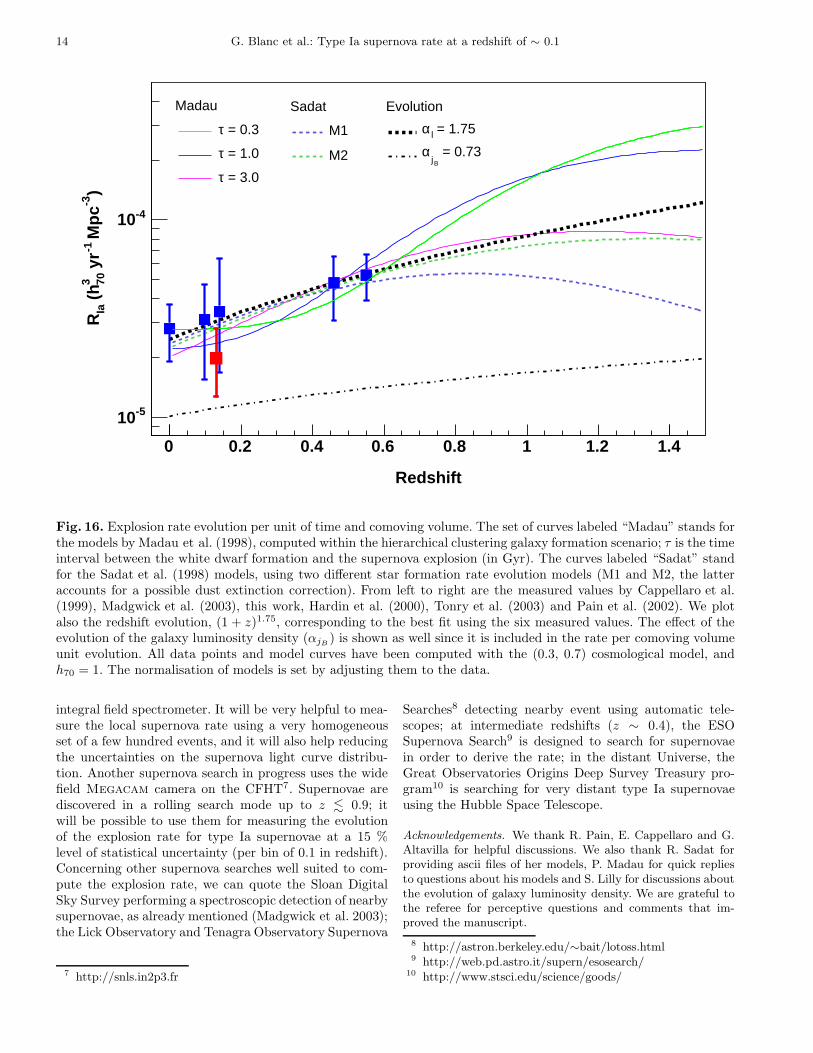
data with that of Pain et al. (2002) is consistent with thevalue αv = 0.8 ± 1.6 derived using only the Pain et al.(2002) data. Nevertheless, fitting all available rate mea-surements either in SNu or per comoving volume unit, pro-vides a lower evolution index (see Fig. 15): αv = 1.75±0.84and αl = 1.21 ± 0.80.

Models such as those by Madau et al. (1998) or bySadat et al. (1998) can fit the observations (Fig. 16). Inthe Madau et al. (1998) models, the evolution depends notonly on the time delay between the white dwarf formation


RSN Ia〈z〉(h2

70 SNu) (10−5 h370 Mpc−3 yr−1)

(ΩM , ΩΛ ) SNe nb author

∼ 0 0.18 ± 0.05 2.8±0.9 70 Cappellaro et al. (1999)a

0.098 0.196 ± 0.098 3.12 ± 1.58 19 Madgwick et al. (2003)a

0.13 0.125+0.044+0.028

−0.034−0.0281.99+0.70+0.47

−0.54−0.47(0.3, 0.7) 14 this work

0.14 0.22+0.17+0.06−0.10−0.03 3.43+2.7+1.1

−1.6−0.6 (0.3, 0.7) 4 Hardin et al. (2000)a,b

0.25+0.12−0.07 0.20+0.82

−0.19 (0.3, 0.7) 1 Gal-Yam et al. (2002)c

0.38 0.40+0.26+0.18−0.18−0.12 (1.0, 0.0) 3 Pain et al. (1996)

0.46 4.8 ± 1.7 (0.3, 0.7) 8 Tonry et al. (2003)

0.55 0.28+0.05+0.05−0.04−0.04 5.25+0.96+1.10

−0.86−1.06 (0.3, 0.7) 38 Pain et al. (2002)

0.55 0.46+0.08+0.07−0.07−0.0.7 11.1+2.0+1.1

−1.8−1.1 (1.0, 0.0) 38 Pain et al. (2002)

0.90+0.37−0.07 0.40+1.21

−0.38 (0.3, 0.7) 5 Gal-Yam et al. (2002)c

Table 3. Comparison with other published restframe type Ia supernova explosion rate measurements. These rates aregiven together with the mean redshift of the observed SNe and the cosmological model assumed (especially for distantvalues). The fifth column gives the number of supernovae from which the rate is computed. Notes: a) the value percomoving volume unit is derived from the SNu value using the 2dF luminosity density (the error on the luminositydensity is added quadratically to the systematic uncertainty if distinct); b) Hardin et al. (2000) computed the rateusing a (ΩM

, ΩΛ) = (0.3, 0.0) cosmological model. Nevertheless no important difference from the (0.3, 0.7) model is

expected (less than 10%); c) Gal-Yam et al. (2002) have measured the rate in galaxy clusters, with could be differentfrom the rate in the field; they do not give a value per unit of comoving volume.

)-1

yr

-3 M

pc

3 70)

(hIa

log

(R

-5

-4.8

-4.6

-4.4

-4.2

Observed Values(column 3 of table 3)

0.84± = 1.75 vαSlope -

a)

0 0.1 0.2 0.3 0.4 0.5 0.6 0.7 0.8 0.9

SN

u)

2 70)

(hIa

log

(R

-1.2

-1

-0.8

-0.6

-0.4

-0.2

b)

Redshift0 0.1 0.2 0.3 0.4 0.5 0.6 0.7 0.8 0.9

Observed values(column 2 of table 3)

0.80± = 1.21 lαSlope -

Fig. 15. Derivation of the evolution index α using allavailable SNIa rate measurements (see Table 3), withinthe (0.3, 0.7) cosmological model.

and the supernova explosion6, but also on the galaxy for-

6 According to Dahlen & Fransson (1999), the τ = 0.3 Gyrmodel corresponds to the double degenerate progenitor sce-nario, while the τ = 1 Gyr model simulates the single degen-erate – or cataclysmic – progenitor scenario; the τ = 3 Gyrexpands the range to cover all likely models.

mation scenario, especially at high redshift. In these mod-els the supernova rate follows roughly a (1+z)αv evolutionwith αv & 1.8 (τ = 0.3), αv ∼ 2.4 (τ = 3) up to αv ∼ 2.8(τ = 1). The Sadat et al. (1998) models depend on thechoice of star formation rate evolution model and on dustextinction. They predict αv ∼ 1.4 for “M1” model andαv ∼ 1.8 for the “M2” model.

Too few data points exist up to now in or-der to constrain accurately many parameters fromthe models, such as the galaxy formation scenario(Madau et al. 1998) (only good quality data at redshift& 1.5 could eventually distinguish between the two fa-vored galaxy formation scenarios), the progenitor model(Ruiz-Lapuente & Canal 1998), environmental effects likethe metallicity (Kobayashi et al. 2000) or the cosmology(Dahlen & Fransson 1999).

9.3. Conclusion

We have measured the type Ia supernova explosion rateat a redshift of 0.13. Combined with other measurementsat different redshifts, it suggests a slight evolution of therate with the redshift. Nevertheless, the scatter and thestill large error bars of the current measurements do notallow us to make definite conclusions about it.

Future supernova searches will shed more light on therate evolution. Among them, two dedicated supernovasearches, are well suited to improve and measure the evolu-tion of the explosion rate. The Nearby Supernova Factory

(Aldering et al. 2002) is a nearby (z . 0.1) supernovasearch using two dedicated telescopes, one for the searchand one for the follow-up of discovered events using an


Redshift

0 0.2 0.4 0.6 0.8 1 1.2 1.4

)-3

Mp

c-1

yr

3 70 (

hIa

R

-510

-410

Madau

= 0.3τ

= 1.0τ

= 3.0τ

Sadat

M1

M2

Evolution

= 1.75lα

= 0.73Bj

α

Fig. 16. Explosion rate evolution per unit of time and comoving volume. The set of curves labeled “Madau” stands forthe models by Madau et al. (1998), computed within the hierarchical clustering galaxy formation scenario; τ is the timeinterval between the white dwarf formation and the supernova explosion (in Gyr). The curves labeled “Sadat” standfor the Sadat et al. (1998) models, using two different star formation rate evolution models (M1 and M2, the latteraccounts for a possible dust extinction correction). From left to right are the measured values by Cappellaro et al.(1999), Madgwick et al. (2003), this work, Hardin et al. (2000), Tonry et al. (2003) and Pain et al. (2002). We plotalso the redshift evolution, (1 + z)1.75, corresponding to the best fit using the six measured values. The effect of theevolution of the galaxy luminosity density (αjB

) is shown as well since it is included in the rate per comoving volumeunit evolution. All data points and model curves have been computed with the (0.3, 0.7) cosmological model, andh70 = 1. The normalisation of models is set by adjusting them to the data.

integral field spectrometer. It will be very helpful to mea-sure the local supernova rate using a very homogeneousset of a few hundred events, and it will also help reducingthe uncertainties on the supernova light curve distribu-tion. Another supernova search in progress uses the widefield Megacam camera on the CFHT7. Supernovae arediscovered in a rolling search mode up to z . 0.9; itwill be possible to use them for measuring the evolutionof the explosion rate for type Ia supernovae at a 15 %level of statistical uncertainty (per bin of 0.1 in redshift).Concerning other supernova searches well suited to com-pute the explosion rate, we can quote the Sloan DigitalSky Survey performing a spectroscopic detection of nearbysupernovae, as already mentioned (Madgwick et al. 2003);the Lick Observatory and Tenagra Observatory Supernova

7 http://snls.in2p3.fr

Searches8 detecting nearby event using automatic tele-scopes; at intermediate redshifts (z ∼ 0.4), the ESOSupernova Search9 is designed to search for supernovaein order to derive the rate; in the distant Universe, theGreat Observatories Origins Deep Survey Treasury pro-gram10 is searching for very distant type Ia supernovaeusing the Hubble Space Telescope.

Acknowledgements. We thank R. Pain, E. Cappellaro and G.Altavilla for helpful discussions. We also thank R. Sadat forproviding ascii files of her models, P. Madau for quick repliesto questions about his models and S. Lilly for discussions aboutthe evolution of galaxy luminosity density. We are grateful tothe referee for perceptive questions and comments that im-proved the manuscript.

8 http://astron.berkeley.edu/∼bait/lotoss.html9 http://web.pd.astro.it/supern/esosearch/

10 http://www.stsci.edu/science/goods/


This work was supported in part by the Director, Office ofScience, Office of High Energy and Nuclear Physics, of theU.S. Department of Energy under Contract No. DE-AC03-76SF000098.

The observations described in this paper were based inpart on observations using the CNRS/INSU Marly telescopeat the European Southern Observatory, La Silla, Chile; in partusing the Nordic Optical Telescope, operated on the islandof La Palma jointly by Denmark, Finland, Iceland, Norway,and Sweden, in the Spanish Observatorio del Roque de losMuchachos of the Instituto de Astrofisica de Canarias; inpart using the Apache Point Observatory 3.5-meter telescope,which is owned and operated by the Astrophysical ResearchConsortium; in part using telescopes at Lick Observatory,which is owned and operated by the University of California;and in part using telescopes at the National Optical AstronomyObservatories, which are operated by the Association ofUniversities for Research in Astronomy, Inc., under a coop-erative agreement with the United States National ScienceFoundation.

References

Afonso, C., Albert, J. N., Alard, C., et al. 2003a, A&A,404, 145, (The EROS collaboration)

Afonso, C., Albert, J. N., Andersen, J., et al. 2003b, A&A,400, 951, (The EROS collaboration)

Aldering, G., Adam, G., Antilogus, P., et al. 2002,in Survey and Other Telescope Technologies andDiscoveries. Edited by Tyson, J. Anthony; Wolff,Sidney. Proceedings of the SPIE, Volume 4836, pp. 61-72 (2002)., 61–72

Bauer, F. & de Kat, J. 1997, in Optical Detectors forAstronomy, held at ESO, Garching, october 8-10, 1996,ed. J. W. Beletic & P. Amico, (The EROS collabora-tion)

Bertin, E. & Arnouts, S. 1996, A&AS, 117, 393Bertin, E. & Dennefeld, M. 1997, A&A, 317, 43Cappellaro, E., Evans, R., & Turatto, M. 1999, A&A, 351,

459Cappellaro, E., Turatto, M., Benetti, S., et al. 1993, A&A,

273, 383Carroll, S. M., Press, W. H., & Turner, E. L. 1992,

ARA&A, 30, 499Contardo, G., Leibundgut, B., & Vacca, W. D. 2000,

A&A, 359, 876Cousins, A. W. J. 1976, MmRAS, 81, 25Cross, N., Driver, S. P., Couch, W., et al. 2001, MNRAS,

324, 825Dahlen, T. & Fransson, C. 1999, A&A, 350, 349Gal-Yam, A., Maoz, D., Guhathakurta, P., & Filippenko,

A. V. 2003, AJ, 125, 1087Gal-Yam, A., Maoz, D., & Sharon, K. 2002, MNRAS, 332,

37Grogin, N. A. & Geller, M. J. 1999, AJ, 118, 2561Hamuy, M., Phillips, M. M., Suntzeff, N. B., et al. 1996,

AJ, 112, 2408Hardin, D., Afonso, C., Alard, C., et al. 2000, A&A, 362,

419, (The EROS Collaboration)

Howell, D. A., Wang, L., & Wheeler, J. C. 2000, ApJ, 530,166

Johnson, H. L. 1965, Communications of the Lunar andPlanetary Laboratory, 3, 73

Kobayashi, C., Tsujimoto, T., & Nomoto, K. 2000, ApJ,539, 26

Landolt, A. U. 1992, AJ, 104, 340Lasserre, T., Afonso, C., Albert, J. N., et al. 2000, A&A,

355, L39, (The EROS collaboration)Lilly, S. J., Le Fevre, O., Hammer, F., & Crampton, D.

1996, ApJ, 460, 1Lin, H., Kirshner, R. P., Shectman, S. A., et al. 1996, ApJ,

464, 60Livio, M. 2001, in The greatest Explosions since the

Big Bang: Supernovae and Gamma-Ray Bursts, held3-6 May, 1999 at Space Telescope Science Institute,Baltimore, MD, ed. M. Livio, N. Panagia, & K. Sahu(Cambridge University Press), 334, astro-ph/0005344

Madau, P., della Valle, M., & Panagia, N. 1998, MNRAS,297, 17

Madgwick, D. S., Hewett, P. C., Mortlock, D. J., & Wang,L. 2003, ApJ, 599, L33

Nobili, S., Goobar, A., Knop, R., & Nugent, P. 2003, A&A,404, 901

Nugent, P., Kim, A., & Perlmutter, S. 2002, PASP, 114,803

Pain, R., Fabbro, S., Sullivan, M., et al. 2002, ApJ, 577,120, (The Supernova Cosmology Project)

Pain, R., Hook, I. M., Deustua, S., et al. 1996, ApJ, 473,356, (The Supernova Cosmology Project)

Palanque-Delabrouille, N., Afonso, C., Albert, J. N., et al.1998, A&A, 332, 1

Phillips, M. M. 1993, ApJ, 413, 105Poggianti, B. M. 1997, A&AS, 122, 399Regnault, N., Aldering, G., Blanc, G., et al. 2001,

American Astronomical Society Meeting, 199Riess, A. G., Kirshner, R. P., Schmidt, B. P., et al. 1999,

AJ, 117, 707Ruiz-Lapuente, P. & Canal, R. 1998, ApJ, 497, 57Sadat, R., Blanchard, A., Guiderdoni, B., & Silk, J. 1998,

A&A, 331, L69Schlegel, D. J., Finkbeiner, D. P., & Davis, M. 1998, ApJ,

500, 525Shectman, S. A., Landy, S. D., Oemler, A., et al. 1996,

ApJ, 470, 172Strolger, L.-G., Smith, R. C., Suntzeff, N. B., et al. 2002,

AJ, 124, 2905Tammann, G. A. 1970, A&A, 8, 458Tonry, J. L., Schmidt, B. P., Barris, B., et al. 2003, ApJ,

594, 1Udalski, A., Szymanski, M., Kubiak, M., et al. 2000, Acta

Astronomica, 50, 307Zucca, E., Zamorani, G., Vettolani, G., et al. 1997, A&A,

326, 477

Type Ia supernova rate at a redshift of ˜0.1

Documents

Transcript of Type Ia supernova rate at a redshift of ˜0.1