Eur. Phys. J. C manuscript No.(will be inserted by the editor)

Van der Meer Scan Luminosity Measurement and Beam–BeamCorrection

Vladislav Balaguraa,1

1 Laboratoire Leprince-Ringuet, CNRS/IN2P3, École polytechnique, Institut Polytechnique de Paris

Received: date / Accepted: date

Abstract The main method for calibrating the luminosity atLargeHadron Collider (LHC) is van derMeer scanwhere thebeams are swept transversely across each other. This beau-tiful method was invented in 1968. Despite the honourableage, it remains the preferable tool at hadron colliders. It de-livers the lowest calibration systematics, which still oftendominates the overall luminosity uncertainty at LHC exper-iments. Various details of the method are discussed in thepaper. One of the main factors limiting proton–proton vander Meer scan accuracy is the beam–beam electromagneticinteraction. It modifies the shapes of the colliding bunchesand biases the measured luminosity. In the first years ofoperation, four main LHC experiments did not attempt tocorrect the bias because of its complexity. In 2012 a correc-tion method was proposed and then subsequently used byall experiments. It was based, however, on a simplified lin-ear approximation of the beam–beam force and, therefore,had limited accuracy. In this paper, a new simulation is pre-sented, which takes into account the exact non-linear force.Depending on the beam parameters, the results of the newand old methods differ by ∼ 1%. This needs to be propagatedto all LHC cross-section measurements after 2012. The newsimulation is going to be used at LHC in future luminositycalibrations.

1 Van der Meer scan

1.1 Calibration methods

An absolute value of the luminosity or the cross section canbe measured at an accelerator by separating the beams in thetransverse plane and performing the so-called van der Meerscan [1]. To illustrate the idea, let us consider the collisionof two bunches with 𝑁1,2 particles moving in the opposite

ae-mail: balagura@cern.ch

directions. If the first bunch is separated by −Δ𝑥, −Δ𝑦 inthe plane perpendicular to the beams, the average numberof interactions ` with the cross section 𝜎 normalized by thenumber of particles is

`(Δ𝑥, Δ𝑦)𝑁1𝑁2

= 𝜎𝐿

𝑁1𝑁2

= 𝜎

∬𝜌1 (𝑥2 + Δ𝑥, 𝑦2 + Δ𝑦)𝜌2 (𝑥2, 𝑦2)𝑑𝑥2 𝑑𝑦2, (1.1)

where the subscript “2” of the coordinates 𝑥2, 𝑦2 refers to thestationary second beam, 𝐿 is the integrated luminosity and𝜌1,2 (𝑥2, 𝑦2) are the normalized transverse particle densitiesof the unseparated bunches whenΔ𝑥 = Δ𝑦 = 0. For example,if 𝜌1 (𝑥, 𝑦) is a delta-function 𝛿(𝑥, 𝑦), the shifted density𝛿(𝑥 + Δ𝑥, 𝑦 + Δ𝑦) peaks at −Δ𝑥,−Δ𝑦 (note the minus sign).Integration over Δ𝑥 and Δ𝑦 drastically simplifies (1.1) since∫

𝜌1 (𝑥2 + Δ𝑥, 𝑦2 + Δ𝑦)𝜌2 (𝑥2, 𝑦2)𝑑𝑥2 𝑑𝑦2 𝑑Δ𝑥 𝑑Δ𝑦 = 1,

(1.2)

as can be easily proved by substituting 𝑥1 = 𝑥2+Δ𝑥, 𝑦1 = 𝑦2+Δ𝑦. In the new variables the integrals

∬𝜌1 (𝑥1, 𝑦1)𝑑𝑥1 𝑑𝑦1

and∬𝜌2 (𝑥2, 𝑦2)𝑑𝑥2 𝑑𝑦2 decouple and reduce to unity by

definition.From (1.1) and (1.2) we obtain van der Meer formula

𝜎 =

∬`(Δ𝑥, Δ𝑦)𝑁1𝑁2

𝑑Δ𝑥 𝑑Δ𝑦. (1.3)

The ratio

`𝑠𝑝 = `/𝑁1𝑁2. (1.4)

is often called the “specific” number of interactions. Theirtotal number accumulated during the scan,

∬`𝑠𝑝𝑑Δ𝑥 𝑑Δ𝑦,

gives 𝜎.

arX

iv:2

012.

0775

2v2

[he

p-ex

] 3

0 D

ec 2

020

2

Though van der Meer method is well known, the formula(1.3) is sometimes reduced in the literature to the Gaussianbunch densities or the case when `𝑠𝑝 is distributed indepen-dently in 𝑥 and 𝑦, discussed in the next section. Here, wepresent the method in its full generality. This is required, inparticular, for explaining the novel two-dimensional scans [2],which will probably be in wide use at LHC in Run 3. Afteranalyzing van der Meer scans for several years, the authortries to share the accumulated experience on various calibra-tion details in the first half of the paper. The discussion isconcentrated on the general method and its accuracy but noton the detector effects varying from one luminometer to theother. The second half of the paper is fully devoted to thebeam–beam electromagnetic interaction, which is one of themain factors limiting the accuracy.The derivation of (1.3) uses only `𝑠𝑝 but not ` or 𝑁1,2

separately. Therefore, it remains valid even if ` and 𝑁1𝑁2change arbitrarily but proportionally during the scan, eg.due to a gradual decrease of beam currents with time. It isrequired, however, that 𝜌1,2 remain constant.Equation (1.3) can also be understood from other but

equivalent perspective. The transverse movements of thefirst bunch smear and“wash out” its profile 𝜌1, so that ef-fectively it becomes constant 𝜌1. This reduces the compli-cated overlap integral to

∬𝜌1𝜌2𝑑𝑥2 𝑑𝑦2 = 𝜌1, ie. to unity

𝜌1 =∫𝜌1𝑑Δ𝑥 Δ𝑦 = 1 if 𝜌1,2 are normalized. Equiva-

lently, the scan can be viewed from the transverse positionof the first beam ie. in the coordinates 𝑥1, 𝑦1. Then thefirst beam is stationary while the second moves. In this case𝜌2 (𝑥1−Δ𝑥, 𝑦1−Δ𝑦) is “washed out” by Δ𝑥, Δ𝑦 movements,and the overlap integral reduces to

∫𝜌1𝑑𝑥1 𝑑𝑦1 = 1 and

drops out as before.To make a parallel translation of one beam in one trans-

verse direction, one needs 4 magnets placed at the cornersof the trapezoid-like beam trajectory. Therefore, to steer twobeams in two directions one needs 4×2×2 = 16magnets perone interaction point. It is not easy to synchronize preciselyall of them and ensure a parallel translation of the beamswith constant speeds. Therefore, the scan, eg. at LHC, is per-formed not “dynamically” using the single continuous pass,but stepwise. Ie. the function `𝑠𝑝 (Δ𝑥, Δ𝑦) is measured onlyin the predefined set of discrete points and interpolated be-tween them or fitted to some analytic function to get the finalintegral. In moving the beams from one point to the next, onewaits when the slowest magnet reaches it is desired currentvalue, and only then the luminosity measurement starts.This beautiful method was invented by van der Meer

more than 50 years ago for the ISR accelerator [3]. It wasproposed for Spp̄S [4], successfully applied with variousmodifications at RHIC [5, 6] and LHC [7–18]. The methoddelivered a record accuracy between 0.7% and a few percent.At 𝑒+-𝑒− colliders van der Meer method is biased by

strong beam–beam interactions. The luminosity is usually

measured “indirectly” by countingBhabha scattering 𝑒+𝑒− →𝑒+𝑒− events,which have a high cross-section precisely knownfrom quantum electrodynamics. Contrary to that, in the col-lisions of non-elementary hadrons it is difficult to find aphysical process with accurately predicted cross-section andconvenient for the detection. In the hadron accelerators, thebest accuracy is achieved by measuring the luminosity “di-rectly” using its definition (1.1).

At LHC, which will only be discussed in the following,in addition to van der Meer scans there are two alternativedirect methods of the luminosity calibration. They utilizeprecise vertex detectors. The first is the so-called beam–gasimaging [19]. Here, the profiles 𝜌1,2 (𝑥, 𝑦) of the bunchesare “revealed” in their interactions with a tiny amount ofgas in the beam pipe. One effectively records the bunch“photos” using the vertex detector as a “camera” and the gasas a “film”. Unfolding the images with the vertex resolutionyields 𝜌1,2 densities. To improve the accuracy, one also usesthe high statistics profile of the “luminous region” formedby the interactions of two bunches. This provides a powerfulconstraint on the product 𝜌1𝜌2. The overlap integral is thencalculated analytically from the reconstructed 𝜌1,2 densities.This method is used up to now only at LHCb [8, 11], whichhas a dedicated gas injection system [20], an excellent vertexdetector and a flexible trigger suitable for recording beam–gas interactions.

The secondmethod is called the beam–beam imaging [21].It is very similar, but the role of the gas plays another beameffectively “smeared” by the transverse movements in vander Meer scan. After sweeping eg. the first bunch, it effec-tively becomes a wide and uniform “film” independentlyof the initial 𝜌1 distribution. It allows making a “photo” of𝜌2 with high statistics. Alternatively, the same vertex distri-bution data can be viewed from the transverse position ofthe first bunch, where it is effectively stationary. The accu-mulated image gives a “photo” of 𝜌1 “filmed” by smeared𝜌2. In the original van der Meer approach the smearing al-lows integrating overΔ𝑥 Δ𝑦 and reducing the overlap integral∫𝜌1𝜌2 𝑑𝑥 𝑑𝑦 to unity. In the beam–beam imaging the same

integration is applied to the luminous region profile, ie. tothe product 𝜌1𝜌2 not integrated over 𝑑𝑥 𝑑𝑦, and allows re-constructing the individual densities 𝜌1,2.

Up to now, the beam–beam imageswere taken at LHCb [8]and CMS experiments [22]. Since in both imaging methodsthe overlap integrals are calculated from the measured ver-tex distributions, they have different systematic errors andare complementary to the “classical” van der Meer approachwhere the vertex distributions are ignored. All three meth-ods might achieve similar levels of accuracy. The imagingmethods are more complicated, however, because they re-quire a deconvolution with the vertex resolution comparableto the transverse bunch widths. Due to the simplicity and suf-

3

ficiency of the classical van der Meer technique, it remainsthe main tool of the luminosity calibrations at LHC.

1.2 X-Y factorization

It is impossible to guide particles exactly parallel to a beamaxis. Therefore, in any accelerator the optic elements are de-signed such that the particles going away from the axis aresent back and in the end “oscillate” in the transverse plane.This creates the transverse bunch widths and determines thedensity profiles 𝜌1,2. In more detail this will be discussed inSec. 3.1. To ensure stable operation, the accelerator is de-signed such that the oscillatory motions are separately stablein the transverse coordinates 𝑥 and 𝑦 and are almost indepen-dent of each other. Any “coupling” between the coordinatescould create extra resonances in the oscillatory motions and,therefore, should be avoided. The bunch densities can oftenbe factorized into 𝑥- and 𝑦-dependent parts:

𝜌1,2 (𝑥, 𝑦) = 𝜌𝑥1,2 (𝑥) · 𝜌𝑦

1,2 (𝑦). (1.5)

From (1.1) it follows that the specific number of interactionsthen also factorizes, `𝑠𝑝 (Δ𝑥,Δ𝑦) = `𝑥𝑠𝑝 (Δ𝑥) · `

𝑦𝑠𝑝 (Δ𝑦).

This is sufficient to simplify the two-dimensional integral∬`𝑠𝑝 (Δ𝑥,Δ𝑦)𝑑Δ𝑥 𝑑Δ𝑦 and to reduce it to a product of

one-dimensional integrals along the lines Δ𝑥 = Δ𝑥0 andΔ𝑦 = Δ𝑦0. Indeed,

𝜎 =

∬`𝑠𝑝 (Δ𝑥,Δ𝑦)𝑑Δ𝑥 𝑑Δ𝑦

=

∫`𝑥𝑠𝑝 (Δ𝑥)𝑑Δ𝑥

∫`𝑦𝑠𝑝 (Δ𝑦)𝑑Δ𝑦

`𝑦𝑠𝑝 (Δ𝑦0)`𝑥𝑠𝑝 (Δ𝑥0)`𝑦𝑠𝑝 (Δ𝑦0)`𝑥𝑠𝑝 (Δ𝑥0)

=

∫`𝑠𝑝 (Δ𝑥,Δ𝑦0) 𝑑Δ𝑥 ×

∫`𝑠𝑝 (Δ𝑥0,Δ𝑦) 𝑑Δ𝑦

`𝑠𝑝 (Δ𝑥0,Δ𝑦0). (1.6)

The integrals in the enumerator can be measured in two one-dimensional scans over Δ𝑥 at fixed Δ𝑦0 and vice versa. Notethat the formula is valid for any point (Δ𝑥0,Δ𝑦0). This israrely stressed in the literature. It might be advantageous tochoose (Δ𝑥0,Δ𝑦0) not far from the point of maximal lumi-nosity to collect sufficient statistics of interactions. Theremight be another advantage if the beam coordinates arenot accurately measured. The potential slow drifts of thebeam orbits from their nominal positions might affect bothscanned and not scanned coordinates and bias the luminos-ity measurement. The bias from not scanned coordinate isminimized at the maximum of ` where the derivative of eg.`𝑠𝑝 (Δ𝑥0,Δ𝑦) on Δ𝑥0 is zero.Performing a pair of one-dimensional scans instead of

an expensive two-dimensional scan allows saving the beamtime. Reducing the time also helps to minimize the influenceof the slow drifts of the beam orbits if they are not accuratelymeasured. Therefore, at LHC the cross-sections are usually

calibrated using (1.6) instead of (1.3). This approach, how-ever, relies on the 𝑥-𝑦 factorizability of `, which is goodat LHC but not perfect. It can be violated by many factors,essentially, by any imperfection in the accelerator leading toan 𝑥-𝑦 coupling.The remaining non-factorizability is usually studied us-

ing the distributions of the interaction vertices. After un-folding with the vertex resolution they give the products oftwo bunch densities. Ideally, the shape of their projectionsto one coordinate should remain invariant when scanninganother coordinate. The deviations are interpreted as thenon-factorizability and are propagated to the cross-sectioncorrections. This procedure is complicated because it re-quires the characterization of two unknown bunch shapesusing only one luminous region profile. One can use theimaging methods to measure directly 𝜌1,2 densities [23].However, the beam–gas interactions have limited statisticswhile the beam–beam imaging suffers from the uncertain-ties in the beam positions and the beam–beam systematicsdiscussed later. Because of the complexity of the 𝑥-𝑦 non-factorization studies, usually the bunch shapes are fitted as-suming some smooth bunch shape model. This makes themmodel-dependent. The cross-section corrections due to 𝑥-𝑦non-factorizability and the associated systematic errors aretypically at the level . 1%.The accuracy can be improved further by performing

two-dimensional scans over the central region giving thedominant contribution to the integral in (1.3). This approachwas pioneered at LHCb in 2017 [2]. Scanning only the centralregion was relatively fast but allowed evaluating ∼ 90% ofthe integral. The method is model-independent and allowsreducing the non-factorization systematics by an order ofmagnitude.

1.3 Crossing angle between the beams

In van der Meer scans at LHC the beams are not alwaysopposite. They may collide at a small angle of the order𝑂 (100 `𝑟𝑎𝑑). This separates the beams outside the interac-tion region and suppresses possible parasitic collisions be-tween nominally not colliding bunches. It is not immediatelyobvious how van der Meer formalism should be extended tothe case of not parallel beams. In addition, the particles in thetwo beams can be different. Up to now, LHC has performedvan der Meer scans with the proton and lead ion beams. Itmight be not clear whether in the asymmetric proton - ioncollisions the cross-section can be calibrated in the labora-tory frame, or it is necessary to make a transformation to thecenter-of-mass system.These questions were answered in [21] using two alter-

native derivations. In the first, the simple two-dimensionalintegral in (1.1) was extended to four dimensions and takenoverΔ𝑥,Δ𝑦 in the sameway as (1.3) was obtained from (1.1).

4

In the second, equivalent derivation the direct mathematicalcalculation was substituted by simple physical arguments.They will be elaborated in more detail below.Let’s denote the velocities of the beam particles by v1,2 as

shown in Fig. 1.1. They can be decomposed into two parallel(v1,2) and one common perpendicular component v⊥ withrespect to their difference v1 − v2 = Δv.

wv1

v1

®1

beam 1

beam 2

v1

– v2 = 4v

v? v

2

v2

w ®2

Fig. 1.1 Decomposition of the beam particle velocities v1,2 to theperpendicular v⊥ and the parallel v1‖ , v2‖ components with respect totheir difference v1 − v2 = Δv.

There exist infinitely many relativistic frames where thebeams are parallel. In any of them, (1.3) is valid, for example,in the center-of-mass or the rest frame of one of the particles.It is even valid in the frame where the particles move in thesame direction one running after the other. All such framescan be obtained by boosting the laboratory frame first withthe velocity v⊥ and then with an arbitrary velocity parallelto Δv. Indeed, in the laboratory frame boosted by v⊥, or,equivalently, after the “active” boost of the beam particlesby −v⊥, their perpendicular momentum transforms to p′

⊥ =

𝛾⊥p⊥ − 𝛾⊥𝛽⊥𝐸/𝑐, which is zero since by construction 𝛽⊥ =

p⊥𝑐/𝐸 . Here, 𝑐 is the speed of light, 𝐸 is the energy inthe laboratory system, 𝛽⊥ = v⊥/𝑐 and 𝛾⊥ = (1 − 𝛽2⊥)−1/2are the beta- and gamma-factors of the boost, respectively.Therefore, after the active boost by −v⊥ the beams becomeparallel to Δv and any further boost along Δv preserves thisparallelism.Note that although the perpendicular velocity after the

boost by −v⊥ becomes a simple difference v⊥ − v⊥ = 0, theremaining velocity v′

‖ is, of course, not equal to the differencev − v⊥ = v‖ . This would be the case for the Galilean but notfor the Lorentz transformation. The correct formula followsmost easily from the opposite transformation from the primedto the laboratory frame: p‖ = p′

‖ , 𝐸 = 𝛾⊥𝐸 ′, so v′‖ = 𝛾⊥v‖ .

Let’s find out how van der Meer formula (1.3), provedin the primed coordinates with the parallel beams, modi-fies in the laboratory frame. The quantities `, 𝑁1,2 and 𝜎are Lorentz-invariant, only the transverse area 𝑑Δ𝑥 𝑑Δ𝑦 isnot. Following notations of this subsection, the latter will bedenoted in the primed coordinates as 𝑑Δ𝑥 ′ 𝑑Δ𝑦′. Its trans-formation to the laboratory system requires some explana-tions given below. This material complements the discussionin [21].The space-time coordinates 𝑥 = (𝑡, x) of any particle

moving with the four-momentum 𝑝 = (𝐸, p) satisfy the

equation

𝑥 − 𝑥0 = _𝑝, (1.7)

where _ is a free parameter and 𝑥0 = (𝑡0, x0) is an arbitrarypoint on the particle trajectory corresponding to _ = 0. Fourequations in (1.7) with one free parameter define a line in thefour-dimensional space. The values of _ uniquely label theline points and can be expressed, for example, via the timecoordinate: _ = (𝑡 − 𝑡0)/𝐸 .The beam displacements Δ = (0,𝚫) during van der Meer

scan change the 𝑥0 parameter:

𝑥 − 𝑥0 − Δ = _𝑝. (1.8)

Note that the definition of the scan implies that the beamsare moved only spatially, so there is no time component in Δ.In the following, it will be convenient to decompose spa-

tial vectors into three components: parallel to v⊥, to thevector-product [Δv × v⊥] and to Δv. They will be denotedby the subscripts ⊥, ‖ × ⊥ and ‖, respectively, eg.

Δ = (0, Δ⊥,Δ‖×⊥,Δ‖). (1.9)

The ‖ × ⊥ component is perpendicular to the plane ofFig. 1.1. Ideally, the beam displacements should be orthog-onal to Δv but we consider below the general case Δ‖ ≠ 0.After the active boost by −Δv, the line defined by (1.8)

transforms to

𝑥 ′ − 𝑥0′ − Δ′ = _𝑝′. (1.10)

Note that the solutions 𝑥, 𝑥 ′ of (1.8) and (1.10) for the same_ correspond to the same four-dimensional point in the lab-oratory and primed frames, respectively.After the boost, the beam displacement

Δ′ = (−𝛽⊥𝛾⊥Δ⊥, 𝛾⊥Δ⊥, Δ‖×⊥, Δ‖) (1.11)

acquires the time componentΔ′𝑡 = −𝛽⊥𝛾⊥Δ⊥. In otherwords,

it is impossible to transform a spatial scan in the laboratoryto merely a spatial scan in the primed frame. To resolvethis complication one can use the following argument. Anysystemwith the parallel beams is special in the sense that thenumber of interactions created by two particles is determinedonly by the transverse distance between their lines. It does notdepend on the initial positions of the particles 𝑥0′‖ +Δ′

‖ alongthe lines or on the initial time 𝑡0′ + Δ′

𝑡 since the particlesare anyway assumed to travel from 𝑡 ′ = −∞ to 𝑡 ′ = +∞.Contrary to the transverse initial coordinates, the time andlongitudinal shifts do not change the particle line. Therefore,the scan with Δ′ from (1.11) is equivalent to the one with

Δ̃′ = (0, 𝛾⊥Δ⊥, Δ‖×⊥, 0), (1.12)

where the time and longitudinal coordinates are simply set tozero. Comparing this equation with (1.9) one can see that the

5

beam displacements Δ‖×⊥ transform from the laboratory tothe primed system without any changes while the displace-ments Δ⊥ are “extended” by the 𝛾⊥-factor. Therefore, thearea element 𝑑Δ𝑥 ′ 𝑑Δ𝑦′ in the primed coordinates is largerthan in the laboratory system by 𝛾⊥:

𝑑Δ𝑥 ′ 𝑑Δ𝑦′ = 𝛾⊥𝑑Δ𝑥 𝑑Δ𝑦. (1.13)

Note that one can invert the arguments and make theopposite boost from the primed scan with the displacements(0,Δ′

⊥, Δ′‖×⊥, 0) to the laboratory system:

Δ = (𝛽⊥𝛾⊥Δ′⊥, 𝛾⊥Δ

′⊥, Δ

′‖×⊥, 0).

Here, the 𝛾⊥-factor again appears in the transverse compo-nents but now in the laboratory system.Concluding from thisformula that 𝛾⊥𝑑Δ𝑥 ′ 𝑑Δ𝑦′ = 𝑑Δ𝑥 𝑑Δ𝑦 with 𝛾⊥ on the oppo-site side would be a mistake, however, since the time andlongitudinal components can be freely changed and zeroedonly in the primed frame with the parallel beams. SettingΔ𝑡 = 𝛽⊥𝛾⊥Δ′

⊥ to zero in the formula above is not allowedand spoils the equivalence of the scans in the laboratory andthe primed frames.Using (1.13), the cross-section formula in the laboratory

system can finally be written as

𝜎 = 𝛾⊥

∫`(Δ𝑥,Δ𝑦)𝑁1𝑁2

𝑑Δ𝑥 𝑑Δ𝑦. (1.14)

Note that the relativistic correction 𝛾⊥ depends on thevelocities but not on the momenta or masses of the particles.For example, it coincides for proton and lead ion beams iftheir velocities are the same. The formula is relativisticallyinvariant and is valid in any frame. The area element 𝑑Δ𝑥 𝑑Δ𝑦by definition lies in the plane perpendicular to Δv. Let’sdenote this plane by 𝑃. If the scan plane �̃� is inclined withrespect to 𝑃 at an angle 𝛼, an area element 𝑑Δ̃𝑥 𝑑Δ̃𝑦 on �̃�should be projected to 𝑃, ie.

𝜎 = 𝛾⊥

∫`(Δ̃𝑥, Δ̃𝑦)𝑁1𝑁2

cos𝛼 𝑑Δ̃𝑥 𝑑Δ̃𝑦. (1.15)

The longitudinal translations along Δv do not matter.The beam crossing angles at LHC are small, so 𝛽⊥ <

10−3 and 𝛾⊥−1 < 10−6. Therefore, the relativistic correctionat LHC can be safely neglected.The luminosity, however, is modified as it can be seen

from the following. The typical longitudinal sizes of the LHCbunches 𝜎𝑖𝐿 along the beam 𝑖 = 1, 2 in the laboratory frameare 5–10 cm. They are much larger than the transverse sizes𝜎𝑖𝑇 ∼ 100 `𝑚. Since 𝛾⊥ ≈ 1, the Lorentz and Galileantransformations from the laboratory to primed coordinatesare almost equivalent. The latter preserves the bunch shapes.Therefore, in the primed system the longitudinal spread 𝜎𝑖𝐿gets projected to v⊥ at the angles 𝛼1,2 shown in Fig. 1.1. For

the Gaussian bunches this increases the primed transversewidth 𝜎′

𝑖⊥ in the beam crossing plane to

𝜎′𝑖⊥ ≈ 𝜎𝑖𝑇

√︁1 + (𝛼𝑖 𝜎𝑖𝐿/𝜎𝑖𝑇 )2. (1.16)

This formula is valid up to the second-order 𝛼𝑖-terms en-hanced by 𝜎𝑖𝐿/𝜎𝑖𝑇 � 1 factor.Note that often in the literature 𝜎′

𝑖⊥ is expressed in theform of a rotation as

√︁(𝜎𝑖𝑇 cos𝛼𝑖)2 + (𝜎𝑖𝐿 sin𝛼𝑖)2. Writing

cos𝛼𝑖 = 1 − 𝛼2𝑖 /2 + . . . instead of unity as in (1.16) impliesits validity at least up to the terms ∝ 𝛼2

𝑖not enhanced by

𝜎𝑖𝐿/𝜎𝑖𝑇 . At this level of accuracy one can not neglect thedifference between Lorentz and Galilean transformations,however, and should take into account the relativistic correc-tions.The exact formula can be obtained using the same for-

malism as for van der Meer scan above. Let’s interpret theparameter Δ = (0,𝚫) in (1.8) not as the beam displacementbut as a stochastic variable describing the spatial spread ofthe particles in the bunch in the laboratory frame. For ex-ample, 𝚫 can be a zero-mean random variable normally andindependently distributed along the transverse 𝑥, 𝑦 and longi-tudinal axeswith the standard deviations𝜎𝑥,𝑦,𝐿 , respectively.Let’s consider the general case when neither 𝑥 nor 𝑦 lies inthe crossing plane of Figure 1.1. Then, the transverse bunchwidths in the laboratory frame along ⊥ and ‖ × ⊥ directionsare

𝜎𝑖⊥ =

√︃[𝜎𝑖𝑥 cos(𝑥𝑖 ,⊥)]2 +

[𝜎𝑖𝑦 cos(𝑦𝑖 ,⊥)

]2 + [𝜎𝑖𝐿 sin𝛼𝑖]2

𝜎𝑖 ‖×⊥ =

√︃[𝜎𝑖𝑥 cos(𝑥𝑖 , ‖ ×⊥)]2 +

[𝜎𝑖𝑦 cos(𝑦𝑖 , ‖ ×⊥)

]2.

(1.17)

Here, the notation like cos(𝑥𝑖 ,⊥) denote the cosine of the an-gle between the 𝑥 direction of the 𝑖-th bunch and v⊥. Accord-ing to (1.12), the bunch spread 𝜎⊥ is multiplied by the 𝛾⊥-factor in the primed frame, while 𝜎‖×⊥ remains unchanged:

𝜎′𝑖⊥ = 𝛾⊥𝜎𝑖⊥, 𝜎′

𝑖 ‖×⊥ = 𝜎𝑖 ‖×⊥. (1.18)

If one of the transverse axes, eg. 𝑥, lies in the crossingplane, this simplifies to

𝜎′𝑖⊥ = 𝛾⊥

√︃[𝜎𝑖𝑥 cos𝛼𝑖]2 + [𝜎𝑖𝐿 sin𝛼𝑖]2, 𝜎′

𝑖 ‖×⊥ = 𝜎𝑦 .

(1.19)

For ultrarelativistic beams with 𝑣1,2 ≈ 𝑐, like at LHC,and arbitrary 𝛼1,2, which should be approximately equal inthis case, 𝛼1 ≈ 𝛼2 ≈ 𝛼, the beta- and gamma-factors can beexpressed via the angle 𝛼:

𝛽⊥ ≈ sin𝛼, 𝛾⊥ ≈ 1/√︁1 − sin2 𝛼 = 1/cos𝛼. (1.20)

6

This gives

𝜎′𝑖⊥ ≈

√︃𝜎2𝑖𝑥+ (𝜎𝑖𝐿 tan𝛼)2. (1.21)

One can see that 𝜎𝑖𝑥 is not multiplied by cos𝛼. Instead of therotation formula, for 𝜎′

𝑖⊥ one should use either exact (1.17),(1.18), (1.19) or one of the approximate equations (1.16),(1.21).The smallness of 𝛼𝑖 at LHC is partially compensated

by the large 𝜎𝑖𝐿/𝜎𝑖𝑇 ratio, so due to the crossing anglethe effective transverse widths 𝜎′

𝑖⊥ increase by 5–20%. Theluminosity reduces by the same amount. Once again, thisdoes not modify van der Meer formula (1.14), since thenormalization

∫𝜌𝑖 (𝑥, 𝑦) 𝑑𝑥 𝑑𝑦 = 1 remains invariant. For

broader bunches, one just needs to enlarge proportionallythe region of integration.Note that if the transverse bunch densities 𝜌1,2 factorize

in the primed directions 𝑥 ′ and 𝑦′ but none of them lies in thecrossing plane of Figure 1.1, 𝜎𝑖𝐿 has non-zero projectionson both 𝑥 ′ and 𝑦′. This makes 𝑥 ′ and 𝑦′ distributions slightlycorrelated and to some extent breaks the 𝑥 ′-𝑦′ factorizability.

1.4 Luminosity calibration accuracy

Van derMeer scan is the main tool of the absolute luminositycalibration at LHC. For the given beamparticles and the LHCenergy, the scan is performed in every experiment at leastonce a year to check the stability of the luminosity detectors.One or two LHC fills with carefully optimized experimentalconditions are allocated for this purpose. The accuracy isdetermined by various factors discussed below. The overallcalibration uncertainty is typically 1-2%.The calibration constant is then propagated to the lu-

minosity of the whole physics sample using linear lumi-nometers. In ATLAS and CMS operating at higher pile-up`-values, the accurate linearity is required in larger dynamicrange since van der Meer scans are typically performed with` . 1. The uncertainties caused by the deviations from thelinearity due to irradiation ageing, long-term instabilities etc.are reduced by comparing several luminometers with differ-ent systematics. Therefore, the overall luminosity uncertaintyis often dominated by the calibration error.Averaging over many colliding bunch pairs and several

van der Meer scans often reduces the statistical error of thecalibration to a negligible level. The systematics from thebunch population 𝑁1𝑁2 measurements is typically at thelevel ∼ 0.2−0.3% except in the very first LHC scans in 2010with low-intensity beams.The cross-section has the dimensionality of a length unit

square. It appears in van der Meer formula (1.14) due tothe integration over Δ𝑥 and Δ𝑦. Any error in the beam dis-placements directly affects the cross-section. An accuratemeasurement of Δ𝑥, Δ𝑦 scale is performed in a dedicated

“length scale calibration” (LSC), which always accompaniesvan der Meer scans. The simplest LSC is described below.Let’s assume that the true beam positions 𝚫𝑖 in the labo-

ratory frame for the beam 𝑖 = 1, 2 can be written as

𝚫𝑖 = 𝛼𝑖a𝑖 + 𝛽𝑖b𝑖 + 𝚫0𝑖 , (1.22)

where a𝑖 , b𝑖 are unknown vectors close but not exactly equalto the unit 𝑥, 𝑦-vectors and 𝛼𝑖 , 𝛽𝑖 are the nominally setvalues for 𝑥, 𝑦 beam movements, respectively. The latter areknown exactly. Potential nonlinearities in the 𝚫𝑖 dependenceon 𝛼𝑖 , 𝛽𝑖 eg. due to beam orbit drifts, are neglected herebut will be briefly discussed later. The constant vectors 𝚫0

𝑖

corresponding to 𝛼𝑖 = 𝛽𝑖 = 0 are also unknown.In the simplest LSC the beams are nominally displaced by

the same amount, ie. with 𝛼1 = 𝛼2 = 𝛼𝐿𝑆𝐶 , 𝛽1 = 𝛽2 = 𝛽𝐿𝑆𝐶 .If the bunches have equal shapes, the center of the luminousregion O𝐿𝑆𝐶 is positioned in the middle between them,

O𝐿𝑆𝐶 = 𝛼𝐿𝑆𝐶

a1 + a22

+ 𝛽𝐿𝑆𝐶b1 + b22

+𝚫01 + 𝚫022

. (1.23)

It can be accurately measured by the vertex detectors.Most often van der Meer scans at LHC are performed

such that the beams are displaced symmetrically in oppositedirections corresponding to 𝛼1 = −𝛼2 = 2𝛼𝑠𝑦𝑚, 𝛽1 = −𝛽2 =2𝛽𝑠𝑦𝑚. The advantage of the symmetric scan is that it allowsto reach maximal separations in the limited allowed rangeof the beam movements. The distance between the beams𝚫12 = 𝚫1 − 𝚫2 is then

𝚫12 = 𝛼𝑠𝑦𝑚 a1 + a2

2+ 𝛽𝑠𝑦𝑚 b1 + b2

2+𝚫01 − 𝚫022

. (1.24)

A comparison of (1.23) and (1.24) shows that the measure-ments of O𝐿𝑆𝐶 in the vertex detector are sufficient to cali-brate the scales (a1 + a2)/2, (b1 + b2)/2 necessary for thesymmetric scans. The fact that the shapes of the collidingbunches are different can normally be neglected at LHC af-ter averaging over many colliding bunch pairs.Non-symmetric scans depend on other linear combina-

tions than (a1 + a2)/2 and (b1 + b2)/2measurable in (1.23).The simplest way to calibrate the lengths |a1,2 | = 𝑎1,2 and|b1,2 | = 𝑏1,2 individually is to use the measurements of theluminosity. Ideally it should be stationary during LSC. Anysmall variation indicates that the distance between the beamschanges.For example, let’s consider the LSC in the 𝑥-direction.

Assuming 𝑥-𝑦 factorizability and neglecting the angle be-tween a1,2 and the 𝑥-axis, one arrives at the scalar equations

Δ𝑖,𝑥 = 𝛼𝐿𝑆𝐶 𝑎𝑖 + Δ0𝑖,𝑥 ,

Δ12,𝑥 = 𝛼𝐿𝑆𝐶 (𝑎1 − 𝑎2) + (Δ01,𝑥 − Δ02,𝑥),

𝑂𝐿𝑆𝐶,𝑥 = 𝛼𝐿𝑆𝐶

𝑎1 + 𝑎22

+Δ01,𝑥 + Δ02,𝑥

2. (1.25)

7

The movement of the luminous region between any two LSCpoints, 𝑂1

𝐿𝑆𝐶,𝑥− 𝑂2

𝐿𝑆𝐶,𝑥, allows to measure the average

𝑥-scale

𝑎1 + 𝑎22

=𝑂1

𝐿𝑆𝐶,𝑥−𝑂2

𝐿𝑆𝐶,𝑥

𝛼1𝐿𝑆𝐶

− 𝛼2𝐿𝑆𝐶

. (1.26)

The corresponding change of the 𝑥-distance between thebeams Δ112,𝑥 − Δ212,𝑥 can be deduced from the luminositychange 𝐿1

𝐿𝑆𝐶− 𝐿2

𝐿𝑆𝐶and van der Meer scan data. For ex-

ample, if one of the 𝑥-scans was performed symmetrically,the beam separation change required to modify the luminos-ity by a given amount can be calculated from the derivative𝑑Δ12,𝑥/𝑑𝐿 = 𝑑𝛼𝑠𝑦𝑚/𝑑𝐿𝑠𝑦𝑚 · (𝑎1 + 𝑎2)/2. This leads to theequation

Δ112,𝑥 − Δ212,𝑥 = (𝛼1𝐿𝑆𝐶 − 𝛼2𝐿𝑆𝐶 ) (𝑎1 − 𝑎2)

=𝑑𝛼𝑠𝑦𝑚

𝑑𝐿𝑠𝑦𝑚· 𝑎1 + 𝑎22

(𝐿1𝐿𝑆𝐶 − 𝐿2𝐿𝑆𝐶 ), (1.27)

which allows to obtain (𝑎1 − 𝑎2)/(𝑎1 + 𝑎2) from the measur-able values 𝑑𝛼𝑠𝑦𝑚/𝑑𝐿𝑠𝑦𝑚, 𝐿1

𝐿𝑆𝐶− 𝐿2

𝐿𝑆𝐶and the set differ-

ence 𝛼1𝐿𝑆𝐶

− 𝛼2𝐿𝑆𝐶. Together with (𝑎1 + 𝑎2)/2 from (1.26)

this allows to calibrate the scales 𝑎1,2 individually.To improve the sensitivity of the method and to increase

𝐿1𝐿𝑆𝐶

− 𝐿2𝐿𝑆𝐶, LSC can be performed at a point close to

the maximum of the derivative 𝑑𝐿/𝑑Δ12, where the secondderivative is zero. For the Gaussian bunches with the widths𝜎1,2, the luminosity dependence on the beam separation isalsoGaussianwith the sigmaΣ =

√︃𝜎21 + 𝜎

21 , and the optimal

LSC beam separation is Δ12 = Σ.After the calibration, the length scale systematics is typ-

ically well below 1%.Note that LSC is not needed for the “static” imaging

methods, namely, for the beam-gas and also for the beam–beam imaging if in the latter the reconstructed bunch is sta-tionary during the scan in the laboratory frame. In bothcases, the reconstruction is performed in the vertex detectorcoordinates, which always define an accurate scale.

The remaining most important sources of systematics in-clude 𝑥-𝑦 non-factorizability of the bunch densities, the beamorbit drifts and the so-called beam–beam effects due to theelectromagnetic interaction between two colliding bunches.As itwas discussed in Sec. 1.2, the 𝑥-𝑦 non-factorizability

can be circumvented by performing two-dimensional scansover the central region giving the main contribution to theintegral in (1.14). Three two-dimensional scans, already per-formed at LHCb at the end of Run 2, allowed to reduce thisuncertainty approximately by an order of magnitude [2].The beams can drift at LHC by a few microns leading

to the cross-section uncertainties at the level of 1%. Fur-ther improvements require accurate monitoring of the beampositions. The LHC Beam Position Monitors (BPMs) could

not provide the necessary accuracy in Run 1 because of thetemperature drifts in the readout electronics. In Run 2 theywere upgraded and all interaction points were equipped withthe so-called DOROS BPMs. The accuracy was significantlyimproved and reached a sub-micron level. This was provedby calibrating and comparing with the beam positions recon-structed with the beam-gas imaging at LHCb. The latter isrelatively slow and requires one or a fewminutes to reach therequired accuracy even with the gas injection. This is suffi-cient for the calibration, however, and after that, the DOROSBPMs can accurately measure even fast beam drifts with 0.1second time resolution. Sufficient accuracy can, possibly, beachieved also at other experiments without the beam–gasimaging using the correlations between the DOROS mea-surements and the positions of the luminous centers. Us-ing well-calibrated DOROS BPM data, one can significantlyreduce the scan-to-scan non-reproducibility and potentiallyachieve the overall calibration accuracy below 1%.The last beam–beam systematics is caused by the elec-

tromagnetic interaction between the bunches. The electro-magnetic force kicks the beam particles and modifies theiraccelerator trajectories and the bunch densities 𝜌1,2. If theperturbations were constant during the scan it would not pro-duce any bias since van der Meer formula (1.3) is valid forany densities. The kick strength, however, depends on thetransverse profile of the opposite bunch and the distance toit. The perturbation of the densities 𝜌1,2, therefore, dependson Δ𝑥, Δ𝑦. For example, it vanishes at large beam separa-tions. Such 𝜌1,2 dependence on Δ𝑥, Δ𝑦 breaks the derivationof (1.3) from (1.1) and introduces biases in the cross-sectionformulas that are difficult to estimate. The beam–beam cor-rection is the main subject of this paper and will be discussedin detail in the following sections.The lead ion bunches in LHC van der Meer scans carry

much smaller charge than the proton ones. Therefore, thebeam–beam systematics is more significant for the proton–proton scans.The beam–beam interaction also affects the imagingmeth-

ods. Like the classical van der Meer approach, the beam–beam image is biased when 𝜌1,2 densities vary during thescan. The beam–gas imaging is also biased when the beam–beam interaction changes, eg. during van der Meer scan atthe same or any other LHC experiment. In the latter case, theassociated beam–beam distortions propagate through the ac-celerator everywhere in the ring. If the beams are stationary,however, the densities 𝜌1,2 are constant and the appropriate𝜌1,2 fit model can describe the bunches accurately. The re-quired model might be complicated, however, and dependenton the constant beam–beam interactions at all LHC experi-ments.In the first LHC publications, the experiments either

not considered the beam–beam systematics or assigned ∼1% error to their luminosity measurements in the proton–

8

proton scans without making any correction. In 2012 themethod [24] was proposed for correcting the classical vander Meer technique. It was subsequently used by all LHCexperiments, and the systematic error was reduced to 0.3 −0.7% [9–11, 13, 15–18]. However, the beam–beam force inthis method was oversimplified and approximated by a lin-ear function of the transverse coordinates. More specifically,the electromagnetic field was described by the dipole andquadrupole magnets responsible for the offset and the slopeof this linear function, respectively.This was discovered by the author of this paper in Jan-

uary 2019 using a new, independently developed simulation.It will be presented in this paper. Instead of the linear ap-proximation, the simulation uses the accurate formula of thebeam–beam force. Unfortunately, the old and new beam–beam corrections differ by ∼ 1% as shown in Fig. 3.8. Thedifference is dependent on van der Meer scan beam param-eters. This requires the corresponding rescaling of all LHCcross-sections after 2012 that were based on the luminositycalibrated with the old oversimplified beam–beam model.The new simulation is primarily oriented at the classi-

cal van der Meer method. It is optimized for calculating theluminosity but not the bunch shapes required in the imag-ing methods. Some limited tools for predicting the shapesare implemented in the simulation, however, and can be ex-tended.The beam–beam force depends on both transverse co-

ordinates and, therefore, introduces 𝑥-𝑦 coupling and non-factorization. The new simulation allows to correct the lu-minosity measurements at each point of van der Meer scansuch that the beam–beam perturbation is effectively removedtogether with its 𝑥-𝑦 coupling. The cross-section can then becalculated from the corrected ` values using unmodified(1.3) or (1.6).The new simulation is sufficiently general. The bunch

profiles can be approximated by an arbitrary weighted sum ofthe Gaussians with the common center. The 𝑥- and 𝑦-widthscan be different. In addition, the luminosity correction canbe calculated in the presence of the beam–beam kicks at anarbitrary number of interaction points. The bunch shapes ofall colliding bunches are specified individually.

2 Momentum kick induced by the beam–beaminteraction

For LHC physics one usually considers the collision of twoprotons (or ions) ignoring other particles in the bunches.Contrary to that, the beam–beam electromagnetic interac-tions have a long-range and act simultaneously betweenmanyparticles. At large distances, onemay neglect quantum effectsand use classical electrodynamics. Any associated electro-magnetic radiation of protons or ions at LHCwill be ignored.

The formula of themomentumkick induced by the beam–beam interaction iswell known in the accelerator community.However, it might be not so easy to find in the literature itsrigorous derivation with the discussion of all simplifyingassumptions affecting the accuracy. To make the material ofthis paper self-contained, we present below the derivation ofthis formula from the first principles.

2.1 Electromagnetic interaction of two particles

As it will be shown in a moment, at LHC the beam–beamforce changes the transverse particle momentum in the lab-oratory frame by a few MeV, ie. negligibly compared to thetotal momentum. Therefore, one can assume that all particlescreating the electromagnetic field move without deflectionswith constant velocity. Since the equality and constancy ofvelocities are preserved by boosts, this approximation can beused in any other frame.

q2

┴┴

+z0

E1(z0)

β0c

q1

R

-z0

0

E1(-z

0)E

1(0)┴z

Fig. 2.1 The electrical field from the charge 𝑞1 at rest acting on thecharge 𝑞2 from another bunch.

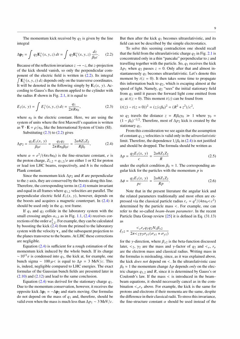
The electromagnetic field of a particle with the charge 𝑞1is simplest in its rest frame where it reduces to the electricalCoulomb component E1 shown in Fig 2.1. The momentumkick exerted on a particle 𝑞2 from another bunch can becalculated in this frame as an integral of the infinitesimalmomentum changes along the trajectory. According to ourassumption, the velocity of 𝑞1 is constant, so its positionis fixed. Since 𝑞2 in the rest frame of 𝑞1 has even largermomentum than in the laboratory, while the transverse kickis the same, one can safely assume that its speed 𝑑𝑧/𝑑𝑡 = 𝛽0𝑐is also constant and 𝑞2 moves along the straight line denotedas the 𝑧-axis in Fig. 2.1.If the velocities of the colliding particles in the laboratory

system are ±𝛽𝑐, 𝛽0 can be expressed as

𝛽0 = 2𝛽/(1 + 𝛽2), (2.1)

which is the double-angle (or double-rapidity) formula forthe hyperbolic tangent, the analog of tan(2𝜙) = 2 tan 𝜙/(1−tan2 𝜙). Of course, at LHCone can safely assume 𝛽 ≈ 𝛽0 ≈ 1.

9

The momentum kick received by 𝑞2 is given by the lineintegral

Δp2 =∫

𝑞2E⊥1 (𝑥, 𝑦, 𝑧) 𝑑𝑡 =

∫𝑞2E⊥

1 (𝑥, 𝑦, 𝑧)𝑑𝑧

𝛽0𝑐. (2.2)

Because of the reflection invariance 𝑧 → −𝑧, the 𝑧-projectionof the kick should vanish, so only the perpendicular com-ponent of the electric field is written in (2.2). Its integral∫

E⊥1 (𝑥, 𝑦, 𝑧) 𝑑𝑧 depends only on the transverse coordinates.

It will be denoted in the following simply by E1 (𝑥, 𝑦). Ac-cording to Gauss’s flux theorem applied to the cylinder withthe radius 𝑅 shown in Fig. 2.1, it is equal to

𝐸1 (𝑥, 𝑦) =∫

𝐸⊥1 (𝑥, 𝑦, 𝑧) 𝑑𝑧 =

𝑞12𝜋𝑅𝜖0

, (2.3)

where 𝜖0 is the electric constant. Here, we are using thesystem of units where the first Maxwell’s equation is writtenas ∇ · E = 𝜌/𝜖0, like the International System of Units (SI).Substituting (2.3) to (2.2) gives

Δ𝑝2 =𝑞2𝐸1 (𝑥, 𝑦)

𝛽0𝑐=

𝑞1𝑞22𝜋𝑅𝜖0𝛽0𝑐

=2𝛼ℏ𝑍1𝑍2𝑅𝛽0

, (2.4)

where 𝛼 = 𝑒2/(4𝜋𝑐ℏ𝜖0) is the fine-structure constant, 𝑒 isthe proton charge, 𝑍1,2 = 𝑞1,2/𝑒 are either 1 or 82 for protonor lead ion LHC beams, respectively, and ℏ is the reducedPlank constant.Since the momentum kick Δ𝑝2 and 𝑅 are perpendicular

to the 𝑧-axis, they are conserved by the boosts along this line.Therefore, the corresponding terms in (2.4) remain invariantand equal in all frames where 𝑞1,2 velocities are parallel. Theperpendicular electric field 𝐸1 (𝑥, 𝑦), however, depends onthe boosts and acquires a magnetic counterpart. In (2.4) itshould be used only in the 𝑞1 rest frame.If 𝑞1 and 𝑞2 collide in the laboratory system with the

small crossing angles 𝛼1,2 as in Fig. 1.1, (2.4) receives cor-rections of the order𝛼21,2. For example, they can be calculatedby boosting the kick (2.4) from the primed to the laboratorysystem with the velocity v⊥ and the subsequent projection tothe planes transverse to the beams. At LHC these correctionsare negligible.Equation (2.4) is sufficient for a rough estimation of the

momentum kick induced by the whole bunch. If its charge∼ 1011𝑒 is condensed into 𝑞1, the kick at, for example, onebunch sigma ∼ 100 `𝑚 is equal to Δ𝑝 = 3 MeV/𝑐. Thisis, indeed, negligible compared to LHC energies. The exactformulas of the Gaussian bunch fields are presented later in(2.10) and (2.12) and lead to the same conclusion.Equation (2.4) was derived for the stationary charge 𝑞1.

Due to the momentum conservation, however, it receives theopposite kick Δp1 = −Δp2 and starts moving. Our formulasdo not depend on the mass of 𝑞1 and, therefore, should bevalid even when the mass is much less than Δ𝑝1 ∼ 3MeV/𝑐.

But then after the kick 𝑞1 becomes ultrarelativistic, and itsfield can not be described by the simple electrostatics.To solve this seeming contradiction one should recall

that the field from the ultrarelativistic charge 𝑞2 in Fig. 2.1 isconcentrated only in a thin “pancake” perpendicular to 𝑧 andtravelling together with the particle. So, 𝑞1 receives the kickΔ𝑝1 when 𝑞2 passes 𝑧 = 0. Only after that and almost in-stantaneously 𝑞1 becomes ultrarelativistic. Let’s denote thismoment by 𝑡 (𝑧 = 0). It then takes some time to propagatethis information back to 𝑞2, which is escaping almost at thespeed of light. Namely, 𝑞2 “sees” the initial stationary fieldfrom 𝑞1 until it passes the forward light cone emitted from𝑞1 at 𝑡 (𝑧 = 0). This moment 𝑡 (𝑧) can be found from

(𝑡 (𝑧) − 𝑡 (𝑧 = 0))2 = (𝑧/𝑐𝛽0)2 = (𝑅2 + 𝑧2)/𝑐2,

so 𝑞2 travels the distance 𝑧 = 𝑅𝛽0𝛾0 � 1 where 𝛾0 =

(1 − 𝛽0)−1/2. Therefore, most of Δ𝑝2 kick is created by thestationary 𝑞1.From this consideration we see again that the assumption

of constant 𝑞1,2 velocities is valid only in the ultrarelativisticlimit. Therefore, the dependence 1/𝛽0 in (2.4) is not justifiedand should be dropped. The formula should be written as

Δ𝑝 =𝑞2𝐸1 (𝑥, 𝑦)

𝑐=2𝛼ℏ𝑍1𝑍2

𝑅(2.5)

under the explicit condition 𝛽0 ≈ 1. The corresponding an-gular kick for the particles with the momentum 𝑝 is

Δ𝜙 =𝑞2𝐸1 (𝑥, 𝑦)

𝑝𝑐=2𝛼ℏ𝑍1𝑍2𝑅𝑝

. (2.6)

Note that in the present literature the angular kick andthe related parameters traditionally and most often are ex-pressed via the classical particle radius 𝑟𝑐 = 𝑞2/(4𝜋𝜖0𝑚𝑐2)determined by the particle mass 𝑚. For example, one canrefer to the so-called beam–beam parameter. In the recentParticle Data Group review [25] it is defined in Eq. (31.13)as

b𝑦2 =𝑚𝑒𝑟𝑒𝑞1𝑞2𝑁1𝛽𝑦2

2𝜋𝑚2𝛾2𝜎𝑦1 (𝜎𝑥1 + 𝜎𝑦1)

for the 𝑦-direction, where 𝛽𝑦2 is the beta-function discussedlater, 𝑚2, 𝛾2 are the mass and 𝛾-factor of 𝑞2 and 𝑚𝑒, 𝑟𝑒are the electron mass and classical radius. Writing mass inthe formulas is misleading, since, as it was explained above,the kick does not depend on 𝑚. In the ultrarelativistic case𝛽0 ≈ 1 the momentum change Δ𝑝 depends only on the elec-tric charges 𝑞1,2 and 𝑅, since it is determined by Gauss’s orCoulomb’s law. If the mass 𝑚 is introduced in the beam–beam equations, it should necessarily cancel as in the com-bination 𝑚𝑒𝑟𝑒 above. For example, the kick is the same forprotons and electrons if their momenta are the same, despitethe difference in their classical radii. To stress this invariance,the fine-structure constant 𝛼 should be used instead of the

10

classical radius because only the electromagnetic interactionis relevant here. It is better to drop completely the mass 𝑚from the formulas.

2.2 Simplifying assumptions in the particle interaction withthe opposite bunch

Let’s demonstrate that for calculating the kick from thewholebunch one can assume that all bunch particles move in thesame direction with the same speed. As it will be discussedin Sec. 3.1, the angular spread in the laboratory frame is ofthe order 𝛿𝛼 = 𝜎𝑇 /𝛽 . 𝑂 (10−5) where 𝜎𝑇 is the transversebunch size (40 − 100 `𝑚) and 𝛽 is the beta-function in therange 1 − 20 m during van der Meer scans in the interactionpoints at LHC. Note also that the kick is perpendicular to thevelocity difference Δv = v1 − v2 from Fig. 1.1, so the kickangular variation is of the same negligible order 𝛿𝛼.There is one effect where this spread is enhanced. An

angular deviation of one particle changes its crossing anglewith respect to the opposite bunch. This affects the transversebunch width 𝜎′

𝑇visible from the particle according to (1.16).

Therefore, the angular variation 𝛿𝛼 leads to the effectivesmearing of 𝜎′

𝑇:

𝛿𝜎′𝑇

𝜎′𝑇

≈(𝜎𝐿

𝜎𝑇

)2𝛼 𝛿𝛼 =

(𝜎𝐿

𝜎𝑇

) (𝜎𝐿

𝛽

)𝛼. (2.7)

In spite of the large enhancement factor 𝜎𝐿/𝜎𝑇 . 1000, thevalues of 𝜎𝐿/𝛽 . 𝑂 (10−2) and 𝛼 . 𝑂 (10−4) are so smallthat in van der Meer scans the variations of the transversewidth 𝛿𝜎′

𝑇/𝜎′

𝑇. 0.01 can be neglected in the beam–beam

kick calculations.The longitudinal momentum spread 𝛿𝑝/𝑝 of the beam is

completely negligible for our purposes, since the beam–beamkick is determined by the velocities that are close to the speedof light at LHC and almost insensitive to the momentumchange. Namely, if 𝑣 is the velocity corresponding to therapidity 𝜙, 𝑣 = tanh 𝜙, its change is 𝛿𝑣 = 𝛿𝜙/cosh2 𝜙 =

𝛿(sinh 𝜙)/cosh3 𝜙 = (𝛿𝑝/𝑝) · 𝛽/𝛾2 ∝ 1/𝛾2. The associatedangular variation of Δv = v1 − v2 due to the crossing angleis additionally suppressed by the smallness of 𝛼 < 10−3.Finally, the angular variation due to the beam–beam kick

itself is also small, Δ𝑝/𝑝 ∼ 10−6. Since the typical longi-tudinal bunch length 𝜎𝐿 is 5–10 cm, the kick has no timeto develop to a sizable displacement during the interaction.The particles should travel freely much longer distances ofthe order𝜎𝑇 ·𝑝/Δ𝑝 ∼ 100mbefore their transverse displace-ments reach 𝜎𝑇 . However, the accelerator elements control-ling the transverse movements correct the trajectories andbring the particles back. In Sec. 3.8 equation (3.37) it will beshown that in the end the beam orbit is shifted by less than1% of the bunch width. The angular distribution shifts byΔ𝑝/2𝑝 . 10−6. The beam–beam luminosity bias typically

does not exceed 1%. Therefore, to achieve the required over-all calibration accuracy of 0.1% and to estimate the bias withthe relative uncertainty < 0.1%/1% = 10%, it is sufficientto calculate the momentum kicks using the electromagneticfields of the unperturbed densities 𝜌1,2.If one can assume that the particles in the bunches move

with constant and opposite velocities, this greatly simplifiesour four-dimensional electromagnetic problem and reducesit to the two-dimensional electrostatics. Indeed, in (2.3) onecan easily recognize the Coulomb’s law in two dimensions.The circle circumference 2𝜋𝑅 in the denominator substitutesthe sphere area 4𝜋𝑅2 in the three-dimensional Coulomb’slaw in accordance with the Gauss’s electric flux theorem.Therefore,

F12 = Δp1𝑐 = 𝑞1E2 = −𝑞2E1 = −Δp2𝑐 (2.8)

from (2.5) is just the Coulomb’s two-dimensional force be-tween 𝑞1 and 𝑞2. The calculation of 𝚫𝑝1,2 kick, ie. theproblem of the electromagnetic interaction of the ultrarel-ativistic laboratory bunches, reduces to the calculation ofthe two-dimensional electrostatic forces between the trans-versely projected static charges in the frame with the parallelbeams.As itwas already discussed, the longitudinal bunch distri-

butions do not matter in this frame. Indeed, the accumulatedkick remains invariant if particles in the opposite bunch arearbitrarily displaced longitudinally as long as they follow thesame lines and traverse the whole interaction region.

2.3 Electrostatic field from two-dimensional Gaussiandistribution

In this subsection we present the formulas of the electrostaticfield from the two-dimensional Gaussian density

𝜌 =𝑄

2𝜋𝜎𝑥𝜎𝑦

exp

(− 𝑥2

2𝜎2𝑥− 𝑦2

2𝜎2𝑦

). (2.9)

For the round bunchwith𝜎𝑥 = 𝜎𝑦 = 𝜎, the azimuthally sym-metric field can be determined from the charge𝑄

(1 − 𝑒−𝑅2/2𝜎2

)inside the disk 𝑥2 + 𝑦2 < 𝑅2 and the Gauss’s flux theorem:

𝐸 =𝑄

2𝜋𝜖0𝑅

(1 − 𝑒−𝑅2/2𝜎2

). (2.10)

Therefore, the beam–beam angular kick of the particle withthe charge 𝑍1𝑒 induced by the round Gaussian bunch with𝑁2 particles with the charges 𝑍2𝑒 is

Δ𝜙 =𝑍1𝑒𝐸

𝑝𝑐=2𝛼ℏ𝑍1𝑍2𝑁2

𝑝𝑅

(1 − 𝑒−𝑅2/2𝜎2

). (2.11)

11

The field from an elliptical bunch with 𝜎𝑥 ≠ 𝜎𝑦 is morecomplicated. It was derived by Bassetti and Erskine in [26]:

𝐸𝑥 − 𝑖𝐸𝑦 =𝑄 · 𝑒−𝑧22

𝜋𝜖0

√︃2(𝜎2𝑥 − 𝜎2𝑦

) ∫ 𝑧2

𝑧1

𝑒Z2𝑑Z, (2.12)

where the path-independent integral is taken in the complexplane between the points

𝑧1 =𝑥𝜎𝑦

𝜎𝑥+ 𝑖𝑦 𝜎𝑥

𝜎𝑦√︃2(𝜎2𝑥 − 𝜎2𝑦

) , 𝑧2 =𝑥 + 𝑖𝑦√︃2(𝜎2𝑥 − 𝜎2𝑦

) . (2.13)

It can be expressed via the complex error function erf (𝑧) =2∫ 𝑧

0 𝑒−Z 2 𝑑Z/

√𝜋 or its scaled version named Faddeeva func-

tion

𝑤(𝑧) = 𝑒−𝑧2(1 + 2𝑖√

𝜋

∫ 𝑧

0𝑒Z2𝑑Z

)(2.14)

as

𝐸𝑥 − 𝑖𝐸𝑦 = −𝑖𝑄𝑤(𝑧2) − 𝑤(𝑧1) exp

(− 𝑥2

2𝜎2𝑥− 𝑦2

2𝜎2𝑦

)2𝜖0

√︃2𝜋(𝜎2𝑥 − 𝜎2𝑦 )

. (2.15)

Note that in [26] the sign in front of 𝑦2/2𝜎2𝑦 was misprintedas plus. A simplified proof ofBassetti–Erskine formula foundby the author will be published in a separate paper.The Faddeeva function 𝑤(𝑧) grows exponentially when

the imaginary part 𝐼𝑚(𝑧) of its argument tends to −∞. In thiscase, calculating the difference between two large numbersin the enumerator of (2.15) becomes numerically unstable.In practice, to ensure the positiveness of 𝐼𝑚(𝑧1,2), the cal-culation can be performed in the following way. In the case𝜎𝑥 < 𝜎𝑦 the formulas might be applied with the swapped𝑥- and 𝑦-directions. The obtained components 𝐸𝑥 and 𝐸𝑦

should be swapped back. This ensures that the square rootsin (2.13) are always taken with 𝜎𝑥 > 𝜎𝑦 and, therefore, arereal. Then 𝐼𝑚(𝑧1,2) becomes negative only if 𝑦 < 0. Sincethe field is centrally symmetric, E(𝑥, 𝑦) = −E(−𝑥,−𝑦), thiscase can be circumvented by calculating the field at the oppo-site point (−𝑥,−𝑦) and by inverting the signs of the obtainedcomponents 𝐸𝑥 , 𝐸𝑦 .

2.4 Average kick of bunch particles

Up to now, we have discussed the kicks of individual parti-cles. In this subsection we present a simple formula for thekicks averaged over the bunches. For the Gaussian shapes,it was derived in Appendix A in [27]. Here we give an al-ternative proof based on simple arguments and extend theformulas to arbitrary 𝜌1,2.

Let’s denote the momentum kick of the 𝑖-th particle inthe first bunch exerted by the 𝑗-th particle in the second byΔp𝑖 𝑗 . It can be calculated as Δp𝑖 𝑗 = F𝑖 𝑗/𝑐 where

F𝑖 𝑗 =𝑞𝑖𝑞 𝑗

2𝜋𝜖0Δr𝑖 𝑗|Δr𝑖 𝑗 |2

(2.16)

is the two-dimensional Coulomb’s force between the charges𝑞𝑖 , 𝑞 𝑗 separated by Δr𝑖 𝑗 = r𝑖 − r 𝑗 in the transverse plane.The full force on the first bunch is the sum

∑𝑖, 𝑗 F𝑖 𝑗 that can

be approximated by the integral

F1 =∑︁𝑖, 𝑗

F𝑖 𝑗 = 𝑁1𝑁2

∫F(r1 − r2)𝜌1 (r1)𝜌2 (r2) 𝑑r1 𝑑r2,

(2.17)

where 𝑁1,2 are the number of particles in the bunches. SinceF depends only on the differenceΔr = r1−r2, it is convenientto use Δr as the integration variable

F1 = 𝑁1𝑁2∫

F(Δr)𝜌(Δr) 𝑑Δr, (2.18)

where 𝜌 also depends only on Δr:

𝜌(Δr) =∫

𝜌1 (Δr + r2)𝜌2 (r2) 𝑑r2. (2.19)

This is the cross-correlation 𝜌2 ★ 𝜌1 or, equivalently, theconvolution 𝜌1 ∗ �̃�2 where �̃�2 (r) = 𝜌2 (−r) ie. 𝜌2 (r) with anopposite argument.Equations (2.17) and (2.18) show that Δr spread in the

integral can be equivalently represented either by the twobunch densities 𝜌1,2 or by only one 𝜌. In the latter case thesecond bunch effectively collapses to the point-like chargeat the origin. Indeed, (2.18) follows from (2.17) if 𝜌1 and 𝜌2are substituted by the artificial bunch density 𝜌 = 𝜌1 ∗ �̃�2 andby the delta-function at zero, respectively.This is illustrated schematically in Fig. 2.2. The left pic-

ture shows the overall electrostatic force∑

𝑗 F𝑖 𝑗 exerted bythe second bunch on the 𝑖-th particle. The origins of F𝑖 𝑗 vec-tors are varied according to the density 𝜌2 (𝑥, 𝑦). To obtainthe full force, one needs to sum over 𝑖, ie. to vary the endsof F𝑖 𝑗 vectors. Fig. 2.2b shows such variations for the 𝑗-thparticle of the second bunch. Since parallel translations donot change vectors F𝑖 𝑗 , the variations of their ends can be ob-tained by the opposite variations of the origins, as shown inthe picture. The full sum

∑𝑖, 𝑗 F𝑖 𝑗 in Fig. 2.2c, therefore, can

be calculated by smearing the origins with both probabilitydensities 𝜌1 (−r) and 𝜌2 (r). Equivalently, it can be calculatedby varying the ends ofΔr by 𝜌 = 𝜌1 (r)∗𝜌2 (−r) in agreementwith (2.19). For the Gaussian bunches the convolution 𝜌1∗ �̃�2is again Gaussian with the sigmas Σ𝑥,𝑦 =

√︃𝜎21𝑥,𝑦 + 𝜎

22𝑥,𝑦 .

Since the momentum is conserved, the full momentumkicks of two bunches are opposite, F1 = −F2. The averagekicks of the particles are equal to 𝐹1/𝑁1, 𝐹2/𝑁2 and aredifferent if 𝑁1 ≠ 𝑁2.

12

σ2

a)

=σ1 σ

1

b)

Σ=√(σ1

2 +σ22)

c)

Fig. 2.2 The force between the bunches does not change when onebunch density 𝜌𝑖 (r) (𝑖 = 1, 2) is collapsed to the point charge at theorigin while the other is convolved with 𝜌𝑖 (−r) . For the Gaussian 𝜌1,2densities the convolution has sigma Σ =

√︃𝜎21 + 𝜎22 .

3 Beam–beam numeric simulation B*B

Unfortunately, there is no known analytic method that canpredict the luminosity change caused by the beam–beameffect. Below we describe a new numerical simulation devel-oped for this purpose named “B*B” or “BxB” (pronounced“B-star-B”) [28], [29]. Before going into details, let’s brieflyremind the transverse dynamics of the particles in an ideal-ized accelerator, the so-called “betatron motion”.

3.1 Recurrence relation

Every particle in the beam oscillates around a stable orbitwith a constant amplitude. Ideally, the oscillations in 𝑥 and 𝑦are independent. They are described by the Hill’s equation

𝑢′′ + 𝐾𝑢 (𝑠)𝑢(𝑠) = 0, (3.1)

where 𝑢 is the transverse coordinate (𝑥 or 𝑦), 𝑠 is the circu-lar coordinate along the ring, 𝑢′′ = 𝜕2𝑢/𝜕𝑠2 and 𝐾𝑢 (𝑠) isa function defined by the quadrupole accelerator elementswhose field is proportional to 𝑢. The solutions of (3.1) are

𝑢 =√︁𝜖𝑢𝛽𝑢 (𝑠) cos(𝜙𝑢 (𝑠) − 𝜙0,𝑢), (3.2)

where 𝜖𝑢 is a constant defining the oscillation amplitude andcalled “emittance” in the accelerator language, 𝛽𝑢 (𝑠) is theso-called “beta-function” determined by the equation

12𝛽𝑢𝛽

′′𝑢 − 14𝛽′2𝑢 + 𝛽2𝑢𝐾𝑢 = 1, (3.3)

while

𝜙𝑢 (𝑠) =∫ 𝑠

0

𝑑Z

𝛽𝑢 (Z). (3.4)

is the “phase advance” whose value at 𝑠 = 0 is denoted by𝜙0,𝑢 . From (3.2) and (3.4) one can calculate 𝑢′ = 𝜕𝑢/𝜕𝑠, ie.the tangent of the angle between the particle and the orbit:

𝑢′ =

√︂𝜖𝑢

𝛽𝑢

(𝛽′𝑢2cos(𝜙𝑢 − 𝜙0,𝑢) − sin(𝜙𝑢 − 𝜙0,𝑢)

). (3.5)

At the interaction point the beams are maximally focused toreach the maximal luminosity. As it follows from (3.2), 𝛽𝑢is then minimal and 𝛽′𝑢 = 0, so that (3.5) simplifies to

𝑢′ = −√︂𝜖𝑢

𝛽𝑢sin(𝜙𝑢 − 𝜙0,𝑢). (3.6)

After every turn in the accelerator the particle phase advanceincreases by the constant

𝑄𝑢 =12𝜋

∫ 𝐿

0

𝑑Z

𝛽𝑢 (Z)(3.7)

called the “tune”. Here, the integral is taken over the wholeaccelerator length 𝐿. As it follows from (3.2) and (3.6), at theinteraction point it is convenient to merge the phase-spacecoordinates (𝑢, 𝑢′) to one complex variable

𝑧𝑢 = 𝑢 − 𝑖𝑢′𝛽𝑢 . (3.8)

Its evolution is described by the simple rotation in the com-plex plane

𝑧𝑛+1,𝑢 =√︁𝜖𝑢𝛽𝑢𝑒

𝑖 (𝜙𝑛+1,𝑢−𝜙0,𝑢) = 𝑧𝑛,𝑢𝑒2𝜋𝑖𝑄𝑢 , (3.9)

where 𝑧𝑛+1,𝑢 and 𝑧𝑛,𝑢 =√𝜖𝑢𝛽𝑢𝑒

𝑖 (𝜙𝑛,𝑢−𝜙0,𝑢) are the complexcoordinates at the turns 𝑛+1 and 𝑛, respectively. Note that theminus sign in (3.8) is chosen according to the minus in (3.6),so that the rotation is counter-clockwise by definition. Sincethere are two transverse axes 𝑥 and 𝑦, there are independentrotations in the two complex planes 𝑧𝑥 = 𝑥 − 𝑖𝑥 ′𝛽𝑥 , 𝑧𝑦 =

𝑦 − 𝑖𝑦′𝛽𝑦 and the full phase-space is four-dimensional.The bunch transverse shapes are typically approximated

by Gaussians. The distributions in every complex plane thenhave a form of the two-dimensional Gaussians with the samestandard deviations along 𝑢 and −𝑢′𝛽𝑢 . They are invariantunder rotations around the origin and transform to themselvesafter every accelerator turn.As it was discussed, the beam–beam kick changes the

angle 𝑢′ while the instantaneous change of 𝑢 is negligible.Equation (3.9) then modifies to the recurrence relation

𝑧𝑛+1,𝑢 = (𝑧𝑛,𝑢 − 𝑖𝛽𝑢Δ𝑢′)𝑒2𝜋𝑖𝑄𝑢 . (3.10)

According to (2.8), the angular kicks in the first bunch, forexample, are determined by (Δ𝑥 ′, Δ𝑦′) = 𝑞1E2 (𝑥, 𝑦)/𝑝𝑐.The electrostatic field is given by (2.10) or (2.12) for roundand elliptical bunches, respectively. The beam–beam defor-mations of the bunch creating the field are neglected, as itwas explained in sect. 2.2.The strategy of the B*B simulation is, therefore, the fol-

lowing. In the beginning, the particles are distributed in thephase-space according to the given initial density. Then, theyare propagated through the accelerator turn-by-turn using(3.10) and the change of the luminosity integral∫

(𝜌1 + 𝛿𝜌1)𝜌2𝑑𝑥 𝑑𝑦 (3.11)

13

is calculated. To take into account the beam–beam perturba-tion of the second bunch shape, the simulation is repeatedwith the swapped bunches yielding

∫𝜌1 (𝜌2 + 𝛿𝜌2) 𝑑𝑦. The

full luminosity change with respect to the unperturbed valueis approximated as∫

(𝜌1 + 𝛿𝜌1) (𝜌2 + 𝛿𝜌2) 𝑑𝑥 𝑑𝑦 −∫

𝜌1𝜌2𝑑𝑥 𝑑𝑦

≈∫

(𝛿𝜌1 · 𝜌2 + 𝜌1 · 𝛿𝜌2) 𝑑𝑥 𝑑𝑦. (3.12)

The second-order term∫𝛿𝜌1𝛿𝜌2𝑑𝑥 𝑑𝑦 is neglected. If the

bunches are identical, two terms in (3.12) coincide and itis sufficient to perform one simulation and to double thecorrection.The main challenge of the numerical calculation of the

beam–beam modified luminosity (3.11) is the required ac-curacy. It should be negligible compared to other systematicuncertainties, ie. less than 0.1% at LHC. Reaching this levelwith the Monte Carlo integration in the four-dimensionalphase space requires simulatingmany particles and toomuchCPU time. Therefore, several optimizations are implementedin B*B that are described below.

3.2 Particle weights

In (3.12) only the integrals of perturbed and unperturbeddensities are required. Contrary to the unperturbed profiledefined in B*B by a continuous analytic formula, the otherdensity, eg. 𝜌1 + 𝛿𝜌1 in (3.11), should be represented bythe point-like particles. This can be achieved by splittingthe full phase-space into volumes 𝑉𝑖 , 𝑖 = 1, 2, . . . . Eachof them can be assigned to one “macro-particle” with theweight 𝑤𝑖 equal to the phase-space density integrated over𝑉𝑖 , 𝑤𝑖 =

∫𝑉𝑖(𝜌1 + 𝛿𝜌1)𝑑4𝑉 , where 𝑑4𝑉 = 𝑑𝑥 𝑑𝑥 ′ 𝑑𝑦 𝑑𝑦′. In

this way any continuous density can be approximated by aweighted sum of delta-functions placed at the macro-particlecoordinates. The integral from (3.11) can then be expressedas the discrete sum∫

(𝜌1 + 𝛿𝜌1)𝜌2𝑑𝑥 𝑑𝑦 ≈𝑁∑︁𝑖=1

𝜌2 (𝑥𝑖 , 𝑦𝑖)∫𝑉𝑖

(𝜌1 + 𝛿𝜌1)𝑑4𝑉

=

𝑁∑︁𝑖=1

𝑤𝑖𝜌2 (𝑥𝑖 , 𝑦𝑖). (3.13)

Here, the density 𝜌2 is considered constant in 𝑥-𝑦 projectionof each𝑉𝑖 and substituted by its value 𝜌2 (𝑥𝑖 , 𝑦𝑖) at the particleposition (𝑥𝑖 , 𝑦𝑖).Let’s assume that 𝑁1 real particles in the first bunch are

approximated by 𝑁𝐵∗𝐵1 � 𝑁1 macro-particles. Let’s define

that the association of the real and macro-particles does notchange, so that each𝑉𝑖 always contains the same 𝑁1

∫𝑉𝑖(𝜌1 +

𝛿𝜌1)𝑑4𝑉 = 𝑁1𝑤𝑖 particles. With this definition, the volumes

𝑉𝑖 deform due to the beam–beam force but the weights𝑤𝑖 areconserved as it follows from the conservation of particles.To simplify notations, the simulated macro-particles in thefollowing discussion will also be called “particles” as themeaning will be clear from the context.Since 𝑤𝑖 are conserved, in B*B they are defined using

the simplest unperturbed density 𝜌1 as explained below. Toensure a good sampling of the four-dimensional space, B*Badopts a two-step approach. Initially, the macro-particles aredistributed at the circles whose radii 𝑟𝑥,𝑦 form an equidistantgrid

𝑟 𝑖𝑥 = (𝑛𝑖𝑥 − 0.5)Δ𝑥 , 𝑟 𝑖𝑦 = (𝑛𝑖𝑦 − 0.5)Δ𝑦 , (3.14)

where 𝑛𝑖𝑥,𝑦 = 1, 2, . . . , 𝑛𝑚𝑎𝑥 . The index 𝑖 runs across all1, 2, . . . , 𝑛2𝑚𝑎𝑥 radii pairs (𝑟𝑥 , 𝑟𝑦), where

𝑛2𝑚𝑎𝑥 = 𝑁𝑝𝑎𝑟𝑡 ∼ 𝑂 (1000) (3.15)

is the configurable parameter of the simulation. Each pairreceives one macro-particle placed randomly at the circlesin the 𝑧𝑥 , 𝑧𝑦 planes. In this way the sampling of the abso-lute values |𝑧𝑥 |, |𝑧𝑦 | is realized. The sampling of 𝑧𝑥,𝑦 phasesis performed by the accelerator simulation itself. After ev-ery turn the particle gets rotated by 2𝜋𝑄𝑥,𝑦 angles in thecorresponding planes around the origin and slightly shiftedvertically by the beam–beam kick according to (3.10). Sincethe beam–beam interaction is small at LHC, the particletrajectories remain approximately circular. After 𝑁𝐵𝐵

𝑡𝑢𝑟𝑛 ∼𝑂 (100 − 1000) accelerator turns the particle well samplesits circular trajectory and 𝑧𝑥 , 𝑧𝑦 phases. It was proved thatthe initial choice of random phases has negligible impact onthe final integral. Equation (3.10) is applied approximately𝑁𝑝𝑎𝑟𝑡 × 𝑁𝐵𝐵

𝑡𝑢𝑟𝑛 = 𝑂 (106 − 107) times and all calculated co-ordinates contribute to the sampling and the final integral.The luminosity sum over all particles (3.13) is calculated inB*B after every turn. The average gives the final result.In principle, it is possible to assign initially not one but

several particles to the 𝑖-th pair of 𝑧𝑥,𝑦-circles with the radii(𝑟 𝑖𝑥 , 𝑟 𝑖𝑦). This would reduce the phase sampling dependencyon the tunes and the associated evolution in the accelerator.The choice of one particle per circle in B*B was made tosimulate more accelerator turns using the same number ofcalculations. This allows checking that no new effects appearafter a very large number of turns.For the normally distributed density in the complex plane

𝑧𝑢 = 𝑢 − 𝑖𝛽𝑢𝑢′,

𝜌𝑢1 (𝑧𝑢) =12𝜋𝜎2𝑢

exp(− |𝑧𝑢 |2

2𝜎2𝑢

), (3.16)

where 𝑢 = 𝑥, 𝑦, and the equidistant radii 𝑟𝑢 from (3.14), themacro-particle weights 𝑤𝑖 are given by the integrals over therings 𝑛𝑖𝑢Δ𝑢 < 𝑟𝑢 < (𝑛𝑖𝑢 + 1)Δ𝑢:

𝑤𝑢𝑖 =

∬𝑖

𝜌𝑢1 𝑑𝜙𝑢 𝑑𝑟𝑢 ≈ 1𝜎2𝑢exp

(− (𝑟 𝑖𝑢)2

2𝜎2𝑢

)𝑟 𝑖𝑢Δ𝑢 . (3.17)

14

The final weight of the particle placed at the radii (𝑟 𝑖𝑥 , 𝑟 𝑖𝑦) isthe product

𝑤𝑖 = 𝑤𝑥𝑖 𝑤

𝑦

𝑖. (3.18)

In van der Meer scans at LHC, the Gaussian bunch ap-proximation is not always sufficient. The 𝑥, 𝑦-projectionssometimes can be better described by the sum of two Gaus-sians. For flexibility, B*B simulation allows defining 𝜌1,2 asthe sum of an arbitrary number of Gaussians with config-urable weights and widths and independently in 𝑥 and 𝑦. Thefield E(𝑥, 𝑦) is calculated from each Gaussian individuallyusing (2.10) or (2.12). After weighing, all contributions aresummed. To speed up the simulation, the field map is pre-calculated in the beginning, and then the interpolations areused. This is especially important in the case 𝜎𝑥 ≠ 𝜎𝑦 whenthe field should be computed using the complicated Bassetti-Erskine formula (2.12). Similarly, both the initial weights 𝑤𝑖

and the densities 𝜌2 (𝑥𝑖 , 𝑦𝑖) at every turn appearing in (3.13)are calculated as weighted sums of the contributions from allGaussians.The radii limits 𝑛𝑚𝑎𝑥Δ𝑥 , 𝑛𝑚𝑎𝑥Δ𝑦 in (3.14) in the multi-

Gaussian case are chosen in the B*B simulation such thatthey have the same efficiency as 𝑟𝑥 < 𝑁𝜎𝜎𝑥 and 𝑟𝑦 < 𝑁𝜎𝜎𝑦

cuts for the simple single Gaussian shape. The parame-ter 𝑁𝜎 is configurable. Its default value 𝑁𝜎 = 5 is usu-ally sufficient to reach the required accuracy. For the singleGaussian bunch the excluded weight, ie. the density inte-gral of the not simulated region (𝑟𝑥 > 5𝜎𝑥 or 𝑟𝑦 > 5𝜎𝑦), is1− (1−𝑒−52/2)2 = 7.5 ·10−6. To additionally reduce the CPUtime, the largest (𝑟𝑥 , 𝑟𝑦) pairs are not simulated, namely, itis required that[

𝑟𝑥

𝑛𝑚𝑎𝑥Δ𝑥

]2+

[𝑟𝑦

𝑛𝑚𝑎𝑥Δ𝑦

]2< 1. (3.19)

This increases the lost weight to (52/2+1)𝑒−52/2 = 5.0 ·10−5.The remaining weights are normalized.The default value of the configurable 𝑁𝑝𝑎𝑟𝑡 parameter

from (3.15) is 5 000. The real number of generated parti-cles is 23% less due to (3.19). This default value is usedin the simulation examples discussed in the following. Theother beam parameters are listed in Table 3.1. They are takenfrom [24] to compare its old, biased method used at LHC in2012–2019 and the results of the B*B simulation. Increas-ing 𝑁𝑝𝑎𝑟𝑡 to 100 000 with the default B*B settings changesrelatively the luminosity integral by ≤ 4 · 10−5 in the fullsimulated range of bunch separations from 0 to 200 `m.

3.3 Stages in the simulation

The bias associated to the phase space limit (3.19) and to theapproximation of the continuous integral by the discrete sum

Table 3.1 Bunch parameters from [24] describing one of van der Meercalibration scans in ATLAS.

p 𝑍1,2 𝛽𝑥,𝑦 tune 𝑄𝑥 , 𝑄𝑦 bunch 𝜎 𝑁1,2

3500, GeV 1 1.5 m 64.31, 59.32 40 `m 8.5 · 1010

in (3.13) partially cancels in the ratio

𝑅 =

∫(𝜌1 + 𝛿𝜌1)𝜌2𝑑𝑥 𝑑𝑦∫

𝜌1𝜌2𝑑𝑥 𝑑𝑦(3.20)

if both integrals are taken numerically in the same way.Therefore, B*B starts from simulating 𝑁𝑛𝑜 𝐵𝐵

𝑡𝑢𝑟𝑛 acceleratorturns without the beam–beam interaction ie. with the beam–beam kick Δ𝑢′ = 0 in (3.10). The unperturbed luminosity∫𝜌1𝜌2𝑑𝑥 𝑑𝑦 is estimated turn-by-turn using (3.13). The de-

fault value of 𝑁𝑛𝑜 𝐵𝐵𝑡𝑢𝑟𝑛 is conservatively chosen to be 1000. In

Sec. 3.4 it will be explained, however, that for the tunes𝑄𝑥,𝑦

with two digits after the comma, like at LHC, any multipleof 100 leads to identical results. Therefore, 𝑁𝑛𝑜 𝐵𝐵

𝑡𝑢𝑟𝑛 = 100is sufficient in this case. With the beam parameters listedin Table 3.1 this value gives the relative deviation betweenthe numerical and analytical

∫𝜌1𝜌2𝑑𝑥 𝑑𝑦 integrals less than

2 · 10−4 in the practically important region of the beam sep-arations contributing ∼ 99.9% to the cross-section integralin (1.3). The resulting bias of the ratio 𝑅 in (3.20) should,therefore, be smaller.After the first 𝑁𝑛𝑜 𝐵𝐵

𝑡𝑢𝑟𝑛 turns the beam–beam kick isswitched on. The user has two options: either instantaneouslyapply the nominal kick Δ𝑢′ in (3.10) or increase it slowly or“adiabatically”, namely, linearly from zero to the nominalvalue during 𝑁𝑎𝑑𝑖𝑎𝑏

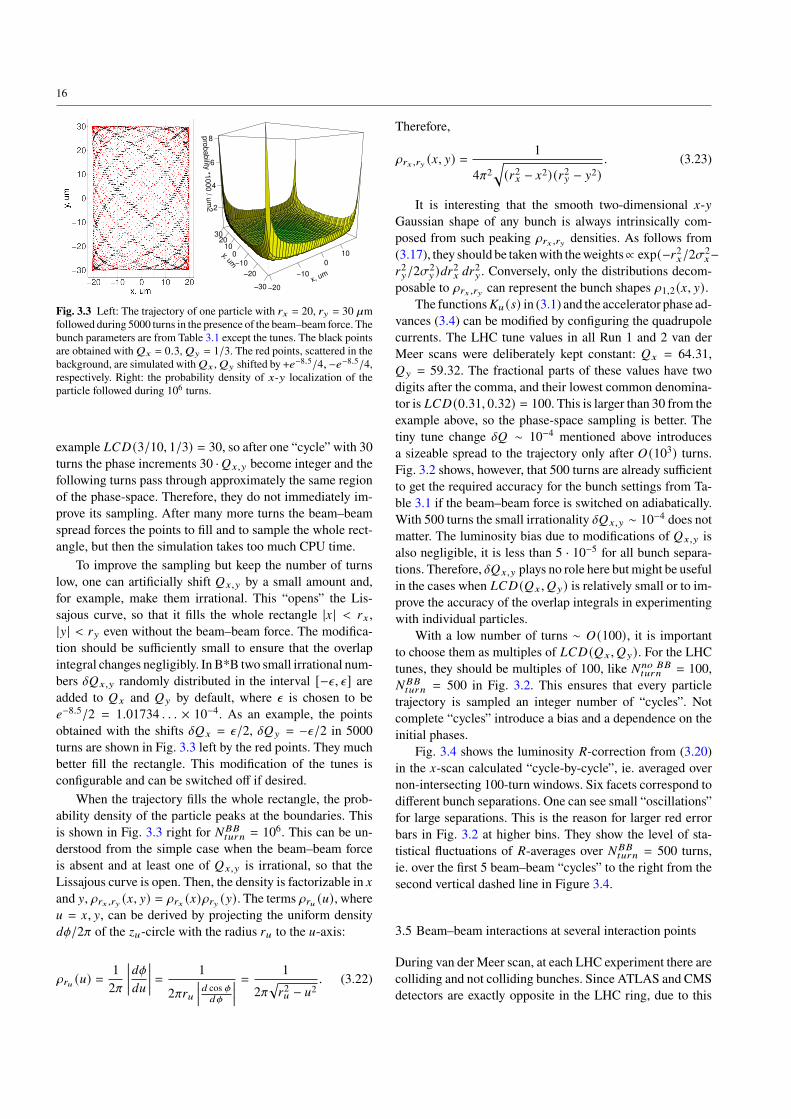
𝑡𝑢𝑟𝑛 turns. In the former case, the particletrajectory instantaneously changes from the ideal circle tothe one perturbed by the beam–beam force. The intersectionof the two trajectories is the last point on the ideal circle. It ispositioned randomly, and different points on the ideal circlelead to different perturbed trajectories. This is depicted inFig. 3.1. Two initially opposite points, marked in the figureby the small open circles, create two outer blue trajectories.Their evolution is followed during 107 turns and every 1000-th point is shown in the plot. The region in grey in the middleis filled with all other trajectories. The unperturbed ideal cir-cle with the center at the origin is shown by the green dashedline. As one can see, the center of the blue circles is shifteddue to the change of the orbit in 𝑥 and 𝑥 ′. This will be dis-cussed in more detail in section 3.8. Note that the ideal greencircle is infinitely “thin”, but the blue points are scatteredbecause of the beam–beam 𝑥-𝑦 coupling and the variationsin the other 𝑧𝑦-projection. The “thickness” of the blue tra-jectories increases with the force strength. For much largerforces the trajectory becomes significantly non-circular.In the adiabatic case, the trajectories change slowly and

the particles have time to redistribute over them. The initial

15

Fig. 3.1 The trajectories of the particles with 𝑟𝑥 = 20, 𝑟𝑦 = 30 `min 𝑧𝑥 projection for the bunches separated in 𝑥 by 40 `m with theparameters from Table 3.1 as an example. The outer blue trajectoriesare formed by two initially opposite particles (marked by small opencircles) after the instantaneous switch of the beam–beam force. The greyband between them is composed of such trajectories from all particles.The adiabatic trajectory is in red and the initial circle with 𝑟𝑥 = 20 `mis shown by the green dashed line.

position on the circle then has little importance, and thewholeinitial circle transforms to approximately one final trajectoryshown in red in Fig. 3.1. Here, the beam–beam interactionis slowly switched on during 1000 turns and then, as in theprevious case, every 1000-th turn is shown out of 107 intotal. The red trajectory has approximately the same spreadas the blue outer ones but less than the grey band composedof many trajectories initiated by the instantaneous switch.In any case, the spread is negligible compared to the

width of the opposite bunch, namely, 40 `m in Fig. 3.1.Therefore, the contribution to the overlap integral in (3.13)is essentially determined by the infinitely “thin” average tra-jectory, which is the same in both instantaneous and adiabaticswitch cases. The integral does not depend on the way howthe beam–beam force is switched on. This is demonstratedin Fig. 3.2 by the blue and red points for various beam sepa-rations.In both cases only 500 (100) accelerator turns were sim-

ulated to determine the perturbed (initial) overlap integral.In the adiabatic case the force was switched on during 100turns. The error bars show the standard deviations of the re-sults obtainedwith different randomgenerator seeds. Clearly,the adiabatic switch is preferable. The instantaneous switchleads to the spread of the trajectories and larger statisticalfluctuations of the final integral.The central black points in Fig. 3.2 are the result of

the simulation when the beam–beam force was switched onslowly in 104 turns and the luminosity integral was calculatedover 106 turns. As one can see from Fig. 3.2, simulating only

-6

-4

-2

0

2

0 1 2 3 4 5bunch separation / bunch σ

(R-1

)×10

3

Fig. 3.2 The deviation of the ratio 𝑅 defined in (3.20) from unityin per mille in the 𝑥-scan versus the separation of the bunches ex-pressed in the bunch widths. The beam parameters are taken fromTable 3.1. The error bars show the standard deviation of the resultswhen the simulation was repeated with different random seeds 100 and25 times for instantaneous (blue) and adiabatic (red points) switch ofthe beam–beam force, respectively. The number of simulated turns are[𝑁 𝑛𝑜 𝐵𝐵

𝑡𝑢𝑟𝑛 , 𝑁 𝑎𝑑𝑖𝑎𝑏𝑡𝑢𝑟𝑛 , 𝑁 𝐵𝐵

𝑡𝑢𝑟𝑛 ] = [100, 0, 500] (blue), [100, 100, 500](red), [10 000, 10 000, 1 000 000] (black). The red and blue points aredisplaced horizontally to the left and right, respectively, to reduce over-lapping.

500 turns already gives sufficient accuracy. The default B*Bvalues, 𝑁𝑛𝑜 𝐵𝐵

𝑡𝑢𝑟𝑛 = 1000, 𝑁𝑎𝑑𝑖𝑎𝑏𝑡𝑢𝑟𝑛 = 1000 and 𝑁𝐵𝐵

𝑡𝑢𝑟𝑛 = 5000,are, therefore, quite conservative and may be reduced by afactor of 10 in practice.After the beam–beam force is fully switched on and be-

fore calculating the overlap integral over 𝑁𝐵𝐵𝑡𝑢𝑟𝑛 turns in the

final stage, the B*B simulation has an option to run 𝑁𝑠𝑡𝑎𝑏𝑡𝑢𝑟𝑛

turns for a “stabilization”. This period is not used for calcu-lating the luminosity integral. Normally this parameter canbe set to zero because, for example, in the adiabatic casethe particle arrives at its final trajectory as soon as the forcereaches its nominal value. The following evolution does notchange the trajectory. 𝑁𝑠𝑡𝑎𝑏

𝑡𝑢𝑟𝑛 parameter exists only for flexi-bility and for experimenting with the B*B simulation.

3.4 Lissajous curves

Without the beam–beam interaction the 𝑥-𝑦 trajectory of aparticle placed at the 𝑧𝑥 , 𝑧𝑦-circles with the radii (𝑟𝑥 , 𝑟𝑦) andwith the initial phases 𝜙0𝑥,𝑦 is described by (3.9):

𝑥𝑛 = 𝑟𝑥 cos(2𝜋𝑄𝑥𝑛+𝜙0𝑥), 𝑦𝑛 = 𝑟𝑦 cos(2𝜋𝑄𝑦𝑛+𝜙0𝑦), (3.21)

ie. appears to be a Lissajous curve. The beam–beam forceleads to the dispersion of the trajectory as shown in Fig. 3.3left by the black points for the artificial values 𝑄𝑥 = 0.3,𝑄𝑦 = 1/3 and 5000 accelerator turns.In general, for the rational 𝑄𝑥,𝑦 and a small beam–beam

force the trajectory “cycles” after 𝐿𝐶𝐷 (𝑄𝑥 , 𝑄𝑦) turns where𝐿𝐶𝐷 denotes the lowest common denominator. In the above

16

x, um

−20

−10

0

10y, um

−30

−20

−10

010

2030

pro

bability

*1000 / u

m2 2

4

6

8

Fig. 3.3 Left: The trajectory of one particle with 𝑟𝑥 = 20, 𝑟𝑦 = 30 `mfollowed during 5000 turns in the presence of the beam–beam force. Thebunch parameters are from Table 3.1 except the tunes. The black pointsare obtained with𝑄𝑥 = 0.3,𝑄𝑦 = 1/3. The red points, scattered in thebackground, are simulated with𝑄𝑥 ,𝑄𝑦 shifted by +𝑒−8.5/4, −𝑒−8.5/4,respectively. Right: the probability density of 𝑥-𝑦 localization of theparticle followed during 106 turns.

example 𝐿𝐶𝐷 (3/10, 1/3) = 30, so after one “cycle” with 30turns the phase increments 30 ·𝑄𝑥,𝑦 become integer and thefollowing turns pass through approximately the same regionof the phase-space. Therefore, they do not immediately im-prove its sampling. After many more turns the beam–beamspread forces the points to fill and to sample the whole rect-angle, but then the simulation takes too much CPU time.To improve the sampling but keep the number of turns

low, one can artificially shift 𝑄𝑥,𝑦 by a small amount and,for example, make them irrational. This “opens” the Lis-sajous curve, so that it fills the whole rectangle |𝑥 | < 𝑟𝑥 ,|𝑦 | < 𝑟𝑦 even without the beam–beam force. The modifica-tion should be sufficiently small to ensure that the overlapintegral changes negligibly. In B*B two small irrational num-bers 𝛿𝑄𝑥,𝑦 randomly distributed in the interval [−𝜖, 𝜖] areadded to 𝑄𝑥 and 𝑄𝑦 by default, where 𝜖 is chosen to be𝑒−8.5/2 = 1.01734 . . . × 10−4. As an example, the pointsobtained with the shifts 𝛿𝑄𝑥 = 𝜖/2, 𝛿𝑄𝑦 = −𝜖/2 in 5000turns are shown in Fig. 3.3 left by the red points. They muchbetter fill the rectangle. This modification of the tunes isconfigurable and can be switched off if desired.When the trajectory fills the whole rectangle, the prob-

ability density of the particle peaks at the boundaries. Thisis shown in Fig. 3.3 right for 𝑁𝐵𝐵

𝑡𝑢𝑟𝑛 = 106. This can be un-derstood from the simple case when the beam–beam forceis absent and at least one of 𝑄𝑥,𝑦 is irrational, so that theLissajous curve is open. Then, the density is factorizable in 𝑥and 𝑦, 𝜌𝑟𝑥 ,𝑟𝑦 (𝑥, 𝑦) = 𝜌𝑟𝑥 (𝑥)𝜌𝑟𝑦 (𝑦). The terms 𝜌𝑟𝑢 (𝑢), where𝑢 = 𝑥, 𝑦, can be derived by projecting the uniform density𝑑𝜙/2𝜋 of the 𝑧𝑢-circle with the radius 𝑟𝑢 to the 𝑢-axis:

𝜌𝑟𝑢 (𝑢) =12𝜋

����𝑑𝜙𝑑𝑢 ���� = 1

2𝜋𝑟𝑢��� 𝑑 cos 𝜙𝑑𝜙

��� = 1

2𝜋√︁𝑟2𝑢 − 𝑢2

. (3.22)

Therefore,

𝜌𝑟𝑥 ,𝑟𝑦 (𝑥, 𝑦) =1

4𝜋2√︃(𝑟2𝑥 − 𝑥2) (𝑟2𝑦 − 𝑦2)

. (3.23)

It is interesting that the smooth two-dimensional 𝑥-𝑦Gaussian shape of any bunch is always intrinsically com-posed from such peaking 𝜌𝑟𝑥 ,𝑟𝑦 densities. As follows from(3.17), they should be takenwith theweights∝ exp(−𝑟2𝑥/2𝜎2𝑥−𝑟2𝑦/2𝜎2𝑦 )𝑑𝑟2𝑥 𝑑𝑟2𝑦 . Conversely, only the distributions decom-posable to 𝜌𝑟𝑥 ,𝑟𝑦 can represent the bunch shapes 𝜌1,2 (𝑥, 𝑦).The functions𝐾𝑢 (𝑠) in (3.1) and the accelerator phase ad-

vances (3.4) can be modified by configuring the quadrupolecurrents. The LHC tune values in all Run 1 and 2 van derMeer scans were deliberately kept constant: 𝑄𝑥 = 64.31,𝑄𝑦 = 59.32. The fractional parts of these values have twodigits after the comma, and their lowest common denomina-tor is 𝐿𝐶𝐷 (0.31, 0.32) = 100. This is larger than 30 from theexample above, so the phase-space sampling is better. Thetiny tune change 𝛿𝑄 ∼ 10−4 mentioned above introducesa sizeable spread to the trajectory only after 𝑂 (103) turns.Fig. 3.2 shows, however, that 500 turns are already sufficientto get the required accuracy for the bunch settings from Ta-ble 3.1 if the beam–beam force is switched on adiabatically.With 500 turns the small irrationality 𝛿𝑄𝑥,𝑦 ∼ 10−4 does notmatter. The luminosity bias due to modifications of 𝑄𝑥,𝑦 isalso negligible, it is less than 5 · 10−5 for all bunch separa-tions. Therefore, 𝛿𝑄𝑥,𝑦 plays no role here but might be usefulin the cases when 𝐿𝐶𝐷 (𝑄𝑥 , 𝑄𝑦) is relatively small or to im-prove the accuracy of the overlap integrals in experimentingwith individual particles.With a low number of turns ∼ 𝑂 (100), it is important

to choose them as multiples of 𝐿𝐶𝐷 (𝑄𝑥 , 𝑄𝑦). For the LHCtunes, they should be multiples of 100, like 𝑁𝑛𝑜 𝐵𝐵

𝑡𝑢𝑟𝑛 = 100,𝑁𝐵𝐵𝑡𝑢𝑟𝑛 = 500 in Fig. 3.2. This ensures that every particletrajectory is sampled an integer number of “cycles”. Notcomplete “cycles” introduce a bias and a dependence on theinitial phases.Fig. 3.4 shows the luminosity 𝑅-correction from (3.20)

in the 𝑥-scan calculated “cycle-by-cycle”, ie. averaged overnon-intersecting 100-turn windows. Six facets correspond todifferent bunch separations. One can see small “oscillations”for large separations. This is the reason for larger red errorbars in Fig. 3.2 at higher bins. They show the level of sta-tistical fluctuations of 𝑅-averages over 𝑁𝐵𝐵

𝑡𝑢𝑟𝑛 = 500 turns,ie. over the first 5 beam–beam “cycles” to the right from thesecond vertical dashed line in Figure 3.4.

3.5 Beam–beam interactions at several interaction points

During van der Meer scan, at each LHC experiment there arecolliding and not colliding bunches. Since ATLAS and CMSdetectors are exactly opposite in the LHC ring, due to this

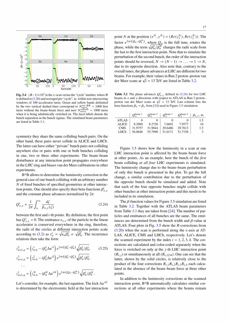
17

●●●●●●●●●●●●●●●●●●

●

●●●●●●●●●●

●

●●●●●●●●●●●

●●●●

●●●

●●●●●●●

●●●●●●●●●●●●●●●●●

●●●●

●●●●●●

●●●

●●●●●

●●●●●●●●●

●●●

●●●●●●●●●

●●●●

●●●●●

●●●●●●●●●●

●

●

●

●

●

●

●

●

●

●●●

●

●●

●●●

●●●●●

●

●●

●●●

●●●

●●

●

●

●

●

●

●●

●

●

●

●

●

●●

●

●●

●

●

●

●●●●●

●●

●●●

●●●●●●

●●●

●

●●

●●●●●

●●●●●

●

●

●

●

●

●

●●

●

●

●

●

●

●●

●

●●

●●

●

●●

●

●●●●●●●●●●●●●●●●●●

●●●

●

●

●

●●●●●●

●

●●●●●●●

●

●●●●●

●

●●●

●●●

●

●●

●

●

●●●●

●

●●●●

●

●

●

●●●

●

●

●

●●●●●●

●●

●

●●●

●●

●

●●

●●

●

●●

●●

●

●●

●

●●●●

●●●●

●

●

●●

●●●

●

●

●

●●●●●●●●●●●

●

●

●

●

●

●

●

●●

●

●●

●

●

●

●

●

●●●●●

●

●●

●

●

●●●●●

●●

●

●●

●

●

●●

●

●●●

●●●●

●

●●●

●

●●

●

●●●

●

●●

●

●

●

●

●

●●

●

●●

●

●●

●

●

●●

●

●●

●

●

●●

●●●

●●●

●●●●●●●

●●●

●●

●

●●

●

●●●●●●●●●●●●

●

●

●●●●

●

●

●

●

●●●●●●●●●●●

●●●●

●

●

●●

●●●

●●

●●●●●

●●

●●

●●●●

●●●●●

●●

●

●●

●●

●●

●●●●●

●●

●

●●

●

●

●

●

●

●

●

●●

●●

●●●●

●●●●

●

●●

●●

●

●

●●●●

●●●●●●

●

●●●●●●●●●●●

●

●

●

●

●

●

●

●

●●●●●●

●

●●●

●

●

●●

●

●

●●●

●

●

●●●

●

●

●●●

●

●●●●

●

●●●

●●●

●

●●

●

●●●●

●

●●●

●●●●

●●●

●●

●

●●●

●

●

●●

●

●

●●

●

●

●●●

●

●●●

●

●

●●●●●●●

●●

●●●

●●●●

3σ 4σ 5σ

0σ 1σ 2σ

0 50 100 0 50 100 0 50 100

−8

−6

−4

−2

0

2

−8

−6

−4

−2

0

2

Turn/100

(R−

1)×

103

Fig. 3.4 (𝑅−1)×103 in the 𝑥-scan versus the “cycle” number, where 𝑅is defined in (3.20) and averaged per “cycle”, ie. within non-intersectingwindows of 100 accelerator turns. Green and yellow bands delimitedby the two vertical dashed lines correspond to 𝑁 𝑛𝑜 𝐵𝐵

𝑡𝑢𝑟𝑛 = 1000 firstturns without the beam–beam force and next 𝑁 𝑎𝑑𝑖𝑎𝑏

𝑡𝑢𝑟𝑛 = 1000 turnswhen it is being adiabatically switched on. The facet labels denote thebunch separation in the bunch sigmas. The simulated beam parametersare listed in Table 3.1.

symmetry they share the same colliding bunch pairs. On theother hand, these pairs never collide in ALICE and LHCb.The latter can have either “private” bunch pairs not collidinganywhere else or pairs with one or both bunches collidingin one, two or three other experiments. The beam–beamdisturbance at any interaction point propagates everywherein the LHC ring and biases van derMeer calibrations in otherexperiments.B*B allows to determine the luminosity correction in the

general case of one bunch colliding with an arbitrary number𝑁 of fixed bunches of specified geometries at other interac-tion points. One should also specify their beta-functions 𝛽𝑖𝑥,𝑦and the constant phase advances normalized by 2𝜋

𝑄𝑖𝑥,𝑦 =

12𝜋

∫ 𝑠𝑖

𝑠1

𝑑Z

𝛽𝑥,𝑦 (Z)(3.24)

between the first and 𝑖-th points. By definition, the first pointhas 𝑄1𝑥,𝑦 = 0. The emittance 𝜖𝑥,𝑦 of the particle in the linearaccelerator is conserved everywhere in the ring, therefore,the radii of the circles at different interaction points scaleaccording to (3.2) as 𝑟 𝑖𝑢 =

√︁𝜖𝑢𝛽

𝑖𝑢 ∝

√︁𝛽𝑖𝑢 . The recurrence

relations then take the form

𝑧2𝑛+1,𝑢 =

(𝑧1𝑛,𝑢 − 𝑖𝛽1𝑢Δ𝑢′1

)𝑒2𝜋𝑖(𝑄2𝑢−𝑄1𝑢)

√︃𝛽2𝑢/𝛽1𝑢 , (3.25)

𝑧3𝑛+1,𝑢 =

(𝑧2𝑛,𝑢 − 𝑖𝛽2𝑢Δ𝑢′2

)𝑒2𝜋𝑖(𝑄3𝑢−𝑄2𝑢)

√︃𝛽3𝑢/𝛽2𝑢 ,

. . .

𝑧1𝑛+1,𝑢 =

(𝑧𝑁𝑛,𝑢 − 𝑖𝛽𝑁𝑢 Δ𝑢′𝑁

)𝑒2𝜋𝑖(𝑄𝑢−𝑄𝑁

𝑢 )√︃𝛽1𝑢/𝛽𝑁𝑢 .

Let’s consider, for example, the last equation. The kick Δ𝑢′𝑁is determined by the electrostatic field at the last interaction

point 𝑁 at the position (𝑥𝑁 , 𝑦𝑁 ) = (𝑅𝑒(𝑧𝑁𝑥 ), 𝑅𝑒(𝑧𝑁𝑦 )). Thefactor 𝑒2𝜋𝑖(𝑄𝑢−𝑄𝑁

𝑢 ) , where 𝑄𝑢 is the full tune, rotates thephase, while the term

√︁𝛽1𝑢/𝛽𝑁𝑢 changes the radii scale from

the last to the first interaction point. Note that to simulate theperturbation of the second bunch, the order of the interactionpoints should be reversed, 𝑁 → (𝑁 − 1) → . . . → 1→ 𝑁 ,due to its opposite direction. Also note that, contrary to theoverall tunes, the phase advances at LHC are different for twobeams. For example, their values in Run 2 proton–proton vander Meer scans at

√𝑠 = 13 TeV are listed in Table 3.2.

Table 3.2 The phase advances 𝑄𝑖𝑥,𝑦 defined in (3.24) for two LHC

beams in 𝑥 and 𝑦 directions with respect to ATLAS in Run 2 proton–proton van der Meer scans at

√𝑠 = 13 TeV. Last column lists the

beta-functions 𝛽𝑥 = 𝛽𝑦 from [24] used in Figure 3.5 simulation.

𝑄beam 1𝑥 𝑄beam 2𝑥 𝑄beam 1𝑦 𝑄beam 2𝑦 𝛽𝑥,𝑦 , mATLAS 0 0 0 0 1.5ALICE 8.2960 8.2728 7.6692 7.9577 10CMS 31.9757 31.9844 29.6486 29.7613 1.5LHCb 56.0648 55.7990 51.0171 51.7158 3

Figure 3.5 shows how the luminosity in a scan at oneLHC interaction point is affected by the beam–beam forceat other points. As an example, here the bunch of the firstbeam colliding at all four LHC experiments is simulated.The luminosity change due to the beam–beam perturbationof only this bunch is presented in the plot. To get the fullchange, a similar contribution due to the perturbation ofthe opposite bunch should be simulated and added. Notethat each of the four opposite bunches might collide withother bunches at other interaction points and this needs to beincluded in its simulation.The 𝛽-function values for Figure 3.5 simulation are listed

in Table 3.2. Together with the ATLAS beam parametersfrom Table 3.1 they are taken from [24]. The number of par-ticles and emittances of all bunches are the same. The emit-tances are determined from the bunch width and 𝛽-value atATLAS. Four plots in Fig. 3.5 show the 𝑅-corrections from(3.20) when the scan is performed along the 𝑥-axis at AT-LAS, ALICE, CMS and LHCb, respectively. Let’s denotethe scanned experiment by the index 𝑖 = 1, 2, 3, 4. The cor-rections are calculated and color-coded separately when theforce is switched on only at the 𝑗-th LHC interaction point(𝑅𝑖, 𝑗 ) or simultaneously at all (𝑅𝑖,1234). One can see that thelatter, shown by the solid circles, is relatively close to theproduct of the four corrections 𝑅𝑖,1𝑅𝑖,2𝑅𝑖,3𝑅𝑖,4 each calcu-lated in the absence of the beam–beam force at three otherpoints.In addition to the luminosity corrections at the scanned

interaction point, B*B automatically calculates similar cor-rections at all other experiments where the beams remain

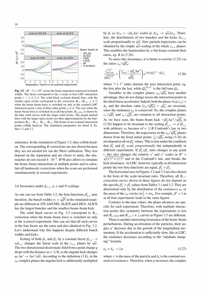
18

● ● ● ● ●●

●●

●●

●● ● ● ● ● ● ● ● ● ●

● ● ● ● ● ● ● ● ● ● ● ● ● ● ● ● ●●

●●

●

● ● ● ● ● ● ● ●● ●

●●

●●

●●

●●

●●

●

● ● ● ● ● ● ● ● ● ●● ● ● ● ● ● ● ● ● ● ●

● ● ● ● ● ●●

●●

●●

● ● ● ● ● ● ●●

●●

● ● ● ● ● ●●

●●

●●

●● ● ● ● ●

●●

●●

● ● ● ● ● ● ● ●●

●●

●●

●●

●●

●●

●●

● ● ● ● ●●

●●

●●

●●

●

●

●

●

●

●

●

●

●

● ● ● ● ●●

●●

●●

●● ● ● ● ● ● ● ● ● ●

● ● ● ● ● ● ●●

●●

●●

●●

●●

●●

●●

●

● ● ● ● ● ● ● ● ● ● ● ●●

●●

●●

●●

●●

● ● ● ● ● ● ● ● ● ● ● ●●

●●

●●

●●

●●

● ● ● ● ● ● ● ● ● ● ● ● ● ● ●● ●

●●

●●

● ● ● ● ●●

●●

●●

● ● ● ● ● ● ● ● ● ● ●

● ● ● ● ●●

●●

●●

●●

●

●

●

●

●

●

●

●

●

● ● ● ● ● ● ● ● ● ● ● ● ● ● ● ● ● ● ● ● ●

● ● ● ● ● ● ● ● ● ● ● ● ● ● ●●

● ● ● ● ●

● ● ● ● ● ● ● ● ● ● ● ● ● ●●

●●

●● ● ●

● ● ● ● ● ● ● ● ● ● ● ●● ● ● ● ● ● ● ● ●

● ● ● ● ● ● ● ● ● ● ● ● ● ● ● ● ● ● ● ● ●● ● ● ● ● ● ●

●●

●●

●●

●●

●●

●●

●●

● ● ● ● ●●

●●

●●

●● ● ● ● ● ● ● ● ● ●

● ● ● ● ● ● ● ● ● ● ● ● ●●

●●

●●

● ● ●

● ● ● ● ● ● ● ● ● ● ● ●●

●●

●●

●●

●●

scan at CMS scan at LHCb

scan at ATLAS scan at ALICE

0 1 2 3 4 5 0 1 2 3 4 5

−20

−10

0

10

20

−20

−10

0

10

20

Separation / bunch σ at scanned experiment

(R−

1)×

103

beam−beam at●

●

●

●

●

●

ATLASALICECMSLHCball4−product

Fig. 3.5 (𝑅 − 1) × 103 versus the beam separation expressed in bunchwidths. The facets correspond to the 𝑥-scans at four LHC interactionpoints 𝑖 = 1, 2, 3, 4. The solid black (colored dotted) lines with thesmaller open circles correspond to the correction 𝑅𝑖,𝑖 (𝑅𝑖, 𝑗 , 𝑗 ≠ 𝑖)when the beam–beam force is switched on only at the scanned LHCinteraction point 𝑖 (one of three other points 𝑗 ≠ 𝑖). The case when thebeam–beam force is switched on at all four points, 𝑅𝑖,1234, is shown bythe blue solid curves with the larger solid circles. The purple dashedlines with the larger open circles are their approximations by the four-products 𝑅𝑖,1 · 𝑅𝑖,2 · 𝑅𝑖,3 · 𝑅𝑖,4. The beams at not scanned interactionpoints collide head-on. The simulation parameters are listed in Ta-bles 3.1 and 3.2.

stationary. In the simulation of Figure 3.5, they collide head-on. The corresponding 𝑅-corrections are not shown becausethey are not needed for van der Meer calibration. They lessdepend on the separation and are closer to unity, the mis-matches do not exceed 4 · 10−3. B*B also allows to simulatethe beam–beam interactions at multiple points and to calcu-late all luminosity corrections when the scans are performedsimultaneously in several experiments.

3.6 Invariance under 𝛽𝑥,𝑦 , 𝑝, 𝜖 and 𝑁 scalings

As one can see from Table 3.2, the beta-functions 𝛽𝑖𝑥,𝑦 and,therefore, the bunch widths 𝜎𝑖 ∝

√︁𝛽𝑖 in the simulated exam-

ple are different at ATLAS/CMS, ALICE and LHCb. ALICEhas the largest bunches and the smallest beam–beam kick.The solid black curves in Fig. 3.5 correspond to 𝑅𝑖,𝑖

correction when the beam–beam force is switched on onlyat the scanned experiment. One can see that all such curvesin the four facets are the same and also identical to Fig. 3.2.Let’s understand why this happens despite different bunchwidths and kicks.Scaling of both 𝛽𝑥 and 𝛽𝑦 by a constant factor 𝛽𝑥,𝑦 →

𝛼𝛽𝑥,𝑦 changes the linear scale in the 𝑧𝑥,𝑦 planes by√𝛼.

The two-dimensional electrostatic field from a point charge 𝑞drops with the distance as∝ 1/𝑅, so the angular kick changesas Δ𝑢′ → Δ𝑢′/

√𝛼. According to the definition (3.8), in the

𝑧𝑢 complex planes the angular kick is additionally multiplied

by 𝛽, so Δ𝑧𝑢 = −𝑖𝛽𝑢Δ𝑢′ scales as Δ𝑧𝑢 →√𝛼Δ𝑧𝑢 . There-

fore, the distributions of two bunches and the kicks Δ𝑧𝑥,𝑦scale proportionally to

√𝛼. New particle trajectories can be

obtained by the simple√𝛼-scaling of the whole 𝑧𝑥,𝑦 planes.

This modifies the luminosities by 𝛼 but keeps constant theirratios, eg. 𝑅 in (3.20).To stress this invariance, it is better to rewrite (3.25) via

the ratios 𝑧𝑢/√𝛽𝑢:

𝑧”𝑖+1”𝑛+1,𝑢√︁𝛽”𝑖+1”𝑢

=

(𝑧𝑖𝑛,𝑢 − 𝑖𝛽𝑖𝑢Δ𝑢′𝑖√︁

𝛽𝑖𝑢

)𝑒2𝜋𝑖(𝑄”𝑖+1”𝑢 −𝑄𝑖

𝑢) , (3.26)

where ”𝑖 + 1” index denotes the next interaction point, eg.the first after the last, while 𝑄”𝑁+1”

𝑢 is the full tune 𝑄𝑢 .Variables in the complex planes 𝑧𝑢/

√𝛽𝑢 have another

advantage: they do not change across the interaction points inthe ideal linear accelerator. Indeed, both the phase 𝐴𝑟𝑔(𝑧𝑢) =𝜙𝑢 and the absolute value

��𝑧𝑢/√𝛽𝑢 �� =√𝜖𝑢 are invariant,

since the emittance 𝜖𝑢 is conserved. So, the complex planes𝑧𝑥/

√𝛽𝑥 and 𝑧𝑦/

√︁𝛽𝑦 are common to all interaction points.

As we have seen, the beam–beam kick −𝑖𝛽𝑖𝑢Δ𝑢′𝑖/√︁𝛽𝑖𝑢 in

(3.26) happen to be invariant to the scaling 𝛽𝑖𝑥,𝑦 → 𝛼𝑖𝛽𝑖𝑥,𝑦with arbitrary 𝛼𝑖 because of ∝ 1/𝑅 Coulomb’s law in twodimensions. Therefore, the trajectories in the 𝑧𝑢/

√𝛽𝑢 planes

drawn from the fixed initial points 𝑧1𝑢/√𝛽𝑢 using (3.26) do

not depend at all on 𝛽𝑖𝑢 values. This is true under the conditionthat 𝛽𝑖𝑥 and 𝛽𝑖𝑦 scale proportionally but independently indifferent experiments. If 𝛽𝑖𝑥/𝛽𝑖𝑦 ratio changes at any point𝑖, this also changes the relative 𝑥𝑖 and 𝑦𝑖 scales in 𝑅𝑖 =√︁(𝑥𝑖)2 + (𝑦𝑖)2 and in the Coulomb’s law, and breaks thekick invariance. At LHC, however, typically at all interactionpoints the two beta-functions are equal, 𝛽𝑖𝑥 = 𝛽𝑖𝑦 .The horizontal axes in Figures 3.2 and 3.5 are also chosen

in the form of the scale-invariant ratio. Therefore, all 𝑅𝑖,𝑖-correction curves shown in these figures do not depend onthe specific 𝛽𝑖𝑥 = 𝛽𝑖𝑦 values fromTables 3.1 and 3.2. They aredetermined only by the distribution of the emittances 𝜖𝑢 orthe areas of the 𝑧𝑢-circles 𝜋𝑟2𝑢 = 𝜋𝜖𝑢 . For example, 𝛽𝑖 = 1mat all four experiments leads to the same figures.Contrary to the tune values, the phase advances are spe-

cific for each experiment. Therefore, with multiple interac-tion points this symmetry between the experiments is lostand 𝑅𝑖,1234 and 𝑅𝑖, 𝑗 , 𝑖 ≠ 𝑗 curves in Figure 3.5 are different.There is another interesting invariance of the beam–beam

perturbations. During acceleration of the particles, their an-gles 𝑢′ decrease due to the growth of the longitudinal mo-mentum. If the acceleration is sufficiently slow, like at LHC,the emittance decreases according to the “adiabatic damp-ing” formula

𝜖𝑢 = 𝜖𝑢 · 𝑚/𝑝, (3.27)

where𝑚 is the mass of the particle and 𝜖𝑢 is the constant nor-malized emittance. Therefore, when 𝑝 increases, the complex

19

plane 𝑧𝑢/√𝛽𝑢 shrinks as 1/

√𝑝 and the beam–beam force in-

creases as √𝑝. The angular beam–beam kick Δ𝑝/𝑝 contains𝑝 in the denominator as in (2.6), and decreases as 1/√𝑝, ie.coherently with the 𝑧𝑢/

√𝛽𝑢 complex plane. Therefore, in the

complex plane corresponding to the normalized emittances𝑧𝑢

√︁𝑝/𝑚𝛽𝑢 =

√𝜖𝑢𝑒

𝑖𝜙𝑢 the trajectories remain invariant ifthe phase advances are constant and 𝜖𝑢 are conserved. Thebeam–beam perturbations of the bunches with identicallydistributed normalized emittances are identical.Finally, let’s formulate the scaling law for the number of

particles 𝑁2 in the opposite bunch. It will be called “second”in the following to distinguish from the “first” bunch withthe studied trajectories. The bunch variables will be markedby the corresponding indices.Multiplying the normalized emittance of the first bunch

by 𝛼 increases the linear scale by√𝛼 and reduces the beam–

beam angular kick by 1/√𝛼. In order to have the same

√𝛼

change in the linear and angular scales for the first bunch, thebeam–beam force from the second should be enhanced by𝛼. This can be achieved by increasing 𝑍1𝑍2𝑁2. Therefore,the simultaneous scaling of 𝜖1𝑢 and 𝑍1𝑍2𝑁2 by the samefactor changes the scale but not the shapes of the first bunchtrajectories. It also keeps constant the luminosity correctionratios. If the trajectories are analyzed in the complex plane

𝑧1𝑢

√︂𝑝1

𝑚1𝛽𝑢1𝑍1𝑍2𝑁2=

√︂𝜖1𝑢

𝑍1𝑍2𝑁2𝑒𝑖𝜙1𝑢 , (3.28)

the results depend only on the initial distributions, the phaseadvances and 𝛽1𝑥/𝛽1𝑦 ratios, but do not depend on the in-dividual values of 𝛽1𝑥,1𝑦 , 𝜖1𝑢 , 𝑝1, 𝑍1,2 or 𝑁2. Only theircombination

𝜖1𝑢𝑍1𝑍2𝑁2

=𝜖1𝑢 𝑝1

𝑍1𝑍2𝑁2𝑚1(3.29)

matters. This can also be confirmedwith the B*B simulation.

3.7 Simulation of the beam crossing angle

If the beams collide with the crossing angle as in Figure 1.1,the betatron oscillations occur in the planes transverse to thebeam vectors v1,2. They determine the transverse widths 𝜎𝑖𝑇of the bunches 𝑖 = 1, 2. The luminosity, however, dependson the bunch widths 𝜎′

𝑖𝑇perpendicular to Δv. According to

(1.21), they get additional contributions from the longitudi-nal widths 𝜎𝑖𝐿 .The beam–beam kick is also perpendicular to Δv either

in the laboratory or, for example, in the rest frame of thefirst bunch particle 𝑞1 shown in Figure 2.1. Therefore, 𝑞1“sees” the opposite bunch width 𝜎′

2𝑇 enhanced by 𝜎2𝐿 , andthis value should be used in the B*B simulation for 𝜌2. Thebunch creating the field is “static” in the B*B model, itsbetatron transverse motion and 𝜎2𝑇 do not matter.

However, to simulate the betatron trajectories in the firstbunch, the initial widths 𝜎1𝑥 , 𝜎1𝑦 should be specified in B*Bwithout the longitudinal component. The betatron oscilla-tions are insensitive to 𝜎1𝐿 spread. Since the crossing anglesare small at LHC, 𝛼1,2 = 𝛼 < 10−3, the kicks calculated inthe primed frame with the parallel beams can be propagatedwithout changes to the frame of the betatron motion. Simi-larly, the simulated 𝑥, 𝑦 beam transverse coordinates can bepropagated back for the luminosity calculation.In this way the luminosity correction is determined for

the unperturbed widths 𝜎1𝑇 , 𝜎′2𝑇 instead of the required

𝜎′1𝑇 , 𝜎

′2𝑇 . Therefore, the final density 𝜌1 + 𝛿𝜌1, correspond-

ing to 𝜎1𝑇 , should be additionally smeared by the contri-bution from 𝜎1𝐿 . This is performed in the B*B simulationin the following way. Let’s consider the general case whenneither 𝑥 nor 𝑦 of the first bunch lies in the crossing plane,and denote by 𝛽1 the angle between the 𝑥-axis and the pro-jection of the crossing plane to the 𝑥-𝑦 plane. The perturbeddensity 𝜌1 + 𝛿𝜌1 should then be convolved with the two-dimensional Gaussian 𝐺 (𝑥, 𝑦) with the sigmas 𝛼𝜎1𝐿 cos 𝛽1and 𝛼𝜎1𝐿 sin 𝛽1 in 𝑥 and 𝑦, respectively. If, for example,the 𝑥-axis belongs to the crossing plane and 𝛽1 = 0, thesmearing occurs only along 𝑥 with the sigma 𝛼𝜎1𝐿 , while𝐺 (𝑥, 𝑦) projection to 𝑦 reduces to the delta-function. Insteadof smearing 𝜌1 + 𝛿𝜌1 in the overlap integral, it is simpler toperform an equivalent smearing of 𝜌2:

𝐿 ∝∫

((𝜌1 + 𝛿𝜌1) ∗ 𝐺) 𝜌2 𝑑2r

=

∫ (∫(𝜌1 + 𝛿𝜌1) (r′)𝐺 (r − r′)𝑑2r′

)𝜌2 (r)𝑑2r

=

∫(𝜌1 + 𝛿𝜌1) (r′)

(∫𝐺 (r′ − r)𝜌2 (r)𝑑2r

)𝑑2r′

=

∫(𝜌1 + 𝛿𝜌1) (𝐺 ∗ 𝜌2) 𝑑2r′, (3.30)

since 𝐺 (r − r′) = 𝐺 (r′ − r), where r and r′ denote thetwo-dimensional vectors in the (𝑥, 𝑦) plane.To implement this scheme, the B*B simulation takes the

values

Δ𝜎𝑖1𝑥 = 𝛼𝜎1𝐿 cos 𝛽1, Δ𝜎𝑖

1𝑦 = 𝛼𝜎1𝐿 sin 𝛽1 (3.31)

as configurable parameters defining the Gaussian 𝐺𝑖 (𝑥, 𝑦)for each interaction point 𝑖. Its convolution with the multi-Gaussian 𝜌2 is performed analytically. The result is used in(3.13) instead of 𝜌2 for the overlap integral calculation. Notethat it receives contributions from both 𝜎1𝐿 and 𝜎2𝐿 . Thefield is determined from 𝜌2 not smeared by 𝐺𝑖 (𝑥, 𝑦), whereonly 𝜎2𝐿 contributes. The beam–beam perturbation of thelongitudinal beamdynamics is neglected and the longitudinalspread is always approximated by a single Gaussian. Bydefault the parameters (3.31) are zero.

20

3.8 Cross-checks and comparison with the old model usedat LHC in 2012–2019

In Section 2.4 it was shown that the full beam–beam forceexerted on the first bunch can be easily calculated as theforce between the first bunch collapsed to the origin (0, 0)and the second one with the density “inflated” from 𝜌2 to�̃�1 ∗ 𝜌2. In case of the Gaussian bunches with the widths𝜎1,2;𝑥,𝑦 and the centers r01,2, the cross-correlation �̃�1 ∗ 𝜌2 isalso Gaussian and has the widths Σ𝑥,𝑦 =

√︃𝜎21;𝑥,𝑦 + 𝜎

22;𝑥,𝑦

and the centerΔr021 = r02−r01. Its electrostatic field 𝐸2𝑢 , givenby (2.10) or (2.12), allows to calculate the average angularbeam–beam kick Δ𝑢′ = 𝑞1𝐸2𝑢/𝑝1𝑐 = 𝑒𝑍1𝐸2𝑢/𝑝1𝑐, of thefirst bunch particles. This value is exact if all bunch particlesmove with the opposite and constant velocities close to thespeed of light, so that one can calculate the kicks using thelaws of electrostatics.Let’s substitute the beam–beam angular kick by its av-

erage. The 𝑥- and 𝑦-directions then decouple. To simplifynotations, let’s drop the coordinate subscript 𝑢, denote theone-turn phase advance by 2𝜋𝑄 = 𝜙, introduce the constantΔ = 𝛽1Δ𝑢

′ = 𝛽1𝑞1𝐸2𝑢/𝑝1𝑐 and consider for simplicity thecase with only one interaction point. The recurrence relation(3.10) then defines the geometric sequence

𝑧𝑛+1 = (𝑧𝑛 − 𝑖Δ)𝑒𝑖𝜙

= 𝑧1𝑒𝑖𝑛𝜙 − 𝑖Δ𝑒𝑖𝜙

(1 + 𝑒𝑖𝜙 + 𝑒2𝑖𝜙 + . . . + 𝑒𝑖 (𝑛−1)𝜙

)= 𝑧1𝑒

𝑖𝑛𝜙 − 𝑖Δ𝑒𝑖𝜙 𝑒𝑖𝑛𝜙 − 1𝑒𝑖𝜙 − 1 . (3.32)

This can be rewritten as

𝑧𝑛+1 −𝑖Δ𝑒𝑖𝜙

𝑒𝑖𝜙 − 1 =

(𝑧1 −

𝑖Δ𝑒𝑖𝜙

𝑒𝑖𝜙 − 1

)𝑒𝑖𝑛𝜙 . (3.33)

A comparison with the equation 𝑧𝑛+1 = 𝑧1𝑒𝑖𝑛𝜙 without the

beam–beam interaction shows that the constant kick onlyshifts the center of rotation from the origin to the point

𝑧0 =𝑖Δ𝑒𝑖𝜙

𝑒𝑖𝜙 − 1 =𝑒𝑖𝜙/2

2 sin 𝜙

2

=Δ

2 tan 𝜙

2

+ 𝑖Δ2. (3.34)

Its real part determines the shift of the beam orbit, whilethe scaled imaginary part −𝐼𝑚(𝑧0)/𝛽1 = −Δ𝑢′/2 gives theangular shift just before the beam–beam interaction. Afterreceiving the kick +Δ𝑢′, it flips from −Δ𝑢′/2 to +Δ𝑢′/2,while the next accelerator turn changes it back to −Δ𝑢′/2.The orbit shift expressed in the bunch widths should be

invariant and should depend only on 𝜖1/𝑍1𝑍2𝑁2. Indeed,since Δ = 𝛽1Δ𝑢

′ =(𝜎21 𝑝1/𝜖1𝑚1

)· (𝑒𝑍1𝐸2𝑢/𝑝1𝑐), it can be

written as

𝑅𝑒(𝑧0)𝜎1

=𝑒(𝐸2𝑢𝜎1)𝑍2𝑁2

· 12𝑚1𝑐 tan 𝜙

2

· 𝑍1𝑍2𝑁2𝜖1

. (3.35)

Here, 𝐸2𝑢 has ∝ 𝑍2𝑁2/𝑅 dependence, so 𝑒(𝐸2𝑢𝜎1)/𝑍2𝑁2is invariant. For example, for the round bunches with 𝜎1 =𝜎2 = 𝜎, Σ𝑥,𝑦 =

√2𝜎 separated in 𝑥 by Δ𝑥, substituting 𝐸2𝑢

from (2.10) or (2.11) gives

𝑅𝑒(𝑧0)𝜎

=1 − 𝑒−Δ𝑥2/4𝜎2

Δ𝑥/𝜎 · 𝛼ℏ

𝑚1 tan 𝜙

2

· 𝑍1𝑍2𝑁2𝜖1

. (3.36)

The maximal value of the first term depending only on Δ𝑥/𝜎is 0.31908 . . . . Therefore, for protons one has

𝑅𝑒(𝑧0)𝜎

≤ 𝑁2

(2.0420 . . . × 1012) · [𝜖1/`m] · tan 𝜙

2

, (3.37)

which is less than 1% for the typical LHC values 𝜖1 ≈ 3 −4 `m, 𝑁2 ≈ (7− 9) · 1010 and 𝜙𝑥/2 = 0.31𝜋, 𝜙𝑦/2 = 0.32𝜋.In case of several interaction points with the phase ad-

vances 2𝜋𝑄𝑖 = 𝜙𝑖 with respect to the first point where bydefinition 𝜙1 = 0, and the constant kicks Δ𝑖 , 𝑖 = 1, 2, . . . , 𝑁 ,the first equation in (3.32) modifies to

𝑧𝑛+1 = 𝑧𝑛𝑒𝑖𝜙 − 𝑖Δ1𝑒𝑖𝜙 − 𝑖Δ2𝑒𝑖 (𝜙−𝜙2) − . . . − 𝑖Δ𝑁 𝑒

𝑖 (𝜙−𝜙𝑁 ) ,

(3.38)

which becomes equivalent to (3.32) after the substitution

𝑁∑︁𝑖=1

Δ𝑖𝑒−𝑖𝜙𝑖 = Δ. (3.39)

So, we have again a circular trajectory with the center shiftedto

𝑧0 =𝑖

(∑𝑁𝑖=1 Δ𝑖𝑒

−𝑖𝜙𝑖

)𝑒𝑖𝜙

𝑒𝑖𝜙 − 1 =

∑𝑁𝑖=1 Δ𝑖𝑒

𝑖 [𝜙/2−𝜙𝑖 ]

2 sin 𝜙

2

=

∑𝑁𝑖=1 Δ𝑖 cos( 𝜙2 − 𝜙𝑖)

2 sin 𝜙

2

+ 𝑖∑𝑁

𝑖=1 Δ𝑖 sin( 𝜙2 − 𝜙𝑖)2 sin 𝜙

2

, (3.40)

whose real and opposite imaginary parts define the spatialand 𝛽1-scaled angular shifts, respectively. This formula isvery well known in the accelerator physics, which uses dif-ferent tools for its derivation [30].For experimenting and debugging, B*B has configurable

options to substitute the exact kick formula by its averageand to output the 𝑥, 𝑦 orbit shifts. The latter are calcu-lated as weighted sums

∑𝑁𝑖=1 𝑤𝑖𝑢𝑖 over the simulated par-

ticle coordinates 𝑢𝑖 , averaged over accelerator turns simi-larly to (3.13). For example, with (𝑁𝑛𝑜 𝑏𝑏

𝑡𝑢𝑟𝑛 , 𝑁𝑎𝑑𝑖𝑎𝑏𝑡𝑢𝑟𝑛 , 𝑁𝑏𝑏

𝑡𝑢𝑟𝑛) =(100, 100, 500), default other settings and the single interac-tion point with the parameters from Table 3.1, the mismatchbetween the simulated and predicted orbit shifts averagedover the beam separation range [0 − 200] `m has the stan-dard deviation 𝜎 . 2 nm. The maximal predicted orbit shiftis 0.28 `m. The simulated shifts without the beam–beamforce are compatible with zero with 𝜎 . 0.3 nm.

21

If the beam–beam interaction is small, even with theexact, not constant kick the particle trajectory remains ap-proximately circular as illustrated in Figure 3.1. One parti-cle trajectory corresponds to two circles in 𝑧𝑥,𝑦-planes. Theorbit shift is then approximately determined by the beam–beam force F𝑡𝑟 averaged over the trajectory like shown inFigure 3.3, with the 𝑥-𝑦 density projection (3.23). The circlefrom Figure 3.1 in the 𝑧𝑥-plane shifts according to the aver-age 𝑥-component of the force 𝐹𝑡𝑟

𝑥 , dependent, however, onthe radius in 𝑧𝑦-plane. So, different 𝑧𝑥,𝑦-circle pairs have dif-ferent F𝑡𝑟 and shift differently. However, the ratio 𝑟𝑅𝑒/𝐼𝑚 ofthe real and imaginary parts in equations (3.34) and (3.40)remains constant regardless of F𝑡𝑟 . Therefore, the shiftedcenters 𝑧0 = 𝑥0 + 𝑖𝑦0 lie on the line 𝑟𝑅𝑒/𝐼𝑚 = 𝑥0/𝑦0 and thespatial and angular shifts are proportional. Averaging overthe bunch should preserve this proportionality. Therefore, ifΔ, Δ𝑖 denote exactly known average bunch angular kicks in(3.34) and (3.40), these equations should correctly predictthe average 𝑧0 shifts. For example, the real part 𝑅𝑒(𝑧0) pre-dicts the spatial average or “orbit” shifts. Note that contraryto the exact average angular kicks Δ𝑢′ and Δ, the values of𝑧0, ie. the angular and the orbit shifts calculated from (3.34)and (3.40), depend on the assumption that the trajectories areapproximately circular, which is violated for strong kicks ora large number of interaction points.

As an example, Figure 3.6 shows the 𝑥-orbit shifts in thesame simulation as in Figure 3.5. The beam–beam kick isswitched on at all four interaction points. The mismatchesbetween the shifts calculated by the B*B simulation and theanalytic approximation (3.40) reach 26 nm. Although smallin the absolute scale, they are significantly larger than thestatistical fluctuations. The orbit shift along 𝑦-coordinate,where the beams are not separated, is compatible with zerowithin 𝜎 = 0.4 nm.

In the old beam–beam model used at LHC in 2012–2019, the field E2 in the momentum kick Δp1 = 𝑞1E2/𝑐was not taken from (2.10) or (2.12) but was approximatedby a simple linear function of the 𝑥 and 𝑦 coordinates. Theconstant term was chosen to reproduce the orbit shift from(3.34). The slopes were taken from the derivatives 𝜕Δp1/𝜕𝑥,𝜕Δp1/𝜕𝑦 at the first bunch center. The model was limitedto the case when the Gaussian bunches collided head-onin the not scanned coordinate. Under this assumption, thecross-derivatives 𝜕Δ𝑝1,𝑦/𝜕𝑥, 𝜕Δ𝑝1,𝑥/𝜕𝑦 vanish, and the 𝑥,𝑦-slopes were taken as 𝜕Δ𝑝1,𝑥/𝜕𝑥, 𝜕Δ𝑝1,𝑦/𝜕𝑦, respectively.They can be calculated from (2.10) for the round bunches.For example, in the 𝑥-scan at the center of the first bunch,

ATLAS ALICE CMS LHCbaverage x

Δx

0 1 2 3 4 50 1 2 3 4 50 1 2 3 4 50 1 2 3 4 5

-500

0

500

1000

-20

-10

0

10

Separation / bunch σ at scanned experiment

x, n

m

head-onscan

ATLASALICECMSLHCb

Fig. 3.6 Upper row: 𝑥-coordinate averaged over the first bunch at fourexperiments, lower row: its deviation from (3.40) approximation, bothin nm, versus the beam separation expressed in the bunch widths. Thecolumn labels denote the scanned interaction points (marked by thesolid lines in the plots), at other points the beams collide head-on (thedashed lines). The simulation is the same as in Figure 3.5.

where 𝑅 = Δ𝑥, one has

1𝑘1

𝜕Δ𝑝1,𝑥

𝜕𝑥

����𝑥=Δ𝑥,𝑦=0

= − 1Δ𝑥2

+(1𝜎22

+ 1Δ𝑥2

)𝑒−Δ𝑥

2/2𝜎22 ,

1𝑘1

𝜕Δ𝑝1,𝑦

𝜕𝑦

����𝑥=Δ𝑥,𝑦=0

=1 − 𝑒−Δ𝑥2/2𝜎22

Δ𝑥2, (3.41)

where 𝑘1 = 2𝛼ℏ𝑍1𝑍2𝑁2. The full kick at Δ𝑥-separation wasapproximated as the following linear function of 𝑥 and 𝑦:

Δ𝑝1,𝑥 ≈ 𝑥 ·𝜕Δ𝑝1,𝑥

𝜕𝑥

����𝑥=Δ𝑥,𝑦=0

+ 𝑘11 − 𝑒−Δ𝑥2/2(𝜎21+𝜎22 )

Δ𝑥

Δ𝑝1,𝑦 ≈ 𝑦 ·𝜕Δ𝑝1,𝑦

𝜕𝑦

����𝑥=Δ𝑥,𝑦=0

. (3.42)

Note that to reproduce the orbit shift in the first formula, theconstant term is not equal to the value of the kick at the bunchcenter 𝑘1 (1 − 𝑒−Δ𝑥

2/2𝜎22 )/Δ𝑥. It contains 𝜎21 + 𝜎22 instead of

𝜎2 in the exponent. Therefore, (3.42) is not a linear expansionof Δ𝑝1,𝑥 .The linear kick significantly simplifies the analysis. As

known from the accelerator physics, in this case the Gaussianbunch remains Gaussian. The offset term is equivalent to thedipole magnet. It shifts the Gaussian center according to(3.34). The linear terms 𝑢 · 𝜕Δ𝑝1,𝑢/𝜕𝑢

��𝑥=Δ𝑥,𝑦=0 represent

the quadrupole magnets usually used to focus or defocus thebeams [30]. They modify the Gaussian widths according tothe formula

𝜎′𝑢 = 𝜎𝑢

√︄1 + 𝛽12 tan(2𝜋𝑄𝑢)

𝜕Δ𝑝1,𝑢

𝜕𝑢

����𝑥=Δ𝑥,𝑦=0

. (3.43)

Another simplification of (3.42) is that the 𝑥 and 𝑦 kicksare independent, so the beam–beam 𝑥-𝑦 coupling is ne-glected. Multiple interaction points also decouple and the

22

analysis can be limited to the point where the scan is per-formed. Indeed, other interactions only modify bunch Gaus-sian widths and centers, but in any case, they are consid-ered as free parameters in van der Meer analyses. Since thetransverse positions of the beams at not scanned points arekept constant, the beam–beam modifications are also con-stant and do not bias van der Meer calibration. Although thebeam–beam kick at multiple points have been discussed andsimulated in [24], where the old model was introduced, inpractice this was never used.For the Gaussian bunches, the luminosity can be calcu-

lated from the known centers andwidths. In the oldmodel theluminosity modification due to the orbit shift, induced by theequivalent dipole magnet, was calculated analytically. Thecontribution from the quadrupolemagnet was obtained usingLHC MAD-X accelerator simulation for the beam parame-ters from Table 3.1. They were tabulated and then extrapo-lated analytically to other bunch settings. Two contributionswere summed.The results of the old quadrupole simulation for Ta-

ble 3.1 settings are shown in Figure 3.7 by the open cir-cles. The curves denoted by “D”, “Q” and “D+Q” corre-spond to the dipole, quadrupole contributions and their sum,respectively. As in other plots, the luminosity bias 𝑅 − 1from (3.20) due to the perturbation of only one bunch isshown. The analytic corrections due to the dipole orbit shifts(3.34), the quadrupole bunch width changes (3.43) or bothare shown by the corresponding solid lines. One can see thatthe quadrupoleMAD-X simulation is well described analyti-cally and (3.43) could be used instead of the tabulated valuesin practice.To compare these known results with B*B, its exact

kick formula was replaced by (3.42), by only its dipole orquadrupole parts. The simulated values 𝑅 − 1 are shown inFigure 3.7 by the solid points. They are also in good agree-ment with the analytic predictions “D+Q”, “D” and “Q”,respectively.The B*B results with the exact kick are shown by the

solid circles connected by the dashed line “E”. They werealready shown in Figure 3.2. These results significantly differfrom the old “D+Q” simulation.Both “E” and “D+Q” containthe dipole contribution. To compare with “Q” alone, the B*Bsimulationwas performedwith the dipole constant subtractedfrom the exact kick in the recurrence relation. The result isshown as “E-D” curve. It differs significantly from “Q” andto a larger extent compensates the luminosity reduction by“D”. As expected, the sum of “D” and “E-D” is in agreementwith “E”.The knowledge of the 𝑅-correction allows determining

the bias induced on the reference cross-section 𝜎 eg. whenusing (1.6) for the Gaussian bunches in one-dimensional 𝑥,𝑦 van der Meer scans. The integrals in (1.6) should be taken

●●●●●●●●●●●●●●●●●●●●●●●●●●●●●●●●●●●●●●●●●●●●●●●●●●●

●●●●

●●

●●

●

●

●

●

●

●

●●

●●

●●

●●

●●

●●●●●●●●●●●●●●●●●●●●●●●●●●●

● ● ● ●●

●

●

●

●

●

●

●● ● ● ●

● ●● ●

●

● ●●

●

●

●

●

●

●

●

●

●●

●● ● ● ● ● ● ●

● ●●

●●

●● ● ● ● ● ● ● ● ● ● ● ● ● ● ●

●●

●

●

●

●

●

●

●

●

●

●●

● ●● ● ● ● ● ●

●●

●

●

●● ● ●

●●

● ● ● ●●

●●

●●

●●

E

D

Q

D+Q

E−D

−10

−5

0

5

0 1 2 3 4 5bunch separation / bunch σ

(R−

1)×

103

●

●

analyticB*Bold

Fig. 3.7 (𝑅 − 1) × 103 correction for the bunches with the parametersfrom Table 3.1 colliding at one interaction point versus their separationin the 𝑥-scan expressed in the bunch widths. The solid points are theresults of the B*B simulation when in the recurrence relation (3.10)the exact formula (E), dipole constant dependent on the separation (D)or their difference (E-D) are used. The open circles show the tabulatedvalues from the old simulation with the quadrupole kick (Q) and theirsumwith the values from the dipole analytic formula (D+Q). The curvesare analytic predictions for the dipole (D), quadrupole (Q) kicks andtheir sum (D+Q).

over the unperturbed values

`𝑠𝑝 ∝ 𝑒−Δ𝑥2/2(𝜎21+𝜎

22 )

2𝜋𝜎1𝜎2(3.44)

modulated by 𝑅2 from Figure 3.7 or the corresponding fig-ure for the 𝑦-scan. 𝑅 should be squared to take into accountthe perturbation of the second bunch. The luminosity cor-rections for the 𝑥- and 𝑦-scans are slightly different becauseof the difference in the fractional parts of the tunes 𝑄𝑥 , 𝑄𝑦 ,0.31 ≠ 0.32. The resulting biases of van der Meer cross-section 𝜎′/𝜎−1 are shown in Figure 3.8 separately for B*B,dipole (D), quadrupole (Q) approximations and their sum(D+Q). For the proton bunches colliding at one point, thecorrection depends only on the specific normalized emit-tance 𝜖/𝑁 assuming identical bunches with 𝑁 = 𝑁1 = 𝑁2and 𝛽1 = 𝛽2. Therefore, this variable is chosen as the hor-izontal axis. As shown by the dashed line, the differencebetween B*B and the old model for Table 3.1 settings is0.96%. The old linear kick approximation was too simple todescribe accurately the beam–beam luminosity bias.

4 Conclusions

The main tool for the absolute luminosity calibration at LHCis van der Meer scan. Its systematics dominates the overallluminosity uncertainty, which, in turn, gives one of the maincontributions to the uncertainty of the accurate cross-sectionmeasurements, for example, in the electroweak sector.

23

●

●

●

●

●

●

●

●

●

●

●

●

●

●

●

●

●

●

●

●

●

●

●

●

●

●

●

●

●

●

●

●

●

●

●

●

●

●

●

●

●

●

●

●

●

●

●

●

●

●

●

●

●

●

●

●

●

●

●

●

●

●

●

●

●

●

●

●

●

●

●

●

●

●

●

●

●●

●

●

●●

●

●

●●

●

●

●●

●

●

●●

●

●

●●

●

B*B

Q

D

D+Q−30

−20

−10

0

0 2 4 6 8 10 12 14normalized emittance × 1011/ N, µm

(σ'

σ−1)

×10

3

Fig. 3.8 The beam–beam cross-section bias (𝜎′/𝜎 − 1) × 103 de-termined from (1.6) versus 𝜖 /𝑁 · 1011, where 𝜖 is the normalizedemittance 𝜖 = 𝜖 /(𝑝/𝑚𝑝) , identical for both bunches, 𝑚𝑝 is the pro-ton mass and 𝑁 = 𝑁1 = 𝑁2 is the number of protons. The bias iscalculated for the single interaction point using B*B, analytic dipole(D), quadrupole (Q) approximations or their sum (D+Q). The tunes are𝑄𝑥 = 0.31, 𝑄𝑦 = 0.32 and it is assumed that 𝛽𝑥 = 𝛽𝑦 = 𝛽. Underthese conditions, 𝜎′/𝜎 depends only on the combination 𝜖 /𝑁 but noton 𝜖 , 𝑝, 𝑁 or 𝛽 individually. The vertical dashed line shows the value𝜖 /𝑁 · 1011 for the bunch parameters from Table 3.1.

Various details of van der Meer method are discussed inthe paper. Currently, the main sources of systematic uncer-tainties are the beam orbit drifts, 𝑥-𝑦 non-factorizability andthe bunch deformations induced by the beam–beam elec-tromagnetic interaction. The first two can be significantlyreduced by the accurate monitoring of the beam positionsand the two-dimensional scans, respectively. The formalismof one- and two-dimensional scans is presented in the paperin detail. Other sources of systematics include the measure-ments of the bunch populations, the length scale calibration,luminometer detector effects, other bunch shape changes dur-ing the scan, eg. after particle losses, and various unknownfactors contributing to the scan-to-scan non-reproducibility.The alternative beam–gas and beam–beam imaging calibra-tion methods are also briefly mentioned.The beam–beam bias is the main subject of the paper.

The derivation of the beam–beam kick is presented in Sec-tion 2 from the first principles together with the discussion ofvarious approximations and the induced errors. It is shownthat under the assumption of the constant and opposite veloc-ities of the bunch particles, the calculation of the beam–beamelectromagnetic force reduces to the simple electrostatics be-tween the charges in the transverse plane. In particular, thisallows deriving the average kick formulas (2.18) and (2.19)for the bunches of arbitrary shapes.In the last section, we present the B*B simulation for cal-

culating the beam–beam luminosity corrections. Contrary tothe previousmodel with the linear kick used at LHC in 2012–2019, it is based on the exact nonlinear electrostatic force be-

tween the point and the Gaussian charge density, either round(2.10) or elliptical (2.12). The perturbed particle trajectoriesare followed in the accelerator assuming their ideal trans-verse betatron motion with the known phase advances. Theperturbed luminosity is calculated at the interaction pointswith maximally focused beams, where the derivative of the𝛽-function is zero, and the elliptical phase-space trajectoriesof the betatron motion become circular.The luminosity corrections due to the perturbations of

two bunches are calculated separately and then summed. Itis assumed that the bunch creating the field is not disturbedby the beam–beam interaction. Therefore, the coherent os-cillation modes of the two beams are neglected.The B*B simulation allows to correct the beam–beam

luminosity bias in van der Meer scan point-by-point and toremove it togetherwith the associated 𝑥-𝑦 non-factorizability.The bunch shapes may be approximated by an arbitrary sumof Gaussians. The electrostatic field is pre-calculated andthen the interpolations are used to save CPU time. An arbi-trary number of interaction points is allowed. The simulationof different particles is parallelized in the processors withmultiple cores. The B*B code is written in C++. It can beused as a standalone application or as a library available infour computer languages: C, C++, python and R.In section 3.6 it is shown that, for example, the first

bunch phase-space trajectories drawn in the complex planes√︁𝜖1𝑥,1𝑦/𝑍1𝑍2𝑁2 · 𝑒𝑖𝜙1𝑥,1𝑦 are determined only by the initialdistribution of 𝜖1𝑥,1𝑦/𝑍1𝑍2𝑁2 ratios, by the phase advancesand 𝛽1𝑥/𝛽1𝑦 ratios, if the normalized emittances 𝜖1𝑥,1𝑦 =

𝜖1𝑥,1𝑦/(𝑝1/𝑚1) are conserved. They do not depend on theindividual values of the beta-functions 𝛽1𝑥,1𝑦 , the emittances𝜖1𝑥,1𝑦 , the momentum 𝑝1, the proton numbers 𝑍1,2 or thenumber of particles in the opposite bunch 𝑁2. This leadsto the corresponding invariance of the luminosity correctionratios.For the bunch parameters from Table 3.1, ie. for the ref-

erence values of the old model with the linear kick, the B*Bsimulation predicts 0.96% less van der Meer cross-sectioncorrection than the old model. As one can see from Fig-ure 3.8, the latter significantly overcorrects the bias. Thisneeds to be propagated to all LHC cross-sections after 2012taking into account the bunch parameters in the correspond-ing van der Meer calibrations. For other Run 2 proton–proton van der Meer scans the discrepancies are in the range0.8−1.4%. The B*B predictions are going to be used at LHCin the future calibration analyses, for example, they alreadyappear in [31].

Acknowledgements The author wishes to thank the members of LHCLuminosity Calibration andMonitoringWorkingGroup and, in particu-lar, Guido Sterbini for calculating the phase advances in Table 3.2 usingLHC MAD-X software in July 2019 and Tatiana Pieloni and ClaudiaTambasco for confirming Figure 3.1 results using COMBI simulationin August 2019.

24

References

1. S. van der Meer, Calibration of the effective beamheight in the ISR. Tech. Rep. CERN-ISR-PO-68-31, CERN, Geneva (1968). https://cds.cern.ch/record/2967522. V. Balagura, Non factorization in LHCb vdMscans: experience in Run-2, impact on luminositycalibration. Proceedings of LHC Lumi Days: LHCWorkshop on LHC Luminosity Calibration (CERN,Geneva, 2019). https://indico.cern.ch/event/813285/contributions/34060973. G. Carboni et al., Nucl. Phys. B 254, 697 (1984). https://cds.cern.ch/record/1564994. C. Rubbia, Measurement of the luminosity of pp̄ col-lider with a (generalized) Van der Meer Method. Tech.Rep. CERN-pp̄-Note-38, CERN, Geneva (1977). https://cds.cern.ch/record/10257465. A. Drees, S. White, Vernier Scan Results from the FirstRHIC Proton Run at 250 GeV. Proceedings of Inter-national Particle Accelerator Conference, Kyoto, Japan,2010, p. MOPEC013. https://cds.cern.ch/record/13078726. A. Drees, Analysis of vernier scans during RHIC Run-13(pp at 255 GeV/beam). Tech. Rep. BNL-102438-2013-IR,C-A/AP/488 (RHIC), BNL (2013). https://www.bnl.gov/isd/documents/83218.pdf7. S. White, R. Alemany-Fernandez, H. Burkhardt andM. Lamont, First Luminosity Scans in the LHC. Tech.Rep. CERN-ATS-2010-096, CERN, Geneva (2010), pro-ceedings of International Particle Accelerator Conference,Kyoto, Japan, 2010, p.MOPEC014. https://cds.cern.ch/record/12716948. R. Aaij et al. (LHCb Collaboration), JINST 7 (2012)P01010. https://arxiv.org/abs/1110.28669. CMS Collaboration, CMS Luminosity Based on PixelCluster Counting – Summer 2013 Update, Tech. Rep.CMS-PAS-LUM-13-001, CERN, Geneva (2013). https://cds.cern.ch/record/159886410. G. Aad et al. (ATLAS Collaboration), Eur. Phys. J. C73(2013) 2518. https://arxiv.org/abs/1302.439311. R. Aaij et al. (LHCb Collaboration), JINST 9 (2014)P12005. https://arxiv.org/abs/1410.014912. Abelev et al. (ALICE Collaboration), JINST 9 (2014)P11003. https://arxiv.org/abs/1405.184913. M. Aaboud (ATLAS Collaboration), Eur. Phys. J. C 76(2016) 653. https://arxiv.org/abs/1608.0395314. J. Adam et al. (ALICE Collaboration), ALICE luminos-ity determination for pp collisions at

√𝑠=13 TeV. Tech.

Rep. ALICE-PUBLIC-2016-002, CERN, Geneva (2016).https://cds.cern.ch/record/2160174

15. CMS Collaboration, CMS luminosity measurement forthe 2015 data-taking period. Tech. Rep. CMS-PAS-LUM-15-001, CERN, Geneva (2017). https://cds.cern.ch/record/213868216. CMS Collaboration, CMS Luminosity Measurementsfor the 2016 Data Taking. Tech. Rep. CMS-PAS-LUM-17-001, CERN, Geneva (2017). https://cds.cern.ch/record/225706917. CMS Collaboration, CMS luminosity measurement forthe 2017 data-taking period at

√𝑠 = 13 TeV. Tech. Rep.

CMS-PAS-LUM-17-004, CERN, Geneva (2018). https://cds.cern.ch/record/262196018. ATLAS Collaboration, Luminosity determination in𝑝𝑝 collisions at

√𝑠 = 13 TeV using the ATLAS de-

tector at the LHC. Tech. Rep. ATLAS-CONF-2019-021, CERN, Geneva (2019). https://cds.cern.ch/record/267705419. M. Ferro-Luzzi, Nucl. Instrum. Methods A553, 388(2005). https://cds.cern.ch/record/84456920. C.Barschel, Precision luminositymeasurement at LHCbwith beam-gas imaging. PhD thesis, RWTH Aachen U.,2014, CERN-THESIS-2013-301. https://cds.cern.ch/record/169367121. V. Balagura, Nucl. Instrum. Meth. A654, 634 (2011).https://arxiv.org/abs/1103.112922. M. Zanetti, Beams Scan based Absolute Normaliza-tion of the CMS Luminosity Measurement. Tech. Rep.CERN-Proceedings-2011-001, Geneva (2011), p. 69, pro-ceedings of LHC Lumi Days: LHC Workshop on LHCLuminosity Calibration (CERN, Geneva, 2012). https://cds.cern.ch/record/135785623. M. Klute et al, JINST 12 (2017) P03018. https://arxiv.org/abs/1603.0356624. W. Herr, Beam–beam and dynamic beta. Proceedings

of LHC Lumi Days: LHC Workshop on LHC LuminosityCalibration (CERN, Geneva, 2012). https://indico.cern.ch/event/162948/contributions/141743025. P.A. Zyla et al. (Particle Data Group), Prog. Theor. Exp.Phys. 2020, 083C01 (2020). https://academic.oup.com/ptep/article/2020/8/083C01/589121126. M. Bassetti, G.A. Erskine, Closed expression forthe electrical field of a two-dimensional Gaussiancharge. Tech. Rep. CERN-ISR-TH-80-06, ISR-TH-80-06, CERN, Geneva (1980). https://cds.cern.ch/record/12222727. K. Hirata, Nucl. Instrum.Meth.A269, 7 (1988). https://cds.cern.ch/record/17983128. V. Balagura, BxB standalone simulationand interfaces to C, C++ and phython lan-guages (2020). https://github.com/balagura/beam-beam-simulation-for-vdM-scans-at-LHC

25

29. V. Balagura, BxB simulation interface to R pro-gramming language (2020). https://github.com/balagura/BxB30. A.W. Chao, K.H. Mess, M. Tigner, F. Zimmermann,

Handbook of accelerator physics and engineering, 2nded. (World Scientific, Singapore, 2013). https://cds.cern.ch/record/1490001

31. ATLAS Collaboration, Luminosity determination forlow-pileup datasets at

√𝑠 = 5 and 13 TeV using the

ATLAS detector at the LHC. Tech. Rep. ATLAS-CONF-2020-023, CERN, Geneva (2020). https://cds.cern.ch/record/2725195