arX

iv:1

105.

0899

v1 [

hep-

ph]

4 M

ay 2

011

Accessing GPDs from experiment

— potential of a high-luminosity EIC —

K. Kumericki 1, T. Lautenschlager 2, D. Muller 3,4, K. Passek-Kumericki 5, A. Schafer 2,

M. Meskauskas 4

1 Department of Physics, University of Zagreb, Zagreb, Croatia2 Institut fur Theoretische Physik, University Regensburg, Regensburg, Germany3 Lawrence Berkeley National Lab, Berkeley, USA4 Institut fur Theoretische Physik II, Ruhr-University Bochum, Bochum, Germany5 Theoretical Physics Division, Rudjer Boskovic Institute, Zagreb, Croatia

Abstract

We discuss modeling of generalized parton distributions (GPDs), their access frompresent experiments, and the phenomenological potential of an electron-ion col-lider. In particular, we present a comparison of phenomenological models of GPDH, extracted from hard exclusive meson and photon production. Specific em-phasis is given to the utilization of evolution effects at moderate xBj in a futurehigh-luminosity experiment within a larger Q2 lever arm.

1 Introduction

Generalized parton distributions (GPDs), introduced some time ago [1, 2, 3], have receivedmuch attention from both the theoretical and the experimental side. This was triggeredby the hope to solve the ‘spin puzzle’, referring to the mismatch of quark contributionto proton spin, as extracted from polarized deep inelastic scattering, and as given by theconstituent quark model. We view the ‘spin puzzle’ first and foremost as a quest to quantifythe partonic structure of the nucleon in terms of quark and gluon angular momenta, wherean appropriate decomposition of the nucleon spin in terms of energy-momentum tensor formfactors Aq(Q2) and Bq(Q2) has been suggested by X. Ji [4]:

1

2= JQ + JG, JQ =

∑

q=u,d,···

Jq,

J i(Q2) =1

2

[Ai(Q2) +Bi(Q2)

]=

∫ 1

−1

x

2

[H i(x, η, t = 0,Q2) + Ei(x, η, t = 0,Q2)

].

(1)

The quark and gluon contributions are given by the first moments of parity-even and targethelicity (non-)conserved GPD H (E).

Furthermore, it has been realized that GPDs allow for a three-dimensional imagingof nucleons and nuclei [5], providing, in the zero-skewness case (η = 0), a probabilisticinterpretation in terms of partonic degrees of freedom [6]. By definition GPDs are linked to

1

parton distribution functions (PDFs) and elastic form factors. In phenomenology they areused for modeling elastic form factors and the description of hard exclusive leptoproductionor even photoproduction. For these hard exclusive processes factorization theorems havebeen proven in the collinear framework at twist-two level [7, 8]. In fact, GPDs build up awhole framework for description of hadron structure [9, 10], with the ‘spin puzzle’ beingjust one interesting aspect.

Much effort to measure hard exclusive processes has been spent in the last decade bythe H1 and ZEUS collaborations (DESY) in the small xBj region and at the fixed targetexperiments HERMES (DESY), CLAS (JLAB), and Hall A (JLAB) in the moderate xBj

region. Thereby, deeply virtual Compton scattering (DVCS) off nucleon is considered asthe theoretically cleanest process offering access to GPDs. Its amplitude can be parame-terized by twelve Compton form factors (CFFs) [11], which are given in terms of twist-two(including gluon transversity) and -three GPDs. E.g., at leading order (LO) parity-eventwist-two CFFs, H and E , can be expressed through quark GPDs H and E and they takethe form:

{H

E

}(xBj, t,Q

2)LO=

∫ 1

−1dx

2x

ξ2 − x2 − iǫ

{H

E

}(x, η = ξ, t,Q2) . (2)

Here both quark and anti-quark GPDs might be defined in the region x ∈ [−ξ, 1]. Sim-ilar expressions can be written for twist-two parity-odd CFFs H and E , while for otherCFFs they are a bit more intricate [11]. The Bjorken variable xBj might be set equal to2ξ/(1 + ξ). Analogous formulae hold for the LO description of γ∗N → MN transitionform factors (TFFs), measurable in deeply virtual electroproduction of mesons (DVEM).Here, in addition to GPDs, the non-pertubative meson distribution amplitude enters, whichdescribes the transition of a quark-antiquark state into the final meson. This induces anadditional uncertainty in the GPD phenomenology.

Let us shortly clarify which GPD information can be extracted from experimental mea-surements. Neglecting radiative and higher twist-contributions, one might view the GPDon the η = x cross-over line as a “spectral function”, which provides also the real part ofthe CFF via a “dispersion relation” [13, 14, 15, 17]:

ℑmF(xBj, t,Q2)

LO= πF (ξ, ξ, t,Q2) , F = {H,E, H, E} , (3)

ℜe

{H

E

}(xBj, t,Q

2)LO= PV

∫ 1

0dx

2x

ξ2 − x2

{H

E

}(x, x, t,Q2)±D(t,Q2). (4)

The GPD support properties ensure that Eqs. (3) and (4) are in one-to-one correspondenceto the perturbative formula (2), where the subtraction constant D, related in a specificGPD representation to the so-called D-term [12], can be calculated from either H or E.However, we note that the “dispersion relation” (4) differs from the physical one by thesupport property of the spectral function1. To pin down the GPD in the outer regiony ≥ η = x, one might employ evolution, e.g., in the non-singlet case the change of the GPD

1The physical or hadronic dispersion relation possesses a t/Q2 dependent threshold that approaches onein the (generalized) Bjorken limit Q2 → ∞, see e.g., Ref. [14]. It is obvious that the twist expansion ofthe DVCS amplitude induces this threshold artifact on partonic level, related to the intricate problem ofhigher twist contributions [16], where even the choice of partonic momentum fraction or scaling variableis nontrivial. We emphasize that for massless pions and within the setting xBj = 2ξ/(1 + ξ) the partonic”dispersion relation” (4) yields the hadronic one, written in terms of xBj within the support 0 ≤ xBj ≤ 1,where, however, both the spectral functions and integral kernels differs by t/Q2-dependent terms.

2

on the cross-over line is governed by (the equation in the whole outer region is needed)

µ2 d

dµ2F (x, x, t, µ2) =

∫ 1

x

dy

xV (1, y/x, αs(µ))F (y, x, t, µ2) . (5)

Here, the kernel might be written to LO accuracy as [1]:

V (1, z ≥ 1, αs) =2αs

3π

{1

z − 1+

∫ 1

−1dz′

1

z′ − 1δ(1− z) +

3

2δ(1 − z)

}+O(α2

s) . (6)

Unfortunately, a large enough Q2 range is not available in fixed target experiments. Hence,we must conclude that in such measurements essentially only the GPD on the cross-overline (thanks to (4), also outside of the experimentally accessible part of this line [17]) andthe subtraction constant D can be accessed. Moments, such as those entering the spin sumrule (1), can only be obtained from a GPD model, fitted to data, or more generally withhelp of some ‘holographic’ mapping [17]:

{F (x, η = 0, t,Q2), F (x, η = x, t,Q2)

}=⇒ F (x, η, t,Q2) . (7)

Here, F i(x, η = 0, t,Q2) are constrained from form factor measurements and, additionally,GPDs H i (H i) by (un)polarized phenomenological PDFs. Of course, a given ‘holographic’mapping holds only for a specific class of GPD models.

2 GPD modeling

The implementation of radiative corrections, even including LO evolution (5), requires tomodel CFFs or TFFs in terms of GPDs. This can be done in different representations,which should be finally considered as equivalent. However, for a specific purpose a particularrepresentation may be more suitable than the others.

First, GPDs might be defined as Radon transform of double distributions (DDs) [1, 18]:

F (x, η, t, µ2) =

∫ 1

0dy

∫ 1−y

−1+y

dz (1− x)pδ(x− y − zη)f(y, z, t, µ2) , (8)

where integer p ∈ {0, 1}. In this representation polynomiality, however, not positivity con-straints are explicitly implemented. Moreover, with the right choice2 for p, the polynomialityof x-moments can be completed to the required order in η. In the central, −η ≤ x ≤ η,and outer, η ≤ x ≤ 1, region the GPD can be interpreted as the probability amplitude of at-channel meson-like and s-channel parton exchange, respectively. Mathematically, F is atwofold image of the DD f , where the central and the outer region can be mapped to eachother [26, 14, 17]. The potential ambiguity, given by a term that lives only in the centralregion, is removed by requiring analyticity [14, 17].

Popular GPD models are based on Radyushkin‘s DD ansatz (RDDA) [18] for t = 0,where the DD factorizes into the PDF analogue f(y) and a normalized profile functionΠ(z). The GPD on the cross-over line is then given as

F (x, x) =

∫ 1

−1

dz

1− xzf

(x(1− z)

1− xz

)Π(z) , (9)

2Note that for the GPD E the factor (1 − x) is suggested by a spectator quark model analysis [19];however, it might be replaced by a more general first order polynomial. For instance, for a spin-zero targetthe choice x looks rather natural [24], which has been recently discussed in detail in Ref. [25].

3

which is a linear integral equation of the first kind within the kernel f(x(1−z)1−zx )/(1 − xz).Knowing the GPD at η = 0, i.e., f(y), and on the cross-over line, allows to determine theprofile function and so to reconstruct the entire GPD3, giving example of the ‘holographic’mapping (7).

On the first glance a GPD in the outer region can be straightforwardly represented byan overlap of light-cone wave functions (LCWF) [27, 28], which guarantees that positivityconstraints are implemented. In simple models one might even reduce the number of non-perturbative functions, e.g., in a spectator diquark model, one only deals with one effectivescalar LCWF for each struck quark species. This predicts for each parton species fourchiral even and four chiral odd GPDs. Also one might utilize the overlap representationto evaluate both GPDs and transverse momentum dependent parton distributions (TMDs)from a given LCWF model. Unfortunately, there is a drawback. In the central region theGPD possesses an overlap representation in which the parton number is not conserved,and where the LCWFs are dynamically tied to those used in the outer region. A closerlook reveals that Lorentz covariance already ties the momentum fraction and transversemomentum dependence of a LCWF [19], see also the work in Refs. [20, 21, 22, 23]. Hence, aoverlap representation is only usable if the LCWFs respect Lorentz symmetry, which wouldallow to restore the GPD in the central region [19].

Strictly spoken, positivity constraints for GPDs are only valid at LO, since they can beviolated by the factorization scheme ambiguity. Nevertheless, it would be desired to imposethem on GPD models. One might follow the suggestion of [29] and model GPDs as anintegral transform of (triangle) Feynman diagrams, i.e., spectator quark models. A specificintegral transformation, namely, a convolution with a spectator mass spectral function, canbe used to include Regge behavior from the s-channel view [30]. Such dynamical modelsprovide also effective LCWFs or TMDs; however, simplicity is lost. In particular, PDFand form factor constraints cannot be implemented, i.e., one has to pin down such modelswithin global fitting.

At present we neglect positivity constraints and we model GPDs in the most convenientmanner by means of a conformal SL(2,R) partial wave expansion, which might be writtenas a Mellin-Barnes integral [26]

F (x, η, t, µ2) =i

2

∫ c+i∞

c−i∞

djpj(x, η)

sin(πj)Fj(η, t, µ

2) . (10)

Here, pj(x, η) are the partial waves, given in terms of associated Legendre functions ofthe first and second kind, and the integral conformal GPD moments Fj(η, t, µ

2) are evenpolynomials in η of order j or j + 1. We note that various other representations are basedon the SL(2,R) partial wave expansion, see e.g., Ref. [26]. In particular, the so-called “dual”parametrization [31], initiated in Ref. [32], has been confronted with the RDDA [33, 34].

In the Mellin-Barnes representation the CFFs possess a rather convenient form, e.g.,Eq. (2) is rewritten as [35, 14]

{H

E

}(xBj, t,Q

2)LO=

1

2i

∫ c+i∞

c−i∞

dj ξ−j−1[i+ tan

(πj

2

)]

×2j+1Γ(j + 5/2)

Γ(3/2)Γ(j + 3)

{Hj

Ej

}(η = ξ, t,Q2)

∣∣∣ξ=

xBj

2−xBj

. (11)

3An example is provided by f(x) ∝ x−α(1− x)β, which yields after some redefinitions the integral kernelk = (1−xz)α−β−1. The solution is then obtained in Mellin space and can be given as a convolution integral.

4

0.0 0.2 0.4 0.6 0.8 1.00.00

0.05

0.10

0.15

0.20

0.25

0.30

0.35

x

qval H

x,Μ

2 =2

GeV

2 L

0 5 10 15 20 25 300.001

0.0050.010

0.0500.100

0.5001.000

-t @GeV2D

F1p H

tL

Figure 1: A simple GPD model (long dashed), based on the ansatz (12), versus Alekhins LO PDFparameterization [39] (grayed area) [left panel] and Kelly‘s [40] (dotted) [Sachs (short dashed)] formfactor parameterization [right panel].

This integral is numerically implemented in an efficient routine in two different factorizationschemes, including the standard minimal subtraction (MS) one at next-to-leading order(NLO) accuracy. Further advantages of this representation are:

• The conformal moments evolve autonomously at LO.

• One can employ conformal symmetry to obtain next-to-next-to-leading order (NNLO)corrections to the DVCS amplitude [35, 36].

• PDF and form factor constraints can be straightforwardly implemented. Namely,Fj(η = 0, t = 0, µ2) are the Mellin moments of PDFs, Fj=0 are partonic contributionsto elastic form factors, Hj=1 and Ej=1 are the energy-momentum tensor form factors,and for general j one immediately makes contact to lattice measurements.

Let us now illuminate the GPD model aspect based on generic arguments and a simpleansatz, e.g., for valence-like contributions at an input scale µ0:

Fj(η = 0, t, µ20) = n

Γ(1− α(t) + j)Γ(1 + p− α+ j)Γ(2 − α+ β)

Γ(1− α)Γ(1 + p− α(t) + j)Γ(2 − α+ j + β)(12)

×

[(1− h) + h

Γ(2− α+ β + δβ)Γ(2 − α+ j + β)

Γ(2− α+ j + β + δβ)Γ(2 − α+ β)

].

Here, n = 2(1) for u (d) quarks, α(t) = α+α′t is the leading Regge trajectory, p determinesthe large −t behavior, β and δβ the large j behavior, and h is a phenomenological parameter.The PDFs are then given by an inverse Mellin transform and read:

q(x, µ20) = n

Γ(2− α+ β)

Γ(1− α)Γ(1 + β)x−α(1− x)β (13)

×

[(1− h) + h

Γ(1 + β)Γ(2− α+ β + δβ)

Γ(2− α+ β)Γ(1 + β + δβ)(1− x)δβ

].

In the case that large x counting rules [37] would not be spoiled by non-leading terms in a1 − x expansion, h × n might be interpreted as the amount of a quark which has oppositehelicity to the longitudinally polarized proton. That such a model provides reasonableresults has been argued for the iso-triplet part of H and E [38]. In Fig. 1 we illustrate this for

5

the valence part of the proton GPD Hval = (4/9)Huval

+(1/9)Hdval and the electromagneticform factor F p

1 , where the model result is shown as long dashed curve. To adopt to AlekhinsLO PDF parameterization [39] we choose the Regge intercept α = 0.43, β = 3.2, δβ = 2.2,h = −1. For the form factor we take the slope parameter α′ = 0.85 and with the choicep = 2.12 the outcome is hardly distinguishable from Kelly’s parameterization (dotted) [40].Note that β, δβ, and p only differ slightly from the canonical values 3, 2, and 2, respectively,and that α(t) = 0.43 + 0.85t is essentially the ρ/ω trajectory. Moreover, an inverse Mellintransform provides the t-dependent zero-skewness GPD, which has been also alternativelymodeled in momentum fraction space [41, 42].

To parameterize the degrees of freedom that can be accessed in hard exclusive reactions,one might expand the conformal moments in terms of t-channel SO(3) partial waves [43]dj(η), expressed by Wigner rotation matrices and normalized to dj(η = 0) = 1. An effectiveGPD model at given input scale Q2

0 is provided by taking into account three partial waves,

Fj(η, t) = dj(η)fj+1j (t) + η2dj−2(η)f

j−1j (t) + η4dj−4(η)f

j−3j (t) , (14)

valid for integral j ≥ 4. In the simplest version of such a model, one might introduce justtwo additional parameters by setting the non-leading partial wave amplitudes to:

f j−kj (η, t) = skf

j+1j (η, t) , k = 2, 4, · · ·. (15)

Such a model allows us to control the size of the GPD on the cross-over line and its Q2-evolution, see Figs. 3 and 11, for small or moderate x values, respectively. A flexibleparameterization of the skewness effect in the large x region requires to decorate the skew-ness parameters sk with some j dependence and for more convenience one might replaceWigner‘s rotation matrices by some effective SO(3) partial waves.

3 GPDs from hard exclusive measurements

Based on the experimental data set from the collider experiments H1 and ZEUS at DESY,the fixed target experiment HERMES at DESY, and the Hall A, CLAS, and Hall C ex-periments at JLAB, GPDs have been accessed from hard exclusive meson and photon elec-troproduction in the last few years. Favorably, DVCS enters as a subprocess into the hardphoton electroproduction where its interference with the Bethe-Heitler bremsstrahlung pro-cess provides variety of handles on the real and imaginary part of twist-two and twist-threerelated CFFs [44, 11]. However, switching from a proton to a neutron target allows only fora partial flavor separation, which is much more intricate than in deep inelastic scattering(DIS). On the other hand DVEM can be used as a flavor filter, however, here one expectsthat both radiative [45, 46, 47] and (non-factorizable) higher-twist contributions might berather important. The onset of the collinear description remains here an issue, which shouldbe phenomenologically explored.

For the DVCS process, the collinear factorization approach has been employed in a spe-cific scheme up to NNLO in the small xBj region [35, 36, 14]. It turns out that NLO cor-rections are moderate, while NNLO ones are becoming much smaller [14]. Experimentally,the unpolarized DVCS cross section has been provided by the H1 and ZEUS collaborations[48, 49, 50, 51]. In these collider kinematics the cross section is primarily given in terms oftwo CFFs, H and E :

dσDVCS

dt(W, t,Q2) ≈

πα2

Q4

W 2x2Bj

W 2 +Q2

[|H|2 −

t

4M2p

|E|2] (

xBj, t,Q2) ∣∣∣

xBj≈Q2

W2+Q2

. (16)

6

0 0.5 1 1.50

0.2

0.4

0.6

0.8

1

0 0.5 1 1.5 2

(a) (b)x = 0.001x = 0.001

dipole t dependence

exp t dependence

b [fm]b [fm]

ρ(b

,x,Q

2)

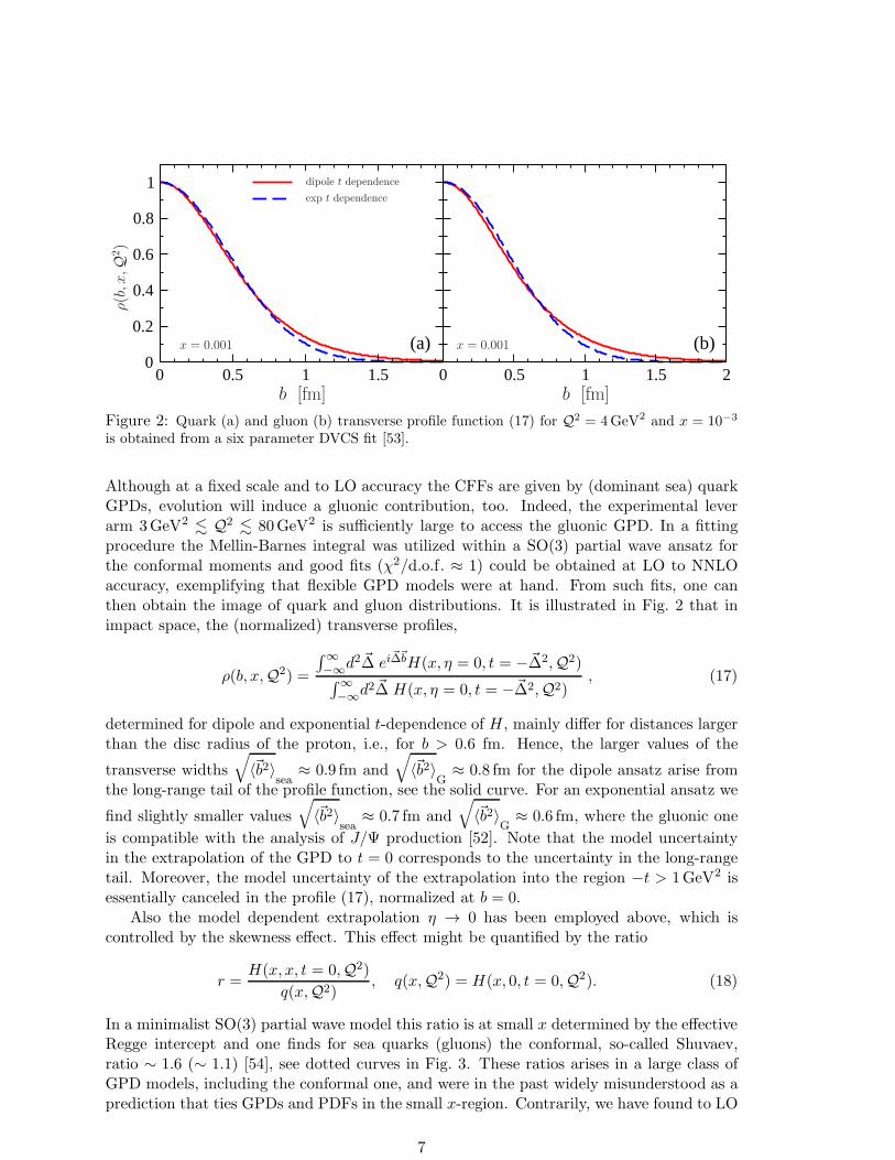
Figure 2: Quark (a) and gluon (b) transverse profile function (17) for Q2 = 4GeV2 and x = 10−3

is obtained from a six parameter DVCS fit [53].

Although at a fixed scale and to LO accuracy the CFFs are given by (dominant sea) quarkGPDs, evolution will induce a gluonic contribution, too. Indeed, the experimental leverarm 3GeV2 . Q2 . 80GeV2 is sufficiently large to access the gluonic GPD. In a fittingprocedure the Mellin-Barnes integral was utilized within a SO(3) partial wave ansatz forthe conformal moments and good fits (χ2/d.o.f. ≈ 1) could be obtained at LO to NNLOaccuracy, exemplifying that flexible GPD models were at hand. From such fits, one canthen obtain the image of quark and gluon distributions. It is illustrated in Fig. 2 that inimpact space, the (normalized) transverse profiles,

ρ(b, x,Q2) =

∫∞−∞

d2~∆ ei~∆~bH(x, η = 0, t = −~∆2,Q2)

∫∞−∞

d2~∆ H(x, η = 0, t = −~∆2,Q2), (17)

determined for dipole and exponential t-dependence of H, mainly differ for distances largerthan the disc radius of the proton, i.e., for b > 0.6 fm. Hence, the larger values of the

transverse widths

√〈~b2〉

sea≈ 0.9 fm and

√〈~b2〉

G≈ 0.8 fm for the dipole ansatz arise from

the long-range tail of the profile function, see the solid curve. For an exponential ansatz we

find slightly smaller values

√〈~b2〉

sea≈ 0.7 fm and

√〈~b2〉

G≈ 0.6 fm, where the gluonic one

is compatible with the analysis of J/Ψ production [52]. Note that the model uncertaintyin the extrapolation of the GPD to t = 0 corresponds to the uncertainty in the long-rangetail. Moreover, the model uncertainty of the extrapolation into the region −t > 1GeV2 isessentially canceled in the profile (17), normalized at b = 0.

Also the model dependent extrapolation η → 0 has been employed above, which iscontrolled by the skewness effect. This effect might be quantified by the ratio

r =H(x, x, t = 0,Q2)

q(x,Q2), q(x,Q2) = H(x, 0, t = 0,Q2). (18)

In a minimalist SO(3) partial wave model this ratio is at small x determined by the effectiveRegge intercept and one finds for sea quarks (gluons) the conformal, so-called Shuvaev,ratio ∼ 1.6 (∼ 1.1) [54], see dotted curves in Fig. 3. These ratios arises in a large class ofGPD models, including the conformal one, and were in the past widely misunderstood as aprediction that ties GPDs and PDFs in the small x-region. Contrarily, we have found to LO

7

conf . ratioGK07KM10aKM10b

5 10 20 50 1000.0

0.5

1.0

1.5

Q2 @GeV2D

rHx=

10-

3 ,t=

0,Q

2 L

5 10 20 50 1000.0

0.5

1.0

1.5

Q2 @GeV2D

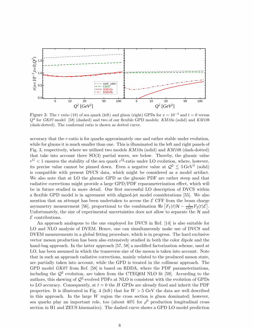
Figure 3: The r ratio (18) of sea quark (left) and gluon (right) GPDs for x = 10−3 and t = 0 versusQ2 for GK07 model [58] (dashed) and two of our flexible GPD models: KM10a (solid) and KM10b

(dash-dotted). The conformal ratio is shown as dotted curve.

accuracy that the r-ratio is for quarks approximately one and rather stable under evolution,while for gluons it is much smaller than one. This is illuminated in the left and right panels ofFig. 3, respectively, where we utilized two models KM10a (solid) and KM10b (dash-dotted)that take into account three SO(3) partial waves, see below. Thereby, the gluonic valuerG < 1 ensures the stability of the sea quark rQ-ratio under LO evolution, where, however,its precise value cannot be pinned down. Even a negative value at Q2 . 5GeV2 (solid)is compatible with present DVCS data, which might be considered as a model artifact.We also note that at LO the gluonic GPD as the gluonic PDF are rather steep and thatradiative corrections might provide a large GPD/PDF reparameterization effect, which willbe in future studied in more detail. Our first successful LO description of DVCS withina flexible GPD model is in agreement with aligned-jet model considerations [55]. We alsomention that an attempt has been undertaken to access the E CFF from the beam chargeasymmetry measurement [56], proportional to the combination ℜe

[F1(t)H − t

4M2F2(t)E].

Unfortunately, the size of experimental uncertainties does not allow to separate the H andE contributions.

An approach analogous to the one employed for DVCS in Ref. [14] is also suitable forLO and NLO analysis of DVEM. Hence, one can simultaneously make use of DVCS andDVEM measurements in a global fitting procedure, which is in progress. The hard exclusivevector meson production has been also extensively studied in both the color dipole and thehand-bag approach. In the latter approach [57, 58] a modified factorization scheme, used atLO, has been assumed in which the transverse size of the meson is taken into account. Notethat in such an approach radiative corrections, mainly related to the produced meson state,are partially taken into account, while the GPD is treated in the collinear approach. TheGPD model GK07 from Ref. [58] is based on RDDA, where the PDF parameterizations,including the Q2 evolution, are taken from the CTEQ6M NLO fit [59]. According to theauthors, this skewing of Q2-evolved PDFs at NLO is consistent with the evolution of GPDsto LO accuracy. Consequently, at t = 0 the H GPDs are already fixed and inherit the PDFproperties. It is illustrated in Fig. 4 (left) that for W > 5 GeV the data are well describedin this approach. In the large W region the cross section is gluon dominated; however,sea quarks play an important role, too (about 40% for ρ0 production longitudinal crosssection in H1 and ZEUS kinematics). The dashed curve shows a GPD LO model prediction

8

Figure 4: Longitudinally total cross section of γ⋆Lp → ρ0p (left) at Q2 = 4GeV2 and γ⋆

Lp → φpat Q2 = 3.8GeV2 (right) versus W from H1 [60, 61, 62] (filled squares), ZEUS [63, 64] (opensquares) and [65] (open triangles), CLAS [66] (open circles), HERMES [67, 68] (filled circles), andCORNELL [69] (filled triangles). Curves display predictions from the hand-bag approach with theGK07 model [58] (solid) and the collinear LO approach within the KM10b model from a DVCS fit[70] (dash-dotted). (Figures are taken form Refs. [71] and [72].)

in the collinear factorization approach, where the gluons have been extracted from smallxBj DVCS data via scaling evolution effects. In a LO description of DIS the gluon PDFis rather steep and although our skewness ratio is ∼ 0.5, we certainly fail to describe thedata. We emphasize that the skewness ratio for sea quarks in the GK07 parametrizationlies below the conformal one and is even rather stable under evolution, cf. LO evolutionexamples within RDDA in Fig. 6 of Ref. [73]. These properties of our GPD models andpartially of the GK07 in the quark sector are qualitatively different from the propertiesof the Durham GPD parameterization [74], which, e.g., is employed in the diffractive J/Ψelectroproduction [75], and provides the conformal ratio, see also dotted curves in Fig. 3.In the resonance region the GK07 model does not describe the ρ0 production data, but itdoes describe the φ production. Whether the approach is not applicable in this region orthe valence-like GPDs looks rather different from those obtained with the RDDA, is for usan open question.

GPD studies were also performed for the DVCS process in the fixed target kinematicsto LO accuracy. In this region, relying on the scaling hypothesis, one might directly ask forthe value of the GPDs on their cross-over line. For instance, for valence quarks we use thegenerically motivated ansatz

Hval(x, x, t) =1.35 r

1 + x

(2x

1 + x

)−α(t) (1− x

1 + x

)b(1−

1− x

1 + x

t

Mval

)−1. (19)

Here, the skewness ratio r = limx→0H(x, x)/H(x, 0), α(t) = 0.43 + 0.85 t/GeV2, b controlsthe x → 1 limit, and Mval the residual t-dependence, which we set to Mval = 0.8GeV,where q(x) = H(x, 0) is a reference PDF, e.g., the LO parameterization of Alekhin [39].The generic (−t)−2 fall-off at large −t for generalized form factors is indirectly encodedin the Regge-trajectory and the residual t dependence, chosen by a monopole with an x-

9

dependent cut-off mass. The subtraction constant is normalized by d and Md controls thet-dependence:

D(t) = d

(1−

t

M2d

)−2. (20)

In a first global fit [53] to hard exclusive photon electroproduction off unpolarized pro-ton we took sea quark and gluon GPD models with two SO(3) partial waves at small x,reparameterized the outcome from H1 and ZEUS DVCS fits at Q2 = 2GeV2, and employedit in fits of fixed target data within the scaling hypothesis. To relate the CFFs with theobservables we employed the BKM formulas [11] within the ‘hot-fix’ convention [76] andused the Sachs parameterization for the electromagnetic form factors. Thereby, we utilizedthe “dispersion relation” (3,4), where the ansatz (19) specifies a valence-like GPD on thecross-over line. Besides the subtraction constant (20), we also included the parameter-freepion-pole model for the E GPD [77] and parameterized the H GPD rather analogously toEq. (19) with b = 3/2. For the fixed target fits we chose two data sets, resulting in two fits(KM09a and KM09b). The first set contains twist-two dominated (preliminary) beam spinasymmetry,

ABS(φ) =

(dσ→

dxBjdtdQ2dφ−

dσ←

dxBjdtdQ2dφ

)/(dσ→

dxBjdtdQ2dφ+

dσ←

dxBjdtdQ2dφ

)

= A(1)BS sin(φ) + · · · , (21)

and beam charge asymmetry,

ABC(φ) =

(dσ+

dxBjdtdQ2dφ−

dσ−

dxBjdtdQ2dφ

)/(dσ+

dxBjdtdQ2dφ+

dσ−

dxBjdtdQ2dφ

)

= A(0)BC +A

(1)BC cos(φ) + · · · , (22)

coefficients A(1)BS and A

(1)BC, respectively, from HERMES [78, 79] and 12 beam spin asymmetry

coefficients A(1)BS, which we obtained by Fourier transform of selected CLAS [80] data with

small −t. The second data set includes also Hall A measurements [81] for four different tvalues. In light of the discussion [82] of Hall A data, we projected on the first harmonic ofa normalized beam spin sum

Σ(1),wBS =

∫ 2π

0dw cos(φ)

dσ

dxBjdtdQ2dφ

/∫ 2π

0dw

dσ

dxBjdtdQ2dφ, (23)

where dw ∝ P1(φ)P2(φ)dφ includes the Bethe-Heitler propagators. We haven’t used HallA helicity-dependent cross sections (beam spin differences). The Hall A data, given atrelatively large xBj = 0.36, can only be described in our model within an unexpectedly

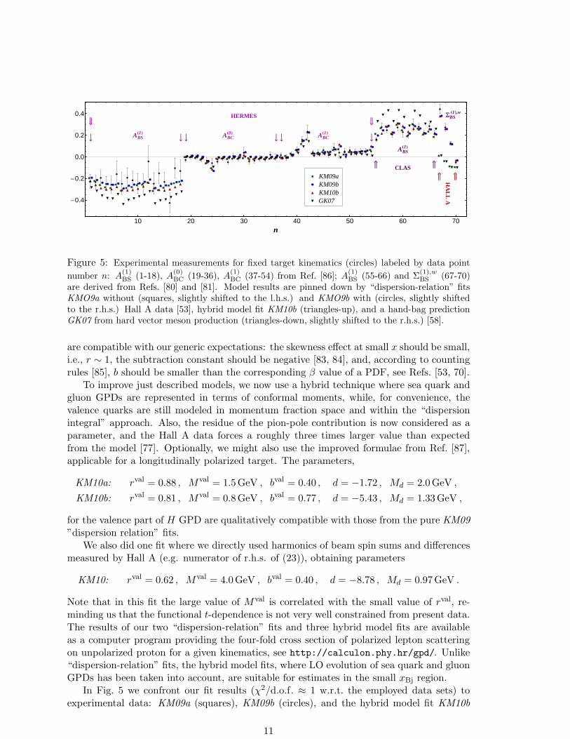
large value of H, which is not visible in single longitudinally target spin asymmetries atsmaller values of xBj. Otherwise, our findings

KM09a: bsea = 3.09 , rval = 0.95 , bval = 0.45 , d = −0.24 , Md = 0.5GeV ,

KM09b: bsea = 4.60 , rval = 1.11 , bval = 2.40 , d = −6.00 , Md = 1.5GeV ,

10

���� �

�

�� �

� ��

� ���� �

� � � ���

� � � � � � � � � � � �� �

��

��

� � � �� �

�� � � �

�

�

� �

�

�

�

�

��

��

�

�

�

� �

ææææ æ

æ

ææ æ

æææ

ææ æ

æææ

æ æ æ æ

æ

æ

æ æ ææææ

æ æ æ æ æææ æ

æ

æ

æ

æ

æ ææ æ

æ

æ

ææ æ æ

æ

æ

æ

æ

æ

æ

æ

æ

æ

ææ

æ

æ

æ

æ

æ

æ

æ

ôô

ôô ô

ô

ô

ôôô ô

ô

ôô ô

ôôô

ô ô ô ôô

ô

ô ô ô ô ô ô ô ô ô ô ô ô ô ôôô

ô

ô

ô ôô ô ô

ô ôô ô ô ô ô

ô

ô

ô

ô

ô

ô

ô

ô

ô

ôô

ô

ô

ô

ô ô

ò

òò ò ò

òò ò ò

òò

ò

òò ò ò

òò

ò ò ò ò

ò

ò

ò ò òò ò

ò

ò ò ò ò òò ò ò

ò

ò

ò

ò

òò ò ò

ò

ò

ò òò ò

ò

ò

ò

ò

ò

ò

òò

òò ò

ò

ò

ò

ò

ò

ò

ò

ì ì

ì

ì ì

ì

ì

ìì

ì ì

ì

ì

ì

ì

ì

ì

ì

ì

ì ììììì

ì

ì

ìì

ì

ì ììì

ììì

ì

ì

ì

ì

ì

ì ìì

ì

ì

ì ììì ì ì ì

ì

ì

ì

ì

ì

ì

ì

ìì

ì

ì

ì

ì

ì

ì

ì

�

HERMES

�

�

ABSH1L

� �

ABCH0L

� �

ABCH1L

�

�

ABSH1L

CLAS

�

�

SBSH1L,w

HA

LL

A�

10 20 30 40 50 60 70

-0.4

-0.2

0.0

0.2

0.4

n

� KM09aæ KM09bò KM10bô GK07

Figure 5: Experimental measurements for fixed target kinematics (circles) labeled by data point

number n: A(1)BS (1-18), A

(0)BC (19-36), A

(1)BC (37-54) from Ref. [86]; A

(1)BS (55-66) and Σ

(1),wBS (67-70)

are derived from Refs. [80] and [81]. Model results are pinned down by “dispersion-relation” fitsKMO9a without (squares, slightly shifted to the l.h.s.) and KMO9b with (circles, slightly shiftedto the r.h.s.) Hall A data [53], hybrid model fit KM10b (triangles-up), and a hand-bag predictionGK07 from hard vector meson production (triangles-down, slightly shifted to the r.h.s.) [58].

are compatible with our generic expectations: the skewness effect at small x should be small,i.e., r ∼ 1, the subtraction constant should be negative [83, 84], and, according to countingrules [85], b should be smaller than the corresponding β value of a PDF, see Refs. [53, 70].

To improve just described models, we now use a hybrid technique where sea quark andgluon GPDs are represented in terms of conformal moments, while, for convenience, thevalence quarks are still modeled in momentum fraction space and within the “dispersionintegral” approach. Also, the residue of the pion-pole contribution is now considered as aparameter, and the Hall A data forces a roughly three times larger value than expectedfrom the model [77]. Optionally, we might also use the improved formulae from Ref. [87],applicable for a longitudinally polarized target. The parameters,

KM10a: rval = 0.88 , Mval = 1.5GeV , bval = 0.40 , d = −1.72 , Md = 2.0GeV ,

KM10b: rval = 0.81 , Mval = 0.8GeV , bval = 0.77 , d = −5.43 , Md = 1.33GeV ,

for the valence part of H GPD are qualitatively compatible with those from the pure KM09

”dispersion relation” fits.We also did one fit where we directly used harmonics of beam spin sums and differences

measured by Hall A (e.g. numerator of r.h.s. of (23)), obtaining parameters

KM10: rval = 0.62 , Mval = 4.0GeV , bval = 0.40 , d = −8.78 , Md = 0.97GeV .

Note that in this fit the large value of Mval is correlated with the small value of rval, re-minding us that the functional t-dependence is not very well constrained from present data.The results of our two “dispersion-relation” fits and three hybrid model fits are availableas a computer program providing the four-fold cross section of polarized lepton scatteringon unpolarized proton for a given kinematics, see http://calculon.phy.hr/gpd/. Unlike“dispersion-relation” fits, the hybrid model fits, where LO evolution of sea quark and gluonGPDs has been taken into account, are suitable for estimates in the small xBj region.

In Fig. 5 we confront our fit results (χ2/d.o.f. ≈ 1 w.r.t. the employed data sets) toexperimental data: KM09a (squares), KM09b (circles), and the hybrid model fit KM10b

11

à

à

à

à

ì

ì

ì

ò

ò

ò

æ

æ

æ

æ

t = 0.28 GeV2

Q2 » 2 GeV2

�H

AL

LA

�C

LA

S

�C

LA

S

�C

LA

S

�H

ER

ME

S

0.10 0.15 0.20 0.25 0.30 0.350

1

2

3

4

xBj

ImHHx

Bj,t

,Q2 L�Π

àà à

à

ìì

ææ

æ

æ

HALL AxB = 0.36

Q2 = 2.3 GeV2

0.15 0.20 0.25 0.30 0.350.0

0.5

1.0

1.5

2.0

2.5

3.0

-t @GeV2D

Figure 6: ℑmH/π obtained from different strategies: our DVCS fits [dashed (solid) curve excludes(includes) Hall A data from ”dispersion relation” KM09a (KM09b) [53] and hybrid KM10b (dash-dotted) models], GK07 model from DVEM (dotted), seven-fold CFF fit [92, 93] with boundary

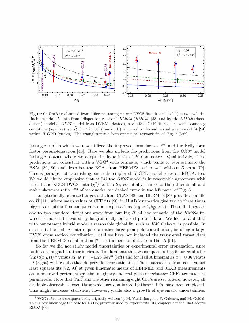
conditions (squares), H, H CFF fit [90] (diamonds), smeared conformal partial wave model fit [94]within H GPD (circles). The triangles result from our neural network fit, cf. Fig. 7 (left).

(triangles-up) in which we now utilized the improved formulae set [87] and the Kelly formfactor parameterization [40]. Here we also include the predictions from the GK07 model(triangles-down), where we adopt the hypothesis of H dominance. Qualitatively, thesepredictions are consistent with a VGG4 code estimate, which tends to over-estimate theBSAs [80, 86] and describes the BCAs from HERMES rather well without D-term [79].This is perhaps not astonishing, since the employed H GPD model relies on RDDA, too.We would like to emphasize that at LO the GK07 model is in reasonable agreement withthe H1 and ZEUS DVCS data (χ2/d.o.f. ≈ 2), essentially thanks to the rather small andstable skewness ratio rsea of sea quarks, see dashed curve in the left panel of Fig. 3.

Longitudinally polarized target data from CLAS [88] and HERMES [89] provide a handleon H [11], where mean values of CFF fits [90] in JLAB kinematics give two to three timesbigger H contribution compared to our expectations (r

H≃ 1, b

H≃ 2). These findings are

one to two standard deviations away from our big H ad hoc scenario of the KM09b fit,which is indeed disfavored by longitudinally polarized proton data. We like to add thatwith our present hybrid model a reasonable global fit, such as KM10 above, is possible. Insuch a fit the Hall A data require a rather large pion pole contribution, inducing a largeDVCS cross section contribution. Still we have not included the transversal target datafrom the HERMES collaboration [79] or the neutron data from Hall A [91].

So far we did not study model uncertainties or experimental error propagation, sinceboth tasks might be rather intricate. To illuminate this, we compare in Fig. 6 our results forℑmH(xB, t)/π versus xB at t = −0.28GeV2 (left) and for Hall A kinematics xB=0.36 versus−t (right) with results that do provide error estimates. The squares arise from constrainedleast squares fits [92, 93] at given kinematic means of HERMES and JLAB measurementson unpolarized proton, where the imaginary and real parts of twist-two CFFs are taken asparameters. Note that ℑmE and the other remaining eight CFFs are set to zero, however, allavailable observables, even those which are dominated by these CFFs, have been employed.This might increase ‘statistics’, however, yields also a growth of systematic uncertainties.

4 VGG refers to a computer code, originally written by M. Vanderhaeghen, P. Guichon, and M. Guidal.To our best knowledge the code for DVCS, presently used by experimentalists, employs a model that adoptsRDDA [83].

12

0.05 0.10 0.15 0.20 0.25 0.30 0.35 0.40xBj

�2

�1

0

1

2

3

4

�eH(

xBj,t)/

�

t=0

t=�0.3 GeV2

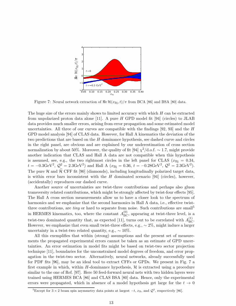
Figure 7: Neural network extraction of ℜeH(xBj, t)/π from BCA [86] and BSA [80] data.

The huge size of the errors mainly shows to limited accuracy with which H can be extractedfrom unpolarized proton data alone [11]. A pure H GPD model fit [94] (circles) to JLABdata provides much smaller errors, arising from error propagation and some estimated modeluncertainties. All three of our curves are compatible with the findings [92, 93] and the HGPD model analysis [94] of CLAS data. However, for Hall A kinematics the deviation of thetwo predictions that are based on the H dominance hypothesis, see dashed curve and circlesin the right panel, are obvious and are explained by our underestimation of cross sectionnormalization by about 50%. Moreover, the quality of fit [94] χ2/d.o.f. ∼ 1.7, might provideanother indication that CLAS and Hall A data are not compatible when this hypothesisis assumed, see, e.g., the two rightmost circles in the left panel for CLAS (xBj = 0.34,t = −0.3GeV2, Q2 = 2.3GeV2) and Hall A (xBj = 0.36, t = −0.28GeV2, Q2 = 2.3GeV2).

The pure H and H CFF fit [90] (diamonds), including longitudinally polarized target data,is within error bars inconsistent with the H dominated scenario [94] (circles), however,(accidentally) reproduces our dashed curve.

Another source of uncertainties are twist-three contributions and perhaps also gluontransversity related contributions, which might be strongly affected by twist-four effects [95].The Hall A cross section measurements allow us to have a closer look to the spectrum ofharmonics and we emphasize that the second harmonics in Hall A data, i.e., effective twist-three contributions, are tiny or hard to separate from noise. Such contributions are small5

in HERMES kinematics, too, where the constant A(0)BC, appearing at twist-three level, is a

twist-two dominated quantity that, as expected [11], turns out to be correlated with A(1)BC.

However, we emphasize that even small twist-three effects, e.g., ∼ 2%, might induce a largeruncertainty in a twist-two related quantity, e.g., ∼ 10%.

All this exemplifies that within (strong) assumptions and the present set of measure-ments the propagated experimental errors cannot be taken as an estimate of GPD uncer-tainties. An error estimation in model fits might be based on twist-two sector projectiontechnique [11], boundaries for the unconstrained model degrees of freedom, and error prop-agation in the twist-two sector. Alternatively, neural networks, already successfully usedfor PDF fits [96], may be an ideal tool to extract CFFs or GPDs. We present in Fig. 7 afirst example in which, within H-dominance hypothesis, H is extracted using a proceduresimilar to the one of Ref. [97]. Here 50 feed-forward neural nets with two hidden layers weretrained using HERMES BCA [86] and CLAS BSA [80] data. Hence, only the experimentalerrors were propagated, which in absence of a model hypothesis get large for the t → 0

5Except for 3× 2 beam spin asymmetry data points at largest −t, xB, and Q2, respectively [86].

13

protonneutron

0 50 100 150 200 250 300 350-0.4

-0.2

0.0

0.2

0.4

Φ @degD

AB

S

xBj=5 10-3

-t=0.2 GeV2

Q2=10 GeV2

10-4 0.001 0.01 0.1 10.4

0.2

0.0

0.2

0.4

xBj

Ee=30 GeVEN=360 GeV

Ee=5 GeVEN=150 GeV

Figure 8: KM10b model estimate for the DVCS beam spin asymmetry (21) with a proton (solid) andneutron (dashed) target. Left panel: ABS versus φ for EN = 250 GeV, Ee = 5 GeV, xBj = 5× 10−3,

Q2 = 10 GeV2, and t = −0.2 GeV2. Right panel: Amplitude A(1)BS of the first harmonic versus xBj

at t = −0.2 GeV2 for small xBj (thin) [Ee = 30 GeV, Ep = 360 GeV, Q2 = 4 GeV2] and large xBj

(thick) [Ee = 5 GeV, Ep = 150 GeV, Q2 = 50 GeV2] kinematics.

extrapolation.

4 Potential of an electron-ion colider

A high luminosity machine in the collider mode with polarized electron and proton or ionbeams would be an ideal instrument to quantify QCD phenomena. It is expected that sucha machine, combined with designated detectors, would allow for precise measurements ofexclusive channels. Besides hard exclusive vector meson and photon electroproduction, onemight address the behavior of parity-odd GPDs H, related to polarized PDFs, and E via theexclusive production of pions even in the small x region. It is obvious from what was saidabove that an access of GPDs requires a large data set with small errors. In the followingwe would like to illustrate the potential of such a machine for DVCS studies, where we alsoaddress the GPD deconvolution problem.

Let us remind that already the isolation of CFFs is rather intricate. For a spin-1/2 targetwe have four twist-two, four twist-three, and four gluon transversity related complex valuedCFFs. The photon helicity non-flip amplitudes are dominated by twist-two CFFs, thetransverse–longitudinal flip amplitudes by twist-three effects, and the transverse–transverseflip ones by gluon transversity. Hence, the first, the second, and the third harmonicsw.r.t. the azimuthal angle of the interference term are twist-two, twist-three, and gluontransversity dominated. In an ideal experiment, assuming that transverse photon helicityflip effects are negligible, cross section measurements would allow to separate the sixteenquantities that are then given in terms of twist-two and twist-three CFFs. The reader mightfind a more detailed discussion, based on a 1/Q expansion, in Ref. [11]. We add that thedefinition of CFFs is convention-dependent.

In a twist-two analyzes on unpolarized, longitudinally and transversally polarized pro-tons one might be able to disentangle the four different twist-two CFFs via the measurementof single beam and target spin asymmetries. In Fig. 8 we illustrate that for a proton target

14

KM09aKM09bKM10b

0 50 100 150 200 250 300 350

-0.2

-0.1

0.0

0.1

0.2

Φ @degD

AT

SÞ

xBj=0.1

-t=0.2 GeV2

Q2=4 GeV2

0 50 100 150 200 250 300 350

0.2

0.1

0.0

0.1

0.2

Φ @degD

xBj=0.01

-t=0.2 GeV2

Q2=4 GeV2

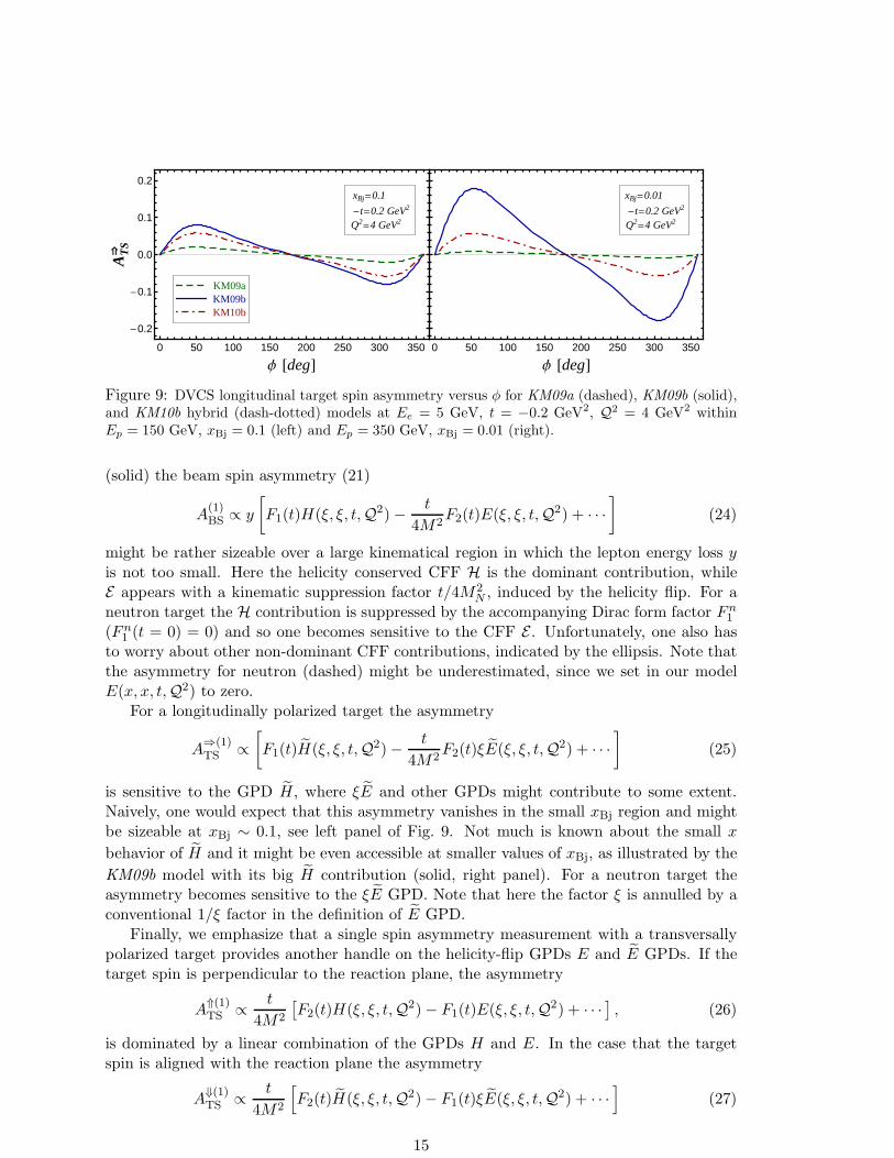
Figure 9: DVCS longitudinal target spin asymmetry versus φ for KM09a (dashed), KM09b (solid),and KM10b hybrid (dash-dotted) models at Ee = 5 GeV, t = −0.2 GeV2, Q2 = 4 GeV2 withinEp = 150 GeV, xBj = 0.1 (left) and Ep = 350 GeV, xBj = 0.01 (right).

(solid) the beam spin asymmetry (21)

A(1)BS ∝ y

[F1(t)H(ξ, ξ, t,Q2)−

t

4M2F2(t)E(ξ, ξ, t,Q2) + · · ·

](24)

might be rather sizeable over a large kinematical region in which the lepton energy loss yis not too small. Here the helicity conserved CFF H is the dominant contribution, whileE appears with a kinematic suppression factor t/4M2

N , induced by the helicity flip. For aneutron target the H contribution is suppressed by the accompanying Dirac form factor Fn

1

(Fn1 (t = 0) = 0) and so one becomes sensitive to the CFF E . Unfortunately, one also has

to worry about other non-dominant CFF contributions, indicated by the ellipsis. Note thatthe asymmetry for neutron (dashed) might be underestimated, since we set in our modelE(x, x, t,Q2) to zero.

For a longitudinally polarized target the asymmetry

A⇒(1)TS ∝

[F1(t)H(ξ, ξ, t,Q2)−

t

4M2F2(t)ξE(ξ, ξ, t,Q2) + · · ·

](25)

is sensitive to the GPD H, where ξE and other GPDs might contribute to some extent.Naively, one would expect that this asymmetry vanishes in the small xBj region and mightbe sizeable at xBj ∼ 0.1, see left panel of Fig. 9. Not much is known about the small x

behavior of H and it might be even accessible at smaller values of xBj, as illustrated by the

KM09b model with its big H contribution (solid, right panel). For a neutron target theasymmetry becomes sensitive to the ξE GPD. Note that here the factor ξ is annulled by aconventional 1/ξ factor in the definition of E GPD.

Finally, we emphasize that a single spin asymmetry measurement with a transversallypolarized target provides another handle on the helicity-flip GPDs E and E GPDs. If thetarget spin is perpendicular to the reaction plane, the asymmetry

A⇑(1)TS ∝

t

4M2

[F2(t)H(ξ, ξ, t,Q2)− F1(t)E(ξ, ξ, t,Q2) + · · ·

], (26)

is dominated by a linear combination of the GPDs H and E. In the case that the targetspin is aligned with the reaction plane the asymmetry

A⇓(1)TS ∝

t

4M2

[F2(t)H(ξ, ξ, t,Q2)− F1(t)ξE(ξ, ξ, t,Q2) + · · ·

](27)

15

protonneutron

0 50 100 150 200 250 300 350-0.4

-0.2

0.0

0.2

0.4

Φ @degD

AB

C

xBj=5 10-3

-t=0.2 GeV2

Q2=10 GeV2

10-4 0.001 0.01 0.1 10.4

0.2

0.0

0.2

0.4

xBj

Ee=30 GeVEN=360 GeV

Ee=5 GeVEN=150 GeV

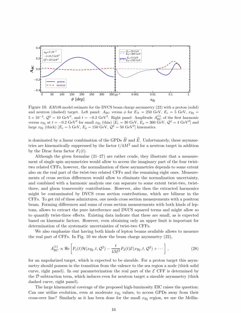
Figure 10: KM10b model estimate for the DVCS beam charge asymmetry (22) with a proton (solid)and neutron (dashed) target. Left panel: ABC versus φ for EN = 250 GeV, Ee = 5 GeV, xBj =

5 × 10−3, Q2 = 10 GeV2, and t = −0.2 GeV2. Right panel: Amplitude A(1)BC of the first harmonic

versus xBj at t = −0.2 GeV2 for small xBj (thin) [Ee = 30 GeV, Ep = 360 GeV, Q2 = 4 GeV2] andlarge xBj (thick) [Ee = 5 GeV, Ep = 150 GeV, Q2 = 50 GeV2] kinematics.

is dominated by a linear combination of the GPDs H and E. Unfortunately, these asymme-tries are kinematically suppressed by the factor t/4M2 and for a neutron target in additionby the Dirac form factor F1(t).

Although the given formulae (21–27) are rather crude, they illustrate that a measure-ment of single spin asymmetries would allow to access the imaginary part of the four twist-two related CFFs, however, the normalization of these asymmetries depends to some extentalso on the real part of the twist-two related CFFs and the remaining eight ones. Measure-ments of cross section differences would allow to eliminate the normalization uncertainty,and combined with a harmonic analysis one can separate to some extent twist-two, twist-three, and gluon transversity contributions. However, also then the extracted harmonicsmight be contaminated by DVCS cross section contributions, which are bilinear in theCFFs. To get rid of these admixtures, one needs cross section measurements with a positronbeam. Forming differences and sums of cross section measurements with both kinds of lep-tons, allows to extract the pure interference and DVCS squared terms and might allow soto quantify twist-three effects. Existing data indicate that these are small, as is expectedbased on kinematic factors. However, even obtaining only an upper limit is important fordetermination of the systematic uncertainties of twist-two CFFs.

We also emphasize that having both kinds of lepton beams available allows to measurethe real part of CFFs. In Fig. 10 we show the beam charge asymmetry (22),

A(1)BC ∝ ℜe

[F1(t)H(xBj, t,Q

2)−t

4M2F2(t)E(xBj, t,Q

2) + · · ·

], (28)

for an unpolarized target, which is expected to be sizeable. For a proton target this asym-metry should possess in the transition from the valence to the sea region a node (thick solidcurve, right panel). In our parameterization the real part of the E CFF is determined bythe D subtraction term, which induces even for neutron target a sizeable asymmetry (thickdashed curve, right panel).

The large kinematical coverage of the proposed high-luminosity EIC raises the question:Can one utilize evolution, even at moderate xBj values, to access GPDs away from theircross-over line? Similarly as it has been done for the small xBj region, we use the Mellin-

16

KM09a Q2=2 GeV2

s2»-0.14, s4=0s2=-0.26, s4»0.04s2=0, s4»-0.04

0.05 0.10 0.20 0.50 1.000.0

0.2

0.4

0.6

0.8

1.0

1.2

1.4

xBj

ImH

val

Q2=2 GeV2

0.05 0.10 0.20 0.50 1.000.0

0.2

0.4

0.6

0.8

1.0

1.2

1.4

xBj

Q2=50 GeV2

s2=0, s4=0s2»-0.14, s4=0s2=-0.26, s4»0.04s2=0, s4»-0.04

0.005 0.010 0.050 0.100 0.500 1.000

0.0

0.1

0.2

0.3

0.4

x

Hva

l

Q2=2 GeV2

0.005 0.010 0.050 0.100 0.500 1.000

0.0

0.1

0.2

0.3

0.4

x

Q2=50 GeV2

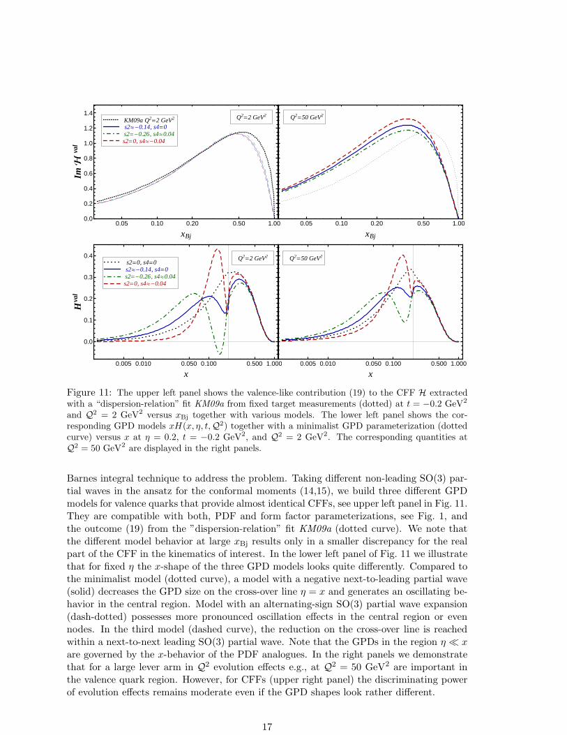
Figure 11: The upper left panel shows the valence-like contribution (19) to the CFF H extractedwith a “dispersion-relation” fit KM09a from fixed target measurements (dotted) at t = −0.2 GeV2

and Q2 = 2 GeV2 versus xBj together with various models. The lower left panel shows the cor-responding GPD models xH(x, η, t,Q2) together with a minimalist GPD parameterization (dottedcurve) versus x at η = 0.2, t = −0.2 GeV2, and Q2 = 2 GeV2. The corresponding quantities atQ2 = 50 GeV2 are displayed in the right panels.

Barnes integral technique to address the problem. Taking different non-leading SO(3) par-tial waves in the ansatz for the conformal moments (14,15), we build three different GPDmodels for valence quarks that provide almost identical CFFs, see upper left panel in Fig. 11.They are compatible with both, PDF and form factor parameterizations, see Fig. 1, andthe outcome (19) from the ”dispersion-relation” fit KM09a (dotted curve). We note thatthe different model behavior at large xBj results only in a smaller discrepancy for the realpart of the CFF in the kinematics of interest. In the lower left panel of Fig. 11 we illustratethat for fixed η the x-shape of the three GPD models looks quite differently. Compared tothe minimalist model (dotted curve), a model with a negative next-to-leading partial wave(solid) decreases the GPD size on the cross-over line η = x and generates an oscillating be-havior in the central region. Model with an alternating-sign SO(3) partial wave expansion(dash-dotted) possesses more pronounced oscillation effects in the central region or evennodes. In the third model (dashed curve), the reduction on the cross-over line is reachedwithin a next-to-next leading SO(3) partial wave. Note that the GPDs in the region η ≪ xare governed by the x-behavior of the PDF analogues. In the right panels we demonstratethat for a large lever arm in Q2 evolution effects e.g., at Q2 = 50 GeV2 are important inthe valence quark region. However, for CFFs (upper right panel) the discriminating powerof evolution effects remains moderate even if the GPD shapes look rather different.

17

5 Conclusions and summary

With all the theoretical tools sketched above plus those which are presently under develop-ment it is clear that our understanding of hadron structure will be revolutionized once mostof the diverse asymmetries can be measured with percent or permille precision (dependingon the observable). A high-luminosity EIC, as it is proposed at Brookhaven National Lab.,would allow to do so.

Let us summarize. At present, the first steps have been undertaken to access GPDs fromexperimental data in the small xBj region with models and in the fixed target kinematicswithin different strategies, providing some insight into the GPD H. In particular for hardexclusive photon electroproduction in the fixed target kinematics, model fits to leading orderaccuracy in αs, relying on the scaling hypothesis, are compatible with least square CFF fitsand with a first result from neural networks, assumingH dominance. The large uncertaintieshere in extracting CFFs, including H, are mainly related to the lack of experimental data.Thus, not only the extraction of the very desired E , playing an important role in the ”spin-puzzle”, but also of other CFFs, requires a comprehensive measurement of all possibleobservables in dedicated experiments. The comparison of H GPDs accessed from DVCS atleading order with model fits and from hard exclusive meson production in the hand-bagapproach within Radyushkin‘s double distribution ansatz shows that in the valence regionthe extracted quark GPDs are somewhat different while at small x they are becomingcompatible. The main difference lies in the gluonic sector and is induced by utilizing PDFparameterizations that where extracted in leading and next-to-leading order from inclusivemeasurements. A more appropriate analysis of these processes requires the inclusion ofradiative corrections in a global fitting procedure, which is in progress. We should alsomention here that hard exclusive processes with nuclei, which at present are not extensivelystudied, opens a new window for a partonic view on their content.

Imaging the partonic content of the nucleon and the phenomenological access to theproton spin sum rule from hard exclusive processes can only be reached through properunderstanding of GPD models. It might be pointed out here that GPDs can also be for-mulated in terms of an effective nucleon (light-cone) wave functions, which links them totransverse momentum dependent parton distributions. A whole framework, consisting ofperturbative QCD, lattice simulations, and dynamical modeling, is available to reveal GPDsand to access the nucleon wave function. Such a unifying description might be consideredas the primary goal, which quantifies the partonic picture. Although such a task looksrather straightforward, much effort is needed on the theoretical, phenomenological, andexperimental side, where experimental data with small uncertainties play the key role. Ahigh-luminosity EIC is an ideal machine that would cover a wide kinematical range, wouldcomplement the planned fixed target experiments at JLAB@11 GeV, and has, besides newmeasurements, great potential to significantly improve existing data sets.

Acknowledgments

We are grateful to P. Kroll for many fruitful discussions. This work was supported by theBMBF grants under the contract nos. 06RY9191 and 06BO9012, by EU (HadronPhysics2),by the GSI FFE program, by the DFG grant, contract no. 436 KRO 113/11/0-1, by CroatianMinistry of Science, Education and Sport, contract nos. 098-0982930-2864 and 119-0982930-1016, and by the DAAD.

18

References

[1] D. Mueller, D. Robaschik, B. Geyer, F. M. Dittes and J. Horejsi, Fortsch. Phys. 42,101 (1994) [arXiv:hep-ph/9812448].

[2] A. V. Radyushkin, Phys. Lett. B 380, 417 (1996) [arXiv:hep-ph/9604317].

[3] X. D. Ji, Phys. Rev. D 55, 7114 (1997) [arXiv:hep-ph/9609381].

[4] X. D. Ji, Phys. Rev. Lett. 78, 610 (1997) [arXiv:hep-ph/9603249].

[5] J. P. Ralston and B. Pire, Phys. Rev. D 66, 111501 (2002) [arXiv:hep-ph/0110075].

[6] M. Burkardt, Phys. Rev. D 62, 071503 (2000) [Erratum-ibid. D 66, 119903 (2002)][arXiv:hep-ph/0005108].

[7] J. C. Collins, L. Frankfurt and M. Strikman, Phys. Rev. D 56, 2982 (1997)[arXiv:hep-ph/9611433].

[8] J. C. Collins and A. Freund, Phys. Rev. D 59, 074009 (1999) [arXiv:hep-ph/9801262].

[9] M. Diehl, Phys. Rept. 388, 41 (2003) [arXiv:hep-ph/0307382].

[10] A. V. Belitsky and A. V. Radyushkin, Phys. Rept. 418, 1 (2005)[arXiv:hep-ph/0504030].

[11] A. V. Belitsky, D. Mueller and A. Kirchner, Nucl. Phys. B 629, 323 (2002)[arXiv:hep-ph/0112108].

[12] M. V. Polyakov and C. Weiss, Phys. Rev. D 60, 114017 (1999) [arXiv:hep-ph/9902451].

[13] O. V. Teryaev, arXiv:hep-ph/0510031.

[14] K. Kumericki, D. Mueller and K. Passek-Kumericki, Nucl. Phys. B 794, 244 (2008)[arXiv:hep-ph/0703179].

[15] M. Diehl and D. Y. Ivanov, Eur. Phys. J. C 52, 919 (2007) [arXiv:0707.0351 [hep-ph]].

[16] A. V. Belitsky and D. Mueller, Phys. Lett. B 507, 173 (2001) [arXiv:hep-ph/0102224].

[17] K. Kumericki, D. Mueller and K. Passek-Kumericki, Eur. Phys. J. C 58, 193 (2008)[arXiv:0805.0152 [hep-ph]].

[18] A. V. Radyushkin, Phys. Rev. D 56, 5524 (1997) [arXiv:hep-ph/9704207].

[19] D. S. Hwang and D. Mueller, Phys. Lett. B 660, 350 (2008) [arXiv:0710.1567 [hep-ph]].

[20] B. C. Tiburzi and G. A. Miller, Phys. Rev. C 64, 065204 (2001)[arXiv:hep-ph/0104198].

[21] B. C. Tiburzi and G. A. Miller, Phys. Rev. D 65, 074009 (2002)[arXiv:hep-ph/0109174].

[22] A. Mukherjee, I. V. Musatov, H. C. Pauli and A. V. Radyushkin, Phys. Rev. D 67,073014 (2003) [arXiv:hep-ph/0205315].

19

[23] B. C. Tiburzi, W. Detmold and G. A. Miller, Phys. Rev. D 70, 093008 (2004)[arXiv:hep-ph/0408365].

[24] A. V. Belitsky, D. Mueller, A. Kirchner and A. Schafer, Phys. Rev. D 64, 116002 (2001)[arXiv:hep-ph/0011314].

[25] A. V. Radyushkin, arXiv:1101.2165 [hep-ph].

[26] D. Mueller and A. Schafer, Nucl. Phys. B 739, 1 (2006) [arXiv:hep-ph/0509204].

[27] M. Diehl, T. Feldmann, R. Jakob and P. Kroll, Nucl. Phys. B 596, 33 (2001) [Erratum-ibid. B 605, 647 (2001)] [arXiv:hep-ph/0009255].

[28] S. J. Brodsky, M. Diehl and D. S. Hwang, Nucl. Phys. B 596, 99 (2001)[arXiv:hep-ph/0009254].

[29] P. V. Pobylitsa, Phys. Rev. D 67, 094012 (2003) [arXiv:hep-ph/0210238].

[30] P. V. Landshoff, J. C. Polkinghorne and R. D. Short, Nucl. Phys. B 28, 225 (1971).

[31] M. V. Polyakov, Phys. Lett. B 659, 542 (2008) [arXiv:0707.2509 [hep-ph]].

[32] M. V. Polyakov and A. G. Shuvaev, arXiv:hep-ph/0207153.

[33] K. M. Semenov-Tian-Shansky, Eur. Phys. J. A 36, 303 (2008) [arXiv:0803.2218 [hep-ph]].

[34] M. V. Polyakov and K. M. Semenov-Tian-Shansky, Eur. Phys. J. A 40, 181 (2009)[arXiv:0811.2901 [hep-ph]].

[35] D. Mueller, Phys. Lett. B 634, 227 (2006) [arXiv:hep-ph/0510109].

[36] K. Kumericki, D. Mueller, K. Passek-Kumericki and A. Schafer, Phys. Lett. B 648,186 (2007) [arXiv:hep-ph/0605237].

[37] S. J. Brodsky, M. Burkardt and I. Schmidt, Nucl. Phys. B 441, 197 (1995)[arXiv:hep-ph/9401328].

[38] C. Bechler and D. Mueller, arXiv:0906.2571 [hep-ph].

[39] S. Alekhin, Phys. Rev. D 68, 014002 (2003) [arXiv:hep-ph/0211096].

[40] J. J. Kelly, Phys. Rev. C 70, 068202 (2004).

[41] M. Diehl, T. Feldmann, R. Jakob and P. Kroll, Eur. Phys. J. C 39, 1 (2005)[arXiv:hep-ph/0408173].

[42] M. Guidal, M. V. Polyakov, A. V. Radyushkin and M. Vanderhaeghen, Phys. Rev. D72, 054013 (2005) [arXiv:hep-ph/0410251].

[43] M. V. Polyakov, Nucl. Phys. B 555, 231 (1999) [arXiv:hep-ph/9809483].

[44] M. Diehl, T. Gousset, B. Pire and J. P. Ralston, Phys. Lett. B 411, 193 (1997)[arXiv:hep-ph/9706344].

[45] A. V. Belitsky and D. Mueller, Phys. Lett. B 513, 349 (2001) [arXiv:hep-ph/0105046].

20

[46] D. Y. Ivanov, L. Szymanowski and G. Krasnikov, JETP Lett. 80, 226 (2004) [PismaZh. Eksp. Teor. Fiz. 80, 255 (2004)] [arXiv:hep-ph/0407207].

[47] M. Diehl and W. Kugler, Eur. Phys. J. C 52, 933 (2007) [arXiv:0708.1121 [hep-ph]].

[48] S. Chekanov et al. [ZEUS Collaboration], Phys. Lett. B 573, 46 (2003)[arXiv:hep-ex/0305028].

[49] A. Aktas et al. [H1 Collaboration], Eur. Phys. J. C 44, 1 (2005) [arXiv:hep-ex/0505061].

[50] F. D. Aaron et al. [H1 Collaboration], Phys. Lett. B 659, 796 (2008) [arXiv:0709.4114[hep-ex]].

[51] S. Chekanov et al. [ZEUS Collaboration], JHEP 0905, 108 (2009) [arXiv:0812.2517[hep-ex]].

[52] M. Strikman and C. Weiss, Phys. Rev. D 69, 054012 (2004) [arXiv:hep-ph/0308191].

[53] K. Kumericki and D. Mueller, Nucl. Phys. B 841, 1 (2010) [arXiv:0904.0458 [hep-ph]].

[54] A. Shuvaev, Phys. Rev. D 60, 116005 (1999) [arXiv:hep-ph/9902318].

[55] L. L. Frankfurt, A. Freund and M. Strikman, Phys. Rev. D 58, 114001 (1998) [Erratum-ibid. D 59, 119901 (1999)] [arXiv:hep-ph/9710356].

[56] F. D. Aaron et al. [H1 Collaboration], Phys. Lett. B 681, 391 (2009) [arXiv:0907.5289[hep-ex]].

[57] S. V. Goloskokov, P. Kroll, Eur. Phys. J. C42, 281-301 (2005) [hep-ph/0501242].

[58] S. V. Goloskokov and P. Kroll, Eur. Phys. J. C 53, 367 (2008) [arXiv:0708.3569 [hep-ph]].

[59] J. Pumplin, D. R. Stump, J. Huston et al., JHEP 0207, 012 (2002) [hep-ph/0201195].

[60] S. Aid et al. [H1 Collaboration], Nucl. Phys. B 468, 3 (1996) [arXiv:hep-ex/9602007].

[61] C. Adloff et al. [H1 Collaboration], Eur. Phys. J. C 13, 371 (2000)[arXiv:hep-ex/9902019].

[62] C. Adloff et al. [H1 Collaboration], Phys. Lett. B 483, 360 (2000)[arXiv:hep-ex/0005010].

[63] M. Derrick et al. [ZEUS Collaboration], Phys. Lett. B 380, 220 (1996)[arXiv:hep-ex/9604008].

[64] J. Breitweg et al. [ZEUS Collaboration], Eur. Phys. J. C 6, 603 (1999)[arXiv:hep-ex/9808020].

[65] S. Chekanov et al. [ZEUS Collaboration], Nucl. Phys. B 718, 3 (2005)[arXiv:hep-ex/0504010].

[66] S. A. Morrow et al. [CLAS Collaboration], Eur. Phys. J. A 39, 5 (2009)[arXiv:0807.3834 [hep-ex]].

21

[67] A. Airapetian et al. [HERMES Collaboration], Eur. Phys. J. C 17, 389 (2000)[arXiv:hep-ex/0004023].

[68] A. B. Borissov [HERMES Collaboration], Nucl. Phys. Proc. Suppl. 99A, 156 (2001).

[69] D. G. Cassel et al., Phys. Rev. D 24, 2787 (1981).

[70] K. Kumericki and D. Mueller, arXiv:1008.2762 [hep-ph].

[71] P. Kroll, arXiv:1009.2356 [hep-ph].

[72] C. E. Hyde, M. Guidal and A. V. Radyushkin, arXiv:1101.2482 [hep-ph].

[73] M. Diehl and W. Kugler, Phys. Lett. B 660, 202 (2008) [arXiv:0711.2184 [hep-ph]].

[74] A. D. Martin, C. Nockles, M. G. Ryskin, A. G. Shuvaev and T. Teubner, Eur. Phys.J. C 63, 57 (2009).

[75] A. D. Martin, C. Nockles, M. G. Ryskin and T. Teubner, Phys. Lett. B 662, 252 (2008)[arXiv:0709.4406 [hep-ph]].

[76] A. V. Belitsky and D. Mueller, Phys. Rev. D 79, 014017 (2009) [arXiv:0809.2890 [hep-ph]].

[77] M. Penttinen, M. V. Polyakov and K. Goeke, Phys. Rev. D 62, 014024 (2000)[arXiv:hep-ph/9909489].

[78] F. Ellinghaus, arXiv:0710.5768 [hep-ex].

[79] A. Airapetian et al. [HERMES Collaboration], JHEP 0806, 066 (2008)[arXiv:0802.2499 [hep-ex]].

[80] F. X. Girod et al. [CLAS Collaboration], Phys. Rev. Lett. 100, 162002 (2008)[arXiv:0711.4805 [hep-ex]].

[81] C. Munoz Camacho et al. [Jefferson Lab Hall A Collaboration and Hall A DVCSCollaboration], Phys. Rev. Lett. 97, 262002 (2006) [arXiv:nucl-ex/0607029].

[82] M. V. Polyakov and M. Vanderhaeghen, arXiv:0803.1271 [hep-ph].

[83] K. Goeke, M. V. Polyakov and M. Vanderhaeghen, Prog. Part. Nucl. Phys. 47, 401(2001) [arXiv:hep-ph/0106012].

[84] K. Goeke, J. Grabis, J. Ossmann, M. V. Polyakov, P. Schweitzer, A. Silva and D. Ur-bano, Phys. Rev. D 75, 094021 (2007) [arXiv:hep-ph/0702030].

[85] F. Yuan, Phys. Rev. D 69, 051501 (2004) [arXiv:hep-ph/0311288].

[86] A. Airapetian et al. [HERMES collaboration], JHEP 0911, 083 (2009) [arXiv:0909.3587[hep-ex]].

[87] A. V. Belitsky and D. Mueller, Phys. Rev. D 82, 074010 (2010) [arXiv:1005.5209 [hep-ph]].

[88] S. Chen et al. [CLAS Collaboration], Phys. Rev. Lett. 97, 072002 (2006)[arXiv:hep-ex/0605012].

22

[89] A. Airapetian et al. [HERMES Collaboration], JHEP 1006, 019 (2010)[arXiv:1004.0177 [hep-ex]].

[90] M. Guidal, Phys. Lett. B 689, 156 (2010) [arXiv:1003.0307 [hep-ph]].

[91] M. Mazouz et al. [Jefferson Lab Hall A Collaboration], Phys. Rev. Lett. 99, 242501(2007) [arXiv:0709.0450 [nucl-ex]].

[92] M. Guidal, Eur. Phys. J. A 37, 319 (2008) [Erratum-ibid. A 40, 119 (2009)][arXiv:0807.2355 [hep-ph]].

[93] M. Guidal and H. Moutarde, Eur. Phys. J. A 42, 71 (2009) [arXiv:0905.1220 [hep-ph]].

[94] H. Moutarde, Phys. Rev. D 79, 094021 (2009) [arXiv:0904.1648 [hep-ph]].

[95] N. Kivel and L. Mankiewicz, Eur. Phys. J. C 21, 621 (2001) [arXiv:hep-ph/0106329].

[96] R. D. Ball, L. Del Debbio, S. Forte, A. Guffanti, J. I. Latorre, J. Rojo and M. Ubiali,Nucl. Phys. B 838, 136 (2010) [arXiv:1002.4407 [hep-ph]].

[97] S. Forte, L. Garrido, J. I. Latorre and A. Piccione, JHEP 0205, 062 (2002)[arXiv:hep-ph/0204232].

23