arX

iv:1

106.

1238

v2 [

phys

ics.

ins-

det]

8 J

un 2

011

The T2K Experiment

K. Abeaw, N. Abgrallp, H. Aiharaav, Y. Ajimar, J.B. Albertm, D. Allanau, P.-A. Amaudruzaz, C. Andreopoulosau, B. Andrieuak,M.D. Anerellaf, C. Angelsenau, S. Aokiaa, O. Araokar, J. Argyriadesp, A. Arigac, T. Arigac, S. Assylbekovk, J.P.A.M. de Andren,

D. Autieroaf, A. Badertschero, O. Ballesters, M. Barbian, G.J. Barkerbd, P. Baronh, G. Barraj, L. Bartoszekj , M. Batkiewiczq, F. Bayc,S. Benthamac, V. Berardiv, B.E. Bergerk, H. Bernsbe, I. Bertramac, M. Besniern, J. Beucherh, D. Beznoskoah, S. Bhadrabg,

P. Birneyba,az, D. Bishopaz, E. Blackmoreaz, F.d.M. Blaszczykh, J. Blockiq, A. Blondelp, A. Bodekao, C. Bojechkoba, J. Bouchezh,†,T. Boussugeh, S.B. Boydbd, M. Boyerh, N. Braamba, R. Bradfordao, A. Bravarp, K. Briggsbd, J.D. Brinsonae, C. Bronnern,

D.G. Brook-Robergee, M. Bryante, N. Buchanank, H. Buddao, M. Cadabeschiay, R.G. Callandad, D. Calveth, J. Caravaca Rodrıguezs,J. Carrollad, S.L. Cartwrightar, A. Carverbd, R. Castillos, M.G. Catanesiv, C. Cavatah, A. Cazesaf, A. Cerverat, J.P. Charrierh,

C. Chavezad, S. Choiaq, S. Cholletn, G. Christodoulouad, P. Colash, J. Colemanad, W. Colemanae, G. Collazuolx, K. Connollybe,P. Cookead, A. Curionio, A. Dabrowskaq, I. Dankoal, R. Dask, G.S. Daviesac, S. Davisbe, M. Dayao, X. De La Broiseh, P. de Perioay,

G. De Rosaw, T. Dealtryaj,au, A. Debrainen, E. Delagnesh, A. Delbarth, C. Denshamau, F. Di Lodovicoam, S. Di Luiseo, P. Dinh Trann,J. Dobsonu, J. Doornbosaz, U. Dorey, O. Drapiern, F. Druilloleh, F. Dufourp, J. Dumarchezak, T. Durkinau, S. Dytmanal,

M. Dziewieckibc, M. Dziombabe, B. Ellisonae, S. Emeryh, A. Ereditatoc, J.E. Escallierf, L. Escuderot, L.S. Espositoo, W. Faszeraz,M. Fechnerm, A. Ferrerop, A. Finchac, C. Fisheraz, M. Fittonau, R. Flightao, D. Forbushbe, E. Frankc, K. Franshamba, Y. Fujiir,

Y. Fukudaag, M. Gallopaz, V. Galymovbg, G.L. Ganetisf, F.C. Gannawayam, A. Gaudinba, J. Gawedas, A. Gendottio, M. Georgeam,S. Giffinan, C. Gigantis,h, K. Giljeah, I. Giomatarish, J. Giraudh, A.K. Ghoshf, T. Golanbf, M. Goldhaberf,†, J.J. Gomez-Cadenast,

S. Gomiab, M. Goninn, M. Goyetteaz, A. Grantat, N. Grantau, F. Granenas, S. Greenwoodu, P. Gumplingeraz, P. Guzowskiu,M.D. Haighaj, K. Hamanoaz, C. Hansent, T. Haraaa, P.F. Harrisonbd, B. Hartfielae, M. Hartzbg,ay, T. Haruyamar, R. Hasanenba,T. Hasegawar, N.C. Hastingsan, S. Hastingse, A. Hatzikoutelisac, K. Hayashir, Y. Hayatoaw, T.D.J. Haycockar, C. Heartye,2,

R.L. Helmeraz, R. Hendersonaz, S. Herlanth, N. Higashir, J. Hignightah, K. Hiraideab, E. Hiroser, J. Holeczekas, N. Honkanenba,S. Horikawao, A. Hyndmanam, A.K. Ichikawaab, K. Iekiab, M. Ievas, M. Iidar, M. Ikedaab, J. Ilicau, J. Imberah, T. Ishidar,

C. Ishiharaax, T. Ishiir, S.J. Ivesu, M. Iwasakiav, K. Iyogiaw, A. Izmaylovz, B. Jamiesone, R.A. Johnsonj, K.K. Jooi , G. Jover-Manass,C.K. Jungah, H. Kajiax, T. Kajitaax, H. Kakunoav, J. Kamedaaw, K. Kaneyukiax,†, D. Karlenba,az, K. Kasamir, V. Kaseyu, I. Katoaz,

H. Kawamukoab, E. Kearnsd, L. Kelletad, M. Khabibullinz, M. Khaleequ, N. Khanaz, A. Khotjantsevz, D. Kielczewskabb,T. Kikawaab, J.Y. Kimi , S.-B. Kimaq, N. Kimurar, B. Kirbye, J. Kisielas, P. Kitchinga, T. Kobayashir, G. Koganu, S. Koiker,

T. Komorowskiac, A. Konakaaz, L.L. Kormosac, A. Korzenevp, K. Kosekir, Y. Koshioaw, Y. Kouzumaaw, K. Kowalikb, V. Kravtsovk,I. Kresloc, W. Kroppg, H. Kuboab, J. Kubotaab, Y. Kudenkoz, N. Kulkarniae, L. Kurchaninovaz, Y. Kurimotoab, R. Kurjatabc,

Y. Kurosawaab, T. Kutterae, J. Lagodab, K. Laihemap, R. Langstaffba,az, M. Lavederx, T.B. Lawsonar, P.T. Leah, A. Le Coguieh, M. LeRossaz, K.P. Leeax, M. Lenckowskiba,az, C. Licciardian, I.T. Limi , T. Lindnere, R.P. Litchfieldbd,ab, A. Longhinh, G.D. Lopezah, P. Lue,L. Ludoviciy, T. Luxs, M. Macaireh, L. Magalettiv, K. Mahnaz, Y. Makidar, C.J. Malafisah, M. Maleku, S. Manlyao, A. Marchionnio,

C. Markaz, A.D. Marinoj,ay, A.J. Maronef, J. Marteauaf, J.F. Martinay,2, T. Maruyamar, T. Maryonac, J. Marzecbc, P. Masliahu,E.L. Mathiean, C. Matsumuraai, K. Matsuokaab, V. Matveevz, K. Mavrokoridisad, E. Mazzucatoh, N. McCauleyad, K.S. McFarlandao,C. McGrewah, T. McLachlanax, I. Mercerac, M. Messinac, W. Metcalfae, C. Metelkoau, M. Mezzettox, P. Mijakowskib, C.A. Milleraz,

A. Minaminoab, O. Mineevz, S. Mineg, R.E. Minvielleae, G. Mitukaax, M. Miuraaw, K. Mizouchiaz, J.-P. Molsh, L. Monfregolat,E. Monmartheh, F. Moreaun, B. Morganbd, S. Moriyamaaw, D. Morrisaz, A. Muirat, A. Murakamiab, J.F. Muratoref, M. Murdochad,

S. Murphyp, J. Myslikba, G. Nagashimaah, T. Nakadairar, M. Nakahataaw, T. Nakamotor, K. Nakamurar, S. Nakayamaaw,T. Nakayaab, D. Naplesal, B. Nelsonah, T.C. Nichollsau, K. Nishikawar, H. Nishinoax, K. Nittaab, F. Nizeryh, J.A. Nowakae, M. Noyu,Y. Obayashiaw, T. Ogitsur, H. Ohhatar, T. Okamurar, K. Okumuraax, T. Okusawaai, C. Ohlmannaz, K. Olchanskiaz, R. Openshawaz,

S.M. Osere, M. Otaniab, R.A. Owenam, Y. Oyamar, T. Ozakiai, M.Y. Pacl , V. Palladinow, V. Paoloneal, P. Paulah, D. Paynead,G.F. Pearceau, C. Pearsonaz, J.D. Perkinar, M. Pflegerba, F. Pierreh,†, D. Pierreponth, P. Plonskibc, P. Poffenbergerba, E. Poplawskaam,B. Popovak,1, M. Posiadalabb, J.-M. Poutissouaz, R. Poutissouaz, R. Preeceau, P. Przewlockib, W. Qianau, J.L. Raafd, E. Radicioniv,

K. Ramosah, P. Ratoffac, T.M. Rauferau, M. Ravonelp, M. Raymondu, F. Retiereaz, D. Richardsbd, J.-L. Ritouh, A. Robertak,P.A. Rodriguesao, E. Rondiob, M. Roneyba, M. Rooneyau, D. Rossaz, B. Rossic, S. Rothap, A. Rubbiao, D. Ruterboriesk, R. Saccoam,

S. Sadlerar, K. Sakashitar, F. Sanchezs, A. Sarrath, K. Sasakir, P. Schaacku, J. Schmidtah, K. Scholbergm, J. Schwehrk, M. Scottu,D.I. Scullybd, Y. Seiyaai, T. Sekiguchir, H. Sekiyaaw, G. Shefferaz, M. Shibatar, Y. Shimizuax, M. Shiozawaaw, S. Shortu, M. Siyadau,

D. Smithae, R.J. Smithaj, M. Smyg, J. Sobczykbf, H. Sobelg, S. Sooriyakumaranaz, M. Sorelt, J. Spitzj , A. Stahlap, P. Stamoulist,O. Staraz, J. Statterac, L. Stawnyczybg, J. Steinmannap, J. Steffensah, B. Stillam, M. Stodulskiq, J. Stoned, C. Strabelo, T. Strausso,

R. Sulejb,bc, P. Sutcliffead, A. Suzukiaa, K. Suzukiab, S. Suzukir, S.Y. Suzukir, Y. Suzukir, Y. Suzukiaw, J. Swierblewskiq,T. Szeglowskias, M. Szeptyckab, R. Tacikan, M. Tadar, A.S. Tadepalliah, M. Taguchiab, S. Takahashiab, A. Takedaaw, Y. Takenagaaw,

†Deceased1Also at JINR, Dubna, Russia2Also at Institute of Particle Physics, Canada3Also at BMCC/CUNY, New York, New York, U.S.A.

Preprint submitted to Nuclear Instruments and Methods in Physics June 10, 2011

Y. Takeuchiaa, H.A. Tanakae,2, K. Tanakar, M. Tanakar, M.M. Tanakar, N. Tanimotoax, K. Tashiroai, I.J. Taylorah,u, A. Terashimar,D. Terhorstap, R. Terriam, L.F. Thompsonar, A. Thorleyad, M. Thorpeau, W. Tokik,ah, T. Tomarur, Y. Totsukar,†, C. Touramanisad,

T. Tsukamotor, V. Tvaskisba, M. Tzanovae,j, Y. Uchidau, K. Uenoaw, M. Usseglioh, A. Vacheretu, M. Vaginsg, J.F. Van Schalkwyku,J.-C. Vaneln, G. Vasseurh, O. Veledarar, P. Vincentaz, T. Wachalaq, A.V. Waldronaj, C.W. Walterm, P.J. Wandererf, M.A. Wardar,G.P. Wardar, D. Warkau,u, D. Warnerk, M.O. Wasckou, A. Weberaj,au, R. Wendellm, J. Wendlande, N. Westaj, L.H. Whiteheadbd,

G. Wikstromp, R.J. Wilkesbe, M.J. Wilkingaz, Z. Williamsonaj, J.R. Wilsonam, R.J. Wilsonk, K. Wongaz, T. Wongjiradm,S. Yamadaaw, Y. Yamadar, A. Yamamotor, K. Yamamotoai, Y. Yamanoir, H. Yamaokar, C. Yanagisawaah,3, T. Yanoaa, S. Yenaz,

N. Yershovz, M. Yokoyamaav, A. Zalewskaq, J. Zalipskae, K. Zarembabc, M. Ziembickibc, E.D. Zimmermanj, M. Zitoh, J. Zmudabf

(The T2K Collaboration)

aUniversity of Alberta, Centre for Particle Physics, Department of Physics, Edmonton, Alberta, CanadabThe Andrzej Soltan Institute for Nuclear Studies, Warsaw, Poland

cUniversity of Bern, Albert Einstein Center for FundamentalPhysics, Laboratory for High Energy Physics (LHEP), Bern, SwitzerlanddBoston University, Department of Physics, Boston, Massachusetts, U.S.A.

eUniversity of British Columbia, Department of Physics and Astronomy, Vancouver, British Columbia, CanadafBrookhaven National Laboratory, Physics Department, Upton, New York, U.S.A.

gUniversity of California, Irvine, Department of Physics and Astronomy, Irvine, California, U.S.A.hIRFU, CEA Saclay, Gif-sur-Yvette, France

iChonnam National University, Department of Physics, Kwangju, KoreajUniversity of Colorado at Boulder, Department of Physics, Boulder, Colorado, U.S.A.

kColorado State University, Department of Physics, Fort Collins, Colorado, U.S.A.lDongshin University, Department of Physics, Naju, Korea

mDuke University, Department of Physics, Durham, North Carolina, U.S.A.nEcole Polytechnique, IN2P3-CNRS, Laboratoire Leprince-Ringuet, Palaiseau, France

oETH Zurich, Institute for Particle Physics, Zurich, SwitzerlandpUniversity of Geneva, Section de Physique, DPNC, Geneva, SwitzerlandqH. Niewodniczanski Institute of Nuclear Physics PAN, Cracow, Poland

rHigh Energy Accelerator Research Organization (KEK), Tsukuba, Ibaraki, JapansInstitut de Fisica d’Altes Energies (IFAE), Bellaterra (Barcelona), Spain

tIFIC (CSIC& University of Valencia), Valencia, SpainuImperial College London, Department of Physics, London, United Kingdom

vINFN Sezione di Bari and Universita e Politecnico di Bari, Dipartimento Interuniversitario di Fisica, Bari, ItalywINFN Sezione di Napoli and Universita di Napoli, Dipartimento di Fisica, Napoli, Italy

xINFN Sezione di Padova and Universita di Padova, Dipartimento di Fisica, Padova, ItalyyINFN Sezione di Roma and Universita di Roma “La Sapienza”, Roma, Italy

zInstitute for Nuclear Research of the Russian Academy of Sciences, Moscow, RussiaaaKobe University, Kobe, Japan

abKyoto University, Department of Physics, Kyoto, JapanacLancaster University, Physics Department, Lancaster, United Kingdom

adUniversity of Liverpool, Department of Physics, Liverpool, United KingdomaeLouisiana State University, Department of Physics and Astronomy, Baton Rouge, Louisiana, U.S.A.

afUniversite de Lyon, Universite Claude Bernard Lyon 1, IPNLyon (IN2P3), Villeurbanne, FranceagMiyagi University of Education, Department of Physics, Sendai, Japan

ahState University of New York at Stony Brook, Department of Physics and Astronomy, Stony Brook, New York, U.S.A.aiOsaka City University, Department of Physics, Osaka, Japan

ajOxford University, Department of Physics, Oxford, United KingdomakUPMC, Universite Paris Diderot, CNRS/IN2P3, Laboratoire de Physique Nucleaire et de Hautes Energies (LPNHE), Paris, France

alUniversity of Pittsburgh, Department of Physics and Astronomy, Pittsburgh, Pennsylvania, U.S.A.amQueen Mary University of London, School of Physics, London,United Kingdom

anUniversity of Regina, Physics Department, Regina, Saskatchewan, CanadaaoUniversity of Rochester, Department of Physics and Astronomy, Rochester, New York, U.S.A.

apRWTH Aachen University, III. Physikalisches Institut, Aachen, GermanyaqSeoul National University, Department of Physics, Seoul, Korea

arUniversity of Sheffield, Department of Physics and Astronomy, Sheffield, United KingdomasUniversity of Silesia, Institute of Physics, Katowice, PolandatSTFC, Daresbury Laboratory, Warrington, United Kingdom

auSTFC, Rutherford Appleton Laboratory, Harwell Oxford, United KingdomavUniversity of Tokyo, Department of Physics, Tokyo, Japan

awUniversity of Tokyo, Institute for Cosmic Ray Research, Kamioka Observatory, Kamioka, JapanaxUniversity of Tokyo, Institute for Cosmic Ray Research, Research Center for Cosmic Neutrinos, Kashiwa, Japan

ayUniversity of Toronto, Department of Physics, Toronto, Ontario, CanadaazTRIUMF, Vancouver, British Columbia, Canada

baUniversity of Victoria, Department of Physics and Astronomy, Victoria, British Columbia, CanadabbUniversity of Warsaw, Faculty of Physics, Warsaw, Poland

bcWarsaw University of Technology, Institute of Radioelectronics, Warsaw, Poland

2

bdUniversity of Warwick, Department of Physics, Coventry, United KingdombeUniversity of Washington, Department of Physics, Seattle,Washington, U.S.A.

bfWroclaw University, Faculty of Physics and Astronomy, Wroclaw, PolandbgYork University, Department of Physics and Astronomy, Toronto, Ontario, Canada

Abstract

The T2K experiment is a long-baseline neutrino oscillationexperiment. Its main goal is to measure the last unknown leptonsector mixing angleθ13 by observingνe appearance in aνµ beam. It also aims to make a precision measurement of the knownoscillation parameters,∆m2

23 and sin2 2θ23, via νµ disappearance studies. Other goals of the experiment include various neutrinocross section measurements and sterile neutrino searches.The experiment uses an intense proton beam generated by the J-PARCaccelerator in Tokai, Japan, and is composed of a neutrino beamline, a near detector complex (ND280), and a far detector (Super-Kamiokande) located 295 km away from J-PARC. This paper provides a comprehensive review of the instrumentation aspect of theT2K experiment and a summary of the vital information for each subsystem.

Keywords: Neutrinos, Neutrino Oscillation, Long Baseline, T2K, J-PARC, Super-KamiokandePACS:14.60.Lm, 14.60.Pq, 29.20.dk, 29.40.Gx, 29.40.Ka, 29.40.Mc, 29.40.Vj, 29.40.Wk, 29.85.Ca

1. Introduction

The T2K (Tokai-to-Kamioka) experiment [1] is a long base-line neutrino oscillation experiment designed to probe themix-ing of the muon neutrino with other species and shed light onthe neutrino mass scale. It is the first long baseline neutrino os-cillation experiment proposed and approved to look explicitlyfor the electron neutrino appearance from the muon neutrino,thereby measuringθ13, the last unknown mixing angle in thelepton sector.

T2K’s physics goals include the measurement of the neutrinooscillation parameters with precision ofδ(∆m2

23) ∼ 10−4eV2

and δ(sin2 2θ23) ∼ 0.01 via νµ disappearance studies, andachieving a factor of about 20 better sensitivity comparedto the current best limit onθ13 from the CHOOZ experi-ment [2] through the search forνµ→νe appearance (sin2 2θµe ≃12 sin2 2θ13 > 0.004 at 90% CL for CP violating phaseδ = 0). Inaddition to neutrino oscillation studies, the T2K neutrinobeam(with Eν ∼ 1 GeV) will enable a rich fixed-target physics pro-gram of neutrino interaction studies at energies covering thetransition between the resonance production and deep inelasticscattering regimes.

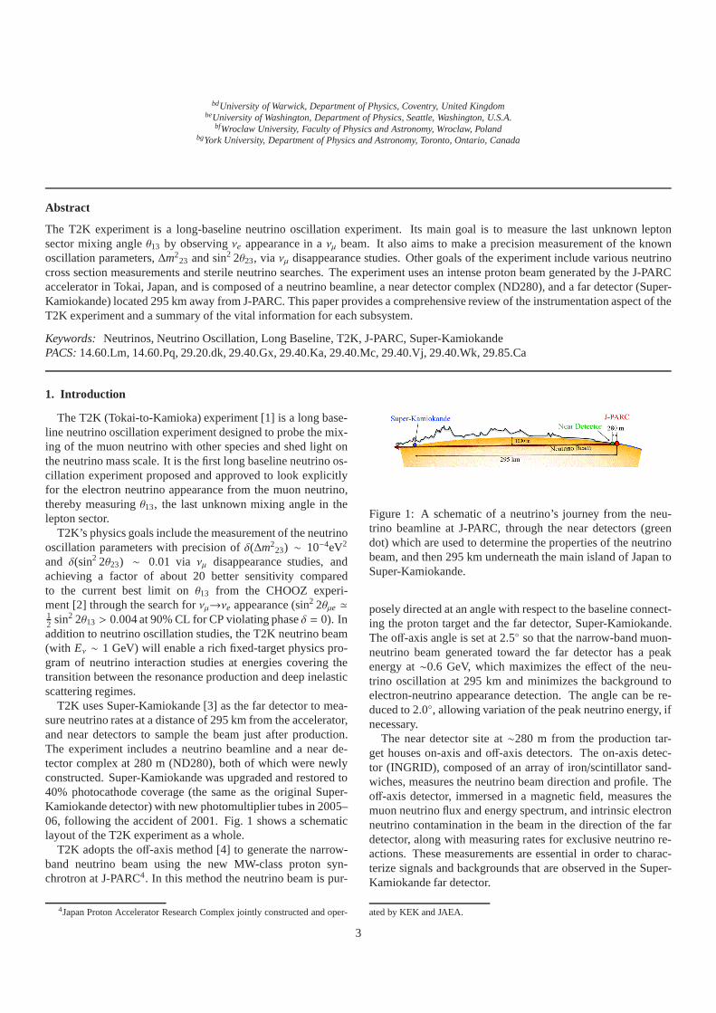
T2K uses Super-Kamiokande [3] as the far detector to mea-sure neutrino rates at a distance of 295 km from the accelerator,and near detectors to sample the beam just after production.The experiment includes a neutrino beamline and a near de-tector complex at 280 m (ND280), both of which were newlyconstructed. Super-Kamiokande was upgraded and restored to40% photocathode coverage (the same as the original Super-Kamiokande detector) with new photomultiplier tubes in 2005–06, following the accident of 2001. Fig. 1 shows a schematiclayout of the T2K experiment as a whole.

T2K adopts the off-axis method [4] to generate the narrow-band neutrino beam using the new MW-class proton syn-chrotron at J-PARC4. In this method the neutrino beam is pur-

4Japan Proton Accelerator Research Complex jointly constructed and oper-

Figure 1: A schematic of a neutrino’s journey from the neu-trino beamline at J-PARC, through the near detectors (greendot) which are used to determine the properties of the neutrinobeam, and then 295 km underneath the main island of Japan toSuper-Kamiokande.

posely directed at an angle with respect to the baseline connect-ing the proton target and the far detector, Super-Kamiokande.The off-axis angle is set at 2.5◦ so that the narrow-band muon-neutrino beam generated toward the far detector has a peakenergy at∼0.6 GeV, which maximizes the effect of the neu-trino oscillation at 295 km and minimizes the background toelectron-neutrino appearance detection. The angle can be re-duced to 2.0◦, allowing variation of the peak neutrino energy, ifnecessary.

The near detector site at∼280 m from the production tar-get houses on-axis and off-axis detectors. The on-axis detec-tor (INGRID), composed of an array of iron/scintillator sand-wiches, measures the neutrino beam direction and profile. Theoff-axis detector, immersed in a magnetic field, measures themuon neutrino flux and energy spectrum, and intrinsic electronneutrino contamination in the beam in the direction of the fardetector, along with measuring rates for exclusive neutrino re-actions. These measurements are essential in order to charac-terize signals and backgrounds that are observed in the Super-Kamiokande far detector.

ated by KEK and JAEA.

3

The off-axis detector is composed of: a water-scintillator de-tector optimized to identifyπ0’s (the PØD); the tracker consist-ing of time projection chambers (TPCs) and fine grained de-tectors (FGDs) optimized to study charged current interactions;and an electromagnetic calorimeter (ECal) that surrounds thePØD and the tracker. The whole off-axis detector is placedin a 0.2 T magnetic field provided by the recycled UA1 mag-net, which also serves as part of a side muon range detector(SMRD).

The far detector, Super-Kamiokande, is located in theMozumi mine of the Kamioka Mining and Smelting Company,near the village of Higashi-Mozumi, Gifu, Japan. The detectorcavity lies under the peak of Mt. Ikenoyama, with 1000 m ofrock, or 2700 meters-water-equivalent (m.w.e.) mean overbur-den. It is a water Cherenkov detector consisting of a weldedstainless-steel tank, 39 m in diameter and 42 m tall, with a totalnominal water capacity of 50,000 tons. The detector containsapproximately 13,000 photomultiplier tubes (PMTs) that im-age neutrino interactions in pure water. Super-Kamiokandehasbeen running since 1996 and has had four distinctive runningperiods. The latest period, SK-IV, is running stably and fea-tures upgraded PMT readout electronics. A detailed descriptionof the detector can be found elsewhere [3].

Construction of the neutrino beamline started in April 2004.The complete chain of accelerator and neutrino beamline wassuccessfully commissioned during 2009, and T2K began ac-cumulating neutrino beam data for physics analysis in January2010.

Construction of the majority of the ND280 detectors wascompleted in 2009 with the full installation of INGRID, thecentral ND280 off-axis sub-detectors (PØD, FGD, TPC anddownstream ECal) and the SMRD. The ND280 detectors be-gan stable operation in February 2010. The rest of the ND280detector (the ECals) was completed in the fall of 2010.

The T2K collaboration consists of over 500 physicists andtechnical staff members from 59 institutions in 12 countries(Canada, France, Germany, Italy, Japan, Poland, Russia, SouthKorea, Spain, Switzerland, the United Kingdom and the UnitedStates).

This paper provides a comprehensive review of the instru-mentation aspect of the T2K experiment and a summary of thevital information for each subsystem. Detailed descriptions ofsome of the major subsystems, and their performance, will bepresented in separate technical papers.

2. J-PARC Accelerator

J-PARC, which was newly constructed at Tokai, Ibaraki, con-sists of three accelerators [5]: a linear accelerator (LINAC),a rapid-cycling synchrotron (RCS) and the main ring (MR)synchrotron. An H− beam is accelerated up to 400 MeV5

(181 MeV at present) by the LINAC, and is converted to anH+ beam by charge-stripping foils at the RCS injection. The

5 Note that from here on all accelerator beam energies given are kineticenergies.

Table 1: Machine design parameters of the J-PARC MR for thefast extraction.

Circumference 1567 mBeam power ∼750 kWBeam kinetic energy 30 GeVBeam intensity ∼3× 1014 p/spillSpill cycle ∼0.5 HzNumber of bunches 8/spillRF frequency 1.67 – 1.72 MHzSpill width ∼5 µsec

beam is accelerated up to 3 GeV by the RCS with a 25 Hz cy-cle. The harmonic number of the RCS is two, and there are twobunches in a cycle. About 5% of these bunches are supplied tothe MR. The rest of the bunches are supplied to the muon andneutron beamline in the Material and Life Science Facility.Theproton beam injected into the MR is accelerated up to 30 GeV.The harmonic number of the MR is nine, and the number ofbunches in the MR is eight (six before June 2010). There aretwo extraction points in the MR: slow extraction for the hadronbeamline and fast extraction for the neutrino beamline.

In the fast extraction mode, the eight circulating protonbunches are extracted within a single turn by a set of five kickermagnets. The time structure of the extracted proton beam is keyto discriminating various backgrounds, including cosmic rays,in the various neutrino detectors. The parameters of the J-PARCMR for the fast extraction are listed in Tab. 1.

3. T2K Neutrino Beamline

Each proton beam spill consists of eight proton bunches ex-tracted from the MR to the T2K neutrino beamline, which pro-duces the neutrino beam.

The neutrino beamline is composed of two sequential sec-tions: the primary and secondary beamlines. In the primarybeamline, the extracted proton beam is transported to pointto-ward Kamioka. In the secondary beamline, the proton beamimpinges on a target to produce secondary pions, which are fo-cused by magnetic horns and decay into neutrinos. An overviewof the neutrino beamline is shown in Fig. 2. Each componentof the beamline is described in this section.

The neutrino beamline is designed so that the neutrino energyspectrum at Super-Kamiokande can be tuned by changing theoff-axis angle down to a minimum of∼2.0◦, from the current(maximum) angle of∼2.5◦. The unoscillatedνµ flux at Super-Kamiokande with this off-axis angle is shown in Fig. 3. Precisemeasurements of the baseline distance and off-axis angle weredetermined by a GPS survey, described in Section 3.6.1.

3.1. Primary Beamline

The primary beamline consists of the preparation section(54 m long), arc section (147 m) and final focusing section(37 m). In the preparation section, the extracted proton beam

4

0 50 100 m

Main Ring

Secondary beamline

(1) Preparation section

(2) Arc section

(3) Final focusing section

(4) Target station

(5) Decay volume

(6) Beam dump

ND280

(1)

(2)

(3)

(4)(5)(6)

Figure 2: Overview of the T2K neutrino beamline.

(GeV)νE0 0.5 1 1.5 2 2.5 3 3.5

]2 P

OT

/50

MeV

/cm

21F

lux[

/10

0

0.2

0.4

0.6

0.8

1

1.2

610×

Figure 3: The unoscillatedνµ flux at Super-Kamiokande withan off-axis angle of 2.5◦ when the electromagnetic horns areoperated at 250 kA.

is tuned with a series of 11 normal conducting magnets (foursteering, two dipole and five quadrupole magnets) so that thebeam can be accepted by the arc section. In the arc section, thebeam is bent toward the direction of Kamioka by 80.7◦, witha 104 m radius of curvature, using 14 doublets of supercon-ducting combined function magnets (SCFMs) [6, 7, 8]. Thereare also three pairs of horizontal and vertical superconductingsteering magnets to correct the beam orbit. In the final focus-ing section, ten normal conducting magnets (four steering,twodipole and four quadrupole magnets) guide and focus the beamonto the target, while directing the beam downward by 3.637◦

with respect to the horizontal.

A well-tuned proton beam is essential for stable neutrinobeam production, and to minimize beam loss in order to achievehigh-power beam operation. Therefore, the intensity, position,profile and loss of the proton beam in the primary sections areprecisely monitored by five current transformers (CTs), 21 elec-trostatic monitors (ESMs), 19 segmented secondary emissionmonitors (SSEMs) and 50 beam loss monitors (BLMs), respec-

Figure 4: Photographs of the primary beamline monitors. Up-per left: CT. Upper right: ESM. Lower left: SSEM. Lowerright: BLM.

Figure 5: Location of the primary beamline monitors.

tively. Photographs of the monitors are shown in Fig. 4, whilethe monitor locations are shown in Fig. 5. Polyimide cables andceramic feedthroughs are used for the beam monitors, becauseof their radiation tolerance.

The beam pipe is kept at∼ 3×10−6 Pa using ion pumps, in or-der to be connected with the beam pipe of the MR and to reducethe heat load to the SCFMs. The downstream end of the beampipe is connected to the “monitor stack”: the 5 m tall vacuumvessel embedded within the 70 cm thick wall between the pri-mary beamline and secondary beamline. The most downstreamESM and SSEM are installed in the monitor stack. Because ofthe high residual radiation levels, the monitor stack is equippedwith a remote-handling system for the monitors.

3.1.1. Normal Conducting MagnetThe normal conducting magnets are designed to be tolerant

of radiation and to be easy to maintain in the high-radiationenvironment. For the four most upstream magnets in the prepa-ration section, a mineral insulation coil is used because ofitsradiation tolerance. To minimize workers’ exposure to radia-

5

tion, remote maintenance systems are installed such as twist-lock slings, alignment dowel pins, and quick connectors forcooling pipes and power lines.

For the quadrupole magnets, “flower-shaped” beam pipes,whose surfaces were made in the shape of the magnetic polesurface, are adopted to maximize their apertures.

3.1.2. Superconducting Combined Function Magnet (SCFM)In total, there are 28 SCFMs [9, 10, 11, 12], each with a coil

aperture of 173.4 mm. The operating current for a 30 GeV pro-ton beam is 4360 A, while the magnets themselves were testedup to 7500 A, which corresponds to a 50 GeV proton beam.

The combined field is generated with a left-right asymmet-ric single layer Rutherford-type coil, made of NbTi/Cu. TwoSCFMs are enclosed in one cryostat in forward and backwarddirections to constitute a defocus-focus doublet, while eachdipole field is kept in the same direction. All the SCFMs arecooled in series with supercritical helium at 4.5 K and are ex-cited with a power supply (8 kA, 10 V).

There are also three superconducting corrector dipole mag-nets, which are cooled by conduction, in the SCFM section.Each magnet has two windings, one for vertical and one forhorizontal deflections. These magnets allow the beam to beprecisely positioned along the beamline (to minimize losses).

The magnet safety system (MSS) protects the magnets andthe bus-bars of the primary beamline in the case of an abnor-mal condition, and supplements the passive safety protectionprovided by cold diodes mounted in parallel with the supercon-ducting magnets. The MSS is based on the detection of a re-sistive voltage difference across the magnet that would appearin the case of a quench. It then secures the system by shuttingdown the magnet power supply and issuing a beam abort inter-lock signal. Most units of the MSS are dual redundant. Thisredundancy increases the reliability of the system. The MSSisbased on 33 MD200 boards [13].

3.1.3. Beam Intensity MonitorBeam intensity is measured with five current transformers

(CTs). Each CT is a 50-turn toroidal coil around a cylindricalferromagnetic core. To achieve high-frequency response upto50 MHz for the short-pulsed bunches and to avoid saturationcaused by a large peak current of 200 A, CTs use a FINEMET®

(nanocrystalline Fe-based soft magnetic material) core, whichhas a high saturation flux density, high relative permeability andlow core loss over a wide frequency range. The core’s innerdiameter is 260 mm, its outer diameter is 340 mm and it has amass of 7 kg. It is impregnated with epoxy resin. To achievehigh radiation hardness, polyimide tape and alumina fiber tapeare used to insulate the core and wire. Each CT is covered byan iron shield to block electromagnetic noise.

Each CT’s signal is transferred through about 100 m of 20Dcolgate cable and read by a 160 MHz Flash ADC (FADC). TheCT is calibrated using another coil around the core, to whichapulse current, shaped to emulate the passage of a beam bunch,isapplied. The CT measures the absolute proton beam intensitywith a 2% uncertainty and the relative intensity with a 0.5%

fluctuation. It also measures the beam timing with precisionbetter than 10 ns.

3.1.4. Beam Position MonitorEach electrostatic monitor (ESM) has four segmented cylin-

drical electrodes surrounding the proton beam orbit (80◦ cov-erage per electrode). By measuring top-bottom and left-rightasymmetry of the beam-induced current on the electrodes,it monitors the proton beam center position nondestructively(without direct interaction with the beam).

The longitudinal length of an ESM is 125 mm for the15 ESMs in the preparation and final focusing sections, 210 mmfor the five ESMs in the arc section and 160 mm for the ESMin the monitor stack. The signal from each ESM is read by a160 MHz FADC.

The measurement precision of the beam position is less than450 µm (20–40µm for the measurement fluctuation, 100–400µm for the alignment precision and 200µm for the system-atic uncertainty other than the alignment), while the require-ment is 500µm.

3.1.5. Beam Profile MonitorEach segmented secondary emission monitor (SSEM) has

two thin (5µm, 10−5 interaction lengths) titanium foils strippedhorizontally and vertically, and an anode HV foil between them.The strips are hit by the proton beam and emit secondary elec-trons in proportion to the number of protons that go throughthe strip. The electrons drift along the electric field and inducecurrents on the strips. The induced signals are transmittedto65 MHz FADCs through twisted-pair cables. The proton beamprofile is reconstructed from the corrected charge distributionon a bunch-by-bunch basis. The strip width of each SSEMranges from 2 to 5 mm, optimized according to the expectedbeam size at the installed position. The systematic uncertaintyof the beam width measurement is 200µm while the require-ment is 700µm. Optics parameters of the proton beam (Twissparameters and emittance) are reconstructed from the profilesmeasured by the SSEMs, and are used to estimate the profilecenter, width and divergence at the target.

Since each SSEM causes beam loss (0.005% loss), they areremotely inserted into the beam orbit only during beam tuning,and extracted from the beam orbit during continuous beam op-eration.

3.1.6. Beam Loss MonitorTo monitor the beam loss, 19 and 10 BLMs are installed near

the beam pipe in the preparation and final focusing sections re-spectively, while 21 BLMs are positioned near the SCFMs inthe arc section. Each BLM (Toshiba Electron Tubes & DevicesE6876-400) is a wire proportional counter filled with an Ar-CO2 mixture [14].

The signal is integrated during the spill and if it exceeds athreshold, a beam abort interlock signal is fired. The raw signalbefore integration is read by the FADCs with 30 MHz samplingfor the software monitoring.

By comparing the beam loss with and without the SSEMsin the beamline, it was shown that the BLM has a sensitivity

6

Target station

Beam dump

(1)

(2)

(3)

(4) (5)(6)

Muon monitor

(1) Beam window

(2) Baffle

(3) OTR

(4) Target and

first horn

(5) Second horn

(6) Third horn

Figure 6: Side view of the secondary beamline. The length ofthe decay volume is∼96 m.

down to a 16 mW beam loss. In the commissioning run, itwas confirmed that the residual dose and BLM data integratedduring the period have good proportionality. This means thatthe residual dose can be monitored by watching the BLM data.

3.2. Secondary Beamline

Produced pions decay in flight inside a single volume of∼1500 m3, filled with helium gas (1 atm) to reduce pion ab-sorption and to suppress tritium and NOx production by thebeam. The helium vessel is connected to the monitor stack viaatitanium-alloy beam window which separates the vacuum in theprimary beamline and the helium gas volume in the secondarybeamline. Protons from the primary beamline are directed tothe target via the beam window.

The secondary beamline consists of three sections: the targetstation, decay volume and beam dump (Fig. 6). The target sta-tion contains: a baffle which is a collimator to protect the mag-netic horns; an optical transition radiation monitor (OTR)tomonitor the proton beam profile just upstream of the target; thetarget to generate secondary pions; and three magnetic hornsexcited by a 250 kA (designed for up to 320 kA) current pulseto focus the pions. The produced pions enter the decay vol-ume and decay mainly into muons and muon neutrinos. All thehadrons, as well as muons below∼5 GeV/c, are stopped by thebeam dump. The neutrinos pass through the beam dump and areused for physics experiments. Any muons above∼5 GeV/c thatalso pass through the beam dump are monitored to characterizethe neutrino beam.

3.2.1. Target StationThe target station consists of the baffle, OTR, target, and

horns, all located inside a helium vessel. The target stationis separated from the primary beamline by a beam window atthe upstream end, and is connected to the decay volume at thedownstream end.

The helium vessel, which is made of 10 cm thick steel, is15 m long, 4 m wide and 11 m high. It is evacuated down to50 Pa before it is filled with helium gas. Water cooling chan-nels, called plate coils, are welded to the surface of the vessel,and∼30◦C water cools the vessel to prevent its thermal defor-mation. An iron shield with a thickness of∼2 m and a concreteshield with a thickness of∼1 m are installed above the hornsinside the helium vessel. Additionally,∼4.5 m thick concreteshields are installed above the helium vessel.

The equipment and shields inside the vessel are removableby remote control in case of maintenance or replacement of thehorns or target. Beside the helium vessel, there is a maintenancearea where manipulators and a lead-glass window are installed,as well as a depository for radio-activated equipment.

3.2.2. Beam WindowThe beam window, comprising two helium-cooled 0.3 mm

thick titanium-alloy skins, separates the primary proton beam-line vacuum from the target station. The beam window assem-bly is sealed both upstream and downstream by inflatable bel-lows vacuum seals to enable it to be removed and replaced ifnecessary.

3.2.3. BaffleThe baffle is located between the beam window and OTR. It

is a 1.7 m long, 0.3 m wide and 0.4 m high graphite block, witha beam hole of 30 mm in diameter. The primary proton beamgoes through this hole. It is cooled by water cooling pipes.

3.2.4. Optical Transition Radiation MonitorThe OTR has a thin titanium-alloy foil, which is placed at 45◦

to the incident proton beam. As the beam enters and exits thefoil, visible light (transition radiation) is produced in anarrowcone around the beam. The light produced at the entrance tran-sition is reflected at 90◦ to the beam and directed away from thetarget area. It is transported in a dogleg path through the ironand concrete shielding by four aluminum 90◦ off-axis parabolicmirrors to an area with lower radiation levels. It is then col-lected by a charge injection device camera to produce an imageof the proton beam profile.

The OTR has an eight-position carousel holding four titan-ium-alloy foils, an aluminum foil, a fluorescent ceramic foil of100µm thickness, a calibration foil and an empty slot (Fig. 7).A stepping motor is used to rotate the carousel from one foilto the next. The aluminum (higher reflectivity than titanium)and ceramic (which produces fluorescent light with higher in-tensity than OTR light) foils are used for low and very low in-tensity beam, respectively. The calibration foil has preciselymachined fiducial holes, of which an image can be taken us-ing back-lighting from lasers and filament lights. It is usedformonitoring the alignment of the OTR system. The empty slotallows back-lighting of the mirror system to study its transportefficiency.

3.2.5. TargetThe target core is a 1.9 interaction length (91.4 cm long),

2.6 cm diameter and 1.8 g/cm3 graphite rod. If a material sig-

7

nificantly denser than graphite were used for the target core, itwould be melted by the pulsed beam heat load.

The core and a surrounding 2 mm thick graphite tube aresealed inside a titanium case which is 0.3 mm thick. The tar-get assembly is supported as a cantilever inside the bore of thefirst horn inner conductor with a positional accuracy of 0.1 mm.The target is cooled by helium gas flowing through the gaps be-tween the core and tube and between the tube and case. For the750 kW beam, the flow rate is∼32 g/s helium gas with a heliumoutlet pressure of 0.2 MPa, which corresponds to a flow speedof ∼250 m/s. When the 750 kW proton beam interacts with thetarget, the temperature at the center is expected to reach 700◦C,using the conservative assumption that radiation damage hasreduced the thermal conductivity of the material by a factoroffour.

The radiation dose due to the activation of the target is esti-mated at a few Sv/h six months after a one year’s irradiation bythe 750 kW beam [15].

3.2.6. Magnetic Horn

The T2K beamline uses three horns. Each magnetic hornconsists of two coaxial (inner and outer) conductors which en-compass a closed volume [16, 17]. A toroidal magnetic field isgenerated in that volume. The field varies as 1/r, wherer is thedistance from the horn axis. The first horn collects the pionswhich are generated at the target installed in its inner conduc-tor. The second and third horns focus the pions. When the hornis run with a operation current of 320 kA, the maximum field is2.1 T and the neutrino flux at Super-Kamiokande is increasedby a factor of∼16 (compared to horns at 0 kA) at the spectrumpeak energy (∼0.6 GeV).

The horn conductor is made of aluminum alloy (6061-T6).The horns’ dimensions (minimum inside diameter, inner con-ductor thickness, outside diameter and length respectively) are54 mm, 3 mm, 400 mm and 1.5 m for the first horn, 80 mm,3 mm, 1000 mm and 2 m for the second horn, and 140 mm,3 mm, 1400 mm and 2.5 m for the third horn. They are opti-mized to maximize the neutrino flux; the inside diameter is assmall as possible to achieve the maximum magnetic field, andthe conductor is as thin as possible to minimize pion absorptionwhile still being tolerant of the Lorentz force, created from the320 kA current and the magnetic field, and the thermal shockfrom the beam.

The pulse current is applied via a pulse transformer with aturn ratio of 10:1, which is installed beside the helium vesselin the target station. The horns are connected to the secondaryside of the pulse transformer in series using aluminum bus-bars.The currents on the bus-bars are monitored by four Rogowskicoils per horn with a 200 kHz FADC readout. The measure-ment uncertainty of the absolute current is less than∼2%. Thehorn magnetic field was measured with a Hall probe before in-stallation, and the uncertainty of the magnetic field strength isapproximately 2% for the first horn and less than 1% for thesecond and third horns.

Figure 7: Top: Photograph of the OTR carousel. Bottom:Cross section of the first horn and target.

3.2.7. Decay Volume

The decay volume is a∼96 m long steel tunnel. The crosssection is 1.4 m wide and 1.7 m high at the upstream end, and3.0 m wide and 5.0 m high at the downstream end. The decayvolume is surrounded by 6 m thick reinforced concrete shield-ing. Along the beam axis, 40 plate coils are welded on the steelwall, whose thickness is 16 mm, to cool the wall and concreteto below 100◦C using water.

3.2.8. Beam Dump

The beam dump sits at the end of the decay volume. Thedistance between the center of the target and the upstream sur-face of the beam dump along the neutrino beam direction forthe off-axis angle of 2.5◦ is 109 m. The beam dump’s core ismade of 75 tons of graphite (1.7 g/cm3), and is 3.174 m long,1.94 m wide and 4.69 m high. It is contained in the helium ves-sel. Fifteen iron plates are placed outside the vessel and twoinside, at the downstream end of the graphite core, to give atotal iron thickness of 2.40 m. Only muons above∼5.0 GeV/ccan go through the beam dump to reach the downstream muonpit.

The core is sandwiched on both sides by aluminum coolingmodules which contain water channels. The temperature in thecenter of the core is kept at around 150◦C for the 750 kW beam.

8

3.3. Muon Monitor

The neutrino beam intensity and direction can be monitoredon a bunch-by-bunch basis by measuring the distribution pro-file of muons, because muons are mainly produced along withneutrinos from the pion two-body decay. The neutrino beamdirection is determined to be the direction from the target tothe center of the muon profile. The muon monitor [18, 19] islocated just behind the beam dump. The muon monitor is de-signed to measure the neutrino beam direction with a precisionbetter than 0.25 mrad, which corresponds to a 3 cm precisionof the muon profile center. It is also required to monitor thestability of the neutrino beam intensity with a precision betterthan 3%.

A detector made of nuclear emulsion was installed just down-stream of the muon monitor to measure the absolute flux andmomentum distribution of muons.

3.3.1. Characteristics of the Muon FluxBased on the beamline simulation package, described in Sec-

tion 3.5, the intensity of the muon flux at the muon monitor, for3.3 × 1014 protons/spill and 320 kA horn current, is estimatedto be 1× 107 charged particles/cm2/bunch with a Gaussian-likeprofile around the beam center and approximately 1 m in width.The flux is composed of around 87% muons, with delta-raysmaking up the remainder.

3.3.2. Muon Monitor DetectorsThe muon monitor consists of two types of detector arrays:

ionization chambers at 117.5 m from the target and silicon PINphotodiodes at 118.7 m (Fig. 8). Each array holds 49 sensorsat 25 cm× 25 cm intervals and covers a 150× 150 cm2 area.The collected charge on each sensor is read out by a 65 MHzFADC. The 2D muon profile is reconstructed in each array fromthe distribution of the observed charge.

The arrays are fixed on a support enclosure for thermal insu-lation. The temperature inside the enclosure is kept at around34◦C (within ±0.7◦C variation) with a sheathed heater, as thesignal gain in the ionization chamber is dependent on the gastemperature.

An absorbed dose at the muon monitor is estimated to beabout 100 kGy for a 100-day operation at 750 kW. Therefore,every component in the muon pit is made of radiation-tolerantand low-activation material such as polyimide, ceramic, oralu-minum.

3.3.3. Ionization ChamberThere are seven ionization chambers, each of which contains

seven sensors in a 150×50×1956mm3 aluminum gas tube. The75× 75× 3 mm3 active volume of each sensor is made by twoparallel plate electrodes on alumina-ceramic plates. Betweenthe electrodes, 200 V is applied.

Two kinds of gas are used for the ionization chambers ac-cording to the beam intensity: Ar with 2% N2 for low intensity,and He with 1% N2 for high intensity. The gas is fed in at ap-proximately 100 cm3/min. The gas temperature, pressure andoxygen contamination are kept at around 34◦C with a 1.5◦C

Figure 8: Photograph of the muon monitor inside the supportenclosure. The silicon PIN photodiode array is on the right sideand the ionization chamber array is on the left side. The muonbeam enters from the left side.

gradient and±0.2◦C variation, at 130± 0.2 kPa (absolute), andbelow 2 ppm, respectively.

3.3.4. Silicon PIN PhotodiodeEach silicon PIN photodiode (Hamamatsu® S3590-08) has

an active area of 10× 10 mm2 and a depletion layer thicknessof 300µm. To fully deplete the silicon layer, 80 V is applied.

The intrinsic resolution of the muon monitor is less than0.1% for the intensity and less than 0.3 cm for the profile center.

3.3.5. Emulsion TrackerThe emulsion trackers are composed of two types of mod-

ules. The module for the flux measurement consists of eightconsecutive emulsion films [20]. It measures the muon fluxwith a systematic uncertainty of 2%. The other module for themomentum measurement is made of 25 emulsion films inter-leaved by 1 mm lead plates, which can measure the momentumof each particle by multiple Coulomb scattering with a preci-sion of 28% at a muon energy of 2 GeV/c [21, 22]. These filmsare analyzed by scanning microscopes [23, 24].

3.4. Beamline Online System

For the stable and safe operation of the beamline, the onlinesystem collects information on the beamline equipment and thebeam measured by the beam monitors, and feeds it back to theoperators. It also provides Super-Kamiokande with the spillinformation for event synchronization by means of GPS, whichis described in detail in Section 3.6.2.

3.4.1. DAQ SystemThe signals from each beam monitor are brought to one of

five front-end stations in different buildings beside the beam-line. The SSEM, BLM, and horn current signals are digitizedby a 65 MHz FADC in the COPPER system [25]. The CT andESM signals are digitized by a 160 MHz VME FADC [26].

9

The GPS for the event synchronization and the OTR both usecustom-made readout electronics. All of these readout systemsare managed by the MIDAS framework [27], and the eventbuilder records fully concatenated events every spill, before thenext spill is issued. MIDAS’s event monitoring system locksthe internal data holding buffer. To minimize the locking time,which can have a negative effect on the DAQ system’s responsetime, an event distributor was developed. It receives eventdatafrom the MIDAS server and distributes the data in ROOT for-mat to the clients. No reduction is applied to the output fromthe ADCs and the event data size remains constant at 1.6 MB.

3.4.2. Beamline Control SystemInformation on the beamline (the beam monitor outputs, spill

number and status of the beamline equipment) is recorded byEPICS [28]. EPICS also controls the beamline equipment usingprogrammable logic controllers (PLCs).

Based on the data from EPICS, the beam orbit and optics aresimulated by SAD [29], and the magnet currents to be adjustedare also calculated.

3.4.3. InterlockThe function of the interlock system is to protect people

(PPS: person protection system) and the machines (MPS: ma-chine protection system). The PPS can be fired by an emer-gency stop button, or safety sensors such as door interlocksandradiation monitors. The MPS can be fired by a quenching of theSCFMs, an error from the normal conducting magnet or hornsystem, an excess in the loss monitor signal, or other machine-related causes.

3.5. Beamline Simulation for Neutrino Flux EstimationThe neutrino flux is predicted by a Monte Carlo simulation

based on experimental data. Specifically, hadron production by30 GeV protons on a graphite target was measured by a ded-icated experiment, NA61/SHINE [30, 31], which fully coversthe kinematic region of interest for T2K.

In the beam MC, the detailed geometry of the secondarybeamline is described in the code. Protons with a kinetic energyof 30 GeV are injected into the graphite target and then sec-ondary particles are produced and focused in the horn magnets.The secondaries and any un-interacted protons are tracked untilthey decay into neutrinos or are stopped at the beam dump. Thetracks of neutrinos are extrapolated to the near and far detec-tors, providing the predicted fluxes and energy spectra at bothdetector sites.

The primary interaction of the 30 GeV proton with car-bon is simulated based on NA61/SHINE data. Other hadronicinteractions inside the target are simulated by FLUKA [32].The interactions outside the target are simulated usingGEANT3/GCALOR [33] with the interaction cross sectionstuned to experimental data.

3.6. Global Alignment and Time Synchronization3.6.1. Global Position Survey and Alignment

In a long baseline neutrino experiment, controlling the direc-tion of the neutrino beam is one of the most important aspects.

For the T2K neutrino experiment, it is necessary to considerthe three-dimensional geometry of the earth, since it covers adistance of∼300 km from J-PARC to Super-Kamiokande. De-termining the correct direction is not simple. Therefore, surveyswere performed, including a long baseline GPS survey betweenTokai and Kamioka.

Based on the surveys, the primary beamline components, tar-get, and horns were aligned in order to send the neutrino beamin the right direction. The muon monitor and the neutrino neardetectors were also aligned in order to monitor the neutrinobeam direction. A good alignment of the components is alsonecessary in order to reduce irradiation in a high-intensity pro-ton beamline.

A complete neutrino beamline survey is carried out on ayearly basis. There are five penetration holes in the neutrinobeamline to connect a ground survey network with an under-ground survey; one at the preparation section, two at the finalfocusing section and two at the muon pit. In the target station,the underground survey points were transferred to the groundlevel so that they can be monitored even after the undergroundhelium vessel is closed. In the primary beamline, a survey andalignment is carried out using a laser tracker with a spatialres-olution of 50µm at a distance shorter than 20 m. The super-conducting magnets were aligned to better than 100µm and thenormal conducting quadrupole magnets were aligned to betterthan 1 mm. In the other places, a survey is carried out using atotal station which gives a spatial resolution of about 2 mm at adistance of 100 m.

We observed a ground sink of a few tens of millimeters dur-ing the construction stage. It was taken into account at the in-stallation of the beamline components. After the installationat the primary beamline, we still observed a sink of severalmillimeters at the final focusing section and the target station.Therefore the beam was tuned to follow the beamline sink.

The required directional accuracy from the physics point ofview is 1×10−3 rad. The directional accuracy of a long baselineGPS survey is several times 10−6 rad. That of a short distancesurvey is a few times 10−5 rad. It was confirmed by surveys af-ter construction that a directional accuracy of significantly bet-ter than 1× 10−4 rad was attained.

The measured distance between the target and the center po-sition of Super-Kamiokande is 295, 335.2± 0.7 m. The mea-sured off-axis angle is 2.504± 0.004◦.

3.6.2. Time SynchronizationThe T2K GPS time synchronization system builds on expe-

rience from K2K, taking advantage of subsequent advances incommercially available clock systems and related technology.The system providesO(50 ns) scale synchronization betweenneutrino event trigger timestamps at Super-Kamiokande, andbeam spill timestamps logged at J-PARC.

The heart of the system is a custom electronics board calledthe local time clock (LTC). This board uses a time base de-rived from a commercial rubidium clock, and references it toGPS time using input from two independent commercial GPSreceivers. The operational firmware was coded to interface effi-

10

ciently with the Super-Kamiokande or J-PARC data acquisitionsystems.

The LTC receives 1 pps (pulse per second) signals fromtwo independent GPS receivers. These signals have theirleading edges aligned with the second transitions in UTC tohigher precision than required for T2K. The primary receiveris a TrueTime (Symmetricom) rack-mounted receiver, and thesecondary receiver is a Synergy Systems SynPaQIII receiver,mounted as a daughtercard on the LTC itself. The receiversare connected to antenna modules located with a clear view ofthe sky, near the mine entrance at Super-Kamiokande, and at J-PARC. The Rb clock which provides a stabilized time base forthe system in case of temporary loss of GPS signals is a Stan-ford Research Systems model FS-725. The LTC is interfaced tothe data acquisition system through a Linux PC with fast net-work connections. At J-PARC, an independent optical fiber linksends data directly to the ND280 data acquisition system.

When the timing signal, synchronized with the MR extrac-tion, is received its time is recorded to an LTC module atJ-PARC. The LTC module counts the accumulated numberof received signals as the spill number. This time informationand the spill number are sent to Super-Kamiokande through aprivate network, and are returned from Super-Kamiokande tocheck consistency. The LTC module also provides the beamtrigger for the beam monitors.

At each site, two independent GPS systems run in parallel atall times to eliminate downtime during T2K running.

4. Near Detector Complex (ND280)

As stated earlier, the T2K experiment studies oscillationsofan off-axis muon neutrino beam between the J-PARC accel-erator complex and the Super-Kamiokande detector, with spe-cial emphasis on measuring the unknown mixing angleθ13 byobserving the subdominantνµ→νe oscillation. The neutrinoenergy spectrum, flavor content, and interaction rates of theunoscillated beam are measured by a set of detectors located280 m from the production target, and are used to predict theneutrino interactions at Super-Kamiokande.

The primary detector at the 280 m site is a magnetized off-axis tracking detector. The off-axis detector elements are con-tained inside the magnet recycled from the UA1 experimentat CERN. Inside the upstream end of this magnet sits a pi-zero detector (PØD) consisting of tracking planes of scintillat-ing bars alternating with either water target/brass foil or leadfoil. Downstream of the PØD, the tracker, comprising threetime projection chambers (TPCs) and two fine grained detec-tors (FGDs) consisting of layers of finely segmented scintillat-ing bars, is designed to measure charged current interactions inthe FGDs. The PØD, TPCs, and FGDs are all surrounded by anelectromagnetic calorimeter (ECal) for detectingγ-rays that donot convert in the inner detectors, while the return yoke of themagnet is instrumented with scintillator to measure the rangesof muons that exit the sides of the off-axis detector. In addi-tion to the off-axis detector, a separate array of iron/scintillatordetectors called INGRID measures the on-axis neutrino beamprofile at the 280 m site, while a set of muon monitor detectors

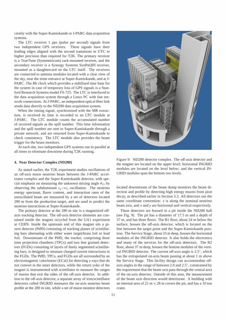
Figure 9: ND280 detector complex. The off-axis detector andthe magnet are located on the upper level; horizontal INGRIDmodules are located on the level below; and the vertical IN-GRID modules span the bottom two levels.

located downstream of the beam dump monitors the beam di-rection and profile by detecting high energy muons from piondecay, as described earlier in Section 3.3. All detectors use thesame coordinate convention:z is along the nominal neutrinobeam axis, andx andy are horizontal and vertical respectively.

These detectors are housed in a pit inside the ND280 hall(see Fig. 9). The pit has a diameter of 17.5 m and a depth of37 m, and has three floors. The B1 floor, about 24 m below thesurface, houses the off-axis detector, which is located on theline between the target point and the Super-Kamiokande posi-tion. The Service Stage, about 33 m deep, houses the horizontalmodules of the INGRID detector. It also holds the electronicsand many of the services for the off-axis detectors. The B2floor, about 37 m deep, houses the bottom modules of the verti-cal INGRID detector. The current off-axis angle is 2.5◦, whichhas the extrapolated on-axis beam passing at about 1 m abovethe Service Stage. This facility design can accommodate off-axis angles in the range of between 2.0 and 2.5◦, constrained bythe requirement that the beam axis pass through the central areaof the on-axis detector. Outside of this area, the measurementof the beam axis direction would deteriorate. A building withan internal area of 21 m× 28 m covers the pit, and has a 10 toncrane.

11

Table 2: Main parameters of the T2K MPPCs

Number of pixels 667Active area 1.3× 1.3 mm2

Pixel size 50× 50µm2

Operational voltage 68− 71 VGain ∼ 106

Photon detection efficiency at 525 nm 26− 30%Dark rate, threshold= 0.5 p.e., T= 25 ◦C ≤ 1.35 MHz

4.1. Multi-Pixel Photon Counter (MPPC)

The ND280 detectors make extensive use of scintillator de-tectors and wavelength-shifting (WLS) fiber readout, with lightfrom the fibers being detected by photosensors that must oper-ate in a magnetic field environment and fit into a limited spaceinside the magnet. Multi-anode PMTs, successfully used inother scintillator and WLS based neutrino experiments, arenotsuitable for ND280 because most of the detectors in the ND280complex have to work in a magnetic field of 0.2 T. To satisfythe ND280 experimental requirements, a multi-pixel avalanchephotodiode was selected for the photosensor. The device con-sists of many independent sensitive pixels, each of which oper-ates as an independent Geiger micro-counter with a gain of thesame order as a vacuum photomultiplier. These novel photo-sensors are compact, well matched to spectral emission of WLSfibers, and insensitive to magnetic fields. Detailed informationand the basic principles of operation of multi-pixel photodiodescan be found in a recent review paper [34] and the referencestherein.

After R&D and tests provided by several groups for threeyears, the Hamamatsu Multi-Pixel Photon Counter (MPPC)was chosen as the photosensor for ND280. The MPPC gainis determined by the charge accumulated in a pixel capacitanceCpixel: Qpixel = Cpixel ·∆V, where the overvoltage∆V is thedifference between the applied voltage and the breakdown volt-age of the photodiode. For MPPCs the operational voltage isabout 70 V, which is 0.8 − 1.5 V above the breakdown volt-age. The pixel capacitance is 90 fF, which gives a gain in therange 0.5−1.5× 106. When a photoelectron is produced it cre-ates a Geiger avalanche. The amplitude of a single pixel signaldoes not depend on the number of carriers created in this pixel.Thus, the photodiode signal is a sum of fired pixels. Each pixeloperates as a binary device, but the multi-pixel photodiodeas awhole unit is an analogue detector with a dynamic range limitedby the finite number of pixels.

A customized 667-pixel MPPC, with a sensitive area of1.3× 1.3 mm2, was developed for T2K [35, 36]. It is based ona Hamamatsu commercial device, the sensitive area of whichwas increased to provide better acceptance for light detectionfrom 1 mm diameter Y11 Kuraray fibers. In total, about 64,000MPPCs were produced for T2K. The T2K photosensor is shownin Fig. 10.

The main parameters of MPPCs are summarized in Table 2.The characterization of the MPPCs’ response to scintillation

Figure 10: Photographs of an MPPC with a sensitive area of1.3× 1.3 mm2: magnified face view (left) with 667 pixels in a26× 26 array (a 9-pixel square in the corner is occupied by anelectrode); the ceramic package of this MPPC (right).

light is presented in Ref. [37].

4.2. INGRID On-axis Detector

INGRID (Interactive Neutrino GRID) is a neutrino detectorcentered on the neutrino beam axis. This on-axis detector wasdesigned to monitor directly the neutrino beam direction andintensity by means of neutrino interactions in iron, with suffi-cient statistics to provide daily measurements at nominal beamintensity. Using the number of observed neutrino events in eachmodule, the beam center is measured to a precision better than10 cm. This corresponds to 0.4 mrad precision at the near de-tector pit, 280 meters downstream from the beam origin. TheINGRID detector consists of 14 identical modules arranged asa cross of two identical groups along the horizontal and verti-cal axis, and two additional separate modules located at off-axisdirections outside the main cross, as shown in Fig. 11. The de-tector samples the neutrino beam in a transverse section of 10 m× 10 m. The center of the INGRID cross, with two overlappingmodules, corresponds to the neutrino beam center, defined as0◦ with respect to the direction of the primary proton beamline.The purpose of the two off-axis modules is to check the axialsymmetry of the neutrino beam. The entire 16 modules are in-stalled in the near detector pit with a positioning accuracyof2 mm in directions perpendicular to the neutrino beam.

The INGRID modules consist of a sandwich structure ofnine iron plates and 11 tracking scintillator planes as shownin Fig. 12. They are surrounded by veto scintillator planes,toreject interactions outside the module. The dimensions of theiron plates are 124 cm× 124 cm in thex andy directions and6.5 cm along the beam direction. The total iron mass serving asa neutrino target is 7.1 tons per module. Each of the 11 track-ing planes consists of 24 scintillator bars in the horizontal di-rection glued to 24 perpendicular bars in the vertical directionwith Cemedine PM200, for a total number of 8,448. No ironplate was placed between the 10th and 11th tracking planes dueto weight restrictions, but this does not affect the tracking per-formance. The dimensions of the scintillator bars used for thetracking planes are 1.0 cm× 5.0 cm× 120.3 cm. Due to the factthat adjacent modules can share one veto plane in the boundaryregion, the modules have either three or four veto planes. Each

12

Figure 11: INGRID on-axis detector

veto plane consists of 22 scintillator bars segmented in thebeamdirection. The dimensions of those scintillator bars are 1.0 cm× 5.0 cm× 111.9 cm (bottom sides) and 1.0 cm× 5.0 cm×129.9 cm (top, right and left sides). The total number of chan-nels for the veto planes is 1,144, which gives a total of 9,592channels for INGRID as a whole.

Figure 12: An INGRID module. The left image shows thetracking planes (blue) and iron plates. The right image showsveto planes (black).

The extruded scintillator bars used for the tracking and vetoplanes are made of polystyrene doped with 1% PPO and 0.03%POPOP by weight. The wavelength of the scintillation lightat the emission peak is 420 nm (blue). They were developedand produced at Fermilab [38]. A thin white reflective coating,composed of TiO2 infused in polystyrene, surrounds the wholeof each scintillator bar. The coating improves light collectionefficiency by acting as an optical isolator. A hole with a diame-ter of about 3 mm in the center of the scintillator bar allows theinsertion of a WLS fiber for light collection.

The WLS fibers used for INGRID are 1 mm diameter Ku-raray double-clad Y-11. The absorption spectrum of the fiberiscentered at a wavelength of 430 nm (blue). The emission spec-trum is centered at 476 nm (green), and the overlap between the

two is small, reducing self-absorption effects in the fiber. Oneend of the fiber is glued to a connector by epoxy resin (ELJENTechnology EJ-500). The surface of the connector was pol-ished with diamond blades. An MPPC is attached to each fiberusing the connector. A detailed description of the MPPCs canbe found in Section 4.1. Some characterization of the MPPCsused for INGRID can be found in [36, 39].

Finally, the set of scintillators, fibers and photosensors is con-tained in a light-tight dark box made of aluminum frames andplastic plates. The readout front-end electronics boards,theTrip-T front-end boards (TFBs), are mounted outside the darkbox and each connected to 48 MPPCs via coaxial cables. Thisforms one complete tracking scintillator plane.

INGRID was calibrated using cosmic ray data taken on thesurface and, during beam, in the ND280 pit. The mean lightyield of each channel is measured to be larger than ten photo-electrons per 1 cm of MIP tracks which satisfies our require-ment. Furthermore the timing resolution of each channel ismeasured to be 3.2 ns.

An extra module, called the Proton Module, different fromthe 16 standard modules, has been added in order to detect withgood efficiency the muons together with the protons producedby the neutrino beam in INGRID. The goal of this Proton Mod-ule is to identify the quasi-elastic channel for comparisonwithMonte Carlo simulations of beamline and neutrino interactions.It consists of scintillator planes without any iron plate and sur-rounded by veto planes. A different size scintillator bar wasused to improve tracking capabilities. A schematic view of theProton Module can be seen in Fig. 13. It is placed in the pit inthe center of the INGRID cross between the standard verticaland horizontal central modules.

Figure 13: The Proton Module. Similar to the INGRID mod-ules, but with finer grain scintillator and without the iron plates.

Typical neutrino events in the INGRID module and the Pro-ton Module are shown in Figs. 14 and 15.

4.3. Off-axis Detector

A large fine grained off-axis detector (see Fig. 16) serves tomeasure the flux, energy spectrum and electron neutrino con-tamination in the direction of the far detector, along with mea-suring rates for exclusive neutrino reactions. This characterizessignals and backgrounds in the Super-Kamiokande detector.

13

Figure 14: A typical neutrino event in an INGRID module. Aneutrino enters from the left and interacts within the module,producing charged particles. One of them makes a track whichis shown as the red circles. Each of the green cells in this figureis a scintillator, and the size of the red circles indicates the sizeof the observed signal in that cell. Blue cells and gray boxesindicate veto scintillators and iron target plates, respectively.

The ND280 off-axis detector must satisfy several require-ments. Firstly, it must provide information to determine the νµflux at the Super-Kamiokande detector. Secondly, theνe con-tent of the beam must be measured as a function of neutrino en-ergy. The beamνe background is expected to be approximately1% of theνµ flux and creates a significant non-removable back-ground. Thirdly, it must measureνµ interactions such that thebackgrounds to theνe appearance search at Super-Kamiokandecan be predicted. These backgrounds are dominated by neutralcurrent singleπ0 production. To meet these goals the ND280off-axis detector must have the capability to reconstruct exclu-sive event types such asνµ andνe charged current quasi-elastic,charged current inelastic, and neutral current events, particu-larly neutral current singleπ0 events. In addition, the ND280off-axis detector should measure inclusive event rates. All ofthese requirements were considered in designing the off-axisdetector.

The constructed off-axis detector consists of: the PØD andthe TPC/FGD sandwich (tracker), both of which are placed in-side of a metal frame container, called the “basket”; an electro-magnetic calorimeter (ECal) that surrounds the basket; andtherecycled UA1 magnet instrumented with scintillator to performas a muon range detector (SMRD). (See Fig. 16).

The basket has dimensions of 6.5 m× 2.6 m× 2.5 m (length× width× height). It is completely open at the top, to allow theinsertion of the various detectors. Two short beams are fixedat the center of the two faces of the basket perpendicular to thebeam axis. The short beam at each end of the basket connectsto an axle which runs through the hole in the magnet coil orig-inally intended to allow passage of the beam-pipe in the UA1experiment. The axle is in turn supported by an external supportframe which is bolted to the floor. When opening the magnet,the half yokes and the coils move apart, while the basket and

Figure 15: A typical neutrino event in the Proton Module. Aneutrino enters from the left and interacts within the module,producing charged particles whose tracks are shown as the redcircles. One of them exits the Proton Module and enters thecentral INGRID horizontal module. Each of the green cells inthis figure is a scintillator, and the size of the red circles in-dicates the size of the observed signal in that cell. Blue cellsindicate veto scintillators.

the inner detector remain fixed in the position chosen for datataking. In the following sections, more detailed descriptions ofthese elements are provided.

4.3.1. UA1 MagnetThe ND280 off-axis detector is built around the old CERN

UA1/NOMAD magnet providing a dipole magnetic field of0.2 T, to measure momenta with good resolution and determinethe sign of charged particles produced by neutrino interactions.

The magnet consists of water-cooled aluminum coils, whichcreate the horizontally oriented dipole field, and a flux returnyoke. The dimensions of the inner volume of the magnet are7.0 m× 3.5 m× 3.6 m. The external dimensions are 7.6 m× 5.6 m× 6.1 m and the total weight of the yoke is 850 tons.The coils are made of aluminum bars with 5.45 cm× 5.45 cmsquare cross sections, with a central 23 mm diameter bore forwater to flow. The coils are composed of individual “pancakes”which are connected hydraulically in parallel and electrically inseries.

The magnet consists of two mirror-symmetric halves. Thecoils are split into four elements, two for each half, and are

14

Figure 16: An exploded view of the ND280 off-axis detector.

mechanically supported by, but electrically insulated from, thereturn yoke. The two half yoke pieces each consist of eight C-shaped elements, made of low-carbon steel plates, which standon movable carriages. The carriages are fitted on rails and op-erated by hydraulic movers, so that each half magnet is inde-pendent of the other and can be separately moved to an open orclosed position. When the magnet is in an open position, theinner volume is accessible, allowing access to the detectors.

The magnet yoke and coils were reused from UA1/NOMAD,while the movers were obtained from the completed HERA-B experiment at DESY. In order to comply with seismic reg-ulations, detailed FEM static and dynamic analyses were per-formed and cross-checked with measurements of deformationand modal frequency of the yoke elements. As a result of this,the carriages were mechanically reinforced by additional steelbars to increase their lateral strength. Additional componentshad to be specially designed and built for the ND280 magnetoperation. These were: the power supply (PS), the coolingsystem (CS), the magnet safety system (MSS), and the mag-net control system (MCS). Finally, the magnetic field map wasdeterminedin situ with a dedicated measurement campaign.

The PS, specially made for ND280, was designed and man-ufactured by Bruker to provide the DC current to energize themagnet. The nominal current is 2900 A with a voltage dropof 155 V. The requirements for the DC current resolution andstability were 300 ppm and± 1000 ppm over 24 hours respec-tively. The PS is also able to cope with AC phase imbalance(± 2%) and short voltage drops. A thyristor switch mode wasemployed, with digital current regulation via a DCCT captor(ULTRASTAB series from Danfysik). The power supply canbe controlled locally or remotely via the MCS.

The CS, assembled by MAN Ferrostaal AG (D), provides upto 750 kW of cooling power via two independent demineral-ized water circuits to compensate for the heat loss from the

coils and in the power supply. The cold source consists of aprimary glycol circuit maintained at 8◦C by a chiller (built byFriotherm, D). The secondary pumping circuit units and theirheat exchangers, the water purification units and the main panelcontroller are mounted in an ISO container, suitable for easyroad and sea transport. They were assembled and tested in Eu-rope before shipment to J-PARC. The secondary circuit dem-ineralized water for the magnet coils has a flow of 30 L/s anda pressure of 10 bar to compensate for the 7 bar pressure dropacross the coil bore holes.

The MSS, based on a hardwired fail-safe interface, was builtto ensure the operational safety of the magnet. It continu-ously monitors a set of input signals from the thermo-switchesmounted on the magnet coils, fault signals from the power con-verter, cooling and magnet control systems, and magnet emer-gency stop signals from manual buttons located in the ND280building. A Boolean OR of all fault signals is generated andlogically combined with the on/off magnet status. When themagnet is off, the system issues a power convert permit signalonly if none of the input signals is in a fault state. When themagnet is operating, a fast abort signal is generated and sentto the power converter in less than 1 ms when any of the inputsignals switches to a fault state. All input and output signals ofthe MSS are monitored by a VME computer, and any changein the status of the signals is recorded with 1 ms timing resolu-tion, meaning that the detailed sequence of events leading up toa fast abort can be understood.

The aim of the MCS is to monitor the behavior of the mag-net and cooling system, to control the current set point of themagnet power supply and to interface all the information andcontrol parameters with the global slow control (GSC). Thesystem is based on an industrial programmable logic controller(PLC) that reads: the coil temperature at 52 points; the waterflow, input and output temperature and pressure on each half ofthe magnet; the voltage drop through each half of the magnet;the power converter voltage and current; and the status flagsof the power converter, CS and MSS. The PLC is linked viaPROFIBUS DP (Process Field Bus for Decentralized Peripher-als) with the power converter, in order to switch on and off, andto read and write, the current and other settings. All this in-formation is processed and analyzed several times per second.If any subsystem should exceed the operational parameters,theMCS will switch off the magnet and trigger the correspondingalarms for later diagnostics. All the information in the PLCcanbe accessed via an open connectivity standard for industrial au-tomation (OPC server). The OPC server is interfaced with theGSC for monitoring and control of the magnet. The measuredcurrent is used offline to define the magnetic field for data anal-ysis.

The refurbishing of the magnet yokes and aluminum coilswas performed at CERN. Then, they were packed and shippedto Japan, and reassembled and installed in the ND280 pit. Dur-ing the installation particular attention was paid to take into ac-count the constraints of alignment coming from the later in-sertion of the SMRD modules within the gaps of the magnetyokes, which required that the 16 individual yoke elements,each weighing 53 tons, be aligned with a precision of better

15

than 1 mm. After successful magnet yoke and coil assembly,the installation of the services was performed. In August 2009the B-field mapping device was installed in the basket and themagnet was then ready to be closed. The commissioning andB-field mapping procedure during August/September 2009 al-lowed for comprehensive testing of many aspects of the magnet.

During the dedicated mapping procedure the magnetic fieldof the ND280 magnet was precisely measured with a computer-controlled movable device equipped with 89 electronic cards,each holding three orthogonal Hall probes and the correspond-ing readout electronics. The overall mechanical structureofthe device had dimensions of 2 m× 2 m × 1 m and could bemoved throughout the whole instrumented region of the bas-ket. Special care was taken in the region of the TPCs. Theintrinsic uncertainty of each Hall probe in our region of inter-est is 0.2 G and the systematic error of the measurements is aslow as 0.5 G. This was ensured by a calibration method em-ploying a very well-known homogeneous field, from a magnetdesigned for the purpose. Higher-order magnetic moments andsecond-order Hall effects were taken into account for the mea-surements.

An important element of the field mapping was surveying theposition and skewing of the measurement device before, during,and after the mapping. Two surveys were carried out. One re-lated the reference frame of the mapping machine to the ND280main reference frame; the accuracy of this survey is better than1 mm in position offset and better than 1 mrad in rotationaluncertainty. The second survey defined the internal referenceframe of the mapping device, which is even more accurate, withthe possibility of measuring changes in position up to a preci-sion of 10µm. The alignment of the Hall probes with respectto each other was ensured at a level of 1 mrad. The above-mentioned systematic error of 0.5 G was achieved by exploitingthe ND280 magnet’s Cartesian symmetry.

The measurements were performed at a magnetic field valueof 0.07 T—lower than the nominal field during neutrino datataking due to limited electrical power available at the timefromthe ND280 facility. It was therefore necessary to rescale tothenominal field, also taking hysteresis and saturation effects intoaccount. By using a quadratic function as a first-order correc-tion, a field uncertainty of 10−3 was obtained after scaling. Theerrors of the measurements scale in the same way, leading toa final magnetic field uncertainty of 2 G for each field compo-nent at the nominal field of 0.2 T. This very precise knowledgeof the magnetic field map, especially for the transverse fieldcomponents, helps to reduce the systematic uncertainty of themomentum determination, which is intended to be below 2%for charged particles below 1 GeV/c.

Figs. 17 and 18 show two performance plots of the magneticfield mapping. Fig. 17 shows a slice of the TPC region. Thefield is quite homogeneous in the center of the magnet but in-creasingly varies the closer one comes to the edges of the TPCregion. In Fig. 18, the difference between our fit to the data andthe actual measured values is plotted for each B-field compo-nent. The widths of the resulting distributions are a measure ofthe systematic error of the B-field measurement. They indicateresiduals less than 1 G for each field component.

z [m]-0.5 0 0.5 1 1.5 2 2.5

y [m

]

-1

-0.8

-0.6

-0.4

-0.2

0

0.2

0.4

0.6

0.8

1

698

700

702

704

706

708

710

712

Figure 17: The color plot shows a slice (x = 0, the basket cen-tral plane) of the mapped B-field (in Gauss) in the TPC region.The neutrino beam is entering the picture from the left.

[G]fit - BmeasB-3 -2 -1 0 1 2 3

0

0.5

1

1.5

2

2.5

310× residualsxB

Mean: -0.01 G

RMS: 0.50 G

[G]fit - BmeasB-3 -2 -1 0 1 2 3

0

1

2

3

4

5

310× residualsyB

Mean: -0.07 G

RMS: 0.34 G

[G]fit - BmeasB-3 -2 -1 0 1 2 3

0

1

2

3

4

5

310× residualszB

Mean: 0.00 G

RMS: 0.31 G

Figure 18: For each B-field component (x, y andz respectively)the residuals between a fit of the data and the actual measure-ments is shown. The RMS of the distributions is taken as ameasure of the systematic uncertainty of the mapping. The fitis performed in the center region.

4.3.2. Pi-zero Detector (PØD)

The primary objective of the PØD is to measure the neu-tral current processνµ + N → νµ + N + π0 + X on a wa-ter (H2O) target with the same neutrino beam flux as reachesSuper-Kamiokande. These aims were realized by a design us-ing x andy planes of scintillator bars, with each bar read outwith a single WLS fiber. The planes of scintillator bars are inter-leaved with fillable water target bags and lead and brass sheets.This arrangement forms a neutrino target where the PØD op-erates with the water target bags filled or emptied, enablingasubtraction method to determine the water target cross sections.The scintillator bars provide sufficiently fine segmentation toreconstruct charged particle tracks (muons and pions) and elec-tromagnetic showers (electrons and photons fromπ0’s).

The main features of the PØD design are shown in Fig. 19.The central section, composed of the “upstream water target”and “central water target”, uses alternating scintillatorplanes,

16

Figure 19: A schematic of the pi-zero detector. The beam iscoming from the left and going right. Insets show details of theWater Target super-PØDule layers and Central ECal layers.

HDPE water bags, and brass sheets. The front and rear sec-tions, the “upstream ECal” and “central ECal”, use alternatingscintillator planes and lead sheets. This layout improves thecontainment of electromagnetic showers and provides a vetoregion before and after the water target region to provide effec-tive rejection of particles entering from interactions outside thePØD.

There are a total of 40 scintillator modules in the PØD. EachPØD module, or PØDule, has two perpendicular arrays of tri-angular scintillator bars. There are 134 vertical bars (2200 mmlong) and 126 horizontal bars (2340 mm long) in each PØDule.Each bar has a single hole filled with a WLS fiber (Kuraraydouble-clad Y11 of 1 mm diameter). Each fiber is mirrored onone end and the other end is optically read out using a Hama-matsu MPPC (see Section 4.1). Each photodetector is read outwith TFB electronics (see Section 4.4). There are 40 PØDules,each with 260 scintillator bars and fibers being read out, total-ing 10,400 channels for the entire PØD detector. The PØDuleswere formed into four “super-groups” called super-PØDules.The two ECal super-PØDules are a sandwich of seven PØDulesalternating with seven stainless steel clad lead sheets (4 mmthick). The upstream (central) water target super-PØDule is asandwich of 13 PØDules alternating with 13 (12) water bag lay-ers (each 28 mm thick), and 13 (12) brass sheets (each 1.5 mmthick). The water target layers each have two bags, for a totalof 50 in the PØD detector, each with dimensions of 1006 mm

× 2062 mm× 28 mm. The dimensions of the active target ofthe entire PØD are 2103 mm× 2239 mm× 2400 mm (width×height× length) and the mass of the detector with and withoutwater is 16.1 tons and 13.3 tons respectively.

The PØD polystyrene scintillator bars were identical to barsoriginally developed for the MINERvA experiment [40]. Thebulk polystyrene is Dow Styron 663 (W), a commercial grade,general-purpose polystyrene without additives. Wavelength-shifting dopants, 1% PPO and 0.03% POPOP, were added intothe bulk polystyrene. The cross section of the extrusion isan isosceles triangle with a 33 mm base and 17 mm height.There is a hole centered in both dimensions, with a diameterof approximately 1.5 mm, through which a WLS fiber may beinserted. A thin (0.03 mm on average) co-extruded layer ofpolystyrene with 20% TiO2 was added to the outside of the stripin order to reflect escaping light back into the bulk and increasethe probability of capture by the center fiber.

The WLS fibers were mounted in the scintillating bars bygluing a custom ferrule over one end of each fiber so that asmall portion of the fiber and epoxy extended past the ferrule.The fiber and epoxy were then diamond-polished. The MPPCswere mounted in custom sleeves designed to snap-fit to a fer-rule, allowing them to be installed and removed as necessary.

The PØD construction was done in three stages. First, thescintillator bars were glued into arrays of 15− 17 bars on atemplate mounted on an optical table. The arrays were cured atroom temperature, under a vacuum film, for a minimum of fourhours. These pre-glued bar arrays were called “planks”. EachPØDule uses 16 planks and a total of 640 are required for theentire detector.

In the next stage, the PØDules were constructed on a gluingtable. The PØDules were assembled as a sandwich of an outerlower PVC skin, eightx-scintillator planks, eighty-scintillatorplanks, and an outer upper PVC skin. All four edges of the as-sembly were enclosed with PVC frames, which had been drilledwith precision holes to allow the fibers to be inserted and con-nected to the MPPCs after the PØDules were assembled. Theassembly was coated with epoxy and cured under a vacuumfilm overnight. After the PØDules were assembled, the fiberswere inserted into each bar, and the MPPCs were attached to thefibers and connected via mini-coaxial cables to the TFB elec-tronics boards. Then the PØDule was scanned with a movable60Co source to characterize the signal from every channel.

In the last stage, the instrumented PØDules were assembledinto super-PØDules by laying a PØDule with lead plates (forthe ECals) or water bags plus brass sheets (for the water tar-gets) on a horizontal strongback table. This strongback tablewas lifted to a vertical position to assemble an upright super-PØDule. Finally, the TFB electronics boards were mountedonto aluminum plates attached to two aluminum cooling extru-sions in which a closed loop of negative pressure cooling waterflows at∼5 L/min. The electronics plus cooling assembly wasmounted on the top and one side of the super-PØDule. A lightinjection system was added that strobes the opposite end of thefiber with an LED flasher. Final testing of the super-PØDules,using a cosmic ray trigger, the water bag filling system and thelight injection system, was done at J-PARC, prior to installation

17

into the ND280 off-axis detector.After installation of the super-PØDules in the pit, airtight alu-

minum cover panels were placed over the electronics and dryair was circulated to moderate temperature fluctuations whilepreventing condensation on the electronics cooling system.

Determining the amount of water in the fiducial volume iscritical to the PØD physics goals. The required precision isachieved by first measuring the mass vs. depth in an externalbuffer tank, filling the water targets to predetermined levels, andthen observing the water volume removed from the tank. Thewater target volume is instrumented using a combination of bi-nary (wet or dry) level sensors and pressure sensors, allowingthe depth of the water to be determined to±5 mm. The watertarget fiducial region is designed to contain 1944± 53 kg ofwater, and the measured mass is 1902± 16 kg.

During initial operations, all but seven of the 10,400 PØD de-tector channels were operational. The detector was calibratedwith minimum ionizing tracks from cosmic ray muons. An av-erage of 19 photoelectrons was obtained for the scintillator barsand 38 photoelectrons perx/y layer. The average attenuationof the pulse height in the scintillator bars from opposite ends isapproximately 30%. The internal alignment of scintillatorbarswas checked using through-going muons with the magnet fieldoff, and was determined to be approximately 3 mm.

4.3.3. Time Projection Chamber (TPC)The TPCs perform three key functions in the near detector.

Firstly, with their excellent imaging capabilities in three dimen-sions, the number and orientations of charged particles travers-ing the detectors are easily determined and form the basis forselecting high purity samples of different types of neutrino in-teractions. Secondly, since they operate in a magnetic field,they are used to measure the momenta of charged particles pro-duced by neutrino interactions elsewhere in the detector, andtherefore determine the event rate as a function of neutrinoen-ergy for the neutrino beam, prior to oscillation. Finally, theamount of ionization left by each particle, when combined withthe measured momentum, is a powerful tool for distinguishingdifferent types of charged particles, and in particular allows therelative abundance of electron neutrinos in the beam to be de-termined.

Each TPC consists of an inner box that holds an argon-baseddrift gas, contained within an outer box that holds CO2 as an in-sulating gas. The inner (outer) walls are made from compositepanels with copper-clad G10 (aluminum) skins. The inner boxpanels were precisely machined to form an 11.5 mm pitch cop-per strip pattern which, in conjunction with a central cathodepanel, produces a uniform electric drift field in the active driftvolume of the TPC, roughly aligned with the field provided bythe near detector magnet. A simplified drawing of the TPC de-sign is shown in Fig. 20.

Charged particles passing through the TPCs produce ioniza-tion electrons in the gas that drift away from the central cathodeand toward one of the readout planes. There, the electrons aremultiplied and sampled with bulk micromegas [41] detectorswith 7.0 mm× 9.8 mm (vertical× horizontal) anode pad seg-mentation. The pattern of signals in the pad plane and the ar-

Outer wall

Inner wall andfield cage

E B,directions

n beamdirection

Central cathode

Centralcathode HV

Front endcards

Micromegasdetector

Figure 20: Simplified cut-away drawing showing the main as-pects of the TPC design. The outer dimensions of the TPC areapproximately 2.3 m× 2.4 m× 1.0 m.

rival time of the signals combine to give complete 3D images ofthe paths of the traversing charged particles. Twelve 342 mm×359 mm micromegas modules tile each readout plane, for a to-tal of 72 modules and nearly 9 m2 of active surface for the threeTPCs, the first to use micropattern gas detectors in a physicsexperiment. The modules are arranged in two vertical columnsthat are offset so that the small inactive regions between mod-ules are not aligned.

Blind vias are used to route connections between the readoutpads and connectors on the back side of the micromegas printedcircuit boards. Six front-end electronics cards, each using fourcustom ASICs called “AFTER”, plug into the connectors andsample and digitize signals from the 1,728 pads. Each AF-TER ASIC shapes the signals and buffers 72 pad signals into511 time-bin switched capacitor arrays. The six front-end cardsconnect to a single front-end mezzanine card that aggregates thedata, performs zero suppression, and sends the remaining dataoff detector over a 2 Gb/s optical link.

The gas system was designed to maintain a stable mix-ture in the inner volume, a constant positive pressure with re-spect to the outer volume, and a constant pressure betweenthe outer volume and the atmosphere. The inner gas mixture,Ar:CF4:iC4H10 (95:3:2) was chosen for its high speed, lowdiffusion, and good performance with micromegas chambers.Each of the three TPC volumes contains 3000 liters, and each ofthe three gap volumes contains 3300 liters. The TPC gas systemwas designed for an operating flow of 10 L/min/TPC (30 L/mintotal flow), corresponding to five TPC-volume flushes per day.To reduce gas operating costs, the system was designed to pu-rify and recycle roughly 90% of the TPC exhaust gas.

A calibration system produces a control pattern of electronson the central cathode in order to measure and monitor impor-

18

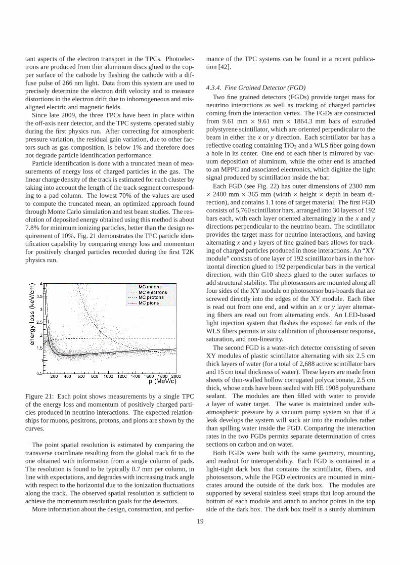
tant aspects of the electron transport in the TPCs. Photoelec-trons are produced from thin aluminum discs glued to the cop-per surface of the cathode by flashing the cathode with a dif-fuse pulse of 266 nm light. Data from this system are used toprecisely determine the electron drift velocity and to measuredistortions in the electron drift due to inhomogeneous and mis-aligned electric and magnetic fields.

Since late 2009, the three TPCs have been in place withinthe off-axis near detector, and the TPC systems operated stablyduring the first physics run. After correcting for atmosphericpressure variation, the residual gain variation, due to other fac-tors such as gas composition, is below 1% and therefore doesnot degrade particle identification performance.

Particle identification is done with a truncated mean of mea-surements of energy loss of charged particles in the gas. Thelinear charge density of the track is estimated for each cluster bytaking into account the length of the track segment correspond-ing to a pad column. The lowest 70% of the values are usedto compute the truncated mean, an optimized approach foundthrough Monte Carlo simulation and test beam studies. The res-olution of deposited energy obtained using this method is about7.8% for minimum ionizing particles, better than the designre-quirement of 10%. Fig. 21 demonstrates the TPC particle iden-tification capability by comparing energy loss and momentumfor positively charged particles recorded during the first T2Kphysics run.

Figure 21: Each point shows measurements by a single TPCof the energy loss and momentum of positively charged parti-cles produced in neutrino interactions. The expected relation-ships for muons, positrons, protons, and pions are shown by thecurves.

The point spatial resolution is estimated by comparing thetransverse coordinate resulting from the global track fit totheone obtained with information from a single column of pads.The resolution is found to be typically 0.7 mm per column, inline with expectations, and degrades with increasing trackanglewith respect to the horizontal due to the ionization fluctuationsalong the track. The observed spatial resolution is sufficient toachieve the momentum resolution goals for the detectors.

More information about the design, construction, and perfor-

mance of the TPC systems can be found in a recent publica-tion [42].

4.3.4. Fine Grained Detector (FGD)

Two fine grained detectors (FGDs) provide target mass forneutrino interactions as well as tracking of charged particlescoming from the interaction vertex. The FGDs are constructedfrom 9.61 mm× 9.61 mm× 1864.3 mm bars of extrudedpolystyrene scintillator, which are oriented perpendicular to thebeam in either thex or y direction. Each scintillator bar has areflective coating containing TiO2 and a WLS fiber going downa hole in its center. One end of each fiber is mirrored by vac-uum deposition of aluminum, while the other end is attachedto an MPPC and associated electronics, which digitize the lightsignal produced by scintillation inside the bar.

Each FGD (see Fig. 22) has outer dimensions of 2300 mm× 2400 mm× 365 mm (width× height× depth in beam di-rection), and contains 1.1 tons of target material. The firstFGDconsists of 5,760 scintillator bars, arranged into 30 layers of 192bars each, with each layer oriented alternatingly in thex andydirections perpendicular to the neutrino beam. The scintillatorprovides the target mass for neutrino interactions, and havingalternatingx andy layers of fine grained bars allows for track-ing of charged particles produced in those interactions. An“XYmodule” consists of one layer of 192 scintillator bars in thehor-izontal direction glued to 192 perpendicular bars in the verticaldirection, with thin G10 sheets glued to the outer surfaces toadd structural stability. The photosensors are mounted along allfour sides of the XY module on photosensor bus-boards that arescrewed directly into the edges of the XY module. Each fiberis read out from one end, and within anx or y layer alternat-ing fibers are read out from alternating ends. An LED-basedlight injection system that flashes the exposed far ends of theWLS fibers permitsin situ calibration of photosensor response,saturation, and non-linearity.

The second FGD is a water-rich detector consisting of sevenXY modules of plastic scintillator alternating with six 2.5cmthick layers of water (for a total of 2,688 active scintillator barsand 15 cm total thickness of water). These layers are made fromsheets of thin-walled hollow corrugated polycarbonate, 2.5 cmthick, whose ends have been sealed with HE 1908 polyurethanesealant. The modules are then filled with water to providea layer of water target. The water is maintained under sub-atmospheric pressure by a vacuum pump system so that if aleak develops the system will suck air into the modules ratherthan spilling water inside the FGD. Comparing the interactionrates in the two FGDs permits separate determination of crosssections on carbon and on water.

Both FGDs were built with the same geometry, mounting,and readout for interoperability. Each FGD is contained in alight-tight dark box that contains the scintillator, fibers, andphotosensors, while the FGD electronics are mounted in mini-crates around the outside of the dark box. The modules aresupported by several stainless steel straps that loop around thebottom of each module and attach to anchor points in the topside of the dark box. The dark box itself is a sturdy aluminum

19

Figure 22: View of an FGD with the front cover removed. XYscintillator modules (green) hang perpendicular to the directionof the neutrino beam. Along the top, six mini-crates with elec-tronics can be seen without their cooling lines, while on theright side the cooling lids covering the mini-crates are shown.

frame that supports the weight of the FGD modules and trans-fers that weight to the detector basket. The walls of the darkboxare made of thin opaque panels to keep its interior light-tight.

The FGD’s front-end electronics resides in 24 mini-cratesthat attach to the outside of the four sides of the dark box. Sig-nals from the photosensors inside the dark box are carried fromthe photosensor bus-boards to the electronics by ribbon cablesthat attach to the crates’ backplanes, which are mounted overcutouts on the four sides of the box. The mini-crates are cooledby a negative-pressure water cooling system running along thesides of the frame of the dark box, and power is carried to themini-crates by a power bus mounted on the frame. The elec-tronics is arranged so that all heat-producing elements arelo-cated outside of the dark box in the mini-crates where they canbe readily cooled by the cooling system, while only elementswith negligible power outputs (the photosensors themselves)are present inside the dark box.

Each mini-crate contains four front-end boards and one cratemaster board (CMB), and can read out 240 photosensors. Thefront-end boards use the “AFTER” ASIC (Section 4.3.3), toshape and digitize high and low attenuation copies of the pho-tosensor signals at 50 MHz, storing the waveform in a 511-deep switched capacitor array. In addition the front-end boardsprovide the photosensor bias voltages and analog trigger prim-itives. Data from each crate is read out over optical fiber linksto data collector cards (DCCs) located outside of the magnet.Slow control systems use a separate data and power bus for re-dundancy.

Figure 23: External view of one ECal module. The scintillatorbars run horizontally inside the module as shown. The readoutelectronics, signal and power cables, and cooling pipes canbeseen mounted on the aluminum plates on the sides of the mod-ule. The gray surface at the top is the carbon fiber sandwichfront plate, which in the final module position is facing towardsthe inner subdetectors (PØD, FGDs and TPCs).

4.3.5. Electromagnetic Calorimeter (ECal)

The ND280 ECal is a sampling electromagnetic calorimetersurrounding the inner detectors (PØD, TPCs, FGDs). It useslayers of plastic scintillator bars as active material withlead ab-sorber sheets between layers, and it provides near-hermetic cov-erage for all particles exiting the inner detector volume. Its roleis to complement the inner detectors in full event reconstructionthrough the detection of photons and measurement of their en-ergy and direction, as well as the detection of charged particlesand the extraction of information relevant for their identification(electron-muon-pion separation). A key function of the ECal isthe reconstruction ofπ0’s produced in neutrino interactions in-side the tracker detectors. In the case ofπ0 production insidethe PØD, the PØD-ECal complements the PØD reconstructionwith information on escaping energy.

The ECal is made of 13 independent modules of three dif-ferent types arranged as in Fig. 16: six Barrel-ECal modulessurround the tracker volume on its four sides parallel to thez (beam) axis; one downstream module (Ds-ECal) covers thedownstream exit of the tracker volume; and six PØD-ECalmodules surround the PØD detector volume on its four sidesparallel to thez axis. Each module is made of consecutive lay-ers of scintillator bars glued to a sheet of lead converter. TheDs-ECal is located inside the basket carrying the inner subde-tectors of the off-axis detector. The other 12 ECal modules aremounted inside of the UA1 magnet. A drawing of a completedmodule is shown in Fig. 23.

All ECal scintillator bars have a 4.0 cm× 1.0 cm cross sec-tion with a 2.0 mm× 3.0 mm elliptical hole running along theirfull length in the middle. The bars were extruded at a dedicatedFermilab facility and the material used was polystyrene doped

20

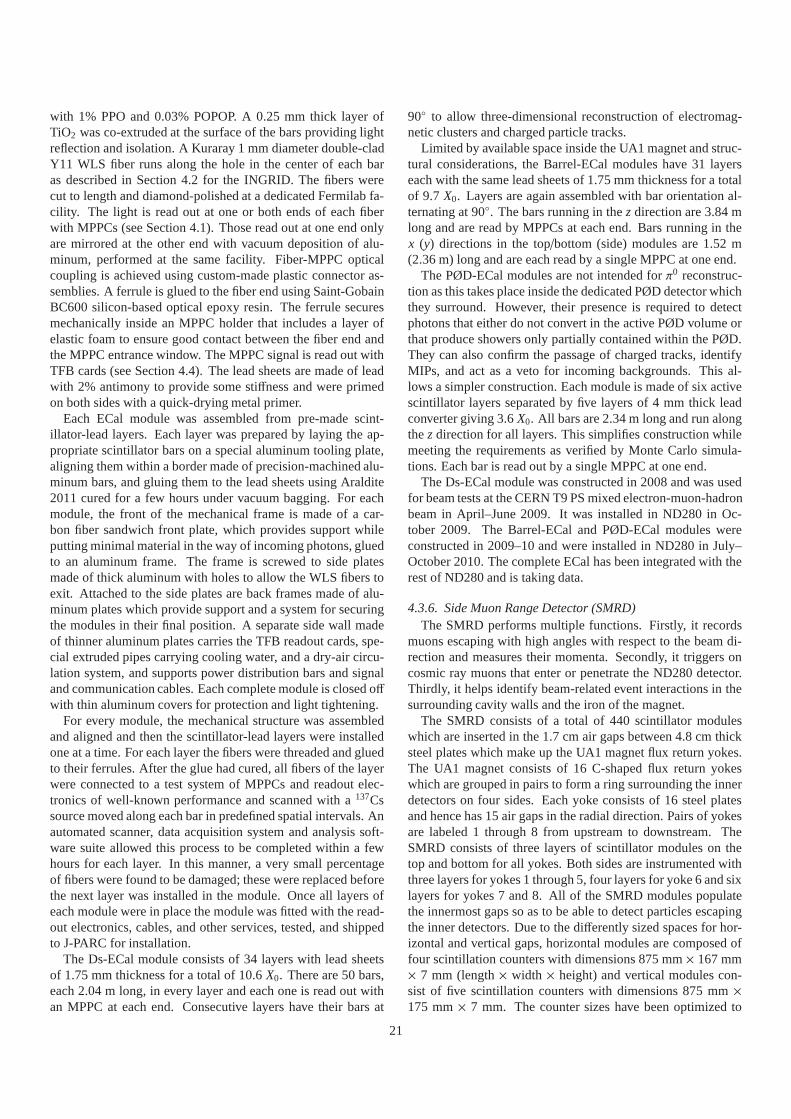
with 1% PPO and 0.03% POPOP. A 0.25 mm thick layer ofTiO2 was co-extruded at the surface of the bars providing lightreflection and isolation. A Kuraray 1 mm diameter double-cladY11 WLS fiber runs along the hole in the center of each baras described in Section 4.2 for the INGRID. The fibers werecut to length and diamond-polished at a dedicated Fermilab fa-cility. The light is read out at one or both ends of each fiberwith MPPCs (see Section 4.1). Those read out at one end onlyare mirrored at the other end with vacuum deposition of alu-minum, performed at the same facility. Fiber-MPPC opticalcoupling is achieved using custom-made plastic connector as-semblies. A ferrule is glued to the fiber end using Saint-GobainBC600 silicon-based optical epoxy resin. The ferrule securesmechanically inside an MPPC holder that includes a layer ofelastic foam to ensure good contact between the fiber end andthe MPPC entrance window. The MPPC signal is read out withTFB cards (see Section 4.4). The lead sheets are made of leadwith 2% antimony to provide some stiffness and were primedon both sides with a quick-drying metal primer.

Each ECal module was assembled from pre-made scint-illator-lead layers. Each layer was prepared by laying the ap-propriate scintillator bars on a special aluminum tooling plate,aligning them within a border made of precision-machined alu-minum bars, and gluing them to the lead sheets using Araldite2011 cured for a few hours under vacuum bagging. For eachmodule, the front of the mechanical frame is made of a car-bon fiber sandwich front plate, which provides support whileputting minimal material in the way of incoming photons, gluedto an aluminum frame. The frame is screwed to side platesmade of thick aluminum with holes to allow the WLS fibers toexit. Attached to the side plates are back frames made of alu-minum plates which provide support and a system for securingthe modules in their final position. A separate side wall madeof thinner aluminum plates carries the TFB readout cards, spe-cial extruded pipes carrying cooling water, and a dry-air circu-lation system, and supports power distribution bars and signaland communication cables. Each complete module is closed off

with thin aluminum covers for protection and light tightening.For every module, the mechanical structure was assembled

and aligned and then the scintillator-lead layers were installedone at a time. For each layer the fibers were threaded and gluedto their ferrules. After the glue had cured, all fibers of the layerwere connected to a test system of MPPCs and readout elec-tronics of well-known performance and scanned with a137Cssource moved along each bar in predefined spatial intervals.Anautomated scanner, data acquisition system and analysis soft-ware suite allowed this process to be completed within a fewhours for each layer. In this manner, a very small percentageof fibers were found to be damaged; these were replaced beforethe next layer was installed in the module. Once all layers ofeach module were in place the module was fitted with the read-out electronics, cables, and other services, tested, and shippedto J-PARC for installation.

The Ds-ECal module consists of 34 layers with lead sheetsof 1.75 mm thickness for a total of 10.6X0. There are 50 bars,each 2.04 m long, in every layer and each one is read out withan MPPC at each end. Consecutive layers have their bars at

90◦ to allow three-dimensional reconstruction of electromag-netic clusters and charged particle tracks.

Limited by available space inside the UA1 magnet and struc-tural considerations, the Barrel-ECal modules have 31 layerseach with the same lead sheets of 1.75 mm thickness for a totalof 9.7 X0. Layers are again assembled with bar orientation al-ternating at 90◦. The bars running in thez direction are 3.84 mlong and are read by MPPCs at each end. Bars running in thex (y) directions in the top/bottom (side) modules are 1.52 m(2.36 m) long and are each read by a single MPPC at one end.

The PØD-ECal modules are not intended forπ0 reconstruc-tion as this takes place inside the dedicated PØD detector whichthey surround. However, their presence is required to detectphotons that either do not convert in the active PØD volume orthat produce showers only partially contained within the PØD.They can also confirm the passage of charged tracks, identifyMIPs, and act as a veto for incoming backgrounds. This al-lows a simpler construction. Each module is made of six activescintillator layers separated by five layers of 4 mm thick leadconverter giving 3.6X0. All bars are 2.34 m long and run alongthez direction for all layers. This simplifies construction whilemeeting the requirements as verified by Monte Carlo simula-tions. Each bar is read out by a single MPPC at one end.

The Ds-ECal module was constructed in 2008 and was usedfor beam tests at the CERN T9 PS mixed electron-muon-hadronbeam in April–June 2009. It was installed in ND280 in Oc-tober 2009. The Barrel-ECal and PØD-ECal modules wereconstructed in 2009–10 and were installed in ND280 in July–October 2010. The complete ECal has been integrated with therest of ND280 and is taking data.

4.3.6. Side Muon Range Detector (SMRD)The SMRD performs multiple functions. Firstly, it records

muons escaping with high angles with respect to the beam di-rection and measures their momenta. Secondly, it triggers oncosmic ray muons that enter or penetrate the ND280 detector.Thirdly, it helps identify beam-related event interactions in thesurrounding cavity walls and the iron of the magnet.

The SMRD consists of a total of 440 scintillator moduleswhich are inserted in the 1.7 cm air gaps between 4.8 cm thicksteel plates which make up the UA1 magnet flux return yokes.The UA1 magnet consists of 16 C-shaped flux return yokeswhich are grouped in pairs to form a ring surrounding the innerdetectors on four sides. Each yoke consists of 16 steel platesand hence has 15 air gaps in the radial direction. Pairs of yokesare labeled 1 through 8 from upstream to downstream. TheSMRD consists of three layers of scintillator modules on thetop and bottom for all yokes. Both sides are instrumented withthree layers for yokes 1 through 5, four layers for yoke 6 and sixlayers for yokes 7 and 8. All of the SMRD modules populatethe innermost gaps so as to be able to detect particles escapingthe inner detectors. Due to the differently sized spaces for hor-izontal and vertical gaps, horizontal modules are composedoffour scintillation counters with dimensions 875 mm× 167 mm× 7 mm (length× width × height) and vertical modules con-sist of five scintillation counters with dimensions 875 mm×175 mm× 7 mm. The counter sizes have been optimized to

21

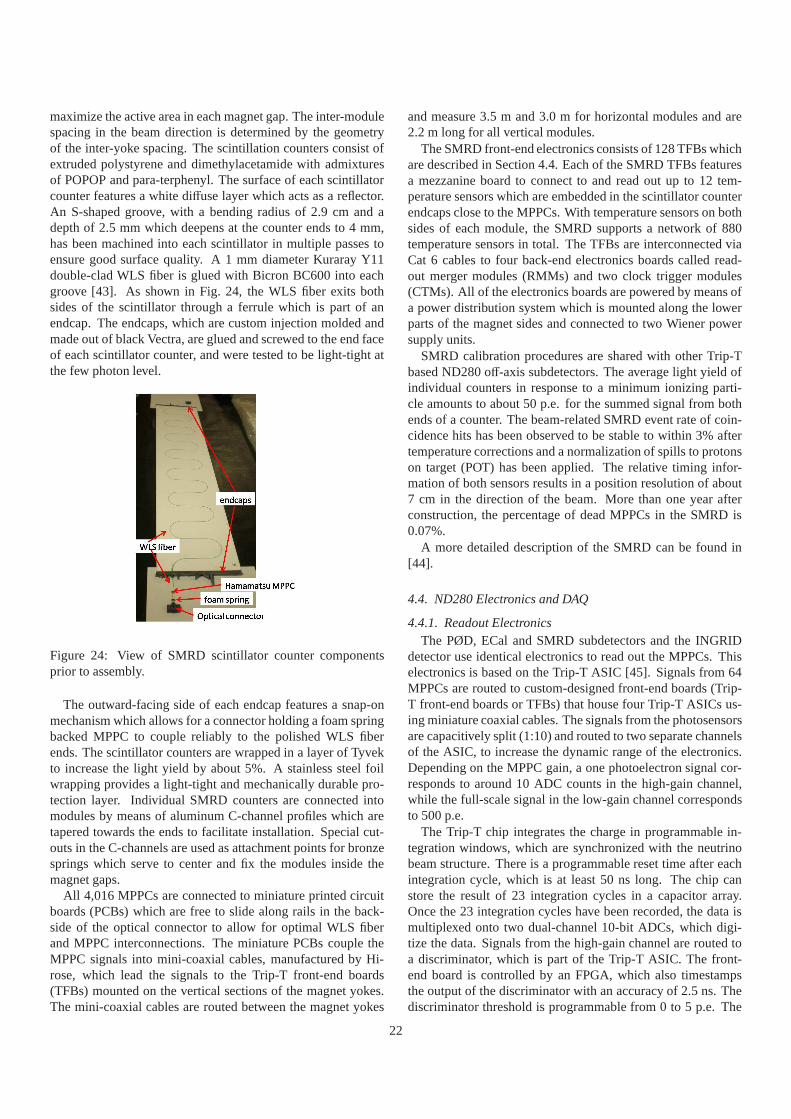
maximize the active area in each magnet gap. The inter-modulespacing in the beam direction is determined by the geometryof the inter-yoke spacing. The scintillation counters consist ofextruded polystyrene and dimethylacetamide with admixturesof POPOP and para-terphenyl. The surface of each scintillatorcounter features a white diffuse layer which acts as a reflector.An S-shaped groove, with a bending radius of 2.9 cm and adepth of 2.5 mm which deepens at the counter ends to 4 mm,has been machined into each scintillator in multiple passestoensure good surface quality. A 1 mm diameter Kuraray Y11double-clad WLS fiber is glued with Bicron BC600 into eachgroove [43]. As shown in Fig. 24, the WLS fiber exits bothsides of the scintillator through a ferrule which is part of anendcap. The endcaps, which are custom injection molded andmade out of black Vectra, are glued and screwed to the end faceof each scintillator counter, and were tested to be light-tight atthe few photon level.

Figure 24: View of SMRD scintillator counter componentsprior to assembly.

The outward-facing side of each endcap features a snap-onmechanism which allows for a connector holding a foam springbacked MPPC to couple reliably to the polished WLS fiberends. The scintillator counters are wrapped in a layer of Tyvekto increase the light yield by about 5%. A stainless steel foilwrapping provides a light-tight and mechanically durable pro-tection layer. Individual SMRD counters are connected intomodules by means of aluminum C-channel profiles which aretapered towards the ends to facilitate installation. Special cut-outs in the C-channels are used as attachment points for bronzesprings which serve to center and fix the modules inside themagnet gaps.

All 4,016 MPPCs are connected to miniature printed circuitboards (PCBs) which are free to slide along rails in the back-side of the optical connector to allow for optimal WLS fiberand MPPC interconnections. The miniature PCBs couple theMPPC signals into mini-coaxial cables, manufactured by Hi-rose, which lead the signals to the Trip-T front-end boards(TFBs) mounted on the vertical sections of the magnet yokes.The mini-coaxial cables are routed between the magnet yokes

and measure 3.5 m and 3.0 m for horizontal modules and are2.2 m long for all vertical modules.

The SMRD front-end electronics consists of 128 TFBs whichare described in Section 4.4. Each of the SMRD TFBs featuresa mezzanine board to connect to and read out up to 12 tem-perature sensors which are embedded in the scintillator counterendcaps close to the MPPCs. With temperature sensors on bothsides of each module, the SMRD supports a network of 880temperature sensors in total. The TFBs are interconnected viaCat 6 cables to four back-end electronics boards called read-out merger modules (RMMs) and two clock trigger modules(CTMs). All of the electronics boards are powered by means ofa power distribution system which is mounted along the lowerparts of the magnet sides and connected to two Wiener powersupply units.

SMRD calibration procedures are shared with other Trip-Tbased ND280 off-axis subdetectors. The average light yield ofindividual counters in response to a minimum ionizing parti-cle amounts to about 50 p.e. for the summed signal from bothends of a counter. The beam-related SMRD event rate of coin-cidence hits has been observed to be stable to within 3% aftertemperature corrections and a normalization of spills to protonson target (POT) has been applied. The relative timing infor-mation of both sensors results in a position resolution of about7 cm in the direction of the beam. More than one year afterconstruction, the percentage of dead MPPCs in the SMRD is0.07%.

A more detailed description of the SMRD can be found in[44].

4.4. ND280 Electronics and DAQ

4.4.1. Readout ElectronicsThe PØD, ECal and SMRD subdetectors and the INGRID

detector use identical electronics to read out the MPPCs. Thiselectronics is based on the Trip-T ASIC [45]. Signals from 64MPPCs are routed to custom-designed front-end boards (Trip-T front-end boards or TFBs) that house four Trip-T ASICs us-ing miniature coaxial cables. The signals from the photosensorsare capacitively split (1:10) and routed to two separate channelsof the ASIC, to increase the dynamic range of the electronics.Depending on the MPPC gain, a one photoelectron signal cor-responds to around 10 ADC counts in the high-gain channel,while the full-scale signal in the low-gain channel correspondsto 500 p.e.

The Trip-T chip integrates the charge in programmable in-tegration windows, which are synchronized with the neutrinobeam structure. There is a programmable reset time after eachintegration cycle, which is at least 50 ns long. The chip canstore the result of 23 integration cycles in a capacitor array.Once the 23 integration cycles have been recorded, the data ismultiplexed onto two dual-channel 10-bit ADCs, which digi-tize the data. Signals from the high-gain channel are routedtoa discriminator, which is part of the Trip-T ASIC. The front-end board is controlled by an FPGA, which also timestampsthe output of the discriminator with an accuracy of 2.5 ns. Thediscriminator threshold is programmable from 0 to 5 p.e. The

22

ADC and timestamp data is assembled by the FPGA and sentto a back-end board for data concentration and buffering. Theoutput from the discriminators is also used to calculate triggerprimitives, which are used to initiate the readout of the detectorfor cosmic ray muons. Monitoring information (mainly tem-perature and voltages) is also recorded by the TFB and asyn-chronously transmitted to the back-end board. More detailsregarding the front-end part of the electronics can be foundin [46].

The back-end of the electronics system consists of readoutmerger modules (RMMs), cosmic trigger modules (CTMs),several slave clock modules (SCMs) and a master clock module(MCM). All the boards were developed at the Rutherford Ap-pleton Laboratory using a common hardware platform, whichhas been built around a high-end Vertex II Pro FPGA from Xil-inx, which is clocked at 100 MHz. The board can drive 14high-speed optical links via its RocketIO and up to 192 LVDSlinks.

The signals from up to 48 TFBs, which are mounted on thedetector and typically less than 1 m away from the photosen-sors, are routed to one RMM via Cat 5e cables. The RMMcontrols the TFBs, distributes the clock and trigger signals andreceives the data after a trigger signal is received by the TFBs.It sends this data asynchronously via a Gigabit Ethernet link to acommercial PC that collects and processes the data. The RMMis equipped with 500 MB DDR2 memory and can buffer up to128 triggers. Each RMM receives trigger and timing signalsfrom the SCMs (see below).

The master clock module receives signals from the acceler-ator that determine when the neutrino spill happens and alsofrom a GPS-based clock. The latter signals are used to syn-chronize the electronics to UTC. The MCM is also connectedto two cosmic trigger modules, which receive signals from upto 192 TFBs or from 48 crate master boards (in the case of theFGD). Based on these signals the CTM will decide whetherthere was a cosmic event in the detector and trigger the read-out. The MCM can also generate pedestal and calibration trig-gers at a programmable rate. All timing and trigger signals aretransmitted via the RocketIO-driven optical link to the slaveclock modules. There is one SCM for each of the subdetectors(SMRD, ECal, PØD, FGD, TPC), which allows the electronicsto be configured for independent operation of each subsystem.The INGRID is operated independently from ND280 and onlyuses one MCM and a single CTM. The general layout of theelectronics has been visualized in Fig. 25.

4.4.2. DAQ and Global Slow ControlThe ND280 data acquisition system has been divided into

two components: DAQ and global slow control (GSC). TheDAQ component takes care of the main data stream, collectingthe data banks from each subdetector front-end system, storingthe data in files and providing online histogramming. The GSCcomponent runs in parallel to the DAQ using the same softwareframework: MIDAS [27].

The ND280 off-axis and INGRID detectors are equippedwith independent DAQ systems which are described in detailin [47]. These have a common architecture and are based on

Figure 25: The general layout of the ND280 electronics.

the MIDAS DAQ framework [27], operating on commerciallyavailable computing hardware running the Scientific Linux op-erating system. MIDAS provides the system with a number ofstandard components necessary for operation and is interfacedto the experimental hardware through custom C/C++ front-endclient applications.

The system architecture is shown in Fig. 26. In both the IN-GRID and off-axis systems the back-end electronics moduleson the Trip-T based subdetectors are interfaced to the DAQby point-to-point optical Gigabit Ethernet links. The MIDASprocesses are distributed across a number of nodes to providethe necessary performance and to allow flexible partitioning ofthe system. An additional MIDAS instance is implemented foreach of the FGDs and TPCs in the off-axis detector system.These assemble data from the respective readout electronics andtransmit it to the global DAQ. A pair of commercial GigabitEthernet switches interconnect the nodes in the DAQ system,providing local infrastructure and data transfer networks. TheDAQ networks are isolated from the main T2K experimentalnetwork by a further node acting as a gateway.

The Trip-T based subdetectors are controlled and read out bythe front-end processor nodes (FPNs), each of which serves upto two back-end boards. The FPN is implemented as three tasksrunning as separate processes, interconnected by shared mem-ory data buffers and communicating via standard inter-processmechanisms. Readout and configuration of the electronics andall connected hardware is provided by the readout task (RXT).The readout is parallelized across electronics boards in a multi-threaded manner and data is buffered for access by the dataprocessing task (DPT). The RXT additionally receives periodicmonitoring data from the TFBs which it passes to the globalslow control. The DPT performs data reduction and basic dataprocessing. It decodes the TFB raw data blocks, associatesamplitude and timing information for individual hits, performspedestal subtraction on a channel-by-channelbasis, applies zerosuppression to the unsparsified data and formats the data foroutput. To preserve monitoring information, the DPT also per-forms per-channel histogramming of signal amplitudes for spe-cific trigger types prior to zero suppression and periodically in-

23

SiP

M 0

SiP

M x

TFB 0

SiP

M 0

SiP

M x

TFB 1

SiP

M 0

SiP

M x

TFB y

RMM 0

SiP

M 0

SiP

M x

TFB 0

SiP

M 0

SiP

M x

TFB 1

SiP

M 0

SiP

M x

TFB y

RMM m

FPN 0 FPN 1 FPN n TPC CascadeFront End

Local Subsystem Backend Nodes

Gigabit Ethernet Switched Backend Network (Copper)

CTM

MCM/SCM

Gigabit Ethernet Off-detector Links(Optical)

DAQ Backend Node

Run Control GUI

Online Monitoring System

OM GUI

Global Slow Control

GSC GUI

Local & Remote Persistent Storage

FGD CascadeFront End

Light Injection Control System

Figure 26: The architecture of the T2K ND280 off-axis andINGRID detectors’ DAQ systems.

serts the histograms into the output data stream. The processedevent fragments are buffered and dispatched to the DAQ back-end by the third process, which implements the MIDAS front-end functionality.

The MIDAS framework provides the core components nec-essary for the DAQ system and is used to gather the event frag-ments from the Trip-T FPNs, and the TPC and the FGD front-ends. An event-building process collects the fragments, per-forms some basic consistency checks and writes the fully as-sembled events to a system buffer for output to a local RAIDarray. A custom archiver process transfers completed files tothe KEK HPSS [48] mass storage facility over the network andadditionally makes a preview copy available to a local semi-offline system for fast-turnaround analysis.

Additional clients are provided to interface the DAQ to thelight injection (LI) hardware for the ECal and PØD subdetec-tors. These configure the LI hardware according to predefinedcalibration sequences and monitor the status of the LI system.This information is provided in real-time to the DPT, where it isused to manage the formation of calibration histograms. A cus-tom online-monitoring server based around the ROOT frame-work retrieves built events from the system buffer and generatesa range of plots for data and detector quality monitoring.

In terms of hardware, the GSC consists of two PCs andtwo network switches connecting to subdetector-specific equip-ment. Front-end tasks running on the GSC PCs or on a subde-tector computer connect to the various equipment of the mag-net and the subdetectors. A central shared memory databasenamed ODB contains the settings and the readback informa-tion from all front-end tasks. This data is in turn stored in aMySQL database at regular intervals. Users interact with theGSC through web pages and can display history plots of any of

the stored variables. Several customized web pages have beendeveloped for controlling the magnet, power supplies, electron-ics parameter settings, and the TPC gas system, or for display-ing detector feedback, such as temperature readings or the PØDwater target levels. Alarms are set up interactively to catch read-back variables going out of range, alerting the shift personaswell as sending messages to remote experts. The GSC systemis the main tool used by the shift person responsible for safetymatters.

The MySQL database containing the GSC information ex-pands at the rate of 0.5 GB per week while taking data. It isan essential element of the calibration process and offline anal-ysis. This database is currently replicated from J-PARC to aserver located at TRIUMF. Thanks to this server, collaboratorscan query the GSC history plots in real-time from a remote lo-cation and can connect to the database from computers and gridsystems all over the world for data processing.

An electronic logbook (Elog) service is used to complementthe GSC system. It runs on a computer in the counting room,with a replica hosted at TRIUMF and is read-write accessibleworldwide, with email capabilities. This provides a recordofeach shift and any maintenance work, and is extremely usefulfor communication of problems between J-PARC shift peopleand remote detector experts.

4.5. ND280 Software and MC Simulation

4.5.1. IntroductionThe ND280 offline software suite consists of about 60 soft-

ware packages totaling over 600,000 lines of original code.Work on the ND280 offline software commenced in 2004 in

order to allow it to be used to aid the early discussions on thedesign of the ND280 detectors. The design principles that havebeen followed include an emphasis on the use of standard par-ticle physics software libraries and conventions where possi-ble, structural modularity, good documentation and openness.Hence ROOT [49] is used for the underlying framework anddata storage model, with Geant4 [50] as the basic simulationli-brary. The CMT [51] software configuration management sys-tem provides the packaging mechanism, with CVS [52] used tostore all versions of the source code files in a repository.

It was anticipated that a large number of physicists, in groupsspread across the nations that form the ND280 Collaboration,would write and maintain the software, so a modular structurewith well-defined interfaces was chosen such that individualcomponents could be developed independently of each other.Approximately 100 collaborators have actively contributed tothe code base as of this writing.

4.5.2. StructureThe general structure of the software suite is indicated in

Fig. 27.The I/O library “oaEvent” defines the file format for the of-

fline software, which is used from the point that the raw MI-DAS [27] data files are converted for offline use, up to theproduction of summarized format files at the end of the chainof processing. It is actively managed to be small and stable.

24

Figure 27: Schematic of the package structure of the ND280Software Suite. Only the most representative packages are in-cluded.

“oaRawEvent” interfaces with the readout data format that isprovided by the DAQ group, and allows the raw MIDAS filesto be read directly by the offline software. Calibration constantsfor the detectors are stored on a centralized MySQL database,and are applied by “oaCalib” and its sub-packages at processingtime. The access routines for the database are based on thosedeveloped for the MINOS experiment.

A representation of the geometry of the detectors is con-structed in Geant4 code, and is converted to ROOT TGeoMan-ager [53] format and stored in version-controlled files. Theseare retrieved from a central repository to be used in the inter-pretation of raw data.

For Monte Carlo simulations, interfaces have been built be-tween the neutrino beam simulation, the neutrino interactiongeneration packages, GENIE [54] and NEUT [55] (see Sec-tion 5.3), and the ND280 software. The neutrino fluxes esti-mated from beam MC are passed through the detector geome-tries, and neutrino cross sections specific to the nuclei presentin the geometries are used to generate interactions that areap-propriate for the distribution of materials in the detector.

Geant4 is used to simulate the energy deposits from the fi-nal state particles that pass through the detector, and the re-sponse of the active detectors (scintillator bars, fibers, MPPCsand electronics, and TPC electron drift and electronics) issim-ulated through custom-written code in the elecSim package.

Individual subdetectors have dedicated packages designedto reconstruct event information internal to them. The Rec-Pack toolkit [56] is used as the framework for event reconstruc-tion across the off-axis detector. It is an independent softwarepackage, but has been developed in close conjunction with theND280 software to meet its needs.

The full event information contained in the oaEvent formatfiles is distilled by the oaAnalysis package into files based on“trees” which are built up from pure ROOT objects. An ac-companying library of analysis tools helps end-users to process

the summarized output using standardized C++ routines andPython macros.

An overall software control package allows for the fully au-tomated running of the software, based on simple configurationfiles which list the inputs and processing steps.

4.5.3. Automated Support ToolsA number of tools have been used by the ND280 software

group to assist in simultaneous code development across a largenumber of packages. The Buildbot software [57] performs au-tomated builds of the full software suite on multiple computingplatforms to test for compilation problems and allow tests to berun. The TUT framework [58] provides a structure for regres-sion tests of code in the low-level packages, to test performanceand compliance to specifications. Also, higher-level validationtests were written in multiple packages, to flag problems thatare introduced during development.

4.5.4. ManagementOne individual acts as the release manager, overseeing the

packages as they are combined to form “releases” several timesa year. In addition to this active management, several toolsareused to assist users in contributing to the overall evolution ofthe software: Bugzilla [59], a widely used management util-ity for tracking the development of software, allows developersand end-users to file bugs and feature requests; ViewVC [60],a browser-based tool to access all past versions of each file thatforms the software suite, tagged with the comments submittedas each change was committed to the repository; and LXR [61],a cross-referenced source code browser.

4.5.5. DocumentationThe Doxygen [62] system is used to generate documenta-

tion from comments that are embedded in the code. An onlineworkbook is also maintained to provide higher-level documen-tation on overall procedures and information for new users ofthe software and developers.

4.5.6. PerformanceFor the dataset from the first data-taking period in 2010, the

neutrino beam events in a single “subrun” file, correspondingto approximately ten minutes of data, take approximately onehour to process fully on a typical CPU.

Fig. 28 shows an event display of an event with a muon trackentering into the PØD and continuing into the tracker (TPC andFGD) region. Multiple secondary particles are produced in theFGD, all of which are finally stopped in the ECal detectors.

This event display illustrates an overall successful perfor-mance of the ND280 off-axis detector system (in terms of bothhardware and software).

4.6. ND280 Data Processing and Distribution

4.6.1. ND280 DataThe ND280 detector produces raw data during normal data

taking on the order of several MB a second. Single raw datafiles are approximately 1 GB in size, and are recorded to disk

25

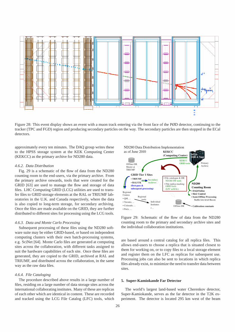
Figure 28: This event display shows an event with a muon trackentering via the front face of the PØD detector, continuing to thetracker (TPC and FGD) region and producing secondary particles on the way. The secondary particles are then stopped in the ECaldetectors.

approximately every ten minutes. The DAQ group writes theseto the HPSS storage system at the KEK Computing Center(KEKCC) as the primary archive for ND280 data.

4.6.2. Data DistributionFig. 29 is a schematic of the flow of data from the ND280

counting room to the end-users, via the primary archive. Fromthe primary archive onwards, tools that were created for theGRID [63] are used to manage the flow and storage of datafiles. LHC Computing GRID (LCG) utilities are used to trans-fer files to GRID storage elements at the RAL or TRIUMF lab-oratories in the U.K. and Canada respectively, where the datais also copied to long-term storage, for secondary archiving.Once the files are made available on the GRID, they are furtherdistributed to different sites for processing using the LCG tools.

4.6.3. Data and Monte Carlo ProcessingSubsequent processing of these files using the ND280 soft-

ware suite may be either GRID-based, or based on independentcomputing clusters with their own batch-processing systems,e.g. SciNet [64]. Monte Carlo files are generated at computingsites across the collaboration, with different tasks assigned tosuit the hardware capabilities of each site. Once these filesaregenerated, they are copied to the GRID, archived at RAL andTRIUMF, and distributed across the collaboration, in the sameway as the raw data files.

4.6.4. File CatalogingThe procedure described above results in a large number of

files, residing on a large number of data storage sites acrosstheinternational collaborating institutes. Many of these arereplicasof each other which are identical in content. These are recordedand tracked using the LCG File Catalog (LFC) tools, which

Figure 29: Schematic of the flow of data from the ND280counting room to the primary and secondary archive sites andthe individual collaboration institutions.

are based around a central catalog for all replica files. Thisallows end-users to choose a replica that is situated closest tothem for working on, or to copy files to a local storage elementand register them on the LFC as replicas for subsequent use.Processing jobs can also be sent to locations in which replicafiles already exist, to minimize the need to transfer data betweensites.

5. Super-Kamiokande Far Detector

The world’s largest land-based water Cherenkov detector,Super-Kamiokande, serves as the far detector in the T2K ex-periment. The detector is located 295 km west of the beam

26

source where it is used to sample the beam’s flavor compo-sition and look forνµ → νe appearance andνµ disappear-ance. Built 1 km deep within the center of Mt. Ikenoyama,Super-Kamiokande is a cylindrical cavern filled with 50 ktonofpure water within which the detector’s roughly 13,000 photo-multiplier tubes (PMTs) image neutrino interactions. Super-Kamiokande has been running since 1996 and has produceddata for a number of well-known results that include world-leading limits on the proton lifetime [65, 66, 67] and themeasurement of flavor oscillations in atmospheric, solar andaccelerator-produced neutrinos [68, 69, 70, 71, 72]. Over thistime there have been four running periods: SK-I, SK-II, SK-III, and SK-IV. The latest period, SK-IV, is still in progress andfeatures upgraded PMT readout electronics. SK-IV is also theperiod in which the T2K experiment takes place.

Because of the detector’s long-running operation, the behav-ior of Super-Kamiokande is well understood. The calibration ofthe energy scale is known to the percent level, and the softwarefor modeling events in the detector matches calibration samplesto the percent level as well.

This section will review the components and operation ofSuper-Kamiokande, describe the upgraded front-end readoutelectronics of the detector, and provide an overview of theMonte Carlo simulation of events in Super-Kamiokande. Fora much more detailed description of the Super-Kamiokande de-tector, refer to [3].

5.1. Super-Kamiokande Detector OverviewThe geometry of the Super-Kamiokande detector consists of

two major volumes, an inner and an outer detector which areseparated by a cylindrical stainless steel structure. Fig.30 givesa schematic of the Super-Kamiokande detector geometry. Theinner detector (ID) is a cylindrical space 33.8 m in diameterand36.2 m in height which currently houses along its inner walls11,129 inward-facing 50 cm diameter PMTs. Enclosing the IDis the outer detector (OD) which is a cylindrical space about2 m thick radially and on the axis at both ends. The OD con-tains along its inner walls 1,885 outward-facing 20 cm diameterPMTs. The ID and OD boundaries are defined by a cylindri-cal structure about 50 cm wide. This structure consists of astainless steel scaffold covered by plastic sheets which serve tooptically separate the ID and OD. The wall facing into the IDis lined with a black sheet of plastic meant to absorb light andminimize the number of photons which either scatter off of theID wall back into the ID volume, or pass through from the ID tothe OD. The walls facing the OD, however, are lined with thehighly reflective material Tyvek®, in order to compensate forthe OD’s sparse instrumentation. With the Tyvek®, photons re-flect off of the surface of the OD walls and have a higher chanceof finding their way to one of the OD PMTs. Finally, within thestainless steel scaffold there is a 50 cm “dead space”, whichcombines with the ID and OD to make Super-Kamiokande atotal of 39 m in diameter and 42 m in height.

The ID is well instrumented, with 40% PMT cathode surfacecoverage, so that there is sufficient spatial resolution to infer anumber of physical quantities from the imaged neutrino inter-actions. The ID is lined with Hamamatsu R3600 hemispheri-

cal PMTs, which feature a combined quantum and collectionefficiency of about 20%. Neutrino interactions often producecharged particles which, if above an energy threshold, producea cone of Cherenkov photons as they traverse the water. Whenthe photons reach the PMTs on the detector walls they producea ring-shaped hit pattern which is used to extract informationabout the interaction such as the event vertex position and mo-menta of product particles.

The primary strategy to measure the flavor composition ofthe T2K neutrino beam at Super-Kamiokande, and thereby ob-serve the oscillation ofνµ to eitherνe or ντ, is to count chargedcurrent quasi-elastic (CCQE) interactions for muon and elec-tron neutrinos, both of which produce leptons of their respec-tive flavor. Muons, counted to measureνµ disappearance, areresilient to changes in their momentum due to their relativelylarge mass. As a result, muons that travel through the detec-tor produce a well-defined cone of Cherenkov radiation whichleads to a clear, sharp ring of PMT hits seen on the detectorwall. In contrast, electrons, used to search forνe appearance,scatter more easily because of their smaller mass and almostalways induce electromagnetic showers at the energies rele-vant to Super-Kamiokande. The result of an electron-inducedshower is a “fuzzy” ring pattern seen by the PMTs, which canbe thought of as the sum of many overlapping Cherenkov lightcones. The routines in the Super-Kamiokande event reconstruc-tion software, sketched out in Section 5.3, use this differencebetween sharp and fuzzy to designate whether the rings imagedin the detector derived from muon-like or electron-like parti-cles.

In contrast to the ID, the OD is only sparsely instrumenteddue to its original purpose as an active veto of cosmic ray muonsand other backgrounds. The PMT array in the OD, made of up611 Hamamatsu R1408 PMTs and 1,274 R5912 PMTs, is capa-ble of an almost 100% rejection efficiency of cosmic ray muonbackgrounds. However, by selecting events in coincidence withthe T2K beam, neutrino-induced events that illuminate the ODcan be efficiently selected from background events. From vol-ume considerations alone, the number of OD events is expectedto roughly equal the number of events in the ID. However, be-cause of the OD’s narrow geometry and sparse instrumentation,the OD lacks spatial and temporal resolution, which preventsdetailed event reconstruction in the OD. Nonetheless, the ODprovides a sample of events which can be categorized into threetypes: events that produced light only in the OD; events whereboth detector segments are illuminated and the particles seemto originate from an interaction vertex inside the ID; and eventswhere both segments are illuminated but the particles seem tooriginate from an interaction vertex outside of the ID.

The detector is calibrated through a number of sources, bothfrom introduced laser light and cosmic ray particles.

5.2. Super-Kamiokande Electronics and DAQ UpgradeIn 2008, the Super-Kamiokande collaboration completed an

upgrade to the detector’s readout electronics [74, 75] betweenthe Super-Kamiokande data-taking periods SK-III and SK-IV.This upgrade introduced a new scheme in the acquisition of hitsfrom the detector’s 13,014 PMTs. In the old system, once the

27

Figure 30: Diagram of the Super-Kamiokande Detector. Thedetector is mainly comprised of two segments, the inner andouter detectors. The boundary between the two segments isdefined by a cylindrical scaffold used to mount photomultipliertubes and optically separate the segments. The figure comesfrom [73].

total number of PMT hits within a 200 ns window exceeded athreshold, a hardware trigger would fire and direct the read-out electronics to record data over a specified time window.However, the old front-end’s data throughput was too low toaccommodate a number of neutrino searches at low threshold,in particular those for solar neutrinos, because the trigger rate atthe required threshold level would overload the front-end elec-tronics. The new upgraded electronics, therefore, includes anew front-end capable of a higher data processing rate. Fur-thermore, it improves upon the triggering method of the oldsystem. In the new system, the arrival time and charge of eachPMT hit is sent to a cluster of PCs that organizes the hit data andsearches for event candidates based on programmable softwaretriggers. The new electronics’ combination of higher through-put and flexible triggers, along with other improvements suchas better impedance matching and a larger front-end dynamicrange, improved Super-Kamiokande’s ability to better accom-modate a larger range of neutrino studies. For example, super-nova relic neutrino searches require not only a lower thresholdbut also a more complicated delayed-coincidence trigger. Thenew electronics is also capable of implementing a coincidencetrigger with a beam arrival time as in the case of the T2K ex-periment.

The new front-end boards are named QBEE which standsfor QTC Based Electronics with Ethernet. The name describesthe units at the start and end of the boards’ signal processingchain. The QTC (Charge to Time Converter) is a custom ASICthat responds to input PMT pulses by producing a square-wavepulse [76]. The front edge of the QTC’s output coincides withthe arrival time of the PMT signal and the length is propor-tional to the integrated charge of the PMT pulse. The outputof the QTC is then fed to a TDC (Time to Digital Converter)that digitizes the QTC pulses’ times and lengths. Finally, thedigitized data from the TDCs is sent to readout PCs using Eth-

ernet technology which provides the needed high rate of datatransfer. Custom-made network interface cards, which trans-fer the data, consist of a TCP/IP firmware, called SiTCP [77],and other interface logic routines that are installed on an FPGAchip. The whole circuit on the QBEE board is able to trans-fer 11.8 MB/s of data according to a test where analog pulsesare sent through the QBEE. This throughput corresponds to aninput pulse rate of 80 kHz/channel and is an order of magni-tude improvement over the old system which had a maximumhit rate of 1.4 kHz/channel. Each QBEE has eight QTC chips,and the whole DAQ system employs 550 QBEE boards whichtogether read out Super-Kamiokande’s 13,014 PMTs and sendtheir hit information to a cluster of online PCs.

The online PCs’ role in the DAQ system is to organize thePMT hit information from the QBEEs and produce data files ofcandidate events which later undergo more offline analysis. ThePCs fall into three groups based on their task. The first groupconsists of 20 “Frontend” PCs. Each PC collects data from 30ID QBEEs (20 OD QBEEs), and then sorts the PMT hit in-formation in order of time. The second group of PCs, called“Mergers”, collects all hits into a time-ordered list of PMThits.They also apply a set of software triggers to select event candi-dates from these lists. There are ten Merger PCs, which eachcollect data from 30 QBEE boards. For each candidate event,a window is defined around the time of the event trigger andall the information for hits falling within that window is sentto a single “Organizer” PC. The Organizer PC collects all ofthe candidate events, eliminating overlaps, and writes them todisk for later offline analysis. During a typical period of de-tector operation, about 470 MB/s of data flows from the Super-Kamiokande PMTs through to the Merger PCs. That stream ofhit information results in a software trigger rate of 3 kHz andeventually 9 MB/s worth of candidate event information beingwritten to disk.

For the T2K experiment, the DAQ system was extended totrigger in time with the beam spills produced by the J-PARCaccelerator. Each beam spill is given a GPS timestamp that ispassed to the online Super-Kamiokande PCs. Each timestampis used to define an additional software trigger that recordsallthe hit information in a 1 ms window around the T2K beamarrival time. These spill events are then collected and writtento disk. Later the events are fed into offline processing whichapplies the usual Super-Kamiokande software triggers usedtosearch for neutrino events, and any candidate events found areextracted for further T2K data analysis.

5.3. Super-Kamiokande Software and MC Simulation

The Super-Kamiokande software can be divided into fourcategories: (1) neutrino event generators, NEUT and GENIE,used to simulate neutrino interactions in the Super-Kamiokandedetector, (2) SKDETSIM, which is responsible for modelingSuper-Kamiokande’s response to particles propagating throughthe detector, (3) the T2K reduction software which selects neu-trino candidate events from detector backgrounds and calibra-tion events, and (4) the Super-Kamiokande event reconstructionlibrary.

28

5.3.1. NEUT Neutrino Event Generator

The first package, NEUT, produces a list of neutrino interac-tions and their product particles from a given neutrino flux andenergy spectrum. Each interaction NEUT generates is the resultof a primary neutrino-nucleon interaction which produces par-ticles that undergo a number of secondary interactions as theypropagate out of the nucleus. The primary interactions includequasi-elastic scattering with both free and bound nucleons, sin-gle meson production, coherent pion production, and deep in-elastic scattering. The secondary interactions are modeled us-ing a particle cascade routine. In the rest of this subsection, aquick overview of the interactions is given. For a more com-plete description of NEUT, including the details on all of theinteractions employed, see [78].

The cross section for CCQE interactions is computed usingone of two different methods depending on whether the scat-tered nucleon is considered free or bound within a nucleus. Forfree nucleons, which in the case of water are the protons inhydrogen, the CCQE cross section is calculated using an ef-fective hadronic current and can be found in [79]. Values forthe form factors in the cross section are taken from experimen-tal data [80, 81]. For interactions on bound nucleons, NEUTfollows the method of [82] for computing the cross section, inwhich the momentum distribution of the nucleons is dictatedbythe Fermi gas model and the outgoing nucleon momentum takesinto account Pauli blocking effects. The Pauli blocking modelis implemented by requiring that the momentum of the recoil-ing nucleon be greater than the Fermi surface momentum. Thisfinal momentum includes the cost of the nucleon first having toescape the nuclear potential, whose values are from [83].

NEUT simulates both incoherent and coherent single pionproduction. Calculation of the incoherent production cross sec-tion follows from the method in [84] in which the decay ofbaryon resonances produces pions. However, NEUT also usesthis method to simulate the production of kaons and etas. Theexcited resonances are restricted to an invariant mass below 2GeV, within which pions make up the majority of the outgo-ing mesons. As for coherent pion production, the calculation ofthe cross section comes from [85]. In this interaction, the neu-trino can be thought of as interacting with the entire nucleus.The result is an enhancement of pion production in the forwarddirection, because with the nucleus much heavier than the neu-trino most of the incoming momentum is carried away by theoutgoing pion.

The deep inelastic scattering (DIS) cross section is computedover an invariant mass energy, W, greater than 1.3 GeV and em-ploys the nucleon structure functions from GRV98 [86], withcorrections suggested by Bodek and Yang. Because a modelof single pion production, described above, is already imple-mented below 2 GeV, the cross section calculation for 1.3 GeV< W < 2 GeV only includes the probability function for pionmultiplicities greater than 1 in order to avoid double-countingof this process. The outgoing particles resulting from the DISinteraction are modeled using PYTHIA/JetSet for interactionswith W above 2 GeV and custom-written routines for interac-tions below 2 GeV. The custom routines were needed because

PYTHIA/JetSet was developed for higher energy interactions.For the interactions below 2 GeV, experimental results are usedto model the DIS event with KNO scaling employed to interpo-late between data points at different values of W [87].

In addition to the primary interactions above, NEUT modelsthe secondary interactions between the nucleus and any prod-ucts of the primary interaction, which include mesons and re-coiling nucleons. For all of the particles, an initial positionof the neutrino interaction in the nucleus is generated in pro-portion to the Woods-Saxon type nucleon density distribution.From there, a cascade model tracks the initial particle and anyof its interaction products out of the nucleus. The interac-tions during the cascade also include the effects of Fermi mo-tion and Pauli blocking. Of all of the particles, the secondaryinteractions for pions are the most important due to both thelarge pion production cross section and the secondary interac-tion cross sections between the pion and the nucleus. Intranu-clear, final state interactions (FSI) of the hadrons produced bythe primary neutrino interaction are simulated by a microscopiccascade model. Forpπ < 500 MeV/c, the mean free pathsfor quasi-elastic scattering, charge exchange and absorption in-teraction channels are calculated by [88], while the scatteringkinematics is determined by [89] with in-medium corrections.For pπ > 500 MeV/c, hadron production is also considered,and the mean free paths for all interactions, as well as thescattering kinematics, are determined from fits to pion-protoncross section data [90]. The model reproduces pion scatteringand photoproduction data for nuclei withA = 12 to 209 [e.g.91, 92, 93, 94, 95]. Secondary interactions for kaons, etas andrecoil nucleons are also modeled by a cascade.

5.3.2. GENIE Neutrino Event Generator

GENIE [54] simulates neutrino interactions, for all neutrinoflavors and all nuclear targets, over the energy range from a fewMeV to several hundred GeV. Over this broad kinematic regimea variety of scattering mechanisms are important.

Charged current quasi-elastic scattering is modeled usinganimplementation of the Llewellyn-Smith model [79]. The vectorform factors are related, via the CVC hypothesis, to electromag-netic form factors measured in electron elastic scattering, withthe BBA2005 form factors [96] used by default. The pseudo-scalar form factor in the Llewellyn-Smith model has the formsuggested by the PCAC hypothesis [79], while the axial formfactor is assumed to have a dipole form. The default quasi-elastic axial vector mass is set to 0.99 GeV/c2 [97].

Neutral current elastic scattering is simulated accordingtothe model described by Ahrens et al. [98]. The axial formfactor is again assumed to have dipole form with the defaultaxial vector mass set to 0.99 GeV/c2. The factorη accountingfor possible isoscalar contributions to the axial current is set toa value of 0.12.

Charged and neutral-current baryon resonance production isdescribed using an implementation of the Rein-Sehgal model[84]. From the 18 baryon resonances of the original paper,GENIE includes the 16 that are listed as unambiguous in thePDG baryon tables [99] and all resonance parameters have been

29

updated. Resonance interference and lepton mass terms are ig-nored in the cross section calculation, although lepton massterms are taken into account in determining the phase spaceboundaries. The default value of the resonance axial vectormass is 1.12 GeV/c2, as determined from global fits [97].

Charged and neutral-current deep inelastic scattering is de-scribed using the effective leading order model of Bodek andYang [100]. The model provides corrections to be applied onthe GRV98 LO parton distributions [86] in order to yield betteragreement with low Q2 electron scattering data. Higher twistand target mass corrections are accounted for through the useof a new scaling variable. The longitudinal structure functionis taken into account using the Whitlow parametrization [101].An overall scale factor of 1.032 is applied to the predictions ofthe Bodek-Yang model to achieve agreement with the measuredvalue of the neutrino cross section at high energy (100 GeV).The same model is extended in the transition region (hadronicinvariant mass below 1.8 GeV/c2) to simulate non-resonancebackgrounds. To avoid double-counting in the transition re-gion, the extrapolated non-resonance background is scaledsothat the sum of the resonance and non-resonance contributionfits exclusive one-pion and two-pion cross section data.

Charged and neutral-current coherent pion production ismodeled using an implementation of the Rein-Sehgal model[85]. The model uses the PCAC form at Q2 and assumesa dipole dependence for non-zero Q2, with an axial mass of1.99 GeV/c2. GENIE uses a recent revision of the Rein-Sehgalmodel [102] where the PCAC formula was updated to take intoaccount lepton mass terms.

Quasi-elastic and deep-inelastic charm production is alsosimulated. Quasi-elastic charm production is simulated usingan implementation of Kovalenko’s local duality inspired model[103] tuned to recent NOMAD data [104]. Deep-inelasticcharm production is modeled according to the Aivazis, Olnessand Tung model [105]. Charm production fractions for neutrinointeractions are taken from [106] and the Peterson fragmenta-tion functions are used [107]. The default value of the charmmass is set to 1.43 GeV/c2.

To calculate neutrino cross sections for scattering off nucleartargets, GENIE employs the impulse approximation. The nu-clear environment is described using a simple Fermi gas modelwith a modification by Bodek and Ritchie to include nucleon-nucleon correlations [108].

Neutrino-induced hadronization is simulated using theAGKY model [109]. At low invariant masses, AGKY uses anempirical model anchored to bubble chamber measurements ofthe average hadronic multiplicity and multiplicity dispersion forneutrino/antineutrino scattering off hydrogen and deuterium.For hadronic invariant masses above 3 GeV/c2, AGKY inte-grates the PYTHIA-6 fragmentation model [110]. There is asmooth transition between the models to ensure continuity ofall simulated observables.

Hadrons produced in the nuclear environment do not im-mediately re-interact with their full cross section. During thetime it takes for quarks to materialize as hadrons, they propa-gate through the nucleus with a dramatically reduced interac-tion probability. This is implemented in GENIE using a step

during which no re-interaction can occur. The step size is de-termined from a formation time of 0.523 fm/c, according to theSKAT model [111].

Once hadrons are fully formed, the effect of nuclear matterin hadron transport is taken into account using a GENIE sub-package called INTRANUKE [112]. INTRANUKE is an in-tranuclear cascade MC which tracks pions and nucleons. Thehadron re-interaction probability is calculated based on the lo-cal density of nucleons [113] and a partial wave analysis of thelarge body of hadron-nucleon cross sections [90]. Once it hasbeen decided that a hadron re-interacts in the nucleus, the typeof interaction is determined based on experimentally measuredcross sections. Where data is sparse, cross section estimates aretaken from calculations of the CEM03 group [114]. A numberof interaction types are simulated: elastic and inelastic scatter-ing, single charge exchange, and pion production and absorp-tion followed by multi-nucleon knockout.

5.3.3. SKDETSIMThe propagation of the particles generated by NEUT across

the Super-Kamiokande detector is handled by SKDETSIM,a program library based on the GEANT3 particle propaga-tion package. For hadronic interactions in water, the CALORphysics package is used because of its success at reproducingpion interactions around 1 GeV [115]. For pions with momen-tum below 500 MeV, however, custom routines have been writ-ten [116]. For the propagation of light in water, SKDETSIMconsiders absorption, Rayleigh scattering, and Mie scatteringas possible interactions. The parameters employed in the modelof these processes have been tuned using a number of laser cal-ibration sources.

The overall agreement for SKDETSIM is checked using anumber of different cosmic ray samples. For example, the re-constructed momentum spectrum of electrons produced fromthe decay of cosmic ray muons is compared to the predictedreconstructed spectrum from SKDETSIM. For all samples, theagreement between data and simulation is within a few percent(Fig. 31).

5.3.4. T2K Data ReductionThe T2K reduction software first selects events tagged with

the T2K beam trigger from the raw data and then categorizesthe beam data into three mutually exclusive samples. Eventsthat are above a certain energy threshold and contain particletracks that originate and terminate within the ID are labeled as“fully contained”, or FC, events. The number of hits seen inthe OD is used to determine whether any particles leave or en-ter the ID, and so the FC events are required to have no morethan 15 hits in the largest OD hit cluster. Those events whichexceed this limit are instead categorized as “outer detector”, orOD, events. Events with energy below the FC energy thresh-old that still display PMT hit patterns suggestive of neutrinointeractions, are classified as ‘low energy”, or LE, events.Af-ter categorization, the reduction software then applies a set ofcuts unique to each sample to remove backgrounds. The eventswhich pass the cuts are used for physics analyses.

30

-8

-6

-4

-2

0

2

4

6

8

102

103

104

105

momentum (MeV/c)

(MC

-DA

TA

)/D

AT

A (

%)

decay electronneutral pionstop muon (sub-GeV)stop muon (multi-GeV)

Figure 31: Comparison between data and the SKDETSIMprediction of the reconstructed momentum of different eventsamples derived from cosmic ray events observed in Super-Kamiokande. For some samples, the comparison is made overdifferent momentum values. ‘Decay Electron’ refers to the re-constructed momentum spectrum of electrons from the decayof cosmic ray muons. ‘Neutral Pion’ is the reconstructed mo-mentum of neutral pions created from atmospheric neutrinos.The ‘Stop Muon’ points indicate the reconstructed momentumof cosmic ray muons which have been determined to stop insidethe inner detector.

5.3.5. Event Reconstruction

The reconstruction of FC and OD events in the detector oc-curs in four stages. First, an initial event vertex is establishedfrom the timing of the PMT hits, and an initial track directionis calculated by searching for a well-defined edge in the PMTcharge pattern. Second, an iterative algorithm utilizes a Houghtransform of the PMT charge distribution to search for Cheren-kov ring candidates. In the third step, a particle identification(PID) algorithm then classifies all the candidate rings observedas either muon-like or electron-like by comparing the observedpattern of charge to an analytically calculated expected patternin the case of muons and an MC-generated expected pattern inthe case of electrons. Finally, the reconstructed momentumforeach particle is determined from the distribution of observedcharge assigned to the particle’s Cherenkov ring. The relation-ship between the observed charge and the particle’s momentumis established using Monte Carlo simulation and detector cali-brations from a number of different sources. More details onthe event reconstruction algorithm can be found in [71].

Fig. 32 shows an event display of two T2K neutrino beaminteraction events. The left display shows a “muon-like” Che-renkov ring with a sharp outer ring edge, which can be com-pared to the right display’s “electron-like” Cherenkov ring withits characteristic fuzzy edges.

These event displays illustrate an overall successful perfor-mance of the Super-Kamiokande detector system (in terms ofboth hardware and software).

6. Conclusion

The T2K experiment, which comprises a new neutrino beam-line and new near detector complex at J-PARC and the up-graded Super-Kamiokande detector, has been constructed suc-cessfully. The construction of the neutrino beamline started inApril 2004. The complete chain of accelerator and neutrinobeamline was successfully commissioned during 2009. T2Kbegan accumulating the neutrino beam data for physics analysisin January 2010. Essentially all components of the experimentperform as expected and there have been no major problems.For example, during the 2010 data taking run, the proportionof good spills for neutrino beams to the total number of spillsdelivered on target was 99.0%. The overall live times of theINGRID detector, the ND280 off-axis detector system and theSuper-Kamiokande detector with regard to the delivered neu-trino beam were 99.9%, 96.7% and 99.9% respectively, demon-strating reliable operation of all of the subcomponents of theT2K experiment.

In this paper, we have described the basic structure and pa-rameters of the detector hardware, electronics, online DAQsys-tem, and offline data reduction and distribution scheme. Moredetailed descriptions of subdetectors can be found in separatepapers, some of which have already been published while oth-ers are being prepared.

AcknowledgmentsThe authors thank the Japanese Ministry of Education, Cul-

ture, Sports, Science and Technology (MEXT) for their supportfor T2K. The T2K neutrino beamline, the ND280 detector andthe Super-Kamiokande detector have been built and operatedusing funds provided by: the MEXT, Japan; the Natural Sci-ences and Engineering Research Council of Canada, TRIUMF,the Canada Foundation for Innovation, and the National Re-search Council, Canada; Commissariat a l’Energie Atomique,and Centre National de la Recherche Scientifique – Institut Na-tional de Physique Nucleaire et de Physique des Particules,France; Deutsche Forschungsgemeinschaft, Germany; IstitutoNazionale di Fisica Nucleare, Italy; the Polish Ministry ofSci-ence and Higher Education, Poland; the Russian Academy ofSciences, the Russian Foundation for Basic Research, and theMinistry of Education and Science of the Russian Federation,Russia; the National Research Foundation, and the MinistryofEducation, Science and Technology of Korea, Korea; CentroNacional De Fısica De Partıculas, Astropartıculas y Nuclear,and Ministerio de Ciencia e Innovacion, Spain; the Swiss Na-tional Science Foundation and the Swiss State Secretariat forEducation and Research, Switzerland; the Science and Tech-nology Facilities Council, U.K.; and the Department of Energy,U.S.A.

We are also grateful to CERN for their generous donation ofthe UA1/NOMAD magnet for our use and their assistance with

31

Super-Kamiokande IVT2K Beam Run 0 Spill 797537

Run 66776 Sub 770 Event 17898767410-05-11:12:14:31

T2K beam dt = 1899.2 ns

Inner: 1332 hits, 3282 pe

Outer: 6 hits, 5 pe

Trigger: 0x80000007

D_wall: 1136.5 cm

mu-like, p = 536.2 MeV/c

Charge(pe) >26.723.3-26.720.2-23.317.3-20.214.7-17.312.2-14.710.0-12.2 8.0-10.0 6.2- 8.0 4.7- 6.2 3.3- 4.7 2.2- 3.3 1.3- 2.2 0.7- 1.3 0.2- 0.7 < 0.2

0

1 mu-edecay

0 500 1000 1500 20000

100

200

300

400

500

Times (ns)

0

1

2

3

4

5

0 500 1000 1500 20000

1

2

3

4

5

OD Times (ns)

(a) muon-like event

Super-Kamiokande IVT2K Beam Run 0 Spill 822275

Run 66778 Sub 585 Event 13422943710-05-12:21:03:26

T2K beam dt = 1902.2 ns

Inner: 1600 hits, 3681 pe

Outer: 2 hits, 2 pe

Trigger: 0x80000007

D_wall: 614.4 cm

e-like, p = 377.6 MeV/c

Charge(pe) >26.723.3-26.720.2-23.317.3-20.214.7-17.312.2-14.710.0-12.2 8.0-10.0 6.2- 8.0 4.7- 6.2 3.3- 4.7 2.2- 3.3 1.3- 2.2 0.7- 1.3 0.2- 0.7 < 0.2

0

0 mu-edecays

0 500 1000 1500 20000

52

104

156

208

260

Times (ns)

0

1

2

3

4

5

0 500 1000 1500 20000

1

2

3

4

5

OD Times (ns)

(b) electron-like event

Figure 32: Example of reconstructed T2K events in Super-Kamiokande for (a) a muon-like ring and (b) an electron-like ring. Bothfigures show the cylindrical detector, unrolled onto a plane. Each colored point represents a PMT, with the color correspondingto the amount of charge, and the reconstructed cone is shown as a white line. The second figure in the upper right corner showsthe same hit map for the OD. The white crosses indicate the location of the reconstructed vertex. The diamond marks the locationwhere a ray starting from the event vertex and heading in the direction of the beam would intersect the detector wall.

the preparation and operation of the magnet; and to DESY fortheir generous donation of the HERA-B magnet movers.

In addition, the participation of individual researchers andinstitutions in the construction of the T2K experiment has beenfurther supported by funds from: the European Research Coun-cil; the Japan Society for the Promotion of Science Fellowshipfor Foreign Researchers program; the U.S. Department of En-ergy Outstanding Junior Investigator (OJI) Program and EarlyCareer program; and the A. P. Sloan Foundation.

The authors also wish to acknowledge the tremendous sup-port provided by the collaborating institutions, including butnot limited to: Ecole Polytechnique – Palaiseau; and the StateUniversity of New York at Stony Brook, Office of the Vice Pres-ident for Research.

References

[1] Letter of intent: Neutrino oscillation experiment at JHF, Let-ter of intent: Neutrino oscillation experiment at JHF, 2003.http://neutrino.kek.jp/jhfnu/loi/loi_JHFcor.pdf .

[2] M. Apollonio, et al., Eur.Phys.J. C27 (2003) 331–374.[3] Y. Fukuda, T. Hayakawa, E. Ichihara, M. Ishitsuka, Y. Itow, et al.,

Nucl.Instrum.Meth. A501 (2003) 418–462.[4] D. Beavis, A. Carroll, I. Chiang, et al., Long Baseline Neutrino Oscil-

lation Experiment at the AGS (Proposal E889), 1995. PhysicsDesignReport, BNL 52459.

[5] J-PARC TDR, KEK-Report 2002-13 and JAERI-Tech 2003-044,http://hadron.kek.jp/~accelerator/TDA/tdr2003/index2.html ,2003.

[6] T. Nakamoto, et al., IEEE Trans. Appl. Supercond. 14 (2004) 616–619.[7] T. Nakamoto, et al. (2005). An invited paper presented atthe 2005 Par-

ticle Accelerator Conference (PAC05), Knoxville, Tennessee, U.S.A.,May 16–20, 2005.

[8] T. Ogitsu, et al., IEEE Trans. Appl. Supercond. 15 (2005)1175–1178.[9] T. Okamura, et al., Applied Superconductivity, IEEE Transactions on 19

(2009) 1125 –1130.

[10] T. Ogitsu, et al., Applied Superconductivity, IEEE Transactions on 19(2009) 1081 –1086.

[11] K. Sasaki, et al., Applied Superconductivity, IEEE Transactions on 20(2010) 242 –245.

[12] T. Nakamoto, et al., Applied Superconductivity, IEEE Transactions on20 (2010) 208 –213.

[13] J.-P. Charrier, T2K MSS, 2009.http://irfu.cea.fr/Phocea/file.php?class=[14] Toshiba Electron Tubes and Devices Co.,Ltd, 2008.

http://www.toshiba-tetd.co.jp/eng/index.htm .[15] T. Nakadaira, et al., AIP Conf. Proc. 981 (2008) 290–292.[16] S. van der Meer (1961). CERN-61-07.[17] R. B. Palmer (1965). Presented at Informal Conference on Experimen-

tal Neutrino Physics, CERN, Geneva, Switzerland, 20–22 Jan1965 (C.Franzinetti, (Ed.), CERN-65-32, pp. 141–146).

[18] K. Matsuoka, et al., Nucl. Instrum. Meth. A623 (2010) 385–387.[19] K. Matsuoka, et al., Nucl. Instrum. Meth. A624 (2010) 591–600.[20] T. Nakamura, et al., Nucl. Instrum. Meth. A556 (2006) 80–86.[21] G. D. Lellis, et al., Nucl. Instrum. Meth. A512 (2003) 539–545.[22] M. Besnier, Reconstruction and analysis of neutrino interactions in

OPERA target emulsion blocks and discrimination of charm backgroundfrom the channelτ → 3h, Ph.D. thesis, Universite de Savoie, 2008.LAPP-T-2008-02.

[23] N. Armenise, et al., Nucl. Instrum. Meth. A551 (2005) 261–270.[24] I. Kreslo, et al., JINST 3 (2008) P04006.[25] T. Higuchi, H. Fujii, M. Ikeno, Y. Igarashi, E. Inoue, etal. (2003)

TUGT004.[26] H. G. Berns, R. J. Wilkes, FADC board for T2K beam monitors,

http://neutrino.phys.washington.edu/~berns/T2K/ADCCARD/adc2_stat

http://neutrino.phys.washington.edu/~berns/T2K/ADCCARD/docs/UWFA

2008.[27] S. Ritt, P. Amaudruz, K. Olchanski, MIDAS (Maximum Integration Data

Acquisition System), 2001.http://midas.psi.ch.[28] M. Clausen, L. Dalesio, ICFA Beam Dyn.Newslett. 47 (2008) 56–66.[29] SAD, Strategic accelerator design, 1986. Developed inKEK,

http://acc-physics.kek.jp/SAD/ .[30] N. Abgrall, et al., Report from the NA61/SHINE experiment at the

CERN SPS, Technical Report CERN-SPSC-2010-025. SPSC-SR-066,CERN, Geneva, 2010.

[31] N. Abgrall, et al., Measurements of Cross Sections and Charged PionSpectra in Proton-Carbon Interactions at 31 GeV/c, 2011. Preprint:

32

CERN-PH-EP-2011-005.[32] FLUKA version 2008.3c, 2008.http://www.fluka.org/fluka.php .[33] GEANT3, A detector description and simulation tool, 1993. Application

Software Group, Computing and Networks Division, CERN, Geneva.[34] D. Renker, E. Lorenz, JINST 4 (2009) P04004.[35] M. Yokoyama, et al., Nucl. Instrum. Meth. A610 (2009) 128–130.[36] M. Yokoyama, et al., Nucl. Instrum. Meth. A622 (2010) 567–573.[37] A. Vacheret, G. Barker, M. Dziewiecki, P. Guzowski, M. Haigh, et al.,

Nucl.Instrum.Meth.A (2011). Preprint: arXiv 1101.1996.[38] A. Pla-Dalmau, Frascati Phys. Ser. 21 (2001) 513–522.[39] F. Moreau, et al., Nucl. Instrum. Meth. A613 (2010) 46–53.[40] A. Pla-Dalmau, A. Bross, V. Rykalin, B. Wood, Nuclear Science Sym-

posium Conference Record 3 (2005) 1298–1300.[41] I. Giomataris, et al., Nucl. Instrum. Meth. A560 (2006)405–408.[42] N. Abgrall, B. Andrieu, P. Baron, P. Bene, V. Berardi, etal., Nucl. In-

strum. Meth. A637 (2011) 25–46.[43] A. Izmaylov, et al., Nucl. Instrum. Meth. A623 (2010) 382–384.[44] SMRD Group, The Side Muon Range Detector (SMRD) in the near de-

tector complex of the T2K experiment, 2011. In preparation.[45] L. Bellantoni, P. Rubinov, Bench test of

first Trip-T prototypes, 2005. D0 note 4845https://plone4.fnal.gov/P1/AFEIIUpgrade/tript/ .

[46] A. Vacheret, S. Greenwood, M. Noy, M. Raymond, A. Weber,in: Nu-clear Science Symposium Conference Record, 2007. NSS ’07. IEEE,volume 3, pp. 1984–1991.

[47] M. Thorpe, et al., in: Proceedings of the 17th IEEE Real Time Confer-ence. To be published.

[48] T. H. Collaboration, High Performance Storage System (HPSS), 2010.http://hpss-collaboration.org .

[49] R. Brun, F. Rademakers, Nucl. Instrum. Meth. A389 (1997) 81–86.[50] S. Agostinelli, et al., Nucl. Instrum. Meth. A506 (2003) 250–303.[51] C. Arnault (2000). Prepared for International Conference on Comput-

ing in High-Energy Physics and Nuclear Physics (CHEP 2000),Padova,Italy, 7-11 Feb 2000.

[52] B. Berliner, J. Polk, Concurrent Versions Systems (CVS), 2001.http://www.cvshome.org .

[53] R. Brun, A. Gheata, M. Gheata, Nucl. Instrum. Meth. A502(2003) 676–680.

[54] C. Andreopoulos, et al., Nucl. Instrum. Meth. A614 (2010) 87–104.[55] Y. Hayato, Acta Phys. Polon. B40 (2009) 2477–2489.[56] A. Cervera-Villanueva, J. J. Gomez-Cadenas, J. A. Hernando, Nucl. In-

strum. Meth. A534 (2004) 180–183.[57] B. Warner, D. Mitchell, Buildbot, 2010.http://buildbot.net.[58] V. Dyuzhev, D. Kononenko, M. Rzechonek, TUT: C++ template unit

test framework, 2009.http://tut-framework.sourceforge.net .[59] T. Weissman, et al., Bugzilla Defect Tracking System, 2010.

http://www.bugzilla.org .[60] B. Fenner, H. Zeller, et al., ViewVC: Web-based versioncontrol reposi-

tory browsing, 2005.http://www.viewvc.org .[61] A. G. Gleditsch, LXR Cross Referencer, 2010.

http://sourceforge.net/projects/lxr .[62] D. van Heesch, Doxygen, 2010.

http://www.stack.nl/~dimitri/doxygen/.[63] I. Bird, (ed.), et al. (2005). CERN-LHCC-2005-024.[64] C. Loken, D. Gruner, et al., Journal of Physics: Conference Series 256

(2010) 012026.[65] M. Shiozawa, et al., Phys.Rev.Lett. 81 (1998) 3319–3323.[66] Y. Hayato, et al., Phys.Rev.Lett. 83 (1999) 1529–1533.[67] H. Nishino, et al., Phys.Rev.Lett. 102 (2009) 141801.[68] Y. Fukuda, et al., Phys.Rev.Lett. 81 (1998) 1562–1567.[69] Y. Fukuda, et al., Phys.Rev.Lett. 82 (1999) 2430–2434.[70] M. Ahn, et al., Phys.Rev. D74 (2006) 072003.[71] Y. Ashie, et al., Phys.Rev. D71 (2005) 112005.[72] J. Hosaka, et al., Phys.Rev. D74 (2006) 032002.[73] Y. Itow, et al., The JHF-Kamioka neutrino project, 2001. ArXiv hep-

ex/0106019.[74] H. Nishino, et al., Nuclear Science Symposium Conference Record,

2007. NSS’07. IEEE 1 (2008) 127–132.[75] S. Yamada, et al., 2009 16th IEEE-NPSS Real Time Conference Poceed-

ings (2009) 201–205.[76] H. Nishino, K. Awai, Y. Hayato, S. Nakayama, K. Okumura,et al.,

Nucl.Instrum.Meth. A610 (2009) 710–717.[77] T. Uchida, M. Tanaka, Nuclear Science Symposium Conference Record,

2006. IEEE 3 (2006) 1411–1414.[78] Y. Hayato, Nucl.Phys.Proc.Suppl. 112 (2002) 171–176.[79] C. Llewellyn Smith, Phys.Rept. 3 (1972) 261–379.[80] H. Grabosch, et al., Z.Phys. C41 (1989) 527.[81] V. Bernard, L. Elouadrhiri, U. Meissner, J.Phys.G G28 (2002) R1–R35.[82] R. Smith, E. Moniz, Nucl.Phys. B43 (1972) 605.[83] F. Brieva, A. Dellafiore, Nucl.Phys. A292 (1977) 445–458.[84] D. Rein, L. M. Sehgal, Ann. Phys. 133 (1981) 79.[85] D. Rein, L. M. Sehgal, Nucl. Phys. B223 (1983) 29.[86] M. Gluck, E. Reya, A. Vogt, Eur. Phys. J. C5 (1998) 461–470.[87] H. Saarikko (1979). Presented at Neutrino ’79, Bergen,Norway.[88] L. Salcedo, E. Oset, M. Vicente-Vacas, C. Garcia-Recio, Nucl.Phys.

A484 (1988) 557.[89] G. Rowe, M. Salomon, R. H. Landau, Phys.Rev. C18 (1978) 584–589.[90] R. A. Arndt, W. J. Briscoe, I. I. Strakovsky, R. L. Workman, M. M.

Pavan, Phys. Rev. C69 (2004) 035213.[91] T. Lee, R. Redwine, Ann.Rev.Nucl.Part.Sci. 52 (2002) 23–63.[92] D. Ashery, I. Navon, G. Azuelos, H. Walter, H. Pfeiffer, et al., Phys.Rev.

C23 (1981) 2173–2185.[93] C. Ingram, P. Gram, J. Jansen, R. Mischke, J. Zichy, et al., Phys.Rev.

C27 (1983) 1578–1601.[94] B. Allardyce, C. Batty, D. Baugh, E. Friedman, G. Heymann, et al.,

Nucl.Phys. A209 (1973) 1–51.[95] J. Arends, J. Eyink, H. Hartmann, A. Hegerath, B. Mecking, et al.,

Z.Phys. A305 (1982) 205.[96] R. Bradford, A. Bodek, H. S. Budd, J. Arrington, Nucl. Phys. Proc.

Suppl. 159 (2006) 127–132.[97] K. S. Kuzmin, V. V. Lyubushkin, V. A. Naumov, Acta Phys. Polon. B37

(2006) 2337–2348.[98] L. A. Ahrens, et al., Phys. Rev. D35 (1987) 785.[99] W. M. Yao, et al., J. Phys. G33 (2006) 1–1232.

[100] A. Bodek, U. K. Yang, J. Phys. G29 (2003) 1899–1906.[101] L. W. Whitlow, S. Rock, A. Bodek, E. M. Riordan, S. Dasu,Phys. Lett.

B250 (1990) 193–198.[102] D. Rein, L. M. Sehgal, Phys. Lett. B657 (2007) 207–209.[103] S. G. Kovalenko, Sov. J. Nucl. Phys. 52 (1990) 934–936.[104] M. Bischofberger, Quasi elastic charm production in neutrino nu-

cleon scattering, Ph.D. thesis, Eidgenoessische Technische HochschuleZuerich (Switzerland), 2005.

[105] M. A. G. Aivazis, F. I. Olness, W.-K. Tung, Phys. Rev. D50 (1994) 3085–3101.

[106] G. De Lellis, F. Di Capua, P. Migliozzi, Phys. Lett. B550 (2002) 16–23.[107] C. Peterson, D. Schlatter, I. Schmitt, P. M. Zerwas, Phys. Rev. D27

(1983) 105.[108] A. Bodek, J. L. Ritchie, Phys. Rev. D24 (1981) 1400.[109] T. Yang, C. Andreopoulos, H. Gallagher, K. Hoffmann, P. Kehayias, Eur.

Phys. J. C63 (2009) 1–10.[110] T. Sjostrand, et al., Comput. Phys. Commun. 135 (2001)238–259.[111] D. Baranov, V. Ermolaev, A. Ivanilov, P. Ivanov, V. Hleborad, et al., PHE

84-04 (1984).[112] S. Dytman, Acta Phys. Polon. B40 (2009) 2445.[113] H. De Vries, C. W. De Jager, C. De Vries, Atom. Data Nucl.Data Tabl.

36 (1987) 495–536.[114] S. G. Mashnik, A. J. Sierk, K. K. Gudima, M. I. Baznat, J.Phys. Conf.

Ser. 41 (2006) 340–351.[115] C. Zeitnitz, T. Gabriel, Nucl.Instrum.Meth. A349 (1994) 106–111.[116] M. Nakahata, et al., J.Phys.Soc.Jap. 55 (1986) 3786.

33