BOBMEX: The Bay of Bengal Monsoon Experiment

2217Bulletin of the American Meteorological Society

1. Introduction

The monsoon governs the very pulse of life on theIndian subcontinent. Understanding and predicting the

variability of the Indian monsoon is, therefore, ex-tremely important for the well-being of over one bil-lion people and the diverse fauna and flora inhabitingthe region. The major thrust of the Indian ClimateResearch Programme (ICRP) is on monsoon variabil-ity, on timescales ranging from subseasonal tointerannual and decadal, and its impact on critical re-sources (DST 1996). The monsoon is strongly coupledto the warm oceans surrounding the subcontinent.Most of the monsoon rainfall occurs in associationwith synoptic-scale systems, that is, the monsoon dis-turbances, which are generated over these waters andmove onto the Indian landmass (e.g., Fig. 1a for themonsoon season of 1999). In particular, the Bay ofBengal (hereafter called the bay) is exceptionally fer-tile, with a very high frequency of genesis of thesesystems (Rao 1976).

The distribution of the summer monsoon (Jun–Sep) rainfall over the Indian region is linked to the

BOBMEX: The Bay of BengalMonsoon Experiment

G. S. Bhat,* S. Gadgil,* P. V. Hareesh Kumar,+ S. R. Kalsi,# P. Madhusoodanan,+

V. S. N. Murty,@ C. V. K. Prasada Rao,+ V. Ramesh Babu,@ L. V. G. Rao,@

R. R. Rao,+ M. Ravichandran,& K. G. Reddy,** P. Sanjeeva Rao,++

D. Sengupta,* D. R. Sikka,## J. Swain,+ and P. N. Vinayachandran*

*Indian Institute of Science, Bangalore, India.+Naval Physical and Oceanographic Laboratory, Kochi, India.#India Meteorological Department, New Delhi, India.@National Institute of Oceanography, Goa, India.&National Institute of Ocean Technology, Chennai, India.**Department of Meteorology and Oceanography, Andhra Uni-versity, Visakhapatnam, India.++Department of Science and Technology, New Delhi, India.##Mausam Vihar, New Delhi, India.Corresponding author address: Sulochana Gadgil, Centre forAtmospheric and Oceanic Sciences, Indian Institute of Science,Bangalore 560 012, India.E-mail: [email protected] final form 15 March 2001.©2001 American Meteorological Society

ABSTRACT

The first observational experiment under the Indian Climate Research Programme, called the Bay of Bengal Mon-soon Experiment (BOBMEX), was carried out during July–August 1999. BOBMEX was aimed at measurements ofimportant variables of the atmosphere, ocean, and their interface to gain deeper insight into some of the processes thatgovern the variability of organized convection over the bay. Simultaneous time series observations were carried out inthe northern and southern Bay of Bengal from ships and moored buoys. About 80 scientists from 15 different institu-tions in India collaborated during BOBMEX to make observations in most-hostile conditions of the raging monsoon.In this paper, the objectives and the design of BOBMEX are described and some initial results presented.

During the BOBMEX field phase there were several active spells of convection over the bay, separated by weakspells. Observation with high-resolution radiosondes, launched for the first time over the northern bay, showed thatthe magnitudes of the convective available potential energy (CAPE) and the convective inhibition energy were com-parable to those for the atmosphere over the west Pacific warm pool. CAPE decreased by 2–3 kJ kg−1 following con-vection, and recovered in a time period of 1–2 days. The surface wind speed was generally higher than 8 m s−1.

The thermohaline structure as well as its time evolution during the BOBMEX field phase were found to be differentin the northern bay than in the southern bay. Over both the regions, the SST decreased during rain events and in-creased in cloud-free conditions. Over the season as a whole, the upper-layer salinity decreased for the north bay andincreased for the south bay. The variation in SST during 1999 was found to be of smaller amplitude than in 1998.Further analysis of the surface fluxes and currents is expected to give insight into the nature of coupling.

2218 Vol. 82, No. 10, October 2001

variation of the convection over the bay (Gadgil 2000).For example, during the summer monsoon of 1998, theconvection over the northern bay was anomalouslylow, with occurrence of relatively few systems,whereas a large number of systems formed over thesouthern parts of the bay. Thus the anomalies of theoutgoing longwave radiation (OLR) were positiveover the northern bay and negative over the southernbay (e.g., Fig. 1b for Jul 1998). Most of these systemsmoved from the southern bay onto and across thesouthern peninsula. The rainfall anomalies were, there-fore, positive over the southern peninsula. Large defi-cits occurred in the north, particularly over the eastcoast of India, adjacent to the northern parts of the bay(e.g., Fig. 1b). The 1998 season was not an exceptionalone in the distribution of rainfall anomalies over theIndian region; in fact, a similar pattern occurred in 2000.

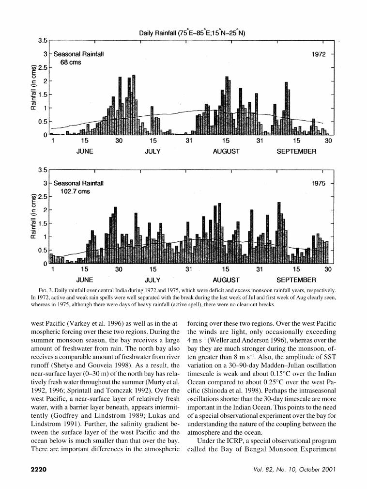
Summer monsoon rainfall over the Indian regionexhibits strong variability on intraseasonal timescalesinvolving a 10–20-day westward propagating mode(Krishnamurti and Bhalme 1976; Krishnamurti andArdunay 1980) and a 30–50-day northward propagat-ing mode (Sikka and Gadgil 1980; Yasunari 1981).The northward propagations over the bay are clearlyseen in Fig. 2, which depicts the variation of micro-wave sounding unit (MSU) precipitation during thesummer of 1986. The major subseasonal variation ofthe monsoon rainfall can be viewed as alternatingactive spells and weak spells or breaks (Fig. 3). Activespells are characterized by high frequency of genesisof synoptic-scale systems over the bay, which propa-gate onto and produce widespread rainfall on the sub-continent; whereas there is a paucity of synopticsystems over central India during a break spell of themonsoon. Revival of the Indian rainfall from mon-soon breaks occurs either with the westward propa-gation of a disturbance generated over the north bay(in association with the 10–20-day mode) or north-ward propagation of the tropical convergence zone(TCZ) generated over the equatorial Indian Oceanacross the bay and Arabian Sea (in association withthe 30–50-day Madden–Julian mode). Thus, convec-tion over the bay plays an important role in the varia-tion of synoptic-scale systems as well as in theintraseasonal variation in which these systems areembedded. Interannual variation of the monsoon isstrongly linked to the intraseasonal variation, withpoor monsoon seasons characterized by long breaks(e.g., Fig. 3). Clearly, for understanding variations ofthe monsoon over the Indian subcontinent onintraseasonal as well as interannual timescales, it is

(a)

(b)

FIG. 1. (a) Tracks of monsoon lows and depressions for themonsoon season of 1999. Monsoon lows and depressions are syn-optic-scale systems and identified in a surface pressure chart byone, and two to three closed contours (at 2-mb interval), respec-tively. (b) OLR anomalies (W m−2) over the Bay of Bengal andrainfall anomalies (% of average) over the Indian subcontinentduring Jul 1998. Deficit convection (positive OLR anomalies)over the ocean and deficit rainfall (negative rainfall anomalies)over land are marked by red, and greenish yellow refers to nor-mal or above normal convection/precipitation.


important to understand processes that determine thevariability of organized convection over the bay.

The intraseasonal variation over the bay is clearlybrought out in the observed SST and wind speed froma moored buoy and Indian National Satellite System(INSAT) OLR (outgoing longwave radiation) dataduring July–August 1998 (Fig. 4). It is seen that thedominant timescale of variation of OLR, wind speed,and SST is intraseasonal, with the maxima–minimaseparated by about 1 month. During this 2-monthperiod, three spells of low OLR were observed. Theamplitude of variation of SST can be about 2°C in thenorth bay (Fig. 4a). The amplitude and timescales ofvariation in SST appear to be comparable to those inthe equatorial west Pacific Ocean (Anderson et al.1996). The phases with decreasing (increasing) OLRare generally associated with decreasing (increasing)SST, with changes in OLR leading those in SST by afew days. Sengupta and Ravichandran’s (2001) studyhas shown that the net heat flux into the ocean is nega-tive in the active phase of convection and positive inthe weak phase of convection in the bay; the observed

SST changes in these phases appear to be largely dueto a direct response to the changes in net heat flux.

Earlier studies suggest that atmospheric conditionshave a significant impact on the SST of the bay.However, the extent to which variation of SST modu-lates the convection over the bay is not known. Theproblem is complex because the SST of the bay isabove the convection threshold of 27.5°C (Gadgil et al.1984; Graham and Barnett 1987) throughout the sum-mer. Understanding the nature of the feedbacks be-tween the atmospheric convection and surfaceconditions of the bay is important for understandingthe variability of convection over the bay. A major in-ternational program, the Tropical Ocean Global Atmo-sphere Coupled Ocean–Atmosphere ResponseExperiment (TOGA COARE), aimed at elucidatingthe coupling of the west Pacific warm pool to the at-mosphere (Webster and Lukas 1992), has given con-siderable insight into ocean–atmosphere coupling onintraseasonal timescales (Godfrey et al. 1998; Shinodaet al. 1998). However, there are important differencesbetween the thermohaline structure of the bay and the

FIG. 2. Variation of rainfall measured by MSU over the 90°–92.5°E longitudinal belt during the summer monsoon of 1986.(Courtesy J. Srinivasan.)

2220 Vol. 82, No. 10, October 2001

west Pacific (Varkey et al. 1996) as well as in the at-mospheric forcing over these two regions. During thesummer monsoon season, the bay receives a largeamount of freshwater from rain. The north bay alsoreceives a comparable amount of freshwater from riverrunoff (Shetye and Gouveia 1998). As a result, thenear-surface layer (0–30 m) of the north bay has rela-tively fresh water throughout the summer (Murty et al.1992, 1996; Sprintall and Tomczak 1992). Over thewest Pacific, a near-surface layer of relatively freshwater, with a barrier layer beneath, appears intermit-tently (Godfrey and Lindstrom 1989; Lukas andLindstrom 1991). Further, the salinity gradient be-tween the surface layer of the west Pacific and theocean below is much smaller than that over the bay.There are important differences in the atmospheric

forcing over these two regions. Over the west Pacificthe winds are light, only occasionally exceeding4 m s−1 (Weller and Anderson 1996), whereas over thebay they are much stronger during the monsoon, of-ten greater than 8 m s−1. Also, the amplitude of SSTvariation on a 30–90-day Madden–Julian oscillationtimescale is weak and about 0.15°C over the IndianOcean compared to about 0.25°C over the west Pa-cific (Shinoda et al. 1998). Perhaps the intraseasonaloscillations shorter than the 30-day timescale are moreimportant in the Indian Ocean. This points to the needof a special observational experiment over the bay forunderstanding the nature of the coupling between theatmosphere and the ocean.

Under the ICRP, a special observational programcalled the Bay of Bengal Monsoon Experiment

FIG. 3. Daily rainfall over central India during 1972 and 1975, which were deficit and excess monsoon rainfall years, respectively.In 1972, active and weak rain spells were well separated with the break during the last week of Jul and first week of Aug clearly seen,whereas in 1975, although there were days of heavy rainfall (active spell), there were no clear-cut breaks.


(BOBMEX) was conducted during July–August1999. BOBMEX was aimed at collecting critical dataon the subseasonal variation of important variablesof the atmosphere, ocean, and their interface to gaindeeper insight into some of the processes that governthe variability of organized convection over the bayand its impact. About 80 scientists from 15 differentinstitutions in India collaborated during BOBMEX tomake observations in the hostile conditions of themonsoon. This paper is written with a view to intro-ducing BOBMEX to the international scientific com-munity and presenting a few initial results. Severalquestions raised by the preliminary analysis ofBOBMEX data are being addressed at present withdetailed investigations. We expect BOBMEX obser-vations to complement the observations from the pi-lot study for the Joint Air–Sea Monsoon InteractionExperiment carried out in the southern Bay of Ben-gal during May–June and September 1999 (Websteret al. 2000, manuscript submitted to Bull. Amer.Meteor. Soc.).

We briefly discuss the background in the next sec-tion, and the scientific objectives and the design of theexperiment in section 3. In section 4, the sensors,instruments, and the observations during the inter-comparison experiments are briefly described. Weconsider the general features of the variation of con-vection and the surface variables over the bay duringBOBMEX in section 5. Some results from the obser-vations of the atmosphere and ocean are presented insections 6 and 7, respectively, and concluding remarksin section 8.

2. Background

a. Earlier observational experimentsTwo major international observational experiments

were conducted over the bay in the 1970s, namely,MONSOON-77 and MONEX-79. MONSOON-77involved four Soviet Union (USSR) ships forming apolygon over the bay centered at 17°N, 89°E during11–19 August 1977. A trough formed in the north bayon 16 August and developed into a depression on19 August. During MONEX-79 (Fein and Kuettner1980), four USSR ships and upper ocean current metermoorings formed a stationary polygon centered at16.2°N, 89.5°E during 11–24 July 1979. In addition,data were collected with dropwindsondes fromaircrafts. This period happened to be a weak phase ofconvection over the bay, and hence disturbed condi-

tions could not be studied. Apart from these two ma-jor experiments, observations from a ship were madeat 20°N, 89°E during 18–31 August and 9–19 Sep-

(a)

(b)

FIG. 4. Variation of INSAT OLR and SST from moored buoysduring Jul–Aug 1998 (after Premkumar et al. 2000). (a) North bay(18°N, 88°E). Wind speed (3-m height) from the buoy is alsoshown. (b) South bay (13°N, 87°E).

2222 Vol. 82, No. 10, October 2001

tember 1990, coinciding with the Monsoon TroughBoundary Layer Experiment (MONTBLEX-90) car-ried out over the northern plains of the Indian subcon-tinent (Goel and Srivastava 1990).

The differences in the horizontal wind fields, ver-tical velocity, and large-scale heat and moisture bud-gets between disturbed and undisturbed conditions inthe bay were studied by analysis of these data (e.g.,Mohanty and Das 1986). Studies based on the datafrom these experiments suggest that the genesis of thesynoptic-scale systems occurs over regions of the baywith high SST and high heat content in the surfacelayer (Rao et al. 1987; Sanil Kumar et al. 1994). Theimpact of the synoptic-scale systems on the ocean be-neath was found to be a decrease in SST that can beas large as 2°–3°C for the most intense systems (Rao1987; Gopalakrishnan et al. 1993). Observations dur-ing MONTBLEX-90 indicated that SST decreased by0.2°–0.3°C for weaker systems (Murty et al. 1996;Sarma et al. 1997). The SST increases after the sys-tem attenuates or moves away. The timescale for thisrecovery was about a week for the systems observedduring MONEX-79 (Rao 1987; Gopalakrishna et al.1993).

b. New observations requiredPrevious observational experiments (MONEX-79,

in particular) have contributed to our knowledge of thelarge-scale features of the Indian summer monsoon(Krishnamurti 1985). However, detailed observationsfor studying the vertical structure of the atmosphere,ocean, and their interface during all phases of convec-tion were not available for the bay. Further, allcomponents of the surface fluxes have not been di-rectly measured over the north bay previously.Accurate measurements of surface fluxes over thewest Pacific have led to realistic simulations of SSTwith ocean mixed layer models (Anderson et al. 1996).The summer mean surface salinity in the north bay isvery low (Levitus and Boyer 1994) and SSTs are high.It is likely that the high upper ocean stability in thisregion (Rao et al. 1993) is responsible for the persis-tent high SST. The upper ocean processes in the pres-ence of strong monsoonal winds and low surfacesalinity need to be understood. Therefore, it is impor-tant to measure heat and freshwater fluxes over the baywith sufficient accuracy, along with upper ocean tem-perature and salinity profiles. Within the bay, thereare marked variations in the freshwater flux betweenthe northern and southern parts. Hence, measurementsof fluxes in each of these regions are required.

Variation of convection in the atmosphere dependsupon dynamics as well as thermodynamics. There isconsiderable understanding of the structure and dy-namics of the synoptic-scale systems over the bay(e.g., Rao 1976; Sikka 1977). However, there have notbeen many detailed observations of the vertical struc-ture of the atmosphere over the bay using high-resolution radiosondes. Hence, the variation in thestability of the atmosphere and its links with variationin convection are yet to be elucidated. We expect feed-backs between convection and the thermodynamics toplay an important role in determining variation of con-vection (Emanuel 1994, chapter 15). A critical param-eter for atmospheric convection is the convectiveavailable potential energy (CAPE), a measure of thevertical instability of the atmosphere under moist con-vection (Moncrief and Miller 1976). CAPE is the workdone by the buoyancy force on a parcel lifted throughthe atmosphere moist adiabatically and is given by(e.g., Williams and Renno 1993)

CAPE = vp ve

LFC

LNB

− −( )∫ T T R d pD (ln ), (1)

where RD is the gas constant of dry air; T

vp and T

ve,

are, respectively, the virtual temperatures of the par-cel and the environment at pressure p; and LFC andLNB are levels of free convection and neutral buoy-ancy, respectively. Deep clouds can develop by theascent of air from a given level only if its CAPE isgreater than zero. When disturbances occur, precipi-tation, strong winds, and downdrafts decrease the en-ergy of the air near the surface, while deep cloudactivity makes the upper troposphere warmer. As aresult, the atmosphere becomes less unstable andCAPE is substantially reduced during disturbances(Emanuel 1994, chapter 15). When disturbances at-tenuate, the air–sea fluxes increase the energy of thesurface air, while the temperature of the air aloft de-creases because of radiative cooling. These factorsdestabilize the atmosphere and build up CAPE. Theperiod between successive disturbances is expected todepend upon the time it takes for the CAPE to buildup. How the instability builds up, the changes that takeplace with the growth/arrival of monsoon distur-bances, how much instability is consumed, and themanner in which it recovers after the disturbance arethe basic issues that are yet be understood for the bay.It is also important to understand if there are any criti-cal values of the height of the atmospheric boundary


layer and air properties (such as moist static energyand equivalent potential temperature) vis-à-vis thethermal stratification of the atmosphere above, for theonset of convection.

Normally air is not saturated to start with and a fi-nite vertical displacement (a few hundred meters to afew kilometers) is needed for the rising air parcel tobecome saturated and reach the level of free convec-tion. Some energy is required for this process, and iscalled convection inhibition energy [CINE, after Wil-liams and Renno (1993)]. CINE is calculated from theintegral (Williams and Renno 1993)

CINE = vp ve

LFC

T T R d pD

pi

−( )∫ (ln ), (2)

where pi is the parcel’s starting pressure level. It is

expected that a larger value of CINE means an in-creased barrier to convection. If CINE is large, deepclouds will not develop even if CAPE is positive.While low values of CINE imply a favorable condi-tion for convection, the critical value of CINE abovewhich convection cannot occur has not been estab-lished. For the estimation of CAPE and CINE, tem-perature and humidity data with high verticalresolution are required. Such data were not availablefor the atmosphere over the north bay, prior toBOBMEX.

3. Scientific objectives and design of theexperiment

A study of the impact of convection on the ocean,the recovery/changes after the convection attenuatesand/or moves away, and the characteristics duringcalm phases when convection is absent for severaldays was envisaged. The emphasis of BOBMEX wason collecting high quality data during different phasesof convection over the bay, which can give insight intothe nature of coupling between the convective systemsand the bay.

In brief, the scientific objectives of BOBMEXwere to document and understand, during differentphases of convection, the variations of (i) the verticalstability of the atmosphere and the structure of the at-mospheric boundary layer, (ii) fluxes at the surfacesof the ocean, and (iii) the thermohaline structure andthe upper ocean currents.

Experiment designIn this first major Indian experiment, it was not

possible to deploy as large a number of observationplatforms as we would have liked. The two deepmoored buoys that provided valuable data during themonsoon of 1998 were stolen a few months before theexperiment. Since buoy data are a critical componentof BOBMEX, new buoys were installed in the north-ern and southern bay (henceforth referred to as DS4and DS3, respectively) during the initial phase ofBOBMEX (Fig. 5a). In addition, RV Sagar Kanya(SK), a research vessel belonging to the Department of

(a)

(b)

FIG. 5. (a) Cruise tracks, time series observation stations (TS1and TS2), and buoy locations (DS3 and DS4) in the Bay of Ben-gal during BOBMEX. Period: 16 Jul–30 Aug 1999. SK, RV SagarKanya; SD, INS Sagardhwani. Observation positions: TS1, 13°N,87°E; TS2, 17.5°N, 89°E; DS3, 13°N, 87°E; and DS4, 18°N,88°E. (b) The RV Sagar Kanya. The boom and manual surfacemeteorological observation (metkit) positions are indicated.

2224 Vol. 82, No. 10, October 2001

Ocean Development, and INS Sagardhwani (SD), ofthe Naval Physical and Oceanographic Laboratory ofthe Defence Research and Development Organisation,were deployed. The India Meteorological Departmentorganized special observations from coastal and islandstations.

The timescales of intraseasonal variation are of theorder of 3–4 weeks for the bay (Fig. 4). The time se-ries from the earlier observational experiments weretoo short to reveal variations on these supersynopticscales. Hence, it was decided to aim for time seriesobservations for about 6 weeks. Two locations—oneeach in the southern and northern bay—were chosenfor the time series observations (henceforth referredto as TS1 and TS2, respectively; see Fig. 5a). Thechoice of these two locations was based on the follow-ing consideration. The occurrence of organized con-vection is high at both the locations. During thenorthward propagation of the tropical convergencezone the systems tend to move across the bay fromsouth to the north (Sikka and Gadgil 1980). Therefore,it is important to document the gradients in atmo-spheric variables and SST between these two regions.Also, there are marked differences in the freshwaterfluxes at these two locations and hence in the thermo-haline structure of the upper layers of the ocean. Thedifferences, if any, in the response of the ocean to con-vection at these locations could provide further insightinto coupling. In fact, the choice of the location of thebuoys was based on a similar rationale. The locationsof the research ships for time series observations were

chosen to be close to the buoys so that reliability ofthe observations from two independent platformscould also be assessed. The cruise tracks of the twoships and buoy locations are also shown in Fig. 5a.In addition to the observations at stationary positionsin the northern and southern bay, observations weremade along zonal sections when the ships made portcalls (at Paradip and Chennai) and north–south sec-tions at the beginning and the end of the experiment(Fig. 5a).

Measurements of all components of surface fluxes,including radiation; the vertical profiles of atmo-spheric temperature, humidity, and winds; and oceantemperature, salinity, and current profiles wereplanned from both the ships.

4. Sensors, instruments, andintercomparison

The basic surface meteorological variables mea-sured were wind (speed and direction), temperature(dry bulb, wet bulb, and sea surface), humidity, pres-sure, radiation, and precipitation. In order to calculatethe fluxes by direct methods, wind velocity, tempera-ture, humidity, and ship acceleration and tilt weremeasured using fast response sensors at 10 Hz. Themajor meteorological sensors and instruments used onthe ships and buoys are listed in Table 1. The loca-tion of the boom and manual (metkit) observation po-sition on the Research Vessel SK are shown in Fig. 5b.

Hand-held cup Deck (~14 m) Ogawaseiki, Japan — b 3 hSK anemometer

(metkit),

sonic anemometer, Boom (~11.5 m) Metek, Germany 0.1 m s−1 1 min Continuous, 0.1 Hz

Wind Gill anemometer Boom (~11.5 m) R. M. Young, U.S.A. 0.2 m s−1 1 min Continuous, 0.1 Hz

SD Hand-held Deck (~10 m) — — b 3 hcup anemometer

DS3 Cup anemometer Tower (3 m) Lambrecht 1.5% FS 10 minc 3 h

TABLE 1. Major meteorological sensors/instruments operated during BOBMEX.

Plat- Averaging SamplingParameter form Sensor/instrument Locationa Make Accuracy time interval

aNumbers inside the parentheses are approximate heights above the sea surface.bThe hand-held instruments were typically exposed for 3 min.cFrom samples collected at 1 Hz.


aNumbers inside the parentheses are approximate heights above the sea surface.bThe hand-held instruments were typically exposed for 3 min.cFrom samples collected at 1 Hz.

Hg in glass Deck (~14 m) — 0.25°C b 3 hthermometer

SK (metkit),

Sonic anemometer, Boom (11.5 m) Metek 0.1°C 1 min Continuous, 0.1 HzPlatinum resistance Boom (11.5 m) R. M. Young 0.3°C 1 min Continuous, 1 Hz

Temperature thermometer

SD Metkit, Hg in Deck — 0.5°C 3 hglass thermometer

DS3 Platinum resistance Tower (3 m) Omega Eng. 0.1°C 10 minc 3 hthermometer

Pressure SK Pressure gauge Met lab — 0.5 hPa — 3 h

SD Pressure gauge Met lab — 0.5 hPa — 3 h

DS3 Capacitor film — Vaisala 0.1 hPa — 3 h

Psychrometer Deck (14 m) IMD — — 3 h

SK Humicap Boom (11.5 m) R. M. Young 2% 1 min Continuous, 1 Hz

Relative IR hygrometer Boom (11.5 m) Applied Technology 0.5 gm m−3 1 min Continuous, 0.1 Hzhumidity

SD Psychrometer Deck (11.5 m) — — — 3 h

SK Automatic rain Open space R. M. Young 1 mm 1 min Continuous, 1 HzPrecipitation gauge

SD Automatic rain Open space R. M. Young 1 mm 1 min Continuous, 1 Hzgauge

Acceleration SK Three-axis Sonic Crossbow 0.05 m s−2 0.1 s Continuous, 0.1 Hztilt accelerometer anemometer Technology Inc.

SK Two-axis tiltmeter Sonic Crossbow 0.5° 0.1 s Continuous, 0.1 Hzanemometer Technology Inc.

SK Spectral Gymbal Eppley, U.S.A. 1 min Continuous, 1 Hzpyranometer (incoming) ~10 W m−2

Boom Eppley 1 min Continuous, 1 Hz(outgoing)

SD Pyranometer Boom/deck Kipp and Zonen ~10 W m−2 5 min Continuous

IR radiometer Gymbal Eppley 1 min Continuous, 1 HzSK (incoming) ~10 W m−2

Boom (outgoing) Eppley 1 min Continuous, 1 Hz

SD Pyrgeometer Boom/deck Kipp and Zonen ±10% 5 min Continuous

TABLE 1. (Continued.)

Plat- Averaging SamplingParameter form Sensor/instrument Locationa Make Accuracy time interval

Globalsolarradiation(incoming)and outgoing)

Globallongwaveradiation(incomingand outgoing)

2226 Vol. 82, No. 10, October 2001

The boom was a 7-m-long horizontal shaft with pro-visions to fix sensors. Measurement of the vertical pro-files of temperature, humidity, and wind were possibleonly from SK. In addition, atmospheric ozone andaerosol concentrations have been measured by the sci-entists from the Indian Institute of Tropical Meteo-rology, in Pune. The basic oceanographic variablesmeasured include current, temperature, salinity, waveheight and period, chlorophyll, and light transmission.The major oceanographic sensors and instrumentsused are given in Table 2. Chemical analysis of the

water samples for dissolved oxygen, nutrients,dimethylsulfide, and nitrous oxide were carried out.The results of the analysis of atmospheric–oceanicchemistry will be presented separately.

BOBMEX envisaged the use of a large number ofstate-of-the-art sensors and instruments, some of themused for the first time on an Indian research ship. Inorder to test the new sensors acquired for BOBMEXand to evolve strategies for coordination among dif-ferent agencies, data quality control, acquisition, ar-chival, dissemination, and analysis, a pilot experiment

SK CTD SBE model 911 −5° to 35°C ±0.01°C 0.0002°C 3 hplus

SD Mini-CTD SD 204 −2° to 40°C ±0.01°C 0.005°C 3 h

SK CTD SBE model 911 0–7a ±0.0003a 0.00004a 3 hplus

SD Mini-CTD SD 204 0–7a ±0.002a 0.001a 3 h

SK CTD — Up to 6800-m ±0.015%b 0.001%b 3 hPressure depth

SD Mini-CTD — Up to 500-m ±0.02%b 0.01%b 3 h depth

SK VM-ADCP RD Instruments 250 mc ±1 cm s−1 0.01 cm s−1, 0.2° 10 min

SD VM-ADCP RD Instruments 250 mc ± 1 cm s−1 10 min

DS3 Acoustic UCM60 — 1 cm s−1 3 hDoppler

SK SWRd — — —

Wave SD SWR — — —

DS3 Accelerometer MRV-6 — 10 cmand compass

SK Bucket T. F. and Co., −13° to 42.5°C 0.25°C — 3 hthermometer, Germany

SST SD bucket — — 0.5°C — 3 hthermometer,

DS3 Platinum resistance UCM-60 −5° to 45°C 0.1°C — 3 hthermometer

TABLE 2. Major oceanographic instruments used during BOBMEX.

Plat- SamplingParameter form Sensor/instrument Make/model Range Accuracy Resolution Interval

Watercolumntemperature

Watercolumnconductivity

Horizontalcurrent

aSiemens−1.bPercent of full scale.cMaximum profiling range.dShipborne wave recorder.


was carried out during October–November 1998 in thesouthern bay on board SK (Sikka and Sanjeeva Rao2000). Preliminary results have been published (e.g.,Bhat et al. 2000; Ramesh Babu et al. 2000) and fur-ther analysis of these data is being carried out.

Considerable efforts have been made to ensure thathigh quality data are obtained in BOBMEX. The se-lection of the sensors/instruments for the surface ob-servations, wherever possible, was made consideringthe Improved Meteorology (IMET) system developedby the Woods Hole Oceanographic Institution for ap-plication in the marine environment (Hosom et al.1995). The makes of the sensors used for wind, pre-cipitation, and radiation measurements (Table 1) in-cluded those selected for the IMET system. Therelative humidity (humicap) and platinum resistancethermometer (PRT) sensors were calibrated in thelaboratory before and after the field experiment us-ing the same cables as those used on the ship. The ra-diation instruments were compared with the standardsat the Central Radiation Laboratory, India Meteoro-logical Department at Pune, and were found to main-tain their original sensitivities. The Gill anemometerand sonic anemometer were tested in the wind tunnelat the Indian Institute of Science in the 4–15 m s−1

wind speed range and were found to be in excellentagreement with the wind tunnel data and with eachother.

Further, intercomparison experiments were carriedout at the TS1 location for about a 12-h duration atthe start and end of the BOBMEX field phase to as-sess the relative accuracies of the data collected on twoships and buoy DS3. The data from intercomparisonexperiments showed consistency and good agreementbetween observations made from DS3, SK, and SD(ICRP 2000). For example, Fig. 6a shows SST, windspeed, and water column temperature and salinitymeasured from the ships and the buoy on 27 Augustat TS1. SSTs shown are bucket SSTs for the ships(measured about 1 m below the surface) and those ofthe buoy are from a platinum resistance thermometerplaced 3 m below the surface. The maximum differ-ence in SSTs is 0.4°C, with the average difference be-ing less than 0.25°C, the reading accuracy of thebucket thermometer. Wind speeds (reduced at 10-mheight using Monin–Obukhov similarity profiles)agreed with each other within 1 m s−1 . The turbulentnature of the wind and the spatial separation (ships andthe buoy were 5–15 km apart owing to safety consid-erations) contributed to the differences, as did instru-ment differences. There is good agreement between the

water column temperatures measured by CTDs fromships, especially in the mixed layer and in the upperthermocline. There is also broad agreement in the sa-linity data, which improved after subjecting the SDsalinity data to spike removal and other standard qual-ity control operations.

Also, data from different instruments measuringthe same variable on the ship have been intercompared.For example, in Fig. 6b the air temperature (T

a), spe-

cific humidity (qa), and horizontal wind speed (U) are

compared. The data for the sensors mounted on theboom and shown in Fig. 6b are 10-min averages cal-culated from the continuous data sampled at 10 Hz forthe sonic anemometer, Gill anemometer, and IR hy-grometer, and 1 Hz for the PRT and humicap sensors(Table 1). The metkit data are typically 2–3-min av-erages. The metkit wind speed has been reduced to11.5-m height (mean height of wind sensors on theboom) using the Monin–Obukhov similarity profiles(Liu et al. 1979). Observed mean and rms differencesfor the period are shown in Table 3. The sonic an-emometer measures the virtual temperature (T

v), while

the humicap measures the relative humidity (RH). Airtemperatures from sonic anemometer data and specifichumidity from humicap data are obtained by iteration.

It is observed from Fig. 6b that air temperaturesmeasured from PRT, sonic anemometer, and metkitare in broad agreement with each other. The metkittemperature shows a large diurnal amplitude comparedto PRT and sonic temperatures, reflecting the partialeffect of the ship deck (which responds more quicklyto radiative heating/cooling) on the metkit tempera-ture. PRT temperature shows a slightly larger diurnalvariation (on 22 and 23 Aug, in particular) comparedto the sonic anemometer air temperature. Perhaps thisis due to the influence of the radiation shield insidewhich the PRT was placed. Good agreement is ob-served for the specific humidity also. Calibrationsusing the standard salt solutions confirmed that thehumicap RH is accurate within 2% in the 70%–90%RH range. This corresponds to about 0.5 gm kg−1 un-certainty in the mixing ratio. IR hygrometer andhumicap data are within this range for the majority ofthe time. Sudden increases in IR hygrometer humid-ity are occasionally seen. The IR hygrometer is basedon the principle of absorption of infrared radiation bythe water vapor in a small volume of air. Its readingsare not accurate when water droplets are present in thesampling volume, for example, when it was rainingon 20 and 22 August. If such periods are not consid-ered, then the mean difference between the humicap

2228 Vol. 82, No. 10, October 2001

and IR hygrometer specific humidities is 0.1 gm kg−1

and the rms difference is 0.3 gm kg−1 (Table 3). Themetkit mixing ratio is also in good agreement with thehumicap data. There is excellent agreement betweenthe wind speeds (corrected for the ship drift) measured

by the sonic and Gill anemometers (average and rmsdifferences are 0.1 and 0.3 m s−1, respectively;Table 3). The metkit wind speed is 1 m s−1 larger inthe mean. This difference is probably due to the ac-celeration of the air caused by the ship structures that

FIG. 6a. Comparison of SST (top) and wind speed (middle) measured from SK, SD, and DS3 on 27 Aug 1999 (IST: Indianstandard time.) The wind speeds shown are calculated at 10-m height using Monin–Obukhov similarity profiles. SST on DS3 wasmeasured at 3-m depth, and from SK and SD around 1-m depth. (bottom) Ocean temperature and salinity profiles measured fromSK and SD.


surrounded the open space where metkit observationswere taken (Fig. 5b).

The measurement accuracies achieved on RVSagar Kanya met the accuracy levels of 0.25°C and0.2 m s−1 (or 2%, whichever is larger) sought by theWorld Ocean Circulation Experiment (WOCE) pro-gram for air temperature and wind speed, respectively,for observations over the oceans (e.g., Hosom et al.1995). The uncertainty in the relative humidity is 2%(~0.5 gm kg−1 in mixing ratio), which is marginallyhigher than the WOCE requirement of 1.7%.

5. Variation of convection over the bayand surface variables during theBOBMEX field phase

The variation of the OLR derived from INSAT forthe grid boxes in the northern and southern bay wheretime series observations were carried out during theBOBMEX field phase is shown in Fig. 7. The SSTand wind speed measured from the buoys are alsoshown in Fig. 7. Comparison with Fig. 4 shows thatthe variation of OLR in 1999 is characterized by asmaller timescale than that in 1998. It is seen that in1999, over the northern and southern bay, there wereseveral active spells with low OLR occurring at in-

tervals varying between 5 and 9 days. The durationof each of these spells varies from 2 to 5 days. Betweenthese active spells there are spells with almost cloud-free conditions, that is, with high OLR, which last for2–7 days. As in 1998, the phases of decreasing (in-creasing) OLR are generally associated with decreas-ing (increasing) SST. The exception is the period6–9 August, in which SST hardly changed, althoughthere were large variations in OLR. This is similar tothe event during 1–7 August in 1998 (Fig. 4b) inwhich the SST remained relatively steady. We returnto a discussion of these events later in this section.Also note that the amplitude of variation of the SSTin 1999 is much smaller than that in 1998. An impor-tant question to address in future studies is understand-ing why there was such a large difference in SSTvariations between the two monsoon seasons over thebay.

In active spell I (Fig. 7a), a low pressure systemwas generated in the north bay on 25 July, intensifiedinto a depression on 27 July, and crossed over to land(Fig. 1a). Active spell II was associated with the gen-esis of a cloud band near 15°N in the eastern bay thatextended up to the Indian coast at 20°N, 86°E on1 August. The monsoon low seen in Fig. 1a during 2–5 August is associated with this disturbance. In spellIII, a cloud band was generated on 4 August around15°N that moved northward and intensified on6 August (Fig. 8a), crossed the Indian coast on 7August, and developed into a depression over land(Fig. 1a). Following this, a weak phase of convectionprevailed over the bay during 9–13 August. Then acloud band was generated around 16°N on 14 August,

FIG. 6b. Comparison of air temperature, specific humidity, andwind speed measured at TS2 on board RV Sagar Kanya. SeeTable 1 for sensor details.

Air temperature (°C) 28.4Sonic and PRT < 0.1 0.3Sonic and metkit 0.3 0.5

Wind speed (m s−1) 5.7Sonic and Gill 0.1 0.3Sonic and metkit 1.0 1.0

Mixing ratio (g kg−1) 20.7Humicap and IR hygro 0.1 0.3Humicap and metkit 0.1 0.4

TABLE 3. Comparison of surface air temperature, specific hu-midity, and wind speed at TS2 during 19–24 Aug 1999.

Variable Average Bias Rms

2230 Vol. 82, No. 10, October 2001

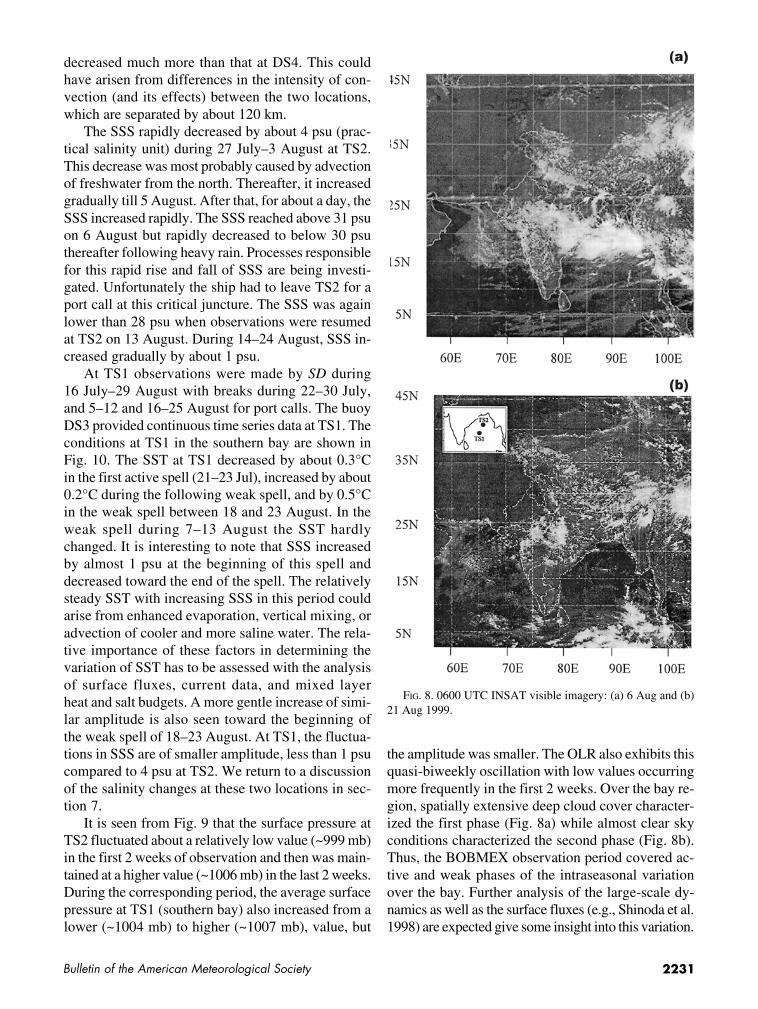
which dissipated on the sea itself on 16 August. Again,clear sky conditions occurred over the bay during 19–23 August (Fig. 8b). Finally, a low pressure area wasgenerated over south-central bay on 24 August thatmoved northward and crossed land on 27 August. Thisevent (marked as spell V in Fig. 7) was associated withconsiderable northward movement of the disturbanceformed over the central bay (Fig. 1a). Thus, all themonsoon lows and depressions over the Indian sub-continent during the BOBMEX period had their ori-gin over the bay. It may also be noted that, while threemonsoon systems formed during 25 July–8 August (aduration of about 2 weeks), no monsoon systemformed during the next 2 weeks (9–23 Aug). Thus aquasi-biweekly variation between active and weakphases of convection occurred during BOBMEX. Wenext consider the variation of surface fields in asso-ciation with active and weak spells.

The Sagar Kanya was positioned at TS2 from27 July to 24 August 1999 with a break (port call)during 6–12 August (Fig. 9). Henceforth, the periods27 July–6 August and 13–24 August are referred to

as leg 1 and leg 2, respectively, for the convenienceof reference. The OLR, daily cumulative rainfall, SST,sea surface salinity (SSS), surface pressure, and windspeed measured in the northern bay are shown inFig. 9. It is seen from Fig. 9 that, as expected, the majorrainfall events of 1, 6, and 15 and 16 August over thenorth bay are associated with troughs in OLR withvalues ranging from 120 to 160 W m−2. SST tends todecrease in high rainfall spells. During 31 July–1 August the TS2 station received about 80 mm ofrainfall and SST decreased by about 0.4°C. A largerdecrease was observed during 15–17 August when theTS2 received about 200 mm of rainfall. SST increasedafter the rain events. The SST increased by more than1°C during 19–24 August, a period characterized byhigh values of OLR and low wind speed. Note that theobserved surface pressure and wind speed from theship and buoy are rather close. However, the SST mea-sured from the ship does differ from that measuredfrom the buoy by as much as 0.5°C on some days. Inparticular, during and after the high rainfall eventsof 1 August and 15 and 16 August, the SST at TS2

(a) (b)

FIG. 7. Variation of INSAT OLR, buoy SST, and wind speed during Jul–Aug 1999. Active spells with OLR values below180 W m−2 are marked by roman numerals. (a) North bay; (b) south bay.


decreased much more than that at DS4. This couldhave arisen from differences in the intensity of con-vection (and its effects) between the two locations,which are separated by about 120 km.

The SSS rapidly decreased by about 4 psu (prac-tical salinity unit) during 27 July–3 August at TS2.This decrease was most probably caused by advectionof freshwater from the north. Thereafter, it increasedgradually till 5 August. After that, for about a day, theSSS increased rapidly. The SSS reached above 31 psuon 6 August but rapidly decreased to below 30 psuthereafter following heavy rain. Processes responsiblefor this rapid rise and fall of SSS are being investi-gated. Unfortunately the ship had to leave TS2 for aport call at this critical juncture. The SSS was againlower than 28 psu when observations were resumedat TS2 on 13 August. During 14–24 August, SSS in-creased gradually by about 1 psu.

At TS1 observations were made by SD during16 July–29 August with breaks during 22–30 July,and 5–12 and 16–25 August for port calls. The buoyDS3 provided continuous time series data at TS1. Theconditions at TS1 in the southern bay are shown inFig. 10. The SST at TS1 decreased by about 0.3°Cin the first active spell (21–23 Jul), increased by about0.2°C during the following weak spell, and by 0.5°Cin the weak spell between 18 and 23 August. In theweak spell during 7–13 August the SST hardlychanged. It is interesting to note that SSS increasedby almost 1 psu at the beginning of this spell anddecreased toward the end of the spell. The relativelysteady SST with increasing SSS in this period couldarise from enhanced evaporation, vertical mixing, oradvection of cooler and more saline water. The rela-tive importance of these factors in determining thevariation of SST has to be assessed with the analysisof surface fluxes, current data, and mixed layerheat and salt budgets. A more gentle increase of simi-lar amplitude is also seen toward the beginning ofthe weak spell of 18–23 August. At TS1, the fluctua-tions in SSS are of smaller amplitude, less than 1 psucompared to 4 psu at TS2. We return to a discussionof the salinity changes at these two locations in sec-tion 7.

It is seen from Fig. 9 that the surface pressure atTS2 fluctuated about a relatively low value (~999 mb)in the first 2 weeks of observation and then was main-tained at a higher value (~1006 mb) in the last 2 weeks.During the corresponding period, the average surfacepressure at TS1 (southern bay) also increased from alower (~1004 mb) to higher (~1007 mb), value, but

the amplitude was smaller. The OLR also exhibits thisquasi-biweekly oscillation with low values occurringmore frequently in the first 2 weeks. Over the bay re-gion, spatially extensive deep cloud cover character-ized the first phase (Fig. 8a) while almost clear skyconditions characterized the second phase (Fig. 8b).Thus, the BOBMEX observation period covered ac-tive and weak phases of the intraseasonal variationover the bay. Further analysis of the large-scale dy-namics as well as the surface fluxes (e.g., Shinoda et al.1998) are expected give some insight into this variation.

FIG. 8. 0600 UTC INSAT visible imagery: (a) 6 Aug and (b)21 Aug 1999.

2232 Vol. 82, No. 10, October 2001

6. Vertical variations in the atmosphere

It was planned to collect data with high-verticalresolution radiosondes from both of the ships.However, unforeseen difficulties were faced in pro-curing radiosondes for one of the ships. Hence, radio-sondes (Vaisala model RS80-15G) were launchedonly from SK. More than 90 ascents covering activeand weak phases of convection are available. The fre-

quency of launch varied be-tween 2 and 5 day−1 dependingon the synoptic conditions andweather advice. Typical verticalresolution is 25 m. During eachlaunch, the radiosonde tempera-ture, humidity, and pressurereadings were compared withthe ground truth and entered intothe radiosonde receiver unit forcorrections. Before corrections,radiosonde temperature, humid-ity, and pressure readings werewithin 0.2°C, 2%, and 0.5 mb,respectively, from the groundtruth. In the final output, the ra-diosonde processor adjusted thecalibration constants to take careof these minor differences.Before each launch, the radio-sonde humidity sensor wastested in a 100% RH chamber.The RH measured by the radio-sonde increased quickly to 90%within a few seconds and the re-sponse became slow above 95%,but all radiosondes showed98%–100% RH values after afew minutes. Since the differ-ences between ground referencevalues and radiosonde-measuredvalues were within the accuracyof the sensor, no correctionshave been applied to the radio-sonde RH data. We may expecta slight underestimation of wa-ter vapor amount if RH valuesof more than 95% occurred in athin layer and the balloon passedthrough this layer before the sen-sor could fully respond.

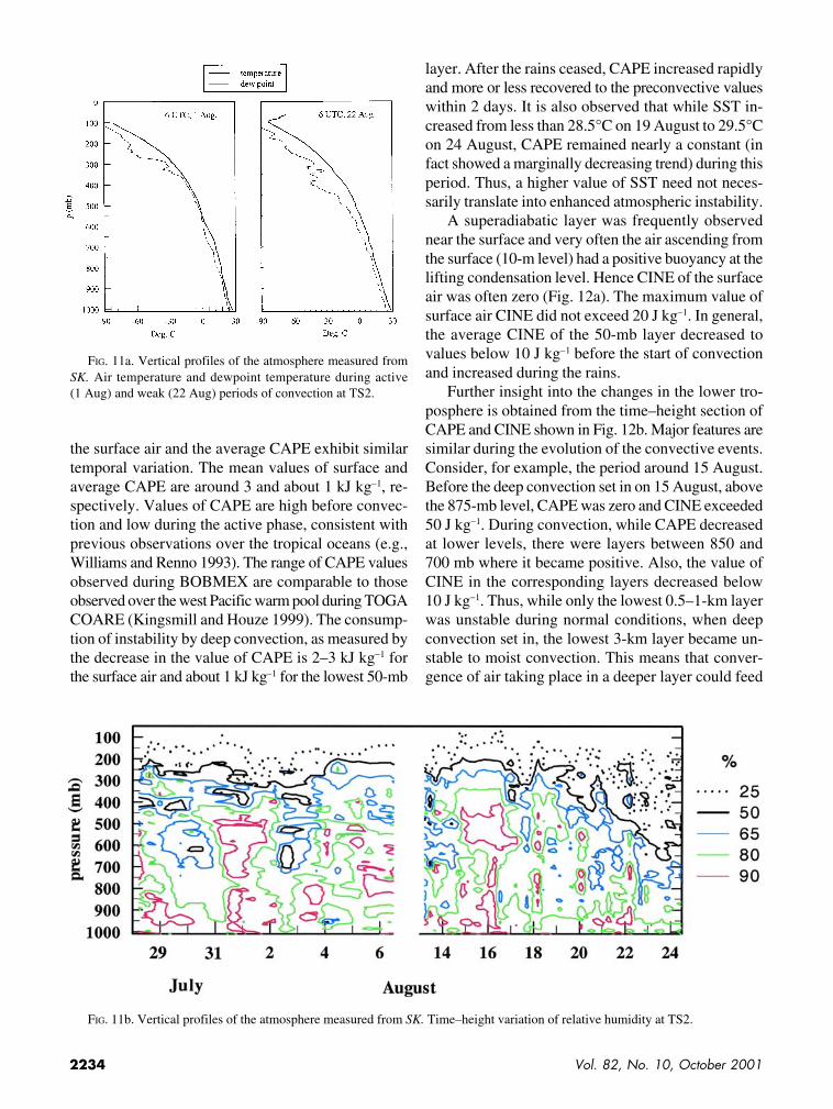
Here we present the observa-tions made from SK. Figure 11a shows one tempera-ture profile each from the active and weak phases ofconvection at TS2. The temperature difference be-tween convectively active and convectively weak at-mospheres is typically less than 2°C except near thesurface, whereas, humidity (dewpoint temperature)and wind fields exhibited larger fluctuations. Figure 11bshows the time–height variation of relative humidity.It is observed from Fig. 11b that the relative humid-

FIG. 9. Variation of INSAT OLR, daily cumulative rainfall starting from local midnight,SST, SSS, surface pressure, and wind speed in the north bay during BOBMEX. Darker andlighter lines refer to observations at TS2 and DS4, respectively. During the periods markedleg 1 and leg 2, RV Sagarkanya was positioned at TS2.


ity was generally high through-out the troposphere during leg 1as compared to that during leg2. During 20–24 August (weakphase of convection), a low hu-midity regime gradually moveddown from around the 350-mblevel (~9 km) to 600 mb (~4 km),and the midtroposphere dried up.

Upper winds are availablefor the second leg of BOBMEXonly. Figure 11c shows the ver-tical variation of wind from 13to 30 August. The ship movedfrom TS2 to TS1 during 24–27 August, and from TS1 toChennai during 27–30 August.Therefore, these two periodscorrespond to meridional andzonal sections over the bay. Theship was in the outer peripheryof the system that developed inthe last week of August (Fig. 1a)and not much rainfall was ob-served from the ship. When aconvective system was presentnearby (e.g., 13–16 and 25–28 Aug), wind speed increasedaround the 900-mb level and inthe upper troposphere near the200-mb level (Fig. 11c). Duringthe weak convective period (20–24 Aug), maximum winds werein the 25–30 m s−1 range, whereaswinds in 35–44 m s−1 rangeprevailed during convectivelyactive periods. Normally, lowwinds prevailed around the500-mb level on all occasions.It is also seen from Fig. 11c thatduring weak convective condi-tions, low wind speed (< 10 m s−1) prevailed from thesurface to the 350-mb level. At low levels, southwest-erly winds prevailed, with the exception being theperiod around 26 August when they became southerly.At upper levels (~200 mb), easterly winds are alwayspresent. During an active period, southwesterly windspenetrated beyond 300-mb height, whereas, as theweak convective conditions continued, easterly windsgradually migrated down to the 600-mb level. In gen-eral, the change from southwesterly to easterly wind di-

rection took place abruptly; that is, the transition wassharp.

The variation of the CAPE of the surface air(~10 mb above sea level) and average of the lowest50-mb layer (referred to as the average of CAPE forconvenience) are shown in Fig. 12a. Average CAPEis calculated by averaging the individual CAPE of airparcels lifted in 5-mb intervals. Also shown in Fig. 12aare SST and daily cumulative rainfall values recordedat TS2. It is observed from Fig. 12a that the CAPE of

FIG. 10. Variation of INSAT OLR, daily cumulative rainfall starting from local midnight,SST, SSS, surface pressure, and wind speed at TS1 location during BOBMEX. In the bot-tom four panels, lighter and darker lines correspond to 3-h time series and a slightlysmoothed version, respectively.

2234 Vol. 82, No. 10, October 2001

the surface air and the average CAPE exhibit similartemporal variation. The mean values of surface andaverage CAPE are around 3 and about 1 kJ kg−1, re-spectively. Values of CAPE are high before convec-tion and low during the active phase, consistent withprevious observations over the tropical oceans (e.g.,Williams and Renno 1993). The range of CAPE valuesobserved during BOBMEX are comparable to thoseobserved over the west Pacific warm pool during TOGACOARE (Kingsmill and Houze 1999). The consump-tion of instability by deep convection, as measured bythe decrease in the value of CAPE is 2–3 kJ kg−1 forthe surface air and about 1 kJ kg−1 for the lowest 50-mb

layer. After the rains ceased, CAPE increased rapidlyand more or less recovered to the preconvective valueswithin 2 days. It is also observed that while SST in-creased from less than 28.5°C on 19 August to 29.5°Con 24 August, CAPE remained nearly a constant (infact showed a marginally decreasing trend) during thisperiod. Thus, a higher value of SST need not neces-sarily translate into enhanced atmospheric instability.

A superadiabatic layer was frequently observednear the surface and very often the air ascending fromthe surface (10-m level) had a positive buoyancy at thelifting condensation level. Hence CINE of the surfaceair was often zero (Fig. 12a). The maximum value ofsurface air CINE did not exceed 20 J kg−1. In general,the average CINE of the 50-mb layer decreased tovalues below 10 J kg−1 before the start of convectionand increased during the rains.

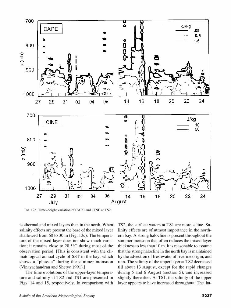
Further insight into the changes in the lower tro-posphere is obtained from the time–height section ofCAPE and CINE shown in Fig. 12b. Major features aresimilar during the evolution of the convective events.Consider, for example, the period around 15 August.Before the deep convection set in on 15 August, abovethe 875-mb level, CAPE was zero and CINE exceeded50 J kg−1. During convection, while CAPE decreasedat lower levels, there were layers between 850 and700 mb where it became positive. Also, the value ofCINE in the corresponding layers decreased below10 J kg−1. Thus, while only the lowest 0.5–1-km layerwas unstable during normal conditions, when deepconvection set in, the lowest 3-km layer became un-stable to moist convection. This means that conver-gence of air taking place in a deeper layer could feed

FIG. 11a. Vertical profiles of the atmosphere measured fromSK. Air temperature and dewpoint temperature during active(1 Aug) and weak (22 Aug) periods of convection at TS2.

FIG. 11b. Vertical profiles of the atmosphere measured from SK. Time–height variation of relative humidity at TS2.


clouds during the active phase of convection. During17–23 August, the atmosphere returned to clear skyconditions, and gradual lowering of the top of theunstable layer below 925 mb was seen and the valueof CINE increased beyond 50 J kg−1 above 925 mb.The drastic reduction in the height of the unstable layeron 24 August (when SST was high) was probably dueto the strong subsidence induced by the system thatintensified in the south-central bay. After the ship

moved away from this time series position, deepclouds were seen in the satellite imagery on 26 August.

7. Thermohaline structure

Temperature and salinity of the water column weremeasured every 3 h from SK at TS2 from 26 July to23 August with a break from 7 to 13 August. At TS1

FIG. 11c. Vertical profiles of the atmosphere measured from SK. Time–height variation of wind speed and wind direction from 13to 28 Aug. (top) Latitudinal position of the ship; the longitudinal position can be seen from Fig. 5a.

2236 Vol. 82, No. 10, October 2001

observations were made by SD during 15 July–29 August with breaks during 22–30 July, and 5–12and 16–25 August for port calls.

a. Vertical structureBased on the BOBMEX vertical profiles of tem-

perature and salinity, the upper layer of the northernbay can be divided into three sublayers: the mixedlayer, a barrier layer including one or more salt strati-fied layers, and the thermocline. An example of sucha profile is shown in Fig. 13a. The uppermost layer ishomogeneous in both temperature and salinity; in thesecond layer, the temperature gradient is small, butthere is a well-marked gradient in salinity and hencedensity. Often the vertical gradient of salinity is notuniform but consists of several steps. Generally thislayer has the same temperature as the surface mixedlayer. Occasionally, there are differences of up to0.5°C from the surface temperature. Below the bar-rier layer the temperature decreases rapidly and the sa-linity and density increase gradually.

The vertical structure at TS1 in the southern bayis different from that of the north bay. On some days,

there is no barrier layer. On 18–19 July,for example, the upper layer is wellmixed in temperature and salinity andabout 60 m deep (Fig. 13b). However,on other days, such as 27 August, salin-ity effects can be seen clearly (Fig. 13c),with an upper isohaline layer and a halo-cline. Below the halocline the salinity isagain uniform. For the profile shownin Fig. 13c, the salinity increases from33.7 psu at 30 m to 34.0 psu at 38 m andthen remains at 34.0 psu till the base ofthe isothermal layer.

b. Mixed layerVarious criteria can be found in the

literature for determining the depth ofthe mixed layer in the tropical oceans(Anderson et al. 1996). Historically thebase of the mixed layer has been takenas the depth at which the temperaturechanges from its surface value by 1°C(sometimes 0.5°C). Using the 1°C cri-terion Rao et al. (1989) calculated theclimatological monthly mean mixedlayer depths in the north Indian Ocean.Using CTD observations Shetye et al.(1996) found that the wintertime surface

layer in the bay that is homogeneous in both tempera-ture and salinity is much shallower than the depth ob-tained by Rao et al. (1989). The reason for thisdiscrepancy was attributed to salinity effects, whichwere not considered by Rao et al. (1989). Murty etal. (1996) observed that during the summer monsoonthe mixed layer in the northern bay is shallower thanthe isothermal layer. The barrier layer was observedfirst in the western equatorial Pacific Ocean (Lukasand Lindstrom 1991). The seasonal evolution of bar-rier-layer thickness in the global Tropics is docu-mented in Sprintall and Tomczak (1992). We definethe mixed layer depth as the depth at which the verti-cal gradient of density exceeds 0.05 kg m−4. The CTDdata spaced at 1-m interval were scanned downwardand the uppermost depth where the above criterion issatisfied was chosen as the mixed layer depth. For theprofile shown in Fig. 13a, for example, the mixedlayer depth is 14 m, whereas the isothermal layer is33 m deep. The mixed layer depth shows consider-able variation with time and space depending on thesurface conditions such as wind speed and freshwa-ter content. In general, the southern bay has deeper

FIG. 12a. Variation of CAPE and CINE at TS2 for the surface air and that ofthe lowest 50-mb layer. Also shown (top panel) are SST and cumulative dailyrainfall at TS2.


isothermal and mixed layers than in the north. Whensalinity effects are present the base of the mixed layershallowed from 60 to 30 m (Fig. 13c). The tempera-ture of the mixed layer does not show much varia-tion; it remains close to 28.5°C during most of theobservation period. [This is consistent with the cli-matological annual cycle of SST in the bay, whichshows a “plateau” during the summer monsoon(Vinayachandran and Shetye 1991).]

The time evolutions of the upper-layer tempera-ture and salinity at TS2 and TS1 are presented inFigs. 14 and 15, respectively. In comparison with

TS2, the surface waters at TS1 are more saline. Sa-linity effects are of utmost importance in the north-ern bay. A strong halocline is present throughout thesummer monsoon that often reduces the mixed layerthickness to less than 10 m. It is reasonable to assumethat the strong halocline in the north bay is maintainedby the advection of freshwater of riverine origin, andrain. The salinity of the upper layer at TS2 decreasedtill about 13 August, except for the rapid changesduring 5 and 6 August (section 5), and increasedslightly thereafter. At TS1, tha salinity of the upperlayer appears to have increased throughout. The ha-

FIG. 12b. Time–height variation of CAPE and CINE at TS2.

2238 Vol. 82, No. 10, October 2001

locline is very sharp and restricted to about 30 m,whereas the thermocline occurs over a deeper layer.This halocline is very tight during the first half of theobservation period but broadens afterward, indicat-ing the weakening salinity effects on the upper layer.There appears to be an increase in the depth of thehalocline during 6–12 August. However, data are notavailable during this period as the ship had to go fora port call.

c. Comparison with the west PacificA large number of convective systems form over

the western equatorial Pacific Ocean (Godfrey et al.1998) and over the Bay of Bengal (Fig. 1a). Conse-quent to freshwater input by rainfall, the upper-layersalinity decreases in both cases. The major featuresof the interaction of the west Pacific with the atmo-sphere are 1) a decrease of the salinity of the upperlayer consequent to freshwater input from rainfall, re-sulting in the formation of a thin surface layer thatfloats over the thermally mixed layer; 2) restrictionof the air–sea interaction to this layer under conditionsof weak wind because the barrier layer inhibits ex-change with the water below; and 3) breaking of thebarrier layer with the occurrence of a strong wind

event leading to a profile with a mixed layer that ishomogeneous in temperature and salinity, like the oneexisting before the rain event. An important questionto address is, do similar events characterize the air–sea interaction over the bay?

The observations during BOBMEX suggest thatthe scenario in the northern bay is rather different fromthat in the west Pacific. First of all, the salinity of theupper layer in the northern bay is several practical sa-linity units less, which makes the surface water in thebay much lighter. Compared to the west Pacific sa-linity of about 34 psu, the surface salinity in the northbay can become as low as 28 psu (e.g., Fig. 9). Second,the halocline that is located at the base of the surfacemixed layer in the bay is much stronger than that inthe west Pacific. Lukas and Lindstrom (1991) ob-served a vertical salinity gradient of 0.01 psu m−1 andthis halocline was located in about 30-m-depth range.It is clearly seen from Fig. 13 that the halocline at TS2is much stronger and often occurs at a much shallowerdepth. We believe that the strong multiple haloclinesin the northern bay observed during BOBMEX havenot been reported previously. The barrier layer in thewest Pacific is destroyed by a westerly wind burst. Themean strength of these westerly winds is 10 m s−1

FIG. 13. Vertical profiles of temperature (T), salinity (s), and density (σθ) from CTD measurements from ORV Sagarkanya: (a)TS2 at 1540 IST 3 Aug, (b) TS1 at 1330 IST 18 Jul, and (c) TS1 at 1330 IST 27 Aug.


(Godfrey et al. 1998). In the northern bay the windsexceed this value on several occasions during the sum-mer monsoon (Fig. 9). Despite the strong winds, it wasobserved during BOBMEX that once it is formed the

barrier layer can persist, perhaps throughout themonsoon.

The southern bay, however, appears to be moresimilar to the west Pacific. On some days, the shape

FIG. 14. Time–depth section of temperature (top) and salinity (bottom) at TS2. Contour interval for isotherms greater than28.5°C is 0.25°C and for less than 28°C it is 1°C. Regions with temperatures greater than 28.5°C are shaded. Contour interval forsalinity is 0.25 psu throughout the water column. Regions with salinity less than 33 psu are shaded.

2240 Vol. 82, No. 10, October 2001

of the temperature at TS1 is very similar to that ofthe Pacific. However the isothermal layer is about60 m deep in the central bay compared to more than100 m in the west Pacific. The mixed layer at TS1 isabout 30 m, which is similar to the Pacific, and thevertical gradient in the halocline also has similar val-ues. Detailed analysis of the thermohaline structureto study the response of the thermohaline structure torain/wind events and cloud-free conditions is underway.

8. Concluding remarks

With the successful implementation of BOBMEX,a beginning has been made in India, in special obser-vational experiments on important facets of thecoupled ocean–atmosphere system, which plays acritical role in the variability of the Indian monsoon.In this paper the experiment has been described andsome initial results presented.

In the BOBMEX field phase, several active andweak spells of convection occurred over the bay. The

FIG. 15. Same as in Fig. 14 but for TS1.


observations of the variation of the atmosphere andthe bay during different phases of convection havealready yielded some interesting results. High-resolution radiosondes were launched for the first timein the northern bay, during BOBMEX. From thesedata, it has been possible to derive important infor-mation about the variation of the vertical stability ofthe atmosphere. CAPE and CINE values over the bayare comparable to those over the west Pacific warmpool. It has been found that the recovery time forCAPE, after a disturbance has passed, is less than2 days. This will have important implications for thefrequency of the genesis of organized convectionover the bay. CINE values in the lowest 50-mb layerdecreased below 10 J kg−1 just before the onset ofconvection.

The thermohaline structure as well as its time evo-lution during the BOBMEX field phase was found tobe different in the north bay than the south bay. Theresponse of these regions to variations in convectionhas been documented. Studies are presently under wayto ascertain the relative importance of the surfacefluxes and upper ocean processes in determining thenature of the variation of SST.

Over the season as a whole, the upper-layer salin-ity decreased for the north bay and increased for thesouth bay. Over both regions, the SST and SSS gen-erally decreased during rain events and increased incloud-free conditions. An exception is the period of7–13 August over the southern bay in which SSThardly changed despite large increases in OLR. TheSSS increased markedly in the early stages of thisevent. Further analysis of the mixed layer heat and saltbudgets is expected to give insight into the relativeimportance of surface fluxes, vertical mixing, andhorizontal advection during individual events/episodes. The variation in SST during 1999 was foundto be of smaller amplitude than in 1998. Whether thiscan be attributed to the interannual variation in con-vection has to be investigated.

A large part of the BOBMEX data from observa-tions at TS2 was distributed within the country by theend of 2000. These data will be made available to theinternational scientific community in 2001. Data col-lected at TS1 and the data on surface fluxes are beingscrutinized by the investigators. Efforts are under wayto distribute these data within the country this year andto the international community in 2002.

Building on what is learned from the observationsduring BOBMEX and process modeling, more obser-vational experiments will be conducted in the Indian seas

to get a deeper understanding of the intraseasonal andinterannual variations of the convection over these warmoceans and their implications for monsoon variability.

Acknowledgments. BOBMEX, the first observational experi-ment under the Indian Climate Research Program, was supportedby the Department of Science and Technology, Department ofOcean Development, Defence Research and Development Or-ganization, and Department of Space, of the government of In-dia. The India Meteorological Department provided crucialsupport in the planning and field phase. The ships were providedby the National Center for Antarctic and Ocean Research andthe Naval Physical and Oceanographic Laboratory, while thebuoys were deployed by the National Institute of Ocean Tech-nology. It is a pleasure to thank Drs. R. R. Kelkar, R. K. Midha,B. D. Acharya, S. M. Kulshrestha, and K. Premkumar for con-stant encouragement and advice; Drs. P. C. Pandey andM. Sudhakar for crucial help and support on the RV SagarKanya; and the director of the National Centre for Medium-Range Weather Forecasts for weather analysis and advice dur-ing BOBMEX. We are grateful to the directors of the IndianInstitute of Science, National Institute of Oceanography, NavalPhysical and Oceanographic Laboratory, National Institute ofOcean Technology, and the director general of Meteorology,India Meteorological Department for encouraging our partici-pation. We also thank other participants and ship crew who havehelped in the collection of the data. We are grateful for the com-ments and suggestions on the earlier version of the manuscriptby the referees, which led to substantial improvements.

References

Anderson, S. P., R. A. Weller, and R. Lukas, 1996: Surface buoy-ancy forcing and the mixed layer of the western equatorialPacific warm pool: Observations and 1D model results. J. Cli-mate, 9, 3056–3085.

Bhat, G. S., S. Ameenulla, M. Venkataramana, and K. Sengupta,2000: Atmospheric boundary layer characteristics during theBOBMEX-Pilot experiment. Proc. Indian Acad. Sci. (EarthPlanet. Sci.), 109, 229–237.

DST, 1996: Indian Climate Research Programme science plan.Department of Science and Technology, New Delhi, India,186 pp.

Emanuel, K. A., 1994: Atmospheric Convection. Oxford Univer-sity Press, 579 pp.

Fein, J. S., and J. P. Kuettner, 1980: Report on the summer ofMONEX field phase. Bull. Amer. Meteor. Soc., 61, 461–474.

Gadgil, S., 2000: Monsoon–ocean coupling. Current Sci., 78,309–323.

——, P. V. Joseph, and N. V. Joshi, 1984: Ocean–atmospherecoupling over monsoon regions. Nature, 312, 141–143.

Godfrey, J. S., and E. Lindstrom, 1989: On the heat budget ofequatorial west Pacific surface mixed layer. J. Geophys. Res.,94, 8007–8017.

——, R. A. Houze Jr., R. H. Johnson, R. Lukas, J. L.Redelsperger, A. Sumi, and R. Weller, 1998: Coupled Ocean–Atmosphere Response Experiment (COARE): An interimreport. J. Geophys. Res., 103C, 14 395–14 450.

2242 Vol. 82, No. 10, October 2001

Goel, M., and H. N. Srivastava, 1990: Monsoon Trough Bound-ary Layer Experiment (MONTBLEX). Bull. Amer. Meteor.Soc., 71, 1594–1600.

Gopalakrishna, V. V., V. S. N. Murty, M. S. S. Sarma, and J. S.Sastry, 1993: Thermal response of upper layers of the Bayof Bengal to forcing of a severe cyclone storm: A case study.Indian J. Mar. Sci., 22, 8–11.

Graham, N. E., and T. P. Barnett, 1987: Sea surface tempera-ture, surface wind divergence and convection over tropicaloceans. Science, 238, 657–659.

Hosom, D. S., R. A. Weller, R. E. Payne, and K. E. Prada, 1995:The IMET (Improved Meteorology) ship and buoy systems.J. Atmos. Oceanic Technol., 12, 527–540.

ICRP, 2000: BOBMEX inter-comparison report. Indian ClimateResearch Programme, Rept. No. ICRP/IISc/01, Centre forAtmospheric and Oceanic Sciences, Indian Institute of Sci-ence, 42 pp. [Available from G. S. Bhat, Centre for Atmo-spheric and Oceanic Sciences, Indian Institute of Science,Bangalore 560 012, India.]

Kingsmill, D. E., and R. H. Houze Jr., 1999: Thermodynamiccharacteristics of air flowing into and out of precipitating con-vection over the west Pacific warm pool. Quart. J. Roy. Me-teor. Soc., 125, 1209–1229.

Krishnamurti, T. N., 1985: Summer monsoon experiment—A re-view. Mon. Wea. Rev., 113, 1590–1626.

——, and H. N. Bhalme, 1976: Oscillations of a monsoon sys-tem. Part I. Observational aspects. J. Atmos. Sci., 33, 1937–1954.

——, and P. Ardunay, 1980: The 10–20 day westward propaga-tion mode and breaks in the monsoon. Tellus, 32, 15–26.

Levitus, S., and Y. P. Boyer, 1994: Temperature. Vol. 4, WorldOcean Atlas 1994, NOAA Atlas NESDIS 4, 117 pp.

Liu, W. T., K. B. Katsaros, and J. A. Businger, 1979: Bulk pa-rameterization of air–sea exchanges of heat and water vaporincluding the molecular constraints at the interface. J. Atmos.Sci., 36, 1722–1735.

Lukas, R., and E. J. Lindstrom, 1991: The mixed layer of thewestern equatorial Pacific Ocean. J. Geophys. Res., 96(Suppl.), 3343–3357.

Mohanty, U. C., and S. Das, 1986: On the structure of the at-mosphere during suppressed and active periods of convec-tion over the Bay of Bengal. Proc. Indian Natl. Sci. Acad.,52, 625–640.

Moncrief, M. W., and M. J. Miller, 1976: The dynamics and simu-lation of tropical cumulonimbus and squall lines. Quart. J. Roy.Meteor. Soc., 102, 373–394.

Murty, V. S. N., Y. V. B. Sarma, D. P. Rao, and C. S. Murty,1992: Water characteristics, mixing and circulation in the Bayof Bengal during southwest monsoon. J. Mar. Res., 50, 207–228.

——, ——, and ——, 1996: Variability of the oceanic bound-ary layer characteristics in the north of the Bay of Bengalduring MONTBLEX-90. Proc. Indian Acad. Sci. (EarthPlanet. Sci.), 105, 41–61.

Premkumar, K., M. Ravichandran, S. R. Kalsi, D. Sengupta, andS. Gadgil, 2000: First results from a new observational sys-tem over the Indian seas. Current Sci., 78, 323–331.

Ramesh Babu, V., V. S. N. Murty, V. G. Rao, C. V. Prabhu, andV. Tilvi, 2000: Thermohaline structure and circulation in theupper layers of the southern Bay of Bengal during BOBMEX-

Pilot (October–November 1998). Proc. Indian Acad. Sci.(Earth Planet. Sci.), 109, 255–265.

Rao, R. R., 1987: Further analysis on the thermal response of theupper Bay of Bengal to the forcing of pre-monsoon cyclonicstorm and summer monsoonal onset during MONEX-79.Mausam, 38, 147–156.

——, S. V. S. Somanathan, S. S. V. S. Ramakrishna, and R.Ramanadhan, 1987: A case study on the genesis of a monsoondepression in the northern Bay of Bengal during MONSOON-77 experiments. Mausam, 38, 387–394.

——, R. L. Molinari, and J. F. Festa, 1989: Evolution of the cli-matological near-surface thermal structure of the tropicalIndian Ocean. I. Description of mean monthly mixed layerdepth, and sea surface temperature, surface current, and sur-face meteorological fields. J. Geophys. Res., 94, 10 801–10 815.

——, B. Mathew, and P. V. Hareeshkumar, 1993: A summaryof results on thermohaline variability in the upper layers ofthe east central Arabian Sea and Bay of Bengal during sum-mer monsoon experiments. Deep-Sea Res., 40, 1647–1672.

Rao, Y. P., 1976: Southwest monsoon. Synoptic Meteorology,Meteorological Monogr., India Meteorological Department,No. 1, 367 pp.

Sanil Kumar, K. V., N. Mohan Kumar, M. X. Joseph, and R. R.Rao, 1994: Genesis of meteorological disturbances and ther-mohaline variability of the upper layers in the north of Bay ofBengal during Monsoon Trough Boundary Layer Experiment(MONTBLEX-90). Deep-Sea Res., 41, 1569–1581.

Sarma, Y. V. B., P. Seetaramayya, V. S. N. Murty, and D. P. Rao,1997: Influence of the monsoon trough on air–sea interactionin the north Bay of Bengal during the southwest monsoon of1990. Bound.-Layer Meteor., 82, 517–526.

Sengupta, D., and M. Ravichandran, 2001: Oscillations of Bay ofBengal sea surface temperature during the 1998 summer mon-soon. Geophys. Res. Lett., 28, 2033–2036.

Shetye, S. R., and A. D. Gouveia, 1998: Coastal circulation in theNorth Indian Ocean. Regional Studies and Syntheses, Vol. 11,The Sea: The Global Coastal Ocean, R. A. Robinson and R. H.Brink, Eds., John Wiley.

——, ——, D. Shankar, S. S. C. Shenoi, P. N. Vinayachandran,D. Sundar, G. S. Michael, and G. Nampoothiri, 1996:Hydrography and circulation in the western Bay of Bengalduring the northeast monsoon. J. Geophys. Res., 101 (C6),14 011–14 025.

Shinoda, T., H. H. Hendon, and J. D. Glick, 1998: Intraseasonalsea surface temperature variability in the tropical Pacific andIndian Oceans. J. Climate, 11, 1685–1702.

Sikka, D. R., 1977: Some aspects of the life history, structure andmovement of monsoon depressions. Pure Appl. Geophys.,115, 1501–1529.

——, and S. Gadgil, 1980: On the maximum cloud zone andthe ITCZ over India longitude during the southwest monsoon.Mon. Wea. Rev., 108, 179–195.

——, and P. Sanjeeva Rao, 2000: Bay of Bengal Monsoon Ex-periment (BOBMEX)—A component of the Indian ClimateResearch Programme (ICRP). Proc. Indian Acad. Sci. (EarthPlanet. Sci.), 109, 207–209.

Sprintall, J., and H. Tomczak, 1992: Evidence of the barrier layerin the surface layer of the tropics. J. Geophys. Res., 97 (C5),7305–7316.


Varkey, M. J., V. S. N. Murty, and A. Suryanarayana, 1996:Physical oceanography of the Bay of Bengal and Andamansea. Oceanography and Marine Biology: An Annual Review,A. D. Ansell et al., Eds., Vol. 34, UCL Press, 1–70.

Vinayachandran, P. N., and S. R. Shetye, 1991: The warm poolin the Indian Ocean. Proc. Indian Acad. Sci. (Earth PlanetSci.), 100, 165–175.

Webster, P. J., and R. Lukas, 1992: TOGA COARE: TheCoupled Ocean–Atmosphere Response Experiment. Bull.Amer. Meteor. Soc., 73, 1377–1416.

Weller, R. A., and S. P. Anderson, 1996: Surface meteorologyand air–sea fluxes in the western equatorial Pacific warm poolduring the Coupled Ocean–Atmosphere Response Experi-ment. J. Climate, 9, 1959–1990.

Williams, E. R., and N. Renno, 1993: An analysis of the condi-tional instability of the tropical atmosphere. Mon. Wea. Rev.,121, 21–35.

Yasunari, T., 1981: Structure of an Indian summer monsoon sys-tem with around 40-day period. J. Meteor. Soc. Japan, 59,336–354.

BOBMEX: The Bay of Bengal Monsoon Experiment

Documents

Transcript of BOBMEX: The Bay of Bengal Monsoon Experiment