Investigation of XBT and XCTD Biases in the Arabian Sea and the Bay of Bengal with Implications for...
21
Investigation of XBT and XCTD Biases in the Arabian Sea and the Bay of Bengal with Implications for Climate Studies TIM BOYER,* V. V. GOPALAKRISHNA, 1 FRANCO RESEGHETTI, # AMIT NAIK, 1 V. SUNEEL, 1 M. RAVICHANDRAN, @ N. P. MOHAMMED ALI, & M. M. MOHAMMED RAFEEQ, & AND R. ANTHONY CHICO 1 * National Oceanographic Data Center, Silver Spring, Maryland 1 National Institute of Oceanography, Dona Paula, Goa, India # Italian National Agency for New Technologies, Energy and Sustainable Economic Development, Lerici, Italy @ Indian National Centre for Ocean Information Services, Hyderabad, India & National Institute of Oceanography Regional Centre, Kochi, India (Manuscript received 18 March 2010, in final form 10 October 2010) ABSTRACT Long time series of XBT data in the Bay of Bengal and the Arabian Sea are valuable datasets for exploring and understanding climate variability. However, such studies of interannual and longer-scale variability of temperature require an understanding, and, if possible, a correction of errors introduced by biases in the XBT and expendable conductivity–temperature–depth (XCTD) data. Two cruises in each basin were undertaken in 2008/09 on which series of tests of XBTs and XCTDs dropped simultaneously with CTD casts were per- formed. The XBT and XCTD depths were corrected by comparison with CTD data using a modification of an existing algorithm. Significant probe-to-probe fall-rate equation (FRE) velocity and deceleration coefficient variability was found within a cruise, as well as cruise-to-cruise variability. A small (;0.018C) temperature bias was also identified for XBTs on each cruise. No new FRE can be proposed for either the Bay of Bengal or the Arabian Sea for XBTs. For the more consistent XCTD, basin-specific FREs are possible for the Bay of Bengal, but not for the Arabian Sea. The XCTD FRE velocity coefficients are significantly higher than the XCTD manufacturers’ FRE coefficient or those from previous tests, possibly resulting from the influence of temperature on XCTD FRE. Mean temperature anomalies versus a long-term mean climatology for XBT data using the present default FRE have a bias (which is positive for three cruises and negative for one cruise) compared to the mean temperature anomalies for CTD data. Some improvement is found when applying newly calculated cruise-specific FREs. This temperature error must be accounted for in any study of tem- perature change in the regions. 1. Introduction Investigations of regional and global change in the heat content of the ocean can be affected by biases in instrumentation as well as changes in the observing system (Gouretski and Koltermann 2007, hereafter GK07; Willis et al. 2009). One of the main components of the observing system for subsurface temperatures in the open ocean for the period of 1970–2001 was the expendable bathythermograph (XBT; Fig. 1). GK07 demonstrate that XBT temperatures are systematically higher, on the order of 0.18C, than those measured with conductivity–temperature–depth (CTD) instruments and bottle samples. Moreover, GK07 show that this warm bias has changed over time and also varies with depth. Wijffels et al. (2008), Levitus et al. (2009), Ishii and Kimoto (2009), and Gouretski and Reseghetti (2010) have all provided statistical corrections on a global scale for the XBT temperature bias. Note that although it is referred to as a temperature bias here, the main cause seems to be actually a fall-rate equation (FRE), which leads to a depth under- or overcalculation. Hanawa et al. (1995, hereafter H95) provided the first generally adop- ted modified fall-rate-equation coefficients (FRECs), which improved upon the original Sippican FRECs, but the H95 FRECs are static in time and space. Thadathil et al. (2002) showed that XBTs dropped in cold Antarctic waters may have a different fall rate with a speed lower Corresponding author address: Tim Boyer, National Oceano- graphic Data Center, Silver Spring, MD 20910. E-mail: [email protected] 266 JOURNAL OF ATMOSPHERIC AND OCEANIC TECHNOLOGY VOLUME 28 DOI: 10.1175/2010JTECHO784.1 Ó 2011 American Meteorological Society
-
Upload
independent -
Category
Documents
-
view
2 -
download
0
Transcript of Investigation of XBT and XCTD Biases in the Arabian Sea and the Bay of Bengal with Implications for...
Investigation of XBT and XCTD Biases in the Arabian Sea and the Bay ofBengal with Implications for Climate Studies
TIM BOYER,* V. V. GOPALAKRISHNA,1 FRANCO RESEGHETTI,# AMIT NAIK,1 V. SUNEEL,1
M. RAVICHANDRAN,@ N. P. MOHAMMED ALI,& M. M. MOHAMMED RAFEEQ,& AND
R. ANTHONY CHICO1
* National Oceanographic Data Center, Silver Spring, Maryland1 National Institute of Oceanography, Dona Paula, Goa, India
# Italian National Agency for New Technologies, Energy and Sustainable Economic Development, Lerici, Italy@ Indian National Centre for Ocean Information Services, Hyderabad, India
& National Institute of Oceanography Regional Centre, Kochi, India
(Manuscript received 18 March 2010, in final form 10 October 2010)
ABSTRACT
Long time series of XBT data in the Bay of Bengal and the Arabian Sea are valuable datasets for exploring
and understanding climate variability. However, such studies of interannual and longer-scale variability of
temperature require an understanding, and, if possible, a correction of errors introduced by biases in the XBT
and expendable conductivity–temperature–depth (XCTD) data. Two cruises in each basin were undertaken
in 2008/09 on which series of tests of XBTs and XCTDs dropped simultaneously with CTD casts were per-
formed. The XBT and XCTD depths were corrected by comparison with CTD data using a modification of an
existing algorithm. Significant probe-to-probe fall-rate equation (FRE) velocity and deceleration coefficient
variability was found within a cruise, as well as cruise-to-cruise variability. A small (;0.018C) temperature
bias was also identified for XBTs on each cruise. No new FRE can be proposed for either the Bay of Bengal or
the Arabian Sea for XBTs. For the more consistent XCTD, basin-specific FREs are possible for the Bay of
Bengal, but not for the Arabian Sea. The XCTD FRE velocity coefficients are significantly higher than the
XCTD manufacturers’ FRE coefficient or those from previous tests, possibly resulting from the influence of
temperature on XCTD FRE. Mean temperature anomalies versus a long-term mean climatology for XBT
data using the present default FRE have a bias (which is positive for three cruises and negative for one cruise)
compared to the mean temperature anomalies for CTD data. Some improvement is found when applying
newly calculated cruise-specific FREs. This temperature error must be accounted for in any study of tem-
perature change in the regions.
1. Introduction
Investigations of regional and global change in the
heat content of the ocean can be affected by biases in
instrumentation as well as changes in the observing
system (Gouretski and Koltermann 2007, hereafter
GK07; Willis et al. 2009). One of the main components
of the observing system for subsurface temperatures
in the open ocean for the period of 1970–2001 was the
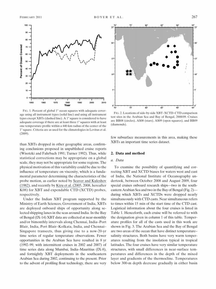
expendable bathythermograph (XBT; Fig. 1). GK07
demonstrate that XBT temperatures are systematically
higher, on the order of 0.18C, than those measured with
conductivity–temperature–depth (CTD) instruments and
bottle samples. Moreover, GK07 show that this warm
bias has changed over time and also varies with depth.
Wijffels et al. (2008), Levitus et al. (2009), Ishii and
Kimoto (2009), and Gouretski and Reseghetti (2010)
have all provided statistical corrections on a global scale
for the XBT temperature bias. Note that although it is
referred to as a temperature bias here, the main cause
seems to be actually a fall-rate equation (FRE), which
leads to a depth under- or overcalculation. Hanawa et al.
(1995, hereafter H95) provided the first generally adop-
ted modified fall-rate-equation coefficients (FRECs),
which improved upon the original Sippican FRECs, but
the H95 FRECs are static in time and space. Thadathil
et al. (2002) showed that XBTs dropped in cold Antarctic
waters may have a different fall rate with a speed lower
Corresponding author address: Tim Boyer, National Oceano-
graphic Data Center, Silver Spring, MD 20910.
E-mail: [email protected]
266 J O U R N A L O F A T M O S P H E R I C A N D O C E A N I C T E C H N O L O G Y VOLUME 28
DOI: 10.1175/2010JTECHO784.1
� 2011 American Meteorological Society
than XBTs dropped in other geographic areas, confirm-
ing conclusions proposed in unpublished cruise reports
(Wisotzki and Fahrbach 1991; Turner 1992). Thus, while
statistical corrections may be appropriate on a global
scale, they may not be appropriate for some regions. The
physical motivation of this variability could be due to the
influence of temperature on viscosity, which is a funda-
mental parameter determining the characteristics of the
probe motion, as earlier noted by Seaver and Kuleshov
(1982), and recently by Kizu et al. (2005, 2008, hereafter
K08) for XBT and expendable CTD (XCTD) probes,
respectively.
Under the Indian XBT program supported by the
Ministry of Earth Sciences, Government of India, XBTs
are deployed onboard ships of opportunity along se-
lected shipping lanes in the seas around India. In the Bay
of Bengal (IX-14) XBT data are collected at near-monthly
and/or bimonthly intervals along Chennai, India–Port
Blair, India, Port Blair–Kolkata, India, and Chennai–
Singapore transects, thus giving rise to a now-20-yr
time series of regular temperature observations. Fewer
opportunities in the Arabian Sea have resulted in 8 yr
(1992–99, with intermittent cruises in 2002 and 2007) of
time series data along Mumbai, India–Mauritius (IX-8),
and fortnightly XBT deployments in the southeastern
Arabian Sea during 2002, continuing to the present. Prior
to the advent of profiling float technology, there are very
few subsurface measurements in this area, making these
XBTs an important time series dataset.
2. Data and method
a. Data
To examine the possibility of quantifying and cor-
recting XBT and XCTD biases for waters west and east
of India, the National Institute of Oceanography un-
dertook, between October 2008 and August 2009, four
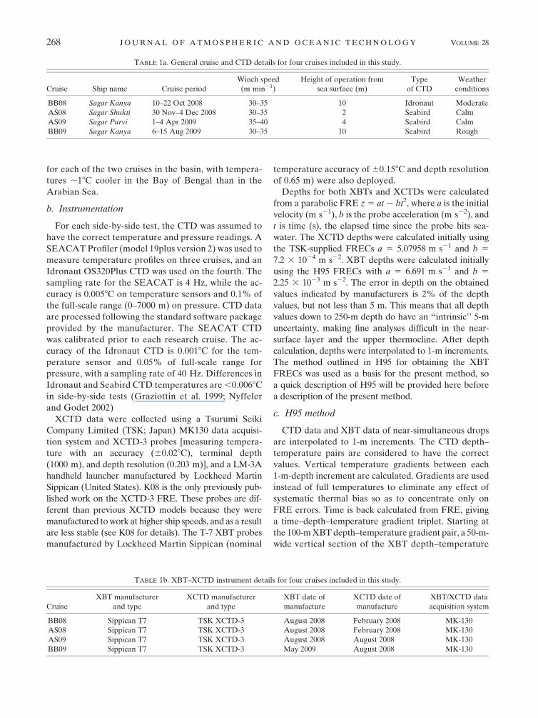
special cruises onboard research ships—two in the south-
eastern Arabian Sea and two in the Bay of Bengal (Fig. 2)—
during which XBTs and XCTDs were dropped nearly
simultaneously with CTD casts. Near simultaneous refers
to times within 15 min of the start time of the CTD cast.
Logistical information about the four cruises is listed in
Table 1. Henceforth, each cruise will be referred to with
the designation given in column 1 of this table. Temper-
ature profiles for all of the casts used in this work are
shown in Fig. 3. The Arabian Sea and the Bay of Bengal
are two areas of the ocean that have distinct temperature–
salinity structures. Both basins have very warm temper-
atures resulting from the insolation typical in tropical
latitudes. The four cruises have very similar temperature
structures, with small differences in near-surface tem-
peratures and differences in the depth of the mixed
layer and gradients of the thermocline. Temperatures
below 300-m depth decrease gradually in either basin
FIG. 1. Percent of global 18 ocean squares with adequate cover-
age using all instrument types (solid line) and using all instrument
types except XBTs (dashed line). A 18 square is considered to have
adequate coverage if there are at least three 18 squares with at least
one temperature profile within a 440-km radius of the center of the
18 square. Criteria are as used for the climatologies in Levitus et al.
(2009).
FIG. 2. Locations of side-by-side XBT–XCTD–CTD comparison
test sites in the Arabian Sea and Bay of Bengal, 2008/09. Cruises
are BB08 (circles), AS08 (stars), AS09 (open squares), and BB09
(diamonds).
FEBRUARY 2011 B O Y E R E T A L . 267
for each of the two cruises in the basin, with tempera-
tures ;18C cooler in the Bay of Bengal than in the
Arabian Sea.
b. Instrumentation
For each side-by-side test, the CTD was assumed to
have the correct temperature and pressure readings. A
SEACAT Profiler (model 19plus version 2) was used to
measure temperature profiles on three cruises, and an
Idronaut OS320Plus CTD was used on the fourth. The
sampling rate for the SEACAT is 4 Hz, while the ac-
curacy is 0.0058C on temperature sensors and 0.1% of
the full-scale range (0–7000 m) on pressure. CTD data
are processed following the standard software package
provided by the manufacturer. The SEACAT CTD
was calibrated prior to each research cruise. The ac-
curacy of the Idronaut CTD is 0.0018C for the tem-
perature sensor and 0.05% of full-scale range for
pressure, with a sampling rate of 40 Hz. Differences in
Idronaut and Seabird CTD temperatures are ,0.0068C
in side-by-side tests (Graziottin et al. 1999; Nyffeler
and Godet 2002)
XCTD data were collected using a Tsurumi Seiki
Company Limited (TSK; Japan) MK130 data acquisi-
tion system and XCTD-3 probes [measuring tempera-
ture with an accuracy (60.028C), terminal depth
(1000 m), and depth resolution (0.203 m)], and a LM-3A
handheld launcher manufactured by Lockheed Martin
Sippican (United States). K08 is the only previously pub-
lished work on the XCTD-3 FRE. These probes are dif-
ferent than previous XCTD models because they were
manufactured to work at higher ship speeds, and as a result
are less stable (see K08 for details). The T-7 XBT probes
manufactured by Lockheed Martin Sippican (nominal
temperature accuracy of 60.158C and depth resolution
of 0.65 m) were also deployed.
Depths for both XBTs and XCTDs were calculated
from a parabolic FRE z 5 at 2 bt2, where a is the initial
velocity (m s21), b is the probe acceleration (m s22), and
t is time (s), the elapsed time since the probe hits sea-
water. The XCTD depths were calculated initially using
the TSK-supplied FRECs a 5 5.07958 m s21 and b 5
7.2 3 1024 m s22. XBT depths were calculated initially
using the H95 FRECs with a 5 6.691 m s21 and b 5
2.25 3 1023 m s22. The error in depth on the obtained
values indicated by manufacturers is 2% of the depth
values, but not less than 5 m. This means that all depth
values down to 250-m depth do have an ‘‘intrinsic’’ 5-m
uncertainty, making fine analyses difficult in the near-
surface layer and the upper thermocline. After depth
calculation, depths were interpolated to 1-m increments.
The method outlined in H95 for obtaining the XBT
FRECs was used as a basis for the present method, so
a quick description of H95 will be provided here before
a description of the present method.
c. H95 method
CTD data and XBT data of near-simultaneous drops
are interpolated to 1-m increments. The CTD depth–
temperature pairs are considered to have the correct
values. Vertical temperature gradients between each
1-m-depth increment are calculated. Gradients are used
instead of full temperatures to eliminate any effect of
systematic thermal bias so as to concentrate only on
FRE errors. Time is back calculated from FRE, giving
a time–depth–temperature gradient triplet. Starting at
the 100-m XBT depth–temperature gradient pair, a 50-m-
wide vertical section of the XBT depth–temperature
TABLE 1a. General cruise and CTD details for four cruises included in this study.
Cruise Ship name Cruise period
Winch speed
(m min21)
Height of operation from
sea surface (m)
Type
of CTD
Weather
conditions
BB08 Sagar Kanya 10–22 Oct 2008 30–35 10 Idronaut Moderate
AS08 Sagar Shukti 30 Nov–4 Dec 2008 30–35 2 Seabird Calm
AS09 Sagar Purvi 1–4 Apr 2009 35–40 4 Seabird Calm
BB09 Sagar Kanya 6–15 Aug 2009 30–35 10 Seabird Rough
TABLE 1b. XBT–XCTD instrument details for four cruises included in this study.
Cruise
XBT manufacturer
and type
XCTD manufacturer
and type
XBT date of
manufacture
XCTD date of
manufacture
XBT/XCTD data
acquisition system
BB08 Sippican T7 TSK XCTD-3 August 2008 February 2008 MK-130
AS08 Sippican T7 TSK XCTD-3 August 2008 February 2008 MK-130
AS09 Sippican T7 TSK XCTD-3 August 2008 August 2008 MK-130
BB09 Sippican T7 TSK XCTD-3 May 2009 August 2008 MK-130
268 J O U R N A L O F A T M O S P H E R I C A N D O C E A N I C T E C H N O L O G Y VOLUME 28
gradient set is moved vertically up 50 m and down
30 m through each 1-m increment of the CTD data. At
each 1-m increment, the difference between the XBT
temperature gradient and the CTD temperature gra-
dient is calculated. These differences are summed for
the entire 50-m section. There are a maximum of 80
such summations. The CTD depth at which the sum-
mation is minimal is recorded as the true depth for the
XBT drop, matched with the original time from the
triplet. This process is repeated for each 50th XBT
time–depth–temperature gradient triplet (100th,
150th, 200th, 250th, etc., to the bottom of XBT drop).
For a 760-m XBT drop, this should result in 13 time–
depth points. A least squares fit to this line gives the
best pair (a, b) of values for FRECs. A similar method
has been used for XCTD data (Johnson 1995; K08).
The H95 method is sensitive to quality control of the
XBT, XCTD, and CTD data. Removal of one or two
minimum summed time–depth pairs can significantly
affect the calculated FRECs. On AS08, winch problems
resulted in the CTD only reaching a maximum of 406-m
depth. For this cruise, after quality control, the H95
method resulted in only four or five points with which to
linearly regress to new FRECs for some XBTs. Because
of this, a modified H95 method was used.
d. Modification to H95 method
We preserve the H95 method of comparing temper-
ature gradients between XBT and CTD instead of full
temperature values. However, we eliminate the need for
linear regression between a possibly sparse set of time–
depth pairs by summing all of the differences between
XBT and CTD gradients over the vertical profile from
100 to 700 m (or to the end of the CTD profile if it does
not extend to the deeper depth) for all sets of probable
initial velocities and decelerations. The sets used were
6.00–7.15 m s21 for initial velocities (a), and 0.00–4.00 3
1023 m s22 for the deceleration (b), both exceeding the
range of published FRECs. Each initial velocity at incre-
ments of 0.01 m s21 in this range is tested with each de-
celeration in its range at 0.01 3 1023 m s22 increments. The
CTD has 1-m-incremented depth–temperature gradient
pairs. The XBT data are interpolated to 1-m increments
and time is back calculated. For each initial velocity pair
and deceleration, depth is calculated and then inter-
polated back to 1-m increments from which 1-m tem-
perature gradients are calculated. The XBT and CTD
gradients are then subtracted and the absolute values
are summed. This sum is then divided by the number of
depth–gradient pairs that were summed to give an aver-
age gradient difference for each (a, b) pair. The minimal
mean gradient difference is indicative of the best-fit (a, b)
pair because it represents the minimum error in the XBT
profile compared with the CTD profile. The same pro-
cedure was used to compare XCTD and CTD side-
by-side pairs, except an initial velocity (a) range of
4.80–5.50 m s21 and decelerations of 0.0–2.0 3 1023 m s22
(b) were used, reflecting the different characteristics of
the XCTDs drop through the water column. Because the
XCTD can reach deeper than 1000 m, the depth interval
of 100–1000 m was used for the summation of gradient
differences. The time is back calculated for XCTDs using
the TSK-provided FRE. In many cases, the very end of the
XBT or XCTD cast deviates from the CTD cast temper-
ature gradients in a manner suggesting some inconsistency
FIG. 3. The CTD temperature profiles from comparison tests for
BB08 (green), AS08 (red), AS09 (blue), and BB09 (magenta).
TABLE 1c. Simultaneous CTD–XBT–XCTD drops from four
cruises included in this study. XBT–CTD and XCTD–CTD pairs
not used were discarded because of thermal bias .0.108C. Num-
bers in parentheses are compared with the first CTD cast only.
Cruise
CTD–XBT
pairs
CTD–XBT
pairs used
CTD–XCTD
pairs
CTD–XCTD
pairs used
BB08 11 10 11 10
AS08 9 9 9 9
AS09 50 (25) 36 (22) 20 (12) 20 (12)
BB09 12 12 8 8
FEBRUARY 2011 B O Y E R E T A L . 269
in the XBT–XCTD data, probably resulting from a wire-
stretching process immediately before the end of the wire
spool. In some cases, the variability in the 100–200-m
depth range caused large differences in the XBT–XCTD
and CTD temperature gradients. Both of these discrep-
ancies near the top and bottom of the cast resulted in less-
than-optimal FREC fit over the entire profile. Thus, the
above procedure was repeated using the depth interval of
200–600 m for XBTs and 200–900 m for XCTDs (or the
bottom of CTD casts, if shallower). The better fit between
the results of the two depth intervals, based on minimum
mean gradient differences, was used for the final FREC
selection.
e. Thermal bias calculation
Once the FRECs have been selected, the new FRE is
applied to the XBT (XCTD) time–temperature pair,
and the XBT (XCTD) depths are again interpolated to
1-m increments. Assuming that the FRE has corrected
any depth bias, any systematic thermal bias can now be
estimated simply by subtracting the full temperature
values of each instrument at each 1-m increment and
taking the average difference as the thermal bias. This
procedure is performed only on the depth interval over
which the new FRECs were estimated.
f. Additional adjustment
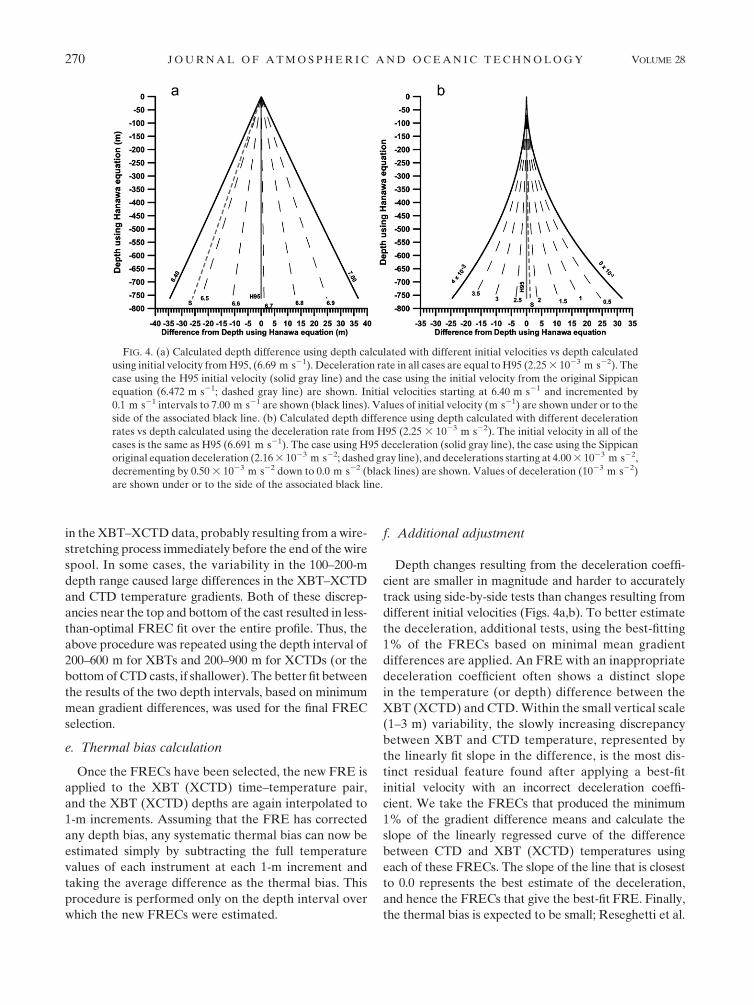
Depth changes resulting from the deceleration coeffi-
cient are smaller in magnitude and harder to accurately
track using side-by-side tests than changes resulting from
different initial velocities (Figs. 4a,b). To better estimate
the deceleration, additional tests, using the best-fitting
1% of the FRECs based on minimal mean gradient
differences are applied. An FRE with an inappropriate
deceleration coefficient often shows a distinct slope
in the temperature (or depth) difference between the
XBT (XCTD) and CTD. Within the small vertical scale
(1–3 m) variability, the slowly increasing discrepancy
between XBT and CTD temperature, represented by
the linearly fit slope in the difference, is the most dis-
tinct residual feature found after applying a best-fit
initial velocity with an incorrect deceleration coeffi-
cient. We take the FRECs that produced the minimum
1% of the gradient difference means and calculate the
slope of the linearly regressed curve of the difference
between CTD and XBT (XCTD) temperatures using
each of these FRECs. The slope of the line that is closest
to 0.0 represents the best estimate of the deceleration,
and hence the FRECs that give the best-fit FRE. Finally,
the thermal bias is expected to be small; Reseghetti et al.
FIG. 4. (a) Calculated depth difference using depth calculated with different initial velocities vs depth calculated
using initial velocity from H95, (6.69 m s21). Deceleration rate in all cases are equal to H95 (2.25 3 1023 m s22). The
case using the H95 initial velocity (solid gray line) and the case using the initial velocity from the original Sippican
equation (6.472 m s21; dashed gray line) are shown. Initial velocities starting at 6.40 m s21 and incremented by
0.1 m s21 intervals to 7.00 m s21 are shown (black lines). Values of initial velocity (m s21) are shown under or to the
side of the associated black line. (b) Calculated depth difference using depth calculated with different deceleration
rates vs depth calculated using the deceleration rate from H95 (2.25 3 1023 m s22). The initial velocity in all of the
cases is the same as H95 (6.691 m s21). The case using H95 deceleration (solid gray line), the case using the Sippican
original equation deceleration (2.16 3 1023 m s22; dashed gray line), and decelerations starting at 4.00 3 1023 m s22,
decrementing by 0.50 3 1023 m s22 down to 0.0 m s22 (black lines) are shown. Values of deceleration (1023 m s22)
are shown under or to the side of the associated black line.
270 J O U R N A L O F A T M O S P H E R I C A N D O C E A N I C T E C H N O L O G Y VOLUME 28
(2007) give an estimated value of ,0.058C. Gouretski and
Reseghetti (2010) give statistical estimates of between
0.08 and 0.048C from 1990 to 2002, and slightly higher
since 2002, which is possibly due to a decrease in CTD
data for statistical comparison. The fluctuations in the
small-scale (1–3 m) vertical structure will, in some cases,
result in coefficient choices with two very similar mean
gradient differences—one with a resultant high thermal
bias and one with a resultant lower thermal bias. In these
cases, given that thermal bias has been shown to be
small, the FRECs resulting in the lower thermal bias are
chosen. It should be noted that this may result in a small
underestimation of thermal bias. Thus, from the mini-
mum 1% of gradient difference means, now ordered in
terms of minimum slope, the first case with the minimum
thermal bias is chosen for the final set of FRECs. That
is, if more than one of the minimal 1% of the gradient
difference means had the same minimal thermal bias
(which is very likely because the XBT temperature
readings are recorded to two decimal places by the pro-
vided software), then the case with the minimum slope is
chosen. It was found that XBTs whose minimal thermal
bias was .0.108C had poor fits to the CTD data, re-
gardless of the FRE (or thermal bias) used. These cases
were not included in the final statistics (see Table 1c).
Only 5 of the 57 XBT–CTD comparisons were dis-
qualified using these criteria, and 1 of 40 XCTDs, ex-
cluding the second cast comparisons for AS09.
3. Results
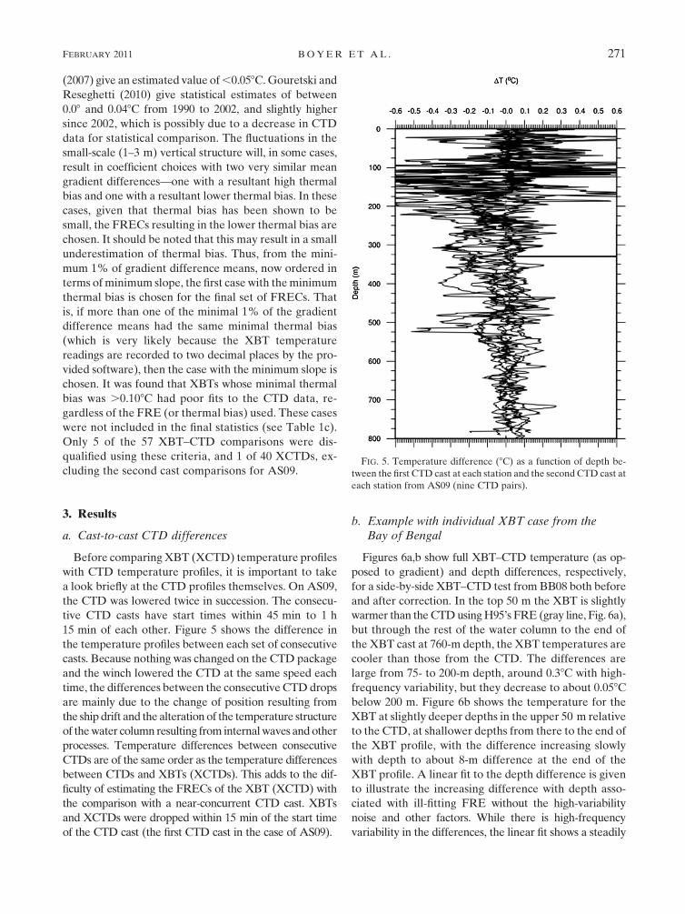
a. Cast-to-cast CTD differences
Before comparing XBT (XCTD) temperature profiles
with CTD temperature profiles, it is important to take
a look briefly at the CTD profiles themselves. On AS09,
the CTD was lowered twice in succession. The consecu-
tive CTD casts have start times within 45 min to 1 h
15 min of each other. Figure 5 shows the difference in
the temperature profiles between each set of consecutive
casts. Because nothing was changed on the CTD package
and the winch lowered the CTD at the same speed each
time, the differences between the consecutive CTD drops
are mainly due to the change of position resulting from
the ship drift and the alteration of the temperature structure
of the water column resulting from internal waves and other
processes. Temperature differences between consecutive
CTDs are of the same order as the temperature differences
between CTDs and XBTs (XCTDs). This adds to the dif-
ficulty of estimating the FRECs of the XBT (XCTD) with
the comparison with a near-concurrent CTD cast. XBTs
and XCTDs were dropped within 15 min of the start time
of the CTD cast (the first CTD cast in the case of AS09).
b. Example with individual XBT case from theBay of Bengal
Figures 6a,b show full XBT–CTD temperature (as op-
posed to gradient) and depth differences, respectively,
for a side-by-side XBT–CTD test from BB08 both before
and after correction. In the top 50 m the XBT is slightly
warmer than the CTD using H95’s FRE (gray line, Fig. 6a),
but through the rest of the water column to the end of
the XBT cast at 760-m depth, the XBT temperatures are
cooler than those from the CTD. The differences are
large from 75- to 200-m depth, around 0.38C with high-
frequency variability, but they decrease to about 0.058C
below 200 m. Figure 6b shows the temperature for the
XBT at slightly deeper depths in the upper 50 m relative
to the CTD, at shallower depths from there to the end of
the XBT profile, with the difference increasing slowly
with depth to about 8-m difference at the end of the
XBT profile. A linear fit to the depth difference is given
to illustrate the increasing difference with depth asso-
ciated with ill-fitting FRE without the high-variability
noise and other factors. While there is high-frequency
variability in the differences, the linear fit shows a steadily
FIG. 5. Temperature difference (8C) as a function of depth be-
tween the first CTD cast at each station and the second CTD cast at
each station from AS09 (nine CTD pairs).
FEBRUARY 2011 B O Y E R E T A L . 271
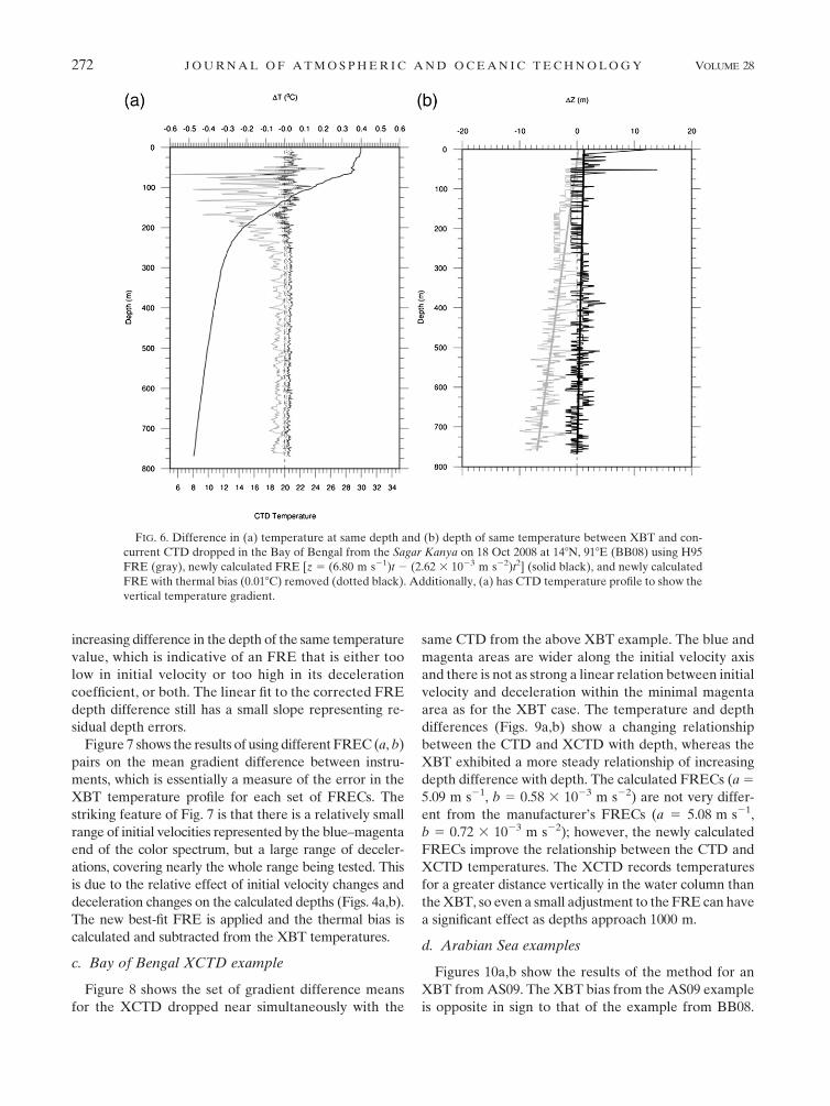
increasing difference in the depth of the same temperature
value, which is indicative of an FRE that is either too
low in initial velocity or too high in its deceleration
coefficient, or both. The linear fit to the corrected FRE
depth difference still has a small slope representing re-
sidual depth errors.
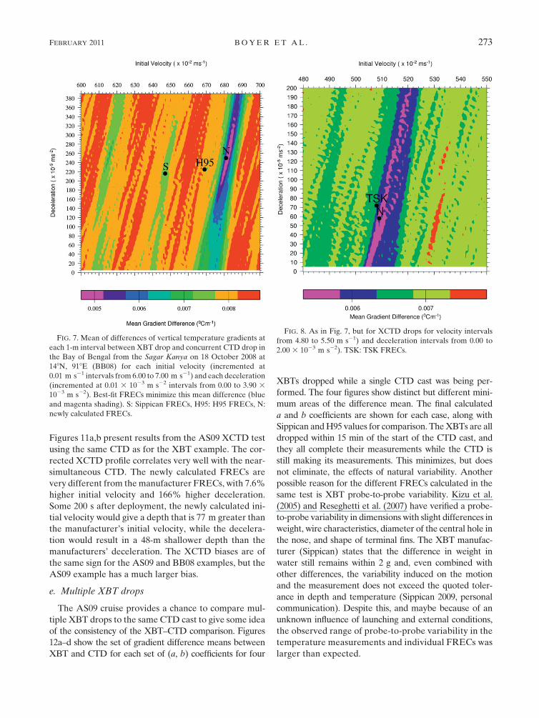
Figure 7 shows the results of using different FREC (a, b)
pairs on the mean gradient difference between instru-
ments, which is essentially a measure of the error in the
XBT temperature profile for each set of FRECs. The
striking feature of Fig. 7 is that there is a relatively small
range of initial velocities represented by the blue–magenta
end of the color spectrum, but a large range of deceler-
ations, covering nearly the whole range being tested. This
is due to the relative effect of initial velocity changes and
deceleration changes on the calculated depths (Figs. 4a,b).
The new best-fit FRE is applied and the thermal bias is
calculated and subtracted from the XBT temperatures.
c. Bay of Bengal XCTD example
Figure 8 shows the set of gradient difference means
for the XCTD dropped near simultaneously with the
same CTD from the above XBT example. The blue and
magenta areas are wider along the initial velocity axis
and there is not as strong a linear relation between initial
velocity and deceleration within the minimal magenta
area as for the XBT case. The temperature and depth
differences (Figs. 9a,b) show a changing relationship
between the CTD and XCTD with depth, whereas the
XBT exhibited a more steady relationship of increasing
depth difference with depth. The calculated FRECs (a 5
5.09 m s21, b 5 0.58 3 1023 m s22) are not very differ-
ent from the manufacturer’s FRECs (a 5 5.08 m s21,
b 5 0.72 3 1023 m s22); however, the newly calculated
FRECs improve the relationship between the CTD and
XCTD temperatures. The XCTD records temperatures
for a greater distance vertically in the water column than
the XBT, so even a small adjustment to the FRE can have
a significant effect as depths approach 1000 m.
d. Arabian Sea examples
Figures 10a,b show the results of the method for an
XBT from AS09. The XBT bias from the AS09 example
is opposite in sign to that of the example from BB08.
FIG. 6. Difference in (a) temperature at same depth and (b) depth of same temperature between XBT and con-
current CTD dropped in the Bay of Bengal from the Sagar Kanya on 18 Oct 2008 at 148N, 918E (BB08) using H95
FRE (gray), newly calculated FRE [z 5 (6.80 m s21)t 2 (2.62 3 1023 m s22)t2] (solid black), and newly calculated
FRE with thermal bias (0.018C) removed (dotted black). Additionally, (a) has CTD temperature profile to show the
vertical temperature gradient.
272 J O U R N A L O F A T M O S P H E R I C A N D O C E A N I C T E C H N O L O G Y VOLUME 28
Figures 11a,b present results from the AS09 XCTD test
using the same CTD as for the XBT example. The cor-
rected XCTD profile correlates very well with the near-
simultaneous CTD. The newly calculated FRECs are
very different from the manufacturer FRECs, with 7.6%
higher initial velocity and 166% higher deceleration.
Some 200 s after deployment, the newly calculated ini-
tial velocity would give a depth that is 77 m greater than
the manufacturer’s initial velocity, while the decelera-
tion would result in a 48-m shallower depth than the
manufacturers’ deceleration. The XCTD biases are of
the same sign for the AS09 and BB08 examples, but the
AS09 example has a much larger bias.
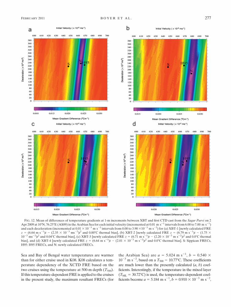
e. Multiple XBT drops
The AS09 cruise provides a chance to compare mul-
tiple XBT drops to the same CTD cast to give some idea
of the consistency of the XBT–CTD comparison. Figures
12a–d show the set of gradient difference means between
XBT and CTD for each set of (a, b) coefficients for four
XBTs dropped while a single CTD cast was being per-
formed. The four figures show distinct but different mini-
mum areas of the difference mean. The final calculated
a and b coefficients are shown for each case, along with
Sippican and H95 values for comparison. The XBTs are all
dropped within 15 min of the start of the CTD cast, and
they all complete their measurements while the CTD is
still making its measurements. This minimizes, but does
not eliminate, the effects of natural variability. Another
possible reason for the different FRECs calculated in the
same test is XBT probe-to-probe variability. Kizu et al.
(2005) and Reseghetti et al. (2007) have verified a probe-
to-probe variability in dimensions with slight differences in
weight, wire characteristics, diameter of the central hole in
the nose, and shape of terminal fins. The XBT manufac-
turer (Sippican) states that the difference in weight in
water still remains within 2 g and, even combined with
other differences, the variability induced on the motion
and the measurement does not exceed the quoted toler-
ance in depth and temperature (Sippican 2009, personal
communication). Despite this, and maybe because of an
unknown influence of launching and external conditions,
the observed range of probe-to-probe variability in the
temperature measurements and individual FRECs was
larger than expected.
FIG. 7. Mean of differences of vertical temperature gradients at
each 1-m interval between XBT drop and concurrent CTD drop in
the Bay of Bengal from the Sagar Kanya on 18 October 2008 at
148N, 918E (BB08) for each initial velocity (incremented at
0.01 m s21 intervals from 6.00 to 7.00 m s21) and each deceleration
(incremented at 0.01 3 1023 m s22 intervals from 0.00 to 3.90 3
1023 m s22). Best-fit FRECs minimize this mean difference (blue
and magenta shading). S: Sippican FRECs, H95: H95 FRECs, N:
newly calculated FRECs.
FIG. 8. As in Fig. 7, but for XCTD drops for velocity intervals
from 4.80 to 5.50 m s21) and deceleration intervals from 0.00 to
2.00 3 1023 m s22). TSK: TSK FRECs.
FEBRUARY 2011 B O Y E R E T A L . 273
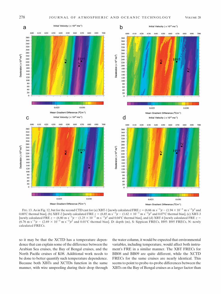
Figures 13a–d show the difference means for the same
four XBTs as in Figs. 12a–d, but versus the second CTD
cast, which occurred 33–45 min after the four XBT
drops; thus, they are not concurrent, but they are within
a very small space–time window. The FRECs for these
four tests are similar to those from the four tests versus
the first CTD cast. However, the area covered by the
blue–magenta color spectrum is wider with respect to
the initial velocity. The range of difference sums for
each of the eight panels in Figs. 12 and 13 (see color
bars) shows the relative range of errors of each XBT
versus each CTD, with those versus the second CTD cast
showing significantly higher errors. Natural variability is
occurring in time and space, which adds to the uncer-
tainty of calculating a new FRE. This shows the impor-
tance of dropping the XBTs as close as possible to the
time when the CTD cast is being carried out while per-
forming studies such as the one described here.
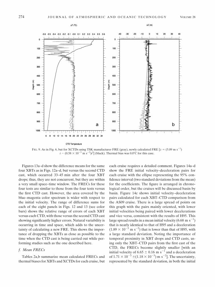
f. Mean FRECs
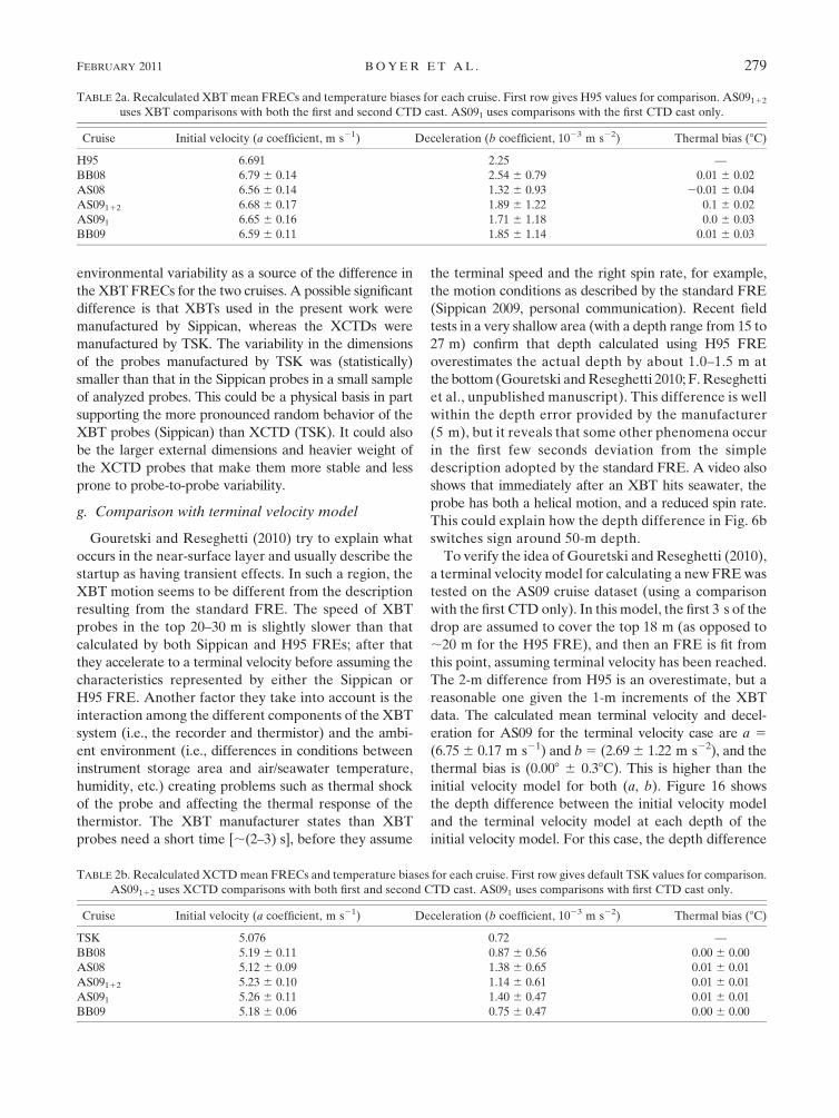
Tables 2a,b summarize mean calculated FRECs and
thermal biases for XBTs and XCTDs for each cruise, but
each cruise requires a detailed comment. Figures 14a–d
show the FRE initial velocity–deceleration pairs for
each cruise with the ellipse representing the 95% con-
fidence interval (two standard deviations from the mean)
for the coefficients. The figure is arranged in chrono-
logical order, but the cruises will be discussed basin by
basin. Figure 14c shows initial velocity–deceleration
pairs calculated for each XBT–CTD comparison from
the AS09 cruise. There is a large spread of points on
this graph with the pairs mainly oriented, with lower
initial velocities being paired with lower decelerations
and vice versa, consistent with the results of H95. This
large spread results in a mean initial velocity (6.68 m s21)
that is nearly identical to that of H95 and a deceleration
(1.89 3 1023 m s22) that is lower than that of H95, with
a large standard deviation. Noting the importance of
temporal proximity in XBT drops and CTD casts, us-
ing only the XBT–CTD pairs from the first cast of the
CTD, the FRECs become slightly smaller [with an
initial velocity of 6.65 6 0.16 m s21 and a deceleration
of 1.71 3 1023 6(1.18 3 1023) m s22]. The uncertainty,
represented by the standard deviation, in both the initial
FIG. 9. As in Fig. 6, but for XCTDs using TSK manufacturer FRE (gray), newly calculated FRE [z 5 (5.09 m s21)
t 2 (0.58 3 1023 m s22)t2] (black). Thermal bias was 0.08C for this case.
274 J O U R N A L O F A T M O S P H E R I C A N D O C E A N I C T E C H N O L O G Y VOLUME 28
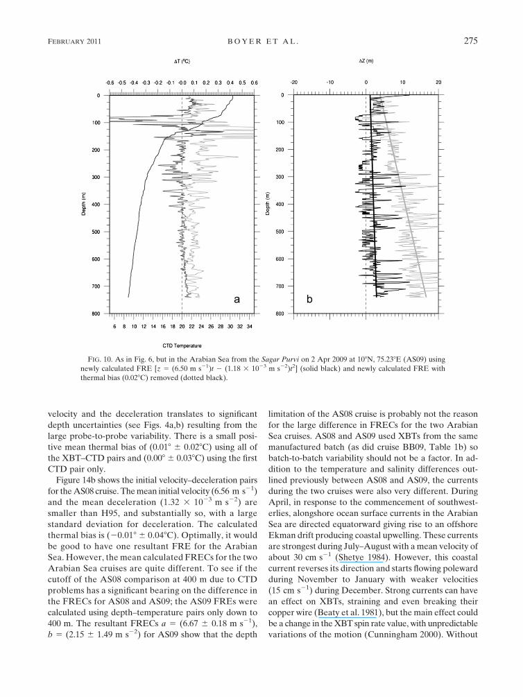
velocity and the deceleration translates to significant
depth uncertainties (see Figs. 4a,b) resulting from the
large probe-to-probe variability. There is a small posi-
tive mean thermal bias of (0.018 6 0.028C) using all of
the XBT–CTD pairs and (0.008 6 0.038C) using the first
CTD pair only.
Figure 14b shows the initial velocity–deceleration pairs
for the AS08 cruise. The mean initial velocity (6.56 m s21)
and the mean deceleration (1.32 3 1023 m s22) are
smaller than H95, and substantially so, with a large
standard deviation for deceleration. The calculated
thermal bias is (20.018 6 0.048C). Optimally, it would
be good to have one resultant FRE for the Arabian
Sea. However, the mean calculated FRECs for the two
Arabian Sea cruises are quite different. To see if the
cutoff of the AS08 comparison at 400 m due to CTD
problems has a significant bearing on the difference in
the FRECs for AS08 and AS09; the AS09 FREs were
calculated using depth–temperature pairs only down to
400 m. The resultant FRECs a 5 (6.67 6 0.18 m s21),
b 5 (2.15 6 1.49 m s22) for AS09 show that the depth
limitation of the AS08 cruise is probably not the reason
for the large difference in FRECs for the two Arabian
Sea cruises. AS08 and AS09 used XBTs from the same
manufactured batch (as did cruise BB09, Table 1b) so
batch-to-batch variability should not be a factor. In ad-
dition to the temperature and salinity differences out-
lined previously between AS08 and AS09, the currents
during the two cruises were also very different. During
April, in response to the commencement of southwest-
erlies, alongshore ocean surface currents in the Arabian
Sea are directed equatorward giving rise to an offshore
Ekman drift producing coastal upwelling. These currents
are strongest during July–August with a mean velocity of
about 30 cm s21 (Shetye 1984). However, this coastal
current reverses its direction and starts flowing poleward
during November to January with weaker velocities
(15 cm s21) during December. Strong currents can have
an effect on XBTs, straining and even breaking their
copper wire (Beaty et al. 1981), but the main effect could
be a change in the XBT spin rate value, with unpredictable
variations of the motion (Cunningham 2000). Without
FIG. 10. As in Fig. 6, but in the Arabian Sea from the Sagar Purvi on 2 Apr 2009 at 108N, 75.238E (AS09) using
newly calculated FRE [z 5 (6.50 m s21)t 2 (1.18 3 1023 m s22)t2] (solid black) and newly calculated FRE with
thermal bias (0.028C) removed (dotted black).
FEBRUARY 2011 B O Y E R E T A L . 275
current measurements for each cruise, the relative ef-
fects of currents on the XBT drops from each cruise are
not known.
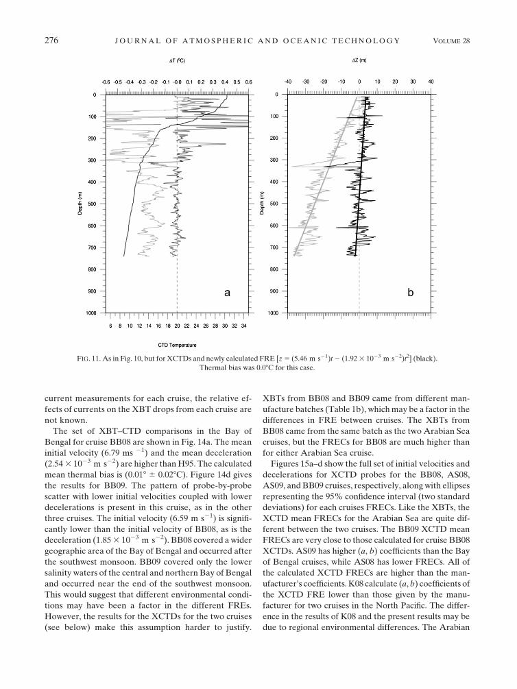
The set of XBT–CTD comparisons in the Bay of
Bengal for cruise BB08 are shown in Fig. 14a. The mean
initial velocity (6.79 ms 21) and the mean deceleration
(2.54 3 1023 m s22) are higher than H95. The calculated
mean thermal bias is (0.018 6 0.028C). Figure 14d gives
the results for BB09. The pattern of probe-by-probe
scatter with lower initial velocities coupled with lower
decelerations is present in this cruise, as in the other
three cruises. The initial velocity (6.59 m s21) is signifi-
cantly lower than the initial velocity of BB08, as is the
deceleration (1.85 3 1023 m s22). BB08 covered a wider
geographic area of the Bay of Bengal and occurred after
the southwest monsoon. BB09 covered only the lower
salinity waters of the central and northern Bay of Bengal
and occurred near the end of the southwest monsoon.
This would suggest that different environmental condi-
tions may have been a factor in the different FREs.
However, the results for the XCTDs for the two cruises
(see below) make this assumption harder to justify.
XBTs from BB08 and BB09 came from different man-
ufacture batches (Table 1b), which may be a factor in the
differences in FRE between cruises. The XBTs from
BB08 came from the same batch as the two Arabian Sea
cruises, but the FRECs for BB08 are much higher than
for either Arabian Sea cruise.
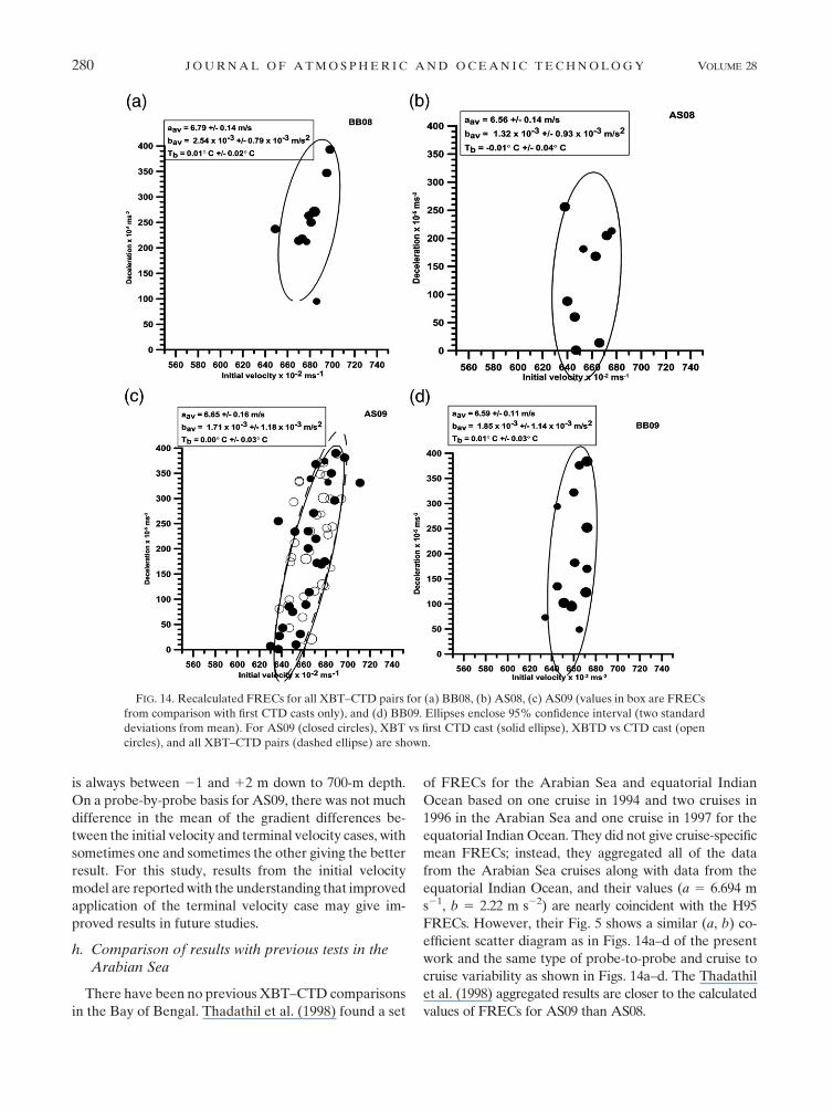
Figures 15a–d show the full set of initial velocities and
decelerations for XCTD probes for the BB08, AS08,
AS09, and BB09 cruises, respectively, along with ellipses
representing the 95% confidence interval (two standard
deviations) for each cruises FRECs. Like the XBTs, the
XCTD mean FRECs for the Arabian Sea are quite dif-
ferent between the two cruises. The BB09 XCTD mean
FRECs are very close to those calculated for cruise BB08
XCTDs. AS09 has higher (a, b) coefficients than the Bay
of Bengal cruises, while AS08 has lower FRECs. All of
the calculated XCTD FRECs are higher than the man-
ufacturer’s coefficients. K08 calculate (a, b) coefficients of
the XCTD FRE lower than those given by the manu-
facturer for two cruises in the North Pacific. The differ-
ence in the results of K08 and the present results may be
due to regional environmental differences. The Arabian
FIG. 11. As in Fig. 10, but for XCTDs and newly calculated FRE [z 5 (5.46 m s21)t 2 (1.92 3 1023 m s22)t2] (black).
Thermal bias was 0.08C for this case.
276 J O U R N A L O F A T M O S P H E R I C A N D O C E A N I C T E C H N O L O G Y VOLUME 28
Sea and Bay of Bengal water temperatures are warmer
than for either cruise used in K08. K08 calculates a tem-
perature dependency of the XCTD FRE based on the
two cruises using the temperature at 500-m depth (T500).
If this temperature-dependent FRE is applied to the cruises
in the present study, the maximum resultant FRECs (for
the Arabian Sea) are a 5 5.024 m s21, b 5 0.540 3
1023 m s22, based on a T500 5 10.778C. These coefficients
are much lower than the presently calculated (a, b) coef-
ficients. Interestingly, if the temperature in the mixed layer
(TML 5 30.728C) is used, the temperature-dependent coef-
ficients become a 5 5.184 m s21, b 5 0.910 3 1023 m s22,
FIG. 12. Mean of differences of temperature gradients at 1-m increments between XBT and first CTD cast from the Sagar Purvi on 2
Apr 2009 at 108N, 76.258E (AS09) in the Arabian Sea for each initial velocity (incremented at 0.01 m s21 intervals from 6.00 to 7.00 m s21)
and each deceleration (incremented at 0.01 3 1023 m s22 intervals from 0.00 to 3.90 31023 m s22) for (a) XBT-1 [newly calculated FRE
z 5 (6.64 m s21)t 2 (2.35 3 1023 ms22)t2 and 0.008C thermal bias], (b) XBT-2 [newly calculated FRE z 5 (6.79 m s21)t 2 (1.75 3
1023 ms22)t2 and 0.048C thermal bias], (c) XBT-3 [newly calculated FRE z 5 (6.71 m s21)t 2 (2.20 3 1023 m s22)t2 and 0.08C thermal
bias], and (d) XBT-4 [newly calculated FRE z 5 (6.64 m s21)t 2 (2.01 3 1023 m s22)t2 and 0.08C thermal bias]. S: Sippican FRECs,
H95: H95 FRECs, and N: newly calculated FRECs.
FEBRUARY 2011 B O Y E R E T A L . 277
so it may be that the XCTD has a temperature depen-
dence that can explain some of the difference between the
Arabian Sea cruises, the Bay of Bengal cruises, and the
North Pacific cruises of K08. Additional work needs to
be done to better quantify such temperature dependence.
Because both XBTs and XCTDs function in the same
manner, with wire unspooling during their drop through
the water column, it would be expected that environmental
variables, including temperature, would affect both instru-
ment’s FRE in a similar manner. The XBT FRECs for
BB08 and BB09 are quite different, while the XCTD
FRECs for the same cruises are nearly identical. This
seems to point to probe-to-probe differences between the
XBTs on the Bay of Bengal cruises as a larger factor than
FIG. 13. As in Fig. 12, but for the second CTD cast for (a) XBT-1 [newly calculated FRE z 5 (6.66 m s21)t 2 (1.94 3 1023 m s22)t2 and
0.008C thermal bias], (b) XBT-2 [newly calculated FRE z 5 (6.85 m s21)t 2 (1.62 3 1023 m s22)t2 and 0.078C thermal bias], (c) XBT-3
[newly calculated FRE z 5 (6.80 m s21)t 2 (1.25 3 1023 m s22)t2 and 0.048C thermal bias], and (d) XBT-4 [newly calculated FRE z 5
(6.76 m s21)t 2 (2.69 3 1023 m s22)t2 and 0.018C thermal bias]. D: depth (m), S: Sippican FRECs, H95: H95 FRECs, N: newly
calculated FRECs.
278 J O U R N A L O F A T M O S P H E R I C A N D O C E A N I C T E C H N O L O G Y VOLUME 28
environmental variability as a source of the difference in
the XBT FRECs for the two cruises. A possible significant
difference is that XBTs used in the present work were
manufactured by Sippican, whereas the XCTDs were
manufactured by TSK. The variability in the dimensions
of the probes manufactured by TSK was (statistically)
smaller than that in the Sippican probes in a small sample
of analyzed probes. This could be a physical basis in part
supporting the more pronounced random behavior of the
XBT probes (Sippican) than XCTD (TSK). It could also
be the larger external dimensions and heavier weight of
the XCTD probes that make them more stable and less
prone to probe-to-probe variability.
g. Comparison with terminal velocity model
Gouretski and Reseghetti (2010) try to explain what
occurs in the near-surface layer and usually describe the
startup as having transient effects. In such a region, the
XBT motion seems to be different from the description
resulting from the standard FRE. The speed of XBT
probes in the top 20–30 m is slightly slower than that
calculated by both Sippican and H95 FREs; after that
they accelerate to a terminal velocity before assuming the
characteristics represented by either the Sippican or
H95 FRE. Another factor they take into account is the
interaction among the different components of the XBT
system (i.e., the recorder and thermistor) and the ambi-
ent environment (i.e., differences in conditions between
instrument storage area and air/seawater temperature,
humidity, etc.) creating problems such as thermal shock
of the probe and affecting the thermal response of the
thermistor. The XBT manufacturer states than XBT
probes need a short time [;(2–3) s], before they assume
the terminal speed and the right spin rate, for example,
the motion conditions as described by the standard FRE
(Sippican 2009, personal communication). Recent field
tests in a very shallow area (with a depth range from 15 to
27 m) confirm that depth calculated using H95 FRE
overestimates the actual depth by about 1.0–1.5 m at
the bottom (Gouretski and Reseghetti 2010; F. Reseghetti
et al., unpublished manuscript). This difference is well
within the depth error provided by the manufacturer
(5 m), but it reveals that some other phenomena occur
in the first few seconds deviation from the simple
description adopted by the standard FRE. A video also
shows that immediately after an XBT hits seawater, the
probe has both a helical motion, and a reduced spin rate.
This could explain how the depth difference in Fig. 6b
switches sign around 50-m depth.
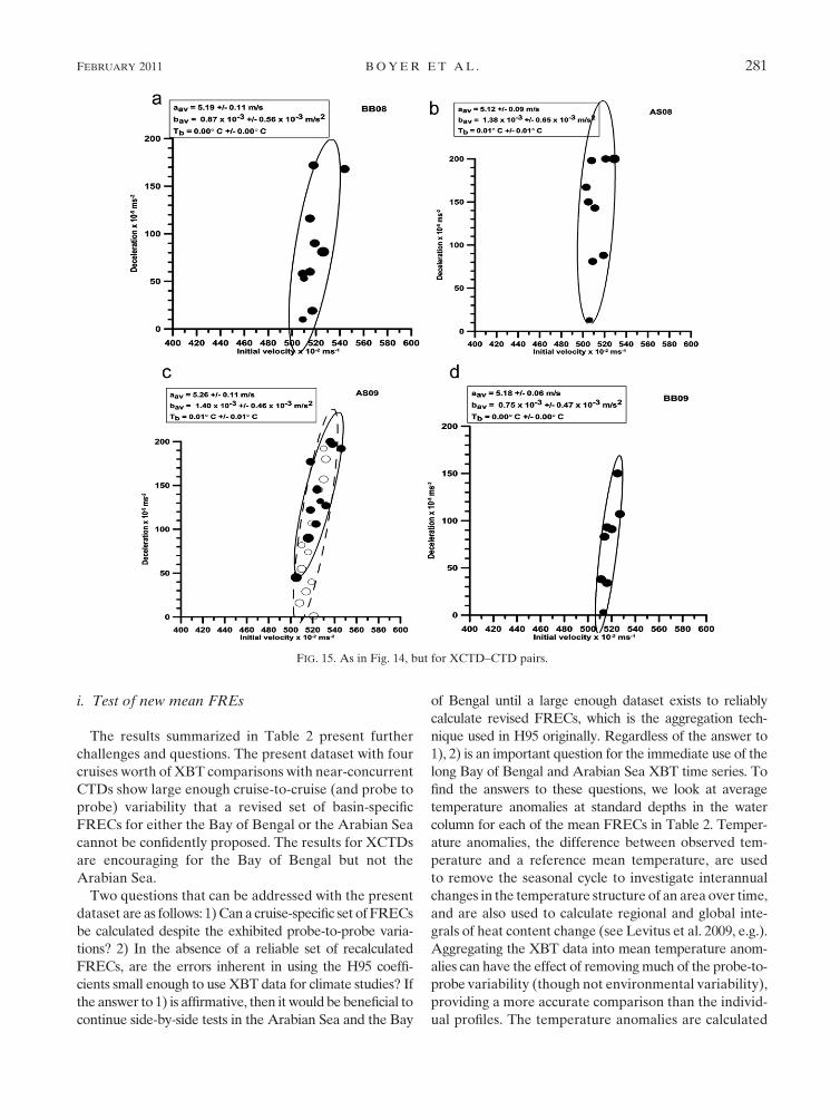
To verify the idea of Gouretski and Reseghetti (2010),
a terminal velocity model for calculating a new FRE was
tested on the AS09 cruise dataset (using a comparison
with the first CTD only). In this model, the first 3 s of the
drop are assumed to cover the top 18 m (as opposed to
;20 m for the H95 FRE), and then an FRE is fit from
this point, assuming terminal velocity has been reached.
The 2-m difference from H95 is an overestimate, but a
reasonable one given the 1-m increments of the XBT
data. The calculated mean terminal velocity and decel-
eration for AS09 for the terminal velocity case are a 5
(6.75 6 0.17 m s21) and b 5 (2.69 6 1.22 m s22), and the
thermal bias is (0.008 6 0.38C). This is higher than the
initial velocity model for both (a, b). Figure 16 shows
the depth difference between the initial velocity model
and the terminal velocity model at each depth of the
initial velocity model. For this case, the depth difference
TABLE 2a. Recalculated XBT mean FRECs and temperature biases for each cruise. First row gives H95 values for comparison. AS09112
uses XBT comparisons with both the first and second CTD cast. AS091 uses comparisons with the first CTD cast only.
Cruise Initial velocity (a coefficient, m s21) Deceleration (b coefficient, 1023 m s22) Thermal bias (8C)
H95 6.691 2.25 —
BB08 6.79 6 0.14 2.54 6 0.79 0.01 6 0.02
AS08 6.56 6 0.14 1.32 6 0.93 20.01 6 0.04
AS09112 6.68 6 0.17 1.89 6 1.22 0.1 6 0.02
AS091 6.65 6 0.16 1.71 6 1.18 0.0 6 0.03
BB09 6.59 6 0.11 1.85 6 1.14 0.01 6 0.03
TABLE 2b. Recalculated XCTD mean FRECs and temperature biases for each cruise. First row gives default TSK values for comparison.
AS09112 uses XCTD comparisons with both first and second CTD cast. AS091 uses comparisons with first CTD cast only.
Cruise Initial velocity (a coefficient, m s21) Deceleration (b coefficient, 1023 m s22) Thermal bias (8C)
TSK 5.076 0.72 —
BB08 5.19 6 0.11 0.87 6 0.56 0.00 6 0.00
AS08 5.12 6 0.09 1.38 6 0.65 0.01 6 0.01
AS09112 5.23 6 0.10 1.14 6 0.61 0.01 6 0.01
AS091 5.26 6 0.11 1.40 6 0.47 0.01 6 0.01
BB09 5.18 6 0.06 0.75 6 0.47 0.00 6 0.00
FEBRUARY 2011 B O Y E R E T A L . 279
is always between 21 and 12 m down to 700-m depth.
On a probe-by-probe basis for AS09, there was not much
difference in the mean of the gradient differences be-
tween the initial velocity and terminal velocity cases, with
sometimes one and sometimes the other giving the better
result. For this study, results from the initial velocity
model are reported with the understanding that improved
application of the terminal velocity case may give im-
proved results in future studies.
h. Comparison of results with previous tests in theArabian Sea
There have been no previous XBT–CTD comparisons
in the Bay of Bengal. Thadathil et al. (1998) found a set
of FRECs for the Arabian Sea and equatorial Indian
Ocean based on one cruise in 1994 and two cruises in
1996 in the Arabian Sea and one cruise in 1997 for the
equatorial Indian Ocean. They did not give cruise-specific
mean FRECs; instead, they aggregated all of the data
from the Arabian Sea cruises along with data from the
equatorial Indian Ocean, and their values (a 5 6.694 m
s21, b 5 2.22 m s22) are nearly coincident with the H95
FRECs. However, their Fig. 5 shows a similar (a, b) co-
efficient scatter diagram as in Figs. 14a–d of the present
work and the same type of probe-to-probe and cruise to
cruise variability as shown in Figs. 14a–d. The Thadathil
et al. (1998) aggregated results are closer to the calculated
values of FRECs for AS09 than AS08.
FIG. 14. Recalculated FRECs for all XBT–CTD pairs for (a) BB08, (b) AS08, (c) AS09 (values in box are FRECs
from comparison with first CTD casts only), and (d) BB09. Ellipses enclose 95% confidence interval (two standard
deviations from mean). For AS09 (closed circles), XBT vs first CTD cast (solid ellipse), XBTD vs CTD cast (open
circles), and all XBT–CTD pairs (dashed ellipse) are shown.
280 J O U R N A L O F A T M O S P H E R I C A N D O C E A N I C T E C H N O L O G Y VOLUME 28
i. Test of new mean FREs
The results summarized in Table 2 present further
challenges and questions. The present dataset with four
cruises worth of XBT comparisons with near-concurrent
CTDs show large enough cruise-to-cruise (and probe to
probe) variability that a revised set of basin-specific
FRECs for either the Bay of Bengal or the Arabian Sea
cannot be confidently proposed. The results for XCTDs
are encouraging for the Bay of Bengal but not the
Arabian Sea.
Two questions that can be addressed with the present
dataset are as follows: 1) Can a cruise-specific set of FRECs
be calculated despite the exhibited probe-to-probe varia-
tions? 2) In the absence of a reliable set of recalculated
FRECs, are the errors inherent in using the H95 coeffi-
cients small enough to use XBT data for climate studies? If
the answer to 1) is affirmative, then it would be beneficial to
continue side-by-side tests in the Arabian Sea and the Bay
of Bengal until a large enough dataset exists to reliably
calculate revised FRECs, which is the aggregation tech-
nique used in H95 originally. Regardless of the answer to
1), 2) is an important question for the immediate use of the
long Bay of Bengal and Arabian Sea XBT time series. To
find the answers to these questions, we look at average
temperature anomalies at standard depths in the water
column for each of the mean FRECs in Table 2. Temper-
ature anomalies, the difference between observed tem-
perature and a reference mean temperature, are used
to remove the seasonal cycle to investigate interannual
changes in the temperature structure of an area over time,
and are also used to calculate regional and global inte-
grals of heat content change (see Levitus et al. 2009, e.g.).
Aggregating the XBT data into mean temperature anom-
alies can have the effect of removing much of the probe-to-
probe variability (though not environmental variability),
providing a more accurate comparison than the individ-
ual profiles. The temperature anomalies are calculated
FIG. 15. As in Fig. 14, but for XCTD–CTD pairs.
FEBRUARY 2011 B O Y E R E T A L . 281
here by subtracting the median temperature for the
depth interval around 16 standard depths from the sur-
face to 700 m from the standard level temperature value
from appropriate geographic location from the World
Ocean Atlas 2005 (WOA05; Locarnini et al. 2006) cli-
matological mean monthly temperature fields at 18 res-
olution. Anomalies based on WOA05 are used to
calculate heat content anomalies in Levitus et al. (2009)
and it is thus of interest to see how XBT FRE errors and
corrections affect these anomalies. Table 3 gives the 16
standard depth levels and the depth interval around
each standard depth from which the median was calcu-
lated. Figures 17a–d show the mean temperature anom-
aly at the 16 standard depths from the surface to 700 m
from all XBT data using the H95 FRE (solid black line
with diamonds), the FRE with the newly calculated
FRECs (dashed black line with circles), and all CTD data
(gray line with crosses). Looking first at Fig. 17c (AS09),
the H95 FRE-calculated anomalies generally result in an
overestimate of water column warming for AS09 for pos-
itive temperature anomalies, and an underestimate for
negative temperature anomalies; the new FRE lessens, but
does not eliminate, this bias. The AS08 cruise (Fig. 17b)
measures a different temperature anomaly structure in the
upper 200 m than the AS09 cruise, and all three AS08
temperature anomaly curves show a large temperature
anomaly around 100-m depth of the opposite sign to the
temperature anomaly found in AS09 in the following
April. In the AS08 case, the H95 FRE XBT anomalies are
;0.58C smaller than CTD anomalies from 50 to 125.
Deeper down the differences are smaller but still signifi-
cant, ;0.28C at the 200-m level. The recalculated FRE
temperature anomalies show considerable improvement
over the H95 FRE temperature anomalies in comparison
with the CTD temperature anomalies. As with AS09,
AS08 has a positive temperature bias. However, in the case
of AS08, the agreement with CTD temperature anomalies
at many depths is significantly improved by applying the
new FRE. At the last depth for the CTDs for this cruise
(400 m), there is a relatively high anomaly that is not seen
in the mean XBT anomalies or in the mean XCTD anom-
alies. The slightly anomalous temperatures may be due to
problems associated with the winch on this cruise.
In the Bay of Bengal, BB08 (Fig. 17a), the mean XBT
temperature anomalies XBT FRE calculated with the
new FRECs correlate more closely with the composite
temperature anomalies from CTD casts than do the
temperature anomalies from the H95 FRE case, except
at the last standard level at 700 m. Even here, all three
mean temperature anomalies are within 0.18C of each
other. Unlike AS08 and AS09, the bias in the tempera-
ture anomaly for BB08 is cooler, and the bias is elimi-
nated when applying the new FRE.
For cruise BB09 (Fig. 17d) at all levels, the adjusted
FRE temperature anomalies are nearly indistinguishable
from the CTD temperature anomalies, and both are lower
FIG. 16. Difference between initial velocity model depth and
terminal velocity model depth for the AS09 cruise mean FRECs
(from first CTD cast comparisons only). The y-axis depths are
calculated from the initial velocity case where initial velocity is
6.65 m s21 and mean deceleration is 1.71 3 1023 m s22. For the
terminal velocity case, initial velocity is 6.75 m s21 and mean de-
celeration is 2.69 3 1023 m s22.
TABLE 3. Standard depths and depth intervals used to calculate
temperature anomalies. The intervals include all depths $ the first
depth shown in column 3, and , second depth shown in column 3.
Standard
level No.
Standard
depth (m)
Depth
interval (m)
1 0 0–5
2 10 5–15
3 20 15–25
4 30 25–40
5 50 40–62.5
6 75 62.5–87.5
7 100 87.5–112.5
8 125 112.5–137.5
9 150 137.5–175
10 200 175–225
11 250 225–275
12 300 275–350
13 400 350–450
14 500 450–550
15 600 550–650
16 700 650–750
282 J O U R N A L O F A T M O S P H E R I C A N D O C E A N I C T E C H N O L O G Y VOLUME 28
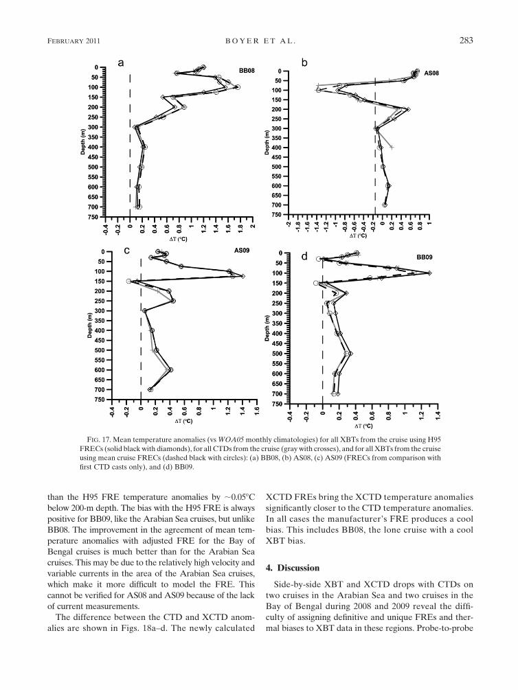
than the H95 FRE temperature anomalies by ;0.058C
below 200-m depth. The bias with the H95 FRE is always
positive for BB09, like the Arabian Sea cruises, but unlike
BB08. The improvement in the agreement of mean tem-
perature anomalies with adjusted FRE for the Bay of
Bengal cruises is much better than for the Arabian Sea
cruises. This may be due to the relatively high velocity and
variable currents in the area of the Arabian Sea cruises,
which make it more difficult to model the FRE. This
cannot be verified for AS08 and AS09 because of the lack
of current measurements.
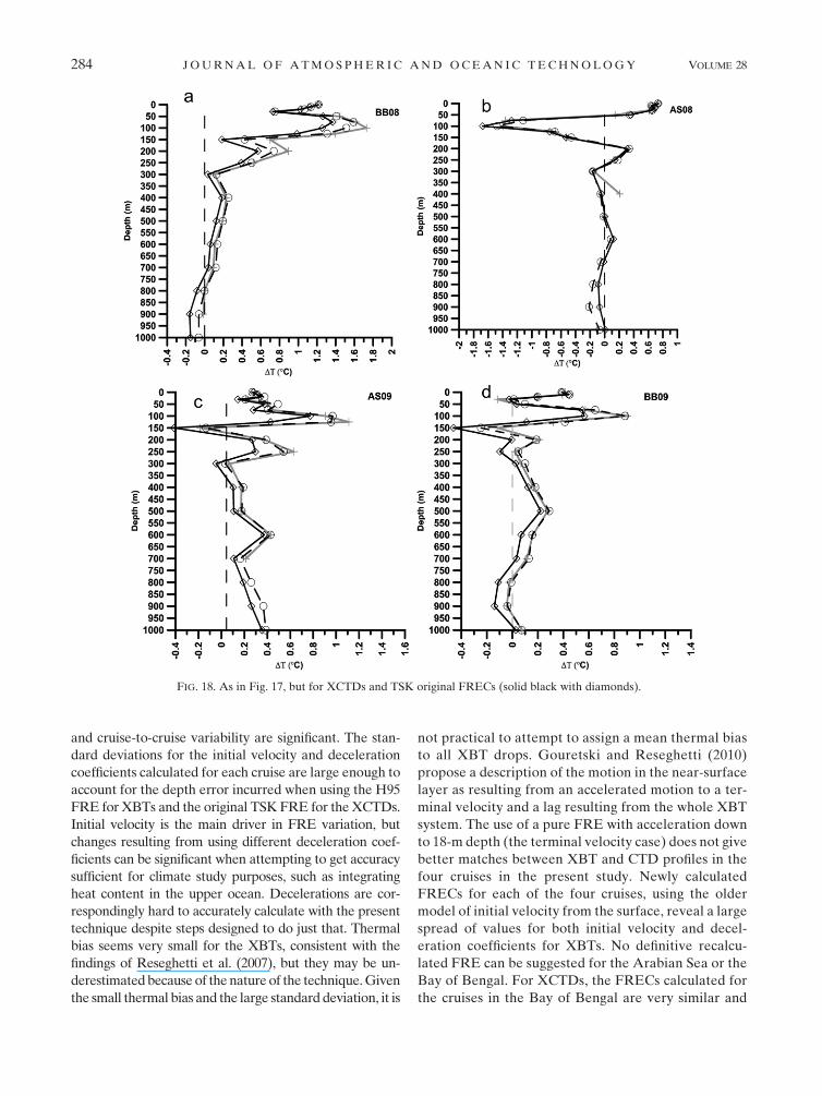
The difference between the CTD and XCTD anom-
alies are shown in Figs. 18a–d. The newly calculated
XCTD FREs bring the XCTD temperature anomalies
significantly closer to the CTD temperature anomalies.
In all cases the manufacturer’s FRE produces a cool
bias. This includes BB08, the lone cruise with a cool
XBT bias.
4. Discussion
Side-by-side XBT and XCTD drops with CTDs on
two cruises in the Arabian Sea and two cruises in the
Bay of Bengal during 2008 and 2009 reveal the diffi-
culty of assigning definitive and unique FREs and ther-
mal biases to XBT data in these regions. Probe-to-probe
FIG. 17. Mean temperature anomalies (vs WOA05 monthly climatologies) for all XBTs from the cruise using H95
FRECs (solid black with diamonds), for all CTDs from the cruise (gray with crosses), and for all XBTs from the cruise
using mean cruise FRECs (dashed black with circles): (a) BB08, (b) AS08, (c) AS09 (FRECs from comparison with
first CTD casts only), and (d) BB09.
FEBRUARY 2011 B O Y E R E T A L . 283
and cruise-to-cruise variability are significant. The stan-
dard deviations for the initial velocity and deceleration
coefficients calculated for each cruise are large enough to
account for the depth error incurred when using the H95
FRE for XBTs and the original TSK FRE for the XCTDs.
Initial velocity is the main driver in FRE variation, but
changes resulting from using different deceleration coef-
ficients can be significant when attempting to get accuracy
sufficient for climate study purposes, such as integrating
heat content in the upper ocean. Decelerations are cor-
respondingly hard to accurately calculate with the present
technique despite steps designed to do just that. Thermal
bias seems very small for the XBTs, consistent with the
findings of Reseghetti et al. (2007), but they may be un-
derestimated because of the nature of the technique. Given
the small thermal bias and the large standard deviation, it is
not practical to attempt to assign a mean thermal bias
to all XBT drops. Gouretski and Reseghetti (2010)
propose a description of the motion in the near-surface
layer as resulting from an accelerated motion to a ter-
minal velocity and a lag resulting from the whole XBT
system. The use of a pure FRE with acceleration down
to 18-m depth (the terminal velocity case) does not give
better matches between XBT and CTD profiles in the
four cruises in the present study. Newly calculated
FRECs for each of the four cruises, using the older
model of initial velocity from the surface, reveal a large
spread of values for both initial velocity and decel-
eration coefficients for XBTs. No definitive recalcu-
lated FRE can be suggested for the Arabian Sea or the
Bay of Bengal. For XCTDs, the FRECs calculated for
the cruises in the Bay of Bengal are very similar and
FIG. 18. As in Fig. 17, but for XCTDs and TSK original FRECs (solid black with diamonds).
284 J O U R N A L O F A T M O S P H E R I C A N D O C E A N I C T E C H N O L O G Y VOLUME 28
suggest that a new FRE, with higher initial velocity
(5.18 m s21) and the same or slightly higher deceleration
than the original TSK FRE, should be used. For the Ara-
bian Sea the FRECs calculated for each cruise are different,
possibly resulting from variations in the currents in the area,
and no new FRE can be proposed.
Tests of the H95 FRECs and new FRECs for each
cruise show that the H95 XBT FRECs result in signifi-
cant errors (.0.28C) between the 75- and 200-m levels,
with most errors ,0.18C below 200 m. Temperature
anomalies with the new FRE for each cruise show much
better agreement with CTD temperature anomalies than
similar anomalies using the H95 FRE at all levels, or
little change, as is the case with AS09. The tests with the
XBT probes show that further side-by-side tests in both
the Arabian Sea and the Bay of Bengal can be beneficial
in aggregating enough data to eventually average out
probe-to-probe variability and propose new FREs that
will substantially improve climate studies, such as inte-
grated ocean heat content change. In the meantime,
individual cruise-corrected XBT FRE from side-by-side
test cruises can be used to do smaller-scale climate
studies with the full set of XBTs from these cruises. For
the full set of the Bay of Bengal and Arabian Sea XBT
cruises, the data can be used for climate studies with the
H95 FRE with the understanding of the errors inherent
in using this FRE shown here for the different depth
levels. However, it must be kept in mind during studies
with these XBT time series, that XBT probe-to-probe
variability is high, and even the sign of the XBT bias for
a given cruise cannot be assumed. Recent tests by Sippican
(personal communication, 2010) show that recently pro-
duced Sippican Deep Blue XBTs have a fall rate that is
modeled correctly by the H95 FRE, while older probes
have a slightly slower fall rate. Thus, it may be that there
will be no need for FRE corrections for XBT drops going
forward. However, it remains to be seen if these results
hold for all XBTs manufactured in the future, or for all
ocean conditions.
For XCTDs, application of the new FREs for each
cruise results in the definite improvement for all cruises.
More study is necessary to modify the temperature de-
pendence of the XCTD-3 FRE as given in K08. Given
the temperature structure of the Arabian Sea and Bay of
Bengal and the lower probe-to-probe variability in the
XCTD as compared with the XBT, the FREs calculated
for the Bay of Bengal can be used to remove the cool
bias in the XCTD data for this region.
Acknowledgments. We would like to acknowledge the
help of Pr. Shoichi Kizu, Tohoku Univeristy, and LM
Sippican for sharing their research and knowledge re-
garding XBT and XCTD fall rates. We would also like to
acknowledge our colleagues Syd Levitus and Ricardo
Locarnini and three anonymous reviewers for their
helpful comments on the manuscript. The data were
collected under the ongoing long-term observational
program supported by the Ministry of Earth Sciences
through INCOIS.
REFERENCES
Beaty, W. H., III, J. G. Bruce, and R. C. Guthrie, 1981: Circulation
and oceanographic properties in the Somali Basin as observed
during the 1979 southwest monsoon. Naval Oceanographic
Office Tech. Rep. 258, 156 pp.
Cunningham, S. A., 2000: RRS Discovery Cruise 242, 07 Sep-06
Oct 1999: Atlantic–Norwegian exchanges. Southhampton
Oceanography Centre Cruise Rep. 28, 128 pp. [Available online
at http://eprints.soton.ac.uk/295/1/soccr028.pdf.]
Gouretski, V., and K. P. Koltermann, 2007: How much is the ocean
really warming? Geophys. Res. Lett., 34, L01610, doi:10.1029/
2006GL027834.
——, and F. Reseghetti, 2010: On depth and temperature biases in
bathythermograph data: Development of a new correction
scheme based on analysis of a global ocean database. Deep-
Sea Res. I, 57, 812–833, doi:10.1016/j.dsr.2010.03.011.
Graziottin, F., G. K. Morrison, R. Stoner, and F. De Strobel, 1999:
Laboratory evaluation and preliminary field trials of new
‘‘WOCE standard’’ Idronaut MK317 and OS316 CTD probes.
Proc. OCEANS‘99 MTS/IEEE: Riding the Crest into the 21st
Century, Vol. 3, Seattle, WA, IEEE, 1211–1217.
Hanawa, K., P. Rual, R. Bailey, A. Sy, and M. Szabados, 1995: A
new depth-time equation for Sippican or TSK T-7, T-6, and
T-4 expendable bathythermographs (XBT). Deep-Sea Res. I,
42, 1423–1451.
Ishii, M., and M. Kimoto, 2009: Reevaluation of historical ocean
heat content variations with time-varying XBT and MBT
depth bias corrections. J. Oceanogr., 65, 287–299.
Johnson, G., 1995: Revised XCTD fall-rate equation coefficients
from CTD data. J. Atmos. Oceanic Technol., 12, 1367–1373.
Kizu, S., S. Ito, and T. Watanabe, 2005: Inter-manufacturer dif-
ference and temperature dependency of the fall rate of T-5
expendable bathythermograph. J. Oceanogr., 61, 905–912.
——, H. Onishi, T. Suga, K. Hanawa, T. Watanabe, and H. Iwamiya,
2008: Evaluation of the fall rates of the present and develop-
mental XCTDs. Deep-Sea Res. I, 55, 571–586.
Levitus, S., J. I. Antonov, T. P. Boyer, R. A. Locarnini, H. E. Garcia,
and A. V. Mishonov, 2009: Global ocean heat content 1955-2008
in light of recently revealed instrumentation problems. Geophys.
Res. Lett., 36, L07608, doi:10.1029/2008GL037155.
Locarnini, R. A., A. V. Mishonov, J. I. Antonov, T. P. Boyer, and
H. E. Garcia, 2006: Temperature. Vol. 1, World Ocean Atlas
2005, NOAA Atlas NESDIS 61, 182 pp.
Nyffeler, F., and C. H. Godet, 2002: A practical comparison be-
tween Seabird SBE911 and Ocean Seven 320 CTD probes.
IDRONAUT, 3 pp. [Available online at http://www.idronaut.it.]
Reseghetti, F., M. Borghini, and G. M. R. Manzella, 2007: Fac-
tors affecting the quality of XBT data—Results of analyses on
profiles from the western Mediterranean Sea. Ocean Sci., 3,
59–75.
Seaver, G. A., and S. Kuleshov, 1982: Experimental and analytical
error of the expendable bathythermograph. Deep-Sea Res. I,
30, 1185–1197.
FEBRUARY 2011 B O Y E R E T A L . 285
Shetye, S. R., 1984: Seasonal variability of the temperature field off the
south-west coast of India. Proc. Indian Acad. Sci., 93, 399–411.
Thadathil, P., A. K. Ghosh, and P. M. Muraleedharan, 1998: An
evaluation of XBT depth equations for the Indian Ocean.
Deep-Sea Res. I, 45, 819–827.
——, A. K. Saran, V. V. Gopalakrishna, P. Vethamony, N. Araligidad,
and R. Bailey, 2002: XBT fall rate in waters of extreme tem-
perature: A case study in the Antarctic Ocean. J. Atmos. Oceanic
Technol., 19, 391–396.
Turner, D., 1992: R/V Discovery cruise report SR01: 11 November
1992–17 December 1992, 93 pp. [Available online at http://
cchdo.ucsd.edu/data/repeat/southern/sr01/sr01_b/sr01_bdo.pdf.]
Wijffels, S. E., J. Willis, C. M. Domingues, P. Barker, N. J. White,
A. Gronell, K. Ridgway, and J. A. Church, 2008: Changing
expendable bathythermograph fall rates and their impact
on estimates of thermosteric sea level rise. J. Climate, 21,5657–5672.
Willis, J., J. M. Lyman, G. C. Johnson, and J. Gilson, 2009:
In situ data biases and recent ocean heat content variability.
J. Atmos. Oceanic Technol., 26, 846–852.
Wisotzki, A., and E. Fahrbach, 1991: XBT-data measured from
1984 to 1991 in the Atlantic Sector of the Southern Ocean by
R.V. ‘‘Meteor’’ and R.V. ‘‘Polarstern.’’ Alfred Wegener In-
stitut Tech. Rep. 18, 96 pp.
286 J O U R N A L O F A T M O S P H E R I C A N D O C E A N I C T E C H N O L O G Y VOLUME 28