Hybridization biases of microarray expression data - Qucosa ...
158
Hybridization biases of microarray expression data A model-based analysis of RNA quality and sequence effects Von der Fakultät für Mathematik und Informatik der Universität Leipzig angenommene DISSERTATION zur Erlangung des akademischen Grades D OCTOR RERUM NATURALUM (Dr. rer. nat) im Fachgebiet Informatik vorgelegt von Diplom Bioinformatiker Mario Fasold geboren am 9. Juli 1981 in Dresden Die Annahme der Dissertation wurde empfohlen von: 1. Professor Dr. Peter F. Stadler, Universität Leipzig 2. Dr. Andrew Harrison, University of Essex, United Kingdom Die Verleihung des akademischen Grades erfolgt mit Bestehen der Verteidigung am 11. Juni 2013 mit dem Gesamtprädikat magna cum laude.
-
Upload
khangminh22 -
Category
Documents
-
view
0 -
download
0
Transcript of Hybridization biases of microarray expression data - Qucosa ...

Hybridization biases of microarray
expression data
A model-based analysis of RNA quality and sequence effects
Von der Fakultät für Mathematik und Informatik der Universität Leipzig
angenommene
DISSERTATION
zur Erlangung des akademischen Grades
DOCTOR RERUM NATURALUM (Dr. rer. nat)
im Fachgebiet
Informatik
vorgelegt
von Diplom Bioinformatiker Mario Fasold
geboren am 9. Juli 1981 in Dresden
Die Annahme der Dissertation wurde empfohlen von:
1. Professor Dr. Peter F. Stadler, Universität Leipzig 2. Dr. Andrew Harrison, University of Essex, United Kingdom
Die Verleihung des akademischen Grades erfolgt mit Bestehen
der Verteidigung am 11. Juni 2013 mit dem Gesamtprädikat magna cum laude.


Abstract
Modern high-throughput technologies like DNA microarrays are powerful tools that are widely used in biomedical research. They target a variety of genomics applications ranging from gene expression profiling over DNA genotyping to gene regulation studies. However, the recent discovery of false positives among prominent research findings indicates a lack of awareness or understanding of the non-biological factors negatively affecting the accuracy of data produced using these technologies. The aim of this thesis is to study the origins, effects and potential correction methods for selected methodical biases in microarray data.
The two-species Langmuir model serves as the basal physicochemical model of microarray hybridization describing the fluorescence signal response of oligonucleotide probes. The so-called hook method allows to estimate essential model parameters and to compute summary parameters characterizing a particular microarray sample. We show that this method can be applied successfully to various types of microarrays which share the same basic mechanism of multiplexed nucleic acid hybridization.
Using appropriate modifications of the model we study RNA quality and sequence effects using publicly available data from Affymetrix GeneChip expression arrays. Varying amounts of hybridized RNA result in systematic changes of raw intensity signals and appropriate indicator variables computed from these. Varying RNA quality strongly affects intensity signals of probes which are located at the 3’ end of transcripts. We develop new methods that help assessing the RNA quality of a particular microarray sample. A new metric for determining RNA quality, the degradation index, is proposed which improves previous RNA quality metrics. Furthermore, we present a method for the correction of the 3’ intensity bias. These functionalities have been implemented in the freely available program package AffyRNADegradation.
We show that microarray probe signals are affected by sequence effects which are studied systematically using positional-dependent nearest-neighbor models. Analysis of the resulting sensitivity profiles reveals that specific sequence patterns such as runs of guanines at the solution end of the probes have a strong impact on the probe signals. The sequence effects differ for different chip- and target-types, probe types and hybridization modes. Theoretical and practical solutions for the correction of the introduced sequence bias are provided.
Assessment of RNA quality and sequence biases in a representative ensemble of over 8000 available microarray samples reveals that RNA quality issues are prevalent: about 10% of

4 Abstract
the samples have critically low RNA quality. Sequence effects exhibit considerable variation within the investigated samples but have limited impact on the most common patterns in the expression space. Variations in RNA quality and quantity in contrast have a significant impact on the obtained expression measurements.
These hybridization biases should be considered and controlled in every microarray experiment to ensure reliable results. Application of rigorous quality control and signal correction methods is strongly advised to avoid erroneous findings. Also, incremental refinement of physicochemical models is a promising way to improve signal calibration paralleled with the opportunity to better understand the fundamental processes in microarray hybridization.

Acknowledgments
First of all, I would like to thank my supervisor Hans Binder for giving me the opportunity to work on this interesting research topic. For each of the many challenging theoretical and practical problems I faced in the past years, I could always be sure he would help with his good advice. Without his continuous and great support much this work would not be possible. I also thank my second supervisor Peter F. Stadler for his great support and always useful scientific advice.
I will always remember Jan Bruecker who died much too early in 2011. He was a cheerful and inspiring character, and he contributed to this thesis by developing parts of the software used and by providing many helpful discussions.
Of course I thank all dear colleagues and friends from the IZBI and the Chair of Bioinformatics of the University of Leipzig. I really enjoyed the vivid discussions, the fun events and the good advice and deep knowledge one could always rely on. I particularly thank Corinna and Petra for their always positive attitude and their indispensable support for all administrative activities. Jens provided great technical support and advice, as did David, Henry and Christian with their helpful discussions about R and other technical obstacles. Additionally, I thank the following people who in some way contributed to the success of this work: Anne, Axel, Berni, Christian, Dom, Edith, Gero, Gunnar, Katrin, Lydia, Konstantin, Jana, Markus, Maribel, Sven, Joerg, Stephan, Stephie, Steve, Volkan, Wolfgang and everybody else I’ve missed. It was really a pleasure to work with you.
Finally, I thank my family and friends who indirectly contributed to this work with their continuous love and encouragement. I particularly thank my beloved Anne, as well as my parents for their support. I express my deep appreciation to all of you.

Related publications
This thesis is partially based on the following publications:
Binder H, Fasold M, Glomb T: Mismatch and G-stack modulated probe signals on SNP microarrays. PloS One 2009, 4.
Fasold M, Stadler PF, Binder H: G-stack modulated probe intensities on expression arrays - sequence corrections and signal calibration. BMC Bioinformatics 2010, 11:207.
Fasold M, Binder H: Estimating RNA-quality using GeneChip microarrays. BMC Genomics 2012, 13:186.
Fasold M, Binder H: AffyRNADegradation: control and correction of RNA quality effects in GeneChip expression data. Bioinformatics 2013, 29:129-131.
Fasold M, Binder H: Prevalence and impact of technical artifacts in microarray expression data. In preparation.

Contents
Abstract ................................................................................................................. 3
Acknowledgments ................................................................................................ 5
Related publications ............................................................................................ 6
1 Introduction ........................................................................................... 11 1.1 The role of high-throughput technologies in modern life sciences ....................... 11 1.2 Physicochemical models for microarray data analysis ......................................... 14 1.3 Objectives and outline........................................................................................... 15
2 Microarray technology .......................................................................... 17 2.1 Microarrays assembly and assay ........................................................................... 17 2.2 3’ expression arrays .............................................................................................. 18 2.3 Gene ST and Exon ST arrays ................................................................................ 20 2.4 Genome-wide SNP arrays ..................................................................................... 21 2.5 Agilent expression arrays ...................................................................................... 23 2.6 Summary and conclusions .................................................................................... 23
3 A model for microarray hybridization .................................................. 25 3.1 Modeling microarray intensity signals.................................................................. 25 3.2 The two-species Langmuir model ......................................................................... 26 3.3 The hook transformation and hybridization modes .............................................. 27 3.4 Positional-dependent sequence models................................................................. 29 3.4.1 Modeling the formation of duplexes ..................................................................... 29 3.4.2 Different characteristics for specific and non-specific binding ............................ 31 3.4.3 Estimation of profiles ............................................................................................ 31 3.5 Fitting the hybridization model ............................................................................. 32 3.6 Chip summary measures characterize RNA quantity ........................................... 34 3.7 Summary and conclusions .................................................................................... 36
4 Hook analysis applied to different types of microarrays ................... 39 4.1 Genome-wide SNP arrays ..................................................................................... 39 4.2 Gene ST and Exon ST arrays ................................................................................ 41 4.3 Agilent expression arrays ...................................................................................... 43 4.4 Summary and conclusions .................................................................................... 45
5 RNA quality effects ............................................................................... 47 5.1 RNA amplification and degradation in microarray experiments .......................... 47 5.1.1 3’-biased transcript coverage of microarray probes after RNA amplification and degradation .............................................................................. 49 5.1.2 Probing transcript abundance using GeneChip arrays .......................................... 50

8 1
5.1.3 Used expression data............................................................................................. 54 5.2 Degradation and hybridization mode .................................................................... 54 5.2.1 Intensity-based degradation metrics ..................................................................... 54 5.2.2 Degradation Hook and Tongs Plot ........................................................................ 57 5.2.3 The 3’-intensity bias depends on the hybridization mode .................................... 61 5.2.4 Short 3’-probe sets are prone to non-specific hybridization ................................. 64 5.3 Metrics for RNA quality ....................................................................................... 66 5.3.1 Positional-dependent intensity decays .................................................................. 66 5.3.2 3’/5’-controls are affected by the hybridization mode .......................................... 70 5.3.3 Affy-slope is affected by absent probes ................................................................ 75 5.3.4 Array-degradation metrics correlate with RIN ..................................................... 76 5.4 Degradation reduces total transcript abundance ................................................... 78 5.5 Correction of the 3’/5’ bias ................................................................................... 79 5.5.1 RNA-quality scaling of gene expression .............................................................. 79 5.5.2 Correcting the 3’/5’ bias of probe intensities ........................................................ 80 5.5.3 Index and position based correction ..................................................................... 82 5.6 An R package for the analysis and correction of RNA quality effects ................. 85 5.7 Summary and conclusions .................................................................................... 87
6 Sequence effects ................................................................................... 89 6.1 Probe sequence affects intensities and expression values ..................................... 89 6.1.1 Used expression data............................................................................................. 91 6.2 Positional-dependent sensitivity profiles .............................................................. 92 6.3 Guanine effects ..................................................................................................... 94 6.3.1 Sequence motif assessment ................................................................................... 94 6.3.2 Quality of fit and standard error ........................................................................... 95 6.3.3 Triple guanine motif causes large intensities ........................................................ 95 6.4 Quality of motif-specific fits ................................................................................. 97 6.4.1 Model-rank assessment with the F-test ................................................................. 97 6.4.2 Motif-specific differences ..................................................................................... 98 6.5 Chip-type and target effects ................................................................................ 100 6.6 Perfect match and mismatch probes ................................................................... 104 6.7 Specific and non-specific hybridization.............................................................. 105 6.8 Correction of microarray data for sequence effects ............................................ 107 6.8.1 The NN+GGG hybrid rank model ...................................................................... 107 6.8.2 Effect of the correction ....................................................................................... 109 6.8.3 Preprocessing of microarray intensity data ......................................................... 111 6.8.4 Comparison of sequence-specific intensity corrections ...................................... 114 6.9 Summary and conclusions .................................................................................. 119
7 Prevalence and impact of technical bias .......................................... 121 7.1 Technical artifacts can be observed in batches ................................................... 121 7.1.1 Human expression data ....................................................................................... 121

1.1 The role of high-throughput technologies in modern life sciences 9
7.1.2 Principal component analysis for gene expression data ..................................... 122 7.2 RNA quality ........................................................................................................ 123 7.3 Amount of hybridized RNA ............................................................................... 126 7.4 Sequence effects ................................................................................................. 128 7.4.1 Maximum sensitivity amplitude ......................................................................... 128 7.4.2 Guanine effects ................................................................................................... 129 7.5 Summary and conclusions .................................................................................. 130
8 Summary and discussion ................................................................... 133
A List of data sets used .......................................................................... 137
List of figures .................................................................................................... 139
List of tables ..................................................................................................... 142
Bibliography ..................................................................................................... 143
Curriculum vitae ............................................................................................... 155
Erklärung........................................................................................................... 157


1 Introduction
1.1 The role of high-throughput technologies in modern life sciences
When a researcher in the field of molecular biology carried out an experiment in the early 1990s he would need experience, craftsmanship and a lot of time. Assume the researcher was interested in gene expression. For example, he would like to know whether a gene that potentially causes cancer is active in some tumor cells or not. He could employ a technique called Northern blot and follow a long protocol of manual steps involving, amongst other things, production of an agarose gel, RNA separation using gel electrophoresis, transfer of RNAs to a membrane and production of labeled probes. Including proper controls the whole procedure would usually take days up to weeks to complete successfully. At the end, he would know whether his gene of interest is expressed in a single cell line of a single species.
If the same researcher was interested in the same question only 10 years later in the early 2000s, the experiment would run markedly different. He could resort to several commercially fabricated instruments and automated techniques specifically designed to aid in his experiment. For example, he could employ a sensitive scanner device that uses lasers to read signals out of miniaturized DNA microarrays. He would be able to simply order some of the pre-manufactured microarrays that contain probes designed to measure the expression of his gene of interest and many other genes at the same time. And he would be able to buy tailor-made reagents that help him preparing his sample for the assay in a few simple steps. The procedure would take only hours instead of weeks.
It is easy to see why high-throughput technologies like microarrays quickly replaced previous techniques in labs all over the world. They revolutionized the way how researchers could approach the problems they were facing in their particular domain. It allowed them conducting experiments hypothesis-free: The researcher could not only study the expression of one single gene he chose because he hypothesized that it relates to the cancer, but he could instead screen thousands of genes for their expression status in the tumor cells. Also it allowed conducting experiments that could not be done before because of time or money restrictions of the previous techniques. Edward Southern, one of the inventors and early adopters of these automated techniques, later commented on this dramatic development: “Genomics, in its early days, used a range of techniques that were developed to explore the composition and sequence organization of the nuclear DNA. High-throughput methods changed that, and most research in genomics is now done in factory-like laboratories, with robots doing much of the work.” [1]

12 1 Introduction
Today, many areas of life sciences rely on the methodological advances provided by a large toolbox of available high-throughput technologies. Gene expression profiling using microarrays is such a tool - being one of the first and more popular ones it is probably the best known representative for the whole toolbox. These assays are now performed routinely and in large-scale for testing the reaction of cells on different treatments and condition changes. Consider the following numbers: More than 25.000 peer-reviewed papers have been published using microarray technology from a single vendor (Affymetrix) alone [2]. Each of these publications refers to one or more experiments. For some experiments the generated data is made publicly available. Over 28.000 datasets comprising over 850.000 microarray samples have been stored in two public data repositories in the last 5 years alone1. The data of many more experiments is not shared in public databases, but is kept secretly, particularly for experiments performed at companies and private institutions.
Every experiment performed using high-throughput technologies has the property of producing large amounts of data that must afterwards be analyzed and interpreted. The analysis of such complex data is no simple task, even for experienced researchers. Without a deep understanding of the limitations of the technology and knowledge about proper statistical analysis it can easily be misinterpreted. Daniel MacArthur notes that “all high-throughput genomic technologies come with error modes and systematic biases that, to the unwary eye, can seem like interesting biology. As a result, researchers who are inexperienced with a technology — and some who should know better — can jump to the wrong conclusion” [3]. The combination of difficult-to-analyze data and the hope of surprising results can lead to so-called ‘false positives’, erroneous research findings that later had to be revoked after other groups have pointed out flaws in the analysis done by the original authors.
One example about how critical it is to ensure accurateness and rigorousness in high-throughput data analysis is given by a study published in 2007 by Spielman et al. [4]. It was previously known that the genetic divergence, the differences in the genetic code, between individuals of our species is drastically small. The human to human nucleotide divergence for example was estimated to be around 0.1% [5]. The study of Spielman et al., which was published in Nature Genetics, sought to find the factors that contributed to the large phenotypic differences between human populations. Their approach was to focus on the variation of gene expression, patterns of genetic activity, rather than on the variation of DNA sequence. Microarray technology was to be used to obtain profiles of genetic activity in lymphoblastoid cell lines from individuals belonging to one of three population groups. The authors found that the expression of about 25% of the tested genes differs significantly
1 Queried on the ArrayExpress website http://www.ebi.ac.uk/arrayexpress/ on January 7, 2013.

1.1 The role of high-throughput technologies in modern life sciences 13
between European and Asian populations. These numbers suggested that phenotypic variability to a large part is reflected in expression variability which constituted an important finding.
However, later concerns about the accuracy of these numbers were raised [6]. Akey et al. reanalyzed the data of Spielman et al. and found 78% of the genes – a rather unrealistic number - to be significantly differentially expressed. After closer inspection of the microarray data, they found that samples have been processed in groups spanning a time of more than 3 years and that European and Asian samples had been mostly processed at different times. Akey et al. then found that 79% of the genes are differentially expressed between processing years but within the same population. This significant variation between the processing groups cannot be explained by biology. They concluded that the data possesses a systematic and confounding technical bias, and that the reliability of the obtained results is therefore at least questionable.
The publication of these spurious results of Spielman et al. in one of the most trusted scientific journals illustrates how difficult it can be to control the quality of high-throughput data and to implement its analysis. Errors and biases can be introduced in many steps and at different levels in the course of such an experiment. Differences in sample storage and treatment, reagent composition, lab worker experience, device or program variants and many other factors can lead to different results. These are methodological issues, relating to technical effects of the employed tools. Note that measurement errors are a critical but common element in scientific research methodology since its earliest days. However, for the recent high-throughput technologies the number of ‘error modes’ is drastically higher, and their impact on the complex data multifaceted and therefore hard to detect.
In summary, the powerful high-throughput technologies enjoy a high popularity in research applications, yet there are issues with the accuracy of data generation and analysis. Many factors aside the biological variable of interest influence the measured quantities. Given the critical impact of these technical effects as illustrated for the case of Spielman et al. it is imperative to thoroughly study them to better understand their origins and ideally to provide solutions for controlling them. Doing so for the important classes of RNA quantity, RNA quality and sequence effects in the context of common high-density microarray technologies is the main aim of this thesis.

14 1 Introduction
1.2 Physicochemical models for microarray data analysis
An essential task in high-throughput data analysis is the obtainment of accurate estimates of the input quantity (e.g. transcript abundances) from the measurement output (e.g. intensity signals) which is affected by various technical disturbances. This calibration step requires a model describing the relationship between both quantities which is subject to the entirety of processes in the experimental system. Note that this modeling of technical processes is complementary to the modeling of the input quantities in their complex biological systems as for example in gene regulatory network models.
Most calibration methods for data originating from high-throughput technologies rely on statistical approaches. A prominent example is the MAS5 algorithm included in the manufacturer software that ships with each Affymetrix microarray device. As the default solution for computing gene expression estimates for various array types it is widely used. This simple method applies a bi-weight estimator to compute a robust mean of the probe signals interrogating one, mostly gene-related transcript [7].
The benefit of such relatively simple approaches is that no prior knowledge of the exact experimental processes is required. The processes involved in a typical microarray measurement, for example, are complex: The hybridization is highly multiplexed with thousands of competing reactions occurring in parallel. The devices are imperfect with manufacturing errors which are hard to detect, for example the probes may vary in length (‘polydispersity’) and sequence. There are a large number of biases and errors that can be introduced during the multi-step assay for sample preparation. Purely statistical approaches here provide a straightforward solution for obtaining fast and effective signal calibrations.
On the other hand, the simplicity of those methods comes with the cost of decreasing accuracy in the obtained results. While it is obviously not feasible to consider all relevant factors, it is possible to incorporate existing knowledge about important processes involved in the measurement. There are accepted physicochemical models that well describe binding of molecules on surfaces as well as the hybridization of nucleic acids, and either of these processes is central in microarray hybridizations. We and a number of peers believe that building upon basal models based on these fundamental physical principles and their incremental refinement will eventually lead to a better high-throughput data analysis. Improving on these models will increase our understanding of these complex technologies and, at the same time, increase our ability to control the data.

1.3 Objectives and outline 15
1.3 Objectives and outline
The objective of this thesis is to rigorously assess the specifics of microarray technology using Affymetrix GeneChip microarrays as an example. We aim to establish a deeper understanding of the limitations of current technology and to investigate how to make the most of available and future microarray data within these limitations. Particularly we intend to
• objectively assess the quality of microarray experiments (quality-control) and detect and possibly correct for confounding factors affecting the reliability of the obtained results
• evaluate and improve the precision and accuracy of microarray gene expression estimates under varying experimental conditions
• improve the understanding of the basal mechanism of surface hybridization by employing physicochemical models of duplex formation
Particularly critical methodical issues relate to variations in quality and quantity of the RNA used for hybridization as well as to variations in sequence-dependent binding due to changing experimental conditions. These effects lead to systematic changes in the microarray data which are however unrelated to the biological changes under study. Using appropriate experimental designs and newly developed methods we are able to study these technical variations and to investigate the physicochemical principles of the processes involved in microarray measurements.
We here focus on the widely adopted Affymetrix GeneChip type of microarrays. The challenges and limitations are however similar for a wide range of other chip types and to a certain degree also for other technologies that exploit the mechanisms of nucleic acid hybridization in general.
This thesis will be laid out as follows. Chapter 2 will describe microarray technology for gene expression analysis, genotyping and other applications. Chapter 3 will lay the foundations for modeling of microarray signals using physicochemical principles of competitive surface hybridization. We will describe the Hook method and its use for the robust estimation of essential model parameters. In Chapter 4 we investigate whether this methodology can also be applied to other microarray technologies besides Affymetrix GeneChip expression arrays. Chapter 5 focuses on RNA quality as a technical bias in microarray experiments and how it can be determined and corrected within the resulting data. Chapter 6 deals with sequence effects largely referring to changes in the observed probe signals due to molecular interactions of complementary nucleotide strands. We will investigate which models are both adequate and practical for modeling the signal

16 1 Introduction
contribution due to sequence variation. Chapter 7 addresses the important and more general question of the impact and prevalence of technical bias in gene expression experiments. We will use the methodology developed in the previous chapters to study the effect of known sources of batch effects in a meta-study comprising thousands of microarray samples. The final Chapter 8 will discuss and conclude the results of this thesis.

2 Microarray technology
2.1 Microarrays assembly and assay
Microarrays are a powerful technology for the targeted analysis of thousands of DNA or RNA molecules in parallel. The basic principle is the hybridization of a mixture of unknown, but marked, nucleotide strands to a set of known nucleotide strands called probes. During the reversible chemical reaction of hybridization, complementary nucleotide strands build up a duplex structure. Quantification of bound nucleotide strands allows then to infer the contents of the mixture.
Microarrays are today available in a wide variety in terms of available instruments and assays, as well as its applications. Possible applications of microarrays include, but are not limited to, gene expression analysis, DNA genotyping, copy-number analysis, isoform expression, microRNA profiling and discovery of novel transcripts or protein/DNA interaction sites. We will here focus on microarrays of the manufacturer Affymetrix with application to gene expression analysis. Other applications and manufacturers differ in the employed protocols, reagents and instruments, but the overall principle is similar for all microarray types. Consider the following four basic elements of a microarray experiment: the microarray with surface-attached probes, the preparation of the target mixture, the scanner device and computational image/data analysis.
The microarray itself refers to a solid surface with attached oligonucleotide probes. Figure 2.1a shows how the surface is separated into thousands of spots or features. The size of a spot ranges between 5 by 5 square microns (HuExon) and 20 by 20 square microns (HG-U95) [8]. Each spot comprises more than one million oligonucleotides that are, separated by a linker molecule, covalently attached to the surface [9]. The oligonlucleotides are built up one base at a time during fabrication using photolotographic masks [10]. In an ideal production, all oligonucleotides attached to one spot have the same length and identical nucleotide composition termed probe sequence.
The mixture sample containing unknown nucleotide strands must be prepared to be suitable for being hybridized to the microarray. Let us consider a target preparation assay for gene expression studies (Affymetrix 3' IVT Express Kit [11]) where one is interested in profiling cellular mRNAs. These assays follow a protocol developed by Van Gelder et al. called the ‘Eberwine method’ [12]. After extraction of the total RNA from the cells or tissue of interest, mRNA is reverse-transcribed into complementary DNA (cDNA). The

18
Figurthousaspot. Ofrom t
amouhigheusingImpoof thstran
The microan eqbounto thmolesequefluorabun
2.2
AffytypesavailE.col
re 2.1: Microands of differOn panel b mthe Affymetrix
unts of RNer than the g in-vitro tortantly, thehe nucleotidnds with a ty
labeled aRNoarray scanquilibrium
nd aRNAs ahe biotin labecules. If thence were arescent will ndance of th
3’ ex
ymetrix Gens to date - thlable for ovli, tomato,
oarray assembrent features warked target n
x Image Libra
NA or DNAamounts thtranscriptio
e aRNAs ardes. The aRypical length
NA fragmenner device.
state. Afterare stained, bel. A cam
he target RNabundant inshine brigh
he targeted R
xpressio
neChip 3’ ehousands ofver 30 diffesugar cane
bly and hybriwith oligonucnucleotide strary [13].
required fohat can be exon (IVT) rere labeled bRNA are thh between 3
nts are thenThis proce
r that the ethat is, larg
mera then reNA moleculn the mixturht. The lighRNA.
on array
expression af studies haverent organiand soybea
idization. Pancleotides of idands bind to p
for hybridizxtracted froesulting in
by attachinghen purified30 and 200
n hybridizess is alloweexceeding sge fluorescenecords howles with seqre, many aR
ht intensity c
ys
arrays are ve been carisms includan. They ar
nel a shows dentical sequeprobes with co
zation to a mom the cells
amplified g the marked and fragmnt.
ed to the sured to take sesample solunt molecule
w laser exciquences comRNAs bind captured by
among the rried out on ding humanre, for exam
2
how the micrence attached omplementary
microarray s. Therefore
RNAs (aRr molecule
mented into
rface-attacheveral hoursution is wases (phycoeryites light frmplementarto the resp
y the camera
most widethese popu
n, mouse, rample, being
Microarray te
roarray is mad to the surfacy sequence. Im
are typicale they are aRNAs or cbiotin to a
o shorter nu
hed probes s aiming at rashed away ythein) are rom the flury to a give
pective spota thus relat
ely used miular arrays. Tat, zebrafishused to un
echnology
ade up of ce of each
mage taken
lly much amplified cRNAs). fraction
ucleotide
within a reaching and the attached
uorescent en probe t and the es to the
icroarray They are h, yeast,
nderstand
2.2 3’ expression arrays 19
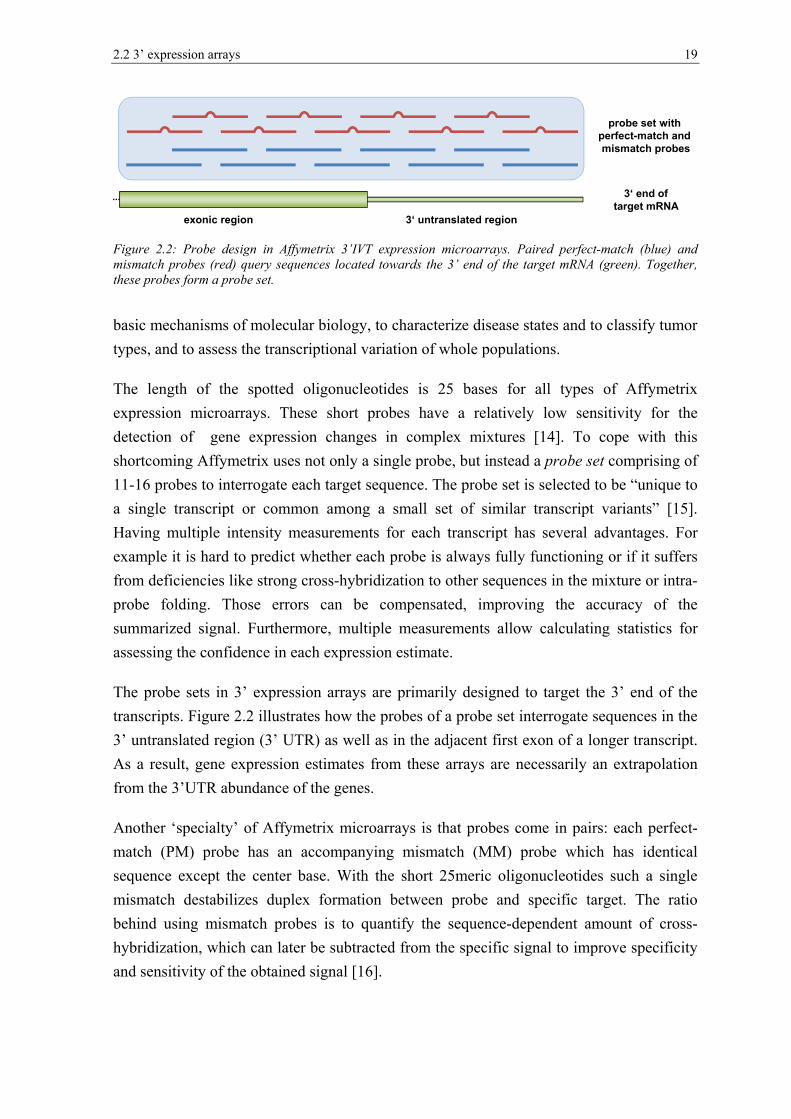
Figure 2.2: Probe design in Affymetrix 3’IVT expression microarrays. Paired perfect-match (blue) and mismatch probes (red) query sequences located towards the 3’ end of the target mRNA (green). Together, these probes form a probe set.
basic mechanisms of molecular biology, to characterize disease states and to classify tumor types, and to assess the transcriptional variation of whole populations.
The length of the spotted oligonucleotides is 25 bases for all types of Affymetrix expression microarrays. These short probes have a relatively low sensitivity for the detection of gene expression changes in complex mixtures [14]. To cope with this shortcoming Affymetrix uses not only a single probe, but instead a probe set comprising of 11-16 probes to interrogate each target sequence. The probe set is selected to be “unique to a single transcript or common among a small set of similar transcript variants” [15]. Having multiple intensity measurements for each transcript has several advantages. For example it is hard to predict whether each probe is always fully functioning or if it suffers from deficiencies like strong cross-hybridization to other sequences in the mixture or intra-probe folding. Those errors can be compensated, improving the accuracy of the summarized signal. Furthermore, multiple measurements allow calculating statistics for assessing the confidence in each expression estimate.
The probe sets in 3’ expression arrays are primarily designed to target the 3’ end of the transcripts. Figure 2.2 illustrates how the probes of a probe set interrogate sequences in the 3’ untranslated region (3’ UTR) as well as in the adjacent first exon of a longer transcript. As a result, gene expression estimates from these arrays are necessarily an extrapolation from the 3’UTR abundance of the genes.
Another ‘specialty’ of Affymetrix microarrays is that probes come in pairs: each perfect-match (PM) probe has an accompanying mismatch (MM) probe which has identical sequence except the center base. With the short 25meric oligonucleotides such a single mismatch destabilizes duplex formation between probe and specific target. The ratio behind using mismatch probes is to quantify the sequence-dependent amount of cross-hybridization, which can later be subtracted from the specific signal to improve specificity and sensitivity of the obtained signal [16].
probe set withperfect-match andmismatch probes
3‘ end oftarget mRNA
exonic region 3‘ untranslated region

20 2 Microarray technology
Figure 2.3: Comparison of how probes align to a target gene for various types of Affymetrix microarrays. Whereas probes are located towards the 3’ end of the target mRNA (the respective genomic region with exons, introns and UTRs is shown in black and green) in 3’ based expression arrays, other array types query sequences in the entire gene. For tiling arrays, probe sets (light blue boxes) are not defined.
2.3 Gene ST and Exon ST arrays
About 40-60% of human genes are not transcribed solely into a single form of mature mRNA [17]. Instead the primary transcripts of these genes are transformed into a number of different isoforms by alternative splicing. Since each splicing isoform can encode for a different, potentially functional protein one is highly interested in their identification and quantification. Affymetrix 3’ expression arrays are however by design unable to discriminate splice variants. Gene ST and Exon ST microarrays are designed to overcome these drawbacks.
For one, these whole transcript expression arrays employ a different target preparation protocol, typically using the Ambion WT Expression Kit [18]. Synthesis of cDNA strands here is not done using poly-T primers starting at the 3’ end of the transcript, but rather using a pool of reverse transcription primers. These bind at various loci in non-ribosomal RNAs to initiate the polymerase reaction. In-vitro transcription is then used to amplify these fragments which span various regions of the available transcripts. Biotinylated sense-strand cDNA, opposed to the cRNA used in 3’ IVT expression arrays, is then fragmented and end-labeled for hybridization to the array. The resulting DNA-DNA duplexes between probes and targets have been found to be more specific than DNA-RNA duplexes [19].
Affymetrix 3’ IVT expression arraysone probe set withperfect-match andmismatch probes
Gene ST arraysone probe set with
perfect-matchprobes
Exon ST arraysmultiple probe setswith perfect-match
probes
Tiling arraysregularly spaced
probes span genomic regions

2.4 Genome-wide SNP arrays 21
The probes of whole transcript arrays interrogate sequences spread across the entire gene with the aim of getting a more complete picture of gene expression. As shown in Figure 2.3, the probe set of a 3’ IVT array contains a fixed number of perfect-match and mismatch probes which concentrate at the 3’ end of the transcript. A transcript is queried by typically one probe set. For the Exon ST arrays, each exon or non-coding region is interrogated by about four probes. Using these exon-level probe sets allows distinguishing between different splicing isoforms. The probes of multiple exons can be combined, giving about 40 probes per gene and allowing a complementary gene-level expression analysis. The Gene ST arrays are designed as a less expensive alternative to the Exon ST arrays containing only a subset of the probes mainly designed for gene-level analysis. A high concordance has been found between the gene-level estimates of Gene ST, Exon ST and 3’ IVT expression arrays [20, 21].
It should be noted that Gene ST arrays are less popular than Affymetrix’ 3’ expression arrays. McCall et al. found that “between 1 June 2010 and 1 June 2011, over 13 000 Affymetrix Human Genome U133 Plus 2.0 samples were added to the Gene Expression Omnibus (GEO)” but “during the same time period, less than 2000 Human Gene 1.0 ST samples were added” [22].
2.4 Genome-wide SNP arrays
Another important application of microarrays is the analysis of genetic variants. In diploid human cells the genetic information is spread on two homologous sets of 23 chromosomes. Alleles are alternative forms of a certain position or region of a chromosome (a locus) that occur between members of a species or within the chromosome set. In the case of the most common type of variation, the single nucleotide polymorphism (SNP), only a single base of DNA is altered. Since there are four possible nucleotides a SNP can have at most four alleles. Most SNPs have however only two alleles [23]. These bi-allelic loci result in three possible states a SNP can take in a diploid chromosome set: either homozygous allele AA with allele A on both chromosomes, homozygous allele BB, or heterozygous AB with two different alleles on both chromosomes. Genotype calling or genotyping aims at inferring these states.
Another form of variation measured by microarrays is copy-number variants. These are alterations of chromosome structure in which large segments (> 1 kb) of the DNA are present in variable copy number compared to a reference genome [24]. A duplication of certain segment of the chromosome, for example, would have the effect that all previously unique genes in that section are now present in two copies. About 12% of the human

22 2 Microarray technology
Figure 2.4: Probe design of Affymetrix SNP Arrays. All probes (blue PM probes and red MM probes) interrogate a single SNP located in genomic DNA. The SNP has the two alleles C and T each being interrogated by an allele set of probes.
genome has been found to be covered by copy number variations [25] rendering them an significant source of genome heterogeneity and a potential factor contributing to phenotypic variation and disease states/susceptibility.
Specific target preparation assays and microarray designs are employed to allow detection of genetic variants with high sensitivity. Compared to gene expression experiments, these assays do not target (m)RNA molecules but instead genomic DNA. Total genomic DNA is digested with restriction enzymes (see Genome-Wide Human SNP Nsp/Sty Assay Kit 6.0 documentation [26]). Adapters are ligated to the resulting fragments which are then used for a PCR procedure that has been optimized to amplify fragments of certain size range to reduce complexity of the genomic DNA. The amplified DNA is further fragmented, end-labeled and finally hybridized to the array [27].
The probes are designed to tile around each SNP with slight variations in perfect matches, mismatches, and flanking sequence [28] as shown in Figure 2.4. The Affymetrix GeneChip Human Mapping 100k Array Set, for example, uses 40 different 25meric probes for each SNP. For each of the two interrogated alleles there is an allele set consisting of 10 probe pairs: 10 PM probes and 10 corresponding MM probes with a mismatch at the center base, depicted separately in Figure 2.4. The probes include the SNP at the center base or are slightly shifted by some offsets δ = -4,..0,..4. Of the 10 PM probes 3 to 7 target the sense strand whereas the remaining ones target the antisense strand. This design with a large number of probed sequence combinations can be used to study the impact of mismatches and other duplex interactions on probe signals [29]. Some arrays such as the Genome-Wide Human SNP Array 6.0 omit the mismatch probes which makes it possible to capture 1.8 million genetic variants with about 6 million probes.
C
allele set C
C/T
T
allele set T
SNP-containinggenomic locus
two variants ofa bi-allelic SNP
each variantis interrogated byan allele-specific
set of probes

2.6 Summary and conclusions 23
2.5 Agilent expression arrays
Agilent’s manufacturing technology differs from that of the other two major producers of high-density microarrays namely Affymetrix (which use photolithographic masking [10]) and Illumina (which use self-assembling silica beads [30]). Agilent prints its arrays similar to how an inkjet printer prints a document - instead of ink on paper, nucleic acids are printed base by base onto the glass surface [31]. A major advance of this technology is that the features can easily be customized for each microarray: probes are designed to interrogate the targets of interest and then added or removed as desired. This flexibility is not given for Affymetrix technology, where only standardized expression microarrays are available.
The most recent Agilent SurePrint G3 Gene Expression Microarrays comprise more than one million features. The printed oligonucleotides have a length of 60 bp. These 60mer probes were shown to be significantly more sensitive to expression changes in complex mixtures compared to 25mer oligonucleotides [14], according to Agilent between five and eight times [32]. Longer probes are however less specific – 25mers are about 20 times more specific for differentiating a single mismatch [14]. This tolerance with respect to sequence mismatches can however also be an advantage when probing highly polymorphic regions. Agilent arrays support different target preparation assays including two-color and one-color preparations.
2.6 Summary and conclusions
Microarrays come in a diverse set of flavors aiming at different genomics applications ranging from gene expression analysis and profiling over DNA analysis and genotyping to gene regulation analysis. The great utility of microarrays in these fields of applications has driven - and vice versa has been driven by - many developments in the private and in the academic sector resulting in the rapid advancement of the technology since its appearance in the 90s. These improvements in terms of accuracy, coverage, reproducibility, standardization and cost have made microarrays an established tool widely used in research and even in clinical settings [33].
The variety in the set of possible applications is enabled by differences in microarray designs and protocols. Specifically, Affymetrix 3’ expression arrays target sequences that reside within the 3’ UTR and act as a proxy for the expression of the respective gene; exon arrays interrogate sequences from exons of known splice isoforms, and tiling arrays have their probes distributed uniformly across large fractions of the genome. Additional to these application-specific differences, each microarray manufacturer has its own ways of

24 2 Microarray technology
production and supports its own instruments and reagents. Affymetrix provides an unparalleled coverage and feature density, as well as a high standardization. Agilent in turn provides highly customizable microarray designs.

3 A model for microarray hybridization
3.1 Modeling microarray intensity signals
The presented technologies share the common mechanism of multiplexed hybridization of fluorescently labeled target molecules against known oligonucleotide probes. The input quantity that one wishes to infer in a microarray experiment is the abundance, or concentration, [S] of specific nucleic acid targets. The measured output quantity is fluorescence signal intensities I for the surface-attached probes. Modeling microarray hybridization with the aim of obtaining accurate signal calibration consequently seeks to identify an adequate functional relationship p
gI f ([S ])= between a probe p and the respective target (gene) g.
Several effects in the microarray measurement prevent an accurate description of the input and output quantity via the simple proportional relationship I [S]∝ . Firstly, there are technical limitations in the optical recording of the intensity signals using the scanner. Even when no specific transcripts are bound to the probes the scanner reports positive intensity values I > 0. An additive optical background term O, i.e. in the form I = [S] + O, should therefore be considered in microarray calibration methods [34, 35].
Secondly, several fundamental binding and folding processes can occur at or near the microarray surface as shown in Figure 3.1a. The yield of the interaction between free probes and specific targets is reduced by bulk-dimerization, non-specific hybridization and intra-molecular folding reactions. During non-specific hybridization additional to the fully complementary specific targets other, only partly complementary, DNA or RNA fragments bind to the probes. Due to the large diversity and quantity of target molecules in the complex mixture solution this type of binding typically is considerable [36]. A practicable solution for incorporating non-specific binding in the hybridization model is to summarize the diversity of non-specific transcripts into a single probe-specific term, i.e. I = [S] + [N] (see also [35, 37]).
Thirdly, the kinetics of the reversible binding reactions of targets in excess to limited, surface-attached oligonucleotides can result in a non-linear response of the probe intensity. The binding reactions can be regarded as a Langmuir adsorption process as exemplified in Figure 3.1b. Accordingly, the amount of adsorbed molecules Θ on a surface in dependence

26
FigurpossibLangmspecif
of th
wherfractirelevto dconc
The tto phobtaiconsiphyssuggabou
3.2
We wexpremeas
re 3.1: Interable binding anmuir adsorptific transcripts
he molecule
K1 K
⋅Θ =
+
re K is the ional cover
vant target mdescribe wentrations [
three descrihysicochemined intensiidered in vicochemica
gests that buut relevant m
The t
will now inession data sured in a m
action processnd folding proon model des S).
e concentrat
[ ][ ]
SSK ⋅
rate consta
rage of oligmolecules inwell microa[38–41].
ibed effectsmical princip
ity signals virtually an
al models fuilding upomechanisms
two-spe
troduce the[36, 42]. A
microarray e
ses and dynaocesses of procribing the oc
tion [S] can
ant. In the gonucleotidn the solutioarray sign
s relate eitheples of the of a microany calibratifor describinon these mo is a promis
ecies La
two-specieAccordinglyexperiment i
amics of surfobes and targeccupancy Θ o
be describe
case of mides of a gion. The Lan
nals based
er to basic thybridizati
array experion methodng the basi
odels and resing strategy
angmui
es Langmuiy, the intenis given to a
3 A
face adsorptioets (image takof surface site
ed with the
icroarray hiven probe ngmuir adso
on exper
technical limion processriment. Oned. Importanic processeefining themy for signal
r mode
r model whsity of a pra good appr
A model for m
on on microaken from [37])s (e.g. probes
Langmuir i
ybridizationand [S] th
orption modriments w
mitations ofses and stroe or more ontly, the shes of microm using adcalibration
l
hich appliesrobe p of tyroximation b
microarray hyb
arrays. Panel). Panel b visus P) with part
isotherm
n, Θ represhe concentrdel has bee
with known
f the instrumongly influeof these fachown relev
oarray hybridditional knn and beyon
s well to miype {P PM∈by
bridization
l a shows ualizes the ticles (e.g.
(3.1)sents the ration of n shown
n target
ments or ence the ctors are vance of idization owledge d.
icroarray }M,MM

3.3 The hook transformation and hybridization modes 27
P,N P,Sp pP
p P,N P,Sp p
X XI M O
1 (X X )+
= ⋅ ++ +
(3.2)where M is the maximum intensity upon saturation and O is the optical background intensity. We here assume that the term O can be corrected in a separate step, for example using the Affymetrix zone algorithm [7], and will rely on background-corrected probe intensities if not stated otherwise. The numerator P P,N P,S
p p pL M (X X )≡ ⋅ + is also denoted the linearized signal and decomposes into contributions due to non-specific and specific binding (see next section) scaled by M. The binding strengths P,hX linearly scale with the respective concentration of specific and non-specific targets, [ ]P,hX h∝ with { }h N,S∈ . Only considering the factors described in the previous section, the binding strengths are given as
[ ]P,S P,S P,N P,Np g p p pchip
X S K and X N K⎡ ⎤= ⋅ = ⋅⎣ ⎦ (3.3)where P,h
pK are the equilibrium constants for the formation of probe/target duplexes.
Two factors not considered in this thesis are washing and target depletion. The washing step that follows hybridization in the microarray assay has been shown to remove probe-bound targets and inversely scales with the respective binding constants [43]. Target depletion in the solution can lead to an underestimation of the concentrations of specific transcripts [44].
3.3 The hook transformation and hybridization modes
The parameters of the Langmuir-type model are not directly accessible given only the intensity signals of the particular microarray hybridization. The target concentrations are unknown in typical applications and the specifics of the hybridization reaction can differ for each microarray experiment. The hook method elegantly solves this challenging problem by using information inherent in the coupled signals of perfect-match (PM) and mismatch (MM) probe pairs [45]. These paired probe signals are transformed in a special mean-difference plot:
( ) ( )
hookpset pset p pset
hookpset p pset
p k k p p p
mvg_avg( ) and
1with log log and log log .2
ΡΜ ΜΜ ΡΜ ΜΜ
Δ = Δ Δ = Δ
Σ = Σ = Σ
Δ ≡ Ι − Ι Σ ≡ Ι + Ι
(3.4)

28
FigurS- andof speΣbreak.
The respelogarprobemvg_probeprovicontr
Parti(S-) hcompIn thsequegenespeci
FigurvisuaregimcontrS- (pinteninten
Consmost
re 3.2: Hook cd sat regimes ecific binding.
Δ and Σ ectively, orithm). <…>es targeting_avg appliee sets for ides the hributions du
icularly, whybridizatioplementary he N-hybridence origin. Probe bindific binding
re 3.2a shoal inspectiomes with inributes to th
predominantnsity and trnsity reache
sider the N-t weakly in
curve with diffand the Σbreak
Panel b show
transformaof logged >pset denoteg the same es a moving
smoothinghook curveue to differe
we differenton. In the Ssequence tr
dization monating howeding of this
g (e.g. [47])
ows the resuon allows thncreasing Σhe signals), tly specificranscript cos its asympt
-regime refencreasing Δ
ferent binding k threshold (blws the first de
ations are probe in
s averagingtranscript)
g average tg. Plotting e which enent modes o
tiate betweS-hybridizaranscribed
ode the probever from m type is termor non-spec
ulting hookhe simple Σ , namelymix- (comb
c hybridizatoncentrationtotic saturat
ferring to prvalues tha
g regimes, andlack vertical lerivation and t
based on ntensity vag over all pr
to obtain to the Δset v
the micronables decf hybridizat
een two mation mode from mRNAbes bind aRmRNA tranmed (ubiquicific hybrid
k plot for aand straigh
y the N- (vbination of
ation), sat-n becomestion level) r
robe sets wat scatter ar
3 A
d computation line) separatinthe linear fits
the PM/Malues (log
robes withinrobust Δset
values withoarray data compositiontion by simp
modes: nonthe probes A transcripRNA fragmnscripts notitous) cross
dization (e.g
a typical Gehtforward dvirtually onnon-specifi(saturation
s progressivregime.
ith the smaround 0 be
A model for m
of Σbreak. Panng non-specifi
which are us
MM differeg ≡ log10 n a probe set
and Σset vah a window
into Δ-ven of the pple visual in
n-specific bind the a
ts which thments of par
t referring -hybridizati
g. [36]).
eneChip exdetection ofnly non-speic and speci
range; thevely non-lin
llest Σ valuexplained?
microarray hyb
nel a shows theic binding andsed for the est
ence and 0 is the t (typically alues. The
w size of abersus-Σ cooprobe signnspection.
(N-) and aRNA fragmhey intend tortly completo the inteion (e.g. [46
xpression arf five hybriecific hybriific hybridie relation near) and
ues. How ca? Δ ≈ 0 refe
bridization
e N-, mix-, d the onset imation of
average, decadic 11 to 16 operator
bout 100 ordinates nals into
specific ments of o detect.
ementary errogated 6]), non-
rray. Its idization idization zations), between as- (the
an the at ers to an

3.4 Positional-dependent sequence models 29
equal intensity level of PM and MM probes for probe sets in this Σ-interval. Targets with exact complementary sequence are however expected to have a significantly higher binding strength compared to those with a single mismatch in the middle of the probe-target duplex. The probes consequently do not bind to the interrogated target but to fragments of partly complementary sequence – they bind non-specifically. Probes or probe sets with virtually only non-specific hybridization are called absent whereas others are called present.
Figure 3.2a also indicates a Σ threshold characterized by a significant increase of the Δ values referring to the onset of specific binding. This threshold breakΣ separates the N and mix-regime and consequently separates absent and present probe sets. The ability for this separation allows the estimation of essential parameters of the hybridization model [42].
Estimation of breakΣ should be both accurate and robust. The following heuristic method has been shown to improve over previously proposed approaches and delivers reliable results over a large variety of chip-types [42, 48, 49]:
1. Compute the empirical first derivation of the hook plot (by fitting a straight line to 7 subsequent data points of (Σ, Δ) sorted by Σ)
2. Find the point of maximum deviation Σmax-d 3. Use linear regression to find the best joint fit of two straight lines (y = mx + n) to
all data points between the smallest Σ of the hook plot and Σmax-d (see [49] for details about the formulation of the least squares error).
4. The intersection point between the two lines defines ( breakΣ , breakΔ )
Figure 3.2b illustrates this approach of estimating breakΣ . The green line is the empirical first derivation computed from the hook curve (shown in blue). The maximum derivation is located in the mix regime. The best fitting two straight lines (shown in orange) intersect at the threshold break 2.6Σ ≈ .
3.4 Positional-dependent sequence models
3.4.1 Modeling the formation of duplexes
In our model, the binding constants from Eq. (3.3) decompose into
P,h P,h P,hp 0 pK K exp( A ( ))= ⋅ δ ξ (3.5)

30
Figurindicain bla
wherlengtnuclesensi
The
iB ∈sequeguanThusneigh
Figurspecisampare rbase The diffesensi
Integvalue
re 3.3: Typicaating positionack, whereas th
re P,h0K is a
th 25. We feotides startitivity terms
P,hpA ( )δ ξ
sensitivity{A,T,G,C}ence. For
nines beginns, r 1 4= … hbor (NNN)
re 3.3 showific, perfectple taken froroughly sym
tuples whesensitivitiesr at the soitivity ampl
gral sensitives either ov
al sensitivity al-dependent he points and
probe indepfurther use ting at posits over all se
25 r 1P,hk
k 1)
− +
== σ∑
y profiles }, 1 i r≤ ≤ )example, (
ning at sequrefers to th
) and quadr
ws sensitivitt-match proom an expe
mmetrical arere the sensis of all pro
olution end itudes.
vities P,hku,koσ
ver all sequ
profiles of rsensitivity terconnecting li
pendent conthe convention k in ξ.
equence pos
h k,k r 1p( ).+ −ξ
P,hk r(b )σ d
) of length
1(GGG) deuence positiohe single n
ruple (NNNN
ty profilesobes (P = PMriment by Sround the mitivities decofiles conve
at k = 1. T
o r(b ) are cence positio
rank r = 2 forms for four sines of the rem
ntribution anntion k,k r+ −ξ
The sequensitions [42, 5
depend onh r with itsenotes a seon 1. The panucleotide (
NN) models,
of rank r =M, h = N)
Su et al. [52middle of thcrease monoerge towardThe base tu
calculated bons or over
3 A
or an Affymeselected base maining 12 bas
nd 1,25ξ = ξ i1− to assign nce effect δA50, 51]
n base tups first baseequence moarameter r s(N), nearestrespectivel
= 2 estimateof an Affy
2]. The posihe probe seqotonically wds the surfauples AA a
by summingr a position
A model for m
trix HG-U13tuples (AA,CCse tuples are s
is the probethe subsequ
A is modele
ples r k(b ) =e at positiootif containspecifies thet neighbor ly.
ed from the ymetrix HGitional-depequence, excewith increasiace-attachedand CC exh
g up the poal range tha
microarray hyb
33a microarraC, GC, GG) ashown in gray
e sequence quence of r ed using the
1 r(B B )= …on k of thning three e rank of th(NN), next
e intensities G-U133a miendent contrept for GC ing sequenc
d side at k =hibit the m
ositional deat was sele
bridization
ay. Points are shown y.
string of adjacent e sum of
(3.6)k) (with
he probe adjacent e model. t nearest
of non-icroarray ributions and GG
ce index. = 24 but
maximum
ependent cted, for

3.4 Positional-dependent sequence models 31
example, to exclude the region of the 1(GGG) effect
koP,h P,hku,ko r k r
k ku(b ) (b ).
=
σ = σ∑ (3.7)3.4.2 Different characteristics for specific and non-specific
binding
Binding characteristics are known to be different between specific and non-specific hybridization modes [36]. Eq. (3.2) simplifies into N
p pM (I O) L⋅ − ≈ for the special case of predominantly non-specific binding far below saturation, N S
p pL L M . Restricting our basic analysis to this regime, we ensure linearity of the intensity response and homogeneous probe-target interactions. The latter are mainly governed by canonical Watson-Crick pairings [53].
We select the subensemble of probes meeting these conditions using the hook method [42]. Typically more than 40% of all probe sets are called ‘absent’ in a particular microarray hybridization, providing a sufficient number of probe intensities to adequately fit the model (see also Table 6.1 in Chapter 6).
The ensemble of present (i.e. not-absent) probes refers to signals which partly or completely originate from specific hybridization. We apply the hook method to filter out probe sets which hybridize predominantly with specific transcripts, (p∈S), and to correct their intensities for the effect of saturation (see [42] for details).
3.4.3 Estimation of profiles
We define the experimental sensitivity of each probe as the deviation of the logged linearized signal of its average over all probes of the respective probe set [54]
exp P,h P,hpsetY log X og X .l= − ⟨ ⟩ (3.8)
After insertion of Eqs. (3.5) and (3.6) into (3.8) and making use of h h0 0 psetlog(K ) log(K [h]h )[ ] = ⟨ ⟩ we obtain the theoretical sensitivity of each probe
25 r 1theo k,k r 1 pset
k r r k rk 1 br
Y (b )·( (b , ) f (b ))− +
+ −
=
= σ δ ξ −∑ ∑ (3.9)

32 3 A model for microarray hybridization
with the Kroenecker function (x, y) 1δ = for x = y and (x, y) 0δ = otherwise. psetk rf (b ) is
the probability to find motif br at sequence position k among the probes of the considered probe set. Note that the transcript concentration (specific and non-specific) is assumed to be constant for each probe set because each probe within the set targets the same transcript. This condition cancels the term 0log(L ) in Eq. (3.5).
The sensitivity profiles are estimated using multiple linear regression. It minimizes the sum of squared residuals [42]
2 2
p
1SSR(r) RES RES#p
= = ⟨ ⟩∑ (3.10)with exp theoRES (Y Y )= − by optimizing k r(b )σ for all r4 ·(25 r 1)− + base tuples r k(b ) . The sum runs over all relevant probes p N∈ or p S∈ and #p defines the respective number of probes. The obtained sensitivity terms meet the center condition
r
k rall b
(b ) 0σ =∑ for each sequence position k.
3.5 Fitting the hybridization model
Application of sequence correction leads to a less noisy and more consistent hook curve. Figure 3.4 shows two versions of the hook curve: before (panel a) and after correction (panel b) of the signal intensities used for the computation of the Δ-Σ-transformation given in Eq. (3.4) with the positional-dependent nearest neighbor model (r = 2) from the previous section. The sequence correction improves the precision of the probe signals: the within-probe set variability is reduced as well as the scattering of probe set averages around the hook curve. Basic features of the hook curve such as the relative positioning of the binding regimes are essentially the same in both versions. The N-regime however differs significantly in its width and slope. In summary, these effects result in an improved hook curve which is sufficiently robust to allow fitting the theoretical hybridization model as described below.
Let us now give a formulation of the two-species Langmuir model that predicts the Δ and Σ coordinates of the hook curve. We define the relative hybridization degree, or S/N ratio R as
PM,Sp g
p PM,Np chip
K [S ]R .
K [N]⋅
≡⋅ (3.11)

3.5 Fi
Figurintensto whi
R is We f
Inserhook
whersatur
Plottthe tcharaare g
itting the hybr
re 3.4: Δ and Σsities of a Genich we fit the h
an expressifurther defin
PMp
p MMp
Ks
K=
rting Eqs. (3k transforma
(R)
and
(R)
Δ = Δ
Σ = Σ re PMB (Rration terms
ting the Δ atheoretical acterizing th
given as
start
slogn
lo
α =
Δ =
ridization mod
Σ transformaneChip Rat Exhybridization
ion measurene pairwise
M,S
pM,S and n =
3.11) and (3ations Δp an
(start
start 12
log R
log
⎡Δ + ⎣
⎡Σ + ⎣
(R) 1 10− β= +s.
and Σ trajechook curvehe position
andng n and
β =
del
tions calculatxpression Arramodel.
e that directPM/MM ra
PM,NpPM,Np
K.
K=
3.12) in the nd Σp given
) (
( ) (
R 1 / R
R 1 R
+ ⋅
+ ⋅
) (start1
2 Rβ− Δ +
ctories in dee shown in and the ge
12
start
log n - lo
log M
=
Σ =
ted from raw ay 230A. Sequ
tly relates toatios of the
basic moden in Eq. (3.4
)
)
10 1
10 1
−α
−α
⎤+ −⎦
⎤⋅ + −⎦
)1 and B
ependence n Figure 3.eometrical d
( PM,Nog K [
M
⋅
−β
(panel a) anduence correct
o the concebinding con
el given in ) we obtain
PM
PM12
l og B (
log B
⎡− ⎣
⎡− ⎣
MMB (R) 1= +
of the relat.5. The pardimensions
)chip
[N]
d sequence cortion leads to a
ntration of nstants
Eq. (3.2) an
MM
M MM
R) / B (R
(R) B (R⋅
( )start1210− β+ Δ+
ive expressrameters Δof the theo
rrected (panean improved h
specific tra
nd afterward
R)
R)
⎤⎦
⎤⎦
(R 10 1−α⋅ +
sion degree Δstart, Σstart, α
oretical hoo
33
el b) probe hook curve
anscripts.
(3.12)ds in the
(3.13))1 are
R gives α and β ok curve
(3.14)

34
Figurcharacharafrom [
wherprobe
The now optimdescehybriintenparambasedand r
3.6
AddiparammicroexpeindicThis alonehybri
re 3.5: Theoracterize the noacterize the w[55].
re p cn n=
es on the ar
alternative be fitted to
mization proent algorithidization m
nsity data ometers whid on the moreversal of t
Chip
itional to tmeters fromoarray hybrriment, for
cators for sosection sh
e from the idized RNA
retical hook con-specific bacwidth of the h
chip and s =
rray. A deta
formulationo the experioblem has ohm. Figure model fits of a typical ch can be odel Eq. (3.the two-spe
p summ
their utilitym the prevridization anr example tources of teows how smicroarray
A.
curve and itsckground leveook and its h
p chips are t
iled descrip
n of the twmental Δ-Σonly a singl
3.4b showwell to Δ GeneChip used to com.2). The hoocies Langm
ary mea
y for the cvious sectiond can be uto identify echnical varselected chiy signals rel
s geometrical el in intensity height in the
the PM/MMption of deri
wo-species LΣ-trajectoriele local max
ws that the and Σ traexpression mpute estimok-method
muir model i
asures
calibration on (Δstart, Σused to com
laboratory riability whip-specific late to the n
3 A
l dimensions. units and theabsence of sa
M ratios fromivation of th
Langmuir ms as explain
ximum and theoretical
ansformationarray. The
mates of thfor signal cis described
charact
of microaΣstart, α and
mpare sampleeffects. Th
ich are diffsummary mnon-biologi
A model for m
The start coN-PM/MM-g
aturation, res
m Eq. (3.12)he model is
model givenned in [42, can be solvhook curv
ns of the e fitting prohe transcripcalibration bd in detail in
terize R
array signald β) characes, or grouphese parameficult to detemeasures thical variabl
microarray hyb
oordinates (Σgain, respectivspectively. Im
) averaged fgiven in [4
n in Eq. (349]. The re
ved using a ve predicted
sequence-covides chippt concentrabased on thn [42].
RNA qua
ls, the bascterize a pps of sampleters are imect by other
hat can be le of the am
bridization
Σstart, Δstart) vely. (α, β)
mage taken
for all 2].
.13) can espective gradient
d by the corrected -specific ation [S] is fitting
antity
sic hook particular es, of an mportant r means. obtained
mount of

3.6 Ch
Figurcompuand Sconce10ug increa
The transall prspeci
This the Rmagn
We condliver Genofromcollewhoswere20ugbut
2 A deordere
hip summary
re 3.6: Chip-suted both parSNB-19) hav
entration. In (Pearson corasing RNA ma
S/N ratio, script relativrobe sets ofific transcri
logλ =
chip-specifR-range ovnitude [45].
computed βducted by G
tissue andome U95A
m total RNAected into ose RNA cone then dilutg. Additiona
have been
etailed descriped from Gene
measures cha
specific paramrameters for thve been hybPanel a <λ>
rrelations of ass. An amoun
R, from Eve to the baf a microarript level, or
R 0.g(R 1)
>+
fic measurever which
β and λ Gene Logic Id CNS Cel
arrays at vA according
ne master sncentrationsted to geneal dilutions n omitted
ption of the stuLogic Inc.
aracterize RNA
meters <λ> ahe samples ofridized at v> increasesr > 0.7), but
nt of 10ug aRN
Eq. (3.11) aseline of nray exceedinmean log S
5;chip.
is typicallythe densit
summary Inc. [56]. Inl Line SNBvarying conto the manusolution fors have beenerate solutiocontaining here. Five
udy design is
A quantity
and β in depf Gene Logic
varying conceroughly line
t saturates aNA is recomm
characterizenon-specificng a given
S/N ratio,
y in the ranty of expre
measures fn this experiB-19, havencentrationsufacturers’ pr each of thn determineons with nomixed RNA
e technica
given in the w
pendence of t’s dilution datentrations wi
ear with incrat 20ug. Panemended for the
es the specc binding. Aexpression
nge of 0.2 <ession valu
for all samiment two d been hybrs2. Multipleprotocol anhe two RNAd using an ominal aRNA of both l
al replicate
white paper ac
the amount ofta set where tith 5 replicareasing RNA el b shows hemployed HG
cific hybridAveraging tthreshold p
< λ < 1.5ues decays
ples of a ddistinct typeridized to Ae samples hd the resulti
A types. Thelectropher
NA masses iver and SNs were pr
ccompanied by
of hybridized two types of Rate samples
mass betweehow β decre
G-U95A platfo
dization levthese R valuprovides the
5 and also d by one o
dilution expes of RNA sAffymetrix have been pting aRNA hhe master sorometer (at between 1
NB-19 are arocessed f
y the data wh
35
RNA. We
RNA (liver for each
en 1 and eases with orm.
vel of a ues over
e relative
(3.15)describes order of
periment samples,
Human prepared has been olutions, 260nm),
1.25 and available for each
ich can be

36 3 A model for microarray hybridization
concentration, leaving a total of 50 samples. This study design enables an assessment of the effect of technical variation within the replicates and between the dilutions.
Panel a of Figure 3.6 displays the obtained λ parameters in dependence of RNA mass for the 50 microarray samples. λ increases with increasing RNA mass between 1 and 10ug with Pearson correlation coefficients of r = 0.71 for liver tissue and r = 0.78 for SNB-19. However, λ does not increase further for a RNA mass of 20ug which can be explained by the up-down effect: increasing RNA concentrations result in a larger non-specific background accompanied by a smaller effective specific binding constant due to bulk dimerization [57]. The λ summary measure which averages the ratio S/N of specific and non-specific binding (see Eqs. (3.15) and (3.11)) is therefore not collinear with RNA mass as the effect of bulk dimerization is not considered in the hybridization model (Eq. (3.2)). In summary, λ describes the amounts of aRNA in a particular microarray hybridization in a non-linear, yet for typical RNA ranges sensitive fashion.
The β parameter from Eq. (3.14) characterizes the width of the theoretic hook and typically is in the range 2.0 < β < 3.2. Since startlog Mβ = − Σ (Eq. (3.14)), the width is limited by the saturation level M and the start of the theoretic hook Σstart at the onset of specific binding, and thus describes the measuring range of specific signals [45]. As shown in Figure 3.6b the parameter β decreases with increasing RNA mass in the dilution experiment. The increasing concentration of RNA in the hybridization solution here results in an increased signal contribution due to non-specific binding and thus in a non-linear, negative effect on the measuring range β.
3.7 Summary and conclusions
Multiplexed hybridization reactions between nucleic acids on a surface can be well described using the two-species Langmuir model. This model is based on fundamental physical principals of surface adsorption and can be easily refined to incorporate additional factors such as sequence-dependent affinities, washing and degradation. Critical is the fitting of the model to the intensity data which should ideally be performed separately for each microarray hybridization due to a significant variation in the described biological and technical factors. The Δ-Σ-transformations provide a practical way to fit the model without prior knowledge of target concentrations.
The Δ-Σ-transformations of probe signals result in the typical hook curve which allows identification of different hybridization regimes. We distinguish between N-, mix-, S- and sat regime depending on the effect of non-specific binding, specific binding and of saturation. The threshold breakΣ separating N- and mix- regime is of particular importance

3.7 Summary and conclusions 37
as it allows independent characterization of specific and non-specific binding. A robust and accurate method to estimate breakΣ is presented.
Additional to their utility for signal calibration, the hybridization model and the hook approach allow studying the technical factors and physicochemical processes involved in microarray hybridization. Fitting an alternative formulation of the two-species Langmuir model provides summary parameters which are of great utility for the assessment of the non-biological variation among the samples of an experiment. Examples are the λ and β parameters which relate to the abundance of hybridized RNA.


4 Hook analysis applied to different types of microarrays
In the previous chapter we presented a model for microarray hybridization and showed that it adequately predicts microarray data based on the Σ–Δ-transformations of intensity signals. We showed this exemplary for Affymetrix GeneChip 3’ IVT expression arrays and it remains an open question whether the same approach can also be applied to other microarray types: those that interrogate DNA instead of RNA targets, those that employ different protocols or different designs, and those produced by other manufactures relying on their own proprietary technologies. The ability to obtain suited Σ-Δ-transformations provides the basis for successful application of the methods described in this thesis to these microarray types.
4.1 Genome-wide SNP arrays
In Section 2.4 we defined so-called allele sets for SNP arrays in analogy to the probe set in expression arrays. All probes within an allele set interrogate a unique variant of a target nucleotide strand, here however referring to fragments of genomic DNA containing a particular SNP. We calculated Δ and Σ transformations according to Eq. (3.4) for a 50K Array Xba 240 from the Human Mapping 100k Array Set as shown in Figure 4.1a. Note that these arrays contain both perfect-match and mismatch probes. Basic features of the obtained SNP hook curve are strikingly similar to those of expression arrays (compare Figure 3.2a): at Σ = 2.3 the curve starts with small values of Δ ≈ 0 which, due to an increasing contribution of specific binding, increases monotonously to Δ = 0.6. The onset of saturation then results in a decrease of the Δ values with increasing Σ up to the highest probe signals at Σ = 4.1.
A noteworthy difference between both array types is that expression arrays have a distinct N-regime containing a substantial amount of probe sets with Δ ≈ 0. A significant change of the slope of the hook curve at breakΣ separates this region from the subsequent mix-regime. In the SNP arrays no change of slope can be observed. The distribution of probe sets in Δ-Σ-coordinates (orange circles in Figure 3.2 and Figure 4.1) shows that a large fraction of probe sets are in the N-regime in expression arrays, whereas in SNP arrays only few probe sets are in this regime of predominant non-specific binding. This is not surprising because by design each allele set should contain probes exactly complementary to the present genomic DNA variant.

40
Figurhave bbindin
In sucharadiffecurvearrayhybrisever
For awith the gheterbind the tset (cgeno
FigurhavesoftwThe expemaxiprobeaffecin the
re 4.1: Hook pbeen used to cng modes: alle
ummary, Δ aacteristics arent targetse, is predicys are theridization. Cral hybridiz
a more fine-different bi
genotype carozygous Athe SNP va
targeted varcross). In t
ome (hetero)
re 4.1b sho been called
ware [58], ahook curvected substaimum valuee-target bin
cted by satue saturation
plots for a Macompute Δ anele, cross and
and Σ transfas in expres and by thcted by the refore subjConsequentlzation regim
-grained vieinding mod
all for a SNAB. Thereforariant whichriant is not the third o).
ws the obtad using the allowing us e of the ‘allantial specie Δ = 0.7 wnding obseruration than n range Σ >
apping50K_Xbnd Σ values. Ind hetero.
formations ession datahe differenttwo-specieect to essly, the inten
mes.
ew of hybrides. AffymeNP can be e
re each alleh is present
present buoption both
ained hook pgenotypingto classify
lele’ bindinfic binding
which agreesrved in exp
in the othe3.4.
4 Hook
Xba SNP micron panel b alle
of SNP arraand the di
t probe dess Langmuir
sentially thnsities of th
idization onetrix SNP areither homoele set can tin the geno
ut instead thh alleles are
plots for thg algorithm
the allele-sng mode stag for the ‘ps well with
pression arrer binding m
k analysis app
oarray. In panele-sets have b
ay data showifferences csign. The r model. O
he same mhe PM and
n SNP arrayrrays considzygous alletake three p
otyped indivhe other vae heterozyg
e same arraGTYPE imsets into on
arts at high present’ SN
the typicalays [42]. T
modes: a sub
plied to differe
nel a all allelebeen separated
w the same can be welcharacteristligonucleot
model of cMM probe
s let us nowder only bi-ele A, homopossible bindvidual (alleleariant cross-gously pres
ay as in Figumplemented ne of the thrvalues Δ >
NP variant. l Δ values f
The probe inbstantial nu
ent types of m
le sets of the Sd for the thre
basic hybrill explainedtic shape, ttide probes competitive es are gove
w address al-allelic SNPozygous all
nding modesle binding m-binds to thsent in the
ure 4.1a. Thin the manu
hree binding> 0.5 confirmΔ increase
for perfect ntensities a
umber of pr
microarrays
SNP array e different
idization d by the the hook on SNP surface
erned by
llele sets Ps, hence lele B or s: it may
mode), or he allele
e diploid
he SNPs ufacturer g modes. ming the es to the matched
are more robes are

4.2 Gene ST and Exon ST arrays 41
In the ‘cross’ binding mode the hook curve starts closely to Δ = 0 and is characterized by smaller Σ and Δ values compared to the ‘allele’ binding mode. The perfectly complementary binding of PM probes to the allele is replaced by a mismatch at the SNP locus. Consequently, the PM probes in ‘cross’ allele sets exhibit a single mismatch and MM probes exhibit either two (in the case of δ ≠ 0, see Figure 2.4) or one (δ = 0) mismatch with respect to their genomic target. Differences in the hook curves of both binding modes thus characterize the effect of incremental total mismatches in the probe-target binding.
In the ‘hetero’ binding mode both alleles are present. The hook curve is a superposition of ‘allele’ and ‘cross’ binding modes, but more resembles the latter one due to the logarithmic signal transformations in the Δ and Σ values. Only few probes are affected by saturation in the ‘allele’ and ‘hetero’ binding modes.
In conclusion, intensity values of probes referring to the ‘allele’ and ‘cross’ binding modes give rise to different hook curves because of the different mismatch configurations. Conversely, the effect of incremental mismatches can be studied using the specific design of the SNP arrays. The hook curve of the heterozygous binding mode can be understood as a superposition of ‘allele’ and ‘cross’ binding modes.
4.2 Gene ST and Exon ST arrays
Gene ST and Exon ST microarrays by design do not include mismatch probes and will thus subsequently be termed PM-only arrays. The key question, therefore, is how the Δ and Σ values of the hook transformation be computed for these arrays. As the average intensity of all probes in a probe set, including perfect matches and mismatches, the Σ values represent a measure of the overall expression level of the target transcript. The use of all perfect-match probes of a probe set should provide a similar measure of the expression level. The Δ values, on the other hand, represent the spread between target abundance measurements of high sensitivity and of lower sensitivity targeting the same transcript. The MM probes with their mismatch position at the center base are expected to have an about one order of magnitude decreased sensitivity compared to the PM probes. While such well-defined sensitivity differences are not given within the PM probes, significant intensity differences between probes of the same probe set nonetheless exist, for example due to variations in

42
Figurhighesit decPM/M‘abseneach Σ = 2
dupleΣ–Δ-
wherlowe
The analothereattribimpa
We stest t4.2b.U133defin
re 4.2: Panel st slope in the
creases with tMM hook (in nt’ (using hoocurve. Both c
2.9 due to satu
ex stability -transforma
hook
hookp
p
*1
m
with
where I
Δ =
Σ = Σ
Δ
re Δ values est third, Δ
resulting cogy to the Peafter continbuted to theact of sensit
suspect thatthis hypothe. Both curv3_Plus2 usined in Eq.
a) Hook plot e non-specific the onset of s
blue/magentok intensity c
curves changeuration.
of probes wation for PM
ps
pset p
pset low
*2
mvg_avg(
log
l
I ... I−
Δ
= Ι
≡
≤ ≤ ≤
are based o
p pset low−Δ , of
urve shownPM/MM honues with ae onset of sivity differe
t the changeesis we comves have bing the PM(4.1). We
for a Gene Sbinding modesaturation. Pta) for a HGcorrected signe their slope w
with differeM-only array
set ps
p pset
*k k 1.. n/3
* * *n 1 2
) and
log
I and (I , I= ⎡⎢
Δ
Ι
on the diffef the perfect
n in Figureook. It startsa slower risesaturation wences on the
e of slope ampare the PMeen compu
M/MM hookhighlighted
4 Hook
ST microarraye to the far lef
Panel b) CompG-U133_Plus2nals) have bewith the onse
ent sequenceys
set p pset
3
* *2 n
and
,..., I ) is a⎤⎥
= Δ
Δ
erence betwt-match pro
e 4.2a hass with a stee. After Σ =
where compe probe inte
at Σ ≈ 1.6 reM-only hoo
uted for a Gk as defined all ‘absen
k analysis app
y obtained byft, then increaparison of PM
2 array (GSMen colored ort of specific b
es. We con
phigh p
p pset high
a permutat
−
−
− Δ
Δ ≡
io
ween the higbe intensiti
characteristep slope in
= 3.0 the Δ petitive bindensity.
elates to theok curve to GeneChip ed in Eq. (3nt’ probe s
plied to differe
Eq. (4.1). Thases to its maxM-only hook
M175849). Prrange and mabinding and b
sequently d
pset low
*k k n
log
−
=⎢⎣≡ Ι
p1 p2on of (I , I
ghest third,es of each p
tics that canthe intervavalues dec
ding of tran
e onset of sthe PM/MM
expression .4) and theets as class
ent types of m
he curve startximum at Σ =
(in green/orarobe sets claagenta, respeboth curves de
define the fo
n n/3 ..n− ⎥⎦
2 pn,..., I )
p pset high−Δ ,
probe set.
an be interpal 1.3 ≤ Σ ≤crease whichnscripts red
specific bindM variant iarray of ty
e PM-only sified by th
microarrays
ts with the 3.0 where ange) and
assified as ectively, in ecrease at
ollowing
(4.1), and the
preted in ≤ 1.6 and h can be
duces the
ding. To n Figure
ype HG-hook as he hook

4.3 Agilent expression arrays 43
method in different colors. Interestingly, both hook variants show a similar change point at Σbreak ≈ 1.9 separating probe sets mainly governed by the N-regime (Σ < 1.9) and the onset of specific binding in the mix-regime (Σ > 1.9).
The sensitivity differences captured in the Δ values vary in the N- and S-regime, in total spanning a range of 0 < Δ < 1.0 in Gene ST arrays which agrees well to 3’ expression arrays. While the sensitivity differences between PM and MM probes of 3’ expression arrays are relatively small in the N-regime, they nonetheless increase to Δ = 1.0 with increasing average expression indicated by Σ. The sensitivity differences within PM probes increase up to Δ = 0.6 in the N-regime. In the S-regime, where Σ increments are accompanied by increments of target abundance, Δ values remain on a flat plateau (as in 3’ expression arrays, Figure 4.2a) or increase only weakly (as in GeneST arrays, Figure 4.2b). The flat plateau is observed also for other PM-only microarray types as for example the Human Exon ST (data not shown).
In summary, the Δ and Σ transformations of the probe signals of PM-only arrays provide a suited approach for characterizing microarray hybridizations. Although of different shape, visual inspection allows detection of the different hybridization regimes in analogy to the PM/MM hook curve analysis. Gene ST and Exon ST show essentially the same hybridization characteristics as 3’ expression arrays.
4.3 Agilent expression arrays
As discussed in Section 2.5 Agilents inking technology allows for full customization of the probe design of ordered microarrays. Predesigned arrays with typically one probe per gene (e.g. SurePrint Human Gene Expression Microarray) or one probe per exon (e.g. SurePrint Human Exon Microarray) are available. However, appropriate Σ–Δ-transformation of probe signals require multiple signals per transcript.
We here employ a custom microarray designed to quantify the expression of splice isoforms. It is the aim of the respective study to assess and compare the technical performance of microarray and high-throughput sequencing data by independently measuring the same RNA samples by both technologies. The microarray probes target 877 different genes which are known to be present in the RNA samples studied and which have a total of 5797 known splice isoforms. Also included are probes targeting 96 external RNA control transcripts from the ERCC initiative [59]. The RNA controls here refer to prepared mixes containing polyadenylated transcripts from the ERCC plasmid reference library. Each target is interrogated by several probes following a tiling design where probes query sequences at regular genomic intervals (compare Figure 2.2).

44
FigurEq. (4shown
An athe sEq. (diffeconcprobetranscolleneithconta
We cthereexplaprimcurvemicrowell.Betwthis eobtai
Noteone dThescompstabilengt
re 4.3: Hook p4.1) with ‘equn in Figure 4.
appropriate same PM-o(4.1). Ideallrent affinitentration. Ces spanning
scribed intoects subsequher by knowaining at lea
computed the is only a smained by th
marily designe exhibits toarray type. The onse
ween 2 and 5experiment.in unbiased
e that the hederived fromse arrays usepared to theility, and thuth. The co
plot for a custivalence regio1.
definition only signal ly, this probty, which hCollecting ag the entire
o a single iuent probewn splice jast four prob
he respectivmall N-regihe particulaned againstthe typical
es, showing et of satura5 percent of. This suggexpression
eight of them (uncorrece spotted ole 25mers onus on intens
omparable l
tom Agilent exons’ as probe
of a probe stransformatbe set shou
however tarall probes oe length of soform. As spanning junctions nbes are cons
ve hook curime at the faar design ot genes whipeak charathat satura
ation is arof the probesests that a cestimates f
e hook curvcted) probe igunucleoti
n Affymetrixsity variabillevels of Δ
4 Hook
xpression mice sets. Note the
set is requirtions as foruld includerget a uniqof a gene inf gene woul
different a DNA sect
nor known sidered.
rve which ifar left of theof the arrayich are expacteristic foation is presound Σ = 3.s are affectecorrection ofrom these d
ve with Δ ≈intensities o
ides of diffex arrays. Thlity, is expeΔ values in
k analysis app
croarray. Δ-Σe similarity to
ed to compr Exon ST a sufficien
que set of tnto a probe ld only giv
approach is tions (‘equintro/exon
is shown ine hook curv
y and the epected to bor the S- ansent in thes5 referring
ed by saturaof saturationdata.
≈ 1.0 is comof Gene STerent lengthhe effect of ected to decrn Agilent
plied to differe
transformatio
o the hook cur
ute Σ–Δ-traand Gene tly large nutranscripts wset would
ve valid sigused here
uivalence reboundaries
n Figure 4.3ve starting aexperiment: e present innd sat-regime Agilent e
g to intensiation in the n effects is
mparable wit arrays in ths: Agilent usequence v
rease with iexpression
ent types of m
ons are compurve of SNP mi
ansformatioST arrays umber of pwith identinot be opti
gnals if thewhere a p
egions’) ints. Only pr
3. It is eminat Σ = 2. Thi probes han the mixtume similar expression aity values 16 array samstrongly ad
th the heighhe previoususes 60merivariations onincreasing s
data sugg
microarrays
uted using icroarrays
ns using given in robes of cal total imal: the
gene is probe set tersected obe sets
nent that is can be ave been ure. The is other
arrays as of 103.5. mples of dvised to
ht of the s section. c probes n duplex sequence gest that

4.4 Summary and conclusions 45
nonetheless strong probe effects with a significant intensity variation are present here. Such high variations are however not uncommon for microarrays with a tiling design since the probes have not been previously optimized.
4.4 Summary and conclusions
We showed that appropriate Σ–Δ-transformations of probe signals can be found for other types of microarrays as well. The necessary modifications to cope with the specifics of each microarray type relate mainly to different definitions of probe sets and the lack of mismatch probes. Genome-wide SNP arrays require substitution of the ‘probe set’ concept, referring to a set of probes with a common mRNA transcript, with the so-called allele-set, referring to a set of probes targeting a common allele at a particular genomic location. The allele sets can be further split up to allele sets with particular binding modes, resulting in a fine-grained view of hybridization on SNP arrays. The lack of mismatch probes in Gene ST and Exon ST arrays is coped with by using existing affinity variations among the probes of each probe set. No probe sets are given by design for the presented Agilent expression array but we showed here how appropriate ones can be defined.
Using the modified Σ–Δ-transformations of probe signals we obtain characteristically shaped hook curves that can be analyzed in a similar fashion to 3’ expression arrays. The differences can be well explained by the specifics of the particular microarray type and the probed targets. For example, there is essentially no N- hybridization regime in SNP chips which can be explained by the expected specific binding of at least one of the two SNP variants in the genomic DNA fragment captured by the allele set. The PM-only hook has a slightly different shape, for example in Gene ST arrays where the slope in the N-regime is higher than that of the mix regime. However, we could show that the change point between these slopes again separates the N- and mix hybridization regimes.
In summary, we showed that it is possible to apply the hook analysis to Affymetrix SNP arrays, Gene ST and Exon ST arrays and a custom Agilent expression array. This creates the possibility to study the characteristics of the different microarray technologies using the methodology presented in this thesis.


5 RNA quality effects
5.1 RNA amplification and degradation in microarray experiments
In this chapter we investigate the effect of varying RNA quality as an ‘unwanted’ covariate inducing potential artifacts in microarray data. Measurement of gene expression is based on the assumption that an analyzed RNA sample closely represents the amount of transcripts in vivo. Several effects can distort the abundance of RNA transcripts during extraction and preparation before RNA analytics using, e.g., microarrays. The first problem concerns the degradation of the RNA in vitro [60–63]: The quality of purified RNA is variable and after the extraction during storage rather unstable (see [64] and the references cited therein). Especially long mRNA fragments up to 10 kb are very sensitive to degradation through cleavage of RNAses introduced by handling with RNA samples. Moreover, transcripts show stability differences of up to two orders of magnitude in vivo, raising the possibility that partial degradation during cell lysis could cause a variable extent of bias in quantification of different transcripts [65]. The second problem concerns amplification of RNA in samples analyzed on microarrays giving rise to the decrease in the length of products that are reverse transcribed and amplified using T7 polymerase [66, 67]. The multiple rounds of in vitro transcription that are used to generate samples from small amounts of RNA thus induce a decrease in transcript yield and length.
The screening of nearly three thousand publicly available GeneChip array data suggests that there are noticeable degradation effects in the majority of the data files and that 2% of the files were even so severely degraded that their worth was questionable [68]. Working with low-quality RNA may strongly compromise the experimental results and lead to erroneous biological conclusions. It is therefore recommended that the highest quality RNA be used for genomic analyses. However, in some cases, such as human autopsy samples or paraffin embedded tissues, high quality RNA samples may not be available [69–71]. It is therefore important to understand how RNA quality affects microarray results and also how reliable current quality measures are at indicating RNA quality issues. The assessment of RNA integrity is a critical first step in obtaining meaningful gene expression data. A second step comprises developing methods to quantify degradation and, most importantly, to correct the induced degradation bias in the data and thereby provide more coherent expression measures.
Several RNA quality measures are established based on conventional wet lab techniques such as gel optical density measurement or denaturating agarose gel-

48 5 RNA quality effects
electrophoresis (see [61, 64] for a review). More novel lab-on-chip gel electrophoresis techniques like Agilents Bioanalyzer are now state of the art. In combination with sophisticated analysis algorithms processing the shape of the electropherogram (and, particularly, the 28S/18S rRNA ratio) they provide accepted integrity measures such as the DegFac-RQS (degradation factor RNA quality scale) [65] or the RIN (RNA integrity number) [72] which have been validated independently using qRT-PCR [64].
Importantly, microarray intensity data itself contains information about the RNA quality used for hybridization due to the 3’/5’-gradient of transcript abundance [73]. On microarrays of the GeneChip-type this gradient is typically measured using either specially-designed control probes or exploiting the specifics of the Affymetrix probe design. Both options estimate transcript abundance at close and more distant positions towards the 3’-end based on the hybridization signal [74, 75].
Although proven in many applications, these measures are based on probe intensities which, in general, are non-linear functions of transcript abundance [37, 38, 40, 54]. The signals can be strongly distorted by effects not related to transcript concentration such as saturation and non-specific background hybridization. Intensity-based RNA quality measures are therefore potentially prone to systematic errors which, in worst case, can provide diametrically opposed information in assessing apparently good RNA quality in samples with largely degraded RNA (see below). Moreover, the important task of correcting microarray signals for RNA degradation effects remained unsolved at least in single chip applications. A linear correction model requiring both expression and RNA quality data from a series of arrays has recently been published [63].
This section addresses the following tasks to overcome these problems: Firstly, we adapt non-linear hybridization theory described in Chapter 3 to the special case of truncated transcripts due to RNA degradation. We will show that our approach consistently explains previous observations such as the effect of RNA quality on transcript intensity level [63] and correlations between probe intensity and probe position along the transcripts and their effect on expression measures [76]. Analysis of the probe signals in terms of this model enables us to define unbiased (in the frame of the hybridization model used) measures of RNA integrity. Secondly, we compare these new measures with established ones. We demonstrate that methods such as affyslope or the RNA-integrity control probes can provide systematically false information on RNA quality. Thirdly, we propose a simple correction method which aims at removing the degradation bias from the probe intensities and which can be integrated into standard preprocessing pipelines.

5.1 RN
Figurdegrainterrattachassocsourcalso rprobecontrabelow
5.1.
AffymotivSectimetholigostran(aRN
Firstthe 5truncstart
NA amplifica
re 5.1: The 3adation (rightrogated transched to the 3’-piated with thee mRNA due tresult in a 3’es as shown iast to convent
w.
.1 3’-biaRNA
ymetrix expvated by thion 2.1 and hod [12]. Ito(dA) primnded cDNANA) which,
-strand cDN5’-end (seecated transcsite with re
ation and degra
’-bias of trant part) of soucript with decpoly-A motif ofe 3’-end of thto RNases from’-enriched lenin the left pation to agree
ased tranamplific
pression mihe specific2.2). The p
t starts witmers followeA fragments
after labelin
NA polymere Figure 5.cripts of varespect to the
adation in mic
nscript abundaurce mRNA. Lcreasing frequof source mRNhe transcriptsm both ends (a
ngth distributiart. aRNA fra
with probe nu
nscript cation and
icroarrays tcs of targetreparation s
th first-straned by secos are subseng, is hybrid
rization is p1). Due to
riable lengthe respective
croarray exper
dance can be Left part: Spuency due to
NA. In contrass giving rise t(a and b) and/ion of amplifiagments are sumbering use
overage d degrad
typically ut preparatiostep appliesnd cDNA
ond strand equently tradized on the
primed at tho incompleth which aree fragment o
riments
caused by inpecific targets
incomplete at, cross-hybridto uniform co/or fragmentatied RNA givinshown in 3’→ed (k = 1, 2...)
of microdation
se a 3’-biaon prior tos IVT protocsynthesis fcDNA syn
anscribed ine arrays.
he 3’-end ofte polymere however cof source m
n vitro transc hybridize to
amplification sdization of nooverage. Rightion at randomng rise to a s→5’ direction
and the inten
oarray pr
ased probe hybridizatcols accordifrom sourcenthesis [66,nto amplifi
f mRNA anization this
characterizemRNA [73]
cription (left o the probes starting at th
on-specific tarht part: Degramly chosen posimilar covera
(from left tonsity decays i
robes aft
location wtion (comp
ding to the Ee mRNA u, 67]. The ied antisen
nd proceeds s method ped by a com(to avoid co
49
part) and along the
he primers rgets is not adation of
ositions (c) age of the o right) in introduced
ter
which is are also
Eberwine using T7
double-se RNA
towards produces
mmon 3’-onfusion
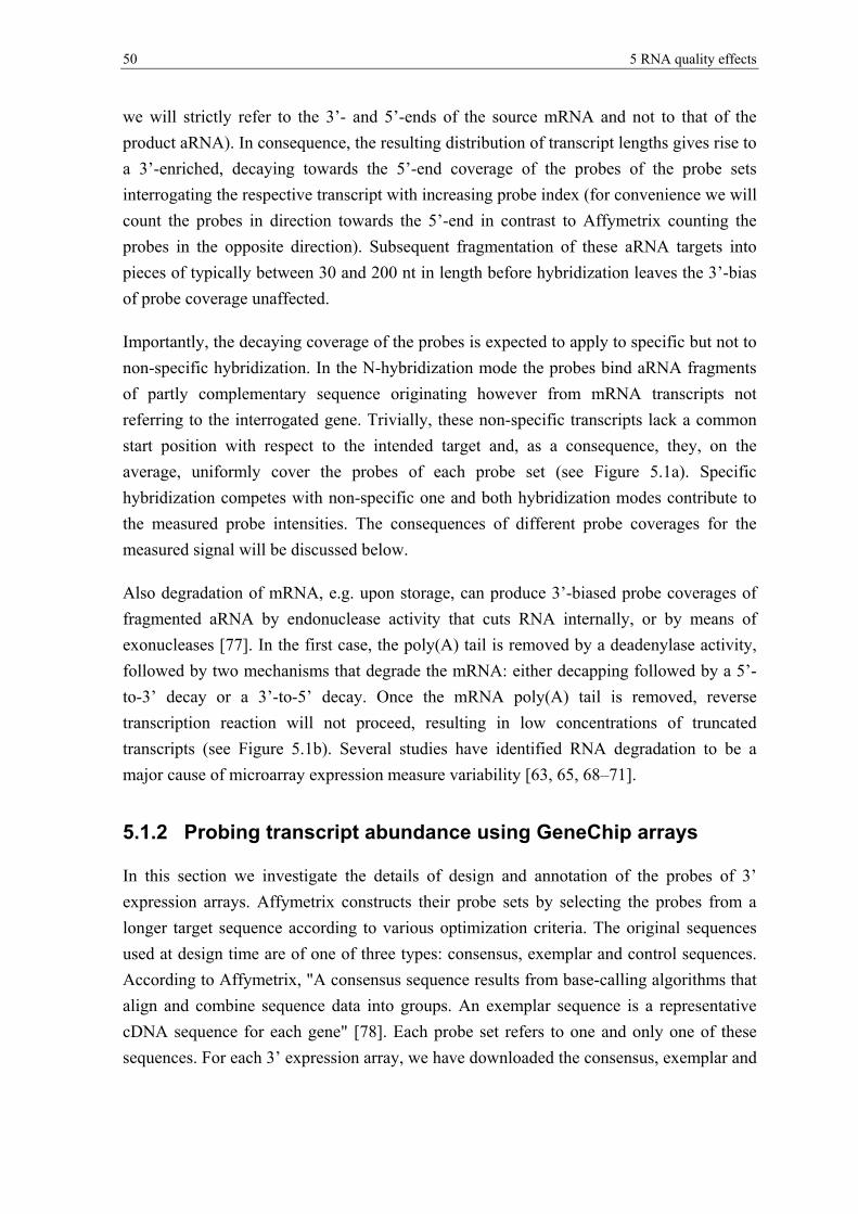
50 5 RNA quality effects
we will strictly refer to the 3’- and 5’-ends of the source mRNA and not to that of the product aRNA). In consequence, the resulting distribution of transcript lengths gives rise to a 3’-enriched, decaying towards the 5’-end coverage of the probes of the probe sets interrogating the respective transcript with increasing probe index (for convenience we will count the probes in direction towards the 5’-end in contrast to Affymetrix counting the probes in the opposite direction). Subsequent fragmentation of these aRNA targets into pieces of typically between 30 and 200 nt in length before hybridization leaves the 3’-bias of probe coverage unaffected.
Importantly, the decaying coverage of the probes is expected to apply to specific but not to non-specific hybridization. In the N-hybridization mode the probes bind aRNA fragments of partly complementary sequence originating however from mRNA transcripts not referring to the interrogated gene. Trivially, these non-specific transcripts lack a common start position with respect to the intended target and, as a consequence, they, on the average, uniformly cover the probes of each probe set (see Figure 5.1a). Specific hybridization competes with non-specific one and both hybridization modes contribute to the measured probe intensities. The consequences of different probe coverages for the measured signal will be discussed below.
Also degradation of mRNA, e.g. upon storage, can produce 3’-biased probe coverages of fragmented aRNA by endonuclease activity that cuts RNA internally, or by means of exonucleases [77]. In the first case, the poly(A) tail is removed by a deadenylase activity, followed by two mechanisms that degrade the mRNA: either decapping followed by a 5’-to-3’ decay or a 3’-to-5’ decay. Once the mRNA poly(A) tail is removed, reverse transcription reaction will not proceed, resulting in low concentrations of truncated transcripts (see Figure 5.1b). Several studies have identified RNA degradation to be a major cause of microarray expression measure variability [63, 65, 68–71].
5.1.2 Probing transcript abundance using GeneChip arrays
In this section we investigate the details of design and annotation of the probes of 3’ expression arrays. Affymetrix constructs their probe sets by selecting the probes from a longer target sequence according to various optimization criteria. The original sequences used at design time are of one of three types: consensus, exemplar and control sequences. According to Affymetrix, "A consensus sequence results from base-calling algorithms that align and combine sequence data into groups. An exemplar sequence is a representative cDNA sequence for each gene" [78]. Each probe set refers to one and only one of these sequences. For each 3’ expression array, we have downloaded the consensus, exemplar and
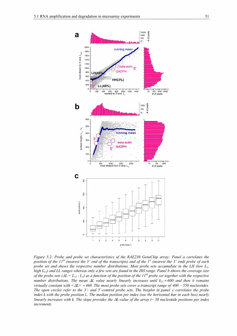
5.1 RN
Figurpositiprobehigh Lof thenumbvirtuaThe oindex linearincrem
NA amplifica
re 5.2: Probe on of the 11th
e set and showL11) and LL rae probe sets (Δer distributio
ally constant wopen circles r
k with the prorly increases wment).
ation and degra
and probe sh (nearest the ws the respecanges whereasΔL = L11 - L1) ons. The meawith <ΔL> ≈ refer to the 3obe position Lwith k. The sl
adation in mic
set characteris5’ end of the
ctive number s only a few seas a function n ΔL value n460. The mos
3’- and 5’-conL. The medianlope provides
croarray exper
istics of the Re transcripts) distributions.ets are found of the positionearly linearlst probe sets cntrol probe sen position perthe ΔL-value
riments
RAE230 Geneand of the 1s
Most probe in the HH rann of the 11th ply increases cover a transcets. The boxp
r index (see the of the array
eChip array: st (nearest thesets accumul
nge. Panel b sprobe set togeuntil k11 ≈ 60
cript range of plot in panel he horizontal b
(~ 50 nucleot
Panel a corre 3’ end) problate in the LHshows the covether with the 00 and then if 400 – 550 nuc correlates
bar in each botide positions
51
relates the be of each H (low L1, verage size respective it remains ucleotides. the probe ox) nearly per index

52 5 RNA quality effects
control sequences together with the probe sequences as provided by Affymetrix (see www.affymetrix.com). Probe distances to the intended 3’-end of the transcript, Lp, were computed by aligning the probe sequences to the respective transcript sequences. The position of each probe Lp (p = 1, 2...) is then defined as the number of nucleotides counted between the 3’-end of the transcript and the first (i.e. nearest) base of the 25meric probe sequence3. The ordering of probes according to increasing distances Lp defines the probe index k within each probe set.
The probes of each probe set cover transcript lengths which largely exceed the length of the individual probes. This design is well suited to study length-dependent alterations of transcript abundance due to RNA degradation and imperfect amplification. Figure 5.2a shows that the majority of probe sets start (first probe with index k = 1) within the first L1 = 100 - 200 nucleotides nearest to their 3’-end and end at position L11 = 250 - 600 for the last probe (index k = 11). Only about 5% of all probe sets are located beyond the range of 600 nucleotides. Within this range, the sets can be roughly classified into ‘low (i.e., more 3’) L1 and low L11’ (LL), ‘low L1 and high (i.e., more 5’) L11’ (LH) and ‘high L1 and high L11’ (HH) sets where low refers to distances close to the 3’ end and high refers to distances farther towards the 5’ end (see Figure 5.2a). The mean length of the covered transcript range (ΔL = L11 – L1) nearly linearly increases with the position of the 11th probe up to L11 ≈ 600, and then it remains virtually constant ΔL ≈ 460 (Figure 5.2b). Hence, short probe sets with ΔL < 300 accumulate near the 3’ end of the transcripts whereas more distant probe sets typically cover a wider length range of the transcripts (350 < ΔL < 600).
The mean position of all probes on the array with a given index k = 1...11 linearly correlates with k to a good approximation (Figure 5.2c). The obtained slope characterizes the mean distance between two neighbored probes. It can be interpreted as the probe sensitivity per index increment and depends on the probe design of the particular array type,
1array array array
array array
L L LL
k 1 k
−Δ = ≈
− (5.1)<...>array denotes averaging over all probes of the array. The approximation in the right part assumes a vanishing intercept in good agreement with the data (see Figure 5.2c).
3 Precomputed probe distances for most GeneChip microarrays are available on our website http://www.izbi.uni-leipzig.de/downloads_ links/programs/rna_integrity.php

5.1 RN
Figurthe 1th
probefor alfractiothree
FigurGeneprobe<ΔL>incre(e.g.,MOEsets i
Affyestimthe mphosthe 3nucleL20 =
NA amplifica
re 5.3: Probe th (nearest to e sets; the slopll probes (<Δon of probe sranges (see th
re 5.3 proveChip typese sets can s>-values wement. Thes, the humanE430a arrayis relatively
ymetrix Genmate the RNmiddle (m) phate dehyd3’- and theeotides betw
= 1104 for 5
ation and degra
and probe sethe 3’ end of pe of the lineaΔL>); the aveets from the Lhe main paper
vides an ovs. It shows trongly vary
which can cse differencen genome Hys, respectivy constant fo
neChip arraNA quality iof relativelydrogenase (
e 5’ probe ween L20 =
5’-probe sets
adation in mic
et characteristf the transcripar regression erage transcrLH, LL and Hr for definition
verview ovethat the mey between thange betwes refer in f
HGU95a andvely). On thor all chip ty
ays include in terms of y long transGADPH) usets of th
= 281 and Ls of GADPD
croarray exper
tics for differept), 5th and 11
of the mean pript range cov
HH ranges andns).
er selected ean positionthe differenween about first instancd HG133a ahe other hanypes consid
a small nuf the 3'/5' biscripts codi
using 20 prohe controls L20 = 378 fD and beta-
riments
ent GeneChipth (nearest to
probe positionvered by the d the residual
probe desin of the fir
nt chip types25 and ab
e to arrays oarrays and tnd, the averdered.
umber of cias. They taing, e.g., beobes per set
together cfor the 3’-p-actin, respe
p microarraysthe 5’ end) p
n L versus the probe sets (a
l fraction not
gn charactest and of ths giving risebout 60 nucof older andhe mouse gage span co
control probarget the 3' ta-actin andt. Figure 5.2over the raprobe sets ectively.
s: the mean poprobe averagee respective pr(average spancontained in
eristics of he last probe to a wide cleotides pd newer gengenome MGovered by th
be sets desend, the 5'-
d glyceralde2a and b shange of aband L20 = 9
53
ositions of ed over all robe index n) and the one of the
different be in the range of er index nerations G74a and he probe
igned to -end and ehyde-3-ows that
bout 700 942 and
54 5 RNA quality effects
5.1.3 Used expression data
Affymetrix microarray raw intensity data (CEL-file format) were downloaded from the public repositories Gene expression omnibus [79] or Array Express [80]. In this section we study the following data sets.
The Human tissue dataset (GSE7307, see supplementary text for the detailed list of samples used) comprises 677 samples taken from over 90 distinct tissue types hybridized to Affymetrix HG-U133 plus 2.0 arrays.
The RatQC (rat quality control) dataset (E-MEXP-1069) from [69] was generated to systemically explore how RNA quality affects microarray results. It consists of 36 rat liver RNA samples hybridized to Affymetrix RAE230A expression arrays. The progressive change in RNA quality was generated either by thawing frozen tissue or by ex vivo incubation of fresh tissue. Each sample was characterized by the RNA integrity number (RIN) and mean transcript length in [69].
The RNeasy data set consists of five pairs of HG-U133A GeneChips which were hybridized with RNA extracted from ovarian cancer samples and processed in two different ways namely with and without a cleanup step using RNeasy reagents [62]. The RNeasy cleanup should lead to good-quality RNA whereas lack of the cleanup step should yield poorer-quality RNA. The RNeasy data set was used in previous work aiming at judging RNA-quality from microarray data [81, 82].
5.2 Degradation and hybridization mode
5.2.1 Intensity-based degradation metrics
In this section we discuss the consequences of the 3’-enriched probe coverage on the observed probe intensities. In the following we will subsume the 3’-bias of probe coverage as ‘degradation effect’ independent of its origin (IVT amplification or degradation) for the sake of convenience. Let us first define the probe-specific and the mean degradation ratio averaged over all probes of the array,
all probes,all genes
g,kg,k g,k
g target
[S ]d and d d
[S ]≡ = (5.2)
respectively, which characterize the decrease of the transcript concentration due to the degradation effect. [Sg]target is the (true) expression degree of a selected gene g given as the total concentration of the target transcripts in the hybridization solution independent of

5.2 Degradation and hybridization mode 55
their length. It refers to the target concentration in the absence of degradation and presumes that RNA processing proceeds without 3’/5’ bias. Contrarily, [S]g,k denotes the apparent expression degree reported by probe with index k = 1,...,Nset designed to interrogate target g. It is given as the concentration of the RNA fragments which specifically bind to this probe. It consequently refers to the probe coverage which decays with increasing distance of the probe to the 3’-end of the target. Angular brackets <…>all probes denote averaging over all probes of the array. One expects [S]g,k ≤ [Sg]target and thus dg,k ≤ 1 owing to the 3’-enrichment after incomplete amplification and degradation of the fragments. The probe specific degradation index, dg,k, thus characterizes the loss of mRNA material at a given probe position along the transcribed region of the gene. The mean degradation index d averages the single probe effects over all probes. It estimates the total loss of RNA probed by the microarray in a given preparation prior to hybridization.
The probe intensities measured in the microarray experiment are described by the Langmuir model in Eq. (3.2) where the probe index p ≡ g,k subsumes the gene and probe index explicitly used in Eq. (5.2). We here consider the reduction of the concentrations [Sg]target and [N]chip after incomplete amplification and/or degradation as an effect of the binding strengths due to specific and non-specific hybridization (compare Eq. (3.3))
[ ]P,S P,S P,S P,N P,Np p p p g p p pchiptarget
X S K d S K and X d N K⎡ ⎤ ⎡ ⎤= ⋅ = ⋅ ⋅ = ⋅ ⋅⎣ ⎦ ⎣ ⎦ (5.3)respectively. Non-specific hybridization is related to the total amount of RNA used for hybridization [57]. [N]chip is consequently reduced by a factor given by the mean degradation factor d.
The probe-specific degradation index dp defines the decrease of transcript concentration after amplification and degradation (Eq. (5.2)). In the next step we define the apparent degradation index as the intensity ratio of probes located at different positions along the target sequence, for example near its 5’- and 3’-end of one selected target,
Papp 5 '5 '/3 ' P
3 '
Ir
I≡ (5.4)
where the intensities are given by Eqs. (3.2) and (5.3) with the respective degradation ratios d5’ and d3’, respectively.
Let us consider two special cases if the probes hybridize either far from saturation in the linear range ( P ,S P , N
p pX , X 1<< ) or in the range of saturation of specific hybridization ( P ,S P , N
p pX 1 X> > ). The apparent degradation index becomes

56 5 RNA quality effects
( )( )
S N true P,S P,S P,S P,S S N5' 5' 5 'app 5 '/3 ' 5 ' 5 ' 3 ' 3'
lin P,N P,N P,N P,N S NS N5' 5 ' 3 ' 3 '3 ' 3' 3 '
P,Sapp 5'sat P,S
3'
d x d x r (K w / K w ) for x x (specific)r
(K w / K w ) for x x (non specific)d x d x
wand r (saturati
w
⋅ + ⋅ ⎧ ⋅ ⋅ ⋅ >>⎪= = ⎨ ⋅ ⋅ << −⋅ + ⋅ ⎪⎩
= on) (5.5)
respectively. The lower case x defines the hybridization strengths at ‘ideal’ transcript concentrations (see Eq. (5.3) with d = dp = 1: [ ]S P,S P,S
p p pt argetx S K w≡ ⋅ ⋅
and
[ ]N P,N P,Np p pchip
x N K w≡ ⋅ ⋅ ) and true5 '/ 3 ' 5 ' 3 'r d / d≡ denotes the ‘true’ relative degradation index
between 5’ and 3’ probes, respectively. Eq. (5.5) shows that the apparent degradation index is proportional to the true one ( app true
lin 5 '/3 'r r∝ ) in the special situation of dominating specific hybridization (xS ≫ xN) far from saturation only. It however scales with the ratio of the specific binding and washing constants of the 3’- and 5’-probes, which might be larger or smaller than unity depending on the sequences of the particular probes (see [43] for details). At dominating non-specific binding or saturation one gets apparent degradation indices which are completely independent of the true one. Their values again depend on the probe sequences and can be larger or smaller than unity. Hence, the use of intensity-based degradation metrics raises problems because they reflect the degradation bias of transcript abundance in special situations only.
On the other hand, two intensity-based degradation measures are well established for quality control of GeneChip arrays: (i) The slope of a linear function fitted to the so-called ‘RNA degradation plot’, r5’/3’
slope. This RNA degradation plot displays the mean logged intensity averaged over all probes with the same index k, taken from one array, as a function of k [75]. (ii) The intensity ratio r5’/3’
control of special control probe sets targeting the 5'- and the 3'-end of relatively long transcripts such as beta-actin and GADPH. A threshold of the 3’/5’-signal intensity ratio of the GADPH controls less than 3 (in logarithmic scale log10 3 = 0.48) is recommended for good quality RNA [83, 84].
In view of the discussed problems of intensity-based degradation measures we will revise theses estimates and judge their suitability for determining RNA quality. Large values of r5’/3’
slope and/or r5’/3’control near unity are generally thought to indicate small degradation bias
and thus good RNA quality. Note that reciprocal values of these measures are often used in practice estimating the respective 3’/5’-ratios. Here we consequently use 5’/3’-ratios to ensure direct comparability between the various measures.
In summary, probes located nearer to the 3’-end of the interrogated transcripts potentially shine brighter than more distant probes due to the 3’-enrichment of probe coverage giving rise to expected ‘true’ intensity ratios r5’/3’ < 1. However, this rule applies only to conditions of specific hybridization far from saturation. RNA quality measures based on

5.2 Degradation and hybridization mode 57
the 5’/3’-intensity ratio consequently require consideration and evaluation of the hybridization mode of the chosen probes. Moreover, the potential dependence of the probe intensities on the degree of degradation gives rise to systematic errors of the estimated expression degree of the transcripts which requires appropriate correction.
5.2.2 Degradation Hook and Tongs Plot
In analogy to the Δ and Σ transformations given in Eq. (3.4) we define the following modified hook representations
( )
s3'/s5' p ps3' s5'
s p ps pset
i 2PM MM1
p k k k k2sk i
(degradation hook)
(tongs plot)
1with and log I log I3
+
=
ΔΣ ≡ Σ − Σ
ΔΣ ≡ Σ − Σ
Σ ≡ Σ Σ ≡ +∑
(5.6)where the subscript s = s3’, s5’ denotes a subset of three consecutive probes within the probe set of size Npset nearest to (s3’, i = 1) or most distant from (s5’, i = Npset - 2) the 3’-end of the transcript, or centered around its middle probe (s = m). The so-called tongs-plot shows the three positional-dependent values ΔΣ3’, ΔΣ5’ and optionally ΔΣm as a function of Σ whereas the ‘degradation hook’ plots ΔΣ3'/5’-versus- Σ. These plots use the same abscissa as the hook curve and they also smooth the noisy data using a running window of 500 - 1000 probes. Both the ‘degradation hook’ and the ‘tongs plot’ estimate the 3’-enrichment of the probes and thus their degradation level in dependence on the hybridization mode. Examples for both plots are shown in Figure 5.5 in the next section.
The two-species Langmuir hybridization isotherm predicts the theoretical hook-curve which was previously used to fit the experimental curves and to extract characteristic chip-related parameters. Here we modify the hook formalism to take into account the effect of incomplete transcript amplification and degradation in terms of the degradation ratios defined in Eq. (5.2). We thus define the probe-specific S/N ratio similar to Eq. (3.11) under consideration of the subset s of probes
PM,SPM,S pp p t arg et chips s
s PM,N PM,Nchip p chip
Kd d [S]XRd X d [N] K
= ⋅ = ⋅ ⋅ (5.7)It scales with p s
d / d , the probe specific 3’-bias of the actual transcript abundance averaged over the subset s and divided by the mean degradation index of the selected chip, d. Similarly to Eq. (3.13), the theoretical expressions for the hook coordinates for the

58 5 RNA quality effects
subset s of probes are obtained by inserting Eqs. (3.2) and (5.3) with P = PM and MM into Eq. (5.6)
{ } { }
{ } { }
PM MMp S S S S Ss
p Ss
start PM MMS S S S
(R ) log (R 1) / (R 10 1) log B (R ) / B (R )
and
(R )
1 1log (R 1) / (R 10 1) log B (R ) / B (R )2 2
−α
−α
Δ ≡ Δ = + ⋅ + −
Σ ≡ Σ
= Σ + + ⋅ + − (5.8)
with the saturation terms
start
start
1( )PM 2S S
1( )MM 2S S
B (R ) 1 10 (R 1) and
B (R ) 1 10 (R 10 1)
− β+ Δ
− β− Δ −α
= + ⋅ +
= + ⋅ ⋅ +
The vertical and horizontal dimensions of the hook curve and its start coordinates are given as
( )PM,Sp chip PM,N
pMM,S chipp chip
start PM,Np chip
Klog , log d log X and
K
log M log X log d
≈ ≈ − +
Σ = + +
α β (5.9)respectively. Note that the width and the start coordinate of the hook curve, β and Σstart, change with the mean degradation index d whereas the height of the hook α doesn’t depend on degradation.
The mean expression index characterizes the mean expression level of present probes of the chip,
PM,S PM,S PM,N PM,Sp p p pchip chip
log(d X ) log(R) logX logd≡ ⋅ ≈ + +ϕ (5.10)The ordinate values of the degradation plots are obtained by inserting Eq. (5.8) into Eq. (5.6),
s s s1/s2 s1 s2(R) (R ) (R) and (R) (R ) (R )ΔΣ ≡ Σ −Σ ΔΣ ≡ Σ −Σ (5.11)One gets after explicit consideration of Eq. (5.8)

5.2 Degradation and hybridization mode 59
( ) ( )( ) ( )
PM MMs1 s1 s1 s11 1
s1/s2 2 2 PM MMs2 p s2s2 s2
R 1 R 10 1 B (R ) B (R )(R) log logB (R ) B (R )R 1 R 10 1
−
−
+ ⋅ ⋅ + ⋅ΔΣ = −⋅+ ⋅ ⋅ +
α
α (5.12)where ΔΣs1(R) refers to the special case rs2 = 1. The parameters
[ ][ ]
[ ][ ]
ss s
chip
3'3'/5' 3' 5'
5'
Slog r log with s 3',5 ',m and
S
Slog
S
γ ≡ = =
Δγ ≡ γ − γ =
(5.13)define the 3’-bias of transcript abundance (see also Eqs. (5.5) and (5.7)). Particularly,
3'/5'Δγ provides the logged fold change of the probe specific transcript concentrations between probes located nearer the 3’- and 5’-ends of the transcript. The mean transcript concentration averaged over all probes can be estimated as the geometric mean over the 3’ and 5’ transcript concentrations,
[ ] 13 '/5 '2 5 '
3 ' 3 ' 5 'chip 3 '3 '
[S]S S 10 [S] [S] [S][S]
− Δγ≈ ≈ ⋅ ≈ ⋅ (5.14)if one assumes uniformly distributed probes along the relevant transcript regions. With
[ ] [ ]t arg et 3 'S S≈ and Eq. (5.2) one gets
3'/5'logd 0.5≈ − ⋅Δγ (5.15)Hence, the mean amount of RNA (Eq. (5.2)) is directly related to the 3’/5’-difference of transcript abundance.

60
Figurplot (pthe podegrathe cudottedmeani
TypihookEq. (degrathe htranslog damplof nconstdiscu
re 5.4: Theor(panel above; Eositive and n
adation hook iurves (paramd curves in thing of selected
cal examplk (ΔΣ3’/5’-v(5.12), paneadation leve
hook. Both csformations d reflects tlification an
non-specifictant of specussed above
retical hook cEqs. (5.11) an
negative amplincrease, accoeter β). The e part above d parameters
es of the hoversus-Σ, Eel above) aels. Increaschanges are
(see Eqs. the decreasnd degradati backgrouncific bindine.
curve (Eq. (5.nd (5.12)) for litudes of the ompanied by tcurves are caare calculatedis indicated by
ook curve (Eq. (5.12), as predictedsing degradae governed b(5.2), (5.9)se of the ion. This trend hybridizng [57]. The
.8), thick curdifferent degr
e tongs plot (the shift of itsalculated withd neglecting t
by arrows (see
(Δ-versus-Σthin curv
d by theoryation increaby the degra), (5.13) anmean tranend is equivzation whice consequen
rves), degradaradation level(the tongs ops increasing bh γ3’ = -γ5’y =the saturation
e text).
, Eq. (5.8), es) and thy are showases the opeadation ratio
nd (5.15)). Tnscript concvalent with ch in turn nces of this
ation hook (tls log d. With ening Δγ3’/5’)
branch toward 0.1, 0.3 and
n term in Eq. (
thick curvehe tongs-pl
wn in Figurening of theo d and rs anThe widenicentration dthe decreasincreases
s so-called
5 RNA qual
thin curves) aincreasing deand the heig
ds the left whid 0.5, respect(5.12). The ge
es), the deglot ((ΔΣ-vere 5.4 for de tongs andnd their loging of the hdue to incse of the methe mean up-down e
lity effects
and tongs egradation ght of the ich widens tively. The eometrical
gradation ersus-Σ,, different d widens garithmic hook by complete ean level
binding ffect are

5.2 D
Figurtaken fGSM1use thprobemixedtongs-three middlhybridand (5formu‘heighfor boThe sreducmaxim
5.2.
Figurdegraplot (hookloggethe iduple
egradation an
re 5.5: Hook- form the hum
175967 in panhe same abscies. The hook cd N and S (mix-plot reveal thprobes neare
le in-between dization wher5.12) for the ulae given in ht’ of the hookoth arrays whsize of the moced number ofmum is prone
.3 The 3
re 5.5 showaded RNA (panel below
k. The curved intensityintensity peexes. Contr
nd hybridizatio
and degradaman body indexnel b) referrinissa scaling (Σcurve revealsx), specific (S)he mean 3’/5
est to the 3’-e(middle bra
reas no bias hook and to
the previous k, see Eq. (5.9hereas the logoving windowf probe sets into increasing
3’-intensi
ws the hook together w
w). The degves reflect y differenceenalty of orarily, the d
on mode
tion hook (abx data set (mung to large an(Σ, see Eq.(5.6 the changing), saturation (’-intensity biand (upper branch). Note this observed
ongs plot, resection using
9); β, ‘width’ ogarithmic 3’-w is decreasedn saturation rerror.
ity bias d
curves for with the resgradation hohowever dibetween pa
one mismatdegradation
bove) and tonguscle, GEO acnd smaller de6)) which is rg hybridizatio(sat) and asymas of the probanch), neareshat the differin the N-ran
espectively). Tg the parametof the hook; Σand 5’-degrad towards thrange. As a c
depends
two selectespective deook shows ifferent effaired PM a
atched basen hook judg
gs-plot (belowccession numbegradation efferelated to the on mode with mptotic (as) rabes. The threest to the 5’-enrent branchesnge as predicThe theoreticaters given in Σ(0), ‘start’ poadation levels e right end o
consequence,
s on the h
ed microarragradation hessentially
fects: The snd MM pro pairing in
ges the logg
w) of two selebers GSM1763fects, respectiv
expression dincreasing si
anges. The dege branches of d (lower bran
s split maximted by theoryal curves arethe figure. Thoint; M, ‘end’
(Eq. (5.15)) aof the tongs pthe part of th
hybridiza
ay hybridizahook (panelthe same shstandard hoobes. It conn the respeged mean i
ected chip hyb301 in panel avely. Note thadegree of the igma: non-sp
egradation hoof the tongs plonch) and loca
mally in the Sy (lines, see e calculated he hook dime’-point) are veare markedlyplot to compe
he curves beyo
ation mo
ations of dil above) anhape as the ook plots thnsequently eective probintensity di
61
bridization a and skin, at all plots respective ecific (N), ok and the ot refer to ated in the S-range of
Eqs. (5.8) using the
ensions (α, ery similar y different. ensate the ond of the
ode
fferently nd tongs standard he mean estimates be/target-ifference

62 5 RNA quality effects
between probes located nearer and farther to the 3’end of the transcripts, and thus the 3’/5’-bias of the probe intensities in the probe sets due to the degradation effect.
Interestingly, the different hybridization modes analogously affect the intensity differences in the standard and the degradation hook as well. For example, upon non-specific hybridization both, the PM/MM difference and the 3’-bias essentially disappear because both effects, the MM-penalty and the 3’/5’-bias, require duplexing of the probes with the intended targets. Non-specific binding doesn’t meet this criterion because the binding of non-specific transcripts is indifferent with respect to the mismatched pairing of the middle base of the MM probes and with respect to the degradation bias as well. Vice versa, both hook-versions show their maximum in the S-range because specific binding is associated with the intended intensity penalty of the MM-probes and of probes located more distant from the 3’-end, respectively.
Note that the two standard hook plots shown in panel a and b of Figure 5.5 are of virtually equal height owing to the similar MM-penalty (α = 0.83 – 0.85) whereas the respective degradation hooks markedly differ in this respect (Δγ3'/5' = 0.57 and 0.29, respectively) revealing marked differences in the degradation level between both samples. Comparison of the heights of both hook-types shows that strong degradation can affect the probe intensities nearly by the same order of magnitude as one mismatched base pairing.
The tongs plots explicitly estimate the intensity bias at three positions of the probe sets and thus it illustrates the progression of degradation with increasing probe index. The ΔΣs curves of all three subsets (s = 3’, 5’ and m) degenerate in the N-hybridzation range indicating the absence of the 3’-bias for non-specific binding as discussed above (see also Eq. (5.5) for xS ≪ xN). In the mix-range the ΔΣs-curves split into three branches which progressively diverge with increasing sigma and thus with increasing contribution of specific hybridization. The ‘opening of the tongs’, i.e. the split between the 3’- and 5’-branches, reaches its maximum in the S-range of hybridization in parallel with the maximum of the hook curve and of the degradation hook. Subsequently, the different branches start to converge as predicted for the range of saturation (see Eq. (5.5)). Both, the experimental degradation hook and the tongs plot are well described by theoretical curves based on the Langmuir-model of array hybridization in Eq. (5.12). The split parameter Δγ3’/5’ characterizes the height of the degradation hook, or equivalently, the ‘tongs opening’ serving as a measure of the maximum vertical difference between the 5’- and the 3’-branches of the tongs, respectively. Δγ3’/5’ estimates the 5’-depletion of probe coverage in terms of the logged concentration increment between the targets covering the 5’- and 3’-probes (Eq. (5.15)). The examples shown in Figure 5.5 a and b refer to relatively strong and weak depletion of targets with 5’/3’-concentration ratios of dtongs= 10-0.57 = 0.27 and
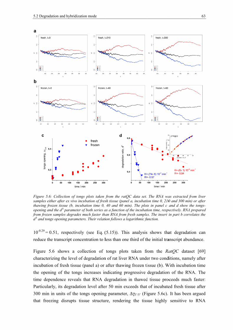
5.2 D
Figursamplthawinopeninfrom fd k and
10-0.2
reduc
Figurcharaincubthe otime Parti300 mthat
egradation an
re 5.6: Collecles either afteng frozen tissng and the d k
frozen sampled tongs openin
29 = 0.51, rece the trans
re 5.6 shoacterizing thbation of freopening of
dependencicularly, its min in unitfreezing d
nd hybridizatio
ction of tongsr ex vivo incusue (b, incubak parameter ofes degrades mng parameter
espectively cript concen
ows a collhe level of desh tissue (pthe tongs i
ce reveals tdegradation
ts of the tondisrupts tiss
on mode
s plots taken fubation of fresation time 0, f both series a
much faster thars. Their relati
(see Eq. (ntration to l
lection of degradationpanel a) or increases inthat RNA dn level aftengs openingsue structur
from the ratQsh tissue (pan40 and 60 m
as a function oan RNA from ion follows a l
(5.15)). Thless than on
tongs plotn of rat liverafter thawin
ndicating prdegradationr 50 min exg parameterre, renderin
QC data set. el a, incubatio
min). The plotof the incubatifresh sample
logarithmic fu
his analysis ne third of th
ts taken frr RNA undeng frozen tirogressive
n in thawedxceeds that r, Δγ3’/5’ (Fing the tiss
The RNA waon time 0, 210ts in panel c ion time, resps. The insert
unction.
shows thahe initial tra
rom the Raer two condissue (b). Wdegradation
d tissue proof incubategure 5.6c).
sue highly
as extracted f0 and 300 minand d show
pectively. RNAin part b corr
at degradatanscript abu
atQC dataditions, nam
With incubatn of the RNoceeds muched fresh tissIt has beensensitive t
63
from liver n) or after the tongs-
A prepared relates the
tion can undance.
set [69] mely after tion time NA. The h faster: sue after n argued to RNA

64 5 RNA quality effects
degradation whereas autolysis of fresh liver tissue appeared to be a much slower process [69].
In summary, the 3’/5’-bias of probe intensities essentially disappears for probes which hybridize predominantly non-specifically and it markedly decreases for probes which are strongly saturated with specific transcripts. The 3’/5’-bias consequently provides a suited metrics for RNA-quality only in the linear range of specific hybridization in agreement with the theoretical predictions made in Section 5.2.1.
5.2.4 Short 3’-probe sets are prone to non-specific hybridization
In the next step we selected the probe sets from the non-specific and specific hybridization ranges of the hook curve and calculated their frequency histograms as a function of L1 and Lmax, the position of the nearest and of the most distant probe from the 3’-end in each probe set.
Figure 5.7 shows the distribution of the fraction of probe sets of either hybridization range normalized with respect to the total number of probe sets in the respective group. Probe sets which cover the range near the 3’-end with L1 < 100 and Lmax < 500 are more prone to non-specific hybridization than probe sets located at larger distances from the 3’-end with L1 > 100 and Lmax > 500 which are more affected by specific hybridization on the average. The relative difference of the fractions in both groups is large: For example, the fraction of N-hybridized probe sets exceeds that of S-hybridized ones by about 50% at small Lmax < 300. Vice versa, at large Lmax > 700, the S-hybridized fraction considerably exceeds the N-fraction. The observed distributions are very similar for the different arrays of the Rat-QC data set showing that the positional-dependent variation of the hybridization mode is virtually insensitive to the degree of RNA-degradation.
We suspect that the increased fraction of non-specific hybridization towards the 3’ end of the transcripts is caused by inaccurate assignment of the 3’-transcript end upon probe design and/or by variations of the 3’-end of the transcripts, e.g. due to effects such as alternative polyadenylation as discussed previously [85, 86]. Alternative polyadenylation leads to transcript isoforms with differences in the 3’ UTR length. In these situations the ‘true’ 3’-end of the transcript can be located at L3’> 0 and all probes at positions closer to the apparent transcript end, L3’ > L > 1, will hybridize exclusively non-specifically owing to the absence of specific transcripts. In consequence, the mean fraction of non-specific hybridization of probes at small L will exceed that of specific hybridization on relative scale, as observed. A very similar plot as shown in Figure 5.7 for the rat genome array RG230A was obtained for alternative array types such the human genome HGU133A plus2 (see Additional File of [87]).

5.2 D
Figura functhat ‘transcbetweto theabout
An aN-hysolutL-rantransdepleaffinincreOn taffinaccumconcdepleof no
In sualong
egradation an
re 5.7: Distribction of the po‘short’ probe cripts at (L1 <een the respece mean fractiot 50% of all pr
alternative oybridizationtion due to nge. In conscript-fragmete its conc
nity of the reease the relathe other hanity of the pmulation ofentrations ietion is, if aon-specific h
ummary, wg the targe
nd hybridizatio
bution of probosition of the fsets located n
< 100 and Lmctive fractions on of probe serobe sets. The
option that n near the 3the high nu
nsequence, ament than at
entration inespective prative contriband, it has probes whif partly ovein a linear aat all, of sechybridizatio
we found a ted transcri
on mode
e sets hybridizfirst (left part)nearer to themax < 500) thaof probe sets
ets in both, S-e distributions
potentially 3’-end can umber of proa larger numt larger distn solution. Srobes for spbution of nobeen showch exponen
erlapping prand thus mucondary impon at small L
biased distipts: Non-s
ized predomin) and last (rig
e 3’-end of than specific ons whereas the pS- and N-group
are calculate
explains thbe sought obes with pmber of protances L. TSuch target pecific bindon-specific
wn that deplntially affecrobes near tuch weakerportance forL.
tribution ofspecific bin
nantly with speght part) probee transcript a
nes. The part part above nops. According
ed using the ra
he increase in depletio
partly overlaobes can beThis compe
depletion eding [44]. Inhybridizatioletion is clects the abunthe 3’-end cr fashion. Wr explaining
f specific anding is mo
ecific and none of each probare more pron
in the middlormalizes this gly, the differeatQC data set.
of the relaton of the reapping probe thought toetition for theffectively rn consequenon as observearly governndance of tcan be assum
We thereforeg the high r
and non-speore heavily
n-specific tranbe set. The grane to bind nole shows the s difference wirential binding.
tive contribespective tabe sequenceo compete he same tareduces thence this chaved in this ned by the targets whemed to affee suspect threlative cont
ecific hybriweighted
65
nscripts as aphs show on-specific difference ith respect g refers to
bution of argets in es in this for each
arget can binding ange can L-range. binding
ereas the ect target hat target tribution
idization near the

66 5 RNA quality effects
3’-end, presumably owing to its inaccurate assignment and to transcript isoforms with variable 3’ UTR lengths.
5.3 Metrics for RNA quality
5.3.1 Positional-dependent intensity decays
The degradation hook and the tongs plot shown in Figure 5.5 highly resolve the 3’-bias of probe intensities in dependence on the hybridization mode. These plots allow classifying each probe set into one of five different hybridization regimes within a microarray experiment. However, this approach only coarsely resolves the positional bias along the transcripts by collecting together three probe intensity values at two or three selected positions only (3’, 5’ and m).
In this subsection we describe an orthogonal method which uses a more coarse graduation of the hybridization mode while highly resolving the 3’-bias with respect to the probe position. Particularly, we select two groups of probe sets taken either from the N- or the S-hybridization range of the hook curve. We then calculated the logged mean intensities of the selected PM-probes as a function of two alternative arguments, namely their probe index k in the probe set or their probe distance L relative to the 3’-end given in units of the number of nucleotides,
p
h h h hp pp k L L L
log I (k) log I and log I (L) log I with h S, N= = ±δ
= = = (5.16)respectively. The angular brackets denote averaging either over all probes with the same index k or over all probes with the same absolute position within a moving window L-δL < Lp ≤ L + δL.
Figure 5.8a shows the obtained intensity profiles for the example shown in Figure 5.5a. The mean intensity due to specific hybridization markedly decays with increasing distance of the probes from the 3’-end of the transcripts whereas the intensity due to non-specific binding is much smaller and remains virtually constant, as expected. The decay due to specific hybridization can be approximated with a distant-dependent degradation index,
P,S Spd d (L)= which is given by an ‘exponential plus constant’ decay law in analogy with
Eq. (5.17) (see below). The obtained curves well describe the intensity decay in the intermediate L-range and its flattening at small and large L-values (see dotted curve b in Figure 5.8a).

5.3 M
FigurdecayFigurper incurvesintensexponthe Rascaledscaled
Metrics for RN
re 5.8: Positioys of specificare 5.5a. The cndex (left part)s in part a ssity decays whnential (d) decat-QC (b) and decay in thd decays in pa
A quality
onal dependenally and non-circles denote t). The decays show fits usinhich consider scays with initid the RNeasye right part o
art b in additio
nt intensity d-specifically hindex-based are normaliz
ng different fsaturation witial shifts (Eq.
y cleanup (c) of panel c areon use a const
decays in relahybridized proaverages whi
zed according functions: Expthout initial sh. (5.18)). Pandata sets. The fit using simtant d∞ > 0.
tive and absoobes (Eq. (5.1ich are plottedto Eq. (5.17)
xponential pluhift (Eq. (5.18el b and c) R
he index-scalemple exponen
olute scale. P16)) referringd as a functio(right part of
us constant (a8)); exponentiaepresentative
ed decays in tntial decays (d
Panel a) Meang to the data on of the meaf the figure). Ta) and exponal plus consta
e decays are tthe left part a(d∞ = 0) where
67
n intensity
shown in n position The dotted nential (b) ant (c) and aken from and the L-eas the L-

68 5 RNA quality effects
This approach attributes the flattening of the decay near the 3’-end to the saturation of the probes with bound transcripts. However this effect becomes relevant usually at large intensity values only (log I ~ log M > 4; see Figure 5.5). The observed mean initial intensity values of the decays are however much smaller (log I(3’) ~ 3). We conclude that another effect and not saturation causes the flattening of the decays at small L-values. The decrease of the relative contribution of specific hybridization near the 3’-end discussed in the previous subsection well explains the observed trend: Non-specific hybridization still adds a small residual contribution to the specific decays due to imperfect decomposition of the different hybridization modes. The decrease of the contribution of specific binding presumably due to inaccurate assignment and transcript isoforms then effectively increases the relative weight of non-specific binding and adds a constant component to the decays at small distances from the 3’end which in consequence flattens the initial decay.
To account for this effect we pursue a simple approach which neglects saturation and normalizes the decays with respect to their maximum intensity level near the 3’ end of the transcripts,
( )h h hd x I (x) / I (3') with x k, L and h N,S= = = (5.17)The obtained degradation index due to non-specific hybridization is given by a constant, dN(x) ≈ 1, to a good approximation (Figure 5.8). The degradation decays due to specific hybridization are well described using a ‘shifted exponential plus constant’ functions of the form,
( ) ( )S x x0
x
x xd x d (x) 1 d exp d∞ ∞
⎛ ⎞−= ≈ − ⋅ − +⎜ ⎟λ⎝ ⎠(5.18)
as illustrated by the dotted curves in Figure 5.8. The obtained decay length λ characterizes the mean slope of the 3’-bias in units of the number of probes (λk) or nucleotides (λL) after which the variable contribution of the intensity decays to 1/e of its initial value. The constant dx
∞ defines the residual constant intensity level at large distances from the 3’-end. The shift-parameters x0 = k0, L0 account for the potential flattening of the decay at small arguments discussed above. Both decay constants are linked via the <ΔL>-value, i.e.
k L Lλ ≈ λ ⋅ Δ (5.19)Panel b and c of Figure 5.8 show selected examples taken from the rat-QC and the RNeasy cleanup data sets which refer to different array types (RAE 230A and HG-U133A, respectively). With decreasing RNA quality the decays become steeper paralleled by

5.3 Metrics for RNA quality 69
increasing absolute values of the limiting intensity levels but almost constant initial shift parameters L0 ≈ 150 – 200 and k0 = 1 - 2. Index- and nucleotide-based length scales give rise to similar trends (compare the right and the left parts in Figure 5.8b and c). The L-scale in units of nucleotides is associated with a slightly more flat and smaller asymptotic level than the relative k-scale using the probe indices as argument. Note that about 95% of the probes of the arrays are positioned with similar frequencies in the range 100 < L < 600 whereas only less than 5% of them are found at larger distances, however with a broad distribution over the range 600 < L < 2800 (Figure 5.2). Most of the more distant probes refer to the probe indices k = 10, 11. This assignment effectively compresses the asymptotic region to the last two probes with indices k = 10 and 11. As a consequence the decays in relative k-scale can be described with sufficient accuracy using a ‘single exponential’ decays (Eq. (5.18) with d∞
k = 0) where the values d(10) and d(11) roughly refer to the limiting decay level obtained in the fits using the L-scale, d∞
L.
The L-decays of specifically hybridized probes obviously behave differently for L > 600 showing a less pronounced loss of intensity than for L < 600. The origin of this difference is unknown. The standard error of the experimental decays roughly agrees with the symbol size (k-dependencies, left part of Figure 5.8b and c) or it slightly exceeds line thickness (L-dependencies, right part of Figure 5.8b and c). The small oscillations in the decays and the relative increase at L > 600 thus reflect systematic effects presumably due to differences of the probe properties in the different subensembles of probes referring to each data point such as their binding affinity and also their degradation degree. Recall that the number of probes drastically decreases at L > 600 which makes this range less relevant for correcting purposes of the majority of probes. We exclude this range therefore from curve fitting.
Our fits show that the values of the decay parameters systematically depend on the chosen decay function and strongly correlate each with another. To illustrate this correlation we show fits with variable d∞
L but constant λL = 150 in Figure 5.8b (right part) and fits with constant d∞
L = 0 but variable λL in Figure 5.8c (right part). The values of the variable parameters d∞
L and λL systematically decrease with progressive degradation. Both options equally well describe the decaying part of d(L) in the range 100 < L < 600.
To obtain a robust decay characteristics we substitute the exponential fit functions in Eq.(5.18) by a simple two-point estimate
k S S
k 10,11 k 1,2logd logI logI
= == − (5.20)
This logged degradation ratio characterizes the intensity decay in the index-range kstart - kend = 2-10, or equivalently, in the positional range Lstart - Lend = <L>1,2 -
70 5 RNA quality effects
<L>10,11 ~ 150 - 550 which comprises the majority of more than 95% of all probes. The degradation ratio can be transformed into estimates of the decay length of the exponential decays: k
k 8 / ln dλ ≈ and kL 8 L / ln dλ ≈ ⋅ Δ .
Please note that the decay function defined in Eq. (5.17) estimates the fold change of transcript abundance at position x and x0, to a good approximation, i.e.
( ) [ ] [ ]0x x
d x S / S≈ (5.21)The degradation ratio (Eq. (5.20)) consequently estimates the mean fold change of transcript abundance reported by the probes positioned near the 5’- and 3’-ends of the probed range. It represents an alternative estimate of the tongs opening parameter introduced above, 3'/5 'k
tongsd d 10Δγ∝ = (Eq. (5.13)). Figure 5.6c shows the time course of RNA degradation in the Rat QC experiment using the tongs opening (panel c) and the dk (panel d) parameters. Both measures strongly correlate (see insertion in Figure 5.6d) and essentially reflect the same degradation behavior of the samples studied.
In summary, the effect of degradation can be described as a function of the probe position in terms of a ‘shifted exponential decay plus constant’-function using either the probe index or the ‘absolute’ probe position as argument. This information can be further condensed into a single degradation ratio parameter characterizing the fold change of transcript abundance over the length of the DNA region interrogated by the probes.
5.3.2 3’/5’-controls are affected by the hybridization mode
It was previously shown that the 3'/5' intensity ratios of special control probe sets interrogating long transcripts such as GADPH and beta-actin might not represent a sufficient measure of the degradation bias at small expression degrees because non-specific binding leads to an underestimation of the 3’/5’-bias [45]. Here we show that the controls are often prone to saturation which also leads to the systematic underestimation of the 3’/5’-bias (see also Eq.(5.5)).
The threshold hook represents a modified version of the degradation hook described in Section 5.2.2. It defines a threshold of the 3’/5-intensity ratio of the probe sets used to assess RNA-quality such a GADPH or beta-actin. The threshold hook accounts for the fact that the probe signals are affected by non-specific binding and by saturation. Both effects give rise to an intensity-dependent threshold for estimating good RNA-quality.

5.3 M
Figur(appahybridof GA
In thcoord
In co
In thcondisothdiffevaluein thThe whic
The ochanNote(Δ3’/5
heighdegradegraprobevaria
Metrics for RN
re 5.9: Thresarent) and vadization regim
ADPH-control
he first stepdinates
control 13' 5' 2
control3'/5'logd
+Σ =
ontrast to the
he second sdition that bherm (see Erent degrade is express
he previous start and en
ch provides
obtained honging exprese that the d5’ = -log(r5’/
ht parameteadation indadation ratie. Hence, t
able one wh
A quality
shold hook foariable (thresme and vanishls taken from t
p one tran
( PM12 3
l control3'/5'
log I
≡ Δ =
e standard h
step, one caboth the 5’- Eq. (3.2)), hdation indicsed as a funsubsection
nd point ofthese data w
ook curve thssion degredelta-coordi/3’
app), see Eer used in dex is adjusio agrees wthe thresholhich depend
or estimating shold hook) Rhed upon non-the tissue data
nsforms the
3'probeset
PM
3'pr
lo
log I
+
hook (Eq. (3
alculates thand 3’-pro
however usces of the rnction of sig
after neglef the threshowith relative
hus describeee of the reinate directEq. (5.4)) wthe fits (Δ
sted in sucwith the emp
ld hook trads on the h
g good RNA RNA quality -specific hybria set (see text)
e intensity
PM
5'probes
robeset
og I
log−
3.4)) we her
he thresholdobes hybridising differerespective tgma using tecting the Mold hook arely high acc
es the ‘trajespective tratly provide
whereas the Δγ3’/5’ = log(rch a way thpirical RNAansforms thhybridizatio
quality usingthreshold. T
idization and ).
values of
)et
PM
5'probesetI
re use only
d hook as aize accordin
ent specific transcripts, he degradat
MM-probes re taken frocuracy.
ctory’ of a panscript (ses the appa‘true’ degr
r5’/3’true), se
hat the maA-quality thhe constant n mode of
g control proThe true thre
upon saturati
the control
the intensiti
a Δ3’/5’-vs-Σng to the hy
binding acd5’ < d3’(Eqtion hook-fo(use Eq. (5
om the stan
pairing of 3e Figure 5.rent loggedradation inde Eq. (5.13ximum val
hreshold of RNA-qualithe control
obe sets: (a) eshold dependion. (b) Error
l probes in
ties of PM-p
Σ3’/5’-plot uyperbolic Lctivities duq. (5.3)). Thformalism d5.12) with
ndard hook
3’/5-probe s.9a for illusd degradatidex is given3)). The lalue of the f the chosenity thresholls. In conse
71
Constant
ds on the r estimates
nto hook
(5.22)probes.
nder the Langmuir ue to the he delta-described
α = -∞). analysis
ets upon stration). ion ratio n by the
atter true apparent
n control ld into a equence,

72 5 RNA quality effects
different data points residing along one hook curve refer to identical true degradation levels irrespective of their different delta coordinates characterizing their apparent degradation level.
The application of a constant threshold instead of the variable one will cause false quality estimates. We estimated the error of the 3’/5’-intensity ratio of the GADPH-control taken from the tissue data set as example: Figure 5.9b shows the hook-coordinates of the GADPH control probe sets of the 677 samples of the human tissue data set (see Eq. (5.22)). The threshold hook and the horizontal line provide the true and the apparent (false) thresholds for good RNA quality in terms of the logged 3’/5’-intensity ratios, Δ3’/5’ < Δthreshold. The constant threshold is assumed to agree with that of the hook curve in the range of specific hybridization. It consequently forms the tangent of the hook-curve at its maximum referring to the S-range of hybridization. The hook curve describes Δthreshold under the realistic assumption of saturation whereas the constant threshold neglects this effect. As a consequence, data located between both thresholds (colored in blue) define false positives (FP) with respect to the constant threshold whereas data below the hook and above the line are true positives (TP, red) and true negatives (TN, orange), respectively. The number of false negatives (FN) is zero because the hook threshold remains below the constant one. The positive predictive value (PPV = TP/(TP+FP)) and the specificity (Sp = TN/(FP+TN)) are 0.48 and 0.79, respectively, meaning that less than 50% of the 3’/5’ controls properly estimate the quality of RNA in terms of good and degraded one. This particular example assumes that the 3'/5' signal ratio for GADPH for good RNA is of no more than 3, or in our notation Δ3’/5’ < log(3) ≈ 0.5.
To assess the effect of the hybridization mode on the 3’/5’ controls we first estimated the hybridization regime of the GADPH and beta-actin controls of the rat-QC and the human tissue data sets using modified hook plots (Figure 5.10). They depict the logged PM-intensity ratio of the 3’- and 5’-probe sets of the controls (Δcontrol
3’/5’, Eq. (5.22)) along the horizontal coordinate and either the sigma coordinate of each probe set (Σ, Eq. (3.4)) or the mean sigma of both probe sets (Σcontrol
3’+5’, Eq. (5.22)) along the vertical coordinate axis. In the former plots, each control (GADPH and beta-actin) thus provides two data points per array referring to the 3’- and 5’-probe sets, respectively (see green and blue dots in Figure 5.10). In the latter plots both data points are merged together to illustrate the mean intensity trend of the controls as a function of the degradation index.
To judge the hybridization mode we also depict the sigma coordinates of the non-specific background intensity (N, red dots) and of the asymptotic saturation level (as, black dots) obtained from the standard hook analysis of each of the arrays. Recall, that the sigma-values of the N- and the as-mode limit the range of possible probe intensities. They

5.3 M
Figurin theThe acontroprobesigmaconstarefer hybridand tr
consepossithat sigmdata exactundemean
It haGADΔcontr
partsinto (respe
Metrics for RN
re 5.10: Hybrie tissue (left) aabscissa providol data sets. Te sets of the ca-levels of nonant quality thrto the same qdization. Applrue negatives.
equently coible hybridismall valu
ma-values neset. We ar
tly estimateerestimate tningless.
as been recoDPH and rol
3’/5’ < log(s of Figur(apparentlyectively.
A quality
idization and Rand rat-QC (rdes the degradThe vertical acontrols, or thn-specific binreshold separuality thresholication of the
onstitute an ization mod
ues of the ear the asymrgued before the degradthe true de
ommended beta-actin
(3) = 0.47 [8re 5.10. Ity) bad and g
RNA-quality cright) data setdation level in
axes plot eitheheir mean (da
nding and of srating good anold. They howee constant thre
intrinsic medes as indicdegradation
mptotic sature that intendation level egradation
that good-n of no 83]. We dispt consequegood ones
characteristicts. Each data n units of the er sigma coorark blue circlsaturation, rend poor appaever explicitlyeshold thus pr
etrics allowcated in then index (Δc
uration limitnsity-basedin the saturlevel; in w
-quality sammore th
play this thently dividfor Δcontrol
3
s of the GADPpoint refers tlogged 3′/5′- m
rdinates of theles). The red
espectively. Tharent RNA quay consider its roduces false p
wing to assige figure (seecontrol
3’/5’ < 0t of the inte
d degradatioration limit oworst case
mples shoulhan three, hreshold as tdes the da
’/5’ > thresh
PH and beta-ato one array omean intensitye 3′- (green dand black do
he vertical orality. The ‘thrdecrease in thpositives toge
gn the probee also Figur0.2) are oftensities espeon measureof the probe
the intens
ld have a 3or in
the vertical ta points old and Δco
actin control pof the respecty ratio of the
dots) and 5′- (ots mark the range lines inreshold’ hookshe N- and satether with true
es to one ofre 5.5). It tten associatecially in th
es are not ses. In best csity ratios
3'/5' signal our notatorange lineof each d
ontrol3’/5’ < th
73
probe sets tive series. respective
(blue dots) respective
ndicate the s (orange) -ranges of e positives
f the five turns out ted with he tissue suited to case they
become
ratio for tion of e in both data set hreshold,

74 5 RNA quality effects
The 3’/5’-intensity ratio of the probe sets is however not constant for a given RNA-quality level. Instead it depends on the hybridization mode (see above and Eq. (5.5)). Particularly, the 3’/5’-intensity ratio referring to a constant RNA-quality level follows the degradation hook shown in Figure 5.5: It is maximal in the S-hybridization range and vanishes near the N- and as-ranges of hybridization. We plot representative degradation hook curves in Figure 5.10 (see the orange curves; note that the x- and y-axes are exchanged in comparison with Figure 5.5) which are calculated using the threshold value of good RNA-quality (Δγ3’/5’ = 0.47) the mean sigma-levels in the N- and as-ranges of the respective data sets. Hence, the degradation hook illustrates that the threshold value of the 3’/5’-intensity ratio strongly decreases in the mix- and sat-ranges due to the progressive effects of non-specific hybridization and of saturation, respectively. It consequently defines a variable, sigma-dependent threshold-curve which allows differentiating between bad and good RNA quality data independent of the particular hybridization mode of the respective probes. In other words, it is more appropriate to apply this variable 3’/5’-‘threshold hook’ for quality assessment beyond the linear hybridization range instead of using a constant threshold value of the 3’/5’-intensity ratio.
For example, a large fraction of the GADPH- and beta-actin intensity ratios of the tissue data set meet the constant quality criterion, Δcontrol
3’/5’ < threshold = 0.47, indicating apparently good RNA quality (Figure 5.10, right part). Consideration of the hybridization-dependent ‘threshold hook’ divides this region further into true positive estimates (Δcontrol
3’/5’ < hookthreshold) and false positives (hookthreshold < Δcontrol3’/5’ < threshold), where
the latter data are located between the curved and linear thresholds as shown in Figure 5.10. We estimated a positive predictive value for GADPH controls of about 0.48 which reflects overestimation of RNA-quality for about 50% of all 677 arrays of the tissue data set. Note also that strong saturation of the probes can completely prevent detection of poor RNA-quality samples because the respective intensity ratio levels off to Δcontrol
3’/5’ = 0.
The mean sigma coordinates (Σcontrol3’+5’) of the Rat-QC data set are found approximately
halfway between the respective N- and as- levels indicating that the controls are predominantly hybridized in the S-range (Figure 5.10, left part). Application of a constant quality threshold seems appropriate for this data.
The sigma values of both data sets studied clearly indicate the decrease of the mean intensity of the controls with decreasing RNA quality due to the loss of material assumed, e.g. in Eq. (5.21). In consequence, the hybridization regime of the controls can shift with changing RNA-quality. Note also that GADPH is associated with slightly larger probe signals than beta-actin in both data sets. Beta-actin controls are consequently less prone to saturation than GADPH controls.

5.3 Metrics for RNA quality 75
In summary, control probes can overestimate RNA-quality if one uses a constant threshold criterion because the true threshold level strongly decays for saturated probes. The problem can be fixed either by using an intensity dependent ‘threshold’ hook or by using alternative RNA-quality estimates such as the degradation ratio dk.
5.3.3 Affy-slope is affected by absent probes
A widely applied metric for RNA quality is the ‘RNA degradation plot’ provided with the R package affy [15-16]. The RNA degradation plot displays the mean log intensity averaged over all probes with the same index k of one microarray as a function of the probe index, k = 1,...,Npset. The slope of the regression line then provides a summary measure to characterize the mean degree of RNA-degradation in a chip-specific fashion. Note that the affy-slope parameter originally does not intend to serve as an absolute RNA quality measure per se but instead, represents a relative measure for comparing RNA quality between different chips in a particular series of measurements.
However, the affy-slope degradation plot is virtually identical with the reciprocal positional dependent degradation index introduced above in Eq. (5.17) (dh(k)-1) except the fact that it considers all probes of the array whereas our approach separately averages over the N- and S-subensembles referring either to the S- or N-hybridization regimes, respectively. The affy-slope estimates are expected to underestimate the degradation level owing to the inclusion of predominantly non-specifically hybridized probes (so-called absent probes) which do not respond to RNA quality as shown above. More importantly, the chip-to-chip variability of the fraction of absent probes (%N; as determined by methods such as MAS5 or hook) is expected to affect the affy-slope measures by factors which are not or only weakly related to RNA quality.
To illustrate this effect, a series of affy-slope curves referring to different degradation levels are shown in Figure 5.11a. Panel b of the figure plots our degradation profiles dS(k) of the specifically hybridized probes for the same arrays. Both presentations provide similar trends for the microarrays with similar %N-values. However, affy-slope and our degradation plot provide different results for arrays with marked differences of %N, as expected. Particularly, affy-slope tends to underestimate the slope for large %N values and thus to overestimate RNA quality.
Hence, the apparent degradation ratio derived from the simple affy-slope intensity measures is strongly modulated by the fraction of non-specifically hybridized ‘absent’ probes leading potentially to the systematic overestimation of RNA quality. Contrarily, the proposed use of specifically hybridized probes largely removes this bias from the data and

76
Figurprobethe affdS(k)-1
curvesabsen50% (
provibetw
5.3.
The qualiBioadegramicroreferhoweregreunamInstebetwversameasthe re
In patransthe d
re 5.11: RNA des (b) for micrffy package [71 (see Eq. (5.1s of steepest s
nt probes. Th(GSM175850)
ides a reliabween differen
.4 Array
RNA Integity based on
analyzer [72aded). A RIoarray anal
rence valueever, the twession linesmbiguously ead, the two
ween the twa. Note alsosure exceedeasons discu
anel b of Figscript lengthdk -vs-RIN
degradation proarrays selec75] whereas 17)). The slopeslope which rhe percentage) and 53% (GS
ble measurent arrays.
y-degrad
rity Numben the electr
2]. The RININ-cutoff oysis [84]. F
es obtained wo samples. In othetransform
o different o types of
o that correlds that betweussed in the
gure 5.12 wh measured plot merge
plot of all probcted from the the curves in es of most of t
reverse order e of absent SM176120) as
e of the deg
ation me
er (RIN) proropherogram
N is widely uf RIN ≥ 7 i
Figure 5.12ain the ratQ
s and incur words, einto one Rsamples anmeasures: ation coeffieen RIN ane previous s
we re-plot thindependen
e into one w
bes (panel a) human tissuepanel b are
the curves ranin both parts probes are s determined
gradation de
etrics co
ovides a num trace of aused and itsis recommea compares QC experim
ubation coneach microRIN-value nd incubatieach RIN vicient betwe
nd affyslopesubsection.
he dk degradntly using thwithin the e
and degradate data set. Pangiven by the
nk in the sameof the figure %N = 40% (by the hook m
egree which
rrelate w
umerical vala RNA sams scale rangnded for obour dk degr
ment. Bothnditions resuoarray degr
especially ion conditiovalue splitseen RIN ande (r = 0.95 v
dation paramhe Bioanalyerror limits.
tion profile ofnel a shows thinverse of th
e order in bothowing to the
(GSM175845)method.
h can be con
with RIN
lue for the ample captureges from 1 tbtaining gooradation me
h measures ult in differadation paat larger
ons reflect s into two dd our impro
vs 0.92, Rat
meter as a fuyzer [69]. T This resul
5 RNA qual
f specifically hhe plots obtai
he degradationh panels, excedifferent perc
), 69% (GSM
nsistently co
assessment ed with theto 10 (mostod-quality Reasure with
correlate serent slopesarameter ddegradationa bimodal
dk options aoved dk-degtQC fresh) o
unction of tThe two bralt confirms
lity effects
hybridized ined using n function ept the two centage of M176301),
ompared
of RNA e Agilent t to least RNA for the RIN
strongly, s of the
does not n levels.
relation and vice
gradation owing to
the mean nches of that our

5.3 M
Figurcontrotransctwo sbrancthe coqualit
microand tRIN electsolutprocewith param‘freshtreatmactin1000100 tthe sdk pa
Metrics for RN
re 5.12: Comols) with thecripts (panel bsample treatmch if plotted asontrol probesty thresholds.
oarray-basethus to the s
however tropherogramtion such aess has procthe RIN-n
meter (Figuh’ samples ments give
n controls c0 nt, see Figto about 55
smaller valuarameter is
A quality
mparison of me RNA integb) obtained in
ments when pls a function of
s in logarithmGood RNA-qu
ed degradatistate of the
represents m features
as the ratio ceeded [69]
numbers revure 5.12c). Pare virtuallyrise to sim
cover a sliggure 5.2b) th50, on the aues of the cocalculated
microarray derity number the ratQC explotted as a fuof transcript lemic scale. Theuality probes
ion measurmRNAs tha
an alternthat are inof larger
]. The correveals subtleParticularlyy independeilar behavio
ghtly wider han the dk daverage (seeontrol ratiosas the avera
egradation m(RIN, panel
xperiment [69]unction of RINength. Panel de vertical andare found in d
re more direat the micronative integndicative alto smaller elation of the differencey, the hybrient of degraor of the co
range of tdegradatione Figure 5.s at larger eage over a
measures (d k al a and c) a]. The d k para
IN whereas thd correlates thd horizontal odirection of th
ectly relatesoarray expergrity measso for addimolecules
he 5’/3’ raties compareddization coadation at Rontrols. Recthe transcrin ratio whic2c). This d
expression dlarge numb
and 5’/3’-ratiand with theameter split inhe d k data virhe d k and the orange lines e arrows.
s to the meariment intenure capturitional propand how f
ios of the dd with the ntrol-measu
RIN<7 whercall that the pts (from ah probes th
difference prdegrees. Moer of probe
io of the hybe mean lengnto two branchirtually merge5’/3’- intensiindicate the
an transcripnds to quantring a seperties of thfar the deg
degradation behavior o
ures taken freas for RINe GADPH aabout 200 the range froresumably ore importaes. Presuma
77
bridization gth of the hes for the e into one ity ratio of respective
pt length tify. The eries of he RNA
gradation controls
of the dk from the
N>7 both and beta-to about
om about explains
antly, the ably both

78 5 RNA quality effects
types of parameters respond differently to changes of the length distribution of the transcripts due to degradation. Below we address this issue more in detail.
The regression line between the dk parameter and the 5’/3’-intensity ratio of the controls allows to transform the quality threshold of the latter ratio into a dk threshold (Figure 5.12d, see orange lines). We replot these thresholds into panel a and c of Figure 5.12: The RIN threshold is clearly more restrictive assigning more samples to bad RNA-quality than the threshold of the microarray-based control probes.
5.4 Degradation reduces total transcript abundance
We so far estimated RNA quality in relative units using suited 5’/3’-intensity metrics which reflect the decrease of transcript abundance with increasing distance from the 3’-end. Trivially, this effect is expected to reduce the total amount of mRNA used for hybridization. The decrease of the mean intensity of the control probe sets with increasing degradation ratio as shown in Figure 5.10 confirms the decrease of the total amount of the respective specific transcripts with progressive degradation. Figure 5.10 also shows the non-specific intensity level of each of the arrays studied (red dots), which tends to decrease with increasing degradation.
The hook method enables the independent estimation of the mean levels of non-specific ‘background’ hybridization and that of specific expression using the simple summary measures β (see Eq. (3.14)) and ϕ (Eq. (5.10) ) which are based on large ensembles of probe sets on each array. Particularly, the width of the hook curve β has been shown to relate to the total amount of RNA material [45, 57]. Figure 5.13a shows how β decreases with progressive degradation. The observed decrement indicates that the amount of RNA material decreases by about 40% in the Rat-QC experiment.
The degree of specific binding drops upon degradation, however to a considerable smaller degree than the amount of non-specific binding (Figure 5.13b). This discrepancy surprises because naively one expects that the loss of material similarly affects specific and non-specific binding on the average, i.e. dN ≈ dS. The mean hybridization levels of specific and non-specific binding are however directly related also to the respective mean binding constants, <KP,S> and <KN>, respectively (Eq. (5.3)). We have previously shown, that the decrease of RNA-material used for hybridization increases the specific binding constant due to weaker bulk hybridization and vice versa [57]. In consequence, this so-called up-down effect will partly compensate the decrease of the concentration of specific transcripts giving rise to the smaller decrease of the specific hybridization strength upon RNA degradation.

5.5 Co
Figurhook cdue toof theThe fr
Part It remmatebindi
5.5
5.5.
It hatoleraprovireveawith obserexam
orrection of th
re 5.13: Hookcurves β increo the loss of me regression lraction of abs
c of Figure mains essen
erial does ning.
Corr
.1 RNA-
as been preated by difide erroneoal that the edegradatio
rved correlample, it is f
he 3’/5’ bias
k-hybridizationeases with promaterial (see Eine. The meanent probes is v
5.13 depictntially unafnot affect
rection o
-quality s
eviously fofferential exous expressiexpression vn quality mations can bfound that
n characteristogressive degrEq. (3.14)). Lon level of spevirtually unaff
ts the percenffected by Rthe detectio
of the 3
scaling o
ound that, axpression aion results values of u
measures sube well expthe expres
tics of the arradation indicog d is the me
ecific hybridizffected by degr
ntage of absRNA degradon threshol
3’/5’ bias
of gene e
although manalysis, be[69, 88]. Sy
up to 30% ouch as the 3plained on thssion values
rrays of the racating the decean degradatization changeradation (c).
sent probes dation. Thild of the a
s
expressio
moderate leveyond a thrystematic laof all probe’/5’-ratios ohe basis of s of weakl
atQC data serease of the nion index (Eq.es only weakly
detected ons result shoarray exper
on
vels of RNeshold espearge-scale md genes sigof control gthe results y expressed
et. (a) The winon-specific baq. (5.2)) and Ky with degrad
n each of thows that theriment for
NA degradaecially longmicroarray gnificantly cgenes [63, 7presented hd genes ne
79
idth of the ackground
K the slope dation (b).
he arrays. e loss of specific
ation are g targets analyses correlate 76]. The here: For egatively

80 5 RNA quality effects
correlate with the quality of their transcripts [63]. The authors explain this ‘…the worse the quality the stronger the signal…’-effect by either the enrichment of low quality RNA in the low signal range due to nonspecific hybridization or by compensating effects due to chip-to-chip normalization. The former interpretation disagrees with our results presented in the Section 5.4. We found that progressive degradation dilutes the sample and by this way decreases the amount of nonspecific hybridization. On the other hand, the observed negative correlations also mean ‘…the better the (apparent) quality the weaker the signal…’ in agreement with our results: For low intensity signals the 3’/5’-ratio indeed improves with decreasing intensity suggesting better RNA-quality. We demonstrated that this trend is however caused by the increasing amount of nonspecific hybridization and not by improved RNA-integrity.
Considering also correlations between 3’/5’-quality measures and signal values (called LEV, ‘labeling extension values’), Lee et al. [76] found that LEV are typically small at low expression values but step-wisely increase beyond a certain expression threshold. The authors hypothesized that the positional 3’/5’-bias is less notable for low abundant transcripts due to inefficient reverse transcription. However, according to our results, the observed trend can be explained by the dominance of non-specific hybridization lacking positional 3’-bias at small expression levels. These two examples demonstrate advantages of model-based expression analysis using physicochemical hybridization theory compared with simple correlation analysis.
The aim is therefore to use the degradation model for correcting the 3’-probe intensity bias to provide (largely) unbiased probe signals for downstream analysis. One expects that the loss of RNA material in general and particularly, RNA-fragments probed far away from the 3’-end, systematically decreases the apparent expression degree extracted from microarray probe intensities.
5.5.2 Correcting the 3’/5’ bias of probe intensities
Two main factors related to RNA quality potentially affect the intensities of the probes : (i) the distance of a probe relative to the 3’-end of the transcript, L (or, alternatively, the probe index in the probe set, k, which counts the probes in direction away from the 3’-end of the transcript) and (ii), the hybridization mode [87]. The specific hybridization regime below saturation is particularly prone to biased intensities as opposed to non-specific hybridization and specific hybridization in the asymptotic saturation range.
Under consideration of these factors, the raw probe intensities of each sample are corrected

5.5 Co
Figur(RIN =Figurindex-expres
by th
1
2
3
4
5
6
Eachpositvaluehybrithe ptransprobeargum
Figurfrombefor
orrection of th
re 5.14: Tongs= 6.1) before
re 5.6). Panel- and positiossion values a
he following
1. Calculatintensitie
2. Probes aprobe
max3'/5' arΣ =
3. The decathe suben
4. The meaeach pro
5. The corrto specifdN(x) = 1
6. The biasfunction
h probe intetion (x = k oe of its pridization raprobes are script. The me intensitiement.
re 5.14 illusm the RatQC
re (panel a
he 3’/5’ bias
s plot for a sin(panel a) and
l c shows theon-based corrafter correctio
g algorithm
e the deges for the cuare consider
set meet{ 3rg max ΔΣ
ay function nsemble of
an fraction oobe set as, frection funcfic and non-1, i.e. C(x, ysed probe in, P,x corr
pI I− =
ensity is reor L) and aobe set y.
ange remainprogressive
maximum ces are scale
strates the eC data set a) and after
ngle array hyd after (panele respective drection (see on.
:
radation hurrent arrayred as specifts the c
}3'/5' ( )y . dS(x) (x = kall specific
of probe intS
3'/f (y) = ΔΣction is cal-specific hyb
Sy) d (x) f= ⋅ntensities ar
PpI / C(x, y) .
escaled accoccording toConsequen
n uncorrecteely scaled uorrection aped using th
effect of thewith strongr (panel b)
ybridized with l b) correctiondistributions onext section)
hook 3'/5'ΔΣy as describefically hybrcondition
k, L) is calccally hybriditensities due
max/5' 3'/5(y) / ΔΣlculated as bridization S Nf (y) d (x+
re then corr.
ording to vo its hybridintly, probe ed. With inup with incpplies to prohe mean lo
e correction g degradatio
correction
strongly degrn of the probeof expression . The right f
' -vs- Σ used in Sectioridized if the
max3'/5' 0.4Σ −
culated as dized probese to specificx5' . weighted suwhere the l
( Sx) 1 f (y)⋅ −rected using
value of thization mod
intensitiesncreasing decreasing disobe sets in t
ogged MM-
by replicaton (RIN = 6
n with the
raded RNA ine intensities fo
values beforflank clearly
sing all pen 5.2.2. e sigma-val
3'/5'4 < Δ <Σ
escribed in . c hybridizat
um of the datter one is
) S) d (x) f= ⋅g the invers
e mean intde as indicat
taken fromegree of spestance fromthe S-hybrid-intensity o
ting the tong6.1, also coalgorithm d
n the RatQC eor the 3’-bias re correction
shifts towar
erfect-match
lue of the remax3'/5' 0.2Σ +
Section 5.3
tion is estim
decay functsimply set
(Sf (y) 1+ −se of the co
tensity decated by the am the nonecific hybri
m the 3’-endization ran
of the prob
gs plot for aompare Figdescribed a
81
experiment
(compare and after
rds larger
h probe
espective where
3.1 using
mated for
ions due to unity,
)Sf (y)
orrection
ay at its abscissa--specific idization d of the
nge. MM e set as
a sample gure 5.6) above. It

82 5 RNA quality effects
demonstrates that the tongs opening, and thus the degradation bias affecting particularly specifically binding probes, is largely removed from the intensity data. Figure 5.14c shows the frequency distributions of expression values obtained after hook calibration of uncorrected, index- and position-based 3’-corrected intensity data (see below). The correction shifts the right flank towards larger expression values. Both correction methods affect the distribution nearly identically. The distribution reflects the mean correction amplitude without emphasis on the individual probe sets.
5.5.3 Index and position based correction
We here compare the effect of the correction on the obtained expression values using either on the absolute probe position (‘L-correction’) or on the relative probe position (index-based, ‘k-correction’) relative to the 3’ transcript end. Consider the special case of predominant specifically hybridized probes below saturation (S-regime, fs = 1) which implies that expression and intensity values roughly agree owing to the small effect of non-specific hybridization. We also assume an exponentially decaying correction function for sake of simplicity (d∞
x = 0 in Eq.(5.18)). The logged mean intensity averaged over a selected probe set then becomes after correction (compare the correction algorithm in Section 5.5.2 with fs = 1)
P,x corr Pp p xpsetpset pset
logI logI x / ln10.− = + λ ⋅ (5.23)Let us first consider the index-based correction. The probe set averaged mean index is identical with the array-related mean index averaged over all probe sets of the array, i.e.
pset arrayk k= , if all probe sets contain the same number of probes. This applies to
GeneChip microarrays to a good approximation because the overwhelming majority of probe sets contains the same number of probes per set (usually kmax = 11 and thus <k>array = 5.5). The index-based correction consequently scales the intensity values referring to specific hybridization (fS = 1) of one array by a constant factor, or, in log-scale, adds the increment term ~ karray
k / λ (see Eq.(5.23)).
Contrarily, the position-based correction applies a specific correction ~ LpsetL / λ to each
probe set. The mean position of the probes of each probe set varies from set to set and thus it usually deviates from the mean value averaged over all probe sets on the array, i.e.
pset arrayL L≠ .
Using the previously defined <ΔL> (Eq. (5.1)) then allows to link the index- and position-corrected mean intensities

5.5 Co
Figurk-corrthe loexpresand f)in red
orrection of th
re 5.15: M-A prected intensiogged probe ssion values o
f). The lower qd and the uppe
he 3’/5’ bias
plots of the Lties (b) of theintensities avobtained afterquartile of proer quartile of p
-corrected vee RIN = 6.1 saeraged over r intensity calobe sets whichprobe sets loc
ersus uncorrecample of the Rthe probe selibration usinh are located cated far away
cted intensitieRatQC seriest. Panel c – f
ng the hook mcloser to the
y from the 3’-e
es (panel a), a. Each symbof show the re
method (panel 3’-end of the end are colore
and L-correcteol refers to threspective M-A
c and d) andtranscripts ar
ed in green.
83
ed-versus- e mean of A plots of d MAS5 (e re colored

84 5 RNA quality effects
psetP,L corr P,k corrp p karraypset pset
array
Llog I log I 1 k / ln10.
L− −
⎛ ⎞⎜ ⎟≈ + − ⋅ λ ⋅⎜ ⎟⎝ ⎠
(5.24)Eq. (5.24) shows that both correction types agree if the set averaged mean position of the probes agrees with the respective total array average,
pset arrayL L= . For probe sets with
a mean position nearer the 3’-transcript end (i.e. pset array
L L< ) the index-based correction exceeds that of the position-based correction whereas for
pset arrayL L> this
relation reverses. The analysis of a series of different array types shows that the 25%- and 75%-percentiles of the distributions of <L>pset provide correction factors
( )pset arrayL / L 1− = - 0.4 – -0.5 and +0.4 - +0.5, respectively (compare Figure 5.3).
Hence, the position-specific correction deviates from the index-based correction by more or less than +0.1/-0.1 for 50% of the probe sets if one assumes λk = 10 referring to relatively strong degradation (e.g. RIN = 6.1 of the ratQC data set, see Figure 5.15b). In the mix-range one expects the same qualitative relations between both options for correcting the 3’-bias of expression values, however with a systematically reduced amplitude due to the down-weighting of the effect (fS < 1).
Hence, the index-based correction effectively applies the same factor to all probe sets which is scaled solely by the degree of specific hybridization whereas the positional correction applies a specific factor to each probe-set. The M-A–plot in Figure 5.15b shows the difference between L-corrected and k-corrected intensities. Each point represents the mean of the logged probe intensities over a probe set using the same strongly degraded microarray sample as in Figure 5.14 (RIN = 6.1 from the RatQC experiment). The points have been colored according to the average location <L> of the probes within each probe set: the lower quartile of probe sets located closer to the 3’-end of the transcripts are colored in red and the upper quartile of probe sets located far away from the 3’-end are colored in green. Figure 5.15a shows that the log-scale correction increment increases with increasing intensity level of the respective probes set, with the strongest corrections of ΔlogI = 0.55 for the probe sets which are more distant to the 3’ end. A comparison of the red and green symbol in Figure 5.15b shows that probe sets located on the average nearer to the 3’-end of the transcripts are corrected to a less degree than probe sets located more distant from the 3’-end of the transcripts for the position-based correction compared to the index-based corrections.
Panels c-f of Figure 5.15 show similar M-A-plots as in panels a and b, but this time based on expression values as computed with MAS5 and with the hook calibration methods. The normalization and summarization steps applied to the probe intensities result in a more heterogeneous effect of the corrections which however shows the same general trend as discussed for the intensity data.

5.6 An R package for the analysis and correction of RNA quality effects 85
In summary, the k-correction applies the same positional factor to all probe sets. In consequence, the probe set-specificity of the correction is solely determined by the degree of specific hybridization. Contrarily, the L-correction applies a specific factor to each probe-set depending on the particular location of its probes. Comparison of both correction methods shows that probe sets located on the average nearer to 3’-end of the transcript are corrected to a less degree using their absolute position than probe sets located more distant from the 3’ transcript end. Hence, the L-correction is more specific with respect to each particular probe set. On the other hand, the k-correction is more robust with respect to outliers.
We recommend use of absolute probe positions to cope with the effect of differently distributed probes. In practice the intensity changes due to index-based and position-based correction differ only slightly with, in general, small differences in the resulting expression values.
5.6 An R package for the analysis and correction of RNA quality effects
We developed the R package AffyRNADegradation that facilitates the analysis of RNA quality of Affymetrix expression data. It provides programmatic access to the RNA quality measure described in Section 5.3.1 that overcomes the drawbacks of existing methods by strictly referring to specific hybridization. Furthermore, it enables correction of the 3’-probe intensity bias for improved downstream analysis. We will here illustrate the functionality of the AffyRNADegradation packages using the RNeasy data set where the same cell extract has been used for multiple microarray hybridizations, however either prepared with RNeasy to remove RNA degrading enzymes, or not [81].
The first package functionality addresses the analysis of the effects of RNA degradation and amplification on the microarray signals. The degradation hook-plot, shown in Figure 5.16a and b, displays this 3’/5’ intensity difference in dependence on the mean logged probe intensity approximating the expression degree of the respective gene (see Section 5.2.2). Cross-hybridization of partly matching targets of other genes causes nearly equal intensities for weakly expressed genes [37]. With increasing expression competitive binding of specific targets progressively unmasks their actual 3’/5’ gradient, until probe saturation sets in. Desirable would be equal intensities for 3’ and 5’ probes for all expression levels. The maximum height of the hook-plot reflects the relevant 3’/5’-intensity gradient of the selected array enabling the unbiased comparison of differentially

86
Figurdata scurve as plodecay
exprePlot
the T
The sampfor tfunctseparFigurrespebe cafrom
We speciestimbasedquali
The DiffeartifaanalybetwrelatiRNeaposithybri
re 5.16: Degraset before (paincreases wit
otted by the Ay.
essed genetDegrada
Tongs Plot (
second pacple. We fouthe estimatition of the rately for eare 5.16c shect to the malculated as
m the 3’-tran
determine ifically hyb
mate for thed metrices. ity estimate
third packerences in Racts which ysis. We her
ween differening to degrasy treatmetional intenidization m
adation hook panel a) and afth increasing AffyRNADegr
es under vaationHoo
(see Section
kage functiund in Sectioion of RNAexpression ach probe inows the res
mean intensits a function
nscript end (
the decay-bridized proe RNA qua
The d(x = is available
kage functiRNA qualitycan affect re aim at rent conditionraded transent. AffyRNAnsity decay mode as de
plots referringfter (panel b) degradation l
radation packa
ariable RNk function
n 5.2.2) whic
ionality addon 5.2.3 thaA quality bdegree. Forndex k = 1…
sulting probty for the fin of the dis(see also Fig
-length parobes. As wality of a pa
k,L) plot ie via the d f
ionality addy and the reexpression moving thens. Figure 5scripts due ADegradati
d(x) after escribed in
g to strongly correction us
level. Panel c kage: the wors
NA quality.in the packch is access
dresses the eat one shoulbecause of r these prob…11 startinbe positionairst probe kstance L of gure 5.8).
rameter d we showed articular arris available function in
dresses theesulting prob
measures e systematic5.16a shows
to increaseion uses a c
applying Section 5
and weakly desing AffyRNADshows the resse the RNA q
The hookkage. A comsible using t
estimation old only use the 3’/5’ g
bes we comng from the al intensity d
= 1. Alternf the probes
from the min Section
ray hybridivia the Pl
the AffyRNA
e correctionbe positionaand the res
c differencess two such ced presencecorrection futhe express
5.5.2. Optio
egraded RNA Degradation. spective probequality, the st
k-plot is acmplementarthe PlotTo
of RNA quspecifically
gradient of mpute the m
3’ end of thdecay after
natively the s given in u
mean intenn 5.3, it proization imprlotDx funcADegradati
n of the Ral intensity sults of diffs in probe pconditions ie of RNaseunction thatsion level onally, the
5 RNA qual
taken from thThe height of
e positional dteeper is the
ccessible ury represenongs funct
uality of a py hybridizedf the intens
mean probe the target trnormalizatintensity de
units of nuc
nsity decayrovides an roving othection and thion package
RNA qualidecay are t
ferential expositional inin the exames not remt reverses thdependencycorrection
lity effects
he RNeasy f the hook
decays d(x) respective
sing the ntation is tion.
particular d probes sity as a intensity anscript. tion with ecay can cleotides
s of all accurate er array-he RNA e.
ity bias. technical xpression ntensities mple data
oved by he probe y of the
can be

5.7 Summary and conclusions 87
performed based on probe indices k as well as probe distances L. Figure 5.16b shows the degradation hook after application of the correction using probe indices k: The 3’/5’ bias is almost completely removed. Corrected probe intensities are available via the afbatch function.
The AffyRNADegradation package extends the Bioconductor package affy [75] and integrates well in a typical microarray analysis workflow. All calculations are performed directly on the AffyBatch object and carried out separately for each particular microarray hybridization in a single-chip approach. Our approach corrects the 3’/5’-bias on the level of raw probe intensities which can afterwards be processed with any method. The runtime is about 2 minutes and 3 minutes per sample for index and distance based corrections, respectively. Since each chip is processed independently, arbitrarily large data sets can be processed.
5.7 Summary and conclusions
Amplification of RNA-material using primed in-vitro transcription protocols and degradation of RNA during extraction, storage and processing of the samples affects RNA-quality in microarray experiments with consequences for expression estimates and their interpretation. We systematically analyzed the effect of varying RNA quality on microarray probe intensities using a physicochemical hybridization model and propose (i) new measures to assess RNA quality and (ii), a method to correct probe intensities for the degradation bias.
Particularly, it is shown that poor RNA quality is associated with a 3’-bias of transcript abundance which affects only the probe signal due to specific hybridization. Estimation and correction of the resulting signal bias of each particular probe requires consideration of its hybridization mode (specific, non-specific or a superposition of both) and of the positional effect of probe intensity along the respective gene due to truncated transcripts. The former issue is solved by applying a modified ‘hook’-approach of data analysis based on Langmuir hybridization theory. The latter effect is taken into account by estimating the mean positional intensity decay on each array as a function of either the probe index or the probe’s distance to the 3’ end of its target transcript.
RNA quality is estimated in terms of the 3’/5’-intensity gradient of specifically hybridized probes. In addition to appropriate quality values (such as the ‘tongs opening’-parameter and the degradation ratio d) we introduce graphical characteristics allowing assessment of RNA quality of each single array (‘tongs plot’ and ‘degradation hook’). The parameters have a well-defined physical meaning related to the fold change of transcript abundance

88 5 RNA quality effects
along the genes. ‘Poor’ RNA quality is characterized roughly by a decay of the mean specific signal by a factor of less than 0.5 between probes near the 3’-end and probes located about 600 nt away.
Our approach improves established RNA-integrity measures such as ‘affyslope’ and the 3’/5’-intensity ratio of degradation control probe sets. Both methods are prone to overestimate RNA quality if the signals are dominated by non-specific hybridization (affyslope) and/or saturation (controls). Our microarray-based quality estimate correlates well with the RNA integrity number (RIN) which, in addition, is affected by more complex properties of RNA degradation not uniquely related to transcript length. Short probe sets near the 3’-end are prone to non-specific hybridization presumably because of uncertainties in 3’UTR length owing to inaccurate assignment of the 3’-end and transcript isoforms.
Poor RNA quality is associated with a decreased amount of RNA material hybridized on the array paralleled by a decreased total signal level. Additionally, it causes a gene-specific loss of signal due to the positional bias of transcript abundance which requires an individual, gene-specific correction. The former total effect can decrease the overall signal level of an array by the factor of 0.5 - 0.7 in the case of poor RNA quality (RIN < 7). The latter local effect can be more pronounced with a penalty in expression measures by a factor of 0.3 - 0.4 or even less in worst cases.
The functionality to assess and to correct RNA quality effects in GeneChip expression data has been implemented in the software package AffyRNADegradation. It provides programmatic access to the degradation measures dk and dL as well to the tongs and degradation plot visualizations which help to assess RNA quality. Furthermore, it allows correcting probe intensities for the degradation bias for more reliable downstream expression analysis. The AffyRNADegradation package is implemented in R and freely available via the Bioconductor software repository4.
4 http://www.bioconductor.org/

6 Sequence effects
6.1 Probe sequence affects intensities and expression values
The mechanism of nucleic acid binding on solid surfaces is the basic principle of microarrays and a significant number of other technologies widely used in life sciences. Yet there are many unknowns among the factors affecting the binding process itself. It is known that the base composition has a large effect on duplex yield in solution, particularly for short oligonucleotides as used in microarrays [89]. This is mainly due to the higher stability of duplexes containing GC base pairs compared to AT base pairs. Besides these probe-target interactions there is a substantial number of additional interactions that occur on microarray surfaces: probe-probe interactions [89], probe-folding [90], non-specific binding [47], intra-target RNA folding [44], target-target interactions [91], steric crowding [92], sequence-specific fluorescence marking and more [37]. These interactions alter the effective binding of marked nucleic acids to the probes, and thus the observed fluorescent intensity signal. They must therefore be studied thoroughly in order to improve the specificity and sensitivity of those signals and to fully understand the dependence of intensity signals on factors like probe sequence.
Figure 6.1 shows the surface image of a hybridized Affymetrix GeneChip expression array. The image clearly reveals dark and bright horizontal stripes which correlate with the non-random arrangement of probe sequences on the chip: Firstly, the vertical position of perfect match probes (PM) alternates with that of paired mismatch (MM) probes. The intensity of the former ones exceeds that of the latter ones on the average due to their altered middle base which mismatches the target. Secondly and more importantly, the probe sequences arrange in rows with respect to short motifs. In particular, the position of most of the probes possessing triple degenerated guanines at the solution end of their sequence ((GGG)1) are found within a horizontal band which exactly matches the brightest stripe of the chip image. The respective intensities exceed the average intensity level of the array typically by a factor of two to ten. It seems unlikely that these strong intensity values are associated with extraordinary large expression levels of the respective target genes. Instead the bright intensities can be attributed to probe effects which typically reflect the sequence specifics of probe/target interactions [54]. Such probe effects must be removed from the data to obtain accurate expression values.

90
Figurarray brightguaniof theobtainassignleast distribto cor(GGGall pro
The to dpreprexpreMAScalibThe bwhicprepr(GGGstron
As ofurthdegemask
re 6.1: (a) Flu(GEO GSE1
t horizontal sines ((GGG)1 e respective pned from thenments). The two probes
butions of rawrrect express
G)1-probes areobe sets.
obligate codownstream rocessing aession meaS5 [96], Plibration of thboxplots are
ch contain arocessing mG)1 sub-ens
ng intensity
ne option toher analysisnerate guan
king of such
uorescence im2545). The ch
stripe matchesmotif). Triple
probes are shoe intensity daboxplots are containing th
w intensity dation values foe systematical
orrection andexpression
algorithms asures (for er [97]). Fihe intensitye calculatedat minimum
methods clesemble to hbias proper
o solve thiss. However,nines along h 'bad' prob
mage of a hyhip surface ds with probes runs of other
own at the rigata shown in
computed sephe (GGG)1-mota. Note that eor the (GGG)lly shifted towa
d summarizn analysis are presentexample, vg. 1b show
y data showd alternatelym two (GGearly revealhigher leverly.
s problem on, we show the whole
bes will exc
hybridized Affdivides into a
the 25meric r nucleotides aigth border of
panel a usinparately for aotif (836, i.eessentially all)1-bias. The r
wards larger ex
zation of rais called
ntly availabvsn [93], RMs the distrib
wn in panel y either for a
GG)1 probesl a systemaels. These c
ne can simpbelow that
sequence, cclude a sign
ffymetrix Gengrid of nearsequence of w
are not associf the figure. (ng various pall probe sets e. 2% of the l methods excerespective disxpression valu
aw intensitiecalibration le to transMA [94] abution of exa using difall probe ses. The resulatic shift of calibrations
ply excludet also othercan cause synificant frac
eChip Mouserly 106 fluoreswhich starts wated with brig(b) Boxplots oreprocessing (45,100) andtotal number
ept Plier and pstributions of ues compared
es into expror preproc
form raw and gcRMAxpression vafferent prepts of the arrlts obtained
f the expres obviously
e the 'bad' (Gr motifs, foystematic inction of the
6 Sequen
e Genome Mscing probe swith triple deght srtipes. Thof expression
methods (sed for probe ser). `log I' departly mas5 a
f probe sets cd with the distr
ression valucessing. Nuintensity d
A [35], dChalues obtain
processing mray or for prd from mosssion values
fail to cor
GGG)1 probor example ntensity biae available i
nce effects
MG430 2.0
spots. The egenerated he position
measures e text for ets with at enotes the are unable containing ribution of
ues prior umerous
data into hip [95], ned after methods. robe sets st of the s of this rrect the
bes from runs of
ases. The intensity

6.1 Probe sequence affects intensities and expression values 91
data from expression analysis and thus reduce the information potentially available from the microarray experiment. We suggest therefore an alternative strategy which intends to correct the probe-related intensity effects. It aims at extracting the 'hidden' information about target abundance in terms of corrected intensities for further use in downstream analysis.
This section addresses this issue and presents a systematic study of the effect of sequence motifs on the probe intensities. We will here focus on short motifs of up to four adjacent nucleotides at all possible sequence positions. Other approaches focusing on longer motifs require combining data from many microarray hybridizations [98]. We here compare the results obtained for different hybridizations after variation of the sample RNA, chip type and/or the amplification protocol. Our approach aims at identifying the minimum motif length for appropriate intensity prediction using a positional and motif dependent model. We focus on the effect of runs of degenerated guanines which have been found to behave unusually compared with other motifs in different chip assays including Affymetrix expression and SNP arrays [29, 99–103].
6.1.1 Used expression data
We here investigate various data sets dealing with different generations and types of Affymetrix GeneChip arrays which were taken from the public Gene Expression Omnibus (GEO) data repository (www.ncbi.nlm.nih.gov/geo/). The central examples are summarized in Table 6.1: (i) Human Genome HG U133A arrays taken from the 'HG133A_S' dataset were reanalyzed to verify the effect of G-stacks reported recently [103]. (ii) Identical human reference RNA was hybridized to both HG U133A and HG U133 Plus 2.0 arrays in the ' HG133P_Z' and 'HG133A_Z' datasets [104]. The latter arrays offer smaller feature sizes (11 versus 18 microns) and a larger number of probe sets (54.675 versus 22.300). All probes of the HG U133A are replicated on the the HG 133 Plus 2.0 array allowing direct comparison of the signal response of identical probes upon hybridization with the same RNA. (iii) In the 'Mouse' dataset we analyzed Mouse Genome 430 arrays referring to the same generation as the HG U133 Plus 2.0 array. (iv) The 'ENCODE'-dataset comprises human tiling arrays taken from the ENCODE-project [105]. This array-type not only contains a further increased number of probes but also uses different hybridization and labelling chemistries compared with the expression arrays of the other data sets. Particularly, cRNA-targets are replaced with cDNA targets and nucleotide-labelling throughout the sequence is changed into end-labelling. Arrays of the ENCODE type can also be applied in ChipChIP experiments with altered amplification protocols to explore protein/DNA interactions. We included ChipChIP data to study the effect of the amplification protocol.

92 6 Sequence effects
Table 6.1: Chip characteristics of selected data sets studied.
Data set HG133A_S Mouse ENCODE HG133P_Z HG133A_Z GEOa GSE1133 GSE12545 GSE6292 GSE3061 GSE3061 Chip type HG U133A MG 430 2.0 Human
Tiling HG U133plus2
HG U133A
# probes × 106 b
≈ 0.5 ≈ 1.0 ≈ 1.5 ≈ 1.2 ≈ 0.5
# probe setsb
22,300 45,101 300,000c 54,675 22,300
% absentd 61.9% 63.1% 94.8% 54.9% 42.8% <logN>chipe 2.0 2.3 1.1 1.94 2.09 <log M>e 4.48 4.71 3.45 4.32 4.45 %(GGG)1 probesf
2% 1.9% 2% 2% 2%
%(GGG)1 probe setsf
20% 19% - 20% 20%
a Gene Expression Omnibus (GEO) accession number b number of probes and of probe sets per array c pseudo sets are assembled using five consecutive probes d percentage of absent probes per array e mean value of the logged non specific background intensity and logged saturation intensity f percentage of probes containing the (GGG)1-motif and of probe sets containing at minimum one of these probes
6.2 Positional-dependent sensitivity profiles
We apply the positional dependent sensitivity model to the intensity data shown in Figure 6.1a. The model provides sensitivity profiles of rank 1-4, the maximum rank being limited by the available number of data points. Figure 6.2 (left part) shows the profiles which were obtained using the intensities of 'absent' called PM probes. The sensitivity terms can be interpreted as the logged intensity increment due to the respective sequence motif of r consecutive bases starting at position k of the 25meric sequence (see subsection 3.4).
The shapes of the four single base profiles (r = 1) virtually agree with previously published data [36, 50, 53, 106, 107]: The sensitivities of adenines (A) and cytosines (C) are roughly symmetrical with respect to the x-axis and change in a parabola-like fashion, the maximum being near the middle of the probe sequence. The profiles of guanine (G) and thymine (T) indicate a more monotonous dependence. All profiles are asymmetrical with respect to the ends of the probe sequence: They converge towards the surface-attached side at k = 25 but differ significantly near the solution end at k = 1. The sensitivities and thus the base- and positional dependent contribution to the intensities increase according to A < T < G < C for most sequence positions.

6.2 Po
Figurspecifbases scales
The ntightlbase for alatterespec
Inspestackprofi
G-quprofias wtriplesurfaadjacprobe
Hencof sefromwith speci
The seque
ositional-depe
re 6.2: Posific (right) hyb(e.g. AAA) ar
s in both rows
nearest neigly group abprofiles for
all sequencer trend is cially of 'TT
ection of thks of cytosiile increases
uadruples cliles of rank
well (e.g. 'GCe-G containace end of tcent cytosine sequence.
ce, the contrelected 'GC'
m r = 1 to r =the respec
ific intensity
sequence eence. With
endent sensitiv
itional-dependbridization core emphasizeds of figures.
ghbor modebout the x-ar A and C. e positions partly cou
T'.
he 384 NNNines ('CCCs compared
learly domir = 4. Also
CCC' and 'Gning motifsthe probes. nes changes.
ribution of a'-rich tuples= 4: more thctive singley effects.
effect of soincreasing
vity profiles
dent sensitiviomputed fromd by thick line
el (r = 2) praxis resembThe contribwhereas th
unterbalance
N-profiles ') and guanwith that o
inate at smao other motiGGGA'). Ths) markedlyNote also,
s into a broa
a few motifs, increases han twofolde nucleotide
ome of the model rank
ity profiles m the Mousees in different
rovides a totbling essentibutions of the GG-profed by nega
(r = 3) shownines ('GGGf 'CCC'.
all position ifs indicate he contribu
y drops forthat the parad plateau w
fs, especiallabove aver
d for CCCCe values. L
motifs reak, these peak
of different e-dataset shot colors. Note
tal of 16 prially the pathe CC-proffile increasative value
ws that theG') where t
indices k <a relatively
ution of 'GGr k > 13, i.rabola-like which decre
ly of degenerage with thC and up toLonger hom
aches its mks reshape i
rank for nwn in Figur
e the different
ofiles. Mosrabola-like file howevees especialls of T-con
se trends futhe relative
< 4 among ty strong conGGG'-quadre. for posishape of theases only n
erated runs he extensiono tenfold fomo-motifs o
aximum in into broad p
non-specific (re 6.1. Runs t ranges of the
st of them rshape of th
er markedlyly at smallntaining NN
further intene level of th
the 1512 quntribution atruples (and itions closehe profile ofnear the end
of C and G n of the mo
or GGGG coobviously a
n the middlplateaus of
93
(left) and
of equal e ordinate
elatively he single y inflates k. This N-terms,
nsify for he latter
uadruple t small k of other
er to the f runs of ds of the
but also odel rank ompared adapt to
e of the virtually

94 6 Sequence effects
constant sensitivity values which markedly change only near the ends of the probe sequence. In contrast, G-rich subsequences add strong intensity contributions at small position indices especially at the first sequence position. The respective contributions progressively increase for r = 1 to 3 but then remain virtually unchanged for r = 4. Note that also the guanine profiles of lower rank (G, GG and GGG), show exceptional large positive values at sequence positions k < 4. The possible origin of this behavior will be discussed below.
The right part of Figure 6.2 shows the corresponding profiles of the PM probes predominantly with specific hybridization. Only 8% to 20% of all probes on the chip meet this criterion. This relative small number of probes restricts the rank of the model to r = 1-3 and, moreover, gives rise to a relatively large level of noise. The specific profiles possess essentially the same properties as the non-specific ones shown in the left part of Figure 6.2 except that for G- and T-rich motifs. In particular, profiles of homo-runs of guanines shift markedly towards smaller values compared with their non-specific values. Note also that the (GG)1 and especially (GGG)1 motifs at the solution end contribute much less to the specific profiles.
6.3 Guanine effects
6.3.1 Sequence motif assessment
We assume that a model of rank r applies with different quality to different sequence motifs of length s at position k, (bs)k. Note that the length of the motif s is independent of the rank of the model. For example, triple motifs (s = 3; e.g., GGC) can be analyzed either using the nearest neighbor model (r = 2; i.e., GG+GC) or the next-nearest neighbor model (r = 3; i.e., GGC). To assess the fit quality in a motif specific fashion we collect all probe sequences which contain (bs)k into class p((bs)k) with #p((bs)k) members per chip and define the motif-specific SSR in analogy with Eq. (3.10)
s k
s k
2 2s k (b )
(b )s k )1SSR(r,(b ) ) RES RES
#p((b )= = ⟨ ⟩∑ (6.1)
One can subsume all motif effects independently of their position by substituting
s k s(b ) b→ in Eq. (6.1) to get the total SSR of tuple bs, SSR(bs).
Note that the total SSR (Eq. (3.10)) is given as the weighted sum of the motif-specific SSR

6.3 Guanine effects 95
s k
s k
(b ) s k(b )
SSR(r) f ·SSR(r, (b ) ),= ∑ (6.2)where
s k(b ) s kf #p((b ) ) / #p= denotes the fraction of probes containing the respective motif.
6.3.2 Quality of fit and standard error
The positional and motif-specific SSR (Eq. (6.1)) estimate the contribution of a subensemble of probes containing the motif (bs)k to the total sum of squared errors after fitting the positional dependent sensitivity model of rank r to the whole ensemble of considered probes (Eq. (6.2)). Ideally, the residuals scatter with equal variance and center zero for each chosen motif. To detect and to estimate systematic biases of the fits in a motif specific fashion we calculate the squared sum of the respective residuals to judge the quality of the fits for each considered sequence motif,
s k
s k
2 2s k (b )
(b )s k
1QF(r,(b ) ) ( RES) RES .#p((b ) )
= = ⟨ ⟩∑ (6.3)Ideally one expects QF(r,(bs)k) = 0 for centered distributions of the residuals. Non-zero values QF(r,(bs)k) ≠ 0 thus indicate systematic deviations of the fits of the model of rank r with respect to motif (bs)k.
The motif-specific variance of the residuals and the respective standard error are given by
s k s k
2 2s k (b ) (b )Var((b ) ) RES RES= ⟨ ⟩ − < ⟩ and
s k s k s kSE((b ) ) Var((b ) ) / # p((b ) ).= (6.4)The standard error allows to estimate the confidence level of the positional dependent sensitivity terms σk(bs).
6.3.3 Triple guanine motif causes large intensities
Part a of Figure 6.3 compares the sensitivity profiles of non-specifically hybridized probes of the mouse data set shown in Figure 6.2 with the respective profiles of the ENCODE and HG133A_S data sets. As a general trend, the sensitivity level of poly-C terms nearly linear increases with increasing rank of the model as indicated by the dotted lines. This trend reflects a constant incremental contribution per additional cytosine in the considered motifs. In contrast, the sensitivity of poly-G motifs starting at k = 1 steeply gains at r = 3 (ENCODE and mouse data sets) or, to a less extend, at r = 4 (HG133A_S data set).

96
Figurrespecand sThe threspec
We rextrafirst probepoly-
The quadthe aFigurthat o
Notedata intenthe fin th
re 6.3: Sensitctive triple-retandard errorhin dotted linectively. Note t
re-plot the raordinary stsequence pe sequence -G-effect, re
(GGG)1-efdruples startarrows in Fire 6.4). It sof the GGG
e that the (Gset by nea
nsity relativformer and lhe middle o
tivity profiles elated fit statisr (d, Eq. (6.4))es indicate ththe different sc
respective strong intensposition in
in the latteespectively
ffect is furtting at k = 1gure 6.3 an
shows that tGB-quadrupl
GGG)1-effearly one hale to the melatter data sof the prob
of rank r =stics: sum of s)). Homo-motife basic trendscaling of the o
sensitivity vsity incremethe former er situation.
ther suppor1 with threed that of thethe (GGG)1
les.
ct of the ENlf order of ean intensityset, respectibe sequence
1-4 of differsquared residuifs of consecus of the poly-Gordinates in p
values in thent due to tsituation;
. We will c
rted by simfold degenee respective1-motif adds
ENCODE-damagnitude
y level by tively. The ine is distinc
rent data setsuals (panel b, utive A, C, G G and poly-Canels a and c.
he left part three conseand four cocall these p
milar valueserated guane triple-G, i.s the domin
ata set large: An initialthe factor ofntensity incctly smaller
s (panel a, seEq. (6.1)), quand T are sho
C motifs at pos.
of Figure 6cutive guanonsecutive roperties sh
s of the seines GGGB.e. σ1(GGG)nating inten
ely exceedsl run of thrf 101.0 = 10 crement duer and amou
6 Sequen
see Table 6.1)uality of fit (c, own by coloresition k = 1 an
6.4. They renines startinguanines a
hortly (GGG
ensitivity teB (B = A,T,G) ≈ σ1(GGG
nsity contrib
s that of three G incre and ~100.4
e to a triple-unts to a f
nce effects
) and the Eq. (6.3))
ed curves. nd k = 12,
eflect an ng at the long the G)1- and
erms for G,C; see
GB) (see bution to
e mouse eases the
= 2.5 in -C motif factor of

6.4 Qu
Figursequelevelsthe stindica
abouhybrisets v
In suexcepprobe
6.4
6.4.
The incre
provi
The using
uality of moti
re 6.4: Sensitience. The datas off for r > 2 trong (GGG)1ates that at lea
ut ~100.2 = 1idization chversus ENC
ummary, tripptionally lae sequence
Qual
.1 Mode
number ofeases with th
# (r) (σ =
iding #σ(r)
significancg the F-stati
if-specific fits
ivity terms ana are replotted
whereas that1-effect. The ast runs of thr
.6. Subtle hemistries (
CODE) will
ple degenerarge intensit
are also ass
lity of m
el-rank as
f independehe rank acco
r(4 1)·(25− −
= 76, 361,
e of increaistics
nd quality of fd from Figuret of GGGC sterespective qu
ree guanines m
difference(DNA/RNAbe discusse
rated guaninties in selectsociated wit
motif-sp
ssessme
ent parameording to
r 1) 1− + +
1450 and 56
sing the ran
fit of selectede 6.3 part a aneeply increaseuality of fit rmust be explic
es between A versus Ded separatel
nes at the sted data setth large inte
ecific fi
ent with t
eters of the
611 for r =
nk ((r-1) →
d motifs of rand c. The fact es for the ENC
reaches accepcitly considere
the sensiNA/DNA ily below.
solution endts. Longer ruensities, how
its
the F-tes
e positional
1...4, respec
→ r) of such
ank r at positithat the sensi
CODE and mptable values ed.
tivities duein the mou
d of the probuns of conswever to a s
st
l dependent
ctively.
h nested mo
ion k = 1 of itivity of dege
mouse data setonly for r >
e to the use and HG
obe sequencsecutive G asmaller exte
t sensitivity
odels can b
97
the probe enerated G t indicated > 2 which
different G133A_S
es cause along the nd.
y model
(6.5)be tested

98 6 Sequence effects
SSR (r 1) SSR (r)F(r) .(df (r 1) df (r))(SSR (r 1) SSR (r))
− −=− − − − (6.6)
It follows the F-distribution with the degrees of freedom df (r) # p # (r) 1= − σ + and allows to estimate the significance of model extension in terms of a p-value. Usually one gets df ≅ #p because the number of probes (> 105) largely exceeds the number of model parameters (< 103). One consequence of the large number of probe values is that essentially each improvement of the fit with F > 1.5 is judged as significant with p < 10-2 for df > 105.
Eq.(6.6) applies under the assumption of normally distributed, independent residuals. We found that systematic errors partly contribute to the estimated SSR questioning the applicability of the F-test. We therefore use the F-values as a simple empirical measure characterizing the improvement of the fits.
Motif-specific F-values F(r,bs) and F(r,(bs)k) can be calculated for the respective SSR and with the respective substitution for the number of probes (#p → #p(bs); #p((bs)k)) to judge the improvement of the model with respect to the chosen sequence motif. The number of relevant parameters is given by the number of model tuples br required to describe the sequence motif bs at all positions for the positional independent case. It provides
s# (b ) (s r 1)·(25 s 1)σ = − + − + and s k# ((b ) ) s r 1σ = − + for the positional dependent and indepentent cases, respectively.
6.4.2 Motif-specific differences
The discussed sensitivity profiles are obtained by multiple linear regression fits of Eq.(3.9) to the intensity data of non-specifically hybridized probes of the respective arrays by minimizing the total sum of squared residuals (SSR) (see Eq. (3.10)). The fit of models of increasing rank r improves the goodness of fit in terms of the total SSR(r) (Eq. (3.10)). Table 6.2 lists the total SSR(1) values of the single base model and the respective F-values for models of rank r = 2-4 (Eq.(6.6)). Maximum improvement is observed for the NN model compared to N and smallest improvement for NNNN compared to NNN.
The total SSR was decomposed into motif and positional dependent terms according to Eq.(6.2)) to characterize the model fits of rank r = 1-4 in more detail (Figure 6.3). In general, the mean level of the SSR-terms decreases with increasing rank of the model indicating the improvement of the fits in parallel with the decrease of the total SSR discussed above. The partial SSR values of selected motifs (e.g. degenerated cytosines and

6.4 Quality of motif-specific fits 99
Table 6.2: Sum of squared residuals of the fits of model ranks r = 1 ... 4: SSR of all probes and of probes containing C-triples and the (GGG)1-motif are given for the N-model (r = 1). The respective F-values for the higher ranks r = 2 - 3 evaluate the improvement of the fits with respect to the model of next smaller rank r - 1.
HG133A_S Mouse ENCODE SSR(1) 0.048 0.072 0.11 SSR(1, CCC) 0.072 0.088 0.094 SSR(1, (GGG)1) 0.071 0.21 0.85 F: N → NN 147.52 202.08 381.73 F: NN → NNN 11.11 20.6 78.07 F: NNN → NNNN 3.09 6.16 8.89
guanines) are larger than the average level for the N-model. Especially the value of the (GGG)1-motif largely exceed the total SSR value by nearly one order of magnitude (ENCODE) and by the factor of 2 - 3 (mouse data set) indicating inadequate fitting of this motif (see Table 6.2 and Figure 6.4).
The SSR-values estimate the deviation between the fitted and the experimental data. They can be attributed to two potential origins, namely the systematic bias due to the inadequacy of the model and/or the random scattering of the experimental data. We calculate motif- and positional dependent profiles of the qualitiy of fit (QF, Eq. (6.3)) and of the standard error (SE, Eq. (6.4)) as suited measures to estimate the respective contributions. Particularly, one expects vanishing QF-values for adequate fits of the model. The motif and positional data shown in part c of Figure 6.3 reveal that the N-model fails fitting the probe intensities of all considered data sets. The NN-model markedly improves the fit for all motifs except (GGG)1. Clearly this motif gives rise to residual systematic deviance between the fits and the respective intensities of the mouse and ENCODE data sets. It however largely vanishes for r = 3. This result confirms our hypothesis that the observed intensity effect is related to threefold degenerated guanines (GGG)1. The QF-profiles of the HG133A_S data set reveal small systematic deviations of degenerated guanines motifs along the whole sequence for r = 3 and 4 due to the poly-G-effect.
The standard error is relatively invariant for most of the motifs and positions with SE < 0.01 as a rule of thumb (part d of Figure 6.3). A notable exception are selected GC-rich motifs in the middle of the probe sequence which show high standard errors up to SE ≈ 0.1 for the ENCODE data set and up to SE ≈ 0.07 for the mouse data set, respectively. Figure 6.5 shows that these motifs are very rare on the MG230 2.0 and ENCODE arrays with partly less than 100 probes containing them. These small numbers gives rise to imprecise estimates of the respective sensitivity terms.

100
FigurprobepartlytogethMG-4spikes
In sudepeAs aadeq
6.5
The chip profieffechybridiffeHG1probeof id
re 6.5: Frequee sequences ofy different scaher with the r430 2.0 array s of the respec
ummary, thndent contr
a clear excepquate fitting.
Chip
data sets sotypes. Both
iles, and, incts due to idizations orent chip 33A_Z. The sets of the
dentical seq
ency of triple mf three selecte
aling of the ordrespective numcontain CCG
ctive standard
he decompributions reption, the (.
p-type a
o far addreh factors p
n particular,target and
of the samtypes, na
he nearly 55e latter one
quences on
motifs. The figd array-types.dinates. Rare mber of probG-triples startd errors for the
position of eveals adequGGG)1 effe
nd targ
ss differentotentially a, the poly-G
chip-type me RNA saamely the 5.000 probeand this wathe two chi
gures show th. Homo-motifstriple motifs a
bes containingting at k = 13e triple terms.
the total uate fits of ect requires
et effec
t target samaffect the mG effects di
we compaample (Uni
newer HGe sets of theay allow dirip types aft
he positional dfs are highlighat position k =g the motif. F3. Note that
fit statisticmost of th
s explicit co
cts
mples whichmotif and poiscussed abare the seniversal HumG133P_Ze former chrect comparter appropri
dependence ofhted by thick c= 13 are expliFor example, these rare mo
cs into moe motifs us
onsideration
h are hybridositional de
bove. To dinsitivity proman Refereand the p
hip integraterison of theiate maskin
6 Sequen
f the triple mocolored curvesicitly given inonly 27 probotifs give rise
otif- and psing the NNn of NNN-t
dized onto ependent sescriminate ofiles for ence RNA)previous-gee more thane intensity ong of the ad
nce effects
otifs in the s. Note the the boxes
bes on the e to large
ositional N-model. erms for
different ensitivity between different to two
eneration n 22.000 of probes dditional

6.5 Ch
Figursensitarrayseffect The ntends the Ap
probevery their sets.
In thtype similfirst compmaxithe dthe (distriusingover
hip-type and t
re 6.6: The ativity terms ofs are ranked w(circles, see t
numbers on thto increase w
ppendix A.
es in the Hsimilar andshape (see
he next step (MG430 2.
lar for the dsequence poparison weimum sensidifference Δ(GGG)1-effibution of tg MG430 2a wide rang
target effects
amplitude of f triple-G andwith respect totext). Sensitiv
he right assignwith the chip g
G133P_Z dd provide noe Figure 6.6
we compar.0, see Figudifferent hyosition whi
e normalizeitivity value
(GGG)Δσ =fect (see Fthe obtaine2.0 arrays. ge for differ
the (GGG)1-ed -C at the firo the differencity profiles ofn the chip geeneration. Th
data set. Theo indication
6a). For exa
re the profilre 6.6b). Al
ybridizationsch indicate e the respee of triple-C
1(GGG)= σ −igure 6.6b d Δσ(GGGThe data shrent target h
effect on Genrst and the mce Δσ (GGG) f three indepeeneration 0 toe GEO-access
e obtained n that the twample, the p
les of differlso in this cs except thedifferent amective tripl
C motifs in
12(CCC)−σfor illustr
G)-values fohow that thhybridizatio
neChips of dimiddle position
which characndent hybridiz
o 3 (see text). sion numbers
three sets owo considerpoly-G effec
rent RNA-hase the profe sensitivitymplitudes ole sensitivithe middle as a relativation). Part
or a series 2he amplitudons of the sa
ifferent type. n of the sequcterizes the amzations are avThe amplitudof the sample
of profiles ored chip typct is observ
hybridizatiofiles of mosy terms of hf the (GGGty term wof the sequ
ve measure t c of Figu29 indepen
de of the (Game chip typ
The bars refuence, respectmplitude of theveraged for eade of the (GGes analyzed ar
of rank r = pes stronglyved in all th
ons to the sast of the mohomo-G run
G)1-effect. Fwith respectuence and cof the ampure 6.6 sh
ndent hybridGGG)1-effecpe.
101
fer to the tively. The e (GGG)1-ach value.
GG)1-effect re given in
1 - 4 are y modify hree data
ame chip otifs look ns at the or direct t to the calculate litude of
hows the dizations ct varies

102 6 Sequence effects
In the next step we estimated the amplitude of the (GGG)1-effect for eigtheen different array types. Figure 6.6 plots the mean sensitivity amplitudes σ1(GGG), σ12(CCC) and their difference. The considered chip types can be roughly classified into four chip-generations (numbered 0 to 3) which use different probe spot sizes, number of probe spots per chip and partly different hybridization chemistries. The spot sizes decrease from 18-20 μm (generations 0 and 1), 11 μm (generation 2) to 5 μm (generation 3) which results in the marked increase of the number of probes per chip. Generation 3 (Human Gene 1.0 ST and Human Exon 1.0 ST arrays) uses a PM-only design without MM-probes and DNA/DNA instead of DNA/RNA hybridization chemistry. We assign the ENCODE arrays also to generation 3 because it applies DNA/DNA hybridizations as well. However, it still uses MM probes and larger spot sizes (10 μm) compared with Gene 1.0 ST and Exon 1.0 ST arrays. `ChipChIP' assigns arrays of the ENCODE-type which are applied in ChipChIP experiments. On chips of generations 1 – 3 most of the probes containing (GGG)1 motifs are located in a row as shown in Figure 6.1.
It turned out that the (GGG)1-effect can be identified for all arrays of generations 1 to 3. Its amplitude tends to increase for chips of later generations 2 and 3. The differences between the chip generations are however moderate without clear indication that type-specific factors such as the arrangement of probes, their spot size, density and number explicitly explain the (GGG)1-effect.
Interestingly, our data reveal a large difference of the amplitude of the (GGG)1-effect between the ENCODE-expression and ENCODE-ChipChIP-hybridizations (Figure 6.6). Both experiments use the same type of ENCODE tiling arrays but different amplification protocols: The former one amplifies sample mRNA via T7-priming and subsequent reverse transcription to double stranded cDNA whereas the latter one amplifies genomic DNA after immunoprecipitation via random priming without the T7-protocol [105, 108–110]. Note that fragments of the T7-primers used in the amplification step of mRNA-sample preparation partly remain bound to the amplified targets as has been discussed in [111]. The respective common G-rich sequence motif of the primer (5'-GGGCGGAGG…) contaminates a large fraction of the targets at their 5'-end and preferentially bind to probes with complementary, C-rich motifs [111].
In summary, we found systematic differences between the amplitude of the guanine effects between GeneChips of different generations which are rather gradual than fundamental. On the other hand, our data suggest that the amplification protocol for the used targets strongly affects the (GGG)1-effect. Previous studies showed that the targets become contaminated with G-rich primer fragments after T7 amplification. One might hypothesize that these fragments are prone to associate to selected G-rich probe sequences.

6.5 Ch
Figurloggedcentradegenby coMM (to theand Mof thePM aindica
hip-type and t
re 6.7: Sensitid intensity diffal base in thnerated homo-lored thick li
(upper and lowe middle tripe MM-probes. Te MM-probes. and MM probates that the in
target effects
ivity differencfference of eache NNN-terms-motifs and thines. The uppwer case letter(sequence po
Their amplitudNote the sym
be sequences ntensities of b
ce profiles obch probe pair,s of the PM
he respective 'er panel givers refer to the
osition k = 11 des refer to themmetries of the
are identicaloth, PM and M
btained by fittr, Δ = log IPM
M probes, xBy'mirror' motifses the respecte probe and th... 13). The tre respective se obtained prol outside the MM probes, s
ting the posit- log IMM. The
y with B,x,y fs with completive base pairhe target respriple terms wiswap of the mofiles for commiddle rangeimilarly respo
tional depende profiles are = A,C,G,T. O
ementary centerings in the duectively). The ithin this rangiddle base at
mplementary de. The absencond to sequenc
dent NNN mosorted accordOnly profilester base are h
duplexes of thee dotted rectange are differenk = 13 in the
degenerated trce of large ace effects.
103
del to the ding to the s of triple ighlighted e PM and ngles refer nt for PM- e sequence riples. The amplitudes

104 6 Sequence effects
6.6 Perfect match and mismatch probes
Each perfect match (PM) probe is paired with one mismatch (MM) probe on most of the Affymetrix microarray types. The MM probes use the same 25meric sequence as the respective PM probes except for the middle base, which is substituted by its complement. To extract subtle differences between the sensitivity profiles of both probe types we calculate the logged intensity difference of each probe pair, PM MMlogI logIΔ = − , and subsequently fit the NNN-sensitivity model of rank r = 3 to the intensity data of the three data sets given in Table 6.1.
The obtained terms characterize subtle intensity differences between both probe types in a motif- and position-dependent way. Their amplitudes virtually vanish for k < 11 and 13 < k (Figure 6.7). This result seems trivial because the sequences of PM and MM probes are identical at these positions. It clearly indicates, however, that the (GGG)1- and poly-G effects apply to the PM and MM probes as well.
The NNN-sensitivity data markedly deviate from the baseline at positions k = 11…13 at which the triple motifs diverge between the PM- and MM-probes owing to the swapped middle base (in Figure 6.7 this range is indicated by the dotted vertical lines). Here we focus our discussion to triple degenerated homo-motifs in the middle of the PM- (or MM-) sequence which combine with motifs of broken degeneracy in the respective paired MM- (or PM-) sequence. For example, (GGG)11 combines with (GGC)11, (GGG)12 with (GCG)12 and (GGG)13 with (CGG)13. The calculated sensitivity amplitudes consequently characterize the logged intensity difference due to both motifs.
Figure 6.7 sorts the profiles with respect to the central base B of the middle triples in the PM sequence, xBy with B,x,y = A,C,G,T. The complete base pairings in the triple motifs are given in the figure. Base pairings in DNA/DNA duplexes are symmetrical with respect to bond reversal [112]. One expects therefore a central symmetrical pattern for the profiles of degenerated triples and the triples with swapped central base, e.g. AAA versus ATA and TTT versus TAT. The obtained sensitivity-profiles indeed show this symmetrical pattern. One expects also equal amplitudes for complementary homo-motifs, e.g. AAA and TTT. The observed effect however ranks according to AAA ≈ TTT < CCC < GGG. The slightly larger peak of (GGG)12 compared with (CCC)12 indicates the poly-G effect along the sequence.
The mouse and HG133A_S data sets refer to DNA/RNA hybridizations. The chemical asymmetry of base-pairings between the DNA probes and RNA targets (see, e.g., [113, 114]) explains the slightly modified pattern of the obtained triple motifs compared with that of the ENCODE data set. Particularly, one gets for the mouse data set

6.7 Specific and non-specific hybridization 105
GGG ≪ AAA ≪ TTT ≪ CCC which is compatible with solution data (see also below). It therefore provides no indication of the poly-G effect. In contrast, in the HG133A_S data one observes the reversed relation for guanines and cytosines, GGG > CCC, which indicates a slightly larger intensity contribution of degenerated runs of guanines.
In summary, the joint analysis of the PM- and MM-intensities shows that both probe types are affected by the poly-G and (GGG)1-effect to a similar extent. It also reveals a relatively large intensity contribution of poly-G motifs in the middle of the sequence in some cases. The amplitude of this effects is however relatively small compared with the (GGG)1-effect.
6.7 Specific and non-specific hybridization
Our analysis so far mainly uses the positional sensitivity profiles of non-specifically hybridized PM probes and of the logged PM-MM difference. Selected profiles due to specific hybridization revealed a decreased sensitivity level of runs of degenerated guanines and, in particular, of the (GGG)1 motif (see the right part of Figure 6.2 for the mouse data set, the specific profiles of the other data sets analyzed are given in the supplementary material). This result suggests that the (GGG)1-effect is only weakly or even not at all associated with specific hybridization.
It should be taken into account, however, that the specific sensitivity profiles are relatively uncertain owing to incomplete correction for parasitic effects such as saturation of the probe spots and bulk hybridization which deform the shape of the profiles and shift their level against each other [54, 57, 115]. Moreover, the number of probes in the sub-ensembles of probes used for calculating the specific profiles are typically much smaller than that of the non-specific probes. In addition, the specific sub-ensemble of probes is typically contaminated with contributions due to non-specific hybridization. All these factors give rise to relatively noisy profiles which still reflect properties of non-specific hybridization.
We therefore apply a different approach to answer the question whether the (GGG)1-effect extends also to specific hybridization or not. Part a of Figure 6.8 plots the smoothed probe intensities of the mouse data set as a function of the expression degree which was calculated using the hook method. This calibration approach inverts the two-species Langmuir hybridization isotherm and estimates the linearized intensity-equivalent due to specific hybridization LS = M · XS (see Section 3.1) using the respective raw intensity values. The graphs in Figure 6.8 thus characterize the mean dependence of the intensity as a function of the specific transcript concentration [S] which is directly related to LS. These

106
Figurplottinconceof 100or, alguanihybridare dowere cof all bindinrelatepoint constastrongmain affine
isothhybriby spwhicinten
Figurcalcuselecrangethat othe sdiffeincre
In pasubstconcthe e
re 6.8: Hybridng the probeentration of sp00 probe intenlternatively, thines starting adization range
dominated eithcalculated usiprobes; (B) s
ng compared ed to KN, the mhalfway betwant of specifiger non-speciflevel of the b
e PM probes w
herms rougidization at pecific hyb
ch both, spensity (see als
re 6.8 showulated by avcting the rese, the intenof all probesensitivity rence betw
easing expre
anel b of Fititution P
pLentration [S
experimenta
dization isothe intensities apecific transcrnsities. The ishe sub-ensemat the first seqes (N, mix an
her by specificing Eq. (3.2) a
stronger non-swith A (see almean binding
ween the N- anic hybridizatiofic binding anbinding streng
with respect to
ghly dividesmall absc
bridization acific and noso Figure 6
ws two difveraging ovspective subsity level oes. The respamplitude
ween both ession degre
igure 6.8 wPL M→ =
S] for P = Pal data: (A)
erms of the mas a functionripts, LS ∞ [S]sotherms wereble of probesuence positiond S) which arc or non-specassuming threspecific bindinlso the text for
g constant of nnd asymptoticon as indicatnd invariant spgth of the arr
o specific bind
e into theissa values;at large abson-specific h.8 for assign
fferent isothver all PM-b-ensemblef the (GGG
pective log-of the (GGtypes of i
ee and virtu
we plot theoP,S(K [S] K⋅ +PM, MM. Th
The `refere
mouse data sn of their exp]. The data wee calculated us containing tn. The horizore described icific hybridizaee scenarios: (ng compared wr details). Not
non-specific hysaturation lev
ted in the figpecific bindinray (scenario
ding.
e N-range ; into the S-scissa valuehybridizationment).
herms for t- (or MM) es of probesG)1-containin
intensity inGG)1-motifisotherms,
ually vanish
oretical isothP,NK [N]) a
hree scenarence' case w
et: The isothepression valuere subsequensing either althe (GGG)1-mntal bar in thein the text. Thation. Panel b(A) the referenwith A and; (Cte that the inteybridization, wvels is inverse
gure. The expeng to (GGG)1- B). The MM
which is-range in whes and into on significa
the PM andprobes of t
s containingng probes i
ncrement of fs σ1(GGG)
however, es in the S-r
herms calcuas a functirios, (A) - (with a param
erms in panelue which is dntly smoothed l PM- or MM
motif, i.e. a rue upper part o
he arrows indib shows theornce situation dC) stronger noensity level inwhereas the pely related to 1erimental dat-motifs compa
M-probes virtu
dominatedhich the intthe mix-ra
antly contrib
d MM probthe chip ang the (GGGs clearly larabout 0.5 r
) ≈ 0.4 (seeprogressiverange.
ulated usingion of the C), are conmeter set w
6 Sequen
el a were calcdirectly relat
d over a movinM-probe data o
un of three coof the figure a
dicate the regiretical isotherdescribing theon-specific an
n the N-range position of the1/KS, the meata are compaared with the ually behave l
d by nontensity is doange in-betwbute to the o
bes each. Ond the otherG)1-motif. Inrger comparoughly agre Figure 6ely decreas
g Eq. (3.2) specific tr
nsidered to which was ch
nce effects
culated by ted to the ng window of the chip onsecutive assigns the ons which rms which e behavior nd specific is directly
e inflection an binding atible with respective like weak-
-specific ominated ween, in observed
One was r one by n the N-
ared with rees with .2). The ses with
with the ranscript interpret hosen to

6.8 Correction of microarray data for sequence effects 107
fit the mean isotherms of the array averaged over all PM- or MM-probes; and scenarios (B) and (C) which aim at reproducing the behavior of the (GGG)1-subensemble. Particularly, in scenario (B) only the value of the non-specific binding constant is increased compared with the reference case (A) according to N 0.5 N
(B) (A)K 10 ·K= whereas the value of the specific binding constant remained unchanged S S
(B) (A)K K= . In scenario (C) also the value of the specific binding constant is increased by the same factor as KN in case (B), i.e.
S 0.5 S(C) (A)K 10 ·K= and N N
(C) (B)K K= .
Comparison of the theoretical and experimental curves clearly reveals that the intensity increment of the (GGG)1-containing subensemble is readily described by the second case (B) which only assumes the stronger non-specific binding of the probes. Case (C) assumes also an increased specific binding. It clearly fails descibing the data: The inflection point of the calculated isotherms shifts to smaller abscissa values whereas that of the experimental isotherms remains roughly at the same position.
Hence, comparison between measured and calculated isotherms provides no indication that specific hybridization contributes to the (GGG)1-effect to a similar extent as non-specific binding. Instead they show that the (GGG)1-effect is mainly associated with non-specific hybridization.
The isotherms of the MM-probes are shown in Figure 6.8 together with the isotherms of the PM-probes. Both probe types are equally affected by non-specific hybridization on the average in both considered probe ensembles. Particularly, the (GGG)1-motif increases the intensity level of the MM-probes in the N-range to the same extent as that of the PM-probes. The slight shift of the mix- and S-ranges of the MM-probes towards larger expression values is caused by the weaker specific binding of the MM due to their swapped middle bases which mismatches the target sequence. Hence, the MM-probes virtually behave like weak-affine PM-probes with respect to specific hybridization. This difference also implies that the mean saturation intensity of the MM-probes is smaller than that of the PM-probes owing to post-hybridization washing [43, 116, 117]. The calculated isotherms of the MM-probes clearly show that specific binding is virtually not affected by the (GGG)1-motif by the same arguments as for the PM-probes.
6.8 Correction of microarray data for sequence effects
6.8.1 The NN+GGG hybrid rank model
Our analysis shows that the quality of fit of sequence models is heterogeneous with respect to the selected motifs and their position along the probe sequence. The positional dependent NN model well describes most sequence-dependent intensity effects due to non-

108 6 Sequence effects
specific hybridization with the exception of motifs of three or more consecutive guanines. Higher order models of rank r = 3 or 4 are able to successfully remove the associated sequence bias. However they are computationally expensive. Minimization of the linear regression model Eq. (3.9) provides a system of (4r - 1) · (25r + 1) linear equations, the solution of which requires a runtime in the order of O(#p·(4r)2). In practice, profiles with rank up to r = 2 can be computed in minutes per array on a standard personal computer whereas models of rank r = 3 and 4 run hours or even days, respectively.
We therefore developed a hybrid-rank model based on the positional dependent nearest neighbor approach plus additional higher order contributions for selected `critical' motifs such as (GGG)1 which applies to the intensity components due to non-specific binding. The algorithm fits the NN-model of rank r = 2 to all probes which do not contain the critical poly-G motifs in their sequence. The intensities of these probes is corrected according to Eq. (3.6). The intensities of probes which contain such motifs are separately fit to a NNN-model of rank r = 3 which only considers triple-G motifs at all possible sequence positions. In general, this approach can be modified to apply to other special motifs.
The algorithm works in detail as follows: 1) The set of predominantly non-specifically hybridized probe sets, the so-called `absent' or N-subset, is identified as described in Section 3.3 2) The N-subset is further split into two sub-ensembles not-containing and containing triple-G motifs, PSNN and PSGGG, respectively. They are subsequently corrected in two steps for sequence effects: 2a) The PSNN sub-ensemble is used to train the NN model by multiple linear regression of the data using (3.8) - (3.10) with r = 2. The fit provides the basal set of NN-terms σNN ≡ σk(b2). 2b) Each probe set of the second PSGGG sub-ensemble contains at least one probe with at minimum one motif of three consecutive guanines. Eq. (3.5) rewrites for these probes into
P,h P,h NN,P,h GGG,P,hp 0 p pK K exp( A ( )) exp( A ( ))= ⋅ δ ξ ⋅ δ ξ (6.7)
where NN,hpA ( )δ ξ is given by Eq. (3.6) with r = 2 and the set of NN-terms estimated in
step 2a. The excess correction term GGG,hpA ( )δ ξ considers the effect of the critical motif in
the probe sequences in analogy with Eq.(3.7)
23GGG,P,h P,h k,k 2
kk 1
A ( ) (GGG)· (GGG, )+
=
δ ξ = σ δ ξ∑ (6.8)With Eq. (3.8) one gets the theoretical sensitivity

6.8 Correction of microarray data for sequence effects 109
23theo theo k,k 2
NN k kk 1
Y Y (GGG)·( (GGG, ) f (GGG))+
=
= + σ δ ξ −∑ (6.9)theoNNY denotes the basal sensitivity which is calculated using Eq. (3.9) and the basal set of
NN-terms estimated in step 2a. After minimizing Eq. (3.10) one gets the profile of excess terms σk(GGG). 3) The corrected intensities of the probes of the PSNN- and PSGGG-subsets are calculated after rearrangement of Eqs. (3.5) and (6.7), respectively. 4) The present probes not included in the N-sub ensemble are corrected as described previously [42, 45]. In short: A NN-model of rank r = 2 is parameterized using the probe sets which are hybridized to more than 80% with specific transcripts. They are then corrected using this model. Probe sets with a fraction of specific-hybridization of less than 80% are corrected by a weighted combination of the sensitivity profiles referring to specific and non-specific hybridization determined in step 2. 5) The sensitivity-corrected intensity data are exported in the standard *.CEL file format. The corrected signal values can then be feed into standard GeneChip preprocessing programs for further improvement and/or downstream analysis.
The correction algorithm is implemented in the Larpack program package which can be downloaded freely from the project website currently available under the URL www.izbi.uni-leipzig.de/downloads_links/programs/hook.php.
6.8.2 Effect of the correction
Figure 6.9 compares the performance of the hybrid rank correction with that of the N and NN models using the same type of representation as in Figure 6.8. It clearly shows that the latter two models only insufficiently correct the (GGG)1-effect as expected. On the other hand, the systematic bias of the (GGG)1-containing probes in the non-specific hybridization range almost completely vanishes after applying the NN+GGG correction to the non-specifically hybridized probes using the algorithm described in the previous subsection.
Residual profiles of the triple-G motifs of four different data sets are shown in Figure 6.10. They clearly reveal the strong intensity excess at position k = 1 due to the (GGG)1-effect (mouse and ENCODE data sets). The mean level of the poly-G effect affecting the remaining sequence positions is about σk(GGG) ≈ 0.1 for these chips. This excess sensitivity value refers to an intensity bias of 100.1 ≈ 1.25 compared with the NN-model. Interestingly, hybridizations of ENCODE arrays using the ChipChIP technique indicate a negative GGG-level throughout the sequence for k > 1. This indicates an average intensity bias in the opposite direction of about 10-0.07 ≈ 0.85.

110
FigurNN+Gcorrecexpresdecreausing model
Figurpoly-Gsequeand Eto neg
re 6.9: CorrecGGG for thected using thssion as in Fases with incrthe NNN m
l (not shown).
re 6.10: PositiG and the strence positionsENCODE arragative residua
ction of microe non-specifiche NN-model Figure 6.8. Treasing rank odel provides
ional dependerong (GGG)1-s with very smays (see Figural GGG-sensit
oarray intensitcally hybridiz
in all casesThe systematiof the model s a plot whic
ent residual se-effect of the mall numbers re 6.5). Interesivity values fo
ty data using mzed probes ofs. The figure ic bias of proand it virtua
ch is virtuall
ensitivity profmouse and Eof probes con
stingly, ChipCor most of the
models of ranf the mouse shows the a
obes containilly vanishes fly indistingui
files of triple-GENCODE datantaining the (
ChIP applicatisequence pos
nk r = 1, 2 anddata set. Sp
averaged inteing the (GGGfor the NN+Gshable from
G motifs. The a sets. The ha(GGG)12-motifions of the ENitions.
6 Sequen
d the hybrid rapecific hybridensity as a fuG)1-motif pro
GGG model. Cthat of the N
e data clearly atched regionif printed on t
NCODE array
nce effects
ank model
dization is unction of ogressively Correction NN+GGG
reveal the n refers to the mouse
ys give rise

6.8 Correction of microarray data for sequence effects 111
We argued above that the ChipChIP targets lack G-rich primer fragments which otherwise cause the strong intensity bias due their involvement into G-stack formation on expression arrays. Their absence would explain a tiny or even zero but not a negative amplitude-level of the triple-G excess sensitivity. A similar negative sensitivity effect of poly-G motifs has been found for SNP GeneChip arrays [29]. These arrays use genomic DNA for hybridization after amplification via ligation and not via T7 priming [118]. This `dim' effect has been attributed to G-stack formation in agreement with previous assumptions [99, 119]. Such probe quadruplexes reduce the amount of free probe oligomers available for the binding of specific and non-specific targets. This trend then decreases the intensity of the respective probe spots because only targets are labeled with optical markers.
In summary, the NN+GGG hybrid-rank model properly corrects the intensity bias associated with probes which contain poly-G motifs. In addition, the obtained excess GGG-profiles provide further insights into the amplitude of the effects due to degenerated guanines in different hybridizations. It changes sign and switches from positive to negative values for hybridizations which use different amplification protocols.
6.8.3 Preprocessing of microarray intensity data
Calibration of microarray measurements aims at removing systematic biases from the probe-level intensity data to get expression estimates which linearly correlate with the transcript abundance in the studied samples. The performance of different preprocessing algorithms to correct intensity data for the (GGG)1-effect are illustrated in Figure 6.1b by means of boxplots which roughly characterize the distribution of the expression values in terms of their median and interquartile range. The results revealed that the strong intensity effect is not removed from the expression data after standard preprocessing with several popular methods.
To get further insights we plot the density distributions of the preprocessed expression values of all 45,100 probe sets of the mouse data set and of the sub-ensemble of 836 probe sets containing at minimum two probes with a (GGG)1-motif (Figure 6.11). The results indicate the systematic shift of the (GGG)1 sub-ensemble towards larger expression values in decreasing order for the preprocessing methods vsn [93], RMA [120–122] and gcRMA [123]. Note that vsn and RMA use global baseline-corrections for non-specific hybridzation which subtracts one common background value from all probe intensities of a selected microarray. Clearly these approaches fail to describe the probe specifics of the (GGG)1-motif giving rise to a strong bias due to improper background correction.

112
Figurvarioudifferewith asets hyvsn, Pdenotcontashiftedcorrec
Figurall potherexpreextensignadistrivirtu
The applyback
re 6.11: The dus preprocessent methods. at least two prybridized excl
Plier) are appltes the distribining (GGG)1d to the rightct expression
re 6.11 alsorobe sets) wr distributioession valunds to probals are potibution is
ually unaffec
preprocessiy probe-sp
kground val
distribution ofsing methods.The distributirobes containlusively nonsplied by compubutions of raw1 probes for Rt compared wvalues for the
o shows thewhich have
ons reveals tue. Howeverbe sets witentially usedominated cted by the
ing methodpecific baslue for eac
f expression m The whole dions are comp
ning a (GGG)1pecifically (45uting intensityw intensity dRMA, gcRMAwith the distrie (GGG)1-bias
distributione been identhat the ampr, it affectsth a signified in downby specific
(GGG)1-eff
s dChip [12eline corre
ch probe. T
measures obtadensity distribputed separat1-motif (836,
5% of all proby data of 5 arrdata. The distA and to a lesibution of all s whereas hoo
n of the subntified usingplitude of th
s not only tficant contrnstream exc hybridizafect.
24], gcRMAection algoThe obtaine
ained from intbutions revealtely for all proi.e. 2% of the
bes). The multirays from the rtributions of s degree for M
l probe sets. Tok and Plier re
b-ensemble g the hook he (GGG)1-the range ofibution of
xpression anation which
A, MAS5 [orithms whed distribut
ensity data shl subtle differobe sets (45,1
e total numberichip methodsrespective expexpression mMAS5 and dCThese methodemove the bias
of `absent' method. Co-bias decreaf non-specispecific hy
nalysis. Thh has been
125], Plier hich estimions signifi
6 Sequen
hown in Figurrences produc100) and for pr) and for abss (RMA, gcRMperimental sermeasures of pChip are systeds are partly as.
probe sets omparison ases with inific backgroybridization
he right tain shown to
[97] and homate an inficantly wid
nce effects
re 6.1 and ced by the probe sets sent probe
MA, dChip, ries. 'log I' probe sets ematically unable to
(49% of with the
ncreasing ound but n. These l of the
o remain
ook [42] ndividual den, and

6.8 Co
Figurmodelseen intens
extenexprereveaand positobvioexplithe Pextenhookwidth
Figurmodeintendisaprespecorre
In suintenMeth
orrection of m
re 6.12: The fil. (a) Pseudo in Figure 6.1sities. The GG
nd towards ession estimals a small gcRMA w
tional depenously insuficitly use thPM signals.nt which enk and Plier h of the dist
re 6.12 repel. Panel a
nsities. The ppeared. Paect to the (ection effect
ummary, mnsity data fhods which
microarray dat
igure shows thimage of the c1a disappear.
GG-bias essent
smaller expmates. The (GGG)1-bia
which is dndent sequefficient to ahe intensitie PM- and Mnables its ealmost comtributions.
produces Fa shows a
bright strianel b illust(GGG)1-biatively remo
ost of estabfor strong sh explicitly
a for sequence
he same data achip calculate. (b) Boxplotstially vanishes
pression valdetailed in
as in the lefdominated bence correctaccount for
es of the MMMM-probeseffective completely rem
igure 6.1 fpseudo-imapes due to
trates the pes after applves the (GG
blished prepsequence efprocess su
e effects
as in Figure 6ed from the Cts of express after correct
lues offerinnspection oft part of thby non-spetion of rankr the (GGGM probes tos are both aorrection bymove the (G
for correcteage of thethe (GGG
erformance lied correct
GG)1-effect
processing ffects of th
uitable refer
6.1 after sensiCEL-file of corssion measurtion (compare
ng a larger dof the densihe distributioecific hybr
k r = 1 similG)1-effect. o estimate taffected by y combiningGGG)1-bias
ed intensitye array usinG)1 probes e
of differention. The bfrom the re
methods onhe non-specrence probe
tivity correctirrected intenses obtained f
e with Figure 6
dynamic ranity distributons obtaineridization. lar to ours (MAS5, dChe non-specthe poly-G g PM- and from the d
y values usng the CELevident in Fnt preprocesboxplots cleesulting exp
nly inadequcific backgres, such as
ion using the Nsities. The brigfrom the pre-6.1).
nge of the otions howe
ed by MAS5gcRMA ap(Eq. (3.6))
Chip and alcific backgrmotifs to aMM-data.
data over th
sing the NNL-file of cFigure 6.1assing methoearly show pression valu
uately calibround cont
s the MM,
113
NN+GGG ght stripes -corrected
obtained ever also 5, dChip pplies a which is lso Plier round of a similar Finally,
he whole
N+GGG corrected a clearly ods with that our ues.
rate raw ribution. perform

114 6 Sequence effects
better than PMonly methods. Precorrection of the intensity data using the NN+GGG sensitivity model removes the bias due to degenerated guanines from the data.
6.8.4 Comparison of sequence-specific intensity corrections
The correction for sequence-specific intensity effects is a crucial step which largely affects the performance of the preprocessing of microarray data. It applies to specific hybridization (`affinity' correction) as well as to non-specific hybridization (correction for the chemical background). Numerous sequence models have been developed for microarray analysis so far. They can be roughly divided into the following four classes:
(i) `Fully' physical, ΔG based approaches (here ΔG symbolizes the change of the free energy upon probe/target binding) [102, 115, 126–133]: These models explicitly and in-detail consider different processes which potentially affect probe hybridization such as probe/target duplexing including their zippering, bulk dimerization of the targets or folding of target and probe in terms of effective reaction constants or statistical thermodynamics. Elementary interactions are described on the level of base pairings using stacking free energy parameters which have been estimated in independent dimerization experiments of oligonucleotides in solution [112, 134]. Such models helped to improve our basic understanding of the functioning of microarrays and also to judge the relevance of different contributions to the observed probe intensities. These approaches often apply special fitting approaches and/or idealized assumptions to describe intensity data of selected microarray experiments (for example spiked-in data sets). Often, the used tools and algorithms however fail in practical microarray analysis because particular factors significantly affecting the performance of chip measurements are either considered in a simplified fashion or even neglected. For example, the lack of knowledge about the exact length, full sequence and concentration of the targets circumvents the detailed estimation of their folding and duplexing products. On the other hand, these `physical' models clearly showed that microarray hybridization is in agreement with elementary physical rules of interacting probes and targets, which however take place in a complex environment owing to the attachment of probes to the chip surface and the heterogeneous composition of the target solution. The latter conclusion was also supported by the results of reverse top-down studies which extract interaction parameters on the level of base pairings from microarray intensity data. For example, the resulting intensity-based NN parameters in most cases correlate well with the respective stacking free energies of independent solution experiments [29, 54, 102, 129].

6.8 Co
FigursolutirespechybridpositicompacoefficNote tsequethe fig
Our rsum to obtermDNAThe coefftermsum
orrection of m
re 6.13: Corron free enerctively. The dizations. Theons 3 - 24 (crarison with cients (R) andthat the integr
ence positions.gure.
results confof all termsbtain positis were corr
A/RNA dupmicroarray
ficients of Rs we calculafor the inte
microarray dat
relation plots rgies of DNA
three panelse integral serosses). The lthe former d
d the slopes aral sensitivitie. However, th
firm these ps of the NNional indeperelated with lexes in sol
y sensitivitiR > 0.7). Toated a secon
egral NN-ter
a for sequence
between the A/DNA- and s refer to Dnsitivities arelatter data ardata. Regres
are given in thes of GG nearee effect on the
previous fin-profiles ovendent meathe respect
ution whichies well coo judge the nd data set wrms (see the
e effects
integral sensDNA/RNA-hy
DNA/DNA (Ee calculated re normalizedssion lines ahe figure. The
rest neighbor me regression r
ndings (Figuver all 24 sean sensitivitive nearesth were takenorrelate with
amplitude which omite crosses in
sitivity of the pybridizations ENCODE) an
using either d using the nore shown foe values in pamotifs clearly remains small
ure 6.13). Iequence posity estimatet-neighbor fn from [112h the solutof the (GGs the first th
n Figure 6.1
positional deptaken from [
nd DNA/RNAall sequence
ormalization for the latter arentheses refdecrease if on
l. Selected NN
In particularitions for th
es. The obtafree energie2, 135] and tion free enG)1-effect o
hree sequen3). Only the
pendent NN-m[112, 135] a
A (mouse, He positions (cfactor 24/21 data. The r
fer to the redne neglects th
N motifs are a
r, we calculhe selected tained integes for DNA/
[114], respenergies (reon the integ
nce positionse values of
115
model and and [114], G133A_S) circles) or for direct
regression duced sum. he first two ssigned in
lated the data sets
gral NN-/DNA or ectively.
egression gral NN-s in each the GG-
116 6 Sequence effects
terms reduce notably in the mouse and ENCODE data sets accompanied by a small improvement of the respective fits.
The latter result shows that global parameter estimates can mask special intensity effects associated with selected sequence motifs such as runs of guanines, which results in the poor modeling of the intensities of probes containing these motifs.
(ii) Positional dependent intensity models with freely adjustable parameters in analogy to the approach used in this study: This class of models was independently introduced by Mei et al. [101] and Naef and Magnasco [50] which originally use single base terms, rank r = 1. Shortly after the method has been upgraded to NN-terms of rank r = 2 [51] and successfully applied in different calibration algorithms for microarray data using either N- [107, 136] or NN-models [34, 42, 137–139]. The parameters are estimated individually for each array. The model thus accounts for the specifics of each particular hybridization which potentially varies from chip to chip due to different levels of non-specific hybridization, bulk dimerization, washing and/or saturation. All these effect are shown to modify the respective parameter profiles [57, 106]. The obtained parameters are therefore called effective affinities [106] or sensitivities [53, 54] depending on the special experimental setup. Moreover, the model also enables to describe subtle differences between non-specific and specific hybridization on the level of base pairings, for example, due to the presence of defined mismatches in the probe/target duplexes [36, 42, 53]. The approach successfully applies to chips of different generations and types [45, 136] and it can be combined with elements of model class (i), for example, to account for probe and target folding [137, 139] or for special motifs and additional factors [101, 136]. For example, the pioneering approach of Mei et al. [101] combines the positional dependent N-model with special correction terms for intramolecular hairpins and G-quadruplexes. The latter effect was separately assigned to runs of at least four guanines at the beginning, the middle and the end of the probes. Here we extended the model to positional dependent triple and quadruplex motifs of rank r = 3 and 4. Our analyses show that the NN-model well accounts for most of the sequence effects except special motifs such as runs of consecutive guanines. We also demonstrated the diagnostic power of this approach to detect subtle sequence effects in terms of position and motif.
(iii) Positional dependent approaches with common `shape functions': This class of models is closely related to the previous class (ii). In contrast, it however factorizes the positional and motif dependent sensitivity profiles into two independent contributions namely into positional independent but motif specific `energy' terms and into a positional dependent but motif independent `shape'-function common for all motifs. This so-called PDNN model was originally introduced by Zhang et al. [47]. It is used with modifications in

6.8 Co
Figurprofildark s
diffePDNnearlwith versushapeor nothe sto thadjus16 soptim
HereSI(bsensimodeAA pictuCCGmotif
orrection of m
re 6.14: Heatmles of rank r =spots indicate
rent algoritNN model cly one orde
the NN-mus 361 NN-e function aot? The inspshape of guhe (GGG)1-stable positisensitivity pmization of
1SSR(b ,b
e b1 and b2
1 2b ,b ) 0.5= ⋅itivities pooerate agreemand TT. Th
ure with poG (see Figur
fs.
microarray dat
maps of the si= 2 (panel a) a
small similar
thms and apconsiderabler of magnimodel with -parametersadequately rpection of thanine-rich peffect. For ional sensitprofiles usa scalable f
25 r 1
2k 1
b ) (− +
== σ∑
2 denote tw
1(SSR(b ,b⋅orly matchement is alsohe similaritoor matchere 6.14b). H
a for sequence
imilarity matrand r = 3 (panrity (see text).
pplications y reduces tude and comotif spec
, see Eq.(6.reflects the he plots in Fprofiles stroa systemat
ivities of cling a simp
factor a and
k 1 k(b ) aσ − σ
wo selectio
2 2) SSR(b+s the remai
o observed bty matrix o
es especiallHence, the
e effects
rix SI (b2, b2)nel b) of the m
[102, 140–the numbeonsequentlycific profil5)). It has hpositional
Figure 6.1 aongly deviatic evaluatilass (ii) andple similara shift-term
2k 2(b ) c)+ ⇒
ons from th
2 1,b )) indeining profilebetween the
of the NNNly for GGG
assumption
) of the shapemouse data set
–142]. The cer of adjusty also the ces ((16 - 1)
however to dependenceand Figure
ates from thion we makcompare al
ity metricsm c;
min⇒
he 16 NN eed reveales, except Te profiles of
N-profiles oG motifs an of a com
es of positiona. Pair-wise sim
common shtable sequecomputation) + 24 = 39 be asked we of the indi6.2 suggest
he shape of ke use of thll pairwise cs based on
terms. Thes that the
TT (Figure 6f other NN-
of rank r = and partly mmon shape
al dependent milarity is col
hape functioence paramnal effort co
PDNN-parwhether the c
ividual NNts, for examother motif
the NN-mocombination
n the least
e similaritye profile 6.14a). Bad-motifs such3 reveals aalso for Ce fails for
117
sensitivity lor-coded:
on of the eters by ompared rameters common -profiles
mple, that fs owing del with ns of the squares
(6.10)y matrix of GG-
d or only h as CC, a similar
CCC and selected

118 6 Sequence effects
iv) Multichip statistical models: These approaches decompose each probe intensity into independent factors due to probe and chip effects. The former factor is assumed to be invariant for each probe in a series of arrays and thus models the respective sequence-specific affinity of the probe. The latter factor is assumed to describe the expression index which usually varies between the chips. The relation between intensity and expression index is either linear (RMA, gcRMA, vsn, dchip, Plier) or hyperbolical assuming a Langmuir isotherm (Nlfit, [143]). The parameters are estimated by fitting the model to the intensities of a series of, at minimum, 5 - 10 arrays. The approach has the potential to correct the intensities for any probe effect because each probe is handled individually without explicitly processing its sequence in terms of a sequence model as in the alternative classes of approaches (i) - (iii). On the other hand, chip and probe effects are not independent in real situations due, e.g., to different levels of bulk dimerization and other effects (see above). More importantly, the probe-related affinity correction of the multichip methods in most cases applies to specific hybridization only whereas the non-specific background is corrected using simpler approaches such as global background (RMA, vsn) or N-profiles (gcRMA). Hence, the performance of the method largely depends on the type of background correction (see also the previous subsection). Note that dChip and Nlfit assume a probe dependent background which partly removes the the (GGG)1-bias from the data (see the results for dChip in Figure 6.11).
We conclude that hybrid models of class (ii) are conceptually best suited to account for special sequence effects in single-chip based calibration algorithms for microarrays which use a high number (> 105) of short (length < 30 bp) oligonucleotide probes such as GeneChips. Here the large number of intensity values allows successful fitting of hundreds of model parameters. Possibly, the performance of models of this class can be further improved using amendments taken from physical models of type (i), e.g. to consider the folding propensity of the targets and/or their length. The non-linear approach [143] offers an interesting option of models of class (iv) because it allows to apply adequate hybridization laws beyond the linear approximation in combination with sophisticated affinity corrections. Its multichip character, however, adds normalization tasks to consider variations between different hybridizations which might produce biased expression estimates [57]. Models of class (iii) must be complemented with special terms to account for special sequence effects deviating from the mean positional dependence of the array. With this amendment they represent an interesting choice for array-types using long oligonucleotide probes (length > 30 bp) because it requires fitting of a reduced number of positional parameters compared with models of class (ii).

6.9 Summary and conclusions 119
6.9 Summary and conclusions
We analyzed the specifics of probe intensities on the level of short motifs of one to four adjacent nucleotides along the 25meric probe sequence using positional dependent sensitivity models. The decomposition of the fit statistics into motif- and positional dependent contributions reveals that most of the motif-specific terms are adequately described using a nearest-neighbor model. In contrast, runs of degenerated guanines require explicit consideration of next nearest neighbor terms for adequate fitting.
Longer runs of at minimum three consecutive guanines along the probe sequence and especially triple degenerated G at its solution end typically cause exceptionally large probe intensities on expression arrays. This intensity bias affects PM- and MM-probes to a similar extend. Our analysis clearly shows that it is associated with non-specific hybridization. Hence, the interpretation of the extraordinary strong signals of probes containing runs of degenerated guanines in terms of high expression levels of the respective genes seems not justified.
The (GGG)1-effect tends to increase gradually for microarrays of later GeneChip generations. It was detected for hybridizations which use DNA/RNA as well as DNA/DNA probe/target-chemistries. Different amplitudes of the guanine effect were found for hybridizations which apply different amplification protocols. In particular, the T7 amplification step for sample messenger RNA is associated with strong amplitudes of the guanine effect whereas amplification protocols for genomic DNA lacking T7 priming behave differently.
The origin of the very strong (GGG)1 effect is unknown. Its association with the T7-protocol however implies that the T7-amplified targets containing the G-rich primer fragments are prone to form mixed probe/target G-stacks via association with G-rich probe motifs. The large concentration of G-rich targets in the hybridization solution facilitate their strong binding to G-rich probes resulting in their strong intensity. The absence of these G-rich target motifs in the ChipChIP hybridization possibly explains the much smaller intensity of the respective (GGG)1 probes compared with the ENCODE. This hypothesis requires further verification using, e.g., methods developed in [111].
Established preprocessing methods only insufficiently remove the guanine bias from data. Methods which explicitly process the intensities of the MM probes as suitable references perform better than PMonly methods. We propose a positional dependent NN+GGG hybrid-rank model to correct the intensity bias associated with probes containing poly-G motifs. It can be applied prior to established preprocessing methods in a pre-correction step. The positional and motif dependent sensitivity models are conceptually best suited to

120 6 Sequence effects
account for special sequence effects in single-chip based calibration algorithms for microarrays which use a high number of short oligonucleotide probes such as GeneChips.
The structural rationale behind the guanine effects has been concordantly assigned to the propensity of degenerated G-motifs to arrange into stable stacks of guanine tetrads which bundle four oligonucleotide strands into molecular quadruplexes [29, 99–101, 103]. These structures potentially affect the efficiency of oligonucleotide synthesis and/or the hybridization of the probes to their target sequences accounting for the abnormal performance of G-runs on the array [29]. Upton et al. [99] suggested a mechanism which increases the intensity of poly-G containing probes via the local opening of regions in the vicinity of quadruplexes formed by adjacent probes.
Alternatively one can assume that G-rich probes form G-quadruplexes of different stoichiometry which involve either exclusively adjacent probe oligonucleotides or also non-specific targets containing longer runs of guanines. We suggest that T7 amplification contaminates the targets with G-rich primer fragments which drastically increase their propensity to form such mixed probe/target G-quadruplexes. This model predicts that the large concentration of G-rich targets in the hybridization solution gives rise to their strong binding to G-rich probes which finally causes their strong intensity. The absence of these G-rich motifs upon hybridization of genomic DNA then explains the much smaller intensity of the respective probes.
7 Prevalence and impact of technical bias
7.1 Technical artifacts can be observed in batches
Non-biological, systematic variation due to varying experimental conditions constitutes a technical bias that negatively affects the reliability of microarray results. This was impressively shown in the introductory example in Section 1.1 where the results of the study of Spielman et al. were found to be spurious because more than 79% of genes were differentially expressed between two groups of samples processed at different times - an unrealistic number that cannot be explained by biological variation. These batch effects are a major issue in microarray data analysis and corrupt gene expression measurements via factors clearly unrelated to biology [144]. Correlation of such a factor with the biological variable of interest can prevent identification of the true biological source of variation and render the results of a microarray experiment worthless.
It is therefore of great importance to study the various sources of batch effects, their prevalence and their impact. A possibility to assess whether batch effects are present in a data set is to test for correlations between the potentially confounding factors and the expression measurements. A prerequisite however is that one has data on the factors potentially varying between batches of samples, for example the quality of the RNA, the used hybridization buffers and the employed instruments. In practice however, only a few of those factors are recorded in the course of an experiment - typically experimental date or location. These are frequently used as surrogate variables for the actual sources of variation.
In this section, we employ the methodology developed in the previous sections to the broader issue of common sources for batch effects. We investigate the general prevalence of a number of known technical effects using a large and representative number of microarray samples. For each of the considered effects, we will assess its impact on the experimental results in the form of gene expression estimates, and suggest how to avoid or remove them.
7.1.1 Human expression data
We have downloaded the HumanExpressionAtlas data set (E-MTAB-62 on Array Express) compiled by Lukk et al. [145] consisting of 5372 (‘qc-included’) samples hybridized to Affymetrix HG-U133a microarrays. This data set has been collected from 206 public experiments and represents 369 distinct human cell and tissue types, disease states and cell

122 7 Prevalence and impact of technical bias
lines. The resulting expression space, the combined and processed gene expression data from this diverse collection of human samples, can also be queried using the dedicated database ArrayExpress Atlas [146].
In [145] the 5372 samples have been selected from a larger data set of 8268 samples after application of strict quality control (qc). We obtained a full list of the 8268 samples from the authors and downloaded the remaining 2896 (‘qc-excluded’) samples from public databases. From these, 137 samples could however not be retained as they were removed from the databases, leaving in total 8268 – 137 = 8131 samples. The full set of 8268 unique samples represents virtually all HG-U133a data publicly available in the two major public databases GEO and ArrayExpress in 2006. This HumanArraysSet therefore is a representative set of available human microarray samples.
7.1.2 Principal component analysis for gene expression data
The typical result of a gene expression experiment has the form of a huge n×m matrix containing estimates for the expression of n genes in m samples. The size of n ranges between a few hundred genes for spotted microarrays up to many thousands of genes. For example there are about 55.000 probe sets representing over 38,500 genes on a recent GeneChip microarray (see Table 6.1). The number of observations m typically ranges between a handful of samples for screening experiments up to thousands of samples for large cohorts.
A widely applied method for explorative analysis of such high-dimensional, multivariate data is Principal Component Analysis (PCA). It reduces the number of dimensions by transforming the possibly depending input variables into linearly independent variables called principal components [147]. These new variables are selected such that they explain most of the variance in the data (see [148]). Consequently, PCA captures the predominant patterns among the experimental features including both biological and technical variability. One typically focuses on the first couple of principal components ordered by decreasing amount of variability explained.
Consider the HumanExpressionAtlas data set described in the previous section. Lukk et al. classified each of the 5372 samples into 369 biological categories representing a particular cell or tissue type, disease state or cell line, and also introduced several ‘meta-groups’. Figure 7.1 displays the first two principal components of the HumanExpressionAltas expression data where each point representing a sample is colored according the meta-groups hematopoietic system, solid tissues, incompletely differentiated cell types and connective tissues (left side) as well as the meta-groups cell lines, neoplasms, non-

7.2 RN
Figurone ofseparaprincisamplfrom [
neopprincthreebiolo
We hare cinterpbetwindicdata.
7.2
Goodmicropropaexpredegra
NA quality
re 7.1: The firof the 5372 sarates hematopipal componeles in the mid[145].
plastic diseacipal axes ine principal ogical interp
here seek toconfoundedpretations o
ween a knowcates the pre
RNA
d RNA quoarray genagates to tession resuadation effe
rst two principamples colorepoietic systement (y-axis) sepddle and nonn
ases, and nondicating a p
componenpretations [1
o investigated by other,of the prin
wn technicaesence of an
A quality
uality is anne expressithe obtainedults. These ect upon th
pal componened according m–derived sameparates ‘malineoplastic dis
ormal (rightpossible bio
nts, which 145].
e whether th, non-biolocipal compl variable (n unwanted
y
important ion experimd gene exprisks comb
e majority
nts of the Humto its biologic
mples from thignancy typessease and nor
t side). Theological inteexplain m
hese biologogical factoponents. Sim(e.g. RNA-q
technical s
prerequisiment (compression esbined with of microarr
manExpressiocal group. Thhe other samps’ with cell linrmal samples
ese categorierpretation.
more than 3
ical factorsors, raisingmilar to thequality) andide-effect in
te for obtampare Secti
timates andthe previo
ray samples
nAtlas data sehe first principples (left sidene samples atat the top (ri
es separate Lukk et al.
37% of the
of the Humthe possib
e approach d a major pn the resulti
aining reliaon 5.1). Ld consequeous detectios [68] sugge
et. Each dot ripal componene) whereas tht the bottom, ight side). Im
along the . found thate variabilit
manExpressbility for
h above, coprincipal coming gene ex
able results Low RNA ently to difon of a noest that var
123
represents nt (x-axis) he second neoplasm
mage taken
first two t the first ty, have
ionAtlas alternate rrelation mponent
xpression
from a quality
fferential oticeable riation in

124 7 Prevalence and impact of technical bias
RNA quality could constitute a major technical bias. In this section we thus investigate the general variability of RNA quality among a large, representative set of array samples, and assess the prevalence of samples with critically low RNA quality. Lastly, we study the impact of this factor on the gene expression estimates of the HumanExpressionAtlas data set.
The RNA Integrity Number (RIN) provides a measure for RNA quality that is determined for most microarray samples before hybridization [72]. RIN values scale between 1 and 10, and using only samples with RIN ≥ 7 is recommended for microarray analyses [84]. However, RIN values are unfortunately seldom stored in conjunction with the experimental data. The dk degradation parameter (Eq. (5.20)) provides a sensitive estimate of RNA-quality that can be computed from raw microarray data and, as we showed in Section 5.3.4, correlates well with RIN. For fresh tissue, the cutoff of RIN ≥ 7 corresponds to a dk ≥ 0.45 cutoff. Note that dk values are not only sensitive, but also specific for RNA quality since only RNA degradation and amplification have such a systematic effect on the probe intensity decay (see Section 5.1.1).
We have computed the dk values for all 8331 samples of the HumanArraySet which were either included or excluded from the HumanExpressionAtlas data set as described above. Figure 7.2a shows the resulting density distribution of the dk values for the qc-included/qc-excluded sample sets. Most samples included after quality control have a degradation index between 0.5 ≤ dk ≤ 0.8 referring to acceptable RNA quality. On the other hand, a large fraction of the qc-excluded samples exhibits values of dk < 0.45 referring to critically low RNA quality. This applies to 25% of the qc-excluded samples and to 10% (868) of all investigated samples.
Furthermore, 3% (162) of the qc-included samples are so severely degraded that they should have been excluded by RIN analysis. Expression estimates of these samples are biased, with negative consequences for the reliability of downstream results. That these samples are however included in the HumanExpressionAtlas suggests that a more rigorous assessment of RNA-quality should be applied in quality control procedures. Note that these results correspond well with a previous estimation of 2% of low RNA-quality samples given by Upton et al. [68].
Interestingly, only few qc-included samples have values larger than of dk = 0.8 which obviously represents an upper limit referring to the ‘least possible intensity decay’ (compare Section 5.3.1). The presence of this limit could be attributed either to the insufficiency of the cleanup assays to stop RNAase activity or to the ubiquitous incomplete amplification of aRNA fragments. A fraction of 8.1% of the qc-excluded samples has values of dk > 0.8 which could be due to other signal deficiencies (e.g. surface effects).

7.2 RN
Figurresultincludindicatwo paccorclearl
To tequalisampof thalongqualiseconthe Rprincby Lsecon
In susuggexcluprincLukknormalso with qualibiolorequi
NA quality
re 7.2: Variatots. Panel a shded or excludates the low qprincipal comrding to the vly visible.
est for conity we re-plples are nothe degradatig the secoity (red spond principaRNA qualicipal compo
Leek el al. [nd principal
ummary, ingests that a uded from fcipal compk et al., thi
mal/non-neodifferentiatlow RNA
ity, identifiogical or is ires further
on of RNA quhows the densded in the Huuality thresho
mponents of thvalue of d k. A
founding olot its first t colored acion index dk
ond principots) at the tal componenity. Formalonents and [149]. We fl componen
nvestigationsubstantia
further analyponent of s so-called
oplastic disees RNA qu
A quality. Gication of tit rather relinvestigatio
ality among asity distributioumanExpressioold correspondhe HumanExpA correlation
f the Humatwo princip
ccording to k. The resulpal axis (‘op and highnt, a major ly, one canthe technicfound the hnt with a Pea
n of the Rl fraction oysis. A corrthe Human
d ‘malignenease tissuesality where
Given the cthe true orlated to theon.
a large set of mon of d k valuonAtlas data ding to RIN ≤
xpressionAtlasbetween the
anExpressiopal componbiological g
lting plot inmalignancyher RNA qpattern in
n test for al factor or
highest corrarson’s corr
RNA qualityof samples relation betwnExpressionncy axis’ d (see Figur
e normal/nonconfoundingrigin of thie preparation
microarray saes measuringset by indepe
≤ 7. Panel b res data set, bu
second princ
onAtlas witnents similagroups but
n Figure 7.2y axis’) wquality (yellthe expresscorrelation
r variable oelation (in relation coe
y of publichas substa
ween degranAtlas dat
differentiatere 7.1). Ourn-neoplasticg of biologis importann of the res
amples and thg the degradatendent qualityeplicates Figuut this time tcipal compone
th the effecar to Figureinstead acc
2b shows a cwith, in gen
low spots) sion space,
between tf interest asabsolute ter
efficient of r
cly availabandard qualdation indexa was fou
es cell liner analysis sc disease tisgical classifnt source ospective cel
he impact on etion for sampy control. Th
ure 7.1 showinthe points arent and degra
ct of variabe 7.1. This cording to thclear color neral, loweat the bottovisibly relathe first cos done for rms) to be r = -0.44.
ble microarrality and shx dk and the
und. Accores, neoplasshows that tssues are asfication wi
of variationll and tissue
125
expression ples either e red line
ng the first re colored adation is
ble RNA time the he value gradient
er RNA om. The ates with ouple of example with the
ray data hould be e second rding to sms and this axis ssociated th RNA
n – is it e types –
126 7 Prevalence and impact of technical bias
7.3 Amount of hybridized RNA
Ideally sufficiently large amounts of aRNA transcripts at constant levels in the range of 10-100ug should be used for hybridization to the surface-attached microarray probes to obtain good quality data [150]. In practice these ideals are hard to archive due to the considerable variation in the amount of available source RNA. In some types of experiments the amount of source RNA is highly limited, down to nanogram and even picogram ranges, for example in applications where specific cells are selected by laser capture microdissection [151]. Specialized RNA amplification and sample preparation assays have been developed helping to obtain sufficient amounts of aRNA (for a comparison of these methods see e.g. [66, 152]). Too low and too high amounts of aRNA can reduce the dynamic range of the fluorescence signals and increase the signal-to-noise ratio by insufficiently exhausting the measuring range for specific transcripts. Consequently, varying RNA amounts can affect gene expression estimates and reduce data quality, rendering the assessment of the prevalence and impact of the thereby induced technical bias reasonable.
In Section 3.6 we showed that the summary measure λ (Eq. (3.15)) within its limitations is a sensitive parameter for varying amounts of RNA. The density distribution of the λ parameter, as previously separated for the qc-included/qc-excluded sample sets, is displayed in Figure 7.3a. For most good quality samples λ ranges between 1.0 and 1.5 with the peak at λ = 1.2. Interestingly, the peak of the λ distribution is significantly shifted to the left to λ = 1.05 for samples excluded by quality control, indicating that low quality samples have decreased relative specific transcript levels possibly relating to low RNA amounts (see below).
Virtually none (< 0.1%) of the samples that passed stringent quality control exhibit values smaller than λ = 0.95, which we consequently consider a conservative threshold for samples of critically low quality due to decreased RNA amounts. We find that 133 (1.6%) of all samples exhibit λ values below this threshold. This equals a fraction of 4.6% from the qc-excluded samples.
It should be noted that λ describes the average specific transcript level of all genes in units of the non-specific one, and the unexpectedly low expression levels of some genes can have other origins than low RNA amounts, for example local surface deficiencies (e.g. fingerprints). Also note that low RNA amounts can as well be a result of degraded RNA (see Section 5.4), suggesting an overlap between both technical effects.

7.3 Am
Figurqc-inccompo
The Sectiare abackcalibarounbroadwe fi
We awith HumfourtprincThe coeffprinc
In suspecifind technHumhigh aboupredo
mount of hyb
re 7.3: Distribcluded/qc-exconents 2 and 4
density diion 3.6) of tassociated wkground witbration [57].nd the peakder with a sind that 344
also assessethe firs
manExpressith principalcipal compo
other threficients of -cipal compo
ummary, a ific transcrithat the pre
nical variabmanExpressi
correlationut 4% of theominant pat
ridized RNA
ution of the <luded samples4 of the Huma
stribution othe microar
with a largerth negative. For qc-inck at β = 2.2second peak4 samples (4
ed the impast five pionAtlas dal componeonent, whichee compon-0.04 < r < 0onents.
significantipt level’ seedominant pble λ whiionAtlas datn with the Re samples htterns in the
λ> and β paras (panels a ananExpressionA
of the β prray hybridir β values we consequencluded samp25 whereas k for smalle4.2%) have
act of the nrincipal cta set. Went. Furtherh we previoents show 0.01, the β
t fraction oet of effectspatterns of eich highly cta. This is a
RNA qualityhave low me expression
rameters charand b) and the cAtlas data (pa
parameters ization is sh
whereas highnces for thples the sum
for qc-excer measuringa low meas
non-biologiccomponents
obtained a rmore, a coously showe
only lowparameter
of the hums that relateexpression correlates wa different py measure d
measurementn space.
acterizing the correlation of anel c, compar
describing hown in Figh RNA amo
he measurinmmary valucluded sampg ranges. Sesurement ran
cal variableof the
correlationorrelation oed to relate
w correlatioexhibits no
man samples to low amvariation ar
with the fourprincipal comdk. Analysist ranges, an
amount of hyf <λ> with there Figure 7.2)
the measugure 7.3b. Lounts increang range, aes are distriples the β velecting a thnge.
es λ and expression
n of r = -0.6of r = -0.33with RNA
ons of -0.1o correlation
s is affecteounts of hyre significanrth principamponent thof the β pa
nd that β ha
ybridized RNAe principal ).
urement ranLow RNA ase the nonand thus thibute closelvalues spreahreshold of
β by relatin space 61 of λ 3 with thequality, wa
16 < r < 0.2n with the f
ed by a ‘dybridized RNntly affecteal componenhan the one arameter shas no impac
127
A for
nge (see amounts -specific
he signal ly (±0.3) ad much f β < 1.8,
ng them of the
with the e second as found. 1. With first five
ecreased NA. We
ed by the nt of the showing ows that ct on the

128 7 Prevalence and impact of technical bias
7.4 Sequence effects
7.4.1 Maximum sensitivity amplitude
Nucleic acid folding and formation of DNA/DNA or DNA/RNA duplexes on surfaces are fundamental reactions for any microarray assay and largely depend on the conditions under which they occur. For example, the temperature and time given for the reactions affects sensitivity and specificity of nucleic acid binding [14]. Condition changes can thus lead to sequence-dependent variations in the probe intensity signals, which can further propagate to the gene expression estimates and therefore constitute potential technical artifacts.
To this end, we investigate how sequence-dependent binding affects gene expression data. We first define the maximum sensitivity amplitude based on most extreme sequence contribution δA (see Eq. (3.6)) in positive and negative direction
P,h P,h P,hmax diff malog(K ) A ( ) A ( )x ( ) min ( )ξ ξΔ ≡ δ δ ξ−ξ (7.1)
measured in units of log intensity contributions. We here refer to the perfect-match probes (P = PM) of the non-specific hybridization mode (h = NS). Given the estimated sensitivities, it determines how much a probe could shine brighter than another one given that both probes target the same transcript. For example, a value of log(Kdiff) = 5 for a particular hybridization means that, on the average, two hypothetical probes (most likely with the sequences AAA…A and CCC…C) would differ in their intensity values by 5 orders of magnitude. It can thus be thought of as the maximum strength, or impact, of the sequence effect.
As previously, we computed log(Kdiff) for all 8331 samples of the HumanArraySet and plot the respective density distribution in Figure 7.4a. By trend qc-excluded samples show a lower maximum sensitivity amplitude, rendering it a potential marker for low quality samples. Based on the observation that barely any good quality samples (< 0.1%) exhibit a smaller maximum sensitivity amplitude , log(Kdiff) = 3 is chosen as conservative threshold selecting samples with critically low sequence effect size. This applies to a fraction of 4.1% of the samples.
In order to assess the impact of the sequence effect size we computed correlations of the log(Kdiff) parameter with the first five principal components of the HumanExpressionAtlas data. The largest correlation in absolute scales is r = -0.17 with the third principal component. Correlations for the remaining principal components are smaller than |r| = 0.11. In conclusion, the sequence effect size is not a technical variable with a large impact on the most common patterns in the expression space.

7.4 Se
FigurincludFigurPanel
7.4.
In Seof gushowof m(GGGbetwparticThis surfaon thguan
We hthe (G
A vaof prtheir appro
equence effect
re 7.4: Distribded or excludre 7.2a). Panel b shows the i
.2 Guan
ection 6.3 wuanines as lowed later thamicroarray aG)1 effect l
ween negativcular, dependependenc
aces [154]. he expressionine effects
here define (GGG)1 mot
1I(GGGδ
alue of δI(Grobes contai
sequence.opriate base
ts
bution of sumded from the l a shows the pintensity incre
nine effec
we found thong or longat this (GGGanalysis anlies in the fvely chargends on the cy on the iGiven bothon results, in microarr
the strengthtif as follow
PMp) log I=
GGG)1 = 0.3 ining the (G. The avereline norma
mmary parameHumanExpreparameter log
ease due to the
cts
at runs of gger than 3, sG)1 effect prd can lead formation Ged nucleic ionic streng
ionic strengh its depend
it is reasonay expressio
h of the guws
1,3p (GGG)ξ =
−
thus reflecGGG)1 motirage intens
alization.
eters related essionAtlas dag(Kdiff) as a me (GGG)1 mot
guanines wisignificantlyropagates thto biased
G-quadrupleacids in g
gth and thugth also appdence on chnable to stuon experim
uanine effec
PMp (TTT)
log
cts an on theif comparedsity of (TT
to sequence ata set by indmeasure of thetif, δI(GGG)1.
ithin the proy affect the hrough the vexpression
ex structuregeneral, andus on the emplies to hy
hanging conudy the ove
ments.
t in terms o
p).
∈ξ
e average 10d to probes TT) contai
effects for grodependent que total strength
obe sequencobtained sigvarious prep estimates. es. The formd between mployed solybridization nditions anderall prevale
of the intens
00.3 ≈ 2 timecontaining ining probe
roups of sampuality control h of the seque
ce, particulagnal intensiprocessing The originmation of dG-quadruplution buffereactions
d its potentience and im
sity increas
es as large i(TTT) anywes here se
129
ples either
(compare ence effect.
arly runs ities. We methods n of the duplexes
plexes in er [153]. on solid ial effect mpact of
se due to
(7.2)intensity where in erves as

130 7 Prevalence and impact of technical bias
Figure 7.4b shows the density distribution of the δI(GGG)1 parameter which varies between 0 < δI(GGG)1 < 0.3 for qc-included samples. We consider samples with a threshold of δI(GGG)1 > 0.25 to be significantly affected by GGG1 bias – this reflects an intensity increase of +75% of the respective probes. Accordingly, 254 (3.1%) of the samples have a GGG1 related intensity bias. Many of them are removed by strict quality control, only 63 (1.1%) of qc-included samples are above the threshold.
Assessing the correlation of GGG1 bias with the first five principal components of the HumanExpressionAtlas expression data we observe correlation coefficients between 0.14 < |r| < 0.19. Consequently, guanine effects have only minor impact on the common patterns in the expression space. Note that the RMA method was used for calibration, and we showed in Section 6.8.3 that expression estimates from this preprocessing approach are in general susceptible to GGG1 effects.
In summary, guanine effects are an important technical artifact that however only affects the expression estimates of some genes in a significant fraction of microarray samples. It does not affect the majority of features and is consequently not a major determinant for the predominant patterns in the expression space.
7.5 Summary and conclusions
In this section we have studied the general prevalence and impact of a RNA quality, RNA quantity and sequence effects using a large and representative set of microarray samples from the Affymetrix HG-U133a platform. To this end, we defined novel parameters, or used previously defined ones, that quantify each technical artifact based on systematic changes in the intensity signals. We determined appropriate thresholds indicating low-quality samples potentially leading to biased expression estimates due to the respective artifact. Their impact on the expression estimates was analyzed by computing correlations between the technical variables and the first five principal components of the expression space of the HumanExpressionAtlas.
We found that a large fraction of 10% of the 8131 samples are so severely degraded, that they should be excluded from further analysis. While most of these samples where indeed excluded from the HumanExpressionAtlas, still about 3% of the low-quality RNA samples passed quality control highlighting the need for a more rigorous assessment of RNA quality in microarray data analysis.
Unexpectedly high impact on the gene expression data was found for RNA quality and RNA abundance variation. Both affect the most common patterns in the expression space. The RNA quality measure dk and the relative specific transcript level λ highly correlate

7.5 Summary and conclusions 131
with different principal components. Together with the observed high prevalence of these artifacts, they constitute major sources of technical bias and should be monitored carefully in every experiment.
We found that sequence effects are highly variable in the investigated Affymetrix HG-U133a platform. The total sequence effect size is particularly low among low-quality samples where 4% of the samples are affected. 3% of the samples have a strong GGG1 effect. While the GGG1 effect can have a critical impact on the expression estimates of some of the genes, we found that the overall impact of the studied sequence effects on the expression space is relatively low.


8 Summary and discussion
In this thesis, we reviewed a number of established microarray technologies with a wide range of genomics applications together with the challenges that arise when their technical limitations meet the high standards required in research and clinical environments. Particularly, we showed how changes in the experimental conditions can have a large impact on the obtained data and can thereby lead to unreliable results. To better understand and control the experimental system we employed a model of microarray hybridization and demonstrated how it can be applied to different types of microarrays.
Using appropriate modifications of that model we studied the effect of selected hybridization biases using publicly available data from Affymetrix GeneChip expression arrays. We showed that varying amounts of hybridized RNA result in changes of the raw intensity signals and of the summary parameters λ and β computed from these. We also found that varying RNA quality strongly affects intensity signals of probes which are located at the 3’ end of transcripts. New theoretical approaches and visualization methods were introduced that help assessing the RNA quality of a particular microarray sample. We developed a new metric for determining RNA quality based on the 3’/5’ intensity bias of specific probes and showed that it outperforms other microarray-based quality metrics. We proposed a method for the correction of the 3’ intensity bias, which, together with the other functionalities, has been implemented in the Bioconductor package AffyRNADegradation.
We further found that probe signals are affected by sequence effects which were studied systematically using positional-dependent nearest-neighbor models. Analysis of the resulting sensitivity profiles revealed that particular sequence patterns such as the GGG1 motif have a strong impact on the probe signals. We showed that sequence effects differ for different chip- and target-types, probe types and hybridization modes. These and other factors introduce a strong sequence bias in the intensities that should be corrected in order to obtain reliable results. We showed that the NN+GGG PDNN model provides a good trade-off between correction efficiency and speed, and provide a software implementation for the sequence correction of raw intensity data of Affymetrix expression arrays in the Larpack program package.
In the final chapter, we used the previously developed methodology for the assessment of technical artifacts to study their general prevalence and impact on available microarray data. Using a representative ensemble of over 8000 human microarray samples, we found that in particular RNA quality and quantity have a strong impact on the obtained expression values. We also showed that about 10% of microarray samples have such low RNA quality that they should be discarded from further analysis.

134 8 Summary and discussion
Despite great advances in the efficiency of biological high throughput technologies and data analysis methodology, we still fail at explaining a significant fraction of the observed variability in the data. For example, probe intensities of tiling arrays exhibit a within-gene variability of several orders of magnitude and it is largely unknown whether there is a yet to be found biological explanation, or if it is due to technical artifacts. Hence there is either a lack of understanding of the complex cellular mechanisms and biochemical reactions leading to the production of the measured biomolecules, or a lack of understanding of the technical steps of sample preparation and the measurement process in these widely-used technologies.
The aim of this thesis is to increase the understanding and the control over systematic technical variation in microarray data. More understanding of the mechanisms of surface hybridization can help to improve on existing and potential future technologies. More control about the sources of technical variation increases the amount of reliable information about true biological variation, and thus the amount of knowledge that can be gained from high-throughput experiments.
In this thesis, we pointed out several problems in current microarray data generation and analysis methods, and proposed new approaches helping to solve them. Undoubtedly, further efforts are necessary to increase the validity and utility of the obtained results. First of all, awareness should be raised about existing technical limitations and possible biases in the data. For example, we showed here that biased expression estimates can be a result of sequence effects like the GGG1 effect, which in turn are highly dependent on the conditions of the hybridization reaction. By these means differences in the experimental conditions, like the use of different buffers in two collaborating laboratories, can propagate to expression measure differences between two batches of samples. Researchers unaware of these effects can easily draw false conclusions.
Further, high standards in data quality control and documentation are immensely valuable, and should be further enforced. A first important step has been made by the establishment of standardized descriptions as MIAME (Minimum Information About a Microarray Experiment, [155]) which are now mandatory on common platforms hosting public microarray data. The required information includes descriptions of the experimental design, the array design and the used biological material and its treatments. While these important community standards help to reproduce and to validate the results of microarray experiments, we believe that the mandatory recording and storage of additional information on the experimental conditions and intermediate measurements would be a large benefit. We showed that more factors than previously thought have a significant impact on the microarray results in the form of expression data. The specifics of the design and protocols of the Affymetrix GeneChip platform allowed us to infer some of the

7.5 Summary and conclusions 135
missing parameters from systematic changes in microarray expression data. However, this is not easily possible for other effects and other platforms. Only storage of intermediate results like RNA integrity or pH measurements along with the primary data enables further analysis of these technical effects and their origins.
Finally and importantly, model-based analysis helped to improve our understanding of microarray technologies. A basic hybridization model based on fundamental physical principles of surface binding applied well to gene expression data, as well as to the data of other microarray technologies with different applications. The model-based analysis of sequence and degradation effects allowed us to understand the introduced biases and to develop appropriate extensions to the basic hybridization model. With continuous refinement of our understanding and of our modeling, we hope to once reach a sufficiently comprehensive model so we can explain most of the technical variation, and can concentrate on understanding biology.


A List of data sets used
Table A.1: Microarray data sets used in this thesis. GSExxxx and GSMxxxx are the accession numbers of datasets downloaded from the GEO repository (http://www.ncbi.nlm.nih.gov/geo/). E-TABM-xxx and E-MEXP-xxx are accession numbers of data sets downloaded from ArrayExpress (http://www.ebi.ac.uk/arrayexpress/).
Chip type Employed publicly available dataset HG-U95A Genelogic dilution series (http://www.genelogic.com/support/scientific-
studies) Mapping50k Xba240
Mapping 100k HapMap Trio Dataset (http://www.affymetrix.com/support/technical/sample_data/hapmap_trio_data.affx)
HG-U133 plus 2.0
GSE7307 (Human tissue)
Rat230A E-MEXP-1069 (RatQC) HG-U133A GSE1133 HG-U133A and HG-U133 plus 2.0
GSE3061
MG430 2.0 GSE12545 ENCODE GSE2800, GSE6292 Yeast_2 GSE9302 MG430_2 GSE12545 Zebrafish GSE5048 EColi_2 GSE6893 CElagans GSE6547 Rice GSE6893 Chicken GSE12268 ATH-121501
GSE7432
Rat230_2 E-TABM-536 MG430A GSM154799, GSM355022, GSM366810 DrosGenome1
Fruitfly time series (http://camda.bioinfo.cipf.es/camda08/contest_dataset)
MG74A GSM104601, GSM34328, GSM4310 HG-U133A Affymetrix Latin Square HG-U133A
(http://www.affymetrix.com/support/technical/sample_data/datasets.affx) HG-U95A Affymetrix Latin Square HG-U95A
(http://www.affymetrix.com/support/technical/sample_data/datasets.affx) 30 random MG430_a arrays
GSM172403, GSM176889, GSM177368, GSM178084, GSM187846, GSM211338, GSM211425, GSM237785, GSM238367, GSM250880, GSM252214, GSM264815, GSM280709, GSM282803, GSM311514, GSM313208, GSM315604, GSM318915, GSM325421, GSM326978, GSM326998, GSM337788, GSM337834, GSM432906, GSM443776, GSM455430, GSM53318, GSM94768
HG-U133A E-MTAB-62 (HumanExpressionAtlas)


List of figures
Figure 2.1: Microarray assembly and hybridization. ........................................................... 18 Figure 2.2: Probe design in Affymetrix 3’IVT expression microarrays.............................. 19 Figure 2.3: Comparison of how probes align to a target gene for various types of
Affymetrix microarrays. ................................................................................... 20 Figure 2.4: Probe design of Affymetrix SNP Arrays. ......................................................... 22 Figure 3.1: Interaction processes and dynamics of surface adsorption on microarrays. ..... 26 Figure 3.2: Hook curve with different binding regimes, and computation of Σbreak. ........... 28 Figure 3.3: Typical sensitivity profiles of rank r = 2 for an Affymetrix HG-U133a
microarray. ........................................................................................................ 30 Figure 3.4: Δ and Σ transformations calculated from raw and sequence corrected probe
intensities of a GeneChip Rat Expression Array 230A. ................................... 33 Figure 3.5: Theoretical hook curve and its geometrical dimensions. .................................. 34 Figure 3.6: Chip-specific parameters <λ> and β in dependence of the amount of
hybridized RNA. ............................................................................................... 35 Figure 4.1: Hook plots for a Mapping50K_Xba SNP microarray. ...................................... 40 Figure 4.2: Hook plot for a Gene ST microarray anc comparison of PM-only hook and
PM/MM hook for a HG-U133_Plus2 array. ..................................................... 42 Figure 4.3: Hook plot for a custom Agilent expression microarray. ................................... 44 Figure 5.1: The 3’-bias of transcript abundance can be caused by in vitro transcription
and degradation of source mRNA. .................................................................. 49 Figure 5.2: Probe and probe set characteristics of the RAE230 GeneChip array. .............. 51 Figure 5.3: Probe and probe set characteristics for different GeneChip microarrays. ........ 53 Figure 5.4: Theoretical hook curve, degradation hook and tongs plot for different
degradation levels log d. ................................................................................... 60 Figure 5.5: Hook- and degradation hook and tongs-plot of two selected chip
hybridization taken form the human body index data set referring to large and smaller degradation effects, respectively. .................................................. 61
Figure 5.6: Collection of tongs plots taken from the ratQC data set. .................................. 63 Figure 5.7: Distribution of probe sets hybridized predominantly with specific and non-
specific transcripts as a function of the position of the first and last probe of each probe set. .................................................................................................. 65
Figure 5.8: Positional dependent intensity decays in relative and absolute scale. .............. 67 Figure 5.9: Threshold hook for estimating good RNA quality using control probe sets. ... 71 Figure 5.10: Hybridization and RNA-quality characteristics of the GADPH and
beta-actin control probe sets in the tissue and rat-QC data sets. ...................... 73
140 List of figures
Figure 5.11: RNA degradation plot of all probes and degradation profile of specifically hybridized probes for microarrays selected from the human tissue data set. ... 76
Figure 5.12: Comparison of microarray degradation measures (d k and 5’/3’-ratio of the hybridization controls) with the RNA integrity number (RIN) and with the mean length of the transcripts obtained in the ratQC experiment. ................... 77
Figure 5.13: Hook-hybridization characteristics of the arrays of the ratQC data set. ......... 79 Figure 5.14: Tongs plot for a single array hybridized with strongly degraded RNA in
the RatQC experiment before and after correction of the probe intensities for the 3’-bias. ................................................................................................... 81
Figure 5.15: M-A plots of the L-corrected versus uncorrected intensities, and L-corrected-versus- k-corrected intensities of the RIN = 6.1 sample of the RatQC series. .................................................................................................... 83
Figure 5.16: Degradation hook plots referring to strongly and weakly degraded RNA taken from the RNeasy data set before and after correction using AffyRNADegradation. .................................................................................... 86
Figure 6.1: Fluorescence image of a hybridized Affymetrix GeneChip Mouse Genome MG430 2.0 array and boxplots of expression measures obtained from the respective intensity data using various preprocessing methods. ...................... 90
Figure 6.2: Positional-dependent sensitivity profiles of different rank for non-specific and specific hybridization computed from the Mouse-dataset. ........................ 93
Figure 6.3: Sensitivity profiles of rank r = 1-4 of different data sets and the respective triple-related fit statistics.. ................................................................................ 96
Figure 6.4: Sensitivity terms and quality of fit of selected motifs of rank r at position k = 1 of the probe sequence.. ............................................................................ 97
Figure 6.5: Frequency of triple motifs. .............................................................................. 100 Figure 6.6: The amplitude of the (GGG)1-effect on GeneChips of different type. ........... 101 Figure 6.7: Sensitivity difference profiles obtained by fitting the positional dependent
NNN model to the logged intensity difference of each probe pair. ................ 103 Figure 6.8: Hybridization isotherms of the mouse data set. .............................................. 106 Figure 6.9: Correction of microarray intensity data using models of rank r = 1, 2 and
the hybrid rank model NN+GGG for the non-specifically hybridized probes of the mouse data set. .......................................................................... 110
Figure 6.10: Positional dependent residual sensitivity profiles of triple-G motifs. ........... 110 Figure 6.11: The distribution of expression measures obtained from intensity data
shown in Figure 6.1 and various preprocessing methods. .............................. 112 Figure 6.12: The figure shows the same data as in Figure 6.1 after sensitivity
correction using the NN+GGG model.. .......................................................... 113
List of figures 141
Figure 6.13: Correlation plots between the integral sensitivity of the positional- dependent NN-model and solution free energies of DNA/DNA- and DNA/RNA-hybridizations. ............................................................................. 115
Figure 6.14: Heatmaps of the similarity matrix SI (b2, b2) of the shapes of positional dependent sensitivity profiles of rank r = 2 and r = 3 of the mouse data set.. .................................................................................................................. 117
Figure 7.1: The first two principal components of the HumanExpressionAtlas data set. . 123 Figure 7.2: Variaton of RNA quality among a large set of microarray samples and the
impact on expression results. .......................................................................... 125 Figure 7.3: Distribution of the <λ> and β parameters characterizing the amount of
hybridized RNA for qc-included/qc-excluded samples and the correlation of <λ> with the principal components 2 and 4 of the HumanExpressionAtlas data . ......................................................................... 127
Figure 7.4: Distribution of summary parameters related to sequence effects for groups of samples either included or excluded from the HumanExpressionAtlas data set by independent quality control. .................. 129

List of tables
Table 6.1: Chip characteristics of selected data sets studied. .............................................. 92 Table 6.2: Sum of squared residuals of the fits of model ranks r = 1 ... 4. .......................... 99 Table A.1: Microarray data sets used in this thesis. .......................................................... 137

Bibliography
1. Southern E: Tools for genomics. Nature Medicine 2005, 11:1029-34.
2. Affymetrix reports second quarter 2012 results [http://www.reuters.com/article/2012/07/31/idUS246048+31-Jul-2012+BW20120731].
3. MacArthur D: Methods: Face up to false positives. Nature 2012, 487:427-28.
4. Spielman RS, Bastone LA, Burdick JT, Morley M, Ewens WJ, Cheung VG: Common genetic variants account for differences in gene expression among ethnic groups. Nature Genetics 2007, 39:226-31.
5. Jorde LB, Wooding SP: Genetic variation, classification and “race”. Nature Genetics 2004, 36:S28-33.
6. Akey JM, Biswas S, Leek JT, Storey JD: On the design and analysis of gene expression studies in human populations. Nature Genetics 2007, 39:807-8.
7. Affymetrix: Statistical Algorithms Description Document. Technical Note 2002:28.
8. Robinson MD, Speed TP: A comparison of Affymetrix gene expression arrays. BMC Bioinformatics 2007, 8:449.
9. Dalma-Weiszhausz DD, Warrington J, Tanimoto EY, Miyada CG: The Affymetrix GeneChip platform: an overview. Methods in Enzymology 2006, 410:3-28.
10. Lipshutz RJ, Fodor SPA, Gingeras TR, Lockhart DJ: High density synthetic oligonucleotide arrays. Nature Genetics 1999, 21:20-24.
11. 3’ IVT Express Kit [http://www.affymetrix.com/estore/browse/products.jsp?categoryIdClicked=&productId=131415#1_1].
12. Van Gelder RN, von Zastrow ME, Yool A, Dement WC, Barchas JD, Eberwine JH: Amplified RNA synthesized from limited quantities of heterogeneous cDNA. Proceedings of the National Academy of Sciences of the United States of America 1990, 87:1663-7.
13. Affymetrix Image Library [http://www.affymetrix.com/about_affymetrix/media/image-library.affx].
14. Relogio A: Optimization of oligonucleotide-based DNA microarrays. Nucleic Acids Research 2002, 30:51e-51.
15. Affymetrix - Help - FAQ - What does the “_s_at” extension represent in the HG-U133 probe set name? [http://www.affymetrix.com/support/help/faqs/hgu133/faq_4.jsp].

144 Bibliography
16. Affymetrix: GeneChip® arrays provide optimal sensitivity and specificity for microarray expression analysis.
17. Kim H, Klein R, Majewski J, Ott J: Estimating rates of alternative splicing in mammals and invertebrates. Nature Genetics 2004, 36:915-6.
18. User Guide: Ambion WT Expression Kit [http://tools.invitrogen.com/content/sfs/manuals/cms_064619.pdf].
19. Eklund AC, Turner LR, Chen P, Jensen RV, deFeo G, Kopf-Sill AR, Szallasi Z: Replacing cRNA targets with cDNA reduces microarray cross-hybridization. Nature Biotechnology 2006, 24:1071-3.
20. Okoniewski MJ, Hey Y, Pepper SD, Miller CJ: High correspondence between Affymetrix exon and standard expression arrays. Biotechniques 2007, 42:181-5.
21. Pradervand S, Paillusson A, Thomas J, Weber J, Wirapati P, Hagenbüchle O, Harshman K: Affymetrix Whole-Transcript Human Gene 1.0 ST array is highly concordant with standard 3’ expression arrays. Biotechniques 2008, 44:759-62.
22. McCall MN, Almudevar A: Affymetrix GeneChip microarray preprocessing for multivariate analyses. Briefings in Bioinformatics 2012, 13:536-46.
23. Brookes AJ: The essence of SNPs. Gene 1999, 234:177-86.
24. Feuk L, Carson AR, Scherer SW: Structural variation in the human genome. Nature Reviews Genetics 2006, 7:85-97.
25. Redon R, Ishikawa S, Fitch KR, Feuk L, Perry GH, Andrews TD, Fiegler H, Shapero MH, Carson AR, Chen W, Cho EK, Dallaire S, Freeman JL, González JR, Gratacòs M, Huang J, Kalaitzopoulos D, Komura D, MacDonald JR, Marshall CR, Mei R, Montgomery L, Nishimura K, Okamura K, Shen F, Somerville MJ, Tchinda J, Valsesia A, Woodwark C, Yang F, Zhang J, Zerjal T, Zhang J, Armengol L, Conrad DF, Estivill X, Tyler-Smith C, Carter NP, Aburatani H, Lee C, Jones KW, Scherer SW, Hurles ME: Global variation in copy number in the human genome. Nature 2006, 444:444-54.
26. Genome-Wide Human SNP Nsp/Sty Assay Kit 6.0 [http://www.affymetrix.com/estore/browse/products.jsp?productId=131534#1_1].
27. Affymetrix: Data Sheet for Genome-Wide Human SNP Array 6.0. 2009.
28. Affymetrix: Package Insert for Mapping 100K Array Set.
29. Binder H, Fasold M, Glomb T: Mismatch and G-stack modulated probe signals on SNP microarrays. PLoS One 2009, 4.
30. Oliphant A, Barker D: BeadArray technology: enabling an accurate, cost-effective approach to high-throughput genotyping. Biotechniques 2002, 32:56-8.
31. Agilent SurePrint Technology [http://www.chem.agilent.com/Library/technicaloverviews/Public/5988-8171en.pdf].

Bibliography 145
32. Performance comparison of Agilent’s 60-mer and 25-mer in situ synthesized oligonucleotide microarrays [http://www.blossombio.com/pdf/services/Agilent60merand25merMicroarray.pdf].
33. Miller DT, Adam MP, Aradhya S, Biesecker LG, Brothman AR, Carter NP, Church DM, Crolla JA, Eichler EE, Epstein CJ, Faucett WA, Feuk L, Friedman JM, Hamosh A, Jackson L, Kaminsky EB, Kok K, Krantz ID, Kuhn RM, Lee C, Ostell JM, Rosenberg C, Scherer SW, Spinner NB, Stavropoulos DJ, Tepperberg JH, Thorland EC, Vermeesch JR, Waggoner DJ, Watson MS, Martin CL, Ledbetter DH: Consensus statement: chromosomal microarray is a first-tier clinical diagnostic test for individuals with developmental disabilities or congenital anomalies. American Journal of Human Genetics 2010, 86:749-64.
34. Binder H, Preibisch S, Berger H: Calibration of microarray gene-expression data. Methods in Molecular Medicine 2008, 576.
35. Wu Z, Irizarry RA, Gentleman R, Murillo FM, Spencer F: A model based background adjustment for oligonucleotide expression arrays. John Hopkins University, Department of Biostatistics Working Paper 2003, 1.
36. Binder H, Preibisch S: Specific and nonspecific hybridization of oligonucleotide probes on microarrays. Biophysical Journal 2005, 89:337-52.
37. Binder H: Thermodynamics of competitive surface adsorption on DNA microarrays - theoretical aspects. Journal of Physics Condensed Matter 2006, 18:S491-S523.
38. Held GA, Grinstein G, Tu Y: Modeling of DNA microarray data by using physical properties of hybridization. Proceedings of the National Academy of Sciences of the United States of America 2003, 100:7575-80.
39. Hekstra D, Taussig AR, Magnasco M, Naef F: Absolute mRNA concentrations from sequence-specific calibration of oligonucleotide arrays. Nucleic Acids Research 2003, 31:1962-68.
40. Burden CJ, Pittelkow YE, Wilson SR: Statistical Analysis of Adsorption Models for Oligonucleotide Microarrays. Statistical Applications in Genetics and Molecular Biology 2004, 3:35.
41. Binder H, Preibisch S: GeneChip microarrays—signal intensities, RNA concentrations and probe sequences. Journal of Physics: Condensed Matter 2006, 18:S537-66.
42. Binder H, Preibisch S: “Hook”-calibration of GeneChip-microarrays: theory and algorithm. Algorithms for Molecular Biology 2008, 3:12.
43. Binder H, Krohn K, Burden CJ: Washing scaling of GeneChip microarray expression. BMC Bioinformatics 2010, 11:291.
44. Burden CJ, Binder H: Physico-chemical modelling of target depletion during hybridization on oligonulceotide microarrays. Physical Biology 2010, 7:016004.

146 Bibliography
45. Binder H, Krohn K, Preibisch S: “Hook”-calibration of GeneChip-microarrays: chip characteristics and expression measures. Algorithms for Molecular Biology 2008, 3:11.
46. Royce TE, Rozowsky JS, Bertone P, Samanta M, Stolc V, Weissman S, Snyder M, Gerstein M: Issues in the analysis of oligonucleotide tiling microarrays for transcript mapping. Trends in Genetics 2005, 21:466-75.
47. Zhang L, Miles M, Aldape K: A model of molecular interactions on short oligonucleotide microarrays. Nature Biotechnology 2003, 21:818-28.
48. Preibisch S: Sequenzspezifische Signalanalyse von Genexpressionsdaten. Diploma Thesis 2006.
49. Fasold M: Methods for genomic tiling array data analysis using thermodynamic models of RNA-RNA interactions. Diploma Thesis 2008.
50. Naef F, Magnasco M: Solving the riddle of the bright mismatches: hybridization in oligonucleotide arrays. Physical Review E 2002, 68:11906-10.
51. Binder H, Kirsten T, Loeffler M, Stadler P: Sequence specific sensitivity of oligonucleotide probes. Proceedings of the German Bioinformatics Conference 2003, 2:145-47.
52. Su AI, Wiltshire T, Batalov S, Lapp H, Ching KA, Block D, Zhang J, Soden R, Hayakawa M, Kreiman G, Cooke MP, Walker JR, Hogenesch JB: A gene atlas of the mouse and human protein-encoding transcriptomes. Proceedings of the National Academy of Sciences 2004, 101:6062-67.
53. Binder H, Preibisch S, Kirsten T: Base pair interactions and hybridization isotherms of matched and mismatched oligonucleotide probes on microarrays. Langmuir 2005, 21:9287-302.
54. Binder H, Kirsten T, Loeffler M, Stadler P: The sensitivity of microarray oligonucleotide probes - variability and the effect of base composition. Journal of Physical Chemistry B 2004, 108:18003-14.
55. Binder H, Ulbricht C, Fasold M, Brücker J: Intrinsic metrics for hybridization control and global expression profiling – the fruit fly developmental time series. 2009.
56. Gene Logic Scientific Studies [http://www.genelogic.com/support/scientific-studies].
57. Binder H, Brücker J, Burden CJ: Nonspecific hybridization scaling of microarray expression estimates: a physicochemical approach for chip-to-chip normalization. The Journal of Physical Chemistry 2009, 113:2874-95.
58. GeneChip® Human Mapping 100K Set [http://media.affymetrix.com/support/technical/datasheets/100k_datasheet.pdf].
59. Baker SC, Bauer SR, Beyer RP, Brenton JD, Bromley B, Burrill J, Causton H, Conley MP, Elespuru R, Fero M, Foy C, Fuscoe J, Gao X, Gerhold DL, Gilles P, Goodsaid F, Guo

Bibliography 147
X, Hackett J, Hockett RD, Ikonomi P, Irizarry RA, Kawasaki ES, Kaysser-Kranich T, Kerr K, Kiser G, Koch WH, Lee KY, Liu C, Liu ZL, Lucas A, Manohar CF, Miyada G, Modrusan Z, Parkes H, Puri RK, Reid L, Ryder TB, Salit M, Samaha RR, Scherf U, Sendera TJ, Setterquist RA, Shi L, Shippy R, Soriano JV, Wagar EA, Warrington JA, Williams M, Wilmer F, Wilson M, Wolber PK, Wu X, Zadro R: The External RNA Controls Consortium: a progress report. Nature Methods 2005, 2:731-4.
60. Lee J, Hever A, Willhite D, Zlotnik A, Hevezi P: Effects of RNA degradation on gene expression analysis of human postmortem tissues. FASEB Journal 2005, 19:1356-8.
61. Copois V, Bibeau F, Bascoul-Mollevi C, Salvetat N, Chalbos P, Bareil C, Candeil L, Fraslon C, Conseiller E, Granci V, Mazière P, Kramar A, Ychou M, Pau B, Martineau P, Molina F, Del Rio M: Impact of RNA degradation on gene expression profiles: assessment of different methods to reliably determine RNA quality. Journal of Biotechnology 2007, 127:549-59.
62. Dumur CI, Nasim S, Best AM, Archer KJ, Ladd AC, Mas VR, Wilkinson DS, Garrett CT, Ferreira-Gonzalez A: Evaluation of quality-control criteria for microarray gene expression analysis. Clinical Chemistry 2004, 50:1994-2002.
63. Popova T, Mennerich D, Weith A, Quast K: Effect of RNA quality on transcript intensity levels in microarray analysis of human post-mortem brain tissues. BMC Genomics 2008, 9:91.
64. Fleige S, Pfaffl MW: RNA integrity and the effect on the real-time qRT-PCR performance. Molecular Aspects of Medicine 2006, 27:126-39.
65. Auer H, Lyianarachchi S, Newsom D, Klisovic MI, Marcucci G, Marcucci U, Kornacker K: Chipping away at the chip bias: RNA degradation in microarray analysis. Nature Genetics 2003, 35:292-3.
66. Viale A, Li J, Tiesman J, Hester S, Massimi A, Griffin C, Grills G, Khitrov G, Lilley K, Knudtson K, Ward B, Kornacker K, Chu C-Y, Auer H, Brooks AI: Big results from small samples: evaluation of amplification protocols for gene expression profiling. Journal of Biomolecular Techniques 2007, 18:150-61.
67. Ma C, Lyons-Weiler M, Liang W, LaFramboise W, Gilbertson JR, Becich MJ, Monzon FA: In vitro transcription amplification and labeling methods contribute to the variability of gene expression profiling with DNA microarrays. The Journal of Molecular Diagnostics 2006, 8:183-92.
68. Upton GJG, Sanchez-Graillet O, Rowsell J, Arteaga-Salas JM, Graham NS, Stalteri MA, Memon FN, May ST, Harrison AP: On the causes of outliers in Affymetrix GeneChip data. Briefings in Functional Genomics and Proteomics 2009, 8:199-212.
69. Thompson KL, Pine PS, Rosenzweig BA, Turpaz Y, Retief J: Characterization of the effect of sample quality on high density oligonucleotide microarray data using progressively degraded rat liver RNA. BMC Biotechnology 2007, 7:57.

148 Bibliography
70. Tomita H, Vawter MP, Walsh DM, Evans SJ, Choudary PV, Li J, Overman KM, Atz ME, Myers RM, Jones EG, Watson SJ, Akil H, Bunney WE: Effect of agonal and postmortem factors on gene expression profile: quality control in microarray analyses of postmortem human brain. Biological psychiatry 2004, 55:346-52.
71. Weis S, Llenos IC, Dulay JR, Elashoff M, Martínez-Murillo F, Miller CL: Quality control for microarray analysis of human brain samples: The impact of postmortem factors, RNA characteristics, and histopathology. Journal of Neuroscience Methods 2007, 165:198-209.
72. Schroeder A, Mueller O, Stocker S, Salowsky R, Leiber M, Gassmann M, Lightfoot S, Menzel W, Granzow M, Ragg T: The RIN: an RNA integrity number for assigning integrity values to RNA measurements. BMC Molecular Biology 2006, 7:3.
73. Spiess A-N, Mueller N, Ivell R: Amplified RNA degradation in T7-amplification methods results in biased microarray hybridizations. BMC Genomics 2003, 4:44.
74. Wilson CL, Miller CJ: Simpleaffy: a Bioconductor package for Affymetrix quality control and data analysis. Bioinformatics 2005, 21:3683-5.
75. Gautier L, Cope L, Bolstad B, Irizarry R: affy—analysis of Affymetrix GeneChip data at the probe level. Bioinformatics 2004, 20:307-15.
76. Lee Y-S, Chen C-H, Tsai C-N, Tsai C-L, Chao A, Wang T-H: Microarray labeling extension values: laboratory signatures for Affymetrix GeneChips. Nucleic acids research 2009, 37:e61.
77. Garneau NL, Wilusz J, Wilusz CJ: The highways and byways of mRNA decay. Nature Reviews Molecular Cell Biology 2007, 8:113-26.
78. NetAffx® IVT Glossary [http://www.affymetrix.com/support/help/IVT_glossary/index.affx].
79. Edgar R, Domrachev M, Lash AE: Gene Expression Omnibus: NCBI gene expression and hybridization array data repository. Nucleic Acids Research 2002, 30:207.
80. Parkinson H, Kapushesky M, Shojatalab M, Abeygunawardena N, Coulson R, Farne A, Holloway E, Kolesnykov N, Lilja P, Lukk M, Mani R, Rayner T, Sharma A, William E, Sarkans U, Brazma A: ArrayExpress - a public database of microarray experiments and gene expression profiles. Nucleic Acids Research 2007, 35:D747-50.
81. Archer KJ, Dumur CI, Joel SE, Ramakrishnan V: Assessing quality of hybridized RNA in Affymetrix GeneChip experiments using mixed-effects models. Biostatistics 2006, 7:198-212.
82. Archer KJ, Guennel T: An application for assessing quality of RNA hybridized to Affymetrix GeneChips. Bioinformatics 2006, 22:2699-701.

Bibliography 149
83. The Tumor Analysis Best Practices Working Group: Expression profiling--best practices for data generation and interpretation in clinical trials. Nature reviews. Genetics 2004, 5:229-37.
84. Raman T, O’Connor TP, Hackett NR, Wang W, Harvey B-G, Attiyeh MA, Dang DT, Teater M, Crystal RG: Quality control in microarray assessment of gene expression in human airway epithelium. BMC Genomics 2009, 10:493.
85. Salisbury J, Hutchison KW, Wigglesworth K, Eppig JJ, Graber JH: Probe-level analysis of expression microarrays characterizes isoform-specific degradation during mouse oocyte maturation. PLoS One 2009, 4:e7479.
86. Stalteri MA, Harrison AP: Interpretation of multiple probe sets mapping to the same gene in Affymetrix GeneChips. BMC Bioinformatics 2007, 8:13.
87. Fasold M, Binder H: Estimating RNA-quality using GeneChip microarrays. BMC Genomics 2012, 13:186.
88. Opitz L, Salinas-Riester G, Grade M, Jung K, Jo P, Emons G, Ghadimi BM, Beissbarth T, Gaedcke J: Impact of RNA degradation on gene expression profiling. BMC Medical Genomics 2010, 3:36.
89. Southern E, Mir K, Shchepinov M: Molecular interactions on microarrays. Nature Genetics 1999, 21:5-9.
90. Mathews DH, Burkard ME, Freier SM, Wyatt JR, Turner DH: Predicting oligonucleotide affinity to nucleic acid targets. RNA 1999, 5:1458-69.
91. Carlon E, Heim T: Thermodynamics of RNA/DNA hybridization in high-density oligonucleotide microarrays. Physica A: Statistical Mechanics and its Applications 2006, 362:433-49.
92. Shchepinov MS, Case-Green SC, Southern EM: Steric factors influencing hybridisation of nucleic acids to oligonucleotide arrays. Nucleic Acids Research 1997, 25:1155-61.
93. Huber W, von Heydebreck A, Sueltmann H, Poustka A, Vingron M: Variance stabilization applied to microarray data calibration and to the quantification of differential expression. Bioinformatics 2002, 18:96-104.
94. Cope L, Irizarry R, Jafee HW, Speed TP: A benchmark for Affymetrix GeneChip expression measures. Bioinformatics 2003, 1:1-13.
95. Li C, Wong WH: Model-based analysis of oligonucleotide arrays: model validation, design issues and standard error application. Genome Biology 2001, 2:1-11.
96. Affymetrix: Affymetrix Microarray Suite 5.0. Santa Clara, CA: 2001.
97. Affymetrix: Guide to probe logarithmic intensity error (PLIER) estimation. Technical Note 2005.

150 Bibliography
98. Upton GJG, Harrison AP: Motif effects in Affymetrix GeneChips seriously affect probe intensities. Nucleic Acids Research 2012, 40:9705-16.
99. Upton GJ, Langdon WB, Harrison AP: G-spots cause incorrect expression measurement in Affymetrix microarrays. BMC Genomics 2008, 9:613.
100. Sharp AJ, Itsara A, Cheng Z, Alkan C, Schwartz S, Eichler EE: Optimal design of oligonucleotide microarrays for measurement of DNA copy-number. Human Molecular Genetics 2007, 16:2770-9.
101. Mei R, Hubbell E, Bekiranov S, Mittmann M, Christians FC, Shen M-M, Lu G, Fang J, Liu W-M, Ryder T, Kaplan P, Kulp D, Webster TA: Probe selection for high-density oligonucleotide arrays. Proceedings of the National Academy of Sciences of the United States of America 2003, 100:11237-42.
102. Zhang L, Wu C, Carta R, Zhao H: Free energy of DNA duplex formation on short oligonucleotide microarrays. Nucleic Acids Research 2007, 35:e18.
103. Wu C, Zhao H, Baggerly K, Carta R, Zhang L: Short oligonucleotide probes containing G-stacks display abnormal binding affinity on Affymetrix microarrays. Bioinformatics 2007, 23:2566-72.
104. Zhang L, Yoder S, Enkemann S: Identical probes on different high-density oligonucleotide microarrays can produce different measurements of gene expression. BMC Genomics 2006, 7:153.
105. The ENCODE Project Consortium: Identification and analysis of functional elements in 1% of the human genome by the ENCODE pilot project. Nature 2007, 447:799-816.
106. Heim T, Wolterink JK, Carlon E, Barkema GT: Effective affinities in microarray data. Journal of Physics: Condensed Matter 2006, 18:S525--36.
107. Wu Z, Irizarry RA: Stochastic Models Inspired by Hybridization Theory for Short Oligonucleotide Microarrays. In RECOMB’04. SanDiego, California: 2004.
108. Affymetrix: Affymetrix Chromatin Immunoprecipitation Assay Protocol. 2005.
109. Cheng J, Kapranov P, Drenkow J, Dike S, Brubaker S, Patel S, Long J, Stern D, Tammana H, Helt G, Sementchenko V, Piccolboni A, Bekiranov S, Bailey DK, Ganesh M, Ghosh S, Bell I, Gerhard DS, Gingeras TR: Transcriptional maps of 10 human chromosomes at 5-nucleotide resolution. Science 2005, 308:1149-54.
110. Emanuelsson O, Nagalakshmi U, Zheng D, Rozowsky JS, Urban AE, Du J, Lian Z, Stolc V, Weissman S, Snyder M, Gerstein MB: Assessing the performance of different high-density tiling microarray strategies for mapping transcribed regions of the human genome. Genome Research 2007, 17:886 - 97.
111. Kerkhoven RM, Sie D, Nieuwland M, Heimerikx M, De Ronde J, Brugman W, Velds A: The T7-primer is a source of experimental bias and introduces variability between microarray platforms. PLoS One 2008, 3:e1980.

Bibliography 151
112. SantaLucia J, Hicks D: The thermodynamics of DNA structural motifs. Annual Review of Biophysics and Biomolecular Structure 2004, 33:415-40.
113. Binder H, Kirsten T, Hofacker I, Stadler P, Loeffler M: Interactions in oligonucleotide duplexes upon hybridisation of microarrays. Journal of Physical Chemistry B 2004, 108:18015-25.
114. Sugimoto N, Nakano S, Katoh M, Matsumura A, Nakamuta H, Ohmichi T, Yoneyama M, Sasaki M: Thermodynamic parameters to predict stability of RNA/DNA hybrid duplexes. Biochemistry 1995, 34:11211-16.
115. Heim T, Tranchevent L-C, Carlon E, Barkema ET: Physical-Chemistry-Based Analysis of Affymetrix Microarray Data. Journal of Physical Chemistry B 2006, 110:22786-95.
116. Burden CJ, Pittelkow YE, Wilson SR: Adsorption models of hybridization and post-hybridization behaviour on oligonucleotide microarrays. Journal of Physics Condensed Matter 2006, 18:5545-65.
117. Skvortsov D, Abdueva D, Curtis C, Schaub B, Tavare S: Explaining differences in saturation levels for Affymetrix GeneChip arrays. Nucleic Acids Research 2007, 35:4154-63.
118. Kennedy GC, Matsuzaki H, Dong S, Liu W-min, Huang J, Liu G, Su X, Cao M, Chen W, Zhang J, Liu W, Yang G, Di X, Ryder T, He Z, Surti U, Phillips MS, Boyce-Jacino MT, Fodor SPA, Jones KW: Large-scale genotyping of complex DNA. Nature Biotechnology 2003, 21:1233-7.
119. Langdon W: Probes containing runs of guanines provide insights into the biophysics and bioinformatics of Affymetrix GeneChips. Briefings in Bioinformatics 2009, 10:259-77.
120. Irizarry RA, Bolstad BM, Collin F, Cope LM, Hobbs B, Speed TP: Summaries of Affymetrix GeneChip probe level data. Nucleic Acids Research 2003, 31:e15.
121. Bolstad B, Irizarry R, Åstrand M, Speed T: A comparison of normalization methods for high density oligonucleotide array data based on variance and bias. Bioinformatics 2003, 19:185-93.
122. Irizarry RA, Hobbs B, Collin F, Beazer-Barclay YD, Antonellis KJ, Scherf U, Speed TP: Exploration, normalization, and summaries of high density oligonucleotide array probe level data. Biostatistics 2003, 4:249-64.
123. Wu Z, LeBlanc R, Irizarry R: Stochastic models based on molecular hybridization theory for short oligonucleotide microarrays. John Hopkins University, Deptartment of Biostatistics Working Paper 2003, 4.
124. Li C, Wong WH: Model-based analysis of oligonucleotide arrays: Expression index computation and outlier detection. Proceedings of the National Academy of Sciences of the United States of America 2001, 98:31-36.

152 Bibliography
125. Affymetrix: Affymetrix Microarray Suite 5.0. In User Guide. Santa Clara, CA: Affymetrix, Inc.; 2001.
126. Burden CJ: Understanding the physics of oligonucleotide microarrays: the Affymetrix spike-in data reanalysed. Physical Biology 2008, 5:16004.
127. Deutsch J, Liang S, Narayan O: Modeling of microarray data with zippering. arXiv preprint q-bio/0406039 2004.
128. Ferrantini A, Allemeersch J, Van Hummelen P, Carlon E: Thermodynamic scaling behavior in genechips. BMC Bioinformatics 2009, 10.
129. Kroll K, Barkema G, Carlon E: Modeling background intensity in DNA microarrays. Physical Review E: Statistical, Nonlinear, and Soft Matter Physics 2008, 77:61915.
130. Matveeva OV, Shabalina SA, Nemtsov VA, Tsodikov AD, Gesteland RF, Atkins JF: Thermodynamic calculations and statistical correlations for oligo-probes design. Nucleic Acids Research 2003, 31:4211-7.
131. Mulders G, Barkema G, Carlon E: Inverse Langmuir method for oligonucleotide microarray analysis. BMC Bioinformatics 2009, 10:64.
132. Naiser T, Kayser J, Mai T, Michel W, Ott A: Stability of a surface-bound oligonucleotide duplex inferred from molecular dynamics: a study of single nucleotide defects using DNA microarrays. Physical Review Letters 2009, 102:218301-218304.
133. Naiser T, Kayser J, Mai T, Michel W, Ott A: Position dependent mismatch discrimination on DNA microarrays - experiments and model. BMC Bioinformatics 2008, 9:509.
134. Sugimoto N, Nakano M, Nakano S: Thermodynamics-structure relationship of single mismatches in RNA/DNA duplexes. Biochemistry 2000, 39:11270-11281.
135. SantaLucia J: A unified view of polymer, dumbbell, and oligonucleotide DNA nearest-neighbor thermodynamics. Proceedings of the National Academy of Sciences of the United States of America 1998, 95:1460-5.
136. Johnson W, Li W: Model-based analysis of tiling-arrays for ChIP-chip. Proceedings of the National Academy of Sciences of the United States of America 2006, 103:12457-12462.
137. Bruun GM, Wernersson R, Juncker AS, Willenbrock H, Nielsen HB: Improving comparability between microarray probe signals by thermodynamic intensity correction. Nucleic Acids Research 2007, 35.
138. Gharaibeh R, Fodor A, Gibas C: Background correction using dinucleotide affinities improves the performance of GCRMA. BMC Bioinformatics 2008, 9:452.
Bibliography 153
139. Ono N, Suzuki S, Furusawa C, Agata T, Kashiwagi A, Shimizu H, Yomo T: An improved physico-chemical model of hybridization on high-density oligonucleotide microarrays. Bioinformatics 2008, 24:1278-1285.
140. Deng Y, He Z, Van Nostrand J, Zhou J: Design and analysis of mismatch probes for long oligonucleotide microarrays. BMC Genomics 2008, 9:491.
141. Furusawa C, Ono N, Suzuki S, Agata T, Shimizu H, Yomo T: Model-based analysis of non-specific binding for background correction of high-density oligonucleotide microarrays. Bioinformatics 2009, 25:36-41.
142. Held GA, Grinstein G, Tu Y: Relationship between gene expression and observed intensities in DNA microarrays - a modeling study. Nucleic Acids Research 2006, 34:e70.
143. Abdueva D, Skvortsov D, Tavaré S: Non-linear analysis of GeneChip arrays. Nucleic Acids Research 2006, 34:e105.
144. Scherer A: Batch Effects and Noise in Microarray Experiments: Sources and Solutions. Wiley; 2009.
145. Lukk M, Kapushesky M, Nikkilä J, Parkinson H, Goncalves A, Huber W, Ukkonen E, Brazma A: A global map of human gene expression. Nature Biotechnology 2010, 28:322-4.
146. Parkinson H, Kapushesky M, Kolesnikov N, Rustici G, Shojatalab M, Abeygunawardena N, Berube H, Dylag M, Emam I, Farne A, Holloway E, Lukk M, Malone J, Mani R, Pilicheva E, Rayner TF, Rezwan F, Sharma A, Williams E, Bradley XZ, Adamusiak T, Brandizi M, Burdett T, Coulson R, Krestyaninova M, Kurnosov P, Maguire E, Neogi SG, Rocca-Serra P, Sansone S-A, Sklyar N, Zhao M, Sarkans U, Brazma A: ArrayExpress update - from an archive of functional genomics experiments to the atlas of gene expression. Nucleic Acids Research 2009, 37:D868-72.
147. Ringnér M: What is principal component analysis? Nature Biotechnology 2008, 26:303-4.
148. Wold S, Esbensen K, Geladi P: Principal component analysis. Chemometrics and Intelligent Laboratory Systems 1987, 2:37-52.
149. Leek JT, Scharpf RB, Bravo HC, Simcha D, Langmead B, Johnson WE, Geman D, Baggerly K, Irizarry RA: Tackling the widespread and critical impact of batch effects in high-throughput data. Nature Reviews Genetics 2010, 11:733-739.
150. User Manual: GeneChip® 3’ IVT Express Kit [http://media.affymetrix.com/support/downloads/manuals/3_ivt_express_kit_manual.pdf].
151. Emmert-Buck MR, Bonner RF, Smith PD, Chuaqui RF, Zhuang Z, Goldstein SR, Weiss RA, Liotta LA: Laser capture microdissection. Science 1996, 274:998-1001.

154 Bibliography
152. Clément-Ziza M, Gentien D, Lyonnet S, Thiery J-P, Besmond C, Decraene C: Evaluation of methods for amplification of picogram amounts of total RNA for whole genome expression profiling. BMC Genomics 2009, 10:246.
153. Lane AN, Chaires JB, Gray RD, Trent JO: Stability and kinetics of G-quadruplex structures. Nucleic Acids Research 2008, 36:5482-515.
154. Gong P, Levicky R: DNA surface hybridization regimes. Proceedings of the National Academy of Sciences of the United States of America 2008, 105:5301-6.
155. Brazma A, Hingamp P, Quackenbush J, Sherlock G, Spellman P, Stoeckert C, Aach J, Ansorge W, Ball CA, Causton HC, Gaasterland T, Glenisson P, Holstege FC, Kim IF, Markowitz V, Matese JC, Parkinson H, Robinson A, Sarkans U, Schulze-Kremer S, Stewart J, Taylor R, Vilo J, Vingron M: Minimum information about a microarray experiment (MIAME)-toward standards for microarray data. Nature Genetics 2001, 29:365-71.

Curriculum vitae
Name: Mario Fasold Date of birth: 09.07.1981 Place of birth: Dresden, Germany Nationality: German
EDUCATION
10/2006 – 02/2008 Diploma Thesis in Bioinformatics Chair of Bioinformatics, Universität Leipzig
08/2004 – 04/2005 Study abroad Umeå Universitet, Umeå, Sweden
09/2002 – 03/2010 Master of Arts in Mathematics Friedrich-Schiller-Universität, Jena
09/2001 – 02/2008 Diploma in Bioinformatics Friedrich-Schiller-Universität, Jena
WORKING EXPERIENCE
07/2005 – 08/2005 Student trainee Dept. of Scientific Computing, Sanofi-Aventis, Frankfurt
02/2004 – 03/2004 Internship Qualitype AG, Dresden
07/2003 – 03/2004 Student assistant Bio-Systems Analysis Group, Universität Jena
07/2002 – 08/2004 Internship Institute for Molecular Biotechnology (IMB), Jena
08/1997 – 07/2000 Course instructor Student Computing Center, Dresden
LIST OF PUBLICATIONS
2013 Fasold M, Binder H: AffyRNADegradation: control and correction of RNA quality effects in GeneChip expression data. Bioinformatics 2013, 29:129-131.
2012 Fasold M, Binder H: Estimating RNA-quality using GeneChip microarrays. BMC Genomics 2012, 13:186.

156 Curriculum vitae
2011 Fasold M, Langenberger D, Binder H, Stadler PF, Hoffmann S: DARIO: a ncRNA detection and analysis tool for next-generation sequencing experiments. Nucleic Acids Research 2011, 39:W112-7. Binder H, Fasold M, Hopp L, Cakir V, von Bergen M, Wirth H: Portraying high-dimensional OMICs data with individual resolution. CAMDA Conference 2011 Proceedings. Binder H, Fasold M, Hopp L, Cakir V, von Bergen M, Wirth H: Molecular phenotypic portraits - exploring the 'OMEs' with individual resolution. HIBIT Conference 2011 Proceedings.
2010 Fasold M, Stadler PF, Binder H: G-stack modulated probe intensities on expression arrays - sequence corrections and signal calibration. BMC Bioinformatics 2010, 11:207.
2009 Binder H, Fasold M, Glomb T: Mismatch and G-stack modulated probe signals on SNP microarrays. PloS One 2009, 4.
LIST OF SCIENTIFIC TALKS
2012 Technical artifacts in GeneChip microarrays. LIFE Science Day. November 2012, Leipzig, Germany.
Detecting single-nucleotide variations in small ncRNAs using next-generation sequencing. Bio-IT World Europe Conference & Expo. October 2012, Vienna, Austria.
SNP detection in deep sequencing data. 10. Herbstseminar der Bioinformatik. October 2012, Doubice, Czech Republic.
Expression quantification. Transcriptomics Journal Club. April 2012, Leipzig, Germany.
2011 Learning about RNA degradation from microarray data. ESF Doktorandenseminar. June 2011, Leipzig, Germany.
Learning about RNA degradation from microarray data. 26th TBI Winterseminar. February 2011, Bled, Slovenia.
2010 Evaluation of statistical methods for normalization and differential expression in mRNA-Seq experiments. Transcriptomics Journal Club. March 2010, Leipzig, Germany.
Chipologie-Basics: Signalverarbeitung und Qualitätskontrolle. IMISE Workshop. February 2010, Leipzig, Germany.
2009 Models for Microarray Analysis: Sequence Effects and RNA Degradation. 24th TBI Winterseminar. February 2009, Bled, Slovenia.

Erklärung
Hiermit erkläre ich, die vorliegende Dissertation selbständig und ohne unzulässige fremde Hilfe angefertigt zu haben. Ich habe keine anderen als die angeführten Quellen und Hilfsmittel benutzt und sämtliche Textstellen, die wörtlich oder sinngemäß aus veröffentlichten oder unveröffentlichten Schriften entnommen wurden, und alle Angaben, die auf mündlichen Auskünften beruhen, als solche kenntlich gemacht. Ebenfalls sind alle von anderen Personen bereitgestellten Materialien oder Dienstleistungen als solche gekennzeichnet.
______________________ _______________________ Datum, Ort Unterschrift