CLIMATE, LAND USE AND VEGETATION TRENDS - Qucosa ...

CLIMATE, LAND USE AND VEGETATION TRENDS: IMPLICATION OF LAND USE CHANGE AND CLIMATE CHANGE ON NORTHWESTERN DRYLANDS OF ETHIOPIA Dissertation for awarding the academic degree

Doctor of Natural Science (Dr. rer. Nat.) Submitted by

MSc. Worku Zewdie Gebrehiwot

born on 24.05.1975 in Shoa, Ethiopia. Supervisors:

Prof. Dr. habil Elmar Csaplovics, Technical University of Dresden, Institute of Photogrammetry and Remote Sensing.

Prof. Dr. habil Marcus Nüsser, Heidelberg University, Department of Geography.

Prof. Dr. habil Michael Köhl, Universität Hamburg, Institute for World Forestry.

Dresden, 08.02.2016

Faculty of Environmental Sciences

Explanation of the doctoral candidate

This is to certify that this copy is fully congruent with the original copy of the thesis with the topic: “Climate, Land Use and Vegetation Trends: Implication of Land Use Change and Climate Change on Northwestern Drylands of Ethiopia”

Dresden, 08.02.2016

Worku Zewdie Gebrehiwot

i

Dedication

To My Mother (Woyzero Agazyu), my wife (Helen), my two lovely children: Sosena and Yohannes.

ii

Table of Contents LIST OF TABLES................................................................................................................................ V

LIST OF FIGURES............................................................................................................................. VI

ACRONYMS AND ABBREVIATIONS ........................................................................................ VIII

ACKNOWLEDGMENT ...................................................................................................................... X

ABSTRACT ....................................................................................................................................... XII

1. CHAPTER 1. BACKGROUND ................................................................................................... 1

1.1 INTRODUCTION........................................................................................................................... 1 1.1.1 Dryland degradation in Africa ......................................................................................... 1

1.1.2 Dryland degradation in Ethiopia...................................................................................... 3

1.1.3 Dryland forest change and resettlement in Ethiopia ........................................................ 8

1.2 PROBLEM STATEMENT AND RATIONALE OF THE STUDY ....................................................... 12 1.3 OBJECTIVES AND SCOPE OF THE STUDY ................................................................................. 13

1.3.1 Conceptual framework .................................................................................................. 13

1.3.2 Objectives ...................................................................................................................... 14

1.4 ORGANIZATION OF THE DISSERTATION .................................................................................. 14

2. CHAPTER 2. GEOSPATIAL DATA, PROCESSING AND LAND USE MONITORING . 16

2.1 CONTRIBUTION OF REMOTE SENSING FOR LULC MONITORING .......................................... 16 2.2 IMAGE CLASSIFICATION .......................................................................................................... 18 2.3 TIME SERIES ANALYSIS ............................................................................................................ 20 2.4 TIME LAG IN TEMPORAL NDVI DATA ANALYSIS ................................................................... 21

3. CHAPTER 3. STUDY AREA ..................................................................................................... 23

3.1 GEOGRAPHICAL LOCATION ..................................................................................................... 23 3.2 SOIL ........................................................................................................................................... 24 3.3 CLIMATE ................................................................................................................................... 25 3.4 VEGETATION ............................................................................................................................ 26

4. CHAPTER 4. DATA AND METHODOLOGY........................................................................ 27

4.1 DATA ......................................................................................................................................... 27 4.1.1 Landsat imagery ............................................................................................................ 27

4.1.2 MODIS NDVI ............................................................................................................... 28

4.1.3 Rainfall data .................................................................................................................. 30

iii

4.1.4 Shuttle Radar Topographic Mission (SRTM) digital elevation model (DEM) ............. 31

4.1.5 Temperature data ........................................................................................................... 32

4.2 IMAGE PRE-PROCESSING ......................................................................................................... 32 4.2.1 Geometric corrections ................................................................................................... 32

4.2.2 Atmospheric correction ................................................................................................. 33

4.2.3 Radiometric corrections ................................................................................................. 34

4.3 IMAGE CLASSIFICATION USING SVM ..................................................................................... 35 4.4 CHANGE DETECTION ................................................................................................................ 38 4.5 TREND ANALYSIS ...................................................................................................................... 40 4.6 SEN’S SLOPE ESTIMATOR TEST ................................................................................................ 42 4.7 IDENTIFICATION OF BREAKS FOR ADDITIVE SEASON AND TREND ........................................ 42 4.8 SYSTEMATIC TRANSITION OF LAND USE CATEGORIES .......................................................... 44 4.9 NDVI RAINFALL CORRELATION ANALYSIS ............................................................................ 46 4.10 MODELLING LAG NDVI AND RAINFALL ................................................................................. 47 4.11. SOCIO-ECOLOGICAL SURVEY ..................................................................................................... 48

5. CHAPTER 5. LAND USE AND LAND COVER DYNAMICS IN NORTHWESTERN ETHIOPIA ........................................................................................................................................... 49

5.1 DYNAMICS OF LULC TRANSITION MATRIX ........................................................................... 50 5.2 STATUS OF LAND USE TRANSITIONS ........................................................................................ 55 5.3 DISTRIBUTION OF LAND USE CHANGES ALONG AN ELEVATION GRADIENT .......................... 57 5.4 DRIVERS OF LULC CHANGES.................................................................................................. 58 5.5 SUMMARY ................................................................................................................................. 61

6. CHAPTER 6: CATEGORICAL LAND USE TRANSITION AND LAND DEGRADATION IN THE NORTHWESTERN ETHIOPIA......................................................................................... 63

6.1 INTERCATEGORICAL LAND USE TRANSITION ......................................................................... 64 6.2 PERSISTENCE IN THE LANDSCAPE ........................................................................................... 66 6.3 NET CHANGE AND SWAP CHANGE ........................................................................................... 68 6.4 INTER-CATEGORICAL TRANSITIONS IN THE LANDSCAPE ...................................................... 69 6.5 LAND DEGRADATION IN DRYLANDS OF NORTHWESTERN ETHIOPIA .................................... 71 6.6 SUMMARY ................................................................................................................................. 77

7. CHAPTER 7: TREND AND CHANGE ASSESSMENT OF NDVI AND CLIMATE VARIABLES OVER NORTHWESTERN ETHIOPIA ................................................................... 78

7.1 NDVI TREND ANALYSIS AND BREAK POINTS .......................................................................... 79 7.2 LONG TERM TREND AND BREAK POINTS OF PRECIPITATION ................................................ 82 7.3 LONG TERM TREND AND BREAKPOINTS OF MONTHLY MEAN TMAX AND MONTHLY MEAN TMIN

84 7.4 MAGNITUDE OF BREAKPOINTS FOR NDVI ............................................................................. 87 7.5 LONG TERM PATTERN OF ANNUAL TOTAL RAINFALL ............................................................ 88 7.6 TREND ANALYSIS OF MEAN ANNUAL RAINFALL ..................................................................... 89 7.7 ANALYSIS OF LONG TERM TRENDS IN ANNUAL MAXIMUM TEMPERATURE (TMAX) ............... 91 7.8 TREND IN MINIMUM ANNUAL TEMPERATURE. ....................................................................... 92 7.9 SUMMARY ................................................................................................................................. 94

iv

8. CHAPTER 8: TEMPORAL RELATIONSHIP OF RAINFALL AND NDVI ANOMALIES OVER NORTHWESTERN ETHIOPIA USING DISTRIBUTED LAG MODELS ..................... 96

8.1 MEAN NDVI AND RAINFALL.................................................................................................... 97 8.2 NDVI AND RAINFALL CORRELATION .................................................................................... 101 8.3 LAG IDENTIFICATION AND CORRELATION ........................................................................... 103 8.4 SUMMARY ............................................................................................................................... 105

9. CHAPTER 9. DISCUSSION, OVERALL CONCLUSION AND RECOMMENDATION FOR FUTURE WORK ..................................................................................................................... 107

9.1 DISCUSSION AND CONCLUSION .............................................................................................. 108 9.1.1 Land cover dynamics in northwestern Ethiopia .......................................................... 108

9.1.2 Random and systematic transitions ............................................................................. 109

9.1.3 Land degradation in Kaftahumera ............................................................................... 111

9.1.4 Detection of breakpoints in NDVI and climate variables ............................................ 112

9.2 CONCLUSION .......................................................................................................................... 118 9.3 LIMITATION OF THE STUDY ................................................................................................... 119 9.4 RECOMMENDATION ............................................................................................................... 120

10. REFERENCE ............................................................................................................................ 121

v

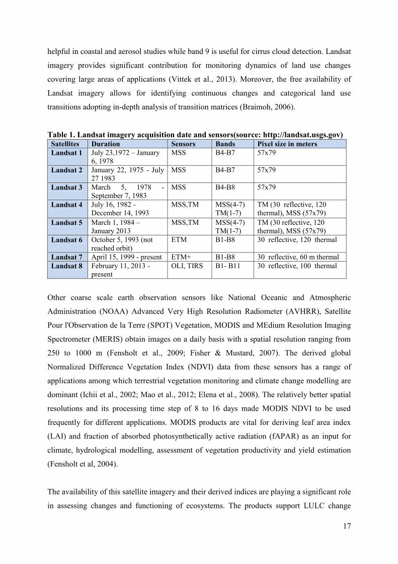
List of tables Table 1. Landsat imagery acquisition date and sensors(source: http://landsat.usgs.gov) ................... 17

Table 2. Data used for land use/land cover change analysis. ............................................................... 27

Table 3. Land cover classification scheme. ............................................................................................ 33

Table 4. Land use/land cover transition matrices (%) (a) 1972 to 1984 (b) 1984 to 2000 (c) 2000 to

2010 and (d) 1972 to 2010. ................................................................................................................... 52

Table 5 .LULC change within the landscape in 1972 and 2010 (%). ...................................................... 54

Table 6.LULC change per class and annual rate of change (%). ........................................................... 55

Table 7. Gain to persistence (gp), loss to persistence (lp) and net change to persistence (np) ratios of

land covers in the period 1972 and 2010. ............................................................................................. 55

Table 8 - Classification of 2010 LULC categories of Kaftahumera overlaying the digital elevation model

(DEM) acquired by the Shuttle Radar Topography Mission (SRTM). .................................................... 59

Table 9 - Perceptions of local people about the causes of the land use/cover change (%).................... 60

Table 10. Confusion matrix for 2014 classification. ............................................................................. 65

Table 11. LULC changes in the period 1986-2014 (%). .......................................................................... 67

Table 12. LULC ratios for the period 1986-2014. .................................................................................. 68

Table 13. Percentage of landscape transition in terms of gains: observed (in bold), expected under

random process of gain (in italics), difference between observed and expected (in normal font) ...... 70

Table 14. Percentage of landscape transition in terms of losses: observed (in bold), expected under

random process of loss (in italics), difference between observed and expected (in normal font) ...... 71

Table 15.MK test statistics of Kaftahumera for the four seasons (1=DJF; 2=MAM; 3=JJA; 4=SON). .... 84

Table 16. Results of Mann-Kendall and Sen’s slope of mean annual precipitation of Kaftahumera .... 90

Table 17. Results of Mann-Kendall and Sen’s slope of Tmax (°C) and Tmin (°C) in Kaftahumera ............. 91

vi

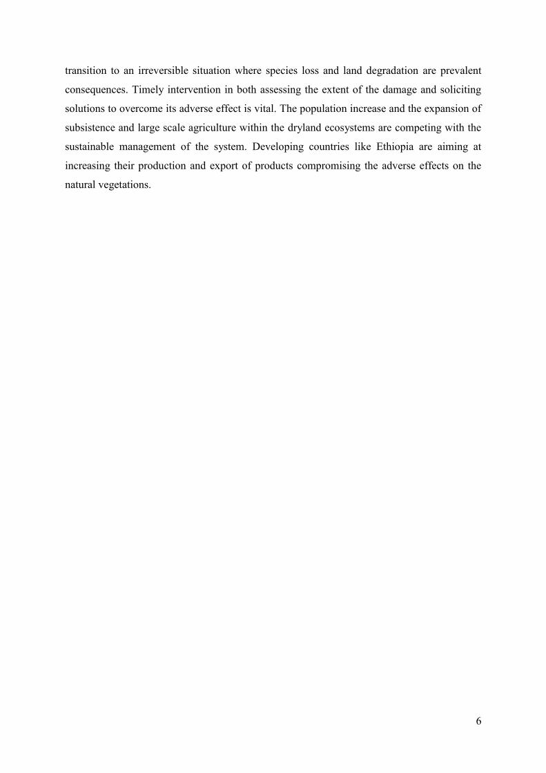
List of figures Figure 1. Conceptual model demonstrating the feedback loop of Land Use/Cover Changes, its

consequences and the underlying and proximate causes (after Reid et al. 2006). ................................ 7

Figure 2. Dust movement towards Ethiopia and Eritrea (Source: URL 3). ............................................ 10

Figure 3. MODIS satellite image showing dust covered areas between Ethiopia, Sudan and South

Sudan (source: URL 4) ........................................................................................................................... 11

Figure 4. Location of the study area. The background image is Landsat 8 false colour composite(753)

with vegetation shows up in shades of green. ...................................................................................... 24

Figure 5. Soil maps of Kaftahumera. ..................................................................................................... 25

Figure 6. Climate graph of Kaftahumera, Ethiopia (Source:National Meteorology Agency of Ethiopia,

2010). ..................................................................................................................................................... 26

Figure 7. Original time-series of NDVI (solid line) and of smoothed time-series NDVI (dotted line) for a

sample pixel of MODIS NDVI of the study area. .................................................................................... 30

Figure 8. DEM classification of Kafthumera. ......................................................................................... 31

Figure 9. Classification using support vectors and separating hyper-plane (after Foody and Mathur,

2004). The two circle types indicate two classes in feature space. ...................................................... 36

Figure 10. Flow chart of the research including the whole methodological approaches. .................... 38

Figure 11. BFAST decomposition of MODIS NDVI time series over 2000-2014 for a single pixel

converted from woodland to cropland ................................................................................................. 44

Figure 12. Mean NDVI and NDVI anomaly for a sample pixel .............................................................. 47

Figure 13. Land use and land cover (LULC) classification of Kaftahumera. ........................................... 50

Figure 14. Percentage of change areas per LULC in the period 1972-2010. ........................................ 53

Figure 15 - Spatial distribution of LULC change from 1972 to 2010 (WL: Woodland, CL: Cropland, GL:

Grassland). ............................................................................................................................................. 56

Figure 16. Land use distribution along an elevation gradient. ............................................................. 57

Figure 17. Population size of Kaftahumera (Source: CSA, 2014) ........................................................... 60

Figure 18. Flow chart of methodological approached used for imagery interpretation ...................... 64

Figure 19. Land use /land cover categories distribution for 1986 and 2014. ....................................... 66

Figure 201. Land use shifts in the period 1986 – 2014 (WL=Woodland; CL=Cropland; GL=Grassland).

68

Figure 21. Spatial regression of NDVI and rainfall over Kaftahumera for the period 2000-2014, the

values indicate pixelwise R2 of NDVI vs rainfall. .................................................................................... 73

Figure 22. Slope of the annual sum of NDVI over Kaftahumera over the period 2000 – 2014 with a

confidence level of 95% (p < 0.05). ....................................................................................................... 74

Figure 23. Linear correlation coefficient of the annual sum of NDVI over the period of 2000-2014 with

a confidence level of 95%. ..................................................................................................................... 75

Figure 24. Linear correlation coefficient of rainfall over the period (2000-2014) with a confidence

level of 95% (p < 0.05). .......................................................................................................................... 76

Figure 25.Fitted St (seasonal), Tt (trend) and et (remainder) components of MODIS NDVI time series

for selected four pixels. ......................................................................................................................... 81

Figure 26.Fitted st (seasonal), Tt (trend) and et (remainder) components of TAMSAT rainfall time

series for selected four sample plots. ................................................................................................... 83

Figure 27. 2Tmax time series for the period 2000-2013 and components resulting from BFAST for four

sample plots of Kaftahumera. There is an overall positive trend with 2 breaks (early 2007 and early

2011), and an abrupt decrease in temperature at the largest magnitude break. ................................ 85

file:///E:/Worku%20papers/Chapters/PhD%20final/Climate,%20land%20use%20and%20vegetation%20trends%20%20Implication%20of%20%20%20land%20use%20change%20and%20climate%20change%20on%20northwestern%20drylands%20of%20%20%20Ethiopia_25%20Nov.docx%23_Toc442650864

vii

Figure 28. Tmin time series for the period 2000-2013 and components resulting from BFAST for four

sample plots of Kaftahumera. There is an overall positive trend without significant breaks. ............. 86

Figure 293.Time of breakpoints and magnitude of most significant change detected in the trend

component.Vt is the deseasonalized NDVI data Yt–St for the period 2000 - 2014. ............................... 88

Figure 30. LOWESS regression line for the annual standardized precipitation of Kaftahumera. ......... 89

Figure 314.Annual rainfall of Kafthumera for the period 1983- 2014. The blue line indicates a 5 year

moving average, the red line is a mean annual trend, and the black line is an annual rainfall. ........... 90

Figure 32.Mean maximum annual temperature of Kaftahumera for the period 1983 - 2013. The black

line depicts mean maximum temperature, the blue line is a 5 year moving average, the red line is a

trend line. .............................................................................................................................................. 91

Figure 33. Standardized mean maximum temperature trend of Kaftahumera. The red line is the

LOWESS regression for the period 1983 - 2013. ................................................................................... 92

Figure 34.Minimum temperature of Kaftahumera for the period 1983-2013. The black line is mean

minimum temperature,the blue line is 5 year moving average, the red line is Lowess trend line. ..... 93

Figure 35. Standardized minimum temperature over Kaftahumera for the period 1983-2013. Red line

indicates the LOWESS regression line over the study period. .............................................................. 94

Figure 36. Mean spatial annual NDVI of Kaftahumera ......................................................................... 98

Figure 37. Long term dekadal and mean dekadal of eMODIS and rainfall of Kaftahumera for the

period of 2000-2014. ............................................................................................................................. 99

Figure 38. Mean annual rainfall (mm) and potential evapotranispiration(mm)of Kaftahumera ....... 100

Figure 39. Potential evapotranspiration (PET) (mm/year) annual PET(black line);five year moving

average(blue line) and annual trend(red line) .................................................................................... 100

Figure 40. Lag distribution of precipitation impact on NDVI. The plot of lag distribution demonstrates the change of R2 with lag time. ........................................................................................................... 101

Figure 41. Scatter plots of NDVI and rainfall for different time lags. ................................................ 102

Figure 42. Spatial regression (R2) between rainfall and NDVI over Kaftahumera. ............................ 103

Figure 43. Spatial lag regression (R2) between NDVI and rainfall up to time lag of 4 decades. .......... 105

Figure 44. LULC size across the study period (%) ................................................................................ 109

Figure 45. Time of breakpoints (BP) in a long term NDVI trend in the period 2000 - 2014 for a single

pixel of Woodland. Vt is the deseasonalized data Yt – St for each iteration of NDVI time series data. Yt

is the original data for the period 2000-2014 and St is the seasonal component. ............................. 114

Figure 46. Slope () and significance ( < 0.05) of NDVI breakpoints for the period 2000 - 2014. .... 115

Figure 47. Trend shifts within the rainfall time series of Kaftahumera. A season-trend model (red line)

was fitted to the rainfall time series (gray). ........................................................................................ 116

viii

Acronyms and abbreviations

AVHRR Advanced Very High Resolution Radiometer

BFAST Breaks For Additive Seasonal and Trend

CO2 Carbon dioxide

CRU Climatic Research Unit

CSA Central Statistics Agency

DEM Digital Elevation Model

DN Digital Numbers

EARO Ethiopian Agricultural Research Organization

EMA Ethiopian Mapping Agency eMODIS EROS Moderate Resolution Imaging Spectroradiometer EROS Earth Resource Observation

ETM+ Enhanced Thematic Mapper plus

GCP Ground Control Points

GPS Global Positioning System

IPCC Intergovernmental Panel on Climate Change

LIBSVM Library for Support Vector Machines

LULC Land Use Land Cover

MERIS:....MEdium Resolution Imaging Spectrometer

MoA…….Ministry of Agriculture

MODIS Moderate Resolution Imaging Spectroradiometer

MOD09….MODIS Terra Surface Reflectance

MYD09….MODIS Aqua Surface Reflectance

MSS Multispectral Scanner

NASA National Aeronautics and Space Administration

NDVI Normalized Difference Vegetation Index

ix

NIR Near Infrared

NMA....…. National Meteorology Agency of Ethiopia

NOAA National Oceanic and Atmospheric Administration

OLI Operational Land Imager

PET Potential evapotranspiration

R² Coefficient of determination

RMSE Residual Mean Square Error

SPOT…….Satellite Pour l'Observation de la Terre

SRTM Shuttle Radar Topography Mission

SVM Support Vector Machines

TAMSAT Tropical Applications of Meteorology using Satellite data

TIR Thermal Infrared

TIRS Thermal Infrared Sensor

TM Thematic Mapper

UNCCD United Nations Convention to Combat Desertification

URL………:Uniform Resource Locator

USGS United States Geological Survey

UTM Universal Transverse Mercator projection

VI Vegetation Index

VNIR Visible and Near-Infrared

WBISPP….Woody Biomass Inventory and Strategic Planning Project

x

Acknowledgment I would like to express my special appreciation and thanks to my advisor Prof. Dr. habil.

Elmar Csaplovics, you have been a fabulous mentor for me. I would like to thank you for your

encouragement and for allowing me to grow as a research scientist. Your guidance on both

my research as well as on my career have been invaluable. I appreciate your sincerity in all

issues and your willingness to support when I come across difficulties in my work or family

cases.

I would also like to thank Prof. Dr. habil. Dominik Faust for being head of the exam

commission. I also want to thank Prof. Dr. habil Michael Köhl (Universität Hamburg) and

Prof. Dr. habil Marcus Nüsser (Heidelberg University) for spending their valuable time to

review my dissertation.

I have got data for my research from different organization including United States

Geological Survey (USGS), NASA's Earth Observing System, University of Reading and

Climatic Research Unit (CRU) of the University of East Anglia. I obtained financial support

for participating in scientific meeting and conferences from GFF (Gesellschaft von Freunden

und Förderern der TU Dresden). I also got a financial assistance from the Graduate Academy

(GA) of the Technical University of Dresden to finalize my study. I want to thank all the

organizations for their generous support towards my study.

I would also like to thank my colleagues Mr. Busha Teshome and Mr.Tatek Dejene who

assisted me during field data collection. My special thanks also to PhD colleagues at the chair

of Remote Sensing with whom I shared workplaces and also discuss technical issues related

to my work activities

A special thanks to my family. Words cannot express how thankful I am to my mother

Woyzero Agazu, my brother Teshome Zewdie, and my sister Felekech Zewdie for all of the

sacrifices that you have made in my life. My mother, you are special in my life, you have not

gone to school, but you know the importance of education. You sent me to school while most

of the children at my stage stay at home. Your continued prayer for me was also what

sustained me so far. I would also like to thank the Ethiopian communities in Dresden with

whom I enjoyed my stay in Dresden. My appreciation goes to all of you for your

encouragement and support during my stay in Dresden. Special thanks to Ms. Marie-Luise

xi

who helped me to translate the abstract of this dissertation into German. Last but not least, I

would like to express my appreciation to my beloved wife Helen Yimer who spent sleepless

nights encouraging me during the ups and downs of the PhD work. You was always my

energy in the moments when there was no one to answer my queries. You have also carried

the entire burden in caring for our children. My lovely children Sosena and Yohannes, you

deserve the highest appreciation. As a father, I have not given you much time while I am

working late in the evening and the weekends too. However, you always be my drive to push

the work forward. Above all I thank God the Almighty, who gave me the strength and power

to accomplish my dream working for my PhD dissertation.

xii

Abstract

Land use / land cover (LULC) change assessment is getting more consideration by global

environmental change studies as land use change is exposing dryland environments for

transitions and higher rates of resource depletion. The semiarid regions of northwestern

Ethiopia are not different as land use transition is the major problem of the region. However,

there is no satisfactory study to quantify the change process of the region up to now. Hence,

spatiotemporal change analysis is vital for understanding and identification of major threats

and solicit solutions for sustainable management of the ecosystem. LULC change studies

focus on understanding the patterns, processes and dynamics of land use transitions and

driving forces of change. The change processes in dryland ecosystems can be either seasonal,

gradual or abrupt changes of random or systematic change processes that result in a pattern or

permanent transition in land use. Identification of these processes of change and their type

supports adoption of monitoring options and indicate possible measures to be taken to

safeguard this dynamic ecosystem.

This study examines the spatiotemporal patterns of LULC change, temporal trends in climate

variables and the insights of the communities on change patterns of ecosystems. Landsat

imagery, MODIS NDVI, CRU temperature, TAMSAT rainfall and socio-ecological field data

were used in order to identify change processes. LULC transformation was monitored using

support vector machine (SVM) algorithm. A cross-tabulation matrix assessment was

implemented in order to assess the total change of land use categories based on net change

and swap change. In addition, the pattern of change was identified based on expected gain and

loss under a random process of gain and loss, respectively. Breaks For Additive Seasonal and

Trend (BFAST) analysis was employed for determining the time, direction and magnitude of

seasonal, abrupt and trend changes within the time series datasets. In addition, Man Kendall

test statistic and Sen’s slope estimator were used for assessing long term trends on detrended

time series data components. Distributed lag (DL) model was also adopted in order to

determine the time lag response of vegetation to the current and past rainfall distribution.

Over the study period of 1972- 2014, there is a significant change in LULC as evidenced by a

significant increase in size of cropland of about 53% and a net loss of over 61% of woodland

area. The period 2000-2014 has shown a sharp increase of cropland and a sharp decline of

woodland areas. Proximate causes include agricultural expansion and excessive wood

harvesting; and underlying causes of demographic factor, economic factors and policy

xiii

contributed the most to an overuse of existing natural resources. In both the observed and

expected proportion of random process of change and of systematic changes, woodland has

shown the highest loss compared to other land use types. The observed transition and

expected transition under random process of gain of woodland to cropland is 1.7%, implies

that cropland systematically gains to replace woodland. The comparison of the difference

between observed and expected loss under random process of loss also showed that when

woodland loses cropland systematically replaces it. The assessment of magnitude and time of

breakpoints on climate data and NDVI showed different results. Accordingly, NDVI analysis

demonstrated the existence of breakpoints that are statistically significant on the seasonal and

long term trends. There is a positive trend, but no breakpoints on the long term precipitation

data during the study period. The maximum temperature also showed a positive trend with

two breakpoints which are not statistically significant. On the other hand, there is no seasonal

and trend breakpoints in minimum temperature, though there is an overall positive trend along

the study period.

The Man-Kendall test statistic for long term average Tmin and Tmax showed significant

variation where as there is no significant trend within the long term rainfall distribution. The

lag regression between NDVI and precipitation indicated a lag of up to forty days. This

proves that the vegetation growth in this area is not primarily determined by the current

precipitation rather with the previous forty days rainfall. The combined analysis showed

declining vegetation productivity and a loss of vegetation cover that contributed for an easy

movement of dust clouds during the dry period of the year. This affects the land condition of

the region, resulting in long term degradation of the environment.

xiv

KURZFASSUNG

Die Erfassung von Landnutzung- und Landbedeckungsveränderungen (LULC) rückt immer

mehr in den Fokus globaler Umweltveränderungsstudien. Durch die weitreichenden

Landnutzungsänderungen in den Trockengebiete werden große Flächen freigelegtn, was zu

einer Degradation der Ressourcen führt.

Die semi- ariden Gebiete im Nordwesten Äthiopiens sind von diesen Veränderungen der

Landnutzung betroffen. In der Region treten durch diesen Wandel schwerwiegende Probleme

zu tage. Bis dato wurde keine aussagekräftige Studie zu dieser Problematik durchgeführt,

welche die Veränderungsprozesse des Gebietes manifestieren. Folglich ist eine raum-

zeitliche Änderungsanalyse von Notwendigkeit zur Identifikation sowie zum Verständnis der

Probleme. Solch eine Studie bildete die Grundlage zur Entwicklung von nachhaltigen

Lösungen hinsichtlich des Ökosystemmanagements. LULC - Veränderungsstudien

thematisieren die Identifikation von Strukturen, Prozessen und der Dynamik von

Landnutzungsübergängen sowie deren Ursachen. Die Änderungsprozesse in den

Trockengebieten laufen entweder saisonal, sukzessiv oder abrupt ab. Diese scheinbar zufällig

oder systematisch ablaufenden Prozesse resultieren in einem gewissen Muster oder führen zu

permanenten Wandel der Bodennutzung. Die Identifikation und Typisierung dieser

Wandlungsprozesse unterstützen die Anpassung von Monitoringmaßnahmen und bieten

optionale Gegenmaßnahmen zum Schutz und Erhalt der Dynamik in diesem Ökosystem.

Diese Studie untersucht die raum- zeitlichen Strukturen der LULC Veränderung, die

zeitlichen Trends der Klimavariablen sowie die Erkenntnisse der lokalen Gemeinden

bezüglich des Wandels des Ökosystems. Landsat Bilder, MODIS NDVI, CRU

Temperaturdaten, TAMSAT Niederschlagsdaten und sozio-ökologische Felddaten wurden

analysiert, um die Veränderungsprozesse zu identifizieren. Die LULC-Änderungen wurde

mittels eine Support-Vektor- Maschine (SVM) Algorithmus detektiert. Aus der

Veränderungsmatrix konnte die gesamte Änderung der Landnutzungskategorien abgeleitet

werden, basierend auf der Nettoänderung und dem Nutzungswechsel. Zusätzlich wurde die

Änderung aus erwartetem Gewinn und Verlust unter einbezug das zufälligen Gewinn/Verlust

kalkuliert.

Zeitpunkt, Richtung und Magnitude der saisonalen, sukzessiven sowie der abrupten

Änderungen innerhalb der Zeitreihe wurden mittels der Breaks For Additive Seasonal and

xv

Trend (BFAST) Analyse determiniert. Weiterführend wurde der Mann-Kendall Statistiktest

und der Theil-Sen Schätzer genutzt, zur Beurteilung der langfristigen Trends auf den

trendbereinigten Zeitreihendatensätzen. Das Distributed Lag (DL) Modell wurde angewendet,

um die zeitversetzten Reaktionen der lokalen Vegetation auf die aktuelle sowie die bisherige

Niederschlagsverteilung zu bestimmen. Während des Untersuchungszeitraumes von 1972 bis

2014 sind signifikante Änderungen in der LULC zu verzeichnen. Evident durch einen

bedeutende Flächenzunahme der Anbaufläche von etwa 53% sowie ein Nettoverlust der

Waldfläche von mehr als 61%. Im Beobachtungszeitraum 2000 bis 2014 wird eine starke

Flächenzunahme der Agraranbaufläche sowie zeitgleich eine starke Abnahme der Waldfläche.

Die unmittelbaren Ursachen hierfür sind landwirtschaftliche Expansion und übermäßige

Abholzung, mittelbare Urschen sind demographische, politische und ökonomische

Gegebenheiten. Die Wechselwirkung jener Elemente führten zu einer extensiven

Übernutzung der natürlich vorhandenen Ressourcen.

Sowohl beider Auswertung der beobachteten als der zu erwarteten Entwicklungsanalyse,

unter Berücksichtigung der systematischen sowie der vermeintlich zufällig stattfindenden

Veränderungsprozesse, verzeichnet der Wald die höchsten Verluste verglichen zu den

weiteren Landnutzungsformen. Die Berechnung des Zufallsprozesses der Zunahme von Wald

in Ackerfläche beträgt 1.7%. Dies impliziert, dass die Waldfläche sukzessiv durch Ackerland

ersetzt wird. Weiterführend verdeutlicht wird diese Annahme im direkten Vergleich der

Differenz von beobachtenn Verlust zu erwartetenn Verlust. Die Auswertung der Magnituden

und Zeitpunkte von Regressionen in den jeweiligen Klimadaten und des NDVI weisen

verschiedene Ergebnisse auf. Dementsprechend weist die NDVI Analyse Regressionen auf,

welche statistisch signifikant auf die saisonalen und langfristigen Trends sind. Die

langfristigen Niederschlagsdaten weisen einen positiven Trend während des

Untersuchungszeitraumes auf, aber keine Regressionen. Ebenso weist die Höchsttemperatur

einen positiven Trend auf mit zwei reduzierenden Schwankungen, diese jedoch sind

statistisch nicht signifikant. Die Minimaltemperatur hingegen verzeichnet weder saisonale

noch sukzessive Anomalien, gleichwohl einen insgesamt positiven Trend während des

Untersuchungszeitraumes. Der Man-Kendall Statistiktest determiniert im langfristigen

Durchschnitt der Tmin und Tmax eine signifikante Veränderung, in den langfristigen

Niederschlagsverteilungen hingegen wurde kein bedeutender Trend manifestiert. Die

Regressionsverzögerung zwischen dem NDVI und dem Niederschlag zeigen einen Zeitversatz

von bis zu 40 Tagen auf. Dies lässt die Schlussfolgerung zu, dass die lokale Vegetation im

Wachstum primär von den vergangenen Niederschlagsereignissen beeinflusst wird, als von

xvi

den aktuellen. Fusionierte Analysen zeigten den Zusammenhang von sinkender

Pflanzenproduktivität und dem Rückgang der Vegetationsdecke. Durch die Abnahme der

geschlossenen Vegetationsdecke häufen sich die Staubwolken während der Trockenperiode

des Jahres. Resultierend in der langfristigen Degradation des Bodens in der Region sowie in

einer Schädigung der Umwelt.

1

1. Chapter 1. Background

1.1 Introduction 1.1.1 Dryland degradation in Africa

Drylands cover an estimated area of up to 40 % of the earth's land mass and support the

livelihood of nearly 2 billion inhabitants (J. Davies & J. Skinner, 2009; Safriel et al., 2005).

They sustain one third of the Global Conservation Hotspot areas and are habitat for 28 % of

endangered species (URL 1). Dependencies of population on dryland ecosystems resulted in

excessive human pressures affecting vegetation cover of the region (Vitousek et al., 1997).

Ten to twenty percent of these areas are suffering from land degradation and about one to six

percent of the inhabitants live in degraded areas with most of those being exposed to further

desertification (Millennium Ecosystem Assessment, 2005) which can destitute the subsistence

well-being of the dryland community.

According to the United Nations Convention to Combat Desertification (UNCCD, 1994) land

degradation signifies the reduction or loss of the biological or economic productivity of the

drylands and desertification is land degradation in arid, semiarid and dry subhumid areas

resulting from various factors, mainly consisting of climatic variations and human activities.

The expansion of degradation which devours the biomass and soil of a particular area,

contributes to the global climate change through releasing green house gases, mainly CO2

emission and inducing soil erosion. The recurrent droughts and the resulting environmental

degradation are forcing the dryland inhabitants to immigration, conflicts on resources arise

and further occupation of new areas which in turn exposes new environments to degradation

(Appelgren, 2008). These effects have been further paving the way for exposure and

worsening the condition of dryland environments and their inhabitants coupled with climate

change and aridification. The degree of the variation in climate variables varies among the

different dryland regions of the world though all of them are being affected due to either

increasing, declining or unpredicted changes of the amount and distribution of rainfall and

increasing mean temperature compared to historical trends (Kotir, 2010; Sarr, 2012;.

Sivakumar et al., 2005). The variability in the distribution and amount of rainfall affects

vegetation productivity and agricultural adaptation of the region which influences the

livelihood of the people and their dynamic ecosystem (Sarr, 2012).

2

The expansion of land degradation not only created an imbalance between the demand of

inhabitants and the services provided by ecosystems (Millennium Ecosystem Assessment,

2005), but can also be a major anthropogenic contributor for the emission of global CO2 due

to the loss of natural vegetation and soils. Even if there is a difference in scenarios in the

amount of carbon content in different vegetation types, there is an estimated amount of about

271 ± 16 Pg of carbon in tropical forests and woodlands with soil organic matter contributing

the most (Grace et al., 2014). Each year, roughly about 2 % of the global terrestrial net

primary production (NPP) is lost due to dryland degradation (Zika & Erb, 2009).Tropical

deforestation, as one of the key components of the global carbon budget, also accounts for

about 20 % of the anthropogenic carbon emission (IPCC, 2007). The loss of dryland

vegetation, mainly due to deforestation is becoming a concern of environmental safety. The

trend in shift of vegetation cover is continuing as a major threat to the dynamic dryland

ecosystems.

The drylands of Africa encompass 43 percent of the continent, and have a population of some

325 million people (UNCCD, 2009). Dryland degradation in Africa is contributing to the

continual decline in the ability of dryland ecosystems to supply a range of ecosystem services

for the livelihood of the people (Scholes, 2009). The decrease in productivity of the land

coupled with regional climate variability is aggravating in several parts of Africa especially

where population growth and improper utilization of the natural resources are significant

(Maitima et al., 2009). Though some studies show recovery of vegetation cover in some parts

of the Sahel due to changes in rainfall distribution and positive contribution of humans

towards maintaining their natural vegetation (Anyamba & Tucker, 2005; Dardel et al., 2014;

Herrmann et al., 2005; Hickler et al., 2005; Olsson et al., 2005), other parts of Africa are still

under sever exposure to degradation. Studies at the landscape level in some parts of the Sahel

re-greening showed fluctuations with both increasing and decreasing trends depending on the

amount and distribution of rainfall through the years (Ouedraogo et al., 2014). The change in

land use in some parts of East Africa has also transformed the natural vegetation towards

human-dominated land use systems, resulting in deforestation, biodiversity loss and land

degradation (Lemenih et al., 2014; Maitima et al., 2009). The global assessment of human

induced land degradation indicates about 16 % of Africa has been degraded in the period

1981- 2003 with soil erosion being the main factor contributing to land degradation and the

regions south of the equator mostly affected within this period (Bai et al., 2008). Different

studies at the local level assessing land use change and land degradation also confirmed a

3

significant amount of decline in the functioning of the ecosystem and more attention for

protection and reclamation of the degraded environments is needed (Bakr et al., 2010; Biazin

& Sterk, 2013; Kindu et al., 2013; Mekasha et al., 2014; REGLAP, 2012; Zewdie &

Csaplovics, 2014). The changes observed in these regions are mainly accounted to a shift

from natural ecosystems to human-dominated landscapes.

The anthropogenic endeavors on these regions have exposed tropical dry forests to

degradation, deforestation and loss of soils. Land use / land cover (LULC) change assessment

of drylands is getting more consideration by studies of global environmental change as land

use transformation is inducing high rates of resource depletion (Lambin et al., 2003). LULC

studies focused on understanding the patterns, processes and dynamics of land transitions and

its drivers over time (Bajocco et al., 2012; Braimoh, 2006; Carmona & Nahuelhual, 2012;

Guida Johnson & Zuleta, 2013; Manandhar et al., 2010). The processes of these land use

transitions can be categorized into either random or systematic changes based on identifying

their pattern of categorical changes (Braimoh, 2006; Pontius, Shusas, & McEachern, 2004). A

random process of change occurs when a LULC category loses to or gains from other

categories by abrupt changes while systematic transitions are driven by the regular processes

of transition characterized by a constant or gradual gradient of change (Braimoh, 2006; Guida

Johnson & Zuleta, 2013). The transformation in land uses together with climate variability is

enforcing changes in landscapes that can deprive the vegetation covers of dryland ecosystems.

1.1.2 Dryland degradation in Ethiopia The loss in dryland vegetation of Africa has been significantly increased, resulting in land

degradation that became a source of dust emissions and loading (Yoshioka et al., 2007). The

situation in Ethiopia is not different as forests are cleared and exposed to severe landscape

changes (Garedew et al., 2012; Lemenih et al., 2014; Zewdie & Csaplovics, 2014). Ethiopia is

known for its varied agro-ecology among which drylands cover an estimated area of over

65% of the land mass with a population of about 12 - 15 million of mainly pastoral and agro-

pastoral communities who depend on livestock raising (Lemenih & Kassa, 2011; REGLAP,

2012). The drylands of Ethiopia, despite their richness in biodiversity, are shrinking in size

due to the pressure of subsistence and large scale agricultural expansion, population growth

and unwise utilization of the natural vegetation (Eshete et al., 2011; Lemenih et al., 2014).

Global assessment of land degradation indicated that more than 26 % of the country has

4

already been degraded and that the livelihood of about 30% of the population in the period

1981 – 2003 has been affected(Bai et al., 2008). Several studies demonstrated the exposure of

drylands to anthropogenic activities mainly due to the involvements of subsistence and large

scale farming and overharvesting of woods (Dejene, Lemenih, & Bongers, 2013; Garedew et

al., 2012; Mekasha et al., 2014; Zewdie & Csaplovics, 2015). As loss in dryland vegetation is

prevalent in arid and semi-arid regions, it could be a significant contributor for the

degradation of drylands of the country. The fundamental causes of land degradation emanated

from poverty, expansion of resettlement, limited opportunities for alternative livelihoods,

inadequate policy support, improper investment and inadequacy of law enforcement (Lemenih

et al., 2014; Zewdie & Csaplovics, 2015).

Most of the drylands of the country are dominated by scattered vegetation types of Acacia

woodlands, bush lands, wooded savannah and scrublands (WBISPP , 2005). Dryland areas are

very sensitive to climate change and the existence of woodlands play a vital role in combating

expansion of aridity (Gimona et al., 2012). The understanding of drylands degradation

processes, incorporating the main driving forces and their effects on ecosystem performance,

are crucial to adopt strategies in order to mitigate and avoid land degradation. The

northwestern woodlands of Ethiopia, which are acting as a buffer zone in sheltering the

southward encroachment of Sudano-Sahelien deserts, require strategies to assess and monitor

the severity of deforestation and degradation processes in order to create awareness among all

responsible stakeholders for sustainable management of the natural resources. In spite of their

immense socioeconomic contribution, these woodlands are still experiencing deforestation

and degradation mainly attributed to anthropogenic activities (Lemenih et al., 2014; Zewdie &

Csaplovics, 2014). It is known that development priorities have focused on how much

humanity can take from ecosystems, and too little attention has been given for assessing the

impacts of human activities and reduction of the pressure exerted on the ecosystems of

drylands (White et al., 2000).

Northwestern Ethiopia became the focus for the governmental initiatives to expand

mechanized agriculture and resettlements. Mechanized farming is attracting annually over

200,000 casual workers from various regions of the country and neighbouring Sudan (URL

2), which in one or other way directly compete with the existing natural vegetation of the

region. The degradation of this ecosystem could be a threat to the current agricultural

investments and it could be an environmental challenge to assure the well-being of the

5

community. The impact on this fragile ecosystem needs continuous monitoring in order to get

long lasting, sustainable production of all the ecosystem services and also to maintain the

livelihood of the local community.

In order to sustainably address the current exposure of the dryland ecosystems of

northwestern Ethiopia, it requires spatiotemporal information that can address their previous

and current status. The assessment and organisation of information on the status and dynamics

of change in the environment allow for a thorough analysis of occurring spatiotemporal

changes through the monitoring period. The analysis of land use changes facilitates the

documentation of varying ecosystem responses due to existing disturbances and the degree of

their significant contribution to the changes (DeFries et al., 2004). The processes of change

are governed by proximity causes which are dependent on the underlying drivers of changes

like fundamental social and biophysical processes (Fig.1). The proximate causes of land use

transition depict how and why local land cover and ecosystem processes are modified directly

by humans, while underlying causes describe the broader context and primary forces

supporting these local actions. The change in ecosystem services of the woodlands that results

from LULC changes is significantly modifying the underlying drivers and proximate causes

resulting in a feedback loop. According to Reid et al (2006) policy plays a vital role in

avoiding positive feedback mechanisms which can accelerate unsustainable land use. Local

policy has the higher potential to impact the proximate causes of change when there exists a

simultaneous action on the underlying causes of change to have a sustainable land use

management (Reid et al., 2006). Proximate causes mainly function at the local level and

underlying causes originate from regional (districts, provinces, or country) or even global

levels, though complex interplays between these levels of organization are common (Reid et

al., 2006). However , the dryland vegetation of northwestern Ethiopia though having higher

potentials for economic contribution (mainly gum and resin production) and ecosystem

services, has been little supported through the local policies that are adopted from the regional

and federal organizational structures and policies (Lemenih et al., 2014). In the current era of

climate change that could potentially become a threat to modifying ecosystems, it is vital to

maintain the integrity of policies that should avoid damages on ecosystems. It is commonly

known that climate change, land degradation, and biodiversity are interrelated, and the

imbalance change trajectory could potentially affect maintaining and restoring healthy

ecosystems for adaptation and mitigation of climate change. The influx of human activities

into this exposed dryland ecosystem exacerbates their exposure for further modification and

6

transition to an irreversible situation where species loss and land degradation are prevalent

consequences. Timely intervention in both assessing the extent of the damage and soliciting

solutions to overcome its adverse effect is vital. The population increase and the expansion of

subsistence and large scale agriculture within the dryland ecosystems are competing with the

sustainable management of the system. Developing countries like Ethiopia are aiming at

increasing their production and export of products compromising the adverse effects on the

natural vegetations.

8

1.1.3 Dryland forest change and resettlement in Ethiopia

According to WBISPP(2005) the dry forest of Ethiopia covers about 26% of the country.

There is a significant amount of spatiotemporal loss of these forests due to deforestation and

degradation in different dryland areas of the country. However, no official organized data

available for quantification of the exact size of loss of the dry forests of the country. There are

few case studies documenting the existence of loss of dry forests due to various driving

factors, mainly from anthropogenic factors that includes cropland expansion, overharvesting

of woods, overgrazing and fire (Biazin & Sterk, 2013; Eshete et al., 2011; Garedew et al.,

2012; Lemenih et al., 2007; Lemenih et al., 2014; Tolera et al., 2013; Zewdie & Csaplovics,

2014). The total forest (both the high forest and woodland) loss of the country is estimated to

reach an annual rate of over 2% (WBISPP, 2005). However, this figure may differ

significantly through years as there is a prevalent variation of population growth and cropland

expansion in most forest areas of the country. Nevertheless, there is no update on the

assessment of forest loss considering the economic activities and the considerable changes on

population size.

The population size of Ethiopia has more than doubled in the last three decades from 40

million in 1984 to over 87 million in 2014 (CSA, 2014). This has led to overexploitation of

the natural resources and consequent land degradation of the highlands. The population of the

degraded highlands was resettled to the lowlands which brought a significant threat to the dry

forests due to lack of monitoring mechanisms and of integration of the newly arrivals with

existing residents (Dessalegn & van den Bergh, 1991; Lemenih et al., 2014). Several case

studies showed that the pressure exerted from the increasing population and expansion of

agriculture within the dryland vegetation resulted in landscape changes (Garedew et al., 2012;

Lemenih et al., 2014; Mulugeta Lemenih & Kassa, 2011; Mekasha et al., 2014; Zewdie &

Csaplovics, 2015).

Despite the degradation of the highlands of the country for decades, the efforts made to

reclaim and overcome the loss of soil and vegetation is very minimal. The country has rather

focused on translocations of the people to other areas since the 1970’s, mainly drylands,

which were considered as potentially fertile regions for inhabiting communities from the

degraded highlands (Kloos et al., 1990; Kloos & Aynalem, 1989). The difference in culture,

origin of immigrants and weak formal regulatory systems are among the major contributing

9

factors to facilitate easy access to the woodland vegetation by the newcomers (Kloos &

Aynalem, 1989; Lemenih et al., 2014). Improper human activities have changed major parts

of the dryland ecosystems in order to fulfil the demands of the growing population for crop

production, firewood and construction wood supply (Lemenih et al., 2014). The continuing

change in ecosystems affected the functioning and services provided by the ecosystem to

fulfil the ever increasing demands of the population. The degradation of dry forests has

economic, social, ecological, policy and institutional dimensions that can affect the livelihood

of the society along the years (Cubbage et al., 2007). Among the anthropogenic factors,

deforestation has played the significant role for the decline in size of the woody resources of

the drylands of Ethiopia (Eshete et al., 2011; Lemenih et al., 2014).

The increase in population size has brought pressure on sustainable resource utilization

facilitating land degradation, resource exhaustion and forest loss. The decline in productivity

of some of these highland areas forced the government to identify lowlands as potential

productive regions for expanding resettlement. Among them the northwestern lowlands have

been used as resettlement for populations affected by recurrent droughts and land degradation

since the 1970’s (Rahmato & van den Bergh, 1991). This trend has been continuing with

resettling more households from resource poor areas to the northwestern woodlands and other

lowland areas which are considered as potential for agricultural expansion (Fesseha, 2007).

This is becoming a major threat in competing with the existing woody vegetation as these

areas are identified as centers for establishing new settlements for the incoming populations.

In addition, there is expansion of commercial agriculture within these woodland regions

which also compete with the available dry forests of the region. The demand of sesame on the

world market highly promoted foreign investments and also local farmers for intensively

involving in sesame cultivation (Dejene et.al, 2013; Lemenih et al., 2014; Tadele, 2005). This

has significantly competes with the woodlands as most incomers are farming on more than

their allocated farming sizes (Lemenih et al., 2014). The livestock size has also significantly

increased with the addition of new settlers and labour forces, who permanently establish

themselves once brought from other parts of the country, induce pressure on the remaining

dryforests. Fire is also among the factors that affect the woodlands which comprise Boswellia

papylifera, one of the endangered lowland tree species of the drylands (Lemenih et al., 2007).

The disturbances in the woody vegetation can disrupt the ecosystem and air quality (Opdam

& Wascher, 2004). The intensification of land use as well as the transition in size of land use

has contributed for affecting the functioning of ecosystems (IPCC, 2007). Due to the ever

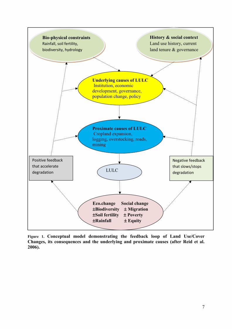
10

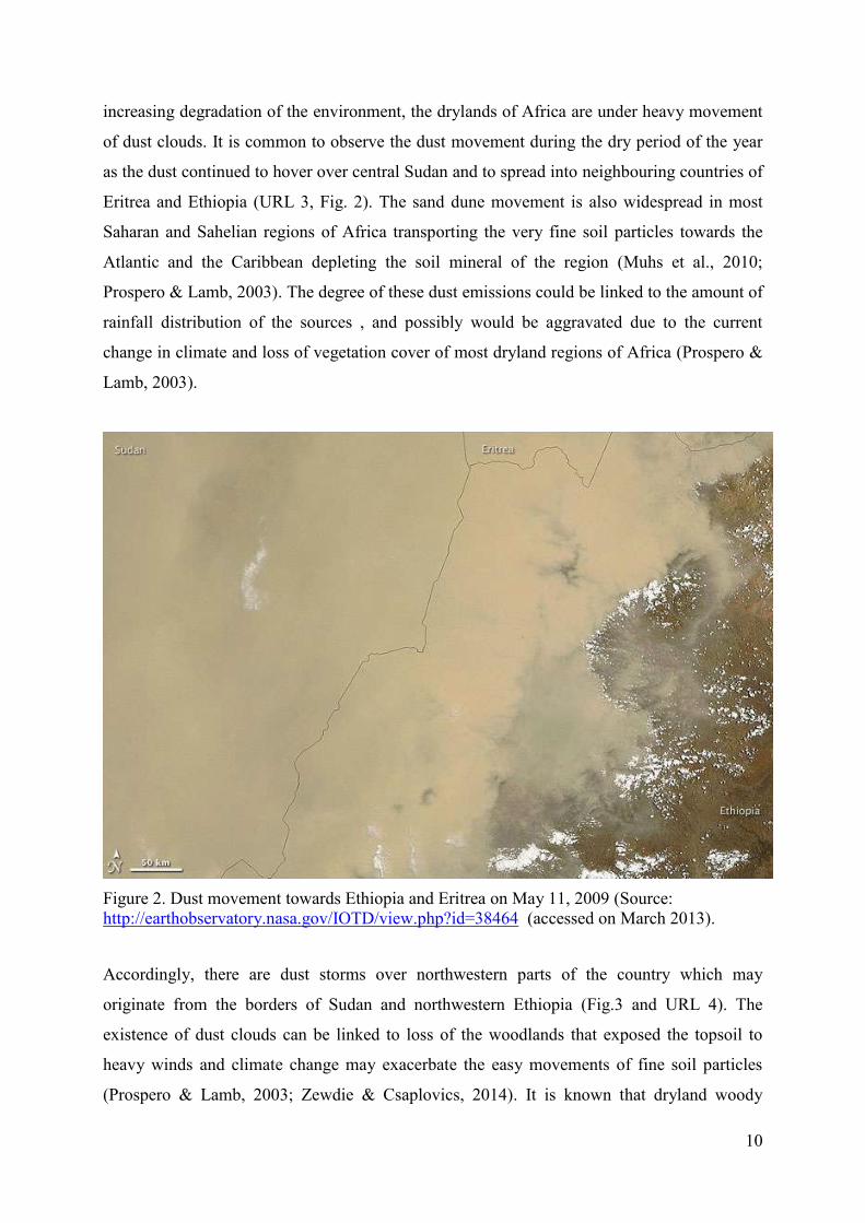
increasing degradation of the environment, the drylands of Africa are under heavy movement

of dust clouds. It is common to observe the dust movement during the dry period of the year

as the dust continued to hover over central Sudan and to spread into neighbouring countries of

Eritrea and Ethiopia (URL 3, Fig. 2). The sand dune movement is also widespread in most

Saharan and Sahelian regions of Africa transporting the very fine soil particles towards the

Atlantic and the Caribbean depleting the soil mineral of the region (Muhs et al., 2010;

Prospero & Lamb, 2003). The degree of these dust emissions could be linked to the amount of

rainfall distribution of the sources , and possibly would be aggravated due to the current

change in climate and loss of vegetation cover of most dryland regions of Africa (Prospero &

Lamb, 2003).

Figure 2. Dust movement towards Ethiopia and Eritrea on May 11, 2009 (Source: http://earthobservatory.nasa.gov/IOTD/view.php?id=38464 (accessed on March 2013).

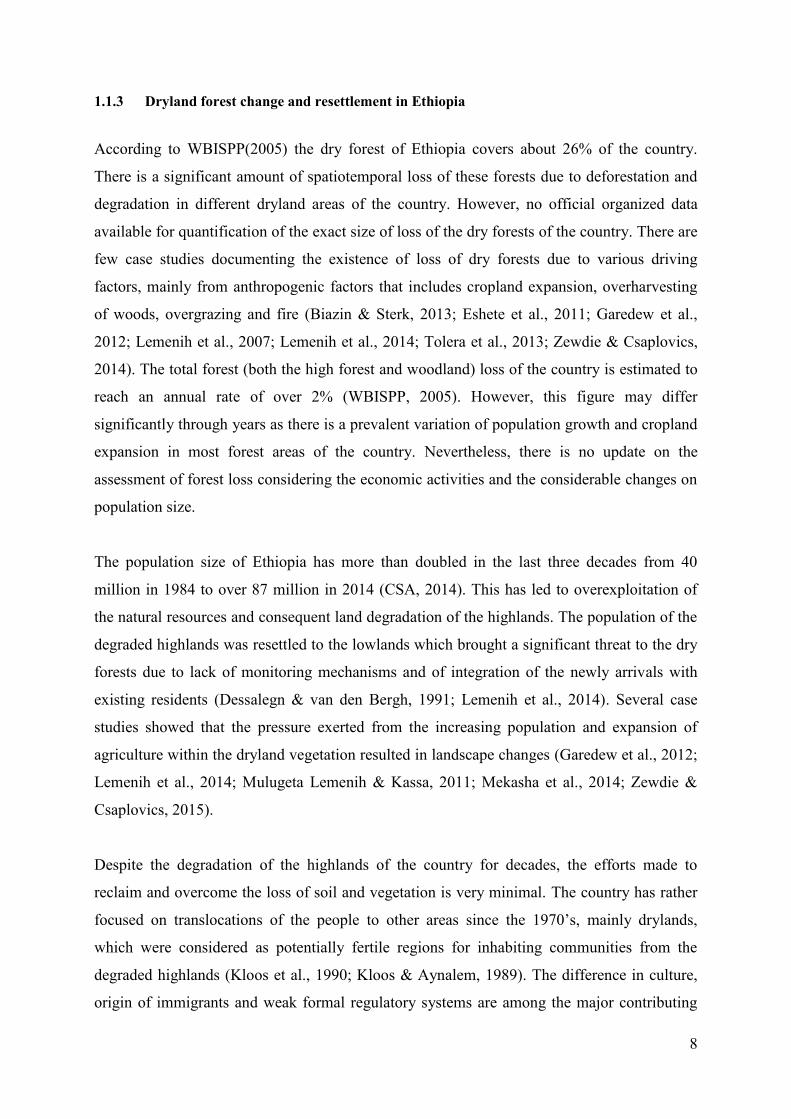
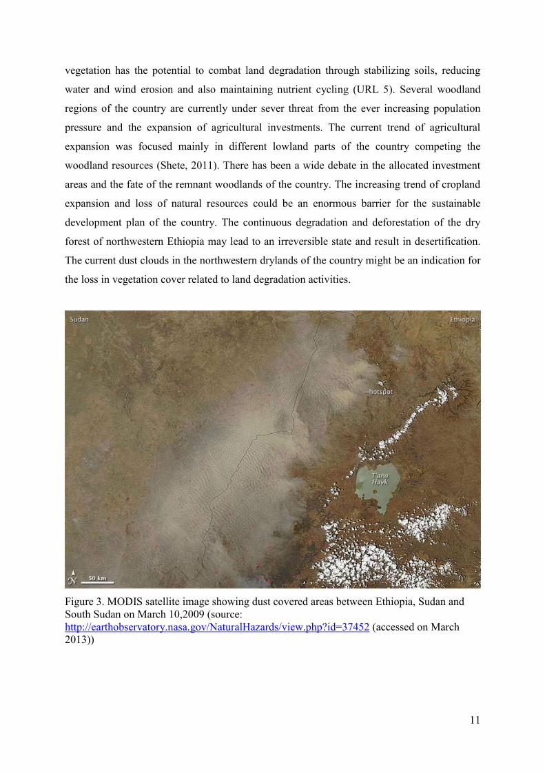
Accordingly, there are dust storms over northwestern parts of the country which may

originate from the borders of Sudan and northwestern Ethiopia (Fig.3 and URL 4). The

existence of dust clouds can be linked to loss of the woodlands that exposed the topsoil to

heavy winds and climate change may exacerbate the easy movements of fine soil particles

(Prospero & Lamb, 2003; Zewdie & Csaplovics, 2014). It is known that dryland woody

http://earthobservatory.nasa.gov/IOTD/view.php?id=38464

11

vegetation has the potential to combat land degradation through stabilizing soils, reducing

water and wind erosion and also maintaining nutrient cycling (URL 5). Several woodland

regions of the country are currently under sever threat from the ever increasing population

pressure and the expansion of agricultural investments. The current trend of agricultural

expansion was focused mainly in different lowland parts of the country competing the

woodland resources (Shete, 2011). There has been a wide debate in the allocated investment

areas and the fate of the remnant woodlands of the country. The increasing trend of cropland

expansion and loss of natural resources could be an enormous barrier for the sustainable

development plan of the country. The continuous degradation and deforestation of the dry

forest of northwestern Ethiopia may lead to an irreversible state and result in desertification.

The current dust clouds in the northwestern drylands of the country might be an indication for

the loss in vegetation cover related to land degradation activities.

Figure 3. MODIS satellite image showing dust covered areas between Ethiopia, Sudan and South Sudan on March 10,2009 (source: http://earthobservatory.nasa.gov/NaturalHazards/view.php?id=37452 (accessed on March 2013))

http://earthobservatory.nasa.gov/NaturalHazards/view.php?id=37452

12

1.2 Problem statement and rationale of the study

The drylands of Ethiopia, despite their richness in biodiversity, are shrinking in size due to

pressures from cropland expansion, fire, expansion of resettlement, over exploitation and

unwise utilization of trees coupled with climate change. As a result, expansion of land

degradation is evident in most parts of the country. The highlands of the country with

elevation ranges of over 1500m are critically degraded for long period of times (Holden &

Shiferaw, 2004) and most of the residents are either resettled in lowland areas to have a better

agricultural plots or living in critical condition to sustain their livelihood. Nevertheless, there

is no sign of minimizing the ever increasing loss of biodiversity, deforestation, overgrazing

and degradation in most parts of the country (Biazin & Sterk, 2013; Garedew et al., 2012;

Lemenih et al., 2014; Mekasha et al., 2014). The driving factors for land use change attributed

to different features which includes poverty, expansion of settlement, inadequate policy

support, inappropriate investment and inadequacy of law enforcement (Lemenih et al., 2014;

Zewdie & Csaplovics, 2014).

The periodic monitoring of changes in LULC in vast areas based on ground measurement is

very costly and time consuming. Moreover, intensive ground surveys cannot keep pace with

the rate of changes over large areas and developing and applying new approaches for

monitoring and assessing landscape changes is crucial (Lambin & Geist, 2001). Remote

sensing imagery has been used in land use and land cover transitions assessment for more

than 40 years with ongoing improvements in algorithms, sensor’s spectral and spatial

resolution and software developments (Archibald & Fann, 2007; Haralick et al., 1973; Lee &

Philpot, 1991; Liu & Zhou, 2004; Roy et al., 2014; Waske et al., 2009). The development of

remote sensing and GIS has enabled to get timely data and perform periodical monitoring and

detection of changes that have occurred in a specific area of interest (Liu & Zhou, 2004). In

addition, satellite imagery helps to assess the historic trends of land use changes and develop

scenarios for predicting future change trends and uncertainties that help long term planning.

The loss in vegetation is prevalent in northwestern drylands occupied with new settlements

and there is a limited participation in tree planting, soil conservation and natural forest

management (Walle, Rangsipaht, & Chanprasert, 2011). The weak formal regulatory system

and the custom of the incoming people plays a considerable role in aggravating the exposure

of woodlands for deforestation (Lemenih et al., 2014). During certain dry periods of the year,

13

it is common to see dust clouds over the northwestern drylands of the country. Yet, the main

causes for the existence of dust clouds have not been assessed so far.

There are vegetation surveys, ecological and socio-economic studies within the northwestern

drylands of Ethiopia in order to investigate vegetation conditions and perceptions of the local

population on the conservation of the natural vegetation (Dejene et al., 2013; Eshete et al.,

2011; Lemenih et al., 2007, 2014; Walle et al., 2011). However, there is limited effort to

spatiotemporally interrelate changes in LULC extent, climate variables and the resulting land

degradation over the northwestern drylands of Ethiopia. In addition, there is no attempt in

identification of magnitude of land degradation across northwestern drylands. Therefore, it is

crucial to assess the occurring land use transitions, vegetation trends and changes in climate

variables in order to identify their implication on the sustainable utilization of the natural

vegetation of northwestern semiarid regions of Ethiopia.

1.3 Objectives and scope of the study

1.3.1 Conceptual framework

The dryland ecosystem of northwestern Ethiopia existed for centuries with a balanced trade-

off between satisfying immediate human needs and maintaining the functioning of the

ecosystem. However, this balanced equilibrium will be interrupted when there is an exceeded

output out of the ecosystem which affects the self maintaining ecosystem functions. The

woodland ecosystem of Kaftahumera is exposed to over utilization of the woody vegetation

due to increasing population pressure from settlement, overexploitation of woodlands, and

subsistence and large scale cropland expansion. The ecosystem of this dryland region

responds to the change in land use resulting in a change in the functioning of the ecosystem

which could have temporal and spatial effects. The loss of vegetation cover, woodland

degradation and climate change of semi-arid regions like Kaftahumera could lead to loss of

topsoil to erosion particularly during the dry period of the year. The consequence of all these

activities will lead to land degradation. Subsequently, the current dust clouds of the region

resulted from either the change in vegetation cover combined with change in climate variables

or a result of land degradation due to loss of vegetation cover. The availability of long term

satellite imagery and geospatial processing techniques support the detection of inter-

categorical land use transitions, temporal and spatial changes, and the relationship between

14

vegetation change and climate change in order to distinguish trends in land use shifts and

climate. This study examines the relationship between the existing changes and driving forces

of changes across the northwestern drylands of Ethiopia.

1.3.2 Objectives

The main intent of this study was to contribute to laying the foundation for an incorporated,

reliable and widely applicable land degradation monitoring system in semiarid lands of

northwestern Ethiopia. This approach incorporates time series analysis and socio-ecologic

data for a consistent identification of climate-induced and human-induced land use transitions.

Consequently, dryland monitoring using consistent spatiotemporal data facilitates better

understanding of the spatiotemporal land conditions for integrated land use management. In

order to address these interconnected problems for dryland monitoring, an analytical method

was followed in order to realize the following objectives:

1. Monitoring land use change processes using satellite and socio-ecological data forcing at

spatiotemporal and elevation gradients.

2. Identification of systematic and random categorical land use change processes.

3. Characterisation of breakpoints and contributing factors in temporal NDVI and climate

data.

4. Modelling NDVI and climate data for estimating climate and vegetation variations and time

lag along the temporal profile.

1.4 Organization of the dissertation

This dissertation is organized into chapters covering different aspects of the work

incorporated to investigate land use change, land degradation and climate change:

Chapter 1 covers the general introduction to land use change, land degradation, dust

movements and the trends in dryland land use change and resettlement in northwestern

Ethiopia. It also discusses the main challenges of northwestern drylands, the theoretical

framework and objectives of the study.

Chapter 2 deals with remote sensing datasets, processing concepts and their application in

land use change monitoring and degradation assessment. It also describes the importance of

consideration of time lag in temporal vegetation responses.

15

Chapter 3 discusses the geographical location, climate and vegetation of the study area.

Chapter 4 encompasses the data set used, the detailed methodological approach and data

analysis performed for the whole study framework.

Chapter 5 deals with the temporal image analysis and its result in determining land use

changes using supervised image classification mainly SVM.

Chapter 6 focuses on intercategorical image analysis for identifying systematic and random

process of changes during assessment of land use transitions.

Chapter 7 deals with trends in vegetation productivity and climate changes on temporal and

spatial gradients. It also discusses the breakpoints on vegetation productivity and climate

variables on a temporal scale to identify causative factors for the breaks in vegetation

productivity.

Chapter 8 focuses on identifying the length of time lag during modeling vegetation responses

to amount and distribution of precipitation.

Chapter 9 summarizes the main findings of the whole study, indicates limitations and

recommendations for future work.

16

2. Chapter 2. Geospatial data, processing and land use monitoring

2.1 Contribution of remote sensing for LULC monitoring

Remote sensing is among the major techniques of earth observation for continuous

monitoring and assessment of ecosystems in a spatiotemporal perspective at different scales

(Chen et al., 2008; DeFries, 2008; Dymond et al, 2001; Xia et al., 2014). Consequently, data

obtained through remote sensing observations have brought the opportunity for monitoring

changes of ecosystems over a long period of time providing information for decision makers

for better understanding and management of the ecosystems (Coppin & Bauer, 1996; DeFries,

2008; Jørgensen et al., 2008). The data obtained through remote sensing techniques helps for

assessing land condition (Ludwig et al., 2007), monitoring functioning of ecosystems

(Cabello et al., 2012) and identifying human induced and climate driven LULC change

processes (Evans & Geerken, 2004; Wessels et al., 2004) for better understanding and

conservation of ecosystems (Rocchini, 2010). There are also geostationary and polar-orbiting

meteorological satellites that provide raw radiance data in order to describe Earth's

atmospheric, oceanic, and terrestrial domains (URL 6). The derivative products from these

satellite observations play a major role for continuous global environmental observations,

monitoring and predicting weather and environmental events.

Among the remote sensing observation satellites, Landsat satellite series are one of the

longest continuous record of satellite-based observation which helps for monitoring global

changes (Chander et al., 2009; Goward et al., 2006). Landsat 1 was launched in 1972, Landsat

2 in 1975, Landsat 3 in 1978 ,Landsat 4 in 1982, Landsat 5 in 1984, Landsat 6 in 1993 and

Landsat 7 in 1999 (Loveland & Dwyer, 2012; Wulder et al., 2008). Landsata 8, launched in

February 11, 2013, carries two sensors, the Operational Land Imager (OLI) and the Thermal

Infrared Sensor (TIRS) (Li et al., 2013) with enhancements in its scanning technology that

replaced whisk-broom scanners by two separate push-broom OLI and TIRS scanners (Roy et

al., 2014). OLI is responsible for collecting imagery in the visible, near infrared, and short

wave infrared portions of the spectrum with a 30 m spatial resolution of all bands except for a

15 m panchromatic band while TIRS collects imagery with 100 m resolution for its two

thermal bands over a 185 km swath (Roy et al., 2014). Landsat 8 has also improved

capabilities with the addition of new spectral bands in the blue and cirrus portion, improved

sensor signal-to-noise performance, and the ability to collect more imagery per day compared

to its predecessors (Roy et al., 2014). Hence regarding the new bands in Landsat 8, band 1 is

17

helpful in coastal and aerosol studies while band 9 is useful for cirrus cloud detection. Landsat

imagery provides significant contribution for monitoring dynamics of land use changes

covering large areas of applications (Vittek et al., 2013). Moreover, the free availability of

Landsat imagery allows for identifying continuous changes and categorical land use

transitions adopting in-depth analysis of transition matrices (Braimoh, 2006).

Table 1. Landsat imagery acquisition date and sensors(source: http://landsat.usgs.gov) Satellites Duration Sensors Bands Pixel size in meters Landsat 1 July 23,1972 – January

6, 1978 MSS B4-B7 57x79

Landsat 2 January 22, 1975 - July 27 1983

MSS B4-B7 57x79

Landsat 3 March 5, 1978 - September 7, 1983

MSS B4-B8 57x79

Landsat 4 July 16, 1982 - December 14, 1993

MSS,TM MSS(4-7) TM(1-7)

TM (30 reflective, 120 thermal), MSS (57x79)

Landsat 5 March 1, 1984 – January 2013

MSS,TM MSS(4-7) TM(1-7)

TM (30 reflective, 120 thermal), MSS (57x79)

Landsat 6 October 5, 1993 (not reached orbit)

ETM B1-B8 30 reflective, 120 thermal

Landsat 7 April 15, 1999 - present ETM+ B1-B8 30 reflective, 60 m thermal Landsat 8 February 11, 2013 -

present OLI, TIRS B1- B11 30 reflective, 100 thermal

Other coarse scale earth observation sensors like National Oceanic and Atmospheric

Administration (NOAA) Advanced Very High Resolution Radiometer (AVHRR), Satellite

Pour l'Observation de la Terre (SPOT) Vegetation, MODIS and MEdium Resolution Imaging

Spectrometer (MERIS) obtain images on a daily basis with a spatial resolution ranging from

250 to 1000 m (Fensholt et al., 2009; Fisher & Mustard, 2007). The derived global

Normalized Difference Vegetation Index (NDVI) data from these sensors has a range of

applications among which terrestrial vegetation monitoring and climate change modelling are

dominant (Ichii et al., 2002; Mao et al., 2012; Elena et al., 2008). The relatively better spatial

resolutions and its processing time step of 8 to 16 days made MODIS NDVI to be used

frequently for different applications. MODIS products are vital for deriving leaf area index

(LAI) and fraction of absorbed photosynthetically active radiation (fAPAR) as an input for

climate, hydrological modelling, assessment of vegetation productivity and yield estimation

(Fensholt et al, 2004).

The availability of this satellite imagery and their derived indices are playing a significant role

in assessing changes and functioning of ecosystems. The products support LULC change

18

detection which quantifies variation in the status of vital environmental indicators or change

process of a landscape over time (Singh 1989). The assessment of land use transition

facilitates to determine the size of degradation, deforestation, desertification and other

changes in habitats (Adamo & Crews-Meyer, 2006; Lung et al., 2012) for better

understanding and sustainable management of ecosystems. Different studies demonstrate the

importance of categorical land use dynamic analysis to identify the magnitude and direction

of land use transitions in different ecosystem types and their degree of exposure for transition

(Braimoh, 2006; Manandhar et al., 2010). In depth analysis of transition matrix provides

identification of direction of changes and also categorizes transitions among land use classes

(Pontius et al., 2004). In addition, it supports to categorize systematic and random process of

changes among the land use classes (Manandhar et al., 2010; Pontius et al., 2004). Moreover

remote sensing imagery records landscape dynamics to assess cumulative impacts of climate

change and anthropogenic disturbances (Chen et al., 2014). These changes produce different

spatiotemporal reflectance trajectories of unique magnitude and shape based on the direction

and size of occurring transitions (Olthof & Fraser, 2014). Satellite imagery has also shown its

potential to detect the link between land use changes and finer particles in the air for

monitoring air quality (Superczynski & Christopher, 2011).

2.2 Image classification

Image classification is categorizing raw digital images into land cover classes for

representation of the real world and its accuracy depends on many factors among which are

complexity of landscape, quality of remote sensing data selected, image processing and

classification methods (Manandhar et al., 2009). The spectral pattern of the digital imagery is

the numerical basis for land cover class categorization with appropriate usage of algorithms to

result in best classification outputs (Lee & Philpot, 1991; Xie et al., 2008). There are two

main approaches of image classification methods, namely: supervised and unsupervised

classification. Supervised classification utilizes training datasets which are representatives for

the spectral classes on the imagery while unsupervised classification examines unknown

pixels to divide into a number of discrete classes based on gray levels to compare to each

cluster to see which one it is closest to (Lee & Lewicki, 2002; Long & Srihann, 2004).

Among the supervised classification approaches, the support vector machine (SVM)

technique is employed in image classification and change detection assessments by different

19

scholar(Archibald & Fann, 2007; Huang et al., 2002; Otukei & Blaschke, 2010; Szuster et al.,

2011; Zewdie & Csaplovics, 2014). SVM is a machine learning process based on statistical

learning theory which is not dependent on the assumption of prior normal distribution of the

input data to be used for classification (Cortes & Vapnik, 1995; Vapnik, 1999; Waske et al.,

2009; Waske et al., 2010). It applies structural risk minimization discriminating two classes

by fitting an optimally separating hyperplane which is nearest to the respective training

samples (García et al., 2011; Vapnik, 1999). SVM includes a penalty parameter that allows a

certain degree of misclassification, which is particularly important for non-separable training

sets. The penalty parameter controls the trade-off between allowing training errors and forcing

rigid margins (Foody & Mathur, 2004). The increase in the value of the penalty parameter

increases the cost of misclassifying points and forces the creation of a more accurate model

but may not generalize well.

SVM was originally developed as a binary classifier, but two approaches are designed to

multiclass classification, namely “one against all” and ”one against one” (Foody & Mathur,

2004; Huang et al., 2002). The “one against all” approach involves the division of an N class

dataset into N two-class cases and compares one class to the rest of the classes; and the class

value is assigned based on the majority vote (Foody & Mathur, 2004). On the other hand, the

“one against one” approach implies constructing a machine for each pair of classes resulting

in N(N-1)/2 machines and gives one vote to the winning class in which point is subsequently

labelled for a class having the most votes (Huang et al., 2002). A detailed description of

methods, algorithms and application of SVM for image classification and change detection

can be found elsewhere (Archibald & Fann, 2007; Burges, 1998; Camps-Valls et al., 2008;

Foody et al., 2006; Chengquan Huang et al., 2008; Szuster et al., 2011).

During image analysis, accuracy assessment shows how the classified land cover classes

represent the real world by comparing the classification result with the ground truth

information (Jensen, 1986; Jensen, 2004). Pixel by pixel comparison of classified image to the

raw data is hardly possible. A randomly selected, identified reference pixel of the classified

imagery, is compared to the ground truth (Jensen, 1986;Congalton, 1991). A confusion matrix

is developed based on comparison of selected samples from the classified images with the

ground features. In this process an overall accuracy, producer’s and user’s accuracies, kappa

coefficient, and errors of commission and omission are calculated for each classified classes.

Producer accuracy is the probability of a reference pixel being correctly classified while

20

user’s accuracy is indicative of the probability that a pixel classified on a map actually

represents that category on the ground (Congalton, 1991). The classification algorithm used

during image classification is compared only when an accuracy assessment is made on the

classified images.

2.3 Time series analysis Time series analysis has been adopted for wider remote sensing applications using either

individual spectral bands or derived indices for remote sensing based forecasts of land surface

or biophysical parameters (Main-Knorn et al., 2013; Omuto et al., 2010; Schmidt et al., 2015).

The spatial and temporal variation in climate, vegetation and soil moisture necessitates

consideration of their linkage during time series assessment. Hence, time series vegetation

indices analysis provides a better understanding of spatial and temporal dynamics of

vegetation. The analysis of time series data has components that help in differentiating

changes in trends and seasonality from noise. The decomposition of these components

depends on the temporal resolution of the time series dataset that are heavily influenced by

seasonal climatic variations (Verbesselt et al., 2010). Identification of changes in the

decomposition of time series enables for recognizing changes within trend like disturbances

(e.g. fire, insects) and changes in seasonal component which identifies phenological changes

(e.g. change in land cover type) (Verbesselt et al., 2010). The long term trend in vegetation

dynamics is an important descriptor for identifying increase or decrease of vegetation

productivity and dynamics of environmental changes.

A pixel wise regression of NDVI and rainfall data determines the condition of the land use

recognizing the symptoms of change in trends either due to change in climate variable or

human impacts (Li et al., 2004). The regression of NDVI along time also determines the slope

to measure the magnitude and direction of changes in vegetation gradients (Forkel et al.,

2013). However, temporal trend analysis requires accurate geometric and radiometric pre-

processing in order to produce comparable data for the designated period of analysis. Several

studies dealt with effects of variation in spatial mis-registration and variation in radiometric

pre-processing for assessing land use transitions (Tan et al., 2012; Teillet, 1992). The

reduction of noise in temporal image processing maximizes the quality of the result of change

detection by deriving accurate natural ecosystem change information from satellite imagery

(Coppin et al., 2004). Time series analysis is widely applicable in identifying land cover

21

condition considering temporal NDVI and climate gradient variations across space and time

(Li et al., 2004; Omuto et al., 2010).

2.4 Time lag in temporal NDVI data analysis

The growth of vegetation mainly depends on climatic factors of temperature, precipitation,

and radiation (Beer et al., 2010; Bonan, 2008; Wu et al., 2015). The effect of these factors on

vegetation growth and productivity varies on geographic locations. Accordingly, radiation in

rainforest regions, precipitation in arid and semiarid areas, and temperature at high northern

latitudes plays vital role for vegetation growth (Nemani et al., 2003). However, different

studies showed the responses of vegetation to climate have a certain time lag which needs

consideration during exploration of climate vegetation interaction.(Chen et al., 2014; Davis,

1989; Guo, Zhou, Wang, & Tao, 2014; Rammig, 2014)

In order to assess the dependency of vegetation growth on precipitation, there is a need to

explore the relationship of NDVI and rainfall considering time lag responses (Eklundh, 1998;

Ji & Peters, 2005; Kileshye Onema & Taigbenu, 2009). Eklundh (1998) has analyzed

temporal relationship between AVHRR NDVI and rainfall data over East Africa at 10-day

and monthly time scales and found current and preceeding rainfall explains the variation in

NDVI value. The vegetation growth responds to the available soil moisture which is an effect

of the current and previous amount and distribution of rainfall (Foody, 2003). This could

significantly affect vegetation condition and needs consideration of time lag to evaluate the

time lag differences in vegetation responses. In order to consider NDVI assessment within the

study area, NDVI should be related to each time lag of rainfall from current time (t0) to

backward time lags of tn. Therefore NDVI is expressed as a function of time as:

NDVIt= f(Pt, Pt-1,….Pt-n) +t (1)

where:

NDVIt is NDVI at time t,

P is the rainfall amount

t is time

n is the lag length,

t is the random error.

22

The association of lag difference to vegetation productivity indicates different lag lengths

based on the study regions, vegetation types, land use and the degree of degradation of the

environment (Ji & Peters, 2005). The lag regression between NDVI and precipitation is also

affected by seasonality as there is a shorter time lag in the early growing season and a longer

time lag in the mid to late growing season (Ji & Peters, 2005; Wang et al., 2003). The lag

length of the relationship also varies accordingly from one to two weeks to several months in

association with responsible time lag factors (Chamaille‐Jammes et al., 2006; Eklundh, 1998;

Fathian et al., 2014; Ji & Peters, 2005; Kileshye et al., 2009; Udelhoven et al., 2009; Wang et

al., 2003). Identification of the time lag supports the mapping of the response of vegetation

activity to the variation in rainfall particularly in arid and semiarid regions in which water is

the dominant limiting factor of vegetation growth. Kaftahumera is also among the semiarid

regions where available moisture plays a vital role in determining the vegetation productivity

of the region. Hence, the analysis of lag responses of vegetation is crucial in order to identify

vegetation responses due to the variation in distribution and amount of rainfall. In addition, it

also helps to differentiate the main causative factors of vegetation loss considering other

variables that affect the surrounding vegetation cover.

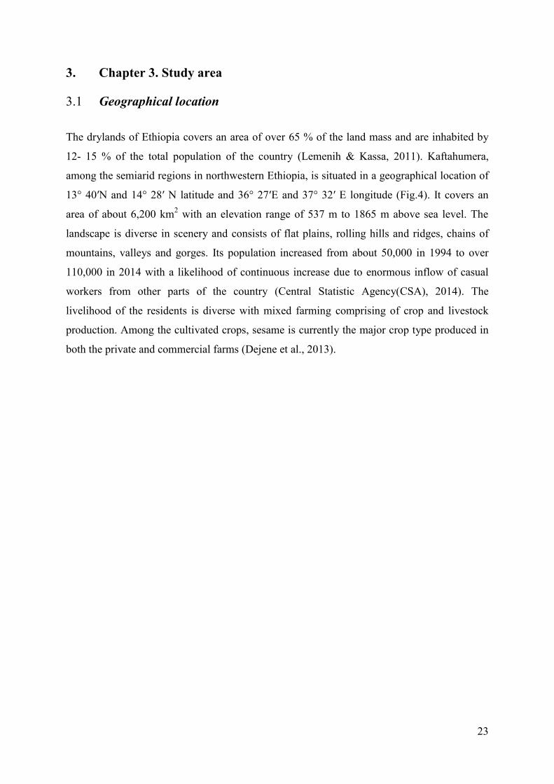
23

3. Chapter 3. Study area

3.1 Geographical location

The drylands of Ethiopia covers an area of over 65 % of the land mass and are inhabited by

12- 15 % of the total population of the country (Lemenih & Kassa, 2011). Kaftahumera,

among the semiarid regions in northwestern Ethiopia, is situated in a geographical location of

13° 40′N and 14° 28′ N latitude and 36° 27′E and 37° 32′ E longitude (Fig.4). It covers an

area of about 6,200 km2 with an elevation range of 537 m to 1865 m above sea level. The

landscape is diverse in scenery and consists of flat plains, rolling hills and ridges, chains of

mountains, valleys and gorges. Its population increased from about 50,000 in 1994 to over

110,000 in 2014 with a likelihood of continuous increase due to enormous inflow of casual

workers from other parts of the country (Central Statistic Agency(CSA), 2014). The

livelihood of the residents is diverse with mixed farming comprising of crop and livestock

production. Among the cultivated crops, sesame is currently the major crop type produced in

both the private and commercial farms (Dejene et al., 2013).

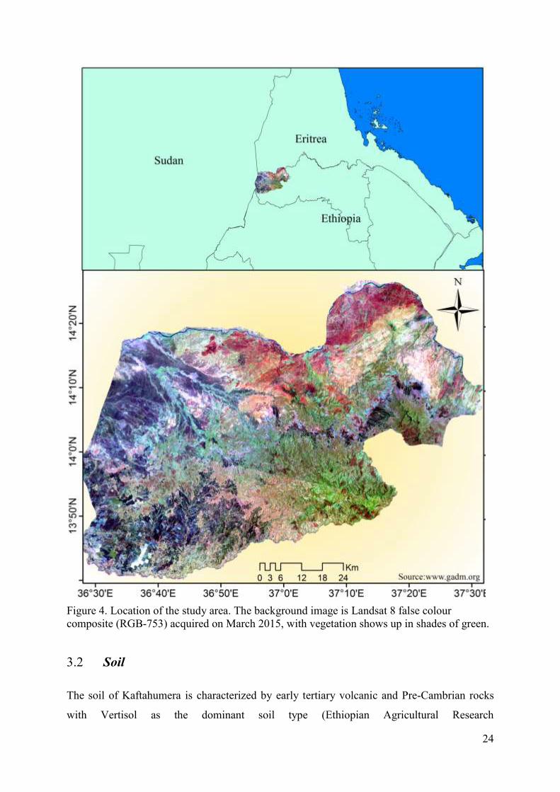
24

Figure 4. Location of the study area. The background image is Landsat 8 false colour composite (RGB-753) acquired on March 2015, with vegetation shows up in shades of green.

3.2 Soil

The soil of Kaftahumera is characterized by early tertiary volcanic and Pre-Cambrian rocks

with Vertisol as the dominant soil type (Ethiopian Agricultural Research

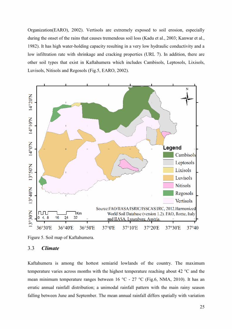
25

Organization(EARO), 2002). Vertisols are extremely exposed to soil erosion, especially

during the onset of the rains that causes tremendous soil loss (Kadu et al., 2003; Kanwar et al.,

1982). It has high water-holding capacity resulting in a very low hydraulic conductivity and a

low infiltration rate with shrinkage and cracking properties (URL 7). In addition, there are

other soil types that exist in Kaftahumera which includes Cambisols, Leptosols, Lixisols,

Luvisols, Nitisols and Regosols (Fig.5, EARO, 2002).

Figure 5. Soil map of Kaftahumera.

3.3 Climate

Kaftahumera is among the hottest semiarid lowlands of the country. The maximum

temperature varies across months with the highest temperature reaching about 42 °C and the

mean minimum temperature ranges between 16 °C - 27 °C (Fig.6, NMA, 2010). It has an

erratic annual rainfall distribution; a unimodal rainfall pattern with the main rainy season

falling between June and September. The mean annual rainfall differs spatially with variation

26

in altitude. The northern part receives as low as up to 450 mm and the southern part has as

high as up to 1102 mm rainfall per year. The agricultural production depends on the available

rains solely during the summer season of the year.

Figure 6. Climate graph of Kaftahumera, Ethiopia (Source:National Meteorology Agency of Ethiopia, 2010).

3.4 Vegetation

Kaftahumera is one of the dryland areas of the country dominated by Combretum–Terminalia

woodlands (Eshete et al., 2011, WBISPP, 2005). The woodland of the regions characterized

by hosting small trees with fairly large deciduous leaves of over fifty-two tree and shrub

species (WBISPP, 2005). Among the woody species Combretum spp., Terminalia spp.,

Boswellia papyrifera, Anogeissus lieocarpa, Acacia mellifera, Balanites aegyptiaca,

Dalbergia melanoxylm and Dicrostachy cineria are some of the dominant species which share

the vegetation types of Kaftahumera. These species are vital for the local communities in

providing both timber and other products for commercial and household usage (Eshete et al.,

2012; Tilahun et al., 2011). However, the vegetation cover has severely dwindled and

degraded due to several driving factors. Main contributing forces are expansion of subsistence

and large scale agriculture coupled with population pressure that impacts the woodland for

different purposes. The lowlands of northwestern Ethiopia are nominated for resettlements of

farmers from overpopulated and degraded highlands of the country since the 1980s which

0

20

40

60

80

100

120

140

160

180

200

0

5

10

15

20

25

30

35

40

45

Jan Feb Mar Apr May Jun Jul Aug Sep Oct Nov Dec

Pre

cip

itat

ion

(mm

)

Tem

pe

ratu

re(°

C)

Climate graph of Kaftahumera,Ethiopia

Mean annual rainfall(mm) Mean Tmax(°C) Mean Tmin(°C)

27

affects the woodland ecosystem dynamics of the region (Rahmato & van den Bergh, 1991;

Rahmato, 2003).

4. Chapter 4. Data and methodology

4.1 Data 4.1.1 Landsat imagery

Satellite imagery used for this study consists of multispectral Landsat data that includes MSS

1972, TM 1984, TM 1986, TM 2000 and Landsat 8 2014 (Table 2). The Landsat series of

satellite imagery are used for multitemporal land use transition and land degradation

assessment over a period of more than four decades. Landsata-8 launched in February 11,

2013 carries two sensors: OLI and TIRS both with enhancements in scanning technology by

replacing whisk-broom scanners by two separate push-broom (OLI and TIRS) scanners (Li et

al., 2013; Roy et al., 2014). All the Landsat imagery is geometrically corrected Level 1T

(L1T) data obtained from the United States Geological Survey (USGS)

(http://glovis.usgs.gov). The imagery used for this study acquired during the dry season and is

free of cloud cover. As there is vibrant behavior of phenological changes over time, it is vital

to consider using similar season imagery in order to avoid natural phenological changes

during the interpretation of actual land use changes (Verbesselt et al., 2010). Multitemporal

imagery was selected based on some policy changes, sociopolitical transitions and availability

of suitable imagery. Since the change in government in 1991, the country has adopted an

Agricultural Development Led Industrialization (ADLI) strategy mainly focusing on export

led development which calls for huge foreign investments (MoA, 2013).

Table 2. Data used for land use/land cover change analysis.

Imagery Path/row Acquisition date

Landsat MSS 83/50,83/51 29 November 1972

Landsat TM 170/50,70/51 29 November 1984



Landsat TM 170/50,70/51 9 December 2010

Landsat 8 170/50,70/51 01 January 2014

Topographic map 1:50,000 1979

http://glovis.usgs.gov/

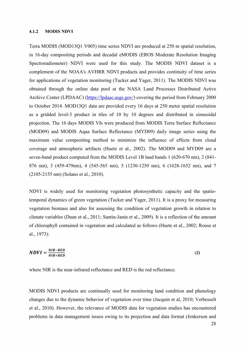
28

4.1.2 MODIS NDVI

Terra MODIS (MOD13Q1 V005) time series NDVI are produced at 250 m spatial resolution,

in 16-day compositing periods and decadal eMODIS (EROS Moderate Resolution Imaging

Spectroradiometer) NDVI were used for this study. The MODIS NDVI dataset is a

complement of the NOAA's AVHRR NDVI products and provides continuity of time series

for applications of vegetation monitoring (Tucker and Yager, 2011). The MODIS NDVI was

obtained through the online data pool at the NASA Land Processes Distributed Active

Archive Center (LPDAAC) (https://lpdaac.usgs.gov/) covering the period from February 2000

to October 2014. MOD13Q1 data are provided every 16 days at 250 meter spatial resolution

as a gridded level-3 product in tiles of 10 by 10 degrees and distributed in sinusoidal

projection. The 16 days MODIS VIs were produced from MODIS Terra Surface Reflectance

(MOD09) and MODIS Aqua Surface Reflectance (MYD09) daily image series using the

maximum value compositing method to minimize the influence of effects from cloud

coverage and atmospheric artifacts (Huete et al., 2002). The MOD09 and MYD09 are a

seven-band product computed from the MODIS Level 1B land bands 1 (620-670 nm), 2 (841-

876 nm), 3 (459-479nm), 4 (545-565 nm), 5 (1230-1250 nm), 6 (1628-1652 nm), and 7

(2105-2155 nm) (Solano et al., 2010).

NDVI is widely used for monitoring vegetation photosynthetic capacity and the spatio-

temporal dynamics of green vegetation (Tucker and Yager, 2011). It is a proxy for measuring

vegetation biomass and also for assessing the condition of vegetation growth in relation to

climate variables (Duan et al., 2011; Santin-Janin et al., 2009). It is a reflection of the amount

of chlorophyll contained in vegetation and calculated as follows (Huete et al., 2002; Rouse et

al., 1973):

(2)

where NIR is the near-infrared reflectance and RED is the red reflectance.

MODIS NDVI products are continually used for monitoring land condition and phenology

changes due to the dynamic behavior of vegetation over time (Jacquin et al, 2010; Verbesselt

et al., 2010). However, the relevance of MODIS data for vegetation studies has encountered

problems in data management issues owing to its projection and data format (Jenkerson and

https://lpdaac.usgs.gov/

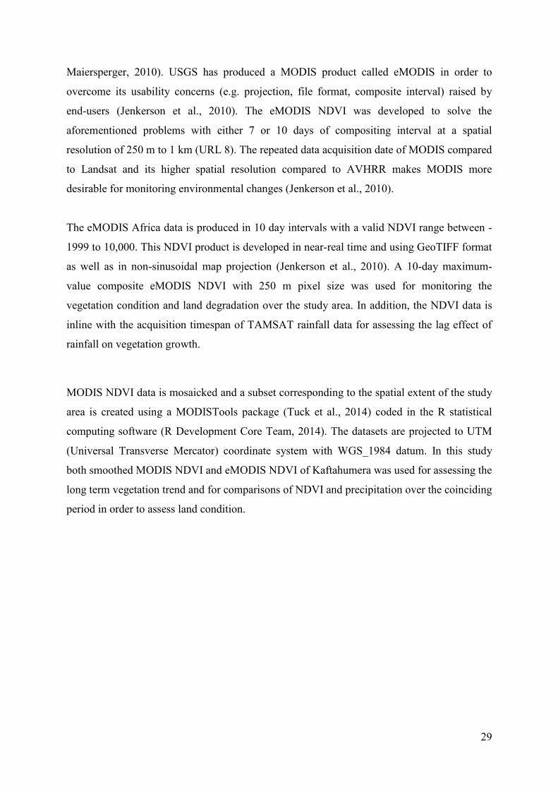
29

Maiersperger, 2010). USGS has produced a MODIS product called eMODIS in order to

overcome its usability concerns (e.g. projection, file format, composite interval) raised by

end-users (Jenkerson et al., 2010). The eMODIS NDVI was developed to solve the

aforementioned problems with either 7 or 10 days of compositing interval at a spatial

resolution of 250 m to 1 km (URL 8). The repeated data acquisition date of MODIS compared

to Landsat and its higher spatial resolution compared to AVHRR makes MODIS more

desirable for monitoring environmental changes (Jenkerson et al., 2010).

The eMODIS Africa data is produced in 10 day intervals with a valid NDVI range between -

1999 to 10,000. This NDVI product is developed in near-real time and using GeoTIFF format

as well as in non-sinusoidal map projection (Jenkerson et al., 2010). A 10-day maximum-

value composite eMODIS NDVI with 250 m pixel size was used for monitoring the

vegetation condition and land degradation over the study area. In addition, the NDVI data is

inline with the acquisition timespan of TAMSAT rainfall data for assessing the lag effect of

rainfall on vegetation growth.

MODIS NDVI data is mosaicked and a subset corresponding to the spatial extent of the study

area is created using a MODISTools package (Tuck et al., 2014) coded in the R statistical

computing software (R Development Core Team, 2014). The datasets are projected to UTM

(Universal Transverse Mercator) coordinate system with WGS_1984 datum. In this study

both smoothed MODIS NDVI and eMODIS NDVI of Kaftahumera was used for assessing the

long term vegetation trend and for comparisons of NDVI and precipitation over the coinciding

period in order to assess land condition.

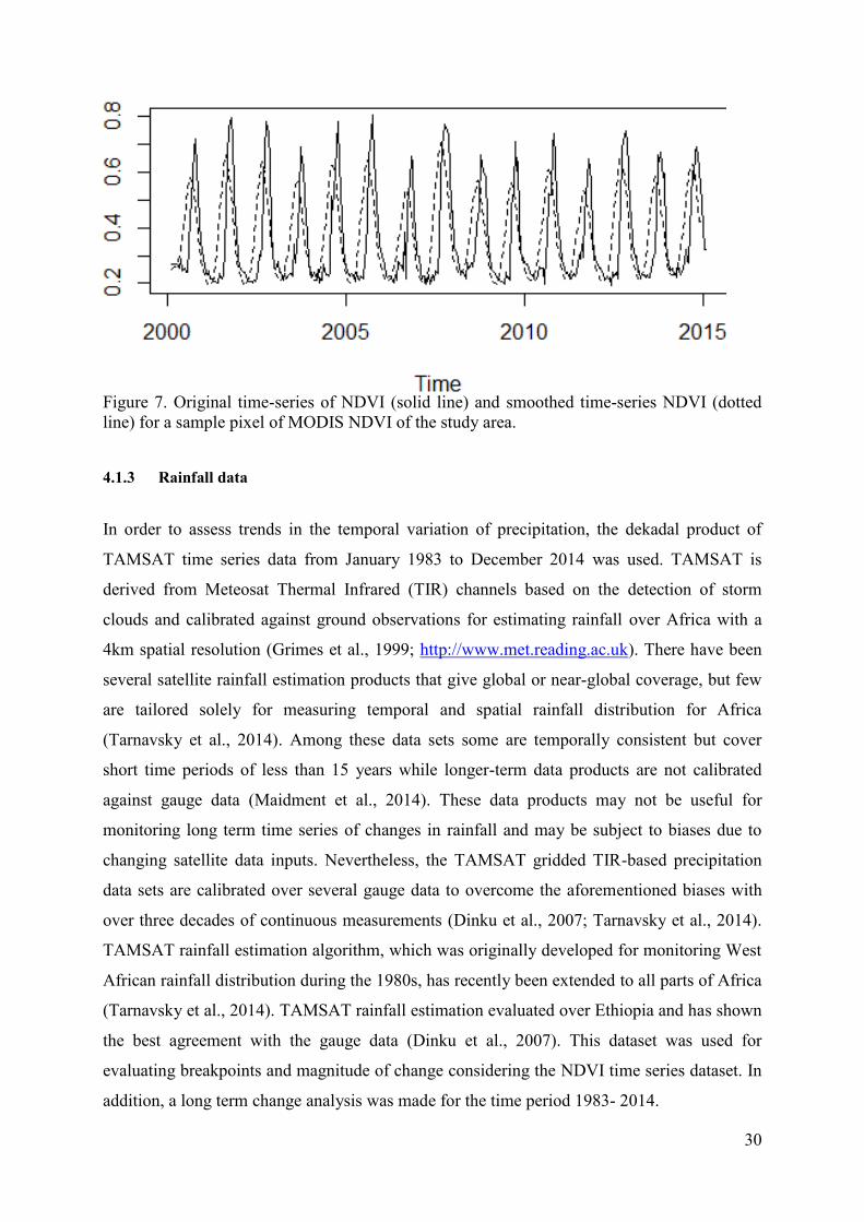
30

Figure 7. Original time-series of NDVI (solid line) and smoothed time-series NDVI (dotted line) for a sample pixel of MODIS NDVI of the study area.

4.1.3 Rainfall data

In order to assess trends in the temporal variation of precipitation, the dekadal product of

TAMSAT time series data from January 1983 to December 2014 was used. TAMSAT is

derived from Meteosat Thermal Infrared (TIR) channels based on the detection of storm

clouds and calibrated against ground observations for estimating rainfall over Africa with a

4km spatial resolution (Grimes et al., 1999; http://www.met.reading.ac.uk). There have been

several satellite rainfall estimation products that give global or near-global coverage, but few

are tailored solely for measuring temporal and spatial rainfall distribution for Africa

(Tarnavsky et al., 2014). Among these data sets some are temporally consistent but cover

short time periods of less than 15 years while longer-term data products are not calibrated

against gauge data (Maidment et al., 2014). These data products may not be useful for

monitoring long term time series of changes in rainfall and may be subject to biases due to

changing satellite data inputs. Nevertheless, the TAMSAT gridded TIR-based precipitation

data sets are calibrated over several gauge data to overcome the aforementioned biases with

over three decades of continuous measurements (Dinku et al., 2007; Tarnavsky et al., 2014).

TAMSAT rainfall estimation algorithm, which was originally developed for monitoring West

African rainfall distribution during the 1980s, has recently been extended to all parts of Africa

(Tarnavsky et al., 2014). TAMSAT rainfall estimation evaluated over Ethiopia and has shown

the best agreement with the gauge data (Dinku et al., 2007). This dataset was used for

evaluating breakpoints and magnitude of change considering the NDVI time series dataset. In

addition, a long term change analysis was made for the time period 1983- 2014.

http://www.met.reading.ac.uk/

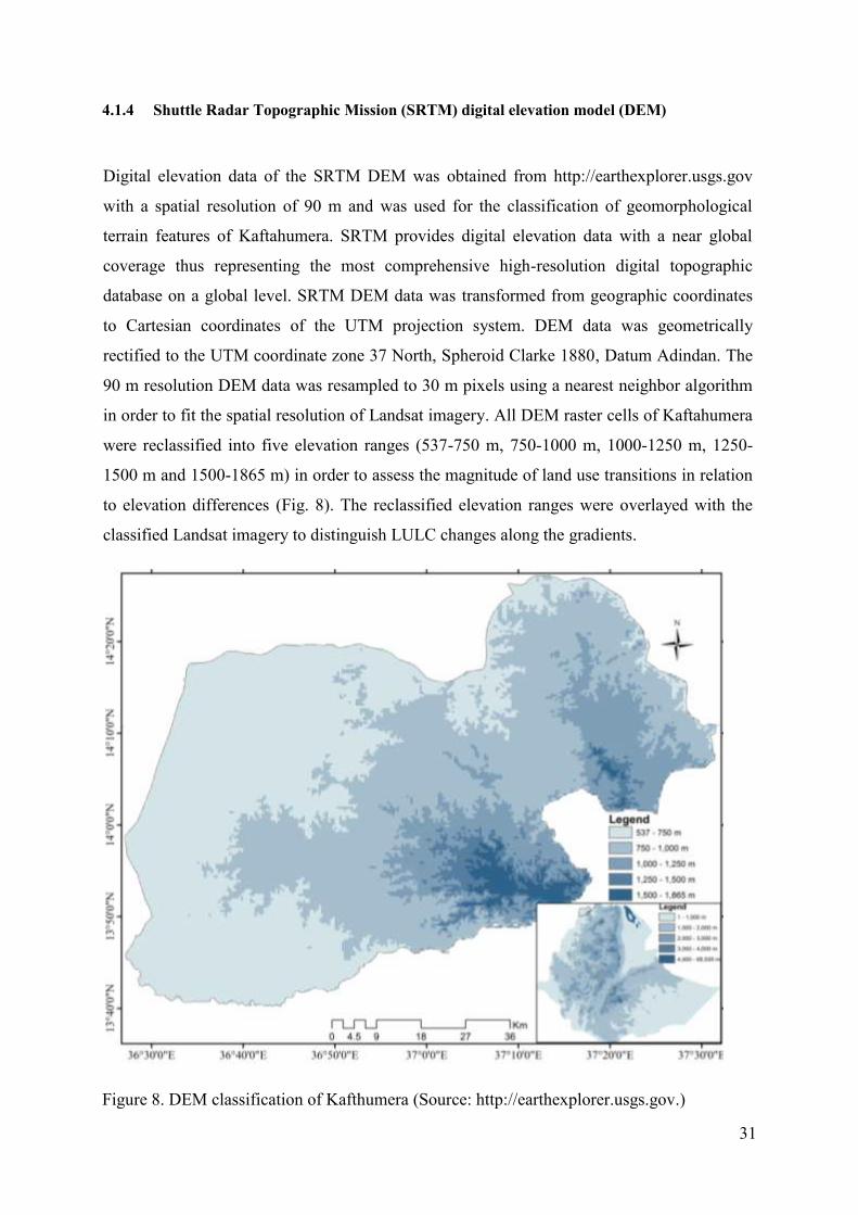
31

4.1.4 Shuttle Radar Topographic Mission (SRTM) digital elevation model (DEM)

Digital elevation data of the SRTM DEM was obtained from http://earthexplorer.usgs.gov

with a spatial resolution of 90 m and was used for the classification of geomorphological

terrain features of Kaftahumera. SRTM provides digital elevation data with a near global

coverage thus representing the most comprehensive high-resolution digital topographic

database on a global level. SRTM DEM data was transformed from geographic coordinates

to Cartesian coordinates of the UTM projection system. DEM data was geometrically

rectified to the UTM coordinate zone 37 North, Spheroid Clarke 1880, Datum Adindan. The

90 m resolution DEM data was resampled to 30 m pixels using a nearest neighbor algorithm

in order to fit the spatial resolution of Landsat imagery. All DEM raster cells of Kaftahumera

were reclassified into five elevation ranges (537-750 m, 750-1000 m, 1000-1250 m, 1250-

1500 m and 1500-1865 m) in order to assess the magnitude of land use transitions in relation

to elevation differences (Fig. 8). The reclassified elevation ranges were overlayed with the

classified Landsat imagery to distinguish LULC changes along the gradients.

Figure 8. DEM classification of Kafthumera (Source: http://earthexplorer.usgs.gov.)

32

4.1.5 Temperature data

The Climate Research Unit Time Series (CRU-TS 3.22) global long-term climate database

was acquired from Climatic Research Unit (CRU) of the University of East Anglia (Harris et

al., 2014). CRU-TS 3.22 is a gridded global dataset with a spatial resolution of 0.5° covering

a period of 1901 – 2013. It is a monthly observation based on datasets obtained from more

than 4000 meteorological stations distributed all over the world (Harris et al., 2014). The

dataset comprises of different climate variables namely mean temperature, diurnal

temperature range, precipitation, wet-day frequency, vapor pressure and cloud cover (Harris

et al., 2014). In order to observe the change in temperature of the study region, this analysis

used only monthly average minimum temperature and monthly average maximum

temperature. The two temperature datasets of the study area were extracted for the period

1983 – 2013. The period 2000 – 2013 was used for magnitude and time of breakpoints

analysis in both minimum and maximum temperature, considering the time span covered by

NDVI and TAMSAT rainfall data products. In addition, long term temperature change

assessment was made over the period of 1983 to 2013.

4.2 Image pre-processing

4.2.1 Geometric corrections

For monitoring multitemporal land cover transitions covering large areas based on time series,

it is crucial to have imagery with consistent geometric corrections at hand (Hansen &

Loveland, 2012). Historical Landsat imagery was produced without geometric correction and

a separate way of in-house correction of the imagery was applied for a longer period of time.

In due progress with the utilization of Landsat imagery for monitoring large areas, a standard

orthorectified and geodetically accurate global land dataset was created for Landsat MSS,

TM, and ETM+ from the 1970s, from ca. 1990, and ca. 2000 respectively (Tucker et al.,

2004). The availability of improved digital elevation models and ground control network

facilitated the adoption and use of consistent Landsat image geometry across epochs (Hansen

& Loveland, 2012). All Landsat imagery is currently distributed as orthorectified Level 1

Terrain-corrected data (L1T). In this study, a terrain corrected (L1T) Landsat imagery of

1972, 1984, 1986, 2010 and 2014 were used.

The imagery was processed using Environment for Visualizing Images (ENVI version 5.1)

and ArcGIS 10 software packages as well as R Development Core Team 2014. Due to the

33

availability of reference data in 2000, the Landsat TM 2000 image was geometrically rectified

to UTM coordinate zone 37 North, Spheroid Clarke 1880, Datum Adindan, using control

points collected from topographic maps of the study area. An image to image registration was

applied between MSS 1972, TM 1984, TM 1986, TM 2010 and Landsat 8 imagery based on

the TM 2000 reference image using the nearest neighbor algorithm. The root mean square

error (RMSE) amounts between 0.3 to 0.5 pixels.

4.2.2 Atmospheric correction

4.2.2.1 Landsat data

All the Landsat imagery used for this study is free of cloud cover during image acquisition.

However, in order to remove scene variation due to atmospheric scattering, atmospheric

correction was employed in all Landsat imagery to have a common radiometric scale (Chavez

Jr, 1989; Song et al., 2001). The digital numbers were recalculated to top of atmosphere

radiance (Chander et al. 2009) and then imagery was corrected using the Fast Line-of-sight

Atmospheric Analysis of Hypercubes (FLAASH) tool in Exelis Visual Information Solutions

(ENVI 5.1; http://www.exelisvis.com) that integrates the MODTRAN algorithim (moderate

resolution atmospheric transmittance and radiance code) (Berk et al., 1999). Five major land

use categories were identified as woodland, cropland, grassland, residence and water for

assessing land use transitions (Table 3).

Table 3. Land cover classification scheme.

Land cover class Description

Woodland Woody plants with a canopy cover of more than 10%

Cropland Crop fields, parklands, fallows

Grassland Pasture lands, grass with scattered trees, shrubs

Residential Cities, villages, roads

Waters Rivers, lakes, reservoirs, streams

http://www.exelisvis.com/

34

4.2.2.2 NDVI data

The effects of cloud contamination and atmospheric variability could disturb the feasibility of

applying time series of NDVI data for monitoring temporal land cover changes as erroneous

results are produced (Atkinson et al, 2012). The improvement of MODIS NDVI data

minimizes the contamination from clouds and other spurious artifacts that can affect the

temporal analysis of time series data. Despite the preprocessing of MOD13Q1 NDVI to avoid

low values, there exists a significant amount of residual noise in the time-series NDVI data

(Lunetta et al., 2006). Hence, a modified Whittaker Smoother (WS) algorithm was used for

temporal filtering of MODIS NDVI time series in order to avoid anomalous values from the

dataset (Atzberger & Eilers, 2011; Eilers, 2003; R Development Core Team, 2014). This

approach is an iterative process in which the filter smoothes the observed time series using the

basic Whittaker algorithm and then all observed values that lie below the fitted curve are

replaced by their fitted value (Atzberger & Eilers, 2011). The iteration continues till the

values below the curves are replaced by the curve values that can be used for the analysis of

temporal NDVI changes. A temporal time series data stack is generated from the smoothed

data during temporal NDVI analysis.

4.2.3 Radiometric corrections

Radiometric correction is mainly performed for normalization of differences among scenes of

imagery taken at different time periods (Coppin et al., 2004). Top of atmosphere reflectance

(TOA), surface reflectance, bi-directional reflectance distribution, viewing angle

normalization, and terrain normalization are among the commonly applied radiometric

correction methods to improve the information obtained from satellite imagery (Hansen &

Loveland, 2012). Sun angle and earth-sun distance adjustment can be made mainly using the

calculation of top of atmosphere reflectance. This correction is applied to the whole scene as

there is no separate Landsat solar geometry supplied for each pixel and hence there is no

distinctive variation in TOA adjustment per each pixel within a scene (Chander et al., 2009;

Hansen & Loveland, 2012). TOA calibration is significant for normalization of differences

between imagery taken at different time intervals in order to cross-calibrate sensor radiometry

(Chander et al., 2009). The rescaling factor developed by Chander et al (2009) was adopted

for consistent evaluation of Landsat imagery obtained at different dates and different sensors

from 1972 to 2014 as:

35

LMINQQQQLMINLMAX

L calcalcalcal

))(( min

minmax

(3)

where

L =Spectral radiance at the sensor’s aperture (W/m2srm)

calQ = Quantized calibrated pixel value (DN)

mincalQ =Minimum quantized calibrated pixel value corresponding to LMIN (DN)

maxcalQ =Maximum quantized calibrated pixel value corresponding to LMAX (DN)

LMIN =spectral at-sensor radiance that is scaled to mincalQ (W/m2srm)

LMAX =Spectral at sensor radiance that is scaled to maxcalQ (W/m2srm)

Multi-temporal image analysis needs reduction of variation in scene to scene and can be

achieved through the conversion of at-sensor spectral radiance to exoatmospheric reflectance

(TOA reflectance). The TOA can be computed according to the equation (Chander et al.

2009) ;

sESUNdL

cos.

.. 2

(4)

where

= Planetary TOA reflectance (unitless)

= constant3.14159 (unitless)

L = Spectral radiance at the sensor’s aperture (W/m2srm)

d= Earth sun distance (astronomical units)

ESUN = Mean exoatmospheric solar irradiance (W/m2m)

s = Solar zenith angle

The solar elevation angle provided with the Landsat metadata was used to calculate the solar

zenith angle. Sine of solar elevation angle is equal to the cosine of solar zenith angle.

Reflectance is unitless.

4.3 Image classification using SVM The use of multi-temporal image classification has the advantage of producing change

trajectories in between the period of data coverage for monitoring the ongoing transitions in

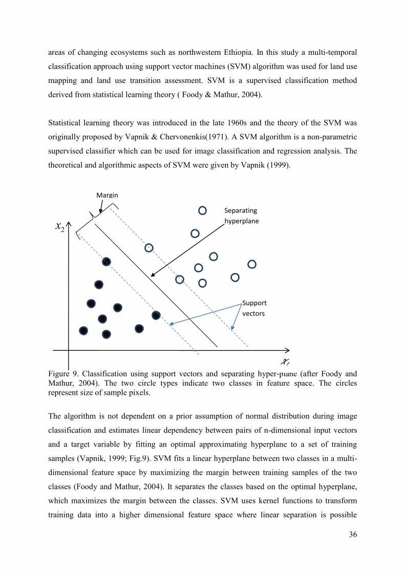
36

areas of changing ecosystems such as northwestern Ethiopia. In this study a multi-temporal

classification approach using support vector machines (SVM) algorithm was used for land use

mapping and land use transition assessment. SVM is a supervised classification method

derived from statistical learning theory ( Foody & Mathur, 2004).

Statistical learning theory was introduced in the late 1960s and the theory of the SVM was

originally proposed by Vapnik & Chervonenkis(1971). A SVM algorithm is a non-parametric

supervised classifier which can be used for image classification and regression analysis. The

theoretical and algorithmic aspects of SVM were given by Vapnik (1999).

Figure 9. Classification using support vectors and separating hyper-plane (after Foody and Mathur, 2004). The two circle types indicate two classes in feature space. The circles represent size of sample pixels.

The algorithm is not dependent on a prior assumption of normal distribution during image

classification and estimates linear dependency between pairs of n-dimensional input vectors

and a target variable by fitting an optimal approximating hyperplane to a set of training

samples (Vapnik, 1999; Fig.9). SVM fits a linear hyperplane between two classes in a multi-

dimensional feature space by maximizing the margin between training samples of the two

classes (Foody and Mathur, 2004). It separates the classes based on the optimal hyperplane,

which maximizes the margin between the classes. SVM uses kernel functions to transform

training data into a higher dimensional feature space where linear separation is possible

2x

Margin

Separating

hyperplane

Support

vectors

X1

37

(Huang et al., 2002). SVM implement the structural risk minimization principle, which

attempts to minimize an upper bound on the generalization of error by striking a right balance

between the training error and the capacity of the machine (Tripathi et al., 2006). The risk of

misclassification is minimized by maximizing the margin between the data points and the

decision boundary.

In this study among the SVM kernels, the Gaussian radial basis function kernel (RBF) was

selected for mapping and change detection assessment. RBF kernel requires setting of two

parameters, the optimum Gaussian radial basis function (γ) that controls the kernel width and

the regularization parameter (C) which controls the penalty of misclassification errors in

order to handle non-separable classification problems (Huang et al., 2008). The Library for

Support Vector Machines (LIBSVM) program developed by Chang & Lin ( 2001) was used

for classification. The model was parameterized based on the training samples of each land

use type. A cross validation test was applied combining γ and C to obtain optimum values of

these parameters for best classification outputs. A “one-against-one” approach, was used in

which each class was compared to every other class individually for multi-class SVM

classification (Melgani & Bruzzone, 2004).

All four bands of MSS, bands 1-5 and 7 of TM and bands 1-7 of OLI imagery were used for

extracting biophysical features. In 2012 stratified random reference samples and their

attributes were collected in the field using handheld Garmin Oregon 450. The field samples

were divided into two as ground-truthing which was used as training dataset during image

classification while the remaining samples were used for accuracy assessment of classified

imagery.

A classification accuracy assessment was performed using stratified random sampling

representing the five land use classes. A confusion matrix was developed relying to the

comparison of selected samples of classified imagery with respective ground sampling. In

this process an overall accuracy, producer and user accuracies and kappa coefficient were

calculated for each of classified imagery from 1972 to 2014 (Congalton, 1991).The whole

workflow of the methodological approach of the study is illustrated in the following

flowchart (Fig.10).

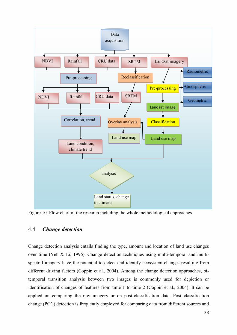
39

dates (Mundia & Aniya, 2006; Yuan et al., 2005). PCC identifies changes by comparing

independently classified multi-date imagery on a pixel-by-pixel basis using a change detection

matrix (Yuan & Elvidge, 1998). However the accuracy of PCC approaches depends on the

reliability of image classification outputs. This method is supportive in determining “from-to”

changes in order to identify the transformations among the land cover classes (Jensen, 1996;

Yuan et al., 2005). In this study, the change detection assessment was performed using

individual image classification outputs of the best performing SVM model in order to identify

respective two-date change trajectories: 1972-1984, 1984-2000, 1986-2014 and 2000-2010.

MSS imagery was downscaled to 30 m pixel cell size in order to have spatial compatibility

with the remaining Landsat imagery before performing the change trajectory analysis.

An overlay analysis between the classified imagery was made in order to produce a transition

matrix to display the amont of LULC transition from 1972 to 2014. The diagonals of the

matrix indicate the amount of land use category which remained unchanged throughout the

study period while the off-diagonal entries account for a transition from one category to other

land use categories.

The gain, loss, persistence, absolute value of net change, swap and total change were

calculated for all the four classified images for each class (Braimoh, 2006; Pontius et al.,

2004). A gain in land use category is a measure of the size of land use added between time 1

and 2 whereas loss accounts for reduction in size of a land use class between time 1 to time 2.

Persistence is the land use class that does not change from time 1 to time 2. Swap

discriminates quantity of both loss and gain in order to account for a land use category lost in

one site whereas equivalent dimension is added in different site (Pontius et al., 2004). It is the

simultaneous loss and gain of a land use class in a landscape, which implies that a given area

of a land use is lost at one location, while the same size is gained at a different location (Equ.

5). The investigation of swap change requires coupling pixels of both gain and loss of the land

use categories (Braimoh, 2006; Pontius et al., 2004). For a land use class j, amount of swap sj

was calculated as:

Sj=2min (Pj+ - Pjj; P+j - Pjj) (5)

where Sj = amount of swap,

Pj+ = Total column proportion of a land use class within the landscape,

40

Pjj = Persistence of land use classes within the landscape, and

P+j = Total row proportion of a land use class within the landscape.

The overall change in a land use category could be either the sum of the net change and the

swap or the sum of the gains and losses (Pontius et al., 2004). In addition, loss to persistence

ratio (lp) that measures the level of prevalence of a land use class for a change, gain to

persistence ratio (gp) that accounts for the amount of increment in a land use category

compared to its initial size , and net change to persistence ratio (np) which is an indicative of

direction and magnitude of transition of a land use class were also calculated (Braimoh,

2006).

4.5 Trend analysis

Mann (1945) proposed a test for randomness against time that incorporates a specific use of

Kendall’s test for correlation commonly known as the ‘Mann–Kendall’ or the ‘Kendall t test’

(Kendall, 1962). Mann-Kendall (MK) test is one of the widely used non-parametric tests for

assessing seasonal variations of mainly hydrological time series (Fathian et al., 2014; Hamed

& Ramachandra Rao, 1998; Modarres & de Paulo Rodrigues da Silva, 2007). However, it is

currently more commonly applied for testing the significance of changes in NDVI trends

(Alcaraz-Segura et al., 2010; de Jong et al., 2011). The MK trend test is less sensitive to

missing data values, irregular data distribution and outliers (Udelhoven, 2011). The test

involves assessing the Kendall score and its variance separately in each season of the

observations.

In this study, the MK was used for assessing long term trends both in NDVI and climate

variables using their detrended data component. The MK test requires the data to be serially

independent in order to avoid larger uncertainty in estimating the trend of serially correlated

data like temperature, rainfall and NDVI (Önöz & Bayazit, 2012; Yue & Wang, 2002).

The occurrence of serial correlation in time series data affects the variance of the estimate of

MK statistic and the existence of trend can change the estimate of amount of serial correlation

(Yue et al., 2002). In this study, the Yue and Pilon Trend Free Pre-whitening (TFPW)

procedure was applied before MK statistics and Theil-Sen’s slope analysis in order to remove

serial correlation from the time series based on the slope estimates (Yue et al., 2002). The

41

TFPW is applied inorder to remove lag1 autocorrelation during the time series processing. If

the estimated slope is equal to zero, it is not necessary to carry out trend analysis as the slope

is estimated using the Theil-Sen approach. When there is a deviation of slope from zero, a

TFPW procedure is applied to the time series data. An MK test is performed on the blended

trend and residuals to assess the significance of the trend (Yue et al., 2002). A pre-whitening

using the following formula was adopted in order to account for serial correlation of time

series data (Yue et al., 2002; Yue & Wang, 2002):

(6)

where:

Xi is the pre-whitened series

X1….Xi is original data series

r1 is is lag-1 serial correlation coefficient.

The pre-whitened data series has the same trend as the original data and also has serially

uncorrelated residuals.

The Mann–Kendall time series for x= x1, x2,… xn, the trend test statistic (S) is defined as:

(7)

where:

sign(x)=

where n is the length of the time series data set and xi ,… xj are the observations at times i to

j, respectively.

The mean of S is E(S)=0 and the variance of S is calculated as:

(8)

where j is the number of tied groups and ti is the size of the ith tied group.

As a result, the standardized Z test statistics follow a normal standardized distribution:

42

(9)

A significance test is determined based on the result of the Z value. The sign of Z either

positive or negative indicates an upward or downward trend of the tested variable. Based on

the outputs of the Z value, the trend is not rejected when the Z value is greater in absolute

value than the critical value Zα, at a selected significance level of α which was 0.05 in our

analysis.

4.6 Sen’s slope estimator test

In order to evaluate the slope magnitude of an existing trend within the time series data, the

Sen’s non-parametric method was used. Here, the slope (Ti) for all data pairs is computed as

(Sen, 1968):

, i=1,2,…N. (10)

where xj and xk are considered as data values at time j and k for j > k. If there are n values of x

in the time series, we obtain as many as N=n (n-1)/2 slope estimates of Ti. The median of

these N values of Ti is the Sen’s estimator of slope ranked from the smallest to the largest

which is given as:

Ti=

(11)

4.7 Identification of breaks for additive season and trend

The seasonal changes in NDVI are useful for monitoring the dynamics of the growing season

and changes in vegetation distribution (Hmimina et al., 2013). Several change detection

algorithms were developed for monitoring vegetation dynamics which consider time series

changes through aggregating data over the years or compare specific periods between the

years without accounting for seasonal variations (Coppin et al., 2004). The BFAST algorithm

is vital for change detection within trends of time series as it accounts for changes in trend and

seasonal variation over time (Schmidt et al., 2015; Verbesselt et al., 2010).

43

The assessment of breaks on season and trend based on locally weighted regression helps to

identify breaks on the trend of continuous vegetation index considering the whole study

period (Verbesselt et al., 2010). BFAST model uses the locally weighted regression smoother

(LOESS) temporal decomposition method for decomposing trends in vegetation growth

(Verbesselt, et al., 2010). This approach decomposes the original NDVI time series into three

additive components: trend, season and remainder (Fig.11). The three components are related

to vegetation condition at different time scales and taken into account the undergoing changes

along the study period. It is the best approach for determining the magnitude, direction and

time of breakpoints of both climate variables and NDVI based on seasonal and long term

trend time series. It determines abrupt changes to identify significant variations of the long

term time series data that helps to identify causative factors of change on the breakpoints. The

BFAST model is an additive decomposition algorithm which iteratively fits a piecewise linear

trend and seasonal model expressed as:

Yt = Tt + St + t, t=1,..., n (12) where: Yt is the original data at time t; Tt is the trend component; St is the seasonal component and t is the noise component (residuals remaining after the elimination of the trend and the seasonal components).

The model checks for existence of abrupt changes before fitting Tt and St. The ordinary least

squares (OLS) residuals based moving sum (MOSUM) test is used to check the availability of

breakpoints in the time series data before fitting the piecewise linear models (Zeileis &

Kleiber, 2005; Zeileis, 2005). If there is significant changes in the temporal NDVI value at <

0.05, the optimal number and position of breakpoints in the time series data returned

following the method of Bai & Perron (2003). In this study the harmonic model was used to

fit the seasonality since it is considered as the most suitable model for natural vegetation

phenology change detection (Verbesselt et al., 2010). The breakpoints for MODIS NDVI and

climate variables were assessed based on four sample plots collected from the study area.

Each plot covers an area of about 1.25 km x 1.25 km which was selected based on the history

of land use changes. The mean NDVI of each sample plot was used for BFAST

decomposition to identify breakpoints. The minimum amount of observations between two

breaks was set to be three years and the minimum segment size between potentially detected

breaks within the trend model (h) to 0.15. Similar sample size, location and method were used

for detecting breakpoints in precipitation and temperature time series data of Kaftahumera.

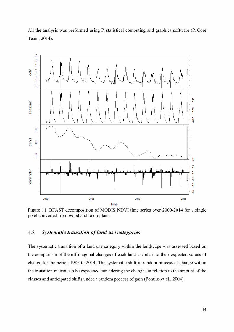
44

All the analysis was performed using R statistical computing and graphics software (R Core

Team, 2014).

Figure 11. BFAST decomposition of MODIS NDVI time series over 2000-2014 for a single pixel converted from woodland to cropland

4.8 Systematic transition of land use categories

The systematic transition of a land use category within the landscape was assessed based on

the comparison of the off-diagonal changes of each land use class to their expected values of

change for the period 1986 to 2014. The systematic shift in random process of change within

the transition matrix can be expressed considering the changes in relation to the amount of the

classes and anticipated shifts under a random process of gain (Pontius et al., 2004)

45

j

ijjjij P

PPPG100

)( (13)

where Gij is the expected land use shift of class i to class j under random process of gain;

P+j is sum of column of category j in the transition matrix;

Pjj is the persistence for the category j;

Pi+ is the row total of land use class i, and

Pj+ the row total of category j.

Equation 13 presumes that the increase in each land use class in 2014 is unchanging, and

accordingly allocates the gain to each category based on their proportional size of 1986. The

expected proportion and the observed proportion of the diagonals are set as equal, so that the

shift in off-diagonal land use classes can be estimated considering the changes in land use

classes. If the variation between the observed and expected proportion of a land use category

is positive, the category in the row lost more than the category in the column than would be

expected under a random process of gain in that category of the column (Pontius et al., 2004).

On the other hand, when the deviation is negative, then the land use class in that row lost less

in the category in column than would be expected by a random process of gain of that

category of the column.

Expected loss under a random process of loss is also calculated following Pontius et al. (2004)

as:

i

jiiiij P

PPPL

100)( (14)

where Lij is the anticipated shift from category i to j; Pi+ is the row total of category i;Pii is

persistence land use category in the period 1986 - 2014 for category i; P+j is the column total

of category j, and P+i is the column total of category i.

Equation 14 presumes loss in each land use class is constant and disburses according to their

relative size of the remaining classes in 2014. The expected value of the diagonals remains the

same to evaluate the off-diagonal transitions in the period 1986-2014. The gain and loss

between categories in the row and column is computed considering the difference between

expected and observed changes of land use classes under a random process of loss. The land

use class in the column is considered as gain when the difference between observed and

expected transition under random process of loss is positive. On the other hand, if the value is

46

negative, the category in the column gained less from the category in the row than would be

expected under a random process of loss in the category of the row (Pontius et al., 2004).

4.9 NDVI rainfall correlation analysis

Land use monitoring and estimation of biomass accumulation can be made using NDVI

(Pereira Coltri et al., 2013; Singh et al., 2003; Zhao et al., 2014). NDVI temporal and spatial

dynamics depend significantly on the precipitation amount and distribution in which the

biomass accumulation follows the precipitation gradient (Xia et al., 2014). The variation in

vegetation productivity of arid areas could be dominantly linked to either change in land use

or variation in rainfall distribution. The assessment of the spatiotemporal relationship between

NDVI and rainfall of each pixel facilitates the understanding of vegetation productivity and

land condition (del Barrio et al, 2010; Higginbottom & Symeonakis, 2014). Accordingly, a

pixel-wise spatiotemporal Ordinary Least Squares (OLS) linear regression analysis between

the long term average NDVI and the long term average TAMSAT rainfall data was made to

evaluate spatial vegetation productivity variation over the whole study area. The OLS

regression model is given as:

NDVI= α + β*rainfall + (15)

where NDVI is the dependent variable, rainfall is the independent variable, α is intercept and

β is the slope coefficient for variable rainfall and is the random error.

The TAMSAT data were resampled to a grid common to the spatial resolution of NDVI data

using a nearest neighbor resampling method. The correlation between the resampled and

original TAMSAT data showed a high correlation coefficient (R2) of over 0.98 (p<0.05).

The pixel-wise spatial regression between TAMSAT and NDVI determines the correlation

coefficient for assessing the status of land conditions. Moreover, the decadal NDVI data were

aggregated to annual NDVI time series in order to have a good estimation of temporal NDVI

profiles (Forkel et al., 2013). The regression of accumulated NDVI along the time gradient

was calculated to evaluate the trend in vegetation productivity. An OLS linear regression

analysis was adopted to evaluate the slope and the significance of annual NDVI changes at a

95 % confidence level (p< 0.05).

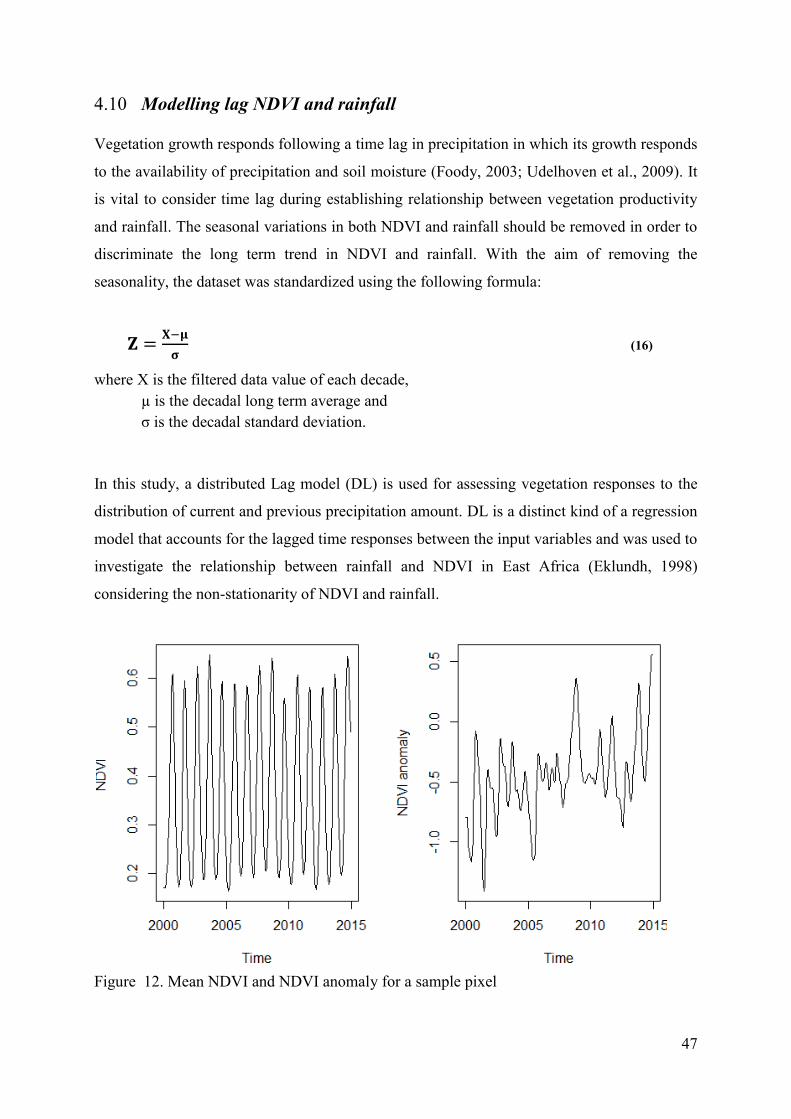
47

4.10 Modelling lag NDVI and rainfall

Vegetation growth responds following a time lag in precipitation in which its growth responds

to the availability of precipitation and soil moisture (Foody, 2003; Udelhoven et al., 2009). It

is vital to consider time lag during establishing relationship between vegetation productivity

and rainfall. The seasonal variations in both NDVI and rainfall should be removed in order to

discriminate the long term trend in NDVI and rainfall. With the aim of removing the

seasonality, the dataset was standardized using the following formula:

(16)

where X is the filtered data value of each decade, µ is the decadal long term average and σ is the decadal standard deviation.

In this study, a distributed Lag model (DL) is used for assessing vegetation responses to the

distribution of current and previous precipitation amount. DL is a distinct kind of a regression

model that accounts for the lagged time responses between the input variables and was used to

investigate the relationship between rainfall and NDVI in East Africa (Eklundh, 1998)

considering the non-stationarity of NDVI and rainfall.

Figure 12. Mean NDVI and NDVI anomaly for a sample pixel

48

A regression analysis using DL models was made between the NDVI and rainfall anomalies

after removing the trends and seasonal variation. DL regression analysis accounts for the

lagged effects of the explanatory variable on the response variable and takes the form:

Yt=a+b0xt+b1xt-1+b2xt-2+……..+et (17)

where vector b is weight of each x series, t is time and e is the model residual.

Accordingly, the formula was adopted assigning rainfall as the explanatory variable and

NDVI as the response variable as:

(18)

where bj is the impulse response weight vectors describing the weights assigned to current and

past rainfall, a is the constant term and is the model residual.

In this study, the maximum lag time is fixed to 8 (in 10 days scale) and a continuous

regression fit was made starting from a model containing zero as first order time lag. A

detailed methodology for assessing NDVI and rainfall time lag using DL model is discussed

in Udelhoven et al.(2009) and elsewhere for assessing response of vegetation to climate

variables (Eklundh, 1998; Fathian et al., 2014; Ji & Peters, 2005; Kileshye Onema &

Taigbenu, 2009). The optimal lag between rainfall and NDVI is determined testing the

significance of t-statistics when the p value is less than 0.05. 4.11. Socio-ecological survey

In order to understand LULC change dynamics and perception of the society on climate

change, major drivers of changes were assessed using key informants. The key informants

were identified from eight purposefully selected villages within the study area. Random

sampling was adopted for selecting 78 households for individual interviews. A structured

questionnaire was used for gathering socio-ecological information on specific land use

transitions and main contributing factors. Descriptive statistics were employed to analyze the

collected information.

49

5. Chapter 5. Land use and land cover dynamics in northwestern Ethiopia

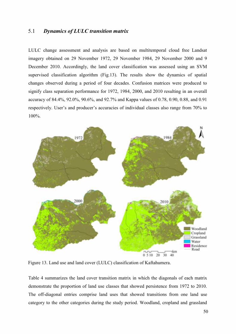
50

5.1 Dynamics of LULC transition matrix

LULC change assessment and analysis are based on multitemporal cloud free Landsat

imagery obtained on 29 November 1972, 29 November 1984, 29 November 2000 and 9

December 2010. Accordingly, the land cover classification was assessed using an SVM

supervised classification algorithm (Fig.13). The results show the dynamics of spatial

changes observed during a period of four decades. Confusion matrices were produced to

signify class separation performance for 1972, 1984, 2000, and 2010 resulting in an overall

accuracy of 84.4%, 92.0%, 90.6%, and 92.7% and Kappa values of 0.78, 0.90, 0.88, and 0.91

respectively. User’s and producer’s accuracies of individual classes also range from 70% to

100%.

Figure 13. Land use and land cover (LULC) classification of Kaftahumera.

Table 4 summarizes the land cover transition matrix in which the diagonals of each matrix

demonstrate the proportion of land use classes that showed persistence from 1972 to 2010.

The off-diagonal entries comprise land uses that showed transitions from one land use

category to the other categories during the study period. Woodland, cropland and grassland

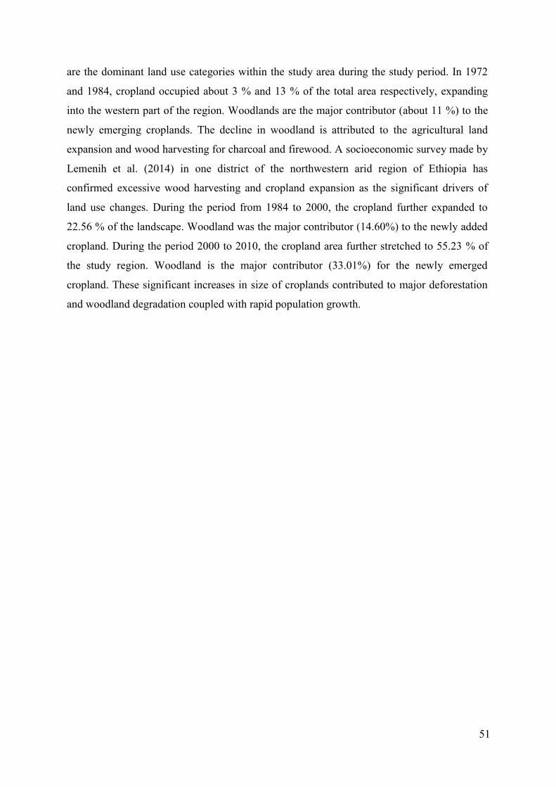
51

are the dominant land use categories within the study area during the study period. In 1972

and 1984, cropland occupied about 3 % and 13 % of the total area respectively, expanding

into the western part of the region. Woodlands are the major contributor (about 11 %) to the

newly emerging croplands. The decline in woodland is attributed to the agricultural land

expansion and wood harvesting for charcoal and firewood. A socioeconomic survey made by

Lemenih et al. (2014) in one district of the northwestern arid region of Ethiopia has

confirmed excessive wood harvesting and cropland expansion as the significant drivers of

land use changes. During the period from 1984 to 2000, the cropland further expanded to

22.56 % of the landscape. Woodland was the major contributor (14.60%) to the newly added

cropland. During the period 2000 to 2010, the cropland area further stretched to 55.23 % of

the study region. Woodland is the major contributor (33.01%) for the newly emerged

cropland. These significant increases in size of croplands contributed to major deforestation

and woodland degradation coupled with rapid population growth.

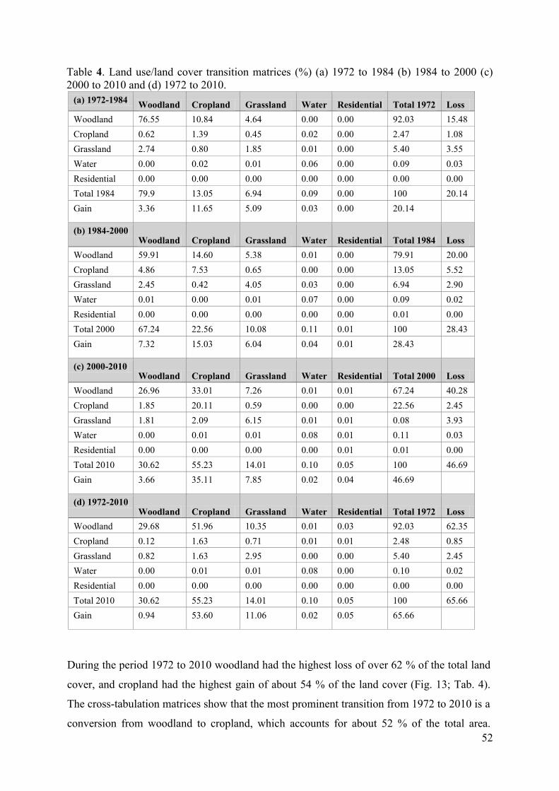
52

Table 4. Land use/land cover transition matrices (%) (a) 1972 to 1984 (b) 1984 to 2000 (c) 2000 to 2010 and (d) 1972 to 2010.

(a) 1972-1984 Woodland Cropland Grassland Water Residential Total 1972 Loss Woodland 76.55 10.84 4.64 0.00 0.00 92.03 15.48 Cropland 0.62 1.39 0.45 0.02 0.00 2.47 1.08 Grassland 2.74 0.80 1.85 0.01 0.00 5.40 3.55 Water 0.00 0.02 0.01 0.06 0.00 0.09 0.03 Residential 0.00 0.00 0.00 0.00 0.00 0.00 0.00 Total 1984 79.9 13.05 6.94 0.09 0.00 100 20.14 Gain 3.36 11.65 5.09 0.03 0.00 20.14

(b) 1984-2000 Woodland Cropland Grassland Water Residential Total 1984 Loss

Woodland 59.91 14.60 5.38 0.01 0.00 79.91 20.00 Cropland 4.86 7.53 0.65 0.00 0.00 13.05 5.52 Grassland 2.45 0.42 4.05 0.03 0.00 6.94 2.90 Water 0.01 0.00 0.01 0.07 0.00 0.09 0.02 Residential 0.00 0.00 0.00 0.00 0.00 0.01 0.00 Total 2000 67.24 22.56 10.08 0.11 0.01 100 28.43 Gain 7.32 15.03 6.04 0.04 0.01 28.43

(c) 2000-2010 Woodland Cropland Grassland Water Residential Total 2000 Loss


(d) 1972-2010 Woodland Cropland Grassland Water Residential Total 1972 Loss


During the period 1972 to 2010 woodland had the highest loss of over 62 % of the total land

cover, and cropland had the highest gain of about 54 % of the land cover (Fig. 13; Tab. 4).

The cross-tabulation matrices show that the most prominent transition from 1972 to 2010 is a

conversion from woodland to cropland, which accounts for about 52 % of the total area.

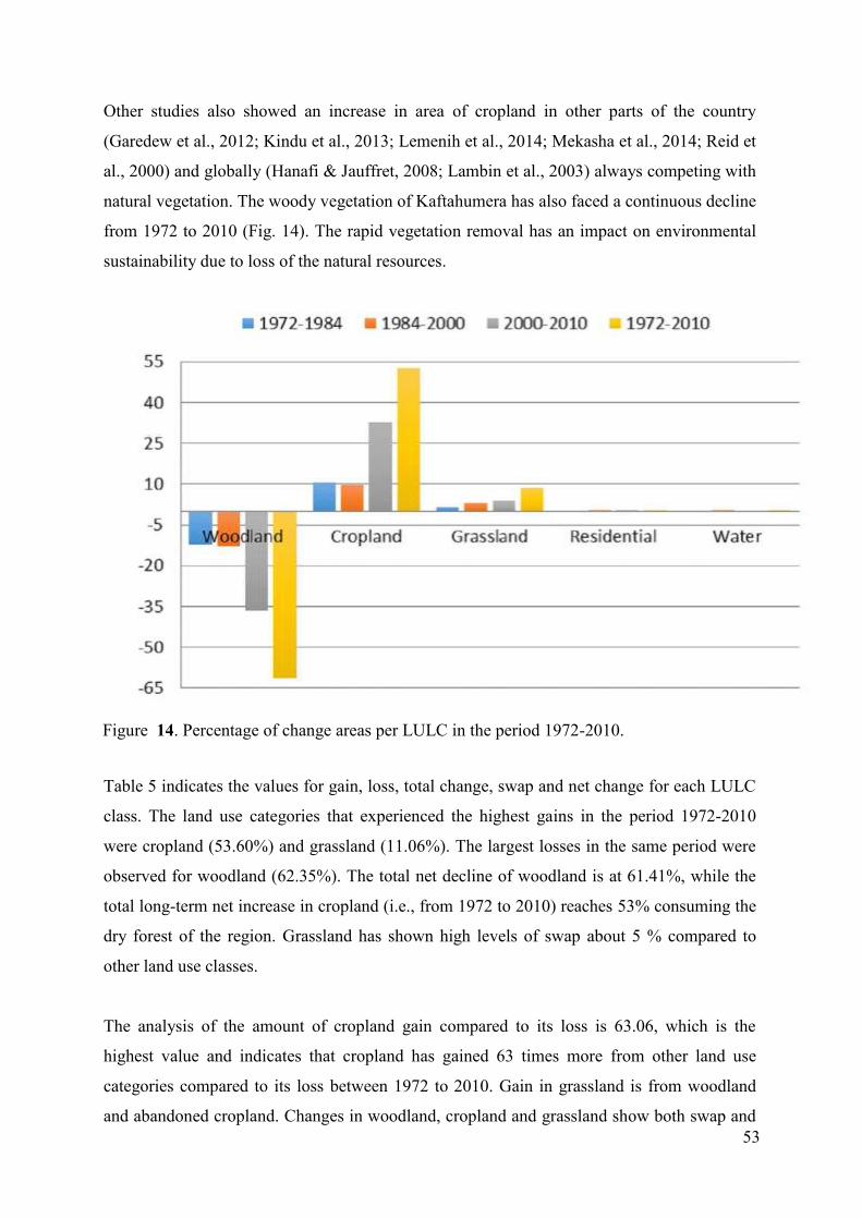
53

Other studies also showed an increase in area of cropland in other parts of the country

(Garedew et al., 2012; Kindu et al., 2013; Lemenih et al., 2014; Mekasha et al., 2014; Reid et

al., 2000) and globally (Hanafi & Jauffret, 2008; Lambin et al., 2003) always competing with

natural vegetation. The woody vegetation of Kaftahumera has also faced a continuous decline

from 1972 to 2010 (Fig. 14). The rapid vegetation removal has an impact on environmental

sustainability due to loss of the natural resources.

Figure 14. Percentage of change areas per LULC in the period 1972-2010.

Table 5 indicates the values for gain, loss, total change, swap and net change for each LULC

class. The land use categories that experienced the highest gains in the period 1972-2010

were cropland (53.60%) and grassland (11.06%). The largest losses in the same period were

observed for woodland (62.35%). The total net decline of woodland is at 61.41%, while the

total long-term net increase in cropland (i.e., from 1972 to 2010) reaches 53% consuming the

dry forest of the region. Grassland has shown high levels of swap about 5 % compared to

other land use classes.

The analysis of the amount of cropland gain compared to its loss is 63.06, which is the

highest value and indicates that cropland has gained 63 times more from other land use

categories compared to its loss between 1972 to 2010. Gain in grassland is from woodland

and abandoned cropland. Changes in woodland, cropland and grassland show both swap and

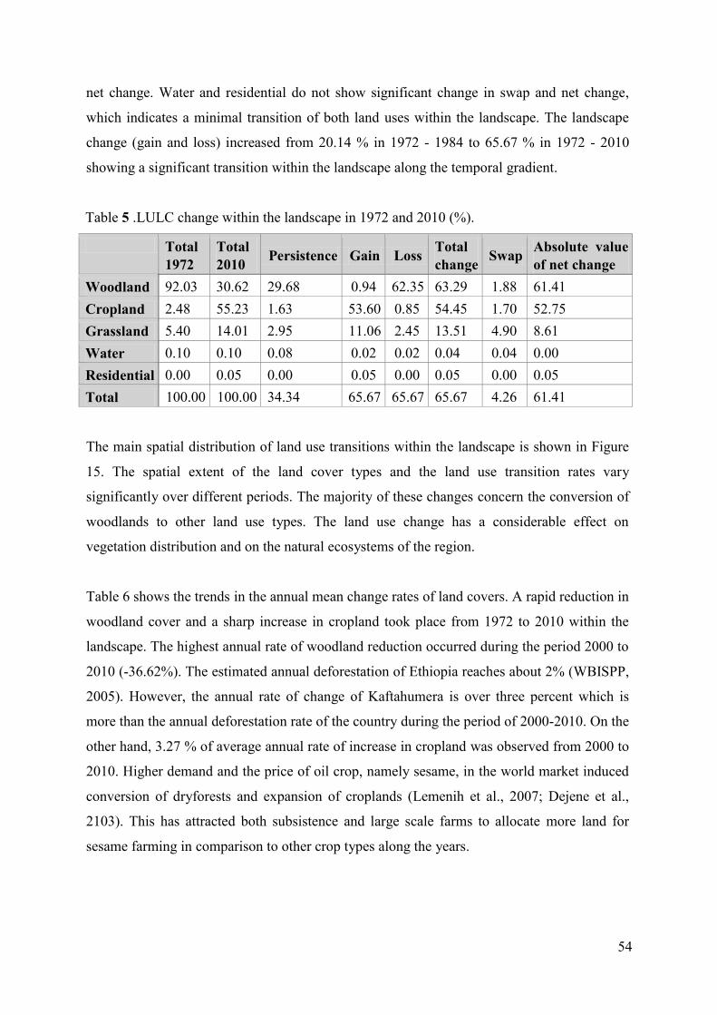
54

net change. Water and residential do not show significant change in swap and net change,

which indicates a minimal transition of both land uses within the landscape. The landscape

change (gain and loss) increased from 20.14 % in 1972 - 1984 to 65.67 % in 1972 - 2010

showing a significant transition within the landscape along the temporal gradient.

Table 5 .LULC change within the landscape in 1972 and 2010 (%).

Total 1972

Total 2010 Persistence Gain Loss Total

change Swap Absolute value of net change

Woodland 92.03 30.62 29.68 0.94 62.35 63.29 1.88 61.41 Cropland 2.48 55.23 1.63 53.60 0.85 54.45 1.70 52.75 Grassland 5.40 14.01 2.95 11.06 2.45 13.51 4.90 8.61 Water 0.10 0.10 0.08 0.02 0.02 0.04 0.04 0.00 Residential 0.00 0.05 0.00 0.05 0.00 0.05 0.00 0.05 Total 100.00 100.00 34.34 65.67 65.67 65.67 4.26 61.41

The main spatial distribution of land use transitions within the landscape is shown in Figure

15. The spatial extent of the land cover types and the land use transition rates vary

significantly over different periods. The majority of these changes concern the conversion of

woodlands to other land use types. The land use change has a considerable effect on

vegetation distribution and on the natural ecosystems of the region.

Table 6 shows the trends in the annual mean change rates of land covers. A rapid reduction in

woodland cover and a sharp increase in cropland took place from 1972 to 2010 within the

landscape. The highest annual rate of woodland reduction occurred during the period 2000 to

2010 (-36.62%). The estimated annual deforestation of Ethiopia reaches about 2% (WBISPP,

2005). However, the annual rate of change of Kaftahumera is over three percent which is

more than the annual deforestation rate of the country during the period of 2000-2010. On the

other hand, 3.27 % of average annual rate of increase in cropland was observed from 2000 to

2010. Higher demand and the price of oil crop, namely sesame, in the world market induced

conversion of dryforests and expansion of croplands (Lemenih et al., 2007; Dejene et al.,

2103). This has attracted both subsistence and large scale farms to allocate more land for

sesame farming in comparison to other crop types along the years.

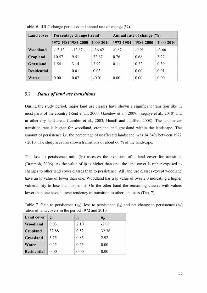
55

Table 6.LULC change per class and annual rate of change (%).

Land cover Percentage change (trend) Annual rate of change (%)

1972-1984 1984-2000 2000-2010 1972-1984 1984-2000 2000-2010

Woodland -12.12 -12.67 -36.62 -0.87 -0.91 -3.66

Cropland 10.57 9.51 32.67 0.76 0.68 3.27

Grassland 1.54 3.14 3.92 0.11 0.22 0.39

Residential 0.01 0.03 0.00 0.01

Water 0.00 0.02 -0.01 0.00 0.00 0.00

5.2 Status of land use transitions

During the study period, major land use classes have shown a significant transition like in

most parts of the country (Reid et al., 2000; Garedew et al., 2009; Tsegaye et al., 2010) and

in other dry land areas (Lambin et al., 2003; Hanafi and Jauffret, 2008). The land cover

transition rate is higher for woodland, cropland and grassland within the landscape. The

amount of persistence i.e. the percentage of unaffected landscape, was 34.34% between 1972

- 2010. The study area has shown transitions of about 66 % of the landscape.

The loss to persistence ratio (lp) assesses the exposure of a land cover for transition

(Braimoh, 2006). As the value of lp is higher than one, the land cover is rather exposed to

changes to other land cover classes than to persistence. All land use classes except woodland

have an lp value of lower than one. Woodland has a lp value of over 2.0 indicating a higher

vulnerability to lose than to persist. On the other hand the remaining classes with values

lower than one have a lower tendency of transition to other land uses (Tab. 7).

Table 7. Gain to persistence (gp), loss to persistence (lp) and net change to persistence (np) ratios of land covers in the period 1972 and 2010. Land cover gp lp np

Woodland 0.03 2.10 -2.07

Cropland 32.88 0.52 32.36

Grassland 3.75 0.83 2.92

Water 0.25 0.25 0.00

Residential 0.00 0.00 0.00

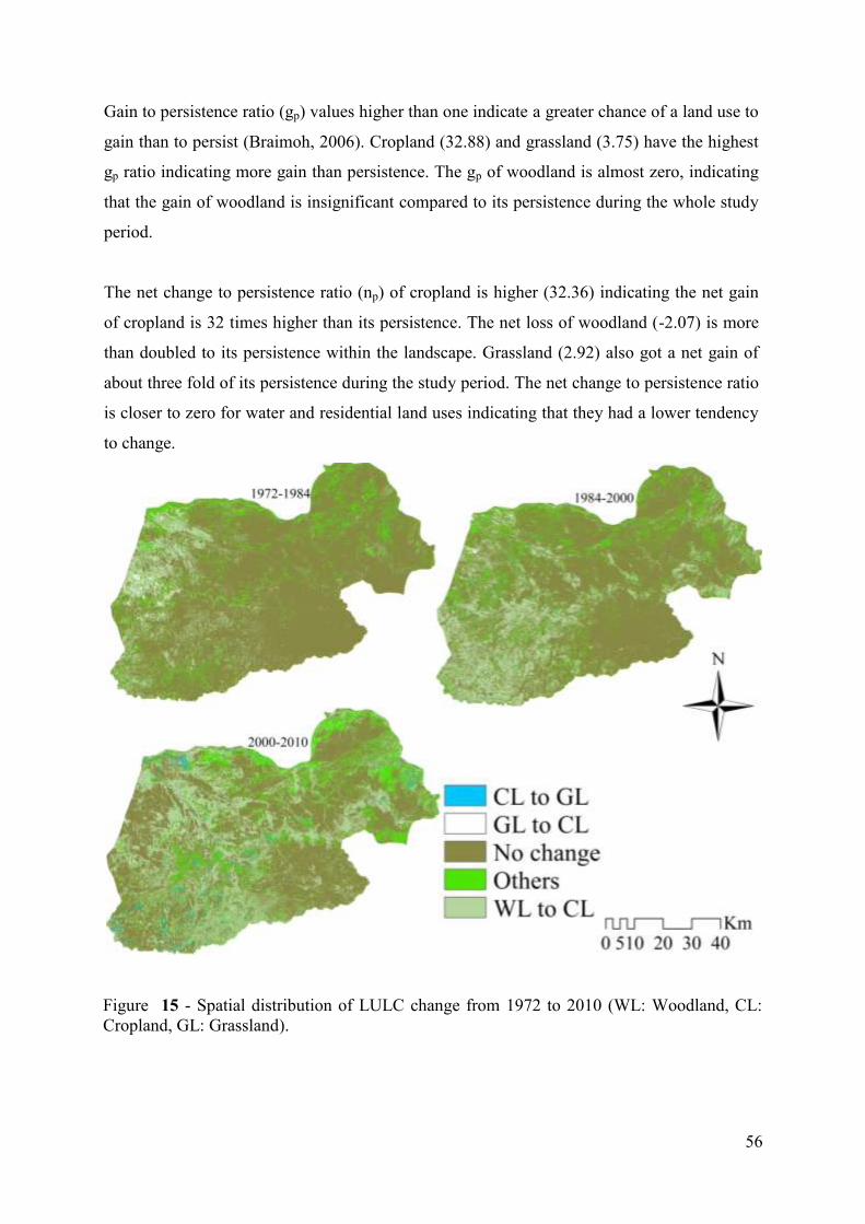
56

Gain to persistence ratio (gp) values higher than one indicate a greater chance of a land use to

gain than to persist (Braimoh, 2006). Cropland (32.88) and grassland (3.75) have the highest

gp ratio indicating more gain than persistence. The gp of woodland is almost zero, indicating

that the gain of woodland is insignificant compared to its persistence during the whole study

period.

The net change to persistence ratio (np) of cropland is higher (32.36) indicating the net gain

of cropland is 32 times higher than its persistence. The net loss of woodland (-2.07) is more

than doubled to its persistence within the landscape. Grassland (2.92) also got a net gain of

about three fold of its persistence during the study period. The net change to persistence ratio

is closer to zero for water and residential land uses indicating that they had a lower tendency

to change.

Figure 15 - Spatial distribution of LULC change from 1972 to 2010 (WL: Woodland, CL: Cropland, GL: Grassland).

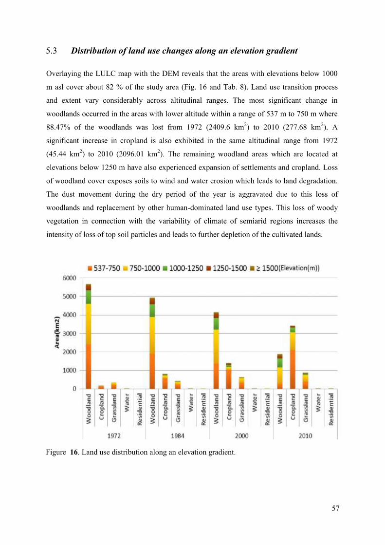
57

5.3 Distribution of land use changes along an elevation gradient

Overlaying the LULC map with the DEM reveals that the areas with elevations below 1000

m asl cover about 82 % of the study area (Fig. 16 and Tab. 8). Land use transition process

and extent vary considerably across altitudinal ranges. The most significant change in

woodlands occurred in the areas with lower altitude within a range of 537 m to 750 m where

88.47% of the woodlands was lost from 1972 (2409.6 km2) to 2010 (277.68 km2). A

significant increase in cropland is also exhibited in the same altitudinal range from 1972

(45.44 km2) to 2010 (2096.01 km2). The remaining woodland areas which are located at

elevations below 1250 m have also experienced expansion of settlements and cropland. Loss

of woodland cover exposes soils to wind and water erosion which leads to land degradation.

The dust movement during the dry period of the year is aggravated due to this loss of

woodlands and replacement by other human-dominated land use types. This loss of woody

vegetation in connection with the variability of climate of semiarid regions increases the

intensity of loss of top soil particles and leads to further depletion of the cultivated lands.

Figure 16. Land use distribution along an elevation gradient.

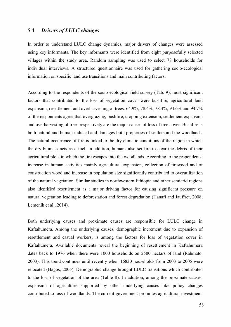
58

5.4 Drivers of LULC changes

In order to understand LULC change dynamics, major drivers of changes were assessed

using key informants. The key informants were identified from eight purposefully selected

villages within the study area. Random sampling was used to select 78 households for

individual interviews. A structured questionnaire was used for gathering socio-ecological

information on specific land use transitions and main contributing factors.

According to the respondents of the socio-ecological field survey (Tab. 9), most significant

factors that contributed to the loss of vegetation cover were bushfire, agricultural land

expansion, resettlement and overharvesting of trees. 64.9%, 78.4%, 78.4%, 94.6% and 94.7%

of the respondents agree that overgrazing, bushfire, cropping extension, settlement expansion

and overharvesting of trees respectively are the major causes of loss of tree cover. Bushfire is

both natural and human induced and damages both properties of settlers and the woodlands.

The natural occurrence of fire is linked to the dry climatic conditions of the region in which

the dry biomass acts as a fuel. In addition, humans also set fire to clear the debris of their

agricultural plots in which the fire escapes into the woodlands. According to the respondents,

increase in human activities mainly agricultural expansion, collection of firewood and of

construction wood and increase in population size significantly contributed to overutilization

of the natural vegetation. Similar studies in northwestern Ethiopia and other semiarid regions

also identified resettlement as a major driving factor for causing significant pressure on

natural vegetation leading to deforestation and forest degradation (Hanafi and Jauffret, 2008;

Lemenih et al., 2014).

Both underlying causes and proximate causes are responsible for LULC change in

Kaftahumera. Among the underlying causes, demographic increment due to expansion of

resettlement and casual workers, is among the factors for loss of vegetation cover in

Kaftahumera. Available documents reveal the beginning of resettlement in Kaftahumera

dates back to 1976 when there were 1000 households on 2500 hectars of land (Rahmato,

2003). This trend continues until recently when 16830 households from 2003 to 2005 were

relocated (Hagos, 2005). Demographic change brought LULC transitions which contributed

to the loss of vegetation of the area (Table 8). In addition, among the proximate causes,

expansion of agriculture supported by other underlying causes like policy changes

contributed to loss of woodlands. The current government promotes agricultural investment.

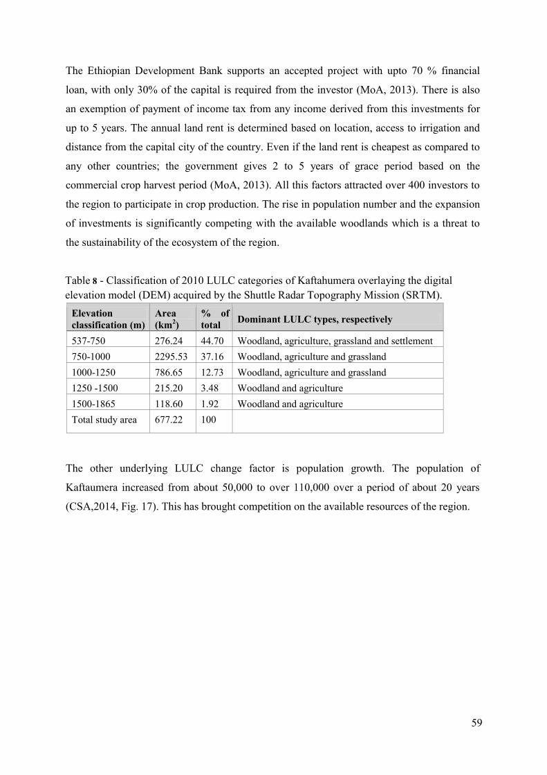
59

The Ethiopian Development Bank supports an accepted project with upto 70 % financial

loan, with only 30% of the capital is required from the investor (MoA, 2013). There is also

an exemption of payment of income tax from any income derived from this investments for

up to 5 years. The annual land rent is determined based on location, access to irrigation and

distance from the capital city of the country. Even if the land rent is cheapest as compared to

any other countries; the government gives 2 to 5 years of grace period based on the

commercial crop harvest period (MoA, 2013). All this factors attracted over 400 investors to

the region to participate in crop production. The rise in population number and the expansion

of investments is significantly competing with the available woodlands which is a threat to

the sustainability of the ecosystem of the region.

Table 8 - Classification of 2010 LULC categories of Kaftahumera overlaying the digital elevation model (DEM) acquired by the Shuttle Radar Topography Mission (SRTM).

Elevation classification (m)

Area (km2)

% of total Dominant LULC types, respectively

537-750 276.24 44.70 Woodland, agriculture, grassland and settlement 750-1000 2295.53 37.16 Woodland, agriculture and grassland 1000-1250 786.65 12.73 Woodland, agriculture and grassland 1250 -1500 215.20 3.48 Woodland and agriculture 1500-1865 118.60 1.92 Woodland and agriculture Total study area 677.22 100

The other underlying LULC change factor is population growth. The population of

Kaftaumera increased from about 50,000 to over 110,000 over a period of about 20 years

(CSA,2014, Fig. 17). This has brought competition on the available resources of the region.

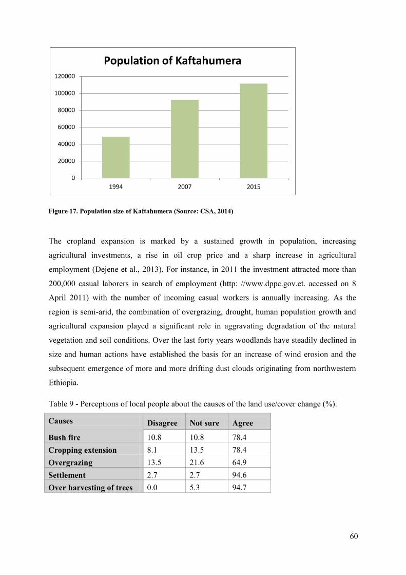
60

Figure 17. Population size of Kaftahumera (Source: CSA, 2014)

The cropland expansion is marked by a sustained growth in population, increasing

agricultural investments, a rise in oil crop price and a sharp increase in agricultural

employment (Dejene et al., 2013). For instance, in 2011 the investment attracted more than

200,000 casual laborers in search of employment (http: //www.dppc.gov.et. accessed on 8

April 2011) with the number of incoming casual workers is annually increasing. As the

region is semi-arid, the combination of overgrazing, drought, human population growth and

agricultural expansion played a significant role in aggravating degradation of the natural

vegetation and soil conditions. Over the last forty years woodlands have steadily declined in

size and human actions have established the basis for an increase of wind erosion and the

subsequent emergence of more and more drifting dust clouds originating from northwestern

Ethiopia.

Table 9 - Perceptions of local people about the causes of the land use/cover change (%).

Causes Disagree Not sure Agree

Bush fire 10.8 10.8 78.4 Cropping extension 8.1 13.5 78.4 Overgrazing 13.5 21.6 64.9 Settlement 2.7 2.7 94.6 Over harvesting of trees 0.0 5.3 94.7

0

20000

40000

60000

80000

100000

120000

1994 2007 2015

Population of Kaftahumera

61

5.5 Summary LULC change detection evaluates spatiotemporal change patterns and identifies the

quantitative dimension of transitions within a landscape. This study examines the LULC

changes of the semi-arid regions of Kaftahumera using multitemporal satellite imagery for

the period 1972-2010 that provides current and historical LULC conditions. Supervised

classification algorithm using SVM algorithm was employed to monitor LULC

transformations. A cross-tabulation matrix was used to assess the total change of land

categories based on net change and swap. Over the study period, there is a significant change

in LULC, as evidenced by a sharp increase in cropland of about 53% and a net loss of over

61% of woodland within the landscape. The period 2000-2010 has shown a sharp increase of

cropland and a sharp decline of woodland areas. The underlying causes mainly policy

changes, population growth and proximate causes like cropland expansion, wood harvesting

are the main driving factors of LULC change in Kaftahumera. Changes in economic growth

and human activities contributed to an overuse of existing natural resources, which resulted

in significant variations in the spatiotemporal patterns of land use changes with respect to

specific altitudinal ranges. The dominant changes are exhibited in areas with elevations

below 1000 m with a loss of 74% of woodlands from 1972 to 2010.

Human activities, such as agriculture and settlement expansion, severely influenced the

drylands by modifying the landscape and diminishing its natural ecosystem. Over the last

forty years the woodlands have steadily declined in size and have been replaced by

croplands. The combination of overgrazing, population growth and agricultural expansion

contributed to the degradation of the woodlands of the region. The disturbance of the

respective woodland ecosystem is closely related to the occurrence of significant land use

transformation within the region. This change may result in an irreversible loss of

biodiversity and in the depletion of ecological services provided by the natural environment.

The results of this study quantify dynamics of land cover change and point towards

appropriate action to implement sustainable use of the ecosystem. In the face of increasing

population size and consequent need for intensifying exploitation of resources, it is vital to

maintain a balance of sustainable utilization. Thus, it is crucial to further develop and

enhance methods of periodical monitoring and assessment of LULC change in order to

evaluate the environmental influences on semi-arid ecosystems that are increasingly affected

by human impact.

63

6. Chapter 6: Categorical land use transition and land degradation in the northwestern Ethiopia.

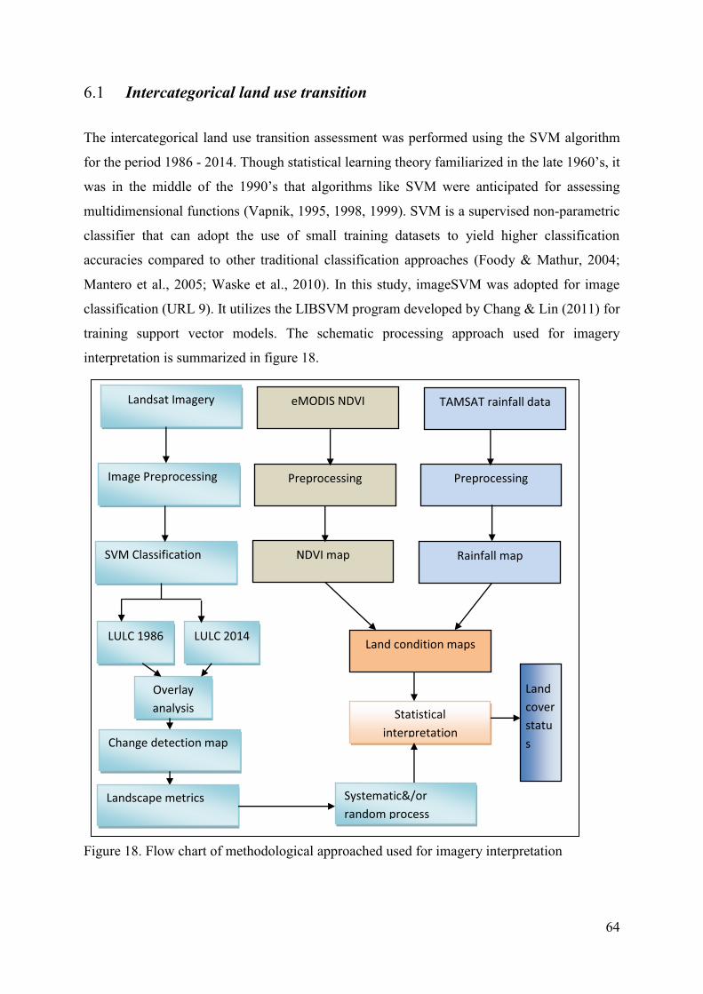
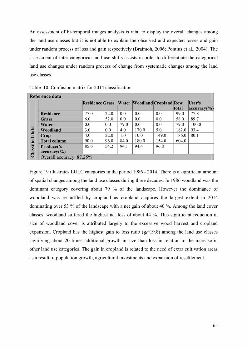
65

An assessment of bi-temporal images analysis is vital to display the overall changes among

the land use classes but it is not able to explain the observed and expected losses and gain

under random process of loss and gain respectively (Braimoh, 2006; Pontius et al., 2004). The

assessment of inter-categorical land use shifts assists in order to differentiate the categorical

land use changes under random process of change from systematic changes among the land

use classes.

Table 10. Confusion matrix for 2014 classification.

Reference data

Cla

ssifi

ed d

ata

Residence Grass Water Woodland Cropland Row total

User's accuracy(%)

Residence 77.0 22.0 0.0 0.0 0.0 99.0 77.8 Grass 6.0 52.0 0.0 0.0 0.0 58.0 89.7 Water 0.0 0.0 79.0 0.0 0.0 79.0 100.0 Woodland 3.0 0.0 4.0 170.0 5.0 182.0 93.4 Crop 4.0 22.0 1.0 10.0 149.0 186.0 80.1 Total column 90.0 96.0 84.0 180.0 154.0 604.0 Producer's accuracy(%)

85.6 54.2 94.1 94.4 96.8

Overall accuracy 87.25%

Figure 19 illustrates LULC categories in the period 1986 - 2014. There is a significant amount

of spatial changes among the land use classes during three decades. In 1986 woodland was the

dominant category covering about 79 % of the landscape. However the dominance of

woodland was reshuffled by cropland as cropland acquires the largest extent in 2014

dominating over 53 % of the landscape with a net gain of about 40 %. Among the land cover

classes, woodland suffered the highest net loss of about 44 %. This significant reduction in

size of woodland cover is attributed largely to the excessive wood harvest and cropland

expansion. Cropland has the highest gain to loss ratio (gl=19.8) among the land use classes

signifying about 20 times additional growth in size than loss in relation to the increase in

other land use categories. The gain in cropland is related to the need of extra cultivation areas

as a result of population growth, agricultural investments and expansion of resettlement

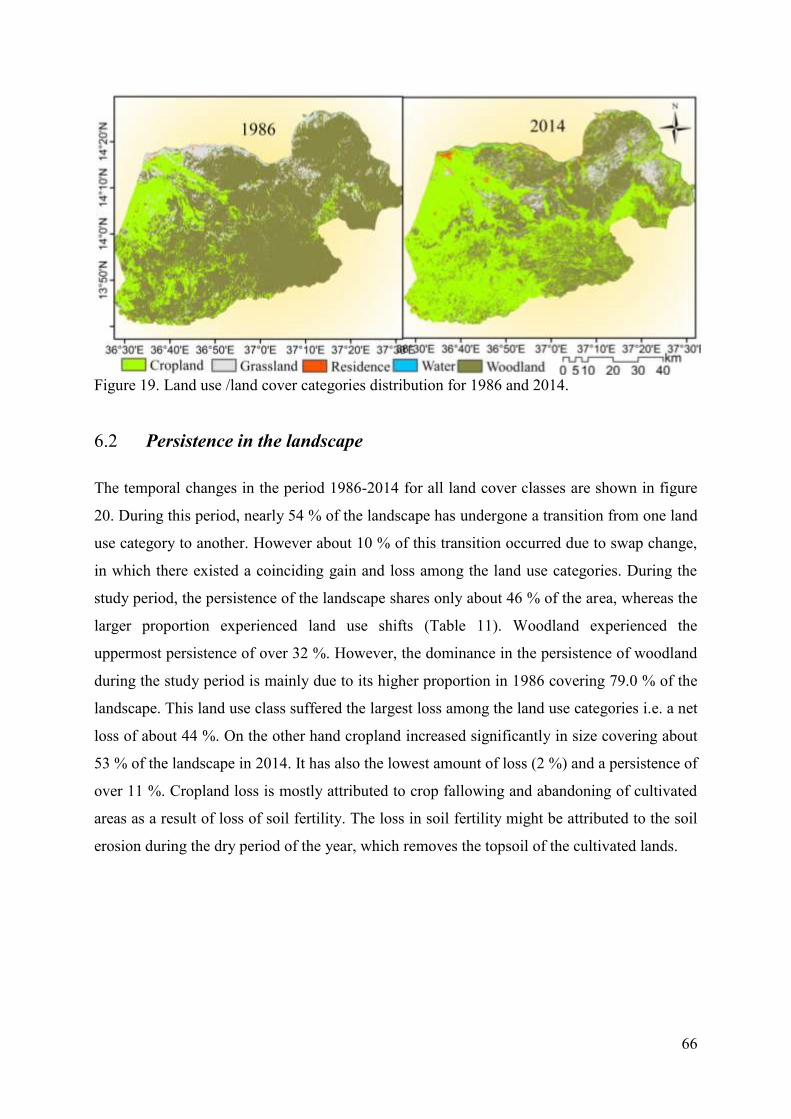
66

Figure 19. Land use /land cover categories distribution for 1986 and 2014.

6.2 Persistence in the landscape

The temporal changes in the period 1986-2014 for all land cover classes are shown in figure

20. During this period, nearly 54 % of the landscape has undergone a transition from one land

use category to another. However about 10 % of this transition occurred due to swap change,

in which there existed a coinciding gain and loss among the land use categories. During the

study period, the persistence of the landscape shares only about 46 % of the area, whereas the

larger proportion experienced land use shifts (Table 11). Woodland experienced the

uppermost persistence of over 32 %. However, the dominance in the persistence of woodland

during the study period is mainly due to its higher proportion in 1986 covering 79.0 % of the

landscape. This land use class suffered the largest loss among the land use categories i.e. a net

loss of about 44 %. On the other hand cropland increased significantly in size covering about

53 % of the landscape in 2014. It has also the lowest amount of loss (2 %) and a persistence of

over 11 %. Cropland loss is mostly attributed to crop fallowing and abandoning of cultivated

areas as a result of loss of soil fertility. The loss in soil fertility might be attributed to the soil

erosion during the dry period of the year, which removes the topsoil of the cultivated lands.

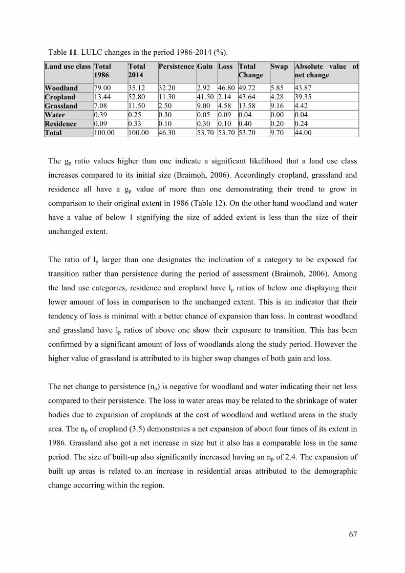
67

Table 11. LULC changes in the period 1986-2014 (%).

Land use class Total 1986

Total 2014

Persistence Gain Loss Total Change

Swap Absolute value of net change

Woodland 79.00 35.12 32.20 2.92 46.80 49.72 5.85 43.87 Cropland 13.44 52.80 11.30 41.50 2.14 43.64 4.28 39.35 Grassland 7.08 11.50 2.50 9.00 4.58 13.58 9.16 4.42 Water 0.39 0.25 0.30 0.05 0.09 0.04 0.00 0.04 Residence 0.09 0.33 0.10 0.30 0.10 0.40 0.20 0.24 Total 100.00 100.00 46.30 53.70 53.70 53.70 9.70 44.00

The gp ratio values higher than one indicate a significant likelihood that a land use class

increases compared to its initial size (Braimoh, 2006). Accordingly cropland, grassland and

residence all have a gp value of more than one demonstrating their trend to grow in

comparison to their original extent in 1986 (Table 12). On the other hand woodland and water

have a value of below 1 signifying the size of added extent is less than the size of their

unchanged extent.

The ratio of lp larger than one designates the inclination of a category to be exposed for

transition rather than persistence during the period of assessment (Braimoh, 2006). Among

the land use categories, residence and cropland have lp ratios of below one displaying their

lower amount of loss in comparison to the unchanged extent. This is an indicator that their

tendency of loss is minimal with a better chance of expansion than loss. In contrast woodland

and grassland have lp ratios of above one show their exposure to transition. This has been

confirmed by a significant amount of loss of woodlands along the study period. However the

higher value of grassland is attributed to its higher swap changes of both gain and loss.

The net change to persistence (np) is negative for woodland and water indicating their net loss

compared to their persistence. The loss in water areas may be related to the shrinkage of water

bodies due to expansion of croplands at the cost of woodland and wetland areas in the study

area. The np of cropland (3.5) demonstrates a net expansion of about four times of its extent in

1986. Grassland also got a net increase in size but it also has a comparable loss in the same

period. The size of built-up also significantly increased having an np of 2.4. The expansion of

built up areas is related to an increase in residential areas attributed to the demographic

change occurring within the region.

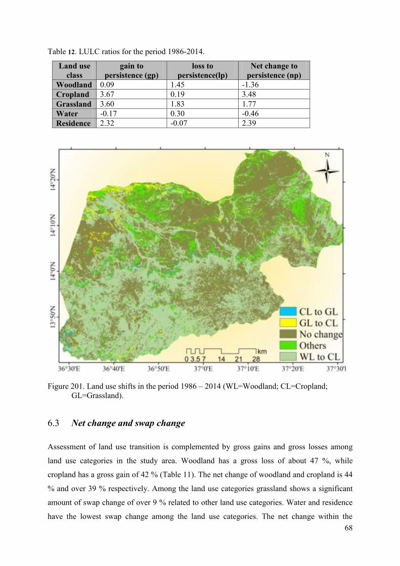
68

Table 12. LULC ratios for the period 1986-2014.

Land use class

gain to persistence (gp)

loss to persistence(lp)

Net change to persistence (np)

Woodland 0.09 1.45 -1.36 Cropland 3.67 0.19 3.48 Grassland 3.60 1.83 1.77 Water -0.17 0.30 -0.46 Residence 2.32 -0.07 2.39

Figure 201. Land use shifts in the period 1986 – 2014 (WL=Woodland; CL=Cropland; GL=Grassland).

6.3 Net change and swap change

Assessment of land use transition is complemented by gross gains and gross losses among

land use categories in the study area. Woodland has a gross loss of about 47 %, while

cropland has a gross gain of 42 % (Table 11). The net change of woodland and cropland is 44

% and over 39 % respectively. Among the land use categories grassland shows a significant

amount of swap change of over 9 % related to other land use categories. Water and residence

have the lowest swap change among the land use categories. The net change within the

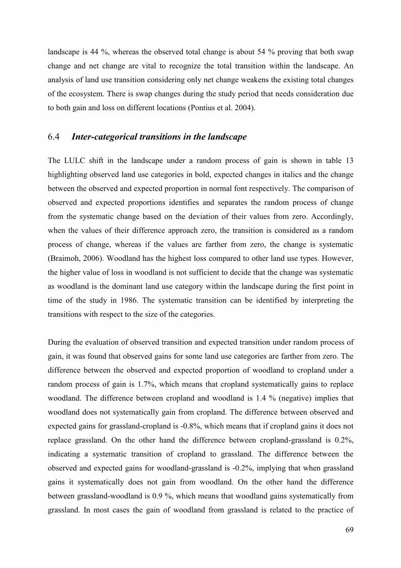
69

landscape is 44 %, whereas the observed total change is about 54 % proving that both swap

change and net change are vital to recognize the total transition within the landscape. An

analysis of land use transition considering only net change weakens the existing total changes

of the ecosystem. There is swap changes during the study period that needs consideration due

to both gain and loss on different locations (Pontius et al. 2004).

6.4 Inter-categorical transitions in the landscape

The LULC shift in the landscape under a random process of gain is shown in table 13

highlighting observed land use categories in bold, expected changes in italics and the change

between the observed and expected proportion in normal font respectively. The comparison of

observed and expected proportions identifies and separates the random process of change

from the systematic change based on the deviation of their values from zero. Accordingly,

when the values of their difference approach zero, the transition is considered as a random

process of change, whereas if the values are farther from zero, the change is systematic

(Braimoh, 2006). Woodland has the highest loss compared to other land use types. However,

the higher value of loss in woodland is not sufficient to decide that the change was systematic

as woodland is the dominant land use category within the landscape during the first point in

time of the study in 1986. The systematic transition can be identified by interpreting the

transitions with respect to the size of the categories.

During the evaluation of observed transition and expected transition under random process of

gain, it was found that observed gains for some land use categories are farther from zero. The

difference between the observed and expected proportion of woodland to cropland under a

random process of gain is 1.7%, which means that cropland systematically gains to replace

woodland. The difference between cropland and woodland is 1.4 % (negative) implies that

woodland does not systematically gain from cropland. The difference between observed and

expected gains for grassland-cropland is -0.8%, which means that if cropland gains it does not

replace grassland. On the other hand the difference between cropland-grassland is 0.2%,

indicating a systematic transition of cropland to grassland. The difference between the

observed and expected gains for woodland-grassland is -0.2%, implying that when grassland

gains it systematically does not gain from woodland. On the other hand the difference

between grassland-woodland is 0.9 %, which means that woodland gains systematically from

grassland. In most cases the gain of woodland from grassland is related to the practice of

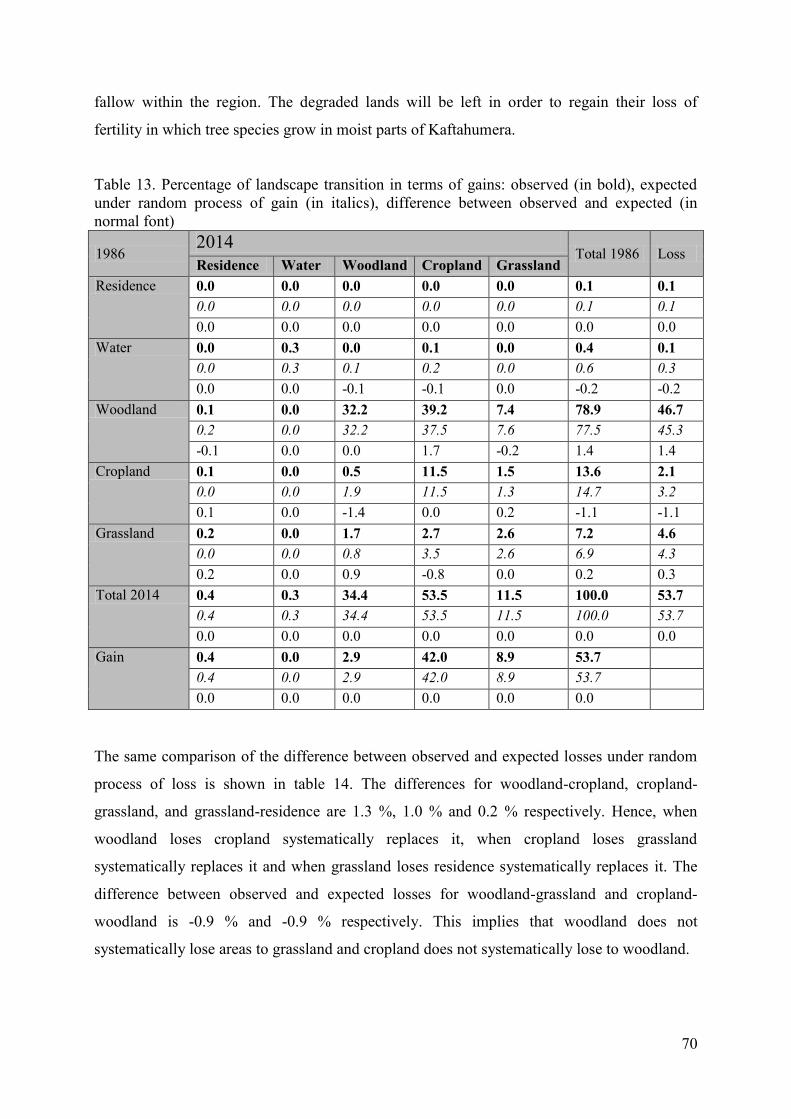
70

fallow within the region. The degraded lands will be left in order to regain their loss of

fertility in which tree species grow in moist parts of Kaftahumera.

Table 13. Percentage of landscape transition in terms of gains: observed (in bold), expected under random process of gain (in italics), difference between observed and expected (in normal font)

1986 2014 Total 1986 Loss

Residence Water Woodland Cropland Grassland Residence 0.0 0.0 0.0 0.0 0.0 0.1 0.1

0.0 0.0 0.0 0.0 0.0 0.1 0.1 0.0 0.0 0.0 0.0 0.0 0.0 0.0

Water 0.0 0.3 0.0 0.1 0.0 0.4 0.1 0.0 0.3 0.1 0.2 0.0 0.6 0.3 0.0 0.0 -0.1 -0.1 0.0 -0.2 -0.2

Woodland 0.1 0.0 32.2 39.2 7.4 78.9 46.7 0.2 0.0 32.2 37.5 7.6 77.5 45.3 -0.1 0.0 0.0 1.7 -0.2 1.4 1.4

Cropland 0.1 0.0 0.5 11.5 1.5 13.6 2.1 0.0 0.0 1.9 11.5 1.3 14.7 3.2 0.1 0.0 -1.4 0.0 0.2 -1.1 -1.1

Grassland 0.2 0.0 1.7 2.7 2.6 7.2 4.6 0.0 0.0 0.8 3.5 2.6 6.9 4.3 0.2 0.0 0.9 -0.8 0.0 0.2 0.3

Total 2014 0.4 0.3 34.4 53.5 11.5 100.0 53.7 0.4 0.3 34.4 53.5 11.5 100.0 53.7 0.0 0.0 0.0 0.0 0.0 0.0 0.0

Gain 0.4 0.0 2.9 42.0 8.9 53.7 0.4 0.0 2.9 42.0 8.9 53.7 0.0 0.0 0.0 0.0 0.0 0.0

The same comparison of the difference between observed and expected losses under random

process of loss is shown in table 14. The differences for woodland-cropland, cropland-

grassland, and grassland-residence are 1.3 %, 1.0 % and 0.2 % respectively. Hence, when

woodland loses cropland systematically replaces it, when cropland loses grassland

systematically replaces it and when grassland loses residence systematically replaces it. The

difference between observed and expected losses for woodland-grassland and cropland-

woodland is -0.9 % and -0.9 % respectively. This implies that woodland does not

systematically lose areas to grassland and cropland does not systematically lose to woodland.

71

Table 14. Percentage of landscape transition in terms of losses: observed (in bold), expected under random process of loss (in italics), difference between observed and expected (in normal font) 1986

2014 Total 1986

Loss Residence Water Woodland Cropland Grassland

Residence

0.0 0.0 0.0 0.0 0.0 0.1 0.1 0.0 0.0 0.0 0.1 0.0 0.1 0.1 0.0 0.0 0.0 -0.1 0.0 0.0 0.0

Water

0.0 0.3 0.0 0.1 0.0 0.4 0.1 0.0 0.3 0.0 0.1 0.0 0.4 0.1 0.0 0.0 0.0 0.0 0.0 0.0 0.0

Woodland

0.1 0.0 32.2 39.2 7.4 78.9 46.7 0.2 0.2 32.2 37.9 8.3 78.9 46.7 -0.1 -0.2 0.0 1.3 -0.9 0.0 0.0

Cropland

0.1 0.0 0.5 11.5 1.5 13.6 2.1 0.0 0.0 1.4 11.5 0.5 13.6 2.1 0.1 0.0 -0.9 0.0 1.0 0.0 0.0

Grass

0.2 0.0 1.8 2.7 2.6 7.2 4.6 0.0 0.0 1.7 2.7 2.6 7.2 4.6 0.2 0.0 0.1 0.0 0.0 0.0 0.0

Total 2014

0.4 0.3 34.5 53.5 11.5 100.0 53.7 0.2 0.5 35.3 52.2 11.4 100.0 53.7 0.2 -0.2 -0.8 1.3 0.1 0.0 0.0

Gain

0.3 0.0 2.3 42.0 8.9 53.7 0.2 0.2 3.1 40.7 8.8 53.7 0.1 -0.2 -0.8 1.3 0.1 0.0

6.5 Land degradation in drylands of northwestern Ethiopia

There are pertinent land-use changes, mainly characterized as gradual transitions, over

Kaftahumera. LULC change assessment of the region shows that about 54 % of the area

undergoes transitions from natural ecosystem to human dominated activities. The removal of

the protective cover leaves the soil highly vulnerable to wind erosion, particularly during the

dry period of the year. Human activities, mainly firewood collection, agricultural land

expansion and expansion of settlement are the main driving forces influencing the change in

vegetation cover of semiarid woodlands of northwestern Ethiopia.

The Sudano-Sahelian region is known as a source of soil-derived aerosols into the atmosphere

which moves southwards towards the northwestern drylands of Ethiopia and further to the

Red Sea (Middleton, 1985). However, in recent years, it is common to observe dust clouds

hovering over the northwestern regions of the country originating between the borders of

northwestern drylands of Ethiopia and Sudan (URL 4). The change in vegetation cover and

the degradation of woodlands that protect the topsoil from wind erosion play a vital role in the

72

accelerated wind erosion. The remarkable changes in agricultural practices and open access to

dryforests have been exacerbating the exposure of the dryforests for change. These

anthropogenic activities are among the driving factors for the degradation of the dryland

ecosystem functions (Foley, 2005). Hence dryland vegetation change contributes to land

degradation in terms of increase of surface albedo and soil moisture retention, exposing the

inherently weak topsoil for both wind and water erosion (Sivakumar, 2007). The change in

vegetation cover of Kaftahumera has affected dust emission and loading which can be directly

attributed to man-made degradation of the environment.

Human land degradation which removes the vegetation cover increases the vulnerability of

the region for wind erosion (Cook et al., 2009). The loss of vegetation, accompanied by

cropland expansion, plays the main role in exposing the topsoil of Kaftahumera for wind

erosion. The severity of loss of vegetal cover is aggravating in most woodland areas of

Kaftahumera. Due to the extended land use changes, there might be a reduction in the

capacity of the land to provide ecosystem goods and services. Image analysis confirmed the

conversion of about 47% of the woody vegetation to other land use types affecting the natural

vegetation. The intensive mechanized farming, mainly for production of oil crops for

international markets, has contributed to the shrinking of the woodlands (Lemenih et al. 2014;

Zewdie & Csaplovics, 2014). In addition, the expansion of subsistence agriculture with ever

increasing population pressure competes with the natural vegetation of the region (Zewdie &

Csaplovics, 2015). The continuous exposure of the landscape for degradation eases the loss of

soil from the region. The soils being blown away from the landscape drain the soil through

transporting sediments and nutrients. Studies on climate change also show a stronger link

between vegetation change and dust aerosols in which precipitation of the Sahel region is

reduced due to changes in vegetation cover and increased occurrence of dust storms

(Yoshioka et al., 2007).

The bi-temporal change assessment of Landsat imagery is augmented by temporal NDVI and

rainfall analysis for detecting land condition. Accordingly a pixel-wise regression analysis

between rainfall data and NDVI was applied to investigate spatial relationships of vegetation

patterns and rainfall over the whole study area (Fig.21). The result shows a high spatial non-

stationary relationship between rainfall and NDVI within the landscape. The coefficient of

determination (R2) between rainfall and NDVI demonstrates a major difference in spatial

distribution, with about 55 % of the study area having low R2 values of below 0.5. The spatial

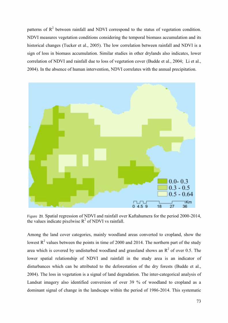
73

patterns of R2 between rainfall and NDVI correspond to the status of vegetation condition.

NDVI measures vegetation conditions considering the temporal biomass accumulation and its

historical changes (Tucker et al., 2005). The low correlation between rainfall and NDVI is a

sign of loss in biomass accumulation. Similar studies in other drylands also indicates, lower

correlation of NDVI and rainfall due to loss of vegetation cover (Budde et al., 2004; Li et al.,

2004). In the absence of human intervention, NDVI correlates with the annual precipitation.

Figure 21. Spatial regression of NDVI and rainfall over Kaftahumera for the period 2000-2014, the values indicate pixelwise R2 of NDVI vs rainfall.

Among the land cover categories, mainly woodland areas converted to cropland, show the

lowest R2 values between the points in time of 2000 and 2014. The northern part of the study

area which is covered by undisturbed woodland and grassland shows an R2 of over 0.5. The

lower spatial relationship of NDVI and rainfall in the study area is an indicator of

disturbances which can be attributed to the deforestation of the dry forests (Budde et al.,

2004). The loss in vegetation is a signal of land degradation. The inter-categorical analysis of

Landsat imagery also identified conversion of over 39 % of woodland to cropland as a

dominant signal of change in the landscape within the period of 1986-2014. This systematic

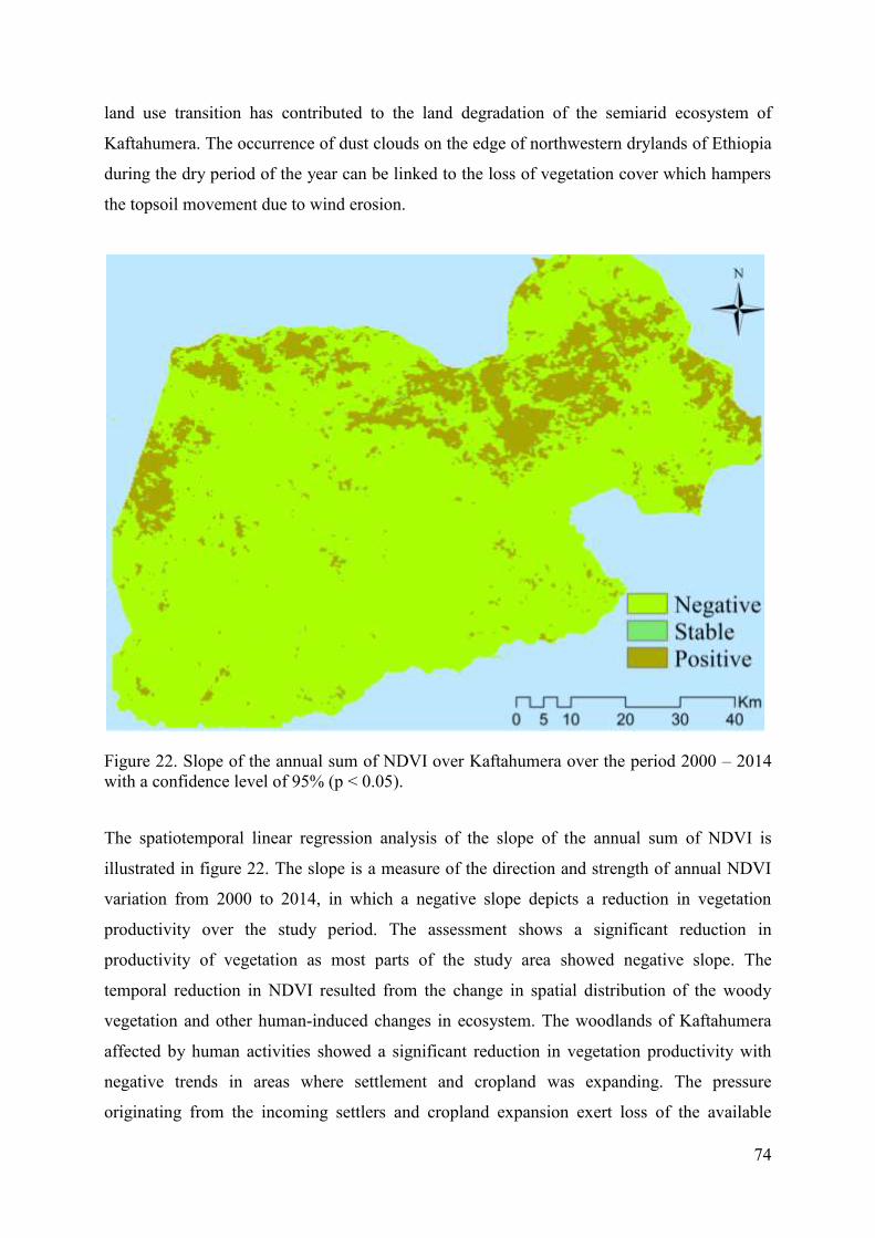
74

land use transition has contributed to the land degradation of the semiarid ecosystem of

Kaftahumera. The occurrence of dust clouds on the edge of northwestern drylands of Ethiopia

during the dry period of the year can be linked to the loss of vegetation cover which hampers

the topsoil movement due to wind erosion.

Figure 22. Slope of the annual sum of NDVI over Kaftahumera over the period 2000 – 2014 with a confidence level of 95% (p < 0.05).

The spatiotemporal linear regression analysis of the slope of the annual sum of NDVI is

illustrated in figure 22. The slope is a measure of the direction and strength of annual NDVI

variation from 2000 to 2014, in which a negative slope depicts a reduction in vegetation

productivity over the study period. The assessment shows a significant reduction in

productivity of vegetation as most parts of the study area showed negative slope. The

temporal reduction in NDVI resulted from the change in spatial distribution of the woody

vegetation and other human-induced changes in ecosystem. The woodlands of Kaftahumera

affected by human activities showed a significant reduction in vegetation productivity with

negative trends in areas where settlement and cropland was expanding. The pressure

originating from the incoming settlers and cropland expansion exert loss of the available

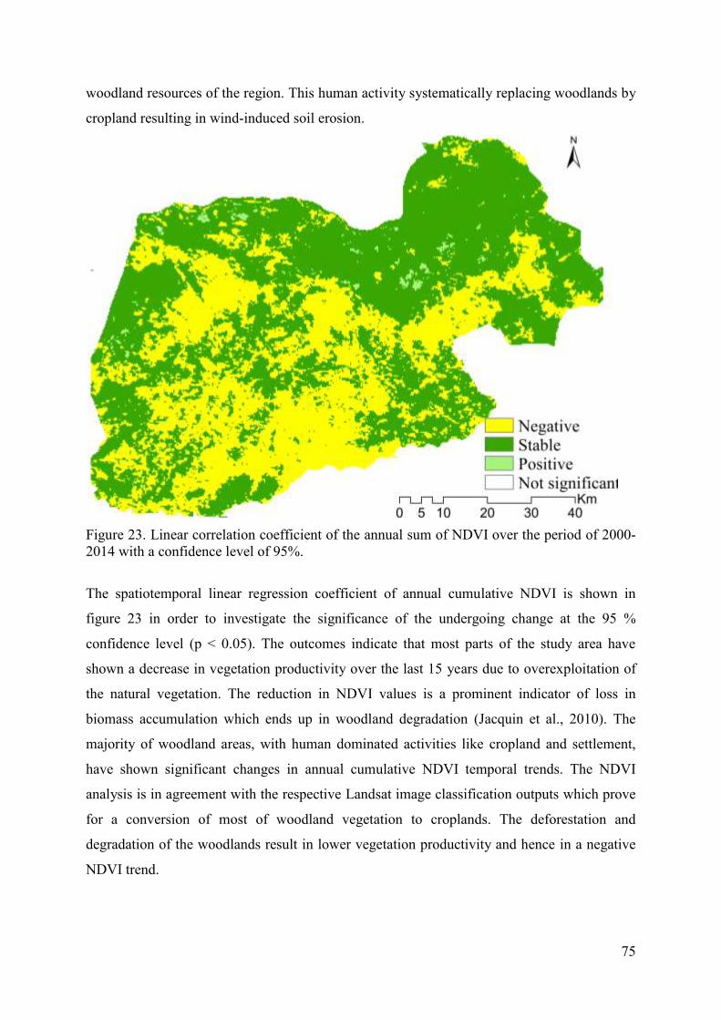
75

woodland resources of the region. This human activity systematically replacing woodlands by

cropland resulting in wind-induced soil erosion.

Figure 23. Linear correlation coefficient of the annual sum of NDVI over the period of 2000-2014 with a confidence level of 95%.

The spatiotemporal linear regression coefficient of annual cumulative NDVI is shown in

figure 23 in order to investigate the significance of the undergoing change at the 95 %

confidence level (p < 0.05). The outcomes indicate that most parts of the study area have

shown a decrease in vegetation productivity over the last 15 years due to overexploitation of

the natural vegetation. The reduction in NDVI values is a prominent indicator of loss in

biomass accumulation which ends up in woodland degradation (Jacquin et al., 2010). The

majority of woodland areas, with human dominated activities like cropland and settlement,

have shown significant changes in annual cumulative NDVI temporal trends. The NDVI

analysis is in agreement with the respective Landsat image classification outputs which prove

for a conversion of most of woodland vegetation to croplands. The deforestation and

degradation of the woodlands result in lower vegetation productivity and hence in a negative

NDVI trend.

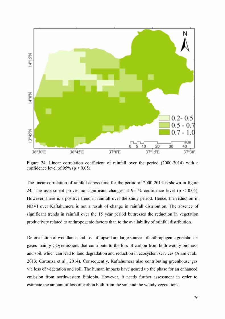
76

Figure 24. Linear correlation coefficient of rainfall over the period (2000-2014) with a confidence level of 95% (p < 0.05).

The linear correlation of rainfall across time for the period of 2000-2014 is shown in figure

24. The assessment proves no significant changes at 95 % confidence level (p < 0.05).

However, there is a positive trend in rainfall over the study period. Hence, the reduction in

NDVI over Kaftahumera is not a result of change in rainfall distribution. The absence of

significant trends in rainfall over the 15 year period buttresses the reduction in vegetation

productivity related to anthropogenic factors than to the availability of rainfall distribution.

Deforestation of woodlands and loss of topsoil are large sources of anthropogenic greenhouse

gases mainly CO2 emissions that contribute to the loss of carbon from both woody biomass

and soil, which can lead to land degradation and reduction in ecosystem services (Alam et al.,

2013; Carranza et al., 2014). Consequently, Kaftahumera also contributing greenhouse gas

via loss of vegetation and soil. The human impacts have geared up the phase for an enhanced

emission from northwestern Ethiopia. However, it needs further assessment in order to

estimate the amount of loss of carbon both from the soil and the woody vegetations.

77

6.6 Summary

There is a significant amount of spatial changes among the land use classes during the period

of three decades, which mainly contributed to an ongoing degradation of woodland

ecosystems. In 1986 woodland is the dominant land use category covering about 79 % of the

area. However the dominance of woodland reshuffled with cropland as cropland acquires the

largest extent in 2014 covering over 53 % of the total area with a net gain of about 40 %. The

net change within the landscape is 44 %, while swap change accounts for about 10 % of the

transition.

The LULC transition matrix of land cover categories under random process of gain identifies

that cropland systematically gains to replace woodland while woodland systematically avoids

to gain from cropland. This proves the loss in vegtal cover of Kaftahumera is associated with

changes due to human activities. The replacement of woodland vegetation by cropland

exposes the topsoil to wind erosion and it is common to observe dust clouds during the dry

period of the year. This approach is helpful in an accounting loss of ecosystem for prioritizing

better options of semiarid environmental managements.

The loss of woodland vegetation is an indicator of ecosystem degradation within the region.

The spatial correlation of NDVI and rainfall shows R2 values of lower than 0.5 in over 55 %

of the study area in the period 2000 - 2014. The temporal change in rainfall is not significant

but there is a negative trend in NDVI in areas of woodlands converted to cropland. The lower

value of R2 between NDVI and rainfall is an indicator of land degradation due to the low

response of degraded landscapes to rainfall. A result of this research indicates a systematic

land use transition and calls for proper measures to combat ecosystem degradation.

78

7. Chapter 7: Trend and change assessment of NDVI and climate variables over northwestern Ethiopia

79

7.1 NDVI trend analysis and break points

The BFAST technique performs the decomposition of time series into trend, seasonal, and

remainder components in order to detect abrupt changes within the seasonal and trend

components (Verbesselt et al., 2010). The bi-temporal land use change assessment using

Landsat imagery exhibited significant inter-categorical land use shifts affecting the vegetation

distribution of the region (Zewdie & Csaplovics, 2015). Hence it is important to consider

temporal trend changes in order to detect the timing and significance of changes in vegetation

growth.

Figure 25 demonstrates the behavior of different trend changes for a selected sample of

MODIS NDVI data. Accordingly, there is a seasonal break in plot b and d but not in the other

two sample plots within the seasonal component of the time series. The existence of seasonal

breaks indicates changes in phenology resulting from land use changes mainly from woodland

to cropland showing a shift in annual phenology cycles within the time series (Verbesselt et

al., 2010). In all the sample plots, there are three distinctive breakpoints with different time of

breaks and statistical significance. In plot a and b, a declining trend is observed till the third

breakpoint and there is a positive trend after the third breakpoint displaying the browning and

greening state of vegetation respectively within the trend series. In both sample plots, the

NDVI continues to decline significantly till 2009 with a distinct state of browning which is

captured in the trend component by the three breakpoints. On the other hand, there is a state of

greening from 2009 to 2014 with a statistically significant positive trend segment. This may

be related to the ongoing demarcation of some of the previous allocated woodlands to national

park. The positive increase in rainfall can also contribute to the enhancement in vegetation

productivity in BFAST sample plot analysis.

In plot c, there are three distinctive breakpoints with varying statistical significance across the

study period. The breakpoints display both positive and negative magnitude in slope. The

declining trend continues till 2008 and then appears a positive trend. However the trend is

statistically significant only in the time period of 2000-2003 (declining trend) and 2012 –

2014 (increasing trend). The period between 2008- 2012 has shown an incremental trend but

not statistically significant. In plot d, two negative and one positive trend is observed with

significant trends in all the three trend phases. However, the period from 2009 to 2014 has

80

zero slopes with no change in its trend. The trend changes between browning and greening are

an important indicator for assessing long term vegetation conditions (de Jong et al., 2011).

In most of the sample plots, NDVI shows negative and positive trends but precipitation has no

significant long term trend (Fig. 25 and Fig. 26). Rainfall significantly influences the

vegetation productivity in arid regions. However the assessments of these two datasets signify

the lower dependency of vegetation change on the long term precipitation changes. Hence,

land use change and forest degradation are crucial aspects to be considered in the semi-arid

northwestern regions of Ethiopia which highly contribute for abrupt and gradual vegetation

changes (Dejene et al., 2013; Eshete et al., 2011; Lemenih et al., 2007, 2014; Zewdie &

Csaplovics, 2015). Consequently, the breakpoints in NDVI are attributed to loss in vegetation

productivity resulting from the loss of vegetation cover and forest degradation due to

expansion of subsistence and large scale agriculture and other driving forces of change. The

availability of vegetation cover is vital for controlling the annual cycle of surface hydrology

and water balance where water is the main limiting factor for vegetation productivity in

dryland regions like Kaftahumera (Gentine et al., 2012). A NDVI-rainfall model is a good

indicator to evaluate the impacts of land use management on dryland ecosystems.

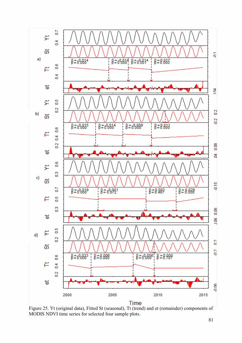
81

Figure 25. Yt (original data), Fitted St (seasonal), Tt (trend) and et (remainder) components of MODIS NDVI time series for selected four sample plots.

a)

b)

d)

c)

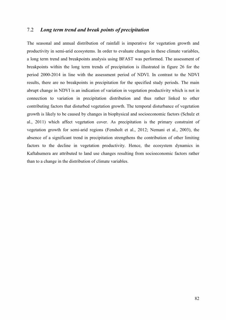
82

7.2 Long term trend and break points of precipitation

The seasonal and annual distribution of rainfall is imperative for vegetation growth and

productivity in semi-arid ecosystems. In order to evaluate changes in these climate variables,

a long term trend and breakpoints analysis using BFAST was performed. The assessment of

breakpoints within the long term trends of precipitation is illustrated in figure 26 for the

period 2000-2014 in line with the assessment period of NDVI. In contrast to the NDVI

results, there are no breakpoints in precipitation for the specified study periods. The main

abrupt change in NDVI is an indication of variation in vegetation productivity which is not in

connection to variation in precipitation distribution and thus rather linked to other

contributing factors that disturbed vegetation growth. The temporal disturbance of vegetation

growth is likely to be caused by changes in biophysical and socioeconomic factors (Schulz et

al., 2011) which affect vegetation cover. As precipitation is the primary constraint of

vegetation growth for semi-arid regions (Fensholt et al., 2012; Nemani et al., 2003), the

absence of a significant trend in precipitation strengthens the contribution of other limiting

factors to the decline in vegetation productivity. Hence, the ecosystem dynamics in

Kaftahumera are attributed to land use changes resulting from socioeconomic factors rather

than to a change in the distribution of climate variables.

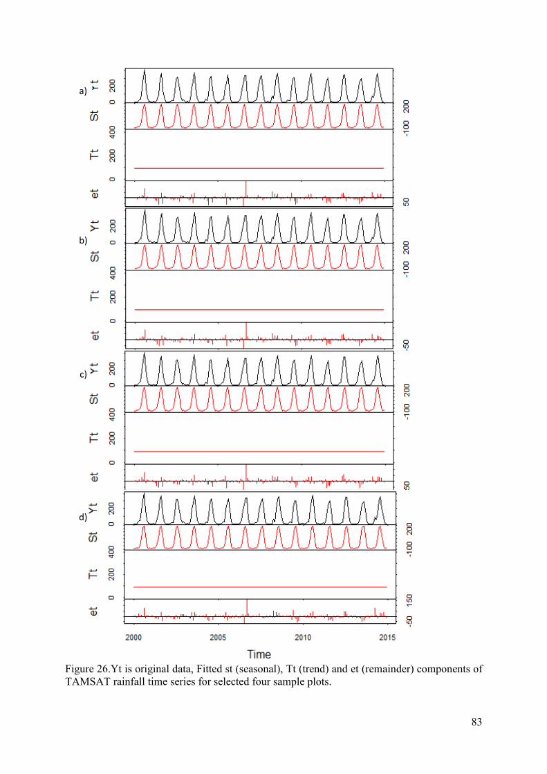
83

Figure 26.Yt is original data, Fitted st (seasonal), Tt (trend) and et (remainder) components of TAMSAT rainfall time series for selected four sample plots.

c)

a)

b)

d)

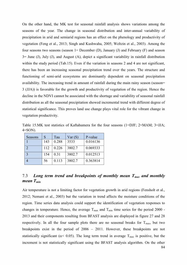
84

On the other hand, the MK test for seasonal rainfall analysis shows variations among the

seasons of the year. The change in seasonal distribution and inter-annual variability of

precipitation in arid and semiarid regions has an effect on the phenology and productivity of

vegetation (Feng et al., 2013; Singh and Kushwaha, 2005; Weltzin et al., 2003). Among the

four seasons two seasons (season 1= December (D), January (J) and February (F) and season

3= June (J), July (J), and August (A), depict a significant variability in rainfall distribution

within the study period (Tab.15). Even if the variation in seasons 2 and 4 are not significant,

there has been an increasing seasonal precipitation trend over the years. The structure and

functioning of semi-arid ecosystems are dominantly dependent on seasonal precipitation

availability. The increasing trend in amount of rainfall during the main rainy season (season=

3 (JJA)) is favorable for the growth and productivity of vegetation of the region. Hence the

decline in the NDVI cannot be associated with the shortage and variability of seasonal rainfall

distribution as all the seasonal precipitation showed incremental trend with different degree of

statistical significance. This proves land use change plays vital role for the vibrant change in

vegetation productivity.

Table 15.MK test statistics of Kaftahumera for the four seasons (1=DJF; 2=MAM; 3=JJA; 4=SON).

Seasons S Tau Var (S) P-value 1 143 0.288 3533 0.016136

2 112 0.226 3802.7 0.069333

3 154 0.31 3802.7 0.012513

4 56 0.113 3802.7 0.363814

7.3 Long term trend and breakpoints of monthly mean Tmax and monthly mean Tmin Air temperature is not a limiting factor for vegetation growth in arid regions (Fensholt et al.,

2012; Nemani et al., 2003) but the variation in trend affects the moisture conditions of the

region. Time series data analysis could support the identification of vegetation responses to

changes in temperature. Hence, the average Tmax and Tmin time series for the period 2000 -

2013 and their components resulting from BFAST analysis are displayed in figure 27 and 28

respectively. In all the four sample plots there are no seasonal breaks for Tmax, but two

breakpoints exist in the period of 2006 – 2011. However, these breakpoints are not

statistically significant (< 0.05). The long term trend in average Tmax is positive, but the

increment is not statistically significant using the BFAST analysis algorithm. On the other

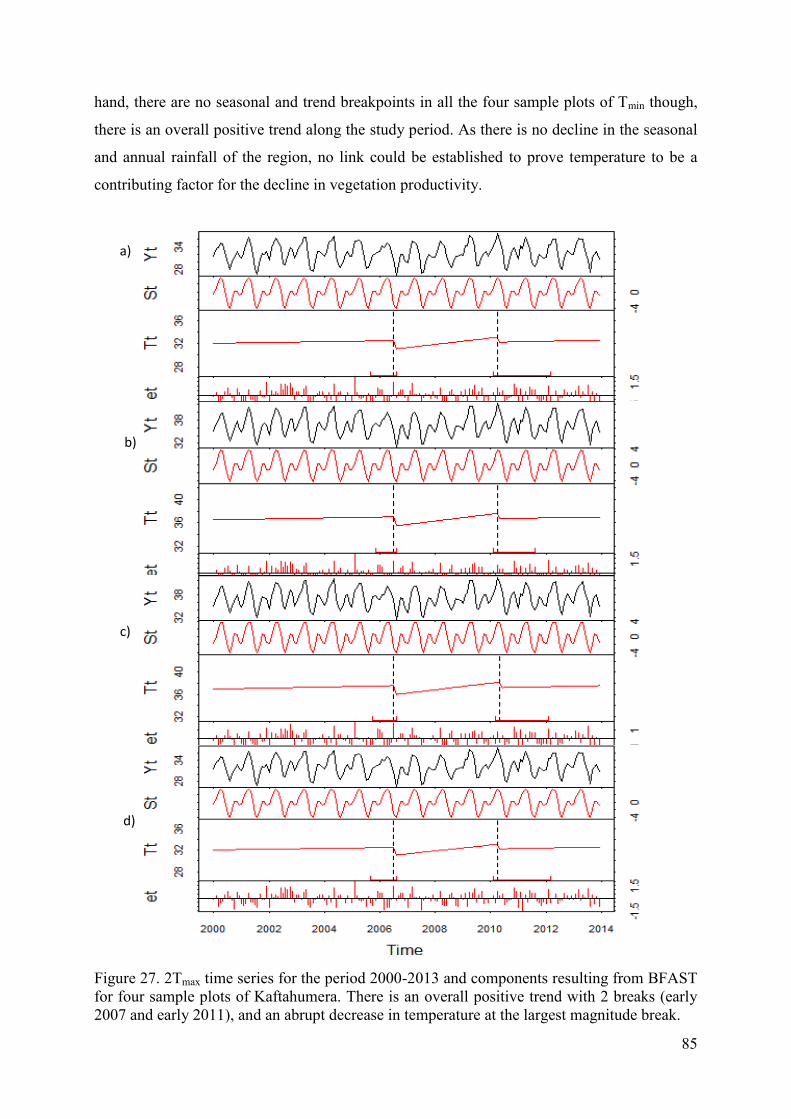
85

hand, there are no seasonal and trend breakpoints in all the four sample plots of Tmin though,

there is an overall positive trend along the study period. As there is no decline in the seasonal

and annual rainfall of the region, no link could be established to prove temperature to be a

contributing factor for the decline in vegetation productivity.

Figure 27. 2Tmax time series for the period 2000-2013 and components resulting from BFAST for four sample plots of Kaftahumera. There is an overall positive trend with 2 breaks (early 2007 and early 2011), and an abrupt decrease in temperature at the largest magnitude break.

a)

b)

d)

c)

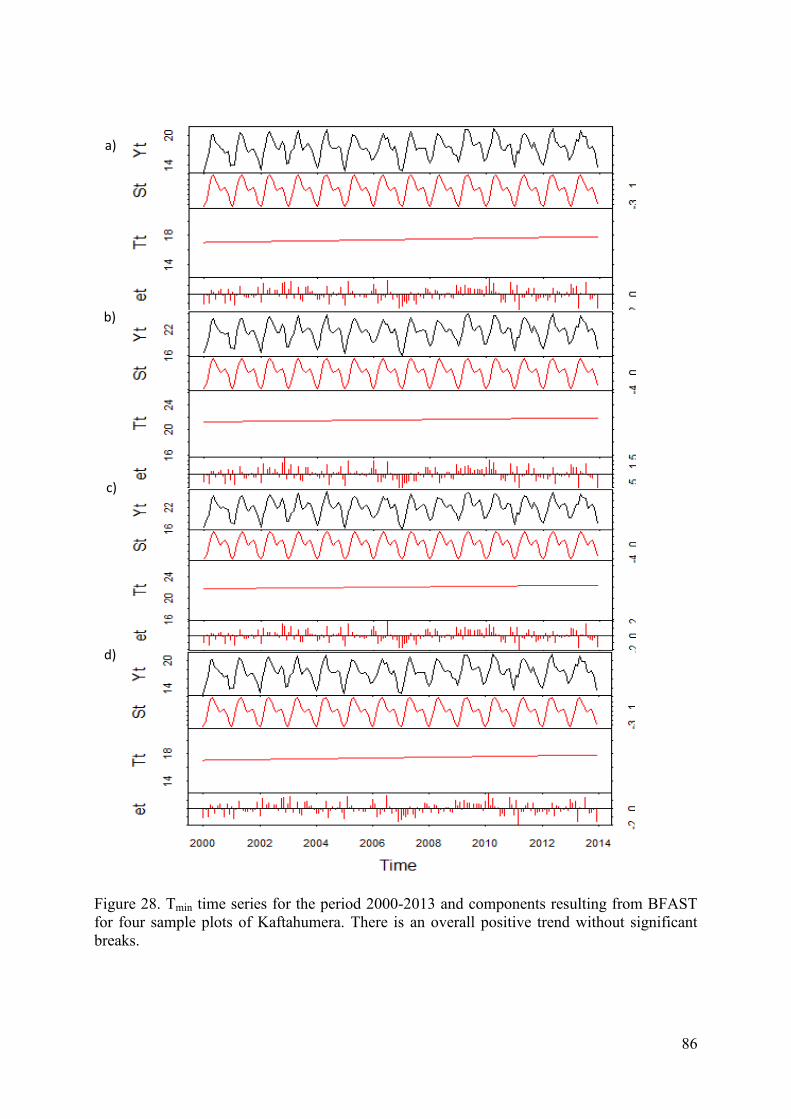
86

Figure 28. Tmin time series for the period 2000-2013 and components resulting from BFAST for four sample plots of Kaftahumera. There is an overall positive trend without significant breaks.

a)

b)

c)

d)

87

7.4 Magnitude of breakpoints for NDVI

Resettlement expansion to overcome famine in Ethiopia has severely affected the vegetation

cover of the country (Lemenih et al., 2014; Rahmato, 2003), particularly resulting in severe

woodland ecosystems loss (Dejene et al., 2013; Lemenih et al., 2014; Zewdie & Csaplovics,

2015). The anthropogenic effect has contributed to the declining trend in vegetation

productivity, affecting the growth cycle of vegetation and thus deteriorating the ecosystem of

the region. The contribution of climate variables is negligible on the decreasing trend of

vegetation productivity. The existence of significant breakpoints in NDVI are attributed

directly to changes between natural and human-modified ecosystems impairing the size of the

woody vegetation.

In all the four sample plots, the highest change in magnitude occurred from 2000 to 2009 with

some degree of improvement afterwards (Fig.29). This period shows significant abrupt

changes due to the disturbance of the woody vegetation and subsequent recovery. Some of the

woodland areas which were previously allocated for resettlement have been demarcated back

to be used as a national park (personal communication) and may be among the contributing

factors for improvement of NDVI trend after the year 2009. In addition, the positive

increment in precipitation can support a more rapid response in vegetation productivity in

dryland ecosystems (Andela et al., 2013). However, the length of break points shows the

severity of loss in productivity of vegetations compared to the length of its recovery. The

abrupt changes in magnitude and breakpoints of NDVI are indicators counting the severity of

loss in biomass as NDVI is a proxy for vegetation biomass measurement.

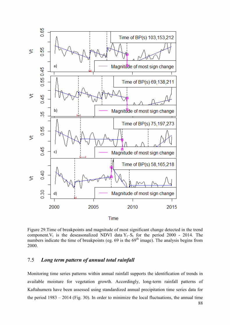
88

Figure 29.Time of breakpoints and magnitude of most significant change detected in the trend component.Vt is the deseasonalized NDVI data Yt–St for the period 2000 - 2014. The numbers indicate the time of breakpoints (eg. 69 is the 69th image). The analysis begins from 2000.

7.5 Long term pattern of annual total rainfall

Monitoring time series patterns within annual rainfall supports the identification of trends in

available moisture for vegetation growth. Accordingly, long-term rainfall patterns of

Kaftahumera have been assessed using standardized annual precipitation time series data for

the period 1983 – 2014 (Fig. 30). In order to minimize the local fluctuations, the annual time

d)

a)

c)

d)

b)

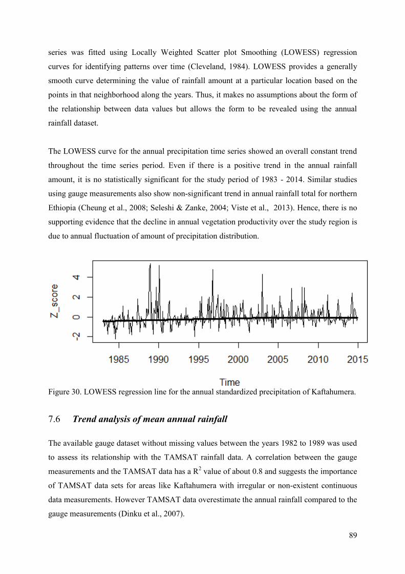
89

series was fitted using Locally Weighted Scatter plot Smoothing (LOWESS) regression

curves for identifying patterns over time (Cleveland, 1984). LOWESS provides a generally

smooth curve determining the value of rainfall amount at a particular location based on the

points in that neighborhood along the years. Thus, it makes no assumptions about the form of

the relationship between data values but allows the form to be revealed using the annual

rainfall dataset.

The LOWESS curve for the annual precipitation time series showed an overall constant trend

throughout the time series period. Even if there is a positive trend in the annual rainfall

amount, it is no statistically significant for the study period of 1983 - 2014. Similar studies

using gauge measurements also show non-significant trend in annual rainfall total for northern

Ethiopia (Cheung et al., 2008; Seleshi & Zanke, 2004; Viste et al., 2013). Hence, there is no

supporting evidence that the decline in annual vegetation productivity over the study region is

due to annual fluctuation of amount of precipitation distribution.

Figure 30. LOWESS regression line for the annual standardized precipitation of Kaftahumera.

7.6 Trend analysis of mean annual rainfall

The available gauge dataset without missing values between the years 1982 to 1989 was used

to assess its relationship with the TAMSAT rainfall data. A correlation between the gauge

measurements and the TAMSAT data has a R2 value of about 0.8 and suggests the importance

of TAMSAT data sets for areas like Kaftahumera with irregular or non-existent continuous

data measurements. However TAMSAT data overestimate the annual rainfall compared to the

gauge measurements (Dinku et al., 2007).

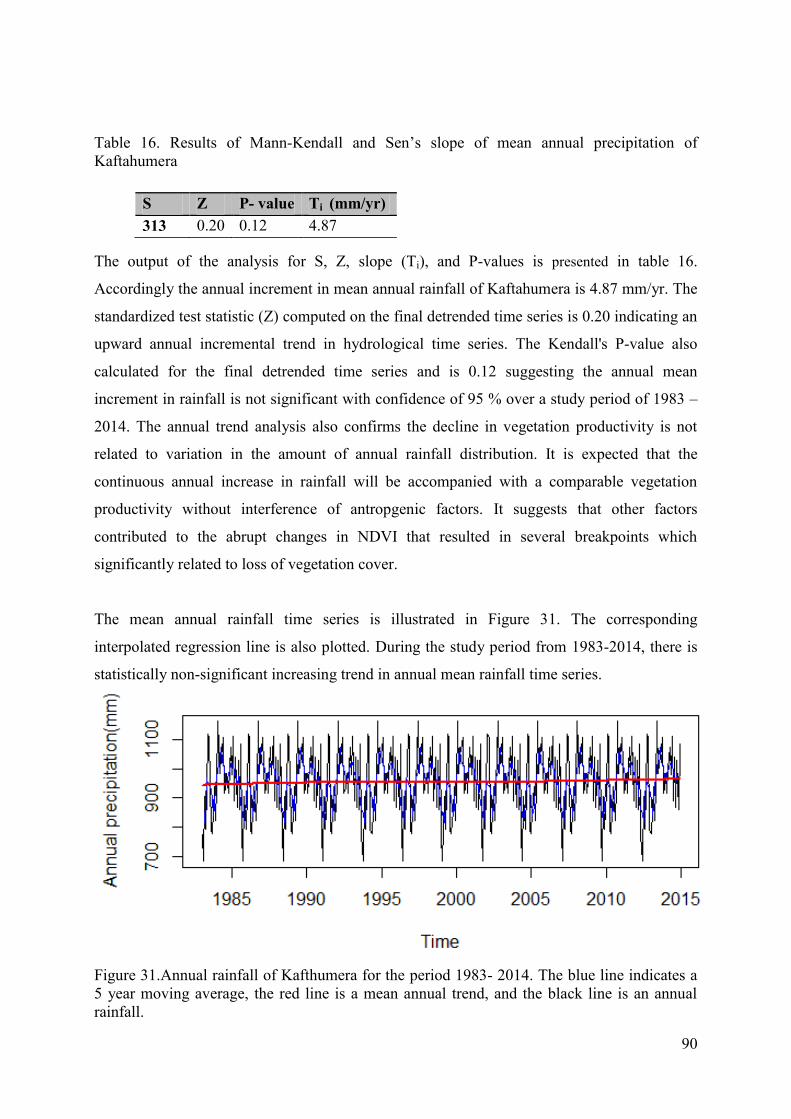
90

Table 16. Results of Mann-Kendall and Sen’s slope of mean annual precipitation of Kaftahumera

The output of the analysis for S, Z, slope (Ti), and P-values is presented in table 16.

Accordingly the annual increment in mean annual rainfall of Kaftahumera is 4.87 mm/yr. The

standardized test statistic (Z) computed on the final detrended time series is 0.20 indicating an

upward annual incremental trend in hydrological time series. The Kendall's P-value also

calculated for the final detrended time series and is 0.12 suggesting the annual mean

increment in rainfall is not significant with confidence of 95 % over a study period of 1983 –

2014. The annual trend analysis also confirms the decline in vegetation productivity is not

related to variation in the amount of annual rainfall distribution. It is expected that the

continuous annual increase in rainfall will be accompanied with a comparable vegetation

productivity without interference of antropgenic factors. It suggests that other factors

contributed to the abrupt changes in NDVI that resulted in several breakpoints which

significantly related to loss of vegetation cover.

The mean annual rainfall time series is illustrated in Figure 31. The corresponding

interpolated regression line is also plotted. During the study period from 1983-2014, there is

statistically non-significant increasing trend in annual mean rainfall time series.

Figure 31.Annual rainfall of Kafthumera for the period 1983- 2014. The blue line indicates a 5 year moving average, the red line is a mean annual trend, and the black line is an annual rainfall.

S Z P- value Ti (mm/yr) 313 0.20 0.12 4.87

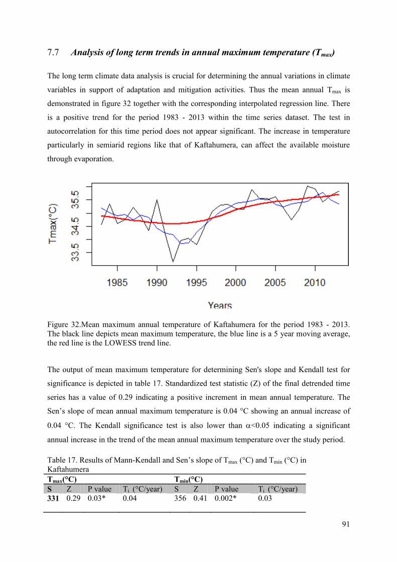
91

7.7 Analysis of long term trends in annual maximum temperature (Tmax)

The long term climate data analysis is crucial for determining the annual variations in climate

variables in support of adaptation and mitigation activities. Thus the mean annual Tmax is

demonstrated in figure 32 together with the corresponding interpolated regression line. There

is a positive trend for the period 1983 - 2013 within the time series dataset. The test in

autocorrelation for this time period does not appear significant. The increase in temperature

particularly in semiarid regions like that of Kaftahumera, can affect the available moisture

through evaporation.

Figure 32.Mean maximum annual temperature of Kaftahumera for the period 1983 - 2013. The black line depicts mean maximum temperature, the blue line is a 5 year moving average, the red line is the LOWESS trend line.

The output of mean maximum temperature for determining Sen's slope and Kendall test for

significance is depicted in table 17. Standardized test statistic (Z) of the final detrended time

series has a value of 0.29 indicating a positive increment in mean annual temperature. The

Sen’s slope of mean annual maximum temperature is 0.04 °C showing an annual increase of

0.04 °C. The Kendall significance test is also lower than <0.05 indicating a significant

annual increase in the trend of the mean annual maximum temperature over the study period.

Table 17. Results of Mann-Kendall and Sen’s slope of Tmax (°C) and Tmin (°C) in Kaftahumera Tmax(°C) Tmin(°C) S Z P value Ti (°C/year) S Z P value Ti (°C/year) 331 0.29 0.03*

0.04 356 0.41 0.002*

0.03

92

The standardized mean annual maximum temperature for the entire Kaftahumera with

LOWESS smooth time series plot is illustrated in figure 33. LOWESS curve was fitted over

time based on the annual precipitation time series data in order to reduce local fluctuations.

The standardized mean annual maximum temperature analysis also indicates a positive trend

over the study region within the period of 1983-2013.

Figure 33. Standardized mean maximum temperature trend of Kaftahumera. The red line is the LOWESS regression for the period 1983 - 2013.

7.8 Trend in minimum annual temperature.

The trend in minimum annual temperature time series for the period 1983-2013 is presented

in figure 34 together with the interpolated regression line and five year moving average. The

mean minimum annual temperature indicates an overall positive increasing trend for the

period of 1983-2013. However, there is few lower measurement records along the years with

the lowest minimum temperature recorded in 1989.

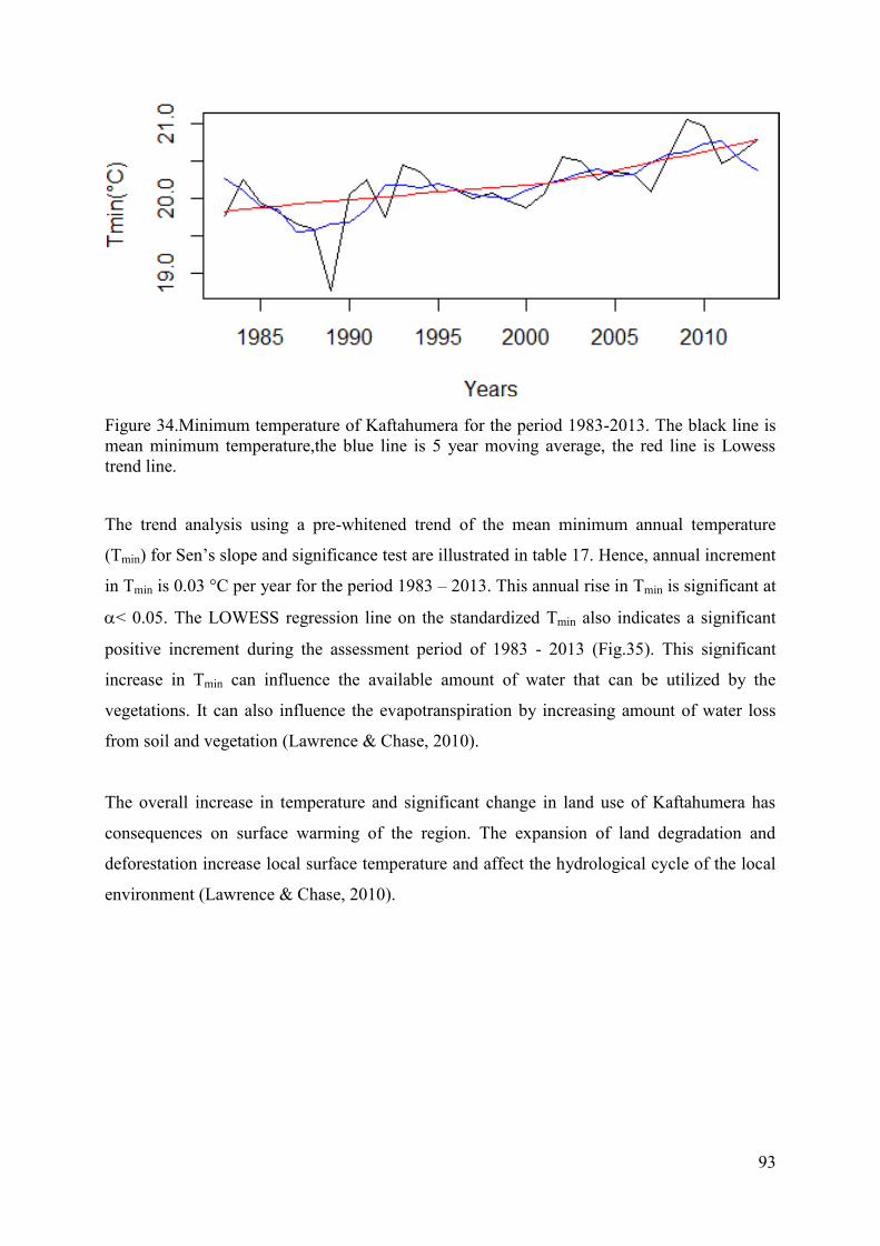
93

Figure 34.Minimum temperature of Kaftahumera for the period 1983-2013. The black line is mean minimum temperature,the blue line is 5 year moving average, the red line is Lowess trend line.

The trend analysis using a pre-whitened trend of the mean minimum annual temperature

(Tmin) for Sen’s slope and significance test are illustrated in table 17. Hence, annual increment

in Tmin is 0.03 °C per year for the period 1983 – 2013. This annual rise in Tmin is significant at

< 0.05. The LOWESS regression line on the standardized Tmin also indicates a significant

positive increment during the assessment period of 1983 - 2013 (Fig.35). This significant

increase in Tmin can influence the available amount of water that can be utilized by the

vegetations. It can also influence the evapotranspiration by increasing amount of water loss

from soil and vegetation (Lawrence & Chase, 2010).

The overall increase in temperature and significant change in land use of Kaftahumera has

consequences on surface warming of the region. The expansion of land degradation and

deforestation increase local surface temperature and affect the hydrological cycle of the local

environment (Lawrence & Chase, 2010).

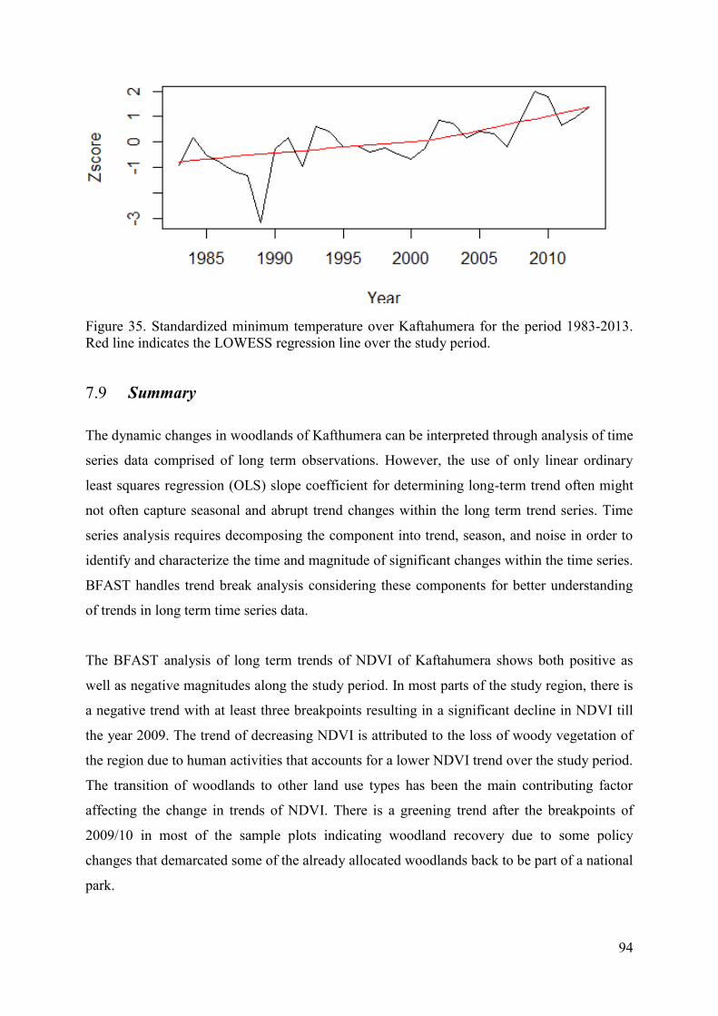
94

Figure 35. Standardized minimum temperature over Kaftahumera for the period 1983-2013. Red line indicates the LOWESS regression line over the study period.

7.9 Summary

The dynamic changes in woodlands of Kafthumera can be interpreted through analysis of time

series data comprised of long term observations. However, the use of only linear ordinary

least squares regression (OLS) slope coefficient for determining long-term trend often might

not often capture seasonal and abrupt trend changes within the long term trend series. Time

series analysis requires decomposing the component into trend, season, and noise in order to

identify and characterize the time and magnitude of significant changes within the time series.

BFAST handles trend break analysis considering these components for better understanding

of trends in long term time series data.

The BFAST analysis of long term trends of NDVI of Kaftahumera shows both positive as

well as negative magnitudes along the study period. In most parts of the study region, there is

a negative trend with at least three breakpoints resulting in a significant decline in NDVI till

the year 2009. The trend of decreasing NDVI is attributed to the loss of woody vegetation of

the region due to human activities that accounts for a lower NDVI trend over the study period.

The transition of woodlands to other land use types has been the main contributing factor

affecting the change in trends of NDVI. There is a greening trend after the breakpoints of

2009/10 in most of the sample plots indicating woodland recovery due to some policy

changes that demarcated some of the already allocated woodlands back to be part of a national

park.

95

The trend in annual precipitation shows an increment of 4.87 mm per year. However, this

overall positive trend in rainfall pattern of Kaftahumera is not statistically significant within

the period of 1983 – 2014. In addition, there is no time of breakpoint along the time series

dataset of rainfall suggesting resulting land use changes dominantly contributed to the

breakpoints in long term NDVI trend.

The mean minimum and maximum annual temperatures have risen during the last 30 years.

Both the minimum and maximum temperature of the region show significant increase in

annual trend. Tmax shows an annual increase of 0.04 °C while Tmin shows an annual increment

of 0.03 °C. The increase in both Tmax and Tmin has an effect on the available moisture, which

is very crucial for dryland vegetation growth. The loss of vegetation cover can raise local

surface temperature. However, further assessment is needed to quantify its effect on the

current and future status of vegetation growth.

96

8. Chapter 8: Temporal relationship of rainfall and NDVI anomalies over northwestern Ethiopia using distributed lag models

97

8.1 Mean NDVI and rainfall

Drylands are characterized by water insufficiency with lower ratio between annual rainfall

and annual potential evapotranspiration. Due to scarcity of rainfall stations in the

northwestern drylands of Ethiopia, it is hardly possible to analyze the exact distribution of

rainfall. However, the use of satellite imagery permitted the assessment of phenological

indicators for identifying a complete growing season in semi-arid region of Kaftahumera.

These data are vital for revealing plant life-cycle trends over time and detecting the impacts of

climate change on ecosystems.

eMODIS NDVI data are provided with quality raster, rating the quality of each pixel within

the scene for quality checking and pre-processing prior to analysis in order to determine

changes in vegetation biomass or land condition. Quality imagery has been used assigning

low weights to bad quality pixels during raw image pre-processing. Through the filtering

process, bad quality imagery with low weighted pixels is less considered during the

construction of the new raster image during our assessment of vegetation responses.

The long term mean eMODIS NDVI and mean dekadal rainfall of Kaftahumera is illustrated

in figure 36 and 37. The distribution of mean long term NDVI varies spatially according to

the land use history and spatial location. The NDVI also varies spatially but with different

patterns of distribution. The woodland areas have higher mean NDVI as an indication of the

existence of higher green biomass in the parts covered by woodland. However, most parts of

Kaftahumera which is mostly dominated by human activities have lower mean NDVI. In most

of the southern parts of the study area, there is lower vegetation productivity measured by the

amount of NDVI. Areas which were once covered with woodlands located in the central and

northwestern parts of Kaftahumera, have lower NDVI values which results from expansion of

subsistence and large scale agricultural activities and human pressures.

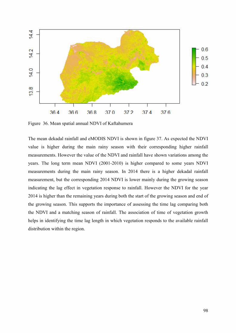
98

Figure 36. Mean spatial annual NDVI of Kaftahumera

The mean dekadal rainfall and eMODIS NDVI is shown in figure 37. As expected the NDVI

value is higher during the main rainy season with their corresponding higher rainfall

measurements. However the value of the NDVI and rainfall have shown variations among the

years. The long term mean NDVI (2001-2010) is higher compared to some years NDVI

measurements during the main rainy season. In 2014 there is a higher dekadal rainfall

measurement, but the corresponding 2014 NDVI is lower mainly during the growing season

indicating the lag effect in vegetation response to rainfall. However the NDVI for the year

2014 is higher than the remaining years during both the start of the growing season and end of

the growing season. This supports the importance of assessing the time lag comparing both

the NDVI and a matching season of rainfall. The association of time of vegetation growth

helps in identifying the time lag length in which vegetation responds to the available rainfall

distribution within the region.

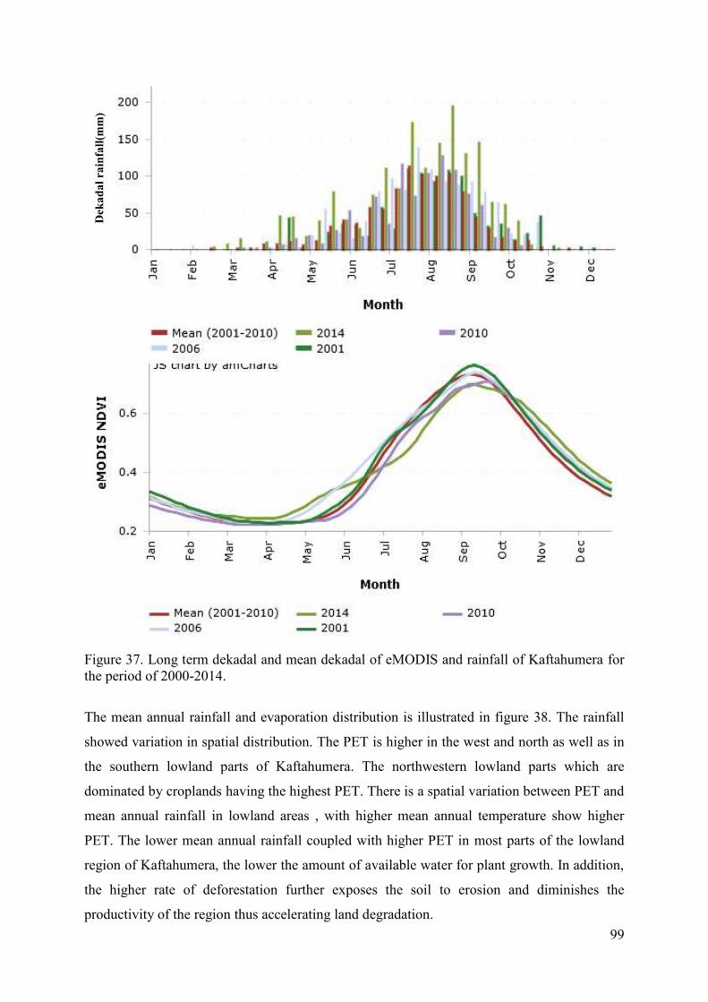
99

Figure 37. Long term dekadal and mean dekadal of eMODIS and rainfall of Kaftahumera for the period of 2000-2014.

The mean annual rainfall and evaporation distribution is illustrated in figure 38. The rainfall

showed variation in spatial distribution. The PET is higher in the west and north as well as in

the southern lowland parts of Kaftahumera. The northwestern lowland parts which are

dominated by croplands having the highest PET. There is a spatial variation between PET and

mean annual rainfall in lowland areas , with higher mean annual temperature show higher

PET. The lower mean annual rainfall coupled with higher PET in most parts of the lowland

region of Kaftahumera, the lower the amount of available water for plant growth. In addition,

the higher rate of deforestation further exposes the soil to erosion and diminishes the

productivity of the region thus accelerating land degradation.

Dek

adal

rai

nfal

l(mm

)

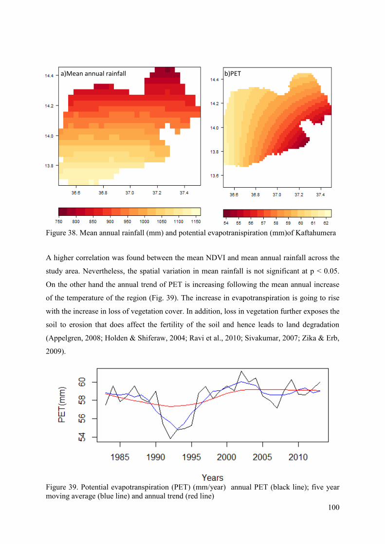
100

Figure 38. Mean annual rainfall (mm) and potential evapotranispiration (mm)of Kaftahumera

A higher correlation was found between the mean NDVI and mean annual rainfall across the

study area. Nevertheless, the spatial variation in mean rainfall is not significant at p < 0.05.

On the other hand the annual trend of PET is increasing following the mean annual increase

of the temperature of the region (Fig. 39). The increase in evapotranspiration is going to rise

with the increase in loss of vegetation cover. In addition, loss in vegetation further exposes the

soil to erosion that does affect the fertility of the soil and hence leads to land degradation

(Appelgren, 2008; Holden & Shiferaw, 2004; Ravi et al., 2010; Sivakumar, 2007; Zika & Erb,

2009).

Figure 39. Potential evapotranspiration (PET) (mm/year) annual PET (black line); five year moving average (blue line) and annual trend (red line)

a)Mean annual rainfall b)PET

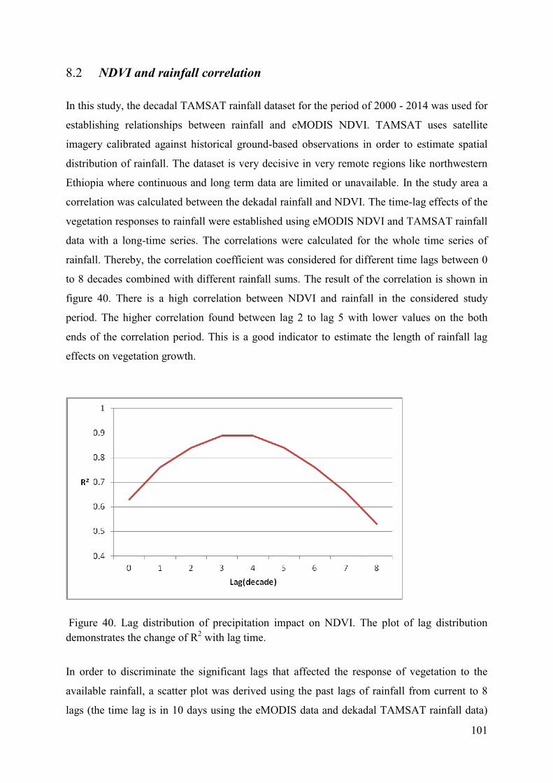
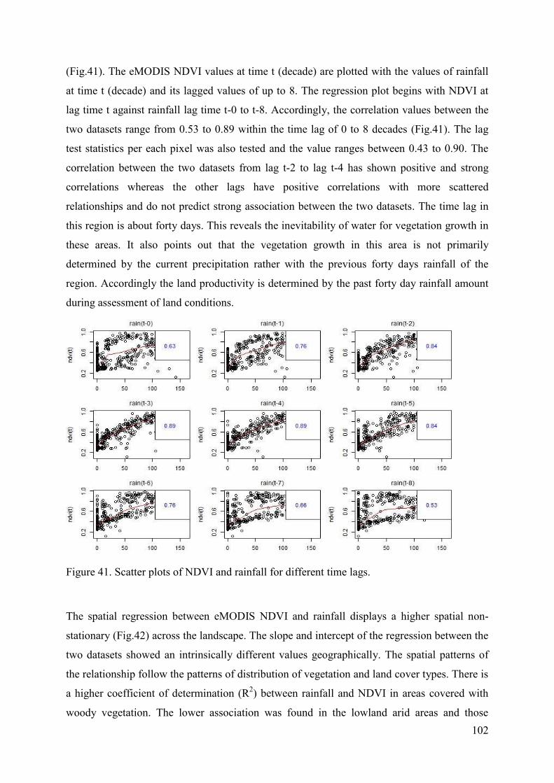
102

(Fig.41). The eMODIS NDVI values at time t (decade) are plotted with the values of rainfall

at time t (decade) and its lagged values of up to 8. The regression plot begins with NDVI at

lag time t against rainfall lag time t-0 to t-8. Accordingly, the correlation values between the

two datasets range from 0.53 to 0.89 within the time lag of 0 to 8 decades (Fig.41). The lag

test statistics per each pixel was also tested and the value ranges between 0.43 to 0.90. The

correlation between the two datasets from lag t-2 to lag t-4 has shown positive and strong

correlations whereas the other lags have positive correlations with more scattered

relationships and do not predict strong association between the two datasets. The time lag in

this region is about forty days. This reveals the inevitability of water for vegetation growth in

these areas. It also points out that the vegetation growth in this area is not primarily

determined by the current precipitation rather with the previous forty days rainfall of the

region. Accordingly the land productivity is determined by the past forty day rainfall amount

during assessment of land conditions.

Figure 41. Scatter plots of NDVI and rainfall for different time lags. The spatial regression between eMODIS NDVI and rainfall displays a higher spatial non-

stationary (Fig.42) across the landscape. The slope and intercept of the regression between the

two datasets showed an intrinsically different values geographically. The spatial patterns of

the relationship follow the patterns of distribution of vegetation and land cover types. There is

a higher coefficient of determination (R2) between rainfall and NDVI in areas covered with

woody vegetation. The lower association was found in the lowland arid areas and those

rain(t-0)

0.63F

o I I 0

I 0 50 100 150

rain(t-3)

I

0.89

50 100 150

rain(t-6)

4 50 144 150

m > o a c

Iv ó

rain(t-1)

0.76

o 50 100

rain(t-4)

150

0 5 O C

9 0 .ó

D 0 50 100

rain(t-7)

150

0.66

0 `0 144 150

> v c

raine :t -2;

rain(t-5)

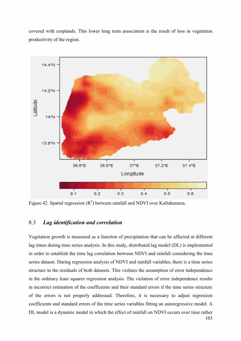
104

than all at once. This means the effect of the current rainfall on vegetation growth is seen

some days after its occurrence

Figure 43 demonstrates the spatial lag regression between NDVI and rainfall. The spatial lag

relationship between the two time series dataset indicates the diminishing effect of rainfall

after a time lag of 4. The lag correlation between rainfall and NDVI has a value of R2 of up to

0.5 at lag 0. This pixel wise regression adopting time lag has also shown that the lagged effect

of rainfall on vegetation growth approaches almost zero after the time lag of 4(40 days). This

implies that the current rainfall has effects on vegetation growth only after a lag length of 40

days. This characterizes on how the temporal distribution of rainfall affects the growth and

development of vegetation in semi-arid regions of Kaftahumera. Similar studies on semi arid

environments and other dryland areas have proven a rainfall lag effect of from two weeks to

several months of time lags (Chamaille-Jammes et al., 2006; Ji & Peters, 2005; Kileshye

Onema & Taigbenu, 2009; Udelhoven et al., 2009).

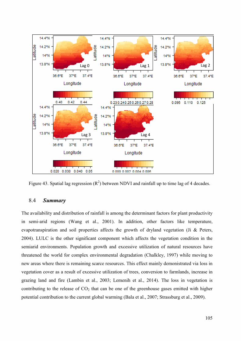
105

Figure 43. Spatial lag regression (R2) between NDVI and rainfall up to time lag of 4 decades.

8.4 Summary

The availability and distribution of rainfall is among the determinant factors for plant productivity

in semi-arid regions (Wang et al., 2001). In addition, other factors like temperature,

evapotranspiration and soil properties affects the growth of dryland vegetation (Ji & Peters,

2004). LULC is the other significant component which affects the vegetation condition in the

semiarid environments. Population growth and excessive utilization of natural resources have

threatened the world for complex environmental degradation (Chalkley, 1997) while moving to

new areas where there is remaining scarce resources. This effect mainly demonistrated via loss in

vegetation cover as a result of excessive utilization of trees, conversion to farmlands, increase in

grazing land and fire (Lambin et al., 2003; Lemenih et al., 2014). The loss in vegetation is

contributing to the release of CO2 that can be one of the greenhouse gases emitted with higher

potential contribution to the current global warming (Bala et al., 2007; Strassburg et al., 2009).

Lag 1 Lag 2 Lag 0

Lag 4 Lag 3

106

The availability of long term satellite measurements of both NDVI and rainfall has helped in

assessing the condition of vegetation and land degradation in data scarce regions of Africa where

there is limited gauge measurements (Maidment et al., 2014; Roy et al., 2014). NDVI is strongly

dependent on climatic variables for both temporal and spatial patterns with time lag effects on

vegetation growth (Li et al., 2004). The change in NDVI could either be a result of anthropogenic

land use changes or variation in the distribution of climate variables of the study region. Hence

the assessment and identification of climate variability is vital to distinguish environmental

changes resulted from either human induced or from the effect of climate change (Evans &

Geerken, 2004).

The evaluation of time of biomass accumulation and its relation to climatic variables is vital in

determining vegetation responses to climate lag effects. An assessment of the time lag

relationship between rainfall and NDVI is fundamental to estimate the time and also to

quantitatively estimate the temporal changes in vegetation productivity as a result of the available

moisture amount for vegetation growth. Hence, a time lag regression between eMODIS NDVI

and rainfall was made for the period 2000 to 2014 using DL models. The autocorrelation of the

two datasets removed before testing for time lag correlation using the autoregressive model.

A lag regression from t-0 to t-8 was assessed between the two datasets of eMODIS NDVI and

rainfall. The scatter plot analysis between time lag of the predictor (rainfall) and the response

(NDVI) has a maximum lag of 50 days (t-5). The time lag is a measure of the lag length when the

previous rainfall has an effect on vegetation productivity. Hence the significance test of lag length

on vegetation productivity showed only up to a time lag of t-4(forty days) that explains the effect

of previous rainfall on the current growth of vegetation of the surrounding. The spatial lag cross-

correlation between NDVI and rainfall also showed higher significant correlations of up to t-4

across the study area. The time lag analysis with the consideration of land use types and time of

the growing season might help to better understand the lag effects across the land use types.

107

9. Chapter 9. Discussion, overall conclusion and recommendation for future work

108

9.1 Discussion and conclusion 9.1.1 Land cover dynamics in northwestern Ethiopia

Despite their significant contribution to both economic and ecological services, dry forests of

Ethiopia are currently under severe threats both from anthropogenic and natural calamities

(Lemenih et al., 2014). Agriculture, expansion of resettlements, fire, population growth and

climatic variation are among the factors that significantly contribute to the decline in size and to

the fragmentation of the dry forests of Ethiopia (Eshete et al., 2011; Lemenih et al., 2007).

Several of these studies attempted to link the loss in dry forests with human activities but lacks

estimates of the spatial extent of the declining woody resources and the major driving forces. In

addition, the extent and severity of land use transition in the ecosystems of the surrounding arid

environment is not well studied. During some periods of the dry season, clouds of haze extend

along the borders of Sudan and northwestern Ethiopia, which may be rooted from the degradation

of the natural woody vegetation of the region. The present study assesses land cover transition

using SVM classification algorithms for examining major contributing factors that influence land

cover transitions. The SVM classification model works well in spectrally complex land cover

categories for enhancing better classification results (Tuia & Camps-Valls, 2011) and

understanding of the significant transitions in land cover.

Kaftahumera like other woodland areas of the country encountered significant land use transitions

during the study period (Biazin & Sterk, 2013; Garedew et al., 2012; Lemenih et al., 2014;

Mekasha et al., 2014; Zewdie & Csaplovics, 2014). The spatiotemporal distribution of land cover

dynamic in the period 1972- 2014 indicates cropland and woodland as the dominant land use

types varying in size along the years. The woodland land use category shows decreasing trend

while cropland has an increased trend at the expense of woodlands. In the period 1972 - 2014,

woodland shows a significant decline from an extent of about 92 % to about 35 %, whereas

cropland showed an increase in size from about 3 % to over 52 %. These noticeable spatial

changes and degradation in woodland occurred mainly in the south, west and southwest parts of

the study area which was replaced subsequently by croplands. However, the change among the

land use classes was unevenly distributed across the study area, with the greatest loss occurring

within the woodland. Overall, the region exhibited a broad conversion of woodland to cropland

during the study period without showing any noticeable gain in size and spatial pattern of

woodlands. The critical period for the deforestation and degradation of woodland is the period

from 2000 to 2014 where woodland experienced the largest amount of loss (Fig.44).

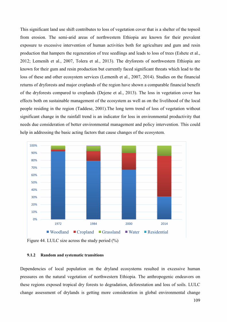
110

studies as land use alteration is exposing them for transitions and high rates of resource depletion

(Lambin et al., 2003). The annual deforestation rate of Ethiopia is estimated at about 2% with the

dry forest loss being prevalent due to the resulting pressure from population growth and cropland

expansion (Eshete et al., 2005; Lemenih et al. 2014 and WBISPP, 2005). The population size of

Ethiopia has more than doubled in the last three decades from 40 million in 1984 to over 87

million in 2014 (CSA, 2014). This has led to overexploitation and consequent land degradation of

the highlands. The population of the degraded highlands was resettled to the lowlands which

brought a significant threat to the dry forests due to lack of monitoring mechanisms and of

integration of the new arrivals with existing residents (Lemenih et al., 2014). The loss in dryland

vegetation of Kaftahumera has been significantly increased, resulting in land degradation that

became sources of dust emissions and loading.

The loss of dryland vegetation needs a temporal image analysis in order to capture the time of

change and trace the driving forces. Post classification change detection is beneficial as it utilizes

a transition matrix comprising two date imagery to investigate the net change among the land use

categories (Braimoh, 2006; Petit et al., 2001). However the analysis of net change alone may not

describe the total change as there might be zero net change due to a simultaneous gain and loss of

a land use category within the landscape (Braimoh, 2006). In addition, it is crucial to discriminate

the significant signals in the process of categorizing land use shifts (Pontius et al., 2004). The

identification of systematic land use changes from a random process of change is also helpful in

determining the severity of land use transitions in a landscape. The large inter-categorical change

may not always indicate systematic land use transitions as large land use shifts may occur in large

land use classes in a random process of change (Braimoh, 2006).

In most studies the occurring net changes were considered as a measure of land use transitions.

However, net change quantifies only the difference between total quantity of each category at

time one and time two of the study period without considering swap changes (Pontius et al.,

2004). A lack of net change along the study period does not mean that there is no change in the

landscape. However , there may be a change in the landscape between time one and time two

without having difference in the quantity of change due to swap changes. This type of change is

characterized by a simultaneous gain and loss of a category within the landscape resulting in zero

net changes over a period of time (Braimoh, 2006; Pontius et al., 2004). Therefore a net change in

the quantity of the category indicates a definite change of land use but lack of net change is not

111

necessarily representative for transitions among the land use classes as it does not account the

swapping component of changes (Pontius et al., 2004).

During the assessment of land use transition of Kaftahumera, the basic concept of net change and

swap change was properly addressed in order to capture all significant transitions along the

temporal gradient. Accordingly the values of gain, loss, net change, swap and total change for the

period 1972 – 2014 for each LULC class are presented in previous chapters of this dissertation.

Along the study period, cropland and grassland are the dominant categories that experienced the

highest gains. The gain in cropland and grassland is about 54 % and over 11 % of the study area

respectively. On the other hand woodland has the highest loss in over 62 % of the area, followed

by grassland with about 3 % of the area. The swap levels of woodland, cropland and grassland are

1.9, 1.7, and 4.9 respectively. The three dominant land categories: woodland, cropland and

grassland show a significant amount of net change over the study period respectively. The loss in

woodland is attributed to expansion of subsistence and large scale farming and underlying causes

like population growth which competes over the natural vegetation of the region. The growth in

population, both from resettlement and immigration due to casual labor pave the way for directly

exerting pressure on the woodlands. The weak approach to set and implement legal procedure for

protecting the natural ecosystem is another factor which allows easy access for the exploitation of

woodlands (Lemenih et al., 2014). In general, the main driving forces for land use transitions in

Kaftahumera are both proximate and resulting from underlying causes of land use changes. This

resulted in systematic transitions affecting mainly the woodland vegetation of the region. The

socio-ecological field survey also confirmed the involvement of human activities and policy

intervention (resettlement and agricultural investment) that played the major role in exposing the

woodland vegetation for change.

9.1.3 Land degradation in Kaftahumera

Mankind has made a considerable amount of progress in scientific innovations to utilize the

available natural resources of the environment for its welfare. However, in the face of increasing

human population and subsequent demand for resource utilization, there is an imbalance between

the resource usage and maintenance of the ecosystem (Bretschger & Smulders, 2012). This has

caused significant changes in the environment in regions with vibrant human dominated

ecosystems (Zewdie & Csaplovics, 2014). Among these ecosystems, the overutilization of

dryland resources has been intensifying land degradation in conjunction with climate change

112

which can result in desertification (Sivakumar, 2007). Desertification is a type of land

degradation process in which a dryland region becomes increasingly arid, typically losing its

bodies of water as well as vegetation and wildlife (Geist and Lambin, 2004)

Satellite measurements are capable of capturing the vulnerability of drylands to change resulting

from both climate and human modification of the landscape. The assessment of the status and

trends of Kaftahumera drylands is decisive in order to evaluate their evolution with respect to

fluctuating rainfall and temperature patterns for developing long-term ecosystem conservation

schemes. The variations in trends of long-term NDVI are influenced by changes in seasonal

climate and other disturbance factors that lead to abrupt changes in NDVI time series. Monitoring

of long term changes incorporating trend and seasonal components is crucial for a better

understanding of change trajectories. Accordingly, no significant decline in precipitation was

observed in Kaftahumera during the study period. However, there is a negative trend in NDVI

with varying degree of change in magnitude.

The loss in vegetation cover leads to land degradation if sustainable utilization is not in action.

Hence the land degradation in Kaftahumera is dominantly related to human activities than the

change in climate variables. The continuous expansion in cropland and associated human growth

is exerting significant pressure on the vegetation of the region. This has ended in exposing the

woody vegetation for change resulting in loss of soil and other vegetal covers. The current change

trends is alarming which needs due attention in order to curve the continuous loss of resources.

As Kaftahumera is one of the semiarid agro-climatic zones of the country, it is at risk of

desertification unless vital improvements are made in land use management.

9.1.4 Detection of breakpoints in NDVI and climate variables

Satellite remote sensing has played a vital role in monitoring ecosystem changes at the regional,

continental, and global scales (Coppin et al., 2004) and derived vegetation indices (VIs)

demonstrate significante importance in monitoring light dependent physiological processes

(Cracknell, 2001; Fensholt et al., 2009; Glenn et al., 2008; Tucker and Yager, 2011). The change

in vegetation cover affects the amount of light absorbed by the plant canopy as a result of change

in vegetation density and hence VIs can be one of the indicators for measuring the status of

environmental conditions.

http://en.wikipedia.org/wiki/Land_degradation

http://en.wikipedia.org/wiki/Land_degradation

http://en.wikipedia.org/wiki/Drylands

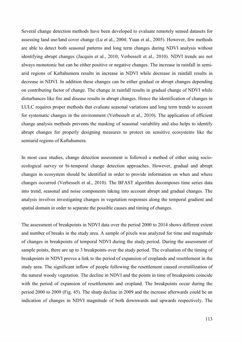
113

Several change detection methods have been developed to evaluate remotely sensed datasets for

assessing land use/land cover change (Lu et al., 2004; Yuan et al., 2005). However, few methods

are able to detect both seasonal patterns and long term changes during NDVI analysis without

identifying abrupt changes (Jacquin et al., 2010; Verbesselt et al., 2010). NDVI trends are not

always monotonic but can be either positive or negative changes. The increase in rainfall in semi-

arid regions of Kaftahumera results in increase in NDVI while decrease in rainfall results in

decrease in NDVI. In addition these changes can be either gradual or abrupt changes depending

on contributing factor of change. The change in rainfall results in gradual change of NDVI while

disturbances like fire and disease results in abrupt changes. Hence the identification of changes in

LULC requires proper methods that evaluate seasonal variations and long term trends to account

for systematic changes in the environment (Verbesselt et al., 2010). The application of efficient

change analysis methods prevents the masking of seasonal variability and also helps to identify

abrupt changes for properly designing measures to protect on sensitive ecosystems like the

semiarid regions of Kaftahumera.

In most case studies, change detection assessment is followed a method of either using socio-

ecological survey or bi-temporal change detection approaches. However, gradual and abrupt

changes in ecosystem should be identified in order to provide information on when and where

changes occurred (Verbesselt et al., 2010). The BFAST algorithm decomposes time series data

into trend, seasonal and noise components taking into account abrupt and gradual changes. The

analysis involves investigating changes in vegetation responses along the temporal gradient and

spatial domain in order to separate the possible causes and timing of changes.

The assessment of breakpoints in NDVI data over the period 2000 to 2014 shows different extent

and number of breaks in the study area. A sample of pixels was analyzed for time and magnitude

of changes in breakpoints of temporal NDVI during the study period. During the assessment of

sample points, there are up to 3 breakpoints over the study period. The evaluation of the timing of

breakpoints in NDVI proves a link to the period of expansion of croplands and resettlement in the

study area. The significant inflow of people following the resettlement caused overutilization of

the natural woody vegetation. The decline in NDVI and the points in time of breakpoints coincide

with the period of expansion of resettlements and cropland. The breakpoints occur during the

period 2000 to 2009 (Fig. 45). The sharp decline in 2009 and the increase afterwards could be an

indication of changes in NDVI magnitude of both downwards and upwards respectively. The

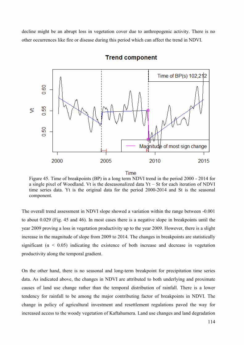
114

decline might be an abrupt loss in vegetation cover due to anthropogenic activity. There is no

other occurrences like fire or disease during this period which can affect the trend in NDVI.

Figure 45. Time of breakpoints (BP) in a long term NDVI trend in the period 2000 - 2014 for a single pixel of Woodland. Vt is the deseasonalized data Yt – St for each iteration of NDVI time series data. Yt is the original data for the period 2000-2014 and St is the seasonal component.

The overall trend assessment in NDVI slope showed a variation within the range between -0.001

to about 0.029 (Fig. 45 and 46). In most cases there is a negative slope in breakpoints until the

year 2009 proving a loss in vegetation productivity up to the year 2009. However, there is a slight

increase in the magnitude of slope from 2009 to 2014. The changes in breakpoints are statistically

significant (α < 0.05) indicating the existence of both increase and decrease in vegetation

productivity along the temporal gradient.

On the other hand, there is no seasonal and long-term breakpoint for precipitation time series

data. As indicated above, the changes in NDVI are attributed to both underlying and proximate

causes of land use change rather than the temporal distribution of rainfall. There is a lower

tendency for rainfall to be among the major contributing factor of breakpoints in NDVI. The

change in policy of agricultural investment and resettlement regulations paved the way for

increased access to the woody vegetation of Kaftahumera. Land use changes and land degradation

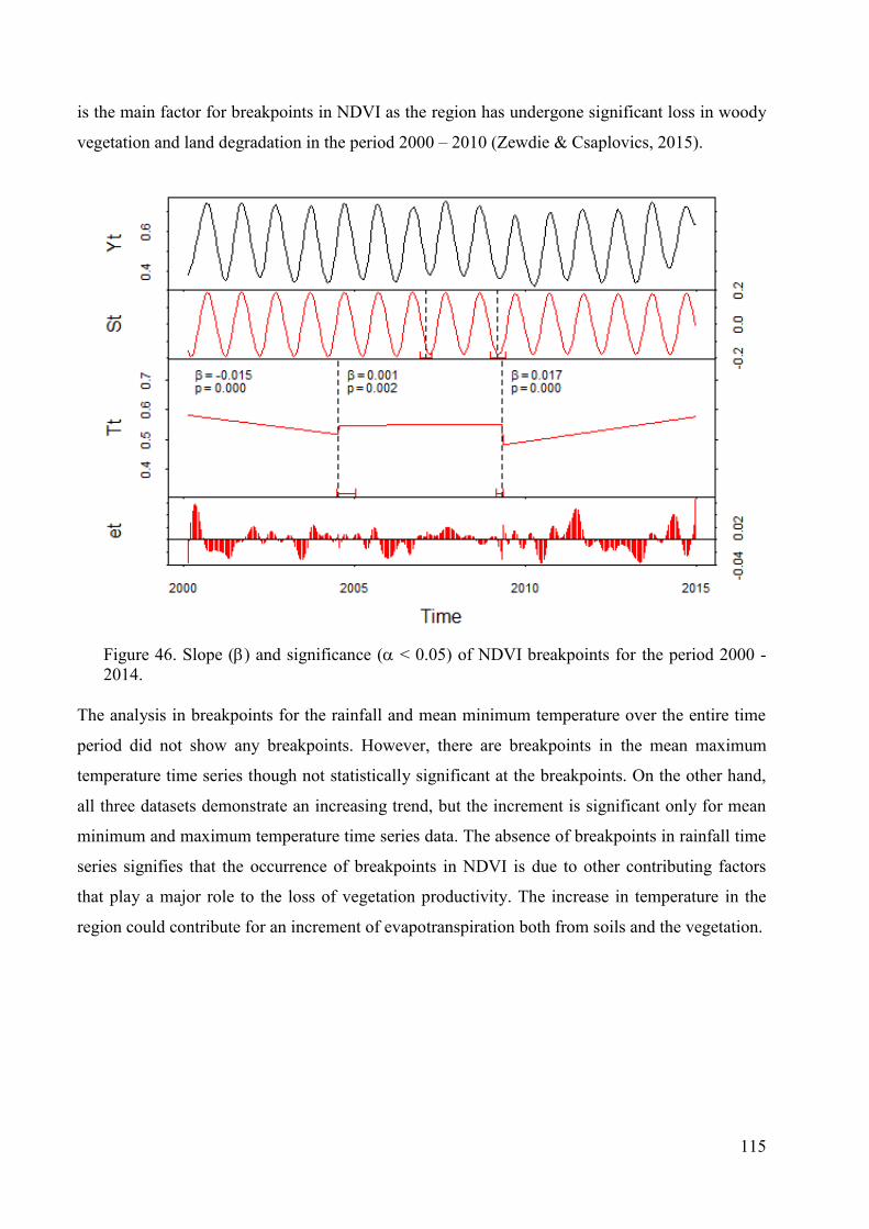
115

is the main factor for breakpoints in NDVI as the region has undergone significant loss in woody

vegetation and land degradation in the period 2000 – 2010 (Zewdie & Csaplovics, 2015).

Figure 46. Slope () and significance ( < 0.05) of NDVI breakpoints for the period 2000 - 2014.

The analysis in breakpoints for the rainfall and mean minimum temperature over the entire time

period did not show any breakpoints. However, there are breakpoints in the mean maximum

temperature time series though not statistically significant at the breakpoints. On the other hand,

all three datasets demonstrate an increasing trend, but the increment is significant only for mean

minimum and maximum temperature time series data. The absence of breakpoints in rainfall time

series signifies that the occurrence of breakpoints in NDVI is due to other contributing factors

that play a major role to the loss of vegetation productivity. The increase in temperature in the

region could contribute for an increment of evapotranspiration both from soils and the vegetation.

116

Figure 47. Trend shifts within the rainfall time series of Kaftahumera. A season-trend model (red line) was fitted to the rainfall time series (gray).

The decadal raw rainfall allow for the assessment of the shift in trends of seasonal rainfall

distribution over the period of 1983 – 2014 (Fig.47). A season-trend model (red line) was fitted to

the rainfall time series (gray). The dashed line indicates the detected trend shift and the

confidence interval for the period 1997. However, this trend is not statistically significant (p<

0.05).

The Mann-Kendall long term trend test shows that there is no trend in the annual rainfall total but

there is trends in seasonal rainfall total over Kaftahumera in the period 1983 – 2014. Similar

studies using gauge measurement revealed the absence of trend in the annual total rainfall over

northwestern Ethiopia (Seleshi & Zanke, 2004). On the other hand the mean minimum

temperature and mean maximum temperature of the region show a significant trend with an

annual increase per year respectively.

The assessment of time lag between NDVI and rainfall is vital in understanding vegetation and

climate interaction during temporal analysis. The lag response of NDVI to rainfall depends on

vegetation type, soils and climate. Hence encompassing all the contributing factors better define

the response of vegetation to the available moisture. In this study DL model was used in order to

identify the relationship between NDVI and lagged precipitation in Kaftahumera. The time lag

was up to forty days and then diminishes both spatially and in temporal gradient. This means that

the current rainfall has no effect on the current NDVI but vegetation greenness can be predicted

117

using antecedent rainfall. Rainfall during the forty day span ending with the current period has the

strongest association with NDVI during the current period. This proves the vegetation growth in

Kaftahumera is not primarily determined by the current precipitation but rather depends on the

previous forty days rainfall.

118

9.2 Conclusion

An assessment of land use transition, long term trends in climate and land condition over

Kaftahumera was made for the period 1972 – 2014 using Landsat imagery, MODIS NDVI,

TAMSAT rainfall and CRU temperature data. Image classification and change detection analysis

was performed using SVM and inter-categorical land use transitions. Among the land use classes,

woodland to cropland was the dominant land use transition within the long term temporal

gradient. The inter-categorical shift among the land use classes varies in size and in spatial

distribution. Over the study period, woodland has encountered a significant amount of reduction

in size. This decline in size is mainly attributed to the expansion of cropland and due to the

pressure of the continuous inflow of population and subsequent resettlement that consumed the

woodlands of the region. This transition from woodland vegetation cover to cropland has exposed

the topsoil to continuous erosion, which exacerbates during the dry period of the year. It is

common to observe clouds of dust in recent years during certain times in the annual dry season.

The spatial and temporal assessment of the relation between NDVI and climate variables also

indicates a significant change in the amount of NDVI over the study period from 2000 to 2014.

The NDVI shows breakpoints in this period with about three breakpoints in NDVI until the year

2009 and a significant greening afterwards. The decline up to 2009 seems to be related to the

expansion of cropland which is confirmed by the bi-temporal analysis of Landsat imagery. This

has significantly consumed the woodland cover of Kafathumera. On the other hand the greening

after the year 2009 could be linked to the demarcation of some of the agricultural plots to national

parks. The protection of the woodlands coupled with an annual increment in rainfall favors fast

recovery of vegetation covers. The spatial regression between NDVI and rainfall also

demonstrates significant changes both spatially and in temporal trends. An overlay analysis

between land use and rainfall has proven the significant reduction in NDVI in areas with loss in

woodlands. However, there is no significant trend in the assessment of long term temporal

precipitation time series data. The temporal reduction in NDVI is likely to be rather a result of

man-induced changes in vegetation than of fluctuations in the distribution of rainfall.

The Mann-Kendall test of long term annual variation in rainfall displays no trend during the study

period of 1983 – 2014. However, the change in magnitude of annual total rainfall demonstrates an

annual increase of 4.87 mm per year over the study period. The temporal assessment in

temperature within the similar study period shows incremental trends in mean minimum and

119

mean maximum temperature. There is an annual increase of 0.03 °C per year and 0.04 °C per year

in mean minimum and mean maximum temperature respectively. The test in temporal trend

points towards a significant increase in both minimum and maximum temperature time series

over the study period. This significant increase in temperature can contribute for higher

evapotranspiration of the available moisture both from soil and vegetation.

A time lag relationship assessment between NDVI and rainfall is crucial for a better

understanding of vegetation and climate interaction. A regression model between the two data

shows strong relationships and significant time lag of about forty days observed during the study

period. This indicates the current NDVI is affected not by the current rainfall distribution, but

rather by the previous forty days rainfall amount and distribution.

The overall results of the study show a significant change in the environment and ecosystem of

Kaftahumera with significant expansion of human-dominated ecosystems. The change in natural

ecosystem of the region exposed the land surface to erosion resulting in the emergence and drift

of dust clouds during the dry period of the year. It is evident that human pressure that affects the

natural system of the region has to be reduced. The intensified over-utilization of the woody

vegetation resulted in degradation and deforestation of the region.

9.3 Limitation of the study

Land degradation of the region is identified. However the use of higher spatial

resolution data will improve the identification and mapping of land degradation

process.

Evaluation of the association between NDVI and rainfall has increased the

understanding of the interaction between vegetation and climate of the region. The

relationship of time lag between NDVI and rainfall may vary based on the time of

growing season and land cover types.

The loss in vegetation and significant increase in temperature of the region exposed

the topsoil to erosion. Size and content of dust movement are not analyzed.

120

9.4 Recommendation Time series analysis of imagery and climate variables has shown the decline in

vegetation productivity. It is advisable to associate and assess the variation in trends of

crop yields and carbon loss of the region.

Detection of breakpoints in NDVI could be attributed to several factors and land use

change is one of them. However, land use change could occur due to several natural

and human induced activities. It would increase the understanding of these processes if

details of other causes of changes, if any, fire, diseases were assessed.

The incorporation of the individual land cover type and growing season may improve

the assessment of the time lag. The consideration of other climate variables (like

temperature, soil moisture,..) and land use during the lag regression modeling may

also improve the identification of the dependencies and lag length.

The dust movement could be aggravated due to the current trend in loss of vegetation

cover. It is prudent to evaluate the trend, the amount and content of dust clouds of

Kaftahumera for a better monitoring of changes in the environment.

121

10. Reference Abd El-Kawy, O. R., Rød, J. K., Ismail, H. a., & Suliman, A. S. (2011). Land use and land

cover change detection in the western Nile delta of Egypt using remote sensing data. Applied Geography, 31(2), 483–494. doi:10.1016/j.apgeog.2010.10.012

Adamo, S. B., & Crews-Meyer, K. a. (2006). Aridity and desertification: Exploring environmental hazards in Jáchal, Argentina. Applied Geography, 26(1), 61–85. doi:10.1016/j.apgeog.2005.09.001

Alam, S. A., Starr, M., & Clark, B. J. F. (2013). Tree biomass and soil organic carbon densities across the Sudanese woodland savannah: A regional carbon sequestration study. Journal of Arid Environments, 89, 67–76. doi:10.1016/j.jaridenv.2012.10.002

Alcaraz-Segura, D., Liras, E., Tabik, S., Paruelo, J., & Cabello, J. (2010). Evaluating the consistency of the 1982-1999 NDVI trends in the Iberian Peninsula across four time-series derived from the AVHRR sensor: LTDR, GIMMS, FASIR, and PAL-II. Sensors, 10(2), 1291–1314. doi:10.3390/s100201291

Andela, N., Liu, Y. Y., van Dijk, a. I. J. M., de Jeu, R. a. M., & McVicar, T. R. (2013). Global changes in dryland vegetation dynamics (1988-2008) assessed by satellite remote sensing: comparing a new passive microwave vegetation density record with reflective greenness data. Biogeosciences, 10(10), 6657–6676. doi:10.5194/bg-10-6657-2013

Anyamba, A., & Tucker, C. J. (2005). Analysis of Sahelian vegetation dynamics using NOAA-AVHRR NDVI data from 1981-2003. Journal of Arid Environments, 63, 596–614. doi:10.1016/j.jaridenv.2005.03.007

Appelgren, B. (2008). Towards Sustainable Dryland Development in Africa: Integrating Groundwater and Land Management. In T. S. Cathy Lee (Ed.), Future of Drylands (pp. 199–208). Tunis,Tunisia: Springer. doi:10.1007/978-1-4020-6970-3

Archibald, R., & Fann, G. (2007). Feature Selection and Classification of Hyperspectral Images With Support Vector Machines. IEEE Geoscience and Remote Sensing Letters, 4(4), 674–677. doi:10.1109/LGRS.2007.905116

Atkinson, P. M., Jeganathan, C., Dash, J., & Atzberger, C. (2012). Inter-comparison of four models for smoothing satellite sensor time-series data to estimate vegetation phenology. Remote Sensing of Environment, 123, 400–417. doi:10.1016/j.rse.2012.04.001

Atzberger, C., & Eilers, P. H. C. (2011). A time series for monitoring vegetation activity and phenology at 10-daily time steps covering large parts of South America. International Journal of Digital Earth, 4(5), 365–386. doi:10.1080/17538947.2010.505664

Bai, J., & Perron, P. (2003). Computation and analysis of multiple structural change models. Journal of Applied Econometrics, 18, 1–22. doi:10.1002/jae.659

Bai, Z. G., Dent, D. L., Olsson, L., & Schaepman, M. E. (2008). Proxy global assessment of land degradation. Soil Use and Management, 24(3), 223–234. doi:10.1111/j.1475-2743.2008.00169.x

Bajocco, S., De Angelis, A., Perini, L., Ferrara, A., & Salvati, L. (2012). The impact of Land Use/Land Cover Changes on land degradation dynamics: A Mediterranean case study. Environmental Management, 49, 980–989. doi:10.1007/s00267-012-9831-8

122

Bakr, N., Weindorf, D. C., Bahnassy, M. H., Marei, S. M., & El-Badawi, M. M. (2010). Monitoring land cover changes in a newly reclaimed area of Egypt using multi-temporal Landsat data. Applied Geography, 30(4), 592–605. doi:10.1016/j.apgeog.2009.10.008

Bala, G., Caldeira, K., Wickett, M., Phillips, T. J., Lobell, D. B., Delire, C., & Mirin, A. (2007). Combined climate and carbon-cycle effects of large-scale deforestation. In P. Vitousek (Ed.), Proceedings of the National Academy of Sciences of the United States of America (Vol. 104, pp. 6550–6555). Stanford, CA. doi:10.1073/pnas.0608998104

Beer, C., Reichstein, M., Tomelleri, E., Ciais, P., Jung, M., Carvalhais, N., … Papale, D. (2010). Terrestrial gross carbon dioxide uptake: global distribution and covariation with climate. Science, 329, 834–838. doi:10.1126/science.1184984

Berk, A., Anderson, G. P., Bernstein, L. S., Acharya, P. K., Dothe, H., Matthew, M. W., … Hoke, M. L. (1999). MODTRAN4 radiative transfer modeling for atmospheric correction. In Allen M. Larar (Ed.), Proceedings of SPIE - The International Society for Optical Engineering (Vol. 3756, pp. 348–353). Denver, CO, USA. doi:doi:10.1117/12.366388

Biazin, B., & Sterk, G. (2013). Drought vulnerability drives land-use and land cover changes in the Rift Valley dry lands of Ethiopia. Agriculture, Ecosystems and Environment, 164, 100–113. doi:10.1016/j.agee.2012.09.012

Bonan, G. B. (2008). Forests and climate change: forcings, feedbacks, and the climate benefits of forests. Science, 320(5882), 1444–1449. doi:10.1126/science.1155121

Braimoh, A. K. (2006). Random and systematic land-cover transitions in northern Ghana. Agriculture, Ecosystems and Environment, 113, 254–263. doi:10.1016/j.agee.2005.10.019

Bretschger, L., & Smulders, S. (2012). Challenges for a sustainable resource use: Uncertainty, trade, and climate policies. Journal of Environmental Economics and Management, 64(3), 279–287. doi:10.1016/j.jeem.2012.09.005

Budde, M. E., Tappan, G., Rowland, J., Lewis, J., & Tieszen, L. L. (2004). Assessing land cover performance in Senegal, West Africa using 1-km integrated NDVI and local variance analysis. Journal of Arid Environments, 59, 481–498. doi:10.1016/j.jaridenv.2004.03.020

Burges, C. J. C. (1998). A tutorial on support vector machines for pattern recognition. Data Mining and Knowledge Discovery, 2, 121–167. doi:10.1023/A:1009715923555

Cabello, J., Fernández, N., Alcaraz-Segura, D., Oyonarte, C., Piñeiro, G., Altesor, A., … Paruelo, J. M. (2012). The ecosystem functioning dimension in conservation: Insights from remote sensing. Biodiversity and Conservation, 21, 3287–3305. doi:10.1007/s10531-012-0370-7

Camps-Valls, G., Gómez-Chova, L., Muñoz-Marí, J., Rojo-Álvarez, J. L., & Martínez-Ramón, M. (2008). Kernel-based framework for multitemporal and multisource remote sensing data classification and change detection. IEEE Transactions on Geoscience and Remote Sensing, 46, 1822–1835. doi:10.1109/TGRS.2008.916201

Carmona, A., & Nahuelhual, L. (2012). Combining land transitions and trajectories in assessing forest cover change. Applied Geography, 32, 904–915.

123

doi:10.1016/j.apgeog.2011.09.006

Carranza M.L., Frate L., Acosta A.T.R., Hoyos L, Ricotta C., C. M. (2014). Measuring forest fragmentation using multitemporal remotely sensed data: three decades of change in the dry Chaco. European Journal of Remote Sensing, 47, 793–804. doi:10.5721/EuJRS20144745

Central Statistic Agency(CSA). (2014). Population of Ethiopia. Addis Abeba, Ethiopia.

Chalkley, K. (1997). Population growth and consumption. Population Today, 25, 4–5.

Chamaille-Jammes, S., Fritz, H., & Murindagomo, F. (2006). Spatial patterns of the NDVI–rainfall relationship at the seasonal and interannual time scales in an African savanna. International Journal of Remote Sensing, 27, 5185–5200. doi:10.1080/01431160600702392

Chander, G., Markham, B. L., & Helder, D. L. (2009). Summary of current radiometric calibration coefficients for Landsat MSS, TM, ETM+, and EO-1 ALI sensors. Remote Sensing of Environment, 113(5), 893–903.

Chang, C. C., & Lin, C. J. (2001). Training nu-support vector classifiers: theory and algorithms. Neural Computation, 13(9), 2119–2147. doi:10.1162/089976601750399335

Chang, C.-C., & Lin, C.-J. (2011). Libsvm. ACM Transactions on Intelligent Systems and Technology, 2(3), 1–27. doi:10.1145/1961189.1961199

Chavez Jr, P. S. (1989). Radiometric calibration of Landsat Thematic Mapper multispectral images. Photogrammetric Engineering & Remote Sensing, 55, 1285 –1294.

Chen, C. H., & Peter Ho, P.-G. (2008). Statistical pattern recognition in remote sensing. Pattern Recognition, 41(9), 2731–2741. doi:10.1016/j.patcog.2008.04.013

Chen, D., Loboda, T., Channan, S., & Hoffman-Hall, A. (2014). Long-term record of sampled disturbances in Northern Eurasian boreal forest from pre-2000 Landsat data. Remote Sensing, 6, 6020–6038. doi:10.3390/rs6076020

Chen, T., de Jeu, R. a M., Liu, Y. Y., van der Werf, G. R., & Dolman, a. J. (2014). Using satellite based soil moisture to quantify the water driven variability in NDVI: A case study over mainland Australia. Remote Sensing of Environment, 140, 330–338. doi:10.1016/j.rse.2013.08.022

Cheung, W. H., Senay, G. B., & Singh, A. (2008). Trends and spatial distribution of annual and seasonal rainfall in Ethiopia. International Journal of Climatology, 28(13), 1723–1734. doi:10.1002/joc.1623

Cleveland, W. S. (1984). Graphs in scientific publications. The American Statistician, 38(4), 261–269. doi:10.2307/2683400

Congalton, R. G. (1991). A Review of Assessing the Accuracy of Classifications of Remotely Sensed Data, 46, 35–46.

Cook, B. I., Miller, R. L., & Seager, R. (2009). Amplification of the North American “Dust Bowl” drought through human-induced land degradation. Proceedings of the National Academy of Sciences of the United States of America, 106(13), 4997–5001. doi:10.1073/pnas.0810200106

124

Coppin, P., Jonckheere, I., Nackaerts, K., Muys, B., & Lambin, E. (2004). Review ArticleDigital change detection methods in ecosystem monitoring: a review. International Journal of Remote Sensing, 25(9), 1565–1596. doi:10.1080/0143116031000101675

Coppin, P. R., & Bauer, M. E. (1996). Change Detection in Forest Ecosystems with Remote Sensing Digital Imagery Digital Change Detection in Temperate Forests. Remote Sensing Reviews, 13, 612–625. doi:10.1080/02757259609532305

Cortes, C., & Vapnik, V. (1995). Support-vector networks. Machine Learning, 20, 273–297. doi:10.1007/BF00994018

Cracknell, A. P. (2001). The exciting and totally unanticipated success of the AVHRR in applications for which it was never intended. Advances in Space Research, 28(1), 233–240. doi:10.1016/S0273-1177(01)00349-0

Cubbage, F., Harou, P., & Sills, E. (2007). Policy instruments to enhance multi-functional forest management. Forest Policy and Economics, 9(7), 833–851. doi:10.1016/j.forpol.2006.03.010

Dardel, C., Kergoat, L., Hiernaux, P., Mougin, E., Grippa, M., & Tucker, C. J. (2014). Re-greening Sahel: 30years of remote sensing data and field observations (Mali, Niger). Remote Sensing of Environment, 140, 350–364. doi:10.1016/j.rse.2013.09.011

Davis, M. B. (1989). Lags in vegetation response to greenhouse warming. Climatic Change, 15, 75–82. doi:10.1007/BF00138846

de Jong, R., de Bruin, S., de Wit, A., Schaepman, M. E., & Dent, D. L. (2011). Analysis of monotonic greening and browning trends from global NDVI time-series. Remote Sensing of Environment, 115(2), 692–702. doi:10.1016/j.rse.2010.10.011

DeFries, R. (2008). Terrestrial Vegetation in the Coupled Human-Earth System: Contributions of Remote Sensing. Annual Review of Environment and Resources, 33(1), 369–390. doi:10.1146/annurev.environ.33.020107.113339

DeFries, R. S., Field, C. B., Fung, I., Collatz, G. J., & Bounoua, L. (1999). Combining satellite data and biogeochemical models to estimate global effects of human-induced land cover change on carbon emissions and primary productivity. Global Biogeochemical Cycles, 13(3), 803–815. doi:10.1029/1999GB900037

DeFries, R. S., Foley, J. A., & Asner, G. P. (2004). Land-use choices: balancing human needs and ecosystem function. Frontiers in Ecology and the Environment, 2(5), 249–257. doi:10.1890/1540-9295(2004)002[0249:LCBHNA]2.0.CO;2

Dejene, T., Lemenih, M., & Bongers, F. (2013). Manage or convert boswellia woodlands? Can frankincense production payoff? Journal of Arid Environments, 89, 77–83. doi:10.1016/j.jaridenv.2012.09.010

del Barrio, G., Puigdefabregas, J., Sanjuan, M. E., Stellmes, M., & Ruiz, A. (2010). Assessment and monitoring of land condition in the Iberian Peninsula, 1989-2000. Remote Sensing of Environment, 114, 1817–1832. doi:10.1016/j.rse.2010.03.009

Dinku, T., Ceccato, P., Grover-Kopec, E., Lemma, M., Connor, S. J., & Ropelewski, C. F. (2007). Validation of satellite rainfall products over East Africa’s complex topography.

125

International Journal of Remote Sensing, 28, 1503–1526. doi:10.1080/01431160600954688

Duan, H., Yan, C., Tsunekawa, A., Song, X., Li, S., & Xie, J. (2011). Assessing vegetation dynamics in the Three-North Shelter Forest region of China using AVHRR NDVI data. Environmental Earth Sciences, 64, 1011–1020. doi:10.1007/s12665-011-0919-x

Dymond, J. R., Bégue, A., & Loseen, D. (2001). Monitoring land at regional and national scales and the role of remote sensing. International Journal of Applied Earth Observation and Geoinformation, 3, 162–175. doi:10.1016/S0303-2434(01)85008-X

Eilers, P. H. C. (2003). A perfect smoother. Analytical Chemistry, 75(14), 3631–3636. doi:10.1021/ac034173t

Eklundh, L. (1998). Estimating relations between AVHRR NDVI and rainfall in East Africa at 10-day and monthly time scales. International Journal of Remote Sensing, 19(3), 563–570. doi:10.1080/014311698216198

Eshete, A., Sterck, F., & Bongers, F. (2011). Diversity and production of Ethiopian dry woodlands explained by climate- and soil-stress gradients. Forest Ecology and Management, 261, 1499–1509. doi:10.1016/j.foreco.2011.01.021

Eshete, A., Sterck, F. J., & Bongers, F. (2012). Frankincense production is determined by tree size and tapping frequency and intensity. Forest Ecology and Management, 274, 136–142. doi:10.1016/j.foreco.2012.02.024

Eshete, A., Teketay, D., Lemenih, M., & Bongers, F. (2012). Effects of resin tapping and tree size on the purity, germination and storage behavior of Boswellia papyrifera (Del.) Hochst. seeds from Metema District, northwestern Ethiopia. Forest Ecology and Management, 269, 31–36. doi:10.1016/j.foreco.2011.12.049

Ethiopian Agricultural Research Organization(EARO). (2002). An assessment of the Agricultural Production Base, Technological Packages and Innovation and Intervention Strategies for Commercial farmers in Kaftahumera Woreda of Tigray Regional State. Addis Abeba, Ethiopia.

Evans, J., & Geerken, R. (2004). Discrimination between climate and human-induced dryland degradation. Journal of Arid Environments, 57, 535–554. doi:10.1016/S0140-1963(03)00121-6

Fathian, F., Dehghan, Z., Bazrkar, M. H., & Eslamian, S. (2014). Trends in hydrologic and climatic variables affected by four variations of Mann-Kendall approach in Urmia Lake basin, Iran. Hydrological Sciences Journal. doi:10.1080/02626667.2014.932911

Feng, X., Porporato, A., & Rodriguez-Iturbe, I. (2013). Changes in rainfall seasonality in the tropics. Nature Climate Change, 3(9), 811–815. doi:10.1038/nclimate1907

Fensholt, R., Langanke, T., Rasmussen, K., Reenberg, A., Prince, S. D., Tucker, C., … Wessels, K. (2012). Greenness in semi-arid areas across the globe 1981-2007 - an Earth Observing Satellite based analysis of trends and drivers. Remote Sensing of Environment, 121, 144–158. doi:10.1016/j.rse.2012.01.017

Fensholt, R., Rasmussen, K., Nielsen, T. T., & Mbow, C. (2009). Evaluation of earth observation based long term vegetation trends - Intercomparing NDVI time series trend

126

analysis consistency of Sahel from AVHRR GIMMS, Terra MODIS and SPOT VGT data. Remote Sensing of Environment, 113, 1886–1898. doi:10.1016/j.rse.2009.04.004

Fensholt, R., Sandholt, I., & Rasmussen, M. S. (2004). Evaluation of MODIS LAI, fAPAR and the relation between fAPAR and NDVI in a semi-arid environment using in situ measurements. Remote Sensing of Environment, 91, 490–507. doi:10.1016/j.rse.2004.04.009

Fichera, C. R., Modica, G., & Pollino, M. (2012). Land Cover classification and change-detection analysis using multi-temporal remote sensed imagery and landscape metrics. European Journal of Remote Sensing, 1–18. doi:10.5721/EuJRS20124501

Fisher, J. I., & Mustard, J. F. (2007). Cross-scalar satellite phenology from ground, Landsat, and MODIS data. Remote Sensing of Environment, 109, 261–273. doi:10.1016/j.rse.2007.01.004

Foley, J. A. (2005). Global Consequences of Land Use. Science, 309(5734), 570–574. doi:10.1126/science.1111772

Foody, G. M. (2003). Geographical weighting as a further refinement to regression modelling: An example focused on the NDVI-rainfall relationship. Remote Sensing of Environment, 88(3), 283–293. doi:10.1016/j.rse.2003.08.004

Foody, G. M., & Mathur, A. (2004). A relative evaluation of multiclass image classification by support vector machines. IEEE Transactions on Geoscience and Remote Sensing, 42(6), 1335–1343.

Foody, G. M., & Mathur, A. (2004). Toward intelligent training of supervised image classifications: Directing training data acquisition for SVM classification. Remote Sensing of Environment, 93, 107–117. doi:10.1016/j.rse.2004.06.017

Foody, G. M., Mathur, A., Sanchez-Hernandez, C., & Boyd, D. S. (2006). Training set size requirements for the classification of a specific class. Remote Sensing of Environment, 104, 1–14. doi:10.1016/j.rse.2006.03.004

Forkel, M., Carvalhais, N., Verbesselt, J., Mahecha, M., Neigh, C., & Reichstein, M. (2013). Trend Change Detection in NDVI Time Series: Effects of Inter-Annual Variability and Methodology. Remote Sensing, 5(5), 2113–2144. doi:10.3390/rs5052113

Gao, J., & Liu, Y. (2011). Climate warming and land use change in Heilongjiang Province, Northeast China. Applied Geography. doi:10.1016/j.apgeog.2010.11.005

García, M., Riaño, D., Chuvieco, E., Salas, J., & Danson, F. M. (2011). Multispectral and LiDAR data fusion for fuel type mapping using Support Vector Machine and decision rules. Remote Sensing of Environment, 115, 1369–1379. doi:10.1016/j.rse.2011.01.017

Garedew, E., Sandewall, M., & Soderberg, U. (2012). A dynamic simulation model of land-use, population, and rural livelihoods in the central rift valley of Ethiopia. Environmental Management, 49, 151–162. doi:10.1007/s00267-011-9783-4

Geist, H. J., & Lambin, E. F. (2004). Dynamic Causal Patterns of Desertification. BioScience, 54(9), 817–829. doi:10.1641/0006-3568(2004)054[0817:DCPOD]2.0.CO;2

Gentine, P., D'Odorico, P., Lintner, B. R., Sivandran, G., & Salvucci, G. (2012). Interdependence of climate, soil, and vegetation as constrained by the Budyko curve.

127

Geophysical Research Letters, 39(19). doi:10.1029/2012GL053492

Gimona, A., Poggio, L., Brown, I., & Castellazzi, M. (2012). Woodland networks in a changing climate: Threats from land use change. Biological Conservation, 149(1), 93–102. doi:10.1016/j.biocon.2012.01.060

Glenn, E. P., Huete, A. R., Nagler, P. L., & Nelson, S. G. (2008). Relationship between remotely-sensed vegetation indices, canopy attributes and plant physiological processes: What vegetation indices can and cannot tell us about the landscape. Sensors, 8(4), 2136–2160. doi:10.3390/s8042136

Goklany, I. (1996). Factors affecting environmental impacts: The effect of technology on long-term trends in cropland, air pollution and water-related diseases. Ambio. Stockholm, 25(8), 497–503.

Goward, S., Arvldson, T., Williams, D., Faundeen, J., Irons, J., & Franks, S. (2006). Historical record of landsat global coverage : Mission operations, NSLRSDA, and international cooperator stations. Photogrammetric Engineering and Remote Sensing, 72(10), 1155–1169.

Grace, J., Mitchard, E., & Gloor, E. (2014). Perturbations in the carbon budget of the tropics. Global Change Biology, 20(10), 3238–3255. doi:10.1111/gcb.12600

Grimes, D. I. F., Pardo-Igúzquiza, E., & Bonifacio, R. (1999). Optimal areal rainfall estimation using raingauges and satellite data. Journal of Hydrology, 222, 93–108. doi:10.1016/S0022-1694(99)00092-X

Guida Johnson, B., & Zuleta, G. A. (2013). Land-use land-cover change and ecosystem loss in the Espinal ecoregion, Argentina. Agriculture, Ecosystems and Environment, 181, 31–40. doi:10.1016/j.agee.2013.09.002

Guo, B., Zhou, Y., Wang, S., & Tao, H. (2014). The relationship between normalized difference vegetation index (NDVI) and climate factors in the semiarid region: A case study in Yalu Tsangpo River basin of Qinghai-Tibet Plateau. Journal of Mountain Science, 11(4), 926–940. doi:10.1007/s11629-013-2902-3

Hagos, A. (2005). Planned resettlement program in the Kafta-Humera district: Prospects and Constraints,Western Tigray Zone, Tigray, Ethiopia.

Hamed, K. H., & Ramachandra Rao, A. (1998). A modified Mann-Kendall trend test for autocorrelated data. Journal of Hydrology, 204(1-4), 182–196. doi:10.1016/S0022-1694(97)00125-X

Hanafi, a., & Jauffret, S. (2008). Are long-term vegetation dynamics useful in monitoring and assessing desertification processes in the arid steppe, southern Tunisia. Journal of Arid Environments, 72(4), 557–572. doi:10.1016/j.jaridenv.2007.07.003

Hansen, M. C., & Loveland, T. R. (2012). A review of large area monitoring of land cover change using Landsat data. Remote Sensing of Environment, 122, 66–74. doi:10.1016/j.rse.2011.08.024

Haralick, R. M., Shanmugam, K., & Dinstein, I. (1973). Textural Features for Image Classification. Systems, Man and Cybernetics, IEEE Transactions on, 3, 610–621. doi:10.1109/TSMC.1973.4309314

128

Harris, I., Jones, P. D., Osborn, T. J., & Lister, D. H. (2014). Updated high-resolution grids of monthly climatic observations - the CRU TS3.10 Dataset. International Journal of Climatology, 34(3), 623–642. doi:10.1002/joc.3711

Heistermann, M., Müller, C., & Ronneberger, K. (2006). Land in sight?Achievements, deficits and potentials of continental to global scale land-use modeling. Agriculture, Ecosystems & Environment, 114(2-4), 141–158. doi:10.1016/j.agee.2005.11.015

Herrmann, S. M., Anyamba, A., & Tucker, C. J. (2005). Recent trends in vegetation dynamics in the African Sahel and their relationship to climate. Global Environmental Change, 15, 394–404. doi:10.1016/j.gloenvcha.2005.08.004

Hickler, T., Eklundh, L., Seaquist, J. W., Smith, B., Ardö, J., Olsson, L., … Sjöström, M. (2005). Precipitation controls Sahel greening trend. Geophysical Research Letters, 32, 1–4. doi:10.1029/2005GL024370

Higginbottom, T. P., & Symeonakis, E. (2014). Assessing Land Degradation and Desertification Using Vegetation Index Data: Current Frameworks and Future Directions, (I), 9552–9575. doi:10.3390/rs6109552

Hmimina, G., Dufrêne, E., Pontailler, J. Y., Delpierre, N., Aubinet, M., Caquet, B., … Soudani, K. (2013). Evaluation of the potential of MODIS satellite data to predict vegetation phenology in different biomes: An investigation using ground-based NDVI measurements. Remote Sensing of Environment, 132, 145–158. doi:10.1016/j.rse.2013.01.010

Holden, S., & Shiferaw, B. (2004). Land degradation, drought and food security in a less-favoured area in the Ethiopian highlands: A bio-economic model with market imperfections. Agricultural Economics, 30, 31–49. doi:10.1016/j.agecon.2002.09.001

Huang, C., Davis, L. S., & Townshend, J. R. G. (2002). An assessment of support vector machines for land cover classification. International Journal of Remote Sensing, 23, 725–749. doi:10.1080/01431160110040323

Huang, C., Song, K., Kim, S., Townshend, J. R. G., Davis, P., Masek, J. G., & Goward, S. N. (2008). Use of a dark object concept and support vector machines to automate forest cover change analysis. Remote Sensing of Environment, 112(3), 970–985. doi:10.1016/j.rse.2007.07.023

Huete, a, Didan, K., Miura, T., Rodriguez, E. ., Gao, X., & Ferreira, L. . (2002). Overview of the radiometric and biophysical performance of the MODIS vegetation indices. Remote Sensing of Environment, 83(1-2), 195–213. doi:10.1016/S0034-4257(02)00096-2

Ichii, K., Kawabata, A., & Yamaguchi, Y. (2002). Global correlation analysis for NDVI and climatic variables and NDVI trends: 1982-1990. International Journal of Remote Sensing, 23(18), 3873–3878. doi:10.1080/01431160110119416

IPCC. (2007). Climate Change 2007 - The Physical Science Basis: Working Group I Contribution to the Fourth Assessment Report of the IPCC (Climate Change 2007). (M. Tignor & H. L. Miller, Eds.)Report of the Interngovermental Panel on Climate Change. Cambridge University Press.

J. Davies, K. F. S. A. L. C., & J. Skinner, and C. W. C. H. J. M. W. N. (2009). Dryland Opportunities A new paradigm for people, ecosystems and development. Gland,

129

Switzerland; IIED, London, UK and UNDP/DDC, Nairobi, Kenya: IUCN.

Jacquin, A., Sheeren, D., & Lacombe, J. P. (2010). Vegetation cover degradation assessment in Madagascar savanna based on trend analysis of MODIS NDVI time series. International Journal of Applied Earth Observation and Geoinformation, 12, 3–10. doi:10.1016/j.jag.2009.11.004

Jenkerson, C., Maiersperger, T., & Schmidt, and G. (2010). eMODIS : A User-Friendly Data Source. Retrieved from http://pubs.usgs.gov/of/2010/1055/pdf/OF2010-1055.pdf

Jensen, J. R. (1996). Introductory digital image processing: a remote sensing perspective. Introductory digital image processing: a remote sensing perspective.

Ji, L., & Peters, A. J. (2004). A spatial regression procedure for evaluating the relationship between AVHRR-NDVI and climate in the northern Great Plains. International Journal of Remote Sensing, 25, 297–311. doi:10.1080/0143116031000102548

Ji, L., & Peters, A. J. (2005). Lag and Seasonality Considerations in Evaluating AVHRR NDVI Response to Precipitation. Photogrammetric Engineering & Remote Sensing, 71(9), 1053–1061. doi:10.14358/PERS.71.9.1053

Jørgensen, S. E., Fath, B. D., Unninayar, S., & Olsen, L. (2008). Monitoring, Observations, and Remote Sensing – Global Dimensions. In Encyclopedia of Ecology (pp. 2425–2446). doi:10.1016/b978-008045405-4.00749-7

Kadu, P. R. R., Vaidya, P. H. H., Balpande, S. S. S., Satyavathi, P. L. a. L. A., & Pal, D. K. K. (2003). Use of hydraulic conductivity to evaluate the suitability of Vertisols for deep-rooted crops in semiarid parts of central India. Soil Use Manage., 19(3), 208–216. doi:10.1079/SUM2003191

Kalnay, E., & Cai, M. (2003). Impact of urbanization and land-use change on climate. Nature, 423(6939), 528–531. doi:10.1038/nature01675

Kanwar, J. ., Kampen, J., AND, & Virmani, S. . (1982). Management of Vertisols for ~ Eximising Crop Production- ICRISAT Experience. Patancheru, Andhra Pradesh, lndia: International Crops Research Institute for the Semi-Arid Tropicr (ICRISAT). Retrieved from http://oar.icrisat.org/4045/1/cp_52.pdf

Karnieli, a., Gilad, U., Ponzet, M., Svoray, T., Mirzadinov, R., & Fedorina, O. (2008). Assessing land-cover change and degradation in the Central Asian deserts using satellite image processing and geostatistical methods. Journal of Arid Environments, 72(11), 2093–2105. doi:10.1016/j.jaridenv.2008.07.009

Kendall, M. (1962). Rank correlation methods. citeulike.org. Great Britain: Charles Griffin & Co. Retrieved from http://www.citeulike.org/user/mortimer/article/3251827

Kileshye Onema, J. M., & Taigbenu, A. (2009). NDVI-rainfall relationship in the Semliki watershed of the equatorial Nile. Physics and Chemistry of the Earth, 34, 711–721. doi:10.1016/j.pce.2009.06.004

Kindu, M., Schneider, T., Teketay, D., & Knoke, T. (2013). Land use/land cover change analysis using object-based classification approach in Munessa-Shashemene landscape of the ethiopian highlands. Remote Sensing, 5(5), 2411–2435. doi:10.3390/rs5052411

Kloos, H., Abate, T., Hailu, A., & Ayele, T. (1990). Social and Ecological Aspects of

130

Resettlement and Villagization among the Konso of Southwestern Ethiopia. Disasters, 14, 309–321. doi:10.1111/j.1467-7717.1990.tb01076.x

Kloos, H., & Aynalem, A. (1989). Settler migration during the 1984/85 resettlement programme in Ethiopia. GeoJournal, 19, 113–127. doi:10.1007/BF00174641

Kotir, J. H. (2010). Climate change and variability in Sub-Saharan Africa: a review of current and future trends and impacts on agriculture and food security. Environment Development and Sustainability, 13(3), 587–605. doi:10.1007/s10668-010-9278-0

Lambin, E. F. (1999). Monitoring forest degradation in tropical regions by remote sensing: Some methodological issues. Global Ecology and Biogeography, 8(3-4), 191–198. doi:10.1046/j.1365-2699.1999.00123.x

Lambin, E. F., & Geist, H. J. (2001). Global land-use and land-cover change. Earth, 46, 27–30. doi:10.1641/0006-3568(2003)053[1159:TECOSA]2.0.CO;2

Lambin, E. F., Geist, H. J., & Lepers, E. (2003). D Ynamics of L and -U Se and L and -C Over C Hange in T Ropical R Egions. Annual Review of Environment and Resources, 28(1), 205–241. doi:10.1146/annurev.energy.28.050302.105459

Lawrence, P. J., & Chase, T. N. (2010). Investigating the climate impacts of global land cover change in the community climate system model. International Journal of Climatology, 30(13), 2066–2087. doi:10.1002/joc.2061

Lee, J. H., & Philpot, W. D. (1991). Spectral texture pattern matching: A classifier for digital imagery. IEEE Transactions on Geoscience and Remote Sensing, 29, 545–554. doi:10.1109/36.135816

Lee, T. W., & Lewicki, M. S. (2002). Unsupervised image classification, segmentation, and enhancement using ICA mixture models. IEEE Transactions on Image Processing, 11, 270–279. doi:10.1109/83.988960

Lemenih, M., Feleke, S., & Tadesse, W. (2007). Constraints to smallholders production of frankincense in Metema district, North-western Ethiopia. Journal of Arid Environments, 71, 393–403. doi:10.1016/j.jaridenv.2007.04.006

Lemenih, M., & Kassa, H. (2011). Opportunities and challenges for sustainable production and marketing of gums and resins in Ethiopia. Center for International Forestry Research.

Lemenih, M., Kassa, H., Kassie, G. T., Abebaw, D., & Teka, W. (2014). Resettlement and woodland management problems and options: A case study from North-Western Ethiopia. Land Degradation and Development, 25, 305–318. doi:10.1002/ldr.2136

Li, J., Lewis, J., Rowland, J., Tappan, G., & Tieszen, L. L. (2004). Evaluation of land performance in Senegal using multi-temporal NDVI and rainfall series. Journal of Arid Environments, 59, 463–480. doi:10.1016/j.jaridenv.2004.03.019

Li, P., Jiang, L., & Feng, Z. (2013). Cross-comparison of vegetation indices derived from landsat-7 enhanced thematic mapper plus (ETM+) and landsat-8 operational land imager (OLI) sensors. Remote Sensing, 6, 310–329. doi:10.3390/rs6010310

Liu, H., & Zhou, Q. (2004). Accuracy analysis of remote sensing change detection by rule-based rationality evaluation with post-classification comparison. International Journal of

131

Remote Sensing, 25(5), 1037–1050. doi:10.1080/0143116031000150004

Long, W., I., & Srihann, S. (2004). Land cover classification of SSC image: unsupervised and supervised classification using ERDAS Imagine. IGARSS 2004. 2004 IEEE International Geoscience and Remote Sensing Symposium, 4, 2707–2712. doi:10.1109/IGARSS.2004.1369859

Loveland, T. R., & Dwyer, J. L. (2012). Landsat: Building a strong future. Remote Sensing of Environment, 122, 22–29. doi:10.1016/j.rse.2011.09.022

Lu, D., Mausel, P., Brondizio, E., & Moran, E. (2004). Change detection techniques. International Journal of Remote Sensing, 25(12), 2365–2407. doi:10.1080/0143116031000139863

Ludwig, J. A., Bastin, G. N., Wallace, J. F., & McVicar, T. R. (2007). Assessing landscape health by scaling with remote sensing: When is it not enough? Landscape Ecology, 22, 163–169. doi:10.1007/s10980-006-9038-6

Lunetta, R., Knight, J., Ediriwickrema, J., Lyon, J., & Worthy, L. (2006). Land-cover change detection using multi-temporal MODIS NDVI data. Remote Sensing of Environment, 105(2), 142–154. doi:10.1016/j.rse.2006.06.018

Lung, T., Peters, M. K., Farwig, N., Böhning-Gaese, K., & Schaab, G. (2012). Combining long-term land cover time series and field observations for spatially explicit predictions on changes in tropical forest biodiversity. International Journal of Remote Sensing, 33(1), 13–40. doi:10.1080/01431161.2010.527867

Maidment, R. I., D. Grimes, R. P. A., E. Tarnavsky, M. Stringer, T. H., & R. Roebeling, E. B. (2014). The 30 year TAMSAT African Rainfall Climatology And Time series (TARCAT) data set. Journal of Geophysical Research: Atmospheres, 119, 10619–10644. doi:10.1002/2014JD021927.Received

Main-Knorn, M., Cohen, W. B., Kennedy, R. E., Grodzki, W., Pflugmacher, D., Griffiths, P., & Hostert, P. (2013). Monitoring coniferous forest biomass change using a Landsat trajectory-based approach. Remote Sensing of Environment, 139, 277–290. doi:10.1016/j.rse.2013.08.010

Maitima, J. M., Mugatha, S. M., Reid, R. S., Gachimbi, L. N., Majule, A., Lyaruu, H., … Mugisha, S. (2009). The linkages between land use change , land degradation and biodiversity across East Africa. African Journal of Environmental Science and Technology, 3, 310–325.

Manandhar, R., Odeh, I. O. A., & Ancev, T. (2009). Improving the Accuracy of Land Use and Land Cover Classification of Landsat Data Using Post-Classification Enhancement. Remote Sensing, 1, 330–344. doi:10.3390/rs1030330

Manandhar, R., Odeh, I. O. A., & Pontius, R. G. (2010). Analysis of twenty years of categorical land transitions in the Lower Hunter of New South Wales, Australia. Agriculture, Ecosystems and Environment, 135, 336–346. doi:10.1016/j.agee.2009.10.016

Mann, H. B. (1945). Nonparametric Tests Against Trend Author(s): Henry B. Mann Source: Econometrica, 13(3), 245–259. Retrieved from http://www.jstor.org/stable/1907187

132

Mantero, P., Moser, G., & Serpico, S. B. (2005). Partially supervised classification of remote sensing images through SVM-based probability density estimation. IEEE Transactions on Geoscience and Remote Sensing, 43(3), 559–570. doi:10.1109/TGRS.2004.842022

Mao, D., Wang, Z., Luo, L., & Ren, C. (2012). Integrating AVHRR and MODIS data to monitor NDVI changes and their: Relationships with climatic parameters in Northeast China. International Journal of Applied Earth Observation and Geoinformation, 18, 528–536. doi:10.1016/j.jag.2011.10.007

Mekasha, A., Gerard, B., Tesfaye, K., Nigatu, L., & Duncan, A. J. (2014). Inter-connection between land use/land cover change and herders’/farmers' livestock feed resource management strategies: A case study from three Ethiopian eco-environments. Agriculture, Ecosystems and Environment, 188, 150–162. doi:10.1016/j.agee.2014.02.022

Melgani, F., & Bruzzone, L. (2004). Classification of hyperspectral remote sensing images with support vector machines. IEEE Transactions on Geoscience and Remote Sensing, 42(8). doi:10.1109/TGRS.2004.831865

Mertes, C., Schneider, A., Sulla-Menashe, D., Tatem, A., & Tan, B. (2015). Detecting change in urban areas at continental scales with MODIS data. Remote Sensing of Environment, 158, 331–347. doi:10.1016/j.rse.2014.09.023

Middleton, N. J. (1985). Effect of drought on dust production in the Sahel. Nature, 316, 431–434. doi:10.1038/318488b0

Millennium Ecosystem Assessment. (2005). Ecosystems and Human Well-Being: Volume 2 Scenarios: Findings of the Scenarios Working Group (Millennium Ecosystem Assessment Series). The Millennium Ecosystem Assessment series (Vol. 1). doi:10.1016/S0961-9534(01)00051-4

MoA. (2013). Agricultural Investment Opportunities in Ethiopia. Addis Abeba, Ethiopia.

Modarres, R., & de Paulo Rodrigues da Silva, V. (2007). Rainfall trends in arid and semi-arid regions of Iran. Journal of Arid Environments, 70(2), 344–355. doi:10.1016/j.jaridenv.2006.12.024

Muhs, D. R., Budahn, J., Skipp, G., Prospero, J. M., Patterson, D., & Bettis, E. A. (2010). Geochemical and mineralogical evidence for Sahara and Sahel dust additions to Quaternary soils on Lanzarote, eastern Canary Islands, Spain. Terra Nova, 22(6), 399–410. doi:10.1111/j.1365-3121.2010.00949.x

Mundia, C. N., & Aniya, M. (2006). Dynamics of landuse/cover changes and degradation of Nairobi City, Kenya. Land Degradation & Development, 17(1), 97–108. doi:10.1002/ldr.702

Nemani, R. R., Keeling, C. D., Hashimoto, H., Jolly, W. M., Piper, S. C., Tucker, C. J., … Running, S. W. (2003). Climate-driven increases in global terrestrial net primary production from 1982 to 1999. Science, 300(5625), 1560–1563. doi:10.1126/science.1082750

NMA. (2010). National Meteorology Agency. Addis Abeba, Ethiopia. doi:http://www.ethiomet.gov.et/stations/regional_information/2

133

Olsson, L., Eklundh, L., & Ardö, J. (2005). A recent greening of the Sahel—trends, patterns and potential causes. Journal of Arid Environments, 63, 556–566. doi:10.1016/j.jaridenv.2005.03.008

Olthof, I., & Fraser, R. (2014). Detecting Landscape Changes in High Latitude Environments Using Landsat Trend Analysis: 2. Classification. Remote Sensing, 6(11), 11558–11578. doi:10.3390/rs61111558

Omuto, C. T., Vargas, R. R., Alim, M. S., & Paron, P. (2010). Mixed-effects modelling of time series NDVI-rainfall relationship for detecting human-induced loss of vegetation cover in drylands. Journal of Arid Environments, 74(11), 1552–1563. doi:10.1016/j.jaridenv.2010.04.001

Önöz, B., & Bayazit, M. (2012). Block bootstrap for Mann-Kendall trend test of serially dependent data. Hydrological Processes, 26(23), 3552–3560. doi:10.1002/hyp.8438

Opdam, P., & Wascher, D. (2004). Climate change meets habitat fragmentation: linking landscape and biogeographical scale levels in research and conservation. Biological Conservation, 117(3), 285–297. doi:10.1016/j.biocon.2003.12.008

Otukei, J. R., & Blaschke, T. (2010). Land cover change assessment using decision trees, support vector machines and maximum likelihood classification algorithms. International Journal of Applied Earth Observation and Geoinformation, 12, S27–S31. doi:10.1016/j.jag.2009.11.002

Ouedraogo, I., Runge, J., Eisenberg, J., Barron, J., & Sawadogo-Kaboré, S. (2014). The Re-Greening of the Sahel: Natural Cyclicity or Human-Induced Change? Land, 3, 1075–1090. doi:10.3390/land3031075

Pereira Coltri, P., Zullo, J., Ribeiro Do Valle Goncalves, R., Romani, L. A. S., & Pinto, H. S. (2013). Coffee crop’s biomass and carbon stock estimation with usage of high resolution satellites images. IEEE Journal of Selected Topics in Applied Earth Observations and Remote Sensing, 6, 1786–1795. doi:10.1109/JSTARS.2013.2262767

Petit, C., Scudder, T., & Lambin, E. (2001). Quantifying processes of land-cover change by remote sensing: Resettlement and rapid land-cover changes in south-eastern Zambia. International Journal of Remote Sensing, 22, 3435–3456. doi:10.1080/01431160010006881

Pielke, R. A., Marland, G., Betts, R. A., Chase, T. N., Eastman, J. L., Niles, J. O., … Running, S. W. (2002). The influence of land-use change and landscape dynamics on the climate system: relevance to climate-change policy beyond the radiative effect of greenhouse gases. Philosophical Transactions. Series A, Mathematical, Physical, and Engineering Sciences, 360(1797), 1705–1719. doi:10.1098/rsta.2002.1027

Pontius, R. G., Shusas, E., & McEachern, M. (2004). Detecting important categorical land changes while accounting for persistence. Agriculture, Ecosystems and Environment, 101, 251–268. doi:10.1016/j.agee.2003.09.008

Prospero, J. M., & Lamb, P. J. (2003). African droughts and dust transport to the Caribbean: climate change implications. Science (New York, N.Y.), 302(5647), 1024–1027. doi:10.1126/science.1089915

Qin, Z., Li, W., Burgheimer, J., & Karnieli, a. (2006). Quantitative estimation of land cover

134

structure in an arid region across the Israel–Egypt border using remote sensing data. Journal of Arid Environments, 66(2), 336–352. doi:10.1016/j.jaridenv.2005.11.003

R Development Core Team. (2014). R: A Language and Environment for Statistical Computing. R Foundation for Statistical Computing Vienna Austria. Retrieved from http://www.r-project.org

Rahmato, D. (2003). Resettlement in Ethiopia. The Tragedy of Population Relocation in the 1980s. Addis Abeba, Ethiopia. doi:10.1016/S0022-3913(12)00047-9

Rahmato, D., & van den Bergh, F. (1991). Famine and survival strategies : a case study from northeast Ethiopia. Food and famine monograph series no. 1. Addis Abeba, Ethiopia.

Rammig, A. (2014). Tree-ring responses to extreme climate events as benchmarks for terrestrial dynamic vegetation models. Biogeosciences, 11(2), 2537–2568. doi:10.5194/bgd-11-2537-2014

Ravi, S., Breshears, D. D., Huxman, T. E., & D’Odorico, P. (2010). Land degradation in drylands: Interactions among hydrologic-aeolian erosion and vegetation dynamics. Geomorphology, 116(3-4), 236–245. doi:10.1016/j.geomorph.2009.11.023

Regional Learning and Advocacy Programme(REGLAP). (2012). Key statistics on the drylands of Kenya, Uganda and Ethiopia. Nairobi, Kenya.

Reid, R. S., Kruska, R. L., Muthui, N., Taye, A., Wotton, S., Wilson, C. J., & Mulatu, W. (2000). Land-use and land-cover dynamics in response to changes in climatic, biological and socio-political forces: The case of southwestern Ethiopia. Landscape Ecology, 15(4), 339–355. doi:10.1023/A:1008177712995

Reid, R. S., Tomich, T. P., Xu, J., Geist, H., Mather, A., Defries, R. S., … Verburg, P. H. (2006). Linking Land-Change Science and Policy: Current Lessons and Future Integration. In Land Use and Land Cover Change - Local processes and Global Impactslobal Impacts (p. 222). doi:10.1007/3-540-32202-7_6

Renó, V. F., Novo, E. M. L. M., Suemitsu, C., Rennó, C. D., & Silva, T. S. F. (2011). Assessment of deforestation in the Lower Amazon floodplain using historical Landsat MSS/TM imagery. Remote Sensing of Environment, 115(12), 3446–3456. doi:10.1016/j.rse.2011.08.008

Rocchini, D. (2010). Ecological status and change by remote sensing. Remote Sensing, 2, 2424–2425. doi:10.3390/rs2102424

Rouse, J. W., Haas, R. H., Schell, J. A., & Deering, D. W. (1973). Monitoring vegetation systems in the Great Plains with ERTS. In Third ERTS Symposium, NASA SP-351 (pp. 309–317). doi:citeulike-article-id:12009708

Roy, D. P., Wulder, M. A., Loveland, T. R., C.E., W., Allen, R. G., Anderson, M. C., … Zhu, Z. (2014). Landsat-8: Science and product vision for terrestrial global change research. Remote Sensing of Environment, 145, 154–172. doi:10.1016/j.rse.2014.02.001

Safriel, U., Adeel, Z., Niemeijer, D., Puigdefabregas, J., White, R., Lal, R., … Mcnab, D. (2005). Dryland Systems. In Ecosystems and Human Well-Being: Current State and Trends (p. 917).

Santin-Janin, H., Garel, M., Chapuis, J. L., & Pontier, D. (2009). Assessing the performance

135

of NDVI as a proxy for plant biomass using non-linear models: A case study on the kerguelen archipelago. Polar Biology, 32, 861–871. doi:10.1007/s00300-009-0586-5

Sarr, B. (2012). Present and future climate change in the semi-arid region of West Africa: A crucial input for practical adaptation in agriculture. Atmospheric Science Letters, 13(2), 108–112. doi:10.1002/asl.368

Schmidt, M., Lucas, R., Bunting, P., Verbesselt, J., & Armston, J. (2015). Multi-resolution time series imagery for forest disturbance- and forest regrowth monitoring in Queensland , Australia. Geo-Information Science, 158, 156–168. doi:10.1016/j.rse.2014.11.015

Scholes, R. J. (2009). Syndromes of dryland degradation in southern Africa. African Journal of Range Forage Science, 26, 113–125. doi:10.2989/AJRF.2009.26.3.2.947

Schulz, J. J., Cayuela, L., Rey-Benayas, J. M., & Schröder, B. (2011). Factors influencing vegetation cover change in Mediterranean Central Chile (1975-2008). Applied Vegetation Science, 14(4), 571–582. doi:10.1111/j.1654-109X.2011.01135.x

Seleshi, Y., & Zanke, U. (2004). Recent changes in rainfall and rainy days in Ethiopia. International Journal of Climatology, 24(8), 973–983. doi:10.1002/joc.1052

Sen, P. K. (1968). Estimates of the Regression Coefficient Based on Kendall’s Tau. Journal of the American Statistical Association, 63(324), 1379–1389. doi:10.2307/2285891

Shete, M. (2011). Implications of land deals to livelihood security and natural resource management in Benshanguel Gumuz Regional State, Ethiopia. In International Conference on Global Land Grabbing, 6-8 April 2011. doi:10.13140/RG.2.1.2648.7208

Singh, A. (1989). Review Article Digital change detection techniques using remotely-sensed data. International Journal of Remote Sensing, 10(6), 989–1003. doi:10.1080/01431168908903939

Singh, K. P., & Kushwaha, C. P. (2005). Emerging paradigms of tree phenology in dry tropics. Current Science, 89(6), 964–975.

Singh, R. P., Roy, S., & Kogan, F. (2003). Vegetation and temperature condition indices from NOAA AVHRR data for drought monitoring over India. International Journal of Remote Sensing, 24(22), 4393–4402. doi:10.1080/0143116031000084323

Sivakumar, M. V. K. (2007). Interactions between climate and desertification. Agricultural and Forest Meteorology, 142, 143–155. doi:10.1016/j.agrformet.2006.03.025

Sivakumar, M. V. K., Das, H. P., & Brunini, O. (2005). Impacts of Present and Future Climate Variability and Change on Agriculture and Forestry in the Arid and Semi-Arid Tropics. Climatic Change, 70(1-2), 31–72. doi:10.1007/s10584-005-5937-9

Slayback, D., Pinzon, J., & Tucker, C. (2003). Northern hemisphere photosyntetic trends 1982-1999. Global Change Biology, 9, 1–15.

Solano, R., Didan, K., Jacobson, A., & Huete, A. (2010). MODIS Vegetation Index User ’ s Guide. MOD13 Series (Vol. C5). Arizona,USA.

Song, C., Woodcock, C. E., Seto, K. C., Lenney, M. P., & Macomber, S. A. (2001). Classification and change detection using Landsat TM data: When and how to correct atmospheric effects? Remote Sensing of Environment, 75, 230–244. doi:10.1016/S0034-

136

4257(00)00169-3

Strassburg, B., Turner, R. K., Fisher, B., Schaeffer, R., & Lovett, A. (2009). Reducing emissions from deforestation-The “combined incentives” mechanism and empirical simulations. Global Environmental Change, 19, 265–278. doi:10.1016/j.gloenvcha.2008.11.004

Superczynski, S. D., & Christopher, S. a. (2011). Exploring land use and land cover effects on air quality in Central Alabama using GIS and remote sensing. Remote Sensing, 3, 2552–2567. doi:10.3390/rs3122552

Szuster, B. W., Chen, Q., & Borger, M. (2011). A comparison of classification techniques to support land cover and land use analysis in tropical coastal zones. Applied Geography, 31(2), 525–532. doi:10.1016/j.apgeog.2010.11.007

Taddese, G. (2001). Land degradation: A challenge to Ethiopia. Environmental Management, 27(6), 815–824. doi:10.1007/s002670010190

Tadele, A. (2005). Sesame (Sesamum indicum L.) research in Ethiopia: a review of past work and potential and future prospects. Sesame and Safflower, 20. Retrieved from http://safflower.wsu.edu

Tan, K. C., Lim, H. S., MatJafri, M. Z., & Abdullah, K. (2012). A comparison of radiometric correction techniques in the evaluation of the relationship between LST and NDVI in Landsat imagery. Environmental Monitoring and Assessment, 184, 3813–3829. doi:10.1007/s10661-011-2226-0

Tarnavsky, E., Garrigues, S., & Brown, M. E. (2008). Multiscale geostatistical analysis of AVHRR, SPOT-VGT, and MODIS global NDVI products. Remote Sensing of Environment, 112(2), 535–549. doi:10.1016/j.rse.2007.05.008

Tarnavsky, E., Grimes, D., Maidment, R., Black, E., Allan, R., Stringer, M., … Kayitakire, F. (2014). Extension of the TAMSAT Satellite-based Rainfall Monitoring over Africa and from 1983 to present. Journal of Applied Meteorology and Climatology, 53, 2805–2822. doi:10.1175/JAMC-D-14-0016.1

Taylor, P., & Omuto, C. T. (2011). A new approach for using time-series remote-sensing images to detect changes in vegetation cover and composition in drylands : a case study of eastern Kenya. International Journal of Remote Sensing, 32, 6025–6045.

Teillet, P. M. (1992). An algorithm for the radiometric and atmospheric correction of AVHRR data in the solar reflective channels. Remote Sensing of Environment, 41, 185–195. doi:10.1016/0034-4257(92)90077-W

Tilahun, M., Muys, B., Mathijs, E., Kleinn, C., Olschewski, R., & Gebrehiwot, K. (2011). Frankincense yield assessment and modeling in closed and grazed Boswellia papyrifera woodlands of Tigray, Northern Ethiopia. Journal of Arid Environments, 75(8), 695–702. doi:10.1016/j.jaridenv.2011.03.005

Tolera, M., Sass-Klaassen, U., Eshete, A., Bongers, F., & Sterck, F. J. (2013). Frankincense tree recruitment failed over the past half century. Forest Ecology and Management, 304, 65–72. doi:10.1016/j.foreco.2013.04.036

Tripathi, S., Srinivas, V. V., & Nanjundiah, R. S. (2006). Downscaling of precipitation for

137

climate change scenarios: A support vector machine approach. Journal of Hydrology, 330(3-4), 621–640. doi:10.1016/j.jhydrol.2006.04.030

Tuck, S. L., Phillips, H. R. P., Hintzen, R. E., Scharlemann, J. P. W., Purvis, A., & Hudson, L. N. (2014). MODISTools - downloading and processing MODIS remotely sensed data in R. Ecology and Evolution, 4, 4658–4668. doi:10.1002/ece3.1273

Tucker, C. J., Grant, D. M., & Dykstra, J. D. (2004). NASA ’ s Global Orthorectified Landsat Data Set. Photogrammetric Engineering & Remote Sensing, 70(3), 313–322. doi:10.14358/PERS.70.3.313

Tucker, C., Pinzon, J., Brown, M., Slayback, D., Pak, E., Mahoney, R., … El Saleous, N. (2005). An extended AVHRR 8-km NDVI dataset compatible with MODIS and SPOT vegetation NDVI data. International Journal of Remote Sensing, 26, 4485–4498. doi:10.1080/01431160500168686

Tucker, C. J. ;Yager, A. (2011). Ten Years of MODIS in space: lessons learned and future perspectives. Italian Journal of Remote Sensing, 43(3), 7–18. doi:10.5721/ItJRS20114331

Tuia, D., & Camps-Valls, G. (2011). Urban image classification with semisupervised multiscale cluster kernels. IEEE Journal of Selected Topics in Applied Earth Observations and Remote Sensing, 4(1), 65–74. doi:10.1109/JSTARS.2010.2069085

Udelhoven, T. (2011). TimeStats: A software tool for the retrieval of temporal patterns from global satellite archives. IEEE Journal of Selected Topics in Applied Earth Observations and Remote Sensing, 4(2), 310–317. doi:10.1109/JSTARS.2010.2051942

Udelhoven, T., Stellmes, M., del Barrio, G., & Hill, J. (2009). Assessment of rainfall and NDVI anomalies in Spain (1989–1999) using distributed lag models. International Journal of Remote Sensing, 30(8), 1961–1976. doi:10.1080/01431160802546829

UNCCD. Integovernmental negotiating committee for the elaboration of an international Convention to Combat Desertification in those countries experiencing serious drought and desertification, particularly in Africa. (1994). doi:Accessed online: http://www.unccd.int/convention/menu.php

UNCCD. (2009). Climate change in the African drylands, -. Retrieved from http://www.unccd.int/Lists/SiteDocumentLibrary/Publications/Climate Change Adaptation and Mitigation final.pdf

Urban, M., Forkel, M., Eberle, J., Hüttich, C., Schmullius, C., & Herold, M. (2014). Pan-Arctic climate and land cover trends derived from multi-variate and multi-scale analyses (1981-2012). Remote Sensing, 6, 2296–2316. doi:10.3390/rs6032296

Vanderpost, C., Ringrose, S., Matheson, W., & Arntzen, J. (2011). Satellite based long-term assessment of rangeland condition in semi-arid areas: An example from Botswana. Journal of Arid Environments, 75(4), 383–389. doi:10.1016/j.jaridenv.2010.11.002

Vapnik, V. N. (1995). The Nature of Statistical Learning Theory. Springer (Vol. 8). doi:10.1109/TNN.1997.641482

Vapnik, V. N. (1998). Statistical Learning Theory (Vol. 2). Canada: Wiley-Interscience. doi:10.2307/1271368

138

Vapnik, V. N. (1999). An overview of statistical learning theory. IEEE Transactions on Neural Networks / a Publication of the IEEE Neural Networks Council, 10, 988–999. doi:10.1109/72.788640

Vapnik, V. N., & Chervonenkis, A. Y. (1971). On the Uniform Convergence of Relative Frequencies of Events to Their Probabilities. Theory of Probability & Its Applications, 16, 264–280. doi:10.1137/1116025

Verbesselt, J., Hyndman, R., Newnham, G., & Culvenor, D. (2010). Detecting trend and seasonal changes in satellite image time series. Remote Sensing of Environment, 114, 106–115. doi:10.1016/j.rse.2009.08.014

Verbesselt, J., Hyndman, R., Zeileis, A., & Culvenor, D. (2010). Phenological change detection while accounting for abrupt and gradual trends in satellite image time series. Remote Sensing of Environment, 114(12), 2970–2980. doi:10.1016/j.rse.2010.08.003

Viste, E., Korecha, D., & Sorteberg, A. (2013). Recent drought and precipitation tendencies in Ethiopia. Theoretical and Applied Climatology, 112(3-4), 535–551. doi:10.1007/s00704-012-0746-3

Vitousek, P. M. (1994). Beyond Global Warming: Ecology and Global Change. Ecology, 75(7), 1861. doi:10.2307/1941591

Vitousek, P. M., Mooney, H. A., Lubchenco, J., & Melillo, J. M. (1997). Human Domination of Earth ’ s Ecosystems. Science, 277, 494–499.

Vittek, M., Brink, A., Donnay, F., Simonetti, D., & Desclée, B. (2013). Land cover change monitoring using landsat MSS/TM satellite image data over west Africa between 1975 and 1990. Remote Sensing, 6, 658–676. doi:10.3390/rs6010658

Walle, T., Rangsipaht, S., & Chanprasert, W. (2011). Natural Resource Conservation Practices of Resettlers in the New Resettlement Areas of Amhara Region, Ethiopia. Kasetsart Journal Social Science, 32, 297–307.

Wang, H., Li, X., Long, H., Gai, Y., & Wei, D. (2009). Monitoring the effects of land use and cover changes on net primary production: A case study in China’s Yongding River basin. Forest Ecology and Management, 258(12), 2654–2665. doi:10.1016/j.foreco.2009.09.028

Wang, J., Price, K. P., & Rich, P. M. (2001). Spatial patterns of NDVI in response to precipitation and temperature in the central Great Plains. International Journal of Remote Sensing, 22, 3827–3844. doi:10.1080/01431160010007033

Wang, J., Rich, P. M., & Price, K. P. (2003). Temporal responses of NDVI to precipitation and temperature in the central Great Plains, USA. International Journal of Remote Sensing, 24, 2345–2364. doi:10.1080/01431160210154812

Waske, B., Benediktsson, J. A., & Sveinsson, J. R. (2009). Classifying remote sensing data with support vector machines and imbalanced training data. In Multiple Classifier Systems, Lecture Notes in Computer Science Volume 5519 (pp. 375–384).

Waske, B., van Der Linden, S., Benediktsson, J. A., Rabe, A., & Hostert, P. (2010). Sensitivity of Support Vector Machines to Random Feature Selection in Classification of Hyperspectral Data. IEEE Transactions on Geoscience and Remote Sensing, 48(7),

139

2880–2889. doi:10.1109/TGRS.2010.2041784

WBISPP. (2005). A national strategy plan for the biomass sector. Addis Abeba, Ethiopia.

Weltzin, J. F., Loik, M. E., Schwinning, S., Williams, D. G., Fay, P. A., Haddad, B. M., … ZAK, J. C. (2003). Assessing the Response of Terrestrial Ecosystems to Potential Changes in Precipitation. BioScience, 53(10), 941. doi:10.1641/0006-3568(2003)053[0941:ATROTE]2.0.CO;2

Wessels, K. ., Prince, S. ., Frost, P. ., & van Zyl, D. (2004). Assessing the effects of human-induced land degradation in the former homelands of northern South Africa with a 1 km AVHRR NDVI time-series. Remote Sensing of Environment, 91(1), 47–67. doi:10.1016/j.rse.2004.02.005

Wu, D., Zhao, X., Liang, S., Zhou, T., Huang, K., Tang, B., & Zhao, W. (2015). Time-lag effects of global vegetation responses to climate change. Global Change Biology, 21(9), 3520–3531. doi:10.1111/gcb.12945

Wulder, M. A., White, J. C., Goward, S. N., Masek, J. G., Irons, J. R., Herold, M., … Woodcock, C. E. (2008). Landsat continuity: Issues and opportunities for land cover monitoring. Remote Sensing of Environment, 112, 955–969. doi:10.1016/j.rse.2007.07.004

Xia, J., Liu, S., Liang, S., Chen, Y., Xu, W., & Yuan, W. (2014). Spatio-temporal patterns and climate variables controlling of biomass carbon stock of global grassland ecosystems from 1982 to 2006. Remote Sensing, 6, 1783–1802. doi:10.3390/rs6031783

Xie, Y., Sha, Z., & Yu, M. (2008). Remote sensing imagery in vegetation mapping: a review. Journal of Plant Ecology, 1, 9–23. doi:10.1093/jpe/rtm005

Yeh, A. G. O., & Li, X. (1996). Urban growth management in the Pearl river delta: An integrated remote sensing and GIS approach. ITC Journal, 77–85. Retrieved from http://www.scopus.com/inward/record.url?eid=2-s2.0-0030461876&partnerID=tZOtx3y1

Yoshioka, M., Mahowald, N. M., Conley, A. J., Collins, W. D., Fillmore, D. W., Zender, C. S., & Coleman, D. B. (2007). Impact of desert dust radiative forcing on sahel precipitation: Relative importance of dust compared to sea surface temperature variations, vegetation changes, and greenhouse gas warming. Journal of Climate, 20, 1445–1467. doi:10.1175/JCLI4056.1

Yuan, D., & Elvidge, C. (1998). NALC Land Cover Change Detection Pilot Study: Washington D.C. Area Experiments. Remote Sensing of Environment, 66(2), 166–178. doi:10.1016/S0034-4257(98)00068-6

Yuan, F., Bauer, M. E., Heinert, N. J., & Holden, G. R. (2005). Multi-level Land Cover Mapping of the Twin Cities (Minnesota) Metropolitan Area with Multi‐ seasonal Landsat TM/ETM+ Data. Geocarto International, 20, 5–13. doi:10.1080/10106040508542340

Yuan, F., Sawaya, K. E., Loeffelholz, B. C., & Bauer, M. E. (2005). Land cover classification and change analysis of the Twin Cities (Minnesota) Metropolitan Area by multitemporal Landsat remote sensing. Remote Sensing of Environment, 98(2-3), 317–328. doi:10.1016/j.rse.2005.08.006

140

Yue, S., Pilon, P., Phinney, B., & Cavadias, G. (2002). The influence of autocorrelation on the ability to detect trend in hydrological series. Hydrological Processes, 16(9), 1807–1829. doi:10.1002/hyp.1095

Yue, S., & Wang, C. Y. (2002). Applicability of prewhitening to eliminate the influence of serial correlation on the Mann-Kendall test. Water Resources Research, 38(6), 41–47. doi:10.1029/2001WR000861

Zeileis, A. (2005). A Unified Approach to Structural Change Tests Based on ML Scores, F Statistics, and OLS Residuals. Econometric Reviews, 24(4), 445–466. doi:10.1080/07474930500406053

Zeileis, A., & Kleiber, C. (2005). Validating Multiple Structural Change Models: A Case Study. Journal of Applied Econometrics, 20, 685–690. doi:10.2307/25146386

Zewdie, W., & Csaplovics, E. (2014). Monitoring land use / land cover dynamics in northwestern Ethiopia using support vector machine. In Ulrich Michel; Karsten Schulz (Ed.), Earth Resources and Environmental Remote Sensing/GIS Applications V, 92450W (Vol. 9245, pp. 1–11). SPIE. doi:10.1117/12.2066461

Zewdie, W., & Csaplovics, E. (2015). Remote Sensing based multi-temporal land cover classification and change detection in northwestern Ethiopia. European Journal of Remote Sensing, 121–139. doi:10.5721/EuJRS20154808

Zhao, F., Xu, B., Yang, X., Jin, Y., Li, J., Xia, L., … Ma, H. (2014). Remote Sensing Estimates of Grassland Aboveground Biomass Based on MODIS Net Primary Productivity (NPP): A Case Study in the Xilingol Grassland of Northern China. Remote Sensing, 6, 5368–5386. doi:10.3390/rs6065368

Zika, M., & Erb, K. H. (2009). The global loss of net primary production resulting from human-induced soil degradation in drylands. Ecological Economics, 69(2), 310–318. doi:10.1016/j.ecolecon.2009.06.014

URL1:http://www.iucn.org/about/work/programmes/ecosystem_management/about_work_global_prog_ecos_dry/ (accessed on 28 march 2015).

URL2: http: //www.dppc.gov.et. accessed on18 April 2011.

URL 3: http://earthobservatory.nasa.gov/IOTD/view.php?id=38464 (accessed on March 2013) URL 4: http://earthobservatory.nasa.gov/NaturalHazards/view.php?id=37452 (accessed on March 2013) URL 5: http://unfccc.int/resource/docs/publications/forest_eng.pdf (accessed on January 2014) URL 6: https://www.ncdc.noaa.gov/data-access/satellite-data (accessed on January 2014) URL 7: http://www.fao.org/wairdocs/ilri/x5493e/x5493e05.htm (accessed on January 2014) URL 8 : https://lta.cr.usgs.gov/emodis accessed on October 2014. URL 9: Rabe, A., Van der Linden, S., Hostert, P. imageSVM, Version 3.0, software available at www.imagesvm.net (accessed on March 2014).

file:///E:/worku_pap/PhD%20paper/URL%201:%20http:/www.iucn.org/about/work/programmes/ecosystem_management/about_work_global_prog_ecos_dry/(accessed

file:///E:/worku_pap/PhD%20paper/URL%201:%20http:/www.iucn.org/about/work/programmes/ecosystem_management/about_work_global_prog_ecos_dry/(accessed

http://earthobservatory.nasa.gov/IOTD/view.php?id=38464

http://earthobservatory.nasa.gov/NaturalHazards/view.php?id=37452

http://unfccc.int/resource/docs/publications/forest_eng.pdf

https://www.ncdc.noaa.gov/data-access/satellite-data

http://www.fao.org/wairdocs/ilri/x5493e/x5493e05.htm

https://lta.cr.usgs.gov/emodis%20accessed%20on%20October%202014

141

Appendix

142

Questionnaire for the household survey for assessing land use change and

climate variability

A. Background information

1. Date……….

2. Respondent’s name…….

3. Peasant Association….

4. Sex: M F

5. Age: 30-40 ……… 41-50………. 51-60……………over 60

6. Household size

7. Primary occupation………..

B. Perception to adapt to climate variability

8. How would you describe the climate over the past 10- 20 years?

a. Drier………. b.Wetter……c. No change

d. Give reasons for changes………………

9. To what extent would you agree or disagree that the options indicated in the table

below apply as possible responses by your household to the climate trend you

indicated above?

Options 1.Strongly disagree

2.Disagree 3.Not sure 4.Agree 5.Strongly agree

a.Diversifying the crops planted

b.Diversifying livestock

c.Integrating livestock into the cropping or integrating crops into livestock raising

d.Adopting moisture conservation measures

e.Irrigation

f.Land use extension

g.land use intensification

Others (specify)……………………….

10. If by crop and livestock diversification, name new crops and livestock involved

Crops Livestock

a…………………………………………………………………………………………………..

b………………………………………………………………………………………………………

C. Perception of and adaptation to land degradation

11. What is your view of the general trend in the status of the land in terms of amounts of

vegetation cover and wildlife size over the past 10- 20 years?

a. Vegetation cover and wildlife size are stable……

143

b. Vegetation cover and wildlife size are declining…….

c. Vegetation cover and wildlife size are increasing…….

12. If the natural vegetation cover and wildlife size are decreasing, to what would you

attribute the change?

Causes 1.Strongly disagree


Bush fire

Cropping extension

Overgrazing

Settlement expansion

Overharvesting of wood

Others (Specify)………………………………………………..

13. How do you evaluate the general trend in the status of natural vegetation diversity?

Vegetation 1.Strongly disagree


Diversity is stable

Diversity is decreasing

Diversity is increasing

14. Name species of plants and wildlife that have become rare(upto five in each case)

Plants animals

a……………………………………………………………………………………………………………………………

b……………………………………………………………………………………………………………………………

c……………………………………………………………………………………………………………………………

d……………………………………………………………………………………………………………………………

e…………………………………………………………………………………………………………………………..

15. If the diversity of plants and animals is declining, to what could you attribute the

change



Bush fire

Cropping extension

Overgrazing



144

Others………………………………………………………………………………………………………..

16. The general trend in soil fertility or productive capacity of the soil is…………………

Option 1.Strongly disagree


Stable

Decreasing

Increasing

17. Declining fertility/productive capacity of the soil is attributed to………………………………



Bush fire

Cropping extension

Overgrazing



Others( specify)……………………………………………………………………………………………………………..

18. If in your view , the land is degrading, especially in terms of soil fertility/ productive

capacity, how could your household seek to adapt to or cope with this adverse

situation?

Options 1.Strongly disagree


Application of chemical fertilizer

Crop intensification

Mixed farming

Irrigation

Integration of trees

Crop rotation

Moisture conservation, eg. mulching

145

D. Vulnerable groups of people 19. Which of the following categories of people in your household suffer the most in case

of food shortage in the wake of adverse environmental conditions?

Categories 1.Strongly disagree


Children

Pregnant and nursing women

Other women

Men

All suffer equally

E. Vulnerable plant and animals

20. Name plants and animals that are most vulnerable to adverse environmental changes(

dry climate, deforestation, declining soil fertility)….rank up to 5

Plants Animals

a……………………………………………………………………………………………………………………

b…………………………………………………………………………………………………………………..

c…………………………………………………………………………………………………………………..

d…………………………………………………………………………………………………………………..

e…………………………………………………………………………………………………………………

Other additional comments if any…………………………………………………………………..

Thank you.

CLIMATE, LAND USE AND VEGETATION TRENDS - Qucosa ...

Documents

Transcript of CLIMATE, LAND USE AND VEGETATION TRENDS - Qucosa ...