Environ Monit AssessDOI 10.1007/s10661-010-1855-z

Dinoflagellate community structure from the stratifiedenvironment of the Bay of Bengal, with special emphasison harmful algal bloom species

Ravidas Krishna Naik · Sahana Hegde ·Arga Chandrashekar Anil

Received: 29 June 2010 / Accepted: 19 December 2010© Springer Science+Business Media B.V. 2011

Abstract Harmful algal blooms (HABs) havebeen documented along the coasts of India andthe ill effects felt by society at large. Most of thesereports are from the Arabian Sea, west coast ofIndia, whereas its counterpart, the Bay of Bengal(BOB), has remained unexplored in this context.The unique characteristic features of the BOB,such as large amount of riverine fresh water dis-charges, monsoonal clouds, rainfall, and weak sur-face winds make the area strongly stratified. Inthis study, 19 potentially harmful species whichaccounted for approximately 14% of the totalidentified species (134) of dinoflagellates wereencountered in surface waters of the BOB duringNovember 2003 to September 2006. The varia-tions in species abundance could be attributedto the seasonal variations in the stratificationobserved in the BOB. The presence of fre-quently occurring HAB species in low abundance(≤40 cell L−1) in stratified waters of the BOB maynot be a growth issue. However, they may play asignificant role in the development of pelagic seedbanks, which can serve as inocula for blooms ifcoupled with local physical processes like eddies

R. K. Naik · S. Hegde · A. C. Anil (B)National Institute of Oceanography,Council of Scientific and Industrial Research,Dona Paula, Goa, 403004, Indiae-mail: acanil@nio.org

and cyclones. The predominance of Ceratiumfurca and Noctiluca scintillans, frequently occur-ring HAB species during cyclone-prone seasons,point out their candidature for HABs.

Keywords Ceratium furca · Noctiluca scintillans ·Bay of Bengal · Stratification · Cyclones · Eddies

Introduction

Harmful algal blooms (HABs) are natural phe-nomena; historical records indicate their occur-rence long before the advent of human activitiesin coastal ecosystems. Recent surveys have dem-onstrated a dramatic increase and geographicspread in HAB events in the last few decades(Anderson 1989; Smayda 1990; Hallegraeff 1993).Thus, knowledge of the present geographic distri-bution and seasonal fluctuations in HAB species isimportant to understand globally spreading HABevents (GEOHAB 2001). In fact, Hallegraeff(2010) has reported that unpreparedness for suchsignificant range expansions or spreading of HABproblems in poorly monitored areas will be oneof the greatest problems for human society in thefuture.

Among the total marine phytoplankton species,approximately 7% are capable of forming algalblooms (red tides; Sournia 1995); dinoflagellates

Environ Monit Assess

are the most significant group producing toxicand harmful algal blooms (Steidinger 1983, 1993;Anderson 1989; Hallegraeff 1993) accounting for75% of the total HAB species (Smayda 1997).

Blooms result from a coupling mechanism in-volving physical, chemical, and biological factors.Though dynamics of blooms is complex, the roleor mechanism of chemical and biological factorsare now reasonably understood (Fistarol et al.2004; Solé et al. 2006; GEOHAB 2006; Adolf et al.2007; Waggett et al. 2008). However, comparableunderstanding about physical factors is lackingexcept for few examples (Maclean 1989; Karl et al.1997; Belgrano et al. 1999; Yin et al. 1999). Im-pacts of these factors in combination with localinter-annual meteorological conditions will varyfrom one geographical location to the other andwill thus influence bloom dynamics differentially.

HAB studies in Indian waters indicate reason-able reports on HABs and their impacts alongthe west coast of India. Direct impacts of HABson human health have also been reported fromMangalore (Karunasagar et al. 1984); they relatedthe death of a boy to an outbreak of paralyticshellfish poisoning (PSP) following consumptionof clams. Dinoflagellate toxins have also beenrecorded in shellfish from surrounding estuariesnear Mangalore in 1985 and 1986 (Segar et al.1989). Planktonic and cyst forms of Gymnodiniumcatenatum, a PSP-producing dinoflagellate fromthis region were detected later on (Godhe et al.1996) and the importance of close monitoringof coastal waters, sediment, and shellfish washighlighted.

Compared to the above regions, the Bay ofBengal (BOB), the eastern arm of the Indian

AndamanSea

PK transect

CP transect

12 3 4 5 6 7

8 9 10 11 12 13

1415

16

17

18

19

20

21

22

75° 80° 85° 90° 95°Longitude

E

N

10°

5°

20°

15°

Lat

itude

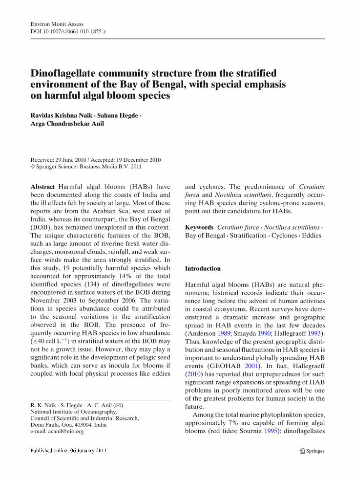
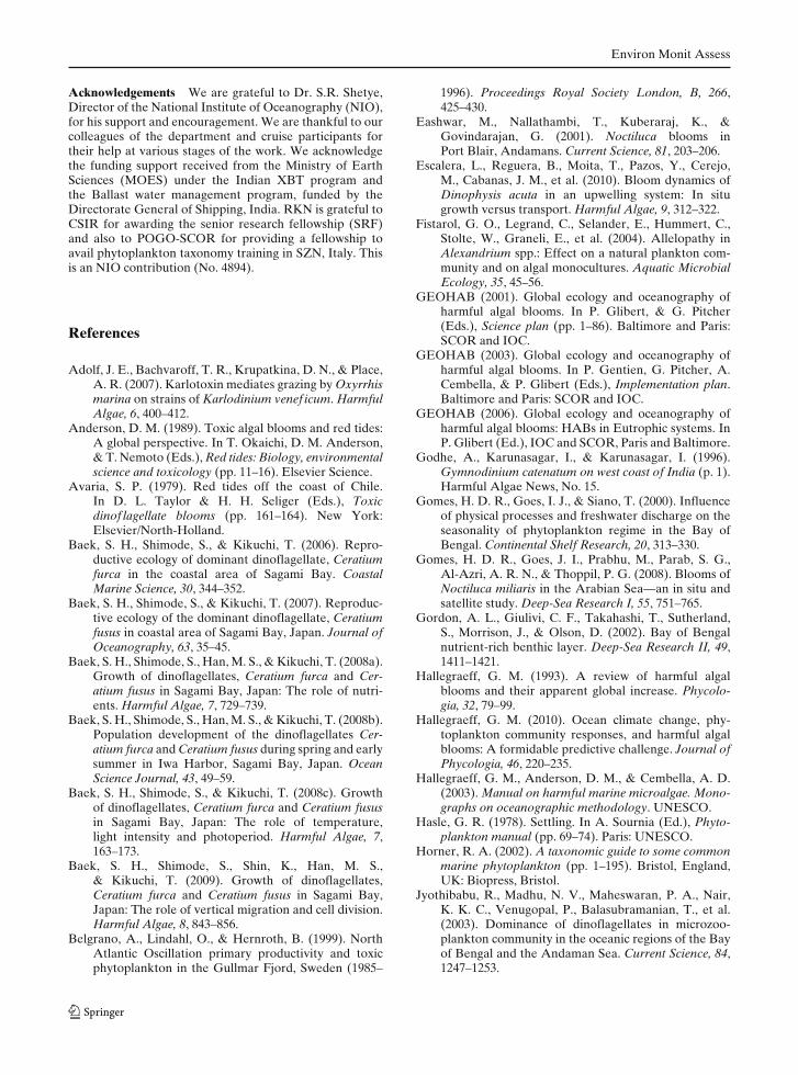
Fig. 1 Study area map showing station locations along the Chennai–Port Blair (CP) and Port Blair–Kolkata (PK) transectsin the Bay of Bengal

Environ Monit Assess

Ocean, remains relatively unexplored in the con-text of HAB studies. The BOB is known for itsunique characteristic features: large volume offreshwater input from river discharge and rainfall,warmer sea surface temperatures, monsoonalclouds and reversal of currents. The riverine in-put into this area injects loads of nutrients andsuspended sediment in the BOB (Gordon et al.2002; Mukhopadhyay et al. 2006). These featurespoint to the suitability of the BOB as a zone pronefor algal blooms including HAB events. However,the strongly stratified surface layer of the BOBrestricts the transport of nutrients from deeperlayers to the surface (Prasanna Kumar et al. 2002).Thus, it is very interesting to understand theseasonal variations in dinoflagellate communitystructure in this inimitable geographic region.

Since taking oceanic cruises on regular intervalsis not cost-effective, the “ships of opportunity”program, supported by the Indian ExpendableBathythermograph (XBT) project, was used.Therefore, the present study on the spatial andtemporal distribution of dinoflagellates in theBOB, with emphasis on HAB species, is the firstof its kind from the region. The following objec-tives were addressed: (1) dinoflagellate distribu-tion in the surface waters of the BOB and (2)detailing of the HAB species present and theirseasonal occurrence.

Materials and methods

Study area and sampling

This study was conducted with the support of theXBT program. Surface water samples were col-lected using steel buckets from the moving ship.This method was selected in order to minimize thephysical damage to cells compared to the methodof collecting samples using a pump. The sampleswere collected on two transects [Chennai to PortBlair (CP, 12 stations) and Port Blair to Kolkata(PK, 10 stations)] (Fig. 1), from passenger shipsplying along these transects. Samples were col-lected at one-degree intervals along both transect,from November 2003 to September 2006 coveringdifferent seasons. Among the sampling stationsfrom CP (central BOB) and PK (northern BOB)

Table 1 Station details of Chennai–Port Blair (CP) andPort Blair–Kolkata (PK) transects

Stations Lat (N) Long (E)

CP transect1 13.04 81.072 13.09 82.033 13.09 834 13.04 84.055 13.05 85.056 12.49 867 12.38 878 12.23 88.039 12.1 8910 11.52 90.0511 11.41 91.0412a 11.28 92.07

PK transect13a 12.03 93.1414a 13.01 93.1415 14 92.5616 15.01 92.2417 16.08 91.2918 17.09 90.4319 18 90.1220 19 89.321 20 88.522a 21.05 88.14

aNear coastal stations

transects, the majority were oceanic whereas, fewstations are near the coast (Table 1). Samples(1 L) were fixed with Lugol’s iodine solution forthe laboratory enumeration and identification ofdinoflagellates to the lowest possible taxonomiclevel.

Microscopic analysis

The 1-L sample was kept settling for 48 h. Afterthat, the volume was brought down to 100 ml andthen to 10 ml final concentration after another48-h settling period (method modified from Hasle1978). From this 10-ml final concentration, 3 mlconcentrated sample was taken in a petri dish(3.8 cm diameter) and examined under an Olym-pus inverted microscope at ×100 to ×400 mag-nification. Identification of the dinoflagellate taxawas carried out using the keys provided bySubrahmanyan (1968), Taylor (1976), Tomas(1997), Horner (2002), and Hallegraeff et al.(2003).

Environ Monit Assess

Tab

le2

Tax

onom

iclis

tofi

dent

ifie

ddi

nofl

agel

late

sdu

ring

the

stud

ype

riod

alon

gth

eC

Pan

dP

Ktr

anse

cts

(*po

tent

ially

HA

Bsp

ecie

s,†

new

repo

rtin

g)

CP

tran

sect

PK

tran

sect

Feb

04Ju

n04

Jul0

4O

ct04

Sep0

6N

ov03

Mar

04A

ug04

Oct

04Se

p06

Aut

otro

phic

dino

flag

ella

tes

Ale

xand

rium

conc

avum

0–2

(1)

Ale

xand

rium

spp.

0–2

(2)

0–9

(1)

0–2

(1)

0–20

(1)

0–6

(1)

Am

phid

iniu

msp

.*0–

7(5

)0–

2(1

)0–

2(1

)0–

5(3

)0–

12(1

0)0–

8(2

)0–

5(1

)0–

9(8

)A

mph

isol

enia

bide

ntat

a0–

2(2

)0–

8(7

)0–

3(1

)0–

3(3

)0–

2(1

)0–

9(3

)A

mph

isol

enia

glob

ifer

a0–

3(2

)B

leph

aroc

ysta

sp.

0–4

(2)

0–4

(3)

0–8

(2)

0–4

(5)

0–8

(6)

0–3

(1)

Cer

atoc

orys

arm

ata

0–2

(1)

0–2

(1)

Cer

atoc

orys

horr

ida

0–4

(2)

0–3

(1)

0–2

(2)

Cor

ytho

dini

umco

nstr

ictu

m0–

2(1

)0–

4(2

)C

oryt

hodi

nium

eleg

ans

0–4

(1)

0–3

(1)

0–3

(1)

0–3

(1)

Cor

ytho

dini

umm

icha

elsa

rsi

0–8

(2)

Cor

ytho

dini

umre

ticul

atum

0–2

(2)

0–2

(2)

Cor

ytho

dini

umte

ssel

atum

0–2

(2)

0–2

(1)

0–3

(2)

0–3

(3)

0–2

(2)

0–3

(2)

Cor

ytho

dini

umsp

.0–

2(1

)0–

3(1

)E

nsic

ulif

era

sp.

0–5

(1)

Gam

bier

disc

ussp

.*†

0–4

(1)

Gon

iodo

ma

poly

edri

cum

0–2

(2)

0–6

(2)

0–2

(1)

0–5

(1)

Gon

iodo

ma

spha

eric

um0–

6(3

)0–

3(1

)0–

6(1

)0–

2(2

)0–

5(1

)0–

3(2

)G

onya

ulax

brev

isul

cata

0–3

(1)

Gon

yaul

axdi

gita

lis0–

5(1

)G

onya

ulax

grin

dley

i0–

2(1

)G

onya

ulax

mon

ospi

na†

0–3

(1)

0–3

(1)

Gon

yaul

axpo

lyed

ra*

0–4

(4)

0–3

(1)

0–2

(1)

Gon

yaul

axpo

lygr

amm

a*0–

8(1

)0–

2(1

)0–

2(1

)0–

8(4

)0–

6(1

)0–

4(2

)0–

4(1

)0–

4(2

)0–

8(3

)0–

6(2

)G

onya

ulax

scri

ppsa

e0–

4(1

)0–

2(2

)0–

3(1

)0–

6(3

)G

onya

ulax

spin

ifer

a*0–

4(4

)0–

3(1

)0–

4(1

)0–

2(2

)G

onya

ulax

sp.

0–2

(1)

0–2

(2)

0–2

(2)

0–3

(1)

0–6

(6)

0–2

(1)

0–4

(2)

0–6

(1)

0–3

(2)

0–3

(5)

Gym

nodi

nium

spp.

*0–

2(1

)0–

5(1

)0–

6(3

)0–

6(1

)0–

6(3

)O

xyto

xum

glob

osum

0–26

(1)

Oxy

toxu

mla

ticep

s0–

3(1

)0–

6(3

)0–

2(1

)0–

6(4

)O

xyto

xum

scol

opax

0–3

(5)

0–2

(2)

0–4

(6)

0–8

(4)

0–3

(5)

0–6

(2)

0–2

(2)

0–5

(1)

0–3

(4)

Oxy

toxu

msc

eptr

um0–

2(1

)0–

4(5

)0–

3(4

)0–

2(3

)0–

3(1

)O

xyto

xum

sp.

0–6

(3)

0–2

(1)

0–2

(2)

0–3

(1)

Environ Monit Assess

Pod

olam

pas

bipe

s0–

2(3

)0–

3(1

)0–

3(2

)0–

2(1

)0–

5(1

)0–

6(2

)P

odol

ampa

sel

egan

s0–

4(3

)0–

2(1

)P

odol

ampa

spa

lmip

es0–

4(4

)0–

2(2

)0–

2(3

)0–

3(3

)0–

6(1

)0–

2(1

)0–

2(1

)0–

5(1

)0–

3(1

)P

odol

ampa

ssp

inif

era

0–2

(1)

0–2

(2)

0–3

(1)

0–5

(1)

Pyr

opha

cus

stei

nii

0–2

(1)

0–3

(1)

0–2

(3)

0–2

(1)

0–18

(1)

Pyr

opha

cus

spp.

0–5

(2)

Tor

odin

ium

tere

do†

0–3

(2)

Mix

otro

phic

dino

flag

ella

tes

Ale

xand

rium

min

utum

*0–

10(1

)C

erat

ium

arie

tinum

0–3

(2)

Cer

atiu

maz

oric

um0–

3(1

)0–

2(1

)C

erat

ium

cand

elab

rum

f.de

pres

sum

0–2

(1)

0–3

(1)

0–3

(1)

Cer

atiu

mco

ntor

tum

0–5

(3)

0–4

(1)

Cer

atiu

mde

clin

atum

0–2

(1)

0–2

(1)

0–5

(4)

0–9

(4)

0–5

(1)

0–9

(3)

Cer

atiu

mde

flex

um0–

3(1

)0–

8(1

)C

erat

ium

dens

0–3

(1)

Cer

atiu

mex

tens

um0–

4(4

)0–

6(1

)C

erat

ium

furc

a*0–

2(1

)0–

2(2

)0–

5(4

)0–

9(5

)0–

20(5

)0–

6(4

)0–

13(4

)0–

18(4

)C

erat

ium

fusu

s*0–

6(4

)0–

2(4

)0–

2(3

)0–

13(9

)0–

6(4

)0–

20(1

)0–

4(1

)0–

6(5

)0–

8(7

)0–

12(3

)C

erat

ium

gibb

erum

0–2

(1)

Cer

atiu

mho

rrid

um0–

2(2

)0–

6(2

)0–

2(1

)0–

3(1

)C

erat

ium

kars

teni

i0–

2(4

)0–

2(1

)C

erat

ium

kofo

idii

0–2

(1)

0–2

(1)

0–2

(1)

Cer

atiu

mlin

eatu

m0–

2(2

)0–

3(2

)0–

3(1

)0–

5(1

)0–

3(1

)C

erat

ium

lunu

la0–

2(1

)C

erat

ium

mac

roce

ros

0–2

(3)

0–2

(1)

0–2

(3)

0–2

(1)

Cer

atiu

mpe

ntag

onum

0–9

(7)

0–2

(1)

0–3

(1)

Cer

atiu

msc

hmid

tii0–

2(2

)0–

5(3

)0–

3(1

)0–

8(2

)C

erat

ium

sym

met

ricu

m0–

10(4

)0–

3(1

)0–

2(2

)C

erat

ium

tere

s0–

8(6

)0–

8(7

)0–

8(7

)0–

9(7

)0–

4(1

)0–

2(1

)0–

3(2

)0–

12(3

)C

erat

ium

tric

hoce

ros

0–2

(2)

0–8

(1)

Cer

atiu

mtr

ipos

0–2

(1)

0–2

(1)

0–2

(1)

Cer

atiu

mvu

ltur

0–4

(1)

0–3

(1)

Cer

atiu

msp

p.0–

2(1

)0–

3(2

)0–

3(3

)0–

5(1

)D

inop

hysi

sca

udat

a*0–

2(1

)0–

5(1

)D

inop

hysi

sm

iles*

0–12

(1)

Din

ophy

sis

schu

ettii

0–3

(1)

Din

ophy

sis

spp.

0–4

(5)

0–2

(2)

0–5

(2)

0–6

(6)

0–5

(1)

0–3

(1)

Dis

sodi

umas

ymm

etri

cum

0–2

(1)

Environ Monit Assess

Tab

le2

(con

tinu

ed)

CP

tran

sect

PK

tran

sect

Feb

04Ju

n04

Jul0

4O

ct04

Sep0

6N

ov03

Mar

04A

ug04

Oct

04Se

p06

Pro

roce

ntru

mar

cuat

um†

0–2

(1)

0–4

(1)

Pro

roce

ntru

mbe

lizea

num

*†

0–24

(1)

Pro

roce

ntru

mco

mpr

essu

m0–

2(1

)0–

5(1

)0–

2(1

)P

roro

cent

rum

grac

ile0–

8(4

)P

roro

cent

rum

lent

icul

atum

0–4

(1)

Pro

roce

ntru

mlim

a*0–

2(1

)P

roro

cent

rum

mic

ans*

0–20

(1)

0–2

(2)

0–3

(1)

0–3

(2)

0–10

(1)

0–10

(2)

0–9

(1)

Pro

roce

ntru

mm

inim

us*

0–2

(1)

0–2

(1)

0–3

(1)

0–2

(1)

Pro

roce

ntru

mm

exic

anum

*0–

5(6

)P

roro

cent

rum

obtu

sum

0–8

(3)

0–3

(2)

0–3

(2)

Pro

roce

ntru

msc

utel

lum

†0–

2(1

)P

roro

cent

rum

sigm

oide

s*0–

2(1

)0–

3(1

)0–

9(4

)P

roro

cent

rum

sp.

0–2

(2)

0–14

(2)

0–4

(3)

0–8

(5)

0–9

(7)

0–4

(4)

0–4

(1)

0–6

(2)

0–8

(3)

0–6

(5)

Pyr

ocys

tisfu

sifo

rmis

0–2

(1)

0–3

(1)

Pyr

ocys

tisha

mul

us0–

2(1

)0–

4(2

)0–

2(1

)P

yroc

ystis

lunu

la0–

4(1

)P

yroc

ystis

spp.

0–2

(1)

0–2

(1)

0–3

(1)

0–3

(2)

0–14

(5)

0–6

(1)

0–5

(2)

0–3

(1)

Scri

ppsi

ella

troc

hoid

ea*

0–14

(9)

0–2

(1)

0–3

(1)

0–9

(7)

0–26

(6)

0–4

(1)

0–5

(2)

0–15

(7)

Scri

ppsi

ella

spp.

0–2

(1)

0–6

(5)

0–10

(3)

0–2

(1)

0–6

(3)

0–8

(1)

Het

erot

roph

icdi

nofl

agel

late

sG

otoi

usab

ei†

0–6

(4)

0–3

(1)

0–10

(5)

0–8

(4)

0–3

(1)

His

tione

isca

rina

ta†

0–2

(1)

0–3

(1)

0–4

(2)

His

tione

isco

stat

a†

0–2

(1)

0–2

(1)

0–2

(1)

His

tione

isde

pres

sa0–

2(2

)0–

2(2

)H

istio

neis

spp.

0–3

(1)

Kat

odin

ium

sp.

0–2

(3)

0–4

(5)

0–10

(2)

0–3

(2)

0–2

(2)

0–5

(1)

Noc

tiluc

asc

intil

lans

0–2

(1)

0–40

(1)

0–2

(1)

Noc

tiluc

asp

p.0–

2(1

)O

rnith

ocer

cus

hete

ropo

rus

0–6

(2)

0–2

(1)

Orn

ithoc

ercu

sm

agni

ficu

s0–

2(2

)0–

4(2

)0–

18(2

)0–

3(1

)0–

5(1

)0–

6(2

)O

rnith

ocer

cus

quad

ratu

s0–

2(1

)0–

2(1

)0–

3(1

)0–

5(1

)O

rnith

ocer

cus

stei

nii

0–2

(1)

0–4

(2)

0–2

(1)

0–2

(1)

0–5

(1)

Orn

ithoc

ercu

sth

umii

0–2

(1)

0–4

(2)

0–2

(1)

0–5

(1)

Environ Monit Assess

Orn

ithoc

ercu

ssp

p.0–

2(1

)0–

3(1

)O

xyph

ysis

spp.

0–3

(1)

Pen

taph

arso

dini

umsp

.†0–

2(1

)0–

4(1

)P

hala

crom

aar

gus

0–2

(1)

Pha

lacr

oma

cune

us0–

2(1

)0–

5(1

)P

hala

crom

ara

pa0–

2(2

)0–

2(1

)0–

3(1

)P

hala

crom

aro

tund

atum

0–3

(1)

0–2

(1)

0–8

(2)

0–3

(2)

Pha

lacr

oma

spp.

0–2

(2)

0–2

(2)

0–2

(1)

Pro

noct

iluca

pela

gica

0–2

(1)

Pro

noct

ulic

asp

inif

era

0–2

(2)

0–2

(1)

0–3

(1)

0–3

(1)

Pro

tope

ridi

nium

asym

met

ricu

m0–

4(3

)0–

2(1

)P

roto

peri

dini

umbr

evip

es0–

2(1

)P

roto

peri

dini

umcr

asip

es*

0–2

(1)

0–2

(1)

Pro

tope

ridi

nium

depr

essu

m0–

2(4

)0–

2(1

)0–

4(2

)0–

2(1

)0–

5(1

)P

roto

peri

dini

umdi

verg

ens

0–2

(1)

0–4

(3)

0–5

(6)

0–3

(1)

0–2

(1)

0–2

(2)

0–3

(5)

Pro

tope

ridi

nium

eleg

ans

0–3

(2)

Pro

tope

ridi

nium

gran

de0–

4(1

)P

roto

peri

dini

umle

onis

0–2

(1)

Pro

tope

ridi

nium

min

utum

0–3

(1)

Pro

tope

ridi

nium

oblo

ngum

0–2

(1)

Pro

tope

ridi

nium

ovat

um0–

4(8

)0–

26(2

)P

roto

peri

dini

umpa

cifi

cum

0–2

(1)

0–10

(2)

0–6

(2)

0–4

(2)

0–8

(3)

Pro

tope

ridi

nium

palli

dum

0–2

(1)

Pro

tope

ridi

nium

pedu

ncul

atum

0–4

(3)

0–2

(2)

0–8

(4)

0–4

(1)

0–2

(3)

0–4

(1)

0–5

(1)

Pro

tope

ridi

nium

pellu

cidu

m0–

4(2

)0–

3(1

)0–

4(1

)0–

2(3

)0–

4(1

)P

roto

peri

dini

umpe

ntag

onum

0–2

(1)

0–10

(1)

0–2

(1)

Pro

tope

ridi

nium

pyri

form

e0–

2(1

)P

roto

peri

dini

umst

eini

i0–

2(1

)0–

3(2

)0–

6(1

)0–

4(1

)0–

8(2

)0–

3(4

)P

roto

peri

dini

umsu

bine

rme

0–3

(1)

0–2

(2)

Pro

tope

ridi

nium

sp.

0–4

(4)

0–4

(6)

0–3

(4)

0–9

(8)

0–2

(1)

0–4

(2)

0–8

(3)

0–5

(1)

0–9

(9)

Zyg

abik

odin

ium

sp.

0–2

(1)

The

valu

esou

tsid

ebr

acke

tin

dica

teth

era

nge

ofab

unda

nce

duri

ngth

atm

onth

and

valu

esin

side

the

brac

ket

indi

cate

sth

efr

eque

ncy

ofoc

curr

ence

atC

P(t

otal

12st

atio

ns)

and

PK

(tot

al10

stat

ions

)tr

anse

cts

duri

ngth

ere

spec

tive

sam

plin

gm

onth

s

Environ Monit Assess

Data analyses

To evaluate seasonal differences, the observa-tional period was classified into three seasons:Pre-monsoon (PrM—February to March 04),South west monsoon (SWM—June 04, July 04,August 04, September 06) and Post-monsoon(PoM—November 03, October 04).

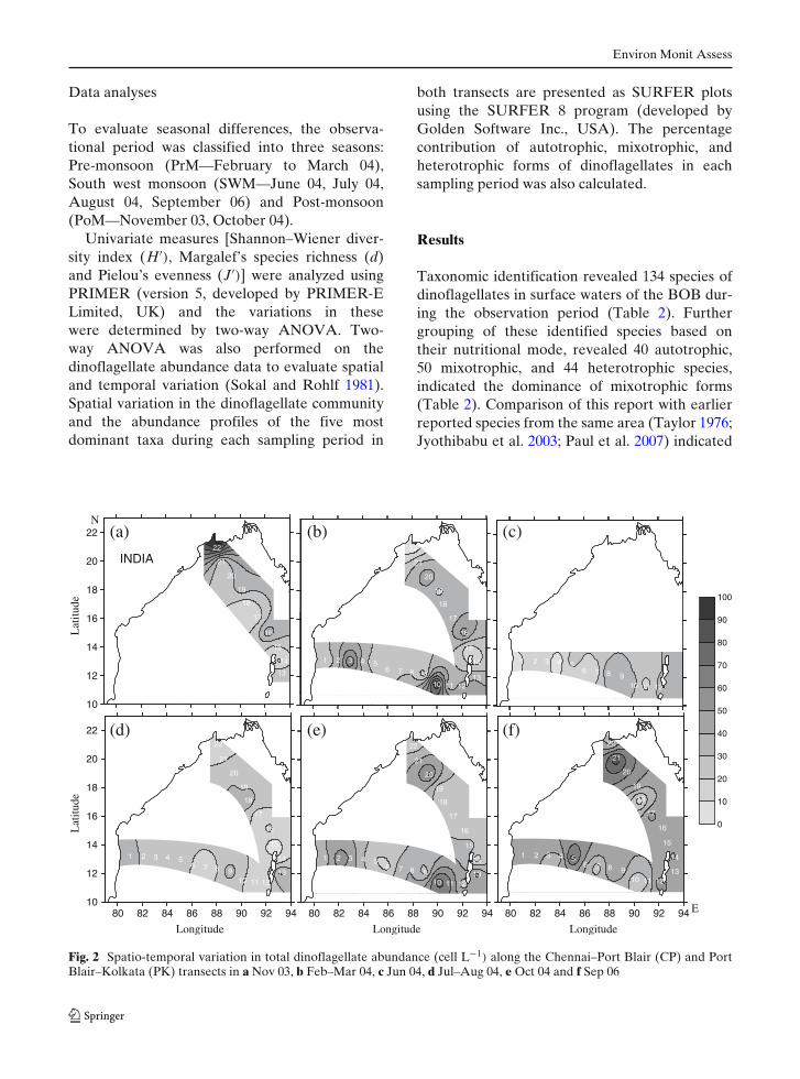
Univariate measures [Shannon–Wiener diver-sity index (H′), Margalef’s species richness (d)and Pielou’s evenness (J′)] were analyzed usingPRIMER (version 5, developed by PRIMER-ELimited, UK) and the variations in thesewere determined by two-way ANOVA. Two-way ANOVA was also performed on thedinoflagellate abundance data to evaluate spatialand temporal variation (Sokal and Rohlf 1981).Spatial variation in the dinoflagellate communityand the abundance profiles of the five mostdominant taxa during each sampling period in

both transects are presented as SURFER plotsusing the SURFER 8 program (developed byGolden Software Inc., USA). The percentagecontribution of autotrophic, mixotrophic, andheterotrophic forms of dinoflagellates in eachsampling period was also calculated.

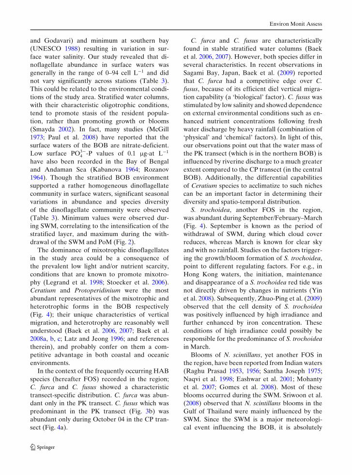
Results

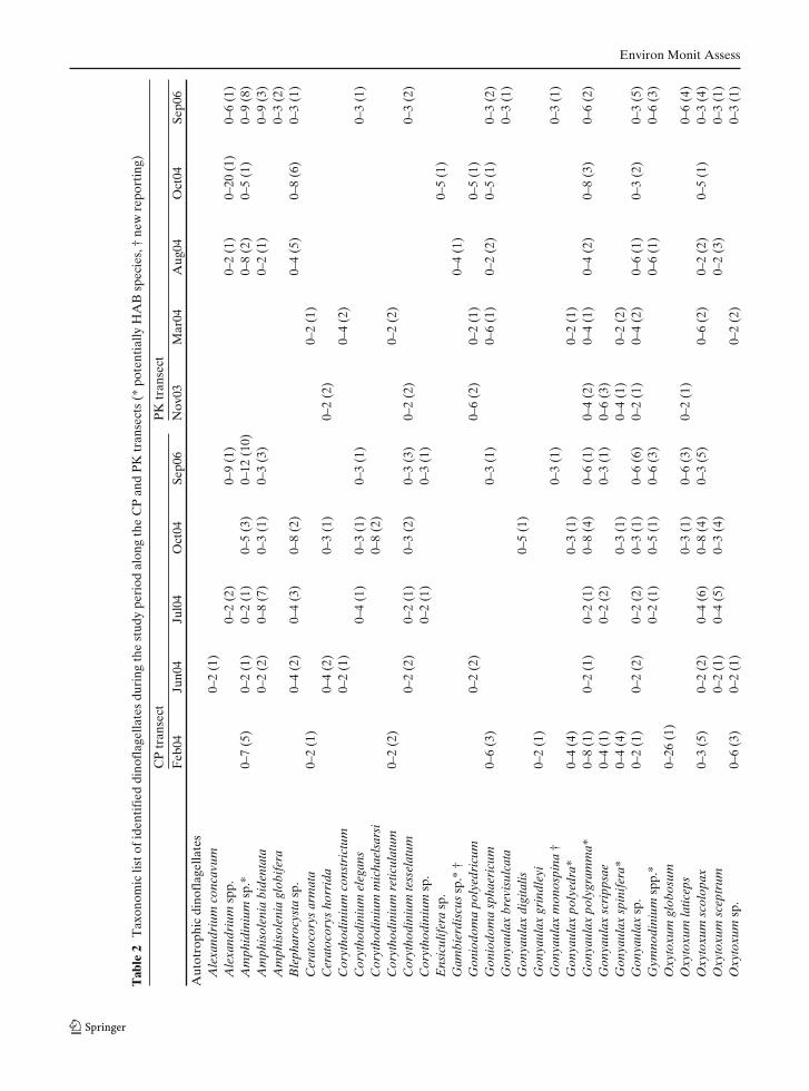
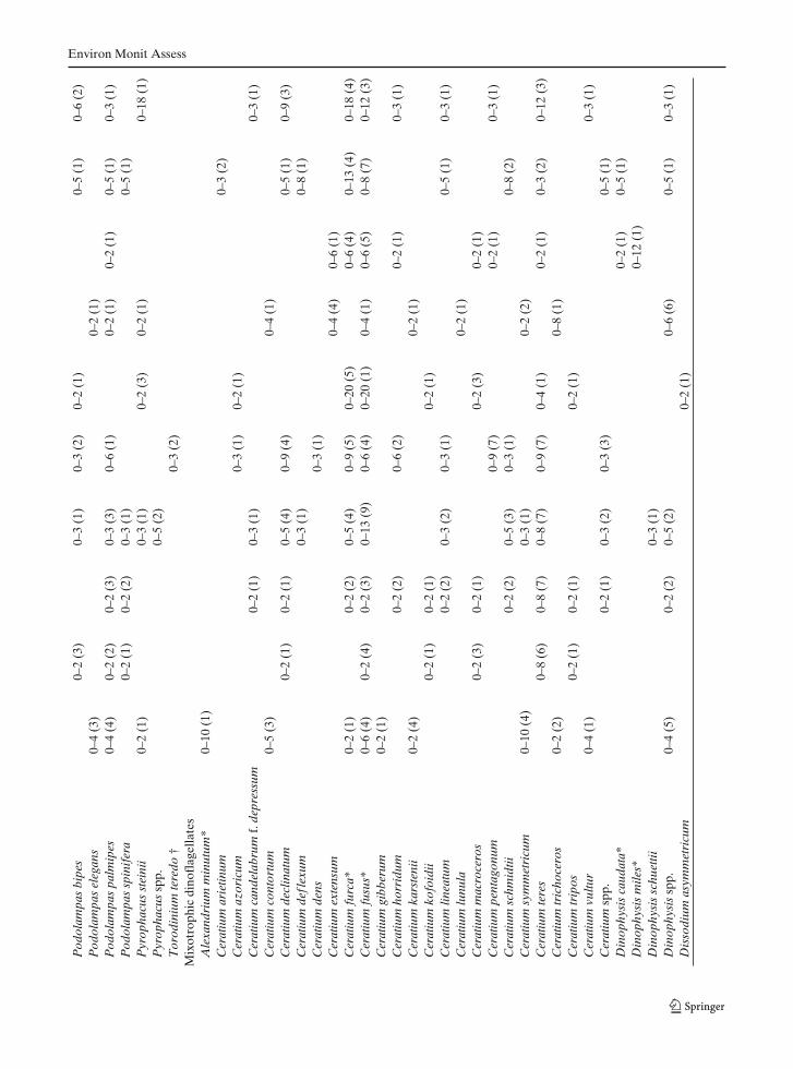
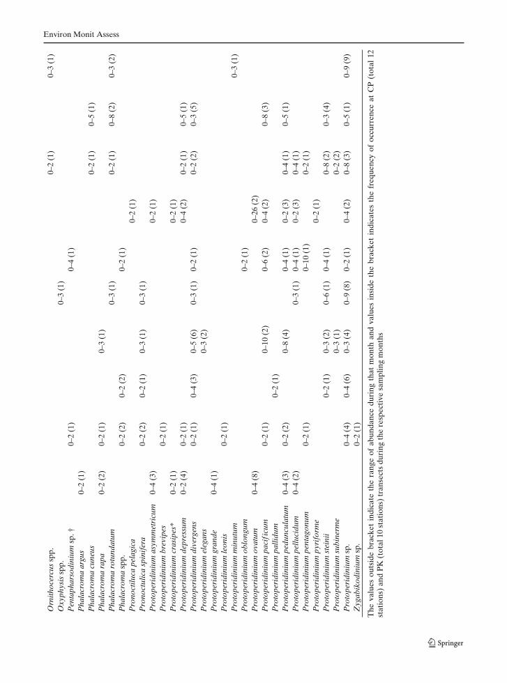
Taxonomic identification revealed 134 species ofdinoflagellates in surface waters of the BOB dur-ing the observation period (Table 2). Furthergrouping of these identified species based ontheir nutritional mode, revealed 40 autotrophic,50 mixotrophic, and 44 heterotrophic species,indicated the dominance of mixotrophic forms(Table 2). Comparison of this report with earlierreported species from the same area (Taylor 1976;Jyothibabu et al. 2003; Paul et al. 2007) indicated

Longitude Longitude Longitude

Lat

itude

N

E

Lat

itude

(b) (c)

13

14

15

16

17

18

19

20

21

22

10

12

14

16

18

20

22

10

12

14

16

18

20

22

15

16

17

18

19

20

22

21

14

13

1 2 3 4 56 7 8 9

10 11 12

INDIAINDIA

INDIA

1 2 3 4 56 7 8 9

10 11 12

80 82 84 86 88 90 92 94 80 82 84 86 88 90 92 94 80 82 84 86 88 90 92 94

15

16

17

18

19

20

22

21

14

13

1 2 4 56 7 8 9

10 11 12

3

15

16

17

18

19

20

22

21

14

13

1 2 3 4 56 7 8 9

10 11 12

15

16

17

18

19

20

22

21

14

13

1 2 3 4 56 7 8 9

10 11 12

0

10

20

30

40

50

60

70

80

90

100

(a) (b) (c)

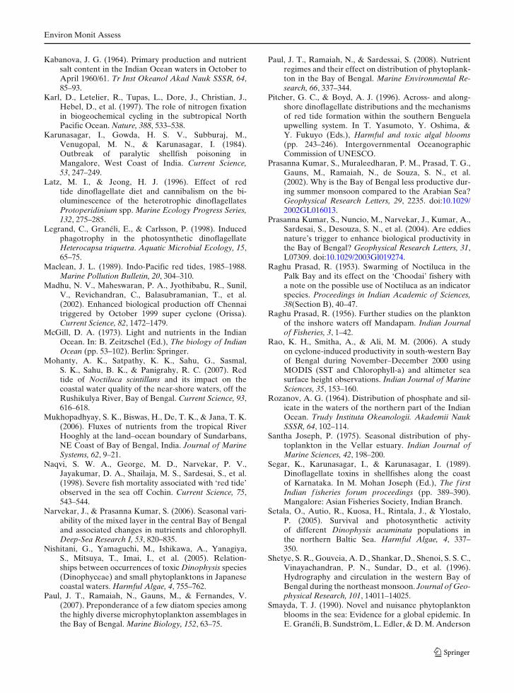
(f)(e)(d)

Fig. 2 Spatio-temporal variation in total dinoflagellate abundance (cell L−1) along the Chennai–Port Blair (CP) and PortBlair–Kolkata (PK) transects in a Nov 03, b Feb–Mar 04, c Jun 04, d Jul–Aug 04, e Oct 04 and f Sep 06

Environ Monit Assess

Tab

le3

Tw

o-w

ayA

NO

VA

toev

alua

teth

eva

riat

ion

into

tald

inof

lage

llate

abun

danc

e,sp

ecie

sri

chne

ss,e

venn

ess,

and

dive

rsit

yal

ong

the

CP

and

PK

tran

sect

s

CP

tran

sect

PK

tran

sect

dfSS

MS

Fs

Pva

lue

dfSS

MS

Fs

Pva

lue

Abu

ndan

ceSt

atio

ns11

3319

302

10.

2817

930

9234

41

0.49

43Se

ason

s4

5025

1256

50.

0016

434

9387

32

0.06

63W

ithi

nsu

b-gr

oup

erro

r44

1057

624

036

1299

436

1T

otal

5918

920

4919

579

Spec

ies

even

ness

Stat

ions

100

01

0.19

229

00

10.

2578

Seas

ons

40

01

0.31

454

00

20.

0710

Wit

hin

sub-

grou

per

ror

400

036

10

Tot

al54

049

1Sp

ecie

sri

chne

ssSt

atio

ns10

101

20.

1661

910

13

0.01

80Se

ason

s4

00

00.

9585

43

12

0.16

14W

ithi

nsu

b-gr

oup

erro

r40

271

3614

0T

otal

5437

4927

Spec

ies

dive

rsit

ySt

atio

ns10

30

20.

1033

94

02

0.03

38Se

ason

s4

10

10.

4078

42

03

0.04

83W

ithi

nsu

b-gr

oup

erro

r40

60

366

0T

otal

549

4912

Environ Monit Assess

ten new dinoflagellate species (Table 2 speciesmarked with †). Approximately 14% of the iden-tified species were potential HAB species (Table 2species marked with *).

Spatial and temporal distributionof dinoflagellate assemblages

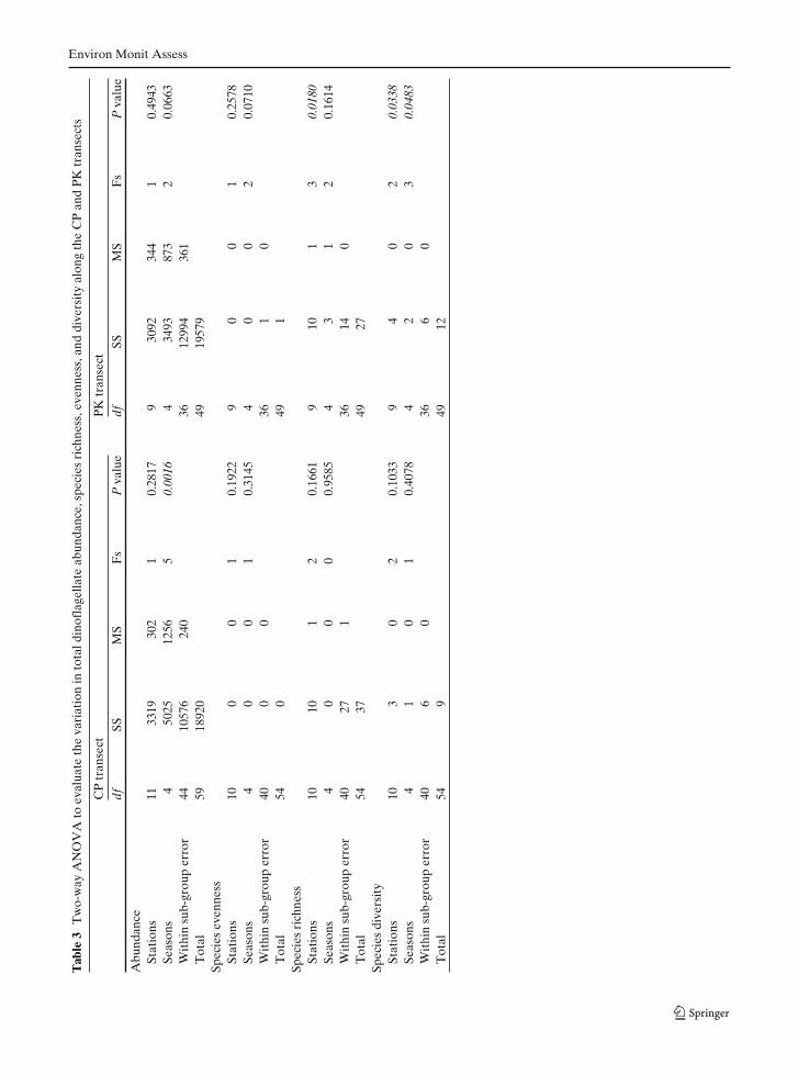
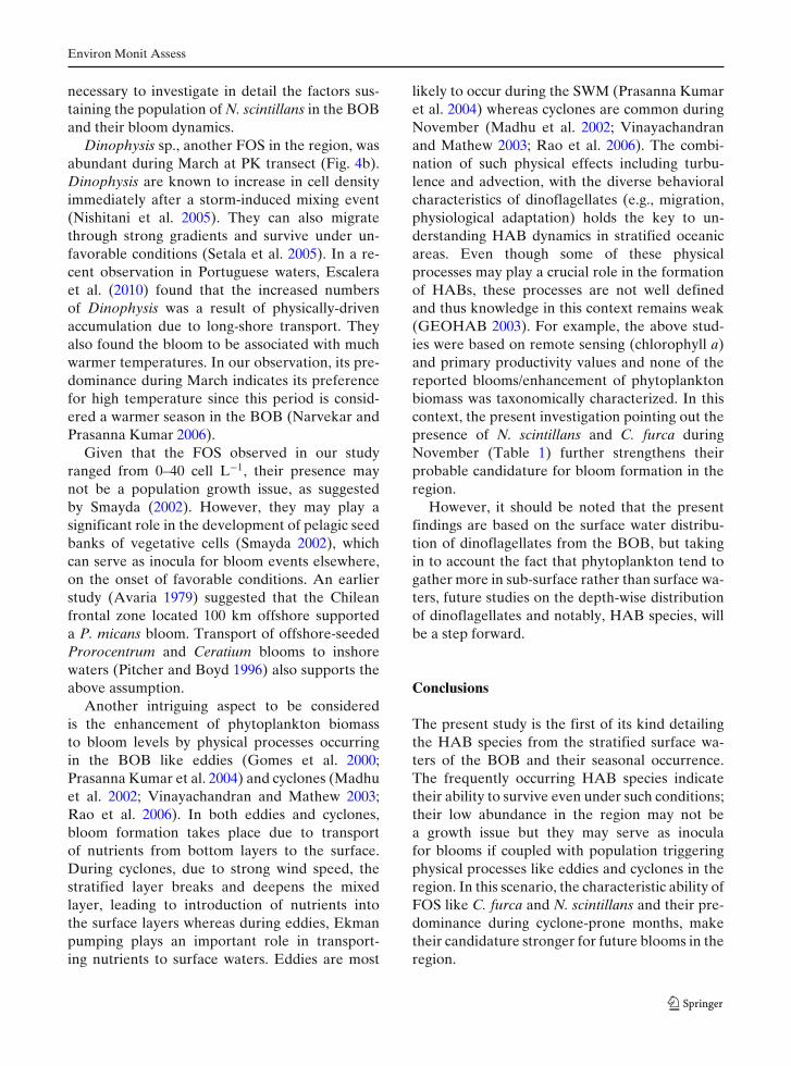
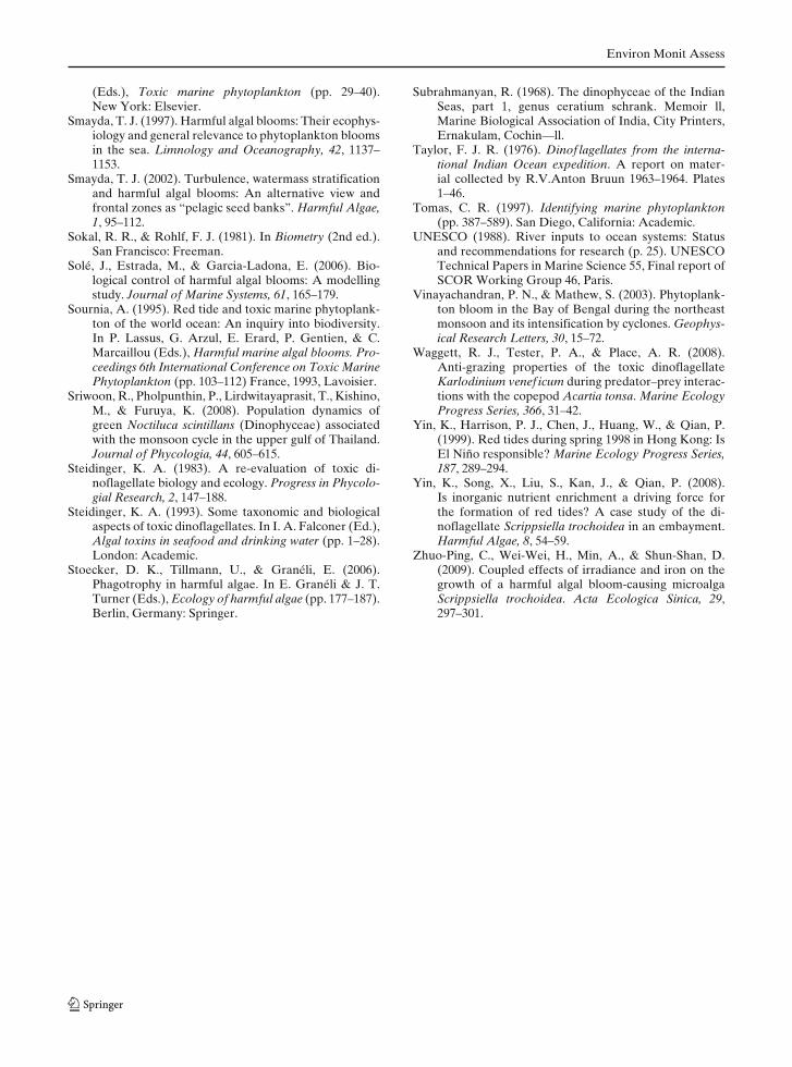
The abundance of dinoflagellates ranged from0–94 cell L−1 throughout the observation periodat both CP and PK transects (Fig. 2). Thoughseasonal variation in dinoflagellate abundancewas observed in both transects, the variation wasstatistically significant at only the CP transect(Table 3). The highest average abundance ofdinoflagellates was observed during September06 (48 cell L−1 at PK) followed by October 04(40 cell L−1 at CP) whereas low abundance wasrecorded during June (21 cell L−1 at CP) andAugust 04 (22 cell L−1 at PK; Fig. 2). The spatialvariation in dinoflagellate abundance was not sta-tistically significant in both transects (Table 3).Species richness and diversity varied significantlyin the PK transect; species richness only acrossstations and diversity across both stations and sea-sons (Table 3). Mixotrophic dinoflagellates dom-inated across both transects, with the exceptionof October 04 at CP and September 06 at PKtransects, that were dominated by heterotrophicforms (Fig. 3). Ceratium was the dominant genusamong the mixotrophic forms whereas Protoperi-dinium was the dominant heterotrophic form.Ceratium fusus, Ceratium teres, Gotoius abei, Oxy-toxum scolopax, Protoperidinium ovatum, andScrippsiella trochoidea were among the abundantforms in both the transects. Amphisolenia biden-tata, Ceratium pentagonum, Ceratium symmet-ricum, Oxytoxum globosum, and Prorocentrumbelizianum were abundant only in CP transect(Fig. 4a) whereas Ceratium extensum, Ceratiumfurca, Dinophysis miles and Noctiluca scintillanswere abundant only in the PK transect (Fig. 4b).

Seasonal variation in HAB species

Overall, 19 potentially HAB species were encoun-tered in this area (Table 2). Some HAB specieswere present during all the seasons throughout the

37

48

15

26

45

29

35

38

27

22

35

43

35

46

18

4146

13

27

42

32

25

38

37

18

51

31

28

23

49

Autotrophic Mixotrophic Heterotrophic

(a)

(b)

(c)

(d)

(e)

(f)

(g)

(h)

(i)

(j)

Nov 03

Feb-Mar 04

Jun 04

Jul-Aug 04

Oct 04

Sep 06

CP transect PK transect

Fig. 3 The percentage contribution of autotrophic,mixotrophic and heterotrophic dinoflagellates along thea–e Chennai–Port Blair (CP) and f–j Port Blair–Kolkata(PK) transects. a Feb 04, b Jun 04, c Jul 04, d Oct 04, e Sep06, f Nov 03, g Mar 04, h Aug 04, i Oct 04 and j Sep 06

study period. These frequently occurring specieswere C. furca, C. fusus, Dinophysis sp., Gonyaulaxpolygramma, Gonyaulax sp., N. scintillans, Pro-rocentrum sp., S. trochoidea, Scrippsiella sp.(Table 2). Season-specific trends were also ob-served. Alexandrium minutum, Prorocentrum

Environ Monit Assess

Fig. 4 The five mostabundant species duringeach sampling period atthe (a) Chennai–PortBlair and (b) PortBlair–Kolkata transects.The maximum diameterof circle corresponds toaverage 9 cell L−1

b)

Feb04

Jun04

Jul04

Oct04

Sep06

Am

phis

olen

ia b

iden

tata

Am

phid

iniu

m s

p.

Cer

atiu

m fu

sus

Cer

atiu

m p

enta

gonu

m

Cer

atiu

m s

ymm

etri

cum

Cer

atiu

m te

res

Got

oius

abe

i

Oxy

toxu

m g

lobo

sum

Oxy

toxu

m s

colo

pax

Pro

roce

ntru

m b

eliz

ianu

m

Pro

roce

ntru

m s

p.

Pro

tope

ridi

nium

ova

tum

Pro

tope

ridi

nium

ped

uncu

latu

m

Pro

tope

ridi

nium

sp.

Scri

ppsi

ella

spp

.

Scri

ppsi

ella

troc

hoid

ea

a)

Oct04

Aug04

Mar04

Nov03

Sep06

Ale

xand

rium

spp

.

Am

phid

iniu

m s

p.

Ble

phar

ocys

ta s

p.

Cer

atiu

m e

xten

sum

Cer

atiu

m fu

rca

Cer

atiu

m fu

sus

Cer

atiu

m te

res

Din

ophy

sis

mil

es

Din

ophy

sis

spp.

Pyr

ocys

tis

spp

.

Got

oius

abe

i

Noc

tilu

ca s

cint

illa

ns

Oxy

toxu

m s

colo

pax

Pro

tope

ridi

nium

ova

tum

Pro

tope

ridi

nium

sp.

Scri

ppsi

ella

spp

.

Scri

ppsi

ella

troc

hoid

ea

lima, and Protoperidinium crassipes occurred onlyduring PrM whereas Dinophysis caudata, D. miles,Prorocentrum micans, P. mexicanum, P. minimus,Gymnodinium sp. and Gambierdiscus sp. werefound during SWM and PoM periods. Gonyaulaxpolyedra and G. spinifera occurred in PrM andPoM but not during SWM. In contrast to this, P.belizianum and P. sigmoides occurred only duringthe SWM.

Discussion

The BOB is a semi-enclosed tropical basin, distin-guished by a strongly stratified surface layer and

a seasonally reversing circulation (Shetye et al.1996). It is also influenced by monsoonal windsand enormous freshwater influx. The surfacestratified water column of the BOB restricts thevertical transport of nutrients from the bottomlayers to the surface, and therefore phytoplank-ton productivity as well (Prasanna Kumar et al.2002). The stratification is especially intense dur-ing the SWM period (Prasanna Kumar et al.2004) due to the influx of freshwater throughprecipitation and riverine discharges. The averageannual riverine discharge varies from the north-ern to southern bay with maximum discharge atnorth (1012 m3 from Ganges and Brahmaputra),medium at central (8.5 × 1010 m3 from Krishna

Environ Monit Assess

and Godavari) and minimum at southern bay(UNESCO 1988) resulting in variation in sur-face water salinity. Our study revealed that di-noflagellate abundance in surface waters wasgenerally in the range of 0–94 cell L−1 and didnot vary significantly across stations (Table 3).This could be related to the environmental condi-tions of the study area. Stratified water columns,with their characteristic oligotrophic conditions,tend to promote stasis of the resident popula-tion, rather than promoting growth or blooms(Smayda 2002). In fact, many studies (McGill1973; Paul et al. 2008) have reported that thesurface waters of the BOB are nitrate-deficient.Low surface PO3−

4 -P values of 0.1 μg-at L−1

have also been recorded in the Bay of Bengaland Andaman Sea (Kabanova 1964; Rozanov1964). Though the stratified BOB environmentsupported a rather homogeneous dinoflagellatecommunity in surface waters, significant seasonalvariations in abundance and species diversityof the dinoflagellate community were observed(Table 3). Minimum values were observed dur-ing SWM, correlating to the intensification of thestratified layer, and maximum during the with-drawal of the SWM and PoM (Fig. 2).

The dominance of mixotrophic dinoflagellatesin the study area could be a consequence ofthe prevalent low light and/or nutrient scarcity,conditions that are known to promote mixotro-phy (Legrand et al. 1998; Stoecker et al. 2006).Ceratium and Protoperidinium were the mostabundant representatives of the mixotrophic andheterotrophic forms in the BOB respectively(Fig. 4); their unique characteristics of verticalmigration, and heterotrophy are reasonably wellunderstood (Baek et al. 2006, 2007; Baek et al.2008a, b, c; Latz and Jeong 1996; and referencestherein), and probably confer on them a com-petitive advantage in both coastal and oceanicenvironments.

In the context of the frequently occurring HABspecies (hereafter FOS) recorded in the region;C. furca and C. fusus showed a characteristictransect-specific distribution. C. furca was abun-dant only in the PK transect. C. fusus which waspredominant in the PK transect (Fig. 3b) wasabundant only during October 04 in the CP tran-sect (Fig. 4a).

C. furca and C. fusus are characteristicallyfound in stable stratified water columns (Baeket al. 2006, 2007). However, both species differ inseveral characteristics. In recent observations inSagami Bay, Japan, Baek et al. (2009) reportedthat C. furca had a competitive edge over C.fusus, because of its efficient diel vertical migra-tion capability (a ‘biological’ factor). C. fusus wasstimulated by low salinity and showed dependenceon external environmental conditions such as en-hanced nutrient concentrations following freshwater discharge by heavy rainfall (combination of‘physical’ and ‘chemical’ factors). In light of this,our observations point out that the water mass ofthe PK transect (which is in the northern BOB) isinfluenced by riverine discharge to a much greaterextent compared to the CP transect (in the centralBOB). Additionally, the differential capabilitiesof Ceratium species to acclimatize to such nichescan be an important factor in determining theirdiversity and spatio-temporal distribution.

S. trochoidea, another FOS in the region,was abundant during September/February–March(Fig. 4). September is known as the period ofwithdrawal of SWM, during which cloud coverreduces, whereas March is known for clear skyand with no rainfall. Studies on the factors trigger-ing the growth/bloom formation of S. trochoidea,point to different regulating factors. For e.g., inHong Kong waters, the initiation, maintenanceand disappearance of a S. trochoidea red tide wasnot directly driven by changes in nutrients (Yinet al. 2008). Subsequently, Zhuo-Ping et al. (2009)observed that the cell density of S. trochoideawas positively influenced by high irradiance andfurther enhanced by iron concentration. Theseconditions of high irradiance could possibly beresponsible for the predominance of S. trochoideain March.

Blooms of N. scintillans, yet another FOS inthe region, have been reported from Indian waters(Raghu Prasad 1953, 1956; Santha Joseph 1975;Naqvi et al. 1998; Eashwar et al. 2001; Mohantyet al. 2007; Gomes et al. 2008). Most of theseblooms occurred during the SWM. Sriwoon et al.(2008) observed that N. scintillans blooms in theGulf of Thailand were mainly influenced by theSWM. Since the SWM is a major meteorologi-cal event influencing the BOB, it is absolutely

Environ Monit Assess

necessary to investigate in detail the factors sus-taining the population of N. scintillans in the BOBand their bloom dynamics.

Dinophysis sp., another FOS in the region, wasabundant during March at PK transect (Fig. 4b).Dinophysis are known to increase in cell densityimmediately after a storm-induced mixing event(Nishitani et al. 2005). They can also migratethrough strong gradients and survive under un-favorable conditions (Setala et al. 2005). In a re-cent observation in Portuguese waters, Escaleraet al. (2010) found that the increased numbersof Dinophysis was a result of physically-drivenaccumulation due to long-shore transport. Theyalso found the bloom to be associated with muchwarmer temperatures. In our observation, its pre-dominance during March indicates its preferencefor high temperature since this period is consid-ered a warmer season in the BOB (Narvekar andPrasanna Kumar 2006).

Given that the FOS observed in our studyranged from 0–40 cell L−1, their presence maynot be a population growth issue, as suggestedby Smayda (2002). However, they may play asignificant role in the development of pelagic seedbanks of vegetative cells (Smayda 2002), whichcan serve as inocula for bloom events elsewhere,on the onset of favorable conditions. An earlierstudy (Avaria 1979) suggested that the Chileanfrontal zone located 100 km offshore supporteda P. micans bloom. Transport of offshore-seededProrocentrum and Ceratium blooms to inshorewaters (Pitcher and Boyd 1996) also supports theabove assumption.

Another intriguing aspect to be consideredis the enhancement of phytoplankton biomassto bloom levels by physical processes occurringin the BOB like eddies (Gomes et al. 2000;Prasanna Kumar et al. 2004) and cyclones (Madhuet al. 2002; Vinayachandran and Mathew 2003;Rao et al. 2006). In both eddies and cyclones,bloom formation takes place due to transportof nutrients from bottom layers to the surface.During cyclones, due to strong wind speed, thestratified layer breaks and deepens the mixedlayer, leading to introduction of nutrients intothe surface layers whereas during eddies, Ekmanpumping plays an important role in transport-ing nutrients to surface waters. Eddies are most

likely to occur during the SWM (Prasanna Kumaret al. 2004) whereas cyclones are common duringNovember (Madhu et al. 2002; Vinayachandranand Mathew 2003; Rao et al. 2006). The combi-nation of such physical effects including turbu-lence and advection, with the diverse behavioralcharacteristics of dinoflagellates (e.g., migration,physiological adaptation) holds the key to un-derstanding HAB dynamics in stratified oceanicareas. Even though some of these physicalprocesses may play a crucial role in the formationof HABs, these processes are not well definedand thus knowledge in this context remains weak(GEOHAB 2003). For example, the above stud-ies were based on remote sensing (chlorophyll a)and primary productivity values and none of thereported blooms/enhancement of phytoplanktonbiomass was taxonomically characterized. In thiscontext, the present investigation pointing out thepresence of N. scintillans and C. furca duringNovember (Table 1) further strengthens theirprobable candidature for bloom formation in theregion.

However, it should be noted that the presentfindings are based on the surface water distribu-tion of dinoflagellates from the BOB, but takingin to account the fact that phytoplankton tend togather more in sub-surface rather than surface wa-ters, future studies on the depth-wise distributionof dinoflagellates and notably, HAB species, willbe a step forward.

Conclusions

The present study is the first of its kind detailingthe HAB species from the stratified surface wa-ters of the BOB and their seasonal occurrence.The frequently occurring HAB species indicatetheir ability to survive even under such conditions;their low abundance in the region may not bea growth issue but they may serve as inoculafor blooms if coupled with population triggeringphysical processes like eddies and cyclones in theregion. In this scenario, the characteristic ability ofFOS like C. furca and N. scintillans and their pre-dominance during cyclone-prone months, maketheir candidature stronger for future blooms in theregion.

Environ Monit Assess

Acknowledgements We are grateful to Dr. S.R. Shetye,Director of the National Institute of Oceanography (NIO),for his support and encouragement. We are thankful to ourcolleagues of the department and cruise participants fortheir help at various stages of the work. We acknowledgethe funding support received from the Ministry of EarthSciences (MOES) under the Indian XBT program andthe Ballast water management program, funded by theDirectorate General of Shipping, India. RKN is grateful toCSIR for awarding the senior research fellowship (SRF)and also to POGO-SCOR for providing a fellowship toavail phytoplankton taxonomy training in SZN, Italy. Thisis an NIO contribution (No. 4894).

References

Adolf, J. E., Bachvaroff, T. R., Krupatkina, D. N., & Place,A. R. (2007). Karlotoxin mediates grazing by Oxyrrhismarina on strains of Karlodinium venef icum. HarmfulAlgae, 6, 400–412.

Anderson, D. M. (1989). Toxic algal blooms and red tides:A global perspective. In T. Okaichi, D. M. Anderson,& T. Nemoto (Eds.), Red tides: Biology, environmentalscience and toxicology (pp. 11–16). Elsevier Science.

Avaria, S. P. (1979). Red tides off the coast of Chile.In D. L. Taylor & H. H. Seliger (Eds.), Toxicdinof lagellate blooms (pp. 161–164). New York:Elsevier/North-Holland.

Baek, S. H., Shimode, S., & Kikuchi, T. (2006). Repro-ductive ecology of dominant dinoflagellate, Ceratiumfurca in the coastal area of Sagami Bay. CoastalMarine Science, 30, 344–352.

Baek, S. H., Shimode, S., & Kikuchi, T. (2007). Reproduc-tive ecology of the dominant dinoflagellate, Ceratiumfusus in coastal area of Sagami Bay, Japan. Journal ofOceanography, 63, 35–45.

Baek, S. H., Shimode, S., Han, M. S., & Kikuchi, T. (2008a).Growth of dinoflagellates, Ceratium furca and Cer-atium fusus in Sagami Bay, Japan: The role of nutri-ents. Harmful Algae, 7, 729–739.

Baek, S. H., Shimode, S., Han, M. S., & Kikuchi, T. (2008b).Population development of the dinoflagellates Cer-atium furca and Ceratium fusus during spring and earlysummer in Iwa Harbor, Sagami Bay, Japan. OceanScience Journal, 43, 49–59.

Baek, S. H., Shimode, S., & Kikuchi, T. (2008c). Growthof dinoflagellates, Ceratium furca and Ceratium fususin Sagami Bay, Japan: The role of temperature,light intensity and photoperiod. Harmful Algae, 7,163–173.

Baek, S. H., Shimode, S., Shin, K., Han, M. S.,& Kikuchi, T. (2009). Growth of dinoflagellates,Ceratium furca and Ceratium fusus in Sagami Bay,Japan: The role of vertical migration and cell division.Harmful Algae, 8, 843–856.

Belgrano, A., Lindahl, O., & Hernroth, B. (1999). NorthAtlantic Oscillation primary productivity and toxicphytoplankton in the Gullmar Fjord, Sweden (1985–

1996). Proceedings Royal Society London, B, 266,425–430.

Eashwar, M., Nallathambi, T., Kuberaraj, K., &Govindarajan, G. (2001). Noctiluca blooms inPort Blair, Andamans. Current Science, 81, 203–206.

Escalera, L., Reguera, B., Moita, T., Pazos, Y., Cerejo,M., Cabanas, J. M., et al. (2010). Bloom dynamics ofDinophysis acuta in an upwelling system: In situgrowth versus transport. Harmful Algae, 9, 312–322.

Fistarol, G. O., Legrand, C., Selander, E., Hummert, C.,Stolte, W., Graneli, E., et al. (2004). Allelopathy inAlexandrium spp.: Effect on a natural plankton com-munity and on algal monocultures. Aquatic MicrobialEcology, 35, 45–56.

GEOHAB (2001). Global ecology and oceanography ofharmful algal blooms. In P. Glibert, & G. Pitcher(Eds.), Science plan (pp. 1–86). Baltimore and Paris:SCOR and IOC.

GEOHAB (2003). Global ecology and oceanography ofharmful algal blooms. In P. Gentien, G. Pitcher, A.Cembella, & P. Glibert (Eds.), Implementation plan.Baltimore and Paris: SCOR and IOC.

GEOHAB (2006). Global ecology and oceanography ofharmful algal blooms: HABs in Eutrophic systems. InP. Glibert (Ed.), IOC and SCOR, Paris and Baltimore.

Godhe, A., Karunasagar, I., & Karunasagar, I. (1996).Gymnodinium catenatum on west coast of India (p. 1).Harmful Algae News, No. 15.

Gomes, H. D. R., Goes, I. J., & Siano, T. (2000). Influenceof physical processes and freshwater discharge on theseasonality of phytoplankton regime in the Bay ofBengal. Continental Shelf Research, 20, 313–330.

Gomes, H. D. R., Goes, J. I., Prabhu, M., Parab, S. G.,Al-Azri, A. R. N., & Thoppil, P. G. (2008). Blooms ofNoctiluca miliaris in the Arabian Sea—an in situ andsatellite study. Deep-Sea Research I, 55, 751–765.

Gordon, A. L., Giulivi, C. F., Takahashi, T., Sutherland,S., Morrison, J., & Olson, D. (2002). Bay of Bengalnutrient-rich benthic layer. Deep-Sea Research II, 49,1411–1421.

Hallegraeff, G. M. (1993). A review of harmful algalblooms and their apparent global increase. Phycolo-gia, 32, 79–99.

Hallegraeff, G. M. (2010). Ocean climate change, phy-toplankton community responses, and harmful algalblooms: A formidable predictive challenge. Journal ofPhycologia, 46, 220–235.

Hallegraeff, G. M., Anderson, D. M., & Cembella, A. D.(2003). Manual on harmful marine microalgae. Mono-graphs on oceanographic methodology. UNESCO.

Hasle, G. R. (1978). Settling. In A. Sournia (Ed.), Phyto-plankton manual (pp. 69–74). Paris: UNESCO.

Horner, R. A. (2002). A taxonomic guide to some commonmarine phytoplankton (pp. 1–195). Bristol, England,UK: Biopress, Bristol.

Jyothibabu, R., Madhu, N. V., Maheswaran, P. A., Nair,K. K. C., Venugopal, P., Balasubramanian, T., et al.(2003). Dominance of dinoflagellates in microzoo-plankton community in the oceanic regions of the Bayof Bengal and the Andaman Sea. Current Science, 84,1247–1253.

Environ Monit Assess

Kabanova, J. G. (1964). Primary production and nutrientsalt content in the Indian Ocean waters in October toApril 1960/61. Tr Inst Okeanol Akad Nauk SSSR, 64,85–93.

Karl, D., Letelier, R., Tupas, L., Dore, J., Christian, J.,Hebel, D., et al. (1997). The role of nitrogen fixationin biogeochemical cycling in the subtropical NorthPacific Ocean. Nature, 388, 533–538.

Karunasagar, I., Gowda, H. S. V., Subburaj, M.,Venugopal, M. N., & Karunasagar, I. (1984).Outbreak of paralytic shellfish poisoning inMangalore, West Coast of India. Current Science,53, 247–249.

Latz, M. I., & Jeong, H. J. (1996). Effect of redtide dinoflagellate diet and cannibalism on the bi-oluminescence of the heterotrophic dinoflagellatesProtoperidinium spp. Marine Ecology Progress Series,132, 275–285.

Legrand, C., Granéli, E., & Carlsson, P. (1998). Inducedphagotrophy in the photosynthetic dinoflagellateHeterocapsa triquetra. Aquatic Microbial Ecology, 15,65–75.

Maclean, J. L. (1989). Indo-Pacific red tides, 1985–1988.Marine Pollution Bulletin, 20, 304–310.

Madhu, N. V., Maheswaran, P. A., Jyothibabu, R., Sunil,V., Revichandran, C., Balasubramanian, T., et al.(2002). Enhanced biological production off Chennaitriggered by October 1999 super cyclone (Orissa).Current Science, 82, 1472–1479.

McGill, D. A. (1973). Light and nutrients in the IndianOcean. In: B. Zeitzschel (Ed.), The biology of IndianOcean (pp. 53–102). Berlin: Springer.

Mohanty, A. K., Satpathy, K. K., Sahu, G., Sasmal,S. K., Sahu, B. K., & Panigrahy, R. C. (2007). Redtide of Noctiluca scintillans and its impact on thecoastal water quality of the near-shore waters, off theRushikulya River, Bay of Bengal. Current Science, 93,616–618.

Mukhopadhyay, S. K., Biswas, H., De, T. K., & Jana, T. K.(2006). Fluxes of nutrients from the tropical RiverHooghly at the land–ocean boundary of Sundarbans,NE Coast of Bay of Bengal, India. Journal of MarineSystems, 62, 9–21.

Naqvi, S. W. A., George, M. D., Narvekar, P. V.,Jayakumar, D. A., Shailaja, M. S., Sardesai, S., et al.(1998). Severe fish mortality associated with ‘red tide’observed in the sea off Cochin. Current Science, 75,543–544.

Narvekar, J., & Prasanna Kumar, S. (2006). Seasonal vari-ability of the mixed layer in the central Bay of Bengaland associated changes in nutrients and chlorophyll.Deep-Sea Research I, 53, 820–835.

Nishitani, G., Yamaguchi, M., Ishikawa, A., Yanagiya,S., Mitsuya, T., Imai, I., et al. (2005). Relation-ships between occurrences of toxic Dinophysis species(Dinophyceae) and small phytoplanktons in Japanesecoastal waters. Harmful Algae, 4, 755–762.

Paul, J. T., Ramaiah, N., Gauns, M., & Fernandes, V.(2007). Preponderance of a few diatom species amongthe highly diverse microphytoplankton assemblages inthe Bay of Bengal. Marine Biology, 152, 63–75.

Paul, J. T., Ramaiah, N., & Sardessai, S. (2008). Nutrientregimes and their effect on distribution of phytoplank-ton in the Bay of Bengal. Marine Environmental Re-search, 66, 337–344.

Pitcher, G. C., & Boyd, A. J. (1996). Across- and along-shore dinoflagellate distributions and the mechanismsof red tide formation within the southern Benguelaupwelling system. In T. Yasumoto, Y. Oshima, &Y. Fukuyo (Eds.), Harmful and toxic algal blooms(pp. 243–246). Intergovernmental OceanographicCommission of UNESCO.

Prasanna Kumar, S., Muraleedharan, P. M., Prasad, T. G.,Gauns, M., Ramaiah, N., de Souza, S. N., et al.(2002). Why is the Bay of Bengal less productive dur-ing summer monsoon compared to the Arabian Sea?Geophysical Research Letters, 29, 2235. doi:10.1029/2002GL016013.

Prasanna Kumar, S., Nuncio, M., Narvekar, J., Kumar, A.,Sardesai, S., Desouza, S. N., et al. (2004). Are eddiesnature’s trigger to enhance biological productivity inthe Bay of Bengal? Geophysical Research Letters, 31,L07309. doi:10.1029/2003Gl019274.

Raghu Prasad, R. (1953). Swarming of Noctiluca in thePalk Bay and its effect on the ‘Choodai’ fishery witha note on the possible use of Noctiluca as an indicatorspecies. Proceedings in Indian Academic of Sciences,38(Section B), 40–47.

Raghu Prasad, R. (1956). Further studies on the planktonof the inshore waters off Mandapam. Indian Journalof Fisheries, 3, 1–42.

Rao, K. H., Smitha, A., & Ali, M. M. (2006). A studyon cyclone-induced productivity in south-western Bayof Bengal during November–December 2000 usingMODIS (SST and Chlorophyll-a) and altimeter seasurface height observations. Indian Journal of MarineSciences, 35, 153–160.

Rozanov, A. G. (1964). Distribution of phosphate and sil-icate in the waters of the northern part of the IndianOcean. Trudy Instituta Okeanologii. Akademii NaukSSSR, 64, 102–114.

Santha Joseph, P. (1975). Seasonal distribution of phy-toplankton in the Vellar estuary. Indian Journal ofMarine Sciences, 42, 198–200.

Segar, K., Karunasagar, I., & Karunasagar, I. (1989).Dinoflagellate toxins in shellfishes along the coastof Karnataka. In M. Mohan Joseph (Ed.), The f irstIndian f isheries forum proceedings (pp. 389–390).Mangalore: Asian Fisheries Society, Indian Branch.

Setala, O., Autio, R., Kuosa, H., Rintala, J., & Ylostalo,P. (2005). Survival and photosynthetic activityof different Dinophysis acuminata populations inthe northern Baltic Sea. Harmful Algae, 4, 337–350.

Shetye, S. R., Gouveia, A. D., Shankar, D., Shenoi, S. S. C.,Vinayachandran, P. N., Sundar, D., et al. (1996).Hydrography and circulation in the western Bay ofBengal during the northeast monsoon. Journal of Geo-physical Research, 101, 14011–14025.

Smayda, T. J. (1990). Novel and nuisance phytoplanktonblooms in the sea: Evidence for a global epidemic. InE. Granéli, B. Sundström, L. Edler, & D. M. Anderson

Environ Monit Assess

(Eds.), Toxic marine phytoplankton (pp. 29–40).New York: Elsevier.

Smayda, T. J. (1997). Harmful algal blooms: Their ecophys-iology and general relevance to phytoplankton bloomsin the sea. Limnology and Oceanography, 42, 1137–1153.

Smayda, T. J. (2002). Turbulence, watermass stratificationand harmful algal blooms: An alternative view andfrontal zones as “pelagic seed banks”. Harmful Algae,1, 95–112.

Sokal, R. R., & Rohlf, F. J. (1981). In Biometry (2nd ed.).San Francisco: Freeman.

Solé, J., Estrada, M., & Garcia-Ladona, E. (2006). Bio-logical control of harmful algal blooms: A modellingstudy. Journal of Marine Systems, 61, 165–179.

Sournia, A. (1995). Red tide and toxic marine phytoplank-ton of the world ocean: An inquiry into biodiversity.In P. Lassus, G. Arzul, E. Erard, P. Gentien, & C.Marcaillou (Eds.), Harmful marine algal blooms. Pro-ceedings 6th International Conference on Toxic MarinePhytoplankton (pp. 103–112) France, 1993, Lavoisier.

Sriwoon, R., Pholpunthin, P., Lirdwitayaprasit, T., Kishino,M., & Furuya, K. (2008). Population dynamics ofgreen Noctiluca scintillans (Dinophyceae) associatedwith the monsoon cycle in the upper gulf of Thailand.Journal of Phycologia, 44, 605–615.

Steidinger, K. A. (1983). A re-evaluation of toxic di-noflagellate biology and ecology. Progress in Phycolo-gial Research, 2, 147–188.

Steidinger, K. A. (1993). Some taxonomic and biologicalaspects of toxic dinoflagellates. In I. A. Falconer (Ed.),Algal toxins in seafood and drinking water (pp. 1–28).London: Academic.

Stoecker, D. K., Tillmann, U., & Granéli, E. (2006).Phagotrophy in harmful algae. In E. Granéli & J. T.Turner (Eds.), Ecology of harmful algae (pp. 177–187).Berlin, Germany: Springer.

Subrahmanyan, R. (1968). The dinophyceae of the IndianSeas, part 1, genus ceratium schrank. Memoir ll,Marine Biological Association of India, City Printers,Ernakulam, Cochin—ll.

Taylor, F. J. R. (1976). Dinof lagellates from the interna-tional Indian Ocean expedition. A report on mater-ial collected by R.V.Anton Bruun 1963–1964. Plates1–46.

Tomas, C. R. (1997). Identifying marine phytoplankton(pp. 387–589). San Diego, California: Academic.

UNESCO (1988). River inputs to ocean systems: Statusand recommendations for research (p. 25). UNESCOTechnical Papers in Marine Science 55, Final report ofSCOR Working Group 46, Paris.

Vinayachandran, P. N., & Mathew, S. (2003). Phytoplank-ton bloom in the Bay of Bengal during the northeastmonsoon and its intensification by cyclones. Geophys-ical Research Letters, 30, 15–72.

Waggett, R. J., Tester, P. A., & Place, A. R. (2008).Anti-grazing properties of the toxic dinoflagellateKarlodinium venef icum during predator–prey interac-tions with the copepod Acartia tonsa. Marine EcologyProgress Series, 366, 31–42.

Yin, K., Harrison, P. J., Chen, J., Huang, W., & Qian, P.(1999). Red tides during spring 1998 in Hong Kong: IsEl Niño responsible? Marine Ecology Progress Series,187, 289–294.

Yin, K., Song, X., Liu, S., Kan, J., & Qian, P. (2008).Is inorganic nutrient enrichment a driving force forthe formation of red tides? A case study of the di-noflagellate Scrippsiella trochoidea in an embayment.Harmful Algae, 8, 54–59.

Zhuo-Ping, C., Wei-Wei, H., Min, A., & Shun-Shan, D.(2009). Coupled effects of irradiance and iron on thegrowth of a harmful algal bloom-causing microalgaScrippsiella trochoidea. Acta Ecologica Sinica, 29,297–301.