Avoiding harmful oscillations in a drillstring through dynamical analysis

ARTICLE IN PRESS

JOURNAL OFSOUND ANDVIBRATION

0022-460X/$ - s

doi:10.1016/j.js

�CorrespondE-mail addr

Journal of Sound and Vibration 307 (2007) 152–171

www.elsevier.com/locate/jsvi

Avoiding harmful oscillations in a drillstringthrough dynamical analysis

Eva M. Navarro-Lopeza,�, Domingo Cortesb

aEscuela Tecnica Superior de Ingenieros Industriales, Universidad de Castilla-La Mancha, Avda. Camilo Jose Cela s/n,

Edificio Politecnico, Campus Universitario, 13071 Ciudad Real, SpainbCentro de Investigacion y Estudios Avanzados del IPN, Departamento de Ingenierıa Electrica, Av. IPN, 2508,

Col. San Pedro Zacatenco, 07360 Mexico, D.F., Mexico

Received 28 November 2005; received in revised form 11 October 2006; accepted 27 June 2007

Abstract

Complexity of oilwell drillstrings makes unfeasible the direct application of control methodologies to suppress non-

desired oscillations existing in these systems. A reasonable alternative is to develop operation recommendations and

parameter selection methods to guide the driller to avoid such oscillations. In this paper, by using dynamical analysis tools,

operation recommendations and the detection of safe drilling parameters in a conventional oilwell drillstring are presented.

To this end, a more generic lumped-parameter model than those considered until now is proposed. Particularly, this model

takes into account the fact that the drillstring length increases as drilling operation makes progress. The analysis of a

sliding motion giving rise to self-excited bit stick–slip oscillations and bit sticking phenomena at the bottom-hole assembly

is performed. Finally, the identification of key drilling parameters ranges for which non-desired torsional oscillations are

present is carried out by studying Hopf bifurcations in the vicinity of the system equilibrium point when rotary velocities

are greater than zero.

r 2007 Elsevier Ltd. All rights reserved.

1. Introduction

Oilwell drillstrings are mechanical systems which undergo complex dynamical phenomena, often involvingnon-desired oscillations. Three main types of oscillations are distinguished: torsional (e.g., stick–sliposcillations), axial (e.g., bit bouncing phenomenon) and lateral (e.g., whirl motion due the out-of-balance ofthe drillstring) [1–4]. These oscillations are a source of failures which reduce penetration rates and increasedrilling operation costs. Stick–slip phenomenon appearing at the bottom-hole assembly (BHA) is particularlyharmful for the drillstring and it is a major cause of drill pipes and bit failures, in addition to well boreinstability problems. For this reason, this paper is focused on stick–slip oscillations. They cause the top of thedrillstring to rotate with a constant rotary speed, whereas the bit (cutting device) rotary speed varies betweenzero and up to six times the rotary speed measured at the surface.

ee front matter r 2007 Elsevier Ltd. All rights reserved.

v.2007.06.037

ing author. Tel.: +34 667 927042; fax: +34 926 295361.

esses: [email protected] (E.M. Navarro-Lopez), [email protected] (D. Cortes).

www.elsevier.com/locate/jsvi

dx.doi.org/10.1016/j.jsv.2007.06.037

mailto:[email protected]

mailto:[email protected]

ARTICLE IN PRESSE.M. Navarro-Lopez, D. Cortes / Journal of Sound and Vibration 307 (2007) 152–171 153

To deal with the problem of stick–slip oscillations, two challenging problems have to be solved:developing models to adequately describe the phenomenon and designing methodologies to help reduce itseffects.

A model describing all drillstring dynamical phenomena would be too complex for analysis purposes.Simplifications are mandatory to keep equations manageable. Lumped-parameter models lead to more simpleanalysis and system simulation, in comparison to partial derivatives models. Several lumped-parametermodels have been proposed in the literature to describe drillstring torsional behaviour. These models are ofone degree [5,6] and two degrees of freedom [1,2,7–10]. Such models fail to reflect two importantcharacteristics: (i) the fact that the drillstring length increases as drilling operation makes progress,(ii) oscillations appearing along the connected drill pipes and the drill collars (just above the bit). In this work,an n-dimensional lumped-parameter discontinuous model which overcomes such disadvantages is proposed.The discontinuity is introduced by the bit–rock interaction which is modelled by means of a dry frictioncombined with an exponential-decaying law.

Due to the complexity of the system and variables involved, the direct application of control methodologiesin order to suppress non-desired oscillations phenomena can be unfeasible. It seems to be more reasonable topropose operation recommendations and drilling parameters selection methodologies in order to suppressoscillations and guide the driller. Following this approach, in this work, an analysis of system complexphenomena and bifurcations is performed. The existence of a sliding motion is proven. This motion isshown to be related to bit stick–slip oscillations and bit sticking phenomena. Transitions between severalbit dynamics are identified. These transitions are shown to depend on the weight on the bit (WOB) andthe torque given by the surface motor. It is shown that the presence of stick–slip and bit sticking pheno-mena is characterized by the dynamics of the drill collars (elements just above the bit) if an n-dimensionalmodel is used, or by means of the top-rotary mechanism dynamics, if only two degrees of freedom areconsidered.

Local Poincare–Andronov–Hopf bifurcations (often referred to as Hopf bifurcations) of the systemequilibrium point when rotary velocities are greater than zero are also studied. Hopf bifurcations imply thebirth, or the death, of a periodic orbit through a change in the stability of an equilibrium point and are thetypical way in which instability arises in physical systems. Changes in drillstring behaviour are studied throughvariations in three parameters: (i) the weight on the bit, (ii) the rotary speed at the top-rotary drillstringsystem, (iii) the torque given by the surface motor (u). Practical experience has shown them to be important forthe drillstring behaviour [11]. Drillers employ these parameters in optimization drilling models [12]. Thesemodels are used to optimize the rate of penetration and drilling costs. However, the rotary speed andthe weight on the bit are considered constant and no study of their influence on drillstring oscillations isusually made.

The intersection of the region of parameters where no Hopf bifurcations are present with the region whereno stuck bit is possible provides a good estimation for parameters weight on the bit, u and angular velocities tohave safe drilling operations.

The paper is organized as follows. Section 2 presents an n-dimensional lumped-parameter model of thetorsional behaviour of the drillstring including the bit–rock interaction. This model properly describes bitstick–slip oscillations and other non-desired bit phenomena. In Section 3, the effects of the weight on the bitand the torque u on the bit behaviour are analysed. For this purpose, the existence of a sliding mode whichcauses different bit sticking phenomena is shown. Section 4 identifies the region of rotary velocities and weighton the bit in which non-desired oscillations are present. This is done by means of studying local bifurcations ofthe system equilibrium point when rotary velocities greater than zero are considered. Conclusions are given inthe last section.

2. A dynamic torsional model of a conventional drillstring

The model presented in this section includes and generalizes other drillstring torsional lumped-parametermodels appeared in the literature [1,2,5–10].

A conventional drillstring consists of the bottom-hole assembly and drill pipes screwed end to end to eachother to form a long pipe (see Fig. 1). The bottom-hole assembly comprises the cutting device, referred to as

ARTICLE IN PRESS

Fig. 1. Important elements in a conventional vertical drillstring. _jr (rad/s) top angular velocity, _jb (rad/s) bit angular velocity, Lp (m) drill

pipe line length, Lb (m) bottom-hole assembly length, W ob (N) weight on the bit, Tb (Nm) torque on the bit.

E.M. Navarro-Lopez, D. Cortes / Journal of Sound and Vibration 307 (2007) 152–171154

bit, stabilizers (at least two spaced apart) which prevent the drillstring from underbalancing, and a series ofpipe sections which are relatively heavy, known as drill collars. Drillstrings usually include a heavy-weight drillpipe at the top of the bottom-hole assembly. While the length of the bottom-hole assembly ðLbÞ remainsconstant, the total length of the drill pipe line ðLpÞ increases as the borehole depth does so and can reachseveral kilometers. An important element in the drilling is the drilling mud or fluid which, among others, hasthe function of cleaning, cooling and lubricating the bit. The drillstring is rotated from the surface by anelectrical motor. The rotating mechanism can be of two types: a rotary table or a top drive.

Fig. 2 depicts a simplified torsional model of a conventional drillstring. It reflects the fact that thelength of the drillstring (number of drill pipes) increases while the drilling operation advances. Four kindsof elements are considered: (i) the top-rotary system, (ii) p drill pipes modelled as linear springs of torsionalstiffness kt and torsional damping ct, (iii) the bottom-hole assembly (including the drill collars), (iv) thebit. The drill pipes are connected to the inertias Jr and J, corresponding to the inertia of the top-rotarysystem and to the inertia of each drill pipe. The number of drill pipes can be modified depending on systemanalysis requirements. The pth drill pipe is connected to the drill collars ðJlÞ by means of ktl and ctl . Finally,the drill collars are connected to the bit (Jb) by means of ktb and ctb. At the bit, a viscous damping torque anda dry friction torque are taken into account. A viscous damping torque is also considered at the top-drivesystem.

The following assumptions are made: (i) the borehole and the drillstring are both vertical and straight, (ii)no lateral bit motion is present, (iii) the friction in the pipe connections and between the pipes and the boreholeare neglected, (iv) the drilling mud is simplified by a viscous-type friction element at the bit, (v) the drillingmud fluids orbital motion is considered to be laminar, i.e., without turbulences, (vi) the motor dynamics is notconsidered, the drive torque is supposed to be constant and positive, (vii) the drill pipes are considered to havethe same inertia. Under these assumptions and according to Fig. 2, the drillstring torsional model takes thefollowing form:

€jr ¼ �ct

Jr

ð _jr � _j1Þ �kt

Jr

ðjr � j1Þ þTm � Tar ð _jrÞ

Jr

, ð1aÞ

€j1 ¼ �ct

Jð2 _j1 � _jr � _j2Þ �

kt

Jð2j1 � jr � j2Þ, ð1bÞ

ARTICLE IN PRESS

Fig. 2. Mechanical model describing the torsional behaviour of a conventional drillstring. All functions and parameters are explained in

the text.

E.M. Navarro-Lopez, D. Cortes / Journal of Sound and Vibration 307 (2007) 152–171 155

..

.

€jj ¼ �ct

Jð2 _jj � _jjþ1 � _jj�1Þ �

kt

Jð2jj � jjþ1 � jj�1Þ, ð1cÞ

..

.

€jp ¼ �ct

Jð _jp � _jp�1Þ �

kt

Jðjp � jp�1Þ �

ctl

Jð _jp � _jlÞ �

ktl

Jðjp � jlÞ, ð1dÞ

€jl ¼ �ctl

Jl

ð _jl � _jpÞ �ktl

Jl

ðjl � jpÞ �ctb

Jl

ð _jl � _jbÞ �ktb

Jl

ðjl � jbÞ, ð1eÞ

€jb ¼ �ctb

Jb

ð _jb � _jlÞ �ktb

Jb

ðjb � jlÞ �TbðxÞ

Jb

, ð1fÞ

with p the number of drill pipes, j ¼ 2; . . . ; p� 1. Eq. (1d) is used for the drill-pipe level p, i.e., for theinertia connected to Jl through ktl and ctl . jr, jp, jl , jb are the angular displacements of the top-rotary system, the drill pipes, the drill collars and the bit, respectively. _jr, _jp, _jl , _jb are the angularvelocities of the top-rotary system, the drill pipes, the drill collars and the bit, respectively. Tm is thedrive torque coming from the electrical motor at the surface. It is assumed that arbitrary torquescan be applied without taking into account the actuator dynamics generating this torque, then Tm ¼ u

with u40 one of the system control inputs. Tar is the viscous damping torque associated with Jr, itcorresponds to the lubrication of the mechanical elements of the top-rotary system and Tar ¼ cr _jr, with cr theviscous damping coefficient. Tb is the torque on the bit, x is the system state vector, and they are definedbelow.

ARTICLE IN PRESSE.M. Navarro-Lopez, D. Cortes / Journal of Sound and Vibration 307 (2007) 152–171156

Let define,

x ¼ ðjr; _jr; . . . ;ji; _ji; . . . ;jl ; _jl ;jb; _jbÞT

¼ ðx1; x2; . . . ;x2ðiþ1Þ�1; x2ðiþ1Þ; . . . ; xn�3; xn�2;xn�1;xnÞT, ð2Þ

as the system state vector, with i ¼ 1; . . . ; p and n the order of the system or number of system variables. Notethat n is an even integer. Then, the system in Eq. (1) can be written as:

_xðtÞ ¼ AxðtÞ þ Buþ TfðxðtÞÞ, (3)

where B and Tf are given by

B ¼

01

Jr

0

..

.

0

0BBBBBBBB@

1CCCCCCCCA; TfðxÞ ¼

0

0

..

.

0

�Tf bðxÞ

Jb

0BBBBBBBB@

1CCCCCCCCA

(4)

and depending on the system dimension, A has the following form:

�
For n ¼ 4. The system consists of two inertias (Jr and Jb) connected through kt and ct. The system withn ¼ 4 is the most common drillstring model appeared in the literature. In this case,
A ¼

0 1 0 0

�kt

Jr

�ct þ cr

Jr

kt

Jr

ct

Jr

0 0 0 1kt

Jb

ct

Jb

�kt

Jb

�ct þ cb

Jb

0BBBBBB@

1CCCCCCA. (5)

�
For n ¼ 6. Three inertias are considered. Jr is connected to Jl through kt and ct, and Jl to Jb through ktb
and ctb. In this case,

A ¼

0 1 0 0 0 0

�kt

Jr

�ct þ cr

Jr

kt

Jr

ct

Jr

0 0

0 0 0 1 0 0kt

Jl

ct

Jl

�kt þ ktb

Jl

�ct þ ctb

Jl

ktb

Jl

ctb

Jl

0 0 0 0 0 1

0 0ktb

Jb

ctb

Jb

�ktb

Jb

�ctb þ cb

Jb

0BBBBBBBBBBBBB@

1CCCCCCCCCCCCCA. (6)


For nX8, that is, pX1. The inertia Jl is connected to its previous element by ktl and ctl . In this case,
�
A ¼

0 1 0 0 0 0 . . . . . . 0 0

�kt

Jr

�ct þ cr

Jr

kt

Jr

ct

Jr

0 0 . . . . . . 0 0

0 0 0 1 0 0 . . . . . . 0 0kt

J

ct

J�2kt

J�2ct

J

kt

J

ct

J0 . . . 0 0

0 0 0 0 0 1 0 . . . 0 0

0 0kt

J

ct

J�2kt

J�2ct

J

kt

J

ct

J. . . 0

0 0 0 0 0 0 0 1 . . . 0

..

. ... ..

. ... ..

. ... ..

. ... ..

. ...

0 . . .kt

J|{z}i¼2ðp�1Þþ1

ct

J�

kt þ ktl

J�

ct þ ctl

J

ktl

J

ctl

J0 0

0 0 0 . . . . . . . . . . . . 1 0 0

0 0 0 . . .ktl

Jl|{z}i¼2pþ1

ctl

Jl

�ktl þ ktb

Jl

�ctl þ ctb

Jl

ktb

Jl

ctb

Jl

0 0 0 . . . . . . . . . 0 0 0 1

0 0 0 . . . . . . . . .ktb

Jb|{z}i¼n�3

ctb

Jb

�ktb

Jb

�ctb þ cb

Jb

0BBBBBBBBBBBBBBBBBBBBBBBBBBBBBBBBBBBBBBBBBB@

1CCCCCCCCCCCCCCCCCCCCCCCCCCCCCCCCCCCCCCCCCCA

.

(7)

Tb represents the dry friction torque plus the viscous damping torque associated with Jb, that is,

TbðxÞ ¼ Tabð _jbÞ þ Tf b

ðxÞ, (8)

Tab¼ cb _jb is the viscous damping torque associated with the contact of the bit (Jb) and the formation. This

torque approximates the influence of the mud drilling on the bit behaviour. Tf bðxÞ is the friction that models

the bit–rock contact and is now defined.The bit–rock contact is proposed as a variation of the Stribeck friction together with the dry friction model

[13]. The dry friction model when _jb ¼ 0, is approximated by a combination of the switch model proposed inRef. [14] and the model in which a zero velocity band is introduced (Karnopp’s model [15]). Thus,

Tf bðxÞ ¼

TebðxÞ if j _jbjoDv; jTeb

jpTsbðstickÞ;

TsbsgnðTeb

ðxÞÞ if j _jbjoDv; jTebj4Tsb

ðstick-to-slip transitionÞ;

f bð _jbÞsgnð _jbÞ if j _jbjXDv ðslidingÞ;

8><>: (9)

where Dv40, Tebis the reaction torque, that is, the torque that the static friction torque Tsb

mustovercome so that the bit moves, and Tsb

¼ msbW obRb, with Rb40 the bit radius. The function f bð _jbÞ is

given by,

f bð _jbÞ ¼ RbW obmbð _jbÞ, (10)

where mbð _jbÞ is the bit dry friction coefficient and W ob40 is the weight on the bit. mbð _jbÞ has the form,

mbð _jbÞ ¼ ½mcbþ ðmsb

� mcbÞe�gb=vf j _jbj�, (11)

where msb, mcb

are the static and Coulomb friction coefficients associated with inertia Jb and 0ogbo1is a constant defining the velocity decrease rate of Tf b

. The constant velocity vf is introduced in order

ARTICLE IN PRESS

Fig. 3. Friction at the bit (Tf b): (a) dry friction with an exponential-decaying law at the sliding phase, (b) switch friction model with a

variation of Karnopp’s friction model. _jb (rad/s) bit angular velocity, Tsb¼ msb

W obRb (Nm) static friction torque, Tcb¼ mcb

W obRb (Nm)

Coulomb friction torque, Dv40.


to have appropriate units. Note that mbð _jbÞ; msb; mcb2 ð0; 1Þ and msb

4mcb. The reaction torque Teb

isgiven by

TebðxÞ ¼

ctð _jr � _jbÞ þ ktðjr � jbÞ � Tabð _jbÞ if n ¼ 4;

ctbð _jl � _jbÞ þ ktbðjl � jbÞ � Tabð _jbÞ if n44:

((12)

The model in Eq. (9) depicted in Fig. 3(b) will be used for simulations. However, for the sake of simplicity, thefunction

Tf bð _jbÞ ¼ RbW ob½mcb

þ ðmsb� mcb

Þe�gb=vf j _jbj�sgnð _jbÞ, (13)

depicted in Fig. 3(a) will be used for analysis purposes.The exponential decaying behaviour of the torque-on-bit Tb coincides with experimental bit torque values

and is inspired in the models given in Refs. [1,7,16].The model in Eq. (3) with Eq. (13) is an n-dimensional discontinuous nonlinear system. The discontinuity

introduced by the bit–rock friction causes different system complex dynamical phenomena.

3. Effects of the WOB and the torque u on stick–slip and other bit phenomena. Sliding motion-based analysis

The influence of the pair ðW ob; uÞ on the existence of stick–slip phenomenon and other non-desired bitsituations will be identified in this section. For this purpose, the existence of a sliding motion is shown, and it isrelated to the presence of bit sticking phenomena. The drillstring sliding motion means that the bit is stuck.The discontinuous model in Eq. (3) with Eq. (13) will be used.

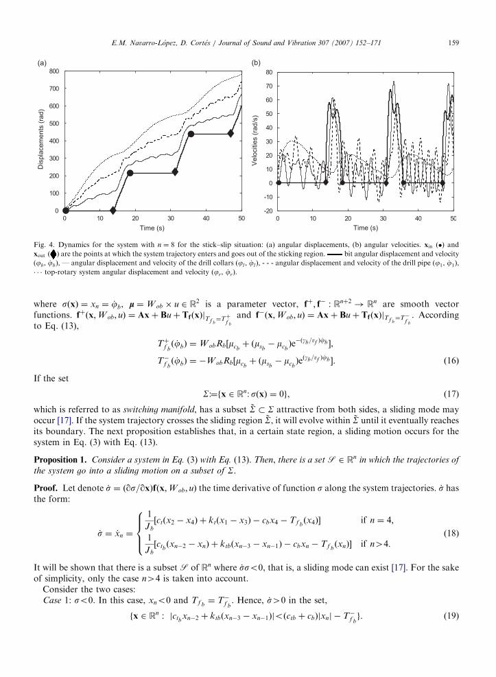
An example of the stick–slip phenomenon appearing at the bit is shown in Fig. 4 for the system in Eqs. (3)–(7)with Eq. (13) with n ¼ 8, W ob ¼ 100N, u ¼ 8:3Nm. The oscillations obtained for the drill pipe and the drillcollars associated with the stick–slip bit motion are in accordance with real drillstrings behaviour. The modelparameters used for the simulations presented along this section correspond to a reduced-scale model:

Jr ¼ 0:518 kgm2; Jb ¼ 0:0318 kgm2; ct ¼ 0:0001Nms/rad; kt ¼ 0:073Nm/rad,

cb ¼ 0:01Nms/rad; cr ¼ 0:18Nms/rad; ktb ¼ kt; ctb ¼ ctl ¼ ct; ktl ¼ kt; Jl ¼ Jb,

J ¼ 0:025 kgm2; mcb¼ 0:5; msb

¼ 0:8; Rb ¼ 0:1m; Dv ¼ 10�6; gb ¼ 0:9; vf ¼ 1. ð14Þ

3.1. Sliding motion existence

The system in Eq. (3) with Eq. (13) can be written as a switching dynamical system:

_x ¼fþðx;lÞ if sðxÞ40;

f�ðx;lÞ if sðxÞo0;

((15)

ARTICLE IN PRESS

Time (s) Time (s)

Dis

pla

ce

me

nts

(ra

d)

Ve

locitie

s (

rad

/s)

Fig. 4. Dynamics for the system with n ¼ 8 for the stick–slip situation: (a) angular displacements, (b) angular velocities. xin (�) and

xout ð ) are the points at which the system trajectory enters and goes out of the sticking region. bit angular displacement and velocity

(jb, _jb), — angular displacement and velocity of the drill collars (jl , _jl), - - - angular displacement and velocity of the drill pipe (j1, _j1),

� � � top-rotary system angular displacement and velocity (jr, _jr).


where sðxÞ ¼ xn ¼ _jb, l ¼W ob � u 2 R2 is a parameter vector, fþ; f� : Rnþ2 ! Rn are smooth vectorfunctions. fþðx;W ob; uÞ ¼ Axþ Buþ TfðxÞjTf b

¼Tþf b

and f�ðx;W ob; uÞ ¼ Axþ Buþ TfðxÞjTf b¼T�

f b

. Accordingto Eq. (13),

Tþf bð _jbÞ ¼W obRb½mcb

þ ðmsb� mcb

Þe�ðgb=vf Þ _jb �,

T�f bð _jbÞ ¼ �W obRb½mcb

þ ðmsb� mcb

Þeðgb=vf Þ _jb �. ð16Þ

If the set

S:¼fx 2 Rn: sðxÞ ¼ 0g, (17)

which is referred to as switching manifold, has a subset ~S � S attractive from both sides, a sliding mode mayoccur [17]. If the system trajectory crosses the sliding region ~S, it will evolve within ~S until it eventually reachesits boundary. The next proposition establishes that, in a certain state region, a sliding motion occurs for thesystem in Eq. (3) with Eq. (13).

Proposition 1. Consider a system in Eq. (3) with Eq. (13). Then, there is a set S 2 Rn in which the trajectories of

the system go into a sliding motion on a subset of S.

Proof. Let denote _s ¼ ðqs=qxÞfðx;W ob; uÞ the time derivative of function s along the system trajectories. _s hasthe form:

_s ¼ _xn ¼

1

Jb

½ctðx2 � x4Þ þ ktðx1 � x3Þ � cbx4 � Tf bðx4Þ� if n ¼ 4;

1

Jb

½ctbðxn�2 � xnÞ þ ktbðxn�3 � xn�1Þ � cbxn � Tf b

ðxnÞ� if n44:

8>><>>: (18)

It will be shown that there is a subset S of Rn where _sso0, that is, a sliding mode can exist [17]. For the sakeof simplicity, only the case n44 is taken into account.

Consider the two cases:Case 1: so0. In this case, xno0 and Tf b

¼ T�f b. Hence, _s40 in the set,

fx 2 Rn : jctbxn�2 þ ktbðxn�3 � xn�1Þjoðctb þ cbÞjxnj � T�f b

g. (19)


Case 2: s40. In this case, xn40 and Tf b¼ Tþf b

. Hence, _so0 in the set,

fx 2 Rn : jctbxn�2 þ ktbðxn�3 � xn�1Þjoðctb þ cbÞjxnj þ Tþf b

g. (20)

Combining both cases, _sso0 is met in the set,

S ¼ fx 2 Rn : jctbxn�2 þ ktbðxn�3 � xn�1Þjoðctb þ cbÞjxnj

þ RbW ob½mcbþ ðmsb

� mcbÞe�ðgb=vf Þjxnj�g. ð21Þ

Since _sso0 in the set S, a sliding motion takes place when the system trajectory hits S within this set. &

From the form of S in Eq. (21), the sliding region ~S � S is obtained as the set,

~S ¼fx 2 S : jktðjr � jbÞ þ ct _jrjomsb

W obRbg if n ¼ 4;

fx 2 S : jktbðjl � jbÞ þ ctb _jljomsbW obRbg if n44:

((22)

Let q ~S denote the boundary of ~S, and q ~S ¼ q ~Sþ[ q ~S

�with:

q ~Sþ¼ x 2 S :

qsqx

fþðx;W ob; uÞ ¼ 0

� �,

q ~S�¼ x 2 S :

qsqx

f�ðx;W ob; uÞ ¼ 0

� �. ð23Þ

For the system in Eq. (3) with Eq. (13), it is obtained,

�
For n ¼ 4:
q ~Sþ¼ fx 2 S : ktðjr � jbÞ þ ct _jr ¼ msb

W obRbg,

q ~S�¼ fx 2 S : ktðjr � jbÞ þ ct _jr ¼ �msb

W obRbg. ð24Þ

�
For n44:
q ~Sþ¼ fx 2 S : ktbðjl � jbÞ þ ctb _jl ¼ msb

W obRbg,

q ~S�¼ fx 2 S : ktbðjl � jbÞ þ ctb _jl ¼ �msb

W obRbg. ð25Þ

The sliding motion can be described by _x ¼ fsðx;W ob; uÞ, where fs is a vector field tangent to S for x 2 ~S. fscan be calculated by means of the equivalent control method [17,18]. For the drillstring model in Eq. (3) withEq. (13), Tf b

plays the role of the equivalent control and,

fsðx;W ob; uÞ ¼ Axþ Buþ TfðxÞjTf b¼Tfbeq

, (26)

where Tfbeq is the solution for Tf bof equation _s ¼ 0, that is,

TfbeqðxÞ ¼ktðjr � jbÞ þ ctð _jr � _jbÞ � cb _jb if n ¼ 4;

ktbðjl � jbÞ þ ctbð _jl � _jbÞ � cb _jb if n44:

((27)

The presence of a sliding mode makes necessary to distinguish different kinds of equilibrium points. Thechange of properties of these equilibria will define different types of system bifurcations, and consequently,different types of system behaviour which will be analysed in Section 3.2.

Definition 2 (Filippov [18], Cunha et al. [19]). x 2 Rn is addressed as standard equilibrium point of thesystem in Eq. (15) if there exists l 2 R2 such that fþðx;lÞ ¼ 0 or f�ðx; lÞ ¼ 0. Let ~x 2 Rn, ~l 2 R2 be such thatfsð ~x; ~lÞ ¼ 0 and sð ~xÞ ¼ 0. ~x is said to be a real quasi-equilibrium point if ~x 2 ~S. If ~xe ~S, ~x is referred to asvirtual quasi-equilibrium point.


By making fsð ~x;W ob; uÞ ¼ 0, the quasi-equilibrium points on S can be calculated, and they have thefollowing form for each time the system trajectory enters S:

�
For n ¼ 4:
~x2 ¼ ~x4 ¼ 0; ~x1 ¼u

kt

þ jb. (28)

�
For n ¼ 6:
~x2 ¼ ~x4 ¼ ~x6 ¼ 0,

~x1 ¼1

kt

þ1

ktb

� �uþ jb,

~x3 ¼u

ktb

þ jb. ð29Þ

�
For n44:
~x2i ¼ 0; i ¼ 1; . . . ;n

2,

~xn�3 ¼ ~jl ¼u

ktb

þ jb,

~xn�5 ¼ ~jp ¼1

ktb

þ1

ktl

� �uþ jb,

~x2j�1 ¼p� j þ 1

kt

þ1

ktb

þ1

ktl

� �uþ jb; j ¼ 1; . . . ; p, ð30Þ

where jb is the constant value of jb during the time the trajectory of the system stays in S, this value variesevery time the system trajectory enters again S. See Fig. 4(a).

Proposition 3. The quasi-equilibrium point ~x given by Eqs. (28)–(30) is asymptotically stable.

Proof. In order to prove the stability of ~x, the following Lyapunov function is considered, which correspondsto the sum of the kinetic and potential energy of the system on S:

�
For n ¼ 4:
V ðx; ~xÞ ¼ 12½ktðx1 � ~x1Þ

2þ Jrx

22�. (31)

�
For n ¼ 6:
V ðx; ~xÞ ¼ 12fkt½ðx1 � x3Þ � ð ~x1 � ~x3Þ�

2 þ ktbðx3 � ~x3Þ2þ Jrx

22 þ Jx2

4g. (32)

�
For n46:
V ðx; ~xÞ ¼ 12ktf½ðx1 � x3Þ � ð ~x1 � ~x3Þ�

2 þ ½ðx3 � x5Þ � ð ~x3 � ~x5Þ�2 þ � � �

þ ½ðxn�7 � xn�5Þ � ð ~xn�7 � ~xn�5Þ�2g

þ 12ktl ½ðxn�5 � xn�3Þ � ð ~xn�5 � ~xn�3Þ�

2 þ 12ktbðxn�3 � ~xn�3Þ

2

þ 12½Jrx

22 þ Jðx2

4 þ � � � þ x2n�4Þ þ Jlx

2n�2�, ð33Þ

ARTICLE IN PRESS

Time (s)

Velo

citie

s (

rad/s

)

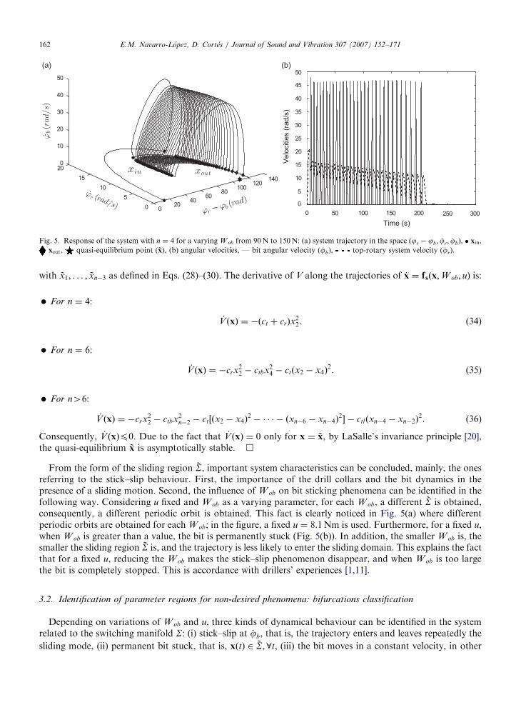
Fig. 5. Response of the system with n ¼ 4 for a varying W ob from 90N to 150N: (a) system trajectory in the space ðjr � jb; _jr; _jbÞ, � xin,

xout, quasi-equilibrium point ( ~x), (b) angular velocities, — bit angular velocity ( _jb), top-rotary system velocity ( _jr).


with ~x1; . . . ; ~xn�3 as defined in Eqs. (28)–(30). The derivative of V along the trajectories of _x ¼ fsðx;W ob; uÞ is:

�
For n ¼ 4:
_V ðxÞ ¼ �ðct þ crÞx22. (34)

�
For n ¼ 6:
_V ðxÞ ¼ �crx22 � ctbx2

4 � ctðx2 � x4Þ2. (35)

�
For n46:
_V ðxÞ ¼ �crx22 � ctbx2

n�2 � ct½ðx2 � x4Þ2� � � � � ðxn�6 � xn�4Þ

2� � ctlðxn�4 � xn�2Þ

2. (36)

Consequently, _V ðxÞp0. Due to the fact that _V ðxÞ ¼ 0 only for x ¼ ~x, by LaSalle’s invariance principle [20],the quasi-equilibrium ~x is asymptotically stable. &

From the form of the sliding region ~S, important system characteristics can be concluded, mainly, the onesreferring to the stick–slip behaviour. First, the importance of the drill collars and the bit dynamics in thepresence of a sliding motion. Second, the influence of W ob on bit sticking phenomena can be identified in thefollowing way. Considering u fixed and W ob as a varying parameter, for each W ob, a different ~S is obtained,consequently, a different periodic orbit is obtained. This fact is clearly noticed in Fig. 5(a) where differentperiodic orbits are obtained for each W ob; in the figure, a fixed u ¼ 8:1Nm is used. Furthermore, for a fixed u,when W ob is greater than a value, the bit is permanently stuck (Fig. 5(b)). In addition, the smaller W ob is, thesmaller the sliding region ~S is, and the trajectory is less likely to enter the sliding domain. This explains the factthat for a fixed u, reducing the W ob makes the stick–slip phenomenon disappear, and when W ob is too largethe bit is completely stopped. This is accordance with drillers’ experiences [1,11].

3.2. Identification of parameter regions for non-desired phenomena: bifurcations classification

Depending on variations of W ob and u, three kinds of dynamical behaviour can be identified in the systemrelated to the switching manifold S: (i) stick–slip at _jb, that is, the trajectory enters and leaves repeatedly the

sliding mode, (ii) permanent bit stuck, that is, xðtÞ 2 ~S;8t, (iii) the bit moves in a constant velocity, in other

ARTICLE IN PRESS

Fig. 6. Regions where stick–slip is possible (shadowed regions): (a) Region Dx in ðxn�3; xn�2Þ with x 2 S, q ~Sþ, q ~S

�(b) stick–slip

region D in the ðW ob; uÞ space, uþ ¼ msbRbW ob ð ~x 2 q ~S

þÞ. Wide-lined region corresponds to ~S. ~xn�3 is the ðn� 3Þth component of the

system quasi-equilibrium point, x�n�3 is the intersection of q ~Sþwith xn�2 ¼ 0, ðW �

ob; u�Þ are reference values of W ob and u.


words, the trajectory moves towards an equilibrium outside S. Different regions in the state space and in thetwo-dimensional parameter space ðW ob; uÞ can be identified through the form of the sliding manifold ~S.

In Fig. 6(a), region ~S with the boundaries q ~Sþand q ~S

�is given. The study is focused on q ~S

þdue to the fact

that the points xout through which the system trajectories go out of ~S are near q ~Sþ.

Two points are distinguished in Fig. 6(a) in the plane ðxn�3;xn�2Þ ¼ ðjl ; _jlÞ: the ðn� 3Þth component of the

quasi-equilibrium point, ~xn�3, and x�n�3 denoting the intersection of q ~Sþ

with xn�2 ¼ 0, which has the

following form:

x�n�3 ¼

msbW obRb

kt

þ jb if n ¼ 4;

msbW obRb

ktb

þ jb if n44:

8>>><>>>: (37)

Note that if n ¼ 4, the study would be restricted to the plane ðjr; _jrÞ.Two key characteristics which determine transitions between different dynamical system behaviours are the

fact that ~x is asymptotically stable and the change of ~x from real to virtual, or viceversa. The real or virtualcharacteristic of ~x can be identified by the distance between ~xn�3 and x�n�3, which depends on the differencebetween u and Tsb

¼ msbW obRb. When ~xn�3 ¼ x�n�3, two reference values of u and W ob are obtained:

u� ¼ msbW obRb; W �

ob ¼u

msbRb

. (38)

Consequently, the following relations can be established:

~x 2 ~S ) �msbW obRbouomsb

W obRb,

~x 2 q ~Sþ) u ¼ msb

W obRb,

~x 2 q ~S�) u ¼ �msb

W obRb,

~xe ~S ) ðu4msbW obRbÞ _ ðuo� msb

W obRbÞ. ð39Þ

A region in a neighbourhood of q ~Sþwhere stick–slip oscillations are present (see Fig. 6(a)) can be defined

as:

Dx:¼fx 2 S : x�n�3 � Z�pxn�3px�n�3 þ Zþg (40)

for some Zþ; Z�40. The region identified in the plane ðxn�3; xn�2Þ can be translated into the two-dimensionalparameter space ðW ob; uÞ considering the relative position of ~xn�3 with respect to the boundaries of ~S. Theboundaries q ~S

þ, q ~S

�are translated into the straight lines:

uþ ¼ msbW obRb; u� ¼ �msb

W obRb,

respectively. The region D �W ob � u where stick–slip is present is obtained (see Fig. 6(b)). It is concluded that:

�
For a fixed value of u, there exist constants ��40 and �þ40 such that:(i) W ob4W �
ob þ �þ ) the bit is permanently stuck (xðtÞ 2 S;8t).

ARTICLE IN PRESS

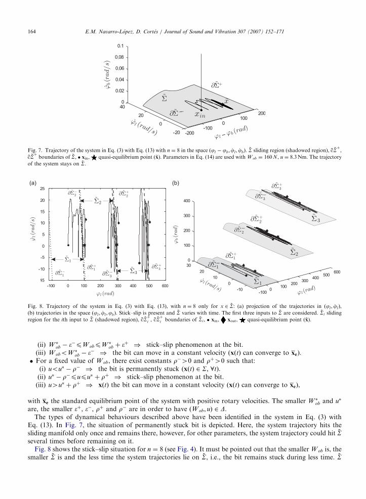
Fig. 7. Trajectory of the system in Eq. (3) with Eq. (13) with n ¼ 8 in the space ðjl � jb; _jl ; _jbÞ. ~S sliding region (shadowed region), q ~Sþ,

q ~Sþboundaries of ~S, � xin, quasi-equilibrium point ( ~x). Parameters in Eq. (14) are used with W ob ¼ 160N, u ¼ 8:3Nm. The trajectory

of the system stays on ~S.

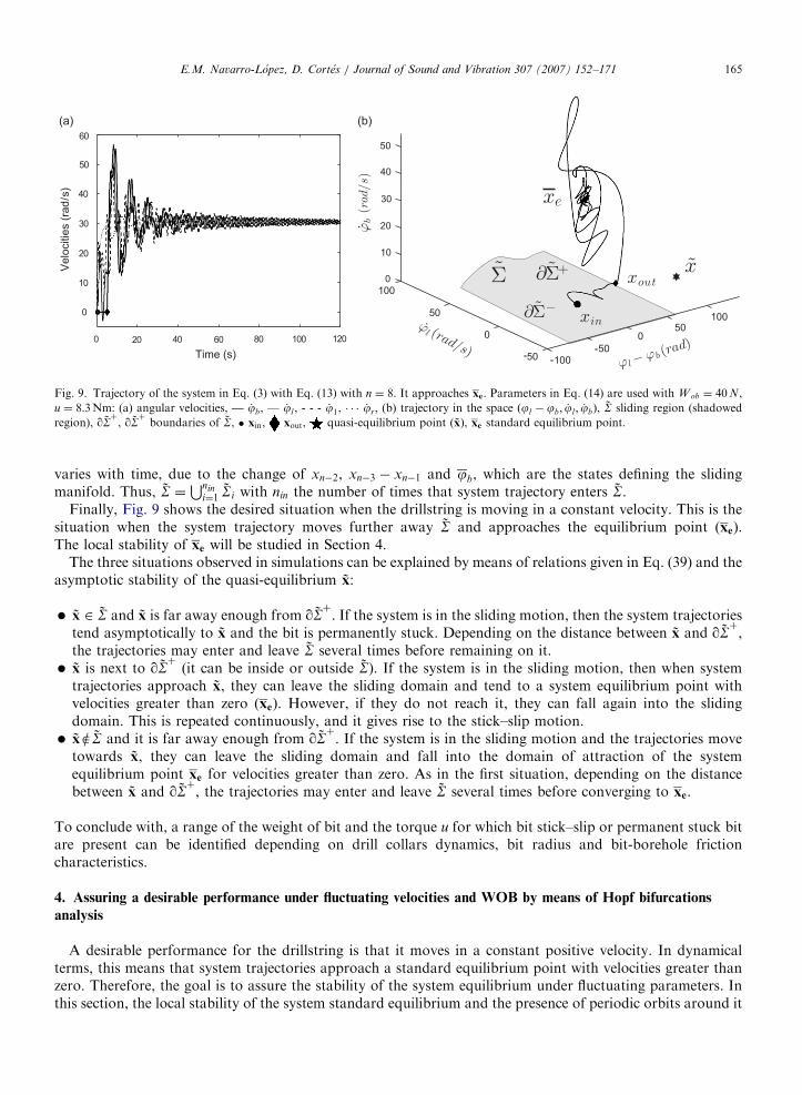
Fig. 8. Trajectory of the system in Eq. (3) with Eq. (13), with n ¼ 8 only for x 2 ~S: (a) projection of the trajectories in ðjl ; _jlÞ,

(b) trajectories in the space ðjl ; _jl ;jbÞ. Stick–slip is present and ~S varies with time. The first three inputs to ~S are considered. ~Si sliding

region for the ith input to ~S (shadowed region), q ~Sþ

i , q ~Sþ

i boundaries of ~Si, � xin, xout, quasi-equilibrium point ( ~x).


(ii) W �ob � �

�pW obpW �ob þ �

þ ) stick–slip phenomenon at the bit.(iii) W oboW � � �� ) the bit can move in a constant velocity (xðtÞ can converge to xe).
ob
�
For a fixed value of W ob, there exist constants r�40 and rþ40 such that:(i) uou� � r� ) the bit is permanently stuck (xðtÞ 2 S; 8t).(ii) u� � r�pupu� þ rþ ) stick–slip phenomenon at the bit.(iii) u4u� þ rþ ) xðtÞ the bit can move in a constant velocity (xðtÞ can converge to xe),
with xe the standard equilibrium point of the system with positive rotary velocities. The smaller W �ob and u�

are, the smaller �þ, ��, rþ and r� are in order to have ðW ob; uÞ 2 D.The types of dynamical behaviours described above have been identified in the system in Eq. (3) with

Eq. (13). In Fig. 7, the situation of permanently stuck bit is depicted. Here, the system trajectory hits thesliding manifold only once and remains there, however, for other parameters, the system trajectory could hit ~Sseveral times before remaining on it.

Fig. 8 shows the stick–slip situation for n ¼ 8 (see Fig. 4). It must be pointed out that the smaller W ob is, thesmaller ~S is and the less time the system trajectories lie on ~S, i.e., the bit remains stuck during less time. ~S

ARTICLE IN PRESSV

elo

citie

s (

rad

/s)

Time (s)

Fig. 9. Trajectory of the system in Eq. (3) with Eq. (13) with n ¼ 8. It approaches xe. Parameters in Eq. (14) are used with W ob ¼ 40N,

u ¼ 8:3Nm: (a) angular velocities, — _jb, — _jl , - - - _j1, � � � _jr, (b) trajectory in the space ðjl � jb; _jl ; _jbÞ, ~S sliding region (shadowed

region), q ~Sþ, q ~S

þboundaries of ~S, � xin, xout, quasi-equilibrium point ( ~x), xe standard equilibrium point.


varies with time, due to the change of xn�2, xn�3 � xn�1 and jb, which are the states defining the slidingmanifold. Thus, ~S ¼

Snini¼1

~Si with nin the number of times that system trajectory enters ~S.Finally, Fig. 9 shows the desired situation when the drillstring is moving in a constant velocity. This is the

situation when the system trajectory moves further away ~S and approaches the equilibrium point (xe).The local stability of xe will be studied in Section 4.

The three situations observed in simulations can be explained by means of relations given in Eq. (39) and theasymptotic stability of the quasi-equilibrium ~x:

�
~x 2 ~S and ~x is far away enough from q ~Sþ. If the system is in the sliding motion, then the system trajectories
tend asymptotically to ~x and the bit is permanently stuck. Depending on the distance between ~x and q ~Sþ,

the trajectories may enter and leave ~S several times before remaining on it.
� ~x is next to q ~S
þ(it can be inside or outside ~S). If the system is in the sliding motion, then when system

trajectories approach ~x, they can leave the sliding domain and tend to a system equilibrium point withvelocities greater than zero (xe). However, if they do not reach it, they can fall again into the slidingdomain. This is repeated continuously, and it gives rise to the stick–slip motion.
� ~xe ~S and it is far away enough from q ~S
þ. If the system is in the sliding motion and the trajectories move

towards ~x, they can leave the sliding domain and fall into the domain of attraction of the systemequilibrium point xe for velocities greater than zero. As in the first situation, depending on the distancebetween ~x and q ~S

þ, the trajectories may enter and leave ~S several times before converging to xe.

To conclude with, a range of the weight of bit and the torque u for which bit stick–slip or permanent stuck bitare present can be identified depending on drill collars dynamics, bit radius and bit-borehole frictioncharacteristics.

4. Assuring a desirable performance under fluctuating velocities and WOB by means of Hopf bifurcations

analysis

A desirable performance for the drillstring is that it moves in a constant positive velocity. In dynamicalterms, this means that system trajectories approach a standard equilibrium point with velocities greater thanzero. Therefore, the goal is to assure the stability of the system equilibrium under fluctuating parameters. Inthis section, the local stability of the system standard equilibrium and the presence of periodic orbits around it


due to Hopf bifurcations are studied. Ranges of velocities at equilibrium and the weight on the bit for whichHopf bifurcations can appear will be identified.

4.1. Preliminary definitions

A new vector state will be defined in order to have a standard equilibrium point of the system with the sameequilibrium velocities and the possibility of choosing them greater than zero. Let define,

jr;1 ¼ jr � j1; jj;jþ1 ¼ jj � jjþ1; jp;l ¼ jp � jl ; jl;b ¼ jl � jb, (41)

with j ¼ 1; . . . ; p� 1, and p the number of drill pipes. The new vector state is:

x0 ¼ ð _jr;jr;1; . . . ; _jj ;jj;jþ1; . . . ; _jp;jp;l ; _jl ;jl;b; _jbÞT

¼ ðx01;x02; . . . ;x

0n�1Þ

T2 Rn�1, ð42Þ

where n is the dimension of the system in Eq. (3). Let consider _jb ¼ x0n�140. The system is now rewritten as:

_x0ðtÞ ¼ A0x0ðtÞ þ B0uþ T0fðx0ðtÞÞ, (43)

with:

B0 ¼

1

Jr

0

..

.

0

0BBBBBB@

1CCCCCCA; T0fðx

0Þ ¼

0

..

.

0

�Tþf bðx0n�1Þ

Jb

0BBBBBB@

1CCCCCCA (44)

and A0 a constant matrix depending on system physical parameters. The dimension of the system in Eq. (43)will be denoted by n0, therefore, x0 2 Rn0 with n0 ¼ n� 1. Note that n0 is an odd integer.

Let O40 be the rotary velocity at equilibrium. The system in Eq. (43) has an unique equilibrium point x0efor each fixed O which is the solution of the set of equations:

_jr ¼ _j1 ¼ . . . _jp ¼ _jl ¼ _jb ¼ O;O40,

u� ðcr þ cbÞO� Tþ

f bðOÞ ¼ 0,

hðOÞ ¼ cbOþ Tþ

f bðOÞ,

jr;1 ¼ jj;jþ1 ¼hðOÞ

kt

; j ¼ 1; . . . ; p� 1,

jp;l ¼hðOÞktl

; jl;b ¼hðOÞktb

, ð45Þ

with

u4msbRbW ob; T

þ

f bðOÞ40; 8O40,

Tþ

f bðOÞ ¼W obRb½mcb

þ ðmsb� mcb

Þe�gb=vf O�. ð46Þ

Let consider a system of the form

_x ¼ fðx; mÞ, (47)

where f : Rn0 � R! Rn0 is a smooth mapping, x 2 Rn0 and m 2 R.

Definition 4 (Hale and Koc-ak [21], Liu [22], Seydel [23]). A system in Eq. (47) with an isolated equilibriumpoint x0e undergoes a Hopf bifurcation (HB) at x0e when a simple pair of complex conjugate eigenvalues of theJacobian Jðx0e;mÞ crosses the imaginary axis from left to right, while all other eigenvalues have negative realparts.


Theorem 5 (Liu [22]). A system in Eq. (47) with an isolated equilibrium point x0e undergoes a Hopf bifurcation

for m ¼ m if:

D1ðmÞ40; D2ðmÞ; . . . ;Dn0�2ðmÞ40; a0ðmÞ40; Dn0�1 ¼ 0 (48)

and

dDn0�1ðmÞdm

��m¼m

a0, (49)

where DiðmÞ stands for the Hurwitz determinants of order i of the characteristic polynomial of Jðx0e; mÞ and a0ðmÞ isthe zero-order term of this polynomial. The condition in Eq. (49) is referred to as transversality condition. Under

conditions in Eqs. (48) and (49), in any neighbourhood U of x0e and any given m04m there is a m� with jm�jom0such that the system has a periodic orbit in U.

4.2. Presence of Hopf bifurcation points for the system of two degrees of freedom

From Theorem 5, the following proposition can be established. It defines the region of angular velocities Oand parameter W ob for which Hopf bifurcations are present in the drillstring for n0 ¼ 3. Let consider thecharacteristic polynomial of the Jacobian matrix of the system in Eq. (43) at the equilibrium point x0e ¼

ðO;jr;b;OÞ as: l3 þ a2l2þ a1lþ a0 ¼ 0, (50)

with:a2ðO;W obÞ ¼

1

JbJr

½Jrðcb þ ct þ dbðOÞÞ þ Jbðcr þ ctÞ�,

a1ðO;W obÞ ¼1

JbJr

½cbðcr þ ctÞ þ ctðcr þ dbðOÞÞ þ dbðOÞcr þ ktðJb þ JrÞ�,

a0ðO;W obÞ ¼kt

JbJr

ðcb þ cr þ dbðOÞÞ,

dbðOÞ ¼ �W obRb

gb

vf

ðmsb� mcb

Þe�ðgb=vf ÞO.

Proposition 6. Consider a system in Eq. (43) with the vector state x0 ¼ ð _jr; jr;b; _jbÞ, _jr40, _jb40 and the

equilibrium point x0e ¼ ðO;jr;b;OÞ with O 2 ð0;Of � and Of 40. Consider the characteristic polynomial of Eq.

(50). Let O; W ob 2 Rþ � f0g and D2ðO;W obÞ ¼ a1ðO;W obÞ a2ðO;W obÞ � a0ðO;W obÞ, Hþ:¼fO�W ob :

a0ðO;W obÞ40; a1ðO;W obÞ40g and H0:¼fO�W ob : D2ðO;W obÞ ¼ 0g. Then, for O�W ob 2Hþ \H0 the

system undergoes a Hopf bifurcation.

Proof. Conditions in Eqs. (48) and (49) of Theorem 5 will be checked. Considering O as a varying velocity,relation D2 ¼ 0 yields to W ob1;2:

W ob1;2 ¼vf eðgbO=vf Þ

2gbRbJrðmsb� mcb

Þðcr þ ctÞ½A

ffiffiffiffiBp�, (51)

where A, B depend on physical parameters.The fact that ðO;W obÞ 2Hþ assures the complex eigenvalues to move from left (stability region) to right

(instability region) of the imaginary axis as W ob and O are varied.The condition in Eq. (49) must be also accomplished. For the system in Eq. (43), it takes the form:

dD2ðO;W obÞ

dW ob

��Wob¼Wob1;2

¼ 1

J2bJ2

r v2f½gbRbðmcb

� msbÞe�gbO=vf

ffiffiffiffiBp�a0. (52)

The condition in Eq. (52) is met for B40, which is the condition for W ob1;2 to be real. Due to the exponentialfunction in Eq. (52), function dD2ðO;W obÞ=dW objWob¼Wob1;2

approaches zero as O approaches infinity. As O isbounded by Of from above, Eq. (52) will never equal zero.

In conclusion, a Hopf bifurcation appears for the set of values ðO;W obÞ 2Hþ \H0. &

ARTICLE IN PRESS

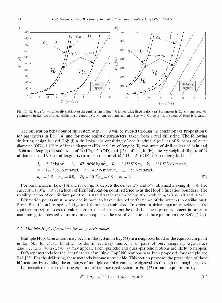
Fig. 10. ðO;W obÞ for which locally stability of the equilibrium in Eq. (45) is met (wide-lined region): (a) Parameters in Eq. (14) are used, (b)

parameters in Eq. (53) of a real drillstring are used. H1, H2 curves obtained making D2 ¼ 0. Curve H2 is the locus of Hopf bifurcation.


The bifurcation behaviour of the system with n0 ¼ 3 will be studied through the conditions of Proposition 6for parameters in Eq. (14) and for more realistic parameters, taken from a real drillstring. The followingdrillstring design is used [26]: (i) a drill pipe line consisting of one hundred pipe lines of 5 inches of outerdiameter (OD), 4.408 in of inner diameter (ID) and 9m of length; (ii) two units of drill collars of 6

12 in and

18.60m of length; (iii) stabilizers of 612 (ID), 12

14 (OD) and 1.5m of length; (iv) a heavy-weight drill pipe of 6

12

of diameter and 9.30m of length; (v) a roller-cone bit of 612 (ID), 12

14 (OD), 1.5m of length. Thus:

Jr ¼ 2122 kgm2; Jb ¼ 471:9698 kgm2; Rb ¼ 0:155575m; kt ¼ 861:5336Nm/rad,

ct ¼ 172:3067Nms/rad; cr ¼ 425Nms/rad; cb ¼ 50Nms/rad,

mcb¼ 0:5; msb

¼ 0:8; Dv ¼ 10�6; gb ¼ 0:9; vf ¼ 1. ð53Þ

For parameters in Eqs. (14) and (53), Fig. 10 depicts the curves H1 and H2, obtained making D2 ¼ 0. ThecurveHþ \H0 ¼H2 is a locus of Hopf bifurcation points referred to as the Hopf bifurcation boundary. Thestability region of equilibrium point x0e is stated as the region below H2 in which a040, a140 and D240.

Bifurcation points must be avoided in order to have a desired performance of the system (no oscillations).From Fig. 10, safe ranges of W ob and O can be established. In order to drive angular velocities at theequilibrium (O) to a desired value, a control mechanism can be added at the top-rotary system in order tomaintain _jr to a desired value, and in consequence, the rest of velocities at the equilibrium (see Refs. [2,24]).

4.3. Multiple Hopf bifurcations for the generic model

Multiple Hopf bifurcations may occur in the system in Eq. (43) in a neighbourhood of the equilibrium pointin Eq. (45) for n043. In other words, an arbitrary number s of pairs of pure imaginary eigenvaluesio1; . . . ;ios with oj40; 8j may appear. Then, periodic and quasi-periodic motions are likely to happen.

Different methods for the identification of multiple Hopf bifurcations have been proposed, for example, seeRef. [25]. For the drillstring, these methods become untractable. This section proposes the prevention of thesebifurcations by avoiding the crossings of multiple complex conjugate eigenvalues through the imaginary axis.

Let consider the characteristic equation of the linearized system in Eq. (43) around equilibrium x0e:

ln0þ an0�1l

n0�1þ � � � þ a1lþ a0 ¼ 0. (54)

ARTICLE IN PRESS

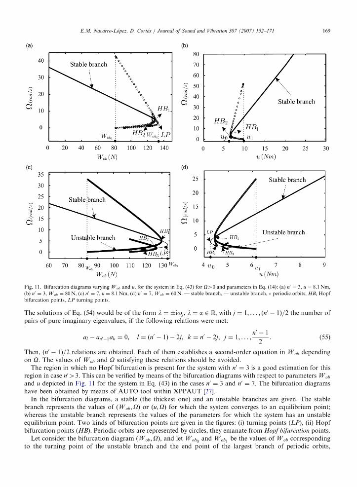
Fig. 11. Bifurcation diagrams varying W ob and u, for the system in Eq. (43) for O40 and parameters in Eq. (14): (a) n0 ¼ 3, u ¼ 8:1Nm,

(b) n0 ¼ 3, W ob ¼ 80N, (c) n0 ¼ 7, u ¼ 8:1Nm, (d) n0 ¼ 7, W ob ¼ 60N. — stable branch, — unstable branch, periodic orbits, HBi Hopf

bifurcation points, LP turning points.


The solutions of Eq. (54) would be of the form l ¼ ioj , l ¼ a 2 R, with j ¼ 1; . . . ; ðn0 � 1Þ=2 the number ofpairs of pure imaginary eigenvalues, if the following relations were met:

al � an0�1ak ¼ 0; l ¼ ðn0 � 1Þ � 2j; k ¼ n0 � 2j; j ¼ 1; . . . ;n0 � 1

2. (55)

Then, ðn0 � 1Þ=2 relations are obtained. Each of them establishes a second-order equation in W ob dependingon O. The values of W ob and O satisfying these relations should be avoided.

The region in which no Hopf bifurcation is present for the system with n0 ¼ 3 is a good estimation for thisregion in case n043. This can be verified by means of the bifurcation diagrams with respect to parameters W ob

and u depicted in Fig. 11 for the system in Eq. (43) in the cases n0 ¼ 3 and n0 ¼ 7. The bifurcation diagramshave been obtained by means of AUTO tool within XPPAUT [27].

In the bifurcation diagrams, a stable (the thickest one) and an unstable branches are given. The stablebranch represents the values of ðW ob;OÞ or ðu;OÞ for which the system converges to an equilibrium point;whereas the unstable branch represents the values of the parameters for which the system has an unstableequilibrium point. Two kinds of bifurcation points are given in the figures: (i) turning points (LP), (ii) Hopfbifurcation points (HB). Periodic orbits are represented by circles, they emanate from Hopf bifurcation points.

Let consider the bifurcation diagram ðW ob;OÞ, and let W ob0and W ob1

be the values of W ob correspondingto the turning point of the unstable branch and the end point of the largest branch of periodic orbits,

ARTICLE IN PRESS

Fig. 12. Values ðW ob; uÞ at which a Hopf bifurcation point can appear for the system in (43) with parameters in (14): (a) n0 ¼ 3, (b) n0 ¼ 7.


respectively. For values W ob1pW obpW ob0

, the system may present oscillations. Notice that bifurcationdiagrams for varying W ob’s are obtained for a fixed u. If a different value of u were used, different values ofðW ob;OÞ at which Hopf bifurcation points are located would be obtained, and consequently, different values ofW ob0

and W ob1. This is confirmed by Fig. 12 where the values ðW ob; uÞ at which a Hopf bifurcation point is

present are depicted. The graphics have been also obtained by means of AUTO tool within XPPAUT [27]. Thesame conclusions can be given for bifurcation diagrams ðu;OÞ. See Figs. 11(b) and (d), here, u0 and u1 are thevalues of u corresponding to the turning point of the unstable branch and the end point of the largest branchof periodic orbits, respectively. The interval u0pupu1 is a non-safe operation range for a fixed W ob. Noticethat u0 and u1 are different for n0 ¼ 3 and n0 ¼ 7 due to the fact that the bifurcation diagrams have beenobtained for a different fixed value of W ob in each case.

To conclude with, the drillstring has a desired performance, that is, it moves in a constant velocity when: (i)for a fixed u, W ob is small enough, (ii) for a fixed W ob, u is high enough. This is accordance with results givenin Section 3, indeed, comparing Figs. 12 and 6(b), it can be seen that region D where stick–slip is presentintersects the values ðW ob; uÞ where a Hopf bifurcation point may appear.

The identified ranges of W ob, the torque supplied by the top-rotary mechanism (u) and the rotary speed forwhich the drillstring has a desired performance are in accordance with field drillers’ experiences [1,5,6,26].Then, by means of the proposed analysis method of identifying bit sticking phenomena (Section 3) andoscillations around a constant velocity (Section 4), it is possible to estimate the problematic parameter rangesfor a specific drillstring design.

5. Conclusions

Different bifurcations have been identified in an n-dimensional model of a conventional oilwell drillstring.Stick–slip oscillations at the bit have been shown to be related to the presence of a discontinuous dry frictionmodelling the bit–rock contact. The drillstring has been considered as a piecewise-smooth system and a slidingmotion has been shown to be present. Ranges of key parameters in any drilling operation, such as, the weighton the bit ðW obÞ, the motor torque given by the top-rotary mechanism (u) and the rotary speed have beenidentified lest non-desired oscillatory phenomena appear in the system. Changes in drillstring behaviour havebeen interpreted as different bifurcations types. Not only system parameters changes have been shown to playan important role in the bifurcation behaviour, but also the characteristics of system equilibria.

Based on the analysis carried out, control methodologies can be designed in order to maintain systemparameters within the proposed safe operation ranges. Finally, the analysis proposed can be applied to othermechanical systems exhibiting stick–slip oscillations which are described by similar models to the one studiedin this work.


Acknowledgements

The authors gratefully acknowledge the valuable discussions and support received by Professor RodolfoSuarez Cortez in developing the first ideas of this work. They are also gratetul to Julien Cabillic (Institut Franc-

ais de Mecanique Avancee) who revised the drillstring mechanical model. This paper has been partially done inthe context of LAFMAA project ‘‘VIBSARTAS’’ under CONACYT grant and under Ramon y Cajalcontract under the support of the Ministerio de Educacion y Ciencia (MEC) of Spain.

References

[1] J.F. Brett, The genesis of torsional drillstring vibrations. SPE Drilling Engineering (1992) 168–174.

[2] E.M. Navarro-Lopez, R. Suarez, Mechanical vibrations in an oilwell drillstring: control problems, Iberoamerican Journal of

Automatic Control and Industrial Computer Science 2 (1) (2005) 43–54 (in Spanish).

[3] S.L. Chen, K. Blackwood, E. Lamine, Field investigation of the effects of stick–slip, lateral and whirl vibrations on roller-cone bit

performance, SPE Drilling and Completion 17 (1) (2002) 15–20.

[4] A.P. Christoforou, A.S. Yigit, Fully coupled vibrations of actively controlled drillstrings, Journal of Sound and Vibration 267 (2003)

1029–1045.

[5] A. Kyllingstad, G.W. Halsey, A study of slip/stick motion of the bit, SPE Drilling Engineering (1988) 369–373.

[6] Y.-Q. Lin, Y.-H. Wang, Stick–slip vibration of drill strings, Journal of Engineering for Industry 113 (1991) 38–43.

[7] F. Abbassian, V.A. Dunayevsky, Application of stability approach to torsional and lateral bit dynamics, SPE Drilling and Completion

13 (2) (1998) 99–107.

[8] J.D. Jansen, L. van den Steen, Active damping of self-excited torsional vibrations in oil well drillstrings, Journal of Sound and

Vibration 179 (4) (1995) 647–668.

[9] N. Mihajlovic, A.A. van Veggel, N. van de Wouw, H. Nijmeijer, Analysis of friction-induced limit cycling in an experimental drill-

string system, ASME Journal of Dynamic Systems, Measurement and Control 126 (2004) 709–720.

[10] A.F.A. Serrarens, M.J.G. van de Molengraft, J.J. Kok, L. van den Steen, H1 control for suppressing stick–slip in oil well drillstrings,

IEEE Control Systems (1998) 19–30.

[11] P. Sananikone, O. Kamoshima, D.B. White, A field method for controlling drillstring torsional vibrations, Proceedings of the IADC/

SPE Drilling Conference, New Orleans, Louisiana, 1992, pp. 443–452.

[12] J.P. Maratier, Optimum Rotary Speed and Bit Weight for Rotary Drilling, MSc Thesis, Louisiana State University, 1971.

[13] B. Armstrong-Helouvry, P. Dupont, C. Canudas de Wit, A survey of models, analysis tools, and compensation methods for the

control of machines with friction, Automatica 30 (7) (1994) 1083–1183.

[14] R.I. Leine, D.H. van Campen, A. de Kraker, L. van den Steen, Stick–slip vibrations induced by alternate friction models, Nonlinear

Dynamics 16 (1998) 41–54.

[15] D. Karnopp, Computer simulation of stick–slip friction in mechanical dynamic systems, ASME Journal of Dynamics Systems,

Measurement, and Control 107 (1) (1985) 100–103.

[16] D.R. Pavone, J.P. Desplans, Application of high sampling rate downhole measurements for analysis and cure of stick–slip in drilling,

Proceedings of the SPE Annual Technical Conference and Exhibition, New Orleans, Louisiana, 1994, pp. 335–345.

[17] V.I. Utkin, Sliding Modes in Control Optimization, Springer, Berlin, 1992.

[18] A.F. Filippov, Differential Equations with Discontinuous Right-hand Sides, Kluwer Academic Publishers, Dordrecht, 1988.

[19] F.B. Cunha, D.J. Pagano, U.F. Moreno, Sliding bifurcations of equilibria in planar variable structure systems, IEEE Transactions on

Circuits and Systems-I: Fundamental Theory and Applications 50 (8) (2003) 1129–1134.

[20] J.P. LaSalle, The Stability of Dynamical Systems, Society for Industrial and Applied Mathematics, Hamilton Press, 1976.

[21] J. Hale, H. Koc-ak, Dynamics and Bifurcations, Springer, New York, 1991.

[22] W.M. Liu, Criterion of Hopf bifurcations without using eigenvalues, Journal of Mathematical Analysis and Applications 182 (1994)

250–256.

[23] R. Seydel, Practical Bifurcation and Stability Analysis, Springer, New York, 1994.

[24] E.M. Navarro-Lopez, R. Suarez, Practical approach to modelling and controlling stick–slip oscillations in oilwell drillstrings,

Proceedings of the IEEE Conference on Control Applications, IEEE Press, Taipei, Taiwan, 2004, pp. 1454–1460.

[25] W. Govaerts, J. Guckenheimer, A. Khibnik, Defining functions for multiple Hopf bifurcations, SIAM Journal on Numerical Analysis

34 (3) (1997) 1269–1288.

[26] Tri-Cone Manual de Barrenas, Hughes Tool Company, U.S.A., 1982.

[27] B. Ermentrout, Simulating, Analyzing, and Animating Dynamical Systems (A Guide to XPPAUT for Researchers and Students), SIAM

Software Environments Tools, 2002.

Avoiding harmful oscillations in a drillstring through dynamical analysis

Documents

Transcript of Avoiding harmful oscillations in a drillstring through dynamical analysis