arX

iv:h

ep-p

h/98

1236

0v4

4 J

un 1

999

UWThPh-1998-61DFTT 69/98KIAS-P98045SFB 375-310

TUM-HEP 340/98hep-ph/9812360

Phenomenology of

Neutrino Oscillations

S.M. Bilenky

Joint Institute for Nuclear Research, Dubna, Russia, and

Institut fur Theoretische Physik, Technische Universitat Munchen, D–85748 Garching,

Germany

C. Giunti

INFN, Sezione di Torino, and Dipartimento di Fisica Teorica,

Universita di Torino, Via P. Giuria 1, I–10125 Torino, Italy, and

School of Physics, Korea Institute for Advanced Study, Seoul 130-012, Korea

W. Grimus

Institute for Theoretical Physics, University of Vienna,

Boltzmanngasse 5, A–1090 Vienna, Austria

Abstract

This review is focused on neutrino mixing and neutrino oscillations in the lightof the recent experimental developments. After discussing possible types ofneutrino mixing for Dirac and Majorana neutrinos and considering in detail thephenomenology of neutrino oscillations in vacuum and matter, we review allexisting evidence and indications in favour of neutrino oscillations that havebeen obtained in the atmospheric, solar and LSND experiments. We presentthe results of the analyses of the neutrino oscillation data in the framework ofmixing of three and four massive neutrinos and investigate possibilities to testthe different neutrino mass and mixing schemes obtained in this way. We alsodiscuss briefly future neutrino oscillation experiments.

1

Contents

1 Introduction 3

2 Neutrino Mixing 5

2.1 Dirac mass term . . . . . . . . . . . . . . . . . . . . . . . . . . . . . . . . 72.2 Dirac–Majorana mass term . . . . . . . . . . . . . . . . . . . . . . . . . . 82.3 Majorana mass term . . . . . . . . . . . . . . . . . . . . . . . . . . . . . 122.4 The one-generation case . . . . . . . . . . . . . . . . . . . . . . . . . . . 132.5 The see-saw mechanism . . . . . . . . . . . . . . . . . . . . . . . . . . . 142.6 Effective Lagrangians . . . . . . . . . . . . . . . . . . . . . . . . . . . . . 162.7 Maximal mixing . . . . . . . . . . . . . . . . . . . . . . . . . . . . . . . . 17

3 Neutrino oscillations in vacuum 18

3.1 The general formalism . . . . . . . . . . . . . . . . . . . . . . . . . . . . 183.2 Oscillations in the two-neutrino case . . . . . . . . . . . . . . . . . . . . 22

4 Neutrino oscillations and transitions in matter 26

4.1 The effective Hamiltonian for neutrinos in matter . . . . . . . . . . . . . 264.2 The two-neutrino case and adiabatic transitions . . . . . . . . . . . . . . 304.3 The resonance . . . . . . . . . . . . . . . . . . . . . . . . . . . . . . . . . 334.4 Non-adiabatic neutrino oscillations in matter and crossing probabilities . 34

5 Indications of neutrino oscillations 37

5.1 Atmospheric neutrino experiments . . . . . . . . . . . . . . . . . . . . . . 375.1.1 The atmospheric neutrino flux . . . . . . . . . . . . . . . . . . . . 385.1.2 Experiments with atmospheric neutrinos . . . . . . . . . . . . . . 425.1.3 The atmospheric neutrino anomaly . . . . . . . . . . . . . . . . . 445.1.4 Long-baseline experiments and tests of the atmospheric neutrino

oscillation parameters . . . . . . . . . . . . . . . . . . . . . . . . 495.2 Solar neutrino experiments . . . . . . . . . . . . . . . . . . . . . . . . . . 505.3 The LSND experiment . . . . . . . . . . . . . . . . . . . . . . . . . . . . 63

6 Analysis of neutrino oscillation data 66

6.1 Mixing of three massive neutrinos . . . . . . . . . . . . . . . . . . . . . . 676.1.1 Solar neutrinos . . . . . . . . . . . . . . . . . . . . . . . . . . . . 696.1.2 Atmospheric neutrinos . . . . . . . . . . . . . . . . . . . . . . . . 706.1.3 The mixing matrix in the case |Ue3| ≪ 1 . . . . . . . . . . . . . . 726.1.4 Accelerator long-baseline experiments . . . . . . . . . . . . . . . . 74

6.2 Mixing of four massive neutrinos . . . . . . . . . . . . . . . . . . . . . . 75

7 Conclusions 88

A Properties of Majorana neutrinos and fields 92

2

1 Introduction

The strong evidence in favour of oscillations of atmospheric neutrinos found by the Super-Kamiokande Collaboration [1,2] opened a new era in particle physics. There is no doubtthat new experiments are necessary to understand the nature of neutrino masses andmixing which are intimately connected with neutrino oscillations, but the first decisivestep has been done: massive and mixed neutrinos can now be considered as real physicalobjects.

The problem of neutrino mass has a long history. Originally, Pauli considered theneutrino as a particle with a small but non-zero mass (smaller than the electron mass) [3]and the method for the measurement of the neutrino mass through the investigation ofthe β-spectrum near the end point was proposed in the first theoretical papers on β-decayof Fermi [4, 5] and Perrin [6].

The first experiments on the measurement of the neutrino mass, based on the Fermi-Perrin method, yielded the upper boundmν . 500 eV [7] which was improved in the fiftiesto mν . 250 eV [8]. Therefore, it became evident that the neutrino mass (if non-zero atall) is much smaller than the electron mass. This was the main reason that in 1957, afterthe discovery of parity violation in β-decay, the authors of the two-component theory ofthe neutrino (Landau [9], Lee and Yang [10], Salam [11]) assumed that the neutrino is amassless particle, the field of which is either a left-handed field νL or a right-handed fieldνR.

In 1958, Goldhaber et al. [12] measured the helicity of the neutrino. The result ofthis experiment was in agreement with the two-component neutrino theory and it wasestablished that the neutrino field is νL.1 The results of the experiment of Goldhaber et

al. could not exclude, however, the possibility of a small neutrino mass. In the V−Atheory (Feynman and Gell-Mann [15], Sudarshan and Marshak [16]) the Hamiltonian ofweak interactions contains the left-handed component of the neutrino field νL, and alsothe left-handed components of all massive fields. Therefore the possibility for the neutrinoto be nevertheless a massive particle became more natural [17] after the confirmation ofthe V−A theory.

In 1957, B. Pontecorvo [18,19] proposed the idea that the state of neutrinos producedin weak interaction processes is a superposition of states of two Majorana neutrinos [20]with definite masses (analogous to the states |K0〉 and |K0〉 which are the superpositionof |K1〉 and |K2〉, the states of particles with definite masses and widths). In this way,B. Pontecorvo arrived at the hypothesis of neutrino oscillations (analogous to K0 ⇆ K0

oscillations). At that time only one type of neutrino was known. The possibility of mixingof the two species of neutrinos νe and νµ was considered in Ref. [21]. All possible typesof neutrino oscillations for this case were investigated by Pontecorvo in 1967 [22].

Gribov and Pontecorvo proposed in 1969 [23] the first phenomenological theory ofneutrino mixing and oscillations. In this theory, the two left-handed neutrino fields νeL

1Notice that in the Goldhaber et al. experiment the helicity of the electron neutrino was measured.The helicity of the muon neutrino was measured in several experiments (for the references see the reviewof V.L. Telegdi [13]). The best accuracy in the measurement of the muon neutrino was achieved in theexperiment by Grenacs et al. [14].

3

and νµL are linear combinations of the left-handed components of the fields of Majorananeutrinos with definite masses and the neutrino mass term contains only the left-handedfields νeL and νµL.

In 1976, neutrino oscillations were considered in the scheme of mixing of two Diracneutrinos based on the analogy between quarks and leptons [24,25] and in the same yearin the general Dirac–Majorana scheme [26] (for later works see Refs. [27–30]).

The theoretical arguments in favour of non-zero neutrino masses and mixing are basedon the models beyond the Standard Model (see, for example, Ref. [31]). In such modelsthe fields of quarks, charged leptons and neutrinos are grouped in the same multiplets andthe generation of the masses of quarks and charged leptons with the Higgs mechanism asa rule provides also non-zero neutrino masses.

In 1979, the see-saw mechanism for the generation of neutrino masses was proposed[32–34]. This mechanism connects the smallness of neutrino masses with the possibleviolation of lepton number conservation at a very large energy scale.

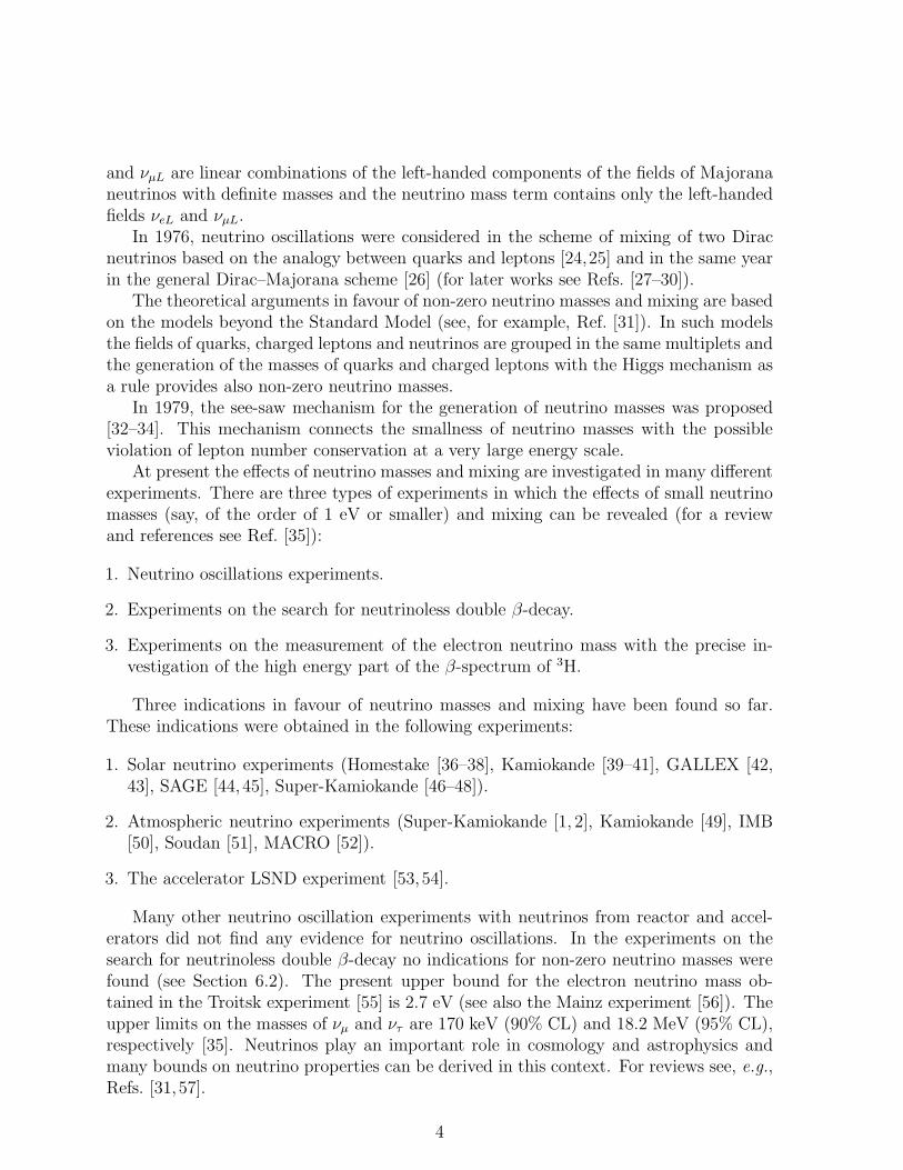
At present the effects of neutrino masses and mixing are investigated in many differentexperiments. There are three types of experiments in which the effects of small neutrinomasses (say, of the order of 1 eV or smaller) and mixing can be revealed (for a reviewand references see Ref. [35]):

1. Neutrino oscillations experiments.

2. Experiments on the search for neutrinoless double β-decay.

3. Experiments on the measurement of the electron neutrino mass with the precise in-vestigation of the high energy part of the β-spectrum of 3H.

Three indications in favour of neutrino masses and mixing have been found so far.These indications were obtained in the following experiments:

1. Solar neutrino experiments (Homestake [36–38], Kamiokande [39–41], GALLEX [42,43], SAGE [44,45], Super-Kamiokande [46–48]).

2. Atmospheric neutrino experiments (Super-Kamiokande [1, 2], Kamiokande [49], IMB[50], Soudan [51], MACRO [52]).

3. The accelerator LSND experiment [53, 54].

Many other neutrino oscillation experiments with neutrinos from reactor and accel-erators did not find any evidence for neutrino oscillations. In the experiments on thesearch for neutrinoless double β-decay no indications for non-zero neutrino masses werefound (see Section 6.2). The present upper bound for the electron neutrino mass ob-tained in the Troitsk experiment [55] is 2.7 eV (see also the Mainz experiment [56]). Theupper limits on the masses of νµ and ντ are 170 keV (90% CL) and 18.2 MeV (95% CL),respectively [35]. Neutrinos play an important role in cosmology and astrophysics andmany bounds on neutrino properties can be derived in this context. For reviews see, e.g.,Refs. [31, 57].

4

In this review we discuss the phenomenological theory of neutrino mixing (Section2), neutrino oscillations in vacuum (Section 3), neutrino oscillations and transitions inmatter (Section 4) and experimental data and results of analyses of the data (Sections 5and 6). We also consider the implications of the existing experimental results on neutrinooscillations for experiments in preparation. After the conclusions (Section 7) we discusssome properties of Majorana neutrinos and fields in Appendix A.

We hope that this review will be useful not only for the physicists that are workingin the field but also for those who are interested in this exciting field of physics. In manycases we present not only results but also derivations of the results. For those who startto study the subject we refer to the books Refs. [31,58–61] and the reviews Refs. [62–73].

2 Neutrino Mixing

All the numerous data on weak interaction processes are perfectly well described by theStandard Model [74–76]. The standard weak interactions are due to the coupling of quarksand leptons with the gauge W and Z vector bosons, described by the charged-current(CC) and neutral-current (NC) interaction Lagrangians

LCCI = − g

2√

2jCCρ W ρ + h.c. , (2.1)

LNCI = − g

2 cos θWjNCρ Zρ . (2.2)

Here g is the SU(2)L gauge coupling constant, θW is the weak angle and the charged andneutral currents jCC

ρ and jNCρ are given by the expressions

jCCρ = 2

∑

ℓ=e,µ,τ

νℓL γρ ℓL + . . . , (2.3)

jNCρ =

∑

ℓ=e,µ,τ

νℓL γρ νℓL + . . . , (2.4)

where the ℓ are the physical charged lepton fields with masses mℓ and we have writtenexplicitly only the terms containing the neutrino fields. The flavour neutrinos νe, νµ, . . .are determined by CC weak interactions: for example, the νµ is the particle producedin the decay π+ → µ+ + νµ and so on. The number of light flavour neutrinos is givenby the invisible width of the Z boson [77] in the Standard Model. It was shown in thefamous LEP experiments on the measurement of the invisible width of the Z boson thatthe number of the light flavour neutrinos is equal to 3. The most recent experimentalvalue of the number of neutrino flavours is 2.994 ± 0.012 [35], showing that are no otherneutrino flavours than the well-known νe, νµ, ντ .

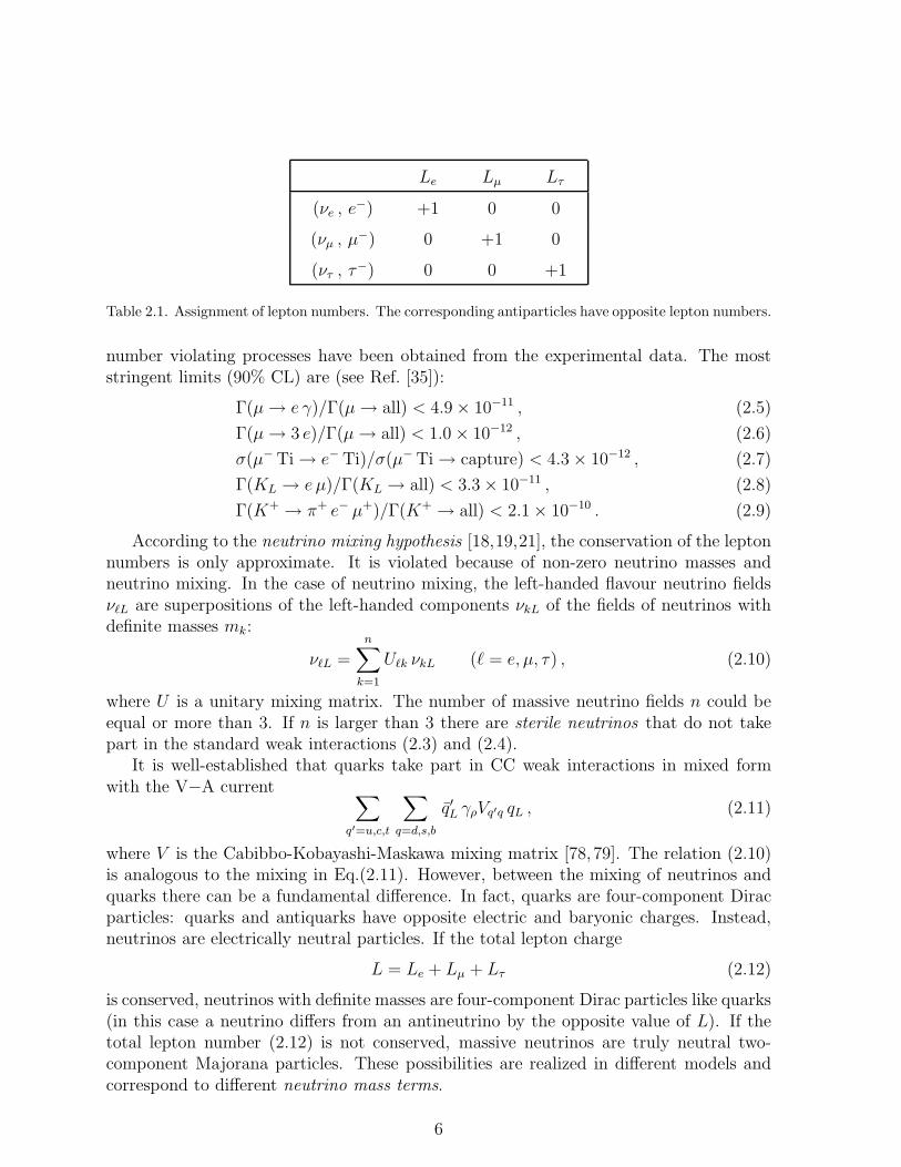
The CC and NC interactions conserve the electron Le, muon Lµ and tau Lτ leptonnumbers, which are assigned as shown in Table 2.1.

There are no indications in favour of violation of the law of conservation of leptonnumbers in weak processes and very strong bounds on the probabilities of the lepton

5

Le Lµ Lτ

(νe , e−) +1 0 0

(νµ , µ−) 0 +1 0

(ντ , τ−) 0 0 +1

Table 2.1. Assignment of lepton numbers. The corresponding antiparticles have opposite lepton numbers.

number violating processes have been obtained from the experimental data. The moststringent limits (90% CL) are (see Ref. [35]):

Γ(µ→ e γ)/Γ(µ→ all) < 4.9 × 10−11 , (2.5)

Γ(µ→ 3 e)/Γ(µ→ all) < 1.0 × 10−12 , (2.6)

σ(µ− Ti → e− Ti)/σ(µ− Ti → capture) < 4.3 × 10−12 , (2.7)

Γ(KL → e µ)/Γ(KL → all) < 3.3 × 10−11 , (2.8)

Γ(K+ → π+ e− µ+)/Γ(K+ → all) < 2.1 × 10−10 . (2.9)

According to the neutrino mixing hypothesis [18,19,21], the conservation of the leptonnumbers is only approximate. It is violated because of non-zero neutrino masses andneutrino mixing. In the case of neutrino mixing, the left-handed flavour neutrino fieldsνℓL are superpositions of the left-handed components νkL of the fields of neutrinos withdefinite masses mk:

νℓL =n∑

k=1

Uℓk νkL (ℓ = e, µ, τ) , (2.10)

where U is a unitary mixing matrix. The number of massive neutrino fields n could beequal or more than 3. If n is larger than 3 there are sterile neutrinos that do not takepart in the standard weak interactions (2.3) and (2.4).

It is well-established that quarks take part in CC weak interactions in mixed formwith the V−A current

∑

q′=u,c,t

∑

q=d,s,b

q′L γρVq′q qL , (2.11)

where V is the Cabibbo-Kobayashi-Maskawa mixing matrix [78, 79]. The relation (2.10)is analogous to the mixing in Eq.(2.11). However, between the mixing of neutrinos andquarks there can be a fundamental difference. In fact, quarks are four-component Diracparticles: quarks and antiquarks have opposite electric and baryonic charges. Instead,neutrinos are electrically neutral particles. If the total lepton charge

L = Le + Lµ + Lτ (2.12)

is conserved, neutrinos with definite masses are four-component Dirac particles like quarks(in this case a neutrino differs from an antineutrino by the opposite value of L). If thetotal lepton number (2.12) is not conserved, massive neutrinos are truly neutral two-component Majorana particles. These possibilities are realized in different models andcorrespond to different neutrino mass terms.

6

2.1 Dirac mass term

A Dirac neutrino mass term can be generated by the Higgs mechanism with the standardHiggs doublet which is responsible for the generation of the masses of quarks and chargedleptons.2 In this case the neutrino mass term is given by3

LD = −∑

ℓ,ℓ′

νℓRMDℓℓ′ νℓ′L + h.c. (ℓ = e, µ, τ) , (2.13)

and MD is a complex 3 × 3 matrix.The Dirac mass term (2.13) can be diagonalized taking into account that the complex

matrix MD can be written asMD = V mU † , (2.14)

where V and U are unitary matrices and m is a positive definite diagonal matrix, mkj =mkδkj, with mk ≥ 0. Hence, the Dirac mass term (2.13) can be written in the diagonalform

LD = −3∑

k=1

mk νk νk , (2.15)

with

νℓL =

3∑

k=1

Uℓk νkL (ℓ = e, µ, τ) . (2.16)

Therefore, in the case of the Dirac mass term (2.13) the three flavour fields νℓL (ℓ =e, µ, τ) are linear unitary combinations of the left-handed components νkL of three fieldsof neutrinos with masses mk (k = 1, 2, 3). On the other hand, we also have

νℓR =3∑

k=1

Vℓk νkR (ℓ = e, µ, τ) , (2.17)

but these right-handed fields do not occur in the standard weak interaction Lagrangian.Therefore, right-handed singlets are sterile and are not mixed in this scheme with theactive neutrinos.4

The field νk is a Dirac field if not only the mass term (2.13) but also the total La-grangian is invariant under the global U(1) transformation

νℓ → eiϕ νℓ , ℓ→ eiϕ ℓ (ℓ = e, µ, τ) , (2.18)

2One needs to assume the existence of right-handed SU(2)L singlet fields νℓR. If these fields do notexist, it is not possible to construct a Dirac mass term for the neutrinos, i.e., neutrinos are masslessparticles. This model is sometimes called Minimal Standard Model [74–76].

3Note that in this review we use four-component spinors. For the equivalent alternative of two-component spinors see, e.g., Refs. [30, 80].

4In the Dirac case it is possible to conceive also the existence of left-handed sterile singlet fields mixedwith the active flavour neutrino fields, in contrast to the right-handed singlets which cannot be mixedwith the active neutrinos because of lepton number conservation.

7

where the phase ϕ is the same for all neutrino and charged lepton fields. Then, usingNoether’s theorem, one can see that the invariance of the Lagrangian under the trans-formation (2.18) implies that the total lepton charge L is conserved. Therefore, L is thequantum number that distinguishes a neutrino from an antineutrino.

The Dirac mass term (2.13) allows processes like µ → e + γ, µ− → e− + e+ + e−.However, the contribution of neutrino mixing to the probabilities of such processes isnegligibly small [81–83].

The unitary 3 × 3 mixing matrix U can be written in terms of 3 mixing angles and 6phases. However, only one phase is measurable [79]. This is due to the fact that in theStandard Model the only term in the Lagrangian where the mixing matrix U enters isthe CC interaction Lagrangian (2.1). With neutrino mixing the lepton charged-currentis given by

jCCρ

†= 2

∑

ℓ=e,µ,τ

ℓL γρ νℓL = 2∑

ℓ=e,µ,τ

3∑

k=1

ℓL γρ Uℓk νkL . (2.19)

Because the phases of Dirac fields are arbitrary one can eliminate from the mixing matrixU five phases by a redefinition of the phases of the charged lepton and neutrino fields,with only one physical phase remaining in U . The presence of this phase causes theviolation of CP invariance in the lepton sector. A convenient parameterization of themixing matrix U is the one proposed in Ref. [84]:

U =

c12c13 s12c13 s13eiδ13

−s12c23 − c12s23s13eiδ13 c12c23 − s12s23s13e

iδ13 s23c13s12s23 − c12c23s13e

iδ13 −c12s23 − s12c23s13eiδ13 c23c13

, (2.20)

where cij ≡ cosϑij and sij ≡ sinϑij and δ13 is the CP-violating phase.Since in the parameterization (2.20) of the mixing matrix the CP-violating phase δ13

is associated with s13, it is clear that CP violation is negligible in the lepton sector ifthe mixing angle ϑ13 is small. More generally, it is possible to show that if any of theelements of the mixing matrix is zero, the CP-violating phase can be rotated away by asuitable rephasing of the charged lepton and neutrino fields.5

2.2 Dirac–Majorana mass term

If none of the lepton numbers is conserved and both, left-handed flavour fields νℓL (ℓ =e, µ, τ) and sterile right-handed gauge singlet fields νsR (s = s1, s2, . . .) enter into themass term we have the so-called Dirac–Majorana mass term

LD+M = LML + LD + LM

R , (2.21)

with

LD = −∑

s,ℓ

νsRMDsℓ νℓL + h.c. , (2.22)

5This can also be seen by noticing that the Jarlskog rephasing-invariant parameter [85–87] vanishesif one of the elements of the mixing matrix is zero.

8

LML = −1

2

∑

ℓ,ℓ′

(νℓL)cMLℓℓ′ νℓ′L + h.c. , (2.23)

LMR = −1

2

∑

s,s′

νsRMRss′ (νs′R)c + h.c. (2.24)

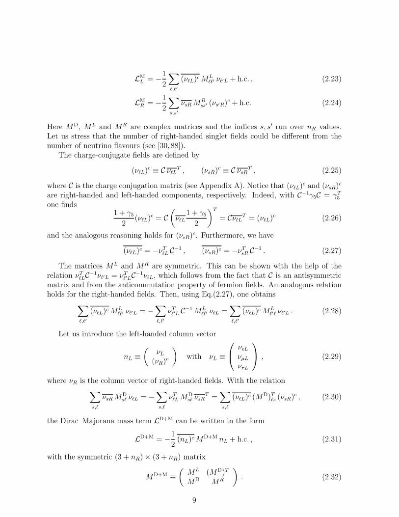
Here MD, ML and MR are complex matrices and the indices s, s′ run over nR values.Let us stress that the number of right-handed singlet fields could be different from thenumber of neutrino flavours (see [30, 88]).

The charge-conjugate fields are defined by

(νℓL)c ≡ C νℓLT , (νsR)c ≡ C νsRT , (2.25)

where C is the charge conjugation matrix (see Appendix A). Notice that (νℓL)c and (νsR)c

are right-handed and left-handed components, respectively. Indeed, with C−1γ5C = γT5one finds

1 + γ5

2(νℓL)

c = C(

νℓL1 + γ5

2

)T

= CνℓLT = (νℓL)c (2.26)

and the analogous reasoning holds for (νsR)c. Furthermore, we have

(νℓL)c = −νTℓL C−1 , (νsR)c = −νTsR C−1 . (2.27)

The matrices ML and MR are symmetric. This can be shown with the help of therelation νTℓLC−1νℓ′L = νTℓ′LC−1νℓL, which follows from the fact that C is an antisymmetricmatrix and from the anticommutation property of fermion fields. An analogous relationholds for the right-handed fields. Then, using Eq.(2.27), one obtains

∑

ℓ,ℓ′

(νℓL)cMLℓℓ′ νℓ′L = −

∑

ℓ,ℓ′

νTℓ′L C−1MLℓℓ′ νℓL =

∑

ℓ,ℓ′

(νℓL)cMLℓ′ℓ νℓ′L . (2.28)

Let us introduce the left-handed column vector

nL ≡(

νL(νR)c

)

with νL ≡

νeLνµLντL

, (2.29)

where νR is the column vector of right-handed fields. With the relation∑

s,ℓ

νsRMDsℓ νℓL = −

∑

s,ℓ

νTℓLMDsℓ νsR

T =∑

s,ℓ

(νℓL)c (MD)Tℓs (νsR)c , (2.30)

the Dirac–Majorana mass term LD+M can be written in the form

LD+M = −1

2(nL)cM

D+M nL + h.c. , (2.31)

with the symmetric (3 + nR) × (3 + nR) matrix

MD+M ≡(

ML (MD)T

MD MR

)

. (2.32)

9

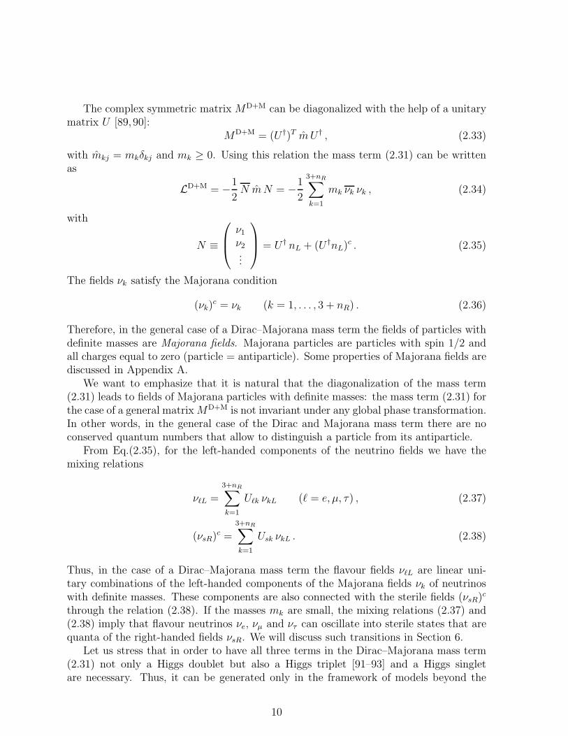
The complex symmetric matrix MD+M can be diagonalized with the help of a unitarymatrix U [89, 90]:

MD+M = (U †)T m U † , (2.33)

with mkj = mkδkj and mk ≥ 0. Using this relation the mass term (2.31) can be writtenas

LD+M = −1

2N mN = −1

2

3+nR∑

k=1

mk νk νk , (2.34)

with

N ≡

ν1

ν2...

= U † nL + (U †nL)c . (2.35)

The fields νk satisfy the Majorana condition

(νk)c = νk (k = 1, . . . , 3 + nR) . (2.36)

Therefore, in the general case of a Dirac–Majorana mass term the fields of particles withdefinite masses are Majorana fields. Majorana particles are particles with spin 1/2 andall charges equal to zero (particle = antiparticle). Some properties of Majorana fields arediscussed in Appendix A.

We want to emphasize that it is natural that the diagonalization of the mass term(2.31) leads to fields of Majorana particles with definite masses: the mass term (2.31) forthe case of a general matrixMD+M is not invariant under any global phase transformation.In other words, in the general case of the Dirac and Majorana mass term there are noconserved quantum numbers that allow to distinguish a particle from its antiparticle.

From Eq.(2.35), for the left-handed components of the neutrino fields we have themixing relations

νℓL =

3+nR∑

k=1

Uℓk νkL (ℓ = e, µ, τ) , (2.37)

(νsR)c =

3+nR∑

k=1

Usk νkL . (2.38)

Thus, in the case of a Dirac–Majorana mass term the flavour fields νℓL are linear uni-tary combinations of the left-handed components of the Majorana fields νk of neutrinoswith definite masses. These components are also connected with the sterile fields (νsR)c

through the relation (2.38). If the masses mk are small, the mixing relations (2.37) and(2.38) imply that flavour neutrinos νe, νµ and ντ can oscillate into sterile states that arequanta of the right-handed fields νsR. We will discuss such transitions in Section 6.

Let us stress that in order to have all three terms in the Dirac–Majorana mass term(2.31) not only a Higgs doublet but also a Higgs triplet [91–93] and a Higgs singletare necessary. Thus, it can be generated only in the framework of models beyond the

10

Standard Model. A typical example is the SO(10) model (see, for example, [31]). For adiscussion of radiative corrections to the Dirac–Majorana mass term see Ref. [94].

Up to now we did not make any special assumption about the Dirac–Majorana massterm (2.31). Let us now consider the possibility that CP invariance in the lepton sectorholds. In this case we have

UCP LD+M(x)U−1CP = LD+M(xP) . (2.39)

where UCP is the operator of CP conjugation, x ≡ (x0, ~x) and xP ≡ (x0,−~x). For thefields nL(x) we take the usual CP transformation

UCP nL(x)U−1CP = η γ0 C nLT (xP) , (2.40)

where η is a diagonal matrix of phase factors. The mass term LD+M can be written inthe form

LD+M(x) =1

2nTL(x) C−1MD+M nL(x) −

1

2nL(x) (MD+M)† C nLT (x) . (2.41)

Using Eq.(2.40) we obtain

UCP nTL(x) C−1MD+M nL(x) U

−1CP = nL(xP) ηMD+Mη C nLT (xP) . (2.42)

Hence, the CP invariance condition (2.39) is satisfied if

ηMD+Mη = −(MD+M)† . (2.43)

Up to now η was an arbitrary diagonal matrix of phase factors. If we choose η = i, inthis case CP invariance in the lepton sector implies that

MD+M = (MD+M)† . (2.44)

Taking into account that MD+M is a symmetric matrix, the condition (2.44) is equivalentto

MD+M = (MD+M)∗ . (2.45)

The real symmetric matrix MD+M can be diagonalized with the transformation

MD+M = Om′ OT , (2.46)

where O is an orthogonal matrix (OT = O−1) and m′ is a diagonal matrix, m′kj = m′

kδkj .The eigenvalues m′

k can be positive or negative and the neutrino masses are thus givenby mk = |m′

k|. Therefore, we write the eigenvalues as

m′k = mk ρk , (2.47)

where ρk = ±1 is the sign of the kth eigenvalue of the matrix MD+M. Then the relation(2.46) can be rewritten in the form

MD+M = (U †)T m U † (2.48)

11

withU † =

√ρOT (2.49)

and mkj = mk δkj . Here ρ is the diagonal matrix with elements ρkj = ρkδkj. Therefore, ifCP is conserved in the lepton sector, the neutrino mixing matrix has the simple structureshown in Eq.(2.49), which implies that

U∗ = U ρ . (2.50)

The CP transformation of the Majorana field νk is given by (see Appendix A)

UCP νk(x)U−1CP = ηCP

k γ0 νk(xP) , (2.51)

where ηCPk is the CP parity of the Majorana field νk which is ηCP

k = ±i (see Ref. [65]).From Eq.(2.51) we have

UCP νkL(x)U−1CP = ηCP

k γ0 νkR(xP) . (2.52)

This relation and Eqs.(2.35), (2.40) and (2.50) imply that the CP parity of the Majoranafield νk is [95–97]

ηCPk = i ρk . (2.53)

Indeed, we have

UCPNL(x)U−1CP = U † i γ0 C nLT (xP) = U † U∗ i γ0 CNL

T(xP) = i ρ γ0NR(xP) . (2.54)

2.3 Majorana mass term

If only left-handed neutrino flavour fields νℓL (ℓ = e, µ, τ) enter into the Lagrangian wecan write down the mass term [23,98]

LM = −1

2

∑

ℓ,ℓ′

(νℓL)cMLℓℓ′ νℓ′L , (2.55)

where ML is a symmetric complex matrix (see previous section). Then we have for themixing

νℓL =3∑

k=1

Uℓk νkL , (2.56)

where νk is the field of Majorana neutrinos with mass mk. In this case the number ofmassive Majorana neutrinos is equal to the number of lepton flavours (three). Note thatthe generation of the Majorana mass term (2.55) requires an enlargement of the scalarsector of the Minimal Standard Model [99]: with a Higgs triplet like in the Majoronmodels Ref. [91–93] Majorana masses are obtained at the tree level, whereas radiativegeneration is possible at the 1-loop level with a singly charged Higgs singlet (plus anadditional Higgs doublet) [31, 100–104]) or at the 2-loop level with a doubly chargedHiggs singlet (plus an additional singly charged scalar) [105].

12

Since the Majorana condition (2.36) does not allow the rephasing of the neutrinofields, only three of the six phases in the 3 × 3 mixing matrix U can be absorbed intothe charged lepton fields in the charged current (2.19). Therefore, in the Majoranacase the mixing matrix contains three CP-violating phases [28, 29, 106] in contrast tothe single CP-violating phase of the Dirac case discussed in Section 2.1. However, theadditional CP-violating phases in the Majorana case have no effect on neutrino oscillationsin vacuum [28,29, 106] (see Section 3) as well as in matter [107].

2.4 The one-generation case

Let us consider the Dirac–Majorana mass term in the simplest case of one generation.We have

LD+M = − 1

2mL (νL)c νL −mD νR νL − 1

2mR νR (νR)c + h.c.

= − 1

2mR (nL)cM nL + h.c. , (2.57)

with

nL ≡(

νL(νR)c

)

, M ≡(

mL mD

mD mR

)

. (2.58)

For simplicity we assume CP invariance in the lepton sector (see Subsection 2.2). Inthis case mL, mD and mR are real parameters. In order to diagonalize the matrix M , letus write it in the form

M =1

2TrM +M0 =

1

2(mL +mR) +M0 , (2.59)

with

M0 =

−1

2(mR −mL) mD

mD1

2(mR −mL)

. (2.60)

The eigenvalues of the matrix M0 are

m01,2 = ∓1

2

√

(mR −mL)2 + 4m2D . (2.61)

Furthermore, we haveM0 = Om0OT , (2.62)

where m0 = diag(m01, m

02) and O is the orthogonal matrix

O =

(

cosϑ sinϑ− sinϑ cosϑ

)

(2.63)

with the mixing angle ϑ given by

cos 2ϑ =mR −mL

√

(mR −mL)2 + 4m2D

, sin 2ϑ =2mD

√

(mR −mL)2 + 4m2D

. (2.64)

13

Hence, the matrix M can be written as

M = Om′ OT , (2.65)

where m′ = diag(m′1, m

′2) and

m′1,2 =

1

2

[

(mR +mL) ∓√

(mR −mL)2 + 4m2D

]

. (2.66)

The eigenvalues of the matrix M are real but can have positive or negative sign. Let uswrite them as

m′k = mk ρk , (2.67)

where mk = |m′k| and ρk is the sign of the kth eigenvalue of the matrix M . As shown

in Eq.(2.53), the CP parity of the Majorana field νk with definite mass mk is ηCPk = iρk.

The relation (2.65) can be written in the form

M = (U †)T m U † , (2.68)

with m = diag(m1, m2) andU † ≡ √

ρOT , (2.69)

with ρ = diag(ρ1, ρ2). Using now the general formulas obtained in Section 2.2, we havethe mixing relation

(

νL(νR)c

)

= U

(

ν1L

ν2L

)

, (2.70)

with

U =

(

(√ρ1)

∗ cosϑ (√ρ2)

∗ sinϑ−(

√ρ1)

∗ sinϑ (√ρ2)

∗ cosϑ

)

. (2.71)

Therefore, the three parameters mL, mD, mR are related with the mixing angle ϑand the neutrino masses mk by the relations (2.64) and (2.66), (2.67). The signs of theeigenvalues of M determine the CP parities of the massive Majorana fields νk.

In the framework of CP conservation, the relations obtained so far are general. Inthe following part of this section we consider some particular cases with special physicalsignificance.

2.5 The see-saw mechanism

Let us consider the Dirac–Majorana mass term (2.57) and assume [32–34] that mL = 0,mD ≃ mf , where mf is the mass of a quark or a charged lepton of the same generation,and mR ≃ M ≫ mf . In this case, from the relations (2.64), (2.66) and (2.67) we have

ϑ ≃ mf

M ≪ 1 , (2.72)

m1 ≃(mf)2

M ≪ mf , ρ1 = −1 , (2.73)

m2 ≃ M , ρ2 = 1 . (2.74)

14

These relations imply that approximately

νL = −i ν1L , (νR)c = ν2L , (2.75)

and the Majorana fields ν1, ν2 are connected with the fields νL and νR by

ν1 = i [νL − (νL)c] , ν2 = νR + (νR)c . (2.76)

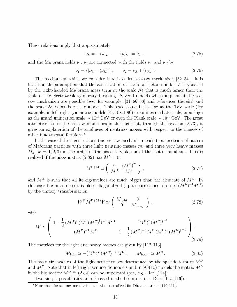
The mechanism which we consider here is called see-saw mechanism [32–34]. It isbased on the assumption that the conservation of the total lepton number L is violatedby the right-handed Majorana mass term at the scale M that is much larger than thescale of the electroweak symmetry breaking. Several models which implement the see-saw mechanism are possible (see, for example, [31, 66, 68] and references therein) andthe scale M depends on the model. This scale could be as low as the TeV scale (forexample, in left-right symmetric models [31,108,109]) or an intermediate scale, or as highas the grand unification scale ∼ 1015 GeV or even the Plank scale ∼ 1019 GeV. The greatattractiveness of the see-saw model lies in the fact that, through the relation (2.73), itgives an explanation of the smallness of neutrino masses with respect to the masses ofother fundamental fermions.6

In the case of three generations the see-saw mechanism leads to a spectrum of massesof Majorana particles with three light neutrino masses mk and three very heavy massesMk (k = 1, 2, 3) of the order of the scale of violation of the lepton numbers. This isrealized if the mass matrix (2.32) has ML = 0,

MD+M ≡(

0 (MD)T

MD MR

)

, (2.77)

and MR is such that all its eigenvalues are much bigger than the elements of MD. Inthis case the mass matrix is block-diagonalized (up to corrections of order (MR)−1MD)by the unitary transformation

W T MD+MW ≃(

Mlight 00 Mheavy

)

, (2.78)

with

W ≃

1 − 1

2(MD)† (MR(MR)

†)−1MD (MD)† (MR)†

−1

−(MR)−1MD 1 − 1

2(MR)−1MD (MD)† (MR)†

−1

.

(2.79)The matrices for the light and heavy masses are given by [112,113]

Mlight ≃ −(MD)T (MR)−1MD , Mheavy ≃ MR . (2.80)

The mass eigenvalues of the light neutrinos are determined by the specific form of MD

and MR. Note that in left-right symmetric models and in SO(10) models the matrix ML

in the big matrix MD+M (2.32) can be important (see, e.g., Ref. [114]).Two simple possibilities are discussed in the literature (see Refs. [115, 116]):

6Note that the see-saw mechanism can also be realized for Dirac neutrinos [110,111].

15

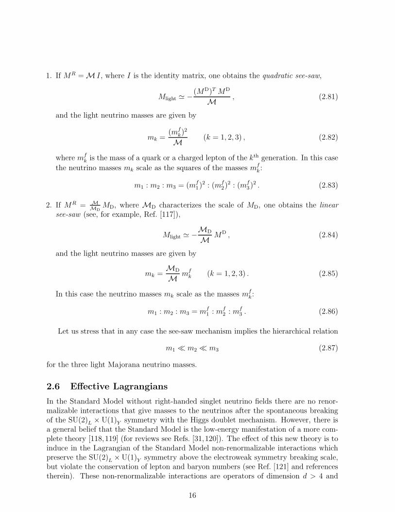
1. If MR = M I, where I is the identity matrix, one obtains the quadratic see-saw,

Mlight ≃ −(MD)T MD

M , (2.81)

and the light neutrino masses are given by

mk =(mf

k)2

M (k = 1, 2, 3) , (2.82)

where mfk is the mass of a quark or a charged lepton of the kth generation. In this case

the neutrino masses mk scale as the squares of the masses mfk :

m1 : m2 : m3 = (mf1)

2 : (mf2)

2 : (mf3)

2 . (2.83)

2. If MR = MMD

MD, where MD characterizes the scale of MD, one obtains the linear

see-saw (see, for example, Ref. [117]),

Mlight ≃ −MD

M MD , (2.84)

and the light neutrino masses are given by

mk =MD

M mfk (k = 1, 2, 3) . (2.85)

In this case the neutrino masses mk scale as the masses mfk :

m1 : m2 : m3 = mf1 : mf

2 : mf3 . (2.86)

Let us stress that in any case the see-saw mechanism implies the hierarchical relation

m1 ≪ m2 ≪ m3 (2.87)

for the three light Majorana neutrino masses.

2.6 Effective Lagrangians

In the Standard Model without right-handed singlet neutrino fields there are no renor-malizable interactions that give masses to the neutrinos after the spontaneous breakingof the SU(2)L × U(1)Y symmetry with the Higgs doublet mechanism. However, there isa general belief that the Standard Model is the low-energy manifestation of a more com-plete theory [118,119] (for reviews see Refs. [31,120]). The effect of this new theory is toinduce in the Lagrangian of the Standard Model non-renormalizable interactions whichpreserve the SU(2)L ×U(1)Y symmetry above the electroweak symmetry breaking scale,but violate the conservation of lepton and baryon numbers (see Ref. [121] and referencestherein). These non-renormalizable interactions are operators of dimension d > 4 and

16

must be multiplied by coupling constants that have dimension M4−d, where M is a massscale characteristic of the new theory. It is clear that the dominant effects at low energiesare produced by the operators with lowest dimension.

In the Standard Model the lepton number non-conserving operator with minimumdimension that can generate a neutrino mass is7 [122–127]

1

M∑

ℓ,ℓ′

gℓℓ′

2(LTℓ C−1 σ2 ~σ Lℓ′) (φT σ2 ~σ φ) + h.c. , (2.88)

where g is a 3 × 3 matrix of coupling constants, ~σ are the Pauli matrices, Lℓ are thestandard leptonic doublets and φ is the standard Higgs doublet:

Lℓ ≡(

νℓLℓL

)

(ℓ = e, µ, τ) , φ ≡(

ϕ+

ϕ0

)

. (2.89)

The effective operator in Eq.(2.88) has dimension five and the coupling constant is pro-portional to M−1.

When SU(2)L × U(1)Y is broken by the vacuum expectation value v/√

2 of ϕ0, theeffective interaction (2.88) generates the Majorana mass term

LM =1

2

v2

M∑

ℓ,ℓ′

gℓℓ′ νTℓL C−1νℓ′L + h.c. = −1

2

v2

M∑

ℓ,ℓ′

(νℓL)c gℓℓ′ νℓ′L + h.c. , (2.90)

where v ≃ 246 GeV. In this mass term there is a suppression factor v/M which isresponsible for the smallness of the neutrino masses [122, 123].

2.7 Maximal mixing

The expression (2.64) for the mixing angle ϑ implies that the mixing is maximal, i.e.,ϑ = π/4, if mR = mL. In this case, assuming that mL ≥ |mD|, the Majorana neutrinomasses are given by

m1,2 = mL ∓mD . (2.91)

The fields νL and (νR)c are connected with the fields ν1 and ν2 by the relations

νL =1√2

(ν1L + ν2L) , (νR)c =1√2

(−ν1L + ν2L) . (2.92)

The massive Majorana fields are given by

ν1,2 =1√2{[νL + (νL)

c] ∓ [νR + (νR)c]} . (2.93)

7This operator can be written also as

1

M∑

ℓ,ℓ′

gℓℓ′ (LTℓ σ2 φ) C−1 (φT σ2 Lℓ′) + h.c.

17

If mR = mL = 0 and mD > 0, the mass term (2.57) is simply a Dirac mass term.Applying Eqs.(2.64) and (2.66), we obtain

ϑ =π

4, m′

1,2 = ∓mD . (2.94)

Using Eq.(2.71) for the mixing matrix U , one can see that the fields νL and (νR)c areconnected to the Majorana fields ν1 and ν2 by the relations

νL =1√2

(−iν1L + ν2L) , (νR)c =1√2

(iν1L + ν2L) , (2.95)

where ν1,2 are Majorana fields with the same mass m1 = m2 = mD and with CP paritiesηCP

1 = −i and ηCP2 = +i (see Eq.(2.53)). Eq.(2.93) implies for a Dirac field

ν =1√2

(−iν1 + ν2) . (2.96)

Thus we arrive at the well-known result that a Dirac field can always be represented asan equal mixture of two Majorana fields with the same mass and opposite CP parities.

One can see this result also directly:

ν = − i√2

(

iν − νc√

2

)

+1√2

ν + νc√2

= − i√2ν1 +

1√2ν2 , (2.97)

where

ν1 = iν − νc√

2, ν2 =

ν + νc√2

(2.98)

are Majorana fields.Finally, there is the possibility that |mL|, |mR| ≪ mD but at least one of the param-

eters mL,R is non-zero. In this case Eqs.(2.95) and (2.96) are approximately valid andν1,2 are two Majorana neutrinos with opposite CP parities and almost degenerate massesgiven by

m1,2 ≃ mD ∓ 1

2(mL +mR) . (2.99)

The field ν is called in this case a pseudo-Dirac neutrino field [62, 65, 128–130].

3 Neutrino oscillations in vacuum

3.1 The general formalism

If there is neutrino mixing, the left-handed components of the neutrino fields ναL (α =e, µ, τ, s1, s2, . . .) are unitary linear combinations of the left-handed components of the n(Dirac or Majorana) neutrino fields νk (k = 1, . . . , n) with masses mk:

ναL =

n∑

k=1

Uαk νkL . (3.1)

18

The number n of massive neutrinos is 3 for the Dirac mass term discussed in Section 2.1and for the Majorana mass term discussed in Section 2.3, in which cases there are onlythe three active flavour neutrinos. The number n of massive neutrinos is more than threein the case of a Dirac–Majorana mass term discussed in Section 2.2 with a mixing ofboth, active and sterile neutrinos. In general, the number of light massive neutrinos canbe more than three. We enumerate the neutrino masses in such a way that

m1 ≤ m2 ≤ m3 ≤ . . . ≤ mn . (3.2)

In this section we will consider in detail the phenomenon of neutrino oscillations in vacuumwhich is implied by the mixing relation (3.1).

If all neutrino mass differences are small, a state of a flavour neutrino να producedin a weak process (as the π+ → µ+νµ decay, nuclear beta-decays, etc.) with momentump ≫ mk is described by the coherent superposition of mass eigenstates (for a discussionof the quantum mechanical problems of neutrino oscillations see Refs. [61, 62, 131–146])

|να〉 =n∑

k=1

U∗αk |νk〉 . (3.3)

Here |νk〉 is the state of a neutrino with negative helicity, mass mk and energy

Ek =√

p2 +m2k ≃ p +

m2k

2p. (3.4)

Let us assume that at the production point and at time t = 0 the state of a neutrinois described by Eq.(3.3). According to the Schrodinger equation the mass eigenstates |νk〉evolve in time with the phase factors exp(−iEkt) and at the time t at the detection pointwe have

|να〉t =

n∑

k=1

U∗αk e

−iEkt |νk〉 . (3.5)

Neutrinos are detected by observing weak interaction processes. Expanding the state(3.5) in the basis of flavour neutrino states |νβ〉, we obtain

|να〉t =∑

β

Aνα→νβ(t) |νβ〉 , (3.6)

where

Aνα→νβ(t) =

n∑

k=1

Uβk e−iEkt U∗

αk (3.7)

is the amplitude of να → νβ transitions at the time t at a distance L ≃ t. Consequently,the probability of this transition is given by

Pνα→νβ= |Aνα→νβ

(t)|2 =

∣

∣

∣

∣

∣

n∑

k=1

Uβk e−iEkt U∗

αk

∣

∣

∣

∣

∣

2

. (3.8)

19

This formula has a very simple interpretation. U∗αk is the amplitude to find the neutrino

mass eigenstate |νk〉 with energy Ek in the state of the flavour neutrino |να〉, the factorexp(−iEkt) gives the time evolution of the mass eigenstate and, finally, the term Uβkgives the amplitude to find the flavour neutrino state |νβ〉 in the mass eigenstate |νk〉. Wewant to remark that weak interaction processes responsible for neutrino production anddetection involve active neutrinos. Therefore, strictly speaking, in the derivation of theEqs.(3.7) and (3.8) the indices α and β take only active flavour indices. However, transi-tions into sterile neutrinos can be revealed through neutral current neutrino experiments(disappearance of active neutrinos). In this sense, the formulas (3.7) and (3.8) have ameaning also for transitions between active and sterile states.

Notice that in order to have a non-negligible active-sterile transition probability thesterile fields must have a mixing with the light neutrino mass eigenfields the numberof which must be more than three. Such a possibility is phenomenologically given bythe Dirac–Majorana mass term (2.21), but it is not realized in the simple see-saw schemediscussed in Section 2.5, where the scale of the right-handed Majorana mass term is large.However, the see-saw scenario can be modified by additional assumptions to include lightsterile neutrinos (“singular see-saw” [147], “universal see-saw [148,149]).

At this point a remark concerning the unitarity of the mixing matrix U is at order.If some of the mass eigenstates are so heavy that they are not produced in the standardweak processes then these mass eigenstates will not occur in the flavour state |να〉 (3.3).Let us assume that the first n′ mass eigenstates are light (n′ < n). Consequently, onlythat part of U plays a role in neutrino oscillations where k ≤ n′. In the following we willalways assume that in the situation described here we can confine ourselves to an n′ × n′

submatrix of U which is unitary to a good approximation (see, e.g., Ref. [150]). Thisis realized in the see-saw mechanism with a sufficiently large right-handed scale. In thefurther discussion we will drop the distinction between n and n′.

From the relation (3.1) it follows that the state describing a flavour antineutrino ναis given by

|να〉 =

n∑

k=1

Uαk |νk〉 . (3.9)

Thus the amplitude of να → νβ transitions is given by

Aνα→νβ(t) =

n∑

k=1

U∗βk e

−iEkt Uαk . (3.10)

Notice that the amplitude for antineutrino transitions differs from the correspondingamplitude (3.7) for neutrinos only by the exchange U → U∗.

Using the unitarity relation

n∑

k=1

Uβk U∗αk = δαβ , (3.11)

20

Experiment L (m) E (MeV) ∆m2 (eV2)

Reactor SBL 102 1 10−2

Reactor LBL 103 1 10−3

Accelerator SBL 103 103 1

Accelerator LBL 106 103 10−3

Atmospheric 107 103 10−4

Solar 1011 1 10−11

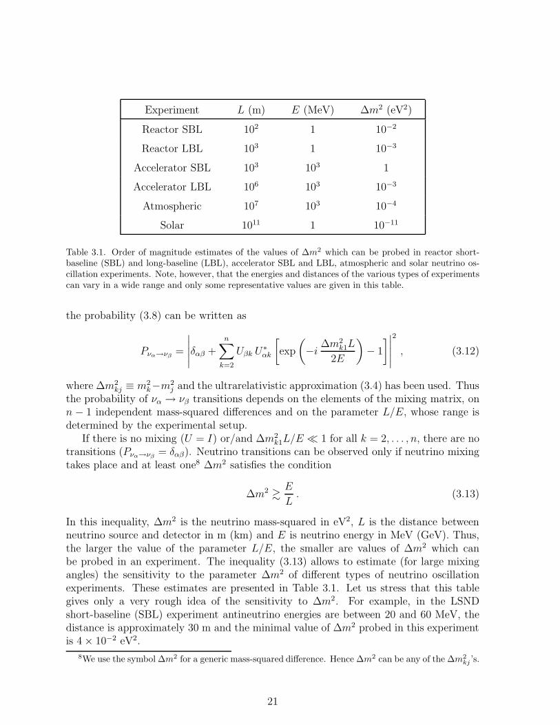
Table 3.1. Order of magnitude estimates of the values of ∆m2 which can be probed in reactor short-baseline (SBL) and long-baseline (LBL), accelerator SBL and LBL, atmospheric and solar neutrino os-cillation experiments. Note, however, that the energies and distances of the various types of experimentscan vary in a wide range and only some representative values are given in this table.

the probability (3.8) can be written as

Pνα→νβ=

∣

∣

∣

∣

∣

δαβ +n∑

k=2

Uβk U∗αk

[

exp

(

−i ∆m2k1L

2E

)

− 1

]

∣

∣

∣

∣

∣

2

, (3.12)

where ∆m2kj ≡ m2

k−m2j and the ultrarelativistic approximation (3.4) has been used. Thus

the probability of να → νβ transitions depends on the elements of the mixing matrix, onn − 1 independent mass-squared differences and on the parameter L/E, whose range isdetermined by the experimental setup.

If there is no mixing (U = I) or/and ∆m2k1L/E ≪ 1 for all k = 2, . . . , n, there are no

transitions (Pνα→νβ= δαβ). Neutrino transitions can be observed only if neutrino mixing

takes place and at least one8 ∆m2 satisfies the condition

∆m2 &E

L. (3.13)

In this inequality, ∆m2 is the neutrino mass-squared in eV2, L is the distance betweenneutrino source and detector in m (km) and E is neutrino energy in MeV (GeV). Thus,the larger the value of the parameter L/E, the smaller are values of ∆m2 which canbe probed in an experiment. The inequality (3.13) allows to estimate (for large mixingangles) the sensitivity to the parameter ∆m2 of different types of neutrino oscillationexperiments. These estimates are presented in Table 3.1. Let us stress that this tablegives only a very rough idea of the sensitivity to ∆m2. For example, in the LSNDshort-baseline (SBL) experiment antineutrino energies are between 20 and 60 MeV, thedistance is approximately 30 m and the minimal value of ∆m2 probed in this experimentis 4 × 10−2 eV2.

8We use the symbol ∆m2 for a generic mass-squared difference. Hence ∆m2 can be any of the ∆m2kj ’s.

21

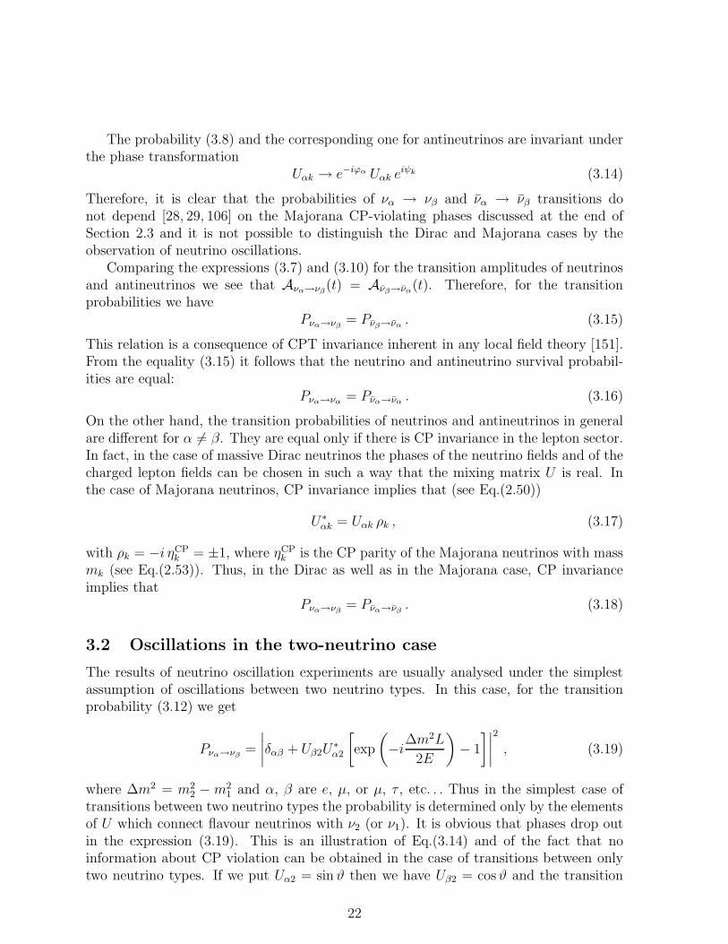
The probability (3.8) and the corresponding one for antineutrinos are invariant underthe phase transformation

Uαk → e−iϕα Uαk eiψk (3.14)

Therefore, it is clear that the probabilities of να → νβ and να → νβ transitions donot depend [28, 29, 106] on the Majorana CP-violating phases discussed at the end ofSection 2.3 and it is not possible to distinguish the Dirac and Majorana cases by theobservation of neutrino oscillations.

Comparing the expressions (3.7) and (3.10) for the transition amplitudes of neutrinosand antineutrinos we see that Aνα→νβ

(t) = Aνβ→να(t). Therefore, for the transition

probabilities we havePνα→νβ

= Pνβ→να. (3.15)

This relation is a consequence of CPT invariance inherent in any local field theory [151].From the equality (3.15) it follows that the neutrino and antineutrino survival probabil-ities are equal:

Pνα→να= Pνα→να

. (3.16)

On the other hand, the transition probabilities of neutrinos and antineutrinos in generalare different for α 6= β. They are equal only if there is CP invariance in the lepton sector.In fact, in the case of massive Dirac neutrinos the phases of the neutrino fields and of thecharged lepton fields can be chosen in such a way that the mixing matrix U is real. Inthe case of Majorana neutrinos, CP invariance implies that (see Eq.(2.50))

U∗αk = Uαk ρk , (3.17)

with ρk = −i ηCPk = ±1, where ηCP

k is the CP parity of the Majorana neutrinos with massmk (see Eq.(2.53)). Thus, in the Dirac as well as in the Majorana case, CP invarianceimplies that

Pνα→νβ= Pνα→νβ

. (3.18)

3.2 Oscillations in the two-neutrino case

The results of neutrino oscillation experiments are usually analysed under the simplestassumption of oscillations between two neutrino types. In this case, for the transitionprobability (3.12) we get

Pνα→νβ=

∣

∣

∣

∣

δαβ + Uβ2U∗α2

[

exp

(

−i∆m2L

2E

)

− 1

]∣

∣

∣

∣

2

, (3.19)

where ∆m2 = m22 −m2

1 and α, β are e, µ, or µ, τ , etc. . . Thus in the simplest case oftransitions between two neutrino types the probability is determined only by the elementsof U which connect flavour neutrinos with ν2 (or ν1). It is obvious that phases drop outin the expression (3.19). This is an illustration of Eq.(3.14) and of the fact that noinformation about CP violation can be obtained in the case of transitions between onlytwo neutrino types. If we put Uα2 = sin ϑ then we have Uβ2 = cosϑ and the transition

22

and survival probabilities are given by the following standard expressions valid for both,neutrinos and antineutrinos:

P(−)να→

(−)νβ

=1

2sin2 2ϑ

(

1 − cos∆m2L

2E

)

(α 6= β) , (3.20)

P(−)να→

(−)να

= P(−)νβ→

(−)νβ

= 1 − P(−)να→

(−)νβ

. (3.21)

The transition probability (3.20) can be written in the form

P(−)να→

(−)νβ

=1

2sin2 2ϑ

(

1 − cos 2.53∆m2L

E

)

(α 6= β) . (3.22)

where L is the source – detector distance expressed in m (km), E is the neutrino energyin MeV (GeV) and ∆m2 is the neutrino mass-squared difference in eV2. Thus, thetransition probability is a periodic function of L/E. This phenomenon is called neutrino

oscillations. The amplitude of oscillations is sin2 2ϑ and the oscillation length is given by

Losc =4 π E

∆m2≃ 2.48

E (MeV)

∆m2 (eV2)m . (3.23)

The condition (3.13) can be rewritten in the form

Losc . L . (3.24)

Therefore, neutrino oscillations can be observed if the oscillation length is not much largerthan the source – detector distance L.

The oscillatory behaviour of the transition probability (3.20) with sin2 2ϑ = 1 is shownin Fig. 3.1, where we have plotted it as a function of ∆m2L/4πE = L/Losc. The grey linerepresents the transition probability (3.20), whereas, in order to demonstrate the effect ofenergy averaging, the black line represents the transition probability (3.20) averaged overa Gaussian energy distribution with mean value E and standard deviation σ = E/10. Theaveraged probability is the measurable quantity in neutrino oscillation experiments. Onecan see that the averaging over the energy spectrum practically reduces the probabilityto the constant 1 − sin2 2ϑ/2 for L≫ Losc.

The expressions (3.20) and (3.21) are usually employed in analyses of the data ofneutrino oscillation experiments. In many SBL experiments with neutrinos from reactorsand accelerators, no indication in favour of neutrino oscillations was found. The dataof these experiments give an upper bound for the transition probability which impliesan excluded region in the space of the parameters ∆m2 and sin2 2ϑ. A typical exclusionplot is presented in Fig. 3.2 [152]. This plot shows the exclusion curves in the νµ → ντchannel obtained in the CDHS [153], FNAL E531 [154], CHARM II [155], CCFR [156],CHORUS [157] and NOMAD [158] experiments. The excluded region lies on the right ofthe curves.

The two most stringent exclusion curves in Fig. 3.2 have been obtained in the CHO-RUS [157] and NOMAD [158] experiments, which are operating at CERN using the

23

∆m2 L / 4 π E

10-2 10-1 100 101

P ν α→ν β

0.0

0.2

0.4

0.6

0.8

1.0

Figure 3.1. Transition probability for sin2 2ϑ = 1 as a function of ∆m2L/4πE = L/Losc, where Losc

is the oscillation length. The grey line represents the transition probability (3.20) and the black linerepresents the same transition probability averaged over a Gaussian energy spectrum with mean valueE and standard deviation σ = E/10.

neutrino beam from the SPS (with an average energy of about 30 GeV). 800 kg of emul-sions are used in the CHORUS experiment as target. The production and decay of τ ’sin the emulsion is searched for. In the NOMAD experiment a magnetic detector is usedand the production of τ ’s is identified with kinematical criteria.

Figure 3.3 shows the exclusion curves obtained in the CHOOZ [159], Gosgen [160],Krasnoyarsk [161] and Bugey [162] reactor νe → νe experiments. The region allowed bythe results of the Kamiokande atmospheric neutrino experiment [49] (see Section 5.1) isalso depicted in this figure. The Gosgen, Krasnoyarsk and Bugey experiments are SBLreactor experiments, whereas the recent CHOOZ experiment is the first LBL reactorexperiment. In this experiment the detector (5 tons of liquid scintillator loaded with Gd)is at the distance of about 1 km from the CHOOZ power station, which has two waterreactors with a total thermal power of 8.5 GW. The antineutrinos are detected throughthe observation of the reaction

νe + p→ e+ + n (3.25)

(the photons from annihilation of the positron and the delayed photons from the captureof neutron by Gd are detected). No indications in favour of neutrino oscillations werefound in the CHOOZ experiment. The ratio R of the numbers of measured antineutrinoevents and of expected antineutrino events in the case of absence of neutrino oscillationsin the CHOOZ detector is [159]

R = 0.98 ± 0.04 ± 0.04 . (3.26)

Since the average value of L/E in the CHOOZ experiment is approximately 300 (〈E〉 ≃3 MeV, L ≃ 1000 m), in this experiment it is possible to probe the value of the relevantneutrino mass-squared difference down to 10−3 eV2.

24

2

-1

CH

OR

US

CDHS

CCFR

E53

1

CH

AR

MII

NO

MA

D

1101010

10

10

10

1

10-1

1

2

3

-3 -2sin2 2#�m2 (eV2 )

10-4

10-3

10-2

10-1

1

0 0.1 0.2 0.3 0.4 0.5 0.6 0.7 0.8 0.9 1

sin2 2ϑ

∆m2 (

eV2 )

Bugey

Krasnoyarsk

Gösgen

Kamiokande(sub + multi-GeV)

Kamiokande(multi-GeV)

CHOOZ

Figure 3.2. Exclusion curves (90% CL) in theνµ → ντ channel obtained in the CDHS [153],FNAL E531 [154], CHARM II [155], CCFR [156],CHORUS [157] and NOMAD [158] experiments.

Figure 3.3. Exclusion curves (90% CL) in theνe → νe channel obtained in the CHOOZ [159],Gosgen [160], Krasnoyarsk [161] and Bugey [162]experiments. The shadowed region is allowed bythe results of the Kamiokande atmospheric neu-trino experiment [49].

With the help of the expression (3.22), it is possible to understand qualitatively thegeneral features of exclusion curves. In the region of large ∆m2 such that the oscillationlength is much smaller than the source – detector distance L, the cosine in the expression(3.22) oscillates very rapidly as a function of the neutrino energy E. Since in practiceall neutrino beams have an energy spectrum and the neutrino sources and detectors areextended in space, only the average transition probability

〈P(−)να→

(−)νβ

〉 =1

2sin2 2ϑ (3.27)

can be determined in the region of large ∆m2. The average probability is independentfrom ∆m2 and, therefore, from an experimental upper bound 〈P(−)

να→(−)νβ

〉0 on 〈P(−)να→

(−)νβ

〉 one

obtains the vertical-line part of the exclusion curve.At

∆m2 ≃ π

2

〈E〉1.27 〈L〉 , (3.28)

where 〈E〉 is the average energy and 〈L〉 is the average distance, the parameter sin2 2ϑhas the minimal value

(sin2 2ϑ)min = 〈P(−)να→

(−)νβ

〉0 (3.29)

25

on the boundary curve. Note that we are using here and in the rest of the section thesame units as in Eq.(3.22).

Typically, the upper bound 〈P(−)να→

(−)νβ

〉0 is much less than one. Then, in the region where

sin2 2ϑ is large the expression (3.22) for the transition probability can be approximatedby

P(−)να→

(−)νβ

≃ sin2 2ϑ

(

1.27∆m2L

E

)2

(3.30)

and in this region the boundary curve in the exclusion plot is given by

∆m2 ≃

√

〈P(−)να→

(−)νβ

〉0

1.27√

sin2 2ϑ 〈L2〉〈E−2〉. (3.31)

Therefore, this part of the exclusion curve is a straight line in the log sin2 2ϑ – log ∆m2

plot as can be seen from Fig. 3.2. From Eq.(3.31) it follows that the minimal value ofthe parameter ∆m2 that can be probed by an experiment is

∆m2 ≃

√

〈P(−)να→

(−)νβ

〉0

1.27√

〈L2〉〈E−2〉. (3.32)

It corresponds to sin2 2ϑ = 1.

4 Neutrino oscillations and transitions in matter

4.1 The effective Hamiltonian for neutrinos in matter

It has been pointed out by Wolfenstein [163] and by Mikheyev and Smirnov [164] thatthe neutrino oscillation pattern in vacuum can get significantly modified by the passageof neutrinos through matter because of the effect of coherent forward scattering. Thiseffect can be described by an effective Hamiltonian. Starting with neutrino oscillationsin vacuum, one can easily check that the transition probability (3.12) can be obtained byconsidering the evolution of the state vector ψ of the neutrino types with the “Schrodingerequation”

idψ(x)

dx= Hvac

ν ψ(x) =1

2EUm2U †ψ(x) , (4.1)

where Hvacν is the effective Hamiltonian for neutrino oscillations in vacuum with U being

the mixing matrix, E the neutrino energy and m the diagonal neutrino mass matrix. Thepresence of matter will give a correction to Eq.(4.1). Note that the variable in Eq.(4.1)is not time but space and the components of ψ(x) are given by the amplitudes denotedby aα(x) for the neutrino types α = e, µ, τ, s. The corresponding effective Hamiltonianfor antineutrinos Hvac

ν is obtained from Hvacν by the exchange U → U∗. After the seminal

work of Wolfenstein about neutrino oscillations in matter (see also Ref. [165]) and thediscovery of the importance of Hmat

ν , the analogue of Hvacν in matter, for the solar neutrino

26

problem [164] many rederivations of the effective matter Hamiltonian [166, 167] havebeen presented using a coupled system of Dirac equations [168,169], field theory [170] orstudying coherent forward scattering in more detail [171].

We want to sketch a derivation using the Dirac equation and following Ref. [169]. Thestarting point in most derivations is the expectation value of the currents for isotropicnon-relativistic matter given by [163,164,172]

〈fLγµfL〉matter =1

2Nfδµ0 , (4.2)

where Nf is the number density of the particles represented by the field f . Note that theγ5 term does not contribute for non-aligned spins [173]. Eq.(4.2) is a good approximationeven for electrons in the core of the sun with a temperature T ≃ 16×106 K [174,175] andthus an average velocity of the electrons of around 10% of the velocity of light and correc-tions of order kT/me ≃ 2.6× 10−3. Starting from the weak interaction Lagrangians (2.1)and (2.2) one gets for low-energy neutrino interactions of flavour ℓ with the backgroundmatter

− Lmatνℓ

=GF√

2ν†ℓ (1 − γ5)νℓ

∑

f

Nf(δℓf + T3fL− 2 sin2 θWQf ) , (4.3)

where GF is the Fermi coupling constant, θW the weak mixing angle, T3fLthe eigenvalue of

the field fL of the third component of the weak isospin (T3fR= 0 in the Standard Model)

and Qf is the charge of f . In the matter Lagrangian (4.3) the charged current interactionis represented by the Kronecker symbol δℓf saying that for neutrinos of flavour ℓ thecharged current only contributes when background matter containing charged leptons ofthe same flavour is present. Concentrating now on realistic matter with electrons, protonsand neutrons which is electrically neutral, i.e., Ne = Np, and taking into account that wehave T3eL

= −T3pL= T3nL

= −1/2 and Qe = −Qp = −1, Qn = 0 for electrons, protonsand neutrons, respectively,9 we get an effective Hamiltonian

HDν = −i~α · ~∇ + β(MPL +M †PR) +

√2GF diag

(

Ne −1

2Nn,−

1

2Nn,−

1

2Nn

)

PL (4.4)

acting on the vector Ψ(t, x) of the flavour neutrino wave functions, where we have definedPL,R = (1 ∓ γ5)/2, αj = γ0γj and β = γ0. M is the non-diagonal mass matrix. Thelast term in Eq.(4.4) is called the matter potential term. Several remarks concerningthe Hamiltonian (4.4), which is the point of departure for deriving the effective matterHamiltonian in Refs. [168, 169], are at order:

1. HDν has spinor and flavour indices, it leads thus to a system of Dirac equations coupled

via the mass term.

2. The neutral current contributions of electrons and protons cancel for realistic matterbecause of opposite T3fL

quantum numbers and electric charges (see discussion abovebefore Eq.(4.4)).9For protons and neutrons this is ensured by CVC (conserved vector current) for the T3 part and

conservation of the electromagnetic current.

27

3. The Hamiltonian (4.4) is valid for Dirac neutrinos. For antineutrinos, M is replaced byMT and the matter potential term of HD

ν has the opposite sign and the projector PRinstead of PL. This is a consequence of proceeding along the same lines as before butusing the charge-conjugate fields to describe antineutrinos (νℓγρPLνℓ = −νcℓγρPRνcℓ ).

4. In the Majorana case, in order to obtain the Hamiltonian HMν the antineutrino matter

potential has to be added to HDν and the neutrino field vector Ψ is subject to the

Majorana condition Ψ = CγT0 Ψ∗. This condition is compatible with the time evolutiongoverned by HM

ν [169].

5. Sterile neutrinos can easily be incorporated into HD(−)ν

and HMν by simply adding the

entry 0 to the matter potential term. Note that the probability of active – activetransitions does not depend on the neutron density Nn, which is, however, importantfor active – sterile transitions (see Table 4.1).

The essence of deriving an effective Hamiltonian for neutrino oscillations in matteris to get rid of the spinor indices in HD

ν and to obtain an equation involving only theindices α for the different neutrino types as in the vacuum case (4.1). To this end, letus now assume that the neutrino propagation proceeds along the x3 ≡ x axis, that theneutrino momentum p > 0 corresponding to propagation in vacuum is much larger thanthe matter potentials and that the neutrinos are ultrarelativistic. Thus we consider aone-dimensional problem from now on. Defining a wave function φ via

Ψ(t, x) = eipxφ(x, t) with i∂φ

∂t=(

pα3 +HDν

)

φ , (4.5)

this wave function changes little over distances of the order of the de Broglie wave lengthof the neutrino. With respect to α3 we can decompose the Hamiltonian (4.4) into HD

ν =Heven + Hodd which are the parts commuting or anticommuting with α3. Hodd consistssolely of the mass term and Heven contains the rest of HD

ν . With p being a large parameterwe can perform a Foldy – Wouthuysen transformation where we truncate the series at1/p leading to the Hamiltonian [169,176]

HDFW,ν = pα3 +Heven +

1

2pα3H

2odd

= α3

(

p− i∂

∂x

)

+√

2GF diag

(

Ne −1

2Nn,−

1

2Nn,−

1

2Nn

)

PL

+1

2pα3(M

†MPL +MM †PR) , (4.6)

such that all terms in HDFW,ν commute with α3 and, therefore, all matrices in HD

FW,ν withspinor indices can be diagonalized at the same time in order to separate positive andnegative energy states. Denoting this unitary diagonalization matrix by U0 we can achieveU0α3U

†0 = diag(1, 1,−1,−1), U0

1−γ52U †

0 = diag(0, 1, 1, 0) and U01+γ5

2U †

0 = diag(1, 0, 0, 1).Note that there are no transitions between left and right-handed states through HD

FW,ν .

28

For neutrinos with magnetic moments (electric dipole moments) the method describedabove would also yield the appropriate left-right transitions [169].

Going back to the Foldy – Wouthuysen transform of the wave function Ψ instead of φremoves the p from the Hamiltonian (4.6). The final step in deriving the effective matterHamiltonian consists of considering stationary states and splitting off the plane wave partby

ΨFW(t, x) = e−iE(t−x)ψ(x) . (4.7)

Then the wave function ψ(x), taken for positive energies and left-handed neutrinos, fulfillsthe first order differential equation (4.1) with Hvac

ν replaced by [163]

Hmatν =

1

2E

(

M †M + 2√

2EGF diag

(

Ne −1

2Nn,−

1

2Nn,−

1

2Nn

))

, (4.8)

correct up to order 1/E. This effective Hamiltonian is valid for left-handed Dirac neutri-nos or Majorana neutrinos, whereas in the case of right-handed (Dirac) antineutrinos orright-handed Majorana neutrinos we have

Hmatν =

1

2E

(

MTM∗ − 2√

2EGF diag

(

Ne −1

2Nn,−

1

2Nn,−

1

2Nn

))

, (4.9)

because for (Dirac) antineutrinos one has to replace M by MT in the Hamiltonian (4.6)and for Majorana neutrinos M = MT holds (see also points 3 and 4 after Eq.(4.4)). With

M = URmU†L and UL ≡ U (4.10)

only the left-handed mixing matrix U enters and connection between Eqs.(4.8) and (4.1)is made. Thus in the final results (4.8) and (4.9) there is no distinction between theDirac and Majorana case for ultrarelativistic neutrinos. This is an illustration of thefact that with neutrino oscillation experiments the Dirac or Majorana nature cannot bedistinguished [98, 177].

The Hamiltonians (4.8) and (4.9) have been used to investigate neutrino oscillationsin the sun, in the earth and in supernovae. In the following we will only be concernedwith the first two subjects. Application limits of the neutrino evolution equations inmatter have been discussed in Ref. [178]. Elastic and inelastic neutrino scattering in-troduces quantum damping into the evolution equations which is proportional to theneutrino interaction rate [179]. In the sun and the earth this effect is negligible, in par-ticular, for low energies, whereas in the early universe it is of crucial importance [179].Density fluctuations have been found to influence considerably neutrino propagation inthe sun [180], however, more realistic considerations with helioseismic waves as densityfluctuations show no observable effect on the solar neutrino problem discussed in termsof neutrino oscillations [181]. Solar neutrinos are also influenced by their passage throughthe earth [182].

29

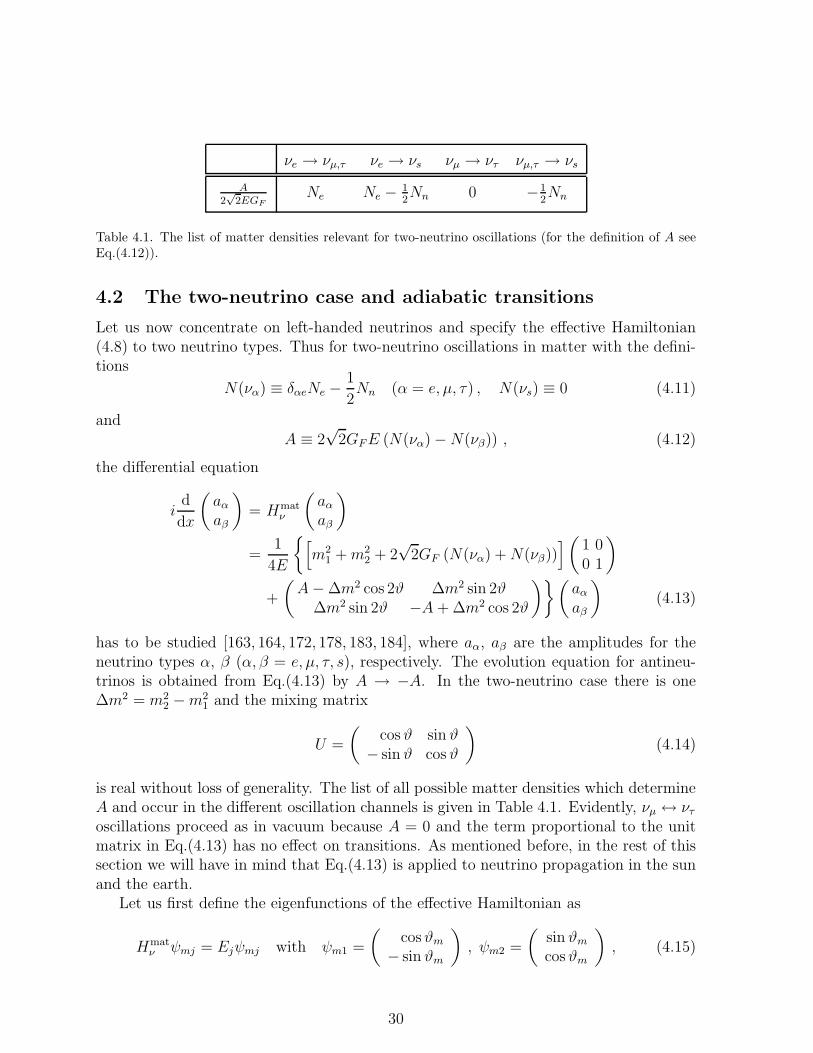
νe → νµ,τ νe → νs νµ → ντ νµ,τ → νs

A2√

2EGFNe Ne − 1

2Nn 0 −1

2Nn

Table 4.1. The list of matter densities relevant for two-neutrino oscillations (for the definition of A seeEq.(4.12)).

4.2 The two-neutrino case and adiabatic transitions

Let us now concentrate on left-handed neutrinos and specify the effective Hamiltonian(4.8) to two neutrino types. Thus for two-neutrino oscillations in matter with the defini-tions

N(να) ≡ δαeNe −1

2Nn (α = e, µ, τ) , N(νs) ≡ 0 (4.11)

andA ≡ 2

√2GFE (N(να) −N(νβ)) , (4.12)

the differential equation

id

dx

(

aαaβ

)

= Hmatν

(

aαaβ

)

=1

4E

{

[

m21 +m2

2 + 2√

2GF (N(να) +N(νβ))]

(

1 00 1

)

+

(

A− ∆m2 cos 2ϑ ∆m2 sin 2ϑ∆m2 sin 2ϑ −A + ∆m2 cos 2ϑ

)}(

aαaβ

)

(4.13)

has to be studied [163, 164, 172, 178, 183, 184], where aα, aβ are the amplitudes for theneutrino types α, β (α, β = e, µ, τ, s), respectively. The evolution equation for antineu-trinos is obtained from Eq.(4.13) by A → −A. In the two-neutrino case there is one∆m2 = m2

2 −m21 and the mixing matrix

U =

(

cosϑ sin ϑ− sin ϑ cos ϑ

)

(4.14)

is real without loss of generality. The list of all possible matter densities which determineA and occur in the different oscillation channels is given in Table 4.1. Evidently, νµ ↔ ντoscillations proceed as in vacuum because A = 0 and the term proportional to the unitmatrix in Eq.(4.13) has no effect on transitions. As mentioned before, in the rest of thissection we will have in mind that Eq.(4.13) is applied to neutrino propagation in the sunand the earth.

Let us first define the eigenfunctions of the effective Hamiltonian as

Hmatν ψmj = Ejψmj with ψm1 =

(

cosϑm− sin ϑm

)

, ψm2 =

(

sin ϑmcosϑm

)

, (4.15)

30

where the matter angle ϑm and the energy eigenvalues Ej are functions of x. In thelimit of vanishing matter density ϑm is identical with the vacuum angle ϑ (4.14). Theeigenvalues Ej and the matter angle are given by

E1,2 =1

4E

{

m21 +m2

2 + 2√

2GF (N(να) +N(νβ))

∓√

(A− ∆m2 cos 2ϑ)2 + (∆m2 sin 2ϑ)2}

(4.16)

and

tan 2ϑm =tan 2ϑ

1 − A

∆m2 cos 2ϑ

, (4.17)

respectively. The general solution of the differential equation (4.13) can be representedas

ψ(x) =

2∑

j=1

aj(x)ψmj(x) exp

(

−i∫ x

x0

dx′Ej(x′)

)

(4.18)

with the coefficients a1,2 fulfilling

d

dx

(

a1

a2

)

=

0 −dϑm

dxexp

(

i∫ x

x0dx′∆E(x′)

)

dϑm

dxexp

(

−i∫ x

x0dx′∆E(x′)

)

0

(

a1

a2

)

(4.19)and ∆E ≡ E2 −E1.

The adiabatic solution is defined as an approximate solution where aj ≃ 0 (j = 1, 2).10

Postponing the discussion of the question under which condition adiabaticity is fulfilled,we consider temporarily the case of an arbitrary number n of neutrino flavours or typesand define the mixing matrix in matter Um(x) via

Um(x)†Hmatν Um(x) = diag(E1(x), . . . , En(x)) with Um(x) = (ψm1, . . . , ψmn) , (4.20)

where the eigenvectors ψmj generalize Eq.(4.15). One readily obtains the generalizationof the vacuum oscillation amplitude Eq.(3.12) for neutrino oscillations in matter if theevolution of the neutrino wave function is adiabatic:

Aadiabνα→νβ

=∑

j

Um(x1)βj exp

(

−i{

δj +

∫ x1

x0

dx′Ej(x′)

})

U∗m(x0)αj . (4.21)

In this formula neutrino production and detection happen at x0 and x1, respectively. Theadiabatic phases δj, which are defined by

δj ≡ −i∫ x1

x0

dx′ψmj(x′)†ψmj(x

′) , (4.22)

10We use the dot above a symbol as abbreviation for ddx

.

31

are necessary for the correct evolution of ψ(x) in the adiabatic limit. Usually, they can beabsorbed into the eigenvectors ψmj [185], except for special matter densities, where thesephases acquire a topological meaning, together with the presence of CP violation [186].Note that for real vectors ψmj one has ψ†

mjψmj = 0 and therefore δj = 0.11 This is so inthe two-dimensional case Eq.(4.15).

Evaluating Eq.(4.21) for two neutrino types and assuming that an averaging overneutrino energies takes place such that

⟨

exp

(

−i∫ x1

x0

dx′∆E(x′)

)⟩

av

= 0 , (4.23)

it is easy to show that the averaged two-neutrino survival probability can be written inthe adiabatic case as

Pνα→να=

1

2(1 + cos 2ϑm(x0) cos 2ϑm(x1)) . (4.24)

Let us now derive a condition for adiabaticity in the two-neutrino case. The evolutionof the neutrino state in matter is adiabatic if the right-hand side of Eq.(4.19) can beneglected. A formal solution of Eq.(4.19) is given by

(

a1(x)a2(x)

)

=∞∑

k=0

∫ x

x0

dx′J(x′)

∫ x′

x0

dx′′J(x′′) · · ·∫ x(k−1)

x0

dx(k)J(x(k))

(

a1(x0)a2(x0)

)

, (4.25)

where J denotes the matrix on the right-hand side of Eq.(4.19). Defining the variable

α ≡ 1

2

∫ x

x0

dx′∆E(x′) (4.26)

and the adiabaticity parameter (as a function of x) [184, 187–189]

γ(x) ≡ ∆E

2|ϑm|(4.27)

one can determine an upper bound to the typical integral which occurs in all the termsof the sum (4.25) on the right end. In an interval [y0, y1] where γ is monotonous there isa value yc such that [190]

±∫ y1

y0

dy ϑm cos 2α =

∫ α(y1)

α(y0)

dα1

γcos 2α =

1

γ(y0)

∫ yc

y0

dα cos 2α +1

γ(y1)

∫ y1

yc

dα cos 2α

(4.28)according to the second mean value theorem of integral calculus (y0 < yc < y1). Thisconsideration allows to put the bound

∣

∣

∣

∣

∫ y1

y0

dy ϑme2iα

∣

∣

∣

∣

≤ 2√

2

γminwith γmin ≡ min

y∈[y0,y1]γ(y) . (4.29)

11The scalar product in Eq.(4.22) is imaginary for arbitrary vectors ψmj(x) normalized to one ∀x,therefore, for real vectors it must be zero.

32

Having found this bound, in the rest of the integrals in the terms in Eq.(4.25) one cansimply take the absolute values of the integrands and one is left with integrations of thetype dx|ϑm| = |dϑm|. With the refinement that the interval [x0, x] possibly has to bedivided into several parts labelled by a such that in each part interval γ(y) is monotonouswe can define

γ−1 ≡∑

a

γ−1min,a (4.30)

and obtain the exact bound

|aj(x) − aj(x0)| ≤2√

2

γ

(

cosh ∆Θ sinh ∆Θsinh ∆Θ cosh ∆Θ

)(

|a1(x0)||a2(x0)|

)∣

∣

∣

∣

j

, (4.31)

where the symbol |j denotes the j-th element of the vector on the right-hand side of thisinequality and ∆Θ has a contribution |∆ϑm| for every interval where ϑm has a definitesign. (∆ϑm is the difference between the angle ϑm in the initial and the final point of suchan interval.) Thus with the exact bound (4.31) we have found the following sufficientcondition:

γ ≫ 1 ⇒ adiabatic evolution . (4.32)

It is fulfilled if on the scale of the oscillation length in matter given by 1/∆E the matterangle ϑm changes very little, i.e., |ϑm| ≪ ∆E. Eq.(4.31) allows to get an upper boundon the crossing or jumping probability from ψm1 to ψm2. Assuming the initial conditionsa1(x0) = 1 and a2(x0) = 0 we get

|a2(x)| ≤2√

2

γsinh ∆Θ (4.33)

which illustrates once more the importance of γ for adiabaticity.

4.3 The resonance

In the context of the solar neutrino problem the discovery that a resonance in the pas-sage of νe through the sun is possible [164] gave a major boost to the investigation of thepropagation of neutrinos in matter. The possibility of a resonance is most easily under-stood in the adiabatic approximation by looking at Eqs.(4.17) and (4.24). For differentneutrino masses we can always label them in such a way that ∆m2 > 0. If on the wayfrom the creation point x0 in matter of νe to a point x1 in vacuum the neutrino passesthrough a point xres where the resonance condition

A(xres) = ∆m2 cos 2ϑ (4.34)

is fulfilled then ϑm(x1) ≡ ϑ has to be between 0◦ and 45◦ (for νe the quantity A ispositive!) whereas according to Eq.(4.17) the matter angle ϑm(x0) is found between 45◦

and 90◦.12 Consequently, the product of cosines in the νe survival probability (4.24) is

12Without loss of generality we consider 0◦ < ϑ < 90◦.

33

negative and the probability to find a νe after the passage through the sun is less than1/2. The interesting phenomenon is that this can happen even for relatively small mixingangles, provided the matter potential at the production point is large enough such thatthere is a point xres where the condition (4.34) is fulfilled. Indeed, for ϑ close to 0◦,one can even have ϑm(x1) close to 90◦ and thus Pνe→νe

≃ 0 (4.24). It has been shownthat the resonance is also effective in a certain area in the ∆m2–sin2 2ϑ plane where theevolution of the neutrino state is non-adiabatic. For antineutrinos a resonance is possibleif 45◦ < ϑ < 90◦.

If there is a resonance, then for reasonable matter densities the adiabaticity parameter(4.27) is smallest at the resonance and thus adiabaticity is most likely violated there.

Therefore, considering γ at the resonance, from Eq.(4.17) one easily computes ϑm

∣

∣

∣

res=

Ares/(2 sin 2ϑ∆m2). A suitable measure of adiabaticity in the case of a resonance is thusgiven by [187,188]

γres ≡∆E

2|ϑm|

∣

∣

∣

∣

res

=∆m2 sin2 2ϑ

2E cos 2ϑ (|A|/A)res

. (4.35)

In the solar interior the electron density is maximal in the center with Ne|max ≃100 ×Navo where Navo = 6.022 × 1023 cm−3 and Nn|max ≃ 1

2Ne|max [174]. This leads to

2√

2GFE Ne|max ≃ 1.5 × 10−5

(

E

1 MeV

)

eV2 . (4.36)

Considering the resonance condition (4.34) one can read off from this equation for which∆m2 a resonance is possible. Whereas the density variation of Ne and Nn in the sunis smooth, in the earth due to its layered structure (lithosphere – mantle – core) thedensities can be approximated as step functions [191, 192]. Furthermore, approximatelyNn ≃ Ne is valid in all layers. In the lithosphere, which is relevant for LBL neutrinooscillation experiments, the average mass density ρ is around 3 g/cm3. It increases toaround 13 g/cm3 in the core. Thus we can conveniently write

2√

2GFENe ≃ 2.3 × 10−4 eV2

(

ρ

3 g cm−3

)(

E

1 GeV

)

. (4.37)

4.4 Non-adiabatic neutrino oscillations in matter and crossing

probabilities

The analogue of the adiabatic formula (4.21) in terms of probabilities is given by

Pνα→νβ=

∣

∣

∣

∣

∣

∑

j,k

Um(x1)βjB(x1, x0)jkU∗m(x0)αk

∣

∣

∣

∣

∣

2

(4.38)

with

B(x1, x0) = U †m(x1)P exp

{

−i∫ x1

x0

dxHmatν (x)

}

Um(x0)

= P exp

{

−i∫ x1

x0

dx(

E − i U †m(x)Um(x)

)

}

, (4.39)

34

where E is the diagonal matrix of energy eigenvalues present in Eq.(4.20) (see Ref. [183]).B(x1, x0) is a unitary n×n matrix which is diagonal in the adiabatic limit correspondingto −i U †

m(x)Um(x) ≃ diag (δ1, . . . , δn) (see Eq.(4.22)).Confining ourselves now to two neutrino types and having in mind neutrino production

in matter and detection in vacuum we use the notation ϑm(x0) ≡ ϑ0m and ϑm(x1) =

ϑ. With the crucial assumption that averaging over neutrino energies and the neutrinoproduction region all terms other than probabilities can be dropped we get

〈BjkB∗j′k′〉av = δjj′δkk′|Bjk|2 and |B12|2 = |B21|2 = Pc , |B11|2 = |B22|2 = 1 − Pc ,

(4.40)where Pc is the crossing probability from ψm1 to ψm2 and in the second part of Eq.(4.40)unitarity has been used. Such averaging procedures have been shown to be effective inthe context of solar neutrinos, e.g., in Refs. [193, 194]. Inserting the relations (4.40) intoEq.(4.38) specialized to the survival probability of νe one obtains after some algebra withtrigonometric functions the Parke formula

Pνe→νe=

1

2+

(

1

2− Pc

)

cos 2ϑ cos 2ϑ0m , (4.41)

which is the generalization of Eq.(4.24) [183, 189]. This formula was first derived in thecontext of an exact solution of Eq.(4.13) for matter densities linear in x [188, 195] (seealso Refs. [187, 196]).

The probability Pc can be estimated with the Landau – Zener method [196, 197].Following the derivation of Landau, the idea is to make an analytic continuation of thematter densities and therefore of the effective matter Hamiltonian (4.8) into the complexplane by x → z where z is a complex variable. Then also the neutrino state ψ (4.18) isanalytic. Considering the energy eigenvalues E1,2(x) (4.16) as functions of z we find twobranching points z0 and z∗0 (Im z0 > 0) defined by the equation

E1(z0) = E2(z0) ⇔ A(z0) = ∆m2e±2iϑ . (4.42)

We consider E1(z) and ψm1(z) for definiteness and follow its evolution along a curve C(z)which starts at a value z in the vicinity of the real axis and goes along a negativelyoriented loop around z0 such that we end at the same point z but now located on thesecond sheet.13 Along this path E1(z) changes into E2(z) [197] and ψm1(z) into ψm2(z).

14

The crucial observation is that, though Ej(z) and ψmj(z) (j = 1, 2) are two-valuedanalytic objects, the analytic continuation ψ(z) of the solution (4.18) of the differentialequation (4.13) is single-valued [198]. From this fact it can easily be shown with Eq.(4.18)that [198]

a1(z) = exp

(

i

∫

C(z)

E1(z)dz

)

a2(z) , (4.43)

13It is convenient to imagine cuts from z0 to z0 + i∞ and z∗0 to z∗0 − i∞ in the complex plane. Crossingthese cuts, one moves from one sheet to the other.

14In general this change is accompanied by a factor of geometrical origin. It has no effect in our casefor the jumping probability [198].

35

where a1(z) is the analytic continuation of a1(x) in the vicinity of the real axis andthen along C(z). The Landau – Zener crossing probability is derived from the followingconsideration. Starting on the real axis at x− ≪ xres, where the evolution of ψ is adiabaticand where the boundary conditions a1(x−) = 1, a2(x−) = 0 hold, and going along a pathin the complex plane which passes above z0 and returning to the real axis at a pointx+ ≫ xres on the second sheet this path can be chosen such that the evolution in thecomplex variable z is adiabatic because we have passed the resonance in safe distanceand we have thus |a1(x+)| ≃ 1. On the other hand, we can go from x+ on the first sheetto the point x+ on the second sheet via C(x+) and with Eq.(4.43) we thus obtain

Pc = |a2(x+)|2 =

∣

∣

∣

∣

exp

(

−i∫

C(x+)

E1(z)dz

)∣

∣

∣

∣

2

, (4.44)

neglecting deviations of |a1(x+)| from 1. From this formula we can read off that integra-tions along the real axis do not contribute to Pc. Because of analyticity, the path C(x+)can be deformed such that it goes along the real axis from x+ to xres from where it leadsto z0, circles around the branching point with infinitely small radius and then goes backto xres and x+ on the second sheet. In this way, we obtain from Eq.(4.44) the final resultfor the Landau – Zener crossing probability

lnPc = − 1

EIm

∫ z0

xres

dz [(A− ∆m2 cos 2ϑ)2 + (∆m2 sin 2ϑ)2]1/2 . (4.45)

To get this formula we have used the explicit form of the energies of the adiabatic states(4.16).

With the variable transformation A = A(z) and dz = dA/dAdz

it is easy to evaluateEq.(4.45) for a linear density [172,187–189] and is also possible for an exponential density[199]. These calculations can be summarized by [183,189]

Pc = exp(

−π2γresF

)

(4.46)

with F = 1 for the linear and F = 1−tan2 ϑ for the exponential case. For an exponentiallyvarying matter density the dependence of Pc on ϑ is particularly simple because γresF =4δ sin2 ϑ with δ ≡ γres cos 2ϑ/ sin2 2ϑ which is independent of the vacuum mixing angle.For a more general discussion of the crossing probability (4.45) see Ref. [200].

Exact solutions of the differential equation (4.13) for neutrino oscillations in matterexist not only for the linear case [187,188,195,196] in terms of Weber functions but alsofor the exponentially varying matter density in terms of Whittaker functions [193, 201].This case is of particular importance for solar neutrinos because it approximates thereal density variation in the sun. Further exact solutions are known for A varying withtanh x [202] and 1/x [189]. In Refs. [183, 189] a list of the factors F for all these cases isgiven, calculated with the Landau – Zener formula (4.45).

The survival probability (4.41) with Pc in the Landau – Zener approximation doesnot reproduce well the exact survival probability in the extremely non-adiabatic region[193,195] (see also Refs. [172,183,189]). In these references the example of an extremely

36

dense medium (A → ∞ and thus ϑ0m = π/2) with a sharp boundary to the vacuum is

given. In this case the neutrino does not oscillate in the medium and therefore Pνe→νe=

1− 12sin2 2ϑ stems purely from vacuum oscillations. This has to be compared with Pc = 1,

because of the jump in density one gets γres = 0, inserted into Eq.(4.41). Obviously, theresulting expression Pνe→νe

= cos2 ϑ does not agree with the previous one.A remedy of this deficiency was found in the framework of the exact solution for an

exponentially varying matter density leading to the following modification [193] of theLandau – Zener crossing probability Pc (4.45):

Pc =

exp

(

−π2γresF

)

− exp

(

−π2γres

F

sin2 ϑ

)

1 − exp

(

−π2γres

F

sin2 ϑ

) . (4.47)

Numerical calculations for solar neutrinos with an exponential electron density using thisformula agree very well with numerical integrations of the differential equation (4.13),typically the agreement is in the percent range for relevant mixing parameters [203]. Ithas been conjectured in Ref. [189] that the form (4.47) of Pc holds for a wide class ofmatter density profiles. In any case, in the limit γres → 0 one gets Pc → cos2 ϑ which,when inserted into formula (4.41), correctly describes the survival probability in the aboveexample of an extremely non-adiabatic evolution.

Concluding this section, we consider again an arbitrary number of neutrino flavoursor types and envisage the interesting case where one of the eigenfunctions (4.20) of Hmat

ν

labelled by the index ℓ0 has an adiabatic evolution whereas the other part of ψ has anarbitrary evolution. We assume exact adiabaticity for ψmℓ0 which amounts to Bjℓ0 =Bℓ0k = 0 for j, k 6= ℓ0. This allows to write

Pνα→νβ= (1− |Um(x1)βℓ0 |2)(1− |Um(x0)αℓ0 |2)P (ℓ0)

να→νβ+ |Um(x1)βℓ0 |2|Um(x0)αℓ0 |2 , (4.48)

where we have defined

P (ℓ0)να→νβ

= [(1 − |Um(x1)βℓ0 |2)(1 − |Um(x0)αℓ0 |2)]−1

∣

∣

∣

∣

∣

∑

j,k 6=ℓ0

Um(x1)βjB(x1, x0)jkU∗m(x0)αk

∣

∣

∣

∣

∣

2

≤ 1 . (4.49)

That P(ℓ0)να→νβ is smaller than 1 follows from the Cauchy – Schwarz inequality and from

the above assumption for B because after dropping the row and the column labelled byℓ0 in B the remaining matrix is again unitary. Eq.(4.49) and similar cases are useful ifneutrino masses differing by orders of magnitude occur.

5 Indications of neutrino oscillations

5.1 Atmospheric neutrino experiments

37

5.1.1 The atmospheric neutrino flux

In 1912 it was discovered by V.F. Hess [204] in a manned balloon flight that the intensityof the ionizing radiation in the atmosphere as a function of the altitude did not conformwith the idea that this ionization was caused by radioactive elements in the surface of theearth but rather pointed to an extraterrestrial origin. In the following decades, beforethe advent of accelerator physics, this radiation, which was called first “ultraradiation”and later baptized “cosmic rays” by R.A. Millikan, proved to be one of the most fruitfulmeans for doing particle physics experiments. At the end of the first half of the 20thcentury such experiments had lead to the discovery of the positron, the pion and themuon and also the first particles with strangeness were found with cosmic rays [205].Eventually, in the beginning of the fifties, proton beams from accelerators replaced thecosmic proton flux as an experimental tool. However, after many years where acceleratorphysics was dominating in particle physics, at the end of the 20th century cosmic raysplay again a major role through atmospheric neutrinos which allow to use the whole globeas a neutrino physics laboratory and to probe neutrino mass-squared differences down toa few 10−4 eV2. In this way convincing evidence for the existence of neutrino oscillationsand thus for non-zero neutrino masses has been obtained [2].

In a simplified picture, the production of atmospheric neutrinos [206–218] proceedsin three steps [219]. In the first step the primary cosmic rays [219, 220] hit the nucleiin the atmosphere, thereby producing charged pions and kaons, either directly or viaintermediate particles. In the second step, the decay of these particles gives rise to partof the atmospheric νµ and νµ neutrino fluxes:

π+ → µ+ + νµ , π− → µ− + νµ and K+ → µ+ + νµ , K

− → µ− + νµ . (5.1)

In the third step, the νe and νe fluxes and further νµ and νµ fluxes are produced by

µ+ → e+ + νe + νµ and µ− → e− + νe + νµ . (5.2)

There is also a contribution to the neutrino fluxes from the decays

KL → π+ + ℓ− + νℓ and K+ → π0 + ℓ+ + νℓ (5.3)

with ℓ = e, µ and the charge conjugate processes [215, 219, 221] which does not conformwith the simple 3-step picture. At low energies the most important process in Eq.(5.1)is the pion decay. The contribution of Kℓ3 decays (5.3) to the neutrino fluxes is small[222, 223]. Let us now describe some useful details of the production of the atmosphericneutrino flux and its properties.

Cosmic rays: Galactic cosmic rays enter the solar system as an isotropic flux of par-ticles. There is convincing evidence that the bulk of the radiation with energies lessthan 106 GeV comes from our galaxy. Though there is no conclusive proof of the originof cosmic rays yet, plausible mechanisms range from material ejected by supernovae tointerstellar medium accelerated in supernova shock waves [224]. Solar cosmic rays are

38

emitted irregularly by major solar flares on the sun. Apart from electrons, primary cos-mic rays consist of protons and bare nuclei (mostly He). Roughly speaking, the chemicalcomposition of the galactic cosmic ray particles is given approximately by 90 % H, 9 % Heand less than 1 % heavier nuclei. However, the chemical composition varies with energy.At energies of around 100 MeV per nucleon the particle number ratio H/He is less than5, it increases to 10 at 1 GeV and is around 30 at 100 GeV [225,226]. The absolute fluxof cosmic protons is not very large: it is of the order of 1000/m2 × sec × sr for energiesof a few GeV and above the atmosphere. As a function of the energy the proton fluxabove a few GeV is well described by the power law E−2.7 until 106 GeV [225]. Above anenergy of 100 GeV per nucleon the cosmic ray fluxes are less precisely known [225,226].

Solar modulation: The solar cosmic rays (solar wind) are important in so far as theyweaken and modulate the flux of galactic cosmic ray particles with the solar activity. Thestronger the solar wind the more difficult it is for the low energy galactic cosmic rays toenter the solar sphere of influence. This modulation is noticeable for kinetic energies ofaround 10 GeV per nucleon or less [215,224]. This variation of the primary cosmic ray fluxwith the approximate 11-year cycle of solar activity can be parameterized as a functionof the neutron monitor at Mt. Washington [215]. It induces a corresponding modulationof the low energy atmospheric neutrino flux but its influence is small. The effect of thesolar wind on cosmic ray particles depends on the rigidity of the nuclei which is definedby momentum/charge. It is strongest for cosmic ray particles with small rigidity. Forneutrino energies Eν ∼ 2 GeV it is practically negligible, for energies around 1 GeV onlyappreciable at high geomagnetic latitudes because the geomagnetic cut-off admits cosmicray particles with smaller rigidity there.

Geomagnetic cut-off: The geomagnetic field prevents primary cosmic particles withlow rigidity from entering the atmosphere [215,218,227,228]. In the atmospheric neutrinoflux calculations it is assumed that the momenta of the neutrinos have the same directionas the primary cosmic ray particles responsible for their production [215,217]. This is agood approximation for Eν > 200 MeV as shown in Ref. [229]. In a first approximation,for a given direction, there is a cut-off in rigidity for the primary cosmic ray particlesbelow which such a particle cannot reach the top of the atmosphere in a vertical altitudeof around 20 km. The value of the geomagnetic cut-off can be obtained by a computersimulation with the help of the “backtracking technique”. In this technique, to establishif a particle with a given charge and momentum coming from a certain direction canreach a point on top of the atmosphere, one integrates the equations of motion for aparticle with opposite charge and reflected momentum starting from its final position.If the backtracked particle reaches infinity it is assumed that the trajectory is allowed.As infinity one can take a distance of around 10 times the radius of the earth wherethe geomagnetic field has decreased to the level of the interstellar magnetic field with astrength ∼ 3×10−8 Tesla [215]. More refined calculations replace the rigidity cut-off by aprobability distribution [218,227,228]. In the rigidity cut-off approximation one can givefor every experimental location a contour map depicting curves with constant cut-off in

39

a plot with the coordinate axes representing azimuth and zenith angles of the primarycosmic ray particle direction. For Kamioka such a plot is found in Ref. [215]. At thegeomagnetic latitude of 90◦ the geomagnetic cut-off disappears, therefore experimentssituated at high geomagnetic latitudes have a higher flux of low energy atmosphericneutrinos. The magnetic field of the earth is not exactly of dipole form but also has aconsiderable multipole contribution which affects the local rigidity cut-off maps and thusthe atmospheric neutrino flux in particular for down-going neutrinos [215].

Hadronic interactions: After entering the atmosphere the cosmic ray particles collidewith the nuclei in the air. Though the fractions of other particles than protons in thecosmic rays are small, their importance for the atmospheric neutrino flux gets enhancedbecause the predecessors of the neutrinos, pions and kaons, are created through thehadronic interactions of the cosmic rays with the air nuclei. These processes depend ratheron the number of nucleons than on the number of nuclei. The ratio of the charged kaonto the charged pion flux depends sensitively on the description of hadronic interactions.In this context the quantities

ZpM ≡∫ 1

0

dxxγdNpM

dx, (5.4)

where M = π,K and γ ≃ 1.7 comes from the power law of the primary cosmic pro-tons, x is the fraction of the proton momentum carried by the meson and dN/dx is thedistribution of the charged mesons produced by collisions of protons with nuclei in the at-mosphere, are important indicators for the fraction of the muon neutrino flux originatingfrom the M meson flux. The ratio ZpK±/Zpπ± ranges from 0.10 to 0.15 in different calcu-lations [217]. As a consequence, at neutrino energies below 100 GeV the pions dominateas neutrino sources [216, 221].

Characteristics of the atmospheric neutrino fluxes: Some of the characteristicproperties of the atmospheric neutrino fluxes are simple consequences of the produc-tion mechanisms (5.1) and (5.2), whereas others follow from a Monte Carlo or analyticcalculation [221] of the neutrino fluxes. As mentioned above, the flux calculations areone-dimensional and energy losses in the air, in particular, for the muons, have to betaken into account [219].

a. Approximately, the(−)

νµ fluxes have a power law energy spectrum E−3ν for 1 . Eν . 103

GeV whereas the(−)

νe fluxes decrease like E−3.5ν [215].

b. Fixing a neutrino energy Eν , the largest contribution to the flux of this energy origi-nates from cosmic ray particles with energy Ecr ∼ 10 ×Eν [215, 216].

c. Denoting neutrino fluxes by (ν) then it follows immediately from Eqs.(5.1) and (5.2)that

(νµ) + (νµ)

(νe) + (νe)≃ 2 . (5.5)

40

However, it can easily be estimated that, at neutrino energies larger than 1 GeV,muons from the reactions (5.1) start to reach the surface of the earth before they

decay. Therefore the neutrino fluxes from muon decay decrease, in particular, the(−)

νeflux, and the ratio (5.5) begins to rise [215, 219].

d. For the same reason muons cease to be the dominant source of (νe) + (νe) aboveEν ≃ 100 GeV and the reactions (5.3) take over [219, 221].

e. Pions cease to be the dominant source of the(−)

νµ flux for neutrino energies above 100GeV [221]. The reason is given by the different masses and lifetimes of the parentmesons M = π,K in the decays M → µν. For relativistic parent mesons and for agiven energy Eν , the lower bound on the energy of the parent meson in such a decayis given by EM ≥ Eν/(1 −m2

µ/m2M). Thus, neutrinos with energy Eν from the decay

of the heavier parent meson need in average a lower parent meson energy where thecorresponding meson flux is higher. This together with the shorter kaon lifetime leadsto the prevailing of kaons as the source of muon neutrinos at sufficiently high neutrinoenergies [215, 216,221,230].

f. The ratio (νe)/(νe) is smaller than 1 because among the primary cosmic ray nucleonsthe protons by far dominate which leads to an enhancement of positively chargedpions over negative ones in the hadronic interactions and, consequently,15 (π+)/(π−) ≃(µ+)/(µ−) > 1 [215,221].

g. On the other hand, for Eν . 1 GeV, where the muons have time to decay in the atmo-sphere, one has (νµ)/(νµ) ≃ 1 because the muons supply the antineutrinos (neutrinos)to the neutrinos (antineutrinos) from pions and kaons. However, for neutrino energiesabove a few GeV, when part of the muons reaches the surface of the earth before theydecay, this ratio becomes smaller than one because the π+ are more numerous thanthe π− (see above).

h. For Eν & 5 GeV the geomagnetic effects become negligible.

The largest error in the atmospheric neutrino flux calculations arises from an overall un-certainty of primary cosmic ray measurements of the order of ±15% [215,217]. Therefore,it is mandatory to use quantities which are ratios such that this uncertainty cancels or,in the case of a fit to the data, to include the overall normalization of the primary cosmicray flux in the set of parameters to be determined by the fit. Among the flux calcula-tions of the different groups the major source of differences comes from the treatment ofpion production in collisions of protons with light nuclei [217, 231]. Thus, the calculatedabsolute fluxes have uncertainties of the order of ±20% and even larger uncertainties atneutrino energies below 1 GeV, whereas flux ratios differ in general only by a few percent(see the comparison between different flux calculations in Refs. [217, 231]).

15In general, we denote particle fluxes by putting the particle symbol within parentheses.

41

The angular dependence of the atmospheric neutrino flux: The direction of theatmospheric neutrino flux at the location of an experiment is described by the zenithangle θ and the azimuth angle φ. Neutrinos going vertically downward have θ = 0whereas those coming vertically upward through the earth have θ = π. The azimuthangle indicates the direction of the flux in the horizontal plane. There are two naturalcauses for an angular dependence [218] of the atmospheric neutrino flux:

a. The development of cosmic ray showers in the atmosphere depends on the density ofthe air. At zenith angles θ ∼ π/2, where along the line of flight the increase in densityis less steep, pion and kaon decay is enhanced compared to vertical directions. It iseasily checked that the situation is symmetric with respect to θ → π − θ. Therefore,the generation of pions and kaons in the atmosphere caused by primary cosmic raysinduces a dependence of the atmospheric neutrino flux on | cos θ|. In other words, thismechanism does not introduce an up-down asymmetry in the flux.

b. The geomagnetic field, which acts on the primary cosmic ray flux, is the cause for aφ and θ dependence of the atmospheric neutrino flux. Because of the positive chargeof the primary cosmic rays the neutrino flux is highest (lowest) for directions comingfrom the west (east). The nature of the geomagnetic effects also generates an up-downasymmetry for low energy neutrinos [215, 218].

A third cause for a dependence on the zenith angle is possibly given by neutrinooscillations which arises because varying θ from 0 to π the neutrino path length variesfrom around 10 km [232] to around 13000 km. Clearly, this dependence is not up-downsymmetric. If it is disentangled from the up-down asymmetry caused by the geomagneticeffects, e.g., by using the high energy component of the neutrino flux, it provides us withvaluable information on neutrino masses and mixing.

5.1.2 Experiments with atmospheric neutrinos

Early efforts for detecting atmospheric neutrinos (see Ref. [233] for a summary) concen-trated on neutrino-induced upward muons, i.e., muons with zenith angles 90◦ ≤ θ ≤ 180◦,or horizontal muons, i.e., muons with a zenith angle around 90◦, using the process

(−)

νµ +N → µ± +X , (5.6)

where N is a nucleon in the rock surrounding the detector located underground [234,235].This method was proposed to distinguish muons generated by atmospheric neutrinosfrom muons originating in the meson decays (5.1) in the atmosphere. There were twoexperiments, the Kolar Gold Field experiment in India [236] and an experiment in SouthAfrica [237], reporting the first evidence for atmospheric muon neutrinos. Since theseexperiments could not distinguish up and down directions they used horizontal muonscrossing the detector which lay, due to the great depth of the experimental sites, in thelarge zenith angle intervals 60◦ ≤ θ ≤ 120◦ and 45◦ ≤ θ ≤ 135◦ for the Indian andthe South African experiment, respectively. These early experiments were accompaniedalready by atmospheric neutrino flux calculations [230, 238–240].

42

Recent detectors [241] are divided into two classes: water Cherenkov detectors wherethe neutrino target is a large volume of water surveyed by a huge array of photomulti-plier tubes sitting on the surface of the volume (the Kamiokande [49, 242, 243], Super-Kamiokande [2] and IMB [50,244,245] collaborations) and iron plate calorimeters whereneutrino-induced charged particles ionize the gas between the plates and the particlepaths are reconstructed electronically (the Frejus [246], NUSEX [247] and Soudan-2 [51]collaborations). In contrast to the early detectors the recent detectors are sensitive tothe direction of tracks and can thus distinguish between up and down through-goingtracks. However, they cannot measure the charge of the leptons ℓ± and thus cannot dis-tinguish between νℓ and νℓ. Therefore, at low energies they are approximately sensitivethe flux combination (νℓ) + 1

3(νℓ) (ℓ = e, µ) because at low energies quasi-elastic scatter-

ing is predominant and the ratio of quasi-elastic antineutrino to neutrino cross sections isapproximately 1/3 [217,233,248]. In atmospheric neutrino physics it is important to dis-tinguish e-like and µ-like events which is accomplished by distinguishing between showersor diffuse Cherenkov rings (e+, e−, γ) and tracks or sharp Cherenkov rings (µ+, µ− andcharged pions, kaons, protons etc.). The separation between e-like and µ-like events isvery good, e.g., for Super-Kamiokande its efficiency is estimated to be 98% or better [2].

For the deep underground detectors two different event classes are defined [241].Events in which the neutrino interacts with the material inside the detector and whereall particles from the neutrino interaction deposit their energies inside the detector arecalled contained events. The second class refers to events where muon neutrinos interactwith the material surrounding the detector via charged current interactions such that thehigh energy muons enter the detector [249]. In this way one distinguishes through-going

muons and stopping muons. Recent measurements of the upward muon flux were per-formed by the Baksan [250], Kamiokande [251,252], IMB [50], Frejus [246], MACRO [52]and Super-Kamiokande [1] collaborations.

Super-Kamiokande – and before also Kamiokande – has an inner detector surroundedby an outer detector. This allows to further subdivided the contained events into fully

contained events (FC) with all energy of an event deposited in the inner detector andpartially contained events (PC) which have exiting tracks detected also in the outerdetector. In Kamiokande and Super-Kamiokande, FC events are separated into thosehaving a visible energy Evis < 1.33 GeV, the sub-GeV events, and those with Evis > 1.33GeV, the multi-GeV events. Among the contained events in Cherenkov detectors thesingle-ring events are well understood, they are predominantly produced by quasi-elasticscattering of electron and muon neutrinos. In Kamiokande and Super-Kamiokande forthe analyses of FC events only single-ring events are used with the additional criteriape ≥ 100 MeV and pµ ≥ 200 MeV for electron and muon momenta, respectively, inthe case of sub-GeV events. To quote the numbers of Super-Kamiokande [2], a MonteCarlo simulation has shown that 88% (96%) of the sub-GeV e-like (µ-like) events arecharged current interactions whereas for multi-GeV events the number is 84% (99%).The remainder is given by neutral current events. The PC events were estimated to be

98%(−)

νµ-induced events for single and multi-ring configurations and, therefore, all PCevents are used for the analyses.

43

For the analyses of atmospheric neutrino data it is very important to have a goodunderstanding of the neutrino interactions in the detector. The deep-inelastic scattering(DIS) formulas are only valid for sufficiently high momentum transfer Q2 from the leptonsto the hadrons. For neutrinos with a few GeV interacting with the detector material,the lowest multiplicity exclusive channels represent an important fraction of the crosssection. Therefore the following decomposition of the neutrino cross section [253] hasbeen proposed:

σCCν = σQEL + σ1π + σDIS , (5.7)

where QEL indicates the quasi-elastic νℓ +n→ ℓ− + p and νℓ + p→ ℓ+ +n cross sectionsand 1π single pion production. In the case of the latter it is assumed that ∆(1232)dominates. To avoid double counting in σ1π + σDIS, the maximal mass of the pion –nucleon system in the final state is taken to be Wc = 1.4 GeV for single pion productionwhereas the kinematical region for DIS is bounded by W ≥ Wc, where W is the mass ofthe hadronic final state.

5.1.3 The atmospheric neutrino anomaly

The first observable to be measured in recent atmospheric neutrino experiments was theratio of µ-like to e-like events denoted by (µ/e)data. As discussed earlier, in flux ratios thelarge uncertainty in the overall normalization of the primary cosmic ray flux cancels andthere is also some cancellation of errors in the theoretical calculation. However, the aboveratio is only a limited reflection of the corresponding ratio of atmospheric neutrino fluxesbecause of detector efficiencies and event selection criteria. Thus for the expected ratioone has to fold the theoretical flux calculations with the cross sections of the neutrinointeractions in the detector and the detection efficiencies and apply the event selectioncriteria. Quoting the result of the Monte Carlo calculation of Super-Kamiokande as anexample, this collaboration obtains (µ/e)MC = 1.50 and 2.83 for the sub-GeV ratio ofFC events and the ratio considering multi-GeV FC and PC events, respectively [2], usingthe neutrino flux calculations of Ref. [215]. Note that these numbers significantly deviatefrom the naive expectation 2. Therefore, the actual physically relevant quantity is givenby the double ratio

R =(µ/e)data

(µ/e)MC

. (5.8)

The first indication that this ratio is smaller than 1 was reported more than ten yearsago [254]. In the meantime the most impressive measurements of R are represented bythe Kamiokande and Super-Kamiokande results:16

R =

0.60 +0.07−0.06 ± 0.05 sub-GeV [243]

0.57 +0.08−0.07 ± 0.07 multi-GeV [49]

Kamiokande

0.63 ± 0.03 ± 0.05 sub-GeV [2]0.65 ± 0.05 ± 0.08 multi-GeV [2]

}

Super-Kamiokande

(5.9)

16For recent results on atmospheric neutrinos see Note added.

44

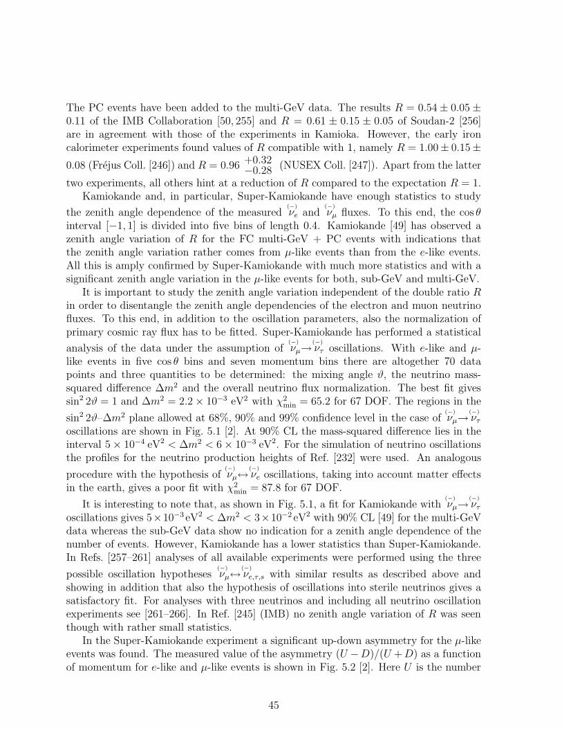
The PC events have been added to the multi-GeV data. The results R = 0.54 ± 0.05 ±0.11 of the IMB Collaboration [50, 255] and R = 0.61 ± 0.15 ± 0.05 of Soudan-2 [256]are in agreement with those of the experiments in Kamioka. However, the early ironcalorimeter experiments found values of R compatible with 1, namely R = 1.00± 0.15±0.08 (Frejus Coll. [246]) and R = 0.96 +0.32

−0.28 (NUSEX Coll. [247]). Apart from the latter

two experiments, all others hint at a reduction of R compared to the expectation R = 1.Kamiokande and, in particular, Super-Kamiokande have enough statistics to study

the zenith angle dependence of the measured(−)

νe and(−)

νµ fluxes. To this end, the cos θinterval [−1, 1] is divided into five bins of length 0.4. Kamiokande [49] has observed azenith angle variation of R for the FC multi-GeV + PC events with indications thatthe zenith angle variation rather comes from µ-like events than from the e-like events.All this is amply confirmed by Super-Kamiokande with much more statistics and with asignificant zenith angle variation in the µ-like events for both, sub-GeV and multi-GeV.

It is important to study the zenith angle variation independent of the double ratio Rin order to disentangle the zenith angle dependencies of the electron and muon neutrinofluxes. To this end, in addition to the oscillation parameters, also the normalization ofprimary cosmic ray flux has to be fitted. Super-Kamiokande has performed a statistical

analysis of the data under the assumption of(−)

νµ→(−)

ντ oscillations. With e-like and µ-like events in five cos θ bins and seven momentum bins there are altogether 70 datapoints and three quantities to be determined: the mixing angle ϑ, the neutrino mass-squared difference ∆m2 and the overall neutrino flux normalization. The best fit givessin2 2ϑ = 1 and ∆m2 = 2.2 × 10−3 eV2 with χ2

min = 65.2 for 67 DOF. The regions in the

sin2 2ϑ–∆m2 plane allowed at 68%, 90% and 99% confidence level in the case of(−)

νµ→(−)

ντoscillations are shown in Fig. 5.1 [2]. At 90% CL the mass-squared difference lies in theinterval 5 × 10−4 eV2 < ∆m2 < 6 × 10−3 eV2. For the simulation of neutrino oscillationsthe profiles for the neutrino production heights of Ref. [232] were used. An analogous

procedure with the hypothesis of(−)

νµ↔(−)

νe oscillations, taking into account matter effectsin the earth, gives a poor fit with χ2

min = 87.8 for 67 DOF.

It is interesting to note that, as shown in Fig. 5.1, a fit for Kamiokande with(−)

νµ→(−)

ντoscillations gives 5×10−3 eV2 < ∆m2 < 3×10−2 eV2 with 90% CL [49] for the multi-GeVdata whereas the sub-GeV data show no indication for a zenith angle dependence of thenumber of events. However, Kamiokande has a lower statistics than Super-Kamiokande.In Refs. [257–261] analyses of all available experiments were performed using the three

possible oscillation hypotheses(−)

νµ↔(−)

νe,τ,s with similar results as described above andshowing in addition that also the hypothesis of oscillations into sterile neutrinos gives asatisfactory fit. For analyses with three neutrinos and including all neutrino oscillationexperiments see [261–266]. In Ref. [245] (IMB) no zenith angle variation of R was seenthough with rather small statistics.

In the Super-Kamiokande experiment a significant up-down asymmetry for the µ-likeevents was found. The measured value of the asymmetry (U −D)/(U +D) as a functionof momentum for e-like and µ-like events is shown in Fig. 5.2 [2]. Here U is the number

45

νµ - ντ

Kamiokande

Super-Kamiokande

68%90%99%

sin22ϑ

∆m2 (

eV2 )

0 0.2 0.4 0.6 0.8 110

-4

10-3

10-2

10-1

1

10-1

1 10 102

-1

-0.5

0

0.5

1

10-1

1 10

-1

-0.5

0

0.5

1

e-like

µ-like

FC PC

(U-D

)/(U

+D

)

Momentum (GeV/c)

Figure 5.1. The 68%, 90% and 99% confidenceregions in the sin2 2ϑ–∆m2 plane for νµ → ντ os-cillations obtained from 33.0 kton year of Super-Kamiokande data [2]. The 90% confidence regionobtained by the Kamiokande experiment is alsoshown.

Figure 5.2. Up-down asymmetry measured in theSuper-Kamiokande atmospheric neutrino experi-ment as a function of the momentum of e-likeand µ-like events [2]. The hatched region showsthe theoretical expectation without neutrino os-cillations, with statistical and systematic errorsadded in quadrature. The dashed line for µ-like events is the theoretical expectation in thecase of two-generation νµ → ντ oscillations with∆m2 = 2.2 × 10−3 eV2 and sin2 2ϑ = 1.0.

of upward-going events with zenith angles in the range −1 < cos θ < −0.2 and D thenumber of downward-going events with 0.2 < cos θ < 1. The value of the asymmetry forFC and PC multi-GeV µ-like events is [2]

Aµ ≡(

U −D

U +D

)

µ

= −0.296 ± 0.048 ± 0.01 . (5.10)

The geomagnetic effect which is one of the causes of an up-down asymmetry contributesless than ±0.01 for multi-GeV events [2]. For the PC events with a mean neutrino energyof 15 GeV [2] this effect is even less important. Note that for multi-GeV events theaverage angle between the incoming neutrino direction and the charged lepton seen inthe single-ring events is of the order of 20◦ or less. Since cos θ = ±0.2 corresponds to90◦ ± 11.5◦, the asymmetry A of the µ-like events is in effect an up-down asymmetry

of the(−)

νµ flux. The result (5.10) constitutes the best indication in favour of neutrinooscillations found so far with Aµ being 6 standard deviations away from 0. This iscorroborated by the plots of Ae,µ(p) as a function of the lepton momentum p in the caseof the single-ring events shown in Fig. 5.2 [2]. For e-like events, Ae(p) is a flat function

consistent with no(−)

νe↔(−)

νµ oscillations. The asymmetry for e-like events analogous toEq.(5.10) is compatible with zero: Ae = −0.036 ± 0.067 ± 0.02. For the µ-like events,Aµ(p) starts with zero and decreases, thus indicating that at small energies both up and

down-going neutrinos oscillate with averaged(−)

νµ→(−)

νµ probabilities 1/2 whereas at muon

46

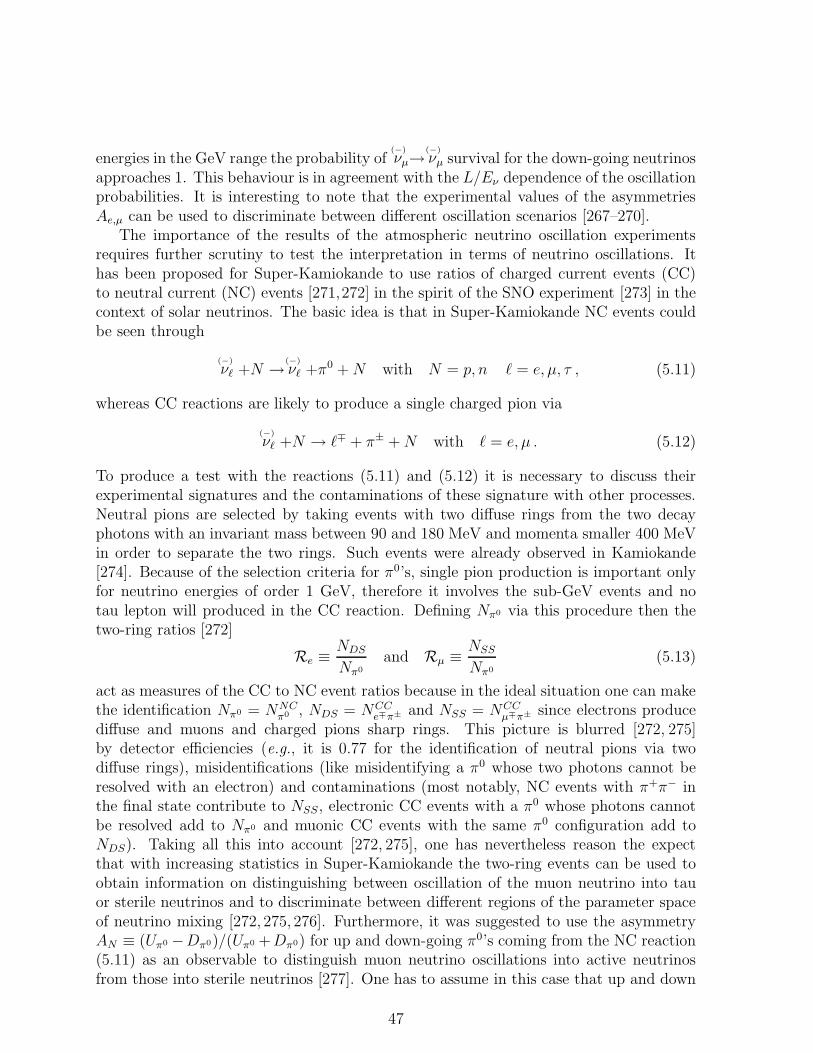
energies in the GeV range the probability of(−)

νµ→(−)

νµ survival for the down-going neutrinosapproaches 1. This behaviour is in agreement with the L/Eν dependence of the oscillationprobabilities. It is interesting to note that the experimental values of the asymmetriesAe,µ can be used to discriminate between different oscillation scenarios [267–270].

The importance of the results of the atmospheric neutrino oscillation experimentsrequires further scrutiny to test the interpretation in terms of neutrino oscillations. Ithas been proposed for Super-Kamiokande to use ratios of charged current events (CC)to neutral current (NC) events [271,272] in the spirit of the SNO experiment [273] in thecontext of solar neutrinos. The basic idea is that in Super-Kamiokande NC events couldbe seen through

(−)

νℓ +N →(−)

νℓ +π0 +N with N = p, n ℓ = e, µ, τ , (5.11)

whereas CC reactions are likely to produce a single charged pion via

(−)

νℓ +N → ℓ∓ + π± +N with ℓ = e, µ . (5.12)

To produce a test with the reactions (5.11) and (5.12) it is necessary to discuss theirexperimental signatures and the contaminations of these signature with other processes.Neutral pions are selected by taking events with two diffuse rings from the two decayphotons with an invariant mass between 90 and 180 MeV and momenta smaller 400 MeVin order to separate the two rings. Such events were already observed in Kamiokande[274]. Because of the selection criteria for π0’s, single pion production is important onlyfor neutrino energies of order 1 GeV, therefore it involves the sub-GeV events and notau lepton will produced in the CC reaction. Defining Nπ0 via this procedure then thetwo-ring ratios [272]

Re ≡NDS

Nπ0

and Rµ ≡ NSS

Nπ0

(5.13)

act as measures of the CC to NC event ratios because in the ideal situation one can makethe identification Nπ0 = NNC

π0 , NDS = NCCe∓π± and NSS = NCC

µ∓π± since electrons producediffuse and muons and charged pions sharp rings. This picture is blurred [272, 275]by detector efficiencies (e.g., it is 0.77 for the identification of neutral pions via twodiffuse rings), misidentifications (like misidentifying a π0 whose two photons cannot beresolved with an electron) and contaminations (most notably, NC events with π+π− inthe final state contribute to NSS, electronic CC events with a π0 whose photons cannotbe resolved add to Nπ0 and muonic CC events with the same π0 configuration add toNDS). Taking all this into account [272, 275], one has nevertheless reason the expectthat with increasing statistics in Super-Kamiokande the two-ring events can be used toobtain information on distinguishing between oscillation of the muon neutrino into tauor sterile neutrinos and to discriminate between different regions of the parameter spaceof neutrino mixing [272, 275, 276]. Furthermore, it was suggested to use the asymmetryAN ≡ (Uπ0 −Dπ0)/(Uπ0 +Dπ0) for up and down-going π0’s coming from the NC reaction(5.11) as an observable to distinguish muon neutrino oscillations into active neutrinosfrom those into sterile neutrinos [277]. One has to assume in this case that up and down

47

π0’s originate from up and down neutrinos, respectively, with high probability. This isnot so obvious, however, since for the identification of the π0 the events should ratherhave low energy as explained above.

The further tests discussed here concern the stopping and through-going muon eventswhere special efforts have been made to calculate the fluxes [249, 253,278]. Whereas theFC events have neutrino energies of around 1 GeV the stopping muon events correspondto a mean neutrino energy of 10 GeV and the through-going muons to 100 GeV [231,249].Thus we are now discussing a different range of energy compared to the discussion above(with the exception of the PC sample).

Obviously, also the zenith angle distribution of upward stopping or through-goingmuons can be used to test the neutrino oscillation hypothesis [279]. Among other exper-iments (see above) upward through-going muons have been studied by Kamiokande [252]and upward muons by MACRO [52]. Kamiokande has 372 such events above an energy

threshold of 1.6 GeV. Fitting the data to the(−)

νµ→(−)

ντ oscillation hypothesis yields a bestfit with ∆m2 = 3.2 × 10−3 eV2 agreeing rather well with the Super-Kamiokande result.The analysis of the MACRO Coll. based on 479 events gives a similar result for ∆m2,however, the zenith angle distribution does not fit very well with the oscillation hypothe-sis into tau neutrinos. An attempt has been made to explain the zenith angle distribution

of the MACRO experiment with(−)

νµ→(−)

νs oscillations where matter effects in the earthplay a crucial role [280].

In the earth, the density profile can approximately be represented by constant densitiesin the mantle and the core, respectively (see end of Section 4.3). Such a profile can leadto an enhancement of neutrino transitions due to the matter effect17 in the earth ifatmospheric neutrinos cross the core18 such that the phase picked up by a neutrino wavefunction traversing the mantle for the first time and the phase acquired by traversing thecore are each approximately equal to π. Such an effect for atmospheric neutrinos wasrecently considered in detail in Refs. [280,282–285]. It has also been proposed to exploit

this effect to discriminate between(−)

νµ→(−)

ντ (no matter effects) and(−)

νµ→(−)

νs transitions ofatmospheric neutrinos [280] and to explain an excess of e-like events [286] possibly seenin the Super-Kamiokande experiment [2].

It was suggested in Ref. [244] to use the observable

r =Nstop

Nthru(5.14)

where Nstop and Nthru are the numbers of stopping and though-going muons, respec-tively, as an indicator for neutrino oscillations because this ratio is reduced for neutrinooscillations with respect to the no-oscillation hypothesis [253, 287]. Also the ratios of“horizontal” to “vertical” muon events for stopping and through-going muons defined by

Sstop,thru ≡ Nhor

Nvert

∣

∣

∣

∣

stop,thru

, (5.15)

17Note that for the case of a periodical matter density the effect of enhancement was considered inRefs. [281].

18Neutrinos with cos θ ≤ −0.837

48

with

Nhor =

∫ 0

cos θc

d cos θdN

d cos θand Nvert =

∫ cos θc

−1

d cos θdN

d cos θ(5.16)

are useful observables as shown in Ref. [287]. In this work a study was made for Super-Kamiokande, taking cos θc = −0.5 as the boundary between “horizontal” and “vertical”,showing that the prospects are good for confirming atmospheric neutrino oscillationsfound with the FC single-ring and PC events by using stopping and through-going muonsand the observables r (5.14), Sstop and Sthru (5.15). However, for a precise determinationof ∆m2 these variables are not suitable.

5.1.4 Long-baseline experiments and tests of the atmospheric neutrino os-

cillation parameters

The explanation of the atmospheric neutrino anomaly in terms of neutrino oscillations canbe checked with long-baseline neutrino oscillation experiments. The first long-baselinereactor experiment CHOOZ [159] (see Section 3.2 and Fig. 3.3) has already excludedatmospheric νµ ⇆ νe oscillations with a large mixing angle for ∆m2

atm & 10−3 eV2. Twoother long-baseline reactor experiments are under construction: Palo Verde [288, 289]and Kam-Land [290, 291]. The Palo Verde experiment has a setup and a sensitivitysimilar to the CHOOZ experiment, whereas the Kam-Land experiment, which is theresult of the conversion of the old Kamiokande detector to a liquid scintillator detector,will detect νe’s produced by Japanese reactors 150–200 km away and will be sensitive to∆m2 & 10−5 eV2 and a large mixing angle. The Borexino experiment (see the end of theSection 5.2 and [291,292]) will allow to perform a similar measurement.

Accelerator long-baseline experiments will study the oscillation channels νµ → νe,µ,τ .The K2K [271] experiment, with a baseline of about 235 km from KEK to Super-Kamiokande and a neutrino beam with 1.4 GeV average energy, will be sensitive to νµdisappearance and νµ → νe transitions with ∆m2 & 2 × 10−3 eV2. A near 1 kton water-Cherenkov detector will be placed at a distance of about 1 km from the beam dump andwill allow to measure the initial flux and energy spectrum of νµ’s. This experiment isunder construction and is planned to begin taking data in the year 1999.

Also the MINOS [293] experiment is under construction. This experiment will have anear detector at Fermilab and a baseline of about 730 km from Fermilab to the Soudanmine, where the far detector will be placed. The neutrino beam will be produced byprotons from the new Main Injector at Fermilab and will have an average energy ofabout 10 GeV. The far detector is an 8 kton sampling calorimeter made of magnetizediron and scintillators. This experiment will be sensitive to νµ disappearance and νµ → νe,νµ → ντ , νµ → νs transitions, with the possibility to distinguish the different channels, for∆m2 & 10−3 eV2 (the possibility to extend the sensitivity to ∆m2 & 5×10−5 eV2 loweringthe neutrino energy is under study). In particular νµ → νs transitions can be revealedthrough the measurement of a deficit in the NC/CC ratio. The MINOS experiment isscheduled to start data-taking around the year 2003.

The ICARUS experiment [294] in Gran Sasso, constituted of a 0.6 kton liquid argondetector is scheduled to start in the year 2000. In the future three new modules with a

49

total mass of 2.4 kton will be installed. This detector will be sensitive to atmospheric andsolar neutrinos and will allow to reveal long-baseline νµ → ντ oscillations using a neutrinobeam produced at CERN about 730 km away. Since the average energy of the neutrinobeam is rather high, about 25 GeV, in order to allow the detection of ντ through theCC production of a τ , this experiment will be sensitive to ∆m2 & 10−3 eV2. Four otherdetectors for future LBL CERN–Gran Sasso experiments, OPERA [295], NOE [296],AQUA-RICH [297] and NICE [298], have been proposed and are under consideration(see Ref. [299]), together with the possibility of a new atmospheric neutrino detectorconsisting of a large-mass and high-density tracking calorimeter [300].

In Ref. [301] a comparison is made between the possibilities using atmospheric neu-trinos and LBL neutrino experiments for the determination of the oscillation parameters.The feasibility to distinguish between atmospheric νµ → ντ and νµ → νs oscillationsusing a combination of the results of future atmospheric, LBL and SBL experiments isdiscussed in Ref. [302].

5.2 Solar neutrino experiments

The earliest indication in favour of neutrino oscillations was obtained about 30 yearsago in the radiochemical solar neutrino experiment by R. Davies et al. [36]. The fluxof solar electron neutrinos measured in this experiment was significantly less than thepredicted one. This phenomenon was called solar neutrino problem. The existence ofthis problem was confirmed in all five solar neutrino experiments (Homestake [36–38],Kamiokande [39–41], GALLEX [42, 43], SAGE [44, 45] and Super-Kamiokande [46–48])which measure a flux of electron neutrinos significantly smaller than the one predicted bythe Standard Solar Model (SSM) [60,174,175,303–310]. The solar neutrino problem (see,for example, [60, 311–316]) arose in the Homestake experiment by the low counting rateshowing that the flux of the high-energy 8B neutrinos (E8B . 15 MeV) and of the medium-energy 7Be neutrinos (E7Be = 0.862 MeV) is suppressed by a factor of about 1/3 withrespect to the SSM prediction. In 1988 the solar neutrino problem was confirmed by theresults of the real-time water-Cherenkov Kamiokande experiment [39] which measured aflux of 8B neutrinos of about half of the SSM flux. The measurements of the Kamiokandeexperiment proved that the observed neutrinos arrive at the detector from the direction ofthe sun. In 1992 the radiochemical GALLEX [42] and SAGE experiments [45] succeededin measuring the neutrino flux with a low energy threshold Eth = 233 keV, which allowedto detect low-energy pp neutrinos produced by the fundamental reaction of the pp cycle.Also these experiments measured a neutrino flux of about half of the one predicted bythe SSM. Finally, the Super-Kamiokande experiment has recently confirmed [46–48] withhigh statistics the suppression of the 8B neutrino flux with respect to the SSM one by afactor of about 1/2.

The energy of the sun is produced in the reactions of the thermonuclear pp and CNOcycles shown in Figs. 5.3 and 5.4 (see, e.g., Ref. [60]). The overall result of both cycles isthe transition

4 p+ 2 e− → 4He + 2 νe +Q , (5.17)

50

(pp) p+ p! 2H+ e+ + �e99.6% XXXXXXXXXXXX (pep)p+ e� + p! 2H+ �e0.4%������������?2H+ p! 3He+ ������������������85%?3He+ 3He! 4He + 2 p XXXXXXXXXXXXXXXXXX 2� 10�5%?3He+ p! 4He+ e+ + �e(hep)?15%3He+ 4He! 7Be + ���������99.87% ?7Be + e� ! 7Li + �e(7Be) ?7Li + p! 2 4He PPPPPPPPP 0.13%?7Be + p! 8B + ?8B! 8Be� + e+ + �e (8B)?8Be� ! 2 4He12C + p! 13N+ - 13N! 13C + e+ + �e (13N)?12C + p! 14N+ ?14N+ p! 15O+ �15O! 15N+ e+ + �e(15O) 615N+ p! 12C + 4He6

?15N+ p! 16O+ ?16O+ p! 17F + - 17F! 17O+ e+ + �e (17F)617O+ p! 14N+ 4He699:9%0:1%Figure 5.3. The pp cycle. Figure 5.4. The CNO cycle.

51

Source r ReactionAverage Neutrino

Energy 〈E〉r (MeV)Maximum Neutrino

Energy (MeV)

pp p+ p→ d+ e+ + νe 0.2668 0.423 ± 0.03

pep p+ e− + p→ d+ νe 1.445 1.445

7Be e− + 7Be → 7Li + νe0.38550.8631

0.38550.8631

8B 8B → 8Be∗ + e+ + νe 6.735 ± 0.036 ∼ 15

hep 3He + p→ 4He + e+ + νe 9.628 18.778

13N 13N → 13C + e+ + νe 0.7063 1.1982 ± 0.0003

15O 15O → 15N + e+ + νe 0.9964 1.7317 ± 0.0005

17F 17F → 17O + e+ + νe 0.9977 1.7364 ± 0.0003

Table 5.1. Sources of solar neutrinos [317–319].

where Q = 4mp+2me−m4He = 26.73 MeV is the energy release.19 Hence, the production

of energy in the sun is accompanied by the emission of electron neutrinos. The main partof the solar energy is radiated through photons and a small part (about 2%) is emittedthrough neutrinos. The sources of solar neutrinos are listed in Table 5.1. The pp, pep,7Be, 8B and hep reactions belong to the pp cycle (see Fig. 5.3), whereas the 13N, 15Oand 17F reactions belong to the CNO cycle (see Fig. 5.4), which produces only about2% of the solar energy. The average and maximum neutrino energies listed in Table 5.1are taken from Refs. [317, 318]. The neutrino fluxes and predictions for the neutrinocapture rates in the chlorine Homestake experiment and in the gallium GALLEX andSAGE experiments given by the Bahcall-Pinsonneault 1998 (BP98) [304] SSM are listedin Table 5.2.

As it is seen from the Tables 5.1 and 5.2, the major part of solar neutrinos are lowenergy neutrinos coming from the pp reaction. Monoenergetic neutrinos with intermediateenergy are produced in the capture of electrons by 7Be and in the pep reaction. Highenergy neutrinos are produced in the decay of 8B (the flux of hep neutrinos is so small thatits contribution to the event rates of solar neutrino experiments is negligible). The fluxof 8B neutrinos is much smaller than the fluxes of pp, 7Be and pep neutrinos. However,as we will see later, these neutrinos give the major contribution to the event rates ofexperiments with a high energy detection threshold. The CNO 13N, 15O, 17F reactionsare sources of intermediate energy neutrinos with a spectrum that extends up to about1.7 MeV. Their contribution to the event rates of solar neutrino experiment is small butnot negligible.

19Here mp = 938.272 MeV is the proton mass, me = 0.511 MeV is the electron mass and m4He =2mp + 2mn − EB

4He is the mass of the 4He-nucleus, where mn = 939.566 MeV is the neutron mass andEB

4He= 28.296 MeV is the binding energy of the 4He-nucleus.

52

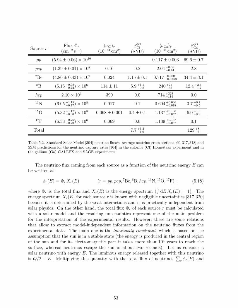
Source rFlux Φr

(cm−2 s−1)〈σCl〉r

(10−44 cm2)S

(r)Cl

(SNU)

〈σGa〉r(10−44 cm2)

S(r)Ga

(SNU)

pp (5.94 ± 0.06) × 1010 – – 0.117 ± 0.003 69.6 ± 0.7

pep (1.39 ± 0.01) × 108 0.16 0.2 2.04 +0.35−0.14 2.8

7Be (4.80 ± 0.43) × 109 0.024 1.15 ± 0.1 0.717 +0.050−0.0.021 34.4 ± 3.1

8B (5.15 +0.98−0.72) × 106 114 ± 11 5.9 +1.1

−0.8 240 +77−36 12.4 +2.4

−1.7

hep 2.10 × 103 390 0.0 714 +228−114 0.0

13N (6.05 +1.15−0.77) × 108 0.017 0.1 0.604 +0.036

−0.018 3.7 +0.7−0.5

15O (5.32 +1.17−0.80) × 108 0.068 ± 0.001 0.4 ± 0.1 1.137 +0.136

−0.057 6.0 +1.3−0.9

17F (6.33 +0.76−0.70) × 106 0.069 0.0 1.139 +0.137

−0.057 0.1

Total 7.7 +1.2−1.0 129 +8

−6

Table 5.2. Standard Solar Model [304] neutrino fluxes, average neutrino cross sections [60, 317,318] andSSM predictions for the neutrino capture rates [304] in the chlorine (Cl) Homestake experiment and inthe gallium (Ga) GALLEX and SAGE experiments.

The neutrino flux coming from each source as a function of the neutrino energy E canbe written as

φr(E) = ΦrXr(E) (r = pp, pep, 7Be, 8B, hep, 13N, 15O, 17F) , (5.18)

where Φr is the total flux and Xr(E) is the energy spectrum (∫

dEXr(E) = 1). Theenergy spectrum Xr(E) for each source r is known with negligible uncertainties [317,320]because it is determined by the weak interactions and it is practically independent fromsolar physics. On the other hand, the total flux Φr of each source r must be calculatedwith a solar model and the resulting uncertainties represent one of the main problemfor the interpretation of the experimental results. However, there are some relationsthat allow to extract model-independent information on the neutrino fluxes from theexperimental data. The main one is the luminosity constraint, which is based on theassumption that the sun is in a stable state (the energy is produced in the central regionof the sun and for its electromagnetic part it takes more than 104 years to reach thesurface, whereas neutrinos escape the sun in about two seconds). Let us consider asolar neutrino with energy E. The luminous energy released together with this neutrinois Q/2 − E. Multiplying this quantity with the total flux of neutrinos

∑

r φr(E) and

53

integrating over the neutrino energy one obtains the luminosity constraint20

∑

r

(

Q

2− 〈E〉r

)

Φr =L⊙

4πR2, (5.19)

where 〈E〉r =∫

EXr(E) dE is the average energy of the neutrinos from the source r (seeTable 5.1), L⊙ = 2.40×1039 MeV s−1 [35] is the luminosity of the sun, R = 1.496×1013 cm[35] is the sun – earth distance. The luminosity constraint can be rewritten in the compactform

∑

r

Qr Φr = K⊙ , (5.20)

where Qr ≡ Q/2 − 〈E〉r and K⊙ ≡ L⊙/4πR2 = 8.54 × 1011 MeV cm−2 s−1 is the solar

constant. Let us emphasize that the luminosity relation is valid under the assumptionthat solar νe’s on their way to the earth do not transform into other states. Neglectingthe small fraction of energy carried away by neutrinos, the luminosity constraint givesthe approximate value of the total solar neutrino flux Φ =

∑

r Φr:

Φ ≃ 2K⊙

Q= 6.4 × 1010 cm−2 s−1 . (5.21)

Since the 3He nuclei necessary for the formation of 7Be and 8B are created by thepp or pep reactions, there is another model-independent constraint for the solar neutrinofluxes of the pp cycle (see [321]):

φ7Be + φ8B ≤ φpp + φpep . (5.22)

Let us now consider the experimental data. The results of five solar neutrino experi-

ments are available at present and are listed in Table 5.3.Homestake [36–38], GALLEX [42, 43] and SAGE [44, 45] are radiochemical exper-

iments. In the pioneering chlorine Homestake experiment of R. Davis et. al., whichstarted in 1967, the detector is a tank with a volume of 6 × 105 liters filled with C2Cl4.Radioactive atoms of 37Ar are produced by solar electron neutrinos through the reac-tion [324,325]

νe + 37Cl → e− + 37Ar , (5.23)

which has an energy threshold Eth = 0.81 MeV. The radioactive 37Ar atoms that arecreated during the time of exposition of each run (about two months) are extracted fromthe detector by purging it with 4He and counted in small proportional counters whichdetect the Auger electron produced in the electron-capture of the 37Ar nuclei. About 0.5atoms of 37Ar are produced every day by solar neutrinos and about 16 atoms are extractedin each run (this number is smaller than 30 because of the 37Ar lifetime of about 35 daysand because of the extraction efficiency of about 90%). Since the energy threshold is

20The corrections to this relation due to the generation of gravitational energy [174] and due to thefact that the abundance of 3He nuclei is out of equilibrium in the outer regions of the solar core [321]are estimated to be less than 1% and thus negligible at the present level of accuracy.

54

Experiment Result Theory ResultTheory

Homestake [38]2.56 ± 0.16 ± 0.16

(2.56 ± 0.23)7.7 +1.2

−1.0 0.33 +0.06−0.05

GALLEX [322]77.5 ± 6.2 +4.3

−4.7

(78 ± 8)129 +8

−6 0.60 ± 0.07

SAGE [323]66.6 +6.8

−7.1+3.8−4.0

(67 ± 8)129 +8

−6 0.52 ± 0.07

Kamiokande [41]2.80 ± 0.19 ± 0.33

(2.80 ± 0.38)5.15 +1.0

−0.7 0.54 ± 0.07

Super-Kamiokande [48] 2.44 ± 0.05 +0.09−0.07

(2.44 +0.10−0.09)

5.15 +1.0−0.7 0.47 +0.07

−0.09

Table 5.3. The results of solar neutrino experiments confronted with the corresponding theoreticalpredictions [304]. The results of the Homestake, GALLEX and SAGE experiments are expressed in termsof event rates in SNU units (1SNU ≡ 10−36eventsatom−1 s−1), whereas the results of the Kamiokande andSuper-Kamiokande experiments are expressed in terms of the 8B neutrino flux in units of 106 cm−2s−1.The first experimental error is statistical and the second is systematic. The experimental values inparenthesis have the statistical and systematic errors added in quadrature.

above the end-point of the pp neutrino spectrum and the cross section of the detectingprocess (5.23) grows with the neutrino energy, the main contribution to the counting ratein the Homestake experiment comes from 8B and 7Be neutrinos. According to the BP98SSM [304] the event rate in the Homestake experiment should be21 7.7 +1.2

−1.0 SNU, of which5.9 SNU come from 8B neutrinos, 1.15 SNU are produced by 7Be neutrinos and 0.7 SNUare due to pep and CNO neutrinos (see Table 5.2). The Homestake event rate presentedin Table 5.3 is the event rate averaged over 108 runs [38].

In the radiochemical gallium experiments GALLEX and SAGE electron neutrinosfrom the sun are detected through the observation of radioactive 71Ge that is producedin the process

νe + 71Ga → e− + 71Ge . (5.24)

The GALLEX detector is a tank containing 30.3 tons of 71Ga (100 tons of a water solutionof gallium chloride), whereas the SAGE experiment uses about 57 tons of 71Ga in metallicform. The event rate measured in the GALLEX experiment is 0.699 ± 0.069 events perday. (Since the 71Ge lifetime is about 16.5 days, only around 7 atoms of 71Ge are extractedin each 3-weeks run.)

Since the threshold of the process (5.24) is E71Gath = 0.233 MeV, neutrinos from all

sources are detected in gallium experiments. According to the SSM, the contributionsto the total predicted event rate from pp, 7Be and 8B neutrinos are [304] 54%, 27% and10%, respectively.

As can be seen from Table 5.3, both gallium detectors measure an event rate that is

21One Solar Neutrino Unit (SNU) is defined as 10−36 events atom−1 s−1.

55

about one half of the SSM prediction. The weighted average of the GALLEX and SAGEresults yields the event rate

SexpGa = 72.5 ± 6 SNU . (5.25)

Taking into account the experimental and theoretical errors, this rate differs from theSSM prediction by about seven standard deviations!

Both the GALLEX and SAGE detectors have been calibrated using an intense 51Crneutrino source. The ratio of observed and expected events is 0.93 ± 0.08 for GALLEX[326] and 0.95±0.12 for SAGE [45]. These results demonstrate the absence of unexpectedsystematic errors at the 10% level in both experiments. In addition, the GALLEX Col-laboration calibrated the detector by introducing a known number of radioactive 71Asatoms in the target solution [326,327]. The atoms of 71Ge resulting from 71As decay havebeen extracted in the usual way, and the As tests prove, at the 1% level, the reliabilityof the technique [328] (the number of 71Ge atoms produced in these tests is of the orderof 105, whereas the number produced in the 51Cr tests is of the order of ten per day). Asemphasized by the GALLEX Collaboration [326,327], these results rule out the presenceof unexpected radiochemical effects that could explain the deficit of solar νe’s measuredby the gallium experiments.

It is necessary to emphasize that the gallium experiments are not only very importantfor the assessment of the solar neutrino problem but also for the theory of thermonuclearenergy production in the sun: They have provided the first observation of low-energy

solar neutrinos produced in the pp reaction that is the basic reaction of the pp cycle and,

therefore, the first direct experimental confirmation of the theory of thermonuclear origin

of solar energy production.

In the Kamiokande [39–41] and Super-Kamiokande [46–48] experiments water-Cherenkov detectors are used for the detection of solar neutrinos through the observationof the Cherenkov light emitted by the recoil electrons in the elastic-scattering process

ν + e− → ν + e− . (5.26)

Since the direction of the recoil electron is peaked in the direction of the incoming neu-trino, water-Cherenkov detectors measure the direction of the neutrino flux and the resultsof Kamiokande and Super-Kamiokande have proven that there is a flux of high-energyneutrinos coming from the sun with an intensity about half of that predicted by the SSM.

The energy threshold of water-Cherenkov detectors is given by the threshold for thedetection of the recoil electron in the reaction (5.26). It is higher than in other solarneutrino experiments because of the large background at low energies: EKam

th ≃ 7 MeV inthe Kamiokande experiment and ESK

th ≃ 6.5 MeV in the Super-Kamiokande experiment.Therefore, only 8B neutrinos can be detected in water-Cherenkov experiments. If nothinghappens to electron neutrinos during their trip from the core of the sun to the earth (i.e.,no neutrino oscillations or other transitions), the results of the Kamiokande and Super-Kamiokande experiments provide a measurement of the total flux Φ8B of 8B neutrinos.Therefore, the results of the Kamiokande and Super-Kamiokande experiments are usuallypresented in terms of the measured flux of 8B neutrinos. In the Super-Kamiokande

56

experiment it was found

ΦSK8B = (2.44 +0.10

−0.09) × 106 cm−2 s−1 , (5.27)

which is about one half of the flux predicted by the SSM (see Table 5.3).22

From the experimental results and the most updated theoretical predictions [304]listed in Table 5.3 one can see that the observed event rates in all solar neutrino ex-periments are significantly smaller than the predicted rates (see also [329] where thecomparison with other theoretical predictions is discussed). This discrepancy constitutesthe solar neutrino problem. The SSM is robust and it has been recently tested in a con-vincing way by comparing its predicted value for the sound speed in the interior of thesun with precise helioseismological measurements (see [304, 315, 330–333]). However, itis clear that a model-independent proof of the existence of the solar neutrino problemwould be more convincing. Such a model-independent approach has been discussed inseveral papers [308, 312, 321, 329, 334–343] using the model-independent luminosity con-straint (5.20) and the fact that the energy spectraXr(E) Eq.(5.18) of the various neutrinosources are practically independent from solar physics [317, 320].

From the luminosity constraint it is possible to obtain a model-independent lowerbound on the gallium event rate. Indeed, since pp neutrinos have the smallest averageenergy and the νe–

71Ga cross section σGa(E) increases with the neutrino energy E, wehave

SGa =

∫

σGa(E)∑

r

φr(E) dE =∑

r

〈σGa〉r Φr ≥ 〈σGa〉ppΦ , (5.28)

where 〈σGa〉r =∫

σGa(E)Xr(E) dE is the average cross section of neutrinos from thesource r (see Table 5.2). Since the luminosity constraint (5.20) implies that

Qpp Φ ≥ K⊙ , (5.29)

we obtain

SGa ≥〈σGa〉ppK⊙

Qpp= 76 ± 2 SNU , (5.30)

where we used the value of 〈σGa〉pp = 11.7 × 10−46 cm2 given in Table 5.2 and Qpp =13.1 MeV.

The lower bound (5.30) is just compatible with the combined result (5.25) of thegallium experiments. This means that the results of the GALLEX and SAGE experimentscan be explained if practically only pp neutrinos are emitted by the sun. This possibilityis incompatible with any solar model constrained by the helioseismological data [304,315].

More stringent model-independent conclusions on the existence of the solar neutrinoproblem can be obtained by comparing the results of different solar neutrino experiments.If the survival probability of solar νe’s is equal to one, the result of the Super-Kamiokandeexperiment gives the value (5.27) for the flux of 8B neutrinos, whose contributions to the

22For recent Super-Kamiokande results on solar neutrinos see Note added.

57

event rates of the chlorine and gallium experiments are

S8B,SKCl = 〈σCl〉8B ΦSK

8B = 2.78 ± 0.27 SNU , (5.31)

S8B,SKGa = 〈σGa〉8B ΦSK

8B = 5.9 +1.9−0.9 SNU . (5.32)

Subtracting the contribution (5.31) of 8B νe’s from the event rate measured in theHomestake experiment (see Table 5.3), one obtains

SexpCl − S

8B,SKCl = −0.22 ± 0.35 . (5.33)

Since the quantity SCl − S8BCl represents the contribution to the chlorine event rate due

to pep, 7Be, hep and CNO neutrinos, it must be positive (or zero) but the result inEq.(5.33) is only marginally compatible with a positive value (the probability is less than26%). Furthermore, the result Eq.(5.33) shows that the fluxes of intermediate energyneutrinos (pep, 7Be and CNO neutrinos) are strongly suppressed with respect to theSSM prediction (see Table 5.2). This is incompatible with any solar model constrainedby the helioseismological data [304, 315] and with the fact that, since both the reactionsthat produce 7Be and 8B neutrinos originate from 7Be nuclei (see Fig. 5.3), it is verydifficult to have a suppression of the 7Be neutrino flux (with respect to the SSM value)that is stronger than the suppression of the 8B neutrino flux.23

Let us consider now the gallium experiments. Subtracting the contribution of 8Bneutrinos from the luminosity constraint (5.20), we have

K⊙ −Q8B Φ8B =∑

r 6=8B

Qr Φr ≤ Qpp

∑

r 6=8B

Φr . (5.34)

Hence, following the same reasoning as in Eq.(5.28) we obtain

SminGa = S

8B,SKGa + 〈σGa〉pp

K⊙ −Q8B ΦSK8B

Qpp

= 82 +3−2 SNU , (5.35)

and the contribution of pep, 7Be, hep and CNO neutrinos to the gallium event rate cannotbe bigger than

SexpGa − Smin

Ga = −9.5 ± 6 . (5.36)

This result is compatible with a positive value with a probability smaller than 6%. Again,the result (5.36) implies that the fluxes of intermediate energy neutrinos (pep, 7Be andCNO neutrinos) are strongly suppressed with respect to the SSM prediction, in contra-diction with any solar model constrained by the helioseismological data and with themoderate suppression of the 8B neutrino flux.

Further model-independent methods for proving the existence of the solar neutrinoproblem on the basis of the data of solar neutrino experiments are nicely discussed in

23Non-standard solar models with low central temperature yield a suppression of the 8B neutrino fluxthat is stronger than that of the 7Be neutrino flux (see [312] and references therein).

58

sin2 2#�m2 (eV2 )

sin2 2#�m2 (eV2 )

Figure 5.5. MSW νe → νµ or νe → ντ transitions:result of the fit of the experimental event rateslisted in Table 5.3. The shadowed regions areallowed at 99% CL [329]. The dots indicate thebest-fit points in each allowed region.

Figure 5.6. Vacuum νe → νµ or νe → ντ oscilla-tions: result of the fit of the experimental eventrates listed in Table 5.3. The shadowed regionsare allowed at 99% CL [329]. The dot indicatesthe best-fit point.

Ref. [312]. In the following we will assume that there is a solar neutrino problem that iscaused by neutrino oscillations.

The solar neutrino data have been analysed in many papers under the assumption oftwo-neutrino mixing (see [329,342,344] and references therein) and in a few papers underthe assumption of three-neutrino mixing (see [345–348] and references therein). Here wewill briefly review the results of the most updated two-generation analysis [329] of allthe solar neutrino data, including those obtained in the first 504 days of operation of theSuper-Kamiokande experiment (see Table 5.3).

The deficit of solar νe’s can be explained in terms of two-generation neutrino mixingeither through vacuum oscillations or through MSW resonant transitions in matter [163,164]. Furthermore, the two mixed neutrinos can be the electron neutrino and anotheractive (νµ or ντ ) neutrino or the electron neutrino and a sterile neutrino. There are twodifferences between transitions of solar νe’s into active and sterile neutrinos:

1. The probability of MSW transitions is different in the two cases, because sterile neu-trinos do not have the weak-interaction potential due to elastic forward scattering thatis present for active neutrinos.

2. The active neutrinos (νµ’s or ντ ’s) that are produced by the oscillation mechanism(either in vacuum or in matter) contribute to the event rates measured in the Kamio-kande and Super-Kamiokande water-Cherenkov experiments (notice, however, that thecross section of νµ–e

− and ντ–e− scattering is about six times smaller than the νe–e

−

cross section).

The formulas for the survival probability of solar νe’s in the case of vacuum oscillations

59

and MSW transitions are given in Eq.(3.21) (with α = e) and in Eq.(4.41) together withEq.(4.47) [193], respectively. These formulas depend on the two mixing parameters ∆m2

and sin2 2ϑ. The allowed regions in the sin2 2ϑ–∆m2 plane, obtained in Ref. [329] fromthe fit of the measured event rates listed in Table 5.3 by using the BP98 SSM [304] andthe analytic formulas in Ref. [193] for the MSW case, are shown in Figs. 5.5–5.6.

Figure 5.5 [329] shows the three allowed regions in the case of MSW νe → νµ orνe → ντ transitions. They are the small mixing angle (SMA-active) region at

∆m2 ≃ 5 × 10−6 eV2 , sin2 2ϑ ≃ 6 × 10−3 (SMA-active) , (5.37)

and the large mixing angle (LMA) region at

∆m2 ≃ 2 × 10−5 eV2 , sin2 2ϑ ≃ 0.76 (LMA) . (5.38)

The best fit, with a confidence level of 19%, is obtained in the SMA region, whereas theLMA region has a confidence level of 4%. In Ref. [329] there is also the so-called lowmass (LOW) region at ∆m2 ≃ 8×10−8 eV2 and sin2 2ϑ ≃ 0.96, however, the LOW regionis only marginally acceptable, with a confidence level of 0.7%.

The allowed regions in the sin2 2ϑ–∆m2 plane in the case of νe → νµ or νe → ντvacuum oscillations are shown in Fig. 5.5 [329]. These regions extend over large rangesof sin2 2ϑ and ∆m2 around the best fit values

∆m2 ≃ 8 × 10−11 eV2 , sin2 2ϑ ≃ 0.75 (Vac. Osc.) . (5.39)

The confidence level of the fit is 3.8%. There is no allowed region in the case of νe → νsvacuum oscillations (the fit has a confidence level of 0.05%) [329,349].

As shown in Fig. 5.7 [329], only the small mixing angle (SMA-sterile) region at

∆m2 ≃ 4 × 10−6 eV2 , sin2 2ϑ ≃ 7 × 10−3 (SMA-sterile) , (5.40)

is allowed in the case of MSW νe → νs transitions, with a confidence level of 19% (thelarge mixing angle and low mass solutions have a confidence level of 0.001% and 0.003%,respectively) [329, 350].

The authors of Ref. [329] performed also global fits of the solar neutrino data includingthe energy spectrum and zenith-angle distribution of the recoil electrons measured inthe Super-Kamiokande experiment [48]. As noted in Ref. [329], since these data are stillpreliminary, the results of this analysis are less robust than those obtained fitting only theglobal rates. However, it is interesting to note that in the case of MSW νe → νµ or νe → ντtransitions only the SMA-active region remains allowed, as shown in Fig. 5.8 [329], witha confidence level of 7%.

During the night, solar neutrinos pass through the earth and the matter effect cancause a regeneration of νe’s (see Ref. [316] and references therein) and, therefore, a zenithangle dependence of the solar neutrino flux. The size of this effect depends on thevalues of ∆m2 and sin2 2ϑ and is sizable only for large values of the mixing angle. The

60

sin2 2#�m2 (eV2 )

sin2 2#�m2 (eV2 )

Figure 5.7. MSW νe → νs transitions: resultof the fit of the experimental event rates listed inTable 5.3. The shadowed region is allowed at 99%CL [329]. The dot indicates the best-fit point.

Figure 5.8. MSW νe → νµ or νe → ντ transi-tions: result of the global fit of the experimentalevent rates listed in Table 5.3 and of the energyspectrum and zenith-angle distribution measuredin the Super-Kamiokande experiment [48]. Theshadowed region is allowed at 99% CL [329]. Thedot indicates the best-fit point.

preliminary value of the day-night asymmetry of solar neutrino events measured in theSuper-Kamiokande experiment is [48]

D −N

D +N= −0.023 ± 0.020 ± 0.014 , (5.41)

compatible with zero. Hence this experimental result tends to exclude solutions of thesolar neutrino problem with a large mixing angle.

As was shown in Refs. [283,351] the step-like profile of the matter density of the earthcould lead to an enhancement of neutrino transitions not only for atmospheric neutrinos(see Section 5.1.3) but also for solar neutrinos.

In conclusion of this section, we would like to emphasize that the results of solarneutrino experiments provide a rather strong indication on favour of neutrino mixing andseveral experiments are under construction [273,322,352] or in project (see [353,354] andreferences therein). In particular, the measurement of the electron neutrino spectrumat SNO may allow to obtain model-independent information on the neutrino oscillationprobability and on the flux Φ8B of 8B neutrinos [355–359], the measurement of the fluxof 7Be neutrinos on the earth in the Borexino experiment and the results of Super-Kamiokande, SNO, Borexino and GNO will allow to distinguish the different possiblesolutions of the solar neutrino problem (see Refs. [350, 360–363] and references therein).

The Sudbury Neutrino Observatory (SNO) [273,364] is located 6800 feet below groundin the Creighton mine, near Sudbury in Ontario (Canada). In the SNO experiment aCherenkov detector with 1 kton of heavy water (D2O) contained in an acrylic vessel of

61

12 m diameter will be used. The Cherenkov light is detected with a geodesic array of104 photomultiplier tubes surrounding the heavy water vessel. The heavy water detectoris immersed in normal water in order to reduce the background. Solar neutrinos will beobserved in real-time through the charged-current (CC), neutral-current (NC) and elasticscattering (ES) reactions

νe + d→ e− + p+ p (CC) , (5.42)

νℓ + d→ νℓ + p+ n , ℓ = e, µ, τ , (NC) , (5.43)

νℓ + e− → νℓ + e− , ℓ = e, µ, τ , (ES) . (5.44)

Since the energy threshold for the observation of the recoil electrons in the CC and ESprocesses is about 5 MeV and the neutrino energy threshold for the NC reaction is 2.2MeV, only 8B neutrinos can be observed. The event rates predicted by the SSM arearound 23 per day for the CC reaction, 7 per day for the NC reaction and 3 per day forthe ES reaction. From the hit pattern of the photomultipliers, the direction and energyof the neutrino in the CC reaction can be reconstructed, allowing a direct measurementof the spectrum of the solar electron neutrino flux on the earth. The observation of adistortion of this spectrum with respect to the one calculated without neutrino oscillationswill represent a model-independent proof of the occurrence of neutrino oscillations. TheNC reaction will allow to detect all active neutrinos with the same cross section (becauseof the e–µ–τ universality of weak interactions), whereas the cross sections of νµ and ντscattering in the ES reaction is about six times smaller than that of νe. The measurementof the neutral current reaction will allow to determine the total flux of active neutrinosfrom the sun [355, 359], which coincides with the produced flux if there are only active-active neutrino oscillations, which can be revealed trough a measurement of a deficit inthe NC/CC event rate. On the other hand, if the NC/CC event rate will not show anydeficit and a distortion of the electron neutrino spectrum will be observed, it will meanthat there are transitions of solar νe’s into sterile states [356] (of course, complicatedscenarios with transitions solar νe’s into active and sterile states are not excluded andmust be taken into account). The SNO experiment is expected to release the first resultsin the year 1999.

The Borexino experiment [352,365] is designed to detect low-energy solar neutrinos inreal-time through the observation of the elastic scattering process (5.44) with an energythreshold for the recoil electron of 250 keV. It will use 300 tons of liquid scintillatorin an unsegmented detector with 2000 photomultiplier tubes. The event rate predictedby the SSM for a fiducial volume of about 100 tons is about 50 events per day, mostlygenerated by the 0.86 MeV monoenergetic line of 7Be solar neutrinos. Since this linegives a characteristic spectral signature in the ES process, the flux on the earth of 7Besolar neutrinos will be determined and it will be possible to check if it is suppressedwith respect to the one predicted by the SSM as suggested by the results of currentexperiments. The neutrino oscillation solutions predict a measurable flux: ∼ 10 eventsper day for the SMA MSW solution, ∼ 30 events per day for the LMA MSW solutionand ∼ 35 events per day for the vacuum oscillation solution (see [360]). The Borexinoexperiment is under construction in the Laboratori Nazionali del Gran Sasso in Italy and

62

is scheduled to start data taking around the year 2001.

5.3 The LSND experiment

The Liquid Scintillator Neutrino Detector (LSND) experiment [53,54,366–371] at the LosAlamos Meson Physics Facility (LAMPF) is a SBL neutrino oscillation experiment witha baseline of about 30 meters. It utilizes the LAMPF proton beam with a kinetic energyof 800 MeV which produces pions by hitting a 30 cm long water target located about 1 mupstream from a copper beam stop. Most of the π+’s are stopped in the target and decayinto muons which come to rest and decay in the target as well. The decay at rest of thepositively charged muons allows to investigate νµ → νe oscillations [53,366,367,370,371].A small fraction of the positively charged pions (∼ 3.4%) decays in flight in the 1 mlong space between the target and the beam stop and is used for the study of νµ → νeoscillations [54, 369–371] (only ∼ 0.001% of the µ+’s decay in flight and produce a smallcontamination of νe’s in the νµ beam). The detector is an approximately cylindricaltank 8.3 m long by 5.7 m in diameter, filled with a scintillator medium consisting mainlyof mineral oil (CH2). In the following we review the results obtained by the LSNDCollaboration from the analyses of the data from µ+ decay at rest and π+ decay in flight.

µ+ decay at rest [53, 366, 367,370,371]. In this case one has the decay chain

π+ → µ+ + νµ↓e+ + νe + νµ .

(5.45)

Note that in these decays no νe appears, which makes the study of νµ → νe transitionspossible. In µ+ decay at rest the upper bound on the νµ energy is mµ/2 = 52.8 MeV(mµ is the muon mass) and the energy spectrum of the νµ flux is very well known, beingdetermined by the kinematics of muon decay. The electron antineutrinos are detected by

νe + p→ e+ + n . (5.46)

The νe signature is a coincidence between e+ and a delayed γ from the capture n+ p→d+ γ (2.2 MeV).

There is a background of νe from the decay chain symmetrical to Eq.(5.45) startingwith π−. This νe flux is suppressed relative to the νµ flux from the π+ chain by a factorof 7.8 × 10−4 for three reasons: π− production in the beam stop is a factor of 8 smallerthan π+ production, only 5 % of the π− decay in flight (all stopped π− are absorbed) andof the resulting µ− only 12 % decay before they are captured by nuclei. In the latter casethey give rise to νµ but not to νe. The LSND apparatus does not distinguish between e+

and e−. Therefore, the reaction νe + 12C → e− + n+ 11N gives a signal like a νe but canonly occur for Ee < 20 MeV.

LSND has seen an excess of e+ events with energies between 20 and 60 MeV of51.0 +20.2

−19.5±8.0 corresponding to a νµ → νe transition probability of (3.1±1.2±0.5)×10−3

[53]. In Refs. [370,371] preliminary results can be found for the data taken from 1993 to

63

sin22ϑ10-3 10-2 10-1

∆ m2

(eV

2 )

10-1

100

101

102

BNL E776

BUGEY

LSND

CCFRKARMEN

BNL E734

10-1

1

10

10-3

10-2

10-1

1sin22ϑ

∆m2 (

eV2 )

Figure 5.9. The shadowed regions are allowedat 90% CL by the µ+ decay at rest analysis ofthe LSND data [370, 371]. Also shown are theexclusion curves of the Bugey [162], BNL E734[372], BNL E776 [373], CCFR [374] and KAR-MEN (Bayesian analysis) [375] experiments.

Figure 5.10. The region between the two solidlines is allowed at 95% CL by the π+ decay inflight analysis of the LSND data [54, 369]. Theregions enclosed by dashed lines are the 99% CLLSND favoured regions obtained with the 1996muon decay at rest analysis [53, 367].

1997. The value for the transition probability agrees with the previous one, except fora reduced statistical error of 0.9 × 10−3 instead of 1.2 × 10−3. The plot of the favouredregion in the sin2 2ϑ–∆m2 plane obtained by the LSND collaboration is shown in Fig. 5.9.In the positron energy range between 36 and 60 MeV the background is reduced becausein this energy range there are no electrons from νe+

12C → e− + 12N induced by electronneutrinos from µ+ decay at rest [53]. LSND has observed 22 events with such positronenergies compared to a background of only 4.6 ± 0.6 events [53].

π+ decay in flight [54, 369–371]. The π+ → µ+ + νµ decay in flight generates a νµbeam with which νµ → νe oscillations are studied. The electron neutrinos are detectedby electrons from the inclusive reaction

νe + 12C → e− +X , (5.47)

where the electrons have an energy Ee between 60 and 200 MeV. In this case the signalis a single electron. The electron neutrinos from µ+ → e+ + νe + νµ decay in flightare suppressed by the longer muon lifetime and the kinematics of the three-body decay,whereas those from π+ → e+ + νe by the small branching ratio of 1.23× 10−4. The lowerbound of 60 MeV on Ee lies well above mµ/2 = 52.8 MeV, the endpoint of the electron

64

spectrum from muon decay at rest. Such muons can be induced by beam-related(−)

νµevents. Also νe from µ+ decay at rest (5.45) generate electrons below this energy. LSNDhas seen 40 electron events compared to a background of 21.9 ± 2.1. This correspondsto a νµ → νe transition probability of (2.6 ± 1.0 ± 0.5) × 10−3 [54], consistent with theone determined by muon decay at rest. The favoured region in the sin2 2ϑ–∆m2 planeobtained by the LSND collaboration is shown in Fig. 5.10 as the area between the twosolid lines [54]. The regions in Fig. 5.10 enclosed by dashed lines are the LSND favouredregions obtained with the 1996 muon decay at rest analysis [53, 367]. One can see thatthe two results are perfectly compatible.

Recently, the LSND collaboration has reported [376] new evidence in favour of νµ → νeoscillations using the νµ beam produced by π+ decay in flight and detecting the νe’sthrough the observation of the reaction

νe + 12C → 12Ng.s. + e− , (5.48)

where 12Ng.s. is the ground state of 12N, which decays with a lifetime of 15 ms into12C + e+ + νe. A temporal (. 15 ms) and spatial (. 30 cm) correlation between theobservations of the e− and e+ allows an almost background-free measurement. The LSNDcollaboration reported [376] the observation of 5 events, with an expected background of0.5 events. These numbers are in agreement with the results of the other two analyses ofthe LSND data summarized above.

The region of neutrino mixing parameters indicated by the results of the LSND ex-periments is presently explored also by the KARMEN experiment [375, 377–382]. TheKARMEN experiment is located at the ISIS spallation neutron facility of the RutherfordLaboratories (UK). At ISIS a pulsed proton beam is used: two 100 ns wide proton pulsesseparated by 330 ns are produced every 20 ms. The proton pulses are directed on a targetwhere they produce positive pions (the negative pions are absorbed in the source beforethey decay) which decay at rest according to the chain (5.45) producing an equal numberof νµ, νe and νµ. The KARMEN Collaboration searches for νe at a distance of about 18m. The time structure of the neutrino beam is important for the identification of theneutrino induced reactions in the KARMEN detector and for the effective suppressionof the cosmic ray background. The KARMEN experiment started in 1990 and ran until1995 as KARMEN 1 [378]. In 1996 the experiment was upgraded to KARMEN 2, elim-inating the main cosmic ray induced background component in the search for νµ → νeoscillations [379]. So far, the KARMEN 2 experiment measured no events [375,380–382],also no background events, of which 2.88 ± 0.13 events were expected. The resultingexclusion curve obtained with a Bayesian analysis [375] is shown in Fig. 5.9. One cansee that the null result of the KARMEN 2 experiment excludes part of LSND-allowedregion in favour of νµ → νe oscillations, but at present the sensitivity of the KARMENexperiment is not enough to check all the LSND-allowed region.24

24The KARMEN 2 result has also been analysed using the Unified Approach [383], which is a frequentistmethod with proper coverage (see Ref. [384]). The resulting exclusion curve seems to forbid almost allof the LSND-allowed region [380, 382], but this result depends on the non-observation of the expectedbackground events. The analysis of the KARMEN 2 null result with an alternative frequentist method

65

The KARMEN experiment is expected to reach a sensitivity that will allow to coverthe LSND-allowed region in one or two years [379]. If the KARMEN experiment will findan oscillation signal compatible with the one observed in the LSND experiment, the LSND

evidence in favour of(−)

νµ→(−)

νe oscillations will be confirmed. On the other hand, if theKARMEN experiment will not find any neutrino oscillation signal, then the KARMENexclusion curve will lie on the left of the LSND allowed region in the sin2 2ϑ–∆m2 plane,but not far away from it [379]. Hence, it is important to test the LSND result with anew experiment with much higher sensitivity. Four such experiments have been proposedand are under study: BooNE [387] at Fermilab, I-216 [388] at CERN, ORLaND [389] atOak Ridge and NESS at the European Spallation Source [390]. Among these proposalsBooNE is approved and will start in 2001.

We would like to finish this section by emphasizing the importance of the resultsobtained in the LSND experiment for neutrino physics. As we will discuss in the next

section, the LSND evidence in favour of SBL(−)

νµ→(−)

νe oscillations taken together with theindications in favour of solar and atmospheric neutrino oscillations require the existenceof at least one sterile neutrino, which represents a manifestation of new physics beyondthe Standard Model. Hence it is important that the LSND indication is checked as soonas possible by another experiment with high sensitivity.

6 Analysis of neutrino oscillation data

As we have discussed in the previous section, at present there are three indications infavour of non-zero neutrino masses and mixing. The analysis of the experimental data(based on the simplest assumption of two neutrino mixing) indicate that there must beat least three different ∆m2, each one relevant for the oscillations of neutrinos in onetype of experiments: ∆m2 ∼ 10−5 eV2 (MSW) or ∆m2 ∼ 10−10 eV2 (Vac. Osc.) isrelevant for oscillations of solar neutrinos, ∆m2 ∼ 10−3 eV2 is relevant for oscillationsof atmospheric neutrinos, and ∆m2 ∼ 1 eV2 is relevant for SBL neutrino oscillationsaccording to the LSND experiment. Three different ∆m2 require the mixing of at leastfour massive neutrinos. Here we consider two possible scenarios:

1. Only the indications in favour of neutrino mixing obtained in atmospheric and solarneutrino experiments are confirmed by future experiments. In this case the mixing ofthree massive neutrinos can accommodate all data.

2. All the existing indications in favour of neutrino mixing, including that obtained inthe LSND experiment, are confirmed by future experiments. In this case, the mini-mal mixing scheme that allows to accommodate all data is one with mixing of fourneutrinos.25.

with proper coverage [385] leads to an exclusion curve compatible with the Bayesian exclusion curveshown in Fig. 5.9 [385,386].

25From time to time special schemes with three neutrinos have been proposed in order to accommodateall neutrino oscillation data [391–397] However, none of these schemes can fit all data in a satisfactory way

66

6.1 Mixing of three massive neutrinos

Let us consider the mixing of three massive neutrinos, i.e., n = 3 in Eqs.(3.3) and (3.9),

|να〉 =3∑

k=1

U∗αk |νk〉 , |να〉 =

3∑

k=1

Uαk |νk〉 (α = e, µ, τ) , (6.1)

and assume the neutrino mass hierarchy26

m1 ≪ m2 ≪ m3 (6.2)

that is indicated by the see-saw mechanism (see Section 2.5) and by the models beyondthe Standard Model (see Section 2.6). In this case, the only available possibility for theexplanation of the solar and atmospheric neutrino anomalies through neutrino oscillationsis that ∆m2

21 ≡ m22 − m2

1 is relevant for the transitions of solar neutrinos and ∆m231 ≡

m23 −m2

1 is relevant for the transitions of atmospheric neutrinos:

∆m221 ∼ 10−5 eV2 (MSW) or ∆m2

21 ∼ 10−10 eV2 (Vac. Osc.) , (6.3)

∆m231 ∼ 10−3 eV2 . (6.4)

Let us consider the oscillations of atmospheric and LBL neutrinos and assume that

∆m221 L

E≪ 1 . (6.5)

The distance L travelled by atmospheric neutrinos ranges from ∼ 10 − 20 km fordownward-going neutrinos to ∼ 1.3×104 km for upward-going neutrinos and the energy Erelevant for the oscillations of atmospheric neutrino experiments ranges from ∼ 100 MeVto ∼ 100 GeV. Therefore, if the solar neutrino problem is due to MSW transitions, thecondition (6.5) is not satisfied by atmospheric neutrinos with energies below ∼ 1 GeV.In this case, the following discussion applies only to high-energy atmospheric neutrinos.On the other hand, the inequality (6.5) is valid in any case for reactor LBL experimentswith a source – detector distance L . 1 km and for accelerator LBL experiments with asource – detector distance L . 103 km and neutrino energy E & 1 GeV.

If the inequality (6.5) is satisfied, from Eq.(3.12), we have for the probability ofνα → νβ transitions

P (atm,LBL)να→νβ

=

∣

∣

∣

∣

δαβ + U∗α3 Uβ3

[

exp

(

−i∆m231L

2E

)

− 1

]∣

∣

∣

∣

2

. (6.6)

[398,399]. Schemes with more than four neutrinos have been considered in the papers in Refs. [130,400](see the review Ref. [401]).

26Actually, the phenomenology of neutrino oscillations discussed in this section depends only on thehierarchy ∆m2

21 ≪ ∆m232 of mass-squared differences. Hence, the discussion of neutrino oscillations

presented in this section applies, for example, also to the case of three almost degenerate neutrinos withmasses in the eV range that give a contribution to the dark matter in the universe. Furthermore, with acyclic permutation of the indices 1, 2, 3, the discussion of neutrino oscillations presented in this sectioncan be applied to all cases in which ∆m2

32 ≪ ∆m221, as, for example, the case of an inverted mass

hierarchy m1 ≪ m2 ≃ m3.

67

Therefore, a mass hierarchy of three neutrinos implies that the transition probabilitiesin atmospheric and LBL experiments depend only on the largest mass squared difference∆m2

31 and on the elements Uα3 that connect flavour neutrinos with the heaviest neutrinoν3. From Eq.(6.6) we obtain [192, 402–405]

P (atm,LBL)να→νβ

=1

2Aα;β

(

1 − cos∆m2

31 L

2E

)

(α 6= β) , (6.7)

P (atm,LBL)να→να

= 1 − 1

2Bα;α

(

1 − cos∆m2

31 L

2E

)

, (6.8)

with the oscillation amplitudes

Aα;β = 4 |Uα3|2 |Uβ3|2 , (6.9)

Bα;α = 4 |Uα3|2(

1 − |Uα3|2)

. (6.10)

The expressions (6.7) and (6.8) have the same dependence on the quantity ∆m231L/2E as

the standard expressions (3.20) and (3.21) that describe neutrino oscillations in the caseof two flavours, with ∆m2 replaced by ∆m2

31. This is due to the fact that only one mass-squared difference is relevant for the oscillations of atmospheric and LBL neutrinos in thecase of the mass hierarchy (6.2). The expressions (6.9) and (6.10) describe, however, allpossible oscillations between three flavour neutrinos: νµ ⇆ νe, νµ ⇆ ντ and νe ⇆ ντ .

The unitarity of the mixing matrix implies that∑

α |Uα3|2 = 1 and LBL and at-mospheric neutrino oscillations in the scheme under consideration are described by onlythree parameters: ∆m2

31, |Ue3|2 and |Uµ3|2.Let us also stress that the transition probabilities (6.7) are independent on the phases

of the mixing matrix U . Thus, in the case of a hierarchy of neutrino masses the relation(3.18) is automatically satisfied and effects of CP violation in the lepton sector cannotbe revealed in neutrino oscillation experiments.

As it is seen from Eq.(6.8), the νe survival probability in reactor LBL experimentsdepends on the parameters ∆m2

31 and |Ue3|2. This fact allows to obtain information onthe value of |Ue3|2 in LBL reactor experiments and, in particular, from the results of thefirst of them, CHOOZ [159], in which no indications in favour of neutrino oscillations werefound. The exclusion curve in the plane of the two-neutrino mixing parameters sin2 2ϑand ∆m2 that was obtained in the CHOOZ experiment is shown in Fig. 3.3.

Comparing Eqs.(3.21) and (6.8), one can see that in the three-neutrino scheme underconsideration in this section

sin2 2ϑ = Be;e = 4 |Ue3|2(

1 − |Ue3|2)

. (6.11)

Therefore, we can obtain information on the parameter |Ue3|2 from the exclusion plotobtained in the CHOOZ experiment. From Eq.(6.11) we have

|Ue3|2 =1

2

(

1 ±√

1 −Be;e

)

, (6.12)

and the exclusion curves shown in Fig. 3.3 imply the constraint

Be;e ≤ B0e;e , (6.13)

68

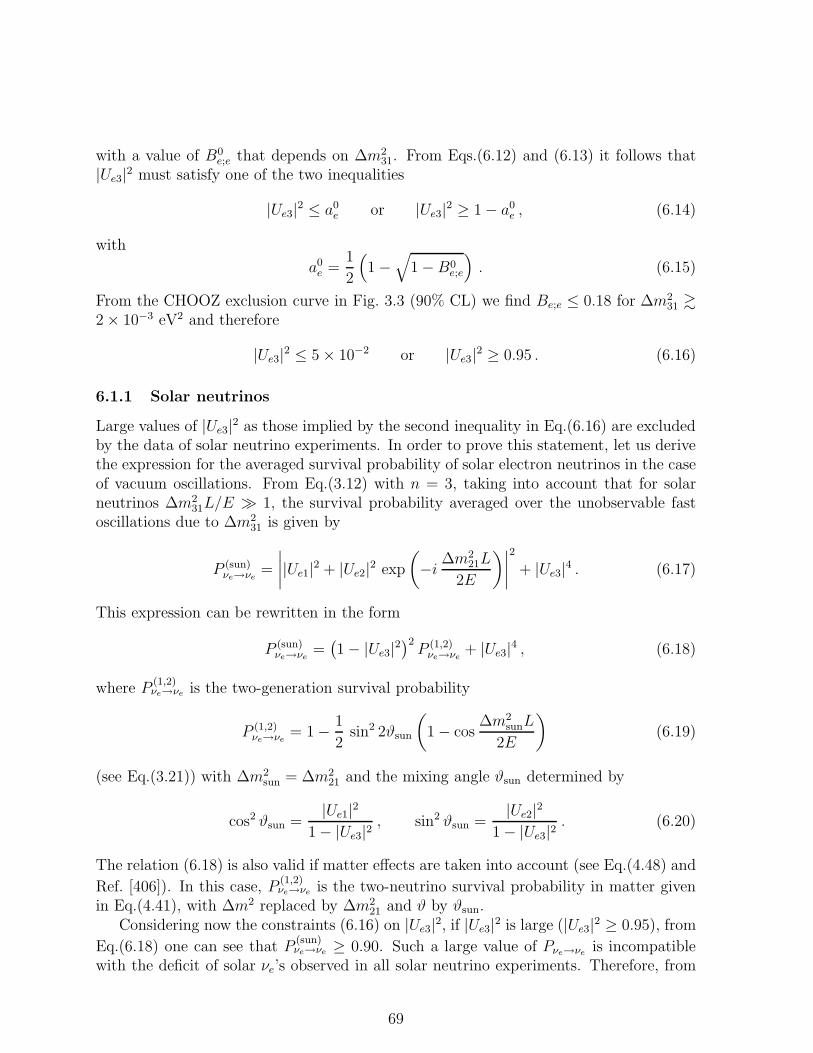
with a value of B0e;e that depends on ∆m2

31. From Eqs.(6.12) and (6.13) it follows that|Ue3|2 must satisfy one of the two inequalities

|Ue3|2 ≤ a0e or |Ue3|2 ≥ 1 − a0

e , (6.14)

with

a0e =

1

2

(

1 −√

1 −B0e;e

)

. (6.15)

From the CHOOZ exclusion curve in Fig. 3.3 (90% CL) we find Be;e ≤ 0.18 for ∆m231 &

2 × 10−3 eV2 and therefore

|Ue3|2 ≤ 5 × 10−2 or |Ue3|2 ≥ 0.95 . (6.16)

6.1.1 Solar neutrinos

Large values of |Ue3|2 as those implied by the second inequality in Eq.(6.16) are excludedby the data of solar neutrino experiments. In order to prove this statement, let us derivethe expression for the averaged survival probability of solar electron neutrinos in the caseof vacuum oscillations. From Eq.(3.12) with n = 3, taking into account that for solarneutrinos ∆m2

31L/E ≫ 1, the survival probability averaged over the unobservable fastoscillations due to ∆m2

31 is given by

P (sun)νe→νe

=

∣

∣

∣

∣

|Ue1|2 + |Ue2|2 exp

(

−i ∆m221L

2E

)∣

∣

∣

∣

2

+ |Ue3|4 . (6.17)

This expression can be rewritten in the form

P (sun)νe→νe

=(

1 − |Ue3|2)2P (1,2)νe→νe

+ |Ue3|4 , (6.18)

where P(1,2)νe→νe is the two-generation survival probability

P (1,2)νe→νe

= 1 − 1

2sin2 2ϑsun

(

1 − cos∆m2

sunL

2E

)

(6.19)

(see Eq.(3.21)) with ∆m2sun = ∆m2

21 and the mixing angle ϑsun determined by

cos2 ϑsun =|Ue1|2

1 − |Ue3|2, sin2 ϑsun =

|Ue2|21 − |Ue3|2

. (6.20)

The relation (6.18) is also valid if matter effects are taken into account (see Eq.(4.48) and

Ref. [406]). In this case, P(1,2)νe→νe is the two-neutrino survival probability in matter given

in Eq.(4.41), with ∆m2 replaced by ∆m221 and ϑ by ϑsun.

Considering now the constraints (6.16) on |Ue3|2, if |Ue3|2 is large (|Ue3|2 ≥ 0.95), from

Eq.(6.18) one can see that P(sun)νe→νe ≥ 0.90. Such a large value of Pνe→νe

is incompatiblewith the deficit of solar νe’s observed in all solar neutrino experiments. Therefore, from

69

the results of the CHOOZ experiment we reach the conclusion that the element |Ue3|2 issmall:

|Ue3|2 ≤ 5 × 10−2 for ∆m231 & 2 × 10−3 eV2 . (6.21)

This limit implies that

P (sun)νe→νe

≃ P (1,2)νe→νe

and sin2 2ϑsun ≃ 4 |Ue2|2(

1 − |Ue2|2)

. (6.22)

Hence, the oscillations of solar neutrinos are practically independent of the value of|Ue3|2 and are decoupled from the oscillations of atmospheric and LBL neutrinos, whichdepend only on the elements Uα3 of the mixing matrix (see Eqs.(6.9) and (6.10)). Thismeans that the two-generation analyses of the solar neutrino data are appropriate alsoin the three-neutrino scheme and they give information on the values of ∆m2

21 = ∆m2sun,

|Ue1| ≃ cosϑsun and |Ue2| ≃ sinϑsun [407].According to a recent analysis of the solar neutrino data [344], which include prelimi-

nary data from Super-Kamiokande [46,408], the ranges of the mixing parameters allowedat 90% CL for the small and large mixing angle MSW solutions and for the vacuumoscillation solution are, respectively,

4 × 10−6 eV2 . ∆m2sun . 1.2 × 10−5 eV2 , 3 × 10−3 . sin2 2ϑsun . 1.1 × 10−2 , (6.23)

8 × 10−6 eV2 . ∆m2sun . 3.0 × 10−5 eV2 , 0.42 . sin2 2ϑsun . 0.74 , (6.24)

6 × 10−11 eV2 . ∆m2sun . 1.1 × 10−10 eV2 , 0.70 . sin2 2ϑsun ≤ 1 . (6.25)

Therefore, taking into account that |Ue3|2 is small and assuming that |Ue2| ≤ |Ue1| (thischoice is necessary only for the MSW solutions in order to fulfill the resonance condition(4.34)), we have

|Ue1| ≃ 1 , |Ue2| ≃ 0.03 − 0.05 (small mixing MSW) , (6.26)

|Ue1| ≃ 0.87 − 0.94 , |Ue2| ≃ 0.35 − 0.49 (large mixing MSW) , (6.27)

|Ue1| ≃ 0.71 − 0.88 , |Ue2| ≃ 0.48 − 0.71 (vacuum oscillations) . (6.28)

Notice that these ranges are statistically rather stable. For example, the range ofsin2 2ϑsun allowed at 99% CL in the case of the large mixing angle MSW solution is0.36 . sin2 2ϑsun . 0.85 [344], which implies |Ue1| ≃ 0.83 − 0.95, |Ue2| ≃ 0.32 − 0.55(compare with Eq.(6.27)).

6.1.2 Atmospheric neutrinos

The atmospheric neutrino data of the Super-Kamiokande experiment give an additionalindication that |Ue3|2 is small. Indeed, the up-down asymmetry of electron events Ae thatcould be generated by νµ → νe or νe → νβ (with β 6=e) transitions is compatible with zero(see Section 5.1.3) [2]:

Ae = −0.036 ± 0.067 ± 0.02 . (6.29)

70

In the three-neutrino scheme under consideration, the Super-Kamiokande atmosphericneutrino data can be explained by νµ → ντ oscillations [2, 261, 409]. The analysis of thedata under the assumption of two-generation mixing yields the following constraints:

Aµ;τ ≡ sin2 2ϑatm & 0.82 , 5 × 10−4 eV2 . ∆m2 . 6 × 10−3 eV2 , (6.30)

from which it follows with Eqs.(6.7) and (6.9) that |Uµ3|2 and |Uτ3|2 must be close to 0.5and therefore |Ue3|2 small.

Coming back to Eq.(6.21) which implies that |Ue3| ≤ 0.22 we see that the CHOOZupper bound for |Ue3| is not very small. It is suggestive, however, to assume that

|Ue3| ≪ 1 , (6.31)

i.e. that the element |Ue3| is so small that it is unimportant for neutrino oscillations[407, 410]. Such an assumption has been recently adopted by several authors [411].

Let us infer some consequences of the assumption (6.31). First of all, it is easy tosee that if the inequality (6.31) is satisfied, matter effects are not essential for νµ →ντ transitions of atmospheric and LBL neutrinos. Indeed, the evolution equation forneutrinos in matter in the flavour representation is (see Section 4)

id

dxψ =

1

2E

(

U ∆M2 U † + A)

ψ , (6.32)

with

ψ ≡

aeaµaτ

, ∆M2 ≡ diag(0,∆m221,∆m

231) , A ≡ diag(ACC , 0, 0) , (6.33)

andACC ≡ 2EVCC , VCC =

√2GFNe . (6.34)

Remember that for anti-neutrinos the matter potential term ACC must be replaced byACC = −ACC .

The inequality (6.5) implies that the phase generated by ∆m221 can be neglected for

atmospheric neutrinos and ∆M2 can be approximated by

∆M2 ≃ diag(0, 0,∆m231) . (6.35)

In this case (taking into account that the phases of the matrix elements Uα3 can beincluded in the charged lepton fields) we have

(U ∆M2 U †)αβ ≃ ∆m231 |Uα3| |Uβ3| . (6.36)

If the condition (6.31) is satisfied, the elements of the matrix U ∆M2 U † with indicesα = e or/and β = e can be neglected. This means that the equation for the wavefunction ae is decoupled from those of aµ, aτ :

idaedx

=ACC2E

ae , (6.37)

idaαdx

=∆m2

31

2E|Uα3|

∑

β=µ,τ

|Uβ3| aβ (α = µ, τ) . (6.38)

71

These equations imply that P(atm,LBL)νe→νe = 1 and P

(atm,LBL)νµ→ντ is given by the two-generation

expression for neutrino oscillations in vacuum,

P (atm,LBL)νµ→ντ

=1

2sin2 2ϑatm

(

1 − cos∆m2

atmL

2E

)

(6.39)

(see Eq.(3.20)), with ∆m2atm = ∆m2

31 and the mixing angle ϑatm determined by

sin2 ϑatm = |Uµ3|2 , cos2 ϑatm = |Uτ3|2 . (6.40)

Therefore, if the condition (6.31) is satisfied, there are no νµ ⇆ νe oscillations in atmo-spheric and LBL neutrino experiments and matter effects are not important for νµ → ντtransitions. This means that the two-generation analyses of the atmospheric neutrinodata in terms of νµ → ντ are appropriate in the three-neutrino scheme under con-sideration and yield information on the values of the parameters ∆m2

31 = ∆m2atm and

|Uµ3| = sinϑatm.According to a recent analysis [409] of the atmospheric neutrino data, the ranges

of ∆m2atm and sin2 2ϑatm for νµ → ντ oscillations allowed at 90% CL by the Super-

Kamiokande multi-GeV data and by the data of atmospheric neutrino oscillation exper-iments are, respectively,

4 × 10−4 eV2 . ∆m2atm . 8 × 10−3 eV2 , 0.72 . sin2 2ϑatm ≤ 1 , (6.41)

4 × 10−4 eV2 . ∆m2atm . 6 × 10−3 eV2 , 0.76 . sin2 2ϑatm ≤ 1 . (6.42)

Taking into account the comments after Eq.(6.5), the ranges (6.42) of the two-generationmixing parameters can be used in order to constrain the values of |Uµ3| and |Uτ3| onlyin the case of the vacuum oscillation solution of the solar neutrino problem. If the solarneutrino problem is due to MSW transitions, we must use the less restrictive ranges(6.41). Thus, assuming that |Uµ3| ≤ |Uτ3|, we have

|Uµ3| ≃ 0.49 − 0.71 , |Uτ3| ≃ 0.71 − 0.87 (solar MSW) , (6.43)

|Uµ3| ≃ 0.51 − 0.71 , |Uτ3| ≃ 0.71 − 0.86 (solar vacuum oscillations) . (6.44)

As in the case of the ranges (6.26)–(6.28), also the ranges (6.43)–(6.44) are statisticallyrather stable. For example, the range of sin2 2ϑsun allowed at 99% CL by all atmosphericneutrino data is 0.66 . sin2 2ϑsun ≤ 1 [409], which implies |Uµ3| ≃ 0.46 − 0.71, |Uτ3| ≃0.71 − 0.89 (compare with Eq.(6.44)).

6.1.3 The mixing matrix in the case |Ue3| ≪ 1

We have seen that, if we assume that |Ue3| is very small, the results of the two-generationanalyses of the data of solar and atmospheric neutrino experiments allow to determinethe moduli of the elements of the first line and of the third column of the mixing matrixU . The moduli of the other elements can be determined from the unitarity of U . Thesimplest way to do it is to start from the parameterization (2.20) of the 3 × 3 mixingmatrix U .

72

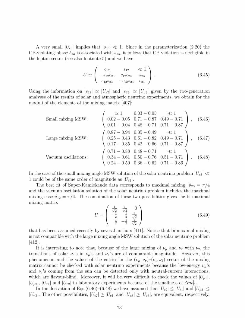
A very small |Ue3| implies that |s13| ≪ 1. Since in the parameterization (2.20) theCP-violating phase δ13 is associated with s13, it follows that CP violation is negligible inthe lepton sector (see also footnote 5) and we have

U ≃

c12 s12 ≪ 1−s12c23 c12c23 s23

s12s23 −c12s23 c23

. (6.45)

Using the information on |s12| ≃ |Ue2| and |s23| ≃ |Uµ3| given by the two-generationanalyses of the results of solar and atmospheric neutrino experiments, we obtain for themoduli of the elements of the mixing matrix [407]:

Small mixing MSW:

≃ 1 0.03 − 0.05 ≪ 10.02 − 0.05 0.71 − 0.87 0.49 − 0.710.01 − 0.04 0.48 − 0.71 0.71 − 0.87

, (6.46)

Large mixing MSW:

0.87 − 0.94 0.35 − 0.49 ≪ 10.25 − 0.43 0.61 − 0.82 0.49 − 0.710.17 − 0.35 0.42 − 0.66 0.71 − 0.87

, (6.47)

Vacuum oscillations:

0.71 − 0.88 0.48 − 0.71 ≪ 10.34 − 0.61 0.50 − 0.76 0.51 − 0.710.24 − 0.50 0.36 − 0.62 0.71 − 0.86

. (6.48)

In the case of the small mixing angle MSW solution of the solar neutrino problem |Ue3| ≪1 could be of the same order of magnitude as |Ue2|.

The best fit of Super-Kamiokande data corresponds to maximal mixing, ϑ23 = π/4and the vacuum oscillation solution of the solar neutrino problem includes the maximalmixing case ϑ12 = π/4. The combination of these two possibilities gives the bi-maximalmixing matrix

U =

1√2

1√2

0

−12

12

1√2

12

−12

1√2

(6.49)

that has been assumed recently by several authors [411]. Notice that bi-maximal mixingis not compatible with the large mixing angle MSW solution of the solar neutrino problem[412].

It is interesting to note that, because of the large mixing of νµ and ντ with ν2, thetransitions of solar νe’s in νµ’s and ντ ’s are of comparable magnitude. However, thisphenomenon and the values of the entries in the (νµ, ντ )–(ν1, ν2) sector of the mixingmatrix cannot be checked with solar neutrino experiments because the low-energy νµ’sand ντ ’s coming from the sun can be detected only with neutral-current interactions,which are flavour-blind. Moreover, it will be very difficult to check the values of |Uµ1|,|Uµ2|, |Uτ1| and |Uτ2| in laboratory experiments because of the smallness of ∆m2

21.In the derivation of Eqs.(6.46)–(6.48) we have assumed that |Ue2| ≤ |Ue1| and |Uµ3| ≤

|Uτ3|. The other possibilities, |Ue2| ≥ |Ue1| and |Uµ3| ≥ |Uτ3|, are equivalent, respectively,

73

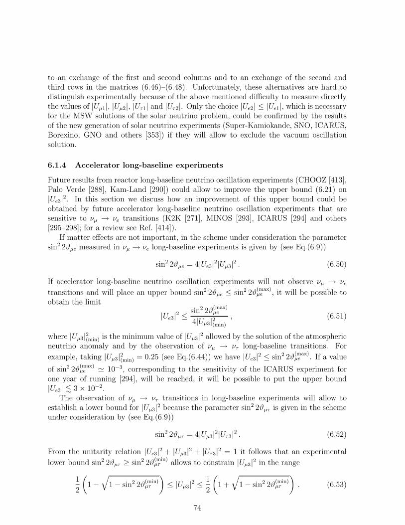
to an exchange of the first and second columns and to an exchange of the second andthird rows in the matrices (6.46)–(6.48). Unfortunately, these alternatives are hard todistinguish experimentally because of the above mentioned difficulty to measure directlythe values of |Uµ1|, |Uµ2|, |Uτ1| and |Uτ2|. Only the choice |Ue2| ≤ |Ue1|, which is necessaryfor the MSW solutions of the solar neutrino problem, could be confirmed by the resultsof the new generation of solar neutrino experiments (Super-Kamiokande, SNO, ICARUS,Borexino, GNO and others [353]) if they will allow to exclude the vacuum oscillationsolution.

6.1.4 Accelerator long-baseline experiments

Future results from reactor long-baseline neutrino oscillation experiments (CHOOZ [413],Palo Verde [288], Kam-Land [290]) could allow to improve the upper bound (6.21) on|Ue3|2. In this section we discuss how an improvement of this upper bound could beobtained by future accelerator long-baseline neutrino oscillation experiments that aresensitive to νµ → νe transitions (K2K [271], MINOS [293], ICARUS [294] and others[295–298]; for a review see Ref. [414]).

If matter effects are not important, in the scheme under consideration the parametersin2 2ϑµe measured in νµ → νe long-baseline experiments is given by (see Eq.(6.9))

sin2 2ϑµe = 4|Ue3|2|Uµ3|2 . (6.50)

If accelerator long-baseline neutrino oscillation experiments will not observe νµ → νetransitions and will place an upper bound sin2 2ϑµe ≤ sin2 2ϑ

(max)µe , it will be possible to

obtain the limit

|Ue3|2 ≤sin2 2ϑ

(max)µe

4|Uµ3|2(min)

, (6.51)

where |Uµ3|2(min) is the minimum value of |Uµ3|2 allowed by the solution of the atmosphericneutrino anomaly and by the observation of νµ → ντ long-baseline transitions. For

example, taking |Uµ3|2(min) = 0.25 (see Eq.(6.44)) we have |Ue3|2 ≤ sin2 2ϑ(max)µe . If a value

of sin2 2ϑ(max)µe ≃ 10−3, corresponding to the sensitivity of the ICARUS experiment for

one year of running [294], will be reached, it will be possible to put the upper bound|Ue3| . 3 × 10−2.

The observation of νµ → ντ transitions in long-baseline experiments will allow toestablish a lower bound for |Uµ3|2 because the parameter sin2 2ϑµτ is given in the schemeunder consideration by (see Eq.(6.9))

sin2 2ϑµτ = 4|Uµ3|2|Uτ3|2 . (6.52)

From the unitarity relation |Ue3|2 + |Uµ3|2 + |Uτ3|2 = 1 it follows that an experimental

lower bound sin2 2ϑµτ ≥ sin2 2ϑ(min)µτ allows to constrain |Uµ3|2 in the range

1

2

(

1 −√

1 − sin2 2ϑ(min)µτ

)

≤ |Uµ3|2 ≤1

2

(

1 +

√

1 − sin2 2ϑ(min)µτ

)

. (6.53)

74

If sin2 2ϑ(min)µτ is found to be close to one, as suggested by the solution of the atmo-

spheric neutrino problem (see Eqs.(6.41) and (6.42)), the lower bound |Uµ3|2(min) =

12

(

1 −√

1 − sin2 2ϑ(min)µτ

)

is close to 1/2.

If matter effects are important, the extraction of an upper bound for |Ue3|2 from thedata of νµ → νe accelerator long-baseline experiments is more complicated. In this casethe probability of νµ → νe oscillations is given by [192]

Pνµ→νe=

4|Ue3|2|Uµ3|2(

1 − ACC

∆m231

)2

+ 4|Ue3|2 ACC

∆m231

sin2

(

∆m231L

4E

√

(

1 − ACC

∆m231

)2

+ 4|Ue3|2 ACC

∆m231

)

,

(6.54)where E is the neutrino energy and L is the distance of propagation. This probabilitydepends on the neutrino energy not only through the explicit E in the denominatorof the phase, but also through the energy dependence of ACC ≡ 2EVCC . For long-baseline neutrino beams propagating in the lithosphere of the earth the charged-currenteffective potential VCC =

√2GFNe is practically constant: Ne ≃ 1.5Navo cm−3 and

VCC ≃ 1.1 × 10−13 eV (see Eq.(4.37)).If long-baseline experiments will not observe νµ → νe transitions (or will find that

they have an extremely small probability) for neutrino energies such that ACC . ∆m231,

it will mean that |Ue3|2 is small and a fit of the experimental data with the formula(6.54) will yield a stringent upper limit for |Ue3|2 (taking into account the lower limit|Uµ3|2 ≥ |Uµ3|2(min) obtained from the solution of the atmospheric neutrino anomaly and

from the observation of νµ → ντ long-baseline transitions). On the other hand, the non-observation of νµ → νe transitions for neutrino energies such that ACC ≫ ∆m2

31 does notprovide any information on |Ue3|2 because in this case the transition probability (6.54) issuppressed by the matter effect. Hence, in order to check the hypothesis |Ue3| ≪ 1, aswell as to have some possibility to observe νµ → νe transitions if this hypothesis is wrong,it is necessary that a substantial part of the energy spectrum of the neutrino beam liesbelow

∆m231

2VCC≃ 30 GeV

(

∆m231

10−2 eV2

)

. (6.55)

This requirement will be satisfied in the accelerator long-baseline experiments underpreparation (K2K [271], MINOS [293], ICARUS [294] and others [295–298]; see [414]) if∆m2

31 is not much smaller than 10−2 eV2.

6.2 Mixing of four massive neutrinos

Let us consider now the case of mixing of four neutrinos [415–417], i.e., n = 4 in Eqs.(3.3)and (3.9),

|να〉 =4∑

k=1

U∗αk |νk〉 , |να〉 =

4∑

k=1

Uαk |νk〉 (α = e, µ, τ, s) , (6.56)

75

6

m1

m2

m3

m46

m1

m2

m3

m46

m1

m2

m3

m46

m1

m2

m3

m46

m1

m2

m3

m46

m1

m2

m3

m4

(I) (II) (III) (IV) (A) (B)

Figure 6.1. The six types of neutrino mass spectra that can accommodate the solar, atmospheric andLSND scales of ∆m2.

which allows to accommodate all the three existing indications in favour of neutrinomixing. Here |νs〉 is a sterile neutrino state (see Section 2.2).

We do not make any assumptions about the mass spectrum of four neutrinos and willconsider all possibilities. The six possible four-neutrino mass spectra with three differentscales of neutrino mass-squared differences (atmospheric, solar and LSND) are shown inFig. 6.1. In all these mass spectra there are two groups of close masses separated bythe “LSND gap” of the order of 1 eV. The small mass-squared differences correspondto ∆m2

sun (the smallest one, ∆m221 in schemes I and B, ∆m2

32 in schemes II and IV,∆m2

43 in schemes III and A) and ∆m2atm (∆m2

31 in schemes I and II, ∆m242 in schemes III

and IV, ∆m221 in scheme A, ∆m2

43 in scheme B) and the largest mass squared difference∆m2

41 = ∆m2LSND is relevant for the oscillations observed in the LSND experiment.

Let us consider SBL oscillations in the case of neutrino mass spectra presented inFig. 6.1. Taking into account that

∆m2sunL

E≪ 1 and

∆m2atmL

E≪ 1 , (6.57)

from the general formula (3.12) we obtain that the probabilities of να → νβ transitionsand of να survival in SBL experiments are given by

P (SBL)να→νβ

=1

2Aα;β

(

1 − cos∆m2

41 L

2E

)

(α 6= β) , (6.58)

P (SBL)να→να

= 1 − 1

2Bα;α

(

1 − cos∆m2

41 L

2E

)

. (6.59)

The oscillation amplitudes Aα;β and Bα;α depend on the elements of the mixing matrixand on the type of neutrino mass spectrum:

Aα;β = 4

∣

∣

∣

∣

∣

∑

k

U∗αk Uβk

∣

∣

∣

∣

∣

2

, (6.60)

Bα;α = 4

(

∑

k

|Uαk|2)(

1 −∑

k

|Uαk|2)

, (6.61)

76

where the index k runs over the indices of the first or (because of the unitarity of themixing matrix) of the second group of neutrino masses (see Fig. 6.1). The expressions(6.58) and (6.59) have the same form as the corresponding two-neutrino formulas (3.20)and (3.21) and are a direct generalization of the expressions (6.7) and (6.8) presented inSection 6.1 for the case of three massive neutrinos and a neutrino mass hierarchy. FromEq.(6.60) it is obvious that the amplitude of να → νβ oscillations is equal to Aα;β and

P(SBL)να→νβ

= P (SBL)να→νβ

. (6.62)

Thus, CP violation in the lepton sector cannot be revealed in SBL neutrino oscillationexperiments if only one mass-squared difference is relevant for SBL oscillations.

The expression (6.61) allows to obtain information on the quantities∑

k |Uek|2 and∑

k |Uµk|2 from the results of SBL νe and νµ disappearance experiments, whose exclusioncurves imply the constraint

Bα;α ≤ B0α;α (α = e, µ) . (6.63)

The upper bound B0α;α depends on the value of ∆m2

41. Equations (6.59) and (6.63) implythat each

∑

k |Uαk|2 for α = e, µ must satisfy one of the two inequalities

∑

k

|Uαk|2 ≤ a0α or

∑

k

|Uαk|2 ≥ 1 − a0α , (6.64)

with

a0α =

1

2

(

1 −√

1 − B0α;α

)

. (6.65)

The most stringent limits on Be;e and Bµ;µ are given by the exclusion curves of theBugey [162] reactor νe → νe experiment and of the CDHS [153] and CCFR [418] accelera-tor νµ → νµ experiments. The values of a0

e and a0µ corresponding to the 90% CL exclusion

curves of these experiments are shown in Fig. 6.2. One can see that

a0e ≤ 4 × 10−2 for ∆m2

41 & 0.1 eV2 , (6.66)

a0µ ≤ 2 × 10−1 for ∆m2

41 & 0.3 eV2 . (6.67)

Hence, from Eq.(6.64) it follows that the quantities∑

k |Uek|2 and∑

k |Uµk|2 are eithersmall or large (close to one). We will show now that from the four possibilities for thetwo quantities

∑

k |Uek|2 and∑

k |Uµk|2 (small-small, small-large, large-small, large-large)for each neutrino mass spectrum in Fig. 6.1 only one possibility is compatible with theresults of solar and atmospheric neutrino experiments [416, 419,420].

Let us consider, for example, the hierarchical mass spectrum

m1 ≪ m2 ≪ m3 ≪ m4 , (6.68)

which corresponds to type I in Fig. 6.1. In this case, the inequalities (6.64) become

|Uα4|2 ≤ a0α or |Uα4|2 ≥ 1 − a0

α (α = e, µ) . (6.69)

77

aα0

10-2 10-1

∆m2

(eV

2 )

10-1

100

101

102

103

ae0

aµ0

41

Aµ;e

10-4 10-3 10-2 10-1 100

∆m2

(e

V2 )

10-1

100

101

102

103

BNL E776

BUGEY

LSNDνe→νe , νµ→νµ

KARMEN

BNL E734

41

CCFR

Figure 6.2. Values of a0e and a0

µ (see Eq.(6.65))as functions of ∆m2

41 obtained from the exclusioncurves of the Bugey [162], CDHS [153] and CCFR[418] SBL disappearance experiments.

Figure 6.3. The region on the right of the solidline passing through the black circles is excludedat 90% CL by the results of SBL disappearanceexperiments for small |Ue4|2 and |Uµ4|2 in themodel with mixing of four neutrinos and a masshierarchy. The shadowed regions are allowed at90% CL by the results of the LSND experiment.Also shown are the exclusion curves of the Bugey[162], BNL E734 [372], BNL E776 [373], CCFR[374] and KARMEN (Bayesian analysis) [375] ex-periments.

The survival probability of solar νe’s averaged over the fast, unobservable oscillationsdue to ∆m2

41 and ∆m231 is given by [421]

P (sun)νe→νe

=

(

1 −∑

k=3,4

|Uek|2)2

P (1,2)νe→νe

+∑

k=3,4

|Uek|4 , (6.70)

where P(1,2)νe→νe is the νe survival probability due to the mixing of νe with ν1 and ν2.

This probability has the two-generation form (3.21) and depends on the neutrino energy,∆m2 = ∆m2

sun = ∆m221 and

sin2 2ϑ = sin2 2ϑsun =4 |Ue1|2 |Ue2|2

(|Ue1|2 + |Ue2|2)2. (6.71)

Though Eqs.(6.70) and (6.71) were derived here for vacuum oscillations, the considera-tions in Section 4.4 show that they are also valid including matter effects. If |Ue4|2 ≥ 1−a0

e ,

78

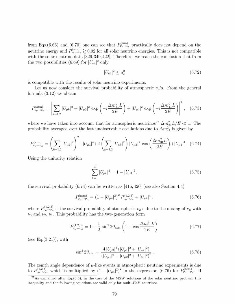
from Eqs.(6.66) and (6.70) one can see that P(sun)νe→νe practically does not depend on the

neutrino energy and P(sun)νe→νe & 0.92 for all solar neutrino energies. This is not compatible

with the solar neutrino data [329,349,422]. Therefore, we reach the conclusion that fromthe two possibilities (6.69) for |Ue4|2 only

|Ue4|2 ≤ a0e (6.72)

is compatible with the results of solar neutrino experiments.Let us now consider the survival probability of atmospheric νµ’s. From the general

formula (3.12) we obtain

P (atm)νµ→νµ

=

∣

∣

∣

∣

∣

∑

k=1,2

|Uµk|2 + |Uµ3|2 exp

(

−i∆m231L

2E

)

+ |Uµ4|2 exp

(

−i∆m241L

2E

)

∣

∣

∣

∣

∣

2

, (6.73)

where we have taken into account that for atmospheric neutrinos27 ∆m221L/E ≪ 1. The

probability averaged over the fast unobservable oscillations due to ∆m241 is given by

P (atm)νµ→νµ

=

(

∑

k=1,2

|Uµk|2)2

+|Uµ3|4+2

(

∑

k=1,2

|Uµk|2)

|Uµ3|2 cos

(

∆m231L

2E

)

+|Uµ4|4 . (6.74)

Using the unitarity relation

3∑

k=1

|Uµk|2 = 1 − |Uµ4|2 , (6.75)

the survival probability (6.74) can be written as [416, 420] (see also Section 4.4)

P (atm)νµ→νµ

=(

1 − |Uµ4|2)2P (1,2;3)νµ→νµ

+ |Uµ4|4 , (6.76)

where P(1,2;3)νµ→νµ is the survival probability of atmospheric νµ’s due to the mixing of νµ with

ν3 and ν2, ν1. This probability has the two-generation form

P (1,2;3)νµ→νµ

= 1 − 1

2sin2 2ϑatm

(

1 − cos∆m2

31L

2E

)

(6.77)

(see Eq.(3.21)), with

sin2 2ϑatm =4 |Uµ3|2 (|Uµ1|2 + |Uµ2|2)

(|Uµ1|2 + |Uµ2|2 + |Uµ3|2)2 . (6.78)

The zenith angle dependence of µ-like events in atmospheric neutrino experiments is dueto P

(1,2;3)νµ→νµ, which is multiplied by (1 − |Uµ4|2)2

in the expression (6.76) for P(atm)νµ→νµ. If

27As explained after Eq.(6.5), in the case of the MSW solutions of the solar neutrino problem thisinequality and the following equations are valid only for multi-GeV neutrinos.

79

|Uµ4|2 is large, as given by the second inequality in Eq.(6.69), |Uµ4|2 ≥ 1 − a0µ, we have

(1 − |Uµ4|2)2 ≤ 4 × 10−2 for ∆m241 & 0.3 eV2 (see Eq.(6.67)). A zenith-angle variation

of µ-like events smaller than 4 × 10−2 is incompatible with the up-down asymmetry ofmulti-GeV µ-like events observed by the Super-Kamiokande experiment (see Section 5.1).Therefore, from the two inequalities (6.69) for |Uµ4|2 only the first one is compatible withthe results of the atmospheric neutrino experiments:

|Uµ4|2 ≤ a0µ . (6.79)

The same conclusion can be reached for all the neutrino mass spectra in Fig. 6.1 inwhich one mass is separated by the other three by the LSND gap, i.e., for the spectraI, II, III, IV. Hence, in the framework of these spectra the results of SBL disappearanceexperiments and of solar and atmospheric neutrino experiments imply that

|Uej|2 ≤ a0e , |Uµj |2 ≤ a0

µ , (6.80)

with j = 4 in the schemes I and II and j = 1 in the schemes III and IV. These inequalities

imply that(−)

νµ→(−)

νe transitions in SBL experiments are strongly suppressed. Indeed, fromEqs.(6.60) and (6.80) we have

Aµ;e = 4 |Uej|2 |Uµj |2 ≤ 4 a0e a

0µ . (6.81)

Thus, the amplitude of SBL(−)

νµ→(−)

νe oscillations is quadratic in the small quantities |Uej |2and |Uµj |2. The upper bound (6.81) obtained from the values of a0

e and a0µ presented

in Fig. 6.2 is shown in Fig. 6.3 by the solid line passing through the black circles. Thesolid, dotted, dashed, dash-dotted and dash-dot-dotted curves in Fig. 6.3 are the 90%CL exclusion curves obtained in the Bugey [162], BNL E734 [372], BNL E776 [373],CCFR [374] and KARMEN (Bayesian analysis) [375] experiments. The shadowed regionsare allowed by the results of the LSND [370,371] experiments at 90% CL. From this figureone can see that the result of the LSND experiment, taken together with the results of SBLdisappearance experiments and solar and atmospheric neutrino experiments, disfavoursthe schemes I, II, III and IV of Fig. 6.1.28

Let us consider now the spectra A and B in Fig. 6.1. In this case the inequalities(6.64) apply with the index k running over 1, 2 or 3, 4 (the two choices are equivalentbecause of the unitarity of the mixing matrix). We consider explicitly only the spectrumA, but all the following results are valid also for scheme B and can be obtained with theindex exchange 1, 2 ⇆ 3, 4.

In the case of spectrum A, the survival probability of solar νe’s is given by [421]

P (sun)νe→νe

=∑

k=1,2

|Uek|4 +

(

1 −∑

k=1,2

|Uek|2)2

P (3,4)νe→νe

, (6.82)

28The presence of a small allowed region in Fig. 6.3 for 0.2 eV2 . ∆m241 . 0.3 eV2 is due to the fact that

for ∆m241 . 0.3 eV2 there are no constraints on B0

µ;µ from the results of νµ disappearance experiments.

80

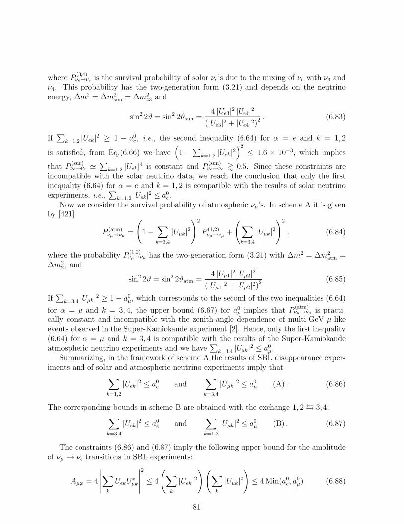
where P(3,4)νe→νe is the survival probability of solar νe’s due to the mixing of νe with ν3 and

ν4. This probability has the two-generation form (3.21) and depends on the neutrinoenergy, ∆m2 = ∆m2

sun = ∆m243 and

sin2 2ϑ = sin2 2ϑsun =4 |Ue3|2 |Ue4|2

(|Ue3|2 + |Ue4|2)2 . (6.83)

If∑

k=1,2 |Uek|2 ≥ 1 − a0e, i.e., the second inequality (6.64) for α = e and k = 1, 2

is satisfied, from Eq.(6.66) we have(

1 −∑

k=1,2 |Uek|2)2

≤ 1.6 × 10−3, which implies

that P(sun)νe→νe ≃

∑

k=1,2 |Uek|4 is constant and P(sun)νe→νe & 0.5. Since these constraints are

incompatible with the solar neutrino data, we reach the conclusion that only the firstinequality (6.64) for α = e and k = 1, 2 is compatible with the results of solar neutrinoexperiments, i.e.,

∑

k=1,2 |Uek|2 ≤ a0e.

Now we consider the survival probability of atmospheric νµ’s. In scheme A it is givenby [421]

P (atm)νµ→νµ

=

(

1 −∑

k=3,4

|Uµk|2)2

P (1,2)νµ→νµ

+

(

∑

k=3,4

|Uµk|2)2

, (6.84)

where the probability P(1,2)νµ→νµ has the two-generation form (3.21) with ∆m2 = ∆m2

atm =∆m2

21 and

sin2 2ϑ = sin2 2ϑatm =4 |Uµ1|2 |Uµ2|2

(|Uµ1|2 + |Uµ2|2)2 . (6.85)

If∑

k=3,4 |Uµk|2 ≥ 1 − a0µ, which corresponds to the second of the two inequalities (6.64)

for α = µ and k = 3, 4, the upper bound (6.67) for a0µ implies that P

(atm)νµ→νµ is practi-

cally constant and incompatible with the zenith-angle dependence of multi-GeV µ-likeevents observed in the Super-Kamiokande experiment [2]. Hence, only the first inequality(6.64) for α = µ and k = 3, 4 is compatible with the results of the Super-Kamiokandeatmospheric neutrino experiments and we have

∑

k=3,4 |Uµk|2 ≤ a0µ.

Summarizing, in the framework of scheme A the results of SBL disappearance exper-iments and of solar and atmospheric neutrino experiments imply that

∑

k=1,2

|Uek|2 ≤ a0e and

∑

k=3,4

|Uµk|2 ≤ a0µ (A) . (6.86)

The corresponding bounds in scheme B are obtained with the exchange 1, 2 ⇆ 3, 4:∑

k=3,4

|Uek|2 ≤ a0e and

∑

k=1,2

|Uµk|2 ≤ a0µ (B) . (6.87)

The constraints (6.86) and (6.87) imply the following upper bound for the amplitudeof νµ → νe transitions in SBL experiments:

Aµ;e = 4

∣

∣

∣

∣

∣

∑

k

UekU∗µk

∣

∣

∣

∣

∣

2

≤ 4

(

∑

k

|Uek|2)(

∑

k

|Uµk|2)

≤ 4 Min(a0e, a

0µ) (6.88)

81

(here the index k runs over 1, 2 or over 3, 4). This bound is linear in the small quantitiesa0e and a0

µ and turns out to be compatible with the results of the LSND experiment.Actually, this bound is worse than the unitarity bound

Aµ;e ≤ Min(B0e;e, B

0µ;µ) , (6.89)

which causes the exclusion of the large sin2 2ϑ part of the LSND allowed region (seeFig. 6.3, where B0

e;e is represented by the Bugey curve).We want to note that the bound a0

µ ceases to exist shortly below ∆m241 = 0.3 eV2

(see Fig. 6.2). On the other hand, it follows from the LSND and Bugey experiments that∆m2

41 & 0.2 eV2 (see Fig. 6.3). Thus, for the small interval 0.2 eV2 . ∆m241 . 0.3 eV2

our arguments leading to schemes A and B have to be considered with caution and itwould be desirable to have experimental information on Bµ;µ in this interval.

Let us now discuss some consequences of the schemes A and B, taking into accountthe constraints (6.86) and (6.87). First of all, we will show that these bounds lead toconstraints on the neutrino mass measured in tritium β-decay experiments and on theeffective Majorana mass that determines the probability of neutrinoless double-β decay.

The electron spectrum in the decay 3H → 3He + e− + νe is given by

dN

dE= C peEe (Q− T )F (Ee)

∑

i

|Uei|2√

(Q− T )2 −m2i , (6.90)

where Q is the energy release, pe and Ee are the electron momentum and energy, T =Ee − me, F (Ee) is the Fermi function and C is a constant. Taking into account thatm1 ≃ m2 ≪ m3 ≃ m4, the first inequality in Eq.(6.86) implies that in scheme A theeffective neutrino mass determined from the measurement of the high-energy part of theβ-spectrum of 3H is practically equal to the “LSND mass” m4:

m(3H) ≃∑

k=3,4

|Uek|2m4 =

(

1 −∑

k=1,2

|Uek|2)

m4 ≃ m4 . (6.91)

If massive neutrinos are Majorana particles, the matrix element of neutrinoless double-β decay is proportional to the effective Majorana mass [95, 106] (see Appendix A)

〈m〉 =4∑

k=1

U2ekmk . (6.92)

In the case of scheme A, the first inequality in Eq.(6.86) implies that

|〈m〉| ≃∣

∣

∣

∣

∣

∑

k=3,4

U2ek

∣

∣

∣

∣

∣

m4 ≃ m4

√

1 − 4 |Ue4|2 (1 − |Ue4|2) sin2 φ , (6.93)

where φ is the difference of the phases of Ue3 and Ue4. Since φ is unknown, from Eq.(6.93)we obtain the constraints

∣

∣1 − 2 |Ue4|2∣

∣m4 . |〈m〉| . m4 , (6.94)

82

where the upper and lower bounds correspond to φ = 0 or π and φ = ±π/2, respectively.29

Taking into account Eqs.(6.83) and (6.86), we have

|Ue3| ≃ cosϑsun and |Ue4| ≃ sinϑsun , (6.95)

and Eq.(6.94) can be written as

m4

√

1 − sin2 2ϑsun . |〈m〉| . m4 . (6.96)

If sin2 2ϑsun ≪ 1, which corresponds to the MSW solution with a small mixing angle, wehave |〈m〉| ≃ m4, independent of the value of φ and of the conservation of CP. In thecase of a large value of the parameter sin2 2ϑsun, which correspond to the MSW solutionwith a large mixing angle or to the vacuum oscillation solution, in the future it will bepossible to obtain information about the violation of CP in the lepton sector if boththe 3H β-decay and neutrinoless double-β decay experiments will obtain positive results.Indeed, from the measurements of m(4H) ≃ m4, |〈m〉| and sin2 2ϑsun with the help ofEq.(6.96) it will be possible to determine the value of sin2 φ (if sin2 2ϑsun is large). Let usemphasize that in the case of CP conservation the relative CP parities of ν3 and ν4 canbe determined: the CP parities are equal if sin2 φ = 0 and opposite if sin2 φ = 1.

Considering now scheme B, the first inequality in Eq.(6.87) implies that both m(3H)and |〈m〉| are strongly suppressed:

m(3H) ≃(

∑

k=3,4

|Uek|2)

m4 ≤ a0em4 ≪ m4 . (6.97)

|〈m〉| ≃∣

∣

∣

∣

∣

∑

k=3,4

U2ek

∣

∣

∣

∣

∣

m4 ≤(

∑

k=3,4

|Uek|2)

m4 ≤ a0em4 ≪ m4 . (6.98)

Therefore, only if scheme A is realized in nature, there is some possibility to measure theeffect of the LSND mass in future tritium decay experiments and neutrinoless double-βdecay experiments.

We discuss now the implications of the schemes A and B for LBL neutrino oscillationexperiments [423]. The smallness of

∑

k=1,2 |Uek|2 in scheme A and of∑

k=3,4 |Uek|2 inscheme B implies that the electron neutrino has a small mixing with the neutrinos whosemass-squared difference is responsible for the oscillations of atmospheric neutrinos (i.e.,ν1, ν2 in scheme A and ν3, ν4 in scheme B). Hence, as shown in the following part ofthis section, the transition probability of electron neutrinos and antineutrinos into otherstates in atmospheric and LBL experiments is suppressed.

Taking into account that in scheme A we have ∆m243L/E ≪ 1 and ∆m2

41L/E ≫ 1 inLBL experiments, we obtain from the general formula (3.12) the following expression for

29If CP is conserved, we have φ = 0 or π if the CP parities of ν3 and ν4 are equal and φ = ±π/2 ifthey are opposite. Indeed, if CP is conserved from Eq.(2.50) we get U∗

ek = Uekρk where ρk = ±1 andthe CP parity of νk is ηCP

k = iρk (see Eq.(2.53)) [96,97]. Writing Uek = |Uek|eiφk , we obtain φk = 0 or πif ρk = +1 and φk = ±π/2 if ρk = −1. Hence, we have φ3 − φ4 = 0 or π if ρ3 = ρ4 and φ3 − φ4 = ±π/2if ρ3 = −ρ4.

83

the measurable probability of να → νβ transitions averaged over the fast oscillations dueto ∆m2

41:

P (LBL;A)να→νβ

=

∣

∣

∣

∣

Uβ1 U∗α1 + Uβ2 U

∗α2 exp

(

−i ∆m221L

2E

)∣

∣

∣

∣

2

+

∣

∣

∣

∣

∣

∑

k=3,4

Uβk U∗αk

∣

∣

∣

∣

∣

2

. (6.99)

The corresponding probability in scheme B is given by the exchange 1, 2 ⇆ 3, 4 and theprobability of να → νβ transitions is obtained changing Uβk U

∗αk → U∗

βk Uαk.Let us consider reactor LBL experiments which measure the survival probability

P(LBL)νe→νe

. We will show that the negative results of SBL reactor experiments and the resultsof solar neutrino experiments imply strong constraints on the transition probability ofLBL reactor νe’s into other states. Indeed, from Eq.(6.99) and the corresponding one inscheme B, for the survival probability of LBL reactor νe’s we have the lower bounds

P(LBL;A)νe→νe

≥(

∑

k=3,4

|Uek|2)2

=

(

1 −∑

k=1,2

|Uek|2)2

, (6.100)

P(LBL;B)νe→νe

≥(

∑

k=1,2

|Uek|2)2

=

(

1 −∑

k=3,4

|Uek|2)2

, (6.101)

in schemes A and B, respectively. From the inequalities (6.86) and (6.87) it follows thatin both schemes

P(LBL)νe→νe

≥(

1 − a0e

)2. (6.102)

Since a0e is small (see Fig. 6.2 and Eq.(6.66)), the lower bound (6.102) implies that the

survival probability P(LBL)νe→νe

is close to one. For the transition probability of νe’s into anyother state in LBL experiments,

1 − P(LBL)νe→νe

=∑

β 6=eP

(LBL)νe→νβ

, (6.103)

we have the upper bound1 − P

(LBL)νe→νe

≤ a0e

(

2 − a0e

)

. (6.104)

The value of this bound, which depends on ∆m241 through the dependence of a0

e on ∆m241

(see Fig. 6.2), is shown in Fig 6.4 (the solid line), where it is compared with the upper

bound for 1 − P(LBL)νe→νe

obtained in the CHOOZ experiment [159] (dash-dotted line) andwith the final sensitivity of the CHOOZ experiment (dash-dot-dotted line). The shadowedregion in Fig 6.4 corresponds to the range of ∆m2

41 allowed at 90% CL by the resultsof the LSND and other experiments. One can see from Fig 6.4 that if ∆m2

41 lies in the

LSND range, the upper bound for 1 − P(LBL)νe→νe

is much less than the sensitivity of theCHOOZ experiment and it will be very difficult to measure the disappearance of reactorνe in future LBL experiments.

Let us consider now νµ → νe transitions, which will be investigated in the near futureby the K2K [271], MINOS [293], ICARUS [294] and/or other [295–298] experiments

84

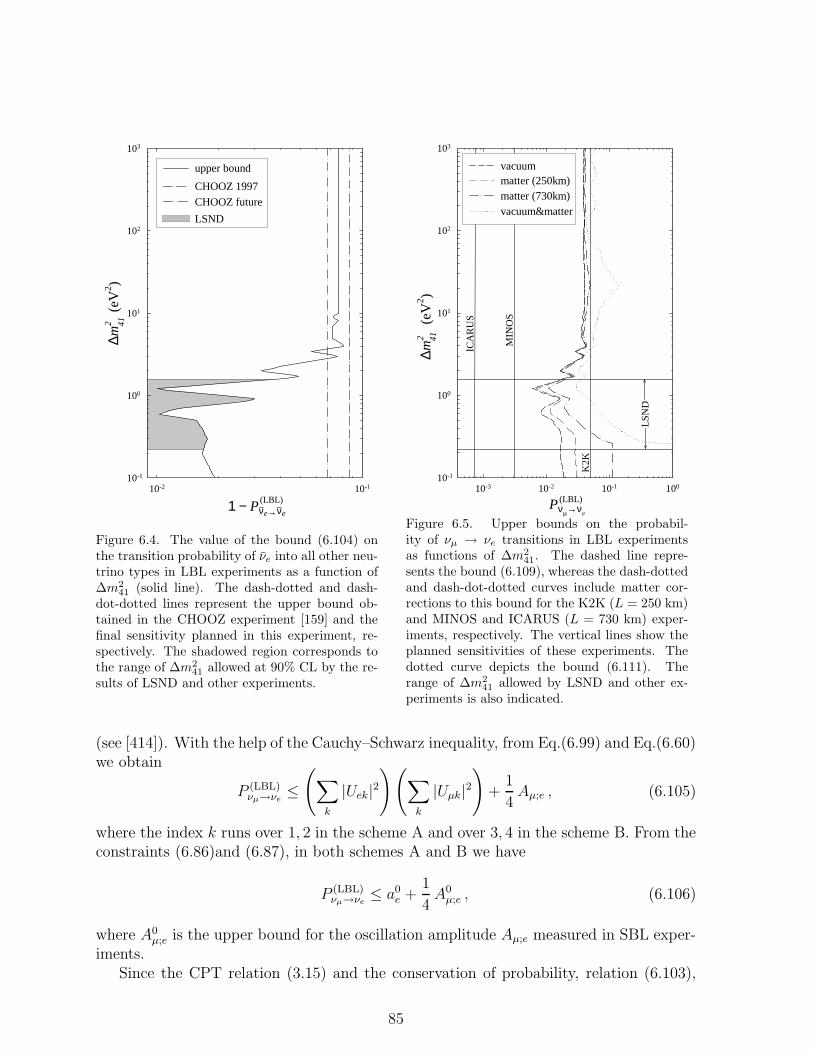
1 − Pνe→νe

10-2 10-1

∆ m2

(eV

2 )

10-1

100

101

102

103

upper bound

CHOOZ 1997

CHOOZ future

LSND

(LBL)

41

Pνµ→νe

10-3 10-2 10-1 100

∆m2

(eV

2 )

10-1

100

101

102

103

matter (250km)

(LBL)

vacuum&matter

vacuum

LSN

D

MIN

OS

ICA

RU

S

K2K

matter (730km)

41

Figure 6.4. The value of the bound (6.104) onthe transition probability of νe into all other neu-trino types in LBL experiments as a function of∆m2

41 (solid line). The dash-dotted and dash-dot-dotted lines represent the upper bound ob-tained in the CHOOZ experiment [159] and thefinal sensitivity planned in this experiment, re-spectively. The shadowed region corresponds tothe range of ∆m2

41 allowed at 90% CL by the re-sults of LSND and other experiments.

Figure 6.5. Upper bounds on the probabil-ity of νµ → νe transitions in LBL experimentsas functions of ∆m2

41. The dashed line repre-sents the bound (6.109), whereas the dash-dottedand dash-dot-dotted curves include matter cor-rections to this bound for the K2K (L = 250 km)and MINOS and ICARUS (L = 730 km) exper-iments, respectively. The vertical lines show theplanned sensitivities of these experiments. Thedotted curve depicts the bound (6.111). Therange of ∆m2

41 allowed by LSND and other ex-periments is also indicated.

(see [414]). With the help of the Cauchy–Schwarz inequality, from Eq.(6.99) and Eq.(6.60)we obtain

P (LBL)νµ→νe

≤(

∑

k

|Uek|2)(

∑

k

|Uµk|2)

+1

4Aµ;e , (6.105)

where the index k runs over 1, 2 in the scheme A and over 3, 4 in the scheme B. From theconstraints (6.86)and (6.87), in both schemes A and B we have

P (LBL)νµ→νe

≤ a0e +

1

4A0µ;e , (6.106)

where A0µ;e is the upper bound for the oscillation amplitude Aµ;e measured in SBL exper-

iments.Since the CPT relation (3.15) and the conservation of probability, relation (6.103),

85

imply that∑

α6=eP (LBL)να→νe

=∑

α6=eP

(LBL)νe→να

= 1 − P(LBL)νe→νe

, (6.107)

another upper limit for P(LBL)νµ→νe can be obtained from the inequality (6.104):

P (LBL)νµ→νe

≤ a0e

(

2 − a0e

)

. (6.108)

Combining the upper bounds (6.106) and (6.108) and taking into account that they arevalid also for antineutrinos [423], we have

P(LBL)

(−)νµ→

(−)νe

≤ Min

(

a0e +

1

4A0µ;e , a

0e

(

2 − a0e

)

)

. (6.109)

The curve corresponding to this limit obtained from the 90% CL exclusion plots of theBugey [162] experiment for a0

e and of the BNL E734 [372], BNL E776 [373], CCFR [374]and KARMEN (Bayesian analysis) [375] experiments for A0

µ;e is represented by the dashedline in Fig. 6.5. For comparison, the expected sensitivities of the LBL accelerator neutrinoexperiments K2K [271], MINOS [293] and ICARUS [294] are also indicated (the threestraight vertical lines). The dash-dotted and dash-dot-dotted lines in Fig. 6.5 represent,

respectively, the upper bound for P(LBL)νµ→νe in the K2K and MINOS, ICARUS experiments

corrected for the matter effects [423] due to the propagation of the neutrino beam inthe crust of the earth. These effects are different for the K2K and MINOS, ICARUSexperiments because of the different value of L in this experiments: L ≃ 250 km in K2Kand L ≃ 730 km in MINOS and ICARUS. (It is obvious that the bound for other LBLexperiments with a neutrino beam from CERN to Gran Sasso is the same as that for theICARUS experiment.)

The region between the two horizontal solid lines in Fig. 6.5 corresponds to the rangeof ∆m2

41 allowed at 90% CL by the results of the LSND and other experiments. Onecan see that if ∆m2

41 is in the LSND region, the sensitivity of the K2K experiment is notsufficient for the observation of νµ → νe transitions, whereas experiments with highersensitivities like MINOS and ICARUS could reveal these transitions.

Finally, another upper bound on P(LBL)

(−)νµ→

(−)νe

can be obtained from Eq.(6.106) noting that

Aµ;e ≤ 4

(

1 −∑

k

|Uµk|2)(

1 −∑

k

|Uek|2)

, (6.110)

with k = 1, 2 in scheme A and k = 3, 4 in scheme B. Taking into account the inequalities(6.86) and (6.87), we obtain

P(LBL)

(−)νµ→

(−)νe

≤ a0e + a0

µ − 2a0ea

0µ . (6.111)

This bound is stable against matter effects [423] and its value is represented by the dottedcurve in Fig. 6.5. For a0

µ ≪ a0e ≪ 1 this bound is about half of that given by Eq.(6.108).

86

Scheme A

∆m2SBL

Scheme B6

m

ν1

ν2

ν3

ν4

νµ, ντ

νe, νs

HH�� ∆m2

atm

HH�� ∆m2

sun AAAAA

�����

��HH∆m2

sun

��HH∆m2

atm��

��

�

AA

AA

A

6

m

ν1

ν2

ν3

ν4

νe, νs

νµ, ντ

Figure 6.6. The two types of neutrino mass spectra that can accommodate the solar, atmospheric andLSND scales of ∆m2 and the mixing schemes that emerge if the Big-Bang Nucleosynthesis constraint onthe number of light neutrinos is less than 4.

However, since a0µ is only small in the same range of ∆m2 where A0

µ;e is small, numericallythe bound (6.111) turns out to be worse than the bound (6.109) (dashed line in Fig. 6.5)and the corresponding matter-corrected bound (dash-dotted and dash-dot-dotted lines inFig. 6.5).

Summarizing the results presented in this section, we have shown that only the twofour-neutrino schemes A and B are compatible with the results of all neutrino oscillationexperiments. If scheme A is realized in nature, the effect of non-zero neutrino massescould be observed in the near future in tritium β-decay experiments and neutrinolessdouble-β decay experiments, whereas these effects are strongly suppressed in scheme B.Furthermore, we have shown that the results of SBL νe disappearance experiments andsolar neutrino experiments imply that in both schemes A and B the electron neutrinohas a small mixing with the neutrinos whose mass-squared difference is responsible forthe oscillations of atmospheric neutrinos (i.e., ν1, ν2 in scheme A and ν3, ν4 in schemeB). As a consequence, the transition probability of electron neutrinos and antineutrinosinto other states in atmospheric and LBL experiments is strongly suppressed.

Furthermore, it has been shown in Refs. [417,424] that in the schemes A and B, if thestandard Big-Bang Nucleosynthesis constraint on the number of light neutrinos (see [425]and references therein) is less than 4, then one has a stringent limit on the mixing of thesterile neutrino with the two massive neutrinos that are responsible for the oscillations ofatmospheric neutrinos. In this case, νs is mainly mixed with the two massive neutrinosthat contribute to solar neutrino oscillations (ν3 and ν4 in scheme A and ν1 and ν2 inscheme B) and the unitarity of the mixing matrix implies that ντ is mainly mixed withthe two massive neutrinos that contribute to the oscillations of atmospheric neutrinos.Hence, the two schemes have the form shown in Fig. 6.6 and have the following testableimplications for solar, atmospheric, long-baseline and short-baseline neutrino oscillationexperiments:

• The solar neutrino problem is due to νe → νs oscillations. This prediction will bechecked by future solar neutrino experiments that can measure the ratio of neutral-current and charged-current events [356].

87

• The atmospheric neutrino anomaly is due to νµ → ντ oscillations. This predictionwill be investigated by LBL experiments. Furthermore, the absence of νµ → νs atmo-spheric neutrino oscillations may be checked in the future in the Super-Kamiokandeatmospheric neutrino experiment [271, 272,275,276].

• νµ → ντ and νe → νs oscillations are strongly suppressed in SBL experiments [424].

If these prediction will be falsified by future experiments it could mean that some ofthe indications given by the results of neutrino oscillations experiments are wrong andneither of the two four neutrino schemes A and B is realized in nature, or that Big-BangNucleosynthesis occurs with a non-standard mechanism [426]. On the other hand, if thestandard Big-Bang Nucleosynthesis constraint on the number of light neutrinos is lessthan 4 and one of the two four neutrino schemes depicted in Fig. 6.6 is realized in nature,at the leading order the 4× 4 neutrino mixing matrix has an extremely simple structurein which the νe, νs and νµ, ντ sectors are decoupled: in scheme A

U ≃

0 0 cosϑsun sin ϑsun

cosϑatm sinϑatm 0 0− sin ϑatm cosϑatm 0 0

0 0 − sinϑsun cosϑsun

(6.112)

and in scheme B

U ≃

cosϑsun sinϑsun 0 00 0 cos ϑatm sinϑatm

0 0 − sinϑatm cos ϑatm

− sin ϑsun cosϑsun 0 0

, (6.113)

where ϑsun and ϑatm are, respectively, the two-generation mixing angles relevant in solarand atmospheric neutrino oscillations. Therefore, the oscillations of solar and atmosphericneutrinos are independent and the two-generation analyses of solar and atmospheric neu-

trino oscillations yield correct information on the mixing of four neutrinos. The(−)

νµ→(−)

νetransitions observed in the LSND experiment represent only a slight distortion of thissimple picture.

7 Conclusions

In this review, we have discussed the phenomenological aspects of neutrino oscillations.The phenomenon of neutrino oscillations is possible if neutrinos are massive and mixedparticles. The problem of neutrino masses and mixing is the central problem of today’sneutrino physics and astrophysics. More than 40 different experiments all over the worldare dedicated to the investigation of this problem and several new experiments are inpreparation.

The investigation of the properties of neutrinos is considered as one of the mostimportant direction for the search of new physics (see Ref. [31]). Massive neutrinos are

88

among the plausible candidates for dark matter particles and the number of massive lightneutrinos plays crucial role in Big-Bang Nucleosynthesis [425].

The Super-Kamiokande collaboration obtained recently a rather convincing evidencein favour of transitions of atmospheric νµ into other neutrino states (ντ or νsterile). Otherindications in favour of neutrino mixing were obtained in all solar neutrino experimentsand in the accelerator LSND experiment.

If all these indications will be confirmed by future experiments, it will mean that thenumber of massive light neutrinos is larger than the number of flavour neutrinos, i.e.

that sterile neutrinos exist. This would be an evidence that neutrino masses and mixingare phenomena due to physics beyond the Standard Model with right-handed neutrinosinglets.

If the indications in favour of a “large” ∆m2 ∼ 1 eV2 obtained in the LSND experi-ment will not be confirmed by future experiments, the mixing of three massive neutrinoswith a mass hierarchy is a possible and plausible scenario. In this case, the Dirac orMajorana nature of massive neutrinos can be determined only increasing the sensitivityof the experiments on the search for neutrinoless double-β decay by almost two orders ofmagnitude. It has been shown by an analysis of the existing data [427,428] that the effec-tive Majorana mass in the case of three massive Majorana neutrinos and a mass hierarchyis smaller than 10−2 eV, whereas the present upper bound is about 0.5 eV [429,430] andthe sensitivity of the next generation of experiments will be of the order of 10−1 eV [431].

Future neutrino oscillation experiments will make possible to investigate in detail theregions of ∆m2 and of the elements of the neutrino mixing matrix allowed by the existingresults of neutrino oscillation experiments. Future solar neutrino experiments (SNO,ICARUS, Borexino, GNO and others [353]) will provide model-independent informationon the transition of high energy 8B neutrinos into other states and investigate in detailthe fluxes of medium energy 7Be, pep and CNO neutrinos. Future accelerator LBLexperiments (K2K [271], MINOS [293], ICARUS [294] and others [295–298, 414]) willexplore the region of ∆m2 indicated by the atmospheric neutrino anomaly. Besidesνµ → νµ survival, also νµ → ντ and νµ → νe transitions will be studied. A very importanttask for the neutrino oscillation experiments of the next generation is the check of theindication in favour of neutrino oscillations obtained in the LSND experiment. TheKARMEN experiment will reach the LSND sensitivity in one or two years [379]. Theproposed νµ → νe SBL experiments BooNE [387] at Fermilab, I-216 [388] at CERN,ORLaND [389] at Oak Ridge and NESS at the European Spallation Source [390] planto achieve a sensitivity about two orders of magnitude better than the one of the LSNDexperiment.

It is now widely believed that the recent measurement of an up-down asymmetryof atmospheric µ-like events in the Super-Kamiokande detector represents a strong evi-dence in favour of neutrino oscillations generated by new physics beyond the StandardModel (see, for example, Ref. [432]). We think that in order to understand the originof neutrino masses and mixing it is necessary to investigate in much more detail all thephenomena generated by these properties: neutrino oscillations, neutrinoless double-βdecay, distortion of the high-energy part of the electron spectrum of tritium β decay,

89

neutrino magnetic moments, etc. There is no doubt that the next generation of neutrinoexperiments will lead to a great progress in the understanding the properties of neutrinos,the most puzzling among the known particles.

Note added

After this review was finished and presented to the editor (December 15, 1998), newSuper-Kamiokande data were reported at WIN99 (Capetown, January 24 – 30, 1999)by Y. Suzuki and at the VIIIth International Workshop on Neutrino Telescopes (Venice,February 23 – 26, 1999) by K. Scholberg and K. Inoue. Also Soudan-2 published anupdated result. Below we will shortly present the new development.

Atmospheric neutrinos

For the double ratio R (5.8) the new values based on 736 days for FC events and 685days for PC events are

R =

{

0.67 ± 0.02 ± 0.05 sub-GeV,0.66 ± 0.04 ± 0.08 multi-GeV.

For the up-down asymmetry (5.10) of µ-like events in the multi-GeV region the new value

Aµ = −0.311 ± 0.043 ± 0.01

is more than 7 standard deviations away from zero. Thus, the new data confirm the Super-Kamiokande evidence in favour of oscillations of atmospheric neutrinos. The updateddependence of the up-down asymmetry A as a function of the lepton momentum fore-like and µ-like events is given in Fig. A. The new allowed region in the plane of theoscillation parameters under the assumption of νµ → ντ oscillations is shown in Fig. B.The region allowed by Kamiokande and the allowed region found from the analysis ofprevious Super-Kamiokande data (see Fig. 5.1) are also depicted. As it is seen fromFig. B, the new Super-Kamiokande data favour higher values of ∆m2 than the previousones. The best-fit values of the parameters are

sin2 2ϑ = 1 , ∆m2 = 3.5 × 10−3 eV2 .

This fit corresponds to χ2min = 62.1 for 67 DOF (the previous best-fit value of ∆m2 was

2.2 × 10−3 eV2). The new allowed range for ∆m2 at 90% CL is 10−3 eV2 . ∆m2 .

8 × 10−3 eV2.The Super-Kamiokande Collaboration also measured the zenith angle dependence of

the number of up-going muon events (for a discussion see Section 5.1.2). Also these dataare compatible with the hypothesis of νµ → ντ oscillations. The best-fit values of theoscillation parameters obtained from the data on the angular dependence of through-going muon events are sin2 2ϑ = 1 and ∆m2 = 3.2× 10−3 eV2 (corresponding to χ2

min = 7for 8 DOF).

90

10-1

1 10 102

-1

-0.5

0

0.5

1

10-1

1 10

-1

-0.5

0

0.5

1

e-like

-like

FC PC

(U-D

)/(U

+D

)

Momentum (GeV/c)

10-4

10-3

10-2

10-1

1

0 0.2 0.4 0.6 0.8 1sin22

m2 (

eV2 )

-

90 C.L.KamiokandeSuper-Kamiokande (Dec. 98)Super-Kamiokande (Jun. 98)

Figure A. The up-down asymmetry A of e-likeand µ-like events as a function of the lepton mo-mentum. The hatched region shows the theo-retical expectation without neutrino oscillations.The dashed line for µ-like events represents the fitof the data in the case of two-generation νµ → ντ

oscillations with ∆m2 = 3.5 × 10−3 eV2 andsin2 2ϑ = 1.0.

Figure B. The region allowed at 90% CL in thesin2 2ϑ–∆m2 plane for νµ → ντ oscillations ob-tained by Super-Kamiokande (December 98). Forcomparison, the allowed regions found by theKamiokande Collaboration and by the Super-Kamiokande Collaboration (June 98) are alsoshown.

The atmospheric neutrino FC and PC data can also be described if one assumes thatνµ → νs transitions take place. In this case the best-fit values of the oscillation parametersare given by sin2 2ϑ = 1 and ∆m2 = 4.5 × 10−3 eV2 with χ2

min = 64.3 for 67 DOF.The Super-Kamiokande Collaboration reported also the observation of 231.8 NC π0

events (see Eq.(5.11)), after subtraction of background, with two e-like tracks with aninvariant mass in the range from 90 to 180 MeV. As a preliminary result it was foundthat

(

π0

e

)

data

/

(

π0

e

)

MC

= 1.11 ± 0.06 (data stat) ± 0.02 (MC stat) ± 0.26 (syst) .

In the case of νµ → ντ transitions this ratio should be equal to one, whereas in the caseof νµ → νs transitions this ratio should be about 0.75. The large systematic error in thepresent data does not allow to reach a definite conclusion on the transition channel.

The updated value for the double ratio R of the Soudan-2 experiment is R = 0.64 ±0.11 ± 0.06 (W.W.M. Allison et al., hep-ex/9901024).

Solar neutrinos

In the region of recoil electron energies between 6.5 and 20 MeV, during 708 days, theSuper-Kamiokande Collaboration has observed 9531 +167

−155 events (about 13.5 events perday). For the value of the 8B neutrino flux it was found ΦSK

8B = (2.42± 0.04± 0.07)× 106

91

cm−2s−1. The ratio of this flux to the flux predicted by the SSM [304] is equal to 0.470±0.008 ± 0.013.

Now Super-Kamiokande has also data with an energy of the recoil electrons in therange from 5.5 to 6.5 MeV. This lowering of the electron energy threshold is the mostimportant difference of the new data with respect to the previous ones. The best fit tothe recoil energy spectrum is given by vacuum oscillations with the best-fit parameterssin2 2ϑ = 0.80 and ∆m2 = 4.3 × 10−10 eV2. This is mainly because of the observedexcess of events with respect to the SSM prediction in the high energy region of the recoilelectron spectrum.

The contribution to the recoil spectrum in the region Ee & 14 MeV comes from hepneutrinos, which according to the SSM is small (see Table 5.2). If the flux of hep neutrinosis considered as a free parameter, then from a fit of the Super-Kamiokande data underthe assumption of absence of neutrino oscillations it was found Φfit

hep =(

14.0 +7.6−6.4

)

ΦSSMhep .

The contribution of hep neutrinos in the Super-Kamiokande recoil energy spectrum wasanalysed in detail in the papers of J. Bahcall and P. Krastev, Phys. Lett. B 436, 243(1998) and G. Fiorentini et al., Phys. Lett. B 444, 387 (1998).

Super-Kamiokande also presented a new measurement of the day-night asymmetrywith the result N/D − 1 = 0.060 ± 0.036 +0.028

−0.027.

Acknowledgements

S.M.B. acknowledges the support of the “Sonderforschungsbereich 375-95 fur Astro-Teilchenphysik der Deutschen Forschungsgemeinschaft”. C.G. would like to express hisgratitude to the Korea Institute for Advanced Study (KIAS) for the kind hospitalityduring part of this work. Furthermore, we thank V.A. Naumov for reading a preliminaryversion of the manuscript and providing several useful comments. We are particularlygrateful to K. Scholberg for providing us with the latest Super-Kamiokande figures.

A Properties of Majorana neutrinos and fields

In this Appendix we summarize the main properties of Majorana particles associatedwith Majorana fields. These particles have spin 1/2 and all charges equal to zero. A freeMajorana field ν(x) satisfies the Dirac equation

(i γµ∂µ −m) ν(x) = 0 (A.1)

together with the Majorana condition

ν(x) = νc(x) ≡ C νT (x) , (A.2)

where νc is the charge-conjugate field and C is the charge-conjugation matrix which fulfillsthe relations

CγTµ C−1 = −γµ , C† = C−1 , CT = −C . (A.3)

92

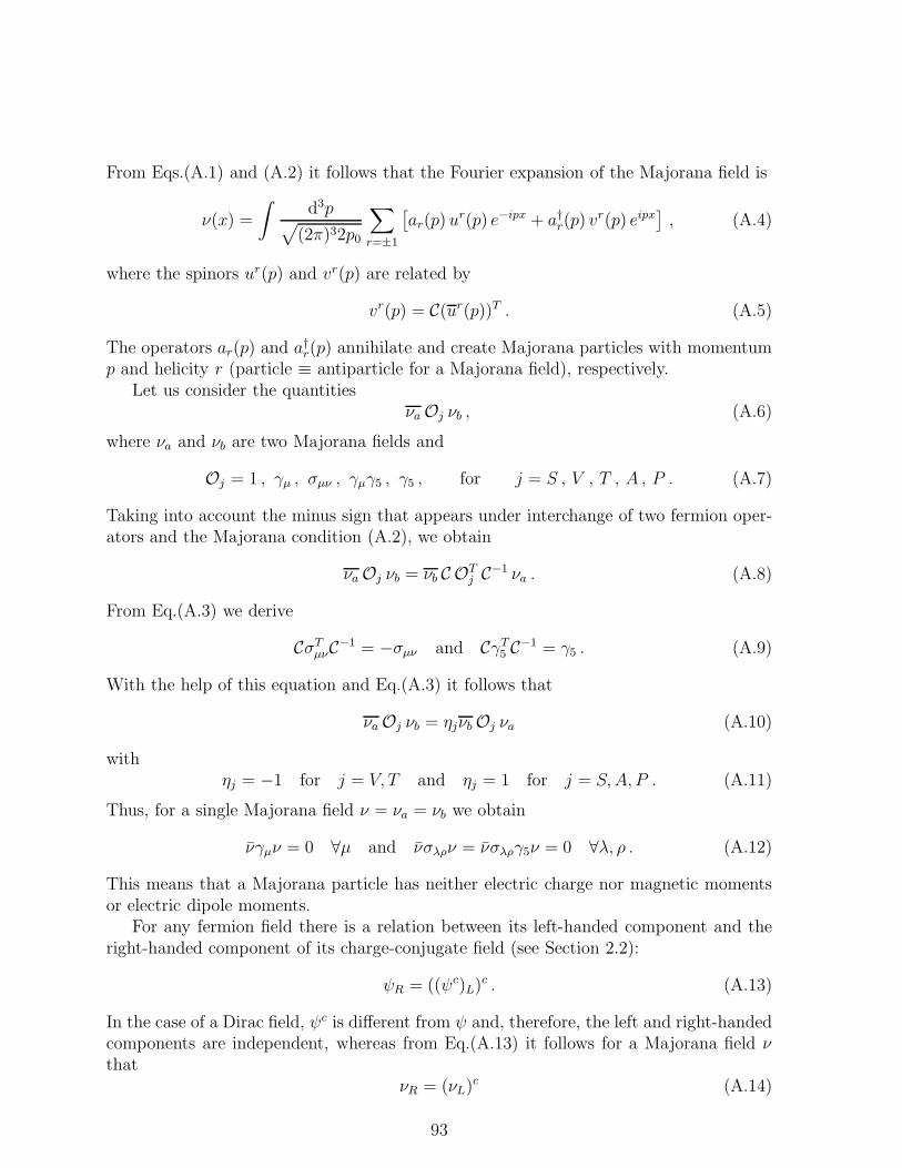
From Eqs.(A.1) and (A.2) it follows that the Fourier expansion of the Majorana field is

ν(x) =

∫

d3p√

(2π)32p0

∑

r=±1

[

ar(p) ur(p) e−ipx + a†r(p) v

r(p) eipx]

, (A.4)

where the spinors ur(p) and vr(p) are related by

vr(p) = C(ur(p))T . (A.5)

The operators ar(p) and a†r(p) annihilate and create Majorana particles with momentump and helicity r (particle ≡ antiparticle for a Majorana field), respectively.

Let us consider the quantitiesνaOj νb , (A.6)

where νa and νb are two Majorana fields and

Oj = 1 , γµ , σµν , γµγ5 , γ5 , for j = S , V , T , A , P . (A.7)

Taking into account the minus sign that appears under interchange of two fermion oper-ators and the Majorana condition (A.2), we obtain

νaOj νb = νb C OTj C−1 νa . (A.8)

From Eq.(A.3) we derive

CσTµνC−1 = −σµν and CγT5 C−1 = γ5 . (A.9)

With the help of this equation and Eq.(A.3) it follows that

νaOj νb = ηjνbOj νa (A.10)

withηj = −1 for j = V, T and ηj = 1 for j = S,A, P . (A.11)

Thus, for a single Majorana field ν = νa = νb we obtain

νγµν = 0 ∀µ and νσλρν = νσλργ5ν = 0 ∀λ, ρ . (A.12)

This means that a Majorana particle has neither electric charge nor magnetic momentsor electric dipole moments.

For any fermion field there is a relation between its left-handed component and theright-handed component of its charge-conjugate field (see Section 2.2):

ψR = ((ψc)L)c . (A.13)

In the case of a Dirac field, ψc is different from ψ and, therefore, the left and right-handedcomponents are independent, whereas from Eq.(A.13) it follows for a Majorana field νthat

νR = (νL)c (A.14)

93

and thus the left and right-handed components of a Majorana field are not independent

(in other words, a Majorana field is a two-component field).Though Dirac and Majorana neutrinos differ in the number of degrees of freedom,

it is nevertheless difficult to distinguish between the two in practice. The reason isthat in the standard weak interaction Lagrangians (2.1) and (2.2) only the left-handedcomponents νℓL (ℓ = e, µ, τ) of the flavour neutrino fields are present. These are connectedwith the left-handed components νkL of the neutrino mass eigenfields by the relationνℓL =

∑

k UℓkνkL (see Section 2). The mass eigenfields could be of Dirac or Majoranatype. In the first case we have νDk = νkL + νkR, where the νkR are independent degreesof freedom, whereas in the second case we have νMk = νkL + (νkL)

c. The only differencebetween the Dirac and Majorana case with respect to the standard weak interactionsresides in the mass term. In the limit of vanishing neutrino masses the right-handedDirac fields decouple from the standard weak interaction Lagrangians and the distinctionbetween Dirac and Majorana gets lost. Then the physical fields are simply given by theνℓL. In summary, we have arrived at the following conclusion [433]: With the standardweak interactions one cannot distinguish between the Dirac and Majorana nature of theneutrinos in the limit of vanishing neutrino masses. In other words, for the standardweak interactions, Dirac neutrinos with negative helicity and Dirac antineutrinos withpositive helicity are the same as Majorana neutrinos with positive and negative helicities,respectively, in this limit.

In neutrinoless double-β decay, which can occur only with Majorana neutrinos (seeSection 6), one needs to calculate the propagator

〈0|T(

νeL(x1)νTeL(x2)

)

|0〉 . (A.15)

With the Majorana mass eigenfields νk satisfying the relation νTk = −νkC this propagatoris obtained by the following steps:

〈0|T(

νeL(x1)νTeL(x2)

)

|0〉

=1 − γ5

2

∑

k

U2ek〈0|T

(

νk(x1)νTk (x2)

)

|0〉1 − γT52

= −1 − γ5

2

∑

k

U2ek〈0|T (νk(x1)νk(x2)) |0〉

1 − γ5

2C

= −∑

k

U2ekmk i

∫

d4p

(2π)4

e−ip(x1−x2)

p2 −m2k

1 − γ5

2C . (A.16)

Finally, we want to prove that the CP parity of a Majorana field is ±i. The CPtransformation of a Majorana field ν(x) is given by

UCP ν(x)U−1CP = ηCP γ0 ν(xP) , (A.17)

where the phase factor ηCP is the CP parity of the field ν(x), UCP is the unitary operatorof CP conjugation, x ≡ (x0, ~x) and xP ≡ (x0,−~x). The relation (A.17) can be written as

UCP C νT (x)U−1CP = −η∗CP γ0 C νT (xP) . (A.18)

94

Using the Majorana condition (A.2) one obtains

UCP ν(x)U−1CP = −η∗CP γ0 ν(xP) . (A.19)

From the comparison of the expressions (A.17) and (A.19) one finds that ηCP = −η∗CP,which implies that

η2CP = −1 (A.20)

and ηCP = ±i. As it can be seen from Eq.(A.18) written as

UCP νc(x)U−1

CP = −η∗CP γ0 νc(xP) , (A.21)

in general the product of the CP parities of particles and antiparticles is equal to −1.The relation (A.20) results from the fact that in the Majorana case there is no differencebetween particles and antiparticles.

References

[1] T. Kajita, Super-Kamiokande Coll., Talk presented at Neutrino ’98 [434], 1998.

[2] Y. Fukuda et al., Super-Kamiokande Coll., Phys. Rev. Lett. 81, 1562 (1998).

[3] W. Pauli, in Neutrino Physics, p. 1, edited by K. Winter, Cambridge University Press, 1991.

[4] E. Fermi, Ricerca Scient. 2, 12 (1933).

[5] E. Fermi, Z. Physik. 88, 161 (1934).

[6] F. Perrin, Comptes Rendues 197, 1625 (1933).

[7] O. Kofoed-Hansen, Phys. Rev. 71, 451 (1947); G.C. Hanna and B. Pontecorvo, Phys. Rev. 75, 451(1949).

[8] L.L. Langer and R.J.D. Moffat, Phys. Rev. 88, 689 (1952).

[9] L. Landau, Nucl. Phys. 3, 127 (1957).

[10] T.D. Lee and C.N. Yang, Phys. Rev. 105, 1671 (1957).

[11] A. Salam, Il Nuovo Cim. 5, 299 (1957).

[12] M. Goldhaber, L. Grodzins and A.W. Sunyar, Phys. Rev. 109, 1015 (1958).

[13] V.L. Telegdi, History of Original Ideas and Basic Discoveries in Particle Physics, edited by H.B.Newman and T. Ypsilantis, p. 421, Plenum Press, New York, published in cooperation with NATOScientific Affairs Division, 1996.

[14] L. Grenacs et al., Am. J. Phys. 50, 931 (1982).

[15] R.P. Feynman and M. Gell-Mann, Phys. Rev. 109, 193 (1958).

[16] E.C.G. Sudarshan and R. Marshak, Phys. Rev. 109, 1860 (1958).

[17] L.D. Landau, unpublished (1957), private communication of B. Pontecorvo to S.M. Bilenky.

[18] B. Pontecorvo, J. Exptl. Theoret. Phys. 33, 549 (1957) [Sov. Phys. JETP 6, 429 (1958)].

[19] B. Pontecorvo, J. Exptl. Theoret. Phys. 34, 247 (1958) [Sov. Phys. JETP 7, 172 (1958)].

[20] E. Majorana, Il Nuovo Cim. 14, 170 (1937).

95

[21] Z. Maki, M. Nakagawa and S. Sakata, Prog. Theor. Phys. 28, 870 (1962).

[22] B. Pontecorvo, Zh. Eksp. Teor. Fiz. 53, 1717 (1967) [Sov. Phys. JETP 26, 984 (1968)].

[23] V. Gribov and B. Pontecorvo, Phys. Lett. B 28, 493 (1969).

[24] S.M. Bilenky and B. Pontecorvo, Phys. Lett. B 61, 248 (1976).

[25] H. Fritzsch and P. Minkowski, Phys. Lett. B 62, 72 (1976).

[26] S.M. Bilenky and B. Pontecorvo, Lett. Nuovo Cim. 17, 569 (1976).

[27] V. Barger, P. Langacker, J.P. Leveille and S. Pakvasa, Phys. Rev. Lett. 45, 692 (1980).

[28] S.M. Bilenky, J. Hosek and S.T. Petcov, Phys. Lett. B 94, 495 (1980).

[29] I.Yu. Kobzarev et al., Yad. Fiz. 32, 1590 (1980) [Sov. J. Nucl. Phys. 32, 823 (1980)].

[30] J. Schechter and J.W.F. Valle, Phys. Rev. D 22, 2227 (1980).

[31] R.N. Mohapatra and P.B. Pal, Massive Neutrinos in Physics and Astrophysics, World ScientificLecture Notes in Physics, Vol. 41, World Scientific, Singapore, 1991.

[32] M. Gell-Mann, P. Ramond and R. Slansky, in Supergravity, p. 315, edited by F. van Nieuwenhuizenand D. Freedman, North Holland, Amsterdam, 1979.

[33] T. Yanagida, Proc. of the Workshop on Unified Theory and the Baryon Number of the Universe,KEK, Japan, 1979.

[34] R.N. Mohapatra and G. Senjanovic, Phys. Rev. Lett. 44, 912 (1980).

[35] C. Caso et al., Particle Data Group, Eur. Phys. J. C 3, 1 (1998).

[36] R. Davis, Harmer and K.C. Hoffman, Phys. Rev. Lett. 21, 1205 (1968).

[37] R. Davis, Prog. Part. Nucl. Phys. 32, 13 (1994).

[38] B.T. Cleveland et al., Astrophys. J. 496, 505 (1998).

[39] K.S. Hirata et al., Kamiokande Coll., Phys. Rev. D 38, 448 (1988).

[40] K.S. Hirata et al., Kamiokande Coll., Phys. Rev. D 44, 2241 (1991).

[41] K.S. Hirata et al., Kamiokande Coll., Phys. Rev. Lett. 77, 1683 (1996).

[42] P. Anselmann et al., GALLEX Coll., Phys. Lett. B 285, 376 (1992).

[43] W. Hampel et al., GALLEX Coll., Phys. Lett. B 388, 384 (1996).

[44] A.I. Abazov et al., SAGE Coll., Phys. Rev. Lett. 67, 3332 (1991).

[45] D.N. Abdurashitov et al., SAGE Coll., Phys. Rev. Lett. 77, 4708 (1996).

[46] K. Inoue, Super-Kamiokande Coll., Talk presented at the 5th International Workshop on Topics

in Astroparticle and Underground Physics, Gran Sasso, Italy, September, 1997 (http://www-sk.-icrr.u-tokyo.ac.jp/doc/sk/pub/pub sk.html).

[47] Y. Fukuda et al., Super-Kamiokande Coll., Phys. Rev. Lett. 81, 1158 (1998).

[48] Y. Suzuki, Super-Kamiokande Coll., Talk presented at Neutrino ’98 [434], 1998.

[49] Y. Fukuda et al., Kamiokande Coll., Phys. Lett. B 335, 237 (1994).

[50] R. Becker-Szendy et al., IMB Coll., Nucl. Phys. B (Proc. Suppl.) 38, 331 (1995).

[51] W.W.M. Allison et al., Soudan-2 Coll., Phys. Lett. B 391, 491 (1997).

[52] M. Ambrosio et al., MACRO Coll., Phys. Lett. B 434, 451 (1998).

96

[53] C. Athanassopoulos et al., LSND Coll., Phys. Rev. Lett. 77, 3082 (1996).

[54] C. Athanassopoulos et al., LSND Coll., Phys. Rev. Lett. 81, 1774 (1998).

[55] V. Lobashov, Talk presented at Neutrino ’98 [434].

[56] C. Weinheimer, Talk presented at Neutrino ’98 [434], 1998.

[57] E.W. Kolb and M.S. Turner, The Early Universe, Addison-Wesley, 1990.

[58] F. Boehm and P. Vogel, Physics of Massive Neutrinos, Cambridge University Press, Cambridge,1987.

[59] B. Kayser, F. Gibrat-Debu and F. Perrier, The Physics of Massive Neutrinos, World ScientificLecture Notes in Physics, Vol.25, World Scientific, Singapore, 1989.

[60] J.N. Bahcall, Neutrino Physics and Astrophysics, Cambridge University Press, 1989.

[61] C.W. Kim and A. Pevsner, Neutrinos in Physics and Astrophysics, Contemporary Concepts inPhysics, Vol. 8, Harwood Academic Press, Chur, Switzerland, 1993.

[62] S.M. Bilenky and B. Pontecorvo, Phys. Rep. 41, 225 (1978).

[63] P.H. Frampton and P. Vogel, Phys. Rep. 82, 339 (1982).

[64] J.D. Vergados, Phys. Rep. 133, 1 (1986).

[65] S.M. Bilenky and S.T. Petcov, Rev. Mod. Phys. 59, 671 (1987).

[66] J.W.F. Valle, Prog. Part. Nucl. Phys. 26, 91 (1991).

[67] L. Oberauer and F. von Feilitzsch, Rept. Prog. Phys. 55, 1093 (1992).

[68] G. Gelmini and E. Roulet, Rept. Prog. Phys. 58, 1207 (1995).

[69] J. Brunner, Fortsch. Phys. 45, 343 (1997).

[70] K. Zuber, Phys. Rep. 305, 295 (1998).

[71] J.M. Conrad, Talk presented at the 29th International Conference on High-Energy Physics (ICHEP98), Vancouver, Canada, 23-29 July, 1998 (hep-ex/9811009).

[72] J.W.F. Valle, hep-ph/9809234 (1998).

[73] G. Raffelt, hep-ph/9902271 (1999).

[74] S.L. Glashow, Nucl. Phys. 22, 597 (1961).

[75] S. Weinberg, Phys. Rev. Lett. 19, 1264 (1967).

[76] A. Salam, Proc. of the 8th Nobel Symposium on Elementary Particle Theory, Relativistic Groups

and Analyticity, edited by N. Svartholm, 1969.

[77] R. Bertlmann and H. Pietschmann, Phys. Rev. D 15, 683 (1977); J. Ellis et. al., Ann. Rev. Nucl.Part. Sci. 32, 443 (1982).

[78] N. Cabibbo, Phys. Rev. Lett. 10, 531 (1963).

[79] M. Kobayashi and T. Maskawa, Prog. Theor. Phys. 49, 652 (1973).

[80] J. Schechter and J.W.F. Valle, Phys. Rev. D 24, 1883 (1981) [Erratum: D 25, 283 (1982)].

[81] S.T. Petcov, Yad. Fiz. 25, 641 (1977) [Sov. J. Nucl. Phys. 25, 340, 698(E) (1977)].

[82] T.P. Cheng and L.F. Li, Phys. Rev. D 16, 1425 (1977).

[83] B.W. Lee and R.E. Shrock, Phys. Rev. D 16, 1444 (1977).

[84] L.L. Chau and W.Y. Keung, Phys. Rev. Lett. 53, 1802 (1984).

97

[85] C. Jarlskog, Phys. Rev. Lett. 55, 1039 (1985); Z. Phys. C 29, 491 (1985); C. Jarlskog and R.Stora, Phys. Lett. B 208, 268 (1988); C. Jarlskog, Proc. of CP Violation, edited by C. Jarlskog,Advanced Series in High Energy Physics Vol. 3, p. 3, World Scientific, Singapore, 1989.

[86] D.D. Wu, Phys. Rev. D 33, 860 (1986); I. Dunietz, O.W. Greenberg and D.D. Wu, Phys. Rev.Lett. 55, 2935 (1985).

[87] J.D. Bjorken and I. Dunietz, Phys. Rev. D 36, 2109 (1987); I. Dunietz, Ann. Phys. 184, 350(1988).

[88] J. Schechter and J.W.F. Valle, Phys. Rev. D 21, 309 (1980).

[89] I. Schur, Am. J. Math. 67, 472 (1945).

[90] B. Zumino, J. Math. Phys. 3, 1055 (1962).

[91] G. Gelmini and M. Roncadelli, Phys. Lett. B 99, 411 (1981).

[92] H. Georgi et al., Nucl. Phys. B 193, 297 (1983).

[93] J.E. Kim, Phys. Rep. 150, 1 (1987).

[94] W. Grimus and H. Neufeld, Nucl. Phys. B 325, 18 (1989).

[95] L. Wolfenstein, Phys. Lett. B 107, 77 (1981).

[96] S.M. Bilenky, N.P. Nedelcheva and S.T. Petcov, Nucl. Phys. B 247, 61 (1984).

[97] B. Kayser, Phys. Rev. D 30, 1023 (1984).

[98] S.M. Bilenky and S.T. Petcov, Rev. Mod. Phys. 59, 671 (1987).

[99] W. Konetschny and W. Kummer, Phys. Lett. B 70, 433 (1977).

[100] A. Zee, Phys. Lett. B 93, 387 (1980).

[101] A. Zee, Phys. Lett. B 161, 141 (1985).

[102] A. Zee, Nucl. Phys. B 264, 99 (1986).

[103] M.B. Voloshin, Sov. J. Nucl. Phys. 48, 512 (1988).

[104] K.S. Babu and R.N. Mohapatra, Phys. Rev. D 43, 2278 (1991).

[105] K.S. Babu, Phys. Lett. B 203, 132 (1988).

[106] M. Doi et al., Phys. Lett. B 102, 323 (1981).

[107] P. Langacker et al., Nucl. Phys. B 282, 589 (1987).

[108] J.C. Pati and A. Salam, Phys. Rev. D 10, 275 (1975); R.N. Mohapatra and J.C. Pati, Phys. Rev.D 11, 566 and 2558 (1975).

[109] R.N. Mohapatra and G. Senjanovic, Phys. Rev. D 23, 165 (1981).

[110] G. Ecker, W. Grimus and M. Gronau, Nucl. Phys. B 279, 429 (1987).

[111] G.C. Branco, W. Grimus and L. Lavoura, Nucl. Phys. B 312, 492 (1989).

[112] K. Kanaya, Prog. Theor. Phys. 64, 2278 (1980).

[113] J. Schechter and J.W.F. Valle, Phys. Rev. D 25, 774 (1982).

[114] D. Chang, R.N. Mohapatra and M.K. Parida, Phys. Rev. Lett. 52, 1072 (1984); D. Chang andR.N Mohapatra, Phys. Rev. D 32, 1248 (1985); D.G. Lee and R.N. Mohapatra, Phys. Lett. B 329,463 (1994).

[115] S.A. Bludman, D.C. Kennedy and P.G. Langacker, Phys. Rev. D 45, 1810 (1992).

98

[116] S.A. Bludman, D.C. Kennedy and P.G. Langacker, Nucl. Phys. B 374, 373 (1992).

[117] E. Witten, Phys. Lett. B 91, 81 (1980).

[118] J.C. Pati and A. Salam, Phys. Rev. Lett. 31, 661 (1973).

[119] H. Georgi and S.L. Glashow, Phys. Rev. Lett. 32, 438 (1974).

[120] P. Langacker, Phys. Rep. 72, 185 (1981).

[121] F. Wilczek and A. Zee, Phys. Rev. Lett. 43, 1571 (1979).

[122] S. Weinberg, Phys. Rev. Lett. 43, 1566 (1979).

[123] S. Weinberg, Phys. Rev. D 22, 1694 (1980).

[124] H.A. Weldon and A. Zee, Nucl. Phys. B 173, 269 (1980).

[125] S. Weinberg, Int. J. Mod. Phys. A 2, 301 (1987).

[126] E.Kh. Akhmedov, Z.G. Berezhiani and G. Senjanovic, Phys. Rev. Lett. 69, 3013 (1992).

[127] E.Kh. Akhmedov, Z.G. Berezhiani, G. Senjanovic and Z. Tao, Phys. Rev. D 47, 3245 (1993).

[128] L. Wolfenstein, Nucl. Phys. B 186, 147 (1981).

[129] M. Kobayashi, C.S. Lim and M.M. Nojiri, Phys. Rev. Lett. 67, 1685 (1991).

[130] C. Giunti, C.W. Kim and U.W. Lee, Phys. Rev. D 46, 3034 (1992).

[131] S. Nussinov, Phys. Lett. B 63, 201 (1976).

[132] B. Kayser, Phys. Rev. D 24, 110 (1981).

[133] C. Giunti, C.W. Kim and U.W. Lee, Phys. Rev. D 44, 3635 (1991).

[134] C. Giunti, C.W. Kim and U.W. Lee, Phys. Rev. D 45, 2414 (1992).

[135] C. Giunti, C.W. Kim and U.W. Lee, Phys. Lett. B 274, 87 (1992).

[136] C. Giunti, C.W. Kim, J.A. Lee and U.W. Lee, Phys. Rev. D 48, 4310 (1993).

[137] J. Rich, Phys. Rev. D 48, 4318 (1993).

[138] K. Kiers, S. Nussinov and N. Weiss, Phys. Rev. D 53, 537 (1996).

[139] W. Grimus and P. Stockinger, Phys. Rev. D 54, 3414 (1996).

[140] J.E. Campagne, Phys. Lett. B 400, 135 (1997).

[141] Y. Grossman and H.J. Lipkin, Phys. Rev. D 55, 2760 (1997).

[142] K. Kiers and N. Weiss, Phys. Rev. D 57, 3091 (1998).

[143] C. Giunti, C.W. Kim and U.W. Lee, Phys. Lett. B 421, 237 (1997).

[144] C. Giunti and C.W. Kim, Phys. Rev. D 58, 017301 (1998).

[145] W. Grimus, P. Stockinger and S. Mohanty, Phys. Rev. D 59, 013011 (1998).

[146] L. Stodolsky, Phys. Rev. D 58, 036006 (1998).

[147] E.J. Chun, C.W. Kim and U.W. Lee, Phys. Rev. D 58, 093003 (1998).

[148] Y. Koide, Phys. Rev. D 57, 5836 (1998).

[149] Y. Koide and H. Fusaoka, Phys. Rev. D 59, 053004 (1998).

[150] S.M. Bilenky and C. Giunti, Phys. Lett. B 300, 137 (1993).

[151] N. Cabibbo, Phys. Lett. B 72, 333 (1978).

99

[152] D. Orestano, NOMAD Coll., Talk presented at the CAPP 98 Workshop, CERN, June, 1998 [435].

[153] F. Dydak et al., CDHS Coll., Phys. Lett. B 134, 281 (1984).

[154] N. Ushida et al., Phys. Rev. Lett. 57, 2897 (1986).

[155] P. Vilain et al., CHARM II Coll., Z. Phys. C 64, 539 (1994).

[156] K.S. McFarland et al., CCFR Coll., Phys. Rev. Lett. 75, 3993 (1995).

[157] CHORUS Coll., Talk presented at the 29th International Conference on High-Energy Physics

(ICHEP 98), Vancouver, Canada, 23-29 July 1998 (preprint hep-ex/9807024).

[158] J. Altegoer et al., NOMAD Coll., Phys. Lett. B 431, 219 (1998).

[159] M. Apollonio et al., CHOOZ Coll., Phys. Lett. B 420, 397 (1998).

[160] G. Zacek et al., Phys. Rev. D 34, 2621 (1986).

[161] G.S. Vidyakin et al., JETP Lett. 59, 390 (1994).

[162] B. Achkar et al., Bugey Coll., Nucl. Phys. B 434, 503 (1995).

[163] L. Wolfenstein, Phys. Rev. D 17, 2369 (1978); ibid. 20, 2634 (1979).

[164] S.P. Mikheyev and A.Yu. Smirnov, Yad. Fiz. 42, 1441 (1985) [Sov. J. Nucl. Phys. 42, 913 (1985)];Il Nuovo Cim. C 9, 17 (1986); Zh. Eksp. Teor. Fiz. 91, 7 (1986) [Sov. Phys. JETP 64, 4 (1986)].

[165] V. Barger, K. Whisnant, S. Pakvasa and R.J.N. Phillips, Phys. Rev. D 22, 2718 (1980).

[166] S.P. Rosen and J.M. Gelb, Phys. Rev. D 34, 969 (1986).

[167] H.A. Bethe, Phys. Rev. Lett. 56, 1305 (1986).

[168] A. Halprin, Phys. Rev. D 34, 3462 (1986); P.D. Mannheim, Phys. Rev. D 37, 1935 (1988).

[169] W. Grimus and T. Scharnagl, Mod. Phys. Lett. A 8, 1943 (1993).

[170] P.B. Pal and T.N. Pham, Phys. Rev. D 40, 259 (1989).

[171] J. Liu, Phys. Rev. D 45, 1428 (1992).

[172] P.B. Pal, Int. J. Mod. Phys. A 22, 5387 (1992).

[173] C. Giunti, C.W. Kim and W.P. Lam, Phys. Rev. D 43, 164 (1991).

[174] J.N. Bahcall and R. Ulrich, Rev. Mod. Phys. 60, 297 (1988).

[175] J.N. Bahcall and M.H. Pinsonneault, Rev. Mod. Phys. 67, 781 (1995).

[176] L.L. Foldy and S.A. Wouthuysen, Phys. Rev. 78, 29 (1950).

[177] P.G. Langacker et al., Nucl. Phys. B 282, 589 (1987).

[178] S.P. Mikheyev and A.Yu. Smirnov, Prog. Part. Nucl. Phys. 23, 41 (1989).

[179] L. Stodolsky, Phys. Rev. D 36, 2273 (1987).

[180] H. Nunokawa, A. Rossi, V.B. Semikoz and J.W.F. Valle, Nucl. Phys. B 472, 495 (1996); A.B.Balantekin, J.M. Fetter and F.N. Loreti, Phys. Rev. D 54, 3941 (1996); C.P. Burgess and D.Michaud, Ann. Phys. 256, 1 (1997).

[181] P. Bamert, C.P. Burgess and D. Michaud, Nucl. Phys. B 513, 319 (1998).

[182] A.J. Baltz and J. Weneser, Phys. Rev. D 37, 3364 (1988).

[183] T.K. Kuo and J. Pantaleone, Rev. Mod. Phys. 61, 937 (1989).

[184] W.C. Haxton, Ann. Rev. Astron. Astrophys. 33, 459 (1995).

100

[185] L.I. Schiff, Quantum Mechanics, McGaw-Hill, Singapore, 1987.

[186] V. A. Naumov, Zh. Eksp. Teor. Fiz. 101, 3 (1992) [Sov. Phys. JETP. 74, 1 (1992)]; Int. J. Mod.Phys. D 1, 379 (1992); Phys. Lett. B323, 351 (1994).

[187] S.J. Parke, Phys. Rev. Lett. 57, 1275 (1986).

[188] W.C. Haxton, Phys. Rev. Lett. 57, 1271 (1986); Phys. Rev. D 35, 2352 (1987).

[189] T.K. Kuo and J. Pantaleone, Phys. Rev. D 39, 1930 (1989).

[190] M. Born and V. Fock, Z. Phys. 51, 165 (1928).

[191] E. Lisi and D. Montanino, Phys. Rev. D 56, 1792 (1997).

[192] C. Giunti, C.W. Kim and M. Monteno, Nucl. Phys. B 521, 3 (1998).

[193] S.T. Petcov, Phys. Lett. B 200, 373 (1988); Phys. Lett. B 214, 139 (1988).

[194] S.T. Petcov and J. Rich, Phys. Lett. B 224, 426 (1989).

[195] S.T. Petcov, Phys. Lett. B 191, 299 (1987).

[196] C. Zener, Proc. Roy. Soc. Lon. A 137, 696 (1932).

[197] L. Landau, Phys. Z. Sov. 2, 46 (1932).

[198] A. Joye and Ch.-E. Pfister, preprint math-ph/9807031 (1998).

[199] P. Pizzochero, Phys. Rev. D 36, 2293 (1987).

[200] A.B. Balantekin and J.F. Beacom, Phys. Rev. D 54, 6323 (1996); A.B. Balantekin, J.F. Beacomand J.B. Fetter, Phys. Lett. B 427, 317 (1998).

[201] T. Kaneko, Prog. Theor. Phys. 78, 532 (1987); S. Toshev, Phys. Lett. B 196, 170 (1987); M. Ito,T. Kaneko and M. Nakagawa, Prog. Theor. Phys. 79, 13 (1988).

[202] D. Notzold, Phys. Rev. D 36, 1625 (1987).

[203] P.I. Krastev and S.T. Petcov, Phys. Lett. B 207, 64 (1988) [Erratum: B 214, 661 (1988)].

[204] V.F. Hess, Phys. Zeitschr. 13, 1084 (1913).

[205] A. Pais, Inward bound, Oxford University Press, Oxford, 1994.

[206] L.V. Volkova, Jad. Fiz. 31, 784 (1980) [Sov. J. Nucl. Phys. 31, 1510 (1980)].

[207] K. Mitsui, Y. Minorikawa and H. Komori, Il Nuovo Cim. C 9, 995 (1986).

[208] E.V. Bugaev and V.A. Naumov, Izv. Akad. Nauk SSSR, Ser. Fiz. 50, 2239 (1986) [Bull. Acad. ofSci. of the USSR, Phys. Ser. 50, 156 (1986)].

[209] E.V. Bugaev and V.A. Naumov, Yad. Fiz. 45, 1380 (1987) [Sov. J. Nucl. Phys. 45, 857 (1987)].

[210] A.V. Butkevich, L.G. Dedenko and I.M. Zeleznykh, Yad. Fiz. 50, 142 (1989) [Sov. J. Nucl. Phys.50, 90 (1989)].

[211] G. Barr, T.K. Gaisser and T. Stanev, Phys. Rev. D 39, 3532 (1989).

[212] H. Lee and Y.S. Koh, Il Nuovo Cim. 105 B, 883 (1989).

[213] E.V. Bugaev and V.A. Naumov, Phys. Lett. B 232, 391 (1989).

[214] M. Honda, K. Kasahara, K. Hidaka and S. Midorikawa, Phys. Lett. B 248, 193 (1990).

[215] M. Honda, T. Kajita, K. Kasahara and S. Midorikawa, Phys. Rev. D 52, 4985 (1995).

[216] V. Agrawal, T.K. Gaisser, P. Lipari and T. Stanev, Phys. Rev. D 53, 1314 (1996).

101

[217] T.K. Gaisser, M. Honda, K. Kasahara, S. Midorikawa, V. Naumov and T. Stanev, Phys. Rev. D54, 5578 (1996).

[218] P. Lipari, T. Stanev and T.K. Gaisser, Phys. Rev. D 58, 073003 (1998).

[219] T.K. Gaisser, Cosmic Rays and Particle Physics, Cambridge University Press, Cambridge, 1990.

[220] V.A. Dogiel, V.S. Berezinsky, S.V. Bulanov and V.S. Ptuskin, Astrophysics of Cosmic Rays, editedby V.L. Ginzburg, North-Holland, Amsterdam, 1990.

[221] P. Lipari, Astropart. Phys. 1, 195 (1993).

[222] A. Misaki, V.A. Naumov, T.S. Sinegovskaya and S.I. Sinegovsky, Proc. of the 25th International

Cosmic Ray Conference, Durban, South Africa, edited by M. S. Potgieter et al., p. 129, 1997.

[223] V.A. Naumov, T.S. Sinegovskaya and S.I. Sinegovsky, Il Nuovo Cim. A 111, 129 (1998).

[224] J.A. Simpson, Ann. Rev. Nucl. Part. Sci. 33, 323 (1983).

[225] W.R. Webber and J.A. Lezniak, Astrophys. Space Sci. 30, 361 (1974).

[226] E.-S. Seo et al., Proc. of the 22nd International Cosmic Ray Conference, Dublin, Ireland, editedby M. Cawley et. al., Vol. 2, p. 627, Reprint Ltd., Dublin, Ireland, 1991.

[227] E.V. Bugaev and V.A. Naumov, Proc. of the Second International Symposium Underground

Physics’87, Baksan Valley, August 1987, edited by G. V. Domogatsky et al., Nauka, Moscow,p. 255, 1988.

[228] P. Lipari and T. Stanev, Proc. of the 24th International Cosmic Ray Conference, Rome, Vol. 1,p. 694, 1995.

[229] H. Lee and S.A. Bludman, Phys. Rev. D 37, 122 (1988).

[230] J.L. Osborne, S.S. Said and A.E. Wolfendale, Proc. Phys. Soc. 86, 93 (1965).

[231] T.K. Gaisser, Proc. of Neutrino ’96, Helsinki, June 1996, edited by K. Enqvist et al., p. 211, WorldScientific, Singapore, 1997.

[232] T.K. Gaisser and T. Stanev, Phys. Rev. D 57, 1977 (1998).

[233] T.K. Gaisser, Phil. Trans. Roy. Soc. Lon. A 346, 75 (1994).

[234] M.A. Markov, Proc. of 1960 Annual International Conference on High Energy Physics, Rochester,edited by E.C.G. Sudarshan et al., 1960.

[235] K. Greisen, Ann. Rev. Nucl. Sci. 10, 63 (1960).

[236] C.V. Achar et al., Phys. Lett. 18, 196 and 19, 78 (1965).

[237] F. Reines et al., Phys. Rev. Lett. 15, 429 (1965).

[238] M.A. Markov and I.M. Zhelenykh, Nucl. Phys. 27, 385 (1961).

[239] G.T. Zatsepin and V.A. Kuzmin, Sov. J. Nucl. Phys. 14, 1294 (1962).

[240] R. Cowsik, Y. Pal and S.N. Tandon, Proc. Ind. Acad. Sci. 63, 217 (1966).

[241] E.W. Beier and E.D. Frank, Phil. Trans. Roy. Soc. Lon. A 346, 63 (1994).

[242] K.S. Hirata et al., Kamiokande Coll., Phys. Lett. B 205, 416 (1988).

[243] K.S. Hirata et al., Kamiokande Coll., Phys. Lett. B 280, 146 (1992).

[244] R. Becker-Szendy et al., IMB Coll., Phys. Rev. Lett. 69, 1010 (1992).

[245] R. Clark et al., IMB Coll., Phys. Rev. Lett. 79, 345 (1997).

[246] K. Daum et al., Frejus Coll., Z. Phys. C 66, 417 (1995).

102

[247] M. Aglietta et al., NUSEX Coll., Europhys. Lett. 8, 611 (1989).

[248] T.K. Gaisser, F. Halzen and T. Stanev, Phys. Rep. 258, 174 (1995).

[249] W. Frati et al., Phys. Rev. D 48, 1140 (1993).

[250] M.M. Boliev et al., Proc. of the 24th International Cosmic Ray Conference, ICRC ’95, Rome, Vol.1, p. 686, Arti Grafiche Editoriali, Urbino, Italy, 1995; ibidem, p. 722; S.P. Mikheyev, Proc. of the8th Rencontres de Blois on Neutrinos, Dark Matter, and the Universe, Blois, France, 1996; M.M.Boliev et al., Proc. of the International Workshop on Aspects of Dark Matter in Astrophysics and

Particle Physics, DARK ’96, Heidelberg, Germany, 1996.

[251] Y. Totsuka et al., Kamiokande Coll., Nucl. Phys. B 31 (Proc. Suppl.), 428 (1993).

[252] S. Hatakeyama et al., Kamiokande Coll., Phys. Rev. Lett. 81, 2016 (1998).

[253] P. Lipari, M. Lusignoli and F. Sartogo, Phys. Rev. Lett. 74, 4384 (1995).

[254] T.J. Haines et al., IMB Coll., Phys. Rev. Lett. 57, 1986 (1986).

[255] E. Kearns, Nucl. Phys. B (Proc. Suppl.) 70, 315 (1999) (hep-ex/9803007).

[256] T. Kafka, Nucl. Phys. B (Proc. Suppl.) 70, 340 (1999) (hep-ex/9712281).

[257] M.C. Gonzalez-Garcia et al., Phys. Rev. D 58, 033004 (1998).

[258] M.C. Gonzalez-Garcia et al., preprint FTUV/98-56, IFIC/98-57, hep-ph/9807305 (1998).

[259] R. Foot, R.R. Volkas and O. Yasuda, Phys. Rev. D 58, 013006 (1998).

[260] O. Yasuda, Phys. Rev. D 58, 091301 (1998).

[261] G.L. Fogli, E. Lisi, A. Marrone and G. Scioscia, Phys. Rev. D 59, 033001 (1999).

[262] G.L. Fogli, E. Lisi and D. Montanino, Phys. Rev. D 49, 3626 (1994).

[263] G.L. Fogli, E. Lisi and D. Montanino, Astropart. Phys. 4 177 (1995).

[264] G.L. Fogli and E. Lisi, Phys. Rev. D 52, 2775 (1995).

[265] G.L. Fogli, E. Lisi, D. Montanino and G. Scioscia, Phys. Rev. D 55, 4385 (1997).

[266] G.L. Fogli, E. Lisi, A. Marrone and D. Montanino, Phys. Lett. B 425, 341 (1998).

[267] J.N. Flanagan, J.G. Learned and S. Pakvasa, Phys. Rev. D 57, R2649 (1998).

[268] J. Bunn, R. Foot and R. Volkas, Phys. Lett. B 413, 109 (1997).

[269] R. Foot, R. Volkas and O. Yasuda, Phys. Rev. D 58, 013006 (1998).

[270] R. Foot, C.N. Leung and O. Yasuda, Phys. Lett. B 443, 185 (1998).

[271] Y. Suzuki, Proc. of Neutrino 96, Helsinki, June 1996, edited by K. Enqvist et. al., p. 237, WorldScientific, Singapore, 1997.

[272] F. Vissani and A.Yu. Smirnov, Phys. Lett. B 432, 376 (1998).

[273] A. McDonald, SNO Coll., Talk presented at Neutrino ’98 [434], 1998.

[274] Y. Fukuda et al., Kamiokande Coll., Phys. Lett. B 388, 397 (1996).

[275] K.R.S. Balaji, G. Rajasekaran and S. Uma Sankar, preprint hep-ph/9806256 (1998).

[276] F. Vissani, Talk presented at the Ringberg Euroconference New Trends in Neutrino Physics, Te-gernsee, Germany, May 1998, preprint DESY-98-135, 1998.

[277] J.G. Learned, S. Pakvasa and J.L. Stone, Phys. Lett. B 435, 131 (1998).

[278] E. Akhmedov, P. Lipari and M. Lusignoli, Phys. Lett. B 300, 128 (1993).

103

[279] G.L. Fogli, E. Lisi and A. Marrone, Phys. Rev. D 57, 5893 (1998).

[280] Q.Y. Liu and A.Yu. Smirnov, Nucl. Phys. B 524, 505 (1998).

[281] V.K. Ermilova, V.A. Tsarev and V.A. Chechin, Kr. Soob., Fiz. [Short Notices of the LebedevInstitute] 5, 26 (1986); E.Kh. Akhmedov, Yad. Fiz. 47, 475 (1988) [Sov. J. Nucl. Phys. 47, 301(1988)].

[282] Q.Y. Liu, S.P. Mikheyev and A.Yu. Smirnov, hep-ph/9803415 (1998).

[283] S.T. Petcov, Phys. Lett. B 434, 321 (1998).

[284] E.Kh. Akhmedov, Nucl. Phys. B 538, 25 (1999).

[285] M. Chizhov, M. Maris and S.T. Petcov, hep-ph/9810501 (1998).

[286] E.Kh. Akhmedov, A. Dighe, P. Lipari and A.Yu. Smirnov, hep-ph9808270 (1998).

[287] P. Lipari and M. Lusignoli, Phys. Rev. D 57, 3842 (1998).

[288] F. Boehm et al., The Palo Verde experiment, 1996 (http://www.cco.caltech.edu/˜songhoon/Palo-Verde/Palo-Verde.html).

[289] F. Boehm et al., Palo Verde Coll., Nucl. Phys. B (Proc. Suppl.) 70, 191 (1999).

[290] F. Suekane, preprint TOHOKU-HEP-97-02 (1997).

[291] A. Suzuki, Talk presented at NOW’98 [376], 1998.

[292] S. Schonert et al., Nucl. Phys. B (Proc. Suppl.) 70, 195 (1999).

[293] D. Ayres et al., MINOS Coll., report NUMI-L-63 (1995).

[294] P. Cennini et al., ICARUS Coll., report LNGS-94/99-I (1994).

[295] H. Shibuya et al., OPERA Coll., report CERN-SPSC-97-24 (1997).

[296] M. Ambrosio et al., NOE Coll., Nucl. Instr. Meth. A 363, 604 (1995); G.C. Barbarino et al., NOEColl., report INFN/AE-96/11 (1996).

[297] T. Ypsilantis et al., AQUA-RICH Coll., report CERN-LAA/96-13 (1996).

[298] G. Baldini et al., NICE Coll., report LNGS-LOI 98/13 (1998).

[299] P. Picchi and F. Pietropaolo, Talk presented at Neutrino ’98 [434] (preprint hep-ph/9812222)(1998).

[300] M. Aglietta et al., preprint CERN-SPSC-98-28 (1998).

[301] G. Battistoni and P. Lipari, to appear in the Proc. of the 1998 Vulcano Workshop on Frontier

Objects in Astrophysics and Particle Physics, 1998 (hep-ph/9807475).

[302] A. Geiser, Contribution to NOW’98 [376], 1998 (hep-ph/9810493).

[303] J.N. Bahcall and M.H. Pinsonneault, Rev. Mod. Phys. 64, 885 (1992).

[304] J.N. Bahcall, S. Basu and M.H. Pinsonneault, Phys. Lett. B 433, 1 (1998).

[305] S. Turck-Chieze, S. Cahen, M. Casse and C. Doom, Astrophys. J. 335, 415 (1988).

[306] S. Turck-Chieze and I. Lopes, Astrophys. J. 408, 347 (1993).

[307] S. Turck-Chieze et al., Phys. Rep. 230, 57 (1993).

[308] V. Castellani, S. Degl’Innocenti and G. Fiorentini, Astron. Astrophys. 271, 601 (1993).

[309] V. Castellani et al., Phys. Lett. B 324, 425 (1994).

[310] F. Ciacio, S. Degl’Innocenti and B. Ricci et al., Astron. Astrophys. Suppl. Ser. 123, 449 (1997).

104

[311] M. Koshiba, Phys. Rep. 220, 229 (1992).

[312] V. Castellani et al., Phys. Rep. 281, 309 (1997).

[313] V.S. Berezinsky, Invited lecture at the 25th International Cosmic Ray Conference, Durban, 28 July– 8 August, 1997 (astro-ph/9710126).

[314] J.N. Bahcall, Lectures presented at the XXV SLAC Summer Institute on Particle Physics, Physics

of Leptons, August 4–15, 1997 (hep-ph/9711358).

[315] J.N. Bahcall, Talk presented at Neutrino ’98 [434], 1998 (hep-ph/9808162).

[316] A.Yu. Smirnov, Talk presented at Neutrino ’98 [434], 1998 (hep-ph/9809481).

[317] J.N. Bahcall et al., Phys. Rev. C 54, 411 (1996).

[318] J.N. Bahcall, Phys. Rev. C 56, 3391 (1997).

[319] J.N. Bahcall, Phys. Rev. D 49, 3923 (1994).

[320] J.N. Bahcall, Phys. Rev. D 44, 1644 (1991).

[321] J.N. Bahcall and P.I. Krastev, Phys. Rev. D 53, 4211 (1996).

[322] T. Kirsten, GNO Coll., Talk presented at Neutrino ’98 [434], 1998.

[323] V.N. Gavrin, SAGE Coll., Talk presented at Neutrino ’98 [434], 1998.

[324] B. Pontecorvo, Chalk River Report PD-205 (1946).

[325] L.W. Alvarez, University of California Radiation Laboratory Report UCRL-328 (1949).

[326] W. Hampel et al., GALLEX Coll., Phys. Lett. B 420, 114 (1998).

[327] W. Hampel et al., GALLEX Coll., preprint DAPNIA-SPP-98-07 (1998).

[328] M. Cribier et al., GALLEX Coll., Nucl. Phys. B (Proc. Suppl.) 70, 284 (1999).

[329] J.N. Bahcall, P.I. Krastev and A.Yu. Smirnov, Phys. Rev. D 58, 096016 (1998).

[330] J.N. Bahcall, M.H. Pinsonneault, S.Basu and J. Christensen-Dalsgaard, Phys. Rev. Lett. 78, 171(1997).

[331] B. Ricci et al., Phys. Lett. B 407, 155 (1997).

[332] D. Gough, Talk presented at Neutrino ’98 [434], 1998.

[333] A.S. Brun, S. Turck-Chieze and P Morel, preprint astro-ph/9806272 (1998).

[334] M. Spiro and D. Vignaud, Phys. Lett. B 242, 279 (1990).

[335] V. Castellani, S. Degl’Innocenti and G. Fiorentini, Phys. Lett. B 303, 68 (1993).

[336] N. Hata, S.A. Bludman and P. Langacker et al., Phys. Rev. D 49, 3622 (1994).

[337] V.S. Berezinsky, Comm. Nucl. Part. Phys. 21, 249 (1994).

[338] J.N. Bahcall, Phys. Lett. B 338, 276 (1994).

[339] S. Degl’Innocenti, G. Fiorentini and M. Lissia, Nucl. Phys. B (Proc. Suppl.) 43, 66 (1995).

[340] S. Parke, Phys. Rev. Lett. 74, 839 (1995).

[341] K.H. Heeger and R.G.H. Robertson, Phys. Rev. Lett. 77, 3270 (1996).

[342] N. Hata and P. Langacker, Phys. Rev. D 56, 6107 (1997).

[343] H. Minakata and H. Nunokawa, Phys. Rev. D 59, 073004 (1999).

[344] G.L. Fogli, E. Lisi and D. Montanino, Astropart. Phys. 9, 119 (1998).

105

[345] M. Narayan, M.V.N. Murthy, G. Rajasekaran and S. Uma Sankar, Phys. Rev. D 53, 2809 (1996).

[346] S. Goswami, K. Kar and A. Raychaudhuri, Int. J. Mod. Phys. A 12, 781 (1997).

[347] G.L. Fogli, E. Lisi and D. Montanino, Phys. Rev. D 54, 2048 (1996).

[348] P. Osland and G. Vigdel, Phys. Lett. B 438, 129 (1998).

[349] P.I. Krastev and S.T. Petcov, Phys. Rev. D 53, 1665 (1996).

[350] P.I. Krastev, Q.Y. Liu and S.T. Petcov, Phys. Rev. D 54, 7057 (1996).

[351] M. Maris and S.T. Petcov, Phys. Rev. D 56, 7444 (1997); Phys. Rev. D 58, 113008 (1998).

[352] L. Oberauer, Borexino Coll., Talk presented at Neutrino ’98 [434], 1998.

[353] Y. Suzuki (SuperKamiokande), Proc. of the Fourth International Solar Neutrino Conference, Hei-delberg, Germany, 8–11 April 1997, edited by W. Hampel, p. 163, Max-Planck-Institut fur Kern-physik, 1997; R. Meijer Drees (SNO), ibid., p. 210; F. von Feilitzsch (Borexino), ibid., p. 192; E.Bellotti (GNO), ibid., p. 173; K. Lande (Homestake Iodine), ibid., p. 228; C. Tao (HELLAZ), ibid.,p. 238; A.V. Kopylov (Lithium), ibid., p. 263; Yu.G. Zdesenko (Xenon), ibid., p. 283; P. Cenniniet al. (ICARUS), LNGS-94/99-I, May 1994; T.J. Bowels (GaAs), Proc. of Neutrino 96, Helsinki,Finland, 13–19 June 1996, edited by K. Enqvist et al., p. 83, World Scientific, Singapore, 1997.

[354] R.E. Lanou, Talk presented at Neutrino ’98 [434], 1998 (hep-ex/9808033).

[355] S.M. Bilenky and C. Giunti, Phys. Lett. B 311, 179 (1993).

[356] S.M. Bilenky and C. Giunti, Phys. Lett. B 320, 323 (1994); Astrop. Phys. 2, 353 (1994); Z. Phys.C 68, 495 (1995).

[357] W.K. Kwong and S.P. Rosen, Phys. Rev. D 51, 6159 (1995).

[358] W.K. Kwong and S.P. Rosen, Phys. Rev. D 54, 2043 (1996).

[359] F.L. Villante, G. Fiorentini and E. Lisi, Phys. Rev. D 59, 013006 (1999).

[360] J.N. Bahcall and P.I. Krastev, Phys. Rev. C 55, 929 (1997).

[361] J.N. Bahcall and P.I. Krastev, Phys. Rev. C 56, 2839 (1997).

[362] G.L. Fogli, E. Lisi and D. Montanino, Phys. Lett. B 434, 333 (1998).

[363] B. Faid, G.L. Fogli and E. Lisi D. Montanino, Astropart. Phys. 10, 93 (1999).

[364] SNO WWW page: http://www.sno.queensu.ca.

[365] Borexino WWW pages: http://almime.mi.infn.it/; http://pupgg.princeton.edu/˜borexino/-welcome.html.

[366] C. Athanassopoulos et al., LSND Coll., Phys. Rev. Lett. 75, 2650 (1995).

[367] C. Athanassopoulos et al., LSND Coll., Phys. Rev. C 54, 2685 (1996).

[368] C. Athanassopoulos et al., LSND Coll., Nucl. Instrum. Methods Phys. Res. A 388, 149 (1997).

[369] C. Athanassopoulos et al., LSND Coll., preprint nucl-ex/9706006 (1997).

[370] D.H. White, Talk presented at Neutrino ’98 [434], 1998.

[371] LSND WWW page: http://www.neutrino.lanl.gov/LSND/.

[372] L.A. Ahrens et al., BNL E734 Coll., Phys. Rev. D 36, 702 (1987).

[373] L. Borodovsky et al., BNL E776 Coll., Phys. Rev. Lett. 68, 274 (1992).

[374] A. Romosan et al., CCFR Coll., Phys. Rev. Lett. 78, 2912 (1997).

106

[375] B. Zeitnitz, KARMEN Coll., Talk presented at Neutrino ’98 [434], 1998.

[376] Neutrino Oscillation Workshop NOW’98, Amsterdam, 7–9 September 1998; WWW page: http://-www.nikhef.nl/pub/conferences/now98/.

[377] G. Drexlin et al., KARMEN Coll., Nucl. Instrum. Methods Phys. Res. A 289, 490 (1990).

[378] G. Drexlin et al., KARMEN Coll., Prog. Part. Nucl. Phys. 32, 375 (1994).

[379] B. Armbruster, KARMEN Coll., Talk presented at the XXXIIInd Rencontres de Moriond: Elec-

troweak Interactions and Unified Theories, Les Arcs 1800 (France), March 14-21, 1998 [382].

[380] K. Eitel and B. Zeitnitz, KARMEN Coll., Contribution to Neutrino ’98 [434], 1998 (hep-ex/9809007).

[381] B. Armbruster, KARMEN Coll., Contribution to NOW’98 [376], 1998 (see also [382]).

[382] KARMEN WWW page: http://www-ik1.fzk.de/www/karmen/karmen e.html.

[383] G.J. Feldman and R.D. Cousins, Phys. Rev. D 57, 3873 (1998).

[384] R.D. Cousins, Am. J. Phys. 63, 398 (1995).

[385] C. Giunti, Phys. Rev. D 59, 053001 (1998).

[386] C. Giunti, in the Summary of the Phenomenology Working Group at NOW’98 [376], 1998.

[387] Booster Neutrino Experiment (BooNE), http://nu1.lampf.lanl.gov/BooNE.

[388] I-216 νµ → νe proposal at CERN, http://chorus01.cern.ch/˜pzucchel/loi/.

[389] Oak Ridge Large Neutrino Detector, http://www.phys.subr.edu/orland/.

[390] NESS: Neutrinos at the European Spallation Source, http://www.isis.rl.ac.uk/ess/neut%5Fess.-htm.

[391] C.Y. Cardall and G.M. Fuller, Phys. Rev. D 53, 4421 (1996).

[392] K. Kang, J.E. Kim and P. Ko, Z. Phys. C 72, 671 (1996).

[393] A. Acker and S. Pakvasa, Phys. Lett. B 397, 209 (1997).

[394] T. Teshima, T. Sakai and O. Inagaki, preprint hep-ph/9801276 (1998).

[395] R.P. Thun and S. McKee, Phys. Lett. B 439, 123 (1998).

[396] G. Barenboim and F. Scheck, Phys. Lett. B 440, 332 (1998).

[397] G. Conforto, M. Barone and C. Grimani, Phys. Lett. B 447, 122 (1998).

[398] G.L. Fogli, E. Lisi, D. Montanino and G. Scioscia, Phys. Rev. D 56, 4365 (1997).

[399] G.L. Fogli, in the Summary of the Phenomenology Working Group at NOW’98 [376], 1998.

[400] R. Foot, Mod. Phys. Lett. A 9, 169 (1994); R. Foot and R.R. Volkas, Phys. Rev. D 52, 6595 (1995);Z. Berezhiani and R.N. Mohapatra, ibid 52, 6607 (1995); J. Bunn, R. Foot and R.R. Volkas, Phys.Lett. B 413, 109 (1997); B. Brahmachari and R.N. Mohapatra, Phys. Lett. B 437, 100 (1998);J.P. Bowes and R.R. Volkas, J. Phys. G 24, 1249 (1998); M. Collie and R. Foot, Phys. Lett. B432, 134 (1998); R.R. Volkas and Y.Y.Y. Wong, Phys. Rev. D 58, 113001 (1998); D. Suematsu,Prog. Theor. Phys. 99, 483 (1998); hep-ph/9805305; W. Krolikowski, Acta Phys. Polon. B 29, 629(1998); ibid. 29, 755 (1998); hep-ph/9803323; hep-ph/9808207; hep-ph/9808307; Y. Koide and H.Fusaoka, Phys. Rev. D 59, 053004 (1999); A. Geiser, Phys. Lett. B 444, 358 (1999).

[401] A. Geiser, in the Summary of the Phenomenology Working Group at NOW’98 [376], 1998.

[402] A. De Rujula et al., Nucl. Phys. B 168, 54 (1980).

107

[403] V. Barger and K. Whisnant, Phys. Lett. B 209, 365 (1988).

[404] S.M. Bilenky, M. Fabbrichesi and S.T. Petcov, Phys. Lett. B 276, 223 (1992).

[405] S.M. Bilenky, C. Giunti and C.W. Kim, Astrop. Phys. 4, 241 (1996).

[406] X. Shi and D.N. Schramm, Phys. Lett. B 283, 305 (1992).

[407] S.M. Bilenky and C. Giunti, Phys. Lett. B 444, 379 (1998).

[408] R. Svoboda, Super-Kamiokande Coll., Talk presented at the Conference on Solar Neutrinos: News

About SNUs, Santa Barbara, California, 2–6 December, 1997 (http://www.itp.ucsb.edu/online/-snu/).

[409] M.C. Gonzalez-Garcia et al., Phys. Rev. D 58, 033004 (1998).

[410] F. Vissani, preprint hep-ph/9708483 (1997).

[411] V. Barger, S. Pakvasa, T.J. Weiler and K. Whisnant, Phys. Lett. B 437, 107 (1998); A.J. Baltz,A.S. Goldhaber and M. Goldhaber, Phys. Rev. Lett. 81, 5730 (1998); Y. Nomura and T. Yanagida,Phys. Rev. D 59, 017303 (1999); G. Altarelli and F. Feruglio, Phys. Lett. B 439, 112 (1998); M.Tanimoto, Phys. Rev. D 59, 017304 (1999); E. Ma, Phys. Lett. B 442, 238 (1998); N. Haba, Phys.Rev. D 59, 035011 (1999); H. Fritzsch and Z.Z. Xing, Phys. Lett. B 440, 313 (1998); M. Jezabekand Y. Sumino, Phys. Lett. B 440, 327 (1998); H. Georgi and S.L. Glashow, hep-ph/9808293; S.Davidson and S.F. King, Phys. Lett. B 445, 191 (1998); R.N. Mohapatra and S. Nussinov, Phys.Lett. B 441, 299 (1998); hep-ph/9809415; G. Altarelli and F. Feruglio, JHEP 9811, 021 (1998); C.Jarlskog, M. Matsuda, S. Skadhauge and M. Tanimoto, hep-ph/9812282.

[412] C. Giunti, Phys. Rev. D 59, 077301 (1999).

[413] M. Apollonio et al., CHOOZ Coll., Phys. Lett. B 420, 397; C. Bemporad, Talk presented at theRingberg Euroconference New Trends in Neutrino Physics, Ringberg Castle, Tegernsee, Germany,May, 1998.

[414] K. Zuber, Invited talk at the International Workshop on Simulations and Analysis Methods for

Large Neutrino Detectors, Zeuthen, Germany, 6-9 Jul, 1998 (hep-ex/9810022).

[415] J.T. Peltoniemi, D. Tommasini and J.W.F. Valle, Phys. Lett. B 298, 383 (1993); J.T. Peltoniemiand J.W.F. Valle, Nucl. Phys. B 406, 409 (1993); D.O. Caldwell and R.N. Mohapatra, Phys. Rev.D 48, 3259 (1993); E. Ma and P. Roy, ibid 52, R4780 (1995); S. Goswami, ibid 55, 2931 (1997);A.Yu. Smirnov and M. Tanimoto, ibid 55, 1665 (1997); N. Gaur et al., ibid 58, 071301 (1998); E.J.Chun, C.W. Kim and U.W. Lee, ibid 58, 093003 (1998); V. Barger et al., ibid 58, 093016 (1998);K. Benakli and A.Yu. Smirnov, Phys. Rev. Lett. 79, 4314 (1997); E.J. Chun et al., Phys. Lett.B 357, 608 (1995); V. Barger, T.J. Weiler and K. Whisnant, ibid 427, 97 (1998); S.C. Gibbonset al., ibid 430, 296 (1998); J.J. Gomez-Cadenas and M.C. Gonzalez-Garcia, Z. Phys. C 71, 443(1996); Q.Y. Liu and A.Yu. Smirnov, Nucl. Phys. 524, 505 (1998); S. Mohanty, D.P. Roy and U.Sarkar, Phys. Lett. B 445, 185 (1998).

[416] S.M. Bilenky, C. Giunti and W. Grimus, Eur. Phys. J. C 1, 247 (1998).

[417] N. Okada and O. Yasuda, Int. J. Mod. Phys. A 12, 3669 (1997).

[418] I.E. Stockdale et al., CCFR Coll., Phys. Rev. Lett. 52, 1384 (1984).

[419] S.M. Bilenky, C. Giunti and W. Grimus, Proc. of Neutrino ’96, Helsinki, June 1996, edited by K.Enqvist et al., p. 174, World Scientific, Singapore, 1997 (hep-ph/9609343).

[420] S.M. Bilenky, C. Giunti and W. Grimus, Proc. of the 5th Workshop on High Energy PhysicsPhenomenology, IUCAA, Pune, India, January, 12-26, 1998 (hep-ph/9805368).

[421] S.M. Bilenky, C. Giunti, C.W. Kim and S.T. Petcov, Phys. Rev. D 54, 4432 (1996).

108

[422] G. Conforto, A. Marchionni, F. Martelli and F. Vetrano, Phys. Lett. B 427, 314 (1998).

[423] S.M. Bilenky, C. Giunti and W. Grimus, Phys. Rev. D 57, 1920 (1998).

[424] S.M. Bilenky, C. Giunti, W. Grimus and T. Schwetz, preprint hep-ph/9804421 (1998) [to be pub-lished in Astropart. Phys.].

[425] S. Sarkar, Rept. Prog. Phys. 59, 1493 (1996); D.N. Schramm and M.S. Turner, Rev. Mod. Phys.70, 303 (1998); K.A. Olive, preprint astro-ph/9707212; Nucl. Phys. (Proc. Suppl.) 70, 521 (1999);A.D. Dolgov, preprint astro-ph/9807134.

[426] R. Foot, M.J. Thomson and R.R. Volkas, Phys. Rev. D 53, 5349 (1996); X. Shi, ibid. 54, 2753(1996); R. Foot and R.R. Volkas, ibid. 55, 5147 (1997); R. Foot, preprint hep-ph/9809315.

[427] S.M. Bilenky, C. Giunti, C.W. Kim and M. Monteno, Phys. Rev. D 57, 6981 (1998).

[428] S.M. Bilenky, C. Giunti and W. Grimus, Proc. of Neutrino ’98, Takayama, Japan, June, 1998(hep-ph/9809368).

[429] M. Gunther et al., Phys. Rev. D 55, 54 (1997); Phys. Lett. B 407, 219 (1997).

[430] G. Pantis, F. Simkovic, J.D. Vergados and A. Faessler, Phys. Rev. C 53, 695 (1996); F. Simkovic,J. Schwieger, G. Pantis and A. Faessler, Found. Phys. 27, 1275 (1997).

[431] Talks presented by A. Morales, H. Ejiri, F. Piquemal, H.V. Klapdor-Kleingrothaus and O. Cre-monesi at Neutrino ’98 [434].

[432] F. Wilczek, Talk presented at Neutrino ’98 [434], 1998 (hep-ph/9809509).

[433] C. Ryan and S. Okubo, Il Nuovo Cim. Suppl. 2, 234 (1964).

[434] International Conference on Neutrino Physics and Astrophysics Neutrino ’98, Takayama, Japan,June 1998; WWW page: http://www-sk.icrr.u-tokyo.ac.jp/nu98.

[435] NOMAD WWW page: http://nomadinfo.cern.ch/.

109