arX

iv:h

ep-p

h/02

0411

5v2

17

May

200

2

DESY 02-041hep-ph/0204115

Small x PhenomenologySummary and Status

The Small x Collaboration

Bo Andersson1, Sergei Baranov2, Jochen Bartels3,Marcello Ciafaloni4, John Collins5, Mattias Davidsson6,

Gosta Gustafson1, Hannes Jung6, Leif Jonsson6, Martin Karlsson6,Martin Kimber7, Anatoly Kotikov8, Jan Kwiecinski9,

Leif Lonnblad1, Gabriela Miu1, Gavin Salam10, Mike H. Seymour11,Torbjorn Sjostrand1, Nikolai Zotov12

Abstract

The aim of this paper is to summarize the general status of our under-standing of small-x physics. It is based on presentations and discussions atan informal meeting on this topic held in Lund, Sweden, in March 2001.

This document also marks the founding of an informal collaboration be-tween experimentalists and theoreticians with a special interest in small-xphysics.

This paper is dedicated to the memory of Bo Andersson, who died un-expectedly from a heart attack on March 4th, 2002.

1Department of Theoretical Physics, Lund University, Sweden2Lebedev Institute of Physics, Moscow, Russia3II. Institut fur Theoretische Physik, Universitat Hamburg, Germany4Dipartimento di Fisica, Universita di Firenze and INFN - Sezione di Firenze, Firenze (Italy)5Penn State Univ., 104 Davey Lab., University Park PA 16802, USA.6Department of Physics, Lund University, Sweden7Department of Physics, University of Durham, Durham, UK8Bogoliubov Theoretical Physics Laboratory, Joint Institute for Nuclear Research, Dubna,

Russia.9 H. Niewodniczanski Institute of Nuclear Physics, Krakow, Poland

10LPTHE, Universites P. & M. Curie (Paris VI) et Denis Diderot (Paris VII), Paris, France11Theoretical Physics, Department of Physics and Astronomy, University of Manchester, UK12Skobeltsyn Institute of Nuclear Physics, Moscow State University, Moscow, Russia

1 Introduction

In this paper we present a summary of the workshop on small-x parton dynamicsheld in Lund in the beginning of March 2001. During two days we went througha number of theoretical and phenomenological aspects of small-x physics in shorttalks and long discussions. Here we will present the main points of these discussionsand try to summarize the general status of the work in this field.

For almost thirty years, QCD has been the theory of strong interactions. Althoughit has been very successful, there are still a number of problems which have notbeen solved. Most of these have to do with the transition between the perturbativeand non-perturbative description of the theory. Although perturbative techniqueswork surprisingly well down to very small scales where the running coupling startsto become large, in the end what is observed are hadrons, the transition to whichis still not on firm theoretical grounds. At very high energies another problemarises. Even at high scales where the running coupling is small the phase spacefor additional emissions increases rapidly and makes the perturbative expansion ill-behaved. The solution to this problem is to resum the leading logarithmic behaviorof the cross section to all orders, thus rearranging the perturbative expansion intoa more rapidly converging series.

The DGLAP[ 1, 2, 3, 4] evolution is the most familiar resummation strategy. Giventhat a cross section involving incoming hadrons is dominated by diagrams wheresuccessive emissions are strongly ordered in virtuality, the resulting large loga-rithms of ratios of subsequent virtualities can be resummed. The cross sectioncan then be rewritten in terms of a process-dependent hard matrix element con-voluted with universal parton density functions, the scaling violations of whichare described by the DGLAP evolution. This is called collinear factorization. Be-cause of the strong ordering of virtualities, the virtuality of the parton enteringthe hard scattering matrix element can be neglected (treated collinear with theincoming hadron) compared to the large scale Q2. This approach has been verysuccessful in describing the bulk of experimental measurements at lepton–hadronand hadron–hadron colliders.

With HERA, a new kinematic regime has opened up where the very small x partsof the proton parton distributions are being probed. The hard scale, Q2, is notvery high in such events and it was expected that the DGLAP evolution shouldbreak down. To some surprise, the DGLAP evolution has been quite successful indescribing the strong rise of the cross section with decreasing x. For some non-inclusive observables there are, however, clear discrepancies as summarized belowin table 1.

At asymptotically large energies, it is believed that the theoretically correct de-scription is given by the BFKL [ 5, 6, 7] evolution. Here, each emitted gluon isassumed to take a large fraction of the energy of the propagating gluon, (1− z) forz → 0, and large logarithms of 1/z are summed up to all orders. Although the riseof F2 with decreasing x as measured at HERA can be described with the DGLAP

1

collinear k⊥-factorization factorization

HERA observables

high Q2 D∗ production OK [ 8, 9] OK [ 9, 10]low Q2 D∗ production OK [ 8, 9] OK [ 9, 10]direct photoproduction of D∗ 1/2 [ 11] OK [ 10, 12, 13, 14, 15]resolved photoproduction of D∗ NO [ 11] 1/2 [ 12, 13, 14, 15]high Q2 B production NO [ 16] ?low Q2 B production NO [ 16] ?direct photoproduction of B OK? [ 17], NO [ 18] OK [ 19, 20, 21]resolved photoproduction of B OK? [ 17] OK [ 19, 20, 21]high Q2 di-jets OK [ 22, 23] ?low Q2 di-jets NO [ 22, 23, 24, 25] ?direct photoproduction of di-jets 1/2 [ 22, 24, 25] ?resolved photoproduction of di-jets NO [ 22, 24, 25] ?

HERA small-x observables

forward jet production NO [ 26] OK [ 14]forward π production NO [ 26] 1/2 [ 27]particle spectra NO [ 28] OK [ 14]energy flow NO [ 28] ?photoproduction of J/Ψ NO [ 29] 1/2 [ 30, 31]J/Ψ production in DIS NO ?

TEVATRON observables

high-p⊥ D∗ production ? ?low-p⊥ D∗ production ? ?high-p⊥ B production OK? [ 32] OK [ 20, 21, 33, 34]low-p⊥ B production OK? [ 32] OK [ 20, 21, 33, 34]J/Ψ production NO ?high-p⊥ jets at large rapidity differences NO ?

Table 1: Summary of the ability of the collinear and k⊥-factorization approaches toreproduce the current measurements of some observables: OK means a satisfactorydescription; 1/2 means a not perfect but also a not too bad description, or in partof the phase space an acceptable description; OK? means satisfactory descriptionif a heavy quark excitation component is added in leading order; NO means thatthe description is bad; and ? means that no thorough comparison has been made.

evolution, a strong power-like rise was predicted by BFKL. Just as for DGLAP,it is possible to factorize an observable into a convolution of process-dependenthard matrix elements with universal parton distributions. But as the virtualityand transverse momentum of the propagating gluon are no longer ordered, thematrix elements have to be taken off-shell and the convolution is also over trans-

2

verse momentum with unintegrated parton distributions. We therefore talk aboutk⊥-factorization [ 35, 36] or the semihard approach [ 37, 38].

Recently, the next-to-leading logarithmic (NLL) corrections to the BFKL equationwere calculated and found to be huge [ 39, 40]. This is related to the fact thatat any finite energy, the cross section will also get contributions from emissions ofgluons which take only a small fraction of the energy of the propagating gluon.

The CCFM [ 41, 42, 43, 44] evolution equation resums also large logarithms of1/(1 − z) in addition to the 1/z ones. Furthermore it introduces angular orderingof emissions to correctly treat gluon coherence effects. In the limit of asymptoticenergies, it is almost equivalent to BFKL [ 45, 46, 47], but also similar to theDGLAP evolution for large x and high Q2. The cross section is still k⊥-factorizedinto an off-shell matrix element convoluted with an unintegrated parton density,which now also contains a dependence on the maximum angle allowed in emissions.

An advantage of the CCFM evolution, compared to the BFKL evolution, is thatit is fairly well suited for implementation into an event generator program, whichmakes quantitative comparison with data feasible also for non-inclusive observables.There exist today three such generators [ 14, 48, 49, 50, 51, 52, 53, 54, 55] andthey are all being maintained or/and developed by people from the departmentsof physics and of theoretical physics at Lund University.

Since 1998 there has been an on-going project in Lund, supported by the SwedishRoyal Academy of Science, trying to get a better understanding of the differencesbetween the different generators and to compare them to measured data. Thisproject is what led up to the meeting in Lund in early March 2001, where a numberof experts in the field were invited to give short presentations and to discuss thecurrent issues in small-x physics in general and k⊥-factorization in particular.

In this article we will try to summarize these discussions and give a general statusreport of this field of research. We also suggest the formation of an informalcollaboration of researchers in the field, to facilitate a coherent effort to solve someof the current problems in small-x parton dynamics.

The outline of this article is as follows. First we give a general introduction tok⊥-factorization in section 2. Then, in section 3, we discuss the off-shell matrixelements, both at leading order and the prospects of going to next-to-leading order.In section 4, we discuss the unintegrated parton distributions and how they areevolved. Here we also try to quantify the transition between DGLAP and BFKL.We present a number of parameterizations of unintegrated parton distributionsand make a few comparisons. Then we describe the next-to-leading logarithmiccorrection to the evolution. In section 5 we describe the available event generatorsfor small-x evolution. Finally in section 6 we present our conclusions and discussthe forming of an informal collaboration to better organize the future investigationsof small-x phenomenology.

3

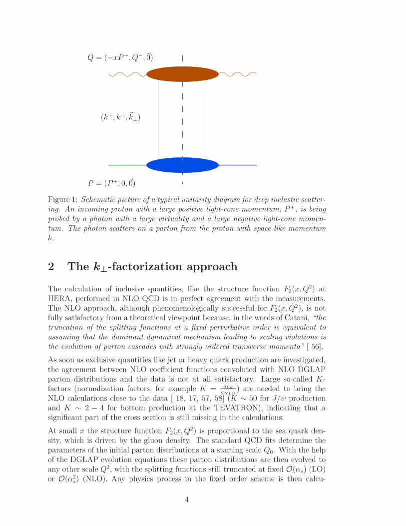
Q = (−xP+, Q−,~0)

P = (P+, 0,~0)

(k+, k−, ~k⊥)

Figure 1: Schematic picture of a typical unitarity diagram for deep inelastic scatter-ing. An incoming proton with a large positive light-cone momentum, P+, is beingprobed by a photon with a large virtuality and a large negative light-cone momen-tum. The photon scatters on a parton from the proton with space-like momentumk.

2 The k⊥-factorization approach

The calculation of inclusive quantities, like the structure function F2(x,Q2) at

HERA, performed in NLO QCD is in perfect agreement with the measurements.The NLO approach, although phenomenologically successful for F2(x,Q

2), is notfully satisfactory from a theoretical viewpoint because, in the words of Catani, “thetruncation of the splitting functions at a fixed perturbative order is equivalent toassuming that the dominant dynamical mechanism leading to scaling violations isthe evolution of parton cascades with strongly ordered transverse momenta” [ 56].

As soon as exclusive quantities like jet or heavy quark production are investigated,the agreement between NLO coefficient functions convoluted with NLO DGLAPparton distributions and the data is not at all satisfactory. Large so-called K-factors (normalization factors, for example K = σtot

σNLO) are needed to bring the

NLO calculations close to the data [ 18, 17, 57, 58] (K ∼ 50 for J/ψ productionand K ∼ 2 − 4 for bottom production at the TEVATRON), indicating that asignificant part of the cross section is still missing in the calculations.

At small x the structure function F2(x,Q2) is proportional to the sea quark den-

sity, which is driven by the gluon density. The standard QCD fits determine theparameters of the initial parton distributions at a starting scale Q0. With the helpof the DGLAP evolution equations these parton distributions are then evolved toany other scale Q2, with the splitting functions still truncated at fixed O(αs) (LO)or O(α2

s) (NLO). Any physics process in the fixed order scheme is then calcu-

4

y,Q2

xn, kn

x0, k0

xn−1, kn−1

xn−2, kn−2

xn−3, kn−3

pn

pn−1

pn−2

pn−3

Ξ

p

Figure 2: Kinematic variables for multi-gluon emission. The t-channel gluon mo-menta are given by ki and the gluons emitted in the initial state cascade havemomenta pi. The upper angle for any emission is obtained from the quark box, asindicated with Ξ. We define z±i = k±i/k±(i∓1) and qi = p⊥i/(1 − z+i).

lated via collinear factorization into the coefficient functions Ca(xz) and collinear

(independent of k⊥) parton density functions: fa(z,Q2):

σ = σ0

∫

dz

zCa(

x

z)fa(z,Q

2) (1)

At large energies (small x) the evolution of parton distributions proceeds over alarge region in rapidity ∆y ∼ log(1/x) and effects of finite transverse momenta ofthe partons may become increasingly important. Cross sections can then be k⊥ -factorized [ 37, 38, 35, 36] into an off-shell (k⊥ dependent) partonic cross sectionσ(x

z, k2

⊥) and a k⊥ - unintegrated parton density function F(z, k2⊥):

σ =∫

dz

zd2k⊥σ(

x

z, k2

⊥)F(z, k2⊥) (2)

The unintegrated gluon density F(z, k2⊥) is described by the BFKL [ 5, 6, 7]

evolution equation in the region of asymptotically large energies (small x). Anappropriate description valid for both small and large x is given by the CCFMevolution equation [ 41, 42, 43, 44], resulting in an unintegrated gluon densityA(x, k2

⊥, q2), which is a function also of the additional scale q described below.

Here and in the following we use the following classification scheme: xG(x, k2⊥) de-

scribes DGLAP type unintegrated gluon distributions, xF(x, k2⊥) is used for pure

5

BFKL and xA(x, k2⊥, q

2) stands for a CCFM type or any other type having twoscales involved.

By explicitly carrying out the k⊥ integration in eq.(2) one can obtain a form fullyconsistent with collinear factorization [ 56, 59]: the coefficient functions and alsothe DGLAP splitting functions leading to fa(z,Q

2) are no longer evaluated in fixedorder perturbation theory but supplemented with the all-loop resummation of theαs log 1/x contribution at small x. This all-loop resummation shows up in theRegge form factor ∆Regge for BFKL or in the non-Sudakov form factor ∆ns forCCFM, which will be discussed in more detail in chapter 4.

3 Off-shell matrix elements

NLOLO resolved photon

k⊥ = 0

k⊥ = 0 k⊥ = 0

k⊥ 6= 0

k⊥ − factorisation

Figure 3: Diagrammatic representation of LO, NLO and resolved photon processesin the collinear approach (top row) and compared to the k⊥-factorization approach.

It is interesting to compare the basic features of the k⊥-factorization approach tothe conventional collinear approach. In k⊥-factorization the partons entering thehard scattering matrix element are free to be off-mass shell, in contrast to thecollinear approach which treats all incoming partons massless. The full advantage

6

of the k⊥-factorization approach becomes visible, when additional hard gluon radi-ation to a 2 → 2 process like γg → QQ is considered. If the transverse momentump⊥g of the additional gluon is of the order of that of the quarks, then in a con-ventional collinear approach the full O(α2

s) matrix element for 2 → 3 has to becalculated. In k⊥-factorization such processes are naturally included to leading log-arithmic accuracy, even if only the LO αs off-shell matrix element is used, since thek⊥ of the incoming gluon is only restricted by kinematics, and therefore can aquirea virtuality similar to the ones in a complete fixed order calculation. In Fig. 3 weshow schematically the basic ideas comparing the diagrammatic structure of thedifferent factorization approaches. Not only does k⊥-factorization include (at leastsome of the) NLO diagrams [ 60] it also includes diagrams of the resolved photontype, with the natural transition from real to virtual photons.

However, it has to be carefully investigated, which parts of a full fixed NLO cal-culation are already included in the k⊥-factorization approach for a given off-shellmatrix element and which are still missing or only approximatively included. Itshould be clear from the above, that the O(αs) matrix element in k⊥-factorizationincludes fully the order O(αs) matrix element of the collinear factorization ap-proach, but includes also higher order contributions. In addition, due to the unin-tegrated gluon density, also parts of the virtual corrections are properly resummed(Fig. 4b,c).

3.1 Order αs off-shell matrix elements

Several calculations exist for the process γg → QQ and gg → QQ, where the gluonand the photon are both allowed to be off-shell [ 35, 36] and Q(Q) can be a heavyor light quark (anti quark).

P2

P1

g(k1)

g(k2)

Q(p3)

Q(p4)

g(k1)

g

g(k1)

(a) (b) (c)

F(x, k2⊥),

A(x, k2⊥, q2)

Figure 4: Schematic diagrams for k⊥-factorization: (a) shows the general case forhadroproduction of (heavy) quarks. (b) shows the one-loop correction to the Borndiagram for photoproduction (c) shows the all-loop improved correction with thefactorized structure function F(x, k2

⊥) or A(x, k2⊥, q

2).

7

The four-vectors of the exchanged partons k1, k2 (in Sudakov representation) are(Fig 4a):

kµ1 = z1P

µ1 + z1P

µ2 + kµ

⊥1 (3)

kµ2 = z2P

µ1 + z2P

µ2 + kµ

⊥2 (4)

with zi, zi being the two components (+,−) of the light cone energy fraction. The(heavy) quark momenta are denoted by p3, p4 and the incoming particles (partons)by P1, P2 with

P1,2 =1

2

√s(~0,±1, 1), 2P1P2 = s (5)

where ~0 indicates the vanishing two-dimensional transverse momentum vector. Inthe case of photoproduction or leptoproduction this reduces to:

kµ1 = P µ

1 , kµ2 = kµ photo-production (6)

kµ1 = qµ = yP µ

1 + yP µ2 + qµ

⊥2, q2 = −Q2 leptoproduction (7)

In all cases the off-shell matrix elements are calculated in the high energy approx-imation, with z1 = z2 = 0:

kµ1 = z1P

µ1 + kµ

⊥1 (8)

kµ2 = z2P

µ2 + kµ

⊥2, (9)

which ensures that the virtualities are given by the transverse momenta, k21 = −k2

⊥1

and k22 = −k2

⊥2. The off-shell matrix elements involve 4-vector products not onlywith k1, k2 and the outgoing (heavy) quark momenta p3, p4, but also with themomenta of the incoming particles (partons) P1, P2. This is a result of defining the(off-shell) gluon polarization tensors in terms of the gluon (ki) and the incomingparticle vectors (P1,2), which is necessary due to the off-shellness. In the collinearlimit, this reduces to the standard polarization tensors. In [ 35, 36] it has beenshown analytically, that the off-shell matrix elements reduce to the standard onesin case of vanishing transverse momenta of the incoming (exchanged) partons k1,k2.

Due to the complicated structure of the off-shell matrix elements, it is also necessaryto check the positivity of the squared matrix elements in case of incoming partonswhich are highly off shell (k2

1, k22 ≪ 0). It has been proven analytically in [ 61]

for the case of heavy quarks with both incoming partons being off mass shell.We have also checked numerically, that the squared matrix elements are positiveeverywhere in the phase space, if the incoming particles (electron or proton) areexactly massless (P 2

1 = P 22 = 0). As soon as finite masses (of the electron or proton)

are included, the exact cancellation of different terms in the matrix elements isdestroyed, and unphysical (negative) results could appear.

From the off-shell matrix elements for a 2 → 2 process, it is easy to obtain the highenergy limit of any on-shell 2(massless partons) → 2+n(massless partons) process,with n = 1, 2 (see Fig. 4b for the case of photoproduction), by applying a correction

8

as given in [ 35, page 180]. By doing so, the corrections coming from additional realgluon emission are estimated (i.e. γg → QQg corrections to γg → QQ) with theincoming gluons now treated on-shell. In the case of hadroproduction one obtainsthe NNLO corrections gg → QQgg. In this sense k⊥-factorization provides an easytool for estimating K-factors in the high energy limit:

K =σtot

σ(LO or NLO)≃ σ(2 → 2) + σ(2 → 2 + n)

σ(2 → 2)(10)

In Tab. 2 we give an overview over the different off-shell matrix elements avail-able. It has been checked, that the different calculations [ 35, 62] of the pro-cess γ(∗)g∗ → QQ give numerically the same result. Also the matrix elements of [35, 36, 34] are identical.

process comments referenceγg∗ → QQ |M |2 [ 35, 62, 19]γ∗g∗ → QQ |M |2 [ 35, 62]γ∗g∗ → QQ partially integrated [ 63, 64]g∗g∗ → QQ |M |2 [ 35, 36, 34]γg∗ → J/ψg |M |2 [ 65, 30]γg∗ → J/ψg helicity amplitude [ 66]γ∗g∗ → J/ψg helicity amplitude [ 66]g∗g∗ → J/ψg helicity amplitude [ 67]

Table 2: Table of calculations of O(αs) off-shell matrix elements for different typesof processes.

3.2 Next-to-Leading corrections to αs off-shell matrix ele-

ments

So far we have been dealing with matrix elements only in O(αs), but even herek⊥-factorization has proven to be a powerful tool in the sense that it includes al-ready in lowest order a large part of the NLO corrections [ 60] of the collinearapproach. However, LO calculations are still subject to uncertainties in the scaleof the coupling and in the normalization. As the next-to-leading corrections (in-cluding energy-momentum conservation) to the BFKL equation are now availablealso the matrix elements need to be calculated in the next-to-leading order.

NLO corrections to the process γ∗g∗ → X contain the virtual corrections to γ∗g∗ →qq (Fig. 5a) and the leading order off-shell matrix element for the process γ∗g∗ →qqg (Fig. 5b). The calculation of the former ones has been completed, and theresults for the matrix elements are published in [ 68]. The real corrections (γ∗g∗ →qqg) have been obtained for helicity-summed squares of the matrix elements. For

9

+ ... + ...

+

(c)(a) (b) (d)

(e)

sM2

t

M2

Figure 5: Schematic diagrams for next-to-leading contributions: (a) virtual cor-rections, (b) real corrections, (c) the process γ∗ + q → (qq) + q, (d) the processγ∗ + q → (qqg) + q, (e) diagrams showing the reggeization of the gluon

the longitudinally polarized photon they are published in [ 69], and results for thetransversely polarized photon will be made available soon [ 70].

The starting point of these calculations is a study of the Regge limit of the processesγ∗ + q → (qq) + q (Fig. 5c) and γ∗ + q → (qqg) + q (Fig. 5d), i.e. the contributingQCD diagrams have been calculated in the region s = (q + p)2 ≫ Q2, M2, t andQ2 ≫ ΛQCD, with q(p) being the four-vector of the photon (quark). In this limit,the exchanged gluon is not an elementary but a reggeized gluon: the two gluonexchange diagrams (Fig. 5e) contain a term proportional to ω(t) log(s), where ω(t)is the gluon Regge trajectory function. This term is not part of the subprocessγ∗g∗ → qq but rather belongs to the exchanged gluon. In order to find the con-tribution of Fig. 5e to this scattering subprocess, one first has to subtract thereggeization piece. This means that, for the subprocess γ∗g∗ → qq, the notation‘g∗’ in NLO not only stands for ‘off-shellness’ but also for ‘reggeized’. It also hasimportant consequences for the factorization of the NLO off-shell subprocess insidea larger QCD diagram: the t-channel gluons connecting the different subprocesses(see, for example, g(k1) in Fig. 4) are not elementary but reggeized, and the QCDdiagrams include subsets of graphs with more than two gluons in the t-channel (seeFig. 5e)

The results for the virtual corrections contain infrared singularities, both soft andvirtual ones. As usual, when integrating the real corrections over the final stategluon, one finds the same infrared singularities but with opposite signs. So inthe sum of virtual and real corrections one obtains an infrared finite answer. Apeculiarity of this NLO calculation is the interplay with the LO process γ∗ +q → (qq) + g + q. In the latter, the process is calculated in the leading log(s)

10

approximation (LO BFKL approximation), where the gluon has a large rapidityseparation w.r.t. the qq-pair (i.e. it is emitted in the central region between theqq-pair and the lower quark line in Fig. 5d). As a result of this high energy (smallx- or Regge) factorization, expressions for the vertex g∗ + g∗ → g and for thesubprocess γ∗g∗ → qq are obtained. When turning to the NLO corrections ofthe process γ∗ + q → (qqg) + q, the calculation extends to next-to-leading log(s)accuracy, but it contains, as a special case, also the LO BFKL process. In order toavoid double counting, one has to subtract the central region contribution. Onlyafter this subtraction we have a clean separation: qqg final states without or witha large rapidity separation between the gluon and the quark-antiquark pair. Theformer one belongs to the NLO approximation, whereas the latter one is countedin the leading log(s) approximation.

The results for real corrections in [ 69] are very interesting also in the context ofthe QCD color dipole picture. It is well-known that the total LO γ∗q cross sectionat high energies can be written in the form [ 71, 72]:

σγ∗qtot =

∫

dz∫

dρ(

ψγ∗

qq (Q, z, ρ))∗σqq(x, z, ρ)ψ

γ∗

qq (Q, z, ρ) (11)

where z and (1−z) denote the momentum fractions (w.r.t. the photon momentumq) of the quark and the antiquark, respectively, ρ is the transverse extension of thequark-antiquark pair, ψqq stands for the qq Fock component of the photon wavefunction, and σqq is the color dipole cross section. This form of the scattering crosssection is in agreement with the space time picture in the target quark rest frame:a long time before the photon reaches the target quark at rest, it splits into thequark-antiquark pair which then interacts with the target. During the interactionthe transverse extension of the quark-antiquark pair remains frozen, i.e the initialquark-antiquark pair has the same ρ-value as the final one. Via the optical theoremthe γ∗q total cross section is related to the square of the scattering matrix elementof the process γ∗+q → (qq)+q; the dipole cross section form eq.(11) must then be aconsequence of the special form of the LO amplitude for the subprocess γ∗g∗ → qq.Since this form of the total γ∗q cross section (which is preserved when the targetquark is replaced by the target proton) looks so appealing (and also has turnedout to be extremely useful in phenomenological applications), that it is desirableto investigate its validity also beyond leading order.

When trying to generalize eq.(11) to NLO, one is led to study the square of thereal corrections γ∗ + q → (qqg) + q. If the color dipole picture remains correct(factorization in wave function and dipole cross section), this contribution naturallyshould lead to a new qqg Fock component of the photon wave function, and to anew interaction cross section σqqg, which describes the interaction of the quark-antiquark-gluon system with the target quark. In [ 69, 70] it is shown that thisis indeed the case. The form of the new photon wave function is rather lengthy(in particular for the transverse photon), and a more detailed investigation is stillneeded. Nevertheless, one feels tempted to conclude that the color dipole formeq.(11) is the beginning of a general color multipole expansion, where the different

11

Fock components of the photon wave function describe the spatial distributionof color charge inside the photon. However, before this conclusion can really bedrawn, it remains to be shown that also the virtual corrections to the scatteringamplitude of γ∗ + q → (qq) + q fit into the form eq.(11). These corrections shouldlead to NLO corrections of the photon wave function or the dipole cross section.They also may slightly ‘melt’ the transverse extension of the quark-antiquark pairduring the interaction with the target.

In summary, the results in [ 68, 69, 70] provide the starting point for discussingexclusive final states in the k⊥-factorization scheme in NLO accuracy. However, be-fore these formulae can be used in a numerical analysis, virtual and real correctionshave to be put together, and IR finite cross sections have to be formulated. TheNLO corrections to the off-shell matrix elements described in this subsection alsorepresent the main ingredients to the NLO photon impact factor. Its importancewill be discussed in section 4.6.1

3.3 Gauge-invariance

The off-shell matrix elements and the cross section taken in lowest order αs aregauge invariant, as argued in [ 35]. However, when extended to next order inperturbation theory, as depicted in Fig. 3, problems will occur and the off-shellmatrix elements and unintegrated parton distributions are no longer necessarilygauge invariant. The following critique indicates that their definition needs furtherspecification and that further work is needed to properly justify the formalism [73].

Basically, parton distributions are defined as a hadron expectation value of a quarkand antiquark field (or two gluon fields):

〈p|ψ(y)Γψ(0)|p〉, (12)

with an appropriate Fourier transformation on the space-time argument yµ, someappropriate Dirac matrix Γ and some appropriate normalization. This definitionis not gauge invariant, so one must either specify the gauge or one modifies thedefinition to make it gauge invariant:

〈p|ψ(y)ΓPe−ig∫ y

0dy′µAα

µ(y′)tαψ(0)|p〉. (13)

Here, tα are generating matrices for the SU(3) color group of QCD, and the symbolP denotes that the gluon fields are laid out in their order on the path in the integralfrom 0 to y.

The big question is which path is to be used. For the integrated parton distribu-tions, y is at a light-like separation from 0: normally y− 6= 0, y+ = y⊥ = 0, andthen taking the path along the light-like straight line joining 0 and y = (0, y−, 0⊥)is natural and correct. But for unintegrated distributions, this is not so simple; one

12

has a choice of paths. The choice is not arbitrary but is determined by the deriva-tion: i.e., the definition is whatever is appropriate to make a correct factorizationtheorem.

This can be seen from the analysis of gluon emission that we have already de-scribed. This analysis is only applicable if ladder diagrams, as in Fig. 3, actuallydominate. In fact, in a general gauge, non-ladder diagrams are as important as lad-der diagrams. This is the case, for example, in the Feynman gauge. The standardleading-logarithm analysis suggests, as is commonly asserted, that the appropriategauge is a light-cone gauge n·A = 0, where n is a light-like vector in a suitable direc-tion, for then non-ladder contributions are suppressed in the LLA analysis. Fromthis one would conclude that the off-shell matrix elements and the unintegratedparton distributions are defined as the appropriate field theory Green functions inlight-cone gauge.

Closer examination shows that there must be problems since the unintegrated par-ton distributions are divergent. This was shown quite generally by Collins andSoper [ 74, 75] as part of their derivation of factorization for transverse-momentumdistributions. They found they needed to derive factorization and to define un-integrated parton distributions in a non-light-like axial gauge, i.e., with n2 6= 0.1

They derived an evolution equation for the dependence on the gauge-fixing vector;the evolution is quite important and contains doubly-logarithmic Sudakov effects.In the limit n2 → 0, the parton distributions become so singular that they arenot defined. The divergences are associated with the emission of gluons of arbi-trarily negative rapidity with respect to the parent hadron; commonly these arecalled soft gluons, and a non-light-like gauge-fixing vector provides a cutoff on thedivergences. It is normally said that soft gluons cancel in QCD cross sections.However, the standard cancellation requires an integral over all parton transversemomentum, which is of course not applicable in an unintegrated parton density.

The divergences can readily be seen in one-loop graphs, and are a generalization ofdivergences known to occur in light-cone gauge. Modification of the iǫ prescriptionof the 1/k ·n singularity of the gluon propagator, as is commonly advocated, is notsufficient, since this does not remove the divergence in the emission of real gluons,for which the singularity is an endpoint singularity in k · n.

Clearly, in all the derivations of the BFKL and related equations, there must bean appropriate cutoff. Unfortunately, this is not normally made very explicit, eventhough an explicit specification of the cutoff is vitally important if the formalismis to make sense beyond LO. One can expect, that such a cutoff is a cutoff inangle or rapidity, and it should be related to angular ordering, supporting theintuitive approximate picture. However, the presence of the cutoff implies thatthere is an extra parameter in the parton distributions, whose variation should beunderstood. Balitsky [ 76] has worked in this direction, although his formulationdoes not appear to have developed far enough to address the issues in the present

1 An equivalent and probably better definition can be made with suitable path-ordered expo-nential in the operator.

13

document.

A proper derivation will also result in an explicit definition of a reggeized gluon.Such a definition is not readily extracted from the original BFKL publications. Atmost these publications provide a definition as a property of a solution of theirequation. No explicit definition is given whereby quantities involving reggeizedgluons are matrix elements of some operator or other.

4 Unintegrated parton distributions

4.1 Introduction

The conventional parton distributions describe the density of partons carrying acertain longitudinal momentum fraction inside the proton. These distributions areintegrated over the transverse momenta of the partons up to the factorization scaleµ. However, in order to describe some exclusive processes it becomes necessary toconsider the transverse momenta of the partons and thus use so called unintegratedgluon distributions A(x, k2

⊥, µ2). Unintegrated parton distributions account for the

resummation of a variety of logarithmically enhanced terms, such as(

αs log(µ2/Λ2))n,(

αs log(µ2/Λ2) log(1/x))n, (αs log(1/x))n and

(

αs log2(µ2/k2⊥))n

(14)The unintegrated parton distributions describe the probability of finding a partoncarrying a longitudinal momentum fraction x and a transverse momentum k⊥ atthe factorization scale µ. The unintegrated gluon density xA(x, k2

⊥, µ2) can be

related to the integrated one xg(x, µ2) by:

xg(x, µ2) ≃∫ µ2

0dk2

⊥xA(x, k2⊥, µ

2) (15)

The ≃ sign in the above equation indicates, that there is no strict equality betweenunintegrated and integrated parton distributions, as neither are observables.

In unintegrated parton distributions, the contribution from the large logarithmsin x and µ2, the terms specified above in expression (14), can be correctly dis-entangled. However, the unintegrated parton distributions are defined only as afunctions of three variables x, k2

⊥, µ2. The 4-vector k of the propagator gluon ininitial state cascade is given by:

k = (k+, k−, k⊥)

with k+ = x+P+, k− = x−P− The virtuality k2 is:

k2 = k+k− − k2⊥ = x+x−P−P+ − k2

⊥.

In the region of strongly ordered k+, the typical values of k− are small enoughthat it can be neglected in the hard scattering factor. For example, the virtuality

14

is dominated by the transverse momentum only:

k2 ≃ −k2⊥.

However, the k− integral is still present, and in fact, part of the definition ofan unintegrated parton density is, that the relevant matrix element of a gluonicoperator is integrated over all k−. This is the reason, why only x = x+ is kept inthe unintegrated gluon density.

The all-loop resummation of the αs log 1/x contribution at small x leads to Reggeiza-tion of the gluon vertex, giving rise to a significant form factor. The Regge formfactor ∆Regge, often also called non-Sudakov form factor ∆ns, regularizes the 1/zdivergence in the splitting function,

Pg(z+) ∝ ∆Regge(k⊥, z+)

z+. (16)

The ∆Regge of BFKL is given by [ 77]:

∆Regge(z+, k2⊥) = exp

(

−αS

∫ 1

z+

dz′

z′

∫

dq′2⊥

q′2⊥

Θ(k2⊥ − q

′2⊥)Θ(q

′2⊥ − q2

0)

)

(17)

with αS = CAαs

π= 3αs

πand q0 being a lower cutoff. This form factor can be ex-

panded by a power series and then symbolically represented as:

+ + + ... +

αS(k⊥) 1z+

[ 1 + αS log (z) log(

k2⊥

q20

)

+(

12!αS log (z) log

(

k2⊥

q20

))2

... ]

where the small x resummation of the virtual corrections becomes obvious. Such adiagrammatic representation is of course gauge dependent. It should be noted thatthe Regge form factor in this way looks like the Sudakov form factor [ 78, 79] usedto regularize the 1/(1− z) pole in standard DGLAP evolution, but the resummeddiagrams involve small z rather than large ones. This similarity is used in thederivation of the Linked Dipole Chain model below.

In interpreting the results quoted in this section, the reader should bear in mindthe caveats explained in Sec. 3.3, that as yet, no fully explicit definition of theparton distributions has been given.

4.2 The CCFM evolution

According to the CCFM [ 41, 42, 43, 44] evolution equation the emission of gluonsduring the initial cascade is only allowed in an angular-ordered region of phase

15

space. The maximum allowed angle Ξ is defined by the hard scattering quark box,producing the (heavy) quark pair. In terms of Sudakov variables the quark pairmomentum is written as:

pq + pq = Υ(P1 + ΞP2) + ~Q⊥ (18)

where Υ (ΥΞ) is the positive (negative) light-cone momentum fraction of the quark

pair, P1,2 are the four-vectors of incoming beam particles, respectively and ~Qt isthe vectorial sum of the transverse momenta of the quark pair in the laboratoryframe. Similarly, the momenta pi of the gluons emitted during the initial statecascade are given by (here treated massless):

pi = υi(P1 + ξiP2) + p⊥i , ξi =p2⊥i

sυ2i

, (19)

with υi = (1 − zi)xi−1, xi = zixi−1 and s = (P1 + P2)2 being the squared center of

mass energy. The variable ξi is connected to the angle of the emitted gluon withrespect to the incoming proton and xi and υi are the momentum fractions of theexchanged and emitted gluons, while zi is the ratio of the energy fractions in thebranching (i− 1) → i and p⊥i is the transverse momentum of the emitted gluon i.

The angular-ordered region is then specified by (Fig. 2):

ξ0 < ξ1 < · · · < ξn < Ξ (20)

which becomes:zi−1qi−1 < qi (21)

where the rescaled transverse momenta qi of the emitted gluons is defined by:

qi = xi−1

√

sξi =p⊥i

1 − zi(22)

It is interesting to note, that the angular ordering constraint, as given by eq.(21),reduces to ordering in transverse momenta p⊥ for large z, whereas for z → 0, thetransverse momenta are free to perform a so-called random walk.

The CCFM evolution equation with respect to the scale q2 can be written in adifferential form [ 44]:

q2 d

dq2

xA (x, k2⊥, q

2)

∆s(q2, Q20)

=∫

dzdφ

2π

P (z, (q/z)2, k2⊥)

∆s(q2, Q20)

x′A(

x′, k′2⊥ , (q/z)

2)

(23)

where A(x, k2⊥, q

2) is the unintegrated gluon density, depending on x, k2⊥ and the

evolution variable µ2 = q2. The splitting variable is z = x/x′ and ~k⊥′

= (1 −z)/z~q + ~k⊥, where the vector ~q is at an azimuthal angle φ. The Sudakov formfactor ∆s is given by:

∆s(q2, Q2

0) = exp

(

−∫ q2

Q20

dq2

q2

∫ 1−Q0/q

0dzαS (q2(1 − z)2)

1 − z

)

(24)

16

with αS = CAαs

π= 3αs

π. For inclusive quantities at leading-logarithmic order the Su-

dakov form factor cancels against the 1/(1−z) collinear singularity of the splittingfunction.

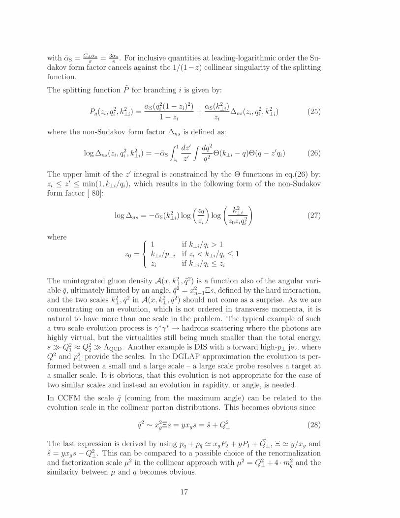
The splitting function P for branching i is given by:

Pg(zi, q2i , k

2⊥i) =

αS(q2i (1 − zi)

2)

1 − zi+αS(k

2⊥i)

zi∆ns(zi, q

2i , k

2⊥i) (25)

where the non-Sudakov form factor ∆ns is defined as:

log ∆ns(zi, q2i , k

2⊥i) = −αS

∫ 1

zi

dz′

z′

∫

dq2

q2Θ(k⊥i − q)Θ(q − z′qi) (26)

The upper limit of the z′ integral is constrained by the Θ functions in eq.(26) by:zi ≤ z′ ≤ min(1, k⊥i/qi), which results in the following form of the non-Sudakovform factor [ 80]:

log ∆ns = −αS(k2⊥i) log

(

z0zi

)

log

(

k2⊥i

z0ziq2i

)

(27)

where

z0 =

1 if k⊥i/qi > 1k⊥i/p⊥i if zi < k⊥i/qi ≤ 1zi if k⊥i/qi ≤ zi

The unintegrated gluon density A(x, k2⊥, q

2) is a function also of the angular vari-able q, ultimately limited by an angle, q2 = x2

n−1Ξs, defined by the hard interaction,and the two scales k2

⊥, q2 in A(x, k2

⊥, q2) should not come as a surprise. As we are

concentrating on an evolution, which is not ordered in transverse momenta, it isnatural to have more than one scale in the problem. The typical example of sucha two scale evolution process is γ∗γ∗ → hadrons scattering where the photons arehighly virtual, but the virtualities still being much smaller than the total energy,s≫ Q2

1 ≈ Q22 ≫ ΛQCD. Another example is DIS with a forward high-p⊥ jet, where

Q2 and p2⊥ provide the scales. In the DGLAP approximation the evolution is per-

formed between a small and a large scale – a large scale probe resolves a target ata smaller scale. It is obvious, that this evolution is not appropriate for the case oftwo similar scales and instead an evolution in rapidity, or angle, is needed.

In CCFM the scale q (coming from the maximum angle) can be related to theevolution scale in the collinear parton distributions. This becomes obvious since

q2 ∼ x2gΞs = yxgs = s+Q2

⊥ (28)

The last expression is derived by using pq + pq ≃ xgP2 + yP1 + ~Q⊥, Ξ ≃ y/xg ands = yxgs−Q2

⊥. This can be compared to a possible choice of the renormalizationand factorization scale µ2 in the collinear approach with µ2 = Q2

⊥ + 4 ·m2q and the

similarity between µ and q becomes obvious.

17

4.3 LDC and the transition between BFKL and DGLAP

The Linked Dipole Chain (LDC) model [ 50, 51] is a reformulation of CCFMwhich makes the evolution explicitly left–right symmetric, which will be discussedin section 4.6 in more detail. LDC relies on the observation that the non-Sudakovform factor in eq.(26), despite its name, can be interpreted as a kind of Sudakovform factor giving the no-emission probability in the region of integration. Todo this an additional constraint on the initial-state radiation is added requiringthe transverse momentum of the emitted gluon to be above the smaller of thetransverse momenta of the connecting propagating gluons:

p2⊥i > min(k2

⊥i−1, k2⊥i). (29)

Emissions failing this cut will instead be treated as final-state emissions and need tobe resummed in order not to change the total cross section. In the limit of small zand imposing the kinematic constraint of eq.(64) (see section 4.6 for further details)gives a factor which if it is multiplied with each emission, completely cancels thenon-Sudakov and thus, in a sense de-reggeizes the gluon.

One may ask when it is appropriate to use collinear factorization (DGLAP) andwhen we must account for effects of BFKL and k⊥-factorization. Clearly, when k⊥is large and 1/x is limited we are in the DGLAP regime, and when 1/x is largeand k⊥ is limited we are in the BFKL regime. An essential question is then: Whatis large? Where is the boundary between the regimes, and what is the behaviorin the transition region? Due to the relative simplicity of the LDC model, whichinterpolates smoothly between the regimes of large and small k⊥, it is possibleto give an intuitive picture of the transition. In the following x is always keptsmall, and leading terms in log 1/x are studied. Thus the limit for large k⊥ doesnot really correspond to the DGLAP regime, but more correctly to the double-logapproximation.

First we will discuss the case of a fixed coupling. For large values of k⊥ (in the“DGLAP region”) the unintegrated structure function F(x, k2

⊥) is dominated bycontributions from chains of gluon propagators which are ordered in k⊥. The result

is a product of factors αS · dxi

xi· dk2

⊥i

k2⊥i

[ 1, 2, 3, 4]:

F(x, k2⊥) ∼

∑

N

∫ N∏

αS dliθ(li+1 − li) dκiΘ(κi+1 − κi)

where αS ≡3αs

π, l ≡ log(1/x) and κ ≡ log(k2

⊥/Λ2) (30)

Integration over κi with the Θ-functions gives the phase space for N ordered valuesκi. The result is κN/N !. The integrations over li give a similar result, and thus weobtain the well-known double-log result

F(x, k2⊥) ∼

∑

N

αN · lN

N !· κ

N

N != I0(2

√αlκ) (31)

18

In the BFKL region also non-ordered chains contribute, and the result is a power-like increase ∼ x−λ for small x-values [ 5, 6, 7].

The CCFM [ 41, 42, 43, 44] and the LDC model [ 50, 51, 81] interpolate betweenthe DGLAP and BFKL regimes. In the LDC model the possibility to “go down”in k⊥, from κ′ to a smaller value κ, is suppressed by a factor exp(κ − κ′). Theeffective allowed distance for downward steps is therefore limited to about one unitin κ. If this quantity is called δ, the result is, that the phase space factor κN

N !is

replaced by (κ+Nδ)N

N !.

Thus we obtain:

F(x, k2⊥) ∼

∑

N

(αl)N

N !

(κ +Nδ)N

N !(32)

When κ is very large, this expression approaches eq.(31). When κ is small wefind, using Sterling’s formula, that F(x, k2

⊥) ∼ ∑

N(αSlδe)N/N ! = exp(λl) ≡ x−λ,

with λ = αSδe. For δ = 1 this gives λ = eαS = 2.72αS, which is very close to theleading order result for the BFKL equation, λ = 4 log 2 αS = 2.77αS. Thus eq. (32)interpolates smoothly between the DGLAP and BFKL regimes. It is also possibleto see that the transition occurs for a fixed ratio between κ and l, κ/l ≈ eαS.

For a running coupling a factor αS dκ in eq.(30) is replaced by α0 dκ/κ = α0 du,where α0 ≡ αSκ, u ≡ log(κ/κ0) and κ0 is a cutoff. In the large k⊥ region (the“DGLAP region”) the result is therefore similar to eq. (31), but with αSκ replacedby α0u. For small x-values we note that the allowed effective size of downwardsteps, which is still one unit in κ, is a sizeable interval in u for small κ, but a verysmall interval in u for larger κ.

This is the reason for an earlier experience [ 51], which showed that a typical chaincontains two parts. In the first part the k⊥-values are relatively small, and it istherefore easy to go up and down in k⊥, and non-ordered k⊥-values are important.The second part is an ordered (DGLAP-type) chain, where k⊥ increases towardsits final value.

Let us study a chain with N links, out of which the first N −k links correspond tothe first part with small non-ordered k⊥ values, and the remaining k links belongto the second part with increasing k⊥. Assume that the effective phase space foreach ui in the soft part is given by a quantity ∆. Then the total weight for thispart becomes ∆N−k. For the k links in the second, ordered, part the phase spacebecomes as in the DGLAP case uk/k!. Thus the total result is (G ≡ κF)

G ∼∑

N

(α0l)N

N !

N∑

k=0

uk

k!∆N−k =

∑

N

(α0l∆)N

N !

N∑

k=0

(u/∆)k

k!. (33)

This simple model also interpolates smoothly between the DGLAP and BFKLregions. For large u-values the last term in the sum over k dominates, which givesthe “DGLAP” result

G ∼∑

(α0lu)N/(N !)2 = I0(2

√

α0lu) ≈ (16π2α0lu)−1/4 · exp(2

√

α0lu). (34)

19

0

1

2

3

4

5

6

7

8

9

0 0.5 1 1.5

ln(G

)

α0u / (λ2l)

kT2 (GeV2)20 600 7*104

λl = 3 , x ~ 5*10-5

Full modelBFKL limit

DGLAP limit

Figure 6: Results for a running coupling for λl = 3, which for λ = 0.3 meansx = 5 · 10−5. (Note that this x-value corresponds only to the chain between the“observed” low energy gluon and the parent soft gluon.) The solid line correspondsto the model in eq. (33), the dashed line to the BFKL limit, eq. (35), and the dottedline to the DGLAP limit in eq. (34). The abscissa is the variable w = α0u/λ

2ldefined so that the transition occurs for w ≈ 1. The corresponding values for k2

⊥in GeV 2 for λ = 0.3 and λl = 3 are also indicated.

For small u-values the sum over k gives approximately exp (u/∆), and thus

G ∼ exp(α0∆l) · exp(u/∆) = x−λκα0/λ, with λ = α0∆. (35)

The transition between the regimes occurs now for a fixed ratio between u/l ≈λ2/α0, which is of order 0.1 if λ is around 0.3. The result is illustrated in fig. 6,which shows how the expression in eq. (33) interpolates between the DGLAP andBFKL limits in eqs. (34) and (35) for large and small k⊥.2

The simple models in eqs. (32) and (33), for fixed and running couplings respec-tively, interpolate smoothly between large and small k⊥-values. They contain theessential features of the CCFM and LDC models, and can therefore give an intu-itive picture of the transition between these two regimes. The transition occurs fora fixed ratio between log k2

⊥ and log 1/x for fixed coupling, and between log(log k2⊥)

and log 1/x for a running coupling. A more extensive discussion, including effectsof non-leading terms in log 1/x and the properties of Laplace transforms, is foundin ref. [ 86].

2 In the framework of N = 4 SUSY, where the corresponding coupling is not running, therelations between DGLAP and BFKL equations has been found in [ 82, 83, 84, 85] for the firsttwo orders of perturbation theory. These results can be useful for possible future study of thecorresponding approximate relations in QCD.

20

4.4 The CCFM equation in the transverse coordinate rep-

resentation

It might be useful to consider the CCFM equation using the transverse coordinate(or impact parameter) [ 87] b conjugate to the transverse momentum k⊥ and tointroduce the b dependent gluon distribution A(x, b, q2) defined by the Fourier-Bessel transform of A(x, k2

⊥, q2):

A(x, b, q2) =∫ ∞

0k⊥dk⊥J0(bk⊥)A(x, k2

⊥, q2). (36)

where J0(u) is the Bessel function. The advantage of this representation becomesparticularly evident in the so called ’single -loop’ approximation that corresponds tothe replacement q/z → q and ∆NS → 1. In this approximation the CCFM equationreduces to the conventional DGLAP evolution and eq.(23) is diagonalized by theFourier - Bessel transformation provided that we set the same argument µ2 ∼ q2

in both terms in this equation. The evolution equation for A(x, b, q2) reads:

q2 d

dq2

xA(x, b, q2)

∆s(q2, Q20)

= αS(q2)∫

dzP (z)J0[(1 − z)qb]x′A(x′, b, q2)

∆s(q2, Q20)

(37)

where

P (z) =1

1 − z− 2 + z(1 − z) +

1

z(38)

In equation (37) the argument µ2 of the QCD coupling was set µ2 = q2 and

∆s(q2, Q2

0) = exp

(

−∫ q2

Q20

dq2

q2

∫ 1−Q0/q

0dzαS(q2)zP (z)

)

(39)

In the splitting function P (z) we have included the terms which are non-singularat z = 0 or z = 1 in order to get a complete DGLAP evolution equation forthe integrated gluon distribution. For the same reason we have also extended thedefinition of the Sudakov form factor by including the complete splitting functionP (z) and not only its part which is singular at z = 1 (cf. eq. (39)).Equation (37) can be solved exactly after going to the moment space and intro-ducing the moment function Aω(b, q2) defined by:

Aω(b, q2) =∫ 1

0dxxωA(x, b, q2) (40)

The solution of the evolution equation for the moment function Aω(b, q2) reads:

Aω(b, q2) = A0ω(b) · exp

[

∫ q2

Q20

dq2

q2αS(q2)

∫ 1−Q0/q

0dzzP (z)(zω−1J0(bq(1 − z)) − 1)

]

(41)where A0

ω(b) is the Fourier-Bessel transform of the (input) unintegrated distributionat q = Q0. It should be noted that at b = 0, Aω(b, q2) is proportional to the moment

21

function of the integrated gluon distribution g(x, q). The solution (41) at b = 0reduces to the solution of the LO DGLAP equation for the moment function ofthe integrated gluon distribution. It should also be noted that the integrand ineq.(41) is free from singularities at z = 1 and so we can set Q0 = 0 in the upperintegration limit over dz. The formalism presented above is similar to that usedfor the description of the transverse momentum distributions in (for instance) theDrell-Yan process (see e.g. [ 88, 89, 90, 91]).In order to obtain more insight into the structure of the unintegrated distributionwhich follows from the CCFM equation in the single loop approximation it is usefulto adopt in eq.(36) the following approximation of the Bessel function:

J0(u) ≃ Θ(1 − u) (42)

which gives:

A(x, k2⊥, q

2) ≃ 2dA(x, b = 1/k⊥, q

2)

dk2⊥

(43)

Using the same approximation for the Bessel function in eq.(41) we get, after somerearrangements, the following relation between unintegrated and integrated gluondistributions:

A(x, k2⊥, q

2) ≃ d

dk2⊥

[g(x, k2⊥)∆s(q

2, k2⊥)] (44)

Similar relation has also been used in refs. [ 92, 93] (see also eq.(54) in the nextsection).In the general ’all loop’ case, the non-Sudakov form-factor generates contributionswhich are no longer diagonal in the b space and so the merit of using this represen-tation is less apparent. However in the leading log(1/x) approximation at small xthe CCFM equation reduces to the BFKL equation with no scale dependence andthe kernel of the BFKL equation in b space is the same as that in the (transverse)momentum space. The work to explore the CCFM equation in b space beyond the’single loop’ and BFKL approximations is in progress.

4.5 Available parameterizations of unintegrated gluon dis-

tributions

Depending on the approximations used, different unintegrated gluon distributionscan be obtained (see eq.(15)). Here we describe some of the so far publishedones and make some comparisons.3 We use the following classification scheme:xG(x, k2

⊥) describes DGLAP type unintegrated gluon distributions, xF(x, k2⊥) is

used for pure BFKL and xA(x, k2⊥, q

2) stands for a CCFM type or any other typehaving two scales involved.

3Parameterizations of the unintegrated gluon distributions described here are available as aFORTRAN code from http://www.thep.lu.se/Smallx

22

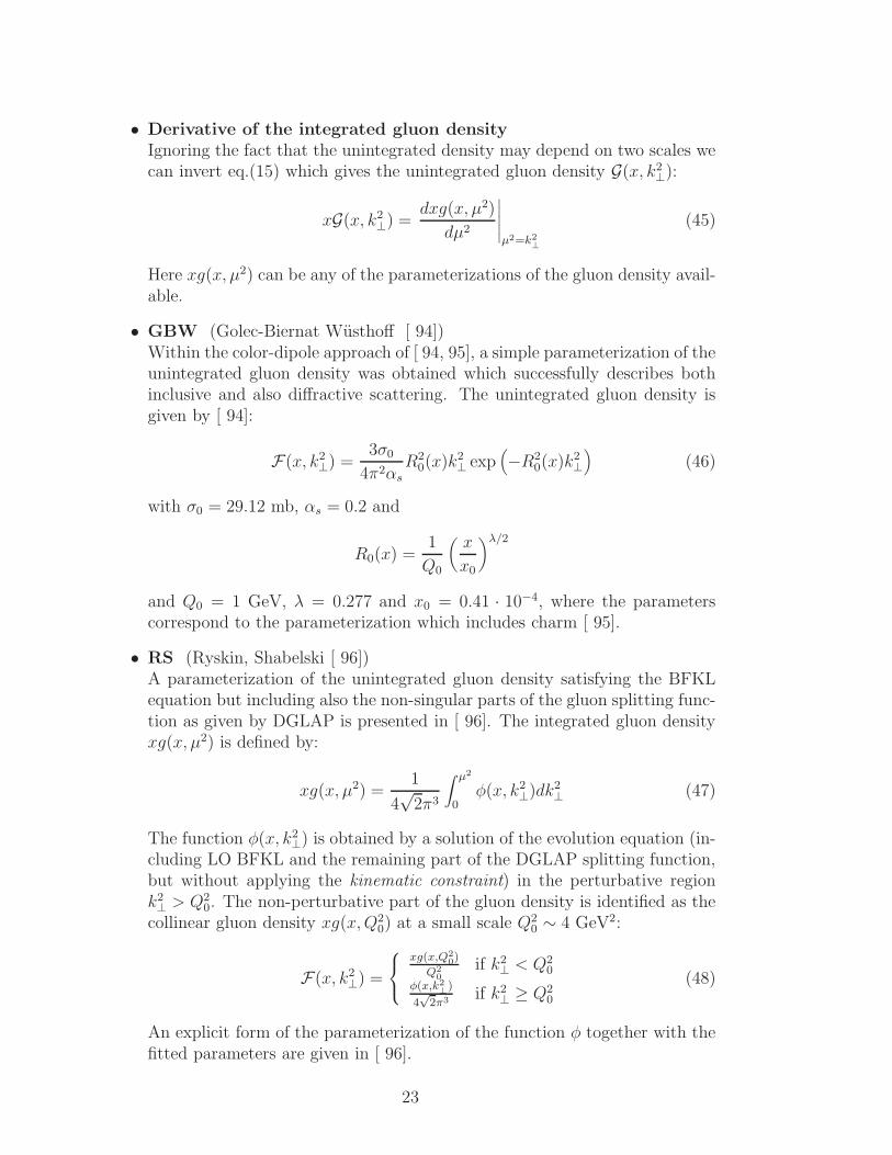
• Derivative of the integrated gluon density

Ignoring the fact that the unintegrated density may depend on two scales wecan invert eq.(15) which gives the unintegrated gluon density G(x, k2

⊥):

xG(x, k2⊥) =

dxg(x, µ2)

dµ2

∣

∣

∣

∣

∣

µ2=k2⊥

(45)

Here xg(x, µ2) can be any of the parameterizations of the gluon density avail-able.

• GBW (Golec-Biernat Wusthoff [ 94])Within the color-dipole approach of [ 94, 95], a simple parameterization of theunintegrated gluon density was obtained which successfully describes bothinclusive and also diffractive scattering. The unintegrated gluon density isgiven by [ 94]:

F(x, k2⊥) =

3σ0

4π2αsR2

0(x)k2⊥ exp

(

−R20(x)k

2⊥

)

(46)

with σ0 = 29.12 mb, αs = 0.2 and

R0(x) =1

Q0

(

x

x0

)λ/2

and Q0 = 1 GeV, λ = 0.277 and x0 = 0.41 · 10−4, where the parameterscorrespond to the parameterization which includes charm [ 95].

• RS (Ryskin, Shabelski [ 96])A parameterization of the unintegrated gluon density satisfying the BFKLequation but including also the non-singular parts of the gluon splitting func-tion as given by DGLAP is presented in [ 96]. The integrated gluon densityxg(x, µ2) is defined by:

xg(x, µ2) =1

4√

2π3

∫ µ2

0φ(x, k2

⊥)dk2⊥ (47)

The function φ(x, k2⊥) is obtained by a solution of the evolution equation (in-

cluding LO BFKL and the remaining part of the DGLAP splitting function,but without applying the kinematic constraint) in the perturbative regionk2⊥ > Q2

0. The non-perturbative part of the gluon density is identified as thecollinear gluon density xg(x,Q2

0) at a small scale Q20 ∼ 4 GeV2:

F(x, k2⊥) =

xg(x,Q20)

Q20

if k2⊥ < Q2

0

φ(x,k2⊥

)

4√

2π3if k2

⊥ ≥ Q20

(48)

An explicit form of the parameterization of the function φ together with thefitted parameters are given in [ 96].

23

• KMS (Kwiecinski, Martin, Stasto [ 97])In the approach of KMS [ 97] three modifications to the BFKL equationare introduced in order to extend its validity to cover the full range in x.Firstly, a term describing the leading order DGLAP evolution is added. Theinclusion of this term has the effect of softening the small x rise and tochange the overall normalization. Secondly, the kinematic constraint eq.(64)is applied, which has its origin in the requirement that the virtuality of theexchanged gluon is dominated by its transverse momentum. Thirdly, theBFKL equation is solved only in the region of k⊥ > k⊥0, whereas the non-perturbative region is provided by the collinear gluon density xg(x, k2

⊥0) atthe scale k⊥0. The border between the perturbative and non-perturbativeregions has been taken to be k⊥0 = 1 GeV2.

Also a term which allows the quarks to contribute to the evolution of thegluon has been introduced. The single quark contribution is controlledthrough the g → qq splitting. The input gluon and quark distributionsto this unified DGLAP-BFKL evolution equation are determined by a fitto HERA F2 data. The unintegrated gluon density F(x, k2

⊥) is still only afunction of x and k2

⊥, which strictly satisfies:

xg(x,Q2) =∫ Q2 dk2

⊥k2⊥f(x, k2

⊥) =∫ Q2

dk2⊥F(x, k2

⊥). (49)

• JB (J. Blumlein [ 98])In the approach of JB [ 98] the general k⊥-factorization formula:

σ(x, µ2) =∫

dk2⊥σ(x, k2

⊥, µ2) ⊗A(x, k2

⊥, µ2)

is rewritten in the form [ 36]:

σ(x, µ2) = σ0(x, µ2)⊗g(x, µ2)+∫ ∞

0dk2

⊥

(

σ(x, k2⊥, µ

2) − σ0(x, µ2))

⊗A(x, k2⊥, µ

2),

(50)which gives the relation:

g(x, µ2) =∫ ∞

0dk2

⊥A(x, k2⊥, µ

2).

In the case of eq.(50) the k⊥ dependent gluon distribution satisfying theBFKL equation can be represented as the convolution of the integratedgluon density xg(x, µ2) (for example GRV [ 99]) and a universal functionB(x, k2

⊥, µ2):

A(x, k2⊥, µ

2) =∫ 1

xB(z, k2

⊥, µ2)x

zg(x

z, µ2) dz, (51)

The universal function B(x, k2⊥, µ

2) can be represented as a series (see [ 98]):

N=∞∑

i=1

diIi−1(...),

24

where Ii = Ii if k2⊥ > µ2 and Ii = Ji if k2

⊥ < µ2, respectively and Ji and Ii areBessel functions for real and imaginary arguments. The series comes fromthe expansion of the BFKL anomalous dimension with respect to αs. Thefirst term of the above expansion explicitely describe BFKL dynamics in thedouble-logarithmic approximation:

B(z, k2⊥, µ

2) =αS

z k2⊥J0(2

√

αS log(1/z) log(µ2/k2⊥)), k2

⊥ < µ2, (52)

B(z, k2⊥, µ

2) =αS

z k2⊥I0(2

√

αS log(1/z) log(k2⊥/µ

2)), k2⊥ > µ2, (53)

where J0 and I0 are the standard Bessel functions (for real and imaginaryarguments, respectively) and αS = 3αs/π is connected to the pomeron inter-cept ∆ of the BFKL equation in LO ωLL = αS4 log 2. An expression for ωNLL

in NLO is given in [ 39, 40]: ωNLL = αS4 log 2−Nα2S. Since the equations be-

have infrared finite no singularities will appear in the collinear approximationfor small k⊥.

• KMR (Kimber, Martin, Ryskin [ 100])In KMR [ 100] the dependence of the unintegrated gluon distribution on thetwo scales k⊥ and µ was investigated: the scale µ plays a dual role, it acts asthe factorization scale and also controls the angular ordering of the partonsemitted in the evolution. Already in the case of DGLAP evolution, uninte-grated parton distributions as a function of the two scales were obtained byinvestigating separately the real and virtual contributions to the evolution.In DGLAP the unintegrated gluon density A(x, k2

⊥, µ2) can be written as:

xA(x, k2⊥, µ

2) = T (k2⊥, µ

2)1

k2⊥

αs(k⊥)

2π

∫ (1−δ)

xP (z)x′g(x′, k⊥)dz (54)

= T (k2⊥, µ

2)dxg(x, µ2)

dµ2

∣

∣

∣

∣

∣

µ2=k2⊥

where T (k2⊥, µ

2) is the Sudakov form factor, resumming the virtual correc-tions:

T (k2⊥, µ

2) = exp

(

−∫ µ2

k2⊥

αs(k⊥)

2π

dk′2⊥

dk′2⊥

∫ (1−δ)

0P (z′)dz′

)

The structure of eq.(54) is similar to the differential form of the CCFM equa-tion in eq.(23), but with essential differences in the Sudakov form factor aswell as in the scale argument in eq.(54). The splitting function P (z) in eq.(54)is now taken from the single scale evolution of the unified DGLAP-BFKL ex-pression discussed before in KMS [ 97]. As in KMS the unintegrated gluondensity f(x, k2

⊥, µ2) starts only for k2

⊥ > k2⊥0 = 1 GeV2. An extrapolation to

cover the whole range in k2⊥ has been performed [ 101] such, that:

xA(x, k2⊥, µ

2) =

xg(x,k2⊥0

)

k2⊥0

if k⊥ < k⊥0

f(x,k2⊥

,µ2)

k2⊥

if k⊥ ≥ k⊥0

(55)

25

with xg(x, k2⊥0) being the integrated MRST [ 102] gluon density function.

The unintegrated gluon density xA(x, k2⊥, µ

2) therefore is normalized to theMRST function when integrated up to k2

⊥0.

• JS (Jung, Salam [ 14, 54])The CCFM evolution equations have been solved numerically [ 14, 54] us-ing a Monte Carlo method. The complete partonic evolution was generatedaccording to eqs.(18-27) folded with the off-shell matrix elements for bosongluon fusion. According to the CCFM evolution equation, the emission ofpartons during the initial cascade is only allowed in an angular-ordered regionof phase space. The maximum allowed angle Ξ for any gluon emission setsthe scale q for the evolution and is defined by the hard scattering quark box,which connects the exchanged gluon to the virtual photon (see section 4.2).

The free parameters of the starting gluon distribution were fitted to thestructure function F2(x,Q

2) in the range x < 10−2 and Q2 > 5 GeV2 asdescribed in [ 14], resulting in the CCFM unintegrated gluon distributionxA(x, k2

⊥, q2).

In the following we show comparisons between the different unintegrated gluon dis-tributions. The JS unintegrated gluon density serves as our benchmark, becausecalculations based on this have shown good agreement with experimental mea-surements, both a HERA and at the TEVATRON. In Fig. 7 we show the gluondistributions at µ = q = 10 GeV obtained from the different BFKL sets (KMR, JB)as a function of x for different values of k2

⊥ and as a function of k2⊥ for different val-

ues of x together with the JS unintegrated gluon density. It is interesting to note,that the JS gluon is less steep at small x compared to the others. However, afterconvolution of the JS gluon with the off-shell matrix element, the scaling violationsof F2(x,Q

2) and the rise of F2 towards small x is reproduced, as shown in [ 14,Fig. 4 therein]. In the lower part of Fig. 7, the effect of the evolution scale on thedistribution in k2

⊥ is shown: The JS and KMR sets both consider angular orderingfor the evolution, whereas in JB the evolution in k⊥ is decoupled from the evolu-tion in µ, resulting in a larger k⊥ tail. JS also includes exact energy-momentumconservation in each splitting which further suppresses the high-k⊥ tail. Fig. 7 alsoshows, that the small k2

⊥ region, which essentially drives the total cross sections,is very different in different parameterizations.

In Fig. 8 we show a comparison of the gluon density distribution obtained from thederivative method (using GRV98 LO) and KMS and compare it to the JS gluonat q = 10 GeV. The KMS and “derivative of GRV” give very similar unintegratedgluon distributions, which is a result of the strict relation between the collinear(integrated) and unintegrated gluon distributions, that was used in KMS. Onealso has to note, that KMS and GRV98 use very similar data sets from HERAfor their fits. In Fig. 9 we show a comparison of the unintegrated gluon densityparameterizations from GBW and RS and compare it to the JS gluon at q = 10GeV. The RS set is shown only for historical reasons, since it was one of the first

26

10-410

-310

-210

-110-5

10-4

10-3

10-2

10-1

1

k2⊥ =10 GeV2

x

xA(x,k

2 ⊥,q_2 ) JS

KMRJB

10-410

-310

-210

-1

k2⊥ =30 GeV2

x10

-410

-310

-210

-11

k2⊥ =50 GeV2

x

10-1

1 10 102

10-6

10-5

10-4

10-3

10-2

10-11

10

x=0.001

k2⊥ (GeV2)

xA(x,k

2 ⊥,q_2 ) JS

KMRJB

10-1

1 10 102

x=0.01

k2⊥ (GeV2)

10-1

1 10 102

103

x=0.1

k2⊥ (GeV2)

Figure 7: The unintegrated, two scale dependent gluon distributions at q = µ =10 GeV as a function of x for different values of k2

⊥ (upper) and as a function ofk2⊥ for different values of x (lower): JS [ 54, 14] (solid line), KMR [ 100] (dashed

line) and JB [ 98] (dotted line)

unintegrated gluon distributions available. The GBW unintegrated gluon density,although successful in describing inclusive and diffractive total cross sections atHERA, is suppressed for large k⊥ values (see Fig. 9), which is understandable, sincelarge k⊥ values can only originate from parton evolution, but were not treated inGBW. However, it is interesting to compare it also to more exclusive measurements.One can also see, that the GBW gluon decreases for k⊥ → 0.

27

10-410

-310

-210

-110-5

10-4

10-3

10-2

10-1

1

k2⊥ =10 GeV2

x

xG(x,k

2 ⊥) JSKMSGRV 98 LO

10-410

-310

-210

-1

k2⊥ =30 GeV2

x10

-410

-310

-210

-11

k2⊥ =50 GeV2

x

10-1

1 10 102

10-6

10-5

10-4

10-3

10-2

10-11

10

x=0.001

k2⊥ (GeV2)

xG(x,k

2 ⊥) JSKMSGRV 98 LO

10-1

1 10 102

x=0.01

k2⊥ (GeV2)

10-1

1 10 102

103

x=0.1

k2⊥ (GeV2)

Figure 8: The unintegrated, one scale gluon distributions as a function of x for dif-ferent values of k2

⊥ (upper) and as a function of k2⊥ for different values of x (lower):

KMS [ 97] (dashed line) and derivative GRV LO (dotted line) here compared to thetwo scale gluon distribution of JS [ 54, 14] (solid line) at q = µ = 10 GeV (sameas in Fig.7)

In Table 3 we present cross sections calculated with four of the different uninte-grated gluon distributions discussed above for heavy flavor production and inclusivedeep inelastic scattering at HERA energies (

√s = 300 GeV) as well as the total

bottom cross section at the TEVATRON. The benchmark is again the JS param-eterization, which is able to describe the corresponding measurements at HERAand at the TEVATRON reasonably well. Large variations in the predicted cross

28

10-410

-310

-210

-110-5

10-4

10-3

10-2

10-1

1

k2⊥ =10 GeV2

x

F(x,k2 ⊥) JS

GBWRS

10-410

-310

-210

-1

k2⊥ =30 GeV2

x10

-410

-310

-210

-11

k2⊥ =50 GeV2

x

10-1

1 10 102

10-6

10-5

10-4

10-3

10-2

10-11

10

x=0.001

k2⊥ (GeV2)

F(x,k2 ⊥) JS

GBWRS

10-1

1 10 102

x=0.01

k2⊥ (GeV2)

10-1

1 10 102

103

x=0.1

k2⊥ (GeV2)

Figure 9: The unintegrated, one scale gluon distributions as a function of x fordifferent values of k2

⊥ (upper) and as a function of k2⊥ for different values of x

(lower): GBW [ 94] (dashed line) and RS [ 96] (dotted line) here compared to thetwo scale gluon distribution of JS [ 54, 14] (solid line) at q = µ = 10 GeV (sameas in Fig.7)

sections are observed. It is clear that the parameterizations of the unintegratedgluon distributions are very poorly constrained, both theoretically and experi-mentally. The differences in definition makes it difficult to go beyond a purelyqualitative comparison between the different parameterizations. Also, since eventhe integrated gluon density is only indirectly constrained by a fit to F2(x,Q

2), itmay be necessary to look at less inclusive quantities to get a good handle on the

29

σ[nb]JS KMR JB GBW

ep→ e′ccX (Q2 < 1 GeV2) 696.8 412.8 741.3 735.3ep→ e′ccX (Q2 > 1 GeV2) 80.2 47.4 87.7 82.0ep→ e′bbX (Q2 < 1 GeV2) 5.36 2.78 4.38 5.64ep→ e′X (Q2 > 1 GeV2) 838.7 610.0 6550.0 4134.0ep→ e′X (Q2 > 5 GeV2) 212.8 127.2 585.1 564.0pp→ bbX (

√s = 1800 GeV) 88100. 27489. 78934. 65990.

Table 3: Cross sections for different processes at HERA and TEVATRON using dif-ferent parameterizations of the unintegrated gluon distributions. The cross sectionsare calculated with the Cascade [ 55] Monte Carlo generator. In all cases the one-loop αs(µ

2) is used with µ2 = p2⊥+m2

q, where p⊥ is the transverse momentum of oneof the quarks in the partonic center-of-mass frame and mq = 0.140, 1.5, 4.75 GeVis mass of the light, charm and bottom quarks.

unintegrated gluon.

4.6 Beyond leading logarithms

In this section the attempts to go beyond leading order are described and summa-rized. First, general aspects of next-to-leading effects are discussed and then theCCFM approach is critically considered,

We write the momenta of the t-channel gluons (in Sudakov representation) aski = x+

i P1 + x−i P2 + k⊥i and the emitted gluons as pi = vi(P1 + ξiP2) + p⊥i

(eq.(19)). The discussion in this section will be based on the strong ordering limit,that is x+, angles and x− are strongly ordered, which means that factors of (1− z)can be safely ignored since they are of O(1) for z → 0. In the high energy limitwith strong ordering, one can talk of x+ ordering of exchanged gluons or of angularordering of the emitted gluons. The variable ξ (related to the angle of the emittedgluons) can be written (in this approximation) as:

√

ξi =p⊥i

x+i−1

√s

=

√

√

√

√

x+i−1

x−i−1

, (56)

with vi ∼ x+i−1 for z → 0 (eq.(19)). The last expression in the above equation is

obtained from:

x−i−1 ∼ viξi ∼ x+i−1

(

p⊥i

x+i−1

√s

)2

. (57)

30

4.6.1 General next-to-leading order investigations

It is known from many contexts of QCD that for reasonably accurate predictions itis necessary (at the very least) to go to next-to-leading order. In what follows, onehas to remember that the role of next-to-leading corrections in the k⊥-factorizationapproach is very different to the ones in the collinear approach, since part of thestandard NL corrections are already included at LO level in k⊥-factorization, aswas discussed in chapter 3.

For a next-to-leading logarithmic (NLL) calculation of a cross section at high en-ergies, there are two main ingredients. One is the NLL corrections to the ‘kernel’of the BFKL equation, generating terms αs(αs log 1/x)n. This part should be in-dependent of the process under consideration. The second part is the correctionto the impact factors (off-shell matrix elements) at either end, and is the source ofthe process dependence in the NLL corrections. Processes of interest include γ∗γ∗

scattering in electron positron annihilation, forward jets at HERA and Mueller-Navelet jets at hadron-hadron colliders. In order to describe these processes atNLO level of accuracy, one needs the photon impact factor and the jet vertex. Forboth elements NLO calculations are on the way: for the photon impact factor themain are the off-shell matrix elements described in section 3.2 (refs. [ 68, 69, 70]),and the quark induced jet vertex has recently been computed in [ 103].

One of the major developments in past years has been the completion of the calcu-lation of the NLL corrections to the BFKL kernel. This was a significant enterprise,lasting almost a decade [ 39, 40]. Once the various contributions have been as-sembled, the final result can be given in a fairly compact form [ 39, 40]. It canbe summarized through the following relation between the next-to-leading BFKLpower, ωNLL, and the leading power ωLL = αS4 log 2:

ωNLL = αS4 log 2 −Nα2S ≃ ωLL(1 − 6.2αs) . (58)

Substituting a typical value for αs, say 0.2, one finds a negative power — so ratherthan improving the accuracy of the predictions, the NLL corrections seem to lead tononsensical answers. A more detailed analysis suggests that for problems involvingtwo substantially different transverse scales, the inclusion of the NLL correctionsleads to an even worse problem, namely negative cross sections [ 104]. So at firstsight it seems that the perturbation series for BFKL physics is simply too poorlyconvergent for it to be of any practical use.

Despite this, there are indications that ways exist of using the NLL correctionsfor phenomenological purposes (γ∗γ∗, forward jets or TEVATRON jets with largerapidity separation might be examples for this). This is because it is possible toidentify a well-defined physical origin for large parts of the NLL terms. Theseparts can then be calculated at all orders, and the remaining pieces are then amuch smaller NLL correction.

A clue as to the origin of the large corrections can be obtained by examining theirstructure in the collinear limit (where one transverse scale is much larger than

31

the other). From DGLAP we think we understand the origin of all terms involving(αs logQ2)n – they are associated with strong orderings in k⊥. So e.g. in the BFKLNLO corrections (terms ∝ α2

s) we have a piece with (α2s log2Q2) which is something

we already know about from DGLAP. Terms with this “collinear” enhancement (anumber of powers of log Q) turn out to be responsible for over 90% of the NLOcorrections to BFKL, and so are the reason for the large size of these corrections.But since their origin is just DGLAP physics, which we know well, we can alsopredict the terms that arise at NNLO (α3

s log3Q2) etc. and resum them.

Suppose one wishes to calculate the high-energy behavior of a Green’s functionwith a squared center of mass energy s and transverse scales Q,Q0 at the two endsof the chain. It is convenient to examine this in Mellin transform space, with ωconjugate to s/(QQ0) and γ conjugate to the squared transverse momentum ratioQ2/Q2

0. One can then write the BFKL kernel as

ω = αS (χ0 + αSχ1 + · · ·) , αS =αsNC

π. (59)

For small γ (corresponding to a large ratio of transverse momenta) the leading partof the BFKL kernel goes as

χ0 ≃1

γ+ O(γ2) . (60)

In the same region the NLL corrections behave as

χ1 ≃ − 1

2γ3− 11

12γ2+ O(1) . (61)

The extra divergences at small γ can be quite easily understood because each powerof 1/γ (after inverse Mellin transform) corresponds to a logarithm of transversemomentum (logQ). So for example the term with 1/γ2, given that it multipliesα2

s, corresponds to a contribution (αs logQ2/Q20)

2, and so looks like a standard termfrom DGLAP evolution. One can verify the coefficient that would be expected fromleading-log DGLAP evolution and it comes out as exactly −11/12.

The term proportional to 1/γ3 is slightly more subtle because it looks super-leadingcompared to DGLAP. Recalling that it is multiplied by α2

S, we can see that it isrelated (after a Mellin transform) to a term which we can write as (αs logQ2/Q2

0)×(αs log2Q2/Q2

0), i.e. a normal DGLAP term, multiplied by a double log of Q2. Suchdouble logs ofQ2 will be discussed in more detail in the next subsection. Essentially,their presence or absence depends on whether we resum high energy logs of x+, x−

or√

x+/x− (or equivalently Q2/s, Q20/s or QQ0/s). The small-γ part of the NLO

BFKL kernel has been shown above with the high-energy logs defined in terms of√

x+/x− — converting to the natural evolution variable for DGLAP evolution, x+,

the 1/γ3 pole disappears, and one is left with just the 1/γ2 term. In other wordsthe small-γ behavior is entirely constrained by known results from DGLAP.

It is important to note though that the 1/γ3 term is not purely an artefact inthat there is an analogous triple pole around γ = 1, associated with transverse

32

logarithms for Q0 ≫ Q, and there is no convention for the definition of the high-energy logs which allows one to get rid of the triple poles simultaneously at γ = 0and γ = 1.

Given that these collinearly enhanced contributions have a simple physical origin,namely the strong ordering in transverse momenta, they can be quite straightfor-wardly calculated not just to NLL, but to all orders. For example the generalizationof the 1/γ3 and 1/(1 − γ)3 terms can be obtained by implementing the kinematicconstraint discussed above. The generalization of the 1/γ2 and 1/(1 − γ)2 termscomes from the leading-log DGLAP kernel and from the running of the coupling.

Of course an understanding of the structure of the kernel around γ = 0 does notformally tell us anything about γ = 1/2, which is the region of interest for small-x predictions. What is remarkable though is that a collinear approximation, i.e.taking just the known poles at γ = 0 and γ = 1,

χcoll1 = − 1

2γ3− 1

2(1 − γ)3− 11

12γ2− 11

6(1 − γ)2, (62)

approximates the full next-to-leading corrections to better than 93% over the wholerange 0 < γ < 1. The above equation is just the expression in ‘γ’-space (the Mellintransform of Q space) of terms that we know from DGLAP.

This suggests that a practical approach to ‘improving’ NLL BFKL might just be toinclude the higher-order collinear terms at all orders. This has been done in [ 105,106, 107], and is found to considerably improve the stability of the predictions for ω,giving a phenomenologically sensible value of ω in the range 0.25 to 0.3 for αs ≃ 0.2.These kinds of improvements are necessary whenever exact NLO corrections areused, because without them the result is very unstable (large renormalization scaleuncertainty, negative power ω for αs > 0.15). The same approach can be extendedto the calculation of Green’s functions and physical cross sections, and work in thisdirection is currently in progress [ 108].

There have been other approaches to supplementing the NLL corrections withhigher-order contributions, notably performing a BLM (Brodsky Lepage Macken-zie) change of the scale for αs [ 109] and enforcing rapidity separations betweenemissions [ 110]. The basic idea behind the BLM scale choice is that a large partof the NLO corrections come about because in the LO calculation the scale choicefor αs was unreasonable. This is reflected in the NLO corrections by a large pieceproportional to β0, which is one of the parameters of the β function controllingthe renormalization scale dependence of αs. However, in a NLO calculation oneobtains coefficients of nf , and of CA, but not of β0 as such, so one can’t identifywhat the actual coefficient of β0 is. BLM identifies the “amount” of β0 with theentire nf part, effectively guessing from the coefficient of nf the coefficient of β0,and then saying that it should all be re-absorbed into a different choice of scalefor αs in the LO piece. When the authors of [ 109] tried this for NLO BFKL theyfound that it made the calculations marginally worse (even more unstable), unlessthey chose a very specific renormalization scheme. They argue that this scheme,

33

which appears in certain other contexts involving three-gluon couplings (thoughnot particularly in a small-x limit) might be a more natural choice when applyingthe BLM procedure, and find a value for ω of around 0.15.

The approach which enforces rapidity separations is motivated by the observationthat the approximations in the LL calculation for BFKL are satisfied only whenthere is a large gap in rapidity between successive emissions, but that one never-theless integrates over all possible separations between emissions (up to the limitwhere emissions have the same rapidity), which is plainly in violation of the initialapproximations. One can choose instead to integrate up to some (a priori arbi-trary) minimum rapidity separation, ∆η. This modifies one’s prediction at higherorders, and in particular can partially mimic the NLL corrections. However itsexplicit merging with the NLL corrections by Schmidt [ 110] revealed a significantremaining instability with respect to variations of ∆η. There is evidence thoughthat when combined with the collinear resummation described above, much ofthe instability with respect to the variation of ∆η disappears [ 111]. Essentiallyboth methods (collinear enhancement, rapidity separation) cut out certain regionsof phase space. With the “collinear” approach the piece cut out is well defined,whereas with the rapidity cut, the amount cut out depends on ∆η. But when thetwo methods are put together, a large fraction of the phase space that would beremoved by a rapidity cut has already been removed by the collinearly enhancedterms, so the effect of rapidity cut is much reduced.

4.6.2 Anomalous dimensions.

So far the discussion has been most relevant to processes with two similar hardscales. In the case of re-summed small-x splitting functions (anomalous dimen-sions) in addition to the issues discussed above, there is a further subtlety relatedto iteration of the running of the coupling. It has been discussed with comple-mentary methods but similar conclusions in [ 107, 110, 112], [ 113, 114, 115] and [116]. Essentially the result is that for a small-z splitting function at scale Q2, thetypical scale in the evolution is considerably higher than Q2 4. Similar results havebeen found before also in [ 120, 121, 122, 123] in the framework of DGLAP, andin [ 109] in the framework of BFKL. The splitting function is only independent ofQ2 at leading order. At NLO it is no longer scale invariant because the NLO piececomes in with a different relative weight according to αs(Q

2), as do NNLO etc.When deducing the small-x enhanced part of the splitting function then the NLO,NNLO, NNNLO (in the DGLAP hierarchy, αn+m

s lognQ2 ⇒ NmLO) pieces whichare small-x enhanced need to be determined at all orders. And the final ‘splittingfunction’ then depends on Q2 because the relative weights of all these pieces isdifferent according to the Q2 value. The inclusion of all these terms causes the

4The effective high scale could be responsible (see discussions in [ 117, 118, 119]) for the goodagreement between the experimental data for the F2 structure function and the perturbativeestimations in the small x range.

34

Pgg(z) splitting function to grow as a power 1/z1+ωc at small z. Initial calculationsof this dependence led to a large value for ωc and consequent incompatibility withthe data (see e.g. [ 124]). However these predictions are modified by two classesof large effects: NLL contributions, similar to those discussed above, and also cor-rections associated with the fact that the effective scale of αs relevant to small-zsplitting functions is substantially larger than Q2. After an involved calculationone finds that, parametrically, this implies corrections to ωc of order α5/3

s , α7/3s , . . .

(which need to be resummed) and leads to a significant reduction in the small-xpower of the splitting function compared to the fixed-coupling case, as well as in-creased stability with respect to the NLL corrections. This means that the powerωc for the small-z dependence of the splitting function, 1/z1+ωc , is smaller thanone would expect (i.e. it’s not the same ω(αs(Q

2)) that is calculated for a processsuch as γ∗(Q)γ∗(Q)) and furthermore it sets in only at very small z (below 10−5).

An approach which also involves some of the elements discussed above has beenproposed and used in [ 125, 126] to study scaling violations in the HERA F2 data [127]. In their approach the authors make use of a collinear resummation aroundγ = 0, however argue that this cannot also be applied to γ = 1, which implies thatit is not possible to predict the height of the minimum of the characteristic function.Accordingly the asymptotic power λ of the small-x splitting function ∼ x−λ mustbe fitted to the data. Within this approach the authors find an improved agreementwith the F2 data compared to a pure NLO DGLAP fit. The optimal value for λdepends on the details of how the resummation is implemented, in one case beingnegative (λ ≃ −0.25), while in the other it is of the order of λ ≃ 0.2 which wouldalso be consistent with other resummation approaches.

4.6.3 CCFM and problems beyond leading logs

The CCFM evolution involves three partonic variables, the light-cone momen-tum fraction, the emission angle and the transverse momentum. Looking at thecase where a forward jet in DIS has a p2

⊥ much smaller than Q2, the naturalvariable when going up in scale from the proton towards the virtual photon isthe positive light-cone momentum fraction, x+ = Q2/(sy) ∼ xbj , giving rise to

the standard double-logs,(

αS log Q2

p2⊥

log 1x+

)n

, coming from integrals of the form∫Q2

p2⊥

dq2/q2∫ 1x dz/z. Naively going from the photon side with the negative light-

cone momentum fraction (compare eq.(57)) x− = p2⊥/(sy) = x+p2

⊥/Q2 will give us

so-called illegal double-logs of Q2/p2⊥

(

αS logQ2

p2⊥

log1

x−

)n

=

(

αS logQ2

p2⊥

log1

x++ αS log2 Q

2

p2⊥

)n

(63)

The wording illegal comes from the observation, that the renormalization groupequations (DGLAP) tell us what classes of logs we can expect (they are first orderdifferential equations so we expect only single logs of Q2). When we get a double

35

log of Q2 then this is illegal because it cannot be compatible with the renormaliza-tion group. Subtleties, of course, arise because different ways of writing the sameexpression can lead to the double log being visible or not, and that is what theabove eq.(63) describes. CCFM uses the angle (or more specifically ξ) as evolutionvariable. Using

√ξ = p⊥

x+√

s, then the ordinary collinear evolution with increasing

p⊥ and automatically decreasing x+ results in angular ordering or ordering in√ξ.

If on the other hand the p⊥’s decrease then a decrease in x+ does not automaticallyimply an increase in angle – so angular ordering becomes a stronger condition. It

is the angular ordering√ξ ∼

√

x+/x− which is responsible for the illegal doublelogs.

In the original formulation of CCFM a kinematic constraint was noted:

k2i > z+ik

2i−1,

which was derived already in [ 128, eq.(2.11)] and in [ 129] in a frame whereparton i is along the z axis. If the transverse momenta k⊥i are to be the dominantcontributions to the virtualities k2

i (as assumed in the derivation of the CCFMequation) then the so-called kinematical or consistency constraint is obtained:

k2⊥i > z+ik

2⊥i−1. (64)

To merely have a self-consistent evolution equation (no infrared unsafety, properreal-virtual cancellations), which gives correct cross sections and final-state distri-butions at leading logarithmic accuracy, the consistency constraint is not neededin the CCFM equation. The way the consistency constraint was originally writ-ten into the CCFM equation should not be used because it messes up real-virtualcancellations as discussed below in section 4.6.4.

4.6.4 NLL corrections and event generators

There are also aspects in which the NLL corrections may be able to help guidethe construction of event generators. They give a hint about the kind of physicaleffects which are likely to be important (splitting functions, kinematic constraint).There are also situations when building an event generator in which one is facedwith two possible strategies, and sometimes the NLL corrections give clues as tothe direction to be followed.

One example relates to the running of the coupling. A priori it is not necessarilyclear what scale to use and for simplicity, in various phenomenological contexts,the scale has often been chosen to be k2

⊥i (as related to the branching (i− 1) → iin figure 2). However, in the full NLO calculation for BFKL a term appears

− α2Sβ0 ln

p2⊥i

µ2. (65)

The interpretation is very simple: the right scale in the LO kernel is simply theemitted p⊥ (because if included in the LO kernel and then expanded in powers ofαs, one obtains precisely such a term at NLO).

36

But knowledge of the ‘ingredients’ needed for an event generator is not always suf-ficient. One generally has a basic equation for the branching, such as the CCFMequation, but inserting the relevant corrections such as to obtain the correct struc-ture of logs at the end is often not trivial, because the full set of logs comes out ofthe iteration of the branching. Furthermore some care is often needed to maintainproper cancellation of real and virtual corrections.

For example in normal BFKL the correct cubic poles around γ = 1 can be obtainedby inserting the requirement k2

i > zik2i−1 for each branching. This corresponds to

symmetrizing evolution up in transverse scale (with x+ as the evolution variable)and evolution down in transverse scale (with x−).

However implementing this constraint directly into CCFM leads to the wrong coef-ficient for the 1/(1−γ)3 term — in other words the symmetrization is not properlyaccomplished. One can partially solve the problem by modifying the virtual cor-rections (non-Sudakov) form factor

ln ∆ns(z, q2, k2

⊥) = −∫

dq′2

q′2

∫ 1

z

dz′

z′αS(q

′2)Θ(q′2 − z′

2q2)Θ(k2

⊥ − q′2)Θ

(

k2

q2− z′

)

,

(66)where the last Θ function accounts for the kinematic constraint in the virtualcorrections. This will not make the cross section exactly symmetric, but it willensure that for evolution downwards in scale the evolution variable does at leastcorrespond roughly to x−. On the other hand as far the final state structure isconcerned, this ‘hack’ [ 130] cuts out certain regions of phase space that should beleft in. An a priori way of determining whether the ‘hacks’ are any good shouldbe to examine how they compare to exact NLO calculations (but that meansdetermining their expansion to O(α2

s), which isn’t necessarily an easy task).

Another source of next-to-leading-log corrections is the gluon splitting function.At very large energies, the 1/z term in Pgg, included in BFKL and CCFM, willcertainly be dominant. However, the question is whether the treatment of just thisterm is sufficient at energies available at present colliders.

The effect of the new small x is best seen in forward jet production in deep inelasticscattering, where the contribution from typical DGLAP dynamics is suppressed.In such a process, using a Monte Carlo simulation, the distribution of z-values canbe studied, and the validity of the small x approximation can be checked.

The basic event selection criteria for forward jet production at HERA are given inFig. 10.

The criterion E2T /Q

2 is essential to suppress the DGLAP contribution within a typ-ical range in x of 10−3 < x < 10−2. The evolution takes place from the large xjet

down to the small x with a typical range at HERA energies of ∆x = x/xjet > 0.01.In order to justify the use of an evolution equation (instead of a fixed order cal-culation) one would require at least 2 or more gluon emissions during the evolu-tion. To roughly estimate the energy fractions zi of 3 gluon emissions between10−3 < x < 10−1, one can assume that all gluons carry equal energies. Then the

37

Q2 > 10 GeV2

ET jet > 5 GeVηjet < 2.6xjet > 0.0360.5 < E2

T/Q2 < 2

z

dσ/

dz

fwd jet 7o 30x920

10-1

1

10

10-2

10-1

Figure 10: The values of the splitting variable z for events satisfying the shownforward jet criteria, with θ = 7o at HERA energies.

range of ∆x ∼ 0.01 results in z ∼ 0.2, which is far from being in the very small zregion, where the BFKL or CCFM approximations (treating only the 1/z terms inthe gluon splitting function) are expected to be appropriate. In Fig. 10 we showthe values of the splitting variable z in events satisfying the forward jet criteria atHERA energies obtained from the Monte Carlo generator Cascade [ 14]. Sincethe values of the splitting variable z are indeed extending into the medium andlarge z region (the majority has z > 0.1), it is questionable, whether the BFKLevolution equations, including only the 1/z part of the gluon splitting function,are applicable. CCFM also has a 1/(1 − z) term, which means that in any caseone expects quite a few emissions for z → 1, but still, the medium z range isquestionable.

The implementation of the full DGLAP splitting function into CCFM is problem-atic. Naively one would simply replace

1

1 − z→ 1

1 − z− 2 + z(1 − z) , (67)

in the CCFM splitting function. However doing this leads to negative branchingprobabilities, so one needs to be a little more ‘subtle’.

For example a positive definite branching probability can be obtained by makingthe following replacements

1

z→ 1 − z

z+Bz(1 − z) ,

1

1 − z→ z

1 − z+ (1 − B)z(1 − z) , (68)

38

resulting in:

P (z, q, k) = αS

(

k2⊥

)

(

(1 − z)

z+ (1 − B)z(1 − z)

)

∆ns(z, q, k) (69)

+αS

(

(1 − z)2q2)

(

z

1 − z+Bz(1 − z)

)

where B is a parameter to be chosen arbitrarily between 0 and 1. As a consequenceof the replacement, the Sudakov form factor will change to:

log ∆s(q2, Q2

0) = −∫ q2

Q20

dq2

q2

∫ 1−Q0/q

0dzαS

(

q2(1 − z)2)

(

1 − z

z′+ (1 −B)z(1 − z)

)

(70)and also the non-Sudakov form factor needs to be replaced by:

log ∆ns = −αs

(

k2⊥

)

∫ 1

0dz′

(

1 − z

z′+ (1 −B)z(1 − z)

)∫

dq′2

q′2Θ(k − q′)Θ(q′ − z′q)

(71)which can be rewritten

log ∆ns = −αs

(

k2⊥

)

∫ 1

0dz′

(

1 − z

z′+ (1 − B)z(1 − z)

)

2 lnk

z′qΘ(k − z′q) (72)

The proposed changes to the original CCFM splitting function are ‘hacks’. Thereare reasonable arguments, to change the scale in αs to q2(1 − z)2 everywhere,to include the full splitting function instead of only the singular parts and alsoto impose the kinematic constraint, with its consequences. These ‘hacks’ are ofcourse constrained by the requirement that the NLL corrections corresponding tothe given branching equation are similar to the true NLL corrections. However,this will not be the real final solution and perhaps it is a need for a better startingpoint, embodying both angular ordering and symmetry right from the start.

5 Generators for small-x evolution

Three different Monte Carlo event generators are available, specifically devoted tosmall x processes (in chronological order): Smallx [ 48, 49], LDCMC [ 50, 51,52, 53] and Cascade [ 14, 54, 55]

5.1 Smallx

Smallx [ 48, 49] is a Monte Carlo event program which generates events on partonlevel at small x in ep scattering. It uses the CCFM [ 41, 42, 43, 44] evolutionequation for the initial state cascade convoluted with the k⊥-factorized off-shellmatrix elements of [ 35] for light and heavy quark pair production. Modifications

39

of the original Smallx [ 48, 49] version concerning the non-Sudakov form factor∆ns were necessary to obtain a reasonable description of the structure functionF2(x,Q

2) as well as hadronic final states like the forward jets at HERA [ 131, 54].

In Smallx the initial state gluon cascade is generated in a forward evolutionapproach. The gluon evolution starts from the proton side with an initial gluondistribution according to (including a Gaussian intrinsic k⊥ distribution aroundk0):

x0G0(x0, k2⊥0) = N · (1 − x0)

4 · exp(

−k2⊥0/k

20

)

(73)

with N being a normalization constant. A gluon with momentum fraction xi andtransverse momentum k⊥i is allowed to branch into a virtual (t-channel) gluonwith momentum ki+1 and a final state gluon with momentum pi+1 according tothe CCFM splitting function [ 41, 42, 43, 44]. This procedure is repeated until thenext emitted gluon would violate the angular bound q given by the matrix element.

Smallx generates the full parton level structure, but due to the complicated struc-ture of the initial state branchings and the phase space of the matrix element, aweight is associated with each event. Although Smallx produces weighted eventsand therefore is inefficient for generating specific exclusive signatures, it can beused for the CCFM evolution and to calculate the inclusive structure functionF2(x,Q

2). By performing a fit to measurements of the inclusive structure func-tion F2(x,Q

2), Smallx can be used to determine the unintegrated CCFM gluondensity xA(x, k2

⊥, q2) in a grid in x, k2

⊥ and q2 (with q being the scaled maximumangle allowed for any emission with q2 = x2

n−1Ξs). This numerical representationcan be used for any other calculation. It is advantageous, that the full partonlevel is generated during the evolution, since this information can be used for com-parison with other event generators adopting a more efficient backward evolutionapproach [ 14, 54, 55].

5.2 Cascade

Cascade [ 14, 54, 55] is a full hadron level event generator which uses k⊥-factorization of the cross section into an off-shell matrix element and an uninte-grated gluon density function. The initial state cascade is generated in a backwardevolution approach, which was necessary for an efficient event generation. TheLund string fragmentation package Jetset/Pythia [ 132] is used for hadroniza-tion. Cascade can be used in ep, γp and also pp processes.

The hard scattering process is calculated using the off-shell matrix elements givenin [ 35] for light and heavy quark pair production, or γg → J/ψg [ 65] convolutedwith the unintegrated gluon density xA(x, k2

⊥, q2). It could be shown in [ 14, 54, 55]

that a backward evolution approach [ 14, 54, 55, 133, 134] is possible for small xprocesses, which are not restricted to strong k⊥ ordering in the initial state cascade.This was the main ingredient for the development of a time efficient Monte Carloevent generator.

40

The backward evolution starts from the hard scattering process and evolves thepartons backwards towards the proton. This approach is much more efficient, com-pared to the strategy of Smallx which uses a forward evolution approach. How-ever, it requires the unintegrated gluon density to be determined beforehand. TheCCFM unintegrated gluon distribution has been determined from a Monte Carlosolution of the CCFM evolution equation which has been fitted to the measuredstructure function F2(x,Q

2). It is advantageous to have the unintegrated gluondensity determined in a Monte Carlo approach with full control over the partonicstate, as available in Smallx, since this allowed to show [ 14] that the backwardevolution produces identical results to the forward evolution approach on the par-ton level. The proof of equivalence of the forward and backward evolution is aunique feature of CCFM. For DGLAP this has only been shown at at an inclusivelevel, while at the exclusive level, complications can arise related to differences inthe treatment of angular ordering between forward and backward evolution.

The program code is available from http://www.quark.lu.se/~hannes/cascade

5.3 LDCMC

Since the LDC model is inherently forward–backward symmetric, it is natural todesign a Monte Carlo in the same way. In the LDCMC program all emissions aregenerated in one go from an incoming, non-perturbative gluon with energy fractionx0, using a generating function

G(a = logQ2x0

k2⊥0x

, b = logx0

x) =

√

αSa

bI1(2αS

√ab) =

∞∑

n=1

αnSa

nbn−1

n!(n− 1)!(74)

=∞∑

n=1

∫

αnSΠj

dzj+

zj+

dzj−

zj−δ(log

x

x0

−∑

j

log zj+).

After this, the azimuthal angles of each emission are selected according to a flatdistribution and a number of correction factors are included to produce a weightfor the generated partonic state. LDCMC can either produce weighted events oruse the weight as a hit-or-miss probability to produce unweighted events. Theweight can include many things such as:

• The full splitting functions (also for quark propagators) instead of the sim-

plified dzj+

zj+

dzj−

zj−. Optionally the full matrix element for a 2 → 2 sub-collision

can be used. In particular for the quark box closest to the virtual photon thefull off-shell matrix element can be used.

• The standard Sudakov form factors.

• Emissions not satisfying the LDC constraint in eq.(29) are given zero weight.

• The running of αs. The scale is taken to be the transverse momentum ofthe emitted parton which, due to the LDC constraint, is always close to thehighest scale in the emission.

41

Name QCD cascade applicable processes event recordSmallx forward evolution ep γ∗g∗ → qq parton level[ 48, 49] with CCFM γ∗g∗ → QQ weighted eventsCascade backward evolution ep,γp, pp γ∗g∗ → qq parton level[ 14, 54, 55] with CCFM γ∗g∗ → QQ unweighted events

using unintegrated γg∗ → J/ψg hadronizationgluon density g∗g∗ → qq via Jetset/Pythia [ 132]

g∗g∗ → QQLDCMC forward–backward ep γ∗g∗ → qq weighted or[ 50, 51, 52, 53] symmetric LDC γ∗g∗ → QQ unweighted events

evolution final state cascadehadronization

via Jetset/Pythia [ 132]

Table 4: Summary and overview over existing Monte Carlo event generators forsmall x physics.

Averaging over weights for a given x0, x and Q2, it is then possible to fit the inputgluon (and quark) distribution(s) to describe eg. F2(x,Q

2).

Using these input distributions, parton-level events can be generated. Final-stateparton cascades are added using the colour-dipole cascade implemented in Ari-

adne for e+e− annihilation but only allowing emissions which are below the LDCconstraint in eq.(29). Finally, standard Lund string fragmentation can be addedto produce final-state hadrons.

LDCMC is distributed together with the Ariadne program, available fromhttp://www.thep.lu.se/~leif/ariadne but in using it, one should keep in mind,that the reproduction of data on eg. forward jets is very poor. The problem can betraced to the non-singular parts of the gluon splitting function. In a newer (not yetreleased) version, it is possible to allow only gluonic chains and only the singularparts of the gluon splitting function. The results are then consistent with what isobtained with Smallx and Cascade.

6 Conclusions

In this summary report we presented the state of the art of small x physics inthe year 2001. Significant progress has been made in the understanding of thesmall x evolution equations, CCFM and BFKL. It has been possible for the firsttime to describe the structure fucntion F2(x,Q

2) and also hadronic final statemeasurements, like forward jet production, with the CCFM evolution equationimplemented into a Monte Carlo program. In more detailed studies the need forimproving the small x splitting functions became evident, also from consideringnext-to-leading corrections to the BFKL equation. However, considering these

42

improvements in detail, it became also clear, that this is not a trival task.

Significant progress has also been made in the understanding of k⊥-factorizationin general and the calculation of the off-shell matrix elements. In certain ap-proximations the off-shell matrix elements are already calculated to order O(α2

s).However, some critical points still need to be clarified, as the gauge invariance ofthe k⊥-factorization approach is not yet clear, if considered beyond leading order.

For the first time, a comparison of all available paramerisations of unintegratedgluon distributions was made, showing significant differences, which indicate, thatmore (and more exclusive) measurements need to be used in constraining the un-integrated gluon distributions further. For the first time, we are in a position totry to perform a global fit, similar to those using the collinear approximation, todetermine the unintegrated gluon density.

Our understanding of small-x physics is far from complete. There are a numberof theoretical and phenomenological issues which need to be further settled. Inthis overview we have mentioned many such issues. On the theoretical side, weneed to understand the convergence of the perturbative expansion of the evolutionkernel, and we also need to calculate the impact factors to next-to-leading order.On the phenomenological side it is important to understand the importance ofnon-singular terms in the gluon splitting function especially when implemented inevent generators. It is also important to understand the uncertainties involved withfitting unintegrated parton distributions to data. These parameterizations shouldthen be compared to a wide variety of data, possibly requiring the calculation ofnew off-shell matrix elements for other than the mentioned processes.

Finally, we want to note that not all aspects of small-x physics have been coveredin this paper. Phenomena such as rapidity gaps, shadowing effects and multipleinteractions are also interesting aspects of small-x evolution, and will be includedin forthcoming meetings and publications.

Appendix: The small-x collaboration

Today the work on these issues is spread out on a number of different small groupsaround the world. Although some of these group are already collaborating on aninformal basis, it was agreed in the meeting, that the future work could be morecoordinated. As a consequence of this a Small-x Collaboration was formed. Theidea is to start small and informal and to set up a web site an a mailing list, butalso to organize small meetings such as the one held in Lund resulting in this paper.

The web site is located at http://www.thep.lu.se/Smallx and will among otherthings contain a compilation of subroutines implementing parameterizations ofunintegrated parton distributions and off-shell matrix elements and compilationsof relevant papers, theoretical as well as phenomenological and experimental. Themailing list would be used to announce new results, to ask for help from experts

43

in the field and so on.

The Small-x Collaboration will, of course, be open to anyone in the field. Tojoin the collaboration one can simply join the mailing list by sending a mail tosmallx-subscribe@thep.lu.se (more instructions can be found on the web site).

References

[1] V. Gribov, L. Lipatov, Sov. J. Nucl. Phys. 15 (1972) 438 and 675.

[2] L. Lipatov, Sov. J. Nucl. Phys. 20 (1975) 94.

[3] G. Altarelli, G. Parisi, Nucl. Phys. B 126 (1977) 298.

[4] Y. Dokshitser, Sov. Phys. JETP 46 (1977) 641.

[5] E. Kuraev, L. Lipatov, V. Fadin, Sov. Phys. JETP 44 (1976) 443.

[6] E. Kuraev, L. Lipatov, V. Fadin, Sov. Phys. JETP 45 (1977) 199.

[7] Y. Balitskii, L. Lipatov, Sov. J. Nucl. Phys. 28 (1978) 822.

[8] ZEUS Collaboration; J. Breitweg et al., Eur. Phys. J. C 12 (1999) 35,DESY 99-101.

[9] H1 Collaboration; C. Adloff et al., Phys. Lett. B528 (2002) 199,hep-ex/0108039.

[10] S. P. Baranov et al., A phenomenological interpretation of open charmproduction at HERA in terms of the semi-hard approach, 2002,DESY 02-017, hep-ph/0203025.

[11] ZEUS Collaboration; J. Breitweg et al., Eur. Phys. J. C 6 (1999) 67.

[12] S. Baranov, N. Zotov, Phys. Lett. B 458 (1999) 389.

[13] S. Baranov, H. Jung, N. Zotov, Charm production in the semi-hardapproach of QCD, in Proceedings of the Workshop on Monte Carlogenerators for HERA physics, edited by A. Doyle, G. Grindhammer,G. Ingelman, H. Jung (DESY, Hamburg, 1999), p. 484, hep-ph/9910210.

[14] H. Jung, G. Salam, Eur. Phys. J. C 19 (2001) 351, hep-ph/0012143.

[15] S. Baranov, N. Zotov, Phys. Lett. B 491 (2000) 111.

[16] H1 Collaboration; C. Adloff et al., bbar in dis, in Contributed (1999).

[17] ZEUS Collaboration; J. Breitweg et al., Eur. Phys. J. C 18 (2001) 625.

44

[18] H1 Collaboration; C. Adloff et al., Phys. Lett. B 467 (1999) 156, anderratum ibid.

[19] A. V. Lipatov, V. A. Saleev, N. P. Zotov, Mod. Phys. Lett.A15 (2000) 1727, hep-ph/0008283.

[20] H. Jung, Unintegrated parton densities applied to heavy quark productionin the CCFM approach, in Proceedings of the Rinberg workshop on ”Newtrends in HERA physics”, Ringberg Castle, Tegernsee, Germany. (2001),hep-ph/0109146.

[21] H. Jung, Phys. Rev. D 65 (2002) 034015, DESY-01-136, hep-ph/0110034.

[22] ZEUS Collaboration; J. Breitweg et al., Phys. Lett. B479 (2000) 37.

[23] H1 Collaboration, T. Ahmed et al., Eur. Phys. J. C 13 (2000) 415,DESY 98-076 and hep-ex/9806029.

[24] ZEUS Collaboration; J. Breitweg et al., Eur. Phys. J. C 11 (1999) 35,DESY 99-057.

[25] H1 Collaboration, C. Adloff et al., Phys. Lett. B483 (2000) 36.

[26] H1 Collaboration, C. Adloff et al., Nucl. Phys. B 538 (1999) 3.

[27] J. Kwiecinski, A. Martin, J. Outhwaite, Eur. Phys. J. C 9 (1999) 611,hep-ph/9903439.

[28] H1 Collaboration; I. Abt et al., Z. Phys. C 63 (1994) 377, DESY 94-033.

[29] H1 Collaboration, T. Ahmed et al., Phys. Lett. B 338 (1994) 507.

[30] A. V. Lipatov, N. P. Zotov, Mod. Phys. Lett. A15 (2000) 695.

[31] H. Jung, Heavy quark production at HERA in k(t) factorizationsupplemented with CCFM evolution, 2001, hep-ph/0110345.

[32] R. D. Field, The sources of b-quarks at the Tevatron and their correlations,2002, hep-ph/0201112.

[33] P. Hagler et al., Phys. Rev. D62 (2000) 071502.

[34] A. V. Lipatov, V. A. Saleev, N. P. Zotov, Heavy quark production at theTEVATRON in the semihard QCD approach and the unintegrated gluondistribution, 2001, hep-ph/0112114.

[35] S. Catani, M. Ciafaloni, F. Hautmann, Nucl. Phys. B 366 (1991) 135.

[36] J. Collins, R. Ellis, Nucl. Phys. B 360 (1991) 3.

[37] L. Gribov, E. Levin, M. Ryskin, Phys. Rep. 100 (1983) 1.

45

[38] E. M. Levin, M. G. Ryskin, Y. M. Shabelski, A. G. Shuvaev, Sov. J. Nucl.Phys. 53 (1991) 657.

[39] V. S. Fadin, L. N. Lipatov, Phys. Lett. B429 (1998) 127, hep-ph/9802290.

[40] M. Ciafaloni, G. Camici, Phys. Lett. B 430 (1998) 349, hep-ph/9803389.

[41] M. Ciafaloni, Nucl. Phys. B 296 (1988) 49.

[42] S. Catani, F. Fiorani, G. Marchesini, Phys. Lett. B 234 (1990) 339.

[43] S. Catani, F. Fiorani, G. Marchesini, Nucl. Phys. B 336 (1990) 18.

[44] G. Marchesini, Nucl. Phys. B 445 (1995) 49.

[45] J. R. Forshaw, A. Sabio Vera, Phys. Lett. B440 (1998) 141.

[46] B. R. Webber, Phys. Lett. B444 (1998) 81.

[47] G. Salam, JHEP 03 (1999) 009.

[48] G. Marchesini, B. Webber, Nucl. Phys. B 349 (1991) 617.

[49] G. Marchesini, B. Webber, Nucl. Phys. B 386 (1992) 215.

[50] B. Andersson, G. Gustafson, J. Samuelsson, Nucl. Phys. B 467 (1996) 443.

[51] B. Andersson, G. Gustafson, H. Kharraziha, J. Samuelsson, Z. Phys. C

71 (1996) 613.

[52] G. Gustafson, H. Kharraziha, L. Lonnblad, The LCD Event Generator, inProc. of the Workshop on Future Physics at HERA, edited by A. De Roeck,G. Ingelman, R. Klanner (1996), p. 620.

[53] H. Kharraziha, L. Lonnblad, JHEP 03 (1998) 006.

[54] H. Jung, CCFM prediction on forward jets and F2: parton level predictionsand a new hadron level Monte Carlo generator Cascade, in Proceedings ofthe Workshop on Monte Carlo generators for HERA physics, edited byA. Doyle, G. Grindhammer, G. Ingelman, H. Jung (DESY, Hamburg,1999), p. 75, hep-ph/9908497.

[55] H. Jung, Comp. Phys. Comm. 143 (2002) 100,hep-ph/0109102, DESY 01-114, http://www.quark.lu.se/ hannes/cascade/.

[56] S. Catani, Aspects of QCD, from the Tevatron to LHC, in Proceedings ofthe International Workshop Physics at TeV Colliders (Les Houches, France,8-18 June, 1999), hep-ph/0005233.

[57] CDF Collaboration; F. Abe et al., Phys. Rev. D 55 (1997) 2546.

46

[58] D0 Collaboration; B. Abbott et al., Phys. Lett. B 487 (2000) 264.

[59] S. Catani, kt-factorisation and perturbative invariants at small x, inProceedings of the International Workshop on Deep Inelastic Scattering,DIS 96 (Rome, Italy, 15-19 April, 1996), hep-ph/9608310.

[60] M. G. Ryskin, A. G. Shuvaev, Y. M. Shabelski, Phys. Atom. Nucl.64 (2001) 120.

[61] M. Ciafaloni, Proof of positivity of off-shell squared matrix element.,private communication, 2001.

[62] V. Saleev, N. Zotov, Mod. Phys. Lett. A 11 (1996) 25.

[63] G. Bottazzi, G. Marchesini, G. Salam, M. Scorletti, JHEP 12 (1998) 011,hep-ph/9810546.

[64] A. V. Kotikov, A. V. Lipatov, G. Parente, N. P. Zotov, The contribution ofoff-shell gluons to the structure functions F2(c) and F(L)(c) and theunintegrated gluon distributions, 2001, hep-ph/0107135.

[65] V. Saleev, N. Zotov, Mod. Phys. Lett. A 9 (1994) 151.

[66] S. Baranov, Phys. Lett. B 428 (1998) 377.

[67] S. Baranov, Matrix element for g∗g∗ → J/ψg, private communication, 2001.

[68] J. Bartels, S. Gieseke, C. F. Qiao, Phys. Rev. D63 (2001) 056014,hep-ph/0009102.

[69] J. Bartels, S. Gieseke, A. Kyrieleis, Phys. Rev. D65 (2002) 014006.

[70] J. Bartels, S. Gieseke, A. Kyrieleis, in preparation.

[71] A. H. Mueller, Nucl. Phys. B 415 (1994) 373.

[72] N. N. Nikolaev, B. G. Zakharov, V. R. Zoller, JETP Lett. 59 (1994) 6,hep-ph/9312268.

[73] J. Collins, Talk presented at Lund Small x Workshop, March 2001, Lund,Sweden (unpublished).

[74] J. C. Collins, D. E. Soper, Nucl. Phys. B194 (1982) 445.

[75] J. C. Collins, D. E. Soper, Nucl. Phys. B193 (1981) 381,Erratum-ibid. B 213, 545 (1981).

[76] I. Balitsky, Nucl. Phys. B463 (1996) 99.

[77] J. Kwiecinski, A. Martin, P. Sutton, Z. Phys. C 71 (1996) 585.

47

[78] Yu.L. Dokshitzer, V.A. Khoze, A.H. Mueller, S.I. Troyan, Basics ofperturbative QCD (Edition Fontieres, 1991).

[79] R.K. Ellis, W.J. Stirling, B.R. Webber, QCD and collider physics(Cambridge University Press, 1996).

[80] J. Kwiecinski, A. Martin, P. Sutton, Phys. Rev. D 52 (1995) 1445.

[81] B. Andersson, G. Gustafson, H. Kharraziha, Phys. Rev. D57 (1998) 5543,hep-ph/9711403.

[82] L. N. Lipatov, Nucl. Phys. Proc. Suppl. 99A (2001) 175.

[83] A. V. Kotikov, L. N. Lipatov, DGLAP and BFKL evolution equations inthe N = 4 supersymmetric gauge theory, 2001, DESY 02-002,hep-ph/0112346.

[84] A. V. Kotikov, L. N. Lipatov, 2002, in preparation.

[85] A. V. Kotikov, L. N. Lipatov, Nucl. Phys. B582 (2000) 19.

[86] G. Gustafson, G. Miu, 2001, preprint in preparation.

[87] J. Kwiecinski, Unintegrated gluon distributions from the transversecoordinate representation of the CCFM equation in the single loopapproximation, 2002, hep-ph/0203172.

[88] Y. L. Dokshitzer, D. Diakonov, S. I. Troian, Phys. Lett. B79 (1978) 269.

[89] G. Parisi, R. Petronzio, Nucl. Phys. B154 (1979) 427.

[90] J. C. Collins, D. E. Soper, G. Sterman, Nucl. Phys. B250 (1985) 199.

[91] J. C. Collins, D. E. Soper, Phys. Rev. D16 (1977) 2219.

[92] Y. L. Dokshitzer, D. Diakonov, S. I. Troian, Phys. Rept. 58 (1980) 269.

[93] M. A. Kimber, A. D. Martin, M. G. Ryskin, Eur. Phys. J. C 12 (2000) 655.

[94] K. Golec-Biernat, M. Wusthoff, Phys. Rev. D 60 (1999) 114023.

[95] K. Golec-Biernat, M. Wusthoff, Phys. Rev. D 59 (1998) 014017.

[96] M. Ryskin, Y. Shabelski, Z. Phys. C 66 (1995) 151.

[97] J. Kwiecinski, A. Martin, A. Stasto, Phys. Rev. D 56 (1997) 3991.

[98] J. Blumlein, On the kt dependent gluon density of the proton, in Proc. ofthe Workshop on Deep Inelastic Scattering and QCD, edited by J. Laporte,Y. Sirois (1995), DESY 95-121 and hep-ph/9506403.

48

[99] M. Gluck, E. Reya, A. Vogt, Z. Phys. C 67 (1995) 433.

[100] M. A. Kimber, A. D. Martin, M. G. Ryskin, Phys. Rev. D63 (2001) 114027.

[101] M. Kimber, Extrapolation of unintegrated gluon density, privatecommunication.

[102] A. D. Martin, R. G. Roberts, W. J. Stirling, R. S. Thorne, Nucl. Phys.Proc. Suppl. 79 (1999) 105, hep-ph/9906231.

[103] J. Bartels, D. Colferai, G. P. Vacca, The NLO jet vertex forMueller-Navelet and forward jets: The quark part, 2001, hep-ph/0112283,to be published in Phys. Rev. D.

[104] D. A. Ross, Phys. Lett. B431 (1998) 161.

[105] G. Salam, JHEP. 07 (1998) 019, hep-ph/9806482.

[106] M. Ciafaloni, D. Colferai, Phys. Lett. B452 (1999) 372.

[107] M. Ciafaloni, D. Colferai, G. P. Salam, Phys. Rev. D60 (1999) 114036.

[108] M. Ciafaloni, D. Colferai, G. Salam, A. Stasto, in preparation.

[109] S. J. Brodsky et al., JETP Lett. 70 (1999) 155.

[110] C. R. Schmidt, Phys. Rev. Lett. 78 (1997) 4531.

[111] J. R. Forshaw, D. A. Ross, A. Sabio Vera, Phys. Lett. B455 (1999) 273,hep-ph/9903390.

[112] M. Ciafaloni, D. Colferai, G. P. Salam, JHEP 07 (2000) 054.

[113] R. S. Thorne, Phys. Lett. B474 (2000) 372.

[114] R. S. Thorne, Phys. Rev. D60 (1999) 054031.

[115] R. S. Thorne, Phys. Rev. D64 (2001) 074005.

[116] G. Altarelli, R. D. Ball, S. Forte, Nucl. Phys. B621 (2002) 359.

[117] A. V. Kotikov, G. Parente, Nucl. Phys. B B549 (1999) 242.

[118] A. V. Kotikov, G. Parente, Nucl. Phys. Proc. Suppl. 99A (2001) 196.

[119] A. V. Kotikov, G. Parente, Higher twist operator effects to parton densitiesat small x, 2001, hep-ph/0106175.

[120] Y. L. Dokshitzer, D. V. Shirkov, Z. Phys. C 67 (1995) 449.

[121] A. V. Kotikov, JETP Lett. 59 (1994) 667.

49

[122] A. V. Kotikov, Phys. Lett. B 338 (1994) 349.

[123] W. K. Wong, Phys. Rev. D 54 (1996) 1094.

[124] S. Forte, R. D. Ball, Double scaling violations, 1996, hep-ph/9607291.

[125] G. Altarelli, R. D. Ball, S. Forte, Nucl. Phys. B 575 (2000) 313,hep-ph/9911273.

[126] G. Altarelli, R. D. Ball, S. Forte, Nucl. Phys. B 599 (2001) 383,hep-ph/0011270.

[127] H1 Collaboration, C. Adloff et al., Eur. Phys. J. C 21 (2001) 331,hep-ex/0012053.

[128] A. Bassetto, M. Ciafaloni, G. Marchesini, Phys. Rep. 100 (1983) 201.

[129] M. Bengtsson, T. Sjostrand, M. van Zijl, Z. Phys. C 32 (1986) 67.

[130] See e.g. Free On-Line dictionary of Computing,http://wombat.doc.ic.ac.uk/foldoc/index.html.

[131] H. Jung, CCFM prediction for F2 and forward jets at HERA, inProceedings of Workshop on Deep Inelastic Scattering and QCD (DIS 99)(DESY, Zeuthen, 1999), hep-ph/9905554.

[132] T. Sjostrand, Comp. Phys. Comm. 82 (1994) 74.

[133] T. Sjostrand, Phys. Lett. B 157 (1985) 321.

[134] M. Bengtsson, T. Sjostrand, Z. Phys. C 37 (1988) 465.

50