Large Eddy Simulation of Stratified Turbulent Flows over Heterogeneous Landscapes

ISSN 0001�4338, Izvestiya, Atmospheric and Oceanic Physics, 2015, Vol. 51, No. 4, pp. 351–361. © Pleiades Publishing, Ltd., 2015.Original Russian Text © A.V. Glazunov, V.M. Stepanenko, 2015, published in Izvestiya AN. Fizika Atmosfery i Okeana, 2015, Vol. 51, No. 4, pp. 403–415.

351

1 INTRODUCTION

Along with increasing spatial resolution and simu�lating the atmospheric dynamics more accurately, amore consistent increase in the accuracy of parame�terizations of subgrid�scale physical processes isrequired to improve numerical weather prediction andclimate models. A simulation of lake thermodynamicsbecomes an integral part of these models (see, e.g.,[1]). In some papers [2, 3] it is shown that a consider�ation of lakes leads to significant regional and globalresponses in atmospheric circulation characteristics.Observations in northern Europe [4] also suggest thatlakes have a large effect on the boundary�layer waterbalance, especially in the fall period.

Lake models require methods for calculating tur�bulent heat, moisture, and momentum fluxes at thewater surface. The direct use of the Monin–Obukhovsimilarity theory (MOST) is acceptable only for largelakes, for which the condition of horizontal homoge�neity is met. For lakes surrounded by a flat surface withlow vegetation, the concept of the internal boundarylayer, which grows deeper downwind from the shore,can be used. At altitudes less than 10% of the displace�ment height (the height at which surface heterogeneityis not manifested), it is assumed that the IBL is fullyadjusted to the new surface and follows usual universalMOST relations [5–8]. The IBL concept allowsparameterizations to be constructed for a surface withvariable roughness at relatively small variations in sur�

1 The paper is dedicated to the memory of AcademicianG.I. Marchuk.

face aerodynamic characteristics. The concept wasrefined by the LES for a neutrally stratified boundarylayer [9–12] and for stable stratification [13].

Lakes smaller than 10 km2 make up 99.9% of thenumber of inland water bodies on the Earth’s surface,and their total area is 54% of the global area of inlandwaters [14]. Northern Russia and Europe are charac�terized by an abundance of small lakes for which tradi�tional flux calculation methods are unsuitable. It isshown in [15, 16] that the structure of a turbulent flowdownwind of a forest edge is fundamentally differentfrom the IBL, while with dense vegetation it mayresemble the structure of a backward�facing step flowwith the formation of a recirculation zone (a two�dimensional vortex in the vertical plane). Laboratorymeasurements of turbulent flows arising in the transi�tion from surfaces covered with objects imitating treesto a flat surface have been made in [17, 18]. It is shownin [18] that the influence of a forest edge on the meansurface wind speed may extend from the shore over adistance of 30 to 50 times the tree height. A parameter�ization of a wind�sheltering coefficient (the ratio ofthe surface of a lake with high and approximately con�stant wind speeds to the entire lake surface area) wasproposed for round lakes on the basis of laboratorymeasurements. The distribution of surface windspeeds was assumed to be universal and dependentonly on the ratio of the tree height to the lake diameter.Field measurements in a forest clearing that demon�strated the formation of a recirculation zone are pre�sented in [19]. The structure of the transition layerbetween the forest edge and a flat surface with low

Large�Eddy Simulation of Stratified Turbulent Flows over Heterogeneous Landscapes1

A. V. Glazunova, b and V. M. Stepanenkoc

a Institute of Numerical Mathematics, Russian Academy of Sciences, ul. Gubkina 8, Moscow, 119991 Russiab Research Computing Center, Moscow State University, Moscow, 119234 Russia

e�mail: [email protected] Moscow State University, Moscow, 119234 Russia

e�mail: [email protected] October 23, 2014

Abstract—Large�eddy simulation (LES) runs are performed to calculate flows over heterogeneous surfacesimitating small forest lakes. Regularities in the turbulent exchange of heat and momentum over such objectsare examined. A weak sensitivity of turbulence characteristics over a “lake” to thermal stratification is noted.Problems of the representativeness of field eddy covariance measurements of turbulent fluxes over suchobjects are discussed.

Keywords: atmospheric boundary layer, lake, turbulence, large�eddy simulation, LES

DOI: 10.1134/S0001433815040027

352

IZVESTIYA, ATMOSPHERIC AND OCEANIC PHYSICS Vol. 51 No. 4 2015

GLAZUNOV, STEPANENKO

roughness was investigated using the LES and RANSmethods.[20–25].

Most numerical modeling studies consider neu�trally stratified flows, whereas the heat and moistureexchange at the surface of water bodies is of mostimportance. The limited capabilities of field measure�ments offer no way to determine momentum and sca�lar fluxes directly across the air–water interface. Thesemeasurements are usually taken at a height of ~1.5 m,and the eddy covariance fluxes of momentum and sca�lars are then identified with surface fluxes. In the zoneof the influence of a shore, the assumption of the pres�ence of a constant�flux layer may be strongly violated.For example, it is shown in [25] that the horizontaland vertical momentum transport by the mean flowand the terms induced by pressure gradients are com�parable in magnitude to the divergence of the turbu�lent momentum flux and very heterogeneous in space,even far away from the forest edge. Field measure�ments are made occasionally at one or several sites ofthe lakes and give no complete picture of the spatialdistribution of surface characteristics. The disagree�ment between the eddy covariance fluxes of heat andmomentum and actual average values of these fluxesleads to a wrong calculation of the heat balance [26,27] and to modeling errors of the thermal regime ofwater bodies [28, 29], in which a systematic underesti�mation of measured fluxes of sensible and latent heatis indicated. It should be noted separately that, evenwith known distributions of surface mean wind, tem�perature, and humidity, there are no reliable methodsof calculating the corresponding fluxes on the lake sur�face because of the disappearance of the layer in whichstandard self�similar relations are valid. Furthermore,empirical (obtained in measurements over open waterareas; see. e.g., [30]) data on the dynamic drag andheat and water vapor transfer coefficients cannot begeneralized to the case of a rough lake surface becauseof different wind�wave generation mechanisms and asmall fetch induced by the proximity of the shore.

In this paper we have chosen to simplify the formu�lation of the problem and not consider processeswithin a forest canopy and possible space and timevariations in the roughness of a wavy lake surface.These simplifications make it possible to perform LEScalculations of stratified turbulence over an object imi�tating a small forest lake and, on their basis, identifyqualitative regularities necessary for the improvementof setting up experimental measurements over suchobjects.

2. SETUP OF NUMERICAL EXPERIMENTS AND WINDSTREAM CHARACTERISTICS

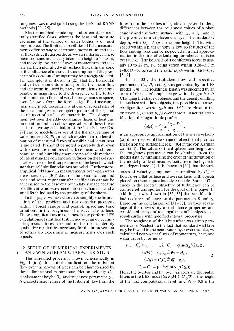
The simulated process is shown schematically inFig. 1 (top). In neutral stratification, the turbulentflow over the crown of trees can be characterized bythree dimensional parameters: friction velocity displacement height , and roughness parameter A characteristic feature of the turbulent flow from the

1

,*U

wD 0 .wz

forest onto the lake lies in significant (several orders)differences between the roughness values of a plantcanopy and the water surface, with and inthe presence of a displacement layer of considerabledepth, with (h is the tree height). The windspeed within a plant canopy is low, so features of theflow among trees can be neglected in a first approxi�mation in the task of calculating turbulence statisticsover a lake. The height h of a coniferous forest is usu�ally 10 to 27 m, being varied within 0.28–3.9 m(∼0.03h–0.15h) and the ratio within 0.61–0.92[5–7].

In [31–33], the turbulent flow with specifiedparameters D, and was generated by an LESmodel [34]. The roughness length was specified by anarray of objects of simple shape with a height Changing the shape of objects and the density of fillingthe surface with these objects, it is possible to choose aconfiguration where and are close to theobserved and over a forest. In neutral strat�ification, the logarithmic profile

(1)

is an appropriate approximation of the mean velocity irrespective of the shape of objects that produce

friction on the surface (here κ = 0.4 in the von Karmanconstant). The values of the displacement height andthe roughness parameter can be obtained from themodel data by minimizing the error of the deviation ofthe model profile of mean velocity from the logarith�mic dependence (1). It is shown in [31] that the vari�

ances of velocity components normalized by inflows over a flat surface and over surfaces with objectsplaced on them approximately coincide. Some differ�ences in the spectral structure of turbulence can beconsidered unimportant for the goal of this paper. Inaddition, it was shown in [32, 33] that stratificationhad no large influence on the parameters D and Based on the conclusions of [31–33], we took advan�tage of the universality of turbulence properties andconsidered arrays of rectangular parallelepipeds as arough surface with specified integral properties.

The roughness of the lake surface was given para�metrically. Neglecting the fact that standard wall lawsmay be invalid in the near�water layer over the lake, wecalculated near�water fluxes of momentum, heat, andwater vapor by formulas

(2)

Here, the overbar and hat over variables are the spatialfilters in the LES model (see [34]), (Δg/2) is the heightof the first computational level, and Pr = 0.8 is the

0 0 ,w lz z�

wD h∼

0wz

wD h

,*U 0z

.h D>

0z h D h

0wz h wD h

*ln0

( ) ,w

w

z DUu zz

⎛ ⎞−= ⎜ ⎟κ ⎝ ⎠

( )u z

2

*U

0.z

' '

' '

23 0

10

ˆ , 1,2, ln( (2 )),

ˆ ( ),

ˆ ( ),

ln( (2 )).Pr

si u i u g l

u s

u q s

q g t

C u u i C z

w C C u

w q C C u q q

C C z

Θ

−

Θ

τ = = = κ Δ

Θ = Θ −Θ

= −

= = κ Δ


LARGE�EDDY SIMULATION OF STRATIFIED TURBULENT FLOWS 353

specified turbulent Prandtl number at the surface.Because simulations used fine grids ( m), theinfluence of stratification in the 25�cm layer above thesurface was disregarded (note that the stratificationeffects above the first computational level influencethe flow, properly changing its dynamics). The valuesof the dynamic roughness and the parameter fortemperature and water vapor were kept constant at

m. This corresponds in order of magni�tude to the averaged values of these parameters mea�sured in observations over a water surface in lightwinds [30]. Close values of can be obtained using

Charnock’s formula [35] ( ) or a

combined formula = ( )

which takes into account a transition to the law of a

0 5gΔ = .

0lz 0tz

40 0 10l tz z −

= =

0lz2

0 *lz Ugα

= 0 02α = .

20 *lz U

gα

=

*a

Uν

ν 0 12aν= .

turbulent boundary layer near a smooth wall in lightwinds [36].

The scheme of computations is shown at the bot�tom of Fig. 1. The turbulent flow is generated by anauxiliary model (a) with double�periodic boundaryconditions and a specified array of objects placed onthe surface. The data from model (a) taken in one ofthe vertical cross sections are transmitted to model (b)at every time step and are then used as Dirichletboundary conditions at the left boundary. This proce�dure provides a nonstationary boundary condition formodel (b) that matches the model dynamics. Thesame program executed on processors of differentgroups in parallel computations is used as the auxiliaryand the basic LES models. Periodic boundary condi�tions in model (b) are given on the Y axis. The flow inmodel (a) is maintained by a time� and space�constantvolume force (computation with a constant gradient of

60555045

1201101009080706050403020100

4035302520151050

–0.5 0 0.5 1.0 1.5 2.0 2.5 3.0 3.5 4.0 4.5 5.0

60555045

1201101009080706050403020100

40353025201510

50

–0.5 0 0.5 1.0 1.5 2.0 2.5 3.0 3.5 4.0 4.5 5.0

Meanwindspeed

z0w >> z0l

Lake

Vegetation

hD

(а) (b)

Fig. 1. (top) Schematic image of a turbulent flow moving from the forest onto a lake. (Bottom) Scheme of calculations with theLES model. (a) The computational domain of the auxiliary model with periodic boundary conditions and (b) the basic compu�tational domain. Wind speed and direction are indicated by dashed lines and streamlines. Rectangles are objects that form surfaceroughness.

354



background pressure. The large�scale external pres�

sure gradient in all computations was set so as to

ensure the friction velocity m/s at the top ofthe roughness layer (at z = h) in a steady�state wind�stream. The “lake” is at the center of the numericaldomain (b) and represents an ellipse with semiaxes a =200 m and b = 60 m. The lake is surrounded by objectsof the same shape and size as the objects in the domain(a). Here we used an array of rectangular parallelepi�peds ordered in the same way as the arrays of cubes in[31–33]. The fraction of the surface occupied byobjects was 0.25. Computations were run for differentparallelepiped heights h (16 and 8 m). The grid size ofthe domain (b) in basic computations was 1024 × 512 ×128 or 512 × 1024 × 128 grid points; the grid spacing

in all three spatial directions. In the auxiliarydomain (a), computations were run on grids having256 × 512 × 128 points or 512 ×1024 ×128 grid points,depending on the wind direction. The time step was0.025 s. The flow was first computed in the auxiliarydomain until a steady state was reached. This takesabout 1.5 h of model time. Models (a) and (b) werethen integrated for 1 h. The last half hour was used toaverage and calculate statistics. Computations wereperformed on Moscow State University’s Lomonosovsupercomputer [37] using up to 2048 cores in parallelimplementation.

The flow in all computations was neutrally strati�fied. The unstable or stable stratification over the lakewas maintained by specifying the surface temperature

which was 5 K above or below the airflow temper�ature ( 282 K in all computations). The spe�cific air humidity q in the windstream was set equal to4 g/kg (no water vapor flux from the “forest” canopysurface). The lake�surface humidity was taken equalto its saturation at a corresponding temperature andpressure P = 1000 mb.

A total of six basic experiments were run: ECB16, and ESB16. Additionally, two

auxiliary computations were run, one of which was with a coarse grid m for evaluating the

sensitivity of results to a spatial resolution and another with a fine grid m but a modified con�

figuration of objects in the roughness layer for evaluat�ing the influence of this configuration on turbulenceover the lake. The subscripts in the names of the exper�iments have the following meaning: C means unstablestratification (convection over a lake); S, stable strati�fication over a lake; A, average wind blows along themajor axis of the ellipse; B, wind blows along theminor axis; 16 means that the tree height is 16 m; and8 stands for h = 8 m.

Px

∂

∂

* 0 4U = .

1

0 5gΔ = .

,sΘ

0Θ 0Θ =

1

sq

16,CAE

8,CAE 16,SAE 8,SAE

161CAA 1gΔ =

162CAA 0 5gΔ = .

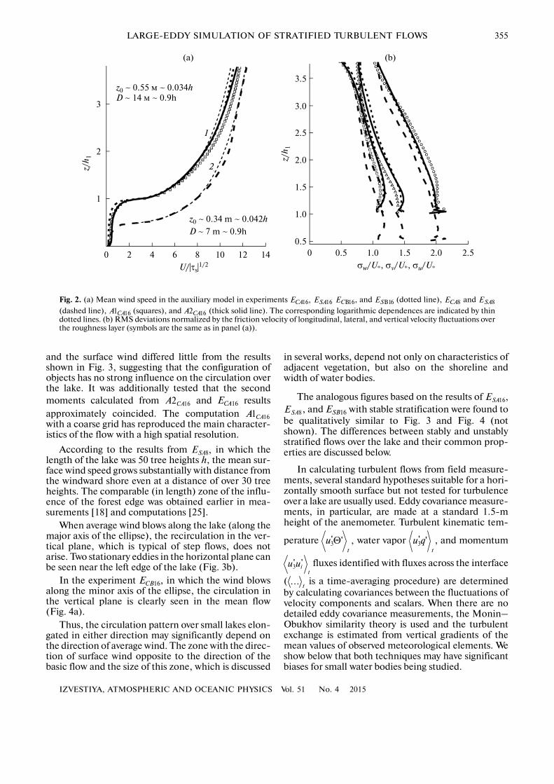
Mean wind profiles derived from auxiliary model(a) in , and ESB16 (dotted line); and (dashed line); (squares); and (thick solid curve) are shown in Fig. 2a.

The ratio of the side of the base of a parallelepipedto its height was 1 : 4 in and 1 : 2 in . Thedensity of the objects placed on the surface was thesame, 0.25. As can be seen from Fig. 2a, the meanwinds in and almost coincide over theroughness layer. Thus, and are identicalfor these two surfaces. In with a coarse modelgrid ( = 1 m), the mean velocity at some distancefrom the surface slightly exceeds velocities in compu�tations with a fine grid ( = 0.5 m).

Minimizing the root�mean�square deviation of thecalculated profiles from the logarithmic dependence(1) in the height range we have deter�mined the following values of the roughness lengthand displacement height: m ~ 0.034h and

m for and , and m ≈ 0.042h and m for These valuesof and fall within a range of values typical offorest vegetation. The exact coincidence of the profileof mean velocity with self�similar solution (1) shouldnot be expected either in the model or in naturebecause of the influence of surface heterogeneity, theabsence of a rigid boundary from below, and theimpossibility of using the constant�flux layer approxi�mation (see [31]). Therefore, the resulting values of

and should be considered only as one of thepossible approximations, which depend, in particular,on the choice of a height range within which the pro�file is approximated by a logarithmic dependence ormeasurements are made.

The root�mean�square (RMS) deviations (nor�

malized by the friction velocity ) of the fluc�tuations of the longitudinal, lateral, and vertical veloc�ity components over the roughness layer are shown inFig. 2. In this case, we have a distribution of turbulencekinetic energy (TKE) between the three components,which is typical of a shear turbulent flow.

Thus, in the auxiliary model (a), turbulent flowshave been generated with characteristics typical ofnear�wall neutrally stratified flows and with displace�ment heights and roughness parameters lying in therange of the values typical of forest vegetation.

3. CHARACTERISTICS OF TURBULENT FLOWS OVER A “LAKE”

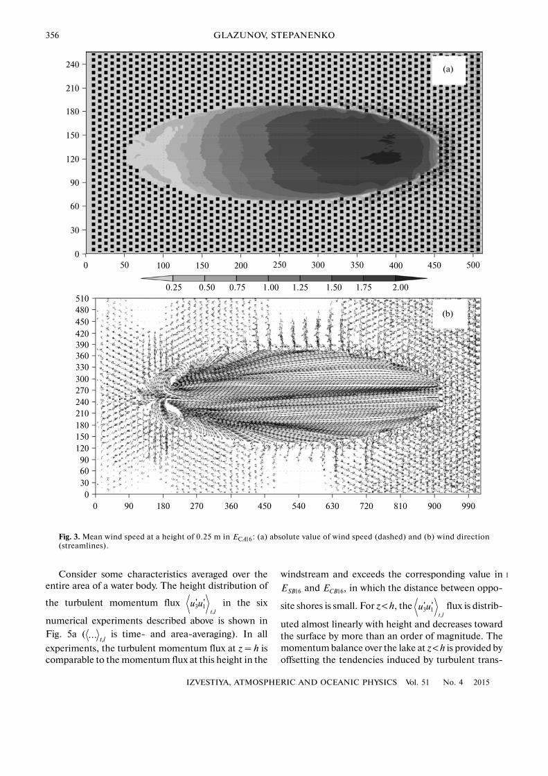
The mean surface wind speed derived from ECA16 isshown in Figs. 3a and 3b ((a.) the magnitude of windspeed is dashed and (b) wind direction is indicated bystreamlines). Black squares are objects that form theroughness imitating a forest. In , the structure

16,CAE 16SAE 16CBE 8CAE

8SAE 161CAA 162CAA

16CAE 162CAA

16CAE 162CAA

0wz h wD h

161CAA

gΔ

gΔ

2 5 ,h z h< < .

0 0 55wz ≈ .

14wD ≈ 0 9h≈ . 16CAE 162CAA 0 0 34wz ≈ .

7wD ≈ 0 9h≈ . 8.CAE

0wz wD

0wz 0wD

*1 2

sU = τ

162CAA



and the surface wind differed little from the resultsshown in Fig. 3, suggesting that the configuration ofobjects has no strong influence on the circulation overthe lake. It was additionally tested that the secondmoments calculated from and ECA16 resultsapproximately coincided. The computation with a coarse grid has reproduced the main character�istics of the flow with a high spatial resolution.

According to the results from in which thelength of the lake was 50 tree heights h, the mean sur�face wind speed grows substantially with distance fromthe windward shore even at a distance of over 30 treeheights. The comparable (in length) zone of the influ�ence of the forest edge was obtained earlier in mea�surements [18] and computations [25].

When average wind blows along the lake (along themajor axis of the ellipse), the recirculation in the ver�tical plane, which is typical of step flows, does notarise. Two stationary eddies in the horizontal plane canbe seen near the left edge of the lake (Fig. 3b).

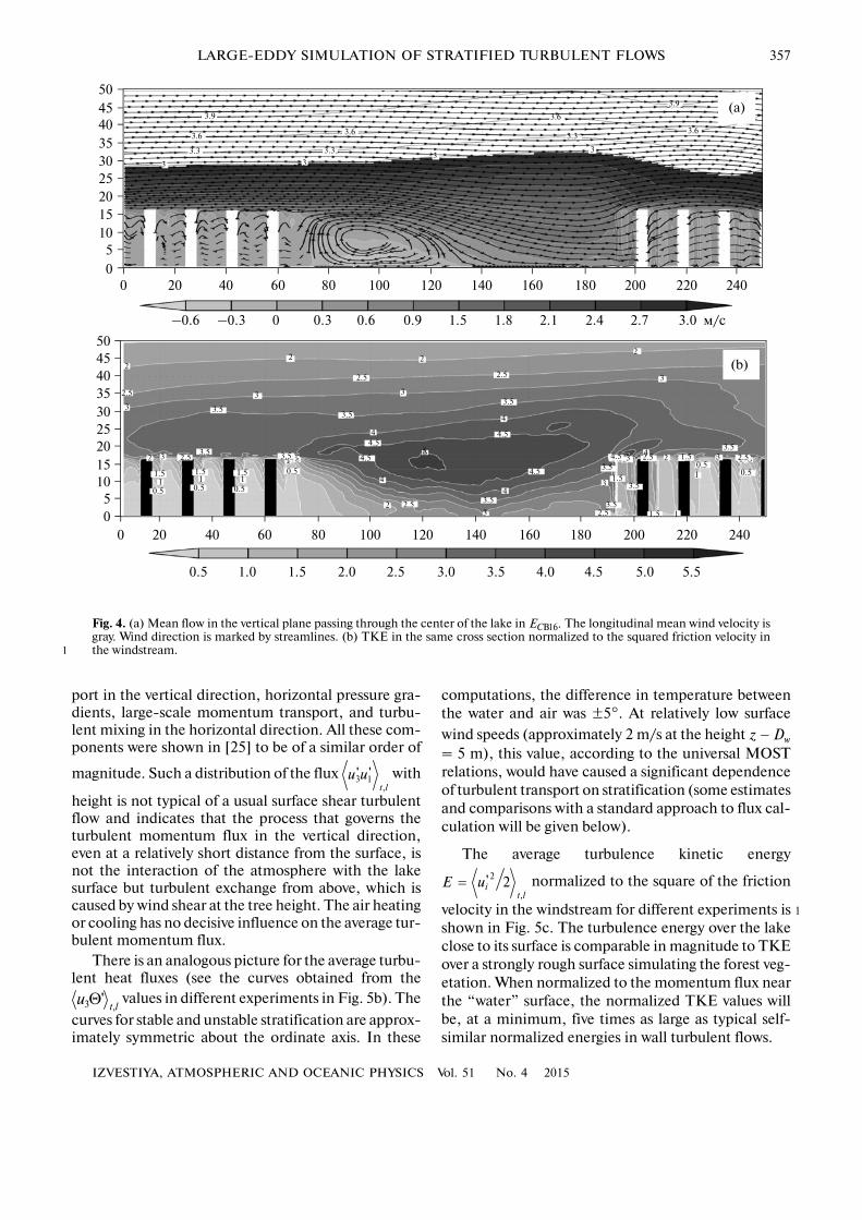
In the experiment ECB16, in which the wind blowsalong the minor axis of the ellipse, the circulation inthe vertical plane is clearly seen in the mean flow(Fig. 4a).

Thus, the circulation pattern over small lakes elon�gated in either direction may significantly depend onthe direction of average wind. The zone with the direc�tion of surface wind opposite to the direction of thebasic flow and the size of this zone, which is discussed

162CAA

161CAA

8,SAE

in several works, depend not only on characteristics ofadjacent vegetation, but also on the shoreline andwidth of water bodies.

The analogous figures based on the results of , and ESB16 with stable stratification were found to

be qualitatively similar to Fig. 3 and Fig. 4 (notshown). The differences between stably and unstablystratified flows over the lake and their common prop�erties are discussed below.

In calculating turbulent flows from field measure�ments, several standard hypotheses suitable for a hori�zontally smooth surface but not tested for turbulenceover a lake are usually used. Eddy covariance measure�ments, in particular, are made at a standard 1.5�mheight of the anemometer. Turbulent kinematic tem�

perature water vapor , and momentum

fluxes identified with fluxes across the interface

( is a time�averaging procedure) are determinedby calculating covariances between the fluctuations ofvelocity components and scalars. When there are nodetailed eddy covariance measurements, the Monin–Obukhov similarity theory is used and the turbulentexchange is estimated from vertical gradients of themean values of observed meteorological elements. Weshow below that both techniques may have significantbiases for small water bodies being studied.

16,SAE

8SAE

Θ' '3 ,t

u ' '3t

u q

3' 'it

u u

t...

3

2

1

10 14128640 2

3.0

2.5

2.0

2.52.01.51.00 0.5

3.5

1.5

1.0

0.5

z/h 1

1

2

z0 ~ 0.55 м ~ 0.034hD ~ 14 м ~ 0.9h

U/|τs|1/2

(a) (b)

z0 ~ 0.34 m ~ 0.042h

D ~ 7 m ~ 0.9h

z/h 1

σw/U*, σv/U*, σu/U*

Fig. 2. (a) Mean wind speed in the auxiliary model in experiments , and (dotted line), and

(dashed line), (squares), and (thick solid line). The corresponding logarithmic dependences are indicated by thindotted lines. (b) RMS deviations normalized by the friction velocity of longitudinal, lateral, and vertical velocity fluctuations overthe roughness layer (symbols are the same as in panel (a)).

16,CAE 16SAE B16CE B16SE 8CAE 8SAE

161CAA 162CAA

356



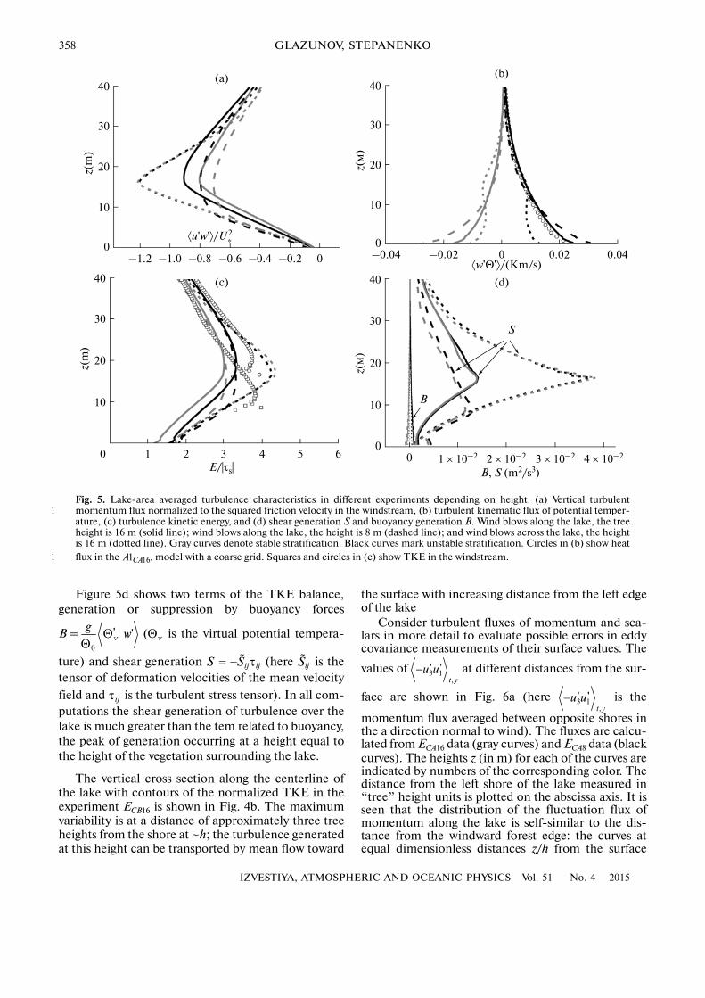
Consider some characteristics averaged over theentire area of a water body. The height distribution of

the turbulent momentum flux in the six

numerical experiments described above is shown inFig. 5a ( is time� and area�averaging). In all

experiments, the turbulent momentum flux at z = h iscomparable to the momentum flux at this height in the

3 1' 't l

u u,

t l,...

windstream and exceeds the corresponding value in

and in which the distance between oppo�

site shores is small. For z < h, the flux is distrib�

uted almost linearly with height and decreases towardthe surface by more than an order of magnitude. Themomentum balance over the lake at z < h is provided byoffsetting the tendencies induced by turbulent trans�

1

16SBE 16,CBE

3 1' 't l

u u,

240

210

180

150

120

90

60

30

0200 250150100500 300 350 400 450 500

390360330

270

210

150

9060

0450 5403602701800 630 720 810 900 99090

30

120

180

240

300

420450480510

0.25 0.50 0.75 1.00 1.25 1.50 1.75 2.00

(а)

(b)

Fig. 3. Mean wind speed at a height of 0.25 m in : (a) absolute value of wind speed (dashed) and (b) wind direction(streamlines).

C 16AE



port in the vertical direction, horizontal pressure gra�dients, large�scale momentum transport, and turbu�lent mixing in the horizontal direction. All these com�ponents were shown in [25] to be of a similar order of

magnitude. Such a distribution of the flux with

height is not typical of a usual surface shear turbulentflow and indicates that the process that governs theturbulent momentum flux in the vertical direction,even at a relatively short distance from the surface, isnot the interaction of the atmosphere with the lakesurface but turbulent exchange from above, which iscaused by wind shear at the tree height. The air heatingor cooling has no decisive influence on the average tur�bulent momentum flux.

There is an analogous picture for the average turbu�lent heat fluxes (see the curves obtained from the

values in different experiments in Fig. 5b). The

curves for stable and unstable stratification are approx�imately symmetric about the ordinate axis. In these

3 1' 't l

u u,

'3 t lu

,

Θ

computations, the difference in temperature betweenthe water and air was ±5°. At relatively low surfacewind speeds (approximately 2 m/s at the height = 5 m), this value, according to the universal MOSTrelations, would have caused a significant dependenceof turbulent transport on stratification (some estimatesand comparisons with a standard approach to flux cal�culation will be given below).

The average turbulence kinetic energy

normalized to the square of the friction

velocity in the windstream for different experiments isshown in Fig. 5c. The turbulence energy over the lakeclose to its surface is comparable in magnitude to TKEover a strongly rough surface simulating the forest veg�etation. When normalized to the momentum flux nearthe “water” surface, the normalized TKE values willbe, at a minimum, five times as large as typical self�similar normalized energies in wall turbulent flows.

wz D−

2' 2it l

E u,

=

1

50454035302520

0240220200180160140120100806040200

1510

5

50454035302520

0240220200180160140120100806040200

1510

5

–0.6 –0.3 0 0.6 0.9 1.5 1.8 2.1 2.4 2.7 3.0

0.5 1.0 1.5 2.0 2.5 3.0 3.5 4.0 4.5 5.0 5.5

м/с

(а)

(b)

0.3

2

2.5

3

2 3

1.51

0.5

2.53.5

1.51

0.5

1.51

0.5

0.5

3.5

3.5

3

2

2.5

3.5

3

2

44.5

4.5

4

2 2.5

5

3.5

3

2.5

3.5

4

4.5

4.5

4

4.53.5

3

2

2

31 0.5

1.5

3.52.5

0.5

3.5

1.5

342.5 1.5 3

3.52.5

1

3

3.6

3.6

3.3

3

3.9

3.6

33

3.9

3.6

3.3 3.3

Fig. 4. (a) Mean flow in the vertical plane passing through the center of the lake in The longitudinal mean wind velocity isgray. Wind direction is marked by streamlines. (b) TKE in the same cross section normalized to the squared friction velocity inthe windstream.

B16.CE

1

358



Figure 5d shows two terms of the TKE balance,generation or suppression by buoyancy forces

B = ( is the virtual potential tempera�

ture) and shear generation (here is thetensor of deformation velocities of the mean velocityfield and is the turbulent stress tensor). In all com�putations the shear generation of turbulence over thelake is much greater than the tem related to buoyancy,the peak of generation occurring at a height equal tothe height of the vegetation surrounding the lake.

The vertical cross section along the centerline ofthe lake with contours of the normalized TKE in theexperiment ECB16 is shown in Fig. 4b. The maximumvariability is at a distance of approximately three treeheights from the shore at ~h; the turbulence generatedat this height can be transported by mean flow toward

ΘΘ

' 'v

0

gw Θ

v

ij ijS S= − τ�

ijS�

ijτ

the surface with increasing distance from the left edgeof the lake

Consider turbulent fluxes of momentum and sca�lars in more detail to evaluate possible errors in eddycovariance measurements of their surface values. The

values of at different distances from the sur�

face are shown in Fig. 6a (here is the

momentum flux averaged between opposite shores inthe a direction normal to wind). The fluxes are calcu�lated from ECA16 data (gray curves) and ECA8 data (blackcurves). The heights z (in m) for each of the curves areindicated by numbers of the corresponding color. Thedistance from the left shore of the lake measured in“tree” height units is plotted on the abscissa axis. It isseen that the distribution of the fluctuation flux ofmomentum along the lake is self�similar to the dis�tance from the windward forest edge: the curves atequal dimensionless distances z/h from the surface

3 1' 't y

u u,

−

3 1' 't y

u u,

−

40

30

20

10

–0.4 0–0.2–0.6–0.8–1.00

–1.2

z(m

)

⟨u'w'⟩/U 2*

40

30

20

10

0.040.020–0.020

z(м

)

⟨w'Θ'⟩/(Km/s)40

30

20

10

4 × 10–23 × 10–22 × 10–21 × 10–20

0

z(м

)

40

30

20

10

4 65320 1

z(m

)

–0.04

B

S

B, S (m2/s3)E/|τs|

(а) (b)

(c) (d)

Fig. 5. Lake�area averaged turbulence characteristics in different experiments depending on height. (a) Vertical turbulentmomentum flux normalized to the squared friction velocity in the windstream, (b) turbulent kinematic flux of potential temper�ature, (c) turbulence kinetic energy, and (d) shear generation S and buoyancy generation B. Wind blows along the lake, the treeheight is 16 m (solid line); wind blows along the lake, the height is 8 m (dashed line); and wind blows across the lake, the heightis 16 m (dotted line). Gray curves denote stable stratification. Black curves mark unstable stratification. Circles in (b) show heatflux in the model with a coarse grid. Squares and circles in (c) show TKE in the windstream.

1

161 .CAA1



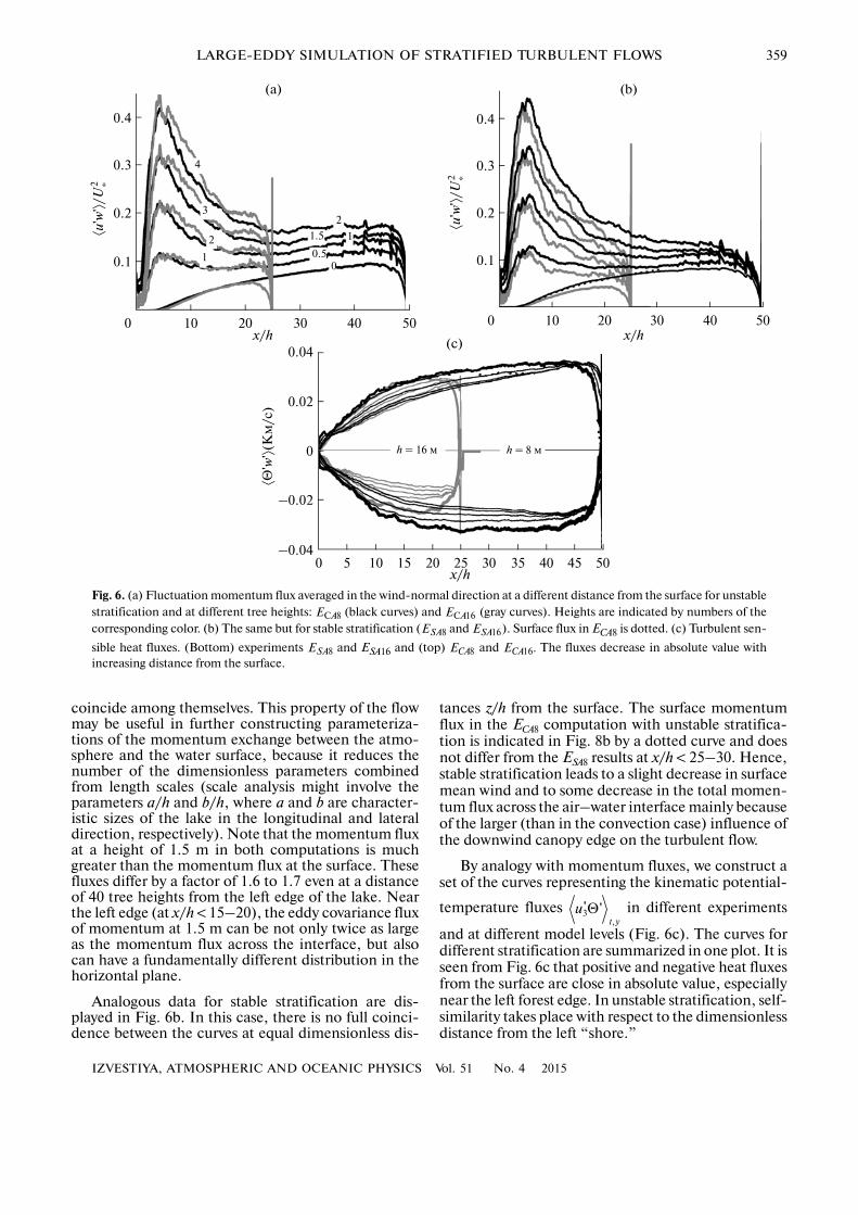
coincide among themselves. This property of the flowmay be useful in further constructing parameteriza�tions of the momentum exchange between the atmo�sphere and the water surface, because it reduces thenumber of the dimensionless parameters combinedfrom length scales (scale analysis might involve theparameters a/h and b/h, where а and b are character�istic sizes of the lake in the longitudinal and lateraldirection, respectively). Note that the momentum fluxat a height of 1.5 m in both computations is muchgreater than the momentum flux at the surface. Thesefluxes differ by a factor of 1.6 to 1.7 even at a distanceof 40 tree heights from the left edge of the lake. Nearthe left edge (at x/h < 15–20), the eddy covariance fluxof momentum at 1.5 m can be not only twice as largeas the momentum flux across the interface, but alsocan have a fundamentally different distribution in thehorizontal plane.

Analogous data for stable stratification are dis�played in Fig. 6b. In this case, there is no full coinci�dence between the curves at equal dimensionless dis�

tances z/h from the surface. The surface momentumflux in the ECA8 computation with unstable stratifica�tion is indicated in Fig. 8b by a dotted curve and doesnot differ from the ESA8 results at x/h < 25–30. Hence,stable stratification leads to a slight decrease in surfacemean wind and to some decrease in the total momen�tum flux across the air–water interface mainly becauseof the larger (than in the convection case) influence ofthe downwind canopy edge on the turbulent flow.

By analogy with momentum fluxes, we construct aset of the curves representing the kinematic potential�

temperature fluxes in different experiments

and at different model levels (Fig. 6c). The curves fordifferent stratification are summarized in one plot. It isseen from Fig. 6c that positive and negative heat fluxesfrom the surface are close in absolute value, especiallynear the left forest edge. In unstable stratification, self�similarity takes place with respect to the dimensionlessdistance from the left “shore.”

'3't y

u,

Θ

0.4

0.3

0.2

0.1

50403020100

⟨u'w

'⟩/U

2 *

0.4

0.3

0.2

0.1

50403020100

⟨u'w

'⟩/U

2 *

0.04

0.02

0

–0.02

50454035200

⟨Θ'w

'⟩(К

м/с

)

302515105–0.04

x/h

x/h

x/h

h = 16 м h = 8 м

1

2

3

4

2

11.5

0.50

(а) (b)

(c)

Fig. 6. (a) Fluctuation momentum flux averaged in the wind�normal direction at a different distance from the surface for unstablestratification and at different tree heights: (black curves) and (gray curves). Heights are indicated by numbers of thecorresponding color. (b) The same but for stable stratification ( and ). Surface flux in ECA8 is dotted. (c) Turbulent sen�

sible heat fluxes. (Bottom) experiments and ESA16 and (top) and The fluxes decrease in absolute value withincreasing distance from the surface.

C 8AE C 16AE

8SAE 16SAE

8SAE 8CAE 16.CAE

360



In large�scale atmospheric circulation models, theair temperature, humidity, and wind speed are knownonly on average for a model cell that is larger than thesize of the lakes considered and at a distance from thesurface equal to the height of the first model level (usu�ally one to several tens of meters). When the MOST isused, it is implied implicitly that the model ground sur�face is found at the displacement height Consider�ing the LES�derived mean wind speed m/sin the incoming flow at a height of = 10 an ana�logue of wind speed in a large�scale atmosphericmodel, it is possible to estimate an error of calculatingthe fluxes from the lake surface using standard MOSTrelations. Using the universal function from [34] and

specifying for the lake surface, we obtain thefollowing estimates of the sensible heat and momen�

tum fluxes: = –1.25 × 10–5 Km/s and =

–7.1 × 10–6 m2/s2 (for stable stratification at =

–5 K) and = 3.5 × 10–2 Km/s, = –1.4 ×

10–2 m2/s2 (for unstable stratification at =5 K). Thus, the standard method used to calculatefluxes from the surface leads to significant differences(of several orders of magnitude) in the absolute valueof these fluxes for different types of stratification. Thisis not observed in the LES experiments. In particular,in and , the following values were obtainedfor the fluxes averaged over the entire lake surface:

= –3.1 × 10–2 Km/s and = –2.1 × 10–3

m2/s2 (for stable stratification) and =

Km/s, = m2/s2 (for

unstable stratification). It is interesting to note that thetotal negative heat flux from the surface in is inabsolute value two orders of magnitude greater than

the estimate ( = Km/s) of this flux

determined by a standard technique using the rough�ness parameter m for a forested surface.Large differences are also obtained for unstable strati�fication, where the corresponding estimate using a

standard technique gives = 0.6 Km/s.

4. CONCLUSIONS

The most important effect revealed in the course ofthe investigation is the low sensitivity of statistics of aturbulent flow over a lake to thermal stratification. Thereason is that most of the turbulence kinetic energy isgenerated by wind shear at the tree height. This mech�anism provides a more intense turbulent mixing overthe lake surface than mixing over a homogeneous sur�face with the same aerodynamic characteristics. In a

.wD

10 2 8U ≈ .

wz D−

40 10lz −

=

'3's

u Θ 3 1' 's

u u

10sΘ − Θ

'3's

u Θ 3 1' 's

u u

10sΘ − Θ

C 8AE 8SAE

'3's

u Θ 3 1' 's

u u

'3's

u Θ

22 96 10−

. × 3 1' 's

u u31 96 10−

− . ×

8SAE

'3's

u Θ41 5 10−

− . ×

0 0 34wz ≈ .

'3's

u Θ

first approximation, the turbulent transport of heatand water vapor over the surface of small water bodiessurrounded by forest can be regarded as a process sim�ilar to the transport of passive scalars.

For small water bodies surrounded by forest, thecalculation of sensible and latent heat fluxes from thesurface cannot be made using standard methods, forexample, the Monin–Obukhov similarity theory. Thisequally concerns any other heterogeneous surfacewith alternate vegetation types. The most importanteffect of surface heterogeneity is a significant intensi�fication of turbulent exchange in stable stratification.The problem of simulating strongly stable boundarylayers in the framework of weather forecasting and cli�mate models is among the unresolved tasks of modernmeteorology. It is shown in [38], for example, thatmodern numerical weather prediction models sub�stantially underestimate surface temperature inver�sions and overestimate surface temperatures in thewinter period.

One more conclusion that follows from the numer�ical results concerns the interpretation of field eddycovariance measurements over the surface of waterbodies. It was found that turbulent momentum fluxes,even at a relatively short distance from the surface, dif�fered significantly from the fluxes across the interface.The use of standard techniques for surface momentumflux estimation, which imply that sensors are mountedat a height of ~1.5 m, can result in a large overestima�tion of their values. A systematic measuring error(which overestimates the surface frictional stress by afactor of 1.6 to 1.7) will exist even far away from theshore, at a distance of 26 to 30 times the tree height.Close to the shore (at a distance less than 15 to 20 treeheights), the eddy covariance fluxes better representthe mixing process induced by velocity shear in thewindstream at the tree height and may radically differfrom the surface frictional stresses, including the spa�tial distribution in the horizontal plane.

ACKNOWLEDGMENTS

The study was supported by the Russian Founda�tion for Basic Research (grant nos. 13�05�00978�a and14�05�91752�AF�a) and the Leading Science SchoolNSh�6147.2014.5. Resources of Moscow State Uni�versity’s Lomonosov supercomputer were used.

REFERENCES

1. D. Mironov, E. Heise, E. Kourzeneva, et al., “Imple�mentation of the lake parameterisation scheme flakeinto the numerical weather prediction modelCOSMO,” Boreal Environ. Res. 15 (2), 218–230(2010).

2. E. Dutra, V. M. Stepanenko, G. Balsamo, et al., “Anoffline study of the impact of lakes on the performanceof the ECMWF surface scheme,” Boreal Environ. Res.15 (2), 100–112 (2010).

3. G. Balsamo, R. Salgado, E. Dutra, et al., “On the con�tribution of lakes in predicting near�surface tempera�

1



ture in a global weather forecasting model,” Tellus A64, 15829 (2012).

4. W. R. Rouse, C. J. Oswald, J. Binyamin, et al., “Therole of northern lakes in a regional energy balance,”J. Hydrometeorol. 6 (3), 291–305 (2005).

5. T. R. Oke, Boundary Layer Climates (Routledge Taylorand Francis, New York, 1987).

6. R. B. Stull, An Introduction to Boundary Layer Meteo�rology (Kluwer, Norwell, MA, 1988).

7. J. R. Garratt, The Atmospheric Boundary Layer (Cam�bridge Univ. Press, New York, 1994).

8. L. Mahrt, “Surface heterogeneity and vertical structureof the boundary layer,” Boundary�Layer Meteorol. 96(1–2), 33–62 (2000).

9. J. W. Glendening and C�L. Lin, “Large eddy simula�tion of internal boundary layers created by a change insurface roughness,” J. Atmos. Sci. 59 (10), 1697–1711(2002).

10. E. Bou�Zeid, C. Meneveau, and M. B. Parlange,“Large�eddy simulation of neutral atmospheric bound�ary layer flow over heterogeneous surfaces: Blendingheight and effective surface roughness,” Water Resour.Res. 40 (2), W02505 (2004).

11. E. Bou�Zeid, M. Parlange, and C. Meneveau, “On theparameterization of surface roughness at regionalscales,” J. Atmos. Sci. 64 (1), 216–227 (2007).

12. R. Stoll and F. Porte�Agel, “Dynamic subgrid�scalemodels for momentum and scalar fluxes in large�eddysimulations of neutrally stratified atmospheric bound�ary layers over heterogeneous terrain,” Water Resour.Res. 42 (1), W01409 (2006).

13. R. Stoll and F. Porte�Agel, “Surface heterogeneityeffects on regional�scale fluxes in stable boundary lay�ers: surface temperature transitions,” J. Atmos. Sci. 66(2), 412–431 (2009).

14. J. A. Downing, Y. T. Praire, J. J. Cole, et al., “The glo�bal abundance and size distribution of lakes, ponds, andimpoundments,” Limnol. Oceanogr. 51 (5), 2388–2397 (2006).

15. S. A. Condie and I. T. Webster, “Estimating stratifica�tion in shallow water bodies from mean meteorologicalconditions,” J. Hydraul. Eng 127 (4), 286–292 (2001).

16. B. Boehrer and M. Schultze, “Stratification of lakes,”Rev. Geophys. 46 (2), RG2005 (2008).

17. J. M. Chen, T. A. Clack, M. D. Novak, and R. S.Adams, “A wind tunnel study of turbulent airflow inforest clear cuts,” in Wind and Trees, Ed. by M. P.Coutts and J. Grace (Cambridge Univ. Press, NewYork, 1995), pp. 71–87.

18. C. D. Markfort, A. L. S. Perez, J. W. Thill, et al., “Windsheltering of a lake by a tree canopy or bluff topogra�phy,” Water Resour. Res. 46 (3), W03530 (2010).

19. M. Detto, G. G. Katul, M. Siqueira, et al., “The struc�ture of turbulence near a tall forest edge: The backward�facing step flow analogy revisited,” Ecol. Appl. 18 (6),1420–1435 (2008).

20. J. Liu, J. M. Chen, T. A. Black, and M. D. Novak, “E–ε modelling of turbulent air flow downwind of a modelforest edge,” Boundary�Layer Meteorol. 77 (1), 21–44(1996).

21. E. G. Patton, R. H. Shaw, M. J. Judd, and M. R. Rau�pach, “Large�eddy simulation of windbreak flow,”Boundary�Layer Meteorol. 87 (2), 275–306 (1998).

22. J. D. Wilson and T. K. Flesch, “Wind and remnant treesway in forest cutblocks. III. A windflow model to diag�

nose spatial variation,” Agric. For. Meteorol. 93 (4),259–282 (1999).

23. B. Yang, M. R. Raupach, R. H. Shaw, et al., “Large�eddy simulation of turbulent flow across a forest edge.Part I: Flow statistics,” Boundary�Layer Meteorol. 120(3), 377–412 (2006).

24. B. Yang, A. Morse, R. H. Shaw, and K. T. Paw, “Large�eddy simulation of turbulent flow across a forest edge.Part II: Momentum and turbulent kinetic energy bud�get,” Boundary�Layer Meteorol. 121 (3), 433–457(2006).

25. M. Cassiani, G. G. Katul, and J. D. Albertson, “Theeffects of canopy leaf area index on airflow across forestedges: Large�eddy simulation and analytical results,”Boundary�Layer Meteorol. 126 (3), 433–460 (2008).

26. T. Foken, “The energy balance closure problem: Anoverview,” Ecol. Appl. 18 (6), 1351–1367 (2008).

27. A. Nordbo, S. Launiainen, I. Mammarella, et al.,“Long�term energy flux measurements and energy bal�ance over a small boreal lake using eddy covariancetechnique,” J. Geophys. Res. 116 (D2), 1–17 (2011).

28. V. M. Stepanenko, A. Martynov, K. D. Jöhnk, et al.,“A one�dimensional model intercomparison study ofthermal regime of a shallow, turbid midlatitude lake,”Geosci. Model Dev. 6 (4), 1337–1352 (2013).

29. V. Stepanenko, K. D. Jöhnk, E. Machulskaya, et al.,“Simulation of surface energy fluxes and stratificationof a small boreal lake by a set of one�dimensional mod�els,” Tellus A 66, 21389 (2014).

30. J. DeCosmo, K. B. Katsaros, S. D. Smith, et al., “Air�sea exchange of water vapor and sensible heat: TheHumidity Exchange Over the Sea (HEXOS),” J. Geo�phys. Res. 101 (C5), 12001–12016 (1996).

31. A. V. Glazunov, “Numerical modeling of turbulentflows over an urban�type surface: Computations forneutral stratification,” Izv., Atmos. Ocean. Phys. 50(2), 134–142 (2014).

32. A. V. Glazunov, “Numerical simulation of stably strati�fied turbulent flows over flat and urban surfaces,” Izv.,Atmos. Ocean. Phys. 50 (3), 236–245 (2014).

33. A. V. Glazunov, “Numerical simulation of stably strati�fied turbulent flows over an urban surface: Spectra andscales and parameterization of temperature and wind�velocity profiles,” Izv., Atmos. Ocean. Phys. 50 (4),356–368 (2014).

34. A. V. Glazunov, “Large�eddy simulation of turbulencewith the use of a mixed dynamic localized closure: Part1. Formulation of the problem, model description, anddiagnostic numerical tests,” Izv., Atmos. Ocean. Phys.45 (1), 5–24 (2009).

35. H. Charnock, “Wind stress on a water surface,” Q. J. R.Meteorol. Soc. 81 (350), 639–640 (1955).

36. S. S. Zilitinkevich, “On the computation of the basicparameters of the interaction between the atmosphereand the ocean,” Tellus 21 (1), 17–24 (1969).

37. V. Sadovnichy, A. Tikhonravov, Vl. Voevodin, andV. Opanasenko, “”Lomonosov”: Supercomputing atMoscow State University," in Contemporary High Per�formance Computing: From Petascale Toward Exascale(CRC, Boca Raton, USA, 2013), pp. 283–307.

38. E. Atlaskin and T. Vihma, “Evaluation of NWP resultsfor wintertime nocturnal boundary�layer temperaturesover Europe and Finland,” Q. J. R. Meteorol. Soc. 138(667), 1401–1680 (2012).

Translated by N. Tret’yakova

SPELL: 1. windstream

Large Eddy Simulation of Stratified Turbulent Flows over Heterogeneous Landscapes

Documents

Transcript of Large Eddy Simulation of Stratified Turbulent Flows over Heterogeneous Landscapes