arX

iv:n

lin/0

2050

03v1

[nl

in.C

D]

1 M

ay 2

002

Turbulent Pair Diffusion

F. NicolleauThe University of Sheffield, Department of Mechanical Engineering, Mappin Street, Sheffield, S1 3JD, UK

J. C. VassilicosImperial College of Science, Technology and Medicine, Department of Aeronautics, Prince Consort Road, South Kensington,

London, SW7 2BY, UK

(February 8, 2008)

Kinematic Simulations of turbulent pair diffusion in planar turbulence with a k−5/3 energy spec-trum reproduce the results of the laboratory measurements of Jullien et al Phys. Rev. Lett. 82,2872 (1999), in particular the stretched exponential form of the PDF of pair separations and theircorrelation functions. The root mean square separation is found to be strongly dependent on initialconditions for very long stretches of times. This dependence is consistent with the topological pic-ture of turbulent pair diffusion where pairs initially close enough travel together for long stretchesof time and separate violently when they meet straining regions around hyperbolic points. A newargument based on the divergence of accelerations is given to support this picture.

PACS numbers: 47.27.Eq 47.27.Gs 92.10.Lq 47.27.Qb

The rate with which pairs of points separate in phase space or in physical space is of central importance to the studyof dynamical systems. Pairs of points in the phase space of a low-dimensional chaotic dynamical system separateexponentially. This is the celebrated butterfly effect: dynamics are extremely sensitive to initial conditions. Pairsof fluid elements in fully choatic flows [1] also separate exponentially. However, in fully developed homogeneous andisotropic turbulence, Richardson’s law [2] stipulates that fluid element pairs separate on average algebraically and insuch a way that their separation statistics in a certain range of times are the same irrespective of initial conditions.Richardson’s law is therefore a remarkable claim of universality. Specifically, it stipulates that in a range of times

where the root mean square separation ∆21/2

is larger than the Kolmogorov length-scale η and smaller than theintegral length-scale L, ∆2 is increasingly well approximated by

∆2 = G∆ǫt3 (1)

for increasing values of L/η, where t is time, ǫ is the kinetic energy rate of dissipation per unit mass and G∆ is auniversal dimensionless constant.

Richardson accompanied his empirical law (1) with a prediction for the probability density function (PDF) ofpair separations ∆. The effective diffusivity approach leading to this prediction was criticised by Batchelor [3] whodeveloped a different approach leading to (1) but also to a different form of the PDF. Kraichnan [4] derived yet anotherexpression for the PDF based on his Lagrangian history direct interaction approximation and so did Shlesinger et al

[5] on the assumption that turbulent pair diffusion is well described by Levy walks.

Setting σ(t) ≡ ∆21/2

and r ≡ ∆/σ, the PDFs of ∆ predicted by Richardson [2], Batchelor [3] and Kraichnan [4]are all of the form

P (∆, t) ∼ σ−1 exp(−αrβ) (2)

with different values of the dimensionless parameters α and β. Richardson’s prediction for the exponent β is β = 2/3,Batchelor’s is β = 2 and Kraichnan’s is β = 4/3. The Lagrangian modelling approach of Shlesinger et al [5] leads toa totally different, in fact algebraic, PDF form. More recently Jullien et al [6] reported laboratory measurements ofP (∆, t) which are well fitted by (2) with α ≈ 2.6 and β = 0.5±0.1. These laboratory measurements invalidate the PDFpredictions of Batchelor, Kraichnan and Shlesinger et al. and might raise a question mark over the PDF predictionof Richardson even though they can be considered consistent with it if we account for experimental uncertainties.Jullien et al [6] also observed that fluid element pairs stay close to each other for a long time until they separatequite suddenly, a behaviour which seems qualitatively at odds with the effective diffusivity approach adopted byRichardson [2] to derive (2) with β = 2/3. In particular, they measured the Lagrangian autocorrelation function ofpair separations R(t, τ) ≡< ∆(t)∆(t + τ) > for −t ≤ τ ≤ 0 and found a Lagrangian pair correlation time τc ≈ 0.6twhich is surprisingly long. In this paper we report that Kinematic Simulation (KS) [7] reproduces the experimentalresults of Jullien et al [6]. KS is a Lagrangian model of turbulent diffusion which is distinct from Levy walks [5] andmakes no use of Markovianity assumptions so that it cannot be reduced to an effective diffusivity approach such as

1

Richardson’s [2]. Furthermore, the observation that fluid element pairs travel close together for long stretches of timeuntil they separate quite suddenly has in fact already been made using KS [7].

KS Lagrangian modelling consists in integrating fluid element trajectories by solving dx(t)dt = u(x(t), t) in synthesised

velocity fields u(x, t). Statistically homegeneous, isotropic and stationary KS velocity fields are superpositions of ran-dom Fourier modes [7]. KS velocity fields are gaussian but not delta-correlated in time [7], and this non-Markovianityis an essential ingredient in KS. The Lagrangian measurements of [6] were made in an inverse cascade two-dimensionalturbulent flow. Our KS velocity field is therefore prescribed to be planar and given by

u =

m=M∑

m=1

[Am × km cos (km · x + ωmt)

+Bm × km sin (km · x + ωmt)] (3)

where M = 500 is the number of modes, km is a random unit vector (km = kmkm) normal to the plane of theflow whilst the vectors Am and Bm are in that plane. The random choice of directions for the mth wavemode isindependent of the choices of the other wavemodes. Note that the velocity field u is incompressible by construction.The amplitudes Am and Bm of the vectors Am and Bm are determined by the Kolmogorov energy spectrum E(k)via the relations A2

m = B2m = E(km)∆km where ∆km = (km+1 − km−1)/2. Finally the unsteadiness frequencies ωm

are determined by the eddy turnover time of wavemode m, that is ωm = 0.5√

k3mE(km).

The Lagrangian measurements in [6] were made when the two-dimensional flow had developed an inverse cascadewith a well-defined k−5/3 energy spectrum. The energy spectrum we have therefore chosen for this study is E(k) ≈2u′2

3L2/3k−5/3 in the range 2π

L ≤ k ≤ 2πη and equal to 0 outside this range (u′2 is the total kinetic energy of the

turbulence). The M = 500 wavenumbers are algebraically distributed between 2πL and 2π

η . The eddy turnover time

at the largest wavenumber 2πη can be considered to correspond to a Kolmogorov time scale τη.

1e-09

1e-08

1e-07

1e-06

1e-05

0.0001

0.001

0.01

0.1

0 5 10 15 20 25 30 35

0.10 td0.20 td0.30 td0.40 td0.50 td0.10 td0.20 td0.30 td0.40 td0.50 td

exp(-2.9 s^0.5)

FIG. 1. Semi-log plot of σp(r) as a function of r = ∆σ

in the case Lη

= 1691. ∆0

η= 0.1 and tu′

L= + 0.10, × 0.20, ∗ 0.30,

empty box 0.40, black box 0.5. ∆0

η= 1 and tu′

L= ⊙ 0.10, • 0.20, △ 0.30, black triangle 0.4 and ▽ 0.5. The solid line is

σp(r) ∼ e−2.9r0.5

.

The inertial range ratio Lη is O(10) in the laboratory experiment of [6] but here we have also run simulations with

Lη = 10, 100, 1691, 11180, 38748, 250000. For initial pair separations ∆0 smaller or equal to η our KS integrations lead

to σP (∆, t) ∼ exp(−αrβ) where r = ∆/σ(t) with 2.6 ≤ α ≤ 3 and 0.46 ≤ β ≤ 0.5 in very good agreement with thelaboratory results of [6] and for all the L

η values that we tried (see example in Figure 1). (We record, however, that

this PDF does seem to depend on the initial separation ∆0 when ∆0 > η.) It has already been noted in [8] thatKS gives non-gaussian stretched exponential PDFs of pair separations without, however, estimating α and β. Thesynthetic velocity fields of [9] lead to the Richardson stretched exponential form with β = 2/3. An approach based onasymmetric Levy walks [10] gives rise to stretched exponential forms of σP (∆, t) where β can be tuned as a functionof a persistence parameter.

2

0

0.1

0.2

0.3

0.4

0.5

0.6

0.7

0.8

0.9

1

-1 -0.9 -0.8 -0.7 -0.6 -0.5 -0.4 -0.3 -0.2 -0.1 0

2.01 td1.51 td1.01 td0.76 td0.11 td0.06 td

1.250.620.160.080.04

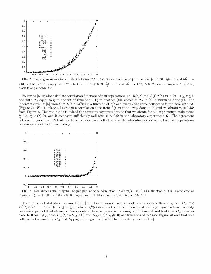
FIG. 2. Lagrangian separation correlation factor R(t, τ )/σ2(t) as a function of τt

in the case Lη

= 1691. ∆0

η= 1 and tu′

L= +

2.01, × 1.51, ∗ 1.01, empty box 0.76, black box 0.11, ⊙ 0.06. ∆0

η= 0.1 and tu′

L= • 1.25, △ 0.62, black triangle 0.16, ▽ 0.08,

black triangle down 0.04.

Following [6] we also calculate correlation functions of pair separations, i.e. R(t, τ) ≡< ∆(t)∆(t+τ) > for −t ≤ τ ≤ 0and with ∆0 equal to η in one set of runs and 0.1η in another (the choice of ∆0 in [6] is within this range). Thelaboratory results [6] show that R(t, τ)/σ2(t) is a function of τ/t and exactly the same collapse is found here with KS(Figure 2). We calculate a Lagrangian correlation time from R(t, τ) in the way done in [6] and we obtain τc ≈ 0.45tfrom Figure 2. This value 0.45 is indeed the constant asymptotic value that we obtain for all large enough scale ratiosLη , i.e. L

η ≥ O(10), and it compares sufficiently well with τc ≈ 0.6t in the laboratory experiment [6]. The agreement

is therefore good and KS leads to the same conclusion, effectively as the laboratory experiment, that pair separationsremember about half their history.

-0.2

0

0.2

0.4

0.6

0.8

1

-1 -0.9 -0.8 -0.7 -0.6 -0.5 -0.4 -0.3 -0.2 -0.1 0

0.03 td0.06 td0.08 td0.11 td0.25 td0.50 td0.76 td1.00 td

FIG. 3. Non dimensional diagonal Lagrangian velocity correlation D11(t, τ )/D11(t, 0) as a function of τ/t. Same case as

Figure 2. tu′

L= + 0.03, × 0.06, ∗ 0.08, empty box 0.11, black box 0.25, ⊙ 0.50, • 0.76, △ 1.

The last set of statistics measured by [6] are Lagrangian correlations of pair velocity differences, i.e. Dij ≡<V L

i (t)V Lj (t + τ) > with −t ≤ τ ≤ 0, where V L

i (t) denotes the ith component of the Lagrangian relative velocitybetween a pair of fluid elements. We calculate these same statistics using our KS model and find that Dij remainsclose to 0 for i 6= j, that D11(t, τ)/D11(t, 0) and D22(t, τ)/D22(t, 0) are functions of τ/t (see Figure 3) and that thiscollapse is the same for D11 and D22 again in agreement with the laboratory results of [6].

3

0.0001

0.001

0.01

0.1

1

10

0.01 0.1 1 10

1e-10

1e-09

1e-08

1e-07

1e-06

1e-05

0.0001

0.001

0.01

0.1

1

10

0.001 0.01 0.1 1 10

FIG. 4. Pair diffusion as a funtion of time for Lη

= 38748 and τη = 0.0027 Lu′ and different initial separations. a) (∆−∆0)2

u′3t3/Las

a function of tu′

L, from top to botom ∆0

η= 1000, 100, 10, 1, 0.1, 0.01 and 0.001. b) (∆−∆0)2

fas a function of tu′

Lfor ∆0

η= 1,

0.1, 0.01 and 0.001.

Having validated our KS Lagrangian model of pair diffusion in planar turbulence against the laboratory experimentof [6], we now turn our attention to Richardson’s law (1) and the claim of universality that it is based on. We do indeedobserve this law over the entire inertial range of times τη < t < L/u′, but only for initial separations ∆0 between

η and 0.1η, and this for all the ratios Lη that we tried (see Figure 4a). Of course this ratio should be large enough,

otherwise Richardson’s law is not observed for any ∆0, but it is surprising that Richardson’s law is so ∆0-specificeven at enormous values of L

η reaching O(105).

When ∆0 ≤ η, Richardson’s law (1) is observed over the limited large scale range 0.2 Lu′

to Lu′

(Figure 4), and the

coefficient 0.2 seems to have no dependence on Lη in our simulations as long as L/η is order 103 or larger, so if it has

one it must be weak. In the remainder of the inertial range between τη and 0.2 Lu′

, the time dependencies of (∆ − ∆0)2

and ∆2 are different from Richardson’s (1) and different for different values of ∆0 ≤ η (Figure 4), even at extremelyhigh L

η . We tried to replace t by t − t0(∆0), where t0(∆0) is a virtual origin significantly smaller than 0.2 Lu′

but

did not recover Richardson’s law (1), particularly since the discrepancies we observe are over such wide time ranges.When ∆0 is significantly larger than η there is no clear indication of a Richardson law at all (Figure 4).

We have carefully studied the time dependence of (∆ − ∆0)2 in the range between τη to Lu′

for different values of∆0 ≤ η and have found the following formula to collapse the data in that range (see Figure 4b):

(∆ − ∆0)2 = G∆u′3

Lt3f(t, ∆0) (4)

where the dimensionless function f is given by (using T ≡ 0.2 Lu′

)

f(t, ∆0) = exp

[

ln[ 5G∆

(∆0/η)2]

2 ln(τη/T )

(

ln(t/T )−

√

ln2(t/T ) + 2

)

]

. (5)

Note that f(t, ∆0) tends to 1 when t is between T and Lu′

and L/η → ∞ (i.e. T/τη → ∞). The Richardson constant

G∆ is determined from the value of (∆−∆0)2

(u′3/L)t3 in the range 0.2 Lu′

to Lu′

and we find G∆ ≈ 0.03 for large enough scale

ratio Lη (of order 103 and larger). We should stress that in KS, G∆ effectively contains both the original Richardson

constant as in G∆ǫt3 but also the constant of proportionality relating the kinetic energy dissipation rate to u′3

L . Wetherefore retain the orders of magnitude of G∆ obtained by KS but not the actual values.

Integrations of ∆2 in Direct Numerical Simulations (DNS) of two-dimensional turbulence in the inverse energycascade regime also show a strong dependence on ∆0, even when the simulations are very highly resolved [11].Nowadays, such DNS cannot reach well-defined −5/3 ranges over more than two decades, i.e. L/η = O(100), andthis at the very highest resolutions currently available. The deviations from Richardson’s law (1) observed whenL/η = O(100) might perhaps be due to edge effects (L/η too small to reach the asymptotic Richardson’s law expectedto be valid for L/η ≫ 1). But can this also be the case in our KS where L/η reaches O(105)? Clearly one cannot

4

answer this question with numerical simulations except if in the future KS and/or DNS runs with even higher L/ηeventually converge to Richardson’s law without ∆0 - dependencies.

Nevertheless, the success of our KS to reproduce the laboratory observations of [6] and its failure to retrieveRichardson’s law without ∆0 - dependencies even at extremely high L/η does raise the question of the validity ofRichardson’s universality and of the locality assumption that it is based on [7], even asymptotically for arbitrarily

high L/η. In general, ∆2 is a function of t, L, η, ∆0 and u′ in KS, and the Richardson locality assumption adapted for

KS states that, for large enough L/η, ddt∆

2 should only depend on ∆2 and E(k) at k = 2π/√

∆2 when max(η, ∆0) ≪√

∆2 ≪ L. Fung & Vassilicos (1998) [7] found this assumption to be valid in planar KS for different spectral exponentsp between 1 and 2 (E(k) ∼ k−p) but specifically for ∆0 = η/2 and unsteadiness parameter λ = O(1) and smaller than

1 in ωm = λ√

k3mEn(km). The direct consequence of this assumption is that ∆2 ∼ tγ with γ = 4

3−p which is indeed

observed in KS for different values of p but only for ∆0 close to and below η [7]. What could invalidate locality andRichardson’s law for ∆0 very different from η?

The low values of G∆ and the very large Lagrangian flatness factors of V Li also observed in KS [7] are consistent

with the observation that fluid element pairs travel close to each other for long stretches of time and separate in

sudden bursts [6,7]. Fluid element accelerations a ≡ DDtu (where D

Dt ≡ ∂∂t + u · ∇) are such that ∇ · a = s

2 − ω2

2where s is the strain rate matrix and ω the vorticity vector. Hence, ∇ · a is large and positive most often in strainingregions around hyperbolic points of the flow where s

2 is large and ω2 close to 0. Close fluid element pairs can separateviolently where ∇ · a is large and positive, and the separation is effective if the streamline structure of the turbulenceis persistent enough in time. Hence, such violent separation events will most often occur where close fluid elementpairs meet hyperbolic points that are persistent enough.

Based on their KS results which were limited to ∆0 = η/2, Fung & Vassilicos (1998) [7] rephrased Richardson’s

locality assumption as follows: “in the inertial range, the dominant contribution to the turbulent diffusivity ddt∆

2

comes from straining regions of size√

∆2; these straining regions are embedded in a fractal-eddy structure of cat’seyes within cat’s eyes and therefore straining regions exist with a variety of length-scales over the entire inertial range.”Davila & Vassilicos [12] have related γ to the fractal dimension D of this fractal-eddy streamline structure of strainingregions when ∆0 is close to and below η (γ = 4/D). These results suggest that when ∆0 is between η and 0.1η, theevolution of fluid element pairs by bursts when they meet straining regions somehow tunes into the straining fractalstructure of the flow and gives rise to Richardson’s law. This requires some persistence of the streamline structure,and indeed Richardson’s law is lost when the unsteadiness parameter λ is made significantly larger than 1 [7].

This topological picture of turbulent pair diffusion suggested by results in previous papers and our argumentconcerning ∇ · a could also explain the strong ∆0 - dependence of ∆2. As ∆0 decreases well below η, the probabilityfor fluid element pairs to encounter a hyperbolic point and be separated by it also decreases and can become so smallfor ∆0 ≪ η that pairs may travel close to each other for very long times. Eventually, at times nearing L/u′, the eddyturnover time of the turbulence, the two fluid elements will be separated by the unsteadiness of the flow rather thanby its streamline structure as they will have to become independent at times t ≫ L/u′. They therefore largely bypassthe relatively persistent straining fractal streamline structure of the turbulence and also Richardson’s law as a result.For initial conditions ∆0 ≫ η, the argument based on ∇ · a does not apply and the separation of fluid element pairscannot be considered to be dominated by straining events in the vicinity of hyperbolic regions. In the framework ofthe topological turbulent pair diffusion picture, this is consistent with the absence of a Richardson law for ∆0 ≫ η.

F.N. and J.C.V. are grateful for financial support from the Royal Society and EPSRC.

[1] J.M. Ottino, The kinematics of mixing: stretching, chaos and transport (Cambridge University Press, Cambridge, 1989).[2] L.F. Richardson, Proc. R. Soc. London Sect. A 110, 709 (1926).[3] G.K. Batchelor, Proc. Cambridge Philos. Soc. 48, 345 (1952).[4] R.H. Kraichnan, Phys. Fluids 9, 1937 (1966).[5] M.F. Shlesinger, B.J. West and J. Klafter, Phys. Rev. Lett. 58, 1100 (1987).[6] M.-C. Jullien, J. Paret and P. Tabeling, Phys. Rev. Lett. 82, 2872 (1999).[7] J.C.H. Fung et al., J. Fluid Mech. 236 281 (1992); J.C.H. Fung and J.C. Vassilicos, Phys. Rev. E 57 1677 (1998); N.A.

Malik and J.C. Vassilicos, Phys. Fluids 6 1572 (1999).[8] P. Flohr and J.C. Vassilicos, J. Fluid Mech. (2000). J. Fluid Mech. 407 315 (2000).[9] G. Boffetta, A. Celani, A. Crisanti and A. Vulpiani, Phys. Rev. E 60 6734 (1999).

5

[10] I.M. Sokolov, J. Klafter and A. Blumen, Phys. Rev. E 61 2717 (2000).[11] G. Boffetta, In “Advances In Turbulence VIII” (ed. C. Dopazo et al.), CIMNE, Barcelona (2000).[12] J. Davila & J.C. Vassilicos, preprint to be submitted, 2002.

6