Turbulent Boundary Layer Heat Transfer Experiments

NASA Contractor Report 3510

Turbulent Boundary Layer Heat Transfer Experiments: Convex Curvature Effects Including Introduction and Recovery

T. W. Simon, R. J. M&at,

J. P. Johnston, and W. M. Kays

GRANTS NSG312Li and NAG 3-3 FEBRUARY 1982

TECH LIBRARY KAFB, NM

IInIlll~llll~lilllnllllaYRllllll llllb2227

NASA Contractor Report 3510

Turbulent Boundary Layer Heat Transfer Experiments: Convex Curvature Effects Including Introduction and Recovery

T. W. Simon, R. J. Moffat, J. P. Johnston, and W. M. Kays Stanford University Stanford, CaZifornia

Prepared for Lewis Research Center under Grants NSG-3124 and NAG 3-3

National Aeronautics and Space Administration

Scientific and Technial Information Branch

1982

$ 4

d-

TABLE OF CONTENTS

Nomenclature . . . . . . . . . . . . . . . . . . . . . . . . . . . .

Chapter

1.

2.

3.

4.

5.

INTRODUCTION . . . . . . . . . . . . . . . . . . . . . . . . . . 1

1.1 Previous Research .................. . . . 2 1.2 Objectives ..................... . . . 10 1.3 The Experiment ................... . . . 11

THE EXPERIMENTAL APPARATUS . . . . . . . . . . . . . . . . . . . 19

2.1 General Description . . . . . . . . . . . . . . . . . . . . 19 2.2 Hydrodynamic Aspects of the Facility . . . . . . . . . . . 20 2.3 Heat Transfer Aspects of the Facility . . . . . . . . . . . 21 2.4 Instrumentation for hydrodynamic Measurements . . . . . . . 24 2.5 Instrumentation for Heat Transfer Measurements . . . . . . 25 2.6 Qualifications of the Facility: Hydrodynamic . . . . . . . 28 2.7 Qualifications of the Facility: HeatTransfer . . . . . . 28 2.8 The Energy Balance . . . . . . . . . . . . . . . . . . . . 31

THE EXPERIMENTAL RESULTS . . . . . . . . . . . . . . . . . . . . 39

3.1 The Baseline Case .................. 3.2 The Effect of Initial Boundary Layer Thickness ... 3.3 The Effect of Upw .................. 3.4 The Effect of Free-Stream Acceleration ....... 3.5 The Effect of Unheated Starting Length ....... 3.6 The Effect of the Maturity of the Momentum Boundary

Layer ........................

HEAT-TRANSFER PREDICTIONS . . . . . . . . . . . . . . . . . . .

4.1 State of Art . . . . . . . . . . . . . . . . . . . . 4.2 Predicitng the Effect of Curvature for the Baseline

Case . . . . . . . . . . . . . . . . . . . . . . . . 4.3 Predictions of Cases with Differing Initial Boundary

Layer Thickness . . . . . . . . . . . . . . . . . . . 4.4 Prediction of Cases with Differing U . . . . . . . 4.5 Prediction of Cases with Free-StreamPxcceleration . . 4.6 Prediction of Cases with Differing Unheated Starting

Length . . . . . . . . . . . . . . . . . . . . . . .

CONCLUSIONS . . . . . . . . . . . . . . . . . . . . . . . . . .

5.1 Conclusions . . . . . . . . . . . . . . . . . . . . . 5.2 Recommendations for Future Work on the Convex

Problem.......................

. . . 39

. . . 43

. . . 46

. . . 48

. . . 49

. . .

. . .

. . .

. . .

. . .

. . .

. . .

. . .

Page V

51

67

67

72

74 74 75

75

85

85

87

-._... . _ .-.. ..--.- -~

References..............................

Appendices

A.

B.

C.

D.

E.

F.

G.

H.

The Uncertainty Analysis ............

Curved-Wall Integral Parameters and the Momentum

and Energy Integral Equations .........

Calibration of the Heat Flux Meters .......

Simple Model for Ordering the Transitional

Boundary Layer Cases .............

Listing of Profile Program ...........

Listing of the Stanton Program .........

The Reduced Data ................

Modifications to STAR5 for Convex Cunrature

Predictions ..................

. . . . .

. . . . .

. . . . .

. . . . . 105

. . . . . 108

. . * . . 120

. . . . . 137

. . . . . 203

Page

89

94

99

102

iV

Nomenclature

A+

Cf/2

C P

=P F

H

HP

i

K

Ki

k

R

RO

M

n

n+

P'

p, ps Pr

-t

%

P SW l mm 9

q2

R

Effective sublayer thickness in the Van Driest model.

Skin-friction coefficient, rw/pIJ2 Pw'

Static pressure coefficient, es-P 1 s,ref I $ PU2

Pw l

Specific heat.

Blowing fraction, pwVw/p,Uao.

Shape factor, 61/62.

Heat flux meter signal.

Enthalpy.

Acceleration parameter, v/U;wWpw/ds) l

Heat flux meter calibration constant.

Inverse radius of curvature, l/R.

Mixing length.

Flat-wall mixing length.

Mach number.

Distance normal to the test wall.

Nondimensional distance normal to the test wall, nu,/v.

An independent parameter.

Static pressure.

Prandtl number.

Turbulent Prandtl number.

Total pressure.

kll static pressure.

Heat flux.

'+,Tz.7 Turbulent kinetic energy, u' .

Radius of curvature.

Effective radius of curvature. Reff

V

Rex(Res) x(s)-Reynolds number, Up&v oJpws/v> l

Recs 2

ReA 2 RI

S

S'

Si

S

St

T

T+

TO

U

U+

U'

5

V

V’

W’

Y

Ycrit

Y Sl

2

Momentrrm thickness Reynolds number, upw62'v'

Enthalpy thickness Reynolds number, UpwA2/v.

Richardson number.

Streamwise distance referenced to start of curvature.

Sensitivity coefficient (see App. A).

Streamwise conductance for plate-plate heat flux.

Stability parameter, LJ/R/(aU/an).

Stanton number, ;“/PC~U~~(T~-T,) l

Temperature.

Dimensionless temperature, (Tw-T)u,/($/Pc~) l

Stagnation temperature.

Mean streamwise velocity.

Nondimensional streamwise velocity, U/u,.

Fluctuating streamwise velocity.

Shear velocity, dv.

Mean velocity normal to test wall.

Fluctuating velocity normal to the test wall.

Fluctuating cross-stream velocity.

Distance normal to test wall.

Distance from wall where S = Scrit.

Distance from wall where extrapolated shear stress equals zero.

Distance in spanwise direction.

Greek Lztters

6 Empirical constant in curvature mixing-length correlation.

8' Empirical constant in turbulent Prandtl number model.

Vi

Y

6 sl

6*sl

699

6995

61

62

a( >

A2

EH

EM

8

K

x

P'

P

T

T W

The value of the turbulent Prandtl number for plane flow.

Shear layer thickness (see Sec. 1.1).

Displacement thickness integrated to 6,1*

Thickness of boundary layer, where mean velocity is 99% of the potential for mean velocity.

Thickness of boundary layer, where mean velocity is 99.5% of the potential flow mean velocity.

f

OD Displacement thickness,

( Wp-U)/Upw) dn l

Momentum thickness, /

OD 0

0

(l+kn)U(Up-U)/UEwdn.

Uncertainty in ( >.

Enthalpy thickness (see App. B).

Turbulent diffusivity of thermal energy.

Turbulent diffusivity of momentum.

Angle of turn from start of curvature.

Rarman constant, 0.41.

Mixing length proportionality factor.

An independent parameter.

Density.

Total shear stress.

Surface shear stress.

Subscripts

P Of the potential flow.

Pw Of the potential flow at the wall.

ref Reference.

W At the wall.

P' Of an independent parameter P'. OD

In the free stream.

Vii

Chapter 1 INTRODUC\TION

Turbulent boundary layers on convexly curved walls are encountered

in many engineering applications: the forward part of a blunt body,

leading edges of air intakes, blade passages of turbomachinery, aircraft

wings, and rocket nozzles. Curved boundary layers with high heat trans-

fer rates are encountered on gas turbine blades, where accurate predic-

tion of and design for turbine blade heat loads are critical to the

reliability and efficiency of modern high-performance engines. There is

ample evidence that curvature affects heat transfer. Some of this effect has been attributed to the extra rates of strain associated with

streamwise curvature which significantly affect the structure of turbu-

lent boundary layers [2,35] and the heat transfer rates [13,32].

The primary objective of this experiment was to measure the effect of convex curvature on the heat transfer rate over a representative

domain of initial and boundary conditions. The work was undertaken as

part of an ongoing series of projects at Stanford University sponsored

by NASA-Lewis Labs. The motivating problem was the need to understand the mechanisms and accurately predict the heat transfer rates on gas

turbine blades.

khen the curvature project began, the state of the art for design

heat-load calculations was the computer code STAN5 [l]. This code

solves the partial differential equations which govern transport of

thermal energy and momentum in boundary layers. 'Ihe quality of the pre-

dictions it makes is dependent upon the applicability of the Reynolds

stress model it uses. Though the stress modeling of STAN5 is quite

simple, it is a trusted program for use within its data base, because

its Reynolds stress model is supported with empirical input from twelve

years of careful experimentation at Stanford. STAN5 accurately accounts

for streamwise acceleration or deceleration and/or transpiration blowing

or suction. Presently, however, it does not account for streamwise cur-

vature. The purpose of the Stanford curvature program is to add curvature to its useful domain.

1

During the course of the work , numerous colleagues made significant

contributions. Dr. J. Gillis had a major role in the eonstivction and

qualification of the facility. Robin A. Birch aided in the design and

construction of much of the facility, resulting in a very reliable ap-

paratus. Kokichi Furuhama, Michael Glass, and Vanessa MacLaren assist-

ed with the qualification of the facility and the updating of the data-

reduction programs. Professor Shinji Hinami, a Visiting Professor, made

many helpful suggestions.

1.1 Previous Research

A comprehensive survey of the literature on curvature effects, prior

to 1972, was given by Bradshaw (2). He pointed out that the effect of cur-

vature is about ten times as strong as one would predict from a thin shear

layer, eddy-viscosity model by simply adding the extra rate of strain W/ax

to the existing strain field.

Experimental work on the effects of curvature dates back to the

days of Ludwig Prandtl. One early study by kilcken [3], a student of

Prandtl, was the first documented study of curvature effects where the

facility was designed to keep secondary flow effects to a minimum. At

that time, Prandtl had put forth a stability argument for curvature,

Wflcken was to test it.

"Because the various parts of the boundary layer are variously affected by centrifugal force in the presence of a curved surface, a concave surface produces a tendency to force the fast parts of the flow toward the surface and the slow parts away from it. This tendency favors the exchange of the slow layers next to the surface with the faster ones on the inside of the flow. Thus, it reinforces the already existing turbulent exchange procedure. The contrary is the case for the convex faces. Here the centrifugal force has a stabilizing effect, reducing the turbulence.

Prandtl also had developed the early form of a mixing length model, then

called "free path," for a flat plate. WLlcken, though admitting some

secondary flow influence, found that curvature significantly affected

2

the "free path lengths." Hz stated, "Boundary layer events on curved

surfaces should be ascribed more importance than has generally been the

case up to the present." Curved flow research continued under Prandtl at

the Kaiser kttlhelm Institute for Flow Research with the studies of Wandt

[4] and Schmidbauer [5]. The general conclusion was that, even for weak

curvature, the boundary layer hydrodynamics are significantly affected.

The next documented study was in a curved channel, where the flow

could become fully developed. This study by Wttendorf [63 in 1934

showed that the fully developed flow was significantly influenced by

curvature, although the overall pressure drop was not. kttendorf also

found, from his mean velocity and wall static pressures measurements,

that the power, n, in the power-law velocity profile, LI+ = cy +1/n , decreases with stronger convex curvature and increases for stronger

concave curvature. His descriptor of the strength of curvature was the

parameter vhu, , where R was positive for concave curvature.

In 1937, Clauser and Clauser [7] investigated the effect of curvature on the transition from laminar to turbulent flow. This is

the first time that hot-wire anemometry had been applied to curved flows. They found that stabilizing convex curvature increased the

critical Reynolds number and delayed transition. Their observations

showed that, on typical airfoils of the time, convex curvature might

double the critical Reynolds number. Hans Liepmann [8] extended the

study of the effect of curvature on transition to very weak curvature

(0 < 62/R < 0.001). In this range it was found that transition was not

affected by convex curvature but was affected by concave curvature.

This indicated that the process of transition was different for the

concave wall than for the flat or convex wall.

In 1955, Frank Kreith [9] performed a clever heat transfer test

that showed quite conclusively that the heat transport from a concave

wall was considerably more than from a convex wall. For his channel

flow, he concluded that curvature effects scaled on U/r, the forced

vortex parameter. No measurements of local heat transfer rates were

taken. The hydrodynamics of a fully developed, curved, turbulent chan-

nel flow similar to the Kreith facility were studied in detail by

Eskinazi and Yeh [lo]. Using hot-wire anemometry, they measured the

downstream development of profiles of streamwise velocity fluctuations

and, for the fully developed flow, 22 measured the profiles of u' , v' ,

and u'v'. They stated that one of the most important influences of 2 curvature is on the v' -production term -u'v'(U/r). They noted that

near the convex wall u'v' was positive, indicating a supession 2 (negative production) of v' . Their spectral measurements of u' 2 and

VI2 showed that the decrease in turbulent mixing activity was largest

in the low-wave-number range.

The first curved-flow heat transfer test with wall-measured heat

flux data was that of Schneider and Wade [ll]. With plug-type heat flow

transducers they measured local heat fluxes on a convex wall that were

50% of the predicted flat-wall values and considerably less than would be predicted by the model of Kreith [9]. Their tunnel aspect ratio

was 1.0, so considerable contamination by secondary flow was prob-

able.

V. C. Pate1 [12] studied the hydrodynamics of the flow through a

90" curved duct similar to the facility used in the Schneider and Wade

study, except that the aspect ratio was 5.0. No attempt was made to

separate streamwise acceleration and deceleration from the other effects

of streamwise curvature, and there was some confusion about whether the

change in the mean velocity profiles was due to curvature or the local

acceleration and deceleration within the bend. Pate1 measured only mean

quantities, which, even with the increased aspect ratio, may have been

influenced by secondary flows. He noted that curvature affects the

shape factor and, therefore, the rate of entrainment.

Also in 1968, lhomann [13], at the Aeronautical Research Institute

of Sweden, made detailed local heat transfer measurements on surfaces

that were straight and convexly and concavely curved. The Ihomann

study was performed in a wind tunnel with a freestream Mach number of

2.5, uniform static pressure on the test wall, and a boundary layer

thickness-to-radius of curvature ratio of "99'R = 0.02. The resultant

effect of curvature was found to be an increase in convective heat flux

of = 20% for the concave case and a decrease of = 15% for the convex

case with respect to the flat-wall case (see Fig. l-l). Since the

4

Thomann study was done in a supersonic freestream, significant compres-

sible effects were present. As discussed by Rradshaw [2], compression

or dilation produces strong extra rate-of-strain effects in the boundary

layer which may alter the turbulent transport process in much the same

fashion as does curvature.

In 1969, Rradshaw [14] discussed the analogy between streamwise

curvature and buoyancy in turbulent shear flow and introduced a modifi-

cation of the Richardson number used in meteorological work to curved

and rotating flow computation. The gradient Richardson number for

curved flows is written: Ri = 2S(l+S) where S is the stability

parameter, S = (u/R)/(au/an>, positive for the convex wall and negative for the concave wall. He then proposed [14,15] that the Monin-

Obouhkov formula for the correlation of the apparent mixing length with

small buoyancy effects a/a; = 1 - f3Ri could be used to model the effects of weak curvature. This approach met with considerable success.

In fact, the value of the constant B could be inferred by analogy from

meteorological experiments in stably and unstably stratified boundary

layers. It is generally agreed to be the order 10.

So and Mellor [16,17,18] published results from a very detailed hy-

drodynamic experiment on curved-wall boundary layers. In their experi-

ment, the ratio of boundary layer thickness to radius of curvature ratio

was "99'R (J 0.07, and the aspect ratio was - 8.0. Because of an

imaginative design which employed wall jets, secondary flows were kept

acceptably small. Profiles of all the Reynolds stresses were measured. On the convex wall it was found that the turbulent shear stress was

"turned off" in the outer half of the boundary layer. Over the concave

wall, they found evidence of a stationary system of longitudinal vor-

tices, analogous to those formed between rotating cylinders. Mall shear

stress was inferred from a Clauser plot technique, but the turbulent

shear stress profile was not measured close enough to the wall to enable

them to check the wall value by extrapolation. The Qauser plot tech-

nique has since become an accepted method for inferring wall shear

stress and has been verified by later experimenters, e.g., Gillis [35].

Ellis and Joubert [19] of the University of Melbourne measured

profiles of mean velocity in boundary layers.of a curved duct. aey

5

noted that the width of the logarithmic zone was curvature-dependent.

Convex curvature caused the velocity profile to become wake-like at a

lower value of n+ and the opposite for concave. They searched for,

but could not find, similarity of the mean flow, as represented by a

defect type law for either the fully developed, curved, turbulent

channel flow or the outer regions of convex wall boundary layers. On

the concave surface, Ellis and Joubert found evidence of Taylor-

Gijrtler vortices.

During the 197Os, Bradshaw undertook a series of experiments on

curvature effects. The first experiment was one of very weak curvature

(dgg5/R = 0.01). Ihe early results were presented by Meroney [20] and

the final results by Hoffmann [21]. Mean and turbulence data were taken

in a curved duct of 30" bend and aspect ratio of 6.0. No attempt was

made to separate the weak acceleration/deceleration effects. The data

consisted of mean quantities and the important higher-order quantities

through order 4. Spanwise variations of skin friction due to weak

Taylor-Gb'rtler cellular activity were observed on the concave wall; they

measured variations of 20% in local skin-friction coefficient. Later

experiments on curvature at the Imperial College included the recovery

from an "impulse" of curvature in a curved duct (Smits, Young, and

Bradshaw [22]) and in an axisymmetric flare (Smits, Eaton, and Bradshaw

[23]). The second case showed the combined effects of sustained lateral

divegence and recovery from curvature. It was found that Taylor-

Gijrtler cells were established in the curved duct but not in the

axisymmetric flare, indicating an effect of lateral divergence. In both

studies, mean data and fluctuating data through order 4 were taken.

lXlring this same time, Castro and Bradshaw [24] were studying the con-

vexly curved, free-mixing layer.

Effects of mild curvature were studied by Ramaprian and Shivapra-

shad [25,26,27,28]. Their test facility was very similar to the Hoff-

mann and Bradshaw facility, with the notable exception of an aspect

ratio of 2.5. They did not observe Taylor-Gb'rtler cells on the concave

wall, contrary to the findings of Boffmann and Bradshaw. Ihe authors

admit that this difference may be attributed to significant secondary flows.

6

Detailed measurements of the hydrodynamics of a curved channel flow

were made by Hunt and Joubert [29] in 1979. The data for this study

were taken in an apparatus in which a duct downstream of the nozzle

could be straight or bent into a large-radius curve. The channel was

shallow, allowing the convex and concave boundary layers to merge about

40% of the distance around the 45" bend. The curve started at the exit

of the nozzle, so the ratio of boundary layer thickness to radius of

curvature was extremely small (dgg/R = 0.005) at the start of curva-

ture, then grew rapidly around the bend. The aspect ratio was large,

13.2 to 1.0, to minimize secondary flow effects. Roll-cell vortices of

the Taylor-GErtler type were observed in the channel just off the concave wall. These cells resulted in variations in skin friction across

the span of f 4%. Data taken included mean velocity profiles and profiles of the important Reynolds stresses. It was found that the

measured Reynolds shear stress extrapolated to the convex wall agreed with skin friction values found with the Clauser plot technique.

Profiles at the end of the test region were fully developed in the mean quantities and nearly fully developed in the turbulence quantities.

In 1977, Rrinich and Graham ]301 measured mean velocity and

temperature profiles and wall heat transfer rates in a curved channel

similar to the one in which Eskinazi and Yeh [lo] took hydrodynamic

data. The heat transfer facility, however, had an aspect ratio of 6.0,

and considerable secondary flow influence was observed. Nevertheless,

they noted an increase in the heat transfer rate on the outer (concave)

wall and a slight decrease on the inner (convex) wall. Their tempera-

ture profiles reached an asymptotic shape characterized by a skew of the

peak toward the concave wall, giving a much steeper temperature gradient

on the concave than on the convex wall. Temperature profiles were not

plotted in inner coordinates, so it is not known whether they showed a

log-law relationship.

R. M. C. So [31] continued his curvature work beyond the hydrodyl

namic studies discussed earlier [16,17,18] with an analytical prediction

of the effect of curvature on the turbulent Prandtl number. He devel-

oped the rather simple relationship:

7

I I II

1 EM

- ; B’Ri(1 - -+

4Y2 1 -+ f3'(4ivm - 1)(1 ++

where y is the value of the turbulent Prandtl number of a correspond-

ing plane flow. The value B' = 6.0 has been found to give the best

correlations with curved-flow data, swirling-flow data, and meteorologi-

cal data [55,56,57]. This equation gives an increase of "M/&R for Ri

> 0 (convex) and Pr < 1. This ratio will decrease if,either one of the

two inequalities is reversed. For air flowing over a convex wall, the

diffusivity of thermal energy decreases faster than the eddy diffusiv-

ity. Since the Prandtl number for air is nearly unity, the deviation

from Reynolds analogy (EM/CR = 1) is predicted by the above equation

to be small.

Recently, Mayle, Blair, and tipper [32] measured local heat trans-

fer rates in a curved duct which had an aspect ratio of 4.25. Their

study was with low-velocity air (M = 0.06 as opposed to the high-

velocity study of Thomann [13]), in which the test wall static pressure

and temperature were uniform. The ratio of boundary layer thickness to

radius of curvature at the start of the curve was - 0.01. Their find-

ings (see Fig. l-2), confirming those of lhomann, showed a decrease in

the wall heat flux of IJ 20% for the convex wall and an increase of

m 33% for the concave wall relative to the flat-wall heat flux predic-

tion of Reynolds, Rays, and Kline [33].

Previous heat transfer studies dealt only with the curved region,

none reported results of recovery downstream of the curve. The present

investigation is the first time the effects on heat transfer of both the

introduction of and recovery from curvature have been investigated.

hhen looking at the problem of gas turbine blade cooling or many other

applications where curvature effects on heat transfer are significant,

one realizes that the regions of strong curvature are often followed by

regions of weak or no curvature, so the recovery effects are as perti-

nent as the.effects of the introduction of curvature.

8

The present heat transfer results are from a program studying both the heat transfer and fluid mechanics of a convexly curved flow. Since

heat transport is by turbulent motion, the hydrodynamic study is an

essential input to the heat transfer study. Detailed results of the

hydrodynamic study have been reported by Gillis and Johnston [34,35].

Their work was performed on essentially the same tunnel configuration as

the present study (see Fig. 2-l) and with boundary layer thickness-to-

radius of curvature ratios of 0.10 and 0.05, two of the cases pre-

sented herein. The Gillis and Johnston results are summarized in Figs.

1-3 through 1-7. Fig. 1-3 shows the effect of convex curvature on skin

friction, as calculated using a Glauser plot. The initial response to

the introduction of curvature was fast, and the behavior was seemingly

near-asymptotic. At the end of the curved region (= 16 boundary layer

thicknesses downstream from the start of curvature for the dgg/R = 0.10 case), the skin friction reached a value - 30% less than the

flat-wall predicted value. In the recovery region, the return of the

skin friction was slow. After - 20 boundary layer thicknesses from the start of the recovery region, the skin friction was still - ZO-25%

below the flat-wall value. They also found that, though the boundary layer thickness at the beginning of curvature differed by a factor of

two for the two experiments, the variation of Cf/2 with distance

within the curved region was surprisingly similar for the two cases.

Fig. l-4, a typical plot of mean velocity profiles in wall coordinates, shows that the log region shortens within the curved section but is

always discernibile. The effect of convex curvature on profiles of the turbulence quantities (u' 2 2 , q , and 1 , uv> is shown on Figs. 1-5, l-

6, and 1-7, respectively. Within the curved region, the turbulence activity declined quickly throughout the boundary layer, but especially

in the outer regions, to a near self-similar profile. The recovery to a normal flat-wall profile was slow and appears to be by propagation from

the wall. The slow growth of the turbulence profiles in the recovery region may be responsible for the slow return of the skin friction to

flat-wall values. Fig. 1-7 shows that, at the beginning of curvature,

the shear stress in the outer portion of the boundary layer changes sign

for a short distance. This term is linked to the production of TKR, a sign-reversal indicates a negative production of TKE in this region.

9

Gillis and Johnston identified a parameter called the "shear layer

thickness," the n-distance of the extrapolated shear stress profile (see

Fig. l-8) labeled Yisl ." They proposed a model by which to visualize

the strongly curved boundary layer: a two-layer model shown in Fig. 1-9.

The inner layer is characterized by non-zero TKE and shear stress; a

typical boundary layer, but constrained in thickness to 6s., which

remains essentially constant within the curve. The outer layer is char-

acterized by non-zero TKE but essentially zero shear stress. The outer

layer is the decaying residue of the upstream boundary layer. At the

beginning of the recovery region, the restriction on 6s. due to curva-

ture is lifted and the inner layer grows within what remains of the

outer layer. The results of the present heat transfer study are consis-

tent with this model.

The hydrodynamic study of Gillis and Johnston is part of an over-

all program involving heat transfer rates on smooth, convexly curved surfaces. The present experiments build upon their study of the hydro-

dynamic processes, investigating the heat transfer processes through

structurally similar, but heated, boundary layers.

1.2 Ob iectives

The final objective of the Stanford curvature program is to add

curvature to the list of effects that can be appropriately predicted

with turbulent boundary layer prediction programs, e.g., STAN5 [l].

With this goal in mind, the objectives of the present study were to:

1. Accurately measure wall heat transfer rates from a smooth, convexly

curved wall and downstream flat recovery plate over a large enough

domain of carefully controlled initial and boundary conditions so

that the eventual model can be used with minimal extrapolation. 2. Build upon the understanding of the curved boundary layer gained

during the Gillis and Johnston study [35] and others listed in

Section 1.1. For this study a series of 15 runs were made with

differing initial and boundary conditions to learn about the sen-

sitivity of the curvature effect to various parameters thought to

be important. This will aid in developing a prediction model based

on maximum physical insight.

10

3. Test the preliminary prediction model proposed by Gillis and John-

ston 1351, making changes where appropriate.

4. Construct a heat transfer facility that is sufficiently flexible

to accomplish the above objectives and future objectives of the

overall program, specifically, convex curvature with discrete jet

injection, which simulates modern gas turbine film-cooling geom-

etries.

1.3 The Experiment

In the following experiment, thermal and hydrodynamic boundary

layers were grown on a flat preplate, then were introduced to a 90", 45

cm radius of curvature convex wall, followed by a recovery wall. The

wall temperature was maintained uniform, and the static pressure on the

test wall was controlled to a prescribed function of downstram distance,

either uniform or constant K (v/UL Pw

l dUpw/ds). Detailed wall heat

flux data as well as profiles of velocity and temperature were measured in the developing, curved, and recovery regions. The initial and

boundary conditions were varied to determine sensitivity to various

parameters. The 15 cases in the present study investigated the sensi-

tivity of the effect of convex curvature on heat transfer to:

4 Initial boundary layer thickness.

b) Magnitude of free-stream velocity.

c> Free-stream acceleration.

d) Location of the beginning of heating with respect to the beginning

of curvature or the beginning of recovery.

e> Maturity of the momentum boundary layer at the beginning of curvature.

One other parameter which should be varied systematically is the

radius of curvature of the test wall. The cost and complexity of a test

facility with such flexibility precluded this entry.

11

+----+---- i - -,j-=-G

Fig. l-l. Stanton number versus streamwise distance, M = 2.5, To-T, = 77.5 K , from Thomann [13].

6(10)-3 1 I I I d 6 3 l CONVEX \

fi

; I-;-

zi -0 .@

t- l o

4= m ( 1or3 * I I I I,

2(1015 4 6 (IOP 2

REYNOLDS NUMBER, Re,

Fig. l-2. Stanton number versus x-Reynolds number, from Mayle, Blair, and K opper 1321.

12

.003 - - - FLAT WALL PREDICTION, FIRST EXPERIMENT - FLAT WALL PREDICTION, SECOND EXPERIMENT

D DATA, FIRST EXPERIMENT A DATA, SECOND EXPERIMENT

.002 -

cr AA- m

2 --m- --*-- -------

l A n A WA .A .A

A A A

.OOl - n 3

0’ I I 1 I I I I I I I -75 -50 -25 0 25 50 75 100 I25 I50 I75

8, cm

-%-FLAT-&-CURVED+-RECOVERY+-

Fig. l-3. Skin friction versus streamwise distance, b&R = 0.10, from Gillis and Johnston [35].

13

35

30

25

20

15

IO

5 U+

0

0

0

0

0

0

0

LINE IS U+ = 2.44 LOG n+ +5.0

80”

60’

40”

20”

112 cm

97 cm

82 cm

64 cm

51 cm

34 cm

16 cm

-71 cm

I 11111111 I I lllllll I IIIU

IO .- -

100 1000 lO$OO n+

Fig. l-4. Mean velocity profiles in wall coordinates, 0.10, from Gillis and Johnston [35].

6gg/R =

14

h CURVATURE

Pig. l-5. Streamwise turbulence intensity profiles versus distance in the streamwise direction, from Gillis and Johnston [35].

6gg/R = 0.10,

15

q* 2 “PW

Fig. l-6. T.K.E. profiles versus distance in the streamwise direction,

699’R = 0.10, from Gillis and Johnston

r351.

16

l WALL SKIN FRICTION (CLAUSER PLOT)

16

I2 -uv u2 8 Pw

x IO4

Fig. l-7. Reynolds shear stress profiles versus distance in the streamwise direction, 6gg/R = 0.10, from Gillis and Johnston [35].

17

8.0

d- 6.0

9 X

‘,a 4.0 I-

72 - 2.0

0

n STA. 5,40° + STA. 6,60° . STA. 7, 80”

-2.0 - 0 .20 .40 .60 .80 1.00 n/6

Fig. l-8. Reynolds shear stress profile showing 116slrr, from Gillis and Johnston [35].

Fig. l-9. Two-layer curved boundary layer structure, from Gillis and Johnston [35].

18

Chapter 2

THE EXPERIMENTAL APPARATUS

The test facility used in the present heat transfer study was used

in the hydrodynamic study of Gillis and Johnston* [35]. The hydrody-

namic aspects of the tunnel, discussed in detail in Ref. 35, are summar-

ized below. Systems added to the facility to broaden the hydrodynamic

operating domain and systems specific to the heat transfer measurements

are discussed in detail.

2.1 General Description

A curved-wall heat transfer facility has been constructed (Fig.

2-1) that allows development of a smooth, flat-wall, heated boundary

layer upstream of a 90" bend of 45 cm radius of curvature followed by a

flat-wall recovery. There were five circuits to the facility:

(1) me main loop: from the main fan, through the return

ducting, oblique header, heat exchanger and screen pack and contraction nozzle combination, then into the test

regions and back to the main fan via a plenum box.

(2) The charging loop: discharge flow to the room via louvres

and slots then return to the tunnel via the filter box and charging blower.

(3) The suction loop: suction from the preplate, reinjected to

the plenum box via the suction fan.

(4) The cooling water loop for the heat exchanger: a 303R capacity water tank, water supply, and discharge lines to

and from the tank, for circulation and for make-up.

(5) me hot water loop: heated the preplate and recovery

walls, using two temperature-controlled water heaters.

*Gases 2 and 3 of Ref. 35.

19

2.2 Hvdrodvnamic Asnects of the Facilitv

The main flow was driven by a fan which delivered air to an oblique

header that turned the flow into a heat exchanger. The flow passed through the exchanger, a screen pack, and an 11:l contraction nozzle

before entering the tunnel test region. Details of the screen pack and nozzle can be found in Ref. 44. Flow exited the test region into a

plenum box, which supplied the main fan. The tunnel velocity was

controlled by changing pulleys and belts on the fan and motor, and could

be varied from 3.5 m/s to 26 m/s.

The developing region was 16.5 cm by 56 cm in cross section and -

200 cm long. The outer wall was straight and adjustable by pivoting

about its upstream edge so that the static pressure could be made nearly

uniform, allowing the growth of a normal flat-wall (non-accelerated) boundary layer. A 15 cm section of the test wall in the preplate

beginning - 84 cm upstream of the start of curvature was constructed

with - 2000-l/16 inch diameter holes uniformly spaced across the span

and connected to an auxiliary fan (Fig. 2-la) allowing boundary layer

suction. This system extended the operating domain to thinner boundary

layers and very low momentum thickness Reynolds number laminar and

transitional boundary layers. hhen a thick, fully turbulent, two-

dimensional boundary layer was desired at the beginning of curvature, the boundary layer was tripped just downstream of the nozzle. khen the

suction fan was operating to produce thinner boundary layers, the trip

was located downstream of the suction holes.

Within the curved region, the flexible outer (concave) wall was

adjusted so that the static pressure on the convex test wall followed

the desired function of streamwise distance, usually uniform. khen the

static pressure on the test wall was uniform, there was no streamwise

acceleration of the inner region of the boundary layer. Cases with

acceleration were set up by trial and error until a nearly constant K

was achieved within the curve. Twenty-six 0.025-inch (0.6 mm) diameter

static pressure tap holes distributed in both the streamwise and span-

wise directions were used for these adjustments. The tunnel was main-

tained slightly above ambient pressure with the charging blower (Fig.

2-la), which took air from the room via a filter box. Because the

20

tunnel was pressurized, separation of the boundary layer on the concave wall, upon entering the curved region, could be prevented by discharge of the boundary layer fluid through a series of seven spanwise louvres.

Secondary flows in and downstream of the bend were reduced by peeling

off the sidewall boundary layers upon entry to the bend, by using side-

wall slots within the bend, and by installing boundary layer fences on

the convex surface near the side walls beyond the heated portion of the

span. The secondary flow control was developed by J. C. Gillis. The

details of the evolution and a more thorough discussion of the final design are presented in Ref. 35.

The recovery region was a straight tunnel of dimensions 15 cm by 53 cm and approximately 125 cm long. Boundary layer fences continued down-

stream of the curve for the first 60 cm of recovery length.

The outer walls were constructed so that profile data could be

taken at five stations in the developing region, six stations within the

curve, and six stations within the recovery region. Stations typically

had seven spanwise positions for checking two-dimensionality.

2.3 &at Transfer Aspects of the Facility

The test wall was constructed of copper and segmented and instrumented so that the local heat flux could be measured on the preplate,

the convexly curved wall and the recovery wall.

The preplate was divided into 48 segments, each 2.5 cm long in

the streamwise direction and each instrumented with an embedded iron- constantan thermocouple. The last 24 segments were heated with circu-

lating hot water (Fig. 2-lb) and were instrumented for direct heat flux measurement. Each segment consisted of a 3 mm thick copper plate backed

with 3-0.5 mm thick bakelite sheets, the center one containing a silver- constantan thermopile at the centerline location. The thermopile signal

was correlated with heat flux by calibration (see Appendix C for calibration details). The heated water circulated through a 1.2 x 2.5 cm

copper waveguide channel behind the bakelite sheets. This wall was constructed in 1960 and had been used in the studies of Refs. 43 through 47. Although the circulating water was isothermal, a film buildup over the years prevented the test wall from being perfectly isothermal.

21

Small segment-to-segment temperature differences existed, typically

smaller than 0.2"C, which resulted in scatter of the Stanton number data

of approximately 2%. This scatter was not considered in the uncertainty

analysis. The plate-to-plate streamwise conductance for each gap within

the preplate was measured during the heat flux meter calibration. lhese

values were then used in the data-reduction program to correct for small

plate-to-plate heat flows.

The convex wall was constructed of 6 mm thick copper stock seg-

mented into 5 cm lengths in the streamwise direction. Each segment was

electrically heated, allowing steady-state measurement of the spanwise-

averaged wall heat flux by energy-balance techniques. Data reduction

included correction for: plate-to-plate heat conduction, losses to the

support assembly, and radiation losses. The plate-to-plate conductances were calculated. Gap conductances at the ends of the plates and for the

preplate/curve and curve/recovery wall gaps were measured during prelinr

inary tests where the temperature drop across the gap under study was

made artificially large and the other heat flow paths were insulated or

controlled to zero AT. The power delivered to each plate, less correc-

tions for other losses, was presumed to be conducted across the gap with

the measured AT. Gap-conductance uncertainties were incorporated into

the uncertainty analysis; they are typically small contributors to the overall uncertainty. The 14 segments of the curved wall were supported

by ten circumferential phenolic ribs. The ends of the ribs were held by

a large aluminum frame. The curve was cut by first adding aluminum ribs

(see Fig. 2-2) for additional support then turning the entire assembly while cutting the 90" arc with a single-point cutting tool. After the

machining operation, the aluminum support ribs and side rail spacers

were removed. The center used for the machining operation was part of

the frame and was the center of rotation of an arm used for traversing the various boundary layer probes. The heating elements for each curved

wall segment were two 46 cm lengths of AK; #28 chrome1 wire embedded

into parallel heater grooves and epoxy-bonded. At one end of each

plate, the two embedded wires were connected by a large copper bus bar and at the other end were connected to the output terminal of a variable

transformer. The overall heater resistance was about 8 fi.

22

To have well-stabilized power to the plates, the building power was passed through two voltage regulators in series. The output of the second regulator was connected to the input of a step-down transformer.

This reduced the voltage to typically N 40 volts AC. Next in line were

powerstats that controlled each test plate power. This arrangement al-

lowed individual control of the power over a wide range with accuracy.

All electrical power cables were enclosed inside conduit to minimize in-

terference with instrumentation cables. A switching arrangement permit-

ted the insertion of a precision wattmeter into each circuit.

Constructed into the test facility but not used for the present

study was a system for injecting 1 cm diameter discrete jets of air through the last 13 plates of the curved wall at a 30" injection angle.

These will be used in future curved-wall, film-cooling experiments [48] which are a continuation of the Stanford flat-wall studies [43,44,45].

For the present study, the injection holes were filled with balsa wood plugs before the surface was sanded and polished.

Each plate had three iron-constantan thermocouples distributed across the span for redundancy and to detect spanwise variation of

temperature. For most cases, the output of the three thermocouples was nearly the same, indicating two-dimensionality, but for cases where

transition occurred within the curved section, the convective heat transfer coefficient was significantly higher near the ends of the

plates where corner secondary flows promoted earlier transition. For

these cases, a simple spanwise heat-conduction model was necessary that

could be used to estimate the centerline heat flux from the measured spanwise average heat flux. This model was tested by comparison to

measurements of centerline heat flux using stick-on heat flux meters

(see Section 2.5.~). Although this correction was small for cases where

transition was complete at the beginning of the curve, it was used in reducing the data of all the heat transfer runs. the uncertainty of

this correction was included in the overall uncertainties given in Appendix G. The embedded thermocouples were laid into milled slots SO

that there was a long contact length (L/D > 20) to minimize conduction error, following the techniques of Wffat [49]. The aluminum frame sec-

tion near the ends of the copper plates was heated with hot circulating

23

water to minimize end losses. lhe copper tubes for ducting this heating

water were crushed against the aluminum with the side-rail blocks shown

in Fig. 2-2. The side-rail, frame, and tube assembly was filled with

high-conductivity grease before crushing. Ihe large support drum was

heated with patch heaters that were controlled to a specified tempera-

ture.

The recovery wall was the same as the preplate wall, so that the

test surface was symmetric about the center of the curve.

To minimize the radiation heat transfer from the heated copper

walls, they were sanded with progressively finer sandpaper then polished

with commercial copper polish. After polishing, the surface was shiny

enough that details of the surroundings could be examined in the reflec-

tion on the surface. Ihe surface was regularly polished to remove oxide buildup. Rith these precautions, the surface emissivity was held to an

estimated 0.05 to 0.15.

2.4 Instrumentation for Hydrodynamic Measurements

Mean velocity profile measurements were taken using a total pres-

sure probe and wall static pressure ports. Ihe outside diameter of the

total pressure probe was 0.7 mm. The wall-static pressure and total-to-

static pressure differences were read from a Statham model PM-97 trans-

ducer calibrated to assure linearity to within f 0.25% of full-scale

output. Output was read with a Hewlett-Packard integrating digital

voltmeter model 2401C using a 33-second integration time. Before each

test, a two-point recalibration against a Combist micromanometer was

made. Pressure differences less than approximately 0.25 mm of water

were read directly off the Combist micromanometer. In the curved

region, the static pressure was read at the wall. The local velocity

was then calculated from the formula:

U i (Pt(n) - Ps(n> 1 l/2 =

where Pt(n) was the measured local total pressure and W 4 , the

local static pressure, was calculated from Psw as

24

PU2 Wn) = Pew+-< 1

(l+kn)2

which presumes the potential velocity distribution:

U u --

P (LX)

Flow angles were measured with a Conrad probe constructed with 45O bevels and an indicator to measure relative angles. 03nvergence angles

in the boundary layer were referenced to the potential core flow direction at the same streamwise and spanwise position. The uncertainty

of the angle measurement was an estimated 1". The differential pressure across the two tubes of the probe was sensed with the Statham PM-97

transducer and read with the Hewlett-Packard Model 2401C integrating digital voltmeter.

2.5 Instrumentation for Ueat Transfer Measurements

a. Temperature Measurements

All temperature measurements were taken with iron-constantan

thermocouples, except for the boundary layer traversing thermocouple, which was chromel-constantan. Samples of the curved section iron-

constantan thermocouples and the traversing chromel-constantan thermocouple were calibrated against a Hewlett-Packard Quartz Thermometer,

which was accurate to within 0.02OC. The samples of iron-constantan showed the same calibration curve, at the beginning of the data-taking

and near the end, to within 0.08"C. The calibration curves and the uncertainty of calibration were incorporated into the data-reduction

program.

The embedded thermocouples in the preplate and recovery wall were calibrated at operating temperature by referencing them to a calibrated sample of iron-constantan wire. This was done by taping the reference

wire onto the copper plate section over the thermocouple to be calibra-

ted, then pressing a 2.5 cm thick by 15 cm wide by 53 cm high layer of Styrofoam over the thermocouples so that they were centered. Outside the Styrofoam was a full-area patch heater which was controlled so that the temperature difference across the Styrofoam was less than N O.lC.

25

After about 20 minutes, the entire assembly reached thermal equilibrium,

with no temperature gradient across the copper and air gap separating

the two thermocouple junctions. The calibration for each thermocouple

in the preplate and recovery wall was then taken and incorporated into

the data-reduction program.

All the thermocouple wires were brought together into an isothermal

zone at the back of the console panel, where they were connected to

rotary thermocouple selector switches leading to the display of the

signal through a Hewlett-Packard digital voltmeter, Model 3465B. to

avoid temperature gradients along the thermocouple wires, they were in-

serted into l/8-in. polyflo tubing for a portion of their length and a

metal cable tray thermally insulated on the inside for the remainder.

The isothermal zone box was lined inside with 0.8 mm copper sheets to conduct away local hot spots and insulated on the outside with aluminum

foil-backed rock wool insulation. An aluminum free-standing radiation

shield was inserted between the isothermal zone box and power equipment

in the lab. One diagnostic thermopile was installed from corner to corner within the zone box to test for thermal gradients. The output of

this thermopile was typically less than 3-4 ~JV and never larger than 9

ilv (- O.l"C). All the iron-constantan thermocouples shared the same

ice bath reference junction.

Temperature traverses were made with a chromel-constantan thermo-

couple probe constructed with 0.08 mm wire and designed for minimum

conduction error [50]. This probe was calibrated against the quartz

thermometer and measured temperature of the flowing stream with an esti-

mated uncertainty of f 0.08C. Processing of the traverse data included

correction for viscous heating, following Moffat [51], and for the

effects on fluid properties of temperature and humidity. The output was

read on a Hewlett-Packard integrating digital voltmeter Model 2401°C.

b. Embedded Heat Flux Meters

Surface heat flux for each preplate or recovery wall section was

measured with a heat flux meter installed between bakelite laminates behind each 0.3 mm thick copper plate segment. Each meter is 5 cm wide

26

and 0.4 mm thick and is wound with multiple silver-constantan thermopiles to measure temperature difference across its thickness.

The embedded heat flux meter calibration was done with a specially constructed calibration heater. Power to the heater was measured with a Sensitive Research Galvanometric type precision wattmeter. After cali-

bration, the heat flux meter constant was known to an estimated uncertainty of f 3%. Details of the calibration and the uncertainty estimate

are given in Appendix C. The heat flux meter output was connected to a

selector switch via shielded instrument wire. lhe output was read on a Hewlett-Packard digital voltmeter model 3465B.

C. Stick-On Heat Flux Meters

Stick-on heat flux meters were used for spanwise uniformity studies and for coarse verification of the installed instrumentation. They were

multi-junction copper-constantan thermopiles laminated into 0.08 mm thick sheets of Mylar and were attached with double-stick plastic tape.

Since they were detachable, they could be moved from place to place

during a test. They measured local heat flux with an estimated uncer-

tainty of 5-10%. Though they were calibrated with the same procedure as with the embedded meters (App. C), the calibration changed slightly with

each sticking and removing cycle--hence the larger uncertainty.

d. Electric Power

Power delivered to each plate of the curved section was measured

with a single Sensitive Research galvanometric type precision AC wattmeter by switching it into the power circuit of each plate, one at a

time. The wattmeter was calibrated in a DC mode against a standard to within 0.05 watt. lhe wattmeter calibration was incorporated into

the data-reduction program. A correction was made within the data- reduction program for the wattmeter insertion losses. lhis correction

is discussed in detail in Ref. 44.

27

2.6 Qualification of the Facility--Hydrodynamics

A detailed discussion of the hydrodynamic qualification of the flow

was presented by Gillis and Johnston [35]; important points are summa-

rized below.

The potential flow in the developing region was found to be uniform

in velocity to typically Jo 0.15 percent, and the level of turbulence

intensity

was typically less than 0.5%. The spanwise variation of the momentum

thickness at the beginning of curvature was typically less than f 5%.

wherever there is streamline curvature, there is a cross-stream

pressure gradient. If the flow is in a tunnel of finite dimensions,

this pressure gradient will accelerate boundary layer fluid on the side

walls from the concave surface to the convex. Streamlines on the convex

surface then tend to converge toward the centerline as the secondary

flows continue their spiral. Converging streamlines are inevitable; the

designer of the curved tunnel must make the convergence acceptably

small. Convergence angles, measured with a Conrad probe, were 2" over

the central span of 13 cm and less than 5" over a span of 25 cm.

Streamline convergence became perceptible after about 60" of curvature,

and continued to grow throughout the remainder of the curve, then per-

sisted down the recovery wall. An integral momentum balance using

curved flow definitions of the integral parameters suggested by Honami

[52] was presented in Ref. 37 and showed closure to within 5% for the

baseline case. The influence of secondary flow is seen predominantly in

the wake region of the boundary layer and is expected not to influence

significantly the wall-measured data or extrapolations from the log

region to the wall.

2.7 Qualification of the Facility--Heat Transfer

The flow in the developing region was found to be uniform in

temperature to within 0.05C. It was monitored continuously during each

run and controlled constant to within 0.05C. Temperature control of the

28

tunnel air was achieved by dumping a portion of the water circulating through the heat exchanger and replenishing with make-up water from a

cold-water supply main. The spanwise uniformity of the heated boundary layer at the introduction of curvature was checked by measuring the

local heat flux with stick-on heat-flux meters and by measuring the

local enthalpy thickness at various spanwise stations. The enthalpy

thickness non-uniformity was less than f 5X, and the local heat-flux

non-uniformity was of the order of, or less than the uncertainty of the

meter.

Within the curved region, thermocouples distributed across the span

of each plate indicated that spanwise non-uniformity of the wall tem-

perature was typically less than 0.07C and as low as 0.03C when preplate

wall suction was applied. Spanwise uniformity of the heat flux within

the bend was tested with the stick-on heat-flux meters. In the first

half of the bend, the heat flux was uniform to within the uncertainty of

the stick-on heat flux meter. In the last half of curvature, a spiral

vortex driven by secondary flow spilling over the top of each boundary

layer fence was observed by using a tuft on a wand. This vortex was

centered about 1 cm inboard of the fence and about 5 cm away from the

wall. Measurements of the local heat flux using the stick-on heat-flux

meters (Fig. 2-3) indicated that these vortices were augmenting the heat

transfer over a 2 cm span at the end of each segment. These vortices

are not believed to have influenced the average heat flux significantly,

what little influence they may have had should have been accounted for

by the spanwise conduction correction model incorporated into the data-

reduction program. In the afterplate, the fences were located inboard 4

cm from the walls to catch this vortex, break it up, and contain it be-

tween the fence and the wall. The corner vortices are not believed to

have influenced the afterplate data significantly, since these data were

taken with heat flux meters embedded at the wall centerspan. A conduc-

tion analysis on the wall showed that the 3 mm thick copper plate sepa-

rating the heat flux meter from the air averaged the heat flux over an

effective span of only about 8 cm of the 40 cm fence-to-fence total

span.

29

Since two different techniques were being used to measure the

average heat flux, it seemed appropriate to measure, as a means of

qualification, the heat flux on the preplate, curve, and recovery walls

with a common instrument, i.e., a stick-on heat flux meter. During a

representative run, this stick-on heat flux meter was moved progress-

ively from the last of the preplate to the first of the curve, the last

of the curve, and the first of the recovery wall. It was found that the

built-in instruments and stick-on meters agreed to within their uncer-

tainties.

The effect of small secondary flows on the wall-measured data or

data found by extrapolation from the log region to the wall is expected

to be minimal. An earlier design of the boundary layer fences allowed

convergence angles in the recovery region that were about 50% more than

those for the final design. Stanton number data taken before and after

the modification were the same to within their uncertainty, indicating

no significant sensitivity to small secondary flows. Secondary flows

slightly influence the wake regions of the thermal and hydrodynamic

boundary layers, however, making an integral energy or momentum balance

along the tunnel centerline difficult.

Further qualification of the Stanton number data was made by com-

parison to the mean temperature profiles for the baseline cases. These

profiles extended into the conduction layer to n+ values as low as

4.0. They followed the curve T+ = Pr n+ (see Fig. 3-3), indicating

accurate values of wall and fluid temperatures, Stanton number, and skin

friction. Also, local heat flux values were calculated from the

temperature profiles as

T - <z-k n

Tw

where T was taken a distance n away from the wall near n+ = 6.5.

This local heat flux was then used to calculate the local Stanton

number, which was within 5% of the wall-measured values for all the

stations except the last station of the recovery region, where the

gradient-calculated value was - 9% higher.

30

The Stanton number data were repeatable within their uncertainty band. The baseline case was the last case run of the 15 cases discussed

herein. The first qualified case to be run was ostensibly the same case, but was completed eight months prior to the baseline case. Al-

though the tunnel had been set up in many different configurations in the interim, the Stanton number data for the two cases were the same to

within 5%.

2.8 The Energy &lance

A final all-inclusive test of the hydrodynamic and heat transfer

measurements is the energy balance. This was performed by taking detailed wall measurements and velocity and temperature profile measure-

ments while the rig was carefully controlled to the same steady-state conditions. lbe wall measurements taken at each wall segment are shown

in Fig. 2.4. The energy balance data are tabulated in Appendix G as case 100779 and are also plotted as Fig. 2.5 in St versus ReA coor-

2 dinates. Table 2.1 shows the excess flowing energy in the boundary

layer per meter of span for various streamwise locations:

/

(P

pu(i-i,) dn = 0

Re,,, v~,co(T;T,) L

This was calculated for each of the spanwise positions by: (1) inte-

grating the velocity and temperature profiles and (2) integrating the energy integral equation in the streamwise direction using wall-measured

values of heat flux. If all measurements were perfectly certain and the streamlines were perfectly parallel, the agreement between the two meth-

ods would be exact.

The overall closure was 93%. Ibis is reasonable; the closure for the momentum balance for the same case [35] was 95X, which is considered

good [37]. Closure for the first 80% of the curve is better than 93%,

indicating secondary flow effects only on the profiles taken downstream

of the curve. This secondary flow effect is expected to be on the wake region of the profiles and is expected to have no significant effect on

the wall-measured Stanton numbers.

31

Table 2.1

Energy Balance

S (cd Flowing

Energy (KJ/sec-m)

-35 10 41 61 119

13" 52" 78"

From Profiles 0.216 0.475 0.648 0.720 1.027

From Wall Measurements 0.227 0.506 0.663 0.746 0.981

Closure (X) 93 99 97 93

32

PRIMARY BLOWER 1

w W

:.

INSTRUMENT PANEL

I I

kJtlLIQUE HEADER

nOW 6 POWER

/ FILTER MAIN FAN SUCTION BOX

SUCTION FAN

REGION

HEAT EXCHANGER I I

1 TEST\;

1, p-’ NOZZLE DEVELOPING REGION

Fig. 2-la. Plan view of the facility.

RETURN DUCT

-CURVED REGTON

r RETURN DUCTING

: --- -

a -a 4 fTff

I -----~~~----)

PRIMARY BLOWER TEST SECTION

=ij w I

I-, -_--- uL!-AL

;2: 5 I

k * ,k Y

I’ I

u II I t WATER

TANK

i OVERFLOW DISCHARGE

, I I n -- J t [F---J

-----I

-- WATER SUPPLY

B VALVE

-c MAIN AIR LOOP

- SECONDARY AIR LOOP

- - COOLING WATER LOOP

----- HEATING WATER LOOP AFTERPLATE

TEST SECTION (SIDE VIEW)

Fig. 2-lb. Schematic of the facility.

0 X MEASURING STATION c-0 0 13

T Fig. 2-h. Location of measuring stations.

Copper Plate rPhenolic Web Tube

Rib End Plate

,Tube

Fig. 2-2. Cutaway of the curved test section.

60

-12.7 -6.3 0 6.3 12.7 19 Z(m)

Fig. 2-3. Spanwise variation in local heat flux near the end of the curvature.

37

0.0040

0.0030

&

E 2 0.0020

%

5 ti

0.0010

o.oooo

0 0

0

o* 00 00 oo*oo o**

000 o 0

000 *o

*oo* 0 000*00*00*, OOo

*0**00**0 0 0

*

STREAMWISE DISTANCE (CM)

Fig. 2-4. Stanton number versus streamwise distance for the energy balance run.

LOE-02

0.6E-02

I.OE-04

ENTHALPY THICKNESS REYNOLDS NUMBER

300 0

Fig. 2-5. Stanton number versus enthalpy thickness Reynolds number for the energy balance run.

38

Chapter 3

THE EXPERIMENTAL RRSULTS

The following chapter first discusses a representative heat trans-

fer run in some detail, then presents results of investigations of sepa-

rate effects: cases similar to the baseline case but with varying values

of a particular parameter.

3.1 The Baseline Case

The baseline case is a fully turbulent boundary layer responding to

the introduction of, then withdrawal of, convex curvature subject to

uniform wall static pressure and temperature. Data from this case are shown in Figs. 3-l through 3-5.

3.1.1 Stanton Number versus Streamwise Distance

Figure 3-1 shows the local Stanton number versus distance in the

streamwise direction for a ratio of boundary layer thickness-to-radius

of curvature of 699/R = 0.10. The wall static pressure coefficient on the test surface, C

P' was held constant to within * 0.02 and the wall-

to-freestream temperature difference, nominally 17"C, was held constant

to within f 0.6"C. The Reynolds number based on momentum thickness at

the beginning of curvature was 4173, and the shape factor was 1.41, indicating a mature turbulent boundary layer. The uncertainty of the

Stanton number data was typically 3.3%, 4.8%, and 3.5% for the upstream

developing region, the curved region, and the recovery region, respec-

tively. These typical values are shown in Fig. 3-1. The 95% certainty

band for each data point is listed with the data in Appendix G for all

the cases discussed. The uncertainty analysis is presented in Appendix

A. Small differences in temperature from segment to segment introduce

variations in local Stanton number which appear as scatter. These vari-

ations are not considered in evaluating the uncertainty intervals.

Figure 3-l shows that the effect of curvature on the heat transfer rate is quite dramatic. The wall heat flux decreases - 15% when the

curvature is introduced and continues to decrease within the bend so

that, at the end of the 90" curve, the Stanton number is - 35-40% below

39

the value that would be expected on a flat wall (dashed line). 'Ihe recovery of the heat transfer rates on the flat wall downstream of the

bend is extremely slow. After 60 cm of recovery length, the Stanton

number is still = 15% below the flat-plate expected value. This beha-

vior is the same as that of the skin friction shown in Fig. l-3.

If Reynolds analogy held, the behavior of the turbulent transport --

of thermal energy (v't') would be similar to that of the Reynolds

shear stress (-u'v') measured by Gillis and Johnston [35], Fig. 1-7.

The shear stress profile at the beginning of curvature is dramatically

altered. The shear stress is essentially shut off in the outer part of

the boundary layer and reduced in the inner layer, resulting in reduced

wall shear and heat flux and a steepening of the velocity and tempera-

ture profiles at the wall. Note also, from the shear-stress profiles

(Fig. l-7), that the turbulent mixing activity returns very slowly to

flat-plate values in the recovery region-- hence the slow recovery of

skin friction and Stanton number.

3.1.2 Stanton Number versus Enthalpy Thickness Reynolds Number

There exists a definite relationship [36] between the Stanton num-

ber and the enthalpy thickness Reynolds number for a fully turbulent

boundary layer on a flat plate with uniform wall temperature and static

pressure and no unheated starting-length effect. This relationship is

shown in Fig. 3-2, along with the data from the present baseline case.

'Ihe preplate data join this correlation as the unheated starting length

effect disappears, but, when curvature is introduced, the data begin to

drop below the correlation. Shown also in Fig. 3-2 is the equivalent

correlation for a laminar boundary layer. The slope of the laminar

boundary layer correlation is -1.0, which is the same as the slope for

the turbulent curved-wall data. Ihis would lead one to think that sta-

bilizing convex curvature is causing something similar to "relaminariza-

tion," a name used in connection with strongly accelerated turbulent

boundary layers [36]. Turbulence measurements by Gillis and Johnston

[35] and others, show that the curved turbulent boundary layer is still

very much a turbulent boundary layer, but one in which the production of

turbulence is contained to a thinner layer than if the streamlines were

not curved. Their mean velocity profiles [35] also show no lasting

40

* growth of the viscous sublayer with convex curvature. Therefore,

though the St versus ReA 2

trace appears similar to that of a laminar

boundary layer, the boundary layer is not laminar nor is the sublayer

growing significantly within the curve. In the recovery region, Fig. 3-

2 shows the Stanton number slowly returning to the flat-plate corre-

lation. After a sufficient downstream distance, the curvature effect

becomes distant history and data should once again fall on the corre-

lation (similar to the disappearance of the unheated starting length

effect). Comparing the data to the flat-plate correlation of St versus ReA seems

2 a reasonable way of determining the degree of

recovery from curvature. The ReA 2

correlation of Fig. 3-2 is based

upon local conditions, whereas the Rex correlation of Fig. 3-1 is

based upon the virtual origin of the turbulent boundary layer, which is

permanently altered by curvature. Viewing the data in terms of St

versus ReA allows one to see the effect of curvature without 2

contamination by Reynolds number effects. Figure 3-2 shows that, at the

end of the recovery section, the local Stanton number is still N 20%

below the flat-plate correlation.

3.1.3 Mean Temperature Profiles

Figure 3-3 shows representative temperature profiles expressed in

inner coordinates. One profile is taken from the preplate region, one

at the beginning of the curve, four from the curved region, and three

from the recovery region. The first profile in the recovery region was

taken only 1.6 cm downstream of the end of the 90" bend. The profiles

show that the effect of curvature is to increase the strength of the

wake region. This is seen as a steepening of the temperature profiles

in the outer part of the boundary layer. Curvature apparently does not

result in a noticeable lasting change of the thickness of the conduction

layer.

Since the mean velocity profiles (Fig. 1-4) had a discernible log

region, both within the curved region and the recovery region, and since

*There appears to be a small, rapid increase of the sublayer thickness, followed by a quick return to normal as curvature is introduced 1351 l

41

local Reynolds analogy is expected to be approximately true , EMkH =

1.0 [31], one would expect the temperature profiles to have a log region

as well. Figure 3-3 shows that there is indeed a log-linear region of

the temperature profiles, though it becomes quite small within the curve

(as with the mean velocity profiles). The thermal law-of-the-wall ex-

pression which was used is:

T+ Prt n+ = 13.2 Pr+Tkn 13 (Ref. 36) . (1)

This expression was derived for a normal flat-wall turbulent boundary

layer. Since the Stanton number and skin friction coefficients are measured independently, the only unknown available with which to force

Eqn. (1) into the data is the average turbulent Prandtl number. The log-region dashed lines in Fig. 3-3 are from Eqn. (l), which fits ac-

ceptably well the log-linear region or each profile, except the one

taken 1.6 cm downstream of the end of the curve. This boundary layer

is apparently not in equilibrium. The mean velocity profiles used in

deducing Cf/2 for Eqn. (L) (and making a recovery correction to the

indicated temperature) were measured in the heated boundary layer with a

pitot tube. The turbulent Prandtl numbers used to match Eqn. (1) to

the data are plotted versus streamwise distance in Fig. 3-4. The intro-

duction of curvature causes a slight increase in the turbulent Prandtl

number, as predicted by R.M.C. So [31]. The rise in Prt when curva-

ture is introduced is partly due to the disappearance of a weak unheated

starting length effect and partly due to the introduction of curvature, so that the curvature effect would be slightly smaller than the total

effect shown in Fig. 3-4. Shown also are Prt values found with the

same technique, but for the case hg9/R = 0.05. It is expected that the

unheated starting length effect is insignificantly small by the first

point (S = -35 cm) for the bg9/R = 0.05 case and by - 30" of cur-

vature for the 6g9/R = 0.10 case.

The effect of the withdrawal of curvature on the turbulent Prandtl

number is quite dramatic. hhen the turbulent activity begins to in-

crease near the wall and propagate outward (as shown in Figs. 1-6 and

L-7), the transport of thermal energy apparently increases faster than

the transport of momentum. It's not unreasonable to expect a violation

42

of Reynolds analogy with this rapidly changing boundary layer, since the

two quantities in the ratio EM'EH are fundamentally different, one a

scalar and the other a vector. It is remarkable, however, that this violation persists so far downstream. The trend is similar to that seen

in the strongly decelerating, but attached, turbulent boundary layer and

is repeated for the "99/R = 0.05 case.

3.1.3 Energy Balance

Since both detailed profiles and detailed wall data were taken for

this example case, all the terms in the energy integral equation (Appen-

dix B) are available.

A check on the data was made by comparing the growth of the en-

thalpy thickness Reynolds number, as calculated from the energy integral equation, to the enthalpy thickness Reynolds numbers for each profile.

The comparison, Fig. 3-5, shows that they agree to within N 9%. The largest contributor to the lack of agreement is the influence of the

small secondary flows on the wake of the boundary layer, as previously discussed. Secondary flows convect thermal energy toward the tunnel

centerline on the convex wall, resulting in higher measured enthalpy

thicknesses than predicted by integrating the energy equation along the

centerline streamline. Agreement within 9% is reasonable [37]. Second-

ary flows are not expected to significantly influence the wall-measured

Stanton number or the portions of the profiles between the wall and the wake.

The following sections present several studies made to investigate

separate parameters. Descriptors of the baseline case and cases in the

following studies are presented in Table 3-l.

3.2 The Effect of the Initial Boundary layer Thickness

Three cases were compared for this study: the baseline case (6gg/R

(f3=0) = OJO), a case with "gg/R (e--O> = 0.05, and a third case with

6gg/R (e=O> = 0.02 (see Fig. 3-6). The data upstream of the curve dif- fer slightly for the three cases because they have different virtual

origins (Reynolds number effect). Within the curve, the data (Fig- 3-6) are similar for the three cases, in these coordinates, showing the

43

Table 3-l

HEAT TRANSFER RUN DESCRIPTORS

Case I

T.B.L. U,,W~)

ReA ReA Re6 Extrapolated to S - 0 Virtual 2 2

I.D. 2 (ref.) (S - -35 cm)

Re6 2 699fR Origin (Beginning (Beginning (cm) Curve Recovery)

100779

070280

022680

060480

112779

011380

113079

030280

010680

012480

062880

062580

060980

042280

051080

Energy balance

6,,/R(S-0) - 0.10

6gg/R('3-O) - 0.05

6gg/R(8-O) - 0.02

bgg/R(8-0) - 0.05

U - 26 m/e

6gg;~(8-0, - 0.08

U PW - 7 m/s, K - 0.0

Turbulent agg/R(e-O) - 0.05

A2/R(9-0) - 0

bgg/~(810) - 0.05

A,/R(8-90") - 0.0

U PW - 7 m/e

Late transitional

U PW - 5.2 m/e

Transitional

Early transitional

Very early transitional

u PW - 3.5 m/e

Transitional 6gg/R(e-O) - 0.05

U PW - 13 m/m, K - .57E-6

agg/R(e-o) - 0.05 u

pr - 9 m/s, K - 1.253-6

15.1 3712 4270 0.10 -217 1641 2759 14.8 3613 4173 0.10 -214 1775 2845

14.5 1937 2563 0.05 -119 1825 2892 24.2 464 1724 0.02 -39 1755 3572

26.4 3826 4795 0.06 -142 2476 4368

7.0 1365 1696 0.08 -147 998 1496

14.5 1937 2563 0.05 -119 0 1498

14.5 1937 2563 0.05 -119 0 0

7.0 689 1060 0.05 -81 697 1270

5.2 618 874 0.06 -86 480 953

12.4 322 724 0.02 -30 600 1109

7.0 238 275 0.02 -15 472 746

3.5 145 222 0.02 -23 323 653

13.3 1719 2313 0.05 -113 1560 2869

9.0 883 1349 0.05 -85 1181 2038

first evidence of the way in which convex curvature organizes the data. The parameter 699/R, labeled the "strength of curvature," has been used

as a curved-wall flow descriptor [2]. Figure 3-6 shows that, within the

range 0.02 ( "qq/R (6 = 0) C 0.10 and for the conditions tested, there

is only a weak dependence on "gg/R (6 = 0) as viewed in these coordi-

nates.

If the streamwise distance were scaled on the radius of curvature

or shear layer thickness, 6sl, the above conclusion about the effect

of 699 would again hold. If the streamwise distance were scaled on

the boundary layer thickness (either the local value or the value at the

beginning of the curve), one would reach a quite different conclusion.

If the abscissa were s'699 the case with larger B would have the

abscissa compressed relative to those with smaller 6. One would then conclude that, for cases of larger Bgg(B=O)/R, the effect of curvature

is more than for cases of smaller 699(8=0)/K because the slope of

St versus S/&g9 (f)=O) is steeper. At this point, there is no strong

reason to choose one scaling length over the others, so the data are

left in terms of the dimensional quantity "S".

Figure 3-7 shows these data recast in the coordinates St versus

enthalpy thickness Reynolds number. Eventually the Stanton number data

for all three cases follow a line of -1 slope in these coordinates.

The data of the dgg/R = 0.10 and 0.05 cases rapidly approach the

-1 sloped line at the start of curvature. Because the cases of cSgg/R

= 0.10 and 0.05 immediately enter the asymptotic state, they can be

considered to represent strong curvature. It appears that, once the

curvature is sufficiently strong, the parameter 699'R is of minimal

further significance. Gillis and Johnston [35] found that rSsl/R = 0.03

for both their cases (6gg/R = 0.10 and 0.05). Therefore, one could

expect that, if no other parameter were changed from its test value

but 6gg/R, cases with 6gg/R > 0.03 would have their region of non- 7 zero u'v compressed to 0.03 R, whereas cases with 6gg/R < 0.03

would show continued growth of the boundary layer until &99/R = 0.03.

The data of the "99/R = 0.02 case is quite different from the above "strong" curvature cases. The asymptotic state is reached much more

slowly, presumably because the initial boundary layer thickness is less

45

than the eventual shear layer thickness. The abrupt introduction of curvature results in an immediate decrease in Stanton number in this

weak curvature case similar to that seen for the strong curvature cases,

however. The minimum Stanton numbers for the three cases of Fig. 3.7

are 30-40% below the flat-wall correlation.

Hthin the 60 cm recovery length, the Stanton data for each case

returns to within lo-15% of the ReA correlation values. The rate of 2

return of the Stanton number to the flat-wall turbulent boundary layer

correlation seems to be proportional to the difference between the local

Stanton number and the flat-plate Stanton number for the same enthalpy

thickness Reynolds number.

* 3.3 The Effect of uPw

Figures 3-8 through 3-10 show the results of a study of the effect

of u Pw' Figure 3-8 shows Stanton number versus distance in the stream-

wise direction for the baseline case, uPw = 15 m/s, and for two other

values of U pw: 7 m/s and 26 m/s. lhe two high-velocity cases re-

spond nearly the same (when corrected for the Reynolds number effect),

while the low-velocity case seems to be approaching closely to the same

state in the last 30" of the curve. Since U Pw

appears in the denomi-

nator of Stanton number, this means that the wall heat flux at any posi-

tion on the curve increases almost linearly with U Pw' Ihe shear stress

profiles from Gillis and Johnston (Fig. l-7) display an asymptotic state

for 8 > 60". The cases of higher velocity (112779, 070280 in Fig. 3-8)

show the Stanton number data rapidly locking into this curved flow

state. The lower velocity case (011280) shows the data approaching the other data more slowly, and about 60" of the curve is needed for the

low-velocity data to attain the curved boundary layer condition. In the

last 30" of bend, one can find a very weak Upw dependence as viewed in

these coordinates; the data of the 26 m/s case (112779) is 8% below the

baseline data (070380) and the Upw = 7 m/s case (011380) data are 14%.

above.

* The velocity that would exist at the test wall, were there no

boundary layer.

46

Figure 3-10 shows a three-dimensinal plot in which Upw is used as the third axis. This allows one to visualize the surface more easily

and provides space for insertion of a fourth case which has the interme-

diate velocity but a boundary layer thickness of dgg/R = 0.05 (see

Table 3-l). In Fig. 3-10, the low- and high-velocity cases can each be

compared with an intermediate case of nearly the same boundary layer

thickness at the beginning of the curve, separating the effect of "99'R from the effect of U Pw'

The following paragraph exemplifies the difficulty in viewing data

in these coordinates. The Stanton number data at any given S-location

within the last 30" of bend are nearly the same for the three cases, the

lower-velocity cases yield lower Re X

values and therefore higher pre-

dicted flat-wall Stanton numbers. The flat-wall Stanton number plane is shown in Fig. 3-10 as a nearly horizontal plane. The lower-velocity

cases would therefore show a stronger effect of curvature in terms of St/St

0’ The minima within the curve are 50%, 42%, and 39% below the

flat-plate correlations for Upw = 7, 15, and 26 m/s, respectively.

If, in the asymptotic curved boundary layer, the Stanton number is de-

pendent upon only local conditions, as now appears to be true, the his-

tory of the development of the boundary layer upstream of the bend is

not important. Comparisons to flat-wall values in these coordinates, as

done above and commonly done with curvature studies, are not appropri-

ate. The Reynolds number effect must be separated from the curvature effect.

Figure 3-9 shows that the data within the curved region, for all

three cases, eventually follow a -1 relationship with ReA . Careful 2

examination of the introduction of curvature shows that, for the low-

velocity case, the data approach this -1 slope in the first 30-40% of

the curve. In the mid-velocity case, the data quickly reach the -1

correlation (as observed in the previous study, Fig. 3-7) at the begin-

ning of the curve. The data of the highest-velocity case drop below

the -1 correlation, then approach this correlation in the first 20-30" of curvature. This seems to be the principal effect of Upw: to change

the shape of the St versus ReA curve without 2

changing its even-

tual -1 slope.

47

Figure 3-8 or 3-10 shows that the increase in Stanton number in the recovery region is faster in the lower-velocity cases. The reason for

this becomes evident when the data are viewed in the coordinates of Fig.

3-9. The rate of return of Stanton number within the recovery region

appears to be proportional to the distance from the flat-plate correla-

tion (a first-order lag in these coordinates).

3.4 Effect of Freestream Acceleration

Figures 3-11 and 3-12 show the combined effects of streamwise cur-

vature and acceleration. The curved region is the only region where

there is freestream acceleration; K = 0.0 for the preplate and recov-

ery regions. In their discussion of the accelerating boundary layer,

Kays and tiffat [38] point out that, for the asymptotic accelerated

boundary layer, the momentum thickness Reynolds number reaches a

constant value while the enthalpy thickness Reynolds number continues to

increase. In the following study, the momentum thickness Reynolds

number at the start of curvature was within 10% of the value they gave

for the asymptotic state corresponding to the acceleration parameter

K. Therefore, the momentum bnoundary layer was expected to lock into

the asymptotic acceleration state at the start of curvature.

Three cases are compared for this study: K = 0.0, 0.57 x 10-6,

and 1.25 x 10-t The boundary layer thickness-to-radius of curvature

ratio for all three cases was about 0.05. The K = 1.25 x lo+ case

of Fig. 3-12 shows a different Stanton number trace within the curved

region than seen in the preceding figures or in the case of milder

acceleration. There apparently is an acceleration effect which is as

important as the curvature effect.

A considerable amount of work has been done on accelerating bound-

ary layers on flat walls, (e.g., Ref. 38). The following is a very

brief review: Examples of the effect of acceleration on smooth, flat-

wall boundary layers [38] for K = 0.57 x lo+ and K = 1.45 x 10B6 are

shown in Figs. 3-13 and 3-14, respectively. Figure 3-13 shows that

acceleration with K = 0.57 x lo6 does not significntly influence the

heat transfer rates. Figure 3-14 shows that acceleration with K =

1.45 x 10-6 results in a dramatic dropoff of the Stanton number.

48

This is predominantly a result of the acceleration's thickening the viscous sublayer or conduction layer; that is, it is predominantly an

inner-region effect. Figure 3-14 shows also that, for the strong acceleration cases studied, the slope of the Stanton number curve in

these coordinates is between -0.25 and -1.0.

The combined case of curvature and acceleration (Fig. 3-12), shows

a combination of two effects which act on different parts of the bound-

ary layer, acceleration on the inner and curvature on the outer. The

slope of Stanton number versus enthalpy thickness Reynolds number for

the case of strong curvature with strong acceleration of K = 1.25 X

10-6 (Fig. 3-12) is approximately -2.0, which shows that both effects

are significant and the two effects are additive. The case of K = 0.57

x 10 -6 (Fig. 3-12) shows an eventual -1 slope, but there appears to

be an effect of this lesser acceleration at the beginning of curvature.

A careful review of the data for this study shows an interaction of

the effects of curvature and acceleration. Figure 3-13 shows that, on

the flat wall, acceleration with K = 0.57 x 10 -6 should not show an

effect of acceleration. Figure 3-12 shows that K = 0.57 x lO+

results in an effect of acceleration at the introduction of curvature

that apparently disappears as the expected -1 slope appears. Figure

3-14 for the flat wall shows that K = 1.45 x lo+ results in a -0.5

slope; a K value of 2.5 x 10 -6 would be required to have a -1.0

slope. Figure 3-12 shows that K = 1.25 x lo+ results in a -2

slope. It appears, therefore, that the curved boundary layer is more

sensitive to the growth of the conduction layer than is the flat-wall

boundary layer. This is similar to the interaction between acceleration

and wall suction [38].

3.5 Effect of Unheated Starting Length

Figures 3-15 and 3-16 show the effect of the location of the begin-

ning of heating with respect to (1) the virtual origin of the turbulent

momentum boundary layer and (2) the beginning and ending of curvature.

The first comparison is to show that the unheated starting length

is not influencing the studies already discussed. Cases 070280 and

060480 have heating beginning - 63 cm upstream of the beginning of cur-

49

vature. Case 070280 has heating beginning 154 cm downstream of the virtual origin of the turbulent momentum boundary layer, whereas case

060480 has heating beginning 24 cm upstream. The two cases are there- . fore quite different in unheated starting length. Figure 3-16 shows

that, even for case 070280, where the unheated starting length is most

severe, the effect of the unheated starting length disappears quickly

and is gone before curvature is introduced, the Stanton number data are

on the correlation. Differences in the Stanton number data from case to

case for all the cases discussed thus far, therefore, cannot be attrib-

uted to the unheated starting length effect.

The second comparison is to show the effect of starting a thermal

boundary layer inside of a well-developed turbulent momentum boundary

layer in the vicinity of the curved section.

Case 113079 of Figs. 3-15 and 3-16 shows the effect of curvature

where the thermal boundary layer began at the start of curvature. *en

curvature is introduced, the production of turbulence is confined to the

inner part of the boundary layer, effectively reducing the scale of the

layer. In the cases where heating begins within the curve, it is rea-

sonable to assume that much of the added thermal energy is contained

within the inner (active) region. If this is so, .the thermal energy is

not allowed to mix effectively to the outer region and the Stanton num-

ber drops fast at first, then quickly levels off. Fhen viewed in the

coordinates of Fig. 3-16, the data of the two cases where heating began

upstream of the curve (cases 070280 and 060480) eventually reach the

presumed asymptotic state characterized by the line of -1 slope. In

the case where heating began at the beginning of curvature, the data

again attain this -1 sloped line as well. Using the above scenario,

this condition was eventually reached when the inner layer received a

sufficient amount of thermal energy to establish an asymptotic tempera-

ture profile. Fig. 3-16 shows that the recovery for this case is

similar to that of cases 070280 and 060480 characterized by a rate of

return proportional to the difference between the local Stanton number

and the correlation.

Case 030280 had the same hydrodymamic boundary layer as 113079, but

the heating began at the beginning of the recovery section. In this

50

case, the thermal boundary layer began to grow as the shear layer of the Gillis and Johnston model began to recover to flat-wall conditions. The

data finally attained a trajectory where its return to the correlation

of Fig. 3-16 was at about the same rate as seen for the other cases, and

was slower than would be expected in a normal flat-wall boundary layer.

There is evidence from this study that the state of the flow

outside of the shear layer is not important in the recovery process. A

comparison of cases 070280 and 030280 shows that they recover similarly

after the unheated starting length effect of case 030280 disappears.

However, the distributions of the thermal energy within the recovering

layers for the two cases are quite different. Case 070280, in which

heating began within the preplate region, would have a considerable

amount of thermal energy as residue outside "6,l" . Case 030280, in which heating began at the beginning of the recovery section, would have

minimal thermal energy beyond "6,l" . Since they recover in a similar

fashion, this residual thermal energy must not be instrumental in the

recovery process.

3.6 The Effect of the Maturity of the Momentum Boundary Layer

The results of a study showing the effect of the maturity of the

momentum boundary layer at the start of curvature are shown in Figs.

3-17 through 3-21. The descriptor to identify the separate cases is the

momentum thickness Reynolds number at the start of curvature. * For this

study, Res 2 (e=o) varies from 222, indicating a laminar-to-early tran-

sitional boundary layer, to the baseline case of 4173 indicating a fully

turbulent boundary layer.

Figure 3-17 shows that, if the boundary layer is sufficiently tur-

bulent, (cases 070280, 011380, 010680, and 012480), the convex curvature

becomes an effective organizer of the data. Though the preplate data

for the four cases are radically different, the traces of Stanton number

versus streamwise distance within the curved region (Fig. 3-17) are

* A simple model has been devised for extrapolating the measured

starting profile data to the beginning of the curve. This model is presented as Appendix D.

51

remarkably similar. A plausible explanation of this can be made by using the "shear layer" model proposed by Gillis and Johnston [35]. If

the boundary layer is sufficiently turbulent, the thin layer (- 30% of

the original boundary layer), which will become the shear layer, has

well established turbulent mixing activity. hhen curvature is intro-

duced, the turbulence production is confined to this inner region, and

the remainder of the boundary layer is of minor importance. A mature

turbulent boundary layer would have large-scale turbulent mixing. In

the asymptotic curved turbulent boundary layer, the scales become adjus-

ted to the shear layer thickness. Mithin the shear layer, then, the

asymptotic states of both transitional and fully turbulent cases are

essentially the same. The history is contained in the outer layer,

which apparently has a minor influence. These late transitional and

turbulent cases, Fig. 3-18, display the slope -1, considered to be the

asymptotic curved turbulent boundary layer state.

Figure 3-18 shows that the recovery data for cases of late transi-

tional or turbulent boundary layers are similar to those of the mature

turbulent boundary layer.

In contrast to the above four cases are those in which the boundary

layer is laminar or early transitional at the start of curvature, Figs.

3-19 and 3-20, characterized by the nearness of the data to the laminar

flat-plate correlation. For the nearly laminar cases (e.g., 062880 and

062580), the small amount of turbulent activity that may be present is

not sufficient to force transition to continue in the face of stabiliz-

ing curvature. The data remain near the laminar correlation until the

layer has matured: the convex curvature has therefore delayed transi-

tion. hhen transition finally begins, within the bend, it appears to be

retarded by curvature. Figure 3-20 shows the transition, as seen by an

increase of Stanton number toward the turbulent correlation, to be slow

until the stabilizing convex curvature is removed and then to progress

quickly.

A notable difference from the two cases discussed above is case

060980, a case with extremely low velocity and momentum thickness Rey-

nolds numbers. In this case, although there appears to be some effect

of curvature, particularly at the introduction, the curvature does not

52

seem to retard the transition as strongly as it did in the other cases

and transition is nearly complete by the end of the curved region.

The laminar and early transitional cases in Fig. 3-20 show that the

curvature did not prevent transition. The introduction of the stabiliz-

ing curvature resulted in a momentary return toward the laminar correla-

tion, but transition effects dominated the trajectory within the curved

region. At the very end of the curve, cases 060980 showed a trend simi-

lar to that observed in fully turbulent curved boundary layers (the -1

slope). This may be due to the growth of the boundary layer, as dis-

cussed above, in conjunction with the emergence of turbulence activity

as the dominant transport mechanism. The uncertainty for these transi-

tional data was as large as f lo-13% (see App. G for details).

Figure 3-20 shows the recovery data for laminar-to-early-transi-

tional boundary layers. The data return quickly to the turbulent flat-

wall boundary layer correlation. Ihe most significant effect of curva-

ture was the delay and retardation of transition.

Figure 3-21 shows the combined plot of Figs. 3-17 and 3-19 as a

three-dimensional view of Stanton number versus streamwise distance and

momentum thickness Reynolds number at the beginning of the curve Reg 2

(e=o). The figure shows three distinct regimes. In the first, exempli-

fied by the most distant curve, transition dominates the trajectory and

curvature is only a mild retardant. In the second, the next two curves

in order of increasing Reg 2 v=w, curvature delays and retards the

transition process and, when curvature is removed, the boundary layer

returns to "normal" quickly. In the third regime, there is the typical

response of a mature turbulent boundary layer to convex curvature.

53

0.0040

0.0030

2

is 2 0.0020

E

5 tii

0.0010

o.oQoo

r

0 0

-60


Fig. 3-l. Stanton number versus streamwise distance for the baseline case (070280) - Turbulent 6gg/R(8=0) = 0.10, TJpw = 14.8 m/s , K = 0.0.

,.OE-02

O.SE-02

5

2

2 l.OE-03

5 b o.m-03

I.OE-Q4

__ -F SC - 0.0125 p,-o.s q0.25

\ -- --

\ \ --

\ \

\ \

\ \

\ \

\

0.220 p,-1.33 Re -1.00

\ \

1000 6000 10000 6Qooo 10


Fig. 3-2. Stanton number versus enthalpy thickness Reynolds number for the baseline case (070280) - Turbulent, 6g,/R@=O) = 0.10. uPW = 14.8 m/s , K = 0.0.

54

25

20 F ,S=O.Ocm

15 T+

IO

5

0

n+

Fig. 3-3. Temperature profiles in inner coordinates for the baseline case (070280) - Turbulent, $,/R(e=O) = 0.10, upw = 14.8 m/s , K 2 0.0.

1.2

I.0

.8 prt

.6

.4

.2

0

CASE

A 070280

’ r- cuRVE’-j o 022680

-40 -20 0 20 40 60 80 100 120 S (cm)

Fig. 3-4. Turbulent Prandtl number versus streamwise distance for the baseline case (070280) - Turbulent, &,,/R(e=O) = 0.10 , Upw = 14.8 m/s , K N 0.0.

2000

Re* -Re ref .2 *;

1000

0

oFROt PROFILES -FRoMuALL?fE.ASuRp[ENTs 0

o”/ /

/ / /

CURVE

/ x

10 -50 v 0 50 100 150 S(d

Fig. 3-5. Comparison of ReA 2

from the energy integral equation and ReA Erom the measured profiles for the baseline case2(070280) - Turbulent, $g/R(8=0) = 0.10, lJ

PW = 14.8 m/s , K e 0.0.

57

0.0030

0.0000

Fig. 3-6.

l.OE-02

O.SE-02

5

9 2 l.OE-03

%

!s

2 O.SE-03

l.OE-M

Fig.

CASE 6..IR

. , 070280 0.10

0 0 022680 0.05 .

.O A 060480 0.02

o.“,O

I I , 1 -20 20 60 100


The effect of initial boundary layer thickness - Stanton number versus streamwise distance.

F

- St - 0.0~25 pr-o-5 p.A2-o-25

--- --\

. -%&seug

a

CASE 6,./R

. 070280 0.10

0 022680 0.05

I Y 0604.30 0.02

I lmo J bW0 low0 bWO0 IO0000


3-7. The effect of initial boundary layer thickness - Stanton number versus enthalpy thickness Reynolds number.

58

-

0.0010

o.m30

6

9

r’ 0.0020

oz G

E

O.rnlO

0.0000

l.OE-02

O.M-02

i l.OE-03

E O.bE-03

LI

CASE UPu (m/s) L . 070280 14.8

c

. . 0

. 0

t- CmVE -I I I I

-80 -20 20 m 100


Fig. 3-8. The effect of UP - Stanton number versus streamwise distance

r Sr - 0.0125 Pr-0.5 Re -".25 &2

CASE Upw (m/s)

. 070280 14.8

0 011380 7.0

0 112779 26.4

i.OE-01 .- - I lmo 6000 10000 WOO.0 100000


Fig. 3-9. The effect of U r

- Stanton number versus enthalpy thickness Reynol s number.

59

STANTON NUMBER vs STREAMWISE DISTANCE

.0030

.0025

.0020 St

.0015

.OOlO

.0005

STREAMWISE DISTANCE, cm Fig. 3-10. The effect of u

wise distance 8" - Stanton number versus stream-

an ‘Jpw l

0.0010

0.0030

!i 5 2 0.0020

E

ii

00010

0 WOI,

-_

CASE K

. 022680 0

*o&J 0 00 042280 0.57x10-6 00 ah 000 00 0 051080 1.25~10 -6

oooo 0 O*

a:% 06. 0

6 ‘rd L .O

00 00 o” 0

I- CURVE

I

/ -20 20 80 100

STREAMWISE DISTANCE (CM) Fig. 3-11. The effect of free-stream acceleration on the curved

boundary layer - Stanton number versus streamwise distance. distance.

I.OE-02

0.6E-01

1 OE-04

1 J.st - 0.0125 p;O.S rkqO.25 r.S, - 0.0125 P;“.5 ReA2-0.25

0

- ~-=@L#&\ 0

ooooo~~~- - -.... -

“w” ‘Y-, T

:I?: K CAiE K . . 022680 022680 0 0

a a 042280 042280 0.57x10-6 0.57x10-6 Y Y 051080 051080 1.25~10 1.25~10 -6 -6

I , I , ,

5mo lom0 mm0 loo000


, I , , I 0 5mo lom0 mm0 loo000


Fig. 3-12. The effect of free-stream acceleration on the curved boundary layer - Stanton number versus enthalpy thickness Reynolds number.

61

8 6

4

2 Stanton

nu&er 1 x10-

.8

.6

.4

.2

I I I11 I I I I I I I

a! I III I ---- 0, constant xm

. . -- -- F=O.ObO I III

g&o.;?2 ## -~qg+o.o04

I

I

102 2 46103 2 4 6 10' 2 4 6

Enthalpy thickness Reynolds number,

Fig. 3-13. The effect of mild free-stream acceleration (from Kays and Moffat [38]) - Stanton number versus enthalpy thickness Reynolds number.

4

Stanton number

K 2

A 1.45 10 -6

x 0 1.99 x 10 -6

m z.55 x lo -6

1x10-: 3

10' 2 4 6 10' 2 4 6 1


Fig. 3-14. The effect of strong free-stream acceleration (from Kays and Moffat [38]) - Stanton number versus enthalpy thickness Reynolds number.

62

0.0040

0.0030

E

B 3 2 0.0020

E

E

O.WlO

o.oolm

0 .

STREaMWISE DISTANCE (CM)

Fig. 3-15. The effect of unheated starting length - Stanton number versus streamwise distance.

l.OC-CQ

OAC-02

B

2 1.01-03

E

E om-03

l.OC-04

CASE RtA2 Be62 -

. 070280 1770 4173

n 060180 1750 1724

0 113019 0 2563

o 030280 Aft. 2563 -

I im.0 5000 IWO0 WO60 1OOW.O

ENTHALPY THICKNESS REYNOLDS NUMBER Fig. 3-16. The effect of unheated starting length - Stanton

number versus enthalpy thickness Reynolds number.

63

-

0.0030

O.JOOO

Fig.

l.oE-02

OAE-02

E

E.

2 l.OE-03

E t; om-03

. 070280 4173 0

a 011380 lb96 06 . Aa

0 01 0 0 010680 1060

. **Aaa

oo-

-a 0 0 012480 674

CURVE

-60 20 20 50 100


3-17. The effect of the maturity of the momentum boundary layer - Stanton number versus streamwise distance for the late-transitional and turbulent cases.

0

CASE %, . 070280 4173

\ \ \ \

St - 0.0125 Pr-Om5 BeA2-op25 O 010580

--- / - 1 011380

Paah --iA% -0 012480

\ \

1060

1696

a74

.OG

1.OE-04 ,000 5000 1000 0 3oooO loo


0

Fig. 3-18. The effect of the maturity of the momentum boundary layer - Stanton number versus enthalpy thickness Reynolds number for the late-transitional and turbulent cases.

64

0.0060

O.W30

g

E 2 0.0020

1

o.m10

0.0000

.

-.

D

0

-bc

CASE Reb2 0 060980 222

CURVE

1 -20 20 60 loo

STREAYWISE DISTANCE (CM) Fig. 3-19. The effect of the maturity of the momentum boundary

layer - Stanton number versus streamwise distance Sor the Laminar and early-transitional cases.

Irn-02

0.6X-02

g

z l.oc-03

\ om-03

I.OE-04 1’

L 06.t

m 0.220 ,;1.33 P. A2

-l.OO-

\ ca(Ic w2 \

0 060980 222

. 062580 275

0 0628.90 724

I so00 10060 WOO0 1oooO.

ENTHALPY THICKNESS REYNOLDS NUHBER

Fig. 3-20. The effect of the maturity of the momentum boundary layer - Stanton number versus enthalpy thickness Reynolds number for the laminar and early- transitional cases.

65

0.W CASE

o.oo(o OMmo

/ STREAMWISE DISTANCE (CM)

3-21. The effect of the maturity of the momentum boundary layer - Stanton number versus enthalpy thickness Reynolds number and momentum thickness Reynolds number at the start of curvature.

66

Chapter 4 HEAT TRANSFER PREDICTIONS

One of the objectives of the curvature project was to develop a

turbulence model for curved-wall heat transfer predictions that could be used for practical engineering calculations. lhis is, in fact, the most

useful form in which to convey the results of these curvature experiments.

4.1 State of the Art

Prior to the beginning of the curved-wall studies at Stanford, the

most prevalent curvature model was one which stemmed from a suggestion

by Bradshaw [14] and was formulated and tested by Johnston and Eide

[401- Recently, Gillis and Johnston [35], with the benefit of their

recovery data, proposed a second model consistent with their "shear layer" interpretation of the curved turbulent boundary layer. both

models are discussed below. They modified the distribution of the mixing length across the boundary layer to account for streamwise curva-

ture.

Other, higher-order, models have been developed by launder et al.

[541, Irwin and Smith [39], and Gibson [53]. These models are quite

good for mild curvature. Although higher-order models give more detail

of the turbulence structure, they are generally more difficult to run

and less useful as engineering tools. In order to make the results of

the modeling effort most useful to industry, it was deemed desirable to

keep the computation scheme simple-- hence the mixing-length approach.

'Ihe mixing-length hypothesis uses an empirically prescribed length

scale to relate the mean velocity gradient to the Reynolds shear stress, through the formula:

- - uv = %2 au au anan I 1

(4-l)

A typical distribution of mixing length "R" for a flat-wall boundary layer is:

67

R = Kn r 1 - exp(-n+/A+) 1 (4-2) L -I

the modified van Driest model [36] for the inner portion of the boundary

layer, where K, the Karman constant, is 0.41. For the outer portion

of the boundary layer, the typical flat-wall mixing length distribution

has

R = 0.085 6gg

The smaller of (4-2) or (4-3) is used. The parameter A+ identifies

the thickness of the viscous sublayer and is affected by acceleration/

deceleration or blowing/suction. The value for a flat-wall boundary

layer with uniform freestream velocity and no transpiration is A+ = 25.

The curvature model suggested by Bradshaw [14] modified this flat-

wall distribution for curvature according to the relationship:

11 = llo(l - f3Ri) ,

where R 0

is the local flat-wall mixing length and Ri is the local

gradient Richardson number defined by

Ri = 2S(l + S) ,

where S, the stability parameter, is

S U I

au =- R eff an

The parameter 8 is an empirical parameter generally of the order 10.

The effective radius of curvature, Reff' comes from a first-order lag

model proposed by Johnston and Eide [41]:

W/Reff) 1 = - dx 10 6gg [ 1

Ro 1 1 Reff

-

Ro is the wall radius of curvature. This mixing-length model was in-

vestigated in detail by Johnston and Eide [40,41]. Their recommenda-

tion for the value of the constant f3 was 6.0. Figure 4-1 shows its

68

performance for the baseline case. The prediction was initialized with starting profiles taken 35 cm upstream of the beginning of the curve.

The test wall was isothermal and Upw was uniform. No correction for the effect of curvature on turbulent Prandtl number was made. The re-

sponse to the introduction of curvature was predicted quite well, but,

after the curve, Cf/2 and St recovered far too quickly. If the tur-

bulent Prandtl number were decreased in the recovery region according to

the curve of Fig. 3-4, the recovery process would be even faster. This

model was devised before recovery data had been taken. Since it is merely an empirical fit of curved and rotating wall mixing lengths, it

is not surprising that the model's performance in the recovery region was poor.

Gillis and Johnston [35] improved the recovery prediction by devis- ing a model in which the main effect of curvature was to confine the

turbulent motions close to the wall and allow the previously existing

large-scale motions to decay. In the recovery region, they modeled the

regrowth of the inner boundary layer as a normal boundary layer growing on a flat plate within a velocity gradient. Their model follows.*

The mixing length in the outer portion of the boundary layer was

modeled as:

R 0: 6 sl 4* Sl

* where 6

Sl is the width of the active shear layer and 6 sl is the dis-

placement thickness of the boundary layer integrated out to the shear Layer thickness hsl. The constant of proportionality was found to be

0.10. The shear layer thickness in the flat-wall preplate or recovery

wall was found by extrapolating the linear portion of the shear stress profile to Uv = 0, as shown in Fig. l-8. Within the curve, Gillis and Johnston use a proposal from Gibson [42], that there is a critical value

of the stability parameter, S, defined as:

* See Kef. 35 for more details.

69

above which the shear stress cannot sustain itself. Gibson found that

this critical value was approximately 0.17. Gillis and Johnston found

that a critical value of 0.11 optimized the prediction of their data.

The model used in the following predictions of the heat transfer

data is essentially the same model as presented in Ref. 35, with the

exceptions of two changes made to the estimation of 6sl within the

curve.

To describe the first change, it is necessary to define the follow-

ing two parameters:

Y crit The n-distance away from the wall where s = scrit.

Y Sl

The n-distance away from the wall where the extrapolated shear stress equals zero.

In the Gillis and Johnston model,

11 = 0.10 (6sl - Cl)

where 6sl = Ysl in the developing or recovery regions and bsl =

Y crit in the curved region. With their model it was found that the

switchover at the beginning of curvature quickly altered the shear

stress profile driving Y,l down to a small fraction of Ycrit. But,

as the change in the shear stress profile began to alter the mean veloc-

ity profile, Ysl began to rebound, passing up through and finally well

above Y crit' This rebound eventually affected the mean velocity and

temperature profiles, causing the calculated values of Cf/2 and St

to increase in a manner much like recovery from curvature, though still

within the curve. The critical stability argument states that, in the asymptotic curved state, the extrapolated shear layer thickness. Ysl,

equals the n-distance where ' = 'crit' 'crit' But in this model,

Y Sl

could be well above Y crit' especially, it was found, when "99/R was small. The change in the model was to construct a "controller" that

would not allow Ysl to grow much above Ycrit. The new model calcu-

lated the 6sl to be used in computing the curved-region mixing length

profile as:

6 sl = Ycrit when Y,l < Ycrit

70

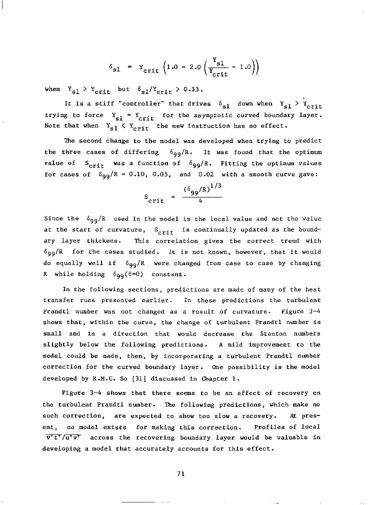
6 sl = 'crit ( Y

1.0 - 2.0 p- - 1.0 ( crit )I

when Y sl ' 'crit but Gsl/Ycrit > 0.33.

It is a stiff "controller" that drives 6sl down when Ysl > Ycrit

trying to force Ysl = Ycrit for the asymptotic curved boundary layer. Note that when Ysl < Ycrit the new instruction has no effect.

The second change to the model was developed when trying to predict

the three cases of differing "gg/R. It was found that the optimum value of Scrit was a function of 6gg/R. Fitting the optimum values

for cases of 6gg/R = 0.10, 0.05, and 0.02 with a smooth curve gave:

S (~gg/R)l”

= crit 4

Since the dgg/R used in the model is the local value and not the value at the start of curvature, Scrit is continually updated as the bound-

ary layer thickens. This correlation gives the correct trend with 699/R for the cases studied. It is not known, however, that it would

do equally well if 6gg/R were changed from case to case by changing R while holding sgg(e=O) constant.

In the following sections, predictions are made of many of the heat transfer runs presented earlier. In these predictions the turbulent

Prandtl number was not changed as a result of curvature. Figure 3-4 shows that, within the curve, the change of turbulent Prandtl number is

small and in a direction that would decrease the Stanton numbers slightly below the following predictions. A mild improvement to the

model could be made, then, by incorporating a turbulent Prandtl number correction for the curved boundary layer. One possibility is the model

developed by R.M.C. So [31] discussed in Chapter 1.

Figure 3-4 shows that there seems to be an effect of recovery on

the turbulent Prandtl number. The following predictions, which make no

such correction, are expected to show too slow a recovery. At pres-

ent, no model exists for making this correction. Profiles of local v' t' 127 across the recovering boundary layer would be valuable in

developing a model that accurately accounts for this effect.

71

The present model can be quite temperamental. The calculation of Y sl is done by extrapolation of a linear portion of the shear stress

profile to the wall. After some distance downstream of the beginning of

curvature, F the shear stress profile develops inflections that can cause

Y sl to jump a considerable distance from step to step. This usually

results in variations in the slope of St versus ReA 2 (

or s), os-

cillating about what appears to be a reasonable value. Occasionally the

program will extrapolate to an extremely small Ysl due to an inflection

very near the wall. Wen this happens, the solution goes irreparably

out of control. Because of this, the program can be quite frustrating

and expensive to run. An improvement might be to calculate the shear

layer thickness as an integral thickness: n

0

Y sl is a function of s

$dn , W

0

where no is the n-distance when the shear stress goes to zero. This

would stabilize the model considerably.

The following sections demonstrate how well the above model with

the above changes predicts the heat transfer cases discussed in (;hapter

3.

4.2 Predicting the Effect of Curvature for the Baseline Case

Figures 4-2 and 4-3 show the prediction of the baseline case. The

introduction of curvature rapidly decreases the skin friction and Stan-

ton number. For this case the effect is strong enough to overshoot and

oscillate for some time before settling down to the asymptotic curved

state. The prediction of both the skin friction and the Stanton number

within the curve is quite good. Note that a Prt correction would de-

crease St slightly near the end of the curve. The recovery is quite

accurately predicted. Note that the Prt correction would increase the

predicted St in the recovery region. To try to assess just how much

the correction would increase St, the ratio of St/(Cf/2) was calcu-

lated from the profile data for this case from Chapter 3, then multi-

plied by the predicted Cf/2 to get an estimated Stanton number with a

recovery correction on Prt. This corrected Stanton number is shown in

72

2000

ReA -Re ref 2 “;

1000

0

0 FROM PROFILES -FRoMu&LLMEASmmENTS 0

/ 0 ,I

/ 0’

0% 1’

/ /

1’ 1’ 1' c CURVE -

/ A

-50 LJ 0 50 100 150 S(a)

Fig. 3-5. Comparison of ReA equation and ReA 2

from the energy integral Erom the measured profiles for

the baseline case2(070280) - Turbulent, 0.10, u = 14.8 m/s , K N 0.0.

&&R(8=0) =

PW

57

0.0040 I I

b CASE b..IR

. 0 070280 0.10 I

be ‘a 022640 0.05 I

a 060480 0.02


Fig. 3-6. The effect of initial boundary layer thickness - Stanton number versus streamwise distance.

‘.OC-02

0.x-02

E

s

i: l.OE-03

%

s

2 O.SE-03

,.OE-04

F

r- SL - 0.0125 Pr-Oe5 Bc -Oez5 A2

CASE b,,lR

. 070280 0.10

0 022680 0.05

Y 060480 0.02

I I IWO 6000 10000 WOO0 1M


Fig. 3-7. The effect of initial boundary layer thickness - Stanton number versus enthalpy thickness Reynolds number.

58

o.oobo

0.0030

g 2 0.0020 z

ii

E

0.0010

O.OWO

_ I *

.

3

0

CASE WV (m/s)

070280 14.8 011380 7.0

112779 26.4

CURVE

1 -20 20 40 loo


Fig. 3-8. The effect of U, - Stanton number versus streamwise distance r-

l.OC-02

OBZ-02

I I.Ol?-03

E OSE-03

l.OE-04

1

CASE upw (m/s)

. 070280 14.8

a oil380 7.0

0 112779 26.4


-I

Fig. 3-9. The effect of U El"

- Stanton number versus enthalpy thickness Reynol s number.

59

STANTON NUMBER vs STREAMWISE DISTANCE

STREAMWISE DISTANCE, cm

Fia. 3-10. The effect of LJpb7 r Stanton number versus stream-

IT wise distance and “pw l

0.0040

0.0030

1 5 2. 0.0020

% k

2

0.0010

0 0001,

CASE K

. 022680 0 , ,a %oo a 00 042280 0.57x10-6

0.3 0-a %O 00 0 051080 1.25x10 -6

. -0 l a&, oooo 0 l wco 6‘. O.2 0

’ ‘.a* L -0

-20 20 40 100

STREAMWISE DISTANCE (CM) Fig. 3-11. The effect of free-stream acceleration on the curved

boundary layer - St.mton number versus streamwise distance.

LOE-02

OS-02

ri

4 z I.OE-03

E t; 0.5E-03

LOE-04

m 0.0125 P;"'5 Re -".25 "2

C&E K . 022680 0

a 042280 o.57x1o-6

" 051080 1.25~10-~ J

1 I IIIII.I 0 5000 10000 50000 lWW0


Fig. 3-12. The effect of free-stream acceleration on the curved boundary layer - Stanton number versus enthalpy thickness Reynolds number.

61

8 6

4

2 Stanton

number 1 x10-

.8

.6

.4

.2

I I III I I III I I

a! I I II I ---- U, constant m

t

K = 0.57 x lo -6 I I,

102 2 4 6 lo3 2 46104 2 11 6


Fig. 3-13. The effect of mild free-stream acceleration (from Kays and Moffat [38]) - Stanton number versus enthalpy thickness Reynolds number.

4

Stanton number

2

1 x10- 2 4 6 10' 2 4 6


Fig. 3-14. The effect of strong free-stream acceleration (from Kays and Moffat [38]) - Stanton number versus enthalpy thickness Reynolds number.

62

o.owo

Fig.

l.oE-02

0.5C-02

I! 2 l.OE-03 i5 E E om-03

La!-M


3-15. The effect of unheated starting length - Stanton number versus streamwise distance.

--- /-- SL - 0.0125 Pr-0.5 1e+-O.Z5

CASE Ry2 %

. 070280 1770 4173

0 060480 1750 1724

0 113079 0 2563

0 030280 Aft. 2563

I 100.0 WC.0 1ooO.O W.0 IP

DlTHALPY THICKNESS REYNOLDS NUUBER Fig. 3-16. The effect of unheated starting length - Stanton


63

O.W40

0.0030

&

B

E 0.0020

E

E

0.0010

0.3000

Fig.

I.ol!-02

0.5E-02

&

ii

i: l.OE-03

8 b 0.6E-03

0 CASE ne** ie-01

. 070280 417;

a 011380 1696

0 010680 1060

o 012480 074

t- CURVE 1 -60 20 20 60 100


3-17. The effect of the maturity of the momentum boundary layer - Stanton number versus streamwise distance for the late-transitional and turbulent cases.

-I -1 I I-1111, I I I11111

CASE %az - . 070280 4173

St - 0.0125 Pr-".5 p.A2-o.25 0 0106~30 1060 -

- a 011380 -\ 1696

-0 012480 874

I-----,

\

l.OE-04 1 4 1000 5000 10000 so000 100000


Fig. 3-18. The effect of the maturity of the momentum boundary layer - Stanton number versus enthalpy thickness Reynolds number for the late-transitional and turbulent cases.

64

r 1 CASE R-62

0 060980 222

0 . 062580 275 “0 0 0 0”“” < 0 0

062880 724 o”* u” ” “0”” ” 0

0

CURVE

__I-.--- '.- ' -20 20 00 loo


Fig. 3-19. The effect of the maturity of the momentum boundary layer - Stanton number versus streamwise distance for the laminar and early-transitional cases.

lS-co.

o.ec-OP.

lg

z Lot-05

1 0.69-03

I.OE44

I 0.0125 Pr-Oe5 PC -Oez5 62

ENTHALPY THICKNESS REYNOLDS NUHBER

Fig. 3-20. The effect of the maturity of the momentum boundary layer - Stanton number versus enthalpy thickness Reynolds number for the laminar and early- transitional cases.

65

/ STREAMWISE DISTANCE (CM)

Fig. 3-21. The effect of the maturity of the momentum boundary layer - Stanton number versus enthalpy thickness Reynolds number and momentum thickness Reynolds number at the start of curvature.

66

Chapter 4 HRAT TRANSFER PKEDICTIONS

One of the objectives of the curvature project was to develop a

turbulence model for curved-wall heat transfer predictions that could be used for practical engineering calculations. This is, in fact, the most

useful form in which to convey the results of these curvature experiments.

4.1 State of the Art

Prior to the beginning of the curved-wall studies at Stanford, the

most prevalent curvature model was one which stemmed from a suggestion

by Eradshaw [14] and was formulated and tested by Johnston and Eide

1401. Recently, Gillis and Johnston [35], with the benefit of their

recovery data, proposed a second model consistent with their "shear layer" interpretation of the curved turbulent boundary layer. Roth

models are discussed below. They modified the distribution of the mixing length across the boundary layer to account for streamwise curva-

ture.

Other, higher-order, models have been developed by launder et al.

c541, Irwin and Smith [39], and Gibson [53]. These models are quite

good for mild curvature. Although higher-order models give more detail

of the turbulence structure, they are generally more difficult to run

and less useful as engineering tools. In order to make the results of

the modeling effort most useful to industry, it was deemed desirable to

keep the computation scheme simple-- hence the mixing-length approach.

The mixing-length hypothesis uses an empirically prescribed length

scale to relate the mean velocity gradient to the Reynolds shear stress, through the formula:

- - uv = pJ Q I 1 an an (4-l)

A typical distribution of mixing length "II" for a flat-wall boundary layer is:

67

R = Ktl 1- r exp(-n+/*+) L I

(4-2)

the modified van Driest model [36] for the inner portion of the boundary

layer, where K, the Karman constant, is 0.41. For the outer portion

of the boundary layer, the typical flat-wall mixing length distribution

has

R = 0.085 6gg

The smaller of (4-2) or (4-3) is used. The parameter A+ identifies

the thickness of the viscous sublayer and is affected by acceleration/

deceleration or blowing/suction. The value for a flat-wall boundary

layer with uniform freestream velocity and no transpiration is A+ = 25.

The curvature model suggested by Bradshaw [14] modified this flat-

wall distribution for curvature according to the relationship:

a. = go(l - BRi) ,

where R 0

is the local flat-wall mixing length and Ri is the local

gradient Richardson number defined by

Ri = 2S(l + S) ,

where S, the stability parameter, is

S LJ

I

aLJ =- R eff an

The parameter B is an empirical parameter generally of the order 10.

The effective radius of curvature, Reff, comes from a first-order lag

model proposed by Johnston and Eide [41]:

W/Reff> dx

c

Ro is the wall radius of curvature. This mixing-length model was in-

vestigated in detail by Johnston and Eide [40,41]. Their recommenda-

tion for the value of the constant f3 was 6.0. Figure 4-l shows its

68

performance for the baseline case. The prediction was initialized with starting profiles taken 35 cm upstream of the beginning of the curve.

The test wall was isothermal and Upw was uniform. No correction for the effect of curvature on turbulent Prandtl number was made. lhe re-

sponse to the introduction of curvature was predicted quite well, but,

after the curve, Cf/2 and St recovered far too quickly. If the tur-

bulent Prandtl number were decreased in the recovery region according to the curve of Fig. 3-4, the recovery process would be even faster. This

model was devised before recovery data had been taken. Since it is

merely an empirical fit of curved and rotating wall mixing lengths, it

is not surprising that the model's performance in the recovery region was poor.

Gillis and Johnston [35] improved the recovery prediction by devis- ing a model in which the main effect of curvature was to confine the

turbulent motions close to the wall and allow the previously existing large-scale motions to decay. In the recovery region, they modeled the

regrowth of the inner boundary layer as a normal boundary layer growing on a flat plate within a velocity gradient. Their model follows.*

The mixing length in the outer portion of the boundary layer was

modeled as:

where 6sl *

is the width of the active shear layer and hsl is the dis-

placement thickness of the boundary layer integrated out to the shear

layer thickness hsl. 'Ihe constant of proportionality was found to be

0.10. The shear layer thickness in the flat-wall preplate or recovery

wall was found by extrapolating the linear portion of the shear stress profile to uv = 0, as shown in Fig. 1-8. Within the curve, Gillis and Johnston use a proposal from Gibson [42], that there is a critical value

of the stability parameter, S, defined as:

* See Kef. 35 for more details.

69

above which the shear stress cannot sustain itself. Gibson found that

this critical value was approximately 0.17. Gillis and Johnston found

that a critical value of 0.11 optimized the prediction of their data.

The model used in the following predictions of the heat transfer

data is essentially the same model as presented in Ref. 35, with the

exceptions of two changes made to the estimation of 6sl within the

curve.

To describe the first change, it is necessary to define the follow-

ing two parameters:

Y crit The n-distance away from the wall where S = Scrit.

Y sl The n-distance away from the wall where the extrapolated shear stress equals zero.

In the Gillis and Johnston model,

II = 0 .lO (As1 - Cl)

where 6 Sl = Ysl in the developing or recovery regions and hsl =

Y crit in the curved region. With their model it was found that the

switchover at the beginning of curvature quickly altered the shear

stress profile driving Ysl down to a small fraction of Ycrit. But,

as the change in the shear stress profile began to alter the mean veloc-

ity profile, Y,l began to rebound, passing up through and finally well

above Y crit' This rebound eventually affected the mean velocity and

temperature profiles, causing the calculated values of Cf/2 and St

to increase in a manner much like recovery from curvature, though still

within the curve. The critical stability argument states that, in the

asymptotic curved state, the extrapolated shear layer thickness. Ysl,

equals the n-distance where ' = 'crit' 'crit' But in this model,

Y Sl

could be well above Ycrit, especially, it was found, when &99/R was small. The change in the model was to construct a "controller" that

would not allow Ysl to grow much above Ycrit. The new model calcu-

lated the 6sl to be used in computing the curved-region mixing length

profile as:

6 Sl

= Ycrit when Y,l < Ycrit

70

6 Sl

= Y crit (

1.0 - 2.0 &- 1.0)) (

when 'sl > 'crit but Gsl/Ycrit > 0.33.

It is a stiff "controller" that drives 6sl down when Ysl > Ycrit

trying to force Ysl = Ycrit for the asymptotic curved boundary layer. Note that when Ysl < Ycrit the new instruction has no effect.

The second change to the model was developed when trying to predict

the three cases of differing "gg/R. It was found that the optimum

value of Scrit was a function of 6gg/R. Fitting the optimum values for cases of 6gg/R = 0.10, 0.05, and 0.02 with a smooth curve gave:

S (sgg/R)1’3

= crit 4

Since the 6gg/R used in the model is the local value and not the value at the start of curvature, Scrit is continually updated as the bound-

ary layer thickens. This correlation gives the correct trend with bgg/R for the cases studied. It is not known, however, that it would

do equally well if hgg/K were changed from case to case by changing R while holding dgg(8=O) constant.

In the following sections, predictions are made of many of the heat transfer runs presented earlier. In these predictions the turbulent

Prandtl number was not changed as a result of curvature. Figure 3-4

shows that, within the curve, the change of turbulent Prandtl number is

small and in a direction that would decrease the Stanton numbers slightly below the following predictions. A mild improvement to the

model could be made, then, by incorporating a turbulent Prandtl number correction for the curved boundary layer. One possibility is the model

developed by R.M.C. So [31] discussed in Chapter 1.

Figure 3-4 shows that there seems to be an effect of recovery on

the turbulent Prandtl number. The following predictions, which make no

such correction, are expected to show too slow a recovery. At pres-

ent, no model exists for making this correction. Profiles of local v't'fi?T across the recovering boundary layer would be valuable in

developing a model that accurately accounts for this effect.

71

The present model can be quite temperamental. The calculation of Y sl is done by extrapolation of a linear portion of the shear stress

profile to the wall. After some distance downstream of the beginning of

curvature, the shear stress profile develops inflections that can cause e Y sl to jump a considerable distance from step to step. This usually

results in variations in the slope of St VerSUS ReA 2 (

Or S), OS-

cillating about what appears to be a reasonable value. Occasionally the

program will extrapolate to an extremely small Ysl due to an inflection

very near the wall. hhen this happens, the solution goes irreparably

out of control. Because of this, the program can be quite frustrating

and expensive to run. An improvement might be to calculate the shear

layer thickness as an integral thickness: n

0

Y sl is a function of s

gdn , W

0

where no is the n-distance when the shear stress goes to zero. This

would stabilize the model considerably.

The following sections demonstrate how well the above model with

the above changes predicts the heat transfer cases discussed in Chapter

3.

4.2 Predicting the Effect of Curvature for the Baseline Case

Figures 4-2 and 4-3 show the prediction of the baseline case. The

introduction of curvature rapidly decreases the skin friction and Stan-

ton number. For this case the effect is strong enough to overshoot and

oscillate for some time before settling down to the asymptotic curved

state. The prediction of both the skin friction and the Stanton number

within the curve is quite good. Note that a Prt correction would de-

crease St slightly near the end of the curve. The recovery is quite

accurately predicted. Note that the Prt correction would increase the

predicted St in the recovery region. To try to assess just how much

the correction would increase St, the ratio of St/(Cf/2) was calcu-

lated from the profile data for this case from Chapter 3, then multi-

plied by the predicted Cf/2 to get an estimated Stanton number with a

recovery correction on Prt. This corrected Stanton number is shown in

72

Figs. 4-2 and 4-3. With this correction, the prediction and the data are quite close. Ideally, the prediction curve of Fig. 4-3 would follow

the data with a -1 slope. The strong introduction results in a

steeper slope. As the shear layer thickens, Y,l continues to grow,

and the slope decreases. hhen Y,l becomes larger than Ycrit, the

"controller" decreases bsl, trying to drive it to Ycrit, seen as a

downward trend near the end of the curve. Runs made with sustained

curvature show that the model predicts a continued decrease in St with

nearly a -1.0 slope in these coordinates. The shape of the recovery

is approximately correct, characterized by a rate of return roughly pro-

portional to the distance from the flat-wall correlation.

The following sections discuss the predictions of cases with dif-

fering values of a single parameter. Table 4-l shows the case numbers and figure numbers that constitute each separate-effect study.

Table 4-l

Prediction Runs

Effect

"99/R

u Pw

K

Unheated

Starting

Length

f Parameter Case Value Figure %'s

070280 0.10 4-2, 4-3 022680 0.05 4-4, 4-5

060480 0.02 4-6, 4-7

112779 26.4 m/s 4-8, 4-9

070280 14.8 m/s 4-2, 4-3 011380 7.0 m/s 4-10, 4-11

022680 0 4-4, 4-5

051080 1.25 x 10 -6 4-12, 4-13

022680 Base 4-4, 4-5

113079 A2/R(9=0) = 020 4-14, 4-15

030280 A,/R(9=90“) = 0.0 4-16, 4-17

73

4.3 Prediction of Cases with Differing Initial Boundary Iayer lhickness

Figures 4-2 through 4-7 show the ability of the program to model

cases of differing boundary layer thickness. The "predictions" are

goods even for the thin boundary layer case where 699'R = 0.02. The

term "prediction" might be misleading, especially in this study, because

values of Scrit were chosen that would optimize the comparison of cal-

culated and measured Stanton number and skin friction. No adjustment to

the model has been made for subsequent studies; therefore, sections 4-4

through 4-6 can, more honestly, be called predictions.

Note that the preplate prediction of Stanton number (Figs. 4-3, 4-

5, and 4-7) is progressively lower than the correlation for thinner

boundary layer cases. 'Ihis is probably due to the Reynolds number ef-

fect. In Case 060480, where dgg/R(6=0) = 0.02 (Figs. 4-6, 4-7), the

momentum thickness Reynolds number was 464 at S = -35 cm and estimated

to be 1724 at the start of curvature, indicating a late-transitional and

early turbulent boundary layer. Ihe turbulence model was developed for

a fully turbulent boundary layer and apparently underpredicts the pre-

plate data for the thin boundary layer cases. Ihe modeling is expected

to improve as the boundary layer thickens downstream. The predicted

Re6 at the end of the curve for Case 060480 was 3200. 2

The predicted recovery of the thinner boundary layer cases appears

to be slightly too rapid. Case 022680, where 6gg/R(8=0) = 0.05 (Figs.

4-4, 4-S), shows a faster recovery of skin friction than seen in the

measured values and a recovery of Stanton number similar to that seen in

the data. Figure 3-4 shows a decrease in Prt within the recovery re-

gion for this case, however, so that a Stanton number prediction with

a Prt correction would show too strong a recovery.

4.4 Prediction of Cases with Differing Upw

Figures 4-2, 4-3, and 4-8 through 4-11 show predictions of cases

with differing Upw. There seems to be a slight Upw effect that is

not modeled. Ihis effect apparently begins at the introduction of cur-

vature. Since the present model is based mainly on data from the asymp-

totic state, it is not surprising that there are some deficiencies near

74

the beginning of curvature. One might expect that the strength of the introduction of curvature might scale as

4.5 Prediction of Cases with Freestream Acceleration

Figures 4-12 and 4-13 show the prediction of the combined effects of strong free-stream acceleration and curvature. The prediction models

the -2 slope (Fig. 4-13) quite well in the early region. Apparently, however, the shear stress profile has developed an inflection, and the

extrapolation technique is jumping from one 6sl to another quite dif-

ferent one. This is seen both near the end of the curve and in the recovery section. The model proposed in Section 4.1, where hsl is calculated by integration might correct this problem, and it is expected

that the prediction of the acceleration case would be quite good.

4.6 Prediction of Cases with Differing Unheated Starting Lengths

Figures 4-14 and 4-15 show the prediction of the case in which

heating begins at the beginning of curvature inside a mature momentum boundary layer. Figures 4-16 and 4-17 show the prediction of a similar

case in which heating begins at the start of the recovery region. The figures show an excellent prediction of the two cases.

75

0.0040

0.0030

Ei 52

2 0.0020 z E 4 t;

0.0010

0.0000

0

0 00

00 00

oo”oo

FLAT PLATE 000

0 0 O0 9,-l\

\ \ 1

CURVE

0 0’0, o~;./---~~~~~~~

00 -- 0 OO

0

CURVE

, -ZlJ 20 0” 1””


Fig. 4-l. Prediction of the baseline case with the Johnston and Eide model.

76

o St - BASELINE CASE a Cf12 - BASELINE CASE

- PtiDICTION - St --PREiXCTION - Cf/2

x yltb Prt brr.Ctim

L- -60 -20 20 60 101)


Fig. 4-2. Prediction of the baseline case: Stanton number versus streaawise distance.

I.OL-62

O.M-02

6

B

E l.OE-63

E

2 o.m-on

l.OC-04 LOO.0 LOO.0 1606.0 60060 1oooO.O


Fig. 4-3. Prediction of the baseline case: Stanton mmber versus enthalpy thickness Reynolds number.

77

O.oo10

0.6030

c s

i-5 2 o.owo

2

B

z

2 O.WlO

0.6600

0 St - CASE 022680 cf12 - CASE 022680

" PREDICTION - St -- PREDICTION - Cf/2

a --- . \

-a- --- -o-- 0 __--

-b---*b a 6

, -20 -

20 60 106


Fig. 4-4. Prediction of Case 022680, $,/R(e=O) = 0.05: Stanton number versus streamwise distance.

l.OC-02

0.6C-02

&

B

ii I.OC-w

E

ii

2 0.6E-a3

1.6E-W I11111

1 .O 600.0 loon0 66600 101


0 CASE 022680 - PREDICTION

Fig. 4-5. Prediction of Case 022680, $g/R(e=O) = 0.05: Stanton number versus enthalpy thickness Reynolds number.

78

o.omo

0.0030

c e

f o.OWo

i3

1 0.0010

O.OOW

l.OC-02

O.fiC-02

az

3

5 z l.oc-03

8 z

2 O.M-OS

l.OE-04

o St - CASE - 060480 - PREDICTION - St --PREDICTION - Cf/Z

0 CURVE -

1 -2.0 20 2.0 100

STREAYWISE DISTANCE (CU)

Fig. 4-6. Prediction of Case 060480, 6gg/R(+O> = 0.02: Stanton number versus streamwise distance.

7

. 0.~~2~ pr-o.5 Pe -0.25

--- c--Tz< f

O CASE 060480 - PREDICTION

lW.0 6000 10000 5000.0 1WOO.O

ENTHALPY THICKNESS REYNOLDS NUMBER Fig. 4-7. Prediction of Case 060480, 6g,/R(e=O> - 0.02:

Stanton number versus enthalpy thickness Reynolds number.

79

O.oo10

0.0030

s u

ii ; 0.0020

2

5 !s

2 0.0010

0.0000

o St - CASE 112779 - PREDICTION - St --PREDICTION - Cfl2

I CURVE -

--20 20 80 100

STREWWISE DISTANCE (CM)

Fig. 4-8. Prediction of Case 112779, % = 26 m/s: Stanton number versus streamwise distance.

l.OE-02

OAE-02

f!i

B

2 l.OE-03

5 !2

2 o.ec-03

l.OE-04

---~ St - 0.0125 Pr-0.5 P.qO.25

--\ --_

uoo\

0

u St - CASE 112779 - PREDICTION

ENTHALPY THICKNESS REYNOLDS NUUBER Fig. 4-9. Prediction of Case 112779, UPw = 26 m/s: Stanton


80

0 St - CASE 011380 - PREDICTION - St --PREDICTION - Cfl2

-- --- 0 _---

I -20 ?

20 60 100

.STREAMWISE DISTANCE (CM)

Fig. 4-10. Prediction of Case 011380, UP = 7 m/s: Stanton number versus streamwise distance.

1.0~~02

O&E-02

2 l.OC-03

z $

s 0.6E-03

l.OE-04

St -o-25 -

/ 0.0125 Pr-0’5 Pe 62

0 St - CASE 011380 - PREDICTION

1000 600 0 10000 so00 0 lOMO.0


Fig. 4-11. Prediction of Case 011380, Upw = 7 m/s: Stanton number versus enthalpy thickness Reynolds number.

81

0.0040

O.CW30

s ”

6 g O.MZO

2

!3

2 2 v-2 o.w10

O.WW

0 ""

- St CASE 051080 - - PREDlCTION St - --PREDICTION - Cf/2

/- , - -. Y 1,--,--

- -0 I

, -20


Fig. 4-12. Prediction of Case 051080, K = 1.25 x 10m6: Stanton number versus streamwise distance.

I .OE-02

O.bd-02

,.Od-04 1

r

/--- St - 0.0125 Pr-005 Ilc -".25 A2

--_ / ---

" St - CASE 051080 - PREDICTION

1 _-_ ^ .^^^ ^ _^^^^ ._

) 50” ” l”““” XJLXJ” IU


b.0

Fig. 4-13. Prediction of Case 1351080, K = 1.25 x 106: Stanton number versus enthalpy thickness Reynolds number.

82

o St - CASE 113079 o St - CASE 113079 -PREDICTION - St -PREDICTION - St

--PREDICTION - Cff2 --PREDICTION - Cff2

--__ _--- --__ __-- --- I CURVE CURVE

-20 -20 20 20 60 60 100 100

STREAYWISE DISTANCE (CM)

Fig. 4-14. Prediction of Case 113079, A2/R(B=O) = 0.0: Stanton number versus streamwise distance.

l.OE-02

O.bE-02

l.OE-0,

- St - 0.0125 P;"'5 Be -"'25 -- A2

--- -- a 0 --

--- 4 P

9

“SC - CASE 113079 -PREDICTION

5000 1000 0 5000 0 10

ENTHALPY THICKNESS REYNOLDS NUMBER Fig. 4-15. Prediction of Case 113079, A2/~(tl=O) = 0.0:

Stanton number versus enthalpy thickness Reynolds number.

30

83

-

cl St - CASE 030280 - PREDICTION - St

-- PREDICTION - Cf/Z

c 3 2 p o.w+?o 2 oz 5 it 0.0010

O.OWO

I.oE-02

0.5E-02

5

B 3 z l.OE-03

0”

5 E o.sc-03

LOC-04

oc

--- \ \

-20

\ . .

-- -.__

-- _/--

-_0 /

-“’ 20 60 loo


Fig. 4-16. Prediction of Case 030280, A2/R(B=900) = 0.0: Stanton number versus stream&se distance.

100

. . . . . . . .

-- _ _ _ cst - 0.0125 p,-O*5 Re+-0.25

-- 0 ---_ ----od,

-- ---

LI SC - CASE 030280 - PREDICTION

.o 500 0 LOW0 wooo 1,


,OC

Fig. 4-17. Prediction of Case 030280, &/R( =90"> = 0.0: Stanton number versus enthalpy thickness Reynolds number.

84

Chapter 5 CONCLUSIONS AND RECOMMENDATIONS

This study presents results of experiments on the effect of convex

curvature on heat transfer through turbulent and transitional boundary layers. For the baseline case, the effect of curvature was separated

from other effects such as streamwise accleration, which usually ac- companies curvature in practice. hhere there were combined effects,

they were carefully controlled, i.e., where streamwise acceleration with curvature was to be tested, acceleration was with a constant K =

v/U2 Pw

l dUpw/ds.

The results of the 15 cases studied here provide considerable in-

sight into the effects of curvature on turbulent boundary layer heat transfer. They complement the detailed hydrodynamic measurements of the

previous investigations, e.g., Gillis and Johnston [35], So and Mellor [16], etc. The studies of separate effects isolated several important

parameters and revealed some new characteristics of curved boundary layers (e.g., the -1 slope in Stanton number versus enthalpy thickness

Reynolds number coordinates). Also, they checked the robustness of hypotheses, like the "shear layer hypothesis," derived in single--run

experiments by subjecting them to a broad range of conditions. Most

important to the modeler and, eventually, the designer, these tests

provide a broad data base with which to verify future prediction models.

5.1 CDnclusions

The main conclusions are as follows:

1. The effect of convex curvature on heat transfer rates is signifi-

cant for all the cases studied. Reductions of Stanton n~ber of 20-50% below the expected flat-wall values were observed. The effect of convex

curvature is seen immediately at the beginning of curvature and continues to grow throughout the curve. The recovery of the heat transfer

rate on a downstream flat wall is extremely slow. After 60 cm of recovery length, (15-20 boundary-layer thicknesses), the local Stanton number

may still be 15-20X below what would be expected without upstream curvature, at the same enthalpy thickness Reynolds number.

85

2. The boundary layer eventually reaches an asymptotic curved condi-

tion characterized by St Q: Re slope is considered to be

significant. “; l The -l It may be indicat ng that the overall heat transfer from

the wall has become conduction-dominated as in a laminar boundary layer

or a strongly accelerated boundary layer.

3. Separate effects studies on this one curved surface show that the

boundary layer thickness, free-stream velocity, and maturity of the

boundary layer affect the response to the introduction of curvature and

the rate at which the asymptotic state is approached, but not the even-

tual asymptotic state characterized by the -1 slope.

4. Studies of combined streamwise acceleration and streamwise curva-

ture effects show that they both can be significant and that they seem to be additive. Convex curvature seems to increase the boundary layer's

sensitivity to acceleration, as has previously been observed when accel-

eration and wall suction were combined.

5. Studies of the effect of convex curvature on laminar and transitional boundary layers show that this stabilizing curvature delays tran-

sition from laminar to turbulent. hhen the curved boundary layer is near-laminar or early-transitional, the effect of the curved region is

soon "forgotten," and the recovery data rapidly return to flat-wall expected values. bhen the curved boundary layer is late-transitional,

recovery is slow, similar to that of a mature turbulent boundary layer.

6. Turbulent Prandtl number deduced from the thermal law-of-the-wall

or calculated as St/( Q/2) increases slightly (lo-15%) within the curved region and decreases rapidly in the recovery region. At the end

of the recovery section, the log-law deduced Prt is N 0.50 and con-

tinuing to decrease.

7. The "shear layer" model proposed by Gillis and Johnston [35] seems

to be an effective model with which to view the effect of convex curva-

ture on turbulent boundary layers.

8. The curvature prediction model presented by Gillis and Johnston

1351 and modified herein predicts the present heat transfer studies

reasonably well, although it must still be considered "developmental."

86

5.2 Recommendations for Future Lbrk on the Convex Problem

This program has answered several important questions about the

curved wall convective heat transfer problem. It dealt with the scaling and sensitivity questions and provided a broad data base to build upon.

An important next step is to study in detail the difference between the effects of curvature on the diffusivity of heat and momentum. 'IhiS

involves taking profiles of the shear stress u'v' and the turbulent

transport of heat V't' to give profiles of Prt. Development of a

four-wire anemometer probe at Stanford is now nearly complete, and such

data should be available soon. Of the four wires, three are for measur-

ing the three components of velocity and the fourth is a temperature

sensor. Prediction of the recovery of Stanton number will require de-

velopment of a turbulent Prandtl model, which, in turn, will require

that we know more about the processes than the present data can reveal.

Another important separate effect study not done in the present

experiment would be of the effect of radius of curvature. It has been

assumed, but not shown, that the appropriate parameter for the strength

of curvature is 6&R. This study has indicated that 699/K affects only the rate at which the asymptotic state is approached. The ques-

tions that remain are: (1) If the radius is changed but 699/R(R=O) is held constant, does the approach trajectory to the asymptotic state

change? (2) Does the nature of the asymptotic state itself change?

Other important questions remain about the curved and recovery

regions. These are: If the curved wall were allowed to continue indefi- nitely (without influence of secondary flow), would the conclusion that

the asymptotic state is represented by St 0: Re -1

*2 remain true? or, if

the recovery wall were much longer, what would be the continued trajectory of Prt versus s (Fig. 3-4)?

Still unanswered are questions about the combined effects of convex

curvature and transpiration, or surface roughness. These are key ques-

tions to the designer. A hydrodynamically smooth wall may become tran- sitionally rough when it becomes convexly curved and the scale of the

boundary layer decreases. It has been shown that convex curvature or

wall suction increases sensitivity to streamwise acceleration. Row

87

sensitive to acceleration would a curved boundary layer with wall suc-

tion become?

Another important question to gas turbine blade designers is: Ebw

does convex curvature influence the jet-freestream interaction for film-

cooled blades? *

It most likely will be learned that the optimum blowing

rate is curvature-dependent.

* Research activity now under way at Stanford.

88

1.

2.

3.

4.

5.

6.

7.

8.

9.

10.

11.

12.

13.

14.

References

Crawford, M. E. and W. M. Rays, "STAN5--A Program for Numerical Computation of Iwo-dimensional Internal and External Boundary Layer Flows ;' NASA CR-2742, Dec. 1976.

Bradshaw, P., "Effects of Streamline Curvature on Turbulent Flow," AGARDograph No. 169, 1972.

Wilcken, H., "Turbulente Grenzschichten an Gewoelbten Flaechen," Berlin, Vol. 1, No. 4, Sept. 1930, translated as NASA TT-F-11, 421, Dec. 1967.

Is3ndt, F., "Turbulente StrSmungen zwischen zesi rotierenden honax- ialen Zylindren," Ing.-Arch., Vol. 4, p. 577 (1933).

Schmidbauer, H., "Behavior of Turbulent Boundary Layers on Curved Convex Wlls" (1936), NACA-TM No. 791.

GBttendorf, F. L., "A Study of the Effect of Curvature on Fully Developed Turbulent Flow," Proc. Royal Sot., Vol. 148, 1935.

Clauser, M., and F. Qauser, "The Effect of Curvature on the Tran- sition from Laminar to Turbulent Boundary Layer," NACA-TN No. 613 (1937).

Liepmann, H. W., "Investigations on Iaminar Boundary-Layer Stabil- ity and Transition on Curved Boundaries," NACA Advance Confidential Report (1943).

Rreith, F., "The Influence of Curvature on Heat Transfer to Incom- pressible Fluids," Trans. ASME, Nov. 1955.

Eskinazi, S., and Y. Yeh, "An Investigation of Fully Developed Turbulent Flows in a Curved Channel," J. of Aero Science, Vol. 23, No. 1 (1956).

Schneider, W. G., and J. H. T. h&de, "Flow Phenomena and Heat Transfer Effects in a 90" Rend," Canadian Aeronautics and Space Journal, Feb. 1967.

Patel, V. C., "The Effects of (Xlrvature on the Turbulent Boundary Layer ," Aeronautical Research Council, A.R.C. 30 427, F.M. 3974, Aug. 1968.

Ihomann, II., "Effect of Streamwise kill Curvature on Heat Transfer in a Turbulent Boundary Layer," JFM., Vol. 33, Part 2, pp. 283-292 (1968).

Bradshaw, P., "The Analogy Between Streamwise Curvature and Ruoy- ancy in Turbulent Shear Flow," JFM, Vol. 36, Part 1, pp. 177-191 (1969).

89

15.

16.

17.

18.

19.

20.

21.

22.

23.

24.

25.

26.

27.

28.

Bradshaw, P., "Review--Complex Turbulent Flows," Transactions of the ASME, June 1975.

so , R.M.C., and G. L. Mellor, "An Experimental Investigation of Turbulent Boundary Layers along Curved Surfaces," NASA-CR-1940, April 1972.

so , R.M.C., and G. L. Mellor, "Experiment on Turbulent Boundary Layers on a Concave Wll," The Aeronautical Quarterly, Vol. 16, 25, Feb. 1975.

so , R.M.C., and G. L. Mellor, "Experiment on Convex Curvature Effects in Turbulent Boundary Layers," JFM, Vol. 60, Part 1, pp. 43-62 (1973).

Ellis, L. B., and Joubert, P. N., "Turbulent Shear Flow in a Curved Duct )I' JFM, Vol. 62, Part 1, pp. 54-84 (1974).

Meroney, R. N., and P. Bradshaw, "Turbulent Boundary Layer Growth over a Longitudinally Curved Surface," AIAA Journal, Vol. 13, No. 11, Nov. 1975.

l-bffmann, P. H., and P. Bradshaw, "Turbulent Boundary Layers on Surfaces of Mild Longitudinal Curvature," Imperial College, Aero. Rept. 78-04 (1978) (submitted to JFM).

Smits, A. J., S.T.B. Young, and P. Bradshaw, "The Effects of Short Regions of High Surface Curvature on Turbulent Boundary Layers," JFM, Vol. 94, Part 2, pp. 209-242, Dec. 1978.

Smits, A. J., J. A. Eaton, and P. Bradshaw, "The Response of a Tur- bulent Boundary Layer to Lateral Divergence," JFM, Vol. 94, Part 2, pp. 243-268, Dec. 1978.

Castro, I. R., and P. %adshaw, "The Turbulence Structure of a Highly Curved Mixing Layer," JFM, Vol. 73, Part 2, pp. 265-304 (1976).

Ramaprian, B. R., and B. G. Shivaprasad, "Mean Flow Measurements in Turbulent Boundary Layers along Mildely (Xlrved Surfaces," AIAA Journal, Vol. 15, No. 2 (1977).

Ramaprian, B. R., and B. G. Shivaprasad, "Turbulence Measurements in Boundary layers along Mildly Curved Surfaces," ASME 77-HA/FE-6, Dec. 1977.

Ramaprian, B. R., and B. G. Shivaprasad, "Some Effects of Longitud- inal kll Curvature on Turbulent Boundary Layers," presented at First Turbulent Shear Flow Conference, April 1977.

.Ramaprian, B. R., and B. G. Shivaprasad, "The Structure of Turbu- lent Boundary Layers along Mildly Curved Surfaces," JFM, Vol. 85, p. 273 (1978).

90

29. Hunt, I. A., and Joubert, P. N., "Effects of Small Streamline Cur- vature on Turbulent Duct Flow," JFM, Vol. 91, Part 4, pp. 633-659.

30. Brinich, P. F., and R. W. Graham, "Flow and Heat Transfer in a Curved Channel," NASA TND-8464, May, 1977.

31. So, R.M.C., "The Effects of Streamline Curvature on Reynolds Anal- WY 3" ASME 77-WA/FE-17 (1977).

32. Mayle, R. E., M. F. Blair, and F. C. Kopper, "Turbulent Boundary Layer Heat Transfer on Curved Surfaces," J. of Heat Transfer, Vol. 101, No. 3, Aug. 1979.

33. Reynolds, W. C., W. M. Kays, and S. J. Kline, "Heat Transfer in a Turbulent Incompressible Boundary Layer. I. Constant Wall Tempera- ture," NASA Memo 12-l-588, 1958.

34. Gillis, J. C., and J. P. Johnston, "Experiments on the Turbulent Boundary Layer over Convex Walls and Its Recovery to Flat-Wall Conditions," 2nd Symposium on Turbulent Shear Flows, July 1979.

35. Gillis, J. C., and J. P. Johnston, "Turbulent Boundary Layer on a Convex, Curved Surface," draft of technical report for NASA-Lewis Research Center (Ph.D. thesis of J. C. Gillis, Dept. of Mech. Engrg - , Stanford University) (1980). NASA-CR 3391, March 1981.

36. Kays, W. M., and M. E. Crawford, Convective Heat and Mass Transfer, McGraw-Hill Publishing Co. (1980)

37. Simon, T. W., and S. IJDnami, "Final Evaluation Report: Incompress- ible Flow Entry Test Cases Having Boundary Layers with Streamwise Wall Curvature (0230)," 1980-81 AFOSR-HTTM-Stanford Conference on Cmplex Turbulent Flows: Comparison of Computation and Experiment, Stanford University, 1980.

38. Kays, W. M., and R. J. Moffat, "The Behavior of Transpired Ikbu- lent Boundary Layers," HMT-20, Thermoscience Division, Department of Mechanical Engineering, Stanford University, April 1975.

39. Irwin, H.P.A.H., and P. A. Smith, "Prediction of the Effect of Streamline Curvature on lkrbulence," Physics of Fluids, Vol. 18, No. 6, June 1975.

40. Johnston, J. P., and S. A. Eide, "Turbulent Boundary Layers in Cen- trifugal Compressor Blades: Prediction of the Effects of Surface Curvature and Rotation," J. of Fluids Engrg., 98(l), 374-381 (1976).

41. Johnston, J. P., and S. A. Eide, "Prediction of the Effects of Lon- gitudinal Wall Curvature and System Rotation on Turbulent Boundary Layers," Report PD-19, Thermosciences Division, Dept. of Mechanical Engrg l , Stanford University, Nov. 1974.

91

42.

43.

44.

45.

46.

47.

48.

49.

50.

51.

52.

53.

54.

Gibson, M. M., "An Algebraic Stress and Heat-Flux Model for Turbu- lent Shear Flow with Streamline Curvature," Int'l. Jour. of Heat and Mass Transfer, Vol. 21, 1609-1617 (1978).

Crawford, M. E., W. M. Kays, and R. J. Moffat, "Heat Transfer to a Full-Coverage Film-Cooled Surface with 30" Slant-Hole Injection," NASA Contractors' Report CR-2786, Dec. 1976.

aloe, H., W. M. Kays, and R. J. bffat, "Turbulent Boundary Layer on a Full-Coverage, Film-Cooled Surface - An Experimental Heat Transfer Study with Normal Injection," NASA Contractors' Report CR-2642, Jan. 1976.

Kim, H. K., R. J. tiffat, and W. M. Kays, "Heat Transfer to a Full- Coverage, Film-Cooled Surface with Compound-Angle (30" and 45") Hole Injectin," HMT-28, Thermosciences Division, Mech. Engrg. Dept., Stanford University, 1978.

MzCuen, P., "Heat Transfer with Laminar and Turbulent Flow between Parallel Planes with Constant and Variable h&l1 Temperature and Heat FLux," Ph.D. thesis, Ihermosciences Division, Mech. Engrg. Dept.3 Stanford University, 1962.

mrretti, P. A., "Heat Transfer through an Incompressible Turbulent Boundary Iayer with Varying Free-Stream Velocity and Varying Sur- face Temperature," Ph.D. thesis, Thermosciences Division, Mech. Engrg. Dept., Stanford University, 1965.

Kays, W. M., R. J. hoffat, and J. P. Johnston, "Heat Transfer and Hydrodynamic Studies on a Curved Surface with Full-Coverage Film Cooling," Proposal to NASA-Lewis Research Center, June 1976.

Moffat, R. J., "Temperature Measurement in Solids," ISA Paper 68-514 (1968).

Blackwell, B. F., and R. J. Moffat, "Design and Construction of a Iow-Velocity Boundary Layer Temperature Probe," Transactions of the ASME, Journal of Heat Transfer, May 1975.

tiffat, R. J., "Gas Temperature Measurement," Temperature--Its Measurement and Control in Science and Industry, Vol. 3, Part 2, 553-571, Reinhold Publishing Corp., New York, N. Y. (1962).

Pbnami, S., "New Definition of Integral thickness on the Curved Surface," Internal Lab. Report, Thermosciences Division, Dept. of Mech. Engrg., Stanford University (1980).

Gibson, M. M., "An Algebraic Stress and Heat-Flux Model for Turbu- lent Shear Flow with Streamline Curvature," Int. Jour. of Heat and Mass Transfer, Vol. 21, 1609-1617 (1978).

Launder, B. E., C. H. Priddin, and B. I. Sharma, "The Calculation of Turbulent Boundary Layers on Spinning and Curved Surfaces," ASME J. of Fluids Engrg., March 1977.

92

55. Mzllor, G. L., "Analytic Prediction of the Properties of Stratified Planetary Surface Layers," J. Atmos. Sci., 30, 1061-1069 (1973).

56. So, R. M. C., "A Turbulence Velocity Scale for tirved Shear Flows," J. Fluid Mech., 70, 37-57 (1975).

57. So, R. M. C., "Turbulence Velocity Scales for Swirling Flows," Ikr- bulence in Internal Flows, edited by S. N. B. Murthy, Hemisphere Publishing Corp., kshington/I.ondon, 347-369 (1977).

Appendix A

THE UNCERTAINTY ANALYSIS

Processing the data included the calculation of each reduced

quantity and the uncertainty of that quantity (output in Appendix G).

The uncertainty can be interpreted as the band above or below the stated

value within which it is believed the value would lie, with 2O:l odds,

or 95% of the time. Ihe uncertainty tells how closely each stated value

listed in Appendix G and discussed in the body of this report can be

believed. The uncertainty analysis also tells the designer or data-

taker how much effort should be given to the measurement of any partic-

ular quantity. Ihe uncertainty analysis was brought on-line early in

the design phase of this project and used in that capacity to guide the design.

One note: the uncertainty interval applies to any one data point.

When many data points are taken over a region where there are no discon-

tinuities, i.e., the preplate, the curved wall, or the recovery wall,

the mean of the data is known with more certainty than any one data

point; integration or averaging tends to decrease the uncertainty.

Though the uncertainty presented is typically 3-5%, the uncertainty of

the mean of the data is much smaller.

The uncertainty analysis built into the Stanton number data-

reduction program was one that, as a first step, calculated all the

sensitivity coefficients,

the influence on the Stanton number uncertainty of the uncertainty of a

particular parameter, P'. This is done by first rerunning the data-

reduction with that parameter changed by, typically, l%, to get the par-

tial derivative, then multiplying by the uncertainty of P'. After the

sensitivity coefficients was calculated, the overall uncertainty was

calculated using Kline and McGlintock [A-l]:

m 3 2 6St = Z& 6P'i

i

94

The following table shows the parameters included in the uncertainty analysis and their estimated uncertainty:

Table A-1

Input to the Uncertainty halysis

Parameter Uncertainty

Embedded, calibrated thermocouple output

Calibration constant for thermocouples in pre-

and after-plate

Plate-plate gap heat conductance

Heat flux meter signal

hkttmeter reading

Heat flux meter calibration constant

Plate area

lhnbient pressure

Relative humidity

Free-stream temperature

Dynamic pressure difference

Emissivity

Mttmeter calibration constant

Plate heater electrical resistance

3 PV

30%

10%

20 pv

0.05 w

3%

0.46 mm2

7.6 mm Hg

1%

3 PV

0.13 mm H20

0.02

0.015 w

0.015 R

95

(Table k-1 (cont.)

Plate Heater and delivery line electrical

resistance

Plate heater and delivery line electrical

resistance, including transformer

Resistance of the ammeter circuitry

Tunnel static pressure

Spanwise heat transfer correction

Support section temperature

Recovery factor of free-stream thermocouple

Thermocouple calibration constant

Saturation pressure of water

Saturation density of water

Inductance of ammeter circuitry

Resistance of voltmeter

Resistance between wattmeter and transformer

Preplate-curved section gap conductance

Curved section/afterplate gap conductance

0.015 n

0.015 n

0.005 R

0.13 mm 30

20%

4 uv

0.04

0.10

0.14 atm

0.0016 kg/m3

0.003 D

100 n

0.005 a

10%

10%

96

The uncertainty analysis was written into both the profile data- reduction program (listed in App. E) and the Stanton number-reduction

program (listed in App. F). The total uncertainty of each quantity is

given, along with the reduced quantity in Appendix G. More detailed

output giving the maxima and minima of the sensitivity coefficients within the developing region, curved region, or recovery region for each

input to the uncertainty analysis is also available. This is the de-

tailed information used in the rig design. AI example of this is given

on the following page for the baseline case.

References

A-l. Kline, S. J., and F. A. McClintock, "Describing Uncertainties in Single-Sample Experiments," Mechanical Engineering, Jan. 1953.

97

RUN 070280 l ** CURVATURE RIG l ** NASA-NAG-3-3 SENSITIVITY COEFFICIENTS IDST/LJARG l DELTA ARGJ

TO(I) , J= 2 DELTA ARG= TTOPI I I I J= 3 DELTA ARG- TCE:I( I I I J' 4 DELTA ARG= TBOTI I J I J= 5 DELTA ARG= B(I) 1 J- 6 DELTA ARG: S(I) ( J= 7 DELTA ARG: HJ'llIl 1 J= 8 DELTA ARG= 9111 I J= 9 DELTA ARG: KIII ( J=lO DELTA ARG- A( I I 1 J=ll DELTA ARG' PAna ( J=lZ DELTA ARG' RHUM I J-13 DELTA ARG: TRECOV I J=14 DELTA ARG: PDYN f J-15 DELTA ARG' EflIS 1 J=16 DELTA ARC: WCAL 1 J-17 DELTA ARG=

0.00300 I

0.00300 I

0.00300 J

0.00300 I

0.00039 J

0.07700 J

0.02000 1

0.05000 I

0.98160 )

0.00050 J

0.30000 J

1.00000 1

0.00300 I

0.00500 I

0.02000 I

0.05000 J RO1IJ 1 J-18 DELTA ARG' 0.01500 J RBOI I I 1 J=19 DELTA ARG' 0.01500 I RLODIII I J=20 DELTA ARG- 0.01500 J RA 1 J-21 DELTA ARG: 0.00500 J PSTAT 1 J=22 DELTA ARG= 0.00500 J SPANI I J 1 J'23 DELTA ARG- -0.19815 J TSUPPI 0 1 J=24 DELTA ARG- 0.00400 J RFY 1 J=25 DELTA ARG' 0.04000 I TCAL 1 J-26 DELTA ARG= O.lOOOO J PS 1 J'27 DELTA ARG= 2.00000 J RHOS I J'28 DELTA ARG' 0.00010 J XA I J=29 DELTA ARG: 0.00300 J RV 1 J=30 DELTA ARG=l00.00000 J RB 1 J=31 DELTA ARG= 0.00500 J KUP I J'32 DELTA ARG= 0.00860 J KDWN 1 J=33 DELTA ARG' 0.01790 J

PREP 'LATE

nAx

0.26079E-04 0.26079E-04 III 1) III 1)

0.00000E 00 0.00000E 00 (0 11 (0 11

0.82705E-05 0.82705E-05 (U24J (U24J

O.OOOOOE 00 O.OOOOOE 00 (II 11 (II 11

0.45173E-05 0.45173E-05 IZ 0 IZ 0

O.l3696E-03 O.l3696E-03 III IJ III IJ

O.l0121E-04 (II 1)

O.OOOOOE 00 ICI 11

O.l3056E-03 (I) 11

0.37771E-05 IX 1)

0.22846E-06 (A 21

0.36lOSE-04 III 2)

O.l3754E-04 IX 1)

0.30459E-05 1s 2)

0.74226E-05 1922)

0. OOOOOE 00 1s 11

O.OOOOOE 00 IA 11

O.OOOOOE 00 Ia 0

O.OOOOOE 00 Itl 1)

O.OOOOOE 00 11) 0

0.83559E-08 (tl 11

O.OOOOOE 00 (# 11

O.OOOOOE 00 10 0

O.l0429E-05 (S lJ

0.67102E-06 IO lJ

O.l662lE-07 I# 7)

O.l4268E-05 I# 2)

O.OOOOOE 00 1s 1)

O.OOOOOE 00 ltl 1)

O.OOOOOE 00 11) 1)

O.OOOOOE 00 IC 1)

O.OOOOOE 00 f# 11

DIN

O.l9330E-04 (t22J

O.OOOOOE 00 II 1)

O.OOOOOE 00 111 11

O.OOOOOE 00 (8 1)

O.l0257E-05 1x24)

0.53416E-06 (#15J

0.3196lE-05 IU 5)

O.OOOOOE 00 Ill 1)

0.69306E-04 (%17J

0.22978E-08 (ti23J

O.l6041E-06 (%24J

0.25454E-04 1024)

0.84155E-05 (P24J

0.21380E-05 (1)24J

0.72271E-05 Ill 41

O.OOOOOE 00 Ill 1)

O.OOOOOE 00 (it 1,

O.OOOOOE 00 (0 11

O.OOOOOE 00 (cl 0

O.OOOOOE 00 (A 1)

0.26587E-08 Ill 91

O.OOOOOE 00 (II 1)

O.OOOOOE 00 I* 11

0.63785E-06 (1124)

O.l9418E-06 (11191

0.90028E-08 (1124)

0.99635E-06 (#24J

O.OOOOOE 00 (0 1)

O.OOOOOE 00 IO 1)

O.OOOOOE 00 III 11

O.OOOOOE 00 (0 1,

O.OOOOOE 00 1: 1)

TEST S

tlAX

0.38653E-05 (U25J

0.60197E-05 11125)

0.43886E-04 (11251

O.l4686E-04 lG25J

O.OOOOOE 00 lU25J

O.l7573E-05 I11381

O.OOOOOE 00 1325)

0.76188E-05 (U25J

0.34976E-06 III31 I

0.42677E-05 l#25J

O.l3699E-06 (#25J

0.21862E-04 (8251

0.71244E-05 (#25J

0.182592-05 Ilt.25)

0.73668E-05 (a281

0.76684E-05 ((1253

0.46238E-05 (t25J

0.45330E-05 11125)

0.75734E-07 (11251

O.l2569E-05 IR251

0.41780E-08 (f25J

O.OOOOOE 00 18251

0.96736E-06 (025)

0.5512lE-06 (0251

0.16857E-06 (U25J

O.l1773E-07 (t125J

0.85607E-06 (#25J

O.l2196E-07 1035)

0.5537OE-07 (825)

O.l2995E-05 11125)

0.43539E-06 10251

0.20978E-06 (238)

ECTION

ttIN

O.OOOOOE 00 (126)

0.42149E-05 1026)

0.26972E-04 (tl38J

0.99133E-05 11137)

O.OOOOOE 00 It251

O.l5367E-06 (11321

O.OOOOOE 00 IP25J

0.70733E-05 lt38J

0.28317E-07 1837)

O.P4642E-05 I#381

0.82757E-07 (U38J

O.l3102E-04 (U381

0.43376E-05 (3381

O.l1031E-05 11)38J

0.72550E-05 (1371

0.71334E-05 (0381

0.43014E-05 1038)

0.42166E-05 (338)

0.70482E-07 is381

0.78217E-06 (038)

O.l1394E-08 (#38J

O.OOOOOE 00 I8251

O.OOOOOE 00 (831 J

0.32596E-06 (S38J

0.94995E-07 (t137J

0.49477E-08 (838)

0.51332E-06 111301

0.55436E-08 11301

0.35375E-07 1:38J

0.8077lE-06 (0381

O.OOOOOE 00 IX261

O.OOOOOE 00 lt25J

AFTERPLATE

UAX HIN

0.20279E-04 0.171718-04 1861 J (a1461

O.OOOOOE 00 O.OOOOOE 00 (039) (139)

0.44829E-05 (#39J

O.OOOOOE 00 (11391

0.75369E-05 W44J

0.46905E-04 (11621

0.7777lE-05 Is58J

O.OOOOOE 00 (11391

0.53652E-04 18623

O.l5659E-05 lit62J

O.l1104E-06 1856)

O.l7679E-04 111561

0.57944E-05 IPbOJ

O.l480lE-05 (lt56J

0.74413E-05 (3411

O.OOOOOE 00 (P39J

O.OOOOOE 00 (tJ39J

O.OOOOOE 00 (U39J

O.OOOOOE 00 ct391

O.OOOOOE 00 (039)

0.34183E-08 (S39J

O.OOOOOE 00 (839)

O.OOOOOE 00 111391

0.44075E-06 (lt6OJ

0.45029E-06 cc!441

0.96954E-08 (1156)

0.69187E-06 18561

O.OOOOOE 00 11139)

O.OOOOOE 00 (1139)

O.OOOOOE 00 1139)

O.OOOOOE 00 111391

O.OOOOOE 00 (1391

0. OOOOOE 00 (1401

O.OOOOOE 00 1839)

O.l6503E-05 (1141 I

0.46892E-06 (11481

0.45852E-05 1155)

O.OOOOOE 00 (839)

0.44104E-04 (lt401

O.l5342E-07 (#47J

0.93708E-07 (1162)

O.l4917E-04 (0621

0.50328E-05 (045)

O.l2493E-05 (A62J

0.73016E-05 It621

O.OOOOOE 00 (1139)

O.OOOOOE 00 10391

O.OOOOOE 00 (P391

O.OOOOOE 00 111391

O.OOOOOE 00 (1139)

O.l5193E-08 11148)

O.OOOOOE 00 (X39)

O.OOOOOE 00 11391

0.38336E-06 10451

O.P0955E-07 (1(43J

0.55402E-08 (1152)

0.58347E-06 (X62)

O.OOOOOE 00 (1;39J

O.OOOOOE 00 (0391

O.OOOOOE 00 1139)

O.OOOOOE 00 1039)

O.OOOOOE 00 (139)

98

Appendix B

Curved-Wall Integral Parameters and the Momentum

and Energy Integral Equations

&en there is streamwise curvature, it becomes necessary to alter

the definitions of the integral parameters somewhat and, hence, the form

for the momentum and energy integral equations. The following curved-

wall definitions of the displacement and momentum thickness presented by

Honami [52,37] were used in the present study:

Displacement Thickness of Curved-I&11 Boundary layers

h1 = J m (Up-U) ___ dn U (B-1)

0 Pw

Momentum Thickness of Curved-k&11 Boundary layers

s

m 62 = (l+kn)

u (Up-U) (B-2)

0 u2 dn

Pw hhere it is assumed that Up = Upw/(l+kn), the integral momentum

equation becomes 152,371:

dU k w2pw”2) + yJpw * - u'pw q,(s) g = uf (B-3)

where

q,(s) = /

m nUp(Up-U) dn +

s

m nLJ(Up-U)

v2 dn

0 0 Pw

The definition of the curved-wall enthalpy thickness used in the

following study was derived by starting with the basic equation:

/

*2 OD

0

pmUp(iw-im) dn = s

pU(i-ioD) dn (B-4) 0

After substituting the estimate Up = Upw/(l+kn) and integrating:

99

-1

The simplest form of the energy integral equation is:

f

OD l . .

q. = & WJ(i-i,) dn)

0

(B-5)

(B-6)

Writing ii in terms of the Stanton number defined as

St = $1 b,upw(iw-i,> I

Eqn. (B-6) (assuming constant free-stream enthalpy and density) becomes:

) dn + k an(l+kA2) (B-7)

Taking the derivative, Eqn. (B-5) becomes

dA2 4 dk - = -rds+ k ds

d OD f

pU( i-i,>

+ kds o Po,U pw(iw-qJ dn

Equating the two terms that (B-7) and (B-8) have in common leads to:

St = 1 dA2 + C

*2 k(l+kA2) - an(1+kA2) 1 dk

1 + kA2 ds ds (B-9)

+$ Iln(l+kA2) dU diw

-&*+A--- 1-l ds Pw w co

on the flat wall, k = 0, and (B-9) reduces to

di ti -d$

w OD (B-10)

Equation (B-9) is the integral energy equation used in the present

study. Note that the appropriate equation for high-speed flows would have accounted for changes in i,,, and p,.

100

In the Stanton number data-reduction program, Eqn. (B-9) is integrated over a wall streamwise distance 6s to determine the change in

enthalpy thickness as:

611 1+ kA2

6iW 2 = (l+kA2) St 6s - k Iln(l+kA2) + 6U + i _ i

pw pw w 00 1+kA2

k2 En(l+kA2) 6k 1 -

101

Appendix C Calibration of the Heat Flux Meters

Calibration of the heat flux meters required designing a heater

that would asure a precisely known and carefully controlled one-

dimensional heat flow through the heat flux meter. This device is shown

in Fig. C-l.

The heater consisted of a uniform-power-distribution patch heater

that was 15.2 cm wide by 45.7 cm high, backed by a 2.5 cm thick piece of

Styrofoam. On the outside of the Styrofoam was another patch heater,

and beyond that another 2.5 cm thick piece of Styrofoam. The power to

the heating pad sandwiched between the two Styrofoam sheets was con-

trolled so that the temperature difference between the two heaters was

small (typically less than O.l"C), preventing any back-loss from the

heater adjacent to the copper plates. The input signal to the control-

ler came from an iron-constantan thermopile.

The power supplied to the heater adjacent to the copper plates was

adjusted to give a representative heat flux. Ihe input power was regu-

lated AC power controlled with a transformer and was measured with a

galvanometric-type precision AC wattmeter. The temperature of the cop-

per plates was controlled to a representative value with the built-in

controller on the hot-water circulating system. After one-half hour,

the entire assembly reached steady-state, and the average heat flux of

the heating pad was equal to the local heat flux near the center of the

assembly.

The heating pad covered six copper plate segments. It was found

that heat flux meter calibration constants, K, measured with the plate

at the two center positions agreed with one another to within less than

2%, and usually less than 1%.

Writing down the energy balance for the ith plate and dividing by

the plate area gives:

l . .

91 = Kimi + Si-1 (Ti-T+l) + Si+l (Ti-TI+l)

where

102

l 1.

9i = the measured heating pad power divided by pad area, with small corrections for tiattmeter insertion and back-

conduction; I-Pi = the output signal of the heat flux meter;

S i-1' si+l = the gap conductance between the ith plate and the upstream or downstream plate.

hhen the test plate was in one of the two center positions, there were either two or three guard plates on each side, and the neighboring

plates were at nearly the same temperature. Therefore, only a very small correction was needed in the above equation for streamwise conduc-

tion. This correction was made using estimated values of S. The only unknown, then, was the desired calibration constant, Ki. The measured

calibration constant was then input to the Stanton number data-reduction program along with a correction for temperature, as suggested by the manufacturer,

Ki = Kref i , (l - (Ti-80°F)/700"F)

Once the calibration constant was found, the plate was moved to one

side of the heater and the above test was rerun--then to the other side. hhen on the side of the heater, plate-plate temperature differences were larger and the streamwise conduction terms became significant. The two S-values could then be calculated from the two tests, since there were

two equations and two unknowns. The calibration device was designed for very accurate calibration of the heat flux meters but, unfortunately,

did not give accurate S-value measurements. The estimated uncertainty on the S-values was 10%. This term is not a large contributor to the

overall uncertainty, however.

An uncertainty analysis on the heat flux meter calibration using

representative values was performed with the technique of Kline and McClintock [C-l]. It was found that the uncertainty on K was -

2.7%. A value of 3% was used in the Stanton number data-reduction program.

References

C-l. Kline, S. J., and F. A. McClintock, "Describing Uncertainties in Single-Sample Experiments," Mechanical Engineering, Jan. 1953.

103

r CALIBRATION HEATER

COP&t PLATES

PRRPLATE OR RECOVERY WALL

COPPER PLATES

Fig. C-l. Heat flux meter calibration heater.

Appendix D Simple Model for Ordering the

Transitional Boundary Iayer Cases

In the study of the effect of maturity of the momentum boundary layer, it was decided to order the cases according to

Re62(e=o). Initializing profiles were taken 35 cm upstream of curvature, and, in the case of a fully turbulent boundary layer at this point, standard

correlations were used to estimate Reg2(0=O). khen the boundary layer

at S=-35cm was laminar or transitional, the extrapolation became more difficult. The following simple model was used for this extrapolation.

The following correlations were used for the fully laminar or fully

turbulent boundary layers:

Turbulent: --

Refi 2 = 0.037 Reio8,

Cf/2 -0.2 = 0.0295 Res

Cf/2 z ds2/ds

leading to:

and

d8 '/ds = 0.0129 Re -0.25

62

(8 is the distance from turbulent boundary layer virtual origin.)

Laminar:

Re6 = 0.664 Re1'2 2

Cf/2 -81/2 = 0.664 Res

Cf I2 z ds2/ds

105

leading to:

db2/ds -1 .o = 0.441 Re6

2

and

62 = 0.664

(s is distance from laminar boundary layer virtual origin.)

It was also assumed, where needed, that transition was always in

the interval

400 < Reg < 800 2

khen Reg (s = -35 cm) was less than 400, the average Res between

s = -35 c2 and the beginning of transition was estimated as 2

iG6 = (Re& (S = -35 cm) + 400)/2 2 2

from which the average ds2/ds was calculated.

ds2 -1.0 - = 0.441 Res ds 2

Since 62(s = -35 cm) and 62 (Reg 2

= 400) are available, the s-

distance where Res = 400 can be estimated as: 2

s(Re6 = 400) = 2

-35 cm + A62 z I

q

klthin the transition region,

Re6 = (400 + 800)/2 2

and

d62 -1.0 -= ds 0.441 Reg

-I + 0.0129 Rei0*25

9 L L

and s&g 2

= 800) is estimated.

106

'Ihe virtual origin of the turbulent boundary layer can be calculated from

SW+, 2

= 800) and 62(Rea 2

= 800)

from which Res2(8=O) can be calculated.

Of course, each case is different; some may be transitional at s =

-35 cm and others at s = 0 cm, requiring variations on the above

scheme.

107

Appendix E

Listing of the Profile Program

The following listing is that of the Fortran program used to reduce

the velocity and temperature-profile data.

108

SWATFIV LIST C c c C

1 2 3 4 5 6 7 8

C c *1* C C C C C C C C C C C C C C C C C

9 10 10

C 11

C c *2* C

12 13 50

C c *3x C C C C C C C

14 15 100

C 16 17

C c *4* C C C C C

18 19 2Q 150 21 22 23 200

VELOCITY C TEMPERATURE DATA REDUCTION PROGRAM REVISED JULY 1980

DIMENSION NRN(36)rAUB(60).ATB~60),ZAo DIMENSION UI6O),Y(60)rV(60),T(60~,2~6O),CF(60) DIMENSION TU(60),DUR(60),Q(60),QGRADo,YM(60) DATA KCT,NMAX,NZ~AX,AUINF,AUB,ATB,ATOtAVISC,U,V,T/3*0,303*0./ DATA Y,Z /120*0./ DATA DEH2,DELT99,VPW,VIST,TO/5*0./ INTEGER ZLIM,REG ZLIM=60

READ PROFILE INFORMATION

NPDRT PORT NUMBER FOR PROFILE HEASURENENT IPT PRESSURE TRANSDUCER FOR VELOCITY PROFILE

IPT=l COMBIST HICROMANDflETER IPT=2 PRESSURE TRANSDUCER

ITC THERMOCOUPLE PROBE FOR TEMPERATURE PROFILE ITC=O NO ACCOMPANYING TEMPERATURE PROFILE ITC= 1 GOOSE NECK THERIIDCOUPLE PROBE(6.5 MIL OFFSET) ITC=L ELBOW THERMOCOUPLE PROBE (21.5 MIL OFFSET) ITC=3 BLACKWELL PROBE (5.0 MIL OFFSET)

MODE TYPE OF DATA REDUCTION REQUIRED MODE=0 COMPUTATION OF INTEGRAL PARAMETERS,U+,Y+,XVO MODE=1 COMPUTATION OF INTEGRAL PARAMETERS ONLY

REG FLOW REGIME - FOR CALCULATION OF CF/2 AND XV0 REG=O TURBULENT REG=l LAMINAR

READ (5,101 NPORT,IPT,ITC,tlODE,REG FORMAT (515 1 PGfl RETURNS HERE *** TO TERPIINATE PGll, READ BLANK CARD IF (NPORT.EQ.O.AND.tlODE.EQ.0) GO TO 670

READ RUN NUMBER AND RUN INFO. , A FORMAT COL l-72

READ (5,501 (NRN(I), 1=1,36) FORMAT ( 36A2 1

READ TUNNEL CONDITIONS FOR VELOCITY PROFILE

TRECOV HAINSTREAM TEMPERATURE, I-C TC tMV, PSTAT WALL STATIC PRESSURE (INCHES H20) PAMB AMBIENT PRESSURE (INCHES HG CORRECTED TO 32 DEG F) RH AMBIENT RELATIVE HUMIDITY (PERCENT) X PROFILE MEASUREMENT LOCATION FROM START OF CURVATURE-IN RAD RECIPROCAL OF RADIUS OF CURVATURE (l/INCHES)

READ (5,100) TRECDV,PSTAT,PAMB,RH,X,RAD FORMAT (6F10.0) PITOT TUBE O.D.=0.028 INCH DD=0.028 DFFSET=0.014

READ VELOCITY PROFILE DATA

Y ?lICROMETER READING (INCHES) U TRANSDUCER READING ( INCHES OF WATER) READ BLANK CARD AS LAST PROFILE POINT

DO 200 I=(,50 READ (5,150) Y(I)rU(I) FORHAT(2FlO.O) NMAX=I-1 IF (U(I1.LE.O.) GO TO 250 CONTINUE

24 250 CONTINUE C c *5* READ LIMITS FOR COMPUTING SHEAR STRESS FROM CLAUSER PLOT C

109

YPLO LOWER LIMIT OF LOG REGION SUGGESTED VALUE 75 FOR HI REDEL2 FLOWS

22 FOR VERY LOW REDEL2 FLOWS 40 FOR CURVE OR RECOVERY

YPHI UPPER LIMIT OF LOG REGION SUGGESTED VALUE 125 TO 200 FOR HI REDELL FLOWS

62 FOR VERY LOW REDELL FLOWS 90 FOR CURVE OR RECOVERY

25 26

27

28

29 30 31 32 33 34 35

36 37

38 39

40 41

42 43 44 45 46 47

48 49 50 51 52 53

54 55 56 57

58 59 60

C *6*

READ (5,150) YPLO,YPHI IF (ITC.EQ.O) GO TO 370

READ TUNNEL CONDITIONS FOR TEMPERATURE PROFILE READ(5,901) PAtl,PSTA,PDN,RL,TO,STANT

C C C C C C C

901 C c *7* C C C C

PAM AMBIENT PRESSURE (INCHES HG CORRECTED TO 32 DEG F) PSTA WALL STATIC PRESSURE (INCHES H20) PCN MAINSTREAM TOT PRES-WALL STATIC PRES (IN H20) RL AMBIENT RELATIVE HUMIDITY (PERCENT) TO PLATE TEMPERATURE, I-C TC (NV) STANT LOCAL STANTON NUMBER

FORMATf 7F10.0 )

READ TEMPERATURE PROFILE DATA Z MICROMETER READING (INCHES) T THERMOCOUPLE READING tMV, READ BLANK CARD AS LAST PROFILE POINT

151

360 370

C C

DO 360 1=1,50 READ (5,151 1 Z(I),T(I) FORMAT (2F10.0) NZMAX=I-1 IF (T(I1.LE.O.) GO TO 370 CONTINUE CONTINUE

WRITE ALL RAW DATA WRITE (6.5) (NRN(I), 1=1,36)

5 FORMAT (lHl,/SX,‘CURVATURE PROJECT *** NASA-NAG-3-3 *** CONVEX 1TEST SECTION’/lOX,‘VELOCITY AND TEMPERATURE PROFILE RAW DATA’,/lOX 2,36A2)

WRITE (6, 6) NPORT,IPT,ITC,tlODE,REG 6 FORHAT (/iOX,‘NPORT=‘,I3,’ IPT=‘,I3,’ ITC=‘,I3,’ HODE=‘,I3,

7’ REG=’ ,131 WRITE (698)

8 FORMAT (/lOX,‘NPORT’,5X,‘IPT(PRESSURE)‘,4X,’ITC(THERHDCOUPLE) HOD lE’,l4X,‘REGIME’/lOX,‘l=BOTTOM l=COMBIST MICRO O=ND TEMP PROFILE 5 O=INTEGRAL.+.XVO’ 2,2X,‘O=TURBULENT’/lOX,‘4=CENTER 2=TRANSDUCER l=GOOSE NECK’ 3,7X,‘l=INTEGRAL DNLY’,3X,‘l=LANINAR’/lOX,‘7=TOP’,2ZX,’2=ELBOW’, 4/37X,‘3=BLACKWELL PROBE’)

WRITE (6,7)RAD 7 FORMAT (/lOX,‘INVERSE RADIUS OF CURVATURE’,F6.4,‘Il/INCHES)‘)

WRITE (6,121 12 FORMAT (/10X, 'VELOCITY PROFILE RAW DATA’ 1

WRITE (6,151 TRECOV,PSTAT,PAMB,RH,X 15 FORMAT (/lOX,‘TRECOV(MV)=‘,F6.3,’ PSTAT(IN.H20)=‘,F6.3,

1 ’ PAMB(IN.HG,32F)=‘,F6.2,’ RH(PCT)=‘,F4.0,’ XfIN.)=',F7.2) IF (IPT.EQ.1) WRITE (6,201 IF lIPT.EQ.2) WRITE (6,211

21 FORMAT (lOX,'Y(IN).,U(INCHES OF WATER) 2’) 23 FORMAT (lOX,'Y(IN.), UCINCHES OF COHBIST FLUID-S.G.=.8154 :'I

WRITE (6,25) (Y(I),UlI), I=l,NMAX) 25 FORMAT ( 9X,F6.4,F8.3,4X,F6.4,F8.3,4X,F6.4,F8.3,4X,F6.4,F8.3,4X

1 rF6.4rF8.3) IF (ITC.NE.0) WRITE (6,301

30 FORMAT (/lOX,‘TEMPERATURE PROFILE RAW DATA’) IF (ITC.NE.0) WRITE (6,351 PAM,PSTA,PDN,RL,TO

35 FORMAT (/lOX,‘PAPl(IN.HG,32F)=‘,F6.2,’ PST-WALL(IN.HZO)=‘,F6.3, 1 ’ PDN(IN.H20)=‘,F6.3,’ RL(PCT)=‘,F4.0,’ TWALL(MV)=‘,F6.3) IF (ITC.NE.0) WRITE (6,401

40 FORMAT tlOX,'Z(IN.), T(MVI: ‘1 IF (ITC.NE.0) WRITE (6,251 (Z(I),T(I), I=l,NZHAX)

110

61 62 63

64 65

66

67

68 69

70 71 72 73 74 75 76 77 78 79 80 81 82 83 84 85 86 87 88 89 90 91 92 93 94 95 96 97 98 99

100 101 102 103 104 105 106 107 108 109 110 111 112 113 114 115 116 117 118 119 120 121

C IF(IPT.EQ.1) CALIB=0.8154 TRECOV=TC(TRECOV) IF(IPT.EQ.2) CALIB=l.O

C PDYN=DYNAtlIC PRESSURE IN INCHES OF H20 PDYN=U( NHAX )*CALIB CALL TUNNEL(PDYN,RAD,Y(NMAX),PSTAT,PAflB,TRECOV,RH,UINF,TINF,VISC,C

lP~RHOG,RM,P,PR) UPW=UINF*(l.O+RAD*Y(NHAX))

C C C C C

C

120 C C

123

124 126 128

892

894

380

309 300

301 302

CORRECTION TO MICROMETER READING APPLY YOUNG & MAAS CORRECTION FOR PROBE SHEAR ERROR FIND DYNAMIC PRESSURE DO 120 I=l,NMAX INTERPOLATE TO FIND TOTAL PRESSURE A=1 tRAD*Y( I) Q(I)=lJ(I)-PDYN*(l.O-l.O/fA*A)) FIND GRADIENT’OF DYNAMIC PRESSURE, YOUNG AND MAAS PARAMETER QGRAD(1 1=9(2)/Y(2) Nl =NMAX-1 DO 123 1=2,Nl QGRAD(I)=(Q(Itl)-9(1-l ))/(Y(Itl)-Y(I-1)) QGRAD(NMAX)=QGRAD(Nl 1 DO 128 I=l,NMAX YH(I)=OD*QGRAD(I)/Q(I) IF (YM(I).GT.O.l) GO TO 124 DELTA=OD*1.80*YM( I) GO TO 128 DELTA=O.l8*OD TU( I )=TINF YII)=Y(I)tDELTAtOFFSET

IF (ITC.NE.0) GO TO 894 DO 892 I=l*NMAX 2(11=0. TU( I)=TINF NZHAX=O GO TO 312 IF (ITC.EQ.l) OFFS=O.O065 IF (ITC.EQ.2) OFFS=O.O215 IF (ITC .EQ. 3) OFFS=.0055 DO 380 I=l,NZHAX Zl I )=Z( I ItOFFS IF (NPORT.EQ.1) ZA(I)=Z(I) T(I)=TTC(T(I)) TO=TC(TO) TINFF=T(: NZMAX 1 IF INPORT.EQ.l) ZLIM=NZMAX IF (t10DE.EQ.2) GO TO 312 IF (Y(l).GE.Z(O) GO TO 301 DO 309 I=l,NHAX NT=1 IF (Y(I).GE.Z(ll) GO TO 300 TlJ(I)=TOt(T(l)-TO)*YO/Z(l) KC=NT GO TO 302 KC=1 NC=1 DO 303 I=KC>NMAX IF (Y(I).GE.Z(NZHAX)) GO TO 307 DO 304 K=NC,NZMAX IF (.NOT.Z(K).GT.Y(I)) GO TO 304 J=K-1 TU(I)=(T(Jtl)-T(J))+(Y(I)-Z(J))/(Z(Jtl)-Z(J))tT(J) JJ=K GO TO 308

304 CONTINUE 307 TUII)=T(NZHAX)

GO TO 303 308 NC=JJ 303 CONTINUE

111

123

124

125

126

127 128 129 130 131

132 133

134 135 136 137 138 139 140 141

142 143 144 145 146 147 148 149 150 151 152 153 154 155 156 157 158 159 160 161 162 163 164 165 166 167

168

169 170 171

172 173

174 175 176 177

312 CONTINUE C X LOCATION UNCERTAINTY, INCHES

DX=O. 1 C TEMPERATURE UNCERTAINTY, DEG F

DT=0.12 C DYNAHIC, STATIC PRESSURE UNCERTAINTY, SLANT NBE.MANO., IN. H20

DPMAN=O.OlO C DYNAHIC PRESSURE UNCERTAINTY, PM-5~97 TRANSDUCERS, PCT/lOO.

DPTR=O.5/100. C AMBIENT PRESSURE UNCERTAINTY, IN. HG

DPAMB=O. 10 GC=32.1739 PUNITS=2116.21/33.932/12. C=2.*GC*PUNITS*RM*CALIB/P DO 275 I=1 ,NMAX

C VELOCITY UNCERTAINTY, RATIO DUR(I)=0.5*SQRT((DT/(TINF+459.69))**2tDPTR**2t(DPAMB/PAMB)**2) U~I~=C*~TU~I~t459.69~*U~I~-UPW*UPW*RAD*Y~I~*~2.OtRAD*Y~I~~/~ (1 .OtR

IAD*Y(I) 1*+2.) U(I)=SQRT(U(I))

275 CONTINUE DUINFR=DUR(NHAX) WRITE (6,451

45 FORMAT (/lOX,‘Y LOC (IN.), VELOCITY UNCERTAINTY RATIO, PC-f :‘) WRITE (6,251 (Y(I),DUR~I)+lOO. , I=1 ,NMAX) CF2=1. IF (MODE.EQ.O) CALL STRESS (NMAX,REG,U,Y,UPW,VISC,CF2,DUR,YPLO,

tYPHI,CF) 890 CALL DEL99 (lrNMAX,U,UPW,RAD,T,Y,TO,DEL)

891

893

310 305

CALL DEL12 (NHAX,RAD,UPW,U,Y,TU,DEl,DUR,DDE2R) H=DEl/DEL REM=UPW*DE2/(VISC*l2.) DREMR=SQRTIDUINFR**2tDDE2R**2~*100. xvo=o. DXVO=O. REX=l. DREXR=O. DEH2=0. DDEH2=0. IF (tlODE.NE.0) GO TO 310 IF(REG.EQ.l 1 GO TO 891 XVO=DE2*((UPW/VISC)*x0.2)/(l2.*O.O37) XVO=(XVO**l.25)*12. DXVO=XVO*SQRT((1.25*DDE2R)++2+(0.25xDUINFR)**21 GO TO 893 XVO=(DE2*DEZ*UPW)/(5.292*VISC) DXVO=XVO*SQRT((2.0*DDE2R)wuZ+(DUINFR)**2~ DXVOR=DXVO/XVO xvo=x-xv0 IF (REG.EQ.0) REX=(REH/0.037)**1.25 IF (REG.EQ.1 1 REX=(REM/0.664)**2 DREXR=SPRT~DUINFR**2+(DX/XVO~~*2t~DXVOR~**2~*lOO. WRITE (6,305) REX,DREXR,REM,DREHR,XVO,DXVO FORMAT (/lOX,‘REX=‘,E12.5,5X,‘UNCERTAINTY IN REX (PCT) =‘,F6.3,//,

11OX,‘REM=‘,F6.0,5X,‘UNCERTAINTY IN REM (PCT) q ‘,F6.3,//lOX, 2 ‘XV0 (IN.) =‘,Fb.f,5X ,‘UNCERTAINTY IN XV0 (IN.) =‘,F6.3)

IF (ITC.EQ.0) GO TO 600 C C ***** TEMPERATURE REDUCTION SECTION ***** C

u1sc=v1sc DUINFR=DPMAN/PDN CALL DEL99 (2,NZMAX,U,UPW,RAD,T,Z,TO,DELT99)

C NO PROVISION IS HADE TO HAKE SLIGHT ADJUSTMENT IN VELOCITY C PROFILE IF PDN.NE.PDYN

PDN=PDYN CALL TUNNEL (PDN,RAD,ZINZMAX),PSTA,PAM,TINFF,RL,VINF,TINF,VIST,CP,

lRHOG,RM,P,PR) VPW=VINF*~l.OtRAD*Z(NZtlAX)) IF ( Z(l).GE.Y(l)) GO TO 401 DO 399 I=l,NZNAX NT=1

178 179 180 181 182 183 184 185 186 187 188 189 190 191 192 193 194 195 196 197 198 199

200 201 202 203 204 205 206 207 208 209

210 211 212 213 214 215 216 217 218 219 220 221 222 223 224 225 226

227

228 229 230

231

399 40G

401 402

404 407

40E;

403 C C

987

595 C C C

6CO 605

SF IZ(I).GE.Y(l)) GO TO 400 v(I)=u(l)*z(I)/Y( 1) CONTINUE KC=NT

GO TO 402 KC=1 NC=1 DO 403 I=KC,NZMAX IF (Z(I).GE.Y(NMAXI) GO TO 407

DO 404 K=NC,NHAX IF (.NOT.Y(K).GT.Z(I)) GO TO 404 J=K-1 V(I)=U(J)t(U(Jtl )-U(J))W(Z(I)-Y(J))/(Y(Jtl )-Y(J)) JJ=K GO TO 408 CONTINUE V( I )=UPW/( 1 .OtRAD*Z( I) 1 DUR ( I )=DUINFR GO TO 403 NC=JJ IF (NZMAX.GT.NtlAX) DUR(I)=DUINFR CONTINUE OBTAIN STATIC TEMPERATURE PROFILES RECOVERY FACTOR FOR TC WIRE NORMAL TO FLOW RTC=O .68 DO 987 I=1 ,NZMAX T(I)=T(I)-RTC+V(I)+V(I)/~2.*32.2*778.26*CPl DELT=TO-TINF CALL DELHZ (NZMAX,RAD,UPW,V,T,Z,TO,CP,DEH2,DUR,DSUMHR~ REH=VPW*DEH2/VIST/12. DREHR=SSRT(DUINFR+*2tDSUtlHR**2~*lOO. DDEH2=DEH2*DSUMHR WRITE (6,595) REH,DREHR FORMAT (/lOX,‘REH=‘,F6.0,5X,‘UNCERTAINTY IN REH (PCT) =‘,F6.3)

WRITE (6,605) (NRN(I), I=(,361 FORMAT{ 1Hl ,/9X,36A2) XVOCM=XVO*2.54 DE2CM=DE2*2.54 DEH2CM=DEH2*2.54 UPWMS=UPN*O. 3048 DELCM=DEL*2.54 DELTCM=DELT99*2.54 VISCSI=VISC*O.O929 RHOGM=RHOG*l6.O2 DElCtl=DE1*2.54 VPWtlS=VPW*O.3048 VISTSI=VIST*O. 0929 XCM=X*2.54 TINFC=5.+fTINF-32.1/9. TOC=5.*(TO-32. j/9. IF (ITC.NE.0) WRITE (6,610) REX,REM,REHrXVOCtlrDE2CM,DEH2CH,

1 UPWMS,DELCM,DELTCM,VISCSI,DElCM,VPWnS,NPORT,H,VISTSI,XCM, 2 CF2,TINFC,RHOGM,TOC

610 FORMAT (/IoX,‘REX =‘,El2.5,7X,‘REM =‘,F12.0,24X,‘REH =‘,F12.0 l/lOX,‘XVO =‘,Fl2.2,’ CM DEL2 =‘,Fl2.3,’ CM’,2lX,‘DEH2 =’ rF12 2.3,’ CM ‘,/lOX,‘UPW =‘,Fl2.2,’ M/S DEL99=‘,F12.3,’ CM’,2lX,‘DEL 3T99 =‘,F12.3,’ CM ‘,/lOX,‘VISC =‘,El2.5,’ M2/S DELI =‘,F12.3,’ CM 4’,2lX,‘UPW =‘,Fl2.2,’ M/S ‘,/lOX.‘PORT =‘,9X,I3,7X,‘H =‘,Fl2 5.3,24X,‘VISC =‘,E12.5,’ M2/S ‘,/lOX,‘XLOC =‘,F12.2,’ CM CF/2 6=‘,E12.5,24X,‘TINF =‘,F12.2,’ DEG C’,/lOX,‘DENS q ‘,Fl2.2,’ KG/M3 7’,43X,‘TPLATE =‘,Fl2.2,’ DEG C’)

IF (ITC.NE.0 .AND. STANT.NE.O.0) WRITE (6,611) STANT 611 FORMAT (77X,‘STANTON=‘,E12.5)

IF (ITC.EQ.O) WRITE (6,615) REX,REM,XVOCM,DE2CM,UPWMS,DELCM, 1 VISCSI,DElCM,NPORT,H,XCH,CF2,RHOGM

615 FORMAT (/lOX,‘REX =‘,E12.5,7X,‘REM =‘,F12.0, //lO IX, ‘XV0 =‘,F12.2,’ CM DEL2 =‘,F12.3,’ CM ‘, 2 /lOX>‘UPW =‘,F12.2,’ H/S DEL99=‘,Fl2.3,’ CM ‘, 3 /lOX,'VISC =‘,El2.5,’ H2/S DEL1 q ‘,Fl2.3,’ CM ‘s

113

232 233

234 235

236 237 238 239 240 241 242 243 244 245 246 247 248 249 250 251 252 253 254 255 256 257 258 259 260 261 262 263 264 265 266 267 268 269 270 271 272 273

4 /lOX,‘PORT =‘,9X,I3,7X,‘H q ‘,Fl2.3, 5 /lOX,‘XLOC =‘,F12.2,’ CM CF/2 q ‘,E12.5, 6/lOX,‘DENS =‘rFl2.2,’ KG/M3’)

IF (ITC.NE.0 .ANO.STANT.EQ.O.O) WRITE (6,620) 620 FORMAT r/lOX,‘YrCH) Y/DEL UrM/S, U/UP Yt Ut’ ,6X,

1 ‘CF/2 TrDEG C) YrcM) Yt UrM/S, TrDEG C) TBAR 1-TBAR 2’ I

IF (ITC.NE.0 .AND.STANT.NE.O.O) WRITE (6,621) 621 FORMAT r/lOX,‘Y(CH) Y/DEL U(tl/S, U/UP Yt Ut’ ,6X,

1 ‘CF/2 T(DEG C) Yrctl) Yt U(M/S) TrDEG C) TBAR Tt 1 PRT’ 1

IF (ITC.EQ.O) WRITE (6,625) 625 FORtlATr/lOX,‘Y[CM) Y/DEL U(H/S) U/UP Yt ut CF/2’/)

Fl=URJ*SQRT( CF2)/VISC/l2.

601 60;:

603

274

F2=l./SQRT(CF2)/UPW MIN=NMAX IF (NZMAX.LT.NMAX) HIN-NZHAX MAX=NHAX IF rNZMAX.GT.NMAX) MAX=NZMAX KK=O DO 660 I=1 ,tlAX KK=KKt 1 IF rKK.NE.6) GO TO 602 KK=l WRITE I61601 1 FORMAT (10X) CONTINUE YCtl=Y(I)*2.54 zcM=z( 11*2.54 UtlS=U(11*0.3048 UMST=V( 1)*0.3048 TK=5.*(T(I)-32.)/9. YBAR=Y( I )/DEL UBAR=UrI)*( 1 .O+RAD*Y(I) )/UPW YPL=Y(I)*Fl ZPL=ZlI )*Fl UPL=U( I )rF2 IF (ITC.EQ.0) WRITE (6,645) YCM,YBAR,UMS,UBAR,YPL,UPL,CFO IF (ITC.EQ.O) GO TO 660 TBAR=( TO-T( I) )/DELT IF (STANT.EQ.O.O) GO TO 603 IF (I .GT. NZHAX) GO TO 603 TPLUS=( (SQRT(CF2 1 )/STANT)*TBAR PRT=r(TPLUS-13.2*PR)*O.41 )/rALOG(ZPV13.2)) CONTINUE TMl=l .-TBAR IF rI.LE.NMAX) TKK=5.*(TU(I)-32.119. IF (I.GT.MIN) GO TO 640 IF (STANT.EQ.O.O) WRITE (6,630) YCM,YBAR,UMS,UBAR,YPL,UPL,CFrI),TK

2K’ZCH’ZPL,UMST,TK’TBAR’TMl IF (STANT.NE.O.0) WRITE (6,630) YCM,YBAR,UMS’UBAR’YPL,UPL’CFrI),TK

2K,ZCM,ZPL,UllST,TK,TBAR,TPLUS,PRT 275 630 FORMAT r8X,F7.3,F7.3,F7.2,F8.3’F7.l,F8.2,FlO.6,F8.2, 5X,F8.4,F8.2’

276 277

2F7.2,F9.2,2F7.3,1F9.3) GO TO 660

640 IF rNMAX.GT.NZMAX) WRITE (6,645) YCM,YBAR,UMS,UBAR,YPL,UPL,CFrI~‘T 2KK

278 645 FORMAT r8X,F7.3,F7.3,F7.2’F8.3,F7.l,F8.2,FlO.6,F8.2~ 279 IF (NZMAX.GT.NflAX .ANO. STANT.EQ.O.O) WRITE (6,650) ZCM,ZPL,UMST,T

lK’TBAR,TMl 280 IF rNZMAX.GT.NMAX .AND. STANT.NE.O.0) WRITE (6,650) ZCM,ZPL.UMST,T

281 282 283 284 285 286

287

lK’TBAR’TPLUS,PRT 650 FORflAT r74X,F9.4,F8.2,F7.2,F9.2,2F7.3,lF9.3) 660 CONTINUE

GO TO 1 670 CONTINUE

WRITE (6,680) 680 FORMAT r lH1 )

C RETURN

288 END

114

289 FUNCTION TC(T) C FUNCTION CONVERTS TEMP FROM IRON-CONSTANTAN HV TO DEG F C FREE-STREAM THERMOCOUPLE CALIBRATED 3-80

290 TC=32.350+35.300*T-.405*T*T 291 RETURN 292 END

293 FUNCTION TTC(T) cc THIS FUNCTION CONVERTS TEMP FROM CHROMEL-CONSTANTAN MV TO DEG F.

BLACKWELL THERMOCOUPLE PROBE CALIBRATION 3-80 C 294 295 296

TTC=32.478+31.028*T-.59OOO*T*T RETURN END

297

C C C C C C C C C C C C C

298 299

SUBROUTINE TUNNEL (PDYNIRAD,YMAX,PSTAT,PAMB,TRECOV,RHUM,UINFDTINF, 1 VISC,CP,RHOG,RM,P,PR)

RHOG FREE STREAN DENSITY VISC FREE STREAM KINEMATIC VISCOSITY CP FREE STREAM SPECIFIC HEAT PR FREE STREAM PRANOTL NUMBER W FREE STREAM ABSOLUTE HUMIDITY

THIS ROUTINE COMPUTES THE WIND TUNNEL FLOW CONDITIONS

UINF FREE STREAM VELOCITY TINF FREE STREAM STATIC TEMPERATURE

300

301

302 303 304 305 306 307 308 309 310 311 312 313 314 315 316 317 318 319 320 321 322 323 324 325 326 327 328 329

SATURATION DATA FROM K AND K 1969 STEAM TABLES OIflENSION TEMP(10),PSAT(l0)rRHOSAT~lO) DATA TEtlP/ 40.) 50.0’ 60.0, 70.0, 80.0,

1 90.0, 100.0, 110.0’ 120.0, 130.0/ DATA PSAT/ 17.519, 25.636, 36.907, 52.301, 73.051,

1 100.627, 136.843, 183.787, 244.008, 320.400/ DATA RHOSAT/ 0004090, .0005368r .0006286, .00115?5, .0015603,

1 .03:1381, : 0028571 , .0037722, .0049261, .0063625/ REAL NU,MFA,MFV,MWA,MWV,JF TAHB-TRECOV 00 10 N-l,9 IF(TEMP(N).GT.TAHB) GO TO 20

10 CONTINUE ‘0 T q TEPlP(N)

EPS q T - TAMB VAPH q PSAT(N) VAPL = PSAT(N-1 1 VEPS q VAPH - VAPL RHOH = RHOSATLN) RHOL = RHOSATLN-1 1 REPS = RHOH - RHOL RHOG = RHOL t (IO.0 - EPS)*REPS/lO. RA=l545.32/28.970 PG q VAPL t (IO.0 - EPS)*VEPS/lO.O PUNITS=2116.21/33.932/12. P=PAMB~fi2116.21/29.9213 t PSTAT*PUNITS RHUM=RHUH/lOO. PVAP = RHUM*PG PA = P - PVAP RHOA = PA/(RA*fTAHB t 459.67)) RHOV = RHUH*RHOG W=RHOV/RHOA RHOM = RHOA t RHOV MWA = 20.970 MWV q 18.016 MFV = RHOV/RHOH

115

330 331 332 333 334 335 336 337

c

c” C

338 339 340 341

C 342 343

344 C C C C C C C C C C C

345 346

C

MFA = 1.0 - MFV RN = 1545.32*(tlFA/MWA + tlFV/MWV) CP = PlFA*O.240 + flFVwO.445 GC=32.1739 JF=778.26 RCF=0.7**0.33333 RHOG=~P/RMtPDYN*PUNITSxRCF/~CP*JF~~/~TRECOVt459.67~ UINF=SQRT(2.+GC+PDYN*PUNITS/RHOG)/(l.OtRAD*YtlAX~

OBTAIN STATIC TEMPERATURE USING UINF FOR RECOVERY CORRECTION UINF IS APPROX FREESTREAM VELOCITY AT FREESTREAM THERMOCOUPLE RECOVERY FACTOR FOR TC WIRE PARALLEL TO FLOW

RTC=0.86 TINF=TRECOV-RTC*UINF*UINF/(2.*GC*JF*CP) VISC=(11.+0.0175+TINFI/(I.E06+RHOGl*~l.-.7*Nl PR=.710+(530.,‘(T1NF+459.67))++0+(1.+.9*W~ NOTE FOR HIGH VELOCITY THIS ROUTINE SHOULD BE RETURN END

ITERATED

SUBROUTINE STRESS~NMAX,REG,U,Y,UINF,VISC,CFL,DUR,YPLO,YPHI,PSUHCF)

FRICTION COEFFICIENT FOUND BY SEARCHING DATA FOR ALL POINTS SATISFYING FLAT PLATE LAW-OF-THE-WALL BETWEEN THE RANGES OF YPLUS OF 75 AND 125 FOR THE CASE OF LOW RE USE THE INTERVAL OF YP BETWEEN 22 AND 62. FOR CURVED AND RECOVERY REGIONS USE THE INTERVAL OF YP BETWEEN 40 AND 90 AN AVERAGE CF2 IS OBTAINED FOR THESE YPLUS VALUES FOR LAMINAR BOUNDARY LAYER USE THE INTERVAL OF YP BETWEEN 0 AND 20.

DIMENSION U~1),Y(1),DUR(l),PSUllCF(6O~,YPLUS(bO~,YLIST~6O~ INTEGER REG

c****** NOTE: HIGH RE FOR UINF= 55- 112 FT/SEC c****** NOTE: LOW RE FOR UINF .LT. 50 FT/SEC C

347 SUMCF=O. 348 NUMCF=O 349 FYPO=O. 350 DCFR=O. 351 EPS=5.E-3 352 J=O 353 YP=YPLo 354 DUINFR=DUR(NMAX)

C UNCERTAINTY IN Y POSITION, IN. 355 DY=0.002 356 IF (REG.EQ.0) GO TO 602 357 DO 601 I=l,NMAX 358 PSUMCF(I)=12.0*U(Il*VISC/(UINFwUINF*UINF*Y~I)~ 359 601 YPLUS~I)=SQRT(PSUtlCF(I))*UINF*Y(I)/(VISC*l2.O~ 360 602 DO 800 I=l,NMAX 361 PuY=u(I)*Y(I)/(l2.*vIsc)

C UNCERTAINTY IN Yt, RATIO 362 DYPR=O.lO 363 IF (REG .NE. 0 1 GO TO 603 364 KONT=O 365 600 KONT=KONTtl 366 FYP=YP*(ALOG(YP)/0.4(+5. )-PUY 367 IF (YP.GT.YPHI 1 EPS=5.E-2 368 IF (ABS(FYP-FYPO).LT.EPS) GO TO 700 369 EPS=5.E-3 370 FDERV=(ALOG(YP)tl. j/0.41+5. 371 YP=YP-FYP/FDERV _ 372 IF (KONT.LE.200) GO TO 600 373 WRITE (6,910) Y(I) 374 910 FORMAT (lOX,‘FAILURE TO CONVERGE FOR CFZ’,lOX,‘Y=‘,F8.3)

116

376 377 378 379 380 381 382 383 384 385 386 387 388 389

RETURN 700 CONTINUE

YPLUScI)=YP PSUMCF(I)=(VISC*YP*12./(Yo+UINF))wUe

895 CONTINUE 603 CONTINUE

DO 825 I=1 ,NMAX IF (YPLUS(I).LT.YPLO) GO TO 825 IF (YPLUS(I).GT.YPHI) GO TO 850 SUMCF=SUtlCFtPSUHCF(I) OCFR=SQRT~DCFR**2t4.*~DY/Y~I~~**2t4.*DUINFR**2t4.*DYPR**2~ NUMCF=NUMCFt 1

825 CONTINUE 850 CF2=SUMCF/FLOAT(NUHCF)

DCFR=DCFR/FLOAT( NUMCF )*l 00. 390 WRITE (6,900) CF2rDCFR 391 900 FORMAT (/lOX,‘CF/2=’ ,El2.5,5X,‘UNCERTAINTY IN CF/2 (PCT) =',F6.2) 392 RETURN 393 END

394 SUBROUTINE DEL99 (M,Kl,U,UPW,RAD,T,Y,TPL,DE) C SUBROUTINE WRITTEN BY MARCOS PIHENTA

395 DIMENSION U(1 ),T(l ),Y(l ),2(60) 396 m=.99 397 DO 101 K=l ,Kl 398 IF~H.EQ.1)Z(K)=U(K)*(l.OtRAD*Y~K~~/UPW 399 IF(M.EQ.2)Z(K)=(TPL-T(K))/fTPL-T(K1 )) 400 101 CONTINUE 401 DO 10 K=l,Kl 402 IF(Z(K).GE.ZB)GO TO 2 403 10 CONTINUE 404 2 D=Y(K-21**2*Y(K-1 )tY(K)**2*Y(K-Z)tY(K-1 )**2*Y(K)-Y(K)**2*Y(K-1 )-Y(

IK-1 )**2*Y(K-2)-Y(K-2)**2*Y(K) 405 406

407

408 409 410 411 412 413 414 415 416

Fl=~~Z~K-l~-Z~K-2~~*~Y~K~-Y~K-2~~-~Z~K~-ZlK-2~~*~Y~K-l~-Y~K-2~~~/D F2=((ZlK)-Z(K-2))*(Y(K-l)**2-Y(K-2)**2)-(Z(K-l~-Z~K-2))+o*x2-Y

l(K-21*+2)1/D F3=(Y(K-2)+*2*Y(K-1 )*Z(K)tY(K)++2*Y(K-2)*Z(K-1 )tY(K-1 )**2*Y(K)*Z(K

1-2)-Y(K)++2+Y(K-1 )*Z(K-2)-Y(K-1 )+*2*Y(K-2)*Z(K)-Y(K-2)**2*Y(K)+Z(K 2-l )1/D

DE=Y( K-l 1 DO 3 I=l,lO DE=DEt(ZB-Fl+DE**2-F2*DE-F3~/(2.*Fl*DEtF2~ ERR=(ZB-Fl+DEtf+2-F2*DE-F3)/(2.*Fl*DEtF2) IF(ERR.LE.1 .E-03)GO TO 4


RETURN END

117

417 418 419

420 421 422 423 424 425 426 427 428 429 430 431 432 433 434 435 436 437 438 439 440 441 442 443 444 445

446

447 448 449 450 451 452 453 454 455 456 457 458 459 460 461 462 463 464 465 466 467

SUBROUTINE DEL12 (Kl,RAD,UPW,U,Y,T,DElT,DE2T,DURrDDE2R) DIMENSION U(l),Y(l~,TIl),DUR(l),F(b01r6(60) DIMENSION FF(60),66(60)

C DUR, UNCERTAINTY IN VELOCITY, RATIO C DY, UNCERTAINTY IN Y LOCATION, IN.

DY=0.002 DO 10 I=l,Kl F(I)=U(I)/(T(I)+459.69) FF(I)=l.-U(I)/UPW GG( I )=U( I )*FF( I )/UPW

10 G(I)=F(I)+U(I) FOl=F(l )*0.5 GOl=G( 1 )+0.5 DYOl =Y( 1 1 SUM1 =FOl*DYOl SUMP=DYOl/(~.O+RAD*Yo) SUM2=GOl*DYOl*(l.O+RAD*Y~l)) DSUMl=( 0.5*FF( 1 )+DY I**2 DSlJM2=( 0.5*GG( 1 )*DY I**2 KLIM=Kl-1 DO 20 1=2,KLIM DYlL=Y(I)-Y(I-1 1 Fl2=0.5*(F(I)+F(I-1)) Gl2=0.5*(G(I)tG(I-1)) SUMl=SUMltFl2*DYl2 YM=0.5*(Y(I)tY(I-l)) SUMP=SUMP+DY12/(1.0+RAD*Ytl) SUM2=SUM2tG12*DYl2*(l.OtRAD*YM) DFl=l.4l4*DUR(I)*UlI)/UPW DGl=DFl*( 1 .-2.*U(Il/UPW 1 DSUMl=DSUMlt(0.5+(Y~Itl )-Y(I-1 ))+DFl I+*2 t (0.5*(FFfI-1 )-

1 FF( It1 1 l*DY l**2 DSUM2=DSUM2t(0.5*(Y(Itl )-Y(I-1 ))*DGl I**2 t (0.5*(GG(I-1 )-

1 GG(Itl))*DY)**P 2C DYOl =DYl2

DYN=Y(Kl)-Y(Kl-1 1 SUMl=SUfllt0.5*(F(Kl )tF(Kl-1 ))*DYN YM=0.5*(Y(Kl )tY(Kl-1 1) SUMP=SUMPtDYN/(l.OtRAD*YM) SUM2=SU112+0.5*(G(K1 )tG(Kl-1 ))*DYN*(l.OtRAD*YM) DFN=l.414*DUR(Kl 1 DGN=DFN*[ 1. -2.1 DSUMl=DSUMlt(0.5*DYN*DFN)**2 t (0.5*(FF(Kl )+FF(Kl-1 ))*DYl**2 DSUMZ=DSUM2+(0.5*DYN*DGN)**Z t (0.5*(GGIKl)tGGlKI-l))*DY)**Z DSUMl q SQRT(DSUMl 1 DSUl%Z=SQRT( DSUML 1 DElT=SUMP-SUMl*(T(Kl)t459.69)/UPW DE2T=SUMP-DElT-SUM2*(T(K1 )+459.69)/(UPW*UPW) DDEER=DSUM2/DE2T WRITE (6,301 DElT,DSUMl

33 FORMATI/l OX, ‘DE1 (IN. 1 =‘,F7.4,5X,‘UNCERT IN DE1 (IN.) q ',F7.4) WRITE (6,401 DELT,DSUML

40 FDRMAT(/l OX, ‘DE2 (IN. 1 q ‘,F7.4,5X,‘UNCERT IN DE2 (IN.) =',F7.4) RETURN END

118

468

469

470

471 472 473 474 475 476

477 478 479 480 481 482 483 484 485 486

487 488 489

490

491 492 493 494 495 496 497 498 499 500 501 502 503 504

SUBROUTINE DELHL (Kl,RAO,UPW,U~T,Y,TPL,CPl,SUMH,DUR,DSUMHR) C CAUTION THIS ROUTINE COMPUTES ENTHALPY THICKNESS BASED C UPON STAGNATION ENTHALPY PROFILES. THIS PRESUMES C THAT THE TEMPERATURE PROFILES ARE STATIC TEMPERATURE.

DIMENSION U~l),T(l),Y(l)rDUR(l),Z~6O),DZ~6O),ZZ~6O~ C OUR, UNCERTAINTY IN VELOCITY, RATIO C DT, UNCERTAINTY IN TEMPERATURE, DEG F

DT=O. 25 C DY, UNCERTAINTY IN Y POSITION, IN.

DY=0.002 00 10 I=l,Kl TB=(T(I)-T(KlI)/(TPL-TO) DZ(I)=U(I)*TB/U(Kl )*l.4l4*SQRT(DUR~I)*+2t(DT/(TPL-T(Kl )))r*2) ZZ(I)=U(I)*TB/U(KO Z~I~=CPl+~T~I~-T~Kl~~t~U~I~**2-~UPW/~l.OtRAD*Y~I~~~**2~/

1 (2.+32.174*778.) 10 Z(I)=U(I)*Z(I)/(T(I)t459.69)

ZW=CPl+(TPL-T(K1 )I-UPW*+2/(2.*32.174*778.) zol=zI 11*0.5 DYOl=Y( 1) SUHH=ZOl*DYOl DSUMH=( 0.5*ZZ( 1 )*DY I**2 KLIM=Kl-1 DO 20 I=L,KLIM oYl2=Y(I)-Y(I-l) c=~~~z~I-l~-z~I~~/~Y~I-l~-Y~I~~~-~~z~I~-z~Itl~~/~Y~I~-Y~Itl~~~~/

l(Y(I-I)-Y(Itl)) B=((Z(I)-Z(Itl)MY(I)-Y(Itl))-cxo+Y~Itl~~ A=Z(I-1 )-B*Y(I-1 )-C*Y(I-l)*Y(I-1) SUMH=SUMHtA*(Y(Itl)-Y(I-l))/2.t.l25*B*~(Y~Itl)tY~I))~*2-(Y(I-l~t

lY~I~~**2~to.o4l7*c*~~Y~Itl~tY~I~~**3-~Y~I-l~tY~I~~**3~ DSUHH=DSUMHt(0.5+(Y(Itl~-Y(I-l))xDZ(I))+*2 t (0.5+(ZZ(I-l)-ZZ(It1)

1 )*DY I**2 20 DYOl=DYlZ

DYN=Y(Kl )-Y(Kl-1 1 SUMH=SUMHt(Z(KlltZ(Kl-l)J*DYN*O.5 OSUMH=DSUMHt(0.5~DZ(Kl )I**2 t (O.S*(ZZ(Kl )tZZ(Kl-1 ))*OY)**2 DSUtlH=SQRT( OSUMH 1 SUElH=SUMH*(T(Kl )+459.69)/(UPW*ZW) DSUMHR=DSUMH/SU!lH IF(RAD .LT. 0.001) GO TO 25 SUMH=SUMH*RAO SUMH=( 1 .O/RAD I*( EXP( SUMH 1-l. 0 1

25 WRITE (6,301 SlJNH,DSUMH 30 FORMAT(/lOX, ‘DEHZ (IN. I=’ ,F7.4,5X,‘UNCERT IN DEH2 (IN.)=‘,F7.4)

RETURN END

119

Appendix F

Listing of the Stanton Program

The following listing is that of the Fortran program used to reduce

the wall-measured heat flux data.

120

SWATFIV c C C C C C C C

1 2 3

3

STANTON NUMBER DATA REDUCTION PROGRAM CURVATURE RIG NASA-NAG-3-3 THIS PROGRAM CALCULATES STANTON NUHBERS AND ENTHALPY THICK. REVISED JULY 1980 PRESENT VERSION ALSO CALCULATES SENSITIVITY COEFFICIENTS FOR STANTON NUMBER AND UNCERTAINTY IN STANTON NUMBER

REAL K INTEGER PLATEO, PLATEl, DtLOC, PLATE2 COMMON ARG(631,ARGO DIMENSION SCT(62,40,31 DIMENSION SMAXDR(40l,StlINDR(40)rSMAXTS(40),SllINTS(40),

1 SMAXRR ( 40 1, SMINRR ( 40 1 OINENSION ST(62),PD(62),UNCERT(33),DST(62),

1 USTREL162),DELQCl62),DDEL9Co DIMENSION DESC( 64 1 ,XCM( 62 1 COMMON/ BLKI /PAMB,PSTAT,TRECOV,RHUM,PDYN,TAMB COMMON/ BLKZ /UINF,TINF,TAOIAB,RHOINF.I~SC,PR,CP,W COMMON/ BLK3 /TOO,T0(63),HM(62l,Q(38l,fBNO(38),

1 TFRAtlE(38),QOOT~62l,DQDOT~62),QW~38~, 2 OKK(62)rDSS(63t,NTAG(63)rNTAGO,REENPo,STP~62t

COMMON/ BLKC/OST(62l,USTABS(62),REEN(62),DREEN(62),D2(62),DO2(62) 1 ,PCOEFF(62l,X(621 COMMON/ BLK5 /SENC0(62,39),VtlAX,VHIND OIMENSION TTOP(38)rTCEN(38t,TBOT(38),REX(62),

1 NRN~4~~K011ilt~T~40~~TSUPP~l2lrB~64~~NUM~63~rUB~63~ DIMENSION TTOPMV(39),TCENMV(39),TBOTtlV~39l,TSUPtlV~l2t,

1 TOMV(64),POST(62),PXCtlf62) CALL STARTG( ‘GENIL*‘,O. 1 DATA X/ 25.17,26.20,27.23,28.25,29.28,30.31,31.34,32.37,33.39,

1 34.42,35.45,36.48,37.51,38.53,39.56,40.59,41.62,42.64, 2 43.67,44.70,45.73,46.76,47.78,48.81,50.25,52.18,54.18, 3 56.17.58.17,60.16,62.16,64.15,66.15,68.15,70.14,72.14, 4 74.13,76.13r77.64,78.67,79.70,80.73,81.75,82.78,83.81, 5 84.84,85.86,86.89,87.92,88.95,89.98,91.00,92.03,93.06, 6 94.09,95.12,96.14,97.17,98.20,99.23,100.26,101.28/

6

7 8 9

10

11

12 13

14

15 16

C 17 18

19 C C C C

20 21 22

BO=O.Ol DATA B/ .0157, .0123, .0113, .0065, .0139,

1 .0120, .0147, .0144, .0080, .0097, .0105, 1 .0113, .0102, 2 .00909, .01026, -00962, .01530, .01028, 3 .00585, .00907, .00704, .00808, -00437, .00382, 4 14*0.0, 5 .00752, .00866, .00631, .01165, .00838, .02904, 6 .01560,

.00801; .00843, .01218, -00971, .01562, -01238.

7 .01207, .00818, .01077, .01384, .01067; 8 .01231, .00833, .00788, .01455, .01579, .00776, .oi ,o.o/

IRUN=O

CHANGE ORIGIN OF X FROM START OF COPPER PLATES TO START OF CURVATURE

UBO=. 05+BO DO 130 1=1,62 UB(I)=.O5+B(I)

23 130 X(I) = X(I) - 49.3125 24 UB(63)=.05*B(63)

C 25 DO 120 1=1,24 26 120 NUN(I) = I t 24 27 00 121 1=25,38 28 121 Null(I) = I - 24 29 00 122 1=39,63 30 122 NUtI = I - 38

C c *1* READ RUN NUMBER AND CONTROL PARAMETER C C NRN 8 DIGIT RUN NUMBER C IOUT PARAMETER TO TERMINATE PROGRAM

121

31 32 33

34 35

36 37 38

39

40 41 42 43 44 45 46

C IOUT=O TO READ DATA SET C IOUT NE 0 TO TERMINATE PROGRAM C JOUT UNCERTAINTY OUTPUT INDEX C JOUT=O OUTPUTS ALL UNCERTAINTIES WITH BASIC C OUTPUT INFORMATION (INPUT DATA, CONVERTED C DATA, STANTON NUMBERS, ETC.) C PLUS MAXIHUti AND MINIMUM SENSITIVITY C COEFFICIENTS FOR EACH VARIABLE OR PARAMETER C JOUT=l OUTPUTS ONLY RAW AND CONVERTED INPUT DATA C JOUT=L OUTPUTS ONLY MAXIMUM AND tlINItlUM SENSITIVITY C COEFFICIENTS FOR EACH VARIABLE OR PARAMETER C JOUT=3 OUTPUTS SENSITIVITY COEFFICIENTS AT ALL C STATIONS PLUS MAXItlUtlS AND MINIMUMS C JOUT=4 OUTPUTS UNCERTAINTIES WITH BASIC OUTPUT C PLUS SENSITIVITY COEFFICIENTS AT ALL STATIONS C PLUS tlAXIMUtlS AND MINIMUMS C YWf NOTE SW6 C JOUT=3 AND JOUT=4 YIELD LARGE AMOUNTS OF C OUTPUT. FOR SOME CONTROL OF OUTPUT SIZE C MODIFY SIZE OF MAIN UNCERTAINTY LOOP FIRST. C

200 READ l5,lOOO) (NRN(I)rI=lr4),IOUT,JOUT 1000 FORMAT(4A2,12,13)

IF (IOUT.NE.0) GO TO 210 C c *2* READ DATA RUN DESCRIPTION, A FORMAT COL I-80 C

READ (5,lOlOt (KOMMNT(I), I=(,,351 1010 FORMAT (35A23

C c *3* READ TEST CONDITIONS C C TAMB AMBIENT TEMPERATURE (DEG F) C PAMB AMBIENT PRESSURE (INCHES HG CORRECTEO TO 32 DEG F) C RHUM RELATIVE HUMIDITY (PERCENT)

READ (5,1020) TAtiB,PAMB,RHUM 1020 FORMAT 17FlO.O,13)

PLATE2=0 C c *4* READ TUNNEL CONDITIONS C C TRECMV TUNNEL AIR RECOVERY TEMPERATURE (1-C TC, NV) C PDYN TUNNEL AIR VELOCITY DYNAMIC PRESSURE (INCHES H201 C PSTAT TUNNEL GAGE STATIC PRESSURE (INCHES H20) C xv0 VIRTUAL ORIGIN, TBL, FROtl PGtl PROFILE (INCHES) C DXVO UNCERTAINTY IN XVD, FROM PGtl PROFILE [INCHES) l- D2INIT ENTHALPY THICKNESS, FROM PGtl PROFILE (INCHES) C DD2INT UNCERTAINTY IN D2LOC, FROM PGM PROFILE (INCHES) C 02 LOC LOCATION OF PROFILE MEASUREMENTS (PLATE #t C

READ (5,1020) TRECMV,PDYN,PSTAT,XVO,DXVO,D2INIT,DO2INT,D2LOC C c *5* READ DEVELOPMENT SECTION CONDITIONS C C PLATE 1 PLATE 8 WHERE DATA BEGINS C PLATE2 PLATE # WHERE HEATING BEGINS C TOMV( It PLATE TEMPERATURE (NV, C HtI( I) HEAT FLUX tlETER SIGNAL (NV1 C PCOEFF(It PRESSURE COEFFICIENT

READ (5,1030) PLATEi,PLATE2 1030 FORMAT (2131

PLATE0 = PLATE1 - 1 READ (5,1031 1 TOMVO READ (5,1031 1 (TOMY( HflrI), PCOEFFTI), I=PLATEl,24)

1031 FORMAT(3FlO.O) 1032 FORPIAT(FlO.Ot

C C +6* READ TEST SECTION CONDITIONS C C TTOPMV( I t PLATE TOP TEMPERATURE (NV) C TCENMV(1) PLATE CENTER TEMPERATURE (MVt

122

47

48

49 50

51 READ (5,10501 (TSUPMV(I), 1=1,12) 52 1050 FORMAT (6FlO.O)

53 54 55 56

57 58

59 60

61 62

63 64

65 66 67 68

69 70

71

72

73 74 75

76 77 78 79 80 81

82

C TBOTElV( I 1 PLATE 60TTOll TEMPERATURE ( tlV1 C QW(I) PLATE POWER 1 WATTS) C PCOEFF(1) PRESSURE COEFFICIENT

READ (5,1040) (TBOTMV(I),TCENMVl I),TTOPMV( I),QW(I), 1 PCOEFFtI), 1=25,38)

1040 FORilAT (5FlO.O) C c *7* READ RECOVERY SECTION CONDITIONS C C TOMV( I) PLATE TEMPERATURE (1-C TC, MV, C HM(I) HEAT FLUX METER SIGNAL ttlV1 C PCOEFFl I) PRESSURE COEFFICIENT

READ (5,1031 1 ~TOMV(I)rHMlI1,PCOEFF(I),I=39,62) READ 15,1032) TOllVl63~

C C *8* READ SUPPORT TEMPERATURES C C TSUPMVlI) TEST SECTION SUPPORT TEMPERATURE 11-C TC, NV) C

C c ******* WRITE OUT ALL RAW DATA ******* C

IF(JOUT.EQ.3.0R.JOUT.EQ.2) GO TO 252 WRITE(6,30001 WRITE(6,2000) (NRN(I), 1=1,4)

2000 FORllAT ( 1 OX, 'RUN ' r4A2, ’ **X CURVATURE RIG *** NASA-NAG-3-3’, 1 5X,‘INPUT DATA’/)

WRITE(6,2010) (KCMMNT(I1, I=19351 2010 FORHAT (lOX,35A2/)

C WRITE( 6 r2020 1 TAtiG, PA1:3,RHUM

2020 FCRMAT(lOX,‘At+B TEMP =‘,F6.1,’ F’,5X,‘All3 PRESS =‘,F6.2,’ IN HG’, 1 5S,‘REL HUM =‘,F5.1,’ %‘,/I

l!IITE(6,?G30) PST~~T,PDYlJ,TRECN’~,D7IE!IT,D:I.~C,~D~J:JT,.~’/D,~x?‘r‘ 2030 FORMAT llOX,‘STAT PRESS =‘,F5.2,’ IN H20 DYN PRESS q ‘,F6.3,

1 ’ IN H20 RECOV TEMP =‘,F6.3,’ PlV’//l Ox, ‘ENTHALPY THICKt1ESS =’ 2 ,F7.4,’ IN AT PLATE #‘,13,4X,‘UNCERTAINTY q ‘,FE.5,’ IN’,//, 3 lOX,‘VIRTUAL ORIGIN: x q ‘,F6.1 ,’ IN’ ,4x, ‘UNCERTAINTY =I, 4 F5.2,’ IN’,/)

C KRITE(6,2040)

2040 FOR~AT(/,lOX,‘PLATE’,6X,‘TPLATE’,6X,’HM’,SX,’CP’,/,22X,‘~HV)’,bX, 1 ‘tnv,‘,/)

I q 24 WRITE(6,2050) PLATEO, I, TOMVO WRITE(6,2050) ~I,NUM~I~,TO~IVlIl,t!~l~I~, PCOEFFlIl, I=PLATEl,241

2050 F0RMAT(10X,12,14,2F11.3,F10.3) C

WRITEt6,2060) 2060 FORHAT (/,lOX,‘PLATE’,7X,‘TTOP TCEN TBOT’,6X,‘QDOT’,

1 SX,‘CP’/22X,‘lMV) crlv, r MV 1 (WATTS)‘,/) WRITE(6r2070) (I,NUM(I1rTTOPllV(I1,TCENHV(Il,TBOTHV(I1,QW(I1,

1 PCOEFFlIl, 1=25,38) 2070 FORMAT (10X,12,14,1X,3F10.3,3X,F7.2,F10.3)

WRITE(6,30001 I<RITE(6,2000) (NRNJ(II, I=(,41 URITE(b,:OlO) (KOtlMNT(I), 1=1,35)

C WRITE(6,2040) HRITE(6,20501 ~I,NUM~I~,TOMVlIl,HM~I)r PCOEFFlIl, 1=39,621 I = 63 WRITE(6,2050) I, NUPI(I), TOMV(1) WRITE(6,2080) (TSUPilV(I1, 1=1,121

2080 FCRIIAT ~///,lOX,‘SUPPORT TEMPERATURES (MV)‘,///,24X, 1 ‘TOP CEN GOT’,.‘/,lOX,‘UPSTREAtl ‘,3F8.3,/,1OX, 2 ‘DOKNSTREAM’,3F8.3,//,24X,‘UP CEN DOWN’ ,//, 3 lOX,‘TOP ‘,3F8.3,/,10X,‘BOTTOM ‘,3F8.33

252 CONTINUE

123

..--_

C **(xY*Y* PERTURBATION BLOCK ****I** C C C C C C C C C C C C C C

83

INPUTS VARIED INDIVIDUALLY BY 1%

84

85 88 89 90 91 160 92 93 94 95 96 98

1:; 103 104 105 106 107 108 109 110 111 225 112 113 114 115 116 226 117 118 223 119 120 121 122 123 224 124 125 220 126 127 128 129 130 131

PERTURBATION LOOP INDICES:

J MAIN PERTURBATION LOOP JT SUBSIDIARY LOOP TO ALLOW CALCULATION OF PARTIAL

DERIVATIVES WITH RESPECT TO T(I+l 1 AND T( I-l 1 AS WELL AS T(I)

JS SUBSIDIARY LOOP FOR S( It1 1 AND S(I)

NTAG(1) HARKS ARGUMENT IN SUBISIDIARY LOOPS, DISTINGUISHING AMONG I, I+1 , AND I-l FOR LATER USE IN COMPUTING SENSITIVITY COEFFICIENTS.

DATA DESC/ ‘TOT I', ' 1 ‘,‘TTOP’r’(I) ‘,‘TCEN’,‘(I) ‘, 1 ‘TBOT’,‘(I) ‘,‘B(I)‘,’ ‘,‘S(I)‘,’ ‘9 2 ‘HMfI’,‘) ‘,‘Q(I)‘,’ ‘,‘K(I)‘,’ ‘9 3 'A(I)',' ‘,‘PAMB’,’ ‘,‘RHUM’,’ ‘9 4 ‘TREC’ , ‘OV ‘,‘PDYN’,’ ‘,‘EMIS’,’ ‘I 5 ‘WCAL’,’ ‘r’RO(I’,‘) ‘,‘RBO(‘,‘I) ‘, 6 ‘RLOO’,‘(I) ‘,‘RA ‘,’ ‘,‘PSTA’,‘T ‘, 7 ‘SPAN’,‘(I) ‘,‘TSUP’,‘PlO ‘,‘RFW ‘,I ‘9 8 ‘TCAL’,’ ‘,‘PS 1,’ ‘,‘RHOS’,’ ‘9 9 ‘XA ‘,’ ‘,‘RV ‘,’ ‘,‘RB ‘,’ ‘, 1 ‘KUP I,’ ‘,‘KOOW’,‘N ‘/ DATA UNCERT/400.0,4+0.003, 0.003, 0.01, 0.020, 0.05, 0.02,

1 0.0005, 0.30, 1.00, 0.003, 0.00500, 0.02, 0.05,3*.015. 2 0.005, 0.005, zo., 0.004, 0.04, 0.1, 2.0, 0.0001, 3 0.003, 100.0, .005, 0.0086, 0.01790/ JS=l; JSC=l; JT=l ARGO=lOO.O DO 160 I=PLATEl,63 ARG(I)=lOO.O CONTINUE DO 500 J=1,33 JCOUNT=J DO 141 JS=l,Z JSC=JS NT=Z; MT=62 TOMV(64)=0.0 TTOPMV(39)=0.0; TCENMV(39)=0.0; TBOTMV(39)=0.0 00 142 JT=l,3 IF(J.GT.6) GO TO 245 IF(J.EQ.1) GO TO 280 JTC=JT IF(JT.EQ.31 MT=63 IF(NT.NE.0) GO TO 225 IF(J.EQ.21 CALL CHANGE(O,JTC,TOMVO,TOMV~l)) IF(J.EQ.6) CALL CHANGE(O,JTC,BO,B(l 1) NT=3 CONTINUE 00 143 I=NT,MT,3 ICOUNT=I IF(I.LE.38.ANO.I.GE.25) GO TO 220 IF(J.EQ.2) CALL CHANGE(ICOUNT,JTC,TOflV~I),TOMV~Itl 1) IF(J.EQ.3.AND.JT.EQ.l) GO TO 223 GO TO 224 TOMV( 24 )=ARG( 24 1 TOMV(63)=ARG(63) TOMVO=ARGO IF(I.EQ.40.OR.I.EQ.39) GO TO 224 IF(I.GT.2) TOMV(I-Z)=ARG(I-2) IF(J.EQ.6) CALL CHANGE(ICOUNT,JTC,B(I),B(Itl)) GO TO 221 IF(J.EQ.31 CALL CHANGE(ICOUNT,JTC,TTOPMV(I),TTOPMV(I+f II IF(J.EQ.4.AND.JT.EQ.l.ANO.I.GT.26) TTOPMVCI-Z)=ARG(I-2) IF(J.EQ.4.AND.JT.EQ.l 1 TTOPMV(25)=ARG(25) IFIJ.EQ.4) CALL CHANGE(ICOUNT,JTC,TCENHV~I),TCENHV~I+l 1) IF(J.EQ.5.AND.JT.EQ.l.AND.I.GT.26) TCENMV(I-2)=ARG(I-2) IF(J.EQ.5.ANO.JT.EQ.l 1 TCENMV(25)=ARG(25) IF(J.EQ.5) CALL CHANGE(ICOUNT,JTC,TBOTtlV~I),TBOTMV~Itl 1)

124

132 133 134 135 136 137 138 139 140 141 142 143 144 145 146 147 148 149 150 151 152 153 154 155 156 157 158 159 160 161 162 163 164 165 166 167 168 169 170 171 172

173

174

175 176 177 178

179 180 181 182 183 184 185 186 187 188 189 190 191 192 193 194 195 196

IF(J.NE.61 GO TO 221 IF(JT.EQ.l.AND.I.GT.26) TBOTMV(I-2)=ARG(I-2) IF(JT.EQ.l 1 TBOTMV(25)=ARG(25) ARG(Il=O.O IF(I.EQ.O) GO TO 228

221 NTAG( I )=O 228 NTAGO=O

IF(I.EQ.63) GO TO 222 NTAG( It1 )=-I IF(I.EQ.1) GO TO 143

222 NTAG( I-l )=l 143 CONTINUE 245 IF(J.EQ.7) BO=ARGO

DO 144 1=1,63 ICOUNT= IF(J.EQ.7.ANO.JS.EQ.l 1 B(I)=ARG(I) IF(I.GE.25.AND.I.LE.38) GO TO 247 IF(I.GT.62) GO TO 144 IF(J.EQ.8) CALL CHAN(ICOUNT,Htl(I)) IF(J.EQ.9) Htl(I)=ARG(I) GO TO 144

247 IF(J.EQ.9) CALL CHAN(ICOUNT,QW(I)) IF(J.EQ.10) QW(I)=ARG(I)

144 CONTINUE IF(J.EQ.12) CALL CHAN(l,PAMB) IF(J.EQ.13) CALL CHANGE(1,4,RHUM,PAMB) IF(J.EQ.14) CALL CHANGE(l,4,TRECMV,RHUN) IF(J.EQ.15) CALL CHANGE(1,4,PDYN,TRECMV) IF(J.EQ.16) PDYN=ARG(lt IF(J.EQ.22) CALL CHAN(l,PSTATt IF (J.EQ.23) PSTAT=ARG(l 1 IF (J.NE.23 .AND. J.NE.24) GO TO 145 DO 146 1=25,38 ICOUIdT=I IF (J.EQ.23) CALL CHAN(ICOUNT,DELQC(I)) IF (J.EQ.24) OELQC(It=ARG[I)


IF(J.EQ.24) CALL CHAN(l,TSUPMV(lO)) IF(J.ECi.25) TSUPMV(lO)= ARG(1)

280 CONTItWE

; *t***** DATA CONVERSION BLOCK ******* C

IF(J.GT.1) GO TO 250 C AVOIDS CONVERTING PRESSURE AND HUMIDITY MORE THAN ONCE

RHUM = RHUM / 100. C CONVERT ALL PRESSURES TO LBF/SQFT

PDYN q PDYN * 5.195 PSTAT q PSTAT * 5.195 PAMB q PAMB * 70.726

250 CONTINUE C CONVERT ALL TEMPERATURES FROM MV TO DEG F

IF(J.EQ.7.AND.JS.EQ.2) GO TO 253 TRECOV=TC(JCOUNT,TRECMV,O.O,TAM3) TOO=TC( JCOUNT,TOMVO,BO,TAM3) DO 100 1=1,12 TSUPP(I)=TC(JCOUNT,TSUPMVo,O.O,TAMB~

100 CONTINUE DO 101 I=PLATE1,24 TO~Il=TC(JCOUNT,TOflVo,B(I),B~I~,TAMB)

101 CONTINUE 00 102 1=25,38 TTOP( I )=TC( JCOUNT,TTOPtlV( I I ,B( I) ,TAMB) TCEN(I)=TC(JCOUt~T,TCEt~MV(I),B~I~,TAM3l TBOT(I)=TC(JCOLlNT,TBOTMV~I),B(I),TAMB1

102 CONTINUE DO 103 1=39,63 TO(I)=TC(JCOUNT,TOflV(I),B(I),TAMB)

103 CONTINUE 253 CONTINUE c

125

COMPUTE THE TEMPERATURES IN THE FRAME NEAR THE ENDS OF THE PLATES BY A QUADRATIC FIT TO THE TEMPS. MEASURED SN THE PLATE SUPPORTS.

C ALSO COMPUTE AVERAGES OF END AND OVERALL TEtlPS. OF THE PLATES.

197 A2 = L(TSUPPt7)+TSUPP~lO)-TSUPP(8)-TSUPP(11)~/5. - ITSUPP[B)+ 1 TSUPP(ll)-TSUPP(91-TSUPP(l2)1/6.1/22.

198 Al = (TSUPPL8)tTSUPP(ll )-TSUPP(T)-TSUPPIlO))/lO. - A2 * 9. 199 A0 = (TSUPP(71tTSUPP110))/2. - Al * 2. - A2 * 4.

C 200 DO 104 1=25,38 201 202 203

TFRAME( Ii = A0 + At * (I-24) t A2 * (I-24)*(1-24) TO(I) = TCEN(1) TEND(I) = (TTOP(II t lBOT(I)) 12. -

204 104 CONTINUE C

205 206

C C

207 C C C

208 C

209 210 211 106 212 213 214 215 216 217 218 219 109

C

TUP q 1 TSUPP( 1 ) t TSUPP12 ) + TSUPP( 3 ) ) 13. TDOWN = 1TSUPP14) t TSUPP15) + TSUPP161) /3.

COMPUTE WIND TUNNEL FLOW CONDITIONS CALL TUNNEL 1 JCOUNT)

COMPUTE NET ENERGY TRANSFER FROM DEVELOPMENT REGION, TEST SECTION AND RECOVERY REGION

CALL POWER 1JSCrJCOUNT,TINF,TUP’TDO11N,PLATEl) CORRECTION FOR SPANWISE HEAT FLOW AND UPDATE PLATE CENTER TEMP 00 106 1=1,62 ODELQClI)=O.O CONTINUE DO 109 I=25,38 TFC=0.022I*~TBOT~I1-TCEN~X))-O.Ol27*~TCEN~I~-TTOP~I~~ TFB=-O.l42+(TCEN(I )-TTOP( I) )-4.06*TFC T011)=TB0T11)+5.56+TFB-30.9*TFC OELQC(Il=414.0*TFC DDEL9ClI)=O.10*DELQCO QDOT1 I )=QDOT( I ltOELQC( I ) CONTINUE

220 221 222 223 224 225 226

227 228 229 230

C *tt?t%t** WRITE ALL CONVERTED DATA ******+ C

IF(J.GT.l) GO TO 251 IF(JOUT.EQ.3.0R.JOUT.EQ.2) GO TO 251 WRXTE16,30001 WRITE(6,2140) (NRNII)’ I=1’4) WRITE16,2010) (KOMtlNT(I), 1=1,35) IiRITE(6,21001

2100 FCRMAT~/,10X,‘PLATE’,6X,‘TPLATE’,5X,’HM’,8X,’QFLUX1,/~ I 22X,‘(F)‘,bX,‘(MV) (BTU/HR/SQFT)’ ‘/I

I q PLATE0 t 24 WRITE16,2110) PLXTEO, I, TOO bRITE16,21101 (I,NUM(I),TO1I),HM(I1,QOOT~I~,I=PLATEl,24~

2110 FCRMAT 110X,12,14,F10.2,F10.3’F11.2)

231 232

233 234

235 236 237

238

239 240 241 242 243 244

L WRITE(6,2120)

2120 FORMAT (/,lOX,‘PLATE’,6X, ‘TPLATE’,5X,‘QDOT1,6X”QFLUX’~ 1 6X,‘TFEAME’,/,22X,‘(F)“5X,‘(WATTS) (BTU/HR/SQFT ) fF)‘,/)

WRITE16,?130) 1I,NUM~3~,TO~I~,Q~X~,9DDT(I~,TFRAME~I)1 1=25,38) 2130 FCR1lAT1lOX,I2,I4,2FI0.2,Fll.2,F12.21

c 6RITE(6,3000) WZITE(6’2 1401 (NRN(I1, I=1,4)

2140 FORMAT IlOX,‘RUN ‘,4A2,’ *** CURVATURE RIG **Jt NASA-NAG-3-3 ‘, 1 5X,‘CONVERTED DATA’/)

WRITE(6,2010) (KOMMNT(I), 1=1,35) C

WRITE(6,2100) WRITE(6,2ilO) lI,NUM~I~,TO~I~,HM1I~,QDOT1I~,I=39,62~ I = 63 WRITE(6,2110) I, NUM(I), TO(I) HRITE16,2150) 1TSUPP(I1, 1=1,121

2150 FOEPIAT (///,lOX,‘SUPPORT TEflPERATURES (OEG F)‘,///,24X, I ‘TOP CEN BDT’,//‘lOX,‘UPSTREAM ‘,3F8.2,/,lOX’ 2 ‘C”!:NSTREAM’,3F8.2,//,24Xr’UP CEN DOWN’ ,//,

126

245

246 247 248 249

250 251 252 253

3 lOX,'TOP ',3F8.2,/,10X,"BOTTOM ',3F8.2) 251 CONTINUE C C ******it COMPUTE STANTON NUMBER *****tie C C X REYNOLDS NUMBER BASED ON VIRTUAL ORIGIN TBL

FACT=UINF/(VISC*lZ.) DREX=FACT+DXVO DO 110 1=1,62

110 REX(I)=FACT*(X(I)-XVO)+((.O-PCOEFFo)++O.5 C COMPUTE STANTON NUMBERS

DEt~Otl=RHOINF*UINF*CP*3bOO. DO 111 I=l,b2 ST~I~=9DOT~I~/~DENOM*~TO~I~-TADIAB~*~l.O-PCOEFF~I~~**O.5~

111 CCNTINUE C ****** COMPUTE UNCERTAINTY IN STANTON NUMBER ****** C C C C C C C C C

254 255 256 257 258 259 260 261

C C

262 290 263 181 264 201 265 266 267 263

C C C C

269 282 270

271 272 273 274 275

C C

276 277 278 279 280 '281

C 282 283 445

C 284 285 286 283 287 238 180 289 290

OSTtI) ORIGINAL (UNPERTURBED) STANTON NUMBER DSTLI) CHANGE IN STANTON NUMBER DUE TO PERTURBATON DARG CHANGE IN VARIABLE OR PARAMETER DUE TO PERTURBATION PD(It PARTIAL DERIVATIVE DST/DARG SENCO(I,J) SENSITIVITY COEFFICIENT PDlI)*ADSOLUTE UNCERTAINTY

IN VARIABLE OR PARAMETER

IF(J.EQ.0 GO TO 284 DO 180 I=1 ,b2 DST(It=OST(I)-ST(I) IF(J.GE.lZ.AND.J.LE.16) GO TO 290 IF(J.GE.21.AND.J.LE.25 .AND. J.NE.23) GO TO 290 IFIJ.GE.27) GO TO 290 IF(J.GE.33) GO TO 290 GO TO 281

FOR VARIABLES OR PARAMETERS APPLYING TO ALL PLATES, DARG IS MADE THE SAME AT EACH PLATE

DO 181 IARG-1 ,b2 Al?G(IARG)=ARG(l t CONTINUE DARG=ARG(I)*O.Ol IF(J.GT.7) GO TO 232 IF(NTAG(It.EQ.1) DARG=ARG(I+O+O.Ol IF(NTAG(I).EQ.-1) DARG-ARG(I-l)*O.Ol

FOR J=6, B(25)-B(28) ALL EQUAL ZERO FOR J=?8, THE THERMOCOUPLE CALIBRATION EQUATION RESULT IS PERTURBED BY 0.05F RATHER THAN 1% TO SIMPLIFY DETERMINATION OF ARG FOR J=3+r XB(I)=0.0

IF(J.E'-?.b;AND.I.LE.38.AND.I.GE.25) DARG=O.OOOl IF(J.EQ.&.AND.I.LE.38.AND.I.GE.25t DARG-0.0001

IF(J.EQ.6.AND.JT.EQ.l.AND.I.EQ.39t DARG-0.0001 IF(J.EQ.b.AND.JT.EQ.2.AND.I.E9.24) DARG=O.OOOl IF(J.EG.261 DARG=0.05 IF (ABS(DARGt .LT. l.OE-8) DARG=l.OE-8 PD(It DSTtI)/DARG

t UN ERTAINTIES IN K(I) AND S(I) CALCULATED IN SUBROUTINE POWER USItJG RELATIVE (PERCENT) UNCERTAINTIES

UNCERT(lO)=DKK(I) UNCERTt 7 )=DSS( I) UNCERTt 6 t=UB( I) UNCERT( 23 )=DDEL’XI I) Ii (I .GE. 38) UNCERT(23)=DDELQCt38) PDU=PD(Il*UNCERT(Jl

COtlPUTE SENSITIVITY COEFFICIENTS SENCO(I,J)=ABS(PDUt CONTINUE

DETERMINE ARRAYS IN SUBSIDIARY LOOPS Ii(J.GT.6) GO TO 283 SCT(I,J,JTt=SENCOtI,Jt IFtJ.NE.71 GO TO 180 SCT(I,J,JSl=SENCO(I,J) CONTINUE NT=NT-1 MT-MT-1

127

291 292 293 294 295 296 297 298 299 300 301 302

303

304 305 306

307 308 309 310 311 312 313 314

315 316 317 318 319 320 321 322 323

324 325 326 327

328 329 330 331 332 333 334 335 336

337 338 339 340

341 342 343 344 345 346 347 348 349

142 292 141 291

284 185

500

182

183

170

171 C C

IF(J.GT.6) GO TO 292 CONTINUE IF(J.NE.7) GO TO 291 CONTINUE CONTINUE GO TO 500 DO 185 1=1,62 OSTL I)=ST(I) NT=2 MT=62 CONTINUE SCT124,2,1 )=S9RT(SENCO(24,3)*SENCO(24,3)+SENCO(24,4)*SENCO(24,4)

1 tSENCOI24,5)*SENCOl2415)) SCT(39,2,1 )=S4RT(SENC0(39,3)*SENCO(39,3)tSENCO~39,4)*SENCO(39,4)

1 tSEtdCO( 39,5)*SENCO( 39,5) 1 DO 182 J=2rb DO 182 1=1,62 SENCO(I,J)=(SCT(I,J,l )*SCT(I,J,l)tSCT(I,J,2~*SCT(I,J,2)

1 tSCT(I,J,3J*SCT(I,J,3) J++O.5 DO 183 1=1,62 SENCO~I,J~=~SCT~I,J,l~*SCT~I,J,l~tSCT~I,J,2~*SCT~I,J,2~~**O.5 DO 171 1=1,62 surr=o. 0 DO 170 J=2,33 SUfl=SUMtSENCO(I,J)*SENCO(I,J) USTABS( I)=SUM**0.5 USTREL(I)=USTABS(I)/ST(I)*lOO.O

COMPUTE DEL2 AND REDEL2 BASED ON ACTUAL ST-DATA CALL ENTHAL (FACT,D2INIT,DD2INT,D2LOC) DO 172 1=1,62 REENP(Il=O.O STP(I)=O.O IF (I .LT. DLLOC) GO TO 172 NP=I-D2LOCtl REENPCNP J=REEN( I I STP(NP)=OST(I)

172 CONTINUE C C ******* WRITE STANTON NUMBER DATA ******* C

IFLJOUT.LE.3.AND.JOUT.GE.l) GO TO 285 WRITE(b,3000) KRITE(b,2200) (NRN(I), 1=1,4)

2200 FORMAT (lOX,‘RUN ‘,4A2,’ *** CURVATURE RIG *** NASA-NAG-3-3 ‘, 1 5X,‘STANTON NUMBER DATA’/)

TADBC=5.*(TADIAB-32. j/9. TINFC=5.*(TINF-32. j/9. UINFMS=UINF*O. 3048 XVOCM=XVO*2.54 RHOKM3=RHOINF*lb.02 VISCI=VISC+O.O929 CPJKGK=CP*4184. WRITE(b,2210) TADBC,UINFMS,TINFC,RHOKtl3,VISCI,XVOCM,CPJKGK,PR

2210 FORMAT(lOX,‘TADB=‘,Fb.2,’ DEG C UREF=‘,F12.2,’ M/S TINF= ’ , 1 Fb.2,’ DEG C’/lOX,‘RHO=‘,F7.3,’ KG/M3 VISC=‘,E12.5,’ M2/S’, 2 4X,‘XVO=‘,F7.1,’ CH’/lOX,‘CP=‘,F8.0,’ J/KGK PR=’ ,F14.3/)

WRITE( b,2220 1 (KOtlMNT(I),I=l,35) 2220 FORMAT(lOX,35A2/)

WRITE(b,2230) 2230 FORMAT~lOX,‘PLATE’,3X,‘X’,3X,‘UPW’,5X,’K’,5X,bX,‘REXVO’,7X,’TO’,bX

1 ,‘STANTON NO’,bX,‘REENTH’, 7X,‘DST1,9X,‘DST(%)‘,7X,‘DREEN’,/ 2 lbX,‘(CM) I,’ (tl/S)‘,27X,‘DEG Cl,/)

DO 113 I=1162 POSTL I )=OST( I) XCN(I)=X(I)*2.54 FXCfl(I)=XCrl(I) IF (I .EQ. 25) WRITE(b,4000) IF (I .EQ. 391 WRITE(b,4100)

4000 FORMAT(/lOX,‘CURVE BEGINS’/) 4100 FORMAT(/lOX,‘RECOVERY BEGINS'/)

IF (I.EQ.39) WRITE(6,3000)

128

350 351 352 353

354 355 356 357 358 359 360

361

362 363

364

365 366 367

368

369 370 371 372

373 374 375 379 381 382 386 387 391 392 396 398

399 400 401

402 403 404

405 406 407 408 409 410 412 413 414

IF (I .GT. 1) XCHL=X(I-1)*2.54 ULOC=UINFMS*( 1 .O-PCOEFFI I) )**O .5 TEtlPC=S.*(TO~I)-32.)/9. IF (I .GT. I) ACC=(lOO.*(VISCI/(2.O*ULOC))*

1 ~~PCOEFF~I-l~-PCOEFF~I~~/[XCn(I~-XCHL~~~/~l.O-PCOEFF~I~~ IF (I .EQ.l) ACC=O.O IF (I .GE. D2LOC) GO TO 114 IF (I .GE. PLATE21 GO TO 115 WRITE (6,2245) I,XCfl(I),ULOC,ACC,REX(I),TEHPC

2245 FORMAT(lOX~I3,F7.l,F7.2rlX,ElO.3,lX,El2.5,F7.Z~ GO TO 113

115 WRITElb,2240) I,XCH~I~,ULOC,ACC,REX~I~,TEMPC,OST~I~,USTABS~I~,USTR 2ELfI)

2240 FORMAT~lOX,I3,F7.l,F7.2,lX,ElO.3,lX,El2.5,F7.2,2X,El2.5,l6X,E9.3, 1 3X,F9.3)

GO TO 113 114 WRITE(6,2250) I,XCH~I~,ULOC,ACC,REX~I~,TEHPC,OST~I~,REEN~I~~USTABS

1 (I),USTREL(I),DREEN(I) 2250 FORHAT~lOX,I3,F7.l,F7.2,lX,ElO.3,lX,El2.5,F7.Z,2~2X,El2.5~,2X,

1 E9.3,3X,F9.3,4X,F7.0) 113 CONTINUE

WRITE(6,2260) DREX 2260 FORMAT (/lPX,‘UNCERTAINTY IN REX=‘,FC.O)

c 285 CONTINUE C C ***** ADDITIONAL UNCERTAINTY INFORMATION *+I** C C C C

2340

2300

2310

184

293 C C C

190

COHPUTE AND WRITE OUT MAXIMUM AND tlINIHUM SENSITIVITY COEFFICIENTS FOR EACH VARIABLE OR PARAMETER

IF(JOUT.EQ.1 I GO TO 293 WRITE(6,3000) WRITE(6,2340)(NRN(I),I=l,4) FORHAT(lOX,‘RUN’,4A2,’ *** CURVATURE RIG *** NASA-NAG-3-3 ',

1 SX,‘SENSITIVITY COEFFICIENTS (DST/DARG * DELTA ARG)‘//, 2 50X,‘PREPLATE’,lbX,‘TEST SECTION’,l5X,‘AFTERPLATE’//5X, 8’ ARGUMENT ’ ,25X, 9 ‘MAX KCN HAX MIN' ,10X, 1 ‘MAX MIN'//)

DO 184 J=2,33 JCOUNT=J SMAXDR(J)=25.0;SMINDR(J)=25.O;SHAXTS(J)=25.O;SMINTS~J~=25.0 SMAXRR(J)=25.0;SMINRRo=25.0 CALL MAXMINt 1 ,24, JCOUNT 1 SMAXDR(J)=VMAX; SMINDR(J)=VMIN; Nl=NA; N2=NB CALL HAXMIN(25,38,JCOUNT) SHAXTS(J)=VMAX; StlINTS(J)=VMIN; N3=NA; N4=NB CALL MAXMIN(39,62,JCOUNT) SMAXRR(J)=VMAX; SMINRR(J)=VMIN; N5=NA; Nb=NB JDESCl=2+J-3; JDESC2=2+J-2 WRITE~b,2300lDESC~JDESCl~,DESC2),SMAXDR~Jl,SHINDR~Jl,

1 StlAXTS(J),SMINTS~J),SHAXRR~J),SMINRR(J) FORflAT(6X,2A4,26X,El3.5,5E13.5) WRITE(b,23lO)J,UNCERT(J),Nl,N2,N3,N4,N5,N6 FORMAT(bX,‘( J=‘,IZ,’ DELTA ARG=‘,F9.5,’ I’, 8X,‘(t’,I2,‘)‘,

1 5( BX,‘(G’,I2,‘)‘)) CONTINUE WRITE16.3000) CONTINUE

WRITE OUT ALL SENSITIVITY COEFFICIENTS

IF(JOUT.LT.3) GO TO 286 WRITE(6,3000) WRITE(6,2350)(NRN(I),I=(r4) DO 190 J=2,33 WRITE(6,3000) JDESCl=2*J-3; JDESC2=2*J-2 WRITEf6,2351) DESC(JDESCl),DESC(JDESC2) DO 190 1=1,62 WRITE(6,2352) I,SENCO(I,J),ST(I)

129

415

416

417 418 419 420 421 422 423 424

425 426 427 428 429 430 431 432 433 434 435 436 437

438 439 440 441 442 443 444 445

446 447 448 449 450 451 452

2350 FORMAT(lOX,‘RUN’,4A2,’ *** CURVATURE RIG *** NASA-NAG-3-3 1 SENSITIVITY COEFFICIENTS’/)

2351 FORMAT(lOX,‘PLATE SENSITIVITY (DST/D’,2A4,‘) STANTON f NUM3ER ’ 1

2352 FORMAT(l2X,I2,llX,El2.6,l2X,El2.6) 286 CONTINUE

NU:IPl=62-PLATE1 IF (PLATE2.GT.PLATEl) NUMP1=62-PLATE2 IF (PLATE2 .LT. PLATE1 1 GO TO 287 DO 288 I=PLATE2,62 NOFF-I-PLATE2+1 POST(NOFFl=OST(I) PXCMCNOFF )=XCMf I)

288 COffTINUE 287 CONTINUE

NUEIP2=62-D2LOC IF (IRUN .EQ. 1 I CALL PICTRG(O.0) CALL SETSMG(23,0.0) CALL SETSMG(24,O.O) CALL SUBJEGC-60.,0.0,130.0,0.0040) CALL SETSMG(130,0.00 CALL SETStlG(l31 ,O.Ol 1 CALL SETSMG(l32,l.O) CALL CSETG( ‘DUPLEX*’ I CALL GRAPHG(‘*‘,O,NUtlPl,PXCM,POST,3,’STREAMWISE DISTANCE (CM)+‘,

I’STANTON NUMBER*‘, ‘STANTON NUMBER VERSUS STREAMWISE DISTANCE*‘) CALL PICTRG(O.0) CALL SETStlG(23,l.O) CALL SETSMG( 24,l .O 1 CALL CSETG( ‘DUPLEX*’ 1 CALL SUBJEG~200.,0.0005,5000.,0.005) CALL SETSMG(l33,2.0) CALL SETSMG(134,2.0) CALL GRAPHG(‘*‘,O,NUMP2,REENP,STP,3,‘ENTHALPY THICKNESS REYNOLDS N

2UP:BER+’ , ‘STANTON NUMBER*’ ,‘STANTON NUMBER VERSUS ENTHALPY THICKKES 3s REYNOLDS NUMBER*’ 1

IRUN=l GO TO 200

210 CONTINUE 3000 FORMAT (1Hl 1

CALL EXITG RETURN END

453 FUNCTION TC(J,EMF,B,TAflB) C FUNCTION CONVERTS TEMP FROM IRON-CONSTANTAN MV TO DEG F

454 T = 32.350 + 35.300 * EMF - 0.405 * EMF * EMF 455 IF(J.EQ.26) T=Tt0.05 456 TC = T t B * (T - TAMB) 457 RETURN 458 END

130

459 C C C c C C C C C C C

460 461 462

C C

463 464 465

466

467

468 469 470 471 472 473 474 475 476 477 478 479 480 481 482 483 484 485 486 487 488 489 490 491

C C C

492 493 494 495 496 497 498

C 499 500 501 502

SUBROUTINE TUNNEL (J 1

THIS ROUTINE COMPUTES THE WIND TUNNEL FLOW CONDITIONS

UINF FREE STREAM TINF FREE STREAM RHOINF FREE STREAM VISC FREE STREAH CP FREE STREAM

VELOCITY ( FT/SEC 1 STATIC TEMPERATURE (DEG F) DENSITY ( LBM/FT3 1 KINEMATIC VISCOSITY (FTi?/SEC) SPECIFIC HEAT (BTU/LBtl/DEG R) PRANDTL NUllBER ABSOLUTE HUMIDITY ( LBM HLO/LBtl DRY AIR)

PR FREE STREAH W FREE STREAM

COtlMON/ BLKI /PAtlB,PSTAT,TRECOV,RHUM,PDYN,TAtlB COPIMON/ BLK2 /UINF,TINF,TADIAB,RHOINF,VISC,PR,CP,W CO?ltlON ARG( 63 1 ,ARGO

SATURATION DATA FROM K AND K 1969 STEAM TABLES DIMENSION TEMP(lO),PSATIlO),RHOSATIlO) REAL MFA,tlFV,MPIA,HWV,JF DATA TEtlP/ 40.. 50.0, 60.0, 70.0, 80.0,

1 90.0, 100.0, 110.0, 120.0, 130.0/ DATA PSAT/ 17.519, 25.436, 36.907, 52.301, 73.051,

1 100.627, 136.843, 183.787, 244.008, 320.400/ DATA RHOSAT/ .0004090, .0005868, .0006286, .0011525, .0015803,

1 . 0021381, .0028571, .0037722, .0049261, .0063625/ DO IO N=l,9 IF(TEMP(N).GT.TAMB) GO TO 20

10 CONTINUE 20 DT q (TAMS - TEMP(N-l))/lO.

PS = PSAT(N-I) t DT*(PSAT(N) - PSATCN-I)) RHOS = RHOSATCN-1 1 t DT*(RHOSATIN) - RHOSATLN-1 1) IF(J.EQ.27) CALL CHAN( 1 ,PS) IF(J.EQ.28) CALL CHAN(l,RHOS) RA=1545.32/28.970 P = PAMB + PSTAT RHOV = RHUil*RHOS PVAP = RHUM*PS PA = P - PVAP RHOA = PA/(RA*(TAMB t 459.67)) W=RHOV/RHOA RHOM = RHOA t RHOV MWA = 28.970 r1wv = 18.016 MFV = RHOV/RHOtl MFA q 1.0 - MFV RM q 1545.32*lMFA/MWA t MFV/MWV) CP = MFAr0.240 t HFV*O.445 GC=32.1739 JF=77a. 26 RFW: RECOVERY FACTOR FOR WIRE

RFW=0.68 WIRE NORPlAL TO FLOW RFW=0.86 WIRE PARALLEL TO FLOW

RFW=O .86 IF(J.EQ.25) CALL CHAN( 1 ,RFW) TINF=(TRECOVt459.67)/( 1. + RFW*PDYN*Rfl/(JF*CP+P)) - 459.67 RtlOIt~F=P/Rfl/(TINFt459.67J UINF=SQRT(2.*GC*PDYN/RHOINF) VISC=(ll.t0.0l75*TINF)/(l.EO6*RHOINF)+(1.-.7*W~ PR=.7l0*(530./~TINF+459.67))**~.l)a(l.+.9*W~ CONVERT TO ADIABATIC WALL TEMPERATURE RCF=PR**0.33333 TADIAB=TINFtRCF*UINF*UINF/(2.*GC*JF*CP~ RETURN END

131

503 C C C C C c C C C

504

505 506 507 508 509

C 510

C

C

C C C

511 512 513 514 515 516 130 517 132 518 519 520 521 522 131

C 523 524 525 526 527 528 529 120 530 220 531 532 121 533 222

c ’ 534

535 536 537

C C C

538 539

SUBROUTINE POWER (JSC,J,TINF,TUP,TDOWN,PLATElJ

THIS ROUTINE :

(1) CORRECTS THE INDICATED PLATE POWER READING FOR WATTMETER CALIBRATION AND CIRCUIT INSERTION LOSSES

(2) COMPUTES NET ENERGY LOST FROM PLATES BY FORCED CONVECTION HEAT TRANSFER

(3) COMPUTES HEAT FLUX FROM RECOVERY REGION PLATES

COMMON/ BLK3 /TOO,T0(63J,HM(62J,Q(38J,TEND(38J, 1 TFRAME(38l,QD0T(62J,DQDOT(62),9W(38J, 2 DKK(62),DSS(63J,NTAG(63),NTAGO,REENP(62J,STPL62J

COMtlON ARG(63J ,ARGO INTEGER PLATE1 REAL KL,KR,KBP,K,KUP,KDOWN DIMENSION RO( 14J,RBO( 14J,RLOD( 14) DIMENSION RL(l4J,K(62J,S(64J,SS(63J,

1 A(62J,AA(62J,QR(62J HEAT FLUX METER CALIBRATION CONSTANTS # 1-24 (BTU/HR/SQFTJ/MV DATA K/ 40.07, 32.59, 30.42, 32.79, 13.97, 35.72,

1 31.88, 29.86, 31.58, 35.70, 34.36, 34.47, 2 31.58, 41.04, 28.65, 30.51, 27.39, 32.62, 3 29.46, 31.15, 27.47, 32.11, 34.37, 35.80,

END LOSS CONSTANTS FOR TEST SECTION (PLATES 25-38) (BTU/HR/FJ 4 .244, .293, .256, .224, .241, .283, .227, 5 .227, .227, .230, .225, .196, .296, .244,

HEAT FLUX METER CALIBRATION CONSTANTS # 39-62 (BTU/HR/SQFTJ/t’lV 6 33.46, 33.05, 35.21, 33.64, 33.53, 31.92, 7 25.16, 33.10, 27.15, 30.71, 30.42, 31.39, 8 33.01, 33.91, 31.47, 29.60, 22.66, 31.41, 9 32.34, 38.41, 32.70, 22.08, 36.58, 32.721

COMPUTE UNCERTAINTIES IN K(I)

IF(J.GT.1) GO TO 132 DO 130 1=1,62 DKK(I)=O.Ol IF(I.LE.24) DKK(I)=O.O3*K(IJ IF(I.GE.39) DKK(I)=O.O3*K(I) CONTINUE CONTINUE DO 131 1=1,62 ICOU:JT=I IF(J.EQ.10) CALL CHAN(ICOUNT,KlIJ) IF(J.EQ.11) K(I)=ARG(I) CONTINUE

DATA A / 24x0.15706, 0.2320, 13X0.2495, 24*0.1290/ IF(J.NE.11) GO TO 220 DO 120 1=1,62 ICOUCT=I AA(Il=A(I) CALL CHAN( ICOUNT,A( I J J CONTINUE IF(J.NE.12) GO TO 222 DO 121 1=1,62 A( I J=AA( I J CONTINUE

AXIAL CONDUCTION LOSS CONSTANTS (BTU/HR/FJ DATA S / 24*0.7, 0.847, 13*1 .08,

1 .545, .654, .689, .696, .690, .710, .720, .664, .624, 2 .761, .697, ,777, .730, .718, .730, .744, .724, .746, 3 ‘.775, .693, .755, .677, .772, .770, -776, .OO/

DO 142 1=1,63 IF(J.EQ.81 S(I)=SS(I) IF(JSC.NE.1) GO TO 142

COMPUTE UNCERTAINTIES IN S(I)

DSS( I J-O. 1 O*S( 11 ss(I)=s(IJ

132

540 142 CONTINUE 541 IF(J.NE.7) GO TO 241 542 NS=2;NS=62 544 IFIJSC.EQ.1 1 GO TO 240 545 NS=l ;flS=63 547 240 00 140 I=NS,HS,2 548 iCOUNT=I 549 CALL CHANGE(ICOUNT,JSC,SlI),So) 550 NTAG(I)=O 551 IF(I.NE.1) GO TO 249 552 NTAGO=l 553 GO TO 140 554 249 NTAGI I-l )=l 555 140 CONTINUE 556 241 CONTINUE

C WATTMETER CIRCUIT RESISTANCES 557 DATA RO / 8.18, 8.03, 8.19, 8.12. 8.03. 8.11. 8.09.

558 1 8.11, 8.25, 8.04, 8.07; 8.17; 7.98; 7.97;

DATA RBO / 8.08, 7.92, 8.08, 8.01, 7.92, 7.99, 7.96,

559

560 561 562 563 564 565 566 567 568 150 569 570 571 572 573 574 575 576 577 250

1 7.97, 8.08, 7.93, 7.96, 8.08, 7.88, 7.88/ DATA RLOD/ 7.89, 7.84, 7.83, 7.86, 7.84, 7.84, 7.85,

1 7.84, 7.87, 7.83, 7.87, 7.88, 7.87, 7.86/ DATA RA,XA,RV,RB/ 0.080, 0.063, 7569.0, 0.1780/ DATA KUP, KDONN / 0.086, 0.179/ DO 150 I= 1,14 ICOUNT=I IF(J.EQ.18) CALL CHAN(ICOUNT,ROlI)) IF(J.EQ.19) CALL CHANGE(ICOUNT,4.RBO(I).RO(I)) IF(J.EQ.20) CALL CHANGE(ICOUNT,4,RLOD(I;,RBO(I)) IF(J.EQ.21) RLOD(I)=ARG(I) CONTINUE IF(J.EQ.21 1 CALL CHAN( 1 ,RAl IF(J.EQ.22) RA=0.064 IF(J.LT.29) GO TO 250 IF(J.EQ.29) CALL CHAN( 1 ,XA) IF(J.EQ.30) CALL CHANGEI1,4rRV,XA) IF(J.EQ.31 1 CALL CHANGE( 1,4,RB,RV) IF(J.EQ.321 CALL CHANGE(1,4,KUP,RB) IF(J.EQ.33) CALL CHANGE( 1 ,4,KDOWN,KUP) CONTINUE IF(J.EQ.34) KDOWN-0.179 578

C C C

579 580 581 582 583 584 585 586 587

C C

588 589 590 591 592 593 594

595 C C C

596 597 598 599 600

11

THIS BLOCK CORRECTS INDICATED WATTMETER READING USING WATTMETER CALIBRATION EQUATION

DO 10 I-25,38 JWC= I-24 ICOUNT-I QP=QW( I l/75. QCOR=QP*lO.O728*QP-O.O427*QP*QP-0.0292) QCOR=0.99*9W(I)tQCOR*75.0 IF (QW(I) .LT. 5.0) GO TO 11 QCOR=QCORt(0.00833/QP)*SIN(QP*4O.551 IF(J.EQ.17) CALL CHAN(ICOUNT,QCOR)

THIS BLOCK CORRECTS FOR WATTMETER INSERTION LOSSES SUMRD=RO( JWC 1 SlJtlRBO=RBO(JWC) ZROSQ=SUMRO+SUMROt(XA+XA) ZRBOSQ=SlJMRBO*SUtlRBO RLLJWC) q RLOD(JWC) - RB ZVALSQ=(RVtRAtRLOD( JWC) )*(RVtRA+RLOD( JWC) )tXA*XA Q( I )=QCOR*( ZROSQ/ZRBOSQ )*I ZVALSQ/RV/RV 1

1 *(RL(JWC)/(RAtRLOD(JWCl)) 10 CONTINUE

THIS BLOCK CORRECTS POWER DELIVERED TO PLATES IN TEST SECTION FOR CONDUCTION AND RADIATION LOSSES

SF=1 . EMIS=O. 05 IF(J.EQ.16) CALL CHANfl,EtlIS) TAR=tTINFt460. )/lOO. DO 109 1=25.38

133

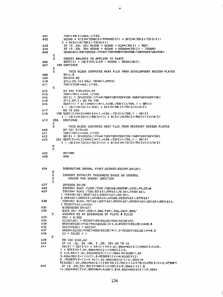
601 602

603 604 605

606 607

608 609 610 611

612 613 614 615 616

617 618

619

620 621 622 623

TOR=(TO(I)t460. I/100. QCOND = K(I)*(TEND(I)-TFRAHEO) t S(I)*(TO(I)-TO(I-I))

1 + S(Itl)+(TO(I)-TO(Itl)) IF 1 I .EQ. 25) QCOND = QCOND t KUP*(TOl I) - TUP) IF 1 I .EQ. 38) QCOND = QCOND t KDOWN*[TO( I) - TDOWN) QRAD=A~I~*SF+EMIS*.l7l4*~TOR*TOR*TOR*TOR-TAR*TAR*TAR*TAR~

C C ENERGY BALANCE IS APPLIED TO PLATE

QDOTl I) = (9(1)*3.4129 - QCDND - QRAD)/A(I) 109 CONTINUE

C C THIS BLOCK COMPUTES HEAT FLUX FROM DEVELOPMENT REGION PLATES

SF=1 .O EMIS=0.05 IF(J.EQ.16) CALL CHAN(l,EMIS) TAR=(TINFt460. )/lOO.

C DO 200 I=PLATEl,24 TOR=(TO(I)t460. )/lOO. QR[I) q SF*EMIS*.l7l4*(TOR*TOR*TOR*TOR-TAR*TAR*TAR*TAR) IF(I.GT.l) GO TO 195 QDOTLI) = K(1)+HM(1)*(1.+(80.-T0(1~)/700.) - QR(0

1 - (Sll)*(TO(l)-TOO) t S(2)*(TO(l)-T0(2)))/A(I) GO TO 200

195 QDOT(I)=K(I)*HM(I)*(1.+(80.-TO(I))/700.) - QR(I) 1 - (S(I)*(TO(I)-TO(I-1)) t S(I+l)*(TO(I)-TO(Itl)))/A(I)

200 CONTINUE C C THIS BLOCK COMPUTES HEAT FLUX FROM RECOVERY REGION PLATES

DO 201 1=39,62 TOR=(TO(I)t460. l/100. QR(I) q SF*EMIS+.l714*fTOR*TOR*TOR*TOR-TAR*TAR*TAR*TAR)

C C

624 625

626 C C C C

627 628 629

630

631 632

C 633 634 635 636 637 638

C 639 640 641

642

201 QD0T(I)=K(I)*HM(I)*(l.t(80.-TO(I))/700.) 1 QR(I) 1 - (S(I)*[TO(I)-TO(I-I)) t S~Itl)*(TOlI)-TOlIt )11/A(I)

RETURN END

SUBROUTINE ENTHAL (FACT,D2INIT,DD2INT,D2iOC)

COMPUTE ENTHALPY THICKNESS BASED ON CONTROL VOLUME FOR ENERGY ADDITION

INTEGER D2LOC COMMON/ ELK2 /UINF,TINF,TADIAB,RHOINF,VI.SC,PR,CP,W COMMON/ BLK3 /TOO,T0(63),HM(62),Qo,TENDO,

1 TFRAME(38),QDOT(62),DQDOT(62),9W(38), 2 DKKl62),DSS(63),NTAG(63),NTAGO,REENP(6P),STPL62)

COMtiON/ BLK4 /ST(62),DST(62),REEN(62),DREEN(62),D2(62),DD2(62), 1 PCOEFFl62),X(62) DIMENSION DX(62) DATA DX/ 24*1.028,1.856,13*1.996,24*1.028/ ASSUMES D2 AT BEGINNING OF PLATE # DELOC DDX = 0.005 D2(DZLOC) q D2INITtST(D2LOC)*DX(D2LOC)72. REENlD2LOCl=FACT*D2(D2LOClx( 1 .O-PCOEFF(D2LOC) )**0.5 DD:(DELOC) = DDZINT DREEN(D:LOC)=FACT+DD2(D2LOC)*( 1 .O-PCOEFF(D2LOCl)**O.5 12 = D2LOC t 1

DO 100 1=12,62 IF (I .LE. 24 .OR. I .GE. 39) GO TO 20 D21.I) q D2lI-I) t STlI-1)*(1.0+.0564*D2(1-l))*DX(I-1)/2.

1 t ST(1)*(1.0+.0564+D2(1-1~~*DX(1)/2. 2 +(0.5*~(1.0+.0564~D2(1-1))/.0564)*~AL0G(1.0t 3.0564*D21I-l)))/~l.O-PCOEFFO))~*~PCOEFF~I~ 4 -PC0EFF~1-1))-2.*((1.0+.0564*D2~1-1))/.0564~* 5~ALOG~l.0t.0564*D2~I-l~~~*~TO~I~-TO~~-l~~/~TO~I~tTO~I-l~-2.*TINF~

IF (I .EQ.25) D2(11=D2(1)-((D2(1)/0.0564)-((1.0

134

643 GO TO 10 644 20 CONTINUE 645 D2(1) = D2(1-I) t STfI-l)+DX(I-1)/2. t ST(I)+DX(I)/2. - .-

646

647 648

649

1 t(0.5+D2~I-l)/(l.0-PCOEFF(I)))+(PCOEFF(I~ 2 -PCOEFF(I-1 I)-2.+02(3-l )+(TD(I)-TOtI-l))/(TOo+TO(I-l)-2.*TINF)

IF (I .EQ.391 D2(1)=D2(1)+((D2(1)/0.0564)-((1.0 1+.0564+D2~1~~/.003186+(AL0G~(.0+0.0564+D2~1~1~~~*.0564

10 CONTINUE DD2lIl = SQRT( DD2(1-1,x+2 t (ST(I-1 ,+DUX/2.1**2

1 t (DX(I-l)+DST(I-1)/2.)**2 t (ST(I)*DDX/2.)**2 t i tDX( I )iDST( 1)/2.)+*2 1 REEN(1) = FACT * D2(1,*(1 .O-PCOEFF(I))+*0.5

650 DREENI I) = FACT * DD2(1) *ll.O-PCOEFFII))**O.5 651 100 CONTINUE 652 RETURN 653 END

C

654 C C C C C

655 656 657 658 659 IO 660 20 661 662

C C

663 C C C C C

664 665 666 667 668 669 670 10 671 672 673 674

C C

SUBROUTINE CHAN(N,XX)

SUBROUTINE CHAN FIRST STORES THE VALUE OF XX AS A MEMBER OF THE DUMMY ARRAY ARG AND THEN INCREASES XX BY ONE PERCENT.

COMMON ARG( 63 1 ,ARGO IF(N.NE.0) GO TO 10 ARGO=XX GO TO 20 ARG( N )=Xx xx=xx+xx*0.01 RETURN END

SUBROUTINE CHANGE(N,M,XX,YY)

SUBROUTINE RESTORES THE VALUE OF YY, THE PREVIOUSLY PERTURBED INPUT, TO ITS ORIGINAL VALUE, THEN STORES XX IN THE ARRAY ARG, THEN INCREASES XX BY ONE PERCENT.

COMMON ARG( 63 1, ARGO IF(M.EQ.l.OR.N.GE.63) GO TO 10 YY=ARG(N+l 1 IF(M.LT.4) GO TO 10 IF(N.EQ.O) YY=ARGO IFIN.NE.0) YY=ARG(N) IF(N.NE.0) ARG(N)=XX IF(N.EQ.01 ARGO=XX xx=xx+xx*0.01 RETURN END

135

675 C C C C C

676 677 678 679 680 681 682 683 684 820 685 686 840 687 688 810 689 690 691

SUBROUTINE HAXHIN(N,M,JCOUNT)

SUBROUTINE MAXMIN FINDS THE MAXIMUM AND tlINIMUM VALUES IN THE COMMONED ARRAY OVER THE RANGE OF I FROM N TO Pi AND MARKS THE I-LOCATIONS OF THE MAXIMUM AND MINIMUM

COMMON/ BLK5 /SENC0(62,39),VHAX,VMIN,NA,NB VMAX=O.O VMIN=lO.O DO 810 I=N,M IF(SENCO(I,JCOUNT).LE.VMAX) GO TO 820 VMAX=SENCO( I, JCOUNT 1 NA=I GO TO 810 IF(SENCOtI,JCOUNT).LT.VMIN) GO TO 840 GO TO 810 VMIN=SENCO( I, JCOUNT 1 NB=I COIJTINUE IF(VMAX.EQ.O.O) NA=NB RETURN END

136

Appendix G

The Reduced Data

The following pages show lists and plots of the reduced data of the

15 cases shown in Table 3-l. Stanton number data and starting profile

data are presented for each case. Additional velocity and temperature

profile data are listed according to the following cases:

Case # s-distance in cm of profile data, in addition to

the s = -35 cm starting profiles.

100779 10.0 (e = 13")

41.0 (0 = 52")

61.0 (0 = 78")

119.0

070280 0.0

10.03 (0 = 13")

25.5 (0 = 32")

40.5 (e = 51")

61.3 (6 = 77")

72.3

88.2

104.0

119.1

022680 10.0 (e = 13")

(Profiles 25.0 (0 = 32")

are 41.0 (8 = 52")

030180) 61.5 (8 = 78")

89 .O

104.0

119.0

060480 9.9 (0 = 12.6"), velocity only

25.0 (0 = 32"), velocity only

051080 40.8 (0 = 52.5'), velocity only

137

100779 STARTING PROFILES; ENERGY BALANCE -DEL99/R(:THETA=O)=O.l0 S=-35 CM

H

REX = 0.17857E 07 REM = 3712. xv0 = -217.41 CM DEL2 q 0.379 CM UPW = 15.11 M/S DEL99= 3.334 CM VISC = O.l5434E-04 Me/S DELI q 0.531 CM PORT = 4 H = 1.399 XLOC = -35.05 CM CF/2 = O.l6090E-02 DENS = 1.18 KGM3

Y(W) Y/DEL Utfl/S, U/UP Y+ u+ CF/2 T(DEG C) 0.048 0.015 6.57 0.435 19.0 10.84 0.001324 31.74 0.074 0.022 7.87 0.521 29.0 12.98 0.001562 30.72 0.099 0.030 8.44 0.559 38.9 13.92 0.001607 30.11 0.150 0.045 9.07 0.600 58.9 14.95 0.001611 29.27 0.201 0.060 9.50 0.628 78.9 15.66 0.001611 28.75

0.249 0.075 9.82 0.650 97.8 16.20 0.001613 28.40 0.323 0.097 10.18 0.673 127.0 16.79 0.001604 27.94 0.373 0.112 10.40 0.688 146.4 17.16 0.001608 27.72 0.448 0.134 10.68 0.707 175.8 17.61 0.001610 27.43 0.549 0.165 10.99 0.727 215.5 18.12 0.001612 27.12

0.675 0.202 11.38 0.753 265.1 18.77 0.001634 26.83 0.801 0.240 11.69 0.773 314.6 19.28 0.001647 26.60 1.004 0.301 12.11 0.801 394.3 19.98 0.001668 26.34 1.207 0.362 12.50 0.827 473.9 20.62 0.001696 26.18 1.486 0.446 12.97 0.858 583.5 21.39 0.001731 26.04

1.739 0.522 13.35 0.883 683.2 22.02 0.001764 25.98 2.247 0.674 14.01 0.927 882.5 23.12 0.001826 25.92 2.754 0.826 14.55 0.963 1081.9 24.00 0.001875 25.90 3.389 1.016 14.99 0.992 1331.1 24.73 0.001901 25.90 4.151 1.245 15.15 1.002 1630.4 24.98 0.001863 25.90

REH q 796. DEH2 = 0.082 CM DELT99 = 1.461 CM UPW = 15.15 M/S VISC = O.l5540E-04 Fl2/S TINF = 25.81 DEG C TPLATE q 40.52 DEG C

Y(CM) Y+ U(M/S) T(DEG C) 0.0140 0.0394 0.0648 0.1156 0.1664

5.49 15.46 25.44 45.39 65.35

1.90 5.35 7.41 8.64 9.20

35.21 32.18 30.92 29.69 29.03

TBAR l-TBAR 0.361 0.639 0.567 0.433 0.652 0.348 0.736 0.264 0.781 0.219

0.2172 85.30 9.61 28.58 0.812 0.188 0.2934 115.23 10.03 28.07 0.846 0.154 0.3442 135.18 10.27 27.80 0.865 0.135 0.4204 165.11 10.58 27.49 0.886 O.-l14 0.5220 205.02 10.90 27.15 0.909 0.091

0.6490 254.91 11.30 26.83 0.930 0.070 0.7760 304.79 11.63 26.59 0.947 0.053 0.9792 384.60 12.06 26.31 0.966 0.034 1.1824 464.42 12.46 26.14 0.977 0.023 1.4618 574.16 12.93 25.99 0.987 0.013

1.7158 673.93 13.32 2.2238 873.46 13.98 2.7318 1073.00 14.52

25.93 0.992 0.008 25.86 0.997 0.003 25.83 0.998 0.002

100779 PROFILEiENERGY BALANCE-DEL99/R(THETA=O)=O,lO S=lO.OCM THETA=13DEG

t: W

REX = 0.23369E 07 REM = 4604. xv0 q -232.34 CM DEL2 = 0.478 CH UPW = 14.98 M/S DEL99= 4.190 CM VISC q O.l5549E-04 H2/S DEL1 = 0.678 CH PORT q 4 H = 1.420 XLOC = 10.16 CM CF/2 = O.l4291E-02 DENS = 1.17 KG/n3

Y(CM) Y/DEL U(H1.S) U/UP Yt ut CF/2 T(DEG C) 0.048 0.012 5.85 0.391 17.6 10.33 0.001115 33.31 0.074 0.018 7.16 0.478 26.9 12.63 0.001357 32.26 0.099 0.024 7.68 0.514 36.1 13.57 0.001397 31.64 0.150 0.036 8.34 0.559 54.6 14.73 0.001424 30.80 0.201 0.048 8.78 0.589 73.1 15.50 0.001434 30.25

0.251 0.060 9.11 0.611 91.4 16.08 0.001439 29.84 0.2172 79.11 8.89 30.06 0.726 0.274 0.325 0.077 9.54 0.642 118.3 16.85 0.001460 29.36 0.2934 106.87 9.36 29.50 0.763 0.237 0.373 0.089 9.76 0.657 135.8 17.23 0.001466 29.11 0.3442 125.38 9.63 29.22 0.781 0.219 0.447 0.107 10.02 0.675 163.0 17.69 0.001468 28.78 0.4204 153.14 9.93 28.85 0.805 0.195 0,548 0.131 10.28 0.695 199.6 18.15 0.001462 28.42 0.5220 190.15 10.22 28.46 0.831 0.169

0.674 0.161 10.59 0.717 245.6 18.69 0.001466 28.06 0.6490 236.42 10.53 28.09 0.855 0.145 0.801 0.191 10.80 0.734 291.7 19.07 0.001460 27.77 0.7760 282.68 10.76 27.78 0.875 0.125 1.003 0.239 11.18 0.762 365.5 19.73 0.001473 27.41 0.9792 356.71 11.13 27.40 0.899 0.101 1.206 0.288 11.46 0.785 439.4 20.24 0.001480 27.11 1.1824 430.73 11.43 27.09 0.920 0.080 1.485 0.354 Il.82 0.815 541.1 20.87 0.001495 26.77 1.4618 532.52 11.79 26.75 0.942 0.058

1.739 0.415 12.09 0.838 633.5 21.35 0.001506 26.54 1.7158 625.05 12.07 26.50 0.958 0.042 2.247 0.536 12.59 0.882 818.4 22.23 0.001536 26.24 2.2238 810.11 12.57 26.19 0.978 0.022 2.754 0.657 12.97 0.918 1003.4 22.90 0.001554 26.06 2.7318 995.17 12.95 26.01 0.990 0.010 3.389 0.809 13.33 0.957 1234.6 23.54 0.001568 25.97 3.3668 1226.50 13.32 25.91 0.997 0.003 4.151 0.991 13.57 0.989 1512.0 23.95 0.001555 25.94 4.1288 1504.09 13.56 25.88 0.999 0.001

4.913 1.172 13.51 1.000 1789.6 23.86 0.001495 25.94

REH = 1669. DEH2 = 0.173 CM DELT99 = 2.637 CH UPW = 14.98 H/S VISC = O.l5549E-04 n2/s TINF = 25.86 DEG C TPLATE = 41.21 DEG C

Y(CM) Yt U(H/S) TIDEG C) TBAR I-TBAR 0.0140 5.09 1.69 0.0394 14.34 4.76 0.0648 23.60 6.69 0.1156 42.10 7.90 0.1664 60.61 8.48

36.66 0.296 0.704 33.76 0.485 0.515 32.46 0.570 0.430 31.22 0.651 0.349 30.56 0.694 0.306

100779 PROFILEiENERGY BALANCE-DEL99/R(THETA=O)=O.l0 S=4lCM THETA=52DEG

REX q 0.28112E 07 REM = 5337. xv0 = -251.93 CM DEL2 = 0.556 CM UPW q 14.93 n/s DEL99= 4.514 CM VISC = O.l5549E-04 H2/S DEL1 = 0.844 CM PORT = 4 H = 1.518 XLOC = 40.89 CM CF/2 = O.l0540E-02 DENS = 1.18 KG/M3

Y(Ctl) YMEL U(M/S) U/UP Yt ut CF/2 T(DEG C) 0.048 0.011 4.57 0.307 15.1 9.43 0.000748 34.59 0.074 0.016 5.72 0.384 23.0 11.81 0.000939 33.61 0.099 0.022 6.27 0.421 30.9 12.95 0.000998 33.04 0.150 0.201

0.033 0.044

0.252 0.056 0.327 0.072 0.377 0.083 0.452 0.100 0.552 0.122

0.677 0.150 0.802 0.178

6.95 0.467 46.7 7.30 0.491 62.6

7.61 0.513 78.4 8.05 0.543 101.9 8.28 0.559 117.4 8.66 0.586 140.7 9.09 0.616 171.9

9.57 0.650 210.9 9.92 0.676 250.1

14.34 0.001049 32.22 15.07 0.001051 31.69

0.0140 4.35 0.0394 12.27 0.0648 20.19 0.1156 36.02 0.1664 51.85

6.49 32.65 0.556 0.444 7.06 31.99 0.599 0.401

15.70 0.001062 31.27 0.2172 67.69 7.40 31.51 0.630 0.370 16.61 0.001092 30.75 0.2934 91.44 7.86 30.93 0.668 0.332 17.09 0.001106 30.46 0.3442 107.27 8.13 30.63 0.688 0.312 17.88 0.001143 30.05 0.4204 131.02 8.51 30.18 0.717 0.283 18.75 0.001183 29.57 0.5220 162.69 8.96 29.67 0.749 0.251

19.74 0.001234 29.04 0.6490 202.27 9.46 20.46 0.001263 28.63 0.7760 241.85 9.84

29.11 0.786 0.214 28.67 0.815 0.185 28.07 0.853 0.147 27.60 0.884 0.116 27.16 0.913 0.087

1.005 0.223 10.42 0.714 313.1 21.50 0.001311 28.05 1.207 0.267 10.83 0.745 376.2 22.34 0.001347 27.60 1.486 0.329

1.739 0.385 2.247 0.498 2.754 0.610 3.389 0.751 4.151 0.920

4.912 1.088 13.41 0.997 1531.0 27.68 0.001487 25.89 5.674 1.257 13.26 1.000 1768.5 27.36 0.001417 25.89

11.28 0.781 463.1

11.59 0.806 542.1 12.13 0.853 700.3 12.55 0.892 858.5 13.01 0.937 1056.3 13.37 0.978 1293.7

23.28 0.001386 27.17

23.91 0.001405 26.89 1.7158 534.77 11.56 26.86 0.932 0.068 25.02 0.001445 26.46 2.2238 693.10 12.10 26.42 0.960 0.040 25.89 0.001475 26.21 2.7318 851.43 12.53 26.16 0.977 0.023 26.84 0.001510 26.02 3.3668 1049.34 12.99 25.96 0.990 0.010 27.59 0.001527 25.92 4.1288 1286.84 13.36 25.86 0.997 0.003

REH = 2267. DEH2 = 0.236 CM DELT99 = 3.254 CH UPW q 14.93 M/S VISC = O.l5545E-04 H2/S TINF = 25.81 DEG C TPLATE q 41.23 DEG C

Y(CM) Yt U(M/S) T(DEG C) TBAR 1-TBAR 1.32 37.26 0.257 0.743 3.72 35.01 0.403 0.597 5.31 33.80 0.482 0.518

0.9792 305.18 10.36 1.1824 368.52 10.78 1.4618 455.60 11.24

4.8908 1524.34 13.41 25.83 0.999 0.001

100779 PROFILEiENERGY BALANCE-DEL99/R(THETA=O)=O.l0 S=6lCfl THETA=78DEG

E

REX q 0.28542E 07 REM = 5402. xv0 q -231.97 CM DEL2 = 0.555 CH UPW = 15.12 M/S DEL99= 4.504 CH VISC = O.l5536E-04 M2/S DEL1 = 0.845 CM PORT = 4 H = 1.522 XLOC = 61.39 CM CF/2 = O.l0601E-02 DENS q 1.18 KG&l3

Y(M) Y/DEL U(H/S) U/UP Yt Ut CF/2 T(OEG C) 0.048 0.011 4.94 0.327 15.3 10.03 0.000827 34.97 0.074 0.016 5.94 0.394 23.4 12.08 0.000976 33.97 0.099 0.022' 6.51 0.432 31.4 13.23 0.001036 33.34 0.150 0.033 7.07 0.469 47.5 14.36 0.001053 32.52 0.201 0.045 7.44 0.495 63.6 15.13 0.001060 32.01

0.252 0.056 7.75 0.515 79.7 15.74 0.001067 31.60 0.326 0.072 8.15 0.543 103.1 16.57 0.001090 31.10 0.375 0.083 8.35 0.557 118.7 16.98 0.001097 30.82 0.451 0.100 8.66 0.579 142.8 17.59 0.001114 30.43 0.551 0.122 9.08 0.608 174.6 18.45 0.001153 29.97

0.677 0.150 9.51 0.639 214.5 19.33 0.001191 29.45 0.803 0.178 9.93 0.668 254.4 20.17 0.001234 28.97 1.005 0.223 10.49 0.709 318.4 21.31 0.001293 28.33 1.207 0.268 10.95 0.744 382.5 22.24 0.001339 27.82 1.486 0.330 11.45 0.782 470.7 23.26 0.001387 27.28

1.739 0.386 11.78 0.809 550.9 23.94 0.001412 26.96 2.247 0.499 12.31 0.855 711.7 25.00 0.001447 26.54 2.754 0.612 12.72 0.893 872.5 25.84 0.001473 26.26 3.389 0.752 13.16 0.936 1073.6 26.75 0.001505 26.10 4.151 0.922 13.54 0.978 1314.9 27.50 0.001521 25.99

4.912 1.091 13.60 0.998 1556.1 27.64 0.001486 25.94 5.674 1.260 13.43 1.000 1797.5 27.28 0.001413 25.92

REH = 2601. DEH2 q 0.267 CM DELT99 = 3.544 CM UPW = 15.12 M/S VISC = O.l5534E-04 H2/S TINF = 25.84 DEG C TPLATE = 40.78 DEG C

Y(Ctl1 Yt UtM/S, T(DEG C) TBAR I-TBAR 37.56 0.215 0.785 0.0140

0.0394 0.0648 0.0902 0.1410

4.43 12.47 20.52 28.56 44.66

1.43 4.02 5.59 6.31 6.97

35.38 0.362 0.638 34.22 0.439 0.561 33.48 0.489 0.511 32.60 0!548 0.452

0.1918 60.75 7.38 32.07 0.583 0.417 0.2426 76.84 7.69 31-64 0.612 0.388 0.3188 100.98 8.12 31.12 0.646 0.354 0.3696 117.07 8.33 30.82 0.667 0.333 0.4458 141.21 8.64 30.43 0.693 0.307

0.5474 173.39 9.06 0.6744 213.62 9.50 0.8014 253.86 9.92 1.0046 318.22 10.49 1.2078 382.59 10.95

1.4872 471.10 11.45 27.24 0.907 0.093 1.7412 551.56 11.78 26.91 0.929 0.071 2.2492 712.49 12.31 26.49 0.957 0.043 2.7572 873.41 12.72 26.21 0.976 0.024 3.3922 1074.56 13.16 26.04 0.987 0.013

4.1542 1315.95 13.54 25.92 0.995 0.005 4.9162 1557.33 13.60 25.88 0.998 0.002 5.6782 1798.71 13.42 25.86 0.999 0.001

29.96 0.724 0.276 29.43 0.760 0.240 28.94 0.792 0.208 28.30 0.836 0.164 27.78 0.871 0.129

100779 PROFILE FOR ENERGY BALANCE -DEL99/R(THETA=O)=O.l0 S=ll9 CH

REX = 0.33816E 07 REH = 6187. xv0 = -227.16 CM DEL2 q 0.633 CM UPW = 15.20 H/S DEL99= 4.922 CM VISC = O.l5548E-04 M2/S DEL1 = 0.975 CH PORT q 4 H q 1.540 XLOC = 118.87 CM CF/2 = O.l0737E-02 DENS = 1.17 KG/M3

Y(Ctl) Y/DEL U(M/S) U/UP Yt ut CF/2 T(OEG C1 0.048 0.010 4.90 0.322 15.5 9.84 0.000808 34.66 0.074 0.015 6.08 0.400 23.6 12.21 0.001004 33.80 0.099 0.020 6.59 0.434 31.8 13.24 0.001047 33.32 0.150 0.030 7.18 0.473 48.0 14.42 0.001071 32.67 0.201 0.041 7.56 0.497 64.3 15.18 0.001077 32.22

REH = 3655. DEH2 = 0.374 cn

DELT99 = 4.209 CM UPW = 15.19 H/S VISC = O.l5549E-04 H2/S TINF = 25.90 DEG C TPLATE = 41.06 DEG C

Y(CHl Yt U(M/S) T(DEG C1 TBAR 1-TBAR

0.249 0.051 7.81 0.514 79.9 15.68 0.001073 31.91 0.324 0.066 8.13 0.535 103.9 16.32 0.001074 31.54 0.374 0.076 8.33 0.549 119.8 16.74 0.001081 31.34 0.449 0.091 8.61 0.567 143.7 17.29 0.001093 31.06 0.549 0.112 8.90 0.586 175.9 17.88 0.001103 30.73

0.0140 4.47 0.0394 12.61 0.0648 20.74 0.1156 37.01 0.1664 53.28

0.2172 69.54 0.2934 93.94 0.3442 110.21 0.4204 134.61 0.5220 167.15

1.41 36.98 0.269 0.731 3.99 35.03 0.398 0.602 5.66 33.96 0.468 0.532 6.78 33.00 0.532 0.468 7.30 32.49 0.566 0.434

7.64 32.07 8.00 31.65 8.21 31.43 8.51 31.14 8.82 30.78

0.593 0.621 0.635 0.655 0.678

0.676 0.137 9.23 0.607 216.5 18.53 0.001118 30.37 0.6490 207.81 9.16 0.803 0.163 9.59 0.631 257.0 19.26 0.001149 30.02 0.7760 248.48 9.51 1.005 0.204 10.10 0.665 321.9 20.29 0.001197 29.50 0.9792 313.55 10.04 1.208 0.245 10.59 0.697 386.8 21.27 0.001250 29.05 1.1824 378.62 10.53 1.487 0.302 11.23 0.739 476.2 22.55 0.001326 28.45 1.4618 468.09 11.17

30.41 0.702 30.06 0.726 29.52 0.761 29.07 0.791 28.45 0.832

1.740 0.354 11.76 0.774 557.3 23.62 0.001392 27.97 1.7158 549.43 11.71 27.96 0.864 2.248 0.457 12.68 0.835 719.8 25.47 0.001512 27.18 2.2238 712.10 12.64 27.15 0.918 2.755 0.560 13.41 0.882 882.2 26.92 0.001603 26.65 2.7318 874.77 13.37 26.61 0.954 3.390 0.689 14.05 0.924 1085.4 28.21 0.001675 26.34 3.2398 1037.45 13.90 26.33 0.972 4.151 0.843 14.64 0.963 1329.3 29.39 0.001734 26.16 3.7478 1200.12 14.32 26.16 0.983

4.659 0.947 14.93 0.983 1491.9 30.00 0.001760 26.10 4.2558 1362.79 14.70 26.08 0.989 5.167 1.050 15.12 0.995 1654.5 30.36 0.001765 26.06 5.928 1.204 15.19 0.999 1898.4 30.50 0.001735 26.03 6.386 1.297 15.20 1.000 2044.8 30.53 0.001714 26.01

4.7638 1525.46 14.97 5.2718 1688.14 15.13 5.7798 1850.81 15.17 6.2878 2013.48 15.20

26.01 0.993 25.97 0.995 25.96 0.996 25.94 0.998

6.7958 2176.16 15.20 25.92 0.999

0.407 0.379 0.365 0.345 0.322

0.298 0.274 0.239 0.209 0.168

0.136 0.082 0.046 0.028 0.017

0.011 0.007 0.005 0.004 0.002 6

0.001

RUN (00779 I** CURVATURE RIG **I NASA-NAG-3-3 STANTON NLRiBER DATA

TAOB= 25.92 DEG C LIREF- 15.15 n/s TINF= 25.82 DEG C RHO= 1.176 KG/H3 ;;pC= O.l5542E-04 !l2/5 XVO' -217.4 CPl cp= 1014. J/KGK 0.716

BTAh-TON Rw FDR ENERGY BALAWE - DEL99/R (META -0) '0.10

PLATE X UPU K REXVO TO JTAh-TON NO REEh-iH tcnn, In/S) DE6 C

1 -61.3 15.10 O.OOOE 00 0.15167E 07 38.21 0.3lllBE-02 2 -58.7 (5.10 O.OOOE 00 0.1542lE 07 39.49 0.33498E-02 3 -56.1 15.10 O.OOOE 00 0.15675E 07 39.78 0.3237lE-02 4 -53.5 15.11 0.200E-07 0.15935E 07 39.99 0.30737E-02

DST DSTIX) DREEN

O.l95E-03 0.113E-03 O.lObE-03 O.l03E-03 0.847E-04 0.963E-04 0.906E-04 O.a7lE-04 0.883E-04 0.855E-04 O.a57E-04

6.260 3.37l 3.266 3.356 3.152 3.362 3.300 3.274 3.286 3.282 3.302 3.299 3.280 3.297 3.294 3.346 3.233 3.316 3.323 3.287 3.271 3.318 3.302 3.348

4.980 4.672 4.685 4.693 4.710 4.812 4.845 4.796 4.886 4.870 4.912 5.042 4.974 5.113

3.472 3.420 3.534 3.523 3.482 3.547 3.529 3.443 3.492 3.470 3.506 3.548 3.438 3.522 3.460 3.556 3.392 3.535 3.541 3.474 3.536 3.391 3.689 5.284

5 -50.9 15.11 O.OOOE 00 0.16189E 07 39.29 0.26B73E-02 6 -48.3 15.11 O.OOOE 00 0.16443E 07 40.19 0.28643E-02 7 -45.7 15.12 O.l97E-07 0.16706E 07 40.36 0.27465E-02 8 -ii.0 15.12 O.OOOE 00 0.16960E 07 40.35 0.26607E-02 9 -40.4 15.12 O.OOOE 00 0.17212E 07 40.45 0.26873E-02

10 -37.8 15.12 O.OOOE 00 0.17467E 07 40.47 0.26052E-02 11 -35.2 15.12 O.l97E-07 0.17730E 07 40.56 0.2594lE-02 0.82879E 03

5. 5.

12 -32.6 15.12 O.OOOE 00 0.17985E 07 40.52 13 -30.0 15.12 O.OOOE 00 0.18239E 07 40.44 14 -27.4 15.13 O.l99E-07 0.1850lE 07 40.52 15 -24.8 15.11 -0.593E-07 0.18727E 07 40.58 16 -22.2 15~09 -0.595E-07 0.18953E 07 40.59 17 -19.5 15.06 -0.598E-07 0.19178E 07 40.12 18 -16.9 15.04 -0.607E-07 0.19399E 07 40.41 19 -14.3 15.02 -0.604E-07 O.l%22E 07 40.57 20 -11.7 14.99 -O.BlOE-07 0.19835E 07 40.41 21 -9.1 (4.96 -O.a15E-07 0.2004bE 07 40.36 22 -6.5 15.03 O.ZOlE-06 0.20402E 07 40.58 23 -3.9 15.11 O.POOE-06 0.20757E 07 40.68 24 -1.3 15.16 O.l95E-06 0.21116E 07 40.72

0.24934E-02 0.89593E 03 O.a23E-04 0.24843E-02 0.96362E 03 0.8!5E-04 0.25203E-02 0.1022lE 04 0.83lE-04 0.24928E-02 O.lOal9E 04 0.821E-04 0.24906E-02 0.11444E 04 O.a33E-04 0.2359lE-02 0.12423E 04 0.763E-04 0.24878E-02 0.12790E 04 0.825E-04 0.25139E-02 0.1328lE 04 0.835E-04 0.24570E-02 0.1405lE 04 O.aOaE-04 0.237aaE-02 0.14705E 04 0.77aE-04 0.23743E-02 0.150alE 04 0.788E-04 0.24233E-02 0.15594E 04 O.BOOE-04 0.22922E-02 0.16145E 04 0.767E-04

6. 6. 6. 6. 6. 6. 7. 7. 7. 7. 7.

CURVE BEGINS

25 2.4 26 7.3 27 12.4

15.25 O.l24E-06 0.21570E 07 40.67 15.28 0.4OaE-07 0.22094E 07 40.73 15.19 -O.l2OE-06 0.22460E 07 40.86 15.10 -O.l23E-Ob 0.22817E 07 40.88 15.11 O.l02E-07 0.23322E 07 40.90 15.15 0.50aE-07 0.23873E 07 41.01 15.17 0.302E-07 0.24405E 07 41.03 15.14 -0.407E-07 0.2484BE 07 40.88 15.15 O.lOlE-07 0.25356E 07 40.94 15.13 -0.203E-07 0.25825E 07 40.83 15.11 -0.307E-07 0.26277E 07 40.98 15.16 0.705E-07 0.26865E 07 41.20 15.30 O.l77E-06 0.27603E 07 40.97 15.30 0.979E-08 0.28117E 07 41.00

O.l984OE-02 O.l9496E-02 O.l9474E-02 O.l8443E-02 O.l7725E-02

0.16965E 04 0.990E-04 0.17844E 04 0.913E-04 0.18659E 04 0.914E-04

8. 8. 9. 9.

10. 10. 11. 11. 11. 1 2.. 12.

28 17.4 29 22.5 30 27.6 31 32.6 32 37.7 33 42.8 34 47.8 35 52.9 36 58.0 37 63.0 38 68.1

0.19578E 04 0.867E-04 0.20447E 04 0.836E-04 0.21144E 04 0.804E-04 0.21943E 04 0.795E-04 0.22960E 04 0.779E-04 0.23676E 04 0.775E-04 0.2<609E 04 0.744E-04 0.25124E 04 0.742E-04 0.2549lE 04 0.738E-04 0.2659OE 04 0.689E-04 0.2720lE 04 0.645E-04

O.l6667E-02 O.l6375E-02 O.l6206E-02 O.l5824E-02 O.l525lE-02 O.l508lE-02 O.l4604E-02 0.13818~-02 O.l2597E-02

12. 13. 13.

RECOVERY BEGIN5

39 72.0 15.15 -O.ZBlE-06 0.28200E 07 40.93 40 74.6 15.00 -0.383E-06 0.28183E 07 40.82 41 77.2 15.02 0.603E-07 0.28479E 07 41.14 42 79.8 15.05 0.799E-07 0.28790E 07 41.22 43 82.4 15.08 0.602E-07 0.29085E 07 41.21 44 85.0 15.10 0.594E-07 0.29384E 07 41.24 45 87.6 15.11 O.l98E-07 0.29653E 07 41.26 46 90.2 15.12 0.394E-07 0.29937E 07 41.11 47 92.8 15.14 0.397E-07 0.30219E 07 41.04 48 95.4 15.15 O.l96E-07 0.30489E 07 40.98 49 98.1 15.15 O.OOOE 00 0.30744E 07 41.02 50 100.7 15.15 O.OOOE 00 0.30999E 07 41.12 51 103.3 15.15 O.OOOE 00 0.31254E 07 40.99 52 105.9 15.15 O.OOOE 00 0.31507E 07 41.11 53 108.5 15.15 O.OOOE 00 0.31762E 07 41.05 54 111.1 15.15 O.OOOE 00 0.32017E 07 41.09 55 113.7 15.15 O.OOOE 00 0.32272E 07 40.80 56 116.4 15~15 O.OOOE 00 0.32527E 07 41.05 57 118.9 15.15 O.OOOE 00 0.32779E 07 41.06 58 121.6 15.l5 O.OOOE 00 0.33034E 07 40.83 59 124.2 15.15 O.OOOE 00 0.332898 07 40.77 60 126.0 15.15 O.OOOE 00 0.335441 07 40.43 61 129.4 15.15 O.OOOE 00 0.33799E 07 40.73 62 132.0 15.15 O.OOOE 00 0.3405lE 07 40.37

LMCERTAINTY IN REX=27203.

0.14782E-02 O.l5313E-02 O.l5716E-02 O.l5109E-02 O.l5469E-02 O.l5300E-02 O.l5004E-02 O.l5646E-02 0.15298E-02 O.l6084E-02 O.l5502E-02 O.l6048E-02 O.l6204E-02 O.l6166E-02 O.l6344E-02 0.16099E-02 O.l6242E-02 O.l6664E-02 O.l6154E-02 O.l6176E-02 O.l6323E-02 O.l605lE-02 O.l6266E-02 O.l4045E-02

0.27790E 04 0.513E-04 0.2838OE 04 0.524E-04 0.28169E 04 0.555E-04 0.28407E 04 0.532E-04 0.28818E 04 0.539E-04 0.29145E 04 0.543E-04 0.29489E 04 0.529E-04 0.30164E 04 0.539E-04 0.307OYE 04 0.534E-04 0.31218E 04 0.558E-04 0.31550E 04 0.544E-04 0.31742E 04 0.569E-04 0.324lOE 04 0.557E-04 0.32568E 04 0.569E-04

13. 13. 13. 13. 13. 13. 13. 13. 13. 13. 13. 13. 13. 13. 13. 13. 13. 13. 13. 14. 14. 14. 14. 14.

0.33llOE 04 0.565E-04 0.33436E 04 0.572E-04 0.34495E 04 0.55lE-04 0.34334E 04 0.589E-04 0.34738E 04 0.572E-04 0.35678E 04 0.562E-04 0.36242E 04 0.577E-04 0.37475E 04 0.544E-04 0.37117E 04 0.600E-04 0.38423E 04 0.742E-04

143

070280 DEL99/R(THETA=O)=O.l0 PROFILES AT STATION 5 S=-35.05CM

REX = 0.17262E 07 REM q 3613. xv0 = -213.75 CM DEL2 = 0.374 CH UPW = 14.76 M/S DEL99= 3.173 CM VISC = O.l5283E-04 H2/S DEL1 = 0.527 CH PORT q 4 H = 1.410 XLOC = -35.05 CM CF/2 = O.l6097E-02 DENS = 1.18 KG/M3

REH = 941. DEH2 = 0.098 CM DELT99 = 1.740 CM UPW = 14.81 H/S VISC = O.l540lE-04 M2/S TINF q 24.09 DEG C TPLATE = 40.50 DEG C STANTON= 0.256OOE-02

Y(CM) Yt U(M/S) T(DEG C) TBAR Tt Y(Ctl) Y/DEL UtH/S, U/UP Yt ut CF/2 TfDEG C) 0.048 0.015 6.55 0.443 18.7 11.05 0.001376 31.18 0.053 0.017 6.80 0.461 20.7 11.48 0.001417 30.83 0.074 0.023 7.73 0.524 28.6 13.05 0.001583 29.78 0.099 0.031 8.30 0.562 38.4 14.02 0.001633 28.99 0.150 0.047 8.91 0.603 58.1 15.04 0.001633 28.01

0.0165 6.40 2.24 35.62 0.297 4.658 0.0190 7.38 2.58 35.19 0.323 5.067 0.0216 8.37 2.92 34.65 0.356 5.583 0.0241 9.35 3.27 34.14 0.387 6.069 0.0267 10.34 3.61 33.73 0.413 6.465

PRT 2.711 3.090 3.475 4.018 4.999

0.201 0.063 9.29 0.629 77.8 15.69 0.001622 27.40 0.0292 11.32 3.95 33.31 0.438 6.861 6.902 0.248 0.078 9.58 0.649 96.2 16.17 0.001615 27.00 0.0317 12.31 4.30 32.95 0.460 7.212 13.049 0.323 0.102 9.92 0.672 125.3 16.74 0.001603 26.49 0.0368 14.27 4.99 32.27 0.501 7.854 -8.346 0.373 0.118 10.14 0.687 144.5 17.13 0.001609 26.25 0.0419 16.24 5.67 31.73 0.534 8.376 -2.116 0.448 0.141 10.41 0.705 173.5 17.57 0.001608 25.94 0.0470 18.21 6.36 31.26 0.563 8.822 -0.796

0.548 0.173 10.72 0.726 212.5 18.09 0.001613 25.60 0.0622 24.12 7.20 30.21 0.627 9.821 0.255 0.675 0.213 11.04 0.748 261.5 18.64 0.001619 25.28 0.0825 31.99 7.93 29.41 0.676 10.592 0.530 0.801 0.253 11.36 0.769 310.5 19.17 0.001636 25.04 0.1181 45.77 8.53 28 47 0.733 11.487 0.673 1.004 0.316 11.77 0.797 389.0 19.87 0.001657 24.76 0.1689 65.46 9.05 27.69 0.780 12.230 0.713 1.207 0.380 12.13 0.822 467.6 20.48 0.001680 24.58 0.2197 85.15 9.41 27.19 0.811 12.711 0.718

1.486 0.468 12.62 0.855 575.8 21.31 0.001724 24.44 1.739 0.548 13.03 0.882 674.f 21.99 0.001766 24.35 2.247 0.708 13.75 0.931 870.9 23.21 0.001845 24.27 2.754 0.868 14.31 0.969 1067.5 24.16 0.001905 24.23 3.389 1.068 14.72 0.997 1313.4 24.84 0.001923 24.21

4.151 1.308 14.77 1.001 1608.7 24.94 0.001862 24.20

0.2959 114.68 9.79 26.62 0.846 13.255 0.722 0.3467 134.37 10.02 26.33 0.864 13.535 0.722 0.4229 163.90 10.32 26.00 0.884 13.847 0.716 0.5245 203.28 10.64 25.62 0.906 14.206 0.714 0.6515 252.50 10.98 25.28 0.927 14.534 0.707

0.7785 301.72 11.30 25.03 0.942 14.769 0.697 0.9817 380.47 11.72 24.74 0.960 15.052 0.684 1.1849 459.23 12.09 24.54 0.972 15.241 0.669 1.4389 557.67 12.54 24.40 0.981 15.369 0.649 1.6929 656.11 12.95 24.30 0.987 15.466 0.632

2.2009 852.99 13.68 24.22 0.992 15.550 0.600 2.7089 1049.87 14.26 24.16 0.996 15.602 0.577 3.3439 1295.97 14.69 24.14 0.997 15.621 0.552 4.1059 1591.29 14.77 24.12 0.998 15.638 0.530 4.8679 1886.61 14.76 24.11 0.999 15.653 0.513

5.0889 1972.26 14.76 24.11 0.999 15.653 0.508

-

070280 DEL99/RITHETA=OI=O.l0 PROFILES AT STATION 6 S=O.O

REX = 0.22368E 07 REM q 4445. xv0 q -235.20 CH DEL2 = 0.467 CM UPW = 14.54 n/s DEL99= 4.256 CM VISC = O.l5284E-04 M2/S DEL1 = 0.666 CM PORT q 4 H = 1.426 XLOC = 0.00 CH CF/2 = O.l5497E-02 DENS = 1.18 KG/M3

Y(CMI Y/DEL U(M/S) U/UP Yt ut CF/2 T(DEG C) 0.089 0.021 7.31 0.503 33.3 12.77 0.001402 30.22 0.135 0.032 8.18 0.563 50.4 14.29 0.001501 29.25 0.180 0.042 8.65 0.595 67.6 15.12 0.001522 28.66 0.261 0.061 9.23 0.635 97.6 16.14 0.001544 28.03 0.321 0.075 9.52 0.655 120.2 16.64 0.001543 27.63

0.396 0.093 9.84 0.677 148.2 17.20 0.001552 27.25 0.483 0.114 10.15 0.699 180.9 17.75 0.001560 26.89 0.599 0.141 10.48 0.721 224.3 18.31 0.001565 26.50 0.738 0.173 10.84 0.746 276.2 18.95 0.001585 26.10 0.917 0.216 11.18 0.769 343.4 19.54 0.001593 25.70

0.0267 9.98 0.0292 10.94 0.0317 11.89 0.0343 12.84 0.0394 14.74

2.19 2.40 2.61 2.82 3.23

34.53 0.363 6.217 4.742 34.18 0.384 6.575 6.255 33.81 0.406 6.949 9.768 33.35 0.434 7.421 29.813 32.69 0.473 8.090 -5.039

1.133 0.266 11.54 0.794 424.1 20.17 0.001609 25.31 0.0444 16.64 3.65 32.23 0.500 8.564 -1.560 1.399 0.329 11.95 0.822 523.8 20.88 0.001634 24.94 0.0597 22.35 4.90 31.25 0.559 9.565 0.093 1.726 0.406 12.36 0.850 646.3 21.59 0.001659 24.61 0.0800 29.95 6.57 30.44 0.607 10.391 0.473 2.135 0.502 12.82 0.882 799.3 22.40 0.001696 24.35 0.1156 43.27 7.81 29.50 0.663 11.350 0.657 2.635 0.619 13.31 0.916 986.6 23.26 0.001739 24.17 0.1664 62.29 8.50 28.76 0.708 12.110 0.704

3.255 0.765 13.80 0.949 1218.5 24.12 0.001781 24.05 4.022 0.945 14.25 0.980 1505.6 24.90 0.001811 24.00 4.489 1.055 14.54 1.000 1680.4 25.41 0.001839 23.99 4.961 1.166 14.54 1.000 1857.3 25.41 0.001805 23.98

0.2172 81.30 8.92 28.31 0.735 12.574 0.706 0.2934 109.83 9.39 27.77 0.767 13.122 0.711 0.3442 128.85 9.62 27.46 0.785 13.437 0.718 0.4204 157.38 9.93 27.10 0.806 13.803 0.721 0.5220 195.42 10.26 26.70 0.831 14.219 0.726

REH = 1756. DEH2 = 0.185 CM DELT99 q 2.824 CH UPW q 14.58 H/S VISC q O.l538lE-04 H2/S TINF = 23.86 OEG C TPLATE = 40.61 DEG C STANTON= 0.23000E-02

Y(CM) Yt UtM/S, T(DEG C) 0.0140 5.23 1.15 37.04 0.0165 6.18 1.36 36.51 0.0190 7.13 1.56 36.00 0.0216 8.08 1.77 35.53 0.0241 9.03 1.98 34.99

0.6490 242.96 0.7760 290.51 0.9792 366.58 1.1824 442.66 1.4364 537.75

10.61 10.92 11.29 11.62 11.99

26.30 0.854 14.619 0.728 25.96 0.875 14.969 0.733 25.52 0.901 15.420 0.737 25.18 0.921 15.772 0.738 24.85 0.941 16.107 0.737

1.6904 632.84 12.31 24.59 0.957 16.376 0.734 2.1984 823.03 12.88 24.25 0.977 16.714 0.721 2.7064 1013.21 13.37 24.09 0.987 16.885 0.703 3.3414 1250.95 13.85 23.97 0.994 17.006 0.681 4.1034 1536.22 14.30 23.93 0.996 17.044 0.655

4.8654 1821.50 14.54 23.91 0.997 17.063 0.634 6.1354 2296.97 14.54 23.90 0.998 17.079 0.607 7.4054 2772.43 14.54 23.88 0.999 17.096 0.587 8.6754 3247.89 14.54 23.88 0.999 17.096 0.570

TBAR Tt PRT 0.213 3.644 2.570 0.245 4.193 2.839 0.275 4.710 3.154 0.304 5.196 3.553 0.336 5.747 3.999

070280 DEL99/R(THETA=OI=O.l0 PROFILES AT STATION 7 S=lO.O3CM THETA=l3DEG

REX = 0.23539E 07 REM q 4630. xv0 q -236.27 CM DEL2 q 0.485 CM UPW = 14.61 M/S DEL99= 4.074 CM VISC = O.l5284E-04 M2/S DEL1 = 0.699 CM PORT q 4 H q 1.443 XLOC q 10.03 CM CF/2 = O.l4282E-02 DENS = 1.18 KG/M3

REH = 1827. DEH2 = 0.192 CM DELT99 = 2.857 CM UPW = 14.65 M/S VISC = O.l5399E-04 H2/S TINF = 24.07 DEG C TPLATE = 40.61 DEG C STANTON= 0.20000E-02

Y(W) Y/DEL U(H/S) U/UP Yt ut CF/2 T(DEG C) 0.048 0.012 5.57 0.382 17.5 10.09 0.001075 33.12 0.053 0.013 5.90 0.405 19.3 10.69 0.001143 32.80 0.074 0.018 6.85 0.470 26.6 12.42 0.001321 31.77 0.099 0.024 7.34 0.504 35.8 13.30 0.001353 30.94 0.150 0.037 7.97 0.547 54.2 14.43 0.001378 29.85

Y(CM1 Yt U(M/S) T(DEG C) TBAR Tt 0.0140 5.05 1.61 0.0165 5.96 1.90 0.0190 6.88 2.19 0.0216 7.80 2.49 0.0241 8.71 2.78

37.85 0.167 3.157 37.17 0.208 3.931 36.62 0.241 4.563 36.13 0.271 5.123 35.68 0.298 5.630

PRT 2.681 2.845 3.073 3.367 3.768

0.201 0.049 8.40 0.577 72.5 15.21 0.001390 29.15 0.0267 9.63 3.07 35.30 0.321 6.065 4.399 0.251 0.062 8.76 0.603 90.5 15.87 0.001409 28.66 0.0292 10.55 3.36 34.92 0.344 6.501 5.388 0.324 0.080 9.12 0.629 117.2 16.51 0.001412 28.09 0.0343 12.38 3.95 34.30 0.382 7.210 14.373 0.373 0.092 9.36 0.646 134.9 16.96 0.001428 27.81 0.0394 14.22 4.54 33.79 0.412 7.793 -9.113 0.448 0.110 9.61 0.664 161.7 17.41 0.001429 27.44 0.0444 16.05 5.12 33.36 0.439 8.287 -2.429

0.548 0.135 9.88 0.685 197.9 17.90 0.001429 27.04 0.0597 21.56 6.19 32.40 0.497 9.385 -0.051 0.674 0.165 10.16 0.706 243.4 18.40 0.001427 26.65 0.0800 28.90 6.97 31.47 0.553 10.449 0.524 0.801 0.197 10.36 0.722 289.1 18.77 0.001421 26.31 0.1156 41.74 7.54 30.45 0.614 11.605 0.769 1.003 0.246 10.71 0.749 362.4 19.40 0.001431 25.89 0.1664 60.09 8.11 29.53 0.670 12.655 0.868 1.206 0.296 11.01 0.774 435.7 19.94 0.001443 25.55 0.2172 78.43 8.52 28.94 0.706 13.339 0.895

1.485 0.365 11.36 0.803 536.5 20.58 0.001460 25.17 0.2934 105.95 8.97 28.26 0.747 14.115 0.919 1.739 0.427 11.68 0.830 628.1 21.16 0.001483 24.91 0.3442 124.30 9.21 27.93 0.767 14.486 0.921 2.247 0.551 12.18 0.875 811.5 22.06 0.001517 24.55 0.4204 151.82 9.52 27.53 0.791 14.950 0.924 2.754 0.676 12.64 0.918 994.8 22.89 0.001555 24.35 0.5220 188.52 9.81 27.09 0.818 15.451 0.926 3.389 0.832 13.04 0.960 1224.0 23.63 0.001580 24.21 0.6490 234.38 10.10 26.68 0.842 15.916 0.922

4.150 1.019 13.27 0.992 1499.0 24.04 0.001568 24.15 4.912 1.206 13.18 1.001 1774.1 23.87 0.001499 24.15 5.674 1.393 12.98 1.001 2049.3 23.51 0.001419 24.15

0.7760 280.25 10.32 26.32 0.864 16.325 0.923 0.9792 353.64 10.67 25.90 0.890 16.810 0.918 1.1824 427.03 10.97 25.54 0.911 17.221 0.917 1.4364 518.76 11.30 25.18 0.933 17.632 0.914 1.6904 610.50 11.62 24.90 0.950 17.951 0.909

2.1984 793.97 12.13 24.52 0.973 18.383 2.7064 977.44 12.59 24.31 0.986 18.630 3.3414 1206.78 13.01 24.16 0.995 18.801 4.1034 1481.99 13.26 24.09 0.999 18.878 4.8654 1757.19 13.18 24.09 0.999 18.878

0.894 0.875 0.849 0.819 0.791

070280 DEL99/R(THETA=O)=O.l0 PROFILES AT STATION 8 S=25.5CM THETA=32DEG

REX = 0.26062E 07 REM q 5024. xv0 = -247.05 CM DEL2 = 0.525 CM UPW = 14.62 M/S DEL99= 4.212 CM VISC = O.l5284E-04 M2/S DELI = 0.779 CM PORT = 4 H 1.483 XLOC = 25.40 CM CF/2 : O.l2072E-02 DENS q 1.18 KG/M3

Y(CM) Y/DEL U[H/S) U/UP Yt ut CF/2 T(DEG C) 0.048 0.011 5.13 0.351 16.1 10.11 0.000938 33.87 0.053 0.013 5.45 0.373 17.8 10.73 0.001001 33.56 0.074 0.018 6.31 0.432 24.5 12.41 0.001146 32.55 0.099 0.024 6.77 0.464 33.0 13.33 0.001178 31.74 0.150 0.036 7.36 0.505 49.8 14.50 0.001202 30.71

0.201 0.048 7.78 0.534 66.7 15.31 0.001215 30.04 0.0267 8.86 2.83 0.251 0.060 8.01 0.551 83.3 15.77 0.001204 29.56 0.0292 9.71 3.10 0.326 0.077 8.43 0.580 108.3 16.58 0.001228 28.95 0.0343 11.40 3.64 0.375 0.089 8.64 0.596 124.7 17.01 0.001238 28.61 0.0394 13.09 4.18 0.450 0.107 8.98 0.620 149.6 17.68 0.001265 28.17 0.0444 14.77 4.72

0.550 0.131 9.34 0.647 182.8 18.39 0.001290 27.68 0.0597 19.84 5.72 33.16 0.447 9.192 -0.255 0.676 0.160 9.74 0.676 224.6 19.17 0.001322 27.17 0.0800 26.59 6.42 32.25 0.503 10.336 0.521 0.802 0.190 10.06 0.700 266.5 19.80 0.001345 26.74 0.1156 38.41 6.96 31.27 0.562 11.562 0.812 1.004 0.238 10.47 0.732 333.7 20.62 0.001373 26.22 0.1664 55.30 7.50 30.42 0.614 12.631 0.911 1.206 0.286 10.78 0.757 401.0 21.22 0.001388 25.85 0.2172 72.18 7.85 29.83 0.651 13.378 0.949

1.486 0.353 11.18 0.790 493.7 22.00 0.001415 25.43 0.2934 97.51 8.25 29.16 0.691 14.207 0.976 1.739 0.413 11.48 0.816 578.0 22.61 0.001436 25.15 0.3442 114.39 8.51 28.79 0.714 14.673 0.992 2.247 0.533 11.99 0.861 746.8 23.61 0.001472 24.74 0.4204 139.72 8.85 28.29 0.744 15.303 1.018 2.755 0.654 12.44 0.903 915.5 24.48 0.001508 24.49 0.5220 173.49 9.24 27.77 0.776 15.953 1.036 3.389 0.805 12.90 0.949 1126.4 25.39 0.001546 24.32 0.6490 215.70 9.65 27.23 0.809 16.625 1.054

4.150 0.985 13.22 0.988 1379.5 26.03 0.001554 24.23 5.420 1.287 13.06 1.001 1801.6 25.71 0.001444 24.17

0.7760 257.91 9.99 26.78 0.836 17.196 1.069 0.9792 325.45 10.42 26.23 0.870 17.891 1.080 1.1824 392.98 10.74 25.85 0.893 18.361 1.077 1.4364 477.40 11.11 25.44 0.918 18.874 1.077 1.6904 561.83 11.42 25.15 0.936 19.243 1.071

REH = 2198. DEH2 q 0.231 CH DELT99 q 3.333 CM UPW = 14.67 M/S VISC q O.l540lE-04 M2/S TINF = 24.10 DEG C TPLATE q 40.50 DEG C STANTON= O.l6900E-02

Y(CM) Yt UtH/S, T(DEG C) TBAR Tt 0.0140 4.64 1.48 38.04 0.150 3.085 0.0165 5.49 1.75 37.59 0.177 3.638 0.0190 6.33 2.02 37.14 0.205 4.212 0.0216 7.18 2.29 36.66 0.234 4.806 0.0241 8.02 2.56 36.25 0.259 5.321

35.90 0.280 5.758 35.56 0.301 6.195 35.05 0.332 6.833 34.52 0.364 7.491 34.11 0.390 8.011

3.798 4.339 7.296

91.910 -5.225

2.1984 730.67 11.94 24.72 0.962 19.779 1.055 2.7064 899.51 12.39 24.45 0.978 20.110 1.036 3.3414 1110.57 12.86 24.27 0.989 20.340 1.008 4.1034 1363.83 13.20 24.17 0.995 20.466 0.974 4.8654 1617.10 13.13 24.12 0.998 20.527 0.945

6.1354 2039.21 12.87 24.11 0.999 20.544 0.903 7.4054 2461.31 12.56 24.11 0.999 20.541 0.870

PRT 2.496 2.713 2.921 3.122 3.394

070280 DEL99/R(THETA=O)=O.l0 PROFILES AT STATION 9 S=40.5CH THETA=5lDEG

H

REX = 0.28145E 07 REM = 5342. xv0 = -254.92 CM DEL2 = 0.561 CM UPW = 14.66 H/S DEL99= 4.422 CM VISC q O.l5383E-04 M2/S DEL1 = 0.855 CM PORT = 4 H q 1.525 XLOC q 40.39 CM CF/2 = O.l0712E-02 DENS = 1.18 KG/M3

REH = 2459. DEH2 q 0.258 CM DELT99 = 3.675 CM UPW = 14.66 H/S VISC = O.l5392E-04 tl2/S TINF = 24.00 DEG C TPLATE q 40.67 DEG C STANTON= O.l5890E-02

Y(W) Y/DEL U(M/SI U/UP Y+ u+ CF/2 T(DEG C) 0.048 0.011 4.66 0.318 15.1 9.72 0.000798 34.36 0.074 0.017 5.72 0.391 23.0 11.92 0.000969 33.09 0.099 0.022 6.23 0.426 30.9 12.99 0.001020 32.33 0.150 0.034 6.82 0.466 46.8 14.20 0.001049 31.33 0.201 0.045 7.23 0.496 62.6 15.07 0.001069 30.66

Y(Cll) Yt U(M/S) T(DEG C1 TBAR Tt 0.0140 4.36 1.35 38.24 0.145 2.997 0.0165 5.15 1.59 37.85 0.169 3.483 0.0190 5.94 1.84 37.45 0.193 3.970 0.0216 6.73 2.08 36.93 0.224 4.614 0.0241 7.53 2.33 36.62 0.243 5.004

PRT 2.386 2.598 2.813 2.944 3.242

0.252 0.057 7.52 0.515 78.5 15.66 0.001073 30.16 0.0267 8.32 2.57 36.25 0.265 5.454 3.546 0.327 0.074 7.93 0.545 101.9 16.53 0.001100 29.53 0.0292 9.11 2.82 36.00 0.280 5.767 4.070 0.376 0.085 8.17 0.562 117.3 17.02 0.001116 29.19 0.0343 10.70 3.31 35.46 0.312 6.434 5.873 0.451 0.102 8.50 0.586 140.7 17.72 0.001144 28.74 0.0394 12.28 3.80 34.98 0.341 7.023 13.771 0.551 0.125 8.91 0.615 172.0 18.56 0.001182 28.21 0.0444 13.87 4.29 34.58 0.365 7.515 -16.089

0.677 0.153 9.35 0.647 211.1 19.48 0.001225 27.61 0.0597 18.62 5.13 0.802 0.181 9.70 0.674 250.3 20.22 0.001257 27.10 0.0800 24.96 5.85 1.005 0.227 10.18 0.710 313.4 21.21 0.001300 26.49 0.1156 36.05 6.42 1.207 0.273 10.55 0.739 376.5 21.99 0.001331 26.02 0.1664 51.90 6.95 1.460 0.330 10.95 0.771 455.5 22.83 0.001364 25.58 0.2172 67.74 7.32

33.68 0.419 8.638 32.81 0.471 9.705 31.90 0.526 10.833 31.03 0.578 11.904 30.45 0.613 12.619

-0.963 0.166 0.566 0.736 0.795

1.714 0.388 11.27 0.798 534.6 23.48 0.001387 25.27 0.2934 91.51 7.75 29.76 0.654 13.476 0.853 2.221 0.502 11.82 0.846 693.0 24.64 0.001432 24.80 0.3442 107.36 8.02 29.37 0.677 13.954 0.882 2.729 0.617 12.26 0.887 851.3 25.54 0.001466 24.51 0.4204 131.13 8.37 28.89 0.707 14.554 0.912 3.364 0.761 12.73 0.933 1049.3 26.52 0.001505 24.31 0.5220 162.83 8.79 28.32 0.741 15.254 0.948 4.125 0.933 13.15 0.979 1286.9 27.41 0.001535 24.16 0.6490 202.44 9.25 27.71 0.778 16.016 0.987

4.887 1.105 13.20 0.998 1524.4 27.51 0.001495 24.10 6.157 1.392 12.90 1.000 1920.6 26.89 0.001374 24.07

0.7760 242.06 9.63 27.15 0.811 16.698 1.022 0.9792 305.45 10.12 26.52 0.849 17.483 1.049 1.1824 368.83 10.51 26.03 0.878 18.087 1.064 1.4364 448.07 10.92 25.57 0.906 18.653 1.071 1.6904 527.30 11.24 25.24 0.925 19.058 1.069

2.1984 685.77 11.80 24.77 0.954 19.646 2.7064 844.24 12.24 24.47 0.972 20.013 3.3414 1042.32 12.71 24.26 0.985 20.279 4.1034 1280.02 13.14 24.11 0.994 20.465 4.8654 1517.72 13.20 24.04 0.998 20.546

1.059 1.042 1.017 0.988 0.959

6.1354 1913.89 12.91 24.01 0.999 20.584 0.918 7.4054 2310.06 12.59 24.01 0.999 20.580 0.884

070280 DEL99/RTTHETA=O)=O.10 PROFILES AT STATION 10 S=61.3CH THETA=77DEG

REX = 0.30167E 07 REM = 5647. xv0 = -254.38 CM DEL2 = 0.591 CM UPW q 14.71 n/s DEL99= 4.620 CM VISC q O.l5384E-04 M2/S DEL1 = 0.918 CM PORT = 4 H q 1.553 XLOC = 61.21 CM CF/2 = O.l0041E-02 DENS = 1.18 KG/H3

REH = 2886. DEH2 = 0.302 CH DELT99 = 3.975 CM UPW q 14.71 H/S VISC = O.l5392E-04 tl2/S TINF = 24.00 DEG C TPLATE = 40.55 DEG C STANTON= O.l3600E-02

Y(CM) Y/DEL UtH/S, U/UP Yt ut CF/2 T(DEG C) 0.048 0.010 4.43 0.301 14.6 9.50 0.000729 34.93 0.074 0.016 5.49 0.374 22.3 11.78 0.000900 33.61 0.099 0.021 6.06 0.413 30.0 13.01 0.000968 32.85 0.150 0.032 6.66 0.454 45.4 14.29 0.001003 31.90 0.201 0.043 7.00 0.478 60.8 15.02 0.001004 31.25

Y(Ctl) Yt U(M/S) TTDEG C) 0.0140 4.23 1.28 38.41 0.0165 5.00 1.51 38.00 0.0190 5.77 1.74 37.66 0.0216 6.54 1.98 37.36 0.0241 7.31 2.21 37.04

TBAR Tt PRT 0.129 3.012 2.319 0.154 3.588 2.475 0.175 4.076 2.661 0.193 4.498 2.889 0.212 4.942 3.124

0.251 0.054 7.26 0.496 76.0 15.58 0.001006 30.78 0.326 0.070 7.61 0.521 98.6 16.33 0.001019 30.19 0.375 0.081 7.83 0.537 113.7 16.80 0.001031 29.86 0.451 0.098 8.13 0.558 136.6 17.44 0.001051 29.42 0.551 0.119 8.52 0.587 167.0 18.29 0.001087 28.90

0.0267 8.08 0.0292 8.85 0.0343 10.39 0.0394 11.93 0.0444 13.46

0.0597 18.08 0.0800 24.23 0.1156 35.01 0.1664 50.39 0.2172 65.78

2.44 36.79 0.227 5.298 3.463 2.67 36.54 0.243 5.654 3.886 3.14 36.03 0.273 6.368 5.265 3.60 35.59 0.300 6.993 9.902 4.07 35.17 0.325 7.575 -38.763

0.677 0.147 8.94 0.617 205.1 19.18 0.001125 28.31 0.803 0.174 9.33 0.646 243.3 20.03 0.001167 27.79 1.005 0.218 9.89 0.688 304.6 21.22 0.001228 27.05 1.208 0.261 10.36 0.723 365.8 22.22 0.001279 26.45 1.461 0.316 10.80 0.758 442.4 23.18 0.001323 25.86

4.90 34.22 0.383 8.919 -0.687 5.63 33.32 0.437 10.177 0.493 6.26 32.43 0.491 11.438 0.837 6.77 3Y.63 0.539 12.566 0.955 7.08 31.05 0.574 13.380 1.004

1.714 0.3Yl 11.14 0.786 519.1 23.90 0.001350 25.46 0.2934 88.86 7.46 30.41 0.613 14.285 1.040 2.222 0.481 11.70 0.835 672.9 25.10 0.001396 24.93 0.3442 104.25 7.69 30.04 0.635 14.807 1.064 2.729 0.591 12.17 0.878 826.7 26.12 0.001438 24.66 0.4204 127.33 8.00 29.57 0.664 15.465 1.089 3.364 0.728 12.61 0.921 1018.9 27.06 0.001470 24.39 0.5220 158.10 8.41 29.02 0.697 16.239 1.122 4.126 0.893 13.07 0.970 1249.6 28.04 0.001508 24.21 0.6490 196.57 8.85 28.40 0.734 17.104 1.163

4.887 1.058 13.23 0.997 1480.2 28.38 0.001492 24.13 6.157 1.333 12.94 1.000 1864.8 27.78 0.001373 24.10 7.427 1.608 12.63 1.000 2249.5 27.10 0.001269 24.08

0.7760 235.04 9.25 27.87 0.766 17.858 1.198 0.9792 296.59 9.82 27.10 0.813 18.933 1.250 1.1824 358.14 10.30 26.47 0.851 19.826 1.289 1.4364 435.08 10.76 25.87 0.887 20.676 1.317 1.6904 512.01 11.10 25.44 0.913 21.274 1.326

2.1984 665.88 11.67 24.90 0.946 22.035 1.316 2.7064 819.76 12.15 24.62 0.963 22.430 1.289 3.3414 1012.10 12.59 24.34 0.980 22.825 1.264 4.1034 1242.91 13.05 24.16 0.991 23.083 1.230 4.8654 1473.72 13.22 24.07 0.996 23.200 1.196

6.1354 1858.40 12.95 7.4054 2243.08 12.63 8.6754 2627.76 12.33

24.04 0.998 23.242 24.03 0.998 23.262 24.01 0.999 23.281

1.143 1.103 1.072

070280 DEL99/R(THETA=O)=O.l0 PROFILES AT STATION 11 S=72.3CM

REX = 0.30495E 07 REM = 5696. xv0 q -252.37 CM DEL2 = 0.607 CM UPW = 14.45 M/S DEL99= 4.689 CM VISC = O.l5384E-04 M2/S DEL1 = 0.947 CM PORT = 4 H 1.561 XLOC = 72.39 CM CF/2 : 0.99139E-03 DENS = 1.18 KG/H3

Y(CM) Y/DEL UtH/S, U/UP Yt ut CF/2 T(DEG C) 0.048 0.010 4.53 0.314 14.3 9.95 0:000783 34.92 0.074 0.016 5.49 0.381 21.8 12.08 0.000934 33.83 0.099 0.021 6.00 0.416 29.3 13.18 0.000935 33.17 0.150 0.032 6.54 0.454 44.3 14.37 0.001006 32.27 0.201 0.043 6.82 0.474 59.4 14.99 0.000995 31.66

0.249 0.053 7.03 0.489 73.8 15.46 0.000988 31.21 0.325 0.069 7.34 0.511 96.0 16.13 0.000991 30.61 0.375 0.080 7.53 0.526 110.7 16.56 0.001000 30.27 0.451 0.096 7.79 0.545 133.5 17.13 0.001011 29.81 0.551 0.118 8.23 0.577 163.0 18.10 0.001060 29.31

0.677 0.144 8.59 0.604 200.1 18.89 0.001087 28.73 0.0444 13.14 0.804 0.171 8.98 0.633 237.7 19.75 0.001129 28.23 0.0597 17.65 1.006 0.215 9.59 0.678 297.4 21.08 0.001204 27.49 0.0800 23.65 1.208 0.258 10.09 0.717 357.1 22.19 0.001266 26.84 0.1156 34.17 1.461 0.312 10.53 0.753 431.9 23.15 0.001310 26.20 0.1664 49.19

1.714 0.366 10.88 0.782 506.7 23.91 0.001341 25.70 0.2172 64.21 6.89 31.47 0.564 11.381 0.501 2.222 0.474 11.42 0.829 656.8 25.10 0.001386 25.07 0.2934 86.74 7.21 30.82 0.602 12.141 0.587 2.729 0.582 11.89 0.873 806.9 26.14 0.001429 24.71 0.3442 101.75 7.41 30.45 0.623 12.580 0.629 3.364 0.717 12.28 0.913 994.5 26.99 0.001452 24.44 0.4204 124.28 7.69 29.95 0.653 13.171 0.681 4.126 0.880 12.76 0.964 1219.7 28.05 0.001496 24.24 0.5220 154.32 8.10 29.42 0.684 13.802 0.726

4.887 1.042 12.99 0.997 1444.8 28.56 0.001496 24.13 6.157 1.313 12.71 1.000 1820.2 27.95 0.001378 24.10 7.427 1.584 12.41 1.001 2195.7 27.28 0.001273 24.10

0.6490 191.87 8.51 28.82 0.719 14.510 0.776 0.7760 229.42 8.90 28.31 0.749 15.124 0.815 0.9792 289.49 9.51 27.54 0.794 16.027 0.874 1.1824 349.57 10.03 26.88 0.833 16.817 0.922 1.4364 424.66 10.49 26.21 0.872 17.608 0.964

REH = 2930. DEHL = 0.312 CM DELT99 = 3.972 CM UPW = 14.45 n/s VISC q O.l5395E-04 M2/S TINF = 24.03 DEG C TPLATE = 41.08 DEG C STANTON= O.l5600E-02

Y(CM) Yt lJ(M/S) T(DEG C) TBAR Tt 0.0140 4.13 1.31 38.79 0.134 2.706 0.0165 4.88 1.55 38.22 0.167 3.376 0.0190 5.63 1.78 37.80 0.192 3.880 0.0216 6.38 2.02 37.41 0.215 4.347 0.0241 7.13 2.26 37.11 0.233 4.702

0.0267 7.89 0.0292 8.64 0.0317 9.39 0.0343 10.14 0.0394 11.64

2.50 2.73 2.97 3.21 3.69

36.76 0.253 5.114 3.448 36.46 0.271 5.469 3.843 36.17 0.288 5.807 4.377 35.95 0.301 6.070 5.245 35.52 0.326 6.577 9.351

4.16 35.12 0.349 7.048 4.96 34.30 0.398 8.029 5.62 33.61 0.438 8.841 6.17 32.76 0.488 9.844 6.63 32.01 0.532 10.735

1.6904 499.76 10.85 25.69 0.903 18.226 0.991 2.1984 649.95 11.39 25.05 0.940 18.981 1.003 2.7064 800.14 11.87 24.67 0.963 19.429 0.997 3.3414 987.88 12.26 24.39 0.979 19.761 0.980 4.1034 1213.16 12.74 24.19 0.991 19.997 0.957

4.8654 1438.45 12.98 6.1354 1813.93 12.72 7.4054 2189.40 12.41

24.07 0.998 20.134 24.04 0.999 20.170 24.05 0.999 20.167

PRT 2.378 2.502 2.679 2.878 3.161

222.009 -2.002 -0.425

0.172 0.402

0.934 0.893 0.860

070280 DEL99/R(THETA=O)=O.l0 PROFILES AT STATION 12 S=88.2CH

REX = 0.32702E 07 REM = 6024. xv0 = -257.00 CM DEL2 = 0.636 CM UPW = 14.58 M/S DEL99= 4.834 CM VISC = O.l5383E-04 H2/S DELI = 0.990 CM PORT q 4 H q 1.557 XLOC = 88.14 CM CF/2 = O.l0083E-02 DENS = 1.18 KG/M3

REH = 3236. DEH2 = 0.342 CM DELT99 q 4.298 CM UPW q 14.58 M/S VISC q O.l5394E-04 M2/S TINF q 24.01 DEG C TPLATE = 41.58 DEG C STANTON= O.l4900E-02

Y(CM) Y/DEL U(M/S) U/UP Yt ut CF/2 T(DEG C) 0.048 0.010 4.86 0.333 14.6 10.49 0.000863 35.04 0.074 0.015 5.78 0.397 22.2 12.50 0.001000 33.69 0.099 0.021 6.21 0.426 29.8 13.42 0.001026 32.91 0.150 0.031 6.70 0.460 45.1 14.49 0.001032 32.04 0.201 0.042 6.98 0.479 60.4 15.09 0.001018 31.48

YfCtl) Yt UtWS, TTDEG C) 0.0178 5.35 0.0203 6.11 0.0229 6.88 0.0254 7.64 0.0279 8.41

-i.79 2.04 2.30 2.55 2.81

38.49 38.11 37.72 37.37 37.06

TBAR Tt PRT 0.176 3.744 2.588 0.197 4.203 2.793 0.220 4.680 2.997 0.239 5.101 3.259 0.257 5.484 3.600

0.249 0.051 7.19 0.493 74.9 15.54 0.001009 31.10 0.0305 9.17 3.06 36.71 0.277 5.906 3.985 0.324 0.067 7.48 0.513 97.4 16.16 0.001007 30.60 0.0330 9.93 3.32 36.42 0.293 6.252 4.609 0.374 0.077 7.65 0.525 112.6 16.52 0.001008 30.32 0.0381 11.46 3.83 35.92 0.322 6.867 7.496 0.450 0.093 7.92 0.543 135.3 17.11 0.001023 29.96 0.0432 12.99 4.34 35.47 0.348 7.406 52.517 0.551 0.114 8.23 0.565 165.7 17.78 0.001041 29.53 0.0483 14.52 4.85 35.04 0.372 7.927 -6.536

0.677 0.140 8.63 0.592 203.8 18.64 0.001076 29.00 0.0635 19.11 5.41 34.10 0.425 9.066 -0.422 0.804 0.166 9.03 0.620 241.9 19.52 0.001121 28.53 0.0838 25.22 5.95 33.26 0.474 10.091 0.409 1.006 0.208 9.66 0.663 302.8 20.88 0.001199 27.81 0.1194 35.92 6.41 32.43 0.521 11.100 0.677 1.209 0.250 10.21 0.700 363.6 22.06 0.001269 27.17 0.1702 51.20 6.82 31.75 0.559 11.916 0.747 1.462 0.302 10.82 0.743 439.8 23.38 0.001351 26.47 0.2210 66.49 7.07 31.27 0.587 12.500 0.774

1.715 0.355 11.35 0.779 515.9 24.52 0.001421 25.92 0.2972 89.41 7.38 30.74 0.617 13.143 0.792 2.222 0.460 12.14 0.833 668.5 26.24 0.001520 25.17 0.3480 104.70 7.56 30.44 0.634 13.514 0.805 2.730 0.565 12.76 0.876 821.2 27.58 0.001595 24.77 0.4242 127.62 7.83 30.05 0.656 13.983 0.820 3.364 0.696 13.39 0.918 1012.2 28.92 0.001667 24.49 0.5258 158.19 8.15 29.61 0.681 14.511 0.836 4.126 0.854 14.03 0.962 1241.3 30.31 0.001744 24.31 0.6528 196.40 8.55 29.07 0.712 15.177 0.870

4.887 1.011 14.45 0.992 1470.4 31.23 0.001783 24.18 6.157 1.274 14.58 1.000 1852.5 31.51 0.001736 24.13

0.7798 234.61 8.96 28.60 0.739 15.747 0.898 0.9830 295.75 9.59 27.85 0.781 16.652 0.950 1.1862 356.88 10.15 27.20 0.818 17.441 0.994 1.4402 433.30 10.77 26.48 0.859 18.311 1.041 1.6942 509.72 11.31 25.91 0.892 19.004 1.073

2.2022 662.56 12.11 25.14 0.936 19.938 1.098 2.7102 815.40 12.74 24.73 0.959 20.437 1.093 3.3452 1006.45 13.37 24.43 0.976 20.800 1.074 4.1072 1235.71 14.01 24.24 0.987 21.024 1.046 4.8692 1464.97 14.44 24.11 0.994 21.187 1.022

6.1392 1847.07 14.58 24.06 0.997 21.248 0.979 7.4092 2229.18 14.58 24.04 0.998 21.268 0.945 8.6792 2611.28 14.58 24.03 0.999 21.288 0.918

070280 DEL99/R(THETA=O)=O.l0 STATION 13 S=l04.0CH

REX = 0.34015E 07 REM = 6216. xv0 = -255.20 CM DEL2 = 0.657 CM UPW = 14.56 H/S DEL99= 4.977 CM VISC = O.l5383E-04 M2/S DEL1 = 1.019 CM PCRT = 4 H = 1.552 XLOC = 104.14 CM CF/2 = 0,10523E-02 DENS = 1.18 KG/H3

REH = 3539. DEH2 = 0.374 CM DELT99 q 4.567 CM UPW q 14.56 M/S VISC q O.l5394E-04 M2/S TINF = 24.01 DEG C TPLATE = 41.28 DEG C STANTON= O.l6200E-02

Y(M) Y/DEL Uttl/S, U/UP Yt Ut CF12 T(DEG C) 0.048 0.010 4.90 0.336 14.8 10.37 0.000877 34.67 0.074 0.015 5.86 0.402 22.6 12.40 0.001023 33.40 0.099 0.020 6.28 0.431 30.4 13.29 0.001047 32.68 0.150 0.030 6.80 0.467 46.0 14.39 0.001059 31.83 0.201 0.040 7.13 0.490 61.6 15.10 0.001058 31.30

Y(CM) Yt U(M/S) TlDEG C) TBAR Tt 0.0165 5.07 1.67 38.16 0.181 3.616 0.0190 5.85 1.93 37.82 0.201 4.018 0.0216 6.63 2.19 37.44 0.223 4.456 0.0241 7.41 2.44 37.09 0.243 4.859 0.0267 8.19 2.70 36.76 0.262 5.244

PRT 2.498 2.735 2.971 3.257 3.609

0.249 0.050 7.34 0.504 76.3 15.53 0.001048 30.93 0.323 0.065 7.62 0.523 99.3 16.13 0.001043 30.47 0.373 0.075 7.78 0.535 114.7 16.48 0.001043 30.24 0.449 0.090 8.02 0.551 137.9 16.99 0.001049 29.90 0.550 0.110 8.33 0.572 168.8 17.64 0.001066 29.51

0.0292 8.97 2.96 0.0317 9.75 3.21 0.0343 10.53 3.47 0.0368 11.31 3.73 0.0419 12.87 4.24

36.41 0.282 5.647 4.031 36.16 0.297 5.941 4.742 35.87 0.313 6.272 5.757 35.60 0.329 6.585 7.588 35.16 0.355 7.101 37.853

0.676 0.136 8.65 0.594 207.6 18.32 0.001084 29.04 0.0470 14.43 4.76 34.74 0.379 7.581 -8.595 0.803 0.161 8.99 0.617 246.6 19.03 0.001113 28.63 0.0622 19.11 5.42 33.83 0.431 8.633 -0.901 1.006 0.202 9.51 0.653 308.8 20.13 0.001168 28.02 0.0825 25.35 6.00 33.05 0.476 9.540 0.059 1.208 0.243 10.00 0.687 371.0 21.18 0.001226 27.46 0.1181 36.27 6.47 32.24 0.524 10.486 0.422 1.462 0.294 10.59 0.727 448.9 22.42 0.001302 26.81 0.1689 51.87 6.92 31.56 0.563 11.267 0.546

1.715 0.345 11.13 0.764 526.6 23.56 0.001375 26.24 0.2197 67.46 7.21 31.11 0.589 11.788 0.589 2.222 0.447 12.01 0.825 682.4 25.42 0.001493 25.36 0.2959 90.86 7.52 30.58 0.619 12.404 0.629 2.730 0.548 12.67 0.870 838.2 26.81 0.001576 24.89 0.3467 106.46 7.70 30.34 0.633 12.684 0.636 3.364 0.676 13.32 0.915 1033.0 28.21 0.001657 24.57 0.4229 129.86 7.94 29.99 0.654 13.095 0.654 4.126 0.829 13.94 0.957 1266.9 29.51 0.001727 24.36 0.5245 161.06 8.26 29.58 0.677 13.563 0.675

4.887 0.982 14.38 0.988 1500.7 30.45 0.001770 24.23 6.157 1.237 14.57 1.000 1890.7 30.84 0.001736 24.13

0.6515 200.05 8.59 0.7785 239.05 8.92 0.9817 301.44 9.45

29.10 0.705 14.125 0.706 28.68 0.730 14.612 0.731 28.06 0.765 15.327 0.771 27.49 0.798 15.986 0.808 26.82 0.837 16.760 0.854

1.1849 363.84 9.95 1.4389 441.83 10.54

1.6929 519.82 11.08 26.24 0.871 17.441 0.892 2.2009 675.81 11.97 25.34 0.923 18.484 0.942 2.7089 831.80 12.64 24.84 0.952 19.056 0.951 3.3439 1026.78 13.30 24.51 0.971 19.440 0.941 4.1059 1260.76 13.92 24.29 0.983 19.692 0.921

4.8679 1494.74 14.37 24.16 0.991 19.849 0.902 6.1379 1884.70 14.57 24.06 0.997 19.964 0.869 7.4079 2274.67 14.56 24.04 0.998 19.983 0.839 8.6779 2664.63 14.56 24.03 0.999 20.002 0.815

070280 DEL99/R(THETA=O)=O.l0 PROFILES AT STATION 14 S=ll9.lCH

REX = 0.35033E 07 REM = 6365. xv0 = -250.60 CM DEL2 = 0.672 CM UPW = 14.58 M/S DEL99= 5.086 CM VISC = O.l5383E-04 H2/S DEL1 = 1.035 CM PORT = 4 H = 1.541 XLOC = 119.13 CM CF/2 = O.l0829E-02 DENS = 1.18 KG/M3

REH = 3746. DEH2 = 0.396 CM DELT99 = 4.664 CM UPW q 14.58 H/S VISC = O.l5394E-04 H2/S TINF = 24.01 DEG C TPLATE = 41.26 DEG C STANTON= O.l7lOOE-02

YfCM) Y/DEL U(M/S) U/UP Yt Ut CF/2 T(DEG C) 0.048 0.010 5.03 0.345 15.1 10.48 0.000914 34.57 0.074 0.015 6.04 0.414 23.0 12.59 0.001074 33.30 0.099 0.019 6.48 0.445 30.9 13.51 0.001103 32.58 0.150 0.029 6.99 0.479 46.8 14.56 0.001107 31.73 0.201 0.039 7.28 0.500 62.6 15.18 0.001094 31.21

Y(Crl) Yt U(M/S) TLDEG C1 TBAR T+ 0.0140 4.36 1.45 38.59 0.155 2.984 0.0165 5.15 1.72 38.07 0.185 3.563 0.0190 5.94 1.98 37.67 0.208 4.003 0.0216 6.73 2.24 37.23 0.234 4.495 0.0241 7.52 2.51 36.90 0.253 4.865

PRT 2.390 2.561 2.795 3.014 3.341

0.249 0.049 7.51 0.515 77.5 15.66 0.001089 30.85 0.0267 8.32 2.77 36.55 0.273 5.253 3.721 0.323 0.064 7.79 0.534 100.7 16.23 0.001081 30.39 0.0292 9.11 3.04 36.27 0.290 5.571 4.281 0.373 0.073 7.95 0.545 116.2 16.57 0.001080 30.17 0.0317 9.90 3.30 35.90 0.311 5.977 4.943 0.448 0.088 8.16 0.560 139.8 17.00 0.001078 29.86 0.0343 10.69 3.56 35.68 0.323 6.225 6.266 0.549 0.108 8.44 0.579 171.3 17.59 0.001087 29.46 0.0394 12.28 4.09 35.16 0.354 6.810 14.887

0.676 0.133 8.75 0.601 210.8 18.25 0.001104 29.04 0.0444 13.86 4.62 34.79 0.375 7.219 -18.734 0.802 0.158 9.08 0.623 250.1 18.94 0.001132 28.67 0.0597 18.61 5.48 33.90 0.427 8.214 -1.470 1.005 0.198 9.51 0.653 313.4 19.83 0.001166 28.14 0.0800 24.95 6.15 33.02 0.478 9.194 -0.162 1.208 0.237 9.96 0.684 376.6 20.77 0.001215 27.64 0.1156 36.03 6.64 32.17 0.527 10.140 0.283 1.462 0.287 10.47 0.719 455.7 21.84 0.001274 27.03 0.1664 51.87 7.08 31.50 0.566 10.891 0.433

1.715 0.337 11.00 0.755 534.8 22.93 0.001344 26.51 0.2172 67.71 7.36 31.05 0.592 11.393 0.488 2.222 0.437 11.89 0.816 692.9 24.79 0.001464 25.63 0.2934 91.47 7.68 30.53 0.622 11.967 0.534 2.730 0.537 12.60 0.865 851.1 26.27 0.001558 25.00 0.3442 107.31 7.85 30.26 0.638 12.272 0.553 3.364 0.661 13.28 0.911 1049.0 27.68 0.001643 24.60 0.4204 131.07 8.08 29.95 0.655 12.614 0.566 4.126 0.811 13.91 0.954 1286.4 29.00 0.001717 24.37 0.5220 162.75 8.36 29.53 0.680 13.082 0.593

4.887 0.961 14.35 0.985 1523.9 29.92 0.001760 24.24 6.157 1.211 14.58 1.000 1919.9 30.40 0.001736 24.13

0.6490 202.35 8.69 29.10 0.705 13.569 0.619 0.7760 241.95 9.01 28.71 0.728 14.002 0.642 0.9792 305.30 9.46 28.17 0.759 14.599 0.673 1.1824 368.66 9.91 27.67 0.788 15.160 0.704 1.4364 447.86 10.42 27.05 0.824 15.850 0.745

1.6904 527.06 10.95 26.51 0.855 16.450 0.779 2.1984 685.45 11.85 25.61 0.907 17.453 0.831 2.7064 843.85 12.57 24.96 0.945 18.185 0.862 3.3414 1041.84 13.25 24.54 0.969 18.645 0.863 4.1034 1279.43 13.89 24.31 0.982 18.906 0.848

4.8654 1517.02 14.34 24.18 0.990 19.056 0.830 6.1354 1913.01 14.58 24.06 0.997 19.186 0.802 7.4054 2308.99 14.58 24.04 0.998 19.204 0.775 8.6754 2704.98 14.58 24.03 0.999 19.223 0.753 9.9377 3098.59 14.58 24.03 0.999 19.223 0.734

RUN ‘070280 Z(H) C"RVAT"RE RIG l ** NASA-NAG-3-3 STANTON NLWBER DATA

TADB' 23.98 OEG C UREF' 14.76 n/s TINF= 23.88 DEG C Phi"= 1.189 KG/"3 VISC- O.l5282E-04 M2/S XVO' -213.9 CM _ - . cp= 1014. J/KGK PR' 0.717

STANTON RUN DEL99/R(THETA=O)=O.l0

PLATE X UPU K REXVO (cfl) In/s1

1 -61.3 14.76 O.OOOE 00 0.14737E 07 2 -58.7 14.76 O.OOOE 00 0.14990E 07 3 -56.1 14.76 O.OOOE 00 0.15242E 07 4 -53.5 14.76 O.OOOE 00 0.15493E 07 5 -50.9 14.76 O.OOOE 00 0.1574bE 07 6 -48.3 (4.76 O.OOOE 00 0.15998E 07 7 -45.7 14.76 O.OOOE 00 0.1625lE 07 8 -43.0 14.76 O.OOOE 00 0.16504E 07 9 -40.4 14.76 O.OOOE 00 0.16754E 07

10 -37.8 14.76 O.OOOE 00 0.17007E 07 11 -35.2 14.82 O.l5bE-06 0.1732&E 07 12 -32.6 14.82 O.OOOE 00 0.17582E 07 lj -30.0 14.8, -0.39:E-07 0.17818E 07 14 -27.4 14.79 -0.397E-07 0.1805lE 07 15 -24.8 14.78 -0.394E-07 0.1828bE 07 lb -22.2 14.76 -0.396E-07 0.1852lE 07 17 -19.5 14.76 O.OOOE 00 0.18774E 07 18 -16.9 14.76 O.OOOE 00 0.19024E 07 19 -14.3 14.76 -O.l98E-07 0.19267E 07 20 -11.7 14.68 -0.20lE-06 0.19422E 07 21 -9.1 14.62 -O.l84E-06 0.19583E 07 22 -6.5 14.56 -O.l65E-06 0.19752E 07 23 -3.9 14.54 -0.418E-07 0.19978E 07 24 -1.3 14.65 0.284E-06 0.20373E 07

CURVE BEGINS

TO DEG C

STANTON NO REENTH DST DST(%l DREEN

37.61 0.31359E-02 39.15 0.33214E-02 39.50 0.32034E-02 39.77 0.30439E-02 38.97 0.27050E-02 40.02 0.28242E-02 40.19 0.27219E-02 40.19 0.26335E-02 40.30 0.26488E-02 40.33 0.25728E-02 40.41 0.2570bE-02 40.37 0.24664E-02 40.30 0.245?9E-02 40.30 0.25060E-02 40.45 O.E4639E-02 40.48 O.P4550E-C2 39.92 0.23740E-02 40.28 0.243bbE-02 40.44 0.24718E-02 40.26 0.24325E-02 40.21 0.23580E-02 40.45 0.23813E-02 40.53 0.24475E-02 40.59 0.23314E-02

25 2.4 14.88 0.442E-06 0.21058E 07 40.76 26 7.3 14.88 O.OOOE 00 0.21535E 07 40.73 27 12.4 14.76 -O.l63E-06 0.2185bE 07 40.79 28 17.4 14.7, -0.724E-07 0.22265E 07 40.79 29 22.5 14.73 0.205E-07 0.22777E 07 40.71 30 27.6 (4.76 0.512E-07 0.23323E 07 40.71 31 32.6 14.79 0.304E-07 0.23849E 07 40.70 32 37.7 14.78 -O.l02E-07 0.2432bE 07 40.72 33 42.8 14.76 -0.204E-07 0.24793E 07 40.72 34 47.8 14.73 -0.513E-07 0.25220E 07 40.76 35 52.9 14.72 -O.l03E-07 0.2369rE 07 40.80 36 58.0 14.74 0.307E-07 0.26223E 07 40.71 37 63.0 14.88 O.l90E-06 0.26964E 07 40.67 38 68.1 14.88 O.OOOE 00 0.27459E 07 40.72

RECOVERY BEGINS

39 72.0 14.64 -0.457E-06 0.2737bE 07 40.93 40 74.6 14.58 -O.l64E-06 0.27514E 07 40.84 41 7i.2 14.56 -0.412E-07 0.27735E 07 41.21 42 79.8 14.62 O.l43E-06 0.28085E 07 41.28 43 82.4 14.66 O.l22E-06 0.28420E 07 41.25 44 85.0 14.68 O.b03E-07 0.28714E 07 41.31 45 87.6 14.72 0.998E-07 0.29039E 07 41.32 46 90.2 14.68 -O.lOlE-06 0.29217E 07 41.15 47 92.8 14.75 O.lBOE-06 0.29bOOE 07 41.06 48 95.4 14.76 0.39bE-07 0.29882E 07 41.02 49 98.1 14.76 O.OOOE 00 0.30135E 07 41.04 50 100.7 14.76 O.OOOE 00 0.30387E 07 41.16 51 103.3 14.76 O.OOOE 00 0.30640E 07 41.03 52 105.9 14.76 O.OOOE 00 0.30890E 07 41.16 53 108.5 14.76 O.OOOE 00 0.31143E 07 41.07 54 111.1 14.76 O.OOOE 00 0.3139bE 07 41.13 55 113.7 14.76 O.OOOE 00 0.31649E 07 40.84 56 116.4 14.76 O.OOOE 00 0.3190lE 07 41.11 57 118.9 14.76 O.OOOE 00 0.32152E 07 41.10 58 121.6 14.76 O.OOOE 00 0.32404E 07 40.83 59 124.2 14.76 O.OOOE 00 0.32657E 07 40.77 60 126.8 14.76 O.OOOE 00 0.329lOE 07 40.36 61 129.4 14.78 0.394E-07 0.3319bE 07 40.74 62 132.0 14.78 O.OOOE 00 0.3344bE 07 40.22

IMCERTAINTY IN REX=27041.

0.98104E 03 0.10475E 04 0.11144E 04 0.11705E 04 0.12293E 04 0.12893E 04 0.13943E 04 0.14240E 04 0.1472lE 04 0.15477E 04 0.16140E 04 0.16493E 04 0.17019E 04 0.17549E 04

O.l95E-03 O.l15E-03 O.l07E-03 O.l04E-03 0.870E-04 0.970E-04 0.9lbE-04 0.880E-04 0.889E-04 0.861E-04 0.865E-04 0.829E-04 0.820E-04 0.842E-04 0.827i-04 0.839E-04 0.780E-04 0.825E-04 0.836E-04 0.814E-04 0.78iE-04 0.805E-04 0.822E-04 0.787E-04

6.222 3.452 3.337 3.428 3.245 3.434 3.364 3.342 3.353 3.347 3.367 3.363 3.342 3.362 3.357 3.417 3.286 3.385 3.381 3.348 3.338 3.380 3.360 3.377

O.l99lOE-02 0.18139E 04 0.544E-04 2.733 O.l9EltE-02 0.19108E 04 0.432E-04 2.250 O.l9llOE-02 0.1998bE 04 0.424E-04 2.221 O.l7877E-02 0.20894E 04 0.415E-04 2.324 O.l7117E-02 0.21847E 04 0.409E-04 2.391 O.l6087E-02 0.22658E 04 0.400E-04 2.484 O.l5732E-02 0.234bbE 04 0.397E-04 2.525 O.l5498E-02 0.24207E 04 0.395E-04 2.548 O.l5223E-02 0.24964E 04 0.394E-04 2.590 O.l48:4E-02 0.25633E 04 0.390E-04 2.633 O.l4450E-02 0.26295E 04 O.JBbE-04 2.671 O.l3540E-02 0.27126E 04 0.380E-04 2.810 O.l3137E-02 0.2785lE 04 0.375E-04 2.853 O.l2030E-02 0.28398E 04 0.353E-04 2.933

O.l4699E-02 0.28478E 04 0.522E-04 3.553 O.l4993E-02 0.2900bE 04 0.518E-04 3.456 O.l5249E-0: 0.28747E 04 0.547E-04 3.586 O.l4743E-02 0.29011E 04 0.525E-04 3.560 O.l5109E-02 0.29441E 04 0.530E-04 3.508 O.l47bOE-02 0.29710E 04 0.530E-04 3.591 O.l4487E-02 0.3005lE 04 0.517E-04 3.572 O.l5259E-02 0.30719E 04 0.532E-04 3.483 O.l4749E-02 0.31262E 04 0.520E-04 3.525 O.l5548E-02 0.31715E 04 0.547E-04 3.516 O.l4983E-02 0.32068E 04 0.530E-04 3.537 O.l5560E-02 0.3223lE 04 0.558E-04 3.585 O.l5720E-02 0.328blE 04 0.547E-04 3.480 O.l56blE-02 0.33026E 04 0.557E-04 3.558 O.l591lE-02 0.33578E 04 0.556E-04 3.492 O.l5686E-02 0.33ebOE 04 0.563E-04 3.589 O.l5875E-02 0.3483bE 04 0.544E-04 3.429 O.l6138E-02 0.34687E 04 0.577E-04 3.578 O.l559bE-02 0.3511,E 04 0.558E-04 3.576 0.15808E-02 0.3bOblE 04 0.554E-04 3.505 O.l5800E-02 0.36595E 04 0.567E-04 3.590 O.l5779E-02 0.37888E 04 0.538E-04 3.412 O.l569lE-02 0.37423E 04 0.59lE-04 3.766 O.l362lE-02 0,389bPE 04 0.765E-04 5.613

7. 8. 8. 8. 8. 8. 8. 8. 8. 9. 9. 9. 9. 9.

9. 9. 9.

10. 10. 10. 10. 10. 10. 10. 10. 10. 11. 11.

10. 10. 11. 11. 11. 11. 11. 11. 11. 11. 11. 11. 11. 11. 11. 11. 11. 11. 11. 11. 11. 11. 12. 12.

154

0.0030

00010

oomo

I oe-02

0 SE-02

E 2 z LOE-03

E b 0.62-03

l.OE-04

r

f_ CURVE -

-20 20 60 100


Fig. G-l. Case 070280: Stanton number versus streamwise distance.

/- SC - 0.0125 er-0.5 Fq0.25

- -- --

--

%a ooN:s- -


Fig. G-2. Case 070280: Stantcn number versus enthalpy thickness Reynolds number.

155

022680 STARTING PROFILES DEL99/R(THETA=O)=O.O5 S=-35 CM

REX = 0.79165E 06 REM = 1937. xv0 = -118.56 CM DEL2 q 0.204 CM UPW = 14.48 M/S DEL99= 1.779 CM VISC = O.l5276E-04 M2/S DEL1 = 0.322 CH PORT = 4 H q 1.578 XLOC = -35.05 CM CF/2 = O.l7785E-02 DENS = 1.19 KG/M3

YLCM) Y/DEL U(M/S) U/UP Y+ ut CF/2 T(DEG C) 0.084 0.047 7.27 0.502 33.6 11.90 0.001425 28.56 0.125 0.070 8.64 0.597 49.8 14.15 0.001700 27.28 0.163 0.091 9.16 0.632 65.0 14.99 0.001740 26.57 0.201 0.113 9.54 0.658 80.3 15.61 0.001762 26.15 0.266 0.150 10.00 0.691 106.4 16.38 0.001777 25.56

0.317 0.178 10.33 0.713 126.8 16.91 0.001797 25.20 0.379 0.213 10.64 0.735 151.7 17.43 0.001811 24.85 0.454 0.255 11.01 0.760 181.7 18.02 0.001837 24.49 0.550 0.309 11.39 0.787 219.8 18.65 0.001866 24.13 0.668 0.376 11.84 0.817 267.2 19.38 0.001907 23.77

0.815 0.458 12.33 0.852 325.9 20.19 0.001961 23.45 0.995 0.559 12.89 0.890 397.6 21.11 0.002030 23.15 1.217 0.684 13.46 0.929 486.6 22.04 0.002097 22.92 1.490 0.838 14.00 0.967 595.8 22.93 0.002157 22.77 1.830 1.029 14.37 0.992 731.5 23.53 0.002165 22.72

2.246 1.263 14.47 0.999 898.0 23.69 0.002103 22.69

REH = 957. DEH2 q 0.101 CM DELT99 q 1.337 CM UPW = 14.47 M/S VISC q O.l5226E-04 H2/S TINF q 22.60 DEG C TPLATE = 37.24 DEG C

Y(CH) Yt U(M/S) T(DEG C) TBAR l-TBAR 0.0140 5.59 1.21 35.99 0.086 0.914 0.0165 6.60 1.43 35.87 0.094 0.906 0.0190 7.62 1.65 35.76 0.101 0.899 0.0216 8.63 1.87 35.65 0.109 0.891 0.0241 9.65 2.09 35.51 0.118 0.882

0.0267 10.66 2.31 35.40 0.126 0.874 0.0292 11.68 2.53 35.27 0.135 0.865 0.0317 12.69 2.75 35.11 0.146 0.854 0.0368 14.72 3.19 34.67 0.176 0.824 0.0419 16.76 3.63 33.31 0.268 0.732

0.0571 22.85 4.95 30.53 0.459 0.541 0.0775 30.97 6.71 28.78 0.578 0.422 0.1130 45.19 8.25 27.47 0.668 0.332 0.1638 65.50 9.17 26.53 0.732 0.268 0.2299 91.90 9.74 25.79 0.782 0.218

0.3162 126.43 10.32 25.17 0.825 0.175 0.4178 167.05 10.83 24.60 0.864 0.136 0.5321 212.74 11.32 24.14 0.895 0.105 0.7099 283.83 11.98 23.59 0.932 0.068 0.9639 385.38 12.80 23.13 0.964 0.036

1.2179 486.92 13.46 22.86 0.982 0.018 1.4719 588.47 13.97 22.71 0.993 0.007 1.9799 791.57 14.41 22.62 0.999 0.001

030180 STATION 5 DEL99/R(THETA=OI=O.O5 S=-35 CM

REX = 0.76698E 06 REM = 1888. xv0 = -116.27 CM DEL2 = 0.200 CM UPW = 14.43 n/s DEL99= 1.747 CM VISC = O.l528lE-04 M2/S DEL1 = 0.294 CM PORT = 4 H = 1.472 XLDC = -35.05 CM CF/2 q O.l8528E-02 DENS q 1.19 KG/M3

REH q 900. DEH2 = 0.095 CM DELT99 = 1.263 Ctl UPW = 14.44 n/s VISC q O.l5275E-04 H2/S TINF = 23.14 DEG C TPLATE = 37.24 DEG C STANTON= 0.25000E-02

Y(CM) Y/DEL U(M/S) U/UP Yt ut CF/2 TLDEG C) 0.048 0.028 7.45 0.517 19.7 12.00 0.001787 29.43 0.074 0.042 8.38 0.581 30.0 13.49 0.001900 28.22 0.099 0.057 8.82 0.611 40.3 14.19 0.001893 27.55 0.150 0.086 9.39 0.650 61.0 15.11 0.001871 26.77 0.201 0.115 9.78 0.677 81.6 15.74 0.001853 26.25

Y(CH) Yt U(tl/S) T(DEG C) TBAR Tt 0.0140 5.68 2.15 33.83 0.242 4.173 0.0165 6.71 2.54 33.30 0.280 4.815 0.0190 7.74 2.94 32.74 0.319 5.498 0.0216 8.78 3.33 32.26 0.353 6.084 0.0241 9.81 3.72 31.83 0.384 6.612

PRT 2.565 2.809 3.039 3.382 3.919

0.249 0.143 10.11 0.701 101.3 16.28 0.001855 25.87 0.324 0.186 10.49 0.727 131.7 16.89 0.001850 25.41 0.374 0.214 10.76 0.746 152.1 17.33 0.001867 25.15 0.449 0.257 11.10 0.769 182.4 17.88 0.001886 24.82 0.550 0.315 11.49 0.796 223.4 18.50 0.001908 24.49

0.0267 10.84 4.11 31.44 0.411 7.082 0.0292 11.87 4.50 31.07 0.438 7.533 0.0317 12.91 4.89 30.77 0.459 7.907 0.0343 13.94 5.28 30.51 0.478 8.222 0.0368 14.97 5.68 30.28 0.494 8.498

4.932 7.420

28.056 -9.262 -3.104

0.676 0.387 11.95 0.828 274.7 19.24 0.001948 24.14 0.0394 16.00 6.07 30.07 0.508 8.755 -1.482 0.802 0.459 12.36 0.856 326.1 19.89 0.001989 23.88 0.0444 18.07 6.85 29.69 0.536 9.230 -0.288 1.005 0.575 12.96 0.898 408.3 20.87 0.002060 23.60 0.0495 20.13 7.50 29.33 0.561 9.666 0.209 1.207 0.691 13.47 0.933 490.6 21.68 0.002119 23.42 0.0546 22.20 7.68 29.02 0.583 10.041 0.465 1.485 0.850 14.00 0.970 603.7 22.54 0.002173 23.30 0.0597 24.26 7.87 28.73 0.604 10.396 0.637

1.738 0.995 14.28 0.989 706.5 22.99 0.002179 23.26 2.246 1.286 14.44 1.001 913.0 23.24 0.002109 23.23

0.0648 26.33 8.05 28.52 0.619 10.653 0.714 0.0775 31.49 8.44 28.07 0.651 11.208 0.829 0.0902 36.65 8.66 27.69 0.677 11.663 0.888 0.1029 41.81 8.86 27.45 0.695 11.960 0.892 0.1156 46.98 9.00 27.21 0.712 12.258 0.907

0.1283 0.1410 0.1664

52.14 9.14 27.04 0.723 12.457 0.897 57.30 9.29 26.85 0.737 12.695 0.906 67.62 9.51 26.54 0.759 13.073 0.909 77.95 9.71 26.29 0.777 13.371 0.905 88.27 9.89 26.07 0.793 13.650 0.906

0.1918 0.2172

0.2680 108.92 10.21 0.3188 129.57 10.46 0.3696 150.22 10.74 0.4204 170.87 10.97 0.4712 191.52 11.19

25.71 0.818 14.089 25.40 0.840 14.468 25.13 0.859 14.788 24.89 0.876 15.088 24.69 0.890 15.328

0.901 0.901 0.900 0.903 0.901

0.5220 212.17 0.6490 263.79 0.7760 315.41 1.0300 418.65 1.2840 521.90

11.38 11.85 12.27 13.03 13.61

24.53 0.902 15.529 0.897 24.15 0.929 15.991 0.895 23.87 0.949 16.334 0.889 23.50 0.975 16.780 0.869 23.30 0.989 17.026 0.845

1.5380 625.14 14.06 23.22 0.995 17.131 0.816 2.0460 831.63 14.38 23.16 0.999 17.194 0.766

030180 STATION 7 DEL99/R(THETA=O)=O.05 S=10 CM THETA=13 DEG

REX = 0.1272lE 07 REM = 2830. xv0 = -125.13 CM DEL2 = 0.301 CM UPW = 14.40 M/S DEL99= 2.484 CM VISC q O.l5312E-04 M2/S DEL1 = 0.451 CM PORT = 4 H = 1.499 XLOC q 10.16 CM CF/2 q O.l5174E-02 DENS = 1.19 KG/M3


0.251 0.101 9.06 0.633 92.0 16.15 0.001537 27.26 0.325 0.131 9.47 0.663 119.1 16.89 0.001554 26.69 0.374 0.151 9.73 0.681 136.9 17.35 0.001573 26.42 0.448 0.181 10.01 0.702 164.3 17.86 0.001581 26.13 0.549 0.221 10.36 0.728 201.1 18.47 0.001598 25.81

0.675 0.272 10.72 0.756 247.3 19.12 0.001617 25.43 0.801 0.323 11.03 0.780 293.6 19.67 0.001636 25.11 1.004 0.404 11.49 0.816 367.8 20.49 0.001671 24.65 1.207 0.486 11.93 0.851 442.1 21.27 0.001715 24.25 1.486 0.598 12.43 0.892 544.2 22.16 0.001765 23.85

1.739 0.700 12.83 0.925 637.0 22.87 0.001806 23.61 2.246 0.904 13.38 0.976 822.8 23.86 0.001849 23.27 2.753 1.109 13.54 0.998 1008.5 24.15 0.001814 23.15 3.388 1.364 13.40 1.000 1241.1 23.89 0.001707 23.12

REH q 1774. DEH2 q 0.188 CM DELT99 q 2.183 CM UPW = 14.38 M/S VISC q O.l5260E-04 M2/S TINF q 23.04 DEG C TPLATE = 37.64 DEG C STANTON= O.l9740E-02

Y(CM) Yt U(M/S) T(DEG C) TBAR Tt 0.0140 5.12 1.75 34.81 0.194 3.819 0.0216 7.91 2.70 33.54 0.281 5.541 0.0368 13.49 4.61 31.81 0.399 7.877 0.0571 20.93 6.42 30.54 0.486 9.597 0.0927 33.96 7.45 29.23 0.576 11.364

0.1435 52.56 8.18 28.34 0.637 12.567 0.925 0.2095 76.75 8.77 27.61 0.687 13.554 0.956 0.2959 108.38 9.31 26.82 0.741 14.631 1.009 0.3975 145.60 9.82 26.26 0.779 15.380 1.013 0.5118 187.46 10.23 25.89 0.805 15.889 0.995

0.6896 252.58 10.76 25.35 0.842 16.618 0.996 0.9436 345.62 11.35 24.72 0.885 17.460 1.006 1.1976 438.65 11.91 24.21 0.920 18.149 1.018 1.4516 531.68 12.37 23.84 0.946 18.661 1.022 1.9596 717.75 13.07 23.34 0.980 19.331 1.014

2.4676 903.81 13.45 23.11 0.996 19.645 0.989 3.1026 1136.39 13.46 23.06 0.999 19.712 0.944

PRT 2.436 3.129

-29.711 0.131 0.830

030180 STATION 8 DEL99/R(THETA=O)=O.O50 S=25 CM THETA=32 DEG

REX = 0.13989E 07 REM q 3054. xv0 q -124.64 CM DEL2 q 0.328 CM UPW = 14.28 M/S DEL99= 2.593 CM VISC = O.l5319E-04 M2/S DELI = 0.509 CM PORT = 4 H = 1.555 XLOC q 25.40 CM CF/2 = O.l3303E-02 DENS q 1.19 KG/M3

REH q 2269. DEHL = 0.243 CM DELT99 q 2.470 CM UPW q 14.26 M/S VISC = O.l5259E-04 H2/S TINF = 23.03 DEG C TPLATE = 37.09 DEG C STANTON= O.l6lOOE-02

Y(CM) Y/DEL U(M/S) U/UP Yt ut CF/2 TLDEG C) 0.048 0.019 5.17 0.363 16.4 9.93 0.000996 31.57 0.074 0.028 6.34 0.445 25.t 12.17 0.001213 30.41 0.099 0.038 6.96 0.489 33.7 13.37 0.001295 29.85 0.150 0.058 7.57 0.532 51.0 14.53 0.001322 29.05 0.201 0.077 7.98 0.561 68.3 15.31 0.001332 28.51

Y(CM) Yt U(H/S) T(DEG C) TBAR Tt 0.0140 4.75 1.49 34.76 0.166 3.750 0.0165 5.61 1.77 34.42 0.190 4.313 0.0190 .6.48 2.04 34.00 0.220 4.980 0.0216 7.34 2.31 33.65 0.245 5.544 0.0241 8.21 2.58 33.35 0.266 6.032

PRT 2.287 2.464 2.575 2.730 2.948

0.252 0.097 8.28 0.583 85.5 15.90 0.001338 28.07 0.0267 9.07 2.85 0.326 0.126 8.71 0.614 111.0 16.73 0.001364 27.54 0.0317 10.80 3.40 0.376 0.145 8.97 0.634 127.8 17.23 0.001395 27.26 0.0368 12.52 3.94 0.451 0.174 9.33 0.660 153.4 17.90 0.001416 26.87 0.0521 17.71 5.34 0.551 0.213 9.78 0.693 187.4 18.78 0.001467 26.41 0.0724 24.62 6.28

33.12 0.282 6.392 32.66 0.315 7.139 32.28 0.342 7.758 31.33 0.410 9.285 30.43 0.474 10.737

3.341 4.716

13.207 -0.231

0.846

0.677 0.261 10.25 0.728 230.1 19.68 0.001517 25.93 0.1079 36.71 7.07 29.64 0.530 12.010 1.026 0.802 0.309 10.64 0.758 272.8 20.42 0.001557 25.55 0.1587 53.98 7.64 28.91 0.582 13.181 1.086 1.005 0.387 11.15 0.798 341.6 21.40 0.001609 25.01 0.2248 76.44 8.12 28.25 0.629 14.250 1.120 1.207 0.466 11.59 0.833 410.5 22.24 0.001655 24.58 0.3111 105.81 8.63 27.60 0.675 15.295 1.151 1.486 0.573 12.12 0.877 505.3 23.27 0.001715 24.19 0.4127 140.36 9.15 27.03 0.716 16.212 1.173

1.739 0.671 12.51 0.910 591.5 24.01 0.001755 23.92 2.247 0.866 13.16 0.967 764.0 25.26 0.001824 23.44 2.754 1.062 13.40 0.996 936.4 25.73 0.001809 23.'8 3.389 1.307 13.29 1.000 1152.3 25.W U.G01709 23.10

0.5270 179.23 9.67 26.47 0.755 17.104 1.203 0.7048 239.69 10.34 25.79 0.804 18.209 1.239 0.9588 326.07 11.03 25.07 0.855 19.369 1.268 1.2128 412.44 11.60 24.53 0.893 20.240 1.285 1.4668 498.82 12.08 24.16 0.919 20.824 1.284

1.9748 671.57 12.81 23.62 0.958 21.701 1.278 2.4828 844.32 13.27 23.17 0.990 22.418 1.279 3.1178 1060.26 13.34 23.04 0.999 22.629 1.232

030180 STATION 9 DEL99/R(THETA=O)=O.O5 S=41 CM THETA=52 DEG

REX = 0.15577E 07 REM = 3328. xv0 = -126.95 CM DEL2 = 0.359 CM UPW = 14.23 H/S DEL99= 2.729 CM VISC = O.l5329E-04 M2/S DEL1 = 0.574 CM PORT = 4 H q 1.600 XLOC = 40.89 CM CF/2 = O.l169lE-02 ECN.5 = 1~19 KG/M3

REH = 2359. DEH2 = 0.254 CM DELT99 q 2.604 CM UPW = 14.21 M/S VISC q O.l5285E-04 M2/S TINF = 23.32 DEG C TPLATE = 37.28 DEG C STANTON= O.l5670E-02

Y(Crl) Yt U(M/S) TLDEG C) TBAR Tt Y(Ctl) Y/DEL U(M/S) U/UP Yt ut CF/2 WDEG C) 0.048 0.018 4.65 0.327 15.3 9.56 0.000842 31.93 0.074 0.027 5.67 0.399 23.4 11.65 0.001013 31.03 0.099 0.036 6.29 0.443 31.5 12.93 0.001099 30.40 0.150 0.055 6.96 0.491 47.6 14.31 0.001153 29.61 0.201 0.074 7.37 0.520 63.7 15.15 0.001172 29.09

0.0190 6.05 1.83 0.0343 10.88 3.30 0.0546 17.33 4.90 0.0902 28.61 6.07 0.1410 44.73 6.84

34.26 0.217 4.728 32.68 0.330 7.196 31.59 0.408 8.902 30.54 0.483 10.536 29.69 0.544 11.872

PRT 2.480 4.785

-0.827 0.575 0.813

0.252 0.092 7.68 0.543 79.8 15.78 0.001182 28.68 0.2070 65.69 7.41 29.01 0.593 12.933 0.890 0.327 0.120 8.12 0.575 103.8 16.68 0.001214 28.17 0.2934 93.09 7.92 28.34 0.640 13.970 0.949 0.377 0.138 8.37 0.593 119.7 17.21 0.001235 27.88 0.3950 125.33 8.47 27.76 0.682 14.884 0.990 0.452 0.165 8.77 0.623 143.3 18.04 0.001282 27.51 0.5093 161.60 9.02 27.21 0.722 15.748 1.031 0.552 0.202 9.19 0.654 175.0 18.90 0.001325 27.06 0.6871 218.02 9.72 26.49 0.773 16.869 1.084

0.678 0.248 9.69 0.691 215.1 19.92 0.001384 26.56 0.9411 298.62 10.57 25.64 0.834 18.197 1.150 0.803 0.294 10.16 0.727 255.0 20.89 0.001447 26.13 1.1951 379.23 11.24 25.02 0.879 19.170 1.187 1.005 0.368 10.76 0.773 319.0 22.11 0.001522 25.52 1.4491 459.83 11.74 24.56 0.911 19.888 1.205 1.208 0.442 11.27 0.813 383.2 23.16 0.001587 25.04 1.9571 621.03 12.51 23.95 0.955 20.841 1.213 1.486 0.544 11.82 0.858 471.6 24.29 0.001652 24.56 2.4651 782.23 13.07 23.55 0.984 21.460 1.206

1.740 0.637 12.22 0.892 552.0 25.11 0.001695 24.26 2.247 0.823 12.90 0.952 713.0 26.52 0.001773 23.78 2.754 1.009 13.29 0.991 873.8 27.32 0.001796 23.51 3.389 1.242 13.24 1.001 1075.3 27.22 0.001712 23.40

3.1001 983.73 13.26 23.34 0.999 21.795 1.174

030180 STATION 10 DEL99/R(THETA=O)=O.O5 S=61.5 CM THETA=78 DEG

REX = 0.17932E 07 REM = 3725. xv0 = -131.49 cn DEL2 = 0.401 CM UPW = 14.24 M/S DEL99= 2.924 CM VISC = O.l5323E-04 M2/S DEL1 = 0.656 CM PORT = 4 H = 1.636 XLOC = 61.47 CM CF/2 q O.l0724E-02 DENS = 1.19 KG/M3

REH = 2730. DEH2 q 0.293 CM DELT99 q 2.935 CM UPW q 14.22 H/S VISC = O.l5284E-04 M2/S TINF = 23.31 DEG C TPLATE = 37.37 DEG C STANTON= O.l36lOE-02

YLCM) Y/DEL U(M/S) U/UP Yt ut CF/2 TLDEG C) 0.048 0.017 4.27 0.300 14.7 9.15 0.000730 32.49 0.074 0.025 5.36 0.377 22.4 11.49 0.000920 31.56 0.099 0.034 6.01 0.423 30.2 12.90 0.001017 30.86 0.150 0.051 6.65 0.469 45.6 14.26 0.001065 30.14 0.201 0.069 7.02 0.495 61.1 15.05 0.001075 29.61

Y(CM) Yt U(H/S, T(DEG C) TBAR Tt PRT 0.0140 4.25 1.23 35.37 0.143 3.433 2.178 0.0190 5.80 1.68 34.65 0.193 4.655 2.390 0.0241 7.34 2.13 34.05 0.236 5.688 2.631 0.0394 11.98 3.47 32.90 0.318 7.654 7.606 0.0597 18.17 4.75 31.97 0.384 9.244 -0.265

0.252 0.086 7.28 0.514 76.6 15.62 0.001077 29.23 0.0952 28.99 5.91 30.91 0.460 11.059 0.838 0.326 0.111 7.66 0.542 99.2 16.43 0.001098 28.76 0.1460 44.45 6.60 30.17 0.512 12.326 0.971 0.376 0.129 7.88 0.558 114.5 16.90 0.001110 28.49 0.2121 64.54 7.08 29.48 0.562 13.512 1.049 0.452 0.154 8.23 0.584 137.5 17.65 0.001144 28.12 0.2984 90.83 7.52 28.89 0.603 14.507 1.075 0.552 0.189 8.65 0.615 167.9 18.55 0.001189 27.69 0.4000 121.75 7.99 28.34 0.642 15.449 1.107

0.678 0.232 9.11 0.649 206.3 19.54 0.001239 27.19 0.5143 156.53 8.49 27.81 0.680 16.365 1.146 0.804 0.275 9.57 0.684 244.6 20.52 0.001299 26.75 0.6921 210.64 9.16 27.11 0.730 17.561 1.200 1.006 0.344 10.18 0.731 306.2 21.83 0.001377 26.08 0.9461 287.94 10.00 26.23 0.792 19.067 1.279 1.208 0.413 10.78 0.777 367.7 23.11 0.001462 25.46 1.2001 365.24 10.75 25.44 0.848 20.409 1.353 1.487 0.508 11.42 0.829 452.4 24.49 0.001551 24.88 1.4541 442.54 11.35 24.89 0.888 21.362 1.390

1.740 0.595 11.89 0.867 529.5 25.49 0.001612 24.51 1.9621 597.13 12.21 24.13 0.942 22.656 1.420 2.247 0.768 12.62 0.931 683.9 27.07 0.001702 23.96 2.4701 751.73 12.85 23.73 0.970 23.335 1.408 2.754 0.942 13.15 0.980 838.2 28.20 0.001759 23.64 3.1051 944.98 13.21 23.39 0.994 23.926 1.390 3.389 1.159 13.25 1.001 1031.4 28.42 0.001712 23.43 4.1211 1254.18 13.05 23.32 0.999 24.036 1.313

030180 STATION 12 DEL99/R(THETA=O)=O.O5 S=89 CM

REX = 0.21356E 07 REM = 4284. xv0 = -138.65 CM DEL2 = 0.456 CM UPW = 14.36 M/S DEL99= 3.174 CM VISC q O.l528lE-04 M2/S DEL1 = 0.743 CM PORT = 4 H = 1.629 XLOC q 88.65 CM CF/2 = O.l1089E-02 DENS q 1.19 KG/M3


Y(CM) Yt U(M/S) T(DEG C) TBAR Tt 0.0165 5.17 1.71 35.60 0.168 3.749 0.0190 5.96 1.97 35.26 0.191 4.272 0.0216 6.75 2.23 34.94 0.213 4.748 0.0267 8.34 2.76 34.40 0.249 5.559 0.0317 9.93 3.29 33.89 0.283 6.324

PRT 2.492 2.670 2.878 3.479 4.510

0.249 0.079 7.40 0.515 78.0 15.48 0.001090 29.72 0.0470 14.70 4.86 32.83 0.354 7.907 -5.876 0.325 0.102 7.76 0.541 101.6 16.23 0.001104 29.32 0.0673 21.06 5.70 31.90 0.416 9.300 -0.132 0.374 0.118 7.92 0.552 116.9 16.57 0.001104 29.11 0.1029 32.18 6.49 31.07 0.473 10.553 0.507 0.449 0.142 8.18 0.570 140.6 17.11 0.001115 28.81 0.1537 48.08 6.95 30.41 0.517 11.542 0.663 0.551 0.173 8.51 0.593 172.3 17.80 0.001136 28.44 0.2197 68.74 7.30 29.88 0.552 12.339 0.718

0.677 0.213 8.92 0.621 211.8 18.65 0.001173 27.96 0.3061 95.76 7.67 29.38 0.586 13.090 0.753 0.804 0.253 9.31 0.648 251.5 19.47 0.001216 27'.54 0.4077 127.55 8.04 28.94 0.615 13.744 0.776 1.007 0.317 9.96 0.694 314.9 20.83 0.001301 26.89 0.5220 163.31 8.42 28.52 0.644 14.376 0.803 1.209 0.381 10.57 0.736 378.3 22.10 0.001388 26.31 0.6998 218.94 8.99 27.85 0.688 15.373 0.865 1.488 0.469 11.34 0.790 465.4 23.73 0.001506 25.57 0.9538 298.41 9.79 27.01 0.745 16.642 0.946

1.741 0.549 11.98 0.835 544.7 25.06 0.001607 25.02 1.2078 377.88 10.56 26.27 0,794 17.743 1.014 2.248 0.708 13.06 0.909 703.3 27.31 0.001778 24.17 1.4618 457.34 11.27 25.59 0.841 18.773 1.078 2.755 0.868 13.83 0.963 861.9 28.92 0.001892 23.69 1.9698 616.28 12.47 24.47 0.915 20.446 1.173 3.389 1.068 14.33 0.998 1060.3 29.96 0.001937 23.41 2.4778 775.22 13.41 23.81 0.960 21.436 1.206 4.151 1.308 14.37 1.001 1298.7 30.05 0.001872 23.30 3.1128 973.89 14.11 23.38 0.989 22.082 1.204

REH = 3386. DEH2 q 0.360 CM DELT99 = 3.109 CM UPW = 14.37 M/S VISC = O.l5276E-04 Me/S TINF = 23.21 DEG C TPLATE = 38.10 DEG C STANTON= O.l49lOE-02

4.1288 1291.77 14.37 23.23 0.999 22.306 1.150

030180 STATION 13 DEL99/R(THETA=O)=O.O5 S=lO4 CM

REX = 0.23164E 07 REM = 4571. xv0 q -143.41 cn DEL2 = 0.488 CM UPW = 14.33 n/s DEL99= 3.299 CM VISC = O.l528lE-04 fl2/S DEL1 q 0.791 CM PORT = 4 H q 1.623 XLOC = 103.63 CM CF/2 = O.l1177E-02 DENS = 1.19 KG/M3

REH = 3804. DEH2 = 0.405 cl-l DELT99 = 3.398 CM UPW = 14.34 n/s VISC = O.l5274E-04 M2/S TINF q 23.20 DEG C TPLATE = 37.86 DEG C STANTON= O.l6300E-02

Y(CH, Y/DEL U(M/S) U/UP Yt ut CF/2 T(DEG C) 0.048 0.015 5.05 0.352 15.2 10.54 0.000949 32.56 0.074 0.022 5.98 0.417 23.1 12.48 0.001091 31.59 0.099 0.030 6.39 0.446 31.1 13.34 0.001111 31.00 0.150 0.045 6.93 0.484 47.0 14.46 0.001127 30.36 0.201 0.061 7.23 0.504 62.9 15.09 0.001116 29.93

Y(CM) Yt U(M/S) T(DEG C) TBAR Tt PRT 1.46 1.72

0.0140 4.38 0.0165 5.18 0.0190 5.97 0.0241 7.56 0.0292 9.16

1.99 2.52 3.05

35.51 0.160 3.289 2.290 35.18 0.183 3.754 2.494 34.83 0.207 4.243 2.692 34.32 0.242 4.955 3.311. 33.82 0.275 5.645 4.266

0.249 0.075 7.46 0.520 78.0 15.56 0.001110 29.64 0.0444 13.93 4.64 32.74 0.349 7.166 - ,17.307 0.324 0.098 7.73 0.540 101.5 16.14 0.001103 29.28 0.0648 20.30 5.65 31.79 0.414 8.489 -0.916 0.374 0.113 7.92 0.553 117.1 16.54 0.001108 29.07 0.1003 31.45 6.40 30.96 0.471 9.658 0.098 0.449 0.136 8.16 0.569 140.8 17.03 0.001113 28.76 0.1511 47.38 6.94 30.33 0.514 10.536 0.348 0.550 0.167 8.48 0.592 172.5 17.71 0.001134 28.38 0.2172 68.08 7.31 29.78 0.551 11.302 0.463

0.676 0.205 8.85 0.617 212.0 18.47 0.001162 27.99 0.3035 95.15 7.66 0.803 0.243 9.17 0.640 251.8 19.14 0.001189 27.64 0.4051 127.00 8.02 1.006 0.305 9.75 0.680 315.3 20.34 0.001258 27.09 0.5194 162.83 8.38 1.209 0.366 10.27 0.716 378.8 21.43 0.001324 26.55 0.6972 218.57 8.90 1.488 0.451 10.95 0.764 466.3 22.86 0.001421 25.96 0.9512 298.19 9.59

29.34 0.581 11.912 0.511 28.92 0.609 12.500 0.552 28.45 0.641 13.157 0.605 27.90 0.679 13.928 0.654 27.20 0.727 14.906 0.718

1.741 0.528 11.58 0.808 545.8 24.17 0.001518 25.40 1.2052 377.81 10.26 26.52 0.773 15.864 0.784 2.248 0.681 12.72 0.888 704.8 26.55 0.001704 24.45 1.4592 457.44 10.88 25.98 0.810 16.618 0.829 2.755 0.835 13.62 0.950 863.7 28.42 0.001848 23.86 1.9672 616.68 12.09 24.86 0.886 18.177 0.931 3.389 1.027 14.24 0.994 1062.4 29.73 0.001924 23.50 2.4752 775.93 13.12 24.02 0.943 19.351 0.996 4.151 1.258 14.34 1.001 1301.2 29.93 0.001873 23.28 3.1102 974.99 13.97 23.51 0.978 20.069 1.012

4.1262 1293.48 14.33 23.21 0.999 20.485 0.987

030180 STATION 14 DEL99/R(THETA=O)=O.O5 S=119 CH

REX q 0.25633E 07 REM q 4957. xv0 = -154.22 CM DEL2 = 0.528 CM UPW q 14.34 M/S DEL99= 3.504 CM VISC q O.l5281E-04 M2/S DELI q 0.856 CM PORT = 4 H = 1.620 XLOC q 118.87 CM CF/2 q O.l0967E-02 DENS = 1.19 KG/M3

REH = 4261. DEH2 = 0.454 CH DELT99 = 3.575 CM UPW = 14.35 n/s VISC = O.l5283E-04 M2/S TINF q 23.29 DEG C TPLATE = 37.94 DEG C STANTON= O.l6540E-02

Y(CM) Yt U(M/S) T(DEG C) TBAR Tt PRT Y(CM) Y/DEL UtH/S, U/UP Yt ut CF/2 T(DEG C) 0.048 0.014 4.69 0.327 15.0 9.88 0.000840 32.61 0.074 0.021 5.80 0.404 22.9 12.20 0.001034 31.71 0.099 0.028 6.32 0.441 30.8 13.31 0.001089 31.12 0.150 0.043 6.87 0.479 46.6 14.46 0.001108 30.41 0.201 0.057 7.14 0.498 62.4 15.03 0.001090 30.04

0.0140 4.34 1.36 35.56 0.162 3.253 2.286 0.0165 5.13 1.60 35.19 0.187 3.751 2.474 0.0190 5.92 1.85 34.86 0.210 4.207 2.682 0.0241 7.50 2.34 34.30 0.248 4.968 3.252 0.0292 9.08 2.83 33.83 0.281 5.621 4.196

0.250 0.071 7.40 0.516 77.7 15.58 0.001092 29.77 0.0444 13.82 4.31 0.324 0.092 7.71 0.537 100.6 16.23 0.001094 29.44 0.0648 20.13 5.40 0.374 0.107 7.87 0.549 116.2 16.57 0.001093 29.24 0.1003 31.19 6.33 0.449 0.128 8.13 0.567 139.5 17.12 0.001105 28.95 0.1511 46.98 6.87 0.550 0.157 8.41 0.586 170.8 17.71 0.001115 28.62 0.2172 67.50 7.23

0.676 0.193 8.75 0.610 210.1 18.43 0.001138 28.25 0.803 0.229 9.06 0.632 249.5 19.07 0.001162 27.93 1.006 0.287 9.55 0.666 312.6 20.11 0.001212 27.42

0.3035 94.35 7.62 0.4051 125.93 7.98 0.5194 161.46 8.33 0.6972 216.72 8.80 0.9512 295.68 9.42

32.77 0.353 7.064 -21.434 31.90 0.412 8.248 -1.168 31.08 0.468 9.369 -0.039 30.38 0.516 10.337 0.286 29.91 0.548 10.976 0.383

29.50 0.576 11.529 0.433 29.08 0.604 12.104 0.482 28.68 0.632 12.657 0.525 28.16 0.668 13.366 0.574 27.53 0.711 14.233 0.631

1.208 0.345 10.06 0.702 375.6 21.19 0.001276 26.92 1.487 0.424 10.69 0.745 462.3 22.50 0.001357 26.36

1.741 0.497 11.24 0.783 541.2 23.66 0.001435 25.89 1.2052 374.63 10.06 26.89 0.754 15.101 0.692 2.248 0.642 12.31 0.858 698.9 25.92 0.001603 24.99 1.4592 453.58 10.62 26.37 0.790 15.816 0.738 2.756 0.786 13.28 0.926 856.5 27.96 0.001764 24.27 1.9672 611.49 11.72 25.42 0.855 17.114 0.819 3.389 0.967 14.11 0.984 1053.5 29.71 0.001889 23.72 2.4752 769.39 12.75 24.55 0.914 18.305 0.893 4.151 1.185 14.34 1.000 1290.1 30.19 0.001870 23.38 3.1102 966.77 13.75 23.79 0.966 19.342 0.944

4.913 1.402 14.35 1.001. 1527.0 30.22 0.001814 23.38 4.1262 1282.58 14.33 23.31 0.999 19.997 0.945

RUN 022680 *WI CURVATURE RIG l ** NASA-NAG-3-3 STANTON WER DATA

TADS= 23.25 DEG C UREF- 14.48 n/s TINF= 23.16 DEG C RHO- 1.189 KG/H3 VISC= O.l527lE-04 tie/S XVO- -118.6 CM cp= ,Dl3. J/KGK PR=

STANTON RUN DELPI/R(THETA=C

PLATE X UPW K tcnr (H/S,

1 -61.3 14.42 O.OOOE 00

0.716

l)=o.os

REXVO TO OEG C

34.90 36.19 36.50 36.73 36.06 36.95 37.14 37.13

STANTON NO REENTH DST DST(%) DREEN

0.34250E-02 0.36114E-02 0.34785E-02 0.33063E-02 0.28660E-02 0.30478E-02 O.t9lOlE-02 0.28185E-02 0.28212E-02 0.27294E-C2 O.P7167E-02 0.26043E-02 0.25722!-02 0.26308E-02 0.25902E-02 0.25792E-02 0.2448lE-02 0.2570lE-02 0.25923E-02 0.25204E-02 0.24339E-02 0.24310E-02 0.24920E-02 0.22690E-02

0.98729E 03 0.1055lE 04 0.11230E 04 0.11841E 04 0.12427E 04 0.13057E 04 0.14122E 04 0.14423E 04 0.14909E 04 0.15694E 04 0.16359E 04 0.16705E 04 0.1719SE 04 0.17687E 04

O.P04E-03 5.954 O.l25E-03 3.449 O.l16E-03 3.340 O.l13E-03 3.422 0.928E-04 3.237 O.lOSE-03 3.434 0.982E-04 3.375 0.943E-04 3.346 0.942.E-04 3.362 0.916E-04 3.355 0.916E-04 3.372 0.878E-04 3.372 0.864E-04 3.360 0.887E-04 3.370 0.874E-04 3.373 0.884E-04 3.426 0.810E-04 3.308 0.872E-04 3.392 0.88lE-04 3.398 0.848E-04 3.366 0.815E-04 3.348 0.825E-04 3.396 0.840E-04 3.372 0.806E-04 3.553

10. 10. 10. 10. 10. 10. 10. 10. 11. 11. 11. 11. 11. 11.

O.POOBOE-02 0.19358E 04 O.l04E-03 5.152 11. O.l9362E-02 0.20253E 04 0.965E-04 4.848 12. 0.20273E-02 0.20619E 04 O.lOlE-03 4.961 12. O.l8426E-02 0.21804E 04 0.908E-04 4.920 13. O.l794!E-02 0.22769E 04 0.891E-04 4.957 13. O.l6960E-02 0.23570E 04 0.86lE-04 5.058 13. O.l6715E-02 0.24327E 04 0.850E-04 5.075 14. O.l6383E-02 0.24959E 04 0.845E-04 5.146 14. O.l6049E-02 0.2588lE 04 0.824E-04 5.122 14. O.l5533E-02 0.26511E 04 0.816E-04 5.239 15. O.l5333E-02 0.27380E 04 0.798E-04 5.195 15. O.l4325E-02 0.27967E 04 0.773E-04 5.384 15. 0.13782E-02 0.28835E 04 0.754E-04 5.462 15. O.l2272E-02 0.2941lE 04 0.682E-04 5.544 16.

3.666 16. 3.521 16. 3.651 16. 3.620 16. 3.567 16. 3.664 16. 3.625 16. 3.533 16. 3.584 16. 3.576 16. 3.597 16. 3.654 16. 3.554 16. 3.598 16. 3.571 16. 3.650 16. 3.491 16. 3.633 16. 3.647 16. 3.570 16. 3.650 16. 3.489 16. 3.828 16. 3.412 16.

0.54106E 06 0.56605E 06 0.59107E 06 0.61587E 06 0.64093E 06 0.66602E 06 0.691!4E 06 0.71627E 06

2 -58.7 14.43 0.204E-07 3 -56.1 14.44 0.203E-07 4 -53.5 14.44 0.205E-07 5 -50.9 14.45 0.203E-07 6 -48.3 14.46 0.202E-07 7 -45.7 14.46 0.202E-07 8 -43.0 14.47 O.P02E-07 9 -40.4 14.48 0.204E-07

10 -37.8 14.48 O.OOOE 00 11 -35.2 14.48 O.OOOE 00 12 -32.6 14.48 O.OOOE 00 13 -30.0 14.48 O.OOOE 00 14 -2i.4 14.4s O.OOOE 00 15 -24.8 14.47 -0.202E-07 16 -22.2 14.46 -0.202E-07 17 -19.5 14.46 -0.2O?E-07 18 -16.9 14.44 -0.4lOE-07 19 -14.3 14.44 -0.203E-07 20 -11.7 14.46 0.607E-07 21 -9.1 14.48 0.605E-07 22 -6.5 14.50 0.602E-07

0.7412OE 06 0.76600E 06 0.7908lE 06 0.8156lE 06 0.84042E 06

37.24 37.26 37.36 37.34 37.28 37.33 37.40 37.41 36.93 37.25 37.40 37.25

0.86498E 06 0.88934E.06 0.91368E 06 0.93799E 06 0.96155E 06 0.98579E 06 0.10120E 07 0.10384E 07 0.10648E 07

37.21 37.43 37.53 37.61

23 -3.9 14.52 0.404E-07 0.10905E 07 24 -1.3 14.54 0.593E-07 0.11170E 07

CURVE BEGINS

25 2.4 14.55 0.284E-07 26 7.3 14.54 -O.l06E-07 27 12.4 14.41 -0.200E-06 28 17.4 14.36 -0.749E-07 29 22.5 14.37 0.212E-07 30 27.6 14.40 0.4:4E-07 31 32.6 14.44 0.628E-07 32 37.7 14.46 0.210E-07

0.11529E 07 0.11991E 07 0.12356E 07 0.12788E 07 0.13279E 07 0.13i82E 07 0.14305E 07 0.14797E 07 0.1530lE 07 0.15704E 07 0.16173E 07 0.1671OE 07 0.17326E 07 0.17846E 07

36.88 36.91 37.33 37.15 37.09 37.11 37.15 37.24

33 42.8 14.48 0.31lE-07 34 47.8 14.41 -O.!OSE-06 35 52.9 14.40 -O.lObE-07 36 58.0 14.45 0.73lE-07 37 63.0 14.5i O.l64E-06 38 68.1 14.59 0.405E-07

RECOVERY BEGINS

39 72.0 14.55 -0.813E-07

37.16 37.23 37.17 37.23 37.14 37.17

0.18159E 07 0.18353E 07 0.18537E 07

37.74 37.72 38.08 38.16 38.13 38.19

O.l499lE-02 O.l5259E-02 O.l542lE-02 O.l4979E-02 O.l5478E-02 O.lSlOSE-02 O.l49lOE-02 O.l5678E-02 O.l5205E-02 O.l592lE-02 O.l543lE-02 O.l5841E-02 O.l5937E-02

0.28677E 04 0.550E-04 0.29095E 04 0.537E-04 0.28760E 04 0.563E-04 0.28990E 04 0.542E-04

40 74.6 14.51 -O.l2OE-06 41 77.2 14.46 -O.l42E-06 42 79.8 14.41 -O.l43E-06 43 82.4 14.36 -O.l46E-06 44 85.0 14.40 O.l23E-06 45 87.6 14.44 O.l02E-06 46 90.2 14.47 O.lOlE-06 47 92.8 14.51 O.lOlE-06 48 95.4 14.52 0.400E-07 49 98.1 14.54 0.398E-07 50 100.7 14.54 O.OOOE 00 51 103.3 14.54 O.OOOE 00 52 105.9 14.54 O.OOOE 00 53 108.5 14.54 O.OOOE 00

0.18718E 07 0.18896E 07 0.19200E 07 0.19496E 07 0.19792E 07 0.20088E 07 0.20357E 07

0.29416E 04 0.552E-04 0.29674E 04 0.553E-04 0.30075E 04 0.540E-04 0.30772E 04 0.554E-04 0.31282E 04 0.545E-04 0.3174lE 04 0.569E-04 0.32118E 04 0.555E-04 0.32275E 04 0.579E-04 0.32968E 04 0.566E-04 0.33322E 04 0.572E-04 0.33716E 04 0.583E-04 0.33992E 04 0.585E-04 0.34998E 04 0.568E-04 0.34832E 04 0.602E-04 0.35183E 04 0.582E-04 0.3612OE 04 0.575E-04 0.36630E 04 0.589E-04

38.17 38.02 37.96 37.92 37.93 38.03 37.90 37.92 37.92 37.97 37.71 37.95 37.98 37.75

0.20626E 07 0.20875E 07 0.21124E 07 0.2137lE 07 0.2162OE 07 0.21869E 07 0.22118E 07 0.22378E 07 0.22625E 07 0.22874E 07 0.23123E 07 0.23372E 07 0.2362lE 07 0.23868E 07

O.!5893E-02 O.l6319E-02 O.l6019E-02 O.l6279E-02 O.l6569E-02 O.l5950E-02 O.l6106E-02 O.l6125E-02 O.l5992E-02 O.l5995E-02 O.l9120E-02

54 Ill.1 14.54 O.OOOE 00 55 113.7 14.54 O.OOOE 00 56 116.4 14.54 O.l99E-07 57 118.9 14.54 O.OOOE 00 58 121.6 14.54 O.OOOE 00 59 124.2 14.54 O.OOOE 00 60 126.8 (4.54 O.OOOE 00 61 129.4 14.54 O.OOOE 00 62 132.0 14.54 O.OOOE 00

37.71 37.36 0.379llE 04 0.558E-04

0.3756lE 04 0.612E-04 0.39179E 04 0.652E-04

37.64 37.20

WCERTAINTY IN REX=l2523.

le.65

o.oc4o

0.w30

6 B 3 2 00020

E

2

0.0010

0.0000

t- CURVE 1 -20 20 80 100


Fig. G-3. Case 022680: Stanton number versus streamwise distance.

102-02

O.SE-02

E

YE

2 LOE-03

%

!i

; O.JE-03

l.OE-04

ENTHALPY THICKNESS REYNOLDS NUHBCR

Fig. G-4. Case 022680: Stanton number versus enthalpy thickness Reynolds rumber.

166

060480 STARTING PROFILES DEL99/R(THETA=O)=O.O2 S=-35 CM

REX q 0.13279E 06 REM = 464. xv0 = -43.46 CM DEL2 q 0.029 CM UPW = 24.25 M/S DEL99= 0.228 CM VISC q O.l5346E-04 HZ/S DEL1 = 0.081 CM PORT q 4 H q 2.759 XLOC = -35.05 CM CF/Z = 0.24844E-02 DENS = 1.19 KG/H3

YLCH) Y/DEL U(M/S) U/UP Yt Ut CF/2 T(DEG C) Y(CH) Yt MM/S) T1DEG C) TBAR I-TBAR 0.048 0.212 8.69 0.358 38.1 7.19 0.000819 34.38 0.0140 11.00 2.51 38.44 0.172 0.828 0.059 0.256 10.13 0.418 46.1 8.38 0.000997 33.40 0.0241 19.00 4.34 37.27 0.240 0.760 0.069 0.301 11.75 0.485 54.1 9.72 0.001221 32.49 0.0343 27.00 6.16 35.78 0.327 0.673 0.089 0.390 14.98 0.618 70.1 12.39 0.001716 30.70 0.0546 43.00 9.57 33.72 0.448 0.552 0.109 0.479 17.47 0.720 86.1 14.45 0.002114 29.09 0.0749 59.00 12.74 31.88 0.555 0.445

0.130 0.568 19.72 0.813 102.1 16.32 0.002494 27.62 0.0952 75.01 15.74 30.07 0.661 0.339 0.160 0.701 21.94 0.905 126.1 18.15 0.002845 26.13 0.1257 99.01 19.29 27.72 0.798 0.202 0.180 0.790 22.86 0.943 142.1 18.92 0.002969 25.43 0.1460 115.01 20.91 26.52 0.868 0.132 0.211 0.924 23.70 0.978 166.1 19.61 0.003044 24.89 0.1765 139.01 22.68 25.33 0.938 0.062 0.243 1.066 24.16 0.996 191.7 19.99 0.003042 24.67 0.2172 171.01 23.79 24.59 0.980 0.020

0.290 1.272 24.27 1.001 228.7 20.08 0.002941 24.54 0.2680 211.02 24.21 24.37 0.993 0.007 0.340 1.491 24.27 1.001 268.1 20.09 0.002836 24.51 0.3188 251.02 24.27 24.31 0.997 0.003 0.417 1.824 24.27 1.001 328.1 20.09 0.002709 24.51 0.3950 311.03 24.27 24.31 0.997 0.003

REH q 442. DEH2 = 0.028 CH DELT99 = 0.226 CM UPW = 24.26 H/S VISC q O.l5382E-04 M2/S TINF q 24.26 DEG C TPLATE = 41.39 DEG C

060480 VELOCITY PROFILE DEL99/R(THETA=O)=O.O2 S=25 CH

REX q 0.91519E 06 REM = 2175.

xv0 = -32.04 CH DEL2 = 0.136 CH UPW = 24.57 H/S DEL99= I.049 CM VISC = O.l5351E-04 H2/S DEL1 q 0.216 CH PORT = 4 H = 1.587 XLOC = 25.15 CH CF/2 = O.l4919E-02 DENS q 1.19 KG/M3

Y(CH) Y/DEL U(tl/S) U/UP Yt ut CF/2

0.048 0.046 12.27 0.500 29.9 12.93 0.001425

H 0.059 0.069 0.056 0.065 12.81 13.28 0.522 0.542 42.5 36.2 13.50 14.00 0.001446 0.001466 0.089 0.085 13.91 0.567 55.0 14.66 0.001472 0.109 0.104 14.42 0.589 67.6 15.20 0.001479

0.130 0.124 14.84 0.606 80.1 15.64 0.001483 0.160 0.153 15.43 0.630 99.0 16.26 0.001501 0.180 0.172 15.76 0.644 Ill.5 16.61 0.001510 0.211 0.201 16.28 0.666 130.4 17.15 0.001535 0.252 0.240 16.91 0.692 155.5 17.83 0.001571

0.302 0.288 17.64 0.723 186.9 18.59 0.001617 0.353 0.336 18.30 0.751 218.1 19.29 0.001664 0.427 0.407 19.23 0.790 264.2 20.27 0.001737 0.502 0.478 20.06 0.826 310.3 21.14 0.001804 0.628 0.598 21.31 0.880 387.9 22.46 0.001912

0.727 0.693 22.17 0.917 449.4 23.36 0.001987 0.928 0.885 23.41 0.973 573.7 24.67 0.002079 1.053 1.003 23.77 0.990 650.8 25.05 0.002082 I.179 1.123 23.89 0.998 728.5 25.18 0.002052 1.432 1.365 23.80 1.000 885.3 25.08 0.001960

I.813 1.728 23.62 1.000 1120.7 24.89 0.001844 2.194 2.091 23.43 1.000 1356.2 24.69 Q.001751

THETA=32 DEG 060480 VELOCITY PROFILE DEi.99/RfTHETA=O)=O.O2 S=9.92 Cfl THETA=l2.6 DEG

REX = 0.66220E 06 REM = 1679.

xv0 = -31.33 CM DEL2 = 0.105 cn UPW = 24.63 H/S DEL99= 0.892 CM VISC q O.l5335E-04 H2/S DEL1 = 0.164 CM PORT = 4 H q 1.565 XLOC q 9.91 CM CF/2 q O.l7973E-02 DENS = 1.19 KG/H3

YLCH) Y/DEL U(H/S, U/UP Yt ut CF/2

0.048 0.054 13.66 0.555 32.9 13.08 0.001699 0.059 0.066 14.55 0.592 39.8 13.94 0.001787 0.069 0.077 14.90 0.606 46.8 14.27 0.001774 0.089 0.100 15.53 0.632 60.6 14.87 0.001769 0.109 0.123 16.02 0.652 74.4 15.34 0.001763

0.130 0.145 16.49 0.672 88.3 15.79 0.001771 0.160 0.180 17.10 0.697 109.0 16.38 0.001786 0.180 0.202 17.51 0.714 122.8 16.77 0.001804 0.211 0.237 18.04 0.736 143.6 17.28 0.001828 0.252 0.282 18.69 0.763 171.3 17.90 0.00186!

0.302 0.339 19.40 0.793 205.6 18.58 0.001903 0.351 0.393 20.04 0.820 238.7 19.19 0.001945 0.425 0.477 20.84 0.854 289.5 19.96 0.001994 0.500 0.561 21.56 0.885 340.4 20.65 0.002042 0.626 0.702 22.58 0.930 426.0 21.63 0.002llO

0.725 0.813 23.27 0.960 493.5 22.29 0.002156 0.926 1.039 23.96 0.993 630.6 22.95 0.002157 I.052 I.179 24.02 0.998 715.9 23.01 O.OO2lll 1.305 1.464 23.93 1.000 888.6 22.92 0.002007 1.559 I.748 23.80 1.000 1061.5 22.80 0.001918

RUN obot,&o c”* CURVATURE RIG l ** NASA-NAG-3-3 STANTON HMBER RATA

TADB= 24.04 DEG C IJREF- 24.45 n/s TINF= 23.78 DEG C RHO= I. 187 KG/tl3 VISC= O.I5339E-04 M2/S XVO’ -38.9 cn cp= 101 I . J/KGK PR= 0.715

STANTON RW DEL99/R(THETA=Ol=0.02

PLATE X UPC’ K REXVO EG :

STANTON Ho REENTH tcn1 III/S)

I -61.3 24.45 O.OOOE 00 -0.358061 06 36.32. 0.25btaE-02 2 -58.7 24.45 O.OOOE 00 -0.3163bE 06 38.66 0.1914BE-02 3 -56.1 24.45 O.OOOE 00 -0.27465E 06 39.81 O.l5632E-02 4 -53.5 24.45 O.OOOE 00 -0.23334E 06 40.36 O.I32bbE-02 5 -50.9 24.34 -O.I09E-06 -0.19077E 06 40.06 O.I0637E-02 6 -48.3 24.34 O.OOOE 00 -0.14925E 06 40.95 O.I0735E-02 7 -45.7 24.34 O.OOOE 00 -0.10773E 06 41.26 0.9655bE-03 8 -43.0 24.34 O.OOOE 00 -0.662llE 05 41.43 O.B6694E-03 9 -40.4 24.36 O.l23E-07 -0.25IObE 05 41.58 O.B2784E-03

DST DST(%) DREEN

O.I34E-03 O.b82E-04 0.532E-04 0.460E-04 0.35IE-04 0.37BE-04 0.335E-04 0.302E-04 0.289E-04

5.226 3.563 3.401 3.467 3.299 3.525 3.473 3.486 3.487 3.715 3.460 3.525 3.497 3.353 3.286 3.336 3.245 3.329 3.329 3.305 3.296 3.322 3.311 3.320

10 -37.8 24.36 O.OOOE 00 0.16435E 05 41.80 II -35.2 24.36 O.OOOE 00 0.57976E 05 41.40 12 -32.6 24.36 O.OOOE 00 0.99517E 05 41.07 13 -30.0 24.36 O.OOOE 00 0.14106~ 06 40.36 I4 -27.4 24.36 O.OOOE 00 0.1822OE 06 39.19 I5 -24.8 24.33 -0.243E-07 0.22351E 06 38.21 lb -22.2 24.33 O.OOOE 00 0.26501E 06 37.78 17 -19.5 24.32 -O.l22E-07 0.30635E 06 36.96 I8 -16.9 24.30 -0.247E-07 0.34708E 06 37.45 I9 -14.3 24.30 O.OOOE 00 0.38852E 06 37.73 20 -1t.7 24.28 -O.I22E-07 0.42973E 06 37.62 21 -9.1 24.27 -O.I23E-07 0.4709IE 06 37.60 22 -6.5 24.10 -O.I75E-06 0.50865E 06 37.91 23 -3.9 24.05 -0.509E-07 0.54822E 06 38.11 24 -1.3 24.22 O.I73E-06 0.59348E 06 38.27

CURVE BEGINS

25 2.4 25.06 0.550E-06 0.67375E 06 38.48 26 7.3 24.95 -0.542E-07 0.75059E 06 38.53 27 12.4 24.67 -O.I38E-06 0.82397E 06 38.72 28 17.4 24.58 -0.489E-07 0.90171E 06 38.72 29 22.5 24.54 -O.l83E-07 0.98164E 06 38.66 30 27.6 24.55 O.b13E-08 0.10630E 07 38.70 31 32.6 24.55 O.OOOE 00 0.11443E 07 38.68 32 37.7 24.58 O.l22E-07 0.12265E 07 38.61 53 42.8 24.49 -0.430E-07 0.13033E 07 38.52 34 47.8 24.49 O.OOOE 00 0.13844E 07 38.55 35 52.9 24.48 -O.b19E-08 0.14644E 07 38.71 36 58.0 24.66 0.903E-07 0.15570E 07 38.65 37 63.0 24.87 O.IOOE-06 0.16519E 07 38.76 38 68.1 25.00 O.b3bE-07 0.17434E 07 38.91

RECOVERY BEGINS

39 72.0 24.18 -0.5bbE-06 0.17471E 07 39.02 40 74.6 24.04 -O.I52E-06 0.17773E 07 38.88 41 77.2 24.04 O.OOOE 00 0.18183E 07 39.40 42 79.8 24.10 O.b2bE-07 0.1864IE 07 39.42 43 82.4 24.18 0.87bE-07 0.19117E 07 39.39 44 85.0 24.28 0.9BOE-07 0.19609E 07 39.35 45 87.6 24.37 0.848E-07 0.20094E 07 39.42 46 90.2 24.45 O.B39E-07 0.20582E 07 39.26 47 92.8 24.48 0.241E-07 0.2IOIbE 07 39.12 48 95.4 24.66 O.l75E-06 0.21593E 07 39.09 49 98.1 24.b3 -0.352E-07 0.2198lE 07 39.08 50 100.7 24.63 O.OOOE 00 0.22401E 07 39.26 51 103.3 24.64 O.I17E-07 0.22832E 07 39.10 52 105.9 24.64 O.OOOE 00 0.23249E 07 39.23 53 108.5 24.65 O.I17E-07 0.23680E 07 39.16 54 111.1 24.65 O.OOOE 00 0.241OlE 07 39.22 55 113.7 24.65 O.OOOE 00 0.24521E 07 38.82 56 116.4 24.64 -O.l17E-07 0.24929E 07 39.18 57 118.9 24.64 O.OOOE 00 0.2534bE 07 39.18 58 121.6 24.64 O.OOOE 00 0.257bbE 07 38.86 59 124.2 24.63 -O.I17E-07 0.26173E 07 3B.82 60 126.8 24.60 -0.23bE-07 0.26567E 07 3B.28 61 129.4 24.58 -0.23bE-07 0.269bOE 07 3B.78 62 132.0 24.58 O.OOOE 00 0.273751 07 38.42

WCERTAINTY IN REX= 5102.

O.b9035E-03 0.25bE-04 0.91659E-03 0.46264E 03 0.317E-04 0.97264E-03 0.51045E 03 0.343E-04 O.I213bE-02 0.57733E 03 0.424E-04 O.l8518E-02 0.68302E 03 O.btlE-04 0.24IbbE-02 O.Blb45E 03 0.794E-04 0.26667E-02 0.9461IE 03 0.890E-04 0.25858E-02 0.11119E 04 0.839E-04 O.E7164E-02 O.IIB12E 04 0.904E-04 0.27028E-02 0.12691E 04 0.900E-04 0.25733E-02 0.13880E 04 0.85IE-04 0.24508E-02 0.14945E 04 0.80aE-04 0.2492IE-02 0.15624E 04 0.828E-04 0.2524bE-02 0.16437E 04 0.83bE-04 0.23459E-02 0.17255E 04 0.779E-04

0.20339E-02 0.20045E-02 O.l9443E-02 O.IBObbE-02 O.I7bOlE-02 O.l7189E-02 O.I665IE-02 O.I65blE-02 O.I6003E-02 O.l5624E-02 O.l5362E-02 O.I4963E-02 O.l45!8E-02 O.l3552E-02

O.I5313E-02 O.l5210E-02 O.l5547E-02 O.I5233E-02 O.l54bOE-02 O.I54IbE-02 O.l4995E-02 O.l553IE-02 O.I5069E-02 O.l5BBOE-02 O.l5262E-02 0.42182E 04 O.SlbE-04 O.I58BIE-02 0.42339E 04 0.545E-04 O.l5863E-02 O.lbOQOE-02 O.l6084E-02 O.I5BblE-02 O.lSBOOE-02 O.l6377E-02 O.I5731E-02 O.l573bE-02 O.l5704E-02 O.I5498E-02 O.l5932E-02 O.l4239E-02

0.18285E 04 0.45IE-04 0.19823E 04 0.3bbE-04 0.21188E 04 0.355E-04 0.22720E 04 0.34IE-04 0.24267E 04 0.338E-04 0.25blbE 04 0.332E-04 0.2702lE 04 0.329E-04 0.28504E 04 0.32BE-04 0.30008E 04 0.325E-04 0.31235E 04 0.322E-04 0.32151E 04 0.317E-04 0.33522E 04 0.312E-04 0.34495E 04 0.305E-04 0.3531bE 04 0.285E-04

0.359IBE 04 0.52OE-04 0.36859E 04 0.50bE-04 0.3b259E 04 0.53bE-04 0.36839E 04 0.517E-04 0.375YOE 04 0.523E-04 0.382BOE 04 0.524E-04 0.38733E 04 0.5121-04 0.39772E 04 0.523E-04 0.40757E 04 0.5lOE-04 0.41503E 04 0.537E-04

0.43439E 04 0.532E-04 0.43729E 04 0.547E-04 0.44bIbE 04 0.542E-04 0.45123E 04 0.54bE-04 0.469462 04 0.523E-04 0.46535E 04 0.562E-04 0.47194E 04 0.540E-04 0.48849E 04 0.530E-04 0.4965IE 04 0.544E-04 0.52091E 04 0.5lOE-04 0.51012E 04 0.564E-04 0.52075E 04 O.b3bE-04

12. 12. 12. 12. 12. 13. 13. 13. 13. 14. 14. 14. 14. 15.

2.216 15. 1.825 15. 1.827 15. I .a89 15. 1.918 15. I.933 lb. I.975 lb. I .983 lb. 2.033 lb. 2.059 lb. 2.063 lb. 2.088 lb. 2.102 17. 2.100 17.

3.399 3.325 3.450 3.392 3.383 3.399 3.416 3.367 3.382 3.382 3.379 3.432 3.351 3.409 3.370 3.444 3.312 3.432 3.431 3.367 3.462 3.2% 3.542 4.465

lb. lb. lb. lb. 17. 17. 17. 17. 17. 17. 17. 17. 17. 18. 18. 18. 18. 18. 18. 18. 18. 18. 18. 18.

169

O.CWO

0.0030

O.WOO

T

0 00 0 0 0 oo” 0

O*o 0 *o Ooo 0 oo**oo”ooo > Q*o* 00*0***** 0 or 0 0 0 0

00 0 00

Ooo I-- cuRvE --I I

, -PO 20 60 100



LOE-02

0 SE-02

Ei

g

= LOE-03

z LG

2 0.5E-03

I.OE-04


Fig. G-6. Case 060480: Stanton number versus enthalpy thickness Reynolds number.

170

112779 STARTING PROFILE AT X=-35 CH UPW=26 H/S

REX q 0.18543E 07 REM q 3826. REH = 1069. xv0 = -142.53 CM DEL2 = 0.222 CM DEHZ q 0.062 CH UPW q 26.37 M/S DEL99= 1.899 CH DELT99 = 1.066 CH VISC = O.l5284E-04 HZ/S DEL1 q 0.321 CM UPW = 26.38 H/S PORT = 4 H = 1.448 VISC q O.l5295E-04 HZ/S XLOC q -35.05 CM CF/2 = O.l5451E-02 TINF q 23.80 DEG C DENS = 1.19 KG/M3 TPLATE = 38.29 DEG C

Y(W) Y/DEL UtM/S) U/UP Yt ut CF12 T(DEG C) 0.048 0.025 14.07 0.534 32.8 13.58 0.001558 28.76 0.074 0.039 15.24 0.578 50.0 14.71 0.001575 28.05 0.099 0.052 15.95 0.605 67.2 15.39 0.001567 27.60 0.150 0.079 16.89 0.640 101.7 16.29 0.001548 26.93 0.201 0.106 17.58 0.667 136.1 16.96 0.001542 26.47

Y(Crl) Yt UtH/S, T(DEG C) TBAR l-TBAR 0.0140 9.47 4.07 0.0394 26.70 11.46 0.0648 43.92 14.83 0.1156 78.37 16.25 0.1664 112.82 17.11

31.70 0.455 0.545 29.01 0.640 0.360 28.13 0.701 0.299 27.23 0.764 0.236 26.65 0.804 0.196

0.249 0.131 18.19 0.690 169.0 17.55 0.001550 26.15 0.2172 147.27 17.79 0.324 0.170 18.89 0.716 219.4 18.23 0.001557 25.75 0.2934 198.95 18.61 0.373 0.197 19.31 0.732 253.2 18.63 0.001565 25.54 0.3442 233.40 19.07 0.449 0.236 19.90 0.755 304.2 19.20 0.001582 25.27 0.4204 285.07 19.68 0.549 0.289 20.59 0.781 372.6 19.86 0.001605 24.98 0.5220 353.97 20.40

26.24 0.832 0.168 25.77 0.864 0.136 25.54 0.880 0.120 25.22 0.902 0.098 24.90 0.924 0.076

0.676 0.356 21.40 0.812 458.3 20.65 0.001643 24.71 0.6490 440.10 21.23 24.60 0.945 0.055 0.802 0.422 22.12 0.839 543.9 21.35 0.001681 24.52 0.7760 526.22 21.98 24.39 0.959 0.041 1.005 0.529 23.16 0.878 681.2 22.35 0.001740 24.29 0.9792 664.02 23.03 24.13 0.977 0.023 1.207 0.636 24.07 0.913 818.6 23.22 0.001795 24.17 1.1824 801.82 23.96 23.99 0.987 0.013 1.486 0.782 25.16 0.954 1007.5 24.27 0.001864 24.11 1.4618 991.29 25.06 23.90 0.993 0.007

1.738 0.915 25.82 0.979 1178.9 24.91 0.001894 24.10 2.246 1.182 26.36 1.000 1522.9 25.43 0.001871 24.10 2.754 1.450 26.39 1.001 1867.4 25.46 '0.001804 24.10

1.7158 1163.54 25.76 23.88 0.995 0.005

RW 112779 l WI CURVAlUE RIG H* NASA-NAG-3-3 STANTON NlMBER DATA

TADB= 24.04 DEG C UREF= 26.36 n/s TINF: 23.74 DEG C .QQz= 1.191 KG&l3 VISC= O.l5291E-04 llZ/S Xv01 -142.5 CH

1011. J/KGK PR‘ 0.714

STANTON RUN DEL99,RlT"ETA=Ol=O.O5 "PM I=Lbll/S

PLATE X UPN K REXVO TO (CN) IWE) DEG C

1 -61.3

: -58.7 -56.1 4 -53.5 5 -50.9 6 -48.3 7 -45.7 8 -43.0 9 -40.4

10 -37.8 11 -35.2 12 -32.6 13 -30.0 14 -27.4

26.36 O.OOOE 00 0.13992E 07 35.44 O-324948-02 26.36 O.OOOE 00 0.14443E 07 36.90 0.31507$-02 26.36 O.OOOE 00 0.14894E 07 37.20 0.30643E-02 26.36 O.OOOE 00 0.15341E 07 37.49 0.29104E-02 26.36 O.OOOE 00 0.15792E 07 36.41 0.2617OE-02 26.31 -0.446E-07 0.162lOE 07 37.73 0.27368E-02 26.32 O.lllE-07 0.16669E 07 37.98 0.26015E-02 26.35 0.222E-07 0.17136E 07 37.95 0.25339E-02 26.36 O.l12E-07 0.17592E 07 38.12 0.2532lE-02 26.36 O.OOOE 00 0.18043E 07 38.15 0.24490E-02 26.36 O.OOOE 00 0.18494E 07 38.29 0.24392E-02 26.36 O.OOOE 00 0.18944E 07 38.23 0.23466E-02 26.33 -0.222E-07 0.19376E 07 38.13 0.23209E-02 26.28 -0.452E-07 0.19782E 07 38.31 0.23766E-02

STANTON NO REENTH DST DSTlXl GREEN

4.626 3.335 3.255 3.337 3.145 3.333 3.273 3.247 3.265 3.252 3.272 3.264 3.242 3.270 3.261 3.314 3.199 3.282 3.284 3.262 3.241 3.276 3.262 3.271

9. 9. 9.

10. 10. 10. 11. 11. 11. 11. 12. 12. 12. 12.

4.680 4.549 4.593 4.564 4.616 4.675 4.653 4.693 4.721 4.813 4.893 4.984 5.078 5.149

14. 15. 16. 17. 18. 19. 19. 20. 20. 21. 21.

f:: 22.

3.345 22. 3.267 23. 3.387 23. 3.346 23. 3.311 23. 3.373 23. 3.356 23. 3.300 23. 3.330 23. 3.322 23. 3.318 23. 3.375 23. 3.286 23. 3.357 23. 3.297 23. 3.382 23. 3.242 23. 3.371 24. 3.370 24. 3.301 24. 3.394 24. 3.216 24. 3.458 24. 4.462 24.

O.l50E-03 O.l05E-03 0.997E-04 0.97lE-04 0.823E-04 0.912E-04 0.852E-04 0.823E-04 0.827E-04 0.796E-04 0.798E-04 0.766E-04 0.752E-04 0.777E-04 0.769E-04 0.776E-04 0.710E-04 0.774E-04 0.777E-04 0.744E-04 0.718E-04 0.735E-04 0.754E-04 O.TZfE-04

0.11232E 04 0.12358E 04 0.13487E 04 0.14382E 04 0.15405E 04 0.16448E 04 0.18355E 04 0.18765E 04 0.19500E 04 0.2078lE 04 0.21949E 04 0.22527E 04 0.2338bE 04 0.24331E 04

15 -24.8 26.23 -0.450E-07 ,0.2019lE 07 38.34 0.23588E-02 16 -22.2 26.21 -O.l13E-07 0.20630E 07 38.35 0.23405E-02 17 -19.5 26.24 0.225E-07 0.21099E 07 37.59 0.22202E-02 18 -16.9 26.27 0.226E-07 0.21566E 07 38.06 0.23594E-02 19 -14.3 26.29 O.E23E-07 0.22037E 07 38.31 0.23674E-02 20 -11.7 26.32 0.223E-07 0.225lOE 07 38.14 0.22813E-02 PI -9.1 26.36 0.333E-07 0.22995E 07 38.03 0.2216bE-02 22 -6.5 26.40 0.331E-07 0.2348lE 07 38.31 0.22433E-02 23 -3.9 26.44 0.333E-07 24 -1.3 26.48 0.328E-07

CURVE BEGINS

0.23%4E 07 38.42 0.23124E-02 0.24452E 07 38.47 O.Z2042E-02

25 2.4 28.61 O.l05E-05 0.27105E 07 38.54 O.l8363E-02 26 7.3 28.90 O.l08E-06 0.28306E 07 38.61 O.l840ZE-02 27 12.4 28.83 -0.262E-07 0.29193E 07 38.67 O.l78blE-02 28 17.4 28.78 -O.l76E-07 0.3009bE 07 38.63 O.l692lE-02 29 22.5 28.73 -O.l76E-07 0.31000E 07 38.76 O.l6480E-02 30 27.6 28.74 0.443E-08 0.31963E 07 38.85 O.l5595E-02 31 32.6 28.76 0.440E-08 0.32932E 07 38.74 O.l5252E-02 32 37.7 28.76 O.OOOE 00 0.33882E 07 38.75 O.l4639E-02

0.25608E 04 0.27194E 04 0.28835E 04 0.30565E 04 0.31902E 04 0.33238E 04 0.34958E 04 0.36363E 04 0.37634E 04 0.3857bE 04 0.39842E 04 0.40595E 04 0.42065E 04 0.43232E 04

0.861E-04 0.839E-04 0.822E-04 0.774E-04 0.762E-04 0.73lE-04 0.71lE-04 0.688E-04 0.682E-04 0.668E-04 0.63iE-04 O.b28E-04 0.624E-04 0.576E-04

33 42.8 28.65 -0.400E-07 0.34705E 07 38.80 O.l4413E-02 34 47.8 28.52 -0.451E-07 0.35506E 07 38.96 O.l3853E-02 35 52.9 28.46 -0.228E-07 0.36371E 07 38.97 O.l2985E-02 36 58.0 28.52 0.225E-07 0.373%E 07 39.14 O.l2563E-02 37 63.0 28.69 0.623E-07 0.38568E 07 39.03 O.l2257E-02 38 68.1 28.77 0.264E-07 0.39621E 07 39.02 O.l1160E-02

RECOVERY BEGINS

39 72.0 28.51 40 74.6 28.51 41 77.2 28.51 42 79.8 28.51 43 82.4 28.51 44 85.0 28.51 45 87.6 28.51 46 90.2 28.51 47 92.8 28.51 48 95.4 28.51 43 98.1 28.51 50 100.7 28.51 51 103.3 28.51

-O.l25E-06, O.OOOE 00 O.OOOE 00 O.OOOE 00 O.OOOE 00 O.OOOE 00 O.OOOE*)O O.OOOE 00 O.OOOE 00

0.39985E 07 0.40473E 07 0.40961E 07 0.41448E 07

39.07 38.92 39.43 39.46 39.39 39.45 39.42 39.16 39.04 38.94 38.90 39.10 38.91

O.l3656E-02 O.l3606E-02 O.l3882E-02 O.l3559E-02

0.4390OE 04 0.4499iE 04 0.44189E 04 0.44760E 04 0.45644E 04 0.46138E 04 0.46912E 04 0.48365E 04 0.4945bE 04 0.50479E 04 0.51309E 04 0.51378E 04 0.52741E 04 0.52856E 04 0.54023E 04 0.54488E 04 0.56760E 04 0.56073E 04 0.56938E 04 0.59148E 04 0.60155E 04 0.63461E 04 0.61475E 04 0.63204E 04

0.457E-04 0.444E-04 0.470E-04 0.454E-04 0.464E-04 0.466E-04 0.462E-04 0.479E-04 O.Y66E-04 0.498E-04 0.475E-04 0.511E-04 0.499E-04 O.SlOE-04 O.SlOE-04 0.520E-04 0.495E-04 0.533E-04 0.614E-04 0.5llE-04 0.524E-04 0.502E-04 0.545E-04 0.609E-04

0.41932E 07 0.42419E 07 0.42907E 07 0.43395E 07 0.43878E 07 0.44366E 07 0.44854E 07 0.45341E 07 0.45829E 07

O.l4018E-02 O.l3810E-02 O.l3769E-02 O.l4515E-02 O.l399bE-02 O.l4982E-02 O.l4329E-02 O.l5139E-02 O.l518fE-02

O.OOOE 00 O.OOOE 00 O.OOOE 00 O.OOOE 00

52 105.9 28.51 O.OOOE 00 0.46312E 07 39.09 O.l5203E-02 53 108.5 28.51 O.OOOE 00 0.46800E 07 38.97 O.l5480E-02 54 111.1 28.51 O.OOOE 00 0.47288E 07 39.05 O.l5373E-02 55 113.7 28.51 O.OOOE 00 0.4777bE 07 38.63 O.l5263E-02 56 116.4 28.51 O.OOOE 00 0.48264E 07 39.01 O.l5798E-02 57 118.9 28.51 O.OOOE 00 0.48747E 07 38.98 O.l5268E-02 58 121.6 28.51 O.OOOE 00 0.49234E 07 38.60 O.l5464E-02 59 (24.2 28.51 O.OOOE 00 0.49722E 07 38.53 O.l5454E-02 60 126.8 28.51 O.OOOE 00 0.502lOE 07 37.92 O.l5609E-02 61 129.4 28.51 O.OOOE 00 0.50698E 07 38.55 O.l5749E-02 62 132.0 28.51 O.OOOE 00 0.5118lE 07 38.30 O.l3638E-02

UNCERTAINTY IN REX-34371.

172

0.0040

o.m3o 0

0

o Ooo 00

o**oo OO* 0 o*“o

**o 00

00 O*o Oo

000*00*0-

O*o **0**00*0

0

I I I -20 20 80 Loo

STREAMWISE DISTANCE (04)

Fig. G-J. Case 1127 79 : Stanton number versus streamwise distance.

I.OC-02

0 5B-02

1.09-M 1000

_ __ F Sr - 0.0125 Pr-0.5 Re‘;0**5

-- -_

-0- 0 o*** *~0& --

000 %%;*

0

, 6O”O loo00 5uooO 10

ENTHALPY THICKNESS REYNOLDS NUMBER Fig. G-8. Case 112779: Stanton number versus enthalpy


‘3

ool 10

173

011380 STARTING PROFILES DEL99/R(THETA=O)=O.O8 UPW=7 H/S TURBULENT

REX = 0.51124E 06 REM = 1365. REH q 520. xv0 = -147.42 CM DEL2 = 0.300 CM DEHZ = 0.114 CM UPW = 7.00 H/S DEL99= 2.699 CM DELT99 = I.613 CM VISC = O.l539lE-04 HZ/S DEL1 = 0.432 CM UPW = 7.00 M/S PORT = 4 H q 1.440 VISC q O.l538lE-04 HZ/S XLOC = -35.05 CM CF/2 = 0.20816E-02 TINF = 22.82 DEG C DENS = 1.18 KG/H3 TPLATE = 38.57 DEG C

Y(CH) Y/DEL UIM/S) U/UP Yt ut CF/2 T(DEG C) 0.048 0.018 2.87 0.410 10.0 9.00 0.001589 31.40 0.074 0.027 3.42 0.488 15.3 10.70 0.001806 29.79 0.099 0.037 3.83 0.547 20.6 11.98 0.001972 28.81 0.150 0.056 4.25 0.606 31.1 13.29 0.002056 27.47 0.201 0.074 4.53 0.647 41.7 14.19 0.002105 26.72

YICM) Yt UtH/Sl T(DEG C) TBAR l-TBAR 0.0140 2.90 0.0394 8.17 0.0648 13144 0.1156 23.99 0.1664 34.53

0.83 2.34 3.23 3.96 4.34

37.34 0.078 0.922 32.09 0.412 0.588 30.13 0.536 0.464 28.17 0.661 0.339 27.13 0.726 0.274

0.248 0.092 4.71 0.673 51.6 14.76 0.002116 26.24 0.2172 45.08 4.60 26.51 0.766 0.234 0.323 0.120 4.84 0.692 67.0 15.16 0.002060 25.65 0.2934 60.90 4.79 25.83 0.809 0.191 0.374 0.139 4.97 0.710 77.7 15.56 0.002069 25.36 0.3442 71.44 4.90 25.51 0.829 0.171 0.448 0.166 5.14 0.734 92.9 16.08 0.002088 25.01 0.4204 87.26 5.08 25.12 0.854 0.146 0.549 0.203 5.26 0.751 114.0 16.45 0.002060 24.60 0.5220 108.35 5.22 24.68 0.882 0.118

0.675 0.250 5.49 0.784 140.1 17.19 0.002109 24.21 0.6490 134.71 0.801 0.297 5.60 0.800 166.3 17.54 0.002095 23.89 0.7760 161.07 1.004 0.372 5.86 0.836 208.5 18.33 0.002145 23.53 0.9792 203.25 1.207 0.447 6.07 0.867 250.5 18.99 0.002187 23.28 I.1824 245.43 1.486 0.550 6.31 0.900 308.4 19.74 0.002231 23.06 1.4618 303.43

5.44 5.58 5.83 6.04 6.28

24.27 0.908 0.092 23.93 0.930 0.070 23.55 0.954 0.046 23.29 0.970 0.030 23.06 0.985 0.015

1.739 0.644 6.47 0.924 361.0 20.25 0.002254 22.97 2.247 0.833 6.79 0.969 466.3 21.25 0.002321 22.87 2.754 1.020 6.94 0.991 571.6 21.73 0.002313 22.84 3.769 1.397 7.00 1.000 782.4 21.92 0.002200 22.84 4.531 1.679 7.00 1.000 940.6 21.92 0.002119 22.84

1.7158 356.15 6.45 22.96 0.991 0.009 2.2238 461.60 6.77 22.86 0.998 0.002 2.7318 567.05 6.93 22.82 1.000 0.000 3.3668 698.86 6.98 22.82 1.000 0.000

RUN 01,380 *ita CURVATURE RIG *we NASA-NAG-3-3 STANTON NUtlBER DATA

TAllB= 22.95 DEG C U?EF= 7.00 n/s TINF- 22.93 DEG C Etll= 1.178 KG/n3 VI%= O.l5393E-04 tl2/S xvo= -147.3 cn

1014. J/KGK PR= 0.717

STANTON RUN OEL99/R(THETA=Ol=O.O8 uPu=7tl/s K'O.0 TURBULENT

PLATE X Upw K REXVO TO ICtll Ltvs) DEG C

1 -61.3 2 -58.7 3 -56.1 4 -53.5 5 -50.9 6 -48.3 7 -45.7 a -43.0 9 -40.4

10 -37.8 11 -35.2 12 -32.6 13 -30.0 14 -27.4 15 -24.8 16 -22.2 17 -19.5 18 -16.9 19 -14.3 20 -11.7 21 -9.1 22 -6.5 23 -3.9 24 -1.3

7.00 O.OOOE 00 0.39099E 06 7.00 O.OOOE 00 0.40288E 06 7.00 O.OOOE 00 0.41478E 06 7.00 O.OOOE 00 0.42655E 06 7.00 O.OOOE 00 0.43845E 06 7.00 O.OOOE 00 0.45034E 06 7.00 O.OOOE 00 0.46224E 06 7.00 O.OOOE 00 0.47413E 06

36.65

7.00 7.00 7.00 7.00 7.00 7.00 7.00 7.00 7.00 7.00 7.00 7.00

O.OOOE 00 O.OOOE 00 O.OOOE 00 O.OOOE 00 O.OOOE 00 O.OOOE 00 O.OOOE 00 O.OOOE 00 O.OOOE 00 O.OOOE 00 O.OOOE 00 O.OOOE 00 O.OOOE 00 O.OOOE 00 O.OOOE 00 O.OOOE 00

0.4859lE 06 0.4978lE 06 0.50970E 06 0.52159E 06 0.53349E 06 0.54527E 06 0.557Y6E 06 0.56906E 06 0.58095E 06 0.59273E 06

7.00 7.00 7.00 7.00

37.84 38.09 38.25 37.81 38.48 38.62 38.61 38.63 38.68 38.73 38.73 38.67 38.69 38.71 38.74 38.44 38.65 38.75 38.62 38.64 38.77 38.84 38.92

0.60462E 06 0.61652E 06 0.6284lE 06 0.6403lE 06 0.65209E 06 0.66398E 06

CURVE BEGINS

38.83 38.83

25 2.4 6.31 -0.773E-05 0.6133lE 06 26 7.3 6.20 -0.837E-06 0.62317E 06 27 12.4 6.07 -O.l13E-05 0.62957E 06 28 17.4 6.00 -0.587E-06 0.642llE 06 29 22.5 6.00 O.OOOE 00 0.66191E 06 30 27.6 6.00 O.OOOE 00 0.68161E 06 31 32.6 6.00 O.OOOE 00 0.70142E 06 32 37.7 6.00 O.OOOE 00 0.72112E 06 33 42.8 6.11 0.848E-06 0.75391E 06 34 47.8 6.00 -0.693E-06 0.76072E 06 35 52.9 5.97 -0.281E-06 0.77616E 06

38.82 38.85 38.94 39.01 36.93 39.02 39.04 38.99 39.02 39.00 39.08 39.12

STANTDN NO REENTR DST DSTLXI DREEN

11.296 3.574 3.422 3.510 3.323 3.554 3.489 3.471 3.461 3.490 3.494 3.518 3.491 3.513 3.488 3.555 3.455 3.541 3.535 3.485 3.503 3.546 3.518 3.672

4.710 3.786 3.812 4.055 4.149 4.509 4.744 4.851 5.068 5.285 5.418 5.529 5.752 6.315

4.489 4.394 4.321 4.302 4.139 4.347 4.255 4.005 4.159 4.113 4.215 4.222 4.058 4.166 4.041 4.156 3.935 4.127 4.145 4.039 4.098 3.955 4.481 7.508

23. 23. 23. 23. 23. 23. 23. 23. 23. 23. 23. 23. 23. 23.

21. 21. 20. 20.. 20. 20. 20. 20. 21. 20. 20. 20. 21. 21.

21. 21. 21. 21. 21. 21. 21. 21. 21. 21. 21. 21. 21. 21. 21. 21. 21. 21. 21. 21. 21. 21. 21. 21.

0.30762E-02 0.41987E-02 0.40432E-02 0.3832lE-02 0.33413E-02 0.34930E-02 0.33405E-02 0.32290E-02 0.327lOE-02 0.3147lE-02 0.31567E-02 0.30094E-02 0.30082E-02 0.30776E-02 0.30520E-02 0.30272E-02 0.285llE-02 0.2944lE-02 0.29846E-02 0.29574E-02 0.283llE-02 0.28053E-02 0.28737E-02 0.26773E-02

0.347E-03 O.lSOE-03 O.l38E-03 O.l35E-03 O.lllE-03 O.l24E-03 O.l17E-03 O.l12E-03 O.l13E-03 O.llOE-03

0.53840E 03 O.llOE-03 0.57517E 03 O.l06E-03 0.61296E 03 O.l05E-03 0.64835E 03 O.lOEE-03 0.6839lE 03 O.!06E-03 0.71884E 03 O.lOBE-03 0.76756E 03 0.985E-04 0.79124E 03 O.l04E-03 0.82173E 03 O.lOSE-03 0.86394E 03 O.l03E-03 0.897lOE 03 0.992E-04 0.92311E 03 0.995E-04 0.95289E 03 O.lOlE-03 0.98080E 03 0.983E-04

0.10306E 04 O.llSE-03 0.10781E 04 0.90lE-04 0.11271E 04 0.893E-04 0.11700E 04 0.892E-04 0.12063E 04 0.883E-04 0.12417E 04 0.867E-04 0.12850E 04 0.867E-04 0.13136E 04 0.859E-04 0.13472E 04 0.843E-04 0.1364tE 04 0.855E-04 0.14128E 04 0.855E-04 0.14456E 04 0.850E-04 0.14685E 04 0.835E-04 0.14916E 04 0.784E-04

0.24397E-02 0.23791E-02 0.2343lE-02 0.22002E-02 0.21276E-02 O.l9218E-02 O.l8269E-02 O.l771lE-02 O.Y6635E-02 O.l617lE-02 O.l5784E-02 O.l5373E-02 O.l452lE-02 O.l2424E-02

36 58.0 6.00 0.275E-06 0.80022E 06 37 63.0 6.04 0.305E-06 0.82493E 06 38 68.1 6.07 0.266E-06 0.84938E 06

RECOVERY BEGINS

39 72.0 6.07 40 74.6 6.07 41 77.2 6.07 42 79.8 6.07 43 82.4 6.07 44 85.0 6.07 45 87.6 6.07 46 90.2 6.07 47 92.8 6.07 48 95.4 6.07 49 98.1 6.07 50 100.7 6.07 51 103.3 6.07 52 105.9 6.07 53 108.5 6.07 54 111.1 6.07 55 113.7 6.07 56 116.4 6.07 57 118.9 6.07 58 121.6 6.07 59 124.2 6.07 60 126.8 6.07 61 129.4 6.07 62 132.0 6.07

0.86450E 06 0.87481E 06 0.88513E 06 0.89544E 06 0.90566E 06 0.91597E 06 0.92629E 06

O.OOOE 00

O.OOOE 00

O.OOOE 00 O.OOOE 00

O.OOOE 00

O.OOOE 00 O.OOOE 00

O.OOOE 00

O.OOOE 00 O.OOOE 00 O.OOOE 00 O.OOOE 00 O.OOOE 00 O.OOOE 00 O.OOOE 00 O.OOOE 00 O.OOOE 00 O.OOOE 00 O.OOOE 00 O.OOOE 00 O.OOOE 00 O.OOOE 00 O.OOOE 00 O.OOOE 00

0.93660E 06 0.94682E 06

0.10807E 07

0.95713E 06 0.96745E 06

O.lOPlOE 07

0.97776E 06 0.98807E 06

0.11012E 07

0.99829E 06 0.10086E 07 0.10189E 07 0.10292E 07 0.10395E 07 0.10498E 07 0.1060lE 07 0.10704E 07

0.14979E 04 0.643E-04 0.15200E 04 0.674E-04

0.19798E 64 0.820E-04

0.15282E 04 0.737E-04

0.19769E 04 0.912E-04

0.15458E 04 0.741E-04 0.15697E 04 0.769E-04

0.2054lE 04 O.l30E-03

0.1585lE 04 0.793E-04 0.16023E 04 0.758E-04 0.16356E 04 0.770E-04 0.16560E 04 0.770E-04 0.1680lE 04 0.803E-04 0.16970E 04 0.797E-04 0.17128E 04 0.825E-04 0.17432E 04 0.808E-04 0.17560E 04 0.829E-04 0.17843E I)4 0.833E-04 0.18024E 04 0.845E-04 0.18454E 04 0.83lE-04 0.18473E 04 0.873E-04 0.18677E 04 0.85lE-04 0.19082E 04 O.aSlE-04 0.19330E 04 O.BSaE-04

39.23 39.16 39.25 39.25 39.19 39.23 39.24 39.09 39.09 39.04 39.07 39.11 39.01 39.08 39.02 39.04 38.85 39.02 39.03 38.87 38.84 38.63 38.83 38.37

O.l432OE-02

0.20734E-02

O.l5339E-02 O.l7057E-02

0.20358E-02

O.l7218E-02

0.17375E-02

O.l8579E-02 O.l8232E-02 O.l7817E-02 O.l923lE-02 O.l8514E-02 O.l9522E-02 O.l8906E-02 O.l9550E-02 O.l9918E-02 O.l9887E-02 0.20607E-02 0.20335E-02 0.21117E-02 0.21157E-02 0.20527E-02 0.21059E-02 0.20947E-02

WCERTAINTY IN REX'l2518.

175

0.0040

0.0030

6

i! 2 o.wzo

E b

0 WI0

OOOW

0

0

00 00

00 *go ** **o

0 *o” 0

O*o

Oo 00 ****oe 0 * o*o**

*o

*o 00

*o* 0

00 Q o”

0

I--- CURVE

I



l.OE-02

O.IE-02

6

2

ii l.OC-03

8

!G

; O.SE-03

l.OE-M

--- rst - 0.0125 Pr-0.5 rie+-o.25

- *ooooo@o@

oG~o<I+s - - _ _ -

0

0 50” 0 10000 50000 IWWO



176

RUN 113079 *XI CVRVATURE RIG “H NASA-NAG-53 STAliTQl HReER DATA

TADB' 23.43 DEG C UREF= 14.52 n/S TINF= 23.33 DEG C RHO= 1.189 KGA3 VISC- O.l5305E-04 tl2/!3 XVO- -118.7 Ctl cp= 1011. J/KGK PR- 0.715

STANTON RUN DEL99/RITiiETA=Ol=0.05 DEH2/R(THETA=O)=O.O TIRBULENT

PLATE X UPU K ten, lW.5)

REXVD m DEG C

STANTDN M) REENTH DST DSTIX) DREEN

1 -61.3 14.52 O.OOOE 00 0.544711 06 23.33 2 -58.7 14.52 O.OOOE 00 0.56953E 06 23.32 3 -56.1 14.52 O.OOOE 00 0.59436E 06 23.32 4 -53.5 14.52 O.OOOE 00 0.61895E 06 23.33 5 -50.9 14.52 O.OOOE 00 0.6437&E 06 23.34 6 -48.3 14.52 O.OOOE 00 0.6686lE 06 23.36 7 -45.7 14.52 O.OOOE 00 0.69343E 06 23.36 8 -43.0 14.52 O.OOOE 00 0.71826E 06 23.38 9 -40.4 14.52 O.OOOE 00 0.74285E 06 23.39

10 -37.8 14.52 O.OOOE 00 0.7676&E 06 23.40 11 -35.2 14.52 0.030E 00 0.79250E 06 23.42 12 -32.6 14.52 O.OOOE 00 0.81733E 06 23.46 13 -30.0 14.52 O.OOOE 00 0.84216E 06 23.49 14 -27.4 14.52 O.OOOE 00 0.86675E 06 23.47 15 -24.6 14.52 O.OOOE 00 16 -22.2 14.52 O.OOOE 00 17 -19.5 14.52 O.OOOE 00 18 -16.9 14.52 O.OOOE 00

0.89157E 06 0.91640E 06

23.53 23.61 23.65 23.69 23.72 23.70 23.64 23.49 23.22 22.66

0.94123E 06 0.96582E 06 0.99064E 06 0.10155E 07 0.10403E 07 0.10651E 07 0.10897E 07 0.11145E 07

19 -14.3 14.52 O.OOOE 00 20 -11.7 14.52 O.OOOE 00 21 -9.1 14.52 O.OOOE 00 22 -6.5 14.52 O.OOOE 00 23 -3.9 14.52 O.OOOE 00 24 -1.3 14.52 O.OOOE 00

CURVE BEGIN IS

25 2.4 26 7.3 27 12.4 28 17.4

14.60 O.l42E-06 14.59 -O.l06E-07 14.45 -0.20OE-06 14.40 -0.749E-07

6.972 4.552 4.549 4.600 4.613 4.632 4.665 4.693 4.699 4.734 4.718 4.820 4.847 4.983

0. 7. B. 9.

10. 10.

0.11550E 07 37.43 0.120llE 07 37.56 0.12377E 07 37.59 0.12809E 07 37.61

0.37250E-02 0.8374lE 02 0.260E-03 0.28531E-02 0.23565E 03 O.l30E-03 0.27202E-02 0.36855E 03 0.124E-03 0.24689E-02 0.49196E 03 O.!14E-03 O.P3397E-02 0.60654E 03 O.l08E-03 0.22120E-02 0.71609E 03 O.l03E-03 0.21405E-02 0.81893E 03 O.lOOE-03

29 22.5 14.42 0.212E-07 0.1330lE 07 37.62 30 27.6 14.44 0.424E-07 0.13805E 07 37.61 31 32.6 14.49 0.627E-07 0.14327E 07 37.64 11.

11. 12. 12. 13.

32 37.7 14.50 0.209E-07 0.1482lE 07 37.70 33 42.8 14.52 0.3llE-07 0.15325E 07 37.71 34 47.8 14.45 -O.lOSE-06 0.1572&E 07 37.70 35 52.9 14.44 -O.lObE-07 0.16197E 07 37.68 36 53.0 14.50 0.730E-G7 0.16735E 07 37.68 37 63.0 14.61 O.l64E-06 0.17352E 07 37.65 38 68.1 14.64 0.405E-07 0.17872E 07 37.66

RECOV 'ERY BEGINS

39 40 41 42 43 44 45 46 47

72.0 14.60 -0.812E-07 0.18185E 07 37.70 74.6 14.55 -O.l2OE-06 0.18380E 07 37.51 77.2 14.50 -O.l42E-06 0.18563E 07 37.83 79.8 14.45 -O.l43E-06 0.18745E 07 37.87 82.4 14.40 -O.l46E-06 0.18923E 07 37.84 85.0 14.44 O.l23E-06 0.19227E 07 37.91 87.6 14.48 O.lOeE-06 0.19523E 07 37.92 90.2 14.52 O.lOlE-06 0.1982OE 07 37.75 92.8 14.55 O.lOlE-06 0.20116E 07 37.63

0.20914E-02 0.91780E 03 0.983E-04 0.20312E-02 0.10163E 04 0.956E-04 O.l9820E-02 0.11135E 04 0.940E-04 O.l9253E-02 0.12083E 04 0.910E-04 O.l7970E-02 0.12986E 04 O.@68E-04 O.l692lE-02 0.13853E 04 O.&22E-04

13. 13. 14. O.lSOPSE-02 0.14622E 04 0.750E-04

0.1670&E-02 0.15160E 04 0.589E-04 O.l7257E-02 0.15783E 04 0.592E-04 O.l7605E-02 0.15861E 04 0.627E-04 O.l7002E-02 0.16239E 04 0.602E-04

3.524 3.431 3.561 3.541 3.487 3.581 3.549 3.473 3.502 3.507 3.525 3.574 3.476 3.553 3.491 3.582 3.411 3.569 3.567 3.499 3.596 3.404 3.730 5.236

14. 14. 14. 14. 14. 14. 14. 14. 14. 14. 14. 14. 14. 14. 14. 14. 15. 15.

O.l7717E-02 0.1670lE 04 0.61&E-04 O.l7183E-02 0.1705lE 04 0.615E-04 O.l6934E-02 0.17467E 04 0.601E-04 O.l773SE-02 0.18099E 04 0.616E-04 O.l7286E-02 0.18676E 04 0.605E-04 O.l8127E-02 0.19141E 04 0.636E-04 0.1734&E-02 0.19589E 04 0.6llE-04 O.l8075E-02 0.19863E 04 0.646E-04 O.l8184E-02 0.20459E 04 0.632E-04 O.l8104E-02 0.2074lE 04 0.643E-04 O.l8329E-02 0.213082 04 0.640E-04 O.l8033E-02 0.21729E 04 0.646E-04 O.l8380E-02 0.22662E 04 0.627E-04 O.l8626E-02 0.22654E 04 0.665E-04 O.l8004E-02 0.23100E 04 0.642E-04 O.l8030E-02 0.23923E 04 0.63lE-04 O.l7963E-02 0.24415E 04 0.646E-04 O.l8127E-02 0.25556E 04 0.617E-04 O.l7850E-02 0.25305E 04 0.666E-04 O.l5729E-02 0.26284E 04 0.824E-04

48 95.4 14.57 0.399E-07 0.20385E 07 37.62 49 98.1 14.58 0.39SE-07 0.20655E 07 37.61 50 100.7 14.58 O.OOOE 00 0.20904E 07 37.73 51 103.3 14.58 O.OOOE 00 0.21153E 07 37.63 52 105.9 14.58 O.OOOE 00 0.21400E 07 37.75 53 108.5 14.58 O.OOOE 00 0.21650E 07 37.67 54 111.1 14.58 O.OOOE 00 0.21899E 07 37.69 55 113.7 14.58 O.OOOE 00 0.2214&E 07 37.38 56 116.4 14.59 O.l99E-07 0.2240&E 07 37.67 57 118.9 14.59 O.OOOE 00 0.22655E 07 37.67 58 121.6 14.59 O.OOOE 00 0.22905E 07 37.44

15. 15. 15. 15. 15.

59 124.2 14.59 O.OOOE 00 0.23154E 07 37.42 60 126.8 14.59 O.OOOE 00 0.23404E 07 37.02 61 129.4 14.59 O.OOOE 00 0.23653E 07 37.40 62 132.0 14.59 O.OOOE 00 0.23900E 07 37.10

UNCERTAINTY IN REX=l2534.

15.

177

o.w40

O.MW

6

z 2 0.0020

0” %

2

O.WlO

0.0000

t- CURVE

1

STREAMWlSE DISTANCE (CM)


LOE-02

0 SE-02

: 5 z I OE-03

B k ; OX-03



178

RI.04 030280 HI ClRVATlRPE RIG )HI* NASA-NA6-3-3 STANTGN MMBER DATA

TADB= 21.78 DEG C LREF= 14.46 n/s TINF: 2t.69 UEG C t??!’ 1.187 KG/tl3 VISC- O.l5245E-04 HZ/S XVO= -118.6 Cll

1012. JfiGK PR= 0.716

STANTON RUI DEL99/R(THETA=01=0.05 BEHZ/RlTHETA=PO DEG)=O.O TURBULEN

PLATE X UPU K REXVO TO STANTON HD REENTH DST tctl, (WSI DES C

DSTlX) DREEN

I -61.3 14.46 -58.7 14.46 -56.1 14.46 -53.5 14.46 -50.9 14.4b -48.3 14.46 -45.7 14.46 -43.0 14.46 -40.4 14.46 -37.8 14.46 -35.2 14.46 -32.6 14.46 -30.0 14.46 -27.4 14.46 -24.8 14.46 -22.2 14.46 -19.5 14.46 -16.9 14.46 -14.3 14.46 -11.7 14.46

-9.1 14.46 -6.5 14.46 -3.9 14.46 -1.3 14.46

O.OOOE 00 O.OOOE 00

0.54348E 0.56830E 0.5931lE 0.61769E 0.64250E 0.66732E 0.69213E 0.71695E 0.74153E 0.76634E 0.791 P6E 0.81597E 0.84079E 0.86536E 0.89018E 0.915OOE 0.93981E 0.96439E 0.98920E 0.10140E 0.10388E 0.10637E 0.10882E 0.1113OE

06 06 06 06 06 06 06 06 06 06 06 06 06 06 06 06 06

21.59 21.57 21.57 O.OOOE 00

O.OOOE 00 O.OOOE 00 O.OOOE 00 O.OOOE 00 O.OOOE 00 O.OOOE 00 O.OOOE 00 O.OOOE 00 O.OOOE 00

21.57 21.57 21.57 21.57 21.57 21.57 21.57 21.57 21.57

O.OOOE 00 O.OOOE 00 O.OOOE 00 O.OOOE 00

21.59 21.53 21.55 21.55 21.55

14 15 lb 17 18 19 20 21 22 23 24

O.OOOE 00 O.OOOE 00 O.OOOE 00 O.OOOE 00 O.OOOE 00 O.OOOE 00 O.OOOE 00 O.OOOE 00

06 06

21.57 21.57 21.59 21.57 21.59 21.61 21.63

07 07 07 07 07

CURVE BEGINS

26 2.4 14.46 O.OOOE 00 0.11477E 07 21.57 ii 5;3 14.46 O.OOOE 00 0.1194ZE 07 21.65 27 12.4 14.46 O.OOOE 00 0.12424E 07 21.65 28 17.4 14.46 O.OOOE 00 0.12904E 07 21.69 29 22.5 14.46 O.OOOE 00 0.1338bE 07 21.68 30 27.6 14.46 O.OOOE 00 0.13865E 07 21.69 31 32.6 14.46 O.OOOE 00 0.14347E 07 21.68 32 37.7 14.46 O.OOOE 00 0.14826E 07 21.68 ii 42.8 14.46 O.OOOE 00 0.15308E 07 21.70 34 47.8 14.46 O.OOOE 00 0.15790E 07 21.70 s5 52.9 14.46 O.OOOE 00 0.16269E 07 21.77 36 58.0 14.46 O.OOOE 00 0.1675lE 07 21.92 37 63.0 14.46 O.OOOE 00 0.17231E 07 22.46 38 68.t 14.46 O.OOOE 00 0.17713E 07 24.67

RECOVERY BEGINS

39 72.0 14.53 O.l35E-06 0.18167E 07 35.73 0.31?53E-02 0.38771E 02 O.l70E-03 40 74.6 14.49 -O.lZOE-06 0.18361E 07 36.89 0.28238E-02 0.10942E 03 0.955E-04 41 77.2 14.44 -O.l42E-06 0.18545E 07 37.83 0.26441E-02 0.17045E 03 0.905E-04 42 79.8 14.39 -O.l43E-06 0.18727E 07 38.05 0.24651E-02 0.23113E 03 0.825E-04 43 82.4 14.34 -O.l46E-06 0.18904E 07 38.15 O.P4480E-02 0.29007E 03 0.815E-04 44 85.0 14.38 O.l23E-06 0.19208E 07 38.27 0.23435E-02 0.34691E 03 0.791E-04 45 87.6 14.42 O.lOZE-06 0.19504E 07 38.34 0.2272lE-02 0.40243E 03 0.76bE-04

5.444 0. 2. 3. 3. 4. 4. 4. 4. 5. 5. 5. 5. 5. 5. 6. 6. 6. 6. 6. 6. 6.

3.381 3.424 3.348 3.328 3.376 3.372 3.324 3.335 3.343 3.346 3.405 3.321 3.391 3.338 3.432 3.268 3.421 3.413 3.352 3.444 3.258 3.546 5.262

46 90.2 14.45 O.lOlE-06 0.19801E 07 38.20 0.23210E-02 0.46259E 03 0.772E-04 47 92.0 14.49 O.lOlE-06 0.20097E 07 38.10 0.22349E-02 0.5222lE 03 0.745E-04 48 95.4 14.50 0.399E-07 0.20366E 07 38.11 O.P3248E-02 0.57831E 03 0.777E-04 49 98.1 14.52 0.398E-07 0.20635E 07 38.15 0.22064E-02 0.633288 03 0.738E-04 50 100.7 14.52 O.OOOE 00 0.20884E 07 38.36 0.22526E-02 0.68058E 03 0.767E-04 51 103.3 14.52 O.OOOE 00 0.21134E 07 38.27 O.P2365E-02 0.74009E 03 0.7432-04 52 105.9 14.52 O.OOOE 00 0.21380E 07 38.45 0.22291E-02 0.78762E 03 0.756E-04 53 108.5 14.52 O.OOOE 00 0.21629E 07 38.39 0.22309E-02 0.84609E 03 0.745E-04 54 111.1 14.52 O.OOOE 00 0.21879E 07 38.45 0.21792E-02 0.8978lE 03 0.748E-04 55 113.7 14.53 O.l99E-07 0.22139E 07 38.07 0.21943E-02 0.97314E 03 0.717E-04 56 116.4 14.53 O.OOOE 00 0.22388E 07 38.47 0.22077E-02 0.10042E 04 0.755E-04 57 118.9 14.53 O.OOOE 00 0.22635E 07 38.50 0.21188E-02 0.10564E 04 0.723E-04 58 121.6 14.53 O.OOOE 00 0.22884E 07 38.22 0.21184E-02 0.11265E 04 0.710E-04 59 124.2 14.53 O.OOOE 00 0.23133E 07 38.18 O.ZlllOE-02 0.1182lE 04 0.727E-04 60 126.8 14.53 O.OOOE 00 0.23383E 07 37.66 0.20999E-02 0.12723E 04 0.684E-04 61 129.4 14.53 O.OOOE 00 0.23632E 07 38.15 0.21076E-02 0.12858E 04 0.747E-04 62 132.0 14.53 O.OOOE 00 0.23879E 07 37.82 O.l8014E-02 0.13blOE 04 0.948E-04

LHCERTAINTY IN REX-1 2528.

7. 7. 7.

179

o.oo#o

om30

6

i! 2. 0.0020

8 2

5

O.WlO

o.owu



, OE-02

0.5E-02

LOE-04



180

- -

010680 STARTING PROFILE AT X=-35 CM UPW=7 M/S LATE TRANSITIONAL

REX = 0.21762E 06 REM = 689. xv0 = -82.63 CM DEL2 = 0.151 CM UPY = 7.01 n/s DEL99= 1.028 CM VISC = O.l5317E-04 M2/S DEL1 = 0.366 CM PORT = 4 H = 2.431 XLOC = -35.05 CM CF/2 q O.l8677E-02 DENS = 1.19 KG/M3

YtCtl, Y/DEL U(M/S) U/UP Y+ U+ CF/2 T(DEG C1 0.048 0.047 1.39 0.198 9.6 4.58 0.000496 35.54 0.074 0.072 1.48 0.211 14.6 4.87 0.000460 34.32 0.099 0.096 1.65 0.236 19.6 5.46 0.000493 33.24 0.150 0.146 1.89 0.270 29.6 6.25 0.000530 31.14 . 0.201 0.195 2.24 0.320 39.7 7.39 0.000637 29.23

REH = 222. DEH2 = 0.049 cn DELT99 = 0.593 CM UPW = 7.00 M/S VISC q 0.152912-04 H2/S TINF = 22.64 DEG C TPLATE = 39.12 DEG C

Y(CH) Y+ UtH/S, T(DEG C) TBAR 1-TBAR 0.0140 2.76 0.40 37.82 0.079 0.921 0.0394 7.78 1.13 36.00 0.189 0.811 0.0648 12.80 1.44 34.70 0.268 0.732 0.1156 22.84 1.73 32.54 0.399 0.601 0.1664 32.88 2.00 30.47 0;525 0.475

0.252 0.245 2.71 0.388 49.7 8.97 0.000821 27.58 0.2172 42.92 2.39 28.64 0.636 0.364 0.328 0.319 3.37 0.482 64.8 11.14 0.001099 25.51 0.2934 57.99 3.08 26.29 0.778 0.222 0.379 0.368 3.85 0.549 74.8 12.71 0.001323 24.59 0.3442 68.03 3.53 25.14 0.848 0.152 0.455 0.442 4.50 0.643 89.9 14.87 0.001650 23.64 0.4204 83.09 4.21 23.91 0.923 0.077 0.556 0.541 5.31 0.758 110.0 17.54 0.002085 23.01 0.5220 103.17 5.04 23.09 0.972 0.028

0.683 0.665 6.10 0.871 135.1 20.15 0.002525 22.75 0.6490 128.27 5.89 22.76 0.992 0.008 0.804 0.782 6.60 0.942 159.0 21.81 0.002787 22.69 0.7760 153.37 6.49 22.68 0.998 0.002 1.003 0.976 6.91 0.987 198.3 22.83 0.002868 22.66 0.9792 193.53 6.87 22.65 1.000 0.000 1.204 1.172 6.97 0.995 238.1 23.03 0.002792 22.66 1.1824 233.70 6.97 22.64 1.000 0.000 1.484 1.443 7.00 1.000 293.3 23.13 0.002683 22.66

RUN 010680 z** CURVATURE RIG l WI NASA-NAG-3-3 STANTON WER DATA

TADB- 22.95 DEG C UREF: 7.00 n/s TINF= 22.93 DEG C RHO= 1.187 KG/II3 ;;zC= O.l5318E-04 tl2/S XVO- -81.5 CR CP: 1011. J/KGK 0.715

STANTON RUN uPu=7n/s LATE TRANSITIONIL

PLATE X UPW K REXVO TO STANTON Ml REENlH ICtl) tn/s, DEG C

DST DET(%) DREEN

1 -61.3 7.00 O.OOOE 00 0.92406E 05 37.71 0.99772E-03 0.308E-03 2 -58.7 7.00 O.OOOE 00 0.10437E 06 38.75 0.24263E-02 0.946E-04 3 -56.1 7.00 O.OOOE 00 0.11633E 06 38.97 0.23270E-02 0.856E-04 4 -53.5 7.00 O.OOOE 00 0.12817E 06 39.06 0.2227&E-02 0.844E-04 5 -50.9 7.00 O.OOOE 00 0.14013E 06 38.69 0.20842E-02 0.742E-04 6 -48.3 7.00 O.OOOE 00 0.15209E 06 39.19 0.21013E-02 0.8lOE-04 7 -45.7 7.00 O.OOOE 00 0.16405E 06 39.29 0.20142E-02 0.766E-04 8 -43.0 7.00 O.OOOE 00 0.17602E 06 39.23 0.20125E-02 0.755E-04 9 -40.4 7.00 O.OOOE 00 0.18786E 06 39.19 0.20769E-02 0.773E-04

10 -37.8 7.00 O.OOOE 00 0.19982E 06 39.18 O.E0716E-02 0.778E-04 11 -35.2 7.00 O.OOOE 00 0.21178E 06 39.14 0.21933E-02 0.23489E 03 0.812E-04 12 -32.6 7.00 O.OOOE 00 0.22374E 06 39.08 0.21690E-02 0.26183E 03 0.809E-04 13 -30.0 7.00 O.OOOE 00 0.23570E 06 38.95 0.22967E-02 0.29063E 03 0.84lE-04 14 -27.4 7.00 O.OOOE 00 0.24755E 06 38.83 0.24893E-02 0.32125E 03 0.905E-04 15 -24.8 7.00 O.OOOE 00 0.2595lE 06 38.78 0.26115E-02 0.35283E 03 0.935E-04 16 -22.2 7.00 O.OOOE 00 0.27147E 06 38.71 0.27488E-02 0.38632E 03 0.995E-04 17 -19.5 7.00 O.OOOE 00 0.28343E 06 38.35 0.27733E-02 0.42828E 03 0.969E-04 18 -16.9 7.00 O.OOOE 00 0.29527E 06 38.46 0.29416E-02 0.45936E 03 O.l05E-03 19 -14.3 7.00 O.OOOE 00 0.30724E 06 38.46 0.3109lE-02 0.49536E 03 O.llOE-03 20 -11.7 7.00 O.OOOE 00 0.3192OE 06 38.27 0.3184lE-02 0.53913E 03 O.lllE-03 21 -9.1 7.00 O.OOOE 00 0.33116E Ob 38.20 0.31507E-02 0.57941E 03 O.l09E-03 22 -6.5 7.00 O.OOOE 00 0.34312E 06 38.37 0.31465E-02 0.61067E 03 O.lllE-03 23 -3.9 7.00 O.OOOE 00 0.35496E 06 38.38 0.32987E-02 0.64852E 03 O.l15E-03 24 -1.3 7.00 O.OOOE 00 0.36692E 06 38.47 0.313llE-02 0.68334E 03 O.l12E-03

30.892 3.899 3.681 3.790 3.558 3.854 3.801 3.751 3.721 3.756 3.704 2. 3.730 2. 3.662 3. 3.634 3. 3.582 3. 3.619 3. 3.492 3. 3.555 3. 3.533 3. 3.483 3. 3.462 3. 3.530 4. 3.474 4. 3.561 4.

CURVE BEGINS

25 2.4 6.31 -0.76&E-05 0.3457lE 06 38.60 0.27310E-02 0.72571E 03 O.l66E-03 6.080 4. 26 7.3 6.21 -0.832E-06 0.36000E 06 38.60 0.26846E-02 0.77982E 03 O.l46E-03 5.440 4. 27 12.4 6.07 -O.l12E-05 0.37226E 06 38.73 0.26912E-02 0.8277lE 03 O.l48E-03 5.487 5. 28 17.4 6.00 -0.564E-06 0.38784E 06 38.75 0.25112E-02 0.87896E 03 O.l4lE-03 5.597 5. 29 22.5 6.00 O.OOOE 00 0.40776E 06 38.76 0.23480E-02 0.92655E 03 O.l35E-03 5.745 6. 30 27.6 6.00 O.OOOE 00 0.42757E 06 38.82 0.21542E-02 0.96840E 03 O.l30E-03 6.032 6. 31 32.6 6.00 O.OOOE 00 0.44748E 06 38.76 0.20541E-02 0.10136E 04 O.l26E-03 6.130 6. 32 37.7 6.00 O.OOOE 00 0.46729E 06 38.72 O.l9465E-02 O.lOSblE 04 O.l22E-03 6.263 6. 33 42.8 6.11 0.843E-06 0.49574E 06 38.82 O.l8843E-02 0.10889E 04 O.l2lE-03 6.383 7. 34 47.8 6.00 -0.838E-06 0.5071lE 06 38.79 O.l8645E-02 0.1128lE 04 O.lZlE-03 6.468 7. 35 52.9 5.97 -0.279E-06 0.52405E 06 38.78 O.l8396E-02 0.11658E 04 O.l20E-03 6.496 7. 36 58.0 6.00 0.273E-06 0.54683E 06 38.86 O.l7587E-02 0.11959E 04 O.l19E-03 6.746 7. 37 63.0 6.04 0.303E-06 0.57010E 06 38.70 O.l5242E-02 0.12416E 04 O.lllE-03 7.261 7. 38 68.1 6.07 0.264E-06 0.59330E 06 38.76 O.l2585E-02 0.12646E 04 O.lOlE-03 7.988 8.

RECOVERY BEGINS

39 72.0 6.07 O.OOOE 00 0.6085lE 06 38.88 O.l6142E-02 0.12734E 04 0.698E-04 4.325 8. 40 74.6 6.07 O.OOOE 00 0.61888E 06 38.79 O.l7419E-02 0.12983E 04 0.730E-04 4.189 8. 41 77.2 6.07 O.OOOE 00 0.62925E 06 38.94 O.l8675E-02 0.13048E 04 0.789E-04 4.223 8. 42 79.8 6.07 O.OOOE 00 0.63962E 06 38.95 O.l8587E-02 0.13230E 04 0.783E-04 4.210 8. 43 82.4 6.07 O.OOOE 00 0.64990E 06 38.90 O.l9616E-02 0.13473E 04 0.803E-04 4.092 8. 44 85.0 6.07 O.OOOE 00 0.66027E 06 38.93 O.l9267E-02 0.13646E 04 0.82lE-04 4.261 8. 45 87.6 6.07 O.OOOE 00 0.67064E 06 38.98 O.l8553E-02 0.13801E 04 0.784E-04 4.225 8. 46 90.2 6.07 O.OOOE 00 0.68lOlE 06 38.84 0.20038E-02 0.14119E 04 0.798E-04 3.981 8. 47 92.8 6.07 O.OOOE 00 0.69128E 06 38.83 O.l9256E-02 0.14335E 04 0.794E-04 4.125 8. 48 95.4 6.07 O.OOOE 00 0.70166E 06 38.79 0.20217E-02 0.14576E 04 0.827E-04 4.092 8. 49 98.1 6.07 O.OOOE 00 0.71203E 06 38.81 O.l9624E-02 0.14763E 04 0.819E-04 4.173 8. 50 100.7 6.07 O.OOOE 00 0.72240E 06 38.87 0.20285E-02 0.14913E 04 0.851E-04 4.196 8. 51 103.3 6.07 O.OOOE 00 0.73277E 06 38.78 0.20452E-02 0.15209E 04 O.BZBE-04 4.050 8. 52 105.9 6.07 O.OOOE 00 0.74304E 06 38.85 0.20481E-02 0.15357E 04 0.849E-04 4.145 8. 53 108.5 6.07 O.OOOE 00 0.75342E 06 38.78 0.21054E-02 0.15634E 04 0.850E-04 4.039 8. 54 Ill.1 6.07 O.OOOE 00 0.76379E 06 38.81 0.20655E-02 0.15826E 04 0.86lE-04 4.167 8. 55 113.7 6.07 O.OOOE 00 0.77416E 06 38.59 0.21687E-02 0.1626lE 04 0.849E-04 3.917 8. 56 116.4 6.07 O.OOOE 00 0.78453E 06 38.79 0.21398E-02 0.16283E 04 0.887E-04 4.146 8. 57 118.9 6.07 O.OOOE 00 0.79480E 06 38.79 0.20765E-02 0.16493E 04 0.862E-04 4.152 8. 58 121.6 6.07 O.OOOE 00 0.80518E 06 38.63 0.21122E-02 0.16877E 04 0.856E-04 4.055 8. 59 124.2 6.07 O.OOOE 00 0.81555E 06 38.63 0.20894E-02 0.17102E 04 0.864E-04 4.135 8. 60 126.8 6.07 O.OOOE 00 0.82592E 06 38.41 0.20899E-02 0.17553E 04 0.830E-04 3.971 8. 61 129.4 6.07 O.OOOE 00 0.83629E 06 38.58 0.20380E-02 0.17573E 04 0.916E-04 4.492 8. 62 132.0 6.07 O.OOOE 00 0.84656E 06 38.13 O.l726lE-02 0.1828lE 04 O.l30E-03 7.526 8.

LWJCERTAINTT IN REX=23225.

182

0.0040

0.0034

6

g 2 ooozo

8 5

2

O.WlO

00000

,.OE-02

0.62-02

E 2 2 I.0243 z

% 2 O.OE-03

I.0244

0

I, CURVE ,

-20 20 80 100



ENTHALPY THICKNESS REYNOLDS NUMBER Fig. 616. Case 010680: Stanton number versus enthalpy


183

012480 STARTING PROFILES UPW=5.2 H/S TRANSITION&L B.L. AT THETA=0

REX = 0.18995E 06 REM = 618. REH = 217. xv0 q -91.07 CM DEL2 q 0.182 CM DEHP = 0.064 CM UPW = 5.16 M/S DEL99= 1.291 CM DELT99 q 0.896 CM VISC = O.l5226E-04 M2/S DEL1 q 0.485 CM UPW = 5.16 M/S PORT = 4 H = 2.662 VISC = O.l5234E-04 M2/S XLOC = -35.05 CM CF/2 = 0.42870E-03 TINF = 22.76 DEG C DENS = 1.19 KG/M3 TPLATE q 40.12 DEG C

Y(CMI Y/DEL UtM/S, U/UP Y+ u+ CF/2 T(DEG C) Y(Crl) Y+ U(tl/S) T(DEG C) TBAR 1-TBAR 39.64 0.028 0.972 0.048

0.074 0.099 0.150 0.201

0.037 0.057 0.077 0.116 0.156

0.32 0.60 0.71 0.96 1.22

0.062 0.117 0.137 0.186 0.237

3.4 5.2 7.0

10.5 14.1

2.97 5.63 6.62 8.96

11.45

0.000099 0.000206 0.000233 0.000320 0.000429

37.83 36.80 35.85 34.02 32.28

0.0140 0.0394 0.0648 0.1156 0.1664

0.98 2.76 4.55 8.11

11.68

0.09 0.26 0.50 0.79 1.04

38.21 0.110 0.890 37.14 0.172 0.828 35.24 0.281 0.719 33.43 0.386 0.614

0.252 0.195 1.54 0.299 17.7 14.45 0.000584 30.67 0.2172 15.25 1.33 31.74 0.483 0.517 0.328 0.254 1.96 0.380 23.0 18.37 0.000804 28.43 0.2934 20.60 1.77 29.38 0.619 0.381 0.379 0.293 2.24 0.433 26.6 20.91 0.000959 27.19 0.3442 24.16 2.05 27.98 0.700 0.300 0.455 0.352 2.64 0.512 31.9 24.74 0.001212 25.67 0.4204 29.51 2.46 26.23 0.801 0.199 0.556 0.431 3.18 0.616 39.1 29.74 0.001574 24.31 0.5220 36.65 3.00 24.58 0.895 0.105

0.683 0.529 3.77 0.730 48.0 35.28 0.002003 23.46 0.6490 45.56 3.61 23.57 0.953 0.047 0.810 0.628 4.29 0.8'30 56.9 40.11 0.002399 23.11 0.7760 54.48 4.15 23.15 0.978 0.022 1.008 0.780 4.83 0.935 70.7 45.15 0.002797 22.91 0.9792 68.75 4.75 22.92 0.991 0.009 1.206 0.934 5.05 0.979 84.7 47.28 0.002906 22.84 1.1824 83.01 5.03 22.83 0.996 0.004 1.484 1.150 5.15 0.998 104.2 48.19 0.002863 22.79 1.4618 102.63 5.14 22.78 0.999 0.001

1.738 1.346 5.16 1.000 122.0 48.31 0.002773 22.78 1.7158 120.46 5.16 22.77 1.000 0.000

RUN 012480 **II CURVATURE RIG mu* NASA-NAG-3-3 STANTON MMBER DATA

TAOB= 22.68 DEG C UREF= 5.16 B/S TINF= 22.67 DE6 C RHO+ ,.193 KG/fl3 VISC- O.l5225E-04 Hz/S xvo= -86.4 cn cP= 1011. J/KGK PR= 0.715

STAHTDN RUN UPU=5.2WS TRANSITIMJIL B.L. AT THETA'O.

REENYH DST DST(%) DREEN

134.390 4.269

0.225OOE 03 0.24105E 03 0.25754E 03 0.27499E 03 0.29217E 03 0.3092lE 03 0.32993E 03 0.34613E 03 0.36452E 03 0.38599E 03 0.4068lE 03 0.42465E 03 0.44736E 03 0.47006E 03

0.380E-03 0.986E-04 O.&74E-04 O.&SSE-04 0.747E-04 O.&09E-04 0.763E-04 0.742E-04 0.750E-04 0.749E-04 0.765E-04 0.753E-04 0.760E-04 0.797E-04 0.789E-04 O.&l6E-04 0.789E-04 O.&:&E-04 O.&62E-04 O.SSSE-04 O.&64E-04 O.&90E-04 0.95!E-04 0.993E-04

4.029 4.li6 3.979 4.306 4.271 4.291 4.210 4.294 4.247 4.294 4.231 4.210 4.108 4.160 4.057 4.102 4.012 4.000 3.919 4.007 3.860 3.976

2. 2. 2. 2. 2. 2. 2. 2. 2. 2. 2. 2. 2. 3.

0.49926E 03 0.53363E 03 0.57013E 03 0.61307E 03 0.64859E 03 0.68293E 03 0.71934E 03 0.75227E 03 0.78349E 03 0.82037E 03 0.85263E 03 0.88327E 03 0.91416E 03 0.94056E 03

0.12&E-03 0.973E-04 0.953E-04 0.955E-04 0.954E-04 0.943E-04 0.936E-04 0.935E-04 0.934E-04 0.935E-04 0.932E-04 0.927E-04 0.90&E-04 0.859E-04

5.274 3. 4.437 4.262 4.507 4.455 4.569

3. 3. 4. 4.

4.808 4.743 5.088 5.030 5.201 5.096 5.731 6.035

4. 4. 4. 4. 5. 5. 5. 5. 5.

0.95937E 03 0.97922E 03 0.99104E 03 0.10073E 04 0.1030lE 04 0.10463E 04 0.10615E 04 0.10887E 04 0.11086E 04 0.11290E 04 0.11482E 04 O.li632E 04 0.11875E 04 0.12024E 04 0.12265E 04 0.12445E 04 0.12730E 04 0.12844E 04 0.13035E 04 O.l3339E 04 0;13540E 04 0.139098 04 0.13926E 04 0.14427E 04

0.72&E-04 0.783E-04 0.854E-04 0.85lE-04 O.&&OE-04 O.&97E-04 O.&55E-04 0.872E-04 O.&60E-04 0.9OlE-04 O.&&PE-04 0.919E-04 O.S95E-04 0.912E-04 0.909E-04 0.91&E-04 0.909E-04 0.942E-04 0.915E-04 0.910E-04 0.915E-04 O.&77E-04 O.%3E-04 O.l39E-03

4.441 4.321 4.263 4.296 4.129 4.310 4.284 4.044 4.189 4.170 4.232 4.267 4.13-6 4.233 4.l36 4.258 4.012 4.254 4.252 4.170 4.249 4.067 4.605 8.061

5. 5. 5. 5. 5. 5. 5. 5. 5. 5. 5. 5. 6. 6. 6. 6. 6. 6. 6. 6. 6. 6. 6. 6.

PLATE X UPW tcn1 tn/s)

K TO STAMDN ND DE6 C

1 -61.3 5.16 O.OOOE 00 0.84896E 05 38.58 0.28255E-03 2 -58.7 5.16 O.OOOE 00 0.93767E 05 39.57 O.L3105E-02 3 -56.1 5.16 O.OOOE 00 0.10264E 06 39.78 0.21689E-02 4 -53.5 5.16 O.OOOE 00 0.11142E 06 39.86 0.2078OE-02 5 -50.9 5.16 O.OOOE 00 0.12029E 06 39.66 O.l8766E-02 6 -48.3 5.16 O.OOOE 00 0.12916E 06 40.04 O.l8790E-02 7 -45.7 5.16 O.OOOE 00 0.13803E 06 40.12 O.l7859E-02 8 -43.0 5.16 O.OOOE 00 0.14690E 06 40.12 O.l7289E-02 9 -40.4 5.16 O.OOOE 00 0.15569E 06 40.07 O.l7819E-02

10 -37.8 5.16 O.OOOE 00 0.16456E 06 40.08 O.l7446E-02 11 -35.2 5.16 O.OOOE 00 0.17343E 06 40.09 O.l8OllE-02 12 -32.6 5.16 13 -30.0 5.16

O.OOOE 00 0.1823OE 06 40.07 O.OOOE 00 0.19117E 06 40.01 O.OOOE 00 0.19996E 06 39.94 O.OOOE 00 0.20883E 06 39.92 O.OOOE 00 0.21770E 06 39.93 O.OOOE 00 0.22657E 06 39.74 O.OOOE 00 0.23535E 06 39.81

O.l753lE-02 0.1796&E-02 O.l8921E-02 O.l9215E-02 O.l9602E-02 O.l9435E-02 0.20196E-02 0.21495E-02 0.2136&E-02 0.22050E-02 0.22207E-02 0.2463&E-02 0.24984E-02

14 15 16 17 18 19 20 21 22 23 24

CUR!

-27.4 5.16 -24.8 5.16 -22.2 5.16 -19.5 5.16 -16.9 5.16 -14.3 5.16 -11.7 5.16

O.OOOE 00 0.24422E 06 39.81 O.OOOE 00 0.25309E 06 39.69 O.OOOE 00 0.26197E 06 39.62 -9.1 5.16

-6.5 5.16 -3.9 5.16 -1.3 5.16

JE BEGINS

O.OOOE 00 0.27084E 06 39.69 O.OOOE 00 0.27962E 06 39.62 O.OOOE 00 0.28849E 06 39.59

25 2.4 5.20 0.541E-06 0.30295E 06 39.64 0.2426lE-02 26 7.3 5.22 0.239E-06 0.32097E 06 39.79 0.21919E-02 27 12.4 5.19 -0.372E-06 0.33623E 06 39.85 0.22369E-02 ;8 17.4 ;I17 -O.l33E-06 0.35263E 06 29 22.5 5.17 O.l15E-07 0.36997E 06 30 27.6 5.19 O.lblE-06 0.38623E 06 31 32.6 5.21 O.l90E-06 0.40688E 06 32 37.7 5.21 0.709E-07 0.42469E 06 33 42.8 5.18 -0.336E-06 0.43953E 06 34 47.8 5.20 O.ZOiE-06 0.4584&E 06 35 52.9 5.20 -0.343C-07 0.47546E 06 36 58.0 5.22 0.205E-06 0.4945&E 06 37 63.0 5.26 0.442E-06 0.51589E 06 38 68.1 5.28 O.ZlSE-06 0.53546E 06

RECO\ lERY BEGINS

39 72.0 5.26 -O.ZlOE-06 40 74.6 5.26 O.OOOE 00

0.54723E 06 0.55627E 06 0.56532E 06 0.57436E 06 0.58332E 06 0.59236E 06 0.6014OE 06 0.61045E 06 0.61940E 06

39.69 0.21189E-02 39.73 0.21412E-02 39.76 0.20637E-02 39.75 O.l9462E-02 39.78 O.l9722E-02 39.82 O.l8351E-02 39.72 O.l8591E-02 39.70 39.72 39.7l 39.71

0.1791&E-02 O.l8193E-02 O.l5850E-02 O.l4240E-02

39.70 39.63 39.72 39.75 39.68 39.73 39.78 39.64 39.63

O.l6386E-02 O.l8122E-02 0.2004lE-02 O.l9821E-02 0.2l32lE-02 0.20809E-02 O.l9952E-02 0.21553E-02 0.2053&E-02

41 77.2 5.26 O.OOOE 00 42 79.8 5.26 O.OOOE 00 43 82.4 5.26 O.OOOE 00 44 85.0 5.26 O.OOOE 00 45 87.6 5.26 O.OOOE 00 46 90.2 5.26 O.OOOE 00 47 92.8 5.26 O.OOOE 00 48 95.4 5.26 O.OOOE 00 0.62845E 06 39.61 0.21596E-02 49 98.1 5.26 O.OOOE 00 0.63749E 06 39.61 0.2099&E-02 50 100.7 5.26 O.OOOE 00 0.64653E 06 39.67 0.21526E-02 51 103.3 5.26 O.OOOE 00 0.65558E 06 39.60 0.21629E-02 52 105.9 5.26 O.OOOE 00 0.66453E 06 39.67 0.2154lE-02 53 108.5 5.26 O.OOOE 00 0.673578 06 39.60 0.21983E-02 54 111.1 5.26 O.OOOE 00 0.68262E 06 39.63 0.2156&E-02 55 113.7 5.26 O.OOOE 00 0.69166E 06 39.43 0.22653E-02 56 116.4 5.26 O.OOOE 00 0.70070E 06 39.62 0.22150E-02 57 118.9 5.26 O.OOOE 00 0.70966E 06 39.63 0.21515E-02 58 121.6 5.26 O.OOOE 00 0.71870E 06 39.49 0.21815E-02 59 124.2 5.26 O.OOOE 00 0.72775E 06 39.48 0.21531E-02 60 126.8 5.26 O.OOOE 00 0.73679E 06 39.27 0.21567E-02 61 129.4 5.26 O.OOOE 00 0.74583E 06 39.48 0.20906E-02 62 132.0 5.26 O.OOOE 00 0.75479E 06 39.09 O.l7259E-02

UNCERTAINTY IN REX=l7225.

185

0.0040

0.0030

B

5 2 0.0020 x

E

2

0.0010

0.0000

- CmvE -

-20 20 60 100



I OE-02

0.6E-02

5 B 3 X I.OE-03 x 0 2 E O.bE-03

LOE-04

L

\ \

\ \

.25

\ \

y- St - 0.220 P,-1*33 ReA;lvoo

\ \

1 I 100.0 500.0 1000.0 5000.0 10000.0

ENTHALPY THICKNESS REYNOLDS NUUEER

Fig. G-18.‘ Case 012480: Stanton number versus enthalpy thickness Reynolds number.

186

062880 STARTING PROFILES UPW=l2.3H/S EARLY TRANSITIONAL B.L. AT THETA=0

REX = 0.23589E 06 REM = 322. xv0 = -65.71 CM DEL2 = 0.042 CM UPW = 12.36 M/S DEL99= 0.306 CM VISC = O.l6062E-04 M2/S DEL1 q 0.112 CM PORT q 4 H q 2.682 XLOC = -35.05 CM CF/2 = 0.68213E-03 DENS = 1.15 KG/H3

Y(Ctl) Y/DEL U(tl/S) U/UP Y+ ut CF/2 T(DEG C) 0.048 0.158 3.20 0.259 9.7 9.90 0.000695 39.98 0.053 0.175 3.51 0.284 10.7 10.87 0.000690 39.69 0.059 0.191 3.80 0.307 11.8 11.77 0.000683 39.41 0.069 0.224 4.54 0.367 13.8 14.06 0.000695 38.86 0.079 0.258 5.05 0.409 15.8 15.65 0.000674 38.26

0.089 0.291 5.66 0.458 17.9 17.53 0.000669 37.69 0.104 0.341 6.48 0.524 20.9 20.07 0.000654 36.86 0.114 0.374 7.06 0.571 23.0 21.87 0.000649 36.32 0.130 0.424 7.88 0.637 26.0 24.40 0.000639 35.59 0.150 0.490 8.81 0.713 30.1 27.30 0.000618 34.66

0.175 0.573 9.85 0.797 35.2 30.52 0.000591 33.65 0.201 0.656 10.65 0.862 40.3 32.99 0.000558 32.80 0.239 0.781 11.49 0.930 48.0 35.61 0.000506 31.87 0.276 0.903 12.00 0.971 55.5 37.19 0.000457 31.39 0.332 1.087 12.30 0.995 66.8 38.10 0.000389 30.92

0.379 1.239 12.36 1.001 76.2 38.31 0.000343 30.79 0.481 1.571 12.36 1.000 96.6 38.30 0.000270 30.71

REH = 359. DEH2 = 0.047 cn DELT99 = 0.341 CM UPW = 12.36 M/S VISC = O.l6078E-04 tl2/S TINF = 30.65 DEG C TPLATE = 43.22 DEG C

Y(Ctl) Yt U(H/Sl T(DEG C) TBAR 1-TBAR 42.11 0.088 0.912 0.0140

0.0190 0.0241 0.0343 0.0444

0.92 1.26

2.81 3.83 4.85 6.89 8.93

41.83 0.111 0.889 1.59 2.27 2.94

41.48 0.138 0.862 40.81 0.192 0.808 40.20 0.240 0.760

0.0546 10.97 3.57 39.62 0.286 0.714 0.0698 14.03 4.60 38.78 0.353 0.647 0.0800 16.08 5.12 38.19 0.400 0.600 0.0952 19.14 5.99 37.33 0.468 0.532 0.1156 23.22 7.12 36.24 0.555 0.445

0.1410 28.32 8.40 0.1664 33.43 9.48 0.2045 41.08 10.73 0.2426 48.74 11.54 0.3061 61.50 12.16

0.3569 71.70 12.33 0.4585 92.12 12.36 0.5220 104.88 12.36

35.03 0.652 0.348 33.93 0.739 0.261 32.64 0.841 0.159 31.74 0.913 0.087 30.98 0.973 0.027

30.76 0.991 0.009 30.66 0.999 0.001 30.66 0.999 0.001

RUi 062880 - CURVATURE RIG l H NASA-NAG-3-3 STANTON WER DATA

TAOB- 30.53 DEG C UREF- 12.35 Ii/S TINF- 30.46 OEG C RHO= 1.151 KG/H3 VISC= O.f6ObOE-04 He/S xvo- -29.9 CN cP= 1014. J/KGK PR= 0.715

STANTON RUN EARLY TRANSITIONAL B.L. AT ~ETA=O

PLATE X IJFU K REXVO TO STANTON NO REENTH cell, IWS) DE6 C

1 -61.3 12.30 2 -58.7 12.30 3 -56.1 12.30 4 -53.5 12.30 5 -50.9 12.30 6 -48.3 12.30 7 -45.7 12.32 8 -43.0 12.32 9 -40.4 12.33

10 -37.8 12.34 11 -35.2 12.35 12 -32.6 12.35 13 -30.0 12.35 14 -27.4 12.35 15 -24.8 12.35 lb -22.2 12.35 17 -19.5 12.35 18 -16.9 12.35 19 -14.3 12.35 20 -11.7 12.35 21 -9.1 12.35 22 -6.5 12.35 23 -3.9 12.35 24 -1.3 12.35

CURVE BEGINS

O.OOOE 00 -0.2409bE 06 39.74 0.36192E-02 O.OOOE 00 -0.22092E 06 41.51 0.2781bE-02 O.OOOE 00 -0.20087E 06 42.12 0.2253bE-02 o.OOOE 00 -0.18103E 06 42.46 O.l9004E-02 O.OOOE 00 -0.16098E 06 42.34 O.l5105E-02 O.OOOE 00 -0.14094E 06 42.84 O.l495bE-02 0.50lE-07 -O.lPlOZE 06 43.04 O.l3252E-02 O.OOOE 00 -0.10095E 06 43.10 O.l2086E-02 0.505E-07 -0.81165E 05 43.15 O.l1768E-02 0.49BE-07 -0.6114EE 05 43.23 0.10857E-02 0.497E-07 -0.41079E 05 43.28 O.l07llE-02 O.OOOE 00 -0.20955E 05 43.32 0.97732E-03 O.OOOE 00 -0.83047E 03 43.31 0.9blbOE-03 O.OOOE 00 0.19099E 05 43.35 0.96397E-03 O.OOOE 00 0.39223E 05 43.37 0.928bOE-03 O.OOOE 00 0.59347E 05 43.38 0.91568E-03 O.OOOE 00 0.7947lE 05 43.28 0.86528E-03 O.OOOE 00 0.99400E 05 43.37 0.84673E-03 O.OOOE 00 0.11952E 06 43.44 0.83518E-03 0.0002 00 0.13965E 06 43.41 0.807bOE-03 O.OOOE 00 0.15977E 06 43.46 0.7520bE-03 O.OOOE 00 0.17990E 06 43.49 0.75082E-03 O.OOOE 00 0.19983E 06 43.46 0.79427E-03 O.OOOE 00 0.21995E 06 43.43 0.82875E-03

0.3702bE 03 0.38945E 03 0.40935E 03 0.42734E 03 0.44585E 03 0.46401E 03 0.48542E 03 0.49931E 03 0.51332E 03 0.53116E 03 0.5448lE 03 0.5585bE 03 0.5753lE 03 0.59275E 03

25 2.4 12.35 O.OOOE 00 0.24809E 06 43.49 0.89%3E-03 0.61407E 03 26 7.3 12.42 O.l31E-06 0.28722E 06 43.47 0.71522E-03 0.64563E 03 27 12.4 12.35 -O.l28E-06 0.32487E 06 43.39 O.b450bE-03 0.67630E 03 28 17.4 12.35 O.OOOE 00 0.36375E 06 43.27 0.64922E-03 0.70770E 03 29 22.5 12.34 -0.38bE-07 0.40222E 06 43.27 O.b9558E-03 0.73420E 03 30 27.6 12.38 0.895E-07 0.44259E 06 43.23 0.70052E-03 0.76383E 03

DST DSTIX)

0.239E-03 6.615 O.lllE-03 4.003 O.BbOE-04 3.815 0.743E-04 3.909 0.578E-04 3.828 0.610E-04 4.076 0.543E-04 4.098 0.500E-04 4.139 0.489E-04 4.153 0.46bE-04 4.293 0.459E-04 4.288 0.433E-04 4.435 0.423E-04 4.400 0.434E-04 4.500 0.412E-04 4.440 0.413E-04 4.512 0.391E-04 4.522 0.393E-04 4.646 0.388E-04 4.648 0.378E-04 4.676 0.3blE-04 4.804 0.366E-04 4.870 0.377E-04 4.752 0.4llE-04 4.958

0.82lE-04 O.b52E-04 O.b43E-04 O.b41E-04 0.675E-04 O.b72E-04

9.101 8. 9.094 9. 9.943 9. 9.839 9. 9.472 9. 9.569 9. 9.289 9. 9.334 10. 9.055 10. 8.756 10. 8.271 10. 8.169 11. 7.583 11. 8.132 11.

31 32.6 12.39 0.254E-07 0.48223E 06 43.15 0.75352E-03 0.79695E 03 O.?02E-04 32 37.7 12.39 O.OOOE 00 0.52122E 06 43.15 0.75405E-03 0.8264bE 03 0.706E-04 33 42.8 12.36 -0.639E-07 0.55902E 06 43.09 0.81046E-03 0.86125E 03 0.73bE-04 34 47.8 12.35 -0.25bE-07 0.59752E 06 43.01 0.8408bE-03 0.89869E 03 0.739E-04 35 52.9 12.37 0.385E-07 0.63734E 06 42.98 0.92793E-03 0.93559E 03 0.770E-04 36 58.0 12.43 O.l38E-06 0.68015E 06 42.92 0.93318E-03 0.97708E 03 0.764E-04 37 63.0 12.52 O.l73E-06 0.72424E 06 42.76 O.l0370E-02 0.1028bE 04 0.789E-04 38 68.1 12.52 O.OOOE 00 0.76384E 06 42.63 0.88109E-03 0.10776E 04 0.718E-04

RECOVERY BEGINS

39 72.0 12.51 -0.327E-07 0.79297E 06 42.43 O.l1902E-02 0.11249E 04 0.507E-04 40 74.6 12.48 -O.l21E-06 0.81135E 06 42.29 O.l3048E-02 0.1163lE 04 0.546E-04 41 77.2 12.45 -O.l21E-06 0.82964E 06 42.38 O.l4834E-02 0.11830E 04 0.620E-04 42 79.8 12.42 -O.l22E-06 0.84782E 06 42.27 O.l6447E-02 0.12252E 04 0.665E-04 43 82.4 12.39 -O.l25E-06 0.86569E 06 42.16 O.l8581E-02 0.12722E 04 0.733E-04 44 85.0 12.39 O.OOOE 00 0.88587E 06 42.07 O.l982bE-02 0.1320bE 04 0.780E-04 45 87.6 12.35 -O.l24E-06 0.90379E 06 42.05 0.20155E-02 0.13627E 04 0.788E-04 46 90.2 12.35 O.OOOE 00 0.92391E 06 41.90 0.21730E-02 0.14233E 04 0.827E-04 47 92.8 12.35 O.OOOE 00 0.94384E 06 41.81 0.21309E-02 0.14777E 04 0.820E-04 48 95.4 12.35 O.OOOE 00 0.9639bE 06 41.78 0.22783E-02 0.15256E 04 0.875E-04 49 98.1 12.35 -0.249E-07 0.983bOE 06 41.79 0.21991E-02 0.15693E 04 0.850E-04 50 100.7 12.35 O.OOOE 00 0.10037E 07 41.89 0.22731E-02 0.16009E 04 0.88bE-04 51 103.3 12.35 O.OOOE 00 0.10238E 07 41.82 0.2272OE-02 0.16561E 04 0.866E-04 52 105.9 12.35 O.OOOE 00 0.10437E 07 41.92 0.2263bE-02 0.16868E 04 0.878E-04 53 108.5 12.35 O.OOOE 00 0.10639E 07 41.88 0.22704E-02 0.17387E 04 0.870E-04 54 111.1 12.35 O.OOOE 00 0.10840E 07 41.90 0.22249E-02 0.17794E 04 0.869E-04 55 113.7 12.35 O.OOOE 00 0.11041E 07 41.71 0.22219E-02 0.18542E 04 0.841E-04 56 116.4 12.35 O.OOOE 00 0.11242E 07 41.92 0.22638E-02 0.18b50E 04 0.88bE-04 57 118.9 12.35 O.OOOE 00 0.11441E 07 41.92 0.21717E-02 0.19096E 04 0.852E-04 58 121.6 12.35 O.OOOE 00 0.11642E 07 41.73 0.21796E-02 0.19860E 04 0.842E-04 59 124.2 12.35 O.OOOE 00 0.11843E 07 41.70 0.21749E-02 0.20339E 04 0.857E-04 60 126.8 12.35 O.OOOE 00 0.12045E 07 41.42 0.21479E-02 0.2129bE 04 0.814E-04 61 129.4 12.34 -0.249E-07 0.1224OE 07 41.72 O.t1491E-02 0.21157E 04 0.876E-04 62 132.0 12.34 O.OOOE 00 0.124398 07 41.51 O.l8259E-02 0.21937E 04 O.l05E-03

CHCERTAINTY IN REX'19538.

DREEN

8. 8. 8. 8. 8. 8. 8. 8. 8. 8. 8. 8. 8. 8.

4.259 11. 4.188 11. 4.179 11. 4.041 11. 3.943 11. 3.936 11. 3.909 11. 3.804 11. 3.847 11. 3.840 11. . 3.864 11. 3.900 12. 3.813 12. 3.879 12. 3.833 12. 3.905 12. 3.785 12. 3.913 12. 3.923 12. 3.865 12. 3.939 12. 3.791 12. 4.077 12. 5.769 12.

188

0.0040

0.0030

j

2 0.0020

f

it

0.0010

o.ww

r------

CURVE _

0 -20 20 60 100



l.OE-02

cum-02

E

5 2 I.OE-05

B

5 b O.SE-03

l.OE-04


Fig. 620. Case 062880: Stanton number versus enthalpy thickness Reynolds number.

189

062580 STARTING PROFILES UPW=7M/S VERY EARLY TRANSITIONAL B.L.; THETA=0

REX = 0.12896E 06 REM = 238. REH = 288. xv0 = -63.20 CM DEL2 = 0.052 CM DEH2 = 0.063 CM UPW = 7.05 n/s DEL99= 0.411 CM DELT99 = 0.426 CM VISC = O.l5381E-04 M2/S DEL1 q 0.141 CM UPW = 7.05 n/s PORT = 4 H = 2.712 VISC = O.l5421E-04 M2/S XLOC q -35.05 CM CF/2 = 0.89985E-03 TINF q 24.45 DEG C DENS q 1.18 KG/M3 TPLATE = 39.55 DEG C

Y(CM) Y/DEL U(M/S) U/UP Y+ u+ CF/2 TLDEG C) Y(CM) Yt U(M/S) T(DEG C) TBAR l-TEAR 1.92 38.87 0.045 0.955 0.048

0.053 0.059 0.069 0.07(.*

0.118 0.130 0.142 0.167 0.192

1.40 0.199 1.58 0.224 1.71 0.243 1.98 0.281 2.32 0.330

6.6 7.3 8.0 9.4

10.8

6.64 7.47 8.10 9.38

11.00

o.obo9oo 0.000916 0.000906 0.000894 0.000913

36.82 36.53 36.24 35.67 35.11

0.0140 0.0190 0.0241 0.0343 0.0444

2.62 3.32 4.71 6.11

0.41 0.55 0.70 1.00 1.29

38.57 0.065 0.935 38.16 0.092 0.908 37.72 0.121 0.879 37.04 0.166 0.834

0.089 0.216 2.63 0.373 12.2 12.44 0.000915 34.55 0.0546 7.50 1.61 36.46 0.204 0.796 0.104 0.253 3.00 0.426 14.3 14.21 0.000893 33.72 0.0698 9.60 2.02 35.60 0.261 0.739 0.114 0.278 3.28 0.466 15.7 15.54 0.000889 33.19 0.0800 10.99 2.36 35.05 0.298 0.702 0.130 0.315 3.72 0.528 17.8 17.59 0.000888 32.42 0.0952 13.09 2.78 34.19 0.355 0.645 0.150 0.365 4.25 0.603 20.6 20.12 0.000878 31.39 0.1156 15.88 3.32 33.12 0.425 0.575

0.175 0.426 4.81 0.683 24.1 22.76 0.000850 30.17 0.1410 19.37 4.02 31.84 0.510 0.490 0.201 0.488 5.37 0.763 27.6 25.43 0.000829 29.09 0.1664 22.86 4.61 30.55 0.596 0.404 0.239 0.581 5.94 0.843 32.8 28.09 0.000770 27.69 0.2045 28.10 5.43 28.92 0.704 0.296 0.27? 0.673 6.42 0.912 38.1 30.40 0.900719 26.66 0.2426 33.33 5.98 27.54 0.795 0.205 0.339 0,825 6.82 0.967 46.6 32.25 0.000622 25.41 0.3061 42.06 6.61 25.89 0.905 0.095

0.383 0.930 6.92 0.982 52.6 32.75 0.000561 25.01 0.48" 1.172 7.04 0.999 66.3 33.31 0.000452 24.53 0.5L.l 1.327 7.05 1.001 75.0 33.36 0.000400 24.47

0.3569 49.04 6.86 25.14 0.954 0.046 0.4585 63.00 7.01 24.55 0.993 0.007 0.5220 71.73 7.05 24.46 1.000 0.000 0.6490 89.18 7.05 24.46 1 .ooo 0.000

RUN 062580 I** CWVATWE RIG H* NASA-NAG-3-3 STANTW EnmBER DATA

TADB= 24.03 DEG C UREF= 7.04 n/s TINF= 24.01 DEG C ;",p= 1.184 KG/f?3 "ISC' O.l5380E-04 tl2/5 xvo- -15.0 cn

1012. J/KGK PR= 0.715

STANTON RUN VERY EARLY TRANSITIONAL B.L. AT THETA=0

PLATE X LJPW K REXVO TO STANTON NO ten) (H/S) DEG C

1 -61.3 7.04 O.OOOE 00 -0.21210E 06 35.73 0.45641E-02 2 -58.7 7.04 O.OOOE 00 -0.20012E 06 37.84 0.36884E-02 3 -56.1 7.04 O.OOOE 00 -0.18815E 06 38.49 0.29993E-02 4 -53.5 7.04 O.OOOE 00 -0.17629E 06 38.86 0.25253E-02

REENTH DST DSTIX) DREEN

0.367E-03 O.l47E-03 O.lllE-03 0.959E-04 0.742E-04 0.782E-04 0.704E-04 0.649E-04 O.b34E-04 0.60bE-04

0.29657E 03 0.595E-04 0.31185E 03 0.567E-04 0.32639E 03 0.551E-04 0.34026E 03 0.564E-04 0.35475E 03 0.534E-04 0.36820E 03 0.539i-04 0.38389E 03 0.5lOE-04 0.39490E 03 0.512E-04 0.40589E 03 0.505E-04 0.41910E 03 0.49bE-04 0.43030E 03 0.476E-04 0.44026E 03 0.480E-04 0.45331E 03 0.492E-04 0.46615E 03 0.539E-04

8.043 3.984 3.692 3.799 3.726 4.033 4.024 4.112 4.120 4.292 4.321 4.449 4.468 4.588 4.504 4.595 4.627 4.784 4.783 4.816 4.929 5.1!3 4.929 5.271

5 -50.9 7.04 O.OOOE 00 -0.t6431E 06 38.77 O.l9919E-02 6 -48.3 7.04 O.OOOE 00 -0.15234E 06 39.30 O.l9399E-02 7 -45.7 7.04 O.OOOE 00 -0.1403bE 06 39.47 O.l7496E-02 8 -43.0 7.04 O.OOOE 00 -0.12839E 06 39.54 O.l5778E-02 9 -40.4 7.04 O.OOOE 00 -0.11653E 06 39.58 O.l5393E-02

10 -37.8 7.04 O.OOOE 00 -0.10455E 06 39.66 O.l4llbE-02 I1 -35.2 7.04 O.OOOE 00 -0.9i5i8E 05 39.73 O.l377bE-02 12 -32.6 7.04 O.OOOE 00 -0.80602E 05 39.i6 O.l2742E-02 13 -30.0 7.04 O.OOOE 00 -0.68627E 05 39.78 O.l2325E-02 14 -27.4 7.04 O.OOOi 00 -0.56767E 05 39.82 0.12299E-0:

12. 12. 12. 12. 12. 12. 12. 12. 12. 12. 12. 12. 12. 12.

15 -24.8 7.04 O.OOOE 00 -0.44792E 05 39.8: O.l1864E-02 16 -22.2 7.04 O.OOOE 00 -0.328lbE 05 39.P5 O.l1719E-02 17 -19.5 7.04 O.OOOE 00 -0.2084lE 05 39.76 O.l1014E-02 18 -16.9 7.04 O.OOOE 00 -0.89816E 04 39.84 O.l0697E-02 19 -14.3 7.04 O.OOOE 00 0.29938E 04 39.91 O.l0551E-02 20 -11.7 7.04 O.OOOE 00 0.14969E 05 39.88 0.10299E-02 21 -9.1 7.04 O.OOOE 00 0.26945E 05 39.91 0.36593E-03 22 -6.5 7.04 O.OOOE 00 0.38920E 05 39.96 0.93eeiE-03 23 -3.9 7.04 O.OOOE 00 0.50780E 05 39.91 0.99847E-03 24 -1.3 7.04 O.OOOE 00 0.62755E 05 39.88 O.l0227E-02

CURVE BEGINS

28 17.4 7.02 -0.283E-06 0.14796E 06 39.52 0.65615E-03 29 22.5 7.01 -0.653E-07 0.17089E 06 39.48 O.b7262E-03 30 27.6 7.00 -O.b59E-07 0.19364E 06 39.42 O.b90lbE-03 31 32.6 7.00 O.OOOE 00 0.21677E 06 39.48 0.68524E-03

25 2.4 7.07 0.23bE-06 0.79815E 05 39.84 0.88748E-03 0.48279E 03 O.l05E-03 26 7.3 7.12 0.302E-06 0.10305E 06 39.71 0.70520E-03 0.50490E 03 0.822E-04 27 12.4 7.07 -0.297E-06 0.12569E 06 39.71 O.b2371E-03 0.52029E 03 0.817E-04

0.54164E 03 O.BPlE-04 0.55836E 03 0.851E-04 0.57616E 03 0.855E-04 0.59003E 03 0.883E-04 0.60883E 03 0.871E-04 0.62134E 03 0.911E-04 0.64134E 03 0.909E-04

32 37.7 6.99 -0.662E-07 0.23941E 06 39.40 0.68583E-03 33 42.8 6.99 O.OOOE 00 0.26250E 06 39.49 O.b9805E-03 34 47.8 6.99 O.OOOE 00 0.28559E 06 39.41 0.76707E-03

11.792 11.619 13.061 12.475 12.606

12. 12. 12. 12. 12. 12. 12.

12.354 12.841 12.662 12.996 11.811 10.209 11.134 10.052 11.379

12. 12. 12.

35 52.9 7.01 O.l3lE-06 0.30951E 06 39.43 0.94081E-03 0.66035E 03 0.964E-04 36 58.0 7.06 0.319E-06 0.33517E 06 39.37 0.83136E-03 0.68361E 03 0.929E-04

13. 13. 13. 13.

37 63.0 7.11 0.293E-06 0.36087E 06 39.30 0.96652E-03 38 68.1 7.09 -O.l47E-06 0.38305E 06 39.15 0.76353E-03

RECOVERY BEGINS

39 72.0 7.08 -0.559E-07 0.40033E 06 39.16 O.l1965E-02 40 74.6 7.08 -0.823E-07 0.41197E 06 39.04 O.l3565E-02 41 77.2 7.07 -0.825E-07 0.42359E 06 39.16 O.l4621E-02 42 79.8 7.06 -0.828E-07 0.43518E 06 39.10 O.l5790E-02

0.70832E 03 0.975E-04 0.73556E 03 0.871E-04

0.75097E 03 0.565E-04 0.772lOE 03 0.609E-04 0.78292E 03 O.b62E-04 0.8042bE 03 O.b88E-04 0.82974E 03 0.742E-04 0.85563E 03 0.785E-04 0.87739E 03 0.783E-04 0.91270E 03 0.8292-04 0.94212E 03 0.835E-04 0.97298E 03 0.898E-04 0.10016E 04 0.893E-04 0.10244E 04 0.938E-04 0.10597E 04 0.92bE-04 0.10836E 04 0.950E-04 0.11182E 04 0.956E-04 0.11469E 04 0.9bBE-04 0.11949E 04 0.95lE-04 0.12084E 04 0.995E-04 0.12398E 04 0.963E-04 0.12852E 04 0.959E-04 0.13173E 04 0.974E-04 0.13726E 04 0.928E-04 0.13749E 04 O.lOlE-03 0.143lOE 04 O.l40E-03

4.725 4.492 4.528 4.355 4.165 4.158 4.124 3.872 3.962 3.903 3.926 3.962 3.831 3.905 3.825 3.919 3.730 3.919 3.912 3.841 3.922 3.738 4.145 7.189

13. 13. 13. 13. 13. 13.

43 82.4 7.05 -0.838E-07 0.44663E 06 39.00 O.l7805E-02 44 85.0 7.05 -0.833E-07 0.45817E 06 38.93 O.l8891E-02 45 87.6 7.04 -0.835E-07 0.46969E 06 38.95 O.l8986E-02 46 90.2 7.04 0.417E-07 0.48190E 06 38.76 0.21399E-02

13. 13. 13. 13. 13.

47 92.8 7.05 0.420E-07 0.49402E 06 38.49 0.21082E-02 48 95.4 7.05 O.OOOE 00 0.50600E 06 38.62 0.22995E-02 49 98.1 7.05 0.416E-07 0.51825E 06 38.61 0.22746E-02 50 100.7 7.05 O.OOOE 00 0.53024E 06 38.68 0.23672E-02 51 103.3 7.05 0.415E-07 0.5425lE 06 38.58 0.24167E-02

13. 13.

52 105.9 7.05 O.OOOE 00 0.55439E 06 38.65 0.2432bE-02 53 108.5 7.06 0.414E-07 0.56667E 06 38.58 0.25005E-02

13. 13. 13. 13. 13. 13. 13. 13. 13. 13. 14.

54 111.1 7.06 O.OOOE 00 0.57868E 06 38.60 0.24698E-02 55 113.7 7.06 0.414E-07 0.59098E 06 38.37 0.25498E-02 56 116.4 7.06 O.OOOE 00 0.60299E 06 38.58 O.P5388E-02 57 118.9 7.06 O.OOOE 00 0.61488E 06 38.56 O.P4619E-02 58 121.6 7.06 O.OOOE 00 0.62689E 06 38.38 0.24978E-02 59 124.2 7.06 O.OOOE 00 0.63890E 06 38.35 0.24839E-02 60 126.8 7.06 O.OOOE 00 0.65092E 06 38.08 0.24828E-02 61 129.4 7.06 0.413E-07 0.6632bE 06 38.36 0.24256E-02 62 132.0 7.06 O.OOOE 00 0.67516E 06 38.05 O.l9539E-02

UNCERTAINTY IN REX=ll627.

191

MC-02

O.bE-02

5

B

z" I.OE-03

E

z

2 O.SE-03

ME-04

0

ObO 00***00

00

00

*o 00

0 0

00 0

00 O0

o**OO 0

0% O* *O

0 0 0

* 0

0 0 *00****

CURVE

, -20 20 60 loo


Fig. 621. Case 062580: Stanton number versus streamwise distance.

\ \ \ \

- -_ -4- --*a---, % -_ --

.oo

J

IWO 500 0 I0000 5owo 10000.0



192

060980 STARTING PROFILES UPW=3.5H/S TRANSITIONAL B.L. AT THETA=0

REX = 0.47913E 05 REM = 145. xv0 = -55.83 CM DEL2 = 0,063 CM UPW = 3.54 M/S DEL99= 0.456 CM VISC = O.l5336E-04 fli?/S DEL1 q 0.180 CM PORT = 4 H = 2.849 XLOC = -35.05 CM CF/2 = O.l3310E-02 DENS = 1.18 KG/H3

Y(CMI Y/DEL U(tl/S, U/UP Yt ut CF/2 T(DEG C) 0.048 0.106 0.50 0.142 4.1 3.88 0.001270 37.55 0.053 0.117 0.60 0.169 4.5 4.62 0.001369 37.40 0.0190 1.60 0.059 0.128 0.68 0.193 4.9 5.29 0.001430 37.12 0.0241 2.03 0.069 0.151 0.71 0.200 5.8 5.48 0.001262 36.49 0.079 0.173 0.88 0.250 6.6 6.86 0.001377 35.99

0.089 0.195 0.94 0.266 7.5 7.30 0.001298 35.53 0.104 0.229 1.10 0.311 8.8 8.52 0.001293 34.86 0.114 0.251 1.19 0.337 9.6 9.23 0.001277 34.43 0.130 0.285 1.41 0.398 10.9 10.91 0.001332 33.82 0.150 0.329 1.62 0.457 12.6 12.53 0.001322 32.99

0.0546 0.0698 0.0800 0.0952 0.1156

8.01 9.72

0.62 37.36 0.73 36.41 0.89 35.94 1.01 35.24 1.21 34.38

0.175 0.385 1.91 0.541 14.7 14.83 0.001338 31.96 0.1410 11.86 1.52 0.201 0.441 2.21 0.626 16.9 17.17 0.001353 31.01 0.1664 13.99 1.81 0.239 0.524 2.55 0.721 20.1 19.76 0.001309 28.93 0.2045 17.20 2.25 0.277 0.608 2.85 0.807 23.3 22.11 0.001263 27.77 0.2426 20.40 2.58 0.340 0.747 3.19 0.902 28.6 24.72 0.001149 26.29 0.3061 25.74 3.01

0.391 0.858 3.36 0.950 32.9 26.04 0.001054 25.58 0.486 1.066 3.53 0.999 40.9 27.38 0.000892 24.72 0.549 1.206 3.54 1.002 46.2 27.46 0.000791 24.53

0.3569 30.01 3.24 25.97 0.889 0.111 0.4585 38.56 3.48 24.81 0.964 0.036 0.5220 43.90 3.54 24.58 0.979 0.021 0.6490 54.58 3.54 24.32 0.996 0.004 0.7760 65.26 3.54 24.29 0.998 0.002

REH q 171. DEH2 = 0.074 CM DELT99 q 0.589 CPl UPN = 3.54 M/S VISC q O.l5428E-04 H2/S TINF = 24.26 DEG C TPLATE = 39.68 DEG C

Y(CM) Yt U(M/S) T(DEG C) TBAR I-TEAR 0.0140

0.0343 2.88 0.0444 3.74

0.14 0.20 0.25 0.35 0.46

37.82 37.67

0.050 0.950 0.068 0.932 0.080 0.920 0.121 0.879 0.130 0.870

4.59 0.150 0.850 5.87 6.73

0.212 0.788 0.242 0.758 0.288 0.712 0.343 0.657

33.37 0.409 0.479 0.571 0.711 0.825

0.591 32.30 30.87

0.521 0.429

28.72 26.96

0.289 0.175

0.9030 75.94 3.54 24.27 0.999 0.001 1.1570 97.31 3.54 24.26 1.000 0.000

1.17 38.90 38.63 38.45

RUN 060980 z*i CURVATURE RIG =* NASA-NAG-3-3 STANTON NUMSER DATA

TADS= 24.03 DEG C UREF: 3.49 n/s TINF' 24.03 DEG C RHO' 1.183 KG/H3 VISC: O.l5406E-04 l?2/S xvo: -23.1 Cfl w= 1011. J/KGK IV?= 0.714

STANTON RUN UPW=3.5M/S TRANSITIMUL B.L. AT THETA=0

PL4TE X UPW K REXVO TO STANTON NO REENTH ICHI (n/s1 DEG c

1 -61.3 3.49 O.OOOE 00 -0.86600E 05 30.33 0.65263E-02 2 -56.7 3.49 O.OOOE 00 -0.80670E 05 35.41 0.67406E-02 3 -56.1 3.49 O.OOOE 00 -0.74740E 05 37.49 0.52956E-02 4 -53.5 3.49 O.OOOE 00 -0.6686aE 05 38.41 0.45032E-02 5 -50.9 3.49 O.OODE 00 -0.62938E 05 38.64 0.3366lE-02 6 -48.3 3.49 O.OOOE 00 -0.57009E 05 39.18 0.3ZOllE-02 7 -45.7 3.49 O.OOOE 00 -0.51079E 05 39.35 0.275lOE-02 8 -43.0 3.49 O.OOOE 00 -0.45149E 05 39.25 0.24072E-0: 9 -40.4 3.49 O.OOOE 00 -0.39277E 05 35.69 0.23645E-02

10 -37.8 3.49 O.OOOE 00 -0.33347E 05 39.43 0.21870E-02 11 -35.2 3.49 O.OOOE 00 -0.27418E 05 39.69 0.20987E-02 0.17489E 03 12 -32.6 3.49 O.OOOE 00 -0.214a8E 05 39.77 O.l8858E-02 0.18572E 03 13 -30.0 3.49 O.OOOE 00 -0.15558E 05 39.82 O.l8127E-02 0.19617E 03 14 -27.4 3.49 O.OOOE 00 -0.96662E 04 39.73 O.l909SE-02 0.20832E 03 15 -24.8 3.49 O.OOOE 00 -0.37565E 04 39.74 O.l7890E-02 0.21905E 03 16 -22.2 3.49 O.OOOE 00 0.21733E 04 39.73 O.l8113E-02 0.22983E 03 17 -19.5 3.49 O.OOOE 00 0.81030E 04 39.66 18 -16.9 3.49 O.OOOE 00 0.13975E 05 39.70 19 -14.3 3.49 O.OOOE 00 0.19905E 05 39.76 20 -11.7 3.49 O.OOOE 00 0.25835E 05 39.69 21 -9.1 3.49 O.OOOE 00 0.31764E 05 39.66 22 -6.5 3.49 O.OGOE 00 0.37694E 05 39.67 23 -3.9 3.49 O.OOOE 00 0.43566E 05 39.62 24 -1.3 3.49 O.OOOE 00 0.49496E 05 39.58

CURVE BEGINS

25 2.4 3.54 O.lSlE-05 0.58532E 05 39.79 26 7.3 3.58 O.l12E-05 0.70699E 05 39.79 27 12.4 3.54 -O.l13E-05 0.814h9E 05 39.88 28 17.4 3.54 O.OOOE 00 0.93054E 05 39.81 29 22.5 3.54 O.OOOE 00 0.10472E 06 39.90 30 27.6 3.49 -O.l13E-05 0.11484E 06 39.99 31 32.6 3.49 O.OOOE 00 0.12635E 06 40.07 32 37.7 3.54 O.l09E-05 0.13959E 06 40.10 33 4t.a 3.54 O.OOOE 00 0.15125E 06 40.15 34 47.8 3.49 -O.l13E-05 0.160a4E 06 40.12 35 52.9 3.49 O.OOOE 00 0.17229E 06 39.97 36 58.0 3.49 O.OOOE 00 0.18381E 06 39.91 37 63.0 3.49 O.OOOE 00 0.1952bE 06 39.92 38 68.1 3.54 O.l09E-05 0.20945E 06 39.96

RECOVERY BEGINS

39 72.0 3.54 0.220E-06 0.2186aE 06 39.59 40 74.6 3.55 0.321E-06 0.22513E 06 39.49 41 77.2 3.56 0.319E-06 0.2316lE 06 39.67 42 79.8 3.56 0.317E-06 0.23811E 06 39.69 43 82.4 3.57 0.318E-06 0.24457E 06 39.66 44 85.0 3.58 0.313E-06 0.25111E 06 39.67 45 87.6 3.58 0.234E-06 0.25756E 06 39.74 46 90.2 3.58 O.OOOE 00 0.26364E 06 39.62 47 92.8 3.58 O.OOOE 00 0.26967E 06 39.60 48 95.4 3.58 O.OOOE 00 0.27575E 06 39.60 49 98.1 3.58 O.OOOE 00 0.28184E 06 39.63 50 100.7 3.58 -0.235E-06 0.2875lE 06 39.71 51 103.3 3.57 -0.395E-06 0.29289E 06 39.65 52 105.9 3.56 -0.401E-06 0.29817E 06 39.71 53 108.5 3.55 -0.400E-06 0.30349E 06 39.66 54 111.1 3.54 -0.403E-06 0.30877E 06 39.67 55 113.7 3.54 -0.406E-06 0.31403E 06 39.51 56 116.4 3.53 -0.409E-06 0.31925E 06 39.67 57 118.9 3.52 -0.416E-06 0.32438E 06 39.69 58 121.6 3.51 -0.415E-06 0.32954E 06 39.56 59 124.2 3.50 -0.41&E-06 0.33467E 06 39.58 60 126.8 3.49 -0.422E-06 0.33976E 06 39.36 61 129.4 3.49 O.OOOE 00 0.34569E 06 39.57 62 132.0 3.49 O.OOOE 00 0.35157E 06 39.20

UNCERTAINTY IN REX= 5757.

O.l7466E-02 0.24144E 03 0.965E-04 O.l7476E-02 0.25iOaE 03 0.98OE-04 O.l762lE-02 0.26063E 03 O.?79E-04 O.l8403E-02 0.27243E 03 0.997E-04 O.l8243E-02 0.28376E 03 0.983E-04 O.l7848E-02 0.2941aE 03 0.992E-04 O.l9357E-02 0.30614E 03 O.l03E-03 0.20037E-02 0.31869E 03 O.l12E-03

O.l8043E-02 O.l3534E-02 O.l3274E-02 O.l2472E-02 O.l4020E-02 O.l7525E-02 O.l7863E-02 0.21702E-02 O.t1997E-02 0.24902E-02 0.26354E-02 0.27854E-02 0.26665E-02 O.t4904E-02

0.30090E-02 0.66532E 03 O.l35E-03 0.68804E 03 O.l4lE-03 0.69953E 03 0.1488-03 0.71822E 03 0.1468-03 0.73908E 03 O.l49E-03 0.75841E 03 O.lSOE-03 0.77443E 03 O.l42E-03 0.79956E 03 O.l45E-03 0.82034E 03 O.l42E-03 0.83956E 03 O.l49E-03 0.85795E 03 0.1468-03

0.31474E-02 0.32383E-02 0.31922E-02 0.33096E-02 0.32636E-02 0.30767E-02 0.3302lE-02 0.31249E-02 0.32656E-02 0.31778E-02 0.31856E-02 0.32069E-02 0.31837E-02 0.32658E-02 0.32098E-02 0.33078E-02 0.32624E-02 0.314lYE-02 0.32227E-02 0.31727E-02 0.32440E-02 0.30569E-02 0.24816E-02

DST MT(%) DREEN

0.753E-03 0.427E-03 0.249E-03 O.l97E-03 O.l45E-03 O.l48E-03 O.l30E-03 O.l23E-03 O.llSE-03 O.l19E-03 O.llOE-03 O.l02E-03 O.lOOE-03 O.l04E-03 O.?.SlE-04 O.?95E-04

11.532 6.328 4.709 4.378 4.317 4.620 4.733 5.105 4.855 5.449 5.231 5.432 5.521 5.453 5.483 5.492 5.523 5.607 5.557 5.419 5.306 5.556 5.337 5.585

25. 25. 25. 25. 25. 25. 25. 25. 25. 25. 25. 25. 25. 25.

0.33023E 03 0.34799E 03 0.36175E 03 0.37854E 03 0.39184E 03 0.40784E 03 0.4261lE 03 0.44655E 03 0.47261E 03 0.50050E 03 0.53489E 03 0.5683ZE 03 0.59949E 03 0.62818E 03

O.l93E-03 O.l45E-03 O.l41E-03 O.l42E-03 O.l42E-03 O.l45E-03 O.l45E-03 O.l47E-03 O.l47E-03 O.l51E-03 O.l54E-03 O.l55E-03 O.l54E-03 O.l45E-03

0.87239E 03 O.l49E-0; 0.89504E 03 O.l46E-03 0.91117E 03 O.l48E-03 0.93367E 03 O.l48E-03 0.95214E 03 O.l49E-03 0.98184E 03 O.l47E-03 0.99107E 03 O.lSZE-03 0.10088E 04 O.l48E-03 0.1036OE 04 O.l48E-03 0.10542E 04 O.l49E-03 0.10877E 04 O.l45E-03 0.10918E 04 O.l55E-03 0.11346E 04 0.223E-03

10.680 26. 10.702 26. 10.655 26. 11.357 26. 10.123 26.

8.298 26. 8.132 26. 6.763 26. 6.671 26. 6.069 26. 5.838 26. 5.580 26. 5.784 26. 5.828 26.

4.473 26. 4.478 26. 4.580 26. 4.560 26. 4.490 26. 4.594 26. 4.618 27. 4.403 27. 4.538 27. 4.532 27. 4.594 27. 4.672 27. 4.542 26. 4.635 26. 4.544 26. 4.648 26. 4.452 26. 4.667 26. 4.699 26. 4.599 26. 4.692 26. 4.475 26. 5.070 26. 8.974 26.

194

0.0010

0.0030

fs 2

2 0.0020

i3 5

2

0.0010

00000 20 60



1 OE-02

0 M-02

E 9 2 2 LOE-03

B !i 2 0.52-03

LOE-04



195

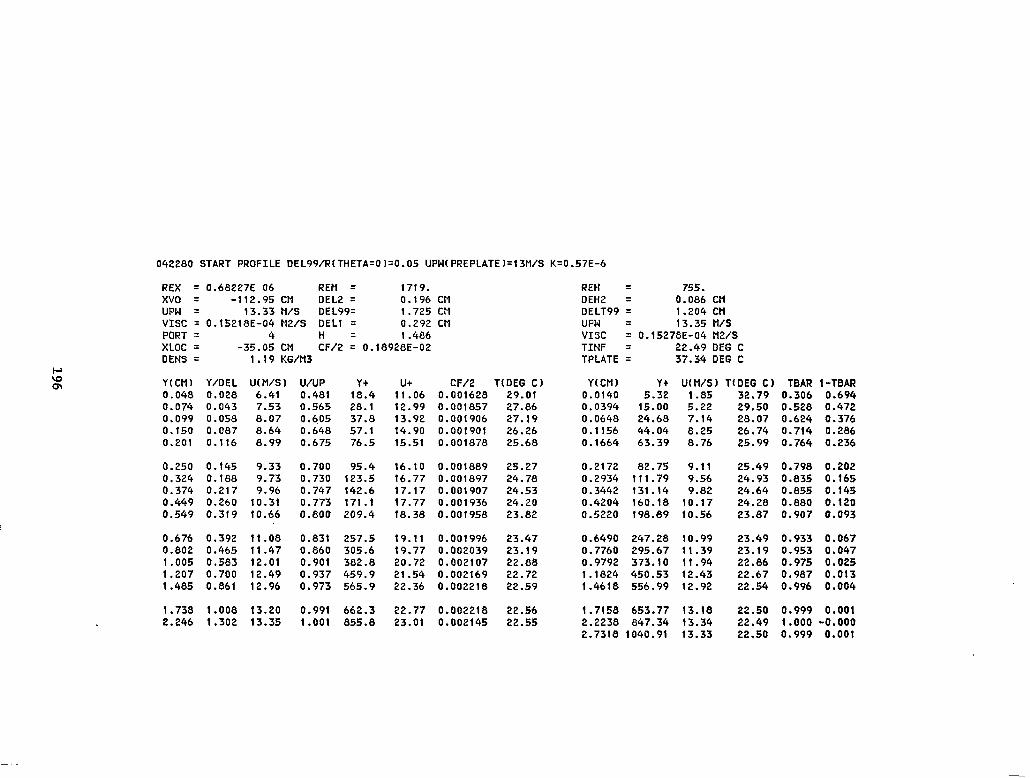
042280 START PROFILE DEL99/R(THETA=O)=O.O5 UPW(PREPLATE)=l3M/S K=0.57E-6

REX q 0.68227E 06 REM = 1719. REH = 755. xv0 = -112.95 CM DEL2 = 0.196 CM DEH2 = 0.086 CM UPW = 13.33 H/S DEL99= 1.725 CM DELT99 = 1.204 CM VISC = O.l5218E-04 Me/S DEL1 = 0.292 CM UPW q 13.35 H/S PORT = 4 H = 1.486 VISC = O.l5278E-04 H2/S XLOC = -35.05 CM CF/2 q O.l8928E-02 TINF = 22.49 DEG C DENS = 1.19 KG/M3 TPLATE = 37.34 DEG C

Y(CM) Y/DEL U(M/S) U/UP Y+ u+ CF/2 T(DEG C) Y(CH) Y+ U(tl/S) T(DEG C) TBAR l-TBAR 0.048 0.028 6.41 0.481 18.4 11.06 0.001628 29.01 0.0140 5.32 1.85 32.79 0.306 0.694 0.074 0.043 7.53 0.565 28.1 12.99 0.001857 27.86 0.0394 15.00 5.22 29.50 0.528 0.472 0.099 0.058 8.07 0.605 37.8 13.92 0.001906 27.19 0.0648 24.68 7.14 28.07 0.624 0.376 0.150 0.087 8.64 0.648 57.1 14.90 0.001901 26.26 0.1156 44.04 8.25 26.74 0.714 0.286 0.201 0.116 8.99 0.675 76.5 15.51 0.001878 25.68 0.1664 63.39 8.76 25.99 0.764 0.236

0.250 0.145 9.33 0.700 95.4 16.10 0.001889 25.27 0.2172 82.75 9.11 25.49 0.798 0.202 0.324 0.188 9.73 0.730 123.5 16.77 0.001897 24.78 0.2934 111.79 9.56 24.93 0.835 0.165 0.374 0.217 9.96 0.747 142.6 17.17 0.001907 24.53 0.3442 131.14 9.82 24.64 0.855 0.145 0.449 0.260 10.31 0.773 171.1 17.77 0.001936 24.20 0.4204 160.18 10.17 24.28 0.880 0.120 0.549 0.319 10.66 0.800 209.4 18.38 0.001958 23.82 0.5220 198.89 10.56 23.87 0.907 0.093

0.676 0.392 11.08 0.831 257.5 19.11 0.001996 23.47 0.802 0.465 11.47 0.860 305.6 19.77 0.002039 23.19 1.005 0.583 12.01 0.901 382.8 20.72 0.002107 22.88 1.207 0.700 12.49 0.937 459.9 21.54 0.002169 22.72 1.485 0.861 12.96 0.973 565.9 22.36 0.002218 22.59

0.6490 247.28 10.99 23.49 0.933 0.067 0.7760 295.67 11.39 23.19 0.953 0.047 0.9792 373.10 11.94 22.86 0.975 0.025

1.738 1.008 13.20 0.991 662.3 22.77 0.002218 22.56 2.246 1.302 13.35 1.001 855.8 23.01 0.002145 22.55

1.1824 450.53 12.43 22.67 0.987 0.013 1.4618 556.99 12.92 22.54 0.996 0.004

1.7158 653.77 13.18 22.50 0.999 0.001 2.2238 847.34 13.34 22.49 1.000 -0.000 2.7318 1040.91 13.33 22.50 0.999 0.001

RW 042280 l i” CLRVATIRE RIG l us NASA-NAS-3-3 STANTON H+BER DATA

TADB= 22.28 DEG C lJREF= 13.34 N/s TINF= 22.20 DEG C RHO= I.189 KGA3 VISC: O.l5253E-04 W/S XVD= -113.0 Ctl cp= 1011. J/KGK PR- 0.715

STANTON RUN DEL99/RlTHETA=O.O)=0.05 “PWPREPLATE)=l3lVS K=O.S7E-6

PLATE X UPY ten) IN/S)

K REXVD TO DEG C

STANTON ND REENTll DST

1 -61.3 13.34 2 -58.7 13.34 3 -56.1 13.34 4 -53.5 13.34 5 -50.9 13.34 6 -48.3 13.34 7 -45.7 13.34 a -43.0 13.34 9 -40.4 13.34

10 -37.8 13.34 11 -35.2 13.34 12 -32.6 13.34 13 -30.0 13.34 14 -27.4 13.34 15 -24.8 13.34 16 -22.2 13.34 17 -19.5 13.34 la -16.9 13.34 19 -14.3 13.34 20 -11.7 13.34 21 -9.1 13.34 22 -6.5 13.34 23 -3.9 13.34 24 -1.3 13.34

CURVE BEGINS

25 2.4 13.83 26 7.3 14.08 27 12.4 14.33 28 17.4 14.64 7.9 22.5 15.00 30 27.6 15.40 31 32.6 15.87 32 37.7 16.38 33 42.8 16.87 34 47.8 17.33 35 52.9 17.81 3s 58.0 18.42 37 63.0 19.23 38 68.1 19.87

RECOVERY BEGINS

39 72.0 20.31 40 74.6 20.31 41 77.2 20.31 42 79.8 20.31 43 82.4 20.31 44 85.0 20.31 45 87.6 20.31 46 90.2 20.31 47 92.8 20.31 48 95.4 20.31 49 98.1 20.31 50 100.7 20.31 51 103.3 20.31 52 105.9 20.31 53 108.5 20.31 54 111.1 20.31 55 113.7 20.31 56 116.4 20.31 57 118.9 20.31 58 121.6 20.31 59 124.2 20.31 60 126.8 20.31 61 129.4 20.31 62 132.0 20.31

DST(%) DREEN

O.t17E-03 O.l27E-03 O.llbE-03 O.l14E-03 0.949E-04 O.l06E-03 0.993E-04 0.953E-04 0.956E-04 0.925E-04

0.78892E 03 0.926E-04 0.85225E 03 0.8BbE-04 0.91689E 03 O.a77E-04 0.97177E 03 0.892E-04 0.10276E 04 O.B79E-04 0.10870E 04 O.B88E-04 0.11790E 04 0.823E-04 0.12136E 04 0.875E-04 0.12607E 04 0.882E-04 0.1333lE 04 0.857E-04 0.13934E 04 0.818E-04 0.14313E 04 0.833E-04 0.14800E 04 0.85lE-04 O.!5340E 04 0.822E-04

6.293 3.413 3.304 3.390 3.186 3.396 3.336 3.310 3.323 3.316 3.334 3.336 3.314 3.341 3.336 3.386 3.270 3.358 3.363 3.322 3.316 3.356 3.340 3.388

0.16127E 04 O.l03E-03 0.16798E 04 O.B48E-04 0.17469E 04 0.928E-04 0.18440E 04 0.865E-04 0.19347E 04 0.844E-04 0.20203E 04 0.82bE-04 O.PlOOOE 04 0.799E-04 0.21890E 04 0.783E-04 0.228lOE 04 0.774E-04 0.23631E 04 0.772E-04 0.24688E 04 0.759E-04 0.2546bE 04 0.743E-04 0.26437E 04 0.7lbE-04 0.27757E 04 0.655E-04

5.158 4.463 4.947 4.903 4.911 4.923 4.949 4.933 4.902 4.937 4.832 4.880 4.952 4.903

0.29158E 04 0.516E-04 3.358 0.30133E 04 0.515E-04 3.313 0.29899E 04 0.552E-04 3.437 0.30438E 04 0.534E-04 3.389 0.31057E 04 0.547E-04 3.368 0.31557E 04 0.546E-04 3.414 0.32100E 04 0.540E-04 3.406 0.33009E 04 0.553E-04 3.351 0.338lt.E 04 0.536E-04 3.374 0.3442bE 04 0.567E-04 3.373 0.34967E 04 0.543E-04 3.384 0.352!6E 04 0.574E-04 3.421 0.35994E 04 0.558E-04 3.352 0.36297E 04 0.5728-04 3.404 0.3702lE 04 0.565E-04 3.367 0.37505E 04 0.569E-04 3.439 0.38898E 04 0.543E-04 3.308 0.38632E 04 0.584E-04 3.433 0.39196E 04 O.SbOE-04 3.433 0.40502E 04 0.549E-04 3.365 0.41138E 04 0.563E-04 3.459 0.43002E 04 0.526E-04 3.291 0.42243E 04 0.580E-04 3.543 0.43546E 04 0.680E-04 4.701

1. 2. 2. 3. 3. 3. 4. 4. 4. 4. 5. 5. 5. 5.

6. 7. 7. a. 9.

10. 10. 11. 12. 13. 13. 14. 15. 16.

17. 17. 17. 17. 17. 17. 17. 17. 17. 17. 17. 17. 17. 17. 17. 17. 17. 17. 1B. 18. 18.

ii: 18.

O.OOOE 00 0.45206E 06 O.OOOE 00 0.47493E 06 O.OOOE 00 0.4978OE 06 O.OOOE 00 0.52045E 06 O.OOOE 00 0.54332E 06 O.OOOE 00 0.56620E 06 i.OOOE 00 0.58907E 06 O.OOOE 00 0.61194E 06 O.OOOE 00 0.63459E 06 O.OOOE 00 0.6574bE 06 O.OOOE 00 0.68033E 06 O.OOOE 00 0.7032lE 06 O.OOOE 00 0.72608E 06 O.OOOE 00 0.74873E 06 O.OOOE 00 0.77160E 06 O.OOOE 00 0.79447E 06 O.OOOE 00 0.01735E 06 O.OOOE 00 0.84000E 06 O.OOOE 00 0.86287E 06 O.OOOE 00 0.88574E 06 O.OOOE 00 0.9086lE 06 O.OOOE 00 0.93148E 06 O.OOOE 00 0.95413E 06 O.OOOE 00 0.9770lE 06

34.09 0.34503E-02 36.27 0.37068E-02 36.60 0.35638E-02 36.83 0.33725E-02 36.12 0.29778E-02 37.08 0.31163E-02 37.28 0.29763E-02 37.27 0.28799E-02 37.38 0.28774E-02 37.41 0.27900E-02 37.52 0.27767E-02 37.49 0.26564E-02 37.42 0.26462E-02 37.51 0.26708E-02 37.59 0.26342E-02 37.60 O.P6223E-02 37.13 0.25175E-02 37.44 0.26063E-02 37.60 0.26232E-02 37.44 0.25784E-02 37.41 0.24662E-02 37.61 0.24819E-02 37.70 0.25487E-02 37.73 0.24257E-02

O.lOSE-05 0.104blE 07 0.396E-06 0.11107E 07 0.363E-06 0.11782E 07 0.42@E-06 0.12519E 07 0.48:E-06 0.13332E 07 0.499E-06 0.14195E 07 0.5r;SE-06 0.15154E 07 0.56?E-06 0.16181E 07

37.68 37.88 38.09 38.02 38.00 38.01

O.l9964E-02 O.l8970E-02 O.l8727E-02 O.l7615E-02 0.1714&E-02 O.l6742E-02 O.l6105E-02 O.l5835E-02 O.l5760E-02 O.l56lOE-02

38.07 38.07 38.05 38.12

0.512E-06 0.17229E 07 0.456E-06 0.18279E 07 0.447E-06 0.19370E 07 0.534E-06 0.2065lE 07 0.649E-06 0.22200E 07 0.476E-06 0.2359bE 07

38.04 O.l5668E-02 38.15 O.l5188E-02 38.15 O.l4421E-02 37.93 O.l3339E-02

0.422E-06 0.24632E 07 O.OOOE 00 0.24981E 07 O.OOOE 00 0.25329E 07 O.OOOE 00 0.25678E 07 O.OOOE 00 0.26023E 07 O.OOOE 00 0.26371E 07 O.OOOE 00 0.26719E 07 O.OOOE 00 0.27068E 07 O.OOOE 00 0.27413E 07 O.OOOE 00 0.277blE 07

O.l5360E-02 O.l5553E-02 O.l60blE-02 O.l5765E-02 O.l6237E-02 O.lbOOOE-02 O.l5852E-02 0.16496E-02

37.55 37.32 37.72 37.72 37.69 37.72 37.73 37.56 37.45 37.43 37.44 37.58 37.50 37.42 37.56 37.60 37.26

O.OOOE 00 0.28llOE 07 O.OOOE 00 0.28458E 07 O.OOOE 00 0.28B06E 07 O.OOOE 00 0.2915lE 07 O.OOOE 00 0.29500E 07 O.OOOE 00 0.29848E 07 O.OOOE 00 0.3019bE 07

O.l5888E-02 O.l6818E-02 O.l6054E-02 O.l67BlE-02 O.l6650E-02 O.l6805E-02 O.l6782E-02 O.l6547E-02 O.l6408E-02 O.l7004E-02 O.l6313E-02 O.l6317E-02 O.l62SlE-02 O.l5995E-02 O.l6382E-02 O.l4449E-02

O.OOOE 00 0.30545E 07 O.OOOE 00 0.30890E 07 O.OOOE 00 0.3123BE 07 O.OOOE 00 0.315B7E 07 O.OOOE 00 0.31935E 07 O.OOOE 00 0.32283E 07 O.OOOE 00 0.32628E 07

37.59 37.60 37.31 37.29 36.82 37.27 37.00

UNCERTAINTY IN REX=ll258.

197

0.0040

o.co30

5 m

5 2 0.w20

E

!G 4 Li

0.0010

0.0000

I CURVE

-80 -20 20 80 100



1.02-02

0.62-02

2 ii 2 I.OE-03 z e z 2 052-03

1.02-04

ENTHALPY THICKNESS REYNOLDS NUmER Fig. 626. Case 042280: Stanton number versus enthalpy


198

-

051080 STARTING PROFILES DEL99/R(THETA=O)=O.O5 K=l.25E-6

REX = 0.29659E 06 REM = 883. REH = 565. xv0 = -85.26 CM DEL2 = 0.149 CM DEH2 = 0.096 CM UPW = 9.05 n/s DEL99= 1.460 CM DELT99 = 1.319 CM VISC = O.l5319E-04 HZ/S DEL1 = 0.229 CM UPW q 9.06 M/S PORT = 4 H = 1.529 VISC = O.l5353E-04 M2/S XLOC q -35.05 CM CF/2 = 0.23124E-02 TINF = 22.54 DEG C DENS = 1.18 KG/H3 TPLATE = 38.40 DEG C

Y(CM) Y/DEL U(M.'SI U/UP Yt ut CF/2 TTDEG C) 0.048 0.033 4.50 0.498 13.7 10.35 0.001976 30.38 0.074 0.051 5.32 0.588 21.0 12.23 0.002254 28.66 0.099 0.068 5.66 0.626 28.2 13.02 0.002276 27.73 0.150 0.103 6.12 0.677 42.6 14.07 0.002291 26.56 0.201 0.138 6.39 0.706 57.0 14.68 0.002265 25.88

0.250 0.172 6.65 0.734 71.1 15.27 0.002279 25.43 0.325 0.223 6.92 0.765 92.3 15.90 0.002279 24.90 0.375 0.257 7.13 0.788 106.6 16.38 0.002311 24.64 0.450 0.308 7.39 0.816 127.8 16.98 0.002347 24.30 0.550 0.377 7.69 0.850 156.3 17.67 0.002396 23.92

0.676 0.463 8.01 0.885 191.9 18.40 0.002447 23.58 0.802 0.549 8.26 0.913 227.7 18.99 0.002483 23.29 1.004 d.688 8.61 0.951 285.1 19.78 0.002534 23.00 1.205 0.826 8.82 0.975 342.4 20.28 0.002540 22.82 1.484 1.017 8.96 0.991 421.6 20.60 0.002494 22.64

Y(CM) Yt U(M/S) T(DEG Cl TBAR 1-TBAR 35.38 0.190 0.810 0.0140

0.0394 0.0648 0.1156 0.1664

3.97 11.18 18.40 32.83 47.26

-1.30 3.67 5.03 5.81 6.21

31.14 0.458 0.542 28.98 0.594 0.406 27.11 0.712 0.288 26.28 0.764 0.236

0.2172 61.69 6.47 25.66 0.803 0.197 0.2934 83.33 6.80 25.09 0.839 0.161 0.3442 97.76 7.00 24.77 0.860 0.140 0.4204 119.40 7.28 24.41 0.883 0.117 0.5220 148.26 7.61 23.98 0.909 0.091

0.6490 184.33 7.94 23.62 0.932 0.068 0.7760 220.41 8.21 23.31 0.952 0.048 0.9792 278.13 8.57 23.00 0.972 0.028 1.1824 335.84 8.80 22.82 0.983 0.017 1.4618 415.20 8.95 22.62 0.995 0.005

1.738 1.190 9.03 0.998 493.6 20.76 0.002443 22.59 2.245 1.538 9.06 1.001 637.8 20.81 0.002324 22.56 2.753 1.886 9.06 1.001 782.1 20.81 0.002228 22.58

1.7158 487.35 9.03 22.57 0.998 0.002 2.2238 631.64 9.05 22.54 1.001 -0.001 2.7318 775.94 9.06 22.55 1.000 0.000 3.2398 920.23 9.05 22.55 1.000 0.000

051080 VELOCITY PROFILE K=l.Z5E-6 THETA=52.5 DEG. S=40.8 CM

REX = 0.18836E 06 REM = 614.

xv0 = 20.08 CM DEL2 = 0.068 CM UPW = 13.75 n/s DEL99= 0.936 CM VISC = O.l5199E-04 H2/S DELI = 0.111 CM P0R.r = 4 H q 1.642 XLOC = 40.89 CM CF/2 q 0.28298E-02 DENS = 1.19 KG/M3

Y(CM) Y/DEL U(M/S) U/UP Y+ u+ CF/2

0.048 0,052 6.96 0.507 23.3 9.51 0.001752 0.074 0.079 8.87 0.646 35.5 12.13 0.002299 0.099 0.106 10.07 0.734 47.7 13.77 0.002612 0.125 0.133 10.82 0.789 60.0 14.79 0.002768 0.175 0.187 11.61 0.847 84.4 15.86 0.002843

0.223 0.239 12.03 0.879 107.5 16.44 0.002840 0.270 0.289 12.29 0.899 130.2 16.80 0.002807 0.345 0.368 12.57 0.921 166.1 17.18 0.002747 0.394 0.421 12.70 0.931 189.8 17.36 0.002709 0.470 0.502 12.84 0.943 226.3 17.55 0.002647

0.571 0.610 13.03 0.960 274.8 17.81 0.002597 0.672 0.717 13.13 0.969 323.4 17.95 0.002535 0.824 0.680 13.26 0.982 396.6 18.12 0.002463 1.052 1.123 13.41 0.998 506.3 18.33 0.002382 1.305 1.394 13.37 1.000 628.3 18.27 0.002261

1.432 1.530 13.33 1.000 689.5 18.22 0.002206

200

RLM 051080 HI CLRYATLRE RIG - NASA-NAG-53 STANTON ta.nmER DATA

TADB: 22.55 DEG C LiREF= 9.05 n/s RHO= 1.184 KGA3 "IX= O.l5350E-04 X2/S

E;r= 22.51 DEG C - -25.3 cn

CP- 1010. J/KGK Pa= 0.714

STANTON RUN DEL99/RIlHETA=Ol=O-05 UPXIPREPlATE)=9.0 WS K=l.tSE-6

PLATE X UPH K REXW TO STANTOHND REEhTK ten, Ill/S1 DEG C

DST DST(X) DRE’ZN

1 -61.3 9.05 O.OOOE 00 0.14167E 06 37.36 O.t1119E-02 O.L59E-03 2 -58.7 9.05 O.OOOE 00 0.157lOE 06 M.35 0.31740E-02 O.l13E-03 3 -56.1 9.05 0.000E 00 0.17253E 06 38.35 0.32894E-02 O.lllE-03 4 -53.5 9.05 O.OOOE 00 0.1878lE 06 38.37 0.33287E-02 O.llbE-03 5 -50.9 9.05 O.OOOE 00 0.20324E 06 37.63 0.31549E-02 O.l02E-03 6 -48.3 9.05 O.OOOE 00 0.21867E 06 38.38 0.33696E-02 O.l17E-03 7 -45.7 9.05 O.OOOE 00 0.234lOE 06 38.46 0.33213E-02 O.l13E-03 8 -43.0 9.05 O.OOOE 00 0.24953E 06 38.40 0.32829E-02 O.lllE-03 9 -40.4 9.05 O.OOOE 00 0.2648lE 06 38.43 0.33378E-02 O.l13E-03

10 -37.8 9.05 O.OOOE 00 0.28024E 06 38.46 0.32268E-02 O.lOPE-03

12.255 3.551 3.381 3.405 3.245 3.477 3.400 3.373 3.377 3.386 3.398 3.407 3.387 3.416 3.400 3.460 3.350 3.439 3.436 3.403 3.397 3.451 3.414 3.502

12. 12. 12. 12. 12. 12. 12. 12. 12. 12. 12. 13. 13. 13.

3.565 13. 2.988 14. 2.949 14. 3.058 15. 3.068 lb. 3.150 17. 3.195 ia. 3.233 19. 3.277 20. 3.310 22. 3.183 23. 3.341 25. 3.158 27. 3.227 29.

3.620 3.478 3.544 3.488 3.431 3.451 3.439 3.372 3.390 3.387 3.381 3.423 3.349 3.401 3.362 3.431 3.308 3.427 3.423 3.361 3.452 3.283 3.520 4.462

29.

ii: 30. 30.

i:: 30.

::: 31. 31. 31.

f:: 31.

I::

f:: 32.

f:: 32.

11 -35.2 9.05 O.OOOE 00 12 -32.6 9.05 O.OOOE 00

0.29567E 06 0.31109E 06 0.32652E 06 0.34180E 06 0.35723E 06 0.372bbE 06 0.38809E 06 0.40337E Ob 0.41880E 06 0.43423E 06 0.4496bE 06 0.46509E 06 0.48037E 06 0.495BOE 06

38.53 38.52 38.49

0.32191E-02 0.58953E 03 O.l09E-03 0.30792E-02 0.6382bE 03 O.l05E-03 0.30529E-02 0.68691E 03 O.l03E-03 0.30680E-02 0.73073E 03 O.lOSE-03 0.30119E-02 0.77585E 03 O.lOZE-03 0.29763E-02 0.82062E 03 O.l03E-03 0.28369E-02 0.88428E 03 0.950E-04 0.29178E-02 0.91390E 03 O.lOOE-03 0.29421E-02 0.95223E 03 O.lOlE-03 0.28868E-02 0.10042E 04 0.982E-04 0.27735E-02 0.1048bE 04 0.942E-04 0.27595E-02 0.10790E 04 0.952E-04 0.28662E-02 0.11200E 04 0.978E-04 0.27185E-02 0.11597E 04 0.95ZE-04

13 -30.0 9.05 O.OOOE 00 14 -27.4 9.05 O.OOOE 00 (5 -24.8 9.05 O.OOOE 00 16 -22.2 9.05 O.OOOE 00 17 -19.5 9.05 O.OOOE 00

3-8.56 38.60 38.63 38.26 38.53 38.65 38.53 38.51 38.70

18 -16.9 9.05 O.OOOE 00 19 -14.3 9.05 O.OOOE 00 20 -11.7 9.05 O.OOOE 00 21 -9.1 9.05 O.OOOE 00 22 -6.5 9.05 O.OOOE 00 23 -3.9 9.05 O.OOOE 00 24 -1.3 9.05 O.OOOE 00

CURVE BEGINS

25 2.4 9.44 26 7.3 9.76 27 12.4 10.15 28 17.4 10.59 29 22.5 11.15 30 27.6 11.79

O.l78E-05 O.lOSE-05 O.llOE-05 O.f18E-05 O.l33E-05 O.l3bE-05

38.74 38.78

0.53940E 06 38.69 0.58912E 06 38.68 0.645BOE 06 38.77 0.70910E 06 38.72 0.78361E 06 38.79 0.86735E 06 38.88

0.2258bE-02 0.20024E-02 O.l893lE-02 O.l7360E-02 0.16366E-02 O.l4819E-02 O.l3773E-02 O.l2657E-02 O.l1740E-02 O.l0884E-02 0.10738E-02 0.9476BE-03 0.93669E-03 0.80338E-03

0.12232E 04 0.8058-04 0.12907E 04 0.598E-04 0.1349bE 04 0.558E-04 0.14192E 04 0.53lE-04 0.1477lE 04 0.502E-04 0.15308E 04 0.467E-04 0.1592bE 04 0.440E-04 0.16439E 04 0.409E-04

31 32.6 12.52 O.l3bE-05 0.96234E 06 38.69 32 37.7 13.31 O.l31E-05 0.10664E 07 38.98 33 42.8 34 47.8

14.11 O.l19E-05 14.99 O.l14E-05 15.89 O.lOSE-05 (6.96 O.l09E-05 18.49 O.l30E-05 20.02 O.lllE-05

IGINS

0.11772.E 07 38.99 0.13002E 07 39.01 0.14309E 07 39.09 0.1563bE 07 39.06 0.17870E 07 39.00 0.20014E 07 38.%

0.17031E 04 0.385E-04 0.17593E 04 0.360E-04 0.98104E 04 0.342E-04 0.18747E 04 0.317E-04 0.19463E 04 0.29bE-04 0.20152E 04 0.259E-04

35 52.9 36 58.0 37 63.0 38 68.1

RECOVERY BI

39 72.0 20.20 O.l79E-06 0.20702E 07 39.03 0.957428-03 0.20498E 04 0.347E-04 20.28 O.l15E-06 0.21130E 07 38.71 O.l03bbE-02 0.21247E 04 0.36lE-04 20.36 O.l14E-06 0.21561E 07 38.82 O.l1826E-02 0.21482E 04 0.4198-04 20.44 O.l13E-06 0.21995E 07 38.64 O.l2442E-02 0.22144E 04 0.434E-04 20.52 O.llEE-06 0.22427E 07 38.40 O.!3838E-02 0.22936E 04 0.475E-04

40 74.6 41 77.2 42 79.8 43 82.4 44 85.0 20.60 O.llOE-06 0.2286bE 07 38.24 O.l4536E-02 0.23669E 04 O.SOZE-04 45 87.6 20.68 O.l09E-06 0.2330bE 07 38.13 O.l4990E-02 0.24350E 04 0.516E-04 46 90.2 20.76 O.l07E-06 0.23749E 07 37.84 O.l623bE-02 0.25371E 04 0.547E-04 47 92.8 20.84 O.l07E-06 0.2419lE 07 37.63 O.l6lOOE-02 0.26295E 04 0.546E-04 48 95.4 20.92 O.l05E-06 0.24639E 07 37.53 O.l7433E-02 0.27054E 04 0.590E-04 49 98.1 20.92 O.OOOE 00 0.24995E 07 37.45 O.l6999E-02 0.2782OE 04 0.575E-04 50 100.7 20.98 0.78lE-07 0.25423E 07 37.55 O.l8005E-02 0.28250E 04 0.616E-04 51 103.3 21.04 0.775E-07 0.25853E 07 37.42 O.l8083E-02 0.29159E 04 O.bObE-04 52 105.9 21.12 O.l03E-06 0.26305E 07 37.53 0.183lOE-02 0.2958bE 04 O.b23E-04 53 108.5 21.17 0.760E-07 0.26738E 07 37.46 O.l8398E-02 0.30397E 04 O.b19E-04 54 111.1 21.23 0.754E-07 0.27173E 07 37.49 O.l8123E-02 0.30980E 04 0.622E-04 55 113.7 21.23 O.OOOE 00 0.27535E 07 37.14 O.l789lE-02 0.32372E 04 0.592E-04 56 116.4 21.31 0.994E-07 0.27998E 07 37.47 O.l8637E-02 0.32300E 04 O.b39E-04 57 118.9 21.39 0.993E-07 0.2846OE 07 37.46 O.l7B7OE-02 0.32995E 04 0.612E-04 58 121.6 21.48 O.l2lE-06 0.28953E 07 37.16 O.l7764E-02 0.3432bE 04 0.597E-04 59 124.2 21.56 O.%OE-07 0.29423E 07 37.11 O.l7707E-02 0.35080E 04 O.bllE-04 60 126.8 21.63 0.950E-07 0.29895E 07 36.60 O.l7352E-02 0.36988E 04 0.570E-04 61 129.4 21.63 O.OOOE 00 0.30264E 07 37.11 O.l7833E-02 0.363142 04 0.628E-04 62 132.0 21.63 O.OOOE 00 0.30629E 07 36.aB O.l5944E-02 0.37503E 04 0.711E-04

UNCERTAINTY IN REX= 8658.

201

o.w40

O.WSO

&

ii z o.cmo

E

E

0.0010

O.WOO

DO *0*0 00 0

000 00 ***o

oooo

0

0 0

0 0

00 oo*“*oo***< 00

0 0 boo 0

0 o” 00

00 o” 0

CURVE

1 -20 20 80 loo



.

1.0~~02

om-02

ui E 3 2 l.OE-03

5

5 g 0.5E-03

I.OE-04



202

Appendix H

Modifications to STAN5 for Convex Curvature Predictions

The following listing shows the modifications made to STAN5 [l] to

account for convex curvature effects. This version of the program was

used to make the predictions of Figs. 4-2 through 4-17. New programming

is listed, bracketed with the preceding and following lines of the original STAN5 program (lines with identification on right side).

203

C . . . . . C C

. . . . . THIS PROGRAM HAS BEEN MODIFIED FOR CONVEX CURVATURE

. . . . . USING THE GILLIS MODEL WITH THE SIMON CHANGES C . . . . . SEE THE TWO.THESES FOR DETAILS C . . . . . LATEST REVISION ******* SEPTEPIBER 1980 **Y*Y**+~

1 INTEGER GEOH,FLUID,SOURCE(5)rSPACE,BODFOR,OUTPUT,TYPBC

MAIN01 50

tlAIN0160

~/AOD/RBO~~~~~~,O~D~~~~,ROPIO~~~~.ITKE,CBC~~~~~,CEFF~~~~,CLAG,CURV, tlAIN0290 4CWrPL~54l,SKIt~~100~,STANT~100~,XPLOT~100~,REEE~Ttl~100~,IPLOT,XSTART

3 DItIENSIOtI AHEFt 5 I ,AtIIFI 5 1 tlAIN0300 4 DIHENSION FPP(1001,AFPP(1001,BFPP[100),CFPP(lOO) MAIN031 0 5 CALL STARTG( 'GENIL*' ,O. 1

C . . . . . MAIN031 1

7 NItJJ=O 8 IPLOT=O 9 NPLOT-0

10 5 KERROR=O 11 00 7 1=1,100 12 SKIN(Il=O.O 13 STAtdTt I )=O. 0 14 XPLOT(I)=O.O 15 REEtlTH( I t-O.0 16 7 COtdTINUE 17 t~ItuJ=t~IIm?l

MAIN0340

MAIN0350

tlAIN0360

19 IF~KERROR.GT.O)GO TO 1000 tlAIN0390 20 XSTART=X( 1 1 21 DO 8 fl=2,NXBC 22 IF (CBC(M) .LT. -1 .OE-6 .AND. CBCtM-1 I .GT. -1 .OE-61 XSTART=X(tl) 23 8 CONTINUE

C ----------------------------------------------------------- STEP5 ----,,AINO400

30 AUXtl?=AUX2(tl-1 )?(AUXZ(M)-AUX2(H-1 1 )*(XU-X(tl-1 I l/(X(MJ-X(M-1 1 I MAIN0470 C Y***~*YK*****~************************K*N********~***** C CURVATURE MOOIFICATION, INTERP. WALL RADIUS

31 CW=CBC(tl-1 l?(CBC(ll)-CBCfM-1 I )*(XU-X(tl-1 1 I/(X(M)-Xftl-1 I) C *Z~*K*Y*X****~*~**~***~R*N~~***K*N*N*NR***~~~KN*~*~***N

32 IF (KEX.ED.1) AME=AMIE MAItl0480

204

290 H=DELl/DELL 291 8Xx=DELI 292 REM=DEL2*UGU*RHG/VISG

345 346 347 348 349 350 351 561 352

CALL OUT SKItIC IPLOT)=CFZ STANTt IPLOT )=STI 1 I IF (ST(1 1 .LT. l.OE-6) STANTLIPLOTI=l.O XPLOTtIPLOT)=(XU-XSTART)*30.48 REEtdTtIf IPLOTt=REH COttTItktE IF(LVAR.GT.1 )GO TO 1000

MAIN3490

tlAIN3500

HAIN

HAIN

359 AUXtlZ=AUXEttl-1 )+(AUX2(tl)-AUXZttl-I ))*(XD-X(M-1 )l/(X(tll-Xttl-1 1) tlAIN4250 C ******************************************************* C CURVATURE MODIFICATION, INTERP. WALL RADIUS

360 CW-CBCttl-1 l+(CBCttl)-CBCttl-1 1 )*LXU-Xttl-1 1 t/(X(H)-Xttl-1 11 361 SP(P)=ABStCBC(tl))

C *************Y***********************************~*** C . . . ..IF IT IS DESIRED TO INTRODUCE THE WALL BOUNDARY CONDITION AS MAIN4260

332 383 364 385 386 387 368 389 390 391 392

393 394 395 396 397 398 399 400 401

402 403 404 405

GO TO 15 HAIN 1000 CONTIttUE

IF (NPLOT .EQ. 11 CALL PICTRG(O.0) CALL SETSPlGt23,O.Ot CALL SETStIGt 24~0.0 1 CALL SUBJEGt-60.,0.0,130.0,0.004) CALL SETStIG( 130,O.Ol t CALL SETStIGt 131 ,O.Ol 1 CALL SETStIG(132.1.0) CALL CSETGt ‘DUPLEX*’ 1 CALL GRAPHGt’*‘,l,IPLOT,XPLOT,STANT,O ,‘STREAMWISE DISTANCE (CM)*’

1 , ‘STANTOtt ttUtIBERr CF/2*‘, ‘*’ 1 CALL LItIESGt’DASH*‘,IPLOT,XPLOT,SKIN1 CALL PICTRG(O.0) CALL SETSHG(23,l .Ot CALL SETSllG(24,l .O) CALL CSETG( ‘DUPLEX*’ 1 CALL SU6JEG(200.,0.0005,5000.0,0.005) CALL SETStlG(133.2.0) CALL SETStlG(l34,2.01 CALL GRAPtIGt ‘* ‘,l,IPLOT,REENTH,STANT,O,‘ENTHALPY THICKNESS REYNDLD

1s NUtlBER*‘,‘STANTON NUMBER*‘,‘+‘) NPLOT=l IFtNIND.LT.NUtlRUN)GO TO 5 CALL EXITG STOP

MAIN4600

tlAIN4610

205

~/ADD/RB~~~~~~~,O~ID~~~~,ROIID~~~~,ITKE,CDC~~~~~,CEFF~~~~~CLAG,CURVI STEP0150 4CW,PL~54t,SKIN~100l,STANTO,XPLOT~iOOt,REENTH~lOO~,IPLOT,XSTART

C . . . . . STEP0160

1224

1232 YPUT=RHW*UTAU/VISW 1233 KTHRU-0 1234 IF (ItiTG.GT.l) G5 T’G 10

AUX00240

AUX00250

1236 IF (tlODE.EQ.21 KOUNT-1 AUX00270 C *Y**YY*******k*********************************************** C CURVATURE MODIFICATION -- GUESS INITIAL VALUES OF PARAPIETERS

1237 SLT-Y L 1238 DISSHR-BXX 1239 ALAM=SLT-DISSHR 1240 PLAtl=ALAtl 1241 P?LAfI=PLAtl 1242 P3LAM=P2LAM 1243 ISLT-ti 1244 REHS=REM

C *u**~Y******************************************************* 1245 1 RAVG=Rt 1 t AUX00280

C . . . . . 1270 10 KTHRU=KTHRU?l 1271 DO 89 1=2,tJPl

AUXOOblO

AUXOOb20

C . . , . .COtlPUTE IlIXIttG LEtIGTlI AUXOIOOO

C ****Y~*****Y~I******~**************************************

C CURVATURE tlODIFICATIDN TO WAKE tlIXING LENGTH

1301 ALAHA-ALAI1

1302 IF (XU .LT. XSTART) ALAHA=0.85*YL

206

1303 IF(INTG.LT.27t ALAtlA=.85*YL 1304 30 AL=ALtlG*ALAttA*l .1765 AUXOlOlO 1305 ALtlAX=AL

C *********************************************************** 1306 IF (KASE.EQ.l .AttD.Ytl.LT.AL/AKt AL=AK*Yfl AUXOlO20

1314 35 EtlUT=RHOAV*AL*AL+ABS((ULI+l I-U(I))/(Y(I+l )-YLIt))*DV(I)*DV(I) AUXOI 080 1315 PLt I l=AL/YL 1316 SP( 2 )=BXX 1317 SP( 3 )=SLT 1318 IFtK2.NE.Z.OR.KASE.EQ.Z)GO TO 36 AtXO 1090

1332 1333 1334

1357 80 PREFtJ,I)=O.S*(PR(J,If( )+PR(J,Itt 1358 88 COt4TItiUE 1359 89 COIITINUE 1360 Ylz-0.00 1361 YCRIT=O.O 1362 IF(CW.GE.-l.OE-6) GO TO 91 1363 SCRIT=0.25*((-CW*YLt**O.331 1364 DO 90 I=Z,tIPl 1365 VELGRD(I)=(U(I)-U(I-1 l)/(Y(I)-YCI-1 1) 1366 STAB(I)=CW*U(I)/VELGRDO 1367 IFtSTABtIt.GT.-SCRIT) GO TO 90 1368 Y12=(-SCRIT-STABtI-l))/oTAB(I)-STAB(I-1)) 1369 YCRIT=YlZ*(Y(I)-Y(I-1 t)+Y(I-1) 1370 GO TO 91 1371 90 CONTItJUE 1372 91 P3LAM=P2LAtl 1373 PZLAM=PLAtl 1374 PLAtl=SLT-DISSHR 1375 NPSHR-NPl-1 1376 TAUtlAX=O.O 1377 DO 92 1=3,NPSHR 1378 92 IF(TPLtIl.GT.TAUHAXt TAUMAX=TPL(I) 1379 CtiTR=O. 65 1380 BAND=0 .25 1381 93 KLUNK=O 1382 NFIT=O 1383 SUM1=0.0 1384 suP12=0.0 1335 suI13=0.0 1386 SUM4=0.0 1387 DO 94 I=1 ,NPSHR 1388 UPPER=t CNTRtBAND t*TAUtlAX

l(YtI+l )-Y(IlIt/(GC*TAUWt TPL~I~=ABS~EMU~I~*~U~I’I)-U~I~t/~Y~I+1)-Y~I~~t/~GC*TAUW~ VELGRD(It=(U(I+l )-U(I)t/(Y(I’l t-Y(I)) IF (tIPH.EQ.0) GO TO 89

AUXOl240

AUXOl250

AUX01560

207

1339 1390 1391 1392 1393 1394 1395 1396 1397 1393 1399 1400 1401 1402 1403 1404 1405 1406 1407 1403 1409

1410

1411 1412 1413 1414 1415 1416 1417 1418 1419 1420 1421 1422 1423

1424

1425 f426 1427 1428 1429 1430 1431 1432 1433 1434 1435 1436

1437 1438 1439 1440 1441 1442 1443 1444 1445 1446

1447

1448 1449 1450

ALOWR=I CNTR-BAND )*TAUMAX IF(KLUt(K.GT.0) co TO 94 NSRC-NPl-I IF(TPLtNSRCt.GE.(O.93*TAUMAXtt KLUNK=l IF(TPL(NSRC).GT.UPPER.OR.TPL(NSAC).LT.ALOWR) GO To 94 NFIT-NFITtl SUM1 =SUMl +Y( NSRC) SUM2=SUM2+TPL[ NSRC t SUM3=SUtl3’TPL( NSRC )*Y( NSRC ) SUM4=SUM4+TPLfNSRC)wTPL(NSRC)

94 CONTINUE IF (NFIT .EQ. 0) GO TO 98 ANUM=SUM3-( SUM1 *SUEIL/NFIT) DENUM-SUM4-( SUM2*SUM2/NFIT) IF(DENUM.LE.O.0) WRITE(6,96) (I,Y(It,U(It,TPL(I), I=l,NPSHR) IF(BAND.GT.0.50t GO TO 100 IF(DEt~UM.GT.O.O.AND.NFIT.GT.2l GO TO 100

96 FORMATt2X,I3,4X,F9.5,4X,F7,2,4X,F7.4) 98 BAHD=BAND*l .25

GO TO 93 100 YE=( SUM1 -SUM2*(At#JM/DENUH) )/NFIT

IF(INTG.GT.19.AND.INTG.LT.301 WRITE(6,97) (I,Y(Il,U(Il, lTPL(I),VELGRD(I),PLO, I=1 ,NPStIRl

97 FORMAT(2X,I3,4X,F9.5,4X,F7.2,4X,F7.4,4X,F7.0,4X,F7.4) 102 CONTINUE

SLT=YE WRITE(b,lll) YE,YCRIT,SLT,CW IF [CW .GE. -l.OE-6 .OR. YCRIT .LT. l.OE-6) GO TO 107 SLT=YCRIT IF (YE .LE. YCRITl GO TO 107 AC022.00 SLTR=l .O-ACO*(lYE/YCRIT)-1 .Ot IF ISLTR .LT. 0.33) SLTR=0.33 SLT=SLTR*YCRIT WRITE (6,111) YE,YCRIT,SLT,CW

111 FORMAT (lX,‘DELSL FROM SHEAR STRESS PROFILE q ‘,FlO.5 l,lOX,‘DELSL FROM SCRIT=‘,Fl0.5,‘DELSL IN MIXING LENGTH =’ 2,FlO.5,‘CW= ‘,F10.5)

107 IFtSLT.GT.l.2*YL) SLT=l.Z*YL c FIND NEW DELTASTAR BASED ON SHEAR LAYER THICKNESS C FIND NEW EDGE VELOCITY

KSLT=O DO 103 1=2,NPl IF(KSLT.EQ.O.AND.Y(I).GT.SLTt ISLT=I IF(Y(It.GT.SLT) KSLT=l

103 CONTIttUE IF(KSLT.EQ.01 GO TO 105 USLT-UGU DISSHR=(l.-U(2)/USLT)*~Y~2t/21 DtIOMT=(U(2)/USLTt*DISSHR ISLTl =ISLT-1 DO 104 1=3,ISLTl DISSHR=DISSHR’([l.-LHI-lt/USLT)‘(1.-UO/USLTtt

l*(Y(It-Y(I-l tt/2. DMTl=(U(II/USLTt*[l.-[Uo/USLT)t DMT2=(UtI-1 l/UlISLTtt*(l.-CUtI-1 I/U(ISLTtI)

104 DflOMT=DMOMTt(DMTI?DMT2)*(Y(It-Y(I-1 )1/2. DISSHR=DISSHR?( 1 .-UC ISLTl )/USLT l*(SLT-Y( ISLTl 1 t/2. DMINC=lU(ISLTl )/USLT)*( 1. -Ut ISLTl )/USLT)*( SLT-Yt ISLTl 1 t/2. DMOtIT=DHOMT+DMINC REMS=DtIOMT~USLT*RHO( 1 )/VISCo( 1 1

105 IF(KSLT.EQ.01 DISSHR=BXX ALAM=SLT-DISSHR IF(INTG.GT.O.AND.INTG.LT.299) WRITE(6,lObt INTG,SLT,DISSHR,

lYL,NFIT,REMS,ALtlAX,KTHRU 106 FORMAT(lX,‘INTG =‘,14,3X,‘SLT =‘,F8.5,3X,‘DISSHR =‘,F3.5,3Xs

~‘DEL~~=‘,F~.~,~X,‘KFIT=‘,I~,~X,’REHS=’,F~.~,~X,‘LMAX=‘,F~.~~ 22X,‘KTHRU=‘,I3)

IF(AES(ALAM-P2LAM).LE.(0.05+YL)I ALAtl=(PLAM’ALAMI/L. 108 COttTINUE

DO 110 1=2,NPl

208 AUX01600

1512 1513 1514 1515 1516 1517 1518 1519 1520

1559 WRITE(6,284)NINTG,XU,UGU,CAY,FAH,REM,CF2,H,REH,STA,F~l,l~,CPL~AME OUT00640 1560 IPLOT=IPLOT+l 1561 IF(K1.GT.lOlWRITE(6,286)(SP(I),I=l,5),G,BTA OUT00650

2/CN/AXX,BXX,CXX,DXX,EXX,Kl,K2,K3,SP~54~,AUXl~lOO~,AUX2~lOO~,YPHAX OUT00140 3/ADD/RBOPl~54l~OMD~54~,ROMD154~,ITKE,CBCIl00~,CEFF~54~,CLAG,CURV, 4CU,PL~54~,SKIN~lOO~,STANTI100~,XPLOT[10O~,REENTH~lOO~,IPLOT,XSTART

C . . . . . OUT00150

C . . . ..PROPERLY. IT MUST BE THE LAST EQUATION SOLVED. IF(INTG.GT.29.AND.INTG.LT.391 SPACE=1 IF(ItdTG.GT.39) SPACE=10 IF(INTG.GT.29.AND.INTG.LT.39) KSPACE=l IFIINTG.GT.39) KSPACE=lO IF(IttTG.GT.59.AND.INTG.LT.70) SPACE=1 IFIItUG.GT.70! SPACE=10 IF(INTG.GT.59.AND.INTG.LT.70) KSPACE=l IF(ItlTG.GT.70) KSPACE=lO IF(KIN.NE.1 )GO TO 600

OUT00240

OUT00250

2/CN/AXX,BXX,CXX,DXX,EXX,Kl,K2,K3,SP(54~,AUXl~lOO~~AUX2~lOO~~YPtlAX INPUD14D 3/ADD/RBDM~54~,OIlD~54~,AOHD~54~,ITKE,CBC~l001,CEFF~54l,CLAG,CURV~ 4CW,PL~54~,SKIN~l001,STAt~T~lOO~,XPLoT~lOO~,REENTH~lOO~,IPLOT,XSTART

C INPUOl50 . . . . .

C [DECItlAL NUHBERS, IN THE FORM OF A TABLE.1 c *******************Y**~******************************* C CURVATURE MODIFICATION, READ WALL CURVATURE

1817 90 READ(5,580) X~fl),RW(M),AUXl(M),AUX2~MJ,CBC(Ml C ****~*****Y*************************~*****************

INPU2140

INPU2150

INPU2160 C . . . . .

209

C ~*~*Y~XtY*tf****Y****~*U********UN*********&******~**U***~~**~********~NpU3500 C (DECIHAL NUtlSERS 1

1 a54 READ(5,580) CLAG,CURV C . . . . . C CLAG IS THE CONSTANT IN THE EFFECTIVE CURVATURE LAG EQUATION. C RECOHMENDEO VALUE IS 3.3, CURV IS THE HIXING LENGTH MODIFICATION C CONSTANT, RECOMMENDED VALUE IS 8. c ***********~******t*************~******************************~** C [DECItlAL NUNBERS)

1830 READ(515801 GC,CJ,AXX,BXX,CXX,DXX,EXX 1881 CXX-CURV 1882 AXX=C LAG

INPU3510 INPU4010

C . . . . . INPU4020

210

1. Report No.

NASA CR-3510 4. Title and Subtitle

. Recipient’s Catalog No.

-___ - _ .~

TURBULENT BOUNDARY LAYER HEAT TRANSFER EKPERI- 5’ %%%y 1982 MENTS: CONVEK CURVATURE EFFECTS INCLUDING INTRO- 6. Performing Organization Code

DUCTION AND RECOVERY 7. Author(s) 0. Performing Organization Report No.

T. W. Simon, R. J. Moffat, J. P. Johnston, and W. M. Kays HMT-32 _ 10. Work Unit No.

9. Performing Organization Name and Address

Stanford University 11. Contract or Grant No.

Department of Mechanical Engineering NSG-3124 and NAG 3-3 Stanford, California 94305

12. Sponsoring Agency Name and Address

National Aeronautics and Space Administration

13. Type of Report and Period Covered

Contractor Report 14. Sponsoring Agency Code

Washington, D. C. 20546 505-32-2B 15. Supplementary Notes

Final report. Project Manager, Raymond E. Gaugler, Aerothermodynamics and Fuels Division, NASA Lewis Research Center, Cleveland, Ohio 44135.

16. Abstract

Measurements have been made of the heat transfer rate through turbulent and transitional boundary layers on an isothermal, convexly curved wall and downstream flat plate. The effect of convex curvature on the fully turbulent boundary layer was a reduction of the local Stanton numbers 20 to 50% below those predicted for a flat wall was under the same circumstances. The recovery of the heat transfer rates on the downstream flat wall was extremely slow. After 60 cm of recovery length, the Stanton number was still typically 15 to 20% below the flat-wall predicted value Various effects important in the modeling of curved flows were studied separately. These are: (1) the effect of initial boundary layer thickness, (21 the effect of freestream velocity, (31 the effect of freestream acceleration, (4) the effect of unheated starting length, and (5) the effect of the maturity of the boundary layer. An existing curvature-prediction model was tested against this broad heat transfer data base to determine where it could appropriately be used for heat transfer predictions.

7. Key Words (Suggested by Author(s))

Boundary layer Curvature Turbulence modeling

18. Distribution Statement

Unclassified - unlimited STAR Category 34

9. Security Classif. (of this report) 20. Security Classif. (of this page) 21. No. of Pages

Unclassified Unclassified 214

* For sale by the National Technical Information Service, Springfield, Virginia 22161

22. Price*

Al0

NASA-Langley, 1982

Turbulent Boundary Layer Heat Transfer Experiments

Documents

Transcript of Turbulent Boundary Layer Heat Transfer Experiments