A model for adiabatic supersonic turbulent boundary layers

Theoret. Comput. Fluid Dynamics (1996) 8:349 364 Theoretical and Computational Fluid Dynamics © Springer-Verlag 1996

A Model for Adiabatic Supersonic Turbulent Boundary Layers I

J. He, J.Y. Kazakia, A.I. Ruban, and J.D.A. Walker

Department of Mechanical Engineering and Mechanics, Lehigh University, Bethlehem, PA 18015, U.S.A.

Communicated by Philip Hall

Received 4 October 1994 and accepted 14 December 1995

Abstract. An asymptotic analysis of the equations describing supersonic turbulent flow over an adiabatic wall is carried out for high Reynolds numbers, Re, and mainstream Mach numbers, M e = O(1). A general expression for the adiabatic-wall temperature is derived. The asymptotic theory constrains the types of turbulence models that are suitable to represent the effects of viscous dissipation. A simple algebraic turbulence model is proposed and comparisons with measured total enthalpy profile data show good agreement, capturing the overshoot observed in total enthalpy near the boundary- layer edge.

1. Introduction

The need for accurate evaluation of skin friction and heat-transfer distribution in high-speed compressible turbulent flow arises in a variety of applications. It is widely believed that standard turbulence models for subsonic flow can be utilized in the supersonic range, almost without modification, as long as the mainstream Mach number M e is less than about 5. The range of validity of this hypothesis has not been established theoretically, and since some changes in boundary-layer structure are inevitable with increasing Mach number, an asymptotic analysis of the problem is taken up in this study. Much of the present theory is general, but, for simplicity, the portion of the paper relating to specific turbulence models and comparison with experimental data focuses on algebraic moldels; these are known to yield credible results for attached turbulent boundary-layer flow on a smooth surface and typical modern examples include the Cebeci-Smith (1974), Ba ldwin-Lomax (1978), and Johnson-King (1985) models. However, it is emphasized that most of the issues considered here concern the general behavior of the velocity and total enthalpy profiles in the overlap region near the wall and are therefore also important whenever higher-order closure schemes are contemplated for compressible flow.

• Algebraic turbulence models are known to produce useful predictions for attached subsonic boundary layers, for which there is a considerable body of experimental profile data taken under a variety of conditions. At subsonic speeds, accurate measurements of velocity are possible not only throughout the outer layer and overlap zone of the boundary layer, but also within the wall layer. This wealth of reliable data has served as a basis to validate turbulence models in low-speed flows. However, with increasing M e,

1 This work was supported by NASA Langley Research Center under Grant NAG-I-832 and the Air Force Office of Scientific Research under Grants AFOSR-91-0069 and F49620-93-0130; Dr. Ruban was supported by a grant from United Technologies Corporation.

349

350 J. He, J.Y. Kazakia, A.I. Ruban, and J.D.A. Walker

the physical thickness of the wall layer diminishes and data in the wall layer for either of the velocity or total enthalpy profiles are very rare. As a consequence, the data base for high-speed compressible turbulent boundary layers is not as extensive nor as complete as that for low-speed flows. The lack of data near the surface is a particularly serious deficiency since many of the key modeling issues relate to the behavior of the velocity and total enthalpy profiles within and close to the wall layer.

It has been common to extrapolate the use of subsonic turbulence models to the calculation of supersonic boundary layers. Most modern algebraic models employ an eddy viscosity model for the outer tier of the boundary layer and a mixing-length model in an inner tier immediately adjacent to the wall. The key aspects of the outer model are that the eddy viscosity:

(i) behaves linearly in distance from the overlap region near the surface, and (ii) is bounded at large distances from the wall.

The mixing length is also linear in the overlap zone between the inner and outer layers but is then typically reduced closer to the wall through multiplication by the Van Driest damping factor (see, for example, Cebeci and Smith, 1974). The near-wall linear behavior in the eddy-viscosity and mixing-length formula- tions is necessary to produce the logarithmic "law of the wall" in the overlap zone; this is a well-accepted functional behavior for subsonic boundary-layer velocity data. For M e = O ( 1 ) , it is expected that some type of "compressible law of the wall" will also exist; however, the form of this relation for either velocity or static temperature has been controversial and is not universally agreed upon (see, for example, Fernholz and Finley, 1980, Barnwell and Wahls, 1989; Degani et al., 1991).

Perhaps the most popular approach to modeling the velocity profile in the overlap zone is the "effective velocity" concept due to Van Driest (1951). This form of a compressible law of the wall is developed by assuming a specific type of mixing-length formulation. Upon taking into account density variations, an incompressible law of the wall is ultimately produced but in terms of an "effective velocity"; the latter quantity is obtained from the actual velocity through a transformation involving an inverse sine function. This transformation has received wide use (see for example, Fernholz and Finley, 1977) and does yield good comparisons with data, especially for adiabatic walls; however, the range of validity in terms of M e is not known and, in addition, the functional form of the velocity profile in the overlap zone is somewhat inconvenient. Recently, He et al. (1995) have considered an alternative approach wherein the Howarth- Dorodnitsyn variable Y is used as the coordinate normal to the surface; Y is defined as an integral of the density normal to the wall and is known to be the appropriate variable in the description of high-speed compressible laminar boundary layers (Stewartson, 1964). He et aI. (1995) hypothesized that the velocity and total enthalpy profiles are logarithmic within the overlap zone in the Hawarth-Dorodnitsyn variable and proposed simple extensions of conventional low-speed algebraic turbulence models to ensure this logarithmic behavior. The approach was validated by showing that calculated self-similar velocity and total enthalpy profiles represented experimental data very well over a wide range of M e and surface heat-transfer rates.

The compressible equations assume a particularly convenient form when cast in the Howarth- Dorodnitsyn variable, and it has been shown (He et al., 1995) that flows with heat transfer exhibit a simple logarithmic behavior in Y for velocity and total enthalpy in the overlap zone. Consequently, a reasonable basis has been established from which to extend the theory to account for other effects, and in this study the effect of mean viscous dissipation is addressed. The total enthalpy equation contains a term associated with mean viscous dissipation, which vanishes for a gas having Prandtl number Pr = 1; for convenience this term is referred to as being the "effect" of viscous dissipation. He et al. (1995) addressed the case of surface heat transfer and showed that in the limit of large R e and for M e = O ( 1 ) , the effects of mean viscous dissipation do not explicitly enter the leading-order equations for total enthalpy. This is consistent with current physical views of the structure of the supersonic turbulent boundary layer (Fernholz and Finley, 1980). Nevertheless, it is expected that, with increasing mainstream Me, the term in question will become significant at some stage and this issue is of principal interest here.

To concentrate on the effect of viscous dissipation, the case of supersonic flow with an adiabatic wall is considered exclusively. In this situation the asymptotic expansions for total enthalpy obtained by He et al. (1995) reduce to a statement that total enthalpy is constant across the boundary layer. However, measured profile data for total enthalpy for adiabatic walls show a small but significant derivation from constant total enthalpy within the boundary layer and this deviation is observed to increase with increasing M e. In

A Model for Adiabatic Supersonic Turbulent Boundary Layers 351

addition, the total enthalpy for adiabatic flows is observed to exceed the mainstream value in the outer part of the boundary layer. This overshoot is consistently observed but is not predicted by the theory of He et al. (1995) or any other current turbulence model. To determine the corrections for an adiabatic wall, an asymptotic analysis of the governing equations is carried out here for large Re and M e = O(1). It is found that viscous dissipation gives rise to a term in the expansion for total enthalpy in the wall layer which is a perturbation from the value at the surface, and this in turn suggests the existence of a defect law for total enthalpy in the outer layer. The asymptotic analysis determines the appropriate gauge functions and also serves to constrain the types of turbulence models that could be used to represent such effects. Unfortunate- ly, there is no experimental data for the turbulent flux near an adiabatic surface in a supersonic boundary layer which could give guidance as to an appropriate turbulence model. A model is proposed here that is based on the results of the asymptotic analysis. In the course of the analysis, a general expression for the recovery factor is developed. A majority of profile data taken for an adiabatic wall has been for constant-pressure boundary layers and a set of self-similar velocity and total enthalpy profiles are obtained for this situation. A direct comparison of these profiles with measured profile data shows good agreement and supports both the turbulence model and the general approach.

2. Govern ing Equat ions

The basic equations governing a nominally steady two-dimensional compressible turbulent boundary- layer flow are summarized here. Let s, n be the longitudinal and normal coordinates made dimensionless with respect to a reference length L'a; corresponding time-mean velocity components (u, v) are normalized with respect to a reference velocity U*ef. The density p, viscosity #, total enthalpy H, and static temperature T are made dimensionless with respect to characteristic quantities Pr*ef, ]'/reD* Cp* Tref,* and T*ref, respectively,

* is the specific heat at constant pressure. If the Howarth-Dorodnitsyn transformation (see, for where cp example, Stewartson, 1964)

Y = dn, g=--+Po u&-s' (2.1)

is introduced, the compressible boundary-layer equations become

0(ru) 0(r~) Os e ~ - = O, (2.2)

Ou _Ou PeuedUe + 1 ~z (2.3) U~ss + v ~ = 7 ds poOY'

~H OH 1 Oq U~s + ~ - Po c~Y" (2.4)

In (2.1), Po denotes the density evaluated at a reference dimensionless temperature To, which will be defined subsequently. In addition, U e is the mainstream speed at the boundary-layer edge, and r(s) is a dimensionless radius of revolution for axisymmetric bodies, with r = 1 for two-dimensional flows. The dimensionless total enthalpy is defined by

U*2 7 - 1 2 2 2 ref (2.5)

H = T + ~ - Mrau , M r e f - y R T r . f ,

where Mre f is a reference Mach number, R is the gas constant, and 7 = c*/c* is the ratio of specific heats (which is assumed constant). The total stress z and energy flux q in (2.3) and (2.4) are defined by

pp 1 ~?u = a -} (2.6)

Po Re 0 Y'

l " ] # p 1 0 q = (P + ~ M2ef 1-~T]~o l~eUy(U2)+

#p 1 OH

Po RePr OY" (2.7)

HereRe * * * * " = Pref grefLref/l"lref lS the Reynolds number and Pr = #*c*/k* is the Prandtl number, where #* and


k* are the dimensional viscosity and thermal conductivity, respectively. The Prandtl number Pr is assumed constant and O(1), while the Reynolds number Re is large. The Reynolds stress a and turbulent heat flux

(p are defined in the usual way (in terms of time-averages of fluctuating quantities) by a = -pu ' v ' ,

(p = -- pv'H'.

3. T h e W a l l L a y e r

The terms associated with viscous dissipation are represented in the energy equations (2.4) by the second and a portion 2 of the third term on the right-hand side of(2.7) for the flux q; such terms are proportional to u Ou/@, and to assess the behavior of this quantity, it is useful to examine a typical plot. First define a conventional dimensionless friction velocity in terms of the wall shear % by

2__ #w ~/7 ~g/ n=0 = T~w" u~ pwR~ e Pw

(3.1)

In high-speed compressible turbulent boundary layers, substantial changes in density may occur across the boundary layer even when the wall is adiabatic, with the bulk of the density changes occurring within the wall layer. The reference density Po in the transformations (2.1) is to be characteristic of density within the wall layer and is evaluated at the reference temperature T o . The velocity in the wall layer should (hen be a function of Po, #o, Y, and this suggests a functional relationship of the form u = Gof(PoGoY/#o) for the velocity in the wall layer, where the velocity scale Go is defined by

Go = = u~. (3.2)

It has been shown by He et al. (1995) that the reference temperature T o may be selected as either an average or a mean temperature across the wall layer, with essentially equivalent results.

As discussed by He et al. (1995), a scaled walMayer variable may be defined by

Y #w'°w (3.3) Y = ~ , Ai - - 2 '

P o R ego

and it is easily shown that this variable reduces to the conventional definition of y+ = pwnReG/#w in the incompressible limit M e --+ 0. He et al. (1995) have obtained self-similar velocity profiles for a supersonic turbulent boundary layer and have demonstrated that use of the velocity scale (3.1) and the wall-layer coordinate (3.3) leads to good representation of compressible velocity profile data. A typical result for U ÷ = u/G is shown in Figure 1 for a flow a t M e = 2.3 with an adiabatic wall, where it is evident that a close representation of measured profile data is obtained; on this plot, the quantity U ÷ 0 U +/6 Y + is also shown, which exhibits an absolute maximum deep within the wall layer (at Y÷ -~ 8) and decreases rapidly toward zero near the outer edge of the wall layer (near Y+ -~ 120). It is evident that the mean viscous dissipation is largest in the wall layer, and since the influence of this quantity is expected to become progressively more important as M e increases, the wall layer is the starting point for the present analysis.

In the wall layer, u is O(U~o) and using (3.3), it is easily verified that (2.3) reduces to &c/~?Y + = 0, since it will subsequently be shown that u,0 ~ 0 in the limit Re --, oo. Thus the total stress is constant across the wall layer and equal to the value at the wall, namely

_ z (3.4) "C = "C w = p w u 2 - - POUro .

To leading order, the velocity and Reynolds stress may be written

u = U~oU + ( y +) + ..., ~ = poU~0~,(y +) + ..., (3.5)

where U + and o- 2 are profile functions which must satisfy

0U + c 3 y + = l , U + = 0 , a , = 0 at Y + = 0 , (3.6)

2 When H is written in terms of T and u.

A Model for Adiabatic Supersonic Turbulent Boundary Layers

• ' ' ' ' " " 1 1 ' ' > ' " ' ~ ' ' ' " ' " ' 3 " ' . . . . " 1 4 ' ' ' ' ' " 0 ° 1 0 1 0 2 1 0 1 0 y+

o

Oy +

Figure 1. Typical velocity and mean dissipation distribution in a supersonic boundary layer; data is from Carvin (1988) for an adiabatic wall and with Me = 2.3.

353

IJ +

and

U+ ~-1 log Y+ + Ci, (71 --4 1 as Y+ ~ oo. (3.7) K

In this inner logarithmic law, tc is the von Karman constant and C i is the inner log-law constant, usually assumed to have universal values of~ = 0.41 and C i = 5,0 (He et al., 1995). Using (2.6), (3.4), and (3.5), it may be easily shown that

, u p 8U + /ZwPw 8 y + t- a 1 = 1, (3.8)

which describes the fundamental relation between the velocity profile and the Reynolds stress function in the wall layer. It is noted in passing that specification of either U ÷ or a 1 provides closure within the wall layer.

Now consider the energy equation (2.4) and using (3.3) and (3.5), it follows that 8q/SY + = 0, to leading order in the limit Re -> oo. Thus the total energy flux is constant across the wall layer and equal to its value at the wall, namely

U~oJO o J~+ r+=o" (3.9) q = q w - p~-

Here qw denotes a dimensionless heat flux (with respect to prefU~acp Tref) from fluid to wall. Using (3.2) and (3.5), (2.7) can therefore be written in the inner layer as

qw=(o+poU~o ( p# I 8H ( 1 ' / p# ' / H e ' 3 + gU+ Pr \Pw#w/0Y ~ - + 1 - a - I I - - I | ~ |c~p°u~os (3.10) rr J \Pw#wJ \ e / BY+"

Here the quantity ~ is defined in terms of the mainstream Mach number M e by

(7- 1)M~ U 2 - 1 + ((7 -- 1)/2)M~ - (7 -- 1)M~of ~ , (3.11)

and ~ therefore lies in the range 0 to 2 (0 _< M e < oo). Note that for steady flow the mainstream total enthalpy H e is constant and M e is related to the H~ and U e by (3.11).

When significant heat transfer occurs at the surface, the form of (3.10) suggests (He et al., 1995) that q0 is 0(%) and H - Hw is O(qw/poU,o ) in the wall layer, where qw = O(U~o). In this case the principal balance in (3.10) arises from the left-hand side and the first two terms on the right-hand side, with the third term being


negligible. Asymptotic expansions for (p and H may then be written down, in which (p approaches a constant at the edge of the wall layer (Y+ ~ oo) and H - H w is logarithmic.

On the other hand, when the wall is adiabatic qw = 0, (3.10) suggests the following expansions for the turbulent flux (p and total enthalpy

3 H e / 1 - P r ~ [ #,o "~ q0 = (XD0/./.r0~2e2 ~ - - p ~ - ) ~ p D D D ~ ) (/)2(Y+) ~- " ' ' ' (3.12)

H = Taw + ~(1 - Pr)/4o 0 + (Y+) + . - . . (3.13)

Here Taw denotes the recovery or adiabatic wall temperature. Although the following equation is not used explicitly in the present development, the adiabatic wall temperature is often represented by the semi- theoretical relation

'314,

where T e is the mainstream static temperature and r a is the recovery factor, which is usually estimated from empirical data for turbulent boundary layers as G ~ (Pr) 1/3. Note that the Chapman-Rubesin density- viscosity law/~p = #wPw would be used to simplify the expansion (3.12); it can be shown (He et aI., 1995) that this relation is valid to leading order in the wall layer for other viscosity relations such as the Sutherland law (Stewartson, 1964).

Substitution of (3.12) and (3.13) into (3.10) leads to

00~- g + ° g + (3.15)

The right-hand side of(3.15) should be regarded as a known function with properties described by (3.6) and (3.7). In addition, at the wall

00+ = 0 at Y+ =0. (3.16) % =0~- - 0 y +

Both ~0 2 and 0 3 are unknown, apart from conditions (3.16) and the fact that they satisfy (3.15). There is essentially no measured data for either the turbulence term or the total enthalpy near an adiabatic wall to give guidance for the general behavior of these functions in a supersonic boundary layer. Furthermore, the gauge functions associated with these terms in (3.12) and (3.13) indicate that the turbulent heat flux and the deviation of total enthalpy from the wall value H w are relatively small in the wall layer. Thus it is not expected that experimental information concerning these quantities will be forthcoming in the near future. In spite of this, it is still possible to make progress, and integrating (3.15) from 0 to Y+ results in

02 = ½ v + 2 - ~02dY +. (3.17)

The function (P2 is associated with the turbulence and is unknown; however, it is assumed here, subject to confirmation that, at most,

qo 2 d Y + ~ log 2 Y + + O l l o g Y + + . . , as Y+--+o% (3.18)

where (I)2, • 1 . . . . are constants to be determined. Condition (3.18) implies that (~2 ~ (~2/Y+)log Y+ as Y+ --+ o% and since it is anticipated that each term in (3.15) approaches zero for large Y+, this is equivalent to assuming that (P2 does not decay slower than the right-hand side of (3.15) for Y+ -~ oo. It follows from (3.17) that

~ y ~5-q~2 l o g 2 y + + - O 1 l o g Y + + '.. as Y+~oo . (3.19)


4. The Outer Layer

A streamfunction satisfying (2.2) may be defined by ru = aO/OY and rg = - ~O/Os, and a scaled outer-layer variable is defined by t /= Y/Ao, where A o is a quantity characteristic of the local boundary-layer thickness which will be selected subsequently. The streamwise velocity and total enthalpy are both written in the form of a defect law according to

{ t}FI+.-.}, H=He{I+u,F01+...}, (4.1) u = U e l + u , Or/

where F is a gauge function to be determined, u, = Go/Ue, and F 1 and ®1 are functions of s and r/to be found. Note that the defect form for velocity in (4.1) is well established (see, for example, He et al., 1995); in the outer layer the deviation of the total enthalpy from the mainstream value is expected to be small, and the form for H in (4.1) is assumed subject to confirmation. The corresponding expansion for the streamfunction is

~b = Ao(s, Re)Ue(s)r(s ) {r/+ u,FI(s , n) + . . . }. (4.2)

Matching of the inner and outer velocity profiles will subsequently establish a relation for u,, showing that u, ~ 0 as Re -4 oo; in addition A o is O(u,) and du/ds is O(u2). Consequently, substitution of(4.1) into (2.3) and (2.4) gives, to leading order,

' M ' { 20F1"~ + 1 & °2F1 (AorUe) ~ 2 F 1 - - e FO 1 _ (4.3) 3s0r/ AorUe F] (~r/2 Me ~ - ~ j poAoUeU~ ° ~r/,

~O 1 (AoFUe)' (~Ol_ 1 69q (4.4) Os AorU e r~ Or/ poAoH~GoF Or/'

where a prime denotes differentiation with respect to s. The boundary conditions associated with these equations are taken to be

0F1 ~-1 logr/+ Co, Ol ~ l l o g r / + Bo as r /~0, (4.5) dr/ K G

and

0F1 O1- ,0 as r /~0. (4.6) &/ '

Here ~c is the von Karman constant and C o is a function of s, which is to be determined (in general) and whose distribution depends on the specific outer region Reynolds stress model adopted. The boundary conditions for velocity are well known, but conditions for total enthalpy, particularly near r/= 0, require discussion. The quantity K a is the analogous quantity to the von Karman constant but both G and Bo(s ) are unknown at this stage; the second asymptotic form (4.5) should be regarded as an assumption at this point, which is subject to confirmation and which is motivated by the fact that a similar behavior is known to occur for H in flows with heat transfer at the wall (He et al., 1995).

5. Matching

Matching the wall-layer and outer-layer profiles given by (3.5) and (4.1), using the asymptotic forms in (3.7) and (4.5), leads to the matching condition for velocity

_ = ) 1 1 log o ReUeu,Ao + C i _ C o . (5.1) u, ~c \ tt,vPw

This result relates the skin friction to the outer scale A o and also shows that u* ~ tc (log Re) - 1 as Re --+ oo. The inner variable Y+ is related to the outer variable r/by

log Y+ = -• + logr/+ ~c(C o - Ci), (5.2) u,

356 J. He, J.Y. Kazakia, A.I. Raban, and J.D.A. Walker

and to match the total enthalpy, (5.2) is substituted into the asymptotic form (3.19); this yields, to leading order,

Of ~2@(1-K2002) q-1-,{(1-~2002)[logrlq-g(Co-Ci)]q-Ci--K001}q (5 .3)

Using (3.13) and (4.1), (4.5), and (5.3), it may be confirmed that in order for the leading terms to match in the total enthalpy profile,

1 = law + 2(1 - Pr)(1 - ~c2002), (5.4)

where law = Taw/H e is the ratio of total enthalpy at the wall to that in the mainstream. Similarly matching the logarithmic terms in (4.1) and (5.3) yields

r _ ~ (1 - p r ) ( 1 - ~ c 2 % ) , ( 5 . 5 ) K a K

and using (5.4), it follows that

F 2 - - = - (1 - Iaw)" (5 .6 ) /£ a /£

The quantity ~c~ is related to the slope of the total enthalpy profile in the overlap zone and is expected to be O(1); on the other than, law is known to be a function of M e. It is therefore convenient to select the gauge function F and ~c, from (5.6) according to

F = 2(1 - - / a w ) , t¢a = / ¢ , (5 .7)

and hence tca is equivalent to the von Karman constant. Note that the quantity 002, appearing in (5.4) and originally introduced in (3.18) may be expressed in terms of the recovery factor, as shown in the next section.

Lastly it may be shown using (3.13), (4.5), and (5.3) that an expression for the constant 001 (cf. (3.18)) may be obtained through matching of the terms O(u,); it can be shown that

1 C i --{- 1 ( 1 - - / £ 2 ( I ) 2 ) ( C o - - C i - Bo) , (5 .8) 0 0 j - - - / c

which gives 001 as a function ofs. Note that for universal values of~c, Ci, and 002,001 = 001(s) since C O and B o are functions of s, in general, whose values depend on the specific outer-region turbulence model adopted in the momentum and energy equations, respectively.

6 . T h e R e c o v e r y F a c t o r

The recover factor r~ is defined by the relation (3.14) and since

in general, it is easily shown that

(6.1)

Taw l aw = = 1 - - 2 (1 - - ra) , (6 .2)

He

where ~ is defined by (3.11); note that in the hypersonic limit M e --, 0% Iaw --+ r a. Comparing (5.4) and (6.2), it follows that the recovery factor is given by

ra = Pr + (1 - Pr)~c2002. (6.3)

The conventional expression for the recovery factor for turbulent flow is r~ = Pr 1/3, which is based on a correlation of empirical data (see, for example, White, 1991). The functional dependence on Pr exhibited in (6.3) is different from the conventional relation; unfortunately, available experimental data for Taw is for

A M o d e l for Ad iaba t i c Supersonic Turbu len t B o u n d a r y Layers 357

@ . 2

,3"

r~ ~.

Figure 2. Recovery factor r~: ©, eva lua ted from d a t a ; - - , (1)2 = 3.736; . . . . , m a x i m u m and m i n i m u m es t imate for r~ for d

1% percentage error in t empera tu re data; . . . . . . , l inear regression ~.s

to data.

. . . . . . . g o o o o

o o ° O o O , . . . . . . .

. . . . . 10

Ms

gases having Prandtl numbers in the range 0.71-0.72, and this is not a sufficiently broad range to discern a dependence on Pr in the data. If the conventional expression is equated to (6.3) for Pr = 0.71, a universal value of ( I ) 2 = 3.736 is implied. In Figure 2, values of the recovery factor r a computed from the compilation of data in Fernholz and Finley (1977) and the recent experiments of Carvin (1988) are shown. For each point, ra was calculated from the definition (3.14) using experimental values of Taw, T e, and M e. For the majority of the data Pr = 0.71 and the solidline denotes the standard value of the recovery factor of(0.71) 1/3 for which ( I ) 2 = 3.736. A regression analysis was carried out for the points shown on Figure 2 and yielded the broken straight line having almost zero slope; this also tends to support the hypothesis of a constant value of ( I ) 2 = 3.736, at least for an almost constant Pr. There is considerable scatter in the "data" shown on Figure 2 but to an extent this is to be expected because of the nature of the evaluation of r~. Suppose for the sake of argument that fa = (0.71) 1/3 is the true value of ra and that errors of ATaw and AT e are present in the experimental data for Taw and Te, respectively. Then it is easily shown that

T,w[ATaw AT¢'] 2 r. -~ f. + ~ - ~ ~ Te ] (7 - 1)M 2 + ' " ' (6.4)

As an example, suppose that errors of 1% are present in the temperature data; then maximum and minimum values of r. are given by

0.04 Taw r, = f, _+ (7 _ 1)M2 T¢" (6.5)

These curves are shown in Figure 2 and are seen to bound most of the "data." For the lower values of Me, there is considerable scatter in the data; in some of these experiments, there is uncertainty in the temperature data as well as whether or not the wall was truly adiabatic. Consequently, although (I) 2 could, in principal, be correlated as a function of Me, neither the accuracy of presently available data or the trends in the data itself justifies such a correlation.

7. Turbulence Models

In order to develop profiles for the outer region, it is necessary to introduce specific turbulence models for total stress r and flux q in the outer layer. For the momentum equation, a simple eddy viscosity model defined by

z = p e ~ n, e = Ue6*~(rl), (7.1)

was used, where e is the eddy viscosity function. The first equation of(7.1) is a general definition of the eddy viscosity model (Degani et al., 1993), while the second equation constitutes the extension of the Cebeci- Smith (1974) model to compressible flows described by He et al. (1995). Here 6" is the incompressible (or


kinetic displacement thickness) defined by

U e )

and ~ is the simple ramp function

with

{ K, t /> t/m ,

g(tt) = •rl, rl < rl,,,,

(7.2)

(7.3)

p~Ue6* Krl 1 r h - , t/,~ - K = 0.0168. (7.4)

,O0Aour0 /c '

Note that the form of the eddy viscosity in the second equation of (7.1) involving the density factors is suggested by the requirement of producing the logarithmic behavior shown in (4.5) for the defect function 3Fj&l (He et al., 1995). In addition, the kinetic displacement thickness was determined to be an effective definition of a length scale for the outer layer which depends principally on the velocity distribution. It is noted in passing that He et al. (1995) also discuss an extended Baldwin-Lomax (1978) model, and the necessary modifications of the present theory for this model can easily be inferred from that study.

When there is heat transfer at the surface, a simple eddy conductivity model of the form

q = P M On' M = Ue6*g~(~l), (7.5)

was found to be suitable for high-speed compressible flow (He et al., 1995); here g~/is a simple ramp function similar to that defined in (7.3). However, as shown in the Appendix, this type of model cannot represent the total flux adequately for an adiabatic wall, and the alternative model proposed here is

q:pe ,~OH_2(1 H e Ou) Prt ( On - - I a w ) - ~ u ~ } , (7.6)

where Pr t denotes the turbulent Prandtl number, which is taken to be constant in the outer layer; the eddy conductivity is then defined by en = e/Pr t. It may be noted that although the model (7.6) is unconventional, a modification of this nature is necessary in order that q ~ 0 as ~1 ~ O; the second (and unconventional) term in (7.6) vanishes in the incompressible limit Me ~ 0 (since law ~ 1) and is generally small at the low end of the supersonic range. It is possible to model q in other ways, but the relation (7.6) has proven to be effective for supersonic adiabatic boundary layers, as is subsequently shown.

Substitution of the present turbulence models (7.1) and (7.6) into (4.3) and (4.4) results in

02F1 0F 1 ) 02F1 3 [~02F1 ~ a(s)tl~dg_q2+ b(s){(1- /aw)l~ , - -G~=C(S)~sOr] , (7.7)

o ,> 00 , --&l\ &l ) +a(s) r d T ~ - ~ = c ( s ) P r t ~ + ~ t e ~ - ~ 2 ) [^ 02F1~ (7.8)

where the coefficients in these equations are given by

a(s) - (A°rUe)' b(s) = 2c(s) M; c(s) A°Ue (7.9) r tl l U .~I ' Mee ' tl l Uz~o "

Here the primes denote differentiation with respect to s.

8. Self-Similar Profiles

A set of self-similar outer-layer velocity and total enthalpy profiles is now derived to facilitate a direct comparison with experimental data. Most of the measured total enthalpy data for adiabatic walls is for


constant-pressure boundary layers, and therefore solutions of (7.7) and (7.8) are sought for which M e is constant (b = 0) and F~ and Oz are functions oft/alone. As discussed by He et al. (1995), a convenient choice for the outer length scale, that yields self-similar solutions, is

PeUe~) * A o - - - ( 8 . 1 )

p0ur0

This selection leads to a particularly simple formulation since it follows from (7.4) that t/, = 1 and in (7.3) g is a function of r/alone. For self-similarity in the outer layer

u H - - = 1 + u,F'~(tl) + . . . . . 1 + 2(1 - Iaw)u,Ol(ri ) + " ' , (8.2) U~ ' H~

where u, = U~o/U o, Iaw is given by (5.4) and the defect profile functions F' i and O~ satisfy

subject to the conditions

d [^ d2Fl'~ d2F1 (8.3)

\ ~ ] + aPqrl dr 1 ~17 (e ~ ) , (8.4)

11og17 + Co, O l ~ l l o g t / + B® as 11--+0, (8.5)

and F'I, 01 --+ 0 as t/--+ oo. In these equations, the parameter a defined in (7.9) must be constant; a method for determining a will be described subsequently. Note that by integrating (8.3) across the outer layer, it can be shown that a = - 1 / F I ~ , where F I~ is the limiting value of Fa(t/) as t I --+ oo. A similar integration of (8.4) yields the result

o ® l dri = 0, (8.6)

from which it follows that O1 must change sign in the outer region. In the inner layer,

u=u~oU+(Y+)+ ..., H=Hw+c~(1--Pr)u2HeOf(Y+)+ .... (8.7)

A convenient wall-layer profile function for velocity U ÷ has been described by He et al. (1995), but the function 0] is unknown except for conditions (3.16) and (3.19).

The solution of (8.3) satisfying condition (3.5) and vanishing for large ~/is given by

f _ /~e-,,K/2,derfc~ ~a~rl, tl>rlm, dF 1 "X/ z~a ( ~ zlv } - ( 8 . 8 )

dri _1 - K E1 + C ° - ~ 7 ° - l ° g a ' t/<t/m'

where r/m = K/K and the outer log-law constant C O is given by

1{ _ log (~)+Ea(aK)} /~-e_aK/2~2erfc { a~} C° = -~c 70 ~ - - xj ~ . (8.9)

In (8.8) and (8.9), erfc and E 1 denote the complementary error function and exponential integral, respectively, and 7o is Euler's constant. An exact solution of (8.4) may also be obtained. In the outer tier,

O1 (1 --Prt) ~ e - a K v r ' / 2 ~ e r f c ri - e-~K/2~2erfc rl ' 11 > rim' (8.1o)


and in the inner tier

i - PrtE1 + B® - Z 7o -- log O 1 - tc(1--Pr O El 1 - P r t log Pr t },

(8.11)

The outer log-law constant for total enthalpy is given by

{ ( ~ ) } 1 5 E f a K ~ (aKPr ,~} 1 Prt log Pr t -~ - B® = ~ 7o - log 1 -- e r t /~(1 - PYt) [ i k/£2 / PrtE1 k K2 /

1 [~c f ~ - a K F ~ / 2 ~ : aK~t_e_aK/2~:e r fc a/~K~. (8.12) +l_Pr~t~/~a-a~lx/erte ~ erfc i ~ 7 ~ 2 ' ~/2tc~j

The exact solutions (8.8), (8.10), and (8.11) provide a convenient representation of the defect profiles for the simple turbulence models (7.1) and (7.6). More complicated models such as the Baldwin-Lomax (1978) model or those involving outer region intermittency effects, may be considered, but it is then necessary to obtain numerical solutions of the similarity equations. This is easily accomplished using the two-region scheme described by Yuhas and Walker (1982) and Degani et al. (1992, 1993); in this approach, numerical solutions of (8.3) and (8.4) are obtained (for a given value of a) using finite difference methods in an outer tier defined by t/m < ~/ < o0; these solutions satisfy ®1, F] + 0 as t 1 ~ oo. In the inner region for ~/< r/m, power series solutions are constructed for small ~/containing the logarithmic behavior in (8.5). The two sets of solutions are joined at r/= r/m in such a manner that the defect functions and their derivatives are continuous there. Numerical solutions obtained in this manner for the modified Cebeci-Smith (1974) method were found to agree closely with the exact solutions given in (8.8), (8.10), and (8.11); essentially the same results are obtained using a modified Baldwin-Lomax model (He et al., 1995; He and Walker, 1995).

It remains to describe the iterative procedure used to calculate the constant a in (8.3) and (8.4) at a given station along the wall where the mainstream conditions M e and T e are known. It is also assumed that the kinetic displacement thickness is known; this quantity is utilized to fix the normal physical scale associated with the boundary layer and can either be estimated or calculated from measured velocity profile data. The wall temperature can be evaluated from (3.14) and (6.3) with ~2 = 3.736. A Reynolds number based upon the kinetic displacement thickness is defined by Rea, = RepeUe6*/~w and with A o defined by (8.1), the match condition (5.1) for velocity is

1 - 1 l o g ~ P ° Rea, ~ + C i - C o. (8.13)

u, ~c (Pw J

As discussed by He et al. (1995), the reference temperature T o should be representative of the static temperature within the wall layer. In view of(3.13), the temperature variation across the wall layer is small for an adiabatic boundary layer (unlike the situation where there is surface heat transfer), and thus the reference condition may be taken as T o = Taw with P0 = Pw. Consequently, for a given value of Re®, and an estimate of a (to determine Co), (8.15) determines a value of u, (since values of ~c = 0.41 and C~ = 5.0 are known). Using (8.1), it may be shown that (7.2) becomes

Po do P (. Uee dY, (8.14)

and the constant a must be determined iteratively so that this integral condition is satisfied. Since, in general,

p~ I I + L ~ _ M 2 ~ H 1 [ u ~2) P : v - - ~ j [ H - ~ e l ~ - ~ ~. (8.15)

It is evident from (8.14) that the solution of the momentum and energy equations (8.3) and (8.4) is coupled. The integral in (8.14) is across the entire boundary layer, and its evaluation requires some care. As described by He et al. (1995), the integral may be split into two parts from 0 to II1, where Y~ is some small value of Y, and then from I11 to oo. By utilizing the wall-layer expansion in the inner portion of the integral and the


outer expansions for Y > Y~, it can be shown that, for large Reo,,

-=al 1 + u, 1 + M~ 2(1 . . . . . . . . Iow)O~V~-- ~(F'~) ~ ~u,(f~) +.. d~ + Re+, He

(8.16)

to leading order. Since ®1 and F' I depend on a, this is a nonlinear equation for a. The integrals in (8.16) are easily evaluated numerically and are contributions to 6* from the outer layer. The last term in (8.16) is associated with the wall layer; here D i is a constant which, in general, depends on the distribution of velocity U + ( Y + ) in the wall layer (D i -- - 66.9 for the model described by He et al. (1995). Note that a term O(u,) has been retained in the integrand in (8.16), although this term is only significant for small r/where F' 1 is logarithmic.

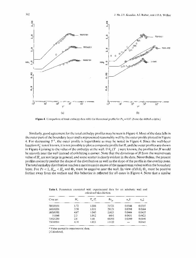
Direct comparisons of the present self-similar profiles were carried out for available experimental data sets, where the total enthalpy was measured directly for an adiabatic wall, and are shown in Figures 3 and 4 for the cases listed in Table 1. In these comparisons, a value ofPr t = 0.87 was used; this value is consistent with accepted values for Pr t at subsonic speeds and is the value predicted by the analysis of He et al. (1995) in the low supersonic range. The majority of the data is taken from the compilation of data by Fernholz and Finley (1977) and the identification scheme for each profile used there is also repeated here; the one exception corresponds to recent data from Carvin (1988), which is identified in Table 1 as f-1048. For each data set, the velocity and total enthalpy profiles nearest the end of the test section were selected, since these were expected to be closest to self-similar conditions. Unfortunately, it is not possible to ascertain how close each situation is to an equilibrium flow; in addition, it is difficult to assess the degrees to which the wall is truly adiabatic. Nevertheless, the results of the direct comparisons for velocity are shown in Figure 3, and it may be seen that the representation of the velocity profiles in Figure 3 are quite good over the entire range of Mach numbers listed in Table 1; note that the plotted profiles are composite containing the inner- and outer-layer contributions. In addition, the computed values of u, are relatively close to the quoted experimental values; note that quoted experimental values (Fernholz and Finley, 1977) were often inferred by various indirect means rather than a true measurement.

N- N

o • 55030301 C~"

, 58030201

58030101

U + (:3" U ÷ o "

73021203

+i; o 10 10 a 10 + 104 y+

73010501

O "

i i i ' + " 1 1 1 + ~ n i I I n N l ' ~ I I l l l l l I [ ~ i i i i b L ~ i i 1 1 1 1 4 I

l O t 1 0 a lb' lO' y÷

(a) (b)

Figure 3. Comparison of velocity profile data with the theoretical profile. (Note the shifted origins.)


0

Q P l

H/H~ ~-

°7

0

~h g.

58030301

58030201

58030101

°i ,,.41 73010501

2- °

H,Ho ,-1048

i I I I I 1~110 ' I I J I I I I 01 2 I I I I I J l l 110 3 I I I I I I I I I 10 ~ I I I ~ l l [ l t 1Q {l I I I I IH I [ [ } I I I ~11111 10 2 I I ~ l J I I I I 1~ 3 I I I I l l l l l 10 4 I E I I I I I I I

y+ y+

(a) (b)

Figure 4. Comparison of total enthalpy data with the theoretical profile for P r t = 0.87. (Note the shifted origins.)

Similarly, good agreement for the total enthalpy profiles may be seen in Figure 4. Most of the data falls in the outer part of the boundary layer and is represented reasonably well by the outer profile plotted in Figure 4. For decreasing Y+, the outer profile is logarithmic as may be noted in Figure 4. Since the wall-layer function 0 + is not known, it is not possible to plot a composite profile for H, and the outer profiles are shown in Figure 4 joining to the value of the enthalpy at the wall. If 0~ (Y ÷) were known, the profiles for H would be smooth near the wall instead of exhibiting a corner. Note that the diviations of H from the mainstream value of H e are not large in general, and some scatter is clearly evident in the data. Nevertheless, the present profiles correctly predict the shape of the distribution as well as the slope of the profile in the overlap zone. The total enthalpy distribution reaches a maximum (in excess of the mainstream value) within the boundary layer. For Pr < 1, Haw < H e and ®1 must be negative near the wall. In view of (8.6), O 1 must be positive further away from the surface and this behavior is reflected for all cases in Figure 4. Note that a similar

Table 1, Parameters associated with experimental data for an adiabatic wall and calculated skin friction.

Case no. Me Tw/Tr Re®, u, t u,~

58030101 1.72 1.006 31521 0.0346 0.0355 58030201 3.56 1.031 29121 0.0398 0.0384 58030301 4.67 1.045 13621 0.0444 0.0433

51048 2.3 1.012 6451 0.0431 0.0423 73021203 2.8 1.00 66393 0.0380 0.0346 73010501 4.78 1.021 11122 - - 0.0445

"~ Value quoted in experimental data. Calculated,

A M o d e l for Adiabat i c Supersonic Turbulent B o u n d a r y Layers 363

0 l / / o. //

, / /

u/U. o

c5

/ / -

, / ,/

! : / _ _ . M e = 0 . 2

. . . . . M e = 2 . 0

. . . . . . M e = 5 . 0

. . . . . M e = 8 . 0

H /H~

co

- - M e = l . 0

~ M e = 2 . 0

~ ~ ~ Me=5.0

M e = 8 . 0

i i i i i ' ~ ' ~ J 0.00 0.40 O.BO 120

0.00 0.40 0,80 1 2, y16 Wa

Figure5 . Var ia t ion of the ve loc i ty profile with M r for F igure6 . Var ia t ion of the total enthalpy profile with Mo for Re6, = 10,000. Re6, = 10,000 a n d P r t = 0.87.

profile behavior, with overshoot near the mainstream, occurs in laminar compressible boundary layers (see, for example, Schetz, 1984, p. 100). Lastly, it should be emphasized that the theoretical profiles shown in Figures 3 and 4 are predicted results and that the comparisons have not been enhanced through adjustement of any model parameters.

9. Summary and Conclusions

A theory describing the influence of mean viscous dissipation in supersonic turbulent boundary layers has been developed. Utilizing simple algebraic turbulence models, calculated profiles have been shown to agree well with measured experimental data for velocity and total enthalpy. The variation of the self-similar profiles with Mach number can be seen in Figures 5 and 6 for a fixed value of R%.. The trends shown in these figures are similar for other values of R%.. Note that only the outer profile for total enthalpy is plotted in Figure 6. It is evident that with increasing Me, the wall layer occupies an increasing percentage of the boundary layer. In addition, H exceeds the mainstream value over an increasing portion of the boundary layer as M e increases.

Much of the present theory is general, but even the specific turbulence model for total enthalpy described here should be applicable in prediction methods for a wider class of two-dimensional adiabatic flows (including those with pressure gradient). At the same time, simple algebraic models are known to be deficient when complex effects, such as relaminarization, occur and, in such situations, more complicated closure schemes may need to be considered.

Appendix

Here it is demonstrated that a simple outer eddy conductivity model cannot adequately represent the turbulent heat flux near the wall layer for an adiabatic wall. It follows from (4.4) and (4.5) that for the special


case of a self-similar solution {~1 ----- ~)l(t]) ,

0q P°u*HeF(AorUe)'+... as t/--* 0. (A.1)

&/ ~c.r

U p o n integration and using (5.7) and the fact that qw = 0 for an adiabatic wall, it follows that

q 2p°u*He(AorUe)'(1--Iaw)rl+... as q ~ 0 . (A.2) gr

Since Iaw< 1, in general, and (AoUe)' > 0 for a flat plate boundary layer, it follows that the total flux q is negative for small t/. Consequently, it is clear that if an attempt is made to model the turbulent flux in the outer layer with a simple eddy conductivity of the form (7.5), then en would have to be negative for small r /and also quadratic in t/. Formulae of this nature were not considered to be physically appealing and although several were tried, it was not possible to find one which gave satisfactory outer-layer representa- tions for H.

Since the model (7.5) is not suitable, consider a model of the form

OH ~?u q = P~H ~n + Bpeu ~n' (A.3)

where B is a function to be determined and for an adiabatic wall must be selected so that q ~ 0 as r /~ 0. A conventional choice for the eddy conductivity model in the outer layer is a constant turbulent Prandtl number model defined in terms of the eddy viscosity e by en = e/Pr t. Upon substitution of (2.1), (4.1), (4.5), (7.1) into (A.3), it may be readily verified that

B = 2(1 - l a w ) H e P r t U 2 , (1.4)

in order that q ~ 0 as t / ~ 0.

Re ferences

Baldwin, B.S., and Lomax, H. (1978), Thin-Layer Approximation and Algebraic Model for Turbulent Separated Flows, AIAA Paper 78-257.

Barnwell, R.W., and Wahls, R.A. (1989), A Skin Friction Law for Compressible Turbulent Flow, AIAA Paper 89-1864. Carvin, C. (1988), Etude experimentale d'une couche limite turbulente supersonique fortement chauffee, Ph.D. Thesis, Universit6 d'Aix

Marseille. Cebeci, T., and Smith, A.M.O. (1974), Analysis of Turbulent Boundary Layers, Academic Press, New York. Degani, A.T., and Walker, J.D.A. (1993), Computation of three-dimensional turbulent boundary layers using the embedded function

method, J. Comput. Phys., 109, 202-214. Degani, A.T., Walker, J.D.A., Ersoy, S., and Power, G. (1991), On the Application of Algebraic Turbulence Models to High Mach

Number Flows, AIAA Paper 91-0616. Degani, A.T., Smith, F.T., and Walker, J.D.A. (1992), The three-dimensional turbulent boundary layer near a plane of symmetry, J.

Fluid Mech., 234, 329-360. Degani, A.T., Smith, F.T., and Walker, J.D.A. (1993), The structure of a three-dimensional turbulent boundary layer, J. Fluid Mech.,

250, 43-68. Fernholz, H.H., and Finley, PJ. (1977), A Critical Compilation of Compressible Turbulent Boundary Layer Data, AGARD-AG-223. Fernholz, H.H., and Finley, P.J. (1980), A Critical Commentary on Mean Flow Data for Two-Dimensional Compressible Turbulent

Boundary Layers, AGARD-AG-253. He, J., and Walker, J.D,A. (1995), A note on the Baldwin-Loxam model, Trans. ASME J Fluids Engrg., 117, 528-531. He, J., Kazakia, J.Y., and Walker, J.D.A. (1995), An asymptotic two-layer model for supersonic turbulent boundary layers, J. Fluid

Mech., 295, 159-198. Johnson, D.A., and King, LS. (1985), A mathematically simple turbulence closure model for attached and separated turbulent

boundary layers, AIAA J., 23, 1684-1692. Schetz, J.A. (1984), Foundation of Boundary Layer Theory for Momentum, Heat and Mass Transfer, Prentice-Hall, New York. Stewartson, K. (1964), The Theory of Laminar Boundary Layers in Compressible Fluids, Oxford University Press, Cambridge. Van Driest, E.R. (1951), Turbulent boundary layer in compressible fluids, J. Aeronaut. Sci., 18, 145-161. Yuhas, L.J., and Walker, J.D.A. (1982), An Optimization Technique for the Development of Two-Dimensional Steady Turbulent

Boundary-Layer Models, Report FM-1, Department of Mechanical Engineering, School of Engineering, Lehigh University; also AFOSR-TR-0417.

A model for adiabatic supersonic turbulent boundary layers

Documents

Transcript of A model for adiabatic supersonic turbulent boundary layers