On the Influence of Nozzle Geometries on Supersonic Curved ...

On the Influence of Nozzle Geometries on Supersonic Curved

Wall Jets

A THESIS SUBMITTED TO THE UNIVERSITY OF MANCHESTER FOR THE DEGREE OF DOCTOR OF PHILOSOPHY IN THE

FACULTY OF SCIENCE AND ENGINEERING

2017

By Bradley Robertson-Welsh

School of Mechanical, Aerospace and Civil Engineering

2

Table of Contents

Table of Contents ..................................................................................................................... 2

Table of Figures ........................................................................................................................ 6

Table of Tables ....................................................................................................................... 16

Glossary of Terms................................................................................................................... 17

Acronyms ........................................................................................................................... 17

Parameters ......................................................................................................................... 18

Abstract .................................................................................................................................. 22

Declaration ............................................................................................................................. 23

Copyright Statement .............................................................................................................. 24

Chapter 1 Introduction ....................................................................................................... 25

Chapter Overview .............................................................................................................. 25

1.1 Fluidic Flight Control .............................................................................................. 26

1.1.1 Trailing Edge Circulation Control ................................................................... 28

1.1.2 Fluidic Thrust Vectoring ................................................................................. 29

1.2 Thesis Aim and Objectives ..................................................................................... 31

Chapter 2 Circulation Control ............................................................................................. 32


2.1 Boundary and Shear Layers ................................................................................... 33

2.2 The Coanda Effect .................................................................................................. 35

2.3 Wing Trailing Edge Circulation Control .................................................................. 38

2.4 Effect of Geometry ................................................................................................. 40

2.5 Importance of Mass Flow ....................................................................................... 43

2.6 Summary ................................................................................................................ 44

Chapter 3 Supersonic Curved Wall Jets .............................................................................. 45

3


3.1 Introduction to Supersonic Curved Wall Jets ......................................................... 46

3.1.1 Supersonic Jets ............................................................................................... 46

3.1.2 Isentropic Relations ....................................................................................... 47

3.1.3 Supersonic Flow Interactions ......................................................................... 48

3.1.4 Convergent-Only Nozzles ............................................................................... 51

3.1.5 Convergent-Divergent Nozzles ...................................................................... 53

3.1.6 The Method of Characteristics ....................................................................... 59

3.1.7 Supersonic Curved Wall Jet ............................................................................ 63

3.2 Effect of Nozzle Geometry on Supersonic Curved Wall Jets in Quiescent Air ....... 66

3.2.1 Convergent-Only Nozzles ............................................................................... 66

3.2.2 Symmetrical Convergent-Divergent Nozzles ................................................. 70

3.2.3 Irrotational Vortex and Asymmetric Convergent-Divergent Nozzles ............ 72

3.2.4 Summary of Nozzle Geometries .................................................................... 83

3.3 Effectiveness Metrics for Supersonic Curved Wall jets ......................................... 86

3.4 The Effect of Free-Stream ...................................................................................... 88

3.5 Proposed Study ...................................................................................................... 89

Chapter 4 Supersonic Curved Wall Jet Detachment: Research Methods........................... 91


4.1 Objectives............................................................................................................... 92

4.2 Apparatus ............................................................................................................... 93

4.2.1 Test Rig ........................................................................................................... 93

4.2.2 Nozzles ........................................................................................................... 94

4.2.3 Optical Apparatus ........................................................................................ 100

4.2.4 Pressure Transducers ................................................................................... 101

4.3 Combined Shadowgraph and Schlieren ............................................................... 115

4.3.1 Introduction ................................................................................................. 116

4

4.3.2 Experimental Setup ...................................................................................... 120

4.3.3 Experimental Procedure .............................................................................. 123

4.3.4 Post-Processing ............................................................................................ 124

4.4 Pressure Sensitive Paint ....................................................................................... 128

4.4.1 Introduction ................................................................................................. 128

4.4.2 Experimental Setup ...................................................................................... 129

4.4.3 Experimental Procedure .............................................................................. 131

4.4.4 Post-Processing ............................................................................................ 132

4.4.5 Uncertainty Analysis .................................................................................... 134

Chapter 5 Supersonic Curved Wall Jet Detachment: Results and Analyses ..................... 136

Chapter Overview ............................................................................................................ 136

5.1 Flow physics of supersonic curved wall jet detachment ..................................... 137

5.1.1 H/R 0.1 ......................................................................................................... 137

5.1.2 H/R 0.15 ....................................................................................................... 148

5.1.3 H/R 0.2: NPRD 3 ........................................................................................... 158

5.1.4 H/R 0.2: NPRD 4 ........................................................................................... 164

5.1.5 Summary of Separation Mechanism ............................................................ 174

5.2 Comparison with Method of Characteristics ....................................................... 183

5.3 The Need for Adaptive Nozzles ............................................................................ 186

5.3.1 Maintaining Attachment .............................................................................. 186

5.3.2 Improving Efficiency ..................................................................................... 190

5.3.3 Improving Effectiveness ............................................................................... 192

Chapter 6 Conclusions and Future Work .......................................................................... 195

6.1 Conclusions .......................................................................................................... 196

6.1.1 On the state of the art of circulation control ............................................... 196

6.1.2 On experimental techniques used to observe supersonic curved wall jet

separation .................................................................................................................... 197

6.1.3 On the flow physics of supersonic curved wall jets ..................................... 197

5

6.1.4 On the method of characteristics as a tool for predicting supersonic curved

wall jet behaviour ........................................................................................................ 199

6.1.5 On the need for adaptive nozzles for supersonic circulation control .......... 200

6.2 Future Work ......................................................................................................... 201

6.2.1 Development of a low order analytical model capable of predicting

circulation control performance on a wide range of planforms .................................. 201

6.2.2 Augmenting morphing trailing edges with mid-chord blowing ................... 201

References ........................................................................................................................... 202

Appendix A: Semi-Empirical Model for Sizing Circulation Control Effectors ....................... 207

A.1 Introduction ......................................................................................................... 207

A.2 Sizing of Circulation Control Effectors ................................................................. 208

A.2.1 Determination of the NPR ............................................................................ 210

A.2.2 Modification of Lanchester-Prandtl Lifting Line Theory .............................. 213

A.2.3 Determination of Momentum Coefficient from 2D Lift Coefficient ............ 215

Appendix B: Shadowgraph Boundary Layer Measurement ................................................ 225

B.1 Introduction, Limitations and Conclusions .......................................................... 225

B.2 Post Processing Methodology .............................................................................. 226

B.3 Results and Discussion ......................................................................................... 227

Appendix C: Publications and Contributions outside the Scope of this Thesis ................... 230

C.1 Participation on NATO AVT 239 ........................................................................... 230

C.2 Structural Health Monitoring ............................................................................... 230

C.3 MFC Morphing Between Contours ...................................................................... 231

Word count: 52,584

6

Table of Figures

Figure 1.1 Effect of plain flap deflection on lift coefficient. Adapted from(Anderson 2007) 26

Figure 1.2 Schematic of a Eurofighter Typhoon with conventional control surfaces

highlighted. Manoeuvring is achieved through deflecting control surfaces so as to induce

moments about the x, y and z axis. The canards, or foreplanes control pitch (rotation about

the y-axis), the rudder controls yaw (rotation about the z-axis) and ailerons control roll

(rotation about the x-axis). Adapted from (Eurofighter Jagdflugzeug GmbH 2013) ............. 27

Figure 1.3 Supersonic circulation control implementation. Taken from (Chard et al. 2013).28

Figure 1.4 Schematic of FTV Methods. (a) corresponds to coflow, where injecting secondary

air serves to attach the exhaust jet to the reaction surface. (b) represents normal blowing

FTV, where air is injected along the reaction surface and serves to separate the flow. ....... 30

Figure 1.5 FTV using a 2D reaction surface to control pitch (a), and using a scarfed, 3D

reaction surface to control pitch and yaw (b). Taken from (Jegede 2016) ............................ 30

Figure 2.1 Boundary layer growth and transition from laminar to turbulent. Adapted from

(Groh 2016). ........................................................................................................................... 33

Figure 2.2 A subsonic free jet (neglecting viscosity upstream of orifice exit). As the jet exits

the orifice, the potential core undergoes a rapid decay due to transfer of momentum to the

ambient air via a shear layer. With increasing distance from the orifice exit, the jet spreads

out and slows down. Adapted from (Jegede 2016) and (Llopis-Pascual 2016) ..................... 35

Figure 2.3 Curved wall jet showing initial attachment, development of boundary layer and

separation due to adverse stream-wise pressure gradient. The attachment (and separation)

of the jet can be described by Equation 2-4. ......................................................................... 36

Figure 2.4 Subsonic circulation control aerofoil. Adapted from (Michie 2008) and (Englar

1975) ...................................................................................................................................... 39

Figure 2.5 Empirical graph showing previous area of desired operation (yellow) from Englar

(1974) and new area of desired operation (red) following the FLAVIIR project. From (Michie

2008) ...................................................................................................................................... 41

Figure 2.6 Momentum coefficient vs radius to chord ratio for major historical circulation

control studies, colour coordinated by decade. Constructed from (Englar 1970; Englar &

Williams 1971; Englar 1975; Loth et al. 1976; Englar & Huson 1983; Englar et al. 1981;

Abramson & Rogers 1983; Wilkerson & Montana 1982; Mclachlan 1989; Shah et al. 2008;

Frith & Wood 2003; Cagle & Jones 2002; Jones et al. 2003; Schlecht & Anders 2007; Sparks

et al. 2005; Crowther et al. 2009). Note that flight demonstrations took place in 1974 and

7

1979 but were only published in 1976 and 1983 respectively in (Loth et al. 1976) and

(Englar & Huson 1983). .......................................................................................................... 42

Figure 3.1 Supersonic free jet (neglecting viscosity upstream of orifice exit). Relative to the

subsonic jet shown in Figure 2.2, a supersonic jet undergoes a much more gradual decay of

the potential core. This is due to the Mach angle limiting the development of span-wise

mixing structures such as vortices. Adapted from (Rajaratnam 1976). ................................ 47

Figure 3.2 Simplified diagrams representing the formation expansion fan (left) and shock

waves (right) as typically caused by surface interactions. From (Anderson 2007) ............... 49

Figure 3.3 Simplified shock reflections from a solid boundary. From (Anderson 2007) ....... 49

Figure 3.4 Shock reflections from a free-stream boundary. From (Anderson 2007) ............ 50

Figure 3.5 Shock induced boundary layer separation. Adopted from (Anderson 2007) ....... 51

Figure 3.6 Schematic of a convergent-divergent nozzle ........................................................ 53

Figure 3.7 Quasi-one-dimensional flow through a tube. Adapted from (Anderson 2007) ... 53

Figure 3.8 Combined shadowgraph and schlieren images of convergent-divergent nozzle. In

all cases, a normal shockwave is present in the divergent section of the nozzle (indicated by

a vertical black/magenta line). As the NPR is increased, the shockwave moves further

toward the nozzle exit (right edge of each image). The green region is a region of expansion

occurring around the throat. For more information on combined shadowgraph and

schlieren imaging, see Section 4.3. ........................................................................................ 56

Figure 3.9 The operating conditions of free jets issuing from convergent-divergent nozzles.

In the upper-left image, oblique shockwaves (labelled ‘OS’) form at both sides of the nozzle

exit as the static pressure at the exit is lower than ambient. In the upper-centre image, the

static pressure at the nozzle exit is equal to ambient, consequently there are no waves and

the nozzle is operating at its correctly expanded condition. The shear layer in this image is

denoted ‘SL’. In the upper-right image, the static pressure at the nozzle exit is greater than

ambient, consequently, expansion forms at the exit from both sides (denoted ‘EF’). The

lower three images correspond to the same NPR as the upper three, however the

asymmetrical nozzle causes an exit static pressure profile such that the static pressure at

the lower side is always lower than the upper. ..................................................................... 57

Figure 3.10 The operating conditions of wall jets issuing from convergent-divergent nozzles.

The six schematics are directly comparable with Figure 3.9; however the addition of the

wall has prevented any pressure difference occurring on the lower side of the nozzle exit.

Consequently, there are no waves propagating from the lower side, except those reflected

8

from the other side. The major consequence of this is the lower-left image, where the case

of NPR < NPRd for the asymmetrical nozzle results in a correctly expanded jet. ................. 58

Figure 3.11 Implemented method of characteristics for a convergent-divergent nozzle.

Taken from (Anderson 2007) ................................................................................................. 60

Figure 3.12 Schlieren image with method of characteristics overlaid. Taken from (Ashley

2012) ...................................................................................................................................... 62

Figure 3.13 Method of characteristics simulation of supersonic curved wall jet from a

symmetrical convergent-divergent nozzle (exit is located at 0 degrees, Mach number is

1.43). Regions are labelled as the nozzle dependence region (1), expansion region (2), free

surface region (3), and compression region (4) (Ashley 2012). The surface pressure

distribution of the supersonic curved wall jet, adapted from (Jegede 2016), shows the

propagation of favourable and adverse pressure gradients. ................................................ 64

Figure 3.14 Schlieren images of supersonic curved wall jets obtained for different nozzle

geometries. Image (a) is a convergent-only nozzle from (Gregory-Smith & Gilchrist 1987);

image (b) is convergent-only stepped nozzle from (Gregory-Smith & Senior 1994); Image (c)

is a symmetrical convergent-divergent nozzle from (Llopis-Pascual 2016) and image (d) is an

asymmetrical convergent-divergent nozzle from (Ashley 2012). .......................................... 66

Figure 3.15 Experimental setup of variable slot height convergent-only study (Gregory-

Smith & Gilchrist 1987) .......................................................................................................... 67

Figure 3.16 Separation NPR plotted against H/R for a convergent only slot. Note, in its

original format the graph was plotted as stagnation pressure ratio (i.e. 1/NPR) against H/R.

It has been adapted for this study from (Gregory-Smith & Gilchrist 1987). ......................... 68

Figure 3.17 Schlieren image of shock induced boundary layer separation on a curved wall

jet. Note that the incident shockwave is actually caused by a reflected expansion fan, which

in turn is caused by a gap at the nozzle exit. Adapted from (Chippindall 2009). .................. 70

Figure 3.18 Experimental setup for convergent-divergent study performed in (Cornelius &

Lucius 1994) ........................................................................................................................... 71

Figure 3.19 Supersonic curved wall jet detachment. From (Chippindall 2009) ..................... 72

Figure 3.20 Irrotational vortex theory. Creating an irrotational velocity profile creates an

irrotational vortex which can be matched to a contour. The end result is no stream-wise

pressure gradients on the surface. Taken from (Ashley 2012) .............................................. 73

Figure 3.21 Method of characteristics simulation of a curved wall jet issuing from an

irrotational vortex nozzle. Note the complete absence of any stream-wise pressure

gradients in the lower image (Jegede 2016). Reconsidering the supersonic curved wall jet

9

discussed in Figure 3.13, the effect of the irrotational vortex nozzle is the conditioning of

the nozzle dependence region to match the expected secondary wave structure caused by

the reaction surface. .............................................................................................................. 74

Figure 3.22 Comparison of Mach exit profiles for (Ashley 2012), irrotational vortex and

symmetrical nozzles ............................................................................................................... 79

Figure 3.23 Comparison of nozzle contours for (Ashley 2012), irrotational vortex and

symmetrical nozzles. .............................................................................................................. 80

Figure 3.24 Method of characteristics simulation of the (Ashley 2012) nozzle. Compared to

Figure 3.13, the stream-wise pressure gradients are much reduced relative to the

symmetrical curved wall jet, but are not eliminated. ............................................................ 81

Figure 3.25 Area ratio distribution for the (Ashley 2012), irrotational vortex, and

symmetrical nozzles. Equivalent symmetrical nozzle design nozzle pressure ratio is shown in

the legend. ............................................................................................................................. 83

Figure 3.26 Separation nozzle pressure ratio vs H/R for different nozzle geometries. Note

that red crosses are convergent-only nozzles; convergent-divergent nozzles are

appropriately labelled, with symmetrical nozzles identified by their design NPR (NPRD), and

asymmetrical nozzles identified by their correctly expanded NPR (CENPR). Constructed

from (Bevilaqua & Lee 1980; Gregory-Smith & Gilchrist 1987; Lytton 2006; Chippindall

2009; Ashley 2012; Jegede 2016; Llopis-Pascual 2016) ......................................................... 84

Figure 3.27 Normalised momentum efficiency for various nozzle geometries. All

momentums are normalised to a convergent-only nozzle operating at NPR 2. ................... 88

Figure 4.1 Schematic of air supply ......................................................................................... 93

Figure 4.2 Area ratio distribution of adjusted asymmetrical nozzles .................................... 94

Figure 4.3 exit Mach number distribution of adjusted nozzles ............................................. 95

Figure 4.4 Symmetrical and Asymmetrical nozzle contours designed for H/R = 0.1, design

NPR = 3 ................................................................................................................................... 96


NPR = 3 ................................................................................................................................... 96


NPR = 3 ................................................................................................................................... 97

Figure 4.7 Symmetrical and Asymmetrical nozzle contours designed for H/R = 0.2, NPR = 4

............................................................................................................................................... 97

Figure 4.8 Full assembly of 3D SLA printed nozzle section (AIV1HR02NPR3) with Perspex

side-walls and aluminium backing plate ................................................................................ 98

10

Figure 4.9 Nozzle section (SYM1HR01) and side view schematic showing pressure tap

locations. Design modified from (Afilaka 2017) to eliminate discontinuities at the nozzle

exit. ........................................................................................................................................ 99

Figure 4.10 Schematic of the setup of pressure transducers .............................................. 102

Figure 4.11 Pressure variation from pressure tap: P7 for nozzle: SYM1HR015. Separation is

clearly indicated by a sharp rise in pressure. Applying a median filter (red) and finding the

derivative (yellow) allows the automatic calculation of the time at which the flow

separates. ............................................................................................................................. 104

Figure 4.12 Variation in time of separation of P3-P14 for SYM1HR015 .............................. 105

Figure 4.13 Example image of pressure coefficients overlaid on the combined schlieren and

shadowgraph image ............................................................................................................. 106

Figure 4.14 Schematic showing force components at each pressure tap along the reaction

surface .................................................................................................................................. 108

Figure 4.15 Example calibration curve for transducer P1 .................................................... 110

Figure 4.16 Example surface pressure coefficient distribution plot for the H/R 0.15 nozzles

operating at NPR 3. Small error bars are indicative of good accuracy ................................ 111

Figure 4.17 Vertical Force Coefficient plotted against NPR for three repeats of

SYM1HR02NPR3 ................................................................................................................... 112

Figure 4.18 Typical NPR measurement taken during an experiment. Also shown are the

resampled maximum, minimum and mean values (25Hz). ................................................. 113

Figure 4.19 Noise to signal ratio .......................................................................................... 114

Figure 4.20 Fast Fourier Transform of Noise to signal ratio, with the frequency at which

likely sources of noise occurs also highlighted by red dashed lines. Note the absence of a

clear peak suggests broadband noise. ................................................................................. 114

Figure 4.21 Example vertical force coefficient against NPR plot, including the 25Hz

resampled maximum and minimum NPR (as dashed lines) so as to account for potential

unsteadiness. ....................................................................................................................... 115

Figure 4.22 Simplified schematic of shadowgraph. Light emitted from a point source is

focussed by the lens, and upon interacting with a soap bubble is refracted. The effect of

shadowgraph is an image consisting of lower intensity at the source of the refraction, and a

higher intensity at an offset distance (Δa) in the direction of the refraction. In the image to

the right, the outer diameter of the black circle corresponds to the diameter of the soap

bubble. Adapted from (Settles 2001). ................................................................................. 117

11

Figure 4.23 Schematic showing the schlieren technique using an extended light source.

Note that the knife edge reduces the intensity of the image at the point of refraction, but

does not cut the image out completely. The reduction in intensity is a function of the

refraction angle (Ɛ), which is proportional to a first order spatial density gradient (Equation

4-8). Adapted from (Settles 2001). ...................................................................................... 118

Figure 4.24 Typical schlieren image of a separated supersonic curved wall jet, taken from

(Llopis-Pascual 2016). .......................................................................................................... 119

Figure 4.25 Setup of combined schlieren and shadowgraph experiment ........................... 121

Figure 4.26 Snapshot images of test-card from Schlieren (left) and shadowgraph (right)

setup .................................................................................................................................... 122

Figure 4.27 Typical NPR variation during course of experiment ......................................... 124

Figure 4.28 Schematic showing the process of combining shadowgraph and schlieren

images. Note that in the final image, expansion fans are identified as green regions, and

areas of compression are highlighted in magenta............................................................... 126

Figure 4.29 Combined shadowgraph and schlieren image with key flow features labelled

(discussed in text) ................................................................................................................ 127

Figure 4.30 Schematic showing polymer, or conventional PSP (left) and porous PSP (right).

Luminophores are excited by light of a specific wavelength. The excitation causes an

emission of light which is inversely proportional to the partial pressure of oxygen (hence,

static pressure). Taken from (Quinn et al. 2011) ................................................................. 129

Figure 4.31 Pressure Sensitive Paint experiment setup. Note that the PSP is applied to the

opaque side wall on the side closest to the camera. ........................................................... 130

Figure 4.32 Typical NPR variation during pressure sensitive paint experiment. Separation is

indicated by a red cross, and the start/stop positions of the extracted video are indicated

by black circles. .................................................................................................................... 132

Figure 4.33 PtTFPP calibration curve from (Sakaue 2003), compared to reference pressure

and image intensity taken for each PSP image. Note that crosses correspond to PSP images

of attached flow, and circles represent PSP images following separation. ......................... 133

Figure 4.34 Schematic showing pressure sensitive paint post-processing and calibration . 134

Figure 4.35 Calibrated pressure sensitive paint image following separation. Thermal echo of

previously attached jet is still visible close to reaction surface, with an apparent pressure of

0.7bar ................................................................................................................................... 135

Figure 5.1 H/R 0.1 nozzles operating at an approximate NPR of 2.5. .................................. 137

Figure 5.2 H/R 0.1 nozzles operating at an approximate NPR of 3 ...................................... 138

12

Figure 5.3 Surface pressure distribution for SYM1HR01 and AIV1HR01 operating at an NPR

of 3 ....................................................................................................................................... 139

Figure 5.4 H/R 0.1 nozzles before separation ...................................................................... 140

Figure 5.5 Surface pressure distribution for SYM1HR01 and AIV1HR01 immediately prior to

separation ............................................................................................................................ 140

Figure 5.6 High speed Schlieren images showing the propagation of the point of separation

upstream. Time between frames (a) and (d) is 0.025 seconds ........................................... 141

Figure 5.7 Pressure sensitive paint image of SYM1HR01 before separation. The colour scale

to the right of the image shows the range of relative pressures, with red representing

relatively high pressure, and blue representing relatively low pressure. ........................... 142

Figure 5.8 Pressure sensitive paint image of SYM1HR01 following separation. The colour

scale to the right of the image shows the range of relative pressures, with red representing


Figure 5.9 H/R 0.1 nozzles immediately following separation ............................................ 144

Figure 5.10 H/R 0.1 nozzles before reattachment ............................................................... 145

Figure 5.11 H/R 0.1 nozzles after reattachment .................................................................. 145

Figure 5.12 Vertical force coefficient of SYM1HR01 and AIV1HR01 across a range of

ascending NPRs. Error range previously discussed in Section 4.2.4 is also shown .............. 146

Figure 5.13 Vertical force coefficient of SYM1HR01 and AIV1HR01 across the full range of

NPRs tested in the experiment. ........................................................................................... 147

Figure 5.14 H/R 0.15 nozzles operating at approximately NPR 2.5 ..................................... 149

Figure 5.15 H/R 0.15 nozzles operating at an NPR of approximately 3 ............................... 150

Figure 5.16 Surface pressure profiles for SYM1HR015 and AIV1HR015 operating at an NPR

of approximately 3 ............................................................................................................... 150

Figure 5.17 H/R 0.15 nozzles before separation .................................................................. 151

Figure 5.18 Surface pressure profiles of SYM1HR015 and AIV1HR015 immediately before

separation ............................................................................................................................ 151

Figure 5.19 H/R 0.15 nozzles immediately following separation ........................................ 152

Figure 5.20 Pressure sensitive paint image of SYM1HR015 before separation The colour



Figure 5.21 Pressure sensitive paint image of SYM1HR015 following separation. The colour



13

Figure 5.22 H/R 0.15 nozzles before reattachment ............................................................. 154

Figure 5.23 H/R 0.15 nozzles after reattachment ................................................................ 155

Figure 5.24 Vertical force coefficient of SYM1HR015 and AIV1HR015 across a range of

ascending NPRs. Error range previously discussed in Section 5.6.2 is also shown .............. 156

Figure 5.25 Vertical force coefficient of SYM1HR015 and AIV1HR015 across the full range of

NPRs tested in the experiment. ........................................................................................... 157

Figure 5.26 H/R 0.2, NPR 3 nozzles operating at approximately NPR 2.5 ........................... 158

Figure 5.27 H/R 0.2, NPR 3 nozzles immediately before full separation ............................. 159

Figure 5.28 Surface pressure distribution for SYM1HR02NPR3 and AIV1HR02NPR3 at the

onset of separation (pressure tap P6 for AIV1HR02NPR3 was omitted due to blockage) .. 160

Figure 5.29 Surface pressure distribution for SYM1HR02NPR3 and AIV1HR02NPR3 at NPR 3

(pressure tap P6 for AIV1HR02NPR3 was omitted due to blockage) .................................. 160

Figure 5.30 H/R 0.2, NPR 3 nozzles immediately following separation ............................... 161

Figure 5.31 H/R 0.2, NPR 3 nozzles before reattachment ................................................... 161

Figure 5.32 H/R 0.2, NPR 3 nozzles following reattachment ............................................... 162

Figure 5.33 Vertical force coefficient of SYM1HR02NPR3 and AIV1HR02NPR3 across a range

of ascending NPRs. Error range previously discussed in Section 5.6.2 is also shown ......... 163

Figure 5.34 Vertical force coefficient of SYM1HR02NPR3 and AIV1HR02NPR3 across the full

range of NPRs tested in the experiment. ............................................................................. 163

Figure 5.35 H/R 0.2, NPR 4 nozzles operating at approximately NPR 2.5 ........................... 165

Figure 5.36 H/R 0.2, NPR 4 nozzles before full separation .................................................. 166

Figure 5.37 Surface pressure distribution for SYM1HR02NPR4 and IV1HR02NPR3 at the

onset of separation. ............................................................................................................. 166

Figure 5.38 Pressure sensitive paint image of SYM1HR02NPR4 before separation. The

colour scale to the right of the image shows the range of relative pressures, with red

representing relatively high pressure, and blue representing relatively low pressure. ...... 167

Figure 5.39 Pressure sensitive paint image of SYM1HR02NPR4 after separation. The colour



Figure 5.40 High speed Schlieren images showing the propagation of the point of

separation upstream. Time between frame (a) and (d) is approximately 0.03 seconds ..... 169

Figure 5.41 H/R 0.2 NPR 4 nozzles immediately following full separation .......................... 169

Figure 5.42 H/R 0.2, NPR 4 nozzles operating at approximately NPR 4 .............................. 170

Figure 5.43 H/R 0.2, NPR 4 nozzles before reattachment ................................................... 170

14

Figure 5.44 H/R 0.2, NPR 4 nozzles after reattachment ...................................................... 171

Figure 5.45 Vertical force coefficient of SYM1HR02NPR4 and IV1HR02NPR3 across a range

of ascending NPRs. Error range previously discussed in Section 5.6.2 is also shown ......... 172

Figure 5.46 Vertical force coefficient of SYM1HR02NPR4 and IV1HR02NPR3 across the full

range of NPRs tested in the experiment. ............................................................................. 173

Figure 5.47 Simplified schematic of wave interactions of a fully attached, overexpanded

supersonic curved wall jet. Arrows indicate the change in flow direction, with expansion

(green) and compression/shock waves (red) reflecting appropriately. .............................. 174

Figure 5.48 Simplified schematic of wave interactions of an underexpanded supersonic

curved wall jet showing the formation of a separation bubble. Arrows indicate the change

in flow direction, with expansion (green) and compression/shock waves (red) reflecting

appropriately. ...................................................................................................................... 175

Figure 5.49 Comparison of NPR 3 nozzles operating at NPR 3, with adverse pressure

gradients (A, B and C) occurring a similar linear distance from nozzle exit......................... 176


curved wall jet immediately prior to full separation. Arrows indicate the change in flow

direction, with expansion (green) and compression/shock waves (red) reflecting

appropriately. In this case, the reattachment point is about to move beyond the edge of the

reaction surface. .................................................................................................................. 177

Figure 5.51 Surface pressure distributions immediately prior to separation for all nozzle

geometries ........................................................................................................................... 177


curved wall jet immediately following full separation. Arrows indicate the change in flow


appropriately. In this case, the separation point has moved upstream to intersect the

expansion fan propagating from the nozzle exit ................................................................. 178

Figure 5.53 Combined Schlieren and shadowgraph images of SYM1HR01 (top) and

SYM1HR02NPR4 (bottom) immediately following separation ............................................ 179


curved wall jet immediately prior to reattachment. Arrows indicate the change in flow


appropriately. In this case, the separation point is about to move downstream as the jet

reattaches. ........................................................................................................................... 180

15

Figure 5.55 Illustration of how a larger distance between the free-stream boundary and

reaction surface translates to a longer shock cell ............................................................... 181

Figure 5.56 Correctly expanded surface pressure distributions for SYM1HR01 and

AIV1HR01, compared with the prediction from method of characteristics. ....................... 183

Figure 5.57 Correctly expanded surface pressure distributions for SYM1HR015 and

AIV1HR015, compared with the prediction from method of characteristics. ..................... 184

Figure 5.58 Correctly expanded surface pressure distributions for SYM1HR02NPR3 and

AIV1HR02NPR3, compared with the prediction from method of characteristics. .............. 184

Figure 5.59 Correctly expanded surface pressure distributions for SYM1HR02NPR4 and

IV1HR02NPR3, compared with the prediction from method of characteristics. ................ 185

Figure 5.60 Separation NPR vs A*/R for all nozzle geometries. Also plotted are the two

limits proposed by (Cornelius & Lucius 1994). Red circles represent convergent stepped

nozzles from (Gregory-Smith & Senior 1994), red crosses represent convergent-only nozzles

from (Gregory-Smith & Gilchrist 1987). Appropriate convergent-divergent nozzles have

been included from (Cornelius & Lucius 1994; Ashley 2012; Jegede 2016; Llopis-Pascual

2016). ................................................................................................................................... 188

Figure 5.61 Separation NPR vs A*/R for all convergent-divergent nozzles (appropriately

labelled). Black hexagons correspond to nozzles with unique exit to throat area ratios.

Other design NPRs are indicated by colour, with NPRd = 4 (red), NPRd = 3.6 (blue) and NPRd

= 3 (black) highlighted. Circles correspond to asymmetrical nozzles of equivalent area ratio,

stars correspond to symmetrical nozzles. In addition to results from this study, it is

constructed from (Cornelius & Lucius 1994; Ashley 2012; Jegede 2016; Llopis-Pascual 2016)

............................................................................................................................................. 189

Figure 5.62 Vertical force coefficient across a range of ascending NPRs for all symmetrical

nozzles tested ...................................................................................................................... 191

Figure 5.63 Vertical force coefficient across a range of ascending NPRs for all asymmetrical

nozzles tested ...................................................................................................................... 192

Figure 5.64 Normalised vertical force coefficient across a range of ascending NPRs for all

nozzles tested ...................................................................................................................... 193

Figure 5.65 Necessary A*/R to avoid separating across a range of operating NPRs ........... 194

16

Table of Tables

Table 4.1 Summary of nozzle geometries and their respective experiments ....................... 93

Table 4.2 Summary of camera properties. .......................................................................... 100

Table 4.3 Summary of camera settings used for each experiment ..................................... 101

Table 4.4 Summary of error sources for absolute pressure transducer .............................. 110

Table 4.5 Summary of error sources for differential pressure transducer .......................... 112

Table A.1 Predicted values and associated errors for the four empirical rules tested ........ 218

Table A.2 Mean error, standard deviation of the error and coefficient of determination (R2)

calculated for each of the four empirical rules tested ......................................................... 220

17

Glossary of Terms

Acronyms

A*/R Throat height to reaction surface radius ratio

AIV1HR01 Adjusted irrotational vortex nozzle designed with an H/R value

of 0.1 and for a design NPR value of 3

AIV1HR015 Adjusted irrotational vortex nozzle designed with an H/R value of 0.15 and for a design NPR value of 3

AIV1HR02NPR3 Adjusted irrotational vortex nozzle designed with an H/R value of 0.2 and for a design NPR value of 3

FTV Fluidic thrust vectoring

H/R Nozzle slot height to reaction surface radius ratio

IV1HR02NPR3 Irrotational vortex nozzle designed with an H/R value of 0.2 and for a design NPR of 4 (and with a correctly expanded NPR of 3)

M Mach number

NPR Nozzle pressure ratio

PSP Pressure sensitive paint

PtTFPP Platinum tetrakisPentaFluoroPhenyl Porphryn

RAM Random access memory

RANS Reynolds-averaged Navier-Stroke

RGB Red-Green-Blue (image)

SYM1HR01 Symmetrical convergent-divergent nozzle designed with an H/R value of 0.1 and for a design NPR of 3

SYM1HR015 Symmetrical convergent-divergent nozzle designed with an H/R value of 0.15 and for a design NPR of 3

SYM1HR02NPR3 Symmetrical convergent-divergent nozzle designed with an H/R value of 0.2 and for a design NPR of 3

SYM1HR02NPR4 Symmetrical convergent-divergent nozzle designed with an H/R value of 0.2 and for a design NPR of 4

UV Ultraviolet

18

Parameters

A Cross sectional area (m2)

a Speed of sound (ms-1)

Ax Nozzle cross sectional area at point x (m2)

A* Nozzle throat area (m2)

amb Subscript refers to ambient

C or c Depending on context can denote:

contour or shape of object wing cord

CL 3D lift coefficient

Cl 2D or section lift coefficient

𝐶𝑙,0 2D lift coefficient at zero angle of attack and zero blowing

Cp Pressure coefficient

𝐶𝜇 Momentum coefficient

Cz Vertical force coefficient

ds Infinitesimal section of the contour (m)

e Subscript denotes nozzle exit

FTotal Total force produced by the jet at the nozzle exit (due to momentum) or total force generated by the nozzle (N)

Fi Force component at the pressure tap ‘i’ (N)

Fz Total force in the z-direction (N)

H Nozzle slot height (m)

H/R Slot height to reaction surface or circulation control trailing edge ratio

IAtm Pixel intensity for region of PSP image subjected to atmospheric pressure

Iref Pixel intensity for region of PSP image subjected to reference pressure

j Subscript denote jet properties

𝐾+ Constant along any left-running Mach wave (C+)

𝐾− Constant along any right-running Mach wave (C-)

19

k Gladstone-Dale coefficient (0.23 cm3g-1 for air)

L Can denote, depending on context:

total lift force (N) thickness of the source of the refraction (m), in shadowgraph and

schlieren experiment representative shock cell length (m)

Li Length between pressure taps (m)

M Mach number

Me Mach number at nozzle exit

𝑀∞ Free-stream Mach number

�̇� Mass flow rate of tangentially blown air (kgs-1)

NPR Nozzle pressure ratio

NPRd Design NPR

NPRsep Nozzle pressure ratio at separation

n Refractive index of light for the shadowgraph and schlieren experiment

n0 Refractive index of light in ambient air

P Pressure (Pa)

PAtm Atmospheric pressure

Pamb Ambient pressure of the room (recorded during experiment)

PE Pressure at nozzle exit

PRef Reference pressure (for PSP image calibration)

𝑃0 Stagnation pressure of the jet during experiment (calculated from the NPR)

𝑃𝑦 Static pressure at vertical position y

pi Absolute pressure measured at the pressure tap ‘i’ (Pa)

𝑞∞ Dynamic free-stream pressure (Pa)

R can denote depending on context:

reaction surface radius gas constant (287 Jkg-1K-1 for dry air)

Re Reynolds number

𝑅𝑒∞ Free-stream Reynolds number

R/C Reaction surface to wing chord ratio

20

S Area of aerodynamic surface (m2)

T static temperature (K)

u Velocity component in x-direction (ms-1 )

V fluid velocity (ms-1 )

v Velocity component in y-direction (ms-1 )

𝑉∞ Free-stream velocity (m)

𝑉𝑗 Velocity of the jet (ms-1 )

𝑉𝑗�̇�𝑗 Jet momentum

W Reaction surface width of nozzle (6cm for all nozzle presented in the current study)

x Depending on context can denote:

x-direction or horizontal axis of the orthonormal coordinate system horizontal position (in mm) roll axis a single dimension in an arbitrary axis system

y Depending on context can denote:

y-direction or vertical axis of the orthonormal coordinate system vertical position (in mm) pitch axis

z Depending on context can denote:

z-direction yaw axis as subscript denote the position in the z-axis of the associated

properties

Γ Circulation

Δa Final displacement of the image in Shadowgraph experiment

∆𝐶𝑙 2D lift coefficient due to circulation control

𝐶𝑙𝑐𝑐 2D lift coefficient due to circulation control

α Angle of attack of aerodynamic surface (°)

δ Flap deflection of the mechanic control surface (°)

δl Thickness of laminar boundary layer

δt Thickness of turbulent boundary layer

Ɛ System-level efficiency of a circulation control wing

ε or εx Refraction angle (°)

21

𝜃 Angle of the streamline with respect to the x-direction (in rad)

θi Angle along of the position of the pressure tap, i, with respect to the nozzle exit (rad.)

μ Depending on context can denote:

Dynamic viscosity of the fluid (Ns/m2) Mach angle (rad)

𝜈(𝑀) Prandtl-Meyer function

ρ Fluid density (kg/m3)

ρ∞ Free-stream density (kg/m3)

𝛾 Ratio of specific heats

𝑑𝑃

𝑑𝑟 Radial pressure gradient

(𝜕𝐶𝑙

𝜕𝛼) 2D lift curve slope (rad-1)

(𝜕𝐶𝑙

𝜕𝐶𝜇) 2D lift augmentation

(𝑑𝜀𝑥

𝑑𝑥) Spatial change in refraction angle in shadowgraph or schlieren experiment

0 Subscript refers to stagnation or total property as oppose to static property

1 or 2 Subscript refers to position in a flow field

∞ Subscript refers to free stream

22

ABSTRACT OF THE THESIS submitted by Bradley

Robertson-Welsh for the degree of Doctor of Philosophy at The University of Manchester, entitled “On the Influence of Nozzle Geometries on Supersonic Curved Wall Jets”

Circulation control involves tangentially blowing air around a rounded trailing edge in order to augment the lift of a wing. The advantages of this technique over conventional mechanical controls are reduced maintenance and lower observability. Despite the technology first being proposed in the 1960s and well-studied since, circulation control is not in widespread use today. This is largely due to the high mass flow requirements. Increasing the jet velocity increases both the efficiency (in terms of mass flow) and effectiveness. However, as the jet velocity exceeds the speed of sound, shock structures form which cause the jet to separate. Recent developments in the field of fluidic thrust vectoring (FTV) have shown that an asymmetrical convergent-divergent nozzle capable of producing an irrotational vortex (IV) has the potential to prevent separation through eliminating stream-wise pressure gradients. In this study, the feasibility of preventing separation at arbitrarily high jet velocities through the use of asymmetrical nozzle geometries designed to maintain irrotational (and stream-wise pressure gradient free) flow is explored. Furthermore, the usefulness of an adaptive nozzle geometry for the purpose of extending circulation control device efficiency and effectiveness is defined.

Through a series of experiments, the flow physics of supersonic curved wall jets is characterised across a range of nozzle geometries. IV and equivalent area ratio symmetrical convergent-divergent nozzles are compared across three slot height to radius ratios (H/R): H/R = 0.1, H/R = 0.15, H/R = 0.2. The conclusion of this study is that at low H/R (0.1 and 0.15), there is no significant difference in behaviour between IV and symmetrical nozzles, whilst at high H/R (0.2), the IV nozzles begin separating whilst correctly expanded due to the propagation of pressure upstream from the edge of the reaction surface via the boundary layer. Consequently, it is shown that symmetrical nozzles of equivalent mass flow at high H/R have a higher separation NPR compared to IV nozzles. Specifically, the elimination of favourable, in addition to adverse stream-wise pressure gradients contradicts the expected behaviour of IV nozzles. The separation NPR for nozzles tested in this study, in addition to past studies is subsequently plotted against the throat height to radius ratios (A*/R). This shows that in fact, no previous experiments have shown a higher separation NPR for IV nozzles compared to symmetrical nozzles of equivalent mass flow.

The overall outcome is that neither fixed geometry IV, nor adaptive nozzles are justified to maintain attachment, or to improve efficiency. This is because fixed nozzle geometries designed for higher separation NPR do not show any performance deficit when operating at lower NPRs. However, the throat height could be varied to maximise effectiveness (at the expense of mass flow).

The contributions to new knowledge made by this study are as follows: the development of a new method of combining shadowgraph and schlieren images to simplify and enhance visualisation of supersonic flows; the use of pressure sensitive paint (PSP) to study the structure of the supersonic curved wall jet before and after separation; the identification of a clear mechanism for the separation of supersonic curved wall jets, valid over a broad range of nozzle geometries (including a clarification of previously unexplained behaviour witnessed in prior studies); the explanation that reattachment hysteresis occurs due to the upstream movement of the point of local separation at full separation (specifically, this explains why certain geometries such as backward-facing steps prevent reattachment hysteresis).

23

Declaration

No portion of the work referred to in this thesis has been submitted in

support of an application for another degree or qualification of this or

any other university or other institute of learning.

24

Copyright Statement

i. The author of this thesis (including any appendices and/or schedules to this

thesis) owns certain copyright or related rights in it (the “Copyright”) and

s/he has given The University of Manchester certain rights to use such

Copyright, including for administrative purposes.

ii. Copies of this thesis, either in full or in extracts and whether in hard or

electronic copy, may be made only in accordance with the Copyright,

Designs and Patents Act 1988 (as amended) and regulations issued under it

or, where appropriate, in accordance with licensing agreements which the

University has from time to time. This page must form part of any such

copies made.

iii. The ownership of certain Copyright, patents, designs, trademarks and other

intellectual property (the “Intellectual Property”) and any reproductions of

copyright works in the thesis, for example graphs and tables

(“Reproductions”), which may be described in this thesis, may not be owned

by the author and may be owned by third parties. Such Intellectual Property

and Reproductions cannot and must not be made available for use without

the prior written permission of the owner(s) of the relevant Intellectual

Property and/or Reproductions.

iv. Further information on the conditions under which disclosure, publication

and commercialisation of this thesis, the Copyright and any Intellectual

Property 29 and/or Reproductions described in it may take place is available

in the University IP Policy (see

http://documents.manchester.ac.uk/DocuInfo.aspx?DocID=487), in any

relevant Thesis restriction declarations deposited in the University Library,

The University Library’s regulations (see

http://www.manchester.ac.uk/library/aboutus/regulations) and in The

University’s policy on presentation of Theses.

25

Chapter 1 Introduction

Chapter Overview

This chapter provides an introduction to the motivation and general concepts behind fluidic

flight control. Specific attention is paid to wing trailing edge circulation control and fluidic

thrust vectoring, and how this study fits in with current and future research in the field. The

final part of this chapter is dedicated to the aim and objectives of this thesis.

26

1.1 Fluidic Flight Control

Current military and civilian fixed wing aircraft manoeuvre through the use of mechanical

control surface deflections which induce moments by altering the lift distribution of

aerodynamic surfaces (Anderson 2007). The lift force produced by an aerodynamic surface

is defined in Equation 1-1 (Anderson 2007):

𝐿 = 𝑞∞𝑆𝐶𝐿 Equation 1-1

Where:

𝑞∞ is the dynamic free-stream pressure (Pa);

𝑆 is the surface area (m2);

𝐶𝐿 is the lift coefficient, which is a function of the angle of attack, shape, surface roughness,

Reynolds number and Mach number.

Control surfaces act to modify the lift coefficient, and are usually highly loaded in flight

(Michie 2008; Chippindall 2009; Ashley 2012). An example simple flap control surface is

shown in Figure 1.1, alongside a graph indicating the effect that the flap deflection (δ) has

on the lift coefficient across a range of angles of attack (𝛼):

Figure 1.1 Effect of plain flap deflection on lift coefficient. Adapted from(Anderson 2007)

27

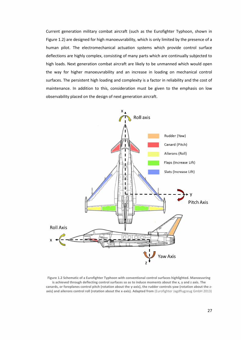
Current generation military combat aircraft (such as the Eurofighter Typhoon, shown in

Figure 1.2) are designed for high manoeuvrability, which is only limited by the presence of a

human pilot. The electromechanical actuation systems which provide control surface

deflections are highly complex, consisting of many parts which are continually subjected to

high loads. Next generation combat aircraft are likely to be unmanned which would open

the way for higher manoeuvrability and an increase in loading on mechanical control

surfaces. The persistent high loading and complexity is a factor in reliability and the cost of

maintenance. In addition to this, consideration must be given to the emphasis on low

observability placed on the design of next generation aircraft.

Figure 1.2 Schematic of a Eurofighter Typhoon with conventional control surfaces highlighted. Manoeuvring is achieved through deflecting control surfaces so as to induce moments about the x, y and z axis. The

canards, or foreplanes control pitch (rotation about the y-axis), the rudder controls yaw (rotation about the z-axis) and ailerons control roll (rotation about the x-axis). Adapted from (Eurofighter Jagdflugzeug GmbH 2013)

28

Future unmanned combat air vehicles (UCAV) are likely to be designed to counter high

threat surveillance, tracking and missile seeker lock (Hitzel 2013; Osterhuber 2013). This

will force the required radar cross section (RCS) of the vehicle under -30Db (Hitzel 2013).

Conventional control surfaces compromise this level of low observability through the

presence of slots, hinges, geometric discontinuities and the side edges (Hitzel 2013;

Osterhuber 2013). Consequently, there is significant motivation for developing an

alternative means of flight control.

Of the many alternative methods of controlling an aircraft currently and recently

researched (Williams et al. 2013; Kontis et al. 2013; Nangia & Palmer 2013; Miller &

Mccallum 2013; DeSalvo et al. 2013; Graff & Lin 2013), this study has applications to two of

them:

1) Trailing Edge Circulation Control

2) Fluidic Thrust Vectoring

1.1.1 Trailing Edge Circulation Control

Circulation control is the process of blowing air tangentially over the rounded trailing edge

of a wing for the purpose of roll control (as a replacement for ailerons) or lift augmentation

(as a replacement for flaps) (Frith & Wood 2003). A proposed implementation of a fluidic

effector system is shown in Figure 1.3 for a typical UCAV (Neuron) (Chard et al. 2013).

Figure 1.3 Supersonic circulation control implementation. Taken from (Chard et al. 2013).

The effectiveness and efficiency of circulation control systems is improved by increasing the

velocity of the tangentially blown jet (discussed in detail in Chapter 2). However, the extent

to which this is possible is limited as at the supersonic jet velocities produced by high

nozzle pressure ratios, the jet no longer remains attached to the trailing edge (Englar 1975).

29

This current study looks to identify the mechanism behind supersonic curved wall jet

separation with principal application to circulation control. More specifically, opportunities

to improve circulation control effectiveness and efficiency by extending supersonic curved

wall jet attachment through the use of different nozzle geometries is investigated. In

addition to this, the desirability of an adaptive nozzle geometry is assessed.

1.1.2 Fluidic Thrust Vectoring

Fluidic thrust vectoring (FTV) is the creation and control of a pitching and/or yawing

moment through deflecting the thrust of a jet engine without the use of a mechanical

device (Warsop & Crowther 2013). FTV, like circulation control, usually involves a rounded

reaction surface (Lytton 2006). Unlike circulation control, however, control authority is

derived from controlling attachment of the jet (Lytton 2006). Figure 1.4 shows two

methods of controlling attachment recently and currently researched: coflow (Ashley 2012)

and normal blowing (Afilaka 2017; Jegede 2016). In each case, secondary air, taken from

the compressor stage of the jet engine, is injected to effect the attachment of the jet. In

the case of coflow, secondary air is used to attach the jet (attachment based FTV), whereas

for normal blowing, secondary air is used to separate the jet from the reaction surface

(detachment based FTV) (Chippindall 2009). A deep understanding of the separation of

supersonic curved wall jets is required in order to achieve the latter (Afilaka 2017; Jegede

2016).

30

Figure 1.4 Schematic of FTV Methods. (a) corresponds to coflow, where injecting secondary air serves to attach the exhaust jet to the reaction surface. (b) represents normal blowing FTV, where air is injected along

the reaction surface and serves to separate the flow.

Pitching moments are induced by controlling attachment of the jet to a 2D reaction surface.

Pitching and yawing moments can be induced by using a scarfed reaction surface, as

illustrated in Figure 1.5 (Jegede 2016).

Figure 1.5 FTV using a 2D reaction surface to control pitch (a), and using a scarfed, 3D reaction surface to control pitch and yaw (b). Taken from (Jegede 2016)

The main performance drivers of FTV are control linearity and control authority (Lytton

2006; Chippindall 2009; Ashley 2012; Bevilaqua & Lee 1980; Jegede 2016). This translates

31

to improving the ability to reliably and rapidly attach and separate the jet, and maximising

the change in jet deflection angle per unit secondary mass flow (Lytton 2006).

Whilst the context of the current study is very much set in the domain of circulation

control, outcomes regarding the mechanism behind supersonic curved wall jet detachment

and the effect of various nozzle geometries have the potential to inform research in the

field of FTV.

1.2 Thesis Aim and Objectives

The aim of this thesis (comprehensively derived through chapters 2 and 3) is stated as

follows:

To investigate the effect internal nozzle geometry has on the performance of supersonic

curved wall jets across a range of nozzle pressure ratios

The specific objectives are listed below:

1) To perform a critical review of trends in circulation control, clearly defining exactly

the effectiveness and system-level efficiency of circulation control can be improved

through supersonic curved wall jets and highlighting the importance of mass flow

(Chapter 2).

2) Critically assess existing theories of supersonic curved wall jet behaviour,

identifying any opportunities for extending jet attachment via nozzle geometry

(Chapter 3);

3) Through investigating the flow physics behind supersonic curved wall jet behaviour,

define the mechanism behind supersonic curved wall jet detachment. Additionally,

identify how nozzles of different geometry effect supersonic curved wall jet

behaviour and how this could be exploited for circulation control and fluidic thrust

vectoring (Chapters 4 & 5);

4) Compare and contrast supersonic curved wall jet behaviour with inviscid

simulations (using the method of characteristics) (Chapter 5);

5) Quantify the relative quiescent (static ambient) performance of supersonic curved

wall jets in order to identify whether an adaptive nozzle is necessary for either

extending jet attachment, improving efficiency, or increasing effectiveness of

circulation control. If it is necessary, identify precisely how a nozzle should adapt

(Chapter 5).

32

Chapter 2 Circulation Control

Chapter Overview

The aim of this chapter is to define the motivation for this study with application to

circulation control. It begins with an overview of the background knowledge necessary to

understand subsonic circulation control (e.g. boundary layers, shear layers and the Coanda

effect). This is followed by an extensive literature review where key historical trends are

identified leading to the definition of the motivation: in order to improve the system-level

efficiency and effectiveness of circulation control devices, the velocity of the attached jet

needs to be increased.

33

2.1 Boundary and Shear Layers

Consider a fluid travelling tangentially to a solid wall. Shear stress, or friction, between the

fluid and the solid wall leads to the formation of a boundary layer, which is usually assumed

to be very thin relative to the length-scale of the wall (Schlichting & Gersten 1979;

Anderson 2007). At the interface between the boundary layer and the wall, the fluid

velocity is zero, and at the interface between the boundary layer and the rest of the fluid,

the velocity is approximately the same as the fluid (Babinsky & Harvey 2011; Anderson

2007; Schlichting & Gersten 1979). Defining the boundary layer in such a way is useful for

flow analyses as it allows a distinction to be brought between principally inviscid (shear

stress is negligible) and viscous (shear stress is dominant) regions of a flow (Anderson

2005).

Figure 2.1 Boundary layer growth and transition from laminar to turbulent. Adapted from (Groh 2016).

As the fluid travels along the wall, the thickness of the boundary layer will grow due to

internal shear stress (Schlichting & Gersten 1979). Initially, the boundary layer will be

laminar (i.e. no turbulence). Depending on the length of the wall, at some distance, it will

transition to turbulence (i.e. flow is highly rotational), as shown in Figure 2.1 (Anderson

2005; Groh 2016). The growth of both laminar and turbulent boundary layers is principally

related to the Reynolds number, which is the ratio between inertial and viscous forces,

defined in Equation 2-1 (Anderson 2007):

𝑅𝑒 =𝜌𝑉𝐿

𝜇

Equation 2-1

Where:

𝜌 is the fluid density (kg/m3);

𝑉 is the fluid velocity (m/s);

34

𝐿 is the reference length (m);

𝜇 is the dynamic viscosity of the fluid (Ns/m2).

The thickness of both a laminar and turbulent boundaries is defined as the distance from

the wall at which the flow velocity reaches 99% of the free-stream fluid velocity (Schlichting

& Gersten 1979). For incompressible flow over a flat plate, a solution for the boundary

layer thickness is derived from Blasius’ equation (full derivation shown in (Anderson 2007)).

The thickness of a laminar boundary layer is shown in Equation 2-2:

𝛿𝑙 =5𝑥

√𝑅𝑒

Equation 2-2

Where 𝑥 is the reference distance from the start of the wall (m).

The thickness of a turbulent boundary layer is shown in Equation 2-3:

𝛿𝑡 =0.37𝑥

𝑅𝑒0.2

Equation 2-3

Equation 2-2 and Equation 2-3 are used in Appendix B as an estimation of the laminar and

turbulent boundary layer thicknesses for comparison with optical thickness measurements

taken via shadowgraphy.

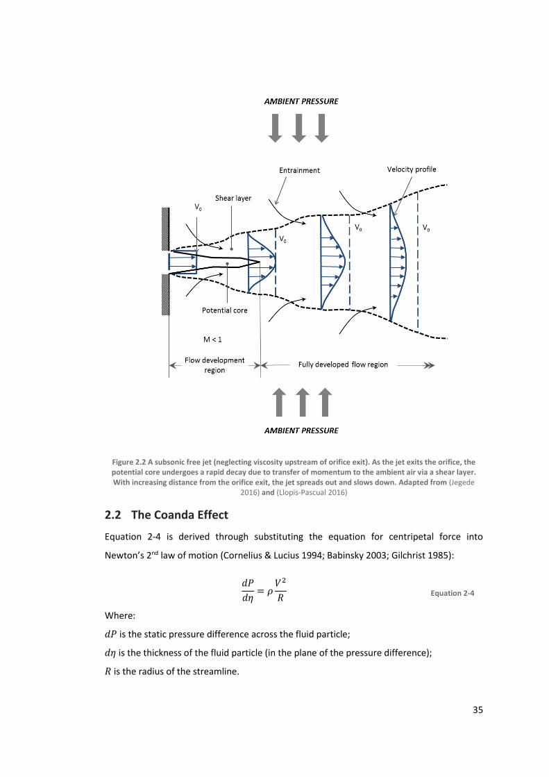
A subsonic free jet is shown in Figure 2.2, and occurs when a relatively smaller volume of

fluid (i.e. the jet) discharges through an orifice into another, relatively larger volume of

fluid. If the velocity of the jet is higher than the ambient conditions, shear stress between

the jet and the surrounding air will cause the momentum of the jet to be transferred to the

ambient air via a shear layer (Schlichting & Gersten 1979). Such a process causes

entrainment of the surrounding ambient air (Labus & Symons 1972; Gregory-Smith &

Gilchrist 1987). As a consequence of this mixing, as the distance from the orifice increases,

there is a simultaneous reduction in the velocity and increase in the diameter of the jet

(Schlichting & Gersten 1979). The distance over which this occurs is a function of the

properties of both fluids (e.g. density, velocity, static pressure), in addition to the Reynolds

number of the jet. For most applications of propulsive jets in aerospace, the Reynolds

number is between 104 and 107, indicative of a turbulent flow (Krzywoblocki 1956).

A turbulent jet transfers momentum at a faster rate compared to a laminar jet of lower

Reynolds number (Schlichting & Gersten 1979). The formation of relatively large, three-

dimensional turbulent structures (such as vortices) speeds up the growth of the shear layer,

facilitating improved momentum transfer (Rossmann 2001).

35

Figure 2.2 A subsonic free jet (neglecting viscosity upstream of orifice exit). As the jet exits the orifice, the potential core undergoes a rapid decay due to transfer of momentum to the ambient air via a shear layer. With increasing distance from the orifice exit, the jet spreads out and slows down. Adapted from (Jegede

2016) and (Llopis-Pascual 2016)

2.2 The Coanda Effect

Equation 2-4 is derived through substituting the equation for centripetal force into

Newton’s 2nd law of motion (Cornelius & Lucius 1994; Babinsky 2003; Gilchrist 1985):

𝑑𝑃

𝑑𝜂= 𝜌

𝑉2

𝑅

Equation 2-4

Where:

𝑑𝑃 is the static pressure difference across the fluid particle;

𝑑𝜂 is the thickness of the fluid particle (in the plane of the pressure difference);

𝑅 is the radius of the streamline.

36

Consider a jet discharging tangentially to a convex wall, as shown in Figure 2.3. Immediately

downstream of the orifice, there is a lower static pressure on one side than the other due

to the presence of a wall (Sarpkaya 1988). The reduced static pressure on one side of the

jet (i.e. the side of the wall) leads to the attachment of the jet to the wall. This is known as

the Chilowsky effect (Cornelius & Lucius 1994).

Figure 2.3 Curved wall jet showing initial attachment, development of boundary layer and separation due to adverse stream-wise pressure gradient. The attachment (and separation) of the jet can be described by

Equation 2-4.

The jet will remain attached as long as the static pressure difference between the wall and

the ambient air is equivalent to the centrifugal force caused by the change in direction of

the jet (as dictated by Equation 2-4) (Rayleigh 1917; Cutbill 1998; Babinsky 2003). As

before, the jet slows down and spreads with increasing distance from the orifice, resulting

in a gradual increase in surface pressure (Rayleigh 1917; Cutbill 1998). Eventually, this

increase in static pressure results in the separation of the boundary layer from the convex

wall (Rayleigh 1917; Cutbill 1998). Boundary layer separation occurs in the presence of a

positive stream-wise pressure gradient (adverse pressure gradient) (Babinsky & Harvey

2011). As the static pressure increases in the stream-wise direction, the flow within the

boundary layer slows down (Schlichting & Gersten 1979). At the point of separation, the

37

flow in the boundary layer, close to the surface (but not at the surface) has reached zero

velocity (Schlichting & Gersten 1979). Beyond this point, recirculation causes reverse flow

to occur between the separated boundary layer and the surface (i.e. negative velocity in

the separated region), as shown in Figure 2.3 (Schlichting & Gersten 1979; Anderson 2005).

Provided there is a substantial favourable (i.e. negative) stream-wise pressure gradient

downstream the boundary layer will reattach (referred to as local separation or a

separation bubble), otherwise, the boundary layer becomes a shear layer (Babinsky &

Harvey 2011).

As the attached jet proceeds around the reaction surface, the growth in the shear layer

occurs at a faster rate compared to a plane wall jet (Rayleigh 1917; Gilchrist 1985; Cutbill

1998). Considering a fluid particle displaced radially from its curved streamline, if the

angular momentum of the flow is greater in its new position, then the radial pressure

gradient (𝑑𝑃

𝑑𝑟) would force the fluid particle back towards its original streamline (Rayleigh

1917). For a convex wall jet, this occurs in the boundary layer (Cutbill 1998). If, instead, the

angular momentum is smaller at the new position, then the fluid particle has a larger

velocity than the steady flow around it. In this case the radial pressure gradient would be

insufficient to keep the fluid particle on its path and so the fluid particle would move

further out (Rayleigh 1917). This occurs in the shear layer of the curved wall jet (Cutbill

1998)*.

To summarise, the Coanda effect comprises three phenomena (Gilchrist 1985; Cutbill

1998):

1) Attachment of a tangential jet to a wall;

2) Once attached, the jet remains attached (subject to stream-wise pressure

gradients);

3) A convex wall jet destabilises the shear layer, increasing turbulence and, hence,

mixing relative to a straight wall jet.

* By definition, irrotational flow (discussed in detail in 3.2.3) has a constant angular momentum distribution through the thickness of the jet (Rayleigh 1917). Consequently, for irrotational flow convex wall jets there is no increase in mixing due to the shear layer becoming destabilised (i.e. the third Coanda effect, as identified above, does not occur). This potentially explains why the asymmetrical nozzle tested in free-stream by Llopis-Pascual (2016) does not outperform the symmetrical nozzle, despite having higher momentum.

38

2.3 Wing Trailing Edge Circulation Control

Wing trailing edge circulation control was first patented by Davidson in 1962 (Davidson

1962). It involves replacing a conventional, sharp, trailing edge of a wing with a rounded

reaction surface and blowing air tangentially. This is illustrated for a wing cross section in

Figure 3.1. The circulation provided by this device for given a free-stream condition is a

function of both the wing geometry and the momentum of the jet attached to the rounded

trailing edge (Englar 1970; Englar 1975; Englar et al. 1981). Consequently, the circulation,

hence, the lift of the wing can be controlled through changing the momentum of the jet.

Equation 2-5 is a revised definition of the 2D lift coefficient, accounting for tangentially

blown jet (Loth & Boasson 1983):

𝐶𝑙 = 𝐶𝑙,0 + 𝛼 (𝜕𝐶𝑙

𝜕𝛼) + 𝐶𝜇 (

𝜕𝐶𝑙

𝜕𝐶𝜇)

Equation 2-5

Where:

𝐶𝑙,0 is the lift coefficient at zero angle of attack and blowing;

𝛼 is the angle of attack (rad);

(𝜕𝐶𝑙

𝜕𝛼) is the lift curve slope (rad-1);

(𝜕𝐶𝑙

𝜕𝐶𝜇) is the lift augmentation;

𝐶𝜇 is the momentum coefficient defined by Equation 2-6 (Englar 1970):

𝐶𝜇 =�̇�𝑉𝑗

𝑞∞𝑆

Equation 2-6

Where:

�̇� is the mass flow rate of tangentially blown air in kgs-1;

𝑉𝑗 is the velocity of the jet, in ms-1;

𝑞∞ is the dynamic pressure of the free-stream in Pa;

𝑆 is the aerodynamic reference area in m2.

39

Figure 2.4 Subsonic circulation control aerofoil. Adapted from (Michie 2008) and (Englar 1975)

The majority of early research on wing circulation control looked at it as an alternative to

high lift devices such as flaps, as opposed to roll control devices such as ailerons (Englar

1970; Englar 1975; Englar 1979; Englar et al. 1981; Abramson & Rogers 1983). Englar et al

(1981) observed that the section lift coefficient for a circulation control aerofoil was 6.5.

This was more than double the section lift coefficient generated with a similar aerofoil

(NACA 64A212) with leading edge slat and double slotted mechanical flap (Clmax = 3.1).

Additionally, Abramson & Rogers (1983) concluded that even at transonic speeds,

circulation control aerofoils exceeded the capacity of conventional aerofoils to generate

lift. Aside from the increase in comparative aerodynamic effectiveness, other advantages

include reduced maintenance and reduced observability due to the absence of moving

parts, actuator mechanisms and hinge lines (Michie 2008; Abramson & Rogers 1983; Englar

1975)

A clear relationship between the lift and momentum coefficients was defined across

multiple studies (Englar, 1970; Englar et al, 1981; Abramson & Rogers, 1983; Loth &

Boasson, 1983; Loth & Boasson, 1984) which satisfies the Kutta condition, such that as long

as the tangentially injected jet remains attached, increasing the momentum coefficient will

increase the lift coefficient. Empirical laws relating the change in section lift coefficient to

the momentum coefficient have been derived from Englar (1981) by Loth and Boasson

(1983) and Loth and Boasson (1984). Such laws have been used in the preliminary sizing of

circulation control effectors by the relatively recent FLAVIIR project (Michie 2008). An

extended validation of these relations was performed as part of a new proposed circulation

control sizing methodology discussed in detail in Appendix A. Following the extended

validation, a more appropriate empirical relationship was proposed, shown in Equation 2-7.

40

For details on the extended validation and a full derivation of Equation 2-7, see Appendix A

(specifically, Section A.2.3 page 215).

∆𝐶𝑙 = 𝐶𝜇 (𝜕𝐶𝑙

𝜕𝐶𝜇) =

1

400√

𝐶𝜇𝑅𝑒∞

𝑀∞

Equation 2-7

Where:

∆𝐶𝑙 is the change in 2D lift coefficient caused by circulation control;

𝑀∞ is the free-stream Mach number (defined by Equation 3-1);

𝑅𝑒∞ is the free-stream Reynolds number (defined by Equation 2-1).

Equation 2-7 suggests a correlation between the effectiveness of the circulation control

system, and the free-stream Mach and Reynolds number. The inverse relationship between

the effectiveness of circulation control and free-stream Mach number is well reported, and

suggests that the velocity of the jet will have to increase as the free-stream Mach number

is increased in order to maintain effectiveness (Cagle & Jones 2002; Englar 1970; Wilkerson

& Montana 1982; Abramson & Rogers 1983; Wood & Conlon 1983; Llopis-Pascual 2016).

Such an assertion formed the basis of the study by Llopis-Pascual (2016), who

demonstrated comparatively greater circulation control effectiveness with a higher velocity

jet (produced by a convergent-divergent nozzle compared to a convergent-only nozzle).

The lift coefficient will continue to increase with increasing momentum coefficient until the

jet detaches (Englar 1970; Englar 1975; Englar 1979; Englar et al. 1981; Abramson & Rogers

1983; Frith & Wood 2003; Llopis-Pascual 2016). Once the jet detaches from the Coanda

surface, there is a severe reduction in the lift coefficient as the Coanda jet no longer

contributes to the circulation, and produces thrust instead (Llopis-Pascual 2016).

2.4 Effect of Geometry

Englar, and later Abramson and Rogers, pioneered much of the early research into different

slot heights, trailing edge radii and aerofoil thicknesses (Englar 1970; Englar 1975; Englar et

al. 1981; Abramson & Rogers 1983). These studies agreed that the slot height to reaction

surface radius ratio (H/R) and the reaction surface radius to the wing chord ratio (R/C) had

a significant impact on the maximum lift generated by the circulation control device (Englar

1970; Englar 1975; Englar et al. 1981; Abramson & Rogers 1983). Increasing the R/C ratio

was seen to increase the maximum lift attainable through allowing jets to achieve higher

momentum before detachment, but also saw an increase in drag (Englar et al. 1981).

41

Figure 2.5 Empirical graph showing previous area of desired operation (yellow) from Englar (1974) and new area of desired operation (red) following the FLAVIIR project. From (Michie 2008)

Loth et al. (1976) demonstrated circulation control for the purposes of lift augmentation on

a modified US Navy A-6A aircraft with an R/C ratio of 0.036. During this program, it was

noted that reducing the trailing edge radius would provide significant benefits to drag

reduction without significant loss in augmented lift (Loth et al. 1976). Frith and Wood

(2003), and later Sparks et al (2005) showed that it was possible to provide a sufficient

change in lift to control an aircraft in roll at a significantly lower R/C (0.01) (Frith & Wood

2003; Sparks et al. 2005). Figure 2.5 shows the initial region of desired Coanda operation

(yellow), as dictated by R/C and H/R (Englar 1975), with later studies showing a more

recent desired Coanda operation region (red) based on achieving similar Coanda

effectiveness at lower R/C as part of the FLAVIIR project (Sparks et al. 2005; Frith & Wood

2003; Michie 2008). Figure 2.6 has been constructed from the major experimental

circulation control studies performed since 1970, which have been referenced in papers

relating to the flight demonstration of circulation control. It shows the maximum

momentum coefficient tested in the respective study plotted against the radius to chord

ratio used. As can be seen, the major focus for circulation control has shifted in later

decades towards a reduced radius to chord ratio: an acknowledgement of the need to

reduce drag discussed in detail in the previously mentioned studies (Loth et al. 1976; Englar

1975; Frith & Wood 2003; Sparks et al. 2005; Michie 2008).

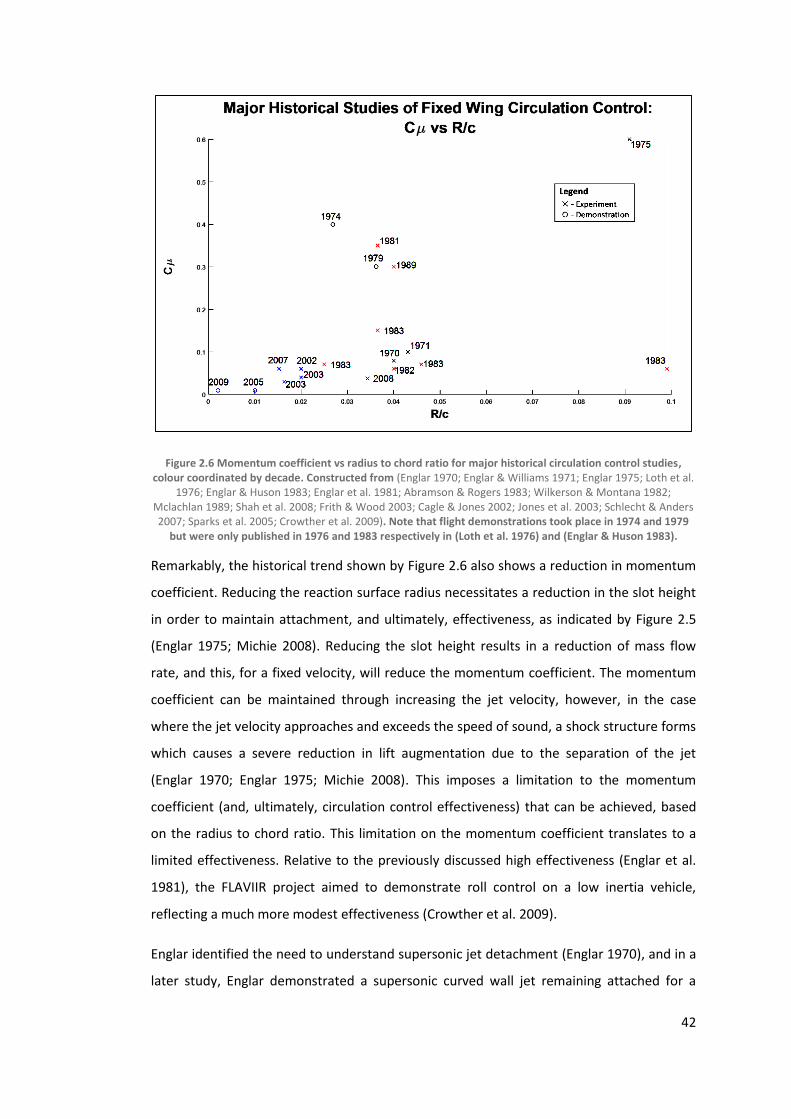
42

Figure 2.6 Momentum coefficient vs radius to chord ratio for major historical circulation control studies, colour coordinated by decade. Constructed from (Englar 1970; Englar & Williams 1971; Englar 1975; Loth et al.

1976; Englar & Huson 1983; Englar et al. 1981; Abramson & Rogers 1983; Wilkerson & Montana 1982; Mclachlan 1989; Shah et al. 2008; Frith & Wood 2003; Cagle & Jones 2002; Jones et al. 2003; Schlecht & Anders 2007; Sparks et al. 2005; Crowther et al. 2009). Note that flight demonstrations took place in 1974 and 1979

but were only published in 1976 and 1983 respectively in (Loth et al. 1976) and (Englar & Huson 1983).

Remarkably, the historical trend shown by Figure 2.6 also shows a reduction in momentum

coefficient. Reducing the reaction surface radius necessitates a reduction in the slot height

in order to maintain attachment, and ultimately, effectiveness, as indicated by Figure 2.5

(Englar 1975; Michie 2008). Reducing the slot height results in a reduction of mass flow

rate, and this, for a fixed velocity, will reduce the momentum coefficient. The momentum

coefficient can be maintained through increasing the jet velocity, however, in the case

where the jet velocity approaches and exceeds the speed of sound, a shock structure forms

which causes a severe reduction in lift augmentation due to the separation of the jet

(Englar 1970; Englar 1975; Michie 2008). This imposes a limitation to the momentum

coefficient (and, ultimately, circulation control effectiveness) that can be achieved, based

on the radius to chord ratio. This limitation on the momentum coefficient translates to a

limited effectiveness. Relative to the previously discussed high effectiveness (Englar et al.

1981), the FLAVIIR project aimed to demonstrate roll control on a low inertia vehicle,

reflecting a much more modest effectiveness (Crowther et al. 2009).

Englar identified the need to understand supersonic jet detachment (Englar 1970), and in a

later study, Englar demonstrated a supersonic curved wall jet remaining attached for a

43

relatively large radius to chord ratio of 0.09 (Englar 1975). Englar noted that whilst it was

possible to demonstrate this at a single design point, the attachment of the supersonic

curved wall jet in different operating conditions was unpredictable (Englar 1975). Other

studies found that, particularly with smaller H/R and R/C ratios, there was a significant loss

in lift augmentation once the nozzle had become choked due to the separation of the

supersonic curved wall jet (Englar 1979; Abramson & Rogers 1983).

2.5 Importance of Mass Flow

In addition to drag, another cost incurred by a circulation control system is the mass flow

rate. Tangentially injected air comes from the compressor stage of a propulsive gas turbine

engine , in many proposed cases (Chard et al. 2013; Michie 2008; Sparks et al. 2005). Whilst

extracting mass flow, or bleed air, from jet engines is already relatively commonplace, it

does have a negative effect on the thrust efficiency of the engine, and consequently should

be minimised (Loth & Boasson 1983). Even when considering cases where compressed air is

provided by a separate compressor, the system cost of such a device (e.g. mass, power and

volume) usually scales with mass flow (Sparks et al. 2005; Michie 2008).

In order to improve the system-level efficiency of a circulation control device, the change in

lift coefficient must be maximised with respect to the mass flow rate, as shown in Equation

2-8:

Ɛ = Δ𝐶𝐿

�̇�

Equation 2-8

Where:

Ɛ is the system-level efficiency of a circulation control wing;

�̇� is the mass flow of air;

Remembering that the lift augmentation is a function of the momentum coefficient, the

efficiency equation can be revised to

Ɛ ∝ 𝐶𝜇

�̇�

Equation 2-9

This equation can be simplified by substituting in the definition of the momentum

coefficient from Equation 2-6 to form Equation 2-10:

Ɛ ∝𝑉𝑗

𝑞∞𝑆

Equation 2-10

44

This means that the system-level efficiency of the circulation control device will be

increased by increasing the velocity of the tangentially injected jet, for any given dynamic

pressure and reference area. Again it must be highlighted that this condition is only

applicable to tangentially injected flow which remains attached. Consequently, the use of

supersonic, as opposed to subsonic Coanda jets is desirable from both an efficiency

(maximising change in lift coefficient per unit mass flow) and an effectiveness (increasing

𝐶𝜇 at low R/C) perspective.

2.6 Summary

A thorough review of past literature has revealed that both the effectiveness and system

level efficiency of circulation control wings are improved by increasing the jet velocity.

However, such relationships are only valid for attached jets. Increasing the trailing edge

radius improves effectiveness through extending attachment, but this is coupled with an

unacceptable increase in drag. Historical trends have shown not only a decrease in trailing

edge radius to chord ratios, but also a reduction in the momentum coefficient. This is

necessary to maintain attachment of the jet, because as the jet velocity approaches and

exceeds the speed of sound, shock structures form which cause the separation of the jet.

To summarise, the following motivation arises from current state of the art in circulation

control:

1) A need to increase the jet velocity at which separation occurs, as this limits

effectiveness and system-level efficiency;

2) A need to increase effectiveness at low R/C through maximising attached jet

velocity;

3) A need to improve system-level efficiency through maximising attached jet velocity

per unit mass-flow.

45

Chapter 3 Supersonic Curved Wall Jets

Chapter Overview

In the previous chapter, motivation for maintaining attachment of supersonic curved wall

jets was established. Increasing the exit velocity of an attached jet would increase both the

effectiveness and the system-level efficiency of a circulation control system. The aim of this

chapter is to derive the precise objectives for this study through a critical overview of both

the theoretical background and past literature in the field of supersonic curved wall jets.

More specifically, past hypotheses regarding the challenge of maintaining attachment as

the jet velocity increases are thoroughly interrogated. This results in a proposed

experiment to determine the cause of supersonic curved wall jet separation, and quantify

the effect of internal nozzle geometry on the behaviour of supersonic curved wall jets.

46

3.1 Introduction to Supersonic Curved Wall Jets

This section provides a comprehensive overview of the background knowledge relevant to

supersonic curved wall jets. Beginning with supersonic and isentropic flow definitions, this

section goes on to discuss the definitions of the design and operating conditions of nozzle

flow, which has significant consequences for the conclusions drawn from both past studies,

and this one.

3.1.1 Supersonic Jets

The Mach number is defined as the ratio between the fluid velocity and the speed of sound

in that fluid, as shown in Equation 3-1 (Houghton & Carpenter 2003):

𝑀 =𝑉

𝑎

Equation 3-1

Where:

𝑉 is the flow velocity (ms-1);

𝑎 is the speed of sound (ms-1), defined by Equation 3-2 (Houghton & Carpenter 2003):

𝑎 = √𝛾𝑅𝑇 Equation 3-2

Where:

𝑇 is the static temperature of the flow (K);

𝑅 is the gas constant (287 Jkg-1K-1 for dry air);

𝛾 is the ratio of specific heats (1.4 for dry air†).

Pressure disturbances in subsonic flow (i.e. M < 1) propagate in all directions from the

source of the disturbance at the speed of sound (Houghton & Carpenter 2003); If the

source of the pressure disturbance is moving faster than the speed of sound (i.e. M > 1),

then the pressure disturbances can no longer propagate upstream. The main consequence

of supersonic flow is that pressure disturbances are characterised by discrete changes in

flow properties, which only propagate downstream (Anderson 2007). These disturbances

are otherwise known as Mach waves, and propagate at the Mach angle (μ), as defined in

Equation 3-3 (Anderson 2007):

††The ratio of specific heats varies due to temperature and the composition of the gas. At 273k, it is 1.403 for dry air, at 500K it is 1.398 (Anderson 2007). The assumed value of 1.4 is used throughout this thesis.

47

𝜇 = sin−1 (1

𝑀)

Equation 3-3

Relative to subsonic jets, supersonic jet shear layers grow at a much slower rate (Jegede

2016; Rossmann 2001). In subsonic jets, a comparatively high amount of mixing occurs due

to the formation of three dimensional phenomena such as span-wise vortices (Rossmann

2001). In supersonic flow, due to the downstream propagation of pressure disturbances,

the propagation of such structures is limited in the span-wise direction in favour of the

stream-wise direction (Jegede 2016; Rajaratnam 1976). As a consequence, mixing,

entrainment and momentum transfer happen at a reduced rate, with the core of the

supersonic jet being maintained for a relatively larger distance. A supersonic jet produced

by a symmetrical convergent-divergent nozzle (with negligible viscosity upstream of the

nozzle exit) is shown at its design NPR in Figure 3.1:

Figure 3.1 Supersonic free jet (neglecting viscosity upstream of orifice exit). Relative to the subsonic jet shown in Figure 2.2, a supersonic jet undergoes a much more gradual decay of the potential core. This is due to the Mach angle limiting the development of span-wise mixing structures such as vortices. Adapted from

(Rajaratnam 1976).

3.1.2 Isentropic Relations

Isentropic relations, derived from the second law of thermodynamics, are shown in

Equation 3-4. For a complete derivation, see (Anderson 2007).

𝑝2

𝑝1= (

𝜌1

𝜌2)

𝛾

= (𝑇2

𝑇1)

𝛾(𝛾−1)

Equation 3-4

Where:

𝑝 is static pressure (Pa);

48

𝜌 is density (kgm-3);

𝑇 is the static temperature (K);

𝛾 is the ratio of specific heats;

1, 2 denote positions within a flow-field.

Considering a calorically perfect gas, the Mach number can be defined as a function of the

static temperature to total temperature ratio. This is shown in Equation 3-5 (Anderson

2007):

𝑇0

𝑇= 1 +

𝛾 − 1

2𝑀2

Equation 3-5

Where:

𝑀 is the Mach number;

0 as a subscript denotes the stagnation or total property, as opposed to the static

property.

Through combining Equation 3-5 with Equation 3-4, the Mach number can be linked to

other flow properties, as shown in Equation 3-6 and Equation 3-7 (Anderson 2007):

𝑝0

𝑝= (1 +

𝛾 − 1

2𝑀2)

𝛾(𝛾−1)

Equation 3-6

𝜌0

𝜌= (1 +

𝛾 − 1

2𝑀2)

1(𝛾−1)

Equation 3-7

3.1.3 Supersonic Flow Interactions

In supersonic flow, pressure disturbances propagate through the flow as either expansion

or compression waves (Anderson 2007). For the case of Prandtl-Meyer flow (i.e. isentropic

and inviscid flow), flow around a concave corner is turned by an expansion fan. Flow

around a sharp convex corner results in compression waves which coalesce to form an

oblique shockwave (Babinsky & Harvey 2011). These interactions are shown in Figure 3.2

(Houghton & Carpenter 2003).

49

Figure 3.2 Simplified diagrams representing the formation expansion fan (left) and shock waves (right) as typically caused by surface interactions. From (Anderson 2007)

Supersonic flow passing through an expansion fan undergoes a reduction in static pressure,

density and static temperature, and an increase in Mach number. Supersonic flow passing

through a compression or shockwave undergoes an increase in static pressure, density and

static temperature and a reduction in Mach number (Anderson 2007).

As the pressure waves propagate through the supersonic flow, it is possible that they

interact with either a solid boundary or a constant pressure boundary (i.e. a free-stream).

Figure 3.3 Simplified shock reflections from a solid boundary. From (Anderson 2007)

In the event of a compression or shock wave intersecting with a solid boundary, the

supersonic flow passes through the incident shock and turns towards the solid boundary.

The flow cannot, however, continue in this direction as it cannot pass through a solid

boundary. Consequently, a reflected shock is formed to turn the supersonic flow parallel to

the solid boundary as shown in Figure 3.3 (Anderson 2007). Therefore, for pressure

disturbances interacting with a solid boundary, the following rule applies:

50

Pressure disturbances impinging on a solid boundary reflect in a likewise manner –

compression waves reflect as compression waves and expansion waves reflect as

expansion waves.

A free-stream or constant pressure boundary, unlike a solid boundary, can change in size

and direction depending on the relative pressure difference between the supersonic jet

and the free-stream (Anderson 2007). Initially (i.e. before any interaction), the supersonic

jet pressure is equal to the free-stream pressure. Any disturbance propagating through the

supersonic jet must act to maintain a constant pressure at the boundary between the

supersonic jet and the free-stream (Anderson 2007; Chippindall 2009).

Figure 3.4 Shock reflections from a free-stream boundary. From (Anderson 2007)

Consider a compression or shock-wave intersecting a free-stream boundary. Before the

flow crosses the incident shock, there is no difference between the pressure in the

supersonic boundary and the free-stream (1 in Figure 3.4). As the supersonic flow passes

through the shock wave, there is an increase in pressure (2 in Figure 3.4). In order to

maintain the constant pressure boundary, there must be a subsequent reduction in

pressure (Anderson 2007; Chippindall 2009). This is achieved through an expansion fan (3

in Figure 3.4). Therefore, for pressure disturbances interacting with a free-boundary, the

following rule applies:

Pressure disturbances impinging on a free-stream boundary reflect in an opposite

manner – compression waves reflect as expansion waves and expansion waves

reflect as compression waves.

51

Figure 3.5 Shock induced boundary layer separation. Adopted from (Anderson 2007)

In addition to the boundary layer separation mechanism described in Section 2.1,

supersonic flow allows for a special separation mechanism called shock induced boundary

layer separation. This occurs when a shockwave impinges on a solid boundary, causing a

severe enough stream-wise adverse pressure gradient to immediately separate the

boundary layer (described by Figure 3.5) (Anderson 2007). Note that the separation point

of the boundary layer is upstream of the incident shockwave in Figure 3.5. This occurs due

to the subsonic part of the boundary layer allowing a pressure gradient to be transmitted

upstream (Babinsky & Harvey 2011). The upstream transmission of pressure is important in

the eventual mechanism for separation determined in this current study.

3.1.4 Convergent-Only Nozzles

A nozzle is a specially shaped tube that increases the velocity of a fluid passing through it.

In the context of propulsive aerospace applications, two nozzles are commonly used,

convergent-only and convergent-divergent. Convergent corresponds to a decreasing cross-

sectional area, and divergent corresponds to an increasing cross-sectional area. Considering

flow through a duct, mass flow is conserved, as defined in Equation 3-8 (Anderson 2007):

�̇� = 𝜌1𝑉1𝐴1 = 𝜌2𝑉2𝐴2 Equation 3-8

Where:

𝐴 is the cross-sectional area (m2).

52

Change in cross-sectional area can be linked to change in flow velocity using Equation 3-9

(Anderson 2007):

𝑑𝐴

𝐴= (𝑀2 − 1)

𝑑𝑉

𝑉

Equation 3-9

There are three consequences of Equation 3-9:

1) When the flow is supersonic (M>1), flow through a convergent duct decreases

velocity and flow through a divergent duct increases velocity;

2) When the flow is subsonic (M<1), flow through a convergent duct increases

velocity and flow through a divergent duct decreases velocity;

3) When the flow is sonic (M=1), the cross sectional area is a minimum (𝑑𝐴 = 0).

Considering a convergent-only nozzle, the third consequence of Equation 3-9 defines the

maximum Mach number at the exit as unity. Depending on the upstream pressure,

however, the static pressure at the nozzle exit can vary (Anderson 2007). In the event that

the static pressure at the exit is greater than the ambient pressure, the jet will be under-

expanded, and an expansion fan will form at the nozzle exit. The expansion fan acts to

reduce the pressure whilst increasing the Mach number. The final Mach number of the fully

expanded flow can be deduced by rearranging Equation 3-6, to form Equation 3-10:

𝑀𝑗 = √(2

𝛾 − 1) ((𝑁𝑃𝑅)

(𝛾−1)𝛾 − 1)

Equation 3-10

Where:

𝑗 as a subscript denotes jet properties.

NPR is the nozzle pressure ratio, defined as the ratio of the upstream stagnation pressure

to the ambient static pressure (Anderson 2007). The velocity of the jet produced by the

convergent-only nozzle is provided by substituting Equation 3-1 and Equation 3-2 into

Equation 3-10, to produce Equation 3-11:

𝑉𝑗 = √(𝛾𝑅𝑇𝑗) (2

𝛾 − 1) ((𝑁𝑃𝑅)

(𝛾−1)𝛾 − 1)

Equation 3-11

Consequently, increasing jet velocity (which is a stated aim of Chapter 2) is achieved by

increasing the NPR (Anderson 2007; Chippindall 2009; Ashley 2012; Jegede 2016; Llopis-

Pascual 2016).

53

3.1.5 Convergent-Divergent Nozzles

Consider a convergent-divergent nozzle, which is arranged such that a convergent duct is

immediately followed by a divergent duct (with the throat necessarily between the two), as

shown in Figure 3.6. With sufficient NPR, the initially subsonic flow (M<1) will be

accelerated through the convergent-only portion, then become sonic (M=1) at the throat,

after which it will continue accelerating to supersonic speeds (M>1) in the divergent

section.

Figure 3.6 Schematic of a convergent-divergent nozzle

Quasi-One-Dimensional Flow

Figure 3.7 Quasi-one-dimensional flow through a tube. Adapted from (Anderson 2007)

54

Considering quasi-one-dimensional‡ flow through a duct (shown in Figure 3.7), the Mach

number at any point along the duct can be calculated using Equation 3-12 (Houghton &

Carpenter 2003):

(𝐴𝑥

𝐴∗)

2

= 1

𝑀𝑥2 [

2

𝛾 + 1(1 +

𝛾 − 1

2𝑀𝑥

2)]

(𝛾+1)(𝛾−1)

Equation 3-12

Where:

𝐴∗ is the minimum-cross sectional area, also known as the throat area.

For any given area ratio (𝐴𝑥

𝐴∗), Equation 3-12 provides two Mach number solutions, one

solution is subsonic and the other is supersonic. Equation 3-12 relates the average Mach

number at any cross-sectional area of the flow, which is assumed as isentropic (Anderson

2007; Houghton & Carpenter 2003). The isentropic relations (Equation 3-4 to Equation 3-7)

can be used to determine average flow properties anywhere in the duct from the Mach

number, provided the assumption of isentropic flow (i.e. shockwave-free) is valid, and the

initial (stagnation) conditions are known.

Mass Flow through a Convergent-Divergent Nozzle

Reconsidering Equation 3-8, where mass flow is conserved throughout the nozzle. When

the flow in the divergent section of a convergent-divergent nozzle is supersonic, pressure

disturbances can no longer propagate upstream (Anderson 2007; Houghton & Carpenter

2003). This means that if the flow is sonic at the throat (M=1), and the static pressure at the

exit is decreased, the mass flow through the throat, and consequently the entire nozzle,

will be unchanged. Such a condition is known as choked flow (Anderson 2007). For choked

flow, the mass flow through a nozzle is defined in Equation 3-13 (for a full derivation see

Anderson, 2005):

�̇� =𝑝0𝐴∗

√𝑇0

√𝛾

𝑅(

2

𝛾 + 1)

(𝛾+1)(𝛾−1)

Equation 3-13

A consequence of Equation 3-13 is that the mass flow for which a nozzle is specifically

designed dictates the throat area (A*), and hence the scale of the nozzle. Where mass flow

‡ The flow is defined as quasi-one dimensional because it only moves in one direction (x-direction as indicated in Figure 3.7), whilst accommodating a change in cross-sectional area. Hence it is not truly one-dimensional.

55

is important (such as circulation control, as discussed in Chapter 2) comparisons must be

made between different nozzles of the same throat area.

Design NPR

Another consequence of Equation 3-12 is that for isentropic flow, with a sufficient NPR, the

Mach number at the exit of a fixed geometry convergent-divergent nozzle will be constant.

This is similar to the convergent-only case discussed in Section 3.1.4, where the exit Mach

number is always unity. The exit Mach number for a convergent divergent nozzle design

can be calculated by substituting the exit area for 𝐴𝑥 in Equation 3-12, and solving for the

Mach number. The design NPR for this Mach number (hence, exit area to throat area ratio)

can be calculated by substituting the ambient conditions into Equation 3-6 to produce

Equation 3-14.

𝑁𝑃𝑅𝑑 =𝑝0

𝑝𝑎𝑚𝑏= (1 +

𝛾 − 1

2𝑀𝑒

2)

𝛾(𝛾−1)

Equation 3-14

Note that the design NPR is defined such that when the operating NPR is equal to the

design NPR, the average static pressure in the jet at the exit is equal to the ambient

pressure (Anderson 2007; Houghton & Carpenter 2003). The definition of design NPR is

independent of the exit static pressure profile: the only consideration is the average static

pressure at the exit, in line with quasi-one-dimensional assumptions. Another important

consequence of the design NPR definition is that any two nozzles with the same design

NPR, operating at the same NPR will have the same mass flow; again this is independent of

the static pressure profile at the nozzle exit (e.g. skewed versus symmetrical).

Nozzle Operating Conditions

Consider a convergent-divergent nozzle as the operating NPR increases. Initially, the

operating NPR is insufficient for the Mach number to ever reach unity (Anderson 2007).

The flow remains subsonic, with the divergent section of the nozzle acting as a diffuser,

slowing the flow down and increasing the static pressure. The NPR is increased to the point

that there is sonic flow in the throat, but insufficient for supersonic flow at the nozzle exit.

A normal shockwave forms in the divergent section of the nozzle. Downstream of the

shockwave, the flow is subsonic (M<1), and consequently the divergent section acts as a

diffuser, slowing the flow down and increasing the static pressure (Anderson 2007). As the

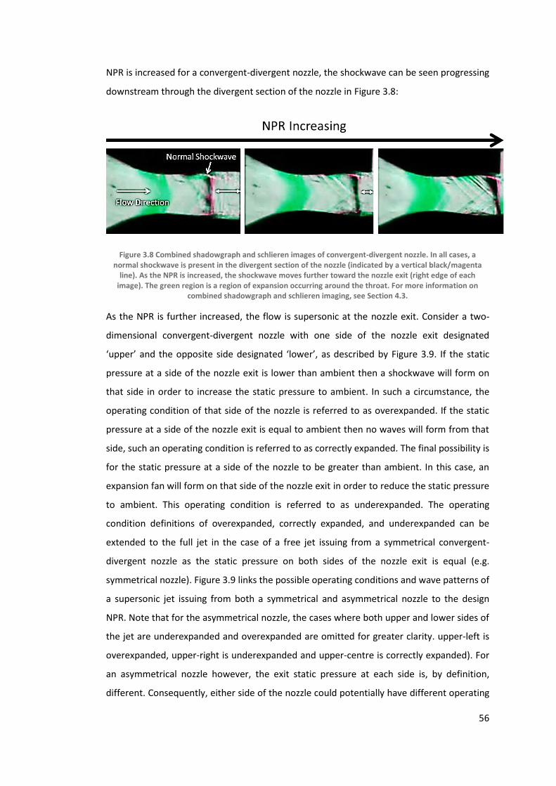
56

NPR is increased for a convergent-divergent nozzle, the shockwave can be seen progressing

downstream through the divergent section of the nozzle in Figure 3.8:

Figure 3.8 Combined shadowgraph and schlieren images of convergent-divergent nozzle. In all cases, a normal shockwave is present in the divergent section of the nozzle (indicated by a vertical black/magenta

line). As the NPR is increased, the shockwave moves further toward the nozzle exit (right edge of each image). The green region is a region of expansion occurring around the throat. For more information on

combined shadowgraph and schlieren imaging, see Section 4.3.

As the NPR is further increased, the flow is supersonic at the nozzle exit. Consider a two-

dimensional convergent-divergent nozzle with one side of the nozzle exit designated

‘upper’ and the opposite side designated ‘lower’, as described by Figure 3.9. If the static

pressure at a side of the nozzle exit is lower than ambient then a shockwave will form on

that side in order to increase the static pressure to ambient. In such a circumstance, the

operating condition of that side of the nozzle is referred to as overexpanded. If the static

pressure at a side of the nozzle exit is equal to ambient then no waves will form from that

side, such an operating condition is referred to as correctly expanded. The final possibility is

for the static pressure at a side of the nozzle to be greater than ambient. In this case, an

expansion fan will form on that side of the nozzle exit in order to reduce the static pressure

to ambient. This operating condition is referred to as underexpanded. The operating

condition definitions of overexpanded, correctly expanded, and underexpanded can be

extended to the full jet in the case of a free jet issuing from a symmetrical convergent-

divergent nozzle as the static pressure on both sides of the nozzle exit is equal (e.g.

symmetrical nozzle). Figure 3.9 links the possible operating conditions and wave patterns of

a supersonic jet issuing from both a symmetrical and asymmetrical nozzle to the design

NPR. Note that for the asymmetrical nozzle, the cases where both upper and lower sides of

the jet are underexpanded and overexpanded are omitted for greater clarity. upper-left is

overexpanded, upper-right is underexpanded and upper-centre is correctly expanded). For

an asymmetrical nozzle however, the exit static pressure at each side is, by definition,

different. Consequently, either side of the nozzle could potentially have different operating

57

conditions. For a free jet issuing from an asymmetrical nozzle, it is impossible for both sides

to be operating at the correctly expanded condition (i.e. wave-free) simultaneously.

Figure 3.9 The operating conditions of free jets issuing from convergent-divergent nozzles. In the upper-left image, oblique shockwaves (labelled ‘OS’) form at both sides of the nozzle exit as the static pressure at the exit is lower than ambient. In the upper-centre image, the static pressure at the nozzle exit is equal to ambient, consequently there are no waves and the nozzle is operating at its correctly expanded condition. The shear layer in this image is denoted ‘SL’. In the upper-right image, the static pressure at the nozzle exit is greater than ambient, consequently, expansion forms at the exit from both sides (denoted ‘EF’). The lower three images correspond to the same NPR as the upper three, however the asymmetrical nozzle causes an exit static pressure profile such that the static pressure at the lower side is always lower than the upper.

In the event that a side of the nozzle is overexpanded or underexpanded, waves will

propagate through the jet, reflecting from the shear layer as opposites, with expansion fans

reflecting as compression waves (coalescing to form shockwaves), and shockwaves

reflecting as expansion fans (Rajaratnam 1976; Anderson 2007).

The term ‘correctly expanded NPR’ (CENPR) is defined as the operating NPR at which there

are no waves propagating from the nozzle exit (e.g. upper-centre in Figure 3.9).

Considering Figure 3.9, the only occasion that the CENPR is achieved for a free jet is when a

symmetrical nozzle is operating at its design NPR (the lower-centre of Figure 3.9 shows that

asymmetrical nozzles operating at their design NPR have neither side correctly expanded).

However, jets issuing from asymmetrical nozzles tangentially to a wall can be correctly

58

expanded as the presence of a wall prevents any wave forming on that side (Ashley, 2012;

Jegede, 2016). Figure 3.10 is an exact recreation of Figure 3.9 with a wall placed

tangentially to the lower nozzle exit. Due to the presence of the wall, any waves which

originated from the lower side of the free jet are now no longer present. Whilst this

changes little in terms of the operating conditions of the jet issuing from the symmetrical

nozzle, the jet issuing from the asymmetrical nozzle is now correctly expanded when the

operating NPR is less than the design NPR. Consequently, the definition of CENPR (wave

free flow) is different to NPRd (average static pressure at exit equal to ambient) for a wall

jet issuing from an asymmetrical nozzle.

Figure 3.10 The operating conditions of wall jets issuing from convergent-divergent nozzles. The six schematics are directly comparable with Figure 3.9; however the addition of the wall has prevented any pressure difference occurring on the lower side of the nozzle exit. Consequently, there are no waves propagating from the lower side, except those reflected from the other side. The major consequence of this is the lower-left image, where the case of NPR < NPRd for the asymmetrical nozzle results in a correctly expanded jet.

To summarise:

The design NPR is the NPR at which the average static pressure at the exit of the jet

is equal to the ambient static pressure.

Any two convergent-divergent nozzles (regardless of symmetry) of equivalent

design NPR have the same mass flow at the same operating NPR.

The correctly expanded NPR is the NPR at which there are no shockwaves or

expansion fans propagating from the nozzle exit.

59

For wall jets or free jets issuing from a symmetrical nozzle, the correctly expanded

NPR is equal to the design NPR.

For wall jets issuing from an asymmetrical nozzle, the correctly expanded NPR is

not equal to the design NPR.

The importance of this cannot be understated: all past studies comparing wall jets issuing

from symmetrical and asymmetrical nozzles have compared nozzles of equivalent CENPR

(Bevilaqua & Lee, 1980; Ashley, 2012; Jegede, 2016; Llopis-Pascual, 2016). This study would

argue, on the basis of the conclusions drawn in Chapter 2, that the design NPR (hence,

mass flow equivalence) is a more important basis for comparison.

Note that confusion of the correctly expanded NPR and design NPR definitions in prior

studies allows the conclusions drawn from this study to be different, without contradicting

past experimental results (Bevilaqua & Lee 1980; Ashley 2012; Jegede 2016; Llopis-Pascual

2016). This is discussed in detail within the context of past studies in Sections 3.2.3, and

5.3.1.

3.1.6 The Method of Characteristics

The method of characteristics takes advantage of the fact that supersonic flow can be

characterised by discrete changes in flow properties. Whilst the properties themselves (e.g.

ρ, T, V) are continuous, their derivatives in particular positions in the flow can be

considered indeterminate (Anderson 2007). These positions at which the derivatives are

indeterminate propagate in lines throughout the flow-field, and are called characteristic

lines (Anderson 2007).

The compatibility equations for the method of characteristics in terms of the angle of the

streamline and the Prandtl-Meyer function, shown in Equation 3-15 and Equation 3-16:

𝐾+ = 𝜃 − 𝜈(𝑀) Equation 3-15

𝐾− = 𝜃 + 𝜈(𝑀) Equation 3-16

Where 𝜈(𝑀) is the Prandtl-Meyer function, defined in Equation 3-17 (Anderson 2007):

𝜈(𝑀) = √(𝛾 + 1

𝛾 − 1) 𝑡𝑎𝑛−1√

𝛾 − 1

𝛾 + 1(𝑀2 − 1) − 𝑡𝑎𝑛−1√(𝑀2 − 1)

Equation 3-17

60

The value 𝐾+ is constant along any left-running Mach wave (C+), and the value 𝐾− is

constant along any right-running Mach wave.

When considered alone, the characteristic lines are not useful at predicting flow properties

at other locations in the flow-field. However, starting with an array of positions where flow

properties are known and propagating multiple characteristic lines can be used to predict a

flow-field. This is because wherever right and left running Mach waves intersect, an exact

solution for flow properties at that location can be calculated by substituting and

rearranging Equation 3-15 and Equation 3-16, as shown in Equation 3-18 and Equation 3-19

(Anderson 2007):

𝜃 = 1

2(𝐾+ + 𝐾−)

Equation 3-18

𝑣(𝑀) = 1

2(𝐾− − 𝐾+)

Equation 3-19

The method of characteristics can be applied directly to a known geometry (e.g. the

external curved wall jet) to calculate the flow-field, or indirectly to find the geometry

required for a known flow-field (e.g. the design of a convergent-divergent nozzle) (Jegede

2016; Ashley 2012; Gilchrist 1985). Taking the example of a direct implementation, for

positions where a Mach line intersects a solid boundary, assuming the flow is fully attached

means the flow angle is specified by the wall contour at that point. This can be substituted

in Equation 3-19 to calculate the Mach number, hence the flow properties at this point. For

the case of a free-boundary, knowing the static pressure of the ambient air and the

stagnation pressure allows the Mach number at this point to be calculated from Equation

3-6. Consequently, the flow angle can be calculated by substituting the known Mach

number into Equation 3-15 or Equation 3-16.

Figure 3.11 Implemented method of characteristics for a convergent-divergent nozzle. Taken from (Anderson 2007)

61

Considering the indirect application of the Method of characteristics to the design of a

convergent-divergent nozzle, the wall contour required for isentropic expansion of

supersonic flow can be calculated by propagating characteristic lines from two points along

the throat (labelled 1 and 2 in Figure 8) where the flow properties are known (Anderson

2007). Other boundary conditions are the exit Mach number and flow angle required from

the nozzle (labelled point 13 in Figure 3.11). The two characteristic lines, C+ and C- are

inclined at an angle θ to the local flow. Wall points are propagated from the flow angle at

the initial condition, every time a characteristic line intersects the predicted wall position, a

new local wall angle is calculated. The final contour of the wall is calculated via

interpolation of the all of the wall points (and angles). Rather than the throat, the initial

starting points for the method of characteristics can be the nozzle exit, with characteristic

lines propagating upstream (as opposed to downstream in Figure 3.11). This is the

approach undertaken in this study as it allows a convergent-divergent nozzle to be

designed for a specified exit Mach/pressure profile (Bevilaqua & Lee 1980; Ashley 2012).

Note that method of characteristics provides an exact solution for isentropic, inviscid and

supersonic non-linear flow, however, as with all forms of computational fluid dynamics, it is

limited to an exact solution only at finite points in the flow field (Anderson 2007). An exact

solution for the global flow field is only possible with an infinite number of characteristic

points. The fundamental difference between method of characteristics and traditional

inviscid computational fluid dynamics is that the ‘grid’ or ‘mesh’ of characteristic points is

defined during the calculation: Starting from a known ‘line’ of flow properties, the flow

field is solved by progressing either upstream or downstream (Anderson 2007; Gilchrist

1985; Ashley 2012; Jegede 2016).

The method of characteristics has, in the past, been used to successfully predict the

location and orientation of compression and expansion waves for the application of

supersonic curved wall jets (Gilchrist 1985; Ashley 2012; Jegede 2016). An example

comparison with a schlieren image is shown in Figure 3.12.

62

Figure 3.12 Schlieren image with method of characteristics overlaid. Taken from (Ashley 2012)

This method is limited, however, by the assumptions of inviscid, isentropic flow which

limits the accuracy when used in flow-fields involving non-isentropic features such as

shockwaves (Jegede 2016). Since the separation of supersonic curved wall jets, especially at

H/R lower than 0.2, often occurs when the nozzle is heavily under-expanded, the method

of characteristics is not suitable for simulating these situations (Gregory-Smith & Gilchrist

1987; Gilchrist 1985; Llopis-Pascual 2016).

The assumption of inviscid flow also means that the method of characteristics fails to

account for the boundary layer. Ashley assumed a boundary layer thickness at the nozzle

exit to be 5% of the nozzle exit height and adjusted the method of characteristics

accordingly (Ashley 2012). Jegede computed the approximate boundary layer thickness at

the nozzle exit as 0.8% of the exit height (Jegede 2016). Jegede preferred to compare the

purely inviscid result with the real solution, whilst accounting for the possibility that

discrepancies will arise as a consequence (Jegede 2016). This is the approach followed in

this study.

Jegede developed and validated two implementations of method of characteristics (Jegede

2016). The first dealt with nozzle design, which was validated through comparison with the

exit profile of asymmetrical convergent-divergent nozzles obtained via experiment, in

addition to a further comparison with inviscid RANS (Jegede & Crowther 2016; Jegede

2016). In both cases, the method of characteristics compared favourably (Jegede 2016).

Jegede’s second implementation of the method of characteristics involved predicting the

surface pressure on the reaction surface of an external curved wall jet (Jegede 2016). This

compared favourably with past simulations from (Gilchrist 1985; Gilchrist & Gregory-Smith

1988) and experimental results from (Ashley 2012) for attached flow, however the accuracy

of the simulation compared to experiment reduced with increasing distance from the

nozzle exit (Jegede 2016).

63

So as to extend the validation performed by Jegede (Jegede 2016) rather than perform a

new validation of a separate implementation, Jegede’s implementation of the method of

characteristics will be used in this study for both the design of the nozzle contours, and the

prediction of the correctly expanded external flow field.

3.1.7 Supersonic Curved Wall Jet

Consider a correctly expanded supersonic jet egressing tangentially to a convex wall. A

method of characteristics simulation of the external flow field is shown in Figure 3.13. The

Mach waves represented in Figure 3.13 (blue and red) are referred to as secondary waves

(Ashley 2012).

64

Figure 3.13 Method of characteristics simulation of supersonic curved wall jet from a symmetrical convergent-divergent nozzle (exit is located at 0 degrees, Mach number is 1.43). Regions are labelled as the

nozzle dependence region (1), expansion region (2), free surface region (3), and compression region (4) (Ashley 2012). The surface pressure distribution of the supersonic curved wall jet, adapted from (Jegede

2016), shows the propagation of favourable and adverse pressure gradients.

Much of the complexity surrounding supersonic curved wall jets originating from

symmetrical nozzles arises due to an offset in the initial propagation of the waves (Ashley

2012; Jegede 2016). The nozzle dependence region (1 in Figure 3.13) is a region where the

flow is entirely dependent on the conditions upstream and is unaffected by the presence of

65

the reaction surface (Ashley 2012). This is followed by an expansion region (2),

characterised by a reduction in pressure (favourable stream-wise pressure gradient)

(Ashley 2012). The next region (3) is referred to as the free surface region representing the

lowest pressure at the wall (Ashley 2012). The final region (4) is the compression region,

and is characterised by an increase in pressure (adverse stream-wise pressure gradient)

(Ashley 2012). This pattern is referred to as a shock cell (Gregory-Smith & Gilchrist 1987),

and, along with the surface pressure gradient shown in Figure 3.13, will repeat until

separation. It is the recompression of the jet via the distributed expansion fan reflecting

from the free-stream boundary that is deemed responsible by most studies for the adverse

pressure gradients which lead to separation (Gilchrist 1985; Gregory-Smith & Gilchrist

1987; Gilchrist & Gregory-Smith 1988; Cutbill 1998; Cornelius & Lucius 1994).

Primary waves are defined as waves propagating from the upper nozzle exit in the event of

an under-expanded or over-expanded jet (Ashley 2012). They propagate downstream in

the following manner:

1) The primary wave would initially reflect in a likewise manner from the solid

reaction surface (i.e. shockwave reflects as shockwave or expansion fan reflects as

expansion fan);

2) The reflected wave would reflect in an opposite manner from the free-stream

boundary (i.e. shockwave reflects as expansion fan or expansion fan reflects as

shockwave);

3) From the free-stream boundary, the wave would reflect in a likewise manner from

the solid reaction surface. At this point, the wave would be reversed from (1).

4) Following this, there would be second reflection from the free-stream boundary

the primary wave would be in the same situation as (1), above, and the pattern

would repeat until separation.

For under-expanded and over-expanded supersonic curved wall jets, the behaviour of the

jet is heavily influenced by the primary wave (due to the effect the primary wave has on

the free-stream boundary position) (Gilchrist 1985; Gregory-Smith & Gilchrist 1987;

Gilchrist & Gregory-Smith 1988; Gregory-Smith & Senior 1994; Cutbill 1998; Lytton 2006;

Chippindall 2009; Ashley 2012; Jegede 2016; Llopis-Pascual 2016). The primary wave

modifies the shock cell caused by the secondary waves as it repeats as per the sequence

defined above. Precisely how the primary wave affects the jet will be considered as part of

the relevant literature discussed in the latter part of this chapter.

66

3.2 Effect of Nozzle Geometry on Supersonic Curved Wall Jets in

Quiescent Air

This section critically assesses past studies of supersonic curved wall jets in quiescent air

(i.e. static ambient conditions). It is divided based on separate nozzle geometries

summarised in Figure 3.14.

Figure 3.14 Schlieren images of supersonic curved wall jets obtained for different nozzle geometries. Image (a) is a convergent-only nozzle from (Gregory-Smith & Gilchrist 1987); image (b) is convergent-only stepped

nozzle from (Gregory-Smith & Senior 1994); Image (c) is a symmetrical convergent-divergent nozzle from (Llopis-Pascual 2016) and image (d) is an asymmetrical convergent-divergent nozzle from (Ashley 2012).

3.2.1 Convergent-Only Nozzles

Dr Gregory-Smith of Durham University led a research team responsible for performing

extensive studies on supersonic curved wall jet separation for the application of a Coanda

flare (Gilchrist 1985; Gregory-Smith & Gilchrist 1987; Gilchrist & Gregory-Smith 1988;

Gregory-Smith & Senior 1994; Morrison & Gregory-Smith 1984; Cutbill 1998). (Gregory-

Smith & Gilchrist 1987) provides a succinct account of the key findings for supersonic

curved wall jet behaviour using convergent-only nozzles, so is discussed in detail. The

apparatus is shown in Figure 3.15 (Gregory-Smith & Gilchrist 1987).

67

Figure 3.15 Experimental setup of variable slot height convergent-only study (Gregory-Smith & Gilchrist 1987)

The slot height to radius ratio was varied from around 0.05 to slightly above 0.3.

Additionally, for each slot height to radius ratio (H/R), the nozzle pressure ratio was varied

up to a maximum of 10, with the nozzle pressure ratio at which the jet fully separated

recorded (Gregory-Smith & Gilchrist 1987). The results of the experiments are shown in

Figure 3.16 (Gregory-Smith & Gilchrist 1987).

68

Figure 3.16 Separation NPR plotted against H/R for a convergent only slot. Note, in its original format the

graph was plotted as stagnation pressure ratio (i.e. 1/NPR) against H/R. It has been adapted for this study

from (Gregory-Smith & Gilchrist 1987).

As Figure 3.16 shows, there is a clear trend between a smaller slot height to reaction

surface radius ratio and higher separation NPR. Gregory-Smith and Gilchrist attributed the

separation of the jet to the Mach wave structure, a conclusion which this study extends to

symmetrical and asymmetrical convergent-divergent nozzles (Gregory-Smith & Gilchrist

1987):

“The compression waves at the end of the first shock cell causes a [local]

separation of the boundary layer on the curved Coanda surface. At low

pressures the separated region is quite small… As the pressure is raised

towards [full separation], the reattachment point moves rapidly

downstream, until… reattachment no longer takes place. The jet ‘flips’

away from the Coanda surface and forms a free jet.”

Additionally, hysteresis in the reattachment of the jet was observed, once a curved wall jet

had detached, the nozzle pressure ratio had to be reduced to between 70-80% of the

69

separation nozzle pressure ratio for the jet to reattach (Gregory-Smith & Gilchrist 1987).

The tendency of curved wall jets at high H/R to demonstrate unsteadiness and bistability at

the point of separation (i.e. high frequency oscillation of the jet from fully attached to fully

separated) was also noted, and is supported by more recent studies (Gregory-Smith &

Gilchrist 1987; Jegede 2016; Ashley 2012).

The effect of adding a backward-facing step between the nozzle exit and the reaction

surface was observed in (Gregory-Smith & Senior 1994). The conclusion was that such a

step significantly increased the nozzle pressure ratio at which separation occurs across a

range of H/R (Gregory-Smith & Senior 1994).

The experimental setup of (Gregory-Smith & Senior 1994) involved the separation of the

reaction surface from the nozzle exit in order for the step height could be adjusted. Within

the study, where the step height was set to zero (theoretically the same as (Gregory-Smith

& Gilchrist 1987)), the discontinuity between the nozzle exit and the reaction surface

caused expansion and compression waves, which propagated downstream. It was noted

that the presence of this feature was responsible for reducing the NPR at which separation

occurred, relative to the past studies (Gregory-Smith & Gilchrist 1987; Gregory-Smith &

Senior 1994). Other studies undertaken with a separate reaction surface witnessed waves

propagating from a geometric discontinuity between the reaction surface and the nozzle

exit (Bevilaqua & Lee 1980; Lytton 2006; Chippindall 2009; Ashley 2012; Jegede 2016;

Llopis-Pascual 2016). Bevilaqua and Lee and Chippindall mislabelled expansion fans

propagating from the discontinuity as turning fans caused by the presence of the reaction

surface (Bevilaqua & Lee 1980; Chippindall 2009). This led Chippindall to popularise the

theory originally attributed to Lytton, and further built upon by Ashley, and Jegede that this

expansion fan propagating from the nozzle exit was generally responsible for supersonic

curved wall jet detachment (Chippindall 2009; Lytton 2006; Ashley 2012; Jegede 2016). As

Ashley pointed out, the incident shockwave blamed for causing separation in (Chippindall

2009) originates as a reflection of an expansion fan caused by the discontinuity between

the nozzle exit and the reaction surface (Ashley 2012). This is shown in the schlieren image

in Figure 3.17, which is adapted from (Chippindall 2009).

70

Figure 3.17 Schlieren image of shock induced boundary layer separation on a curved wall jet. Note that the incident shockwave is actually caused by a reflected expansion fan, which in turn is caused by a gap at the

nozzle exit. Adapted from (Chippindall 2009).

Shock induced boundary layer separation caused by the reflection from this expansion fan

is proposed as the mechanism behind supersonic curved wall jet detachment in (Lytton

2006; Chippindall 2009; Ashley 2012; Jegede 2016), which is a contradiction of the

mechanism proposed in (Gregory-Smith & Gilchrist 1987). It is worth noting that these

studies were each performed at a single, relatively high H/R (0.17-0.2), and all contained a

discontinuity between the nozzle exit and reaction surface.

3.2.2 Symmetrical Convergent-Divergent Nozzles

Cornelius and Lucius carried out a series of experiments into the effects of using

convergent-divergent nozzle on supersonic curved wall jets for the purpose of circulation

control (Cornelius & Lucius 1994). In this case, the throat height to radius ratio (A*/R) was

fixed at 0.04 (Cornelius & Lucius 1994). An adaptive convergent-divergent nozzle

mechanism was devised through extending the edge of the nozzle exit furthest from the

reaction surface (Cornelius & Lucius 1994). The experimental apparatus used in this study is

shown in Figure 3.18 (Cornelius & Lucius 1994).

71

Figure 3.18 Experimental setup for convergent-divergent study performed in (Cornelius & Lucius 1994)

Cornelius and Lucius found that increasing the throat area to exit area ratio (i.e. design

nozzle pressure ratio) of the convergent-divergent nozzle increased the nozzle pressure

ratio at which separation occurred, a theory supported by more recent studies (Cornelius &

Lucius 1994; Chippindall 2009; Llopis-Pascual 2016). Theoretical separation predictions

were based upon the centrifugal momentum balance equation (Equation 2-4) and

isentropic assumptions (Cornelius & Lucius 1994). Whilst initially a surface Mach number of

infinity was presumed to be the limit of attachment, the conclusion Cornelius and Lucius

drew from the study was that at a surface Mach number of 2.5, the surface pressure

distribution caused by the wave structure induced separation (Cornelius & Lucius 1994).

The wave structure, again, was identified as precipitating adverse pressure gradients across

each shock cell which eventually coincides as the nozzle pressure ratio is increased: the

phenomenon previously described in (Gregory-Smith & Gilchrist 1987).

Lytton (Lytton 2006) and Chippindall (Chippindall 2009) investigated the mechanism for

supersonic curved wall jet detachment in order to further validate the use of supersonic

curved wall jets as a method of thrust vectoring. In this application, the aim is to deflect a

supersonic jet exhaust through an angle, in doing so imparting a pitching moment on the

reaction surface, and consequently, the aircraft (Lytton 2006; Chippindall 2009; Ashley

2012; Warsop & Crowther 2013). Chippindall concluded that using a convergent-divergent

nozzle improved receptivity of the reaction surface to attachment compared to a

convergent-only nozzle (Chippindall 2009).

72

Figure 3.19 Supersonic curved wall jet detachment. From (Chippindall 2009)

Chippindall also observed that when full separation occurs, it rapidly propagates upstream,

reducing the detachment angle of the supersonic curved wall jet as it progresses

(Chippindall 2009). This observation is supported by many other studies (Gilchrist 1985;

Gregory-Smith & Gilchrist 1987; Gilchrist & Gregory-Smith 1988; Gregory-Smith & Senior

1994; Cutbill 1998; Ashley 2012; Jegede 2016)

Chippindall also concluded that reaction surface termination angle also effects supersonic

curved wall jet separation: a reaction surface terminating at a smaller angle results in the

jet separating at a lower nozzle pressure ratio (Chippindall 2009). This assertion is

supported by Ashley (Ashley 2012) and Jegede (Jegede 2016), and is potentially explained

by the mechanism for separation proposed by (Gregory-Smith & Gilchrist 1987): A smaller

reaction surface may make it impossible for separation bubbles to form. This is due to the

otherwise locally separated flow extending beyond the edge of the reaction surface, failing

to reattach, and ultimately lowering the NPR at which full separation occurs.

3.2.3 Irrotational Vortex and Asymmetric Convergent-Divergent Nozzles

Bevilaqua and Lee first proposed a method of improving attachment of supersonic curved

wall jets through skewing a convergent-divergent nozzle to produce an irrotational

pressure profile at the nozzle exit (Bevilaqua & Lee 1980). The aim was to create an

irrotational vortex of the same radius as the reaction surface (Bevilaqua & Lee 1980). A

high velocity and low pressure on the reaction surface, with a lower velocity and higher

pressure at the upper nozzle exit would eliminate any surface pressure gradients (Bevilaqua

& Lee 1980). The velocity profile is shown in Figure 3.20 and the method of characteristics

simulation of the nozzle is shown in Figure 3.21.

73

Figure 3.20 Irrotational vortex theory. Creating an irrotational velocity profile creates an irrotational vortex which can be matched to a contour. The end result is no stream-wise pressure gradients on the surface.

Taken from (Ashley 2012)

Reconsidering the correctly expanded supersonic curved wall jet in Figure 3.13, Bevilaqua

and Lee’s irrotational vortex theory acts to alter the nozzle dependent region to match the

wave structure of the flow downstream (Bevilaqua & Lee 1980; Ashley 2012; Jegede 2016).

Consequently, the flow exiting the nozzle is preconditioned for turning (Bevilaqua & Lee

1980). Figure 3.21 shows the method of characteristics simulation of an irrotational vortex

and the surface pressure profile propagated from an irrotational Mach number profile at

the nozzle exit. The surface pressure profile shown in Figure 3.21 is entirely flat, allowing

no stream-wise pressure gradients.

74

Figure 3.21 Method of characteristics simulation of a curved wall jet issuing from an irrotational vortex nozzle. Note the complete absence of any stream-wise pressure gradients in the lower image (Jegede 2016).

Reconsidering the supersonic curved wall jet discussed in Figure 3.13, the effect of the irrotational vortex nozzle is the conditioning of the nozzle dependence region to match the expected secondary wave structure

caused by the reaction surface.

75

Bevilaqua and Lee concluded that there was no difference in attachment between a vortex,

or skewed convergent-divergent nozzle, and a symmetrical convergent-divergent nozzle

(Bevilaqua & Lee 1980). It was noted, however, that for higher design NPRs and smaller

reaction surfaces than those tested; an asymmetric nozzle might still improve attachment,

although no justification for this assertion was provided (Bevilaqua & Lee 1980).

Ashley (Ashley 2012) revived the idea of using asymmetrical convergent-divergent nozzles.

However, a linear exit pressure profile as opposed to the irrotational one proposed by

Bevilaqua and Lee (Bevilaqua & Lee 1980) was used (Ashley 2012). Ashley’s experiment

concluded that the jet remained attached at an NPR 10% higher via the asymmetrical

nozzle, when compared to a symmetrical convergent divergent nozzle designed to

equivalent correctly expanded NPR (Ashley 2012). Both Bevilaqua and Lee (Bevilaqua & Lee

1980) and Ashley (Ashley 2012) performed their experiments at an H/R of 0.2.

More recently, Jegede (Jegede 2016) built upon the study by Bevilaqua and Lee (Bevilaqua

& Lee 1980). Adverse stream-wise surface pressure gradients were highlighted as likely to

cause separation (Jegede 2016). Jegede (Jegede 2016) asserted that removing such adverse

pressure gradients reduced the susceptibility of the curved wall jet to separation. An

experiment was carried out on a 3D, scarfed nozzle for the application of fluidic thrust

vectoring (Jegede 2016). When a symmetrical convergent-divergent nozzle was compared

to a skewed nozzle designed using Bevilaqua and Lee’s (Bevilaqua & Lee 1980) irrotational

exit pressure profile, the symmetrical nozzle was shown to have remained attached to a

higher NPR (Jegede 2016). No explanation for this, or the separation mechanism present in

either case, was provided, however, a more in depth experimental program was proposed

as future work (Jegede 2016).

Llopis-Pascual (Llopis-Pascual 2016) used Ashley’s (Ashley 2012) linear exit profile to design

skewed convergent-divergent nozzles for the purpose of circulation control. The H/R for

this study was 0.1, and two pairs of symmetrical and asymmetrical nozzles were designed

to be correctly expanded for nozzle pressure ratios of 4 and 7, respectively (Llopis-Pascual

2016). In both cases the asymmetrical nozzle profiles separated at a higher NPR than their

symmetrical counterparts (Llopis-Pascual 2016). The cause of separation for this study was

not explicitly stated, however flow features such as expansion fans and compression waves

were often not clearly depicted in the schlieren images (due to the gap at the nozzle exit, in

addition to 3D effects), resulting in a reported lack of clarity as to the exact mechanism

behind separation (Llopis-Pascual 2016).

76

Llopis-Pascual (Llopis-Pascual 2016), like Jegede (Jegede 2016), concluded that a more in

depth experimental program was required to understand the exact mechanism behind

supersonic curved wall jet separation and how nozzle asymmetry affects it.

Effect of Internal Nozzle Geometry on Separation

Two methods of changing the internal nozzle geometry in order to increase the NPR at

which supersonic curved wall jets detached have been studied in the past (Bevilaqua & Lee

1980; Jegede 2016; Ashley 2012; Llopis-Pascual 2016)

1) Skewing the nozzle to produce an irrotational vortex from an irrotational exit

pressure profile (Bevilaqua & Lee 1980).

2) Skewing the nozzle to produce a linear exit pressure profile (Ashley 2012).

These methods are deemed highly relevant to this study: it may be possible to prevent

separation by just skewing the nozzle throat as the NPR increases, eliminating stream-wise

pressure gradients across a range of NPRs. Consequently they are analysed in more detail

in this subsection. Two key points arise from the implementations discussed in the previous

section:

1) Ashley (Ashley 2012) actually created a linear Mach number profile as opposed to

an irrotational profile, suggested by the irrotational vortex theory, at the nozzle

exit (Bevilaqua & Lee 1980). This occurred because Ashley (Ashley 2012) assumed

no static temperature variation across the nozzle exit. In fact, the static

temperature should vary radially (Bevilaqua & Lee 1980). There was no explanation

for this discrepancy in the study by Ashley (Ashley 2012), however more recent

studies have verified that this linear variation does have a beneficial effect on

separation behaviour (subject to point (2), below), so the difference between

irrotational vortex and linear exit pressure profiles is worth quantifying (Llopis-

Pascual 2016).

2) A consequence of the approach taken to generating the exit pressure profile that

both Ashley (Ashley 2012) and (Bevilaqua & Lee 1980) take (e.g. comparing nozzles

of equivalent correctly expanded NPR), is that the average exit Mach number

(hence, design NPR as defined in Section 3.1.5) for the asymmetrical nozzles is

greater than that of the symmetrical nozzles they are compared with. This means

that at the same nozzle pressure ratio and at the same scale, both symmetrical and

asymmetrical nozzles in each case will have different mass flows.

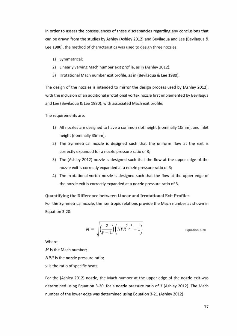
77

In order to assess the consequences of these discrepancies regarding any conclusions that

can be drawn from the studies by Ashley (Ashley 2012) and Bevilaqua and Lee (Bevilaqua &

Lee 1980), the method of characteristics was used to design three nozzles:

1) Symmetrical;

2) Linearly varying Mach number exit profile, as in (Ashley 2012);

3) Irrotational Mach number exit profile, as in (Bevilaqua & Lee 1980).

The design of the nozzles is intended to mirror the design process used by (Ashley 2012),

with the inclusion of an additional irrotational vortex nozzle first implemented by Bevilaqua

and Lee (Bevilaqua & Lee 1980), with associated Mach exit profile.

The requirements are:

1) All nozzles are designed to have a common slot height (nominally 10mm), and inlet

height (nominally 35mm);

2) The Symmetrical nozzle is designed such that the uniform flow at the exit is

correctly expanded for a nozzle pressure ratio of 3;

3) The (Ashley 2012) nozzle is designed such that the flow at the upper edge of the

nozzle exit is correctly expanded at a nozzle pressure ratio of 3;

4) The irrotational vortex nozzle is designed such that the flow at the upper edge of

the nozzle exit is correctly expanded at a nozzle pressure ratio of 3.

Quantifying the Difference between Linear and Irrotational Exit Profiles

For the Symmetrical nozzle, the isentropic relations provide the Mach number as shown in

Equation 3-20:

𝑀 = √(2

𝛾 − 1) (𝑁𝑃𝑅

𝛾−1𝛾 − 1)

Equation 3-20

Where:

𝑀 is the Mach number;

𝑁𝑃𝑅 is the nozzle pressure ratio;

𝛾 is the ratio of specific heats;

For the (Ashley 2012) nozzle, the Mach number at the upper edge of the nozzle exit was

determined using Equation 3-20, for a nozzle pressure ratio of 3 (Ashley 2012). The Mach

number of the lower edge was determined using Equation 3-21 (Ashley 2012):

78

𝑀𝐿𝑜𝑤𝑒𝑟 = 𝑀𝑈𝑝𝑝𝑒𝑟 (𝐻 + 𝑅

𝑅)

Equation 3-21

Where:

𝐻 is the slot height in mm;

𝑅 is the trailing edge radius in mm;

The Mach numbers in between the upper and lower nozzle exits were determined via

linear interpolation, in line with (Ashley 2012).

For the Irrotational Vortex nozzle, the pressure distribution was determined as a function

of distance from the reaction surface, as dictated by Equation 3-22 (Bevilaqua & Lee 1980):

𝑃𝑦 = (( 𝑅 + 𝑦

𝑅)

2

(𝑁𝑃𝑅(

1−𝛾𝛾

)− 1) + 1)

𝛾1−𝛾

Equation 3-22

Where:

𝑦 is the vertical position, in mm;

𝑃𝑦 is the static pressure at vertical position, y;

Equation 3-20 is then used to determine the local Mach number, as a function of the local

static pressure (Bevilaqua & Lee 1980).

The exit Mach number profiles for the three nozzles are shown in Figure 3.22. The lower

Mach number of 1.6294 for the (Ashley 2012) nozzle is 91.53% of the Mach number for the

Irrotational Vortex nozzle (1.7802). If the Irrotational Vortex distribution can be assumed

linear, then the error in the lower Mach number used for the study by Ashley (Ashley

2012), when compared to the theory Ashley (Ashley 2012) referenced, is 8.47%. This

particular relationship is only valid for a slot height to radius ratio of 0.2, as used in the

studies by Ashley (Ashley 2012) and Bevilaqua and Lee (Bevilaqua & Lee 1980). As the slot

height to radius ratio decreases to zero, both of the asymmetrical Mach profiles will tend

towards the symmetrical (uniform) Mach profile.

79

Figure 3.22 Comparison of Mach exit profiles for (Ashley 2012), irrotational vortex and symmetrical nozzles

As with (Ashley 2012), the nozzles are designed from eight predefined points across the

nozzle exit using the method of characteristics, with the Mach number exit profile forming

the initial conditions. Characteristic lines are then propagated upstream to the throat, with

the position of any necessary reflections marking the location and angle of the nozzle wall.

A spline function is then prepended to the contour in order to make a smooth convergent

section. The contours are shown in Figure 3.23.

80

Figure 3.23 Comparison of nozzle contours for (Ashley 2012), irrotational vortex and symmetrical nozzles.

The supersonic curved wall jet issuing from the (Ashley 2012) nozzle was simulated using

the method of characteristics and is shown, along with the surface pressure profile, in

Figure 3.24. As can be seen, the surface pressure profile is close to, but not quite flat, and

the free-stream boundary is close to, but not quite circular.

81

Figure 3.24 Method of characteristics simulation of the (Ashley 2012) nozzle. Compared to Figure 3.13, the stream-wise pressure gradients are much reduced relative to the symmetrical curved wall jet, but are not

eliminated.

82

Mass Flow Considerations

Confusion arises as both Bevilaqua and Lee (Bevilaqua & Lee 1980) and Ashley (Ashley

2012) define the design NPR as the correctly expanded NPR (difference between the design

and correctly expanded NPR is explicitly defined for this study in Section 3.1.5). In doing so,

however, the authors are designing the asymmetrical nozzles to have a higher averaged

exit Mach number than the symmetrical nozzle they were compared with (Bevilaqua & Lee

1980; Ashley 2012). This also results in a higher exit area to throat area ratio relative to the

symmetrical counterparts. A consequence of this is that the mass flow through the two

nozzles would be different at the same nozzle pressure ratio, when both nozzles are scaled

to the same external geometry (H/R) (derived from Equation 3-12 and 3-14).

As discussed in the previous chapter, any discussion of efficiency of a circulation control

system should to take into account the mass flow – as this is the principal cost to the

system (Warsop & Crowther 2013; Michie 2008; Sparks et al. 2005). It can, therefore, be

concluded that the previous studies discussed are not helpful in ascertaining the benefits of

asymmetrical nozzle profiles on attachment in the context of circulation control, because

the asymmetrical nozzles were compared with symmetrical nozzles of different throat area

(and, hence, mass flow).

In terms of nozzle geometry, the asymmetric nozzles of Bevilaqua and Lee (Bevilaqua & Lee

1980) and Ashley (Ashley 2012) have two differences from the symmetrical nozzles they

are compared with:

1) Symmetry of the nozzle contour (as a function of slot height to radius ratio –

producing the asymmetric Mach number profile);

2) Exit area to throat area ratio.

Revisiting the definition of design NPR used in this study (Section 3.1.5), a more valid

comparison metric would be the quasi-one dimensional area-Mach number relation, given

by Equation 3-12, restated below for convenience:

(𝐴𝑥

𝐴∗)

2

= 1

𝑀𝑥2 [

2

𝛾 + 1(1 +

𝛾 − 1

2𝑀𝑥

2)]

(𝛾+1)(𝛾−1)

Equation 3-12

In determining the distribution of the cross sectional area to throat area ratio, the

asymmetric nozzles can be converted to their symmetric equivalent. Figure 3.25 shows the

area ratio distribution for the irrotational vortex and the (Ashley 2012) nozzles, designed to

equivalent correctly expanded NPRs.

83

Figure 3.25 Area ratio distribution for the (Ashley 2012), irrotational vortex, and symmetrical nozzles. Equivalent symmetrical nozzle design nozzle pressure ratio is shown in the legend.

Using the area Mach number relation, it has been calculated that the irrotational vortex

nozzle has an area ratio distribution equivalent to a design NPR of 3.96. Similarly, the

(Ashley 2012) nozzle has a design NPR of 3.58.

Since increasing the design NPR of a convergent-divergent nozzle has already been shown

to increase the separation NPR (Cornelius & Lucius 1994; Llopis-Pascual 2016), the current

study has an opportunity to answer a question of consequence for circulation control

nozzles: What effect does skewing the nozzle have on the separation NPR of a supersonic

curved wall jet, independent of the area ratio?

3.2.4 Summary of Nozzle Geometries

Figure 3.26 shows a summary of the separation nozzle pressure ratio against H/R for the

convergent-only nozzle from (Gregory-Smith & Gilchrist 1987); the four symmetrical and

asymmetrical convergent-divergent nozzles from (Llopis-Pascual 2016); the symmetrical

convergent-divergent nozzle (asymmetrical separation nozzle pressure ratio not provided)

from (Jegede 2016); and the asymmetrical nozzle from (Ashley 2012). Note that the circle

corresponding to ‘Multiple’ relates to the convergent-only nozzle from (Lytton 2006); the

84

symmetrical convergent-divergent nozzles from (Chippindall 2009) and (Ashley 2012); and

both symmetrical and asymmetrical convergent-divergent nozzles from (Bevilaqua & Lee

1980).

Linear exit Mach number profiles were used for the asymmetrical nozzles of (Ashley 2012)

and (Llopis-Pascual 2016), and an irrotational vortex exit Mach number profile was used for

the asymmetrical nozzles of (Bevilaqua & Lee 1980) and (Jegede 2016).

The convergent-divergent nozzles at low H/R clearly show an increase in separation NPR as

the design NPR increases (Llopis-Pascual 2016; Gregory-Smith & Gilchrist 1987). However,

as the H/R increases, the performance of symmetrical and asymmetrical convergent

nozzles offers less of an increase in separation NPR relative to the H/R-equivalent

convergent-only nozzles (Gregory-Smith & Gilchrist 1987; Lytton 2006; Chippindall 2009;

Ashley 2012; Jegede 2016). A particular area of interest is around NPR 3 and H/R 0.2. Only

(Ashley 2012) shows extended attachment above approximately NPR 3.1. Exploring this

region of operation with different fixed geometries is a useful way of testing the hypothesis

that adapting the nozzle geometry to maintain an irrotational vortex at different NPR

prevents separation.

Figure 3.26 Separation nozzle pressure ratio vs H/R for different nozzle geometries. Note that red crosses are convergent-only nozzles; convergent-divergent nozzles are appropriately labelled, with symmetrical nozzles identified by their design NPR (NPRD), and asymmetrical nozzles identified by their correctly expanded NPR (CENPR). Constructed from (Bevilaqua & Lee 1980; Gregory-Smith & Gilchrist 1987; Lytton 2006; Chippindall

2009; Ashley 2012; Jegede 2016; Llopis-Pascual 2016)

85

To summarise past literature, studies have ascertained the following trends:

1) Reducing H/R results in a higher separation NPR, for both convergent-only and

convergent-divergent nozzles (Englar 1975; Gregory-Smith & Gilchrist 1987;

Gilchrist 1985; Gilchrist & Gregory-Smith 1988; Cornelius & Lucius 1994; Gregory-

Smith & Senior 1994; Cutbill 1998; Lytton 2006; Chippindall 2009; Ashley 2012;

Jegede 2016; Llopis-Pascual 2016).

2) A separation mechanism where separation bubbles grow larger as the NPR is

increased until eventually intersecting the edge of the reaction surface has been

proposed (Gregory-Smith & Gilchrist 1987). More recent studies with convergent-

divergent nozzles at H/R of around 0.2 have cited shock induced boundary layer

separation as the cause of the jet fully detaching (Lytton 2006; Chippindall 2009;

Ashley 2012; Jegede 2016). A lack of consistency between recent studies and past

literature has led to the stated need for a study into the exact separation

mechanism for convergent-divergent nozzles (Jegede 2016; Llopis-Pascual 2016).

3) Introducing a step between the exit of the nozzle and the reaction surface results in

a relatively higher separation NPR compared to a convergent-only nozzle at the

same H/R (Gregory-Smith & Gilchrist 1987; Gregory-Smith & Senior 1994).

Additionally, the presence of a small gap between the reaction surface and nozzle

exit has been identified as lowering the nozzle pressure ratio at which flow

separates for convergent-only nozzles (Gregory-Smith & Senior 1994). More recent

studies performed with unstepped convergent-divergent nozzles have identified a

separation mechanism based on the waves propagating from the gap (Chippindall

2009).

4) Convergent-divergent nozzles have a higher separation NPR than convergent-only

nozzles of the same H/R (Gregory-Smith & Gilchrist 1987; Cornelius & Lucius 1994;

Chippindall 2009; Ashley 2012; Jegede 2016; Llopis-Pascual 2016). Additionally,

increasing the exit area to throat area ratio (i.e. ‘design NPR’) of the convergent-

divergent nozzle also results in a higher separation NPR (Cornelius & Lucius 1994;

Llopis-Pascual 2016).

5) Asymmetrical convergent-divergent nozzles have been shown to increase the

separation NPR compared to symmetrical convergent-divergent nozzles, for some

studies (Ashley 2012; Llopis-Pascual 2016) however, for others there were no

significant differences or the asymmetrical performance was actually worse

(Bevilaqua & Lee 1980; Jegede 2016). The asymmetrical nozzles have been

86

designed to have a higher exit area to throat area ratio relative to their

symmetrical counterparts (Bevilaqua & Lee 1980; Ashley 2012). Consequently,

when considered alongside point (2), above, it is not known what the effect of the

asymmetric exit pressure profile alone has on the flow.

3.3 Effectiveness Metrics for Supersonic Curved Wall jets

The effectiveness of a supersonic curved wall jet really depends on the application. For

Coanda flares effectiveness is dictated by attachment – the higher the nozzle pressure ratio

at which the jet is attached the more effective the curved wall jet (Morrison & Gregory-

Smith 1984; Gregory-Smith & Gilchrist 1987; Gilchrist & Gregory-Smith 1988; Gilchrist 1985;

Gregory-Smith & Senior 1994; Cutbill 1998). As stated in Chapter 2, the principal

operational limit for circulation control is the separation of the jet (Englar 1970; Englar

1975; Cornelius & Lucius 1994; Frith & Wood 2003; Michie 2008; Llopis-Pascual 2016).

For fluidic thrust vectoring the main metric used to determine curved wall jet effectiveness

is the vertical force coefficient (Cz), defined in Equation 3-23 (Lytton 2006; Chippindall

2009; Ashley 2012; Jegede 2016):

𝐶𝑧 =𝐹𝑧

𝐹𝑇𝑜𝑡𝑎𝑙

Equation 3-23

Where:

FZ is the force (N) in the vertical direction;

FTotal is the total force (N) produced by the jet at the nozzle exit (due to momentum).

The vertical force coefficient is usually calculated from the magnitude of static pressure

difference between the reaction surface and ambient air resolved in the vertical direction

(Lytton 2006; Chippindall 2009; Ashley 2012; Jegede 2016). Consequently, it can be argued

that this is a valid metric for the relative effectiveness of circulation control, given that the

aim of circulation control nozzle is to augment lift, and lift is a force entirely due to the

relatively lower pressure on the upper surface of the wing compared to the lower surface

of the wing. Llopis-Pascual (Llopis-Pascual 2016) used a normal force coefficient, which

resolves the magnitude of the static pressure difference normal to the reaction surface at

the point at which it is measured, to measure the effectiveness of nozzles for circulation

control.

The normal force and vertical force coefficients are tied intrinsically to separation, indeed,

the largest magnitude of vertical force coefficient usually occurs just before separation

87

(Jegede 2016). Trends established by Ashley (Ashley 2012) and Jegede (Jegede 2016)

suggest that asymmetrical convergent-divergent nozzles have lower vertical force

coefficients when compared to their symmetrical equivalent (same correctly expanded

NPR), when operating at the same NPR. Additionally, a trend established by Llopis-Pascual

(Llopis-Pascual 2016) suggests that convergent-divergent nozzles of higher design NPR have

lower normal force coefficients (and, by extension, vertical force coefficients) compared to

nozzles with a lower design NPR, when operating at the same NPR and fully attached. This

could be due to the way the vertical force coefficient is calculated, however, as any

increase in momentum that occurs due to expansion on the reaction surface is

unaccounted for. Nozzles which produce a lower momentum at their exit will have a

greater vertical force coefficient when severely under-expanded, because the momentum

at the nozzle exit is all that is accounted for in the calculation of this metric: any change in

momentum occurring downstream of the nozzle exit is not factored into the calculation.

Most commonly, for circulation control, the metric for the effectiveness of a curved wall jet

is the momentum of the jet, of which the momentum coefficient is a function (Englar 1970;

Englar & Williams 1971; Englar 1975; Englar 1979; Englar et al. 1981; Abramson & Rogers

1983; Loth & Boasson 1983; LOTH & BOASSON 1984). If a constant mass flow is considered

for the purposes of a comparison, this means that the higher the design nozzle pressure

ratio of a convergent-divergent nozzle, the higher the momentum across the full range of

operating nozzle pressure ratios (Anderson 2007). This is due to the higher exit velocity of

convergent-divergent nozzles at higher design nozzle pressure ratios. This is highlighted in

Figure 3.27, which shows the momentum of the jet at nozzle exits divided by the reference

momentum, calculated for a convergent-only nozzle at an operating nozzle pressure ratio

of 2. The assumptions include isentropic flow (i.e. no shockwaves in the nozzle exit) and an

isentropically compressed upstream pressure. This graph was constructed using the

isentropic equations from Section 3.1.2.

88

Figure 3.27 Normalised momentum efficiency for various nozzle geometries. All momentums are normalised to a convergent-only nozzle operating at NPR 2.

3.4 The Effect of Free-Stream

The past literature studied in this chapter considers quiescent (i.e. static ambient)

conditions. The NPR at which curved wall jets (subsonic and supersonic) separate is

different in non-quiescent conditions for two reasons:

1) The static pressure at the nozzle exit is affected by upstream geometry and free-

stream static pressure. This changes the effective NPR relative to quiescent

conditions at the same upstream stagnation pressure (Englar 1975);

2) The pressure distribution across the free-stream boundary is affected by upstream

geometry and free-stream static pressure. Additionally, the growth of the shear

layer is different due to differences in the relative velocity of the jet and the

ambient conditions causing a difference in shear stress (Englar 1975).

Extensive discussion on the effect of free-stream on curved wall jet separation is provided

by (Englar 1975), which is concisely summarised here for convenience. Evidence compiled

by Englar (Englar 1975) suggests that whilst the separation NPR is different, the relative

performance of trailing edge geometries is the same. This is reflected by the consistency

between the quiescent trend from (Gregory-Smith & Gilchrist 1987) and results referenced

by (Englar 1975), which show trailing edge geometries with a lower H/R have a higher

89

separation NPR (Kizilios & Rose 1969) regardless of free-stream condition. Much confusion

on the topic arises due to ambiguity as to which free-stream pressure authors used to

calculate the NPR: Static pressure local to the exit, static pressure at the free-stream, and

static pressure in quiescent conditions have all been used in different studies (Englar 1975).

Recently, Llopis-Pascual (Llopis-Pascual 2016) compared symmetrical convergent-divergent

(design NPR 4) and asymmetrical convergent-divergent (correctly-expanded NPR 4) in both

quiescent and free-stream conditions. Whilst the separation NPR was different in a free-

stream, the relative performance between the nozzles was the same as the quiescent

condition (Llopis-Pascual 2016).

3.5 Proposed Study

The scope of this PhD is constrained to only consider the effect the internal nozzle

geometry, up to and including the nozzle exit, has on supersonic curved wall jet behaviour.

Consequently, any solution that involves the downstream geometry (such as step height,

reaction surface radius or reaction surface shape) is not considered.

In order to extend the state of the art, the impact on the NPR at which separation occurs

from independently changing the following three geometric aspects is considered:

1) H/R for convergent-divergent nozzles. There have been no previous studies where

the same convergent-divergent nozzle (i.e. same design NPR) has been tested over

a range of H/R. Consequently, the symmetrical nozzle with a design NPR of 3 was

tested at H/R of 0.1, 0.15 and 0.2 in order to ascertain performance trends and

separation behaviour. Furthermore, given the difficulty in understanding the

consequences of having a separate reaction surface with a small gap, each of these

nozzles was manufactured with the reaction surface joined to the nozzle exit. The

symmetrical convergent-divergent nozzle with a design NPR of 3 at an H/R of 0.2

has been tested in past studies (Chippindall 2009; Ashley 2012), and so this

provides a good point of validation for the experimental procedures used in this

study.

2) Irrotational vortex nozzles compared with a symmetrical nozzle of equivalent area

ratio. All asymmetrical nozzles tested in past literature have been compared with a

symmetrical nozzle of different area ratio, hence, mass flow (Bevilaqua & Lee 1980;

Ashley 2012; Jegede 2016; Llopis-Pascual 2016). The three symmetrical nozzles

defined in point (1) were tested against asymmetrical nozzles of the same design

90

NPR, where for each H/R the nozzle is skewed to produce an irrotational vortex at

the nozzle exit, as used in (Bevilaqua & Lee 1980) and (Jegede 2016).

3) Exit area to throat area ratio at high H/R (0.2). Given the crowding of data-points

on Figure 3.26 around H/R 0.2 and nozzle pressure ratio of 3.1, a symmetrical

nozzle, with a design NPR of 4, joined to the reaction surface was compared with

an irrotational vortex nozzle of equivalent design NPR to see if it is possible to

achieve a significantly higher separation NPR at this H/R. Through assessing this

region of operation (i.e. NPR 3, H/R 0.2), the viability of delaying separation

through changing nozzle geometry can be assessed.

These experiments aim first to measure the performance, in terms of vertical force

coefficient and separation nozzle pressure ratio; and secondly to characterise the process

of supersonic curved wall jet separation across a wide range of nozzle geometries as

suggested in (Llopis-Pascual 2016) and (Jegede 2016). Additionally, the outcome of this

study in addition to the past literature highlighted in this section should help determine:

1) Whether a particular internal nozzle geometry is necessary (i.e. to maintain

attachment) or desirable (i.e. to improve efficiency or effectiveness) in the context

of a supersonic curved wall jet;

2) If so, whether there is a benefit of having an adaptive internal nozzle geometry.

91

Chapter 4 Supersonic Curved Wall Jet

Detachment: Research Methods

Chapter Overview

This chapter provides an overview of the research methods used in the study of supersonic

curved wall jets outlined in the previous chapter. It begins with a comprehensive summary

of the apparatus used, including details regarding the design and manufacture of the

nozzles. A broad introduction to shadowgraph and schlieren is presented before the novel

contribution of combined shadowgraph and schlieren images is discussed. Additionally,

discussion regarding the setup, experimental procedure and post-processing of the

pressure sensitive paint experiment is provided.

92

4.1 Objectives

The objectives of this study were:

1) To quantify the performance of convergent-divergent nozzle supersonic curved

wall jets over a range of slot height to radius ratios and nozzle geometries in

quiescent air.

2) To characterise the process of supersonic curved wall jet separation in quiescent

air, applicable across a range of sot height to radius ratios and nozzle geometries.

In total, four sets of experiments were performed, experiment 1 (pressure data) aimed to

achieve objective (1), experiments 1-4 intended to achieve objective (2):

1) Surface pressure data was taken from the reaction surface in order to quantify the

performance of the curved wall jets as the NPR transitioned from an NPR of one

until one beyond the NPR of separation, and back to one.

2) Schlieren and shadowgraph images were taken as the NPR transitioned from an

NPR of one until one beyond the NPR of separation, and back to one. This was

performed in order to identify any pattern in the wave structure prior to

separation.

3) Pressure Sensitive Paint was applied to the side walls of the experimental setup,

with images captured as the pressure varied from an initial condition of just less

than the NPR at which separation occurs, to just after separation occurs. The aim of

this experiment was to qualitatively assess the jet structure, and how it changes

between fully attached and fully separated.

4) Schlieren images were captured at a high frame rate as the NPR was varied from

just under the NPR at which the nozzle separates, until just after separation. The

purpose of this was to observe the exact changes in the wave structure during

separation.

Due to the practicalities of time (principally limited by equipment availability), not all of the

nozzles could be used for all of the experiments. Table 4.1 summarises the nozzle

geometries, alongside the experiments in which they were used.

93

Table 4.1 Summary of nozzle geometries and their respective experiments

4.2 Apparatus

4.2.1 Test Rig

The source of high pressure air was an electric pneumatic compressor, capable of providing

a steady supply of air at up to 17 bar pressure and room temperature. The compressed air

is routed through a manual ball valve, an air filter and a manually adjustable pressure

regulator. Following the pressure regulator the air passes through an electrically operated

ball valve and into a plenum. Halfway along the plenum, a differential pressure transducer

provides the reading for the nozzle pressure ratio used in the experiment. The nozzle

backing plate is bolted to the plenum outlet.

Figure 4.1 Schematic of air supply

The electrically operated ball valve is the sole means of controlling the experiment. It

allows a user, situated outside of the experimental room, to vary the nozzle stagnation

pressure from atmospheric up until the maximum pressure limited by the upstream

pressure regulator, by a keyed safety switch and linear dial. A schematic of the high

pressure air supply is shown in Figure 4.1.

Experiment 1 Experiment 2 Experiment 3 Experiment 4

Pressure

Data

Combined

Schlieren and

Shadowgraph

Pressure

Sensitive

Paint

High Speed

Schlieren

Symmetrical Convegrent-

Divergent3 0.1 SYM1HR01 yes yes yes yes


Divergent3 0.15 SYM1HR015 yes yes yes no


Divergent3 0.2 SYM1HR02NPR3 yes yes no no


Divergent4 0.2 SYM1HR02NPR4 yes yes yes yes

Adjusted Irrotational

Vortex3 0.1 AIV1HR01 yes yes no no


Vortex3 0.15 AIV1HR015 yes yes no no


Vortex3 0.2 AIV1HR02NPR3 yes yes no no

Irrotational Vortex (NPR 3) 4 0.2 IV1HR02NPR3 yes yes no no

Nozzle Geometry

Equivalent

Symmetrical Design

NPR (from area ratio)

H/R Identifier

94

4.2.2 Nozzles

In order to disassociate nozzle asymmetry, as defined in (Bevilaqua & Lee 1980) from exit

area to throat area ratio, the asymmetrical pressure profiles must first be adjusted to have

the same mass flow as their symmetrical counterparts.

Figure 4.2 Area ratio distribution of adjusted asymmetrical nozzles

Using the area ratio distribution as a design metric, the average exit Mach number for the

asymmetrical nozzles can be adjusted to match the symmetric nozzle. The adjusted area

distribution is plotted in Figure 4.2 (note that the contour upstream of the throat is not as

important as the downstream contour because subsonic flow can adjust to downstream

disturbances). The correctly expanded NPR of the adjusted irrotational vortex nozzle is

2.41. The adjusted Mach number profiles are shown in Figure 4.3.

95

Figure 4.3 exit Mach number distribution of adjusted nozzles

This approach aims to provide a nozzle designer a clear appreciation of the effect internal

nozzle geometry has on supersonic curved wall jet separation independent of the design

nozzle pressure ratio. By fixing the throat area (hence mass flow), exit slot height and

reaction surface radius, and only changing the symmetry of the nozzle contours, it is

possible to isolate the exact contribution of asymmetric exit Mach number profile to the

theoretical prolonged supersonic curved wall jet attachment. Given how close the linear

profile is to the irrotational profile with the adjusted nozzles shown in Figure 4.3, only the

adjusted irrotational vortex (AIV) profiles are used to design the nozzles used in this study.

The adjusted nozzle contours, designed using the method of characteristics

implementation are shown in Figure 4.4 to Figure 4.7 alongside the symmetrical

counterpart. Also highlighted in the legend of Figure 4.4 to Figure 4.7 is the correctly

expanded nozzle pressure ratio, which is the nozzle pressure ratio at which no shockwave

or expansion fans are present.

96

Figure 4.4 Symmetrical and Asymmetrical nozzle contours designed for H/R = 0.1, design NPR = 3


97


Figure 4.7 Symmetrical and Asymmetrical nozzle contours designed for H/R = 0.2, NPR = 4

The nozzles shown in Figure 4.4 to Figure 4.7 also highlight the intrinsic link between area

ratio, H/R and the extent of the asymmetry required to produce an irrotational vortex. The

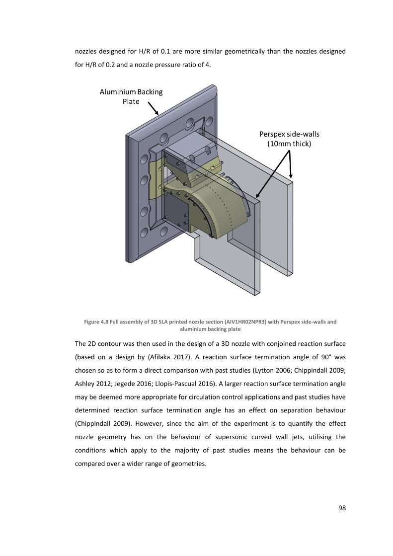
98

nozzles designed for H/R of 0.1 are more similar geometrically than the nozzles designed

for H/R of 0.2 and a nozzle pressure ratio of 4.

Figure 4.8 Full assembly of 3D SLA printed nozzle section (AIV1HR02NPR3) with Perspex side-walls and aluminium backing plate

The 2D contour was then used in the design of a 3D nozzle with conjoined reaction surface

(based on a design by (Afilaka 2017). A reaction surface termination angle of 90° was

chosen so as to form a direct comparison with past studies (Lytton 2006; Chippindall 2009;

Ashley 2012; Jegede 2016; Llopis-Pascual 2016). A larger reaction surface termination angle

may be deemed more appropriate for circulation control applications and past studies have

determined reaction surface termination angle has an effect on separation behaviour

(Chippindall 2009). However, since the aim of the experiment is to quantify the effect

nozzle geometry has on the behaviour of supersonic curved wall jets, utilising the

conditions which apply to the majority of past studies means the behaviour can be

compared over a wider range of geometries.

99

Figure 4.9 Nozzle section (SYM1HR01) and side view schematic showing pressure tap locations. Design modified from (Afilaka 2017) to eliminate discontinuities at the nozzle exit.

Each nozzle featured fifteen surface pressure taps distributed evenly along the reaction

surface, with two additional pressure taps above and below the nozzle exit. The size of the

pressure taps was based on work in (Afilaka 2017), as above a diameter of 1 mm the

attachment of a supersonic curved wall jet is adversely affected. Additionally, the spacing

of the pressure taps was limited by practicality in physically fitting the hypodermic needles

on the inside radius of the reaction surface. For the H/R = 0.2 nozzles, this proved too

difficult, leading to the modification of the design such that the hypodermic needles could

be glued to the side of the reaction surface.

The nozzles were first SLA 3D printed and then CNC machined with a quoted tolerance of

10 µm (Sun Fun Precision manufacturing Co. Ltd, Hong Kong). Side plates were also used in

order to reduce 3D effects in line with previous studies (Cornelius & Lucius 1994; Lytton

2006; Chippindall 2009; Ashley 2012; Jegede 2016). For the high speed schlieren and

combined shadowgraph and schlieren, the side walls were 10 mm Perspex (Bay Plastics

Ltd). For the pressure sensitive paint (PSP) experiment, the side-walls were replaced by UV-

transparent acrylic (Bay Plastics Ltd) on one side, and the PSP prepared surface on the

other.

The nozzle and side walls were fixed using threaded rods, nuts and bolts to an aluminium

backing plate. Figure 4.9 shows the nozzle section as designed in Solidworks, which could

be slid in and out of the backing plate. Note that the line between the nozzle exit and

reaction surface in Figure 4.9 is not a physical feature – the nozzle exit was tangential to

100

the reaction surface. The side view of the nozzle is shown in Figure 4.9, with the fifteen

reaction surface pressure sensors, in addition to the two pressure sensors positioned above

and below the exit labelled appropriately. The nozzle shown in Figure 4.9 is SYM1HR01, and

the nozzle shown as part of the assembly in Figure 4.8 is AIV1HR02NPR3.

4.2.3 Optical Apparatus

For the schlieren and the pressure sensitive paint experiments, a Phantom V1611 camera

(Vision-Research 2015) was used. For the shadowgraph, a Phantom v310 camera (Vision-

Research 2012) was used. The specifications of both cameras are shown in Table 4.2.

Table 4.2 Summary of camera properties. Summarised from (Vision-Research 2012; Vision-Research 2015)

The biggest limitation in using these cameras was the amount of on-board memory (RAM)

available. In order to allow for an experiment to last over one minute in duration

(necessary for the combined shadowgraph and schlieren experiment, discussed in Section

4.3), both cameras were limited to one hundred frames per second (fps), with the

minimum exposure time of 1μs for the combined schlieren and shadowgraph experiment.

Given that the Phantom V1611 was capable of a higher frame rate, it alone was used to

capture schlieren images of the transition from attached to detached at a high temporal

resolution.

Finally, the Phantom V1611 was used in the pressure sensitive paint experiment at a much

higher exposure time and frame rate. The increase in exposure time was necessary in order

to increase sensitivity to the response of the pressure sensitive paint. A summary of the

camera settings for each experiment is shown in Table 4.1.

Phantom V1611 Phantom V310

Full Resolution 1280x800 1280x800

Sensor

CMOS, 28μm pixel size,

12-bit depth, Mono and

colour

CMOS, 20μm pixel size, 12-bit

depth, Mono and colour

Minimum

Exposure Time1μs 1μs

Maximum Frame

Rate

16,000 fps (full

resolution) 1,000,000 fps

maximum

3140 fps (full resolution)

500,000 fps maximum

On-board RAM 96GB 32GB

101

Table 4.3 Summary of camera settings used for each experiment

The cameras were connected individually to separate laptops placed outside of the room

via Ethernet cables. This connection allowed a live video feed of the experiment, in addition

to the remote operation of the cameras.

In addition to the cameras, for the schlieren and shadowgraph experiment, a total of three

plane mirrors and two spherical mirrors (8’ focal length), a 20 mm diameter beam splitter,

a XE 300W continuous light source, a double knife edge, a single knife edge, a condenser

lens and two focussing lenses were used. The arrangement of these around the nozzle test

rig is discussed in Section 4.3.2.

For the pressure sensitive paint experiment, four ISSI air-cooled LM2X 2-inch Air-Cooled

Light Emitting Diode (LED) lamps (Innnovative Scientific Solutions Incorporated n.d.) were

used to provide ultraviolet (UV) light. The lamps have an excitation wavelength of 395nm

with a full width half maximum of approximately +/- 18nm. The Phantom V1611 camera

was used with an 85mm lens and a 600nm low-pass filter with an infrared cut-off.

4.2.4 Pressure Transducers

Metal hypodermic needles were glued into the pressure taps on the 3D printed nozzle

(shown in Figure 4.9), with flexible tubing connecting the needles to a board of pressure

transducers. The pressure transducers (Honeywell truStability SSCSANN100PAAA5) are

capable of recording 0-100 psi absolute pressure at a frequency of 1kHz. 16 unconnected

absolute pressure transducers were left exposed (without a hypodermic connection) and

their averaged value was used as the ambient pressure in the room. In addition to this, a

single pressure transducer (JUMO MIDAS C08) capable of measuring 0-25bar differential

pressure was placed inside the plenum.

Frame Rate (frames per

second)

Exposure Time

(microseconds)

Experiment Duration

(seconds)Resolution (pixels)

Phantom V1611 100 1 106 1280x800

Phantom V310 100 1 106 1280x800


second)

Exposure Time

(microseconds)

Experiment Duration


Phantom V1611 25,000 1 3 800x600

Phantom V310 N/A N/A N/A N/A


second)

Exposure Time

(microseconds)

Experiment Duration


Phantom V1611 5000 100 6 1280x800

Phantom V310 N/A N/A N/A N/A

Schlieren & Shadowgraph

High Speed Schlieren

Pressure Sensitive Paint

102

Two high speed data acquisition cards (National Instruments USB-6351) were used, each

capable of importing 16 channels at a frequency of 1 kHz. Voltages were read from the

pressure transducers, and the post-processing software (NI Signal Express) converted the

voltages to absolute pressure values that were saved to file.

Pressure Transducer Setup

The absolute pressure transducers (Honeywell truStability SSCSANN100PAAA5), were

arranged as arrays on a board located on a table behind the plenum. Flexible tubing was

used to connect them to the pressure taps located on the nozzle, reaction surface and side

walls. Three additional pressure taps located on the side wall were used for the pressure

sensitive paint experiment, as indicated in Figure 4.10. The differential pressure sensor

(JUMO MIDAS C08), located midway along the plenum, was connected to the data

acquisition card (National Instruments USB-6341) via a voltage amplifier and power supply

again located on a table behind the plenum. The total number of channels that could be

used as inputs was 32. Taking away the 20 (maximum) absolute pressure sensors in use and

the differential pressure sensor, the remaining 11 channels were connected to unused

absolute pressure transducers, and averaged to measure the ambient pressure in the

room. Figure 4.10 shows a schematic of the pressure transducer setup.

Figure 4.10 Schematic of the setup of pressure transducers

103

The only control input to all experiments described in this chapter was a voltage signal to a

valve controlling the flow into the plenum. This voltage signal was provided by a key-

enabled, analogue controller that was manually operated from outside of the room.

Feedback was provided by real-time monitoring of the differential pressure sensor inside

the plenum (via the pressure data-logging). Additionally, an adjustable pressure regulator

further upstream acted to prevent any human error that could lead to the mechanical

failure of the nozzle or plenum.

Pressure Coefficient Calculations

The pressure coefficient is defined by Equation 4-1 (Jegede 2016; Ashley 2012):

𝐶𝑃 =𝑃 − 𝑃𝑎𝑚𝑏

𝑃0 − 𝑃𝑎𝑚𝑏

Equation 4-1

Where:

P is the absolute pressure recorded by the pressure transducer;

𝑃𝑎𝑚𝑏 is the ambient pressure of the room;

𝑃0 is the stagnation pressure of the jet (calculated from the NPR).

For each absolute pressure measurement taken on the reaction surface, the pressure

coefficient was calculated and synchronised with the combined schlieren and shadowgraph

video.

In order to synchronise the pressure data with the combined shadowgraph and schlieren,

the point in time of full flow detachment was determined. This point is easily observed for

most of the nozzles in the combined shadowgraph and schlieren video as it usually happens

over a single frame. In terms of the pressure data, the time at which separation occurs is

highlighted by a sharp rise in pressure from a pressure transducer located around halfway

along the reaction surface (pressure tap 7, as described in Figure 4.9).

104

Figure 4.11 Pressure variation from pressure tap: P7 for nozzle: SYM1HR015. Separation is clearly indicated by a sharp rise in pressure. Applying a median filter (red) and finding the derivative (yellow) allows the

automatic calculation of the time at which the flow separates.

Figure 4.11 shows an example plot of the pressure from pressure tap 7 against time for

SYM1HR015. As can be seen, there is a sharp rise indicating the separation of the flow. In

order to ensure the effectiveness of this method across a range of experiments, this

pressure signal was passed through a moving median filter. The median filter recalculated

each element of the signal as the median value of the previous 30 elements and the next

30 elements in time. This filtered signal was then differentiated, which produced a clear

peak showing the time at which separation occurred. Figure 4.11 also shows the median

filtered signal and the derivative of the filtered signal plotted on top of the original signal.

Figure 4.12 shows the calculated time of separation for pressure transducers P3 - P14 for a

single experiment (SYM1HR015). Note that pressure transducers P1 and P2 were omitted

because throughout the experiment the flow was attached at these points. Additionally,

pressure transducer P15 was omitted because the magnitude of pressure readings

throughout experiments was persistently small. This highlights how quickly and

consistently the flow switches from fully attached to fully separated. For this particular

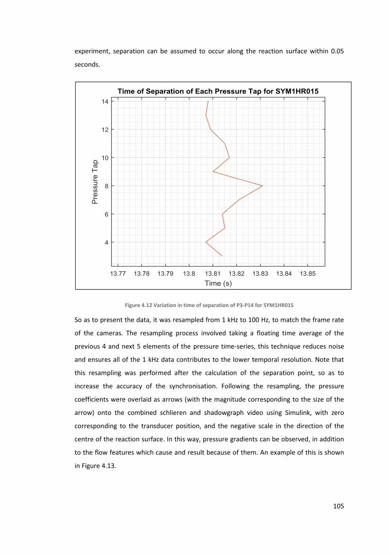
105

experiment, separation can be assumed to occur along the reaction surface within 0.05

seconds.

Figure 4.12 Variation in time of separation of P3-P14 for SYM1HR015

So as to present the data, it was resampled from 1 kHz to 100 Hz, to match the frame rate

of the cameras. The resampling process involved taking a floating time average of the

previous 4 and next 5 elements of the pressure time-series, this technique reduces noise

and ensures all of the 1 kHz data contributes to the lower temporal resolution. Note that

this resampling was performed after the calculation of the separation point, so as to

increase the accuracy of the synchronisation. Following the resampling, the pressure

coefficients were overlaid as arrows (with the magnitude corresponding to the size of the

arrow) onto the combined schlieren and shadowgraph video using Simulink, with zero

corresponding to the transducer position, and the negative scale in the direction of the

centre of the reaction surface. In this way, pressure gradients can be observed, in addition

to the flow features which cause and result because of them. An example of this is shown

in Figure 4.13.

106

Figure 4.13 Example image of pressure coefficients overlaid on the combined schlieren and shadowgraph image

Force Coefficient Calculations

In order to quantify the performance of each nozzle geometry, the force coefficient in the

z-direction (perpendicular to the nozzle exit and reaction surface) was calculated. This

convention is based upon the aircraft reference axis, and has been used as convention for

many fluidic thrust vectoring studies, for example: (Lytton 2006; Chippindall 2009; Ashley

2012; Jegede 2016). The total force generated by the nozzle can be calculated from

Newton’s second law, and is given by Equation 4-2 (Houghton & Carpenter 2003):

𝐹𝑇𝑜𝑡𝑎𝑙 = �̇�𝑉 Equation 4-2

Where:

�̇� is the mass flow (𝑘𝑔𝑚𝑠−1);

𝑉 is the velocity of the flow evacuating the nozzle (𝑚𝑠−1).

Equation 4-3 shows how mass flow is ideally calculated, taking into account the possibility

of a non-uniform exhaust flow (Jegede 2016):

�̇� = ℎ𝑊 ∫ 𝜌𝑧𝑉𝑧. 𝑑𝑧̇

Equation 4-3

Where:

ℎ is the slot height (𝑚);

107

𝜌 is the density of the fluid (𝑘𝑔𝑚−3);

𝑧 as a subscript denotes the position (𝑚);

𝑊 is the reaction surface width (0.06m for all nozzles).

In this study, both mass flow and velocity were calculated through averaging the values

from the absolute pressure measurements taken from the upper and lower nozzle exits.

Isentropic relations were used to calculate the mass flow at both the upper and lower

nozzles exits, and subsequent total mass flow was calculated from an average of these two

values. It is worth noting that this method is not accurate for calculating the mass flow for

the irrotational pressure profile. Jegede (Jegede 2016) showed that, whilst the propagation

of pressure upstream in the boundary layer contributes to an inaccuracy between

isentropically assumed nozzle exit pressures and the measured pressures for both

asymmetrical and symmetrical nozzles, this inaccuracy is a fixed offset: the pressure

gradient for asymmetric nozzles measured was the same as that predicted via isentropic

relations (Jegede 2016). Consequently, for the asymmetrical nozzles, the upper and lower

pressure values were substituted into Equation 3-4, and the distributed mass flow and

velocity calculated from isentropic relations in Section 3.1.2.

The force distribution produced by the nozzle was calculated by multiplying each absolute

pressure measured on the reaction surface by the distance between each pressure tap. An

illustration of the components described is shown in Figure 4.14 where the absolute

pressure is measured from each pressure tap. From this, the total force component is

calculated from Equation 4-4:

𝐹𝑖 = 𝑃𝑖𝐿𝑖𝑊 Equation 4-4

Where:

𝐹𝑖 is the force component, at the pressure tap, 𝑖 (𝑁);

𝑃𝑖 is the absolute pressure, measured at the pressure tap, 𝑖 (𝑃𝑎) ;

𝐿𝑖 is the length, measured from halfway between the previous tap, and halfway to the next

(𝑚). Given that the taps are equally spaced this is assumed constant.

108

Figure 4.14 Schematic showing force components at each pressure tap along the reaction surface

The vertical force components were calculated based upon the angular position of the

pressure tap, and then summed to produce the total vertical force. This is represented in

Equation 4-5:

𝐹𝑧 = ∑ 𝐹𝑖 cos 𝜃𝑖

15

𝑖=1

Equation 4-5

Where:

𝐹𝑧is the total force in the z-direction (𝑁)

𝜃𝑖 is the angle along of the position of the pressure tap, 𝑖, with respect to the nozzle exit

(𝑟𝑎𝑑.)

Finally, Equation 4-6 shows that dividing 𝐹𝑧 (calculated in Equation 4-5) by 𝐹𝑇𝑜𝑡𝑎𝑙

(calculated in Equation 4-2) would produce the force coefficient for the z-direction (𝐶𝑧)

(Lytton 2006; Chippindall 2009; Ashley 2012; Jegede 2016).

𝐶𝑧 =𝐹𝑧

𝐹𝑇𝑜𝑡𝑎𝑙

Equation 4-6

In this study, the 𝐶𝑧 is presented as a graph against NPR. It is this relationship that is used

to define the nozzle efficiency: the higher the 𝐶𝑧 at a given NPR, the more efficient a

circulation control system it is assumed to be at this design point. The major limitation of

this assumption is that the effects of a non-quiescent free-stream (entrainment) and the

wing geometry are not considered. As a relative measure of the effectiveness of the nozzle

109

geometry in isolation, however, a higher 𝐶𝑧 states that under quiescent conditions, such a

geometry produces a lower pressure on the upper surface with respect to the momentum

of the jet. The further assumption is that aspects of this relationship translate to a nozzle

located on the trailing edge of a wing in a free-stream, which was validated for a limited

number of nozzles by (Llopis-Pascual 2016).

Uncertainty Analysis

In order to draw decisive conclusions from the results of this experimental study, it is vital

to assess the uncertainty due to experimental error. Errors are considered to have two

components, systematic or bias errors, and random errors (Quinn 2016). Note that ambient

conditions (i.e. static temperature and static pressure) were measured before and after

experiments. Due to the insulation of the lab and the continuously running air extraction

system, temperature and pressure differences were negligible, and are not considered as

significantly contributing to any error.

Absolute Pressure Sensors

Occasionally, a large systematic error was caused by a blockage in the pressure tap. This is

caused by manufacturing defects in the nozzle. Where such blockages were detected (due

to small change in pressure during experiment), a small hole was drilled to unblock the

pressure tap. Where it was not possible to remedy the defect, the pressure reading was

discarded.

The absolute pressure sensors were calibrated using a Druck PACE5000 vacuum chamber in

a process described in detail in (Llopis-Pascual 2016). An example calibration curve is

shown in Figure 4.15, for the pressure transducer used for pressure tap, P1. Calibration of

all absolute pressure transducers was performed on a regular basis as the experiments

were undertaken.

110

Figure 4.15 Example calibration curve for transducer P1

Table 4.4 is constructed from manufacturer data for the absolute pressure sensor, and

summarises the sources of error.

Table 4.4 Summary of error sources for Honeywell truStability SSCSANN100PAAA5 absolute pressure transducer

The total uncertainty using the method proposed by (Quinn 2016) is calculated as the root

sum square of bias and precision errors (including the likely systematic error from the

differential pressure sensor calculated in Table 4.5), with a confidence interval used to

estimate the error due to a statistical finite population. Using this method, the typical

uncertainty for the surface pressure coefficients was calculated to be ±1.51% using a 95%

confidence interval. This agrees with (Jegede 2016), which used the same apparatus in a

similar setup. An example plot of pressure coefficient profiles is shown, with error bars, in

Figure 4.16. Note that the relatively small size of the error bars indicates good accuracy.

0 0.5 1 1.5 2 2.5 3 3.5 4 4.5 50

10

20

30

40

50

60

70

80

90

100

Pre

ssure

(K

pa)

Voltage (V)

Calibration Curve for P1

Error Source Quoted Accuracy

Accuracy (Linearity, hysteresis, repeatability,

deviation of measuring range initial value and

measuring range end value) (%)

0.25

Data Acquisition Card Accuracy (non-linearity,

offset error) (%)0.02

Likely Systematic Error (RSS - %) 0.251

111

Figure 4.16 Example surface pressure coefficient distribution plot for the H/R 0.15 nozzles operating at NPR 3. Small error bars are indicative of good accuracy

The nature of performing the experiment, consisting of manually adjusting the nozzle

pressure ratio, meant that experiments could never be repeated 100% accurately. A

measure of the repeatability of the results for this set of experiments can be obtained

through calculating the vertical force coefficient across the range of NPRs investigated.

Figure 4.17 shows a comparison between three experiments involving SYM1HR02NPR3, as

can be seen, the small difference between vertical force coefficients (calculated from all

pressure taps) indicates high repeatability, despite the manual operation of the nozzle

pressure ratio control.

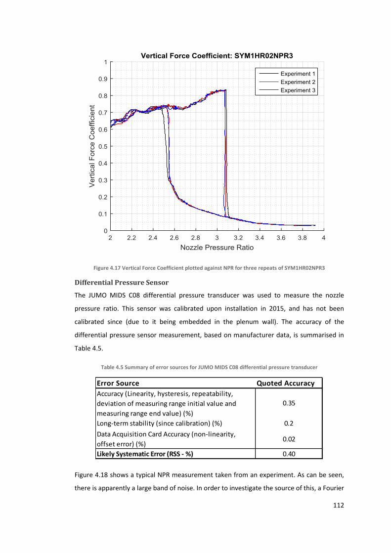
112

Figure 4.17 Vertical Force Coefficient plotted against NPR for three repeats of SYM1HR02NPR3

Differential Pressure Sensor

The JUMO MIDS C08 differential pressure transducer was used to measure the nozzle

pressure ratio. This sensor was calibrated upon installation in 2015, and has not been

calibrated since (due to it being embedded in the plenum wall). The accuracy of the

differential pressure sensor measurement, based on manufacturer data, is summarised in

Table 4.5.

Table 4.5 Summary of error sources for JUMO MIDS C08 differential pressure transducer

Figure 4.18 shows a typical NPR measurement taken from an experiment. As can be seen,

there is apparently a large band of noise. In order to investigate the source of this, a Fourier

Error Source Quoted Accuracy

Accuracy (Linearity, hysteresis, repeatability,

deviation of measuring range initial value and

measuring range end value) (%)

0.35

Long-term stability (since calibration) (%) 0.2

Data Acquisition Card Accuracy (non-linearity,

offset error) (%)0.02

Likely Systematic Error (RSS - %) 0.40

113

transform was taken, converting the signal to the frequency domain. Two frequencies

corresponding to potential error sources are the alternating current frequency of the

power supply (50Hz), and the frequency of the compressor fan upstream (25Hz).

Figure 4.18 Typical NPR measurement taken during an experiment. Also shown are the resampled maximum, minimum and mean values (25Hz).

Figure 4.19 shows a normalised noise to signal graph which was performed using a floating

mean calculated by resampling the data to 25Hz from 1000Hz. Figure 4.20 shows the

Fourier transform of this normalised noise to signal graph, as can be seen, the only

significant peak occurs at less than 1Hz. Consequently, exactly what is causing the

seemingly random variation occurring at around 7% of the magnitude of the signal mean is

unknown.

114

Figure 4.19 Noise to signal ratio

Figure 4.20 Fast Fourier Transform of Noise to signal ratio, with the frequency at which likely sources of noise occurs also highlighted by red dashed lines. Note the absence of a clear peak suggests broadband noise.

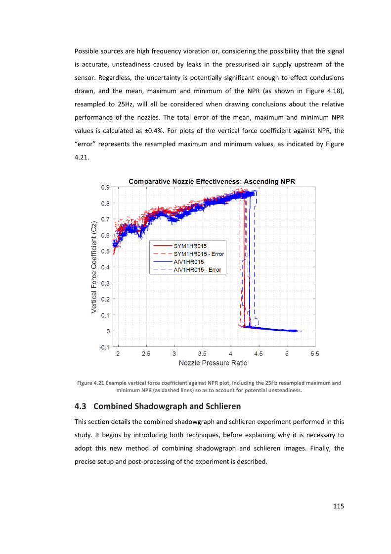
115

Possible sources are high frequency vibration or, considering the possibility that the signal

is accurate, unsteadiness caused by leaks in the pressurised air supply upstream of the

sensor. Regardless, the uncertainty is potentially significant enough to effect conclusions

drawn, and the mean, maximum and minimum of the NPR (as shown in Figure 4.18),

resampled to 25Hz, will all be considered when drawing conclusions about the relative

performance of the nozzles. The total error of the mean, maximum and minimum NPR

values is calculated as ±0.4%. For plots of the vertical force coefficient against NPR, the

“error” represents the resampled maximum and minimum values, as indicated by Figure

4.21.

Figure 4.21 Example vertical force coefficient against NPR plot, including the 25Hz resampled maximum and minimum NPR (as dashed lines) so as to account for potential unsteadiness.

4.3 Combined Shadowgraph and Schlieren

This section details the combined shadowgraph and schlieren experiment performed in this

study. It begins by introducing both techniques, before explaining why it is necessary to

adopt this new method of combining shadowgraph and schlieren images. Finally, the

precise setup and post-processing of the experiment is described.

116

4.3.1 Introduction

Shadowgraph and schlieren are two commonly used techniques used for supersonic flow

visualisation (Settles 2001). Both are based on the relationship between the refractive

index of light, and density, given by Equation 4-7 (Settles 2001):

𝑛 − 1 = 𝑘𝜌 Equation 4-7

Where:

𝑛 is the refractive index;

𝑘 is the Gladstone-Dale coefficient (0.23 cm3g-1 for air (Settles 2001)).

For small angles, the refraction angle, defined in Equation 4-8, is proportional to the spatial

change in refractive index in the same plane (Settles 2001). From Equation 4-7 this means

the refraction angle is also proportional to the change in density in that plane.

휀𝑥 = 𝐿

𝑛0

𝑑𝑛

𝑑𝑥∝

𝑑𝜌

𝑑𝑥

Equation 4-8

Where:

𝑛0 is the refractive index of light in ambient air;

𝐿 is the thickness of the source of the refraction, as viewed (m);

𝑥 denotes a single dimension in an arbitrary axis system (m).

Consequently, the spatial change in refraction angle is proportional to the change in

density gradient in that plane, as shown in Equation 4-9:

𝑑휀𝑥

𝑑𝑥∝

𝑑2𝜌

𝑑𝑥2

Equation 4-9

Consider light travelling in parallel from a source, through a test region where it is refracted

by a change in density, and finally onto a screen. The image on the screen would show a

reduction in intensity at the precise source of the refracted light, and an increase in

intensity at the destination of the refracted light (Settles 2001). This technique is referred

to as shadowgraph, and allows the visualisation of the change in refractive angle through

the test region. It is important to stress that were the image to refract uniformly, the

shadowgraph image would not show the refraction as the entire image would be translated

(Settles 2001). Consequently, it is only the effects of a change in refractive angle across the

image that is visible, not the refraction itself: the higher and lower intensity pixels of the

final image correspond to the change in density gradient (Equation 4-9) (Settles 2001). An

example schematic of shadowgraph is shown in Figure 4.22, again it is important to

117

reinforce that shadowgraph visualises the flow via the final displacement of the image (Δa),

and this does not represent the refraction angle (Ɛ), but the spatial change in refraction

angle (𝑑𝜀𝑥

𝑑𝑥). Increasing the distance between the test region and the screen (which can be

effectively achieved via a focussing lens) increases the sensitivity of the final image to any

change in refraction angle (Settles 2001).

Figure 4.22 Simplified schematic of shadowgraph. Light emitted from a point source is focussed by the lens, and upon interacting with a soap bubble is refracted. The effect of shadowgraph is an image consisting of

lower intensity at the source of the refraction, and a higher intensity at an offset distance (Δa) in the direction of the refraction. In the image to the right, the outer diameter of the black circle corresponds to the

diameter of the soap bubble. Adapted from (Settles 2001).

The schlieren technique allows the refractive angle to be visible through the use of a knife

edge (Settles 2001). Light, emitted from an extended source (i.e. through a slit) is focussed

into parallel rays§. This light then passes through the test region, and is refocused onto the

knife edge (Settles 2001). Following this, a lens refocuses the light for observation, as

shown in Figure 4.23. The presence of the knife edge acts as a cut-off for refracted light in a

particular direction, however, since the light source is extended, the full image is still

preserved by light which does not intersect the light source (Settles 2001). Any refraction

towards the knife edge results in a decrease in intensity and any refraction away from the

knife edge results in an increase in intensity (Settles 2001). The lens following the knife

edge acts to refocus the altered image, ensuring that any change in intensity due to

refraction appears at the source of refraction in the final image (Settles 2001). In this case,

the refocusing of the refraction angle and the presence of the knife edge ensure that it is

the effect of any refraction (Ɛ) that is visible in the final image (Equation 4-8) (Settles 2001).

§ Note that because the light source is extended, focussing of the beam no longer produces exactly parallel rays. In reality, the extent of the light source is much smaller than both the diameter and focal length of the lens/mirror; consequently the light is still referred to as parallel.

118

Figure 4.23 Schematic showing the schlieren technique using an extended light source. Note that the knife edge reduces the intensity of the image at the point of refraction, but does not cut the image out completely. The reduction in intensity is a function of the refraction angle (Ɛ), which is proportional to a first order spatial

density gradient (Equation 4-8). Adapted from (Settles 2001).

Schlieren and shadowgraph allow the visualisation of supersonic flow features through

observation of the consequential change in density (Settles 2001). The schlieren technique

is able to observe density gradients, and changes in density gradients in the plane of the

knife edge orientation, whereas shadowgraph is able to see the change in density gradient

in all planes (as it is not limited by the specific orientation of apparatus in the same way).

Specific examples of flow features observable are as follows:

1) Shock waves are observable by both shadowgraph and schlieren (subject to knife

edge orientation) as they are characterised by discrete changes in static pressure,

static temperature and, crucially, density (Settles 2001).

2) Regions subjected to Prandtl-Meyer expansion are visible to schlieren (subject to

knife edge orientation), but not visible to shadowgraph due to the constant density

gradient** (Settles 2001).

3) Parts of both laminar and turbulent boundary and shear layers are observable by

both shadowgraph and schlieren (subject to knife edge orientation). Laminar

boundary layers in compressible flow have a second order density gradient. For

turbulent boundary or shear layers, turbulent structures in compressible flow

** Subject to sensitivity, the edges of expansion fans may be visible via shadowgraph. This is because there must be a small but finite first order change in refractive index at the onset and conclusion of Prandtl-Meyer expansion.

119

necessitate strong density gradients in multiple planes and are visible to both

methods (Settles 2001).

At first glance it appears that shadowgraph offers no advantages over schlieren, given that

more flow features are visible to schlieren than shadowgraph. However, shadowgraph’s

main advantage is precisely that it is unable to see flow features: The only features to

appear on a shadowgraph image are shockwaves and boundary or shear layers. Figure 4.24

is a schlieren image taken from (Llopis-Pascual 2016). Due to the complexity of the flow-

field, there are a relatively large number of flow features present. Using schlieren alone

makes it very difficult to distinguish flow features from each other (e.g. shockwaves and

expansion fans).

Figure 4.24 Typical schlieren image of a separated supersonic curved wall jet, taken from (Llopis-Pascual 2016).

An expansion fan is observed propagating from the upper edge of the nozzle exit (A), with a

disturbance propagating from the lower nozzle exit (B) caused by a discontinuity between

the nozzle exit and the reaction surface. At (C), there is a separation shockwave.

Uncertainties arise principally due to the nature of (B) and (C). At (B), the disturbance could

be either a shockwave, or an expansion fan, or both (in which case the order may be of

significance). At (C), the black region before separation could be an expansion fan reflected

from (A) occurring immediately before the shockwave, or a composite image of the

separation shockwave which varies in location (due to 3D effects or geometrical defects)

along the width of the reaction surface.

Expansion fans, however, are invisible to shadowgraph, through comparing and contrasting

shadowgraph images with schlieren it becomes possible to distinguish flow features at a

glance. This study proposes an entirely new way of combining shadowgraph and schlieren,

by forming a composite colour image in the format red-green-blue (RGB), with the red

120

component consisting of the schlieren image, the green component consisting of the

shadowgraph image, and the blue component consisting of the average of the two††.

4.3.2 Experimental Setup

Combining shadowgraph and schlieren images is only useful if the images represent

precisely the same flow-field. Consequently, the major challenge with this approach is

simultaneously capturing schlieren and shadowgraph. This necessitates the use of two

cameras and a beam splitter. In this particular experiment, this was made more challenging

by a lack of available space around the test rig. In order to maximise available space, a

double-Z configuration was used, with the experimental apparatus arranged as shown in

Figure 4.25.

†† Whilst the blue component is not necessary to achieve the aim of a combined shadowgraph and schlieren image, its inclusion allows people who are red-green colour-blind to also interpret the end result. Flow features are not as distinguishable when constructing a composite image from blue/red or blue/green components.

121

Figure 4.25 Setup of combined schlieren and shadowgraph experiment

122

Light, originating at the light source, was passed through a condenser lens, and then a

double knife edge so as to recreate a point source. This was reflected from a plane mirror

onto a spherical mirror, such that the full area of the spherical mirror was illuminated. The

spherical mirror was aligned such that all of the light travels perpendicular to the nozzle

exit. Another spherical mirror of equivalent focal length and diameter, placed at the other

side of the test area, then reflects the light back towards a second plane mirror. This

mirror, in turn, reflects the light onto a beam splitter. The beam splitter divided the light

into two paths. One part was allowed to pass through the beam splitter, where, at the focal

point, a knife edge was placed horizontally, followed by a lens and the Phantom V1611

camera. The other part of the light was reflected onto a third plane mirror, which, in turn

reflected the light onto a lens and Phantom V310 camera, paced on a parallel path to the

Phantom V1611 camera. Both the schlieren and shadowgraph setup were bolted via

aluminium rails to a table in order to reduce the impact any vibrations caused by the jet

might have on the final image.

Figure 4.26 Snapshot images of test-card from Schlieren (left) and shadowgraph (right) setup

The Phantom V310 camera (shadowgraph) was placed intentionally out of focus in order to

increase the sensitivity of the shadowgraph to compression waves. The Phantom V1611

camera was focussed by positioning an M4 bolt on the nozzle, and adjusting the position of

the camera until the thread of the bolt came into sharp focus. Despite every effort, any

defects or slight misalignment of the optical apparatus would cause astigmatism to a

different extent in the shadowgraph and schlieren images (Settles 2001). This is due to the

different distance the light has to travel in order to get to both of the cameras (Settles

2001). In order to account for this, once the setup of the cameras was finished, a snapshot

of a test card placed in the test area was taken and the subsequent image adjusted as part

of the post processing. The test card consisted of a series of 9 1 cm x 1 cm squares cut into

an opaque acrylic board to form a chequerboard style pattern on the image. Through

123

comparing the relative dimensions of these squares, the images could be adjusted to

correct for any astigmatism. Figure 4.26 shows a typical snapshot of the test card placed in

the test area, from both the schlieren (left) and the shadowgraph (right) cameras. Notice

the slightly different zoom, orientation, position and intensity of the features, in addition to

the fact that the shadowgraph image is slightly out of focus (apparent when observing on

the bolt thread seen inside the nozzle geometry – the thread is visible in the schlieren

image but not on the shadowgraph). These images were used to align and normalise the

contrast of the shadowgraph and schlieren to form one colour image, a process discussed

in detail in Section 4.3.4.

4.3.3 Experimental Procedure

The combined shadowgraph and schlieren experiment (including the collection of pressure

data) consisted of the following sequence of events:

1) Schlieren and shadowgraph cameras’ on-board RAM was erased, ready to record;

2) Master valve was set to ‘open’, all people were removed from room;

3) Key operated analogue control for electric ball valve was turned to ‘on’ position;

4) Both schlieren and shadowgraph cameras began recording, pressure data began

logging;

5) The NPR (observable in real time via the pressure data log) was varied from 1,

continuously until separation occurs (observable through the live schlieren video

feed, or through the change in the pitch of the noise from the test rig), it was then

increased, uninterrupted, for an additional NPR, before being decreased back to 1.

An example of this pressure variation is shown in Figure 4.27 (NPR calculated from

the differential pressure sensor in the plenum and absolute pressure sensors

recording the ambient pressure in the room);

6) Pressure logging was stopped, schlieren and shadowgraph recordings were

stopped;

7) Key removed from key controlled analogue controller, and master valve set to

‘closed’;

8) Schlieren and shadowgraph videos were copied from the cameras to the respective

laptops;

9) Nozzle geometries were either swapped, in which case a new snapshot of the test

card (Figure 4.26) was taken from both cameras, or inspected for repeat

experiment.

124

Figure 4.27 Typical NPR variation during course of experiment

Using the same setup as the combined shadowgraph and schlieren study, the Phantom

V1611 camera was used in isolation for the high speed schlieren experiment. The same

process was observed as for the combined experiment, the only differences were:

1) No pressure data was taken;

2) The Phantom V1611 camera was manually triggered to record immediately before

the flow separated, and stopped 3 seconds later.

4.3.4 Post-Processing

In order to make the most of the combined shadowgraph and schlieren setup, the images

obtained needed to be combined in such a way that the information from both techniques

was not lost. It was decided that the best way to do this was to produce a colour image,

where the schlieren and shadowgraph images provided the red and green colour

components respectively, with the blue component consisting of an average of the

intensity of the two images.

Depending on the direction of the second order density gradient, features observed via

shadowgraph will appear as either an increase or decrease in light intensity (Settles 2001).

Given that both cameras are aligned in the same plane and provided these features are

observable in schlieren (subject to the orientation of the knife edge), they will also appear

as the same increase or decrease in light intensity in the schlieren image (Settles 2001).

125

Through combining the images in this way, common features observed through both

techniques will be preserved on the colour image as white or black.

Any features, such as expansion fans, which consist of only a first order density gradient,

may be observed through schlieren, but are not observable through shadowgraph (Settles

2001). These features are identifiable as a specific colour on the final image. Additionally,

so as to aid in the identification of shock waves, the shadowgraph camera was intentionally

put out of focus in order to increase the sensitivity to second order density gradients

relative to the schlieren setup. The reason this is necessary is because the cameras are not

precisely synchronised in time and as a consequence of flow unsteadiness, both the

shadowgraph and schlieren could observe the same shock wave but in an apparently

different position. Due to the nature of this combination process, this could be

misrepresented in the final image as a specific colour as opposed to black or white, causing

confusion. In increasing the sensitivity of the shadowgraph, it is ensured that any

compression wave would appear larger on the shadowgraph than the schlieren,

consequently any combined image would feature a black or white line surrounded by a

colour, which should be sufficiently different from the colour identifying a region of

expansion so as to allow easy identification.

The flow chart shown in Figure 4.28 shows the sequence of events used to produce a

colour image combining shadowgraph and schlieren. From the raw image, the two images

have their contrasts normalised (such that both images are of the same average intensity),

they are resized and aligned with respect to each other (from the test card snapshots

shown in Figure 4.26) Then a colour image is created, with the intensity from the adjusted

image forming the red or green component for schlieren or shadowgraph, respectively.

These images are then combined to form an Nx3 RGB matrix (where N corresponds to the

resolution), with the blue component calculated from the average intensities of the red and

green. As can be seen in the final image at the bottom of Figure 4.28, regions of continuous

expansion (including inside the nozzle and the expansion fan at the nozzle exit) are clearly

identifiable as a cyan-green, with areas of compression shown as magenta. The process

described was performed using Simulink.

Note that up to now, simulations using the method of characteristics and past literature

has had a flow direction from left to right. Flow visualisation images in this study have a

flow direction from right to left. This is because the software used to overlay the pressure

126

profiles (shown in Figure 4.13) was developed from an initial image with flow direction

from right to left.

Figure 4.28 Schematic showing the process of combining shadowgraph and schlieren images. Note that in the final image, expansion fans are identified as green regions, and areas of compression are highlighted in

magenta

127

Figure 4.29 Combined shadowgraph and schlieren image with key flow features labelled (discussed in text)

An example combined shadowgraph and schlieren image of SYM1HR01 is shown in Figure

4.29. Beginning inside the nozzle (A), a region of expansion is clearly indicated by the green

colour. Still inside the nozzle (B), surface discontinuities force compression waves to form

that are interpreted as black and white lines. Note that these waves must be discontinuous

because they are visible to both shadowgraph and schlieren, additionally, following the

reflection of some of these waves at the free-stream boundary, they change colour to

green (colour of expansion), further indicating that such discontinuities were compressive

in their original nature. At the nozzle exit (C) there is a classic example of a Prandtl-Meyer

expansion fan (Anderson 2007), again coloured green. The next major flow feature is a

shockwave (D) immediately prior to separation. The colour of this shockwave is white

followed by magenta which indicates that it is observed both via schlieren and

shadowgraph. The shear layer (E) is visible as a turbulent region. Close to the nozzle exit

the shear layer is mostly black, again indicating that it is visible to both schlieren and

128

shadowgraph. Interestingly, the distributed expansion occurring due to the reaction surface

is not visible. This is likely due to an insufficient sensitivity of the schlieren setup meaning

that the very gradual change in density is not detected. The reflections of the distributed

expansion fan, however, are visible as compression waves. These ultimately intersect to

form a region of compression (F) which is shown as magenta and black. The locally

separated boundary layer is visible as a black line (G). Further around the reaction surface,

however, the now turbulent shear layer at the point of reattachment (H) is only visible to

shadowgraph as a large region dominated by magenta. The reason for this is twofold: the

relatively high sensitivity of the shadowgraph setup and the vertical (i.e. horizontal cut-off)

orientation of the schlieren knife edge.

4.4 Pressure Sensitive Paint

This section provides an overview of the background theory of pressure sensitive paint,

before detailing the experimental setup and post-processing for this study.

4.4.1 Introduction

Pressure sensitive paint (PSP) is a pressure measurement technique commonly used in

aerodynamic testing (Quinn et al. 2011; Gregory et al. 2008; Sakaue 2003). Its principal

advantages, when compared to traditional pressure sensors, are high spatial resolution and

low invasiveness (Gregory et al. 2008). Its major disadvantages are temperature sensitivity

and, depending on the binder, response time (Gregory et al. 2014).

The mechanism behind PSP is oxygen quenching of luminescence from luminescent

molecules (luminophores) within the paint (Quinn et al. 2011). Luminophores will absorb

light of a certain wavelength, causing an electronic state higher than its ground state

(Quinn et al. 2011). In order to return to its ground state, luminophores can emit light (in

the case of fluorescence and phosphorescence), release heat (through internal conversion

to a different electronic state) or excite other molecules (Quinn et al. 2011). Molecular

oxygen has an unusual electronic ground state, making it easily excited by the

luminophores’ higher electronic state (Sakaue 2003). Pressure measurement using PSP

involves uniformly illuminating a model painted in PSP with light of appropriate wavelength

and monitoring the intensity of emitted light (Quinn et al. 2011). The proportional change

in intensity of each pixel is inversely proportional to the proportional change in partial

pressure of oxygen at that location (Quinn et al. 2011). Dalton’s law states that the partial

pressure of oxygen is proportional to the static pressure of air (Quinn et al. 2011).

129

In general, two types of binders are used to hold the luminophores within the PSP (Gregory

et al. 2008). Conventional, or polymer, PSP uses an oxygen-permeable polymer layer

containing evenly spread luminophores (Gregory et al. 2008). In porous PSP, luminophores

are present on the surface of a porous material (Gregory et al. 2008). Porous PSP compares

favourably with conventional PSP: the oxygen molecules are free to interact with the

luminophores without the permeation necessary with the presence of a polymer layer,

resulting in a much faster response time (Gregory et al. 2014; Sakaue 2003). Additionally,

an increased surface area allows the porous PSP a higher signal-to-noise ratio and greater

luminescence than the conventional PSP (Quinn et al. 2011). PSP has been extensively used

to study steady nozzle flows and unsteady supersonic aerodynamics (Gregory et al. 2008),

but has not been applied to the study of supersonic curved wall jets before. Figure 4.30

shows a schematic of conventional (polymer) and porous PSP.

Figure 4.30 Schematic showing polymer, or conventional PSP (left) and porous PSP (right). Luminophores are excited by light of a specific wavelength. The excitation causes an emission of light which is inversely proportional to the partial pressure of oxygen (hence, static pressure). Taken from (Quinn et al. 2011)

4.4.2 Experimental Setup

The PSP was applied to specially designed side walls with a hole for a pressure tap. The side

wall was laser cut from 5mm acrylic plastic, sprayed with white acrylic spray paint and

sanded with P850 sandpaper. An in-house polymer-ceramic porous mixture was sprayed

evenly over the top of this sanded acrylic paint, with the piece left to dry in an autoclave at

70°C for 24 hours.

Following this, the side wall was sprayed with Platinum tetrakisPentaFluoroPhenyl

Porphryn (PtTFPP) dissolved in Triflourotouelene. PtTFPP was selected as the PSP as past

studies have shown it is highly sensitive, and it has a fast response time (Sakaue 2003;

Gregory et al. 2014). Consequently, it was intended that transitional flow features such as

supersonic curved wall jet separation could be observed using PtTFPP on a polymer-

130

ceramic porous plate. However, given that PtTFPP is highly sensitive to temperature, the

large stagnation temperature difference between the attached jet and the ambient air (i.e.

when the jet is separated) preclude its use as a quantitative measurement tool for this

application (see Section 4.4.5). Following the application of PtTFPP, the piece was again left

to dry in an autoclave at 70°C for 24 hours. Whilst the paint itself dries relatively quickly,

the autoclave was used so as to remove as much moisture as possible from the

environment. Following manufacture, care was taken to minimise handling and exposure to

light of the painted surface during transportation and assembly.

The pressure sensitive paint experimental setup consisted of the nozzle mounted such that

the reaction surface was above the nozzle exit, with one side wall consisting of the UV-

transparent sunbed acrylic (Bay Plastics Ltd), and the other, opaque sidewall with the

pressure sensitive paint applied. The opaque side wall also had three pressure taps,

connected by hypodermic needles to flexible tubing, which in turn was connected to the

absolute pressure transducers (Honeywell truStability SSCSANN100PAAA5).

Figure 4.31 Pressure Sensitive Paint experiment setup. Note that the PSP is applied to the opaque side wall on the side closest to the camera.

The Phantom V1611 Camera was placed perpendicular to the transparent side wall, with a

clear view of the pressure sensitive paint applied to the other side wall beyond. Below and

around the camera were placed four LM2x Air-Cooled LEP Lamps (labelled UV1, UV2, UV3

and UV4 in Figure 4.31), such that when illuminated, there was as little shadow cast on the

area of interest as practically possible.

131

4.4.3 Experimental Procedure

Note that before the first experiment with each nozzle geometry, a 1000 frame reference

video was recorded at NPR = 1. This video was used to calibrate the pressure sensitive paint

(discussed in Section 4.4.4). Using the setup shown in Figure 4.31, the following steps were

taken.

1) Phantom V1611 camera’s on-board RAM was erased, ready to record;

2) LM2x UV Lamps turned on;

3) Master valve was set to ‘open’, all people removed from room;

4) Key operated analogue control for electric ball valve was turned to ‘on’ position;

5) Pressure data began logging;

6) The NPR (observable in real time via the pressure data log) was varied from 1,

continuously until separation occurs (observable through the live video feed or

through the change in the pitch of the noise from the test rig). Once the separation

NPR was observed by the operator, NPR was reduced until flow reattaches, and

then increased again to just before separation.

7) Camera began recording.

8) The NPR is rapidly varied until beyond separation, and then returned to zero.

9) Recorded footage is studied, with a 5,000 frame section (2,499 frames before

separation and 2,500 frames after separation) saved to the control laptop.

Figure 4.32 shows the NPR profile of a typical test. The crosses (red) indicate the point at

which separation occurs, the circles (black) indicate the start and end point of the PSP

video extracted.

132

Figure 4.32 Typical NPR variation during pressure sensitive paint experiment. Separation is indicated by a red cross, and the start/stop positions of the extracted video are indicated by black circles.

4.4.4 Post-Processing

The raw, 5000 frame video recorded during the pressure sensitive paint experiment was

split into two videos about the frame at which separation occurs. The videos both before

and after separation were respectively averaged. These images of the averaged videos

were then divided (element-wise) by an image composed of the average of the reference

(wind off) video. The subsequent image consistently showed a very low average intensity.

The contrast was adjusted until features within the curved wall jet were observable. A

negative of this image was produced (such that higher pressure corresponded to higher

intensity), and the pressure sensitive paint calibrated, using the averaged intensity of a

relatively undisturbed, 100x200 pixel region along the back plate (indicated in the top,

centre-right image of Figure 4.34) to correspond to the atmospheric pressure, with the

average intensity of a 15x50 pixel area (indicated in the top-right image of Figure 4.34) to

correspond to the reference pressure (measured with the pressure tap, indicated in the

top-right image of Figure 4.34).

133

Sakaue’s (Sakaue 2003) calibration curve for anodised aluminium (a porous binder similar

to the one used in this study) doped with PtTFPP was used for this experiment. The

implemented Stern-Volmer equation for this calibration curve is shown in Equation 4-10,

where the atmospheric readings for intensity and pressure acted as the reference, and the

reference values for intensity and pressure were obtained as shown in Figure 4.34.

𝐼𝑎𝑡𝑚

𝐼𝑟𝑒𝑓= 0.02 + (

𝑃𝑟𝑒𝑓

𝑃𝑎𝑡𝑚)

0.8

Equation 4-10

A comparison of Sakaue (Sakaue 2003) calibration curve with the PSP images obtained in

this study is shown in Figure 4.33. As can be seen, there is a good agreement between the

reference pressure and intensity taken from each image and the calibration curve defined

in Equation 4-10.

Figure 4.33 PtTFPP calibration curve from (Sakaue 2003), compared to reference pressure and image intensity taken for each PSP image. Note that crosses correspond to PSP images of attached flow, and circles represent

PSP images following separation.

The image division, and contrast adjustment was performed using ImageJ, with the

calibration and application of the colour bar done using MATLAB. Figure 4.34 summarises

the post-processing of the pressure sensitive paint images.

134

Figure 4.34 Schematic showing pressure sensitive paint post-processing and calibration

4.4.5 Uncertainty Analysis

For the pressure sensitive paint experiment, a large systematic error is present due to the

temperature sensitivity of the paint used. The observed intensity is affected as it takes a

longer time for the side-wall to return to room temperature following separation than it

does for the pressure to change. Sakaue (Sakaue 2003) claimed thermal variations can

account for up to 90% uncertainty regarding quantitative pressure sensitive paint images.

In order to quantify the uncertainty for this experiment, Figure 4.35 shows a fully calibrated

image of SYM1HR02NPR4 immediately following separation. The region enclosed by a

rectangle indicates an apparent pressure of 0.7bar, however, comparisom,n between

shadowgraph, schlieren and the surface pressure taps shows that the flow is, in fact,

separated in this region. The observed pixel intensity is due to the difference in stagnation

temperature between the previously attached jet and the ambient air. An indicated

pressure of 0.7bar, when the actual value is closer to 1bar, suggests an error due to the

temperature of 30% in this region. It is important to note that the effect of temperature is

obvious in this location; a similar or greater magnitude of error may be present in less

conspicuous areas. As a consequence of this, the PSP is only used for qualitative flow

visualisation in this study. Whilst the calibrated pressure scale is shown in Figure 4.35, it

has been removed from other images in this thesis to avoid confusion.

135

Figure 4.35 Calibrated pressure sensitive paint image following separation. Thermal echo of previously attached jet is still visible close to reaction surface, with an apparent pressure of 0.7bar

136

Chapter 5

Supersonic Curved Wall Jet

Detachment: Results and Analyses

Chapter Overview

This section contains the results of the experiments planned in Chapter 4. Initially, the

nozzles for each H/R tested are studied, with the combined shadowgraph/schlieren and

pressure sensitive paint images, in addition to the surface pressure distribution used to

inform a discussion on the flow physics surrounding supersonic curved wall jet behaviour.

Significant conclusions are drawn from these results regarding the mechanism for

separation and hysteresis for each of the nozzle geometries. Following this, the pressure

data is used to summarise the effect different nozzle geometries have on the separation

nozzle pressure ratio and vertical force coefficient. Finally, results from this study are

compared with past data in order to ascertain performance trends across as wide a range

of geometries as possible.

137

5.1 Flow physics of supersonic curved wall jet detachment

In this section, equivalent area ratio symmetrical and asymmetrical nozzles at each H/R will

be presented side by side so as to highlight any similarities or differences in the flow at

various NPRs. Initially the combined shadowgraph/schlieren images, with pressure

coefficient distribution are shown, in addition to the pressure sensitive paint images and

high speed schlieren, where appropriate.

5.1.1 H/R 0.1

Two nozzles, SYM1HR01 and AIV1HR01 of equivalent area ratio were tested at H/R 0.1.

NPR 2.5

The NPR is increased from an NPR of 1 to an NPR of 2.5. Figure 5.1 shows a green region in

the convergent section of the nozzle indicating expansion (A). At the exit there is a

shockwave in both cases (indicated by the black line which meets the reaction surface at B),

present due to the static pressure difference between the over-expanded air at the nozzle

exit, and the ambient pressure. It is also possible to see the propagation of the reflected

shockwave downstream, albeit less visible the further from the nozzle exit it propagates.

The pressure distribution is similar between the symmetrical and asymmetrical nozzles,

note that on every occasion that a shockwave or an expansion fan intersects a pressure tap

(position roughly indicated by the white circles), a discrete pressure change is observed by

that pressure tap (i.e. P4 in Figure 5.1 (left) for SYM1HR01 indicated by C).

Figure 5.1 H/R 0.1 nozzles operating at an approximate NPR of 2.5.

138

NPR 3

At NPR 3, both nozzles are on-design, that is to say, the average static pressure for the air

at the nozzle exit is equal to ambient. Due to the asymmetric profile, however, the air

immediately adjacent to the top of the nozzle in Figure 5.2 for AIVHR01 is under-expanded

(visible below A). Consequently, an expansion fan can be observed at the nozzle exit,

although closer to the reaction surface it is less obvious. A feature which is not visible is the

distributed expansion fan which propagates from the reaction surface, as the flow turns to

stay attached to the reaction surface. The reason this feature cannot be observed is due to

the limited sensitivity of the experiment and the smoothness of the reaction surface: the

expansion is continuous. The effects of this distributed expansion fan can be seen

downstream, however, as when the expansion fan intersects the free-stream boundary, it

reflects as a distributed compression wave, which converges in three regions. These are

indicated by the magenta regions highlighted in Figure 5.2, but are also observable via the

three areas of relatively higher surface pressures (indicated by B). Figure 5.3 shows that

both surface pressure profiles are very similar.

Figure 5.2 H/R 0.1 nozzles operating at an approximate NPR of 3

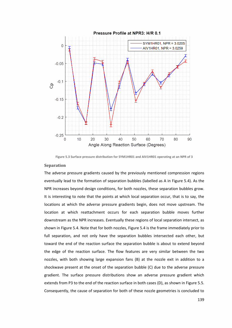
139

Figure 5.3 Surface pressure distribution for SYM1HR01 and AIV1HR01 operating at an NPR of 3

Separation

The adverse pressure gradients caused by the previously mentioned compression regions

eventually lead to the formation of separation bubbles (labelled as A in Figure 5.4). As the

NPR increases beyond design conditions, for both nozzles, these separation bubbles grow.

It is interesting to note that the points at which local separation occur, that is to say, the

locations at which the adverse pressure gradients begin, does not move upstream. The

location at which reattachment occurs for each separation bubble moves further

downstream as the NPR increases. Eventually these regions of local separation intersect, as

shown in Figure 5.4. Note that for both nozzles, Figure 5.4 is the frame immediately prior to

full separation, and not only have the separation bubbles intersected each other, but

toward the end of the reaction surface the separation bubble is about to extend beyond

the edge of the reaction surface. The flow features are very similar between the two

nozzles, with both showing large expansion fans (B) at the nozzle exit in addition to a

shockwave present at the onset of the separation bubble (C) due to the adverse pressure

gradient. The surface pressure distributions show an adverse pressure gradient which

extends from P3 to the end of the reaction surface in both cases (D), as shown in Figure 5.5.

Consequently, the cause of separation for both of these nozzle geometries is concluded to

140

be the extension of the region of local separation beyond the edge of the reaction surface,

which, when combined with the adverse pressure gradient, causes an influx of ambient air

and a subsequent straightening of the jet. The similarity between the surface pressure

distributions of both nozzles indicates that the asymmetry of AIVHR01 makes little

difference to the separation of the supersonic curved wall jet.

Figure 5.4 H/R 0.1 nozzles before separation

Figure 5.5 Surface pressure distribution for SYM1HR01 and AIV1HR01 immediately prior to separation

141

Once full separation occurs, the most obvious effect is the rapid straightening of the jet. In

order for the flow to maintain a static pressure equilibrium across the lower free-stream

boundary (which was locally separated, but now is of ambient pressure), the shockwave

which was present at the onset of local separation has to affect a higher static pressure

increase, similar to an under-expanded nozzle exit. The strengthening of the shockwave

leads to the straightening of the jet. This is observed in four frames from the high speed

schlieren experiment on SYM1HR01 in Figure 5.6.

Figure 5.6 High speed Schlieren images showing the propagation of the point of separation upstream. Time between frames (a) and (d) is 0.025 seconds

A less obvious, but equally important effect is the upstream propagation of the point at

which separation occurs. A hole in the side wall of the reaction surface is used as a

reference point to highlight the significant change in location shown in Figure 5.6. Initially,

Figure 5.6(a) shows the point of separation slightly to the left of the hole; however, by the

time the jet has fully straightened Figure 5.6(d) shows the point of separation to the right

of the hole. The reason the point of separation moves is, again, due to the need to maintain

static pressure equilibrium across the lower free-stream boundary. The effect of the

movement of this point of separation is that subsequently the expansion fan from the

nozzle exit intersects the shockwave and the free-stream boundary. This leads to a

142

fundamental change in the internal structure of the jet. Before the point of separation

moved, the expansion fan reflected from the solid reaction surface as an expansion fan,

creating a reduction in pressure close to the reaction surface and turning the flow towards

the reaction surface. After separation, the separation shockwave has to affect a higher

static pressure change in order to maintain static pressure equilibrium along the lower

shear layer: before the sealed separation bubble was of much lower static pressure than

ambient, after separation, the lower free-stream is of ambient pressure. The strengthening

of the shockwave increases the turning angle of the flow away from the reaction surface.

The pressure distribution before full separation is shown in Figure 5.7. As can be seen, the

jet shows consistently lower pressure closer to the reaction surface, even when locally

separated (A). Also visible is the separation region, which is shown as a slightly higher

pressure immediately following the shockwave (B).

Figure 5.7 Pressure sensitive paint image of SYM1HR01 before separation. The colour scale to the right of the image shows the range of relative pressures, with red representing relatively high pressure, and blue

representing relatively low pressure.

143

Figure 5.8 Pressure sensitive paint image of SYM1HR01 following separation. The colour scale to the right of the image shows the range of relative pressures, with red representing relatively high pressure, and blue


The pressure distribution following full separation is shown in Figure 5.8. The most obvious

change is the pressure distribution within the jet itself. Whereas before, within the jet,

there was a consistently lower pressure closer to the reaction surface, now the jet is visible

as a mosaic of different triangles representing high pressure regions (A) and low pressure

regions (B). These regions are clearly observable despite the difference in stagnation

temperature of the recently attached jet and ambient air confusing the image (C). A

stronger shockwave indicated by a higher pressure region downstream (A) would act to

turn the jet away from the reaction surface. The strength of this interaction acts to prevent

the flow from immediately reattaching following an incremental decrease in NPR.

Following separation, the propagation of flow features such as expansion fans and

shockwaves is fundamentally altered. With the jet turned away from the reaction surface

by both the expansion fan propagating from the upper nozzle exit, and the shockwave

located on the reaction surface, the free jet consists uniquely of compression and

shockwaves propagating from the lower free-stream boundary (e.g. B in Figure 5.9), which

are reflected as expansion fans from the upper free-stream boundary (e.g. A in Figure 5.9).

The subsequent effect is half of a shock-diamond, split along its axis of symmetry in the

144

direction of the flow. This is highlighted for both the SYM1HR01 and AIV1HR01 nozzles in

Figure 5.9, which is the frame immediately following separation.

Figure 5.9 H/R 0.1 nozzles immediately following separation

For both cases, beyond separation, the NPR is increased further and the expansion fan

from the upper nozzle exit increases in size due to the increase in static pressure difference

between the nozzle exit and the ambient air. The effect of this is that the jets are vectored

upwards, away from the reaction surface. It is important to note, however, that the

location at which separation occurs does not noticeably move again, and the jet structure

downstream does not change.

Reattachment

As the NPR is decreased, the jet in both cases does not reattach until well below the NPR at

which it separated. The flow features present immediately before reattachment are shown

in Figure 5.10, and one feature which is notable is the location at which the expansion fan

propagating from the upper nozzle exit (A) intersects the reaction surface. In both cases,

this expansion fan is only just intersecting the point at which the flow separates.

145

Figure 5.10 H/R 0.1 nozzles before reattachment

Revisiting the explanation of the change in structure of the jet at separation previously

discussed, for the flow to reattach, the static pressure within the jet must be closer to

ambient. This would weaken the separation shockwave as it would need to affect a much

smaller static pressure increase in order to obtain static pressure equilibrium on the lower

free-stream. Weakening the shockwave would reduce the extent to which the flow is

turned away from the reaction surface, enabling the reattachment of the jet. Further to

this, if the expansion fan were to once again only reflect from the solid reaction surface

then it would reflect as an expansion fan, which would further lower the pressure prior to

the separation shockwave and turn the flow toward the reaction surface. The wave

structure immediately following reattachment is shown in Figure 5.11.

Figure 5.11 H/R 0.1 nozzles after reattachment

146

Summary

Figure 5.12 shows the vertical force coefficient, including the experimental uncertainty,

plotted against NPR. Both the symmetrical and asymmetrical nozzles are close to identical,

with both separating around NPR 5.2.

Figure 5.12 Vertical force coefficient of SYM1HR01 and AIV1HR01 across a range of ascending NPRs. Error range previously discussed in Section 4.2.4 is also shown

Figure 5.13 shows the vertical force coefficient against NPR for the full experiment,

including the observed hysteresis. Again, both nozzles behave in a very similar manner,

with the symmetrical nozzle obtaining a slightly higher vertical force coefficient (although

both error bars overlap meaning a decisive conclusion is impossible). Both nozzles also

reattach at around the same NPR (3.6).

147

Figure 5.13 Vertical force coefficient of SYM1HR01 and AIV1HR01 across the full range of NPRs tested in the experiment.

To summarise the behaviour of both nozzles:

1) As the NPR is increased, multiple adverse pressure gradients form along the length

of the reaction surface. These adverse pressure gradients are caused by

compression waves (resulting from expansion waves reflecting from the free-

stream boundary) intersecting the reaction surface.

2) As the NPR is increased further, these adverse pressure gradients cause multiple

separation bubbles to form. The point along the reaction surface at which the

separation bubble begins does not change, but the point of reattachment

propagates further downstream with increasing NPR, eventually forming one large

separation bubble. The separation bubble is sealed and of lower pressure than

ambient.

3) Full separation occurs as this region of local separation extends beyond the edge of

the reaction surface. The adverse pressure gradient causes an influx of air at

ambient pressure into the previously sealed separation bubble.

4) The increase in pressure on the lower free-stream boundary of the jet increases the

pressure difference across the shockwave located at the onset of separation, which

148

has the effect of straightening the jet (turning it away from the reaction surface).

Additionally, this increase in pressure moves the location at which the previously

sealed separation bubble began upstream.

5) The expansion fan propagating from the upper nozzle exit intersects the lower

free-stream boundary. The free jet is composed of compression waves propagating

from the lower free-stream boundary, and expansion waves propagating from the

upper free-stream boundary.

6) Further increasing the NPR vectors the jet away from the reaction surface.

7) The jet will not reattach until the static pressure of the jet upstream of the

separation shockwave is closer to ambient. Such a condition in the case of the H/R

0.1 nozzles occurs when the expansion fan no longer intersects the locally

separated region. A smaller pressure difference across the separation shockwave

would reduce the extent to which the shockwave turns the flow away from the

reaction surface.

8) There is no significant difference in the observed behaviour between the

symmetrical and asymmetrical nozzles; both the static pressure distribution and

observed flow features are very similar at all stages.

5.1.2 H/R 0.15

Due to manufacturing inconsistencies, both SYM1HR015 and AIV1HR015 had a noticeably

rougher finish to the reaction surface. This is evidenced through a simple comparison

between Figure 5.14 and Figure 5.1 which show the nozzles at both H/R at the same NPR.

For the H/R of 0.15 nozzles, there are discrete compression and expansion waves visibly

propagating from the reaction surface, whereas for the smoother, H/R 0.1 nozzles, the

distributed expansion fan propagating from the reaction surface was invisible.

NPR 2.5

Similar to the H/R 0.1 nozzles previously discussed, at NPR 2.5, SYM1HR015 shows a

shockwave propagating from the upper edge of the nozzle (A). Additionally, there is a small

difference between the surface pressure distributions, with AIV1HR015 having a slightly

flatter pressure distribution. This is expected, since at NPR 2.5 the flow exiting the nozzle at

the upper edge is the close to the pressure of the ambient air, the flow represents an

irrotational vortex.

149

Figure 5.14 H/R 0.15 nozzles operating at approximately NPR 2.5

NPR 3

At an NPR of 3, the average static pressure at the exit for both nozzles is ambient. Figure

5.15 shows the AIV1HR015 nozzle has an expansion fan emanating from the upper nozzle

exit (A). Similar to the case for H/R of 0.1, both nozzles show multiple regions of

compression (B). However, this time the first region of compression starts around the

pressure tap P6, which is located approximately 33° from the nozzle exit. For SYM1HR01

and AIV1HR01, the first region of compression began around the pressure tap P4, which is

around 21° from the nozzle exit. Whilst this may seem of no consequence, calculating the

linear distance along the reaction surface at which the compression region occurs in both

cases yields distances of approximately 36.65mm for SYM1HR01 and approximately 38mm

for SYM1HR015. Consequently, it can be concluded that the compression regions begin

around the same linear distance from the nozzle exit for both H/R 0.1 and H/R 0.15. This

suggests that at this nozzle pressure ratio, there is little difference between the lengths of

the shock cells for the four nozzles tested at H/R of 0.15 and H/R of 0.1. As shown in Figure

5.16 the pressure distribution for nozzles SYM1HR015 is similar to that of AIV1HR015, the

only notable difference being that for AIV1HR015, the first compression is more gradual.

150

Figure 5.15 H/R 0.15 nozzles operating at an NPR of approximately 3

Figure 5.16 Surface pressure profiles for SYM1HR015 and AIV1HR015 operating at an NPR of approximately 3

Separation

The frame before separation, for both the SYM1HR015 and AIV1HR015 nozzles, is shown in

Figure 5.17. As with the SYM1HR01 and AIV1HR01 nozzles previously discussed, the most

remarkable attribute is the similarity between the symmetrical and asymmetrical nozzles,

both in flow features and surface pressure distributions. Note that whilst the NPR at which

separation occurs is around 0.2 higher for the AIV1HR015 nozzle relative to the SYM1HR01

nozzle, this is within the 7% uncertainty attributed to the NPR signal. In both the

symmetrical and asymmetrical cases, the separation mechanism is seen as the same as for

the H/R 0.1 nozzles: the separation bubbles (located further around the reaction surface

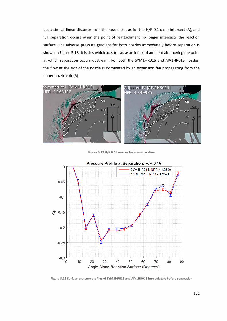
151

but a similar linear distance from the nozzle exit as for the H/R 0.1 case) intersect (A), and

full separation occurs when the point of reattachment no longer intersects the reaction

surface. The adverse pressure gradient for both nozzles immediately before separation is

shown in Figure 5.18. It is this which acts to cause an influx of ambient air, moving the point

at which separation occurs upstream. For both the SYM1HR015 and AIV1HR015 nozzles,

the flow at the exit of the nozzle is dominated by an expansion fan propagating from the

upper nozzle exit (B).

Figure 5.17 H/R 0.15 nozzles before separation

Figure 5.18 Surface pressure profiles of SYM1HR015 and AIV1HR015 immediately before separation

152

Following full separation, as shown in Figure 5.19, the separation point moves upstream

(A), with the separation shockwave intersecting the upper shear layer and reflecting as an

expansion fan (B). As before, the free jet structure is composed of expansion waves

propagating from the upper free-stream boundary and compression waves propagating

from the lower free-stream boundary. Whilst the images shown in Figure 5.19 are certainly

noisier than those obtained for the H/R of 0.1 nozzles shown in Figure 5.9, the trend of

expansion followed by compression is still easily visible.

Figure 5.19 H/R 0.15 nozzles immediately following separation

The pressure sensitive paint images also support the alteration of the fundamental

structure of the jet following full separation. Figure 5.20 shows the pressure distribution

before separation where a lower pressure region closer to the reaction surface is easily

visible (A). Interestingly, observing the pressure distribution closer to the nozzle exit reveals

pressure contours which are not parallel to the nozzle exit (B). Comparing this contour to

the expansion fan shown in Figure 5.17, it would appear to be the yellow contour is close to

the onset of the expansion fan, which would make the angle it makes to the flow equal to

the Mach angle. This suggests that anywhere upstream of the nozzle is unaffected by the

presence of the shear layer and is essentially an internal flow.

153

Figure 5.20 Pressure sensitive paint image of SYM1HR015 before separation The colour scale to the right of the image shows the range of relative pressures, with red representing relatively high pressure, and blue


Figure 5.21 Pressure sensitive paint image of SYM1HR015 following separation. The colour scale to the right of the image shows the range of relative pressures, with red representing relatively high pressure, and blue


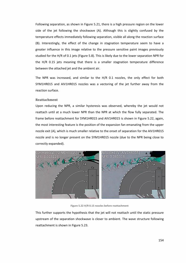
154

Following separation, as shown in Figure 5.21, there is a high pressure region on the lower

side of the jet following the shockwave (A). Although this is slightly confused by the

temperature effects immediately following separation, visible all along the reaction surface

(B). Interestingly, the effect of the change in stagnation temperature seem to have a

greater influence in this image relative to the pressure sensitive paint images previously

studied for the H/R of 0.1 jets (Figure 5.8). This is likely due to the lower separation NPR for

the H/R 0.15 jets meaning that there is a smaller stagnation temperature difference

between the attached jet and the ambient air.

The NPR was increased, and similar to the H/R 0.1 nozzles, the only effect for both

SYM1HR015 and AIV1HR015 nozzles was a vectoring of the jet further away from the

reaction surface.

Reattachment

Upon reducing the NPR, a similar hysteresis was observed, whereby the jet would not

reattach until at a much lower NPR than the NPR at which the flow fully separated. The

frame before reattachment for SYM1HR015 and AIV1HR015 is shown in Figure 5.22, again,

the most interesting feature is the position of the expansion fan emanating from the upper

nozzle exit (A), which is much smaller relative to the onset of separation for the AIV1HR015

nozzle and is no longer present on the SYM1HR015 nozzle (due to the NPR being close to

correctly expanded).

Figure 5.22 H/R 0.15 nozzles before reattachment

This further supports the hypothesis that the jet will not reattach until the static pressure

upstream of the separation shockwave is closer to ambient. The wave structure following

reattachment is shown in Figure 5.23.

155

Figure 5.23 H/R 0.15 nozzles after reattachment

Summary

Figure 5.24 shows the vertical force coefficient plotted against NPR for the H/R of 0.15

nozzles. Also included is the total error, which mainly consist of the uncertainty regarding

the NPR measurement. Like the H/R of 0.1 nozzles, both nozzles behave very similarly. The

asymmetrical nozzle in this case is shown to fully separate at a higher NPR, however given

that the error of both nozzles overlaps consistently, it is not possible to conclude this

definitively. The conclusion from this experiment is that there is no significant difference

caused by asymmetry.

156

Figure 5.24 Vertical force coefficient of SYM1HR015 and AIV1HR015 across a range of ascending NPRs. Error range previously discussed in Section 5.6.2 is also shown

Figure 5.25 shows the vertical force coefficient for the full operating range. For both

nozzles it is clear to see hysteresis, where the curved wall jet reattaches at a much lower

NPR. The separation NPR according to Figure 5.25 is 4.2 for the symmetrical nozzle, and 4.3

for the asymmetrical nozzle. The NPR at which reattachment occurs was 3.0 for the

symmetrical nozzle and 3.1 for the asymmetrical nozzle. The maximum vertical force

coefficient was similar for both nozzles, occuring around 0.87.

157

Figure 5.25 Vertical force coefficient of SYM1HR015 and AIV1HR015 across the full range of NPRs tested in the experiment.

To summarise the behaviour of SYM1HR015 and AIV1HR015:

1) The separation and reattachment mechanism for both nozzles is the same as

described for H/R 0.1, with separation bubbles eventually extending beyond the

edge of the reaction surface. The jet does not reattach until the separation

shockwave is considerably weaker.

2) There were numerous manufacturing defects present, when compared to the H/R

0.1 nozzles. This caused multiple small shock and expansion waves to propagate

throughout the flow. The extent to which these defects affected the behaviour is

assumed to be small. This is due to the similarities between the flow features and

pressure gradients for both the symmetrical and asymmetrical nozzles, when

compared with their counterparts for H/R of 0.1.

3) Shock cells occurred a similar linear distance from the nozzle exit as the H/R 0.1

nozzles. Due to the smaller reaction surface radius present in the H/R of 0.15

experiments, this meant such features occurred further around the reaction

surface, closer to the edge.

158

4) There were more differences in flow features and surface pressure distributions

between AIV1HR015 and SYM1HR015 nozzles than there were between the

AIV1HR01 and SYM1HR01 nozzles. This difference, however, was still very small

across the range of NPRs tested.

5.1.3 H/R 0.2: NPRD 3

A total of four nozzles were tested at H/R of 0.2. This section deals with the nozzles with a

design NPR of 3. Note that the nozzle: AIV1HR02NPR3 suffered from a blocked pressure tap

(P6). This has been highlighted in the relevant figures with a red square.

NPR 2.5

At NPR 2.5, as Figure 5.26 shows, if pressure tap P6 is ignored for AIV1HR02NPR3, the

surface pressure distributions are very similar, with SYM1HR02NPR3 having a relatively

lower static pressure and AIV1HR02NPR3 having a flatter distribution (as seen with

AIV1HR015). Both nozzles already show two adverse pressure gradients, one starting

around P6, and a second, much steeper pressure gradient occurring beyond P10 (57°). The

pressure towards the end of the reaction surface is tending toward ambient, indicating that

the flow may be about to separate at the edge of the reaction surface. In terms of flow

features, the average condition for both nozzles is slightly over-expanded, with a

shockwave observed propagating from the upper nozzle exit in both cases (A). Again,

however, for the asymmetrical nozzle, this flow feature is less apparent closer to the

reaction surface.

Figure 5.26 H/R 0.2, NPR 3 nozzles operating at approximately NPR 2.5

For the lower H/R cases (0.1 and 0.15) previously discussed, there were three clear peaks of

low static pressure observable along the reaction surface. In this case, it would seem that

the reaction surface is sufficiently short so as to prevent the third peak from existing.

Consequently, separation is to be expected much sooner. At NPR 2.5, already there are

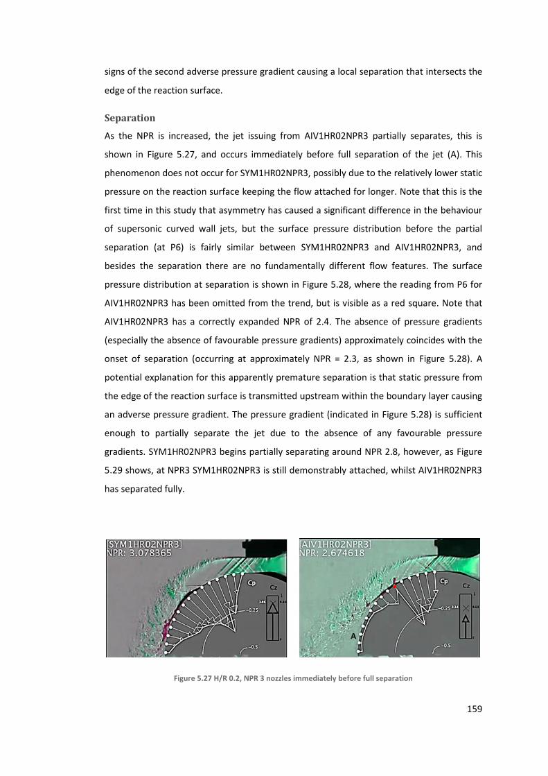
159

signs of the second adverse pressure gradient causing a local separation that intersects the

edge of the reaction surface.

Separation

As the NPR is increased, the jet issuing from AIV1HR02NPR3 partially separates, this is

shown in Figure 5.27, and occurs immediately before full separation of the jet (A). This

phenomenon does not occur for SYM1HR02NPR3, possibly due to the relatively lower static

pressure on the reaction surface keeping the flow attached for longer. Note that this is the

first time in this study that asymmetry has caused a significant difference in the behaviour

of supersonic curved wall jets, but the surface pressure distribution before the partial

separation (at P6) is fairly similar between SYM1HR02NPR3 and AIV1HR02NPR3, and

besides the separation there are no fundamentally different flow features. The surface

pressure distribution at separation is shown in Figure 5.28, where the reading from P6 for

AIV1HR02NPR3 has been omitted from the trend, but is visible as a red square. Note that

AIV1HR02NPR3 has a correctly expanded NPR of 2.4. The absence of pressure gradients

(especially the absence of favourable pressure gradients) approximately coincides with the

onset of separation (occurring at approximately NPR = 2.3, as shown in Figure 5.28). A

potential explanation for this apparently premature separation is that static pressure from

the edge of the reaction surface is transmitted upstream within the boundary layer causing

an adverse pressure gradient. The pressure gradient (indicated in Figure 5.28) is sufficient

enough to partially separate the jet due to the absence of any favourable pressure

gradients. SYM1HR02NPR3 begins partially separating around NPR 2.8, however, as Figure

5.29 shows, at NPR3 SYM1HR02NPR3 is still demonstrably attached, whilst AIV1HR02NPR3

has separated fully.

Figure 5.27 H/R 0.2, NPR 3 nozzles immediately before full separation

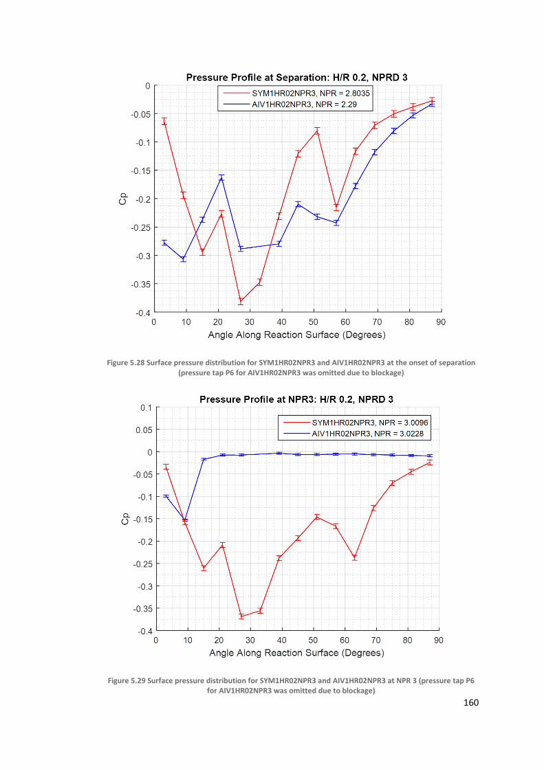
160

Figure 5.28 Surface pressure distribution for SYM1HR02NPR3 and AIV1HR02NPR3 at the onset of separation (pressure tap P6 for AIV1HR02NPR3 was omitted due to blockage)

Figure 5.29 Surface pressure distribution for SYM1HR02NPR3 and AIV1HR02NPR3 at NPR 3 (pressure tap P6 for AIV1HR02NPR3 was omitted due to blockage)

161

After full separation, the jet structure in the case of SYM1HR02NPR3 is as described for H/R

of 0.1 and 0.15. The flow features are shown in Figure 5.30. The nozzle has an expansion

fan propagating from the upper edge of the nozzle exit (A), with the separation shockwave

causing expansion fans to reflect from the upper shear layer (B). The jet itself is deflected

more toward the reaction surface for the case of AIV1HR02NPR3; this is because the jet

separates as the nozzle is over-expanded. The point of separation moves gradually

upstream from the partial separation to just downstream of the shockwave propagating

from the upper nozzle exit.

Figure 5.30 H/R 0.2, NPR 3 nozzles immediately following separation

Reattachment

As the NPR is increased, as before, both jets deflect further away from the reaction surface.

Upon decreasing the NPR, however, reattachment for both nozzles occurs at roughly the

same NPR. Further to this, the NPR at which reattachment occurs is similar to the NPR at

which the flow fully separated for the asymmetrical nozzle (2.6). The AIV1HR02NPR3 nozzle

shows little to no hysteresis, with the point of separation moving downstream in the same

manner as it separated. The frames before reattachment are shown in Figure 5.31.

Figure 5.31 H/R 0.2, NPR 3 nozzles before reattachment

162

Following reattachment, both surface pressure distributions return to the case before

separation. Note that, as can be seen in Figure 5.32, both nozzles are partially separated

towards the end of the reaction surface (A), with AIV1HR02NPR3 more noticeably so, due

to the separation occurring further upstream. Further reduction in the NPR allows the full

reattachment of the jet.

Figure 5.32 H/R 0.2, NPR 3 nozzles following reattachment

Summary

Figure 5.33 shows the first significant difference between symmetrical an asymmetrical

nozzles observed in this study, with AIVHR02NPR3 separating partially around NPR 2.5, and

fully around 2.65. Even including the error margin this is far earlier than SYM1HR02NPR3,

which separates around NPR 3.1. This separation NPR is the same as for past studies

(Lytton 2006; Chippindall 2009; Ashley 2012), suggesting that the gap between the nozzle

exit and the reaction surface makes little difference at this H/R. The maximum vertical

force coefficient obtained was 0.84 for SYM1HR02NPR3. Interestingly, the gradient of the

vertical force coefficient against NPR is similar for the symmetrical and asymmetrical

nozzles.

163

Figure 5.33 Vertical force coefficient of SYM1HR02NPR3 and AIV1HR02NPR3 across a range of ascending NPRs. Error range previously discussed in Section 5.6.2 is also shown

Figure 5.34 Vertical force coefficient of SYM1HR02NPR3 and AIV1HR02NPR3 across the full range of NPRs tested in the experiment.

164

Figure 5.34 shows the difference in behaviour between the symmetrical and asymmetrical

nozzles across the full range of NPRs. As can be seen, AIV1HR02NPR3 reattaches around

the same NPR as it fully separated, with SYM1HR02NPR3 showing much greater hysteresis.

To summarise the behaviour of SYM1HR02NPR3 and AIV1HR02NPR3:


described for H/R 0.1 and H/R 0.15, with separation bubbles eventually extending

beyond the edge of the reaction surface, allowing an injection of ambient air which

straightens the jet. The main difference is due to the insufficient length of the

reaction surface at H/R 0.2 preventing a third peak in low static pressure, meaning

that it is the second separation bubble that intersects the edge of the reaction

surface as opposed to the third for lower H/R. This means full separation occurs at

a much lower NPR. Additionally, this can lead to partial separation of the jet,

particularly noticeable on AIV1HR02NPR3, but also present on SYM1HR02NPR3.

2) There was a significant difference in the separation characteristics of

SYM1HR02NPR3 and AIV1HR02NPR3, due to the fact that the symmetrical nozzle

produced peaks of lower static pressure relative to the asymmetrical nozzle (which

is designed to produce no pressure gradients around NPR = 2.4). Consequently, the

asymmetrical nozzle partially and fully separated at an NPR which was 87% of its

symmetrical counterpart. Both AIV1HR02NPR3 and SYM1HR02NPR3 were over-

expanded when they began separating.

3) Despite the difference in separation characteristics, both SYM1HR02NPR3 and

AIV1HR02NPR3 reattached at the same NPR. Additionally, the NPR at which

AIV1HR02NPR3 reattached was very similar to the NPR at which it fully separated.

5.1.4 H/R 0.2: NPRD 4

The final set of experiments concerned two nozzles with an equivalent area ratio designed

so the average exit conditions would be on design at NPR 4. The asymmetrical nozzle in this

case corresponded to irrotational vortex nozzle first designed by (Bevilaqua & Lee 1980),

and is denoted IV1HR02NPR3 (designed to be correctly expanded at NPR 3). The equivalent

symmetrical nozzle is SYM1HR02NPR4.

NPR 2.5

At NPR 2.5, both nozzles are heavily over-expanded; the most prominent features

observable in Figure 5.35 are the shockwaves propagating from the upper nozzle exits (A).

165

These shockwaves cause a compression region downstream due to the severe increase in

pressure experienced across them. This compression region is present on the surface

pressure distributions (B), but is apparently more severe for the IV1HR02NPR3 nozzle.

Following this, further downstream there is another compression region (C) due to the

reflection of the expansion fan from the upper free-stream boundary (similar to the

phenomena witnessed with previous nozzles). Even at this stage, the rough pattern of the

flow features and the surface pressure distributions is similar between the two nozzles, but

the magnitude of the pressure gradients appear far more severe for IV1HR02NPR3.

Figure 5.35 H/R 0.2, NPR 4 nozzles operating at approximately NPR 2.5

As the NPR is increased, the flow behaves similarly to the H/R 0.2 NPRD 3 cases previously

discussed, despite there being three relatively peaks of relatively high static pressure; the

first peak is shock-induced, caused by the impingement of the shock wave on the reaction

surface. The adverse pressure gradient toward the edge of the reaction surface even at

NPR 2.5 in both cases looks similar to SYM1HR02NPR3 and AIV1HR02NPR3 nozzles

previously encountered.

Separation

Once the adverse pressure gradient induces local separation, the result is the partial

separation of the jet, as shown in Figure 5.36, which is the frame immediately prior to full

separation. In both cases full separation of the jet occurs not long after this. At around NPR

3.1, which is very similar to the SYMHR02NPR3 case, the symmetrical nozzle rapidly

separates. Note that at this NPR, the nozzle is still very much over-expanded, and a

shockwave is still present at the nozzle exit. The separation point is downstream of this

shockwave, with the resultant separation shock forming from both the need for static

pressure equilibrium and as a reflection from this incident shockwave. The IV1HR02NPR3

nozzle also undergoes a similar process of partial separation, however, full separation

occurs gradually over the course of the next 0.7 bar NPR. Figure 5.37 shows the pressure

166

gradients at the onset of separation. Note that IV1HR02NPR3 separates so gradually that

there is no difference between the partial separation of the jet and the onset of full

separation, the distinction between partial and full separation comes courtesy of the

behaviour of SYM1HR02NPR4. Interestingly, a very steep pressure gradient is present in

IV1HR02NPR3, similar to the pressure gradient observed for AIV1HR02NPR3 in Figure 5.28.

Figure 5.36 H/R 0.2, NPR 4 nozzles before full separation

Figure 5.37 Surface pressure distribution for SYM1HR02NPR4 and IV1HR02NPR3 at the onset of separation.

The pressure sensitive paint images, shown in Figure 5.38 and Figure 5.39, show that the

separation process is similar for both SYM1HR02NPR4 and SYM1HR02NPR3. Before full

separation, close to the nozzle the effects of the shockwave propagating from the upper

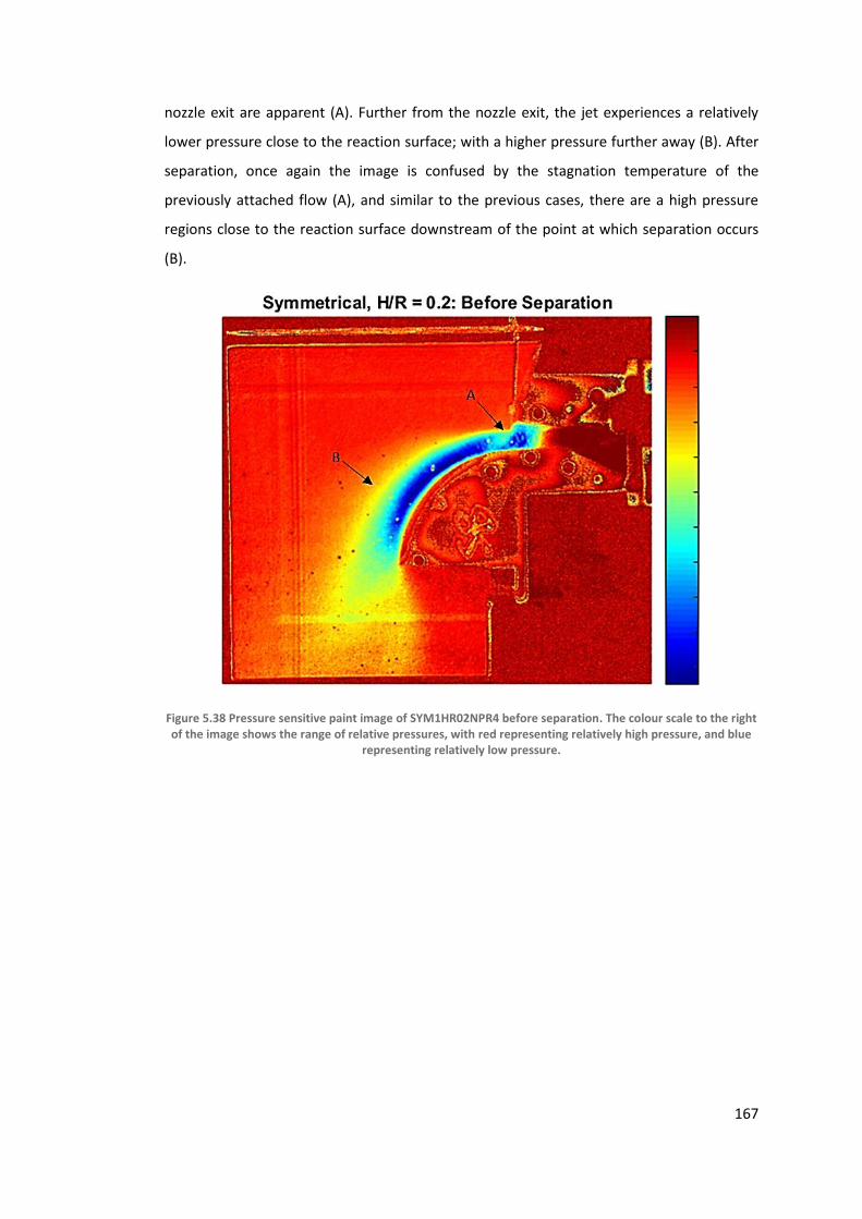
167

nozzle exit are apparent (A). Further from the nozzle exit, the jet experiences a relatively

lower pressure close to the reaction surface; with a higher pressure further away (B). After

separation, once again the image is confused by the stagnation temperature of the

previously attached flow (A), and similar to the previous cases, there are a high pressure

regions close to the reaction surface downstream of the point at which separation occurs

(B).

Figure 5.38 Pressure sensitive paint image of SYM1HR02NPR4 before separation. The colour scale to the right of the image shows the range of relative pressures, with red representing relatively high pressure, and blue


168

Figure 5.39 Pressure sensitive paint image of SYM1HR02NPR4 after separation. The colour scale to the right of the image shows the range of relative pressures, with red representing relatively high pressure, and blue


As has been previously seen, once the flow is locally, or partially separated, full separation

occurs when this region no longer intersects the edge of the reaction surface, and there is

insufficient static pressure in the flow at the point of the onset of separation to prevent an

influx of air at ambient pressure. Consequently, separation is followed by the upstream

propagation of the point of separation. In the case of IV1HR02NPR3, this propagation is

relatively slow, and can be reversed at any time. For SYM1HR02NPR4, it is sudden. This

propagation, in addition to the key flow features observed during this rapid separation is

shown in Figure 5.40, from the high speed schlieren experiment.

169

Figure 5.40 High speed schlieren images showing the propagation of the point of separation upstream. Time between frame (a) and (d) is approximately 0.03 seconds

The case following separation is shown in Figure 5.41. The structure of the jet in both cases

is as has been previously described, with compression waves propagating from the lower

shear layer (A), and expansion waves propagating from the upper shear layer (B).

Interestingly, following separation the IV1HR02NPR3 experiences an expansion fan

propagating from the upper nozzle exit (C), which is less easily observed closer to the

reaction surface. SYM1HR02NPR4 is still over-expanded, and there is still a shockwave

propagating from the upper nozzle exit (D).

Figure 5.41 H/R 0.2 NPR 4 nozzles immediately following full separation

Increasing the NPR further straightens the jet in both cases, as has been seen with all

previous nozzle geometries.

170

NPR 4

At NPR 4, the average static pressure at the nozzle exit for both nozzle exits is ambient,

such a case is shown in Figure 5.42, where an expansion fan is present for IV1HR02NPR3

(A), and a shockwave is still present for SYM1HR02NPR4 (B). As the NPR is increased

further, an expansion fan forms in the symmetrical nozzle, similar to the asymmetrical case

in Figure 5.30.

Figure 5.42 H/R 0.2, NPR 4 nozzles operating at approximately NPR 4

Reattachment

As the NPR is reduced, hysteresis is again observed for the symmetrical nozzle. The flow

does not reattach until the shockwave no longer reflects close to the separation shock, in a

mechanism similar to what has been previously described. The IV1HR02NPR3 jet

experiences a gradual return to reattachment, beginning at NPR ~3.2, and finally becoming

fully attached at NPR 2.7. SYM1HR02NPR4 reattaches suddenly at NPR ~2.8. The frames

taken before and after reattachment are shown in Figure 5.43 and Figure 5.44,

respectively.

Figure 5.43 H/R 0.2, NPR 4 nozzles before reattachment

171

Figure 5.44 H/R 0.2, NPR 4 nozzles after reattachment

Summary

Figure 5.45 shows the vertical force coefficients plotted against NPR as the NPR is

increasing. As can be seen, both nozzles show quite similar behaviour, however the NPR at

which IV1HR02NPR3 begins to separate (2.8) is lower than SYM1HR02NPR4 (3.1).

Incidentally, SYM1HR02NPR4 separates at the same NPR as SYM1HR02NPR3. The gradient

for the asymmetrical nozzle is somewhat shallower, evidence of the gradual separation

previously discussed. The peak vertical force coefficient is slightly smaller than the nozzles

designed for NPR3, suggesting that increasing the design nozzle pressure ratio reduces the

corresponding effectiveness. This could be due to the nature of the vertical force

coefficient metric: at higher design NPRs, the supersonic jet will have greater momentum

at the nozzle exit, since Cz is inversely proportional to this momentum, as opposed to the

total momentum of the curved wall jet (including expansion occurring on the reaction

surface), this could somewhat account for the reduction in Cz.

172

Figure 5.45 Vertical force coefficient of SYM1HR02NPR4 and IV1HR02NPR3 across a range of ascending NPRs. Error range previously discussed in Section 5.6.2 is also shown

Figure 5.46 shows the vertical force coefficient of both nozzles plotted against NPR for the

full experiment. Hysteresis is much less apparent for these nozzles than for any of the

others previously discussed. Additionally, both nozzles begin reattachment around the NPR

at which they separated, but return to fully attached gradually. Given that both nozzles are

severely over-expanded at the separation NPR, the effect of the reversal of wave

reflections as point of separation moves upstream, whilst still present, is less severe due to

the separation point still being downstream of the incident shockwave.

173

Figure 5.46 Vertical force coefficient of SYM1HR02NPR4 and IV1HR02NPR3 across the full range of NPRs tested in the experiment.

To summarise the behaviour of SYM1HR02NPR4 and IV1HR02NPR3:


described for H/R 0.1, H/R 0.15 and H/R 0.2 NPRD 3, with separation bubbles

eventually extending beyond the edge of the reaction surface, allowing an injection

of ambient air which straightens the jet. Unlike the H/R 0.2 NPRD3 case, and like

the H/R 0.1 and H/R 0.15 cases, there are three peaks of low static pressure around

NPR 2.5, however the compressive region between the first and second peak is

caused by the shockwave due to the jet at the nozzle exit being over-expanded.

Consequently the third peak for these nozzles is in the same location as the second

peak for both SYM1HR02NPR3 and AIV1HR02NPR3, and the separation mechanism

is very similar. SYM1HR02NPR4 separates at the same NPR as SYM1HR02NPR3.

2) There was no significant difference in the nozzle pressure ratio at which

SYM1HR02NPR4 and IV1HR02NPR3 separated fully; however the asymmetrical

nozzle separated gradually as opposed to the sudden separation witnessed with

other symmetrical nozzles.

174

3) Like AIVHR02NPR3, IV1HR02NPR3 displayed little hysteresis. The hysteresis

displayed by SYM1HR02NPR4 was to a much lesser extent than symmetrical

nozzles previously discussed.

5.1.5 Summary of Separation Mechanism

To summarise the mechanism observed in this study:

1) As the nozzle pressure ratio is increased, adverse pressure gradients form at the

end of each shock cell due to the impingement of compression waves (caused by a

distributed expansion fan reflection at the free-stream boundary) on the reaction

surface. The wave structure which propagates from the nozzle exit of an

overexpanded supersonic curved wall jet is shown in Figure 5.47.

Figure 5.47 Simplified schematic of wave interactions of a fully attached, overexpanded supersonic curved wall jet. Arrows indicate the change in flow direction, with expansion (green) and compression/shock waves (red) reflecting appropriately.

2) For a specific operating NPR, adverse pressure gradients occur a similar linear

distance from the nozzle exit, regardless of H/R (as shown in Figure 5.49). The

175

adverse pressure gradients (A, B and C) will eventually form separation bubbles,

reattachment to the reaction surface occurs provided there is a favourable

pressure gradient (caused by the expansion section of the next shock cell) between

the adverse pressure gradient and the edge of the reaction surface. For the

duration that the jet is locally separated, the Mach waves are reflected in an

opposite manner (i.e. expansion reflects as compression and vice versa) from both

free-stream boundaries. This results in mainly compression waves propagating

from the upper free-stream boundary and mainly expansion waves propagating

from the lower free-stream boundary, as indicated on Figure 5.48. This serves to

create a relatively lower pressure on the side of the separated jet closer to the

reaction surface as the flow is turned toward the reaction surface. Upon

reattachment further downstream, Mach waves are again reflected in a likewise

manner (i.e. expansion reflects as expansion), essentially producing a new shock

cell. This separation bubble is of lower static pressure than the ambient condition.

Figure 5.48 Simplified schematic of wave interactions of an underexpanded supersonic curved wall jet showing the formation of a separation bubble. Arrows indicate the change in flow direction, with expansion (green) and compression/shock waves (red) reflecting appropriately.

176

Figure 5.49 Comparison of NPR 3 nozzles operating at NPR 3, with adverse pressure gradients (A, B and C) occurring a similar linear distance from nozzle exit

3) Increasing the NPR further moves the point of reattachment for the separation

bubbles further downstream (as indicated in Figure 5.50). The effect of this from

the perspective of the surface pressure distribution is an apparent lengthening of

the shock cell. This occurs until all of the regions of local separation are merged,

and then lengthened further until the jet no longer reattaches to the reaction

surface. At such a point the surface pressure gradients for all nozzles are adverse at

the edge of the reaction surface as shown in Figure 5.51. Interestingly, the point at

which the separation bubble first occurs does not move until the jet fully separates.

In the case of IV1HR02NPR3 and AIV1HR02NPR3, both surface pressure

distributions display very steep adverse pressure gradients towards the end of the

reaction surface which causes partial separation of the jet, with the point at which

the jet separates dictated by the edge of the next favourable pressure gradient

upstream.

177

Figure 5.50 Simplified schematic of wave interactions of an underexpanded supersonic curved wall jet immediately prior to full separation. Arrows indicate the change in flow direction, with expansion (green) and compression/shock waves (red) reflecting appropriately. In this case, the reattachment point is about to move beyond the edge of the reaction surface.

Figure 5.51 Surface pressure distributions immediately prior to separation for all nozzle geometries

178

4) Once the separation bubble extends beyond the edge of the reaction surface, the

adverse pressure gradient causes an influx of ambient air to the previously sealed

separation bubble. This serves to move the point of separation upstream, as shown

in Figure 5.52. Consequently, the Mach waves which were reflecting against the

solid boundary (i.e. expansion reflecting as expansion) now intersect the separation

shockwave. For under-expanded jets, this mechanism of altering the reflection of

the expansion fan, in addition to the strengthening of the separation shockwave as

the separation point moves upstream, cause the flow to turn away from the

reaction surface (in Figure 5.50, the reflected expansion fan from the lower surface

acted to turn the flow toward the reaction surface, whilst still present, is weakened

as less of the incident expansion fan intersects the solid boundary). For over-

expanded jets, the point of separation does not move further upstream than the

incident shockwave from the upper nozzle exit. Consequently, this shock is

reflected from the solid boundary at the same point as the separation shock,

resulting in the same tuning effect on the flow. This phenomenon is visible in the

combined schlieren and shadowgraph images shown in Figure 5.53.

Figure 5.52 Simplified schematic of wave interactions of an underexpanded supersonic curved wall jet immediately following full separation. Arrows indicate the change in flow direction, with expansion (green) and compression/shock waves (red) reflecting appropriately. In this case, the separation point has moved upstream to intersect the expansion fan propagating from the nozzle exit

179

Figure 5.53 Combined Schlieren and shadowgraph images of SYM1HR01 (top) and SYM1HR02NPR4 (bottom) immediately following separation

5) Following separation, further increasing the nozzle pressue ratio serves to vector

the jet away from the reaction surface. For most of the nozzles tested, the jet will

not reattach until at a lower NPR than the NPR at which it separated. In under-

expanded jets this coincides with the expansion fan propagating from the upper

edge of the nozzle exit once again entirely intersecting the solid boundary (as

shown in Figure 5.54). This has the twofold effect of reducing the strength of the

separation shock and reflecting as an expansion fan from the reaction surface, both

of which alter the flow direction in favour of returning toward the reaction surface.

In over-expanded jets this occurs when the reflected shockwave propagating from

the upper edge of the nozzle exit no longer coincides with the separation shock. In

some cases of over-expanded jets, little to no hysteresis is observed. For the

irrotational vortex nozzles high H/R, which separate at their correctly expanded

NPR, the reduction of stream-wise pressure gradients greatly reduces hysteresis.

This is further validation that hysteresis is caused by a fundamental change to wave

interactions, suggesting that when no waves are present, hysteresis does not

occur.

180

Figure 5.54 Simplified schematic of wave interactions of an underexpanded supersonic curved wall jet immediately prior to reattachment. Arrows indicate the change in flow direction, with expansion (green) and compression/shock waves (red) reflecting appropriately. In this case, the separation point is about to move downstream as the jet reattaches.

In addition to the mechanism for separation identified, the following conclusions can

be drawn from placing the results from this study into the wider context of separation

of supersonic curved wall jets.

The more shock cells present (i.e. negative pressure peaks on the reaction surface),

the further from separation the curved wall jet is. Adverse pressure gradients

caused by compression waves intersecting the reaction surface cannot fully

separate the jet provided there are substantial favourable pressure gradients

downstream. This is in complete agreement with past literature which suggested

shock cell length was the principal determinant of separation nozzle pressure ratio

for a given H/R (Gregory-Smith & Gilchrist 1987; Cornelius & Lucius 1994; Gregory-

Smith & Senior 1994).

Higher H/R nozzles separate at a lower nozzle pressure ratio because the reaction

surface is relatively shorter; consequently there are relatively fewer shock cells

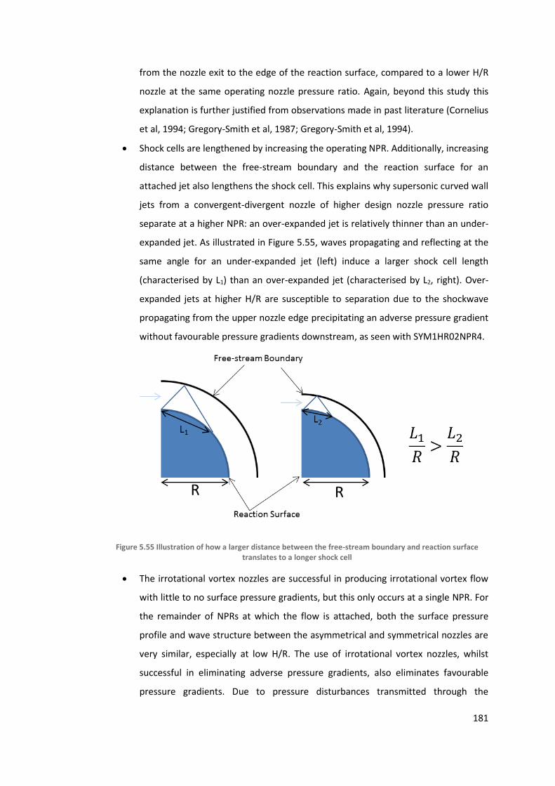
181

from the nozzle exit to the edge of the reaction surface, compared to a lower H/R

nozzle at the same operating nozzle pressure ratio. Again, beyond this study this

explanation is further justified from observations made in past literature (Cornelius

et al, 1994; Gregory-Smith et al, 1987; Gregory-Smith et al, 1994).

Shock cells are lengthened by increasing the operating NPR. Additionally, increasing

distance between the free-stream boundary and the reaction surface for an

attached jet also lengthens the shock cell. This explains why supersonic curved wall

jets from a convergent-divergent nozzle of higher design nozzle pressure ratio

separate at a higher NPR: an over-expanded jet is relatively thinner than an under-

expanded jet. As illustrated in Figure 5.55, waves propagating and reflecting at the

same angle for an under-expanded jet (left) induce a larger shock cell length

(characterised by L1) than an over-expanded jet (characterised by L2, right). Over-

expanded jets at higher H/R are susceptible to separation due to the shockwave

propagating from the upper nozzle edge precipitating an adverse pressure gradient

without favourable pressure gradients downstream, as seen with SYM1HR02NPR4.

Figure 5.55 Illustration of how a larger distance between the free-stream boundary and reaction surface translates to a longer shock cell

The irrotational vortex nozzles are successful in producing irrotational vortex flow

with little to no surface pressure gradients, but this only occurs at a single NPR. For

the remainder of NPRs at which the flow is attached, both the surface pressure

profile and wave structure between the asymmetrical and symmetrical nozzles are

very similar, especially at low H/R. The use of irrotational vortex nozzles, whilst

successful in eliminating adverse pressure gradients, also eliminates favourable

pressure gradients. Due to pressure disturbances transmitted through the

182

boundary layer, there will always be an adverse pressure gradient towards the end

of the reaction surface, in the absence of favourable pressure gradients,

irrotational vortex nozzles close to their design condition are more susceptible to

separation (as seen with IV1HR02NPR3 and AIV1HR02NPR3) relative to their

symmetrical counterparts, especially at high H/R. This contradicts the basis for

designing irrotational vortex nozzles, as proposed by (Bevilaqua & Lee 1980).

However, this provides an explanation of past experimental results such as (Jegede

2016) (asymmetrical nozzle curved wall jet separating whilst correctly expanded),

and (Bevilaqua & Lee 1980) (asymmetrical nozzle showing no significant difference

from its symmetrical counterpart). Additionally, this also provides an explanation as

to the apparently superior performance of Ashley’s (Ashley 2012) linear pressure

gradient: perhaps the optimum surface pressure gradient is the not-quite flat

gradient shown in Figure 3.24.

Hysteresis occurs because the point at which the jet locally separates moves

upstream due to an infux of ambient air as the jet fully separates. This changes the

fundamental structure of the jet by altering the wave interactions. Where

previously, a reflected expansion fan turned the flow toward the reaction surface,

after the point of separation moves upstream, a separation shock turns the flow

away from the reaction surface. Consequently, for under-expanded jets it is

impossible for the jet to reattach at the separation NPR, because the circumstances

are fundamentally different. At higher H/R, where the curved wall jet separates

while it is over-expanded, the separation point does not move further upstream

than the reflected shockwave (propagating from the nozzle’s upper exit). This

mechanism explains why hysteresis is not always observed at high H/R (e.g.

IV1HR02NPR3 and AIV1HR02NPR3 and for (Gregory-Smith & Gilchrist 1987; Matsuo

et al. 2000)), and hysteresis was certainly observed to a lesser extent in the

symmetrical nozzle operating at high H/R in this study (SYM1HR02NPR4 compared

with SYM1HR01). Revisiting (Gregory-Smith & Senior 1994), the reason hysteresis is

not observed when a base-step is present is also explained by this mechanism: The

edge of the step is a point of (full or local) separation at all NPRs, once fully

separated this point does not change location, meaning reattachment occurs under

the same circumstance as separation, and at the same nozzle pressure ratio.

183

5.2 Comparison with Method of Characteristics

Jegede (Jegede 2016) produced a method of characteristics model capable of predicting

curved wall jet behaviour. The validation of this implementation is extended in this section.

The assumptions of inviscid, isentropic flow prevent this model from converging on a

solution in any condition other than close to their correctly expanded condition, defined as

the operating condition where no shockwaves or expansion fans are present at the nozzle

exit. Figure 5.56 to Figure 5.59 show the surface pressure profiles predicted by the method

of characteristics (dotted line), compared with experimentally obtained surface pressure

profiles (solid line, crosses) for both symmetrical (red) and asymmetrical (blue) nozzles.

Note that due to the comparable nozzles being of equivalent design NPR (as opposed to

correctly expanded NPR), the nozzle pressure ratios at which the jet is correctly expanded,

as previously defined, are lower for the asymmetrical nozzles than the corresponding

symmetrical nozzles. NPRs at which the flow is correctly expanded are specified in the

legend of each figure.

Figure 5.56 Correctly expanded surface pressure distributions for SYM1HR01 and AIV1HR01, compared with the prediction from method of characteristics.

184

Figure 5.57 Correctly expanded surface pressure distributions for SYM1HR015 and AIV1HR015, compared with the prediction from method of characteristics.

Figure 5.58 Correctly expanded surface pressure distributions for SYM1HR02NPR3 and AIV1HR02NPR3, compared with the prediction from method of characteristics.

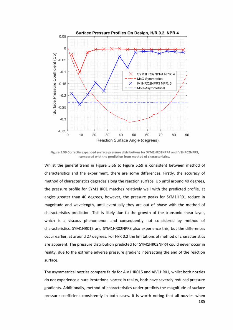
185

Figure 5.59 Correctly expanded surface pressure distributions for SYM1HR02NPR4 and IV1HR02NPR3, compared with the prediction from method of characteristics.

Whilst the general trend in Figure 5.56 to Figure 5.59 is consistent between method of

characteristics and the experiment, there are some differences. Firstly, the accuracy of

method of characteristics degrades along the reaction surface. Up until around 40 degrees,

the pressure profile for SYM1HR01 matches relatively well with the predicted profile, at

angles greater than 40 degrees, however, the pressure peaks for SYM1HR01 reduce in

magnitude and wavelength, until eventually they are out of phase with the method of

characteristics prediction. This is likely due to the growth of the transonic shear layer,

which is a viscous phenomenon and consequently not considered by method of

characteristics. SYM1HR015 and SYM1HR02NPR3 also experience this, but the differences

occur earlier, at around 27 degrees. For H/R 0.2 the limitations of method of characteristics

are apparent. The pressure distribution predicted for SYM1HR02NPR4 could never occur in

reality, due to the extreme adverse pressure gradient intersecting the end of the reaction

surface.

The asymmetrical nozzles compare fairly for AIV1HR015 and AIV1HR01, whilst both nozzles

do not experience a pure irrotational vortex in reality, both have severely reduced pressure

gradients. Additionally, method of characteristics under predicts the magnitude of surface

pressure coefficient consistently in both cases. It is worth noting that all nozzles when

186

correctly expanded experience an adverse pressure gradient towards the end of the

reaction surface. This is likely to be due to pressure disturbances propagating upstream

from the edge of the reaction surface via the boundary layer: a viscous phenomenon

previously discussed in Section 2.1. Consequently, for H/R 0.2 the asymmetrical nozzles

have begun separating whilst correctly expanded.

This highlights a potential flaw in the theory that irrotational vortices are less likely to

separate, as suggested by previous studies (Bevilaqua & Lee 1980; Ashley 2012; Jegede

2016; Llopis-Pascual 2016). Separation, as has been discussed in Section 5.1.5, results

because of adverse pressure gradients combined with an absence of substantial favourable

pressure gradients downstream. Whilst correctly expanded, irrotational vortices induce

flow with little to no adverse pressure gradients, however, in doing so they also prevent

favourable pressure gradients. In reality, when correctly expanded there will be adverse

pressure gradients at the end of the reaction surface due to the propagation of pressure

upstream in the boundary layer. At high H/R, where such pressure gradients are steepest,

irrotational vortex nozzles are actually more susceptible to separation due to the lack of

favourable pressure gradients than symmetrical nozzles of equivalent design NPR. This is

evidenced by the fact that AIV1HR02NPR3 and IV1HR02NPR3 both begin separating while

correctly expanded.

5.3 The Need for Adaptive Nozzles

At the onset of this study, adaptive nozzles were proposed in order to improve three

aspects of supersonic curved wall jets:

1) Attachment across a range of NPRs typically experienced in flight;

2) Efficiency of a circulation control device by maximising the lift augmentation per

unit mass flow across a range of NPRs typically experienced in flight;

3) Effectiveness of a circulation control device by maximising the lift augmentation

across a range of NPRs typically experienced in flight.

5.3.1 Maintaining Attachment

The idea of adapting a nozzle in order to keep a curved wall jet attached is fundamentally

flawed by a fact seen in both past literature and this study: for a fixed geometry the curved

wall jet only separates at one NPR (Morrison & Gregory-Smith 1984; Gregory-Smith &

Gilchrist 1987; Gilchrist & Gregory-Smith 1988; Gregory-Smith & Senior 1994; Cutbill 1998;

Cornelius & Lucius 1994; Lytton 2006; Chippindall 2009; Ashley 2012; Llopis-Pascual 2016;

187

Jegede 2016). Provided the operational NPR consistently remains below the separation

NPR, the jet will remain attached. Consequently, designing a fixed geometry nozzle to

remain attached at the maximum operating NPR the system is expected to encounter will

ensure the jet remains permanently attached throughout its operation, and no adaptable

mechanism is justified to meet this particular challenge in isolation.

Designing an adaptive mechanism to increase the separation NPR for a given H/R is also

deemed unviable. Exploring the limit of NPR 3.1 experienced by all unstepped nozzles at

H/R of 0.2, underexpanded, overexpanded and correctly expanded all separate around this

NPR. Irrotational vortex nozzles at this H/R begin separating whilst correctly expanded,

with the AIV1HR02NPR3 nozzle separating around its correctly expanded NPR of 2.4,

despite having the same area ratio as SYM1HR02NPR3 (which separated around its

correctly expanded NPR of 3).

In order to aid the design of even this fixed geometry, however, it is necessary to explore

the limits of attachment. For a given mass flow of air, determining the separation nozzle

pressure ratio for different geometric properties is a worthwhile enterprise. (Cornelius &

Lucius 1994) predicted two theoretical limits of separation based on Coanda momentum

balance (Equation 2-4); where the low pressure on the reaction surface must balance the

centrifugal force of the jet in order for the jet to remain attached.

The two limits proposed by (Cornelius & Lucius 1994) were the liquefaction of oxygen

molecules, which occurs at a Mach number of around 3.6, and the absolute limit of Mach

infinity (i.e. vacuum). Both of these cases would occur on the reaction surface of a fully

attached jet, since that is where the Mach number is the highest.

In the vast majority of past literature, including this study, the cause of separation was

attributed to the wave structure, meaning separation occurs well before these theoretical

limits (Morrison & Gregory-Smith 1984; Gregory-Smith & Gilchrist 1987; Gilchrist &

Gregory-Smith 1988; Gregory-Smith & Senior 1994; Cutbill 1998; Cornelius & Lucius 1994;

Lytton 2006; Chippindall 2009; Ashley 2012; Llopis-Pascual 2016; Jegede 2016). However,

the similarity between the trend provided by these limits, and the experimental data when

the separation nozzle pressure ratio is plotted against throat height to reaction surface

radius ratio (A*/R) is remarkable. Figure 5.60 shows the convergent only study from

(Gregory-Smith & Gilchrist 1987; Gregory-Smith & Senior 1994; Cornelius & Lucius 1994;

Ashley 2012; Jegede 2016; Llopis-Pascual 2016) and the current study all plotted alongside

188

the Mach limits proposed by (Cornelius & Lucius 1994). Note that the red circles and

crosses on Figure 5.60 represent convergent-only nozzles, with the circles representing a

step to radius ratio of 0.147 from (Gregory-Smith & Senior 1994). Black shapes represent

convergent-divergent nozzles of various area ratios and skew.

Figure 5.60 Separation NPR vs A*/R for all nozzle geometries. Also plotted are the two limits proposed by (Cornelius & Lucius 1994). Red circles represent convergent stepped nozzles from (Gregory-Smith & Senior 1994), red crosses represent convergent-only nozzles from (Gregory-Smith & Gilchrist 1987). Appropriate

convergent-divergent nozzles have been included from (Cornelius & Lucius 1994; Ashley 2012; Jegede 2016; Llopis-Pascual 2016).

A second, remarkable feature of Figure 5.60, is that above A*/R of 0.08, there are no

significant advantages provided by convergent-divergent nozzles over convergent-only

nozzles in terms of increasing separation NPR, due to the dominant role H/R plays in

determining separation. In fact, only (Llopis-Pascual 2016) shows a significant increase in

separation NPR relative to the convergent-only nozzles studied in (Gregory-Smith &

Gilchrist 1987). Again, asymmetrical nozzles, for example, from (Ashley 2012), do not offer

any advantages in terms of separation over convergent-only nozzles or symmetrical

convergent-divergent nozzles of equivalent A*/R. Indeed, the asymmetrical nozzles used

for this study for H/R of 0.2 show a much lower separation NPR relative to any of the other

geometries. This contradicts (Llopis-Pascual 2016), whose asymmetrical nozzles show a

189

significantly higher separation NPR compared to other unstepped geometries. This also

represents an overall trend in terms of sensitivity which has been discussed both in this

study, and in past literature before – the higher the H/R, the higher the sensitivity to

separation (Gregory-Smith & Gilchrist 1987). It is not known how the asymmetrical nozzles

from (Llopis-Pascual 2016) compare to symmetrical nozzles of equivalent area ratio. Based

on trends from this study, however, it is fair to assume that the performance will be similar.

Figure 5.61 shows the separation NPR for all of the convergent-divergent nozzles, which are

appropriately labelled. Note that in Figure 5.61, circles represent asymmetrical nozzles and

stars represent symmetrical nozzles. The hexagons represent nozzles which are unique in

their design nozzle pressure ratio, for all others the design nozzle pressure ratio is colour-

coordinated: red corresponds to 4, blue is 3.6 and black is 3. As Figure 5.61 shows, it is

difficult to extract definitive proof that increasing design nozzle pressure ratio increases the

separation NPR.

Figure 5.61 Separation NPR vs A*/R for all convergent-divergent nozzles (appropriately labelled). Black hexagons correspond to nozzles with unique exit to throat area ratios. Other design NPRs are indicated by

colour, with NPRd = 4 (red), NPRd = 3.6 (blue) and NPRd = 3 (black) highlighted. Circles correspond to asymmetrical nozzles of equivalent area ratio, stars correspond to symmetrical nozzles. In addition to results

from this study, it is constructed from (Cornelius & Lucius 1994; Ashley 2012; Jegede 2016; Llopis-Pascual 2016)

190

It is, however, likely that convergent-divergent nozzles increase the NPR at which flow

separates due to the reduction in shock cell length provided by an over-expanded jet, as

discussed in Section 5.1.5. The effect this has on the number of shock cells on a reaction

surface will be largely insignificant at higher A*/R due to the relatively shorter reaction

surface. This potentially explains why in Figure 5.60, only the lower A*/R convergent-

divergent nozzles show any significant increase in separation NPR relative to convergent-

only nozzles.

The empirical rule, shown in Figure 5.60 as a dotted red line, represents a ‘do not cross’ in

terms of nozzle operation. Regardless of whether convergent-divergent nozzles

(symmetrical or not significantly asymmetrical) or convergent-only nozzles are utilised for a

particular curved wall jet application, provided the A*/R is to the left of that line for a given

operational NPR, then the jet will remain attached. The formula, shown in Equation 5-1, is

based on the trend line for Gregory-Smith & Gilchrist (1987), and has been adapted to

accommodate the other geometries.

𝑁𝑃𝑅𝑆𝑒𝑝 = 0.75 +1

3 × [atan (𝐴∗

𝑅)]

Equation 5-1

This equation represents how the throat area of a nozzle of any geometry would have to

adapt in order to avoid separation. However, such an adaptative mechanism is completely

unnecessary in the absence of motivation to maintain as high a A*/R as possible.

5.3.2 Improving Efficiency

For this section, efficiency is taken as vertical force coefficient in quiescent conditions. The

vertical force coefficient itself takes account of mass flow (as part of the momentum

calculation). Consequently, the vertical force coefficients shown in this section have

constant mass flows, but different reaction surface sizes. The aim is to establish which

nozzle geometry has the greatest efficiency in terms of vertical force per unit nozzle

momentum.

Figure 5.62 shows the average vertical force coefficients plotted against NPR for all of the

symmetrical nozzles. At relatively low NPR, all of the nozzles follow roughly the same

gradient, with SYM1HR015 and SYM1HR02NPR4 slightly lower than SYM1HR01 and

SYM1HR02NPR3. Ultimately, the maximum vertical force coefficient is achieved at the

maximum nozzle pressure ratio, with SYMHR01 showing the greatest vertical force

coefficient at NPR 5.2.

191

Figure 5.62 Vertical force coefficient across a range of ascending NPRs for all symmetrical nozzles tested

Figure 5.63 shows much the same trend for the asymmetrical nozzles. Interestingly, the

shallower separation gradient of IV1HR02NPR3 is potentially useful for fluidic thrust

vectoring (FTV), which involves controlling the separation of supersonic curved wall jets.

The small amount of hysteresis displayed by the asymmetrical nozzles at high H/R, coupled

with the gradual separation and reattachment characteristics are positive attributes for

controlling separation.

192

Figure 5.63 Vertical force coefficient across a range of ascending NPRs for all asymmetrical nozzles tested

Concluding that the most efficient operating point is the highest possible NPR regardless of

H/R, the solution to achieving this is, as before, to design a fixed geometry nozzle capable

of maintaining attachment at the highest operating NPR. An adaptive nozzle geometry

would not provide any advantage in terms of the system-level efficiency of a supersonic

curved wall jet.

5.3.3 Improving Effectiveness

In Figure 5.62, the vertical force coefficients were plotted against NPR, where, with the

exception of SYM1HR02NPR4, all nozzles have equivalent mass flow. In reality, this means

that the reaction surface for the H/R 0.1 nozzle is twice as big as the reaction surface for

the H/R 0.2 nozzle. Considering a single physical implementation on the trailing edge of a

wing, where the reaction surface is fixed, it is possible to consider increasing the mass flow

at lower NPRs in order to maximise the effectiveness of the system. Figure 5.64 shows a

reconstruction of Figure 5.62 and Figure 5.63, where in this case the reaction surface is of

constant length. Note that relative to SYM1HR01, SYM1HR02NPR3 has twice the mass flow.

193

Figure 5.64 Normalised vertical force coefficient across a range of ascending NPRs for all nozzles tested

At NPR 3, Figure 5.64 shows that SYM1HR02NPR3 produces a normalised vertical force

coefficient of 0.84, whilst SYM1HR01 produces a normalised vertical force coefficient of

only 0.44. Consequently, per unit mass flow the vertical force coefficient is roughly similar

(as seen in Figure 5.62). However, the force produced by the H/R 0.2 nozzle is roughly twice

that of the H/R 0.1 nozzle for the same reaction surface.

The requirement to improve effectiveness across a range of NPRs, independent of mass

flow, does justify an adaptive nozzle. For an unstepped nozzle, the throat height to radius

ratio would have to be adjusted according to Figure 5.65, which is based on Equation 5-1.

This would enable the system to achieve maximum effectiveness at that operating NPR

whilst avoiding separation with a safety margin.

194

Figure 5.65 Necessary A*/R to avoid separating across a range of operating NPRs

195

Chapter 6

Conclusions and Future Work

196

6.1 Conclusions

The contributions to new knowledge made by this thesis are as follows:

6.1.1 On the state of the art of circulation control (Section 2.3, Page 38):

1) An extensive literature review has been carried out, including the identification of

two clear historical trends. The first is well established, and considers the historical

reduction in trailing edge radius of circulation control wings, so as to reduce drag.

The second is not well established, and concerns the historical reduction in

momentum coefficient (and therefore effectiveness) due to reducing trailing edge

radius. Motivation for increasing the velocity of the attached jet to supersonic

speeds was established in order to increase the effectiveness.

2) Circulation control is principally limited by the high mass flow requirements.

System level efficiency was defined as the change in lift coefficient per unit mass

flow. Algebraic substitution (of the momentum coefficient) and reduction

suggested that the system-level efficiency of circulation control will be improved by

increasing the velocity of the attached jet. When combined with conclusion (1),

above, the clear need to extend attachment of supersonic curved wall jets at higher

nozzle pressure ratio was defined.

3) An extended validation of empirical relations predicting the change in lift

coefficient due to circulation control proposed by (Loth and Boasson, 1983; Loth

and Boasson, 1984) has been performed using results from 46 wind tunnel

experiments across 9 studies. The widely used empirical rule proposed by (Loth and

Boasson, 1984) had a coefficient of determination of less than 0.5 across a broad

range of wind tunnel data. Consequently, new empirical methods were proposed

with a coefficient of determination of approximately 0.9 and a mean error of 30%

(standard deviation of the error is 28%). For more information, see Appendix A

(Page 215).

197

6.1.2 On experimental techniques used to observe supersonic curved

wall jet separation (Section 4.3, Page 115 and Section 4.4, Page 128)

4) A new method of combining shadowgraph and schlieren has been developed in

order to provide an image where unambiguous identification of shockwaves and

expansion fans can be carried out at a glance (Section 4.3 page 115). This technique

is particularly useful for visualising complicated flow-fields containing multiple

features, such as supersonic curved wall jets.

5) Supersonic curved wall jet separation has been observed using pressure sensitive

paint for the first time. Whilst there is a large amount of uncertainty due to the

high sensitivity of the PSP to temperature, qualitative assessments of the jet

structure both before and after separation enhances understanding of the

composition of the jet, both before and after separation (Section 4.4, page128).

In addition to those detailed above, another novel post processing technique was

developed, and is discussed in Appendix B:

6) Shadowgraph boundary layer measurement: The aim was to use shadowgraph to

measure the proportional thickness of the boundary layer. Whilst magnitudes

measured compared well with estimates of incompressible boundary layer

thicknesses of flat plates, large systematic errors were present due to the camera

shaking. Additionally, the behaviour of the boundary layer did not inform any

conclusions drawn leading to its exclusion from the main body of the thesis. More

details are in Appendix B (Page 225).

6.1.3 On the flow physics of supersonic curved wall jets (Section 5.1.5,

Page 174)

7) The mechanism behind supersonic curved wall jet separation valid for a range of

H/R has been clearly defined (Page 174). This directly addresses issues raised by

Lytton (2006), Chippindall (2009), Ashley (2012), Jegede (2016) and Llopis-Pascual

(2016) regarding curved wall jet separation, whilst providing an explanation in line

with observations made by Gregory-Smith & Gilchrist (1987), Gregory-Smith &

198

Senior (1994) and Cornelius & Lucius (1994). This is the first time a single

mechanism has explained the separation of supersonic curved wall jets for all of

the previous studies identified.

8) The mechanism behind hysteresis regarding supersonic curved wall jet

reattachment has been clearly defined. This mechanism explains why hysteresis is

present to a lesser extent for over-expanded jets separating at high H/R and why it

is not present when a base step is introduced (Gregory-Smith & Senior, 1994). This

is particularly important for fluidic thrust vectoring applications which require

linear control over separation and reattachment. This is the first time hysteretic

behaviour in supersonic curved wall jet reattachment has been attributed to the

point of local separation moving upstream during full separation.

9) For low H/R (0.1 and 0.15), nozzles which produce an irrotational vortex show no

significant difference in performance compared to symmetrical nozzles of

equivalent area ratio. Whilst this does not necessarily contradict results obtained

by Bevilaqua & Lee (1980), Ashley (2012), Jegede (2016) and Llopis-Pascual (2016),

it does provide a more useful comparison from a design perspective as it places

importance on mass flow, which is the primary cost to any fluidic system. This is

the first time different convergent-divergent geometries of equivalent mass flow

have been compared for the application of supersonic curved wall jets.

10) At high H/R (0.2), nozzles designed to produce an irrotational vortex begin

separating at their design NPR due to the absence of favourable pressure gradients

towards the end of the reaction surface. This does contradict the basis for the use

of irrotational vortex nozzles as a means of postponing curved wall jet separation,

as initially provided by Bevilaqua & Lee (1980), and built upon by Ashley (2012),

Jegede (2016) and Llopis-Pascual (2016), but the contradiction is justified by the

separation mechanism described on page 174.

11) Considering mass flow, the use of A*/R as opposed to H/R as a design metric shows

that above A*/R 0.08, convergent-divergent nozzles do not provide a significant

increase in separation NPR relative to the convergent-only nozzles studied by

Gregory-Smith et al (1987). Again, this does not directly contradict Chippindall

199

(2009), Ashley (2012), Jegede (2016) and Llopis-Pascual (2016); however it does

provide a more useful design metric, because it places importance on mass flow.

Below A*/R of 0.08, convergent-divergent nozzles (Llopis-Pascual, 2016) do show

significantly higher separation NPR relative to convergent-only nozzles, however,

stepped convergent-only nozzles (Gregory-Smith & Senior, 1994) provide the

closest separation NPR to the theoretical limit proposed by Cornelius & Lucius

(1994) across a range of A*/R. This offers a revised perspective on the design of

fluidic effectors, with mass flow as the prime consideration.

6.1.4 On the method of characteristics as a tool for predicting supersonic

curved wall jet behaviour (Section 5.2, Page 183)

12) This study compared the surface pressure coefficients predicted by the method of

characteristics with experimental data for the correctly expanded (i.e. wave-free)

case. The accuracy of the method of characteristics is limited by its assumptions. In

principle, the main assumptions are of inviscid, isentropic and fully attached flow.

Close to the nozzle exit the method of characteristics is relatively accurate, a

conclusion in agreement with Gregory-Smith & Gilchrist (1988), Jegede (2016) and

Ashley (2012). However, the growth of the transonic shear layer, a fundamentally

viscous effect, is responsible for the growth in inaccuracy further from the nozzle

exit. Up to around 40 degrees for H/R of 0.1 and 0.5 and 27 degrees for H/R 0.2,

NPR 3, the trend predicted by method of characteristics is well followed by the

experimental data. For the NPR 4, H/R 0.2 nozzles, which separate well below

design NPR, the method of characteristics is not useful for predicting surface

pressure distributions.

13) Propagation of high pressure upstream via the boundary layer (again, a

fundamentally viscous effect), is responsible for an adverse pressure gradient

towards the end of the reaction surface for all nozzles experimentally tested.

However, the method of characteristics is unable to predict this. For lower H/R

asymmetrical nozzles, this gradient has little effect, however at H/R 0.2, the

severity of the adverse pressure gradient is sufficient to cause separation for the

asymmetrical nozzles on design. This provides an explanation for Jegede (2016),

200

where the asymmetrical nozzle began separating while correctly expanded in

contradiction to the behaviour predicted by the method of characteristics.

6.1.5 On the need for adaptive nozzles for supersonic circulation control

(Section 5.3, Page 186)

14) Adaptive nozzles are not justified for maintaining attachment of a supersonic

curved wall jet. Exploring the limit of H/R 0.2, where all unstepped nozzle

geometries separate at around NPR=3.1, nozzles separate regardless of whether

they are over-expanded (SYM1HR02NPR4), close to on-design (SYM1HR02NPR3) or

under-expanded (Gregory-Smith & Gilchrist, 1987). Irrotational vortex nozzles of

different area ratio at this H/R begin to separate when they are on-design

(AIV1HR02NPR3 and IV1HR02NP3). Consequently, selecting a fixed nozzle

geometry (including H/R) which ensures attachment at the maximum operating

NPR would ensure permanent attachment during operation and there is no

advantage provided by an adaptive geometry.

15) Adaptive nozzles are not justified for maximising efficiency of a supersonic

circulation control system. For all nozzles tested, maximum efficiency (in terms of

momentum and vertical force coefficient) is achieved at the highest NPR for which

the jet is attached. Consequently, a fixed geometry nozzle as described in (9),

above, would also be capable of the maximum lift augmentation per unit mass

flow. Additionally, there is no loss in efficiency for such a nozzle operating below its

maximum NPR, relative to other nozzle geometries.

16) Adaptive nozzles are justified for maximising effectiveness of a supersonic

circulation control system across a range of NPRs. The maximum effectiveness can

be achieved through maximising the mass flow for an attached jet (hence A*/R).

Equation 5-1 (page 190), based on the separation NPR for the nozzles tested in this

current study, in addition to all past literature considered, describes how

unstepped nozzle geometries should adapt to maximise effectiveness based on the

current NPR.

201

6.2 Future Work

6.2.1 Development of a low order analytical model capable of predicting

circulation control performance on a wide range of planforms

Appendix A shows the development of a semi-empirical model for the sizing of circulation

control effectors. It is, however, limited to high aspect ratio, low sweep wings (due to its

use of Lanchester-Prandtl lifting line theory). Extending the use of such a model to low

aspect ratio, moderately or highly swept planforms (such as delta or lambda wing

configurations), possibly making use of vortex lattice method, would profoundly improve

its usefulness. Whilst many experimental and CFD studies are dedicated to assessing the

cost of specific implementations on UCAV planforms, it seems there is much to be gained

through the development of a low order analytical model capable of performing design

trade-offs at low cost, rapidly and with reasonable confidence.

6.2.2 Augmenting morphing trailing edges with mid-chord blowing

Morphing wings have the potential to meet many of the low observability requirements

future UCAVs are expected to meet. Macro-Fibre Composite (MFC), discussed in the latter

part of Appendix C, shows great potential for morphing aerospace applications. Like other

‘smart materials’, however, it is limited by the relatively low magnitude of deformation and

blocking force it can produce. Circulation control is seen as an expensive (in terms of mass

flow) method of manoeuvring. Building on work from the NATO AVT 239 group regarding

lift augmentation with mid-chord blowing, and supplementing this with an MFC compliant

trailing edge providing small deflections could provide a solution to the conflicting

demands for low observability and high manoeuvrability, whilst significantly reducing the

mass flow demands compared to circulation control alone.

202

References

Abramson, J. & Rogers, E.O., 1983. High-Speed Characteristics of Circulation Control Airfoils. AIAA-83-0265, AIAA 21st Aerospace Sciences Meeting, pp.0–11.

Afilaka, O., 2017. Normal Blowing Fluidic Thrust Vectoring. PhD Thesis, University of Manchester. (UNPUBLISHED WORK)

Anderson, J.D., 2007. Fundamentals of Aerodynamics 4th Edition, New York, NY 10020: McGraw-Hill. ISBN: 13 978-0-07-295046-5.

Anderson, J.D., 2005. Ludwig Prandtl’s Boundary Layer. Physics Today, 58(12), p.42.

Ashley, J.N., 2012. Aft-Deck Coflow Fluidic Thrust Vectoring. PhD Thesis, University of Manchester.

Babinsky, H., 2003. How do wings work? Physics Education, 38(6):p497-503. ISSN 0031-9120. Doi: 10.1088/0031-9120/38/6/001.

Babinsky, H. & Harvey, J.K., 2011. Shock Wave-Boundary-Layer Interactions 1st ed., Cambridge: Cambridge University Press. ISBN: 978-0-521-84852-7.

Bevilaqua, P.M. & Lee, J.D., 1980. Development of a nozzle to improve the turning of supersonic Coanda jets, Technical report, USAF, Wright Aeronautical Laboratories.

Bilgen, O. & Friswell, M.I., 2013. Implementation of a Continuous-Inextensible-Surface Piezocomposite Airfoil. Journal of Aircraft, 50(2), pp.508–518. Available at: http://arc.aiaa.org/doi/abs/10.2514/1.C031908.

Cagle, C.N. & Jones, G.S., 2002. A Wind Tunnel Model to Explore Unsteady Circulation Control for General Aviation Applications. 22nd AIAA Aerodynamic Measurement Technology and Ground Testing Conference Proceedings, (AIAA 2002--3240), pp.1–12.

Chard, J, Jegede, O, Llopis-Pascual, A, et al., 2013. Towards high speed fluidic flight controls. AVT-215 Innovative Control Effectors for Military Aircraft, pp.1–14.

Chippindall, J.M., 2009. Coflow Fluidic Thrust Vectoring of Supersonic Jets with a Fixed Geometry Convergent Divergent Nozzle. PhD Thesis, University of Manchester

Cornelius, K.C. & Lucius, G.A., 1994. Physics of Coanda Jet Detachment at High-Pressure Ratio. Journal of Aircraft, 31(3), pp.591–596.

Crowther, W.J. et al., 2009. Towards integrated design of fluidic flight controls for a flapless aircraft. Aeronautical Journal, 113(1149), pp.699–713.

Cutbill, S., 1998. A Study of the Turbulent Flow of a High Speed Coanda Jet. PhD thesis, University of Durham.

Davidson, I.M., 1962. Aerofoil Boundary Layer Control Systems. US Patent Office

DeSalvo, M.E., Whalen, E.A. & Glezer, A., 2013. Aerodynamic control of attached and separated flows using synthetic jet actuation. Nato Avt-215, pp.1–20.

Englar, R.J. et al., 1981. Design of the Circulation Control Wing Stol Demonstrator Aircraft.

203

Journal of Aircraft, 18(1), pp.51–58. Available at: http://www.scopus.com/inward/record.url?eid=2-s2.0-0019477324&partnerID=40&md5=6b0347d486c55217ae95ef51f3326bb8.

Englar, R.J., 1979. Development of the A-6/Circuation Control Wing Flight Demonstrator Configuration, Bethesda, Md.

Englar, R.J., 1975. Experimental Investigation of the High Velocity Coand Wall Jet Applied to Bluff Trailing Edge Circulation Control Airfoils, Bethesda, Md.

Englar, R.J., 1970. Two-Dimensional Transonic Wind Tunnel Tests of Three 15-Percent Thick Circulation Control Airfoils, Washington, D.C.

Englar, R.J. & Huson, G.G., 1983. Desvelopment of Advanced Circulation Wing High Lift Airfoils. AIAA Paper 83-1847.

Englar, R.J. & Williams, R.M., 1971. Design of a Circulation Control Stern Plane for Submarine Appications [Technical Note AL-200], Bethesda, Md.

Eurofighter Jagdflugzeug GmbH, 2013. Eurofighter Technical Guide. Available at: https://www.eurofighter.com/downloads/TecGuide.pdf%0A.

Frith, S. & Wood, N., 2003. Effect of trailing edge geometry on a circulation control delta wing. AIAA, 21 st Applied Aerodynamics Conference, …, (June), pp.1–7. Available at: http://arc.aiaa.org/doi/pdf/10.2514/6.2003-3797.

Gilchrist, A.R., 1985. The development and breakaway of a compressible air jet with streamline curvature and its application to the coanda flare. PhD thesis, Durham University.

Gilchrist, A.R. & Gregory-Smith, D.G., 1988. Compressible Coanda wall jet: predictions of jet structure and comparison with experiment. International Journal of Heat and Fluid Flow, 9(3), pp.286–295. ISSN 0142727X. doi: 10.1016/0142-727X(88)90039-2.

Graff, E. & Lin, R.S.J., 2013. Sweeping Jet Actuators - a New Design Tool for High Lift Generation. AVT-215 Innovative Control Effectors for Military AircraftInnovative Control Effectors for Military Vehicles, pp.1–25. Available at: https://ntrs.nasa.gov/search.jsp?R=20130013994.

Gregory-Smith, D.G. & Gilchrist, A.R., 1987. The compressible Coanda wall jet-an experimental study of jet structure and breakaway. International Journal of Heat and Fluid Flow, 8(2), pp.156–164.

Gregory-Smith, D.G. & Senior, P., 1994. The effects of base steps and axisymmetry on supersonic jets over coanda surfaces. International Journal of Heat and Fluid Flow, 15(4), pp.291–298.

Gregory, J.W. et al., 2008. A review of pressure-sensitive paint for high-speed and unsteady aerodynamics. Journal of Aerospace Engineering, 222(2), pp.249–290.

Gregory, J.W. et al., 2014. Fast Pressure-Sensitive Paint for Flow and Acoustic Diagnostics. Annu. Rev. Fluid Mech, 46(January), pp.303–30.

Groh, R., 2016. Boundary Layers. The Aerospace Engineering Blog. Available at: http://aerospaceengineeringblog.com/boundary-layers/ [Accessed January 24, 2017].

204

Hanna, B.., 1975. Quantitative Schlieren Measurements of Boundary Layer Phenomena. Proceedsing of the 11th International Congress on High Speed Photography, pp.539–545.

Hitzel, S.M., 2013. Perform and Survive Evolution of Some U ( M ) CAV Platform Requirements. AVT-215 Innovative Control Effectors for Military Aircraft, (M), pp.1–10.

Houghton, E.L. & Carpenter, P.W., 2003. Aerodynamics for Engineering Students 5th Editio., Oxford: Butterworth-Heinemann.

Innnovative Scientific Solutions Incorporated, Operating Instructions for. Assembly, (978), p.12107277. Available at: http://www.psp-tsp.com/.

Janeke, C.E., 2005. Asonic Aerospike Engine. US Patent office.

Jegede, O., 2016. Dual-Axis FTV of High-Aspect Ratio Supersonic Jets.

Jegede, O.O. & Crowther, W.J., 2016. Low Order Supersonic Nozzle Design using Superimposed Characteristics. In 54th AIAA Aerospace Sciences Meeting. American Institute of Aeronautics and Astronautics, pp. 1–13. Doi: AIAA2016-0805.

Jones, G.S. et al., 2002. An Active Flow Circulation Controlled Flap Concept for General Aviation Aircraft Applications. AIAA Paper 2002-3157, (June).

Jones, G.S., Englar, R.J. & Jones, G.S., 2003. Advances in Pneumatic-Controlled High- Lift Systems Through Pulsed Blowing 21 st Applied Aerodynamics Conference. , (June).

Kanistras, K. et al., 2014. An experimental study of circulation control wings at low reynolds numbers. 32nd AIAA Applied Aerodynamics Conference, pp.1–17.

Kizilios, A.P. & Rose, R.E., 1969. Experimental Investigations of Flight Control Surfaces Using Modified Air Jets, Technical Report, Honeywell Inc. Document 12055-FRI DDC AD864.

Kontis, K. et al., 2013. Plasma flow control effectors for low and high speed applications. AVT-215 Innovative Control Effectors for Military Aircraft.

Krzywoblocki, M.Z., 1956. Jets — Review of Literature. Journal of Jet Propulsion, 26(9), pp.760–780.

Kutta, M.W., 1902. Lift forces in flowing fluids. Aeronaut. Mitt, III, pp.133–135.

Labus, T.L. & Symons, E.P., 1972. Experimental investigation of an axisymmetric free jet with an initially uniform velocity profile.

Llopis-Pascual, A., 2016. Supercritical Coanda Jets for Flight Control Effectors. PhD Thesis, University of Manchester. (UNPUBLISHED WORK – awaiting resubmission).

Loth, J.L. & Boasson, M., 1983. Circulation Controlled STOL Wing Optimization. AIAA 21st Aerospace Sciences Meeting, 21(2).

Loth, J.L. & Boasson, M., 1984. Circulation controlled STOL wing optimization. Journal of Aircraft, 21(2), pp.128–134. Available at: http://arc.aiaa.org/doi/10.2514/3.48235.

Loth, J.L., Fanucci, J.B. & Roberts, S.C., 1976. Flight Performance of a Circulation Controlled STOL Airfoil. Journal of Aircraft, 13(3), pp.169–173.

205

Lytton, A., 2006. Fluidic Thrust Vectoring of High Aspect Ratio Underexpanded Jets. PhD thesis, University of Manchester.

Matsuo, S., Setoguchi, T. & Kaneko, K., 2000. Study on the Characteristics of Supersonic Coanda Jet. Journal of the Visualization Society of Japan, 20(79), pp.327–332.

Mclachlan, B.G., 1989. Study of a circulation control airfoil with leading/trailing-edge blowing. Journal of Aircraft, 26(9), pp.817–821. Available at: http://arc.aiaa.org/doi/abs/10.2514/3.45846.

Michie, S.N., 2008. A design methodology for Circulation Control manoeuvre effectors. PhD thesis, University of Manchester

Miller, D.N. & Mccallum, B.N., 2013. Invited : Prospects for Fluidic Thrust Vectoring Technology on a Next-Generation Air Vehicle Some Needs for Tomorrow. AVT-215 Innovative Control Effectors for Military AircraftInnovative Control Effectors for Military Vehicles, (1), pp.1–16.

Morrison, J.F. & Gregory-Smith, D.G., 1984. Calculation of an axisymmetric turbulent wall jet over a surface of convex curvature. International Journal of Heat and Fluid Flow, 5(3), pp.139–148.

Nangia, R.K. & Palmer, M.E., 2013. Exploiting Wing Trailing Edges Geometry as Novel Control Effectors for Aircraft Control , Trim , Load-Alleviation , and High-Lift (Particular Reference to MALE Aircraft ). AVT-215 Innovative Control Effectors for Military Aircraft, (May), pp.20–22.

Osterhuber, R., 2013. FCS-Requirements for Combat Aircraft – Lessons Learned for Future Designs. AVT-215 Innovative Control Effectors for Military Aircraft, pp.1–24.

Quinn, M., 2016. Experimental Methods for Aerodynamics - Lecture Notes. Uncertainty Analysis, pp.1–25.

Quinn, M.K., Yang, L. & Kontis, K., 2011. Pressure-sensitive paint: Effect of substrate. Sensors, 11(12), pp.11649–11663.

Rajaratnam, N., 1976. Turbulent jets. American Elservier Publishing Company, Inc. Edmonton. ISBN: 978-0-444-41372-7.

Rayleigh, L.O.M., 1917. On the Dynamics of Revolving Fluids. Proceedings of the Royal Society of London, Philosophical Transactions of the Royal Society, 148(4).

Roskam, J., 1987. Airplane Design: Preliminary calculation of aerodynamic, thrust and power characteristics, Part VI, Roskam Aviation Engineering Corporation.

Rossmann, T., 2001. An Experimental Investigation of High Compressibility Mixing Layers, Technical report, Stanford University. Available at: http://hanson.stanford.edu/dissertations/Rossmann_2001.pdf.

Sakaue, H., 2003. Anodized Aluminium Pressure Sensitive Paint for Unsteady Aerodynamic Applications. PhD thesis, Purdue University, West afayette, IN.

Sarpkaya, T., 1988. The Deflection of Plane Turbulent Jets By Convex Walls, Technical Report , Naval Postgraduate School, Monterey, California. FEDDOCS D 208.14/2: NPS-

206

59SL8061A

Schlecht, R. & Anders, S.G., 2007. Parametric Evaluation of Thin, Transonic Circulation- Control Airfoils. AIAA Paper, pp.1–25.

Schlichting, H. & Gersten, K., 1979. Boundary-layer theory. European Journal of Mechanics - B/Fluids, 20, p.817.

Settles, G.., 2001. Schlieren and Shadowgraph Techniques 1st Editio., New York: Springer-Verlag. ISBN: 3540661557

Shah, N., Wong, C. & Kontis, K., 2008. Active Flow Control Using Steady and Pulsed Blowing at Subsonic Speeds. 46th AIAA Aerospace Sciences Meeting and Exhibit, (January), pp.1–32.

Skotnikov, M.M., 1976. Quantitative Schlieren Methods in Gas Dynamics. Izdatelt’zvo Nauka, Moscow, USSR 1st Ed.

Sparks, R. et al., 2005. Development of an Integrated Circulation Control/Fluidic Thrust Vectoring Flight Test Demonstrator. … of Excellence for Integrated …, (August), pp.1–10. Available at: http://scholar.google.com/scholar?hl=en&btnG=Search&q=intitle:Development+of+an+INtergrated+Circulation+COntrol+/+Fluidic+Thrust+Vectoring+Flight+Test+Demonstrator#0.

Stojković, D., Breuer, M. & Durst, F., 2002. Effect of high rotation rates on the laminar flow around a circular cylinder. Physics of Fluids, 14(9), pp.3160–3178.

Trindade, M.A. & Benjeddou, A., 2011. Finite element homogenization technique for the characterization of d15 shear piezoelectric macro-fibre composites. Smart Materials and Structures, 20(7), p.75012. Available at: http://stacks.iop.org/0964-1726/20/i=7/a=075012?key=crossref.ad753228f7a7bf91262a4977358b0c46.

Vision-Research, 2012. Phantom v310 Datasheet. , pp.1–4. Available at: www.komiweb.co.kr/data/v310.pdf.

Vision-Research, 2015. V1611 Datasheet, Available at: www.phantomhighspeed.com/Products/Phantom-Camera-Products/v1611.

Warsop, C. & Crowther, W.J., 2013. Fluidic Thrust Vectoring and the FLAVIIR DEMON Flight Demonstration Air vehicle. AVT-215 Innovative Control Effectors for Military Aircraft, pp.1–20.

Wilkerson, J.B. & Montana, P.S., 1982. Transonic Wind Tunnel Test of a 16-Percent Thick Circulation Control Airfoil with One-Percent Asymmetric Camber, Bethesda, Md.

Williams, J.E. & Vukelich, S.R., 1977. The USAF Stability and Control Digital DATCOM. Volume I. Users Manual, St Louis, MO. Available at: www.dtic.mil/cgi-bin/GetTRDoc?AD=ADA086557.

Williams, T., Jemcov, A. & Corke, T., 2013. DBD Plasma Actuator Design for Optimal Flow Control. AVT-215 Innovative Control Effectors for Military Aircraft, pp.1–16.

Wood, N. & Conlon, J., 1983. The performance of a circulation control airfoil at transonic speeds. 21st Aerospace Sciences Meeting,AIAA-84-0083

207

Appendix A:

Semi-Empirical Model for Sizing

Circulation Control Effectors

A.1 Introduction

In the preliminary design of aircraft, semi-empirical methods such as DATCOM and Roskam

are often used (Roskam 1987; Williams & Vukelich 1977). Analytical methods regarding

stability and control (including the calculation of aerodynamic derivatives and conventional

control sizing) such as the vortex-lattice method (VLM) are augmented by past experiential

(i.e. flight test), experimental, and CFD data. The end result of this approach is very low

order models which can rapidly inform design trade-offs with reasonable confidence.

Recent research trends in the field of active flow control specifically target highly swept,

low aspect ratio planforms (e.g. delta or lambda wing). Frith and Wood (2003) performed a

circulation control experiment using a 50° sweep delta wing, and obtained a much lower lift

augmentation compared to a higher aspect ratio, lower sweep wing of similar geometry

(Englar, 1981). Additionally, Frith and Wood (2003) noted that the 3D wing geometry,

including the leading edge and span-wise thickness distribution affected the performance

of the circulation control wing. The aerodynamic complexities have led researchers to

propose standardised aircraft geometries for the purpose of characterising the

performance of fluidic controls on high sweep, low aspect ratio planforms. Examples of

such geometries are provided below:

1) SACCON (Stability And Control CONfiguration), which has been involved in many

experimental and CFD studies. This is a 53° sweep lambda wing of varying leading

edge radius and 5° washout. It was originally developed by the NATO AVT 161 task

group as a standardised UCAV geometry. It is currently used by the NATO AVT 239

task group in characterising the performance of fluidic controls.

2) ICE (Innovative Control Effector) developed by Lockheed Martin is also used by the

NATO AVT 239 task group as a standardised geometry for characterising the

performance of fluidic controls. It is a delta wing with 65° leading edge sweep.

3) Boeing 1303 UCAV is a lambda wing, with 47° leading edge sweep. Despite the

number of studies on this geometry, it is not used as a standardised geometry for

208

the NATO AVT 239 task group due to a lack of data regarding stability and control.

The NATO AVT 239 task group, however, is planning a flight demonstration of

supersonic circulation control on-board a variant of this planform in 2017.

Despite the significant on-going effort to characterise the performance of circulation

control on these planforms, the vast majority of experimental data is for low-sweep wings

(Englar 1970; Englar & Williams 1971; Englar 1975; Englar 1979; Englar et al. 1981; Loth et

al. 1976; Englar & Huson 1983; Abramson & Rogers 1983; Kanistras et al. 2014; Jones et al.

2002; Cagle & Jones 2002; Shah et al. 2008; Llopis-Pascual 2016; Mclachlan 1989;

Wilkerson & Montana 1982). At this stage, proposing a general model for highly swept,

delta or lambda wing configurations is deemed premature.

This chapter proposes a semi-empirical design methodology for implementing trailing edge

circulation control effectors on low-sweep and high aspect ratio planforms. The

methodology proposed can be used to estimate the necessary system mass and mass flow

required to perform a prescribed manoeuvre, and is designed so as to be easily adapted to

lower aspect ratio and higher sweep planforms, when sufficient data is available for

validation.

A.2 Sizing of Circulation Control Effectors

A sizing method for circulation control effectors is illustrated in Figure A.1. It is

supplemented by past work courtesy of Frith (2003), Michie (2008) and Chard et al (2013).

The aim of this methodology is to provide a low-order estimation of mass flow

requirements, actuator size and position in addition to system mass; based on operating

conditions, mission requirements and aircraft dimensions. Such a tool is particularly useful

for estimating the cost and benefits of a circulation control system at a preliminary design

stage.

209

Figure A.1 Schematic of proposed methodology

Beginning with the external conditions, the compressor bleed pressure ratio is calculated

from the compressor map of the engine (A). Depending on performance and system

requirements (discussed later), it may be beneficial to limit this pressure (B). The

compressed air is transported to the control effector on the trailing edge of the wing, with

the pressure loss calculated based on Chard et al (2013), starting from an initial guess (C).

The NPR at the slot is then calculated by dividing this pressure by the external pressure at

the slot exit (D). The maximum throat height for the given NPR is calculated from Equation

5-1, and the proposed trailing edge radius (E). Following this, a modified Lanchester-Prandtl

lifting line theory is used with increasing section lift coefficients until the mission

requirement (i.e. prescribed 3D lift coefficient or roll moment) is met, for the given Mach

number and aircraft dimensions (e.g. wing shape) (F). The required section lift coefficient to

meet the 3D lift distribution is used to calculate the momentum coefficient (G) using an

empirical rule and the slot height required to produce this for the NPR is compared with

the maximum (from (E)). Following this process, model outputs are slot geometry and

location (H), mass flow requirements (I), and the required pipe dimensions (J), which

inform the pressure loss calculated in (C).

210

Design feedback is based on the principle that reducing the pressure limit at (B) increases

effectiveness but reduces efficiency, whereas increasing the pressure limit at (B) reduces

effectiveness but increases efficiency:

1) If the pipe mass is too large, reduce the pressure limit at (B).

2) If the pipe volume is too large, increase the pressure limit at (B).

3) If the required mass flow is too large, increase the pressure limit at (B).

4) If the required slot height exceeds the maximum reduce the pressure limit

at (B).

5) If the pressure limit cannot be changed anymore (either too low or too

high), increase the trailing edge radius.

A.2.1 Determination of the NPR

The determination of the pressure loss accumulated through transporting air from the

compressor stage of a gas turbine engine to a fluidic effector forms the basis of (Chard et

al. 2013). It is summarised here for convenience.

1) Determine viscosity using Sutherland’s formula in Equation A.1:

𝜇 = 𝜇𝑟𝑒𝑓 (0.555∙𝑇𝑟𝑒𝑓+𝑆𝐶

0.555∙𝑇𝑎𝑣𝑔+𝑆𝐶 ) (

𝑇𝑎𝑣𝑔

𝑇𝑟𝑒𝑓)

32⁄

Equation A.1

2) Determine average flow velocity through the pipes using the ‘One Seventh Power

Law’, in Equation A.2:

𝑉𝑎𝑣𝑔 = 𝜇2𝑛2

(𝑛+1)(2𝑛+1)

Equation A.2

3) Determine the friction factor using Equation A.3:

𝑓 = −1.8𝑙𝑜𝑔 [6.9

𝑅𝑒+ (

𝜀𝐷⁄

3.7)

1.11

]

−2

Equation A.3

4) Calculate the major pressure loss using Equation A.4:

∆𝑃𝑚𝑎𝑗𝑜𝑟 = 𝑓𝐿

𝐷

𝜌𝑉𝑎𝑣𝑔2

2

Equation A.4

5) Calculate the minor pressure loss, caused by features such as bends and valves,

using Equation A.5:

∆𝑃𝑚𝑖𝑛𝑜𝑟 = 𝐾𝐿𝜌𝑉𝑎𝑣𝑔

2

2

Equation A.5

211

6) The total pressure loss is calculated by adding the major and minor pressure losses.

In Equation A.6, ‘m’ corresponds to the number of sources of minor pressure

losses:

∆𝑃 = ∆𝑃𝑚𝑎𝑗𝑜𝑟 + ∑ ∆𝑃𝑚𝑖𝑛𝑜𝑟𝑖𝑖=𝑚𝑖=1

Equation A.6

For this implementation, input parameters are:

Engine/pressure source location (s)

Number of plenums on trailing edge

Location of plenums on trailing edge

Considering an Airbus A400M wing, shown as a schematic Figure A.2, two engines are

present on the wing leading edge (located approximately 25% and 55% of the semi-span).

These engines each supply compressed air via a pipe, with each pipe joining a main supply

pipe located parallel to the trailing edge of the wing. The main supply pipe transports the

compressed air to each of the plenums located on the trailing edge. Between the main

supply pipe and the plenum is a control valve allowing independent operation of each

plenum. The use of multiple plenums is necessary to provide an even distribution of

pressure, in Figure A.2, the width of the plenum (i.e. occupied distance along the trailing

edge) is approximately 1.5m.

212

Figure A.2 Example implementation of fluidic effector plumbing on an Airbus A400M. Plenums are shaded in grey, control valves are blue stars, pressure sources (and regulators) are blue diamonds, and the pipes are blue lines. Note that none of the components are to scale and positions are only accurate in the span-wise

direction. Sourced from Airbus.

Due to the difference in distance between the multiple plenums and the source of

compressed air, the pressure loss is calculated for each. Figure A.3 shows the nozzle

pressure ratio at each plenum after accounting for pressure loss from the compressor

(calculated with 2.5cm inner-diameter stainless steel pipes and an assumed initial

compressor pressure ratio of 25).

0 0.2 0.4 0.6 0.8 1-0.7

-0.6

-0.5

-0.4

-0.3

-0.2

-0.1

0

0.1

0.2

x/S

em

i-span

y/Semi-span

Example Implementation of Fludic Effector Plumbing on Airbus A400M Wing

213

Figure A.3 NPR distribution across the span of an Airbus A400M wing by plenum

A.2.2 Modification of Lanchester-Prandtl Lifting Line Theory

Past studies have used an empirically calculated 2D lift coefficient as estimation for the 3D

lift coefficient for the finite wing (Chard et al. 2013; Michie 2008). This study proposes

superimposing the 2D circulation (calculated from the empirically obtained 2D lift

coefficient) onto a 3D finite wing using the Lanchester-Prandtl lifting line theory, as an

improvement to the previous method.

Note that whilst lifting line theory is limited to high aspect ratio, low sweep wings, the

validity of superimposing a 2D circulation from trailing edge circulation control onto a

highly 3D planform (e.g. delta wing) using vortex-lattice method is questionable (Frith &

Wood 2003; Anderson 2007). In future, when sufficient experimental and numerical (CFD)

data from the various configurations discussed in Section A.1 is available, either a

correction could be applied to this empirical model, or a new empirical model proposed

and combined with vortex-lattice method.

Considering an infinite wing, the circulation of a two-dimensional aerofoil can be described

as a bound vortex (Anderson 2007). Considering a finite wing, Helmholtz’s theorem states

that a vortex filament cannot end in the fluid (Anderson 2007). Consequently, the edge of

the bound vortex (i.e. the wingtip) must continue into the fluid as two free vortices trailing

0.1 0.2 0.3 0.4 0.5 0.6 0.7 0.8 0.9

17

18

19

20

21

22

23

24

25

26

y/Semi-span

Pre

ssure

Ratio

Pressure Loss by Plenum

Plenum NPR

Compressor Pressure Ratio

214

downstream (Anderson 2007). Figure A.4 shows how a finite wing can be represented as a

horseshoe vortex, consisting of the bound vortex (i.e. the wing), and two trailing vortices

(created at the wing tip) (Anderson 2007).

Figure A.4 A finite wing is represented by a horseshoe vortex. Note that Lanchester-Prandtl lifting line theory is based on the principle of modifying the effective angle of attack across the span of the wing to accommodate the downwash caused by the free-trailing vortices. Adapted from (Anderson 2007)

The net effect of the vortices is to produce a varying downwash (vertical component of

flow velocity) across the span of the wing. The fundamental principle of Lanchester-Prandtl

lifting line theory is that the downwash produced by the horseshoe vortex at a span-wise

location (𝑦0) represents an effective modification to the angle of attack at the same

position, as shown by Equation A.7:

𝛼(𝑦0) = 𝛼𝑒𝑓𝑓(𝑦0) + 𝛼𝑖(𝑦0) Equation A.7

Where:

𝛼(𝑦0) is the geometric angle of attack (rad) at a span-wise location (𝑦0);

𝛼𝑒𝑓𝑓(𝑦0) is the effective angle of attack (rad);

𝛼𝑖(𝑦0) is the angle of attack (rad) induced by the downwash component of the vortices;

The modification to Lanchester-Prandtl lifting line theory that this study proposes is the

addition of another angle of attack term, by substitution of the 2D lift coefficient due to

circulation control divided by a nominal 2π lift curve slope, as shown in Equation A.8:

𝛼(𝑦0) = 𝛼𝑒𝑓𝑓(𝑦0) + 𝛼𝑖(𝑦0) + 𝐶𝑙𝑐𝑐

2𝜋

Equation A.8

Where 𝐶𝑙𝑐𝑐 is the 2D lift coefficient due to wing trailing edge circulation.

215

Following this, Lanchester-Prandtl lifting line theory is used exactly the same as in its

unmodified form. For a derivation of the governing equation, and Glauert’s proposed

Fourier sine series solution see (Anderson 2007).

The input to this part of the model is the free-stream Mach number, aircraft dimensions

and mission requirement, which is either based on lift augmentation (i.e. 3D lift coefficient

regardless of distribution), or a roll moment. For the purpose of this study, only a lift

augmentation is considered.

Note that, as Section A.2.3 shows, the lift coefficient due to circulation control is

proportional to the jet velocity. Consequently, the NPR distribution calculated in section

A.2.1 is used to modify each input circulation control lift coefficient, creating a span-wise

2D lift coefficient distribution based on the plenum location.

The process is as follows:

1) A low value of 𝐶𝑙𝑐𝑐 is assumed;

2) The 𝐶𝑙𝑐𝑐 is modified to account for the relative difference in jet velocity based on

span-wise location;

3) Lanchester-Prandtl lifting line theory is used to calculate the 3D lift coefficient

(𝐶𝐿0);

4) The 3D lift coefficient is corrected for the free-stream Mach number using Prandtl-

Glauert compressibility correction, shown in Equation A.9 (Anderson 2007):

𝐶𝐿 =𝐶𝐿0

√1−𝑀∞2

Equation A.9

5) If the calculate 3D lift coefficient matches or exceeds the required 3D lift coefficient

then the values of 𝐶𝑙𝑐𝑐 is output. If the calculated 3D lift coefficient is less than that

required, then 𝐶𝑙𝑐𝑐 is increased incrementally and the process is repeated.

The output from this part of the model is the lift coefficient due to circulation control

required to meet the mission requirement for the given aircraft dimension and Mach

number.

A.2.3 Determination of Momentum Coefficient from 2D Lift Coefficient

Loth and Boasson (1983) proposed an empirical rule to describe the increase in lift due to

circulation control as a function of momentum coefficient based on a single experiment.

This is shown in Equation A.10:

216

𝐶𝑙𝑐𝑐 = 6.6√𝐶𝜇 Equation A.10

In a later study, Loth and Boasson (1984) proposed a different empirical rule based on a

series of experiments by Englar (Englar, 1981). The experiments consisted of measuring the

lift augmentation from changing the slot height to chord ratio of five different aerofoils

(Englar, 1981). Loth and Boasson (1984) based the empirical relation on best fit lines from

multiple slot heights for a single aerofoil tested‡‡; proposing that the augmented lift was a

function of slot height to chord ratio and jet to free-stream velocity ratio. This is shown in

Equation A.11:

𝐶𝑙𝑐𝑐 = 40 (𝐻

𝐶)

0.64(

𝑉𝑗

𝑉∞− 1)

Equation A.11

Where:

H is the slot height (m);

C is the wing chord (m);

𝑉𝑗 is the jet velocity (ms-1);

𝑉∞ is the free-stream velocity (ms-1).

Equation A.11 has since been used by (Frith and Wood 2003) and Chard et al (2013) in

proposed methodologies for sizing fluidic effectors. In order to provide further validation

for this rule, it was tested against a much wider scope of experimental data. Data was

gathered from 46 different experiments (from (Englar 1970; Englar 1975; Englar 1979;

Englar et al. 1981; Wilkerson & Montana 1982; Abramson & Rogers 1983; Wood & Conlon

1983; Mclachlan 1989; Jones et al. 2002)) performed on a circular trailing edge at zero

degrees angle of attack and is summarised in Table A.1. In particular, the data included:

geometry (chord, reaction surface radius and slot height), free-stream conditions (Reynolds

number and Mach number), jet-to-free-stream velocity ratio, momentum coefficient and

the measured change in lift coefficient at a single point from each experiment. Where

certain data was not explicitly presented (e.g. jet velocity in (Englar, 1975)), it was

calculated using isentropic relations based on explicitly presented data. Studies were

excluded from this table on the grounds of insufficient data, unsteady blowing or a non-

rounded trailing edge (e.g. jet flaps used in (Englar, 1981))

‡‡ Of the five aerofoil geometries tested, only three serve to validate this rule. Results from the two smallest H/C aerofoils did not share a common trend with the empirically predicted rule. No explanation for this was given (Loth and Boasson, 1984)

217

Table A.1 Summary of 2D wind tunnel data for various geometries and free-stream conditions. Collected from (Englar 1970; Englar 1975; Englar 1979; Englar et al. 1981; Wilkerson & Montana 1982; Abramson & Rogers

1983; Wood & Conlon 1983; Mclachlan 1989; Jones et al. 2002).

The measured change in lift coefficient was then compared with the change in lift

coefficient predicted by Equations A.10 and A.11. For each experiment, the percentage

error was calculated using Equation A.12.

휀 = √(100 ×𝐶𝑙𝑐𝑐

∆𝐶𝑙𝑚− 100)

2

Equation A.12

R

(mm)

C

(mm)

H

(mm)R/C H/R H/C Re∞ M∞ Vj/V∞ Cμ

7.823 195.580 0.025 0.0400 0.0032 0.00013 1,400,000 0.3 3.55 0.04 33.75

7.823 195.580 0.025 0.0400 0.0032 0.00013 1,600,000 0.4 2.50 0.02 37.50

7.823 195.580 0.025 0.0400 0.0032 0.00013 2,000,000 0.5 1.80 0.01 38.00

7.823 195.580 0.025 0.0400 0.0032 0.00013 2,200,000 0.6 1.40 0.005 60.00

7.823 195.580 0.025 0.0400 0.0032 0.00013 2,500,000 0.7 1.30 0.005 40.00

7.823 195.580 0.025 0.0400 0.0032 0.00013 2,600,000 0.8 1.25 0.005 36.00

7.823 195.580 0.025 0.0400 0.0032 0.00013 2,650,000 0.9 1.20 0.005 10.00

25.400 307.340 2.540 0.0826 0.1000 0.00826 760,000 0.3 2.83 0.1 14.00

25.400 307.340 1.270 0.0826 0.0500 0.00413 840,000 0.3 4.01 0.1 23.00

25.400 307.340 0.813 0.0826 0.0320 0.00264 840,000 0.3 5.01 0.1 29.00

25.400 307.340 0.635 0.0826 0.0250 0.00207 840,000 0.3 5.66 0.1 29.00

25.400 307.340 0.330 0.0826 0.0130 0.00107 840,000 0.3 7.85 0.1 29.00

6.778 187.089 0.396 0.0362 0.0585 0.00212 990,000 0.1 5.50 0.2 15.00

6.778 187.089 0.297 0.0362 0.0438 0.00159 990,000 0.1 5.50 0.2 15.00

6.778 187.089 0.198 0.0362 0.0292 0.00106 990,000 0.1 6.00 0.2 14.50

22.225 607.240 0.178 0.0366 0.0080 0.00029 1,200,000 0.1 8.29 0.2 22.50

22.225 607.240 0.356 0.0366 0.0160 0.00059 1,252,693 0.1 8.66 0.2 25.00

22.225 607.240 0.711 0.0366 0.0320 0.00117 1,353,072 0.1 9.35 0.2 27.50

11.125 598.129 0.178 0.0186 0.0160 0.00030 1,200,000 0.1 8.29 0.2 25.00

11.125 598.129 0.356 0.0186 0.0320 0.00059 1,252,693 0.1 8.66 0.2 23.50

11.125 598.129 0.711 0.0186 0.0639 0.00119 1,353,072 0.1 9.35 0.2 26.50

5.563 591.766 0.178 0.0094 0.0320 0.00030 1,200,000 0.1 8.29 0.2 21.00

5.563 591.766 0.356 0.0094 0.0639 0.00060 1,252,693 0.1 8.66 0.2 21.50

5.563 591.766 0.533 0.0094 0.0959 0.00090 1,337,901 0.1 9.25 0.2 24.00

5.563 591.766 0.711 0.0094 0.1279 0.00120 1,352,448 0.1 9.35 0.2 23.50

10.498 477.200 0.762 0.0220 0.0726 0.00160 3,020,000 0.3 2.88 0.02 65.00

10.498 477.200 0.762 0.0220 0.0726 0.00160 3,602,000 0.4 2.85 0.02 70.00

10.498 477.200 0.762 0.0220 0.0726 0.00160 4,184,000 0.5 1.54 0.006 83.33

10.498 477.200 0.762 0.0220 0.0726 0.00160 4,766,000 0.6 1.51 0.006 58.33

10.498 477.200 0.762 0.0220 0.0726 0.00160 5,348,000 0.7 1.48 0.006 36.67

45.263 457.200 1.829 0.0990 0.0404 0.00400 3,100,000 0.3 2.57 0.04 32.50

11.430 457.200 0.732 0.0250 0.0640 0.00160 3,100,000 0.3 4.07 0.04 47.50

21.031 457.200 0.914 0.0460 0.0435 0.00200 3,100,000 0.3 3.64 0.04 50.00

21.031 457.200 0.914 0.0460 0.0435 0.00200 3,840,000 0.4 2.85 0.025 64.00

21.031 457.200 0.914 0.0460 0.0435 0.00200 4,580,000 0.5 2.51 0.02 65.00

21.031 457.200 0.914 0.0460 0.0435 0.00200 5,320,000 0.6 2.40 0.019 47.37

21.031 457.200 0.914 0.0460 0.0435 0.00200 6,060,000 0.7 2.16 0.016 25.63

21.031 457.200 0.914 0.0460 0.0435 0.00200 6,800,000 0.8 1.83 0.012 4.17

15.240 152.400 0.254 0.1000 0.0167 0.00167 1,400,000 0.3 4.89 0.06 46.67

15.240 152.400 0.254 0.1000 0.0167 0.00167 1,800,000 0.4 2.79 0.02 55.00

15.240 152.400 0.254 0.1000 0.0167 0.00167 2,350,000 0.5 2.75 0.02 52.50

15.240 152.400 0.254 0.1000 0.0167 0.00167 2,700,000 0.55 2.72 0.02 40.00

15.240 152.400 0.254 0.1000 0.0167 0.00167 3,000,000 0.6 1.91 0.01 45.00

15.240 152.400 0.254 0.1000 0.0167 0.00167 3,100,000 0.65 1.89 0.01 1.00

McL

ach

lan

19

89

4.064 101.600 0.152 0.0400 0.0375 0.00150 200,000 0.1 11.67 0.3 7.33

4.760 238.760 0.508 0.0199 0.1067 0.00213 1,130,000 0.1 4.00 0.05 58.00

4.760 238.760 0.254 0.0199 0.0534 0.00106 1,130,000 0.1 5.66 0.05 58.00

Aerodynamics

Author YearW

oo

d

19

83

Jon

es

20

02

Engl

arEn

glar

Engl

arEn

glar

Ab

ram

son

Augmentation

Geometry

Wilk

erso

n

1982

1983

1970

1975

1979

1981

218

Where:

𝐶𝑙𝑐𝑐 is the predicted change in lift coefficient;

∆𝐶𝑙𝑚 is the measured change in lift coefficient.

The measured change in lift coefficient, the predicted change in lift coefficient from both

empirical rules, and the error for each experiment is shown in Table A.2.

Table A.1 Predicted values and associated errors for the four empirical rules tested

ΔCl Measured

Loth & Boasson

(1983)% Error

Loth & Boasson

(1984)% Error

Simplified

Empirical Rule% Error

Optimised

Empirical Rule% Error

1.35 1.32 2.22 0.33 75.40 1.08 19.99 1.40 3.44

0.75 0.93 24.45 0.20 73.95 0.71 5.72 0.66 12.04

0.38 0.66 73.68 0.10 72.58 0.50 31.58 0.19 49.21

0.3 0.47 55.56 0.05 82.64 0.34 12.83 -0.19 164.62

0.2 0.47 133.35 0.04 80.47 0.33 67.04 -0.20 198.15

0.18 0.47 159.27 0.03 81.91 0.32 77.05 -0.22 223.82

0.05 0.47 833.38 0.03 47.91 0.30 506.68 -0.25 601.83

1.4 2.09 49.08 3.40 143.16 1.26 10.12 1.92 37.49

2.3 2.09 9.26 3.58 55.80 1.32 42.48 2.03 11.78

2.9 2.09 28.03 3.59 23.80 1.32 54.38 2.03 30.03

2.9 2.09 28.03 3.57 23.07 1.32 54.38 2.03 30.03

2.9 2.09 28.03 3.45 19.01 1.32 54.38 2.03 30.03

3 2.95 1.61 3.50 16.61 3.52 17.26 5.02 67.43

3 2.95 1.61 2.91 3.00 3.52 17.26 5.02 67.43

2.9 2.95 1.78 2.49 13.99 3.52 21.30 5.02 73.20

4.5 2.95 34.41 1.60 64.49 3.87 13.93 5.42 20.51

5 2.95 40.97 2.61 47.72 3.96 20.86 5.52 10.32

5.5 2.95 46.33 4.44 19.22 4.11 25.23 5.69 3.37

5 2.95 40.97 1.61 67.73 3.87 22.54 5.42 8.46

4.7 2.95 37.20 2.64 43.84 3.96 15.81 5.52 17.36

5.3 2.95 44.31 4.49 15.36 4.11 22.40 5.69 7.28

4.2 2.95 29.72 1.62 61.32 3.87 7.79 5.42 29.12

4.3 2.95 31.36 2.66 38.19 3.96 7.97 5.52 28.28

4.8 2.95 38.51 3.71 22.70 4.09 14.80 5.66 17.93

4.7 2.95 37.20 4.51 3.94 4.11 12.52 5.68 20.95

1.3 0.93 28.20 1.22 6.10 1.12 13.71 1.30 0.29

1.4 0.93 33.33 1.20 14.36 1.06 24.22 1.23 11.81

0.5 0.51 2.25 0.35 30.33 0.56 12.04 0.23 53.41

0.35 0.51 46.07 0.33 5.49 0.55 55.94 0.22 37.48

0.22 0.51 132.38 0.31 41.30 0.54 143.30 0.21 4.81

1.3 1.32 1.54 1.84 41.45 1.61 23.64 2.17 67.05

1.9 1.32 30.53 2.00 5.00 1.61 15.41 2.17 14.29

2 1.32 34.00 1.98 1.04 1.61 19.64 2.17 8.58

1.6 1.04 34.78 1.38 13.58 1.22 23.45 1.53 4.21

1.3 0.93 28.20 1.13 13.11 1.07 17.69 1.27 2.22

0.9 0.91 1.08 1.05 16.63 1.03 14.01 1.21 34.47

0.41 0.83 103.62 0.87 111.70 0.93 126.94 1.04 153.03

0.05 0.72 1345.99 0.62 1138.61 0.80 1496.87 0.78 1457.09

2.8 1.62 42.26 2.59 7.47 1.32 52.75 1.88 32.84

1.1 0.93 15.15 1.19 8.37 0.75 31.82 0.73 33.26

1.05 0.93 11.11 1.16 10.92 0.77 27.00 0.78 25.65

0.8 0.93 16.67 1.15 43.64 0.78 2.08 0.82 2.20

0.45 0.66 46.67 0.61 34.54 0.56 24.23 0.31 30.32

0.01 0.66 6500.00 0.59 5828.55 0.55 5359.64 0.29 2847.02

2.2 3.61 64.32 6.65 202.39 1.94 11.98 3.18 44.61

2.9 1.48 49.11 2.34 19.32 1.88 35.20 2.44 15.70

2.9 1.48 49.11 2.33 19.64 1.88 35.20 2.44 15.70

Lift Coefficient

219

The mean error, standard deviation of that error and coefficient of determination (R2) from

all experiments were calculated for each empirical method in order to assess the

robustness of the predictions. In addition to the two empirical methods presented, two

more were developed based on the free-stream Reynolds number, free-stream Mach

number and momentum coefficients shown in Table A.1. The attempt resolved to

determining coefficients in Equation A.13 (A, B, C, D and E) which provided the highest R2

and lowest mean and standard deviation of error.

𝐶𝑙𝑐𝑐 = 𝐴 × 𝐶𝜇𝐵 × 𝑅𝑒𝐶 × 𝑀∞

𝐷 + 𝐸 Equation A.13

For the correlation optimised empirical rule, the power coefficients, (B, C and D) were

limited to two decimal places, and varied until the combination which provided the highest

R2 was found. Following this, coefficients A and E were adjusted to minimise the mean and

standard deviation of the errors. The correlation optimised empirical rule is shown in

Equation A.14.

𝐶𝑙𝑐𝑐 = 0.077178𝐶𝜇

0.41𝑅𝑒0.32

𝑀∞0.28 − 1.2797

Equation A.14

The simplified empirical rule was created as a simplification of Equation A.14, and is shown

in Equation A.15.

𝐶𝑙𝑐𝑐 =1

400√

𝐶𝜇𝑅𝑒∞

𝑀∞

Equation A.15

The mean error, standard deviation of the mean error, and coefficient of determination are

shown in Table A.3 for all empirical rules. Note that small values of measured lift

coefficients (usually occurring at high Mach numbers) can give rise to large errors, Table

A.3 also shows the robustness metrics of the empirical rules excluding measured lift

coefficients of less than 0.1.

220

Table A.2 Mean error, standard deviation of the error and coefficient of determination (R2) calculated for each of the four empirical rules tested

The predicted values of lift coefficients are plotted against the measured lift coefficients for

each empirical rule in Figure A.4. Note that if the prediction method was completely

accurate, all points would occur on the idea trend line (y=x). Plotting the data this way

provides a useful visualisation of the robustness metrics.

Loth-Boasson

(1983)

Loth-Boasson

(1984)

Correlation

Optimised

Empirical Rule

Simplified

Empirical Rule

Mean Error (%) 221.844 187.476 165.484 185.597

Standard Deviation of

Error (%)951.650 847.561 725.365 794.686

R2 0.804 0.499 0.892 0.874

Mean Error (%) 39.712 40.825 26.861 30.906

Standard Deviation of

Error (%)34.527 40.104 23.200 28.415

R2 0.791 0.414 0.904 0.895

Excluding Measured

ΔCl < 0.1

Englar (1970, 1975, 1979,

1981), Wilkerson (1982),

Abramson (1983), Wood

(1983), McLachlan (1989),

Jones (2002)

221

Figure A.4 Comparison of the four empirical rules discussed, showing measured lift coefficients against predicted lift coefficients. The best empirical rules show the least spread of experimental data (black circles)

and ideally should be along the line described by y=x.

As can be seen, by far the least representative empirical rule is Loth and Boasson (1984),

with an R2 of less than 0.5 over a broad range of data. Additionally, it has the largest mean

and standard deviation of the error of all empirical rules tested. Loth and Boasson (1983)

shows much better correlation and a much lower mean and standard deviation of error.

This reflects the previously stated dependence of the lift augmentation on the momentum

coefficient (Englar, 1970). The correlation optimised empirical model, unsurprisingly, is the

most representative of the experimental data. The R2 for data excluding low lift coefficients

is above 90%, meaning it represents the trend of data remarkably well. Additionally, the

mean error is 29% with a standard deviation of 23%, reflected by the increased point

density close to the trend line in Figure A.4. The simplified empirical model shows a much

0 1 2 3 4 50

0.5

1

1.5

2

2.5

3

3.5

4

4.5

5

5.5Loth & Boasson (1983)

Measured Cl

Pre

dic

ted C

l

Trend Line

Ideal Trend Line

Experimental Results

0 1 2 3 4 50

0.5

1

1.5

2

2.5

3

3.5

4

4.5

5

5.5Loth & Boasson (1984)

Measured Cl

Pre

dic

ted C

l

Trend Line

Ideal Trend Line


0 1 2 3 4 50

0.5

1

1.5

2

2.5

3

3.5

4

4.5

5

5.5Correlation Optimised Empirical Rule

Measured Cl

Pre

dic

ted C

l

Trend Line

Ideal Trend Line


0 1 2 3 4 50

0.5

1

1.5

2

2.5

3

3.5

4

4.5

5

5.5

Measured Cl

Pre

dic

ted C

l

Simplified Empirical Rule

Trend Line

Ideal Trend Line


222

lower mean and standard deviation of error relative to both Loth and Boasson (1983, 1984)

models, and only a slightly smaller R2 compared to the correlation optimised empirical

model.

It is important to state the empirical relationships described herein do not imply causality,

merely a method of best fitting wind tunnel data. However, the physical meaning of the

simplified empirical model is presently discussed. Taking the momentum coefficient term,

Equation A.15 shows it is proportional to the jet-to-free-stream velocity ratio, as Loth and

Boasson (1984) suggested:

√𝐶𝜇 = √�̇�𝐽𝑉𝑗

1

2𝜌∞𝑉∞

2= √2

𝜌𝑗𝑏𝐻𝑉𝑗2

𝜌∞𝑏𝐶𝑉∞2 = 2

𝑉𝑗

𝑉∞√

𝐻

𝐶

𝜌𝑗

𝜌∞

Equation A.15

The free-stream Mach number can be related to any of the isentropic property ratios

detailed in Section 3.1.2. The square root of the Reynolds number is seen in the Blasius

relation, which relates the thickness of a laminar boundary layer. Whilst the wind tunnel

experiments referenced were certainly not considered laminar, the free-stream Reynolds

number and Mach number both effect the mixing of the jet with the free-stream.

Consequently it is easy to understand why accounting for these properties improves the

correlation of the data. For the purpose of this study, the simplified empirical relation will

be used.

The output from this part of the model is the mass flow and required slot height. First, the

momentum coefficient is calculated by rearranging Equation A.14 to form Equation A.16:

𝐶𝜇 =𝑀∞(400𝐶𝑙𝑐𝑐)2

𝑅𝑒∞

Equation A.16

Following this, the mass flow rate is calculated using EquationA.17:

�̇� =𝐶𝜇𝑞∞𝑆

𝑉𝑗

Equation A.17

Where:

𝑆 is the wing area (m2);

𝑞∞ is the free-stream dynamic pressure (Pa).

Finally, the required slot height is calculated from the mass flow rate, using Equation A.18:

223

𝐴∗ =�̇�

𝑉∗𝜌∗𝑏𝑐𝑐

Equation A.18

Where:

𝐴∗ is the throat height (m);

𝑉∗ is the velocity in the throat of the nozzle (ms-1), calculated from isentropic relations;

𝜌∗ is the density in the throat of the nozzle (kgm-3), calculated from isentropic relations;

𝑏𝑐𝑐 is the span of the circulation control actuator (m).

The throat height above is compared with the maximum throat height calculated from

Equation 5.1, for the operating NPR and trailing edge radius. If the throat height calculated

in Equation A.18 is smaller than the throat height calculated from Equation 5.1, then it is

assumed the jet will remain attached and the process is validated.

Figure A.5 shows the section lift distribution of an Airbus A400M using circulation control

to cruise (𝑀∞ = 0.72, 𝐴𝑙𝑡𝑖𝑡𝑢𝑑𝑒 = 9450𝑚) at zero degrees angle of attack:

Figure A.5 Lift distribution due to circulation control for an A400M cruising at zero degrees angle of attack. Also shown is the centre of lift (red star). Dimensions sourced from Airbus.

Finally, the system mass can be calculated via the method described in (Chard et al. 2013),

where mass estimates for each component (e.g. plenum, control valve and pressure

regulator) are added to an estimate of the pipe wall thickness required (based on the

pressure previously calculated) multiplied by the pipe length.

225

Appendix B:

Shadowgraph Boundary Layer

Measurement

B.1 Introduction, Limitations and Conclusions

The thickness of boundary layers is usually measured using hot wire anemometry. Despite

the relatively small size of this sensor, it is still an invasive technique incapable of field

measurements. Schlieren and shadowgraph are commonly used to provide qualitative

information regarding boundary layers (Section 5.1 providing a very good example).

Additionally, quantitative schlieren and shadowgraph has, in the past, been used to

measure the thickness of boundary layers, particularly at high Mach number (Hanna 1975;

Skotnikov 1976; Settles 2001; Matsuo et al. 2000) This section documents an attempted

quantitative optical measurement of the boundary layer of supersonic curved wall jets

using shadowgraph.

Before proceeding it is worth stating the severe limitations of this study, which justify its

omission from the main body of the thesis:

Whilst comparison was drawn with turbulent and laminar flat plate solutions to

Blasius’ incompressible equation (detailed in Section 2.1), no validation was

performed with hot wire anemometry. Past empirical studies have shown

boundary layer growth at relatively low supersonic Mach number (like M = 1.35 in

this study) is similar to the incompressible solution (Anderson 2007).

Due to the lack of validation, no calibration curve was produced. Consequently, the

actual thickness observed is only proportional to the boundary layer thickness.

The relatively low supersonic Mach number limits the visibility of laminar boundary

layer. This is the principal reason the optical boundary layer measurements in past

literature have been performed on hypersonic flows. Increased compressibility (i.e.

at higher Mach numbers) increases the density gradient within a laminar boundary

layer, increasing its visibility to a shadowgraph or schlieren system.

226

The experimental setup (the same as documented in Section 4.3.2) placed the

camera in the same room as the flow. The resulting shakes lead to large systematic

errors which could not be corrected.

Having emphasised the limitations, it is worth stating that the main conclusion from this

study is that the technique compares favourably with incompressible predictions until local

separation. Consequently, the technique presented provides a good order of magnitude

estimation of boundary layer growth, and potentially could be used to qualify whether a

boundary layer is laminar or turbulent. Further study, including validation with hot wire

anemometry, across a range of Mach numbers and shapes is recommended.

B.2 Post Processing Methodology

For the purposes of turbulent boundary layers, shadowgraph is sensitive to the spatial

derivative of the refractive index, as previously discussed in section 4.3.1. Turbulence

provides an abundance of changes in refractive index. Laminar boundary layers are only

observable in the presence of a second order density gradient, which occurs for

compressible (i.e. supersonic) flow.

Figure B.1 - Shadowgraph image of SYM1HR02NPR3 operating at NPR 2.6. The top right image shows the automatically detected edge (A) of the boundary layer (B). The lower right image shows confusion caused by

a separation shockwave (C).

Figure B.1 shows a typical shadowgraph image of a supersonic curve wall jet (issuing from

nozzle SYM1HR02NPR3). The boundary layer is clearly visible between the attached flow

and the reaction surface. The technique involves projecting 90 lines from the centre of

radius of curvature of the reaction surface. The first line is projected from the centre of the

reaction surface in the direction of the nozzle exit (i.e. vertically) and the last to the

227

reaction surface edge (i.e. horizontally). Each intermediate line is separated equally by an

angle of 1°. Pixels are counted along each line until there is a 10% difference in intensity.

The range to the centre of the reaction surface is then calculated for each degree of

reaction surface. This value is subtracted from the baseline (i.e. NPR = 1, wind off) value to

obtain the boundary layer thickness in pixels. This is converted to distance using the 10mm

nozzle exit as a reference scale.

Visualisation of the measurement process on the shadowgraph image is provided in Figure

B.1 as the white circles (A), which represent the automatically observed edge of the

boundary layer (B). Note that another limitation of this technique is that it is unable to

distinguish between the boundary layer and shockwaves (C).

B.3 Results and Discussion

Figures B.2 to B.8 show that the boundary layer measurements for an ascending NPR

compare favourably to incompressible, flat plate estimations provided by Blasius’ Equations

(for laminar and turbulent flow) (Anderson 2007). Initially, the boundary layer is close to

the laminar solution (Figures B.2 and B.3). As the NPR increases, the thickness corresponds

to the turbulent gradient (Figures B.5, B.6 and B.7) for the region of flow up until local

separation (labelled).

Figure B.2 Boundary layer measurements for SYM1HR02NPR3 operating at NPR 1.6

228




229


Figure B.7 Boundary layer measurements for SYM1HR02NPR3 operating at NPR 3 (before full separation)

Figure B.8 Boundary layer measurements for SYM1HR02NPR3 operating at NPR 3 (after full separation)

230

Appendix C:

Publications and Contributions

outside the Scope of this Thesis

The scope of this thesis is constrained to developments specifically related to the feasibility

of adaptive nozzles for high speed circulation control. This section introduces the reader to

other contributions to new knowledge made by the author during the PhD, which are not

considered within the immediate scope. For more information, refer to the publications

mentioned.

C.1 Participation on NATO AVT 239

North Atlantic Treaty Organisation’s (NATO) Applied Vehicle Technology (AVT) group 239,

entitled “Innovative Control Effectors for Manoeuvring Air Vehicles” is a multinational

collaborative group of industry, academic and government participants. The group is

dedicated to increasing the technology readiness levels of fluidic flight control

technologies. The author has been an active member since its creation in 2015, presenting

twice to the group regarding the research detailed inside the thesis, in addition to the

progress of a flight demonstration program:

35th AVT panel business week, Rzeszów, Poland, 20th-24th April, 2015

37th AVT panel business week, Tallinn, Estonia, 25th-29th March 2016

The scientific report is due in December 2017.

C.2 Structural Health Monitoring

Structural health monitoring (SHM) is based on the assessment of structures using

integrated sensors. SHM in aerospace engineering originated from the need to reduce costs

associated with the maintenance of aircraft. The introduction of SHM to aerospace allows

the detection of barely visible impact damage in composite structures and potentially

extends the operating life of ageing metal aircraft. The development of SHM systems is not

limited to sensing with a heavy focus also placed on signal processing. Some of the main

objectives are: (1) to characterise damage through continuous (passive) or on demand

(active – on demand) sensing; (2) to provide fast and straightforward information; (3) to

predict the remaining lifetime of a structure.

231

The author contributed to research looking at developing a SHM system providing

ultrasonic imaging of materials using Lamb waves. This led to the publication of the

following Journal and Conference papers:

Muller, A., Robertson-Welsh, B., Gaydecki, P. et al. Applied Composites Materials

(2016). doi:10.1007/s10443-016-9549-5.

Available at: http://link.springer.com/article/10.1007/s10443-016-9549-5

Muller, A., Robertson-Welsh, B., Gaydecki, P. et al. 8th European Workshop on

Structural Health Monitoring (2016).

Available at:

http://www.ndt.net/events/EWSHM2016/app/content/Paper/77_Muller.pdf

The Figure C.1 shows the identification of a contour caused by a 10 mm diameter circular

hole in a 1m×1m aluminium plate. Both images display 100 pixel linear resolutions covering

1000 mm (image on the left) and 250 mm (image on the right). The images were obtained

using Lamb wave signals, collected using 16 piezo-electric transducer (PZT or Piezoelectric

Wafer Active Sensor) and processed with a sum and delay beam forming algorithm known

as Total Focusing Method (or Synthetic Aperture Focusing Technique).

Figure C.1 Ultrasonic image captured using synthetic aperture focussing technique (SAFT) of a 10mm diameter circular damage in an aluminium plate.

C.3 MFC Morphing Between Contours

Macro-fibre composites (MFC) are a special implementation of lead zirconate titanate (PzT)

developed by NASA in 1996 (Trindade & Benjeddou 2011; Bilgen & Friswell 2013). It

http://link.springer.com/article/10.1007/s10443-016-9549-5

http://www.ndt.net/events/EWSHM2016/app/content/Paper/77_Muller.pdf

232

consists of a series of rectangular cross-sectioned, unidirectional PzT fibres sandwiched

between electrodes insulated using Kapton and Acrylic, as shown in Figure C.2 (Trindade &

Benjeddou 2011; Bilgen & Friswell 2013). The relative orientation of the PzT fibre and the

interdigitated electrodes make MFC the most power dense piezoelectric implementation at

a high technology readiness level (Trindade & Benjeddou 2011; Bilgen & Friswell 2013).

Other major advantages of MFC are the thin, flexible geometry, its low power

consumption, and the fact it produces a bending deformation when a substrate is bonded

to one side (Trindade & Benjeddou 2011; Bilgen & Friswell 2013).

Figure C.2. Schematic of MFC, taken from (Bilgen & Friswell 2013)

Research carried out by the author extended the field through attempting to precisely

morph between two curvatures through implementing a substrate of predefined Young’s

modulus distribution. Multiple combinations of substrates and MFC were actuated from -

500V to 1500V. Substrates tested included: stainless steel, steel, glass fibre composite and

carbon fibre composite. For the composite substrates, the Young’s modulus was varied

along the length of the MFC/substrate actuator. Problems such as hysteresis and creep

were solved through closed loop operation via the addition of optical Fibre Bragg Grating

(FBG) sensors, providing distributed embedded strain feedback.

233

Figure C.3. Images of MFC contour morphing experiment, showing automatic edge detection and extraction (left), and data processing (right).

Optical experimental techniques, in addition to a laser displacement sensor were used to

monitor the curvature distribution across the length of the MFC/substrate actuator, with

image processing allowing a comparison to Euler-Bernoulli beam theory. Figure C.3 shows a

stainless steel substrate actuated at 1000V. First, both upper and lower edges are extracted

from the side-view image (left), with the middle of the actuator determined as an average

of the upper and lower edges. Following this, a polynomial best fit function is applied to

both edges and the middle contour (upper right), and then the three are differentiated

twice to find the curvature. The radius of curvature is calculated as the inverse of the

curvature (lower right). As can be seen by the lower right image in Figure C.3, the

experimentally obtained radius of curvature compares favourably to Euler-Bernoulli beam

theory (range of values is proposed to match the potential range of Young’s moduli for

stainless steel). Potential applications for this technology are shape-specific (as opposed to

deflection) morphing under aerodynamic loading, and adaptive beam-forming.

On the Influence of Nozzle Geometries on Supersonic Curved ...

Documents

Transcript of On the Influence of Nozzle Geometries on Supersonic Curved ...