Supersonic Combustion Modelling Using the Conditional ...
111
Supersonic Combustion Modelling Using the Conditional Moment Closure Approach Mark PICCIANI MRes Final Thesis Supervisors : Dr. Ben Thornber, Prof. Dimitris Drikakis Division of Engineering Sciences School of Engineering Cranfield University Cranfield, United Kingdom 2014
-
Upload
khangminh22 -
Category
Documents
-
view
0 -
download
0
Transcript of Supersonic Combustion Modelling Using the Conditional ...

Supersonic Combustion Modelling Using theConditional Moment Closure Approach
Mark PICCIANI
MRes Final ThesisSupervisors : Dr. Ben Thornber, Prof. Dimitris Drikakis
Division of Engineering SciencesSchool of EngineeringCranfield University
Cranfield, United Kingdom
2014

ii
c© 2014Mark PICCIANI
All Rights Reserved

Abstract
This work presents a novel algorithm for supersonic combustion modelling. The method in-volved coupling the Conditional Moment Closure (CMC) modelto a fully compressible, shockcapturing, high-order flow solver, with the intent of modelling a reacting hydrogen-air, super-sonic jet.
Firstly, a frozen chemistry case was analysed to validate the implementation of the algorithmand the ability for CMC to operate at its frozen limit. Accurate capturing of mixing is crucialas the mixing and combustion time scales for supersonic flowsare on the order of milliseconds.The results of this simulation were promising even with an unexplainable excess velocity decayof the jet core. Hydrogen mass fractions however, showed fair agreement to the experiment.
The method was then applied to the supersonic reacting case of ONERA. The results showedthe method was able to successfully capture chemical non-equilibrium effects, as the lift-offheight and autoignition time were reasonably captured. Distributions of reactive scalars weredifficult to asses as experimental data was deemed to be very inaccurate. As a consequence,published numerical results for the same test case were utilised to aid in analysing the results ofthe presented simulations. Due to the primary focus of the study being to assess non-equilibriumeffects, the clustering of the computational grid lent itself to smeared and lower magnitude wallpressure distributions. Nevertheless, the wall pressure distributions showed good qualitativeagreement to experiment.
The primary conclusions from the study were that the CMC method is feasible to modelsupersonic combustion. However, a more detailed analysis of sub-models and closure assump-tions must be conducted to assess the feasibility on a more fundamental level. Also, from theresults of both the frozen chemistry and the reacting case, the effects of assuming constantspecies Lewis number was visible.

iv

Acknowledgements
First and foremost, I would like to thank my family and friends back home for continuouslyshowing me love and support during the past 17 months of beingaway. Their patience andunderstanding of me missing birthdays and family is greatlyappreciated. I love you all morethan words can describe.
I would like to thank Dr. Ben Thornber, Prof. Dimitris Drikakis, and Dr. Andy Aspdenfor their guidance, support, and unparalleled knowledge and ideas throughout the duration ofmy masters. To Charles specifically, I can’t even begin to quantify how much you have helpedme develop since arriving at Cranfield. If it wasn’t for your support, guidance, brain, and ourcountless discussions, I wouldnt have been able to achieve half of what I have, as quickly as Ihave. I am forever grateful. I look forward to working with you all in the future.
To my colleagues of F51 and Cranfield: Francis, Charles, Mike, Mudassir, Hernan, Henry,Ramey: You all made the late nights in the office that little bit more tolerable, and the university,that little more enjoyable. Thank you.
Fabio Furlan, you left the university too early. All those late nights in Mitchell Hall watchingYouTube videos, head-banging to heavy metal, nights out, and our vacations, were beyondmemorable. If it wasnt for those bits of relaxation and laughs, I would have gone insane andlost my mind ages ago.
Charles, Francis, Hernan, thank you for giving me a place to stay the last few months, lettingme sleep on your couch, and tolerating me using up one of your communal rooms. Being athome with you guys has provided a great, and much needed distraction in the last few months:cooking/eating together, watching movies, and most importantly, the countless nights screamingat our computers getting owned in BF3/BF4 by 12 year old kids. The most memorable of timeshearing Francis scream when his computer would crash, providing hours of laughter at hisexpense. You all alleviated a major stress by offering me a place to stay when I had none, andfor that, I am forever grateful and in you debt.

vi

Contents
Abstract iii
Acknowledgements v
Contents vii
List of Figures ix
List of Tables xi
1 Introduction 11.1 Current State of Scramjets. . . . . . . . . . . . . . . . . . . . . . . . . . . 1
1.1.1 Current Scramjet Projects. . . . . . . . . . . . . . . . . . . . . . . 31.1.2 High Enthalpy Shock Tunnel Gottingen (HEG). . . . . . . . . . . . 3
1.2 Problem Description. . . . . . . . . . . . . . . . . . . . . . . . . . . . . . 51.2.1 Previous Studies. . . . . . . . . . . . . . . . . . . . . . . . . . . . 51.2.2 Goals/Objectives for Current Work . . . . . . . . . . . . . . . . . . 61.2.3 Scientific Challenges. . . . . . . . . . . . . . . . . . . . . . . . . . 61.2.4 Layout . . . . . . . . . . . . . . . . . . . . . . . . . . . . . . . . . 6
2 Literature Review 92.1 What is Turbulence?. . . . . . . . . . . . . . . . . . . . . . . . . . . . . . 9
2.1.1 Transition to Turbulence. . . . . . . . . . . . . . . . . . . . . . . . 112.1.2 Scales of Turbulence and the Energy Cascade. . . . . . . . . . . . . 132.1.3 Turbulence Modelling. . . . . . . . . . . . . . . . . . . . . . . . . 17
2.2 Combustion. . . . . . . . . . . . . . . . . . . . . . . . . . . . . . . . . . . 202.2.1 Non-Premixed Combustion Characteristics. . . . . . . . . . . . . . 212.2.2 State of the art in Non-Premixed combustion Modelling. . . . . . . 302.2.3 CMC . . . . . . . . . . . . . . . . . . . . . . . . . . . . . . . . . . 34
3 Governing Equations and Numerical Methods 373.1 Governing Equations. . . . . . . . . . . . . . . . . . . . . . . . . . . . . . 37
3.1.1 Governing Equations. . . . . . . . . . . . . . . . . . . . . . . . . . 383.1.2 Combustion Modelling. . . . . . . . . . . . . . . . . . . . . . . . . 41
3.2 Numerical Methods. . . . . . . . . . . . . . . . . . . . . . . . . . . . . . . 46

viii
3.2.1 Godunov’s Method. . . . . . . . . . . . . . . . . . . . . . . . . . . 46
4 CMC for Supersonic Combustion 514.1 Supersonic Mixing - Frozen Chemistry. . . . . . . . . . . . . . . . . . . . . 52
4.1.1 Computational Grids and Domain. . . . . . . . . . . . . . . . . . . 524.1.2 Initial Conditions and Boundary Conditions. . . . . . . . . . . . . . 544.1.3 Averaging of Results. . . . . . . . . . . . . . . . . . . . . . . . . . 564.1.4 Simulation Results. . . . . . . . . . . . . . . . . . . . . . . . . . . 57
4.2 Supersonic Combustion - Reacting Case. . . . . . . . . . . . . . . . . . . . 654.2.1 Computational Grids and Domain. . . . . . . . . . . . . . . . . . . 654.2.2 Initial Conditions and Boundary Conditions. . . . . . . . . . . . . . 704.2.3 Averaging of Results. . . . . . . . . . . . . . . . . . . . . . . . . . 724.2.4 Simulation Results. . . . . . . . . . . . . . . . . . . . . . . . . . . 724.2.5 Effect of Differential Diffusion . . . . . . . . . . . . . . . . . . . . . 774.2.6 Chemical Non-Equilibrium Effects. . . . . . . . . . . . . . . . . . . 774.2.7 Effect of CMC Grid . . . . . . . . . . . . . . . . . . . . . . . . . . 78
5 Conclusion 855.1 Future Research/Work . . . . . . . . . . . . . . . . . . . . . . . . . . . . . 86
Bibliography 89
A Chemical Mechanism - Backward Rates A-1A.1 Validation . . . . . . . . . . . . . . . . . . . . . . . . . . . . . . . . . . . . A-4

List of Figures
1.1 Efficiencies of Propulsion Systems [81] . . . . . . . . . . . . . . . . . . . . 21.2 Schematic diagram of ramjet and scramjet [77] . . . . . . . . . . . . . . . . 21.3 Example of Scramjet Projects. . . . . . . . . . . . . . . . . . . . . . . . . . 41.4 Schematic of the High Enthalpy Shock Tunnel in Gottingen[30] . . . . . . . 5
2.1 Example of everyday turbulence [6]. . . . . . . . . . . . . . . . . . . . . . . 102.2 Streamwise velocity component at a given location in space for an unsteady
turbulent flow.. . . . . . . . . . . . . . . . . . . . . . . . . . . . . . . . . . 102.3 Kelvin-Helmholtz instability in the atmosphere of Saturn [2] . . . . . . . . . 122.4 Evolution of Kelvin-Helmholtz instability [1]. . . . . . . . . . . . . . . . . . 142.5 Schematic representation of energy cascade [20](Modified). . . . . . . . . . 152.6 Turbulent kinetic spectrum depicting the energy dissipation trends proposed by
Kolmogorov [76]. . . . . . . . . . . . . . . . . . . . . . . . . . . . . . . . . 172.7 Diffusion flame structure [75]. . . . . . . . . . . . . . . . . . . . . . . . . . 222.8 z diagram of finite rate chemistry compared to equilibrium chemistry [75]. . . 242.9 Effect of increased strain on flame structure [71]. . . . . . . . . . . . . . . . 252.10 Example of chemical reaction scheme consisting of 33 reactions for H2, with
N2 chemistry [45]. . . . . . . . . . . . . . . . . . . . . . . . . . . . . . . . 262.11 Laminar diffusion flame vortex interaction spectral log-log diagram [19] plotted
versus velocity and length scale ratios of the vortex and flame. . . . . . . . . 282.12 Schematic of non-premixed turbulent combustion regimes as a function of Da
and the turbulent Reynolds number [92]. . . . . . . . . . . . . . . . . . . . . 292.13 Modelling approaches for turbulent combustion [92]. . . . . . . . . . . . . . 302.14 Triplet map [50]. . . . . . . . . . . . . . . . . . . . . . . . . . . . . . . . . 332.15 Scalar dissipation rate distribution in a cross section of the Sandia D Flame.
The stoichiometric mixture fraction iso-contour is indicated by the solid blackline [72]. . . . . . . . . . . . . . . . . . . . . . . . . . . . . . . . . . . . . . 34
2.16 Reignition sequence of the flame front depicted by OH mass fraction [8]. . . 352.17 Conditionally averaged mass fractions at (a) t= 1.44 and (b)= 1.8. DNS data
against doubly conditioned CMC (solid line) and singly conditioned CMC(dashedline) [60]. . . . . . . . . . . . . . . . . . . . . . . . . . . . . . . . . . . . . 36
3.1 Example of CMC vs CFD grid: colours-CMC cells; black grid-CFD cells . . 42
4.1 Computational Domain for Eggers Jet. . . . . . . . . . . . . . . . . . . . . 53

x
4.2 Inlet velocity profile used for Eggers jet simulations. . . . . . . . . . . . . . 564.3 Sampling frequency comparison. . . . . . . . . . . . . . . . . . . . . . . . 574.4 Effect of averaging initialisation time on converged density averages for 4 probe
locations throughout the domain. . . . . . . . . . . . . . . . . . . . . . . . 584.5 Centreline distribution of velocity and H2 mass fraction. . . . . . . . . . . . 594.6 Centreline profiles of velocity and H2 mass fraction with no turbulent inlet. . 614.7 Radial distributions at x/D=5.51 of velocity and H2 mass fraction. . . . . . . 624.8 Radial distributions at x/D=9.58 of velocity and H2 mass fraction. . . . . . . 624.9 Radial distributions at x/D=15.44 of velocity and H2 mass fraction. . . . . . 634.10 Radial distributions at x/D=25.2 of velocity and H2 mass fraction. . . . . . . 634.11 Computational Domain for LAERTE Jet. . . . . . . . . . . . . . . . . . . . 664.12 Distribution of major species at a Scalar dissipation of 1; boundary conditions
are set to those of the LAERTE Jet.. . . . . . . . . . . . . . . . . . . . . . . 674.13 Normalised unconditional mass OH fraction. . . . . . . . . . . . . . . . . . 684.14 Distribution of conditional bins in conditional space. . . . . . . . . . . . . . 704.15 Inlet velocity profile used for LAERTE Jet Simulations. . . . . . . . . . . . 714.16 Centreline distributions of H2 mass fraction and velocity. . . . . . . . . . . 734.17 Radial ditributions of temperature at selected axial locations . . . . . . . . . 734.18 Time averaged mid-plane contour of mixture fraction along with selected cross
stream contours. . . . . . . . . . . . . . . . . . . . . . . . . . . . . . . . . 744.19 Time averaged mid-plane contour of temperature along with selected cross
stream contours. . . . . . . . . . . . . . . . . . . . . . . . . . . . . . . . . 744.20 Instantaneous mid-plane contour of mixture fraction. . . . . . . . . . . . . . 754.21 Instantaneous mid-plane contour of temperature. . . . . . . . . . . . . . . . 764.22 Instantaneous mid-plane contour of OH. . . . . . . . . . . . . . . . . . . . 764.23 Pressure Distribution of LAERTE Experiment. . . . . . . . . . . . . . . . . 794.24 Instantaneous centre-plane contour of LAERTE Jet with8 CFD/CMC . . . . 804.25 Average cross-stream OH mass fraction. . . . . . . . . . . . . . . . . . . . 814.26 Kinetic energy spectra for coarse and fine simulations at center of computational
domain . . . . . . . . . . . . . . . . . . . . . . . . . . . . . . . . . . . . . 844.27 Kinetic energy spectra at 3 different axial centreline locations for the medium
resolution . . . . . . . . . . . . . . . . . . . . . . . . . . . . . . . . . . . . 84
A.1 Evolution of temperature comparing published vs calculated reverse rates. . A-4

List of Tables
4.1 Computational domain used in Eggers Jet Simulations. . . . . . . . . . . . 524.2 Eggers jet CMC grid . . . . . . . . . . . . . . . . . . . . . . . . . . . . . . 544.3 Boundary species mass fractions for Eggers simulations. . . . . . . . . . . . 544.4 Boundary conditions for Eggers simulations. . . . . . . . . . . . . . . . . . 554.5 LAERTE Jet computation sizes. . . . . . . . . . . . . . . . . . . . . . . . . 654.6 CMC Grid size for the CFD grid convergence study for the LAERTE Jet. . . 664.7 Initial and boundary mass fractions for the LAERTE Jet. . . . . . . . . . . . 704.8 Initial and boundary flow conditions for the LERTE Jet. . . . . . . . . . . . 71
A.1 Initial conditions . . . . . . . . . . . . . . . . . . . . . . . . . . . . . . . . A-4

xii

C H A P T E R 1
Introduction
1.1 Current State of Scramjets
Ramjets and supersonic combusting ramjets (scramjets) primary advantage over conventionalair breathing propulsions systems such as turbofans and turbojets is that they have a higher op-erational velocity ( Mach∼ 7 ). This extends the operating limits of air breathing propulsioninto high Mach regimes where other forms of propulsion dominate (i.e rocket propulsion) asshown in Fig.1.1. The image also shows the performance characteristics of the various propul-sion systems. It is clear that ramjets and scramjets offer an alternative to rockets at high Machnumbers, and are the only solution for the air breathing class of propulsion to achieve these highvelocities.
However, it is not to say that scramjets overall are more efficient than conventional air breath-ing systems. As with any form of propulsion, there are specific operational envelopes that eachtype of engine can operate efficiently within. With all forms of propulsion there are design re-strictions based on predicted operating conditions. Both the ramjet and scramjet share similarcomponents (or sections) and the engines themselves are comprised of three main sections asshown in Fig.1.2; the inlet ramp, the combustor and the nozzle.
Unlike conventional air breathing engines that use a seriesof compressors to compress theair before combustion, the ramjet class of engines use theirforward velocity and a specificinlet geometry to “ram” compress the incoming air as it passes into the combustor. The inletramp is designed in such a way that it uses specific geometry tocreate shockwaves that turnthe flow towards the combustion chamber, and compress it. Shockwaves will have differentproperties depending on the incoming freestream velocity,and it is therefore a crucial designparameter to know the minimum operating Mach number of the jet in order to design an efficientinlet section. The absence of moving parts and active compressors means a much simpleroverall engine design. However, the primary issue arising from this is that in order to achievethis ramming effect induced by generated shockwaves, the vehicle (or engine) must have anhigh initial velocity. With the lack of active engine components this can prove to be nearlyimpossible, and in order for the engine to achieve/utilise its only form of compression, theremust be an additional propulsion system to give it its initial forward velocity. That is why the

2 Introduction
Figure 1.1: Efficiencies of Propulsion Systems [81]
general idea behind ramjets and scramjets is to couple it with another form of propulsion to givethe vehicle its initial forward velocity.
Figure 1.2: Schematic diagram of ramjet and scramjet [77]
One of the main differences between the ramjet engine and the scramjet, is that for the ramjet,which tends to operate at supersonic velocities, the incoming air is diffused to subsonic speedsupon entering the combustion chamber. Consequently, combustion takes place with locallysubsonic air. For operation at hypersonic speeds (typically above Mach∼ 5), it is not efficientto diffuse the incoming air to subsonic velocities, therefore the scramjet allows supersonic airto pass into the combustion chamber (typically around Mach∼ 2) and the combustion processtakes place with locally supersonic air.

1.1 Current State of Scramjets 3
Supersonic flow within the combustion chamber leads to many design issues and challenges.Firstly, due to the high speeds of the flow entering the combustion chamber, the flow residencetime within the combustor is on the order of milliseconds. This proves to be a challenge forproper mixing of the fuel and air, and for combustion to occur. As a result of this short residencetime, the typical fuel chosen in these engines is hydrogen. It is chosen specifically for itstendency to auto-ignite when exposed to high temperatures such as those already present in thecombustion chamber. This avoids the need to incorporate conventional ignition mechanismssuch as flame holders which may alter the flow and generate shocks which add unnecessarycomplications and inefficiencies to an already challenging problem.
1.1.1 Current Scramjet Projects
There have been, and continue to be, many research initiatives taking place all over the worldthat are attempting to learn more about the processes and physics behind scramjet operationand design. The FALCON (Force Application and Launch from Continental United States)is a joint project by DARPA (Defence Advanced Research Projects Agency) and the UnitedStates Air Force (USAF). The first part of the project involved the development of a reusableHypersonic Cruise Vehicle (HCV). The second part of the project involved the development ofa launch system for the HCV to attain hypersonic speeds. The Hyper-X program , headed byNASA, realised the X-43 unmanned hypersonic aircraft. It flew a total of 3 times, of whichtwo of the flights failed. However the third flight in Novemberof 2004, set a speed recordachieving Mach∼ 9.65. The X-51 program is a collaboration between Boeing, Pratt & WhitneyRocketdyne, NASA, the Air Force Research Laboratory, and the Defence Advanced ResearchProjects Agency. The latest launch was in May of 2010 and successfully achieved Mach 5.LAPCAT (Long-Term Advanced Propulsion Concepts and Technologies) is funded by the Eu-ropean Union to develop Air-breathing propulsion systems for hypersonic passenger aircraftand is currently headed by Reaction Engines Limited.
The HyShot project is an initiative from the University of Queensland Australia to under-stand the relation between pressure measurements made during supersonic combustion in theUniversity of Queensland’s T4 shock tunnel, and those obtained in flight. It has developed intoa large international project receiving support from Germany, South Korea, Japan, UK, and theUSA. To date, there have been a total of 5 launches: HyShot (I-IV) and in 2007 the HyCAUSE.In-flight combustion was realised only in HyShot II and III. The next phase is the HypersonicInternational Flight Research Experimentation (HiFire),where the aim of the program is to in-vestigate the fundamental science of hypersonics and its use for future aerospace applications.
1.1.2 High Enthalpy Shock Tunnel Gottingen (HEG)
With the increasing complexity of modern aircraft, and the continually increasing flight speeds,standard wind tunnel testing becomes increasingly difficult. The inefficiency is compoundedwhen breaking into the hypersonic flight range. The extreme temperatures and high pressures

4 Introduction
(a) X-34A after release from the B-52B [3] (b) Artists concept of the X-51A [4]
(c) HyShot-II flight test in2002 [5]
Figure 1.3: Example of Scramjet Projects
are very difficult to recreate without specialized equipment. There onlyexist a few tunnels thatare capable of operating at hypersonic velocities; The T4 Shock Tunnel at the University ofQueensland in Australia, the NASA Langley Research Center in Virginia, USA, and the HighEnthalpy Shock Tunnel Gottingen (HEG) at the German Aerospace Center (DLR).
The HEG is a free-piston driven shock tunnel and is capable oftesting a full geometry scram-jet with internal combustion and external aerodynamic effects. HEG has been utilised in numer-ous space programs and has been linked to many CFD investigations. The investigations rangedfrom basic aerodynamic configurations in high enthalpy flows, to complex re-entry regimes.HEG is designed to provide a pulse of gas to a nozzle at stagnation pressures of up to 200MPaand stagnation enthalpies of 24MJ/kg.

1.2 Problem Description 5
Figure 1.4: Schematic of the High Enthalpy Shock Tunnel in Gottingen [30]
1.2 Problem Description
1.2.1 Previous Studies
The scramjet combustion process is still being scrutinised, and studies have gone into attempt-ing to simulate it. However, most of these simulations have been done and validated usingthe Reynolds Averaged Navier-Stokes (RANS) approach to turbulence modelling. In order tofully understand the processes that occur within the combustion chamber, flow studies need tobe conducted on mixing mechanisms, fuel injection and penetration, and on general flow in-stabilities. The RANS method of flow modelling is inherentlyless capable of capturing andresolving instantaneous detailed flow attributes with respect to other methods such as LargeEddy Simulations (LES) for example.
Karl et al. [47] stressed the “necessity and urgency of precise validationexperiments and ofa close link between ground testing, CFD analysis and flight experiments”. In 2011, Rana [77]began a study to model the mixing in the combustion chamber ofa scramjet using a higherresolution turbulence modelling technique. The study comprised of two main parts:
1. An Implicit Large Eddy Simulation (ILES) case study of a transverse sonic circular jetinjection into a supersonic cross-flow (JISC). This was doneto validate a digital filterbased turbulent boundary condition. The digital filter was analysed against other forms ofturbulent data inflow generation methods to view its reliability and suitability. The filterwas then used to study the JISC of a single hydrogen jet.
2. An analysis of the full geometry (internal and external) of the HyShot-II scramjet wasconducted to get the inflow conditions to the combustion chamber in two dimensions.Once the inflow conditions were determined, they were applied as the inlet conditions inthe simulating of a purely mixing (frozen chemistry) three-dimensional (3D) section ofthe Hyshot-II combustion chamber.

6 Introduction
1.2.2 Goals/Objectives for Current Work
In response for a higher fidelity combustion model for scramjet applications, the primary ob-jective of this work is to demonstrate a first approach and validation of a novel algorithm tosuccessfully model supersonic combustion. This is to be achieved through the following steps:
• Validation of a proposed chemical mechanism
• Application of the numerical methods to simulate a inert hydrogen-air mixing case
• Simulate a simple supersonic reacting hydrogen-air jet
Once validated, the code will be used to simulate the flow within the a 3D section of a scramjetcombustion chamber. The results can then be compared to the results obtained from the tunneltest at HEG at DLR.
1.2.3 Scientific Challenges
• Model Validation - The combustion model used has been extensively validated in thesubsonic regime but not yet validated in the supersonic regime. This becomes problematicas its underlying assumptions, and the sub models used to close certain terms, may not bevalid for high speed compressible flows.
• Supersonic Combustion - High speed combustion is a difficult phenomena to model. Thechemical reaction time scales become comparable to flow timescales and thus, manyassumptions used to model low speed combustion are no longervalid. The increased flowtime scales can create combustion instabilities, and potential over-strain of flames canlead to areas of local or complete extinction.
1.2.4 Layout
Chapter 2 will give the reader an overview of the underlying theory behind the study. First, is anintroduction to turbulence, where processes and importantfundamental characteristics will bedeveloped and explained, followed by a section on common turbulence modelling techniques.Following turbulence, combustion will be introduced to thereader. More emphasis will beplaced on the non-premixed turbulent combustion within thechapter, as it is pertinent to thecurrent study. This section will be followed by an overview of the more popular combustionmodels.
In chapter 3 the numerics and governing equations will be developed. Firstly, an overview ofthe governing flow equations used within the code will be presented, followed by the outliningof the specific combustion model used. The sub-models implemented within the code that are

1.2 Problem Description 7
used to close the system of equations and model specific termswill then be explained, followedby a discussion of the implemented numerical scheme.
Chapter 4 will present the results of the study, beginning with a frozen chemistry case toassess the implementation, and the mixing behaviour captured by the code and methods. Thissection is followed by a presentation of the reacting case, where the combustion model will beused and allowed to simulate the supersonic mixing and combustion process of a supersonichydrogen jet.

8 Introduction

C H A P T E R 2
Literature Review
This chapter will explain the elementary concepts associated with turbulence. More specifically,the concepts of turbulence that are of more relevance to its modelling in engineering applica-tions will be discussed: The transition of flow to turbulent from laminar, types of turbulent flowsuch as shear layers, the scales of turbulent, and the idea ofenergy dissipation in turbulentflows.
2.1 What is Turbulence?
Turbulence exists everywhere. It is rare that everything islaminar and smooth. It is visiblein many things and everyday events, yet it is considered to bea normal phenomena and mostpeople don’t think anything of it; from doing laps in a pool, to pouring cream in a morningcoffee, turbulence is all around. What is not realized is the inherent complexity within turbulentflows. By “definition” turbulence is chaotic, random, and unpredictable. The word definitionis used loosely here, because there is no clear idea of what laws turbulence follows and thus,is difficult to define precisely. To better exemplify the chaotic nature of this flow, consider anexperiment where the objective is to measure the velocity ata certain point in a field. If thesame point in space were chosen as the measurement point, regardless of the number of timesthe experiment was run, there would be different temporal velocity distributions for every run.This irregularity of the flow means that is is very difficult to model explicitly. Hinze [40] andDavidson [20] both state that the definition and theory of turbulence mustbe statistical, and ispossible to describe only by the laws of probability.
To make the modelling of turbulence easier, the velocity components in all three directions(one dimension considered in the processing example) can bebroken down into a mean, and afluctuating term as shown in Eq. 2.1.
u = u+ u′ (2.1)
where u is the mean velocity, andu′ is the fluctuations at a given time. Fig.2.2 shows aschematic diagram for the time history of a stream-wise velocity component for unsteady turbu-lent flow. This image depicts the instantaneous mean, and fluctuating velocities associated withthis velocity component. The breaking up of the velocity into multiple components is an im-

10 Literature Review
Figure 2.1: Example of everyday turbulence [6].
portant relationship because certain turbulence modelling methods use this assumption in theirconstruction. More of this is discussed in§. 2.1.3.
Figure 2.2: Streamwise velocity component at a given location in space for an unsteady turbulent flow.
Turbulence can be broken down into different categories, each with underlying assumptionsas to how it behaves [76].
• Homogeneous turbulence, being the simplest and most general, assumes that the turbu-lence has the same structure in all parts of the flow field. The local velocity fluctuationsmay be different in the three principle directions (assuming a Cartesian coordinate sys-tem), but the respective magnitudes must be constant throughout regardless of spatialposition. i.e.u′(x1, t1) = (1, 2, 3);u′(x2, t1) = (1, 2, 3)
• Isotropic turbulence is an extension of homogeneous turbulence, however, in the case ofisotropic turbulence, there is no directional preference;The velocity fluctuations are the

2.1 What is Turbulence? 11
same in all directions. Similar to homogeneous turbulence,the mean velocity possess nogradient i.e.u′(x1, t1) = (1, 1, 1);u′(x2, t1) = (1, 1, 1)
• Anisotropic turbulence, is the most complex method of describing turbulence, but also themost realistic. The statistical features have directionalpreference and the mean velocityexhibits a gradient.
These classifications are designated to make modelling easier, because in certain flow scenariosthe flow can be approximated to have some of the properties previously discussed which makesanalysis much simpler.
One of the most important properties in fluid dynamics is the Reynolds number (Re). It isdefined as the dimensionless ratio between the inertial and viscous forces in the fluid, and hasa profound ability to hint at what regime the flow may be experiencing (laminar, transition, orturbulent). It is not definitive that a certain Reynolds number flow will be experiencing a certainflow condition. Depending on the type of flow, the approximatecritical Reynolds numbersseparating the regimes will be different. The three main classifications of flows are shear layerflows, wall-bounded (boundary layer), and grid-generated turbulence. In this study, only thefirst will be considered and presented in§. 2.1.1
In certain engineering applications, turbulence is often preferred over laminar flows such aswhen fluids must be mixed. An important characteristic of turbulence is its ability to transportand mix fluid much more efficiently and rapidly than a comparable laminar flow. In aerody-namic flows (aircraft, automotive etc.), drag is of extreme importance as it is a characteristicparameter in assessing the efficiency of the system in question. In turbulent flows the shearstresses (and hence the drag) are much larger that it would beif the flow were laminar [76].Therefore, care must be taken into aerodynamic design as to not allow unexpected transitioninto turbulence.
In order to understand turbulence and how it is formed, the three phases (or processes) mustbe understood. The first processproduction, is simply the initial process of producing theturbulence. This exact process varies for different flow regimes, but remains the same in theaspect that within the flow you will have formation of eddies of varying scales. Secondly, thereisdiffusion. This process defines the part of the turbulent flow that acts to transport the generatededdies, and thus mass, energy, and momentum, within the fluid. Lastly is thedissipationphase.As the eddies become smaller and smaller, eventually the viscous forces becomes larger anddominate consequently dissipating the eddies. The first twophases can also be considered to bepart of the transition process from laminar to turbulent flow.
2.1.1 Transition to Turbulence
Returning to the definition of turbulence, Davidson [20] stated that “it is hard to give a def-inition to what turbulence is, it is better to simply note that whenν[viscosity] is made smallenough, all flows develop random, chaotic component of motion”. Although this may not de-scribewhat turbulence is exactly, it is a very good definition of flow behaviour and its response

12 Literature Review
to changes in specific properties, with respect to Reynolds number. One of the general ideasbehind transitional flow is stability. Several factors affect the transition to turbulence, suchas surface roughness, heat transfer, pressure gradient, velocity gradient, and free-stream tur-bulence. These factors all culminate to produce perturbations in the flow, but what generallydetermines whether the flow remains laminar or transitions to turbulent, is the ability for theflow to naturally dampen out the excess energy caused by disturbances or instabilities. This isof course a very general stability criterion, but for the sake of explaining the concept behindtransition it will be left as such. Based on the Reynolds number definition, assuming we havea low Reynolds number (common for laminar flows) with no additional varying flow param-eters, it can be confidently assumed that the viscous forces are dominant and that any smallperturbations within the flow will be dissipated. Thus, the flow is “stable”. However, in veryhigh Reynolds number flow (which is common for turbulent flows), the inertial forces can beconsidered to be dominant and thus, the same perturbations presented to the laminar flowmaycause the flow to become unstable, and thus turbulent. The processes that turns flow turbulentis different for wall bound flows and free-shear flows, the latter is to be discussed in the nextsection.
Turbulent Shear Layer Flows
For shear flows, instabilities mainly arise from the mean velocity differences at the interfaceof two parallel flow fields. This instability is known as the Kelvin-Helmholtz (KH) instability.Hoffmann [41] exemplifies this instability by giving an example of two flows at different ve-locities separated by a splitter plate. When the flows pass the plate and come into contact, theinstability occurs. The KH instability in the free shear layer is due to the inviscid characteristicsof the flow, and viscosity has little effect on the phenomena [48] as long as it remains low.
Figure 2.3: Kelvin-Helmholtz instability in the atmosphere of Saturn [2]
The stability criterion of parallel flows can be broken down by the following analysis. Two

2.1 What is Turbulence? 13
parallel flows are given an infinitesimal perturbation, which itself, can be broken down intoseparate modes. Each mode is analysed to see its effect on the flow interface instability; whetherit grows in amplitude, remains stable, or dissipates in time. The instability is defined below bythe two modes wheres is the instability shape, andkx is the component of the wavenumber inthe direction of the principle velocity. More information along with full detailed analysis canbe seen in [25,85]:
s= −ikxρ1U1 + ρ2U2
ρ1 + ρ2±
[k2xρ1ρ2(U1 − U2)2
(ρ1 + ρ2)2−
kg(ρ12 − ρ2
2)ρ1 + ρ2
] 12
(2.2)
Taking an example of a simple shear layer we can assume a simple case by settingg = 0(gravity). This simplifies the above equation to,
s= −ikxρ1U1 + ρ2U2
ρ1 + ρ2±
kx√ρ1ρ2(U1 − U2)
ρ1 + ρ2(2.3)
Eq. 2.3 shows that the KH interface is unstable at all wavenumbers, ass always takes on apositive real component. To further exemplify the instability growth, the assumption of uniformdensity (ρ1 = ρ2) can be made to further simplify Eq. 2.3 to yield,
s= −12
ikx (U1 + U2) ±12
kx (U1 − U2) (2.4)
This form of the equation shows more clearly that the instability grows proportionally to thewavenumber i.e. larger wavenumbers grow more rapidly, and to the initial velocity differencebetween the parallel flows i.e. larger differences grow more rapidly. Since wavenumber isinversely proportional to wavelength, the instability grows faster for smaller wavelengths thanfor larger wavelengths.
Fig. 2.4 demonstrates the evolution of the KH instability. It is obvious that the instabilitiesgrow in size with time. As the instabilities grow, they entrain the surrounding flow eventuallyturning the flow fully turbulent. From Fig.2.4 it is apparent that the KH instability creates agreat deal of mixing within the shear layer and thus, can be extremely beneficial for applicationssuch as combustion where rapid mixing is required. In the case of industrial systems, jets arecommonly used to inject fuel into combustion chambers, thus, the primary mechanism for jetbreakdown and mixing, are shear layer instabilities. From the above analysis, it would seemthat the jet injection velocity has a great influence on mixing and jet breakdown, and by simplytweaking the velocities, the mixing characteristics can bealtered significantly. The effect on theinitial stream velocities will be demonstrated in the proceeding chapters.
2.1.2 Scales of Turbulence and the Energy Cascade
Turbulence can be considered to be comprised of eddies of different sizes. An eddy is a turbulentmotion with a local region of finite size and is a fairly coherent structure. Turbulent flows aregenerally characterized by a wide range of eddies varying insize and vorticities, and the size

14 Literature Review
Figure 2.4: Evolution of Kelvin-Helmholtz instability [1].
of these eddies, have distinguishable upper and lower limits. The upper limits of the largeeddies is determined mainly by the characteristic length ofthe problem under investigation, andcontain the majority of kinetic energy of the flow. The lower limit is determined by viscosityand typically at these scales, the viscous and molecular effects are dominant [40]. The transferof kinetic energy from the large eddies to the small eddies isknown as the energy cascade.
For homogeneous turbulence, the rate of energy dissipation(ǫ) is estimated to be equal to therate of energy production by the turbulence. The large scaleeddies are assumed to have energyon the order of their specific kinetic energy (u2
O) whereuO is the characteristic velocity of thesame order of magnitude of the mean velocity of the flow. The large eddy length scalelO, iscomparable to the flow scale L. An important parameter for thedissipation, is the time scale ofthe large eddy (or the turnover time) which essentially represents the lifetime of the eddy. Thisturnover time is given byτO = lO/uO. Together, these parameters give the energy dissipationrate,
ǫ =u2
O
τO=
u3O
lO(2.5)
This equation shows that the energy dissipation at large scales is independent of viscosity. Forthe smallest scales, or Kolmogorov scales, length, velocity, and turnover times can be definedas
η =(ν3ε
) 14 (2.6)
uη = (νε)14 (2.7)

2.1 What is Turbulence? 15
τη =(νε
) 12 (2.8)
For homogeneous steady turbulence, energy is not created nor destroyed, and thereforethrough the energy cascade, the dissipation must also equalthe rate of transfer to the nextscale and so on. This occurs forM scales until finally reaching the Kolmogorov scale. Withinthe equations previously shown for the Kolmogorov scales, an expression can be obtained forthe energy dissipation at this scale to be:
ǫ∼νu2
η2(2.9)
In this case, there is a clear dependence on viscosity at the smallest scales. Through the cascadeof energy from one scale to the next, it can ultimately be saidthat the energy created by theturbulence at the large scales is dissipated by the smallestscales. This again is only for ho-mogeneous steady turbulence where energy is constant. Due to the dissipative nature of flows,if we take unsteady turbulence, without any external energysource, the viscosity effects theof the small scales will eventually decay out the turbulence. Theη scale, can be consideredas a measure of the dimension of eddies which produce the samedissipation as the turbulenceconsidered. [40]
Figure 2.5: Schematic representation of energy cascade [20](Modified).
This process is graphically represented in Fig.2.5. This figure is known as the energy spec-trum, and is commonly used to analyse turbulent kinetic energy. The turbulent scales are com-monly represented graphically using their wavenumbers (k). The energy spectrum is dividedinto two main sections, the Energy Containing Range and the Universal Equilibrium Range. Inthe Energy Containing Range, the energy is produced by the turbulence and contained in thelarge eddies. In general, large eddies are anisotropic, andare affected by boundary conditions

16 Literature Review
of the flow. Kolmogorov argued that all information about thegeometry of the large eddies islost during the cascading process, and that after a certain threshold the eddies were statisticallysimilar in nature. The universal equilibrium range can be defined as the point (or the scale) inwhich anisotropy of the large eddies ends, and isotropy of the small scales begin. This lengthscale is given bylEI and is approximated to have a value oflEI = lO/6.
The Universal Equilibrium Range can be divided into two subranges. The Inertial Subrange,and the Dissipation Range. The Dissipation Range is where all the energy of the turbulent flowis dissipated by the smallest scales due to viscous effects. The Inertial Subrange is the portionof the spectrum that contains most of the cascade. Kolmogorov derived an expression for theenergy density of the Inertial Subrange given by,
E(k) = Cǫ23 k−53 (2.10)
where C is universal constant. According to Kolmogorov, theenergy cascade follows the sametrend upon entering the Inertial Subrange regardless of thegeometry and properties of the flow.This has not been proven analytically, but Fig.2.6shows the energy density distributions of vari-ous experiments of different geometries and properties. This figure shows significant agreementto Kolmogorovs hypothesis.
Returning once again to the definition of Reynolds number, using the aforementioned largescales one would obtain the Reynolds number of the large eddies asRe0 = u0l0/ν. This Reynoldsnumber is large (comparable to the Re of the flow) so the effects of viscosity are negligiblysmall. The large eddies are typically unstable and break up,transferring their energy to thesmaller eddies. The smaller eddies undergo a similar breakup process, and transfer their energyto yet smaller eddies. This energy cascade continues until the Re(l) = u(l)l/ν is sufficientlysmall that the eddy motion is stable, and molecular viscosity is effective in dissipating thekinetic energy. The Reynolds number obtained using the Kolmogorov scales is unity, whichdemonstrates that the cascade process takes place until thethe Reynolds number is small enoughfor viscous dissipation to become comparable to inertial forces. This illustrates once again, thatat the small scales, viscosity is dominant. The small scalescan be related to the big scales by,
η
l∼Re−
34 (2.11)
uηu0∼Re−
14 (2.12)
τη
τ0∼Re−
12 (2.13)
The relationships above show that the larger the Reynolds number, the smaller the Kolmogorovscales. This has tremendous repercussions when choosing a method to numerically representa turbulent flows because, as will be discussed in the next section, different methods to modelturbulence exist, each with their own underlying assumptions.

2.1 What is Turbulence? 17
Figure 2.6: Turbulent kinetic spectrum depicting the energy dissipation trends proposed by Kolmogorov[76].
2.1.3 Turbulence Modelling
The three main models for numerically modelling the turbulence effects areDirect Numeri-cal Simulation(DNS), Reynolds Averaged Navier Stokes(RANS), andLarge Eddy Simulation(LES). Each of these methods have their own advantages and disadvantages, but the main ad-vantage behind having such a wide range of modelling techniques, is the flexibility to be ableto use any of them for a specific application, and a desired accuracy. In this study, a deriva-tive of LES will be used, Implicit Large Eddy Simulation (ILES). In the following section thethree main turbulence modelling methods will be described along with their advantages anddisadvantages, however, more emphasis will be placed on LESand ILES.
Direct Numerical Simulation (DNS)
In DNS, the governing flow equations are numerically computed directly. This method aims toresolve all scales of turbulence, from the large visible scales all the way to the small Kolmogorovscale. Due to the resolving of even the smallest scale, in order to successfully and accurately

18 Literature Review
capture these scales, the spatial resolution of the computation must be sufficiently small tocapture all the fluctuations. Based on the discussion in§. 2.1.2, specifically Eq. 2.11, we cansee that the smallest scale are inversely proportional to the Reynolds number to the power ofthree quarters. For industrially applicable turbulent flows, Reynolds numbers can be on theorder of 105 ∼ 106, resulting in extremely small Kolmogorov scales. To resolve such smalllength scales with DNS, the spatial resolution would need tobe smaller than the smallest scale.The number of grid points on the computational grid would therefore need to be on the orderof Re9/4. This means for a Reynolds number of 105, the number of grid points would be on theorder of 2× 10¹¹.
Aside from the spatial resolution of the method, the DNS technique must also have hightemporal resolution. In order to maintain accuracy and model the time scales, the temporalresolution must be smaller than the lifespan (turnover-time) of the smallest eddy. From Eq. 2.13it can be seen that this is also quite small. Coupled together, the total computational time tosimulate a reasonable Reynolds number for a short time, could be on the order of months withthe current available computing power. Typically, the applications for DNS are limited to lowReynolds flow with simple geometries (periodic). Aside fromthe tremendous computationalcost required by DNS, it is the most accurate form of simulating turbulent flow. It is often usedto validate experimental results, or to provide validationdata for lower resolution turbulencemodelling methods.
Reynolds Averaged Navier-Stokes
RANS is the most commonly used method for simulating turbulence, specifically in industry.The premise behind RANS is the decomposition of variables into mean and fluctuation com-ponents with the final solution of the simulation being the time averaged quantity of the flowvariables. The process of obtaining RANS from the governingequations (by time averaging)introduces additional unknowns terms that must be modelled. The time averaged results, alongwith with the addition of submodels to close the system of equations, lends to the fact thatRANS is much less accurate than DNS. It should be stressed that the term accuracy in this case,is relative. The accuracy depends highly on the applicationand the desired results. Anothermain difference between RANS and DNS is the method in which they solve the flow. In DNSthe flow field is resolved, while in RANS it is modelled. This difference comes with the ben-efit that the grid for RANS can be much coarser than that of DNS which makes it simpler andless computationally expensive. The consequence of this, is that the RANS solution is free offluctuations and instantaneous flow phenomena. However, resolving of all the turbulent scalesdown the the smallest, may not be required in many engineering applications, and the meanflow quantities may be sufficient.

2.1 What is Turbulence? 19
Large Eddy Simulation
Between these two extremes of DNS and RANS, there exists a middle ground, LES. Thepremise of LES is that the large scale eddies (up to predetermined filter size) are resolved whilethe smaller scales are modelled. Operating as a low-pass filter, the small scales are filtered outof the governing equations to eliminate the necessity to resolve them, and the flow equationsonly resolve the large scales of turbulence, and model the small scales. The modelling of thesmall scale eddies comes from equations known as thesubgrid scalemodels (SGS) which actas small scale turbulence models for the flow.
The SGS models objective is to close the system of flow equations that generated additionaldissipation terms when filtered, and to capture the cascade of kinetic energy through the inertialrange (Fig.2.6). There are many SGS models, but some of the more popular onesare theSmagorinksy, and the Dynamic-Smagorinksy models. The Smagorinksy model gives generallygood predictions of dissipation, but tends to break down in transitional flow and near walls. TheDynamic-Smagorinksy model uses a different method to calculate subgrid dissipation, and hasbeen seen to be valid at near wall locations. The formation ofSGS models is still an on-goingresearch area and new developments are still being developed. For example, In 2007 You andMoin [61] developed a dynamic global-coefficient SGS. The specific attributes of each SGSmodel will not be discussed, but as mentioned, different models are better applied in differentsituations, such as flow near a walls.
Since LES models the small scales, it allows the spatial resolution to be more coarse thanDNS. This allows LES to simulate (less accurately) more complex, higher Reynolds numberflows for a lower computational cost than that of simulating asimilar flow with DNS. Comparedto RANS, LES provides a much more accurate solution but at a higher computational cost.However, practically, the main issue with LES is that it was shown to be too dissipative incertain areas, making it difficult to calculate transitional flows or flows with discontinuities.One method to bypass this excess dissipation was to eliminate the SGS models all together.This method is known as the Implicit Large Eddy Simulation (ILES). ILES attempts to utilizethe truncation error and the artificial viscosity generatedby the numerical scheme in place ofthe SGS viscosity model that the Classic LES modelling utilises [38]. This method however,has problems of its own. It requires in depth knowledge of thenumerical scheme used, morespecifically, the truncation error generated. Thornber et al. [87, 88] derived a ILES schemewhere they were successfully able to match the dissipation of the numerical scheme to that ofthe inertial energy cascade. More importantly, excellent agreement between simulations andexperimental results was shown in the presence of discontinuities.

20 Literature Review
2.2 Combustion
Combustion can be considered a collection of chained self-accelerated elementary chemicalprocesses that vary in time scale. It is a temperature dependant, exothermic process betweena fuel and oxidant, that utilises the bond energy between molecules to produce heat and light.There are two classifications of combustion:
• Non-premixed Combustion or diffusion flames: Normally involving only two streams,the fuel and oxidizer are initially contained separately and brought together for combus-tion. The flame cannot exist anywhere else except where the two streams meet becauseon either side of the flame front, the mixture is either too rich or too lean for combustionto occur. At any point in time, the removal of one stream automatically terminates thecombustion process. This property makes non-premixed combustion a very safe com-bustion mechanism. It has been studied extensively and can be seen in many everydayapplications such as furnaces, diesel engines etc.
• Premixed Combustion: This form of combustion has not been studied as extensivelyasnon-premixed combustion. In premixed combustion, the fueland oxidiser are not initiallyseparate, but instead, brought together to form a volatile mixture prior to combustion. Theprocess of combustion occurs by the propagation of a flame separating the burnt and un-burnt mixtures. In this combustion mechanism, the flame can begin anywhere within themixture that has a temperature high enough for ignition as mixture already has fuel andoxidizer mixed together in appropriate proportions. This means that practically, this is amuch more dangerous mechanism than non-premixed combustion. Many everyday ap-plications exist for premixed combustion such as spark-ignition engines, and gas fuelledturbine engines.
However different the mechanism is for either premixed and non-premixedcombustion, boththese combustion mechanisms are similar when analysing their higher-level characteristics.They both utilise similar parameters and characteristics to describe the overall efficiency ofcombustion. Among these characteristics, one of the most important parameters in combustionmodelling is the mass fraction. It indicates the total quantity of a specific chemical specieswithin a mixture. The mass fraction is given by,
Yk =mk
m(2.14)
wheremk represents the mass of a chemical speciesk, andm is the total mass of the mixture.Extending beyond this concept, the total amount of fuel and oxidizer in a system have a greateffect on the combustion characteristics. However different premixed and non-premixed com-bustion are, the similarity between any chemically reacting systems is the amount of respectivefuel and oxidizer for an ”ideal” combustion process. This ratio is known as the stoichiometricratio. Considering a chemical reaction, the ratio between the oxidizer (O) and the fuel (F) is the

2.2 Combustion 21
stoichiometric ratio, and is given by,
s=(YO
YF
)
st(2.15)
In reality, the mixture of fuel and oxidizer will not always exist in stoichiometric proportions,and therefore it is convenient to define a different ratio that relates the actual mixture ratiopresent, to the stoichiometric ratio. This relationship isknown as the equivalence ratio. Theequivalence ratio for the premixed regime (denoted by subscript p) is
φp = sYF
YO= s
mF
mO(2.16)
and for non-premixed (denoted by a subscript np)
φnp = sY1
F
Y2O
(2.17)
φnpg = smF
mO(2.18)
As previously mentioned, for non-premixed combustion, theoxidizer and fuel are kept sepa-rately and only brought together for mixing and combustion.It is not said that the stream ofeither is pure fuel or oxidizer, and thus,Y1
F andY2O in Eq. 2.17 represent the mass fractions of
fuel and oxidizer in the respective streams. The physical significance of the equivalence ratio isto indicate the quality of the mixture. When the equivalenceratio isφ < 1 the mixture is said tobe lean (excess oxidizer) and whenφ > 1 the mixture is said to be rich (excess fuel).
2.2.1 Non-Premixed Combustion Characteristics
Laminar Di ffusion Flames
In the proceeding section, aspects of diffusion flames will be discussed as they are the mostpertinent to the study. Before the extension to turbulent combustion, an analysis of a simplercase such as laminar flames must be undertaken. The structureof a diffusion flame is shown inFig. 2.7.
• Far away on each side of the flame, the gas is either too rich or too lean to burn. Reactionsonly occur when both the fuel and oxidizer are mixed adequately; The ideal case beingwhen they are mixed in stoichiometric proportions. The flamenormally lies along thepoints where this ratio is met.
• Diffusion flames do not have a reference “speed”. The flame does notpropagate towardseither fuel or oxidizer stream because of the lack of the other (either fuel or oxidizer) deepin either non-mixed stream. This means that the flame does notmove significantly withinthe flow field and thus, is more susceptible to perturbations and turbulence.

22 Literature Review
Figure 2.7: Diffusion flame structure [75].
• Unlike premixed flames, diffusion flames do not have a reference thickness; strain isrequired to drive fuel and oxidizer together. Without the presence of strain, a diffusionflame will stretch (thicken) and eventually dissipate.
In non-premixed combustion, there are different classes of combustion models. The mostpopular are conserved scalar methods. In these methods it iscommon to analyse flame structurewith respect to z-space. This z-space (or the mixture fraction) allows the flame in question to beanalysed for the respective amounts of oxidizer and fuel using a single parameter. The mixturefraction is commonly represented by,
z=sYF − Yo + Y0
o
sY0F + Y0
o
(2.19)
From this definition of mixture fraction, the boundary conditions can determined as follows.
1. The value ofz in the fuel stream is 1; converselyz is 0 in the oxidizer stream
2. The temperature atz= 0 andz= 1 are respectively the initial temperature of the oxidizerand fuel respectively. The temperature is maximum at the point wherez= zst where ”st”denotes the stoichiometric point.
3. The initial mass fractions of both oxidizer and fuel is equal to their mass fraction presentin their respective streams prior to mixing.
Chemistry
With respect to the chemical reactions that lead to the combustion process, there are certainclassifications and characteristics that can be assigned tothe elementary reactions that describesits chemical behaviour. Firstly is thereversibilityof the reaction. Irreversible reactions mean

2.2 Combustion 23
that the reaction can proceed only in the forwards direction, and that the reverse reaction doesnot take place i.e reactants are converted into products only. Conversely, reversible reactions arethe opposite, signifying that the reaction can also proceedin the reverse direction as well. Thesecond characteristic is the “speed” of the reaction. Equilibrium or “fast chemistry” assumesthat the chemical times (chemical reaction times) are extremely short and that they are smallerthan all other flow characteristics; the reaction happens instantaneously.
When dealing with a reacting problem, there can exist any combination of the aforemen-tioned assumptions. The irreversible fast chemistry (equilibrium) assumption is the idealisedsolution, and is often implemented to give the bounds to the solution of the specific reactingproblem. What is important in this assumption, is that the fuel and oxidizer cannot exist atthe same time in a specific point in space. The solution to the irreversible fast chemistry as-sumptions is the idealised case, and is known as the Burke-Shaumann [14] flame structure.Conversely, the opposite extreme is finite rate, reversiblechemistry. This corresponds to actualcombustion conditions, but as a consequence, is the most complex to model.
When entering into the finite rate chemistry regime, the chemical time scales may no longerbe the dominant time-scales in the flow and flow time-scales must be considered. It is thereforesuitable to define a parameter that describes the dominance of one time-scale (or process) withrespect to another. This parameter is known as the Damkohler number,
Da =τ f
τc(2.20)
whereτ f is the flow time andτc is the chemical time. As an example, when equilibrium chem-istry is assumed, the Damkohler number tends towards infinity, however, whenDa takes onfinite values, the flame is taking on finite chemistry characteristics, and the flow time-scales arebecoming comparable to the chemical.
Without going into too much detail at the moment in regards tothe reasons behind the be-haviour, Fig.2.8 shows the structure of the Burke-Shaumann solution to that obtained fromfinite rate chemistry for a irreversible process.
In this figure, the mixing line denotes the extreme state where fuel and oxidizer would mixwithout reaction, and is important when considering ignition or quenching problems or be-haviour. The other extreme case, is the upper-bound equilibrium lines which correspond tostates where reaction occurs with infinitely fast chemistry. At any given location in a reactingproblem, the temperature at a given mixture fraction will besomewhere in these bounds. Whenmost of the points are located near the mixing lines, it meansthe flame is almost extinguished, orhas not yet ignited. On the contrary, if most most of the points are located near the equilibriumlines, it indicate vigorous flames.
It is clear that there is a difference between the ideal combustion and finite rate chemistryas seen in Fig.2.8. The total temperature is seen to decrease slightly and the “consumption”of both species extends slightly beyond the stoichiometricpoint. These discrepancies occurwith finite rate chemistry because of the diffusion of reactants past the stoichiometric flameregion which, for infinitely fast chemistry does not occur. The occurrence of this “leakage”

24 Literature Review
Figure 2.8: z diagram of finite rate chemistry compared to equilibrium chemistry [75].
of one species into the other is a direct consequence of the strain on the flame, or the scalardissipation. This leakage causes the reaction zone to go from being infinitesimally small tohaving a certain width. A higher strain (or scalar dissipation) results in a wider reaction zoneand a lower maximum temperature. The extreme case is where the strain is too high and theflame is quenched resulting in the distributions tending towards the mixing line. The effect ofincreased strain is further illustrated in Fig.2.9.
When attempting to calculate the Damkohler number, because the flow times (τ f ) are gener-ally hard to describe and quantify within the flows under investigation, a common assumptionis that flow time (τ f ) is inversely proportional to the scalar dissipation at thestoichiometricpoint. As a consequence of this assumption, and through its definition, the Damkohler numberis inversely proportional to the scalar dissipation at the stoichiometric point.
Strain and Scalar Dissipation
The last point above leads to an important way of describing the flame behaviour. Without straina flame will not be steady. Strain acts to push reactants towards the flame and without it (or toomuch) the flame will inevitably dissipate and extinguish. Directly connected to this strain, isthe scalar dissipation. Through z-space analysis, the scalar dissipation can be represented byEq. 2.23.

2.2 Combustion 25
Figure 2.9: Effect of increased strain on flame structure [71].
χ = 2D(∂z∂xi
∂z∂xi
) (2.21)
For the process of understanding the relationships, a steady strained one-dimensional diffusionflame with infinitely fast chemistry and constant density will be assumed. With this assumptionthe scalar dissipation can be written in terms of the strain ratea by,
χ = 2D(∂z∂xi
∂z∂xi
) ≈aπ
exp(−aD
x21) (2.22)
What must be taken from the the above equation is the manner inwhich the scalar dissipationrate is related to the strain rate. The valuea/π signifies the maximum possible scalar dissipation.The strain ratea, is constant and dependant on the flow characteristics, morespecifically thevelocity gradients. The scalar dissipation on the other hand, depends on the the velocity gradi-ents as well as the spatial location. It measures the mixturefraction gradients as a consequenceof the strain.
χ =aπ
exp[−2(erf−1(φ − 1φ + 1
))2] (2.23)
Chemical Schemes
There exist many degrees of modelling combustion mechanisms. Complete chemical mecha-nisms may consist of hundreds of elementary chemical reactions, and modelling them all may

26 Literature Review
be too expensive. It must be considered that within the CFD regime, at every cell, it is requiredto solve the governing flow equations for every species, along with every elementary reactionin the mechanism. With hundreds of mechanisms and with many species, this could prove tobe too computationally expensive for grids required to resolve detailed flow phenomena. Toavoid this high computational cost, reduced mechanism havebeen proposed ranging from 33reactions [45], down to 4 [15] and even as far as 2 [69].
Figure 2.10: Example of chemical reaction scheme consisting of 33 reactions for H2, with N2 chemistry[45].
The elementary reactions can be broken down into 3 categories [37]: Chain initiating step,chain carrying or propagating steps, and chain terminatingstep. This three step definition of areaction mechanism implies that the process of combustion is initiated by a single step, specif-ically the one that produces radicals. At low temperatures,this step (or reaction) is usuallydetermined by the elementary reaction that has the lower activation energy, and tends to behighly endothermic and very slow. Conversely, the chain reaction mechanisms have a low acti-vation energy, and are important because they determine theoverall reaction propagation rate.Eventually, after a certain amount of intermediate chain reactions, the process is terminated bythe recombination of radicals, or when a radical combines with a molecule to give products oflower activity that cannot propagate the chain.
The dominance of certain elementary reactions over other depends on a few factors: theactivation energy, and overall temperature of the system. Both these factors affects the reaction

2.2 Combustion 27
rate which is modelled by the Arrhenius Law.
k = ATn exp(−Ea
RT
)(2.24)
whereR is the universal gas constant,T is the temperature,n is the temperature exponent, andA is the pre-exponential factor. The temperature exponent and pre-exponential factor are bothdetermined by experiments and are known to be highly dependant on temperature.
In order to determine the global effect of specific reactions, often a sensitivity analysis is con-ducted on chemical schemes. Sensitivity analysis is fairlystraight forward and involves scalingthe reaction coefficients and observing the changes in combustion characteristics. Therefore,the basic idea of a reduced mechanism is the elimination of reactions that produce negligibleinfluence on the overall combustion process. This is a valid assumption as long as the overallcombustion mechanism proposed is still representative of the original process. Computation-ally, reduced mechanisms are used as approximations and to enhance computing efficiency, andmay used when not describing the full mechanism is not required. The number of equationsused to model the reaction depends on the application, and towhat extent the chemical featureswant to be modelled [15].
Turbulent Di ffusion Flames
The laminar flamelet (LFA) is a common method to model combustion using z-space and hasthe fundamental assumption that combustion is the ensembleof laminar flames occurring atthe smallest scales. Based on this description, another assumption in its formulation is that theDa >> 1. However, is was shown that as the flow times-scales decrease (as occurs in turbulentflows),Da begins to deviate from is very large value and approach unity. To study the effect ofturbulence on non-premixed combustion, Cuenot and Poinsot[19] conducted a DNS study offlame-vortex interaction utilising the popular flamelet model. This was study was conducted tostudy the validity limits of the laminar flamelet assumption(LFA) at different turbulence levels.The aim was to propose a diagram (Fig.2.11) for possible turbulent non-premixed combustionregimes, similar to those present for premixed.
Four regimes and two transition Damkohler numbers,DLFAa andDext
a were identified by thestudy [75].
• Case A in Figure Fig.2.11corresponds to very large Damkohler numbers. In this regime,LFA applies, and the inner structure of the flame is unaffected by the vortices.
• Case B shows strong curvature of the flame front, and molecular and heat diffusion alongthe tangential direction to the flame front must be considered.
• for Case C, the chemical time becomes non-negligible compared to the vortex charac-teristic time. The chemistry is not fast enough to be accurately modelled by the LFAand unsteady effects are become noticeable. In this regime, the evolution ofthe flame isdelayed compared to the evolution of the flow.

28 Literature Review
Figure 2.11: Laminar diffusion flame vortex interaction spectral log-log diagram [19] plotted versusvelocity and length scale ratios of the vortex and flame.
• In case D, the Damkohler number is very small, and the straininduced on the flame bythe vortex is too strong. In this regime extinction occurs, but was evidenced to occur at alower Damkohler number than expected from flamelet libraries.
Vervisch and Veynante [92] provide a similar diagram, with explicit reference to the turbulentReynolds number and the Damkohler number (Fig.2.12).
The one difficulty of turbulent diffusion flames is the inability to confidently define its scales,even if there are definitions for them. Non-premixed flames have no intrinsic length scales, andstrongly depend on highly fluctuating local flow conditions such as strain rate. This is theprimary difference (and difficulty) between premixed and non-premixed turbulent combustion,and is also a reason why the diagrams presented above should be used with care, and more as aguide; they neglect to model precise local phenomena that can be different at various locationswithin the flow.
Nevertheless, two length scales can be introduced for the flame region. The diffusion layerthicknessld is the thickness of the zone where the mixture fraction changes indicating reactantsmixing.
ld ≈
√Dst
χst(2.25)
whereχst denotes the conditional scalar dissipation rate forz = zst and theDst represents themolecular diffusivity on the stoichiometric surface. The second length scale is the reaction zonethicknesslr . This quantity corresponds to the region where the reactionrate is non-zero.

2.2 Combustion 29
Figure 2.12: Schematic of non-premixed turbulent combustion regimes asa function of Da and theturbulent Reynolds number [92].
Similar to the laminar diffusion flame case, the flow time scales can be approximated as theinverse of the scalar dissipation as seen in Eq. 2.26. The scalar dissipation is replaced by itsconditional counterpart leading to
τ f ≈1χst=
l2dDst
(2.26)
thus the Damkohler number becomes
D f la =τ f
τc≈ (χstτc)
−1 (2.27)
Turbulent Combustion Modelling
The main objective of combustion modelling is to close the system of equations for the meanreaction rates. Veynante and Vervisch [92], summarise three main physical approaches to modelturbulent combustion.
• Geometrical analysis- The flame front is defined as the geometrical surface evolvingin the turbulent flow field. It can be related to the total surface covered by the flameduring combustion (flame brush), but is more often linked to an instantaneous iso-surfacemixture fraction and is usually combined with flamelet assumptions.
• Turbulent mixing - If the assumption is made that the chemical time scales are shorterthan turbulent time scales, then the mean reaction rate is controlled by the mean turbulent

30 Literature Review
Figure 2.13: Modelling approaches for turbulent combustion [92].
mixing rate which can be approximated by the scalar dissipation rate. The most popularmodels are the Eddy-Break-Up and Eddy Dissipation Concept.
• One point statistics - The most general of the modelling approaches, is based on thejoint Probability Density Function (PDF). No flame structure assumption is required andit closes the mean reaction rate by combining instantaneousreaction rates given by theArrhenius law, with the joint PDF of the thermodynamic variables.
2.2.2 State of the art in Non-Premixed combustion Modelling
In the previous section, combustion characteristics were described. In the proceeding section,a more detailed description of popular models will be given.As the current work deals withLES, the models that will be described will be done so with theunderlying implementation toLES. However, for non-premixed combustion, the models usedare simply extensions of theirRANS counterparts. The three more popular combustion models are the probability densityfunction (PDF) transport models, the Flamelet models, Linear Eddy model, and the relativelynew Conditional Moment Closure (CMC).
PDF Transport Models
The main idea behind the PDF approach is that the mean reaction rates are determined as afunction of the instantaneous reaction rates, and the PDF. The PDF, that describes every point inthe flow field, is a unique description of fluctuating turbulent field, and contains all the necessaryinformation. The instantaneous reaction rates, on the other hand, can be a function of a numberof thermochemical variables. The general formulation of this approach is given below.

2.2 Combustion 31
ωk =
∫
φ1
...
∫
φk
ωk (φ1...φk) p (φ1...φk) dφ1...dφk (2.28)
whereφk represents a thermochemical parameter, ˙ωk is the instantaneous source term of speciesk calculated via the chemical mechanism,p (φ1...φk) represents the joint probability densityfunction conditioned onk thermochemical parameters, andωk represents the source term ina closed form. The primary difficulty in this approach is determining the joint-PDF, as thedimensionality of the PDF, scales with the number of independent thermochemical parameters.There are currently two approaches to this problem. The firstis by assuming a PDF shape, andthe second is where a modelled conservation equation of the joint-pdf is solved.
Presumed PDF
A PDF can take on any shape, and contains information about the mean and higher order mo-ments of a variable. In combustion applications, PDF functions have displayed common fea-tures which lends to an assumption that a PDF could possibly be described using a limited num-ber of variables. Williams [94] proposed that the shape of the PDF is fixed, and parametrisedby the first and second moments of the variable in question. This is a popular method, and hasbeen used in a variety of combustion studies [59,91]. For single composition PDF’s the mostpopular shape is defined by theβ-PDF.
f (x;α, β) =xα−1(1− x)β−1
B(α, β)=Γ(α + β)Γ(α)Γ(β)
xα−1(1− x)β−1 (2.29)
Where B(α, β) is the beta function defined by
B(α, β) =∫ 1
0xα−1(1− x)β−1 dx (2.30)
andΓ(z) is the gamma function.
Γ(z) =∫ ∞
0tz−1e−t dt (2.31)
The presumed PDF approach provides good results when there is only one parameter in ques-tion. Its usage carries the underlying assumption that the species production rates are dependantonly on one quantity (typically the mixture fraction). In reality, the source term is dependanton more than one parameter, and therefore it is common to approximate the thermochemicalvariable joint-PDF as being statistically independent. Taking an example of mixture fraction,and temperature, the joint-PDF can be rewritten as,
p(z,T) = p(z)p(T) (2.32)
where in this case, the PDFs of each thermochemical variablecan be constructed independently.This is a better assumption than using a single parameter, however this method still falls short ofthe true behaviour and accurate modelling requires constructing a multi-dimensional joint-PDF.

32 Literature Review
PDF Method
A less practical method (but more accurate) when dealing with multiple parameters, involvessolving an exact balance equation (a transport equation) for the joint-PDF. The main attractionto the balance PDF equation, is that the chemical source termis closed within it and dependsonly on the chemical variables, therefore it does not need tobe modelled and can handle anycomplex chemical schemes. Also, this method provides all the higher moments of the flow,whereas most other approaches provide only mean values.
The main drawback of this modelling method is that it is extremely expensive. It has beenmade slightly more efficient by using Monte-Carlo simulations, however its applicability stillremains within the research community. Additionally, there also remains unclosed terms whichare difficult to model, specifically the molecular diffusion which requires additional length scaleinformation. Therefore in using this method, the issues related to the closure of the system isshifted from treatment of the chemical source terms, to modelling unclosed molecular mixingterms [80].
Linear Eddy Model (LEM)
This model was first developed by Kerstein [49, 50] for non-reactive flows but extended toreactive scalars in 1992 [51, 52]. Linear eddy modelling is a method of simulating molecularmixing on a one-dimensional domain embedded in a turbulent flow. The LEM approach aimsto treat two different mechanisms that describe the evolution of a scalar: turbulent stirring (orconvection), and the molecular diffusion and chemical processes.
∂
∂t(ρYi) + Fi =
∂
∂x
(ρDi∂Yi
∂x
)+ ωi (2.33)
whereF is symbolic convection term,Y is a scalar, andx is an arbitrary spatial coordinate. Thefist phase involves solving the equation shown above (minus the convection term). Secondly,the convection term is modelled. This process consists of a stochastic sequence of independentrearrangementevents that happen instantaneously on the linear domain at intervals dependanton the flow. Both of these processes take place at the sub-gridscale, and therefore this methodtends to be fairly computationally expensive.
The rearrangement events are supposed to represent the effect that a single eddy would haveon the scalar profile. The size of the rearrangement domain ischosen based on the eddy sizedistribution within the flow, and lies between the Kolmogorov scale, and the filter size. Thismimicking of the effects of eddies is known as the “triplet map” [50]. The triplet map modelsthe distortion placed on a scalar field segment of a predetermined size by an eddy of similarsize. The map maintains continuity and causes a spatial redistribution of the scalar field. It alsocauses an increase in scalar gradients and a compression as shown in Fig.2.14.

2.2 Combustion 33
Figure 2.14: Triplet map [50].
Laminar Flamelet
Peters [70, 71] was the first to introduce the idea of the flamelet. One of the most popularmodels, the underlying assumption of the flamelet model is that the chemical time scales areshort compared to the turbulent time scales (high Damkohler number) and that reactions occurin a thin wrinkled layer (known as flamelets). The reactions take place around the stoichiometricmixture iso-line on a scale smaller than the small scales of the turbulence. This assumption hastwo consequences: firstly, the structure of the reaction zone is assumed to remain laminar, andsecondly, the diffusive transport occurs roughly in the direction normal to the surface of thestoichiometric mixture iso-line. The steady flamelet modelis often used in LES because of itssimplicity but loses accuracy when slow chemical or physical processes have to be considered.
There are two variations for the flamelet model, both that solve for the unsteady flamelets:The lagrangian flamelet model (LFM) [73] and the Eularian flamelet model [72]. Below, theequation for the Lagrangian form is shown
ρ∂Yi
∂τ− ρχ
2∂2Yi
∂Z2− mi = 0 (2.34)
whereρ is the density,Z is the mixture fraction,Yi denotes the mass fraction of the chemicalspecies, andτ is time. It should be noted that time in this case is the time defined in a coordinatesystem attached to the stoichiometric surface (Lagrangian).
The main disadvantage of the LFM is that only a conditionallyaveraged scalar dissipationrate is used. However, it is known that the scalar dissipation is a highly fluctuating quantity asshown in Fig.2.15. In this cross-section shown, it can be seen that there is an uneven distributionof scalar dissipation across the stoichiometric iso-line.Local fluctuations can have a stronginfluence on the flame, and can lead to local extinction or ignition [74]. Thus, by taking itsconditional average value, localized characteristics areignored.
In order to capture the local fluctuations, the Lagrangian model was reconstructed into theEularian flamelet model [72] shown below. The Eularian flamelet equations shown here is verysimilar to the first-order CMC model.
ρ∂Yi
∂t+ ρv · ∇Yi − ρ
χ
2∂2Yi
∂Z2− mi = 0 (2.35)

34 Literature Review
Figure 2.15: Scalar dissipation rate distribution in a cross section of the Sandia D Flame. The stoichio-metric mixture fraction iso-contour is indicated by the solid black line [72].
2.2.3 CMC
The CMC model for non-premixed combustion is considered to be one of the more advancedmodels for turbulent combustion, and was developed separately by Klimenko [57] and Bil-ger [11] for RANS using two different approaches; Bilger used the decomposition method,while Klimenko used the joint-PDF method. Both approaches yielded the same results whichgives credibility to the models formulation. Bilger observed that most of the fluctuations of thereactive scalars are associated with fluctuations of the mixture fraction. Klimenko’s outlook onthe other hand, was that turbulent diffusion in mixture fraction space can be modelled betterthan in physical space.
The premise of CMC is to take advantage of the strong correlations between the mixturefraction and reactive scalars (chemical species, temperature, etc), and rather than consideringthe conventional approach to modelling by averaging, such as the Lagrangian Flamelet model,the CMC approach conditions the reactive scalars on the mixture fraction (or progress variableif considering premixed combustion).
If the fluctuations of the conditional mean of reactive scalars at a given mixture fractionvalue are small enough, they can be neglected, resulting in first order closure for the chemicalsource term. The first order CMC equation shares similarities with the Lagrangian flameletequation except for the addition of spatial diffusion and convection terms which constitute themain modelling difference. The presence of these terms suggests that the physical processespresent at the smaller scales of combustion are captured andaccounted for within the CMCframework.
Over the past few years countless studies have been conducted within the RANS framework,on simple geometries using CMC for non-premixed combustion, such as of lifted jets [22,53],

2.2 Combustion 35
bluff body burners [55, 56], and attached jets [28, 79]. The difference between the simulatedresults and the experimental results were concluded to be due to the chemical scheme used(normally simple chemical scheme with few species). It was deduced that the chemical schemeswere not detailed enough to accurately model the combustionprocess, and errors occurred dueto the underlying assumption of the first order CMC; it neglects the fluctuations of the reactivescalars.
As long as the fluctuations of the scalar around its conditional mean remain small, the modelremains fairly accurate, but as the fluctuations increase they can no longer be neglected. Themodel will still hold, but suffers greatly in terms of accuracy. Areas that tend to have variablemagnitude fluctuations in reactive scalars are those of nearextinction and ignition. Once thefluctuations of the conditional mean become large, the first order CMC is no longer applicable,and higher order representations must be made
Figure 2.16: Reignition sequence of the flame front depicted by OH mass fraction [8].
There are two possibilities to extend the first order CMC model as outlined by Kronen-burg [60]. Firstly, is to consider the second moment closure. It is developed by expandingthe chemical source term via Taylor expansion which inherently accounts for the fluctuationsin reactive scalars. The other approach suggested by Bilger[10] was to introduce an addi-tional conditioning scalar (double conditioning). However, double conditioning has its ownchallenges.
• The choice of second conditioning variable is difficult but suggestions include, sensibleenthalpy, scalar dissipation, temperature and progress variable.
• The unclosed terms (scalar dissipation, cross correlations between scalar gradients etc)are difficult to model and also cannot be measured via experimentation and thus cannotbe validated experimentally.
The effect of doubly conditioned CMC can be seen in Figure Fig.2.17where Kronenburg[60] used this model to predict combustion for a simplified 2 stephydrocarbon flame with unityLewis number. The aim of his study was to determine the accurate closure of the conditional

36 Literature Review
source term while using DNS data to close the other unclosed terms. He was able to successfullypredict species mass fractions at different times, and capture local extinction and the onset ofreignition. His results shows the potential of the doubly conditioned CMC, but due to factthat the unclosed terms still cannot be modelled accurately, the practicality of this methods isoutweighed by its complexity and uncertainty. The extension to 3D and more detailed chemicalschemes still presents a challenge.
Figure 2.17: Conditionally averaged mass fractions at (a) t= 1.44 and (b)= 1.8. DNS data against doublyconditioned CMC (solid line) and singly conditioned CMC(dashed line) [60].
In 2005, the CMC equations were extended to LES by Martinez [66] with the result thatthe form of the equations in the LES framework, was similar tothat of the CMC in the RANSframework. Since then, simulations of LES-CMC have been preformed on common flames thathave previously been performed with RANS-CMC, such as bluff-body [64] and lifted jet [65] asexamples. In 2012, Ayache and Mastorakos [8] performed a study on the Delft-III non-premixedflame where they utilised first order 3D LES-CMC with a detailed chemical mechanism. Theywere able to successfully reproduce the experimental data along with capturing local extinctionsalong the flame front.
Until recently, CMC has only been used to model combustion for moderately low Reynoldsnumbers with simple geometries, consequently limiting itsapplications to only simple cases.What has never been verified to the knowledge of the author, was the ability of CMC to suc-cessfully model supersonic compressible flow, and forms thebasis for the current study.
as the gradients are smoother in CMC cspace, it can be solved on a coarser grid.

C H A P T E R 3
Governing Equations and Numerical Methods
3.1 Governing Equations
Combustion codes that utilize a purely incompressible formulation eg. [63], in their basic for-mulation, are limited in their ability to resolve certain flow characteristics due to the inherentassumptions of incompressibility or constant density. When applied to combustion modelling,they may still provide relevant information on the general flow phenomena created by the influ-ence of combustion.
Low-Mach formulations eg. [12,21] provide an increased modelling potential to incompress-ible solvers. In these formulations, density may be allowedto vary but remains independent ofpressure, and any compressible features such as shocks, arenot resolved. As the name suggests,these formulations are limited to subsonic applications. When interactions between acousticsand combustion need to be analysed, or applications of higher speed regimes want to be mod-elled, this formulation falls short of its fully compressible counterpart, and the compressibleNavier-Stokes equations must be solved.
Compressible formulations eg. [63] represent the most comprehensive formulations. Theyallow for almost all flow features to be fully resolved. In this family of methods, density is afunction of both temperature and pressure. Some of the of themain advantages of compressiblemethods is the ability to model supersonic combustion, detonation waves, combustion noise,and most importantly, study combustion instabilities. Secondly, a compressible method will em-ploy an explicit time discritisation (mainly Runge-Kutta), and can avoid costly implicit iterativeloops that would be needed for incompressible flow. The principle disadvantage with compress-ible codes is, the acoustic CFL is drastically smaller than for incompressible codes. This meansthat for a similar flow scenario, using a compressible solverto model a subsonic/incompressibleflow would be extremely inefficient. In combustion modelling, one of the criteria for the stablelimiting time-step is the chemistry. Depending on the chemistry being modelled, in some casesthese two criteria can be comparable. Normally, chemistry is the limiting factor, and thereforethe inclusion of compressibility effects does not theoretically increase the computation costdramatically.
Although there exist a handful of fully compressible methods able to model complex chem-

38 Governing Equations and Numerical Methods
istry [9, 17, 23, 42, 62], only those proposed by Berglund et al. [9] and Molkov et al. [62] arecapable of capturing shocks. The Compressible High Order Combustion (CHOC), is a singleblock, Cartesian grid code, and was designed in repose to theneed for a high order compressibleshock capturing method, coupled with robust combustion modelling.
3.1.1 Governing Equations
The proceeding section presents the governing equations used for modelling compressible re-acting LES as presented by Poinsot and Veynante [75] and Verman et al. [93]. In the followingpresentation, (˜.) represents Favre filtered quantities, and(.) represents spatially filtered values.These set of equations consist of the continuity equation,
∂ρ
∂t+∂ρui
∂xi= 0 (3.1)
and the filtered momentum equation,
∂ρui
∂t+∂ρuiu j
∂xj+∂p∂xi−∂σi j
∂xj= −∂τ ji
∂xj︸︷︷︸A1
+∂
∂xj
(σi j − σi j
)
︸ ︷︷ ︸A2
(3.2)
Where p is the pressure,ρ is the density,ui are the velocity components,τi j = ρ(uiu j − uiu j
)is
the Reynolds stress tensor, andσi j is the viscous stress tensor, with ˆσi j = σi j
(∂ui/∂xj , T
).
As the combustion model utilised in this formulation is of the conserved scalar method fam-ily, only one conserved scalar is utilised to represent the fluid mixture. Its conservation equationis represented by,
∂ρζ
∂t+∂ρui ζ
∂xi−∂
∂xi
(ρDζ∂ζ
∂xi
)= −
∂
∂xiρ(uiζ − ui ζ
)
︸ ︷︷ ︸S1
(3.3)
whereζ denotes the mixture fraction, andDζ represents it molecular diffusivity. The mixturefractionζ, is represented by the scaled O2 mass fraction given by,
ζ =Yo
O2− YO2(x, t)
YoO2− Y f
O2
(3.4)
where superscript o and f denote the mass fraction of oxygen in the oxidizer and fuel streamrespectively. Similar to the explanation in§. 2.2.1, in the oxidizer stream the mixture fractiontakes on a value of 0, and in the fuel stream a value of 1.
The formation of the energy equation follows the evolution of sensible energy and kineticenergy. This is also known as “total non-chemical energy” asdefined by Poinsot and Veynante[75]. The resulting equations is,

3.1 Governing Equations 39
∂ρE∂t+∂ui
(ρE + p
)
∂xi+∂q j
∂xj−∂
∂xj
(σi j ui
)=
∂
∂xi
ρN∑
k=1
hs,kYkJk
︸ ︷︷ ︸
R1
+ wT︸︷︷︸R2
− B1 − B2 − B3 + B4 + B5 + B6 − B7 (3.5)
whereρE = ρes + 1/2ρuiui (es represents the sensible energy, ˜es =∑N
k=1 es,k =∫ T
ToCv,kdT −
RuTo/Wk, Ru is the perfect gas constant,Wk is the species molecular weight, andCv,k is the
species heat capacity at constant volume),wT = −∑N
k=1∆hof ,kρwk is the heat release due to
chemical reaction (∆hof ,k is the enthalpy of formation of speciesk at 298K), and finally,qi =
−λ (∂T/∂xi) (λ is the thermal conductivity) with ˆqi = qi (∂T/∂xi). However in this study, amodified formulation of energy was used, namely “the total chemical energy” and the newenergy equation is
∂ρE∂t+∂ui
(ρE + p
)
∂xi+∂q j
∂xj−∂
∂xj
(σi j ui
)=∂
∂xi
ρN∑
k=1
hs,kYkJk
︸ ︷︷ ︸
R1
−B1−B2−B3+B4+B5+B6−B7
(3.6)
where in this caseρE = ρes + 1/2ρuiui +∑N
k=1∆hof ,kYk . The primary difference with these two
formulations is the absence of the explicit source termR2. In the latter formulation, the chem-istry is used to calculate the mass fractions and then used toupdate energy. In both formulationshowever, all the terms on the left hand side are computable using the LES flow field, while thoseon the right-hand side need to be modelled. These are defined as:
B1 =∂
∂xi
(ρesui − ρesui
)(3.7)
B2 = p∂ui
∂xi− p∂ui
∂xi(3.8)
B3 =∂
∂xi
(τi j ui j
)(3.9)
B4 = τi j∂ui
∂xi(3.10)
B5 + B6 =∂
∂xj
(σi jui − σi j ui
)(3.11)
B7 =∂
∂xi
(qi − qi
)(3.12)

40 Governing Equations and Numerical Methods
Equation of State
In order to close the above system of equations, an additional relationship must be provided.Commonly this relationship employs a dependence of primitive thermodynamic variables tocalculate another. In this study, the gases are assumed to bethermally perfect, meaning the heatcapacities are dependant only on temperature. As such, the thermodynamic data (specificallythe heat capacity at constant pressure), is extrapolated through JANAF polynomials. However,it should be noted that under this assumption the ideal gas law is still a valid assumption, and isin fact, utilised in the present work in the following form.
p(ρ,T) = ρRT (3.13)
Based on the assumption of thermally perfect gas, the relationship between the species heatcapacity at constant volume, and species heat capacity at constant pressure, is that of a perfectgas. In this study, variable ratio of heat capacities is usedtaking the form,
Cv,k = Cp,k − Rk (3.14)
γk =Cp,k
Cv,k(3.15)
Modelling Assumptions in CHOC
Following Verman et al. [93] it is common to neglect termsA2, B5, B6, andB7. The numeri-cal methods implemented in this code [88, 89] are used to model termsA1, B3 and B4. Thisnumerical method is not kinetic energy conserving, but is designed to give leading order dis-sipation of the kinetic energy proportional to the velocityincrement at the cell interface cubed(∆u3
)as expected from Kolmogorov’s analysis. The improved interpolation approach helps
overcome the typical poor behaviour of the compressible Godunov-type methods at high wavenumbers [31,85]. It acts as an implicit sub-grid model while naturally stabilising the numericalsolution and retaining monotonicity. Making the assumption that the implicit dissipation of thenumerical methods is sufficient to model the dissipation of turbulent kinetic energy,the termsreferring to the Reynolds stresses are also neglected (A1, B3 andB4). This leaves the terms as-sociated with species turbulent diffusion, reaction rates, and turbulent pressure/internal energyfluxes to model (S1,R1,R2, B1, andB2).
Smooke and Giovangigli [84] demonstrated that the terms including enthalpy diffusion couldbe neglected by comparison to the other terms in the energy equation. Based on this, termR1
is neglected here. The termS1 is modelled using a gradient model in combination with theturbulent Schmidt number and represents species turbulenttransport.
S1 =∂
∂xi
(ρDt∂ζ
∂xi
)(3.16)

3.1 Governing Equations 41
TermsB1 + B2 can be represented together by thermal diffusion via the Prandtl analogy.
B1 + B2 = −∂
∂xi
ρ νtCp
Prsgs
∂T∂xi
(3.17)
where the eddy viscosity (νt) is estimated using the Smagorinsky model [83].
νt = (Cs∆)2(2Si j Si j
)1/2(3.18)
and,
Si j =12
(∂ui
∂xj+∂u j
∂xi
)(3.19)
3.1.2 Combustion Modelling
The source termR2 is determined bywT = −∑N
k=1∆hof ,kρwk. Closure for this term is typically
achieved by a combustion model, which in the case of this study, is the Conditional MomentClosure model. In this model, an equation is solved for the transport of the conditional meanmass fractions of every species taken into consideration.
∂Q∂t+ u∗i |ζ︸︷︷︸
C1
∂Q∂xi= N∗|ζ︸︷︷︸
C2
∂2Q∂ζ2+ ˜ω∗k|ζ︸︷︷︸
C3
+ eQ︸︷︷︸C4
(3.20)
whereQ = Y∗k |ζ represents the mass fractions conditioned on the mass fraction, and the starred(∗) quantities denote parameters on the CMC grid. The equationabove contains unclosed termsthat require modelling, specifically the conditional velocity term (C1), the correlation of theconditional fluctuation ofu∗i |ζ andY∗k |ζ term (C4), the conditional scalar dissipation (C2), andthe species conditional production/consumption source term (C3).The termC4 is given by
eQ =1
ρ∗|ζ p∗(ζ)∇ ·
[ρ|ζ p∗(ζ)
(˜(uiYk)|ζ − ui |ζQ
)](3.21)
where, by applying a gradient model,C4 becomes,
eQ =1
ρ∗|ζP∗(ζ)∂
∂xi
[ρ∗|ζP∗(ζ)Dt
∂Q∂xi
](3.22)
whereP∗(ζ) is the FDF on the CMC grid, andDt is a turbulent diffusivity.
The gradients in conditional space have been shown to be smoother than the gradients in thespatial domain, and thus, CMC is typically solved on a grid coarser than the spatial CFD grid.In CHOC there is an algebraic relationship between the number of CFD cells and CMC cells,and is prescribeda priori. An example of the grid relationship can be seen in Fig.3.1 wherethe CMC grid (coloured cells) is seen to be comprised of a certain number of CFD cells (black

42 Governing Equations and Numerical Methods
Figure 3.1: Example of CMC vs CFD grid: colours-CMC cells; black grid-CFD cells
cells). Within each CMC cell (similar to the mechanism of solving the Naiver-Stokes equations)the CMC equations are solved for every species under investigation.
Every CMC and CFD cell is extended by an additional dimensionknown as conditionalspace, and the “cells” within this 1D domain are known as “bins”. On the CFD grid, withinevery cell, conditional space is required in order to model sub-grid mixing behaviour and togather unconditional reactive scalar distributions. The conditional information within the CFDcells is required by the conditional space in each CMC cell, in order to evolve the CMC equa-tions. The information is passed between the grids by averaging the information from all theCFD cells contained within the CMC cell; the CMC cell essentially determines the conditionalaveraging domain. This procedure involves averaging conditional quantities bin by bin, andpassing the averaged bin values, to the corresponding bin inthe CMC conditional space. Theprimary parameter that affects the communication and distribution between the CMC andCFDgrids is the Filtered Density Function (FDF).
Filtered Density Function
As mentioned in§. 2.2.2, the Beta-PDF is a common distribution used in combustion modelling.However, this code employs the Top-hat distribution because it was shown by Floydet al. [29]that it was better for the use in time dependant turbulent flows. In order to construct the FDF,the scalar variance needs to be modelled. In this case it is estimated using a gradient model [13]instead of the typical transport equation.
c′2 =Cc′
4
[(cn − cs)
2 + (ce − cw)2 + (cu − cd)2]
(3.23)
Cc′ is 1/12 and the subscriptsn, s, e,w, u, andd, refer to the neighbouring cell locations ’North’,’South’ ’East’, ’West’, ’Up’, and ’Down’. More details can be found in [29].

3.1 Governing Equations 43
To obtain the FDF on the CMC grid as is needed by term C4, a density weighted average istaken of all the FDF’s in the CFD cells within a respective CMCcell,
P∗(ζ) =
∫Vcmcρ P(ζ) dV′
∫VcmcρdV′
(3.24)
whereP(ζ) is the FDF in each CFD cell.
As detailed previously, solving the flow-field variables requires passing information from theCFD grid to the CMC grid, and conversely back to the CFD grid. When a specific quantity isneeded on the CMC grid, a density weighted average of all CFD cells within the CMC cell istaken. This takes the form
g∗|ζ =
∫Vcmcρg|ζ P(ζ)dV′
∫Vcmcρ P(ζ)dV′
(3.25)
whereg∗|ζ is then a conditionally averaged quantityg on the CMC grid.
Scalar Dissipation
For the conditional scalar dissipation (C2), there are two popular models that can be used torepresent the scalar dissipation in non-premixed combustion: the Amplitude Mapping Clo-sure(AMC) [67], and the Girimaji model [36]. In these models, the unconditional scalar dissi-pation is explicitly conditioned through some functionG(η). The conditioning takes the form.
N|ζ = N G(η) (3.26)
However in CHOC, a different modelling technique is utilised. In this formulation, no explicitcondition of the scalar dissipation used, and the conditional scalar dissipation is assumed to beequal to its unconditional counterpart.
N|ζ = N (3.27)
The scalar dissipation in every CFD cell is calculated usingequation Eq. 3.28 and volumeaveraged to the CMC grid through means explained in the preceding paragraph (Eq. 3.25).Since the turbulent diffusivity (Dt) has to be modelled to close dissipation terms in on the CFDgrid, it is also used to compute the scalar dissipation in theCFD cells. Thus the model for scalardissipation becomes,
N = Dt
˜ζ′2
Cc′∆2
(3.28)
where ˜ζ′2 is the mixture fraction variance,∆ is the filter width calculated by3√∆x∆y∆z, andCc′
is a constant chosen to be 1/12. The turbulent diffusivity is modelled by,
Dt =νt
Sct=
(Cs∆)2
Sct
√2Si jSi j (3.29)

44 Governing Equations and Numerical Methods
where the eddy viscosityνt, is determined through the Smagorinsky model,Cs is the Smagorin-sky constant chosen to be 0.1,Sct is the turbulent Schmidt number, andSi j is the rate of strain.Finally, the conditionally averaged scalar dissipation onthe CMC grid is obtained throughEq. 3.25 yielding Eq. 3.30.
N∗|ζ =
∫VcmcρN|ζ P(ζ)dV′
∫Vcmcρ P(ζ)dV′
(3.30)
Conditional Velocity
The conditional velocity (C1),is fairly straightforward in its assumption and modelling. Follow-ing the work of [66], it is assumed to be independent of the conditional variable. Therefore ateach CFD cell interface, it is assumed thatui |ζ = ui. This assumption has not been explicitlyvalidated, but has shown to be a good assumption as it has beenused in may of the LES studiespreviously mentioned, which themselves, show very good results. The conditional velocitiesare required at the CMC cell interfaces, and are computed based on the solution of the local
Riemann problem at each CMC cell interface. Thus,ui |ζ = uRSi where superscriptRS, indi-
cates the solution to the Riemann problem. The conditional velocities are obtained to the CMCboundaries by integrating using equation Eq. 3.25.
CMC Source Term and Conditional Thermodynamics Quantities
Finally the source term (C3), is closed using the first order CMC assumption,
ω∗|ζ =W
(Q∗|ζ, T∗|ζ, p∗|ζ
)
ρ|ζ(3.31)
whereW is the conditionally filtered chemical mass production ratesimply determined bysolving the chemical mechanism implemented for given conditional pressure, temperature, andspecies concentration. Pressure equilibrium is assumed within a computational cell, i.ep|ζ = p,thus, the conditional pressures are calculated as follows,
p∗|ζ =
∫Vcmc
p|ζ P(ζ)dV′∫
VcmcP(ζ)dV′
(3.32)
The source term calculation,C3, is highly dependant on temperature. Typically when util-ising CMC as a closure method, there are k+1 equations to solve; k for the number of speciespresent, and one for some form of energy. This temperature evolution is necessary as the con-ditional temperatures are a necessary parameter to calculate the conditional source term, andevolve the conditional mass fractions.
If considering incompressible flow, the evolution of energyon the CMC grid would be suffi-cient to describe the flow on the CFD grid due to the lack of sharp gradients and discontinuities.

3.1 Governing Equations 45
However, in shock capturing compressible codes, the acoustics are of utmost importance andrequire adequate resolution. As the CMC equations are typically solved on a coarser grid thanthat of the CFD, they may lack the adequate resolution to resolve compressible features. There-fore in this work, as temperature is calculated through the energy equation (Eq. 3.6) on theresolved CFD grid, they are used to calculate the standardized enthalpy within each CFD cell.Eq. 3.25 is then used to bring the standardized enthalpy to the CMC grid at every time-step.
h∗|ζ =
∫Vcmcρ h P(ζ)dV′
∫Vcmcρ P(ζ)dV′
(3.33)
This allows the influence of temperature inhomogeneities due to any compressible flow featureson the conditional reaction rates. The conditional enthalpy distribution is then converted intoconditional temperatures distribution through iterativetechniques, using the conditional speciesmass fractions.
Once the CMC equation has evolved in time, information from the CMC cells are thenrequired once again in the CFD domain. Depending on the definition of energy used, Eq. 3.34will either bring the conditional mass fractions, or conditional source terms to spatial CFDdomain to update to energy equation. This process takes the form,
g =
1∫
0
g∗|ζ P(ζ)dζ (3.34)
whereg∗|ζ represents the conditionally averaged quantity, andP(ζ) is the FDF of the CFD cellin question.
Transport Properties
Species viscosity is calculated by using the Sutherland’s law,
µk = µk,re f
(TT0
)3/2 T0 + ST + S
(3.35)
whereT0 is the reference temperature,µk,re f is the reference viscosity atT0, andS is the Suther-land’s constant for the species considered. From there, thethermal conductivity can be esti-mated by using the kinetic theory,
λk =154
Ru
Wkµk
(415
Cp,kWk
Ru+
13
)(3.36)
The mixture properties are computed using the Wilke’s law which is valid for both the viscosityand the thermal conductivity.
Λmix =
n∑
k=1
XkΛk∑3
j=1 X jφk j
(3.37)

46 Governing Equations and Numerical Methods
whereΛ stands for either the viscosity or the thermal conductivity, andφk j is the weightingmatrix defined as,
φk j =1√
8
1√1+ Wk
Wj
1+√Λi
Λ j
(Wj
Wk
)1/4
2
(3.38)
In the current formulation, the ratio between momentum and molecular diffusion are assumedto be constant. This ratio is known as the Schmidt number, andby presuming it for a givenspecies, the species diffusivity can be obtained.
Dk =ν
Sck(3.39)
whereν is the kinematic viscosity. A different assumption that can be made, is on the Lewisnumber, or the ratio between species and thermal diffusion. Species Lewis numbers are com-monly assumed to be constant, and with a specification of the mixture Prandtl number, theSchmidt number can be obtained and used to calculate the species diffusivity as in Eq. 3.39.
Sck =PrLek
(3.40)
withPr =
cpµ
λ(3.41)
whereλ is the mixture thermal conductivity,µ is the dynamic viscosity, andcp is the mixturespecific heat at constant pressure. The formulation of Eq. 3.20 inherently assumes that thespecies Lewis numbers are constant, and in the case of this study, unity.
Le=ScPr=α
D= 1 (3.42)
with Sc = ν/D, andPr = ν/α. Making this assumption or presuming these values is oftendone for simplicity, but carries additional assumption on species thermodynamic behaviour.By presuming them, thermodynamic behaviour is assumed to act in a certain way under allconditions, which is known to not be true; misrepresenting the value of any of these quantitiescan lead to erroneous results.
3.2 Numerical Methods
3.2.1 Godunov’s Method
When the objective is to generate a shock-capturing method,an attractive approach is to utilisea conservative scheme that is Total Variation Diminishing (TVD) [39]. The reason a TVD

3.2 Numerical Methods 47
scheme is desired is that it allows sharp gradients to be resolved without the generation ofspurious oscillations. In this work, a conservative FiniteVolume based TVD discritisation isused with the aid of the Godunov method. The first order classical Godunov method can bewritten in vector form as follows,
Un+1i = Un
i +∆t∆x
(Fi− 1
2− Fi+ 1
2
)(3.43)
WhereF are the inter-cell fluxes, andU is the vector of conserved variables at time stepsn andn+ 1. In its basic form it is first order accurate, but one of the attributes that makes this methodattractive, is it ability to be used as a basic algorithm witheasy extendibility to higher ordermethods. The simplified solution process of the Godunov method is as follows:
1. Piece-wise discretisation is applied to the cell using finite volume method that representvolumetric averages.
2. A reconstruction step interpolates the data introducinghigher order accuracy, and a non-linear stability criterion is employed to avoid oscillations in the reconstruction step (§. 3.2.1).
3. Values at the left and right cell interface act as left and right discontinuities as modelledin the Riemann problem. Using these values, the Riemann problem can now be solvedwith an appropriate solver (§. 3.2.1).
Within the framework of CHOC, the methods of lines is used which allows for separatetemporal and spatial discritisation. In CHOC, a spatial accuracy of order 5 is used along witha temporal accuracy of order 2. The hyperbolic part of the governing equations are calculatedusing the above Godunov method, while the viscous terms are calculated based on second ordercentral differencing, and Runge-Kutta methods are used for the explicittime integration.
Reconstruction
The spatial accuracy of a scheme is essentially determined by the order of stencil or reconstruc-tion order. With increasing spatial accuracy, comes a reduction in numerical dissipation and inthe presence of shocks or sharp gradients, the decreased numerical dissipation can cause highresolution schemes to generate spurious oscillations. Methods have been proposed to overcomethese oscillations [90], but the most common method is by the use of slope limiters. High reso-lution schemes together with slope limiters render a schemeTVD. TVD schemes are inherentlymonotonically preserving [39] meaning their very nature and formulations inhibit generation ofoscillation (local extrema).
High resolutions schemes are attractive for compressible codes because they allow sharperresolution of shocks on a coarser grid, and they require fewer cell within the discontinuity toachieve proper resolution. Within CHOC there are three limiters implemented namely the VanLeer and Minmod limiters, both of which are second order accurate, and theMUSCL5th of Kim

48 Governing Equations and Numerical Methods
and Kim [54]. The latter has been used in all the computations in this study and therefore willbe presented.
ULi+1/2 = Ui +
12φ (rL) (Ui − Ui−1) (3.44)
URi+1/2 = Ui+1 −
12φ (rR) (Ui+2 − Ui+1) (3.45)
(3.46)
the ratio of subsequent gradients is given by
rLi =
Ui+1 − Ui
Ui − Ui−1(3.47)
rRi =
Ui − Ui−1
Ui+1 − Ui(3.48)
where the limitersφ (r) are determined by,
φL =−2/rL
i−1 + 11+ 24rLi − 3rL
i rLi+1
30(3.49)
φR =−2/rR
i+2 + 11+ 24rRi+1 − 3rR
i+1rRi
30(3.50)
monotonicity of the solution is preserved by using the relationships below to limit the limiters.
φL = max(0,min,
(2, 2rL
i , φL
))(3.51)
φR = max(0,min,
(2, 2rR
i , φR
))(3.52)
Riemann Solver
In the present study the Harten-Lax-van Leer-Contact (HLLC) Riemann solver is utilised [90].This solver assumes a three wave structure to the Riemann problem which allows for two inter-mediate states to be enclosed by the two characteristic waves. It accounts for rarefaction waves,shockwaves and also a contact surface which is crucial in multi-component modelling.
Low Mach Number Correction
In Godunov type methods, there is a certain level of artificial dissipation associated with itsimplementation and usage. Thornberet al.[89] presented an analysis that the incorrect pressurescaling at low Mach numbers in Godunov type methods is causedby the large velocity jumpsat the cell interfaces. A low Mach treatment was developed totreat this excess numericaldissipation by a functionz, which gives reconstructed velocities.

3.2 Numerical Methods 49
ucL =
uL + uR
2+ z
uL − uR
2(3.53)
ucR =
uL + uR
2+ z
uR − uL
2(3.54)
wherez is defined by the local Mach number by,
z= min(MLocal, 1) (3.55)
whereMlocal is given by,Mlocal = max(ML,MR) (3.56)
It was also shown that based on this reconstruction function, the kinetic energy dissipationwas proportional tou3/∆x which is similar to that proposed by Kolmogorov for the decayingturbulence. As indicated previously, this allows an implicit modelling of thermsA1, B3 andB4
in Eqs. 3.2, 3.5 and 3.6, leads to the conclusion that this code belongs to the class of ImplicitLarge Eddy simulation.
Time integration
As the time step is very small compared to that of incompressible solvers, it is not necessary toimplement very high order time integration. With fifth orderreconstruction there is very littledifference in solution between second and higher order time integration, and as a consequence,an explicit time integration in CHOC is achieved using a two stage second order TVD Runge-Kutta method [82].
U(1) = Un +∆t∆x
F (Un) (3.57)
Un+1 =12
[Un + U(1) +
∆t∆x
F(U(1)
)](3.58)
where the limiting time step size is determined from the following
1. Acoustic CFL condition -CFL = (∆t (|u| + a)) /∆ < 1
2. Conditional Velocity -∆t(u∗i |ζ
)/∆ < 1
3. Peclet number due to the conditional scalar dissipation- 2∆tN∗|η/∆ζ2
4. Chemistry - to avoid excess consumption of species(Yk > 0)
where∆ is the minimum cell spacing, and∆ζ is the minimum spacing in conditional space. Inthis work, an additional time integration scheme has been implemented. A second order four

50 Governing Equations and Numerical Methods
step Runge-Kutta was also implemented into the code. This allowed the maximum CFL to havea value of 3.
U(1) = Un +13∆t∆x
F (Un) (3.59)
U(2) = U(1) +13∆t∆x
F(U(1)
)(3.60)
U(3) = U(2) +13∆t∆x
F(U(2)
)(3.61)
Un+1 =14
Un +34
U(3) +14∆t∆x
F(U(3)
)(3.62)

C H A P T E R 4
CMC for Supersonic Combustion
The objective of this work was to use demonstrate a first approach in utilising the CMC tomodel supersonic combustion. The availability of supersonic combustion experimental datais very limited, and therefore the choice of test cases are not vast. Along with the lack ofavailable data, the test case must also be chosen based on thecurrent limitations of CHOC (1block/Cartesian).
Typically, supersonic combustion validation cases lack quantitative information of chemicalspecies, and are limited to wall pressure distributions. This form of validation is difficult asthe simulation then becomes an acoustic simulation requiring a substantially resolved grid withhigher order time integration. Wall-bound flows also require adequate mesh refinement nearthe walls in order to capture the boundary layer and correct heat flux, and thus pressure. Forhigh Reynolds flows, the boundary layer becomes smaller and smaller, requiring more and morerefinement near the wall if no wall functions are present within a code. Therefore, cases wherepressure distributions are the form of validation for combustion processes, are generally morecomputationally demanding and complex.
Reactive supersonic shear layer studies on the other hand, although more scarce and complexexperimentally, provide a relatively better indication ofa combustion models ability to capturetransient phenomena and combustion physics. As there are usually no walls, the only exper-imental measurements are the averaged quantitative reactive scalar data, which are normallygiven at different locations in the flow. This allows a spatial evaluationof modelling poten-tial and limitations, and removes the uncertainty caused bywall bounded flows and boundarylayers.
In order to assess the ability of CMC to capture supersonic combustion, a shear layer studywas preferred for the aforementioned reasons, however, thenext obstacle was determining aviable validation case within the limitations of CHOC. One of the best reacting supersonic shearlayer studies is that by Chenet al. [16]. Along with species and temperature information atdifferent locations, this case also provides additional statistical information in the form of RMSvalues of species concentrations and temperature. However, due to the experimental setup andgeometry, the case is too complex geometrically, and requires advanced boundary conditionscurrently non-existent in CHOC.

52 CMC for Supersonic Combustion
– NX NY NZ Cells Count(106)Coarse 64 64 256 1.048
Medium 100 100 384 3.84Fine 128 128 512 8.388
Table 4.1: Computational domain used in Eggers Jet Simulations
The test case chosen and to which the present study was mimicked, was the publicationby Karacaet al. [46]. This study analysed a high-speed reacting and non-reacting hydrogen-air jet using similar order numerics to those implemented inCHOC. Most importantly, thecomputational domain was well within the capabilities of CHOC. For this, these test cases weredeemed suitable. As a consequence of the similarity betweenthe two studies, the computationalsetup was influenced by those published by Karacaet al..
4.1 Supersonic Mixing - Frozen Chemistry
The first section of the study investigates a frozen chemistry case. The motivation for conduct-ing a frozen chemistry case was to assess the ability for the solver to model the flow correctlyand capture adequate mixing i.e. the breakdown length of thepotential core, and developmentof the shear layer. These are important phenomena, and are fundamental characteristics that arecrucial to capture correctly in modelling reactive and non-reactive jets. Poor capturing of thesephenomena in frozen chemistry, has the implication for potentially poor results within reactingflows. The test case analysed for this flow regime is the experiment by Eggers [26]. This testcase involves injection of a circular jet of H2 into a supersonic co-flow of air in a constant testsection, allowing mixing at near atmospheric pressure.
4.1.1 Computational Grids and Domain
CFD Grid
The computational domain for this test case is a 70mm× 70mm× 700mmdomain as shown inFig. 4.1. Three simulations were conduced on meshes ranging from 1 million (1M) to 8.3Mcells. Details of the grid setup are given in Table4.1. Ideally isotropic grid spacing should beused, especially when using higher order spatial discritization, however, if the grid is sufficientlysmooth, clustering can be acceptable. In this case, grid clustering is used, and is achieved in thetransverse and cross-stream directions by utilizing a hyperbolic sine relationship given below.
x = 0.5
[1.0+ sinh(δ (X − 0.5)
sinh(δ)
](4.1)
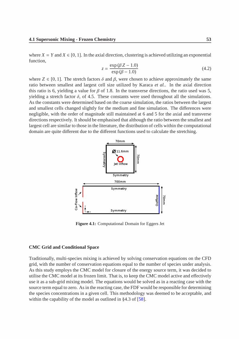
4.1 Supersonic Mixing - Frozen Chemistry 53
whereX = Y andX ∈ [0, 1]. In the axial direction, clustering is achieved utilizing an exponentialfunction,
z=exp(βZ − 1.0)exp(β − 1.0)
(4.2)
whereZ ∈ [0, 1]. The stretch factorsδ andβ, were chosen to achieve approximately the sameratio between smallest and largest cell size utilized by Karacaet al.. In the axial directionthis ratio is 6, yielding a value forβ of 1.8. In the transverse directions, the ratio used was 5,yielding a stretch factorδ, of 4.5. These constants were used throughout all the simulations.As the constants were determined based on the coarse simulation, the ratios between the largestand smallest cells changed slightly for the medium and fine simulation. The differences werenegligible, with the order of magnitude still maintained at6 and 5 for the axial and transversedirections respectively. It should be emphasised that although the ratio between the smallest andlargest cell are similar to those in the literature, the distribution of cells within the computationaldomain are quite different due to the different functions used to calculate the stretching.
Figure 4.1: Computational Domain for Eggers Jet
CMC Grid and Conditional Space
Traditionally, multi-species mixing is achieved by solving conservation equations on the CFDgrid, with the number of conservation equations equal to thenumber of species under analysis.As this study employs the CMC model for closure of the energy source term, it was decided toutilise the CMC model at its frozen limit. That is, to keep theCMC model active and effectivelyuse it as a sub-grid mixing model. The equations would be solved as in a reacting case with thesource term equal to zero. As in the reacting case, the FDF would be responsible for determiningthe species concentrations in a given cell. This methodology was deemed to be acceptable, andwithin the capability of the model as outlined in§4.3 of [58].

54 CMC for Supersonic Combustion
NXC NYC NZC CMC Cell CountCoarse 1 1 32 32
Medium 1 1 48 48Fine 1 1 64 64
Table 4.2: Eggers jet CMC grid
Air Co-flow H2 JetH2 0.0 1.0O2 0.232 0.0N2 0.768 0.0
Table 4.3: Boundary species mass fractions for Eggers simulations
For the case setup previously described, it was seen that forCMC operating at its frozenlimit, having a fine CMC grid versus a coarse CMC grid made no difference term C2 in Eq. 3.20was the leading order term both cases. As a consequence of this, the proceeding simulationswere run with a coarser CMC grid to slightly reduce the computational cost. In addition to this,as the conditional gradients in the cross-stream directionare very small in comparison to themean axial conditional gradients, there was no need for a multi-dimensional CMC grid. Thisyielded a 1 dimensional CMC grid with each CMC cell having thedimensionsNX × NY× 8CDF/CMC. The total distribution of CMC cells for all the simulations is given in Table4.2
Much of the analysis of the CMC and conditional space grids was omitted in this section.They are not as influential in the frozen chemistry simulations, as they are in the reacting cases.With the lack of chemistry and consequently sharp gradients, the effects of these two grids isdifficult to analyse as no relevant of conditional reactive scalars occurs. A more detailed analysisis presented in the portion of the study concerning reactingflows, more specifically§. 4.2.1
4.1.2 Initial Conditions and Boundary Conditions
The boundary conditions for the Eggers simulations are presented in Tables4.3 and4.4. Themass fractions used in this simulation are only that of the major species in air, namely O2 and N2.The presence of H2 in this case does not cause a chemical reaction as the temperatures of the twostreams are well below the autoignition temperature of the mixture. Simulations at these lowtemperatures are beneficial because they allow fuel mixtures to be studied without the influenceof combustion, which normally make pure mixing studies of fuels difficult. Additionally theutilisation of a specific fuel as opposed to thermodynamically different inert species (such asN2 or He), allows more accurate, species specific, mixture phenomena and behaviour, to beobserved and studied.
In all of the simulations, Lewis numbers were all kept constant at unity (Le=1), as the current

4.1 Supersonic Mixing - Frozen Chemistry 55
Air Co-flow H2 JetU [m/s] 1074 394Tstat [K] 260 222
Pstat [kPa] 100 100ρ [kg/m3] 1.563 0.093
M 1.32 0.886
Table 4.4: Boundary conditions for Eggers simulations
formulation of CMC is based on unity Lewis assumption. The Prandtl number was assumedconstant at 0.709, and the turbulent Schmidt number was unity (Sct = 1.0).
Boundary Conditions
The boundary conditions utilised in this simulation are shown in Fig. 4.1. In the transversedirections are Euler wall (symmetry), while the outflow is supersonic outflow. The inflow isslightly modified to accommodate velocity profiles and a turbulence generator.
Velocity Profile
Fig.4.2shows the inlet velocity profile that was extracted from numerical simulations by Karacaet al.. It corresponds to the velocity profile at the fictitious cross-stream plane at H2 jet exit. Itis important to capture the correct velocity profiles and gradients at the interface of the fluids asthese quantities are paramount in the development of the shear layer and mixing of the fluids.All the simulations conducted for this test case use this profile as a template, interpolating basedon the grid resolution and distribution. Points were clustered in regions of higher gradients toadequately capture the profile features even at low resolutions.
Turbulence Generator
In order to help trigger the transition to turbulence, a simple white noise turbulence generatorwas implemented at the boundary. It takes the form,
u′ = (ǫwJetr1) (4.3)
v′ = (ǫwJetr2) (4.4)
where in this case, fluctuations are only applied in the transverse directions, and are confinedonly to the jet. The random valuesr1, r2 are recalculated every time-step, and only determine thedirection of the fluctuation; they can take on values of−1 or 1. The magnitude of the fluctuation(ǫ) was constant at 1% of the maximum jet velocity, giving a fluctuation of approximately10.7m/s. This method of turbulence has been shown to be a poor representation of turbulence

56 CMC for Supersonic Combustion
0
200
400
600
800
1000
1200
-0.02 -0.015 -0.01 -0.005 0 0.005 0.01 0.015 0.02
Velo
city [m
/s]
Radial Distance [m]
Figure 4.2: Inlet velocity profile used for Eggers jet simulations
[77], however given the time frame and priority of this study, a simple turbulence generator wasneeded to aid in the transition to turbulence and the white noise generator was deemed feasible.
4.1.3 Averaging of Results
Interactive time averaging began after allowing the flow to stabilise for 3 flow through times. Aflow through time was considered the time required for the co-flow to enter and exit the domainwhich was determined to be approximately 1.6ms. Temporallyaveraged results were obtainedby averaging a total of 480 evenly spaced samples over 3 flow through times (160 samples/flow-through), giving each simulation a total of 6 flow through times. Fig.4.3 shows the effect ofsample rate where different sampling frequencies were taken ranging from 50/flow-through, to250/flow-through. It was seen that for 160 samples and above, the difference was negligible onthe resulting average.
Fig. 4.4 shows a temporal forward-averaged density at 4 different probe locations through-out the domain for the fine simulation. The fine simulation wasused in this demonstrationbecause, theoretically, this simulation would exhibit more fluctuations, and thus take longer toconverge given a similar sampling frequency. The sampling frequency for all these locationsis 160 sample/flow-through as determined above, however, these figures show the effect ofinitialisation time of the interactive averaging process on the averaged results. The earliest ini-tialisation time is after one flow-through, and the latest isat the 5th flow-through. It can be seenthat it takes approximately 2 flow-through times for the averages to stabilise at this sampling

4.1 Supersonic Mixing - Frozen Chemistry 57
0.65
0.7
0.75
0.8
0.85
0.9
0.95
0.006 0.007 0.008 0.009 0.01
De
nsity [
kg
/m3]
Time [s]
50 samples
100 samples
160 samples
200 samples
250 samples
Figure 4.3: Sampling frequency comparison
frequency. As a consequence, beginning the averaging after4 or 5 flow-though times wouldresult in non-converged results. Elaborating on that point, it can also be said that it is indeedpossible to begin the averaging process after 1 flow-throughtime. This is evident as beginningat 1, 2, or 3 flow-through times all converged to the same values. It can therefore be concludedthat, instead of waiting 3 flow-through times to begin averaging for an additional 3 flow-throughtimes, averaging could have commenced earlier reducing thetotal simulation time.
4.1.4 Simulation Results
Presented in Figs.4.5 to 4.10, are the major results of the simulations plotted against the ex-perimental results from Eggers [26] and Karacaet al. [46]. The locations of the experimentaldata of centreline profiles shown in Fig.4.5, correspond to all the locations that have radial dis-tributions as well. In this study only four axial locations are investigated radially:x/D = 5.51(x=63.3mm),x/D = 9.58 (x=110.17mm),x/D = 15.44 (x=177.56mm), andx/D = 25.2(x=289.9mm). These locations are important because this region exhibits the largest gradients,and they describe the transient processes/phases of the jet before it becomes self-similar.
A preliminary conclusion from the centreline data shows that qualitatively, the simulationseems to fit the experimental data moderately well. However,a difference is visible betweenthe H2 profiles and the velocity profiles. The H2 mass fraction profiles fit well up to about anx/D ≈ 25.2. Thereafter, the H2 mass fraction level off while the experiment shows continuedgradual decay. The velocity appears to begin to decrease roughly at the correct location, butdecays more sharply and for a longer distance compared to theexperimental results.

58 CMC for Supersonic Combustion
0.2
0.4
0.6
0.8
1
1.2
1.4
1.6
0 0.002 0.004 0.006 0.008 0.01
De
nsity [
kg
/m3]
Time [s]
(a)
0.2
0.4
0.6
0.8
1
1.2
1.4
1.6
0 0.002 0.004 0.006 0.008 0.01
De
nsity [
kg
/m3]
Time [s]
(b)
0.2
0.4
0.6
0.8
1
1.2
1.4
1.6
0 0.002 0.004 0.006 0.008 0.01
De
nsity [
kg
/m3]
Time [s]
(c)
0.2
0.4
0.6
0.8
1
1.2
1.4
1.6
0 0.002 0.004 0.006 0.008 0.01
De
nsity [
kg
/m3]
Time [s]
(d)
Figure 4.4: Effect of averaging initialisation time on converged density averages for 4 probe locationsthroughout the domain
H2
The two centreline figures are accompanied by the numerical results of Karacaet al.. The rateof mixing of H2 seems to be similar for both simulations up till aboutx/D = 17, where thepresent results show a decreased rate. It is not entirely certain what causes this, however one ofspeculations for this is the assumption of incorrect modelling of species diffusivity.
The assumption of constant Lewis number in mixing simulations is not a bad assumptionas the temperatures do not vary significantly as they would for reacting cases. However, whenconsidering species with such a difference in molecular transport such as H2 and air, accuratethermodynamic transport representation is necessary. Dueto the unity Lewis assumption inthis work, the Schmidt numbers are also kept constant at 0.709. For O2 and N2 this may notbe a very inaccurate assumption, but it is well known that assuming unity Lewis and “typical”Schmidt values for H2 can result in skewed, inaccurate results. According to Giacomazzi [35]

4.1 Supersonic Mixing - Frozen Chemistry 59
300
400
500
600
700
800
900
1000
1100
1200
0 10 20 30 40 50 60 70
Ve
locity [
m/s
]
x/D
Reference Eggers
Karaca 1M
Karaca 8M
Coarse(1M)
Medium (4M)
Fine (8M)
0
0.2
0.4
0.6
0.8
1
1.2
0 10 20 30 40 50 60 70
H2 M
ass f
ractio
n
x/D
Reference Eggers
Karaca 1M
Karaca 8M
Coarse (1M)
Medium (4M)
Fine (8M)
Figure 4.5: Centreline distribution of velocity and H2 mass fraction
the typical Schmidt numbers for these molecules are about 0.8 for both O2 and N2 and about0.35 for H2 (Le= 1.26, 1.27 and 0.35 for O2, N2, and H2 respectively).
Karacaet al. use variable molecular transport, and in addition to the Navier-Stokes (N-S),perform an additional simulation using a Euler formulation. The immediately obvious resultsfrom these simulations, is that the N-S simulation shows a faster breakdown of the concentrationpotential core, and a slightly steeper decay of the H2 mass fraction compared to the Euler. Theprofiles begin to deviate at aboutx/D = 15.44 with the N-S simulation ultimately reachinga slightly lower final mass fraction at the domain exit. This would indicate that although theprinciple mixing mechanism in these high Reynolds flows is inviscid turbulent mixing, diffusionhas a noticeable influence on the overall mixing of the fluids.Whether this noticeable influenceis specific to the species in question (H2), or diffusion in general is unclear, but nevertheless,accurate modelling of diffusion is necessary.
In the case of the present simulation, the downstream regionof higher mass fraction of H2may be caused for multiple reasons. Firstly is the stretch rate of the grid compared to that ofKaracaet al.. As mentioned earlier, although the ratio between the smallest and largest cellsare similar, due to the stretching functions being different, the inlet section of the domain ismore resolved, and the opposite it true for the downstream section. This decreased resolutiondownstream acts to smear and dissipate much of the turbulentmotions that are in fact, thedominant mixing mechanism. The well resolved inlet sectioncould also explain the improvedcapturing of the potential cores by the presented 1M resultsto those of the 8M of Karacaetal.. Secondly, the assumption of constant Schmidt (Lewis) numbers does not isolate H2 as astrong diffusive species compared to the others, and does not conform tothe established needfor accurate molecular transport. The current numerics implemented lack this capability asconstant species diffusivities is assumed in the formulations of the CMC equations.

60 CMC for Supersonic Combustion
Velocity
Compared to the H2 profiles, the velocity profiles hint that the simulation may be too dissipative.In conjunction with the experiment, Eggers did a numerical study on various eddy viscositymodels. The primary conclusion was that there was a difference in centreline profiles and jetdecay rates based on the eddy viscosity model chosen; The larger the eddy viscosity component,the faster the jet decay rate. Additionally, Uzunet al. [43]. performed a classical LES study ofa Mach 0.9 jet of air-air and studied the effect of the Smagorinsky constant on the simulated jetbehaviour. The study involved multiple simulations, whereonly the Smagorinksy constant wasvaried. What was seen was that the larger constant resulted in a faster jet decay, and a lower jetmomentum spread. A 5.56% difference in the constants led to approximately a 15.20% increasein decay rate and 18.87% reduction in jet spread. The resultsof studies illustrate the sensitivityof the jet decay rate to viscosity.
This type of study could prove to be difficult for ILES simulations of jets, as the sub-griddissipation is a function of the numerical scheme and is not quantifiable. It was thought that theexcess decay of the jet was perhaps a consequence of the current numerical schemes, and that itwas overly dissipative. Based on the results of Uzunet al.[43], a variation of sub-grid dissipationdoes not have to be substantial to have a large influence on jetbehaviour. However, the excessdissipation seems to be localised after about x/D=9.58, where the present jet continues to decay,while the experimental data gradually stabilises. Prior tothis location, the simulation jet decayrates are comparable to experiment. The initial jet decay rate calculated (x/D ≈ 8) as indicatedin [43], gives the experimental Eggers jet a decay rate of 9.25, andthe present simulations arate of about 9.88. In addition to this, due to the presence ofthe low Mach number correction,Thornberet al. [85] illustrated that the modified MUSCL 5th scheme used in CHOC, was lessdissipative than the standard MUSCL 5th, and the WENO 5th. Therefore it can be concludedthat the numerical scheme is not overly dissipative and is not the reason for the localised excessdecay.
It was therefore thought that the random white noise turbulence inlet was the cause of theexcess decay. As a result of this doubt, a simulation for the medium case was run without the aidof the turbulence generator. Fig.4.6shows that without turbulence the initial trends of velocityare still captured well although there is a shift in breakdown location. This gives reassurancethat the turbulence generator is not the principle reason for the apparent excess decay of the jet.
What must also be mentioned is the effect of laminar viscosity. In the early stages of the jet,as the momentum dissipation is still primarily laminar as the flow has not yet fully developed,the effective viscosity is dominated by the laminar contribution.In the simulations, the Suther-land law is used to calculate the mixture viscosity, however, the coefficients used for all speciesis that of air. This greatly overestimates the viscosity as at 298K, the viscosity of air is 2.5 timesgreater than H2. This overestimated viscosity contribute and provide insight to the excess decayof velocity.

4.1 Supersonic Mixing - Frozen Chemistry 61
300
400
500
600
700
800
900
1000
1100
1200
0 5 10 15 20 25
Ve
locity [
m/s
]
x/D
Reference Eggers
Karaca 8M
Medium (4M)
Medium-No turb (4M)
0
0.2
0.4
0.6
0.8
1
1.2
0 5 10 15 20 25
H2 M
ass f
ractio
n
x/D
Reference Eggers
Karaca 8M
Medium (4M)
Medium-No turb (4M)
Figure 4.6: Centreline profiles of velocity and H2 mass fraction with no turbulent inlet
Effect of Grid Distribution
It is true that with the exponential clustering implementedin the axial direction, the inlet sec-tion of the present simulation would have an effective resolution much higher than the averageddomain resolution. Exponential clustering (inherent to its name) places and unbalanced numberof cells at either extreme of the coordinate direction it alters. In the present case, the upstreamportion of the domain may be over-resolved with respect to the downstream portion. Furtherincreasing the resolution while keeping the stretch coefficient constant, may not always be re-quired as further refinement in the upstream portions of the domain may not be necessary to thesame extent as the factor of cell increase. In fact, perhaps with increasing grid resolution, thestretch coefficient should be relaxed to give a better overall resolution increase. Nevertheless,this clustering distribution was implemented because it was thought that even at coarse resolu-tion, capturing the initial development of shear layer instabilities was crucial in modelling thejet.
This asymmetric distribution of the grid, could potentially lead to visible asymmetries whenapproaching very fine simulations. This effect is apparent through the profiles of the currentsimulation varying much more upstream between the coarse, medium, and fine, as opposedto the downstream sections where only minor differences are seen. This is in contrast to thenumerical results of Karacaet al. where, because a more relaxed clustering distribution wasused, the effect of increasing resolution was more noticeable throughout the entire simulation.Increasing the resolution showed a global convergence towards the experimental values, asopposed to isolated regions of the domain shown in the present simulation.
As a consequence of this, an additional simulation was conducted simulating a half domainwith 8M cells (effective 16M) with a stretch factorβ of 1.1. The hope was that any under-resolved regions were to blame for the excess decay of the jet. The results showed slightlybetter agreement downstream with the upstream portions having an almost negligible change.Most importantly, the region of excess decay was not significantly altered giving credence to

62 CMC for Supersonic Combustion
400
600
800
1000
1200
1400
-2 -1.5 -1 -0.5 0 0.5 1 1.5 2
Ve
locity [
m/s
]
r/D
Reference Eggers
Coa
Med
Fine
0
0.2
0.4
0.6
0.8
1
1.2
1.4
-2 -1.5 -1 -0.5 0 0.5 1 1.5 2
H2 M
ass F
ractio
n
r/D
Reference Eggers
Coa
Med
Fine
Figure 4.7: Radial distributions at x/D=5.51 of velocity and H2 mass fraction
400
600
800
1000
1200
1400
-2 -1.5 -1 -0.5 0 0.5 1 1.5 2
Ve
locity [
m/s
]
r/D
Reference Eggers
Coarse
Med
Fine
0
0.2
0.4
0.6
0.8
1
-2 -1.5 -1 -0.5 0 0.5 1 1.5 2
H2 M
ass F
ractio
n
r/D
Reference Eggers
Coarse
Med
Fine
Figure 4.8: Radial distributions at x/D=9.58 of velocity and H2 mass fraction
the idea that this region is a consequence of a different or underlying more fundamental issue.It also verifies that the grid in it’s current form, is satisfactory in capturing the flow features andis adequately converged.
Radial Distributions
Typically for jet simulations, if the centreline data is accurate, radial distributions will not be faroff. Nevertheless, it is worth investigating the radial distributions, more specifically the earlyregions of the jet, e.g. the potential core region. This region is important in jet physics becauseit dictates the region where the shear layer merges, and where the transition region begins. Thistransition region location is dictated by the shear layer growth rate, and has a direct effect onthe jet spread and the jet decay rates.

4.1 Supersonic Mixing - Frozen Chemistry 63
400
600
800
1000
1200
1400
-2 -1.5 -1 -0.5 0 0.5 1 1.5 2
Ve
locity [
m/s
]
Radial Location [m]
Reference Eggers
Coarse
Med
Fine
0
0.2
0.4
0.6
0.8
1
-2 -1.5 -1 -0.5 0 0.5 1 1.5 2
Ve
locity [
m/s
]
Radial Location [m]
Reference Eggers
Coarse
Med
Fine
Figure 4.9: Radial distributions at x/D=15.44 of velocity and H2 mass fraction
400
600
800
1000
1200
1400
-2 -1.5 -1 -0.5 0 0.5 1 1.5 2
Ve
locity [
m/s
]
r/D
Reference Eggers
Coarse
Med
Fine
0
0.2
0.4
0.6
0.8
1
-2 -1.5 -1 -0.5 0 0.5 1 1.5 2
H2 M
ass F
ractio
n
r/D
Reference Eggers
Coarse
Med
Fine
Figure 4.10: Radial distributions at x/D=25.2 of velocity and H2 mass fraction

64 CMC for Supersonic Combustion
Fig.4.7shows the results of the simulations for the region at the approximated potential corelength, with the difference between the three resolutions immediately visible.With increasinggrid resolution, the traces of the initial velocity gradient/discontinuity at the fluid interface dis-appears. In addition to this, the profile widths indicate that the shear layers at this location areof different sizes. They indicate different capturing of shear layer instabilities upstream of thisregion. At this location, from experiment, the shear layer non-dimensional thickness based onthe mass fraction of H2, was determined to be 0.706. From the simulations, the shearlayerthickness approximations are 0.527, 0.64335, and 0.79623,for the coarse, medium, and finerespectively. As expected the finer simulation tends to growsooner as at this location the shearlayer is the thickest of all three simulations. However, theover estimation of the shear layerthickness for the fine simulation, indicates that perhaps the inadequate turbulence generatoradded additional non-physical perturbations that caused the instabilities to grow sooner thanthey should have. This can also be verified with the potentialcore being shorter than what wasobserved in experiment (Fig.4.5).
Figs.4.8 to 4.10show the remaining radial profiles at different axial locations downstreamof the potential core. As expected the correlation between centreline fit and radial profilesis illustrated. The H2 profiles seem to correlate fairly well with experiment, but as expectedfrom the accuracy of the centreline profile of velocity, the radial profiles of velocity seem todeviate substantially. Due to the nature of modelling jets and the sharp decay of parameters theyexperience after the potential core, a small shift in jet breakdown length can have a profoundimpact on the radial profile distributions. This consequently leads to relative inaccuracies of thesimulation. Therefore one of the key characteristics to capture accurately when modelling anyjet, is the initial development of the shear-layer, and thus, the potential core length.

4.2 Supersonic Combustion - Reacting Case 65
4.2 Supersonic Combustion - Reacting Case
The proceeding section aims to demonstrate the first application of the conditional momentclosure model to a supersonic reacting H2-air jet. The test case chosen for this demonstrationwas the LAERTE jet from ONERA [32, 46]. Similar to the motivation chosen for the frozenchemistry case, this case was deemed acceptable as it was a shear-flow test case that removedthe complexities of wall modelling. Additionally, the geometry of the test section was simpleenough to be used within the capabilities of CHOC.
A comprehensive grid convergence study for the reacting case would involve a coarse,medium, and fine simulation on the CFD grid, with coarse, medium, and fine, 1D, 2D, and3D CMC grids. Assuming three resolutions in conditional space, that would be equivalent toa minimum of 81 simulations. This is indeed not practical, however, some assumptions andsimplifications can be made to help reduce this number.§. 4.2.1presents a study that enabledthe determination of the conditional space grida priori. Additionally, in a previous paper byThornberet al. [86], it was shown that the difference between 1D CMC, and 2D or 3D was notsubstantial. Therefore, based on those results, and the notion that the jet is axis-symmetric andthe conditional gradients in the cross-stream direction are small compared to the axial direc-tion, only a 1D CMC grid was used in the axial direction. Lastly, presented in§. 4.2.7, is thestudy that led to the usage of a single CMC resolution, further reducing the number of simula-tions required in the grid convergence study. Based on theseassumptions and studies, the totalnumber of simulations was greatly reduced from 81. The proceeding section presents, a totalof 3 simulations utilising an axial, 1D, medium resolution CMC grid, with a fixed, equispacedconditional space distribution.
4.2.1 Computational Grids and Domain
The computational domain for this test case is a 45mm× 45mm× 350mmthat corresponds tothe constant cross section portion of the ONERA LAERTE combustion chamber. As with thefrozen chemistry case, three simulations were conduced ranging from 1M to 8.3M cells. Detailsof the grid resolution are given in Table4.5.
NX NY NZ Cells Count(106)Coarse 64 64 256 1.048
Medium 100 100 384 3.84Fine 128 128 512 8.388
Table 4.5: LAERTE Jet computation sizes
Clustering is achieved in the transverse and cross-stream directions by utilising the hyper-bolic sine relationship given for the frozen chemistry casein §. 4.1.1. The stretch factorsδ andβ, were once again chosen to achieve approximately the same ratio between smallest and largest

66 CMC for Supersonic Combustion
cell size utilised in the previous section. In the axial direction this ratio is 6 yielding a value forβ of 1.8, while in the transverse directions, the ratio used was 5 yielding a value forδ, of 4.5.
Figure 4.11: Computational Domain for LAERTE Jet
CMC Grid
Unlike the previous test case where CMC was operating at its frozen limit, for the reactingcases, the CMC grid was altered and refined. Having too coarseof a CMC grid for a reactingcase can have a profound impact on the simulations as will be demonstrated in section§. 4.2.7.Therefore, the proceeding simulations were conducted withwhat was deemed, a medium CMCgrid. For all the simulations unless otherwise indicated, each CMC cell has the dimensionsNX× NY× 4 CFD/CMC. The total number of CMC cells in the computational domain can beseen in Table4.6.
NXC NYC NZC CMC Cell CountCoarse 1 1 64 64
Medium 1 1 96 96Fine 1 1 128 128
Table 4.6: CMC Grid size for the CFD grid convergence study for the LAERTE Jet
Conditional Space
A convenient property of conditional space, is that it represents the combustion process givencertain external inputs. These inputs come in the form of specific parameters of which the

4.2 Supersonic Combustion - Reacting Case 67
0
0.2
0.4
0.6
0.8
1
1.2
0 0.2 0.4 0.6 0.8 1
Mass fra
ction
Mixture Fraction
O2
H2
OHx10
H2O
Figure 4.12: Distribution of major species at a Scalar dissipation of 1; boundary conditions are set tothose of the LAERTE Jet.
solution in conditional space is explicitly dependant on. What makes this a convenient attributeis that it allows the solution in conditional space to be obtained with only a few inputs. As aresult, the effect of grid resolution in conditional space can be analysed independently andapriori to the full simulations which allows the simulation convergence study to be reduced by adimension.
Solving conditional space and obtaining averaged mixture quantities only requires informa-tion from the CFD grid; information that for the sake of analyses, can be artificially providedto the CMC equations. The primary parameters required are the scalar dissipation, mixturefraction, and mixture fraction variance. As the scalar dissipation increases, the gradients inconditional space become smoother, the opposite is true fora decreasing scalar dissipation.Therefore, the extreme case (or the case with the sharpest gradients) occurs when the scalardissipation approaches 0. To analyse the grid sensitivity in conditional space, a solution in con-ditional space was obtained for a scalar dissipation rate of1(1/s) using 6 different, equispacedgrid resolutions: 50, 100, 120, 180, 200, and 500; 500 being considered as the control. Toillustrate the solution-space, Fig.4.12shows the steady-state solution of the conditional massfractions in conditional space using 500 conditional bins.The boundary conditions used toobtain this solution are those listed in Tables4.7and4.8.
Calculating the unconditional mass fractions from this distribution of conditional mass frac-tions is done using Eq. 3.34. The FDF shapes that are used, corresponded to the shapes gen-erated in the region of mixture fraction space near stoichiometry(ζst ≈ 0.0298), as this regionexhibits the sharpest gradient. The FDF can either be an analytical or discrete function (Beta

68 CMC for Supersonic Combustion
0.965
0.97
0.975
0.98
0.985
0.99
0.995
1
1.005
1.01
40 60 80 100 120 140 160 180 200
Norm
alis
ed O
H M
ass fra
ction
Number of Conditional Bins
SV=0.001
SV=0.01
Figure 4.13: Normalised unconditional mass OH fraction
and Top-hat respectively) of the mixture fraction and it’s variance. This means for any givennumber of realisations of these two parameters, similar combinations of the two always producethe same FDF shapes.
As a measure of convergence, the unconditional OH mass fraction was used. Using thepreviously indicated number of conditional bins, two possible FDF shapes were constructedand integrated yielding an unconditional OH mass fraction.This value was then normalisedbased on the value obtained from a simulation using the control at 500 bins. The 500 binlimit represents an extreme upper limit for the resolution in mixture fractions space, as the totalnumber of calculations per time-step and memory requirement scale proportionally with it’ssize.
Fig. 4.13shows that relative errors of less than 1% begin after about 100-120 bins whichleads to the conclusion, that obtaining a relatively high accuracy, does not require an highnumber of bins. To see the effect of conditional space resolution where the gradients arenot assharp as the region about stoichiometry, a similar study wasperformed near a mixture fractionof 0.97. In this case, the same variances as in the previous study were used, however, H2 wasused as at this mixture fraction, OH is not present and H2 experiences the sharpest gradients.This study yielded a maximum unconditional H2 mass fraction difference between 50 and 500conditional bins of 0.00297%. This result is not surprisingas in this region the conditional massfractions profiles are quite linear.
The results presented here represent idealised results with “clean” values of mixture fractionand variance. In reality, these two parameters will not takeon such ideal values. The mean

4.2 Supersonic Combustion - Reacting Case 69
mixture fraction given to conditional space determined where the FDF is constructed around,and may not coincide with the distribution of conditional bins. This in turn may introduce smallerrors in the location of the FDF mean. The variance on the other hand, affects the broadness ofthe FDF and bounds. The Beta-PDF is less prone to this error, as it’s distribution is analytical,and a solution can theoretically be obtained for any distribution of conditional bins. The Top-hat on the other hand, is built from discrete functions, and uses specific locations in conditionalspace for its bounds. Therefore these locations are also susceptible to their values not coincidingwith grid locations on the conditional space grid. Althoughthe implementation of the FDFsaims to conserve the mean, and avoid these very small errors,they are inevitable. However,it should be noted that the errors are not very large and are quantifiable. As an example, for120 conditional bins, the extreme case of both Top-hat FDF endpoints being located in-betweenconditional bins locations, leads to a maximum error of about 0.83%.
The aforementioned discussion, plus the obvious differences in gradients at locations nearstoichiometry compared to the rest of conditional space, raise an obvious question about gridclustering. Fig.4.14shows the grid points for 120 bins for the grid convergence study men-tioned above, along with the OH distribution. It can be seen that only about 13 conditional binsfall within the OH distribution. Therefore only about 10% ofthe points used in conditionalspace are used to capture OH. Ideally, grid clustering can beimplemented in conditional spacearound the stoichiometric mixture fraction to greatly reduce the number of grid points present,decrease conditional space computation time, and increasethe effective resolution. However,decreasing the spacing between conditional bins also increases the influence of the Peclet num-ber criteria for limiting time step. In this criteria, the minimum conditional grid spacing is used.In the case of a multi-step, time-splitting, time integration as implemented in this code, havinga smaller Peclet number would increase the overall computation time. A balance between gridclustering and number of conditional bins is required, and whether the increased computationaltime due to the increased iterations from a smaller time-step, is outweighed by the accuracyand decreased computational time from the clustered conditional space grid, is the subject ofanother study. From the presenteda priori study, 120 equispaced bins were chosen to representmixture fractions space for all the simulations.

70 CMC for Supersonic Combustion
0
10
20
30
40
50
60
70
80
90
0 0.05 0.1 0.15 0.2 0.250
0.002
0.004
0.006
0.008
0.01
0.012
0.014
0.016F
DF
Mass F
raction
Mixture Fraction
Shape1
Shape2
OH
Figure 4.14: Distribution of conditional bins in conditional space
4.2.2 Initial Conditions and Boundary Conditions
Contrary to the frozen chemistry case, the initial/boundary species mass fractions for the airco-flow were not of strictly of the major species in air, and included traces of H2O and O, H,and OH radicals. Specific quantities can be seen in Table4.7. Additionally, the temperatureof the jet and air co-flow in this case, were much higher. This ensured that the mixed H2-airstreams were well above the autoignition temperature. Specific details of the inlet conditionsare shown in Table4.8 Lewis numbers were kept constant at unity (Le=1) for all species as
Air Co-flow H2 JetH2 0.0 1.0O2 0.2447 0.0
H2O 0.1124 0.0OH 2.285×10⁻⁴ 0.0O 1.8×10⁻⁵ 0.0N2 0.64265 0.0
Table 4.7: Initial and boundary mass fractions for the LAERTE Jet
required by the formulation of CMC utilised in this study. For the proceeding simulations, thePrandtl number was assumed constant and fixed at 0.709. The turbulent Schmidt number wasconstant at unity (Sct = 1.0).

4.2 Supersonic Combustion - Reacting Case 71
Air Co-flow H2 JetU[m/s] 1366 1970Tstat[K] 1170 160
Pstat[kPa] 92 84ρ[kg/m3] 0.259 0.127
Table 4.8: Initial and boundary flow conditions for the LERTE Jet
Velocity Profile
The inlet velocity profile shown in Fig.4.15 was extracted from numerical simulations byKaracaet al., and represents the velocity profile at the fictitious cross-stream plane at the jetexit. Points on the profile, were clustered around the regions of highest gradients to ensureadequate profile resolution, even at lower grid resolutions.
0
500
1000
1500
2000
-0.02 -0.015 -0.01 -0.005 0 0.005 0.01 0.015 0.02
Velo
city [m
/s]
Radial Distance [m]
Figure 4.15: Inlet velocity profile used for LAERTE Jet Simulations
Turbulence Generator
In order to help trigger the transition to turbulence a simple white noise turbulence generatorwas used, taking the form similar to the turbulence generator used in the frozen chemistrysimulations. The fluctuations were only applied in the transverse directions and are confined to

72 CMC for Supersonic Combustion
the jet. The magnitude of the fluctuation (ǫ) was constant at 1% of the maximum jet velocity,giving transverse fluctuations of approximately 19.7m/s.
4.2.3 Averaging of Results
Interactive time averaging began after allowing the flow to stabilise for 3 flow through times.Temporally averaged results were obtained by averaging a total of 480 evenly spaced samplesover 3 flow through times (160 samples/flow-through) giving each simulation a total of 6 flowthrough times. A flow through time was considered the time required for the co-flow to enterand exit the domain which was determined to be approximately0.27ms.
4.2.4 Simulation Results
Centreline distributions of H2 mass fraction and velocity are shown in Fig.4.16, showing ad-equate convergence between the medium and fine simulations.What is almost immediatelyevident is that the velocity decay is not as sharp as with the frozen chemistry case. Instead,there is a much smoother decay towards the self-similar region. The fine simulations is similarto the medium expect that near the domain outflow, there is a slightly better mixing captured.What is also shown, is that between the medium and fine simulations, the potential core iscaptured almost identically. This is in comparison to the previous case, where there was a no-ticeable difference in potential core breakdown location with grid refinement. It appears as ifthe white noise turbulence no longer has an substantial effect on the simulations, or the effectis the same for both grid resolutions. As the time-step is decreased with increasing grid resolu-tion, the overall frequency (and wavenumber) of the synthetic turbulence is increased. As largewavenumbers are dissipated more quickly than lower wavenumbers, at the given resolutions ofboth the medium and fine simulations, it is possible that the perturbations by the turbulencegenerator are immediately dissipated.
In reacting flows, the more important representative quantity in simulations is the temper-ature. Fig.4.17 shows radial distributions of temperature at two axial locations, along withexperimental data and those obtained by Karacaet al.. Unfortunately, the experimental temper-ature data shown was the only data available for this test case, and it was stated in the paper [46]that the experimental results are very poor — The velocity was underestimated and the meantemperatures were overestimated because of the flapping nature of the jet. No relative errorswere published and therefore it is unclear how inaccurate the data truly is.
The experimental data resembles the early stages of the averaging procedure of the simula-tions, and it is possible (but uncertain) that the high temperature point at 1600K is an outlier.Instantaneous temperature profiles from the simulations experienced similar peak temperatures(sometimes even reaching 2000K), but due to the flapping nature of the jet, the averaged tem-perature dropped substantially to those shown. However, even if the temperatures are overesti-mated, the trend of the experimental data is still expected to maintain some accurate qualitative

4.2 Supersonic Combustion - Reacting Case 73
0
0.2
0.4
0.6
0.8
1
1.2
0 10 20 30 40 50 60
H2 M
ass F
ractio
n
x/D
Coarse
Medium
Fine
(a) Centreline distribution of H2
1000
1200
1400
1600
1800
2000
2200
2400
0 10 20 30 40 50 60
Ve
locity [
m/s
]
x/D
Coarse
Medium
Fine
(b) Centreline distribution of velocity
Figure 4.16: Centreline distributions of H2 mass fraction and velocity
500
1000
1500
2000
-3 -2 -1 0 1 2 3
Te
mp
era
ture
[K
]
r/D
ONERA EXP
Coarse
Medium
Fine
Karaca 8M
(a) Radial Distribution of temperature at x/D=35
500
1000
1500
2000
-3 -2 -1 0 1 2 3
Te
mp
era
ture
[K
]
r/D
Coarse
Medium
Fine
(b) Radial Distribution of temperature at x/D=57.5
Figure 4.17: Radial ditributions of temperature at selected axial locations
description of the structure of the jet. Based on this criteria, the presented simulations fol-low the trends very well except for a perhaps a slightly lowertemperature in the shear-layer atr/D ≈ 1.3.
A independent analysis of the temperature profiles gives clear indication that combustion isoccurring at the exit of the computational domain (x/D = 57.5), as there is an approximateincrease in temperature of 500K from the air co-flow temperature. Even atx/D = 35, the tem-peratures are lower than the exit plane, but still higher than the mixture temperatures, indicatingthe presence of chemical reactions. If indeed the experimental temperatures are over estimated,then it is safe to conclude that the results of the present study match well to the experiment. Thelower temperatures experienced atx/D = 35 also indicate that the combustion process has onlyjust begun in this region.

74 CMC for Supersonic Combustion
Figure 4.18: Time averaged mid-plane contour of mixture fraction along with selected cross streamcontours
Figure 4.19: Time averaged mid-plane contour of temperature along with selected cross stream contours

4.2 Supersonic Combustion - Reacting Case 75
Figure 4.20: Instantaneous mid-plane contour of mixture fraction
It should be emphasises that the low temperatures atx/D = 35 do not indicate that thisis the lift off height of the flame, nor do they indicate that it happens near this region. Atthe advective velocities experienced in this experiment, small differences in ignition time, cancause large differences in lift of height. As an example, a± 0.01ms difference in ignitiontime can theoretically translate the ignition point approximately± 2.87D (17.22mm). Furtherinvestigation into the non-equilibrium effects and lift-off height will be investigated in§. 4.2.6.
The results from Karacaet al. in Fig. 4.17 appear to be of the same order of magnitudeas the experimental results. As no other definitive/quantitative data is compared to in Karacaet al. to assess chemical non-equilibrium effects or reactive scalar distributions (due to poorexperimental results), it is difficult to conclude on the true validity of their results. Basedonthe contour plots published, it appears that the lift-off height was located significantly fartherupstream compared to the results of the present simulations, and thus can explain the highertemperatures at similar axial locations.
Karacaset al. closure to the chemical source term is left to diffusion (as DNS normallyis) and is a dangerous closure at the published grid resolutions. As the flow is under-resolvedcompared to a DNS resolution, the sub-grid fluctuations are being left to numerical diffusionwhich may or may not be modelling them accurately; This potentially giving rise to erroneousproduction rates. As numerical dissipation is highly dependant on grid resolution in ILES, avarying numerical dissipation will give rise to fictitious sub-grid diffusion of species, whichmay create large variations in the local temperature. Although the mean flowmaybe capturedadequately, the effect of turbulence on sub-grid mixing is poorly represented.Therefore, to con-clude that the results of Karacaset al. are accurate, would be just as incorrect as saying they areinaccurate, and should be accepted with caution. The conclusions extrapolated from this pub-lication are used merely to strengthen findings of the present study, and are valid only becausethe comparisons (between Euler and N-S), are based on results from consistent numerics.

76 CMC for Supersonic Combustion
Figure 4.21: Instantaneous mid-plane contour of temperature
Figure 4.22: Instantaneous mid-plane contour of OH

4.2 Supersonic Combustion - Reacting Case 77
4.2.5 Effect of Differential Diffusion
In the previous analyses, the importance of the effect of differential diffusion when modellingH2 was emphasised. In fact, there have been many DNS studies showing the effect of non-unityLewis numbers on H2 flames. Doom and Mahesh [24] showed that non-unity Lewis numbereffects increase the overall temperature and heat release, andcan decrease the ignition delaytime by up to 64%. Dineshet al. [78] performed a DNS study of an impinging jet (Re=2000),and also concluded an increase in overall combustion temperature. It was also shown, that non-unity Lewis altered the structure of the reacting jet, shifting the combustion mixture towardsleaner conditions. The DNS studies of turbulent diffusion flames tend to be limited to lowReynolds flows as the Kolmogorov length scale, scales with Reynolds as shown in Eq. 2.13.Thus, the results of such DNS studies are mainly describing flows who’s mixing processes areinfluenced by both turbulence and diffusion in comparable proportions. In high Reynolds flows,the principle mechanics still remain the same except that mixing tends to be bias/dominated byturbulence while the component of diffusion begins to diminish. Thus, the DNS findings cannotbe applied definitively to the present case as the Reynolds number is approximately 100 timeslarger than the case of Doom and Mahesh. However, they do still provide a good indication ofexpected behaviour when assuming non-unity species Lewis numbers.
Similar to the Eggers case above, Karacaet al. performs a reacting case with a Euler formu-lation as well as a N-S formulation. In this case, the effect of non-unity Lewis is more stronglyvisualised though the temperature distributions. The difference in radial temperature distribu-tion at a given axial location between the Euler and N-S simulations, showed the N-S simulationwith a temperature 70K higher than the Euler simulation. In addition to this, although not con-clusive, instantaneous centre-plane contours of temperature distributions showed the N-S hav-ing a slightly earlier ignition point. This difference is far from the immense difference shownin Doom and Mahesh [24] of about 450K, but the difference can perhaps be correlated to theReynolds number. In flows where turbulent-diffusion time-scale are comparable (low Reynoldsnumber), the temperature differences may be as large as determined by [24], but in cases whereturbulent transport is dominant (large Reynolds number), it may be smaller. Referring back toFig. 4.17, it could therefore be concluded that the lower radial temperatures nearr/D ≈ 1.3 areslightly underestimated due the inaccurate modelling of species molecular transport.
4.2.6 Chemical Non-Equilibrium Effects
The results to this point look promising, but due to the lack of reliable experimental data it isstill uncertain whether the implementation models correctly and captures the appropriate non-equilibrium effects. Quantitative comparison to the numerical results of Karacaet al. can not bedone confidently because of the questionable conslusions provided by the numerical methodsused.
In order to analyse the chemical non-equilibrium effects, an additional simulation was con-ducted. This test case came from ONERA [32] as well, and was identical to the test case

78 CMC for Supersonic Combustion
previously analysed, except for the pressure boundary conditions. In this case the pressure forboth the jet and the co-flow were 80kPa. The primary focus of this experiment was to assesslift-off height, and does not provide velocity, mass fraction, or temperature data. Along witha quantitative value for flame lift-off height, wall pressure distributions were also published.Ideally a simulation would be conducted assessing the wall pressure distribution, but for thereasons described at the beginning of this section, the wallpressure distribution is not the pri-mary interest and validation tool. The focus of these simulations was to assess combustionphenomena, and therefore the grid was clustered around the central jet regions, limiting theresolution of the wall. As pressure is highly dependant on the grid resolution, the resultant wallpressure distributions were not expected to be very accurate. However, even though the flowin these wall-regions was under resolved, quantitatively the results can be expected to deviate,while qualitatively, similar trends should still be visible as in the experiments.
Georgeet al.[32] conduct two experiments; a reacting case and and non-reacting case, wherethe non-reacting case injects N2 as opposed to H2. They use the wall pressure distributions toapproximate the lift-off height, and state that autoignition is determined where thetwo pressureprofiles deviate. From the published wall pressure distributions, this occurs at about 0.20mdownstream. It is unclear exactly how the authors extrapolated the approximate lift-off height,however they also preform Planar laser-induced fluorescence (PLIF) along with pressure mea-surements. Therefore, it is probable they use a combinationof both the pressure and averagedOH distributions to determine lift-off height. From the experiments, it was stated that lift-offheight was about 0.170m downstream from the jet exit. Using the definition of autoignitionof Gerliner [34] as being the point of largest OH gradient, the lift-off height for the simulationwas approximately 0.165-0.183m. A similar methodology of comparing a reacting case to anon-reacting case could not be applied, as the exact boundary conditions for the non-reactingcase where not published and could only be speculated.
The resultant wall pressure of the simulation is shown in Fig. 4.23. Indeed the pressuredistribution shown does not resemble the experimental values quantitatively as expected, andthe right scale had to be adjusted to better compare the trends of the distributions downstream.However, qualitatively, they match fairly well. Peaks occur roughly in the same regions as thepeaks in the experiment, and there is a pressure increase downstream where the experimentalpressure appears to begin to increase.
4.2.7 Effect of CMC Grid
One of the more difficult compromises in utilising a conserved scalar methods, is the governingof multiple grids in a given physical domain. When using direct Arrhenius rate closure tothe chemical source term (as in DNS), the chemistry is calculated directly on the CFD gridfor every CFD cell, and determining the CFD grid is the only requirement. However, at theopposite extreme, when utilising CMC, there is the CFD grid,CMC grid, and conditional spaceto consider. An accurate solution requires a delicate balance between all these grids as they arecoupled. Inaccuracies in one affect all the others.

4.2 Supersonic Combustion - Reacting Case 79
0.12
0.125
0.13
0.135
0.14
0 0.05 0.1 0.15 0.2 0.25 0.3 0.35
0.12
0.14
0.16
0.18
0.2
0.22
0.24P
elu
m P
ressure
- S
im
Pelu
m P
ressure
- E
XP
X/D
ONERA EXP
Reacting
Figure 4.23: Pressure Distribution of LAERTE Experiment
The choice of utilising 4 CFD/CMC in the axial direction was not chosen randomly. Initially,8 CFD/CMC was chosen for the simulations, however, the results obtained were non-physicaland a refinement of the CMC grid by a factor of 2 led to seeminglygood results. The CMCgrid was not refined beyond this point, as the results for the “medium” resolution were deemedadequate. As a demonstration to the sensitivity of CMC and it’s method, the results for theaxial 8 CFD/CMC on the medium CFD grid are presented. Fig.4.24 shows instantaneousmid-plane contours of density, and OH mass fractions. It canbe seen that about 1/6th of theway downstream, a discontinuity is formed through the onsetof combustion. The density fromone cell to the next experiences sudden sharp gradient due tocombustion, leading to shockformation which travels downstream. It is obvious that the results obtained are incorrect, as theignition process should be smoother and, show a gradual transition as seen in Figs.4.20to 4.22.
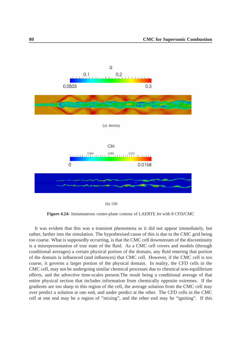
80 CMC for Supersonic Combustion
(a) denisty
(b) OH
Figure 4.24: Instantaneous centre-plane contour of LAERTE Jet with 8 CFD/CMC
It was evident that this was a transient phenomena as it did not appear immediately, butrather, farther into the simulation. The hypothesised cause of this is due to the CMC grid beingtoo coarse. What is supposedly occurring, is that the CMC cell downstream of the discontinuityis a misrepresentation of true state of the fluid. As a CMC cellcovers and models (throughconditional averages) a certain physical portion of the domain, any fluid entering that portionof the domain is influenced (and influences) that CMC cell. However, if the CMC cell is toocoarse, it governs a larger portion of the physical domain. In reality, the CFD cells in theCMC cell, may not be undergoing similar chemical processes due to chemical non-equilibriumeffects, and the advective time-scales present.The result being a conditional average of thatentire physical section that includes information from chemically opposite extremes. If thegradients are too sharp in this region of the cell, the average solution from the CMC cell mayover predict a solution at one end, and under predict at the other. The CFD cells in the CMCcell at one end may be a region of ”mixing”, and the other end may be “igniting”. If this

4.2 Supersonic Combustion - Reacting Case 81
is indeed the case, the CMC cell will have information from both extremes being fed into itssolution. If the average is bias towards the ignition process, the CMC solution will inevitablytend towards autoignition over time. However as detailed previously, not all CFD cells shouldbe experiencing this autoignition, and if indeed this CMC cell “ignites”, the entire conditionalsolution space of that CMC cell will be that of a burning solution. This translates back to theCFD grid, giving what should be a point in space of mixing, theinformation that it is in factburning. If the solution of the CMC cell upwind of the discontinuity tends towards the mixingsolution due to the larger influence of the mixing cells, the autoignition process will be seen tooccur over a CMC cell interface. This leading to a discontinuity and an unrealistic solution aspresented above in Fig.4.24.
Decreasing the number of CFD/CMC to 4, results in a relatively smoother solution as shownin Figs.4.20to 4.22. A more representative indication of the CMC methodology can be seen inFig. 4.25, where it shows the average cross-stream OH mass fractions for every CFD cell in theaxial direction.
2.0e-04
2.5e-04
3.0e-04
3.5e-04
4.0e-04
4.5e-04
5.0e-04
5.5e-04
6.0e-04
6.5e-04
20 25 30 35 40
OH
Mass F
raction
x/D
Figure 4.25: Average cross-stream OH mass fraction
Fig. 4.25shows three distinct regions: beforex/D ≈ 20 and near the exit of the domain,the distribution is smooth, while in-between these two regions, the distribution appears to havesmall discontinuities. This behaviour can be explained with the aid of the conditional massfraction profiles. At the locations where the distribution in Fig. 4.25is smooth, the differencebetween conditional profiles corresponding to adjacent CMCcells is small. Conversely, thesteps are created because the relative difference between conditional profiles for adjacent CMCcell is larger; the larger the difference, the larger the step. The smooth profile with low OH

82 CMC for Supersonic Combustion
concentration near the inlet, indicate that this is a regionof mixing, while the discontinuous re-gion indicates the region of the jet where transient chemical effects are occurring. In conditionalspace, this region is where the conditional profiles appear to be evolving the fastest. The smoothprofile near the exit on the other hand, would indicate that chemical transient effects have be-gun to cease, and that beyond this location, combustion would begin to be established. It isexpected that if the domain was larger, the OH distribution would eventually level off indicatinga steady-state flame.
The CMC cells can be clearly seen in this image by the 4 points per “cluster” representing the4 CFD/CMC. One would expect that if decreasing to 2 CFD/CMC, the piecewise distributionsof the OH mass fractions in the high gradient regions would behalved, creating a smootherprofile. The extreme case would correspond to 1 CFD/CMC, which should give the smoothestsolution, however, at this resolution, the advantage of CMC(and conditional averaging) dimin-ishes, and the solution process approaches a similar methodto the presumed PDF methods.Additionally, at these resolutions, CMC becomes very expensive, and the main advantage ofmodelling sections of the domain through conditional averages becomes questionable.
Naturally, increasing the CFD resolution will have the effect of increasing the resolution ofthe CMC grid as well. This will make the physical size of the CMC cells smaller, and there-fore, the “steps” seen in Fig.4.25, may also become smoother. However, it can also be arguedthat this increased CMC resolution is only necessary in regions where the conditional profilesare evolving the quickest. The upstream portion of the domain has the largest cluster of CFDcells, and the downstream, the lowest, yet the profiles in these regions are smooth. This wouldindicate that the CMC grid in these regions is adequately resolved for the gradients experi-enced. Hence, the increasing of the resolution of the CMC grid to avoid these steps and obtaina globally smooth solution, may come at cost of decreased efficiency, and wasted computationin the upstream and downstream regions. Currently the implementation of CMC only allows apredetermined ratio of CFD to CMC cells in the three principle directions. Therefore, what isneeded, is the ability to decouple the algebraic dependenceof CMC to CFD, and allow a vari-able CMC grid. This would enable adequate clustering of the CMC grid in regions of expectedhigh gradients, while reducing the resolution in regions ofsmoother gradients (i.e steady-statecombustion regions).
Nevertheless, keeping a modest resolution of 4 CFD/CMC still results in miniature discon-tinuities, but does not affect the flow as in the case of 8 CFD/CMC. It is uncertain if thesediscontinuities exist in flows of lower advective velocities, or if it is a new phenomena presentonly in the case of supersonic flows. To the knowledge of the author, detailed distributions suchas this have never been published for subsonic flows, however, it is expected that solutions insubsonic flows are much smoother. If 1 CFD/CMC is required for a smooth solution, this couldcertainly be a limitation of CMC and its application to supersonic reacting flows, or indicationthat better modelling is required.
The hypothesised term that would require better modelling would be the conditional veloc-ity. The spatial advection of a conditional quantity (termC1 in §. 3.1.2) passes information ofconditional scalars from a conditional bin in one CMC cell, to the same bin in another CMC

4.2 Supersonic Combustion - Reacting Case 83
cell. The fact that there exists a discontinuity in scalars at the CMC cell interface indicates thatperhaps information is not being passed correctly, or that for supersonic flow, this term must betreated in a different manner.
Kinetic Energy Dissipation
The energy spectra of the coarse and fine simulations are shown in Fig. 4.26. The energyspectra was determined based on the time history of a point after the flow was established (ap-proximately after 3 flow-through times). As this was a temporal signal, the Taylor Hypothesisof frozen turbulence was applied in order to convert this to aspatial signal to obtain the spectrain terms of wavenumber. Ingenito and Bruno [44] performed a dimensional analysis on kineticenergy density, with a dependence on density, dissipation,and wavenumber. They found thatfor flows dependant on density (compressible flows), the dissipation no longer follows a -5/3slope but a steeper -8/3 instead. The reader is encouraged to refer to [44] for further details.Fig. 4.26shows that both spectra have a small region where they followthe -5/3 dissipation, buta larger region where they follow -8/3.
To show the effect of the stretched grid and varying local resolution, Fig.4.27 shows thespectra at three different axial locations on the centreline for the medium simulation. The down-stream point that corresponds to the locally coarser grid location, captures more -5/3 and less-8/3, than the upstream location where the spectra shows a larger -8/3 region. It is uncertainwhether the -8/3 slope is an appropriate indication of the dissipation ratein these simulations,but the results show fair agreement to this hypothesis. It isknown that the -5/3 is an idealiseddissipation rate for incompressible homogeneous turbulent flows, and the recurring theme inliterature is that compressible flows do not follow -5/3 slope. In addition to the -8/3 decay ofIngenito and Bruno [44], Passaroet al. [68] propose a -11/3 decay for weakly turbulent hy-personic flows. Regardless of the dissipation rates experienced in the present simulations orthose hypothesised in literature, the results in the presented figures show that the simulationsare successfully capturing dissipation and some apart of the inertial range.

84 CMC for Supersonic Combustion
1.0E+00
1.0E+01
1.0E+02
1.0E+03
1.0E+04
1.0E+05
1.0E+06
1.0E+07
1.0E+08
1.0E+01 1.0E+02 1.0E+03 1.0E+04 1.0E+05
E(k
)
kx
Coarse
Fine
-5/3
-8/3
Figure 4.26: Kinetic energy spectra for coarse and fine simulations at center of computational domain
1.0E-01
1.0E+00
1.0E+01
1.0E+02
1.0E+03
1.0E+04
1.0E+05
1.0E+06
1.0E+07
1.0E+01 1.0E+02 1.0E+03 1.0E+04 1.0E+05
E(k
)
kx
X=175
X=210
X=290
-5/3
-8/3
Figure 4.27: Kinetic energy spectra at 3 different axial centreline locations for the medium resolution

C H A P T E R 5
Conclusion
The study presented a first approach for the novel application of the conditional moment clo-sure model (CMC) for modelling supersonic combustion. The combustion model was appliedto a fully compressible, shock capturing flow solver that utilised a finite volume based Godunovscheme, with MUSCL 5th reconstruction, and low Mach number correction. The time integra-tion used, was a robust TVD, 3-step, 2nd order Runge-Kutta method. The study was broken intotwo steps: the first assessing the ability for the solver to capture supersonic turbulent mixing.The second step assessing the ability for the solver to modelsupersonic reacting flows.
This study firstly presented results for a non-reacting casewhere a hydrogen jet was injectedinto a supersonic co-flow at temperatures well below hydrogen autoignition temperatures. Thistest case was chosen in an attempt to validate the implementation of the CMC equations, andtheir applicability to model supersonic mixing. From the results it was seen that velocity ap-peared to decay quickly in certain regions of the jet, but still followed the trends of the experi-ential results. This excess jet decay was attributed to inaccurate modelling of mixture viscosity.Moreover, the H2 mass fractions seemed to fit the experimental data well, withonly a slightdiscrepancy downstream. This downstream discrepancy was attributed to the fact that the gridclustering functions used in this study was overly bias to the inlet portion of the domain. Anyincreases in grid resolution did not significantly increasethe downstream resolution as they didto the upstream domain. Additionally, a small contributionto this discrepancy was placed onthe misrepresented molecular transport utilised in the current numerical formulation of CMC.
Secondly, a supersonic lifted jet was presented. It was shown that too coarse of a CMC gridcan cause un-realistic behaviour. Refining the CMC grid removed the non-physical behaviour,but still showed miniature discontinuances at the CMC cell interfaces when cross-stream av-eraging was applied. To achieve a smoother solution, further refinement of the CMC grid ishypothesised to be needed. However, further refinement begins to remove the primary advan-tage of CMC, and therefore could represent a practical limitation of this method in supersonicflows. It is also unclear if more accurate modelling of CMC terms is required and is in fact,the cause of these miniature discontinuities. The non-equilibrium effect, namely, flame lift-offheight were also studied. A lift-off height of about 0.165-0.183m was calculated based on peakgradient of OH production, which compares well to an experimental lift-off height of about0.170m. The similar lift-off height provides good confirmation to the feasibility of thismethod,

86 Conclusion
and gives reassurance that the results obtained for the reacting case may not be far off from thetrue flow.
The reactive scalar profiles of these simulations were more difficult to analyse as the experi-mental data was not reliable, nor readily available. However, qualitatively, trends similar to thenumerical results of Karacaet al. and the experiment were shown. If the errors of the experi-ment were quantified, a better conclusion on the accuracy of the results of the simulations couldhave been made. Generally, the temperature results of the present simulations are lower thanthe presumably overestimated experimental results. This hints that the presented results couldin fact be similar to the experimental conditions.
The recurring theme in the analyses of the results, was the influence of differential diffusion.It is well known in the combustion community that assuming constant unity Lewis number inreacting flows is a big assumption, but is commonly used for simplicity nonetheless. VariableLewis is always important to model, as it allows for a better representation of the moleculartransport. Based on the results of Karacaset al.s’ Euler vs N-S study, and the results presentedin this study, the effects of differential diffusion at these Reynolds numbers are not the sameas those experienced in Low Reynolds flows and in the presented DNS studies. Therefore, atthese Reynolds numbers, the influence of differential diffusion on the large scale flow field maynot be as strong as some authors indicate. However, this is not to say that diffusion does notplay an important role. The results shown from the same sources that the previous conclusionwas deduced from, that there exist small differences which are concluded to bedue to differ-ential diffusion effects. Perhaps as the shift from advection-diffusion controlled mixing at lowReynolds numbers, to a more turbulent biased mixing that occurs at high Reynolds numbers,the influence of differential diffusion on the large scale flow field becomes smaller, and theassumption of constant/unity Lewis, is not as inaccurate as was previously believed.
Overall, the CMC method for supersonic combustion seems feasible, as good agreementwas obtained from the limited data available. Naturally, the present work does not confirm, orrefute, the detailed accuracy of the proposed method as concluding this requires better analysisand data. It does however, give confirmation to its feasibility and application, and gives riseto potential modelling uncertainties and areas of improvement both in the CHOC code, andalso the CMC method. Potential drawbacks of the methods are also presented, such as CMCresolution issues, but it is uncertain whether these limitations are a function of the model or ofthe manner in which the model has been used. These vague conclusions also illustrate the needfor more reliable, simple experimental data for supersonicreacting flows.
5.1 Future Research/Work
CMC
• To be certain on the validity of using CMC at is frozen limit, atest case similar to [27]of single-species mixing should be conducted to validate the method by removing the

5.1 Future Research/Work 87
uncertainty of variable molecular diffusion. If hydrogen is to be further investigated,CMC formulation needs to be expanded to accept non-unity Lewis.
• In this implementation, the conditional velocity is assumed to be its unconditional coun-terpart. Typically, the contribution of this term is not as dominant as the diffusion term, orthe source term, however, when approaching supersonic velocities, the influence of advec-tion increases. Using this closure for this term was deemed adequate for most CMC-LESsimulations as the gradient model [58] has not been validated for LES to date. This clo-sure may have been satisfactory for the low speed, subsonic flows previously analysedwith CMC, but it is unclear if different modelling is required, or if this assumption holdsfor high speed flows.
• The scalar dissipation model needs to be further investigated. The scalar dissipation mod-elling used in this study assumed the unconditional scalar dissipation is the conditionalscalar dissipation. Other popular models are the AmplitudeMapping Closure(AMC) [67]and the Girimaji model [36], where explicit conditioning of the scalar dissipation isusedto condition the scalar dissipation before conditional averaging. Simulations should beconducted with these scalar dissipation models to assess their influence.
• To test the hypothesis of the smoothness of the CMC solution illustrated in Fig.4.25, asimulation utilising 1 CFD/CMC should be conducted to isolate whether this effect comesfrom a coarse CMC solution or inadequate modelling.
– A block structured CMC grid should be implemented. This would remove the cur-rent algebraic dependence of the CMC grid on the CFD grid, andclustering of CMCcells in regions of expected large gradients can result in a smoother solution whilestill maintaining the advantage of CMC’s modelling method
• A simulation utilising a 3D CMC grid should be conducted. Although a 1D-CMC gridis sufficient in the case of an axis-symmetric jet, it may also suppress asymmetric non-equilibrium effects such as extinction and re-ignition at different radial locations of thejet.
• Clustering of conditional space around stoichiometry would greatly reduce computationaltime, as it has been stated that when clustering, as few as 50 points in conditional spaceare needed for accurate results
• In the present formulation, termR1 in Eqs. 3.5 and 3.6 is neglected. This assumption wasbased on a methane-air flame however, [18] shows that this term is not as negligible aspreviously assumed.
CFD
• Another major area of concern is the turbulent inflow used. Itwas shown by Rana [77] thatwhite noise turbulence is a poor approximation to the perturbations required for accurate

88 Conclusion
turbulence generation. However, in the time frame of this study, it was not a priority, butmore to demonstrate the validity of this model and method. The next steps should involveimplementing a synthetic turbulence generator.
– Given the turbulence model, the present simulations shouldhave been run with asimilar time step at all resolutions. This would have reduced the influence of thewhite noise turbulence on the relative resolution level of the grid, and would haveeliminated the changing boundary conditions upon grid refinement. It would havekept the inflow turbulence as consistent as possible.

Bibliography
[1] “Web Reference: Image downloaded 13th November 2012 from:http://commons.wikimedia.org/wiki /File:KHI.gif”.
[2] “Web Reference: Image downloaded 13th November 2012 from:http://photojournal.jpl.nasa.gov/catalog/PIA06502”.
[3] “Web Reference: Image downloaded 23rd November 2012 from:http://www.dfrc.nasa.gov/Gallery/Photo/X-43A/HTML /EC04-0092-32.html”.
[4] “Web Reference: Image downloaded 29th October 2012 from:http://www.af.mil/shared/media/photodb/photos/100520-F-9999B-111.jpg”.
[5] “Web Reference: Image downloaded 29th October 2012 from:http://www.uq.edu.au/hypersonics/index.html?page=19501”.
[6] “Web Reference: Image downloaded 31st October 2012 from:http://modernistcuisine.com/wp-content/uploads/2010/12/Coffee-Cream.jpg”.
[7] Anderson, J. Hypersonic and High-Temperature Gas Dynamics, Second Edition. Amer-ican Institute of Aeronautics & Astronautics, 2006.
[8] Ayache, S. and Mastorakos, E.“Conditional Moment Closure/Large Eddy simulationof the Delft-III Natural Gas Non-premixed Jet Flame”.Flow, Turbulence and Combustion,2012:88(1-2):pp. 207–231.
[9] Berglund, M., Fedina, E., and Fureby, C.“Finite rate chemistry Large-eddy simulationsof self–ignition in a supersonic combustion ramjet”.AIAA, 2010:48:pp. 540–550.
[10] Bilger, R.W. “Advanced Laser Diagnostics: Implications of Recent Results for AdvancedCombustor Models”.Aerothermodynamics in Combustors, 1992:pp. 3–16.
[11] Bilger, R.W. “Conditional Moment Closure for turbulent reacting flows”.Physics ofFluids, 1993:5:pp. 436–444.
[12] Birbaud, A. and Pitsch, H. “Compressible solvers for combustion noise simulations”.Center for Turbulence Research Annual Research Briefs, 2007:pp. 265–275.

90 BIBLIOGRAPHY
[13] Branley, N. and Jones, W.“Large eddy simulations of a turbulent non-premixed flame”.In Proceedings of the 11th Symposium on Turbulent Shear Flows,Grenoble, France, 1997:pp. 21.1–21.6.
[14] Burke, S.P. and Schumann, T.E.W. “Diffusion Flames”. Industrial & EngineeringChemistry, 1928:20(10):pp. 998–1004.
[15] Chen, J., Chang, W., and Koszykowski, M. “Numerical Simulation and Scaling ofNOx Emissions from Turbulent Hydrogen Jet Flames with Various Amounts of HeliumDilution”. Journal of Combustion Science and Technology, 1995:110-111:pp. 505–529.
[16] Cheng, T.S., Wehrmeyer, J., Pitz, R.W., Jarrett, O., and Northam, G. “Raman Mea-surement of Mixing and Finite Rate Chemistry in a SupersonicHydrogen-Air DiffusionFlame”. Combustion and Flame, 1994:99:pp. 357–393.
[17] Colin, O., Ducros, F., Veynante, D., and Poinsot, T.“A thickened flame model forlarge eddy simulations of turbulent premixed combustion”.Physics of Fluids, 2000:12:pp.1843–1863.
[18] Cook, W.A. “Enthalpy diffusion in multicomponent flows”.Physics of Fluids, 2009:21.
[19] Cuenot, B. and Poinsot, T. “Effects of curvature and unsteadiness in diffusion flames.Implications for turbulent diffusion flames”. Proceedings of the Combustion Institute,1994:25:pp. 1383–1390.
[20] Davidson, P.A. Turbulence: an Introduction for Scientists and Engineers. Oxford Uni-versity Press, 2004.
[21] Desjardins, O., Blanquart, G., Balarac, G., and Pitsch, H.“High-order conservativefinite difference scheme for variable density low Mach number turbulent flows”. Journalof Computational Physics, 2008:227:pp. 7125–7159.
[22] Devaud, C. and Bray, K. “Assessment of the applicability of conditional moment closureto a lifted turbulent flame: first order model”.Combustion and Flame, 2003:132:pp. 102–114.
[23] Domingo, P., Vervisch, L., and Veynante, D.“Large-eddy simulation of a lifted methanejet flame in a vitiated coflow”.Combustion and Flame, 2008:152:pp. 415–432.
[24] Doom, J. and Mahesh, K. “DNS of auto-ignition in turbulent diffusion H2/airflames”. 47th AIAA Aerospace Sciences Meeting Including The New Horizons Forumand Aerospace Exposition 5-8 January, Orlando, Florida, USA, AIAA Paper 2009-240,2009:.
[25] Drazin, P. and Reid, W. Hydrodynamic Stability. Cambridge University Press, 2004.
[26] Eggers, J. “Turbulent mixing of coaxial compressible hydrogen-air jets”. Tech. rep.,NASA TN D-6487, 1971.

BIBLIOGRAPHY 91
[27] Eggers, J. and Torrence, M.“An Experimental Investigation of the Mixing of Compress-ible -Air Jets in a Coaxial Configuration”.Tech. rep., NASA - TN D-5315, 1969.
[28] Fairweather, M. and Woolley, R. “first-order conditional moment closure modeling ofturbulent, non-premixed hydrogen flames”.Combustion and Flamem, 2003:133:pp. 393–405.
[29] Floyd, J., Kempf, A., Kronenburg, A., and Ram, R. “A simple model for the filtereddensity function for passive scalar combustion LES”.Combustion Theory and Modelling,2009:13(4):pp. 559–588.
[30] Gardner, D. and Hannemann, K. “Evaluation of Full-Engine Scramjet Technology”.Tech. rep., German Aerospace Center, DLR, 2004.
[31] Garnier, E., Mossi, M., Sagaut, P., Comte, P., and Deville, M. “On the use of shock-capturing schemes for large-eddy simulation”.Journal of Computational Physics, 1999:153:pp. 273–311.
[32] George, E., Sabel’nikov, V., and Tretyakov, P. “Numerical Simulations of Self-Ignition of Hydrogen-Hydrocarbons Mixtures in a Hot Supersonic Air Flow”. 42ndAIAA/ASME/SAE/ASEE Joint Propulsion Conference and Exhibit 9-12 July, SacramentoCalifornia, USA, AIAA Paper 2006-4611, 2006:.
[33] Gerlinger, P. Numerische Verbrennungssimulation. Springer, 2005.
[34] Gerlinger, P., Nold, K., and Aigner, M. “Investigation of Hydrogen-Air Reaction Mech-anisms for Supersonic Combustion”.AIAA, 2008:.
[35] Giacomazzi, E., Bruno, C., and Favini, B. “Fractal modeling of turbulent mixing”.Combustion Theory and Modelling, 1999:3:pp. 637–655.
[36] Girimaji, S. “Assumed B-pdf model for turbulent mixing: Vadation and extension tomultiple scalar mixing”.Combustion Science and Technology, 1991:78:pp. 177–196.
[37] Glassman, I. and Yetter, R.A.Combustion. Elsevier Inc, 4th ed., 2008.
[38] Grinstein, F., Margolin, L., and Rider, W. Implicit large eddy simulation: computingturbulent fluid dynamics.Cambridge University Press.
[39] Harten, A. “High resolution schemes for hyperbolic conservation laws”. Journal ofComputational Physics, 1983:49:pp. 357–393.
[40] Hinze, J. Turbulence: An Introduction to Its Mechanisms and Theory. McGraw-Hill BookCompany Inc, 1959.
[41] Hoffmann, Klaus, A. and Chiang, S.T. Computational Fluid Dynamics Vol.III. Engi-neering Education System, 4th ed., 2000.

92 BIBLIOGRAPHY
[42] Ihme, M. and Pitsch, H. “Prediction of extinction and reignition in non-premixed tur-bulent flames using a flamelet/progress variable model 2. applications in LES of Sandiaflames D and E”.Combustion and Flame, 2008:155:pp. 90–107.
[43] Ingenito, A. and Bruno, C. “Recent Progress Towards a Large Eddy Simulation Codefor Jet Aeroacoustics”.AIAA Paper 2002-2598, 2002:.
[44] Ingenito, A., Bruno, C., and Cecere, D.“LES of the HyShot scramjet combustor”. In48th AIAA Aerospace Sciences Meeting Including the New Horizons Forum and AerospaceExposition, 2010: .
[45] Jachimowski, C. “An Analytical Study of the Hydrogen-Air Reaction Mechanism WithApplication to Scramjet Combubstion”.Tech. rep., Langley Research Center, NASA,1988.
[46] Karaca, M., Lardjane, N., and Fedioun, I. “Implicit Large Eddy Simulation og high-speed non-reacting and reacting air/H2 jets with a 5th order WENO scheme”.Computersand Fluids, 2012:62:pp. 25–44.
[47] Karl, S., Hannemann, K., Mack, A., and Steelant, J.“CFD Analysis of the HyShot IIScramjet Experiments in the HEG Shock Tunnel”.15th AIAA International Space Planesand Hypersonic Systems and Technologies Conference, Ohio, 2008:AIAA-2548:pp. 1–16.
[48] Kelvin, R. “Hydrokinetic Solutions and Observations”.Phil. Mag., 1871:42:pp. 362–377.
[49] Kerstein, A.R. “Linear eddy model of turbulent scalar transport and mixing”. CombustionScience and Technology, 1988:60:pp. 391–421.
[50] Kerstein, A.R. “Linear-eddy modelling of turbulent transport. Part 6. Microstructure ofdiffusive scalar mixing fields”.Journal of Fluid Mechanics, 1991:231:pp. 361–394.
[51] Kerstein, A.R. “Linear-eddy modelling of turbulent transport. Part 4. Structure of Diffu-sion Flames”.Combustion Science and Technology, 1992:81:pp. 75–96.
[52] Kerstein, A.R. “Linear-eddy modelling of turbulent transport. Part 7. Finite Rate Chem-istry and multi-stream Mixing”.Journal of Fluid Mechanics, 1992:240:pp. 289–313.
[53] Kim, I. and Mastorakos, E. “Simulation of Turbulent Lifted Jet Flame with Two-Dimensional Conditional Moment Closure”.Proceedings of the Combustion Institute,2005:30:pp. 911–918.
[54] Kim, K. and Kim, C. “Accurate, Efficient and Monotonic Numerical Methods for Multi-Dimensional Compressible Flows, Part II: Multi-Dimensional Limiting Process”.Journalof Computational Physics, 2005:208:pp. 570–615.
[55] Kim, S. and Huh, K. “Use of Conditional Moment Closure Model to Predict NO For-mation in a Turbulent CH4/H2 Flame over a Bluff-Body”. Combustion and Flame, 2002:130:pp. 94–111.

BIBLIOGRAPHY 93
[56] Kim, S., Huh, K., and Tao, L. “Application of the elliptic conditional moment closuremoidel to a two-dimensional non-premixed methanol bluff-body flame”.Combustion andFlame, 2000:28:pp. 185–191.
[57] Klimenko, A. “Multicomponent diffusion of various admixtures in turbulent flow”.Jour-nal of Fluid Dynamics, 1990:25:pp. 327–334.
[58] Klimenko, A. and Bilger, R. “Conditional moment closure for turbulent combustion”.Progress in Energy and Combustion Science, 1999:25:pp. 595–687.
[59] Koo, H., Donde, P., and Raman, V. “LES-based Eularian PDF approach for the sim-ulation of Scramjet Combustors”.Proceedings of the Combustion Institute, 2013:34:pp.2093–2100.
[60] Kronenburg, A. “Double conditioning of reactive scalar transport equations in turbulentnonpremixed ames”.Physics of Fluids, 2004:16:pp. 2640–2648.
[61] Moin, P. and You, D. “A Dynamic Global-Coefficient Subgrid-Scale Model for Large-Eddy Simulation of Turbulent Scalar Transport in Complex Geometries”.Tech. rep., Cen-ter for Turbulence Research, Stanford University, 2007.
[62] Molkov, V., Verbecke, F., and Makarov, D. “LES of hydrogen-air deflagrations in a78.5m tunnel”.Journal of Combustion Science and Technology, 2008:180:pp. 796–808.
[63] Moureau, V. andBerat, C. and Pitsch, H.“An efficient semi-implicit compressible solverfor large-eddy simulations”.Journal of Computational Physics, 2007:226:pp. 1256–1270.
[64] Navarro-Martinez, S. and Kronenburg, A. “LES-CMC simulations of a tubulent bluff-body flame”.Proceedings of the Combustion Institute, 2007:11(4):pp. 527–552.
[65] Navarro-Martinez, S. and Kronenburg, A. “LES-CMC simulations of a lifted methaneflame”. Proceedings of the Combustion Institute, 2009:32:pp. 1509–1516.
[66] Navarro-Martinez, S., Kronenburg, A., and DiMare, F. “Conditional Moment Closurefor Large Eddy Simulation”.Flow, Turbulence and Combustion, 2005:75:pp. 245–274.
[67] O’Brien, E. and Jiang., T. “The conditional dissipation rate of an initially binary scalarin homogeneous turbulence.”Physics of Fluids, 1991:3(12):pp. 3121–3123.
[68] Passaro, A., Biagioni, L., and d’Agostino, L. “Compressibility Effects in Weakly Tur-bulent Hypersonic Flow Fields”.EUROPEAN SPACE AGENCY -PUBLICATIONS- ESA,2002:487:pp. 709–716.
[69] Pereira, F.N., Andreis, G.S.L., Bortoli, A.L.D., and Marcılio, N.R. “Analyitical-numerical solution for turbulent jet diffusion flames of hydrogen”.Journal of Mathe-matical Chemistry, 2012:pp. 1–13.

94 BIBLIOGRAPHY
[70] Peters, N. “Local quenching due to flame stretch and non-premixed turbulent combus-tion”. Combustion Science and Technology, 1983:30:pp. 1–17.
[71] Peters, N. “Laminar diffusion Flamelet models in non-premixed turbulent combustion”.Progress in Energy and Combustion Science, 1984:10:pp. 319–339.
[72] Pitsch, H. “Improved pollutant predictions in large eddy simulationsof turbulent non-premixed combustion by considering scalar dissipation rate fluctuations.” InCombustionInstitute, 2002: pp. 1971–1978.
[73] Pitsch, H., Chen, M., and Peters, N.“Unsteady flamelet modelling of turbulent hydro-gen/air diffusion flames”. InCombustion Institute, vol. 27, 1998: pp. 1057–1064.
[74] Pitsch, H. and Fedotov, S.“Investigation of scalar dissipation rate fluctuations in non-premixed turbulent combustion using a stochastic approach”. Combustion Theory andModelling, 2001:5:pp. 41–57.
[75] Poinsot, T. and Veynante, D.“Theoretical and Numerical Combustion”:.
[76] Pope, S.B.Turbulent Flows. Cambridge University Press, 2000.
[77] Rana, Z.A. “Implicit LES of Turbulent Compressible High-Speed Flows with TransverseJet Injection by”. Ph.D. thesis, Cranfield University, 2011.
[78] Ranga Dinesh, K., Jiang, X., van Oijen, J., Bastiaans, R., and de Goey, L.“Hydrogen-enriched nonpremixed jet flames: Effects of preferential diffusion”. International Journalof Hydrogen Energy, 2013:38:pp. 4848–4863.
[79] Roomina, M. and Bilger, R.W. “Conditional Moment Closure Modelling of a TurbulentMethane Air Jet Flame”.Combustion and Flame, 2001:125:pp. 1176–1195.
[80] Sankaran, V., Drozda, T.G., and Oefelein, J.C.“A tabulated closure for turbulent non-premixed combustion based on the linaer eddy model”.Proceedings of the CombustionInstitute, 2009:32:pp. 1571–1578.
[81] Segal, C.The Scramjet Engine: Processes and Characteristics, 2009.
[82] Shu, C.W. “Total-variation-diminishing time discretizations”.SIAM Journal on Scientificand Statistical Computing, 1988:9:pp. 1073–1084.
[83] Smagorinsky, J.“General circulation experiments with the primitive equations”. MonthlyWeather Review, 1963:91:pp. 99–164.
[84] Smooke, M. and Giovangigli, V. “Formulation of the premixed and non-premixed testproblems”.Lect. Notes Physics, 1991:384:pp. 1–28.
[85] Thornber, B. “Implicit Large Eddy Simulation for Unsteady Multi-Component Com-pressible Turbulent Flows”. Ph.D. thesis, Cranfield University, 2007.

BIBLIOGRAPHY 95
[86] Thornber, B., Bilger, R., Masri, A., and Hawkes, E. “An Algorithm for LES of pre-mixed compressible flows using the Conditional Moment Closure model”. Journal ofComputational Physics, 2011:.
[87] Thornber, B., Drikakis, D., Williams, R., Mosedale, A., andYoungs, D.“An ImprovedReconstruction Method for compressible Flows with Low-Mach Number Features”.Jour-nal of Computational Physics, 2008:227(10):pp. 4873–4894.
[88] Thornber, B., Drikakis, D., Youngs, D., and Williams, R. “On Entropy Generation andDissipation of Kinetic Energy in High-Resolution Shock-Capturing Schemes”.Journal ofComputational Physics, 2008:227(10):pp. 4853–4872.
[89] Thornber, B., Mosedale, A., Drikakis, D., Williams, R., andYoungs, D. “An improvedreconstruction method for compressible flows with low Mach number features”.Journalof Computational Physics, 2008:227:pp. 4873–4894.
[90] Toro, E. Rieman Solvers and Numerical Methods for Fluid Dynamics. Springer-Verlag,Cambridge, 1997.
[91] Torrez, S., Driscoll, J., Matthias, I., and Fotia, M. “Reduced Order Modeling of Turbu-lent Reacting Flows with Application to Ramjets and Scramjets”. Journal of Propulsionand Power, 2011:27(2):pp. 371–382.
[92] Veynante, D. and Vervisch, L. “Tubulent Combustion Modelling”.Progress in Energyand Combustion Science, 2002:28:pp. 193–266.
[93] Vreman, B., Geurts, A., and Kuerten, H. “A priori tests of large eddy simulation ofthe compressible plane mixing layer”.Journal of Engineering and Math, 1995:29:pp.299–327.
[94] Williams, F. Combustion Theory. Benjamin Cummings, Menlo Park, CA,, 1985.

A P P E N D I X A
Chemical Mechanism - Backward Rates
When utilising a published chemical mechanism, it is commonfor only the forward rates tobe published. If detailed finite-rate chemistry is to be usedin the combustion modelling, itis necessary for the backward rates to be calculated for the individual reactions. In order toincrease efficiency, a program was developed to aid in the process of calculating the reverserates, as the process of calculating the reverse reactions rates can be a tedious especially if themechanism consist of hundreds of reactions. However, sincethe objectives of this study didnot specify the mechanism to be used, the program was extended to allow the calculation of thereverse reaction rates for any chemical mechanism ofn of reactions. The early version of thiscode is limited to basic reaction and cannot analyse complexchemical mechanisms with fall-offreactions. The expansion of this program to generic simple mechanisms was considered to bebeneficial for future studies where comparisons of different mechanisms is required.
For consistency and illustrative purposes, consider the reaction,
αA+ βB⇋ηC + δD (A.1)
it is convenient to know the equilibrium constant for such a reaction because it would allowfor the determination of specific information about the products of the species to be known atequilibrium, given a set of initial conditions.
There are two methods to calculate the equilibrium constant. One is using the partial pres-sures, the other is using the molar concentrations. The pressure based equilibrium constant canbe calculated by
Kp =(C)η (D)δ
(A)α (B)β(A.2)
where the terms in parenthesis are the partial pressures of the products and reactants. It isimportant to note that the partial pressures used in Eq. A.2 are only those of gaseous phasecompounds. From the ideal gas law, knowing that
PV = nRT (A.3)
we can conclude that the partial pressure is equal to the molar concentration multiplied by aconcentration correction in the formRT. Therefore Eq. A.2 can be reformulated to represent

A-2 Chemical Mechanism - Backward Rates
the equilibrium constant considering the molar concentrations of the reaction.
Kp =[C]η · [D]δ
[A]α · [B]βRTη · RTδ
RTα · RTβ(A.4)
When calculating the equilibrium constant, the obvious assumption is that the mixture is atequilibrium and therefore, the second term can be grouped, and the exponents summed. Thus,Eq. A.4 becomes
Kp =[C]η · [D]δ
[A]α · [B]βRT∆n (A.5)
where∆n∆n =
∑moleso f Products−
∑moleso f Reactants (A.6)
and it can be stated thatKp = Kc · RT∆n (A.7)
Based on the above formulations, it can be seen that in order to obtain the equilibrium constant,information about both products and reactions must be know.This can sometimes be difficultespecially when considering large systems of reactions at various states. Therefore a differentformulation must be used where information of final states isnot required.
The method used to calculate the reverse rates in the presentwork follows the Gibbs freeenergy approach. Gibbs free energy is a measure of the thermodynamic potential (or chemicalpotential) of an isobaric, isothermal system. The change infree energy of a reaction is given by
∆G = ∆Go + RT ln Q (A.8)
WhereQ is the reaction quotient,∆Go is the standard-state Gibbs free energy at 1 atmosphere,and∆G is the change in Gibbs free energy of the reaction. When the reaction reaches equi-librium, ∆G = 0 andQ = Kp, thus we obtain an expression for the equilibrium constant as,
Kpi = exp
(−∆Gi
o
RT
)(A.9)
The Gibbs free energy change of a system (or reaction), is a state equation because is comprisedof two state properties; Enthalpy and entropy. At standard-state (1 atmosphere)
∆Go = ∆Ho − T∆So (A.10)
substituting Equation Eq. A.10 into Equation Eq. A.9, an expression for the pressure basedequilibrium constant with respect to state functions can beshown to be
Kpi = exp
(∆So
i
R−∆Ho
i
RT
)(A.11)
The changes of enthalpy and entropy respectively for a reaction are determined by
∆Hoi
RT=
k∑
k=1
αki
Hok
RT(A.12)

Chemical Mechanism - Backward Rates A-3
∆Soi
R=
k∑
k=1
αki
Sok
R(A.13)
where alpha represents the number of moles of the specific compound in the reaction. The coef-ficient takes on positive values for products and negative values for reactants. In this study, thethermodynamic properties are assumed to be thermally perfect and therefore only depend ontemperature. Therefore the standard state values are the values at temperatureT and the indi-vidual contributions of enthalpy and entropy are determined using thermodynamic polynomialsof the form
Hoi
RT= ak1 +
ak2
2Tk +
ak3
3T2
k +ak4
4T3
k +ak5
5T4
k +ak6
Tk(A.14)
Soi
R= ak1 ln Tk + ak2Tk +
ak3
2T2
k +ak4
3T3
k +ak5
4T4
k + ak7 (A.15)
From Eq. A.7 it is obvious thatKc does not equalKp. This condition exists only when there isan equal number of mols for both reactants and products. Since CHOC utilises molar concen-trations to calculate reaction rates, theKc form is being considered. The reverse rate coefficientcan be determined by
kr i =kfi
Kci
(A.16)
Although this equation is derived assuming equilibrium, itis a relation between the forward andreverse rate constants, and therefore holds in general for non-equilibrium conditions [7]. UsingEq. A.7, Eq. A.11, and Eq. A.16, the molar concentration based equilibrium constant can beexpressed as
kr i = kfi
[exp
(∆Si
o
R−∆Ho
i
RT+ ∆n ln
(1
RT
))]−1
(A.17)
The final formulation used was derived simply by substituting Eq. A.12 and Eq. A.13 intoEq. A.17 to yield,
kr i = kfi
[ k∑
k=1
vki ak7 −k∑
k=1
vki ak1 +Tk
2
k∑
k=1
vki ak2 +T2
k
6
k∑
k=1
vki ak3 +T3
k
12
k∑
k=1
vki ak4
+T4
k
20
k∑
k=1
vki ak5 −1Tk
k∑
k=1
vki ak6 + ln(Tk)k∑
k=1
vki ak1 + ∆n ln
(1
RT
) ]−1
(A.18)
Another good thing about this formulation is that the code can be modified to output the gibbsfree energy as a function of time or temperature. this can be done to analyse a reaction mech-anism and determine spontaneity of an individual reaction.or it can be done to determine thedriving reaction without having to preform a a sensitivity analysis.

A-4 Chemical Mechanism - Backward Rates
A.1 Validation
A simple test case is presented to validate the calculated reverse rates. The test case involvesutilising a 0D combustion evolution of temperature for boththe published reverse rates, and thereverse rates from the program. The reference data was obtained from [33].
Table A.1: Initial conditionsTo[K] Po[atm] YH2 YO2 YN2
1200 1 0.029126 0.23301 0.73786
Figure A.1: Evolution of temperature comparing published vs calculated reverse rates