Experimental studies of zero pressure-gradient turbulent ...
203
TRITA-MEK Technical Report 1999:16 ISSN 0348- 467X ISRN KTH/MEK/TR--99/16--SE Experimental studies of zero pressure-gradient turbulent boundary layer flow Jens M. Österlund Doctoral Thesis Stockholm, 1999 Royal Institute of Technology Department of Mechanics
-
Upload
khangminh22 -
Category
Documents
-
view
2 -
download
0
Transcript of Experimental studies of zero pressure-gradient turbulent ...

TRITA-MEKTechnical Report 1999:16
ISSN 0348- 467XISRN KTH/MEK/TR--99/16--SE
Experimental studies of zero pressure-gradientturbulent boundary layer flow
Jens M. Österlund
Doctoral Thesis
Stockholm, 1999
Royal Institute of Technology
Department of Mechanics

Experimental Studies of Zero Pressure-Gradient
Turbulent Boundary-Layer Flow
by
Jens M. Osterlund
Department of Mechanics
December 1999Technical Reports from
Royal Institute of TechnologyDepartment of Mechanics
SE-100 44 Stockholm, Sweden

Typsatt i AMS-LATEX med KTHs thesis-stil.
Akademisk avhandling som med tillstand av Kungliga Tekniska Hogskolan iStockholm framlagges till offentlig granskning for avlaggande av teknologiedoktorsexamen fredagen den 17:e december 1999 kl 10.15 i sal D3, KTH, Val-hallavagen 79, Stockholm.
c© Jens M. Osterlund 1999
Norstedts tryckeri, Stockholm 1999

Jens M. Osterlund 1999 Experimental studies of zero pressure-gradient turbu-lent boundary layer flowDepartment of Mechanics, Royal Institute of TechnologySE-100 44 Stockholm, Sweden
Abstract
This thesis deals with the problem of high Reynolds number zero pressure-gradient turbulent boundary layers in an incompressible flow without any ef-fects of heat-transfer. The zero-pressure gradient turbulent boundary layer isone of the canonical shear flows important in many applications and of largetheoretical interest. The investigation was carried out through an experimentalstudy in the MTL wind-tunnel at KTH, where the fluctuating velocity com-ponents and the fluctuating wall-shear stress in a turbulent boundary layerwere measured using hot-wire and hot-film anemometry. Attempts were madeto answer some basic and “classical” questions concerning turbulent boundaryboundary layers.
The classical two layer theory was confirmed and constant values of theslope of the logarithmic overlap region (i.e. the von Karman constant) and theadditive constants were found and estimated to κ = 0.38, B = 4.1 and B1 = 3.6(δ = δ95). The inner limit of overlap region was found to scale on the viscouslength scale (ν/uτ) and was estimated to be y+ = 200, i.e. considerably furtherout compared to previous knowledge. The outer limit of the overlap region wasfound to scale on the outer length scale and was estimated to be y/δ = 0.15.This also means that a universal overlap region only can exist for Reynoldsnumbers of at least Reθ ≈ 6000. The values of the newly determined limitsexplain the Reynolds number variation found in some earlier experiments.
Measurements of the fluctuating wall-shear stress using the hot-wire-on-the-wall technique and a MEMS hot-film sensor show that the turbulence in-tensity τr.m.s./τw is close to 0.41 at Reθ ≈ 9800.
A numerical and experimental investigation of the behavior of double wireprobes were carried out and showed that the Peclet number based on wireseparation should be larger than about 50 to ensure an acceptably low level ofthermal interaction.
Results are presented for two-point correlations between the wall-shearstress and the streamwise velocity component for separations in both the wall-normal-streamwise plane and the wall-normal-spanwise plane. Turbulence pro-ducing events are further investigated using conditional averaging of isolatedshear-layer events. Comparisons are made with results from other experimentsand numerical simulations.
Descriptors: Fluid mechanics, turbulence, boundary layers, high Reynoldsnumber, zero-pressure gradient, hot-wire, hot-film anemometry, oil-film inter-ferometry, structures, streak spacing, micro-electro-mechanical-systems.

Preface
This thesis is an experimental study of high Reynolds number zero pressure-gradient turbulent boundary layer flow and is based on the following papers.
Paper 1. Osterlund, J. M., Johansson, A. V., Nagib, H. M. & Hites, M. H.1999 A note on the overlap region in turbulent boundary layers. Accepted forpublication in Phys. of Fluids.
Paper 2. Osterlund, J. M., Johansson, A. V., Nagib, H. M. & Hites, M. H.1999 Mean-flow characteristics of High Reynolds Number Turbulent BoundaryLayers from Two Facilities. To be submitted.
Paper 3. Osterlund, J. M. & Johansson, A. V. 1999 Turbulence Statistics ofZero Pressure-Gradient Turbulent Boundary Layers. To be submitted.
Paper 4. Bake, S. & Osterlund, J. M. 1999 Measurements of skin-frictionfluctuations in turbulent boundary layers with miniaturized wall-hot-wires andhot-films. Submitted to Phys. of Fluids..
Paper 5. Osterlund, J. M. & Johansson, A. V. 1994 Dynamic behavior ofhot-wire probes in turbulent boundary layers. Published in Advances in tur-bulence V, 398–402, 1995.
Paper 6. Osterlund, J. M., Lindgren, B. & Johansson, A. V. 1999 Structuresin zero pressure-gradient turbulent boundary layers. To be submitted.
Paper 7. Osterlund, J. M. & Johansson, A. V. 1999 Turbulent BoundaryLayer Experiments in the MTL Wind-Tunnel.
v

vi

Contents
Preface v
Chapter 1. Introduction 1
Chapter 2. Basic concepts 32.1. Boundary layer equations 42.2. Inner region 52.3. Outer region 52.4. Overlap region 62.5. Similarity description of the outer layer 7
Chapter 3. Experiments 103.1. History 103.2. Experimental set-up 103.3. Results 12
Chapter 4. Concluding Remarks 22
Acknowledgments 23
References 24
Paper 1 29
Paper 2 39
Paper 3 59
Paper 4 95
Paper 5 109
Paper 6 119
Paper 7 141
vii

viii
CHAPTER 1
Introduction
Whenever a fluid flows over a solid body, such as the hull of a ship or an aircraft,frictional forces retard the motion of the fluid in a thin layer close to the solidbody. The development of this layer is a major contributor to flow resistanceand is of great importance in many engineering problems.
The concept of a boundary layer is due to Prandtl (1904) who showed thateffects of friction within the fluid (viscosity) are present only in a very thin layerclose to the surface. If the flow velocity is high enough the flow in this layerwill eventually become unordered, swirling and chaotic or simply described asbeing turbulent. The transition from laminar to turbulent flow state was firstinvestigated by Reynolds (1883) who made experiments on the flow of water inglass tubes visualizing the flow state using ink as a passive marker. He foundthat the flow state was determined solely by a non-dimensional parameter thatis since then called the Reynolds number. The Reynolds number is a measureof the ratio between inertial and viscous forces in the flow, i.e. a high Reynoldsnumber flow is dominated by inertial forces.
The motion of a fluid is governed by the Navier-Stokes equations, namedafter Navier and Stokes who first formulated them in 1845. The Navier-Stokesequations are nonlinear and time dependent partial differential equations andonly a few analytical solutions exist for simple flows. No analytical solutionsexist for turbulent flows and to solve the equations for turbulent flows one hasto do numerical simulations. The computational effort increases rapidly withincreasing Reynolds number and for most practical engineering flow cases itis not possible to solve the full problem numerically even with todays mostpowerful super-computers. Therefore, one usually makes a simplification ofthe problem by splitting the velocity field into a mean and a fluctuating part,as first done by Reynolds (1895), and averaging the equations over time. Theresulting statistical description is the Reynolds averaged equations. This newset of equations is not closed, new terms appears in the averaging processand they need to be modeled. The statistical quantities needed in models canbe determined from simple low Reynolds number flows using direct numericalsimulations (DNS) or from experiments.
The Reynolds number in typical engineering applications with boundarylayer flow are often several orders of magnitude larger than what is possible
1

2 1. INTRODUCTION
DNS
102
103
104
105
106
107
108
Reθ
Car Ship & Aircraft
AtmosphereWind-tunnel
Figure 1.1. Typical Reynolds number in applications andattainable in lab facilities and simulations.
to achieve in direct numerical simulations or even compared to what is achiev-able in most experiments, see figure 1.1. Therefore, there is a gap in Reynoldsnumber between practical applications and the experiments which form thebasis for our knowledge of turbulence and turbulence modeling. Experimentsat high Reynolds number is therefore of primary importance to reveal Rey-nolds number trends that might have a large influence in many fluid dynamicapplications.
In the present study experiments on turbulent boundary layer flow withzero-pressure-gradient have been performed using hot-wire and hot-film mea-surement techniques. The goal was to extend the current knowledge of tur-bulent flows into high Reynolds number regime and to generate a databaseavailable to the research community.

CHAPTER 2
Basic concepts
y
z x
U
δU
Figure 2.1. Turbulent boundary layer with thickness δ andfree-stream velocity U∞ (vertical scale greatly expanded).
We here consider a turbulent flow in the immediate vicinity of a wall gen-erated by the uniform flow of a free-stream (with the velocity U∞) of a viscousincompressible fluid. The origin of the co-ordinate axes is placed at the leadingedge of the wall. The x-axis is oriented in the streamwise direction, the y-axis in the wall normal direction and the z-axis in the direction parallel to theleading edge, see figure 2.1. The wall is considered to be infinitely wide in thespanwise (z) direction and infinitely long in the streamwise (x) direction. Theflow conditions in the spanwise direction are uniform, in the statistical sense,with respect to the z-axis.
The flow is governed by the incompressible Navier-Stokes equations andthe continuity equation, which are given by
∂Ui
∂t+ Uj
∂Ui
∂xj= −1
ρ
∂P
∂xi+ ν
∂2Ui
∂x2j(2.1)
∂Ui
∂xi= 0 (2.2)
where Ui is the velocity vector, P is the pressure, and ρ and ν are the den-sity and kinematic viscosity of the fluid. Summation is implied over repeatedindices.
In the turbulent boundary layer the velocity components fluctuate ran-domly with respect to time and space around a mean value. This leads naturallyto the Reynolds decomposition of the velocity into a mean and a fluctuating
3
4 2. BASIC CONCEPTS
part. The velocity components for, the zero pressure-gradient boundary layer,in the different co-ordinate directions can thus be introduced, in the streamwisedirection
U(x, y, z, t) = U(x, y) + u(x, y, z, t), (2.3)
in the wall normal direction
V (x, y, z, t) = V (x, y) + v(x, y, z, t), (2.4)
and in the spanwise direction
W (x, y, z, t) = w(x, y, z, t), (2.5)
where the mean values are designated by an overbar and the fluctuating partby small letters. The same kind of decomposition is also used for the pressure
P (x, y, z, t) = P (y) + p(x, y, z, t) (2.6)
where the x dependence for P disappears by definition of the problem.For statistically steady turbulence averaging can be done either in the
homogeneous z direction or as a time average. In the present case the averagedvalue of a quantity is simply defined by
Q(x, y) = limT→∞
1T
∫ T
0
Q(x, y, z, t′)dt′ (2.7)
where the z dependence disappears because it is a homogeneous direction.
2.1. Boundary layer equations
Equations for the flow in the boundary layer are derived by insertion of theReynolds decomposition (2.3–2.5) into the Navier-Stokes equations 2.1 andsubsequent averaging yield the Reynolds averaged equations and the meancontinuity equation. 1 With the standard boundary layer approximations ofnegligible streamwise diffusion and constant pressure through the boundarylayer we obtain
U∂U
∂x+ V
∂U
∂y=
∂
∂y
(−uv + ν
∂U
∂y
)(2.8)
∂U
∂x+∂V
∂y= 0. (2.9)
The corresponding boundary conditions are
U(x, y = 0) = V (x, y = 0) = 0, (2.10)
U(x, y →∞) = U∞. (2.11)
This set of equations are indeterminate since there are more unknowns thanequations. This is known as the closure problem and additional relations or
1The analysis below was worked out jointly with prof. A. Johansson

2.3. OUTER REGION 5
hypotheses concerning the Reynolds stress −uv is needed to close this set ofequations.
Full similarity of the mean velocity profile, like the solutions for a laminarboundary layer, does not exist for the turbulent boundary layer. Instead, weseek similarity solutions for the velocity profiles in the inner and outer regionsof the boundary layer separately.
In the works of von Karman (1921, 1930), Prandtl (1927, 1932) and Mil-likan (1938) we find the classical theories for the turbulent boundary layer.Discussions of the classical theories can be found in Hinze (1975), Tennekes &Lumely (1972), Schlichting (1979) and Landahl & Mollo-Christensen (1987).There exists numerous refinements and competing theories in the literature andthe works of Coles (1956, 1962), Clauser (1956) Barenblatt (1993); Barenblatt& Prostokishin (1993); Barenblatt & Chorin (1999), George et al. (1997), Rotta(1950, 1962) and Zagarola et al. (1997); Zagarola & Smits (1998b,a), may beconsulted.
2.2. Inner region
The inner layer was first treated in the classical work by Prandtl (1932). Wedefine the governing length scale to be l∗ = ν/uτ , where u2τ = τw/ρ, τw is thewall shear stress, and derive a normalized wall distance y+ = y/l∗ = yuτ/ν .We assume outer geometrical restrictions (i.e. the outer length scale) to be ofnegligible influence sufficiently close to the wall, and assume the velocity andReynolds shear stress profiles to be universal functions of y+
U
uτ= f(y+) (2.12)
and
−uvu2τ
= g(y+). (2.13)
It is easily seen that the leading order balance obtained from the boundarylayer equations 2.8 is given by
0 = f ′′ + g′, (2.14)
which can be integrated once
f ′(y+) = −g(y+) + f ′(0) = −g(y+) + 1 (2.15)
which is seen to be compatible with the ‘law-of-the-wall’ assumptions 2.12 and2.13.
2.3. Outer region
For the outer layer description we define a governing length scale ∆, where ∆is some measure of the boundary layer thickness. A normalized wall distance

6 2. BASIC CONCEPTS
can be formed as η = y/∆. Assume that we can expand the normalized meanvelocity in a straight forward asymptotic expansion
U
U∞= F (η, Re∗) ∼ F0(η) + ε1(Re∗)F1(η) + ε2(Re∗)F2(η) + . . . (2.16)
where Fi are of order unity and εi are gauge functions such that εn+1 = o(εn),see e.g. Hinch (1991). The gauge functions are assumed to approach zero asthe Reynolds number Re∗ tends to infinity. Also assume
−uvu2τ
= G0(η) + h.o.t. (2.17)
If the velocity scale for the normalization of the Reynolds shear stress is leftopen, or chosen as different from uτ (see George et al. 1997) consistency wouldrequire that the ratio uτ/U∞ has to be assumed to approach a constant atinfinite Reynolds numbers.
2.4. Overlap region
For (infinitely) large Reynolds numbers the description (2.12,2.13) for y+ →∞should coincide with that given by (2.16,2.17) for η → 0. This is the classicaltwo-layer hypothesis of Millikan (1938). Hence, for large enough Reynoldsnumbers there should be an overlap region
l∗ y ∆ (2.18)
where both descriptions are valid simultaneously. The matching of the Rey-nolds shear stress simply gives that g and G0 should be constant (and equal)in the overlap region.
In the classical approach for the matching of the velocity we first constructthe normalized velocity gradient
y
uτ
∂U
∂y. (2.19)
This non-dimensional measure should be the same in the outer and the innerlayer description in the overlap region, i.e.
y
uτ
∂U
∂y= y+f ′(y+) =
U∞uτ
ηF ′0(η) + ε1
U∞uτ
ηF ′1(η) = const. (2.20)
From this approach we get the overlap velocity distribution given by
y+f ′(y+) = const =1κ
(2.21)
resulting in the log-law
f =1κ
ln y+ + B (2.22)

2.5. SIMILARITY DESCRIPTION OF THE OUTER LAYER 7
and for both sides of (2.20) to be of the same order of magnitude we get
F ′0 = 0 ⇒ F0 = const(= 1) (2.23)
and
ε1 =uτU∞
(2.24)
which introduced in (2.20) gives
ηF ′1 = const =
1κ
(2.25)
⇒ F1 =1κ
lnη −B1 (2.26)
or equivalently
U∞ − U
uτ= − 1
κlnη +B1. (2.27)
The log-law (2.22) together with the matching of the shear stress is indeedcompatible with the integrated form of the boundary layer equation in ‘innersimilarity form’, i.e. eq.(2.15), as y+ → ∞ (g → 1 as y+ →∞).
2.5. Similarity description of the outer layer
From the above analysis we get the outer layer description (with εn = εn1 ) as
U
U∞= 1 + γF1(η) + γ2F2(η) +O(γ3), (2.28)
where
γ =uτU∞
. (2.29)
Integrating the expression (2.28) from η = 0 to infinity yields
∆ =δ∗γ
− 1∫ ∞
0F1dη
+ γ
∫ ∞0F2dη(∫∞
0F1dη
)2 + O(γ2)
(2.30)
where we have used the definition of the displacement thickness (and thatη = y/∆). We can here choose the definition of ∆ such that∫ ∞
0
F1dη = −1 (2.31)
which hence gives that
∆ =δ∗γ
1 + γ
∫ ∞
0
F2dη +O(γ2). (2.32)
To leading order this is the Clauser-Rotta lengthscale (Rotta 1950; Clauser1956).
8 2. BASIC CONCEPTS
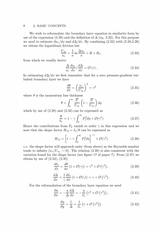
We wish to reformulate the boundary layer equation in similarity form byuse of the expression (2.28) and the definition of ∆ (eq. 2.32). For this purposewe need to estimate duτ/dx and d∆/dx. By combining (2.22) with (2.28,2.26)we obtain the logarithmic friction law
U∞uτ
=1κ
ln∆uτν
+B +B1 , (2.33)
from which we readily derive∆uτ
duτdx
/d∆dx
= O (γ) . (2.34)
In estimating d∆/dx we first remember that for a zero pressure-gradient tur-bulent boundary layer we have
dθ
dx=
(uτU∞
)2
= γ2 (2.35)
where θ is the momentum loss thickness
θ =∫ ∞
0
U
U∞
(1− U
U∞
)dy (2.36)
which by use of (2.28) and (2.32) can be expressed as
θ
δ∗= 1− γ
∫ ∞
0
F 21 dη +O(γ2) (2.37)
Hence the contributions from F2 vanish to order γ in this expression and wenote that the shape factor H12 = δ∗/θ can be expressed as
H12 =[1− γ
∫ ∞
0
F 21 dη
]−1+O(γ2) (2.38)
i.e. the shape factor will approach unity (from above) as the Reynolds numbertends to infinity (uτ/U∞ → 0). The relation (2.38) is also consistent with thevariation found for the shape factor (see figure 17 of paper 7). From (2.37) weobtain by use of (2.34), (2.35)
dδ∗dx
=dθ
dx(1 +O(γ)) = γ2 +O
(γ3
), (2.39)
d∆dx
=1γ
dδ∗dx
(1 +O(γ)) = γ +O(γ2
). (2.40)
For the reformulation of the boundary layer equation we need∂η
∂x= − η
∆d∆dx
= − η
δ∗
(γ2 +O
(γ3
)), (2.41)
∂η
∂y=
1∆
=1δ∗
(γ +O
(γ2
)). (2.42)
2.5. SIMILARITY DESCRIPTION OF THE OUTER LAYER 9
Introduction of (2.28) into the boundary layer equation (2.8), where the viscousterm may be neglected, and by use of (2.34), (2.41), (2.42) and the continuityequation we get the leading order balance
−ηF ′1 = G′
0. (2.43)
The similarity formulation to leading order of the boundary layer equation,i.e. (2.43) can easily be seen to be consistent with the overlap matching results.As η→ 0 we can expand G0 as
G0 = C0 +C1η +O(η2). (2.44)
The matching for the Reynolds shear stress gives in combination with equation(2.15) (since f ′ → 0 as y+ → ∞) that g → 1 as y+ → ∞ and hence thatG0 → 1 as η → 0. Hence, the constant C0 is determined to 1. For the firstorder correction for the beginning of the outer region we further get, fromequation (2.43), (since F ′
1 = 1/(κη)) that C1 = −1/κ.To summarize the above analysis for the outer region we conclude that to
leading order the governing lengthscale is
∆ = δ∗U∞uτ
(2.45)
and the normalized wall distance is
η =y
δ∗
uτU∞
. (2.46)
The velocity distribution can now be written as a defect law
U∞ − Uuτ
= −F1(η) +O(γ), (2.47)
where, in the overlap region, F1 is given by (2.26).It is interesting to note that the logarithmic friction law takes the form
(2.33) which also can be written asU∞uτ
=1κ
lnδ∗U∞ν
+B + B1 (2.48)
which hence is an explicit relation between U∞/uτ and the Reynolds number,Reδ∗ , for which it also can be written as
cf = 2[
1κ
lnReδ∗ + B +B1
]−2(2.49)
In the following papers an alternative form with Reθ instead of Reδ∗ will beused, partly to enable comparisons with existing proposals in the literature.
CHAPTER 3
Experiments
3.1. History
Historically, knowledge of the structure of turbulent boundary layers was gainedexperimentally from wind-tunnel measurements. Among the early measure-ments are those carried out by Schultz-Grunow (1940), Ludwieg & Tillman(1950), Klebanoff (1955) and Smith & Walker (1959). For an extensive surveyof the empirical knowledge of the early data the reader is referred to Coles(1962) classical paper. In the survey by Fernholz & Finley (1996) more recentexperiments can be found.
Modern computers have recently become fast enough to perform directnumerical simulations of the Navier-Stokes equations for fully turbulent flows,although only at low Reynolds number and in simple geometries, see e.g. thelandmark papers by Kim et al. (1987) and Spalart (1988). The first simulationof a turbulent boundary layer was made by the latter, at Reθ up to 1410. Sincethen several boundary layer simulations have been made, also at different ofpressure gradients, see e.g. Skote et al. (1998).
From the large number of experiments performed during the years severalimportant conclusions can be drawn. First, it is of primary importance tomake very accurate and preferably independent measurements of the wall-shearstress. Secondly, at high Reynolds number the distance from the probe to thewall has to be determined with extremely high accuracy (because of the smallviscous length scale). These two goals seem obvious, but was fulfilled only ina few experiments. In the present experimental set-up a large effort was madeto fulfill these conditions.
3.2. Experimental set-up
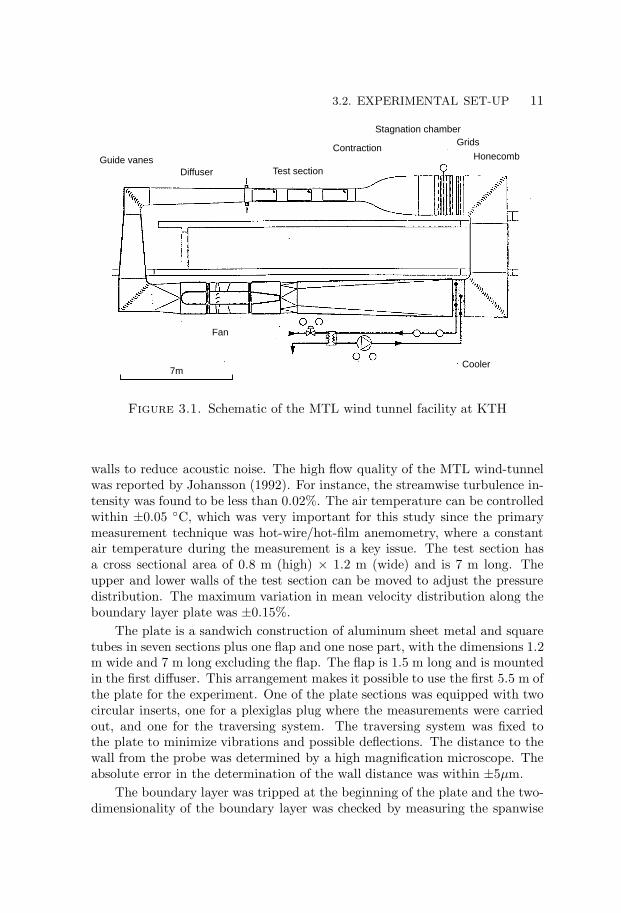
The flow field of a zero pressure-gradient turbulent boundary layer was estab-lished on a seven meter long flat plate mounted in the test section of the MTLwind-tunnel at KTH. The MTL wind tunnel is of closed-return type designedwith low disturbance level as the primary design goal. A brief description ofthe experimental set-up is given below. A more detailed description of theboundary layer experimental set-up can be found in paper 7. After the testsection the flow passes through diffusers and two 90 turns before the fan. Alarge fraction of the wind-tunnel return circuit is equipped with noise-absorbing
10
3.2. EXPERIMENTAL SET-UP 11
Test section
Fan
Cooler
ContractionGrids
Stagnation chamber
Guide vanes
7m
Diffuser
Honecomb
Figure 3.1. Schematic of the MTL wind tunnel facility at KTH
walls to reduce acoustic noise. The high flow quality of the MTL wind-tunnelwas reported by Johansson (1992). For instance, the streamwise turbulence in-tensity was found to be less than 0.02%. The air temperature can be controlledwithin ±0.05 C, which was very important for this study since the primarymeasurement technique was hot-wire/hot-film anemometry, where a constantair temperature during the measurement is a key issue. The test section hasa cross sectional area of 0.8 m (high) × 1.2 m (wide) and is 7 m long. Theupper and lower walls of the test section can be moved to adjust the pressuredistribution. The maximum variation in mean velocity distribution along theboundary layer plate was ±0.15%.
The plate is a sandwich construction of aluminum sheet metal and squaretubes in seven sections plus one flap and one nose part, with the dimensions 1.2m wide and 7 m long excluding the flap. The flap is 1.5 m long and is mountedin the first diffuser. This arrangement makes it possible to use the first 5.5 m ofthe plate for the experiment. One of the plate sections was equipped with twocircular inserts, one for a plexiglas plug where the measurements were carriedout, and one for the traversing system. The traversing system was fixed tothe plate to minimize vibrations and possible deflections. The distance to thewall from the probe was determined by a high magnification microscope. Theabsolute error in the determination of the wall distance was within ±5µm.
The boundary layer was tripped at the beginning of the plate and the two-dimensionality of the boundary layer was checked by measuring the spanwise

12 3. EXPERIMENTS
variation of the wall shear stress τw. The maximum spanwise variation infriction velocity uτ =
√τw/ρ was found to be less than ±0.7%.
The ambient conditions were monitored by the measurement computerduring the experiments using an electronic barometer and thermometer (FCO510 from Furness Ltd., UK). The reference conditions used in the calibrationof the probes were determined using a Prandtl tube in the free-stream directlyabove the measurement station. The pressure and temperature were monitoredat all times during the experiments using a differential pressure transducer anda thermometer connected directly to the measurement computer. The accuracyof the pressure measurement was 0.25 % and the accuracy of the temperaturemeasurement was 0.02 C.
Constant temperature hot-wire anemometry was used in all velocity mea-surements. All hot-wire probes were designed and built at the lab. Three sizesof single-wire probes were used in the experiments with wire diameters of: 2.5,1.27 and 0.63 µm and a length to diameter ratio always larger than 200.
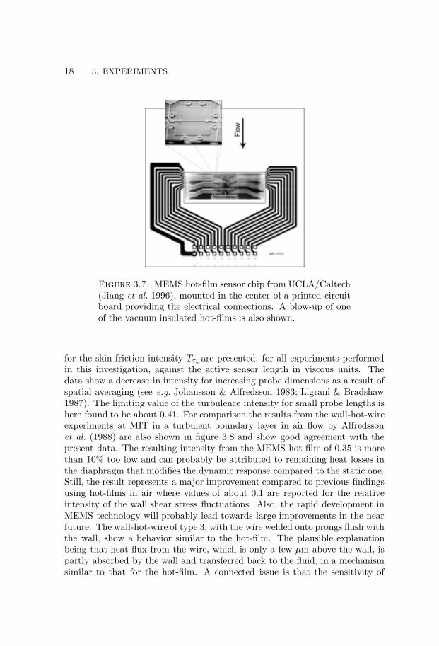
The MEMS hot-film used in the wall-shear stress measurements was de-signed by the MEMS group at UCLA/Caltec (Jiang et al. 1996, 1997; Ho &Tai 1998). It was flush-mounted with a printed circuit board for electrical con-nections which in turn was flush-mounted into a Plexiglas plug fitting into theinstrumentation insert of the measurement plate-section. Accurate alignmentof the chip surface and the circuit board and the flat plate was achieved usinga microscope during the mounting of the sensor set-up. The MEMS sensorchip has four rows of 25 sensors each with a spanwise separation of 300 µm, seefigure 3.7. The length of the hot-film is 150µm and the width 3µm. It is placedon a 1.2µm thick silicon-nitride diaphragm with dimensions 200µm × 200µm.Thermal insulation of the hot-film to the substrate is provided by a 2µm deepvacuum cavity underneath the diaphragm.
The anemometer system (AN1003 from AA lab systems, Israel) had abuilt-in signal conditioner and the signals from the anemometer were digitizedusing an A/D converter board (A2000 from National Instruments, USA) inthe measurement computer. The A/D converter has 12 bit resolution and fourchannels which could be sampled simultaneously at rates up to 1 MHz dividedby the number of channels used. The complete experiment was run from aprogram on the measurement computer which controlled the tunnel velocity,the positioning of probes, digitization of the anemometer signals, monitoringof the pressures and the temperature.
3.3. Results
Different sets of experiments were run with the set-up described in section 3.2and are summarized in table 1. Single-wire measurements (SW) were carriedout at 5 different streamwise positions x = 1.5, 2.5, 3.5, 4.5, 5.5 at 10 differentmean velocity settings ranging from 10 to 55 m/s. At the position x = 5.5 m
3.3. RESULTS 13
Reθ Quantity Pos. (x) Ref.
SW 2500–27300 U 1.5–5.5 paper 1 & 2XW 6900–22500 U, V 5.5 paper 3VW 6900–22500 U, W 5.5 paper 3
MEMS-WW 9700 τw 5.5 paper 4MEMS-MEMS 9700 τw, τw(∆z) 5.5 paper 6MEMS-SW 1 9700 τw, U(∆x, ∆y) 5.5 paper 6MEMS-SW 2 9700 τw, U(∆y, ∆z) 5.5 paper 6
Table 1. Overview of the different sets of experiments.
experiments with three different probe sizes were also conducted. An X-probewas used at the position x = 5.5 m for measurements (XW) of the simultane-ous streamwise U and wall-normal velocity V components. The simultaneousstreamwise and spanwise W velocity components were measured (VW) using aV-probe. The MEMS hot-film sensor, with 25 individual hot-films distributedin the spanwise direction, was utilized to measure the simultaneous skin-frictionin two points at different spanwise separations. The MEMS hot-film sensor wasalso used to measure simultaneously the skin-friction and the streamwise ve-locity separated in either the x-y plane (MEMS-SW 1) or separated in the y-zplane (MEMS-SW 2).
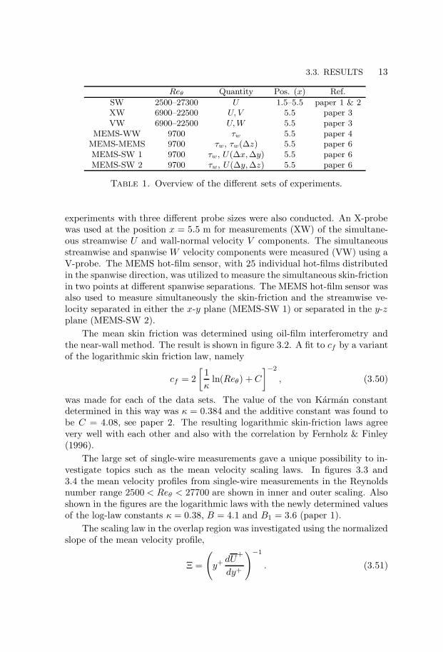
The mean skin friction was determined using oil-film interferometry andthe near-wall method. The result is shown in figure 3.2. A fit to cf by a variantof the logarithmic skin friction law, namely
cf = 2[
1κ
ln(Reθ) +C
]−2, (3.50)
was made for each of the data sets. The value of the von Karman constantdetermined in this way was κ = 0.384 and the additive constant was found tobe C = 4.08, see paper 2. The resulting logarithmic skin-friction laws agreevery well with each other and also with the correlation by Fernholz & Finley(1996).
The large set of single-wire measurements gave a unique possibility to in-vestigate topics such as the mean velocity scaling laws. In figures 3.3 and3.4 the mean velocity profiles from single-wire measurements in the Reynoldsnumber range 2500 < Reθ < 27700 are shown in inner and outer scaling. Alsoshown in the figures are the logarithmic laws with the newly determined valuesof the log-law constants κ = 0.38, B = 4.1 and B1 = 3.6 (paper 1).
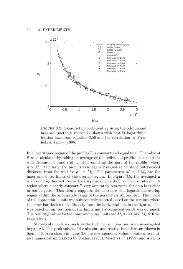
The scaling law in the overlap region was investigated using the normalizedslope of the mean velocity profile,
Ξ =
(y+
dU+
dy+
)−1
. (3.51)
14 3. EXPERIMENTS
Reθ
cf
0 0.5 1 1.5 2 2.5 3
x 104
2
2.5
3
3.5x 10
-3
Fernholz & Finley (1996)Oil-film (series 1)Oil-film (series 2)Oil-film fitNear-wall fitNear-wall, x = 1.5 mNear-wall, x = 2.5 mNear-wall, x = 3.5 mNear-wall, x = 4.5 mNear-wall, x = 5.5 mNear-wall, x = 5.5 m
Figure 3.2. Skin-friction coefficient cf using the oil-film andnear wall methods (paper 7), shown with best-fit logarithmicfriction laws from equation 3.50 and the correlation by Fern-holz & Finley (1996).
In a logarithmic region of the profiles Ξ is constant and equal to κ. The value ofΞ was calculated by taking an average of the individual profiles at a constantwall distance in inner scaling while omitting the part of the profiles whereη > Mo. Similarly, the profiles were again averaged at constant outer-scaleddistances from the wall for y+ > Mi. The parameters Mi and Mo are theinner and outer limits of the overlap region. In Figure 3.5, the averaged Ξis shown together with error bars representing a 95% confidence interval. Aregion where a nearly constant Ξ very accurately represents the data is evidentin both figures. This clearly supports the existence of a logarithmic overlapregion within the appropriate range of the parameters Mi and Mo. The choiceof the appropriate limits was subsequently selected based on the y values wherethe error bar deviates significantly from the horizontal line in the figures. Thiswas based on an iteration of the limits until a consistent result was obtained.The resulting values for the inner and outer limits areMi ≈ 200 and Mo ≈ 0.15,respectively.
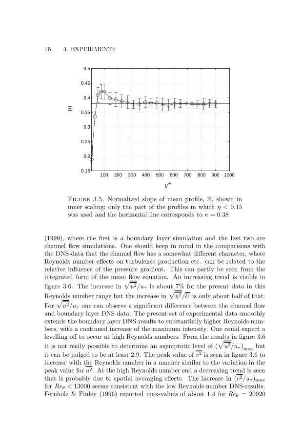
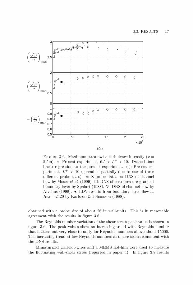
Statistical quantities, such as the turbulence intensities, were investigatedin paper 3. The peak values of the absolute and relative intensities are shown infigure 3.6. Also shown in figure 3.6 are corresponding values obtained from di-rect numerical simulations by Spalart (1988), Moser et al. (1999) and Alvelius

3.3. RESULTS 15
100
101
102
103
104
0
5
10
15
20
25
30
35
U+
y+
Figure 3.3. Profiles of the mean velocity in inner-law scaling.2530 < Reθ < 27300. Dash-dotted line: 1
0.38 ln y+ + 4.1.
10-4
10-3
10-2
10-1
0
5
10
15
20
25
30
U∞−Uuτ
y/∆
Figure 3.4. Profiles of the mean velocity in outer-law scaling.Log-law constants κ = 0.38 and B∆
1 = 1.62. 2530 < Reθ <27300
16 3. EXPERIMENTS
100 200 300 400 500 600 700 800 900 10000.15
0.2
0.25
0.3
0.35
0.4
0.45
0.5
y+
Ξ
Figure 3.5. Normalized slope of mean profile, Ξ, shown ininner scaling; only the part of the profiles in which η < 0.15was used and the horizontal line corresponds to κ = 0.38
(1999), where the first is a boundary layer simulation and the last two arechannel flow simulations. One should keep in mind in the comparisons withthe DNS-data that the channel flow has a somewhat different character, whereReynolds number effects on turbulence production etc. can be related to therelative influence of the pressure gradient. This can partly be seen from theintegrated form of the mean flow equation. An increasing trend is visible infigure 3.6. The increase in
√u2/uτ is about 7% for the present data in this
Reynolds number range but the increase in√u2/U is only about half of that.
For√u2/uτ one can observe a significant difference between the channel flow
and boundary layer DNS data. The present set of experimental data smoothlyextends the boundary layer DNS-results to substantially higher Reynolds num-bers, with a continued increase of the maximum intensity. One could expect alevelling off to occur at high Reynolds numbers. From the results in figure 3.6it is not really possible to determine an asymptotic level of (
√u2/uτ)max but
it can be judged to be at least 2.9. The peak value of v2 is seen in figure 3.6 toincrease with the Reynolds number in a manner similar to the variation in thepeak value for u2. At the high Reynolds number end a decreasing trend is seenthat is probably due to spatial averaging effects. The increase in (v2/uτ)maxfor Reθ < 13000 seems consistent with the low Reynolds number DNS-results.Fernholz & Finley (1996) reported max-values of about 1.4 for Reθ = 20920
3.3. RESULTS 17
Reθ
(√u2
uτ
)max
(√v2
uτ
)max
−(uvu2
τ
)max
2
2.5
3
0
0.5
1
0 0.5 1 1.5 2 2.5
x 104
0.5
0.6
0.7
0.8
0.9
1
Figure 3.6. Maximum streamwise turbulence intensity (x =5.5m). ∗: Present experiment, 6.5 < L+ < 10. Dashed line:linear regression to the present experiment. (·): Present ex-periment, L+ > 10 (spread is partially due to use of threedifferent probe sizes). : X-probe data. : DNS of channelflow by Moser et al. (1999). : DNS of zero pressure gradientboundary layer by Spalart (1988). ∇: DNS of channel flow byAlvelius (1999). •: LDV results from boundary layer flow atReθ = 2420 by Karlsson & Johansson (1988).
obtained with a probe size of about 26 in wall-units. This is in reasonableagreement with the results in figure 3.6.
The Reynolds number variation of the shear-stress peak value is shown infigure 3.6. The peak values show an increasing trend with Reynolds numberthat flattens out very close to unity for Reynolds numbers above about 15000.The increasing trend at low Reynolds numbers also here seems consistent withthe DNS-results.
Miniaturized wall-hot-wires and a MEMS hot-film were used to measurethe fluctuating wall-shear stress (reported in paper 4). In figure 3.8 results
18 3. EXPERIMENTS
Figure 3.7. MEMS hot-film sensor chip from UCLA/Caltech(Jiang et al. 1996), mounted in the center of a printed circuitboard providing the electrical connections. A blow-up of oneof the vacuum insulated hot-films is also shown.
for the skin-friction intensity Tτw are presented, for all experiments performedin this investigation, against the active sensor length in viscous units. Thedata show a decrease in intensity for increasing probe dimensions as a result ofspatial averaging (see e.g. Johansson & Alfredsson 1983; Ligrani & Bradshaw1987). The limiting value of the turbulence intensity for small probe lengths ishere found to be about 0.41. For comparison the results from the wall-hot-wireexperiments at MIT in a turbulent boundary layer in air flow by Alfredssonet al. (1988) are also shown in figure 3.8 and show good agreement with thepresent data. The resulting intensity from the MEMS hot-film of 0.35 is morethan 10% too low and can probably be attributed to remaining heat losses inthe diaphragm that modifies the dynamic response compared to the static one.Still, the result represents a major improvement compared to previous findingsusing hot-films in air where values of about 0.1 are reported for the relativeintensity of the wall shear stress fluctuations. Also, the rapid development inMEMS technology will probably lead towards large improvements in the nearfuture. The wall-hot-wire of type 3, with the wire welded onto prongs flush withthe wall, show a behavior similar to the hot-film. The plausible explanationbeing that heat flux from the wire, which is only a few µm above the wall, ispartly absorbed by the wall and transferred back to the fluid, in a mechanismsimilar to that for the hot-film. A connected issue is that the sensitivity of

3.3. RESULTS 19
l+
Tτw
0 10 20 30 40 50 600.2
0.25
0.3
0.35
0.4
0.45
Figure 3.8. Turbulent skin friction intensity Tτw . Presentexperiments, : WW1, MTL, +: WW3, MTL, ×: MHF, MTL,: WW2, MTL, •: WW1, LaWiKa, : WW2, LaWiKa,: WW2, LaWiKa, : WW2, LaWiKa, : WW2, LaWiKa(for details see table 2 in paper 4). 2: experiment by Alfreds-son et al. (1988).
type 3 wall-hot-wires is very low due to damping resulting from the proximityof the wall.
Kline et al. (1967), showed that a significant part of the turbulence couldbe described in terms of deterministic events, and that in the close proximityof the wall the flow is characterized by elongated regions of low and high speedfluid of fairly regular spanwise spacing of about λ+ = 100. Sequences of orderedmotion occur randomly in space and time where the low-speed streaks beginto oscillate and to suddenly break-up into a violent motion, a “burst”. Kimet al. (1971) showed that the intermittent bursting process is closely related toshear-layer like flow structures in the buffer region. To obtain quantitative datato describe the structures a reliable method to identify bursts with velocity orwall-shear stress measurements is needed. Kovasznay et al. (1970) were the firstto employ conditional averaging, using a trigger, to study individual events suchas bursts or ejections. The triggering signal must be intermittent and closelyassociated with the event under study. Wallace et al. (1972) and Willmart& Lu (1972) introduced the uv quadrant splitting scheme. Blackwelder &Kaplan (1976) developed the VITA technique to form a localized measure of

20 3. EXPERIMENTS
∆z+
Rτwτw
0 50 100 150 200
-0.2
0
0.2
0.4
0.6
0.8
1
Figure 3.9. Spanwise correlation coefficient Rτwτw as a func-tion of ∆z+, Reθ = 9500. Present data, : unfiltered,: f+c = 1.3× 10⁻³, : f+c = 2.6× 10⁻³, : f+c = 5.3× 10⁻³,: f+c = 7.9× 10⁻³, —: spline fit to . DNS of channel flow,−−: Reτ = 590, − · −: Reτ = 385, · · · : Reτ = 180 (Kim et al.1987; Moser et al. 1999).
the turbulent kinetic energy and used it to detect shear-layer events. For acomprehensive overview of the literature in the field of coherent structures thereader is referred to the review article by Robinson (1991).
In paper 6 the mean spanwise separation between low-speed streaks inthe viscous sub-layer was investigated using a MEMS array of hot-films. Thespanwise cross correlation coefficient between the wall-shear stress signals
Rτwτw (∆z) =τw(z)τw(z + ∆z)
τ ′2w, (3.52)
obtained from two hot-films separated a distance ∆z+ in the spanwise directionwas used to estimate the mean streak spacing. At high Reynolds numbers con-tributions to the spanwise correlation coefficient from low frequency structuresoriginating in the outer region conceals the contributions from the streaks andno clear (negative) minimum is visible in figure 3.9 for the measured correlationcoefficient (shown as). This behavior was found also by others, see e.g. Guptaet al. (1971). A trend is clearly visible in the relatively low Reynolds number
3.3. RESULTS 21
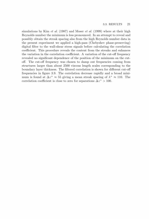
simulations by Kim et al. (1987) and Moser et al. (1999) where at their highReynolds number the minimum is less pronounced. In an attempt to reveal andpossibly obtain the streak spacing also from the high Reynolds number data inthe present experiment we applied a high-pass (Chebyshev phase-preserving)digital filter to the wall-shear stress signals before calculating the correlationcoefficient. This procedure reveals the content from the streaks and enhancesthe variation in the correlation coefficient. A variation of the cut-off frequencyrevealed no significant dependence of the position of the minimum on the cut-off. The cut-off frequency was chosen to damp out frequencies coming fromstructures larger than about 2500 viscous length scales corresponding to theboundary layer thickness. The filtered correlation is shown for different cut-offfrequencies in figure 3.9. The correlation decrease rapidly and a broad mini-mum is found at ∆z+ ≈ 55 giving a mean streak spacing of λ+ ≈ 110. Thecorrelation coefficient is close to zero for separations ∆z+ > 100.

CHAPTER 4
Concluding Remarks
Experimental results were presented for turbulent boundary layer measure-ments spanning over one decade in Reynolds number, 2500 < Reθ < 27000.
The classical two layer theory was confirmed and constant values of theslope of the logarithmic overlap region (i.e. von Karmans constant) and theadditive constants were found and estimated to κ = 0.38, B = 4.1 and B1 = 3.6(δ = δ95). The inner limit of overlap region was found to scale on the viscouslength scale (ν/uτ) and was estimated to be y+ = 200, i.e. considerably furtherout compared to previous knowledge. The outer limit of the overlap region wasfound to scale on the outer length scale and was estimated to be y/δ = 0.15.This means that a universal overlap region can only be expected for Reynoldsnumbers larger than Reθ ≈ 6000. The newly determined limits also explainthe Reynolds number variation found in some earlier experiments.
Measurements of the fluctuating wall-shear stress using the hot-wire-on-the-wall technique and a MEMS hot-film sensor show that the turbulence in-tensity τw/τr.m.s. is close to 0.41 at Reθ ≈ 9800. This was also substantiatedby near-wall single-wire measurements.
A numerical and experimental investigation of the behavior of double wireprobes were carried out and showed that the Peclet number based on wire sep-aration should be larger than about 50 to keep the interaction at an acceptablelevel.
Results are presented for two-point correlations between the wall-shearstress and the streamwise velocity component for separations in both the wall-normal-streamwise plane and the wall-normal-spanwise plane. Results are pre-sented for the streak spacing and the propagation velocity of near wall shearlayer events. Turbulence producing events are further investigated using condi-tional averaging of isolated events detected using the VITA technique. Compar-isons are made with results from other experiments and numerical simulations.
22

Acknowledgments
I would like to sincerely thank my supervisor Prof. Arne Johansson for accept-ing me as his student, imparting his knowledge and and guiding me throughthe maze of turbulence research. Arne has read and and given constructivecriticism an all manuscripts in this work.
I also would like to thank Prof. Henrik Alfredsson for innumerable helpfuldiscussions about fluid mechanics and especially turbulence experiments.
My thanks to Prof. Hassan Nagib at IIT, with whom I had the greatpleasure to work with during his stay at KTH. The enthusiastic and creativecomments from Hassan has been invaluable when finishing this work.
I also wish to thank Dr. Erik Lindborg for clarifying discussions on theanalysis of the boundary layer similarity analysis.
My special thanks go to my dear friend and former colleague AlexanderSahlin together with who I started out doing the experiments leading to thisthesis. Alexander’s sound knowledge of fluid dynamics has been invaluable helpthroughout this work.
Many thanks go to the faculty, my colleagues and fellow students at theDepartment of Mechanics for a pleasant, stimulating and inspiring atmosphere.Especially I want to thank my friends and room mates Torbjorn Sjogren andBjorn Lindgren who have made my time in the lab most enjoyable.
I wish to thank Marcus Gallstedt and Ulf Landen for help with design-ing and building many of the experiments and for skillful assistance in thelaboratory.
Last but not the least, I want to thank my parents and family for theirsupport and especially, Ulrika for your love.
Financial support from the Swedish Research Council for Engineering Science(TFR) and Swedish National Board for Industrial and Technical Development(NUTEK) is gratefully acknowledged.
23

References
Alfredsson, P. H., Johansson, A. V., Haritonidis, J. H. & Eckelmann, H.
1988 The fluctuation wall-shear stress and the velocity field in the viscous sub-layer. Phys. Fluids A 31, 1026–33.
Alvelius, K. 1999 Studies of turbulence and its modeling through large eddy- anddirect numerical simulation. PhD thesis, Department of Mechanics, Royal Insti-tute of Technology, Stockholm.
Barenblatt, G. I. 1993 Scaling laws for fully developed turbulent shear flows. part1. basic hypotheses and analysis. J. Fluid Mech. 248, 513–520.
Barenblatt, G. I. & Chorin, A. J. 1999 Self-similar intermediate structures inturbulent boundary layers at large reynolds numbers. PAM 755. Center for Pureand Applied Mathematics, University of California at Berkeley.
Barenblatt, G. I. & Prostokishin, V. M. 1993 Scaling laws for fully developedturbulent shear flows. part 2. processing of experimental data. J. Fluid Mech.248, 521–529.
Blackwelder, R. F. & Kaplan, R. E. 1976 On the wall structure of the turbulentboundary layer. J. Fluid Mech. 76, 89–112.
Clauser, F. H. 1956 The turbulent boundary layer. Advances Appl. Mech. 4, 1–51.
Coles, D. E. 1956 The law of the wake in the turbulent boundary layer. J. FluidMech. 1, 191–226.
Coles, D. E. 1962 The turbulent boundary layer in a compressible fluid. R 403-PR.The RAND Corporation, Santa Monica, CA.
Fernholz, H. H. & Finley, P. J. 1996 The incompressible zero-pressure-gradientturbulent boundary layer: An assessment of the data. Prog. Aerospace Sci. 32,245–311.
George, W. K., Castilio, L. & Wosnik, M. 1997 Zero-pressure-gradient turbulentboundary layer. Applied Mech. Reviews 50, 689–729.
Gupta, A. K., Laufer, J. & Kaplan, R. E. 1971 Spatial structure in the viscoussublayer. J. Fluid Mech. 50, 493–512.
Hinch, E. J. 1991 Perturbation methods. Cambridge University Press.
Hinze, J. O. 1975 Turbulence , 2nd edn. McGraw-Hill.
Ho, C.-M. & Tai, Y.-C. 1998 Micro-electro-mechanical-systems (MEMS) and fluidflows. Ann. Rev. Fluid Mech. 30, 579–612.
24

REFERENCES 25
Jiang, F., Tai, Y.-C., Gupta, B., Goodman, R., Tung, S., Huang, J. B. & Ho,
C.-M. 1996 A surface-micromachined shear stress imager. In 1996 IEEE MicroElectro Mechanical Systems Workshop (MEMS ’96), pp. 110–115.
Jiang, F., Tai, Y.-C., Walsh, K., Tsao, T., Lee, G. B. & Ho, C.-H. 1997 Aflexible mems technology and its first application to shear stress sensor skin.In 1997 IEEE Micro Electro Mechanical Systems Workshop (MEMS ’97), pp.465–470.
Johansson, A. V. 1992 A low speed wind-tunnel with extreme flow quality - designand tests. In Prog. ICAS congress 1992 , pp. 1603–1611. ICAS-92-3.8.1.
Johansson, A. V. & Alfredsson, P. H. 1983 Effects of imperfect spatial resolutionon measurements of wall-bounded turbulent shear flows. J. Fluid Mech. 137,409–421.
Karlsson, R. I. & Johansson, T. G. 1988 Ldv measurements of higher order mo-ments of velocity fluctuations in a turbulent boundary layer. In Laser Anemome-try in Fluid Mechanics . Ladoan-Instituto Superior Tecnico, 1096 L.C., Portugal.
von Karman, T. 1921 Ueber laminare un turbulente Reibung. Z. angew. Math.Mech. pp. 233–252, NACA TM 1092.
von Karman, T. 1930 Mechanische Aehnlichkeit und Turbulenz. Nachr. Ges. Wiss.Gottingen, Math. Phys. Kl. pp. 58–68, NACA TM 611.
Kim, H. T., Kline, S. J. & Reynolds, W. C. 1971 The production of turbulencenear a smooth wall in a turbulent boundary layer. J. Fluid Mech. 50, 133–160.
Kim, J., Moin, P. & Moser, R. 1987 Turbulence statistics in fully developed channelflow. J. Fluid Mech. 177, 133–166.
Klebanoff, P. S. 1955 Characteristics of turbulence in a boundary layer with zeropressure gradient. TR 1247. NACA.
Kline, S. J., Reynolds, W. C., Schraub, F. A. & Runstadler, P. W. 1967 Thestructure of turbulent boundary layers. J. Fluid Mech. 30, 741.
Kovasznay, L. G., Kibens, V. & Blackwelder, R. S. 1970 Large-scale motionin the intermittent region of a turbulent boundary layer. J. Fluid Mech. 41,283–325.
Landahl, M. T. & Mollo-Christensen, E. 1987 Turbulence and Random Pro-cesses in Fluid Mechanics . Cambridge University Press.
Ligrani, P. M. & Bradshaw, P. 1987 Spatial resolution and measurement of tur-bulence in the viscous sublayer using subminiature hot-wire probes. Experimentsin Fluids 5, 407–417.
Ludwieg, H. & Tillman, W. 1950 Investigations of the wall shearing stress inturbulent boundary layers. TM 1285. NACA.
Millikan, C. B. 1938 A critical discussion of turbulent flows in channels and circulartubes. In Proceedings of the Fifth International Congress of applied Mechanics .
Moser, R. D., Kim, J. & Mansour, N. N. 1999 Direct numerical simulation ofturbulent channel flow up to Reθ = 590. Phys. Fluids 11 (4), 943–945.
Prandtl, L. 1904 Ueber die Flussigkeitsbewegung bei sehr kliner Ribung. In Ver-handlungen des III. Internationalen Mathematiker-Kongress, Heidelberg , pp.484–491.
26 REFERENCES
Prandtl, L. 1927 Ueber den Reibungswiderstand stromender Luft. Ergebn. Aerodyn.Versuchsanst. Gottingen 3, 1–5.
Prandtl, L. 1932 Zur turbulenten Stromung in Rohren und langs Platten. Ergebn.Aerodyn. Versuchsanst. Gottingen 4, 18–29.
Reynolds, O. 1883 On the experimental investigation of the circumstances whichdetermine whether the motion of water shall be direct or sinuous, and the lawor resistance in parallel channels. Phil. Trans. Roy. Soc. Lond. 174, 935–982.
Reynolds, O. 1895 On the dynamical theory of incompressible viscous fluids andthe determination of the criterion. Phil. Trans. Roy. Soc. A 186, 123–164.
Robinson, S. K. 1991 Coherent motions in the turbulent boundary layer. Ann. Rev.Fluid Mech. 23, 601–639.
Rotta, J. C. 1950 Uber die Theorie der Turbulenten Grenzschichten. Mitt. M.P.I.Strom. Forschung Nr 1, also available as NACA TM 1344.
Rotta, J. C. 1962 Turbulent boundary layers in incompressible flow. In Progress inaeronautical sciences (ed. A. Ferri, D. Kuchemann & L. H. G. Sterne), , vol. 2,pp. 1–219. Pergamon press.
Schlichting, H. 1979 Boundary layer theory . McGraw-Hill.
Schultz-Grunow, F. 1940 Neues Reibungswiederstandsgesetz fur glatte Platten.Tech. Rep. 8. Luftfahrtforschung, translated as New frictional resistance law forsmooth plates, NACA TM-986, 1941.
Skote, M., Henkes, R. & Henningson, D. 1998 Direct numerical simulation ofself-similar turbulent boundary layers in adverse pressure gradients. In Flow,Turbulence and Combustion , , vol. 60, pp. 47–85. Kluwer Academic Publishers.
Smith, D. W. & Walker, J. H. 1959 Skin-friction measurements in incompressibleflow. NASA TR R-26.
Spalart, P. R. 1988 Direct simulation of a turbulent boundary layer up to Reθ =1410. J. Fluid Mech. 187, 61–98.
Tennekes, H. & Lumely, J. L. 1972 A first cource in turbulence . The MIT press.
Wallace, J. M., Eckelmann, H. & Brodkey, R. 1972 The wall region in turbulentshear flow. J. Fluid Mech. 54, 39–48.
Willmart, W. W. & Lu, S. S. 1972 Structure of the Reynolds stress near the wall.J. Fluid Mech. 55, 65–92.
Zagarola, M. V., Perry, A. E. & Smits, A. J. 1997 Log laws or power laws: Thescaling in the overlap region. Phys. Fluids 9 (7), 2094–100.
Zagarola, M. V. & Smits, A. J. 1998a Mean-flow scaling of turbulent pipe flow.J. Fluid Mech. 373, 33–79.
Zagarola, M. V. & Smits, A. J. 1998b A new mean velocity scaling for turbulentboundary layers. In Proceedings of FEDSM’98 .

Paper 1


A note on the overlap region in turbulentboundary layers
By Jens M. Osterlund1, Arne V. Johansson1,Hassan M. Nagib2 & Michael H. Hites2
1Dept. of Mechanics, KTH, SE-100 44 Stockholm, Sweden2Illinois Institute of Technology, Chicago, IL 60616, USA
Accepted for publication in Phys. of Fluids
Two independent experimental investigations of the behavior of turbulent bound-ary layers with increasing Reynolds number were recently completed. The ex-periments were performed in two facilities, the MTL wind tunnel at KTH andthe NDF wind tunnel at IIT. Both experiments utilized oil-film interferometryto obtain an independent measure of the wall-shear stress. A collaborativestudy by the principals of the two experiments, aimed at understanding thecharacteristics of the overlap region between the inner and outer parts of theboundary layer, has just been completed. The results are summarized here,utilizing the profiles of the mean velocity, for Reynolds numbers based on themomentum thickness ranging from 2,500 to 27,000. Contrary to the conclusionsof some earlier publications, careful analysis of the data reveals no significantReynolds number dependence for the parameters describing the overlap regionusing the classical logarithmic relation. However, the data analysis demon-strates that the viscous influence extends within the buffer region to y+ ≈ 200,compared to the previously assumed limit of y+ ≈ 50. Therefore, the lowestReθ value where a significant logarithmic overlap region exists is about 6,000.This probably explains why a Reynolds number dependence had been foundfrom the data analysis of many previous experiments. The parameters of thelogarithmic overlap region are found to be constant and are estimated to be:κ = 0.38, B = 4.1 and B1 = 3.6 (δ = δ95).
In the classical theory, the overall description of a turbulent boundary layeris dependent on two separate inner and outer length scales. The outer lengthscale is commonly taken as the thickness of the boundary layer δ, and the innerlength scale as the viscous length l∗ = ν/uτ , where uτ =
√τw/ρ is the friction
velocity, τw is the skin friction and ρ is the density of the air. Dimensionalanalysis of the dynamic equations with boundary conditions leads to a scalingof the mean velocity profile in the inner and the outer parts of the boundary
29
30 J. M. Osterlund et al.
layer in the form:
U+
=U
uτ= f
(y+
); y+ =
yuτν
(1)
U∞ − Uuτ
= F (η) ; η =y
δ(2)
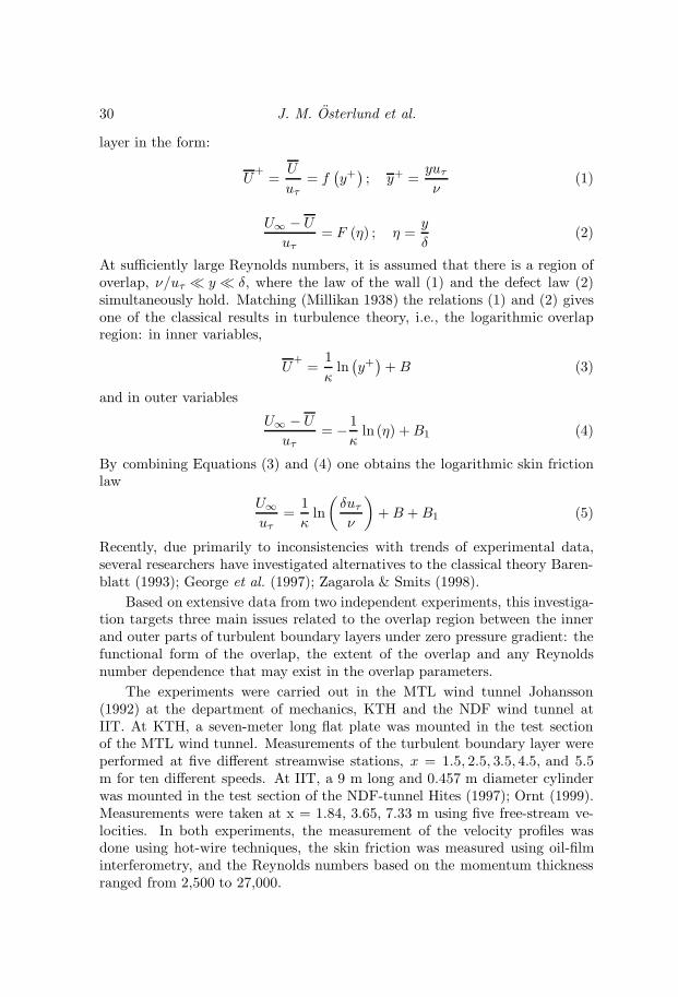
At sufficiently large Reynolds numbers, it is assumed that there is a region ofoverlap, ν/uτ y δ, where the law of the wall (1) and the defect law (2)simultaneously hold. Matching (Millikan 1938) the relations (1) and (2) givesone of the classical results in turbulence theory, i.e., the logarithmic overlapregion: in inner variables,
U+
=1κ
ln(y+
)+ B (3)
and in outer variables
U∞ − Uuτ
= − 1κ
ln (η) +B1 (4)
By combining Equations (3) and (4) one obtains the logarithmic skin frictionlaw
U∞uτ
=1κ
ln(δuτν
)+ B + B1 (5)
Recently, due primarily to inconsistencies with trends of experimental data,several researchers have investigated alternatives to the classical theory Baren-blatt (1993); George et al. (1997); Zagarola & Smits (1998).
Based on extensive data from two independent experiments, this investiga-tion targets three main issues related to the overlap region between the innerand outer parts of turbulent boundary layers under zero pressure gradient: thefunctional form of the overlap, the extent of the overlap and any Reynoldsnumber dependence that may exist in the overlap parameters.
The experiments were carried out in the MTL wind tunnel Johansson(1992) at the department of mechanics, KTH and the NDF wind tunnel atIIT. At KTH, a seven-meter long flat plate was mounted in the test sectionof the MTL wind tunnel. Measurements of the turbulent boundary layer wereperformed at five different streamwise stations, x = 1.5, 2.5, 3.5, 4.5, and 5.5m for ten different speeds. At IIT, a 9 m long and 0.457 m diameter cylinderwas mounted in the test section of the NDF-tunnel Hites (1997); Ornt (1999).Measurements were taken at x = 1.84, 3.65, 7.33 m using five free-stream ve-locities. In both experiments, the measurement of the velocity profiles wasdone using hot-wire techniques, the skin friction was measured using oil-filminterferometry, and the Reynolds numbers based on the momentum thicknessranged from 2,500 to 27,000.
The overlap region in turbulent boundary layers 31
Reθ
cf
0 0.5 1 1.5 2 2.5 3
x 104
2
2.5
3
3.5x 10
-3
Correlation by Fernholz 1969KTH, Oil-film (series 1)KTH, Oil-film (series 2)KTH, Oil-film fitKTH, Near-wall fitKTH, Near-wall, x = 1.5 mKTH, Near-wall, x = 2.5 mKTH, Near-wall, x = 3.5 mKTH, Near-wall, x = 4.5 mKTH, Near-wall, x = 5.5 mKTH, Near-wall, x = 5.5 mIIT Oil-film fit
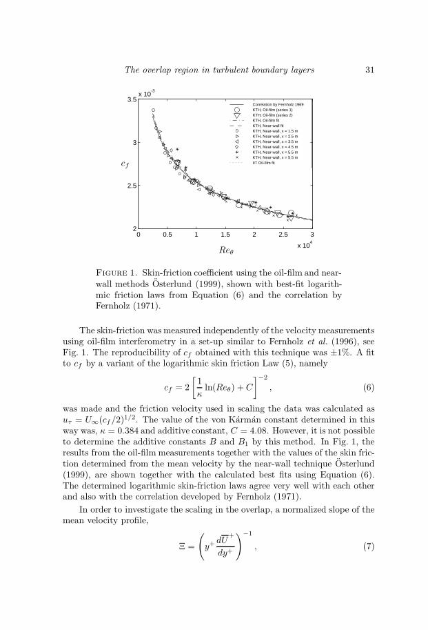
Figure 1. Skin-friction coefficient using the oil-film and near-wall methods Osterlund (1999), shown with best-fit logarith-mic friction laws from Equation (6) and the correlation byFernholz (1971).
The skin-friction was measured independently of the velocity measurementsusing oil-film interferometry in a set-up similar to Fernholz et al. (1996), seeFig. 1. The reproducibility of cf obtained with this technique was ±1%. A fitto cf by a variant of the logarithmic skin friction Law (5), namely
cf = 2[
1κ
ln(Reθ) +C
]−2, (6)
was made and the friction velocity used in scaling the data was calculated asuτ = U∞(cf/2)1/2. The value of the von Karman constant determined in thisway was, κ = 0.384 and additive constant, C = 4.08. However, it is not possibleto determine the additive constants B and B1 by this method. In Fig. 1, theresults from the oil-film measurements together with the values of the skin fric-tion determined from the mean velocity by the near-wall technique Osterlund(1999), are shown together with the calculated best fits using Equation (6).The determined logarithmic skin-friction laws agree very well with each otherand also with the correlation developed by Fernholz (1971).
In order to investigate the scaling in the overlap, a normalized slope of themean velocity profile,
Ξ =
(y+
dU+
dy+
)−1
, (7)
32 J. M. Osterlund et al.
100 200 300 400 500 600 700 800 900 10000.15
0.2
0.25
0.3
0.35
0.4
0.45
0.5
y+
Ξ
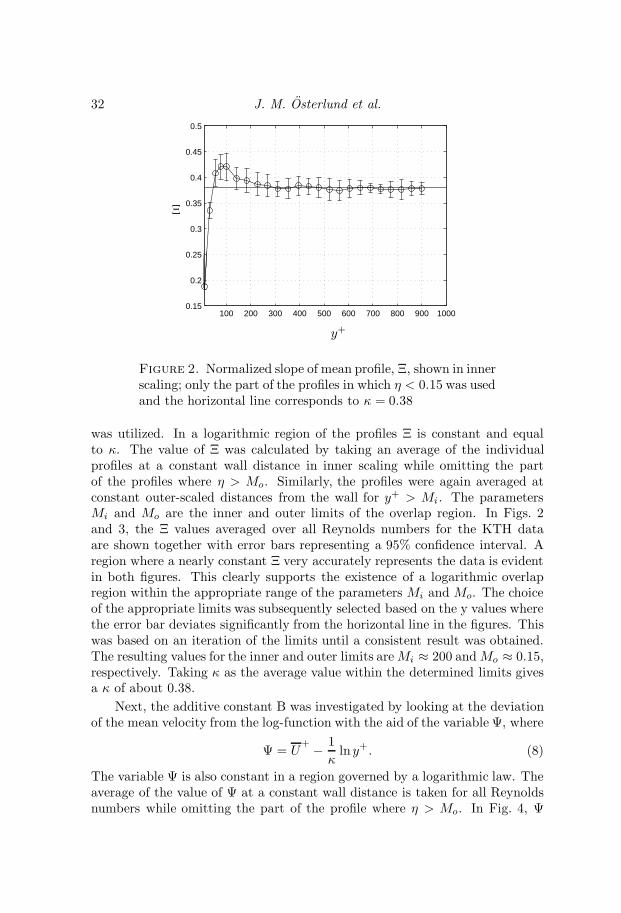
Figure 2. Normalized slope of mean profile, Ξ, shown in innerscaling; only the part of the profiles in which η < 0.15 was usedand the horizontal line corresponds to κ = 0.38
was utilized. In a logarithmic region of the profiles Ξ is constant and equalto κ. The value of Ξ was calculated by taking an average of the individualprofiles at a constant wall distance in inner scaling while omitting the partof the profiles where η > Mo. Similarly, the profiles were again averaged atconstant outer-scaled distances from the wall for y+ > Mi. The parametersMi and Mo are the inner and outer limits of the overlap region. In Figs. 2and 3, the Ξ values averaged over all Reynolds numbers for the KTH dataare shown together with error bars representing a 95% confidence interval. Aregion where a nearly constant Ξ very accurately represents the data is evidentin both figures. This clearly supports the existence of a logarithmic overlapregion within the appropriate range of the parameters Mi and Mo. The choiceof the appropriate limits was subsequently selected based on the y values wherethe error bar deviates significantly from the horizontal line in the figures. Thiswas based on an iteration of the limits until a consistent result was obtained.The resulting values for the inner and outer limits areMi ≈ 200 and Mo ≈ 0.15,respectively. Taking κ as the average value within the determined limits givesa κ of about 0.38.
Next, the additive constant B was investigated by looking at the deviationof the mean velocity from the log-function with the aid of the variable Ψ, where
Ψ = U+ − 1
κlny+ . (8)
The variable Ψ is also constant in a region governed by a logarithmic law. Theaverage of the value of Ψ at a constant wall distance is taken for all Reynoldsnumbers while omitting the part of the profile where η > Mo. In Fig. 4, Ψ

The overlap region in turbulent boundary layers 33
10-1
100
0.15
0.2
0.25
0.3
0.35
0.4
0.45
0.5
η
Ξ
Figure 3. Normalized slope of mean profile, Ξ, shown inouter scaling; only the part of the profiles in which y+ > 200was used and the horizontal line corresponds to κ = 0.38
averaged over all Reynolds numbers for the KTH data is shown with error barscorresponding to a 95% confidence interval. A constant value is found over awide range in y+ , again indicating a log-layer. Calculating the average of Ψwithin the proposed limits, Mi and Mo, gives B = 4.1. A slight under-shootcan be seen around y+ = 200 this was found to be caused by a slight Reynoldsnumber variation of B in the lower part of the range. Using only Reynoldsnumbers above 8–10×103 eliminates the small under-shoot.
In addition to using the above described method to determine the log-law constants, we used the traditional procedure to determine κ and B byperforming a least-squares type of fit to the mean velocity profiles. In Fig. 5, κwas calculated by fitting a log-law relation for each profile using the followingtraditional limits of the fit: Mi = 50 and Mo = 0.15. The process was alsorepeated with the newly established limits of Mi = 200 and Mo = 0.15. Thevalue of κ obtained when using the traditional limits varies with Reynoldsnumber and gives about the commonly used value of 0.41 at low Reynoldsnumbers. Using the new limits, that are more representative of the logarithmiclaw, again yields a value of κ ≈ 0.38 independent of Reynolds number.
To investigate the existence of a power-law as proposed recently by sev-eral authors Barenblatt (1993); George et al. (1997), the following diagnosticfunction averaged for the KTH data is shown in Fig. 6:
Γ =y+
U+
dU+
dy+(9)

34 J. M. Osterlund et al.
200 400 600 800 10000
1
2
3
4
5
6
y+
Ψ
Figure 4. Deviation from the logarithmic function using κ =0.38; the horizontal line correspond to B = 4.1, and only thepart of the profiles in which η < 0.15 is shown.
The function Γ should be a constant in a region governed by a power-law.However, no region of constant Γ is depicted in Fig. 6, in particular whencompared to Figs. 2 and 3. This clearly indicates that a power-law relation isless representative of the entire region of overlap between Mi and Mo.
Therefore, based on analysis of data from two recent experimental investi-gations it can be concluded that a logarithmic overlap region, between the innerand outer parts of the mean velocity profiles, exists for Reθ > 6, 000. Estab-lishing, based on the analysis of the data, an inner limit of the region at abouty+ = 200 and an outer limit at η = 0.15 demonstrated the validity of the loga-rithmic relation with κ = 0.38, B = 4.1 and B1 = 3.6 (δ = δ95). The data willbe made available in electronic form (http://www.mech.kth.se/˜jens/zpg/).

The overlap region in turbulent boundary layers 35
0 0.5 1 1.5 2 2.5 3
x 104
0.35
0.4
0.45
Reθ
κ
Figure 5. The von Karman constant determined by a least-squares fit, with the outer limit fixed at η = 0.15 and the innerlimit at Mi; : KTH, Mi = 50. •: KTH, Mi = 200. Dashedline: KTH, linear fit, Mi = 50. Solid line: KTH, linear fit,Mi = 200. : IIT, Mi = 50. : IIT, Mi = 200. Dotted line:IIT, linear fit, Mi = 50. Dash dotted line: IIT, linear fit,Mi = 200.
100 200 300 400 500 600 700 800 900 10000
0.05
0.1
0.15
0.2
0.25
0.3
0.35
y+
Γ
Figure 6. The power-law diagnostic function Γ; only the partof the profiles in which η < 0.15 is shown.

References
Barenblatt, G. I. 1993 Scaling laws for fully developed turbulent shear flows. part1. basic hypotheses and analysis. J. Fluid Mech. 248, 513–520.
Fernholz, H. H. 1971 Ein halbempirisches Gezetz fur die Wandreibung in kompress-iblen turbulenten Grenzschichten bei isothermer und adiabater Wand. ZAMM51, 148–149.
Fernholz, H. H., Janke, G., Schober, M., Wagner, P. M. & Warnack, D.
1996 New developments and applications of skin-friction measuring techniques.Meas. Sci. Technol. 7, 1396–1409.
George, W. K., Castilio, L. & Wosnik, M. 1997 Zero-pressure-gradient turbulentboundary layer. Applied Mech. Reviews 50, 689–729.
Hites, M. H. 1997 Scaling of high-reynolds number turbulent boundary layers in thenational diagnostic facility. PhD thesis, Illinois Institute of Technology.
Johansson, A. V. 1992 A low speed wind-tunnel with extreme flow quality - designand tests. In Prog. ICAS congress 1992 , pp. 1603–1611. ICAS-92-3.8.1.
Millikan, C. B. 1938 A critical discussion of turbulent flows in channels and circulartubes. In Proceedings of the Fifth International Congress of applied Mechanics .
Ornt, W. 1999 Measurements of wall-shear stress in turbulent channel and boundarylayer flows. Master’s thesis, Illinois Institute of Technology.
Osterlund, J. M. 1999 Experimental studies of zero pressure-gradient turbulentboundary-layer flow. PhD thesis, Department of Mechanics, Royal Institute ofTechnology, Stockholm.
Zagarola, M. V. & Smits, A. J. 1998 Mean-flow scaling of turbulent pipe flow. J.Fluid Mech. 373, 33–79.
36

Paper 2


Mean-flow characteristics of High ReynoldsNumber Turbulent Boundary Layers from Two
Facilities
By Jens M. Osterlund1, Arne V. Johansson1,Hassan M. Nagib2 & Michael H. Hites2
1Dept. of Mechanics, KTH, SE-100 44 Stockholm, Sweden2Illinois Institute of Technology, Chicago, IL 60616, USA
To be submitted
The mean flow characteristics of a zero-pressure-gradient turbulent boundarylayer were investigated through extensive measurements in two different high-quality flow facilities, the MTL wind-tunnel at KTH and the NDF wind-tunnelat IIT. The study was focused on exploring the characteristics of the overlapregion. The wall shear stress is a key quantity in this type of study and wasin both the present experiments determined through oil-film interferometry.Also a large range of reynolds numbers is crucial for this type of study. Wehere report results, for Reynolds numbers based on the momentum thicknessranging from 2,500 to 27,000. Contrary to the conclusions of some recent publi-cations, the present analysis of the data reveals no significant Reynolds numberdependence for the parameters describing the overlap region using the classicallogarithmic relation. However, the data analysis demonstrates that the vis-cous influence extends within the buffer region to y+ ≈ 200, compared to thepreviously assumed limit of y+ ≈ 50. Therefore, the lowest Reθ value wherea significant logarithmic overlap region exists is about 6,000. This probablyexplains the Reynolds number dependence had been found from the data anal-ysis of some previous experiments. The parameters of the logarithmic overlapregion are here found to be constant and are estimated to be: κ = 0.38, B = 4.1and B1 = 3.6.
1. Introduction
In the traditional theory, the overall character of a turbulent boundary layeris given by the two disparate inner and outer length scales. The outer lengthscale is commonly taken as the thickness of the boundary layer δ, and the innerlength scale as the viscous length l∗ = ν/uτ , where uτ =
√τw/ρ is the friction
velocity, τw is the skin friction and ρ is the density of the air. Dimensionalanalysis of the dynamic equations with boundary conditions leads to a scaling
39

40 J. M. Osterlund et al.
of the mean velocity profile in the inner and the outer parts of the boundarylayer in the form:
U+
=U
uτ= f
(y+
); y+ =
yuτν
(1)
U∞ − Uuτ
= F (η) ; η =y
δ(2)
At sufficiently large Reynolds numbers, it is assumed that there is a region ofoverlap, ν/uτ y δ, where the law of the wall (1) and the defect law (2)simultaneously hold. Matching (Millikan 1938) the relations (1) and (2) givesone of the classical results in turbulence theory, i.e., the logarithmic overlapregion: in inner variables,
U+
=1κ
ln(y+
)+ B (3)
and in outer variablesU∞ − Uuτ
= − 1κ
ln (η) +B1 . (4)
By combining Equations (3) and (4) one obtains the logarithmic skin frictionlaw
U∞uτ
=1κ
ln(δuτν
)+ B +B1. (5)
Recently, due primarily to inconsistencies with trends of experimental data,several researchers have investigated alternatives to the classical theory Za-garola & Smits (1998b,a); George et al. (1996); Barenblatt & Chorin (1999).
Based on extensive data from two independent experiments, this investiga-tion targets three main issues related to the overlap region between the innerand outer parts of turbulent boundary layers under zero pressure gradient, viz,the functional form of the overlap, the extent of the overlap and any Reynoldsnumber dependence that may exist in the overlap parameters.
2. Experimental Setup
The experiments were carried out in the MTL-wind tunnel (Johansson 1992)at the department of mechanics, KTH and the NDF-tunnel at IIT (Nagib et al.1994; Hites 1997).
At KTH a seven meter long flat plate was mounted in the test section ofthe MTL wind-tunnel. Zero pressure gradient was achieved by adjusting thewalls opposite to the plate. The variation of the velocity outside the boundarylayer was measured to be less than 0.2% of the free stream velocity. Theboundary layer was tripped using DYMO brand embossing tape with letters“V”. Measurements of the turbulent boundary layer were performed at fivedifferent streamwise stations, x = 1.5, 2.5, 3.5, 4.5, and 5.5 m at 10 different

Mean-flow characteristics of Turbulent Boundary Layers 41
wind-tunnel speeds. Hot-wire anemometry probes, mounted on a traversingsystem protruding from the plate, were used to measure the velocity in theboundary layer. Before the wind tunnel was turned on, the initial distancefrom the wall to the probe was measured, with an accuracy of ±5µm, using amicroscope. During the traversing process, a distance measuring laser systemwas mounted under the plate looking directly at the wire through a Plexiglasplug. This arrangement made it possible to continuously measure the sensordistance to the wall, for y < 2 mm, when the tunnel was running. The error ofthe absolute wall distance measurements was ±5µm
At IIT a 9 m long cylinder was mounted in the test section of the NDF-tunnel. Measurements were taken (Hites 1997; Ornt 1999) along the boundarylayer of this axisymmetric body (0.46 m diameter), at x = 1.84, 3.65, 7.33 m,using five different free-stream velocities. A short fetch of sandpaper roughnesswas used to trigger the transition in the boundary layer at the same locationfor all velocities. The traversing mechanism was mounted in the side wall ofthe NDF wind tunnel and the initial position of the probe with respect to thesurface was regularly monitored using an optical cathetometer from outsidethe test section. The adjustable test-section ceiling was also positioned for azero-pressure gradient along the cylinder model. The high quality of the testsection flow has been previously reported by Nagib et al. (1994). Additionaldetails are found in the PhD thesis of Hites (1997).
3. Skin Friction Measurements
3.1. Near-wall method
One method to determine the skin friction is to measure the mean velocitygradient close to the wall in the viscous sub-layer; i.e., in the region wherey+ < 3. This method is not practical when making measurements at highReynolds numbers and/or low Prandtl numbers. In the current experimentsthis would require performing accurate measurements closer than 30 µm fromthe wall, which is not possible with hot-wire techniques. Therefore, a newmethod to determine the wall-shear stress has been developed. The methodis based on determining the skin friction from the measured velocity profile inthe inner layer, using the law of the wall (Equation (1)) at a distance fromthe wall where it is possible to make accurate measurements. The measuredvelocity profile is fitted to the law-of-the-wall in a procedure minimizing themean-square error. This is similar to what is done when using the Clausermethod in the logarithmic region of the velocity profile. The problem withusing the Clauser method is obvious since it assumes similarity in the overlapregion, which is precisely what we want to investigate. For similar reasons theuse of Preston tubes is not desirable here.
In order to utilize accurate mean velocity measurements to evaluate thewall-shear stress, the form of the law-of-the-wall was chosen from available

42 J. M. Osterlund et al.
0 5 10 15 200
2
4
6
8
10
12
BL flow Re=300, P. R. SpalartBL flow Re=670, P. R. SpalartBL flow Re=1410, P. R. SpalartBL flow Re=200, M. SkoteBL flow Re=335, M. SkoteCouette flow h+=52, J. Komminaho.
y+
U+
Interval used in fit
Figure 1. Mean velocity from DNS of boundary layer bySpalart (1988) and Skote et al. (1998), and Couette flow byKomminaho et al. (1996).
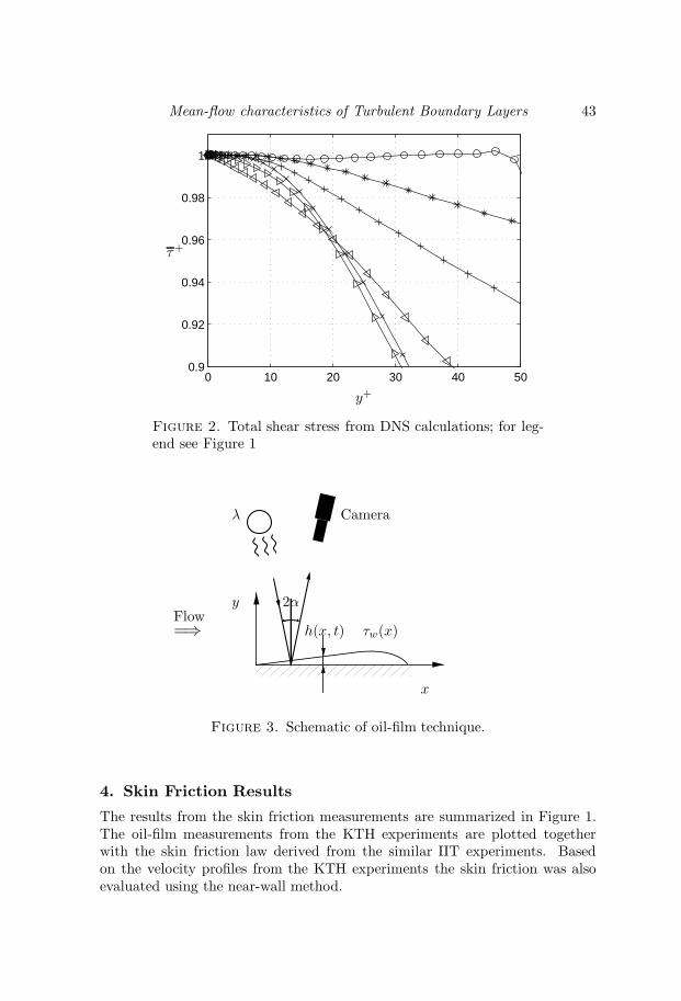
direct numerical simulations (DNS) of turbulent shear flows. Since the DNSdata are available with great detail in the region where accurate measurementscan be achieved and where the measurements are still well within the innerlayer, the range 6 < y+ < 20 was selected for this near-wall method. In Figure1, the mean velocity profiles from several recent direct numerical simulationsare reproduced. The Couette flow simulation was chosen since it most closelyresembles the flow in the inner part of a high Reynolds number turbulentboundary layer. In particular, there is no streamwise pressure gradient in thisflow and the total shear stress is constant, over a range of distances from thewall, as shown in Figure 2. Note that for this flow τ+ = 1 for all y+ .
3.2. Oil-film interferometry
Oil film interferometry was used in both experiments to measure the skin fric-tion. The basic principle of the method is to measure the deformation of athin film of oil when subjected to a shear stress on its top surface. A simpleand convenient measurement technique is based on illuminating the oil-film bya monochromatic light and recording the change in the generated interferencepattern, e.g., with a video camera (see Figure 3). The skin friction is deter-mined from the recording of the fringe patterns and utilizing the wave lengthof the light source λ, the kinematic viscosity of the oil ν , the refractive index ofthe oil n, and the angle of the camera axes to the normal of the plate α. Theaccuracy of the mean skin friction value τw measured by this oil-film methodis better than ±4% (Fernholz et al. 1996).
Mean-flow characteristics of Turbulent Boundary Layers 43
0 10 20 30 40 500.9
0.92
0.94
0.96
0.98
1
y+
τ+
Figure 2. Total shear stress from DNS calculations; for leg-end see Figure 1
x
y 2α
τw(x)h(x, t)
Cameraλ
=⇒Flow
Figure 3. Schematic of oil-film technique.
4. Skin Friction Results
The results from the skin friction measurements are summarized in Figure 1.The oil-film measurements from the KTH experiments are plotted togetherwith the skin friction law derived from the similar IIT experiments. Basedon the velocity profiles from the KTH experiments the skin friction was alsoevaluated using the near-wall method.
44 J. M. Osterlund et al.
Reθ
cf
0 0.5 1 1.5 2 2.5 3
x 104
2
2.5
3
3.5x 10
-3
Fernholz & Finley 1996KTH, Oil-film (series 1)KTH, Oil-film (series 2)KTH, Oil-film fitKTH, Near-wall fitKTH, Near-wall, x = 1.5 mKTH, Near-wall, x = 2.5 mKTH, Near-wall, x = 3.5 mKTH, Near-wall, x = 4.5 mKTH, Near-wall, x = 5.5 mKTH, Near-wall, x = 5.5 mIIT Oil-film fit
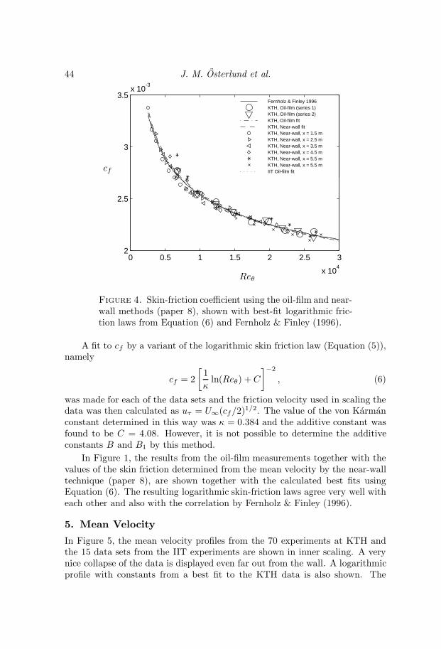
Figure 4. Skin-friction coefficient using the oil-film and near-wall methods (paper 8), shown with best-fit logarithmic fric-tion laws from Equation (6) and Fernholz & Finley (1996).
A fit to cf by a variant of the logarithmic skin friction law (Equation (5)),namely
cf = 2[
1κ
ln(Reθ) +C
]−2, (6)
was made for each of the data sets and the friction velocity used in scaling thedata was then calculated as uτ = U∞(cf/2)1/2. The value of the von Karmanconstant determined in this way was κ = 0.384 and the additive constant wasfound to be C = 4.08. However, it is not possible to determine the additiveconstants B and B1 by this method.
In Figure 1, the results from the oil-film measurements together with thevalues of the skin friction determined from the mean velocity by the near-walltechnique (paper 8), are shown together with the calculated best fits usingEquation (6). The resulting logarithmic skin-friction laws agree very well witheach other and also with the correlation by Fernholz & Finley (1996).
5. Mean Velocity
In Figure 5, the mean velocity profiles from the 70 experiments at KTH andthe 15 data sets from the IIT experiments are shown in inner scaling. A verynice collapse of the data is displayed even far out from the wall. A logarithmicprofile with constants from a best fit to the KTH data is also shown. The

Mean-flow characteristics of Turbulent Boundary Layers 45
100
101
102
103
104
0
5
10
15
20
25
30
35
0
5
10
15
20
25
30
35
y+
U+
Figure 5. Mean velocity inner scaling; solid lines: data fromKTH, dashed lines: data from IIT, dash-dotted lines: log-lawwith constants κ = 0.38 and B = 4.1, and note shift of axis.
constants were found to be: κ = 0.38, B = 4.1 and B1 = 3.6, see section 6.The IIT experiment gives the same value of the von Karman constant, κ, butdifferent values of the additive constants, which is seen as a vertical shift, fromthe KTH log-profile, in figures 5 and 6.
In Figure 6 the same data are replotted using classical outer scaling andthe collapse is very good, although the IIT data again shows another value ofthe additive constant.
The boundary layer thickness δ is a quantity which cannot be exactlydefined and is commonly taken as y when U/U∞ = 0.95 here denoted δ95 andused throughout this article. Other definitions that are often used include theRotta-Clauser length ∆ = δ∗U∞/uτ , first used by Rotta (1950), or the Coles δctwhich is defined as the distance to the wall of the point of maximum deviationfrom the log law, in the outer part of the boundary layer. Comparisons betweenthe defect mean-velocity profiles in the outer part of the boundary layer usingdifferent outer length scales are shown in Figure 7. To put them all on the sameaxis each scaling is multiplied by the mean of the ratio between the length scaleunder consideration and δ95, for all Reynolds numbers.
Except for the scaling with θ, which is somewhat worse than the others, noclear preference for an outer scale can be derived from this figure. However, theRotta-Clauser length scale, ∆, has the advantage of being an integral length
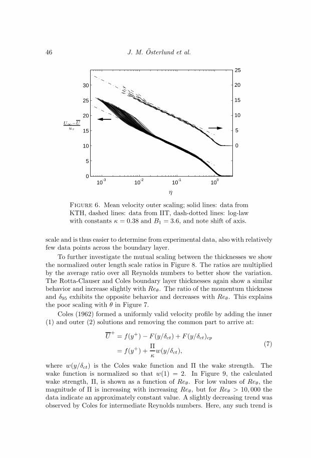
46 J. M. Osterlund et al.
10-3
10-2
10-1
100
0
5
10
15
20
25
30
0
5
10
15
20
25
η
U∞−Uuτ
Figure 6. Mean velocity outer scaling; solid lines: data fromKTH, dashed lines: data from IIT, dash-dotted lines: log-lawwith constants κ = 0.38 and B1 = 3.6, and note shift of axis.
scale and is thus easier to determine from experimental data, also with relativelyfew data points across the boundary layer.
To further investigate the mutual scaling between the thicknesses we showthe normalized outer length scale ratios in Figure 8. The ratios are multipliedby the average ratio over all Reynolds numbers to better show the variation.The Rotta-Clauser and Coles boundary layer thicknesses again show a similarbehavior and increase slightly with Reθ. The ratio of the momentum thicknessand δ95 exhibits the opposite behavior and decreases with Reθ. This explainsthe poor scaling with θ in Figure 7.
Coles (1962) formed a uniformly valid velocity profile by adding the inner(1) and outer (2) solutions and removing the common part to arrive at:
U+
= f(y+) − F (y/δct) + F (y/δct)cp
= f(y+) +Πκw(y/δct),
(7)
where w(y/δct) is the Coles wake function and Π the wake strength. Thewake function is normalized so that w(1) = 2. In Figure 9, the calculatedwake strength, Π, is shown as a function of Reθ. For low values of Reθ, themagnitude of Π is increasing with increasing Reθ, but for Reθ > 10, 000 thedata indicate an approximately constant value. A slightly decreasing trend wasobserved by Coles for intermediate Reynolds numbers. Here, any such trend is

Mean-flow characteristics of Turbulent Boundary Layers 47
0.2 0.4 0.6 0.8 1 1.2 1.4 1.60
2
4
6
8
10
12
14
η
U∞−Uuτ
Figure 7. Mean velocity in outer scaling with the differentdefinitions for η: y/δ95, (y/∆)〈∆/δ95〉, (y/δct)〈δct/δ95〉 and(y/θ)〈θ/δ95〉, where averages over Reθ are denoted by〈...〉; notedata is shifted upwards with an increment of 2 units betweeneach set.
hardly visible. A difference from the data analysis of Coles is that we here haveused the new values (κ = 0.38, B = 4.1) for the log-layer parameters. Thisexplains the lower value of Π obtained here as compared to the value of about0.55 found by Coles (with κ = 0.41, B = 5).

48 J. M. Osterlund et al.
0.9
0.95
1
1.05
1.1
0.9
0.95
1
1.05
0 0.5 1 1.5 2 2.5 3
x 104
0.9
0.95
1
1.05
Reθ
∆δ95/〈 ∆δ95 〉
δct
δ95/〈 δct
δ95〉
θδ95/〈 θ
δ95〉
Figure 8. Normalized outer length scale ratios, where 〈...〉denotes mean values for all Reθ cases.
6. Scaling in the overlap region
In order to investigate the scaling in the overlap region, a normalized slope ofthe mean velocity profile,
Ξ =
(y+
dU+
dy+
)−1
, (8)
was utilized. In a logarithmic region of the profiles Ξ is constant and equal to κ.The value of Ξ was calculated by taking an average of the individual profiles ata constant wall distance in inner scaling while omitting the part of the profileswhere η > Mo. Similarly, the profiles were again averaged at constant outer-scaled distances from the wall for y+ > Mi. The parameters Mi and Mo are theinner and outer limits of the overlap region. In Figures 10 and 11, the averagedΞ is shown together with error bars representing a 95% confidence interval. Aregion where a nearly constant Ξ very accurately represents the data is evidentin both figures. This clearly supports the existence of a logarithmic overlapregion within the appropriate range of the parameters Mi and Mo. The choiceof the appropriate limits was subsequently selected based on the y values wherethe error bar deviates significantly from the horizontal line in the figures. Thiswas based on an iteration of the limits until a consistent result was obtained.The resulting values for the inner and outer limits areMi ≈ 200 and Mo ≈ 0.15,respectively. Taking κ as the average value within the determined limits givesa κ of about 0.38.
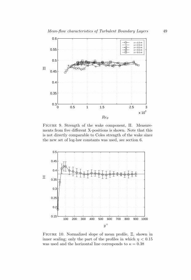
Mean-flow characteristics of Turbulent Boundary Layers 49
0 0.5 1 1.5 2.5 3
x 104
0.3
0.35
0.4
0.45
0.5
0.55
0.6x = 1.5 mx = 2.5 mx = 3.5 mx = 4.5 mx = 5.5 m
Reθ
Π
Figure 9. Strength of the wake component, Π. Measure-ments from five different X-positions is shown. Note that thisis not directly comparable to Coles strength of the wake sincethe new set of log-law constants was used, see section 6.
100 200 300 400 500 600 700 800 900 10000.15
0.2
0.25
0.3
0.35
0.4
0.45
0.5
y+
Ξ
Figure 10. Normalized slope of mean profile, Ξ, shown ininner scaling; only the part of the profiles in which η < 0.15was used and the horizontal line corresponds to κ = 0.38

50 J. M. Osterlund et al.
10-1
100
0.15
0.2
0.25
0.3
0.35
0.4
0.45
0.5
η
Ξ
Figure 11. Normalized slope of mean profile, Ξ, shown inouter scaling; only the part of the profiles in which y+ > 200was used and the horizontal line corresponds to κ = 0.38
Next, the additive constants B and B1 were investigated by looking at thedeviation of the mean velocity profiles, in inner and outer scaling, from thelog-profile with the aid of the variables Ψ and Ψ1, where
Ψ = U+ − 1
κln y+ (9)
Ψ1 =U∞ − Uuτ
+1κ
lnη (10)
The variables Ψ and Ψ1 are also constant in a region governed by a logarithmiclaw. The average of the value of Ψ and Ψ1, respectively, at a constant walldistance is taken for all Reynolds numbers while omitting the part of the profilewhere η > Mo in the calculation of Ψ and y+ < 200 in the calculation of Ψ1. InFigure 12, Ψ is shown with error bars corresponding to the standard deviation.A constant value is found over a wide range in y+, again indicating a log-layer.Calculating the average of Ψ within the proposed limits, Mi and Mo, givesB = 4.1. In Figure 13 Ψ1 is presented in the same manner as for Ψ and givesthe value of the additive constant in the outer scaled log-law B1 = 3.6. Notethat the constant B1 depends on the definition of δ. Here δ95 was used.
In addition to using the above described method to determine the log-law constants, we used the traditional procedure to determine κ and B byperforming a least-squares type of fit to the mean velocity profiles. In Figure 14,κ was calculated by fitting a log-law relation for each profile using the following
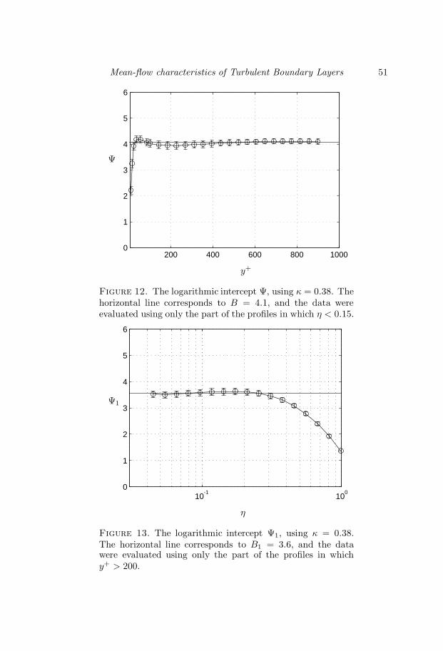
Mean-flow characteristics of Turbulent Boundary Layers 51
200 400 600 800 10000
1
2
3
4
5
6
y+
Ψ
Figure 12. The logarithmic intercept Ψ, using κ = 0.38. Thehorizontal line corresponds to B = 4.1, and the data wereevaluated using only the part of the profiles in which η < 0.15.
10-1
100
0
1
2
3
4
5
6
η
Ψ1
Figure 13. The logarithmic intercept Ψ1, using κ = 0.38.The horizontal line corresponds to B1 = 3.6, and the datawere evaluated using only the part of the profiles in whichy+ > 200.

52 J. M. Osterlund et al.
0 0.5 1 1.5 2 2.5 3
x 104
0.35
0.4
0.45
Reθ
κ
Figure 14. The von Karman constant determined by a least-squares fit, with the outer limit fixed at η = 0.15 and the innerlimit at Mi; : KTH, Mi = 50. •: KTH, Mi = 200. Dashedline: KTH, linear fit, Mi = 50. Solid line: KTH, linear fit,Mi = 200. : IIT, Mi = 50. : IIT, Mi = 200. Dotted line:IIT, linear fit, Mi = 50. Dash dotted line: IIT, linear fit,Mi = 200.
traditional limits of the fit: Mi = 50 and Mo = 0.15. The process was alsorepeated with the newly established limits of Mi = 200 and Mo = 0.15. Thevalue of κ obtained when using the traditional limits varies with Reynoldsnumber and gives about the commonly used value of 0.41 at low Reynoldsnumbers. This is then followed by a decreasing trend with increasing Reynoldsnumber. Using the new limits, that are more representative of the logarithmiclaw, again yields a value of κ ≈ 0.38 independent of Reynolds number.
To investigate the existence of a power-law as proposed recently by sev-eral authors Barenblatt (1993); George et al. (1997), the following diagnosticfunction is plotted in Figure 15.
Γ =y+
U+
dU+
dy+(11)
The function Γ should be a constant in a region governed by a power-law.However, no region of constant Γ is evident in Figure 6, in particular whencompared to Figures 10 and 11. This clearly indicates that a power-law relationis less representative of the entire region of overlap between Mi and Mo.

Mean-flow characteristics of Turbulent Boundary Layers 53
100 200 300 400 500 600 700 800 900 10000
0.05
0.1
0.15
0.2
0.25
0.3
0.35
y+
Γ
Figure 15. The power-law diagnostic function Γ, evaluatedusing only the part of the profiles in which η < 0.15.
7. Concluding Remarks
Based on analysis of data from two recent experimental investigations it can beconcluded that a logarithmic overlap region, between the inner and outer partsof the mean velocity profiles, exists for Reθ > 6, 000. Establishing, based on theanalysis of the data, an inner limit of the region at about y+ = 200 and an outerlimit at η = 0.15 demonstrated the validity of the logarithmic relation. Thislogarithmic overlap region found differs from that found by Zagarola & Smits(1998a) based on measurements in the Superpipe facility. Where they foundthe values κ = 0.436 and B = 6.15. This may suggest that the matching of theinner layer with the outer flow results in a slightly different overlap region inthe two flow cases; namely, the zero pressure gradient boundary layer and thepressure-gradient driven pipe flow. This is perhaps not totally surprising sincethe overlap region depends on both the inner and the outer layers and the outerflow is different in the pipe flow from that for the boundary layer. The foundvalue of the von Karman constant is slightly less than the commonly acceptedvalue of 0.41. Evaluation of the recent high Reynolds number experiment in theGerman-Dutch wind-tunnel by Fernholz et al. (1995) also yields a significantlylower value of the von Karman constant. Re-evaluation of a carefully selectedset of existing experiments would be of great importance for this issue, but outof scope for this article.
54 J. M. Osterlund et al.
8. Acknowledgments
The authors wish to thank Jukka Komminaho and Martin Skote for providingus with DNS data and William Ornt for sharing early versions of his resultswith us. We wish to thank Mr. Ulf Landen and Mr. Marcus Gallstedt whohelped with the manufacturing of the experimental set-up. The support ofAFOSR for the IIT experiments is also acknowledged. Financial support fromNUTEK and TFR for the KTH experiment is also gratefully acknowledged.
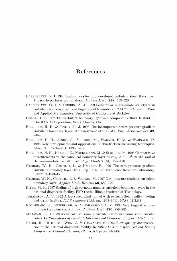
References
Barenblatt, G. I. 1993 Scaling laws for fully developed turbulent shear flows. part1. basic hypotheses and analysis. J. Fluid Mech. 248, 513–520.
Barenblatt, G. I. & Chorin, A. J. 1999 Self-similar intermediate structures inturbulent boundary layers at large reynolds numbers. PAM 755. Center for Pureand Applied Mathematics, University of California at Berkeley.
Coles, D. E. 1962 The turbulent boundary layer in a compressible fluid. R 403-PR.The RAND Corporation, Santa Monica, CA.
Fernholz, H. H. & Finley, P. J. 1996 The incompressible zero-pressure-gradientturbulent boundary layer: An assessment of the data. Prog. Aerospace Sci. 32,245–311.
Fernholz, H. H., Janke, G., Schober, M., Wagner, P. M. & Warnack, D.
1996 New developments and applications of skin-friction measuring techniques.Meas. Sci. Technol. 7, 1396–1409.
Fernholz, H. H., Krause, E., Nockemann, M. & Schober, M. 1995 Comparativemeasurements in the canonical boundary layer at reδ2 < 6 · 104 on the wall ofthe german-dutch windtunnel. Phys. Fluids 7 (6), 1275–1281.
George, W. K., Castilio, L. & Knecht, P. 1996 The zero pressure gradientturbulent boundary layer. Tech. Rep.TRL-153. Turbulence Research Laboratory,SUNY at Buffalo.
George, W. K., Castilio, L. & Wosnik, M. 1997 Zero-pressure-gradient turbulentboundary layer. Applied Mech. Reviews 50, 689–729.
Hites, M. H. 1997 Scaling of high-reynolds number turbulent boundary layers in thenational diagnostic facility. PhD thesis, Illinois Institute of Technology.
Johansson, A. V. 1992 A low speed wind-tunnel with extreme flow quality - designand tests. In Prog. ICAS congress 1992 , pp. 1603–1611. ICAS-92-3.8.1.
Komminaho, J., Lundbladh, A. & Johansson, A. V. 1996 Very large structuresin plane turbulent couette flow. J. Fluid Mech. 320, 259–285.
Millikan, C. B. 1938 A critical discussion of turbulent flows in channels and circulartubes. In Proceedings of the Fifth International Congress of applied Mechanics .
Nagib, H., Hites, M., Won, J. & Gravante, S. 1994 Flow quality documenta-tion of the national diagnostic facility. In 18th AIAA Aerospace Ground TestingConference, Colorado Springs, CO. AIAA paper 94-2499.
55

56 REFERENCES
Ornt, W. 1999 Measurements of wall-shear stress in turbulent channel and boundarylayer flows. Master’s thesis, Illinois Institute of Technology.
Rotta, J. C. 1950 Uber die Theorie der Turbulenten Grenzschichten. Mitt. M.P.I.Strom. Forschung Nr 1, also available as NACA TM 1344.
Skote, M., Henkes, R. & Henningson, D. 1998 Direct numerical simulation ofself-similar turbulent boundary layers in adverse pressure gradients. In Flow,Turbulence and Combustion , , vol. 60, pp. 47–85. Kluwer Academic Publishers.
Spalart, P. R. 1988 Direct simulation of a turbulent boundary layer up to Reθ =1410. J. Fluid Mech. 187, 61–98.
Zagarola, M. V. & Smits, A. J. 1998a Mean-flow scaling of turbulent pipe flow.J. Fluid Mech. 373, 33–79.
Zagarola, M. V. & Smits, A. J. 1998b A new mean velocity scaling for turbulentboundary layers. In Proceedings of FEDSM’98 .

Paper 3


Turbulence Statistics of Zero Pressure GradientTurbulent Boundary Layers
By Jens M. Osterlund & Arne V. Johansson
Dept. of Mechanics, KTH, SE-100 44 Stockholm, Sweden
To be submitted
Single-point turbulence statistics are here reported for zero pressure-gradientboundary layers at Reynolds numbers based on the momentum thickness inthe range 2530 < Reθ < 27300. The experiments were performed in the MTLwind-tunnel at the Department of Mechanics at KTH in Stockholm. A sevenm long flat plate was mounted in the test section and the experiments wereperformed at 5 different streamwise positions. The velocity was measured usinghot-wire techniques and the mean wall shear stress was determined using oil-film interferometry. Reynolds number dependence of the statistical quantitiesand probe size effects are discussed.
1. Introduction
This paper presents an experimental study of the structure single-point turbu-lence statistics in zero-pressure-gradient turbulent boundary layers and Rey-nolds number effects. The Reynolds number in typical applications with bound-ary layer flow are often several orders of magnitude larger than what is possibleto achieve in direct numerical simulations or even compared to what is achiev-able in most wind-tunnels. Therefore, there is a gap in Reynolds number be-tween practical applications and the experiments which form the basis for ourknowledge of turbulence and turbulence modeling. Experiments at high Rey-nolds number is therefore of primary importance to reveal Reynolds numbertrends that might have a large influence in many fluid dynamic applications.Recent reviews of Reynolds number effects in wall-bounded shear flows wasmade by Gad-el-Hak & Bandyopadhyay (1994) and more specifically on zeropressure-gradient boundary layer flow by Fernholz & Finley (1996). Since thepublication of the reviews two more experimental studies was published bySmith (1994) and Hites (1997). For low Reynolds numbers results from directnumerical simulations have become available starting with the simulation bySpalart (1988) followed by e.g. Skote et al. (1998).
59
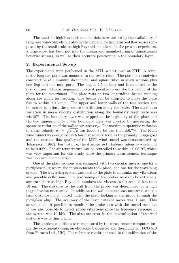
60 J. M. Osterlund & A. V. Johansson
The quest for high Reynolds number data is restrained by the availability oflarge size wind-tunnels but also by the demand for miniaturized flow sensors im-posed by the small scales at high Reynolds numbers. In the present experimenta large effort has been put into the design and manufacturing of miniaturizedhot-wire sensors, as well as their accurate positioning in the boundary layer.
2. Experimental Set-up
The experiments were performed in the MTL wind-tunnel at KTH. A sevenmeter long flat plate was mounted in the test section. The plate is a sandwichconstruction of aluminum sheet metal and square tubes in seven sections plusone flap and one nose part. The flap is 1.5 m long and is mounted in thefirst diffuser. This arrangement makes it possible to use the first 5.5 m of theplate for the experiment. The plate rests on two longitudinal beams runningalong the whole test section. The beams can be adjusted to make the plateflat to within ±0.5 mm. The upper and lower walls of the test section canbe moved to adjust the pressure distribution along the plate. The maximumvariation in mean velocity distribution along the boundary layer plate was±0.15%. The boundary layer was tripped at the beginning of the plate andthe two dimensionality of the boundary layer was checked by measuring thespanwise variation of the wall shear stress τw. The maximum spanwise variationin shear velocity uτ =
√τw/ρ was found to be less than ±0.7%. The MTL
wind tunnel was designed with low disturbance level as the primary design goaland the extreme flow quality of the MTL wind-tunnel was demonstrated byJohansson (1992). For instance, the streamwise turbulence intensity was foundto be 0.02%. The air temperature can be controlled to within ±0.05 C, whichwas very important for this study since the primary measurement techniquewas hot-wire anemometry.
One of the plate sections was equipped with two circular inserts, one for aplexiglass plug where the measurements took place, and one for the traversingsystem. The traversing system was fixed to the plate to minimize any vibrationsand possible deflections. The positioning of the probes needs to be extremelyaccurate since at high Reynolds numbers the viscous (wall) scale is less than10 µm. The distance to the wall from the probe was determined by a highmagnification microscope. In addition the wall distance was measured using alaser distance meter placed under the plate looking at the probe through theplexiglass plug. The accuracy of the laser distance meter was ±1µm. Thissystem made it possible to monitor the probe also with the tunnel running.It was also possible to detect probe vibrations since the frequency response ofthe system was 10 kHz. The absolute error in the determination of the walldistance was within ±5µm.
The ambient conditions were monitored by the measurement computer dur-ing the experiments using an electronic barometer and thermometer (FCO 510from Furness Ltd., UK). The reference conditions used in the calibration of the

Turbulence Statistics 61
probes were determined using a Prandtl tube in the free-stream directly abovethe measurement station. The pressure and temperature were again monitoredat all times during the experiments using a differential pressure transducer anda thermometer connected directly to the measurement computer. The accuracyof the pressure measurement was 0.25 % and the accuracy of the temperaturemeasurement was 0.02 C.
Constant temperature hot-wire anemometry was used in all velocity mea-surements. All hot-wire probes were designed and built at the lab. Threesizes of single-wire probes were used in the experiments with wire diametersof: 2.5, 1.27 and 0.63 µm. Two other types of probes were also used: X- andV-wires. The wire diameter for the X- and V-wire probes was 1.27 µm. Thewire-separation for the X-wire probe was 220 µm and the wire length about300 µm. The wires were placed at an angle of about ±45 to the mean flowangle. The V-wire probe had two wires placed at ±45 to the mean flow lyingin the same horizontal plane. The wire length was 300 µm and the maximumspanwise extent was about 500 µm. The anemometer system (AN1003 fromAA lab systems, Israel) had a built-in signal conditioner and the signals fromthe anemometer were digitized using an A/D converter board (A2000 from Na-tional Instruments, USA) in the measurement computer. The A/D converterhas 12 bit resolution and four channels which could be sampled simultaneouslyat rates up to 1 MHz divided by the number of channels used.
The complete experiment was run from a program on the measurementcomputer which controlled the tunnel velocity, the positioning of probes, digi-tization of the anemometer signals, monitoring of the pressures and the temper-ature. This made it possible to design experiments which could be performedrelatively quickly since monotonous work with moving probes and registeringthe parameters involved was done rapidly by the computer. For the doublewire measurements the time to perform an measurement was also reduced bystreaming the data directly to the hard disk and evaluating only a small amountof the data, for monitoring purpose, during the measurement. This made thetime to carry out an experiment very close to the total sampling time plusthe traversing time. The main reason for all the effort put into this was tominimize the effect of drift which is always present in any anemometer system.Furthermore, the lifetime of probes with 0.63 µm wire diameter was only acouple of hours at the higher tunnel speeds and to manage both calibrationand the measurement before the wire breaks one has to avoid any unnecessarydelays. To further reduce drift all instruments were always on and the tunnelwas kept running for at least three hours before the experiment was performed.For a detailed description of the experiment, see paper 8.
3. Skin Friction Measurements
Accurate determination of the skin friction in the zero pressure gradient bound-ary layer is a very difficult task. Only a few independent methods are available:

62 J. M. Osterlund & A. V. Johansson
the floating element i.e. measurement of the tangential force of a part of thewall and using the definition of the stress τw = F/A, where F is the force on thefloating element and A is the area of the floating element, measurement of thevelocity gradient at the wall and using τw = µ∂U/∂y, where µ is the dynamicviscosity of the air, and oil-film interferometry. In oil-film interferometry thedeformation of a thin film of oil is registered in time using optical interferome-try. It is an independent method since it does not need to be calibrated. Onlyproperties of the oil must be known.
Oil-film interferometry was used to determine the skin friction in this exper-iment and the adapted method is described by Fernholz et al. (1996). Resultsand comparisons with other experiments and other methods can be found inpaper 2 and Osterlund et al. (1999).
A fit to cf by a variant of the logarithmic skin friction law (Equation (6)),namely
cf = 2[
1κ
ln(Reθ) +C
]−2, (1)
was made for each of the data sets and the friction velocity used in scaling thedata was then calculated as uτ = U∞(cf/2)1/2. The value of the von Karmanconstant determined in this way was κ = 0.384 and the additive constant wasfound to be C = 4.08, see Osterlund et al. (1999).
4. Mean Flow Characteristics
The mean flow characteristics of the turbulent boundary layer, with a focus onthe properties of the overlap region, were carefully investigated and are reportedin paper 2. The behavior of the boundary layer confirms the traditional two-layer theory with a logarithmic mean velocity profile in the overlap region.
The outer and inner length scales are chosen as δ, the boundary layerthickness and the viscous length l∗ = ν/uτ , where uτ =
√τw/ρ is the friction
velocity, τw is the skin friction and ρ is the density of the air. Dimensionalanalysis gives the scaling of the velocity in the inner part of the boundarylayer, the law-of-the-wall
U+
=U
uτ= f
(y+
); y+ =
yuτν
(2)
and the scaling in the outer part of the boundary layer, the defect law
U∞ − U
uτ= F (η) η =
y
δ. (3)
At high Reynolds numbers there is a region of overlap, ν/uτ y δ, betweenthe two scalings where both are simultaneously valid. Matching (Millikan 1938)the law-of-the-wall (2) and the defect law (3) in the traditional manner gives

Turbulence Statistics 63
the logarithmic overlap region: in inner variables,
U+
=1κ
ln(y+
)+ B (4)
and in outer variables
U∞ − Uuτ
= − 1κ
ln (η) +B1 . (5)
Equations (4) and (5) also relate the skin friction with the Reynolds numberand can be combined to give the logarithmic skin friction law
U∞uτ
=1κ
ln(δuτν
)+ B +B1. (6)
A simplified variant of the logarithmic skin friction law, see equation 1, was fit-ted to the oil-film experiments and later used in the scaling of the experiments.
In figures 1 and 2 the mean velocity profiles from single-wire measurementsin the Reynolds number range 2500 < Reθ < 27700 are shown in inner andouter scaling. Excellent agreement with the above theoretical result is seenalso over this wide Reynolds number range. Also shown in the figures are thelogarithmic laws with the newly determined values of the log-law constantsκ = 0.38, B = 4.1 and B1 = 3.6. The value of the constant B1 depends on thechoice of outer scale. In this paper we use the Rotta-Clauser lengthscale ∆ =δ∗U∞/uτ , Rotta (1950). As described in paper 2 the Rotta-Clauser length scaleis preferred, compared to the other available and equivalent scalings, because itis experimentally more well defined. One should keep in mind, though, that ∆is substantially larger than the boundary layer thickness. ∆/δ95 ≈ 5.68. Thevalue of B1 was determined in paper 2 using δ95 but can easily be transformedto the ∆-scaling by
B∆1 = Bδ95
1 − 1κ
log(
∆δ95
), (7)
giving the value B∆1 = 1.62 used in figure 2.
5. Streamwise turbulence intensity and spatial resolutioneffects
In any investigation of turbulence statistics spatial averaging due to finite probesize must be carefully addressed. Johansson & Alfredsson (1983) made a de-tailed experimental investigation of spatial resolution effects for near-wall tur-bulence measurements and compiled data from the literature to elucidate sucheffects, see also e.g. Comte-Bellot (1976)
The measured velocity from a hot-wire probe is a weighted average over thewire length. That is, the probe will average out variations in the velocity fieldthat are smaller than the length of the wire. Several attempts to address the
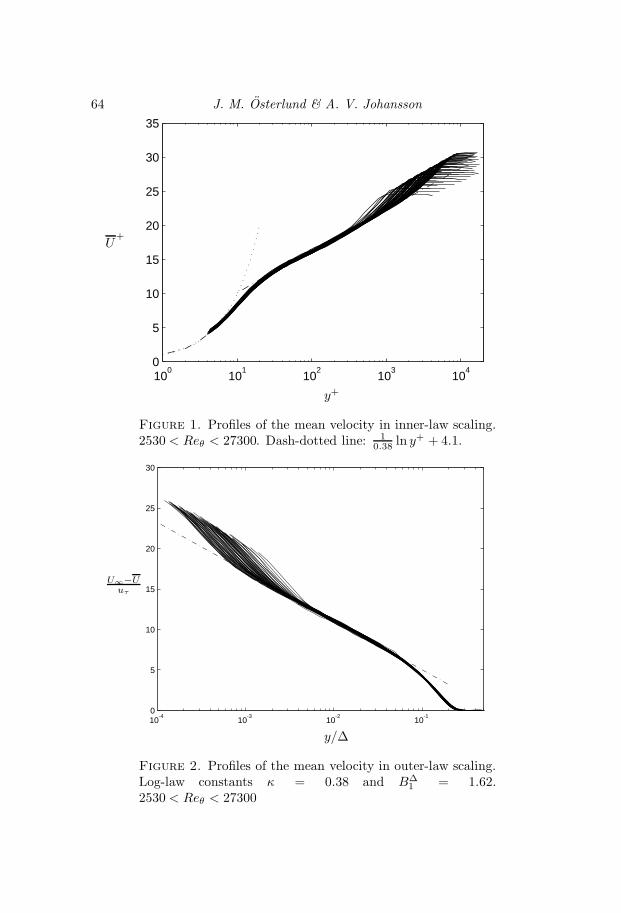
64 J. M. Osterlund & A. V. Johansson
100
101
102
103
104
0
5
10
15
20
25
30
35
U+
y+
Figure 1. Profiles of the mean velocity in inner-law scaling.2530 < Reθ < 27300. Dash-dotted line: 1
0.38 ln y+ + 4.1.
10-4
10-3
10-2
10-1
0
5
10
15
20
25
30
U∞−Uuτ
y/∆
Figure 2. Profiles of the mean velocity in outer-law scaling.Log-law constants κ = 0.38 and B∆
1 = 1.62.2530 < Reθ < 27300

Turbulence Statistics 65
problem of spatial averaging have been reported, see e.g. Ligrani & Bradshaw(1987) and Willmarth & Bogar (1977).
For double wire probes Osterlund (1995) showed that there is a physicallimit where further minimization results in thermal crosstalk between the sens-ing wires that destroys the velocity signal regardless of the spatial resolution.This effect limits the size of double-wire probes to a Peclet number, based onthe separation between the wires, to be larger than about 50. The Peclet num-ber is defined as Pe = RePr = U∆w/χ, where U is the mean velocity, ∆w
is the wire separation and χ the thermometric conductivity 1. This makes itparticularly difficult to design experiments in air because of the low Prandtlnumber (≈ 0.7). The two contradicting limits: L+ < 10 and Pe > 50 result inthe discouraging approximate limit U+ > 7 or y+ > 10 for double-wire probes.Considering also the very high turbulence level in the near-wall region the innerlimit for accurate double-wire probes probably is larger than 50ν/uτ for mea-surements in air. Note that the only solution, for double-wire probes where thethermal interaction must be negligible is to use another medium like water oroil, with Prandtl numbers of 7 and about 100, respectively. The other route foraccurate measurements in the near wall region in air is instead to exploit thethermal interaction, e.g. by two parallel wires very close together, as done byGresko (1988) and Osterlund (1995) (see appendix ). The latter showed thatthe Peclet number based on the separation between the wires must be smallerthan about 10. The manufacturing of this type of probes where the wires mustbe placed less than 10 µm from each other is a severe problem, but the rapiddevelopment in micro-machining technology may solve this problem in a nottoo distant future.
In figures 3 and 4 the turbulence intensity√u2/uτ is shown in inner and
outer scaling for all the measurements. Clearly, it is hard to separate Reynoldsnumber trends from effects of spatial resolution without sorting the data. Thelack of scaling can largely be attributed to spatial averaging, but also Rey-nolds number effects are hidden in the data. We are interested in investigatingReynolds number trends and a subset of the data where L+ < 10 is shown infigure 5. This of course reduces the Reynolds number span but is necessary toremove significant effects of spatial resolution. In the top diagram of figure 5the turbulence intensities are scaled with the friction velocity and in the bottomdiagram with the mean velocity. The latter represents the relative turbulenceintensity, the limiting value (y+ → 0) of which is equal to the relative wall-shear-stress fluctuation intensity. The collapse is about equally good in theviscous sub-layer and the buffer region, y+ < 100 for both scalings. The peakvalues of the absolute and relative intensities are shown in figure 6. Also shownin figure 6 are corresponding values obtained from direct numerical simulations
1χ = κ/ρcp, where κ is the thermal conductivity, ρ the density and cp the specific heat at
constant pressure
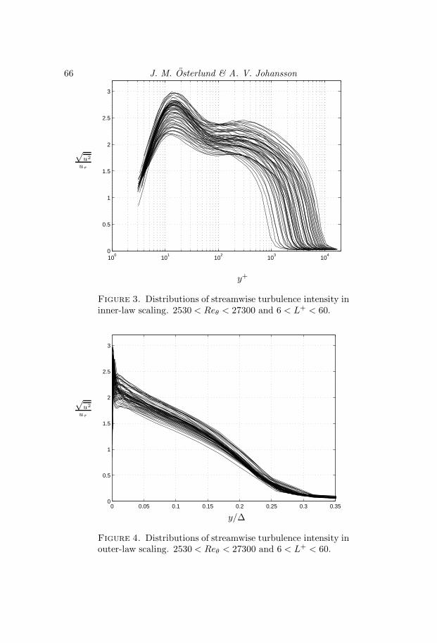
66 J. M. Osterlund & A. V. Johansson
100
101
102
103
104
0
0.5
1
1.5
2
2.5
3
√u2
uτ
y+
Figure 3. Distributions of streamwise turbulence intensity ininner-law scaling. 2530 < Reθ < 27300 and 6 < L+ < 60.
0 0.05 0.1 0.15 0.2 0.25 0.3 0.350
0.5
1
1.5
2
2.5
3
√u2
uτ
y/∆
Figure 4. Distributions of streamwise turbulence intensity inouter-law scaling. 2530 < Reθ < 27300 and 6 < L+ < 60.

Turbulence Statistics 67
0
0.5
1
1.5
2
2.5
3
100
101
102
103
104
0
0.1
0.2
0.3
0.4
√u2
U
√u2
uτ
y+
Figure 5. Streamwise turbulence intensity distributions us-ing only data where 6.5 < L+ < 10. Inner-law scaling.2530 < Reθ < 9700. −−: Boundary layer simulation at Reθ =1410 by Spalart (1988). : LDV Measurements in boundarylayer flow at Reθ = 2420 by Karlsson & Johansson (1988).
by Spalart (1988), Moser et al. (1999) and Alvelius (1999), where the first is aboundary layer simulation and the last two are channel flow simulations. Oneshould keep in mind in the comparisons with the DNS-data that the channelflow has a somewhat different character, where Reynolds number effects onturbulence production etc. can be related to the relative influence of the pres-sure gradient. This can partly be seen from the integrated form of the meanflow equation. An increasing trend is visible in figure 6 for both scalings. Theincrease in
√u2/uτ is about 7% for the present data in this Reynolds number
range but the increase in√u2/U is only about half of that. For
√u2/uτ one
can observe a significant difference between the channel flow and boundarylayer DNS data. The present set of experimental data smoothly extends theboundary layer DNS-results to substantially higher Reynolds numbers, with acontinued increase of the maximum intensity. One could expect a levelling off
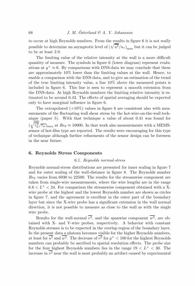
68 J. M. Osterlund & A. V. Johansson
to occur at high Reynolds numbers. From the results in figure 6 it is not reallypossible to determine an asymptotic level of (
√u2/uτ)max but it can be judged
to be at least 2.9.The limiting value of the relative intensity at the wall is a more difficult
quantity of measure. The symbols in figure 6 (lower diagram) represent evalu-ations at y+ ≈ 6. By comparisons with DNS-data we may conclude that theseare approximately 10% lower than the limiting values at the wall. Hence, toenable a comparison with the DNS-data, and to give an estimation of the trendof the true limiting intensity value, a line 10% above the measured points isincluded in figure 6. This line is seen to represent a smooth extension fromthe DNS-data. At high Reynolds numbers the limiting relative intensity is es-timated to be around 0.43. The effects of spatial averaging should be expectedonly to have marginal influence in figure 6.
The extrapolated (+10%) values in figure 6 are consistent also with mea-surements of the fluctuating wall shear stress by the hot-wire-on-the-wall tech-nique (paper 5). With that technique a value of about 0.41 was found for
(√τ2w/τw)max at Reθ ≈ 10000. In that work also measurements with a MEMS-
sensor of hot-film type are reported. The results were encouraging for this typeof technique although further refinements of the sensor design can be foreseenin the near future.
6. Reynolds Stress Components
6.1. Reynolds normal-stress
Reynolds normal-stress distributions are presented for inner scaling in figure 7and for outer scaling of the wall-distance in figure 8. The Reynolds numberReθ varies from 6930 to 22500. The results for the streamwise component aretaken from single-wire measurements, where the wire lengths are in the range6.6 < L+ < 24. For comparison the streamwise component obtained with a X-wire probe at the highest and the lowest Reynolds number are shown as circlesin figure 7, and the agreement is excellent in the outer part of the boundarylayer but since the X-wire probe has a significant extension in the wall normaldirection, it is not possible to measure as close to the wall as with the singlewire probe.
Results for the wall-normal v2, and the spanwise component w2, are ob-tained with X- and V-wire probes, respectively. A behavior with constantReynolds stresses is to be expected in the overlap region of the boundary layer.In the present data a plateau becomes visible for the higher Reynolds numbers,at least for u2 and w2. The decrease of v2 for y+ < 100 for the highest Reynoldsnumbers can probably be ascribed to spatial resolution effects. The probe sizefor the four highest Reynolds numbers lies in the range 19 < L+ < 30. Theincrease in v2 near the wall is most probably an artifact caused by experimental
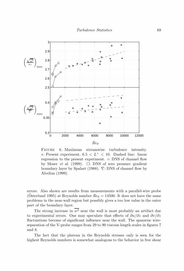
Turbulence Statistics 69
2.5
2.6
2.7
2.8
2.9
3
0 2000 4000 6000 8000 10000 120000.3
0.35
0.4
(√u2
uτ
)max
(√u2
U
)max
Reθ
Figure 6. Maximum streamwise turbulence intensity.∗: Present experiment, 6.5 < L+ < 10. Dashed line: linearregression to the present experiment. : DNS of channel flowby Moser et al. (1999). : DNS of zero pressure gradientboundary layer by Spalart (1988). ∇: DNS of channel flow byAlvelius (1999).
errors. Also shown are results from measurements with a parallel-wire probe(Osterlund 1995) at Reynolds number Reθ = 14500. It does not have the sameproblems in the near-wall region but possibly gives a too low value in the outerpart of the boundary layer.
The strong increase in w2 near the wall is most probably an artifact dueto experimental errors. One may speculate that effects of ∂u/∂z and ∂v/∂zfluctuations become of significant influence near the wall. The spanwise wire-separation of the V-probe ranges from 29 to 90 viscous length scales in figures 7and 8.
The fact that the plateau in the Reynolds stresses only is seen for thehighest Reynolds numbers is somewhat analogous to the behavior in free shear

70 J. M. Osterlund & A. V. Johansson
0
2
4
6
8
10
0
0.5
1
1.5
100
101
102
103
104
0
2
4
6
w2
u2τ
v2
u2τ
u2
u2τ
y+
Figure 7. Distributions of the Reynolds normal-stress com-ponents in inner-law scaling of the wall-distance. 6930 <Reθ < 22500. u2 data from a single-wire probe, v2 from aX-wire probe and w2 from a V-wire probe. ×: X-wire probe atReθ 6930 and 22500. : Parallel-wire probe, Reθ = 14500.−−: Boundary layer simulation at Reθ = 1410 by Spalart(1988). : LDV Measurements in boundary layer flow atReθ = 2420 by Karlsson & Johansson (1988). Dotted partsof curves represent measured data with significant effects ofwire-separation etc.
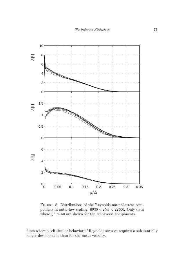
Turbulence Statistics 71
0
2
4
6
8
10
0
0.5
1
1.5
0 0.05 0.1 0.15 0.2 0.25 0.3 0.350
2
4
6
w2
u2τ
v2
u2τ
u2
u2τ
y/∆
Figure 8. Distributions of the Reynolds normal-stress com-ponents in outer-law scaling. 6930 < Reθ < 22500. Only datawhere y+ > 50 are shown for the transverse components.
flows where a self-similar behavior of Reynolds stresses requires a substantiallylonger development than for the mean velocity.

72 J. M. Osterlund & A. V. Johansson
0 0.5 1 1.5 2 2.5
x 104
0
0.5
1
1.5
(v2
u2τ
)max
Reθ
Figure 9. Maximum wall-normal turbulence intensity,(v2/u2τ
)max
. : Present data. Wire separation is L+ = 6
for the low Reynolds number increasing to L+ = 18 for thehighest Reynolds number. : DNS of zero pressure gradientboundary layer by Spalart (1988). •: LDV measurement byKarlsson & Johansson (1988).
The peak value of v2 is seen in figure 9 to increase with the Reynoldsnumber in a manner similar to the variation in the peak value for u2. At thehigh Reynolds number end a decreasing trend is seen that is probably due tospatial averaging effects. The increase in (v2/uτ )max for Reθ < 13000 seemsconsistent with the low Reynolds number DNS-results. Fernholz & Finley(1996) reported max-values of about 1.4 for Reθ = 20920 obtained with aprobe size of about 26 in wall-units. This is in reasonable agreement with theresults in figure 9.
6.2. Reynolds shear-stress
Distributions of the Reynolds shear-stress uv are shown in figures 10 and 11 ininner and outer scaling, respectively. Experimental errors due to the large probesize at the high Reynolds numbers gives large uncertainties of the measurementsin the near-wall region, y+ < 200. The Reynolds number variation of the shear-stress peak value is shown in figure 12. The peak values show an increasingtrend with Reynolds number that flattens out very close to unity for Reynoldsnumbers above about 15000. The increasing trend at low Reynolds numbers
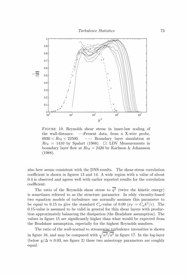
Turbulence Statistics 73
100
101
102
103
104
0
0.1
0.2
0.3
0.4
0.5
0.6
0.7
0.8
0.9
1
−uvu2
τ
y+
Figure 10. Reynolds shear stress in inner-law scaling ofthe wall-distance. —:Present data, from a X-wire probe,6930 < Reθ < 22500. −−: Boundary layer simulation atReθ = 1410 by Spalart (1988). : LDV Measurements inboundary layer flow at Reθ = 2420 by Karlsson & Johansson(1988).
also here seems consistent with the DNS-results. The shear-stress correlationcoefficient is shown in figures 13 and 14. A wide region with a value of about0.4 is observed and agrees well with earlier reported results for the correlationcoefficient.
The ratio of the Reynolds shear stress to q2 (twice the kinetic energy)is sometimes referred to as the structure parameter. In eddy viscosity-basedtwo equation models of turbulence one normally assumes this parameter tobe equal to 0.15 to give the standard Cµ-value of 0.09 (νT = Cµk
2/ε). The0.15-value is assumed to be valid in general for thin shear layers with produc-tion approximately balancing the dissipation (the Bradshaw assumption). Thevalues in figure 15 are significantly higher than what would be expected fromthe Bradshaw assumption, especially for the highest Reynolds numbers.
The ratio of the wall-normal to streamwise turbulence intensities is shownin figure 16, and may be compared with
√w2/u2 in figure 17. In the log-layer
(below y/∆ ≈ 0.03, see figure 2) these two anisotropy parameters are roughlyequal.

74 J. M. Osterlund & A. V. Johansson
0 0.05 0.1 0.15 0.2 0.25 0.3 0.350
0.1
0.2
0.3
0.4
0.5
0.6
0.7
0.8
0.9
1
−uvu2
τ
y/∆
Figure 11. Reynolds shear stress in outer-law scaling.
0 0.5 1 1.5 2 2.5
x 104
0.5
0.6
0.7
0.8
0.9
1
1.1
−(uvu2
τ
)max
Reθ
Figure 12. Maximum value of the shear-stress component.: Present data. : DNS of zero pressure gradient boundarylayer by Spalart (1988). •: LDV Measurement by Karlsson &Johansson (1988).

Turbulence Statistics 75
102
103
104
0
0.1
0.2
0.3
0.4
0.5
0.6
− uv√u2√
v2
y+
Figure 13. Reynolds shear stress correlation coefficient ininner-law scaling.
0 0.05 0.1 0.15 0.2 0.25 0.3 0.350
0.1
0.2
0.3
0.4
0.5
0.6
− uv√u2√
v2
y/∆
Figure 14. Reynolds shear stress correlation coefficient inouter-law scaling.
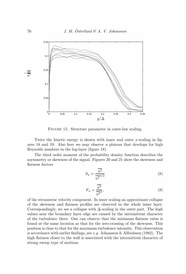
76 J. M. Osterlund & A. V. Johansson
0 0.05 0.1 0.15 0.2 0.25 0.3 0.350
0.05
0.1
0.15
0.2
0.25
−uv
q2
y/∆
Figure 15. Structure parameter in outer-law scaling.
Twice the kinetic energy is shown with inner and outer y-scaling in fig-ures 18 and 19. Also here we may observe a plateau that develops for highReynolds numbers in the log-layer (figure 18).
The third order moment of the probability density function describes theasymmetry or skewness of the signal. Figures 20 and 21 show the skewness andflatness factors
Su =u3
u23/2
(8)
Fu =u4
u22 , (9)
of the streamwise velocity component. In inner scaling an approximate collapseof the skewness and flatness profiles are observed in the whole inner layer.Correspondingly, we see a collapse with ∆-scaling in the outer part. The highvalues near the boundary layer edge are caused by the intermittent characterof the turbulence there. One can observe that the minimum flatness value isfound at the same location as that for the zero-crossing of the skewness. Thisposition is close to that for the maximum turbulence intensity. This observationis accordance with earlier findings, see e.g. Johansson & Alfredsson (1982). Thehigh flatness closer to the wall is associated with the intermittent character ofstrong sweep type of motions.

Turbulence Statistics 77
10-2
10-1
100
0.3
0.4
0.5
0.6
0.7
0.8
0.9
1
1.1
1.2
1.3
√v2
u2
y/∆
Figure 16. Anisotropy parameter in outer scaling.
7. Probability Density Functions
In figure 22 the probability density distributions are shown for different regionsin the boundary layer. The high positive skewness value near the wall is associ-ated with a highly asymmetric probability density distribution at e.g. y+ = 5.The long positive tail at this position can be interpreted as being caused bysweep type of motions originating from positions far from the wall. A successivechange to a negative skewness and corresponding asymmetry of the probabilitydensity distribution is seen in figure 22. To illustrate the variation of the widthof the probability density distribution, an example of a mean velocity profile isshown in figure 23 together with the limits enclosing 95% of the samples.
7.1. Joint probability densities
The joint probability density distributions of u and v are shown in figure 24 forvarious distances from the wall. The direction of the main axis of the ellipse-like curves is directly related to the correlation coefficient, which in figure 24was seen to be roughly constant over a wide region of y-values.
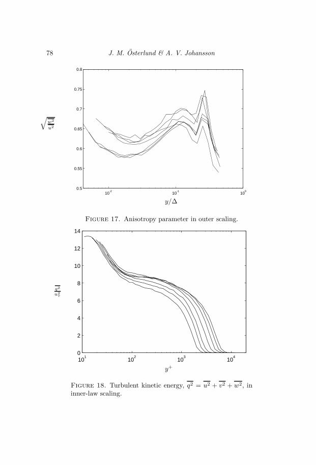
78 J. M. Osterlund & A. V. Johansson
10-2
10-1
100
0.5
0.55
0.6
0.65
0.7
0.75
0.8
√w2
u2
y/∆
Figure 17. Anisotropy parameter in outer scaling.
101
102
103
104
0
2
4
6
8
10
12
14
q2
u2τ
y+
Figure 18. Turbulent kinetic energy, q2 = u2 + v2 + w2, ininner-law scaling.

Turbulence Statistics 79
0 0.05 0.1 0.15 0.2 0.25 0.3 0.350
2
4
6
8
10
12
14
q2
u2τ
y/∆
Figure 19. Turbulent kinetic energy, q2 = u2 + v2 + w2, inouter-law scaling.
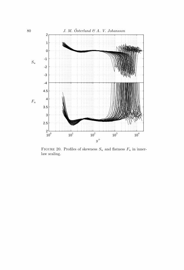
80 J. M. Osterlund & A. V. Johansson
-4
-3
-2
-1
0
1
2
100
101
102
103
104
2
2.5
3
3.5
4
4.5
Su
Fu
y+
Figure 20. Profiles of skewness Su and flatness Fu in inner-law scaling.

Turbulence Statistics 81
-4
-3
-2
-1
0
1
2
10-4
10-3
10-2
10-1
100
2
2.5
3
3.5
4
4.5
Su
Fu
y/∆
Figure 21. Profiles of skewness Su and flatness Fu in outer-law scaling.

82 J. M. Osterlund & A. V. Johansson
-5 -4 -3 -2 -1 0 1 2 3 4 50
0.25
0.5
0.75
1
1.25
1.5
1.75
2
2.25
2.5
2.75
Pu
u√u2
y+ = 5y/δ95 = 0.0012
y+ = 10y/δ95 = 0.0024
y+ = 20y/δ95 = 0.0048
y+ = 100y/δ95 = 0.0193
y+ = 500y/δ95 = 0.121
y+ = 828y/δ95 = 0.2
y+ = 3312y/δ95 = 0.8
y+ = 4140y/δ95 = 1.0
y+ = 4968y/δ95 = 1.2
Figure 22. Probability density functions for the streamwisevelocity at different distances from the wall. Reθ = 17800.

Turbulence Statistics 83
100
101
102
103
104
0
5
10
15
20
25
30
U [m/s]
y [mm]
Figure 23. Example mean velocity profile. Reθ = 17800.Dashed line enclose 95% of the samples.

84 J. M. Osterlund & A. V. Johansson
-4-3-2-1
01234
-4-3-2-1
01234
-4 -3 -2 -1 0 1 2 3 4
-4-3-2-1
01234
-4 -3 -2 -1 0 1 2 3 4
v√v2
v√v2
v√v2
u√u2
u√u2
y/∆ = 0.017 y/∆ = 0.035
y/∆ = 0.09 y/∆ = 0.14
y/∆ = 0.18 y/∆ = 0.21
Figure 24. Joint-probability density functions Puv, for thestreamwise and wall-normal velocities at different outer-scaleddistances from the wall. Reθ = 26600. Contours at ten levelswith logarithmic spacing, i.e. 10−3,−2.66,−2.33,... ,0.
Turbulence Statistics 85
8. Appendix: Measurements with a Parallel-Wire Probe
8.1. Motivation
The use of parallel-wire probes was initiated by the need for near-wall tur-bulence data at high Reynolds numbers where the turbulent scales are smalland the gradients are large. A conventional X-wire probe have severe problemsproblems in the near wall region mainly due to its large wall-normal dimensioncompared to the mean and fluctuating velocity gradients. Efforts have beenmade to miniaturize X-wire probes by several investigators, e.g. Willmarth &Bogar (1977). Osterlund (1995) found that thermal interaction between theheated wires in X-wire probes deteriorates the signal for Peclet numbers lessthan 50. The idea of parallel wires is instead to utilize the thermal interactionbetween the wires and calibrate the probe against the velocity and angle sim-ilarly to the procedure for X-wire probes. For this to work the parallel-wireprobe must always be operated in the under critical region of its transfer func-tion, as opposed to X-wire probes who must not have any thermal interaction.The result of this is that the wires have to be placed very closely togetherin order to achieve a reasonably high sensitivity and a flat response to highenough frequencies. The wall normal extent of the parallel-wire probe geom-etry is therefore only about 1/50 or less than that of an X-wire probe. Theinfluence from high velocity gradients at the wall is therefore much smaller.
8.2. Probe design and calibration
The body of the probe was built of a ceramic tube, designed for use in thermoelements, with 4 holes. The prong material was spring steel. The conical shapeof the prong tips was obtained in an etching process using a bath of nitric acid(60%) applying a small voltage to speed up the etching. The delicate position-ing of the prongs was done under a microscope (80x) with micro manipulatingequipment gearing down the hand movement. When the prongs are fixed inposition a low viscosity epoxy resin is applied. The capillary force pulls theresin into the probe body and fixes the prongs in position after hardening. Tofix the prongs together outside of the ceramic body a mixture of epoxy resinand colloidal silicon was applied. Before gluing the probe together the prongswere covered by a thin layer of solder to protect it from corrosion, also the sol-der is used later when the platinum wires are soldered onto the prong tips. Thesoldering is done by putting the etched piece of the Wollastone wire in position,by use of a micromanipulator, and then heating the prong with the solderingiron a few mm away until the solder melts. The diameter of the prong edge wasabout 20–30 µm. The wires were soldered on the inside of the prongs to makethe distance between the wires as small as possible, see figure 25. Extremecare has to be taken when positioning the prongs to assure that the wires areparallel.
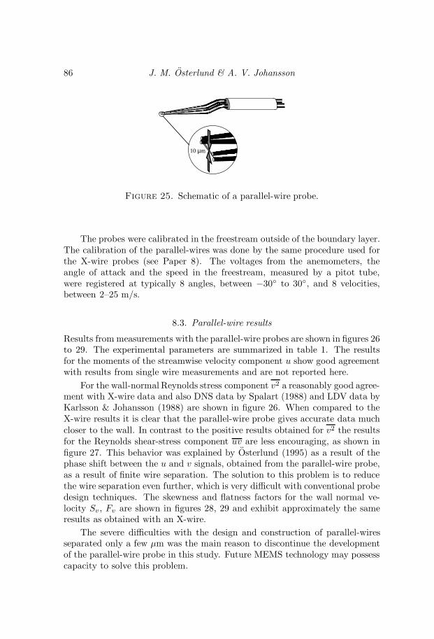
86 J. M. Osterlund & A. V. Johansson
10 µm
Figure 25. Schematic of a parallel-wire probe.
The probes were calibrated in the freestream outside of the boundary layer.The calibration of the parallel-wires was done by the same procedure used forthe X-wire probes (see Paper 8). The voltages from the anemometers, theangle of attack and the speed in the freestream, measured by a pitot tube,were registered at typically 8 angles, between −30 to 30, and 8 velocities,between 2–25 m/s.
8.3. Parallel-wire results
Results from measurements with the parallel-wire probes are shown in figures 26to 29. The experimental parameters are summarized in table 1. The resultsfor the moments of the streamwise velocity component u show good agreementwith results from single wire measurements and are not reported here.
For the wall-normal Reynolds stress component v2 a reasonably good agree-ment with X-wire data and also DNS data by Spalart (1988) and LDV data byKarlsson & Johansson (1988) are shown in figure 26. When compared to theX-wire results it is clear that the parallel-wire probe gives accurate data muchcloser to the wall. In contrast to the positive results obtained for v2 the resultsfor the Reynolds shear-stress component uv are less encouraging, as shown infigure 27. This behavior was explained by Osterlund (1995) as a result of thephase shift between the u and v signals, obtained from the parallel-wire probe,as a result of finite wire separation. The solution to this problem is to reducethe wire separation even further, which is very difficult with conventional probedesign techniques. The skewness and flatness factors for the wall normal ve-locity Sv, Fv are shown in figures 28, 29 and exhibit approximately the sameresults as obtained with an X-wire.
The severe difficulties with the design and construction of parallel-wiresseparated only a few µm was the main reason to discontinue the developmentof the parallel-wire probe in this study. Future MEMS technology may possesscapacity to solve this problem.

Turbulence Statistics 87
100
101
102
103
104
0
0.5
1
1.5
y+
√v2
uτ
Figure 26. Wall normal Reynolds stress, from parallel-wireprobe. For symbols, see table 1. ×: X-wire measurement,Reθ = 15100. : LDV Measurements in boundary layer flowat Reθ = 2420 by Karlsson & Johansson (1988). −−: Bound-ary layer simulation at Reθ = 1410 by Spalart (1988).
100
101
102
103
104
-0.4
-0.2
0
0.2
0.4
0.6
0.8
1
y+
−uvu2
τ
Figure 27. Reynolds shear stress from parallel-wire probe.For symbols, see table 1. −−: Boundary layer simulationat Reθ = 1410 by Spalart (1988). ×: X-wire measurement,Reθ = 15100. : LDV Measurements in boundary layer flowat Reθ = 2420 by Karlsson & Johansson (1988).

88 J. M. Osterlund & A. V. Johansson
Symbol d [µm] 1.27 1.27 2.54∆w [µm] 12 5 20l1 [µm] 230 230 280l2 [µm] 270 270 360Rc1 [Ω] 16.4 16.5 5.4Rc2 [Ω] 20 19.9 6.4x [m] 4.5 4.5 4.5U∞ [m/s] 25.3 25.6 25.1uτ [m/s] 0.894 0.905 0.892Reθ 13800 13900 13800∆+
w 0.7 0.3 1.2l+ 13.8 13.9 16.7l/d 181 181 112
Table 1. Parallel-wire experiments
9. Acknowledgments
The authors wish to thank Krister Alvelius and Martin Skote for providingus with DNS data, and Alexander Sahlin who participated in the parallel-wireexperiments. We wish to thank Mr. Ulf Landen and Mr. Marcus Gallstedt whohelped with the manufacturing of the experimental set-up. Financial supportfrom NUTEK and TFR is also gratefully acknowledged.
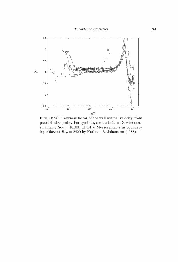
Turbulence Statistics 89
100
101
102
103
104
-1.5
-1
-0.5
0
0.5
1
1.5
y+
Sv
Figure 28. Skewness factor of the wall normal velocity, fromparallel-wire probe. For symbols, see table 1. ×: X-wire mea-surement, Reθ = 15100. : LDV Measurements in boundarylayer flow at Reθ = 2420 by Karlsson & Johansson (1988).

90 J. M. Osterlund & A. V. Johansson
100
101
102
103
104
2
3
4
5
6
7
8
9
10
y+
Fv
Figure 29. Flatness factor of the wall normal velocity, fromparallel-wire probe. For symbols, see table 1. ×: X-wire mea-surement, Reθ = 15100. : LDV Measurements in boundarylayer flow at Reθ = 2420 by Karlsson & Johansson (1988).

References
Alvelius, K. 1999 Studies of turbulence and its modeling through large eddy- anddirect numerical simulation. PhD thesis, Department of Mechanics, Royal Insti-tute of Technology, Stockholm.
Comte-Bellot, G. 1976 Hot-wire anemometry. Ann. Rev. Fluid Mech. 8, 209–231.
Fernholz, H. H. & Finley, P. J. 1996 The incompressible zero-pressure-gradientturbulent boundary layer: An assessment of the data. Prog. Aerospace Sci. 32,245–311.
Fernholz, H. H., Janke, G., Schober, M., Wagner, P. M. & Warnack, D.
1996 New developments and applications of skin-friction measuring techniques.Meas. Sci. Technol. 7, 1396–1409.
Gad-el-Hak, M. & Bandyopadhyay, P. R. 1994 Reynolds number effects in wall-bounded turbulent flows. Appl. Mech. Rev. 47 (8), 307–365.
Gresko, Jr., L. S. 1988 Characteristics of wall pressure and near-wall velocity in aflat plate boundary layer. Tech. Rep. 88-2. Fluid Dynamics Research LaboratoryReport.
Hites, M. H. 1997 Scaling of high-reynolds number turbulent boundary layers in thenational diagnostic facility. PhD thesis, Illinois Institute of Technology.
Johansson, A. V. 1992 A low speed wind-tunnel with extreme flow quality - designand tests. In Prog. ICAS congress 1992 , pp. 1603–1611. ICAS-92-3.8.1.
Johansson, A. V. & Alfredsson, P. H. 1982 On the structure of turbulent channelflow. J. Fluid Mech. 122, 295–314.
Johansson, A. V. & Alfredsson, P. H. 1983 Effects of imperfect spatial resolutionon measurements of wall-bounded turbulent shear flows. J. Fluid Mech. 137,409–421.
Karlsson, R. I. & Johansson, T. G. 1988 Ldv measurements of higher order mo-ments of velocity fluctuations in a turbulent boundary layer. In Laser Anemome-try in Fluid Mechanics . Ladoan-Instituto Superior Tecnico, 1096 L.C., Portugal.
Ligrani, P. M. & Bradshaw, P. 1987 Spatial resolution and measurement of tur-bulence in the viscous sublayer using subminiature hot-wire probes. Experimentsin Fluids 5, 407–417.
Millikan, C. B. 1938 A critical discussion of turbulent flows in channels and circulartubes. In Proceedings of the Fifth International Congress of applied Mechanics .
91
92 REFERENCES
Moser, R. D., Kim, J. & Mansour, N. N. 1999 Direct numerical simulation ofturbulent channel flow up to Reθ = 590. Phys. Fluids 11 (4), 943–945.
Osterlund, J. M. 1995 Dynamic behavior of hot-wire probes in turbulent boundarylayers. In Advances in turbulence V (ed. R. Benzi, (ed.)), pp. 398–402. Kluweracademic publishers.
Osterlund, J. M., Johansson, A. V., Nagib, H. M. & Hites, M. H. 1999 Wallshear stress measurements in high reynolds number boundary layers from twofacilities. In 30th AIAA Fluid Dynamics Conference, Norfolk, VA. AIAA paper99-3814.
Rotta, J. C. 1950 Uber die Theorie der Turbulenten Grenzschichten. Mitt. M.P.I.Strom. Forschung Nr 1, also available as NACA TM 1344.
Skote, M., Henkes, R. & Henningson, D. 1998 Direct numerical simulation ofself-similar turbulent boundary layers in adverse pressure gradients. In Flow,Turbulence and Combustion , , vol. 60, pp. 47–85. Kluwer Academic Publishers.
Smith, R. W. 1994 Effect of reynolds number on the structure of turbulent bound-ary layers. PhD thesis, Department of Mechanical and Aerospace Engineering,Princeton University, USA.
Spalart, P. R. 1988 Direct simulation of a turbulent boundary layer up to Reθ =1410. J. Fluid Mech. 187, 61–98.
Willmarth, W. W. & Bogar, T. J. 1977 Survey and new measurements of turbu-lent structure near the wall. Phys. Fluids 20 (10), 9–21.

Paper 4

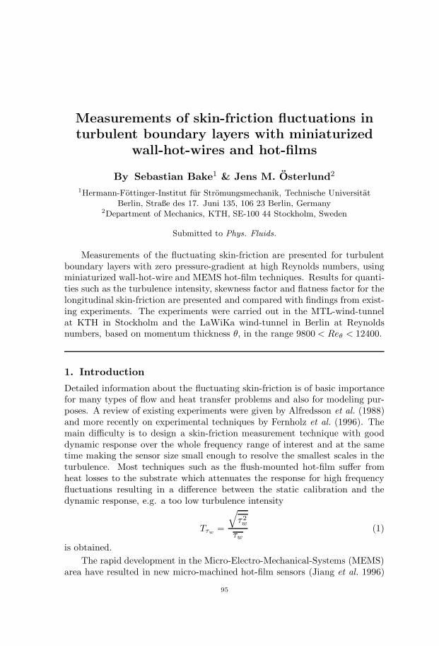
Measurements of skin-friction fluctuations inturbulent boundary layers with miniaturized
wall-hot-wires and hot-films
By Sebastian Bake1 & Jens M. Osterlund2
1Hermann-Fottinger-Institut fur Stromungsmechanik, Technische UniversitatBerlin, Straße des 17. Juni 135, 106 23 Berlin, Germany
2Department of Mechanics, KTH, SE-100 44 Stockholm, Sweden
Submitted to Phys. Fluids.
Measurements of the fluctuating skin-friction are presented for turbulentboundary layers with zero pressure-gradient at high Reynolds numbers, usingminiaturized wall-hot-wire and MEMS hot-film techniques. Results for quanti-ties such as the turbulence intensity, skewness factor and flatness factor for thelongitudinal skin-friction are presented and compared with findings from exist-ing experiments. The experiments were carried out in the MTL-wind-tunnelat KTH in Stockholm and the LaWiKa wind-tunnel in Berlin at Reynoldsnumbers, based on momentum thickness θ, in the range 9800 < Reθ < 12400.
1. Introduction
Detailed information about the fluctuating skin-friction is of basic importancefor many types of flow and heat transfer problems and also for modeling pur-poses. A review of existing experiments were given by Alfredsson et al. (1988)and more recently on experimental techniques by Fernholz et al. (1996). Themain difficulty is to design a skin-friction measurement technique with gooddynamic response over the whole frequency range of interest and at the sametime making the sensor size small enough to resolve the smallest scales in theturbulence. Most techniques such as the flush-mounted hot-film suffer fromheat losses to the substrate which attenuates the response for high frequencyfluctuations resulting in a difference between the static calibration and thedynamic response, e.g. a too low turbulence intensity
Tτw =
√τ2w
τw(1)
is obtained.The rapid development in the Micro-Electro-Mechanical-Systems (MEMS)
area have resulted in new micro-machined hot-film sensors (Jiang et al. 1996)
95

96 S. Bake & J. M. Osterlund
MTL LaWiKatest facility flat plate axisymmetric test sectionlength 7 m 6 mwidth 1.2 m d = 0.41mtemperature variations ∆T < 0.05 C < 0.1 Cfree stream turbulence TU∞ 0.02% 0.04%max U∞ 69 m/s 34 m/sprobe position X 5.5 m 4.3 m
Table 1. Basic characteristics of the MTL and LaWiKa wind-tunnels in Stockholm and Berlin.
where the heat flux to the substrate is being reduced by placing the hot-filmon a diaphragm on top of a vacuum cavity. Also the micro-machining technol-ogy allows for making very small hot-films to address the problem of spatialaveraging.
Instead of using flush-mounted hot-films Alfredsson et al. (1988) used ahot-wire on the wall, that is elevated only a few µm from the wall to reduce theheat flux to the wall. This technique has been further developed by Fernholzet al. (1996) and a large effort has been put into the design and constructionof miniaturized wall-hot-wire sensors for this type of experiment. The mainpurpose of this investigation is to determine statistical quantities of the skin-friction fluctuations in high Reynolds number turbulent boundary layers usingcurrent state-of-the-art hot-films and hot-wire-on-the-wall techniques.
2. The test facilities
Experimental results were obtained using two facilities, the MTL wind-tunnelat KTH and the LaWiKa wind tunnel at HFI. A brief description of the facilitiesand the experimental procedures are given below.
2.1. The set-up at KTH
Part of the experiments were carried out in the MTL-wind tunnel at the depart-ment of mechanics, KTH. The MTL-wind tunnel is specially designed to havegood flow uniformity and low turbulence level. The temperature is controlledto within ±0.05 C. The test section is 7 m long with a cross sectional area of 1m2 (1.2× 0.8m2). The top and bottom walls are adjustable in order to controlthe the streamwise velocity distribution in the test section. Special care havebeen taken to reduce acoustic noise and most of the walls have acoustic treat-ment. The velocity can be controlled between 0-69 m/s. For an overview of thebasic properties of the MTL wind-tunnel see table 1. For a detailed descriptionof the characteristics of the MTL wind-tunnel see Johansson (1992).

Skin-friction fluctuations in turbulent boundary layers 97
The boundary layer plate is a sandwich construction of aluminum sheet andaluminum square tubes and is divided into 7 sections and an adjustable flap thatextends into the first diffuser, giving a total length of the set-up of about 8.7 m.The first section has an elliptical nose (AR = 5) fixed at the leading edge. Twopressure taps in the elliptical nose are used to position the stagnation pointat the centerline of the plate. The positioning of the stagnation point is doneby the flap. The plate is mounted in the tunnel resting on two longitudinalbeams. It is positioned in a horizontal plane. By adjusting the position ofthe top and bottom walls of the tunnel the pressure gradient is minimized.The streamwise variation of the freestream velocity was less than 0.15% of thefreestream velocity at the leading edge of the plate. The measurement sectionof the plate was equipped with two circular inserts, for instrumentation and atraversing system.
The normal transition of the laminar boundary layer occurs at a positionseveral meters from the leading edge. To fix the transition close to the leadingedge a trip was introduced. The trip was selected to give transition at thetrip in the velocity range used in these experiments, and consisted of 8 rowsof Dymo brand embossing tape with the letter “V”. The two-dimensionalityof the boundary layer was checked by measuring the spanwise variation of thefriction velocity uτ , and it was found to be less than ±0.7%.
The mean wall-shear stress was determined by oil-film interferometry, seeFernholz et al. (1996) and Paper 8. The oil-film results was used to fit alogarithmic skin-friction-law of the type
cf = 2[
1κ
ln(Reθ) +C
]−2, (2)
with the resulting constants κ = 0.384 and C = 4.08. The skin friction variationwas found to be in good agreement with other methods including the new near-wall method by Osterlund and Johansson (Paper 8). The near-wall methodutilizes direct measurement of the velocity profiles in the similarity region nearthe wall (the buffer region) but outside the region where hot-wire measurementsin air are subjected to errors due to heat conduction to the wall. The profiles arethen fitted to a universal profile obtained from DNS in the interval 6 < y+ < 20.Results from the oil-film interferometry are shown in figure 1 together with datafrom HFI and the skin friction correlation by Fernholz & Finley (1996).
The mean flow characteristics of the boundary layer showed a well definedlogarithmic overlap region for Reynolds numbers (Reθ) above 6000 and werereported in Osterlund et al. (1999).
2.2. The set-up at HFI
The second part of the experiments was performed in the Laminar Wind Tunnel(LaWiKa) of the Hermann-Fottinger-Institute of Berlin Technical University.It is a closed-circuit tunnel with an axisymmetric test section made of Plexiglas

98 S. Bake & J. M. Osterlund
Reθ
cf
0 0.5 1 1.5 2 2.5 3
x 104
2
2.5
3
3.5
4x 10
-3
Figure 1. Skin-friction coefficient cf . and : KTH oil-film interferometry. –·–: best-fit of logarithmic friction law(equation 2) to the oil-film data. —: Skin-friction law fromFernholz & Finley (1996). : HFI Prestontube measurements.
tubes of various length with an inner diameter of 0.44 m and a total length of6 m. It has a centrifugal fan and an additional blower to remove the nozzleboundary layer at the entry of the test section. To reduce the noise levelin the wind tunnel the fan is mounted in a casing with sound attenuation.The bends are fitted with quarter circle turning vanes filled with mineral woolbetween perforated sheets. The test section has a sound muffler (quarter waveresonator) at the end to reduce the influence of fan-generated noise. In thesettling chamber a non-woven filter mat and a single, precisely manufactured,perforated metal plate (64 % open area ratio) are used for damping of flowdisturbances. The settling chamber is followed by a 2 m long axisymmetricnozzle with a 18:1 contraction ratio. The mean velocity distribution at theentry of the test section was uniform with a deviation from the mean < 1%.The flow temperature can be controlled with a water cooler. For an overviewof the basic characteristics of the LaWiKa see table 1. For a further descriptionof the flow quality see Fernholz & Warnack (1998). The boundary-layer underinvestigation starts at the elliptic leading edge of the test section and developsdownstream on its inner wall. It was tripped by means of a Velcro tape with aheight of 3 mm situated 0.24 m downstream the leading edge. Because of theaxisymmetric shape of the test section no corner-flow effects occur.

Skin-friction fluctuations in turbulent boundary layers 99
100 µm
Figure 2. Photograph of a type 2 wall-hot-wire. Wire length280µm, wire diameter 1.27µm and wire height above the wall35µm.
For the probe insert a streamwise slot of 20 mm width was milled alongone pipe section and filled with a series of interchangeable plugs. The Prestontubes, static taps and the wall hot-wires could be inserted in these plugs. Foran optimal flush mounting the wall hot-wire probes were inserted under amicroscope. The mean skin-friction values to calibrate the wall hot-wires weremeasured with Preston tubes (diameter between 1 and 2 mm) and are comparedwith the correlation by Fernholz & Finley (1996) in figure 1.
3. Sensor design
3.1. Wall-hot-wires
Three types of wall-hot-wire probe designs were used. The probe body of alltypes consists of a ceramic cylinder in a steel tube with 3 mm diameter. Theceramic isolates and holds the two prongs with the hot-wire. The first probedesign was a wire elevated from the wall soldered onto two prongs with largeseparation. The wire ends were gold-plated to obtain a length to diameter ratio> 200 for the active part of the wire with a diameter of 2.5 µm.
The second type had prong tips thinned down to 35 µm and polished flushwith the surface. The wire ends were fixed in two cones of solder plummetextending the prongs to the desired wire height, the active wire length nowbeing the distance between the solder cones (see figure 2). The wires (diameter1.27 and 0.64 µm) made of platinum-rhodium were not plated at the endsbecause of their mechanical infirmity.
The third and last type was designed like type two except that the wire waswelded directly onto the prongs polished flush with the surface. This results ina slightly bent wire with an average height above the wall of only a few µm.This type was first used by Alfredsson et al. (1988).
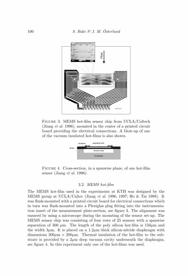
100 S. Bake & J. M. Osterlund
JMO 970127
19 21
1816
15 17
20 22
5 7GND
4 6 8
9 11
10 12
13
14
Flo
w
Figure 3. MEMS hot-film sensor chip from UCLA/Caltech(Jiang et al. 1996), mounted in the center of a printed circuitboard providing the electrical connections. A blow-up of oneof the vacuum insulated hot-films is also shown.
Figure 4. Cross-section, in a spanwise plane, of one hot-filmsensor (Jiang et al. 1996).
3.2. MEMS hot-film
The MEMS hot-film used in the experiments at KTH was designed by theMEMS group at UCLA/Caltec (Jiang et al. 1996, 1997; Ho & Tai 1998). Itwas flush-mounted with a printed circuit board for electrical connections whichin turn was flush-mounted into a Plexiglas plug fitting into the instrumenta-tion insert of the measurement plate-section, see figure 3. The alignment wasensured by using a microscope during the mounting of the sensor set-up. TheMEMS sensor chip was consisting of four rows of 25 sensors with a spanwiseseparation of 300 µm. The length of the poly silicon hot-film is 150µm andthe width 3µm. It is placed on a 1.2µm thick silicon-nitride diaphragm withdimensions 200µm × 200µm. Thermal insulation of the hot-film to the sub-strate is provided by a 2µm deep vacuum cavity underneath the diaphragm,see figure 4. In this experiment only one of the hot-films was used.

Skin-friction fluctuations in turbulent boundary layers 101
4. Experimental procedure
The wall-hot-wire and the hot-film was calibrated in the turbulent boundarylayer against the mean skin-friction obtained using oil-film interferometry orPreston tubes, here denoted τ∗w. A Kings law modified for near-wall effects(Fernholz et al. 1996) was used to relate the anemometer output voltage E andthe skin-friction τw,
τw =
(√u+
k14− k2 −
k12
)2
; u = (1B
(E2 − A))1/n (3)
where A, B, n, k1 and k2 are constants. The constants in equation 3 weredetermined minimizing the sum of the mean-square-error, for all calibrationpoints, between the measured mean skin-friction τ∗w and the mean value τwobtained applying relation 3 to the anemometer voltage signal E
min(∑
(τ∗w − τw)2). (4)
One example calibration is shown in figure 5. In the top half of the figurethe measured mean skin-friction τ∗w is shown against the mean anemometervoltages as circles. The stars represent the mean skin-friction values resultingfrom the calibration procedure of the wall-hot-wire or hot film. The dottedline is the resulting calibration function (equation 3), note that it does notneed to go through the calibration circles since it is the sum of the squareddistances between the stars and the circles that is minimized. In the bottomhalf of the figure the probability density for the anemometer voltage PE isshown. The long tails of the probability density results in a required calibrationinterval for the mean skin-friction from 0.3 to 3 times the value of interest, toavoid extrapolation of the calibration function outside of the calibration limits(dashed lines in figure 5). No extrapolation was used.
5. Experimental results
An overview of the skin-friction experiments carried out in the MTL andLaWiKa wind-tunnels are compiled in table 2 where also symbols are intro-duced. The demand for a large calibration range restricts the investigation toessentially one Reynolds number for each set-up implying that no Reynoldsnumber trends can be extracted from the present data.
In figure 6 results for the skin-friction intensity Tτw are presented, for allexperiments performed in this investigation, against the active sensor length inviscous units. The data show a similar decrease in intensity for increasing probedimensions as a result of spatial averaging (see e.g. Johansson & Alfredsson1983; Ligrani & Bradshaw 1987). The limiting value of the turbulent intensityfor small probe lengths is here found to be about 0.41. For comparison the

102 S. Bake & J. M. Osterlund
E [V]
PE
τw [N/m2]
0
1
2
3
4
1.5 1.55 1.6 1.65 1.7 1.75 1.8 1.85 1.90
5
10
15
Figure 5. Calibration and measurement procedure. : Meanskin-friction from oil-film or Preston tube. · · · : The fitted re-lation between anemometer voltage and skin-friction, equa-tion 3. ∗: Mean skin-friction from hot-wire/hot-film calculatedfrom the anemometer voltage signal using relation 3. -: Prob-ability density function for the anemometer voltage signal (atE = 1.61 V and τw = 0.69N/m2 ).
results from the wall-hot-wire experiments at MIT in a turbulent boundarylayer in air flow by Alfredsson et al. (1988) are also shown in figure 6 and showgood agreement with the present data.The resulting intensity from the MEMShot-film of 0.35 is more than 10% too low and can probably be attributed toremaining heat losses in the diaphragm that modifies the dynamic responsecompared to the static one. Still, the result represents a major improvementcompared to previous findings using hot-films in air where values of about 0.1are reported for the relative intensity of the wall shear stress fluctuations. Also,the rapid development in MEMS technology will probably lead towards largeimprovements in the near future. The wall-hot-wire of type 3, with the wirewelded onto prongs flush with the wall, show a behavior similar to the hot-film. The plausible explanation being that heat flux from the wire, which isonly a few µm above the wall, is partly absorbed by the wall and transferred

Skin-friction fluctuations in turbulent boundary layers 103
Symbol Probe Reθ d l l/d h l+ h+ Facility
type [µm] [µm] [µm]
WW1 12400 2.54 500 200 40 25 2 MTL
+ WW3 12400 1.27 200 160 5 10 0.25 MTL× MHF 12400 – 150 – – 7.5 – MTL
WW2 12400 1.27 200 160 35 12 1.2 MTL• WW1 9800 2.54 500 200 40 24 1.9 LaWiKa
N WW2 9800 1.27 200 160 40 10 1.9 LaWiKa WW2 9800 1.27 280 220 35 13 1.7 LaWiKa
WW2 9800 0.64 130 200 40 6.2 1.9 LaWiKaH WW2 9800 0.64 140 220 40 6.7 1.9 LaWiKa
Table 2. Skin-friction measurements at KTH and HFI. WW:wall-hot-wire (number represents the type, see section 3.1).MHF: MEMS hot-film.
l+
Tτw
0 10 20 30 40 50 600.2
0.25
0.3
0.35
0.4
0.45
Figure 6. Turbulent skin friction intensity Tτw . For symbols,see table 2. 2: experiment by Alfredsson et al. (1988).
back to the fluid, in a mechanism similar to that for the hot-film. A connectedissue is that the sensitivity of type 3 wall-hot-wires is very low due to dampingresulting from the proximity of the wall.
Results for the Skewness and Flatness factors are presented in figure 7. Noobvious trend, similar to the one found for the intensity, associated with thewire length is visible in the data and the values for the Skewness factor and

104 S. Bake & J. M. Osterlund
l+
Sτw
Fτw
0.4
0.6
0.8
1
1.2
0 5 10 15 20 25 303
3.5
4
4.5
5
5.5
Figure 7. Skewness Sτw and Flatness Fτw factors for the fluc-tuating skin-friction. For symbols, see table 2.
for the Flatness factor are estimated as an average to be about 1.1 and 4.9,respectively. This is in good agreement with Alfredsson et al. (1988) who foundthe values 1.0 and 4.8.
6. Concluding Remarks
Based on the set of skin-friction measurements carried out using a variety ofprobe designs in two facilities it can be concluded that for Reynolds numbersof around 10,000 the streamwise fluctuating skin-friction intensity Tτw is closeto 0.41. And that the values of the Skewness and Flatness factors are about1.1 and 4.9, respectively.
The resulting skin-friction intensity from the MEMS type hot-film of 0.35 isa major improvement over existing types of hot-films with previously reportedvalues of the fluctuating skin-friction intensity in air of about 0.1.The MEMStype hot-film and the wall-hot-wire of type 3, with the wire very close to thewall, both exhibits similar behavior and roughly 10% too low value for thefluctuating skin-friction intensity, it is believed to be a result of heat flux inthe diaphragm, or in the wall-wire case heat flux to the wall, and back to theflow, resulting in a difference between static and dynamic responses.

Skin-friction fluctuations in turbulent boundary layers 105
7. Acknowledgments
The authors wish to thank Professor Chih-Ming Ho at UCLA for providing uswith the MEMS hot-film probe. We wish to thank Mr. Ulf Landen and Mr.Marcus Gallstedt who helped with the manufacturing of the experimental set-up at KTH. Financial support from NUTEK and TFR for the KTH experimentis also gratefully acknowledged. We would like to thank Mr. Albrecht Ebnerfor exploring new dimensions while manufacturing the micro wall hot-wiresat HFI. A visit to KTH in Stockholm was financed by the DAAD within acooperation project between Sweden and Germany.

References
Alfredsson, P. H., Johansson, A. V., Haritonidis, J. H. & Eckelmann, H.
1988 The fluctuation wall-shear stress and the velocity field in the viscous sub-layer. Phys. Fluids A 31, 1026–33.
Fernholz, H. & Warnack, D. 1998 The effect of a favourable pressure gradient andof the Reynolds number on an incompressible axissymmetric turbulent boundarylayer. Part 1. The turbulent boundary layer. J. Fluid Mech. 359, 329–356.
Fernholz, H. H. & Finley, P. J. 1996 The incompressible zero-pressure-gradientturbulent boundary layer: An assessment of the data. Prog. Aerospace Sci. 32,245–311.
Fernholz, H. H., Janke, G., Schober, M., Wagner, P. M. & Warnack, D.
1996 New developments and applications of skin-friction measuring techniques.Meas. Sci. Technol. 7, 1396–1409.
Ho, C.-M. & Tai, Y.-C. 1998 Micro-electro-mechanical-systems (MEMS) and fluidflows. Ann. Rev. Fluid Mech. 30, 579–612.
Jiang, F., Tai, Y.-C., Gupta, B., Goodman, R., Tung, S., Huang, J. B. & Ho,
C.-M. 1996 A surface-micromachined shear stress imager. In 1996 IEEE MicroElectro Mechanical Systems Workshop (MEMS ’96), pp. 110–115.
Jiang, F., Tai, Y.-C., Walsh, K., Tsao, T., Lee, G. B. & Ho, C.-H. 1997 Aflexible mems technology and its first application to shear stress sensor skin.In 1997 IEEE Micro Electro Mechanical Systems Workshop (MEMS ’97), pp.465–470.
Johansson, A. V. 1992 A low speed wind-tunnel with extreme flow quality - designand tests. In Prog. ICAS congress 1992 , pp. 1603–1611. ICAS-92-3.8.1.
Johansson, A. V. & Alfredsson, P. H. 1983 Effects of imperfect spatial resolutionon measurements of wall-bounded turbulent shear flows. J. Fluid Mech. 137,409–421.
Ligrani, P. M. & Bradshaw, P. 1987 Spatial resolution and measurement of tur-bulence in the viscous sublayer using subminiature hot-wire probes. Experimentsin Fluids 5, 407–417.
Osterlund, J. M., Johansson, A. V., Nagib, H. M. & Hites, M. H. 1999 Wallshear stress measurements in high reynolds number boundary layers from twofacilities. In 30th AIAA Fluid Dynamics Conference, Norfolk, VA. AIAA paper99-3814.
106

Paper 5

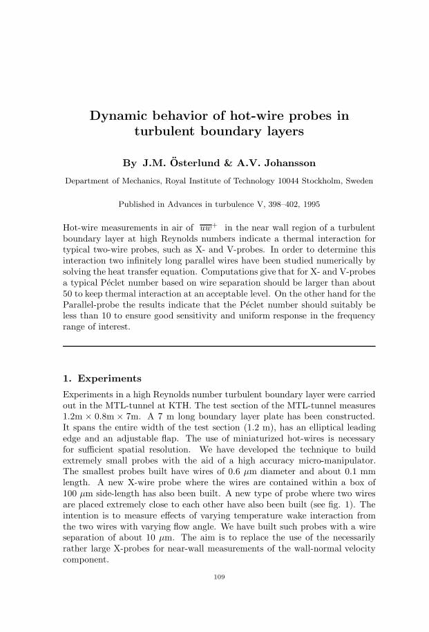
Dynamic behavior of hot-wire probes inturbulent boundary layers
By J.M. Osterlund & A.V. Johansson
Department of Mechanics, Royal Institute of Technology 10044 Stockholm, Sweden
Published in Advances in turbulence V, 398–402, 1995
Hot-wire measurements in air of uw+ in the near wall region of a turbulentboundary layer at high Reynolds numbers indicate a thermal interaction fortypical two-wire probes, such as X- and V-probes. In order to determine thisinteraction two infinitely long parallel wires have been studied numerically bysolving the heat transfer equation. Computations give that for X- and V-probesa typical Peclet number based on wire separation should be larger than about50 to keep thermal interaction at an acceptable level. On the other hand for theParallel-probe the results indicate that the Peclet number should suitably beless than 10 to ensure good sensitivity and uniform response in the frequencyrange of interest.
1. Experiments
Experiments in a high Reynolds number turbulent boundary layer were carriedout in the MTL-tunnel at KTH. The test section of the MTL-tunnel measures1.2m × 0.8m × 7m. A 7 m long boundary layer plate has been constructed.It spans the entire width of the test section (1.2 m), has an elliptical leadingedge and an adjustable flap. The use of miniaturized hot-wires is necessaryfor sufficient spatial resolution. We have developed the technique to buildextremely small probes with the aid of a high accuracy micro-manipulator.The smallest probes built have wires of 0.6 µm diameter and about 0.1 mmlength. A new X-wire probe where the wires are contained within a box of100 µm side-length has also been built. A new type of probe where two wiresare placed extremely close to each other have also been built (see fig. 1). Theintention is to measure effects of varying temperature wake interaction fromthe two wires with varying flow angle. We have built such probes with a wireseparation of about 10 µm. The aim is to replace the use of the necessarilyrather large X-probes for near-wall measurements of the wall-normal velocitycomponent.
109
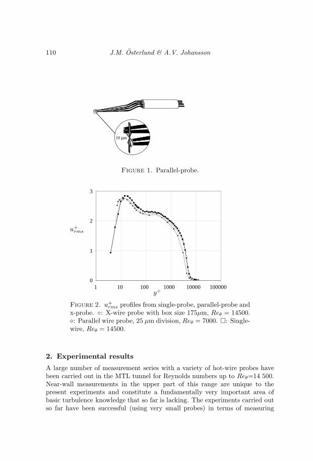
110 J.M. Osterlund & A.V. Johansson
10 µm
Figure 1. Parallel-probe.
0
1
2
3
1 10 100 1000 10000 100000y+
u+rms
Figure 2. u+rms profiles from single-probe, parallel-probe andx-probe. : X-wire probe with box size 175µm, Reθ = 14500.: Parallel wire probe, 25 µm division, Reθ = 7000. : Single-wire, Reθ = 14500.
2. Experimental results
A large number of measurement series with a variety of hot-wire probes havebeen carried out in the MTL tunnel for Reynolds numbers up to Reθ=14 500.Near-wall measurements in the upper part of this range are unique to thepresent experiments and constitute a fundamentally very important area ofbasic turbulence knowledge that so far is lacking. The experiments carried outso far have been successful (using very small probes) in terms of measuring
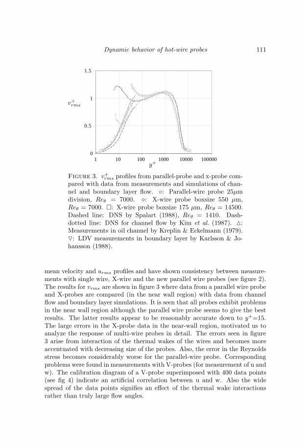
Dynamic behavior of hot-wire probes 111
0
0.5
1
1.5
1 10 100 1000 10000 100000y+
v+rms
Figure 3. v+rms profiles from parallel-probe and x-probe com-pared with data from measurements and simulations of chan-nel and boundary layer flow. : Parallel-wire probe 25µmdivision, Reθ = 7000. : X-wire probe boxsize 550 µm,Reθ = 7000. : X-wire probe boxsize 175 µm, Reθ = 14500.Dashed line: DNS by Spalart (1988), Reθ = 1410. Dash-dotted line: DNS for channel flow by Kim et al. (1987). :Measurements in oil channel by Kreplin & Eckelmann (1979).: LDV measurements in boundary layer by Karlsson & Jo-hansson (1988).
mean velocity and urms profiles and have shown consistency between measure-ments with single wire, X-wire and the new parallel wire probes (see figure 2).The results for vrms are shown in figure 3 where data from a parallel wire probeand X-probes are compared (in the near wall region) with data from channelflow and boundary layer simulations. It is seen that all probes exhibit problemsin the near wall region although the parallel wire probe seems to give the bestresults. The latter results appear to be reasonably accurate down to y+=15.The large errors in the X-probe data in the near-wall region, motivated us toanalyze the response of multi-wire probes in detail. The errors seen in figure3 arise from interaction of the thermal wakes of the wires and becomes moreaccentuated with decreasing size of the probes. Also, the error in the Reynoldsstress becomes considerably worse for the parallel-wire probe. Correspondingproblems were found in measurements with V-probes (for measurement of u andw). The calibration diagram of a V-probe superimposed with 400 data points(see fig 4) indicate an artificial correlation between u and w. Also the widespread of the data points signifies an effect of the thermal wake interactionsrather than truly large flow angles.

112 J.M. Osterlund & A.V. Johansson
0.75
0.8
0.85
0.9
0.95
1
1.05
0.75 0.8 0.85 0.9 0.95 1 1.05
0
-40
40
2 m/s
26 m/s
30 m/s
E1
E2
Figure 4. Calibration plot for the V-probe, superimposedwith 4000 data samples taken at y+ = 6, U∞ = 27 m/s, X =5.5 m, Reθ = 14500
3. Numerical simulation of Parallel-probe
An implicit algorithm for the two dimensional heat-transport equation hasbeen implemented. An implicit algorithm would avoid most of the stability re-strictions of an explicit scheme, but have the problem of achieving an efficientsolution algorithm. The use of an operator splitting method (time-splitting)provides a way to get around this problem. By splitting each time-step into twohalf-steps where at each half step only terms associated with a particular coor-dinate direction are treated implicitly, only three implicit terms appear groupedon the main diagonal of the linear system. The efficient Thomas algorithm canbe used to solve the system. Here a split formulation of the two-dimensionaltransport equation with a two-level Crank-Nicolson finite difference scheme isused on a rectangular grid. Constant temperature anemometry is simulatedby forcing the temperature on the hot-wires to be constant. The fluctuatingvelocities in the turbulent boundary layer is simulated by a homogeneous ve-locity field, ?v = (U cosα, U sinα), α = αmax sin 2πft. The heat flux from thewires is calculated at each time-step. The thermal interaction, if any, gives adifference in heat flux between the two wires.
4. Results from numerical investigation of probecharacteristics
Computations were carried out for the case described above with two pointsources of heat separated by a distance of δ. This can either be regarded as anidealized model of a V-probe were the two wires have been idealized to pointsources or as a more realistic model for a parallel-wire probe. A simple analysis

Dynamic behavior of hot-wire probes 113
10-2
10-1
100
101
102
10-10
10-8
10-6
10-4
10-2
100
Pe=5
Pe=10
Pe=20
Pe=40
S = fδU
∣∣∣ GGcoslaw
∣∣∣
Figure 5. Amplitude of the transfer function G for the re-sponse in v velocity normalized with the response of an idealX- or V-probe.
of the situation yields that the results should best be described in terms of Nus-selt numbers for the two wires as functions of two parameters, viz. the Pecletnumber of the probe Pe = Uδ
κand the Strouhal number S = fδ
U. The results
of the computations are shown in figure 5 in terms of the maximum differencein Nusselt number between the two wires normalized with the correspondingdifference for an ideal V-probe. This means that the curves can be interpretedas the sensitivity obtained with a parallel-wire probe normalized with that ofan ideal V- (or X-) probe.
The phase shift of the parallel-probe (see fig 6) occurs at lower frequencythan the decrease in magnitude. This indicates that correlations like uv maybee more sensitive to errors.
One may illustrate the above mentioned limitations by the situation in anairflow boundary layer at y+ = 3 and a probe length L=0.2 mm. For a freestream velocity of 25 m/s the viscous length scale (at x=5 m) is roughly 0.015mm (giving L+ ≈ 13). The Peclet number at this position becomes about 28.A Strouhal number of 0.1 here corresponds to 1.5 kHz, which indicates thatproblems are likely to occur in this case.
5. Conclusions
For X- and V-probes the computations indicate that thermal interaction be-tween the wire-wakes deteriorate the results for Peclet numbers below 50. Forparallel-wire probes on the other hand the results suggest that the Peclet num-ber should suitably be less than 10. At a Pe of 5 the parallel wire has about50 % of the sensitivity of an x or v-probe. It is also clearly seen from figure

114 J.M. Osterlund & A.V. Johansson
10-2
100
102
104
0
0.5
1
10-2
100
102
104
-2
-1
0
S = fδU
∣∣∣ GG0
∣∣∣
argG
Figure 6. Frequency-response of parallel-probe normalizedwith response at zero frequency. Pe=10.
5 that a static calibration only is valid up to Strouhal numbers of about 0.1(f < 0.1U
δ).
Financial support from NUTEK is gratefully acknowledged.

References
Gresko, Jr., L. S. 1988 Characteristics of wall pressure and near-wall velocity in aflat plate boundary layer. Tech. Rep. 88-2. Fluid Dynamics Research LaboratoryReport.
Karlsson, R. I. & Johansson, T. G. 1988 Ldv measurements of higher order mo-ments of velocity fluctuations in a turbulent boundary layer. In Laser Anemome-try in Fluid Mechanics . Ladoan-Instituto Superior Tecnico, 1096 L.C., Portugal.
Kim, J., Moin, P. & Moser, R. 1987 Turbulence statistics in fully developed channelflow. J. Fluid Mech. 177, 133–166.
Kreplin, H.-P. & Eckelmann, H. 1979 Behavior of the three fluctuating velocitycomponents in the wall region of a turbulent channel flow. Phys. Fluids 22 (7).
Spalart, P. R. 1988 Direct simulation of a turbulent boundary layer up to Reθ =1410. J. Fluid Mech. 187, 61–98.
Willmarth, W. W. & Bogar, T. J. 1977 Survey and new measurements of turbu-lent structure near the wall. Phys. Fluids 20 (10), 9–21.
115


Paper 6


Flow structures in zero pressure-gradientturbulent boundary layers.
By Jens M. Osterlund, Bjorn Lindgren & Arne V. Johansson
Dept. of Mechanics, KTH, SE-100 44 Stockholm, Sweden
To be submitted
An experimental investigation on flow structures was performed in a high Rey-nolds number zero pressure-gradient turbulent boundary layer. Results arepresented for the fluctuating wall-shear stress obtained simultaneously at twospanwise positions using a micro-machined hot-film sensor. Two-point correla-tions are presented and the mean streak spacing is evaluated from the two-pointcorrelation of high-pass filtered wall-shear-stress signals. The streak spacingwas found to be approximately 110ν/uτ at the Reynolds number Reθ = 9700.
Experiments involving the simultaneous measurement of the wall-shearstress and the streamwise velocity component in an array of points in thestreamwise-wall normal (x, y)-plane, directly above the hot-film, was also con-ducted. Results are presented for the conditionally averaged velocity field ob-tained by detecting turbulence generating events from the wall-shear stress,and two-point correlation measurements between the wall-shear stress and thestreamwise velocity. Local propagation velocities and details of shear-layerstructures are presented.
The scaling of the occurrence of VITA events in the buffer layer was inves-tigated and a mixed time scale (i.e. the geometric mean of the inner and outertimescale) was found to give a satisfactory collapse of the data.
1. Introduction
The statistical, Reynolds averaged, description of turbulent boundary layershides a wealth of structure-related phenomena and a quite intermittent char-acter of e.g. turbulence production. This has been illustrated in flow visu-alizations, measurements and from DNS-generated data in a large number ofpapers, see e.g. the landmark paper of Kline et al. (1967), who showed that asignificant part of the turbulence could be described in terms of deterministicevents. These studies showed that in the close proximity of the wall the flow ischaracterized by elongated regions of low and high speed fluid of fairly regularspanwise spacing of about λ+ = 100. Sequences of ordered motion occur ran-domly in space and time where the low-speed streaks begin to oscillate and to
119

120 J. M. Osterlund, B. Lindgren & A. V. Johansson
suddenly break-up into a violent motion, a “burst”. Kim et al. (1971) showedthat the intermittent bursting process is closely related to shear-layer like flowstructures in the buffer region, and also that roughly 70% of the total turbu-lence production was associated with the bursting process. The “bursts” werefurther investigated by Corino & Brodkey (1969) and it was found that twokinds of turbulence producing events are present. The ejection: involving rapidoutflow of low speed fluid from the wall and sweeps: large scale motions orig-inating in the outer region flowing down to the wall. Smith & Metzler (1983)investigated the characteristics of low-speed streaks using hydrogen bubble-flowand a high-speed video system. They found that the streak spacing increasedwith the distance from the wall. Furthermore, they found that the persistenceof the streaks was one order of magnitude longer than the the observed burstingtimes associated with the wall region turbulence production.
To obtain quantitative data to describe the structures a reliable methodto identify bursts with velocity or wall-shear stress measurements is needed.Conditional averaging using some triggering signal can be used to study indi-vidual events such as bursts or ejections and was first employed by Kovasznayet al. (1970). The triggering signal must be intermittent and closely associatedwith the event under study. Wallace et al. (1972) and Willmart & Lu (1972)introduced the uv quadrant splitting scheme. Blackwelder & Kaplan (1976)developed the VITA technique to form a localized measure of the turbulent ki-netic energy and used it to detect shear-layer events. The detected events werestudied using conditional averaging. Chen & Blackwelder (1978) added a slopecondition to the VITA technique to detect only events corresponding to rapidacceleration. The behavior of the conditionally averaged streamwise velocitydetected on strong accelerating events may be explained by tilted shear-layersthat are convected past the sensor. Kreplin & Eckelmann (1979) measured theangle of the shear-layer front from the wall and found that nearest to the wall itwas about 5. At larger distances from the wall Head & Bandyopadhyay (1981)found the angle to be much steeper, about 45. Gupta et al. (1971) investi-gated the spatial structure in the viscous sub-layer using an array of hot-wiresdistributed in the spanwise direction. They used a VITA correlation techniqueto determine the spanwise separations between streaks in the viscous-sub layer.The evolution of shear layers was studied by Johansson et al. (1987a) in theGottingen oil channel by use of two-probe measurements in the buffer regionof the turbulent channel flow. The bursting frequency in turbulent boundarylayers was first investigated by Rao et al. (1971), their experiments indicatedthat outer scaling gave the best collapse of the data. Later, Blackwelder &Haritonidis (1983) carried out experiments on the bursting frequency in tur-bulent boundary layers. They found the non-dimensional bursting frequencywas independent of Reynolds number when scaled with the inner time scaleand found a strong effect of spatial averaging for sensors larger than 20 viscous
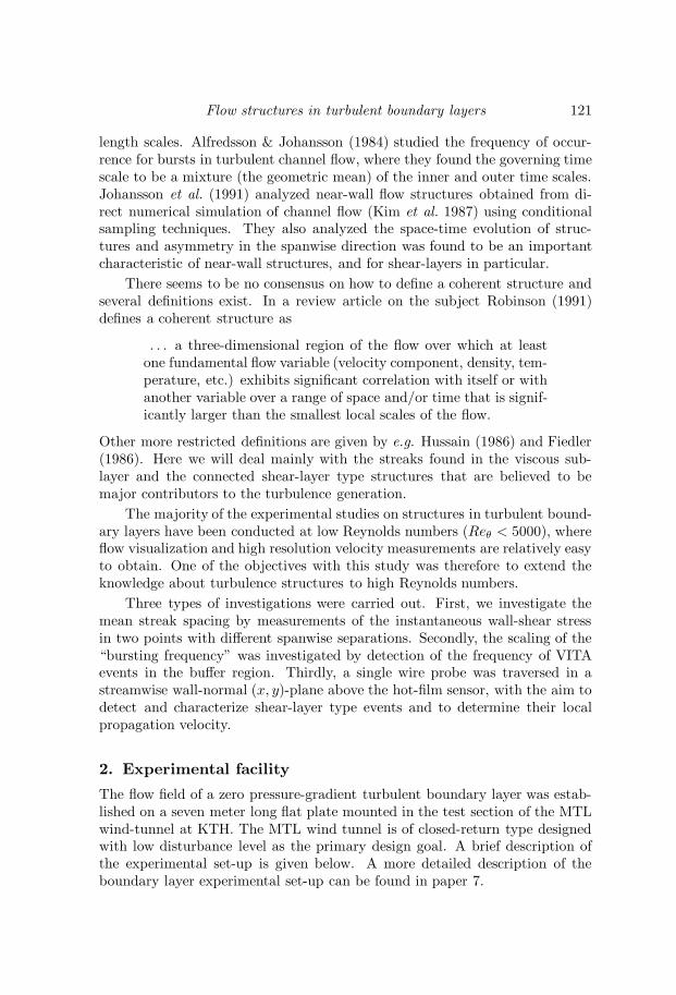
Flow structures in turbulent boundary layers 121
length scales. Alfredsson & Johansson (1984) studied the frequency of occur-rence for bursts in turbulent channel flow, where they found the governing timescale to be a mixture (the geometric mean) of the inner and outer time scales.Johansson et al. (1991) analyzed near-wall flow structures obtained from di-rect numerical simulation of channel flow (Kim et al. 1987) using conditionalsampling techniques. They also analyzed the space-time evolution of struc-tures and asymmetry in the spanwise direction was found to be an importantcharacteristic of near-wall structures, and for shear-layers in particular.
There seems to be no consensus on how to define a coherent structure andseveral definitions exist. In a review article on the subject Robinson (1991)defines a coherent structure as
. . . a three-dimensional region of the flow over which at leastone fundamental flow variable (velocity component, density, tem-perature, etc.) exhibits significant correlation with itself or withanother variable over a range of space and/or time that is signif-icantly larger than the smallest local scales of the flow.
Other more restricted definitions are given by e.g. Hussain (1986) and Fiedler(1986). Here we will deal mainly with the streaks found in the viscous sub-layer and the connected shear-layer type structures that are believed to bemajor contributors to the turbulence generation.
The majority of the experimental studies on structures in turbulent bound-ary layers have been conducted at low Reynolds numbers (Reθ < 5000), whereflow visualization and high resolution velocity measurements are relatively easyto obtain. One of the objectives with this study was therefore to extend theknowledge about turbulence structures to high Reynolds numbers.
Three types of investigations were carried out. First, we investigate themean streak spacing by measurements of the instantaneous wall-shear stressin two points with different spanwise separations. Secondly, the scaling of the“bursting frequency” was investigated by detection of the frequency of VITAevents in the buffer region. Thirdly, a single wire probe was traversed in astreamwise wall-normal (x, y)-plane above the hot-film sensor, with the aim todetect and characterize shear-layer type events and to determine their localpropagation velocity.
2. Experimental facility
The flow field of a zero pressure-gradient turbulent boundary layer was estab-lished on a seven meter long flat plate mounted in the test section of the MTLwind-tunnel at KTH. The MTL wind tunnel is of closed-return type designedwith low disturbance level as the primary design goal. A brief description ofthe experimental set-up is given below. A more detailed description of theboundary layer experimental set-up can be found in paper 7.

122 J. M. Osterlund, B. Lindgren & A. V. Johansson
After the test section the flow passes through diffusers and two 90 turns be-fore the fan. A large fraction of the wind-tunnel return circuit is equipped withnoise-absorbing walls to reduce acoustic noise. The flow quality of the MTLwind-tunnel was reported by Johansson (1992). For instance, the streamwiseturbulence intensity was found to be less than 0.02%. The air temperature canbe controlled to within ±0.05 C, which is very important for this study sincethe primary measurement technique was hot-wire/hot-film anemometry, wherea constant air temperature during the measurement is a key issue. The testsection has a cross sectional area of 0.8 m × 1.2 m (height × width) and is 7 mlong. The upper and lower walls of the test section can be moved to adjust thepressure distribution. The maximum variation in mean velocity distributionalong the boundary layer plate was ±0.15%.
The plate is a sandwich construction of aluminum sheet metal and squaretubes in seven sections plus one flap and one nose part, with the dimensions 1.2m wide and 7 m long excluding the flap. The flap is 1.5 m long and is mountedin the following diffuser. This arrangement makes it possible to use the first5.5 m of the plate for the experiment. One of the plate sections was equippedwith two circular inserts, one for a plexiglas plug where the measurements weredone, and one for the traversing system. The traversing system was fixed tothe plate to minimize any vibrations and possible deflections. The distance tothe wall from the probe was determined by a high magnification microscope.The absolute error in the determination of the wall distance was within ±5µm.
The boundary layer was tripped at the beginning of the plate and the two-dimensionality of the boundary layer was checked by measuring the spanwisevariation of the wall shear stress τw. The maximum spanwise variation infriction velocity uτ =
√τw/ρ was found to be less than ±0.7%.
The ambient conditions were monitored by the measurement computerduring the experiments using an electronic barometer and thermometer (FCO510 from Furness Ltd., UK). The reference conditions used in the calibrationof the probes were determined using a Prandtl tube in the free-stream directlyabove the measurement station. The pressure and temperature were monitoredat all times during the experiments using a differential pressure transducer anda thermometer connected directly to the measurement computer. The accuracyof the pressure measurement was 0.25 % and the accuracy of the temperaturemeasurement was 0.02 C.
Constant temperature hot-wire anemometry was used in all velocity mea-surements. All hot-wire probes were designed and built at the lab. Three sizesof single-wire probes were used in the experiments with wire diameters of: 2.5,1.27 and 0.63 µm and a length to diameter ratio always larger than 200.
The MEMS hot-film (figure 1) used in the wall-shear stress measurementswas designed by the MEMS group at UCLA/Caltec (Jiang et al. 1996, 1997; Ho& Tai 1998). It was flush-mounted with a printed circuit board for electrical
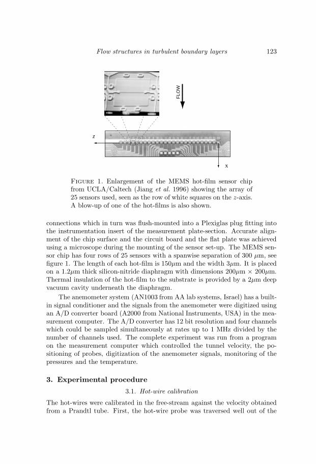
Flow structures in turbulent boundary layers 123
x
z
FLO
WFigure 1. Enlargement of the MEMS hot-film sensor chipfrom UCLA/Caltech (Jiang et al. 1996) showing the array of25 sensors used, seen as the row of white squares on the z-axis.A blow-up of one of the hot-films is also shown.
connections which in turn was flush-mounted into a Plexiglas plug fitting intothe instrumentation insert of the measurement plate-section. Accurate align-ment of the chip surface and the circuit board and the flat plate was achievedusing a microscope during the mounting of the sensor set-up. The MEMS sen-sor chip has four rows of 25 sensors with a spanwise separation of 300 µm, seefigure 1. The length of each hot-film is 150µm and the width 3µm. It is placedon a 1.2µm thick silicon-nitride diaphragm with dimensions 200µm × 200µm.Thermal insulation of the hot-film to the substrate is provided by a 2µm deepvacuum cavity underneath the diaphragm.
The anemometer system (AN1003 from AA lab systems, Israel) has a built-in signal conditioner and the signals from the anemometer were digitized usingan A/D converter board (A2000 from National Instruments, USA) in the mea-surement computer. The A/D converter has 12 bit resolution and four channelswhich could be sampled simultaneously at rates up to 1 MHz divided by thenumber of channels used. The complete experiment was run from a programon the measurement computer which controlled the tunnel velocity, the po-sitioning of probes, digitization of the anemometer signals, monitoring of thepressures and the temperature.
3. Experimental procedure
3.1. Hot-wire calibration
The hot-wires were calibrated in the free-stream against the velocity obtainedfrom a Prandtl tube. First, the hot-wire probe was traversed well out of the
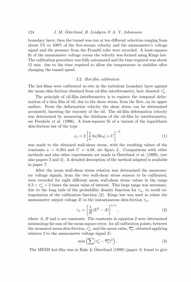
124 J. M. Osterlund, B. Lindgren & A. V. Johansson
boundary layer, then the tunnel was run at ten different velocities ranging fromabout 5% to 100% of the free-stream velocity and the anemometer’s voltagesignal and the pressure from the Prandtl tube were recorded. A least-squaresfit of the anemometer voltage versus the velocity was formed using Kings law.The calibration procedure was fully automated and the time required was about15 min. due to the time required to allow the temperature to stabilize afterchanging the tunnel speed.
3.2. Hot-film calibration
The hot-films were calibrated in-situ in the turbulent boundary layer againstthe mean skin-friction obtained from oil-film interferometry, here denoted τ∗w.
The principle of oil-film interferometry is to register the temporal defor-mation of a thin film of oil, due to the shear stress, from the flow, on its uppersurface. From the deformation velocity the shear stress can be determinedaccurately, knowing the viscosity of the oil. The oil-film deformation velocitywas determined by measuring the thickness of the oil-film by interferometry,see Fernholz et al. (1996). A least-squares fit of a variant of the logarithmicskin-friction law of the type
cf = 2[
1κ
ln(Reθ) + C
]−2(1)
was made to the obtained wall-shear stress, with the resulting values of theconstants κ = 0.384 and C = 4.08, see figure 2. Comparisons with othermethods and also other experiments are made in Osterlund et al. (1999), (seealso papers 2 and 4). A detailed description of the method adapted is availablein paper 7.
After the mean wall-shear stress relation was determined the anemome-ter voltage signals, from the two wall-shear stress sensors to be calibrated,were recorded for eight different mean wall-shear stress values in the range0.3 < τ∗w < 3 times the mean value of interest. This large range was necessary,due to the long tails of the probability density function for τw, to avoid ex-trapolation of the calibration function (2). Kings law was used to relate theanemometer output voltage E to the instantaneous skin-friction τw,
τw =[
1B
(E2 − A)]1/n
, (2)
where A, B and n are constants. The constants in equation 2 were determinedminimizing the sum of the mean-square-error, for all calibration points, betweenthe measured mean skin-friction, τ∗w, and the mean value, τw, obtained applyingrelation 2 to the anemometer voltage signal E:
min(∑
(τ∗w − τw)2). (3)
The MEMS hot-film was in Bake & Osterlund (1999) (paper 4) found to give

Flow structures in turbulent boundary layers 125
a) Reθ
cf
0 0.5 1 1.5 2 2.5 3x 10
4
2
2.5
3
3.5
4x 10
-3
b) y+
U+
100
101
102
103
1040
5
10
15
20
25
30
35
Figure 2. Mean flow characteristics of the boundary layer.2530 < Reθ < 27300. a) Skin-friction coefficient. and : oil-film interferometry. –·–: best-fit of logarithmic friction law(equation 1) to the oil-film data. —: Skin-friction law fromFernholz & Finley (1996). b) Mean velocity profiles shown ininner law scaling of the wall distance. Dashed curves representU+ = y+ and U+ = 1
0.38 lny+ + 4.1
a relative fluctuation intensity of 0.35 (at Reθ ≈ 12400), i.e. somewhat lowerthan the correct value of 0.41 (see Bake & Osterlund 1999). This should notbe of significant influence for the present correlation measurements.
3.3. Mean Flow Characteristics
Velocity profiles at five different streamwise positions (x = 1.5, 2.5, . . .5.5m)were taken over a large span in Reynolds number (2530 < Reθ < 27300),see figure 2. The behavior of the boundary layer was found to confirm thetraditional two layer theory with a logarithmic overlap region for 200ν/uτ <y < 0.15δ95 existing for Reθ > 6000. The values of the von Karman constantand the additive constants were found to be κ = 0.38, B = 4.1 and B1 = 3.6(δ=δ95), see Osterlund et al. (1999) and paper 2.
3.4. Detection of events
In the detection of shear layer structures the variable-interval time average(VITA) was used. The VITA of a fluctuating quantity Q(xi, t) is defined by
Q(xi, t, T ) =1T
∫ t+ 12T
t− 12T
Q(s)ds, (4)

126 J. M. Osterlund, B. Lindgren & A. V. Johansson
where T is the averaging time. The conventional time average results when Tbecomes large, i.e.
Q(xi) = limT→∞
Q(xi, t, T ). (5)
Blackwelder & Kaplan (1976) used the VITA technique to form a localizedmeasure of the turbulent energy
var(xi, t, T ) =1T
∫ t+ 12T
t− 12T
u2(s)ds−(
1T
∫ t+ 12T
t−12T
u(s)ds
)2
. (6)
This quantity is also known as the short-time variance of the signal. TheVITA variance can be used to detect shear-layer type events. An event isconsidered to occur when the amplitude of the VITA variance exceeds a certainthreshold level. The correspondence between shear-layers and VITA eventswas substantiated by e.g. Johansson & Alfredsson (1982) and Johansson et al.(1987b). A detection function is defined as
Du(t, T ) =
1 var > ku2
0 otherwise, (7)
where k is the detection threshold level. A set of events Eu = t1, t2, . . . , tNwas formed from the midpoints of the peaks in the detection function Du (Nis the total number of detected events). Conditional averages of a quantity Qcan then be constructed as
〈Q(τ )〉 =1N
N∑j=1
Q(tj + τ ), (8)
where τ is the time relative to the detection time.In addition to detecting events using the VITA variance technique, events
were detected on the amplitude of the fluctuating quantity itself, e.g. detectionof peaks of the fluctuating wall-shear stress,
Dτw (t, T ) =
1 τw > k
√τ2w
0 otherwise, (9)
where k is the threshold level.
4. Results
4.1. Streak spacing
The mean spanwise separation between low-speed streaks in the viscous sub-layer was investigated using the MEMS array of hot-films, see figure 1. This set-up allowed for 18 different spanwise separations in the range 0 < ∆z+ < 210.The spanwise length of the hot-films was l+ = 5.6, at the Reynolds numberReθ = 9500 (Reτ ≡ δ95uτ/ν = 2300). The spanwise cross correlation coefficient

Flow structures in turbulent boundary layers 127
∆z+
Rτwτw
0 50 100 150 200
-0.2
0
0.2
0.4
0.6
0.8
1
Figure 3. Spanwise correlation coefficient Rτwτw as a func-tion of ∆z+, Reθ = 9500 (Reτ = 2300). Present data,: unfiltered, : f+c = 1.3 × 10⁻³, : f+c = 2.6 × 10⁻³,: f+c = 5.3×10⁻³, : f+c = 7.9×10⁻³, —: spline fit to . DNSof channel flow, correlations of u at y+ = 5, −−: Reτ = 590,− · −: Reτ = 395, · · · : Reτ = 180 (Kim et al. 1987; Moseret al. 1999).
between the wall-shear stress signals obtained from two hot-films separated adistance ∆z+ in the spanwise direction is defined by
Rτwτw (∆z) =τw(z)τw(z + ∆z)
τ ′2w. (10)
The prime denotes r.m.s value. The cross-correlation coefficient was used toestimate the mean streak spacing. At high Reynolds numbers contributions tothe spanwise correlation coefficient from low frequency structures originatingin the outer region conceals the contributions from the streaks and no clear(negative) minimum is visible in figure 3 for the measured correlation coefficient(shown as ). This behavior has also been found by others, see e.g. Guptaet al. (1971). A trend is clearly visible in the relatively low Reynolds numbersimulations by Kim et al. (1987) and Moser et al. (1999) where at their highestReynolds number the minimum is less pronounced. In an attempt to reveal andpossibly obtain the streak spacing also from the high Reynolds number data in

128 J. M. Osterlund, B. Lindgren & A. V. Johansson
the present experiment we applied a high-pass (Chebyshev phase-preserving)digital filter to the wall-shear stress signals before calculating the correlationcoefficient. This procedure emphasizes the contribution from the streaks andenhances the variation in the correlation coefficient. A variation of the cut-offfrequency revealed no significant dependence of the position of the minimumon the cut-off. The cut-off frequency was chosen to damp out contributionsfrom structures larger than about 2500 viscous length scales, or equivalently,larger than the boundary layer thickness. The filtered correlation is shown fordifferent cut-off frequencies in figure 3. The correlation decreases rapidly anda broad minimum is found at ∆z+ ≈ 55 indicating a mean streak spacing ofλ+ ≈ 110. The correlation coefficient is close to zero for separations ∆z+ > 100.This result agrees well with other experiments and simulations at low Reynoldsnumbers, see e.g. Kline et al. (1967), Kreplin & Eckelmann (1979), Smith &Metzler (1983), Kim et al. (1987) and Moser et al. (1999). Gupta et al. (1971)also used a filtering technique to extract information about streak spacing fromtwo-point correlations. They based their filtering on the VITA technique i.e.using short time averages. It is interesting to note that they found that themaximum averaging time for the VITA correlation to give consistent values ofthe streak spacing was 0.5δ/U∞. This corresponds well to the present findingsregarding high-pass filtering cut-off frequencies.
4.2. Propagation velocities
The wall-normal space-time correlations of the wall-shear stress and the stream-wise velocity were measured using one hot-film sensor and one hot-wire tra-versed in the (x, y)-plane. The time-shift of the peaks of the correlation coeffi-cient,
Rτwu(∆x,∆y,∆t) =τw(x, y, t)u(x+ ∆x, y + ∆y, t + ∆t)
τ ′wu′ , (11)
for different ∆x and ∆y separations are shown in figure 4. The peak in thecorrelation moves to negative time-shifts for increasing wall distances, i.e. thestructures are seen earlier away from the wall. This indicates a forward leaningstructure. The propagation velocity of the structure at different distances fromthe wall is defined by the slopes
C+p =
∆x+
∆t+(12)
of lines fitted to the time-shifts at constant wall-distance in figure 4. Theresulting propagation velocity is plotted in figure 5 and was found to be constant(C+
p ≈ 13) up to about y+ = 30. Further out it was found to be close to thelocal mean velocity. This means that the structure becomes stretched by themean shear above y+ = 30. This can be seen also from the variation of theshear layer angle with wall distance, see figure 11.
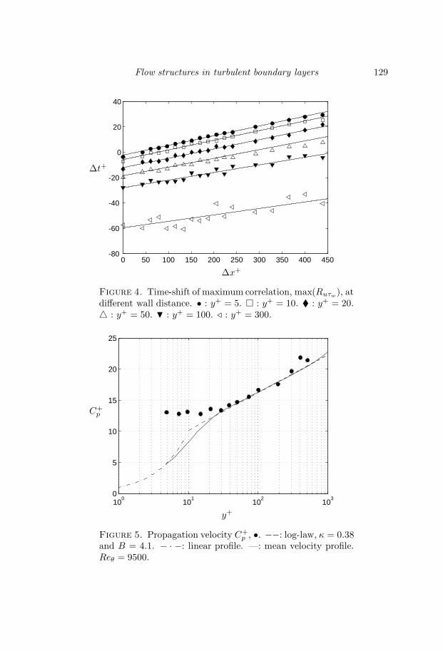
Flow structures in turbulent boundary layers 129
∆x+
∆t+
0 50 100 150 200 250 300 350 400 450-80
-60
-40
-20
0
20
40
Figure 4. Time-shift of maximum correlation, max(Ruτw), atdifferent wall distance. • : y+ = 5. : y+ = 10. : y+ = 20. : y+ = 50. : y+ = 100. D : y+ = 300.
y+
C+p
100
101
102
103
0
5
10
15
20
25
Figure 5. Propagation velocity C+p , •. −−: log-law, κ = 0.38
and B = 4.1. − · −: linear profile. —: mean velocity profile.Reθ = 9500.

130 J. M. Osterlund, B. Lindgren & A. V. Johansson
Symbol Reθ l+ y+
6700 6.6 14.3∇ 8200 8.2 13.8* 9700 9.7 14.5+ 12600 12.8 14.8 15200 15.8 15.2
Table 1. Hot-wire experiments used for VITA detection inthe buffer layer.
4.3. Shear-layer events
Shear-layer events were detected from peaks in the short time variance as de-scribed in section 3.4 using the velocity signal from a hot-wire in the bufferlayer. In table 1 an overview is given of the hot-wire measurements used forVITA detection. An example of the fluctuating velocity signal (top), the cor-responding short time variance (center), and the detection function (bottom)are shown in figure 6. The detection times are taken as the midpoints of thepeaks of the detection function. The events are further sorted on the derivativeof the velocity signal into accelerating and decelerating events, and an ensem-ble average is formed for each type according to equation 8. The acceleratingevents dominate in number over the decelerating events, and correspond to aforward leaning shear layer structure. In figure 7 the conditionally averagedstreamwise velocity signal in the buffer region (y+ ≈ 15) is shown and strongaccelerated and decelerated shear-layer events can be clearly seen.
Alfredsson & Johansson (1984) investigated the scaling laws for turbulentchannel flows and found that the governing timescale for the near-wall regionwas a mixture of the inner and outer time scales
tm =√t∗to. (13)
The frequency of occurrence of the VITA events is shown in figure 8 against theaveraging time for outer, mixed and inner scaling. The mixed scaling appearsrelatively satisfactory also for the boundary layer flow. For very small averagingtimes one should keep in mind the non-negligible influence of finite probe sizefor the highest Reynolds numbers, see table 1. Blackwelder & Haritonidis(1983) reported inner scaling for the ‘bursting frequency’ obtained by the VITAtechnique. However, their values for the friction velocities (obtained from thenear-wall linear profile) deviate substantially from the present correlation forcf and their mean velocity profiles for different Reynolds numbers show a widespread in the log-region.

Flow structures in turbulent boundary layers 131
t+
u/√u2
var(t, T )
D(t, T )
-10
-5
0
5
10
0
0.5
1
1.5
0 500 1000 1500 2000 25000
0.5
1
1.5
Figure 6. a) Time series for the streamwise fluctuating ve-locity component u. y+ = 14.5 and Reθ = 9700. b) Short timevariance of u with integrating window T+ = 10. c) Detectionfunction for k = 1.0. ×: Represents accelerating events and: represents decelerating events.
4.4. Wall-shear stress events
The wall shear stress signal is highly intermittent (flatness factor ≈ 4.9) andpeaks in the wall-shear stress was used to detect events. In figure 9 the con-ditionally averaged wall-shear stress events are shown sorted into positive andnegative peaks using different detection threshold levels k =-1, -0,75, -0.5, 1,2, 3. Broad peaks are seen that are largely symmetric. The negative eventsare slightly wider and less pointed as compared to the positive events.
Detection on peaks in the wall-shear stress was used to form conditional av-erages for the streamwise velocity obtained at a wall-normal separation ∆y+.Conditional averages for the streamwise velocity are shown in figure 10 fordifferent wall-normal separations above the hot-film used as detector. For in-creasing wall-distance the conditionally averaged velocity is shifted towardsnegative times indicating a forward leaning structure. In figure 11 the data infigure 10 are replotted into lines of constant disturbance velocity (normalizedwith the local r.m.s.-level) in the (x, y)-plane using the measured propagationvelocities (figure 5) to transform the time to an x-coordinate. An elongatedand forward leaning high-velocity structure is visible above the high wall-shearevent detected at x = 0. The peaks of the conditionally averaged velocity in

132 J. M. Osterlund, B. Lindgren & A. V. Johansson
τ+
〈upos〉∗
〈uneg〉∗
-1
0
1
2
-50 -40 -30 -20 -10 0 10 20 30 40 50-2
-1
0
1
Figure 7. Conditional average of u for events with positiveslope (top) and negative slope (bottom). T+ = 10, k = 1.0and Reθ = 9700
figure 10 are shown as black circles and agree well with a shear layer angle ofabout 20 found in many investigations, see e.g. Johansson et al. (1987a).
5. Conclusions
A micro machined hot-film sensor array was used together with a hot-wireprobe in series of measurements of coherent structures in turbulent boundarylayers. The small dimensions of the hot-films was a necessity for these mea-surements and the spatial resolution satisfactorily high to determine e.g thestreak spacing.
A new high-pass correlation technique was used to determine the meanstreak spacing for a high Reynolds number turbulent boundary layer. Themean streak spacing was found to be λ+ ≈ 110 which is very close to previousfindings in low Reynolds number flow.
The propagation velocity of disturbances in the boundary layer is constantto 13uτ up to y+ = 30, further out it was found to be close to the local meanvelocity.
It was found that the frequency of occurrence of VITA events in the bufferregion approximately conforms, to a mixed scaling behavior.

Flow structures in turbulent boundary layers 133
10-2
10-1
100
101
102
10-6
10-5
10-4
10-3
10-2
10-1
100
outer
mixed
inner
T ∗
n∗
Figure 8. Frequency of occurrence of VITA events (k=1) asa function of the averaging time with outer, mixed and innerscaling (* denotes nondimensional quantities). y+ = 15, k =1.0. For symbols see table 1.
6. Acknowledgments
The authors wish to thank Professor Chih-Ming Ho at UCLA for providingus with the MEMS hot-film probe. We would like to thank Professor HenrikAlfredsson for many helpful discussions. We also whish to thank Mr. UlfLanden and Mr. Marcus Gallstedt who helped with the manufacturing of theexperimental set-up. Financial support from NUTEK and TFR is gratefullyacknowledged.
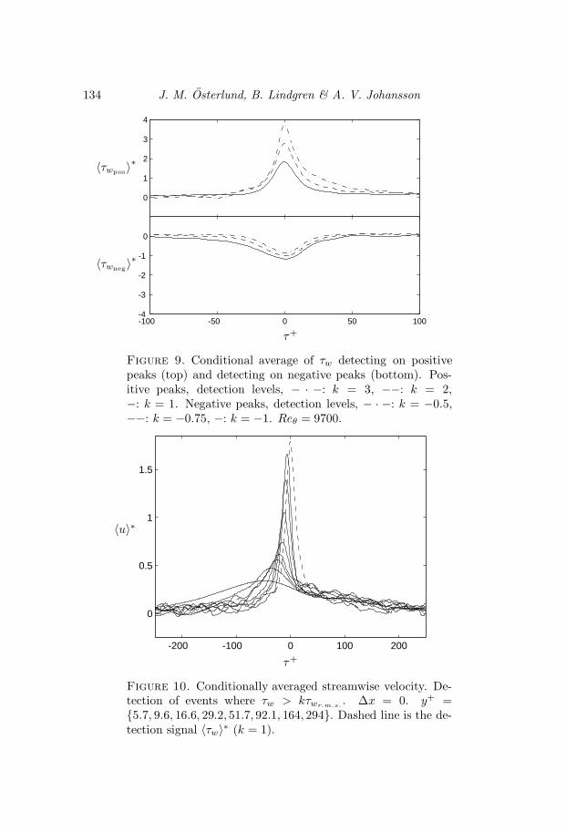
134 J. M. Osterlund, B. Lindgren & A. V. Johansson
τ+
〈τwpos〉∗
〈τwneg〉∗
0
1
2
3
4
-100 -50 0 50 100-4
-3
-2
-1
0
Figure 9. Conditional average of τw detecting on positivepeaks (top) and detecting on negative peaks (bottom). Pos-itive peaks, detection levels, − · −: k = 3, −−: k = 2,−: k = 1. Negative peaks, detection levels, − · −: k = −0.5,−−: k = −0.75, −: k = −1. Reθ = 9700.
τ+
〈u〉∗
-200 -100 0 100 200
0
0.5
1
1.5
Figure 10. Conditionally averaged streamwise velocity. De-tection of events where τw > kτwr.m.s. . ∆x = 0. y+ =5.7, 9.6, 16.6, 29.2, 51.7, 92.1, 164, 294. Dashed line is the de-tection signal 〈τw〉∗ (k = 1).

Flow structures in turbulent boundary layers 135
∆x+
y+
0 200 400 600 800 10000
100
200
300
400
500
Figure 11. Conditionally averaged streamwise velocity. De-tection of events where τw > kτwr.m.s. . k = 1. : locations ofmaximum correlation. −: slope 7. − · −: slope 18.
References
Alfredsson, P. H. & Johansson 1984 Time scales in turbulent channel flow. Phys.Fluids A 27 (8), 1974–81.
Bake, S. & Osterlund, J. M. 1999 Measurements of skin-friction fluctuationsin turbulent boundary layers with miniaturized wall-hot-wires and hot-films.Submitted for publication in Phys. of Fluids.
Blackwelder, R. F. & Haritonidis, J. H. 1983 The bursting frequency in turbu-lent boundary layers. J. Fluid Mech. 132, 87–103.
Blackwelder, R. F. & Kaplan, R. E. 1976 On the wall structure of the turbulentboundary layer. J. Fluid Mech. 76, 89–112.
Chen, K. K. & Blackwelder, R. F. 1978 Large-scale motion in a turbulent bound-ary layer. J. Fluid Mech. 89, 1–31.
Corino, E. R. & Brodkey, R. S. 1969 A visual investigation of the wall regionturbulent flow. J. Fluid Mech. 37, 1–30.
Fernholz, H. H. & Finley, P. J. 1996 The incompressible zero-pressure-gradientturbulent boundary layer: An assessment of the data. Prog. Aerospace Sci. 32,245–311.
Fernholz, H. H., Janke, G., Schober, M., Wagner, P. M. & Warnack, D.
1996 New developments and applications of skin-friction measuring techniques.Meas. Sci. Technol. 7, 1396–1409.
Fiedler, H. E. 1986 Coherent structures. In Advances in turbulence , , vol. 32, pp.320–336. Berlin: Springer-Verlag.
Gupta, A. K., Laufer, J. & Kaplan, R. E. 1971 Spatial structure in the viscoussublayer. J. Fluid Mech. 50, 493–512.
Head, M. R. & Bandyopadhyay, P. 1981 New aspects of turbulent boundary layerstructure. J. Fluid Mech. 107, 297–338.
Ho, C.-M. & Tai, Y.-C. 1998 Micro-electro-mechanical-systems (MEMS) and fluidflows. Ann. Rev. Fluid Mech. 30, 579–612.
Hussain, A. K. M. F. 1986 Coherent structures and turbulence. J. Fluid Mech. 173,303–56.
Jiang, F., Tai, Y.-C., Gupta, B., Goodman, R., Tung, S., Huang, J. B. & Ho,
C.-M. 1996 A surface-micromachined shear stress imager. In 1996 IEEE MicroElectro Mechanical Systems Workshop (MEMS ’96), pp. 110–115.
136
Flow structures in turbulent boundary layers 137
Jiang, F., Tai, Y.-C., Walsh, K., Tsao, T., Lee, G. B. & Ho, C.-H. 1997 Aflexible mems technology and its first application to shear stress sensor skin.In 1997 IEEE Micro Electro Mechanical Systems Workshop (MEMS ’97), pp.465–470.
Johansson, A. V. 1992 A low speed wind-tunnel with extreme flow quality - designand tests. In Prog. ICAS congress 1992 , pp. 1603–1611. ICAS-92-3.8.1.
Johansson, A. V. & Alfredsson, P. H. 1982 On the structure of turbulent channelflow. J. Fluid Mech. 122, 295–314.
Johansson, A. V., Alfredsson, P. H. & Eckelmann, H. 1987a On the evolutionof shear layer structures in near wall turbulence. In Advances in Turbulence (ed.G. Compte-Bellot & J. Mathieu), pp. 383–390. Springer-Verlag.
Johansson, A. V., Alfredsson, P. H. & Kim, J. 1991 Evolution and dynamics ofshear-layer structures in near-wall turbulence. J. Fluid Mech. 224, 579–599.
Johansson, A. V., Her, J.-Y. & Haritonidis, J. H. 1987b On the generation ofhigh-amplitude wall-pressure peaks in turbulent boundary layers and spots. J.Fluid Mech. 175, 119–142.
Kim, H. T., Kline, S. J. & Reynolds, W. C. 1971 The production of turbulencenear a smooth wall in a turbulent boundary layer. J. Fluid Mech. 50, 133–160.
Kim, J., Moin, P. & Moser, R. 1987 Turbulence statistics in fully developed channelflow. J. Fluid Mech. 177, 133–166.
Kline, S. J., Reynolds, W. C., Schraub, F. A. & Runstadler, P. W. 1967 Thestructure of turbulent boundary layers. J. Fluid Mech. 30, 741.
Kovasznay, L. G., Kibens, V. & Blackwelder, R. S. 1970 Large-scale motionin the intermittent region of a turbulent boundary layer. J. Fluid Mech. 41,283–325.
Kreplin, H.-P. & Eckelmann, H. 1979 Propagation of pertubations in the viscoussublayer and adjacent wall region. J. Fluid Mech. 95, 305–322.
Moser, R. D., Kim, J. & Mansour, N. N. 1999 Direct numerical simulation ofturbulent channel flow up to Reθ = 590. Phys. Fluids 11 (4), 943–945.
¨Osterlund, J. M., Johansson, A. V., Nagib, H. M. & Hites, M. H. 1999 Wall
shear stress measurements in high reynolds number boundary layers from twofacilities. In 30th AIAA Fluid Dynamics Conference, Norfolk, VA. AIAA paper99-3814.
Rao, K. N., Narasima, R. & Badri Narayanan, M. 1971 The ”bursting” phe-nomenon in a turbulent boundary layer. J. Fluid Mech. 48, 339–352.
Robinson, S. K. 1991 Coherent motions in the turbulent boundary layer. Ann. Rev.Fluid Mech. 23, 601–639.
Smith, C. R. & Metzler, S. P. 1983 The characteristics of low-speed streaks inthe near-wall region of a turbulent boundary layer. J. Fluid Mech. 129, 27–54.
Wallace, J. M., Eckelmann, H. & Brodkey, R. 1972 The wall region in turbulentshear flow. J. Fluid Mech. 54, 39–48.
Willmart, W. W. & Lu, S. S. 1972 Structure of the Reynolds stress near the wall.J. Fluid Mech. 55, 65–92.


Paper 7


Turbulent Boundary Layer Experiments in theMTL Wind-Tunnel
By Jens M. Osterlund and Arne V. Johansson
Dept. of Mechanics, KTH, SE-100 44 Stockholm, Sweden
1. Introduction
The erection of the MTL wind-tunnel at KTH with its high flow quality andlarge Reynolds number range presented a possibility to design an experimentfor the investigation of high Reynolds number turbulent boundary layers. TheMTL tunnel was partly designed with this type of experiment in mind. Itsdesign characteristics include: long test section, good flow uniformity, very lowturbulence level, very low acoustic level, temperature control and adjustablepressure gradient (walls) along the test section.
In the past a number of experiments on turbulent boundary layers havebeen performed. Most of them in facilities designed for other purposes and mostof them at low to moderate Reynolds numbers. Also most existing experimentshave been made on the walls of the wind-tunnel introducing large uncertain-ties about the starting conditions of the boundary layer. Other troublesomefeatures of existing experiments include low accuracy measurements of probedistance to the wall and the lack of independent skin friction measurements.
This made us decide on a set-up utilizing a flat plate mounted in the testsection. This gives good control over the starting conditions. The adjustablewalls of the MTL wind tunnel makes it possible to mount a 7 m long flat platein the test section and still attain a zero pressure gradient, to a high accuracy,along the the growing boundary layer by adjusting the position of the oppo-site wall. The set-up included a highly accurate traversing mechanism fixedto the boundary layer plate and close to the measurement station to minimizeany vibrations or deflection problems. The measurements were mainly donewith hot-wire techniques and were greatly facilitated by use of the wind-tunneltemperature control system. The distance to the wall was measured by a laserdistance meter aimed directly at the hot-wire probe. The wall distance mea-surement system was possible to use also when the tunnel was running. Finally,the skin friction was independently measured by use of oil-film interferometry.
This paper reports on the background and basics of extensive high Reynoldsnumber experiments that form the basis of the present doctoral thesis.
141

142 Jens M. Osterlund and Arne V. Johansson
Test section
Fan
Cooler
ContractionGrids
Stagnation chamber
Guide vanes
7m
Diffuser
Honecomb
Figure 1. Schematic of the MTL wind tunnel facility at KTH
2. The MTL Wind Tunnel
All experiments were carried out in the MTL-wind tunnel at the departmentof mechanics, KTH. The MTL tunnel is specially designed for turbulence andtransition experiments and the flow quality was reported in Johansson (1992).The tunnel was primarily designed at KTH and built by the French companySessia. It was finished in 1990. The tunnel is a closed return facility, and isshown in figure 1. The test section is 7 m long with a cross sectional area of1 m2 (1.2 m× 0.8 m). The top and the bottom walls are adjustable in orderto be able to control the streamwise velocity distribution in the test section.The circuit is ventilated to the surrounding atmosphere at the end of the testsection giving atmospheric pressure in the test section. All corners utilizespecially designed turning vanes to reduce the losses in the tunnel circuit, seeSahlin & Johansson (1991) and Lindgren et al. (1998). The tunnel is driven bya 86 kW fan located in the return leg between corners 2 and 3. It is equippedwith a heat exchanger after the fan, and the temperature can be kept constantand uniform within ±0.05 C. After the fourth corner the flow passes through ahoneycomb flow-straightener and 5 screens before entering the settling chamberand the contraction, with a contraction ratio of 9, to the test section. Specialcare has been taken to reduce acoustic noise and a large part of the returncircuit is equipped with noise-absorbing walls. The velocity can be controlledbetween 0-69 m/s.

Turbulent Boundary Layer Experiments 143
total length 25 mtest section length 7 mtest section width 1.2 mtest section height 0.8 mcontraction ratio 9mean velocity uniformity < 0.1%mean velocity angularity < 0.1
temperature variations (in time) < ±0.05 Ctemperature uniformity < ±0.2 Cstreamwise turb. intensity
in total ‘central region’ < 0.03%near tunnel centerline < 0.015%
lateral turb. intensity (at 25 m/s)in total ‘central region’ < 0.06%near tunnel centerline < 0.02%
noise (sound level, f > 60 Hz)at 35 m/s 69 dBat 60 m/s 83 dB
Table 1. Basic characteristics of the MTL wind-tunnel at KTH.
3. Experimental set-up
3.1. The boundary layer plate
A 7 m long flat plate was mounted in the test section, see figure 2. The plate isa sandwich construction of aluminum sheet and aluminum square tubes madein 1 m long sections for ease of handling, see figure 3 for a detailed view ofone plate section. The alignment of the edges between the plate sections wasensured by the use of 4 cylindric control pins at every connection. The stepheight was measured to be always less than 5 µm. The plate sections areresting on two horizontal beams running along the test section. The beams areadjusted strait and horizontal in the test section by use of adjustable supports,see figure 4. This system made it possible to adjust the large scale flatness ofthe plate to within ±0.5 mm from the horizontal plane.
The leading edge shape is elliptical with an aspect ratio of 5, see figure 5.It was milled from a solid block of aluminum by use of a CNC machine. Thesurface was then polished to the final finish. Two pressure taps in the ellipticalnose are used to position the stagnation point at the centerline of the plate.The taps are situated close to the point where the difference in pressure havemaximum sensitivity to the angle of attack. The positioning of the stagnationpoint is done by a 1.5 m long flap mounted at the trailing edge on a hinge, seefigures 6 and 7. The flap was adjustable with the tunnel running, which made

144 Jens M. Osterlund and Arne V. Johansson
Adjustable upper wall
Adjustable lower wall
Adjustable flap Measurement stationPlexiglass insert Elliptical nose
Support beam
Figure 2. The boundary layer plate set-up.
it possible to accurately position the stagnation point at the leading edge toavoid any separation.
3.2. Instrumentation
3.2.1. Ambient conditions. Atmospheric pressure, patm, was measured using abarometer (from Furness control systems) located by the tunnel. The sameequipment also registered the temperature, T , in the test section, with anaccuracy of 0.1C. The instrument was connected to the measurement computerand was monitored during all measurements.
The atmospheric pressure and the temperature were used to calculate thedensity, ρ, and the kinematic viscosity using the perfect gas law,
ρ =patmRT (1)
where R = 279.1 J/kgK is the gas constant for air, and Sutherlands correlation,
ν = 1.458 · 10−6T 3/2
ρ(T + 110.4). (2)
3.2.2. Reference conditions and pressure measurement. A reference Prandtltube was positioned above the measurement position and used to monitor ref-erence free stream dynamic and static pressure. The freestream velocity was

Turbulent Boundary Layer Experiments 145
Figure 3. One plate section.
Figure 4. Cross section of the measurement section of theMTL wind-tunnel with the boundary layer plate installed.
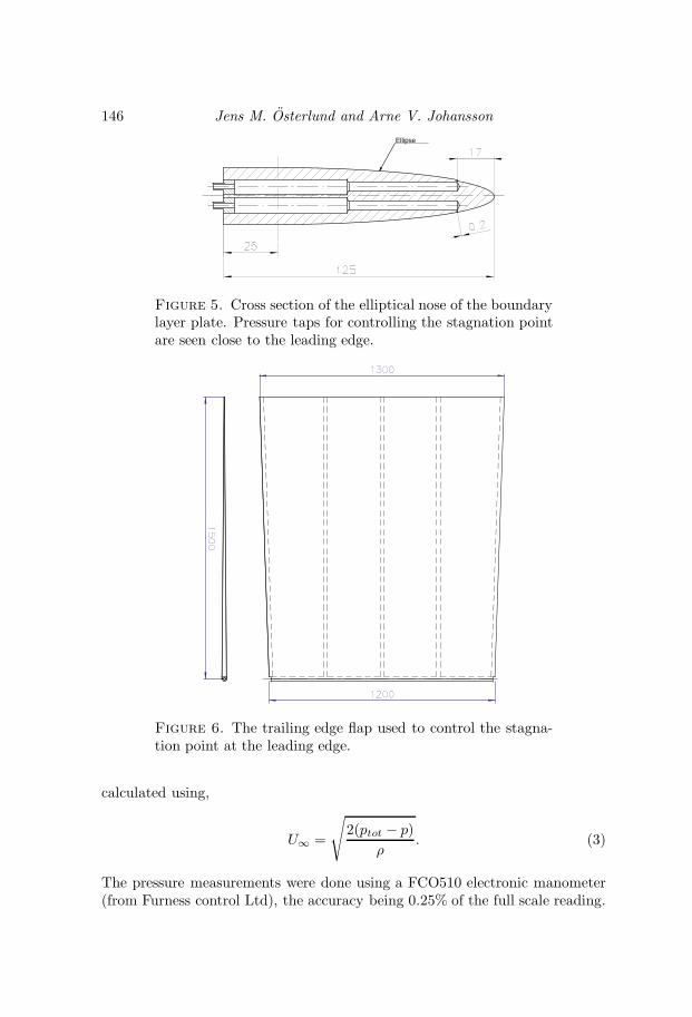
146 Jens M. Osterlund and Arne V. JohanssonEllipse
Figure 5. Cross section of the elliptical nose of the boundarylayer plate. Pressure taps for controlling the stagnation pointare seen close to the leading edge.
Figure 6. The trailing edge flap used to control the stagna-tion point at the leading edge.
calculated using,
U∞ =
√2(ptot − p)
ρ. (3)
The pressure measurements were done using a FCO510 electronic manometer(from Furness control Ltd), the accuracy being 0.25% of the full scale reading.

Turbulent Boundary Layer Experiments 147
Figure 7. Detail of the flap attachment to the plate.
The RS232 output of the instrument was connected to the serial port of themeasurement computer and was monitored during the measurements.
3.2.3. Data acquisition equipment. The voltage signals from the anemometerwas digitized using an A/D-converter (AN-2000) from National instruments.The offset voltages from the signal amplifier, built into the anemometer, wasmeasured using a multimeter connected to the measurement computer (usingIEEE 488).
3.2.4. Probe traversing. A specially designed traversing system protruding fromthe plate was used to position the probes. It was mounted immediately be-hind the measurement station in a circular insert in the measurement stationplate section. Under the plate the traversing mechanism was protected fromthe flow by a streamlined cover fixed to the tunnel floor. This prevented vi-brations generated by vortex shedding to go into the traversing system. Thevertical range of the system is 150 mm with a relative accuracy of ±1µm. Forthe two wire probe measurements a yaw angle traversing system was mountedon top for angular calibrations. The accuracy of that system is ±0.01. Thetraversing is done by servo motors with optical encoders and was controlledfrom the measurement computer. The traversing system was mounted in oneof the plate sections behind the Plexi-glass plug where all measurements were

148 Jens M. Osterlund and Arne V. Johansson
a) b)
A
A
BB
A-A
B-B
50 mm100 mm
servo motor worm gear
Figure 8. a) Schematic of the traversing system with a singlewire probe mounted. The vertical range is 150 mm. b) Whenusing two-wire probes the angular traversing unit was mountedat the top of the traversing arm. See also figure 9
.
taken. The position of the measurement plate section within the whole platecan be changed to obtain the following five streamwise measurement positionsx = 1.5, 2.5, 3.5, 4.5, 5.5m.
3.3. Tripping the boundary layer
Normal transition occurs far downstream on the boundary layer plate. Thismakes it necessary to use a trip at the beginning of the plate. Several tripdesigns were tested. The selection was made by trial and error determining thetransition velocity using a hot-wire 20 cm behind the trip.
The boundary layer was tripped by 8 rows of DYMO brand embossingtape letter “V” (width 8 mm), see figure 10. The height of the trip is 0.7 mmcorresponding to less than half of the laminar boundary layer thickness at the
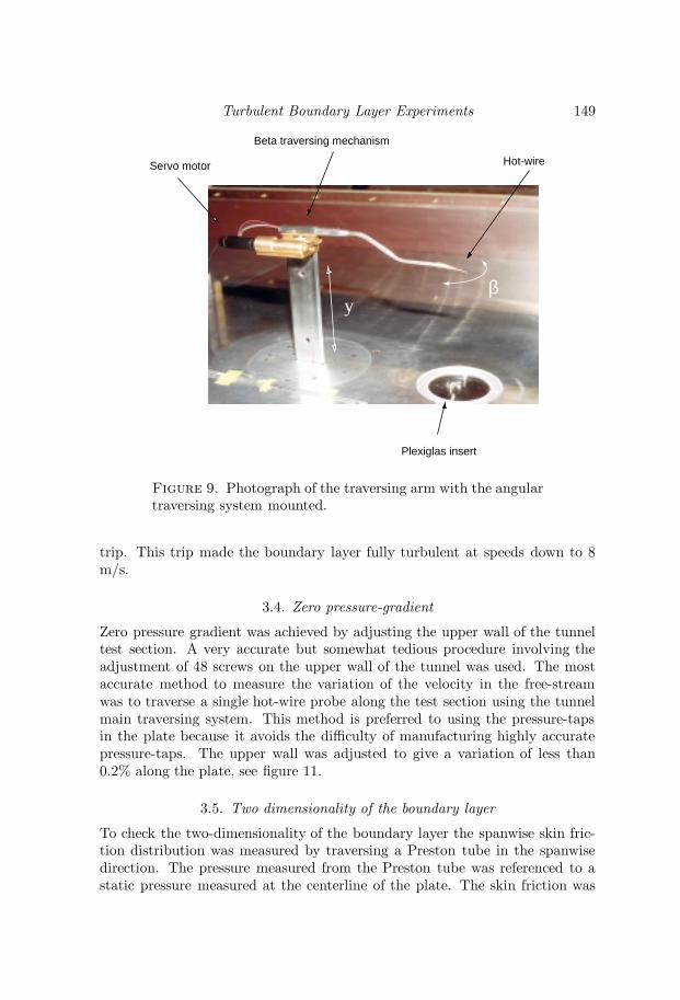
Turbulent Boundary Layer Experiments 149
Plexiglas insert
Beta traversing mechanism
Servo motor Hot-wire
βy
Figure 9. Photograph of the traversing arm with the angulartraversing system mounted.
trip. This trip made the boundary layer fully turbulent at speeds down to 8m/s.
3.4. Zero pressure-gradient
Zero pressure gradient was achieved by adjusting the upper wall of the tunneltest section. A very accurate but somewhat tedious procedure involving theadjustment of 48 screws on the upper wall of the tunnel was used. The mostaccurate method to measure the variation of the velocity in the free-streamwas to traverse a single hot-wire probe along the test section using the tunnelmain traversing system. This method is preferred to using the pressure-tapsin the plate because it avoids the difficulty of manufacturing highly accuratepressure-taps. The upper wall was adjusted to give a variation of less than0.2% along the plate, see figure 11.
3.5. Two dimensionality of the boundary layer
To check the two-dimensionality of the boundary layer the spanwise skin fric-tion distribution was measured by traversing a Preston tube in the spanwisedirection. The pressure measured from the Preston tube was referenced to astatic pressure measured at the centerline of the plate. The skin friction was
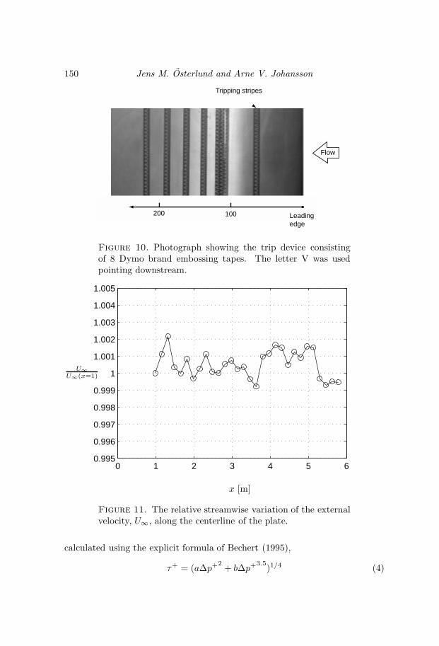
150 Jens M. Osterlund and Arne V. Johansson
100200 Leadingedge
Flow
Tripping stripes
Figure 10. Photograph showing the trip device consistingof 8 Dymo brand embossing tapes. The letter V was usedpointing downstream.
0 1 2 3 4 5 60.995
0.996
0.997
0.998
0.999
1
1.001
1.002
1.003
1.004
1.005
U∞U∞(x=1)
x [m]
Figure 11. The relative streamwise variation of the externalvelocity, U∞, along the centerline of the plate.
calculated using the explicit formula of Bechert (1995),
τ+ = (a∆p+2 + b∆p+3.5)1/4 (4)
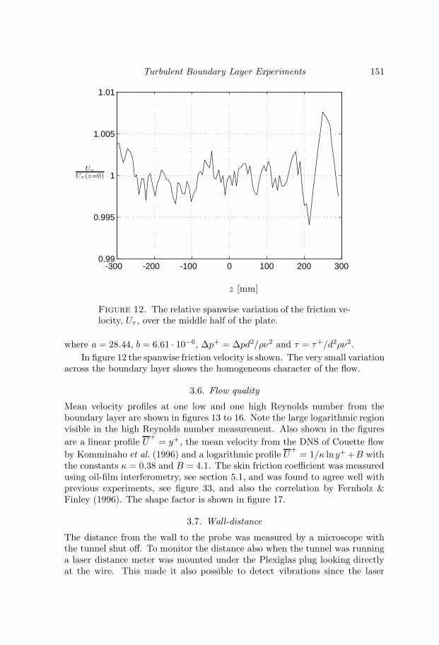
Turbulent Boundary Layer Experiments 151
-300 -200 -100 0 100 200 3000.99
0.995
1
1.005
1.01
Uτ
Uτ(z=0)
z [mm]
Figure 12. The relative spanwise variation of the friction ve-locity, Uτ , over the middle half of the plate.
where a = 28.44, b = 6.61 · 10−6, ∆p+ = ∆pd2/ρν2 and τ = τ+/d2ρν2.In figure 12 the spanwise friction velocity is shown. The very small variation
across the boundary layer shows the homogeneous character of the flow.
3.6. Flow quality
Mean velocity profiles at one low and one high Reynolds number from theboundary layer are shown in figures 13 to 16. Note the large logarithmic regionvisible in the high Reynolds number measurement. Also shown in the figuresare a linear profile U
+= y+ , the mean velocity from the DNS of Couette flow
by Komminaho et al. (1996) and a logarithmic profile U+
= 1/κ lny+ +B withthe constants κ = 0.38 and B = 4.1. The skin friction coefficient was measuredusing oil-film interferometry, see section 5.1, and was found to agree well withprevious experiments, see figure 33, and also the correlation by Fernholz &Finley (1996). The shape factor is shown in figure 17.
3.7. Wall-distance
The distance from the wall to the probe was measured by a microscope withthe tunnel shut off. To monitor the distance also when the tunnel was runninga laser distance meter was mounted under the Plexiglas plug looking directlyat the wire. This made it also possible to detect vibrations since the laser

152 Jens M. Osterlund and Arne V. Johansson
y+
U+
100
101
102
103
104
0
5
10
15
20
25
30
35
Figure 13. Example of a mean velocity profile at Reθ = 2530in inner scaling on logarithmic axis. Dotted line: linear profile.Dashed line: DNS of Couette flow by Komminaho Komminahoet al. (1996). Dash dotted line: log-profile with constants κ =0.38 and B = 4.1.
could follow the wire with frequencies up to 10 kHz. The range of the laserdistance meter is 2 mm with an accuracy of ±1µm. The laser distance meterwas calibrated using the microscope with the tunnel shut off. The error in theabsolute wall distance measurements for the single-wire was ±5 µm and for theX-wire ±50 µm.
4. Hot-wire anemometry
The velocity was measured using constant temperature anemometry (CTA)in all experiments (system AN–1003 from AA lab systems in Israel). In con-stant temperature anemometry the hot-wire temperature is held constant byfeedback control, while the current through the wire changes in response tofluctuating flow properties. The sensing hot-wire is one of the resistors in theactive arm of a Wheatstone bridge. The sensor temperature is set by adjustingRadj. The Wheatstone bridge produces an error voltage across the bridge di-agonal when a resistive imbalance occurs. The amplifier serves as an actuator

Turbulent Boundary Layer Experiments 153
y+
U+
100
101
102
103
104
0
5
10
15
20
25
30
35
Figure 14. Example of a mean velocity profile at Reθ =26600 in inner scaling on logarithmic axis. Dotted line: lin-ear profile. Dashed line: DNS of Couette flow by Kommi-naho Komminaho et al. (1996). Dash dotted line: log-profilewith constants κ = 0.38 and B = 4.1.
feeding current into the top of the bridge until the desired temperature of thesensor is achieved, thus balancing the bridge.
To first order the resistance of the hot-wire RwH is
RwH = RwC [1 + α(TwH − TwC )] (5)
where TwH is the hot temperature, RwC and TwC are the cold resistance andtemperature and α is the temperature coefficient of resistivity. The resistanceand temperature overheat ratios are defined as
aR =RwH −RwC
RwC
(6)
aT =TwH − TwC
TwC
. (7)
The resistance overheat ratio aR was selected to give the desired temperatureoverheat ratio aT = aT /αTwC .

154 Jens M. Osterlund and Arne V. Johansson
y+
U+
0 1000 2000 3000 4000 50000
5
10
15
20
25
30
Figure 15. Example of a mean velocity profile at Reθ = 2530in inner scaling on linear axis. Dotted line: linear profile.Dashed line: DNS of Couette flow by Komminaho Komminahoet al. (1996). Dash dotted line: log-profile with constants κ =0.38 and B = 4.1.
Energy balance for the hot-wire in a cross-flow together with the heattransfer correlation by King results in
I2RwH = (A+ BUn)(TwH − Tamb) (8)
where U is the effective velocity, A, B and n are constants characteristic of theheat transfer from the wire. The expression (8) is useful if temperature driftcompensation is needed.
4.1. Probe manufacturing
The probe-bodies were built using ceramic tubes, designed for use in thermoelements, with 4 holes. The prongs were built from spring wire. The conicalshape at the tips was etched in a bath of nitric acid (60%) using a techniquewhere a small voltage was applied to speed up the etching. The delicate posi-tioning of the prongs was done under a microscope (80x) and the positioningwas done with a micro manipulating equipment. When the prongs are fixedin position a low viscosity epoxy resin is applied. Capillary forces pulls theresin into the probe body and fixes the prongs in position when hardened. To

Turbulent Boundary Layer Experiments 155
y+
U+
0 0.5 1 1.5 2
x 104
0
5
10
15
20
25
30
35
Figure 16. Example of a mean velocity profile at Reθ =26600 in inner scaling on linear axis. Dotted line: linear pro-file. Dashed line: DNS of Couette flow by Komminaho Kom-minaho et al. (1996). Dash dotted line: log-profile with con-stants κ = 0.38 and B = 4.1.
fix the prongs together outside of the ceramic body a mixture of epoxy resinand colloidal silicon was applied. Before gluing the probe together the prongswere covered by a thin layer of solder to protect them from corrosion and tolater be used for the soldering of the platinum wires. The soldering is doneby putting the etched piece of the Wollastone wire in position, by use of amicro-manipulator, and then heating the prong with the soldering iron a fewmm away until the solder melts. The length to diameter ratio was always keptmore than 200. The diameter of the prong edge was about 20 − 30µm. Thewires were soldered on the inside of the prongs to make the distance betweenthe wires as small as possible see figure Extreme care has to be taken whenpositioning the prongs to assure that the wires are parallel. The deviation fromparallelism was kept smaller than about 5µm.
4.2. Hot-wire anemometer calibration procedure
All hot-wires were calibrated in the free stream against a Prandtl-tube im-mediately before every set of measurements. The probes were never moved
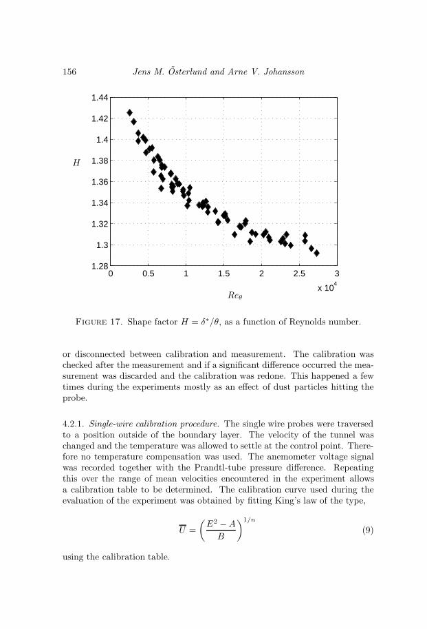
156 Jens M. Osterlund and Arne V. Johansson
Reθ
H
0 0.5 1 1.5 2 2.5 3
x 104
1.28
1.3
1.32
1.34
1.36
1.38
1.4
1.42
1.44
Figure 17. Shape factor H = δ∗/θ, as a function of Reynolds number.
or disconnected between calibration and measurement. The calibration waschecked after the measurement and if a significant difference occurred the mea-surement was discarded and the calibration was redone. This happened a fewtimes during the experiments mostly as an effect of dust particles hitting theprobe.
4.2.1. Single-wire calibration procedure. The single wire probes were traversedto a position outside of the boundary layer. The velocity of the tunnel waschanged and the temperature was allowed to settle at the control point. There-fore no temperature compensation was used. The anemometer voltage signalwas recorded together with the Prandtl-tube pressure difference. Repeatingthis over the range of mean velocities encountered in the experiment allowsa calibration table to be determined. The calibration curve used during theevaluation of the experiment was obtained by fitting King’s law of the type,
U =(E2 −AB
)1/n
(9)
using the calibration table.
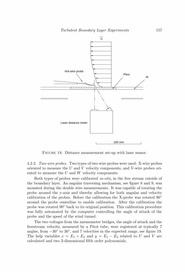
Turbulent Boundary Layer Experiments 157
PlexiAl
Hot-wire probe
Laser distance meter
U
100 mm
Figure 18. Distance measurement set-up with laser sensor.
4.2.2. Two-wire probes. Two types of two-wire probes were used: X-wire probesoriented to measure the U and V velocity components, and V-wire probes ori-ented to measure the U and W velocity components.
Both types of probes were calibrated in-situ, in the free stream outside ofthe boundary layer. An angular traversing mechanism, see figure 8 and 9, wasmounted during the double wire measurements. It was capable of rotating theprobe around the y-axis and thereby allowing for both angular and velocitycalibration of the probes. Before the calibration the X-probe was rotated 90
around the probe centerline to enable calibration. After the calibration theprobe was rotated 90 back to its original position. This calibration procedurewas fully automated by the computer controlling the angle of attack of theprobe and the speed of the wind tunnel.
The two voltages from the anemometer bridges, the angle of attack and thefreestream velocity, measured by a Pitot tube, were registered at typically 7angles, from −30 to 30, and 7 velocities in the expected range, see figure 19.The help variables x = E1 + E2 and y = E1 − E2 related to U and V arecalculated and two 2-dimensional fifth order polynomials,
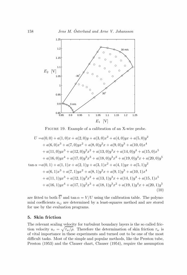
158 Jens M. Osterlund and Arne V. Johansson
E1 [V]
E2 [V]
0.85 0.9 0.95 1 1.05 1.1 1.15 1.2 1.250.85
0.9
0.95
1
1.05
1.1
1.15
1.2
1.25
30 m/s
3 m/s
-30
30
Figure 19. Example of a calibration of an X-wire probe.
U =a(0, 0) + a(1, 0)x+ a(2, 0)y + a(3, 0)x2 + a(4, 0)yx+ a(5, 0)y2
+ a(6, 0)x3 + a(7, 0)yx2 + a(8, 0)y2x+ a(9, 0)y3 + a(10, 0)x4
+ a(11, 0)yx3 + a(12, 0)y2x2 + a(13, 0)y3x+ a(14, 0)y4 + a(15, 0)x5
+ a(16, 0)yx4 + a(17, 0)y2x3 + a(18, 0)y3x2 + a(19, 0)y4x+ a(20, 0)y5
tanα =a(0, 1) + a(1, 1)x+ a(2, 1)y + a(3, 1)x2 + a(4, 1)yx+ a(5, 1)y2
+ a(6, 1)x3 + a(7, 1)yx2 + a(8, 1)y2x+ a(9, 1)y3 + a(10, 1)x4
+ a(11, 1)yx3 + a(12, 1)y2x2 + a(13, 1)y3x+ a(14, 1)y4 + a(15, 1)x5
+ a(16, 1)yx4 + a(17, 1)y2x3 + a(18, 1)y3x2 + a(19, 1)y4x+ a(20, 1)y5
(10)
are fitted to both U and tanα = V/U using the calibration table. The polyno-mial coefficients aij are determined by a least-squares method and are storedfor use by the evaluation programs.
5. Skin friction
The relevant scaling velocity for turbulent boundary layers is the so called fric-tion velocity uτ =
√τw/ρ. Therefore the determination of skin friction τw is
of vital importance in these experiments and turned out to be one of the mostdifficult tasks. Most of the simple and popular methods, like the Preston tube,Preston (1953) and the Clauser chart, Clauser (1954), require the assumption
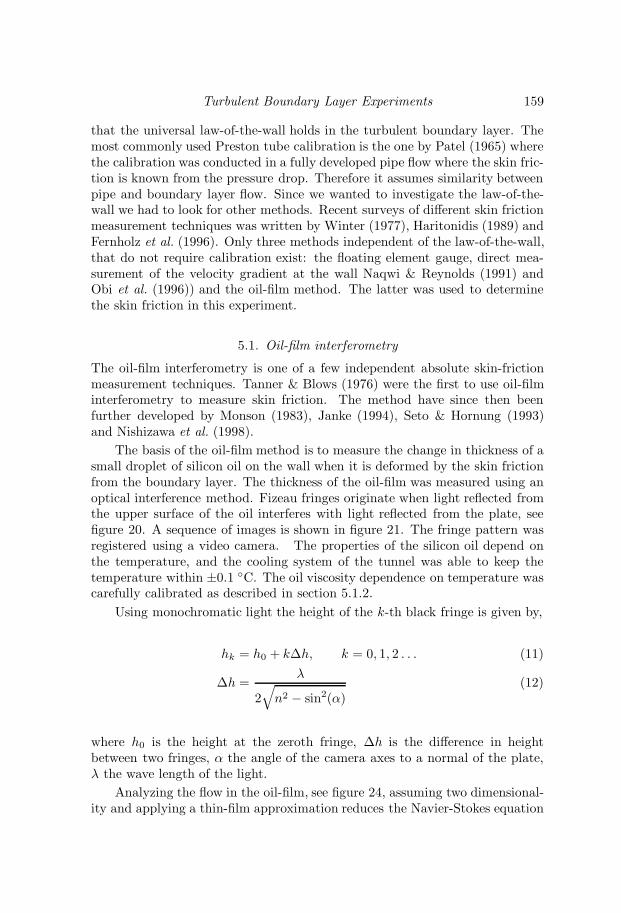
Turbulent Boundary Layer Experiments 159
that the universal law-of-the-wall holds in the turbulent boundary layer. Themost commonly used Preston tube calibration is the one by Patel (1965) wherethe calibration was conducted in a fully developed pipe flow where the skin fric-tion is known from the pressure drop. Therefore it assumes similarity betweenpipe and boundary layer flow. Since we wanted to investigate the law-of-the-wall we had to look for other methods. Recent surveys of different skin frictionmeasurement techniques was written by Winter (1977), Haritonidis (1989) andFernholz et al. (1996). Only three methods independent of the law-of-the-wall,that do not require calibration exist: the floating element gauge, direct mea-surement of the velocity gradient at the wall Naqwi & Reynolds (1991) andObi et al. (1996)) and the oil-film method. The latter was used to determinethe skin friction in this experiment.
5.1. Oil-film interferometry
The oil-film interferometry is one of a few independent absolute skin-frictionmeasurement techniques. Tanner & Blows (1976) were the first to use oil-filminterferometry to measure skin friction. The method have since then beenfurther developed by Monson (1983), Janke (1994), Seto & Hornung (1993)and Nishizawa et al. (1998).
The basis of the oil-film method is to measure the change in thickness of asmall droplet of silicon oil on the wall when it is deformed by the skin frictionfrom the boundary layer. The thickness of the oil-film was measured using anoptical interference method. Fizeau fringes originate when light reflected fromthe upper surface of the oil interferes with light reflected from the plate, seefigure 20. A sequence of images is shown in figure 21. The fringe pattern wasregistered using a video camera. The properties of the silicon oil depend onthe temperature, and the cooling system of the tunnel was able to keep thetemperature within ±0.1 C. The oil viscosity dependence on temperature wascarefully calibrated as described in section 5.1.2.
Using monochromatic light the height of the k-th black fringe is given by,
hk = h0 + k∆h, k = 0, 1, 2 . . . (11)
∆h =λ
2√n2 − sin2(α)
(12)
where h0 is the height at the zeroth fringe, ∆h is the difference in heightbetween two fringes, α the angle of the camera axes to a normal of the plate,λ the wave length of the light.
Analyzing the flow in the oil-film, see figure 24, assuming two dimensional-ity and applying a thin-film approximation reduces the Navier-Stokes equation
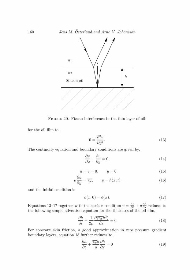
160 Jens M. Osterlund and Arne V. Johansson
hSilicon oil
n2
n1
Figure 20. Fizeau interference in the thin layer of oil.
for the oil-film to,
0 =∂2u
∂y2. (13)
The continuity equation and boundary conditions are given by,
∂u
∂x+∂v
∂y= 0. (14)
u = v = 0, y = 0 (15)
µ∂u
∂y= τw, y = h(x, t) (16)
and the initial condition is
h(x, 0) = φ(x). (17)
Equations 13–17 together with the surface condition v = ∂h∂t + u∂h
∂x reduces tothe following simple advection equation for the thickness of the oil-film,
∂h
∂t+
12µ
∂(τwh2)∂x
= 0 (18)
For constant skin friction, a good approximation in zero pressure gradientboundary layers, equation 18 further reduces to,
∂h
∂t+τwh
µ
∂h
∂x= 0 (19)

Turbulent Boundary Layer Experiments 161
Figure 21. Sequence of images showing the Fizeau fringesgenerated from the interference of the light reflected from thetop and from the bottom of the oil-film. The thinning of theoil-film is clearly seen.
with the solution,
h = φ[x− τwh
µt]. (20)
In fact, at large times the main part of the oil-film will approach the similaritysolution,
h =µx
τwt, (21)
regardless of the initial condition 17. Keeping h = const. = hk, that is stayingon one fringe, equation 20 gives,
∂x
∂t
∣∣∣∣h=hk
=τwhkµ
= uk (22)
the fringe velocity in the x–t plane. Combining 22, 11 and 12 we arrive at,
τwk + τwh0∆h
= µuk2√n2 − sin2 α
λ(23)
where µ, α, n and λ are known and an arbitrary number of fringe velocities ukcan be measured from the x–t diagram. We have an over-determined systemof linear equations for the quantities τw and h0/∆h, which can be computedby a least squares fit.

162 Jens M. Osterlund and Arne V. Johansson
0 200 400 600 800 1000 12000
1
2
3
4
5
6
x 10-3
t [s]
x [m]
Figure 22. X–t diagram showing the development of the oil-film thickness.
The captured images were cut to generate x–t diagrams like figure 22.About 10 fringe velocities uk were deduced from the x–t image by fittingstraight lines to the fringes by use of a computer program. The skin fric-tion τw and h0/∆h were calculated from equation 23. Results are discussed insection 5.4 and shown in figure 33.
5.1.1. Optical set-up. The optical set-up was determined by the need to depictan area less than one cm2 from a distance of about 1 m. The video camera hasan 8 mm black and white ccd-chip with a resolution of 512x640 pixels. A 300mm lens from Nikkor was mounted together with the camera on a steel holderwith a telescopic cover between the two, to prevent light from the sides to reachthe ccd. The holder was mounted on a stand on top of the upper test-sectionwall, see figure 23. The optical path into the test section was through theslit in the wall where the sealing mylar films temporarily were removed underthe camera and the light source. The fringes were obtained on an acrylic plugwith a diameter of 100 mm that was mounted in the test station plate. Toilluminate the oil-film a standard sodium lamp from Osram was used (λ = 589nm). The analog video image from the camera was digitized by a computer(PowerMac 9500/100) at specified time intervals. The image stack was storedon the hard disc together with the necessary parameters for later processingand determination of the wall shear stress.
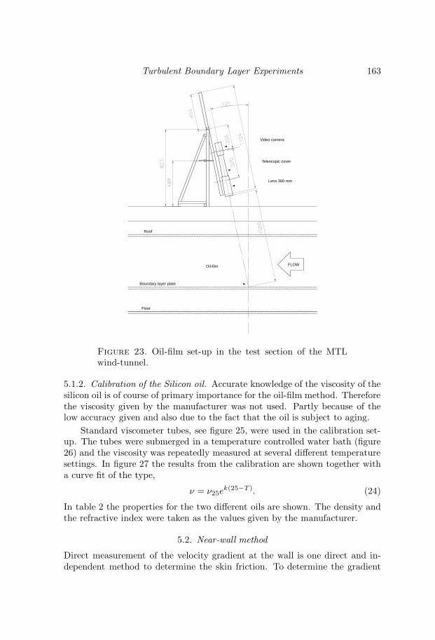
Turbulent Boundary Layer Experiments 163
FLOWOil-film
Lens 300 mm
Video camera
Telescopic cover
Boundary layer plate
Floor
Roof
Figure 23. Oil-film set-up in the test section of the MTLwind-tunnel.
5.1.2. Calibration of the Silicon oil. Accurate knowledge of the viscosity of thesilicon oil is of course of primary importance for the oil-film method. Thereforethe viscosity given by the manufacturer was not used. Partly because of thelow accuracy given and also due to the fact that the oil is subject to aging.
Standard viscometer tubes, see figure 25, were used in the calibration set-up. The tubes were submerged in a temperature controlled water bath (figure26) and the viscosity was repeatedly measured at several different temperaturesettings. In figure 27 the results from the calibration are shown together witha curve fit of the type,
ν = ν25ek(25−T ). (24)
In table 2 the properties for the two different oils are shown. The density andthe refractive index were taken as the values given by the manufacturer.
5.2. Near-wall method
Direct measurement of the velocity gradient at the wall is one direct and in-dependent method to determine the skin friction. To determine the gradient

164 Jens M. Osterlund and Arne V. Johansson
x
y2α
h(x, t)
Cameraλ
U(y)
Figure 24. Schematic of oil-film technique.
Table 2. Silicon oil properties
Oil ρ [kg/m3] n k ν25 [m2/s]DC200/200 970 1.403 1.95 · 10−2 205.1 · 10−6
DC200/20 949 1.4 1.78 · 10−2 19.23 · 10−6
by measurement of the velocity at different heights, and thereby calculate thederivative, one has to do accurate measurements below y+ = 3. With currentlyavailable measurement techniques this is not possible to do, particularly notat high Reynolds numbers and/or low Prandtl numbers. In the current exper-iments this would require accurate measurements closer than 30 µm from thewall.
Therefore, a new method to determine the wall-shear stress has been devel-oped. The new method is not an independent method since it needs calibration.The idea is to determine the skin friction from the measured velocity profile inthe inner layer, using the law of the wall,
U+
=U
uτ= f
(y+
); y+ =
yuτν
(25)
at a distance from the wall where it is possible to make accurate measurements.The measured velocity profile is fitted to the law-of-the-wall in a procedure min-imizing the mean-square error. This is similar to what is done when using theClauser method in the logarithmic region of the velocity profile. The problemwith using the Clauser method is obvious since it assumes similarity in the over-lap region and that is part of our investigation. The underlying assumptionsfor the use of Preston tubes are similar.
In order to utilize accurate mean velocity measurements to evaluate thewall-shear stress, the form of the law-of-the-wall was chosen from available
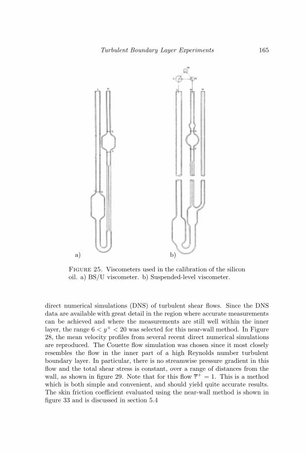
Turbulent Boundary Layer Experiments 165
a) b)
Figure 25. Viscometers used in the calibration of the siliconoil. a) BS/U viscometer. b) Suspended-level viscometer.
direct numerical simulations (DNS) of turbulent shear flows. Since the DNSdata are available with great detail in the region where accurate measurementscan be achieved and where the measurements are still well within the innerlayer, the range 6 < y+ < 20 was selected for this near-wall method. In Figure28, the mean velocity profiles from several recent direct numerical simulationsare reproduced. The Couette flow simulation was chosen since it most closelyresembles the flow in the inner part of a high Reynolds number turbulentboundary layer. In particular, there is no streamwise pressure gradient in thisflow and the total shear stress is constant, over a range of distances from thewall, as shown in figure 29. Note that for this flow τ+ = 1. This is a methodwhich is both simple and convenient, and should yield quite accurate results.The skin friction coefficient evaluated using the near-wall method is shown infigure 33 and is discussed in section 5.4

166 Jens M. Osterlund and Arne V. Johansson
Thermometer
Temperatureregulating unit
Viscometer
Water bath
Figure 26. Viscometer set-up showing the temperature reg-ulated water bath
18 20 22 24 26 28 30185
190
195
200
205
210
215
220
225
230
ν [mm2/s]
T [C]
Figure 27. Kinematic viscosity of the silicon oil (DC200/200).

Turbulent Boundary Layer Experiments 167
0 5 10 15 200
2
4
6
8
10
12
BL flow Re=300, P. R. SpalartBL flow Re=670, P. R. SpalartBL flow Re=1410, P. R. SpalartBL flow Re=200, M. SkoteBL flow Re=335, M. SkoteCouette flow Re=52, J. Komminaho.
y+
U+
Interval used in fit
Figure 28. Mean velocity from DNS of boundary layer bySpalart (1988) and Skote et al. (1998), and Couette flow byKomminaho et al. (1996).
0 10 20 30 40 500.9
0.92
0.94
0.96
0.98
1
y+
τ+
Figure 29. Total shear stress from DNS calculations; for leg-end see Figure 28
5.3. MEMS hot-film
For the measurements of the fluctuating part of the skin-friction MEMS-typeprobes were used and also the near-wall hot-wire technique, Fernholz et al.(1996). The MEMS probe, see figure 30, was designed and constructed byProf. Ho’s group at UCLA/Caltech, Jiang et al. (1996); Ho & Tai (1998). Itwas mounted in a cut-out of a printed circuit board (PCB) with all electricalconnections on the back except the wire-bonding needed to connect the chip tothe PCB, see figure 31. The PCB was fitted into a Plexiglas plug, see figure 32,
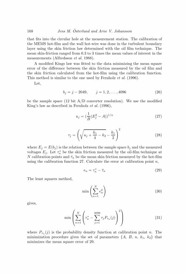
168 Jens M. Osterlund and Arne V. Johansson
that fits into the circular hole at the measurement station. The calibration ofthe MEMS hot-film and the wall hot-wire was done in the turbulent boundarylayer using the skin friction law determined with the oil film technique. Themean skin-friction ranged from 0.3 to 3 times the mean values of interest in themeasurements (Alfredsson et al. 1988).
A modified Kings law was fitted to the data minimizing the mean squareerror of the difference between the skin friction measured by the oil film andthe skin friction calculated from the hot-film using the calibration function.This method is similar to the one used by Fernholz et al. (1996).
Let,
bj = j − 2049, j = 1, 2, . . . , 4096 (26)
be the sample space (12 bit A/D converter resolution). We use the modifiedKing’s law as described in Fernholz et al. (1996),
uj = (1B
(E2j − A))1/n (27)
τj =
(√uj +
k14− k2 −
k12
)2
(28)
where Ej = E(bj) is the relation between the sample space bj and the measuredvoltages Ej. Let τ∗n be the skin friction measured by the oil-film technique atN calibration points and τn be the mean skin friction measured by the hot-filmusing the calibration function 27. Calculate the error at calibration point n,
en = τ∗n − τn (29)
The least squares method,
min
(N∑
n=1
e2n
)(30)
gives,
min
N∑n=1
τ∗n − 4096∑j=1
τjPτn(j)
2 (31)
where Pτn(j) is the probability density function at calibration point n. Theminimization procedure gives the set of parameters A, B, n, k1, k2 thatminimizes the mean square error of 29.

Turbulent Boundary Layer Experiments 169
Figure 30. The UCLA/Caltech MEMS Hot-film sensor chipwith close-up of one hot-film.
5.4. Skin friction results
The results from the skin friction measurements are summarized in Figure 33.A fit to cf by a variant of the logarithmic skin friction law,
cf = 2[
1κ
ln(Reθ) +C
]−2, (32)
was made for each of the data sets. The value of the von Karman constantdetermined from the oil-film data in this way was κ = 0.384 and the additiveconstant was found to be C = 4.08 and the value of the von Karman con-stant determined from the near-wall method was κ = 0.385 and C = 4.28, seeOsterlund et al. (1999). In Figure 33, the results from the oil-film measure-ments together with the values of the skin friction determined from the meanvelocity by the near-wall technique, are shown together with the calculatedbest fits using equation (32). The resulting logarithmic skin-friction laws agreevery well with each other and also with the correlation developed by Fernholz(1971).
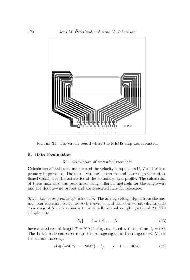
170 Jens M. Osterlund and Arne V. Johansson
JM 970127
19 21
1816
15 17
20 22
5 7GND
4 6 8
9 11
10 12
13
14
Figure 31. The circuit board where the MEMS chip was mounted.
6. Data Evaluation
6.1. Calculation of statistical moments
Calculation of statistical moments of the velocity components U, V and W is ofprimary importance. The mean, variance, skewness and flatness provide estab-lished descriptive characteristics of the boundary layer profile. The calculationof these moments was performed using different methods for the single-wireand the double-wire probes and are presented here for reference.
6.1.1. Moments from single-wire data. The analog voltage signal from the ane-mometer was sampled by the A/D converter and transformed into digital dataconsisting of N data values with an equally spaced sampling interval ∆t. Thesample data
Bi i = 1, 2, . . . , N, (33)
have a total record length T = N∆t being associated with the times ti = i∆t.The 12 bit A/D converter maps the voltage signal in the range of ±5 V intothe sample space bj,
B ∈ −2048, . . . , 2047 = bj j = 1, . . . , 4096. (34)

Turbulent Boundary Layer Experiments 171
Figure 32. The plug where the printed circuit board withthe MEMS hot-film was mounted.
The mean value of the sample data Bi, can be expressed as,
E(B) =1N
N∑i=1
Bi =1N
4096∑j=1
∑Bi=bj
Bi =1N
4096∑j=1
∑Bi=bj
bj (35)
=1N
4096∑j=1
bj∑
Bi=bj
1
︸ ︷︷ ︸nj
=4096∑j=1
bjPj (36)
giving the discrete probability density function,
Pj =njN, j = 1, . . . , 4096. (37)

172 Jens M. Osterlund and Arne V. Johansson
Reθ
cf
0 0.5 1 1.5 2 2.5 3
x 104
2
2.5
3
3.5x 10
-3
Fernholz & Finley (1996)KTH, Oil-film (series 1)KTH, Oil-film (series 2)KTH, Oil-film fitKTH, Near-wall fitKTH, Near-wall, x = 1.5 mKTH, Near-wall, x = 2.5 mKTH, Near-wall, x = 3.5 mKTH, Near-wall, x = 4.5 mKTH, Near-wall, x = 5.5 mKTH, Near-wall, x = 5.5 m
Figure 33. Skin-friction coefficient using the oil-film andnear-wall methods, shown with best-fit logarithmic frictionlaws from Equation (32) and the correlation of Fernholz &Finley (1996).
If the function F (B) is the calibration function mapping the sampled data tovelocities Ui,
Ui = F (Bi) (38)
this gives the expression for the mean,
U = E(U) =4096∑j=1
F (bj)Pj. (39)
With uj = F (Bj)− U then the variance can be expressed as,
u2 = E((U − U)2) =4096∑j=1
u2jPj , (40)
the skewness,
S(U) =u3
u23/2
=1
u23/2
4096∑j=1
u3jPj , (41)

Turbulent Boundary Layer Experiments 173
and the flatness,
F (U) =u4
u22 =
1
u22
4096∑j=1
u4jPj. (42)
The described method is computationally very efficient since only a sumover 4096 values needs to be computed for every moment instead of a sum overthe whole data set. The probability density function was generated in real timewhich made it possible to monitor the progress of the measurement withoutany delays.
6.1.2. Moments from double-wire data. For the calculation of statistical mo-ments from the double-wire data another method was used since generating a2-D (40962) discrete probability density function and using the same methodas for the single-wire data would be very inefficient.
The calculation of these moments was instead done using a binomial ex-pansion of the definitions shown in the expressions 43–45, to give the variance
u2 =1N
N∑i=1
(Ui − U
)2=
1N
N∑i=1
U2i − U
2, (43)
skewness
S(U) =u3
u23/2
=1N
N∑i=1
(Ui − U√
u2
)3
=1
u23/2
[2U
3+
1N
N∑i=1
U3i −
3UN2
N∑i=1
U2i
],
(44)
and flatness
F (U) =u4
u22 =
1N
N∑i=1
(Ui − U√
u2
)4
=1
u22
[1N
N∑i=1
U4i −
4UN
N∑i=1
U3i +
6U2
N
N∑i=1
U2i − 3U
4
].
(45)
The cross-correlation was calculated using,
uv =1N
N∑i=1
uivi − U V . (46)
These expanded versions was chosen because the sums of U , U2, U3 and U4
for each velocity component plus the cross sum of uv can be calculated withone sweep through the data set.

174 Jens M. Osterlund and Arne V. Johansson
6.2. Power spectral estimation
Estimation of auto spectral density functions was done using a direct FFTcalculation procedure. The sampled time series, with the mean removed,
um ≡ u(tm), tm ≡ (m− 1)∆t, m = 1, 2, . . . ,M (47)
with a total length of Tr was divided into nd contiguous segments each of lengthT , giving
uin ≡ u(tin), (48)
tin = ((i− 1)N + (n− 1))∆t (49)
i = 1, 2, . . . , nd, n = 1, 2, . . . , N (50)
Use the discrete Fourier transform,
uik =N∑
n=1
uine2πi(k−1)(n−1)/N k = 1, 2, . . . , N. (51)
to define the so called one-sided periodogram estimate of the power spectrum,
Pik =akN2|uik|2, k = 1, 2, . . . , N/2 + 1 (52)
where,
ak =
1 if k=1 or k=N/2+12 otherwise (53)
and
fk ≡k − 1N∆t
= 2fck − 1N
k = 1, 2, . . . ,N
2+ 1. (54)
The periodogram has the property that its sum equals the variance of thesignal. Using Parsevals relation,
N/2+1∑k=1
Pik =1N
N∑n=1
|uin|2 = u2 (55)
The one-sided auto spectral function can now be calculated by averaging thesegments,
Guu(fk) =∆tNnd
nd∑i=1
Pik. (56)
6.3. Autocorrelation estimation
The auto correlation function is defined as,
Ruu(r∆t) =1
N − r
N−r∑n=1
unun+r, r = 1, 2, . . . , m, (57)

Turbulent Boundary Layer Experiments 175
where N is the record length, r the lag number and m the maximum lagnumber, m < N . The autocorrelation function was not calculated using thedefinition, instead the autocorrelation was determined via FFT.
6.4. Storage and data structures
The digitized data and the corresponding experimental parameters were storedin a number of data bases with similar structures. The whole data base isavailable on the Department of Mechanics web server at the address:http://www.mech.kth.se/~jens/zpg/.
6.4.1. Single wire data base. During the measurement the main program storesthe digitized data in four kinds of files: one header file (text) containing all theexperimental parameters, one binary file containing the probability densitydistributions generated from the data, nj in equation 37, one binary file foreach point in the boundary layer containing the actual time series and finallyone text file with the calculated statistics. Another format is available for usersof MATLAB. During the evaluation process the header and statistics files of allsingle wire measurements were processed into an array of structures containingall 80 measurements. This format is very handy for interactive work while itallows the user to have access to all data at the same time.
The experimental parameters of all single-wire measurements are gatheredin tables 3 to 12.
6.4.2. X- and V-wire data bases. In tables 13, 14 and 15 the flow parametersfor the X-and V-wire experiments are presented. The X- and V-wire programsgenerated three kinds of output files: one text file containing the experimentalparameters, one binary file for each position in the boundary layer containingthe digitized time series of the anemometer signal from the two wires and onefile with statistics calculated from a subset of the time series (to speed up themeasurement) for monitoring purpose. The final statistics were calculated afterthe experiment using the expressions in section 6.1.2.
6.4.3. Double hot-film data base. The double hot-film measurement programgenerated three kinds of files: again one text file containing all experimen-tal parameters, one binary file containing the digitized time series from theanemometer signal from the two hot-films, one file containing the probabilitydensity distributions, and one text statistics file.

176Jens
M.Osterlund
andArne
V.Johansson
index 1 2 3 4 5 6 7Name SW981129A SW981129B SW981129C SW981129D SW981129E SW981129F SW981129G
X m 1.5 1.5 1.5 1.5 1.5 1.5 1.5U∞ m/s 10.6 13.4 16.2 21.8 27.3 32.7 37.9Uτ m/s 0.43 0.54 0.64 0.84 1.03 1.22 1.40cf 3.35e-03 3.22e-03 3.10e-03 2.96e-03 2.86e-03 2.79e-03 2.72e-03Reθ 2533 3058 3651 4613 5486 6263 7147θ m 3.5e-03 3.3e-03 3.2e-03 3.0e-03 2.9e-03 2.8e-03 2.7e-03δ∗ m 4.9e-03 4.7e-03 4.6e-03 4.3e-03 4.0e-03 3.8e-03 3.7e-03H 1.4e+00 1.4e+00 1.4e+00 1.4e+00 1.4e+00 1.4e+00 1.4e+00∆ m 1.2e-01 1.2e-01 1.2e-01 1.1e-01 1.1e-01 1.0e-01 1.0e-01δ m 2.3e-02 2.2e-02 2.1e-02 2.0e-02 1.9e-02 1.9e-02 1.8e-02δ+ 684 801 929 1162 1384 1579 1780dwire m 1.25e-06 1.25e-06 1.25e-06 1.25e-06 1.25e-06 1.25e-06 1.25e-06lwire m 2.50e-04 2.50e-04 2.50e-04 2.50e-04 2.50e-04 2.50e-04 2.50e-04l+wire 7.5 9.3 11.1 14.5 17.9 21.1 24.3fs Hz 40000.0 40000.0 40000.0 40000.0 40000.0 40000.0 40000.0Tr s 33.7 33.7 33.7 33.7 33.7 33.7 33.7
Table 3. Single-wire measurements (continued).

Turbulent
Boundary
LayerExperim
ents177
index 8 9 10 11 12 13 14Name SW981129H SW981129I SW981129J SW981128A SW981128B SW981128C SW981128D
X m 1.5 1.5 1.5 2.5 2.5 2.5 2.5U∞ m/s 43.2 48.5 53.7 10.4 13.2 16.0 21.5Uτ m/s 1.58 1.75 1.91 0.41 0.51 0.61 0.80cf 2.66e-03 2.61e-03 2.54e-03 3.10e-03 3.00e-03 2.89e-03 2.76e-03Reθ 7981 8873 10162 3654 4312 5156 6511θ m 2.7e-03 2.6e-03 2.7e-03 5.2e-03 4.8e-03 4.7e-03 4.4e-03δ∗ m 3.6e-03 3.6e-03 3.6e-03 7.2e-03 6.7e-03 6.6e-03 6.1e-03H 1.4e+00 1.4e+00 1.3e+00 1.4e+00 1.4e+00 1.4e+00 1.4e+00∆ m 9.9e-02 9.9e-02 1.0e-01 1.8e-01 1.7e-01 1.7e-01 1.6e-01δ m 1.8e-02 1.8e-02 1.8e-02 3.3e-02 3.1e-02 3.1e-02 2.9e-02δ+ 1990 2188 2385 918 1092 1270 1594dwire m 1.25e-06 1.25e-06 1.25e-06 1.25e-06 1.25e-06 1.25e-06 1.25e-06lwire m 2.50e-04 2.50e-04 2.50e-04 2.50e-04 2.50e-04 2.50e-04 2.50e-04l+wire 27.4 30.4 33.2 7.0 8.7 10.4 13.6fs Hz 40000.0 40000.0 40000.0 40000.0 40000.0 40000.0 40000.0Tr s 33.7 33.7 33.7 33.7 33.7 33.7 33.7
Table 4. Single-wire measurements (continued).

178Jens
M.Osterlund
andArne
V.Johansson
index 15 16 17 18 19 20 21Name SW981128E SW981128F SW981128G SW981128H SW981128I SW981128J SW981127H
X m 2.5 2.5 2.5 2.5 2.5 2.5 3.5U∞ m/s 26.9 32.2 37.4 42.8 47.9 53.2 10.3Uτ m/s 0.98 1.16 1.33 1.50 1.67 1.84 0.40cf 2.66e-03 2.59e-03 2.53e-03 2.48e-03 2.43e-03 2.39e-03 2.95e-03Reθ 7970 9112 10314 11733 12867 14290 4705θ m 4.3e-03 4.1e-03 4.0e-03 4.0e-03 3.9e-03 3.9e-03 6.6e-03δ∗ m 5.9e-03 5.6e-03 5.4e-03 5.4e-03 5.2e-03 5.2e-03 9.2e-03H 1.4e+00 1.4e+00 1.3e+00 1.3e+00 1.3e+00 1.3e+00 1.4e+00∆ m 1.6e-01 1.6e-01 1.5e-01 1.5e-01 1.5e-01 1.5e-01 2.4e-01δ m 2.9e-02 2.8e-02 2.7e-02 2.7e-02 2.7e-02 2.7e-02 4.3e-02δ+ 1919 2198 2477 2780 3045 3342 1166dwire m 1.25e-06 1.25e-06 1.25e-06 1.25e-06 1.25e-06 1.25e-06 1.25e-06lwire m 2.50e-04 2.50e-04 2.50e-04 2.50e-04 2.50e-04 2.50e-04 2.50e-04l+wire 16.8 19.8 22.8 25.7 28.5 31.4 6.8fs Hz 40000.0 40000.0 40000.0 40000.0 40000.0 40000.0 40000.0Tr s 33.7 33.7 33.7 33.7 33.7 33.7 33.7
Table 5. Single-wire measurements (continued).
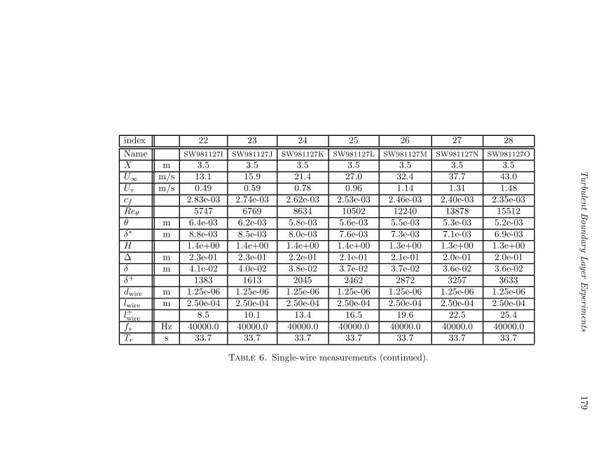
Turbulent
Boundary
LayerExperim
ents179
index 22 23 24 25 26 27 28Name SW981127I SW981127J SW981127K SW981127L SW981127M SW981127N SW981127O
X m 3.5 3.5 3.5 3.5 3.5 3.5 3.5U∞ m/s 13.1 15.9 21.4 27.0 32.4 37.7 43.0Uτ m/s 0.49 0.59 0.78 0.96 1.14 1.31 1.48cf 2.83e-03 2.74e-03 2.62e-03 2.53e-03 2.46e-03 2.40e-03 2.35e-03Reθ 5747 6769 8634 10502 12240 13878 15512θ m 6.4e-03 6.2e-03 5.8e-03 5.6e-03 5.5e-03 5.3e-03 5.2e-03δ∗ m 8.8e-03 8.5e-03 8.0e-03 7.6e-03 7.3e-03 7.1e-03 6.9e-03H 1.4e+00 1.4e+00 1.4e+00 1.4e+00 1.3e+00 1.3e+00 1.3e+00∆ m 2.3e-01 2.3e-01 2.2e-01 2.1e-01 2.1e-01 2.0e-01 2.0e-01δ m 4.1e-02 4.0e-02 3.8e-02 3.7e-02 3.7e-02 3.6e-02 3.6e-02δ+ 1383 1613 2045 2462 2872 3257 3633dwire m 1.25e-06 1.25e-06 1.25e-06 1.25e-06 1.25e-06 1.25e-06 1.25e-06lwire m 2.50e-04 2.50e-04 2.50e-04 2.50e-04 2.50e-04 2.50e-04 2.50e-04l+wire 8.5 10.1 13.4 16.5 19.6 22.5 25.4fs Hz 40000.0 40000.0 40000.0 40000.0 40000.0 40000.0 40000.0Tr s 33.7 33.7 33.7 33.7 33.7 33.7 33.7
Table 6. Single-wire measurements (continued).
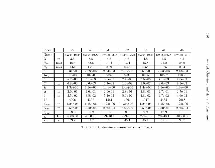
180Jens
M.Osterlund
andArne
V.Johansson
index 29 30 31 32 33 34 35Name SW981127P SW981127Q SW981126C SW981126D SW981126E SW981127A SW981127B
X m 3.5 3.5 4.5 4.5 4.5 4.5 4.5U∞ m/s 48.4 53.6 10.4 13.1 15.8 21.2 26.9Uτ m/s 1.64 1.81 0.39 0.48 0.58 0.75 0.94cf 2.31e-03 2.28e-03 2.84e-03 2.73e-03 2.65e-03 2.53e-03 2.43e-03Reθ 17280 18720 5689 6931 8105 10387 12886θ m 5.2e-03 5.1e-03 8.0e-03 7.7e-03 7.5e-03 7.1e-03 7.0e-03δ∗ m 6.8e-03 6.6e-03 1.1e-02 1.0e-02 1.0e-02 9.6e-03 9.3e-03H 1.3e+00 1.3e+00 1.4e+00 1.4e+00 1.4e+00 1.3e+00 1.3e+00∆ m 2.0e-01 2.0e-01 2.9e-01 2.8e-01 2.8e-01 2.7e-01 2.7e-01δ m 3.5e-02 3.5e-02 5.1e-02 5.0e-02 4.8e-02 4.7e-02 4.6e-02δ+ 4006 4367 1381 1661 1917 2432 2968dwire m 1.25e-06 1.25e-06 1.25e-06 1.25e-06 1.25e-06 1.25e-06 1.25e-06lwire m 2.50e-04 2.50e-04 2.50e-04 2.50e-04 2.50e-04 2.50e-04 2.50e-04l+wire 28.3 31.2 6.7 8.3 9.9 12.9 16.1fs Hz 40000.0 40000.0 29940.1 29940.1 29940.1 29940.1 40000.0Tr s 33.7 33.7 45.1 45.1 45.1 45.1 33.7
Table 7. Single-wire measurements (continued).

Turbulent
Boundary
LayerExperim
ents181
index 36 37 38 39 40 41 42Name SW981127C SW981127D SW981127E SW981127F SW981127G SW981005A SW981005B
X m 4.5 4.5 4.5 4.5 4.5 5.5 5.5U∞ m/s 32.4 37.8 43.3 48.7 52.6 21.4 15.9Uτ m/s 1.11 1.29 1.46 1.63 1.75 0.75 0.57cf 2.37e-03 2.31e-03 2.27e-03 2.23e-03 2.20e-03 2.44e-03 2.56e-03Reθ 14973 17102 19235 20958 22579 12633 9707θ m 6.7e-03 6.6e-03 6.5e-03 6.3e-03 6.3e-03 8.6e-03 8.9e-03δ∗ m 8.9e-03 8.7e-03 8.5e-03 8.2e-03 8.1e-03 1.2e-02 1.2e-02H 1.3e+00 1.3e+00 1.3e+00 1.3e+00 1.3e+00 1.3e+00 1.3e+00∆ m 2.6e-01 2.6e-01 2.5e-01 2.4e-01 2.4e-01 3.3e-01 3.3e-01δ m 4.5e-02 4.5e-02 4.4e-02 4.3e-02 4.3e-02 5.7e-02 5.8e-02δ+ 3457 3944 4418 4856 5197 2903 2272dwire m 1.25e-06 1.25e-06 1.25e-06 1.25e-06 1.25e-06 1.27e-06 1.27e-06lwire m 2.50e-04 2.50e-04 2.50e-04 2.50e-04 2.50e-04 2.50e-04 2.50e-04l+wire 19.1 22.1 25.0 27.9 30.0 12.8 9.8fs Hz 40000.0 40000.0 40000.0 40000.0 40000.0 29940.1 29940.1Tr s 33.7 33.7 33.7 33.7 33.7 35.0 35.0
Table 8. Single-wire measurements (continued).

182Jens
M.Osterlund
andArne
V.Johansson
index 43 44 45 46 47 48 49Name SW981005C SW981005D SW981005E SW981005F SW981006A SW981006B SW981006C
X m 5.5 5.5 5.5 5.5 5.5 5.5 5.5U∞ m/s 13.1 10.4 26.8 32.2 37.4 42.5 48.3Uτ m/s 0.48 0.39 0.92 1.09 1.25 1.41 1.58cf 2.65e-03 2.75e-03 2.36e-03 2.29e-03 2.25e-03 2.20e-03 2.15e-03Reθ 8209 6700 15182 17901 20258 22846 25779θ m 9.1e-03 9.3e-03 8.2e-03 8.1e-03 7.9e-03 7.8e-03 7.8e-03δ∗ m 1.2e-02 1.3e-02 1.1e-02 1.1e-02 1.0e-02 1.0e-02 1.0e-02H 1.4e+00 1.4e+00 1.3e+00 1.3e+00 1.3e+00 1.3e+00 1.3e+00∆ m 3.4e-01 3.4e-01 3.2e-01 3.1e-01 3.1e-01 3.1e-01 3.1e-01δ m 5.9e-02 6.1e-02 5.5e-02 5.4e-02 5.4e-02 5.3e-02 5.3e-02δ+ 1947 1612 3480 4067 4626 5167 5769dwire m 1.27e-06 1.27e-06 1.27e-06 1.27e-06 1.27e-06 1.27e-06 1.27e-06lwire m 2.50e-04 2.50e-04 2.50e-04 2.50e-04 2.50e-04 2.50e-04 2.50e-04l+wire 8.2 6.7 15.8 18.8 21.6 24.3 27.2fs Hz 29940.1 29940.1 29940.1 29940.1 29940.1 40000.0 40000.0Tr s 35.0 35.0 35.0 35.0 35.0 26.2 26.2
Table 9. Single-wire measurements (continued).

Turbulent
Boundary
LayerExperim
ents183
index 50 51 52 53 54 55 56Name SW981008A SW981008B SW981008C SW981008D SW981012A SW981012B SW981012C
X m 5.5 5.5 5.5 5.5 5.5 5.5 5.5U∞ m/s 52.2 46.5 40.0 45.3 36.7 31.7 26.5Uτ m/s 1.71 1.53 1.34 1.50 1.24 1.08 0.92cf 2.14e-03 2.18e-03 2.23e-03 2.19e-03 2.28e-03 2.33e-03 2.39e-03Reθ 26612 23870 21099 23120 18480 16422 14207θ m 7.5e-03 7.5e-03 7.7e-03 7.5e-03 7.6e-03 7.9e-03 8.1e-03δ∗ m 9.7e-03 9.8e-03 1.0e-02 9.7e-03 1.0e-02 1.0e-02 1.1e-02H 1.3e+00 1.3e+00 1.3e+00 1.3e+00 1.3e+00 1.3e+00 1.3e+00∆ m 3.0e-01 3.0e-01 3.0e-01 2.9e-01 3.0e-01 3.0e-01 3.1e-01δ m 5.2e-02 5.2e-02 5.3e-02 5.2e-02 5.3e-02 5.4e-02 5.5e-02δ+ 6019 5443 4828 5304 4300 3822 3313dwire m 1.27e-06 1.27e-06 1.27e-06 1.27e-06 1.27e-06 1.27e-06 1.27e-06lwire m 2.50e-04 2.50e-04 2.50e-04 2.50e-04 2.50e-04 2.50e-04 2.50e-04l+wire 29.2 26.2 22.8 25.6 20.4 17.8 15.1fs Hz 40000.0 40000.0 40000.0 40000.0 40000.0 40000.0 40000.0Tr s 26.2 26.2 26.2 26.2 26.2 26.2 26.2
Table 10. Single-wire measurements (continued).
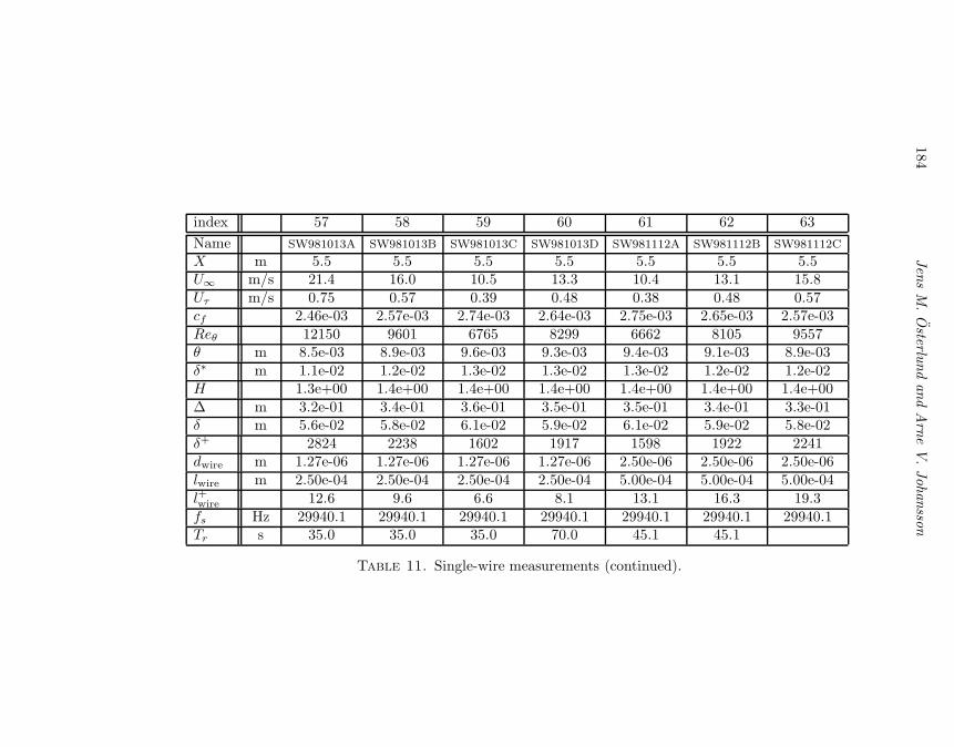
184Jens
M.Osterlund
andArne
V.Johansson
index 57 58 59 60 61 62 63Name SW981013A SW981013B SW981013C SW981013D SW981112A SW981112B SW981112C
X m 5.5 5.5 5.5 5.5 5.5 5.5 5.5U∞ m/s 21.4 16.0 10.5 13.3 10.4 13.1 15.8Uτ m/s 0.75 0.57 0.39 0.48 0.38 0.48 0.57cf 2.46e-03 2.57e-03 2.74e-03 2.64e-03 2.75e-03 2.65e-03 2.57e-03Reθ 12150 9601 6765 8299 6662 8105 9557θ m 8.5e-03 8.9e-03 9.6e-03 9.3e-03 9.4e-03 9.1e-03 8.9e-03δ∗ m 1.1e-02 1.2e-02 1.3e-02 1.3e-02 1.3e-02 1.2e-02 1.2e-02H 1.3e+00 1.4e+00 1.4e+00 1.4e+00 1.4e+00 1.4e+00 1.4e+00∆ m 3.2e-01 3.4e-01 3.6e-01 3.5e-01 3.5e-01 3.4e-01 3.3e-01δ m 5.6e-02 5.8e-02 6.1e-02 5.9e-02 6.1e-02 5.9e-02 5.8e-02δ+ 2824 2238 1602 1917 1598 1922 2241dwire m 1.27e-06 1.27e-06 1.27e-06 1.27e-06 2.50e-06 2.50e-06 2.50e-06lwire m 2.50e-04 2.50e-04 2.50e-04 2.50e-04 5.00e-04 5.00e-04 5.00e-04l+wire 12.6 9.6 6.6 8.1 13.1 16.3 19.3fs Hz 29940.1 29940.1 29940.1 29940.1 29940.1 29940.1 29940.1Tr s 35.0 35.0 35.0 70.0 45.1 45.1
Table 11. Single-wire measurements (continued).

Turbulent
Boundary
LayerExperim
ents185
index 64 65 66 67 68 69 70Name SW981112D SW981113A SW981113B SW981113C SW981113D SW981113E SW981113F
X m 5.5 5.5 5.5 5.5 5.5 5.5 5.5U∞ m/s 21.2 26.9 32.4 37.9 43.6 49.1 54.0Uτ m/s 0.74 0.92 1.10 1.27 1.44 1.61 1.76cf 2.45e-03 2.36e-03 2.30e-03 2.24e-03 2.19e-03 2.15e-03 2.13e-03Reθ 12309 15165 17813 20562 23310 25767 27320θ m 8.5e-03 8.3e-03 8.1e-03 8.0e-03 7.9e-03 7.7e-03 7.5e-03δ∗ m 1.1e-02 1.1e-02 1.1e-02 1.0e-02 1.0e-02 1.0e-02 9.6e-03H 1.3e+00 1.3e+00 1.3e+00 1.3e+00 1.3e+00 1.3e+00 1.3e+00∆ m 3.2e-01 3.2e-01 3.2e-01 3.1e-01 3.1e-01 3.1e-01 2.9e-01δ m 5.6e-02 5.5e-02 5.4e-02 5.4e-02 5.4e-02 5.3e-02 5.1e-02δ+ 2851 3461 4049 4642 5245 5780 6147dwire m 2.50e-06 2.50e-06 2.50e-06 2.50e-06 2.50e-06 2.50e-06 2.50e-06lwire m 5.00e-04 5.00e-04 5.00e-04 5.00e-04 5.00e-04 5.00e-04 5.00e-04l+wire 25.4 31.4 37.3 43.0 48.9 54.7 59.8fs Hz 29940.1 40000.0 40000.0 40000.0 40000.0 40000.0 40000.0Tr s
Table 12. Single-wire measurements (continued).

186Jens
M.Osterlund
andArne
V.Johansson
Index 1 2 3 4 5
Name XW981116A XW981117A XW981117B XW981117C XW981117D
X m 5.5 5.5 5.5 5.5 5.5
U∞ m/s 10.4 13.1 15.8 18.5 21.2
Uτ m/s 0.38 0.47 0.56 0.65 0.74
Reθ 6928 8389 9771 11150 12501
θ m 9.7e-03 9.3e-03 9.0e-03 8.7e-03 8.6e-03
δ∗ m 1.3e-02 1.3e-02 1.2e-02 1.2e-02 1.1e-02
∆ m 3.6e-01 3.5e-01 3.4e-01 3.3e-01 3.3e-01
δ m 6.3e-02 6.1e-02 5.9e-02 5.8e-02 5.7e-02
δ+ m 1676 2002 2310 2618 2919
dwire m 1.27e-06 1.27e-06 1.27e-06 1.27e-06 1.27e-06
lwire m 3.00e-04 3.00e-04 3.00e-04 3.00e-04 3.00e-04
l+wire 7.9 9.8 11.7 13.5 15.3
fs Hz 29940.1 29940.1 29940.1 29940.1 29940.1
Tr s 68.4 68.4 68.4 68.4 68.4
Table 13. X-wire measurements.
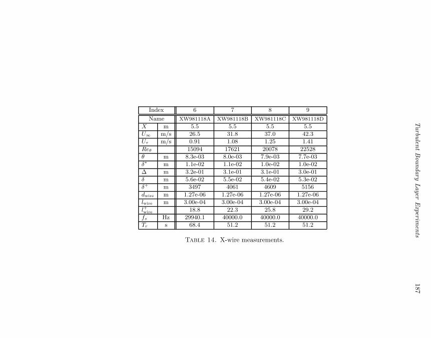
Turbulent
Boundary
LayerExperim
ents187
Index 6 7 8 9
Name XW981118A XW981118B XW981118C XW981118D
X m 5.5 5.5 5.5 5.5
U∞ m/s 26.5 31.8 37.0 42.3
Uτ m/s 0.91 1.08 1.25 1.41
Reθ 15094 17621 20078 22528
θ m 8.3e-03 8.0e-03 7.9e-03 7.7e-03
δ∗ m 1.1e-02 1.1e-02 1.0e-02 1.0e-02
∆ m 3.2e-01 3.1e-01 3.1e-01 3.0e-01
δ m 5.6e-02 5.5e-02 5.4e-02 5.3e-02
δ+ m 3497 4061 4609 5156
dwire m 1.27e-06 1.27e-06 1.27e-06 1.27e-06
lwire m 3.00e-04 3.00e-04 3.00e-04 3.00e-04
l+wire 18.8 22.3 25.8 29.2
fs Hz 29940.1 40000.0 40000.0 40000.0
Tr s 68.4 51.2 51.2 51.2
Table 14. X-wire measurements.

188Jens
M.Osterlund
andArne
V.Johansson
Index 1 2 3 4 5 6 7
Name VW981119A VW981119B VW981119C VW981119D VW981121A VW981121B VW981122A
X m 5.5 5.5 5.5 5.5 5.5 5.5 5.5
U∞ m/s 10.4 13.2 15.9 21.4 26.4 31.1 35.7
Uτ m/s 0.38 0.48 0.57 0.75 0.91 1.06 1.20
Reθ 6976 8500 9953 12748 15117 17401 19532
θ m 9.7e-03 9.2e-03 8.9e-03 8.5e-03 8.3e-03 8.1e-03 7.9e-03
δ∗ m 1.3e-02 1.3e-02 1.2e-02 1.1e-02 1.1e-02 1.1e-02 1.0e-02
∆ m 3.6e-01 3.5e-01 3.4e-01 3.3e-01 3.2e-01 3.1e-01 3.1e-01
δ m 6.3e-02 6.1e-02 5.9e-02 5.7e-02 5.6e-02 5.5e-02 5.4e-02
δ+ m 1686 2026 2350 2974 3503 4012 4487
dwire m 1.27e-06 1.27e-06 1.27e-06 1.27e-06 1.27e-06 1.27e-06 1.27e-06
lwire m 3.00e-04 3.00e-04 3.00e-04 3.00e-04 3.00e-04 3.00e-04 3.00e-04
l+wire 8.0 10.0 11.9 15.6 18.9 22.0 25.0
fs Hz 29940.1 29940.1 29940.1 29940.1 40000.0 40000.0 40000.0
Tr s 68.4 68.4 68.4 68.4 51.2 51.2 51.2
Table 15. V-wire measurements.

Turbulent Boundary Layer Experiments 189
7. Appendix: Measurements of shear stress using afloating-element sensor from MIT
Only a few direct wall-shear stress measurement methods exist. One is tomeasure the tangential force on a small part of the wall, a floating-elementtechnique. The wall-shear stress is then determined by
τw =F
A(58)
where F is the force on the floating-element and A the area. At first this seemsto be an ideal method since it does not rely on specific characteristics of onthe flow field or the fluid properties. Unfortunately the problems connectedwith implementing this method usually outweighs the advantages (Karlsson1980; Bertelrud 1972). The main sources of errors are, misalignment of thefloating-element, gaps around the floating-element and pressure gradients
The relatively large area of the conventional floating element sensors, seee.g. Smith & Walker (1959) and Karlsson (1980), will give the average shearin that area. For measurements of the fluctuating wall-shear stress the floatingelement size has to be of the same order as the viscous length scale. Padman-abhan (1997) used micromachining technology to develop a floating elementoptical shutter and integrated photodiodes for measurements of the fluctuatingwall-shear stress, with the dimensions 120µm × 120µm. The floating-elementis suspended by four tethers, see figures 34 and 35. A pair of photodiodes arelocated under the floating-element on the leading and trailing edges. The sen-sor is subjected to uniform illumination from a light source. With zero shearstress the exposed areas of the photodiodes are the same and the differentialphotocurrent ∆Iphoto is also zero. The differential photocurrent is proportionalto the wall-shear stress
∆Iphoto ∝ τw. (59)
In a co-operation with A. Padmanabhan and Prof. K. Breuer at MIT themicro-machined sensor was tested in the zero pressure-gradient boundary layerset-up in the MTL wind tunnel at KTH. The micro machined floating elementsensor was mounted flush with the boundary layer plate in the sensor insert atx = 5.5 m. A laser was mounted in a traversing system on the upper wall ofthe test section with the beam entering through a slit in the upper wall. Theoptimum laser position was determined for highest possible sensitivity. Thesignal from the laser diodes were connected to two low noise current amplifiers(Stanford research systems, SR570) and digitized. The differential photocur-rent signal ∆Iphoto was then calibrated against the wall-shear stress determinedby a Preston tube.
The following conclusions were drawn from the tests with the MIT sensor.Uniform illumination of the photodiodes was very difficult to achieve for dif-ferent tunnel speeds. The relative position of the laser and the sensor changed

190 Jens M. Osterlund and Arne V. Johansson
Figure 34. Schematic diagram illustrating the sensing prin-ciple (Padmanabhan 1997).
and resulted in a large variation in the photocurrent signals from the diodes.The displacements is believed to be caused by small changes in pressure andskin-friction on the plate and tunnel walls introduced by the change in tun-nel speed during the calibration process. It was therefore impossible to makea meaningful calibration of the sensor. The general impression is that it isunsuitable to have the light source and the sensor separated a large distancemaking the system extremely sensitive to vibrations and small displacementscaused by e.g. aerodynamic forces or thermal elongation. Future improvementsshould possibly include incorporating the light source into the sensor.
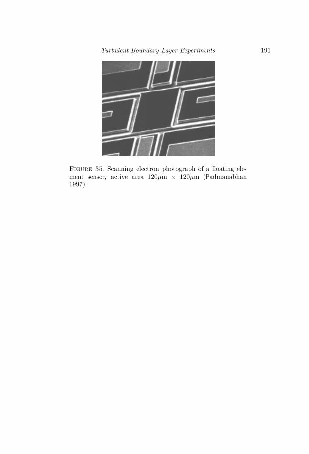
Turbulent Boundary Layer Experiments 191
Figure 35. Scanning electron photograph of a floating ele-ment sensor, active area 120µm × 120µm (Padmanabhan1997).

References
Alfredsson, P. H., Johansson, A. V., Haritonidis, J. H. & Eckelmann, H.
1988 The fluctuation wall-shear stress and the velocity field in the viscous sub-layer. Phys. Fluids A 31, 1026–33.
Bechert, D. W. 1995 Calibration of preston tubes. AIAA J. 34 (1), 205–206.
Bertelrud, A. 1972 Skin friction measurement techniques in incompressible turbu-lent flow – a literature survey. Technical Note FFA AU–726. The AeronauticalResearch Institute of Sweden.
Clauser, F. H. 1954 Turbulent boundary layers in adverse pressure gradients. J.Aero. Sci. 21, 91–108.
Fernholz, H. H. 1971 Ein halbempirisches Gezetz fur die Wandreibung in kompress-iblen turbulenten Grenzschichten bei isothermer und adiabater Wand. ZAMM51, 148–149.
Fernholz, H. H. & Finley, P. J. 1996 The incompressible zero-pressure-gradientturbulent boundary layer: An assessment of the data. Prog. Aerospace Sci. 32,245–311.
Fernholz, H. H., Janke, G., Schober, M., Wagner, P. M. & Warnack, D.
1996 New developments and applications of skin-friction measuring techniques.Meas. Sci. Technol. 7, 1396–1409.
Haritonidis, J. H. 1989 The measurement of wall shear stress. In Advances in FluidMechanics Measurements. (ed. M. Gad-el Hak), pp. 229–261. Springer-Verlag.
Ho, C.-M. & Tai, Y.-C. 1998 Micro-electro-mechanical-systems (MEMS) and fluidflows. Ann. Rev. Fluid Mech. 30, 579–612.
Janke, G. 1994 Uber die Grundlagen und einige Anwendungen der olfilm-interferometrie zur Messung von Wandreibungsfeldern in luftstromungen. PhDthesis, Technische Universitat Berlin.
Jiang, F., Tai, Y.-C., Gupta, B., Goodman, R., Tung, S., Huang, J. B. & Ho,
C.-M. 1996 A surface-micromachined shear stress imager. In 1996 IEEE MicroElectro Mechanical Systems Workshop (MEMS ’96), pp. 110–115.
Johansson, A. V. 1992 A low speed wind-tunnel with extreme flow quality - designand tests. In Prog. ICAS congress 1992 , pp. 1603–1611. ICAS-92-3.8.1.
Karlsson, R. I. 1980 Studies of skin friction in turbulent boundary layers on smooth
192

Turbulent Boundary Layer Experiments 193
and rough walls. PhD thesis, Department of Applied Thermo and Fluid Dynam-ics, Chalmers University of Technology, Goteborg, Sweden.
Komminaho, J., Lundbladh, A. & Johansson, A. V. 1996 Very large structuresin plane turbulent couette flow. J. Fluid Mech. 320, 259–285.
Lindgren, B., Osterlund, J. M. & Johansson, A. V. 1998 Measurement andcalculation of guide vane performance in expanding bends for wind-tunnels. Ex-periments in Fluids 24, 265–272.
Monson, D. J. 1983 A nonintrusive laser interferometer method for the measurementof skin friction. Experiments in Fluids 1, 15–22.
Naqwi, A. A. & Reynolds, W. C. 1991 Measurement of turbulent wall velocitygradients using cylindrical waves of laser light. Experiments in Fluids 10, 257–266.
Nishizawa, N., Marusic, I., Perry, A. E. & Hornung, H. G. 1998 Measurementof wall shear stress in turbulent boundary layers using an optical interferometrymethod. In 13th Australian Fluid Mechanics Conferance, Monash University,Melbourne, Australia .
Obi, S., Inoue, K., Furukawa, T. & Masuda, S. 1996 Experimental study on thestatistics of wall shear stress in turbulent channel flows. Int. J. Heat and FluidFlow 17, 187–192.
Osterlund, J. M., Johansson, A. V., Nagib, H. M. & Hites, M. H. 1999 Wallshear stress measurements in high reynolds number boundary layers from twofacilities. In 30th AIAA Fluid Dynamics Conference, Norfolk, VA. AIAA paper99-3814.
Padmanabhan, A. 1997 Silicon micromachined sensors and sensor arrays for shear-stress measurements in aerodynamic flows. PhD thesis, Massachusetts Instituteof Technology, FDLR TR 97–5.
Patel, V. C. 1965 Calibration of the Preston tube and limitations on its use inpressure gradients. J. R. Aero. Soc. 23, 185–208.
Preston, J. H. 1953 The determination of turbulent skin friction by means of Pitottubes. J. Fluid Mech. 58, 109–1215.
Sahlin, A. & Johansson, A. V. 1991 Design of guide vanes for minimizing thepressure loss in sharp bends. Phys. Fluids A 3, 1934–1940.
Seto, J. & Hornung, H. G. 1993 Two-directional skin friction measurement uti-lizing a compact internally-mounted thin-liquid-film skin friction meter. AIAApaper 93-0180.
Skote, M., Henkes, R. & Henningson, D. 1998 Direct numerical simulation ofself-similar turbulent boundary layers in adverse pressure gradients. In Flow,Turbulence and Combustion , , vol. 60, pp. 47–85. Kluwer Academic Publishers.
Smith, D. W. & Walker, J. H. 1959 Skin-friction measurements in incompressibleflow. NASA TR R-26.
Spalart, P. R. 1988 Direct simulation of a turbulent boundary layer up to Reθ =1410. J. Fluid Mech. 187, 61–98.
Tanner, L. H. & Blows, L. G. 1976 A study of the motion of oil films on surfaces inair flow, with application to the measurement of skin friction. Journal of PhysicsE: Scientific Instruments 9, 194–202.
194 REFERENCES
Winter, K. G. 1977 An outline of the techniques available for the measurement ofskin friction in turbulent boundary layers. Prog. Aerospace. Sci. 18, 1–57.