Enhancement of mass transfer in a two-layer Taylor-Couette apparatus with axial flow
Upload
khangminh22Category
view
2download
0
ISBN 978-90-365-3272-3
1
2
3
4
5
6
Figure: High-speed imaging snapshots of transient ow inside the Taylor-Couette gap at startup of inner cylinder rotation from quiescent ow (1) to fully developed turbu-lence (6). Turbulent plumes grow on the inner cylinder (bottom) and are advected towards the outer cylinder (top). Visualisation by reective akes in a laser sheet.
DENNIS P.M. VAN GILS
Highly Turbulent Taylor-C
ouette Flow
UitnodigingHierbij wil ik u graagvan harte uitnodigen
voor het bijwonen vande openbare verdediging
van mijn proefschrift
Highly TurbulentTaylor-Couette Flow
opvrijdag 16 december 2011
om 16:45 in zaal 4 vanhet gebouw de Waaier van
de Universiteit Twente.
Voorafgaande zal ik om16:30 een korte toelichtinggeven op mijn promotie-
onderzoek.
Na afloop van depromotieplechtigheid
zal er een receptie zijn.
~~~~~~~~~~
Dennis van GilsZuiderhagen 41-27511GJ Enschede
~~~~~~~~~~
Paranimfen:Ivo Peters
Rianne de Jong
Dennis P.M
. van Gils


HIGHLY TURBULENTTAYLOR-COUETTE FLOW
Dennis Paulus Maria van Gils

The work in this thesis was primarily carried out at the Physics of Fluids group of theFaculty of Science and Technology of the University of Twente. It is supported bythe Dutch Technology Foundation STW, which is part of the Netherlands Organisa-tion for Scientific Research (NWO) and partly funded by the Ministry of EconomicAffairs, Agriculture and Innovation (project number 07781).
Committee members:ChairmanProf. dr. Leen van Wijngaarden University of Twente
PromotorProf. dr. Detlef Lohse University of Twente
Assistant promotorDr. Chao Sun University of Twente
MembersProf. dr. ir. Theo H. van der Meer University of TwenteProf. dr. Roberto Verzicco University of Twente & RomeProf. dr. ir. Tom J.C. van Terwisga Delft University of Technology / MARINProf. dr. ir. Jerry Westerweel Delft University of Technology
Nederlandse titel:Hoog Turbulente Taylor-Couette Stroming
Cover:High-speed imaging snapshot showing fully developed turbulent structures inside theT3C gap, seeded with reflective flakes and illuminated by a laser sheet. On the left isthe inner cylinder wall, on the right the outer cylinder wall.
Publisher:Dennis P.M. van Gils, Physics of Fluids, University of Twente,P.O. Box 217, 7500 AE Enschede, The Netherlandshttp://pof.tnw.utwente.nl [email protected]
Copyright c⃝ 2011 by Dennis P.M. van Gils, Enschede, The Netherlands.No part of this work may be reproduced by print, photocopy or any other meanswithout the permission in writing from the publisher.Ph.D. Thesis, University of Twente. Printed by Gildeprint Drukkerijen, Enschede.ISBN: 978-90-365-3272-3 DOI: 10.3990/1.9789036532723

HIGHLY TURBULENT TAYLOR-COUETTE FLOW
PROEFSCHRIFT
ter verkrijging vande graad van doctor aan de Universiteit Twente,
op gezag van de rector magnificus,prof. dr. H. Brinksma,
volgens besluit van het College voor Promotiesin het openbaar te verdedigen
op vrijdag 16 december 2011 om 16.45 uur
door
Dennis Paulus Maria van Gils
geboren op 2 mei 1981te Roosendaal en Nispen

This dissertation has been approved by:
Promotor: Prof. dr. Detlef LohseAssistant promotor: Dr. Chao Sun

Turbulent flows persist to remain enigmaticto mankind – in its details and main features – still
after more than 400 years of scientific research.Does this then imply that to pursue a completeunderstanding of turbulence is an exercise in
futility? Perhaps so, hopefully not, more definitelyit is no reason to stop researching. Let this thesis
be a new part of this ongoing puzzle.


Contents
1 Introduction 11.1 Renewed interest . . . . . . . . . . . . . . . . . . . . . . . . . . . 11.2 Taylor-Couette flow and the analogy to Rayleigh-Benard convection 21.3 Guide through Part I — Experimental setup . . . . . . . . . . . . . 61.4 Guide through Part II — Single-phase Taylor-Couette flow . . . . . 61.5 Guide through Part III — Bubbly Taylor-Couette flow . . . . . . . . 8
I Experimental setup 11
2 The Twente turbulent Taylor-Couette facility 132.1 Introduction . . . . . . . . . . . . . . . . . . . . . . . . . . . . . . 142.2 System description . . . . . . . . . . . . . . . . . . . . . . . . . . 182.3 Examples of results . . . . . . . . . . . . . . . . . . . . . . . . . . 302.4 Summary and outlook . . . . . . . . . . . . . . . . . . . . . . . . . 32
II Single-phase Taylor-Couette flow 35
3 Torque scaling in turbulent Taylor-Couette flow with co- and counter-rotating cylinders 373.1 Introduction . . . . . . . . . . . . . . . . . . . . . . . . . . . . . . 383.2 Experimental method . . . . . . . . . . . . . . . . . . . . . . . . . 393.3 Results . . . . . . . . . . . . . . . . . . . . . . . . . . . . . . . . . 393.4 Conclusion . . . . . . . . . . . . . . . . . . . . . . . . . . . . . . 44
4 Optimal Taylor-Couette turbulence 454.1 Introduction . . . . . . . . . . . . . . . . . . . . . . . . . . . . . . 464.2 Experimental setup and discussion of end-effects . . . . . . . . . . 484.3 Global torque measurements . . . . . . . . . . . . . . . . . . . . . 514.4 Local LDA angular velocity radial profiles . . . . . . . . . . . . . . 594.5 Turbulent flow organization in the TC gap . . . . . . . . . . . . . . 64
i

ii CONTENTS
4.6 Boundary layers . . . . . . . . . . . . . . . . . . . . . . . . . . . . 684.7 Summary, discussion, and outlook . . . . . . . . . . . . . . . . . . 71
5 Angular momentum transport and turbulence in laboratory models ofKeplerian flows 735.1 Introduction . . . . . . . . . . . . . . . . . . . . . . . . . . . . . . 745.2 Apparatus and experimental details . . . . . . . . . . . . . . . . . . 755.3 Results . . . . . . . . . . . . . . . . . . . . . . . . . . . . . . . . . 805.4 Discussion . . . . . . . . . . . . . . . . . . . . . . . . . . . . . . . 885.5 Conclusions . . . . . . . . . . . . . . . . . . . . . . . . . . . . . . 92
III Bubbly Taylor-Couette flow 93
6 Bubbly turbulent drag reduction is a boundary layer effect 956.1 Introduction . . . . . . . . . . . . . . . . . . . . . . . . . . . . . . 966.2 Experimental method . . . . . . . . . . . . . . . . . . . . . . . . . 976.3 Results . . . . . . . . . . . . . . . . . . . . . . . . . . . . . . . . . 996.4 Conclusion . . . . . . . . . . . . . . . . . . . . . . . . . . . . . . 101
7 Bubble deformability is crucial for strong drag reduction in turbulentTaylor-Couette flow 1037.1 Introduction . . . . . . . . . . . . . . . . . . . . . . . . . . . . . . 1047.2 Experimental setup and global measurement techniques . . . . . . . 1067.3 Local measurement techniques . . . . . . . . . . . . . . . . . . . . 1097.4 Global drag reduction measurements . . . . . . . . . . . . . . . . . 1127.5 Local measurements . . . . . . . . . . . . . . . . . . . . . . . . . 1147.6 Conclusion . . . . . . . . . . . . . . . . . . . . . . . . . . . . . . 1237.7 Discussion & outlook . . . . . . . . . . . . . . . . . . . . . . . . . 1247.8 Appendix A: Non-dimensional torque reduction ratio . . . . . . . . 1277.9 Appendix B: Axial dependence at Re = 1.0×10⁶ . . . . . . . . . . 129
IV Conclusions 131
8 Conclusions and Outlook 1338.1 Part I — Experimental setup . . . . . . . . . . . . . . . . . . . . . 1338.2 Part II — Single-phase Taylor-Couette flow . . . . . . . . . . . . . 1348.3 Part III — Bubbly Taylor-Couette flow . . . . . . . . . . . . . . . . 138
References 141

CONTENTS iii
Summary 155
Samenvatting 159
Scientific output 163
Acknowledgements 167
About the author 171


1Introduction
1.1 Renewed interest
Taylor-Couette (TC) flow, i.e. fluid confined between two concentric and independ-ently rotating cylinders, is one of the classical geometries to study turbulence, see Fig.1.1a-left for a schematic drawing. The strong point of such a geometry is the closedflow, enabling a well defined energy-balance between the large-scale power input intothe flow provided by the cylinder walls’ angular velocity, and the small-scale energydissipation rate manifesting itself as a torque on the cylinder walls. Given the correctexperimental conditions it allows for statistically stationary states to be achieved, andsuch flows are relatively straightforward to investigate experimentally.
A widely acknowledged publication by Taylor in 1923 [1] introduced a solidbasis for TC flow at low to moderate turbulence, combining experiments with the-ory. Others have followed in this turbulent regime, studying primarily the onset andtransitions of turbulence, see [2–4] to list a few. In this, mostly experimental, thesiswe will focus on the strong turbulent regime, far beyond the initial transitions intoturbulence. Prior experimental work was done by Wendt [5] and Taylor [6] aroundthe 1930’s, and – after a period of little interest – by Smith & Townsend [7], Town-send [8], Tong et al. [9], Lathrop et al. [10, 11], Lathrop [12], Lewis [13], Lewis &Swinney [14] and van den Berg et al. [15] around the 1980’s to 2000’s, all at mod-erately to highly turbulent TC flow. Remarkably, only the experiments by Wendt [5]featured two independently rotating cylinders in the high turbulent regime, enablingan extra dimension to be studied in the phase space, whereas the rest had a fixed outercylinder, see Fig. 3.1 for an overview.
1

2 CHAPTER 1. INTRODUCTION
Recently several new turbulent TC facilities with independently rotating cylin-ders have been constructed, see e.g. Ravelet et al. [16] and Borrero-Echeverry et al.[17], both operating at fairly high turbulence up to Reynolds numbers of 105. A tre-mendous amount of work can still be done in this regime to aid the understanding ofturbulent TC flow, or turbulence in general. However, we wish to surpass the turbu-lence levels that have been studied before. To enter the domain of unexplored highTC turbulence our Physics of Fluids group has constructed a new TC facility, called“Twente turbulent Taylor-Couette” (T3C) facility, which we present in chapter 2. Itfeatures two independently rotating cylinders of ∼ 1 m in height, is able to reachrotation rates of 20 Hz for the inner cylinder and ±10 Hz for the outer cylinder res-ulting in a liquid power dissipation of> 10 kW, with torque sensors embedded insidethe inner cylinder measuring the drag on the wall, precise temperature and rotationcontrol, and it provides bubble injection, amongst other things.
We kindly acknowledge our colleagues of the University of Maryland (UMD)who recently also entered the highly turbulent TC regime with independently rotatingcylinders by updating their TC facility [18]. Most of the experimental data presentedin this thesis is obtained from the T3C, with the exception of chapter 6 whose dataoriginate from the old UMD TC setup with a stationary outer cylinder, and chapter 5in which we combine experimental results of the UMD TC and the T3C facility.
1.2 Taylor-Couette flow and the analogy to Rayleigh-Benardconvection
A common way to express the dimensionless driving control parameters of TC flowis given by the inner and outer Reynolds numbers,
Rei =ωiri(ro − ri)
ν, (1.1)
Reo =ωoro(ro − ri)
ν, (1.2)
where r is the cylinder radius, ω is the angular velocity and ν is the kinematic viscos-ity of the fluid. The subscripts i and o denote the inner and outer cylinder, respectively,see Fig. 1.1a-left for the geometry. Additional dimensionless control parameters arethe geometric radius ratio η = ri/ro and aspect ratio Γ = L/d, where L is the heightand d = ro − ri is the width of the TC gap. As is depicted in Fig. 1.1a-right, the sys-tem responds to sufficiently strong driving by the organization of convective winds(blue arrows) transporting angular velocity from the inner wall to the outer wall (solidgreen line) under influence of the driving centrifugal force field Fcent (red arrow). Thistransport of angular velocity is coupled to the torque τ , which is necessary to keepthe inner cylinder rotating at constant angular velocity.

1.2. TC FLOW AND THE ANALOGY TO RB CONVECTION 3
A visualization is provided on the turbulent transport inside the TC gap. Theback cover of this thesis shows high-speed imaging snapshots of the transient flowinside the TC gap at the startup of inner cylinder rotation. Turbulent plumes growon the inner cylinder (left) and are advected outwards towards the outer cylinder(right), filling the complete gap with turbulence over time. Visualization is achievedby seeding the flow with reflective flakes (Kalliroscope corp., Massachusetts, USA)illuminated by a laser sheet. The front cover shows the same visualization, but thistime for fully developed turbulence, which is the topic throughout this thesis.
There exists another fundamental type of flow which shares great similarities toTC flow in its emergent turbulent behavior. It occurs inside a Rayleigh-Benard (RB)convection cell [19, 20] of diameter D and height L in which fluid is heated frombelow at an excess temperature ∆ with respect to the cooler top plate of temperatureT0, see Fig. 1.1b-left. The dimensionless driving control parameter∗ is given by theRayleigh number Ra = βg∆L3/κν , where β is the thermal expansion coefficient, g isthe gravitational acceleration and κ is the thermal diffusivity. An additional dimen-sionless control parameter is based on the fluid properties expressed by the Prandtlnumber Pr = ν/κ . Analogously to TC flow, this system responds to sufficientlystrong driving by the organization of convective winds (blue arrows) transportingheat from the bottom plate to the top plate (solid green line) under influence of thedriving gravitational force field Fg inducing buoyancy (red arrow), see Fig. 1.1b-right.This transport of heat is coupled to the power input P, which is necessary to maintaina constant temperature difference between the top and bottom plate.
Building on the work of Bradshaw [21] and Dubrulle & Hersant [22] the ana-logy between both systems is exploited by Eckhardt, Grossmann & Lohse [23], whoderived out of the Navier-Stokes equations exact relations for the transport quant-ities and the energy dissipation rates and predicts scaling laws between the driv-ing control parameters and the dimensionless transport quantities. For RB flow theconserved quantity that is transported is the flux J of the heat field θ , given byJ = ⟨uzθ⟩A,t −κ∂z⟨θ⟩A,t , where the first term is the convective contribution with uz
as the vertical fluid velocity and the second term is the diffusive contribution, with⟨...⟩A,t characterizing averaging over time and a circular surface with constant heightfrom the bottom plate. Likewise, for TC flow, the conserved quantity of transport isthe flux Jω of the angular velocity field ω , given by Jω = r3 (⟨urω⟩A,t −ν∂r⟨ω⟩A,t),where the first term is the convective contribution with ur as the radial fluid velocityand the second term is the diffusive (viscous) contribution, with ⟨...⟩A,t characterizingaveraging over time and a cylindrical surface with constant r from the axis.
The transport of both systems (RB, TC) can now be nondimensionalized by com-paring the turbulent flux to the flux in the ‘base’ state, i.e. (fully conductive Jconductive,fully laminar Jω
lam), expressed by the Nusselt number (Nu, Nuω ). In the case of TC
∗Under the assumption of the Oberbeck-Boussinesq approximation.

4 CHAPTER 1. INTRODUCTION
Fcent
ωi
ωo
Fg
T0
+ ∆
T0
L
T0
+ ∆
T0
D
L
ωi
ωo–
ri
ro(a)
(b)
Figure 1.1: Cartoons of two fundamental flows sharing great similarity in their emergentturbulent characteristics. (a) left: Taylor-Couette (TC) geometry. Fluid confined between twoconcentric cylinders of height L, inner cylinder radius ri and outer cylinder radius ro, rotatingat angular velocities ωi and ωo, respectively. (b) left: Rayleigh-Benard (RB) geometry. Fluidconfined in a cylindrical vessel of height L and diameter D, heated from below at an excesstemperature ∆ compared to the cooler top plate of temperature T0. (a) and (b) right: cartoonsof the flow after turbulence has developed, leading to convective winds (blue arrows) thatmodify the profile of the transported quantity (solid green line) – angular velocity (TC) andheat (RB) under influence of the driving force field, centrifugal Fcent and gravitational Fg,respectively. The dashed line indicates the profile when the system would be fully laminar(TC) or fully conductive (RB).

1.2. TC FLOW AND THE ANALOGY TO RB CONVECTION 5
Table 1.1: Analogous relations between RB and TC flow, leading to similar effective scalinglaws as derived by Eckhardt, Grossmann & Lohse (EGL) [23]. The energy dissipation rateequations (1.9) and (1.10) are listed for completeness but are not mentioned in this chapter.
Rayleigh-Benard Taylor-Couette
Conserved: heat flux Conserved: angular velocity fluxJ = ⟨uzθ⟩A,t −κ∂z⟨θ⟩A,t (1.3) Jω = r3 (⟨urω⟩A,t −ν∂r⟨ω⟩A,t) (1.4)
Dimensionless transport: Dimensionless transport:
Nu =J
Jconductive(1.5) Nuω =
Jω
Jωlam
(=
τ2πLρJω
lam
)(1.6)
Driven by: Driven by:
Ra =βg∆L3
κν (1.7) Ta =14
σ(ro−ri)2(ri+ro)
2(ωi−ωo)2
ν2 (1.8)
Exact relation: Exact relation:εu = (Nu−1)RaPr−2 (1.9) ε ′
u = εu − εu,lam
= (Nuω −1)Taσ−2 (1.10)
Prandtl number: Pseudo ‘Prandtl’ number:
Pr = ν/κ (1.11) σ =(
1+ riro
)4/(
4 riro
)2(1.12)
Scaling: Scaling:
Nu ∝ Raγ (1.13) Nuω ∝ Taγ (1.14)
flow the flux Jωlam can be derived analytically out of the laminar ω profile, and as
NuωJωlam is directly linked to the torque τ one has access to Jω out of experiments by
measuring the torque. By choosing proper dimensionless driving control parametersone can now work out a scaling law between the dimensionless transport quantityand the dimensionless driving control parameters, based on the analogy between theRB and TC system. Whereas for RB flow the effective scaling law Nu ∝ Raγ holds,Eckhardt, Grossmann & Lohse [23] derived an analogues scaling law for TC flow asNuω ∝ Taγ by choosing the Taylor number definition,
Ta =14
σ(ro−ri)2(ri+ro)
2(ωi−ωo)2
ν2
as driving control parameter in which σ plays the role of a pseudo ‘Prandtl’ number.Table 1.1 gives an overview of the mentioned relations.

6 CHAPTER 1. INTRODUCTION
1.3 Guide through Part I — Experimental setup
The Twente turbulent Taylor-Couette facility
In chapter 2 we introduce the new TC facility of our Physics of Fluids group, called“Twente turbulent Taylor-Couette” – T3C for short. In section 2.1.3 we present thefeatures of the T3C facility, in section 2.2 we discuss in detail the global and localsensors it is equipped with and the system control and measurement accuracy, and insection 2.3 we finish with a few examples of initial results.
1.4 Guide through Part II — Single-phase TC flow
Torque scaling in turbulent Taylor-Couette flow with co- and counter-rotatingcylinders
In chapter 3 we go into the proposed effective scaling Nuω ∝ Taγ [23] by perform-ing global torque experiments on the T3C facility with radius ratio η = 0.716. Theparameters we investigate are the nondimensional angular velocity transport Nuω ob-tained from the measured torque as function of Ta and a newly introduced parametera ≡−ωo/ωi, i.e. the ratio between the angular velocity of the outer to the inner cyl-inder wall indicating counter-rotation for a> 0 and co-rotation for a< 0. The rangeswe cover are a = [−0.4, 2] with Ta up to ∼ 1013, equivalent to Reynolds numbers(Rei,Reo)∼ (2×10⁶,±1.4×10⁶). The questions we ask are:
• Does a universal scaling law between Nuω and Ta exist, i.e. is γ constant inNuω = prefactor(a)×Taγ over the investigated range?
• If so, what is the amplitude of the prefactor as function of a?• And at what a does maximum transport of angular velocity occur?
We put this research also in light of the observed ‘ultimate’ regime in RB where Nu∝Ra0.38 is found as indication that the interior of the RB cell is completely filled withturbulent flow [24, 25]. Furthermore, we feature an overview of past experiments inturbulent TC flow presented in (Rei,Reo) parameter space, see Fig. 3.1.
Optimal Taylor-Couette turbulence
In chapter 4 we focus on global and local properties of the flow in the T3C facilitywith radius ratio η = 0.716. We pick up the torque scaling discussed in chapter 3 byproviding further and more precise data on the maximum in the conserved turbulentangular velocity flux Nuω(Ta,a) = f (a) ·Taγ as a function of a. The value of a atwhich we find maximum transport is denoted by aopt . The questions we address insection 4.3 are:
• Can we give an interpretation of the maximum in f (a)?
1.4. GUIDE THROUGH PART II — SINGLE-PHASE TC FLOW 7
• How does this maximum depend on the radius ratio η?
If we exploit TC-RB analogy we can predict [26] the angular velocity transport whichshould scale like Nuω ∼ Ta1/2 × log-corrections, leading to an effective scaling lawNuω ∝ Ta0.38 in the present parameter regime. The log-corrections that need to beapplied on the Ta1/2 scaling associated with fully turbulent boundary layers, dependon the convective wind Reynolds number Rew. Hence in section 4.3 we also ask:
• Does the prediction Nuω ∼ Ta1/2 × log-corrections match the observations?
Next we employ laser Doppler anemometry (LDA) measurements inside the TC gapand we scan the liquid angular velocity ω(r) radially along the gap for the variousinvestigated a. Note that the radial derivative on the ω(r) profile tells us directly theviscous contribution to the total angular velocity flux Jω , i.e. the second term of Eq.(1.4) reading −r3ν∂r⟨ω⟩A,t . In section 4.4 we go into the velocity profiles of the flowin the bulk and ask:
• What is the connection between the transport Nuω and the mean ⟨ω(r)⟩t pro-files?
• What are the relative contributions of the convective and viscous parts of theangular velocity flux Jω per individual case of a?
• What is the radial position of zero angular velocity, i.e. ⟨ω(r)⟩t = 0 or the socalled ‘neutral line’, in the counter-rotation cases a> 0?
It is known that inner cylinder rotation has a destabilizing effect on the flow and outercylinder rotation has a stabilizing but shear enhancing effect [6]. Therefore we canexpect rich flow behavior at the radial border to which these effects reach and meet,presumably around the neutral line. The LDA measurements allow us to go into theprobability density functions of the ω profiles per radial position r and per a. Insection 4.5 we ask:
• How does the turbulent flow organization change for different a?
Eckhardt, Grossmann & Lohse [23] predicted the ratio of the outer to the inner bound-ary layer thickness in turbulent TC flow. We extrapolate the ω(r) profiles in the bulktowards the cylinder walls and find the intersections with the viscous boundary layerprofiles – obtained from assuming a viscosity dominated Jω transport – to approxim-ate the boundary layers. In section 4.6 we ask:
• Does the prediction by Eckhardt, Grossmann & Lohse [23] on the boundarylayer ratio fall in line with our approximations?
Additionally, in section 4.2 we address the height dependence of the azimuthal flowprofile and finite size effects to strengthen the claim that the torque sensing middle

8 CHAPTER 1. INTRODUCTION
section of the inner cylinder is able to measure ‘clean’ torque, i.e. not influenced byend-effects induced by the top and bottom plates, at least for the case of pure innercylinder rotation a = 0.
Angular momentum transport and turbulence in laboratory models of Kep-lerian flows
In chapter 5 we take a look at the angular momentum r2ω transport for Keplerian-likeflow profiles obtained from global torque measurements on the T3C and UMD TCfacilities with nearly equal radius ratios of η ≈ 0.7. The application of this researchcan be found in astrophysical flows such as accretion disks, i.e. often circumstellardisks formed by diffuse material in orbital motion around a central body – typically astar or a black hole – following a Keplerian profile. For matter to fall inwards it must,besides losing gravitational energy, also reduce its angular momentum. As angularmomentum is a conserved quantity, there must be a transport mechanism that trans-fers momentum radially outwards. It is highly debated whether this redistributionof angular momentum can be attributed to hydrodynamics in the form of turbulentviscous dissipation. The angular momentum distribution has a direct influence on therate of accretion M as is elaborated in section 5.2.5. The questions we ask are:
• Do quasi-Keplerian TC flows exhibit turbulent viscous dissipation?• What is the amplitude of the non-dimensional momentum transport inside the
TC apparatuses, in specific for quasi-Keplerian profiles?• Does the accretion rate M deduced from the TC experiments match the ob-
served accretion rates as found in astrophysical disks?• Can TC flow correctly simulate the astrophysical disk flows, taking into ac-
count finite-size effects?
1.5 Guide through Part III — Bubbly TC flow
The motivation behind this part can be found in the naval research, where the goal isto achieve skin friction reduction on ships hulls by injecting bubbles into the bound-ary layer flow, with summum bonum the reduction of fuel consumption and minim-ization of the ecological footprint. Given the complex nature and rich interactionsbetween air bubbles and water in these highly turbulent two-phase flows, it is notsurprising that a practical and efficient application is not commonly achieved yet. Asolid understanding behind the driving mechanism(s) of bubbly drag reduction needsto be provided on a fundamental level first.
TC flow is an ideal flow environment to study drag reduction (DR) under influ-ence of bubble injection, because statistically stationary states are straightforward toachieve and because the liquid energy dissipation rate is directly linked to the torque

1.5. GUIDE THROUGH PART III — BUBBLY TC FLOW 9
on the inner wall. In addition, the global gas volume fraction can easily be controlledand measured due to the confined flow geometry, see section 7.2.3.
Bubbly turbulent drag reduction is a boundary layer effect
In previous experiments by van den Berg et al. [27], performed on the old UMDTC facility which was outfitted with bubble injectors for that occasion, it is shownthat bubble deformability seems to play a crucial role in the observed DR of up to20% when injecting large bubbles of 1 mm in diameter into turbulent TC flow ofRe ∼ 106 up to global gas volume concentrations of 5%. These findings match thedirect numerical simulations by Lu, Fernandez & Tryggvason [28] who performedfront-tracking on large deformable bubbles in the near wall regions of turbulent flows,leading to the physical interpretation that deformable bubbles tend to align them-selves between the boundary layer and the bulk of the flow preventing the transfer ofmomentum and hence resulting in DR.
The cylinder walls in the experimental work of van den Berg et al. [27] wereperfectly smooth. As rough walls are more realistic than smooth walls in practicalapplications, we study in chapter 6 the influence of step-like wall roughness on bub-bly DR on the same TC setup. Using this kind of step-like wall roughness, van denBerg et al. [15] proved that the interior of the TC gap is completely dominated bybulk turbulence and that hence, the smooth turbulent boundary layers are completelydestroyed. In this light we ask:
• Does the injection of large bubbles still lead to DR when the TC walls arestep-like roughened hence preventing a smooth turbulent boundary layer todevelop?
Figure 1.2: Impression of skin friction reduction by bubble injection applied on ships.

10 CHAPTER 1. INTRODUCTION
Bubble deformability is crucial for strong drag reduction in turbulent Taylor-Couette flow
In chapter 7 we continue the research of van den Berg et al. [27] on the T3C facilityby studying the DR on turbulent TC flow under influence of bubble injection withdiameters ∼ 1 mm up to global gas volume fractions of αglobal = 4%. We extend thepreviously explored Reynolds space to Re = 2×10⁶ and we investigate the globallymeasured torque as well as local flow quantities, such as the liquid azimuthal velocityand the local bubble distribution inside the TC gap. In section 7.4 we focus first onthe global torque measurements and we ask:
• Do we observe the same DR behavior as found by van den Berg et al. [27]?• Does the trend of increasing DR with increasing Re continue in our experi-
ments?
Based on the global torque results we chose two separate cases to study the flowlocally: One case at Re = 5.1× 10⁵ and αglobal = 3% falling in the ‘moderate’ DRregime — based on an estimation indicating that the bubbles are nearly spherical inthis regime, expressed by the non-dimensional Weber number We ∼ 1 — and onecase at Re = 1.0× 10⁶ and αglobal = 3% in the ‘strong’ DR regime — based on anestimation indicating that the bubbles are deformable in this regime, i.e. We> 1. Thequestions we address in section 7.5 are:
• How do the bubbles in the two two-phase flow cases change the liquid azi-muthal flow profile with respect to the single-phase case?
• What is the local gas concentration profile across the TC gap for the two cases?
Out of the local liquid velocity and the local bubble concentration statistics we cancalculate a local Weber number and a local ‘centripetal Froude number’ Frcent , thelatter resembling the ability of the turbulent velocity fluctuations to draw bubblesinto the bulk of the flow against the centripetal force pushing the bubbles towards theinner wall. Additionally, we can ask:
• Does the amplitude of the gas concentration profiles match the Frcent profiles?• And ultimately: Do the measured local Weber number profiles match the as-
sumption that bubble deformability is the dominant mechanism behind strongDR in turbulent TC flow?
We finish in section 7.6 with a discussion on the practical application of our findingsand we try to project the results onto other wall bounded flows, such as channel flowsand plate flows.

— PART I —
Experimental setup
11


2The Twente turbulent Taylor-Couette
facility ∗
A new turbulent Taylor-Couette system consisting of two independently rotating cyl-inders has been constructed. The gap between the cylinders has a height of 0.927 m,an inner radius of 0.200 m and a variable outer radius (from 0.279 to 0.220 m). Themaximum angular rotation rates of the inner and outer cylinder are 20 Hz and 10Hz, respectively, resulting in Reynolds numbers up to 3.4×10⁶ with water as work-ing fluid. With this Taylor-Couette system, the parameter space (Rei, Reo, η) extendsto (2.0×10⁶, ±1.4×10⁶, 0.716 − 0.909). The system is equipped with bubble in-jectors, temperature control, skin-friction drag sensors, and several local sensors forstudying turbulent single-phase and two-phase flows. Inner-cylinder load cells detectskin-friction drag via torque measurements. The clear acrylic outer cylinder allowsthe dynamics of the liquid flow and the dispersed phase (bubbles, particles, fibersetc.) inside the gap to be investigated with specialized local sensors and nonintrusiveoptical imaging techniques. The system allows study of both Taylor-Couette flow ina high-Reynolds-number regime, and the mechanisms behind skin-friction drag al-terations due to bubble injection, polymer injection, and surface hydrophobicity androughness.
∗Based on: D.P.M. van Gils, G.-W. Bruggert, D.P. Lathrop, C. Sun, and D. Lohse, The Twente tur-bulent Taylor-Couette (T3C) facility: Strongly turbulent (multiphase) flow between two independentlyrotating cylinders, Rev. Sci. Instrum. 82, 025105 (2011).
13

14 CHAPTER 2. THE T3C FACILITY
2.1 Introduction
2.1.1 Taylor-Couette Flow
Taylor-Couette (TC) flow is one of the paradigmatical systems in hydrodynamics. Itconsists of a fluid confined in the gap between two concentric rotating cylinders. TCflow has long been known to have a similarity [21–23] to Rayleigh-Benard (RB) flow,which is driven by a temperature difference between a bottom and a top plate in thegravitational field of the earth [19, 20]. Both of these paradigmatical hydrodynamicsystems in fluid dynamics have been widely used for studying the primary instability,pattern formation, and transitions between laminar flow and turbulence [29]. Both TCand RB flows are closed systems, i.e., there are well-defined global energy balancesbetween input and dissipation. The amount of power injected into the flow is directlylinked to the global fluxes, i.e. angular velocity transport from the inner to the outercylinder for the TC case, and heat transport from the hot bottom to the cold top platefor RB case. To obtain these fluxes, one only has to measure the corresponding globalquantity, namely the torque required to keep the inner cylinder rotating at constantangular velocity for the TC case, and the heat flux through the plates required tokeep them at constant temperature for the RB case. In both cases the total energydissipation rate follows from the global energy balances [23]. From an experimentalpoint of view, both systems can be built with high precision, thanks to the simplegeometry and the high symmetry.
For RB flow, pattern formation and flow instabilities have been studied intens-ively over the last century in low-Rayleigh (Ra) numbers, see e.g. review [30]. Withincreasing Rayleigh numbers, RB flow undergoes various transitions and finally be-comes turbulent. In the past twenty years, the investigation on RB flow has beenextended to the high-Rayleigh-number regime, which is well beyond onset of turbu-lence. To vary the controlled parameters experimentally, RB apparatuses with dif-ferent aspect ratios and sizes have been built in many research groups in the pasttwenty years [24, 31–38]. Direct numerical simulation (DNS) of three-dimensionalRB flow allows for quantitative comparison with experimental data up to Ra = 1011
[39], which is well beyond the onset of turbulence [31]. The dependence of globaland local properties on control parameters, such as Rayleigh number, Prandtl number,and aspect ratio, has been well-explored. The RB system has shown surprisingly richphenomena in turbulent states (see, e.g., the review articles in Refs. [19] and [20]),and it is still receiving tremendous attention (see Ref. [40]).
With respect to flow instabilities, flow transitions, and pattern formation, TC flowis equally well-explored as RB flow. Indeed, TC flow also displays a surprisinglylarge variety of flow states just beyond the onset of instabilities [2–4]. The con-trol parameters for TC flow are the inner cylinder Reynolds number Rei, the outercylinder Reynolds number Reo, and the radius ratio of the inner to outer cylinders

2.1. INTRODUCTION 15
η = ri/ro. Similar to RB flow, TC flow undergoes a series of transitions from cir-cular Couette flow to chaos and turbulence with increasing Reynolds number [41].The flow-state dependence on the rotation frequencies of the inner and outer cylinderin TC flow at low Reynolds numbers has been theoretically, numerically and experi-mentally well-studied in the last century [1, 42–46]. This is in marked contrast to theturbulent case, for which only very few studies exist, which we will now discuss.
Direct numerical simulation of TC flow is still limited to Reynolds numbers upto 104, which is still far from fully-developed turbulence [47, 48]. Experimentally,few TC systems are able to operate at high Reynolds numbers (Rei > 104), whichis well beyond the onset of chaos. Smith and Townsend [7, 8] performed velocity-fluctuation measurements with a hot-film probe in turbulent TC flow at Rei ∼ 104,when only the inner cylinder was rotating. Systematic local velocity measurementson double rotating systems at high Reynolds numbers can only be found in Ref. [5]from 1933. However, the measurements [5] were performed with pitot tubes, whichare an intrusive experimental technique for closed systems. Recently, Ravelet et al.[16] built a Taylor-Couette system with independently rotating cylinders, capable ofReynolds numbers up to 105, and they performed flow structure measurements in thecounter-rotation region using particle image velocimetry.
The most recent turbulent TC apparatus for high Reynolds numbers (Rei ∼ 106)was constructed in Texas by Lathrop, Fineberg and Swinney in 1992 [11, 12]. Thisturbulent TC setup had a stationary outer cylinder and was able to reach a Reynoldsnumber of Re = 1.2×10⁶. Later, the system was moved to Lathrop’s group in Mary-land. This setup will be referred to as the Texas-Maryland TC, or T-M TC in short.The apparatus was successfully used to study the global torque, local shear stress,and liquid velocity fluctuations in turbulent states [10–15].
The control parameter Rei was extended to Rei ∼ 106 by the T-M TC; however,the roles of the parameters Reo and η in the turbulent regime still have not beenstudied. Flow features inside the TC gap are highly sensitive to the relative rotationof the cylinders. The transition path from laminar flow to turbulence also stronglydepends on the rotation of both the inner and the outer cylinders. A system with arotatable outer cylinder clearly can offer much more information to better understandturbulent TC flow, and this is the aim of our setup. On the theoretical side, Eck-hardt, Grossmann, and Lohse [23] extend the unifying theory for scaling in thermalconvection [49–52] from RB to TC flow, based on the analogy between RB and TCflows. The gap ratio is one of the control parameters in TC flow, and it correspondsto the Prandtl number in Rayleigh-Benard flow [23]. They define the ”geometricalquasi-Prandtl number” as [(1+η)/2]/
√η4. In TC flow the Prandtl number char-acterizes the geometry, instead of the material properties of the liquid as in RB flow[23]. From considerations of bounds on solutions to the Navier-Stokes equation,Busse [53] calculated an upper bound of the angular velocity profile in the bulk of

16 CHAPTER 2. THE T3C FACILITY
the gap for infinite Reynolds number. The prediction suggests a strong radius ratiodependence. It is of great interest to study the role of the ”geometrical quasi-Prandtlnumber” in TC flow. This can only be done in a TC system with variable gap ratios.
The T-M TC system was designed 20 years ago and unavoidably exhibits thelimitations of its time. To extend the parameter space from only (Rei, 0, fixed η)to (Rei, Reo, variable η), we built a new turbulent TC system with independentlyrotating cylinders and variable radius ratio.
2.1.2 Bubbly drag reduction
Another motivation for building a new TC system is the increasing interest in two-phase flows, both from a fundamental and an applied point of view. For example,it has been suggested that injecting bubbles under a ship’s hull will lower the skin-friction drag and thus reduce the fuel consumption; for a recent review on the subjectwe refer to Ref. [54]. In laboratory experiments skin-friction drag reductions (DR)by bubble injection up to 20% and beyond have been reported [55, 56]. However,when supplying an actual-scale ship with bubble generators, the drag reduction dropsdown to a few percent [57], not taking into account the power needed to generate theair bubbles. A solid understanding of the drag reduction mechanisms occurring inbubbly flows is still missing.
The conventional systems for studying bubbly DR are channel flows [58], flatplates [59, 60], and cavitation flows [54]. In these setups it is usually very difficultto control the power input into the flow, and to keep this energy contained inside theflow. In 2005, the T-M TC was outfitted with bubble injectors in order to examinebubbly DR and the effect of surface roughness [27, 61]. The strong point of a Taylor-Couette system, with respect to DR, is its well defined energy balance. It has beenproved that the turbulent TC system is an ideal system for studying turbulent DR bymeans of bubble injection [27, 61, 62].
The previous bubbly DR measurements in TC flow were based only on the globaltorque, which is not sufficient to understand the mechanism of bubbly DR. Variousfundamental issues are still unknown. How do bubbles modify the liquid flow? Howdo bubbles move inside the gap? How do bubbles orient and cluster? What is theeffect of the bubble size? These issues cannot be addressed based on the present TCsystem. Ref. [27] found that significant DR only appears at Reynolds numbers largerthan 5 × 10⁵ for bubbles with a radius ∼ 1 mm. The maximum Reynolds numberof the T-M TC is around 106, which is just above that Reynolds number. A systemcapable of larger Reynolds numbers is therefore favored for study of this hitherto-unexplored parameter regime. The influence of coherent structures on bubbly DRcan be systematically probed with a TC system when it has independently rotatingcylinders.

2.1. INTRODUCTION 17
2.1.3 Twente turbulent Taylor-Couette
Using the design of the T-M TC system as a starting point, we now present a new TCsystem with independently rotating cylinders, and equipped with bubble injectors,dubbed “Twente turbulent Taylor-Couette” (T3C). We list the main features of theT3C facility (the material parameters are given for water at 21C as the workingfluid):
• The inner and outer cylinder rotate independently. The maximum rotation fre-quencies for the inner and outer cylinder are fi = 20 Hz and fo = 10 Hz, re-spectively.
• The aspect ratio and radius ratio are variable.• The maximum Reynolds number for the counter-rotating case at the radius ratio
of η = 0.716 is 3.4 × 10⁶. The Reynolds number for double rotating cylindersis defined as Re = (ωiri −ωoro)(ro − ri)/ν , where ωi = 2π fi and ωo = 2π fo
are the angular velocities of the inner and outer cylinder, and ν is the kinematicviscosity of water at the operation temperature.
• The maximum Reynolds numbers at the radius ratio of η = 0.716 are Rei =
Figure 2.1: A photograph of the T3C system. The height of the cylinder is about 1 m.
18 CHAPTER 2. THE T3C FACILITY
ωiri(ro − ri)/ν = 2.0× 10⁶ for inner cylinder rotation and Reo = ωoro(ro −ri)/ν = 1.4×10⁶ for outer cylinder rotation.
• Bubble injectors are incorporated for injecting bubbles in a range of diameters(100 µm to 5 mm), depending on the shear strength inside the flow.
• The outer cylinder and parts of the end plates are optically transparent, allowingfor optical measurement techniques like laser Doppler anemometry (LDA),particle image velocimetry (PIV) and particle tracking velocimetry (PTV).
• Temperature stability and rotation rate are precisely controlled.• Local sensors (local shear stress, temperature, phase-sensitive constant temper-
ature anemometry (CTA), etc.) are built in or are mountable.
2.2 System description
Figure 2.1 is a photograph of the T3C mounted in the frame. The details of the systemwill be described in Secs. 2.2.1–2.2.9.
2.2.1 Geometry and materials
As shown in Fig. 2.2, the system contains two independently rotating cylinders ofradii ri and ro. The working liquid is confined in the gap between the two cylindersof width d = ro − ri. The height of the gap confined by the top and bottom plate isL. By design, one set of radius ratios (η = ro/ri) and aspect ratios Γ = L/(ro − ri)of the T3C nearly match those of the T-M TC in order to allow for a comparison ofthe results. To increase the system capacity for high Reynolds numbers, the presentT3C system has twice the volume compared to that of the T-M TC. The maximumReynolds number of the T3C system is 3.4 × 10⁶ when the two cylinders at a radiusratio of η = 0.716 are counter-rotating with water at 21 oC as the working fluid. Table2.1 lists the geometric parameters.
As shown in Fig. 2.2, the inner cylinder (IC) consists of three separate sectionsICbot, ICmid and ICtop, each able to sense the torque by means of load cell deformationembedded inside the arms connecting the IC sections to the IC drive shaft. End effectsinduced by the bottom and top of the TC tank are significantly reduced when focusingonly on the ICmid section. The gap between neighbouring sections is 2 mm. Thematerial of the IC sections is stainless steel (grade 316) with a machined cylindricity(radial deviations) of better than 0.02 mm.
The outer cylinder (OC) is cast from clear acrylic, providing full optical access tothe flow between the cylinders. The OC is machined to within tolerances by BlansonLtd. (Leicester, UK) and the final machining was performed by Hemabo (Hengelo,Netherlands), which consisted of drilling holes in the OC for sensors, and removingthe stresses in the acrylic by temperature treatment. The thickness of the OC is 25.4

2.2. SYSTEM DESCRIPTION 19
Lmid
L
ri
ro
o
i
Figure 2.2: Schematic Taylor-Couette setup consisting of two independently rotating coaxialcylinders with angular rotation rates ωi and ωo. The gap between the cylinders is filled witha fluid.
Table 2.1: Geometric parameters of both TC setups, with inner radius ri, outer radius ro, gapwidth d, radius ratio η , aspect ratio Γ and gap volume Vgap. The outer radius of the T3C gapcan be varied resulting in different aspect and radius ratios. The value of 0.220 in the bracketsrefers to the case of a sleeve around the inner cylinder.
T-M TC T3CL (m) 0.695 0.927Lmid (m) 0.406 0.536ri (m) 0.160 0.2000 (0.220)ro (m) 0.221 0.2794 0.260 0.240 0.220d = ro − ri (m) 0.061 0.0794 0.060 0.040 0.020η = ri/ro 0.725 0.716 0.769 0.833 0.909Γ = L/d 11.43 11.68 15.45 23.18 46.35Vgap (m3) 0.051 0.111 0.080 0.051 0.024

20 CHAPTER 2. THE T3C FACILITY
mm. The bottom and top of the TC tank are connected by the OC and rotate as onepiece, embedding the IC completely with the IC drive axle protruding through the topand bottom plates by means of mechanical seals.
The frame itself, as shown in blue in Fig. 2.1, is supported by adjustable airsprings underneath each of its four support feet; they lift the frame fully off theground. In combination with an inclination sensor, the frame can automatically levelitself to ensure vertical alignment of the IC and OC with respect to the gravity.
2.2.2 Varying gap width and IC surface properties
Additional clear acrylic cylinders are available for this new T3C system, and can befitted between the original OC and IC. These ”filler” cylinders will rotate togetherwith the original OC and provide a way to decrease the outer radius of the gap. Thenominal gap width of 0.079 m can thus be varied to gap widths of 0.060, 0.040 and0.020 m, resulting in the aspect and radius ratios as shown in Table 2.1.
Instead of a smooth stainless steel IC surface, other IC surfaces with alternativechemical and/or surface structure properties can be employed, preferably in a per-fectly reversible way. Thus we employed a set of cylindrical stainless steel sleeves,installed around the existing IC sections, leaving the original surface unaltered. Thesesleeves each clamp onto the IC sections by means of a pair of polyoxymethyleneclamping rings between the sleeve and the IC. The inner radius of the gap is henceincreased by 0.020 m. For good comparison at least two sets of sleeves need to beavailable; one set with a bare smooth stainless steel surface to determine the effectof a changing gap width, and one set with the altered surface properties. The sleevesthemselves can be easily transported for surface-altering treatment.
2.2.3 Wiring and system control
A sketch of the control system is shown in Fig. 2.3. All sensors embedded inside theIC are wired through the hollow IC drive axle, and exit to a custom-made slip ringfrom Fabricast (El Monte, USA) on top, with the exception of the shear stress CTA(Constant Temperature Anemometry) sensors described in Sec. 2.2.9. The slip ringconsists of silver-coated electrical contact channels with 4 silver-graphite brushes perchannel. The 4 brushes per channel ensure an uninterrupted signal transfer duringrotation, and increase the signal-to-noise ratio. The most important signals beingtransferred are the signal-conditioned temperature signals and the signal conditionedload cell signals of ICtop, ICmid and ICbot, in addition to grounding and voltage feedlines. These conditioned output signals are current-driven instead of voltage-driven,leading to a superior noise suppression. From the slip ring, each electrical signal runsthrough a single shielded twisted-pair cable, again reducing the noise pick-up withrespect to unshielded straight cables, and is acquired by data acquisition modules

2.2. SYSTEM DESCRIPTION 21
Temp. sensors
Load cells
CTA sensors
Optical sensors
Phase-sensitive
CTA sensors
Other sensors
Signal cond.
Signal cond.
Mercury IC slip ring
Opto-electrical
converterOC
slip
ring
IC
slip
ring
DAQ PC
PL
C s
yste
m c
on
tro
l
IC rotation
OC rotation
Bubble injection
Heat exchanger
Inclination, air
cushion, ...
Figure 2.3: A sketch of the signal and control system of the T3C system. The abbrevi-ations in the sketch: OC (outer cylinder), IC (inner cylinder), DAQ (data acquisition), PLC(programmable logic controllers), and PC (personal computer).
from Beckhoff (Verl, Germany) operating at a maximum sampling rate of 1 kHz at16-bit resolution.
The shear stress CTA signals are fed to a liquid mercury-type slip ring from Mer-cotac (Carlsbad, USA). The liquid mercury inside the slip ring is used as a signal car-rier and eliminates the electrical contact noise inherent to brush-type slip rings. Thisfeature is important as additional (fluctuating) resistance between the CTA probe andthe CTA controller can drastically reduce the accuracy of the measurement.
The sensors embedded in the OC are also wired through the OC drive axle andexit to a custom-made slip ring from Moog (Boblingen, Germany). Those sensorsinclude optional CTA probes and optical fiber sensors for two-phase flow.
The T3C system is controlled with a combination of programmable logic control-lers (PLC) from Beckhoff which interact with peripheral electronics, and with a PCrunning a graphical user interface built in National Instruments LABVIEW that com-municates with the PLCs. The controlled quantities include rotation of the cylinders,bubble injection rate, temperature, and inclination angle of the system.
2.2.4 Rotation rate control
The initial maximum rotation rates of the IC and OC are 20 Hz and 10 Hz, respect-ively. As long as the vibration velocities occurring in the main ball bearings of theT3C fall below the safe threshold value of 2.8 mm/s rms, there is room to increasethese maximum rotation rates in case the total torque on the drive shaft is still belowthe maximum torque of 200 Nm. The measured vibration velocity in the T3C systemwas found to be much less than that threshold, even when the system was runningat these initial maximum rotation rates. The system is capable of operating at even

22 CHAPTER 2. THE T3C FACILITY
0 50 100 150 200 250 300 350 400– 0.015
– 0.010
– 0.005
0.000
0.005
0.010
0.015
time (sec)
fi
fi
fi
(%)
Figure 2.4: The measured instantaneous rotation rate fluctuations normalized by the time-averaged rotation rate. Here the inner cylinder was preset to rotate at 5 Hz.
higher rotation rates.Both cylinders are driven by separate but identical ac motors, using a timing belt
with toothed pulleys in the gear ratio 2:1 for the IC and 9:4 for the OC. Each motor,type 5RN160L04 from Rotor (Eibergen, Netherlands), is a four pole 15 kW squirrel-cage induction motor, powered by a high-frequency inverter, Leroy Somer UnidriveSP22T, operating in closed-loop vector mode. A shaft encoder mounted directly ontothe ac motor shaft provides the feedback to the inverter. Electronically upstream ofeach inverter is a three-phase line filter and an electromagnetic compatibility filterfrom Schaffner (Luterbach, Switzerland), types FN3400 and FS6008-62-07, respect-ively. Downstream, i.e. between the inverter and the ac motor, are two additionalfilters from Schaffner, FN5020-55-34 and FN5030-55-34, which modify the usualpulse-width-modulated driving signal into a sine-wave. Important features of thisfilter technique are foremost the reduction of electromagnetic interference in the laband the reduction of audible motor noise usually occurring in frequency-controlledmotors.
The rotation rate of each cylinder is independently measured by magnetic angularencoders, ERM200, from Heidenhain (Schaumburg, USA), mounted onto the directdrive shafts of the IC and the OC. The magnetic line count used on the IC is 1200,resulting in an angular resolution of 0.3, and 2048 lines, resulting in an angularresolution of 0.18 on the OC. The given angle resolutions do not take into accountthe signal interpolation performed by the Heidenhain signal controller, improving theresolution by a factor of 50 at maximum. Fig. 2.4 shows one measured time seriesof the rotation frequency when the system was rotating at ⟨ fi⟩ = 5 Hz. The figureshows the measured instantaneous rotation rate fi fluctuation as a function of time. Itis clearly shown that the rotation is stable within 0.01% of its averaged value ⟨ fi⟩.
2.2. SYSTEM DESCRIPTION 23
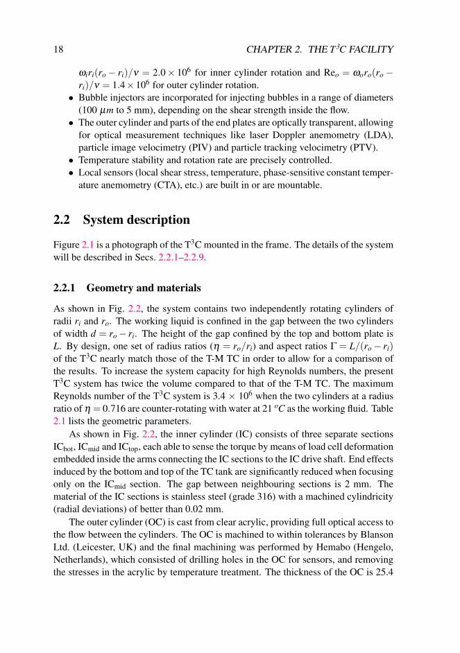
Figure 2.5: Left: Schematic sketch of the coolant flow through the T3C. Coolant enters atthe bottom rotary union (blue) and flows straight up to the top plate by piping on the outsideof the TC tank. Then the coolant enters the curling channels in the top plate (red) and is feddownwards again to run through the curling channels of the bottom plate before it exits at thesecond rotary union. Right: Bottom plate with the copper cover removed.
2.2.5 Temperature control
The amount of power dissipated by degassed water at 21 C, in the case of a stationaryOC and the IC rotating at 20 Hz with smooth unaltered walls, is measured to be10.0 kW. Without cooling this would heat the 0.111 m3 of water at a rate of ≈ 1.3K/min. As the viscosity of water lowers by 2.4% per K, it is important to keep thetemperature stable (to within at least 0.1 K) to exclude viscosity fluctuations and thuserrors. While the temperature-viscosity relation of water is well-tabulated and willbe corrected for during measurements, other fluids like glycerin solutions might notshare this feature. In the case of glycerin, a 1 K temperature increase can lower theviscosity by ≈ 7%.
To ensure a constant fluid temperature inside the TC tank, a 20 kW Neslab HX-750 chiller (Thermo Fisher Scientific Inc., Waltham, USA) with an air-cooled com-pressor and a listed temperature stability of 0.1 K is connected to the T3C. Two rotaryunions, located at the bottom of the OC drive axle, are embedded inside each otherand allow the coolant liquid to be passed from the stationary lab to the rotating OC,as shown in Fig. 2.5. Both the stainless steel bottom and top plate of the OC contain

24 CHAPTER 2. THE T3C FACILITY
internal cooling channels which are covered by a 5 mm-thick nickel-coated copperplate, which in turn is in direct contact with the TC’s inner volume.
The temperature inside the TC tank is monitored by three PT100 temperaturesensors, each set up in a 4-leads configuration with pre-calibrated signal conditionersIPAQ-Hplus from Inor (Malmo, Sweden) with an absolute temperature accuracy of 0.1K. The relative accuracy is better than 0.01 K. Each sensor is embedded at mid-heightinside the wall of the hollow ICtop, ICmid, and ICbot sections, respectively (shown inFig. 2.8). Thus one can check for a possible axial temperature gradient across the IC.The sensors do not protrude through the wall so as to keep the outer surface smooth,leaving 1 mm of stainless steel IC wall between the sensors and the fluid. Exceptfor the direct contact area with the wall, the PT100s are otherwise thermally isolated.Inside each IC section, the signal conditioner is mounted and its electrical wiring isfed through the hollow drive axle, ending in an electrical slip ring. The average overall three temperature sensors is used as feedback for the Neslab chiller. An exampleof temperature time tracers is plotted in Fig. 2.6, which shows that the temperaturestability is better than 0.1 K. This data was acquired with the IC rotating at 20 Hz, astationary OC and water as the working fluid, resulting in a measured power dissipa-tion by the water of 10.0 kW. To check the effects of this small temperature differenceon the TC flow, we calculate the Rayleigh number based on the temperature differ-ence of ∆ = 0.1 K over the distance (LRB = 0.366 m) of the middle and top sensorpositions: the result is Ra = βgL3
RB∆/κν = 5.9 ×10⁶ (β is the thermal expansion coef-ficient, κ the thermal diffusivity and ν the kinematic viscosity). The correspondingReynolds number is estimated to be around ReRB ∼ 0.25×Ra0.49 = 500 [19], which
time (min)
tem
per
ature
(deg
C)
0 10 20 30
18.10
18.05
18.00
17.95
17.90
Figure 2.6: Time traces of the measured temperature at three positions. The data were takenwith the IC rotating at 20 Hz, a stationary OC and water as the working fluid. The measuredpower dissipation by the water was 10.0 kW.

2.2. SYSTEM DESCRIPTION 25
is significantly smaller than the system Reynolds number of 2 × 10⁶. The effects ofthis small temperature gradient can thus be neglected in this high-Reynolds-numberturbulent flow.
2.2.6 Torque sensing
Each of the ICbot, ICmid and ICtop sections are basically hollow drums. Each drum issuspended on the IC’s drive axle by two low-friction ball bearings, which are sealedby rubber oil seals pressed onto the outsides of the drums, encompassing the driveaxle. A metal arm, consisting of two separate parts, is rigidly clamped onto the driveaxle and runs to the inner wall of the IC section. The split in the arm is bridged by aparallelogram load cell (see Fig. 2.7). The load cells can be replaced by cells with dif-ferent maximum-rated load capacity to increase the sensitivity to the expected torque.At this moment two different load cells, type LSM300 from Futek (Irvine, USA), arein use with a maximum-rated load capacity of 2224 N and 222.4 N, respectively.Each load cell comes with a pre-calibrated Futek FSH01449 signal conditioner oper-ating at 1 kHz, which is also mounted inside the drum. The electrical wiring is fedthrough the hollow drive axle to a slip ring on top. The hysteresis of each load cellassembly is less than 0.2 Nm, presented here as the torque equivalent. Calibration ofthe load cells is done by repeated measurements, in which a known series of mono-tonically increasing or decreasing torques is applied to the IC surface. The IC is nottaken out of the frame and is calibrated in situ. The torque is applied by strappinga belt around the IC and hanging known masses on the loose end of the belt, afterhaving been redirected by a low-friction pulley to follow the direction of gravity.
Local fluctuations in the wall-shear stress can be measured using the flush-mounted hot-film probes (type 55R46 from Dantec Dynamics) on the surfaces ofthe inner and outer cylinder, shown in Fig. 2.8.
An important construction detail determines how the torque is transferred to theload cell. Only the azimuthal component is of interest and the radial and axial com-ponents, due to possible non-azimuthal imbalances inside the drum or due to thecentrifugal force, should be ignored. This is accomplished by utilizing the paral-lelogram geometry of the load cell, lying in the horizontal plane. It is evident thatduring a measurement the rotation rate of the IC should be held stable to prevent therotational inertia of the IC sections from acting as a significant extra load. The massbalance of the system is important in decreasing this effect.
2.2.7 Balancing and vibrations
All three sections of the IC and the entire OC are separately balanced, following aone-plane dynamical balancing procedure with the use of a Smart Balancer 2 fromSchenck RoTec (Auburn Hills, USA). The associated accelerometer is placed on the

26 CHAPTER 2. THE T3C FACILITY
load cell
drum ICmid
load cell signal
conditioner
low-friction
ball bearing
drive axle IC
Figure 2.7: Horizontal cut-away showing the load-cell construction inside the ICmid drum.The load cell spans the gap in the arm, connecting the IC drive axle to the IC wall.
main bottom ball bearing. The balancing procedure is reproducible to within 5 gramsleading to a net vibration velocity of below 2 mm/s rms at the maximum rotationrates. According to the ISO standard 101816-1 [63] regarding mechanical vibrations,the T3C system falls into category I, for which a vibration velocity below 2.8 mm/srms is considered acceptable.
Another feature is the air springs, i.e. pressure regulated rubber balloons, placedbetween the floor and each of the four support feet of the T3C frame. They lift theframe fully off the ground and hence absorb vibrations leading to a lower vibrationseverity in the setup itself and reducing the vibrations passed on to the building.
Two permanently installed velocity transducers from Sensonics (Hertfordshire,UK), type PZDC 56E00110, placed on the top and bottom ball bearings, constantlymonitor the vibration severity. An automated safety PLC circuit will stop the IC and

2.2. SYSTEM DESCRIPTION 27
OC rotation when tripped. Thus, dangerous situations or expensive repairs can beavoided, as this acts as a warning of imminent ball bearing failure or loss of balance.
2.2.8 Bubble injection and gas concentration measurement
Eight bubble injectors, equally distributed around the outer perimeter of the TC gapas shown in Fig. 2.8, are built into the bottom plate of the TC tank. Each bubbleinjector consists of a capillary housed inside a custom-made plug ending flush withthe inside wall. They can be changed to capillaries of varying inner diameter: 0.05,0.12, 0.5 and 0.8 mm. This provides a way to indirectly control the injected bubbleradius, estimated to be in the order of 0.5 mm to 5 mm, depending on the shearstress inside the TC. Smaller bubbles of radius less than 0.5 mm, or microbubbles,can be injected by replacing the capillaries inside the plugs with cylinders of porousmaterial.
Two mass flow controllers from Bronkhorst (Ruurlo, Netherlands), series EL-Flow Select, are used in parallel for regulating the gas, i.e. filtered instrument air,with a flow rate at a pressure of 8 bars. One controller with a maximum of 36 l/mintakes care of low-gas volume fractions, and the second controller with a maximumof 180 l/min of high-gas volume fractions, presumably up to 10%. The gas enters thegap by a third rotary union located at the very bottom of the OC drive axle, belowthe coolant water rotary unions. Thus the OC drive axle has three embedded pipesrunning through its center, which are fed by three rotary unions at the bottom. Eachpipe is split into separate channels again inside of the OC drive assembly to be routedwhere needed.
Vertical channels running through the near-center of the TC tank’s top plate con-
Figure 2.8: A sketch of local sensors and bubble injectors in the system.

28 CHAPTER 2. THE T3C FACILITY
nect the tank volume to a higher located vessel in contact with the ambient air. Excessliquid or gas can escape via this route to prevent the build-up of excessive pressure.We refer to it as an expansion vessel. The expansion vessel can also be used to de-termine the global gas volume fraction inside the TC tank. The vessel is suspendedunderneath a balancer which continuously registers the vessel’s mass. Starting at zeropercent gas volume fraction to tare the vessel’s mass, one can calculate the global gasvolume fraction by transforming the liquid’s mass that is subsequently pushed intothe vessel by the injected gas, into its equivalent volume. In the case of a rotatingOC the stationary expansion vessel can not (yet) be connected and excess liquid iscollected in a stationary collecting ring encompassing the rotating top plate.
The original concept for measurement of the global gas volume fraction wouldnot have had the restriction of a stationary OC. It makes use of a differential pressuretransducer attached to the OC that measures the pressure difference between the topand bottom of the TC tank. Comparing this difference to the expected single-phasehydrostatic pressure difference, one could calculate the gas volume fraction. Thismethod depends on the dynamic pressure being equal at the top and bottom. It failshowever, due to unequal dynamic pressure induced by secondary flows. This is notunexpected as a wide variety of flow structures can exist in turbulent TC flow, likeTaylor-vortices.
2.2.9 Optical access and local sensors
Flow structure and velocity fluctuations of TC flow have been studied extensively atlow Reynolds numbers, but few experiments have been performed at high Reynoldsnumber (Re> 105). Previous velocity measurements were mainly done with intrusivemeasurement techniques like hot-film probes. Indeed it was found that the wakeeffects induced by an object inside a closed rotating system can be very strong [64].Better velocity measurements inside the TC gap use nonintrusive optical techniquessuch as LDA [13], PIV [16], PTV. The optical properties of the outer cylinder arehence crucial for this purpose.
The outer cylinder of the T3C is transparent, and four small areas of the top andbottom plates consist of viewing portholes made of acrylic to allow for optical accessin the axial direction, as can be seen in Figs. 2.5 and 2.7. The outer cylinder wasthermally treated to homogenize the refractive index and to remove stresses insidethe acrylic. Thanks to this optical accessibility, all three velocity components insidethe gap can be measured optically. For the velocity profile measurements, we useLDA (see Sec. 2.3.2).
Various experimental studies have been done to examine bubbly DR. However,two main issues of bubbly DR in turbulent TC are still not well-studied. How dobubbles modify the turbulent flow? And: How do bubbles distribute and move insidethe gap? It is certainly important to measure local liquid and bubble information

2.2. SYSTEM DESCRIPTION 29
inside the gap. Various local sensors, shown in Fig. 2.8, can be mounted to the T3Csystem. Here we highlight two of them: the phase-sensitive CTA and the 4-pointoptical fiber probe.
Phase-sensitive CTA
Optical techniques (such as LDA and PIV) are only capable of measuring flow velo-cities in a bubbly flow when the gas volume fraction is very low (typically less than1%). Hot-film measurements in bubbly flows also impose considerable difficulty dueto the fact that liquid and gas information is present in the signal. The challenge is todistinguish and classify the signal corresponding to each phase. The hot-film probedoes not provide by itself means for successful identification [65]. To overcome thisproblem, a device called phase-sensitive CTA has been developed (see Refs. [66–69]). In this technique, an optical fiber is attached close to the hot-film so that whena bubble impinges on the sensor it also interacts with the optical fiber. The principlebehind the optical fiber is that light sent into the fiber leaves the fiber tip with lowreflectivity when immersed in water, and with high reflectivity when immersed in air.Hence the fiber is able to disentangle the phase information by measuring the reflec-ted light intensity. It has proved to be an useful tool for liquid velocity fluctuationmeasurements in bubbly flows [68]. Phase-sensitive CTA probes are only mountedthrough the holes of the outer cylinder when necessary.
4-Point optical probe
Instead of using a single optical fiber to discriminate between phases as describedin the previous paragraph, one can construct a probe consisting of four such fibers.The four fiber tips are placed in a special geometry: three fiber tips of equal lengthare placed parallel in a triangle, and the fourth fiber is placed in the center of gravityand protrudes past the other fiber tips (see Ref. [70] for a schematic of the probe).Knowing this geometry and processing the four time series on the reflected lightintensity, it becomes possible to estimate not only the size of the bubble that impingesonto the fiber tips, but also the velocity vector and the aspect ratio. To measure thebubble distribution inside the TC gap and other bubble dynamics, the 4-point opticalprobe is mounted through the holes of the outer cylinder only when necessary. Werefer to Ref. [71] for details on the measurement principle of the 4-point optical probe.Support for this probe is built into the T3C by incorporating opto-electrical convertersinto the outer cylinder’s bottom plate.

30 CHAPTER 2. THE T3C FACILITY
2.3 Examples of results
In this section we will demonstrate that the facility works by outlining our initialobservations of the torque, velocity profiles and bubbly effects.
2.3.1 Torque versus Reynolds number for single phase flow
We first measure the global torque as a function of the Reynolds number in the presentT3C apparatus with a stationary outer cylinder. The torque τ on the middle sectionof the inner cylinder is measured for Reynolds numbers varying from 3 × 10⁵ to 2× 10⁶. We use the same normalization as Ref. [23] to define the non-dimensional
Rei
Rei
GR
ei
0.18
0G
Lathrop et al. [11]
T C
(a)
(b)
Figure 2.9: (a) The non-dimensional torque and (b) the compensated torque GRe−1.80i versus
Reynolds number in the high-Reynolds-number regime for the measurements with the T-MTC (open triangles) and T3C (open circles) apparatuses.
2.3. EXAMPLES OF RESULTS 31
torque as G = τ/2πρν2Lmid. The present measurements are performed in the T3Cwith a radius ratio η = 0.716, which is close to the value η = 0.725 of the T-M TCexamined by Lathrop et al. [11]. Figure 2.9(a) shows G versus Rei for Rei > 3×10⁵.The fitting exponent for the data by Lathrop et al. [11] is 1.86, and the result of thepresent measurement gives 1.75.
To better compare these data, we use G−1.80 to compensate for the torqueGRe−1.80
i , which is shown in Fig. 2.9(b). Overall, the data of Ref. [11] shows ahigher exponent than the compensated value of 1.80, and the present measurementis lower. However, both data sets clearly exhibit deviations from a single power law.The present measurement shows an oscillating trend when the Reynolds number ishigher than 8×10⁵. This is likely induced by transitions between different flow struc-tures, which will be studied systematically in the T3C apparatus with high scrutinyas this trend was not anticipated.
We also examine the torque versus Reynolds number in the co- and counter-rotation regime, which is the topic of chapters 3 and 4 of this thesis.
2.3.2 Velocity profile measured with LDA
Previous velocity measurements were mainly done with intrusive measurement tech-niques like hot-film probes. A better way for velocity measurements inside the TCgap are nonintrusive optical techniques such as LDA. Due to the curvature, the anglebetween two LDA beams slightly depends on the radial position along the gap. Wehave corrected for this via a ray-tracing calculation based on the system parameters[72]. Refraction effects have also been taken into account. To test the reliabilityof the correction, we perform a velocity profile measurement when the system is insolid-body rotation, i.e. f = fi = fo = 2 Hz. Open circles in Fig. 2.10 show the azi-muthal velocity profile measured with LDA. The exact solid-body velocity profile,r/ro, is shown with the solid line in the figure. The velocity has been normalized byits value on the inner wall of the outer cylinder. Figure 2.10 clearly indicates that theLDA measurements agree with the solid-body profile (within 0.6%).
When only the outer cylinder rotates, the TC flow with an infinite aspect ratiois linearly stable. The laminar azimuthal Couette velocity profile for infinite aspectratio (i.e. without end-plate effects) reads [73]:
uϕ ,lam(r) = Ar+B/r, A =2π fo
1−η2 , B =−2π for2
i
1−η2 . (2.1)
The corresponding laminar profile with the present system parameters, for fo = 7.2Hz, is shown with the dashed line in Fig. 2.10. The open squares are the measuredazimuthal velocity profile with LDA when the outer cylinder is rotating at fo = 7.2Hz. The measurement is carried out with the T3C at a statistically stationary state.The velocity has been normalized by its value on the inner wall of the outer cylinder.

32 CHAPTER 2. THE T3C FACILITY
0.0 0.2 0.4 0.6 0.8 1.00.0
0.2
0.4
0.6
0.8
1.0
Solid-body meas.Solid-body theoryShear meas.Laminar theory
(r − ri)/(ro − ri)
uφ(r
)/u
φ(r
o)
Figure 2.10: Open circles: the azimuthal velocity profile measured with LDA when thesystem is in solid-body rotation ( fi = fo = 2 Hz). The solid line corresponds to r/ro of thesolid-body flow. Open squares: the azimuthal velocity profile measured with LDA in the T3Csystem with a stationary inner cylinder ( fi = 0, fo = 7.2 Hz). The dashed line correspondsto the laminar profile described in Eqn. (2.1), applicable to a laminar profile between thecylinders, with no top and bottom plate effects.
A clear deviation is found between the measurement results with the laminar profile.The reason for this deviation is due to end-plate effects [72, 74, 75] – the laminarflow profile of type (2.1) only exists when the aspect ratio of TC is infinite. Moremeasurements are upcoming for studying velocity profiles in high-Reynolds-numberTaylor-Couette flow. Certainly the end-plate effects will be significantly reduced forthe turbulent cases, when the liquid velocity fluctuations dominate the flow. Addi-tional results on velocity profiles in T3C and a detailed discussion will be publishedelsewhere.
2.3.3 Torque versus gas concentration for bubbly TC flow
The T3C apparatus is designed for studying both single- and two-phase flows. Werefer to chapter 7 in which the focus lies on torque measurements and local informa-tion on bubbly flows in the present T3C apparatus.
2.4 Summary and outlook
A new turbulent Taylor-Couette apparatus, named T3C, has been developed, con-sisting of two independently rotating cylinders. The torque measurements for pureinner cylinder rotation agree well with previous results in the overlapped parameter

2.4. SUMMARY AND OUTLOOK 33
regime. We also performed experiments in the unexplored parameter regime of largeReynolds number and counter-rotation of the cylinders. The data of G versus Rei forthe counter-rotation situation are not simple translations of the pure inner cylindercurve, but depend on the rotation frequency of the outer cylinder in a nontrivial way.The nonintrusive measurement technique LDA is applied to the system for measuringvelocity profiles through the transparent outer cylinder of the T3C, and it has provedto be an excellent tool for flow velocity measurements inside TC. The torque meas-urements of bubbly flow in the T3C system showed surprisingly large drag reduction(more than 50%) at high Reynolds numbers, which was not attainable by previousmeasurements in other TC apparatuses.
The inner cylinder Reynolds number Rei of older existing turbulent TC facilitiescan be as high as 106. However, another two control parameters, the outer cylinderReynolds number Reo and radius ratio η , still have not been explored in the highlyturbulent regime (Re & 105). With this newly-built Taylor-Couette system, the para-meter space (Rei, Reo, η) has been extended to (2.0× 10⁶, ±1.4× 10⁶, 0.716 −0.909), as shown in Fig. 2.11. Various research issues of single-phase turbulent TCflows can be studied with this new T3C facility; for example, turbulent momentumtransport in the unexplored parameter space of co- and counter-rotation, the role ofthe “geometrical quasi-Prandtl number” [23] on turbulent momentum transport, an-gular momentum/velocity profiles, and the connections with the global torque, andstatistics of turbulent fluctuations of different velocity components. These studieswill bridge the gap between RB flow and TC flow in the turbulent regime toward abetter understanding of closed turbulent systems.
The injection of bubbles offers another degree in the parameter space for study-ing two-phase TC flows. The study of the bubbly DR can be improved further bycombining the global torque and the local measurements of the bubble velocity and
Rei
− 1.4 × 10⁶
Reo
η
2 × 10⁶
1.4 × 10⁶
0.716
0.909
Figure 2.11: Parameter space of the T3C.

34 CHAPTER 2. THE T3C FACILITY
distribution (see Fig. 2.12). Apart from studying bubbly DR, T3C is also an idealsystem for studying other issues in dispersed multiphase flows; for example, the Lag-rangian properties of particles/bubbles in turbulence [68, 76, 77], and liquid velocityfluctuations induced by dispersed bubbles/particles [78, 79]. It was found that even inhomogeneous and isotropic turbulence, particles, drops and bubbles are not distrib-uted homogeneously, but cluster [80]. One example of bubble clustering in turbulentTC flow is shown in Fig. 2.12. Given the rich flow structures inside turbulent TC flow,it is of great interest to quantify particles/bubbles clustering with varying turbulentstructures, and this will also be done in future research.
!"#$""
Figure 2.12: A snapshot of the bubble distribution in the T3C, Rei = 1.0× 10⁶. The outercylinder is stationary. This flow is studied in detail in chapter 7.

— PART II —
Single-phaseTaylor-Couette flow
35


3Torque scaling in turbulent
Taylor-Couette flow with co- andcounter-rotating cylinders ∗
We analyze the global transport properties of turbulent Taylor-Couette flow in thestrongly turbulent regime for independently rotating outer and inner cylinders, reach-ing Reynolds numbers of the inner and outer cylinders of Rei = 2×10⁶ and Reo =±1.4×10⁶, respectively. For all Rei, Reo, the dimensionless torque G scales as afunction of the Taylor number Ta (which is proportional to the square of the differ-ence between the angular velocities of the inner and outer cylinders) with a universaleffective scaling law G ∝ Ta0.88, corresponding to Nuω ∝ Ta0.38 for the Nusselt num-ber characterizing the angular velocity transport between the inner to the outer cylin-ders. The exponent 0.38 corresponds to the ultimate regime scaling for the analogousRayleigh-Benard system. The transport is most efficient for the counter-rotating casealong the diagonal in phase space with ωo ≈−0.4ωi.
∗Based on: D.P.M. van Gils, S.G. Huisman, G.-W. Bruggert, C. Sun, and D. Lohse, Torque scalingin turbulent Taylor-Couette flow with co- and counterrotating cylinders, Phys. Rev. Lett. 106, 024502(2011).
37

38 CHAPTER 3. TORQUE SCALING IN CO- AND COUNTER-ROTATION
3.1 Introduction
Global transport properties of turbulent flows are of prime importance for many ap-plications of fluid dynamics, but also for a fundamental understanding, as they reflectthe interplay between the boundary layer and the bulk. The two canonical systemsused to analyze the transport properties in closed turbulent systems are Rayleigh-Benard (RB) convection and Taylor-Couette (TC) flow, and they are conceptuallyclosely related [21–23]. In RB flow, heat (in dimensionless form the Nusselt num-ber) is transported from the hot bottom plate to the cold top plate [19, 20], whereasin TC flow angular velocity is transported from the inner to the outer cylinder (forωi > ωo). In analogy to RB flow, Eckhardt et al. [23] identified, from the underlyingNavier-Stokes equations,
Jω = r3(⟨urω⟩A,t −ν∂r ⟨ω⟩A,t), (3.1)
as a relevant conserved transport quantity, representing the flux of angular velocityfrom the inner to the outer cylinder. Here ur(uϕ ) is the radial (azimuthal) velocity,ω = uϕ/r the angular velocity, and ⟨. . .⟩A,t characterizes averaging over time andan area with constant r from the axis. Jω is made dimensionless with its valueJω
lam = 2νr2i r2
o(ωi −ωo)/(r2o − r2
i ) for the laminar case, giving a “Nusselt number”as a dimensionless transport quantity,
Nuω = Jω/Jωlam, (3.2)
where ri,o and ωi,o denote the radius and the angular velocity of the inner and outercylinders, respectively, and ν is the kinematic viscosity of the fluid. Nuω is closelyconnected to the torque τ that is necessary to keep the inner cylinder rotating at aconstant angular velocity or, in dimensionless form, to
G =τ
2πLρ f luidν2 = NuωJω
lamν2 = NuωGlam, (3.3)
where L is the height of the cylinder and ρ f luid the density of the fluid. Yet an-other often used possibility to represent the data is the friction coefficient c f = [(1−η)2/π]G/Re2
i [10].For RB flow, the scaling properties of the Nusselt number in the fully turbulent re-
gime (i.e., for very large Rayleigh numbers, say Ra ≥ 1010) have received tremendousattention in the last decade and various heat flux measurements have been performed;again, see the review article [19]. In contrast, TC flow in the fully turbulent regimehas received much less attention, with the only exception being the Texas experimentby Swinney, Lathrop, and coworkers [10, 11, 14, 15]. In that experiment a Reynoldsnumber Rei = 106 of the inner cylinder was reached (with the outer cylinder at rest)and an effective power law of G ∝ Reγ
i with γ ≈ 1.6− 1.86 was detected [10, 11]

3.2. EXPERIMENTAL METHOD 39
in the turbulent regime, though the scaling properties are not particularly good and,strictly speaking, γ depends on Rei; i.e., there is no pure scaling. Indeed, in Refs.[23, 81, 82] we have argued that there should be a smooth transition from γ = 3/2for the small Reynolds number of a boundary layer dominated flow to γ = 2 for thelarger Reynolds number of a flow dominated by the turbulent bulk. Turbulent TCexperiments get even more scarce for TC flow with inner and outer cylinders rotatingindependently. We are only aware of the Wendt experiments in the 1930s [5], reach-ing Rei ≈ 105 and Reo ≈ ±105 and the recent ones by Ravelet et al. [16], reachingRei ≈ 5×10⁴ and Reo =±2×10⁴. The hitherto explored phase diagram of TC flowwith independently rotating cylinders is shown in Fig. 3.1. An alternative represent-ation of the phase diagram is given by Dubrulle et al. [75], who introduce a shearReynolds number and a rotation number as an alternative representation of the phasespace (see below).
In the phase diagram [Fig. 3.1] we have also added the Rei, Reo numbers that weexplored with our newly constructed Twente turbulent TC facility (T3C), which wehave described in great detail in section 2.2. One of the goals we want to achieve withthis new facility is to explore the (Rei, Reo, η = ri/ro) parameter space, thus enteringterra incognita, and measure the torque [i.e., transport of the angular velocity (Nuω indimensionless form) or, again expressed differently, the overall drag] and the internalReynolds number of the flow.
3.2 Experimental method
In this chapter we will focus on the required torque for fully developed turbulentflow (Rei, Reo > 105), where η = 0.716 with independently rotating inner and outercylinders, which hitherto has not been explored. The examined parameter space inthis chapter is shown in the space of (Rei, Reo) in Fig. 2.2 (a), (Ta, a) in Fig. 2.2(b), and (Ta, RΩ) in Fig. 2.2 (c), to be explained below. We will not address thequestion whether pure scaling laws exist: First, the explored Reynolds number rangeis too short to answer this question, and second, the earlier work [10, 11, 14, 23, 81,82] gives overwhelming experimental and theoretical evidence that there are no purescaling laws, even up to Reynolds numbers of 106. So all scaling exponents in thischapter have to be read as effective scaling laws.
3.3 Results
Our results for the counter-rotating case for the dimensionless torque G as function ofRei for fixed Reo are shown in Fig. 3.3. One immediately sees that counter-rotationenhances the torque (and thus the overall drag), but that for general Reo = 0 the
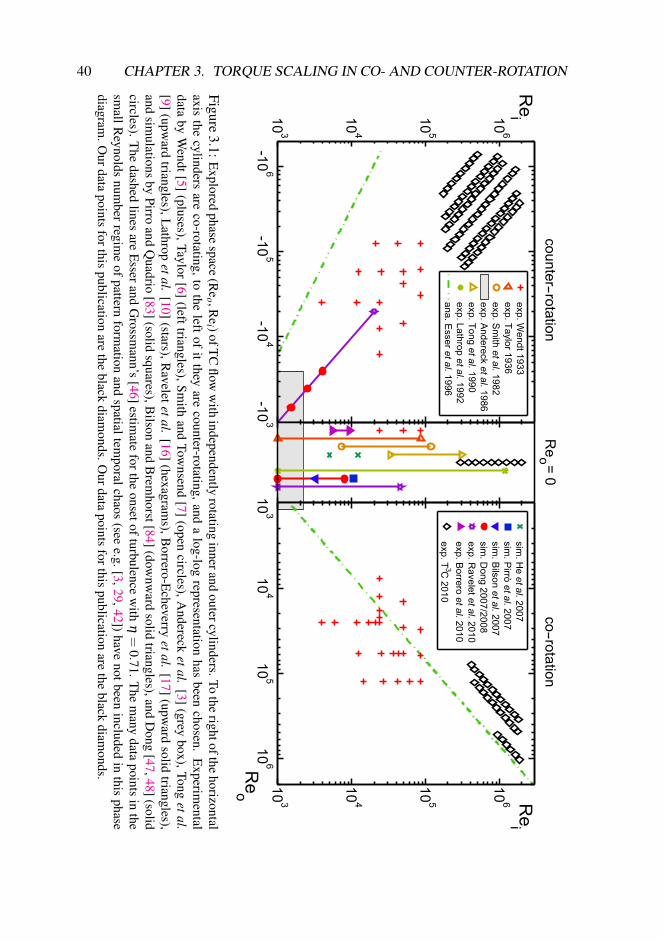
40 CHAPTER 3. TORQUE SCALING IN CO- AND COUNTER-ROTATION
Figure3.1:
Explored
phasespace
(Re
o ,Re
i )ofTC
floww
ithindependently
rotatinginnerand
outercylinders.Tothe
rightofthehorizontal
axisthe
cylindersare
co-rotating,tothe
leftofitthey
arecounter-rotating,and
alog-log
representationhas
beenchosen.
Experim
entaldata
byW
endt[5](pluses),Taylor
[6](lefttriangles),Sm
ithand
Townsend
[7](open
circles),Andereck
etal.[3]
(greybox),Tong
etal.[9]
(upward
triangles),Lathrop
etal.[10]
(stars),Raveletetal.
[16](hexagram
s),Borrero-E
cheverryetal.
[17](upw
ardsolid
triangles),and
simulations
byPirro
andQ
uadrio[83](solid
squares),Bilson
andB
remhorst[84](dow
nward
solidtriangles),and
Dong
[47,48](solidcircles).T
hedashed
linesare
Esserand
Grossm
ann’s[46]estim
ateforthe
onsetofturbulencew
ithη=
0.71.The
many
datapoints
inthe
smallR
eynoldsnum
berregim
eof
patternform
ationand
spatialtemporalchaos
(seee.g.[3,29,42])
havenotbeen
includedin
thisphase
diagram.O
urdatapoints
forthispublication
arethe
blackdiam
onds.Ourdata
pointsforthis
publicationare
theblack
diamonds.

3.3. RESULTS 41
!
! "
! #
$!%&
!
!%&
%&
"
'(
(
!
! "
! #
$!%&
$!%'
$!%(
$!%"
!
!%"
)Ω
*+
(a) (b)
(c)
Figure 3.2: (a) Our data points in the (Reo, Rei) phase diagram on a linear scale. (b) Ourdata points in the phase space (Ta, a); note that Ta also depends on a. (c) Our data points inthe phase space (Ta, RΩ) [see Eq. (3.7)].
effective power law G ∝ Re1.76i , that holds in the case of inner cylinder rotating only,
gets lost; in fact, there is even no effective power law at all.How can we represent the data to better reveal the transport properties of the
system? The analysis of Eckhardt et al. [23] and the analogy of the TC system to theRB system suggest to better plot Nuω as a function of the Taylor number
Ta =14
σd2(ri + ro)2(ωi −ωo)
2ν−2, (3.4)
where σ = [(1+η)/2]/√η4, i.e., along the diagonals
ωo =−aωi (3.5)
in the parameter space†, Fig. 3.2 (a). Indeed, Eckhardt et al. [23] derived, from the
†We define Eq. (3.5) with a minus sign, as our focus is on the counter-rotating case.

42 CHAPTER 3. TORQUE SCALING IN CO- AND COUNTER-ROTATION
105 106
109
1010
1011
Rei
G
–2 –1 00
1
2
Reo
x106
x106
Rei
Figure 3.3: The dimensionless torque G(Rei) for counter-rotating TC flow for four differentfixed values of Reo = −1.4× 10⁶, −0.8× 10⁶, −0.4× 10⁶, and 0 (top to bottom data sets);see inset for the probed area of the parameter space.
underlying Navier-Stokes equation, the exact relation
εw = ε − εlam = ν3d−4σ−2Ta(Nuω −1) (3.6)
for the excess kinetic energy dissipation rate εw [i.e., the total kinetic energy dis-sipation rate ε minus the kinetic energy dissipation rate in the laminar case εlam =4νr2
i r2o(ri + ro)
−2d−2(ωi −ωo)2]. In Eq. (3.6) σ can be interpreted as a (geometric)
Prandtl number, and Ta and Nuω are the exact TC analogs to the Rayleigh and Nus-selt numbers in RB flow. Along the diagonal, Eq. (3.5), in parameter space, one hasTa = 1
4 σd2(ri + ro)2(1+ a)2ω2
i ν−2, and the well-studied [19] effective scaling lawNu ∝ Raγ for RB flow (with γ ≈ 0.31 [19, 34]) would now correspond to an effectivescaling law Nuω ∝ Taγ for TC flow.
Nuω vs Ta is shown in Fig. 3.4 (a) for various a, i.e., along various straight linesthrough the origin of the parameter space, Fig. 3.2 (a). A universal, i.e. a-indepedent,effective scaling Nuω ∝ Taγ with γ ≈ 0.38 is clearly revealed. This corresponds toa scaling of G ∝ Re1.76
i for the dimensionless torque along the straight lines, Eq.(3.5), in the parameter space, Fig. 3.2, to c f ∝ Re−0.24
i for the drag coefficient, and toG∝Ta0.88. The compensated plots Nuω/Ta0.38 in Fig. 3.4 (b) demonstrate the qualityof the effective scaling and, in addition, show the a dependence of the prefactor ofthe scaling law.
The a dependence of the prefactor Nuω/Ta0.38 is plotted in Fig. 3.5. It shows apronounced maximum around a = 0.4, i.e., for the moderately counter-rotating case,signaling the most efficient angular velocity transport from the inner to the outer

3.3. RESULTS 43
Figure 3.4: (a) Nuω vs Ta for various a; see Fig. 3.2(a) for the location of the data inparameter space. A universal effective scaling Nuω ∝ Ta0.38 is revealed. The compensatedplots Nuω/Ta0.38 in (b) show the quality of the effective scaling and the a-dependent prefactorof the scaling law.
cylinder at that value. We mention that it is obvious that this curve has a maximum,as in both limiting cases a → ±∞ (rotating of the outer cylinder only) the flow islaminar and Nuω = 1, but it is interesting to note that the maximum does not occurfor the most pronounced counter-rotating case ωo =−ωi (or a = 1). Compared to thecase of pure inner cylinder rotation (a = 0), at a = 0.4 the angular velocity transportfrom the inner to the outer cylinder is enhanced by more than 20%.
Figure 3.5: Prefactor of the effective scaling law Nuω ∝ Ta0.38 (shown in Fig. 3.4) as afunction of a = −ωo/ωi. The inset shows the effective exponents γ which results from anindividual fit of the scaling law Nuω ∝ Taγ .

44 CHAPTER 3. TORQUE SCALING IN CO- AND COUNTER-ROTATION
The parameter a =−ωo/ωi is connected to the so-called rotation number
RΩ = (1−η)(Rei +Reo)/(ηReo −Rei) (3.7)
introduced by Dubrulle et al. [75] and used by Ravelet et al. [16], namely, RΩ =(1−η)η−1(a−η)(a+1)−1. We also plot our data points in the phase space of (Ta,RΩ), as shown in Fig. 3.2 (c). The optimal value a ≈ 0.4 we found for the transportproperties of the system corresponds to RΩ ≈ −0.09. In this chapter we prefer aas compared to RΩ, as the sign of a immediately signals whether the system is co-rotating or counter-rotating.
3.4 Conclusion
In conclusion, we have explored the terra incognita of fully developed turbulent TCflow with independently rotating inner and outer cylinders, beyond Reynolds num-bers of 106, finding a universal scaling law G ∝ Ta0.88, corresponding to Nuω ∝Ta0.38, for all (fixed) a = −ωo/ωi, with optimal transport quantities at a ≈ 0.4. It isremarkable that the effective scaling exponent 0.38 exactly resembles the analogouseffective scaling exponent in Nu ∝ Ra0.38 in RB convection in the ultimate regime ofthermal convection [24, 25], reflecting the analogy between TC and RB flow also inthe strongly turbulent regime.
The next steps will be to further extend the parameter space, Fig. 3.1, towardsfurther radius ratios η to see whether the observed universality carries on towardsan even larger parameter range, and to also measure the Taylor-Reynolds numberand the wind Reynolds numbers of the internal flow, which are closely connected toNuω and for which theoretical predictions exist [23]. With such measurements andcharacterizations of the flow structures, we will also be able to check whether theseare reflected in the overall transport properties.

4Optimal Taylor-Couette turbulence ∗
Strongly turbulent Taylor-Couette flow with independently rotating inner and outercylinder with a radius ratio of η = 0.716 is experimentally studied. From globaltorque measurements we analyze the dimensionless angular velocity flux Nuω(Ta,a)as a function of the Taylor number Ta and the angular velocity ratio a = −ωo/ωi
in the large Taylor number regime 1011 . Ta . 1013 and well off the inviscid stabil-ity borders (Rayleigh lines) for co-rotation a =−η2 and a = ∞ for counter-rotation.We analyze the data with the common power law ansatz for the dimensionless an-gular velocity transport flux Nuω(Ta,a) = f (a) · Taγ , with an amplitude f (a) andan exponent γ(a). The data are consistent with an exponent γ = 0.39±0.03 for alla, but we discuss a possible a-dependence in the co- and weakly counter-rotatingregime. The amplitude of the angular velocity flux f (a)≡ Nuω(Ta,a)/Ta0.39 is meas-ured to be maximal at slight counter-rotation, namely at an angular velocity ratio ofaopt = 0.368±0.001, i.e. along the lines ωo =−0.368ωi. This value is theoreticallyinterpreted as the result of a competition between the destabilizing inner cylinderrotation and the stabilizing but shear-enhancing outer cylinder counter-rotation. –With the help of laser Doppler anemometry we provide angular velocity profiles andin particular identify the radial position rn of the neutral line, defined by ⟨ω(rn)⟩t = 0for fixed height z. For these large Ta-values the ratio aopt = 0.368 is distinguished bya zero angular velocity gradient ∂ω/∂ r = 0 in the bulk. While for moderate counter-rotation −0.368ωi . ωo < 0 (i.e. 0< a . aopt) the neutral line still remains close to
∗Submitted to J. Fluid Mech. as: D.P.M. van Gils, S.G. Huisman, S. Grossmann, C. Sun, and D.Lohse, Optimal Taylor-Couette turbulence.
45

46 CHAPTER 4. OPTIMAL TC TURBULENCE
the outer cylinder and the probability distribution function of the bulk angular velo-city is observed to be mono-modal, for stronger counter-rotation ωo .−0.368ωi (i.e.a & aopt) the neutral line is pushed inwards towards the inner cylinder; in this regimethe probability distribution function of the bulk angular velocity becomes bi-modal,reflecting intermittent bursts of turbulent structures beyond the neutral line into theouter flow domain, which otherwise is stabilized by the counter-rotating outer cylin-der. Finally, a hypothesis is offered allowing a unifying view and consistent interpret-ation for all these various results.
4.1 Introduction
Taylor-Couette (TC) flow — the flow between two coaxial, independently rotatingcylinders — is next to Rayleigh-Benard (RB) flow — the flow in a box heated frombelow and cooled from above — the most prominent “drosophila” to test hydro-dynamic concepts for flows in closed containers. For outer cylinder rotation andfixed inner cylinder the flow is linearly stable. In contrast, for inner cylinder rotationand fixed outer cylinder the flow is linearly unstable thanks to the driving centrifugalforces, see e.g. DiPrima & Swinney [2], Smith & Townsend [7], Coles [41], Pfister &Rehberg [42], Mullin et al. [43], Pfister et al. [44], Buchel et al. [45], Esser & Gross-mann [46], Mullin et al. [85]. The case of two independently rotating cylinders hasbeen well analyzed for low Reynolds numbers, see e.g. Andereck et al. [3]. For largeReynolds numbers, where the bulk flow is turbulent, studies have been scarce, seefor example the historical work by Wendt [5] or the experiments by Andereck et al.[3], Ravelet et al. [16], Borrero-Echeverry et al. [17], Dubrulle et al. [75], Richard[86], van Hout & Katz [87]. Recently, in two independent experiments, van Gils et al.[88] and Paoletti & Lathrop [18] supplied precise data for the torque scaling in theturbulent regime of the flow between independently rotating cylinders.
We use cylindrical coordinates r,ϕ and z. Next to the geometric ratio η = ri/ro
between the inner cylinder radius ri and the outer cylinder radius ro, and the aspectratio Γ = L/d of the cell height L and the gap width d = ro − ri, the dimensionlesscontrol parameters of the system can either be expressed in terms of the inner andouter cylinder Reynolds numbers Rei = riωid/ν and Reo = roωod/ν , respectively,or, alternatively, in terms of the ratio of the angular velocities
a =−ωo/ωi (4.1)
and the Taylor number
Ta =14
σ(ro − ri)2(ri + ro)
2(ωi −ωo)2ν−2. (4.2)
Here according to the theory by Eckhardt, Grossmann & Lohse [23] (from now oncalled EGL), σ = (((1+η)/2)/
√η)4 (thus σ = 1.057 for the current η = 0.716 of

4.1. INTRODUCTION 47
the T3C facility) can be formally interpreted as a “geometrical” Prandtl number andν is the kinematic viscosity of the fluid. With ra = (ri + ro)/2 and rg =
√riro, the
arithmetic and the geometric mean radii, the Taylor number can be written as
Ta = r6ar−4
g d2ν−2(ωi −ωo)2. (4.3)
The angular velocity of the inner cylinder ωi is always defined as positive, whereasthe angular velocity of the outer cylinder ωo can be either positive (co-rotation) ornegative (counter-rotation). Positive a thus refers to the counter-rotating case onwhich our main focus will lie.
The response of the system is the degree of turbulence of the flow between thecylinders — e.g. expressed in a wind Reynolds number of the flow, measuring theamplitude of the r- and z-components of the velocity field — and the torque τ , whichis necessary to keep the inner cylinder rotating at constant angular velocity. Followingthe suggestion of EGL, the torque can be non-dimensionalized in terms of the laminartorque to define the (dimensionless) “Nusselt number”
Nuω =τ
2πLρ f luidJωlam, (4.4)
where ρ f luid is the density of the fluid between the cylinders and Jωlam = 2νr2
i r2o(ωi −
ωo)/(r2o − r2
i ) is the conserved angular velocity flux in the laminar case. The reasonfor the choice (4.4) is that
Jω = JωlamNuω = r3
(⟨urω⟩A,t −ν∂r ⟨ω⟩A,t
)(4.5)
is the relevant conserved transport quantity, representing the flux of angular velocityfrom the inner to the outer cylinder. This definition of Jω is an immediate con-sequence of the Navier-Stokes equations. Here ur (uϕ ) is the radial (azimuthal) ve-locity, ω = uϕ/r the angular velocity, and ⟨. . .⟩A,t characterizes averaging over timeand a cylindrical surface with constant radius r. With this choice of control and re-sponse parameters, EGL could work out a close analogy between turbulent TC andturbulent RB flow, building on Grossmann & Lohse [49] and extending the earlierwork of Bradshaw [21] and Dubrulle & Hersant [22]. This was further elaborated byvan Gils et al. [88].
The main findings of van Gils et al. [88], who operated the TC setup, knownas the Twente turbulent Taylor-Couette system or T3C, at fixed η = 0.716 and forTa > 1011 as well as the variable a well off the stability borders −η2 and ∞, are asfollows: (i) in the (Ta,a) representation, Nuω(Ta,a) within the experimental preci-sion factorizes into Nuω(Ta,a) = f (a) ·F(Ta). (ii) F(Ta) = Ta0.38 for all analyzed−0.4 ≤ a ≤ 2.0 in the turbulent regime. (iii) f (a) = Nuω(Ta,a)/Ta0.38 has a pro-nounced maximum around aopt ≈ 0.4. Also Paoletti & Lathrop [18], at slightly dif-ferent η = 0.725 found such a maximum in f (a), namely at aopt ≈ 0.35. For this

48 CHAPTER 4. OPTIMAL TC TURBULENCE
aopt the angular velocity transfer amplitude f (aopt(η)) for the transport from the in-ner to the outer cylinder is maximal. — From these findings one has to conclude:Although counter rotation of the outer cylinder should in principle stabilize the flowfor all ωo < 0, the angular velocity transport flux, instead, for not too strong counter-rotation −0.4ωi . ωo < 0 is still further enhanced. There is still stronger turbulenceattributed to the enhanced shear between the counter-rotating cylinders. Only forstrong enough counter-rotation ωo < −aoptωi (i.e. a > aopt) the transport amplitudedecreases with further increasing a.
The aims of this paper are (i) to provide further and more precise data on themaximum in the conserved turbulent angular velocity flux Nuω(Ta,a)/Taγ = f (a)as a function of a and a theoretical interpretation of this maximum, including a spec-ulation on how it depends on η (section 4.3), (ii) to provide laser Doppler anemo-metry (LDA) measurements of the angular velocity profiles ⟨ω(r)⟩t as functions ofheight, and to show that the maximum in f (a), for these asymptotic Ta and deep inthe instability range at a = aopt , coincides with a vanishing angular velocity gradi-ent ∂ω/∂ r in the bulk of the flow, and to identify the location of the neutral line rn,defined by ⟨ω(rn)⟩t = 0 for fixed height z, finding that it remains still close to theouter cylinder ro for weak counter-rotation, 0 < a < aopt , but starts moving inwardstowards the inner cylinder ri for a & aopt (section 4.4), and (iii) to show that theturbulent flow organization totally changes for a & aopt , where the stabilizing effectof the strong counter rotation reduces the angular velocity transport (section 4.5). Inthis strongly counter-rotating regime the probability distribution function of the angu-lar velocity in the bulk becomes bi-modal, reflecting intermittent bursts of turbulentstructures beyond the neutral line towards the outer flow region, which otherwise, i.e.in between such bursts, is stabilized by the counter-rotating outer cylinder. In section4.6 we discuss the BL thicknesses. The paper ends with a summary, further discus-sions of the neutral line inside the flow, and an outlook. However first — in section4.2 — we will provide more experimental details and we will in particular discussthe height dependence of the flow profile and finite size effects.
4.2 Experimental setup and discussion of end-effects
The core of our experimental setup — the Taylor-Couette cell — is shown in Fig.2.2. In particular, the fixed geometric dimensionless numbers are η = 0.716 and Γ =11.68. The details of the setup are given in section 2.2. The working liquid is water ata continuously controlled constant temperature (precision ±0.5K) in the range 19C- 26C. The accuracy in a is ±0.001 based on the angular velocity stability of theT3C facility. To reduce edge effects, similarly as in Lathrop et al. [10, 11] the torqueis measured at the middle part (length ratio Lmid/L = 0.578) of the inner cylinderonly. Lathrop et al. [11]’s original motivation for this choice was that the height of

4.2. EXPERIMENTAL SETUP AND DISCUSSION OF END-EFFECTS 49
the remaining upper and lower parts of the cylinder roughly equals the size of oneTaylor-vortex. While the respective first or last Taylor vortex indeed will be affectedby the upper and lower plates (which in our T3C cell are co-rotating with the outercylinder), the hope is that in the strongly turbulent regime the turbulent bulk is notaffected by such edge effects. Note that for the laminar case — e.g. for pure outercylinder rotation — this clearly is not the case, as has been known since G. I. Taylor,see e.g. the classical experiments by Coles & van Atta [74], the numerical work byHollerbach & Fournier [89], or the review by Tagg [90]. For such weakly rotatingsystems, profile distortions from the plates propagate into the fluid and dominate thewhole laminar velocity field. The velocity profile will then be very different from theclassical height-independent laminar profile (see e.g. Landau & Lifshitz [73]) withperiodic boundary conditions in vertical direction,
uϕ ,lam = Ar+B/r , A =ωo −η2ωi
1−η2 , B =(ωi −ωo)r2
i
1−η2 . (4.6)
To control that edge effects are indeed negligible in the strongly turbulent caseunder consideration here (1011 < Ta < 1013 and −0.40 ≤ a ≤ 2.0, so well off theinstability borders), we have measured time series of the angular velocity ω(r, t) =uϕ (r, t)/r for various heights 0.32 < z/L < 1 and radial positions ri < r < ro withlaser Doppler anemometry (LDA). We employ a backscatter LDA configuration setup with a measurement volume of 0.07mm x 0.07mm x 0.3mm. The seeding particleshave a mean diameter of 5 µm (PSP-50 Dantec Dynamics). We account for therefraction due to the cylindrical interfaces, details are given by Huisman [72]. Figure4.1a shows the height dependence of the time-averaged angular velocity at mid-gap,r = (r− ri)/(ro − ri) = 1/2, for a = 0 and Ta = 1.5×10¹², corresponding to Rei =1.0×10⁶ and Reo = 0. The dashed-dotted line corresponds to the transition from themiddle-part of the inner cylinder, with which we measure the torque, and the upperpart. Along the middle-part the time-averaged angular velocity is a z-independentconstant within 1%, as is demonstrated in the inset, showing an enlarged relevantsection of the ω axis. From the upper edge of the middle-part of the inner cylindertowards the highest position that we can resolve, 0.5 mm below the top plate, themean angular velocity decays by only 5%. This finite difference might be due to theexistence of Ekman layers near the top and bottom plate (Greenspan [91]). Since atz/L = 1 we have ω(r, t) = 0, as the upper plate is at rest for a = 0 or ωo = 0, 95% ofthe edge effects on ω occur in such a thin fluid layer near the top (bottom) plate thatwe cannot even resolve it with our present LDA measurements.
For the angular velocity fluctuations shown in Fig. 4.1b we observe a 25% decayin the upper 10% of the cylinder, but again in the measurement section of the innercylinder 0.2 < z/L < 0.8 there are no indications of any edge effects. The plotsof Fig. 4.1 together confirm that edge effects are unlikely to play a visible role forour torque measurements in the middle-part of the cylinder. Even the Taylor-vortex

50 CHAPTER 4. OPTIMAL TC TURBULENCE
0 0.1 0.2 0.30.3
0.4
0.5
0.6
0.7
0.8
0.9
1
ω(z) t/ωi
z/L
0 0.005 0.01 0.015 0.02 0.0250.3
0.4
0.5
0.6
0.7
0.8
0.9
1
σω(z)/ωi
z/L
r = 0.50
split IC0.33 0.335 0.34 0.345 0.350.3
0.4
0.5
0.6
0.7
0.8
0.9
1(a) (b)
1%
Figure 4.1: Time averaged axial profiles of the azimuthal angular velocity inside the T3Cmeasured with LDA at mid-gap, i.e. r = (r− ri)/(ro − ri) = 0.5, for the case Rei = 1.0×10⁶
and Reo = 0 (corresponding to a = 0 and Ta = 1.5× 10¹²). The height z from the bottomplate is normalized against the total height L of the inner volume of the tank. (a): the time-averaged angular velocity ⟨ω(z, r = 1/2)⟩t normalized by the angular velocity of the innercylinder wall ωi. (b): the standard deviation of the angular velocity σω(z) normalized by theangular velocity of the inner wall. The split between the middle and the top inner cylindersections is indicated by the dash-dotted line. As can be appreciated in this figure, the end-effects are negligible over the middle section where we measure the global torques as reportedin this work. The velocities near the top plate, z/L = 1, are not sufficiently resolved to seethe boundary layer.
roll-structure, which dominates TC flow at low Reynolds numbers (Andereck et al.[3], Dominguez-Lerma et al. [4], Tagg [90], Dominguez-Lerma et al. [92]), is notvisible at all in the time averaged angular velocity profile ⟨ω(z, r = 1/2, t)⟩t .
To double check that this z-independence not only holds at mid-gap r = 1/2 butalso for the whole radial ω profiles, we measured time series of ω(z, r, t) at threedifferent heights z/L= 0.34, 0.50, and 0.66. The radial dependence of the mean valueand of the fluctuations are shown in Fig. 4.2. The profiles are basically identical forthe three heights, with the only exception of some small irregularity in the fluctuationsat z/L = 0.34 in the small region 0.1 < r < 0.2, whose origin is unclear to us. Notethat in both plots of Fig. 4.2 the radial inner and outer boundary layers are again notresolved; in this paper we will focus on bulk properties and global scaling relations.
Based on the results of this section, we feel confident to claim that (i) edge effectsare unimportant for the global torque measurements on the middle-part of the innercylinder as reported in section 4.3 and that (ii) the local profile and fluctuation meas-urements done close to mid-height z/L = 0.44, which will be shown and analyzed insections 4.4 and 4.5, are representative for any height in the mid-part of the cylinder.

4.3. GLOBAL TORQUE MEASUREMENTS 51
r
ω(r
)t/ω
i
z/L = 0.66
z/L = 0.50
z/L = 0.34
r
σω(r
)/ω
i
z/L = 0.66
z/L = 0.50
z/L = 0.34
Figure 4.2: Radial profiles of the azimuthal angular velocity as presented in Fig. 4.1, scannedat three different heights z/L = 0.66, 0.50 and 0.34, plotted against the dimensionless gap dis-tance r = (r − ri)/(ro − ri), again for Reo = 0 and Rei = 1× 10⁶. (a): the time-averagedangular velocity ⟨ω(r)⟩t normalized by the angular velocity of the inner wall ωi. All pro-files fall on top of each other, showing no axial dependence of the flow in the investigatedaxial range. (b) Standard deviation of the angular velocity σω(r) normalized by the angularvelocity of the inner wall. The boundary layers at the cylinder walls are not resolved.
4.3 Global torque measurements
In this section we will present our data from the global torque measurements for in-dependently inner and outer cylinder rotation, which complement and improve preci-sion of our earlier measurements in van Gils et al. [88]. The data as functions of therespective pairs of control parameters (Ta,a) or (Rei,Reo) for which we performedour measurements are given in tabular form in table 4.1 and in graphical form in Figs.4.3a and 4.4, respectively.
As shown in Fig. 4.5a in a compensated plot we find a universal effective scalingNuω(Ta,a)∝ Ta0.39. If each curve for each a is fitted individually, the resulting Ta-scaling exponents γ(a) scatter with a, but only very slightly depend on a, see Figs.4.5b and 4.5c. For linear fits different below and above aopt (or ψ = 0), we obtainγ = 0.3783+0.0284a±0.01, the exponent slightly decreasing towards less counter-rotation, and a constant exponent γ = 0.3941±0.0055 for increasing counter-rotationbeyond the optimum. One cannot safely exclude a trend in the exponents for a< aopt ,but the data are also compatible with a constant γ = 0.386 and a merely statisticalscatter of ±0.03. It is in this approximation that Nuω(Ta,a) factorizes.
Van Gils et al. [88] interpreted the effective scaling Nuω(Ta,a) ∼ Ta0.39 as anindication of the so-called “ultimate regime” – distinguished by both a turbulent bulkand turbulent boundary layers. Such scaling was predicted by Grossmann & Lohse

52 CHAPTER 4. OPTIMAL TC TURBULENCE
Table4.1:
The
measured
globaltorquedata
forthe
individualcasesof
fixeda≡
−ω
o /ωi atincreasing
Ta,aspresented
inFig.4.4,equi-
valenttostraightlines
inthe
(Re
i ,Re
o )parameterspace,as
presentedin
Fig.4.3a.We
listthem
inimum
andm
aximum
valuesofthe
drivingparam
eters—
Ta,ωi ,ω
o ,Re
i ,andR
eo
—and
we
listthem
inimum
andm
aximum
valuesof
theresponse
parameters
—dim
ensionlesstorque
G(Ta
,a)
anddim
ensionlessangular
velocitytransport
fluxN
uω(Ta,a)
=f(a)·F
(Ta).T
hevariable
acan
betransform
edto
theangle
ψ,i.e.the
anglein
(Re
i ,Re
o )spacebetw
eenthe
straightlinecharacterized
bya
andthe
onecharacterized
bya
bis ,describingthe
anglebisector
ofthe
instabilityrange,see
Fig.4.3aand
Eq.(4.9).
The
secondto
lastcolumn
liststhe
effectivescaling
exponentγ(a)obtained
fromfitting
Nu
ω(Ta,a)
toa
least-squarelinear
fitin
log-logspace
foreach
individualcase
ofa,
aspresented
inFig.4.5b
andc.
The
pre-factorf(a
),asgiven
inthe
lastcolumn,is
determined
byfixing
γ(a)atits
averageencountered
valueofγ
≈0.39
andby
averagingthe
compensated
Nu
ωTa −
0.39overTa,as
presentedin
Fig.4.6.
aψ
TaTa
ωi
ωi
ωo
ωo
Rei
Rei
Reo
Reo
GG
Nuω
Nuω
γ (a)
f(a)
min
max
min
max
min
max
min
max
min
max
min
max
min
max
deg×
1011
×10
11rad/s
rad/srad/s
rad/s×
105
×10
5×
105
×10
5×
109
×10
9×
10 −3
2.00043.1
4.0734.0
10.530.7
-61.5-21.1
1.724.99
-13.95-4.82
0.493.29
91212
0.3972.71
1.00027.2
2.0762.3
11.361.9
-61.9-11.3
1.8410.12
-14.15-2.58
0.4910.30
129492
0.3864.84
0.71417.7
1.5257.1
11.469.3
-49.5-8.1
1.8411.31
-11.29-1.84
0.4712.08
143603
0.3996.21
0.65015.0
1.8552.3
12.062.6
-40.7-7.8
2.1211.25
-10.21-1.92
0.5811.91
162621
0.3966.58
0.60012.8
1.5252.2
11.465.8
-39.5-6.9
1.9711.59
-9.71-1.65
0.5312.57
162656
0.3926.98
0.55010.3
1.6353.7
11.967.4
-37.1-6.5
2.1112.13
-9.33-1.63
0.5713.42
168691
0.4017.23
0.5007.7
1.4357.5
11.773.3
-36.7-5.9
2.0412.97
-9.06-1.43
0.5515.32
172762
0.3987.66
0.4504.9
1.3366.5
12.083.0
-37.4-5.4
2.0414.43
-9.08-1.28
0.5418.07
177836
0.3967.98
0.4002.0
1.1585.4
12.693.6
-37.5-5.0
1.9716.93
-9.47-1.10
0.5222.96
184937
0.3868.36
0.3680.0
2.6563.2
18.989.2
-32.8-7.0
3.0514.90
-7.67-1.57
1.0818.20
250864
0.3898.60
0.350-1.2
1.1664.6
12.390.1
-31.5-4.3
2.0415.28
-7.47-1.00
0.5218.67
181876
0.3918.61
0.300-4.5
1.1565.0
12.493.0
-27.9-3.7
2.1115.91
-6.67-0.89
0.5218.36
185859
0.3838.60
0.250-8.0
1.0763.4
13.097.5
-24.4-3.2
2.1216.35
-5.71-0.74
0.4817.35
177822
0.3818.37
0.200-11.6
2.0367.7
19.0105.8
-21.2-3.8
3.0517.59
-4.91-0.85
0.8317.57
219805
0.3758.07
0.143-15.9
2.2769.4
22.1112.5
-16.1-3.2
3.3818.70
-3.73-0.68
0.8317.21
208779
0.3867.69
0.100-19.3
4.7860.0
31.5112.6
-11.3-3.2
5.1018.08
-2.52-0.71
1.5614.72
269717
0.3957.37
0.000-27.2
1.3461.7
18.2124.0
0.00.0
2.9720.15
0.000.00
0.4913.73
158660
0.3756.81
-0.140-38.3
1.9037.4
25.5112.4
3.615.7
4.1118.25
0.803.57
0.557.07
151436
0.3645.76
-0.200-42.8
2.0829.6
28.6107.7
5.721.5
4.6217.44
1.294.87
0.495.10
128354
0.3925.00
-0.400-56.4
4.8722.2
58.3124.3
23.349.8
9.4420.16
5.2811.27
0.471.68
80135
0.3582.21

4.3. GLOBAL TORQUE MEASUREMENTS 53
[26] for very strongly driven RB flow. As detailed in Grossmann & Lohse [26] itemerges from a Nuω(Ta) ∼ Ta1/2 scaling with logarithmic corrections originatingfrom the turbulent boundary layers. Remarkably, the corresponding wind Reynoldsnumber scaling in RB flow does not have logarithmic corrections, i.e. Rew ∼ Ta1/2.These RB scaling laws for the thermal Nusselt number and the corresponding windReynolds number have been confirmed experimentally by Ahlers et al. [93] for Nuand by He et al. [94] for Rew. According to the EGL theory this should have its cor-respondence in TC flow. That leads to the interpretation of γ = 0.39 as an indicationfor the ultimate state in the presently considered TC flow. Furthermore, Huismanet al. [95] indeed also found from particle image velocimetry (PIV) measurements inthe present strongly driven TC system for the scaling of the wind Rew ∝ Ta1/2.
We note that in our available Ta regime the effective scaling law Nuω ∼ Ta0.39
is practically indistinguishable from the prediction of Grossmann & Lohse [26],namely,
Nuω ∼ Ta1/2L (Rew(Ta)), (4.7)
with the logarithmic corrections L (Rew(Ta)) detailed in Eqs. (7) and (9) of Gross-mann & Lohse [26]. The result from Eq. (4.7) is shown as a solid line in Fig. 4.5a,showing the compensated plot Nuω/Ta0.39: Indeed, only detailed inspection revealsthat the theoretical line is not exactly horizontal.
Coming back to our experimental data: The (nearly) horizontal lines in Fig.4.5a imply that Nuω(Ta,a) within present experimental precision nearly factorizesin Nuω(Ta,a) = f (a) ·Ta0.39±0.03. We now focus on the a-dependence of the angularvelocity flux amplitude f (a) = Nuω(Ta,a)/Ta0.39, shown in Fig. 4.6a, and the ideaof its interpretation. One observes a very pronounced maximum at aopt = 0.368, re-flecting the optimal angular velocity transport from the inner to the outer cylinder atthat angular velocity ratio. Naively, one might have expected that f (a) has its max-imum at a = 0, i.e. ωo = 0, no outer cylinder rotation, since outer cylinder rotationstabilizes an increasing part of the flow volume for increasing counter rotation rate.On the other hand, outer cylinder rotation also enhances the total shear of the flow,leading to enhanced turbulence, and thus more angular velocity transport is expected.The a-dependence of f (a) thus reflects the mutual importance of both these effects.
Generally, one expects an increase of the turbulent transport if one goes deeperinto the control parameter range (Ta,a) in which the flow is unstable. The optimumpositions for the angular velocity transport should consist of all points in parameterspace, which are equally distant from both the right branch (1st quadrant, co-rotation)of the instability border and its left branch (2nd quadrant, counter-rotation). In invis-cid approximation these two branches are the Rayleigh lines given by the relationsa = −η2 and a = ∞, respectively. The line of equal distance from both is the angle

54 CHAPTER 4. OPTIMAL TC TURBULENCE
bisector of the instability range. Its relation can easily be calculated to be
abis(η) =η
tan[π
2 −12 arctan(η−1)
] . (4.8)
For η = 0.716 this gives abis = 0.368. Noteworthy the measured value aopt = 0.368±0.001 agrees indistinguishably within experimental precision with the bisector line,supporting our interpretation. It also explains why only the lines a = const scan theparameter space properly. This reflects the straight character of the instability lines— as long as one is not too close to them to see the details of the viscous corrections,i.e. if Ta is large and a is well off the instability borders at a = −η2 for co-rotationand a → ∞ for counter-rotation.
Instead of the line a one can introduce the angle ψ between the line of chosen aand the angle bisector of the instability range denoted by abis; thus a = abis corres-ponds to ψ = 0.
ψ(a) =π − arctan
(η−1
)2
− arctan(η
a
). (4.9)
The transformation (4.9) is shown in Fig. 4.7a and the resulting f (ψ) in Fig. 4.6b.While the function f (a) as a function of a is strongly asymmetric both around itspeak at aopt and at its tails, presumably because of the different viscous correctionsat a =−η2 (decrease ∝ Re−2
o towards the Rayleigh line) and at a = ∞ (nonvanishing,even increasing correction ∝ Re3/5
o ) (and non-normal-nonlinear (shear) instability,see e.g. Grossmann [96]), the function f (ψ) is by definition symmetric around its(quadratic) maximum at ψbis = 0. Of course, the asymmetry at its tails remains.
We do not yet know whether the optimum of f (a) coincides with the bisector ofthe Rayleigh-unstable domain for all η . Both could coincide incidentally for η =0.716, analyzed here. But if this were the case for all η , we can predict the η-dependence of aopt(η). This then is given by equation (4.8). This function is plottedin Fig. 4.7. In future experiments we shall test this dependence with our T3C facility.The three extra points we will be able to achieve are marked as white, empty circles.The precision of our facility is good enough to test equation (4.8), but clearly furtherexperiments at much smaller η are also needed.
We note that for smaller Ta one can no longer approximate the instability borderby the inviscid Rayleigh lines. The effect of viscosity on the shape of the border lineshas to be taken into account. The angle bisector of the instability range in (Rei,Reo)-parameter space (Fig. 4.3a) will then deviate from a straight line; we therefore alsoexpect this for aopt . The viscous corrections of the Rayleigh instability criterion werefirst numerically calculated by Dominguez-Lerma et al. [92], then analytically es-timated by Esser & Grossmann [46], and finally exactly calculated by Dutcher &Muller [97]. Figures 4.3b and 4.3c show enlargements of the (Rei,Reo)-parameterspace, together with the Rayleigh-criterion (green) and the Esser & Grossmann [46]

4.3. GLOBAL TORQUE MEASUREMENTS 55
6
2
6
Reo
Re i
abis
a=∞
a=−
η2
a=
0
ψ
Reo
Re i
stab. bound. E. & G.
angle bisector E. & G.
stab. bound. Rayleigh
4
4
Reo
Re i
(a)
(b)
(c)
aopt( )=
Figure 4.3: (a): Reynolds number phase space showing the explored regime of the T3Cas symbols with washed-out colors. The solid green lines are the boundaries between theunstable (upper-left) and stable (lower-right) flow region, shown here for the radius ratioη = 0.716 as experimentally examined in this work. The green line in the right quadrantis the analytical expression for the stability boundary as found by Esser & Grossmann [46],which recovers to the Rayleigh stability criterion Reo/Rei = η for Rei,Reo ≫ 1, the viscouscorrections decreasing ∝ Re−2
o . The green line in the left quadrant also follows the stabilityboundary by Esser and Grossmann (Rei ∝ Re3/5
o ), but is taken here as Reo = 0. This inviscidapproximation is sufficient, if a is not too large, i.e. away from the stability curve. Similarto van Gils et al. [88], we define the parameter a ≡ −ωo/ωi as the (negative) ratio betweenthe angular rotation rates of the outer and inner cylinders. We assume maximum instabilityand hence optimal turbulence on the bisector of the unstable region, indicated by the solidred line. (b) and (c): enlargements of the Re-space at different scales showing the curvaturesof the stability boundaries and the corresponding bisector (red). Above Rei,Reo > 105 theviscous deviation from straight lines becomes negligible.

56 CHAPTER 4. OPTIMAL TC TURBULENCE
1011
1012
1013
0
1
2
Ta
aa ψ(deg)
43.1
27.2
17.7
15.0
12.8
10.3
7.7
4.9
2.0
0.0
1.2
4.5
8.0
11.6
15.9
19.3
27.2
38.3
42.8
56.4
2.000
1.000
0.714
0.650
0.600
0.550
0.500
0.450
0.400
0.368
0.350
0.300
0.250
0.200
0.143
0.100
0.000
0.140
0.200
0.400
Figure 4.4: The probed (Ta,a) parameter space, equivalent to the (Rei,Reo) space shownin Fig. 4.3. Each horizontal data line corresponds to a global torque measurement on themiddle section of the inner cylinder at different constant a (and hence ψ). The (blue) filledcircles correspond to local measurements on the angular velocity at fixed Ta and a as will bediscussed in section 4.4.
Table 4.2: LDA experimental conditions. Each case of a is examined at fixed Rei −Reo =1.0×10⁶. a,ψ,Ta,ωi,o,Rei,o as defined before, see also Table 4.1. The minimum and max-imum number of detected LDA bursts along the radial scan is given by Nmin and Nmax, re-spectively. Idem for the minimum and maximum average burst rate Fs,min and Fs,max.
a ψ Ta ωi ωo Rei Reo Nmin Nmax Fs,min Fs,maxdeg ×1012 rad/s rad/s ×106 ×106 ×103 ×103 1/s 1/s
2.000 43.1 0.95 16.3 -32.6 0.26 -0.74 35 60 70 2.4k1.000 27.2 1.06 25.8 -25.8 0.42 -0.58 26 60 52 1.6k0.700 17.2 1.12 31.2 -21.9 0.51 -0.49 55 80 46 0.7k0.600 12.8 1.15 33.6 -20.1 0.54 -0.46 67 80 56 0.5k0.500 7.7 1.20 36.4 -18.2 0.59 -0.41 31 60 63 0.6k0.400 2.0 1.22 39.5 -15.8 0.64 -0.36 10 25 57 0.7k0.350 -1.2 1.25 41.4 -14.5 0.67 -0.33 11 25 45 0.5k0.300 -4.5 1.28 43.6 -13.1 0.70 -0.30 12 25 64 0.8k0.200 -11.6 1.34 48.3 -9.65 0.78 -0.22 14 25 78 1.0k0.100 -19.2 1.42 54.2 -5.46 0.88 -0.12 17 25 93 1.3k0.000 -27.2 1.53 61.8 0.00 1.00 0.00 13 25 72 2.3k
-0.100 -35.2 1.67 71.9 7.21 1.16 0.16 25 25 147 1.7k-0.200 -42.8 1.87 85.7 17.1 1.39 0.39 22 25 121 1.6k-0.300 -50.0 2.21 106.0 31.9 1.72 0.72 6 25 32 7.5k

4.3. GLOBAL TORQUE MEASUREMENTS 57
1011
1012
1013
2
3
4
5
6
7
8
9x 10
Ta
Nu
ωTa−
0.3
9
0 1 2
a
γ
0 20 40 60
ψ(deg)
γ
(a)
(b)
(c)
Figure 4.5: (a): Nuω(Ta,a) – compensated by Ta0.39 – for various a as a function of a,revealing universal scaling. The colored symbols follow the same coding as given in thelegend of Fig. 4.4. The solid line shows the predicted exponent from Eq. (4.7), cf. Grossmann& Lohse [26]. We used Rew = 0.0424×Ta1/2 as found by Huisman et al. [95] for the casea = 0 over the range 4× 10⁹ < Ta < 6× 10¹², and the von Karman constant κ = 0.4, andb = 0.9. – The Nuω(Ta) exponent for each of the individual line series, fitted by a least-square linear fit in log-log space, is plotted versus a in (b) and versus ψ in (c). Assuminga-independence the average scaling exponent is γ = 0.39± 0.03, which is well consistentwith the effective exponent γ = 0.386 of the first order fit on log10(Nuω) vs. log10(Ta) in theshown Ta-regime.
−0.5 0 0.5 1 1.5 2 2.52
3
4
5
6
7
8
9x 10
−3
a
〈N
uωTa−
0.3
9〉Ta
−60 −40 −20 0 20 40 602
3
4
5
6
7
8
9x 10
−3
ψ(deg)
〈N
uωTa−
0.3
9〉Ta
(a) (b)
Figure 4.6: Amplitude f (a) of the effective scaling law Nuω ∝ Ta0.39 (shown in Fig. 4.5) asfunction of a (a) and as function of ψ (b). The dashed line in both figures corresponds to thesuggested case of optimal turbulence as given by Eq. (4.8). (The connecting lines betweenthe data points are guides for the eyes.) The angular velocity transport flux amplitude issystematically larger towards the co-rotating instability borders a =−η2 or ψ ≈−62.8.

58 CHAPTER 4. OPTIMAL TC TURBULENCE
0 0.2 0.4 0.6 0.8 10
0.1
0.2
0.3
0.4
0.5
η
abis
abis(η)
η(T3C)
η = 0.716
1 2 3 4
a ≡ −ωo/ωi
ψ(d
eg)
abis = 0.368 η = 0.716
(b)(a)
Figure 4.7: (a): The transformation from a to ψ as given by Eq. (4.9), shown here for theradius ratio η = 0.716 used in the present work. Note that the domain of a = [−η2,∞] fromco- to counter-rotation, spanning the complete unstable flow regime, is transformed to therange ψ ≈ [−62.80,+62.80] for this specific η . (b): The dependence of abis on η as givenby Eq. (4.8), shown as the red line. Four circles: the radius ratios accessible in the T3C, i.e.η = 0.716;0.769;0.833;0.909. Blue indicated circle: radius ratio η = 0.716 of the presentwork, suggesting optimal turbulence at abis = 0.368.
analytical curve (black) for η = 0.716. Note that the minimum of that curve is not atReo = 0, but shifted to a slightly negative value Reo ≈−5, where the instability setsin at Rei ≈ 82. If we again assume that the optimum position for turbulent transportis distinguished by equal distance to the two branches of the Esser-Grossmann curve,we obtain the red curve in Fig. 4.3b. On the Ta-scale of Figs. 4.3c and 4.3a it isindistinguishable from a straight line through the origin and can hence be describedby Eq. (4.8). — As another consequence of the viscous corrections, the factorizationof the angular velocity transport flux Nuω = f (a) ·F(Ta) will no longer be a validapproximation. For this to hold Ta must be large and a well off the instability lines.This could further be tested by choosing the parameter a sufficiently large, the lineapproaching or even cutting the stability border for strong counter-rotation. Then thefactorization property will be lost.
Future low Ta experiments and/or numerical simulations for various a will showhow well these ideas to understand the existence and value of aopt , being near or equalto abis, are correct or deserve modification. Of course, there will be some deviationsdue to the coherent structures in the flow at lower Ta, due to the influence of thenumber of rolls, etc. Similar as in RB the Nu-scaling shows discontinuities, the TCscaling exponent of Nuω shows all these structures for not sufficiently large Ta, seee.g. Fig. 3 of Lewis & Swinney [14] in which one sees how strongly the exponent αdepends on Re up to 104 (Ta about up to 108).

4.4. LOCAL LDA ANGULAR VELOCITY RADIAL PROFILES 59
4.4 Local LDA angular velocity radial profiles
We now wonder on whether the distinguishing property of the flow at aopt — max-imal angular velocity transport — is also reflected in other flow characteristics. Wetherefore performed LDA measurements of the angular velocity profiles in the bulkclose to mid-height, z/L = 0.44, at various −0.3 ≤ a ≤ 2.0, see table 4.2 for a listof all measurements, Fig. 4.8 for the mean profiles ⟨ω(r, t)⟩t at fixed height z, andFig. 4.9 for the rescaled profiles (⟨ω(r, t)⟩t −ωo)/(ωi −ωo), also at fixed height z.With our present LDA technique, we can only resolve the velocity in the radial range0.04 ≤ r ≤ 0.98; there is no proper resolution in the inner and outer boundary layers.Because the flow close to the inner boundary region requires substantially more timeto be probed with LDA, due to disturbing reflections of the measurement volumeon the reflecting inner cylinder wall necessitating the use of more stringent Dopplerburst criteria, we limit ourselves to the range 0.2 ≤ r ≤ 0.98.
From Fig. 4.8 it is seen that for nearly all co- and counter-rotating cases −0.3 ≤a ≤ 2.0 the slope of ⟨ω(r, t)⟩t is negative. Only around a = 0.40 we find a zeromean angular velocity gradient in the bulk. This case is within our a resolution thesame as aopt . The normalized angular velocity gradient as function of a is shown inFig. 4.10a. Indeed, it has a pronounced maximum and zero mean angular velocitygradient very close to a = aopt , the position of optimal angular velocity transfer. Wenote that in strongly turbulent RB flow the temperature also has a (practically) zeromean gradient in the bulk, see e.g. the recent review by Ahlers et al. [19].
A transition of the flow structure at a = aopt can also be confirmed in Fig. 4.9a,in which we have rescaled the mean angular velocity at fixed height as
⟨ω(r)⟩t = (⟨ω(r)⟩t −ωo)/(ωi −ωo). (4.10)
We observe that up to a = aopt the curves for ⟨ω(r)⟩t for all a go through the mid-gap point (r = 1/2,⟨ω(1/2)⟩t ≈ 0.35), implying the mid-gap value ⟨ω(1/2)⟩t ≈0.35ωi + 0.65ωo for the time averaged angular velocity. However, for a > aopt , i.e.stronger counter-rotation, the angular velocity at mid-gap becomes larger, as seen inFig. 4.9b. This transition resembles a continuous phase transition.
Figure 4.10b shows the relative contributions of the molecular and the turbulenttransport to the total angular velocity flux Jω (4.5), i.e. for both the diffusive andthe advective term. The latter always dominates by far with values beyond 99%, butat a = aopt the advective term contributes 100% to the angular velocity flux and thediffusive term nothing, corresponding to the zero mean angular velocity gradient inthe bulk at that a = aopt . This special situation perfectly resembles RB turbulence forwhich, due to the absence of a mean temperature gradient in the bulk, the whole heattransport is conveyed by the convective term. In the (here unresolved) kinetic bound-ary layers the contributions just reverse: The convective term strongly decreases ifr approaches the cylinder walls at 0 or 1 since ur → 0 (uz → 0 in RB), while the
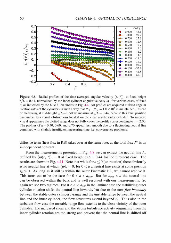
60 CHAPTER 4. OPTIMAL TC TURBULENCE
0 0.2 0.4 0.6 0.8 1
0
0.1
0.2
0.4
0.5
0.6
0.7
r
ω(r
)t/ω
iψ(deg)a
43.1
27.2
17.2
12.8
7.7
2.0
1.2
4.5
11.6
19.2
27.2
35.2
42.8
50.0
2.000
1.000
0.700
0.600
0.500
0.400
0.350
0.300
0.200
0.100
0.000
0.100
0.200
0.300
Figure 4.8: Radial profiles of the time-averaged angular velocity ⟨ω(r)⟩t at fixed heightz/L = 0.44, normalized by the inner cylinder angular velocity ωi, for various cases of fixeda, as indicated by the blue filled circles in Fig. 4.4. All profiles are acquired at fixed angularrotation rates of the cylinders in such a way that Rei −Reo = 1.0×10⁶ is maintained. Insteadof measuring at mid-height z/L = 0.50 we measure at z/L = 0.44, because this axial positionencounters less visual obstructions located on the clear acrylic outer cylinder. To improvevisual appearance the plotted range does not fully cover the profile corresponding to a= 2.00.The profiles of a = 0.50, 0.60, and 0.70 appear less smooth due to a fluctuating neutral linecombined with slightly insufficient measuring time, i.e. convergence problems.
diffusive term (heat flux in RB) takes over at the same rate, as the total flux Jω is anr-independent constant.
From the measurements presented in Fig. 4.8 we can extract the neutral line rn,defined by ⟨ω(rn, t)⟩t = 0 at fixed height z/L = 0.44 for the turbulent case. Theresults are shown in Fig. 4.11. Note that while for a ≤ 0 (co-rotation) there obviouslyis no neutral line at which ⟨ω⟩t = 0, for 0 < a a neutral line exists at some positionrn > 0. As long as it still is within the outer kinematic BL, we cannot resolve it.This turns out to be the case for 0 < a < aopt . But for aopt < a the neutral linecan be observed within the bulk and is well resolved with our measurements. Soagain we see two regimes: For 0 < a < aopt in the laminar case the stabilizing outercylinder rotation shifts the neutral line inwards, but due to the now free boundarybetween the stable outer cylinder r-range and the unstable range between the neutralline and the inner cylinder, the flow structures extend beyond rn. Thus also in theturbulent flow case the unstable range flow extends to the close vicinity of the outercylinder. The increased shear and the strong turbulence activity originating from theinner cylinder rotation are too strong and prevent that the neutral line is shifted off

4.4. LOCAL LDA ANGULAR VELOCITY RADIAL PROFILES 61
r
ω(r
)t
ana. laminar
ω(r
=0.5
)t
ana. laminar
exp. turbulent
a
Figure 4.9: (a) Rescaled angular velocity profiles ⟨ω(r)⟩t = (⟨ω(r)⟩t −ωo)/(ωi −ωo) forvarious a. For a ≤ aopt = 0.368 all of these curves cross the point (r = 1/2,⟨ω⟩t = 0.35).For a > aopt = 0.368 this is no longer the case. The transition of the quantity ⟨ω(r = 1/2)⟩tif a increases from a < aopt to a > aopt is shown in (b). The dashed vertical line indicatesabis = 0.368 = aopt . The solid black lines in (a) and (b) show the ω(r) values for the laminarsolution (4.6).
−0.5 0 0.5 1 1.5 2−0.6
−0.5
−0.4
−0.3
−0.2
−0.1
0
a
∂r〈ω〉t/|ω
o−
ωi|
ro−
ri
−0.5 0 0.5 1 1.5 20
0.1
0.2
0.3
0.4
0.5
−r a
3ν∂
r〈ω〉t/J
ω(%
)
a−0.5 0 0.5 1 1.5 2
99.5
99.6
99.7
99.8
99.9
100
r a3〈u
rω〉t/J
ω(%
)
(a) (b)
Figure 4.10: (a) Radial gradient ∂r⟨ω⟩t of the angular velocity profile in the bulk of theflow, non-dimensionalized with the mean ω-slope |ωo −ωi|/(ro − ri). The values are ob-tained from Fig. 4.8 by fitting a cubic smoothing spline to the profiles in order to increasethe accuracy of the gradient amplitude estimate. Note that the radial gradients are negativethroughout, and approach zero when close to a = aopt . (The connecting lines are guides forthe eyes.) (b) Resulting ratio of the viscous angular velocity transport term −r3
aν∂r⟨ω⟩A,t tothe total transport Jω (red squares and left axis) and ratio of the advective angular velocitytransport term r3
a⟨urω⟩A,t to the total transport Jω (green circles and right axis) for the variousa. These ratios correspond to the second and first term of equation (4.5), respectively.

62 CHAPTER 4. OPTIMAL TC TURBULENCE
a
r
1 2
1
ana. laminar
exp. turbulent
n
Figure 4.11: The measured radial position rn = (rn − ri)/(ro − ri) of the neutral line definedby ⟨ω(rn)⟩t = 0 at fixed height z/L = 0.44 as function of a. The straight vertical line cor-responds to aopt = 0.368, below which the neutral line is within the outer BL and cannot beresolved by our LDA technique. The solid line corresponds to the neutral line in the laminarcase calculated analytically with Eq. (4.6). Note that for significant counter-rotation a = 1and for this particular height, the neutral line in the turbulent case lies farther inside, nearerto the inner cylinder, than in the laminar flow case.
the outer kinematic BL. As described in Esser & Grossmann [46], this is the verymechanism which shifts the minimum of the viscous instability curve to the left ofthe ωo = 0 axis. Therefore, the observed behavior of the neutral line position as afunction of a is another confirmation of above idea that aopt coincides with the anglebisector abis of the instability range in parameter space. The small Reo and the largeReo behaviors perfectly merge. For a > aopt the stabilizing effect from the outercylinder rotation is strong enough, the width of the stabilized range is broad enough,so that a neutral line rn can be detected in the bulk of the TC flow.
Consequently one would expect that for much weaker turbulence Ta ≪ 1011 thecapacity of the turbulence around the inner cylinder to push the neutral line outwardswould decrease, leading to a smaller aopt for these smaller Taylor numbers. Numer-ical simulations by H. Brauckmann and B. Eckhardt in Marburg (Ta up to 1× 10⁹)and independently ongoing DNS by R. Ostillo, R.J.A.M. Stevens et al. in Twente(presently Ta up to 1×10⁷) seem to confirm this view.
For much weaker turbulence one would also expect a more pronounced height-dependence of the neutral line, which will be pushed outwards where the Taylor-rollsare going outwards and inwards where they are going inwards. Based on our height-dependence studies of section 4.2, we expect that this height dependence will bemuch weaker or even fully washed out in the strongly turbulent regime Ta > 1011 inwhich we operate the TC apparatus. However, in Fig. 4.11 we observe that the neutralline in the turbulent case lies more inside than in the laminar case, and this result isdifficult to rationalize apart from assuming some axial-dependence of the neutral line
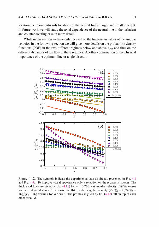
4.4. LOCAL LDA ANGULAR VELOCITY RADIAL PROFILES 63
location, i.e. more outwards locations of the neutral line at larger and smaller height.In future work we will study the axial dependence of the neutral line in the turbulentand counter-rotating case in more detail.
While in this section we have only focused on the time-mean values of the angularvelocity, in the following section we will give more details on the probability densityfunctions (PDF) in the two different regimes below and above aopt and thus on thedifferent dynamics of the flow in these regimes: Another confirmation of the physicalimportance of the optimum line or angle bisector.
0.2 0.3 0.4 0.5 0.6 0.7 0.8
0
0.2
0.3
0.4
0.5
0.6
0.7
r
ω(r
)t/ω
i
a
Eq.(4.11)
1.0000.6000.4000.3000.1000.000
–0.100–0.300
a
Eq.(4.12)
1.0000.6000.4000.3000.1000.000
–0.100–0.300
0.2 0.3 0.4 0.5 0.6 0.7 0.80.2
0.25
0.3
0.35
0.4
0.45
0.5
0.55
r
ω(r
)t
(a)
(b)
Figure 4.12: The symbols indicate the experimental data as already presented in Fig. 4.8and Fig. 4.9a. To improve visual appearance only a selection on the a-cases is shown. Thethick solid lines are given by Eq. (4.11) for η = 0.716. (a) angular velocity ⟨ω(r)⟩t versusnormalized gap distance r for various a. (b) rescaled angular velocity ⟨ω(r)⟩t = (⟨ω(r)⟩t −ωo)/(ωi −ωo) versus r for various a. The profiles as given by Eq. (4.12) fall on top of eachother for all a.

64 CHAPTER 4. OPTIMAL TC TURBULENCE
From considerations of bounds on solutions to the Navier-Stokes equation, Busse[53] derived an expression for the angular velocity in the limit of infinite Reynoldsnumber. Translating his formulas to the notation used in the present thesis, reads
ω =ωi −ωo
r2
[ri
2
4(1−η2)
]+ωi
[η2 −2η4
2−2η4
]+ωo
[2−η2
2−2η4
]. (4.11)
Excellent agreement is found for the case a = 0.00, however for a farther away fromzero there is more discrepancy between the experimental data and the upper-boundtheory by Busse [53], as shown in Fig. 4.12a. When we rescale the angular velocityprofiles to ω , according to Eq. (4.10), the profiles as given by the upper-bound theory[53] fall on top of each other for all a,
ω =ri
2
4(ro4 − ri
4)
[ro
2(ri
2 + ro2)
r2 +2ro2 −4ri
2
](4.12)
In contrast to the collapsing upper-bound profiles, the experimental data in Fig. 4.12bshow a different trend. One would expect good agreement between the case of a =aopt and the upper-bound profiles, however we observe only a good match for thecase of a = 0.00, which may be due to the complexity of the flow structure.
4.5 Turbulent flow organization in the TC gap
Time series of the angular velocity at r = 0.60 below the optimum amplitude ata = 0.35 < aopt = 0.368 (co-rotation dominates) and above the optimum at a =0.60> aopt = 0.368 (counter-rotation dominates) are shown in Fig. 4.13a and 4.13b,respectively. While in the former case we always have ω(t)> 0 and a Gaussian dis-tribution — see Fig. 4.14a — in the latter case we find a bimodal distribution withone mode fluctuating around a positive angular velocity and one mode fluctuatingaround a negative angular velocity. This bimodal distribution of ω(t) is confirmed invarious PDFs shown in Fig. 4.14. We interpret this intermittent behavior of the timeseries as an indication of turbulent bursts originating from the turbulent region in thevicinity of the inner cylinder and penetrating into the stabilized region near the outercylinder. We find such bimodal behavior for all a > aopt , see Figs. 4.14d, e, f, g, h,and i, whereas for a < aopt we find a unimodal behavior, see Figs. 4.14a, b, and c.Apart from one case (a = 0.50) we do not find any long-time periodicity of the burstsin ω(t). In future work we will perform a full spectral analysis of long time series ofω(t) for various a and r.
Three-dimensional visualizations of the ω(t)-PDF for all 0< r < 1 are providedin Fig. 4.15 for unimodal cases a < aopt and in Fig. 4.16 for bimodal cases a > aopt .In the latter figure the switching of the system between positive and negative angularvelocity becomes visible.

4.5. TURBULENT FLOW ORGANIZATION IN THE GAP 65
0 25 500.25
0.30
0.35
0.40
0.45
0.50
t (s)
ω(t
)
ω|ω=0
exp. data
0 25 50 75 1000.25
0.30
0.35
0.40
0.45
0.50
t (s)
ω(t
)
(a) (b)
Figure 4.13: Time series of the dimensionless angular velocity ω(t) as defined in Eq. (4.10)but without t-averaging, acquired with LDA. (a) a = 0.35, co-rotation dominates, at r = 0.60with an average data rate of 456 Hz. (b) a = 0.60, counter-rotation dominates, same r =0.60 with an average data rate of 312 Hz. Figure (a) shows a unimodal velocity distributionwhereas (b) reveals a bimodal distribution interpreted as caused by intermittent bursts out ofthe unstable inner regime with angular velocity between ωi and ω = 0, i.e. (ωo − 0)/(ωo −ωi)< ω < 1 into the stable outer regime with angular velocity between ω = 0 and ω0, i.e. 0<ω < (ωo −0)/(ωo −ωi). The solid pink line indicates the neutral line ω = 0, correspondingto ω = ωo/(ωo −ωi) = a/(1+a), for the specific a.
Further details on the two observed individual modes such as their mean and theirmixing coefficient are given in Figs. 4.17 (for a = 0.60) and 4.18 (for a = 0.70), bothwell beyond aopt . In both cases one observes that the contribution from the large-ω-mode (red curve, ω > 0, apart from positions close to the outer cylinder) is asexpected highest at the inner cylinder and fades away when going outwards, whereasthe small-ω-mode has the reverse trend. Note however that even at r = 0.20, e.g.relatively close to the inner cylinder, there are moments for which ω is negative, i.e.patches of stabilized liquids are advected inwards, just as patches of turbulent floware advected outwards.
This mechanism resembles the angular velocity exchange mechanism suggestedby Coughlin & Marcus [98] just beyond onset of turbulence. These authors sug-gest that for the counter-rotating case there is an outer region which is centrifugallystable, but subcritically unstable, thus vulnerable to distortions coming from the cent-rifugally unstable inner region. Inner and outer region are separated by the neutralline. For the low Re of Coughlin & Marcus [98] the inner region is not yet turbulent,but displays interpenetrating spirals, i.e. a chaotic flow with various spiral Taylor vor-tices. For our much larger Reynolds numbers the inner flow will be turbulent and thedistortions propagating into the subcritically unstable outer regime will be turbulentbursts. These then will lead to intermittent instabilities in the outer regime. In futurework these speculations must further be quantified.

66 CHAPTER 4. OPTIMAL TC TURBULENCE
0.2 0.3 0.4 0.5 0.60
3
6
9
12
15
18
ω
PD
F(ω
)
a = 0.60
r = 0.20
ω|ω=0
exp. data
bimodal fit
mode 1
mode 2
0.2 0.3 0.4 0.5 0.60
3
6
9
12
15
18
ω
PD
F(ω
)
a = 0.60
r = 0.51
(a)
(d)
(g)
0.1 0.2 0.3 0.4 0.5
ω
a = 0.30
r = 0.60
0.2 0.3 0.4 0.5 0.6
ω
a = 0.60
r = 0.29
0.2 0.3 0.4 0.5 0.6
ω
a = 0.60
r = 0.60
(b)
(e)
(h)
0.1 0.2 0.3 0.4 0.5
ω
a = 0.35
r = 0.60
0.2 0.3 0.4 0.5 0.6
ω
a = 0.60
r = 0.80
0.2 0.3 0.4 0.5 0.6
ω
a = 0.60
r = 0.41
(c)
(f )
(i)
0.1 0.2 0.3 0.4 0.50
10
20
30
40
ω
PD
F(ω
)
a = 0.20
r = 0.60
ω|ω=0
exp. data
unimodal fit
Figure 4.14: Probability density functions of the angular velocity ω(t) distributions forvarious cases of a and position r = (r− ri)/(ro − ri). (a) a = 0.20, r = 0.60, (b) a = 0.30,r = 0.60, and (c) a = 0.35, r = 0.60. The other panels all show a = 0.60 but at differentnon-dimensional gap distances r. (d) 0.20, (e) 0.29, (f) 0.41, (g) 0.51, (h) 0.60, and (i)0.80. The gold circles indicate the measured distribution obtained by LDA. While for (a),(b), and (c) one Gaussian distribution (black solid curve) describes the data well, for (e) to(i) a superposition of two Gaussians is needed for a good fit (blue and red curves). We callthe two Gaussians the two “modes” of the flow. The fitting algorithm gives the mean, thestandard deviation, and the mixture coefficient of modes 1 and 2, which recombine to theblack solid line, describing the measured distribution well. The dashed pink vertical lineshows the neutral line ω = 0, implying ω = ωo/(ωo −ωi) = a/(1+a).

4.5. TURBULENT FLOW ORGANIZATION IN THE GAP 67
(b)
= 0.30a
(a)
a = 0.20
Figure 4.15: Three-dimensional visualization of the (normalized) angular velocity PDF witha contiuous scan of r for two unimodal cases (a) a = 0.20 and (b) a = 0.30, both beingsmaller than aopt = 0.368. The pink line corresponds to the neutral line ω = 0, i.e. ω =ωo/(ωo −ωi) = a/(1+a).
(d)
= 1.00a
(c)
= 0.70a
(b)
= 0.60a
(a)
a = 0.50
Figure 4.16: Same as in Fig. 4.15, but now for the bimodal cases a > aopt = 0.368. (a)a = 0.50, (b) a = 0.60, (c) a = 0.70, and (d) a = 1.00. The bimodal character with one modebeing left of the neutral line ω = 0 and the other mode being right of the neutral line becomesparticularly clear for (b) and (c).
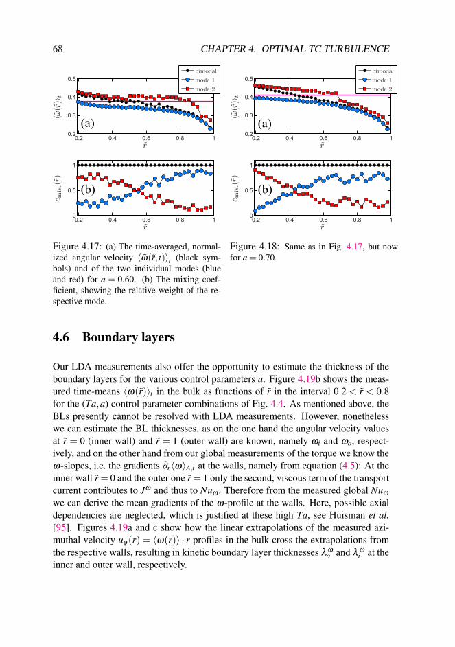
68 CHAPTER 4. OPTIMAL TC TURBULENCE
0.2 0.4 0.6 0.8 10.2
0.3
0.4
0.5
r
ω(r
)t
bimodal
mode 1
mode 2
0.2 0.4 0.6 0.8 10
0.5
1
r
cm
ix.(r
)
(a)
(b)
Figure 4.17: (a) The time-averaged, normal-ized angular velocity ⟨ω(r, t)⟩t (black sym-bols) and of the two individual modes (blueand red) for a = 0.60. (b) The mixing coef-ficient, showing the relative weight of the re-spective mode.
0.2 0.4 0.6 0.8 10.2
0.3
0.4
0.5
r
ω(r
)t
bimodal
mode 1
mode 2
0.2 0.4 0.6 0.8 10
0.5
1
rcm
ix.(r
)
(a)
(b)
Figure 4.18: Same as in Fig. 4.17, but nowfor a = 0.70.
4.6 Boundary layers
Our LDA measurements also offer the opportunity to estimate the thickness of theboundary layers for the various control parameters a. Figure 4.19b shows the meas-ured time-means ⟨ω(r)⟩t in the bulk as functions of r in the interval 0.2 < r < 0.8for the (Ta,a) control parameter combinations of Fig. 4.4. As mentioned above, theBLs presently cannot be resolved with LDA measurements. However, nonethelesswe can estimate the BL thicknesses, as on the one hand the angular velocity valuesat r = 0 (inner wall) and r = 1 (outer wall) are known, namely ωi and ωo, respect-ively, and on the other hand from our global measurements of the torque we know theω-slopes, i.e. the gradients ∂r⟨ω⟩A,t at the walls, namely from equation (4.5): At theinner wall r = 0 and the outer one r = 1 only the second, viscous term of the transportcurrent contributes to Jω and thus to Nuω . Therefore from the measured global Nuωwe can derive the mean gradients of the ω-profile at the walls. Here, possible axialdependencies are neglected, which is justified at these high Ta, see Huisman et al.[95]. Figures 4.19a and c show how the linear extrapolations of the measured azi-muthal velocity uϕ (r) = ⟨ω(r)⟩ · r profiles in the bulk cross the extrapolations fromthe respective walls, resulting in kinetic boundary layer thicknesses λ ω
o and λ ωi at the
inner and outer wall, respectively.

4.6. BOUNDARY LAYERS 69
0 0.2 0.4 0.6 0.8 1
0
20
40
60
80
100
120
r0 0.001 0.0020
20
40
60
80
100
120
r
ω(r
)t
(rad
/s)
0.996 0.998 1
0
10
20
40
50
r
Figure 4.19: Time-averaged angular velocity ⟨ω(r)⟩t for the various (Ta,a) of Fig. 4.4, seethat figure for the color-code. The bulk values in (b) are obtained from our LDA measure-ments and are linearly extrapolated in azimuthal velocity uϕ = ωr -space to the inner (a) andouter (c) cylinders, whose angular velocity is ωi and ωo, respectively. Since also the angularvelocity gradients at the walls are known from the global Nuω measurements via Eq. (4.5),one can estimate the thicknesses λ ω
i and λ ωo of the inner and outer kinematic BLs, i.e. the BL
widths of the azimuthal motion.
1 2
a
λ(m
)
×10−4
λi
λo
1 2
a
λo/λ
i
Prediction
Extrap. exp. results(a)
(b)
ωω
ω
ω
Figure 4.20: (a) Inner and outer viscous BL thicknesses λ ωi and λ ω
o , respectively, as derivedwith the procedure sketched in the caption of Fig. 4.19. Note that Ta is not constant for thedata points shown in this figure; the connecting lines are guides for the eyes. The respectiveTa values are indicated in Fig. 4.4. – (b) Ratio λ ω
o /λ ωi for the extrapolated experimental
results shown in (a) (solid black dots) and for the prediction given by Eq. (4.13) (green stars).

70 CHAPTER 4. OPTIMAL TC TURBULENCE
These thicknesses are shown in Fig. 4.20a. As expected, the outer boundary layeris much thicker than the inner one. This is an immediate consequence of equation(4.5), which leads to the relation r3
i ∂r⟨ω(ri)⟩ = r3o∂r⟨ω(ro)⟩ for the slopes. The in-
ner cylinder angular velocity profile slope thus is ∂r⟨ω(ri)⟩ = η−3∂r⟨ω(ro)⟩. Thusfor η = 0.716 the inner cylinder ω-profile slope is 2.724 times steeper as the outercylinder one, leading to the correspondingly thinner BL at the inner cylinder. AsFig. 4.20a shows, the inner cylinder BL thickness hardly shows any a-dependence,while the outer cylinder BL width increases considerably with increasing degree ofcounter-rotation, viz. increasing a. Note that along the curves of Fig. 4.20a the Taylornumber Ta is not constant. Therefore, in Fig. 4.20b we also show the ratio λ ω
o /λ ωi
versus a, i.e. with increasing counter-rotation. In this figure we have also plotted theprediction for this thickness-ratio obtained from the EGL theory,
λ ωo
λ ωi
= η−3 |ωo − ω||ωi − ω|
. (4.13)
According to the EGL theory ω is the mean bulk angular velocity, here taken asthe measured angular velocity averaged over the bulk ranging from 0.2 < r < 0.8,i.e. ω = ⟨ωcenter⟩t . The EGL prediction nicely agrees with the measured data for0.2 . a . 1. For smaller control parameters a . 0.2, i.e., in the regime of co-rotationor very weak counter-rotation there is some disagreement. This might reflect theshort-comings of our present extrapolation method to determine the BL thicknesses;in fact, given the crudeness of the method we consider the good agreement in therange 0.2 ≤ a ≤ 1 more remarkable than the worse agreement in the other a-ranges.But it could also be another indication of the fundamental difference of the flow spacebelow or above aopt : as shown above there is mono-modal turbulence in the fullyunstable gap for a< aopt , in contrast to bi-modal flow in an only partly unstable (innerpart) and partly stable (outer part) gap. Also for a < aopt as well as far above theoptimum a ≫ aopt the ω-profile has no longer zero slope in the bulk. The differencesbetween both curves in Fig. 4.20b might well reflect this.
To understand the disagreement we study a different representation of ω , asshown in Fig. 4.21. We define a new ⟨ωextrap⟩t by assuming Eq. (4.13) to hold forall a and by filling in the boundary layer ratio as found by the extrapolation method.There is good agreement between ⟨ωcenter⟩t and ⟨ωextrap⟩t in the range 0.2 ≤ a ≤ 1and the agreement is getting worse for other a-ranges, similar to the result in Fig.4.20b. This might be explained by the larger angular velocity gradient in this a-range as shown in Fig. 4.10a. If the boundary layer thickness ratio as proposed bythe EGL theory always holds, what then should the corresponding radial locationr|⟨ω(r)⟩t=⟨ωextrap⟩t be to match ω . Figure 4.21b shows the corresponding radial locationat which the measured angular velocity satisfies Eq. (4.13) as a function of a. Clearlyit is different from r = 0.5 and the radial position strongly depends on a. This has todo with the non-Oberbeck-Boussinesq (NOB) effect of TC flow, which is analogous

4.7. SUMMARY, DISCUSSION, AND OUTLOOK 71
a
r|
ω(r
)t=
ωextrap
t
a
ω
ωcenter t
ωextrap t
Figure 4.21: (a) The rescaled angular velocity versus a. The green stars indicate the meas-ured rescaled angular velocity averaged over the bulk ranging from 0.2< r < 0.8. The blackcircles indicate the rescaled angular velocity extrapolation based on Eq. (4.13) by assumingthis relation holds for all a. (b) The radial location at which the measured angular velocitysatisfies Eq. (4.13) as a function of a.
to NOB-RB flow, see e.g. Ahlers et al. [99, 100], Sugiyama et al. [101]. Since TCflow is strongly NOB, the radial location of zero angular velocity gradient is shifted,similar to the bulk temperature shift in NOB-RB. Figure 4.21b quantifies this shift asfunction of a.
4.7 Summary, discussion, and outlook
In conclusion, we have experimentally explored strongly turbulent TC flow with Ta>1011 in the co- and counter-rotating regimes. We find that in this large Taylor numberTa regime and well off the instability lines the dimensionless angular velocity trans-port flux within experimental precision can be written as Nuω(Ta,a) = f (a) ·Taγ(a)
with either γ = 0.39± 0.03 universally for all a or with a slightly decreasing γ(a)when decreasing the counter-rotation below the optimum a = aopt . This is the effect-ive scaling exponent of the ultimate regime of TC turbulence predicted by Grossmann& Lohse [26] for RB flow and transferred to TC by the close correspondence betweenRB and TC according to the EGL theory. When starting off counter-rotation, i.e.when increasing a beyond zero, the angular velocity transport current does not reducebut instead is first further enhanced, due to the enhanced shear, before finally, beyonda = aopt = 0.368, the stabilizing effect of the counter-rotation leads to a reduction ofthe angular velocity transport flux Nuω . For optimal counter-rotation ωo =−0.368ωi
the angular velocity transport is maximal; the value of aopt = 0.368 is assigned to ourpresent radius ratio η = 0.716. At this very a-value the mean angular velocity profilewas shown to have zero gradient in the bulk for the present large Ta. Despite alreadysignificant counter-rotation for 0 < a < aopt there is no neutral line outside the outer

72 CHAPTER 4. OPTIMAL TC TURBULENCE
BL; furthermore the probability distribution function of the angular velocity has onlyone mode. For larger a, beyond a > aopt , a neutral line can be detected in the bulkand the PDF here becomes bimodal, reflecting intermittent burst of turbulent patchesfrom the turbulent inner r-regime towards the stabilized outer r-regime. We alsopresented first attempts to estimate the BL thicknesses at the inner and outer cylinder,and in agreement with the theoretical expectation the latter one is much thicker. —We offered a hypothesis which gives a unifying view and consistent understanding ofall these various findings.
Clearly, the present study is only the start of a long experimental program tofurther explore turbulent TC flow. Much more work still must be done. In particular,we mention the following open issues:
• For strong counter-rotation, i.e. large a, the axial dependence must be studiedin much more detail. This holds in particular for the location of the neutral line.We expect that for large a ≫ aopt , the flow will be so much stabilized that anaxial dependence of the location of the neutral line shows up again, in spite ofthe large Ta numbers. It is then more appropriate to speak of a neutral surface.
• Modern PIV techniques should enable us to directly resolve the inner and outerBLs.
• With the help of PIV studies we also hope to visualize BL instabilities andthus better understand the dynamics of the flow, in particular in the stronglycounter-rotating case. The key question is: How does the flow manage totransport angular velocity from the turbulent inner regime towards the outercylinder – thereby crossing the stabilized outer regime?
• The studies must be repeated at lower Ta to better understand the transitionfrom weakly turbulent TC towards the ultimate regime as apparently seen inthe present work. In our present setup we can achieve such a regime withsilicon oil instead of water.
• These studies should be complemented with direct numerical simulation of co-and counter-rotating TC flow. Just as happened in recent years in turbulentRB flow, cf. Stevens et al. [39, 102], also for turbulent TC flow we expect tonarrow the gap between numerical simulation and experiment or even to closeit for not too turbulent cases, allowing for one-to-one comparisons.
• Obviously, our studies must be extended to different η values, in order to checkthe hypothesis (4.8) and to see how this parameter affects the flow organization.
Clearly, many exciting discoveries and wonderful work with TC flow is ahead of us.
5Angular momentum transport andturbulence in laboratory models of
Keplerian flows∗ † ‡
We present angular momentum transport (torque) measurements in two recent ex-perimental studies of the turbulent flow between independently rotating cylinders.In addition to these studies, we reanalyze prior torque measurements to expand therange of control parameters for the experimental Taylor-Couette flows. We find thatthe torque may be described as a product of functions that depend only on the Reyn-olds number, which describes the turbulent driving intensity, and the rotation number,which characterizes the effects of global rotation. For a given Reynolds number, theglobal angular momentum transport for Keplerian-like flow profiles is approximately14% of the maximum achievable transport rate. We estimate that this level of trans-port would produce an accretion rate of M/M0 ∼ 10−3 in astrophysical disks. Weargue that this level of transport from hydrodynamics alone could be significant.
∗Submitted to Astron. Astrophys. as: M.S. Paoletti, D.P.M. van Gils, B. Dubrulle, C. Sun, D. Lohse,and D.P. Lathrop, Angular momentum transport and turbulence in laboratory models of Keplerian flows.
†Experiments were performed on the TC facilities of the University of Maryland (UMD TC facility)and the University of Twente (T3C facility).
‡This chapter uses a different notation for the geometric parameters and different non-dimensionalizations from the rest of this thesis as befits the astrophysical community.
73

74 CHAPTER 5. TRANSPORT AND TURBULENCE IN KEPLERIAN FLOWS
5.1 Introduction
Astrophysical disks are ubiquitous in the universe, orbiting around a wide panel ofmassive objects, from black holes to stars. An essential ingredient of their dynamicsis the radial transport of angular momentum that governs the rate of material fallingonto the central object. Realistic models of this process are impeded by the com-plexity of the disk dynamics, including a wide variety of processes such as generalrelativistic effects, self-gravitation, radiation, dynamics of plasma magnetic fieldsand turbulence. In particular, the contribution from hydrodynamics to the angularmomentum transport in such astrophysical flows is not yet understood.
A natural first-step in the construction of a robust model is to consider the min-imal list of ingredients that can capture and reproduce the observed disk properties.Such a model has been proposed several decades ago by Shakura & Sunyaev [103]and Pringle [104], and was given the name α disks. In that model, the radial trans-port of angular momentum is parameterized by a turbulent viscosity coefficient, thatneeds to be prescribed, or measured. In the past, there have been a few attempts tomeasure this coefficient in numerical simulations (Dubrulle [105]).
An alternative promising option, as recognized by Zeldovich [106] and Richard& Zahn [107], is offered by focusing instead on laboratory experiments. Indeed, itmay be shown (Hersant et al. [108]), that under simple, but well founded approxim-ations, the equations governing an α disk are similar to the equation of motion ofan incompressible rotating shear flow, with penetrable boundary conditions and cyl-indrical geometry. This kind of flow can be achieved in the Taylor-Couette flow (seeFig. 5.1), a fluid layer sheared between two independently rotating, coaxial cylinders.
This remark motivated several experimental studies of the transport properties inthe Taylor-Couette flow, with contradicting conclusions. Depending upon the com-munity, the strength of the turbulent transport is quantified in various ways. The mostbasic quantification (Wendt [5]) is the one through the torque T which is necessaryto keep the inner cylinder rotating at a given velocity. The dimensionless versionthereof is G = T/(Lmidρν2), where ρ is the fluid density, ν its kinematic viscosityand Lmid the effective length of the cylinders (Paoletti & Lathrop [18]). Eckhardtet al. [23] and van Gils et al. [88] used Nuω = G/Glam, where Glam is the laminartorque, to quantify the angular velocity flux from the inner to the outer cylinder, inorder to highlight the analogy between Taylor-Couette and Rayleigh-Benard flow(Dubrulle & Hersant [22], Eckhardt et al. [23, 82]). The engineering communityprefers the drag-coefficient c f = G/Re2, where Re = 2
1+η |ηRe2 −Re1| and η = a/bis the radius ratio and Re1/2 the Reynolds number of the inner/outer cylinder. In theastrophysics community, the same information is often expressed in terms of the βcoefficient, defined by β = 2Gη2/(π(1−η)4Re2) = 2η2c f /(π(1−η)4), which canbe interpreted as a dimensionless turbulent viscosity.
By reexamining previous data obtained by Wendt [5] and Taylor [6], Richard &

5.2. APPARATUS AND EXPERIMENTAL DETAILS 75
Zahn [107] showed that the β -parameter is on the order of βRZ ∼ 10−5 for Kepleriandisks. A more complete analysis, including results of new experiments on a classicalTaylor-Couette flow from Richard [86], led to the same conclusion (Dubrulle et al.[75]). In contrast, an original experiment, built in Princeton (Ji et al. [109]) so asto minimize end effects, measured a β coefficient through radial Reynolds stressesand obtained a value smaller by more than an order of magnitude βP ∼ 7× 10⁻⁷.Furthermore, the Princeton experiments could not distinguish the angular momentumtransport in Keplerian flows from their measurements in solid-body rotation, wherethe cylinders rotate together thereby resulting in zero angular momentum transport.
In the present contribution, we report precise angular momentum transport (torque)measurements in two independent experiments performed at very large Reynoldsnumber and compute the resulting β coefficient for different rotation profiles. Tofurther study the scaling of angular momentum transport in rotating shear flows, wecompare our measurements to those of Wendt [5], Taylor [6], Richard [86], andDubrulle et al. [75]. We find a universal scaling of the torque for various rotationprofiles that captures the effects of the various geometries used in the experimentssummarized here.
5.2 Apparatus and experimental details
5.2.1 Apparatus: generalities
The experiments presented here all examine the transport of angular momentum(torque) in classical Taylor-Couette flow. Figure 5.1 shows a schematic represent-ation of our experiments. The fluid is contained between concentric cylinders of radiia< b. The inner (outer) cylinder rotates at an angular velocity of Ω1 (Ω2). The over-all height of the fluid contained between the axial boundaries is given by the lengthL. The geometry of a particular Taylor-Couette flow apparatus is often defined indimensionless form by the radius ratio η ≡ a/b and the aspect ratio Γ ≡ L/(b−a).
The ideal Couette flow is infinite in axial extent. As such, several methods havebeen employed to handle the finite-size effects that are present in any laboratoryexperiment. The most common case has the axial boundaries rotate with one of thetwo cylinders. In other experiments, the axial boundaries are divided at the mid-gap and have the inner (outer) portion rotate with the inner (outer) cylinder. Thissplit-ring approach has been further developed to allow for pairs of rings that canindependently rotate with respect to the cylinders. Allowing the axial boundaries toindependently rotate aids in the suppression of finite-size effects as detailed in Ji et al.[109], Schartman et al. [110], Burin et al. [111].
The data that we analyze and present stems from several different experiments,which are summarized in Table 5.1. The early experiments by Wendt [5] measuredthe torque required to drive the inner cylinder for three values of η . The system had

76 CHAPTER 5. TRANSPORT AND TURBULENCE IN KEPLERIAN FLOWS
Lmid L
a
b
Figure 5.1: Taylor-Couette flow may be used to study angular momentum transport in ro-tating shear flows. The fluid is sheared between two independently rotating cylinders of radiia< b that rotate at angular velocities Ω1 and Ω2 for the inner and outer cylinders, respectively.Although the total fluid height is given by L, some experiments only measure the contributionto the torque over a central section of length Lmid to minimize end effects, as in Lathrop et al.[10, 11], Lewis & Swinney [14], van den Berg et al. [15], Paoletti & Lathrop [18], van denBerg et al. [27, 61], van Gils et al. [88].
Table 5.1: A summary of the parameters used in the experiments discussed here. The geo-metry of the apparatus is given by the outer cylinder radius b, the radius ratio η = a/b andthe aspect ratio Γ = L/(b−a). The range of turbulence intensities are governed by the innerand outer cylinder Reynolds numbers Re1 and Re2. The effects of rotation are parameterizedby the rotation number RΩ introduced by Dubrulle et al. [75].
Experiment b (cm) η Γ max(Re1) max(Re2) min(RΩ) max(RΩ)Wendt [5] 14.7 0.68 10.64 8.47×10⁴ 1.24×10⁵ -0.71 0.47Wendt [5] 14.7 0.85 22.93 4.95×10⁴ 5.83×10⁴ -0.80 0.18Wendt [5] 14.7 0.935 52.63 2.35×10⁴ 2.52×10⁴ -0.42 0.11Taylor [6] 8.11 0.79–0.973 50–384 0 1.08×10⁵ 0.03 0.27Richard [86] 5.00 0.72 27.18 9.50×10⁴ 1.30×10⁵ -1.43 -0.94Richard [86] 5.00 0.72 27.18 9.50×10⁴ 1.30×10⁵ 0.38 0.58Ji et al. [109] 20.3 0.35 2.1 1.20×10⁶ 4.50×10⁵ -1.67 -1.08Maryland 22.09 0.725 11.47 3.70×10⁶ 1.50×10⁶ -2.04 1.46Twente 27.9 0.716 11.68 2.00×10⁶ 1.40×10⁶ -0.74 0.17

5.2. APPARATUS AND EXPERIMENTAL DETAILS 77
a free surface at the top, although we quote an effective aspect ratio defined usingthe axial length of the apparatus. The data from Taylor [6] determined the scalingof the torque for several values of η with the inner cylinder stationary (Ω1 = 0).Richard’s experiments [75, 86] did not directly measure the torque. Instead, criticalReynolds numbers for various transitions were observed and the analysis presentedby Dubrulle et al. [75] was used to estimate the corresponding torque. We do notpresent data from the experiments of Ji et al. [109], but rather use their reportedmeasurements as a basis for comparison, as detailed in Section 5.4. The two mostrecent experiments by Paoletti & Lathrop [18] and van Gils et al. [88] are furtherdescribed in the forthcoming sections.
5.2.2 Apparatus: the Maryland experiment
The experiments presented by Paoletti & Lathrop [18], henceforth referred to as theMaryland experiment, are conducted in the apparatus constructed by Lathrop et al.[10, 11], which was modified to allow the outer cylinder to rotate independently. Theouter cylinder is an anodized aluminum cylinder with the same physical dimensionsas in Lathrop et al. [10, 11], Lewis & Swinney [14], specifically b = 22.085 cm and aworking fluid height L = 69.50 cm. The inner cylinder is stainless steel with a radiusa = 16.000 cm yielding a radius ratio η = 0.7245 and an aspect ratio Γ = 11.47.The inner cylinder is rotated up to Ω1/2π = 20 s−1 while the outer cylinder maybe rotated in either direction up to |Ω2/2π| = 10 s−1. Both angular velocities aremeasured by shaft encoders and controlled to within 0.2% of the set value.
The axial boundaries in the Maryland experiment rotate with the outer cylinder.To reduce end effects in the torque measurements the inner cylinder is divided axiallyinto three sections of length 15.69, 40.64 and 15.69 cm (see schematics in Lathropet al. [10, 11]). Only the central section of length Lmid = 40.64 cm (see Fig. 5.1)senses the torque of the fluid as described by Lathrop et al. [10, 11]. The regions 2.58gap widths from each of the axial boundaries, where secondary circulation setup byfinite boundaries is strongest, are avoided in the torque measurements.
The desired accuracy of our measurements requires that the temperature of thewater be precisely controlled. In contrast to prior experiments (Lathrop et al. [10,11], Lewis & Swinney [14], van den Berg et al. [15, 27, 61], van Gils et al. [88])where the system was cooled at the axial boundaries, we control the temperature ofthe water by heating and cooling the outer cylinder. This allows the working fluidto be temperature-controlled along the entire axial length of the experiment, yieldinga 6.5 fold increase in the temperature-controlled surface area. This is particularlyimportant for Rayleigh-stable flows, where mixing is greatly reduced. In our ex-periments the temperature is 50±0.02C yielding a kinematic fluid viscosity of ν =5.5×10⁻³ cm2/s, except for Re> 2×10⁶ where T = 90 C and ν = 3.2×10⁻³ cm2/s.

78 CHAPTER 5. TRANSPORT AND TURBULENCE IN KEPLERIAN FLOWS
5.2.3 Apparatus: the Twente experiment
The Twente turbulent Taylor-Couette (called T3C) facility, here referred to as theTwente experiment, is described in great detail by van Gils et al. [112]. In short,the working fluid height is L = 92.7 cm, has an inner radius of a = 20.0 cm and anouter radius of b = 27.94 cm. The maximum inner and outer angular velocities areΩ1/2π = 20 Hz and |Ω2/2π|= 10 Hz, respectively. The system is fully temperaturecontrolled through cooling of the upper and lower end plates, which co-rotate withthe outer cylinder. The system is operated with water at a temperature of 20 C,resulting in a kinematic viscosity of ν = 1.04×10⁻² cm2/s. The torque is measuredover the middle part of the inner cylinder of height Lmid = 53.6 cm to minimize theinfluence of the end-plates (similar to Lathrop et al. [10, 11]). The torque is measuredby a load cell imbedded inside the middle section of the inner cylinder in both theTwente and Maryland experiments, in contrast to measuring the torque on the driveshaft that would be affected by mechanical seals in the end plates or by velocimetrymeasurements, as in the Princeton experiments (Ji et al. [109], Schartman et al. [110],Burin et al. [111], Schartman et al. [113]).
5.2.4 Control parameters
The analysis of our results is simplified by a proper choice of the control paramet-ers. As in Dubrulle et al. [75], we use the following three dimensionless controlparameters, which fully describe the geometry and specify the state of the dynamicalTaylor-Couette system:
Re =2
1+η|ηRe2 −Re1|, (5.1)
RΩ = (1−η)Re1 +Re2
ηRe2 −Re1, (5.2)
RC =1−ηη1/2 , (5.3)
where Re1 = aΩ1d/ν and Re2 = bΩ2d/ν are the Reynolds number of the inner andouter cylinder and d = (b−a) is the gap width.
The above control parameters have been introduced so that their definitions applyto rotating shear flows in general and not strictly only to the Taylor-Couette geometry.It is very easy in this formulation to relate the Taylor-Couette flow to the shearingsheet (plane Couette flow with rotation), by considering the limit RC → 0. The linearstability properties of the fluid can also be neatly recast using these control paramet-ers. In the inviscid limit (Re → ∞), and for axisymmetric disturbances, the linearstability properties of the flow are governed by the Rayleigh criterion, namely that

5.2. APPARATUS AND EXPERIMENTAL DETAILS 79
Table 5.2: A summary of the Taylor-Couette control parameters related to some astrophys-ical disks, as computed by Hersant et al. [108]. Here, b is the disk’s outer radius, and M theaccretion rate.
Central object b (a.u.) η Γ max(Re1) max(Re2) RΩ M/M0
TTauri 1000 0 0.94 1012 1014 -1.33 10−5 −10−2
FuOri 5 0 0.94 1013 1015 -1.33 0.1-1
the fluid is stable if the Rayleigh discriminant is everywhere positive:
Ωr
∂rL(r)> 0, (5.4)
where L(r) = r2Ω(r) is the specific angular momentum. Applying this criterion tothe laminar profile leads to
(RΩ +1)(RΩ +1−ab/r2)> 0. (5.5)
Since ab/r2 varies between 1/η and η , one obtains that in the inviscid limit, the flowis unstable against infinitesimal axisymmetric disturbances when R∞
Ω− < RΩ < R∞
Ω+,
where R∞Ω− =−1, respectively R∞
Ω+ = 1/η −1, are the marginal stability thresholds
in the inviscid limit (superscript ∞) in the cyclonic case (RΩ > 0, subscript +), andanticyclonic case (RΩ < 0, subscript −). This means that, in the anticyclonic case,any flow such that RΩ < −1 is linearly stable against axisymmetric disturbances.However, it may be non-linearly stable or unstable against non-axisymmetric dis-turbances, as found in the experiments described here.
In the present paper, we determine the intensity of the momentum transport bymeasuring the torque required to drive the inner cylinder for a given set of paramet-ers (Re,RΩ). Measurements described here suggest that at large enough Reynoldsnumber, the nondimensional torque G = T/(ρν2Lmid), where T is the torque, ρ thefluid density, ν the kinematic viscosity and Lmid is defined in Fig. 5.1, varies approx-imately as G ∼ Reα with 1.75 < α(Re) < 1.85, even for Rayleigh-stable flows. Wenote that these exponents are less than a simple dimensional argument would give:Such an argument would say that in a fully turbulent regime the transport propertiescould not depend on the molecular viscosity, which would imply that the quantityc f ∼ G/Re2 is Reynolds number independent. The deviations from G ∼ Re2 meanthat the viscosity is always relevant for the transport, due to its dominance in theboundary layers. Only when the boundary layers are sufficiently disturbed by intro-ducing wall roughness does one obtain G ∼ Re2, as we have shown in our previouswork (van den Berg et al. [15]).

80 CHAPTER 5. TRANSPORT AND TURBULENCE IN KEPLERIAN FLOWS
5.2.5 Astrophysically relevant quantity
In the astrophysical context, one often considers asymptotic angular velocity profilesof the form Ω(r)∼ r−q where q characterizes the flow. In that case q=−∂ lnΩ/∂ lnr =−2/RΩ, which relates astrophysical profiles in the control parameters space of Taylor-Couette flows. For Keplerian flow, q = 3/2 resulting in RΩ =−4/3, which is an ex-ample of a linearly stable, anticyclonic flow. While Keplerian profiles cannot be pre-cisely achieved by Taylor-Couette flows, states with RΩ <−1 are all linearly stable,anticyclonic flows that may be used to approximate astrophysical settings. We willrefer to cases with RΩ <−1 as quasi-Keplerian, as in Ji et al. [109].
Astrophysical disks are very wide with a≪ b. Therefore, their geometrical globalvalue of RC → ∞. In a local description of disks, one often considers the shearingsheet approximation, in which η → 1, so that RC → 0, as in plane-Couette flow.Here, we focus on global properties and consider only the limit η = 0 applicable todisks in the discussion. As a result of their astronomical size, the Reynolds numbersassociated with accretion disks are very large. To give a few specific examples, para-meters for typical TTauri and FuOri stars have been computed by Hersant et al. [108]and are given in Table 5.2.
In disks, angular momentum transport intensity is quantified through the accre-tion rate M. In fact, as was shown by Dubrulle et al. [75], Hersant et al. [108], thatthis rate is directly related to the turbulent viscosity and the dimensionless torquethrough:
GRe2 =
π2R4
Cβ =
MM0
, (5.6)
where β is a turbulent viscosity parameter such that νt = βSr2, with S a velocityshear, and M0 is an effective accretion rate given by the mean surface density Σ, thedisk inner radius r∗ and the mean disk height H through
M0 = Σr∗rΩ(
Hr
)4
. (5.7)
As such, measurements of G/Re2 in laboratory experiments may be used to estimatethe hydrodynamical contribution to angular momentum transport in accretion disks.
5.3 Results
We study the scaling of the dimensionless torque G over a range of Reynolds num-bers for various constant rotation numbers (see Fig. 5.2), spanning a wide variety offlow states, from anticyclonic flows to cyclonic flows. Corresponding torque meas-urements from the Twente experiment are shown as red squares in Fig. 5.3 while thedata from Maryland are represented by black circles.

5.3. RESULTS 81
-2 -1.5 -1 -0.5 0 0.5 1 1.5 R
Re
(105)
10
2
4
20
40
Figure 5.2: Our experiments span a large range of the Reynolds number Re, which controlsthe turbulence intensity, and the rotation number RΩ, introduced by Dubrulle et al. [75],which compares shear to overall rotation. The rotation number can be used to distinguishbetween Rayleigh-stable flows (RΩ ≤ −1 or RΩ ≤ (1−η)/η) and those that are linearlyunstable (−1< RΩ < (1−η)/η). The data are taken from separate experiments by van Gilset al. [88] (red squares) and Paoletti & Lathrop [18] (black circles).
5.3.1 Existence of turbulence
In laminar flow, angular momentum is transported only by molecular viscosity, sothat the dimensionless torque G is proportional to Re, with the prefactor dependingupon RΩ. In Fig. 5.3, we show the expected laminar angular momentum transport(blue line) for the range of Re explored in this study for the case Ω2 = 0. As can beseen all the torque measurements considered differ from the theoretical expectationfor laminar flow in two ways: (i) they increase faster than Re and (ii) they are muchhigher than the theoretical laminar value. This is an indication that the fluid is turbu-lent, with enhanced angular momentum transport in all the cases reported here. Notethat these cases encompass several situations with RΩ < −1 (anticyclonic flow) andRΩ > 0.4 (cyclonic flow).
In particular, (approximate) Keplerian flows at RΩ =−4/3 are turbulent at Re ∼105 in our experiments. This is in agreement with direct, visual observations ofRichard [86], performed at somewhat lower Reynolds number. We argue that thisindicates that quasi-Keplerian flows can efficiently transport angular momentum in

82 CHAPTER 5. TRANSPORT AND TURBULENCE IN KEPLERIAN FLOWS
spite of their linear stability. However, the nature of this nonlinear instability remainsunclear. We suggest that systematically perturbing quasi-Keplerian flow states atlower values of Re while measuring the torque, as in the experiments by Taylor [6],could aid in the description of this likely nonlinear instability.
5.3.2 Enhancement of momentum transport
We now try to quantify the enhancement of angular momentum transport with re-spect to its laminar value, as a function of both Re and RΩ. As in Paoletti & Lathrop[18], van Gils et al. [88], the torque at a given Re may be either increased or re-duced depending upon RΩ; the Reynolds number alone is insufficient to describe thetransport.
Variation with RΩ
Paoletti & Lathrop [18] observed that variation of the torque at a given Re shows apronounced maximum as a function of RΩ. An analogous dependence of the amp-litude of an effective power-law scaling was also observed by van Gils et al. [88]. Todetermine the effects of global rotation, we normalize G for each Re by G(Re,RΩ = 0)(Dubrulle et al. [75]), which we denote as G0. The dependence of G/G0 on RΩ isshown in Fig. 5.5 with the data from Maryland shown as black circles and Twente inred squares.
The agreement between the Twente and Maryland measurements is an importantcheck, but not surprising given that the experiments have very similar geometries,measurement techniques and control parameters (see Table 5.1). Therefore, it re-mains unclear if the scaling of the normalized torque with RΩ is universal or if itdepends upon other parameters, such as the radius ratio η . While the Twente ex-periment is capable of examining other values of η in future measurements, we maycompare our results to previous experiments by Wendt [5], Taylor [6] and Richard[86], which were analyzed by Dubrulle et al. [75]. The parameters of these pastexperiments are also summarized in Table 5.1. The measurements of Wendt (tri-angles), Taylor (orange diamonds) and Richard (magenta squares) are also shown inFig. 5.4(a).
As can be seen in Fig. 5.4, the dependence of the normalized torque G/G0 onRΩ for various radius ratios in the range 0.68 ≤ η ≤ 0.973 collapse well. The dataappear to follow distinct approximate scalings given by
f (RΩ) =
0.18±0.06 : RΩ ≤−11.79RΩ +0.05e−4.35RΩ +1.59 : −1< RΩ ≤−0.10−7.35RΩ +1.49e2.28RΩ −0.51 : −0.10< RΩ < 0.32−0.13RΩ +0.26 : RΩ ≥ 0.32
(5.8)

5.3. RESULTS 83
Re (105)102 4 20 40
G
1011
1012
1010
109
108
107
Figure 5.3: The scaling of the dimensionless torque G with the Reynolds number Re isindependent of the rotation number RΩ, however the amplitude varies as in Paoletti & Lathrop[18], van Gils et al. [88]. The measurements by Paoletti & Lathrop [18] are in black circleswhile the data from van Gils et al. [88] are shown by red squares. The thick blue line indicatesthe theoretical value for purely laminar flow, where angular momentum is transported onlyby molecular viscosity.
Given the rather different span of Re in each experiment and the varying measure-ment techniques, it is not surprising that a few outliers remain. For example, thevalues of G/G0 from Richard’s experiments [86] (magenta squares) were computedusing theoretical predictions regarding the correlation between the torque and criticalnumbers for stability, as described in Dubrulle et al. [75]. The data from Wendt [5],Taylor [6], Paoletti & Lathrop [18] and van Gils et al. [88] are direct measurementsof the torque, albeit with different apparati and measurement techniques.
Variation with Reynolds number
The fits given in Eq. (5.8) may be used to compensate the torque to account for theeffects of global rotation. Figure 5.5 shows the dimensionless torque G compensatedby the fit f (RΩ) given in Eq. (5.8) as a function of Re. The data from Twente areshown as red squares while those of Maryland are given by black circles. In bothcases, the data agree well with the best fit given by Lewis & Swinney [14] for the caseΩ2 = 0 (blue line). This indicates that the amplitude of the torque is affected by global

84 CHAPTER 5. TRANSPORT AND TURBULENCE IN KEPLERIAN FLOWS
-2 -1.5 -1 -0.5 0 0.5 1 1.50
0.25
0.5
0.75
1
1.25
1.5
-0.3 -0.2 -0.1 0
1
1.1
1.2
1.3
1.4
1.5
(a)
(b)
Figure 5.4: (a) The dimensionless torque G normalized by G0 ≡ G(Re,RΩ = 0) for dif-ferent values of the radius ratio η nicely collapses when plotted as function of RΩ. Thisnormalization is different from Fig. 16 in Dubrulle et al. [75] where G is normalized byG∞ ≡G(Re,Ω2 = 0). The data from Wendt [5] are shown as cyan (η = 0.68), blue (η = 0.85)and green (η = 0.935) triangles. Additional radius ratios are examined using the data fromTaylor [6], shown as orange diamonds, Richard [75, 86], given by magenta squares, Paoletti& Lathrop [18] indicated by black circles and van Gils et al. [88] by red circles. The solidlines are fits given by Eq. (5.8) with smoothened transitions between the 4 regimes. Keplerianflow states are indicated by the dashed line at RΩ = −4/3. In (b) we focus on the peak ofthe curve shown in (a), but only present the data from Twente (van Gils et al. [88]) (red) andMaryland (Paoletti & Lathrop [18]) (black). The solid line is the fit (5.8).

5.3. RESULTS 85
Re (105)
1011
1010
109
102 4 20 40
Figure 5.5: The dimensionless torque G may be compensated by the fit f (RΩ) given by Eq.(5.8). The data from both Paoletti & Lathrop [18] (black circles) and van Gils et al. [88](red squares) agree with the best fit from Lewis & Swinney [14] for the case where the outercylinder was stationary (blue line).
rotation, as measured by G/G0, while the scaling with Re seems to be independent ofRΩ in the investigated regime. Therefore the torque may be approximately factorizedand written as
G = f (RΩ)g(Re), (5.9)
where f (RΩ) is measured in Fig. 5.4 and fit by Eq. (5.8) and our measurementsof g(Re), shown in Fig. 5.5, agree with previous measurements, and may be fit byeffective power-laws or logarithmically varying functions such as the Prandtl-vonKarman form (Lathrop et al. [10, 11], Lewis & Swinney [14]).
Comments
In addition to the observed data collapse, other interesting features arise in the nor-malized torque scaling with RΩ. The data from Taylor’s experiments [6] were ob-tained with a stationary inner cylinder (Ω1 = 0), and the flow is therefore Rayleigh-stable. However, the data from Wendt [5], Maryland [18] and Twente [88] over thesame range of the rotation number, namely 0< RΩ < 0.27, are obtained with counter-rotating cylinders. This configuration is linearly unstable, yet the measured values ofG/G0 agree between all four experiments. We argue, as in Taylor [6], that the flowstates in Taylor’s experiments could not have been laminar and must have undergonea subcritical transition to turbulence.

86 CHAPTER 5. TRANSPORT AND TURBULENCE IN KEPLERIAN FLOWS
(10-2)
1
2
3
Re (105)
10-2
10-3
10-5
1
0.8
2
10-4
10 20 4042
(a)
(b)
Figure 5.6: The scaling of (a) G/Re2, which is proportional to the accretion rate M andviscosity parameter β , decays slowly with Re while having an amplitude that varies with therotation number RΩ (see Fig. 5.4). (b) The effects of global rotation can be accounted for bycompensating G/Re2 by the fits f (RΩ) given in Eq. (5.8). The measurements from Twenteare shown as red squares. The Maryland data are given by black circles, except for quasi-Keplerian flows (RΩ ≤−1), which are indicated by blue diamonds. The green continuous lineis the theoretical fit given in Eq. (5.10) normalized by f (RΩ =−0.2755), which correspondsto Ω2 = 0.

5.3. RESULTS 87
Paoletti & Lathrop [18] observed that the torque scaling varied linearly with RΩin four regions of the parameter space corresponding to: region I: RΩ ≤−1, region II:−1 < RΩ ≤−0.10, region III: −0.10 < RΩ < 0.38 and region IV: 0.38< RΩ, wherewe have reordered the region numbers to correspond to increasing RΩ. Figure 5.4shows that all of the data described here follow the region I–region II and region II–region III crossovers. The crossover between regions I and II corresponds to theRayleigh stability criterion for all values of η . The crossover between regions II andIII occurs at the observed maximum in the normalized torque G/G0 as a function ofRΩ. While this maximum occurs for all of the Wendt [5], Maryland [18] and Twente[88] datasets, there is no general theoretical prediction for the exact location of thismaximum yet.
The last crossover observed by Paoletti and Lathrop, between regions III and IV,corresponded to Ω1 = 0 with Ω1 > 0 and Ω2 < 0 in region III (counter-rotation) toΩ1 > 0 and Ω2 > 0 in region IV (co-rotation). It is unclear whether this crossover isset by RΩ = 0.38 or whether it always occurs at RΩ(Ω1 = 0). The data from Taylor[6] has Ω1 = 0 but given the values of η used in those experiments RΩ < 0.38. TheRichard data for RΩ > 0.38 fall below the observations by Maryland, although thescaling with RΩ is similar. It is unclear if this disparity is a result of the analysis usedto deduce the torques from Richard’s measurements or the difference in the controlparameters from the Maryland experiment (see Table 5.1). It would be fruitful tohave independent, direct measurements of the torque in region IV to compare againstthose of Maryland at different radius ratios to better understand this final crossover.
The Richard and Maryland data both indicate that the observed torque for quasi-Keplerian flows states (RΩ ≤ −1) is approximately 14% of the maximum observedtorque for a given Reynolds number. This is in contrast to the results of Ji et al.[109], who deduced that such flow states are “essentially steady” and unable to trans-port angular momentum hydrodynamically. In addition to the different geometriesbetween the experiments of Ji et al. [109] and those of Richard and Maryland (seeTable 5.1), the measurement techniques and finite-size effects were different betweenthe experiments. This contrast is further discussed in Section 5.4. Clearly, additionalindependent measurements of the angular momentum flux for quasi-Keplerian flowscould aid this debate, as recently discussed by Balbus [114].
Astrophysical implications
As described in Section 5.2.5, the scaling of the torque with Reynolds number maybe used to determine either the turbulent viscosity parameter β or the accretion rateM through Eq. (5.6). Our measurements of G/Re2, which is proportional to bothβ and M, are shown in Fig. 5.6(a). The measurements from Twente are shown asred squares while those of Maryland are given by black circles. The data indicatedby blue diamonds are quasi-Keplerian flow states (RΩ ≤−1) from the Maryland ex-

88 CHAPTER 5. TRANSPORT AND TURBULENCE IN KEPLERIAN FLOWS
periment. The quantity G/Re2 decreases slowly with Re (only logarithmically, seeGrossmann & Lohse [26], Dubrulle et al. [75], Hersant et al. [108]) as expected sinceG ∝ Reα with 1.8 < α(Re) ≤ 2.0 for 105 < Re < ∞ (Lathrop et al. [10, 11], Lewis& Swinney [14]). The amplitude of G/Re2 for a given Re is determined by RΩ. Theeffects of global rotation may be accounted for by compensating the measurements ofG/Re2 by f (RΩ) (see. Eq. (5.8)), as shown in Fig. 5.6(b). As discussed by Dubrulle& Hersant [22] and Hersant et al. [108], the scaling may be fit by a logarithmicallydecaying function, such as:
GRe2 = K7
η2
(1−η)3/2
1ln[η2(1−η)Re2/K8]3/2 , (5.10)
with the values chosen to be K7 = 0.4664 and K8 = 104 to describe the best fit for thetorque scaling provided by Lewis & Swinney [14] for the case Ω2 = 0. An alternativelogarithmic dependence between G/Re2 and Re has been suggested by Grossmann &Lohse [26] (for the analogous case of ultimate Rayleigh-Benard flow), and it equallywell fits the data.
The expected accretion rate, measured by G/Re2 = 3.3×10⁻³, for quasi-Keplerianflows (blue diamonds in Fig. 5.6) is approximately 14% of the maximum accretionrate, which occurs for RΩ =−0.10. This corresponds to a value of βMd = 2×10⁻⁵ orM/M0 = 3.3×10⁻³ at Re = 7×10⁵. Extrapolating towards astrophysical Reynoldsnumbers by using the formula of Hersant et al. [108], we get a value of M/M0 = 10−3
that is consist with values observed in disks around TTauri stars.
5.4 Discussion
The measured accretion rate for all of our quasi-Keplerian flows (RΩ ≤ −1) is ap-proximately 14% of the maximum accretion rate, which occurs at RΩ = −0.10, res-ulting in βMd = 2×10⁻⁵. This is close to the value computed by Richard and ZahnβRZ = 10−5 and to the value of Dubrulle et al. [75] βD = 8× 10⁻⁶. This is some-what surprising given that quasi-Keplerian flow profiles are linearly stable while themaximum accretion rate occurs when the cylinders counter-rotate, which producesdestabilizing shear that dominates the dynamics. This result is in stark contrast to theresults presented by Ji et al. [109] and Schartman et al. [113], where βP was meas-ured to be an order of magnitude smaller, specifically βP = 7× 10⁻⁷. Thus, theyconcluded that hydrodynamics alone cannot efficiently transport angular momentumin quasi-Keplerian flows.
Schartman et al. [113] state that these incompatible results are caused by dif-fering interpretations of finite-size effects, namely Ekman circulation produced bythe axial boundaries. In the Princeton experiments (Ji et al. [109], Schartman et al.[110], Burin et al. [111], Schartman et al. [113]) the aspect ratio is small (Γ ≈ 2) and

5.4. DISCUSSION 89
therefore finite-size effects would likely dominate. To minimize Ekman circulation,their axial boundaries are split into pairs of rings that can independently rotate withrespect to the cylinders. This method has been shown to reduce the effects of Ek-man circulation in the bulk of the fluid (Schartman et al. [110]). Furthermore, whenEkman circulation is not minimized their measured values of β for quasi-Keplerianflows are approximately half of the typical values presented here. Thus, Schartmanet al. [113] argue that our larger values of β are the result of Ekman circulation thatis present in other experiments, but is minimized in their apparatus.
We claim, on the other hand, that our measured torques cannot be solely attributedto finite-size effects. The main premise of our argument is that the normalized torquesG/G0 agree quite well for all of the different experimental data detailed here, eventhough the apparatus geometry, measurement techniques and control parameters varygreatly. Given this widespread disparity in geometry, rotation rates and range ofReynolds numbers, one would expect that the effects of Ekman circulation woulddiffer and result in systematic discrepancies between the experiments. We do notobserve such discrepancies and we further detail our arguments along these linesbelow.
The torques in the Maryland and Twente experiments are measured over only56% of the axial length of the flow centered at the mid-height of the apparatus. Thisdesign has been intentionally implemented such that the torque measurements areunaffected by flows within 2.58 radial gap widths of either axial boundary whereEkman circulation is strongest. Wendt’s experiments [5] had a free upper surface,which is therefore devoid of Ekman circulation. Even though Taylor’s measurements[6] were affected by Ekman circulation for Γ > 100, his measurements of the torquefor Rayleigh-stable flows that are expected to be most affected by Ekman circulationagree with our measurements of counter-rotating flows for the same value of RΩ,where Ekman circulation is dwarfed by the dominant shear.
One of course wonders on whether this Ekman circulation caused by the co-rotating upper and lower plates affect the flow patterns. For laminar flow e.g. forpurely outer cylinder rotation this clearly is the case (Coles & van Atta [74], Hollerbach& Fournier [89]). However, we argue that the strong turbulence destroys such anaxial dependence of the flow field. To check this assumption, we have measuredthe full turbulent velocity profile with Laser Doppler Anemometry (LDA) (van Gilset al. [115]). The result is shown in Fig. 5.7. Evidently, over the length of the cent-ral section of the inner cylinder where we measure the torque there is no visiblez-dependence of the mean velocity; the plate boundary layers only produce an axialdependence far above the domain of the central section of the inner cylinder.
Ji et al. [109] stated that their measured velocity fluctuations and values of βwere much higher for more viscous fluids, even though the flow profiles were thesame. They interpreted this observation to imply that the residual finite-size effects

90 CHAPTER 5. TRANSPORT AND TURBULENCE IN KEPLERIAN FLOWS
0.3
0.4
0.5
0.6
0.7
0.8
0.9
1
0.33 0.335 0.34 0.345 0.35
1%
Figure 5.7: Finite-size effects may be characterized by axial profiles of the angular velocityΩ measured at the mid-gap (r = (a+ b)/2) in the Twente experiment. In this example, thecylinder Reynolds numbers are Re1 = 1.0 × 10⁶ and Re2 = 0 (outer cylinder stationary).The global torque measurements are taken for 0.22 < z/L < 0.78 with the top boundary ofthese measurements indicated by the dashed line at z/L = 0.78. The resolution of the laser-doppler anemometry prohibits measurements of the angular velocity in the boundary layernear z/L = 1 where Ω = Ω2 = 0, in this case.
penetrate deeper into the bulk of the fluid at lower Re, even though Ekman circulationwas claimed to have been minimized in both sets of measurements thereby resultingin similar (nearly ideal-Couette) flow profiles. The values of Re for the experimentspresented here span two orders of magnitude while the values in viscosity vary bya factor of 34, yet no such systematic effects on the measured torques have beenobserved. Furthermore, given the small aspect ratio of the Princeton experiments onewould expect Ekman circulation to produce significantly higher values of β when theaxial boundaries co-rotate with the outer cylinder, as in the experiments presentedhere. However, even in this case their measured values are a factor of two smallerthan those presented here and in Paoletti & Lathrop [18].
The normalized torque G/G0 is approximately constant for each value of RΩcharacterized by the present experiments. This indicates that the amplitude of thetorque varies with RΩ, however the scaling with Re is unchanged (see Fig. 5.5). Pao-letti & Lathrop [18] observed that their torque scaling for Rayleigh-stable and un-stable flows agreed with the Prandtl–von Karman description of Lathrop et al. [10]and Lewis & Swinney [14]. The Twente data, initially presented in van Gils et al.[88], was well-described by the theoretical predictions of Eckhardt et al. [23] forall rotation numbers explored. If Ekman circulation significantly contributed to the

5.4. DISCUSSION 91
torque for Rayleigh-stable flows, as argued by Schartman et al. [113], then one wouldexpect systematic disparities between these theoretical descriptions and the measuredtorques. As shown in Fig. 5.5, though, the torque scaling agrees well with the obser-vations of Lewis & Swinney [14] for the case Ω2 = 0 for all values of RΩ.
The Princeton experiments (Ji et al. [109], Schartman et al. [110], Burin et al.[111], Schartman et al. [113]) measure local velocity correlations to determine theglobal angular momentum flux, whereas the Maryland and Twente experiments dir-ectly measure the global angular momentum flux using precision calibrated force-arm measurements. The distinction between the measured quantities has made directcomparisons of the experiments difficult. To bridge this gap, Burin et al. [111] re-cently used their local velocity measurements to determine the corresponding torqueG. To compare to previous studies with Ω2 = 0 (Lathrop et al. [10, 11], Lewis &Swinney [14]) Burin et al. [111] fit the scaling of c−1/2
f to log10(Re ∗ c f ), wherec f ≡ G/Re2, and determined a slope of 1.40±0.16. The authors claim that this valueagrees with the measured value of 1.52 reported by Lathrop et al. [10, 11] and 1.56measured by Lewis & Swinney [14]. However, the appropriate Prandtl–von Karmanscaling predicts the following relationship (Lathrop et al. [10, 11], Lewis & Swinney[14])
1√c f
= N log10(Re√
c f )+M, (5.11)
in contrast to the scaling shown in Fig. 5 of Burin et al. [111]. Furthermore, the fitparameters N and M are predicted to depend upon the radius ratio in the followingway
N = [(1−η2) ln10]/(ηκ√
2π) (5.12)
M =N
ln10
[ln
(1−η1+η
)1
y+0√
2π
+κy+0
], (5.13)
where κ = 0.40 is the von Karman constant and y+0 = 5. The radius ratio η = 0.35 inthe Princeton experiments, therefore the Prandtl–von Karman skin friction law pre-dicts N = 5.76 and M = −3.15. These values do not agree with our analysis of thedata in Burin et al. [111] where N ≈ 2 and M ≈ −0.4. In fact, the measured valuesof G determined by the local velocity fluctuations are on average five times largerthan those predicted by the Prandtl–von Karman skin friction law that has been veri-fied using direct torque measurements (Lathrop et al. [10, 11], Lewis & Swinney[14], Paoletti & Lathrop [18]). Therefore, we argue that the local velocity fluctuationmeasurements used in the Princeton experiments (Ji et al. [109], Schartman et al.[110], Burin et al. [111], Schartman et al. [113]) face severe experimental challenges.In fact, Huisman et al. [95] showed that the local angular momentum transport un-dergoes fluctuations that are two orders of magnitude larger than the mean value.

92 CHAPTER 5. TRANSPORT AND TURBULENCE IN KEPLERIAN FLOWS
However, once the local angular momentum transport is averaged long enough andover a large enough region, Huisman et al. [95] achieved perfect agreement betweenthe local and the global measurements.
Clearly the contrasting conclusions of the Princeton experiments (Ji et al. [109],Schartman et al. [110], Burin et al. [111], Schartman et al. [113]) and those presen-ted here warrant further experimental and theoretical investigation, as suggested byBalbus [114]. It appears that measurements of the local velocity fluctuations may notaccurately determine the global angular momentum transport, as attempted by Burinet al. [111]. On the other hand, the effects of the axial boundaries on the global torquemeasurements presented here have not yet been characterized in detail. The Twenteexperiments [95] provide both local velocities as well as the global torque, whichthereby presents future opportunities to clarify these distinctions. Vice versa, dir-ect global torque measurements in a split axial-ring apparatus, such as the Princetondevice, would also be scientifically useful.
5.5 Conclusions
The measurements that we present here indicate that the dimensionless torque G maybe described as a product of functions that separately depend upon the Reynoldsnumber Re and the rotation number RΩ. The rotation number RΩ introduced byDubrulle et al. [75] collapses all of the experimental data presented here for variousradius ratios, aspect ratios and Reynolds numbers (see Table 5.1). The effects ofglobal rotation, measured by G/G0, where G0 ≡ G(Re,RΩ = 0), are shown to bewell-described by the function f (RΩ) given in Eq. (5.8) for the entire range of RΩexplored in the present studies.
The most astrophysically relevant result is the scaling of G/Re2, which is pro-portional to both the turbulent viscosity parameter β and the accretion rate M. Weobserve that the expected accretion rate for quasi-Keplerian flows (RΩ ≤ −1) is ap-proximately 14% of the maximum attainable rate for a given Reynolds number. Wetherefore get a dimensionless angular transport parameter βMd = 2×10⁻⁵, in agree-ment with Richard and Zahn but more than an order of magnitude larger than thePrinceton experiments. Such angular momentum transport is able to produce di-mensionless accretion rates on the order of M/M0 ∼ 10−3, which are compatiblewith observations in disks around TTauri stars (Hersant et al. [108]). We have ar-gued that our results are not easily attributed to finite-size effects, such as Ekmancirculation. As such, we conclude that hydrodynamics may be able to transport an-gular momentum at astrophysical rates in spite of the linear stability provided by theradially-increasing angular momentum profile. This level of transport must resultfrom turbulent means, thereby implying that quasi-Keplerian flows can be nonlin-early unstable to finite amplitude disturbances.

— PART III —
Bubbly Taylor-Couette flow
93


6Bubbly turbulent drag reduction is a
boundary layer effect ∗ †
In turbulent Taylor-Couette flow, the injection of bubbles reduces the overall drag. Onthe other hand, rough walls enhance the overall drag. In this work, we inject bubblesinto turbulent Taylor-Couette flow with rough walls (with a Reynolds number up to4×105), finding an enhancement of the dimensionless drag as compared to the casewithout bubbles. The dimensional drag is unchanged. As in the rough-wall caseno smooth boundary layers can develop, the results demonstrate that bubbly dragreduction is a pure boundary layer effect.
∗Based on: T.H. van den Berg, D.P.M. van Gils, D.P. Lathrop, and D. Lohse, Bubbly turbulent dragreduction is a boundary layer effect, Phys. Rev. Lett. 98, 084501 (2007).
†These experiments were performed on the TC facility of the University of Maryland (UMD).
95

96 CHAPTER 6. BUBBLY TURBULENT DR IS A BL EFFECT
6.1 Introduction
Turbulent drag reduction can be achieved by polymers [116–120], by bubbles [27,55, 59, 120–125], or by a combination of both [126]. The phenomenon has hugepotential for applications in the naval transport sector [58]. Even a small reductionof a few percent on the fuel consumption of ships means a considerable annual sav-ing. One drag reduction method is to reduce the skin friction through microbubbleinjection at the ships hull. Using this, a research team in Japan has found drag reduc-tion on an experimental ship, the Seiun-Maru, of up to 5% [57]. An U.S. researchteam achieved reductions of 5% − 15% with a catamaran supplied with a micro-bubble drag reduction system [127]. A generally accepted explanation of the effectis lacking. Several theories are competing: Based on numerical simulations, Ferranteand Elghobashi [128] argue that the microbubbles in a spatially developing turbulentboundary layer push the developing streamwise vortices away from the wall, leadingto less dissipation in the boundary layer. Numerical simulations by Lu, Fernandez,and Tryggvason [28] show that deformable bubbles lead to a significant reduction ofthe drag by the suppression of streamwise vorticity. Van den Berg et al. [27] showthat both mechanisms contribute, though the deformability of the bubbles seems tobe of main importance, leading to stronger drag reduction. Lo, L’vov, and Procaccia[129] conclude that bubble volume oscillations and, thus, the compressibility of thebubble-water mixture play an important role for the drag reduction.
In this chapter, we investigate the effect of the wall roughness on bubbly dragreduction: first, because for practical applications rough walls are more realistic thansmooth ones; second, in order to get more insight into the mechanism of bubbly dragreduction; and, in particular, to probe whether boundary layer (BL) effects play arole. Rough walls drastically modify the dynamics in the laminar BLs and triggerthe development of turbulent BLs. Indeed, by roughening the walls in a single-phaseflow Taylor-Couette setup, the overall drag could be increased by a factor of 50 [15,130]. Moreover, the drag scales more steeply with the Reynolds number as comparedto the smooth-wall case [15, 130], in coherence with what one would expect whentransferring the ideas of the unifying scaling theory for thermal convection [49–52]to the Taylor-Couette case [81].
The effect of bubbles on the drag within a turbulent water tunnel with rough wallshas been examined in Ref. [131]. In these experiments, the drag force was directlymeasured with a drag balance, as a function of the downstream position and of the (in-jected) gas flow rate. In spite of the wall roughness, the addition of bubbles reducedthe drag, similarly as the addition of polymers reduced the drag in such water tunnelexperiments [131, 132]. In these experiments [131, 132], wavy structures or gritswere attached to the surfaces of the walls. In the rough-wall case, the drag reductioneffect of the polymers was even stronger than in the smooth-wall case, presumablybecause of the higher absolute drag for the rough-wall case [132]. In contrast, Cadot,

6.2. EXPERIMENTAL METHOD 97
Bonn, and Douady [133] did not find any polymeric drag reduction for inertiallyforced (with baffles) turbulence. They concluded that the polymeric drag reductioneffect observed in the smooth-wall case is related solely to a diminution of the dis-sipation in the viscous boundary layer where most of the energy is dissipated. Thisis consistent with the present theoretical understanding of polymeric drag reduction;see, e.g., Refs. [119, 134] and references therein.
6.2 Experimental method
To measure the potential drag reduction effect of bubbles in turbulence in a systemwith rough walls, we again choose the Taylor-Couette geometry, just as we did inRef. [15] for the effect of rough walls only and in Ref. [27] for the effect of bubblesonly. The advantage of the Taylor-Couette system is that it is closed, which makesit possible to deduce the overall dissipation rate ε from the well-controlled energyinput rate determined by the torque. Moreover, statistically stationary states are easyto achieve. Thus, by measuring the torque on the inner cylinder (rotating with fixedangular velocity ωi), the total energy dissipation rate of the flow can be deduced,which in turn is a measure of the drag:
ε =τωi
πρL(ro2 − ri
2)=
2ν2Gωi
ro2 − ri
2 . (6.1)
Here τ is the torque, G= τ/2πρν2L is its nondimensionalized form‡, ρ is the densityof the liquid, and ν is the kinematic viscosity. The height of the cylinder is L, and theinner and outer radii are ri and ro, respectively. The drag coefficient cε follows fromnondimensionalization:
cε =ε(ro − ri)
ωi3ri
3 =τ
πρLωi2ri
3(ro + ri). (6.2)
The Taylor-Couette setup used for these experiments is described in detail inRefs. [11, 14, 15, 27]. Here we only briefly summarize its specifications and referto the mentioned papers for more information. The setup has an inner cylinder withradius ri = 16 cm and an outer cylinder with radius ro = 22 cm; the liquid-containinggap is thus 6 cm. The outer cylinder is stationary; the inner one can rotate to frequen-cies up to 16 Hz, resulting in a maximum Re ≈ 106 for the single-phase water case.The total length is L = 69.5 cm, resulting in an aspect ratio of Γ = L/(ro−ri) = 11.6.To minimize the effects of the top and bottom boundaries, the inner cylinder consistsof three parts, with a measuring section in the middle. The length of this section is
‡This definition of G differs by a factor of 2π with the published version to conform to Eckhardt,Grossmann & Lohse [23] as is the case throughout this thesis apart from chapter 5. It has no furtherconsequences to the text or the graphs as originally published [61].

98 CHAPTER 6. BUBBLY TURBULENT DR IS A BL EFFECT
40 cm. It is attached to the inner shaft by low friction bearings. The actual torque onthis part is measured by means of a load cell and strain gauges, which are measuredby means of a lock-in amplifier. The top and bottom sections of the fluid volumeserve as heat sinks in order to maintain a constant temperature of the working li-quid. In this way, we were able to keep the temperature constant within a tenth of adegree. Therefore, we assume the dynamic viscosity and the density to remain con-stant. In the experiments with rough walls, the roughening was achieved by attaching16 square Perspex rods (thickness 3 mm) equally spaced in azimuthal angle on theinner and outer cylinders, as in Refs. [15, 130]. Note that in the rough-wall case theTaylor-Reynolds number is considerably larger than in the smooth-wall case, due tothe enhanced forcing [15, 130, 133].
The air bubbles are injected into the turbulent flow through eight needles locatedat the bottom of the outer cylinder. The void fraction α was estimated by measuringthe excess volume pushed out of the system because of the added gas as in Ref. [27].The bubble size is dictated by the strength of the shear and is typically in the rangeof 2−0.5 mm [135]. The boundary layer inner length scale is significantly smaller,y0 = ν/u∗ ≈ 3µm, with u∗ =
√τw/ρ and the shear stress τw being estimated as
[11, 14] τw = τ/2πri2L.
Because of centrifugal forces, the air bubbles tend to accumulate near the innercylinder, which eventually would lead to a decoupling of the working liquid from theinner cylinder. However, when limiting the void fractions to values of up to 8%, thedecoupling can be prevented.
When injecting bubbles into the flow, the kinematic viscosity and density arechanged. It is ρ = ρ0(1 − α), and the kinematic viscosity for a bubbly liquid isassumed to obey [136]
ν = ν0(1+52
α), (6.3)
where ν0 = ν(α = 0). Another reason to limit ourselves to low overall gas fractionsof up to 8% is that relation (6.3) becomes more and more questionable for largergas fractions (see, e.g., Ref. [137]) — but note that the local gas concentration canbe higher than 8% due to bubble accumulation in the vortices. The flow Reynoldsnumber is defined with the viscosity of the bubbly liquid:
Re =ωiri(ro − ri)
ν=
ωiri(ro − ri)
ν0(1+ 52 α)
. (6.4)
Altogether, we had four different experimental settings: smooth walls with single-phase liquid, smooth walls with two-phase liquid, rough walls with single-phase li-quid, and rough walls with two-phase liquid. The Reynolds number range spans1× 105 < Re < 4× 10⁵, which is limited by the maximum available torque of themotor.
6.3. RESULTS 99
The experimental procedure was as follows: We first measured the dimensionlessdrag without bubble injection as a function of the Reynolds number, cε(α = 0,Re).The resulting data are fitted by a spline or in the smooth-wall case by a crossoverfunction [27, 138], leading to two curves cfit
ε (α = 0,Re), namely, one for the smooth-wall case [shown in the inset in Fig. 6.1(a)] and one for the rough-wall case. We thenkept the rotation rate of the inner cylinder constant and slowly increased the voidfraction while continuously measuring both α and the torque.
In order to keep the measured torque inside the accuracy range of the TC facilityand in order to achieve the same Reynolds number range across the smooth-walls andrough-walls case, different liquids are used. In the smooth-walls case the employedliquid is a 36/64 glycerine/water mixture at 27
C with ρ0 = 1102 kg/m3 and ν0 =
2.53× 10⁻⁶. In the rough-walls case the employed liquid is water at 22 C withρ0 = 998 kg/m3 and ν0 = 9.57×10⁻⁷ m2/s.
6.3 Results
In Fig. 6.1(a), we show the compensated drag coefficient cε(α,Re)/cfitε (0,Re) vs the
Reynolds number for increasing void fractions α for the smooth-wall case. Once αexceeds a threshold of about 2% volume concentration, a strong drag reduction of upto 25% can be observed, as compared to the single-phase case.
For the rough-wall case, the behavior is very different, as can be seen from Fig.6.1(b). In contrast to the smooth-wall case, the drag coefficient increases with in-creasing void fraction α , even up to 16% for the 8% void fraction case. We concludethat the wall roughness prevents bubbly drag reduction. Apparently, drag reductionby bubbles is a boundary layer effect, just as polymeric drag reduction [133]: Inthe rough-wall case, the structure of the viscous BLs and, thus, the energy injectionmechanism into the system seem to be so strongly modified that the mechanism forbubbly drag reduction can no longer be active.
We point the reader to some interpretation ambiguities on what drag reductionmeans. In Fig. 6.2, we present the data for the rough- and smooth-wall cases intheir dimensional form. For the smooth-wall case [Fig. 6.2(a)], with increasing voidfraction a reduction in the required torque for constant rotation rate is observed, justas expected. However, in the rough-wall case [Fig. 6.2(b)], the dimensional torquedoes not seem to depend on the (increasing) void fraction. This means that only whencompensating for the change in density and viscosity can the rough-wall results beinterpreted as drag increase through bubble injection. The smooth-wall case is freeof this interpretation ambiguity: Both the dimensional and the dimensionless dragdecrease with increasing void fraction α .
In order to compare our results with theoretical approaches [129], it would be ofprime interest to know the bubble concentration profile, both in the smooth- and in

100 CHAPTER 6. BUBBLY TURBULENT DR IS A BL EFFECT
1.5 2.0 2.5 3.0
1.00
1.02
1.04
1.06
1.08
1.10
1.12
1.14
1.16
1.18
x 105
(b)
α = 0%
1%
2%
3%
4%
5%
6%
7%
8%
rough walls
1.25 1.50 2.00 2.50
0.75
0.80
0.85
0.90
0.95
1.00
1.05
Re
1.5 2.0 2.56.2
6.4
6.6
6.8
7.0
x 105
x 10
(a)
smooth walls
= 8%
7%
6%
4%
x 105
0.70
Re
α
c(α
,Re)
/cfi
t(0
,Re)
cfit
α=0%
c(α
,Re)
/cfi
t(0
,Re)
c(α
,Re)
Re
Figure 6.1: Compensated drag coefficient cε(α,Re)/cfitε (0,Re) vs the Reynolds number for
increasing void fractions α for (a) the smooth-wall case and (b) the rough-wall case. While(a) in the smooth-wall case, the drag decreases up to 25%, (b) in the rough-wall case, thebubble injection leads to a drag enhancement.
2.5 3 4 5 5.5
10
15
25
20
30
rough walls
(b)
6 8 10 125 7 9 112
3
4
5
6
7
smooth walls
(a)
f (Hz) f (Hz)
τ(N
m)
α = 0%
τ(N
m)
α = 8%
Figure 6.2: Torque (in Nm) versus the rotation rate (in hertz) of the inner cylinder for in-creasing void fractions: (a) smooth-wall case and (b) rough-wall case. In (a), a decreaseof dimensional torque with increasing void fraction α can be seen. In (b), the dimensionaltorque seems to be independent of the void fraction.

6.4. CONCLUSION 101
the rough-wall cases. For low Re, such measurements have been done, revealing astrong Re dependence of the radial bubble distribution [139]. Corresponding meas-urements in the large Re case are presented in chapter 7.
6.4 Conclusion
In conclusion, we have measured the drag for bubbly turbulence in a Taylor-Couettesystem for smooth and rough walls. For the smooth-wall case, a strong reduction indrag coefficient was found, in agreement with our earlier experimental results [27]and in agreement with theory [129]. For the rough-wall case, we found an enhance-ment of the dimensionless drag coefficient with increasing void fraction, whereas thedimensional torque did not change. Independent of these interpretation ambiguities,the general conclusion is quite clear: There is no drag reduction for Taylor-Couetteturbulence with rough walls — at least not in the (Taylor-)Reynolds number regimeaccessible in our experimentswhereas a strong drag reduction is observed for thesmooth-wall case. Bubbly drag reduction is, hence, a boundary layer effect.
Through our results, one can understand why growth of barnacles or other or-ganic material at the ship hull or its corrosion drastically degrade the drag reductioneffect of injected bubbles: The roughness caused by the organic material or by thecorrosion destroys the smooth BL and, therefore, the mechanism leading to bubblydrag reduction.


7Bubble deformability is crucial forstrong drag reduction in turbulent
Taylor-Couette flow ∗
Bubbly turbulent Taylor-Couette (TC) flow at Reynolds numbers of Re = 5.1×105,1.0×106 and 2.0×10⁶ is globally and locally studied in the case of a stationaryouter cylinder and a mean bubble diameter around 1 mm. We measure the dragreduction (DR) based on the global dimensional torque as a function of the globalgas volume fraction (αglobal) over the range 0% up to 4%. We observe a moder-ate DR up to 7% for Re = 5.1×10⁵. Significantly stronger DR is achieved for Re= 1.0×10⁶ and 2.0×10⁶ with, remarkably, more than 40% of DR for αglobal = 4%at Re = 2.0×10⁶.
To shed light on the two apparently different regimes of moderate DR and strongDR we investigate the statistics of the local liquid flow velocity and the local gasconcentration for the two different cases; Re = 5.1×10⁵ at αglobal = 3±0.5% inthe moderate DR regime and Re = 1.0×10⁶ at αglobal = 3±0.5% in the strong DRregime.
In both cases the bubbles mostly accumulate close to the inner cylinder, as canbe quantified by a ‘centripetal Froude number’ comparing the velocity fluctuationsto the centripetal force. Surprisingly, the maximum local gas concentration near theinner cylinder for Re = 1.0×10⁶ is ≈ 2.6 times lower than that for Re = 5.1×10⁵,
∗To be submitted to J. Fluid Mech. as: D.P.M. van Gils, D. Narezo Guzman, C. Sun, and D. Lohse,Bubble deformability is crucial for strong drag reduction in turbulent TC flow.
103

104 CHAPTER 7. BUBBLE DEFORMABILITY IS CRUCIAL FOR STRONG DR
in spite of the stronger DR. A higher local gas concentration near the inner wall doesnot guarantee a larger DR: However, for both cases the local centripetal Froudenumber can account for the difference in the local gas concentration maxima.
By quantifying a local bubble Weber number (We) scanned along one third ofthe TC gap close to the inner cylinder wall, we observe that the crossover of We ∼ 1roughly occurs at the crossover from the moderate to the strong DR regime. In thestrong DR regime at Re = 1.0×10⁶ we find We> 2 reaching a value of 8 whenapproaching the inner wall, indicating that the bubbles increasingly deform whenapproaching the inner wall. In the moderate DR regime at Re = 5.1×10⁵ the localWe is around or less than 1, indicating nearly spherical bubbles even though themean bubble diameter is larger (1.3 mm) as compared to the Re = 1.0×10⁶ case(0.9 mm). Hence, we conclude that bubble deformability is the relevant mechanismbehind the observed strong drag reduction. These local results match the conclusionon the global results as found by van den Berg et al. [27].
7.1 Introduction
Theoretical, numerical and experimental studies on drag reduction of a solid bodymoving in a turbulent flow have been performed in the last three decades. Drag re-duction can be achieved by using surfactants (Saeki et al. [140], Drappier et al. [141]),polymers (Virk [116], Berman [117], Benzi et al. [118], Bonn et al. [142], White &Mungal [143], Procaccia et al. [144]) and bubbles (van den Berg et al. [27], Cec-cio [54], Madavan et al. [55], Takahashi et al. [56], van den Berg et al. [61], Muraiet al. [62], Madavan et al. [123], Sanders et al. [125], Deutsch et al. [126], Muraiet al. [139], Kato et al. [145], Clark III & Deutsch [146], Latorre [147], Sugiyamaet al. [148], Elbing et al. [149], Gutierrez-Torres et al. [150], Jacob et al. [151]).The proper implementation and understanding of drag reduction through bubbles isspecially relevant for naval applications, since it can lead to significant reduction ofthe fuel consumed by ships without adding substances into water. Despite all effortdone to understand the fundamental mechanisms behind this effect, a solid under-standing of the drag reduction mechanisms occurring in bubbly flows is still missing.Several mechanisms have been proposed as relevant, namely bubble splitting (Meng& Uhlman [152]) that may lead to changes in the flow, bubble compressibility (Loet al. [129]) or deformability (van den Berg et al. [27], Lu et al. [28]) and effectivecompressibility of the flow (Ferrante & Elghobashi [128]). It has been found that themechanism responsible for the reduction of drag depends on the Reynolds numberRe of the flow and on the bubble size (Merkle & Deutsch [153], Moriguchi & Kato[154], Shen et al. [155]).
The conventional systems for studying bubbly DR are channel flows (Kodamaet al. [58]), flat plates (Merkle & Deutsch [59], Latorre et al. [60], Sanders et al.

7.1. INTRODUCTION 105
[125]), and cavity flows (see the review article by Ceccio [54]). A general explana-tion of the physical mechanism behind drag reduction is complicated since the flowin each type of the aforementioned systems can exhibit either spatial dependencelike developing boundary layers, or temporal dependence like air film build-up andbubble shedding. This and other factors make it difficult to collapse all bubbly dragreduction data from different setups, see for example the review by Ceccio [54] onexperimental work on bubbly drag reduction measured on plates and on the boundaryof channel flows. More recently experiments on Taylor-Couette flow have been con-ducted overcoming this problem since statistically steady states are easy to achieve(van den Berg et al. [27, 61], Murai et al. [139], Sugiyama et al. [148], Djeridi et al.[156]). The Taylor-Couette system has the advantage of having a well defined energybalance (Eckhardt, Grossmann & Lohse [23]), which has a perfect analogy with theRayleigh-Benard system (Ahlers et al. [19]). In addition, Taylor-Couette flow en-ables the possibility of measuring global torque and gas volume fraction with goodaccuracy. Taking these various aspects into account, Taylor-Couette flow is ideal forstudying the drag that a surface experiences when moving in a bubbly flow.
Bubbly Taylor-Couette flow has been experimentally studied (Murai et al. [139])and theoretically modeled (Sugiyama et al. [148]) for low Re numbers (< 104).The mechanism responsible for the drag reduction in this regime is that the injec-ted bubbles destroy the coherent flow structures, which leads to drag reduction. Theefficacy of this particular mechanism gets lost for high Reynolds numbers when typ-ical fluid fluctuations are larger and coherent structures are unsteady.
In high-Reynolds number regimes, the experimental work by van den Berg et al.[27] on Taylor-Couette flow employing bubbles on one hand and buoyant non-de-formable particles on the other, has proven the existence of two different drag reduc-tion regimes within Re ranging between 7× 10⁴ and 106. The division between thetwo regimes roughly occurs at a Weber number We ∼ 1. The Weber number com-pares the strength of the liquid velocity fluctuations around the bubble surface to thesurface tension. In the regime for Re . 6×10⁵ and We< 1 the bubbles remain closeto spherical. In this regime the drag reduction is moderate, found to be around 5%.The mechanism of effective compressibility of the mixture, suggested in the numer-ical work by Ferrante & Elghobashi [128] explains the drag reduction obtained in thisregime. In the regime for larger Re we have We> 1 and the drag reduction is signific-ant, reaching up to around 20%. In this regime effective compressibility becomes lessdominant and the relevant mechanism is related to the deformability of the bubbles(which are much larger than the Kolmogorov length scale η). In support of this view,van den Berg et al. [27] find that using non-deformable buoyant particles of the samesize lead to little drag reduction. This interpretation has also been suggested in thenumerical work by Lu, Fernandez & Tryggvason [28]. From their simulations theseauthors conclude that the deformable bubbles close to the wall push high vorticity re-

106 CHAPTER 7. BUBBLE DEFORMABILITY IS CRUCIAL FOR STRONG DR
gions far away from the wall, reducing the drag. Therefore, the physical mechanismconsists on the bubble alignment between the bulk and the boundary layer, blockingthe momentum transfer.
In a later work on the same TC setup van den Berg et al. [61] compare the bubblydrag reduction for smooth versus rough walls with Re ranging between 1× 10⁵ and4× 105. Their results support the claim that bubbly drag reduction is a boundarylayer effect, as bubbly drag reduction totally vanishes for the rough-wall case.
Significant bubbly drag reduction with smooth walls has been measured byvan den Berg et al. [27] in a narrow Re regime from 6 × 10⁵ to 1 × 10⁶. Givenabove interpretation on bubble deformability it is expected that a system capable oflarger Reynolds numbers should lead to more DR. This assumption needs to be valid-ated. Furthermore, previous drag reduction measurements were based on the globaltorque, leaving many issues of the mechanism responsible for this effect unknown:How do bubbles modify the liquid flow? How do they distribute themselves insidethe gap? What is the local Weber number of the bubbles? To gain more insight, localinformation on the flow and bubbles is required.
In the present work we explore the Re parameter space with pure inner cylinderrotation up to Re = 2.0× 10⁶ and we measure the drag reduction as function of theglobal gas volume fraction. For Re = 5.1×10⁵ and 1.0×10⁶, we investigate the localmodifications to the azimuthal velocity of the fluid due to the bubbles, we quantify thelocal spatial confinement of the bubbles, and we present their local Weber number.We chose these two Re numbers because the smaller one corresponds to the moderatedrag reduction regime and the higher one to the strong drag reduction regime.
The outline of the paper is as follows. The experimental setup and global meas-urement techniques are introduced in Sec. 7.2, the local measurement techniques inSec. 7.3. The results on the global parameters are presented in Sec. 7.4, and thelocal parameters in Sec. 7.5. Finally conclusions are drawn in Sec. 7.6 followed by adiscussion and outlook in Sec. 7.7.
7.2 Experimental setup and global measurement techniques
7.2.1 Experimental setup
The experiments are performed in the Twente Turbulent Taylor-Couette (T3C) facil-ity. We refer to section 2.2 for a detailed description of the system. We refer to Fig.2.2 for a schematic view of the setup and to table 7.1 for the values of the geometricparameters. The inner cylinder of the T3C is divided into three separate sections, andthe height of the midsection of the inner cylinder (ICmid) is Lmid = 0.536 m, 58% ofthe full cylinder height L = 0.927 m. The inner cylinder has a radius of ri = 20.00cm and the outer cylinder of ro = 27.94 cm, and the maximal inner and outer angularvelocities are ωi/2π = 20 Hz and ωo/2π =±10 Hz, respectively. The system is fully

7.2. EXP. SETUP AND GLOBAL MEASUREMENT TECHNIQUES 107
Table 7.1: Geometric parameters of the present Taylor-Couette system (T3C). The aspectratio is given by Γ ≡ L/(ro − ri) and the radius ratio by η ≡ ri/ro.
ri[m] ro[m] L [m] Lmid [m] Γ η Vgap [m3]0.2000 0.2794 0.927 0.536 11.68 0.716 0.111
temperature controlled through cooling of the upper and lower plate. In the presentwork we only rotate the inner cylinder and keep the outer cylinder stationary, and weuse decalcified water as the working fluid and filtered instrument air for the bubbleinjection.
The Reynolds number Re for pure IC rotation flow is given by
Re =Ui(ro − ri)/ν (7.1)
where Ui = ωiri is the azimuthal velocity of the inner cylinder, ωi is the angularvelocity and ν is the kinematic viscosity of the liquid.
7.2.2 Torque measurement
As shown in Fig. 2.2 the inner cylinder (IC) of the T3C is divided into three separatesections, top, mid and bottom, each designed to measure the torque by acquiringload-cell deformation. Each section is basically a hollow cylinder suspended ontothe IC’s drive axle by two low-friction ball bearings. A metal arm goes from thedrive axle to the inner wall of each IC section. It consists of two parts and these arebridged by a load cell, see Fig. 2.7. The load, equivalently, torque measurements areperformed only on the middle section of the IC of length Lmid in order to minimizethe end plate effects.
7.2.3 Bubble injection and global gas volume fraction measurement
In the bottom plate eight equally distributed bubble injectors are built in. Each con-sists of a capillary housed inside a plug ending flush with the wall facing the flow.The injected bubble size depends only on the shear stress in the flow (Risso & Fabre[135]) for the Re range examined here. In all our measurements we employed thesame capillaries of diameter 1 mm. The gas injection rate is regulated by two massflow controllers, resulting in 216 liters per minute at the maximum injection rate.
When air injection is activated, the excess of liquid and air needs to go out of thetank to avoid pressure build up. Water and air escape through four exits (to whichwe refer to as overflow channels) connecting the inner volume to the outside. Theoverflow channels are located on the top plate, close to the IC. Hoses are attached to

108 CHAPTER 7. BUBBLE DEFORMABILITY IS CRUCIAL FOR STRONG DR
them and lead to a bucket where the escaping water is collected. A balance registersthe weight of the hanging bucket containing the ejected water (see Fig. 7.1).
We set the weight of the bucket for single phase flow as the weight zero-offset.Once the air injection is activated and the two-phase flow achieves stability, i.e., thecontinuous measurement of the bucket’s weight is practically constant over time, theair volume contained inside Vgap can be calculated. Considering the continuouslyacquired temperature of the flow, the density of the water at each moment is knownand thus the gas volume in the tank. The global gas volume fraction αglobal is givenby the gas volume in the gap as percentage of Vgap.
The small distance between the IC sections introduce an increasing error overtime in the global gas volume fraction estimation. The centripetal force pushes thebubbles through the small separations and into the cavities between the sections. Partof the water that initially was inside is pushed eventually into the flow and contributesto the fluid collected in the bucket, thus overestimating the actual global gas volumefraction. We conduct experiments to quantify a maximal error of 0.5% for the globalgas concentration of 3%, and the error is smaller for the small gas concentrations.
x.xx kg
Overflow
channels
Balance
Expansion
vessel
Figure 7.1: Schematic view of the setup showing the overflow channels through whichexcess water and air exit. The ejected water is collected in the bucket. The balance is con-tinuously weighing it, which provides αglobal .

7.3. LOCAL MEASUREMENT TECHNIQUES 109
7.3 Local measurement techniques
7.3.1 Gas concentration measurement - Optical fiber
The optical fiber probe technique has been widely used in bubbly flows (MartinezMercado et al. [68], van den Berg et al. [69], Guet et al. [70], Xue et al. [71], Mudde& Saito [157], Xue et al. [158], Luther et al. [159], Wu et al. [160]). For measuringthe local gas fraction inside the flow, a custom made optical glass fiber probe (0.37NA Hard Polymer Clad Multimode Fiber, Thorlabs Inc., diameter of 200µm) is used.The optical probe is a local phase detection device. Light emitted by a LED is sentthrough one end of the optical fiber. When the light reaches the other end of thefiber (“tip”) part of the light is reflected. The reflection coefficient depends on therefractive index of the phase in which the fiber tip is submerged. For a detaileddescription of the working principle we refer to Cartellier & Achard [161].
In our case the internally reflected light at the (in-house made spherical domeshaped) probe’s tip, see Fig. 7.2a, is collected by a photodiode and is electronicallyamplified (4pp Electronics, Kramer Laboratories). In all our experiments an acquisi-tion card (National Instruments 6221) samples the fiber signal with 16 bit resolutionat a sampling frequency of 120 kHz. The optical probe sticks through a sensor-hole ofthe outer cylinder with the fiber tip placed inside the TC gap, parallel to the azimuthaxis. It is mounted on a manual traversing system with a total radial traveling dis-tance of 27±0.02 mm along the gap, which is around one third of the gap betweenthe cylinders. Fig. 7.2b shows a top view of the gap and the optical probe, madepossible due to transparent windows on the end plates of the T3C.
The accuracy of this technique has been studied in water-air flows by Julia et al.[162] with bubbles of diameter 2.8-5.2 mm and velocities 0.22-0.28 m/s (one order ofmagnitude smaller than in our experiments). The residence time is the time the fibertip is immersed in one bubble and we refer to it as Tbubble. Julia et al. [162] report asmall underestimation of Tbubble, which – according to these authors – is caused by thelocal deformation of the bubble due to probe-induced liquid pressure over the bubbleor due to being hit by the probe in itself. The bubble can possibly also be deceleratedor deviated from its path by an upstream high-pressure region induced by the probe’spresence. In our experiments the bubble velocities are one order of magnitude largerthan in Julia et al. [162], and hence they have a larger added mass. Therefore it is lessprobable that a bubble is decelerated or deviated from its trajectory by the probe’spresence.
In Fig. 7.3a a typical voltage signal as acquired in this work is shown. We seemany voltage peaks with different heights and widths, each indicating bubble-probeinteractions. In Fig. 7.3b a closer look of the voltage signal is shown. What istypically reported in literature is that a signal plateau is reached when the fiber tiphas enough time to dewet completely inside the interacting bubble. In our case the

110 CHAPTER 7. BUBBLE DEFORMABILITY IS CRUCIAL FOR STRONG DR
100 m
(a)
1 cm
(b)
Figure 7.2: (a) Microscopic photograph of the fiber tip. (b) T3C gap - top view: mountedoptical fiber probe to measure the local gas volume fraction close to the IC wall.
100 120 140 160 180 200
0
0.2
0.4
0.6
0.8
1
1.2
time (ms)
sign
al(V
)
signal
threshold(a)
142.5 143.0 143.5 144.0 144.5
0
0.2
0.4
0.6
0.8
1
1.2
time (ms)
sign
al(V
)
signal
threshold
bubble mask(b)
Figure 7.3: (a) Typical voltage signal at Re = 1.0× 10⁶, αglobal = 3%. Each peak abovethe threshold corresponds to the tip immersed in a bubble. (b) Enlarged view of the signalbetween the dashed lines in (a) showing four typical bubble-probe interactions. The width ofthe bubble’s mask is taken as its residence time Tbubble.

7.3. LOCAL MEASUREMENT TECHNIQUES 111
bubbles have velocities greater than 2 m/s, leading to smaller signal amplitudes andwedge-shaped signals because the complete dewetting process of the tip does not oc-cur before the tip encounters the water again, as explained by Julia et al. [162]. As theedges of the bubble are still clearly detected, the acquired bubble-probe interactiontime is not affected by the non-complete dewetting of the tip.
We create a binary bubble mask as indicated by the blue line in Fig. 7.3b by set-ting a voltage threshold, chosen to be 0.08 V throughout this work, on the detrendedvoltage signal. The statistics we obtain out of this masking does not depend on theselection of the threshold due to the steep rise and fall times of the bubble-probe in-teractions. Its value is chosen in order to filter noise out of the signal. Every time thevoltage signal rises above and consecutively drops below this threshold, a bubble iscounted. The residence time of one bubble Tbubble is now given by the correspondingwidth of the bubble mask. The widths of the peaks depend on the bubble size, thebubble velocity, and also on the point the probe’s tip pierces the bubble.
7.3.2 Azimuthal liquid velocity measurement - LDA
Laser Doppler anemometry (LDA) is used to study the fluid’s azimuthal velocitycomponent of the two-phase flow. We make use of a LDA system from Dantec Dy-namics, consisting of a back-scatter probe head (85 mm probe 60X81) with a beamexpander (55X21) of 1.98 expansion and an achromatic front lens of 500 mm focaldistance. This results in a measurement volume of dimensions width x height x depth= 0.07 mm x 0.07 mm x 0.3 mm. The probe head is mounted on a custom-builtcomputer controlled traversing system, rigidly attached to the T3C frame. The LDAsystem further consists of two photomultipliers (57X18) and a burst spectrum ana-lyzer (BSA F80). The seeding particles we use are round and have a density of 1.03g/cm3 and a mean diameter of 5 µm (Polyamid seeding particles, PSP-50 DantecDynamics).
When applying LDA to our setup the two laser beams in the horizontal planerefract in a non-linear way due to the curved surface of the OC. Therefore the anglebetween them, θ , depends on the radial position of the focal point when locatedinside the gap between the cylinders. To correct for the curvature effect, not takeninto account in the Dantec software, the measured speed is multiplied by the factor
Cθ =nairsin(θair/2)
nwatersin(θwater/2)(7.2)
where nair and nwater are the refractive indices of air and water. θair and θwater are theangles between beams when found in air or water. We refer to the work of Huisman[72] for a more detailed explanation of the LDA method used in our Taylor-Couettesetup.

112 CHAPTER 7. BUBBLE DEFORMABILITY IS CRUCIAL FOR STRONG DR
7.4 Global drag reduction measurements
7.4.1 Measurement procedure
We perform measurements on the global torque τ on the middle section of the innercylinder (ICmid) as function of the global gas volume fraction αglobal , with the ICrotating at a fixed rate. We carry out experiments at Re = 5.1× 10⁵, 1.0× 10⁶ and2.0× 106, corresponding to inner cylinder rotation frequencies of ωi/2π = 5.0, 10,and 20 Hz, respectively. We start each experiment with single phase flow and oncetemperature stability at 21±0.1 C is achieved, the acquisition of the torque is initi-ated and the injection of air follows. We start with a small injection rate ∼ 1 l/min.Initially nearly all the air bubbles become trapped in the strong turbulent fluctuationsof the TC flow with little air escaping into the expansion vessel and hence the globalgas volume fraction gradually increases. Eventually the flow becomes saturated withbubbles and a dynamic equilibrium settles in between the volume of air entering andleaving the flow, making αglobal stable. From now on we increase the injection rategradually over time forcing more air into the flow until we reach αglobal ≈ 4%. Thisramp on αglobal takes between 25 and 160 minutes depending on the investigatedReynolds number. Higher Reynolds number flow accumulates bubbles faster andhence αglobal increases more rapidly.
7.4.2 Results
In Fig. 7.4 the dimensional torque data normalized by the torque of the single phaseflow T (0) are plotted as function of αglobal . The general trend of each experiment,carried out at a fixed rotation rate, shows a decrease in dimensional torque for in-creasing global gas volume fraction αglobal . Furthermore, the larger the Re number,the more effective is the reduction of the drag. It is remarkable that there is a majorDR of 40% at Re = 2.0×10⁶ with αglobal = 4±0.5% only, which was not attainableby previous measurements in turbulent Taylor-Couette flows.
In the figure unpublished data from van den Berg et al. [61] have been included,carried out on the University of Maryland TC facility, or UMD TC for short. Theirdata, taken at Re = 7.9×10⁵, lies well between the present data of Re = 5.1×10⁵ and1.0× 106. Thus good agreement for bubbly drag reduction has been found betweenthe present measurements and those by van den Berg et al. [61]. Also note the verygood repeatability as demonstrated by duplicating measurement series taken at Re= 5.1×10⁵ and 1.0×10⁶.
One could argue that the reduction of torque can be explained by just a changeof effective density and viscosity of the liquid due to bubble injection. We show inAppendix 7.8, by introducing a non-dimensional representation of the torque com-pensating for this density and viscosity dependance on the gas volume fraction, that

7.4. GLOBAL DR MEASUREMENTS 113
0 1 2 3 40.6
0.7
0.8
0.9
1.0
0.5 1.0 2.00
10
20
30
40
Re
DR (%)
Re = 7.9 · 105 [UMD]
Re = 5.1 · 105 [T3C]
Re = 5.1 · 105 [T3C]
Re = 1.0 · 106 [T3C]
Re = 1.0 · 106 [T3C]
Re = 2.0 · 106 [T3C]
α = 4%
x 106
α = 3%
τ(α
glo
bal)/
τ(0
)
αglobal (%)
Figure 7.4: Normalized dimensional torque τ as function of αglobal . Closed symbols are datasets from the present experiments for various fixed Re numbers. The horizontal bars indicatethe error of the gas concentration for the present measurements. Data are included fromvan den Berg et al. [61] carried out on the University of Maryland (UMD) TC setup (dashedline). Inset: drag reduction defined as the dimensional torque reduction ratio DR = 1 −τ(αglobal)/τ(0) for various Re numbers at constant αglobal = 3% and 4%. Colored symbolsare the present results, and the open black symbols are results of van den Berg et al. [61].
this dependance can not account for the DR as observed in the strong DR regime byat least a factor of 2 in the Re = 5.1×10⁵ case and a factor of 4 in the 1.0×10⁶ case.The bubbles must modify the flow actively in addition to simply changing the fluidproperties.
A straightforward way to define the drag reduction is DR = 1− τ(αglobal)/τ(0),where τ(αglobal) and τ(0) are the dimensional torque values of the two-phase andsingle-phase case, respectively. Using this drag reduction definition, the net, practicaleffect on the torque is quantified. The inset of the figure shows this DR percentagefor the data points at constant αglobal = 3% and 4%, as function of Re. van denBerg et al. [27] find a pronounced drag reduction for Re & 6× 10⁵, and weak dragreduction for Re less than this. The present measurements show a similar result:strong drag reduction for Re = 1.0×10⁶ and 2.0×10⁶, and moderate drag reductionfor Re = 5.1× 10⁵. The DR is about 6% at Re = 5.1× 10⁵ for αglobal = 3± 0.5%,and the DR at Re = 1.0×10⁶ is about 18% for the same gas concentration. We willfocus on these two cases for the local measurements, the smaller one (Re = 5.1×10⁵)corresponding to the moderate DR regime and the larger one (Re = 1.0×10⁶) fallinginto the strong DR regime.

114 CHAPTER 7. BUBBLE DEFORMABILITY IS CRUCIAL FOR STRONG DR
7.5 Local measurements
Based on the global DR results we select two cases, one falling into the moderateDR regime and one into the strong DR regime, of which we will study the local flowprofiles and bubble concentrations inside the TC flow. The two cases we study are Re= 5.1×10⁵, corresponding to the moderate DR regime, and Re = 1.0×10⁶, fallinginto the strong DR regime, both at a global gas volume fraction of αglobal = 3±0.5%.To provide the reader with a qualitative sense of how such flows look like, we presenthigh-speed image snapshots of the two examined Re-cases in Fig. 7.5.
We will present profiles on the local azimuthal liquid velocity and the local gasconcentration, both scanned in the radial direction at middle height of the TC cell.Profiles at two other axial positions for the Re = 1.0× 10⁶ case were also taken,which we present separately in Appendix 7.9.
7.5.1 Measurement procedure
The global gas volume fraction is maintained at a constant αglobal = 3.0± 0.5% forboth cases of constant Re = 5.1× 10⁵ and 1.0× 10⁶, corresponding to IC rotationrates of 5.0 and 10 Hz, respectively. The temperature of the liquid is maintained at21±0.5C.
The local gas concentration profiles are scanned with the optical fiber probewhich is logged by an acquisition card (National Instruments PCI-6221) with 16bit resolution at a sampling frequency of 120 kHz during 300 s for each radial posi-tion. The measurement time of 300 s is chosen to ensure statistical convergence. Thefirst radial position is as far from the IC wall as the traversing system allows, whichis ≈ 27 mm from the IC wall and roughly one-third into the gap towards the OC.In around 20 evenly radially distributed steps we scan up to the last radial position,which is as close as the probe’s tip can safely be to the IC wall, i.e. down to 0.03 mm.The profile of Re = 1.0×10⁶ is measured twice to demonstrate repeatability.
The local azimuthal liquid velocity profiles are scanned by particle image veloci-metry (PIV) in the pure single-phase case (details to be published elsewhere) and bylaser Doppler anemometry (LDA) in the two-phase case. Both techniques providethe full radial profiles apart from the near-wall boundary layers which presently wecannot resolve. The profiles acquired with LDA consist of around 40 equally distrib-uted radial positions. The number of detected Doppler burst for each radial positionranges from 6× 10³ to 50× 103 for Re = 5.1× 10⁵, and from 28× 103 to 50× 103
for Re = 1.0×10⁶. The inner radial positions are increasingly harder to probe withLDA due to the visual shielding of the bubbles. Hence we achieve an average dataacquisition rate of ≈ 20 Hz close to the IC, going up to > 500 Hz when entering thebulk flow region.
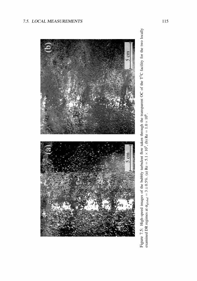
7.5. LOCAL MEASUREMENTS 115
(a)
(b)
5cm
5cm
Figu
re7.
5:H
igh-
spee
dim
ages
ofth
ebu
bbly
turb
ulen
tflo
wta
ken
thro
ugh
the
tran
spar
ent
OC
ofth
eT
3 Cfa
cilit
yfo
rth
etw
olo
cally
exam
ined
DR
regi
mes
atα g
loba
l=
3±
0.5%
.(a)
Re=
5.1×
105 ,(
b)R
e=
1.0×
106 .

116 CHAPTER 7. BUBBLE DEFORMABILITY IS CRUCIAL FOR STRONG DR
7.5.2 Results
Azimuthal liquid velocity profiles
Firstly, we study how the liquid velocity is modified by the injected bubbles in thetwo different Re-cases by comparing the single-phase case to the two-phase case.We measure the time-averaged local azimuthal velocity ⟨Uθ (r)⟩t and the standarddeviation of the local azimuthal velocity fluctuations u′θ (r). Throughout the rest ofthe paper we will work with the non-dimensional gap distance r ≡ (r− ri)/(ro − ri),with 0 indicating the IC wall and 1 indicating the OC wall. The results are displayedin Fig. 7.6 with (a) the mean velocity normalized by the IC wall velocity, which isUi = 6.28 m/s for Re = 5.1× 10⁵ and Ui = 12.6 m/s for Re = 1.0× 10⁶, and (b)the standard deviation of the normalized velocity fluctuations. The solid lines arethe single-phase cases as measured by PIV and the colored symbols are data on thetwo-phase cases obtained by LDA. LDA measurements were also performed on thesingle-phase cases and they are found to be in good agreement (within 0.6%) of thePIV data, but they are left out of the plot as PIV has superior spatial resolution.
The rescaled mean velocity profiles in Fig. 7.6a fall on top of each other in thesingle-phase flow case for both Reynolds numbers. The bubbles clearly destroy thissimilarity. Since we do not have enough spatial resolution to resolve the boundarylayers, we will focus on the bulk regime taken as 0.2< r < 0.8. The mean azimuthalvelocity profiles for both the single and two-phase cases follow roughly the sameshape in the bulk. The reduction of the bulk azimuthal velocity due to the bubbleinjection is ≈ 4% at Re = 5.1 × 10⁵ and ≈ 12% at Re = 1.0 × 10⁶. This is notunexpected as this velocity reduction should reflect the torque reduction ratio on theIC wall.
As shown in Fig. 7.6b, the standard deviation of the normalized velocity fluctu-ations are nearly identical in the single-phase flow case for both Reynolds numbers.For the bubbly flow we observe an increase in u′θ as compared to that of the single-phase flow at radial locations r . 0.3, i.e. close to the IC. For the higher Re-case thisincrement is stronger. The next step is too determine whether the local increase inthe velocity fluctuations can be linked to the spatial distribution of the bubbles.
Local bubble size
Out of the fiber probe data we compute the histogram of the bubble residence timeTbubble at each radial position. Figure 7.7 shows typical probability density functions(pdf’s) for three non-dimensional gap distances r at Re = 1.0× 10⁶. As can be ap-preciated, the mode of the pdf’s (defined here as the average of the bubble residencetime corresponding to normalized probabilities higher than 0.85) is displaced to theright the more distant the fiber tip is located from the IC. This is to be expected sincethe azimuthal flow velocity drops with increasing radius. By multiplying the mean

7.5. LOCAL MEASUREMENTS 117
0 0.2 0.4 0.6 0.8 10.3
0.35
0.4
0.45
0.5
0.55
(r − ri)/(ro − ri)
Uθ(r
)t/U
i
Re = 5.1 · 105, αglobal = 0%
Re = 1.0 · 106, αglobal = 0%
Re = 5.1 · 105, αglobal = 3%
Re = 1.0 · 106, αglobal = 3%
(a)
0 0.2 0.4 0.6 0.8 10.02
0.03
0.04
0.05
0.06
0.07
(r − ri)/(ro − ri)
uθ(r
)/U
i
Re = 5.1 · 105, αglobal = 0%
Re = 1.0 · 106, αglobal = 0%
Re = 5.1 · 105, αglobal = 3%
Re = 1.0 · 106, αglobal = 3%
(b)
Figure 7.6: The radial profiles of (a) the azimuthal liquid mean velocity normalized bythe velocity of the inner wall Ui and (b) the standard deviation of the normalized velocityfluctuations, both at middle height of the TC cell. The solid lines are obtained by PIV and thecolored symbols are obtained by LDA.
azimuthal liquid velocity of the bubbly flow from Fig. 7.6a with the pdf’s mode of thebubble residence time for each radial position, the mean (horizontal) bubble diameteras function of the gap distance ⟨Dbubble(r)⟩t is computed.
Figure 7.8a presents these calculated local mean bubble diameters and we reportan overall larger mean bubble diameter of 1.3 mm for the Re = 5.1× 10⁵ case ascompared to 0.9 mm for the Re = 1.0×10⁶ case due to the stronger shear in the latter.The size of the bubbles weakly depend on the radial position. We also use high-speedimage recordings to measure the bubble size optically at one radial position (focusingat a distance r ≈ 0.3) for each Reynolds number. Out of the high-speed imaging wereport for Re = 5.1×10⁵ an average diameter of 1.8 mm with a standard deviation of

118 CHAPTER 7. BUBBLE DEFORMABILITY IS CRUCIAL FOR STRONG DR
10−5
10−4
10−3
0
1000
2000
3000
4000
Tbubble (sec)
pro
bability
r = 0.007
r = 0.028
r = 0.338
mode
Figure 7.7: Probability density functions of the bubble residence time acquired by the opticalfiber probe for Re = 1.0×10⁶ at three non-dimensional gap distances r = (r− ri)/(ro − ri).The mode of the pdf increases with increasing r.
0 0.05 0.1 0.15 0.2 0.25 0.3 0.35
0.8
1
1.2
1.4
1.6
1.8
2
(r − ri)/(ro − ri)
〈D
bu
bble
(r)〉
t(m
m)
Re = 5.1 · 105, αglobal = 3%
Re = 1.0 · 106, αglobal = 3%
Re = 1.0 · 106, αglobal = 3%
image analysis: Re = 1.0 · 106
image analysis: Re = 5.1 · 105
0 0.1 0.2 0.340
50
60
70
(r − ri)/(ro − ri)
Dbu
bble/η
0 0.1 0.2 0.3200
300
400
(r − ri)/(ro − ri)
Dbu
bble/y
0
(a) (b)
(c)
Figure 7.8: (a) Calculated local mean bubble diameter obtained from the optical fiber signalsand the LDA velocity profiles. The diamonds with the error bars are the results from imageanalysis. (b) Mean bubble diameter expressed in the Kolmogorov length scale η and (c)expressed in the wall unit y0.

7.5. LOCAL MEASUREMENTS 119
0.6 mm, taken over 234 in-focus bubbles. For Re = 1.0× 10⁶ the average diameteris 1.2 mm with a standard deviation of 0.4 mm, taken over 144 focused bubbles.The high-speed imaging results are plotted as the diamond symbols with the verticalerror bars indicating the standard deviation. It confirms the order of magnitude ofthe estimated bubble diameter from the optical fiber signals. The imaging resultsalso show that the bubbles in the lower Re-case are less homogeneous in size as itsstandard deviation is higher than that for the higher Re-case.
We now compare in Figs. 7.8b and 7.8c the local mean bubble diameter to theKolmogorov length scale η and the wall unit y0, both calculated out of the glob-ally measured torque of the single-phase flow at the corresponding Re-numbers, seeLathrop et al. [10], Eckhardt et al. [23] for the definitions. In the radial region of0.05 < r < 0.35 the bubble diameter in the moderate DR case is around 50 η or230 y0, and in the strong DR case it is around 60 η or 300 y0, similar to what hasbeen reported by van den Berg et al. [27].
Gas concentration profiles
We calculate the time-averaged local gas volume fraction as a function of the radialposition out of the bubble mask obtained from the fiber probe data (see Sec. 7.3.1) bysumming over all bubble residence times and dividing this by the total measurementtime, i.e.
⟨α(r)⟩t =
Nbubbles
∑i=1
Tbubble,i
Ttotal, (7.3)
with Nbubbles the total number of detected bubbles. The resulting radial profiles on thegas concentration are shown as percentages in Fig. 7.9a. We stress the good quality ofrepeatability as made apparent by the two independently measured and nonethelesscollapsing profiles at Re = 1.0×10⁶.
Fig. 7.9a clearly shows that the bubbles tend to accumulate close to the IC bound-ary regime for both Reynolds numbers. This phenomena is not surprising as in cent-rifugally driven flow there is in average a favorable pressure gradient, pushing thebubbles towards the center of rotation, here with an acceleration acent(r) = U2
θ/requal to ∼ 3g for Re = 5.1×10⁵, and ∼ 9g for Re = 1.0×10⁶. For this estimate wetook the measured azimuthal liquid velocity at the center of the TC gap.
Next, we discuss the radial distance from the IC wall rαmax at which the gas con-centration is maximum, αmax ≡ max⟨α(r)⟩t. For Re = 5.1 × 10⁵ this distanceis rαmax ≈ 1.2 mm, equivalent to r ≈ 0.016. For the higher Re-case it is locatedat rαmax ≈ 0.6 mm, equivalent to r ≈ 0.008. The value of rαmax for each Reynoldsnumber is close to the respective mean bubble diameter as presented in Fig. 7.8a.However, from our measurements we cannot conclude that the rαmax we measure isthe correct radial distance at which the true maximum gas volume fraction occurs

120 CHAPTER 7. BUBBLE DEFORMABILITY IS CRUCIAL FOR STRONG DR
0 0.05 0.1 0.15 0.2 0.25 0.3 0.350
10
20
30
(r − ri)/(ro − ri)
α(r
)t
(%)
Re = 5.1 · 105, αglobal = 3%
Re = 1.0 · 106, αglobal = 3%
Re = 1.0 · 106, αglobal = 3%
(a)
0 0.05 0.1 0.15 0.2 0.25 0.3 0.350
1
2
3
4
5
6
7
(r − ri)/(ro − ri)
Fr c
en
t(r
)t
Re = 5.1 · 105, αglobal = 3%
Re = 1.0 · 106, αglobal = 3%
Re = 1.0 · 106, αglobal = 3%
(b)
Figure 7.9: Radial profiles at mid-height of the two examined DR regimes: moderate DRat Re = 5.1× 10⁵ and strong DR at Re = 1.0× 10⁶, both at a global gas volume fractionαglobal = 3±0.5%, (a) local gas concentration and (b) local centripetal Froude number.
along the gap. It could be the case that the (intrusive) fiber probe, when located verynear the IC wall, pushes the bubbles away from the tip due to an induced up-flow highpressure region and hence underestimates ⟨α(r)⟩t . Further experiments are requiredto measure this aspect in detail.
Finally, we compare the amplitude of the maximum local gas concentration forthese two Reynolds numbers. For Re = 1.0×10⁶ we find αmax ≈ 13%, whereas forRe = 5.1×10⁵ it arrives to about 30%, which is 2.3 times higher. To understand thisdifference we now evaluate the local Froude number.
If the flow were fully laminar then all the bubbles would be pushed against theIC wall due to the radial pressure gradient associated with the centrifugally drivenflow. With the addition of sufficiently strong turbulent liquid velocity fluctuations

7.5. LOCAL MEASUREMENTS 121
the bubbles will experience pressure fluctuations, leading the bubbles to be pulledaway from the wall into the bulk of the flow. We estimate the relative importanceof the pressure fluctuations’ induced acceleration acting on the bubbles apress f luct ascompared to the centripetal acceleration acent(r) by introducing a ‘centripetal Froudenumber’,
Frcent(r) =apress f luct
acent(r)=
u′2/Dbubble
U2θ/r
, (7.4)
with u′ the standard deviation of the liquid velocity fluctuations, Uθ the mean azi-muthal liquid velocity, Dbubble the bubble diameter and r the radial position to beconsidered.
For u′ we take the azimuthal liquid velocity fluctuations u′θ (r) of the two-phaseLDA data, see Fig. 7.6. Taking only the azimuthal component for u′ is sound asBurin et al. [111] and Huisman [72] report the same order of magnitude for the threecylindrical components of the liquid velocity fluctuations inside turbulent single-phase TC flow as measured by multi-component LDA. We assume that this simil-arity can also be applied to the two two-phase flow cases. For Dbubble we take thetime-averaged radial profile ⟨Dbubble(r)⟩t as shown in Fig. 7.8. Because we use thelocal time-averaged profiles of each of these quantities, we can calculate the localtime-averaged Froude number ⟨Frcent(r)⟩t which is presented in Fig. 7.9b. For bothRe-cases we find Frcent ' 1 and hence the turbulent fluctuations are strong enough topull the bubbles against the centripetal force towards the bulk region of the flow awayfrom the inner wall, which explains the spatial broadening around the gas concentra-tion maxima of Fig. 7.9a.
Now we evaluate the local Frcent-number at the radial position rαmax to understandthe different αmax for each Re-case. The closest we can get is r ≈ 0.06 for which wefind Frcent ∼ 1.5 for Re = 5.1×10⁵ and Frcent ∼ 3.5 for Re = 1.0×10⁶. The lowerRe-case has a lower Frcent-number by a factor of 2.3, indicating that the effective cent-ripetal force on the bubbles is higher and hence, the bubble accumulation is strongernear the IC wall at the expense of a lower concentration in the bulk, as observed.The Frcent-number ratio matches the maximum gas concentration ratio between bothRe-cases.
What is remarkable is the following: one would expect that the DR efficiency iscorrelated to the bubble concentration near the inner wall, and that a higher local gasvolume fraction should give a larger DR. However, the present measurements showan opposite trend: the local gas concentration near the inner wall is higher in themoderate DR regime than that in strong DR regime. This clearly suggests that thehigher local gas concentration near the inner wall does not guarantee a larger DR.What then is the dominant effect for the strong DR at the high Reynolds numbers?To answer this question we will follow van den Berg et al. [27] and now look intobubble deformability and thus the local Weber number.

122 CHAPTER 7. BUBBLE DEFORMABILITY IS CRUCIAL FOR STRONG DR
Local Weber number
Following van den Berg et al. [27], we define the bubble Weber number as
We =ρu′2Dbubble
σ, (7.5)
with u′ the standard deviation of the velocity fluctuations and σ the surface tensionof the bubble-liquid interface. Relation (7.5) is identical† to what it used in van denBerg et al. [27].
For u′ we take the azimuthal liquid velocity fluctuations u′θ (r) of the two-phaseLDA data, see Fig. 7.6b, following the same reasoning as used for the Frcent-numberestimation in section 7.5.2. For Dbubble we use the local time-averaged bubble dia-meter ⟨Dbubble(r)⟩t of the optical fiber probe data, see Fig. 7.8a. Substituting thevalues ρ = 998 kg/m3 and σ = 0.0727 N/m, corresponding to water at 21C, providesus now with the local time-averaged Weber number of the bubbles inside the TC gap,scanned over 1/3 of the radius close to the IC at middle height of the TC cell. Wepresent these ⟨We(r)⟩t profiles for the two examined DR regimes in Fig. 7.10.
The vertical error bars show the Weber number variation due to the uncertaintyin the velocity fluctuations and the bubble size at those r. For Re = 1.0× 10⁶ wesee We > 2 and that the bubbles increasingly deform when approaching the IC wall,where the liquid velocity fluctuations are stronger, finally leading to We ∼ 8 closestto the inner wall. The bubble Weber number for Re = 5.1×10⁵ remains lower and itremains nearly constant with a value around 1. This implies that the bubbles remainnearly spherical although they are larger (1.3 mm) than those for the higher Re-case(0.9 mm), because in the former the velocity fluctuations are not strong enough todeform the bubbles. At Re = 5.1× 10⁵, with nearly spherical bubbles, the globalDR is around 6% whereas the DR is about 18% for the case of Re = 1.0×10⁶ withbubbles of higher deformability. The results thus clearly demonstrate that the bubbledeformability is crucial for the observed strong DR, which is consistent with thefindings by van den Berg et al. [27] and van den Berg et al. [61], based on theirglobal torque measurements, and by Lu, Fernandez & Tryggvason [28], based ontheir numerical calculations. Here we provide a solid evidence on the crucial role ofthe bubble deformability for strong DR in bubbly turbulent TC flow.
†Few typographical errors appear in van den Berg et al. [27]: the Weber number definition liststhe radius of the bubble Rb while it should read the bubble diameter Dbubble. This concerns Eq. 4 andthe Weber number definition three lines above it. Also the abstract should read ’R = 0.5 mm’ as thevalue of the used bubble radius, and in the conclusion the statement ’Rb = 42η = 300y0’ should read’Rb = 21η = 150y0’. The rest of the values, including the right-hand side of Eq. 4, and the graphs theypresent are correct.

7.6. CONCLUSION 123
0 0.05 0.1 0.15 0.2 0.25 0.3 0.350
2
4
6
8
10
12
(r − ri)/(ro − ri)
〈W
e(r)〉
t
Re = 5.1 · 105, αglobal = 3%
Re = 1.0 · 106, αglobal = 3%
Re = 1.0 · 106, αglobal = 3%
Figure 7.10: Local Weber number profiles at of the two examined drag reduction regimes:moderate DR at Re = 5.1×10⁵ and strong DR at Re = 1.0×10⁶.
7.6 Conclusion
We have shown that the net DR, based on global dimensional torque measurementsin bubbly turbulent TC flow with pure inner rotation up to Re = 2.0×10⁶, increaseswith increasing global gas volume fraction αglobal ≤ 4% and that the efficiency ofthe DR increases for increasing Reynolds numbers. We find a net DR of remarkably40% obtained at αglobal = 4± 0.5% for Re = 2.0× 10⁶, which was not attainableby previous TC setups. The present measurements at Re = 5.1× 10⁵ and 1.0× 10⁶
show good agreement with previous measurements from van den Berg et al. [61].We observe a moderate DR for Re = 5.1× 10⁵ up to 7%, and a strong DR for Re= 1.0×10⁶ and 2.0×10⁶ up to 23% and 40%, respectively.
We chose two Re-numbers that each fall into a different DR regime and study theflow locally at fixed αglobal = 3±0.5%. The smaller one, Re = 5.1×10⁵, representsthe moderate DR regime at DR = 6% and the larger one, Re = 1.0×10⁶, representsthe strong DR regime at DR = 18%.
We investigated the azimuthal liquid velocity in the single and two-phase flow foreach Re. The amplitude of the mean azimuthal velocity in the bulk (0.2 < r < 0.8)for the bubbly flow decreases ≈ 4% at Re = 5.1× 10⁵, and ≈ 12% at Re = 1.0×10⁶ as compared to that of the single-phase case. These reduction ratios match theglobal torque reduction ratios. Furthermore, we measured increased liquid velocityfluctuations close to the IC in both two-phase cases as compared to their equivalent

124 CHAPTER 7. BUBBLE DEFORMABILITY IS CRUCIAL FOR STRONG DR
single-phase case. This increase was linked to the spatial distribution of the bubbles.The local gas concentration measurements show that the bubbles tend to accu-
mulate close to the IC boundary regime for both Re-numbers. This can be explainedby the centrifugally driven flow pushing the bubbles towards the IC wall with an ac-celeration of around 3 to 9 g. The velocity fluctuations are strong enough to pull thebubbles towards the bulk of the flow again, as expressed by the centripetal Froudenumber Frcent ' 1. The radial distance from the IC wall at which we find the max-imum local gas concentration is close to the respective bubble diameter. Surprisingly,the maximum local gas concentration at Re = 5.1×10⁵, i.e. in the moderate DR re-gime, is much higher than that at Re = 1.0×10⁶, i.e. in the strong DR regime. Whilewe find a match between the local Frcent(r) and the maximum gas concentration nearthe inner wall explaining this huge concentration difference, this finding clearly sug-gests that the higher local gas concentration near the inner wall does not guarantee alarger drag reduction.
By directly measuring the local Weber number We(r) of the bubbles, we concludethat the larger liquid velocity fluctuations deform the smaller bubbles of Dbubble ≈ 0.9mm in the strong DR regime at Re = 1.0×10⁶ since We> 2. The local Weber numberincreases with decreasing distance from the inner wall, reaching We ∼ 8 close to theinner wall. This suggests that the deformation of the bubbles is stronger near theIC wall, where a large amount of bubbles gather. In the moderate DR regime at Re= 5.1× 10⁵ the bubbles remain close to spherical because We ∼ 1 in the bulk andnear the inner boundary, even though they are larger in size with Dbubble ≈ 1.3 mm.
We conclude that increasing the gas volume fraction has a positive influence onthe azimuthal liquid velocity decrease, which is responsible for the observed dragreduction. What is really crucial for strong DR is that bubbles deform (We> 1) closeto the boundary layer regime of the IC wall, leading to a large azimuthal velocitydecrease and thus a strong DR. These local results match the conclusion on the globaltorque results as found by van den Berg et al. [27] and van den Berg et al. [61], andon the numerical results by Lu, Fernandez & Tryggvason [28].
7.7 Discussion & outlook
7.7.1 Taylor-Couette flow
Both the two-phase cases at Re = 5.1×10⁵ and Re = 1.0×10⁶ show a pronouncedincrease in the liquid azimuthal velocity fluctuations u′θ (r) close to the inner cylinderwall at r . 0.3 when compared to the corresponding single-phase cases, see Fig.7.6b. As both the Frcent- and We-number rely heavily on u′θ (r), it is important toknow the cause of this increase. The local u′θ (r) increase is clearly linked to thebubble distribution as the local gas concentration rises significantly for both Re-casesin the radial region r . 0.1, although it does not extend to r . 0.3, see Fig. 7.9a. To

7.7. DISCUSSION & OUTLOOK 125
support the increase of u′θ (r) in the region 0.1< r < 0.3 we reason that — either theinner region of high gas concentration causes turbulent bubble laden structures to beshed (incidentally as no periodicity has been found in the bubble signal time seriesat any of the examined radial locations) into the region 0.1 < r < 0.3 — or u′θ (r) asinduced from the inner region of high gas concentration is ‘diffused’ outwards into0.1 < r < 0.3. What causes the induction of higher u′θ (r) due to the presence ofbubbles in the first place, is however still not discussed.
The difficulty is that we enter a coupled problem: bubbles are drawn into a radialdistribution as dictated by Frcent(r) and at the same time the magnitude of Frcent(r)is determined by the velocity fluctuations induced by the presence of bubbles. Andlikewise the effect of bubble deformability could also influence the velocity fluctu-ations’ strength. The effect of bubble deformability can be taken out of the discussionby injecting rigid neutrally buoyant particles into the flow, instead of using bubbles,similar to what was used in experiments by van den Berg et al. [27] to investig-ate bubbly TC flow on a global level. One could also further study above problemby changing the Frcent- and We-number independently of each other. This can beachieved by changing the liquid density ρ as it enters the We-definition but not theFrcent-definition. Note that changing the surface tension σ will not results in inde-pendently changing Frcent from We as a different surface tension results in a differentmean bubble diameter, which enters both the Frcent and We definition again.
In this present work the bubble diameter is linked to the driving control parameterRe, because the shear strength of the flow dominates the bubble size. One can achievea different coupling between the Reynolds number and the bubble size by adding alow concentration of surfactant into the bubble carrier liquid. Even small concentra-tions of surfactant are known to significantly increase the effective surface tensionof the liquid/bubble interface as it results in changing the bubble surface boundarycondition from a slip to a no-slip condition, see e.g. the review article by Takagi &Matsumoto [163]. Different low concentrations of different surfactants can result ina variety of mean bubble sizes and deformability, and hence different We. Of course,the huge shear strength of our flows will still play a role. Surfactants also preventbubble coalescence and lead to a more monodisperse bubble size distribution, bothaiding the simplicity of the flow. We assume that adding small amounts of surfactantswill not change the turbulent flow properties, which should be tested experimentally.The bubble deformability and the connection to the global torque DR can be furtherstudied in bubbly turbulent TC flow.
So far we have examined bubbly turbulent TC flow by only rotating the innercylinder and keeping the outer cylinder at rest. The flow profile inside the TC gapbecomes completely different once outer cylinder rotation is activated, which is elab-orated on in chapter 4. In the co-rotation regime the flow will become less turbulentand is hence not the first choice to examine. In the case of counter-rotation the flow

126 CHAPTER 7. BUBBLE DEFORMABILITY IS CRUCIAL FOR STRONG DR
will experience more shear and a ‘neutral line’, i.e. the radial position where the meanangular velocity is zero, will exist inside the TC gap, thereby changing the overall ra-dial pressure gradient induced by the centrifugal force. This could have a pronouncedeffect on the bubble distribution, possibly allowing indirect control of the radial po-sition of maximum gas concentration rαmax from the boundary layer region towardsthe bulk region. The effect of changing the bubble distribution profile on the globaltorque should be examined further.
7.7.2 Wall-bounded flows
Other flow geometries that are widely used to study air-induced DR are channel andflat-plate flows, see the review article by Ceccio [54]. The air phase can be injectedas bubbles, like as in the current work, or an air sheet or cavity can be generatedalong the top plate of the channel, or likewise underneath the flat plate. Gravity willhence act in favor of pushing the air towards the underside of the top surface. Giventhe mean flow velocity U and appropriate length scale d — in the case of bubblyflow d can be set to the mean bubble diameter, for air sheets or air cavities d can bechosen as the maximum sheet length or cavity length, respectively — one can definea Froude number as Fr = U/
√gd, comparing the buoyancy effect to the mean flow
velocity. This Froude number definition bears great resemblance to the centripetalFroude number of two-phase TC flow, see Eq. (7.4). Whereas for channel/plate flowgeometry gravity acts in favor of pushing the air towards the underside of the (top)plate, likewise for TC flow the centripetal force pushes air towards the inner cylinderwall. Both Froude-number definitions decrease as indication of stronger favorable airaccumulation along the wall.
Now how do all the different wall-bounded flow geometries (TC flow/channelflow/flat plate flow) relate to each other in the single-phase case? When we assumefully developed turbulent single-phase flow then, of course, all these wall-boundedflows have compatible boundary layer structures. The channel and plate flows aremost conveniently described in a rectangular coordinate system, whereas centrifu-gally driven TC flow is best described in cylindrical coordinates. This is reflected inthe mathematical description of the boundary layers, and we refer to section VII ofLathrop et al. [10] for the modeling of the boundary layers in turbulent TC flow incylindrical coordinates. At constant driving strength and in combination with a con-stantly maintained fluid temperature, turbulent TC flow results in a statistically sta-tionary flow state. To be specific: No mean velocity gradient exists in the streamwise(azimuthal) direction and the boundary layer thicknesses of the inner and outer cyl-inder walls remain constant. This can be in contrast to the channel and flat-plate geo-metries where measurements could take place in developing boundary layers alongthe streamwise direction. If one would like to compare the bubbly DR results ofchannel/flat plate flows with developing boundary layers against TC flow, then one

7.8. APP. A: NON-DIMENSIONAL TORQUE REDUCTION RATIO 127
should simulate a developing boundary layer in the TC flow. This can be achievedby repeated statistically stationary TC experiments over which the driving strength,i.e. the inner and outer Reynolds number, is increased leading to different boundarylayer thicknesses. By means of post-processing these repeated experiments can thenbe integrated along the Re-axis to simulate a developing boundary layer.
7.7.3 Application towards ships
One of the complications towards practical application of bubble induced skin-frictionDR on ships is keeping the bubbles in the boundary layer regime of the hull, not onlyat the bubble injection point but also downstream of it. An alternative approach toair induced DR is the creation of air cavities underneath the flat bottom of a ship,trapping the pockets of air. Air cavities can also be created and studied in bubbly TCflow by attaching annular strips at several axial locations onto the otherwise smoothinner cylinder surface, in combination with air injection through the inner cylinderwall. As similar to what is stated in section 7.7.2: The role of gravity in the appliedship-case is now resembled by the centripetal force in TC flow, pushing air into theannular cavities. We expect to observe major slip of the inner cylinder as a decoup-ling between the wall and bulk fluid will be created by the air sheet captured in thecavities.
7.8 Appendix A: Non-dimensional torque reduction ratio
When injecting bubbles into a liquid, for small gas concentrations the effective kin-ematic viscosity and density of the two-phase fluid can be respectively approximatedas follows:
ραglobal = ρ(1−αglobal), (7.6)
ναglobal = ν(1+52
αglobal), (7.7)
where αglobal is the global gas volume fraction, and ρ and ν are the density andviscosity of the liquid at αglobal = 0. The “Einstein” equation (7.7) (Einstein [136])is a first order approximation only and assumes the dispersed phase to be non-self-interacting and to be of the same density as the carrier phase. Though the applicabilitybecomes questionable at the bubbly turbulent flows with up to 8% gas concentration,we will use (7.7) throughout this work.
To estimate the magnitude of the torque reduction, purely caused by the changeof fluid properties when injecting bubbles into the flow, we define a non-dimensional

128 CHAPTER 7. BUBBLE DEFORMABILITY IS CRUCIAL FOR STRONG DR
0 1 2 3 40.4
0.6
0.8
1.0
G(αglobal)/
G(0
)
(1−α)−1(1 +2.5α)−2
Re = 7.9 · 105 [UMD]
Re = 5.1 · 105 [T3C]
Re = 5.1 · 105 [T3C]
Re = 1.0 · 106 [T3C]
Re = 1.0 · 106 [T3C]
Re = 2.0 · 106 [T3C]
αglobal (%)
Figure 7.11: Normalized non-dimensional torque G as function of αglobal . This figure showsan alternative representation of the data in Fig. 7.4. The thick green line shows the analyticaldependence of αglobal on the density and viscosity terms of the normalized non-dimensionaltorque.
torque based on the two-phase viscosity and density as:
G(αglobal) =τ
2πραglobal ν2αglobal
Lmid=
τ2πρ(1−αglobal)ν2(1+ 5
2 αglobal)2Lmid, (7.8)
with τ as the measured torque on the middle section of the IC. We focus on the effectof bubbles on the torque and neglect the change of the Reynolds number.
The experimental results on the non-dimensional torque reduction are plotted inFig. 7.11, comparable to the dimensional torque presented in Fig. 7.4. The reasonfor the shift in the UMD data can be contributed to a different fluid temperature of24 C. The solid green curve represents the analytical dependence of αglobal on thedensity and viscosity terms of the normalized non-dimensional torque. Therefore, thedifference between the solid green curve and each of the measured curves tells us thecontribution to the DR that is not solely caused by a change of fluid properties. Thisdifference is close to zero for all curves when αglobal lies between 0 and 1%. In thecase of Re = 5.1×10⁵ the difference remains very small even up to αglobal ≈ 2.5%,but it increases significantly when αglobal > 1% for Re = 1.0× 10⁶ and 2.0× 10⁶.Hence, the bubbles in the strong DR regime must modify the flow actively in additionto simply changing the fluid properties.

7.9. APP. B: AXIAL DEPENDENCE AT RE = 1.0×10⁶ 129
7.9 Appendix B: Axial dependence at Re = 1.0×10⁶
We also investigate the axial dependence of the flow at Re = 1.0×10⁶ with αglobal =3 ± 0.5%. The outer cylinder provides three locations through which the opticalprobe can be inserted. These are located at zmid = L/2, zbot = zmid − 15 cm andztop = zmid + 15 cm, see Fig. 7.12. We will first focus on the mean azimuthal liquidvelocity profiles ⟨Uθ (r)⟩t at these locations, which are presented in Fig. 7.13.
For the single-phase case we find no axial dependence over the examined rangeas the mean velocity profiles are identical to within 0.7%. Hence we represent thesingle-phase case as the single blue solid line. When we inject bubbles into the flowwe observe a weak axial dependence on the mean azimuthal velocity, see the coloredsymbols. The relative amplitude difference in the bulk of the flow for the ztop and zbotprofiles is ±4% when compared to the zmid profile. Can this be linked to the bubbledistribution?
So next we examine the corresponding gas concentration profiles, see Fig. 7.14.We note an increase in the maximal value of the local gas concentration ⟨α(r)⟩t forincreasing height. Between ztop and zmid and between zmid and zbot there is a factor≈ 2.7 difference. These increments in gas volume fraction can be due to two factors:more bubbles or bigger bubbles.
Hence we calculate, in the same manner as described in Sec. 7.5.2, the localbubble diameter individually for each axial position, see the inset of Fig. 7.14. Noaxial dependence on the bubble size is found. When we consecutively calculate thebubble detection rate for each axial position, we indeed find a match to the maximumgas volume fractions.
The reason for this strong axial gradient on the gas volume fraction becomes ap-parent when exploring the following force balance. Let g denote the standard gravity:we find that the bubbles experience a centripetal acceleration U2
θ/r of ∼ 9g in thebulk of the flow as compared to the 1g of axial upward acceleration due to buoyancy.These factors are not well enough apart to neglect the influence of gravity on the gasdistribution.
We conclude that the local gas concentration strongly depends on the axial posi-tion, however, the liquid velocity profiles change only weakly. This suggests that theazimuthal velocity reduction is not sensitive to the local gas concentration along theaxial direction.

130 CHAPTER 7. BUBBLE DEFORMABILITY IS CRUCIAL FOR STRONG DR
ztop
zmid
zbot
15 cm
15 cm
Lm
id=
53.
6 cm
Figure 7.12: Snapshot of the T3C setup at Re= 1.0×10⁶ and αglobal = 3%. The axial meas-urement locations are tagged.
0 0.2 0.4 0.6 0.8 10.25
0.3
0.35
0.4
0.45
0.5
0.55
(r − ri)/(ro − ri)U
θ(r
)t/U
i
αglobal = 0%
αglobal = 3%, top
αglobal = 3%, mid
αglobal = 3%, bot
Figure 7.13: The radial profiles of the liquidazimuthal mean velocity normalized by the ICwall velocity Ui at different axial locations.
0 0.05 0.1 0.15 0.2 0.25 0.3 0.350
10
20
30
40
(r − ri)/(ro − ri)
α(r
)t
(%)
toptop
midmidbotbot
(r − ri)/(ro − ri)
Dbu
bble
(r)
t(m
m)
0 0.05 0.1 0.15 0.2 0.25 0.3 0.350.7
0.8
0.9
1
1.1
1.2
Figure 7.14: Local gas concentration profiles at three axial positions in the flow at Re= 1.0×10⁶ and αglobal = 3%. Inset: corresponding local mean bubble diameter. Two inde-pendent measurements are performed at each height to show the measurement repeatability.

— PART IV —
Conclusions
131


8Conclusions and Outlook
In this thesis we studied various aspects of highly turbulent Taylor-Couette (TC) flowusing a combination of experimental and theoretical techniques. In PART I we intro-duced the new turbulent TC facility of our Physics of Fluids group, called the T3Cfor short. In PART II we focused on single-phase TC flow between independentlyrotating cylinders, and in particular on the associated angular velocity transport. Andin PART III we added an extra dimension to TC flow by injecting air bubbles intoturbulent TC flow and studying the bubbles’ effects on the flow and the relation toskin-friction drag reduction. The most important conclusions for each part of thisthesis are summarized below by answering the questions that were formulated in theintroduction. When appropriate an outlook on future research is given at the end ofeach section.
8.1 Part I — Experimental setup
The Twente turbulent Taylor-Couette facility
In chapter 2 we presented in detail the features of this new TC facility and we demon-strated the accuracy of the main control and response parameters, such as rotationrate stability within 0.01% of the setpoint (Fig. 2.4), temperature control within 0.1K(Fig. 2.6) and torque sensing (Fig. 2.9). Laser Doppler anemometry (LDA) meas-urements can be successfully performed on this facility as we demonstrated perfectagreement between the solid-body rotation flow profile as measured by LDA and thetheoretically expected profile (Fig. 2.10).
133

134 CHAPTER 8. CONCLUSIONS AND OUTLOOK
8.2 Part II — Single-phase TC flow
Torque scaling in turbulent Taylor-Couette flow with co- and counter-rotatingcylinders
• Does a universal scaling law between Nuω and Ta exist, i.e. is γ constant inNuω = prefactor(a)×Taγ over the investigated range?
• If so, what is the amplitude of the prefactor as function of a?• And at what a does maximum transport of angular velocity occur?
Indeed, in the investigated high Reynolds-number regime we found a universal scal-ing of Nuω ∝ Ta0.38 when scanning the (Rei, Reo) parameter space along the diag-onals of fixed a ≡−ωo/ωi between −0.4< a< 2. It is remarkable that the effectivescaling exponent γ ≈ 0.38 exactly resembles the analogous effective scaling expo-nent in Nu ∝ Ra0.38 in RB convection in the ultimate regime of thermal convection[24, 25], reflecting the analogy between TC and RB flow also in the strongly turbulentregime. Figure 3.5 shows the amplitude of the prefactor as function of a, obtainedby averaging Nuω/Ta0.38 over the investigated Ta-range per a-case as shown in Fig.3.4b. The maximum transport occurred at aopt ≈ 0.4, indicating that slight counter-rotation improves the transport of angular velocity from the inner to the outer cylinderwall.
Optimal Taylor-Couette turbulence
By extending the angular velocity transport measurements of the previous chapterwith a higher resolution in a, we found that the experimental data are well capturedby the common power law ansatz Nuω(Ta,a) = f (a) ·Taγ , with γ = 0.39± 0.03 ascan be seen in Fig. 4.5. The a-dependence on the amplitude of the angular velo-city transport is given by f (a) = Nuω(Ta,a)/Ta0.39, as shown in Fig. 4.6, and weobserved maximum transport at aopt = 0.368.
• Does the prediction Nuω ∼ Ta1/2 × log-corrections match the observations?
Yes, as can be seen in Fig. 4.5a the prediction is practically indistinguishable from theobserved effective scaling law Nuω ∝ Ta0.39 when the log-corrections L are takenas L (Rew(Ta)) with the wind Reynolds number Rew = 0.0424× Ta1/2 as experi-mentally found by Huisman et al. [95]. This result again strengthens the analogybetween the RB and the TC system as the prediction originates from the RB systemas Nu ∝ Ra1/2 × log-corrections given by Grossmann & Lohse [26].
• Can we give an interpretation of the maximum in f (a)?• How does this maximum depend on the radius ratio η?

8.2. PART II — SINGLE-PHASE TC FLOW 135
The mutual importance of 1) the shear enhancement of the flow and 2) the stabilizingeffect on the flow, due to outer cylinder rotation is reflected in the a-dependence off (a). When starting off counter-rotation, i.e. when increasing a beyond zero, theangular velocity transport does not reduce but instead is first further enhanced, due tothe enhanced shear, before finally, beyond a = aopt = 0.368, the stabilizing effect ofthe counter-rotation leads to a reduction of the angular velocity transport Nuω .
We expect maximal transport for all points in the (Rei,Reo) parameter space,which are equally distant from both the right branch (1st quadrant of Fig. 4.3, co-rotation) of the instability border and its left branch (2nd quadrant of Fig. 4.3, counter-rotation). In inviscid approximation these two branches are the Rayleigh lines givenby the relations a = −η2 and a = ∞, respectively. The line of equal distance fromboth is the angle bisector of the instability range, which we denote by abis(η) andis given by Eq. (4.8) and plotted in Fig. 4.7b. For η = 0.716 this gives abis = 0.368which is identical to the value of aopt = 0.368 within our experimental resolution. Itneeds to be tested whether abis(η) also predicts optimal transport for all η .
• What is the connection between the transport Nuω and the mean ⟨ω(r)⟩t pro-files?
From Fig. 4.8 it is seen that the slope of ⟨ω(r)⟩t in the bulk is negative for all meas-ured cases of −0.30 ≤ a ≤ 2.00 except for a = 0.40 in which the slope equals zero.The case of a = 0.40 is, within our LDA a-resolution, the same as aopt . We notethat in strongly turbulent RB flow the temperature also has a (practically) zero meangradient in the bulk, see e.g. Ahlers et al. [19]. The rescaled mean angular velocity⟨ω(r)⟩t = (⟨ω(r)⟩t −ωo)/(ωi −ωo), plotted in Fig. 4.9a, shows a ‘phase’ transitionaround aopt for the mid-gap value ⟨ω(1/2)⟩t as shown in Fig. 4.9b: The mid-gapmean angular velocity consists of the relative contributions of the cylinder walls as≈ 0.35ωi + 0.65ωo for weak counter-rotation a < aopt and the relative contributionof the inner cylinder starts to increase for stronger counter-rotation a> aopt .
• What are the relative contributions of the convective and viscous parts of theangular velocity flux Jω per individual case of a?
For all investigated a-cases the convective contribution dominates the viscous con-tribution by far with values beyond 99%, see Fig. 4.10. At a = aopt the convectivecontribution even reaches 100% as the gradient ∂r⟨ω⟩t becomes zero. This specialsituation perfectly resembles RB turbulence for which, due to the absence of a meantemperature gradient in the bulk, the whole heat transport is conveyed by the con-vective term.
• What is the radial position of zero angular velocity, i.e. ⟨ω(r)⟩t = 0 or the socalled ‘neutral line’, in the counter-rotation cases a> 0?

136 CHAPTER 8. CONCLUSIONS AND OUTLOOK
Figure 4.11 shows the measured radial position of the neutral line rn for the examinedturbulent profiles as compared to rn corresponding to the equivalent laminar profiles.Again we see two regimes: For 0< a< aopt in the laminar case the stabilizing outercylinder rotation shifts the neutral line inwards, but due to the now (i.e. in the turbu-lent case) free boundary between the stable outer cylinder r-range and the unstablerange between the neutral line and the inner cylinder, the flow structures extend bey-ond the laminar rn. The increased shear and the strong turbulence activity originatingfrom the inner cylinder rotation are too strong and push the neutral line towards theouter kinematic boundary layer. For a > aopt the stabilizing effect from the outercylinder rotation is strong enough so that a neutral line rn can be detected in the bulkof the TC flow.
• How does the turbulent flow organization change for different a?
For the cases a> aopt , for which we observed a neutral line in the bulk of the flow, wefound a bimodal probability distribution of the instantaneous angular velocity aroundrn, as compared to the otherwise unimodal distribution of the angular velocity in thebulk for a< aopt , see Figs. 4.13 to 4.18. We interpret this intermittent behavior as anindication of turbulent bursts originating from the turbulent region in the vicinity ofthe inner cylinder and penetrating into the stabilized region near the outer cylinder.
• Does the prediction by Eckhardt, Grossmann & Lohse [23] on the boundarylayer ratio fall in line with our approximations?
The a-cases near aopt = 0.368, namely 0.2 ≤ a ≤ 1.0, showed good agreement,whereas the outlying a-cases showed some disagreement, as can be seen in Fig.4.20b. Given the crude boundary layer approximation of extrapolating the experi-mental results as depicted in Fig. 4.19, is it remarkable that we found some goodagreement.
OutlookWe point the reader to the open issues as listed on page 72.
Angular momentum transport and turbulence in laboratory models of Kep-lerian flows
The T3C and UMD TC facility were used to scan the (Re,RΩ) parameter space asshown in Fig. 5.2, with the total Reynolds number Re as given by Eq. (5.1), and RΩas the rotation number comparing shear to overall rotation (Dubrulle et al. [75]) givenby Eq. (5.2). To clarify: The (Re,RΩ) space can be projected onto (Ta,a) space, butthe former is preferred by the astrophysical community. Both facilities measuredthe torques associated to flows of constant RΩ. The cases of RΩ ≤ −1, equivalentto a ≤ −0.512 for the used T3C radius ratio of η = 0.716, indicate quasi-Keplerianflow, similar to Ji et al. [109].

8.2. PART II — SINGLE-PHASE TC FLOW 137
• Do quasi-Keplerian TC flows exhibit turbulent viscous dissipation?
Figure 5.3 shows the measured non-dimensional torque G against Re. All the ex-amined flows, including the quasi-Keplerian flow, reveal a higher torque than thetheoretical value for purely laminar flow. This is an indication that the fluid is tur-bulent and that the angular momentum transport is enhanced by turbulent viscousdissipation.
• What is the amplitude of the non-dimensional momentum transport inside theTC apparatuses, in specific for quasi-Keplerian profiles?
The non-dimensional angular momentum transport amplitude is presented in Fig. 5.4as the ratio of G over G0 ≡ G(Re,RΩ = 0). This renormalization scheme allowsfor the nice collapse of data obtained from different TC facilities of different radiusratios η . The data shows maximal transport at RΩ = −0.10. For quasi-Keplerianflows RΩ ≤ −1 the transport amplitude is still ≈ 14% of this maximum, indicatingthat angular momentum is transferred hydrodynamically.
• Does the accretion rate M deduced from the TC experiments match the ob-served accretion rates as found in astrophysical disks?
We used the procedure as outlined in section 5.3.2 to deduce the normalized accretionrate M/Mo from the global torque measurements. It was found that M/Mo = 10−3,consistent with values observed in disks around TTauri stars [108], see Table 5.2.
• Can TC flow correctly simulate the astrophysical disk flows, taking into ac-count finite-size effects?
Ideally, TC flow should be envisioned as flow in between two infinitely long cylin-ders. In practice one has a restriction on the length of the cylinders, leading to finite-size effects such as Ekman circulation. The normalized torques G/G0 as presentedin Fig. 5.4 originate from a wide variety of TC apparatuses. If the effects of Ek-man circulation on the torque were to play an important role, than one would expectsystematic discrepancies between the different data sources. As all the normalizedtorques agree quite well over the different apparatuses, we claim that our measuredtorques cannot be solely attributed to finite-size effects. Furthermore, the T3C andUMD TC facility only acquire the torque acting on the mid-section of the inner cyl-inder. The flow at mid-gap along this section has been shown to not exhibit an axialdependence on the azimuthal velocity as presented in Fig. 5.7, which otherwise couldbe taken as an indication of significant finite-size effects.
OutlookThe effects of the axial boundaries on the global torque measurements have onlybeen characterized for inner cylinder rotation and not for co- or counter-rotation.

138 CHAPTER 8. CONCLUSIONS AND OUTLOOK
Additional local velocity measurements in the co- and counter-rotating regime arehelpful in this case. Furthermore, additional independent torque measurements inthe quasi-Keplerian regime should be provided. This regime can be accessed by theT3C facility with the use of viscous oil as the employed liquid, thereby increasing thetorque towards our torque sensitivity range.
8.3 Part III — Bubbly TC flow
Bubbly turbulent drag reduction is a boundary layer effect
• Does the injection of large bubbles still lead to DR when the TC walls arestep-like roughened hence preventing a smooth turbulent boundary layer todevelop?
When injecting bubbles up to a gas volume fraction of α = 8% in TC flow at Re ≈2.5× 10⁵ we observed a DR of up 28% in the case of smooth walls, whereas forstep-like roughened walls we did not observe DR, see Fig. 6.2 for the dimensionaltorque reduction. In the rough-walls case the structure of the viscous BLs and, thus,the energy injection mechanism into the system seem to be so strongly modified thatthe mechanism for bubbly DR can no longer be active. Hence, bubbly turbulent DRis a BL effect.
Bubble deformability is crucial for strong drag reduction in turbulent Taylor-Couette flowWe observed DR when injecting bubbles with diameters ∼ 1 mm up to global gasvolume fractions of αglobal = 4% into turbulent TC flow at Re between 105 and 2×10⁶, with a remarkable maximal observed DR of 40% at αglobal = 4% for Re =2×10⁶.
• Do we observe the same DR behavior as found by van den Berg et al. [27]?• Does the trend of increasing DR with increasing Re continue in our experi-
ments?
The DR results based on the global dimensional torque under influence of bubbleinjection can be found in Fig. 7.4. Indeed, we observed the same behavior as foundby van den Berg et al. [27] on the UMD TC setup as compared to the current work onthe T3C setup. The trend of increasing DR with increasing Re was found to continuefor αglobal & 1% up to the maximum explored value of αglobal = 4%. The two caseswe used to study the local properties of the flow, i.e. Re = 5.1×10⁵ in the moderateDR regime and Re = 1.0×10⁶ in the strong DR regime, both at αglobal = 3±0.5%,resulted in a DR of 6% and 18%, respectively.

8.3. PART III — BUBBLY TC FLOW 139
• How do the bubbles in the two two-phase flow cases change the liquid azi-muthal flow profile with respect to the single-phase case?
• What is the local gas concentration profile across the TC gap for the two cases?• Does the amplitude of the gas concentration profiles match the Frcent profiles?
As shown in Fig. 7.6a the mean azimuthal velocity in the bulk of the flow at mid-height of the TC gap diminished by ≈ 4% and ≈ 12% under influence of bubbleinjection at αglobal = 3% for the cases of Re = 5.1×10⁵ and Re = 1.0×10⁶, respect-ively, when compared to their equivalent single-phase flow velocity profile. This isnot unexpected as this velocity reduction should reflect the torque reduction ratio onthe IC wall. The standard deviation on the azimuthal velocity fluctuations, presentedin Fig. 7.6b, showed significantly increased amplitudes close to the IC at r . 0.3 forboth cases. This matches the observed radial region of preferred bubble accumula-tion r . 0.1, as can be seen in Fig. 7.9a. Remarkably, the maximum gas concentrationαmax, which for both cases is roughly located within one bubble diameter from theIC wall with αmax ≈ 30% for Re = 5.1× 10⁵ and αmax ≈ 13% for Re = 1.0× 10⁶,is 2.3 times higher for the moderate DR case than for the strong DR case. We ex-plained this difference in αmax for both cases satisfactorily by introducing the localcentripetal Froude number, presented in Fig. 7.9b. Moreover, apparently: a higherlocal gas concentration near the wall does not necessarily result in stronger DR. Adifferent mechanism must hence be active.
• Do the measured local Weber number profiles match the assumption that bubbledeformability is the dominant mechanism behind strong DR in turbulent TCflow?
The local Weber number profiles can be found in Fig. 7.10. Indeed, the bubbles inthe strong DR case deformed more (We > 2, with We ∼ 8 when approaching the ICwall) than in the moderate DR regime (We ∼ 1 throughout the scanned gap) althoughthe mean reported bubble diameter is smaller in the former case (Dbubble ≈ 0.9 mm)as compared to the latter (Dbubble ≈ 1.3 mm), see Fig. 7.8. It is the liquid velocityfluctuations strength that dictates the Weber number amplitude. So, we found con-firmation to above question and we conclude that bubble deformability is crucial forstrong DR in turbulent TC flow.
OutlookAs detailed in section 7.7 it would be worthwhile to add surfactants to the bubblyflow in order to alter the mean bubble diameter and bubble deformability dependenceon the Reynolds number. Furthermore, the coupling between the velocity fluctu-ations and the preferred bubble distribution as expressed by Frcent , and the couplingbetween the velocity fluctuations and the bubble deformability We, should be ex-amined in more detail; one could study this problem by changing the density of the

140 CHAPTER 8. CONCLUSIONS AND OUTLOOK
liquid. Lastly: Air cavities could be investigated in turbulent TC flow and it couldbe compared against flat-plate/channel cavity flows. Air cavities in TC flow can beachieved by attaching annular strips around the inner cylinder at fixed axial locationsin combination with gas injection into these cavities out of the inner cylinder itself.
References
References
[1] TAYLOR, G. I., Stability of a viscous liquid contained between two rotatingcylinders. Philos. Trans. R. Soc. London, Ser. A 223, 289 (1923).
[2] DIPRIMA, R. C. & SWINNEY, H. L., Instabilities and transition in flowbetween concentric rotating cylinders. Hydrodynamic Instabilities and theTransition to Turbulence (ed. H. L. Swinney & J. P. Gollub), Springer, NewYork pp. 139–180 (1981).
[3] ANDERECK, C. D., LIU, S. S. & SWINNEY, H. L., Flow regimes in a circularCouette system with independently rotating cylinders. J. Fluid Mech. 164, 155(1986).
[4] DOMINGUEZ-LERMA, M. A., CANNELL, D. S. & AHLERS, G., EckhausBoundary and Wavenumber Selection in Rotating Couette-Taylor Flow. Phys.Rev. A 34, 4956 (1986).
[5] WENDT, F., Turbulente Stromungen zwischen zwei rotierenden konaxialenZylindern. Arch. Appl. Mech. 4, 577–595 (1933).
[6] TAYLOR, G. I., Fluid friction between rotating cylinders. Proc. R. Soc. Lon-don A 157, 546–564 (1936).
[7] SMITH, G. P. & TOWNSEND, A. A., Turbulent Couette flow between concent-ric cylinders at large Taylor numbers. J. Fluid Mech. 123, 187–217 (1982).
[8] TOWNSEND, A. A., Axisymmetric Couette flow at large Taylor numbers. J.Fluid Mech. 144, 329 (1984).
[9] TONG, P., GOLDBURG, W. I., HUANG, J. S. & WITTEN, T. A., Anisotropyin turbulent drag reduction. Phys. Rev. Lett. 65, 2780–2783 (1990).
[10] LATHROP, D. P., FINEBERG, J. & SWINNEY, H. L., Transition to shear-driven turbulence in Couette-Taylor flow. Phys. Rev. A 46, 6390–6405 (1992).
141

142 REFERENCES
[11] LATHROP, D. P., FINEBERG, J. & SWINNEY, H. L., Turbulent flow betweenconcentric rotating cylinders at large Reynolds numbers. Phys. Rev. Lett. 68,1515–1518 (1992).
[12] LATHROP, D. P., Turbulent Drag and Transport in High Reynolds numberCouette-Taylor Flow. PhD thesis, University of Texas at Austin (1992).
[13] LEWIS, G. S., Velocity fluctuations, wall shear stress and the transition intorque scaling at Re = 13000 in Turbulent Couette-Taylor flow. PhD thesis,University of Texas at Austin (1996).
[14] LEWIS, G. S. & SWINNEY, H. L., Velocity structure functions, scaling, andtransitions in high-Reynolds-number Couette-Taylor flow. Phys. Rev. E 59,5457–5467 (1999).
[15] VAN DEN BERG, T. H., DOERING, C., LOHSE, D. & LATHROP, D. P.,Smooth and rough boundaries in turbulent Taylor-Couette flow. Phys. Rev.E 68, 36307 (2003).
[16] RAVELET, F., DELFOS, R. & WESTERWEEL, J., Influence of global rotationand Reynolds number on the large-scale features of a turbulent Taylor-Couetteflow. Phys. Fluids 22, 055103 (2010).
[17] BORRERO-ECHEVERRY, D., SCHATZ, M. F. & TAGG, R., Transient turbu-lence in Taylor-Couette flow. Phys. Rev. E 81, 25301 (2010).
[18] PAOLETTI, M. S. & LATHROP, D. P., Angular momentum transport in tur-bulent flow between independently rotating cylinders. Phys. Rev. Lett. 106,024501 (2011).
[19] AHLERS, G., GROSSMANN, S. & LOHSE, D., Heat transfer and large scaledynamics in turbulent Rayleigh-Benard convection. Rev. Mod. Phys. 81, 503(2009).
[20] LOHSE, D. & XIA, K. Q., Small-scale properties of turbulent Rayleigh-Benard convection. Annu. Rev. Fluid Mech. 42, 335–364 (2010).
[21] BRADSHAW, P., The analogy between streamline curvature and buoyancy inturbulent shear flow. J. Fluid Mech. 36, 177–191 (1969).
[22] DUBRULLE, B. & HERSANT, F., Momentum transport and torque scaling inTaylor-Couette flow from an analogy with turbulent convection. Eur. Phys. J.B 26, 379–386 (2002).

REFERENCES 143
[23] ECKHARDT, B., GROSSMANN, S. & LOHSE, D., Torque scaling in turbulentTaylor-Couette flow between independently rotating cylinders. J. Fluid Mech.581, 221–250 (2007).
[24] CHAVANNE, X., CHILLA, F., CASTAING, B., HEBRAL, B., CHABAUD, B.& CHAUSSY, J., Observation of the ultimate regime in Rayleigh-Benard con-vection. Phys. Rev. Lett. 79, 3648–3651 (1997).
[25] CHAVANNE, X., CHILLA, F., CHABAUD, B., CASTAING, B. & HEBRAL,B., Turbulent Rayleigh-Benard convection in gaseous and liquid He. Phys.Fluids 13, 1300–1320 (2001).
[26] GROSSMANN, S. & LOHSE, D., Multiple scaling in the ultimate regime ofthermal convection. Phys. Fluids 23, 45108 (2011).
[27] VAN DEN BERG, T. H., LUTHER, S., LATHROP, D. P. & LOHSE, D., Dragreduction in bubbly Taylor-Couette turbulence. Phys. Rev. Lett. 94, 044501(2005).
[28] LU, J., FERNANDEZ, A. & TRYGGVASON, G., The effect of bubbles on thewall drag in a turbulent channel flow. Phys. Fluids 17, 95102 (2005).
[29] CROSS, M. C. & HOHENBERG, P. C., Pattern formation outside of equilib-rium. Rev. Mod. Phys. 65, 851 (1993).
[30] BODENSCHATZ, E., PESCH, W. & AHLERS, G., Recent developments inRayleigh-Benard convection. Annu. Rev. Fluid Mech. 32, 709–778 (2000).
[31] CASTAING, B., GUNARATNE, G., HESLOT, F., KADANOFF, L.,LIBCHABER, A., THOMAE, S., WU, X. Z., ZALESKI, S. & ZANETTI, G.,Scaling of hard thermal turbulence in Rayleigh-Benard convection. J. FluidMech. 204, 1–30 (1989).
[32] GEBHARDT, T. & GROSSMANN, S., The Taylor-Couette eigenvalue problemwith independently rotating cylinders. Z. Phys. B Condens. Matter 90, 475–490 (1993).
[33] GLAZIER, J. A., SEGAWA, T., NAERT, A. & SANO, M., Evidence againstultrahard thermal turbulence at very high Rayleigh numbers. Nature 398, 307–310 (1999).
[34] NIEMELA, J., SKRBEK, L., SREENIVASAN, K. R. & DONNELLY, R., Turbu-lent convection at very high Rayleigh numbers. Nature 404, 837–840 (2000).

144 REFERENCES
[35] BROWN, E., FUNFSCHILLING, D., NIKOLAENKO, A. & AHLERS, G., Heattransport by turbulent Rayleigh-Benard convection: Effect of finite top- andbottom conductivity. Phys. Fluids 17, 075108 (2005).
[36] SUN, C., REN, L.-Y., SONG, H. & XIA, K.-Q., Heat transport by turbu-lent Rayleigh-Benard convection in 1 m diameter cylindrical cells of widelyvarying aspect ratio. J. Fluid Mech. 542, 165–174 (2005).
[37] DU PUITS, R., RESAGK, C., TILGNER, A., BUSSE, F. H. & THESS, A.,Structure of thermal boundary layers in turbulent Rayleigh-Benard convec-tion. J. Fluid Mech. 572, 231–254 (2007).
[38] AHLERS, G., BODENSCHATZ, E., FUNFSCHILLING, D. & HOGG, J., Turbu-lent RayleighBenard convection for a Prandtl number of 0.67. J. Fluid Mech.641, 157 (2009).
[39] STEVENS, R. J. A. M., VERZICCO, R. & LOHSE, D., Radial boundary layerstructure and Nusselt number in Rayleigh-Benard convection. J. Fluid Mech.643, 495–507 (2010).
[40] See the Focus issue of New Journal of Physics on New Perspectivesin High-Rayleigh-Number Turbulent Convection (ed. J. Schumacher & E.Bodenschatz), January (2011).
[41] COLES, D., Transition in circular Couette flow. J. Fluid Mech. 21, 385–425(1965).
[42] PFISTER, G. & REHBERG, I., Space dependent order parameter in circularCouette flow transitions. Phys. Lett. 83, 19–22 (1981).
[43] MULLIN, T., CLIFFE, K. A. & PFISTER, G., Unusual time-dependent phe-nomena in Taylor-Couette flow at moderately low Reynolds-numbers. Phys.Rev. Lett. 58, 2212–2215 (1987).
[44] PFISTER, G., SCHMIDT, H., CLIFFE, K. A. & MULLIN, T., Bifurcation phe-nomena in Taylor-Couette flow in a very short annulus. J. Fluid Mech. 191,1–18 (1988).
[45] BUCHEL, P., LUECKE, M., ROTH, D. & SCHMITZ, R., Pattern selectionin the absolutely unstable regime as a nonlinear eigenvalue problem: Taylorvortices in axial flow. Phys. Rev. E 53, 4764–4777 (1996).
[46] ESSER, A. & GROSSMANN, S., Analytic expression for Taylor-Couette sta-bility boundary. Phys. Fluids 8, 1814–1819 (1996).

REFERENCES 145
[47] DONG, S., Direct numerical simulation of turbulent Taylor-Couette flow. J.Fluid Mech. 587, 373–393 (2007).
[48] DONG, S., Turbulent flow between counter-rotating concentric cylinders: adirect numerical simulation study. J. Fluid Mech. 615, 371 (2008).
[49] GROSSMANN, S. & LOHSE, D., Scaling in thermal convection: a unifyingtheory. J. Fluid. Mech. 407, 27–56 (2000).
[50] GROSSMANN, S. & LOHSE, D., Thermal convection for large Prandtl num-ber. Phys. Rev. Lett. 86, 3316–3319 (2001).
[51] GROSSMANN, S. & LOHSE, D., Prandtl and Rayleigh number dependence ofthe Reynolds number in turbulent thermal convection. Phys. Rev. E 66, 16305(2002).
[52] GROSSMANN, S. & LOHSE, D., Fluctuations in turbulent Rayleigh-Benardconvection: The role of plumes. Phys. Fluids 16, 4462–4472 (2004).
[53] BUSSE, F. H., The bounding theory of turbulence and its physical significancein the case of turbulent Couette flow. Statistical models and turbulence, theSpringer Lecture Notes in Physics 12, 103 (1972).
[54] CECCIO, S. L., Friction drag reduction of external flows with bubble and gasinjection. Annu. Rev. Fluid Mech. 42, 183 (2010).
[55] MADAVAN, N. K., DEUTSCH, S. & MERKLE, C. L., Reduction of turbulentskin friction by microbubbles. Phys. Fluids 27, 356–363 (1984).
[56] TAKAHASHI, T., KAKUGAWA, A., MAKINO, M., YANAGIHARA, T. &KODAMA, Y., A brief report on microbubble experiments using 50-m longflat plate ship. 74th General meeting of SRI (2000).
[57] KODAMA, Y., KAKUGAWA, A., NAGAYA, S. & KAWAMURA, T., Drag Re-duction of Ships by Microbubbles. Report of 24th US-Japan Joint Meeting,Marine Facilities Panel of the U.S.-Japan Cooperative Program in Natural Re-sources (2001).
[58] KODAMA, Y., KAKUGAWA, A., TAKAHASHI, T. & KAWASHIMA, H., Ex-perimental studies on microbubbles and their applicability to ships for skinfriction reduction. Int. J. Heat Fluid Flow 21, 582–588 (2000).
[59] MERKLE, C. & DEUTSCH, S., Microbubble drag reduction. Frontiers in Ex-perimental Fluid Mechanics – Lecture notes in Engineering, Vol. 46, edited byM. Gad-el-Hak, Springer, Berlin p. 291 (1989).

146 REFERENCES
[60] LATORRE, R., MILLER, A. & PHILIPS, R., Micro-Bubble Resistance Reduc-tion on a model SES catamaran. Ocean Eng. 30, 2297 (2003).
[61] VAN DEN BERG, T. H., VAN GILS, D. P. M., LATHROP, D. P. & LOHSE, D.,Bubbly turbulent drag reduction is a boundary layer effect. Phys. Rev. Lett.98, 084501 (2007).
[62] MURAI, Y., OIWA, H. & TAKEDA, Y., Frictional drag reduction in bubblyCouette-Taylor flow. Phys. Fluids 20, 034101 (2008).
[63] ISO 10816-1:1995, Part 1: General guidelines: Mechanical vibration –Evaluation of machine vibration by measurements on non-rotating parts. In-ternational Organization for Standardization, Geneva, Switzerland (1995).
[64] SUN, C., MULLIN, T., VAN WIJNGAARDEN, L. & LOHSE, D., Drag andlift forces on a counter-rotating cylinder in rotating flow. J. Fluid Mech. 664,150–173 (2010).
[65] ZENIT, R., KOCH, D. L. & SANGANI, A. S., Measurements of the averageproperties of a suspension of bubbles rising in a vertical channel. J. FluidMech. 429, 307–342 (2001).
[66] LUTHER, S., RENSEN, J., VAN DEN BERG, T. H. & LOHSE, D., Data ana-lysis for hot-film anemometry in turbulent bubbly flow. Exp. Therm. Fluid Sci.29, 821–826 (2005).
[67] VAN DEN BERG, T. H., The effect of bubbles on developed turbulence. PhDthesis, University of Twente (2006).
[68] MARTINEZ MERCADO, J., CHEHATA GOMEZ, D., VAN GILS, D. P. M.,SUN, C. & LOHSE, D., On bubble clustering and energy spectra in pseudo-turbulence. J. Fluid Mech. 650, 287–306 (2010).
[69] VAN DEN BERG, T. H., WORMGOOR, W. D., LUTHER, S. & LOHSE, D.,Phase Sensitive Constant Temperature Anemometry. Macromol. Mater. Eng.296, 230–237 (2011).
[70] GUET, S., FORTUNATI, R. V., MUDDE, R. F. & OOMS, G., Bubble velocityand size measurement with a four-point optical fiber probe. Part. Part. Syst.Charact. 20, 219–230 (2003).
[71] XUE, J., AL-DAHHAN, M., DUDUKOVIC, M. P. & MUDDE, R. F., Four-point optical probe for measurement of bubble dynamics: Validation of thetechnique. Flow Meas. and Instrum. 19, 293–300 (2008).

REFERENCES 147
[72] HUISMAN, S. G., Local velocity measurements in Twente Turbulent Taylor-Couette. Master’s thesis, University of Twente (2011).
[73] LANDAU, L. D. & LIFSHITZ, E. M., Fluid Mechanics. Oxford: PergamonPress (1987).
[74] COLES, D. & VAN ATTA, C., Measured distortion of a laminar circular Cou-ette flow by end effects. J. Fluid Mech. 25, 513 (1966).
[75] DUBRULLE, B., DAUCHOT, O., DAVIAUD, F., LONGARETTI, P.-Y.,RICHARD, D. & ZAHN, J.-P., Stability and turbulent transport in Taylor-Couette flow from analysis of experimental data. Phys. Fluids 17, 095103(2005).
[76] LOHSE, D., Particles go with the flow. Physics 1, 18 (2008).
[77] TOSCHI, F. & BODENSCHATZ, E., Lagrangian Properties of Particles in Tur-bulence. Annu. Rev. Fluid Mech. 41, 375–404 (2009).
[78] LANCE, M. & BATAILLE, J., Turbulence in the liquid phase of a uniformbubbly air-water flow. J. Fluid Mech. 222, 95–118 (1991).
[79] RENSEN, J. M., LUTHER, S. & LOHSE, D., The effect of bubbles on de-veloped turbulence. J. Fluid Mech. 538, 153–187 (2005).
[80] CALZAVARINI, E., KERSCHER, M., LOHSE, D. & TOSCHI, F., Dimension-ality and morphology of particle and bubble clusters in turbulent flow. J. FluidMech. 607, 13–24 (2008).
[81] ECKHARDT, B., GROSSMANN, S. & LOHSE, D., Scaling of global mo-mentum transport in Taylor-Couette and pipe flow. Eur. Phys. J. B 18, 541–544(2000).
[82] ECKHARDT, B., GROSSMANN, S. & LOHSE, D., Fluxes and energy dissipa-tion in thermal convection and shear flows. Europhys. Lett. 78, 24001 (2007).
[83] PIRRO, D. & QUADRIO, M., Direct numerical simulation of turbulent Taylor-Couette flow. Eur. J. Mech. B-Fluids 27, 552–566 (2008).
[84] BILSON, M. & BREMHORST, K., Direct numerical simulation of turbulentTaylor-Couette flow. J. Fluid Mech. 579, 227–270 (2007).
[85] MULLIN, T., PFISTER, G. & LORENZEN, A., New observations on hysteresiseffects in Taylor-Couette flow. Phys. Fluids 25, 1134–1136 (1982).
148 REFERENCES
[86] RICHARD, D., Instabilites Hydrodynamiques dans les Ecoulements en Rota-tion Differentielle. PhD thesis, Universite Paris VII (2001).
[87] VAN HOUT, R. & KATZ, J., Measurements of mean flow and turbulencecharacteristics in high-Reynolds number counter-rotating Taylor-Couette flow.Phys. Fluids 23, 105102 (2011).
[88] VAN GILS, D. P. M., HUISMAN, S. G., BRUGGERT, G.-W., SUN, C. &LOHSE, D., Torque scaling in turbulent Taylor-Couette flow with co- andcounterrotating cylinders. Phys. Rev. Lett. 106, 024502 (2011).
[89] HOLLERBACH, R. & FOURNIER, A., End-effects in rapidly rotating cyl-indrical Taylor-Couette flow. In MHD Couette flows: experiments and models(ed. R Rosner, G Rudiger & A Bonanno), AIP conference proceedings, vol.733, pp. 114–121. INAF; Catania Univ; Banca Roma, American Institute ofPhysics (2004).
[90] TAGG, R., The Couette-Taylor problem. Nonlinear Science Today 4, 1 (1994).
[91] GREENSPAN, H. P., The theory of rotating fluids. USA: Breukelen Press(1990).
[92] DOMINGUEZ-LERMA, M. A., AHLERS, G. & CANNELL, D. S., Marginalstability curve and linear growth rate for rotating Couette-Taylor flow andRayleigh-Benard convection. Phys. Fluids 27, 856 (1984).
[93] AHLERS, G., FUNFSCHILLING, D. & BODENSCHATZ, E., Addendum toTransitions in heat transport by turbulent convecion at Rayleigh numbers upto 10ˆ15. New J. Phys. 13, 49401 (2011).
[94] HE, X., FUNFSCHILLING, D., NOBACH, H., BODENSCHATZ, E. &AHLERS, G., Transition to the ultimate state of turbulent Rayleigh-Benardconvection. Submitted to Phys. Rev. Lett.
[95] HUISMAN, S. G., VAN GILS, D. P. M., GROSSMANN, S., SUN, C. &LOHSE, D., Ultimate Taylor-Couette turbulence. Phys. Rev. Lett. (in print),http://arxiv.org/abs/1111.0063.
[96] GROSSMANN, S., The onset of shear flow turbulence. Rev. Mod. Phys. 72,603–618 (2000).
[97] DUTCHER, C. & MULLER, S., Explicit analytic formulas for NewtonianTaylor-Couette primary instabilities. Phys. Rev. E 75, 047301 (2007).

REFERENCES 149
[98] COUGHLIN, K. & MARCUS, P. S., Turbulent bursts in Couette-Taylor flow.Phys. Rev. Lett. 77, 2214–2217 (1996).
[99] AHLERS, G., BROWN, E., FONTENELE ARAUJO, F., FUNFSCHILLING, D.,GROSSMANN, S. & LOHSE, D., Non-Oberbeck-Boussinesq effects in stronglyturbulent Rayleigh-Benard convection. J. Fluid Mech. 569, 409–445 (2006).
[100] AHLERS, G., FONTENELE ARAUJO, F., FUNFSCHILLING, D., GROSS-MANN, S. & LOHSE, D., Non-Oberbeck-Boussinesq effects in gaseousRayleigh-Benard convection. Phys. Rev. Lett. 98, 54501 (2007).
[101] SUGIYAMA, K., CALZAVARINI, E., GROSSMANN, S. & LOHSE, D., Floworganization in non-Oberbeck-Boussinesq Rayleigh-Benard convection in wa-ter. J. Fluid Mech. 637, 105–135 (2009).
[102] STEVENS, R. J. A. M., LOHSE, D. & VERZICCO, R., Prandtl and Rayleighnumber dependence of heat transport in high Rayleigh number thermal con-vection. Submitted to J. Fluid Mech. http://arxiv.org/abs/1102.2307.
[103] SHAKURA, N. I. & SUNYAEV, R. A., Black holes in binary systems. Obser-vational appearance. Astron. Astrophys. 24, 337–355 (1973).
[104] PRINGLE, J. E., Accretion discs in astrophysics. Annu. Rev. Astron. Astro-phys. 19, 137–162 (1981).
[105] DUBRULLE, B., A turbulent closure model for thin accretion disks. Astron.Astrophys. 266, 592–604 (1992).
[106] ZELDOVICH, Y. B., On the friction of fluids between rotating cylinders. R.Soc. London Proc. A 374, 299–312 (1981).
[107] RICHARD, D. & ZAHN, J. P., Turbulence in differentially rotating flows. Whatcan be learned from the Couette-Taylor experiment. Astron. Astrophys. 347,734–738 (1999).
[108] HERSANT, F., DUBRULLE, B. & HURE, J.-M., Turbulence in circumstellardisks. Astron. Astrophys. 429, 531–542 (2005).
[109] JI, H., BURIN, M., SCHARTMAN, E. & GOODMAN, J., Hydrodynamic tur-bulence cannot transport angular momentum effectively in astrophysical disks.Nature 444, 343–346 (2006).
[110] SCHARTMAN, E., JI, H. & BURIN, M. J., Development of a Couette-Taylorflow device with active minimization of secondary circulation. Rev. Sci. In-strum. 80, 024501 (2009).

150 REFERENCES
[111] BURIN, M. J., SCHARTMAN, E. & JI, H., Local measurements of turbulentangular momentum transport in circular Couette flow. Exp. Fluids 48, 763–769 (2010).
[112] VAN GILS, D. P. M., BRUGGERT, G.-W., LATHROP, D. P., SUN, C. &LOHSE, D., The Twente turbulent Taylor-Couette (T3C) facility: strongly tur-bulent (multi-phase) flow between independently rotating cylinders. Rev. Sci.Instrum. 82, 25105 (2011).
[113] SCHARTMAN, E., JI, H., BURIN, M. J. & GOODMAN, J., Stability ofquasi-Keplerian shear flow in a laboratory experiment. ArXiv e-prints (2011).http://arxiv.org/abs/1102.3725
[114] BALBUS, S. A., Fluid dynamics: A turbulent matter. Nature 470, 475–476(2011).
[115] VAN GILS, D. P. M., HUISMAN, S. G., GROSSMANN, S., SUN, C. &LOHSE, D., Optimal Taylor-Couette turbulence. Submitted to J. Fluid Mech.
[116] VIRK, P. S., Drag reduction fundamentals. AIChE J. 21, 625–656 (1975).
[117] BERMAN, N. S., Drag reduction by polymers. Annu. Rev. Fluid Dyn. 10, 47–64 (1978).
[118] BENZI, R., CHING, E. S. C., HORESH, N. & PROCACCIA, I., Theory ofconcentration dependence in drag reduction by polymers and of the maximumdrag reduction asymptote. Phys. Rev. Lett. 92, 78302 (2004).
[119] L’VOV, V. S., POMYALOV, A., PROCACCIA, I. & TIBERKEVICH, V., Dragreduction by polymers in wall bounded turbulence. Phys. Rev. Lett. 92, 244503(2004).
[120] PAL, S., DEUTSCH, S. & MERKLE, C. L., A comparison of shear-stressfluctuation statistics between microbubble modified and polymer modified tur-bulent boundary-layers. Phys. Fluids A 1, 1360–1362 (1989).
[121] XU, J., MAXEY, M. R. & KARNIADAKIS, G. E., Numerical simulation ofturbulent drag reduction using micro-bubbles. J. Fluid Mech. 468, 271–281(2002).
[122] SUGIYAMA, K., KAWAMURA, T., TAKAGI, S. & MATSUMOTO, Y., TheReynolds Number Effect on the Microbubble Drag Reduction. In Proceedingsof the 5th Symposium on Smart Control of Turbulence, pp. 31–43. Universityof Tokyo, Tokyo (2004).

REFERENCES 151
[123] MADAVAN, N. K., DEUTSCH, S. & MERKLE, C. L., Measurements of localskin frictions in a microbubble-modified turbulent boundary layer. J. FluidMech. 156, 237–256 (1985).
[124] L’VOV, V. S., POMYALOV, A., PROCACCIA, I. & TIBERKEVICH, V., Dragreduction by microbubbles in turbulent flows: the limit of minute bubbles.Phys. Rev. Lett. 94, 174502 (2005).
[125] SANDERS, W. C., WINKEL, E. S., DOWLING, D. R., PERLIN, M. & CEC-CIO, S. L., Bubble friction drag reduction in a high-Reynolds-number flat-plate turbulent boundary layer. J. Fluid Mech. 552, 353–380 (2006).
[126] DEUTSCH, S., FONTAINE, A. A., MOENY, M. J. & PETRIE, H., Combinedpolymer and microbubble drag reduction on a large flat plate. J. Fluid Mech.556, 309–327 (2006).
[127] LATORRE, R., MILLER, A. & PHILIPS, R., Micro-bubble resistance reduc-tion for high speed craft. Trans. Soc. Nav. Arch. Mar. Eng. 110, 259 (2002).
[128] FERRANTE, A. & ELGHOBASHI, S., On the physical mechanisms of dragreduction in a spatially-developing turbulent boundary layer laden with mi-crobubbles. J. Fluid Mech. 503, 345 (2004).
[129] LO, T. S., L’VOV, V. S. & PROCACCIA, I., Drag reduction by compressiblebubbles. Phys. Rev. E 73, 36308 (2006).
[130] CADOT, O., COUDER, Y., DAERR, A., DOUADY, S. & TSINOBER, A., En-ergy injection in closed turbulent flows: Stirring through boundary layersversus inertial stirring. Phys. Rev. E 56, 427–433 (1997).
[131] DEUTSCH, S., MOENY, M., FONTAINE, A. A. & PETRIE, H., Microbubbledrag reduction in rough walled turbulent boundary layers with comparisonagainst polymer drag reduction. Exp. in Fluids 37, 731–744 (2004).
[132] VLACHOGIANNIS, M. & HANRATTY, T. J., Influence of wavy structured sur-faces and polymer aggregation on drag reduction. Exp. Fluids 36, 685–700(2004).
[133] CADOT, O., BONN, D. & DOUADY, S., Turbulent drag reduction in a closedflow system: Boundary layer versus bulk effects. Phys. Fluids 10, 426 (1998).
[134] BENZI, R., ANGELIS, E. D., L’VOV, V. S., PROCACCIA, I. &TIBERKEVICH, V., Maximum drag reduction asymptotes and the cross-overto the Newtonian plug. J. Fluid Mech. 551, 185–195 (2006).

152 REFERENCES
[135] RISSO, F. & FABRE, J., Oscillations and breakup of a bubble immersed in aturbulent field. J. Fluid Mech. 372, 323–355 (1998).
[136] EINSTEIN, A., A new determination of molecular dimensions. Ann. Phys.(Leipz.) 19, 289–306 (1906).
[137] ACRIVOS, A., Bingham award lecture - 1994. Shear-induced particle diffu-sion in concentrated suspensions on noncolloidal particles. J. Rheol. 39, 813–826 (1995).
[138] LOHSE, D., Crossover from high to low Reynolds number turbulence. Phys.Rev. Lett. 73, 3223–3226 (1994).
[139] MURAI, Y., OIWA, H. & TAKEDA, Y., Bubble behavior in a vertical Taylor-Couette flow. J. Phys.: Conf. Ser. 14, 143–156 (2005).
[140] SAEKI, T., DE GUZMAN, M. R., MORISHIMA, H., USUI, H. &NISHIMURA, T., A flow visualization study of the mechanism of turbulent dragreduction by surfactants. Nihon Reoroji Gakkaishi 20, 35–40 (2000).
[141] DRAPPIER, J., DIVOUX, T., AMAROUCHENE, Y., BERTRAND, F., RODTS,S., CADOT, O., MEUNIER, J. & BONN, D., Turbulent drag reduction bysurfactants. Europhys. Lett. 74, 362 (2006).
[142] BONN, D., AMAROUCHENE, Y., WAGNER, C., DOUADY, S. & CADOT, O.,Turbulent drag reduction by polymers. J. Phys. Condens. Matter 17, S1195(2005).
[143] WHITE, C. M. & MUNGAL, M. G., Mechanics and prediction of turbulentdrag reduction with polymer additives. Annu. Rev. Fluid Mech. 40, 235–256(2008).
[144] PROCACCIA, I., LVOV, V. S. & BENZI, R., Colloquium: Theory of dragreduction by polymers in wall-bounded turbulence. Rev. Mod. Phys. 80, 225–247 (2008).
[145] KATO, H., MIURA, K., YAMAGUCHI, H. & MIYANAGA, M., Experimentalstudy on microbubble ejection method for frictional drag reduction. J. Mar.Sci. Technol. 3, 122–129 (1998).
[146] CLARK III, H. & DEUTSCH, S., Microbubble skin friction on an axisymmet-ric body under the influence of applied axial pressure gradients. Phys. FluidsA3, 2948–2954 (1991).

REFERENCES 153
[147] LATORRE, R., Ship hull drag reduction using bottom air injection. Ocean Eng.24, 161–175 (1997).
[148] SUGIYAMA, K., CALZAVARINI, E. & LOHSE, D., Microbubble drag reduc-tion in Taylor-Couette flow in the wavy vortex regime. J. Fluid Mech. 608,21–41 (2008).
[149] ELBING, B. R., WINKEL, E. S., LAY, K. A., CECCIO, S. L., DOWLING,D. R. & PERLIN, M., Bubble-induced skin-friction drag reduction and theabrupt transition to air-layer drag reduction. J. Fluid Mech. 612, 1–36 (2008).
[150] GUTIERREZ-TORRES, C. C., HASSAN, Y. A. & JIMENEZ-BERNAL, J. A.,Turbulence structure modification and drag reduction by microbubble injec-tions in a boundary layer channel flow. J. Fluids Eng. 130, 111–304 (2008).
[151] JACOB, B., OLIVIERI, A., MIOZZI, M., CAMPANA, E. F. & PIVA, R.,Drag reduction by microbubbles in a turbulent boundary layer. Phys. Fluids22, 115104 (2010).
[152] MENG, J. C. S. & UHLMAN, J. S., Microbubble formation and splitting ina turbulent boundary layer for turbulence reduction. In Proceedings of theInternational Symposium on Seawater Drag Reduction (ed. US Office of NavalResearch Arlington), pp. 341–355. Newport, Rhode Island (1998).
[153] MERKLE, C. L. & DEUTSCH, S., Microbubble drag reduction in liquid tur-bulent boundary layers. Appl. Mech. Rev. 45, 103–127 (1992).
[154] MORIGUCHI, Y. & KATO, H., Influence of microbubble diameter and distri-bution on frictional resistance reduction. J. Mar. Sci. Technol. 7, 79–85 (2002).
[155] SHEN, X., CECCIO, S. & PERLIN, M., Influence of bubble size on micro-bubble drag reduction. Exp. Fluids 41, 415–424 (2006).
[156] DJERIDI, H., GABILLET, C. & BILLARD, J. Y., Two-phase Couette-Taylorflow: Arrangement of the dispersed phase and effects on the flow structures.Phys. Fluids 16, 128–139 (2004).
[157] MUDDE, R. F. & SAITO, T., Hydrodynamical similarities between bubblecolumn and bubbly pipe flow. J. Fluid Mech. 437, 203–228 (2001).
[158] XUE, J., AL-DAHHAN, M., DUDOKOVIC, M. P. & MUDDE, R. F., Bubbledynamics measurements using four-point optical probe. Can. J. Chem. Eng.81, 375–381 (2003).

154 REFERENCES
[159] LUTHER, S., RENSEN, J. M. & GUET, S., Bubble aspect ratio and velocitymeasurement using a four-point fiber-optical probe. Exp. Fluids 36, 326–333(2004).
[160] WU, C., SUDDARD, K. & AL-DAHHAN, M. H., Bubble dynamics investiga-tion in a slurry bubble column. AIChE Journal 54, 1203–1212 (2008).
[161] CARTELLIER, A. & ACHARD, J. L., Local phase detection probes influid/fluid two-phase flows. Rev. Sci. Instrum. 62, 279–303 (1991).
[162] JULIA, J. E., HARTEVELD, W. K., MUDDE, R. F. & DEN AKKER, H. E.A. V., On the accuracy of the void fraction measurements using optical probesin bubbly flows. Rev. Sci. Instrum. 76, 35103 (2005).
[163] TAKAGI, S. & MATSUMOTO, Y., Surfactant effects on bubble motion andbubbly flows. Annu. Rev. Fluid Mech. 43, 615–636 (2011).

Summary
Science is served by experiments over which one has full control of the system anddriving parameters and which allow for unambiguous observations of the responseparameters. For the field of fluid mechanics the Taylor-Couette (TC) flow geometryfacilitates the design of such well controlled experiments. TC flow in essence is de-scribed by a fluid confined between two concentric cylinders and thereby set intomotion by the rotation of the inner and/or outer cylinder. Under the proper experi-mental conditions, this closed flow geometry ensures a beautiful relation between thelarge-scale power input into the flow and the small-scale fluid’s energy dissipationrate manifesting itself as a torque on the cylinder walls.
The research issues addressed in this mostly experimental thesis, concern highlyturbulent TC flow (Re > 105 ⇔ Ta > 1011) — at a fundamental level to aid ourunderstanding of (TC) turbulence and to interpret towards astrophysical disks — andat a practical level as applications can be found in skin-friction drag reduction towardsships. In PART I we introduce the new TC facility of our Physics of Fluids group,called the Twente turbulent Taylor-Couette (T3C) facility. In PART II we focus onhighly turbulent single-phase TC flow; we use the scaling of the torque as thread andwe provide local angular velocity measurements. In PART III we study the effect ofbubbles on highly turbulent TC flow, focusing not only on the global drag reduction,but also on the local bubble distribution and angular velocity profiles.
In chapter 2 of PART I we present the T3C facility in great detail. It features interalia two independently rotating cylinders capable of rotation rates of 10’s of revolu-tions per second, precise temperature and rotation rate control, torque sensors, bubbleinjection and gas volume fraction control, and it features transparent outer cylindersof different radii providing full optical access to the internal flow. We demonstratethe system’s accuracy and we provide benchmarks on initial torque measurementsand local angular velocity profiles as measured by laser Doppler anemometry.
In chapter 3 of PART II we measure the global torque to investigate the dimen-sionless transport flux of the angular velocity as function of the driving control para-meters. We show that the driving parameters are ideally expressed by the Taylornumber and the ratio of the outer cylinder angular velocity to the inner cylinder an-gular velocity, hence revealing universal scaling of power 0.38 for constant drivingratios. The observed effective scaling exponent is an indication that the TC gap is
155

156 SUMMARY
completely occupied by two fully turbulent kinematic boundary layers and a turbu-lent bulk, analogous to scaling as observed in kinematically fully turbulent Rayleigh-Benard convection cells. We find maximum transport for slight counter-rotation,namely when the outer cylinder counter-rotates at ≈ 0.4 times the angular velocity ofthe inner cylinder. This value is determined for the current radius ratio at the exploredhigh Taylor number regime.
In chapter 4 of PART II we go in detail into the flow examined in the previouschapter, extending it with local angular velocity information and increasing our res-olution in the driving ratios. We find optimum angular velocity transport at slightcounter-rotation, now at the more precise driving ratio of 0.368. This ratio coincideswith the bisector of the (Rei,Reo)-instability range. Apparently, there is a competitionbetween the effects on the flow induced by outer cylinder counter-rotation: Shear en-hancement and thus turbulence amplification at slight counter-rotation, and flow sta-bilization and thus turbulence degeneration for stronger counter-rotation. We provideradial profiles on the angular velocity by laser Doppler anemometry. We find that theflow at optimal transport is characterized by zero slope of the angular velocity asso-ciated with fully convective transport. We also focus on the neutral line, defined asthe radial position of zero angular velocity, and we find that only for strong counter-rotation, i.e. rotating the outer cylinder faster than the maximum transport case, theneutral line is shifted out of the outer cylinder boundary layer towards the inner cylin-der. The flow around the neutral line in the bulk is characterized by bi-modal velocitydistributions, interpreted as turbulent burst arising from the unstable inner cylinder re-gion and crossing the neutral line into the stable outer cylinder region, opposite to theotherwise mono-modal velocity distributions.
In chapter 5 of PART II the main topic is whether the accretion of matter inastrophysical disks can be attributed to turbulent viscous dissipation; a highly debatedissue. We study the Keplerian profiles associated to these disks with the use of TCapparatuses, and we measure the angular momentum transport based on global torquemeasurements. We argue that these quasi-Keplerian profiles can reflect the physicsfound in astrophysical disks, taking into account finite size effects of experimentalTC flow. We measure enhanced angular momentum transport above the theoreticallyexpected laminar transport. Hence, we conclude that quasi-Keplerian profiles exhibitturbulent viscous dissipation. The momentum transport can be transformed into anaccretion rate, which is found to be in line with accretion rates as found for disksaround TTauri stars [108].
In chapter 6 of PART III we measure the drag on the inner cylinder wall whilebubbles of 1 mm in diameter are injected into turbulent TC flow. We find drag re-duction (DR) due to bubble injection in the case of smooth cylinder walls, whereasfor step-like roughened cylinder walls we find no DR. As in the rough-wall case nosmooth boundary layers can develop, the results demonstrate that bubbly DR is a
157
pure boundary layer effect.Finally, in chapter 7 of PART III, we study DR in highly turbulent TC flow un-
der influence of bubble injection of 1 mm in diameter, focussing on global and localparameters. The global DR, based on the measured torque, reaches up to 40% wheninjecting bubbles up to just 4% gas volume fraction. Two different regimes are appar-ent in the global DR results: One regime with moderate DR and the other regime withstrong DR. This was already observed in global experiments by van den Berg et al.[27] who attributed the crossover into the strong DR regime to the bubble deformab-ility mechanism becoming significantly active, in line with the numerical simulationsby Lu, Fernandez & Tryggvason [28]. Here we provide local results on the angu-lar velocity modifications and bubble distribution profiles inside the TC gap for thetwo different regimes. We find that the bubbles are highly concentrated in the innercylinder boundary regime for both DR regimes. We confirm that the bubbles in themoderate DR regime stay nearly spherical and that they deform in the strong DR re-gime. We end the chapter with a discussion on how these findings can be projectedonto other wall-bounded flows.


Samenvatting
Wetenschap heeft baat bij experimenten, waarbij men volledige controle heeft overde systeem- en aansturingsparameters en waarbij men de reactieparameters eenduidigkan observeren. In het vakgebied van de stromingsleer wordt het ontwerp van der-gelijke gecontroleerde experimenten, vergemakkelijkt door de geometrie van Taylor-Couette (TC) stroming. TC stroming kan in essentie omschreven worden als eenvloeistof opgesloten tussen twee concentrische cylinders en daarmee in gang ge-bracht door de binnenste en/of buitenste cilinder te roteren. Onder de juiste experi-mentele omstandigheden zorgt deze gesloten stroming voor een elegante relatie tus-sen het grootschalige toegevoerde vermogen en het kleinschalige vloeistofdissipatief-vermogen, dat zich manifesteert als een koppel op de cilinderwanden.
De vraagstellingen in dit, voornamelijk experimenteel, proefschrift hebben be-trekking op hoog turbulente TC stroming (Re > 105 ⇔ Ta > 1011) — op een fun-damenteel niveau om ons begrip van (TC) turbulentie te ondersteunen en om het toete passen op astrofysische schijven — en op een praktisch niveau aangezien toepas-singen denkbaar zijn ter vermindering van de huidwrijvingsweerstand van schepen.In DEEL I introduceren we de nieuwe TC faciliteit van onze Physics of Fluids on-derzoeksgroep, genaamd de Twente turbulente Taylor-Couette (T3C) faciliteit. InDEEL II richten we ons op hoog turbulente enkelfasige TC stroming; de schaling vanhet koppel dient als rode draad en we presenteren lokale hoeksnelheidsmetingen. InDEEL III bestuderen we het effect van luchtbellen geınjecteerd in hoog turbulente TCstroming, waarbij we ons niet enkel richten op de globale weerstandsvermindering,maar ook op de lokale bellenconcentratie- en hoeksnelheidsprofielen.
In hoofdstuk 2 van DEEL I detaileren we de T3C faciliteit. Het beschikt, on-der meer, over twee onafhankelijk van elkaar draaiende cilinders waarvan de rotatie-snelheden tientallen omwentelingen per seconde bereiken, exacte temperatuurs- enrotatiesnelheidscontrole, koppelsensoren, belleninjectie en gas-volume-fractie con-trole, en het beschikt over transparante buitencilinders van verschillende radii, waar-mee men optische toegangelijkheid verkrijgt tot het inwendige van de stroming. Wedemonstreren de nauwkeurigheid van het systeem en we presenteren ijkpunten vande eerste koppelmetingen en lokale hoeksnelheidsprofielen, verkregen door laser-Doppler-snelheidsmetingen.
In hoofdstuk 3 van DEEL II meten we het globale koppel om de dimensieloze
159
160 SAMENVATTING
transport flux van de hoeksnelheid te onderzoeken als functie van de aansturings-parameters. We laten zien dat de aansturingsparameters idealiter uitgedrukt wordendoor het Taylor-getal en de verhouding van de buitenste cilinder hoeksnelheid opde binnenste cilinder hoeksnelheid, en zodoende een universele schaling onthullenvan de macht 0.38, zolang een constante hoeksnelheidsverhouding wordt gebruikt.De waargenomen effectieve schalingsexponent is een aanwijzing dat de TC spleetvolledig bezet wordt door twee volledig turbulente kinematische grenslagen en eenturbulente bulk, analoog aan de schaling zoals waargenomen in kinematisch volledigturbulente Rayleigh-Benard convectiecellen. We vinden maximaal transport van dehoeksnelheid voor lichte contra-rotatie, namelijk wanneer de buitenste cilinder ca.0.4 keer de hoeksnelheid van de binnenste cilinder heeft. Deze waarde is verkregenvoor de huidige radius-ratio bij het verkende hoge Taylor-getal regime.
In hoofdstuk 4 van DEEL II gaan we gedetaileerd in op de stroming zoals on-derzocht in het vorige hoofdstuk, door het uit te breiden met lokale hoeksnelheids-informatie en door de resolutie in de hoeksnelheidsverhoudingen te vergroten. Wevinden een optimaal transport van de hoeksnelheid voor lichte contra-rotatie, nu bijde meer nauwkeurige verhouding van 0.368. Deze verhouding komt overeen metde bissectrice van de (Rei,Reo)-instabiliteitsruimte. Blijkbaar is er een concurren-tie tussen de effecten op de stroming veroorzaakt door buitencilinder contra-rotatie:versterking van de afschuifspanning en dus een toename van turbulentie bij lichtecontra-rotatie, en stabilisering van de stroming en dus afname van turbulentie bij ster-kere contra-rotatie. We tonen radiale profielen van de hoeksnelheid verkregen doorlaser-Doppler-snelheidsmetingen. We vinden dat de stroming bij optimaal transportwordt gekenmerkt door een vlakke helling van het hoeksnelheidsprofiel, typerendvoor volledig convectief transport. We richten ons ook op de neutrale lijn, gedefini-eerd als de radiale positie van hoeksnelheid nul, en we vinden dat alleen voor sterkecontra-rotatie, d.w.z. wanneer de buitencilinder harder draait dan de verhouding diegeldt voor maximaal transport, de neutrale lijn uit de buitencilinder grenslaag komten verschuift richting de binnencilinder. De stroming rond de neutrale lijn wordtgekenmerkt door bi-modale snelheidsdistributies, geınterpreteerd als turbulente uit-barstingen die vanuit de onstabiele binnencilinder regio de neutrale lijn overstekennaar de stabiele buitencilinder regio, in tegenstelling tot de anders mono-modale snel-heidsdistributies.
In hoofdstuk 5 van DEEL II stellen we de hoofdvraag of de accretie van materiein astrofysische schijven, toegeschreven kan worden aan turbulent visceuze dissipa-tie; een zeer controversieel onderwerp. We bestuderen de Kepleriaanse profielen dietoebehoren aan deze schijven door gebruik te maken van TC apparaten, en we metenhet hoekmomenttransport aan de hand van globale koppelmetingen. We stellen datdeze quasi-Kepleriaanse profielen de fysica nabootsen, zoals aangetroffen kan wor-den in astrofysische schijven, en we nemen hierbij het effect van de eindige grootte

161
van experimentele TC stroming in ogenschouw. We meten een verhoogd hoekmo-menttransport ten opzichte van het theoretisch verwachte laminair transport. Hieruitconcluderen we dat quasi-Kepleriaanse profielen turbulente visceuze dissipatie ver-tonen. Het hoekmomenttransport kan omgezet worden in een accretiesterkte die inovereenstemming is met de aangetroffen accretiesterktes in TTauri sterren [108].
In hoofdstuk 6 van DEEL III meten we de stromingsweerstand op de binnen-cilinder, terwijl belletjes van 1 mm in diameter geınjecteerd worden in turbulente TCstroming. We vinden vermindering van de weerstand, ten gevolge van belleninjectie,in het geval van gladde cilinderwanden, terwijl we voor stapachtig geruwde cilinder-wanden geen vermindering vinden. Omdat er zich geen glad-verlopende grenslagenkunnen ontwikkelen in het geval van geruwde wanden, tonen de resultaten dat weer-standvermindering onder invloed van belleninjectie een grenslaag-effect is.
Tenslotte bestuderen we in hoofdstuk 7 van DEEL III de weerstandsverminde-ring in hoog turbulente TC stroming onder invloed van belleninjectie van 1 mm indiameter, gericht op globale en lokale parameters. De globale weerstandsverminde-ring, gebaseerd op het gemeten koppel, reikt tot wel 40% bij slechts een gas-volume-fractie van 4%. Twee verschillende regimes zijn duidelijk zichtbaar in de globaleweerstandsvermindering: het ene regime met een gematigde weerstandverminderingen het andere regime met een forse weerstandsvermindering. Dit werd al waargeno-men in de globale experimenten door van den Berg et al. [27], die de transitie naar hetforse weerstandsvermindering-regime toeschreven aan het significant actief wordenvan het bellenvervormbaardheids-effect, in lijn met de numerieke simulaties van Lu,Fernandez & Tryggvason [28]. We presenteren hier nu lokale resultaten aangaandede hoeksnelheidswijzigingen en bellendistributieprofielen in de TC spleet voor detwee verschillende regimes. We vinden dat de bellen zich, voor beide regimes, sterkconcentreren in het binnencilinder gebied. We bevestigen dat de bellen in het gema-tigde weerstandsvermindering-regime nagenoeg bolvormig blijven, maar dat ze ver-vormen in het forse weerstandsvermindering-regime. Het hoofdstuk sluit af met eendiscussie over het toepassen van de gevonden resultaten op andere wand-begrensdestromingen.


Scientific output
PUBLICATIONS IN PEER-REVIEWED JOURNALS
1. T.H. VAN DEN BERG, D.P.M. VAN GILS, D.P. LATHROP & D. LOHSE,Bubbly turbulent drag reduction is a boundary layer effect,Phys. Rev. Lett. 98, 084501 (2007).See chapter 6 of this thesis.
• Highlighted by “Bubbels zinloos bij ruwe scheepsromp”, De Volkskrant,February 2nd 2007.http://www.volkskrant.nl/vk/nl/2672/Wetenschap-Gezondheid/article/detail/838869/2007/02/21/Bubbels-zinloos-bij-ruwe-scheepsromp.dhtml
2. J. MARTINEZ MERCADO, D. CHEHATA GOMEZ, D.P.M. VAN GILS, C. SUN
& D. LOHSE,On bubble clustering and energy spectra in pseudo-turbulence,J. Fluid Mech. 650, 287–306 (2010).
3. D.P.M. VAN GILS, G.-W. BRUGGERT, D.P. LATHROP, C. SUN & D. LOHSE,The Twente turbulent Taylor-Couette (T3C) facility: strongly turbulent (multi-phase) flow between independently rotating cylinders,Rev. Sci. Instrum. 82, 025105 (2011).See chapter 2 of this thesis.
4. D.P.M. VAN GILS, S.G. HUISMAN, G.-W. BRUGGERT, C. SUN & D. LOHSE,Torque scaling in turbulent Taylor-Couette flow with co- and counterrotatingcylinders,Phys. Rev. Lett. 106, 024502 (2011).See chapter 3 of this thesis.
• Selected as an “Editor’s suggestion”.• Highlighted by “Exploring the extremes of turbulence”, A.G. Smart,
Physics Today 64, 18–20 (2011).• Highlighted by “Fluid Dynamics: A turbulent Matter”, Steven A. Balbus,
Nature 470, 475–476 (2011).
163

164 SCIENTIFIC OUTPUT
• Highlighted by “Heat and twist of turbulent flows”, D. van Heijnsbergen,Physics: Spotlighting Exceptional Research.http://physics.aps.org/synopsis-for/10.1103/PhysRevLett.106.024502
5. D.P.M. VAN GILS, S.G. HUISMAN, S. GROSSMANN, C. SUN & D. LOHSE,Optimal Taylor-Couette turbulence,submitted to J. Fluid Mech.See chapter 4 of this thesis.
6. S. PAOLETTI, D.P.M. VAN GILS, B. DUBRULLE, C. SUN, D. LOHSE & D.P.LATHROP,Angular momentum transport and turbulence in laboratory models of Kep-lerian flows,submitted to Astron. Astrophys.See chapter 5 of this thesis.
7. D.P.M. VAN GILS, D. NAREZO GUZMAN, C. SUN & D. LOHSE,Bubble deformability is crucial for strong drag reduction in turbulent TC flow,submitted to J. Fluid Mech.See chapter 7 of this thesis.
8. S.G. HUISMAN, D.P.M. VAN GILS & C. SUN,Applying Laser Doppler Anemometry inside a Taylor-Couette geometry — Us-ing a ray-tracer to correct for curvature effects,submitted to EJM-B/Fluids.
9. S.G. HUISMAN, D.P.M. VAN GILS, S. GROSSMANN, C. SUN & D. LOHSE,Ultimate Taylor-Couette turbulence.Phys. Rev. Lett. (in print), http://arxiv.org/abs/1111.0063.
CONTRIBUTED TALKS
1. 61st Annual DFD Meeting, San Antonio, Texas (USA), Bubbly turbulent dragreduction is a boundary layer effect, November 23–25, 2008.
2. 1st Fermat-Impact Meeting, L’Institut de Mecanique des Fluides de Toulouse,Toulouse (France), Bubbly drag reduction in turbulent Taylor-Couette flow,December 17–19, 2008.
3. 62nd Annual DFD Meeting, Minneapolis, Minnesota (USA), Twente turbulentTaylor-Couette, November 22–24, 2009.
4. 63rd Annual DFD Meeting, Long Beach, Florida (USA), Torque scaling in tur-bulent Taylor-Couette flow with co- and counterrotating cylinders, November21–23, 2010.

165
5. J.M. Burgersdag, Delft University of Technology, Delft (The Netherlands),Torque scaling in turbulent Taylor-Couette flow with co- and counterrotatingcylinders, January 1, 2011.
6. Mini-symposium on bubbly flow in Twente, University of Twente, Enschede(The Netherlands), Bubble deformability is crucial for strong drag reductionin bubbly turbulent Taylor-Couette flow, July 15, 2011.
7. 17th International Couette-Taylor Workshop, University of Leeds, Leeds (UK),Drag reduction, bubble distribution and velocity profiles in bubbly turbulentTaylor-Couette flow, July 25–27, 2011.Awarded the best student presentation price
8. 13th European Turbulence Conference, University of Warsaw, Warsaw (Po-land), Drag reduction, bubble distribution and velocity profiles in bubbly tur-bulent Taylor-Couette flow, September 12–15, 2011.
STUDENT MENTORING
1. Sander G. Huisman, Local velocity measurements in Twente turbulent Taylor-Couette, Master Thesis, November 8, 2010.
2. Daniela Narezo Guzman, Bubble deformability is crucial for strong drag re-duction in bubbly turbulent Taylor-Couette flow, Master Thesis, May 11, 2011.
3. Erik Dietrich, Beer flow dynamics, external Master Thesis at Heineken, Octo-ber 31, 2011.
4. Tim J.G. Jannink, Optimal Taylor-Couette turbulence at different radius ratios,Master Thesis, ongoing.
TEACHING EXPERIENCE
1. Teaching assistant for the 2nd year Bachelor course “Physics of Fluids Prac-tical” of the study Applied Physics in Twente, 2009–2010.
2. Teaching assistant for the 1st year Bachelor’s final project “P-project” of thestudy Applied Physics in Twente, 2010.


Acknowledgements
The research described in this thesis was primarily carried out at the Physics of Fluidsgroup of the Faculty of Science and Technology of the University of Twente. Thisresearch is supported by the Dutch Technology Foundation STW, which is part of theNetherlands Organisation for Scientific Research (NWO) and partly funded by theMinistry of Economic Affairs, Agriculture and Innovation (project number 07781). Igratefully acknowledge their support.
∼ · ∼ · ∼ · ∼ · ∼ · ∼ · ∼ · ∼ · ∼ · ∼ · ∼ · ∼
Science heavily leans on the continuation of previous research and on the cooperationbetween fellow scientists, and is therefore never a single man’s or woman’s feat.Many people contributed to the work in this thesis and I express my gratitude towardseveryone that supported it. Some people I would like to thank in particular.
∼ · ∼ · ∼ · ∼ · ∼ · ∼ · ∼ · ∼ · ∼ · ∼ · ∼ · ∼
First of all, I thank my promotor prof. Detlef Lohse for the opportunities he offeredme. He gave me the freedom to explore the engineering side of building up a newTC facility, additional to experimental research. Thanks for your great job in leadinga successful group of which I am proud to have been part of. I greatly value thescientific discussions we had, providing me each time with physical interpretationsbehind new data. Making presentations is a skill I learned from you. My thanks alsogo to my daily supervisor and assistant-promotor dr. Chao Sun. Your enthusiasm andenergy are always uplifting and your guidance is pleasant and good. I will rememberthe great dinners at your place (your wife makes the best dumplings). Thanks, Detlefand Chao, for teaching me how to do science.
Much insight and physical interpretation to this work were also provided by theprofessors Siegfried Grossmann, Guenter Ahlers, Bruno Eckhardt and Gerd Pfister.I thank them sincerely for their valuable input. My gratitude also goes towards theprofessors Leen van Wijngaarden, Roberto Verzicco, Theo van der Meer, Tom vanTerwisga and Jerry Westerweel for taking place in my PhD committee.
In light of the STW programme on ship-drag reduction by air lubrication, I thankall the project members for their effort and their helpful discussions and feedback:From the Delft University prof. Tom van Terwisga (always kindly leading the pro-gramme), dr. Rene Delfos, prof. Jerry Westerweel, ir. Oleksandr Zverkhovskyi and ir.
167

168 ACKNOWLEDGEMENTS
Marc Harleman, from MARIN dr. Evert-Jan Foeth, from DST in Duisburg dr. Cor-nell Thill, from Bluewater dr. Clemens van der Nat, from STW dr. Corine Meulemanand from Spaarnwater Eelco van Rietbergen who also participated in the very firstT3C measurements and whose help was appreciated on the torque calibration andbalancing.
I also owe a debt of gratitude towards prof. Dan Lathrop of the University ofMaryland (UMD). It was in his group that I got my first taste of experimental TCflow by letting me perform my internship on the UMD TC facility. Also the designof the T3C facility started on the fundamental design plans of the UMD TC facility.Without prof. Lathrop, dr. Matthew Paoletti from UMD and prof. Berengere Dubrullefrom the French CNRS center, this thesis would lack chapter 5. I am thankful to themfor letting me incorporate our joint-publication as part of my thesis.
Another one who should not go unmentioned is dr. Ramon van den Berg, formerPhD candidate of our Physics of Fluids group and now working for Heineken. Hesupervised me during my internship and partly during my masters. I had a great timetogether with him in Maryland and he kindly helped me a lot with all the foreignhousing and visa paperwork. I thank him for his work on the publication as featuredin chapter 6. He was the first PhD student to help draw up the T3C device and tocalculate its design parameters.
The T3C facility could not have been realized without the technical expertiseof the following people. Our group’s technician Gert-Wim Bruggert deserves muchcredit for the overall design. His well-thought-out and detailed 3D-design plans havemade the T3C setup easy to work with and a charm to diss- and reassemble. Youcan only guess at the wonderful support tools that are invented by this man to aidin adjusting the TC setup to meet specific needs. There is also TCO to thank, thetechnical service group of the University of Twente. In specific: Sip Jan Boorsmafor mechanical design, Geert Mentink for electrical design, Rindert Nauta for systemautomation, and Henk Waayer for electrical installation. This service group is a valu-able asset to the university as they provide a clear link between scientific demandsand technological realizations. Sandra Bekman and Jan Schepers are acknowledgedfor their support during machining and initial assembly at VDL-ETG in Almelo. Forthe background and technical support on the optical fiber probe technique, I thankprof. Rob Mudde and technician Jaap van Raamt of Delft University.
Three other invaluable cornerstones of our group also deserve my gratitude. Ournice secretary Joanita without whom many paperwork would go amiss, technicianMartin Bos for his always fast service with a smile, and our administrator BasBenschop for maintaining the computer park and having always nice stories to share.
I now come to the colleagues in our group. The daily T3C team consists of severalpeople with whom I shared a good time. Besides Chao Sun, I thank Sander Huisman,who started as master student under my supervision in the lab and who has been my

169
roommate for the last year, for his sharp mind, master student Tim Jannink for hishard work on TC measurements, and once visiting PhD student Agathe Chouippefor her high-speed imaging of bubbly flows. I also owe thanks to my other (former)roommates, for warning me not to become deaf by the volume of my earphones andfor their pleasant company: Richard Stevens, Rodolfo Ostilla Monico, Julian Mar-tinez Mercado and Marine Guemas. I shared a great time with all the people in thegroup, simply too many to list. Thanks for creating a nice and inspiring atmosphere.In particular I thank Ivo Peters for helping me with organizing the children’s exper-iments day, Sander Huisman, Koen Winkels and Vivek Nagendra Prakash for theirsupport during open-house-day demonstrations, and Hanneke Gelderblom for kindlysucceeding me as Burgerscentrum group representative and also for helping me outduring open house days.
A special place is reserved for Daniela Narezo Guzman. As my former masterstudent, she did all of the local bubble-profile measurements of chapter 7 with relent-less effort. She made my days in the lab shine when working together, and this wasmutual. It was therefore unavoidable that our paths in life existed next to each other.I am looking forward to visiting you in Santa Barbara or Mexico and I wish you allthe luck and happiness from the bottom of my heart. Espero que nuestros caminos secrucen otra vez.
I would not have come so far without my loving parents and close family. Iwill address them in Dutch. Pa en ma, bedankt voor jullie onvoorwaardelijke liefdeen steun. Ik denk graag dat mijn affiniteit voor mechanica en sleutelen te dankenis aan jou, pa, en de werkplaats, waar ik als kleine jongen altijd graag naar deautoschadegevallen keek en waar je me veel technieken hebt geleerd. Ik bedank ookm’n zus en haar man, waar ik altijd welkom ben. Sandra en Rene; het geeft me veelvreugde om oom te zijn van twee sterke jongens.
Dennis van GilsNovember 10th, 2011


About the author
Dennis Paulus Maria van Gils was born on May 2nd in Noord-Brabant, the Nether-lands, where he lived in a village called Steenbergen. Dennis graduated from highschool “Het Mollerlyceum” in Bergen op Zoom in 1999, where he also earned hisB-diploma on playing the piano at the local music school. Several months later hemoved to Enschede to study Applied Physics at the University of Twente. He par-ticipated in various sports and musical activities and he was chairman of a physicssymposium committee in 2001. In 2002 he decided that it would be a good time for asabbatical, so he became full-time board member for a year of the study associationfor applied physics “Arago” as commissary of external relations, while also fillinga student representative post for the department Applied Physics of “KIVI NIRIA”,and programming database applications for the department of Communication Sci-ences as a side-job. After a study tour through the south of Europe at end of 2003,he realized that it was becoming about time to finish his studies and so he choose thefluid mechanics track at the Physics of Fluids group.
In 2005 Dennis did his external internship at the University of Maryland (USA)in the group of prof. Dan Lathrop on the topic of ‘Drag reduction in bubbly rough-walled Taylor-Couette flow’, leading to a joint-publication. He continued his Mas-ter project in the Physics of Fluids group on experimental techniques in turbulentflows, working on the Twente water tunnel and helping design the Twente turbulentTaylor-Couette. In December 2007 Dennis earned his Master’s degree, after whichhe immediately continued in the Physics of Fluids group as PhD candidate in January2008. He was teaching assistant for the 2nd-year’s practical on fluid physics in 2009and 2010, and from 2008 up to 2010 he was the group’s representative of the J.M.Burgerscentrum, the Dutch research school for fluid mechanics. He could often befound during the university’s open-house days, giving demonstrations on fluid mech-anics to visitors, and in 2009 he organized, with the help of his colleagues, a physicsand chemistry experiments day for primary school children.
Dennis likes to communicate science to a broad audience. His spare time is filledwith music, dance, swimming and programming. He has had +12 years of lessons inballroom and latin dancing and he is currently learning to play the drums.
171

Copyright © 2022 FDOKUMEN