arX

iv:n

lin/0

1070

03v1

[nl

in.C

D]

3 J

ul 2

001

Fluctuation-response relation in turbulent systems

L. Biferale1, I. Daumont1, G. Lacorata2 and A. Vulpiani21Dept. of Physics and INFM, University of Rome ”Tor Vergata”, Via della Ricerca Scientifica 1, I-00133 Roma, Italy

2Dept. of Physics and INFM, University of Rome ”La Sapienza”, P.le Aldo Moro 2, I-00185 Roma, Italy

We address the problem of measuring time-properties of Response Functions (Green functions)in Gaussian models (Orszag-McLaughin) and strongly non-Gaussian models (shell models for tur-bulence). We introduce the concept of halving time statistics to have a statistically stable tool toquantify the time decay of Response Functions and Generalized Response Functions of high order.We show numerically that in shell models for three dimensional turbulence Response Functionsare inertial range quantities. This is a strong indication that the invariant measure describing theshell-velocity fluctuations is characterized by short range interactions between neighboring shells.

I. INTRODUCTION

Fluctuation-Response (F/R) relation plays an important role in statistical mechanics and, more generally, in systemswith chaotic dynamics. With the term F/R relation one indicates the connection between the relaxation properties ofa system and its response to an external perturbation. The relevance of this relation is evident: it allows to connect“non-equilibrium” features (i.e. response and relaxation) to “equilibrium” [1] properties (correlation functions). Asan important example, we mention the Green-Kubo [2] formulas in the linear response theory which links the responseto an external field with correlations computed at equilibrium.

Consider a system whose state is given by a finite dimension vector x = (x1, ..., xN ), the average linear response

Gji (t) ≡ 〈Rji (t)〉 is the average response after a time t of the variable xi to a small perturbation of the variable xj attime t = 0. Under rather general conditions (basically one has to assume that the system is mixing) it is possible toshow that a generalized F/R relation holds [6,14]:

〈Rij(t)〉 = 〈 δxi(t)δxj(0)

〉 = 〈xi(t)fj [x(0)]〉, (1)

where the functions fj depend on the invariant probability distribution ρ(x):

fj [x] = −∂ ln ρ(x)

∂xj. (2)

The physical meaning of (1) is the following: consider a small perturbation δx(0) = (δx1(0), ..., δxN (0)) at t = 0; theaverage distance 〈δxi(t)〉 from the unperturbed values xi(t) is

〈δxi(t)〉 =∑

j

〈Rij(t)〉δxj(0). (3)

For Hamiltonian systems one realizes that (1) is the usual linear response theory. If ρ(x) is Gaussian, one has a simplerelationship between the response and the correlation function:

〈Rij(t)〉 =〈xi(t)xj(0)〉 − 〈xi〉〈xj〉

〈xixj〉 − 〈xi〉〈xj〉. (4)

In the general case, i.e. non-Gaussian statistics, formula (1) gives just a qualitative information, i.e. the existence ofa link between response and the general correlation function 〈xi(t)fj [x(0)]〉.In particular, in the most interesting cases in which ρ(x) is unknown, it is extremely important that F/R relation (1)exists, because it allows to control some properties of the invariant measure, ρ(x), in terms of the Response-Functionsbehavior. In the past, this has not always been clear, e.g. some authors claim (with qualitative arguments) that infully developed turbulence there is no relation between equilibrium fluctuations and relaxation to equilibrium [12],while a proper statement would limit to the non existence of the usual “Gaussian-like” F/R relation (4).Response Functions have a clear phenomenological importance in many applied problems where one needs to con-trol and/or predict the system reaction as a function of external spatial and/or temporal perturbations. Responsefunctions, also known as Green functions, play also a very important role in many theoretical attempts to attacknon-equilibrium problems. In particular, in many analytical approach to hydrodynamical problems described by

1

Navier-Stokes eqs, or models of them, Greens functions naturally show up both in perturbative schemes [9] andclosure-like attempts like the DIA approximation [8].

We stress that the F/R , in the form (1), is a rather general relation which does not depend too much on thedetails of the measure of the systems, e.g. both in presence or absence of an energy flux. For example, in the fieldof disordered systems the F/R had been widely studied in order to highlight non trivial relaxation aspects e.g. agingphenomena. In this paper we want to address the problem of F/R relation for the case of dynamical models withmany degrees of freedom and many characteristic times. We are also interested in exploiting the F/R relation inmodels which exhibit strong departure from Gaussian statistics. We introduce a suitable new numerical method formeasuring the characteristic times involved in the response functions.This new method is based on the idea to characterize the response behavior as a function of its halving time statistics

(HTS), i.e. the time, τ , necessary for the response from a typical infinitesimal perturbation to reach, say, one half ofits initial value.The plan of the paper is as follows. First we investigate a dynamical system with many degrees of freedom andmany different characteristic times where still a classical Gaussian set of F/R relations holds. The model is the so-called “Orszag-McLaughlin” model which is used to probe the effective improvement of halving-time-statistics withrespect to the usual direct measurement of time decaying properties. Than, we attack the much less trivial case ofcharacterizing response behavior in models for three dimensional turbulent energy cascade, i.e. shell models [5].Also in the latter case, the halving time statistics will allow us to measure with good accuracy the non-trivial timeproperties of Green functions. As a result, we show that also the response function (which probes linear features ofthe dynamical evolution) is strongly affected by the non-linear inertial range physics. As a consequence, short rangeinteractions between neighboring shells are thought to characterize the invariant measure describing shell-velocityfluctuations.

II. NUMERICAL SIMULATIONS

Before entering the detailed description of the results, we want to discuss a practical problem for the numericalcomputation of Gij(t) = 〈Rij(t)〉. In numerical simulations, 〈Rij(t)〉 is computed perturbing the variable xi at timet = t1 with an “infinitesimal” kick of amplitude δxj(t1|t1) = x̃j(t = t1) − xj(t = t1) = ǫ, for ǫ→ 0, and the deviationδx(t|t1) = x̃(t) − x(t) is computed integrating the two trajectories x and x̃ up to a prescribed time t2 = t1 + ∆t. Attime t = t2 the variable xi is again perturbed with another kick, and a new sample δx(t) is computed and so forth.The procedure is repeated M ≪ 1 times and the mean response is then evaluated as

Gji (t) =1

M

M∑

k=1

δxi(tk + t|tk)δxj(tk|tk)

. (5)

In presence of chaos, the absolute value of the deviation, |δxi(tk + t, |tk)|, typically grows exponentially with t.Therefore, the mean response, 〈Rij(t)〉, is the result of a delicate balance of terms with non-fixed sign. As a result, we

have that the error σ(t) on 〈Rij(t)〉 increases exponentially with t

σ(t) ∼ exp(γt)√M

(6)

where γ is the generalized Lyapunov exponent of second order (greater or equal the maximum Lyapunov exponent).One easily understands the main problem in trying to numerically compute any response function for large times: oneneeds to control an observable which is rapidly decaying to zero with exponentially-large fluctuations. In practice, itturns out to be impossible to have a reliable control on the asymptotic behavior of Green functions (see next sectionsand figures therein).In order to avoid this trouble we propose another approach. Let us first consider only diagonal responses, i.e. responseafter a time t of the n-th variable from a perturbation of the same n-th variable at time t = 0, Gnn(t) ≡ 〈Rnn(t)〉.

In this case, we claim that it is possible to have a good characterization of the main temporal properties by lookingat the halving time statistics (HTS), that is at the probability density functions, P(τ) of the time τ necessary to see anappreciable decay of the response function: Rnn(τ = t) = λRnn(0), with the threshold λ fixed to a macroscopic value,say λ = 1/2. In practice, one performs many response experiments, by collecting the statistics of the times necessaryto see the response become one half of its initial value. The advantage of this HTS with respect to the more standardway of characterizing the mean response Gnn(t) with some typical time is that one does not need to know any functionalbehavior for the averaged response and, moreover, one has also a control on the fluctuations of the characteristic times,

2

i.e. the HTS integrates all times corresponding to halving events. In the following, we show that the HTS is at leastable to reproduce with good accuracy the same results of the direct fitting procedure of the averaged response in caseswhen the classical F/R relation (4) holds (Orszag-McLaughlin model, i.e. Gaussian statistics) and, more interesting,it is also able to give new hints on the F/R relations when time-intermittency and strong departure from Gaussianityare present (shell models). In the following we will also discuss the cases of non-diagonal responses, 〈Rnm(t)〉, withn 6= m and the cases of generalized higher order responses

〈Rn1,n2,...,nr

m1,m2,...,mr

(t1, t′

1; t2, t′

2; . . . ; tr, t′

r)〉 = 〈 δxn1(t1)

δxm1(t′1)

δxn2(t2)

δxm2(t′2)

. . .δxnr

(tr)

δxmr(t′r)

〉

.

A. The Orszag-McLaughlin model

Let us consider the following model [3]:

dxndt

= xn+1xn+2 + xn−1xn−2 − 2xn+1xn−1, (7)

with n = (1, 2, ..., N), N = 20, and the periodic condition xn+N = xn. This model contains some of the main features

of inviscid hydrodynamics: a) there are quadratic interactions; b) a quadratic invariant exists (E =∑N

n=1 x2n); c) the

Liouville theorem holds. For sufficiently large N the distribution of each variable xn is Gaussian. In this situation,classical F/R relationship exists for each of the n variables: self-response functions to infinitesimal perturbations areindistinguishable from the corresponding self-correlation functions [6].

We have slightly modified the system (7) in order to have variables with different characteristic times. This can bedone, for instance, by rescaling the evolution time of each variable:

dxndt

= kn(xn+1xn+2 + xn−1xn−2 − 2xn+1xn−1), (8)

where the factor kn is a function of the ”number of identification” (e.g. site in the chain) of the variables defined askn = α · βn, with α = 5 · 10−3 and β = 1.7, for n = 1, 2, ..., N/2, with the ”mirror” property kn+N/2 = kN/2+1−n.An immediate consequence is that the quadratic observable E is no longer invariant during the time evolution ofthe system (8). The mean energy per mode, En = 〈x2

n〉 (not shown), follows a linear law with k = kn. It can bedemonstrated that a new quadratic integral of motion exists, and this has the form:

I =

N∑

n=1

x2n

kn. (9)

Moreover, the xn variables are shown to preserve the Gaussian statistics to a good extent. Therefore, the only effectof the change in the original Orszag-McLaughlin system is that each variable now has its own characteristic time.

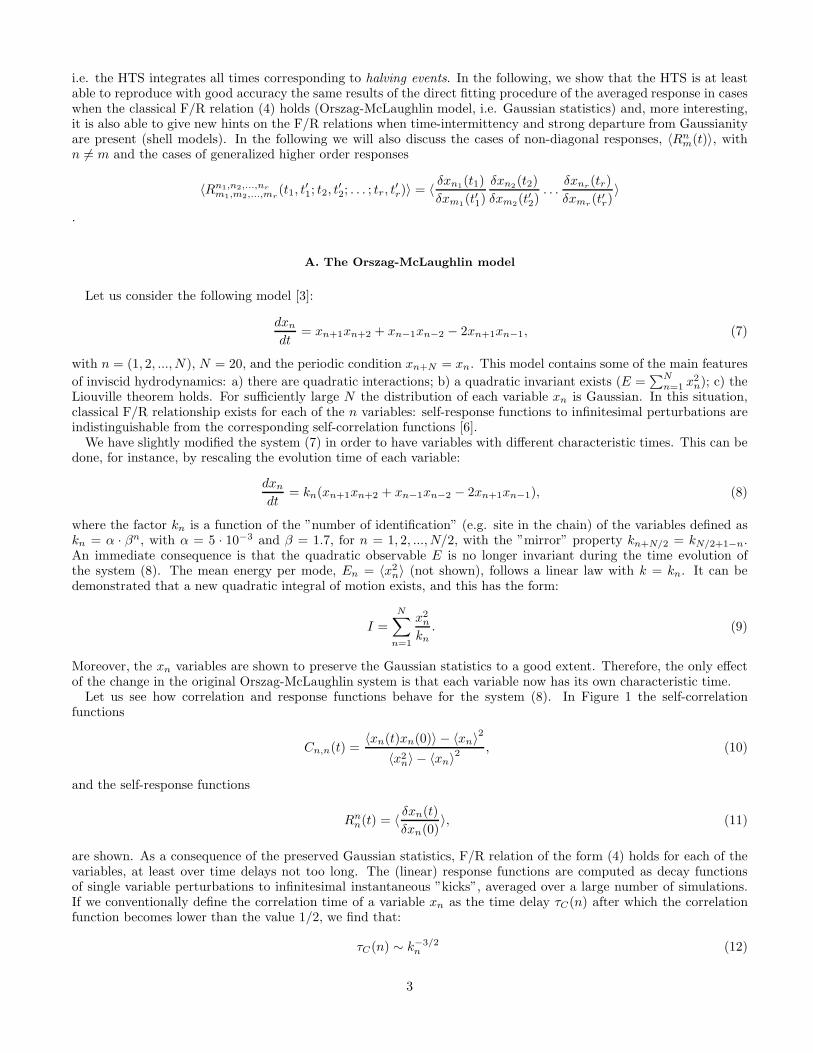
Let us see how correlation and response functions behave for the system (8). In Figure 1 the self-correlationfunctions

Cn,n(t) =〈xn(t)xn(0)〉 − 〈xn〉2

〈x2n〉 − 〈xn〉2

, (10)

and the self-response functions

Rnn(t) = 〈 δxn(t)

δxn(0)〉, (11)

are shown. As a consequence of the preserved Gaussian statistics, F/R relation of the form (4) holds for each of thevariables, at least over time delays not too long. The (linear) response functions are computed as decay functionsof single variable perturbations to infinitesimal instantaneous ”kicks”, averaged over a large number of simulations.If we conventionally define the correlation time of a variable xn as the time delay τC(n) after which the correlationfunction becomes lower than the value 1/2, we find that:

τC(n) ∼ k−3/2n (12)

3

The exponent of the scaling law (12) can be explained with a dimensional argument, by noticing that from the mean

energy per variable we get x2n ∼ kn, so from (8) and (9) the characteristic time results to be τC(n) ∼ k

−3/2n . We

notice that the scaling (12) is robust with respect to the choice of the threshold value, λ, i.e. it is observed even ifthe decay factor λ is chosen slightly different from 1/2.

The response time τR(n) is defined as the time interval after which the averaged response function becomes lowerthan 1/2. We must observe that the computation of the mean response function is practically impossible after acertain time delay, because of exponentially growing errors.

Last, halving times τ(n) have been computed always for the variables of the system (8), using the same procedureas before (i.e. infinitesimal kicks). The halving time PDF’s decay exponentially and, as can be shown, they all can be“collapsed” to the same renormalized PDF for a proper rescaling of the halving time (see below). A comparative plotof 〈τ(n)〉, τC(n) and τR(n) is shown in Figure 2. Halving times and correlation times follow the same scaling law withkn and, for each variable, have values very close to each other. Typical time decaying of the averaged Response, τR(n)are very difficult to estimate due to high errors for slow variables. In fact, only a few points are shown in Figure 2,the ones for which the mean response drops down to 1/2 fast enough, before the statistical error become too large(say larger than 100%). The advantage of the HTS with respect to the mean response function is that, with the samestatistics, halving times can be computed for all variables within reasonable uncertainty, while response times, τR(n),are generally affected by exponentially growing errors and are practically not defined when the typical relaxation timescale is longer than the error growth time scale.

The numerically computed PDF’s of the halving time τ can be rescaled as follows:

τ → τ

〈τ〉 , P (τ) → 〈τ〉P (τ). (13)

We show in Figure 3 the overlap of some rescaled PDF’s of the halving times. As a consequence, all moments of theτ(n) PDF’s have a simple scaling

〈τ(n)p〉 ∼ k−

3

2·p

n .

We have found that in a Gaussian case, the response to infinitesimal perturbations can be characterized both withthe classic mean response function and with the mean halving time technique. It is worth stressing that the HTScould be the only technique usable for studying relaxation to non linear perturbation in complex systems.

B. Shell model

Shell models for turbulent energy cascade have proved to share many statistical properties with turbulent threedimensional velocity fields [4,5]. Let us introduces a set of wavenumber kn = 2nk0 with n = 0, . . . , N . The shell-velocity variables un(t) must be understood as the velocity fluctuation over a distances ln = k−1

n . It is possible towrite down many different sets of coupled ODEs possessing the same kinematical features necessary to mimics Navier-Stokes non-linear evolution. In the following we will present numerical results for a particular choice, the so-calledSabra model [16], namely:

(

d

dt+ νk2

n

)

un = i[

knu∗

n+1un+2 + bkn−1un+1u∗

n−1 + (1 + b)kn−2un−2un−1

]

+ fn, (14)

where b is a free parameter, ν is the molecular viscosity and fn is an external forcing acting only at large scales,necessary to maintain a stationary temporal evolution. The main, strong, difference with the model discussed in theprevious section consists in the existence of a mean energy flux from large to small scales which drives the systemtoward a strongly non-Gaussian stationary temporal evolution [15]. Shell models here discussed presents exactly thesame qualitative difficulties of the original Navier-Stokes eqs: strong non-linearity and far from equilibrium statisticalfluctuations. The most striking quantitative feature of the non-Gaussian statistics is summarized in the existence ofanomalous scaling laws of velocity moments:

〈|un|p〉 ∼ k−ζ(p)n , (15)

with ζ(p) 6= p/2ζ(2). Anomalous scaling, also known as intermittency, is the quantitative way to state that velocityPDF’s at different scales cannot be rescaled by any changing of variables.

4

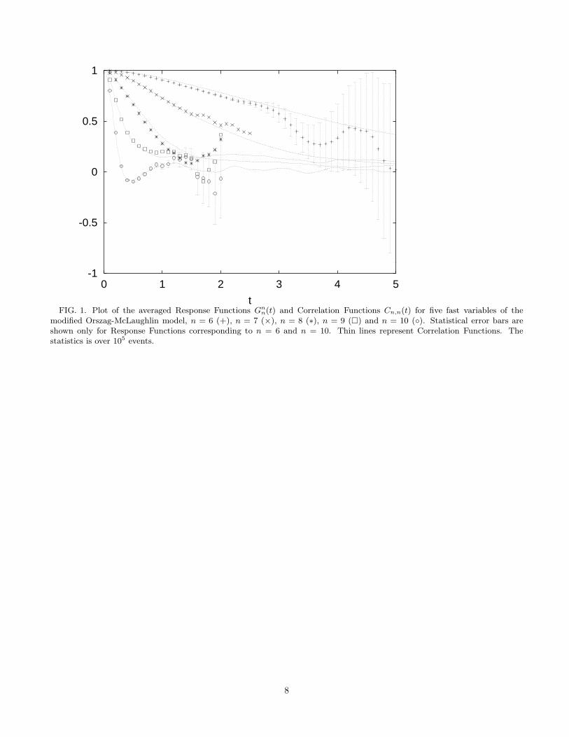
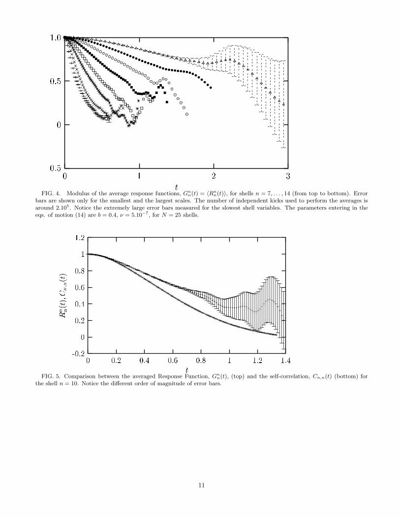
Let us now discuss two subtle points. Using some general arguments from the dynamical systems theory, one hasthat all the (typical) correlation functions at large time delay have to relax to zero with the same characteristictime, related to spectral properties of the Perron-Frobenius operator. If one uses this argument in a blind way,the apparently paradoxical result is that all correlation functions, Cn,n(t) = 〈un(t)un(0)〉, must go to zero with samecharacteristic times. On the contrary one expects a whole hierarchy of characteristic times distinguishing the behaviorof the correlation functions at different scales [17]. In particular, the self-correlation function, Cn,n(t), decays with acharacteristic time decreasing with n. The paradox is only apparent since the dynamical systems argument is valid atvery long times, i.e. much longer than the longest characteristic time, and therefore in systems with many differenttime-fluctuations it is not helpful. In fact, it is well established numerically and well understood theoretically [17–19]that general multi-scale multi-time correlation functions of the kind Cp,qn,m(t) = 〈|un(0)|p|um(t)|q〉 are described by thecascade formalism, In particular, most of the statistical properties in the inertial range can be well parametrized bythe multi-fractal-formalism.On the other hand, the response properties are related to infinitesimal perturbations. Therefore, a priori, it is notobvious that the response depend on inertial range properties. The existence of the F/R relation and the fact thatCn,n(t) (and other similar correlation functions) are determined by the inertial range properties suggest that also theresponse features are ruled by the inertial range behavior if the invariant measure is dominated by local interactionsamong shells.Let us now examine the numerical results concerning Response functions in the shell model.Figure 4 shows the diagonal mean response, Gnn(t), for a range of inertial shells, n ∈ [7 − 14]. The most strikingproperty is the impossibility to follow the response behavior at large scales (small shells) for large times, i.e. theexplicit evidence that errors grow exponentially. In order to compare the different behavior (and different errorpropagation) between response and correlation function, we plot in Fig. (5) both the average response and the self-correlation, Cn,n(t), for the shell n = 10. As it is clear from the previous figures, only response at the smallest scales(fast scales) in the inertial range can be computed with enough accuracy to follow an asymptotic decay. Still, also forthis response the clear departure between the response and the self-correlation shows is another indication that theinertial-range statistics is far from Gaussian. By using HTS we can get an information on the temporal dependence ofresponse function in the whole range of inertial shells. In Figure 6, we report some realizations of the instantaneousresponse function, which shows typical halving time experiments.

In Figure (7), we summarize the results we obtain by comparing the mean halving time, 〈τ(n)〉, with the character-istic times one extract from the decay properties of both mean response, τR(n), and correlation functions, τC(n), forthose shells where such a behavior can be safely extracted. It is worth noticing how the mean halving time allows a fullcharacterization of time properties also for those shells where the mean response Gnn(t) cannot be measured for largetime legs, t. Also, the dependence from the scale of the mean halving time is given as a best fit 〈τ(n)〉 ∼ k−χn , withχ = 0.53± 0.03. The value χ = 0.53± 0.03 can be seen as an intermittent correction to the dimensional inertial-rangeprediction 2/3. On the other hand, the dependency from the scale of τR(n) is difficult to extract due to the smallnumber of points available.

Let us now focus on the whole PDF of the halving time statistics. We first analyze the positive and negativemoments of the halving times:

T p(n) = 〈(τp(n)〉 ∼ k−ψ(p)n , (16)

with p = −5, ..., 3. Dimensional, non intermittent, scaling would predict the linear behavior for the scaling exponents:ψ(p) = 2/3p. In Figure 8 we plot the results for the halving times scaling exponents ψ(p) for all moments from p =−5, . . . , 3 and the straight line corresponding to the dimensional inertial range estimate. We notice that intermittentcorrections are much stronger for the positive moments than for the negative moments. This must be related to thefact that positive moments of the halving times are dominated by rare events where the response has a very longdecaying. We interpret the fact that ψ(p) ≃ (2/3)p as an indication that linear Response Functions are inertial rangequantities. The latter results leads to the important conclusion that the invariant measure is well approximated byshort range interaction among shells in the inertial range.

As for the non-diagonal response function and for the generalized response function of higher order the numericalproblems to measure them are even more pronounced. First, let us examine the off-diagonal response functionRmn (t) = δun(t)/δum(0). Of course these responses start from zero at time zero instead than from one as in thediagonal case. Measure them by a direct average is strictly impossible because of very large errors. We still decidedto measure their characteristic time by using the time the response reach a “macroscopic” fraction, say 1/2, of thetypical fluctuations on the scale where we are measuring the response, i.e. we collect the statistics of the first times τsuch that Rmn (t = τ) = 1/2〈|un|2〉. We expect a strong asymmetry of the characteristic times depending whether theperturbation is done at smaller (m > n) or larger (n > m) scales. Indeed, by using usual inertial range argumentswe expect that the response reacts always with a typical time given by the time of the largest between the two shells

5

involved n,m. By fixing therefore the shell where we perturb, say m, we expect that the typical time of Rmn (t), τ(m)n

is constant when n > m and scales as k−2/3n when n < m. In Figure 9 we show that indeed this behavior is well

reproduced numerically.The strong intermittency shown by halving times in Figure 8 is the clear signature of deviations from simple Gaussian-like behavior of response functions. We must therefore also expect that generalized responses of higher order are notsimply related to the linear response. For example, let us consider the third moments of the linear response [20]:

Snn(t) ≡ 〈(Rnn(t))3〉.

A simple non-intermittent behavior would suggest that Snn(t) ∝ (Gnn(t))3 while in Figure 10 it is possible to see thatthis is definitely not the case for all t legs where we have a measurable signal. Unfortunately the already discussedstatistical problems in measuring averaged response functions for long times are even more pronounced for generalizedresponse functions. Therefore we refrain from showing any results for the scaling behavior of typical times of thegeneralized response functions.

III. CONCLUSIONS

We have addressed the problem of measuring time-properties of response functions in Gaussian models (Orszag-McLaughin) and strongly non-Gaussian models like shell models for turbulence. We have introduced the conceptof halving time statistics with the aim to have a statistically stable tool to quantify the time decaying of responsefunctions and generalized response functions of high-order. We have shown numerically that in shell models for threedimensional turbulence Response functions

are inertial range quantities. This is a strong indication that the invariant measure describing the shell-velocityfluctuations is characterized by short range interactions between neighboring shells.Response functions and generalized response-functions play an important role in any diagrammatic approach for non-linear out-of-equilibrium systems. In this work we have presented the first numerical attempt to measure some of theirproperties in a systematic way. More work is needed, both numerical and analytical, in order to better understandthe detailed structure of the invariant measure governing F/R relations.

We acknowledge useful discussions with G. Boffetta and V. L’Vov. This work has been partially supported by theEU under the Grant No. HPRN-CT 2000-00162 “Non Ideal Turbulence”. GL thanks the Department of Physics ofL’Aquila University for the kind hospitality.

[1] with “statistical equilibrium” we intend the statistical properties described by the invariant probability measure of thedynamical system.

[2] R. Kubo, M. Toda and Hashitsume. Statistical Physics 2, Springer Verlag Berlin (1985).[3] S.A. Orszag and J.B. McLaughlin. Physica D 1, 68 (1980).[4] U. Frisch, “Turbulence: The Legacy of A.N. Kolmogorov” (Cambridge University Press, 1995).[5] T. Bohr, M.H. Jensen, G. Paladin & A. Vulpiani, Dynamical systems approach to turbulence, (Cambridge University Press,

Cambridge, UK, 1998).[6] M. Falcioni, S. Isola and A. Vulpiani. Phys. Lett. A, 144 (1990).[7] R.H. Kraichnan. Phys. Rev. 113, 1181 (1959).[8] R.H. Kraichnan, J. Fluid. Mech. 5 497 (1959).[9] V. L’vov and I. Procaccia, Phys. Rev. E 62, p. 8037 (2000).

[10] C.E. Leith. J. Atmos. Sci 32, 2022 (1976).[11] T.L. Bell, J. Atmos. Sci. 37, 1700 (1980).[12] H.A. Rose and P.L. Sulem. J. Phys. (Paris) 39, 441 (1978).[13] N.G. Van Kampen. Phys. Norv. 5, 279 (1971).[14] G.F. Carnevale, M. Falcioni, S. Isola, R. Purini and A. Vulpiani. Phys. Fluids A 3, 2247 (1991).[15] D. Pisarenko, L. Biferale, D. Courvoisier, U. Frisch and M. Vergassola ; Phys. Fluids A 5, p. 2533 (1993).[16] V. L’vov, E. Podivilov, A. Pomyalov, I. Procaccia and D. Vandembroucq, Phys. Rev. E. 58, 1811 (1998).[17] L. Biferale, G. Boffetta, A. Celani and F. Toschi PhysicaD 127 187 (1999).

6

[18] R. Benzi, L. Biferale and F. Toschi, Phys. Rev. Lett. 80 3244 (1998).[19] V.S. L’vov and I. Procaccia; Phys. Rev. E 54 6268 (1996).[20] even moments, being positive definite, cannot be considered response-function. They posses the typical exponential growth

with a characteristic time given by the lyapunov exponent and than, for times large enough, they saturate to the averagedmaximal distance in the attractor.

7

-1

-0.5

0

0.5

1

0 1 2 3 4 5

tFIG. 1. Plot of the averaged Response Functions Gn

n(t) and Correlation Functions Cn,n(t) for five fast variables of themodified Orszag-McLaughlin model, n = 6 (+), n = 7 (×), n = 8 (∗), n = 9 (�) and n = 10 (◦). Statistical error bars areshown only for Response Functions corresponding to n = 6 and n = 10. Thin lines represent Correlation Functions. Thestatistics is over 105 events.

8

0.01

0.1

1

10

100

1000

0.01 0.1 1kn

FIG. 2. Log-log plot of Correlation Times τC(n) (△), Mean Halving Times 〈τ (n)〉 (�), and Response Times τR(n) (◦)as function of kn, for the modified Orszag-McLaughlin model. Notice the much larger errors found when measuring thecharacteristic Response Times, τR(n). Errors on τC(n) and 〈τ (n)〉 are of the same size as the representative symbols. Thestatistics is over 105 realizations. All these characteristic times follow the same scaling law with kn. The exponent −3/2 of thescaling law follows from dimensional arguments.

9

0.001

0.01

0.1

1

0 1 2 3 4 5

resc

aled

PD

Fs

τ/<τ>FIG. 3. Collapse of the rescaled PDFs of the halving times for the modified Orszag-McLaughlin model. For simplicity,

only the PDFs relative to the fastest four variables are shown, n = 7, ..., 10. The statistics is over 105 impulsive infinitesimalperturbations as in Figure 2.

10

t 3210

1:00:50�0:5FIG. 4. Modulus of the average response functions, Gn

n(t) = 〈Rnn(t)〉, for shells n = 7, . . . , 14 (from top to bottom). Error

bars are shown only for the smallest and the largest scales. The number of independent kicks used to perform the averages isaround 2.105. Notice the extremely large error bars measured for the slowest shell variables. The parameters entering in theeqs. of motion (14) are b = 0.4, ν = 5.10−7, for N = 25 shells.

tRn n(t);C n;n(t)

1.41.210.80.60.40.20

1.210.80.60.40.20-0.2FIG. 5. Comparison between the averaged Response Function, Gn

n(t), (top) and the self-correlation, Cn,n(t) (bottom) forthe shell n = 10. Notice the different order of magnitude of error bars.

11

tj(G10 10(t))j

21.81.61.41.210.80.60.40.20

43.532.521.510.50FIG. 6. Plot of three different diagonal instantaneous responses, Rn

n(t), for the shell n = 10, versus time. Halving time isfixed by the first time when the curve touches the threshold at λ = 1/2.

n 18161412108642

6543210-1-2-3-4-5FIG. 7. Log-log plot of the mean halving times, 〈τ (n)〉 (+) and of decaying time of the mean diagonal response, τR(n) (×),

versus kn. We have checked that a different choice of the threshold λ = 1/2 used to compute halving time does not affect theslope of the graph.

12

p 420-2-4-6

210-1-2-3-4FIG. 8. ψp exponents of the p-th moment of halving times. The straight line corresponds to the dimensional prediction :

ψp = 2/3p.

n 18161412108642

43210-1-2-3-4-5FIG. 9. Log-log plot of the off-diagonal response characteristic times τ

(m)n versus kn. We performed two experiments. First

we perturb at large scales, m = 2, and we follow the response at small scales n > 2, (+); the expected independence ofcharacteristic times from the scale is well reproduced. Second, we perturb at small scales, m = 13, and we follow the responseat larger scales, n < 13, ×. In the latter case, for comparison we also plot the straight line (dashed) with the expecteddimensional slope −2/3.

13

t 0:20:10:0

10.80.60.40.20FIG. 10. Comparison between the third power of the mean diagonal response, |Gn

n(t)|3, (+) and the generalized third orderresponse, |Sn

n(t)|, (×) computed for the shell n = 13, with 5.105 kicks.

14