Symmetry Methods in Turbulent Boundary Layer Theory
10
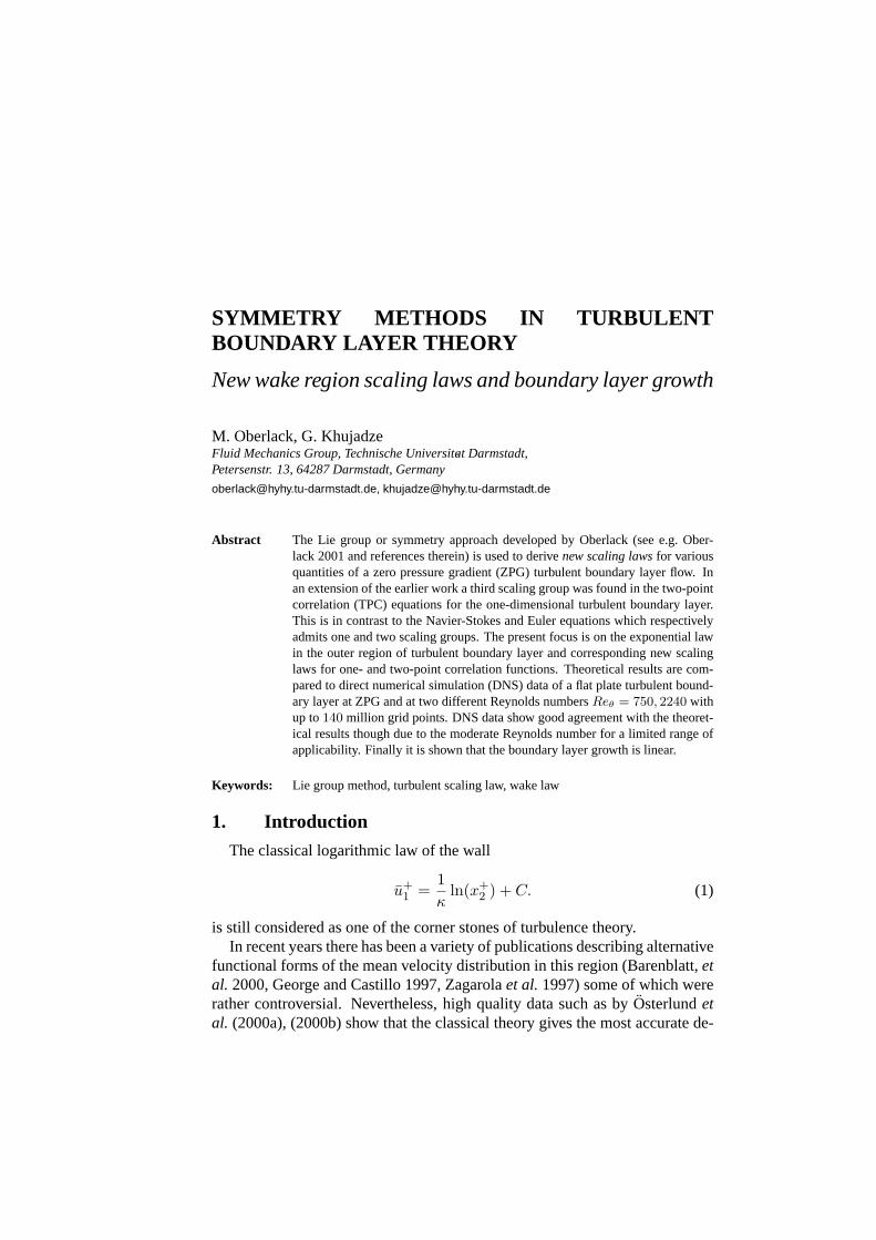
SYMMETRY METHODS IN TURBULENT BOUNDARY LAYER THEORY New wake region scaling laws and boundary layer growth M. Oberlack, G. Khujadze Fluid Mechanics Group, Technische Universit- at Darmstadt, Petersenstr. 13, 64287 Darmstadt, Germany [email protected], [email protected] Abstract The Lie group or symmetry approach developed by Oberlack (see e.g. Ober- lack 2001 and references therein) is used to derive new scaling laws for various quantities of a zero pressure gradient (ZPG) turbulent boundary layer flow. In an extension of the earlier work a third scaling group was found in the two-point correlation (TPC) equations for the one-dimensional turbulent boundary layer. This is in contrast to the Navier-Stokes and Euler equations which respectively admits one and two scaling groups. The present focus is on the exponential law in the outer region of turbulent boundary layer and corresponding new scaling laws for one- and two-point correlation functions. Theoretical results are com- pared to direct numerical simulation (DNS) data of a flat plate turbulent bound- ary layer at ZPG and at two different Reynolds numbers Re θ = 750, 2240 with up to 140 million grid points. DNS data show good agreement with the theoret- ical results though due to the moderate Reynolds number for a limited range of applicability. Finally it is shown that the boundary layer growth is linear. Keywords: Lie group method, turbulent scaling law, wake law 1. Introduction The classical logarithmic law of the wall ¯ u + 1 = 1 κ ln(x + 2 )+ C. (1) is still considered as one of the corner stones of turbulence theory. In recent years there has been a variety of publications describing alternative functional forms of the mean velocity distribution in this region (Barenblatt, et al. 2000, George and Castillo 1997, Zagarola et al. 1997) some of which were rather controversial. Nevertheless, high quality data such as by ¨ Osterlund et al. (2000a), (2000b) show that the classical theory gives the most accurate de-
-
Upload
uni-siegen -
Category
Documents
-
view
0 -
download
0
Transcript of Symmetry Methods in Turbulent Boundary Layer Theory
SYMMETRY METHODS IN TURBULENTBOUNDARY LAYER THEORY
New wake region scaling laws and boundary layer growth
M. Oberlack, G. KhujadzeFluid Mechanics Group, Technische Universit-at Darmstadt,Petersenstr. 13, 64287 Darmstadt, Germany
[email protected], [email protected]
Abstract The Lie group or symmetry approach developed by Oberlack (see e.g. Ober-lack 2001 and references therein) is used to derivenew scaling lawsfor variousquantities of a zero pressure gradient (ZPG) turbulent boundary layer flow. Inan extension of the earlier work a third scaling group was found in the two-pointcorrelation (TPC) equations for the one-dimensional turbulent boundary layer.This is in contrast to the Navier-Stokes and Euler equations which respectivelyadmits one and two scaling groups. The present focus is on the exponential lawin the outer region of turbulent boundary layer and corresponding new scalinglaws for one- and two-point correlation functions. Theoretical results are com-pared to direct numerical simulation (DNS) data of a flat plate turbulent bound-ary layer at ZPG and at two different Reynolds numbersReθ = 750, 2240 withup to140 million grid points. DNS data show good agreement with the theoret-ical results though due to the moderate Reynolds number for a limited range ofapplicability. Finally it is shown that the boundary layer growth is linear.
Keywords: Lie group method, turbulent scaling law, wake law
1. Introduction
The classical logarithmic law of the wall
u+1 =
1κ
ln(x+2 ) + C. (1)
is still considered as one of the corner stones of turbulence theory.In recent years there has been a variety of publications describing alternative
functional forms of the mean velocity distribution in this region (Barenblatt,etal. 2000, George and Castillo 1997, Zagarolaet al.1997) some of which wererather controversial. Nevertheless, high quality data such as byOsterlundetal. (2000a), (2000b) show that the classical theory gives the most accurate de-
mo
Schreibmaschinentext
in: IUTAM Symposium on One Hundred Years of Boundary Layer Research Proceedings of the IUTAM Symposium held at DLR-Göttingen, Germany, August 12-14, 2004 Series: Solid Mechanics and Its Applications, Vol. 129 Meier, G.E.A.; Sreenivasan, K.R.; Heinemann, Hans-Joachim (Eds.) 2006, X, 494 p
mo
Schreibmaschinentext
mo
Schreibmaschinentext
mo
Schreibmaschinentext
2
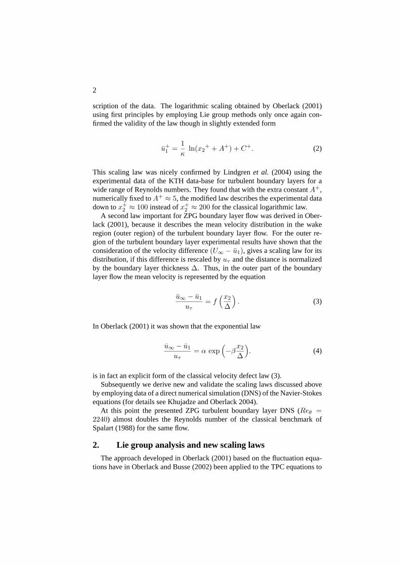
scription of the data. The logarithmic scaling obtained by Oberlack (2001)using first principles by employing Lie group methods only once again con-firmed the validity of the law though in slightly extended form
u+1 =
1κ
ln(x2+ + A+) + C+. (2)
This scaling law was nicely confirmed by Lindgrenet al. (2004) using theexperimental data of the KTH data-base for turbulent boundary layers for awide range of Reynolds numbers. They found that with the extra constantA+,numerically fixed toA+ ≈ 5, the modified law describes the experimental datadown tox+
2 ≈ 100 instead ofx+2 ≈ 200 for the classical logarithmic law.
A second law important for ZPG boundary layer flow was derived in Ober-lack (2001), because it describes the mean velocity distribution in the wakeregion (outer region) of the turbulent boundary layer flow. For the outer re-gion of the turbulent boundary layer experimental results have shown that theconsideration of the velocity difference(U∞ − u1), gives a scaling law for itsdistribution, if this difference is rescaled byuτ and the distance is normalizedby the boundary layer thickness∆. Thus, in the outer part of the boundarylayer flow the mean velocity is represented by the equation
u∞ − u1
uτ= f
(x2
∆
). (3)
In Oberlack (2001) it was shown that the exponential law
u∞ − u1
uτ= α exp
(−β
x2
∆
). (4)
is in fact an explicit form of the classical velocity defect law (3).Subsequently we derive new and validate the scaling laws discussed above
by employing data of a direct numerical simulation (DNS) of the Navier-Stokesequations (for details see Khujadze and Oberlack 2004).
At this point the presented ZPG turbulent boundary layer DNS (Reθ =2240) almost doubles the Reynolds number of the classical benchmark ofSpalart (1988) for the same flow.
2. Lie group analysis and new scaling laws
The approach developed in Oberlack (2001) based on the fluctuation equa-tions have in Oberlack and Busse (2002) been applied to the TPC equations to
Symmetry methods in turbulent boundary layer theory 3
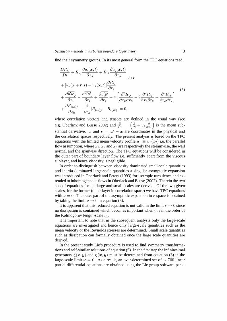
find their symmetry groups. In its most general form the TPC equations read
DRij
Dt+ Rkj
∂ui(x, t)∂xk
+ Rik∂uj(x, t)
∂xk
∣∣∣∣∣x+r
+ [uk(x + r, t)− uk(x, t)]∂Rij
∂rk
+∂p′u′j∂xi
− ∂p′u′j∂ri
+∂u′ip′
∂rj+ ν
[∂2Rij
∂xk∂xk− 2
∂2Rij
∂xk∂rk+
∂2Rij
∂rk∂rk
]
+∂R(ik)j
∂xk− ∂
∂rk[R(ik)j −Ri(jk)] = 0,
(5)
where correlation vectors and tensors are defined in the usual way (see
e.g. Oberlack and Busse 2002) andDDt
=(
∂∂t + uk
∂∂xk
)is the mean sub-
stantial derivative.x and r = x′ − x are coordinates in the physical andthe correlation spaces respectively. The present analysis is based on the TPCequations with the limited mean velocity profileu1 ≡ u1(x2) i.e. the parallelflow assumption, wherex1, x2 andx3 are respectively the streamwise, the wallnormal and the spanwise direction. The TPC equations will be considered inthe outer part of boundary layer flow i.e. sufficiently apart from the viscoussublayer, and hence viscosity is negligible.
In order to distinguish between viscosity dominated small-scale quantitiesand inertia dominated large-scale quantities a singular asymptotic expansionwas introduced in Oberlack and Peters (1993) for isotropic turbulence and ex-tended to inhomogeneous flows in Oberlack and Busse (2002). Therein the twosets of equations for the large and small scales are derived. Of the two givenscales, for the former (outer layer in correlation space) we have TPC equationswith ν = 0. The outer part of the asymptotic expansion inr-space is obtainedby taking the limitν → 0 in equation (5).
It is apparent that this reduced equation is not valid in the limitr → 0 sinceno dissipation is contained which becomes important whenr is in the order ofthe Kolmogorov length-scaleηk.
It is important to note that in the subsequent analysis only the large-scaleequations are investigated and hence only large-scale quantities such as themean velocity or the Reynolds stresses are determined. Small scale quantitiessuch as dissipation can formally obtained once the large scale quantities arederived.
In the present study Lie’s procedure is used to find symmetry transforma-tions and self-similar solutions of equation (5). In the first step the infinitesimalgeneratorsξ(x,y) andη(x, y) must be determined from equation (5) in thelarge-scale limitν = 0. As a result, an over-determined set of∼ 700 linearpartial differential equations are obtained using the Lie group software pack-
4
age by Carminati and Vu (2000). Imposing the reduction of a parallel flow, thesolution of the system for the desired symmetries is given below
ξx2 = c1x2 + c4, (6)
ξr1 = c1r1, (7)
ξr2 = c1r2, (8)
ξr3 = c1r3, (9)
ηu1 = (c1 − c2)u1 + c5, (10)
ηRij = [2(c1 − c2) + c3] Rij , (11)
ηu′ip′
= [3(c1 − c2) + c3]u′ip′ (12)
ηp′u′i= [3(c1 − c2) + c3]p′u′i, (13)
ηZij = [2c1 − 3c2 − c3] Zij . (14)
Zij is the sum of derivatives of the triple correlation functions in (5) andci
are group parameters. Beside the symmetry groups given in (6)-(14) othersymmetries were obtained some of which are unphysical. This has been firstreported in Oberlack (2000).
For the present problem we focus on the scaling symmetries, Galilean in-variance and the translation groups in (6)-(14).
For a better understanding we may employ Lie’s theory, to derive the globaltransformations
Gs1 : x2 = x2ea1 , ri = rie
a1 , ˜u1 = u1ea1 , Rij = Rije
2a1 , · · · (15)
Gs2 : x2 = x2, ri = ri, ˜u1 = u1e−a2 , Rij = Rije
−2a2 , · · · (16)
Gs3 : x2 = x2, ri = ri, ˜u1 = u1, Rij = Rije−a3 , · · · (17)
Gtransl : x2 = x2 + a4, ri = ri, ˜u1 = u1, Rij = Rij , · · · (18)
Ggalil : x2 = x2, ri = ri, ˜u1 = u1 + a5, Rij = Rij , · · · . (19)
The variablesa1 – a5 are the group parameters of the corresponding parameterc1 – c5 in the infinitesimals (6)-(14).
The most interesting fact with respect to the latter groups is thatthree in-dependent scaling groupsGs1, Gs2, Gs3 have been computed. Two sym-metry groups correspond to the scaling symmetries of the Euler equations.The first one is the scaling in space, the second one scaling in time. Thethird group (Gs3) is a new scaling group that is a characteristic feature of theone-dimensional turbulent boundary layer flow. This is in striking contrast tothe Euler and Navier-Stokes equations, which only admit two and one scalinggroups, respectively.Gtransl andGgalil represent the translation symmetry inspace and the Galilean transformation, respectively.
Symmetry methods in turbulent boundary layer theory 5
The corresponding characteristic equations for the invariant solutions read
dx2
c1x2 + c4=
dri
c1ri=
du1
(c1 − c2)u1 + c5=
dRij
[2(c1 − c2) + c3]Rij= ... . (20)
In Oberlack (2001) it has been shown that the symmetry breaking of the scalingof space leads to a new exponential scaling law corresponding to the outer partof a boundary layer flow, the wake region.
Thus, imposing the assumption of symmetry breaking of the scaling of space(c1 = 0) here as well and integrating the corresponding equations we obtainan extended set of scaling laws for the mean velocity and the TPC functions asfollows
u1(x2) = k1 + k2e−k3x2 , with k1 ≡ c5
c2and k3 ≡ c2
c4(21)
andk2 is a constant of integration and
Rij(x2, r) = e−k4x2Bij(r), . . . (22)
wherek4 ≡ 2c2−c3c4
is a constant andBij is a function ofr only.For positivek3 the velocity law (21) converges to a constant velocity for
x2 → ∞ (k1 = u∞). For a plane shear flow this may only be applicable to aboundary layer type of flow. In this flow the symmetry breaking length scaleis the boundary layer thickness.
In normalized and non-dimensional variables the exponential scaling law(21) may be re-written in the form given above in equation (4).
One can derive the scaling laws for the Reynolds stresses from the (22) bytaking the limitr = 0:
u′iu′j(x2)u2
τ
= bij exp(−a
x2
∆
). (23)
bij anda are universal constants that should be taken from DNS or experimen-
tal data. ∆ is the Rotta-Clauser length scale∆ ≡ ∫∞0
u∞ − u1
uτ= u∞
uτδ∗,
while δ∗ is the boundary layer displacement thickness.Recently (4) was validated in detail using high Reynolds number experi-
mental data from the KTH data-base for ZPG turbulent boundary layers byLindgrenet al. (2004). The range of Reynolds number based on momentum-loss thickness was from2500 to 27000. It was found that the exponentialscaling law of the mean velocity defect in the outer or wake region fits wellwith the experimental data over a large part of the boundary layer thickness.
3. Two-dimensional turbulent boundary layer
Putting the strict limit of a fully parallel flow aside and consider the caseof a spatially growing and hence two-dimensional boundary layer the number
6
of symmetries we find is, on the one side, an extended one but, on the otherside, a reduced set of symmetries. The scaling groupGs3 disappears but newsymmetries arise such as the usual rotation group as well as the translation andGalilean group inx2 direction (for an extensive discussion see Oberlack 2000or Oberlack and Busse 2002). For the present problem of a ZPG boundarylayer flow rotation is incompatible and we obtain the characteristic equation
dx1
c1x1 + c3=
dx2
c1x2 + c4=
dri
c1ri=
du1
(c1 − c2)u1 + c5=
du2
(c1 − c2)u2 + c6=
dp
[2(c1 − c2)]p=
dRij
[2(c1 − c2)]Rij= ... . (24)
For the present purpose of investigating the boundary layer growth only thefirst two terms are relevant which, once integrated lead to
δ2D =x2 + c4
c1
x1 + c3c1
(25)
Apparently we find that in a ZPG turbulent boundary layer the boundary layerthickness grows like a linear function which is in contrast to a laminar bound-ary layer which growths like a square root. Note that any scaling constant,
say cs, in front of δ2D in the form csx2+
c4c1
x1+c3c1
would not change the result of
δ2D being a similarity variable. In fact we should mention that it means thatthe growth factor is not determined from the above analysis and appears to besome kind of “eigenvalue” of the flow.
4. DNS and scaling law validation
The DNS code was developed at KTH, Stockholm (for details see Lund-bladhet al.1999 and Skote 2001) using a spectral method with Fourier decom-position in the horizontal directions and Chebyshev discretization in the wallnormal direction. Time integration is performed using a third order Runge-Kutta scheme for the advective and forcing terms and Crank-Nicolson for theviscous terms.
The first simulations were performed at two different resolutions (numberof grid points7.9 and31.2 millions respectively). The simulations in this casewere run for a total of10000 time units (δ∗/u∞) and the sampling for thestatistics was performed during the last5000 time units. The useful region wasconfined to150 − 300δ∗|x=0 which corresponds toReδ∗ from 800 to 1100 orReθ from 540 to 750. The differences between the two resolutions were verysmall.
Thus we decided that the coarser grid is sufficient to resolve the flow withthis Reynolds number and it has to be used as the starting point for the cal-

Symmetry methods in turbulent boundary layer theory 7
culation of the number of grid points for the higher Reynolds number flowsaccording to
N ≈ N0
(Re1
δ∗
Re0δ∗
)9/4
. (26)
Assuming thatN0 ≈ 7.9 ∗ 106 was sufficient to resolve the flow at lowReynolds number (Reδ∗ ≈ 1100) we employedReδ∗ = 3050 into (26) toobtainN ≈ 138.8 million grid points for the larger Reynolds number.
Again the useful region was confined to150 − 300δ∗|x=0 (total length ofcomputational box is450δ∗|x=0) which corresponds toReδ∗ from 2230 to3050 or Reθ from 1670 to 2240. Resolutions in plus units are∆x+ ≈ 15,∆z+ ≈ 11 and∆y+ ≈ 0.13− 18.
Scaling law validation of one- and two-point quantities
The mean velocity of the turbulent boundary layer data is plotted in Figure1 for Reθ = 2240. As it is observed from the figure, DNS and theoreticalresults (4) are in good agreement in the regionx2/∆ ≈ 0.01 − 0.15. Abovethis region the velocity defect law in the outer part of the boundary layer de-creases more rapidly than what was derived from the theoretical result. Theremay be two reasons for this. First it might be the result of the low Reynoldsnumber phenomenon in DNS while for the derivation of the theoretical resultswe assumed the large Reynolds number limit. Second as it is argued in Lind-grenet al. (2004) that the non-parallel effects become dominant in the outerpart of the wake region, which could cause the deviation from the exponen-
logş
u∞−uuτ
ť
0 0.1 0.2 0.3 0.4 0.5
0.1
1
10
x2/∆0 0.03 0.06 0.09 0.12 0.15
0.1
1
10
x2/∆
Figure 1. Mean velocity profile in log-linear scaling. Left figure: Dashed line correspondsto theoretical results from the law (4). Solid line represents DNS results atReθ = 2240; RightFigure: Close up plot of mean velocity profile at different Reynolds numbers.
tial law, while the theoretical results were derived assuming a fully parallelflow. Because of these reasons, we have a relatively small ”coincidence re-gion” of the theoretical and DNS results. The close up of mean velocity pro-files is presented in the same figure (right plot) at different Reynolds numbers
8
Reθ = 1670, 1870, 2060, 2240. Good collapse of profiles in the exponentialregion is seen from the plot.
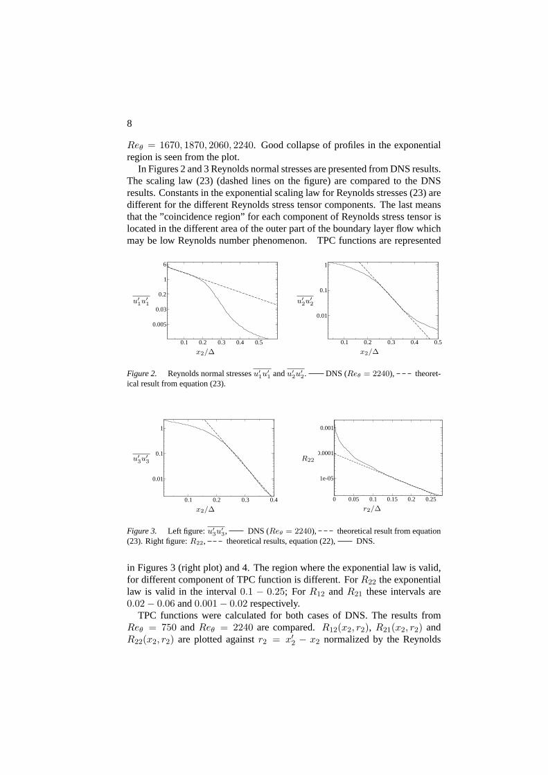
In Figures 2 and 3 Reynolds normal stresses are presented from DNS results.The scaling law (23) (dashed lines on the figure) are compared to the DNSresults. Constants in the exponential scaling law for Reynolds stresses (23) aredifferent for the different Reynolds stress tensor components. The last meansthat the ”coincidence region” for each component of Reynolds stress tensor islocated in the different area of the outer part of the boundary layer flow whichmay be low Reynolds number phenomenon. TPC functions are represented
u′1u′1
0.1 0.2 0.3 0.4 0.5
0.005
0.03
0.2
1
6
x2/∆
u′2u′2
0.1 0.2 0.3 0.4 0.5
0.01
0.1
1
x2/∆
Figure 2. Reynolds normal stressesu′1u′1 andu′2u
′2. DNS (Reθ = 2240), theoret-
ical result from equation (23).
u′3u′3
0.1 0.2 0.3 0.4
0.01
0.1
1
x2/∆
R22
0 0.05 0.1 0.15 0.2 0.25
1e-05
0.0001
0.001
r2/∆
Figure 3. Left figure:u′3u′3, DNS (Reθ = 2240), theoretical result from equation
(23). Right figure:R22, theoretical results, equation (22), DNS.
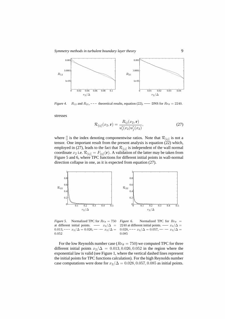
in Figures 3 (right plot) and 4. The region where the exponential law is valid,for different component of TPC function is different. ForR22 the exponentiallaw is valid in the interval0.1 − 0.25; For R12 andR21 these intervals are0.02− 0.06 and0.001− 0.02 respectively.
TPC functions were calculated for both cases of DNS. The results fromReθ = 750 andReθ = 2240 are compared.R12(x2, r2), R21(x2, r2) andR22(x2, r2) are plotted againstr2 = x′2 − x2 normalized by the Reynolds
Symmetry methods in turbulent boundary layer theory 9
R12
0 0.02 0.04 0.06 0.08 0.1
1e-05
0.0001
0.001
r2/∆
R21
0 0.01 0.02 0.03 0.04
1e-05
0.0001
0.001
r2/∆
Figure 4. R12 andR21, theoretical results, equation (22), DNS forReθ = 2240.
stresses
R[ij](x2, r) =Rij(x2, r)
u′i(x2)u′j(x2), (27)
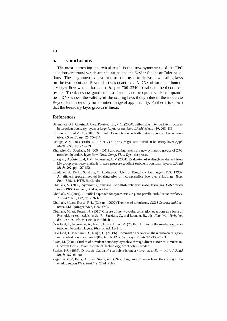
where[] is the index denoting componentwise ratios. Note thatR[ij] is not atensor. One important result from the present analysis is equation (22) which,employed in (27), leads to the fact thatR[ij] is independent of the wall normalcoordinatex2 i.e.R[ij] = F[ij](r). A validation of the latter may be taken fromFigure 5 and 6, where TPC functions for different initial points in wall-normaldirection collapse in one, as it is expected from equation (27).
R22
0.1 0.2 0.3 0.4 0.50
0.2
0.4
0.6
0.8
1
r2/∆
Figure 5. Normalized TPC forReθ = 750at different initial points. x2/∆ =0.013, x2/∆ = 0.026, x2/∆ =0.052
R22
0 0.1 0.2 0.3 0.4 0.50
0.2
0.4
0.6
0.8
1
r2/∆
Figure 6. Normalized TPC forReθ =2240 at different initial points. x2/∆ =0.028, x2/∆ = 0.057, x2/∆ =0.085
For the low Reynolds number case (Reθ = 750) we computed TPC for threedifferent initial pointsx2/∆ = 0.013, 0.026, 0.052 in the region where theexponential law is valid (see Figure 1, where the vertical dashed lines representthe initial points for TPC functions calculation). For the high Reynolds numbercase computations were done forx2/∆ = 0.028, 0.057, 0.085 as initial points.
10
5. Conclusions
The most interesting theoretical result is that new symmetries of the TPCequations are found which are not intrinsic to the Navier-Stokes or Euler equa-tions. These symmetries have in turn been used to derive new scaling lawsfor the two-point and Reynolds stress quantities. A DNS of turbulent bound-ary layer flow was performed atReθ = 750, 2240 to validate the theoreticalresults. The data show good collapse for one and two-point statistical quanti-ties. DNS shows the validity of the scaling laws though due to the moderateReynolds number only for a limited range of applicability. Further it is shownthat the boundary layer growth is linear.
ReferencesBarenblatt, G.I., Chorin, A.J. and Prostokishin, V.M. (2000). Self-similar intermediate structures
in turbulent boundary layers at large Reynolds numbersJ.Fluid Mech.410, 263–283.Carminati, J. and Vu, K. (2000). Symbolic Computation and differential equations: Lie symme-
tries.J.Sym. Comp., 29, 95–116.George, W.K. and Castillo, L. (1997). Zero-pressure-gradient turbulent boundary layerAppl.
Mech. Rev., 50, 689–729.Khujadze, G., Oberlack, M. (2004). DNS and scaling laws from new symmetry groups of ZPG
turbulent boundary layer flow.Theo. Comp. Fluid Dyn., (in press).Lindgren, B.,Osterlund, J. M., Johansson, A. V. (2004). Evaluation of scaling laws derived from
Lie group symmetry methods in zero pressure-gradient turbulent boundary layers.J.FluidMech.502, pp. 127-152.
Lundbladh A., Berlin, S., Skote, M., Hildings, C., Choi, J., Kim, J. and Henningson, D.S. (1999).An efficient spectral method for simulation of incompressible flow over a flat plate.Tech.Rep.1999:11. KTH, Stockholm.
Oberlack, M. (2000). Symmetrie, Invarianz und Selbstahnlichkeit in der Turbulenz.Habilitationthesis RWTH Aachen, Shaker, Aachen.
Oberlack, M. (2001). A unified approach for symmetries in plane parallel turbulent shear flows.J.Fluid Mech., 427, pp. 299-328.
Oberlack, M. and Busse, F.H., (Editors) (2002) Theories of turbulence,CISM Courses and Lec-tures, 442, Springer Wien, New-York.
Oberlack, M. and Peters, N., (1993) Closure of the two-point correlation equations as a basis ofReynolds stress models, in So, R., Speziale, C., and Launder, B., eds.Near-Wall Turbulentflows, 85–94. Elsevier Science Publisher.
Osterlund, J., Johansson, A., Nagib, H. and Hites, M. (2000a). A note on the overlap region inturbulent boundary layers,Phys. Fluids12(1) 1–4.
Osterlund, J., Johansson, A., Nagib, H. (2000b). Comment on ’a note on the intermediate regionin turbulent boundary layers’[Phy.Fluids 12, 2159].Phys. Fluids122360–2363.
Skote, M. (2001). Studies of turbulent boundary layer flow through direct numerical simulation.Doctoral thesis, Royal Institute of Technology, Stockholm, Sweden.
Spalart, P.R. (1988). Direct simulation of a turbulent boundary layer up toRθ = 1410. J. FluidMech.187, 61–98.
Zagarola, M.V., Perry, A.E. and Smits, A.J. (1997). Log laws or power laws: the scaling in theoverlap regionPhys. Fluids9, 2094–2100.