Symm

etry in Applied Mathem

atics • Lorentz Jäntschi and Sorana D. Bolboacă

Symmetry in Applied Mathematics

Printed Edition of the Special Issue Published in Symmetry

www.mdpi.com/journal/symmetry

Lorentz Jäntschi and Sorana D. BolboacăEdited by

Symmetry in Applied Mathematics

Symmetry in Applied Mathematics

Editors

Lorentz Jantschi

Sorana D. Bolboaca

MDPI • Basel • Beijing • Wuhan • Barcelona • Belgrade • Manchester • Tokyo • Cluj • Tianjin

Editors

Lorentz Jantschi

Department of Physics and

Chemistry, Technical University

of Cluj-Napoca

Romania

Sorana D. Bolboaca

Department of Medical

Informatics and Biostatistics,

“Iuliu Hatieganu” University of

Medicine and Pharmacy

Romania

Editorial Office

MDPI

St. Alban-Anlage 66

4052 Basel, Switzerland

This is a reprint of articles from the Special Issue published online in the open access journal

Symmetry (ISSN 2073-8994) (available at: https://www.mdpi.com/journal/symmetry/special

issues/Symmetry Applied Mathematics).

For citation purposes, cite each article independently as indicated on the article page online and as

indicated below:

LastName, A.A.; LastName, B.B.; LastName, C.C. Article Title. Journal Name Year, Volume Number,

Page Range.

ISBN 978-3-03943-791-7 (Hbk)

ISBN 978-3-03943-792-4 (PDF)

c© 2020 by the authors. Articles in this book are Open Access and distributed under the Creative

Commons Attribution (CC BY) license, which allows users to download, copy and build upon

published articles, as long as the author and publisher are properly credited, which ensures maximum

dissemination and a wider impact of our publications.

The book as a whole is distributed by MDPI under the terms and conditions of the Creative Commons

license CC BY-NC-ND.

Contents

About the Editors . . . . . . . . . . . . . . . . . . . . . . . . . . . . . . . . . . . . . . . . . . . . . . vii

Preface to ”Symmetry in Applied Mathematics” . . . . . . . . . . . . . . . . . . . . . . . . . . . ix

Young Chel Kwun, Abdul Rauf Nizami, Mobeen Munir, Zaffar Iqbal, Dishya Arshad and

Shin Min Kang

Khovanov Homology of Three-Strand Braid LinksReprinted from: Symmetry 2018, 10, 720, doi:10.3390/sym10120720 . . . . . . . . . . . . . . . . . 1

Adrian Holhos and Daniela Rosca

Volume Preserving Maps Between p-BallsReprinted from: Symmetry 2019, 11, 1404, doi:10.3390/sym11111404 . . . . . . . . . . . . . . . . . 21

Mujahid Abbas, Hira Iqbal and Manuel De la Sen

Generation of Julia and Mandelbrot Sets via Fixed PointsReprinted from: Symmetry 2020, 12, 86, doi:10.3390/sym12010086 . . . . . . . . . . . . . . . . . . 33

Benedek Nagy and Khaled Abuhmaidan

A Continuous Coordinate System for the Plane by Triangular SymmetryReprinted from: Symmetry 2019, 11, 191, doi:10.3390/sym11020191 . . . . . . . . . . . . . . . . . 53

Andronikos Paliathanasis

One-Dimensional Optimal System for 2D Rotating Ideal GasReprinted from: Symmetry 2019, 11, 1115, doi:10.3390/sym11091115 . . . . . . . . . . . . . . . . . 71

P. V. Negron-Marrero and M. Lopez-Serrano

Minimal Energy Configurations of Finite Molecular ArraysReprinted from: Symmetry 2019, 11, 158, doi:10.3390/sym11020158 . . . . . . . . . . . . . . . . . 85

M. Umar Farooq

Noether-Like Operators and First Integrals for Generalized Systems of Lane-Emden EquationsReprinted from: Symmetry 2019, 11, 162, doi:10.3390/sym11020162 . . . . . . . . . . . . . . . . . 109

Yuanxiang Dong, Chenjing Hou, Yuchen Pan and Ke Gong

Algorithm for Neutrosophic Soft Sets in Stochastic Multi-Criteria Group Decision Making Basedon Prospect TheoryReprinted from: Symmetry 2019, 11, 1085, doi:10.3390/sym11091085 . . . . . . . . . . . . . . . . . 119

Janak Raj Sharma, Deepak Kumar and Lorentz Jantschi

On a Reduced Cost Higher Order Traub-Steffensen-Like Method for Nonlinear SystemsReprinted from: Symmetry 2019, 11, 891, doi:10.3390/sym11070891 . . . . . . . . . . . . . . . . . 137

Janak Raj Sharma, Sunil Kumar and Lorentz Jantschi

On a Class of Optimal Fourth Order Multiple Root Solvers without Using DerivativesReprinted from: Symmetry 2019, 11, 1452, doi:10.3390/sym11121452 . . . . . . . . . . . . . . . . . 157

Jared Lynskey, Kyi Thar, Thant Zin Oo, Choong Seon Hong

Facility Location Problem Approach for Distributed DronesReprinted from: Symmetry 2019, 11, 118, doi:10.3390/sym11010118 . . . . . . . . . . . . . . . . . 171

v

Flavia-Corina Mitroi-Symeonidis, Ion Anghel and Nicus, or Minculete

Parametric Jensen-Shannon Statistical Complexity and Its Applications on Full-ScaleCompartment Fire DataReprinted from: Symmetry 2020, 12, 22, doi:10.3390/sym12010022 . . . . . . . . . . . . . . . . . . 183

Roger Tovar-Falon, Heleno Bolfarine and Guillermo Martınez-Florez

The Asymmetric Alpha-Power Skew-t DistributionReprinted from: Symmetry 2020, 12, 82, doi:10.3390/sym12010082 . . . . . . . . . . . . . . . . . . 195

Lorentz Jantschi

A Test Detecting the Outliers for Continuous Distributions Based on the CumulativeDistribution Function of the Data Being TestedReprinted from: Symmetry 2019, 11, 835, doi:10.3390/sym11060835 . . . . . . . . . . . . . . . . . 217

vi

About the Editors

Lorentz Jantschi was born in Fagaras, , Romania, in 1973. In 1991 he moved to Cluj-Napoca, Cluj,

where he completed his studies. In 1995 he was awarded a B.Sc. and M.Sc. in Informatics, in 1997

a B.Sc. and M.Sc. in Physics and Chemistry, in 2000 a Ph.D. in Chemistry under the supervision of

Prof. Mircea V. Diudea, in 2002 an M.Sc. in Agriculture, in 2010 a Ph.D. in Horticulture under the

supervision of Prof. Radu E. Sestras, , and, finally, in 2013 a postdoctorate in Horticulture. That same

year (2013), he became a Full Profesor of chemistry at the Technical University of Cluj-Napoca and

an associate at Babes-Bolyai University, where he advises Ph.D. studies in chemistry. Both positions

are to date. During the time he had research and education activities deployed under auspices of

different institutions: the G. Barit, iu (1995–1999) and Balcescu (1999–2001) National Colleges, the Iuliu

Hat, ieganu University of Medicine and Pharmacy (2007–2012), Oradea University (2013–2015),

and the Institute of Agricultural Sciences and Veterinary Medicine at University of Cluj-Napoca

(2011–2016). He serves as an editor for the journals Notulae Scientia Biologicae, Notulae Horti Agro

Botanici Cluj-Napoca, Open Agriculture and Symmetry. He was Editor-in-Chief of the Leonardo

Journal of Sciences and the Leonardo Electronic Journal of Practices and Technologies (2002–2018)

and guest editor (2019–2020) for Mathematics.

Sorana D. Bolboaca is a professor of medical informatics and biostatistics at the ”Iuliu Hat, ieganu”

University of Medicine and Pharmacy Cluj-Napoca, Romania. She earned her Ph.D. in Medicine

(2006) from the Iuliu Hatieganu University of Medicine and Pharmacy (thesis title: “Evidence-Based

Medicine: Logistics and Implementation”) and a Ph.D. in Horticulture (2010) from the University

of Agriculture Sciences and Veterinary Medicine Cluj-Napoca (thesis title: “Statistical Models for

Analysis of Genetic Variability”). Her research interests are multidisciplinary, e.g., applied &

computational statistics, molecular modeling, genetic analysis, statistical modeling in medicine,

integrated health informatics system and application of new technologies in medicine, medical

diagnostics research, medical imaging analysis, assisted decision systems, research ethics, social

media and health information, and evidence-based medicine. She is an active member of the scientific

community with more than 200 papers and 19 monographs as well as editorial and reviewing

activities (https://publons.com/researcher/249582/sorana-d-bolboaca/).

vii

Preface to ”Symmetry in Applied Mathematics”

The Symmetry in Applied Mathematics special issue of Symmetry Journal reprinted here is

collecting fourteen papers dealing with various subjects under the auspices of using symmetry

for solving problems. The special issue called for articles from a broad interdisciplinary area,

since ’applied mathematics’ is a specific form of mathematics that involves creating and use of

mathematical models to map out the mathematical core of a practical problem. There is probably

no scientific field in which applied mathematics has not made its necessary presence. On the

other hand, symmetry is about identification and use invariants to any of various transformations

for any paired dataset and characterizations associated with. Inside applied mathematics,

symmetry may work as a powerful tool for problems reduction and solving. Applications include

probability theory (all probabilistic reasoning is ultimately based on judgments of symmetry),

fractals (geometry), supersymmetry (physics), nanostructures (chemistry), taxonomy (biology),

bilateral symmetry (medicine), and the list can go on. The call for papers was closed on

November 15, 2019. The papers reports from mathematical theoretical results (Khovanov Homology

of Three-Strand Braid Links https://www.mdpi.com/2073-8994/10/12/720, Volume Preserving

Maps Between p-Balls https://www.mdpi.com/2073-8994/11/11/1404, Generation of Julia and

Mandelbrot Sets via Fixed Points https://www.mdpi.com/2073-8994/12/1/86) applications in

physics or chenistry (A Continuous Coordinate System for the Plane by Triangular Symmetry

https://www.mdpi.com/2073-8994/11/2/191, One-Dimensional Optimal System for 2D Rotating

Ideal Gas https://www.mdpi.com/2073-8994/11/9/1115, Minimal Energy Configurations of Finite

Molecular Arrays https://www.mdpi.com/2073-8994/11/2/158), designing of the algorithms and

their efficiency (Noether-Like Operators and First Integrals for Generalized Systems of Lane-Emden

Equations https://www.mdpi.com/2073-8994/11/2/162, Algorithm for Neutrosophic Soft Sets in

Stochastic Multi-Criteria Group Decision Making Based on Prospect Theory https://www.mdpi.

com/2073-8994/11/9/1085, On a Reduced Cost Higher Order Traub-Steffensen-Like Method for

Nonlinear Systems https://www.mdpi.com/2073-8994/11/7/891, On a Class of Optimal Fourth

Order Multiple Root Solvers without Using Derivatives https://www.mdpi.com/2073-8994/11/

12/1452), to specific uses (Facility Location Problem Approach for Distributed Drones https://

www.mdpi.com/2073-8994/11/1/118, Parametric Jensen-Shannon Statistical Complexity and Its

Applications on Full-Scale Compartment Fire Data https://www.mdpi.com/2073-8994/12/1/22)

and to probability and statistics (The Asymmetric Alpha-Power Skew-t Distribution https://www.

mdpi.com/2073-8994/12/1/82, A Test Detecting the Outliers for Continuous Distributions Based on

the Cumulative Distribution Function of the Data Being Tested https://www.mdpi.com/2073-8994/

11/6/835).

Lorentz Jantschi, Sorana D. Bolboaca

Editors

ix

symmetryS SArticle

Khovanov Homology of Three-Strand Braid Links

Young Chel Kwun 1, Abdul Rauf Nizami 2, Mobeen Munir 3,* , Zaffar Iqbal 4, Dishya Arshad 3

and Shin Min Kang 5,6,*

1 Department of Mathematics, Dong-A University, Busan 49315, Korea; yckwun@dau.ac.kr2 Faculty of Information Technology, University of Central Punjab, Lahore 54000, Pakistan;

arnizami@ucp.edu.pk3 Department of Mathematics, Division of Science and Technology, University of Education, Lahore 54000,

Pakistan; dishyaarshad@gmail.com4 Department of Mathematics, University of Gujrat, Gujrat 50700, Pakistan; zaffar.iqbal@uog.edu.pk5 Department of Mathematics and RINS, Gyeongsang National University, Jinju 52828, Korea6 Center for General Education, China Medical University, Taichung 40402, Taiwan* Correspondence: mmunir@ue.edu.pk (M.M.); smkang@gnu.ac.kr (S.M.K.)

Received: 7 November 2018; Accepted: 15 November 2018; Published: 5 December 2018

Abstract: Khovanov homology is a categorication of the Jones polynomial. It consists of graded chaincomplexes which, up to chain homotopy, are link invariants, and whose graded Euler characteristic isequal to the Jones polynomial of the link. In this article we give some Khovanov homology groups of3-strand braid links Δ2k+1 = x2k+2

1 x2x21x2

2x21 · · · x2

2x21x2

1, Δ2k+1x2, and Δ2k+1x1, where Δ is the Garsideelement x1x2x1, and which are three out of all six classes of the general braid x1x2x1x2 · · · withn factors.

Keywords: Khovanov homology; braid link; Jones polynomial

MSC: 57M27; 55N20

1. Introduction

Khovanov homology was introduced by Mikhail Khovanov in 2000 in Reference [1] as acategorification of the Jones polynomial, which was introduced by Jones in [2]. His construction,using geometrical and topological objects instead of polynomials, was so interesting that it offered acompletely new approach to tackle problems in low-dimensional topology.

Khovanov homology plays a vital role in developing several important results in the field ofknot theory. Soon after the discovery of Khovanov homology, Bar-Natan proved in Reference [3]that Khovanov’s invariant is stronger than the Jones polynomial. He also proved that the gradedEuler characteristic of the chain complex of a link L is the un-normalized Jones polynomial of thatlink. In 2005, Bar-Natan extended the Khovanov homology of links to tangles, cobordisms, andtwo-knots [4]. In [5] Bar-Natan gave a fast way of computing the Khovanov homology. In 2013,Ozsvath, Rasmussen, and Szabo introduced the odd Khovanov homology by using exterior algebrainstead of symmetric algebra [6]. Gorsky, Oblomkov, and Rasmussen gave some results on stableKhovanov homology of torus links in Reference [7]. Putyra introduced a triply graded Khovanovhomology and used it to prove that odd Khovanov homology is multiplicative with respect to disjointunions and connected sums of links Reference [8]. Manion gave rational Khovanov homology ofthree-strand pretzel links in 2011 [9]. Nizami, Mobeen, and Ammara gave Khovanov homology ofsome families of braid links in Reference [10]. Nizami, Mobeen, Sohail, and Usman gave Khovanovhomology and graded Euler characteristic of 2-strand braid links in [11].

In Reference [12], Marko used a long exact sequence to prove that the Khovanov homologygroups of the torus link T(n; m) stabilize as m → ∞. A generalization of this result to the context of

Symmetry 2018, 10, 720; doi:10.3390/sym10120720 www.mdpi.com/journal/symmetry1

Symmetry 2018, 10, 720

tangles came in the form of Reference [13], where Lev Rozansky showed that the Khovanov chaincomplexes for torus braids also stabilize (up to chain homotopy) in a suitable sense to categorify theJones–Wenzl projectors. At roughly the same time, Benjamin Cooper and Slava Krushkal gave analternative construction for the categorified projectors in Reference [14]. These results, along withconnections between Khovanov homology, HOMFLYPT homology, Khovanov–Rozansky homology,and the representation theory of rational Cherednik algebra (see [15]) have led to conjectures aboutthe structure of stable Khovanov homology groups in limit Kh(T(n; 1)) (see [15], and results alongthese lines in Reference [16]). More recently, in Reference [17], Robert Lipshitz and Sucharit Sarkarintroduced the Khovanov homotopy type of a link L. This is a link invariant taking the form of aspectrum whose reduced cohomology is the Khovanov homology of L.

Although computing the Khovanov homology of links is common in the literature, no generalformulae have been given for all families of knots and links. In this paper, we give Khovanov homologyof the three-strand braid links Δ2k+1, Δ2k+1x2, and Δ2k+1x1, where Δ is the Garside element x1x2x1.Particularly, we focus on the top homology groups.

2. Braid Links

Definition 1. A knot is a simple, closed curve in the three-space. More precisely, it is the image of an injective,smooth function from the unit circle to R3 with a nonvanishing derivative [18]. You can see some knots inFigure 1:

Trivial knot Trefoil knot Figure-eight knot

Figure 1. Knots.

Definition 2. An m-component link is a collection of m nonintersecting knots [18]. A trivial two-componentlink and the Hopf link are given in Figure 2:

Trivial two-component link Hopf link

Figure 2. Links.

Definition 3. Two links L1 and L2 are said to be isotopic or equivalent if there is a smooth map F:[0, 1]× S1 → R3, which confirms that Ft is a link for all t ∈ [0, 1] and that that F0 = L1 and F1 = L2. Map Fis called isotopy. By the isotopy class of a link L, denoted [L], we mean the collection of all links that are isotopicto L.

Since it is hard to work with links in R3, people usually prefer working with their projections on aplane. These projections should be generic, which means that all multiple points are double pointswith a clear information of over- and undercrossing, as you can see in Figure 3. Such a projection of alink is called the diagram of the link.

2

Symmetry 2018, 10, 720

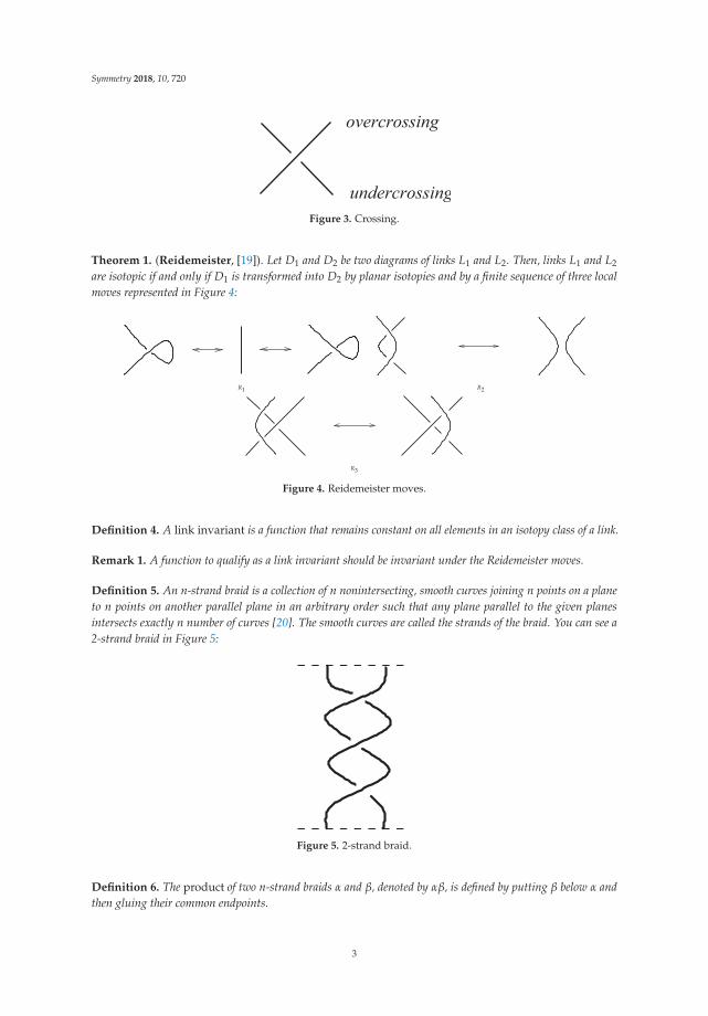
Figure 3. Crossing.

Theorem 1. (Reidemeister, [19]). Let D1 and D2 be two diagrams of links L1 and L2. Then, links L1 and L2

are isotopic if and only if D1 is transformed into D2 by planar isotopies and by a finite sequence of three localmoves represented in Figure 4:

R1 R2

R3

Figure 4. Reidemeister moves.

Definition 4. A link invariant is a function that remains constant on all elements in an isotopy class of a link.

Remark 1. A function to qualify as a link invariant should be invariant under the Reidemeister moves.

Definition 5. An n-strand braid is a collection of n nonintersecting, smooth curves joining n points on a planeto n points on another parallel plane in an arbitrary order such that any plane parallel to the given planesintersects exactly n number of curves [20]. The smooth curves are called the strands of the braid. You can see a2-strand braid in Figure 5:

Figure 5. 2-strand braid.

Definition 6. The product of two n-strand braids α and β, denoted by αβ, is defined by putting β below α andthen gluing their common endpoints.

3

Symmetry 2018, 10, 720

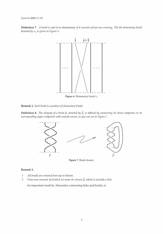
Definition 7. A braid is said to be elementary if it consists of just one crossing. The ith elementary braid,denoted by xi, is given in Figure 6:

Figure 6. Elementary braid xi.

Remark 2. Each braid is a product of elementary braids.

Definition 8. The closure of a braid β, denoted by β, is defined by connecting its lower endpoints to itscorresponding upper endpoints with smooth curves, as you can see in Figure 7.

β β

Figure 7. Braid closure.

Remark 3.

1 All braids are oriented from top to bottom.2 From now onward, by braid β we mean its closure β, which is actually a link.

An important result by Alexander, connecting links and braids, is:

4

Symmetry 2018, 10, 720

Theorem 2. (Alexander [21]). Each link is a closure of some braid.

Definition 9. The 0- and 1-smoothings of crossing are defined, respectively, by and .

Definition 10. A collection of disjoint circles obtained by smoothing out all the crossings of a link L is called theKauffman state of the link [22].

3. Homology

Definition 11. Let V =⊕

n Vn, be a graded vector space with homogeneous components {Vn} of degree n. Thegraded dimension of V is the power series q dim V: = ∑n qn dim Vn.

Definition 12. The degree of the tensor product of graded vector space V1 ⊗V2 is the sum of the degrees of thehomogeneous components of graded vector spaces V1 and V2.

Remark 4. In our case, the graded vector space V has the basis < v+, v− > with degree p(v±) = ±1 and theq-dimension q + q−1.

Definition 13. The degree shift .{l} operation on a graded vector space V =⊕

Vn is defined by(V.{l}

)n= Vn−l .

Construction of Chain Groups: Let L be a link with n crossings, and let all crossings be labeled from1 to n. Arrange all its 2n Kauffman states into columns 1, 2, . . . , n so that the rth column contains allstates having r number of 1-smoothings in it. To every stat α in the rth column we assign gradedvector space Vα(L) := V⊗m{r}, where m is the number of circles in α. The rth chain group, denoted by[[L]]r :=

⊕α:r=|α| Vα(L), is the direct sum of all vector spaces corresponding to all states in the

rth column.

Definition 14. The chain complex C of graded vector spaces Cr is defined as:

. . . −→ Cr+1 dr+1−−→ Cr dr

−→ Cr−1 dr−1−−→ . . .

such that dr ◦ dr+1 = 0 for each r.

In a system of converting the chain group into a complex, we use the maps between graded vectorspaces to satisfy d ◦ d. For this purpose we can label the edges of the cube {0, 1}χ by the sequence ξ

ε{0, 1, �}χ, where ξ contains only one � at a time. Here, � indicates that we change a 1-smoothing toa 0-smoothing. The maps on the edges is denoted by dξ , the height of edges |ξ|. The direct sum ofdifferentials in the cube along the column is

dr := ∑|ξ|=r

(−1)ξ dξ .

Now, we discuss the reason behind the sign of (−1)ξ . As we want from the differentials to satisfyd ◦ d = 0, the maps dξ have to anticommute on each of the vertex of the cube. A way to do this is bymultiplying edges dξ by (−1)ξ := (−1)∑i<j ξi , where j is the location of � in ξ.

For better understanding, please see the n-cube of trefoil knot x−31 in Figure 8.

5

Symmetry 2018, 10, 720

x−31 V{1}

d0�1←−−V⊗2{2}

V⊗2

d0�0←−−V{1} V⊗2{2}

d1�1←−−V⊗3{3}

V{1}d1�0←−−

V⊗2{2}

Figure 8. n-cube of x−31 .

It is useful to note that the ordered basis of V is⟨v+, v−

⟩and the ordered basis of V ⊗ V is⟨

v+ ⊗ v+, v− ⊗ v+, v+ ⊗ v−, v− ⊗ v−⟩.

Definition 15. Linear map m : V ⊗ V → V that merges two circles into a single circle is defined asm(v+ ⊗ v+) = v+, m(v+ ⊗ v−) = v−, m(v− ⊗ v+) = v− and m(v− ⊗ v−) = 0.

Map Δ : V → V ⊗ V that divides a circle into two circles is defined as Δ(v+) = v+ ⊗ v− + v− ⊗ v+ andΔ(v−) = v− ⊗ v−; see Figure 9.

Figure 9. m and Δ maps.

Definition 16. The homology group associated with the chain complex of a link L is defined asHr(L) = ker dr

im dr+1 .

Definition 17. The kernel of the map dr : V⊗r−1 → V⊗r, denoted by ker dr, is the set of all elements of V⊗r−1

that go to the zero element of V⊗r. The elements of the kernel are called cycles, while the elements of im dr+1 arecalled boundaries.

Remark 5. Note that the image of the chain complex of dr+1 is a subset of kernel dr as, in general, dr ◦ dr+1 = 0.

Definition 18. The graded Poincare polynomial Kh(L) in variables q and t of the complex is defined as

Kh(L) := ∑r

trqdimHr(L).

6

Symmetry 2018, 10, 720

Theorem 3. (Khovanov [1]). The graded dimension of homology groupsHr(L) are link invariants. The gradedPoincare polynomial Kh(L) is also a link invariant and Kh(L)

∣∣t=−1 = J(L).

3.1. Homology of x−31

Now, we give the Khovanov homology of link x−31 = :

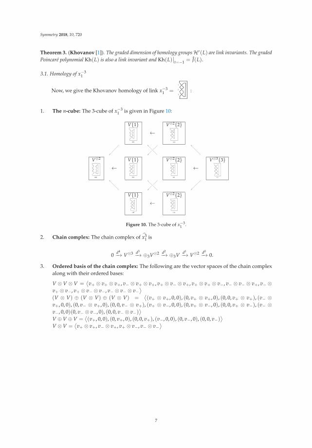
1. The n-cube: The 3-cube of x−31 is given in Figure 10:

V{1}←

V⊗2{2}

V⊗2

←V{1} V⊗2{2}

←V⊗3{3}

V{1}←

V⊗2{2}

Figure 10. The 3-cube of x−31 .

2. Chain complex: The chain complex of x31 is

0 d4−→ V⊗3 d3

−→ ⊕3V⊗2 d2−→ ⊕3V d1

−→ V⊗2 d0−→ 0.

3. Ordered basis of the chain complex: The following are the vector spaces of the chain complexalong with their ordered bases:

V ⊗ V ⊗ V =⟨v+ ⊗ v+ ⊗ v+, v− ⊗ v+ ⊗ v+, v+ ⊗ v− ⊗ v+, v+ ⊗ v+ ⊗ v−, v− ⊗ v− ⊗ v+, v− ⊗

v+ ⊗ v−, v+ ⊗ v− ⊗ v−, v− ⊗ v− ⊗ v−⟩

(V ⊗ V) ⊕ (V ⊗ V) ⊕ (V ⊗ V) =⟨(v+ ⊗ v+, 0, 0), (0, v+ ⊗ v+, 0), (0, 0, v+ ⊗ v+), (v− ⊗

v+, 0, 0), (0, v− ⊗ v+, 0), (0, 0, v− ⊗ v+), (v+ ⊗ v−, 0, 0), (0, v+ ⊗ v−, 0), (0, 0, v+ ⊗ v−), (v− ⊗v−, 0, 0)(0, v− ⊗ v−, 0), (0, 0, v− ⊗ v−)

⟩V ⊕V ⊕V =

⟨(v+, 0, 0), (0, v+, 0), (0, 0, v+), (v−, 0, 0), (0, v−, 0), (0, 0, v−)

⟩V ⊗V =

⟨v+ ⊗ v+, v− ⊗ v+, v+ ⊗ v−, v− ⊗ v−

⟩

7

Symmetry 2018, 10, 720

4. Differential maps in matrix form: Differential map d3(

V1 ⊗V2 ⊗V3

)=(

m(v1 ⊗ v2)⊗ v3, v1 ⊗

m(v2 ⊗ v3), v2 ⊗m(v1 ⊗ v3))

in terms of a matrix is:

d3 =

⎛⎜⎜⎜⎜⎜⎜⎜⎜⎜⎜⎜⎜⎜⎜⎜⎜⎜⎜⎜⎜⎜⎝

1 0 0 0 0 0 0 01 0 0 0 0 0 0 01 0 0 0 0 0 0 00 1 1 0 0 0 0 00 1 0 0 0 0 0 00 0 1 0 0 0 0 00 0 0 1 0 0 0 00 0 1 1 0 0 0 00 1 0 1 0 0 0 00 0 0 0 0 1 1 00 0 0 0 1 1 0 00 0 0 0 1 0 1 0

⎞⎟⎟⎟⎟⎟⎟⎟⎟⎟⎟⎟⎟⎟⎟⎟⎟⎟⎟⎟⎟⎟⎠

,

and map d2(

V1 ⊗ V2, V3 ⊗ V4, V5 ⊗ V6

)=

(m(v3 ⊗ v4) − m(v1 ⊗ v2), m(v5 ⊗ v6) − m(v1 ⊗

v2), m(v5 ⊗ v6)−m(v3 ⊗ v4))

is d2 =

(A 0 0 00 A A 0

), where A =

⎛⎜⎝ −1 1 0−1 0 10 −1 1

⎞⎟⎠ . Also,

d1(

V1, V2, V3

)= Δ(v1)− Δ(v2) + Δ(v3) is d1 =

⎛⎜⎜⎜⎝0 0 0 0 0 01 −1 1 0 0 01 −1 1 0 0 00 0 0 1 −1 1

⎞⎟⎟⎟⎠ .

5. Khovanov Homology: On solving d3x = 0 or⎛⎜⎜⎜⎜⎜⎜⎜⎜⎜⎜⎜⎜⎜⎜⎜⎜⎜⎜⎜⎜⎜⎝

1 0 0 0 0 0 0 01 0 0 0 0 0 0 01 0 0 0 0 0 0 00 1 1 0 0 0 0 00 1 0 0 0 0 0 00 0 1 0 0 0 0 00 0 0 1 0 0 0 00 0 1 1 0 0 0 00 1 0 1 0 0 0 00 0 0 0 0 1 1 00 0 0 0 1 1 0 00 0 0 0 1 0 1 0

⎞⎟⎟⎟⎟⎟⎟⎟⎟⎟⎟⎟⎟⎟⎟⎟⎟⎟⎟⎟⎟⎟⎠

⎛⎜⎜⎜⎜⎜⎜⎜⎜⎜⎜⎜⎜⎝

x1

x2

x3

x4

x5

x6

x7

x8

⎞⎟⎟⎟⎟⎟⎟⎟⎟⎟⎟⎟⎟⎠= 0,

8

Symmetry 2018, 10, 720

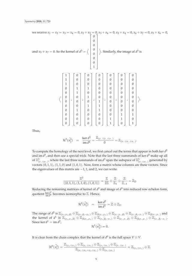
we receive x1 = x2 = x3 = x4 = 0, x2 + x3 = 0, x3 + x4 = 0, x2 + x4 = 0, x6 + x7 = 0, x5 + x6 = 0,

and x5 + x7 = 0. So the kernel of d3 =⟨⎡⎢⎢⎢⎢⎢⎢⎢⎢⎢⎢⎢⎢⎣

00000001

⎤⎥⎥⎥⎥⎥⎥⎥⎥⎥⎥⎥⎥⎦⟩

. Similarly, the image of d3 is

⟨

⎡⎢⎢⎢⎢⎢⎢⎢⎢⎢⎢⎢⎢⎢⎢⎢⎢⎢⎢⎢⎢⎢⎣

111000000000

⎤⎥⎥⎥⎥⎥⎥⎥⎥⎥⎥⎥⎥⎥⎥⎥⎥⎥⎥⎥⎥⎥⎦

,

⎡⎢⎢⎢⎢⎢⎢⎢⎢⎢⎢⎢⎢⎢⎢⎢⎢⎢⎢⎢⎢⎢⎣

000110001000

⎤⎥⎥⎥⎥⎥⎥⎥⎥⎥⎥⎥⎥⎥⎥⎥⎥⎥⎥⎥⎥⎥⎦

,

⎡⎢⎢⎢⎢⎢⎢⎢⎢⎢⎢⎢⎢⎢⎢⎢⎢⎢⎢⎢⎢⎢⎣

000101010000

⎤⎥⎥⎥⎥⎥⎥⎥⎥⎥⎥⎥⎥⎥⎥⎥⎥⎥⎥⎥⎥⎥⎦

,

⎡⎢⎢⎢⎢⎢⎢⎢⎢⎢⎢⎢⎢⎢⎢⎢⎢⎢⎢⎢⎢⎢⎣

000000111000

⎤⎥⎥⎥⎥⎥⎥⎥⎥⎥⎥⎥⎥⎥⎥⎥⎥⎥⎥⎥⎥⎥⎦

,

⎡⎢⎢⎢⎢⎢⎢⎢⎢⎢⎢⎢⎢⎢⎢⎢⎢⎢⎢⎢⎢⎢⎣

000000000011

⎤⎥⎥⎥⎥⎥⎥⎥⎥⎥⎥⎥⎥⎥⎥⎥⎥⎥⎥⎥⎥⎥⎦

,

⎡⎢⎢⎢⎢⎢⎢⎢⎢⎢⎢⎢⎢⎢⎢⎢⎢⎢⎢⎢⎢⎢⎣

000000000110

⎤⎥⎥⎥⎥⎥⎥⎥⎥⎥⎥⎥⎥⎥⎥⎥⎥⎥⎥⎥⎥⎥⎦

,

⎡⎢⎢⎢⎢⎢⎢⎢⎢⎢⎢⎢⎢⎢⎢⎢⎢⎢⎢⎢⎢⎢⎣

000000000101

⎤⎥⎥⎥⎥⎥⎥⎥⎥⎥⎥⎥⎥⎥⎥⎥⎥⎥⎥⎥⎥⎥⎦

⟩.

Thus,

H3(x31) =

ker d3

im d4 =Z(v−⊗v−⊗v−)

0= Z(v−⊗v−⊗v−).

To compute the homology of the next level, we first cancel out the terms that appear in both ker d2

and im d3, and then use a special trick: Note that the last three summands of ker d2 make up allof Z3

(v−⊗v−), where the last three summands of im d3 span the subspace of Z3

(v−⊗v−)generated by

vectors (0, 1, 1), (1, 1, 0) and (1, 0, 1). Now, form a matrix whose columns are these vectors. Sincethe eigenvalues of this matrix are −1, 1, and 2, we can write:

Z3

〈(0, 1, 1), (1, 1, 0), (1, 0, 1)〉 =Z

2Z⊕ Z

Z1⊕ Z

Z−1= Z2.

Reducing the remaining matrices of kernel of d2 and image of d3 into reduced row echelon form,quotient ker d2

im d3 becomes isomorphic to Z. Hence,

H2(x31) =

ker d2

im d3 = Z⊕Z2.

The range of d2 is Z(v+ ,v+ ,0) ⊕ Z(v+ ,0,−v+) ⊕ Z(0,v+ ,v+) ⊕ Z(v− ,v− ,0) ⊕ Z(v− ,0,−v−) ⊕ Z(0,v− ,v−) andthe kernel of d1 is Z(v+ ,v+ ,0) ⊕ Z(0,v+ ,v+) ⊕ Z(v+ ,0,−v+) ⊕ Z(v− ,v− ,0) ⊕ Z(0,v− ,v−) ⊕ Z(v− ,0,−v−).Since ker d1 = im d2,

H1(x31) = 0.

It is clear from the chain complex that the kernel of d0 is the full space V ⊗V.

H0(x31) =

Z(v+⊗v+) ⊕Z(v−⊗v+) ⊕Z(v+⊗v−) ⊕Z(v−⊗v−)

Z(v−⊗v++v+⊗v−) ⊕Z(v−⊗v−)= Z(v+⊗v+) ⊕Z.

9

Symmetry 2018, 10, 720

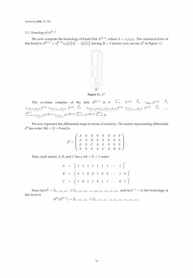
3.2. Homology of Δ2k+1

We now compute the homology of braid link Δ2k+1, where Δ = x1x2x1. The canonical form ofthis braid is Δ2k+1 = x2k+2

1 x2x21x2

2x21 · · · x2

2x21x2

1, having 2k + 2 factors; you can see Δ3 in Figure 11.

Δ3

Figure 11. Δ3.

The co-chain complex of the link Δ2k+1 is 0 d−1−−→ V⊗3 d0

−→ ⊕6k+3V⊗2 d1−→

⊕(2k+1

1 )(4k+21 )

V⊗1 ⊕(2k+1

1 )+(4k+22 )

V⊗3 d3−→ ⊕

(2k+11 )(4k+2

2 )+(2k+12 )(4k+2

1 )V⊗1 ⊕

(2k+11 )+(4k+2

2 )V⊗3 d4

−→ . . .

d6k+1−−−→ ⊕

(4k+21 )

V⊗2k+1 ⊕(2k+1

1 )V⊗2k+3 d6k+2

−−−→ V⊗2k+2 d6k+3−−−→ 0.

We now represent the differential maps in terms of matrices. The matrix representing differentiald0 has order 24k + 12× 8 and is

d0 =

⎛⎜⎜⎜⎝A 0 0 0 0 0 0 00 A B 0 0 0 0 00 0 C A 0 0 0 00 0 0 0 C A B 0

⎞⎟⎟⎟⎠ .

Here, each matrix A, B, and C has a (6k + 3)× 1 order:

A =(

1 1 1 1 1 1 1 · · · 1)t

B =(

0 1 0 0 1 0 0 · · · 1 0)t

C =(

1 0 1 1 0 1 1 · · · 0 1)t

Since ker d0 = Zv−⊗v−⊗v− ⊕ Zv+⊗v−⊗v−−v−⊗v+⊗v−+v+⊗v−⊗v− and im d−1 = 0, the homology atthis level is

H0(Δ2k+1) = Zv−⊗v−⊗v− ⊕Zv+⊗v−⊗v−−v−⊗v+⊗v−+v+⊗v−⊗v− .

10

Symmetry 2018, 10, 720

Now, we go for differential map d1. The matrix that represents it has an order of 20(6k2 + 3)×4(6k + 3) and is

d1 =

⎛⎜⎜⎜⎜⎜⎜⎜⎜⎜⎜⎜⎜⎜⎜⎜⎜⎜⎜⎜⎜⎜⎜⎜⎜⎝

R1 0 0 00 R1 R1 00 0 0 00 0 0 00 0 0 0

R2 0 0 0R2 0 0 00 R2 0 00 0 R2 00 0 0 R2

0 R3 R4 0...

.... . .

...0 0 Rn−1 Rn

⎞⎟⎟⎟⎟⎟⎟⎟⎟⎟⎟⎟⎟⎟⎟⎟⎟⎟⎟⎟⎟⎟⎟⎟⎟⎠

.

The order of each of the matrix Ri is (12k + 6)× (6k + 3):

R1 =

⎛⎜⎜⎜⎜⎜⎜⎜⎜⎜⎜⎜⎜⎜⎜⎜⎝

1 −1 0 0 0 . . . 0 01 0 0 0 −1 0 . . . 01 0 0 0 0 0 . . . −10 1 −1 0 0 0 . . . 00 1 0 −1 0 0 . . . 00 1 0 0 0 −1 . . . 00 1 0 0 0 0 . . . −1...

......

......

......

...0 0 0 0 0 . . . 1 −1

⎞⎟⎟⎟⎟⎟⎟⎟⎟⎟⎟⎟⎟⎟⎟⎟⎠,

R2 =

⎛⎜⎜⎜⎜⎜⎜⎜⎜⎜⎜⎜⎜⎜⎜⎜⎝

1 0 −1 0 0 . . . 0 01 0 . . . −1 0 0 0 01 0 . . . 0 0 −1 0 01 0 . . . 0 0 0 −1 01 0 . . . 0 0 0 0 −10 1 0 0 −1 0 . . . 00 1 . . . 0 0 −1 0 0...

......

......

......

...0 0 0 0 . . . 1 0 −1

⎞⎟⎟⎟⎟⎟⎟⎟⎟⎟⎟⎟⎟⎟⎟⎟⎠,

R3 =

⎛⎜⎜⎜⎜⎜⎜⎜⎜⎜⎜⎜⎜⎜⎜⎜⎜⎜⎜⎜⎝

1 0 −1 0 0 . . . 0 01 0 . . . −1 0 0 0 01 0 . . . 0 0 −1 0 01 0 . . . 0 0 0 −1 01 0 . . . 0 0 0 0 −10 0 1 −1 0 0 . . . 00 0 1 0 0 −1 . . . 00 0 1 0 . . . −1 0 00 0 1 0 . . . 0 0 −1...

......

......

......

...0 0 0 0 . . . 1 0 −1

⎞⎟⎟⎟⎟⎟⎟⎟⎟⎟⎟⎟⎟⎟⎟⎟⎟⎟⎟⎟⎠

,

11

Symmetry 2018, 10, 720

R4 =

⎛⎜⎜⎜⎜⎜⎜⎜⎜⎜⎝

0 0 0 0 0 . . . 0 0...

......

......

......

...0 1 0 0 −1 0 . . . 00 1 . . . 0 0 −1 0 0...

......

......

......

...0 0 0 0 1 0 . . . −1

⎞⎟⎟⎟⎟⎟⎟⎟⎟⎟⎠,

and, at the end, all rows of matrix Rn are zero except for the last row, which is(0 . . . 0 0 1 0 . . . −1

).

Here, ker d1 = Z(v+⊗v++v+⊗v++v+⊗v++v+⊗v++v+⊗v++v+⊗v++v+⊗v++v+⊗v+)⊕Z(v+⊗v−+v+⊗v−+v+⊗v−+v+⊗v−+v+⊗v−+v+⊗v−+v+⊗v−+v+⊗v−)⊕Z(v−⊗v++v−⊗v+−v+⊗v−−v+⊗v−−v+⊗v−)⊕Z(v+⊗v−+v+⊗v−+v+⊗v−+v−⊗v++v−⊗v++v−⊗v++v−⊗v++v−⊗v+)⊕Z(v−⊗v−+v−⊗v−) ⊕Z(v−⊗v−+v−⊗v−+v−⊗v−+v−⊗v−+v−⊗v−)andim d0 = Z(v+⊗v+) ⊕Z(v+⊗v−) ⊕Z(v−⊗v+) ⊕Z(v−⊗v−) ⊕Z(v+⊗v+) ⊕Z(v+⊗v−) ⊕Z(v−⊗v+).Since the number of Z spaces appear in the kernel of d1, it is exactly the same as the image of d0,H1(Δ2k+1) = 0.The image of d1 is obvious. We just need the kernel of d2. The matrix that represents d2 has an order of(26k+3 + 22k+2)(6k + 5)× 20(6k2 + 3) and is⎛⎜⎝

S1 S2 S3 S4 S5 S6 S7 S8 S9 . . . S20

S21 S21 S22 S23 S24 S25 S26 S27 S28 . . . S40

......

......

......

......

......

...Sn−19 Sn−18 Sn−17 Sn−16 Sn−15 Sn−14 Sn−13 Sn−12 Sn−11 . . . Sn

⎞⎟⎠ .

Here, the order of each Si is (4k2 + 3)× (6k2 + 3), and is:

S1 =

⎛⎜⎜⎜⎜⎜⎜⎜⎜⎜⎝

0 −1 0 0 0 0 . . . 01 0 0 0 0 0 . . . 11 0 0 0 0 0 . . . 10 0 0 0 0 0 . . . 00 0 −1 0 0 0 . . . 01 0 0 0 0 0 . . . 01 0 0 0 0 0 . . . 0...

......

......

......

...0 0 0 0 0 0 . . . 0

⎞⎟⎟⎟⎟⎟⎟⎟⎟⎟⎠, S2 =

⎛⎜⎜⎜⎜⎜⎜⎜⎝

0 0 0 0 0 0 . . . 00 0 0 0 0 0 . . . 00 0 0 0 0 0 . . . 00 0 0 0 0 0 . . . 00 0 0 0 0 0 . . . 01 0 0 0 0 0 . . . 0...

......

......

......

...1 0 0 0 0 0 . . . 0

⎞⎟⎟⎟⎟⎟⎟⎟⎠,

S3 =

⎛⎜⎜⎜⎜⎜⎜⎜⎝

0 0 0 0 0 0 . . . 00 −1 0 0 0 0 . . . 00 0 0 0 0 0 . . . 01 0 0 0 0 0 . . . 10 0 −1 0 0 0 . . . 00 0 0 0 0 0 . . . 0...

......

......

......

...0 0 0 0 0 0 . . . 0

⎞⎟⎟⎟⎟⎟⎟⎟⎠, S4 =

⎛⎜⎜⎜⎜⎜⎜⎜⎜⎜⎝

0 0 0 0 0 0 . . . 00 0 0 0 0 0 . . . 0−1 0 0 0 0 0 . . . 00 0 0 0 0 0 . . . 00 0 0 0 0 0 . . . 00 0 0 0 0 0 . . . 00 −1 0 0 0 0 . . . 0...

......

......

......

...0 0 0 0 0 0 . . . 0

⎞⎟⎟⎟⎟⎟⎟⎟⎟⎟⎠,

...

12

Symmetry 2018, 10, 720

Sn−2 =

⎛⎜⎜⎜⎜⎜⎜⎜⎝

0 0 0 0 0 0 . . . 00 0 0 0 0 0 . . . 00 0 −1 0 0 0 . . . 00 0 0 0 0 0 . . . 00 0 0 0 0 0 . . . 00 0 0 0 0 0 . . . 0...

......

......

......

...0 0 0 0 0 0 . . . 0

⎞⎟⎟⎟⎟⎟⎟⎟⎠,

Sn−1 =

⎛⎜⎜⎜⎜⎜⎜⎜⎝

0 0 0 0 0 0 . . . 00 0 0 0 0 0 . . . 00 0 0 0 0 0 . . . 0−1 0 0 0 0 0 . . . −10 0 0 0 0 0 . . . 00 0 0 0 0 0 . . . 0...

......

......

......

...0 −1 0 0 0 0 . . . 0

⎞⎟⎟⎟⎟⎟⎟⎟⎠,

Sn =

⎛⎜⎜⎜⎜⎜⎜⎜⎝

0 0 0 0 0 0 . . . 00 0 0 0 0 0 . . . 00 0 0 0 0 0 . . . 00 0 0 0 0 0 . . . 00 0 0 0 0 0 . . . 00 0 0 0 0 0 . . . 0...

......

......

......

...−1 0 0 0 0 0 . . . 0

⎞⎟⎟⎟⎟⎟⎟⎟⎠.

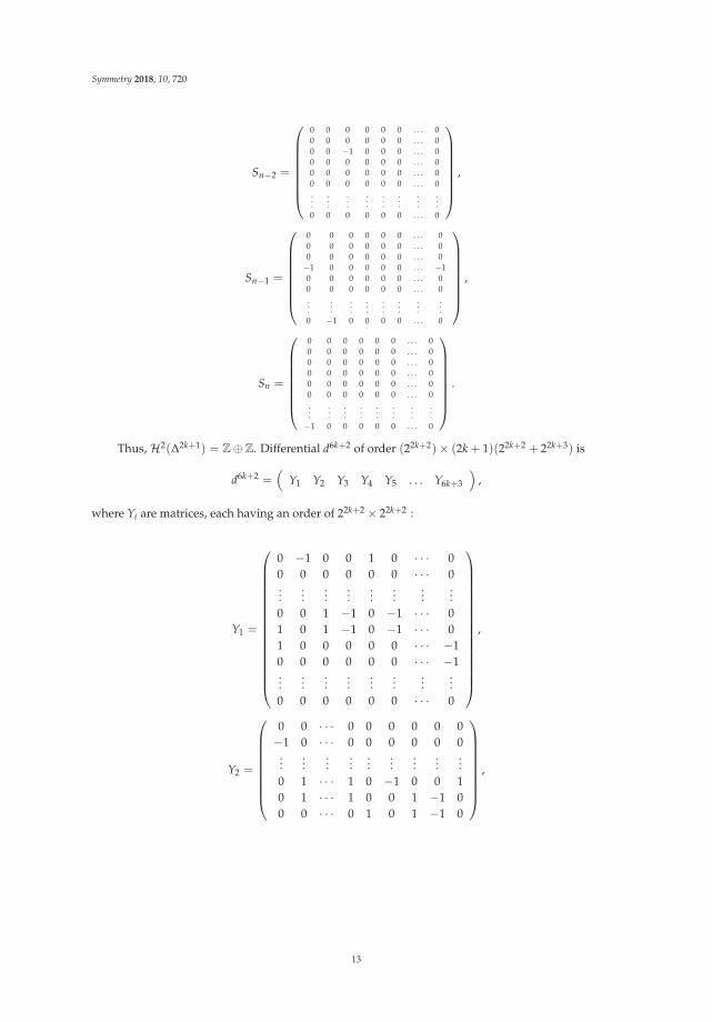
Thus,H2(Δ2k+1) = Z⊕Z. Differential d6k+2 of order (22k+2)× (2k + 1)(22k+2 + 22k+3) is

d6k+2 =(

Y1 Y2 Y3 Y4 Y5 . . . Y6k+3

),

where Yi are matrices, each having an order of 22k+2 × 22k+2 :

Y1 =

⎛⎜⎜⎜⎜⎜⎜⎜⎜⎜⎜⎜⎜⎜⎜⎜⎜⎝

0 −1 0 0 1 0 · · · 00 0 0 0 0 0 · · · 0...

......

......

......

...0 0 1 −1 0 −1 · · · 01 0 1 −1 0 −1 · · · 01 0 0 0 0 0 · · · −10 0 0 0 0 0 · · · −1...

......

......

......

...0 0 0 0 0 0 · · · 0

⎞⎟⎟⎟⎟⎟⎟⎟⎟⎟⎟⎟⎟⎟⎟⎟⎟⎠,

Y2 =

⎛⎜⎜⎜⎜⎜⎜⎜⎜⎝

0 0 · · · 0 0 0 0 0 0−1 0 · · · 0 0 0 0 0 0

......

......

......

......

...0 1 · · · 1 0 −1 0 0 10 1 · · · 1 0 0 1 −1 00 0 · · · 0 1 0 1 −1 0

⎞⎟⎟⎟⎟⎟⎟⎟⎟⎠,

13

Symmetry 2018, 10, 720

Y3 =

⎛⎜⎜⎜⎜⎜⎜⎜⎜⎜⎜⎝

0 0 0 0 0 0 0 0 · · ·0 0 0 0 0 0 0 0 · · ·0 0 −1 0 0 0 0 0 · · ·0 0 0 0 0 −1 0 0 · · ·...

......

......

......

......

−1 1 0 0 0 0 0 0 · · ·−1 1 0 1 0 0 1 −1 · · ·

⎞⎟⎟⎟⎟⎟⎟⎟⎟⎟⎟⎠,

Y4 =

⎛⎜⎜⎜⎜⎜⎜⎜⎜⎜⎜⎜⎜⎜⎜⎜⎜⎝

0 0 0 0 0 0 0 · · ·0 0 0 0 0 0 0 · · ·...

......

......

......

...0 1 0 0 −1 0 0 · · ·0 0 0 0 0 0 0 · · ·−1 0 −1 1 0 0 0 · · ·−1 0 −1 1 0 0 0 · · ·

......

......

......

......

0 0 0 0 0 0 1 · · ·

⎞⎟⎟⎟⎟⎟⎟⎟⎟⎟⎟⎟⎟⎟⎟⎟⎟⎠,

...

Yi =

⎛⎜⎜⎜⎜⎜⎜⎜⎜⎜⎜⎜⎜⎜⎜⎜⎜⎜⎜⎝

0 0 0 0 0 0 0 0 · · ·0 0 0 0 0 0 0 0 · · ·...

......

......

......

......

0 −1 0 0 0 0 0 0 · · ·0 0 0 0 0 0 0 0 · · ·0 0 0 0 −1 1 −1 0 · · ·0 0 1 −1 0 0 0 −1 · · ·−1 0 0 0 0 0 0 0 · · ·

......

......

......

......

...0 0 0 0 0 0 0 0 · · ·

⎞⎟⎟⎟⎟⎟⎟⎟⎟⎟⎟⎟⎟⎟⎟⎟⎟⎟⎟⎠

,

...

Y6k+3 =

⎛⎜⎜⎜⎜⎜⎜⎜⎜⎝

0 0 0 0 0 0 0 · · · 00 0 0 0 0 0 0 · · · 00 0 0 0 0 0 0 · · · 00 0 0 0 0 0 0 · · · 0...

......

......

......

......

0 −1 1 −1 0 0 0 · · · 0

⎞⎟⎟⎟⎟⎟⎟⎟⎟⎠.

Here ker d6k+3 is the full space V⊗2k+1 and the im d6k+2 is

Z(v+⊗v+⊗v+⊗v+) ⊕Z(v+⊗v−⊗v+⊗v++v−⊗v+⊗v+⊗v+)⊕Z(v+⊗v+⊗v−⊗v++v+⊗v−⊗v+⊗v+)Z(v+⊗v−⊗v+⊗v+)⊕Z(v+⊗v−⊗v+⊗v−+v−⊗v+⊗v+⊗v−) ⊕Z(v+⊗v+⊗v−⊗v−+v+⊗v−⊗v+⊗v−)⊕Z(v+⊗v+⊗v+⊗v−) ⊕Z(v+⊗v−⊗v−⊗v++v−⊗v+⊗v−⊗v+)⊕Z(v+⊗v−⊗v+⊗v−+v−⊗v+⊗v+⊗v−) ⊕Z(v+⊗v−⊗v−⊗v+) ⊕Z(v−⊗v−⊗v+⊗v+)

⊕Z(v+⊗v+⊗v−⊗v+) ⊕Z(v−⊗v+⊗v−⊗v++v−⊗v−⊗v+⊗v+)⊕Z(v+⊗v−⊗v−⊗v−+v−⊗v+⊗v−⊗v−) ⊕Z(v+⊗v−⊗v−⊗v−) ⊕Z(v−⊗v−⊗v+⊗v−)⊕Z(v−⊗v−⊗v−⊗v+) ⊕Z(v+⊗v−⊗v+⊗v−) ⊕Z(v−⊗v−⊗v−⊗v−)

14

Symmetry 2018, 10, 720

⊕Z(v+⊗v+⊗v−⊗v−) ⊕Z(v−⊗v+⊗v+⊗v−)⊕Z(v−⊗v+⊗v−⊗v+) ⊕Z(v−⊗v+⊗v−⊗v−).

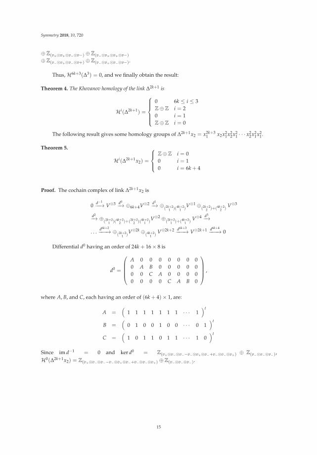
Thus,H6k+3(Δ3) = 0, and we finally obtain the result:

Theorem 4. The Khovanov homology of the link Δ2k+1 is

Hi(Δ2k+1) =

⎧⎪⎪⎪⎨⎪⎪⎪⎩0 6k ≤ i ≤ 3Z⊕Z i = 20 i = 1Z⊕Z i = 0

The following result gives some homology groups of Δ2k+1x2 = x2k+31 x2x2

1x22x2

1 · · · x22x2

1x21.

Theorem 5.

Hi(Δ2k+1x2) =

⎧⎪⎨⎪⎩Z⊕Z i = 00 i = 10 i = 6k + 4

Proof. The cochain complex of link Δ2k+1x2 is

0 d−1−−→ V⊗3 d0

−→ ⊕6k+4V⊗2 d1−→ ⊕

(2k+21 )(4k+2

1 )V⊗1 ⊕

(2k+22 )+(4k+2

2 )V⊗3

d2−→ ⊕

(2k+21 )(4k+2

2 )+(2k+22 )(4k+2

1 )V⊗2 ⊕

(2k+21 )+(4k+2

1 )V⊗4 d3

−→

. . . d6k+2−−−→ ⊕

(2k+21 )

V⊗2k ⊕(4k+2

1 )V⊗2k+2 d6k+3

−−−→ V⊗2k+1 d6k+4−−−→ 0

Differential d0 having an order of 24k + 16× 8 is

d0 =

⎛⎜⎜⎜⎝A 0 0 0 0 0 0 00 A B 0 0 0 0 00 0 C A 0 0 0 00 0 0 0 C A B 0

⎞⎟⎟⎟⎠ ,

where A, B, and C, each having an order of (6k + 4)× 1, are:

A =(

1 1 1 1 1 1 1 · · · 1)t

B =(

0 1 0 0 1 0 0 · · · 0 1)t

C =(

1 0 1 1 0 1 1 · · · 1 0)t

Since im d−1 = 0 and ker d0 = Z(v+⊗v−⊗v−−v−⊗v+⊗v−+v−⊗v−⊗v+) ⊕ Z(v−⊗v−⊗v−),H0(Δ2k+1x2) = Z(v+⊗v−⊗v−−v−⊗v+⊗v−+v−⊗v−⊗v+) ⊕Z(v−⊗v−⊗v−).

15

Symmetry 2018, 10, 720

Now, differential d1 of an order of 18(6k2 + 6)× 4(6k + 4) is

d1 =

⎛⎜⎜⎜⎜⎜⎜⎜⎜⎜⎜⎜⎜⎜⎜⎜⎜⎜⎜⎜⎝

M1 −M1 0 0M1 0 −M1 0M1 0 0 −M1

M2 −M2 0 0M2 0 −M2 0M3 −M3 0 0M3 0 −M3 00 M4 −M4 00 M4 0 −M4...

.... . .

...0 0 Mn−1 Mn

⎞⎟⎟⎟⎟⎟⎟⎟⎟⎟⎟⎟⎟⎟⎟⎟⎟⎟⎟⎟⎠

,

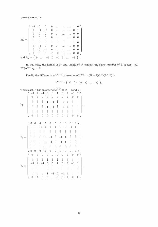
where the order of each Mi is (16k + 2)× (6k + 4) and is

M1 =

⎛⎜⎜⎜⎜⎜⎜⎜⎜⎜⎜⎜⎜⎜⎜⎜⎝

−1 0 0 0 1 0 . . . 00 −1 −1 0 0 1 . . . 00 0 0 0 0 0 . . . 00 0 0 0 0 0 . . . 0−1 0 0 0 0 0 . . . 0−1 0 0 0 0 0 . . . 00 −1 0 0 0 0 . . . 1...

......

......

......

...0 0 0 −1 0 . . . 0 0

⎞⎟⎟⎟⎟⎟⎟⎟⎟⎟⎟⎟⎟⎟⎟⎟⎠,

M2 =

⎛⎜⎜⎜⎜⎜⎜⎜⎜⎜⎜⎜⎜⎜⎜⎜⎝

0 . . . −1 0 . . . 0 00 . . . 0 0 0 0 00 . . . 0 −1 0 0 00 . . . 0 0 −1 0 00 . . . 0 0 −1 0 00 . . . −1 0 . . . 0 00 . . . 0 −1 −1 0 0...

......

......

......

0 . . . 0 −1 0 0 0

⎞⎟⎟⎟⎟⎟⎟⎟⎟⎟⎟⎟⎟⎟⎟⎟⎠,

M3 =

⎛⎜⎜⎜⎜⎜⎜⎜⎜⎜⎜⎜⎜⎜⎜⎜⎝

0 . . . −1 0 0 0 0 0 00 . . . 0 −1 −1 0 0 0 00 . . . 0 0 0 0 0 0 00 . . . −1 0 0 1 0 0 00 . . . −1 0 0 1 0 0 00 . . . 0 0 0 0 0 0 −10 . . . 0 0 0 0 0 0 −1...

......

......

......

... 00 . . . 0 0 0 0 0 0 0

⎞⎟⎟⎟⎟⎟⎟⎟⎟⎟⎟⎟⎟⎟⎟⎟⎠,

16

Symmetry 2018, 10, 720

M4 =

⎛⎜⎜⎜⎜⎜⎜⎜⎜⎜⎜⎜⎜⎜⎝

−1 0 0 0 . . . . . . . . . 1 00 −1 −1 0 . . . . . . . . . 0 10 0 0 0 . . . . . . . . . 0 00 0 0 0 . . . . . . . . . 0 0...

......

......

......

... 00 −1 0 0 . . . . . . . . . 0 00 0 −1 0 . . . . . . . . . 0 00 0 0 −1 0 0 . . . 0 0

⎞⎟⎟⎟⎟⎟⎟⎟⎟⎟⎟⎟⎟⎟⎠,

and Mn =(

0 . . . −1 0 −1 0 . . . −1)

.

In this case, the kernel of d1 and image of d0 contain the same number of Z spaces. So,H1(Δ2k+1x2) = 0.

Finally, the differential of d6k+4 of an order of 22k+1 × (2k + 3)(22k)(22k+1) is

d6k+4 =(

Y1 Y2 Y3 Y4 . . . Yi

),

where each Yi has an order of 22k+1 × 6k + 4 and is

Y1 =

⎛⎜⎜⎜⎜⎜⎜⎜⎜⎜⎜⎝

−1 1 −1 0 0 1 0 0 −1 10 0 0 0 0 0 0 0 0 0...

...... 1 −1

... −1 1...

......

...... 1 −1

... −1 1...

......

......

......

......

......

...0 0 0 0 0 0 0 0 0 0

⎞⎟⎟⎟⎟⎟⎟⎟⎟⎟⎟⎠,

Y2 =

⎛⎜⎜⎜⎜⎜⎜⎜⎜⎜⎜⎜⎜⎜⎝

0 0 0 0 0 0 0 0 0 01 1 −1 0 0 1 0 0 −1 1...

......

......

......

......

......

...... 1 −1

... −1 1...

......

...... 1 −1

... −1 1...

......

......

......

......

......

...0 0 0 0 0 0 0 0 0 0

⎞⎟⎟⎟⎟⎟⎟⎟⎟⎟⎟⎟⎟⎟⎠,

Y3 =

⎛⎜⎜⎜⎜⎜⎜⎜⎜⎜⎜⎝

0 0 0 0 0 0 0 0 0 0...

......

......

......

......

...−1 1 −1 0 0 1 0 0 −1 1

......

......

......

......

......

......

... 1 −1 0 −1 1...

...0 0 0 0 0 0 0 0 0 0

⎞⎟⎟⎟⎟⎟⎟⎟⎟⎟⎟⎠,

17

Symmetry 2018, 10, 720

Y4 =

⎛⎜⎜⎜⎜⎜⎜⎜⎝

0 0 0 0 0 0 0 0 0 0...

......

......

......

......

...−1 1 −1 0 0 1 0 0 −1 1

......

......

......

......

......

0 0 0 1 −1 0 −1 1 0 0

⎞⎟⎟⎟⎟⎟⎟⎟⎠,

...

and Yi =

⎛⎜⎜⎜⎜⎜⎜⎜⎜⎝

0 0 0 0 0 0 0 · · · 00 0 0 0 0 0 0 · · · 00 0 0 0 0 0 0 · · · 00 0 0 0 0 0 0 · · · 0...

......

......

......

......

−1 1 −1 0 0 1 0 · · · 0

⎞⎟⎟⎟⎟⎟⎟⎟⎟⎠.

It is evident that ker d6k+4 is full space V⊗2k+1. Moreover, im d6k+3 is also V⊗2k+1.We also get the Khovanov homology of braid link Δ2k+1x1:

Theorem 6.

Hi(Δ2k+1x1) =

⎧⎪⎨⎪⎩Z⊕Z i = 00 i = 10 i = 6k + 1

Proof. The proof is similar to the proof of Theorem 5: Obtain all states, organized them in columns,assign a graded vector space to each state, form chain groups as a direct sum of all vector spaces alonga column, and form the chain complex. Then, write the differential maps in terms of matrices using theordered bases of the chain groups, and compute their kernels and images. Finally, find the Khovanovhomology groups using the relationHr(L) = ker dr

im dr+1 .

4. Conclusions

Although computing the Khovanov homology of links is common in the literature, no generalformulae have been given for all families of knots and links. In this paper, we considered a generalthree-strand braid x1x2x1x2 · · · , which, depending on the powers of Garside element Δ = x1x2x1,is divided into six subclasses, and gave the Khovanov homology of Δ2k+1, Δ2k+1x2, and Δ2k+1x1

(To learn more about these classes, see Reference [23–26].) The results particularly cover the 0th, 1st,and top homology groups of these classes, and all homology groups, in general, of link Δ2k+1. We hopethe results will help classifying links, and in studying the important properties of these links.

Author Contributions: Formal analysis, Y.C.K.; writing—original draft, A.R.N., Z.I., D.A., and S.M.K.; writing—reviewand editing, M.M.

Funding: This work was supported by the Dong-A University research fund.

Acknowledgments: We are very thankful to the reviewers for their valuable suggestions to improve the qualityof this paper.

Conflicts of Interest: The authors declare that they have no conflicts of interest.

References

1. Khovanov, M. A Categorification of the Jones Polynomial. Duke Math. J. 2000, 101, 359–426. [CrossRef]2. Jones, V.F.R. A Polynomial Invariant for Knots via Von Neumann Algebras. Bull. Am. Math. Soc. 1985,

12, 103–111. [CrossRef]

18

Symmetry 2018, 10, 720

3. Bar-Natan, D. On Khovanov’s categorification of the Jones polynomial. Algeb. Geom. Topol. 2002, 2, 337–370.[CrossRef]

4. Bar-Natan, D. Khovanov Homology for Tangles and Cobordisms. Geom. Topol. 2005, 9, 1443–1499. [CrossRef]5. Bar-Natan, D. Fast Khovanov Homology Computations. J. Knot Theory Ramif. 2007, 16, 243–255. [CrossRef]6. Ozsváth, P.; Rasmussen, J.; Szabó, Z. Odd Khovanov Homology. Algebr. Geom. Topol. 2013, 13, 1465–1488.

[CrossRef]7. Gorsky, E.; Oblomkov, A.; Rasmussen, J. On Stable Khovanov Homology of Torus Knots. Exp. Math. 2013,

22, 265–281. [CrossRef]8. Putyra, K.K. On Triply Graded Khovanov Homology. arXiv 2015, arXiv:1501.05293v1.9. Manion, A. The Rational Khovanov Homology of 3-Strand Pretzel Links. arXiv 2011, arXiv:1110.2239.10. Nizami, A.R.; Munir, M.; Usman, A. Khovanov Homology of Braid Links. Rev. UMA 2016, 57, 95–118.11. Nizami, A.R.; Munir, M.; Sohail, T.; Usman, A. On the Khovanov Homology of 2- and 3-Strand Braid Links.

Adv. Pure Math. 2016, 6, 481–491. [CrossRef]12. Stosic, M. Properties of Khovanov Homology for Positive Braid Knots. arXiv 2006, arXiv:math/0511529.13. Rozansky, L. An Infinite Torus Braid Yields a Categorified Jones-Wenzl Projector. Fundam. Math. 2014,

225, 305–326. [CrossRef]14. Cooper, B.; Krushkal, V. Categorification of the Jones-Wenzl projectors. Quantum Topol. 2012, 3, 139–180.

[CrossRef] [PubMed]15. Gorsky, E.; Oblomkov, A.; Rasmussen, J.; Shende, V. Torus Knots and the Rational DAHA. Duke Math. J.

2014, 163, 2709–2794. [CrossRef]16. Hogancamp, M. Categorified Young Symmetrizers and Stable Homology of Torus Links. Geom. Topol. 2018,

22, 2943–3002. [CrossRef]17. Lipshitz, R.; Sarkar, S. A Khovanov Stable Homotopy Type. J. Am. Math. Soc. 2014, 27, 983–1042. [CrossRef]18. Manturov, V. Knot Theory; Chapman and Hall/CRC: Boca Raton, FL, USA, 2004.19. Reidemeister, K. Elementary Begründung der Knotentheorie. Abh. Math. Sem. Univ. Hambg. 1927, 5, 24–32.

[CrossRef]20. Artin, E. Theory of Braids. Ann. Math. 1947, 48, 101–126. [CrossRef]21. Alexander, J. Topological invariants of knots and links. Trans. Am. Math. Soc. 1928, 20, 275–306. [CrossRef]22. Kauffman, L.H. State Models and the Jones Polynomial. Topology 1987, 26, 395–407. [CrossRef]23. Berceanu, B.; Nizami, A.R. A recurrence relation for the Jones polynomial. J. Korean Math. Soc. 2014, 51,

443–462. [CrossRef]24. Khovanov, M. Patterns in Knot Cohomology I. Exp. Math. 2003, 12, 365–374. [CrossRef]25. Lawson, T.; Lipshitz, R.; Sarkar, S. The Cube and the Burnside Category. arXiv 2015, arXiv:1505.00512.26. Reidemeister, K. Knot Theory; Chelsea Publ. and Co.: New York, NY, USA, 1948.

c© 2018 by the authors. Licensee MDPI, Basel, Switzerland. This article is an open accessarticle distributed under the terms and conditions of the Creative Commons Attribution(CC BY) license (http://creativecommons.org/licenses/by/4.0/).

19

symmetryS SArticle

Volume Preserving Maps Between p-Balls

Adrian Holhos * and Daniela Rosca

Department of Mathematics, Technical University of Cluj-Napoca, str. Memorandumului 28,RO-400114 Cluj-Napoca, Romania; daniela.rosca@math.utcluj.ro* Correspondence: Adrian.Holhos@math.utcluj.ro

Received: 19 October 2019; Accepted: 12 November 2019; Published: 14 November 2019

Abstract: We construct a volume preserving map Up from the p-ball Bp(r) ={

x ∈ R3, ‖x‖p ≤ r}

tothe regular octahedron B1(r′), for arbitrary p > 0. Then we calculate the inverse U−1

p and we alsodeduce explicit expressions for U∞ and U−1

∞ . This allows us to construct volume preserving mapsbetween arbitrary balls Bp(r) and Bp′(r), and also to map uniform and refinable grids between them.Finally we list some possible applications of our maps.

Keywords: equal volume projection; hierarchical grid

1. Introduction

The p-norms in R3 have applications in many branches of mathematics, physics and computerscience. For p ≥ 1, the p-norm of the vector x = (x, y, z) ∈ R3 (also called Lp-norm) is defined as

‖x‖p = (|x|p + |y|p + |z|p)1/p . (1)

For p = 2, we arrive at the Euclidean norm, and when p → ∞ the norm is called the infinity normor the maximum norm and is given by

‖x‖∞ = max(|x|, |y|, |z|).

When p ∈ (0, 1), Formula (1) does not define a norm, because the triangle inequality isnot satisfied.

2. Preliminaries

For p > 0, let Bp(r) be the 3D p-ball of radius r > 0 centered at the origin, defined by

Bp(r) ={

x ∈ R3, ‖x‖p ≤ r

}.

For finite p the parametric equations of Bp(r) are

x = ρ |cos θ|2/p |sin ϕ|2/p sgn(cos θ) sgn(sin ϕ),

y = ρ |sin θ|2/p |sin ϕ|2/p sgn(sin θ) sgn(sin ϕ),

z = ρ |cos ϕ|2/p sgn(cos ϕ),

with ρ ∈ [0, r], θ ∈ [0, 2π), ϕ ∈ [0, π].For p = 1 the ball B1(r) is the regular octahedron with the vertices on the axes, at distance r from

the origin. For p = ∞, the set B∞(r) is the cube with edge of length 2r and for p = 2 the region B2(r)represents the Euclidean ball. For p > 2 the balls are called superellipsoids and they are used in computer

Symmetry 2019, 11, 1404; doi:10.3390/sym11111404 www.mdpi.com/journal/symmetry21

Symmetry 2019, 11, 1404

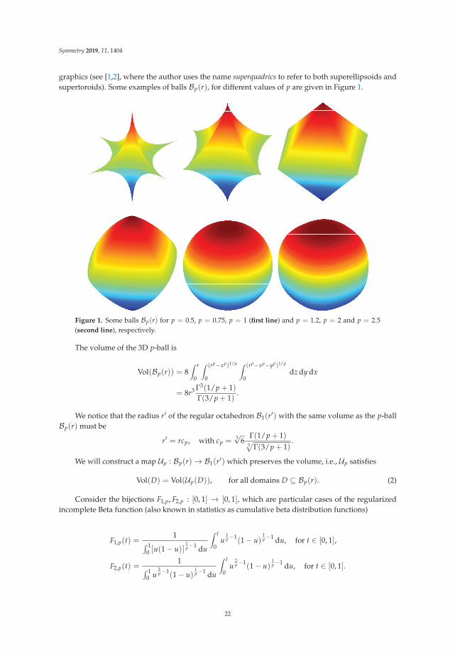
graphics (see [1,2], where the author uses the name superquadrics to refer to both superellipsoids andsupertoroids). Some examples of balls Bp(r), for different values of p are given in Figure 1.

Figure 1. Some balls Bp(r) for p = 0.5, p = 0.75, p = 1 (first line) and p = 1.2, p = 2 and p = 2.5(second line), respectively.

The volume of the 3D p-ball is

Vol(Bp(r)) = 8∫ r

0

∫ (rp−xp)1/p

0

∫ (rp−xp−yp)1/p

0dz dy dx

= 8r3 Γ3(1/p + 1)Γ(3/p + 1)

.

We notice that the radius r′ of the regular octahedron B1(r′) with the same volume as the p-ballBp(r) must be

r′ = rcp, with cp =3√

6Γ(1/p + 1)

3√

Γ(3/p + 1).

We will construct a map Up : Bp(r)→ B1(r′) which preserves the volume, i.e., Up satisfies

Vol(D) = Vol(Up(D)), for all domains D ⊆ Bp(r). (2)

Consider the bijections F1,p, F2,p : [0, 1] → [0, 1], which are particular cases of the regularizedincomplete Beta function (also known in statistics as cumulative beta distribution functions)

F1,p(t) =1∫ 1

0 [u(1− u)]1p−1 du

∫ t

0u

1p−1

(1− u)1p−1 du, for t ∈ [0, 1],

F2,p(t) =1∫ 1

0 u2p−1

(1− u)1p−1 du

∫ t

0u

2p−1

(1− u)1p−1 du, for t ∈ [0, 1].

22

Symmetry 2019, 11, 1404

In the standard notation we have F1,p(t) = It(1/p, 1/p) and F2,p(t) = It(2/p, 1/p), where It isthe so-called regularized incomplete beta function defined as It(α, β) = B(t; α, β)/B(1; α, β), with

B(t; α, β) =∫ t

0uα−1(1− u)β−1du, for α, β > 0.

One has F1,p(0) = F2,p(0) = 0 and F1,p(1) = F2,p(1) = 1, further F1,p, F2,p are increasingfunctions. Let G1,p, G2,p : [0, 1] → [0, 1] be the inverses (in Mathematica one can use the commandInverseBetaRegularized for the inverses G1,p and G2,p) of the functions F1,p and F2,p, respectively.

For a ∈ (0, π/2), let

Bp,a(r) ={(x, y, z) ∈ Bp(r), x, y, z ≥ 0, x tan a ≥ y

}.

Lemma 1. For a ∈ (0, π/2) we have

Vol(Bp,a(r)) =18

F1,p

(tanp a

1 + tanp a

)Vol(Bp(r)).

Proof. The volume of Bp,a(r) can be computed using the double integral

Vol(Bp,a(r)) =∫∫

D(rp − xp − yp)1/p dx dy,

where D ={(x, y) ∈ R2, xp + yp ≤ rp, 0 ≤ y ≤ x tan a

}. With the change of variables

x = (ρ cos t)2/p and y = (ρ sin t)2/p the Jacobian is

J =(

2p

)2ρ

4p−1

(cos t)2p−1

(sin t)2p−1

and the new domain of integration is

Δ ={(ρ, t) ∈ R

2, 0 ≤ ρ ≤ rp/2, 0 ≤ t ≤ arctan(tanp/2 a)}

.

The volume of Bp,a(r) is

Vol(Bp,a(r)) =4p2

∫ rp/2

0(rp − ρ2)

1p ρ

4p−1 dρ

∫ arctan(tanp2 a)

0(cos t)

2p−1

(sin t)2p−1 dt.

With the change of variables u = ρ2/rp and v = sin2 t in the two independent integrals we get

Vol(Bp,a(r)) =r3

p2

∫ 1

0(1− u)

1p u

2p−1 du

∫ tanp a1+tanp a

0v

1p−1

(1− v)1p−1 dv

=r3

p2 B(1/p + 1, 2/p)B(1/p, 1/p)F1,p

(tanp a

1 + tanp a

)= r3 Γ3(1/p + 1)

Γ(3/p + 1)F1,p

(tanp a

1 + tanp a

).

3. Construction of the Volume Preserving Map Up : Bp(r)→ B1(r′) and Its Inverse

Of course, there is no unique map Up with the volume preserving property. In this section, we willconstruct a map Up : Bp(r)→ B1(r′) satisfying the following conditions:

(a) Up has the volume preserving property (2);

23

Symmetry 2019, 11, 1404

(b) Up is continuous on Bp(r) and has continuous partial derivatives at every point of Bp(r), exceptthe points of the coordinate planes;

(c) Up has the symmetry property

Up(x, y, z) = (sgn(x)X, sgn(y)Y, sgn(z)Z), where (X, Y, Z) = Up(|x|, |y|, |z|);

(d) Up maps every Bp,a(r) onto some B1,b(cpr).

Theorem 2. The map Up = (X, Y, Z) with the properties (a)–(d) is defined by

X = sgn(x)cp (|x|p + |y|p + |z|p)1p

[1− F1,p

( |y|p|x|p + |y|p

)]√F2,p

( |x|p + |y|p|x|p + |y|p + |z|p

),

Y = sgn(y)cp (|x|p + |y|p + |z|p)1p F1,p

( |y|p|x|p + |y|p

)√F2,p

( |x|p + |y|p|x|p + |y|p + |z|p

),

Z = sgn(z)cp (|x|p + |y|p + |z|p)1p

[1−

√F2,p

( |x|p + |y|p|x|p + |y|p + |z|p

)],

when |x|p + |y|p > 0, and (X, Y, Z) = (0, 0, cpz) when |x|p + |y|p = 0.

Proof. Let (x, y, z) ∈ Bp(r). Then (X, Y, Z) = Up(x, y, z) ∈ B1(r′). Consider first the casex, y, z > 0. From condition (d) for the limit case a = π

2 and using (a) and (c) we deduce thatVol(Bp(r)) = Vol(B1(cpr)). This relation gives us

X + Y + Z = cp(xp + yp + zp)1/p. (3)

From conditions (a) and (d) there is some b > 0 such that

Vol(Bp,a(r)) = Vol(B1,b(cpr)).

From Lemma 1 we have

F1,p

(tanp a

1 + tanp a

)Vol(Bp(r)) = F1,1

(tan b

1 + tan b

)Vol(B1(cpr)).

Since Bp(r) and B1(cpr) have the same volume and F1,1(t) = t we obtain

F1,p

(tanp a

1 + tanp a

)=

tan b1 + tan b

.

Further, since tan a = y/x and tan b = Y/X, this equality can be written as

F1,p

(yp

xp + yp

)=

YX + Y

. (4)

From conditions (a) and (b) the Jacobian of Up must be 1, i.e.∣∣∣∣∣∣∣∂X∂x

∂X∂y

∂X∂z

∂Y∂x

∂Y∂y

∂Y∂z

∂Z∂x

∂Z∂y

∂Z∂z

∣∣∣∣∣∣∣ = 1. (5)

24

Symmetry 2019, 11, 1404

Further, taking into account Formulas (3) and (4) we have

Z = cp(xp + yp + zp)1/p − X−Y,

Y = XF1,p

(yp

xp + yp

)(1− F1,p

(yp

xp + yp

))−1,

then we calculate the partial derivatives of Y and Z with respect to x, y and z and introduce themin (5). After some calculations, we find that X must be solution of the following first order partialdifferential equation

∂X∂x

xzp−1 +∂X∂y

yzp−1 − ∂X∂z

(xp + yp) =(xp + yp)

2p[1− F1,p

(yp

xp+yp

)]2B(

1p , 1

p

)cp pX(xp + yp + zp)

1p−1

.

With U = X2 the equation is rewritten

∂U∂x

xzp−1 +∂U∂y

yzp−1 − ∂U∂z

(xp + yp) = 2(xp + yp)

2p[1− F1,p

(yp

xp+yp

)]2B(

1p , 1

p

)cp p(xp + yp + zp)

1p−1

.

We have to solve the symmetric system

dxxzp−1 =

dyyzp−1 =

dz−(xp + yp)

=cp p(xp + yp + zp)

1p−1 du

2(xp + yp)2p[1− F1,p

(yp

xp+yp

)]2B(

1p , 1

p

) .

The first equality gives us y = xC1, for some constant C1. Replacing this in the equality

dxxzp−1 =

dz−(xp + yp)

we get xp + yp + zp = C2, for some constant C2. Replacing these two relations in the equality

dxxzp−1 =

cp p(xp + yp + zp)1p−1 du

2(xp + yp)2p[1− F1,p

(yp

xp+yp

)]2B(

1p , 1

p

) ,

integrating and using that the plane x = 0 is mapped onto U = 0 (this follows from the conditions (b)and (c) of the map), we obtain

U =2C

2p

2 B(1/p, 1/p)B(2/p, 1/p)p2cp

[1− F1,p

(Cp

1

1 + Cp1

)]2

F2,p

(xp(1 + Cp

1 )

C2

),

which is equivalent to

X = cp(xp + yp + zp)1/p[

1− F1,p

(yp

xp + yp

)]√F2,p

(xp + yp

xp + yp + zp

). (6)

25

Symmetry 2019, 11, 1404

Then,

Y = cp(xp + yp + zp)1/p F1,p

(yp

xp + yp

)√F2,p

(xp + yp

xp + yp + zp

), (7)

Z = cp(xp + yp + zp)1/p

[1−

√F2,p

(xp + yp

xp + yp + zp

)]. (8)

In the case when z = 0 and also in the case when x = 0 or y = 0 but x + y > 0 we useFormulas (6)–(8) to define the map Up. In the case when x = y = 0, we define Up(0, 0, z) = (0, 0, cpz),for all z ≥ 0, using the continuity property of the map Up.

Finally, for the points (x, y, z) in the other seven octants, the map Up will be defined as

Up(x, y, z) = (sgn(x)X, sgn(y)Y, sgn(z)Z), where (X, Y, Z) = Up(|x|, |y|, |z|).

Remark. Not all the partial derivatives of the map Up which occur in Theorem 2 exist at the points of thecoordinates planes. For example, ∂Y

∂x does not exist at the points (0, y, z), because the partial derivative of

F1,p

( |y|p|x|p+|y|p

)with respect to x does not exist at the points (0, y, z).

The expression of the inverse map of Up is given in the next theorem.

Theorem 3. The map U−1p : B1(r′)→ Bp(r) is defined by

x =X + Y + Z

cpG

1p

1,p

(Y

X + Y

)G

1p

2,p

((X + Y

X + Y + Z

)2)

, (9)

y =X + Y + Z

cp

(1− G1,p

(Y

X + Y

)) 1p

G1p

2,p

((X + Y

X + Y + Z

)2)

, (10)

z =X + Y + Z

cp

(1− G2,p

((X + Y

X + Y + Z

)2)) 1

p

, (11)

for every (X, Y, Z) ∈ B1(r′) and X ≥ 0, Y ≥ 0, Z ≥ 0, X + Y > 0. If X = Y = 0, we have U−1p (0, 0, Z) =

(0, 0, Z/cp).In the other seven octants, we define the inverse of the map Up using the symmetry property (c) of Up.

Proof. Condition (4) is equivalent to

yp

xp + yp = G1,p

(Y

X + Y

).

Replacing (3) in (7) we obtain

X + YX + Y + Z

=

√F2,p

(xp + yp

xp + yp + zp

),

which is equivalent toxp + yp

xp + yp + zp = G2,p

((X + Y

X + Y + Z

)2)

.

After some computations we can express x, y, z in terms of X, Y, Z to obtain (9)–(11).

26

Symmetry 2019, 11, 1404

4. Particular Cases

4.1. The Cases p = 1 and p = 2

For p = 1 one has c1 = 1, F1,p(t) = t and F2,p(t) = t2, therefore U1 is the identity.

For p = 2 one has c2 = π13 , F1,p(t) = 1

π

(arcsin(2t− 1) + π

2)= 2

π arcsin√

t, F2,p(t) = 1−√

1− tand for x, y, z > 0, the map U2 is

X = 2π−2/3

√x2 + y2 + z2 − z

√x2 + y2 + z2 arccos

y√x2 + y2

,

Y = 2π−2/3

√x2 + y2 + z2 − z

√x2 + y2 + z2 arcsin

y√x2 + y2

,

Z = π1/3√

x2 + y2 + z2

(1−

√1− z√

x2 + y2 + z2

).

If we use the spherical coordinates defined by x = ρ cos θ sin ϕ, y = ρ sin θ sin ϕ and z =

ρ cos ϕ we obtain relations (9), (10), (11) from [3], where we also gave the inverse, which has anexplicit expression.

4.2. The Case p = ∞

In this case we will obtain a new map, different from the one constructed in [4].We restrict again to the case x, y, z > 0 because of the symmetry property of the map.First, a simple calculation shows that c∞ = 61/3 and

limp→∞

(xp + yp + zp)1/p = max(x, y, z).

In order to calculate the limits in (6)–(8) when p → ∞ we use the following result.

Lemma 4. For α, β > 0 we have

limp→∞

p

B(

αp , β

p

) =αβ

α + β. (12)

Proof. We use the equality Γ(x) = Γ(x + 1)/x, which holds for x > 0. One has

p

B(

αp , β

p

) =p Γ

(α+β

p

)Γ(

αp

)· Γ(

βp

) =p · α

p ·βp · Γ

(1 + α+β

p

)Γ(

1 + αp

)· Γ(

1 + βp

)· α+β

p

,

and now it is easy to see that the limit when p → ∞ is the one in (12).

Proposition 5. For x, y, z > 0 we have

limp→∞

F1,p

(yp

xp + yp

)=

{ y2x , x > y,

1− x2y , y ≥ x.

Proof. We use the idea in [5].Suppose x > y.

F1,p

(yp

xp + yp

)=

1

B(

1p , 1

p

) ∫ yp/(xp+yp)

0(u(1− u))

1p−1 du.

27

Symmetry 2019, 11, 1404

With the change of variable u = tp we have

F1,p

(yp

xp + yp

)=

p

B(

1p , 1

p

) ∫ y/(xp+yp)1/p

0(1− tp)

1p−1 dt.

From 0 < t < y/(xp + yp) we further deduce that xp/(xp + yp) < 1− tp < 1, and therefore

(xp

xp + yp

) 1p−1

> (1− tp)1p−1

> 1.

After integration we obtain

y

(xp + yp)1p

(xp

xp + yp

) 1p−1

≥∫ y/(xp+yp)1/p

0(1− tp)

1p−1 dt ≥ y

(xp + yp)1p

,

and further,

p

B(

1p , 1

p

) y

(xp + yp)1p

(xp

xp + yp

) 1p−1

≥ F1,p

(yp

xp + yp

)≥ p

B(

1p , 1

p

) y

(xp + yp)1p

.

After applying Lemma 4 for α = β = 1 and replacing the limits

limp→∞

(xp + yp)1p = max(x, y) = x and lim

p→∞

xp

xp + yp = 1,

We finally obtain

limp→∞

F1,p

(yp

xp + yp

)=

y2x

. (13)

For the case y ≥ x we use the formula F1,p(1 − t) = 1 − F1,p(t) for t = xp/(xp + yp) andFormula (13), interchanging x and y.

Proposition 6. For x, y, z > 0 we have

limp→∞

F2,p

(xp + yp

xp + yp + zp

)=

{1

3z2 max(x, y)2, if z = max(x, y, z),1− 2

3z

max(x,y) , otherwise.

Proof. Case 1. Suppose max(x, y, z) = z.With the change of variable t = u2/p we obtain

F2,p

(xp + yp

xp + yp + zp

)=

p

2B(

2p , 1

p

) ∫ (xp+yp

xp+yp+zp

)2/p

0

(1− t

p2

) 1p−1

dt.

Applying Lemma 4 for α = 2, β = 1 we have

limp→∞

p

2B(

2p , 1

p

) =13

.

28

Symmetry 2019, 11, 1404

Further, from the condition that t belongs to the interval of integration we can write

zp

xp + yp + zp < 1− tp2 < 1,

and therefore (zp

xp + yp + zp

) 1p−1

>(

1− tp2

) 1p−1

> 1.

After integration we obtain

(xp + yp

xp + yp + zp

) 2p(

zp

xp + yp + zp

) 1p−1

≥∫ (

xp+yp

xp+yp+zp

) 2p

0

(1− t

p2

) 1p−1

dt ≥(

xp + yp

xp + yp + zp

) 2p

.

A simple calculation shows that

limp→∞

(xp + yp

xp + yp + zp

)2/p=

(max(x, y))2

z2 and limp→∞

zp

xp + yp + zp = 1,

which imply that

limp→∞

∫ (xp+yp

xp+yp+zp

) 2p

0

(1− t

p2

) 1p−1

dt =(max(x, y))2

z2 .

Case 2. Suppose max(x, y, z) = x or y.Using the equality

Ix(α, β) = 1− I1−x(β, α), α, β > 0, x ∈ [0, 1],

we have

F2,p

(xp + yp

xp + yp + zp

)= 1− 1

B(

2p , 1

p

) ∫ zpxp+yp+zp

0u

1p−1

(1− u)2p−1 du.

With the change of variable u = tp we get

F2,p

(xp + yp

xp + yp + zp

)= 1− p

B(

2p , 1

p

) ∫ (zp

xp+yp+zp

)1/p

0(1− tp)

2p−1 dt.

Similarly

z(xp + yp + zp)1/p

(xp + yp

xp + yp + zp

) 2p−1

≥∫ (

zpxp+yp+zp

)1/p

0(1− tp)

2p−1 dt ≥ z

(xp + yp + zp)1/p .

Using

limp→∞

z(xp + yp + zp)1/p =

zmax(x, y)

and limp→∞

xp + yp

xp + yp + zp = 1,

the proof is complete.

29

Symmetry 2019, 11, 1404

In conclusion, for x, y, z > 0, the map U∞ has the values (X, Y, Z) = U∞(x, y, z) given by:

61/3(

x2√

3,

2y− x2√

3, z− y√

3

), x ≤ y ≤ z,

61/3

(x2

√1− 2z

3y,(

y− x2

)√1− 2z

3y, y

(1−

√1− 2z

3y

)), x ≤ z ≤ y,

61/3(

2x− y2√

3,

y2√

3, z− x√

3

), y ≤ x ≤ z,

61/3

((x− y

2

)√1− 2z

3x,

y2

√1− 2z

3x, x

(1−

√1− 2z

3x

)), y ≤ z ≤ x,

61/3

(x2

√1− 2z

3y,(

y− x2

)√1− 2z

3y, y

(1−

√1− 2z

3y

)), z ≤ x ≤ y,

61/3

((x− y

2

)√1− 2z

3x,

y2

√1− 2z

3x, x

(1−

√1− 2z

3x

)), z ≤ y ≤ x,

and can be reduced to

61/3(

x2√

3,

2y− x2√

3, z− y√

3

), x ≤ y ≤ z,

61/3

(x2

√1− 2z

3y,(

y− x2

)√1− 2z

3y, y

(1−

√1− 2z

3y

)), x ≤ y, z ≤ y,

61/3(

2x− y2√

3,

y2√

3, z− x√

3

), y ≤ x ≤ z,

61/3

((x− y

2

)√1− 2z

3x,

y2

√1− 2z

3x, x

(1−

√1− 2z

3x

)), y ≤ x, z ≤ x.

The above formulas can also be used in the case when x = 0 or y = 0 or z = 0, with themention that the denominators cannot be zero, except the case when x = y = z = 0, when we takeU∞(0, 0, 0) = (0, 0, 0).

After some calculations we get that, for X, Y, Z > 0 the inverse U−1∞ (X, Y, Z) is given by

6−1/3(

2√

3X,√

3(X + Y), X + Y + Z)

, on D1,

6−1/3(

2X(X + Y + Z)X + Y

, X + Y + Z,3Z(2X + 2Y + Z)

2(X + Y + Z)

), on D2,

6−1/3(√

3(X + Y), 2√

3Y, X + Y + Z)

, on D3,

6−1/3(

X + Y + Z,2Y(X + Y + Z)

X + Y,

3Z(2X + 2Y + Z)2(X + Y + Z)

), on D4,

where Di, i = 1, 2, 3, 4 are the set of points (X, Y, Z) satisfying the following conditions, respectively:

X ≤ Y,√

3(X + Y) ≤ X + Y + Z,

X ≤ Y,3Z(2X + 2Y + Z)

2(X + Y + Z)≤ X + Y + Z,

Y ≤ X, (X + Y)√

3 ≤ X + Y + Z,

Y ≤ X,3Z(2X + 2Y + Z)

2(X + Y + Z)≤ X + Y + Z.

30

Symmetry 2019, 11, 1404

Condition3Z(2X + 2Y + Z)

2(X + Y + Z)≤ X + Y + Z

can be written as 3((X + Y + Z)2 − (X + Y)2) ≤ 2(X + Y + Z)2, and is equivalent toX + Y + Z ≤

√3(X + Y), since X, Y, Z > 0.

Therefore,

D1 = {X ≤ Y,√

3(X + Y) ≤ X + Y + Z},

D2 = {X ≤ Y, X + Y + Z ≤√

3(X + Y)},

D3 = {Y ≤ X, (X + Y)√

3 ≤ X + Y + Z},

D4 = {Y ≤ X, X + Y + Z ≤√

3(X + Y)}.

Finally, the expressions of (x, y, z) = U−1∞ (X, Y, Z) can be reduced to

x = 6−1/3 min(√

3, 1 +Z

X + Y

)(X + min(X, Y)) ,

y = 6−1/3 min(√

3, 1 +Z

X + Y

)(Y + min(X, Y)) ,

z = 6−1/3 min(

X + Y + Z, 3Z(

1− Z2(X + Y + Z)

)).

These formulas can also be used in the case when Z = 0 and in the case when X = 0 or Y = 0,but X + Y > 0. In the case when X = Y = 0 we take U−1

∞ (0, 0, Z) = (0, 0, 6−1/3Z).If we take arbitrary numbers p, p > 0, the application

U−1p ◦ Up : Bp(r)→ B p(r), with r = cpc−1

p r,

is a volume preserving map, therefore we have defined a volume preserving map between arbitraryp-balls.

5. Possible Applications

A uniform grid of a 3D domain D is a grid in which all the cells have the same volume. This isrequired in statistical applications, in computer graphics in the theory of deformable bodies (see, forexample, Ref. [6] and the references therein) and in construction of wavelet bases of the space L2(D).A refinement process is needed for multiresolution analysis or for multigrid methods, when a gridis not fine enough to solve a problem accurately. A refinement of a 3D grid is called uniform wheneach cell is divided into a given number of smaller cells having the same volume. To be efficient inpractice, a refinement procedure should also be a simple one. One efficient way to construct a uniformand refinable (UR) grid on a domain D is to map on D an existing UR grid by a volume preservingmap. In our case, we can construct (UR) grids on a ball Bp′ by transporting from a ball Bp an alreadyconstructed (UR) grid. The simplest example of such a ball with (UR) grids is the cube B∞, but wehave also constructed such (UR) grids on the regular octahedron B1 (see [3,4]) and on the 3D Euclideanball B2 (see [3,7] ).

The technique used in [3] can be easily adapted to the p-ball Bp in order to constructmultiresolution analysis of L2(Bp) and orthonormal wavelet bases on the p-ball Bp.

The centers of the cells in our (UR) grids in Bp can be taken as points in interpolation formulas,as Monte Carlo interpolation or adaptive interpolation formulas.

Another application of volume preserving maps is in the theory of partial differential equationson Lipschitz domains (see [8]).

31

Symmetry 2019, 11, 1404

Author Contributions: Writing—original draft preparation, A.H.; Writing—review and editing, A.H., D.R.;Visualization, D.R.

Funding: This research received no external funding.

Conflicts of Interest: The authors declare no conflict of interest.

References

1. Barr, A.H. Superquadrics and Angle-Preserving Transformations. IEEE-CGA 1981, 1, 11–23. [CrossRef]2. Barr, A.H. Rigid Physically Based Superquadrics. In Graphics Gems III; Kirk, D., Ed.; Academic Press: San

Diego, CA, USA, 1992; pp. 137–159.3. Holhos, A.; Rosca, D. Orhonormal Wavelet Bases on the 3D Ball via Volume Preserving Map from the

Regular Octahedron. Available online: https://arxiv.org/abs/1910.08067 (accessed on 10 October 2019).4. Holhos, A.; Rosca, D. Uniform refinable 3D grids of regular convex polyhedrons and balls. Acta Math. Hung.

2018, 156, 182–193. [CrossRef]5. Holhos, A. Two Area Preserving Maps from the Square to the p-Ball. Math. Modell. Anal. 2017, 22, 157–166.

[CrossRef]6. Savoye, Y. Cage-Based Performance Capture; Springer: Basel, Switzerland, 2014.7. Rosca, D.; Morawiec, A.; De Graef, M. A new method of constructing a grid in the space of 3D rotations and

its applications to texture analysis. Model. Simul. Mater. Sci. Eng. 2014, 22, 075013. [CrossRef]8. Griepentrog, J.; Höpner, W.; Kaiser, H.C.; Rehberg, J. A bi-Lipschitz continuous, volume preserving map

from the unit ball onto a cube. Note Mat. 2008, 28, 177–193.

c© 2019 by the authors. Licensee MDPI, Basel, Switzerland. This article is an open accessarticle distributed under the terms and conditions of the Creative Commons Attribution(CC BY) license (http://creativecommons.org/licenses/by/4.0/).

32

symmetryS SArticle

Generation of Julia and Mandelbrot Sets viaFixed Points

Mujahid Abbas 1,2, Hira Iqbal 3 and Manuel De la Sen 4,*

1 Department of Mathematics, Government College University, Lahore 54000, Pakistan;abbas.mujahid@gmail.com

2 Department of Medical Research, China Medical University No. 91, Hsueh-Shih Road, Taichung 400, Taiwan3 Department of Sciences and Humanities, National University of Computer and Emerging Sciences,

Lahore Campus, Lahore 54000, Pakistan; hira.iqbal@nu.edu.pk4 Institute of Research and Development of Processes, University of the Basque Country,

Campus of Leioa (Bizkaia), P.O. Box 644, Bilbao, Barrio Sarriena, 48940 Leioa, Spain* Correspondence: manuel.delasen@ehu.eus

Received: 27 November 2019; Accepted: 26 December 2019; Published: 2 January 2020

Abstract: The aim of this paper is to present an application of a fixed point iterative process ingeneration of fractals namely Julia and Mandelbrot sets for the complex polynomials of the formT(x) = xn + mx + r where m, r ∈ C and n ≥ 2. Fractals represent the phenomena of expandingor unfolding symmetries which exhibit similar patterns displayed at every scale. We prove someescape time results for the generation of Julia and Mandelbrot sets using a Picard Ishikawa typeiterative process. A visualization of the Julia and Mandelbrot sets for certain complex polynomials ispresented and their graphical behaviour is examined. We also discuss the effects of parameters onthe color variation and shape of fractals.

Keywords: iteration; fixed points; fractals

MSC: Primary: 47H10; Secondary:47J25

1. Introduction

Fixed point theory provides a suitable framework to investigate various nonlinear phenomenaarising in the applied sciences including complex graphics, geometry, biology and physics [? ? ? ? ].Complex graphical shapes such as fractals, were discovered as fixed points of certain set maps [? ].Informally, fractals can be treated as self similar mathematical structures which have similarity andsymmetry such that considerably small parts of the shape are geometrically akin to the whole shape.Fractals are also known as expanding symmetries or unfolding symmetries. Although, fractals do nothave a formal definition, however they are identified through their irregular structure that cannot befound in Euclidean geometry. Julia [? ] who is considered as one of the pioneers of fractal geometry,studied iterated complex polynomials and introduced Julia set as a classical example of fractals. Let Cbe the complex space, T : C→ C be a complex polynomial of degree n ≥ 2 with complex coefficientsand Ti(x) be the ith iterate of x. The behaviour of the iterates Ti(x) for large i determine the Julia set(see [? ? ? ? ]).

Definition 1 ([? ]). The set of points in C whose orbits do not converge to a point at infinity is known as filledJulia set, KT, that is,

KT ={

x ∈ C : {|Ti(x)|}∞i=0 is bounded

}.

Julia set of T denoted by JT is the boundary of filled Julia set, that is, JT = ∂KT .

Symmetry 2020, 12, 86; doi:10.3390/sym12010086 www.mdpi.com/journal/symmetry33

Symmetry 2020, 12, 86

Therefore, we may say that x ∈ JT if for every neighborhood of x there exist points w and v suchthat Ti(w)→ ∞ and Ti(v) � ∞. The complement of a Julia set is a Fatou set.

Let p ∈ C be a fixed point of T and |(Ti)′p| = ρ, where prime denotes the complex differentiation.A point p is called a periodic point if p = Ti p for some integer i ≥ 0. Let

{p, Tp, ..., Ti p, ...

}be an

orbit of p. The point p is called an attracting point if 0 ≤ ρ < 1 and a repelling point if ρ > 1 [? ? ].The following result gives a significant connection between repelling points of a polynomial and theJulia set.

Theorem 1 ([? ]). If T is a complex polynomial, then JT is the closure of the repelling periodic points of T.

Let p be an attracting fixed point of T. Then, the set A(p) is called the basin of attraction of p if

A(p) ={

x ∈ C : Tix → p as i → ∞}

.

The basin of attraction of infinity, A(∞), is defined in the same way. The following lemma ispivotal in determining Julia sets.

Lemma 1. [? ] Let p be an attracting fixed point of T. Then, JT = ∂A(p).

Thus, the Julia set is the boundary of the basin of attraction of each attracting fixed point ofT, including ∞. The existence of the fixed point p for any complex polynomial is guaranteed byBrouwer fixed point theorem [? ]. However, the existence of an attracting fixed point depends onthe choice of the parameters. Consider the polynomial Qr(x) = x2 + r. Then it has two fixed points

excluding infinity. In this case, a fixed point p is attracting if |2p| < 1 i.e., |1−√

14 − r| < 1. Fix

vr =√

14 − r, then the set of parameters r such that Qr has an attracting fixed point is given by

S = {r ∈ C : |1− vr| < 1}. Julia sets, JQr , on the real axis i.e., r = 0 are reflection symmetric whilethose with complex parameter values, r ∈ C demonstrate rotational symmetry.

Mandelbrot [? ] extended the idea of Julia sets and presented the notion of fractals. He investigatedthe graphical behaviour of connected Julia sets and plotted them for complex function, Qr(x) = x2 + r,where x ∈ C is a complex variable and r ∈ C is an input parameter. He noted that various geometricalproperties involving dimension, symmetry and similarity play consequential role in the study offractal geometry.

Definition 2 ([? ]). Let T be any complex polynomial of degree n ≥ 2. A Mandelbrot set M is the set consistingof all parameters r for which the Julia set, JQr , is connected, that is,

M ={

r ∈ C : JQr is connected}

,

or an equivalent definition is

M = {r ∈ C : {|Qnr (0)|}� ∞ as n → ∞} .

Mandelbrot [? ? ] noted that records of heart beat, irregular coastal structures, variations of trafficflow and many naturally existing textures are examples of fractals.

In order to generate and analyze fractals, various techniques are used such as iterated functionsystems, random fractals, escape time criterion etc. The escape time algorithm is the stopping criterionthat is based on the number of iterations necessary to determine if the orbit sequence tends to infinityor not. This algorithm provides a suitable mechanism used to demonstrate some attributes of dynamicsystem under iterative process. Generally, the escape criterion for Julia and Mandelbrot sets is given by:

34

Symmetry 2020, 12, 86

Theorem 2 ([? ]). For Qr(x) = x2 + r, x, r ∈ C, if there exists i ≥ 0 such that

|Qir(x)| > max {|r|, 2} ,

then Qir(x)→ ∞ as i → ∞.

The term max {|r|, 2} is also known as escape radius threshold. The escape radius varies in eachiteration. The escape radius has a key role in visualizing the fractals.

Historically, Julia and Mandelbrot sets are investigated for the polynomials Qr but the study hasbeen extended to quadratic, cubic, and nth degree complex polynomials. Lakhtakia et al. [? ] exploredthe Julia sets for general complex function of the form T(x) = xn + r where n ∈ N. The superiorJulia and superior Mandelbrot sets for such complex polynomials in the context of noises arising inthe objects were analyzed by Negi et al. [? ? ]. Rochon [? ] considered a more generalized form ofMandelbrot sets in bi-complex planes, see also [? ? ].

Many authors have utilized various iterative processes to generate fractals. Julia and Mandelbrotsets have usually been studied for quadratic, cubic and higher degree polynomials in Picard orbit [? ].Let T : C→ C and x0 ∈ C. The Picard orbit [? ] is a sequence {xi} which is given by

xi+1 = T(xi),

where i ≥ 0.

Since the convergence of Picard process is slow, various faster converging iterative processes havebeen introduced to generate Julia and Mandelbrot sets. Rani and Kumar [? ? ] used one-step Manniterative process to generate superior Julia and Mandelbrot sets for nth degree complex polynomials ofthe form T(x) = xn + r. The Mann orbit, for any x0 ∈ C, is a sequence {xi} which is given by

xi+1 = (1− α)(xi) + αT(xi),

where i = 0, 1, ... and α ∈ (0, 1].In 2010, a two-step Ishikawa iteration was used by Rana and Kumar [? ] and Chauhan et al. [?

] to study relative superior Julia and relative superior Mandelbrot sets, respectively. The dynamicsof the nth order complex polynomial for non integer values were investigated in [? ]. The authorsalso obtained new Julia and Mandelbrot sets via Ishikawa orbit. The Ishikawa orbit, for any x0 ∈ C,is a sequence {xi} which is given by{

xi+1 = (1− α)xi + αTyi,

yi = (1− β)xi + βTxi,

where i = 0, 1, ... and α, β ∈ (0, 1].Ashish and Rani [? ] investigated the three-step Noor iteration process for Julia and Mandelbrot

sets. The Noor orbit, for any x0 ∈ C, is a sequence {xi} which is given by⎧⎪⎪⎨⎪⎪⎩xi+1 = (1− α)Txi + αTyi,

yi = (1− β)Txi + αTui,

ui = (1− γ)Txi + γTxi,

where i = 0, 1, ... and α, β, γ ∈ (0, 1].

35

Symmetry 2020, 12, 86

The modified Ishikawa process, S-iteration, was employed by Kang et al. [? ? ] to study relativesuperior Mandelbrot sets, tricorn and multicorns. The S-orbit, for any x0 ∈ C, is a sequence {xi}given by {

xi+1 = (1− α)xi + αTyi,

yi = (1− β)xi + αTxi,

where i = 0, 1, ... and α, β ∈ (0, 1].Kumari et al. [? ] used a four-step iterative process which is faster than of Picard, Mann and

S-iteration processes and obtained some generalizations of Julia and Mandelbrot sets for quadratic,cubic and higher degree polynomials.

It is noteworthy that for each iterative process the behaviour and dynamics of the Julia andMandelbrot sets differ. For some thought-provoking and fascinating comparisons, the reader mayrefer to [? ? ? ? ? ] and references therein.

Complex polynomials of the form T(x) = xn + mx + r, where m, r ∈ C occur in variousengineering problems including digital signal processing. These complex polynomials are used todetermine the pole-zero plots for signals and the study of the structure and solutions of linear timeinvariant (LTI) state-space models, for details see [? ]. Thus the study of behaviour of these polynomialsand their Julia and Mandelbrot sets has gained immense interest among researchers. Kang et al. [?] introduced Julia and Mandelbrot sets in implicit Jungck Mann and Jungck Ishikawa orbits. Later,several researchers [? ? ? ? ? ] employed this implicit iterative process to generate graphs ofsuch complex polynomials. In order to achieve this, they split the polynomial T into two functionsT1(x) = xn + r and T2(x) = mx. However, the Jungck iterative process and its variants are used todetermine the common fixed points of two mappings. Therefore, the question arises whether we canobtain an escape criterion and generate fractals for polynomials of the form T using explicit iterativeprocesses.

The purpose of this paper is to answer this question. In this paper, we discuss the graphicalbehaviour of the complex polynomial of the form T(x) = xn + mx + r where m, r ∈ C and n ≥ 2using Picard Ishikawa type fixed point iteration process for the generation of fractals. Note that theJulia and Mandelbrot sets generated have distinctive shapes for the proposed iterative process ascompared to already present iterative processes in the literature. Further, we show the effect of changeof parameters on color variation and graph of the sets.

The Picard Ishikawa type iteration process was introduced by Piri et al. [? ]. They claimed thatthis iterative process converges faster than Mann and Ishikawa iteration processes. Let D be a subsetof a Banach space and f : D → D then the three step iteration process is given by⎧⎪⎪⎪⎪⎪⎨⎪⎪⎪⎪⎪⎩

x1 = x ∈ D,

xi+1 = (1− αi)yi + αi f yi,

yi = f zi,

zi = f ((1− βi)xi + βi f xi), i ≥ 0,

(1)

where αi, βi ∈ (0, 1].

2. Main Results

In this section, we use a Picard Ishikawa type iterative process and some prove escape criterionsto determine the escape radius for this process. Throughout this paper we assume that for any complexpolynomial the parameters are chosen in a way that at the least one attracting fixed point exists.

Let C be a complex space and TC : C→ C be a complex polynomial with complex coefficients.The Picard Ishikawa type orbit around any x0 ∈ C, is a sequence {xi} given by

36

Symmetry 2020, 12, 86

⎧⎪⎪⎪⎪⎪⎨⎪⎪⎪⎪⎪⎩xi+1 = (1− α)yi + αTCyi,

yi = TCzi,

zi = TCti,

ti = (1− β)xi + βTCxi,

(2)

where i = 0, 1, 2, ... and α, β ∈ (0, 1].We need the following escape criterions for the quadratics, cubic and higher degree polynomials.

2.1. Escape Criterion for Quadratic Complex Polynomials in a Picard Ishikawa Type Orbit

For the quadratic polynomial TC(x) = x2 + mx + r where m, r ∈ C, we have the following result.

Theorem 3. Suppose that |x| ≥ |r| > max{

2(1+|m|)α , 2(1+|m|)

β

}, α, β ∈ (0, 1]. Define {xi}i∈N as in (??)

where x0 = x, y0 = y, z0 = z and t0 = t. Then, |xi| → ∞ as i → ∞.

Proof. As, TC(x) = x2 + mx + r. From (??), we have

|t| =|(1− β)x + βTCx|=|(1− β)x + β(x2 + mx + r)|≥|(1− β)x + β(x2 + mx)| − β|r|.

The assumption |x| ≥ |r| yields

|t| ≥|(1− β)x + β(x2 + mx)| − β|x|≥β|x2| − (1− β + β|m|)|x| − β|x|=β|x2| − (1 + β|m|)|x|

=|x|(

β|x| − (1 + β|m|))

.

Since β ≤ 1, we obtain −(1 + β|m|) > −(1 + |m|) which implies that

|t| ≥ |x|(

β|x| − (1 + |m|))

.

Thus, we have

|t| ≥ |x|(1 + |m|)(

β|x|1 + |m| − 1

).

Therefore,

|t| ≥ |t|(1 + |m|)

≥|x|(

β|x|1 + |m| − 1

). (3)

From our assumption; |x| > max{

2(1+|m|)α , 2(1+|m|)

β

}, we get

(β|x|

1 + |m| − 1)> 1. (4)

Now, (??) gives that|t| > |x|. (5)

37

Symmetry 2020, 12, 86

As z = z0, (??) gives

|z| =|TC(t)|=|t2 + mt + r| ≥ |t2 + mt| − |r|.

Since β ≤ 1 , it follows from (??) and assumption |x| ≥ |r| that

|z| ≥|t2 + mt| − |x|≥β|t2| − |m||t| − |t|

=|t|(

β|t| − (1 + |m|))

,

which further implies that

|z| ≥ |z|(1 + |m|) ≥ |t|

(β|t|

(1 + |m|) − 1)

. (6)

Using (??) and (??) we have

|t| >|x|

=⇒ β|t|1 + |m| >

β|x|1 + |m|

=⇒(

β|t|1 + |m| − 1

)>

(β|x|

1 + |m| − 1)> 1. (7)

Consequently, (??)–(??) yield|z| > |x|. (8)

Moreover, let y = y0, |y| = |TC(z)| = |z2 + mz + r|. Then, by an assumption |x| ≥ |r|, (??) andthe fact that β ≤ 1 we obtain

|y| ≥|z2 + mz| − |r|≥β|z|2 − |m||z| − |z|

≥|z|(

β|z| − (1 + |m|))

.

This implies

|y| ≥ |z|(

β|z|1 + |m| − 1

).

From (??) and (??) we obtain

|y| ≥ |x|(

β|x|1 + |m| − 1

)> |x|. (9)

Finally, we have

|x1| =|(1− α)y + αTC(y)|=|(1− α)y + α(y2 + my + r)|.

38

Symmetry 2020, 12, 86

Furthermore, from |x| ≥ |r| and (??) we get that

|x1| =|(1− α)y + α(y2 + my + r)|≥α|y2| − (1− α + α|m|)|y| − α|r|≥α|y2| − (1− α + α|m|)|y| − α|y|=α|y2| − (1 + α|m|)|y|

=|y|(

α|y| − (1 + α|m|))

.

As α ≤ 1, we obtain

|x1| ≥|y|(

α|y| − (1 + α|m|))

≥|y|(

α|y| − (1 + |m|))

≥|y|(1 + |m|)(

α|y|(1 + |m|) − 1

).

By (??), we have

|x1| ≥ |x|(

α|x|1 + |m| − 1

).

From our given assumption, we have |x| > 2(1+|m|)α and hence

(α|x|

1+|m| − 1)

> 1. Thus, there

exists a real number ρ > 0 such that (α|x|

1 + |m| − 1)> 1 + ρ.

It follows that|x1| > (1 + ρ)|x|.

In particular, |x1| > |x|. Continuing in the same manner yields

|xi| > (1 + ρ)i|x|.

Therefore, the orbit of x tends to infinity.

The following corollary is the refinement of the Theorem ??.

Corollary 1. Suppose that |xi| > max{|r|, 2(1+|m|)

α , 2(1+|m|)β

}where α, β ∈ (0, 1] then |xi| → ∞ as i → ∞.

2.2. Escape Criterion for Cubic Complex Polynomials in a Picard Ishikawa Type Orbit

For the cubic polynomial TC(x) = x3 + mx + r where m, r ∈ C, we have the following result.

Theorem 4. Suppose |x| ≥ |r| > max

⎧⎨⎩(

2(1+|m|)α

) 12

,(

2(1+|m|)β

) 12

⎫⎬⎭, α, β ∈ (0, 1]. Define a sequence

{xi}i∈N as in (??) where x0 = x, y0 = y, z0 = z and t0 = t. Then, |xi| → ∞ as i → ∞.

39

Symmetry 2020, 12, 86

Proof. As TC(x) = x3 + mx + r, from (??) we have

|t| =|(1− β)x + βTC(x)|=|(1− β)x + β(x3 + mx + r)|≥|(1− β)x + β(x3 + mx)| − β|r|.

The assumption |x| ≥ |r| yields that

|t| ≥|(1− β)x + β(x3 + mx)| − β|x|≥β|x3| − (1− β + β|m|)|x| − β|x|=β|x3| − (1 + β|m|)|x|

=|x|(

β|x2| − (1 + β|m|))

.

As β ≤ 1,

|t| ≥ |x|(

β|x2| − (1 + |m|))

.

Therefore,

|t| ≥ |t|(1 + |m|)

≥|x|(

β|x2|1 + |m| − 1

). (10)

The assumption, |x| > max

⎧⎨⎩(

2(1+|m|)α

) 12

,(

2(1+|m|)β

) 12

⎫⎬⎭ implies that

(β|x2|

1 + |m| − 1)> 1. (11)

It follows from (??) that|t| > |x|. (12)

As z = z0, by (??) we have

|z| =|TC(t)|≥|t3 + mt| − |r|.

As β ≤ 1 , from (??) and assumption |x| ≥ |r| we obtain

|z| ≥|t3 + mt| − |x|

=|t|(

β|t2| − (1 + |m|))

which further implies that

|z| ≥ |t|(

β|t2|(1 + |m|) − 1

). (13)

Now by (??) and (??), we have(β|t|2

1 + |m| − 1)≥(

β|x|21 + |m| − 1

)> 1. (14)

40

Symmetry 2020, 12, 86

Consequently, (??), (??) and (??) imply that

|z| > |x|. (15)

Also, y = y0, |y| = |TC(z)| = |z3 + mz + r|. Then, the given assumption |x| ≥ |r|, (??) and thefact that β ≤ 1 yield

|y| ≥ |z3 + mz| − |r|

≥|z|(

β|z2| − (1 + |m|))

.

Thus

|y| ≥ |z|(

β|z2|1 + |m| − 1

).

From (??) and (??), we obtain

|y| ≥ |x|(

β|x2|1 + |m| − 1

)> |x|. (16)

Lastly, we have

|x1| =|(1− α)y + αTCy|=|(1− α)y + α(y3 + my + r)|.

From |x| ≥ |r|, (??) and α ≤ 1, we have

|x1| =|(1− α)y + α(y3 + my + r)|≥α|y3| − (1− α + α|m|)|y| − α|y|=α|y2| − (1 + α|m|)|y|

≥|y|(

α|y2| − (1 + |m|))

≥|y|(1 + |m|)(

α|y2|(1 + |m|) − 1

).

From (??), we have

|x1| ≥ |x|(

α|x2|1 + |m| − 1

).

By our assumption we have |x| >(

2(1+|m|)α

) 12

and hence(

α|x2|1+|m| − 1

)> 1. Thus, there exists

a real number ρ > 0 such that (α|x2|

1 + |m| − 1)> 1 + ρ.

It follows that|x1| > (1 + ρ)|x|.

Continuing in the same manner, we obtain

|xi| > (1 + ρ)i|x|.

Therefore, the orbit of x tends to infinity.

The following corollary is the refinement of the Theorem ??.

41

Symmetry 2020, 12, 86

Corollary 2. Suppose that |xi| > max

⎧⎨⎩|r|,(

2(1+|m|)α

) 12

,(

2(1+|m|)β

) 12

⎫⎬⎭where α, β ∈ (0, 1] then |xi| → ∞

as i → ∞.

2.3. Escape Criterion for General Complex Polynomials in a Picard Ishikawa Type Orbit

For the general complex polynomial TC(x) = xn + mx + r where m, r ∈ C, we have thefollowing result.

Theorem 5. Suppose |x| ≥ |r| > max

⎧⎨⎩(

2(1+|m|)α

) 1n−1

,(

2(1+|m|)β

) 1n−1

⎫⎬⎭, with n ≥ 2 and α, β ∈ (0, 1].

Define a sequence {xi}i∈N as in (??) where x0 = x, y0 = y, z0 = z and t0 = t. Then, |xi| → ∞ as i → ∞.

Proof. Let TC(x) = xn + mx + r. Note that (??), assumptions |x| ≥ |r| and β ≤ 1 give

|t| =|(1− β)x + βTC(x)|≥|(1− β)x + β(xn + mx)| − β|r|≥β|xn| − (1− β + β|m|)|x| − β|x|

=|x|(

β|xn−1| − (1 + β|m|))

≥|x|(

β|xn−1| − (1 + |m|))

.

Therefore,

|t| ≥ |x|(

β|xn−1|1 + |m| − 1

). (17)

By our assumption, we have |x| >(

2(1+|m|)β

) 1n−1

and hence

(β|xn−1|1 + |m| − 1

)> 1. (18)

It follows from (??) that|t| > |x|. (19)

Since z = z0, so from (??) we obtain

|z| ≥ |tn + mt| − |r|.

As β ≤ 1, from (??) and assumption |x| ≥ |r|, we have

|z| ≥ |t|(

β|tn−1|(1 + |m|) − 1

). (20)

Now by (??) and (??), we have (β|t|n−1

1 + |m| − 1)> 1.

Hence,|z| > |x|. (21)

42

Symmetry 2020, 12, 86

As y = y0, |y| = |TC(z)| = |zn + mz + r|, so using the similar arguments as before we obtain

|y| ≥ |x|(

β|xn−1|1 + |m| − 1

)> |x|. (22)

Also, from |x| ≥ |r|, (??), and α ≤ 1 we have

|x1| =|(1− α)y + α(yn + my + r)|≥α|yn| − (1− α + α|m|)|y| − |r|=α|y2| − (1 + α|m|)|y|

=|y|(

α|y2| − (1 + α|m|))

≥|x|(

α|x2|1 + |m| − 1

).

Furthermore, from our assumption we have |x| >(

2(1+|m|)α

) 1n−1

and thus(

α|xn−1|1+|m| − 1

)> 1.

Thus, there exists a real number ρ > 0 such that(α|xn−1|1 + |m| − 1

)> 1 + ρ.

Finally, we obtain|x1| > (1 + ρ)|x|.

Now, continuing this process|xi| > (1 + ρ)i|x|.

Therefore, the orbit of x tends to infinity.

The following corollary is the refinement of the Theorem ??.

Corollary 3. Suppose that |xi| > max

⎧⎨⎩|r|,(

2(1+|m|)α

) 1n−1

,(

2(1+|m|)β

) 1n−1

⎫⎬⎭ where n ≥ 2 and α, β ∈ (0, 1]

then |xi| → ∞ as i → ∞.

Theorem 6. Suppose that {xi}i∈N∪{0} is a sequence in the Picard Ishikawa type orbit for the complexpolynomial TC(x) = xn + mx + r where m, r ∈ C with n ≥ 2 such that |xi| → ∞ as i → ∞,

then |x| ≥ |r| >(

2(1+|m|)α

) 1n−1

and |x| ≥ |r| >(

2(1+|m|)β

) 1n−1

, α, β ∈ (0, 1].

Proof. Let {xi}i∈N be a sequence in Picard Ishikawa type orbit. First, we prove that |x| ≥ |r|. Accordingto hypothesis, |xi| → ∞ as i → ∞, the sequence {|xi|} must be unbounded. Hence, |xi| ≥ |r| for alli ∈ N ∪ {0} and therefore |x| ≥ |r|. Let TC(x) = xn + mx + r, m, r ∈ C where t0 = t, x0 = x, y0 = yand z0 = z, then |x| ≥ |r| implies that

|t| =|(1− β)x + βTCx|=|(1− β)x + β(xn + mx + r)|≥|βxn|+ ((1− β) + mβ)x| − β|r|≥β|xn| − ((1− β) + |m|β)|x| − β|x|≥β|xn| − (1 + |m|β)|x|.

43

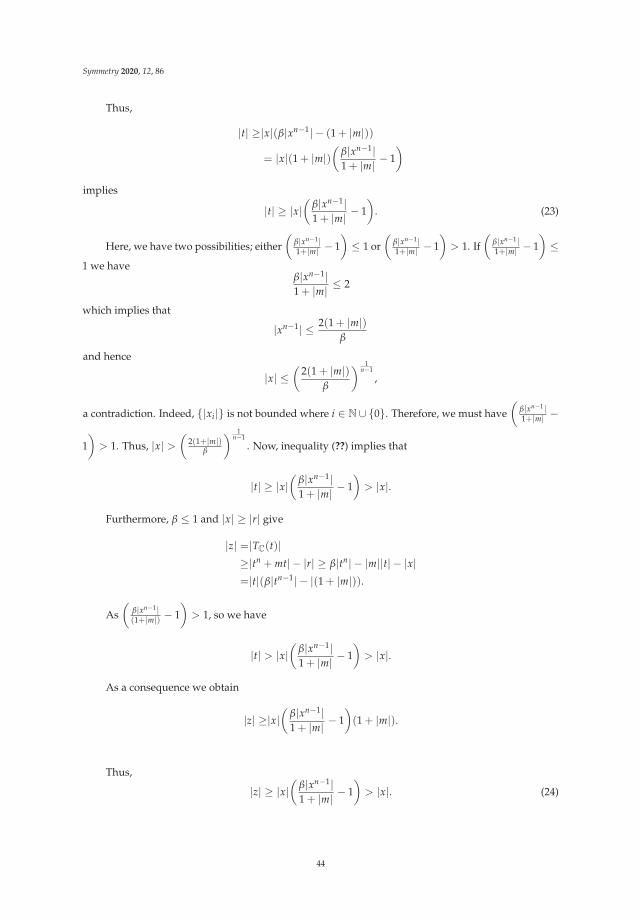
Symmetry 2020, 12, 86

Thus,

|t| ≥|x|(β|xn−1| − (1 + |m|))

= |x|(1 + |m|)(

β|xn−1|1 + |m| − 1

)implies

|t| ≥ |x|(

β|xn−1|1 + |m| − 1

). (23)

Here, we have two possibilities; either(

β|xn−1|1+|m| − 1

)≤ 1 or

(β|xn−1|1+|m| − 1

)> 1. If

(β|xn−1|1+|m| − 1

)≤

1 we haveβ|xn−1|1 + |m| ≤ 2

which implies that

|xn−1| ≤ 2(1 + |m|)β

and hence

|x| ≤(

2(1 + |m|)β

) 1n−1

,

a contradiction. Indeed, {|xi|} is not bounded where i ∈ N∪ {0}. Therefore, we must have(

β|xn−1|1+|m| −

1)> 1. Thus, |x| >

(2(1+|m|)

β

) 1n−1

. Now, inequality (??) implies that

|t| ≥ |x|(

β|xn−1|1 + |m| − 1

)> |x|.

Furthermore, β ≤ 1 and |x| ≥ |r| give

|z| =|TC(t)|≥|tn + mt| − |r| ≥ β|tn| − |m||t| − |x|=|t|(β|tn−1| − |(1 + |m|)).

As(

β|xn−1|(1+|m|) − 1

)> 1, so we have

|t| > |x|(

β|xn−1|1 + |m| − 1

)> |x|.

As a consequence we obtain

|z| ≥|x|(

β|xn−1|1 + |m| − 1

)(1 + |m|).

Thus,

|z| ≥ |x|(

β|xn−1|1 + |m| − 1

)> |x|. (24)

44

Symmetry 2020, 12, 86

Similarly, |y| = |TC(z)| = |zn + mz + r|, |x| > |r| and β ≤ 1 imply that

|y| ≥ |x|(

β|xn−1|1 + |m| − 1

).

Consequently,

|y| ≥ |x|(

β|xn−1|1 + |m| − 1

)> |x|. (25)

Finally, we have

|x1| =|(1− α)y + αTC(y)|=|(1− α)y + α(yn + my + r)|≥α|yn| − (1− α + α|m|)|y| − α|r|≥α|yn| − (1− α + α|m|)|y| − α|y|≥α|yn| − (1 + α|m|)|y|≥α|yn| − (1 + |m|)|y|=|y|(α|yn−1| − (1 + |m|))≥|x|(α|xn−1| − (1 + |m|)).

Hence

|x1| ≥ |x|(

α|xn−1|1 + |m| − 1

).

Using arguments similar to those as before, we only have one possibility that(

α|xn−1|1+|m| − 1

)> 1.

Therefore, |x| >(

2(1+|m|)α

) 1n−1

. This completes the proof.

3. Visualization of Fractals

In this section, we present some Julia and Mandelbrot sets for quadratic and higher orderpolynomials. We found several captivating new fractals having various geometric shapes. However,we have chosen some figures. The color variation occurs due to the change of input parameters.We have also investigated the effect of change of parameters α and β on the shape and the variation ofcolors. The number of iterations was fixed at 10.

3.1. Generation of Julia sets

Following Algorithm 1 is the pseudocode for the generation of Julia sets. Note that T′(z) representsthe iteration process.

45

Symmetry 2020, 12, 86

Algorithm 1: Generation of Julia SetInput : complex polynomial–T : C→ C, parameters–r, m ∈ C, Area–A ⊂ C, number of

iterations–N, colormap with M colors–colormap[0...M− 1]Output :� is the area for Julia set

1 R = Threshold radius2 for c ∈ A3 do

4 k = 05 while k ≤ N do

6 z = T′(z)7 if |z| > R then

8 break9 end

10 k = k + 111 end

12 m = �(M− 1) kN �

13 color c with colormap[m]

14 end

Now, we present quadratic, cubic and septic Julia sets in Picard Ishikawa type orbit for thecomplex polynomial, TC(x) = xn + mx + r.

1. For Figure ??, we consider the polynomial T(x) = x2 + (−0.5 + 0.7i)x + (−0.01 + 0.18i)and A = [−2.5, 2.5]× [−2.1, 2.1]. It is easy to see that T has one attracting fixed point,p = −0.1427 + 0.1019i. Observe that for α = 0.2, β = 0.097 and α = 0.11,β = 0.18 we obtaindifferent images due to color variation caused by parameters. It is interesting to note that forα = 1, β = 1 and α = 10−10, β = 10−10 we have similar shapes but there is clear variation ofcolors.

2. For Figure ??, we consider the polynomial T(x) = x3 + (−0.275 + 0.5i)x + (−0.559 + 0.35i) andA = [−1.5, 1.5]× [−1.8, 1.8]. The polynomial T has attracting fixed point p ∼ −0.6434 + 0.2687iin A. Note that the cubic Julia sets for α = 0.08 and β = 0.09 have more color variation ascompared to the Julia sets for α = 0.1, and β = 0.2. Again, for α = 1, β = 1 and α = 10−10,β = 10−10 the shapes are same but there is variability in colors.

3. For Figure ??, we input T(x) = x7 + (0.23 + 1.2i)x + (0.5 + 0.7i) and A = [−1.3, 1.3]2.The attracting fixed point of the polynomial is p ∼ −0.2391 + 0.5835i. We can see that forα = 0.01 and β = 0.08 the shape is spread and stretched while the shape is dense and neatlypacked for α = 0.1 and β = 0.05. Note the variation of colors in figures (C) and (D) as well.

46

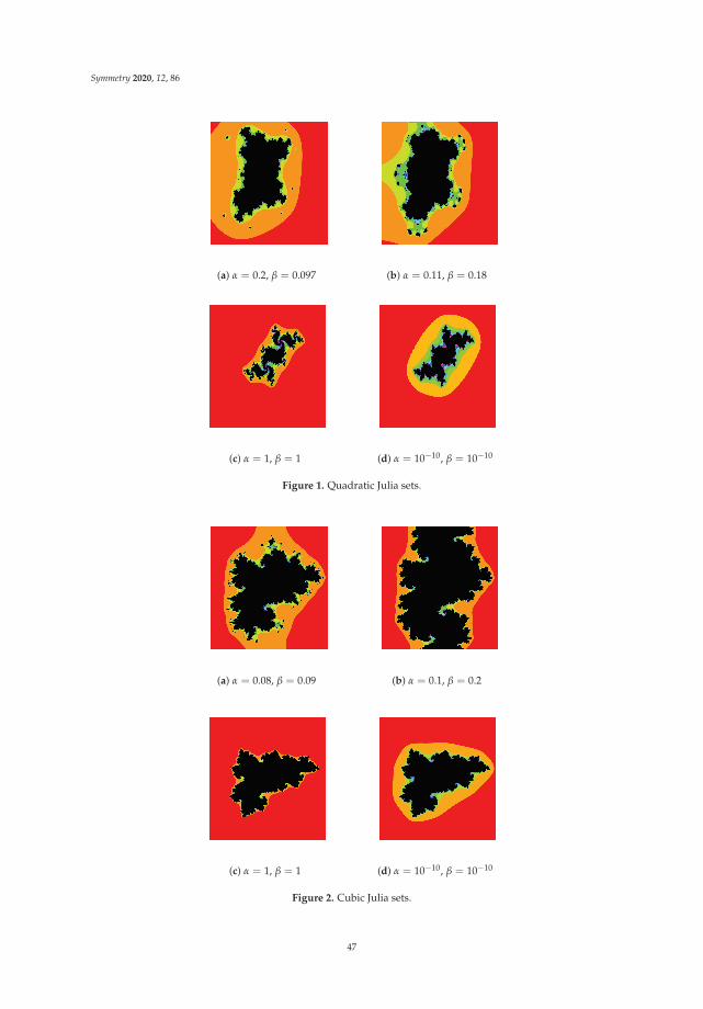
Symmetry 2020, 12, 86

(a) α = 0.2, β = 0.097 (b) α = 0.11, β = 0.18

(c) α = 1, β = 1 (d) α = 10−10, β = 10−10

Figure 1. Quadratic Julia sets.

(a) α = 0.08, β = 0.09 (b) α = 0.1, β = 0.2

(c) α = 1, β = 1 (d) α = 10−10, β = 10−10

Figure 2. Cubic Julia sets.

47

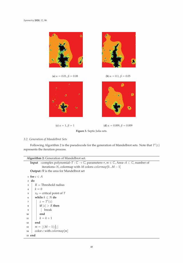
Symmetry 2020, 12, 86

(a) α = 0.01, β = 0.08 (b) α = 0.1, β = 0.05

(c) α = 1, β = 1 (d) α = 0.009, β = 0.009

Figure 3. Septic Julia sets.

3.2. Generation of Mandelbrot Sets

Following Algorithm 2 is the pseudocode for the generation of Mandelbrot sets. Note that T′(z)represents the iteration process.

Algorithm 2: Generation of Mandelbrot set.Input : complex polynomial–T : C→ C, parameters–r, m ∈ C, Area–A ⊂ C, number of

iterations–N, colormap with M colors–colormap[0...M− 1]Output :� is the area for Mandelbrot set

1 for c ∈ A2 do

3 R = Threshold radius4 k = 05 x0 = critical point of T6 while k ≤ N do

7 z = T′(z)8 if |z| > R then

9 break10 end

11 k = k + 112 end

13 m = �(M− 1) kN �

14 color c with colormap[m]

15 end

48

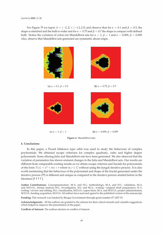
Symmetry 2020, 12, 86

For Figure ?? we input A = [−2, 2]× [−1.2, 2.5] and observe that for α = 0.1 and β = 0.3, theshape is stretched and the bulb is wider and for α = 0.75 and β = 0.7 the shape is compact with definedbulb. Notice the variation of colors for Mandelbrot sets for α = 1, β = 1 and α = 0.009, β = 0.009.Also, observe that Mandelbot sets generated are symmetric about origin.

(a) α = 0.1, β = 0.3 (b) α = 0.75, β = 0.7

(c) α = 1, β = 1 (d) α = 0.009, β = 0.009

Figure 4. Mandelbrot sets.

4. Conclusions

In this paper, a Picard Ishikawa type orbit was used to study the behaviour of complexpoylnomials. We obtained escape criterions for complex quadratic, cubic and higher degreepolynomials. Some alluring Julia and Mandelbrot sets have been generated. We also observed that thevariation of parameters has shown eminent changes in the Julia and Mandelbrot sets. Our results aredifferent from comparable existing results as we obtain escape criterion and fractals for polynomialsof the form T(x) = xn + mx + r where m, r ∈ C without using the Jungck iterative process. It is alsoworth mentioning that the behaviour of the polynomial and shape of the fractal generated under theiterative process (??) is different and unique as compared to the iterative process studied before in theliterature [? ? ? ? ].

Author Contributions: Conceptualization, M.A. and H.I.; methodology, M.A. and H.I.; validation, M.A.and M.D.l.S., formal analysis H.I.; investigation, H.I. and M.A.; writing—original draft preparation, H I.;writing—review and editing, H.I.; visualization, M.D.l.S.; supervision, M.A. and M.D.l.S.; project administration,M.D.l.S.; funding acquisition, M.D.l.S. All authors have read and agreed to the published version of the manuscript.

Funding: This research was funded by Basque Government through grant number IT 1207-19.

Acknowledgments: All the authors are grateful to the referees for their critical remarks and valuable suggestionswhich helped to improve the presentation of the paper.

Conflicts of Interest: The authors declare no conflict of interest.

49

Symmetry 2020, 12, 86

References

1. Barnsley, M. Fractals Everywhere, 2nd ed.; Academic Press: San Diego, CA, USA, 1993.2. Hundertmark-Zauôkovù, A. On the convergence of fixed point iterations for the moving geometry in

a fluid-structure interaction problem. J. Differ. Equ. 2019, 267, 7002–7046. [CrossRef]3. Rahmani, M.; Koutsopoulos, H.N.; Jenelius, E. Travel time estimation from sparse floating car data with

consistent path inference: A fixed point approach. Transp. Res. Part C Emerg. Technol. 2017, 85, 628–643.[CrossRef]

4. Strogatz, S.H. Nonlinear Dynamics and Chaos With Applications to Physics, Biology, Chemistry, and Engineering,2nd ed.; CRC Press: Boca Raton, FL, USA, 2018.

5. Julia, G. Memoire sur l’iteration des functions rationnelles. J. Math. Pures Appl. 1918, 8, 737–747.6. Devaney, R.L. A First Course in Chaotic Dynamical Systems: Theory and Experiment, 2nd ed.; Addison-Wesley:

Boston, MA, USA, 1992.7. Falconer, K. Fractal Geometry: Mathematical Foundations and Applications, 2nd ed.; John Wiley & Sons: Chichester,

UK, 2004.8. Frame, M.; Robertson, J. A generalized Mandelbrot set and the role of critical points. Comput. Graph. 1992,

16, 35–40. [CrossRef]9. Brouwer, L.E.J. Über Abbildungen von Mannigfaltigkeiten. Math. Ann. 1912, 71, 97–115. [CrossRef]10. Mandelbrot, B.B. The Fractal Geometry of Nature; W.H. Freeman: New York, NY, USA, 1983; Volume 2.11. Debnath, L. A brief historical introduction to fractals and fractal geometry. Int. J. Math. Educ. Sci. Technol.

2006, 37, 29–50. [CrossRef]12. Lakhtakia, A.; Varadan, W.; Messier, R.; Varadan, V.K. On the symmetries of the Julia sets for the process

zp + c. J. Phys. A Math. Gen. 1987, 20, 3533–3535. [CrossRef]13. Negi, A.; Rani, M. Midgets of superior Mandelbrot set. Chaos Solitons Fract. 2008, 36, 237–245. [CrossRef]14. Negi, A.; Rani, M. A new approach to dynamic noise on superior Mandelbrot set. Chaos Solitons Fract. 2008,

36, 1089–1096. [CrossRef]15. Rochon, D. A generalized Mandelbrot set for bicomplex numbers. Fractals 2000, 8, 355–368. [CrossRef]16. Wang, X.; Sun, Y. The general quaternionic M-J sets on the mapping z ← zα + c(α ∈ N). Comput. Math. Appl.

2007, 53, 1718–1732. [CrossRef]17. Rani, M. Theoretical Framework for Fractal Models under Two-Step Feedback Process. Ph.D. Thesis, Kumaun

University, Nainital, India, 2016.18. Rani, M.; Kumar, V. Superior Julia set. Res. Math. Educ. 2004, 8, 261–277.19. Rani, M.; Kumar, V. Superior Mandelbrot set. Res. Math. Educ. 2004, 8, 279–291.20. Rani, M.; Chauhan, Y.S.; Negi, A. Non linear dynamics of Ishikawa iteration. Int. J. Comput. Appl. 2010, 7,

43–49. [CrossRef]21. Chauhan, Y.S.; Rana, R.; Negi, A. New Julia sets of Ishikawa iterates. Int. J. Comput. Appl. 2010, 7, 34–42.

[CrossRef]22. Chauhan, Y.S.; Rana, R.; Negi, A. Complex dynamics of Ishikawa iterates for non integer values. Int. J.

Comput. Appl. 2010, 9, 9–16. [CrossRef]23. Ashish; Rani, M.; Chugh, R. Julia sets and Mandelbrot sets in Noor orbit. Appl. Math. Comput. 2014, 228,

615–631.24. Kang, S.M.; Rafiq, A.; Latif, A.; Shahid, A.A.; Ali, F. Fractals through modified iteration scheme. Filomat

2016, 30, 3033–3046. [CrossRef]25. Kang, S.M.; Rafiq, A.; Latif, A.; Shahid, A.A.; Kwun, Y.C. Tricorns and multicorns of S-iteration scheme.

J. Funct. Spaces 2015, 2015, 417167.26. Kumari, M.; Ashish, R.C. New Julia and Mandelbrot sets for a new faster iterative process. Int. J. Pure

Appl. Math. 2016, 107, 161–177. [CrossRef]27. Kang, S.M.; Nazeer, W.; Tanveer, M.; Shahid, A.A. New fixed point results for fractal generation in Jungck

Noor orbit with s-convexity. J. Funct. Spaces 2015, 2015, 963016. [CrossRef]28. Kang, S.M.; Rafiq, A.; Tanveer, M.; Ali, F.; Kwun, Y.C. Julia and Mandelbrot sets in modified Jungck three-step

orbit. Wulfenia J. 2015, 22, 167–185.29. Kwun, Y.C.; Tanveer, M.; Nazeer, W.; Abbas, M.; Kang, S.M. Fractal generation in modified Jungck-S orbit.

IEEE Access 2019, 7, 35060–35071. [CrossRef]

50

Symmetry 2020, 12, 86

30. Proakis, J.G.; Manolakis, D.G. Digital Signal Processing: Principles, Algorithms and Applications, 4th ed.; Pearson:Bengaluru, India, 2007.

31. Mishra, M.K.; Ojha, D.B.; Sharma, D. Fixed point results in tricorn and multicorns of Ishikawa iteration ands-convexity. IJEST 2011, 2, 157–160.

32. Cho, S.Y.; Shahid, A.A.; Nazeer, W.; Kang, S.M. Fixed point results for fractal generation in noor orbit ands-convexity. SpringerPlus 2016, 5, 1843. [CrossRef] [PubMed]

33. Nazeer, W.; Kang, S.M.; Tanveer, M.; Shahid, A.A. Fixed point results in the generation of Julia andMandelbrot sets. J. Inequal. Appl. 2015, 2015, 298. [CrossRef]

34. Piri, H.; Daraby, B.; Rahrovi, S.; Ghasemi, M. Approximating fixed points of generalized α-nonexpansivemappings Banach spaces by new faster iteration process. Numer. Algorithms 2018, 81, 1129–1148. [CrossRef]

c© 2020 by the authors. Licensee MDPI, Basel, Switzerland. This article is an open accessarticle distributed under the terms and conditions of the Creative Commons Attribution(CC BY) license (http://creativecommons.org/licenses/by/4.0/).

51

symmetryS SArticle

A Continuous Coordinate System for the Plane byTriangular Symmetry

Benedek Nagy * and Khaled Abuhmaidan

Department of Mathematics, Faculty of Arts and Sciences, Eastern Mediterranean University, via Mersin 10,Turkey, Famagusta 99450, North Cyprus; kabuhumaidan@yahoo.com* Correspondence: nbenedek.inf@gmail.com

Received: 20 December 2018; Accepted: 31 January 2019; Published: 9 February 2019

Abstract: The concept of the grid is broadly used in digital geometry and other fields of computerscience. It consists of discrete points with integer coordinates. Coordinate systems are essential formaking grids easy to use. Up to now, for the triangular grid, only discrete coordinate systems havebeen investigated. These have limited capabilities for some image-processing applications, includingtransformations like rotations or interpolation. In this paper, we introduce the continuous triangularcoordinate system as an extension of the discrete triangular and hexagonal coordinate systems.The new system addresses each point of the plane with a coordinate triplet. Conversion between theCartesian coordinate system and the new system is described. The sum of three coordinate valueslies in the closed interval [−1, 1], which gives many other vital properties of this coordinate system.

Keywords: barycentric coordinate system; coordinate system; hexagonal grid; triangular grid;tri-hexagonal grid; transformations

1. Introduction

The concept of the grid is essential and heavily used in digital geometry and in digital imageprocessing. A grid is comprised of discrete points addressed with integer vectors. There are threeregular tessellations of the plane, which define the square, hexagonal, and triangular grids (namedafter the form of the pixels used as tiles) [1]. Most of the applications use the square grid because itsorthogonal coordinate system, known as the Cartesian coordinate system (CCS), which fits very wellto it. This addresses each square pixel of the grid by a pair of independent integers. The dual of thesquare grid (the grid formed by the nodes, which are the crossing points of the gridlines) is again asquare grid. Therefore, essentially, the same CCS is used as well. Working with real images, we mayneed to perform operations that do not map the grid to itself, e.g., zooming or rotations. The Cartesiancoordinate system allows real numbers to be used in such cases. Moreover, the digitization operationcan easily be defined by a rounding operation.

The hexagonal grid, tiling the plane by the same size regular hexagons (hexagonal pixels), has beenused for decades in image processing applications [2], in cartography [3,4], in biological simulations [5],and in other fields, since the digital geometry of the hexagonal grid provides better results than thesquare grid in various cases. In addition, it is used in various table and computer games based on itscompactness. It is the simplest 2D grid, since the only usual neighborhood using the nearest neighborsis simpler and less confusing than the two types of neighbors in the square grid [6]. The neighborhoodof a pixel contains six other hexagons (see Figure 1a). In contrast to the square grid, the dual of thehexagonal grid is not the hexagonal, but the triangular grid (see Figure 1a,b). Adequate and elegantcoordinate systems for these kinds of grids are required for their use in both theory and applications,e.g., in image processing or engineering applications. In Reference [7], a three-coordinate-valuedsystem of zero-sum triplets is used to describe the hexagonal grid capturing the triangular symmetry

Symmetry 2019, 11, 191; doi:10.3390/sym11020191 www.mdpi.com/journal/symmetry53

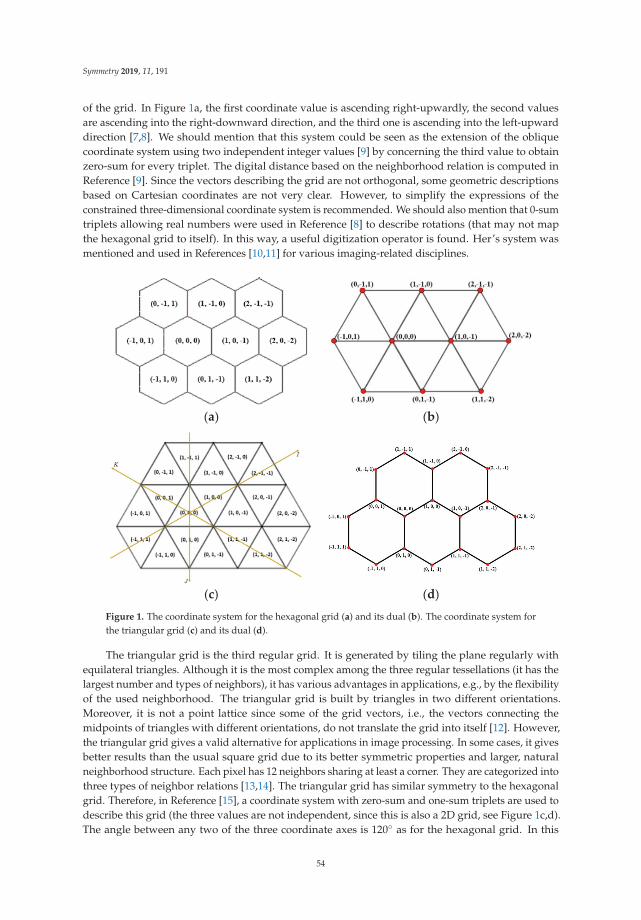
Symmetry 2019, 11, 191

of the grid. In Figure 1a, the first coordinate value is ascending right-upwardly, the second valuesare ascending into the right-downward direction, and the third one is ascending into the left-upwarddirection [7,8]. We should mention that this system could be seen as the extension of the obliquecoordinate system using two independent integer values [9] by concerning the third value to obtainzero-sum for every triplet. The digital distance based on the neighborhood relation is computed inReference [9]. Since the vectors describing the grid are not orthogonal, some geometric descriptionsbased on Cartesian coordinates are not very clear. However, to simplify the expressions of theconstrained three-dimensional coordinate system is recommended. We should also mention that 0-sumtriplets allowing real numbers were used in Reference [8] to describe rotations (that may not mapthe hexagonal grid to itself). In this way, a useful digitization operator is found. Her’s system wasmentioned and used in References [10,11] for various imaging-related disciplines.

Figure 1. The coordinate system for the hexagonal grid (a) and its dual (b). The coordinate system forthe triangular grid (c) and its dual (d).

The triangular grid is the third regular grid. It is generated by tiling the plane regularly withequilateral triangles. Although it is the most complex among the three regular tessellations (it has thelargest number and types of neighbors), it has various advantages in applications, e.g., by the flexibilityof the used neighborhood. The triangular grid is built by triangles in two different orientations.Moreover, it is not a point lattice since some of the grid vectors, i.e., the vectors connecting themidpoints of triangles with different orientations, do not translate the grid into itself [12]. However,the triangular grid gives a valid alternative for applications in image processing. In some cases, it givesbetter results than the usual square grid due to its better symmetric properties and larger, naturalneighborhood structure. Each pixel has 12 neighbors sharing at least a corner. They are categorized intothree types of neighbor relations [13,14]. The triangular grid has similar symmetry to the hexagonalgrid. Therefore, in Reference [15], a coordinate system with zero-sum and one-sum triplets are used todescribe this grid (the three values are not independent, since this is also a 2D grid, see Figure 1c,d).The angle between any two of the three coordinate axes is 120◦ as for the hexagonal grid. In this

54

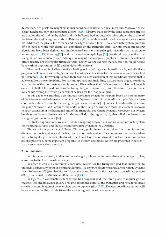
Symmetry 2019, 11, 191

description, two pixels are neighbors if their coordinate values differ by at most one. Moreover, at theclosest neighbors, only one coordinate differs [15,16]. Observe that exactly the same coordinate tripletsare used on the left and on the right-hand side in Figure 1c,d, respectively, which shows the duality ofthe triangular and hexagonal grids. In Reference [17], a combinatorial coordinate system was shownthat addresses the pixels, the corners, and the edges between them. That coordinate system gives anefficient tool to work with digital cell complexes on the triangular grid. Various image processingalgorithms have been defined and implemented for the triangular grid recently such as discretetomography [18,19], thinning [20], and mathematical morphology [21]. We should also mention thattriangulation is a frequently used technique in imaging and computer graphics. However, the obtainedgrid is usually not the regular triangular grid. Lastly, we should note that several non-regular gridshave various applications in 2D and in higher dimensions.

The coordination is vital because it is a leading tool in making a simple, easily usable, and effectivelyprogrammable system with integer numbers (coordinates). The isometric transformations are describedin Reference [12]. However, up to now, there was no such extension of this coordinate system that isable to address the entire plane. For various applications, including, e.g., arbitrary angled rotations,an extension of the coordinate system is needed. We note here that Her’s zero-sum triplets could matchonly up to half of the grid points in the triangular grid (Figure 1c,d), and, therefore, the coordinatesystem addressing the whole plain cannot be used for the triangular grid.

In this paper, we introduce a continuous coordinate system for the plain based on the symmetryof the triangular grid, where every point of the 2D plane has its unique coordinate triplet. We use threecoordinate values to describe the triangular grid as in Reference [15] but also to address the points ofthe plane “between” and “around” the nodes of the dual grid. Our new coordinate system is shownto be an extension of the hexagonal and of the triangular coordinate systems. Moreover, our systembuilds upon the coordinate system for the so-called, tri-hexagonal grid, also called the three-planetriangular grid in Reference [16].

For further applications, we also provide a mapping between our continuous coordinate systemfor the triangular grid and the Cartesian coordinate system of the 2D plane.

The rest of this paper is as follows. The next, preliminary section, describes some importantdiscrete coordinate systems and the barycentric coordinate system. The continuous coordinate systemfor the triangular grid is then introduced in Section 3. Conversions to and from Cartesian coordinatesare also presented. Some important properties of the new coordinate system are presented in Section 4.Lastly, conclusions close the paper.

2. Preliminaries

In this paper, as usual, Z3 denotes the cubic grid, whose points are addressed by integer triplets,according to the three coordinates x, y, z.

In order to create a continuous coordinate system for the triangular grid that enables us touniquely address any point of the triangular grid, we combine discrete triangular coordinate systemsfrom Reference [22] (see also Figure 1 for some examples) with the barycentric coordinate system(BCS), discovered by Möbius (see References [1,23]).

In Figure 2, a coordinate system for the tri-hexagonal grid (the three-plane triangular grid ofregions [16]) and its dual is given. This grid resembles a mix of the triangular and hexagonal gridssince it is a combination of the one-plane and two-plane grids [7,22]. The new coordinate system willbe an extension of the discrete triangular and hexagonal coordinate systems.

55

Symmetry 2019, 11, 191

Figure 2. Representation of the tri-hexagonal coordinate system (a) and its dual (b). The samecoordinate system is used to address the pixels (a) and the nodes of the dual grid (b).

Next, a brief description is given for the discrete triangular coordinate system and BCS.

2.1. Discrete Triangular Coordinate System

The discrete Hexagonal Coordinate System uses 0-sum triplets (Figure 1a,b). The discreteTriangular Coordinate System [22] is a symmetric coordinate system that addresses each pixel by aninteger triplet. The three coordinate axes have angles of 120◦ as in the hexagonal grid. The sum of thetriplets is equal to 0 or 1, which refers to the two types of orientations of triangles (�,�). The triangleswith zero-sum are the “even” triangles (�), and the triangles with one-sum triplets are the “odd”triangles (�) (see Figure 1).

For finding an appropriate extension to this system that is able to address all points of the 2Dplane, we start by addressing the midpoints of triangles with integer triplets of +1 and −1 sum.Therefore, we call them “positive�” and “negative�” triangles, respectively. According to Figure 3,the coordinate system of Figure 2b is used to address midpoints of triangles of the triangular grid.Observe that each triplet assigned to a midpoint (see the blue triplets in Figure 3) builds up from thecoordinate values shared by two of the corners of the given pixel (see the three red triplets aroundeach blue triplet). There is already an important difference between our proposed and Her’s zero-sumcoordinate system, which includes the use of zero-sum triplets to address these midpoints as well(actually, three fractional values for each midpoint), which was a very good and efficient choice toextend the coordinate system of the hexagonal grid. However, it does not meet our requirements.Therefore, we have fixed these coordinate values in another way. We should also mention that Her’ssystem inside the regular triangles can be seen as an application of the barycentric coordinate system(see next subsection) based on the values assigned to the corners of the triangle.

Figure 3. The coordinate system for the tri-hexagonal grid is used for the triangular grid (and for itsdual at the same time).

56

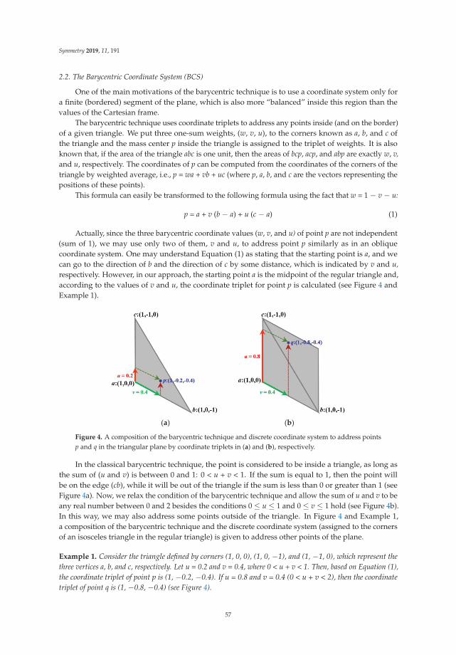
Symmetry 2019, 11, 191

2.2. The Barycentric Coordinate System (BCS)

One of the main motivations of the barycentric technique is to use a coordinate system only fora finite (bordered) segment of the plane, which is also more “balanced” inside this region than thevalues of the Cartesian frame.

The barycentric technique uses coordinate triplets to address any points inside (and on the border)of a given triangle. We put three one-sum weights, (w, v, u), to the corners known as a, b, and c ofthe triangle and the mass center p inside the triangle is assigned to the triplet of weights. It is alsoknown that, if the area of the triangle abc is one unit, then the areas of bcp, acp, and abp are exactly w, v,and u, respectively. The coordinates of p can be computed from the coordinates of the corners of thetriangle by weighted average, i.e., p = wa + vb + uc (where p, a, b, and c are the vectors representing thepositions of these points).

This formula can easily be transformed to the following formula using the fact that w = 1 − v − u:

p = a + v (b − a) + u (c − a) (1)

Actually, since the three barycentric coordinate values (w, v, and u) of point p are not independent(sum of 1), we may use only two of them, v and u, to address point p similarly as in an obliquecoordinate system. One may understand Equation (1) as stating that the starting point is a, and wecan go to the direction of b and the direction of c by some distance, which is indicated by v and u,respectively. However, in our approach, the starting point a is the midpoint of the regular triangle and,according to the values of v and u, the coordinate triplet for point p is calculated (see Figure 4 andExample 1).

Figure 4. A composition of the barycentric technique and discrete coordinate system to address pointsp and q in the triangular plane by coordinate triplets in (a) and (b), respectively.

In the classical barycentric technique, the point is considered to be inside a triangle, as long asthe sum of (u and v) is between 0 and 1: 0 < u + v < 1. If the sum is equal to 1, then the point willbe on the edge (cb), while it will be out of the triangle if the sum is less than 0 or greater than 1 (seeFigure 4a). Now, we relax the condition of the barycentric technique and allow the sum of u and v to beany real number between 0 and 2 besides the conditions 0 ≤ u ≤ 1 and 0 ≤ v ≤ 1 hold (see Figure 4b).In this way, we may also address some points outside of the triangle. In Figure 4 and Example 1,a composition of the barycentric technique and the discrete coordinate system (assigned to the cornersof an isosceles triangle in the regular triangle) is given to address other points of the plane.

Example 1. Consider the triangle defined by corners (1, 0, 0), (1, 0, −1), and (1, −1, 0), which represent thethree vertices a, b, and c, respectively. Let u = 0.2 and v = 0.4, where 0 < u + v < 1. Then, based on Equation (1),the coordinate triplet of point p is (1, −0.2, −0.4). If u = 0.8 and v = 0.4 (0 < u + v < 2), then the coordinatetriplet of point q is (1, −0.8, −0.4) (see Figure 4).

57

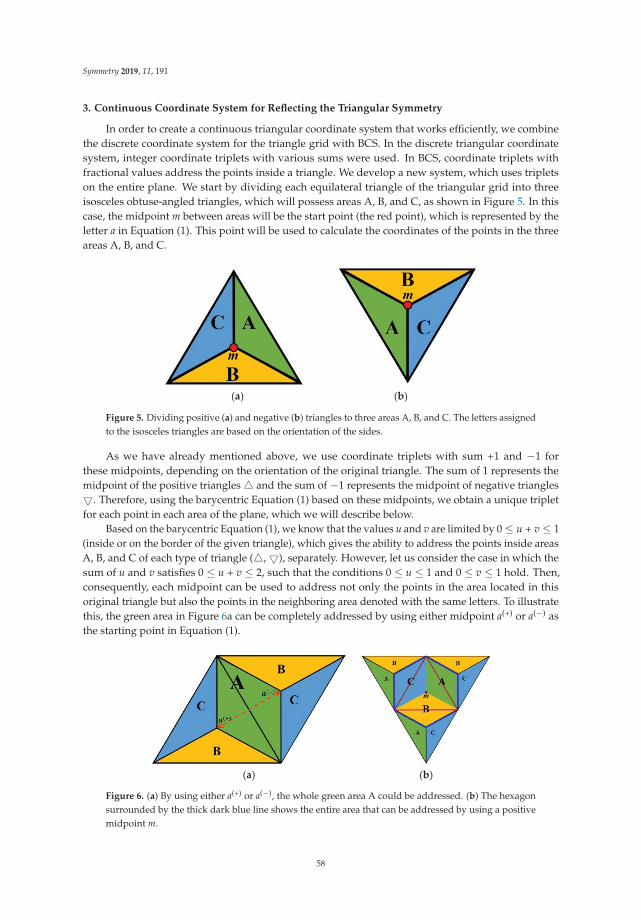
Symmetry 2019, 11, 191

3. Continuous Coordinate System for Reflecting the Triangular Symmetry

In order to create a continuous triangular coordinate system that works efficiently, we combinethe discrete coordinate system for the triangle grid with BCS. In the discrete triangular coordinatesystem, integer coordinate triplets with various sums were used. In BCS, coordinate triplets withfractional values address the points inside a triangle. We develop a new system, which uses tripletson the entire plane. We start by dividing each equilateral triangle of the triangular grid into threeisosceles obtuse-angled triangles, which will possess areas A, B, and C, as shown in Figure 5. In thiscase, the midpoint m between areas will be the start point (the red point), which is represented by theletter a in Equation (1). This point will be used to calculate the coordinates of the points in the threeareas A, B, and C.

Figure 5. Dividing positive (a) and negative (b) triangles to three areas A, B, and C. The letters assignedto the isosceles triangles are based on the orientation of the sides.

As we have already mentioned above, we use coordinate triplets with sum +1 and −1 forthese midpoints, depending on the orientation of the original triangle. The sum of 1 represents themidpoint of the positive triangles� and the sum of −1 represents the midpoint of negative triangles�. Therefore, using the barycentric Equation (1) based on these midpoints, we obtain a unique tripletfor each point in each area of the plane, which we will describe below.

Based on the barycentric Equation (1), we know that the values u and v are limited by 0 ≤ u + v ≤ 1(inside or on the border of the given triangle), which gives the ability to address the points inside areasA, B, and C of each type of triangle (�,�), separately. However, let us consider the case in which thesum of u and v satisfies 0 ≤ u + v ≤ 2, such that the conditions 0 ≤ u ≤ 1 and 0 ≤ v ≤ 1 hold. Then,consequently, each midpoint can be used to address not only the points in the area located in thisoriginal triangle but also the points in the neighboring area denoted with the same letters. To illustratethis, the green area in Figure 6a can be completely addressed by using either midpoint a(+) or a(−) asthe starting point in Equation (1).

Figure 6. (a) By using either a(+) or a(−), the whole green area A could be addressed. (b) The hexagonsurrounded by the thick dark blue line shows the entire area that can be addressed by using a positivemidpoint m.

58

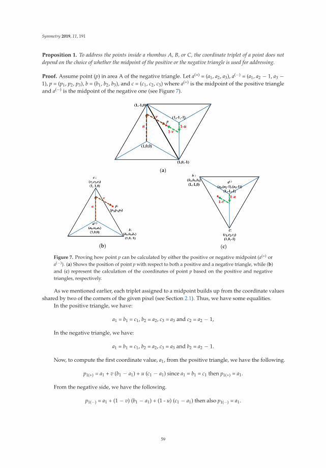
Symmetry 2019, 11, 191

Proposition 1. To address the points inside a rhombus A, B, or C, the coordinate triplet of a point does notdepend on the choice of whether the midpoint of the positive or the negative triangle is used for addressing.

Proof. Assume point (p) in area A of the negative triangle. Let a(+) = (a1, a2, a3), a(−) = (a1, a2 − 1, a3 −1), p = (p1, p2, p3), b = (b1, b2, b3), and c = (c1, c2, c3) where a(+) is the midpoint of the positive triangleand a(−) is the midpoint of the negative one (see Figure 7).

Figure 7. Proving how point p can be calculated by either the positive or negative midpoint (a(+) ora(−)). (a) Shows the position of point p with respect to both a positive and a negative triangle, while (b)and (c) represent the calculation of the coordinates of point p based on the positive and negativetriangles, respectively.

As we mentioned earlier, each triplet assigned to a midpoint builds up from the coordinate valuesshared by two of the corners of the given pixel (see Section 2.1). Thus, we have some equalities.

In the positive triangle, we have:

a1 = b1 = c1, b2 = a2, c3 = a3 and c2 = a2 − 1,

In the negative triangle, we have:

a1 = b1 = c1, b2 = a2, c3 = a3 and b2 = a2 − 1.

Now, to compute the first coordinate value, a1, from the positive triangle, we have the following.

p1(+) = a1 + v (b1 − a1) + u (c1 − a1) since a1 = b1 = c1 then p1(+) = a1.

From the negative side, we have the following.

p1(−) = a1 + (1 − v) (b1 − a1) + (1 - u) (c1 − a1) then also p1(−) = a1.

59

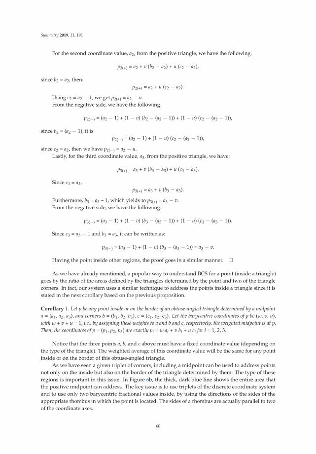
Symmetry 2019, 11, 191

For the second coordinate value, a2, from the positive triangle, we have the following.

p2(+) = a2 + v (b2 − a2) + u (c2 − a2),

since b2 = a2, then:p2(+) = a2 + u (c2 − a2).

Using c2 = a2 − 1, we get p2(+) = a2 − u.From the negative side, we have the following.

p2(−) = (a2 − 1) + (1 − v) (b2 − (a2 − 1)) + (1 − u) (c2 − (a2 − 1)),

since b2 = (a2 − 1), it is:p2(−) = (a2 − 1) + (1 − u) (c2 − (a2 − 1)),

since c2 = a2, then we have p2(−) = a2 − u.Lastly, for the third coordinate value, a3, from the positive triangle, we have:

p3(+) = a3 + v (b3 − a3) + u (c3 − a3).

Since c3 = a3,p3(+) = a3 + v (b3 − a3).

Furthermore, b3 = a3 – 1, which yields to p3(+) = a3 − v.From the negative side, we have the following.

p3(−) = (a3 − 1) + (1 − v) (b3 − (a3 − 1)) + (1 − u) (c3 − (a3 − 1)).

Since c3 = a3 − 1 and b3 = a3, it can be written as:

p3(−) = (a3 − 1) + (1 − v) (b3 − (a3 − 1)) = a3 − v.

Having the point inside other regions, the proof goes in a similar manner. �

As we have already mentioned, a popular way to understand BCS for a point (inside a triangle)goes by the ratio of the areas defined by the triangles determined by the point and two of the trianglecorners. In fact, our system uses a similar technique to address the points inside a triangle since it isstated in the next corollary based on the previous proposition.

Corollary 1. Let p be any point inside or on the border of an obtuse-angled triangle determined by a midpointa = (a1, a2, a3), and corners b = (b1, b2, b3), c = (c1, c2, c3). Let the barycentric coordinates of p be (w, v, u),with w + v + u = 1, i.e., by assigning these weights to a and b and c, respectively, the weighted midpoint is at p.Then, the coordinates of p = (p1, p2, p3) are exactly pi = w ai + v bi + u ci for i = 1, 2, 3.

Notice that the three points a, b, and c above must have a fixed coordinate value (depending onthe type of the triangle). The weighted average of this coordinate value will be the same for any pointinside or on the border of this obtuse-angled triangle.

As we have seen a given triplet of corners, including a midpoint can be used to address pointsnot only on the inside but also on the border of the triangle determined by them. The type of theseregions is important in this issue. In Figure 6b, the thick, dark blue line shows the entire area thatthe positive midpoint can address. The key issue is to use triplets of the discrete coordinate systemand to use only two barycentric fractional values inside, by using the directions of the sides of theappropriate rhombus in which the point is located. The sides of a rhombus are actually parallel to twoof the coordinate axes.

60

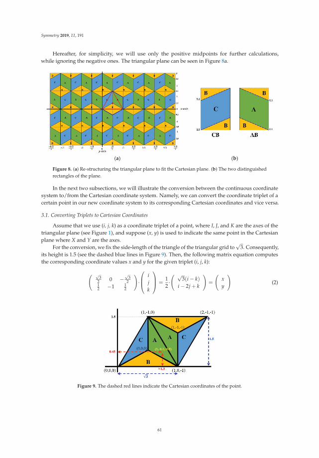
Symmetry 2019, 11, 191

Hereafter, for simplicity, we will use only the positive midpoints for further calculations,while ignoring the negative ones. The triangular plane can be seen in Figure 8a.

Figure 8. (a) Re-structuring the triangular plane to fit the Cartesian plane. (b) The two distinguishedrectangles of the plane.

In the next two subsections, we will illustrate the conversion between the continuous coordinatesystem to/from the Cartesian coordinate system. Namely, we can convert the coordinate triplet of acertain point in our new coordinate system to its corresponding Cartesian coordinates and vice versa.

3.1. Converting Triplets to Cartesian Coordinates

Assume that we use (i, j, k) as a coordinate triplet of a point, where I, J, and K are the axes of thetriangular plane (see Figure 1), and suppose (x, y) is used to indicate the same point in the Cartesianplane where X and Y are the axes.

For the conversion, we fix the side-length of the triangle of the triangular grid to√

3. Consequently,its height is 1.5 (see the dashed blue lines in Figure 9). Then, the following matrix equation computesthe corresponding coordinate values x and y for the given triplet (i, j, k):

( √3

2 0 −√

32

12 −1 1

2

)·

⎛⎜⎝ ijk

⎞⎟⎠ =12·( √

3(i− k)i− 2j + k

)=

(xy

)(2)

Figure 9. The dashed red lines indicate the Cartesian coordinates of the point.

61

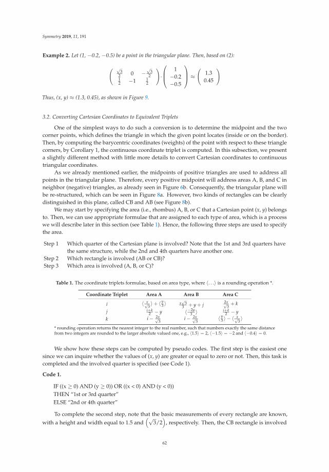
Symmetry 2019, 11, 191

Example 2. Let (1, −0.2, −0.5) be a point in the triangular plane. Then, based on (2):

( √3

2 0 −√

32

12 −1 1

2

)·

⎛⎜⎝ 1−0.2−0.5

⎞⎟⎠ ≈ (1.3

0.45

)

Thus, (x, y) ≈ (1.3, 0.45), as shown in Figure 9.

3.2. Converting Cartesian Coordinates to Equivalent Triplets

One of the simplest ways to do such a conversion is to determine the midpoint and the twocorner points, which defines the triangle in which the given point locates (inside or on the border).Then, by computing the barycentric coordinates (weights) of the point with respect to these trianglecorners, by Corollary 1, the continuous coordinate triplet is computed. In this subsection, we presenta slightly different method with little more details to convert Cartesian coordinates to continuoustriangular coordinates.

As we already mentioned earlier, the midpoints of positive triangles are used to address allpoints in the triangular plane. Therefore, every positive midpoint will address areas A, B, and C inneighbor (negative) triangles, as already seen in Figure 6b. Consequently, the triangular plane willbe re-structured, which can be seen in Figure 8a. However, two kinds of rectangles can be clearlydistinguished in this plane, called CB and AB (see Figure 8b).

We may start by specifying the area (i.e., rhombus) A, B, or C that a Cartesian point (x, y) belongsto. Then, we can use appropriate formulae that are assigned to each type of area, which is a processwe will describe later in this section (see Table 1). Hence, the following three steps are used to specifythe area.

Step 1 Which quarter of the Cartesian plane is involved? Note that the 1st and 3rd quarters have the same structure, while the 2nd and 4th quarters have another one.

Step 2 Which rectangle is involved (AB or CB)? Step 3 Which area is involved (A, B, or C)?

Table 1. The coordinate triplets formulae, based on area type, where 〈. . .〉 is a rounding operation *.

Coordinate Triplet Area A Area B Area C

i 〈 x√3〉+ 〈 y

3 〉 x√

33 + y + j

2x√3+ k

j i+k2 − y 〈 −2y

3 〉 i+k2 − y

k i− 2x√3

i− 2x√3

〈 y3 〉 − 〈 x√

3〉

* rounding operation returns the nearest integer to the real number, such that numbers exactly the same distancefrom two integers are rounded to the larger absolute valued one, e.g., 〈1.5〉 = 2, 〈−1.5〉 = −2 and 〈−0.4〉 = 0.

We show how these steps can be computed by pseudo codes. The first step is the easiest onesince we can inquire whether the values of (x, y) are greater or equal to zero or not. Then, this task iscompleted and the involved quarter is specified (see Code 1).

Code 1.

IF ((x ≥ 0) AND (y ≥ 0)) OR ((x < 0) AND (y < 0))THEN “1st or 3rd quarter”ELSE “2nd or 4th quarter”

To complete the second step, note that the basic measurements of every rectangle are known,with a height and width equal to 1.5 and

(√3/2

), respectively. Then, the CB rectangle is involved

62

Symmetry 2019, 11, 191

whenever the integer part of x and y, are both even or both odd. Otherwise, the AB rectangle isinvolved. See Code 2 to clarify this step.

Code 2.

IF ((int (2x/√

3) mod 2 = 0) AND (int (y/1.5) mod 2) = 0) OR(int (2x/

√3) mod 2 = 1) AND (int (y/1.5) mod 2) = 1))

THEN “CB Rectangle is involved”ELSE “AB Rectangle is involved”

where:

• int takes the integer part of the (decimal) number,• mod is the modulus (or remainder, here after division by two).

Now, the involved rectangle is specified and the third step follows. Since we have two typesof rectangles AB and CB, and they are symmetric, we will discuss only one of them known as typeAB rectangles.

In rectangle AB, a point (x, y) will belong to either part A or part B. To decide which one isinvolved, we consider Line 1 (L1) and Line 2 (L2) in Figure 8b, where they divide the rectangle intoparts A and B. If the point is between L1 and L2, then part A is involved. Otherwise, it is in part B.However, L1 and L2 are considered to be within the area A in cases when the point is on the lines.Equations (3) and (4) of a straight line are used for Line 1 and Line 2, respectively.

m·x + r1 − y = 0, (3)

m·x + r2 − y = 0, (4)

where:

• m is the slope of L1 and L2, which is a constant here, equal to(−√

3/3)

,

• r1 and r2 are the y-axis intercept with L1 and L2, respectively, where r2 = r1 + 1

This step is started by substituting the point (x, y) in Equations (3) and (4). Then, it is determinedthat part A is involved if the left side of Equation (3) is not greater than 0 and the left side of Equation(4) is not less than 0. Otherwise, part B is involved. Code 3 is used to clarify this step.

Code 3.

IF ((r1 − x√

3/3 − y) ≤ 0) AND ((r2 − x√

3/3 − y) ≥ 0)THEN “Area A is involved”ELSE “Area B is involved”

The y-axis intercept with Line 1, r1, in area AB, is computed by computing any point (x, y) on Line1. Therefore, the point at the bottom-right corner of rectangle AB is computed for this purpose (see thered point in Figure 10). Hence, Equation (5) is used to find the value of r1. In Equation (5), we used themodulus (mod) as a function naturally extended to real numbers, i.e., it gives the remainder after thedivision by a real number (and that is between 0 and the divisor). Moreover, by adding 1 to r1, we getthe value of the y-axis intercept with Line 2, r2 (see Code 3).

r1 = y−(

y mod32

)+

√3

3·(

x +

√3

2−(

x mod√

32

))(5)

Similar strategies are used when the CB rectangle is involved, taking care that the slopes of Line 1and Line 2 will be equal to

(√3/3

).

63

Symmetry 2019, 11, 191

Lastly, when the involved area A, B, or C is specified, particular formulae are used that arespecified in Table 1. Example 3 is used for a further explanation.

Figure 10. The red point is used to compute the value of r1, which is the Y-axis intercept with Line 1.

Example 3. Consider a point with Cartesian coordinates: (x, y) = (1.299, 0.45). In order to convert thisCartesian coordinate pair to its corresponding triangular triplet, the three steps below will be followed.

Step 1 The 1st or 3rd quarter is involved.Step 2 It’s odd and even. Therefore, rectangle AB is involved.Step 3 Area A is matched.

Thus, formulae of area A (see Table 1) should be applied in this order, so:

(1) i = 〈0.75〉+ 〈0.15〉 = 1 + 0 = 1(2) k = 1 − 2x√

3≈ −0.500.

(3) j ≈ −y + 0.5 · 0.5 = −0.2

The corresponding triplet is (i, j, k) ≈ (1, −0.2, −0.5), which is approximately the same as in Example 2,as it should be.

To show the conversion of points on other areas (e.g., Area B or Area C), the following examplesare given:

Example 4. (Point in Area B)

(a) Converting from Continuous Coordinate System to CCS.

Let (i, j, k) = (0.683, 0, −0.183) be a point in the triangular plane. To convert to CCS, Equation (2) is used:

( √3

2 0 −√

32

12 −1 1

2

)·

⎛⎜⎝ 0.6830

−0.183

⎞⎟⎠ ≈ (0.750.25

)

(b) Converting from CCS to a Continuous Coordinate System.

Let (x, y) = (0.75, 0.25). The corresponding Continuous Coordinate System triplet can be calculated basedon the three steps above as follows.

Step 1 It belongs to the 1st quarter.Step 2 It belongs to rectangle CB.Step 3 Area B is matched.

64

Symmetry 2019, 11, 191

Thus, formulae of area B from Table 1 are applied in the following order:

(1) j = 〈−2y3 〉 = 0

(2) i = x√

33 + y + j ≈ 0.433 + 0.25 + 0 = 0.683

(3) k = i− 2x√3≈ 0.683 − 0.866 = −0.183

The corresponding triplet is (i, j, k) = (0.683, 0, −0.183), which is exactly the original value.

Example 5. (Point in Area C)

(a) Converting from the Continuous Coordinate System to CCS.

Let (i, j, k) = (0.346, −0.626, 0) be a point in the triangular plane. To convert to CCS, we use Equation(2) below. ( √

32 0 −

√3

212 −1 1

2

)·

⎛⎜⎝ 0.346−0.626

0

⎞⎟⎠ ≈ (0.2990.799

)

(b) Converting from CCS to a Continuous Coordinate System

Let (x, y) = (0.299, 0.799). The corresponding Continuous Coordinate System triplet can be calculatedbased on the three steps below.

Step 1 It belongs to the first quarter.Step 2 It belongs to rectangle CB.Step 3 Area C is matched.

Thus, formulae of area C from Table 1 are applied in the following order.

(1) k = 〈 y3 〉 − 〈 x√

3〉 = 0 − 0 = 0

(2) i = 2x√3+ k ≈ 0.346 + 0 = 0.346

(3) j = i+k2 − y ≈ 0.173 − 0.799 = −0.626

The corresponding triplet is (i, j, k) = (0.346, −0.626, 0), which is exactly the original triplet.

Example 6. (A mid-point)

(a) Converting from Continuous Coordinate System to CCS.

Let (i, j, k) = (1, 0, 0) be a point in the triangular plane. To convert to CCS, Equation (2) is used below.

( √3

2 0 −√

32

12 −1 1

2

)·

⎛⎜⎝ 100

⎞⎟⎠ =

( √3

212

)

(b) Converting from CCS to a Continuous Coordinate System.

Let (x, y) = (√

3/2, 0.5). The corresponding Continuous Coordinate System triplet can be calculated basedon the three steps below.

Step 1 It belongs to the first quarter.Step 2 Based on Code 2, it belongs to rectangle CB (but, since it is a mid-point, then either rectangle AB or CB

may be used).Step 3 Area B is matched.

Thus, formulae of area B from Table 1 are applied in the following order.

65

Symmetry 2019, 11, 191

(1) j = 〈−2y3 〉 = 0

(2) i = x√

33 + y + j = 0.5 + 0.5 + 0 = 1

(3) k = i− 2x√3

= 1 − 1 = 0

The corresponding triplet is (i, j, k) = (1, 0, 0), which is exactly the original value.

4. Properties of the Continuous Triangular Coordinate System

In this section, we will focus on the most important properties of this continuous coordinate system.

4.1. On the Triplets of a General Point

In Figure 6a, consider the red straight line between a(+) and a(−), in the green area. Then, thesum of the coordinate values of the points on this line would change continuously from 1 until −1.Depending on the sum, we can classify the points as follows:

If a point with 3 CV’s sum is:

• equal to 1, then it indicates the positive midpoint (i.e., a(+));• equal to −1, then it indicates the negative midpoint (i.e., a(−));• equal to 0, then it indicates the point on the triangle’s edge;• positive, then the point belongs to the positive triangle;• negative, then the point belongs to the negative triangle.

Theorem 1. The sum of the coordinate triplet of any point in the plane is in the range of the closed interval [−1, 1].

Proof. Consider an area A of a positive triangle with the corners a = (a1, a2, a3), b = (b1, b2, b3),and c = (c1, c2, c3), where b and c are vertices (corners of an equilateral triangle) of the grid, while a isthe midpoint of a positive triangle and p = (p1, p2, p3) is a randomly chosen point belonging to this area(inside or on the border of A). Now based on the barycentric Equation (1), we have the following.

3

∑i=1

pi=3

∑i=1

ai + v·(3

∑i=1

(ci − ai)) + u·(3

∑i=1

(bi − ai))

It is clear that ∑3i=1 ai = 1, whereas

∑3i=1(ci − ai) = (c1 − a1) + (c2 − a2) + (c3 − a3)

= (c1 + c2 + c3)− (a1 + a2 + a3)

= 0− 1 = −1

Similarly, ∑3i=1(bi − ai) = −1.

Then, by substitution, we have the following.

3

∑i=1

pi = 1− u− v = 1− (u + v). (6)

Since 0 ≤ u + v ≤ 2, the maximal and minimal value of the sum of any coordinate triplet is equalto 1 (when u + v = 0) and to −1 (when u + v = 2), respectively. �

Theorem 2. The sum of the coordinates of a triplet is non-negative in a positive triangle and non-positive in anegative triangle.

Proof. Consider a point p that belongs to a positive triangle. Clearly, the coordinates of p are based onu and v such that 0 ≤ u + v ≤ 1. Now, by substituting u + v in Formula (6) (at the proof of Theorem 1,the summation will always be non-negative (moreover, it is positive inside the triangle).

66

Symmetry 2019, 11, 191

Similarly, let p belong to a negative triangle, then 1 < u + v ≤ 2. Thus, by substituting into Formula(6), the sum will always be a non-positive value. �

Every point in the triangular plane has at least one integer value in its triplet. Moreover, the placeof the integer value indicates its area (A, B, or C).

Theorem 3. The first coordinate value of every point in area A is the same as the first coordinate value ofthe midpoint. The second coordinate value of every point in area B equals the second coordinate value of themidpoint. Similarly, the third coordinate value of any point in area C equals the third coordinate value of themidpoint (Figure 11).

Figure 11. The corresponding constant coordinate value for each area.

Proof. Consider an area A of a positive triangle with the corners a = (a1, a2, a3), b = (b1, b2, b3),and c = (c1, c2, c3), where b and c are vertices (corners of an equilateral triangle) of the grid, while a isthe midpoint and p = (p1, p2, p3) is a randomly chosen point belonging to this area (i.e., inside or on theborder of the triangle abc). Since it is area A, we have a1 = b1 = c1. Substituting this into Equation (1),p1 = a1 follows for any point p in this area. A similar proof can be considered for areas B and C. �

If a triplet contains two integer values, then the point is located on the line bordering the areas.For example, a triplet of the form (1, 0, k) addresses a point on the line (side of the obtuse-angledtriangle) between area A and B (0 ≤ k ≤ −1). However, if three integers are a triplet, then this tripletaddresses either a midpoint or a vertex (corner) of a triangle.

4.2. Relation to Discrete Coordinate Systems

In Reference [16], the hexagonal grid is called a one-plane triangular grid since it is a sub-planeof Z3 and because of its symmetry. The triangular grid (nodes of the hexagonal grid) is calleda two-plane triangular grid. Combining one-plane and two-plane grids produces the so-calledthree-plane triangular grid, which is known as the tri-hexagonal grid (Reference [24], Figure 2).In this subsection, their coordinate systems are compared to the new coordinate system.

Theorem 4. The triplets containing only integers such that their sum equals zero represent exactly thehexagonal grid (one-plane triangular grid).

Proof. See Figure 1b for the points of this grid. One may check that exactly those points are addressedwith zero-sum integer triplets for which the Cartesian coordinate pair is described below.

H ={(x, y)

∣∣∣x =(

m√

3)

/2, y = 1.5n, where m, n are integers such that m + n is even}

.

�

67

Symmetry 2019, 11, 191

Theorem 5. The triplets containing only integers such that their sum is either 0 or 1 represent exactly thetriangular grid (two-plane triangular grid).

Proof. See Figure 1d for the points of this grid. The locations of the points with zero-sum coordinatetriplets are already known by Theorem 4. Now, we give the locations of the points addressed with1-sum (integer) triplets.

T ={(x, y)

∣∣∣x =(

m√

3)

/2, y = 1.5n− 1, where m, n are integers such that m + n is even}

.

One can easily see that the union of these two sets (H and T) of points gives back exactly thevertices of the hexagons of the figure, i.e., the coordinate system of the dual triangular grid. �

Theorem 6. The triplets containing only integers such that their sum is either 0 or ±1 represent exactly thetri-hexagonal grid (that is the three-plane triangular grid).

Proof. See Figure 3 for the points of this grid. According to Theorem 5, the locations of the zero-sumand one-sum integer coordinate triplets are already shown. We need to show the locations of thepoints addressed with (integer) triplets that have −1-sum. They are:

M ={(x, y)

∣∣∣x =(

m√

3)

/2, y = 1.5n + 1, where m, n are integers such that m + n is even}

.

Actually, the points of this grid, T ∪ H ∪M, are exactly those that were the base of the method ofcreating the coordinate system. �

5. Conclusions

The presented continuous coordinate system is an extension of some previously known discretecoordinate systems, e.g., of the symmetric coordinate frame for the triangular grid. This extension isneeded and helpful for various applications, where the grid points are not necessarily mapped to gridpoints, e.g., arbitrary angled rotations, zooming or interpolation of images. We should also mentiontranslations of images [25] since the triangular grid is not a point lattice. Mathematical morphologyoperators are also based on local translations [21]. Thus, our coordinate system provides a new tool forthe research direction as well. The proposed system addresses each point of the 2D (triangular) plane.Conversion to and from the Cartesian coordinate system is provided. These mappings are inverses ofeach other. Thus, the new coordinate system is ready to use in various applications including thoseoperations that do not necessarily map the grid to itself.

Author Contributions: B.N. and K.A. both designed research and wrote the paper. Both authors have read andapproved the final manuscript.

Funding: The research was completed under the research project BAPC-04-18-03 of the EasternMediterranean University.

Acknowledgments: Comments of the anonymous reviewers are gratefully acknowledged.

Conflicts of Interest: The authors declare no conflict of interest.

References

1. Coxeter, H.S.M. Introduction to Geometry, 2nd ed.; Wiley: New York, NY, USA, 1969.2. Middleton, L.; Sivaswamy, J. Hexagonal Image Processing—A Practical Approach; Springer: London, UK, 2005.3. Carr, D.B.; Olsen, A.R.; White, D. Hexagon mosaic maps for display of univariate and bivariate geographical

data. Cartogr. Geograph. Inform. Syst. 1992, 19, 228–236. [CrossRef]4. Sahr, K. Hexagonal discrete global grid systems for geospatial computing. Arch. Photogramm. Cartogr.

Remote Sens. 2011, 22, 363–376.

68

Symmetry 2019, 11, 191

5. Sakai, K.I. Studies on the competition in plants. VII. Effect on competition of a varying number of competingand non-competing individuals. J. Genet. 1957, 55, 227–234. [CrossRef]

6. Birch, C.P.; Oom, S.P.; Beecham, J.A. Rectangular and hexagonal grids used for observation, experiment andsimulation in ecology. Ecol. Model. 2007, 206, 347–359. [CrossRef]

7. Her, I. A symmetrical coordinate frame on the hexagonal grid for computer graphics and vision.J. Mech. ASME 1993, 115, 447–449. [CrossRef]

8. Her, I. Geometric Transformations on the Hexagonal Grid. IEEE Trans. Image Proc. 1995, 4, 1213–1222.[CrossRef] [PubMed]

9. Luczak, E.; Rosenfeld, A. Distance on a hexagonal grid. IEEE Trans. Comput. 1976, 532–533. [CrossRef]10. Almansa, A. Sampling, Interpolation and Detection. Applications in Satellite Imaging. Ph.D. Thesis, École

Normale Supérieure de Cachan-ENS Cachan, Cachan, France, 2002.11. Pluta, K.; Romon, P.; Kenmochi, Y.; Passat, N. Honeycomb geometry: Rigid motions on the hexagonal grid.

In Proceedings of the International Conference on Discrete Geometry for Computer Imagery, Vienna, Austria,19 September 2017; LNCS; Springer: Cham, Switzerland, 2017; Volume 10502, pp. 33–45.

12. Nagy, B. Isometric transformations of the dual of the hexagonal lattice. In Proceedings of the 6th InternationalSymposium on Image and Signal Processing and Analysis, Salzburg, Austria, 16–18 September 2009;pp. 432–437.

13. Deutsch, E.S. Thinning algorithms on rectangular, hexagonal and triangular arrays. Commun. ACM 1972, 15,827–837. [CrossRef]

14. Bays, C. Cellular automata in the triangular tessellation. Complex Syst. 1994, 8, 127.15. Nagy, B. Finding shortest path with neighbourhood sequences in triangular grids. In Proceedings of the

2nd International Symposium, in Image and Signal Processing and Analysis, Pula, Croatia, 19–21 June 2001;pp. 55–60.

16. Nagy, B. A symmetric coordinate frame for hexagonal networks. In Proceedings of the ACM TheoreticalComputer Science-Information Society, Ljubljana, Slovenia, 11–15 October 2004; Volume 4, pp. 193–196.

17. Nagy, B. Cellular topology and topological coordinate systems on the hexagonal and on the triangular grids.Ann. Math. Artif. Intel. 2015, 75, 117–134. [CrossRef]

18. Nagy, B.; Lukic, T. Dense Projection Tomography on the Triangular Tiling. Fundam. Inform. 2016, 145,125–141. [CrossRef]

19. Nagy, B.; Valentina, E. Memetic algorithms for reconstruction of binary images on triangular grids with 3and 6 projections. Appl. Soft Comput. 2017, 52, 549–565. [CrossRef]

20. Kardos, P.; Palágyi, K. Topology preservation on the triangular grid. Ann. Math. Artif. Intell. 2015, 75, 53–68.[CrossRef]

21. Abdalla, M.; Nagy, B. Dilation and Erosion on the Triangular Tessellation: An Independent Approach.IEEE Access 2018, 6, 23108–23119. [CrossRef]

22. Nagy, B. Generalized triangular grids in digital geometry. Acta Math. Acad. Paedagog. Nyházi 2004, 20, 63–78.23. Skala, V. Barycentric coordinates computation in homogeneous coordinates. Comput. Graph. 2008, 32,

120–127. [CrossRef]24. Kovács, G.; Nagy, B.; Vizvári, B. Weighted Distances on the Trihexagonal Grid. In Proceedings of the

International Conference on the Discrete Geometry for Computer Imagery, Vienna, Austria, 19 September2017; LNCS; Springer: Cham, Switzerland, 2017; Volume 10502, pp. 82–93.

25. Abuhmaidan, K.; Nagy, B. Non-bijective translations on the triangular plane. In Proceedings of the 2018IEEE 16th World Symposium on Applied Machine Intelligence and Informatics (SAMI), Kosice, Slovakia,7–10 February 2018; pp. 183–188.

© 2019 by the authors. Licensee MDPI, Basel, Switzerland. This article is an open accessarticle distributed under the terms and conditions of the Creative Commons Attribution(CC BY) license (http://creativecommons.org/licenses/by/4.0/).

69

symmetryS SArticle

One-Dimensional Optimal System for 2D RotatingIdeal Gas

Andronikos Paliathanasis

Institute of Systems Science, Durban University of Technology, P.O. Box 1334, Durban 4000, South Africa;anpaliat@phys.uoa.gr

Received: 9 July 2019; Accepted: 2 September 2019; Published: 3 September 2019

Abstract: We derive the one-dimensional optimal system for a system of three partial differentialequations, which describe the two-dimensional rotating ideal gas with polytropic parameter γ > 2.The Lie symmetries and the one-dimensional optimal system are determined for the nonrotating androtating systems. We compare the results, and we find that when there is no Coriolis force, the systemadmits eight Lie point symmetries, while the rotating system admits seven Lie point symmetries.Consequently, the two systems are not algebraic equivalent as in the case of γ = 2 , which was foundby previous studies. For the one-dimensional optimal system, we determine all the Lie invariants,while we demonstrate our results by reducing the system of partial differential equations into asystem of first-order ordinary differential equations, which can be solved by quadratures.

Keywords: lie symmetries; invariants; shallow water; similarity solutions; optimal system

1. Introduction

A powerful mathematical treatment for the determination of exact solutions for nonlineardifferential equations is the Lie symmetry analysis [1–3]. Specifically, Lie point symmetries helpus in the simplification of differential equations by means of similarity transformations, which reducethe differential equation. The reduction process is based on the existence of functions that areinvariant under a specific group of point transformations. When someone uses these invariantsas new dependent and independent variables, the differential equation is reduced. The reductionprocess differs between ordinary differential equations (ODEs) and partial differential equations(PDEs). For ODEs, Lie point symmetries are applied to reduce the order of ODE by one; while on PDEs,Lie point symmetries are applied to reduce by one the number of independent variables, while theorder of the PDEs remains the same. The solutions that are found with the application of thoseinvariant functions are called similarity solutions. Some applications on the determination of similaritysolutions for nonlinear differential equations can be found in [4–9] and the references therein.

A common characteristic in the reduction process is that the Lie point symmetries are notpreserved during the reduction; hence, we can say that the symmetries can be lost. That is not anaccurate statement, because symmetries are not “destroyed” or “created” under point transformations,but the “nature” of the symmetry changes. In addition, Lie symmetries can be used to construct newsimilarity solutions for a given differential equation by applying the adjoint representation of the Liegroup [10].

It is possible that a given differential equation admits more than one similarity solution whenthe given differential equation admits a “large” number of Lie point symmetries. Hence, in orderfor someone to classify a differential equation according to the admitted similarity solutions, all theinequivalent Lie subalgebras of the admitted Lie symmetries should be determined.

The first group classification problem was carried out by Ovsiannikov [11], who demonstrated theconstruction of the one-dimensional optimal system for the Lie algebra. Since then, the classification of

Symmetry 2019, 11, 1115; doi:10.3390/sym11091115 www.mdpi.com/journal/symmetry71

Symmetry 2019, 11, 1115

the one-dimensional optimal system has become a main tool for the study of nonlinear differentialequations [12–15].

In this work, we focus on the classification of the one-dimensional optimal system for thetwo-dimensional rotating ideal gas system described by the following system of PDEs [16–18]:

ht + (hu)x + (hv)y = 0, (1)

ut + uux + vuy + hγ−2hx − f v = 0, (2)

vt + uvx + vvy + hγ−2hy + f u = 0. (3)

where u and v are the velocity components in the x and y directions, respectively, h is the density ofthe ideal gas, f is the Coriolis parameter, and γ is the polytropic parameter of the fluid. Usually, γ isassumed to be γ = 2 where Equations (1)–(3) reduce to the shallow water system. However, in thiswork, we consider that γ > 2. In this work, polytropic index γ is defined as Cp

Cv= γ− 1.

Shallow water equations describe the flow of a fluid under a pressure surface. There are variousphysical phenomena that are described by the shallow water system with emphasis on atmosphericand oceanic phenomena [19–21]. Hence, the existence of the Coriolis force becomes critical in thedescription of the physical phenomena.

In the case of γ = 2, the complete symmetry analysis of the system (1)–(3) is presented in [22].It was found that for γ = 2, the given system of PDEs is invariant under a nine-dimensional Liealgebra. The same Lie algebra, but in a different representation, is also admitted by the nonrotatingsystem, i.e., f = 0. One of the main results of [22] is that the transformation that relates the tworepresentations of the admitted Lie algebras for the rotating and nonrotating system transforms therotating system (1)–(3) into the nonrotating one. For other applications of Lie symmetries on shallowwater equations, we refer the reader to [23–28].

For the case of an ideal gas [17], i.e., parameter γ > 1 from our analysis, it follows that thisproperty is lost. The nonrotating system and the rotating one are invariant under a different number ofLie symmetries and consequently under different Lie algebras. For each of the Lie algebras, we havethe one-dimensional optimal system and all the Lie invariants. The results are presented in tables.We demonstrate the application of the Lie invariants by determining some similarity solutions for thesystem (1)–(3) for γ > 2. The paper is structured as follows.

In Section 2, we briefly discuss the theory of Lie symmetries for differential equations and theadjoint representation. The nonrotating system (1)–(3) is studied in Section 3. Specifically, we determinethe Lie points symmetries, which form an eight-dimensional Lie algebra. The commutators and theadjoint representation are presented. We make use of these results, and we perform, a classification ofthe one-dimensional optimal system. We found that in total, there are twenty-three one-dimensionalindependent Lie symmetries and possible reductions, and the corresponding invariants are determinedand presented in tables. In Section 4, we perform the same analysis for the rotating system.There, we find that the admitted Lie symmetries form a seven-dimensional Lie algebra, while there aretwenty independent one-dimensional Lie algebras. We demonstrate the results by reducing the systemof PDEs (1)–(3) into an integrable system of three first-order ODEs, the solution of which is given byquadratures. In Section 5, we discuss our results and draw our conclusions. Finally, in Appendix A,we present the tables, which include the results of our analysis.

2. Lie Symmetry Analysis

Let HA (xi, ΦA, ΦAi , ...

)= 0 be a system of partial differential equations (PDEs) where ΦA denotes

the dependent variables and xi are the independent variables. At this point, it is important to mentionthat we make use of the Einstein summation convention. By definition, under the action of theinfinitesimal one-parameter point transformation (1PPT):

xi = xi(

xj, ΦB; ε)

, ΦA = ΦA(

xj, ΦB; ε)

, (4)

72

Symmetry 2019, 11, 1115

which connects two different points P(

xj, ΦB) → Q(

xj, ΦB, ε), the differential equation HA = 0

remains invariant if and only if HA = HA, that is [2]:

limε→0

HA (yi, uA, ...; ε)− HA (yi, uA, ...

)ε

= 0. (5)

The latter condition means that the ΦA (P) and ΦA (Q) are connected through the transformation.The lhs of Expression (5) defines the Lie derivative of HA along the vector field X of the

one-parameter point transformation (4), in which X is defined as:

X =∂xi

∂ε∂i +

∂Φ∂ε

∂A.

Thus, Condition (5) is equivalent to the following expression: [2]

LX

(HA

)= 0, (6)

where L denotes the Lie derivative with respect to the vector field X[n], which is the nth-extension ofgenerator X of the transformation (4) in the jet space

{xi, ΦA, ΦA

,i , ΦA,ij, ...

}given by the expression [2]:

X[n] = X + η[1]∂ΦAi+ ... + η[n]∂ΦA

ii ij ...in, (7)

in which:

η[n] = Diη[n−1] − ui1i2...in−1 Di

(∂xj

∂ε

), i � 1 , η[0] =

(∂ΦA

∂ε

). (8)

Condition (6) provides a system of PDEs whose solution determines the components of theX, consequently the infinitesimal transformation. The vector fields X, which satisfy condition (6),are called Lie symmetries for the differential equation HA = 0. The Lie symmetries for a givendifferential equation form a Lie algebra.

Lie symmetries can be used in different ways [2] in order to study a differential equation.However, their direct application is on the determination of the so-called similarity solutions. The stepsthat we follow to determine a similarity solution are based on the determination and application of theLie invariant functions.

Let X be a Lie symmetry for a given differential equation HA = 0, then the differential equationX (F) = 0, where F is a function, provides the Lie invariants where by replacing in the differentialequation HA = 0, we reduce the number of the independent variables (in the case of PDEs) or theorder of the differential equation (in the case of ordinary differential equations (ODEs)).

Optimal System

Consider the n-dimensional Lie algebra Gn with elements X1, X2, ... Xn. Then, we shall say thatthe two vector fields [2]:

Z =n

∑i=1

aiXi , W =n

∑i=1

biXi , ai, bi are constants. (9)

are equivalent iff there:W = limn

j=i Ad (exp (εiXi))Z (10)

or:W = cZ , c = const. (11)

73

Symmetry 2019, 11, 1115

where the operator [2]:

Ad (exp (εXi)) Xj = Xj − ε[Xi, Xj

]+

12

ε2 [Xi,[Xi, Xj

]]+ ... (12)

is called the adjoint representation.Therefore, in order to perform a complete classification for the similarity solutions of a given

differential equation, we should determine all the one-dimensional independent symmetry vectors ofthe Lie algebra Gn.

We continue our analysis by calculating the Lie point symmetries for the system (1)–(3) for thecase where the system is rotating ( f �= 0) and nonrotating ( f = 0).

3. Symmetries and the Optimal System for Nonrotating Shallow Water

We start our analysis by applying the symmetry condition (6) for the Coriolis free system (1)–(3)with f = 0. We found that the system of PDEs admits eight Lie point symmetries, as are presented inthe following [11]:

X1 = ∂t , X2 = ∂x , X3 = ∂y ,

X4 = t∂x + ∂u , X5 = t∂y + ∂v ,

X6 = y∂x − x∂y + v∂u − u∂v,

X7 = t∂t + x∂x + y∂y,

X8 = (γ− 1)(

x∂x + y∂y + u∂u + v∂v)+ 2h∂h.

The commutators of the Lie symmetries and the adjoint representation are presented in Table 1and Table A1, respectively.

Table 1. Commutators of the admitted Lie point symmetries for the nonrotating 2D shallow water.

[ , ] X1 X2 X3 X4 X5 X6 X7 X8

X1 0 0 0 X2 X3 0 − (γ− 1) X1 0X2 0 0 0 0 0 −X3 0 (γ− 1) X2X3 0 0 0 0 0 X2 0 (γ− 1) X3X4 −X2 0 0 0 0 −X5 (γ− 1) X4 (γ− 1) X4X5 −X3 0 0 0 0 X4 (γ− 1) X5 (γ− 1) X5X6 0 X3 −X2 X5 −X4 0 0 0X7 (γ− 1) X1 0 0 − (γ− 1) X4 − (γ− 1) X5 0 0 0X8 0 − (γ− 1) X2 − (γ− 1) X3 − (γ− 1) X4 − (γ− 1) X5 0 0 0

We continue by determining the one-dimensional optimal system. Let us consider the genericsymmetry vector:

Z8 = a1X1 + a2X2 + a3X3 + a4X4 + a5X5 + a6X6 + a7X7 + a8X8

From Table A1, we see that by applying the following adjoint representations:

Z′8 = Ad (exp (ε5X5)) Ad (exp (ε4X4)) Ad (exp (ε3X3)) Ad (exp (ε2X2)) Ad (exp (ε1X1)) Z8

parameters ε1, ε2, ε3, ε4, and ε5 can be determined such that:

Z′8 = a′6X6 + a′7X7 + a′8X8

74

Symmetry 2019, 11, 1115

Parameters a6, a7, and a8 are the relative invariants of the full adjoint action. Indeed, in order todetermine the relative invariants, we solve the following system of partial differential equations [1]:

Δ (φ (ai)) = Ckija

i ∂

∂aj

where Ckij are the structure constants of the admitted Lie algebra as presented in Table 1.

Consequently, in order to derive all the possible one-dimensional Lie symmetries, we should studyvarious cases were none of the invariants are zero, one of the invariants is zero, two of the invariantsare zero, or all the invariants are zero.

Hence, for the first three cases, infer the following one-dimensional independent Lie algebras:

X6 , X7 , X8 , ξ(67) = X6 + αX7 , ξ(68) = X6 + αX8

ξ(78) = X7 + αX8 , ξ(678) = X6 + αX7 + βX8.

We apply the same procedure for the rest of the possible linear combinations of the symmetryvectors, and we find the one-dimensional-dependent Lie algebras:

X1, X2 , X3 , X4 , X5 , ξ(12) = X1 + αX2 , ξ(13) = X1 + αX3 , ξ(23) = X2 + αX3 , ξ(14) = X1 + αX4 ,

ξ(15) = X1 + αX5 , ξ(16) = X1 + αX6, ξ(34) = X3 + αX4 , ξ(25) = X2 + αX5 ξ(45) = X4 + αX5 ,

ξ(123) = X1 + αX2 + βX3 ξ(145) = X1 + αX4 + βX5 , ξ(125) = X1 + αX2 + βX5 , ξ(134) = X1 + αX3 + βX4,

in which α and β are constants.Therefore, by applying one of the above Lie symmetry vectors, we find all the possible reductions

from a system of 1 + 2 PDEs to a system of 1 + 1 PDEs. The reduced system will not admit all theremaining Lie symmetries. The Lie symmetries that survive under a reduction process are given asdescribed in the following example.

Let a PDE admit the Lie point symmetries Γ1, Γ2, which are such that [Γ1, Γ2] = C112X1,

with C112 �= 0. Reduction with the symmetry vector Γ1 leads to a reduced differential equation,

which admits Γ2 as the Lie symmetry. On the other hand, reduction of the mother equation withrespect to the Lie symmetry Γ2 leads to a different reduced differential equation, which does not admitas a Lie point symmetry the vector field Γ1. In case the two Lie symmetries form an Abelian Lie algebra,i.e., C1

12 = 0, then under any reduction process, symmetries are preserved by any reduction.We found that the optimal system admits twenty-three one-dimensional Lie symmetries and

possible independent reductions. All the possible twenty-three Lie invariants are presented inTables A2 and A3.

An application of the Lie invariants is presented below.

Application of ξ145

Let us now demonstrate the results of Tables A2 and A3 by the Lie invariants of the symmetryvector ξ145 and construct the similarity solution for the system.

The application of ξ145 in the nonrotating system (1)–(3) reduces the PDEs in the following system:

(hu)z + (hv)w = 0 (13)

α + uuz + vuw + hγ−2hz = 0 (14)

β + uvz + vvw + hγ−2hw = 0 (15)

where z = x− α2 t2 and w = y− β

2 t2.

75

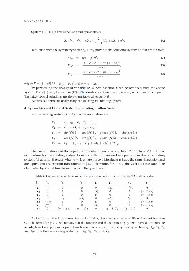
Symmetry 2019, 11, 1115

System (13)–(15) admits the Lie point symmetries:

∂z , ∂w , z∂z + w∂w +2

γ− 1h∂h + u∂u + v∂v (16)

Reduction with the symmetry vector ∂z + c∂w provides the following system of first-order ODEs:

Fhσ = (cα− β) h2, (17)

Fvσ =(α− cβ) chγ − αh (v− cu)2

v− cu, (18)

Fhσ =(α− cβ) cuγ − βh (v− cu)2

v− cu. (19)

where F =(1 + c2) hγ − h (v− cu)2 and σ = z + cw.

By performing the change of variable dσ = f dτ, function f can be removed from the abovesystem. For h (τ) = 0, the system (17)–(19) admits a solution u = u0, v = v0, which is a critical point.The latter special solutions are always unstable when αc > β.

We proceed with our analysis by considering the rotating system.

4. Symmetries and Optimal System for Rotating Shallow Water

For the rotating system ( f �= 0), the Lie symmetries are:

Y1 = ∂t , Y2 = ∂x , Y3 = ∂y ,

Y4 = y∂x − x∂y + v∂u − u∂v ,

Y5 = sin ( f t) ∂x + cos ( f t) ∂y + f (cos ( f t) ∂u − sin ( f t) ∂v)

Y6 = cos ( f t) ∂x − sin ( f t) ∂y − f (sin ( f t) ∂u + cos ( f t) ∂v)

Y7 = (γ− 1)(

x∂x + y∂y + u∂u + v∂v)+ 2h∂h

The commutators and the adjoint representation are given in Table 2 and Table A4. The Liesymmetries for the rotating system form a smaller dimension Lie algebra than the non-rotatingsystem. That is not the case when γ = 2, where the two Lie algebras have the same dimension andare equivalent under point transformation [22]. Therefore, for γ > 2, the Coriolis force cannot beeliminated by a point transformation as in the γ = 2 case.

Table 2. Commutators of the admitted Lie point symmetries for the rotating 2D shallow water.

[ , ] Y1 Y2 Y3 Y4 Y5 Y6 Y7

Y1 0 0 0 0 f Y6 − f Y5 0Y2 0 0 0 −Y3 0 0 (γ− 1)Y2Y3 0 0 0 Y2 0 0 (γ− 1)Y3Y4 0 Y3 −Y2 0 −Y6 Y5 0Y5 − f Y6 0 0 Y6 0 0 (γ− 1)Y5Y6 f Y5 0 0 −Y5 0 0 (γ− 1)Y6Y7 0 − (γ− 1)Y2 − (γ− 1)Y3 0 − (γ− 1)Y5 − (γ− 1)Y6 0

As for the admitted Lie symmetries admitted by the given system of PDEs with or without theCoriolis terms for γ > 2, we remark that the rotating and the nonrotating systems have a common Liesubalgebra of one-parameter point transformations consisting of the symmetry vectors Y1, Y2, Y3, Y4,and Y7 or for the nonrotating system X1, X2, X3, X6, and X8.

76

Symmetry 2019, 11, 1115

We proceed with the determination of the one-dimensional optimal system and the invariantfunctions. Specifically, the relative invariants for the adjoint representation are calculated to bea1 , a7 and a8. From Table 2 and Table A4, we can find the one-dimensional optimal system, which is:

Y1, Y2, Y3, Y4, Y5, Y6, Y7, χ12 = Y1 + αY2, χ13 = Y1 + αY3,

χ14 = Y1 + αY4 , χ15 = Y1 + αY5, χ16 = Y1 + αY6, χ17 = Y1 + αY7,

χ23 = Y2 + αY3 , χ45 = Y4 + αY5, χ46 = Y4 + αY6, χ56 = Y5 + αY6

χ47 = Y4 + αY6 , χ123 = Y1 + αY2 + βY3, χ147 = Y1 + αY4 + βY7.

The Lie invariants, which correspond to all the above one-dimensional Lie algebras, are presentedin Tables A5 and A6.

Let us demonstrate the application of the Lie invariants by the following, from which we cansee that the Lie invariants reduce the nonlinear field equations into a system of integrable first-orderODEs, which can be solved with quadratures.

4.1. Application of χ12

We consider the travel-wave similarity solution in the x-plane provided by the symmetry vectorχ12 and the vector field Y3. The resulting equations are described by the following system of firstorder ODEs:

vz = fu

α− u(20)

Fuz = f (α− u) vh (21)

Fhz = f vh2 (22)

where F = hγ − (a− u)2 h and z = t − αx. Because we performed reduction with a subalgebraadmitted by the nonrotating system, by setting f = 0 in (20)–(22), we get the similarity solution for thenonrotating system, where in this case, it is found to be h (z) = h0, u (z) = u0 and v (z) = v0.

We perform the substitution dz = Ff v dτ, and the latter system is simplified as follows:

vF

vτ =u

α− u(23)

uτ = (α− u) h (24)

hτ = h2 (25)

from which we get the solution:

h (τ) = (h0 − τ)−1 , u (τ) = α + u0 −u0

h0τ (26)

and:

v (t)2 = 2∫ (

a + u0 − u0h0

τ)

u0h0

(h0 − τ)

((h0 − τ)−γ +

(u0

h0

)2τ − (u0)

2

h0

)dτ. (27)

4.2. Application of χ23

Consider now the reduction with the symmetry vector fields χ23. The resulting system of 1 + 1differential equations admits five Lie point symmetries, and they are:

∂t, ∂w , (sin ( f t) + α cos ( f t)) ∂w + f (sin ( f t) ∂u + cos ( f t) ∂v)

(α sin ( f t)− cos ( f t)) ∂w − f (cos ( f t) ∂u − sin ( f t) ∂v) , (γ− 1) (∂w + u∂u + v∂v) + 2h∂h.

77

Symmetry 2019, 11, 1115

where w = y− αx. For simplicity of our calculations, let us assume γ = 3.Reduction with the scaling symmetry provides the following system of first order ODEs:

Ht = 2H (αU −V) , (28)

Ut = αH2 + u (αU −V) + f V, (29)

Vt = −H2 − v (αU −V)− f U, (30)

where h = wH, u = wU, and v = wU. The latter system is integrable and can be solvedwith quadratures.

Reducing with respect to the symmetry vector (α sin ( f t)− cos ( f t)) ∂w − f (cos ( f t) ∂u − sin ( f t) ∂v),we find the reduced system:

Ht

H= −α cos ( f t) + sin ( f t)

cos ( f t)− α sin ( f t), (31)

Ut = −α fsin ( f t)V − cos ( f t)U

cos ( f t)− α sin ( f t), (32)

Vt = − fsin ( f t)V − cos ( f t)U

cos ( f t)− α sin ( f t), (33)

where now:

h = H (t) , (34)

u =cos ( f t)

cos ( f t)− α sin ( f t)f w + U (t) , (35)

v = − sin ( f t)cos ( f t)− α sin ( f t)

f w + V (t) . (36)

System (31)–(33) is integrable, and the solution is expressed in terms of quadratures.

5. Conclusions

In this work, we determined the one-dimensional optimal system for the two-dimensional idealgas equations. The nonrotating system was found to be invariant under an eight-dimensional group ofone-parameter point transformations. and there were twenty-three independent one-dimensional Liealgebras. One the other hand, when the Coriolis force was introduced, the dynamical admitted sevenLie point symmetries and twenty one-dimensional Lie algebras.

For all the independent Lie algebras, we determined all the invariant functions, which correspondedto all the independent similarity solutions.

In a future work, we plan to classify all the independent one-dimensional Lie algebras, which leadto analytic forms for the similarity solutions.

Funding: This research received no external funding.

Acknowledgments: The author wants to thank Kevin Duffy for gracious hospitality and P.G.L.Leach for a fruitfuldiscussion on the subject.

Conflicts of Interest: The author declare no conflict of interest.

Appendix A

In this Appendix, we present the Tables A1–A6, which are referenced in the main article.

78

Symmetry 2019, 11, 1115

Ta

ble

A1

.A

djoi

ntre

pres

enta

tion

ofth

ead

mit

ted

Lie

poin

tsym

met

ries

for

the

nonr

otat

ing

2Dsh

allo

ww

ater

.

Ad( e(

εXi)) X

jX

1X

2X

3X

4X

5X

6X

7X

8

X1

X1

X2

X3

X4−

εX2

X5−

εX3

X6

X7+

ε(γ−

1 )X

1X

8X

2X

1X

2X

3X

4X

5X

6+

εX3

X7

X8−

ε(γ−

1 )X

2X

3X

1X

2X

3X

4X

5X

6−

εX2

X7

X8−

ε(γ−

1 )X

3X

4X

1+

εX2

X2

X3

X4

X5

X6+

εX5

X7−

ε(γ−

1 )X

4X

8−

ε(γ−

1 )X

4X

5X

1+

εX3

X2

X3

X4

X5

X6−

εX4

X7−

ε(γ−

1 )X

5X

8−

ε(γ−

1 )X

5X

6X

1X

2co

sε−

X3

sin

εX

2si

nε+

X3

cosε

X4

cosε−

X5

sin

εX

4si

nε+

X5

cosε

X6

X7

X8

X7

e−(γ−

1 )ε X

1X

2X

3e−

(γ−

1 )ε X

4e−

(γ−

1 )ε X

5X

6X

7X

8X

8X

1e(

γ−

1 )ε X

3e(

γ−

1 )ε X

4e−

(γ−

1 )ε X

4e−

(γ−

1 )ε X

5X

6X

7X

8

Ta

ble

A2

.Li

ein

vari

ants

for

the

opti

mal

syst

emof

the

nonr

otat

ing

syst

em.

Sy

mm

etr

yIn

vari

an

ts

X1

x,y,

h(x

,y)

,u(x

,y)

,v(x

,y)

X2

t,y,

h(t

,y)

,u(t

,y)

,v(t

,y)

X3

t,x,

h(t

,x)

,u(t

,x)

,v(t

,x)

X4

t,y,

h(t

,y)

,x t+

U(t

,y)

,v(t

,y)

X5

t,x,

h(t

,x)

,u(t

,x)

,y t+

V(t

,x)

X6

t,x2

+y2 ,

h( t,

x2+

y2) ,xU

(t,x

2+

y2)+

yV(t

,x2+

y2)

√x2+

y2,

yU(t

,x2+

y2)−

xV(t

,x2+

y2)

√x2+

y2

X7

x t,y t,

h( x t,

y t) ,u( x t,

y t) ,v( x t,

y t)X

8H(x

,y)

t2

1−γ

,U(x

,y)

t−1

,V(x

,y)

t−1

ξ (12)

x−

αt,

y,h(x−

αt,

y ),

u(x−

αt,

y ),

v(x−

αt,

y )ξ (

13)

x,y−

αt,

h(x

,y−

αt )

,u(x

,y−

αt )

,v(x

,y−

αt )

ξ (14)

x−

α 2t2 ,

y,h( x−

α 2t2 ,y

) ,u( x−

α 2t2 ,y

) ,v( x−

α 2t2 ,y

)ξ (

15)

x,y−

α 2t2 ,

h( x,

y−

α 2t2) ,

u( x,

y−

α 2t2) ,

v( x,

y−

α 2t2)

79

Symmetry 2019, 11, 1115

Ta

ble

A3

.Li

ein

vari

ants

for

the

opti

mal

syst

emof

the

nonr

otat

ing

syst

em.

Sy

mm

etr

yIn

va

ria

nts

ξ (16)

t,e−

αt( x2

+y2) ,

u( t,

e−α

t x2+

y2) cos (

αt )+

v( t,

e−α

t x2+

y2) sin(α

t )y x

,h( e−

αt x2

+y2 ,y x

) ,u( t,

e−α

t x2+

y2) sin(α

t )−

v( t,

e−α

t x2+

y2) cos (

αt )

ξ (23)

t,x−

αy,

h(t

,x−

αy )

,u(t

,x−

αy )

,v(t

,x−

αy )

ξ (34)

t,y−

x αt,

h( t,

y−

x αt) ,

u( t,

y−

x αt) ,

v( t,

y−

x αt)

ξ (25)

t,y−

αtx

,h(t

,y−

αtx)

,u(t

,y−

αtx)

,v(t

,y−

αtx)

ξ (45)

t,y−

αx,

h(t

,y−

αx )

,α

x t+

U(t

,y−

αx )

,α

x t+

V(t

,y−

αx )

ξ (12

3 )t−

αx,

t−β

y,h(t−

αx,

t−β

y ),

u(t−

αx,

t−β

y ),v

(t−

αx,

t−β

y )

ξ (14

5 )x−

α 2t2 ,

y−

β 2t2 ,

h( x−

α 2t2 ,y

−β 2

t2) ,α

t+U( x−

α 2t2 ,

y−

β 2t2) ,

βt+

V( x−

α 2t2 ,

y−

β 2t2)

ξ (12

5 )x−

αt,

y−

β 2t2 ,

h( x−

αt,

y−

β 2t2) ,

u( x−

αt,

y−

β 2t2) ,

βt+

V( x−

αt,

y−

β 2t2)

ξ (13

4 )x−

β 2t2 ,

y−

αt,

h( x−

β 2t2 ,y

−α

t) ,β

t+U( x−

β 2t2 ,y

−α

t) ,V( x−

β 2t2 ,y

−α

t)ξ (

67)

lnt

α,w

=t−

α+√

α(α−

4 )−

42α

2√α(α−

4 )−

4

( x−( α

+√ α

(α−

4 )−

4) y) ,z=

t−α+√

α(α−

4 )−

42α

2√α(α−

4 )−

4

( x+( α

+√ α

(α−

4 )−

4) y)h(w

,z)

,U(w

,z)

sin( ln

tα

) +V(w

,z)

sin( ln

tα

) ,U(w

,z)

cos( ln

tα

) −V(w

,z)

sin( ln

tα

)ξ (

68)

t,x2

+y2

,x−

2γ−

1h( t,

x2+

y2) ,U(t

,x2+

y2)

cos (

lnx

α)+

V(t

,x2+

y2)

sin (

lnx

α)

x,

U(t

,x2+

y2)

sin (

lnx

α)−

V(t

,x2+

y2)

cos (

lnx

α)

x

ξ (78)

w=

xt−

(γ−

1 )α(γ−

1 )−

2,

z=

yt−

(γ−

1 )α(γ−

1 )−

2,

t−2α

α(γ−

1 )−

2h(w

,z)

,t−

(γ−

1 )α

α(γ−

1 )−

2u(w

,z)

,t−

(γ−

1 )α

α(γ−

1 )−

2v(w

,z)

ξ (67

8 )t,

t−1−

β( x2

+y2) ,t

−β( U

( t,x2

+y2) si

n(α

t )+

V( t,

x2+

y2) cos (

αt ))

t−2β γ−

1H( t,

x2+

y2) ,t−

β( U

( t,x2

+y2) co

s (α

t )−

V( t,

x2+

y2) sin(α

t ))

Ta

ble

A4

.A

djoi

ntre

pres

enta

tion

ofth

ead

mit

ted

Lie

poin

tsym

met

ries

for

the

rota

ting

2Dsh

allo

ww

ater

.

Ad( e(

εYi)) Y j

Y1

Y2

Y3

Y4

Y5

Y6

Y7

Y1

Y 1Y 2

Y 3Y 4

Y 5co

s (fε)−

Y 6si

n(

fε)

Y 5si

n(

fε)+

Y 6co

s (fε)

Y 7Y

2Y 1

Y 2Y 3

Y 4+

εY3

Y 5Y 6

Y 7−

ε(γ−

1 )Y 2

Y3

Y 1Y 2

Y 3Y 4−

εY2

Y 5Y 6

Y 7−

ε(γ−

1 )Y 3

Y4

Y 1Y 2

cosε−

Y 3si

nε

Y 2si

nε+

Y 3co

sεY 4

Y 5co

sε+

Y 6si

nε

Y 6co

sε−

Y 5si

nε

Y 7Y

5Y 1

+fε

Y 6Y 2

Y 3Y 4−

εY6

Y 5Y 6

Y 7−

ε(γ−

1 )Y 5

Y6

Y 1−

fεY 5

Y 2Y 3

Y 4+

εY5

Y 5Y 6

Y 7−

ε(γ−

1 )Y 6

Y7

Y 1e(

γ−

1 )ε Y 2

e(γ−

1 )ε Y 3

Y 4e(

γ−

1 )ε Y 5

e(γ−

1 )ε Y 6

Y 7

80

Symmetry 2019, 11, 1115

Ta

ble

A5

.Li

ein

vari

ants

for

the

opti

mal

syst

emof

the

rota

ting

syst

em.

Sy

mm

etr

yIn

va

ria

nts

Y1

x,y,

h(x

,y)

,u(x

,y)

,v(x

,y)

Y2

t,y,

h(t

,y)

,u(t

,y)

,v(t

,y)

Y3

t,x,

h(t

,x)

,u(t

,x)

,v(t

,x)

Y4

t,x2

+y2 ,

h( t,

x2+

y2) ,xU

(t,x

2+

y2)+

yV(t

,x2+

y2)

√x2+

y2,

yU(t

,x2+

y2)−

xV(t

,x2+

y2)

√x2+

y2

Y5

t,x

cot (

ft)−

y,

h(t

,xco

t (ft)−

y ),

fxco

t (ft)+

U(t

,xco

t (ft)−

y ),−

fx+

V(t

,xco

t (ft)−

y )Y

6t,

xta

n(

ft)+

y,h(t

,xta

n(

ft)+

y ),−

fxta

n(

ft)+

U(t

,xta

n(

ft)+

y ),−

fx+

V(t

,xta

n(

ft)+

y )Y

7x t,

y t,h( x t,

y t) ,u( x t,

y t) ,v( x t,

y t)χ(1

2 )x−

αt,

y,h(x−

αt,

y ),

u(x−

αt,

y ),

v(x−

αt,

y )χ(1

3 )x,

y−

αt,

h(x

,y−

αt )

,u(x

,y−

αt )

,v(x

,y−

αt )

χ(1

4 )t,

e−α

t( x2

+y2) ,

u( t,

e−α

t x2+

y2) cos (

αt )+

v( t,

e−α

t x2+

y2) sin(α

t )y x

,h( e−

αt x2

+y2 ,y x

) ,u( t,

e−α

t x2+

y2) sin(α

t )−

v( t,

e−α

t x2+

y2) cos (

αt )

81

Symmetry 2019, 11, 1115

Ta

ble

A6

.Li

ein

vari

ants

for

the

opti

mal

syst

emof

the

rota

ting

syst

em.

Sy

mm

etr

yIn

va

ria

nts

χ(1

5 )x+

α fco

s (ft)

,y−

α fsi

n(

ft)

,h( x

+α f

cos (

ft)

,y−

α fsi

n(

ft)) ,

αsi

n(

ft)+

U( x

+α f

cos (

ft)

,y−

α fsi

n(

ft)) ,

αco

s (ft)+

V( x

+α f

cos (

ft)

,y−

α fsi

n(

ft))

χ(1

6 )x−

α fsi

n(

ft)

,y−

α fco

s (ft)

,h( x−

α fsi

n(

ft)

,y−

α fco

s (ft)) ,

αco

s (ft)+

U( x−

α fsi

n(

ft)

,y−

α fco

s (ft)) ,

−α

sin(

ft)+

V( x−

α fsi

n(

ft)

,y−

α fco

s (ft))

χ(1

7 )xe−

αt ,

ye−

αt ,

e2α γ−

1t h( xe

−α

t ,ye−

αt) ,

eαt u( xe

−α

t ,ye−

αt) ,

eαt v( xe

−α

t ,ye−

αt)

χ(2

3 )t,

x−

αy,

h(t

,x−

αy )

,u(t

,x−

αy )

,v(t

,x−

αy )

χ(4

5 )t,

w=( x2

+y2−

2xco

s (ft)+

2ysi

n(

ft)) ,

U(t

,w)+

fsin(

ft)

V(t

,w)+

fcos(

ft),

U(t

,w)2+

V(t

,w)2

2+

f (U(t

,w)

sin(

ft)+

V(t

,w)

cos (

ft))

χ(4

6 )t,

w=( x2

+y2−

2xsi

n(

ft)−

2yco

s (ft)) ,

U(t

,w)−

fcos(

ft)

V(t

,w)+

fsin(

ft)

,U(t

,w)2+

V(t

,w)2

2+

f (V(t

,w)

sin(

ft)−

U(t

,w)

cos (

ft))

χ(5

6 )t,

z=

y−

x (co

s (ft)−

αsi

n (ft))

sin (

ft)+

αco

s (ft)

,h(t

,z)

,fx (

cos (

ft)−

αsi

n (ft))

sin (

ft)+

αco

s (ft)

+U(t

,z)

,−

x+

V(t

,z)

χ(4

7 )t,

x2+

y2,

x−2

γ−

1h( t,

x2+

y2) ,U(t

,x2+

y2)

cos (

lnx

α)+

V(t

,x2+

y2)

sin (

lnx

α)

x,

U(t

,x2+

y2)

sin (

lnx

α)−

V(t

,x2+

y2)

cos (

lnx

α)

xχ(1

23)

t−α

x,t−

βy,

h(t−

αx,

t−β

y ),

u(t−

αx,

t−β

y ),v

(t−

αx,

t−β

y )

χ(1

47)

z=

e−t (

γ−

1 )(x

cost−

ysi

nt )

,w=

e−t (

γ−

1 )(y

cost

+x

sin

t ),

e−t (

γ−

1 )h(z

,w)

,e−

t (γ−

1 )(U

(z,w

)co

st−

V(z

,w)

sin

t ),

e−t (

γ−

1 )(U

(z,w

)si

nt+

V(z

,w)

cost)

82

Symmetry 2019, 11, 1115

References

1. Olver, P.J. Applications of Lie Groups to Differential Equations; Springer: New York, NY, USA, 1993.2. Bluman, G.W.; Kumei, S. Symmetries and Differential Equations; Springer: New York, NY, USA, 1989.3. Ibragimov, N.H. CRC Handbook of Lie Group Analysis of Differential Equations, Volume I: Symmetries,

Exact Solutions, and Conservation Laws; CRS Press LLC: Boca Raton, FL, USA, 2000.4. Webb, G.M. Lie symmetries of a coupled nonlinear Burgers-heat equation system. J. Phys A Math. Gen.

1990, 23, 3885. [CrossRef]5. Tsamparlis, M.; Paliathanasis, A.; Karpathopoulos, L. Dynamics of ionization wave splitting and merging

of atmospheric-pressure plasmas in branched dielectric tubes and channels. J. Phys. A Math. Theor.2012, 45, 275201. [CrossRef]

6. Azad, H.; Mustafa, M.T. Group classification, optimal system and optimal reductions of a class of KleinGordon equations. Commun. Nonlinear Sci. Numer. Simul. 2010, 15, 1132. [CrossRef]

7. Tsamparlis, M.; Paliathanasis, A. Symmetry analysis of the Klein–Gordon equation in Bianchi I spacetimes.Int. J. Geom. Methods Mod. Phys. 2005, 12, 155003.

8. Meleshko, S.V.; Shapeev, V.P. Nonisentropic solutions of simple wave type of the gas dynamics equations.J. Nonlinear Math. Phys. 2011, 18, 195. [CrossRef]

9. Halder, A.; Paliathanasis, A.; Leach, P.G.L. Noether’s Theorem and Symmetry. Symmetry 2018, 10, 744.[CrossRef]

10. Jamal, S.; Leach, P.G.L.; Paliathanasis, A. Nonlocal Representation of the sl (2,R) Algebra for the Chazyequation. Quaest. Math. 2019, 42, 125. [CrossRef]

11. Ovsiannikov, L.V. Group Analysis of Differential Equations; Academic Press: New York, NY, USA, 1982.12. Chou, K.S.; Qu, C.Z. Optimal systems and group classification of (1 + 2)-dimensional heat equation.

Acta Appl. Math. 2004, 83, 257. [CrossRef]13. Galas, F.; Richter, E.W. Exact similarity solutions of ideal MHD equations for plane motions. Phys. D

1991, 50, 297. [CrossRef]14. Coggeshalla, S.V.; Meyer-ter-Vehn, J. Group-invariant solutions and optimal systems for multidimensional

hydrodynamics. J. Math. Phys. 1992, 33, 3585. [CrossRef]15. Hu, X.; Li, Y.; Chen, Y. A direct algorithm of one-dimensional optimal system for the group invariant

solutions. J. Math. Phys. 2015, 56, 053504. [CrossRef]16. Vallis, G.K. Atmospheric and Oceanic Fluid Dynamics: Fundamentals and Large-Scale Circulation;

Cambridge University Press: Cambridge, UK, 2006.17. Courant, R.; Friedrichs, K.O. Supersonic Flow and Shock Waves; Interscience Publishers: Geneva, Switzerland,

1948.18. Kevorkian, J. Partial Differential Equations: Analytical Solutions Techniques; Chapman and Hall:

New York, NY, USA, 1990.19. Caleffi, V.; Valiani, A.; Zanni, A. Finite volume method for simulating extreme flood events in natural

channels. J. Hydraul. Res. 2003, 41, 167. [CrossRef]20. Akkermans, R.A.D.; Kamp, L.P.J.; Clercx, H.J.H.; van Heijst, G.J.F. Three-dimensional flow in

electromagnetically driven shallow two-layer fluids. Phys. Rev. E 2010, 82, 026314. [CrossRef] [PubMed]21. Kim, D.H.; Cho, Y.S.; Yi, Y.K. Propagation and run-up of nearshore tsunamis with HLLC approximate

Riemann solver. Ocean Eng. 2007, 34, 1164. [CrossRef]22. Chesnokov, A.A. Symmetries and exact solutions of the rotating shallow-water equations. Eur. J. Appl. Math.

2009, 20, 461. [CrossRef]23. Xin, X.; Zhang, L.; Xia, Y.; Liu, H. Nonlocal symmetries and exact solutions of the (2 + 1)-dimensional

generalized variable coefficient shallow water wave equation. Appl. Math. Lett. 2019, 94, 112. [CrossRef]24. Szatmari, S.; Bihlo, A. Symmetry analysis of a system of modified shallow-water equations. Comm. Nonlinear

Sci. Num. Simul. 2014, 19, 530. [CrossRef]25. Chesnokov, A.A. Symmetries and exact solutions of the shallow water equations for a two-dimensional

shear flow. J. Appl. Mech. Tech. Phys. 2008, 49, 737. [CrossRef]26. Liu, J.-G.; Zeng, Z.-F.; He, Y.; Ai, G.-P. A Class of Exact Solution of (3 + 1)-Dimensional Generalized Shallow

Water Equation System. Int. J. Nonlinear Sci. Num. Simul. 2014, 19, 37. [CrossRef]

83

Symmetry 2019, 11, 1115

27. Pandey, M. Lie Symmetries and Exact Solutions of Shallow Water Equations with Variable Bottom. Int. J.Nonlinear Sci. Num. Simul. 2015, 16, 93. [CrossRef]

28. Paliathanasis, A. Lie symmetries and similarity solutions for rotating shallow water. Preprint arXiv 2019,arXiv:1906.00689.

c© 2019 by the author. Licensee MDPI, Basel, Switzerland. This article is an open accessarticle distributed under the terms and conditions of the Creative Commons Attribution(CC BY) license (http://creativecommons.org/licenses/by/4.0/).

84

symmetryS SArticle

Minimal Energy Configurations of FiniteMolecular Arrays

Pablo V. Negrón-Marrero * and Melissa López-Serrano

Department of Mathematics, University of Puerto Rico, Humacao, PR 00791-4300, USA; melissa.lopez3@upr.edu* Correspondence: pablo.negron1@upr.edu

Received: 26 December 2018; Accepted: 28 January 2019; Published: 31 January 2019

Abstract: In this paper, we consider the problem of characterizing the minimum energy configurationsof a finite system of particles interacting between them due to attractive or repulsive forces givenby a certain intermolecular potential. We limit ourselves to the cases of three particles arranged in atriangular array and that of four particles in a tetrahedral array. The minimization is constrained toa fixed area in the case of the triangular array, and to a fixed volume in the tetrahedral case. For ageneral class of intermolecular potentials we give conditions for the homogeneous configuration(either an equilateral triangle or a regular tetrahedron) of the array to be stable that is, a minimizerof the potential energy of the system. To determine whether or not there exist other stable states,the system of first-order necessary conditions for a minimum is treated as a bifurcation problemwith the area or volume variable as the bifurcation parameter. Because of the symmetries presentin our problem, we can apply the techniques of equivariant bifurcation theory to show that thereexist branches of non-homogeneous solutions bifurcating from the trivial branch of homogeneoussolutions at precisely the values of the parameter of area or volume for which the homogeneousconfiguration changes stability. For the triangular array, we construct numerically the bifurcationdiagrams for both a Lennard–Jones and Buckingham potentials. The numerics show that there existnon-homogeneous stable states, multiple stable states for intervals of values of the area parameter,and secondary bifurcations as well.

Keywords: molecular arrays; constrained optimization; equivariant bifurcation theory

1. Introduction

Consider a system of N molecules, modeled as identical spherical particles, enclosed in a boundedregion B of R3. At any given instant (or in an equilibrium configuration), the total potential energy ofthe molecular array is given by:

E = ∑i<j

φ(∥∥�ri −�rj

∥∥), (1)

where φ is the intermolecular potential energy with ‖·‖ the standard Euclidean or two-vector norm,and�r1, . . . ,�rN ∈ R3 are the positions of the particles. More general energy potentials have beenconsidered of which (1) is a special case (cf. [1,2]), or those based on the eigenvalues of adjacencymatrices like in [3]. The problem of minimizing (1) subject to certain type of global or local conditionshave been studied extensively (see e.g., [4–6] and the references there in). In these models eitherthe array is infinite, with some local repeating structure, or finite but with N → ∞. In this paper,none of these conditions are required but we expect that our results can be extrapolated to such moregeneral scenarios. Also, we do not commit to any particular intermolecular potential φ (but giveexamples for instance for Lennard–Jones type potentials) so that our results are applicable to any suchsmooth potential.

The particular problems that we consider in this paper are those of characterizing the minimumenergy configurations of (1) in the case of three particles (N = 3) arranged in a triangle and that of four

Symmetry 2019, 11, 158; doi:10.3390/sym11020158 www.mdpi.com/journal/symmetry85

Symmetry 2019, 11, 158

particles (N = 4) in a tetrahedral array. The minimization problem is subject to the constraint of fixedarea for the triangular array and of fixed volume in the tetrahedral case. We are particularly interestedon the dependence of the minimizing states on the parameter of area or volume in the constraint. Bothproblems have the particularity that they can be formulated in terms of the intermolecular distancesonly, that is, without specifying the coordinates corresponding to the positions of the particles, thussubstantially reducing the number of unknowns in each problem.

The motivation to study these problems comes from the following phenomena observed bothin laboratory experiments and molecular dynamics simulations (see e.g., [7,8]). As the density of afluid is progressively lowered (keeping the temperature constant), there is a certain “critical” densitysuch that if the density of the fluid is lower than this critical value, then bubbles or regions with verylow density appear within the fluid. This phenomenon is usually called “cavitation” and it has beenextensively studied as well in solids. (See for instance [9,10] for discussions and further references.)When using discrete models of materials like (1), distinguishing between regions of low vs. highdensity, or whether bubbles or holes have form within the array, is not obvious since one is dealingessentially with a set of points. (See for instance [11,12] for the use of Voronoi polyhedra to studysuch arrays.) Thus, to study this phenomenon within this discrete model, one is naturally led to studyor characterize the stability of homogeneous energy minimizing configurations of such an array, asthe density of the array changes. The problems considered in this paper are the simplest problemswithin such a model. Our main contribution is on the application of global bifurcation theory (asopposed to just local) to study the set of equilibrium configurations for (1) under the stated constraints.In particular, to give specific conditions in terms of the intermolecular potential φ for the existence ofnontrivial states.

In Section 3 we consider the problem of three particles. By Heron’s formula for the area ofa triangle, any three numbers (representing the intermolecular distances) that yield a positive valuefor the area formula, represent a triangle. In this case, we show that the functional (1) subject tothe constraint of fixed area A, has for any value of A, a critical point representing an equilateraltriangle. Moreover, in Theorem 2 we give a necessary and sufficient condition (cf. (22)), in terms of theintermolecular potential, for this equilibrium point to be a (local) minimizer of the energy functional.This condition leads to a set of values A for the area parameter A for which the equilateral triangle isa stable configuration. We give examples of how this set looks for various intermolecular potentialsincluding the classical Lennard–Jones [13] and Buckingham [14] potentials, and those that model hardand soft springs including the usual Hooke’s law.

Next in Section 3.2 we turn to the question of whether there exists other (not equilateral)equilibrium configurations for those values of the area parameter A for which the equilateral trianglebecomes unstable, that is, when it ceases to be a local minimizer. To answer this question, we treat thesystem of equations characterizing the equilibrium points (cf. (13)) as a bifurcation problem with theparameter A as a bifurcation parameter, and the set of equilateral equilibrium configurations as thetrivial solution branch. We find that the necessary condition for bifurcation from the trivial branchfor this system occurs exactly at the boundary points of the set A given by the stability condition (22).To check the sufficiency condition for bifurcation, one must consider the linearization of the system (13)about the trivial branch at a boundary point A0 of A. However, since the kernel of this linearization istwo-dimensional we cannot immediately apply the usual or standard results from bifurcation theory(cf. [15–18]). Because of the symmetries present in this problem (cf (32)), we can apply bifurcationequivariant theory (cf. [16,19]) to construct a suitable reduced problem corresponding to isoscelestriangular equilibrium configurations. The linearization of the reduced problem at the point whereA = A0 has now a one-dimensional kernel and provided that a certain transversality condition issatisfied (cf. (34)), we can show that there are three branches corresponding to isosceles trianglesbifurcating from the trivial branch at the point where A = A0. Since the stability of these bifurcatingbranches can only be determined numerically (because one must linearize about an unknown solution),in Section 5 we construct numerically the bifurcation diagrams, with their respective stability patterns,

86

Symmetry 2019, 11, 158

for instances of the Lennard–Jones and Buckingham potentials. These examples show that the primarybifurcations off the trivial branch are of trans-critical type, and that at least for the Lennard–Jonespotential, there are secondary bifurcations corresponding to stable scalene triangles. Moreover, thereare intervals of values of the area parameter, for which there exists multiple stable states of the systemfor each value of A in such an interval.

In Section 4 we consider an array of four molecules in a tetrahedron. The general treatment in thiscase is similar to the three particle case but with two main differences. First the characterization ofwhen six numbers (representing the lengths of the sides of the tetrahedron) determine a tetrahedron,is given in terms of the Cayley-Menger determinant and the triangle inequalities of one of its faces(cf. [20]). The next complication arises from the fact that the tetrahedron has 24 symmetries as comparedto only six for the triangle! To deal with this many possibilities, once again we make use of the basictechniques of equivariant theory to get suitable reduced problems to work with. As the Cayley–Mengerdeterminant is proportional to the volume of the corresponding tetrahedron, the volume constraint inour problem is basically that of setting this determinant to a given value V for the volume. In this casewe show in Section 4.1 that the functional (1) subject to the constraint of fixed volume V, has for anyvalue of V a critical point representing a regular or equilateral tetrahedron. Moreover, in Theorem 4we give necessary and sufficient conditions (cf. (43)), in terms of the intermolecular potential, for thisequilibrium point to be a (local) minimizer of the energy functional. As for the triangular case,these conditions determine a set of values V for the volume parameter V for which the equilateraltetrahedron is a stable configuration.

In Section 4.2 we consider the question of the existence of non-equilateral equilibriumconfigurations. The equilibrium configurations in this case are given as solutions to a nonlinearsystem of seven equations in eight unknowns (cf. (40)). We treat this system as a bifurcation problemwith the parameter V as a bifurcation parameter, and the set of equilateral tetrahedrons as the trivialsolution branch. The necessary condition for bifurcation from the trivial branch for this system occursexactly at the boundary points of the set V given by the stability conditions (43). At a boundarypoint V0 of V there are two possibilities: the kernel of the linearization has dimension two or three.Using some of the machinery of equivariance theory as in [16], we can construct suitable reducedproblems in each of these two cases, which enables us to establish the existence of non-equilateralequilibrium configurations and to get a full description of the symmetries of the bifurcating branches(cf. Theorems 5–7). As in the triangular case, the stability of this bifurcating branches can only beestablished numerically because one must linearize about the unknown bifurcating branch.

Notation: We let Rn denote the n dimensional space of column vectors with elements denoted by�x, �y,. . . The inner product of�x,�y ∈ Rn is denoted either by 〈�x,�y〉 or�xt�y, where the superscript “t”denotes transpose. We denote the set of n×m matrices by Rn×m. For L ∈ Rn×m, we let ker(L) = {�x ∈Rn : L�x = �0} and Range(L) = {L�x : �x ∈ Rn}. For a function�F : Rn → Rm, we denote its Fréchetderivative by D�F which is given by the m× n matrix of partial derivatives of the components of �F.If the variables in�F are given by (�x,�y), then D�x

�F denotes the derivative of�F with respect to the vectorof variables�x, i.e., the matrix of the partial derivatives of the components of �F with respect to thevariables corresponding to�x.

2. Equivariant Bifurcation from a Simple Eigenvalue

In this section, we provide an overview on some of the basic results on bifurcation theory froma simple eigenvalue for mappings between finite dimensional spaces, where the maps possess certainsymmetries. The literature on this subject is extensive but we refer to [6,15,17] for details on the materialpresented in this section and further developments like for instance, the infinite dimensional case.

87

Symmetry 2019, 11, 158

Let�F : U ×R→ Rn where U is an open subset of Rn, be a C2 function, and consider the problemof characterizing the solution set of:

�F(�x, A) =�0, (�x, A) ∈ U ×R. (2)

We assume that there exists a (known) smooth function�g(·) such that:

�F(�g(A), A) =�0, ∀ A.

The set T = {(�g(A), A) : A ∈ R} is called the trivial branch of solutions of (2). We say that(�x0, A0) ∈ T is a bifurcation point off the trivial branch T , if every neighborhood of (�x0, A0) containssolutions of (2) not in T . If we let

L(A) = D�x�F(�g(A), A),

then by the Implicit Function Theorem, a necessary for (�x0, A0) to be a bifurcation point is that L(A0)

must be singular, a condition well known to be not sufficient.In many applications of bifurcation theory and for the problems considered in this paper,

the mapping �F possesses symmetries due to the geometry of the underlying physical problem.The use of these symmetries in the analysis is useful for example to deal with problems in whichdim ker(L(A0)) > 1. Thus, we assume that for a proper subgroup G of Rn×n, characterizing thesymmetries in the problem, the mapping�F satisfies:

�F(P�x, A) = P�F(�x, A), ∀ P ∈ G. (3)

Let�v ∈ ker(L(A0)) and define the isotropy subgroup of G at�v by

H = {P ∈ G : P�v = �v} , (4)

and theH–fixed point set byR

nH = {�x ∈ R

n : P�x =�x, ∀P ∈ H} . (5)

Clearly�v ∈ RnH.

Let PH : Rn → Rn be a linear map that projects onto RnH that is Range(PH) = Rn

H and PH(RnH) =

RnH. With UH = PH(U ) = U ∩Rn

H, we define�FH : UH ×R→ RnH by:

�FH(�u, A) = PH�F(�u, A), (�u, A) ∈ UH ×R. (6)

An easy calculation now gives that

D�u�FH(�u, A) = PH�F�x(�u, A)PH.

We assume that�g(A) ∈ RnH for all A, so that

�FH(�g(A), A) =�0, ∀ A.

It follows now that LH(A) : RnH → Rn

H is given by:

LH(A) = D�u�FH(�g(A), A) = PHL(A)PH.

Clearly�v ∈ ker(LH(A0)). TheH-reduced problem is now given by:

�FH(�u, A) =�0, (�u, A) ∈ UH ×R. (7)

88

Symmetry 2019, 11, 158

An important property relating (2) and (7) is that (�x, A) ∈ UH ×R is a solution of (2) if and onlyif (�x, A) is a solution of (7). The following result provides the required sufficient conditions for (�x0, A0)

to be a bifurcation point of theH-reduced problem.

Theorem 1 (Equivariant Bifurcation Theorem [19]). Assume that for A = A0 there exists�v ∈ ker(L(A0))

that defines a proper isotropy subgroupH such that:

ker(LH(A0)) = span {�v} , L′H(A0)�v /∈ Range(LH(A0)).

Then there exists a branch CH of nontrivial solutions of�FH(�u, A) =�0 bifurcating from the trivial branchT at the point where A = A0 and such that either:

1. CH is unbounded in Rn+1;2. the closure of CH intersects the boundary ∂U of U ;3. CH intersects T at a point (�x∗, A∗) where A∗ �= A0.

The proof of this theorem is basically an application of a result from Krasnoselski [18] that usesthe homotopy invariance of the topological degree. The three alternatives in the statement of thetheorem are usually referred to as the Crandall and Rabinowitz alternatives. The local version ofthis result (cf. [6]) that is, without the Crandall and Rabinowitz alternatives, can be obtained via theLyapunov–Schmidt reduction method. A useful consequence of this reduction is an approximateformula for the bifurcating branch in a neighborhood of the bifurcation point. Let ker(LH(A0)

t) =

span {�v∗}, where 〈�v∗,�v〉 = 1, so that Range(LH(A0)) ={�y ∈ Rn

H : 〈�v∗,�y〉 = 0}

. Now if we define

A0 = 〈�v∗, (D�u�u�F0H�v)�v〉, B0 = 〈�v∗, L′H(A0)�v〉. (8)

(here the zero superscripts mean evaluated at (�x0, A0)), then the bifurcating branch have the followingasymptotic expansion (cf. [16]):

(�x, A) =(�g(A0 + ε) + εm�v + O(ε2), A0 + ε

), (9)

where

m = −2B0

A0 , A0 �= 0. (10)

3. The Three Particle Case

In this section, we consider the case in which the molecular array consists of three particles.The intermolecular energy is given by a smooth function φ : (0, ∞)→ R called the potential. If (a, b, c)are the distances between the particles in the array, the total energy of the system is given by:

E(a, b, c) = φ(a) + φ(b) + φ(c), a, b, c > 0. (11)

Also, the square of the area of the triangular array is given by Heron’s formula:

g(a, b, c) ≡ s(s− a)(s− b)(s− c),

where s = (a + b + c)/2.For any given number A > 0, we consider the following constrained minimization problem:{

mina,b,c>0

E(a, b, c)

subject to g(a, b, c) = A2.(12)

89

Symmetry 2019, 11, 158

Thus, we are looking for minimizers of the energy functional E subject to the constraint that thearea of the array is A. The first-order necessary conditions for a solution of this problem are given by:{

g(a, b, c)− A2 = 0,�∇E(a, b, c) + λ�∇g(a, b, c) = �0,

(13)

where λ ∈ R is the Lagrange multiplier corresponding to the restriction g(a, b, c) = A2. For any givenvalue of A > 0, this is a nonlinear system of equations for the unknowns (λ, a, b, c) in terms of A.In general this system can have multiple solutions depending on the characteristics of the potential φ

and the value of A.

3.1. Existence and Stability of Trivial States

An easy calculation shows that:

�∇E =

⎡⎢⎣ φ′(a)φ′(b)φ′(c)

⎤⎥⎦ , �∇g =14

⎡⎢⎣ a(b2 + c2 − a2)

b(a2 + c2 − b2)

c(a2 + b2 − c2)

⎤⎥⎦ . (14)

Thus, the system (13) is equivalent to:⎧⎪⎪⎪⎨⎪⎪⎪⎩18 (a2b2 + a2c2 + b2c2)− 1

16 (a4 + b4 + c4)− A2 = 0,φ′(a) + λ

4 a(b2 + c2 − a2) = 0,φ′(b) + λ

4 b(a2 + c2 − b2) = 0,φ′(c) + λ

4 c(a2 + b2 − c2) = 0.

(15)

This system always has a solution with a = b = c. In fact, upon setting a = b = c in (15), thissystem reduces to:

316

a4 = A2, φ′(a) = −λa3

4. (16)

Thus, we have the following result:

Lemma 1. For any value of A > 0, the system (15) has a solution of the form (λA, aA, aA, aA, A) where:

aA =2√

A4√

3, λA = −4φ′(aA)

a3A

. (17)

We now characterize for which values of A, the solution provided in Lemma 16 is actually aminimizer, i.e., a solution of (12). To do this we need to examine the matrix

[∇2E + λ∇2g

](�vA) where

�vA = (λA, aA, aA, aA), over the subspace:

M ={(x, y, z) : �∇g(�vA) · (x, y, z) = 0

}. (18)

A straightforward calculation gives that:

∇2E =

⎡⎢⎣ φ′′(a) 0 00 φ′′(b) 00 0 φ′′(c)

⎤⎥⎦ , (19)

∇2g =14

⎡⎢⎣ b2 + c2 − 3a2 2ab 2ac2ab a2 + c2 − 3b2 2bc2ac 2bc a2 + b2 − 3c2

⎤⎥⎦ . (20)

90

Symmetry 2019, 11, 158

It follows now that

[∇2E + λ∇2g

](�vA) =

⎡⎢⎢⎣φ′′(aA)− λAa2

A4

λAa2A

2λAa2

A2

λAa2A

2 φ′′(aA)− λAa2A

4λAa2

A2

λAa2A

2λAa2

A2 φ′′(aA)− λAa2

A4

⎤⎥⎥⎦ , (21)

and thatM = {(x, y, z) : x + y + z = 0} .

Using (17) one can show now that the matrix (21) is positive definite overM if and only if:

φ′′(aA) +3

aAφ′(aA) > 0. (22)

Thus, we have the following result:

Theorem 2. Let φ : (0, ∞) → R be twice continuously differentiable function. Then the uniform array(a, b, c) = (aA, aA, aA) in Lemma 1 is a relative minimizer for the problem (12) for those values of A forwhich (22) holds.

Example 1. Consider the case of a potential that has the following form:

φ(r) =c1

rδ1− c2

rδ2, (23)

where c1, c2 are positive constants and δ1 > δ2 > 2. (These constants determine the physical properties of theparticle or molecule in question. The classical Lennard–Jones [13] potential is obtained upon setting δ1 = 12and δ2 = 6.) For this function:

φ′(r) = − c1δ1

rδ1+1 +c2δ2

rδ2+1 , φ′′(r) =c1δ1(δ1 + 1)

rδ1+2 − c2δ2(δ2 + 1)rδ2+2 ,

so that:

φ′′(r) +3r

φ′(r) =c1δ1(δ1 − 2)

rδ1+2 − c2δ2(δ2 − 2)rδ2+2 .

Since aA is directly proportional to√

A (see (17)), we have that for (23), the stability condition (22) holdsif and only if A < A0, where A0 is determined from the condition:

c1δ1(δ1 − 2)

aδ1+2A

− c2δ2(δ2 − 2)

aδ2+2A

= 0,

from which it follows that:

A0 =

√3

4

[c1δ1(δ1 − 2)c2δ2(δ2 − 2)

] 2δ1−δ2

. (24)

Thus, (17) is a (local) solution of (12) if and only if A < A0. We will show that for A > A0 there existsolutions that break the symmetry a = b = c.

Example 2. A Buckingham potential has the form ([14,21]):

φ(r) = αe−βr − γ

rη , (25)

91

Symmetry 2019, 11, 158

where α, β, γ, η are positive constants. Thus

φ′(r) = −αβe−βr +γη

rη+1 , φ′′(r) = αβ2e−βr − γη(η + 1)rη+2 ,

from which it follows that:

φ′′(r) +3r

φ′(r) = αβ

[β− 3

r

]e−βr − γη(η − 2)

rη+2 .

After rearrangement, the stability condition (22) is equivalent to:

F(aA) > G(aA), (26)

where

F(r) = αβ(βr− 3)e−βr, G(r) =γη(η − 2)

rη+1 .

These functions generically look as in Figure 1 where for G we assumed that η > 2. Now clearlyF(r) < G(r) for r sufficiently large. Thus generically we expect the set of values of A for which (26) issatisfied to be of the form (A0, A1). Since F has a maximum at rm = 4

β , a sufficient condition for this is thatF(rm) > G(rm), or after rearrangement that the coefficients and exponents in (25) satisfy:

αβe−4 > γη(η − 2)(

β

4

)η+1. (27)

To check this condition against the results in [21], we let D, R, ξ > 0 with ξ > η, and define

α =Dηeξ

ξ − η, β =

ξ

R, γ =

DξRη

ξ − η. (28)

It follows that (25) is now given in terms of D, R, ξ by:

φ(r) = D[

η

ξ − ηeξ(1− r

R ) − ξ

ξ − η

(Rr

)η].

It is easy to check now that provided ξ > η + 1, then φ has negative minimum value at r = R. Theresults in ([21], Table 1, Page 202) show that the best fit of a normalized Buckingham potential to a normalizedLennard–Jones (12-6) potential (δ1 = 12 and δ2 = 6 in (23)) is achieved for ξ = 14.3863 and η = 5.6518. Forthese values one can check that (28) satisfy the inequality (27) independent of the values of D and R.

Example 3. Consider a potential of the form

φ(r) =12

kr2 +14

βr4, (29)

with k > 0 and β ∈ R. This potential corresponds to a Hook-type spring when β = 0, a hard spring ifβ > 0, and a soft spring if β < 0. (More general versions of (29) have been used in the study of the control ofmulti-agent systems, e.g., [22,23].) For this potential

φ′′(r) +3r

φ′(r) = 4k + 6βr2.

Please note that the stability condition (22) holds when β ≥ 0 independent of the value of A! That is,the symmetric state (17) is a minimizer for all values of A. In the case β = 0 is easy to show that this state isa global minimizer.

92

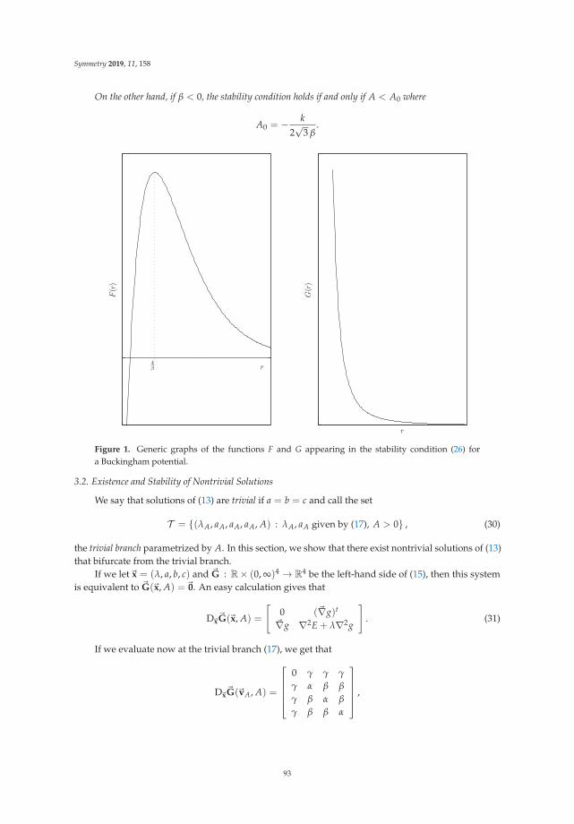
Symmetry 2019, 11, 158

On the other hand, if β < 0, the stability condition holds if and only if A < A0 where

A0 = − k2√

3 β.

F(r)

G(r)

r

r

4β

Figure 1. Generic graphs of the functions F and G appearing in the stability condition (26) fora Buckingham potential.

3.2. Existence and Stability of Nontrivial Solutions

We say that solutions of (13) are trivial if a = b = c and call the set

T = {(λA, aA, aA, aA, A) : λA, aA given by (17), A > 0} , (30)

the trivial branch parametrized by A. In this section, we show that there exist nontrivial solutions of (13)that bifurcate from the trivial branch.

If we let�x = (λ, a, b, c) and �G : R× (0, ∞)4 → R4 be the left-hand side of (15), then this systemis equivalent to �G(�x, A) =�0. An easy calculation gives that

D�x�G(�x, A) =

[0 (�∇g)t

�∇g ∇2E + λ∇2g

]. (31)

If we evaluate now at the trivial branch (17), we get that

D�x�G(�vA, A) =

⎡⎢⎢⎢⎣0 γ γ γ

γ α β β

γ β α β

γ β β α

⎤⎥⎥⎥⎦ ,

93

Symmetry 2019, 11, 158

where�vA = (λA, aA, aA, aA) and

α = φ′′(aA)−λAa2

A4

, β =λAa2

A2

, γ =a3

A4

.

The eigenvalues of this matrix are α− β, which is a double eigenvalue with geometric multiplicitytwo, and the simple eigenvalues

12

[α + 2β±

√(α + 2β)2 + 12γ2

],

which are always nonzero. A pair of linearly independent eigenvectors corresponding to α− β is{(0,−1, 1, 0)t, (0,−1, 0, 1)t}. Since

α− β = φ′′(aA)−34

λAa2A = φ′′(aA) +

3aA

φ′(aA),

the double eigenvalue α− β becomes zero exactly at the value A0 where the stability condition (22)fails by becoming zero. Thus according to standard theory of bifurcation theory, we can have eithernone, two or four branches of solutions of (15) bifurcating at the point where A = A0. We now showthat there are exactly four branches bifurcating from such a point: the trivial branch and three branchescorresponding to isosceles triangles.

To avoid the complications of dealing with the two-dimensional kernel of (31) when evaluated atthe trivial branch at A = A0, we make use of the symmetries possessed by the mapping �G. In particular,if we denote by G the subgroup of R4×4 of permutations that permute just the a, b, c components ofany�x = (λ, a, b, c) ∈ R4, then

�G(P�x, A) = P�G(�x, A), ∀ P ∈ G. (32)

Please note that every permutation in G changes the eigenvectors{(0,−1, 1, 0)t, (0,−1, 0, 1)t} of

α− β. However, the eigenvector

�v ≡ (0,−2, 1, 1)t = (0,−1, 1, 0)t + (0,−1, 0, 1)t,

is unchanged by the proper subgroup of permutationsH of G that permutes just the b, c components ofany�x = (λ, a, b, c) ∈ R4. Thus,H is the isotropy subgroup of G at�v. TheH fixed point set is given by:

R4H =

{(λ, a, b, b)t : λ, a, b ∈ R

}.

The projection PH : R4 → R4H has matrix representation:

PH =

⎡⎢⎢⎢⎣1 0 0 00 1 0 00 0 1

212

0 0 12

12

⎤⎥⎥⎥⎦ ,

and theH reduced problem is now:

�GH(�u, A) ≡ PH�G(�u, A) =�0, (�u, A) ∈ R4H × (0, ∞).

Since T ⊂ R4H × (0, ∞), it follows that T is a branch of solutions for the H reduced problem.

Also, sinceD�u

�GH(�u, A) = PHD�x�G(�u, A)PH.

94

Symmetry 2019, 11, 158

we have that LH(A) : R4H → R4

H is given by:

LH(A) = D�u�GH(�vA, A) = PHD�x

�G(�vA, A)PH.

Letμ(A) = α− β = φ′′(aA) +

3aA

φ′(aA). (33)

We now establish a result for the existence of bifurcating branches for the reduced problem.

Theorem 3. Let μ(A0) = 0 and assume that

dμ

dA(A0) �= 0. (34)

Consider the system (13) and its trivial branch of solutions (30). Then from the point (λ0, a0, a0, a0) ∈ Tbifurcate three branches of nontrivial solutions of (13) each corresponding to isosceles triangles.

Proof. With the definitions and notation as above, a lengthy but otherwise elementary calculationshows that for any A > 0, μ(A) is a simple eigenvalue of LH(A) restricted to R4

H with correspondingeigenvector�v = (0,−2, 1, 1)t. Thus

LH(A)�v = μ(A)�v, ∀ A > 0.

In particular ker(LH(A0)) = span{�v}. If we differentiate with respect to A in the equation aboveand set A = A0, we get that

L′H(A0)�v = μ′(A0)�v.

Since LH(A0) is symmetric, we have that Range(LH(A0)) ={�y ∈ Rn

H : 〈�v,�y〉 = 0}

. Thus,the hypotheses in Theorem 1 are satisfied if and only if μ′(A0) �= 0. Thus, we get a branch ofsolutions of the reduced problem, equivalently (15), bifurcating from the trivial branch at the pointwhere A = A0. Since this branch belongs to R4

H × R, we can use (32) to get that there exist twoadditional branches of solutions, one belonging to

{(λ, b, a, b, A)t : λ, a, b, A ∈ R

}and the other in{

(λ, b, b, a, A)t : λ, a, b, A ∈ R}

.

4. Four Particles in a Tetrahedron

We now consider the case of four particles arranged in a tetrahedron T. Let a, b, c, A, B, C be thedistances between the particles where a, b, c denote the lengths of the edges joining a vertex of T, A thelength of the edge opposite to a, B the length of the edge opposite to b, and C the length of the edgeopposite to c. The six-tuple�a = (a, b, c, A, B, C)t generates a tetrahedron ([20]) if and only if

g(�a) > 0, A < B + C, B < A + C, C < A + B, (35)

where g(�a) is given by the Cayley–Menger determinant:

g(�a) =

∣∣∣∣∣∣∣∣∣∣∣

0 a2 b2 c2 1a2 0 C2 B2 1b2 C2 0 A2 1c2 B2 A2 0 11 1 1 1 0

∣∣∣∣∣∣∣∣∣∣∣. (36)

If we let R+ denote the set of positive real numbers, then we define

S ={�a = (a, b, c, A, B, C)t ∈ R

6+ : (35) holds

}.

95

Symmetry 2019, 11, 158

Please note that S is open in R6. Moreover, any regular tetrahedron in which a = b = c = A =

B = C > 0, is contained in S .If�a = (a, b, c, A, B, C)t generates a tetrahedron, then so does P�a where P = RQ and

1. R permutes (a, b, c) and (A, B, C) with the same permutation of three elements;2. Q is any permutation of (a, b, c, A, B, C) in which the base of the tetrahedron is changed to another

face. For example, (c, A, B, C, a, b) corresponds to reorienting the tetrahedron so that the base isgiven by (C, a, b).

Since there are six permutations of the type R and four of the type Q, we get that there are24 permutations of the form P = RQ. These 24 permutations form a subgroup R of the group ofpermutations of six letters. Also, it is easy to show that

g(P�a) = g(�a), ∀ P ∈ R. (37)

As the Cayley–Menger determinant is directly proportional to the square of the volume of thetetrahedron (cf. (39)), this identity simply states that the volume of the tetrahedron remains the sameafter rotations of the base and independent of which face we use as the base.

The total energy of the system of four particles is given now by:

E(�a) = φ(a) + φ(b) + φ(c) + φ(A) + φ(B) + φ(C), (38)

where the intermolecular potential φ is as before. For any V > 0 we consider the constrainedminimization problem: {

minS

E(�a)

subject to g(�a) = 288V2.(39)

The constraint here specifies that the tetrahedron determined by�a has volume V (cf. [20]). Thefirst-order necessary conditions for a solution of this problem are given by (Since the inequalityconstraints in the definition of the set S are strict (non-active), the multipliers corresponding to theseconstraints are zero.): confirm. {

g(�a)− 288V2 = 0,�∇E(�a) + λ�∇g(�a) = �0,

(40)

which is now a nonlinear system for the seven unknowns (λ,�a) in terms of the parameter V.

4.1. Existence and Stability of Trivial States

Expanding the determinant in (36) and computing its partial derivatives, we get that

�∇g(�a) = 4[a(A2(b2 + c2 + B2 + C2 − 2a2 − A2) + (b2 − c2)(B2 − C2)),

b(B2(a2 + c2 + A2 + C2 − 2b2 − B2) + (a2 − c2)(A2 − C2)),

c(C2(a2 + b2 + A2 + B2 − 2c2 − C2) + (a2 − b2)(A2 − B2)),

A(a2(b2 + c2 + B2 + C2 − 2A2 − a2)− (b2 − C2)(c2 − B2)),

B(b2(a2 + c2 + A2 + C2 − 2B2 − b2)− (a2 − C2)(c2 − A2)),

C(c2(a2 + b2 + A2 + B2 − 2C2 − c2)− (a2 − B2)(b2 − A2))].

Since �∇E(�a) = (φ′(a), φ′(b), φ′(c), φ′(A), φ′(B), φ′(C))t, the system (40) when evaluated at theregular tetrahedron�a = (a, a, a, a, a, a), reduces to

4a6 = 288V2, φ′(a) + 4λa5 = 0.

Thus, we have the following result.

96

Symmetry 2019, 11, 158

Lemma 2. For any V > 0 the system (40) has the solution (λV ,�aV , V) where�aV = (aV , aV , aV , aV , aV , aV) and

a3V = 6

√2 V, λV = −φ′(aV)

4a5V

. (41)

We now examine the stability of the trivial state (41). A lengthy but otherwise elementarycalculation shows that

HV ≡ [∇2E + λV∇2g](�aV) =

⎡⎢⎢⎢⎢⎢⎢⎢⎣

α β β 0 β β

β α β β 0 β

β β α β β 00 β β α β β

β 0 β β α β

β β 0 β β α

⎤⎥⎥⎥⎥⎥⎥⎥⎦, (42)

whereα = φ′′(aV) +

3aV

φ′(aV), β = − 2aV

φ′(aV).

Since �∇g(�aV) = 4a5V(1, 1, 1, 1, 1, 1)t, we need examine the structure of HV on the subspace of R6

given byM =

{�y ∈ R

6 : y1 + y2 + y3 + y4 + y5 + y6 = 0}

.

We have now the following result:

Theorem 4. Let φ : (0, ∞)→ R be twice continuously differentiable function. Then the matrix (42) is positivedefinite overM if and only if α > 0 and α− 2β > 0, which in turn are equivalent to

φ′′(aV) +3

aVφ′(aV) > 0, φ′′(aV) +

7aV

φ′(aV) > 0. (43)

Thus, the regular tetrahedron�aV is a relative minimizer for the problem (39) for those values of V for whichconditions (43) hold.

Proof. It is easy to check thatM = range(M) where

M =

⎡⎢⎢⎢⎢⎢⎢⎢⎣

1 0 0 0 00 1 0 0 00 0 1 0 0

−1 −1 −1 −1 −10 0 0 1 00 0 0 0 1

⎤⎥⎥⎥⎥⎥⎥⎥⎦.

The matrix corresponding to the quadratic form of HV restricted to M is now given by UV =

MtHV M. The eigenvalues of UV are:

α (double), α− 2β,12

[7α− 6β±

√16α2 + 9(α− 2β)2

].

Since the product of the last two of these eigenvalues is 6α(α− 2β), and 7α− 6β = 3(α− 2β) + 4α,we can conclude now that they are all positive if and only if α > 0 and α− 2β > 0. Thus, HV restrictedtoM is positive definite provided these two conditions hold, which in turn implies that�aV is a relativeminimizer for problem (39). That α > 0 and α − 2β > 0 are equivalent to (43) follows from thedefinitions of α and β.

97

Symmetry 2019, 11, 158

Example 4. For the Lennard–Jones potential (23) we have that:

φ′′(r) +3r

φ′(r) =c1δ1(δ1 − 2)

rδ1+2 − c2δ2(δ2 − 2)rδ2+2 ,

φ′′(r) +7r

φ′(r) =c1δ1(δ1 − 6)

rδ1+2 − c2δ2(δ2 − 6)rδ2+2 .

For simplicity, we assume δ1 > 6. We now have two cases:

1. Assume that δ2 ∈ (2, 6]. Then the second condition in (43) is automatically satisfied and the first conditionholds if and only if V < V0, where V0 is determined from the condition (cf. (41)):

c1δ1(δ1 − 2)

rδ1+20

− c2δ2(δ2 − 2)

rδ2+20

= 0, r0 = aV0 ,

from which it follows that:

V0 =

√2

12

[c1δ1(δ1 − 2)c2δ2(δ2 − 2)

] 3δ1−δ2

.

Thus, in this case the regular tetrahedron�aV is a (local) solution of (39) if and only if V < V0.2. If δ2 > 6, then the second condition in (43) holds if and only if V < V1, where V1 is determined from

the condition:c1δ1(δ1 − 6)

rδ1+21

− c2δ2(δ2 − 6)

rδ2+21

= 0, r1 = aV1 ,

from which it follows that:

V1 =

√2

12

[c1δ1(δ1 − 6)c2δ2(δ2 − 6)

] 3δ1−δ2

.

Since δ1 > δ2 > 6, it follows that V1 < V0. Thus, in this case the regular tetrahedron�aV is a (local)solution of (39) if and only if V < V1.

Example 5. For the Buckingham (25), we have that

φ′′(r) +3r

φ′(r) = αβ

[β− 3

r

]e−βr − γη(η − 2)

rη+2 ,

φ′′(r) +7r

φ′(r) = αβ

[β− 7

r

]e−βr − γη(η − 6)

rη+2 .

Please note that the first condition in (43) holds for an interval (V0, V1) of volume values under theconditions (27) in Example 2. The analysis now becomes rather complicated and we just describe it qualitatively.If η > 6, then the second condition in (43) would hold as well for values of V in an interval of the form(V2, V3) provided some condition similar to (27) holds. Depending as to whether or not the intersection(V0, V1) ∩ (V2, V3) is non-empty, we might get stable regular tetrahedrons. On the other hand, if η ∈ (2, 6],then the second condition in (43) would hold as well for values of V in an interval of the form (V4, ∞) and againthe existence of trivial states will depend on whether the corresponding intersection is non-empty.

Example 6. For the potential (29)

φ′′(r) +3r

φ′(r) = 4k + 6βr2, φ′′(r) +7r

φ′(r) = 8k + 10βr2.

Please note that the stability conditions (43) holds when β ≥ 0 independent of the value of V! That is, theregular tetrahedron�aV is a relative minimizer for the problem (39) for all values of V. In the case β = 0, sincethe functional (38) is convex, this state is a global minimizer.

98

Symmetry 2019, 11, 158

On the other hand, if β < 0, the first condition in (43) holds if V < V1 and the second condition ifV < V2 where

V21 = − k3

243 β3 , V22 = − 8k3

1125 β3 .

Since V1 < V2 we get that conditions (43) hold both for V < V1. For V > V1 either one or bothconditions fail.

4.2. Existence and Stability of Nontrivial States

Let �G : R× S × (0, ∞)→ R7 be given by the left-hand side of (40):

�G(�x, V) =

[g(�a)− 288V2

�∇E(�a) + λ�∇g(�a)

],

where�x = (λ,�a). We have now that

D�x�G(�x, V) =

[0 (�∇g(�a))t

�∇g(�a) ∇2E(�a) + λ∇2g(�a)

]. (44)

It follows from (37) that

�∇g(P�a) = P�∇g(�a), (45a)

∇2g(P�a) = P∇2g(�a)Pt, P ∈ R, (45b)

with similar relations for the total energy E. It follows now from (45a) that

�G(Q�x, V) = Q�G(�x, V), Q ∈ G, (46)

where

G =

{Q =

[1 �0t

�0 P

]: P ∈ R

}.

Thus, the system (40) remains the same, up to reordering of the equations, when�x = (λ,�a) isreplaced by Q�x.

We now begin the analysis of the existence of solutions of the system (40) bifurcating from thetrivial branch:

T = {(λV ,�aV , V) : λV , �aV given by (41), V > 0} .

If we evaluate (44) at the trivial state (λV ,�aV , V), then this matrix reduces to:

D�x�G(λV ,�aV , V) =

[0 (�∇g(�aV))

t

�∇g(�aV) HV

], (47)

where �∇g(�aV) = 4a5V(1, 1, 1, 1, 1, 1)t and HV is given by (42). The matrix (47) has two eigenvalues

which are nonzero for every value of V > 0, with the remaining eigenvalues given by:

1. μ1(V) = φ′′(aV) +3

aVφ′(aV) with algebraic and geometric multiplicity three, and corresponding

eigenvectors:

(0,−1, 0, 0, 1, 0, 0)t, (0, 0,−1, 0, 0, 1, 0)t, (0, 0, 0,−1, 0, 0, 1)t. (48)

2. μ2(V) = φ′′(aV) +7

aVφ′(aV) with algebraic and geometric multiplicity two, and corresponding

eigenvectors:(0,−1, 1, 0,−1, 1, 0)t, (0,−1, 0, 1,−1, 0, 1)t. (49)

99

Symmetry 2019, 11, 158

Remark 1. Please note that the expressions for these eigenvalues are the ones that appear in Theorem 4characterizing the stability of the trivial state (λV ,�aV , V). Thus, the trivial state can change stability exactlywhen one of these two eigenvalues becomes zero.

To deal with these kernels with dimension greater than one, we proceed as in the previous sectionby considering a suitable reduced problem in each case. These reductions are determined by thesymmetries present in this problem which are embodied in (46).

4.2.1. The Eigenvalue μ1(V)

Let us take the eigenvector�g = (0, 0, 0,−1, 0, 0, 1)t of the eigenvalue μ1(V) above. (The analysisfor the other two eigenvectors is similar.) By inspection it is easy to get that the isotropy subgroupHof G at�g is given by:

H =

{(λ a b c A B Cλ a b c A B C

),

(λ a b c A B Cλ b a c B A C

),(

λ a b c A B Cλ B A c b a C

),

(λ a b c A B Cλ A B c a b C

)}.

TheH-fixed point set is now given by:

R7H =

{(λ, a, a, c, a, a, C)t : λ, a, c, C ∈ R

}. (50)

The projection PH : R7 → R7H has matrix representation:

PH =

⎡⎢⎢⎢⎢⎢⎢⎢⎢⎢⎣

1 0 0 0 0 0 00 1

414 0 1

414 0

0 14

14 0 1

414 0

0 0 0 1 0 0 00 1

414 0 1

414 0

0 14

14 0 1

414 0

0 0 0 0 0 0 1

⎤⎥⎥⎥⎥⎥⎥⎥⎥⎥⎦,

and theH reduced problem is now:

�GH(�u, V) ≡ PH�G(�u, V) =�0, (�u, V) ∈ R7H × (0, ∞).

Since T ⊂ R7H × (0, ∞), it follows that T is a branch of solutions for the H reduced problem.

Also, sinceD�u

�GH(�u, V) = PHD�x�G(�u, V)PH.

we have that LH(V) : R7H → R7

H is given by:

LH(V) = D�u�GH(λV ,�aV , V) = PHD�x

�G(λV ,�aV , V)PH.

It easy to check now that μ1(V) is a simple eigenvalue of LH(V) restricted to R7H with

corresponding eigenvector�g that is

LH(V)�g = μ1(V)�g, ∀V > 0.

We now have the result for the existence of bifurcating branches for the reduced problem. Weomit the proof as it is similar to that of Theorem 3.

100

Symmetry 2019, 11, 158

Theorem 5. Let μ1(V1) = 0 and assume that dμ1dV (V1) �= 0. Then the system (40) has a branch of nontrivial

solutions in R7H × (0, ∞) bifurcating from the trivial branch T at the point where V = V1, where R7

H is givenby (50).

Remark 2. It follows from (46) that there are two additional branches of nontrivial solutions of the system (40)of the forms:

{(λ, a, c, a, a, C, a) : λ ∈ R, a, c, C > 0} ,

{(λ, c, a, a, C, a, a) : λ ∈ R, a, c, C > 0} .

We now consider the case of the eigenvector �g = (0,−1,−1,−1, 1, 1, 1)T of μ1(V). Thiseigenvector is obtained by adding the three eigenvectors in (48). By inspection, the isotropy subgroupH of G at �g is given by those permutations in G that permute the symbols (a, b, c) and (A, B, C) in(λ, a, b, c, A, B, C) with the same permutation. (Thus, H has six elements.) The H–fixed point set isnow given by:

R7H =

{(λ, a, a, a, A, A, A)t : λ, a, A ∈ R

}. (51)

The projection PH : R7 → R7H has matrix representation:

PH =

⎡⎢⎢⎢⎢⎢⎢⎢⎢⎢⎣

1 0 0 0 0 0 00 1

313

13 0 0 0

0 13

13

13 0 0 0

0 13

13

13 0 0 0

0 0 0 0 13

13

13

0 0 0 0 13

13

13

0 0 0 0 13

13

13

⎤⎥⎥⎥⎥⎥⎥⎥⎥⎥⎦,

It follows now that for theH reduced problem, μ1(V) is a simple eigenvalue with correspondingeigenvector�g. The proof of the following result is as that of Theorem 3.

Theorem 6. Let μ1(V1) = 0 and assume that dμ1dV (V1) �= 0. Then the system (40) has a branch of nontrivial

solutions in R7H × (0, ∞) bifurcating from the trivial branch T at the point where V = V1, where R7

H is givenby (51).

Remark 3. By applying all the transformations in G , it follows from (46) that there are three additional branchesof solutions of the system (40) of the forms:

{(λ, A, A, a, a, a, A) : λ ∈ R, a, A > 0} ,

{(λ, a, A, A, A, a, a) : λ ∈ R, a, A > 0} ,

{(λ, A, a, A, a, A, a) : λ ∈ R, a, A > 0} .

Thus, combining both theorems, we get that there are seven branches of nontrivial solutions bifurcatingfrom the trivial branch {(λV ,�aV , V) : V > 0} at the value of V = V1 where μ1(V1) = 0 and μ′1(V1) �= 0.

4.2.2. The Eigenvalue μ2(V)

We now consider the case of the eigenvector�g = (0,−2, 1, 1,−2, 1, 1)T of μ2(V). This eigenvectoris obtained by adding the eigenvectors in (49). By inspection, the isotropy subgroup H of G at�g isgiven by

101

Symmetry 2019, 11, 158

H =

{(λ a b c A B Cλ a b c A B C

),

(λ a b c A B Cλ a c b A C B

),(

λ a b c A B Cλ A C b a c B

),

(λ a b c A B Cλ A b C a B c

),(

λ a b c A B Cλ A B c a b C

),

(λ a b c A B Cλ A c B a C b

)},

withH–fixed point set given by:

R7H = {(λ, a, b, b, a, b, b) : λ, a, b ∈ R} . (52)

The projection PH : R7 → R7H has matrix representation:

PH =

⎡⎢⎢⎢⎢⎢⎢⎢⎢⎢⎣

1 0 0 0 0 0 00 1

2 0 0 12 0 0

0 0 14

14 0 1

414

0 0 14

14 0 1

414

0 12 0 0 1

2 0 00 0 1

414 0 1

414

0 0 14

14 0 1

414

⎤⎥⎥⎥⎥⎥⎥⎥⎥⎥⎦,

It follows now that for theH-reduced problem, μ2(V) is a simple eigenvalue with correspondingeigenvector�g. The proof of the following result is as that of Theorem 3.

Theorem 7. Let μ2(V2) = 0 and assume that dμ2dV (V2) �= 0. Then the system (40) has a branch of nontrivial

solutions in R7H × (0, ∞) bifurcating from the trivial branch T at the point where V = V2, where R7

H is givenby (52).

Remark 4. By applying all the transformations in G , it follows from (46) that there are two additional branchesof solutions of the system (40) of the forms:

{(λ, b, a, b, b, a, b) : λ ∈ R, a, b > 0} ,

{(λ, b, b, a, b, b, a) : λ ∈ R, a, b > 0} .

5. Numerical Examples

In this section, we present some numerical examples illustrating the results of the previoussections. For simplicity we limit ourselves to the three particle problem. The examples show that thestructure of the bifurcation diagrams is quite rich and complex. To construct the pictures in this section,we use the results of Theorem 3, in particular the symmetries given by (32), together with variousnumerical techniques to get full or detailed descriptions of the corresponding bifurcation diagram.

To compute approximations of the bifurcating solutions predicted by Theorem 3, one employsa predictor-corrector continuation method (cf. [24,25]). The bifurcation points off the trivial branchcan be determined, by Theorem 3, from the solutions of the equation μ(A) = 0 (cf. (17), (33)).Secondary bifurcation points off nontrivial branches can be detected by monitoring the sign of a certaindeterminant. Once a sign change in this determinant is detected, the bifurcation point can be computedby a bisection or secant type iteration. After detection and computation of a bifurcation point, thenone can use formulas (8)–(10) to get an approximate point on the solution curve from which thecontinuation of the bifurcating branch can proceed.

102

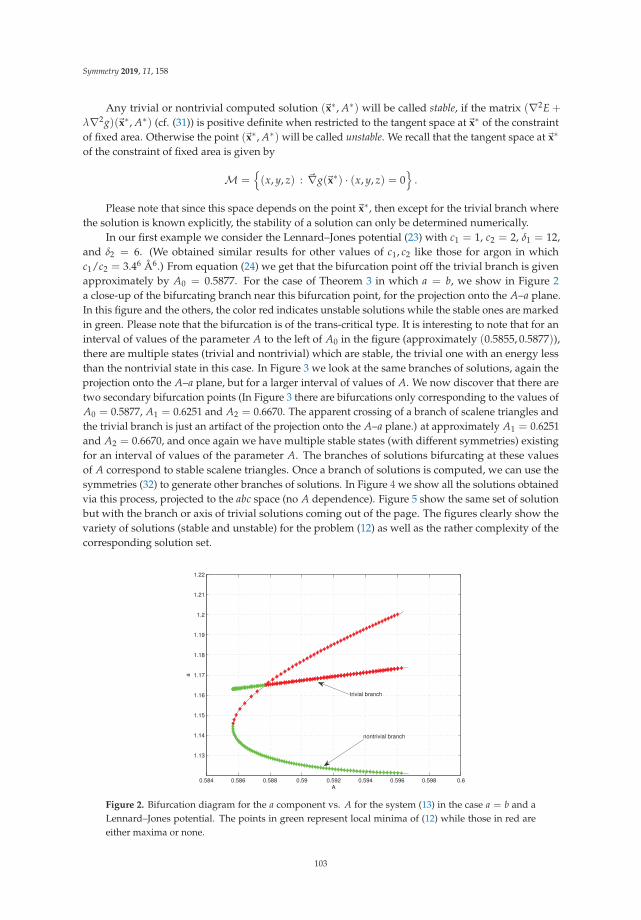
Symmetry 2019, 11, 158

Any trivial or nontrivial computed solution (�x∗, A∗) will be called stable, if the matrix (∇2E +

λ∇2g)(�x∗, A∗) (cf. (31)) is positive definite when restricted to the tangent space at�x∗ of the constraintof fixed area. Otherwise the point (�x∗, A∗) will be called unstable. We recall that the tangent space at�x∗

of the constraint of fixed area is given by

M ={(x, y, z) : �∇g(�x∗) · (x, y, z) = 0

}.

Please note that since this space depends on the point�x∗, then except for the trivial branch wherethe solution is known explicitly, the stability of a solution can only be determined numerically.

In our first example we consider the Lennard–Jones potential (23) with c1 = 1, c2 = 2, δ1 = 12,and δ2 = 6. (We obtained similar results for other values of c1, c2 like those for argon in whichc1/c2 = 3.46 Å6.) From equation (24) we get that the bifurcation point off the trivial branch is givenapproximately by A0 = 0.5877. For the case of Theorem 3 in which a = b, we show in Figure 2a close-up of the bifurcating branch near this bifurcation point, for the projection onto the A–a plane.In this figure and the others, the color red indicates unstable solutions while the stable ones are markedin green. Please note that the bifurcation is of the trans-critical type. It is interesting to note that for aninterval of values of the parameter A to the left of A0 in the figure (approximately (0.5855, 0.5877)),there are multiple states (trivial and nontrivial) which are stable, the trivial one with an energy lessthan the nontrivial state in this case. In Figure 3 we look at the same branches of solutions, again theprojection onto the A–a plane, but for a larger interval of values of A. We now discover that there aretwo secondary bifurcation points (In Figure 3 there are bifurcations only corresponding to the values ofA0 = 0.5877, A1 = 0.6251 and A2 = 0.6670. The apparent crossing of a branch of scalene triangles andthe trivial branch is just an artifact of the projection onto the A–a plane.) at approximately A1 = 0.6251and A2 = 0.6670, and once again we have multiple stable states (with different symmetries) existingfor an interval of values of the parameter A. The branches of solutions bifurcating at these valuesof A correspond to stable scalene triangles. Once a branch of solutions is computed, we can use thesymmetries (32) to generate other branches of solutions. In Figure 4 we show all the solutions obtainedvia this process, projected to the abc space (no A dependence). Figure 5 show the same set of solutionbut with the branch or axis of trivial solutions coming out of the page. The figures clearly show thevariety of solutions (stable and unstable) for the problem (12) as well as the rather complexity of thecorresponding solution set.

0.584 0.586 0.588 0.59 0.592 0.594 0.596 0.598 0.6

1.13

1.14

1.15

1.16

1.17

1.18

1.19

1.2

1.21

1.22

A

a

trivial branch

nontrivial branch

Figure 2. Bifurcation diagram for the a component vs. A for the system (13) in the case a = b and aLennard–Jones potential. The points in green represent local minima of (12) while those in red areeither maxima or none.

103

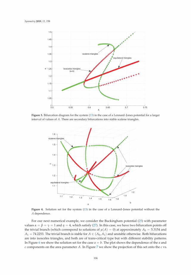
Symmetry 2019, 11, 158

0.5 0.55 0.6 0.65 0.7 0.751

1.05

1.1

1.15

1.2

1.25

1.3

1.35

1.4

1.45

1.5

A

a

scalene triangles

isosceles triangles(a=b)

equilateral triangles

Figure 3. Bifurcation diagram for the system (13) in the case of a Lennard–Jones potential for a largerinterval of values of A. There are secondary bifurcations into stable scalene triangles.

1.1 1.2 1.3 1.4 1.5 1.6

1.2

1.4

1.6

1.1

1.2

1.3

1.4

1.5

1.6

ba

c

scalene triangles

isosceles traingles

equilateral triangles

Figure 4. Solution set for the system (13) in the case of a Lennard–Jones potential without theA dependence.

For our next numerical example, we consider the Buckingham potential (25) with parametervalues α = β = γ = 1 and η = 4, which satisfy (27). In this case, we have two bifurcation points offthe trivial branch (which correspond to solutions of μ(A) = 0) at approximately A0 = 5.3154 andA1 = 74.2253. The trivial branch is stable for A ∈ (A0, A1) and unstable otherwise. Both bifurcationsare into isosceles triangles, and both are of trans-critical type but with different stability patterns.In Figure 6 we show the solution set for the case a = b. The plot shows the dependence of the a andc components on the area parameter A. In Figure 7 we show the projection of this set onto the c vs.

104

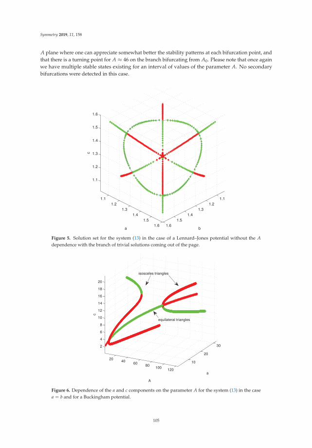
Symmetry 2019, 11, 158

A plane where one can appreciate somewhat better the stability patterns at each bifurcation point, andthat there is a turning point for A ≈ 46 on the branch bifurcating from A0. Please note that once againwe have multiple stable states existing for an interval of values of the parameter A. No secondarybifurcations were detected in this case.

1.11.2

1.31.4

1.51.6

1.11.2

1.31.4

1.51.6

1.1

1.2

1.3

1.4

1.5

1.6

ba

c

Figure 5. Solution set for the system (13) in the case of a Lennard–Jones potential without the Adependence with the branch of trivial solutions coming out of the page.

2040

6080

100120

10

20

302

4

6

8

10

12

14

16

18

20

a

A

c

isosceles triangles

equilateral triangles

Figure 6. Dependence of the a and c components on the parameter A for the system (13) in the casea = b and for a Buckingham potential.

105

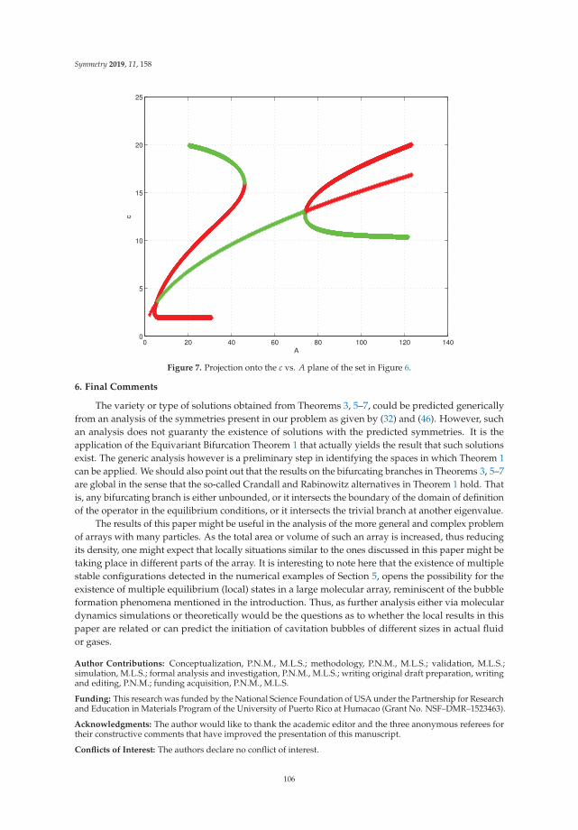
Symmetry 2019, 11, 158

0 20 40 60 80 100 120 1400

5

10

15

20

25

A

c

Figure 7. Projection onto the c vs. A plane of the set in Figure 6.

6. Final Comments

The variety or type of solutions obtained from Theorems 3, 5–7, could be predicted genericallyfrom an analysis of the symmetries present in our problem as given by (32) and (46). However, suchan analysis does not guaranty the existence of solutions with the predicted symmetries. It is theapplication of the Equivariant Bifurcation Theorem 1 that actually yields the result that such solutionsexist. The generic analysis however is a preliminary step in identifying the spaces in which Theorem 1can be applied. We should also point out that the results on the bifurcating branches in Theorems 3, 5–7are global in the sense that the so-called Crandall and Rabinowitz alternatives in Theorem 1 hold. Thatis, any bifurcating branch is either unbounded, or it intersects the boundary of the domain of definitionof the operator in the equilibrium conditions, or it intersects the trivial branch at another eigenvalue.

The results of this paper might be useful in the analysis of the more general and complex problemof arrays with many particles. As the total area or volume of such an array is increased, thus reducingits density, one might expect that locally situations similar to the ones discussed in this paper might betaking place in different parts of the array. It is interesting to note here that the existence of multiplestable configurations detected in the numerical examples of Section 5, opens the possibility for theexistence of multiple equilibrium (local) states in a large molecular array, reminiscent of the bubbleformation phenomena mentioned in the introduction. Thus, as further analysis either via moleculardynamics simulations or theoretically would be the questions as to whether the local results in thispaper are related or can predict the initiation of cavitation bubbles of different sizes in actual fluidor gases.

Author Contributions: Conceptualization, P.N.M., M.L.S.; methodology, P.N.M., M.L.S.; validation, M.L.S.;simulation, M.L.S.; formal analysis and investigation, P.N.M., M.L.S.; writing original draft preparation, writingand editing, P.N.M.; funding acquisition, P.N.M., M.L.S.

Funding: This research was funded by the National Science Foundation of USA under the Partnership for Researchand Education in Materials Program of the University of Puerto Rico at Humacao (Grant No. NSF–DMR–1523463).

Acknowledgments: The author would like to thank the academic editor and the three anonymous referees fortheir constructive comments that have improved the presentation of this manuscript.

Conflicts of Interest: The authors declare no conflict of interest.

106

Symmetry 2019, 11, 158

References

1. Lim, T.-C. Mathematical relationships for development of a molecular potential function converter.Commun. Math. Comput. Chem. 2003, 49, 155–169.

2. Tersoff, J. Modeling solid-state chemistry: Interatomic potentials for multicomponent systems. Phys. Rev. B1989, 39, 5566–5568. [CrossRef]

3. Shang, Y. Lower Bounds for Gaussian Estrada Index of Graphs. Symmetry 2018, 10, 325. [CrossRef]4. Collevecchio, A.; Konig, W.; Morters, P.; Sidorova, N. Phase transitions for dilute particle systems with

Lennard-Jones potential. Commun. Math. Phys. 2010, 299, 603–630. [CrossRef]5. Discher, D.E.; Boal, D.H.; Boey, S.K. Phase transitions and anisotropic responses of planar triangular nets

under large deformation. Phys. Rev. E 1997, 55, 4762. [CrossRef]6. Golubitsky, M. The Bénard problem, symmetry and the lattice of isotropy subgroups. In Bifurcation Theory,

Mechanics and Physics; Bruter, C.P., Aragnol, A., Lichnorowicz, A., Eds.; Reidel: Dordrecht, The Netherlands,1983; pp. 225–256.

7. Bazhirov, T.T.; Norman, G.E.; Stegailov, V.V. Cavitation in liquid metals under negative pressures. Moleculardynamics modeling and simulation. J. Phys. Condens. Matter 2008, 20, 114113. [CrossRef]

8. Blander, M.; Katz, J. Bubble Nucleation in Liquids. AlChE J. 1975, 21, 833–848. [CrossRef]9. Fond, C. Cavitation Criterion for Rubber Materials: A Review of Void-Growth Models. J. Polym. Sci. Part B

Polym. Phys. 2001, 39, 2081–2096. [CrossRef]10. Horgan, C.O.; Polignone, D.A. Cavitation in nonlinearly elastic solids: A review. Appl. Mech. Rev. 1995, 48,

471–485. [CrossRef]11. Chakraborty, D.; Chandra, A. An analysis of voids and necks in supercritical water. J. Mol. Liquids 2011, 163,

1–6. [CrossRef]12. David, E.E.; David, C.W. Voronoi polyhedra as a tool for studying solvation structure. J. Chem. Phys. 1982,

76, 4611. [CrossRef]13. Lennard-Jones, J.E. On the Determination of Molecular Fields. Proc. R. Soc. Lond. A 1924, 106, 463–477.14. Buckingham, R.A. The classical equation of state of gaseous helium, neon and argon. Proc. R. Soc. Lond. Ser.

A Math. Phys. Sci. 1938, 168, 264–283.15. Ambrosetti, A. A Premier on Nonlinear Analysis; Cambridge University Press: Cambridge, UK, 1993.16. Golubitsky, M.; Stewart, I.; Schaeffer, D. Singularities and Groups in Bifurcation Theory: Volume II. In Applied

Mathematical Sciences (Book 69); Springer: New York, NY, USA, 2000.17. Kielhöfer, H. Bifurcation Theory: An Introduction with Applications to Pdes; Springer: New York, NY, USA, 2004.18. Krasnoselski, M.A. Topological Methods in the Theory of Nonlinear Integral Equations; Pergamon: Oxford,

UK, 1965.19. Healey, T.H. Global bifurcation and continuation in the presence of symmetry with an application to solid

mechanics. SIAM J. Math Anal. 1988, 19, 824–840. [CrossRef]20. Wirth, K.; Dreiding, A.S. Edge lengths determining tetrahedrons. Elem. Math. 2009, 64, 160–170. [CrossRef]21. Lim, T.-C. Alignment of Buckingham parameters to generalized Lennard-Jones potential functions.

Z. Naturforsch. 2009, 64, 200–204. [CrossRef]22. Shang, Y. Average consensus in multi-agent systems with uncertain topologies and multiple time-varying

delays. Linear Algebra Appl. 2014, 459, 411–429. [CrossRef]23. Shang, Y. Couple-group consensus of continuous-time multi-agent systems under Markovian switching

topologies. J. Frankl. Inst. 2015, 352, 4826–4844, [CrossRef]24. Keller, H.B. Lectures on Numerical Methods in Bifurcation Problems; Tata Institute of Fundamental Research,

Springer: New York, NY, USA, 1986.25. Allgower, E.L.; Georg, K. Introduction to numerical continuation methods. In Classics in Applied Mathematics

(Book 45); Society for Industrial and Applied Mathematics: Philadelphia, PA, USA, 2003.

c© 2019 by the authors. Licensee MDPI, Basel, Switzerland. This article is an open accessarticle distributed under the terms and conditions of the Creative Commons Attribution(CC BY) license (http://creativecommons.org/licenses/by/4.0/).

107

symmetryS SArticle

Noether-Like Operators and First Integrals forGeneralized Systems of Lane- Emden Equations

M. Umar Farooq

Department of Basic Sciences and Humanities, College of E&ME, National University of Sciences andTechnology, H-12, Islamabad 44000, Pakistan; m_ufarooq@yahoo.com

Received: 18 December 2018; Accepted: 15 January 2019; Published: 1 February 2019

Abstract: Coupled systems of Lane–Emden equations are of considerable interest as they modelseveral physical phenomena, for instance population evolution, pattern formation, and chemicalreactions. Assuming a complex variational structure, we classify the generalized system ofLane–Emden type equations in relation to Noether-like operators and associated first integrals.Various forms of functions appearing in the considered system are taken, and it is observed that theNoether-like operators form an Abelian algebra for the corresponding Euler–Lagrange-type systems.Interestingly, we find that in many cases, the Noether-like operators satisfy the classical Noethersymmetry condition and become the Noether symmetries. Moreover, we observe that the classicalNoetherian integrals and the first integrals we determine using the complex Lagrangian approachturn out to be the same for the underlying system of Lane–Emden equations.

Keywords: generalized Lane–Emden systems; Noether-like operator; conservation laws

1. Introduction

The famous Noether theorem [1] establishes an important connection between the conservationlaws and symmetry properties of a system describable by a Lagrangian. From a mathematical point ofview, it is the case that the essential physical explanation of a Euler–Lagrange system is hidden in itsLagrangian. The Lagrangian function, on the one hand, describes the time behavior of a mechanicalsystem through the Euler–Lagrange equation, and on the other hand, it connects symmetries with firstintegrals of motion if they arise through Noether’s theorem. The availability of a Noether symmetry isessential from two aspects: first, to determine conservation laws and, second, to reduce the underlyingequation. A significant number of studies on Noether symmetries and first integrals have been reportedin recent years. It is well known that if an equation possesses enough conserved quantities, it can beeasily reduced to an integrable form.

In recent papers, the authors of [2,3] introduced the complex symmetry approach, which hasbeen established as an appealing and elegant technique to study integrability properties of systems ofordinary differential equations (ODEs). Following the idea of [3–5], several studies have been done toview integrability properties of systems of partial differential equations (PDEs) and ODEs. For instance,the use of the complex variable technique to discuss linearization of systems of two second-orderODEs and PDEs has been presented in [6]. The procedure of converting a system of two second-orderODEs admitting Lie algebra of dimension d (d ≤ 4) into linearizable form with the help of complexLie point symmetries of the base equation was given in [7]. Using semi-invariants, Mahomed et al. [8]studied systems of two linear hyperbolic PDEs when they arise from a complex scalar ODE. Theyfound that the semi-invariants under linear transformations correspond to complex semi-invariants ofthe (1 + 1) linear hyperbolic equation in the complex domain. They also succeeded in linking thesehyperbolic equations by introducing a complex variable structure on the manifold to the geometry ofunderlying differential equations. Qadir and Mahomed [9] employed the complex variable technique

Symmetry 2019, 11, 162; doi:10.3390/sym11020162 www.mdpi.com/journal/symmetry109

Symmetry 2019, 11, 162

to study three- and four-dimensional systems of ODEs and PDEs that are transformable to a singlecomplex ODEs. They showed that the acquired systems of ODEs are entirely different from the classthat is obtained from single splitting of systems of two ODEs. Naz and Mahomed [10,11] presented adetailed analysis of the computation of Lie and Noether point symmetries of the kth-order system of nODEs by working in the complex domain. They also discussed the transonic gas flow, Maxwelliandistribution, Klein–Gordon equation, dissipative wave, and Maxwellian tails by introducing complexvariables. Wafo Soh and Mahomed [12] showed that by utilizing hypercomplexification, one canlinearize Ermakov systems. Transforming systems of some Riccati-type equations to a single baseequation, they constructed invariants of Able-type systems.

In the current study, we use the formulation of the Noether-like theorem presented in [3–5]and classify systems of Lane–Emden equations with respect to Noether-like operators they admitand related first integrals. On applying the complex symmetry approach, we see that additionalinsights are obtainable by utilizing the fact that a complex Lagrangian encodes information of two realLagrangians, and it is derivable from a variational principle. As a consequence of the present study,many important symmetry properties can easily be analyzed using complex Lagrangians, and thesehelp us to determine the invariant quantities of physically-coupled systems represented by ODEs.

The celebrated Lane–Emden (LE) equation given below is the simplest second-order ODE,which appears frequently in modeling one-dimensional problems in physics, astrophysics,and engineering, and it is still a subject of extensive analysis. A review by Wang [13], even though veryselective in its list of references, covered almost all possible generalizations and qualitative propertiesof the LE equation.

Consider the well-known second-order LE equation:

y′′ +nt

y′ + f (y) = 0, (1)

where n is a real number and f (y) an arbitrary continuous function of y. The LE equation (1) has manyphysical applications. For instance, for fixed values of n and f (y), it specifically models the thermalbehavior of a spherical cloud of gas, stellar structure, an isothermal gaseous sphere, and the theoryof thermionic currents [14–16]. In the literature, various techniques have been proposed concerningthe solutions of Equation (1); see for example [17–20]. Several authors have proven existence anduniqueness results for the LE systems [21–24] (see also the references in these papers) and other relatedsystems. Some other works that involve Noether symmetries and exact solutions of LE-type equationscan be found in [25]. Moreover, the Noether symmetries of Equation (1) and exact solutions by takingvarious forms of f (y) were investigated in [26].

Before going to the main discussion, it is important to recall studies in view of the Noethersymmetry classification of coupled systems of LE equations. Recently, the authors of [27] took a systemof LE equations given by a natural extension of (1), classified it with respect to Noether symmetries,and constructed first integrals of:

f ′′ +nx

f ′ + F1(g) = 0, g′′ +nx

g′ + F2( f ) = 0, (2)

where n is a real number constant and F1(g) and F2( f ) are arbitrary functions. From a Noethersymmetry, Muatjetjeja and Khalique [28], extended their own work and studied the classification ofanother system of LE equations given by:

f ′′ +nx

f ′ + h(x)gq = 0, g′′ +nx

g′ + h(x) f p = 0, (3)

with respect to Noether symmetries and their first integrals. In this paper, we shall make a kind ofcomparison of how the complex Lagrangian formulation and the classical Noether symmetry approachgenerate the same first integrals for the following general class of the LE system:

110

Symmetry 2019, 11, 162

f ′′ +n1

xf ′ − n2

xg′ + F1( f , g) = 0, g′′ +

n2

xf ′ +

n1

xg′ + F2( f , g) = 0. (4)

The famous LE system (4) has been used in modeling various physical problems such as patternrecognition, chemical reactions, and population evolution, to name a few. This system attracted theattention of many authors and has been an area of extensive research during the last couple of years(see [21–24,29,30] and the references therein).

We shall consider various forms of F1 and F2 to construct conserved quantities of the ensuingsystems and show that reduction via quadrature can be obtained only in a few cases. We pointout that the Noether-like operators we find for systems of Euler–Lagrange LE equations also satisfythe classical Noether symmetry condition for one of the known equivalent Lagrangians, emergeas Noether symmetries, and hence yield Noetherian first integrals for the subsequent systems.Thus, the Noetherian first integrals and the first integrals we obtain employing a complex Lagrangianapproach turn out to be the same with respect to the Lagrangians for the underlying systems of ODEs.We shall see that many interesting insights can be obtained for systems of ODEs through the complexsymmetry approach.

The layout of the paper is the following: in the next section, we briefly recall some basic definitionsof Noether-like operators and the Noether-like theorem. Section 3 deals with the classification ofNoether-like operators and associated first integrals for the system (4). In the last section, we presentour concluding remarks.

2. Preliminaries on Noether-Like Operators and First Integrals

Before we consider the generalized system of LE equations in relation to their Noether-likeoperators and corresponding first integrals, it is instructive to have relevant definitions of theseoperators and the Noether-like theorem that will be used in our discussion. Moreover, to makethe comparison, we also recall expressions for classical Noether symmetries and Noether’s theorem.The contents of this section are taken from [3,4] (for more details, the reader is urged to see thereferences therein).

Consider the following system of nonlinear second-order ODEs:

f ′′i = wi(x, f1, f ′1, f2, f ′2), i = 1, 2. (5)

Equation (5) represents a general class of a system of second-order ODEs and models variousphysical problems. However, here, we merely deal with those systems in (5) that are equivalentto a single scalar complex ODE, i.e., there exist transformations f = f1 + i f2, w = w1 + iw2 thatreduce the system (5) to a complex ODE, f ′′ = w(x, f , f ′), which retain a variational structure. It isgenerally conceded that the construction of a Lagrangian for systems of nonlinear ODEs has beenproven to be a complicated problem. However, we see here how one can study symmetry propertiesof Euler–Lagrange-type LE equations straightforwardly with the help of a complex Lagrangian, whichencodes two real Lagrangians and enables us to cast the system (5) in a variational form.

Here, our aim is to determine the Noether-like operators and related first integrals of a coupledsystem of two LE equations. We start by assuming that the system (5) admits a complex LagrangianL(x, f , f ′), i.e. L = L1 + iL2. Therefore, we have two Lagrangians L1 and L2, which when utilizedresult in the following Euler–Lagrange-type system corresponding to (5):

∂L1

∂ f1+

∂L2

∂ f2− d

dx(

∂L1

∂ f ′1+

∂L2

∂ f ′2) = 0,

∂L2

∂ f1− ∂L1

∂ f2− d

dx(

∂L2

∂ f ′1− ∂L1

∂ f ′2) = 0.

(6)

111

Symmetry 2019, 11, 162

The operators X1 = ς1(x, f1, f2)∂

∂x + χ1(x, f1, f2)∂

∂ f1+ χ2(x, f1, f2)

∂∂ f2

and X2 = ς2(x, f1, f2)∂

∂x +

χ2(x, f1, f2)∂

∂ f1− χ1(x, f1, f2)

∂∂ f2

are known as Noether-like operators of (5) for the Lagrangians L1 andL2 if the following conditions hold:

X(1)1 L1 − X

(1)2 L2 + (Dxς1)L1 − (Dxς2)L2 = Dx A1,

X(1)1 L2 − X

(1)2 L1 + (Dxς1)L2 + (Dxς2)L1 = Dx A2,

(7)

for appropriate functions A1 and A2. Here, Dx = ddx .

Noether-like theorem:If X1 and X2 are two Noether-like operators with respect to real Lagrangians L1 and L2, then (5)

possesses the following two first integrals:

I1 = ς1L1 − ς2L2 +∂L1

∂ f ′1(χ1 − f ′1ς1 − f ′2ς2)−

∂L2

∂ f ′1(χ2 − f ′1ς2 − f ′2ς1)− A1,

I2 = ς1L2 + ς2L1 +∂L2

∂ f ′1(χ1 − f ′1ς1 − f ′2ς2) +

∂L1

∂ f ′1(χ2 − f ′1ς2 − f ′2ς1)− A2.

(8)

Classical Noether symmetry condition:A vector field X = ς(x, f1, f2)

∂∂x + χ(x, f1, f2)

∂∂ f1

+ η(x, f1, f2)∂

∂ f2with its prolongation

X[1] = X + (χ− f1ς) ∂∂ f1

+ (η − f2ς) ∂∂ f2

where ‘·′ = ddx is known as a Noether point symmetry

corresponding to the function L(x, f1, f2, f ′1, f ′2) of (5) if the following equation holds:

X[1](L) + Dx(ς)L = Dx(A) (9)

Noether’s theorem:For X to be a Noether symmetry generator for the Lagrangian L(x, f1, f2, f ′1, f ′2), the

following equation:

I = A−[ςL + (χ− ς f1)

∂L∂ f1

+ (η − ς f2)∂L∂ f2

], (10)

provides the Noetherian first integral of (5) related to X.

3. Noether-Like Operators and First Integrals for Different forms of F1 and F2 in (4)

Major computational difficulties occur when trying to classify the general nonlinear LE equationwith respect to Noether symmetry operators and corresponding first integrals. We see here how theNoether-like operators play an important role in deriving conserved quantities for dynamical systemsand their reduction via quadrature.

Consider the following nonlinear system, which is a generalized coupled LE-type system:

f ′′1 +n1 f ′1 − n2 f ′2

x+ F1( f1, f2) = 0,

f ′′2 +n1 f ′2 + n2 f ′1

x+ F2( f1, f2) = 0,

(11)

for which we have analyzed eight cases separately. Here, n1, n2 are constants and F1, F2 are arbitraryfunctions of f1 and f2, respectively. We take different forms of F1 and F2 in (11) and determineNoether-like operators and conserved quantities for the subsequent systems. Therefore, for this,we proceed as: one can readily verify that the pair of Lagrangians for the system (11) when invoking (6)is given by:

112

Symmetry 2019, 11, 162

L1 =12

xn1 [cosθ( f ′21 − f ′22 )− 2sinθ f ′1 f ′2]− xn1 [cosθ∫(F1d f1 − F2d f2)− sinθ

∫(F2d f1 + F1d f2)],

L2 =12

xn1 [2cosθ( f ′1 f ′2) + sinθ( f ′21 − f ′22 )]− xn1 [cosθ∫(F2d f1 + F1d f2) + sinθ

∫(F1d f1 − F2d f2)],

(12)

where θ = n2 ln x.Case 1. F1( f1, f2) and F2( f1, f2) are linear in f1 and f2, respectively.In this case, we have a system of two linear ODEs. Using appropriate transformations, one can

reduce the system of linear equations to a system of free particle equations, viz. f ′′1 = 0, f ′′2 = 0,which possesses nine Noether-like operators associated with the coupled Lagrangians (11), and theygive ten first integrals. This case is well known and can be found in detail in [4].

Case 2. For n1, n2 = 0 and F1( f1, f2), F2( f1, f2) arbitrary and non-linear, as given in Case 1.Equations (7) and (12), after some straightforward calculations, show that ς1 = 1, ς2 = 0,

χ1 = χ2 = 0, and A1, A2 are constants. Therefore, we have a single Noether-like operator X = ∂∂x .

Using the pair of Lagrangians (12) and Noether-like operator X in (8), we obtain the following twofirst integrals:

I1 =12( f ′2 − g′2) +

∫[F1d f − F2dg],

I2 = f ′g′ +∫[F1dg + F2d f ].

(13)

Interestingly, the Noether-like operator X is also a Noether symmetry for each of the Lagrangians (12),and (10) generates the same first integrals as given in (13) for System (11).

Case 3. If:

F1( f1, f2) =α

2log( f 2

1 + f 22 ) + γ f1 + δ, α �= 0,

F2( f1, f2) = α arctan(f2

f1) + γ f2, α �= 0

(14)

and n1, n2 = 0 and δ = 0, we obtain ς1 = x, ς = 0, χ1 = χ2 = 0 with A1, A2 as constants. This fallsinto Case 2.

Case 4. For:

F1( f1, f2) =α

2[ f1 log( f 2

1 + f 22 )− f2 arctan( f2/ f1)] + γ f1 + δ, α �= 0,

F2( f1, f2) =α

2[ f1 arctan( f2/ f1) + f2 log( f 2

1 + f 22 )] + γ f2 + δ, α �= 0.

(15)

If n1, n2 = 0, we obtain ς1 = x, ς2 = 0, χ1 = χ2 = 0, and A1 = A2 = k, k being a constant.This also bring us back to Case 2.

Case 5. If F = αur, α �= 0, r �= 0, 1.Here, we discuss the following three cases:Case 5.1. For n1 = r+3

r−1 and n2 = 0, the Noether-like symmetry conditions (7) resultin ς1 = x, ς2 = 0, χ1 = 2

1−r f1, χ2 = 21−r f2, with A1, A2 as constants. Therefore, we get two

Noether-like operators:

X1 = x∂

∂x+

21− r

(f1

∂

∂ f1+ f2

∂

∂ f2

), X2 =

21− r

(f2

∂

∂ f1− f1

∂

∂ f2

). (16)

113

Symmetry 2019, 11, 162

Utilizing (16) with (12), Equation (8) gives rise to two first integrals:

I1 =12

xn1+1( f ′21 − f ′22 )− α

r + 1xn1+1( f 2

1 + f 22 )

r+12 cosθ +

21− r

xn1( f1 f ′1 − f2 f ′2)− xn1+1( f ′21 − f ′22 ),

I2 = xn1+1 f ′1 f ′2 −α

r + 1xn1+1( f 2

1 + f 22 )

r+12 sinθ +

21− r

xn1( f1 f ′2 + f ′1 f2)− 2xn1+1 f ′1 f ′2,(17)

for (11). Here, θ = (r + 1) arctan( f2/ f1). Utilization of transformations f1 = w1xν+11−r and f2 = w2x

ν+11−r

converts the above system (17) into an integrable form as:

∫ dw±√

4(1− r)−2w2 − 2α(1 + r)−1 f r+1 − C1= lnxC2, (18)

where C1 and C2 are constants. Here, we can see that the Lie algebra of Noether-like operators isAbelian, i.e., [X1, X2] = 0.

Case 5.2. If we set n1 = 2, n2 = 0, and r = 5, Equations (6) and (12) yield the famousEmden–Fowler system [3] given by:

f ′′1 +2x

f ′1 + α( f 51 − 10 f 3

1 f 22 + 5 f1 f 4

2 ) = 0,

f ′′2 +2x

f ′2 + α( f 52 − 10 f 2

1 f 32 + 5 f 4

1 f2) = 0,(19)

while the associated Lagrangians are:

L1 =12

x2( f ′21 − f ′22 )− α

6x2[ f 6

1 − 15 f 41 f 2

2 + 15 f 21 f 4

2 − f 62 ],

L1 = x2 f ′1 f ′2 −α

3x2[3 f 5

1 f2 − 10 f 31 f 3

2 + 3 f1 f 52 ].

(20)

It is easy to see that the Emden–Fowler system (19) admits the following twoNoether-like operators:

X1 = 2x∂

∂x− f1

∂

∂ f1− f2

∂

∂ f2, X2 = f

∂

∂ f2− f2

∂

∂ f1. (21)

Utilizing these operators in Equations (8) and (20), we obtain the following constant quantities:

I1 = x3( f ′21 − f ′22 ) + x2( f1 f ′1 − f2 f ′2) +13

x3( f 61 + 15 f 2

1 f 42 − 15 f 4

1 f 22 − f 6

2 ),

I2 = x3 f ′1 f ′2 +12

x2( f1 f ′2 + f ′1 f2) + x3( f1 f 52 −

103

f 31 f 3

2 + f 51 f2),

(22)

for (19). Upon checking, we see that for L1 and L2, the above system (19) admits X1 as a Noethersymmetry. Therefore, from the classical Noether theorem, we can deduce the first integrals I1 and I2

(Noetherian integrals) for (19).

Case 5.3. If n1 = r+3r+1 with r �= −1, we have ς1 = x

r−1r+1 , ς2 = 0, χ1 = − 2

r+1 x−2r+1 f1,

χ2 = − 2r+1 x

−2r+1 f2, and A1 = 2

2(r+1)2 ( f 21 − f 2

2 ) + q, A2 = 4(r+1)2 f1 f2, where q is constant. By invocation

of the Noether-like theorem, the Noether-like operators given in (24) provide:

I1 =12

x2( f ′21 − f ′22 ) +α

r + 1x2( f 2

1 + f 22 )

r+12 cosθ +

2r + 1

x( f1 f ′1 − f2 f ′2) +2

(1 + r)2 ( f 21 − f 2

2 ),

I2 = x2 f ′1 f ′2 +α

r + 1x2( f 2

1 + f 22 )

r+12 sinθ +

2r + 1

x( f1 f ′2 + f ′1 f2) +4

(r + 1)2 f1 f2,(23)

114

Symmetry 2019, 11, 162

where θ = (r + 1) arctan( f2/ f1). In this case, Noether-like operators are of the form:

X1 = xr−1r+1

∂

∂x− 2

r + 1x−

2r+1

(f1

∂

∂ f1+ f2

∂

∂ f2

), X2 = − 2

r + 1x−

2r+1

(f2

∂

∂ f1− f1

∂

∂ f2

). (24)

Applying the transformations f1 = w1x−ν−1r+1 and f2 = w2x

−ν−1r+1 , System (23) can be converted into

the variable separable form:

∫ dw±√−2α(r + 1)−1wr+1 + C1

=r + 1

2x

2r+1 + C2, (25)

where C1 and C2 are arbitrary constants.Case 6. If F1 and F2 are nonlinear and are of the form F1( f1, f2) = α( f 2

1 − f 22 )+ β f1 +γ, F2( f1, f2) =

2α f1 f2 + β f2, α, β, γ are constants, and α �= 0.Here, the following subcases arise:

Case 6.1. If n1 = 5 and n2 = 0, β = 0 and γ = 0, we obtain from (7) that ς1 = x, ς2 = 0,χ1 = −2 f1, χ2 = −2 f2, and A1, A2 are constants. This case falls into Case 5.1.Case 6.2. If n1 = 5, n2 = 0, β2 = 4αγ, Equations (7) and (12) yield ς1 = x, ς2 = 0, χ1 = −(2 f1 +βα ), χ2 = −2 f2, A1 = βγ

6α x6, and A2 = 0. Therefore, Noether-like operators are of the form:

X1 = x∂

∂x− (2 f1 +

β

α)

∂

∂ f1− 2 f2

∂

∂ f2, X2 = (2 f1 +

β

α)

∂

∂ f2− 2 f2

∂

∂ f1. (26)

Invocation of the Noether-like theorem (8) along with Lagrangians and Noether-like operators X1

and X2 results in two first integrals:

I1 =12

x6( f ′21 − f ′22 ) +13

αx6( f 31 − 3 f1 f 2

2 ) +12

βx6( f 21 − f 2

2 ) + γx6 f + 2x5( f1 f ′1 − f2 f ′2) +β

αx5 f ′1

+βγ

6αx6

I2 = x6 f ′1 f ′2 +13

αx6(3 f 21 f2 − f 3

2 ) + βx6 f1 f2 + γx6 f2 + 2x5( f1 f ′2 + f ′1 f2) +β

αx5 f ′2,

(27)

for (11). Using the transformations w1 = x1+ν f1 +β

2α xν+1 and w1 = xν+1 f2, one can map thesystem (27) to a separable form:

C = 2w2 − 12

x2w′2 − α

3w3, (28)

where w(x) = w1 + iw2.It can be verified that the Noether-like operator X1 in (26) is also a Noether symmetry for the

Lagrangians L1 and L2 in Equation (12). The classical Noether’s theorem generates the same Noetherianfirst integrals I1 and I2 given in Equation (27) with Lagrangians L2 and L1, respectively, for the resultingsystem of LE equations. Furthermore, we observe that [X1, X2] = 0, so these operators form anAbelian algebra.

Case 6.3. For n1 = 53 , n2 = 0, β = 0, and γ = 0, Equation (7) taking L1 and L2 from (12) with simple

calculations gives ς1 = x13 , χ1 = − 2

3 x−23 f1, χ2 = − 2

3 x−23 f2, and A1 = 2

9 ( f 21 − f 2

2 ) + k, A2 = 49 ( f1 f2),

and k is a constant. This case falls into Case 5.2.Case 7. For F1( f1, f2) = αeβ f1 cos(β f2) + γ f1 + δ, F2( f1, f2) = αeβ f1 sin(β f2) + γ f2, where α, β, δ

are constants and α �= 0, β �= 0. Therefore, (11) takes the form:

f ′′1 +n1 f ′1 − n2 f ′2

x+ αexp(β f1)cos(β f2) + γ f1 + δ = 0,

f ′′2 +n1 f ′2 + n2 f ′1

x+ αexp(β f1)sin(β f2) + γ f2 = 0,

(29)

115

Symmetry 2019, 11, 162

For n1 = 1, n2 = 0, γ = 0, δ = 0, and β = 1, we obtain ς1 = x, ς2 = 0, χ1 = −2, χ2 = 0, andA1, A2 = q, where q is a constant. Therefore, the system (29) possesses the Noether-like operators:

X1 = x∂

∂x− 2∂

∂ f1, X2 =

∂

∂ f2. (30)

with the corresponding pair of Lagrangians:

L1 =12

x( f ′21 − f ′22 )− αxe f1 cos f2,

L2 = x f ′1 f ′2 − αxe f1 sin f2.(31)

Utilizing the Noether-like operators and Lagrangians given above, Equation (8) implies thefirst integrals:

I1 =12

x2( f ′21 − f ′22 ) + αx2e f1 cos f2 + 2x f ′1

I2 = x2 f ′1 f ′2 + αx2e f1 sin f2 + 2x f ′2.(32)

It is important to mention here that the system (29) admits Noether-like operator X1 as a Noethersymmetry [3], as it satisfies the classical Noether symmetry condition with Lagrangians L1 and L2 givenin (31). Therefore, application of the classical Noether theorem remarkably generates two Noetherianfirst integrals, namely I1 and I2 given in (32). Here, again, the Lie bracket gives [X1, X2] = 0, whichshows that the algebra of these operators is Abelian.

Case 8. Here, n1, n2 are nonzero, and F1( f1, f2), F2( f1, f2) are arbitrary, but not of the formcontained in the cases given above.

From Equation (7), after simple manipulations, we find that ς1 = ς2 = 0, χ1 = χ2 = 0, and A1, A2

are constants. We deduce that no Noether-like operators exist in this case.

4. Conclusions

In this paper, we have applied the complex Noether approach and attempted to classify atwo-dimensional coupled system of LE equations that appears in physics and applied mathematicswith respect to Noether-like-operators and corresponding first integrals by taking the functions F1 andF2 in their more general forms in Equation (11). In this study, we have observed that for some of thesystems of LE equations, every pair of Noether-like operators forms an Abelian Lie algebra. We havealso highlighted that for certain pairs of Lagrangians, the Noether-like operators become Noethersymmetries of the Euler–Lagrange systems of LE equations and give rise to the same Noetherian firstintegrals as we determined from our complex approach. Therefore, the study of invariant quantities ofmany dynamical systems can be made with the help of complex Lagrangian formalism, which seemsto be more simple and elegant.

Funding: This research received no external funding.

Acknowledgments: M.U. Farooq is thankful to Fazal M. Mahomed for his important comments on this paper.The author also expresses his gratitude to the referees for some useful suggestions.

Conflicts of Interest: The author declares no conflict of interest.

References

1. E Noether, I.V. Koönigliche Gesellschaft der Wissenschaften zu Göttingen. Math. Phys. 1918, 2, 235–269.2. Ali, S.; Mahomed, F.M.; Qadir, A. Complex Lie symmetries for scalar second-order ordinary differential

equations. Nonlinear Anal. Real World Appl. 2009, 10, 3335–3344 . [CrossRef]3. Ali, S.; Mahomed, F.M.; Qadir, A. Complex Lie symmetries for variational problems. J. Nonlinear. Math. Phys.

2008, 15, 25–35. [CrossRef]

116

Symmetry 2019, 11, 162

4. Farooq, M.U.; Ali, S.; Mahomed, F.M. Two dimensional systems that arise from the Noether classification ofLagrangian on the line. Appl. Math. Comput. 2011, 217, 6959–6973. [CrossRef]

5. Farooq, M.U.; Ali, S.; Qadir, A. Invariants of two-dimensional systems via complex Lagrangians withapplications. Commun. Nonlinear Sci. Num. Simul. 2011, 16, 1804–1810. [CrossRef]

6. Ali, S.; Mahomed, F.M.; Qadir, A. Linearizability criteria for systems of two second-order differentialequations by complex methods. Nonlinear Dyn. 2011, 66, 77–88. [CrossRef]

7. Ali, S.; Safdar, M.; Qadir, A. Linearization from complex Lie point Transformations. J. Appl. Math. 2014,2014, 793247. [CrossRef]

8. Mahomed, F.M.; Qadir, A.; Ramnarain, A. Laplace-Type Semi-Invariants for a System of Two LinearHyperbolic Equations by Complex Methods. Math. Prob. Eng. 2011, 2011, 202973. [CrossRef]

9. Qadir, A.; Mahomed, F.M. Higher dimensional systems of differential equations obtainable by iterative useof complex methods. Int. J. Mod. Phys. 2015, 38, 1560077. [CrossRef]

10. Naz, R.; Mahomed, F.M. Lie and Noether symmetries of systems of complex ordinary differential equationsand their split systems. Pramana J. Phys. 2014, 83, 920. [CrossRef]

11. Naz, R.; Mahomed, F.M. A complex Noether approach for variational partial differential equations. Commun.Nonlinear Sci. Numer. Simul. 2015, 27, 120–135. [CrossRef]

12. Soh, C.W.; Mahomed, F.M. Hypercomplex analysis and integration of systems of ordinary differentialequations. Math. Meth. Appl. Sci. 2016. [CrossRef]

13. Wong, J.S. On the generalized Emden–Fowler equation. SIAM Rev. 1975, 17, 339–360. [CrossRef]14. Chandrasekhar, S. An Introduction to the Study of Stellar Structure; Dover: New York, NY, USA, 1957.15. Davis, H.T. Introduction to Nonlinear Differential and Integral Equations; Dover: New York, NY, USA, 1962.16. Richardson, O.W. The Emission of Electricity from Hot Bodies, 2nd ed.; Longmans, Green & Co.: London, UK, 1921.17. Dehghan, M.; Shakeri, F. Approximate solution of a differential equation arising in astrophysics using the

variational iteration method. New Astron. 2008, 13, 53–59. [CrossRef]18. Ramos, J.I. Series approach to the Lane–Emden equation and comparison with the homotopy perturbation

method. Chaos Solitons Fractals 2008, 38, 400–408. [CrossRef]19. Marzban, H.R.; Tabrizidooz, H.R.; Razzaghi, M. Hybrid functions for nonlinear initial-value problems with

applications to Lane–Emden type equations. Phys. Lett. A 2008, 372, 5883–5886. [CrossRef]20. Ertrk, V.S. Differential transformation method for solving differential equations of Lane–Emden type.

Math. Comput. Appl.2007, 12, 135–139. [CrossRef]21. Serrin, J.; Zou, H. Non-existence of positive solutions of Lane–Emden systems. Differ. Int. Equ. 1996, 9, 635653.22. Serrin, J.; Zou, H. Existence of positive solutions of the Lane–Emden system. Atti del Seminario Matematico e

Fisico Dell Universit‘a di Modena 1998, 46, 369–380.23. Qi, Y.W. The existence of ground states to a weakly coupled elliptic system. Nonlinear Anal. Theory

Methods Appl. 2002, 48, 905–925. [CrossRef]24. Dalmasso, R. Existence and uniqueness of solutions for a semilinear elliptic system. Int. J. Math. Math. Sci.

2005, 10, 1507–1523. [CrossRef]25. Muatjetjeja, B.; Khalique, C.M. Exact solutions of the generalized Lane–Emden equations of the first and

second kind. Pramana J. Phys. 2011, 77, 545–554. [CrossRef]26. Khalique, C.M.; Mahomed, F.M.; Muatjetjeja, B. Lagrangian formulation of a generalized Lane–Emden

equation and double reduction. J. Nonlinear Math. Phys. 2008, 15, 152–161. [CrossRef]27. Muatjetjeja, B.; Khalique, C.M. Lagrangian approach to a generalized coupled Lane–Emden system:

Symmetries and first integrals. Commun. Nonlinear Sci. Numer. Simul. 2010, 15, 1166–1171. [CrossRef]28. Muatjetjeja, B.; Khalique, C.M. First integrals for a generalized coupled Lane–Emden system. Nonlinear Anal.

Real World Appl. 2011, 12, 1202–1212. [CrossRef]29. Dai, Q.; Tisdell, C.C. Non-degeneracy of positive solutions to homogeneous second order differential systems

and its applications. Acta Math. Sci. 2009, 29, 437–448.30. Zou, H. A prior estimates for a semilinear elliptic system without variational structure and their application.

Math. Ann. 2002, 323, 713–735. [CrossRef]

c© 2019 by the author. Licensee MDPI, Basel, Switzerland. This article is an open accessarticle distributed under the terms and conditions of the Creative Commons Attribution(CC BY) license (http://creativecommons.org/licenses/by/4.0/).

117

symmetryS SArticle

Algorithm for Neutrosophic Soft Sets in StochasticMulti-Criteria Group Decision Making Based onProspect Theory

Yuanxiang Dong 1,*, Chenjing Hou 1, Yuchen Pan 2 and Ke Gong 3

1 School of Management Science and Engineering, Shanxi University of Finance and Economics,Taiyuan 030006, China

2 Business School, Southwest University of Political Science & Law, Chongqing 401120, China3 School of Economics and Management, Chongqing Jiaotong University, Chongqing 400074, China* Correspondence: dongyx@sxufe.edu.cn; Tel.: +86-1336-836-0537

Received: 24 July 2019; Accepted: 27 August 2019; Published: 29 August 2019

Abstract: To address issues involving inconsistencies, this paper proposes a stochastic multi-criteriagroup decision making algorithm based on neutrosophic soft sets, which includes a pair of asymmetricfunctions: Truth-membership and false-membership, and an indeterminacy-membership function.For integrating an inherent stochastic, the algorithm expresses the weights of decision makers andparameter subjective weights by neutrosophic numbers instead of determinate values. Additionally,the algorithm is guided by the prospect theory, which incorporates psychological expectations ofdecision makers into decision making. To construct the prospect decision matrix, this researchestablishes a conflict degree measure of neutrosophic numbers and improves it to accommodatethe stochastic multi-criteria group decision making. Moreover, we introduce the weighted averageaggregation rule and weighted geometric aggregation rule of neutrosophic soft sets. Later, this studypresents an algorithm for neutrosophic soft sets in the stochastic multi-criteria group decision makingbased on the prospect theory. Finally, we perform an illustrative example and a comparative analysisto prove the effectiveness and feasibility of the proposed algorithm.

Keywords: neutrosophic soft sets; inconsistent information; prospect theory; stochastic multi-criteriagroup decision making

1. Introduction

Many complex issues in engineering, economics, environmental science and medical scienceinvolve uncertainties. In order to address these issues, the theory of possibility, fuzzy set [1], rough set [2],and interval mathematic [3] have been developed successively. However, the above theories have theirinherent defects, which are mainly reflected in the inadequacy of parameterization tools [4]. In 1999,Molodtsov [4] initiated the soft set theory for modeling uncertainties from the parameterized pointof view.

After Molodtsov, the research interests in the soft set theory have been growing rapidly, such asthe algebraic structure [5,6], topology [7,8], normal parameter reduction [9], medical diagnosis [10],game theory [4], and decision making under uncertainties [11,12]. In addition, the study of hybridmodels that are developed by combining the soft set theory with other mathematical tools, such as roughsets [13], fuzzy sets [14], and intuitionistic fuzzy sets [15], has also been an important research topic.

Under uncertain environments, a mass of inconsistent information appears due to diversitiesof source platforms and the differences in the acquisition time. To address issues involvinginconsistencies, Smarandache [16] initiated neutrosophic sets from the perspective of philosophy.Subsequently, Maji [17] integrated neutrosophic sets into soft sets to propose neutrosophic soft

Symmetry 2019, 11, 1085; doi:10.3390/sym11091085 www.mdpi.com/journal/symmetry119

Symmetry 2019, 11, 1085

sets, which retain the characteristics of neutrosophic sets and have adequate parameterization tools.Neutrosophic soft sets are characteristic by three independent functions, including a pair of asymmetricfunctions: Truth-membership and false-membership, and an indeterminacy-membership function.Among them, the truth-membership and false-membership represent the degree of belongingness andnon-belongingness of an element with respect to parameters. The indeterminacy-membership showsthe neutrality degree of an element related to parameters.

In recent years, the theory extensions of neutrosophic soft sets have made a rapid progress.Sahin and Küçük [18] constructed generalised neutrosophic soft sets. Deli and Broumi [19] refinedthe concept and operations of Maji’s neutrosophic soft sets. In addition, they also studied theneutrosophic soft matrix and their operators. Considering that the approximate range is usuallyused to describe complex situations when there is no sufficient information, Deli [20] expanded thevalues of the truth-membership, indeterminacy-membership, and false-membership to the form ofinterval values to construct interval-valued neutrosiphic soft sets. Karaaslan [21] introduced thepossibility of neutrosophic soft sets by assigning probability to the three function values and definedrelated properties and operations. In addition, the concepts of single-valued neutrosophic refined softsets [22], generalized neutrosophic soft expert sets [23], and neutrosophic soft rough sets [24] werepresented successively.

Meanwhile, neutrosophic soft sets are also employed in the fields of clustering, prediction anddecision making under uncertainties, among which decision making under uncertainties is the mostwidely applied. Deli [20] proposed a decision making method of interval-valued neutrosophic softsets by level soft sets, and illustrated it by an example. Peng and Liu [25] constructed three decisionmaking algorithms of neutrosophic soft sets by evaluation based on the distance from average solution(EDAS), similarity measure, and level soft sets, respectively. Abu Qamar and Hassan [26] presentedthe similarity, distance, and fuzzy degree measures of Q-neutrosophic soft sets, and put forward thecorresponding decision rule. Karaaslan [21] constructed a decision making method for the possibilityof neutrosophic soft sets based on the and-product.

However, the existing studies mainly focus on decision making methods under a single decisionmaker, few scholars have studied group decision making problems by neutrosphic soft sets. At thesame time, we also noticed that the existing methods have the following defects. On one hand,the above methods are mainly based on the expected utility theory, which assumes that decisionmakers are completelyrational. Actually, in decision making processes, decision makers do not makedecisions in a complete rational manner, mainly showing that psychological expectations will greatlyaffect the actual decision making behavior. On the other hand, the parameter subjective weights aredirectly given determinate values [25], which do not fully reflect the hesitancies of decision makers’judgments under uncertain environments.

To make up for the gaps of existing researches, this study constructs an algorithm for the stochasticmulti-criteria group decision making based on neutrosophic soft sets. Stochastic means that the weightsof decision makers and parameters are uncertain or completely unknown under uncertainties. In thispaper, neutrosophic numbers rather than determinate values are adopted to express the stochasticof the weights of decision makers and parameters. This method employs the prospect theory [27]rather than the expected utility theory to integrate the hesitancies of alternatives by decision makers’judgements. The prospect theory, a new theory of bounded rationality, is proposed from the point ofview of cognitive psychology. In addition, it integrates the influence of psychological expectations onactual decision making behaviors into the decision making model. Therefore, the prospect theory ismore in line with actual decision making behaviors under uncertainties [28]. Then, to establish theprospect decision matrix, we put forward the conflict degree measure of neutrosophic numbers andmodify it to adapt group decision making. Moreover, on the purpose of aggregating in group decisionmaking processes, this study proposes the weighted average aggregation rule and weighted geometricaggregation rule of neutrosophic soft sets.

120

Symmetry 2019, 11, 1085

To promote our discussion, some fundamental concepts of neutrosophic sets, soft sets, neutrosophicsoft sets, and prospect theory are reviewed in Section 2. In Section 3, we establish the measures ofdeterminacy degree and conflict degree, and construct the weighted average aggregation rule andweighted geometric aggregation rule of a neutrosophic soft set. In Section 4, this paper presents analgorithm for neutrosophic soft sets in the stochastic multi-criteria group decision making based on theprospect theory. In Section 5, to demonstrate the feasibility and effectiveness of the proposed algorithm,we perform an illustrative example and a comparative analysis.

2. Preliminaries

In this section, we briefly recall some basic concepts of neutrosophic sets, soft sets, neutrosophicsoft sets, and prospect theory. More detailed conceptual basics can be found in references [4,16,17,27](pp. 1–2).

2.1. Neutrosophic Soft Sets

Definition 1 [16] (p. 1). Let U be the initial universal set, a neutrosophic set A ={< u : TA(u), IA(u), FA(u) >, u ∈ U

}consists of the truth-membership TA(u), the indeterminacy-membership IA(u), and false-membership FA(u)of element u ∈ U to set A, where T, I, F : U→]−0, 1+[ . ]−0, 1+[ is a non-standard interval, and theleft and right borders of it are imprecise. Between them, (−0) = {0− x : x ∈ R∗, x is infinitesimal},and (1+) = {1 + x : x ∈ R∗, x is infinitesimal}.

For convenience, we employ u =< T, I, F > to represent the element u in the neutrosophic set A,and it can be called a neutrosophic number.

Considering that neutrosophic sets are proposed from the philosophical point of view, it is difficultto apply to practical problems, such as management and engineering problems. Then, Haibin et al. [29]developed single valued neutrosophic sets.

Definition 2 [29]. Let U be the universal set, a single valued neutrosophic set A over U can be defined asA =

{< u : TA(u), IA(u), FA(u) >, u ∈ U

}, where T, I, F : U→ [0, 1] . Similarly, the values of TA(u), IA(u) and

FA(u) stand for the truth-membership, indeterminacy-membership, and false-membership of u toA, respectively.

Definition 3 [30]. Let u =< T, I, F > be a neutrosophic number, then the score function, accuracy function andcertainty function are defined as follows, respectively.

s(u) =2 + T − I − F

3, (1)

a(u) = T − F, (2)

c(u) = T, (3)

The score function is an important index for evaluating neutrosophic numbers. For a neutrosophicnumber R =< Tr, Ir, Fr >, the truth-membership Tr is positively correlated with the score function,and the indeterminacy-membership Ir and false-membership Fr are negatively correlated with the scorefunction. In terms of the accuracy function, the greater the difference between the truth-membershipTr and false-membership Fr is, the more affirmative the statement is. Additionally, in regard to thecertainty function, it positively depends on the truth-membership Tr.

On the basis of Definition 3, the comparison method between two neutrosophic numbers isrepresented as follows.

121

Symmetry 2019, 11, 1085

Definition 4 [30]. Let u1 =< T1, I1, F1 >, u2 =< T2, I2, F2 > be two neutrosophic numbers, the comparisonrelationships between u1 and u2 are as follows:

1. If s(u1) > s(u2), u1 is superior to u2 and it can be denoted by u1 � u2;2. If s(u1) = s(u2), a(u1) > a(u2), u1 is superior to u2 and is denoted by u1 � u2;3. If s(u1) = s(u2), a(u1) = a(u2) and c(u1) > c(u2), u1 is superior to u2 and is denoted by u1 � u2;4. If s(u1) = s(u2), a(u1) = a(u2) and c(u1) = c(u2), u1 is equal to u2, denoted by u1 � u2.

Example 1. For two neutrosophic numbers u1 =< 0.8, 0.2, 0.4 > and u2 =< 0.7, 0.4, 0.1 >, we can obtain thats(u1) = 2.2/3, s(u2) = 2.2/3, a(u1) = 1.2/3, a(u2) = 1.8/3, c(u1) = 2.4/3 and c(u2) = 2.1/3 based onDefinition 3. Considering Definition 4, we can infer that u2 is superior to u1, as denoted by u2 � u1.

Definition 5 [31]. Let u1 =< T1, I1, F1 >, u2 =< T2, I2, F2 > be two neutrosophic numbers, then thenormalized Hamming distance between u1 and u2 is defined as follows:

D�(u1, u2) =(|T1 − T2|+|I1 − I2|+|F1 − F2|)

3. (4)

Definition 6 [4] (p. 1). Let U be the set of initial universe, E be the parameter set, and P(U) be the power set ofU. Then a pair (F, E)is called a soft set over U where F is a mapping given by F : E→ P(U) .

Remark 1 [32]. On account of the single valued neutrosophic set is an instance of the neutrosophic set, it isnatural to infer that a single valued neutrosophic soft set is an instance of the neutrosophic soft set. However,Maji only considers neutrosophic soft sets, which take value from the standard subset of [0, 1] rather than]−0, 1+[, so the definition of the single valued neutrosophic soft set is exactly the same as the concept of theneutrosophic soft set defined by Maji.

Definition 7 [17] (p. 1). Let U be the initial universal set, E be a set of parameters, and P(U) be the set of allneutrosophic subsets of U. The collection (F, E) is regarded as a neutrosophic soft set over U, where F refers tothe mapping F : E→ P(U) .

Example 2. Assume U = {u1, u2, u3} is a set of three cars under consideration, and E ={e1 = cheap, e2 = equipment, e3 = fuel consumption

}be the set of parameters for describing the three.

In this case, we can define a function F : E→ P(U) as a neutrosophic soft set (F, E), and it is representedas follows:

(F, E) =

⎧⎪⎪⎪⎨⎪⎪⎪⎩F(e1) = {< u1, 0.8, 0.4, 0.3 >,< u2, 0.5, 0.7, 0.3 >,< u3, 0.2, 0.5, 0.8 >}F(e2) = {< u1, 0.5, 0.7, 0, 4 >,< u2, 0.7, 0.3, 0.2 >,< u3, 0.5, 0.8, 0.5 >}F(e3) = {< u1, 0.4, 0.6, 0.3 >,< u2, 0.9, 0.3, 0.1 >,< u3, 0.4, 0.7, 0.5 >}

⎫⎪⎪⎪⎬⎪⎪⎪⎭.

2.2. Prospect Theory

The prospect theory [27] (p. 2), proposed by Tversky and Kahneman, is a mainstream theory ofbehavioral science, and it studies human judgments or decision making behaviors under uncertainenvironments. The prospect theory mainly considers the value function and decision weight function.It implies three characteristics: Reference dependence, diminishing sensitivity and lose aversion.Reference dependence refers to the change of people’s perception depending on the change of therelative value. Diminishing sensitivity means that utility decreases as income increases. Additionally,loss aversion signifies that people value losses more than gains.

122

Symmetry 2019, 11, 1085

The prospect theory states that decision makers choose the optimal alternative based on theprospect value, which is determined by the value function and decision weight function. The prospectvalue can be obtained as follows:

V =∑

v(x− r)ω(pt). (5)

v(x− r) is the value function as defined follows:

v(x− r) =

⎧⎪⎪⎨⎪⎪⎩(x− r)α, x ≥ r

−λ(x− r)β, x < r, (6)

where x is the evaluation value of an object, r is the reference point, then (x − r) represents lossesor gains. x ≥ r means gains, and the value function is concave; x < r means losses, and the valuefunction is convex. So α, β stand for the concave degree and convexity degree of the value function,respectively. λ is the risk aversion coefficient, and λ > 1 indicates that decision makers value riskmore. By experimental verification, Tversky and Kahneman took the value of parameters as follows:α = β = 0.88, λ = 2.25.

ω(Pt) is the decision weight function as defined follows:

ω(pt) =ptγ

((ptγ) + ((1− pt)γ))

1γ

, (7)

where pt is the objective possibility, and Tversky and Kahneman took the value of parameter γ as 0.61.

3. The Measures of Determinacy Degree and Conflict Degree and Neutrosophic Soft SetAggregation Rules

In this section, we initiate the determinacy degree measure and conflict degree measure ofneutrosophic numbers, and then develop two kinds of aggregation rules of a neutrosophic soft set.

3.1. The Measures of Determinacy Degree and Conflict Degree

This paper employs the Hamming distance of information theory, which is a well-knownmeasure designed to provide insights into the similarity of information [33,34] and has been widelyemployed in distance measures [26,35], to measure the determinacy degree and conflict degree.Before this, we present the concept of a minimum conflict neutrosophic number and maximum conflictneutrosophic number.

Definition 8. Let Minc =< 1, 0, 0 > be the minimum conflict neutrosophic number, which means that thebelongingness degree of an object is 1, and the non-belongingness degree and the neutrality degree of an object bezero, respectively. That is, the conflict degree of information is the smallest.

Additionally, let Maxc =< 0.5, 1, 0.5 > be the maximum conflict neutrosophic number. That is,the neutrosophic number, whose neutrality degree is one, and the belongingness degree and non-belongingnessdegree is 0.5. In order words, the conflict degree of information is the greatest.

Definition 9. Let u =< T, I, F > be a neutrosophic number, the determinacy degree of u based on Equation (4)can be defined as follows:

dΔ(u) =(|T − 1|+ I + F)

3, (8)

which measures the normalized Hamming distance between u and the minimum conflict neutrosophic number.Similarly, the conflict degree of u is determined by the normalized Hamming distance between u and the

maximum conflict neutrosophic number, and defined as follows:

cΔ(u) =(|T − 0.5|+ |I − 1|+ |F− 0.5|)

3(9)

123

Symmetry 2019, 11, 1085

Example 3. Considering Example 1, the determinacy degree and conflict degree of u1 can be computed asfollows: dΔ(u1) = 0.8/3, cΔ(u1) = 1.2/3.

3.2. Aggregation Rules of a Neutrosophic Soft Set

In this subsection, we define two kinds of aggregation rules of a neutrosophic soft set, namely theweighted average aggregation rule and weighted geometric aggregation rule.

Definition 10. Weighted average aggregation rule. Let U be the initial universal set, E be the set of parameters,(F, E) be a neutrosophic soft set over U, as represented by F(ej)(xi) =< FT(ej)(xi), FI(ej)(xi), FF(ej)(xi) >(i = 1, 2, . . . , m; j = 1, 2, . . . , n). Then, the weighted average aggregation rule of (F, E) can be denoted by(F, E)Γ =

{FΓ(x1), FΓ(x2), . . . , FΓ(xm)

}, and defined as

FΓ(xi) =n∏

j=1

F(ej)(xi)ω j =< 1−n∏

j=1

(1− FT(ej)(xi))

ω j

,n∏

j=1

(FI(ej)(xi))

ω j

,n∏

j=1

(FF(ej)(xi))

ω j

> (10)

where the vector ω = {ω1,ω2, . . . ,ωn} stands for the weights of parameters, andn∑

j=1ω j = 1.

Based on Definition 10, the weighted geometric aggregation rule of a neutrosophic soft set is constructed.

Definition 11. Weighted geometric aggregation rule. Considering the neutrosophic soft set (F, E) in Definition10, we define the weighted geometric aggregation rule as (F, E)Θ = {FΘ(x1), FΘ(x2), . . . , FΘ(xm)}, and

FΘ(xi) =n∏

j=1(F(ej)(xi))

ω j =<n∏

j=1(FT(ej)(xi))

ω j

, 1− n∏j=1

(1− (FI(ej)(xi)))ω j

, 1− n∏j=1

(1− (FF(ej)(xi)))ω j

> (11)

where the vector ω = {ω1,ω2, . . . ,ωn}stands for the weights of parameters, andn∑

j=1ω j = 1.

Example 4. Consider Example 2. Assume that the weight vector of parameters isω = {0.4, 0.2, 0.3}, then we canobtain the results of the weighted average aggregation and weighted geometric aggregation as follows, respectively.

(F, E)Γ = {< u1, 0.6077, 0.5537, 0.3584 >,< u2, 0.7015, 0.4749, 0.2244 >,< u3, 0.3169, 0.6512, 0.6467 >}.(F, E)Θ = {< u1, 0.6049, 0.9905, 0.9987 >,< u2, 0.6837, 0.9973, 0.9998 >,< u3, 0.3474, 0.9798, 0.9885 >}

4. Algorithm for Neutrosophic Soft Sets in Stochastic Multi-Criteria Group Decision MakingBased on Prospect Theory

4.1. Problem Description

In this section, we give a concise description of a stochastic multi-criteria group decisionmaking problem under neutrosophic soft sets. Let U = {x1, x2, . . . , xm} be a set of m alternatives,E = {e1, e2, . . . , en} be a set of n parameters and DM =

{Z1, Z2, . . .Zp

}be a set of p decision makers.

Assume that ω(t) =< ω(t)T ,ω(t)

I ,ω(t)F > (t = 1, 2, . . . , p) is the neutrosophic weight of decision maker

Zt, δ(t)j =< δ

(t)Tj , δ(t)I j , δ(t)Fj > is the neutrosophic subjective weight assigned for parameter ej by decision

maker Zt, and the evaluation value of alternative xi related to parameter ej by decision maker Zt

is expressed as F(t)(ej)(xi) =< F(t)T (ej)(xi), F(t)

I (ej)(xi), F(t)F (ej)(xi) >. Given p neutrosophic soft sets

(F(t), E) (t = 1, 2, . . . , p) of alternatives evaluated by decision makers, and the tabular representation of(F(t), E) (t = 1, 2, . . . , p) is shown in Table 1.

124

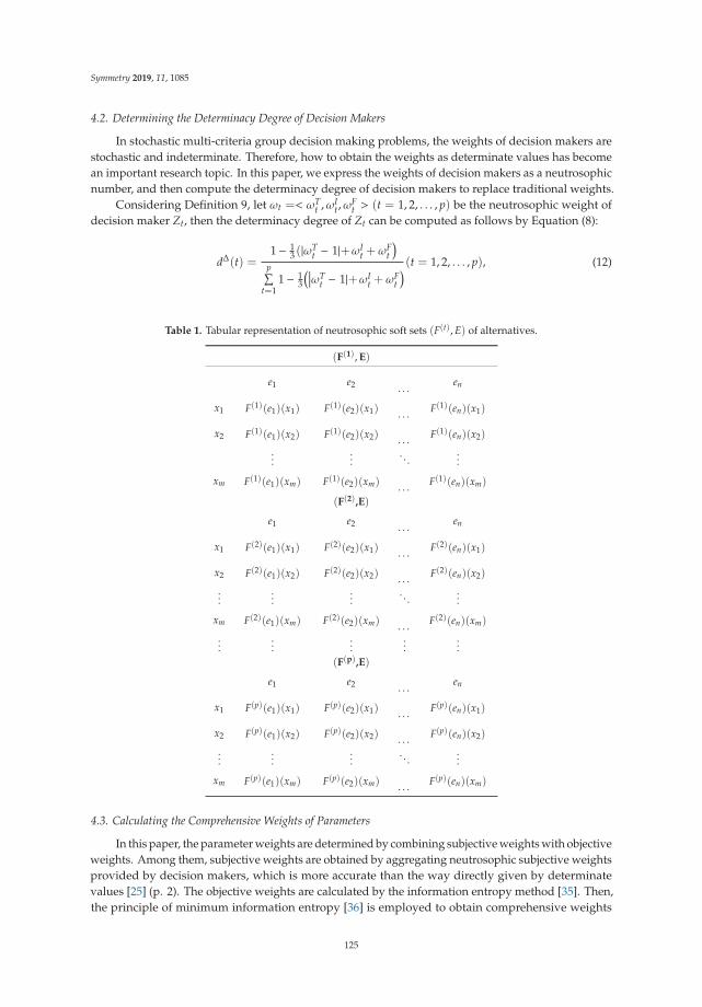
Symmetry 2019, 11, 1085

4.2. Determining the Determinacy Degree of Decision Makers

In stochastic multi-criteria group decision making problems, the weights of decision makers arestochastic and indeterminate. Therefore, how to obtain the weights as determinate values has becomean important research topic. In this paper, we express the weights of decision makers as a neutrosophicnumber, and then compute the determinacy degree of decision makers to replace traditional weights.

Considering Definition 9, let ωt =< ωTt ,ωI

t,ωFt > (t = 1, 2, . . . , p) be the neutrosophic weight of

decision maker Zt, then the determinacy degree of Zt can be computed as follows by Equation (8):

dΔ(t) =1− 1

3 (|ωTt − 1|+ωI

t +ωFt

)p∑

t=11− 1

3

(∣∣∣ωTt − 1|+ωI

t +ωFt

) (t = 1, 2, . . . , p), (12)

Table 1. Tabular representation of neutrosophic soft sets (F(t), E) of alternatives.

(F(1), E)

e1 e2 . . .en

x1 F(1)(e1)(x1) F(1)(e2)(x1) . . .F(1)(en)(x1)

x2 F(1)(e1)(x2) F(1)(e2)(x2) . . .F(1)(en)(x2)

......

. . ....

xm F(1)(e1)(xm) F(1)(e2)(xm) . . .F(1)(en)(xm)

(F(2),E)

e1 e2 . . .en

x1 F(2)(e1)(x1) F(2)(e2)(x1) . . .F(2)(en)(x1)

x2 F(2)(e1)(x2) F(2)(e2)(x2) . . .F(2)(en)(x2)

......

.... . .

...

xm F(2)(e1)(xm) F(2)(e2)(xm) . . .F(2)(en)(xm)

......

......

...(F(p),E)

e1 e2 . . .en

x1 F(p)(e1)(x1) F(p)(e2)(x1) . . .F(p)(en)(x1)

x2 F(p)(e1)(x2) F(p)(e2)(x2) . . .F(p)(en)(x2)

......

.... . .

...

xm F(p)(e1)(xm) F(p)(e2)(xm) . . .F(p)(en)(xm)

4.3. Calculating the Comprehensive Weights of Parameters

In this paper, the parameter weights are determined by combining subjective weights with objectiveweights. Among them, subjective weights are obtained by aggregating neutrosophic subjective weightsprovided by decision makers, which is more accurate than the way directly given by determinatevalues [25] (p. 2). The objective weights are calculated by the information entropy method [35]. Then,the principle of minimum information entropy [36] is employed to obtain comprehensive weights

125

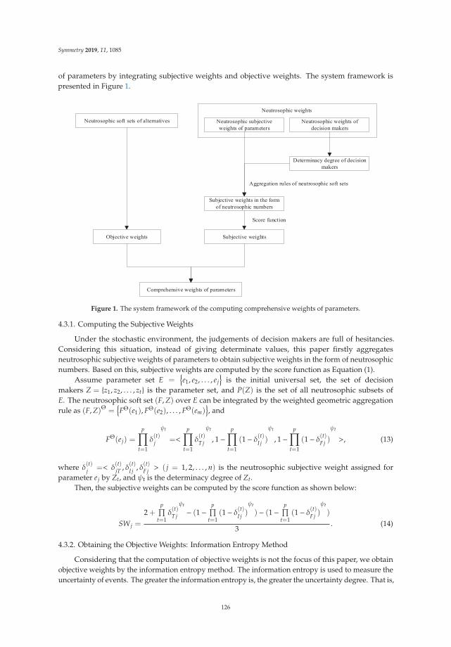
Symmetry 2019, 11, 1085

of parameters by integrating subjective weights and objective weights. The system framework ispresented in Figure 1.

Figure 1. The system framework of the computing comprehensive weights of parameters.

4.3.1. Computing the Subjective Weights

Under the stochastic environment, the judgements of decision makers are full of hesitancies.Considering this situation, instead of giving determinate values, this paper firstly aggregatesneutrosophic subjective weights of parameters to obtain subjective weights in the form of neutrosophicnumbers. Based on this, subjective weights are computed by the score function as Equation (1).

Assume parameter set E ={e1, e2, . . . , ej

}is the initial universal set, the set of decision

makers Z = {z1, z2, . . . , zt} is the parameter set, and P(Z) is the set of all neutrosophic subsets ofE. The neutrosophic soft set (F, Z) over E can be integrated by the weighted geometric aggregationrule as (F, Z)Θ =

{FΘ(e1), FΘ(e2), . . . , FΘ(em)

}, and

FΘ(ej) =

p∏t=1

δ(t)j

ψt

=<

p∏t=1

δ(t)Tj

ψt

, 1−p∏

t=1

(1− δ(t)I j )

ψt

, 1−p∏

t=1

(1− δ(t)Fj )

ψt

>, (13)

where δ(t)j =< δ(t)jT , δ(t)I j , δ(t)Fj > ( j = 1, 2, . . . , n) is the neutrosophic subjective weight assigned for

parameter ej by Zt, and ψt is the determinacy degree of Zt.Then, the subjective weights can be computed by the score function as shown below:

SWj =

2 +p∏

t=1δ(t)Tj

ψt

− (1−p∏

t=1(1− δ(t)I j )

ψt

) − (1−p∏

t=1(1− δ(t)Fj )

ψt

)

3. (14)

4.3.2. Obtaining the Objective Weights: Information Entropy Method

Considering that the computation of objective weights is not the focus of this paper, we obtainobjective weights by the information entropy method. The information entropy is used to measure theuncertainty of events. The greater the information entropy is, the greater the uncertainty degree. That is,

126

Symmetry 2019, 11, 1085

the smaller the amount of information it carries, the smaller the weight is. Note that the uncertainty ofneutrosophic numbers consists of two factors, one is the truth-membership and false-membership,and the other is the indeterminacy-membership.

Based on the information entropy method, we can obtain that the information entropy of parameterej given by decision maker Zt is defined as:

Etj = 1− 1

m

∑m

i=1

(F(t)

T

(ej)(xi) + F(t)

F

(ej)(xi)

)|F(t)

I

(ej)(xi) − F(t)

Ic(ej)(xi)|( j = 1, 2, . . . , n). (15)

Then, the comprehensive information entropy of parameter ej is defined as follows:

Ej =

p∑t=1

ϕtEtj( j = 1, 2, . . . , n) (16)

where ϕt is the determinacy degree of decision maker Zt computed by Equation (8).So, the objective weights are obtained as:

OWj =1− Ej

n∑j=1

1− Ej

( j = 1, 2, . . . , n). (17)

4.3.3. Calculating the Comprehensive Weights

Based on the principle of the minimum information entropy, the comprehensive weight ofparameter j can be calculated as follows:

j =

√OWj · SWj

n∑j=1

√OWj · SWj

, (18)

where SWj and OWj represent the subjective weight and objective weight of parameter ej, respectively.

4.4. Computing the Comprehensive Prospect Values

The comprehensive prospect values of alternatives are determined by the prospect decision matrixand the comprehensive weights of parameters. Next, we expound how to generate the prospectdecision matrix and obtain comprehensive values of alternatives, respectively.

4.4.1. Constructing the Prospect Decision Matrix

The core of constructing the prospect decision matrix is to compute the value function and decisionweight function. In terms of the value function, we need to analyze the distance between the referencepoint and the actual value. This paper regards the maximum conflict neutrosophic number as thereference point, then the distance can be treated as the conflict degree of the actual value. Additionally,actual values refer to the alternative evaluation values with respect to the parameters. As for thedecision weight function, the objective possibility is seen as the determinacy degree of the decisionmakers. The system framework of constructing the prospect decision matrix is shown in Figure 2.

127

Symmetry 2019, 11, 1085

Figure 2. The system framework of constructing the prospect decision matrix.

We assume that the neutrosophic soft sets of alternatives and neutrosophic subjective weights ofparameters are both provided by decision makers. So, the conflict degree of the alternative evaluationvalues with respect to the parameters should take the neutrosophic subjective weights of parametersinto account. Based on the conflict degree measure given by Definition 9, we develop a modifiedconflict degree measure by introducing the neutrosophic subjective weights of parameters.

Assume F(ej)(xi) =< FT(ej)(xi), FI(ej)(xi), FF(ej)(xi) > is a neutrosophic number, which representsthe value of alternative xi related to parameter ej, and α j =< α jT,α jI,α jF > is the neutrosophic subjectiveweight of parameter ej. Considering the sum of α jT,α jI and α jF may not be one, this paper normalizesthem to be more consistent with the reality. Therefore, the measure of the modified conflict degree ofF(ej)(xi) is defined as follows:

mcΔ(F(ej)(xi)) =α jT ·

∣∣∣FT(ej)(xi) − 0.5∣∣∣

α jT + α jI + α jF+α jI ·

∣∣∣FI(ej)(xi) − 1∣∣∣

α jT + α jI + α jF+α jF ·

∣∣∣FF(ej)(xi) − 0.5∣∣∣

α jT + α jI + α jF. (19)

Subsequently, calculate the prospect value of each alternative with respect to the parametersas follows:

Vij =

p∑t=1

w(zt)v(F(t)(ej)(xi) − x0), (20)

where

v(F(t)(ej)(xi) − x0) =

⎧⎪⎪⎨⎪⎪⎩(mcΔ(F(t)(ej)(xi), x0))0.88

, F(t)(ej)(xi) ≥ x0

−2.25(mcΔ(F(t)(ej)(xi), x0))0.88

, F(t)(ej)(xi) < x0, (21)

ω(Zt) =(ψt)

0.61

((ψt)0.61 + (1−ψt)

0.61)1

0.61

. (22)

Then, we can obtain the prospect decision matrix.

128

Symmetry 2019, 11, 1085

4.4.2. Computing the Comprehensive Prospect Values

Based on comprehensive weights of parameters and the prospect decision matrix, we can computethe comprehensive prospect values for alternatives as follows:

Vi =n∑

j=1

jVij. (23)

The system framework of computing the comprehensive prospect values is shown in Figure 3.

Figure 3. The system framework of computing the comprehensive prospect values of alternatives.

4.5. Algorithm for Neutrosophic Soft Sets in Stochastic Multi-Criteria Group Decision Making Based onProspect Theory

In this section, a novel algorithm for neutrosophic soft sets in stochastic multi-criteria groupdecision making based on the prospect theory is proposed. The detailed operation steps of Algorithm1 are presented below.

Algorithm 1: Neutrosophic soft sets in stochastic multi-criteria group decision making based on theprospect theory

Step 1: Input a neutrosophic set, which represents neutrosophic weights of decision makers and twoneutrosophic soft sets, including alternatives description as shown in Table 1 and neutrosophic subjectiveweights of parameters evaluated by decision makers.Step 2: Normalize the neutrosophic soft sets of alternatives as follows:

(�

F(t), E) =

⎧⎪⎪⎨⎪⎪⎩(F(t)T (ej)(xi), F(t)I (ej)(xi), F(t)F (ej)(xi)), ej is a benefit parameter

(F(t)F (ej)(xi), 1− F(t)I (ej)(xi), F(t)T (ej)(xi)), ej is a cos t parameter(24)

Step 3: Compute the determinacy degree vector ψt = (ψ1,ψ2, . . . ,ψp) of decision makers by Equation (8);Step 4: Construct the prospect decision matrix based on Equation (20).Step 5: Obtain the comprehensive weight vector j = (1,2, . . . ,n) by Equation (18);Step 6: Calculate the comprehensive prospect value Vi for each alternative through Equation (23).Step 7: Make a decision by ranking alternatives based on comprehensive prospect values.

5. An Application of the Proposed Algorithm

In order to verify the feasibility of the proposed algorithm, we discuss the investment decision ofa finance institution. Meanwhile, the existing five methods [17,25,37] (pp. 1–2) are employed for acomparative analysis to prove the feasibility and superiority of the proposed algorithm.

5.1. Example Analysis

Credit scoring can help financial institutions reduce financial risks and non-performing loans.Generally, financial institutions assess the credit score of borrowers based on basic information, such asage, profession, education, income, capital gains, residence and borrowing frequency. Recently,a financial institution wants to invest an amount of money in borrowers. The institution initially selects

129

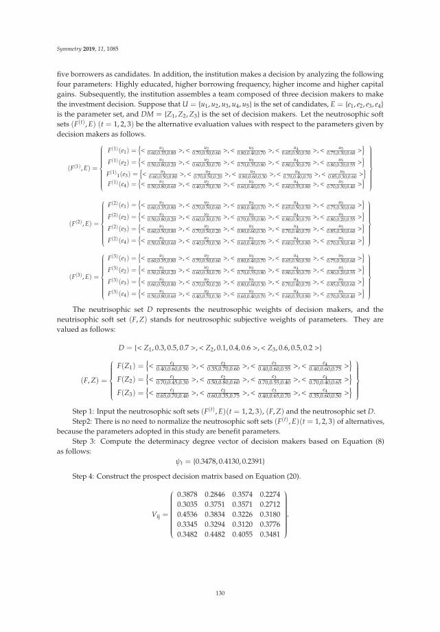
Symmetry 2019, 11, 1085

five borrowers as candidates. In addition, the institution makes a decision by analyzing the followingfour parameters: Highly educated, higher borrowing frequency, higher income and higher capitalgains. Subsequently, the institution assembles a team composed of three decision makers to makethe investment decision. Suppose that U = {u1, u2, u3, u4, u5} is the set of candidates, E = {e1, e2, e3, e4}is the parameter set, and DM = {Z1, Z2, Z3} is the set of decision makers. Let the neutrosophic softsets (F(t), E) (t = 1, 2, 3) be the alternative evaluation values with respect to the parameters given bydecision makers as follows.

(F(1), E) =

⎧⎪⎪⎪⎪⎪⎪⎪⎪⎪⎨⎪⎪⎪⎪⎪⎪⎪⎪⎪⎩

F(1)(e1) ={< u1

0.60,0.35,0.80 >,< u20.70,0.50,0.60 >,< u3

0.80,0.40,0.70 >,< u40.65,0.50,0.50 >,< u5

0.75,0.30,0.60 >}

F(1)(e2) ={< u1

0.50,0.80,0.20 >,< u20.60,0.30,0.70 >,< u3

0.70,0.35,0.80 >,< u40.80,0.30,0.70 >,< u5

0.80,0.20,0.55 >}

F(1)1(e3) =

{< u1

0.60,0.50,0.80 >,< u20.70,0.50,0.20 >,< u3

0.80,0.60,0.30 >,< u40.70,0.40,0.70 >,< u5

0.85,0.30,0.60 >}

F(1)(e4) ={< u1

0.50,0.80,0.60 >,< u20.40,0.70,0.30 >,< u3

0.60,0.40,0.70 >,< u40.60,0.35,0.80 >,< u5

0.70,0.30,0.40 >}

⎫⎪⎪⎪⎪⎪⎪⎪⎪⎪⎬⎪⎪⎪⎪⎪⎪⎪⎪⎪⎭

(F(2), E) =

⎧⎪⎪⎪⎪⎪⎪⎪⎪⎪⎨⎪⎪⎪⎪⎪⎪⎪⎪⎪⎩

F(2)(e1) ={< u1

0.60,0.35,0.80 >,< u20.70,0.50,0.60 >,< u3

0.80,0.40,0.70 >,< u40.65,0.50,0.50 >,< u5

0.75,0.30,0.60 >}

F(2)(e2) ={< u1

0.50,0.80,0.20 >,< u20.60,0.30,0.70 >,< u3

0.70,0.35,0.80 >,< u40.80,0.30,0.70 >,< u5

0.80,0.20,0.55 >}

F(2)(e3) ={< u1

0.60,0.50,0.80 >,< u20.70,0.50,0.20 >,< u3

0.80,0.60,0.30 >,< u40.70,0.40,0.70 >,< u5

0.85,0.30,0.60 >}

F(2)(e4) ={< u1

0.50,0.80,0.60 >,< u20.40,0.70,0.30 >,< u3

0.60,0.40,0.70 >,< u40.60,0.35,0.80 >,< u5

0.70,0.30,0.40 >}

⎫⎪⎪⎪⎪⎪⎪⎪⎪⎪⎬⎪⎪⎪⎪⎪⎪⎪⎪⎪⎭

(F(3), E) =

⎧⎪⎪⎪⎪⎪⎪⎪⎪⎪⎨⎪⎪⎪⎪⎪⎪⎪⎪⎪⎩

F(3)(e1) ={< u1

0.60,0.35,0.80 >,< u20.70,0.50,0.60 >,< u3

0.80,0.40,0.70 >,< u40.65,0.50,0.50 >,< u5

0.75,0.30,0.60 >}

F(3)(e2) ={< u1

0.50,0.80,0.20 >,< u20.60,0.30,0.70 >,< u3

0.70,0.35,0.80 >,< u40.80,0.30,0.70 >,< u5

0.80,0.20,0.55 >}

F(3)(e3) ={< u1

0.60,0.50,0.80 >,< u20.70,0.50,0.20 >,< u3

0.80,0.60,0.30 >,< u40.70,0.40,0.70 >,< u5

0.85,0.30,0.60 >}

F(3)(e4) ={< u1

0.50,0.80,0.60 >,< u20.40,0.70,0.30 >,< u3

0.60,0.40,0.70 >,< u40.60,0.35,0.80 >,< u5

0.70,0.30,0.40 >}

⎫⎪⎪⎪⎪⎪⎪⎪⎪⎪⎬⎪⎪⎪⎪⎪⎪⎪⎪⎪⎭The neutrisophic set D represents the neutrosophic weights of decision makers, and the

neutrisophic soft set (F, Z) stands for neutrosophic subjective weights of parameters. They arevalued as follows:

D = {< Z1, 0.3, 0.5, 0.7 >,< Z2, 0.1, 0.4, 0.6 >,< Z3, 0.6, 0.5, 0.2 >}

(F, Z) =

⎧⎪⎪⎪⎪⎪⎪⎨⎪⎪⎪⎪⎪⎪⎩F(Z1) =

{< e1

0.40,0.60,0.50 >,< e20.35,0.70,0.60 >,< e3

0.40,0.60,0.55 >,< e40.40,0.60,0.75 >

}F(Z2) =

{< e1

0.70,0.45,0.30 >,< e20.50,0.80,0.60 >,< e3

0.70,0.55,0.40 >,< e40.70,0.40,0.65 >

}F(Z3) =

{< e1

0.65,0.70,0.40 >,< e20.60,0.35,0.75 >,< e3

0.40,0.65,0.70 >,< e40.35,0.60,0.50 >

}⎫⎪⎪⎪⎪⎪⎪⎬⎪⎪⎪⎪⎪⎪⎭

Step 1: Input the neutrosophic soft sets (F(t), E)(t = 1, 2, 3), (F, Z) and the neutrosophic set D.Step2: There is no need to normalize the neutrosophic soft sets (F(t), E)(t = 1, 2, 3) of alternatives,

because the parameters adopted in this study are benefit parameters.Step 3: Compute the determinacy degree vector of decision makers based on Equation (8)

as follows:ψt = {0.3478, 0.4130, 0.2391}

Step 4: Construct the prospect decision matrix based on Equation (20).

Vij =

⎛⎜⎜⎜⎜⎜⎜⎜⎜⎜⎜⎜⎜⎜⎜⎜⎜⎜⎝

0.3878 0.2846 0.3574 0.22740.3035 0.3751 0.3571 0.27120.4536 0.3834 0.3226 0.31800.3345 0.3294 0.3120 0.37760.3482 0.4482 0.4055 0.3481

⎞⎟⎟⎟⎟⎟⎟⎟⎟⎟⎟⎟⎟⎟⎟⎟⎟⎟⎠.

130

Symmetry 2019, 11, 1085

Step 5: Determine the comprehensive weight vector j = (1,2, . . . ,n) for the parameters asEquation (18), and the neutrosophic subjective weights are aggregated by the weighted geometricaggregation rule as Equation (11).

j = (0.2991, 0.2260, 0.2898, 0.1851)

Step 6: Obtain the comprehensive prospect value Vi by Equation (23).

V1 = 0.3269, V2 = 0.3292, V3 = 0.3746, V4 = 0.3348, V5 = 0.3874.

Step 7: Make a decision by ranking the comprehensive prospect value of the five candidates.

x5 � x3 � x4 � x2 � x1

Therefore, we can see that the optimal candidate is x5. x3, x4 are suboptimal, and x2, x1 arethe worst.

Furthermore, we also utilize the weighted average aggregation rule to compute the subjectiveweights of parameters. In addition, the computational procedure is shown as follows.

Step 1–4: Be consistent with the above steps 1–4.Step 5: Determine the comprehensive weight vector j = (1,2, . . . ,n) for the parameters

as Equation (18), and the neutrosophic subjective weights are aggregated by the weighted averageaggregation rule.

j = (0.2903, 0.2127, 0.2523, 0.2447).

Step 6: Obtain the comprehensive prospect value Vi by Equation (23).

V1 = 0.3254, V2 = 0.3295, V3 = 0.3744, V4 = 0.3348, V5 = 0.3876.

Step 7: Make a decision by ranking the five candidates.

x5 � x3 � x4 � x2 � x1.

So the best optimal is still x5, the following are x3, x4, and the worst are x2, x1.Obviously, we can see that the ranking orders obtained by two aggregation rules of the neutrosophic

soft set are the same.

5.2. Comparative Analysis

A comparative analysis with existing methods is performed to justify the feasibility and superiorityof the proposed method. The existing methods include the method proposed by Maji [17] (p. 1),the three methods carried out by Peng and Liu [25] (p. 2) and the aggregated neutrosophic setmethod [37] (p. 11).

In the decision making method outlined by Maji [17] (p. 1), the final ranking is obtained based onthe comparison matrix through briefly comparing with three membership function values. The threeneutrosophic soft decision making methods [25] (p. 2) include the non-linear weighted comprehensivemethod to determine parameter comprehensive weights by combining objective weights and subjectiveweights. Objective weights are computed by the grey system method, and subjective weights aredirectly given determinate values. Then, three neutrosophic soft decision making methods areconstructed based on EDAS, similarity measure, and the level soft set to rank alternatives in practicalproblems. Among the three, EDAS and the similarity measure methods obtain the final ranking basedon the accurate calculation of alternative evaluation values. In addition, the level soft set method makesa decision by roughly comparing the threshold value with alternative evaluation values. In terms of

131

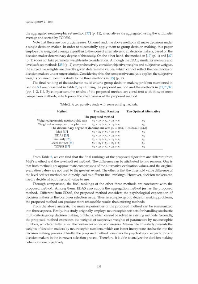
Symmetry 2019, 11, 1085

the aggregated neutrosophic set method [37] (p. 11), alternatives are aggregated using the arithmeticaverage and sorted by TOPSIS.

Note that there are two crucial issues. On one hand, the above methods all make decisions undera single decision maker. In order to successfully apply them to group decision making, this paperemploys the weighted average algorithm to the score of alternatives to all decision makers, based on thedecision maker determinacy degree of this study. On the other hand, the method in [17] (p. 1) and [37](p. 11) does not take parameter weights into consideration. Although the EDAS, similarity measure andlevel soft set methods [25] (p. 2) comprehensively consider objective weights and subjective weights,the subjective weights are directly given determinate values, which cannot reflect the hesitancies ofdecision makers under uncertainties. Considering this, the comparative analysis applies the subjectiveweights obtained from this study to the three methods in [25] (p. 2).

The final ranking of the stochastic multi-criteria group decision making problem mentioned inSection 5.1 are presented in Table 2, by utilizing the proposed method and the methods in [17,25,37](pp. 1–2, 11). By comparison, the results of the proposed method are consistent with those of mostcomparison methods, which prove the effectiveness of the proposed method.

Table 2. A comparative study with some existing methods.

Method The Final Ranking The Optimal Alternative

The proposed method

Weighted geometric neutrosophic rule x5 � x3 � x4 � x2 � x1 x5Weighted average neutrosophic rule x5 � x3 � x4 � x2 � x1 x5

The determinacy degree of decision makers ψt = {0.3913, 0.2826, 0.3261}Maji [17] x5 � x4 � x3 � x2 � x1 x5

EDAS [25] x5 � x3 � x4 � x2 � x1 x5Similarity [25] x5 � x3 � x4 � x2 � x1 x5

Level soft set [25] x5 � x4 � x3 � x2 � x1 x5TOPSIS [37] x5 � x3 � x4 � x2 � x1 x5

From Table 2, we can find that the final rankings of the proposed algorithm are different fromMaji’s method and the level soft set method. The difference can be attributed to two reasons. One isthat both methods are approximate comparisons of the alternative evaluation values, and the originalevaluation values are not used to the greatest extent. The other is that the threshold value difference ofthe level soft set method can directly lead to different final rankings. However, decision makers canhardly decide which threshold value to use.

Through comparison, the final rankings of the other three methods are consistent with theproposed method. Among them, EDAS also adopts the aggregation method just as the proposedmethod. Different from EDAS, the proposed method considers the psychological expectation ofdecision makers in the borrower selection issue. Thus, in complex group decision making problems,the proposed method can produce more reasonable results than existing methods.

From the above analysis, the main superiorities of the proposed method can be summarizedinto three aspects. Firstly, this study originally employs neutrosophic soft sets for handling stochasticmulti-criteria group decision making problems, which cannot be solved in existing methods. Secondly,the proposed method expresses the weights of subjective weights of parameters by neutrosophicnumbers, which can fully reflect the hesitancies of decision makers. Meanwhile, this study presents theweights of decision makers by neutrosophic numbers, which can better incorporate stochastic into thedecision making process. Thirdly, the proposed method considers the psychological expectations ofdecision makers in the borrower selection process. Therefore, it is able to analyze the decision makingbehavior more objectively.

132

Symmetry 2019, 11, 1085

6. Conclusions

Under uncertain environments, a mass of inconsistent information appears. Neutrosophic soft setsare powerful tools to address these issues involving inconsistent information. Considering this,we develop a generalized stochastic multi-criteria group decision making framework underneutrosophic soft sets, by innovatively integrating the prospect theory and neutrosophic soft sets intoour framework. This paper describes the reference point, the psychological expectations of decisionmakers, in the form of neutrosophic sets. Then, in addition, this study demonstrates how to computethe alternative prospect values as the reference for decision making.

We conduct experiments to test the feasibility and validity of our decision making framework.The main contributions of this paper are fourfold. Firstly, we construct a new algorithm for the stochasticmulti-criteria group decision making based on neutrosophic soft sets, which can analyze inconsistentinformation in decision making effectively. Secondly, the weights of decision makers and parametersubjective weights are both expressed in the form of neutrosophic numbers. Compared with the waydirectly given determinate values in existing methods [25] (p. 2), the proposed method can embodythe stochastic into decision making processes. Thirdly, the research successfully combines the prospecttheory with neutrosophic softs sets to construct the stochastic multi-criteria group decision makingalgorithm. Compared with the existing literatures based on the expected utility theory [16,17,25,26](pp. 1-2), this research considers the influence of psychological expectations on decision results.Finally, we explore the conflict degree measure of neutrosophic numbers and two aggregation rules ofneutrosophic soft sets, and further define the measure of the modified conflict degree to accommodatethe multi-criteria group decision making.

The proposed method is not only suitable for credit scoring, but also for decision-making problemsin other fields, especially for decisions with inconsistent information. As a suggestion for futureresearches, we shall integrate more advanced decision theories into neutrosophic soft sets and addressstochastic multi-criteria group decision making issues.

Author Contributions: Funding acquisition, Y.D.; Methodology, Y.D. and C.H.; Validation, Y.D. and C.H.;Writing—original draft, Y.D. and C.H.; Writing—review and editing, C.H., Y.P., and K.G.

Funding: This research was funded by the National Natural Science Foundation of China (Grant Nos. 71701116and 71871034); Humanities and Social Science Fund of Ministry of Education of China (Grant No. 15YJC630016);Science and Technology Innovation Program in Higher Education Institutions of Shanxi Province (“Research onmulti-level dynamic credit evaluation under conflict data”) and Education Innovation Program for Postgraduateof Shanxi Province (“Research on Multi-level Dynamic Credit Evaluation of Personal Consumption Credit underInternet Conflict Data”).

Acknowledgments: The authors gratefully acknowledge the editor of the Journal and anonymous reviewers forthe detailed and valuable comments.

Conflicts of Interest: The authors declare no conflict of interest.

References

1. Zadeh, L.A. Fuzzy sets. Inf. Control 1965, 8, 338–353. [CrossRef]2. Pawlak, Z. Rough sets. Int. J. Comput. Inf. Sci. 1982, 11, 341–356. [CrossRef]3. Gorzałczany, M.B. A method of inference in approximate reasoning based on interval-valued fuzzy sets.

Fuzzy Sets Syst. 1987, 21, 1–17. [CrossRef]4. Molodtsov, D. Soft set theory-first results. Comput. Math. Appl. 1999, 37, 19–31. [CrossRef]5. Aktas, H.; Çagman, N. Soft sets and soft groups. Inf. Sci. 2007, 177, 2726–2735. [CrossRef]6. Acar, U.; Koyuncu, F.; Tanay, B. Soft sets and soft rings. Comput. Math. Appl. 2010, 59, 3458–3463. [CrossRef]7. Min, W.K. A note on soft topological spaces. Comput. Math. Appl. 2011, 62, 3524–3528. [CrossRef]8. Çagman, N.; Karatas, S.; Enginoglu, S. Soft topology. Comput. Math. Appl. 2011, 62, 351–358. [CrossRef]9. Danjuma, S.; Ismail, M.A.; Herawan, T. An alternative approach to normal parameter reduction algorithm

for soft set theory. IEEE Access 2017, 5, 4732–4746. [CrossRef]

133

Symmetry 2019, 11, 1085

10. Yuksel, S.; Dizman, T.; Yildizdan, G.; Sert, U. Application of soft sets to diagnose the prostate cancer risk.J. Inequalities Appl. 2013, 2013, 229. [CrossRef]

11. Kamacı, H.; Atagün, A.O.; Sönmezoglu, A. Row-products of soft matrices with applications inmultiple-disjoint decision making. Appl. Soft Comput. 2018, 62, 892–914. [CrossRef]

12. Fatimah, F.; Rosadi, D.; Hakim, R.B.F.; Alcantud, J.C.R. N-soft sets and their decision making algorithms.Soft Comput. 2018, 22, 3829–3842. [CrossRef]

13. Feng, F.; Li, C.; Davvaz, B.; Ali, M.I. Soft sets combined with fuzzy sets and rough sets: A tentative approach.Soft Comput. 2010, 14, 899–911. [CrossRef]

14. Maji, P.K.; Biswas, R.; Roy, A.R. Fuzzy Soft Sets. J. Fuzzy Math. 2001, 9, 589–602.15. Jiang, Y.; Tang, Y.; Chen, Q. An adjustable approach to intuitionistic fuzzy soft sets based decision making.

Appl. Math. Model. 2011, 35, 824–836. [CrossRef]16. Smarandache, F. A Unifying Field in Logics. Neutrosophy: Neutrosophic Probability, Set and Logic; American

Research Press: Rehoboth, DE, USA, 1999.17. Maji, P.K. Neutrosophic soft set. Comput. Math. Appl. 2013, 45, 555–562. [CrossRef]18. Sahin, R.; Küçük, A. Generalised Neutrosophic Soft Set and its Integration to Decision Making Problem.

Appl. Math. Inf. Sci. 2014, 8, 2751. [CrossRef]19. Deli, I.; Broumi, S. Neutrosophic soft matrices and NSM-decision making. J. Intell. Fuzzy Syst. 2015, 28,

2233–2241. [CrossRef]20. Deli, I. Interval-valued neutrosophic soft sets and its decision making. Int. J. Mach. Learn. Cybern. 2017, 8,

665–676. [CrossRef]21. Karaaslan, F. Possibility neutrosophic soft sets and PNS-decision making method. Appl. Soft Comput. 2017,

54, 403–414. [CrossRef]22. Karaaslan, F. Correlation coefficients of single-valued neutrosophic refined soft sets and their applications in

clustering analysis. Neural Comput. Appl. 2017, 28, 2781–2793. [CrossRef]23. Uluçay, V.; Sahin, M.; Hassan, N. Generalized neutrosophic soft expert set for multiple-criteria

decision-making. Symmetry 2018, 10, 437. [CrossRef]24. Al-Quran, A.; Hassan, N.; Marei, E. A Novel Approach to Neutrosophic Soft Rough Set under Uncertainty.

Symmetry 2019, 11, 384. [CrossRef]25. Peng, X.; Liu, C. Algorithms for neutrosophic soft decision making based on EDAS, new similarity measure

and level soft set. J. Intell. Fuzzy Syst. 2017, 32, 955–968. [CrossRef]26. Abu Qamar, M.; Hassan, N. Entropy, measures of distance and similarity of Q-neutrosophic soft sets and

some applications. Entropy 2018, 20, 672. [CrossRef]27. Kahneman, D.; Tversky, A. Prospect theory: An analysis of decisions under risk. Econometrica 1979, 47,

263–291. [CrossRef]28. Peng, X.; Yang, Y. Algorithms for interval-valued fuzzy soft sets in stochastic multi-criteria decision making

based on regret theory and prospect theory with combined weight. Appl. Soft Comput. 2017, 54, 415–430.[CrossRef]

29. Haibin, W.; Smarandache, F.; Zhang, Y.; Sunderraman, R. Single Valued Neutrosophic Sets. MultispaceMultistruct. 2010, 4, 410–413.

30. Liu, C.; Luo, Y.S. Correlated aggregation operators for simplified neutrosophic set and their application inmulti-attribute group decision making. J. Intell. Fuzzy Syst. 2016, 30, 1755–1761. [CrossRef]

31. Ye, J.; Du, S. Some distances, similarity and entropy measures for interval-valued neutrosophic sets and theirrelationship. Int. J. Mach. Learn. Cybern. 2019, 10, 347–355. [CrossRef]

32. Sahin, R.; Küçük, A. On similarity and entropy of neutrosophic soft sets. J. Intell. Fuzzy Syst. 2014, 27,2417–2430.

33. Alfaro-García, V.G.; Merigó, J.M.; Gil-Lafuente, A.M.; Kacprzyk, J. Logarithmic aggregation operators anddistance measures. Int. J. Intell. Syst. 2018, 33, 1488–1506. [CrossRef]

34. Choi, S.H.; Jung, S.H. Similarity Analysis of Actual Fake Fingerprints and Generated Fake Fingerprints byDCGAN. Int. J. Fuzzy Log. Intell. Syst. 2019, 19, 40–47. [CrossRef]

35. Biswas, P.; Pramanik, S.; Giri, B.C. Entropy based grey relational analysis method for multi-attribute decisionmaking under single valued neutrosophic assessments. Neutrosophic Sets Syst. 2014, 2, 102–110.

36. Wu, K.; Jin, J. Attribute recognition method of regional ecological security evaluation based on combinedweight on principle of relative entropy. Sci. Geogr. Sin. 2008, 28, 754–758.

134

Symmetry 2019, 11, 1085

37. Jiang, W.; Zhang, Z.; Deng, X. Multi-Attribute Decision Making Method Based on Aggregated NeutrosophicSet. Symmetry 2019, 11, 267. [CrossRef]

© 2019 by the authors. Licensee MDPI, Basel, Switzerland. This article is an open accessarticle distributed under the terms and conditions of the Creative Commons Attribution(CC BY) license (http://creativecommons.org/licenses/by/4.0/).

135

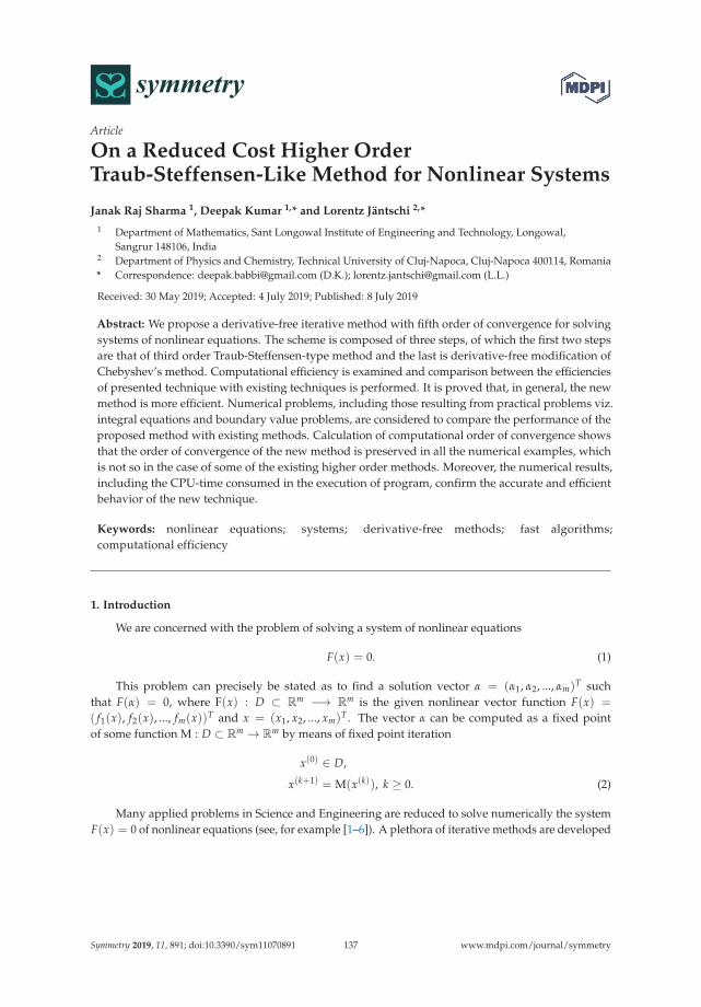
symmetryS SArticle

On a Reduced Cost Higher OrderTraub-Steffensen-Like Method for Nonlinear Systems

Janak Raj Sharma 1, Deepak Kumar 1,* and Lorentz Jäntschi 2,*

1 Department of Mathematics, Sant Longowal Institute of Engineering and Technology, Longowal,Sangrur 148106, India

2 Department of Physics and Chemistry, Technical University of Cluj-Napoca, Cluj-Napoca 400114, Romania* Correspondence: deepak.babbi@gmail.com (D.K.); lorentz.jantschi@gmail.com (L.L.)

Received: 30 May 2019; Accepted: 4 July 2019; Published: 8 July 2019

Abstract: We propose a derivative-free iterative method with fifth order of convergence for solvingsystems of nonlinear equations. The scheme is composed of three steps, of which the first two stepsare that of third order Traub-Steffensen-type method and the last is derivative-free modification ofChebyshev’s method. Computational efficiency is examined and comparison between the efficienciesof presented technique with existing techniques is performed. It is proved that, in general, the newmethod is more efficient. Numerical problems, including those resulting from practical problems viz.integral equations and boundary value problems, are considered to compare the performance of theproposed method with existing methods. Calculation of computational order of convergence showsthat the order of convergence of the new method is preserved in all the numerical examples, whichis not so in the case of some of the existing higher order methods. Moreover, the numerical results,including the CPU-time consumed in the execution of program, confirm the accurate and efficientbehavior of the new technique.

Keywords: nonlinear equations; systems; derivative-free methods; fast algorithms;computational efficiency

1. Introduction

We are concerned with the problem of solving a system of nonlinear equations

F(x) = 0. (1)

This problem can precisely be stated as to find a solution vector α = (α1, α2, ..., αm)T suchthat F(α) = 0, where F(x) : D ⊂ Rm −→ Rm is the given nonlinear vector function F(x) =

( f1(x), f2(x), ..., fm(x))T and x = (x1, x2, ..., xm)T . The vector α can be computed as a fixed pointof some function M : D ⊂ Rm → Rm by means of fixed point iteration

x(0) ∈ D,

x(k+1) = M(x(k)), k ≥ 0. (2)

Many applied problems in Science and Engineering are reduced to solve numerically the systemF(x) = 0 of nonlinear equations (see, for example [1–6]). A plethora of iterative methods are developed

Symmetry 2019, 11, 891; doi:10.3390/sym11070891 www.mdpi.com/journal/symmetry137

Symmetry 2019, 11, 891

in literature for solving such equations. A classical method is cubically convergent Chebyshev’s method(see [7])

x(0) ∈ D,

x(k+1) = x(k) −(

I +12

LF(x(k)))

F′(x(k))−1F(x(k)), k ≥ 0, (3)

where LF(x(k)) = F′(x(k))−1F′′(x(k))F′(x(k))−1F(xk). This one-point iterative scheme dependsexplicitly on the first two derivatives of F. In [7], Ezquerro and Hernández present modificationin Chebyshev’s method that avoids the computation of second derivative F′′ while maintainingthird-order of convergence. It has the following form:

x(0) ∈ D,

y(k) = x(k) − a F′(x(k))−1F(x(k)),

x(k+1) = x(k) − 1a2 F′(x(k))−1((a2 + a− 1)F(x(k)) + F(y(k))

), k ≥ 0. (4)

There is an interest in constructing derivative free iterative processes obtained by considering anapproximation of the first derivative of F from a divided difference of first order. One class of suchmethods is called the class of Secant-type methods which is obtained by replacing F′ with the divideddifference operator [x(k−1), x(k) ; F]. Using this operator a family of derivative free methods is givenin [8]. The authors call this family the Chebyshev-Secant-type method and it is defined as

x(−1), x(0) ∈ D,

y(k) = x(k) − a [x(k−1), x(k) ; F]−1F(x(k)),

x(k+1) = x(k) − [x(k−1), x(k) ; F]−1(b F(x(k)) + c F(y(k))), k ≥ 0, (5)

where a, b and c are non-negative parameters.Another class of derivative free methods is the class of Steffensen-type processes that replaces

F′ with operator [w(x(k)), x(k) ; F], wherein w : Rm → Rm. The work presented in [9] analyzesSteffensen-type iterative method which is given as

x(0) ∈ D,

y(k) = x(k) − a [w(x(k)), x(k) ; F]−1F(x(k)),

x(k+1) = x(k) − [w(x(k)), x(k) ; F]−1(b F(x(k)) + c F(y(k))), k ≥ 0. (6)

For a = b = c = 1 and w(x(k)) = x(k) + βF(x(k)), β is an arbitrary non-zero constant, this methodpossesses third order convergence. In this case y(k) is Traub-Steffensen iteration [6]. For β = 1, y(k)

belongs to Steffensen iteration [10]. Both of these iterations are quadratically convergent.The two-step third order Traub-Steffensen-type method, i.e., the case of (6) for a = b = c = 1,

can be written as

x(0) ∈ D, w(x(k)) = x(k) + βF(x(k)),

y(k) = M2,1(x(k)),

x(k+1) = M3,1(x(k), y(k)) = y(k) − [w(x(k)), x(k) ; F]−1F(y(k)), k ≥ 0, (7)

where M2,1(x(k)) = x(k) − [w(x(k)), x(k) ; F]−1F(x(k)) is the quadratically convergent Traub-Steffensenscheme. Here and in the sequel, the symbol Mp,i is used for denoting an i-th iteration function ofconvergence order p. It can be observed that the third order scheme (7) is computationally moreefficient than quadratically convergent Traub-Steffensen scheme. The reason is that the convergence

138

Symmetry 2019, 11, 891

order is increased from two to three at the cost of only one function evaluation without adding extrainverse operator. We discuss computational efficiency in later sections.

Researchers have always been trying to develop the iterative method with increasing efficiencysince different methods converge to the solution with different convergence speed. This can bedone either by increasing the convergence order or by decreasing the computational cost or both.In [11], Ren et al. have derived a fourth order derivative-free method that uses three F, three divideddifferences and two matrix inversions per iteration. Zheng et al. [12] have constructed two familiesof fourth order derivative-free methods for scalar nonlinear equations, that are extendable to solvesystems of nonlinear equations. First family requires to evaluate three F, three divided differences andtwo matrix inversions, whereas the second family needs three F, three divided differences and threematrix inversions. Grau et al. presented a fourth order derivative-free method in [13] utilizing four F,two divided differences and two matrix inversions. Sharma and Arora [14] presented a fourth orderderivative-free method that uses the evaluations of three F, three divided differences and one matrixinversion per each step.

In search of more fast techniques, researchers have also introduced sixth and seventh orderderivative-free methods in [13,15–18]. The sixth order method in [13] proposed by Grau et al. requiresfive F, two divided differences and two matrix inverses. Sharma and Arora [17] also developed amethod of at least sixth order which requires evaluation of five functions, two divided difference andone matrix inversion per iteration. The seventh order method proposed by Sharma and Arora [15]utilizes four F, five divided differences and two matrix inversions per iteration. The seventh ordermethods presented by Wang and Zhang [16] use four F, five divided differences and three matrixinversions. Ahmad et al. [18] proposed eighth order derivative free method without memory whichuses six functions evaluations, three divided difference and one matrix inversion.

The main goal in this study is to develop a derivative-free method of high computational efficiency,that means a method with high convergence speed and low computational cost. Consequently,we present a Traub-Steffensen-type method of fifth order of convergence which requires the evaluationsfour F, two divided differences and only one matrix inversion per step. The scheme of the presentcontribution is simple and consists of three steps. Of the three steps, the first two are that of cubicallyconvergent Traub-Steffensen-type scheme (7) whereas the third is derivative-free modification ofChebyshev’s scheme (3). We show that the proposed method is more efficient than existing methodsof similar nature.

The content of the rest of the paper is summarized as follows. Basic definitions relevant to thepresent work are stated in Section 2. In Section 3, the scheme of fifth order method is introduced andits convergence behavior is studied. In Section 4, the computational efficiency of the new method isexamined and also compared with the existing derivative-free methods. In Section 5, the basins ofattractors are presented to check the stability and convergence of the new method. Numerical tests areperformed in Section 6 to verify the theoretical results as proved in Sections 3 and 4. Section 7 containsthe concluding remarks.

2. Preliminary Results

2.1. Computational Order of Convergence

Let α be a solution of the function F(x) = 0 and x(k−2), x(k−1), x(k) and x(k+1) be the fourconsecutive iterations close to α. Then, the computational order of convergence (say, pc) can becalculated using the formula (see [19])

pc =log(‖x(k+1) − x(k)‖/‖x(k) − x(k−1)‖)

log(‖x(k) − x(k−1)‖/‖x(k−1) − x(k−2)‖). (8)

139

Symmetry 2019, 11, 891

2.2. Divided Difference

Divided difference operator for multivariable function F (see [4,5,20]) is a mapping [·, · ; F] :D× D ⊂ Rm ×Rm → L(Rm) which is defined as

[x, y; F](x− y) = F(x)− F(y), ∀ (x, y) ∈ Rm. (9)

If F is differentiable, we can also define first order divided difference as (see [4,20])

[x + h, x ; F] =∫ 1

0F′(x + th) dt, ∀ (x, h) ∈ R

m. (10)

This also implies that[x, x ; F] = F′(x). (11)

It can be seen that the divided difference operator [x, y ; F] is an m×m matrix and the definitions (9)and (10) are equivalent (for details see [20]). For computational purpose the following definition(see [5]), is used

[x, y ; F]ij =fi(x1, ....., xj, yj+1, ....., ym)− fi(x1, ....., xj−1, yj, ....., ym)

xj − yj, 1 ≤ i, j ≤ m. (12)

2.3. Computational Efficiency

Computational efficiency of an iterative method for solving F(x) = 0 is calculated by theefficiency index E = p1/C, (for detail see [21,22]), where p is the order of convergence and C isthe total cost of computation. The cost of computation C is measured in terms of the total number offunction evaluations per iteration and the number of operations (that means products and quotients)per iteration.

3. The Method and Analysis of Convergence

Let us begin with the following three-step scheme

y(k) = M2,1(x(k)),

z(k) = y(k) − [w(k), x(k) ; F]−1F(y(k)),

x(k+1) = z(k) −(

I +12

LF(y(k)))

F′(y(k))−1F(z(k)), (13)

where w(k) = x(k) + βF(x(k)), I is m × m identity matrix and LF(y(k)) =

F′(y(k))−1F′′(y(k))F′(y(k))−1F(yk).Note that this is a scheme whose first two steps are that of third order Traub-Steffensen-type

method (7) whereas third step is based on Chebyshev’s method (3). The scheme requires first andsecond derivatives of F at y(k). To make this a derivative-free method, we describe an approachas follows:

Consider the Taylor expansion of F(z(k)) about y(k),

F(z(k)) ≈ F(y(k)) + F′(y(k))(z(k) − y(k)) +12

F′′(y(k))(z(k) − y(k))2. (14)

Then, it follows that

12

F′′(y(k))(z(k) − y(k))2 ≈ F(z(k))− F(y(k))− F′(y(k))(z(k) − y(k)). (15)

140

Symmetry 2019, 11, 891

Using the fact thatF(z(k))− F(y(k)) = [z(k), y(k) ; F](z(k) − y(k)),

(see, for example [4,5]), we can write (15) as

F′′(y(k))(z(k) − y(k)) ≈ 2([z(k), y(k) ; F]− F′(y(k))). (16)

Then, using the second step of (13) in the above equation, it follows that

F′′(y(k))[w(k), x(k) ; F]−1F(y(k)) ≈ −2([z(k), y(k) ; F]− F′(y(k))

). (17)

Let us assume F′(y(k)) ≈ [w(k), x(k) ; F], then (17) implies

F′′(y(k))[w(k), x(k) ; F]−1F(y(k)) ≈ −2([z(k), y(k) ; F]− [w(k), x(k) ; F]

). (18)

In addition, we have that

LF(y(k)) = F′(y(k))−1F′′(y(k))F′(y(k))−1F(yk)

≈ [w(k), x(k) ; F]−1F′′(y(k))[w(k), x(k) ; F]−1F(yk). (19)

Using (18) in (19), we obtain that

LF(y(k)) ≈ [w(k), x(k) ; F]−1F′′(y(k))[w(k), x(k) ; F]−1F(yk)

≈ −2([w(k), x(k) ; F]−1[z(k), y(k) ; F]− I

). (20)

Now, we can write the third-step of (13) in modified form as

x(k+1) = z(k) −(2I − [w(k), x(k) ; F]−1[z(k), y(k) ; F]

)[w(k), x(k) ; F]−1F(z(k)). (21)

Thus, we define the following new method:

y(k) = M2,1(x(k)),

z(k) = M3,1(x(k), y(k)),

x(k+1) = z(k) − H(x(k))[w(k), x(k) ; F]−1F(z(k)), (22)

wherein H(x(k)) = 2I − [w(k), x(k) ; F]−1[z(k), y(k) ; F].Since the scheme (22) is composed of Traub-Steffensen like steps, we call it the

Traub-Steffensen-like method.In order to explore the convergence properties of Traub-Steffensen-like method, we recall some

important results from the theory of iteration functions. First, we state the following well-known result(see [3,23]):

Lemma 1. Assume that M : D ⊂ Rm → Rm has a fixed point α ∈ int(D) and M(x) is Frechet differentiableon α. If

ρ(M′(α)) = σ < 1, (23)

then α is a point of attraction for the iteration x(k+1) = M(x(k)), where ρ is a spectral radius of M′(α).

Next, we state a result which has been proven in [24] by Madhu et al. and that shows α is a pointof attraction for a general iteration function of the form M(x) = P(x)−Q(x)R(x).

141

Symmetry 2019, 11, 891

Lemma 2. Let F : D ⊂ Rm → Rm be sufficiently Frechet differentiable at each point of an open convex setD of α ∈ D, which is a solution of the nonlinear system F(x) = 0. Suppose that P, Q, R : D ⊂ Rm → Rm

are sufficiently Frechet differentiable functions (depending on F) at each point in the set D with the propertiesP(α) = α, Q(α) �= 0, R(α) = 0. Then, there exists a ball

S = S(α, ε) = {‖α− x‖ ≤ ε} ⊂ D, ε > 0,

on which the mappingM : S → R

m, M(x) = P(x)−Q(x)R(x), ∀ x ∈ S

is well defined. Moreover, M(x) is Frechet differentiable at α, thus

M′(α) = P′(α)−Q(α)R′(α).

Let us also recall the definition (10) of divided difference operator. Then, expanding F′(x + th)in (10) by Taylor series at the point x and thereafter integrating, we have that

[x + h, x ; F] =∫ 1

0F′(x + th) dt = F′(x) +

12

F′′(x)h +16

F′′′(x)h2 +1

24F(iv)(x)h3 + O(h4), (24)

where hi = (h, h,i· · · ·, h), h ∈ Rm. Let e(k) = x(k) − α. Assuming that Γ = F′(α)−1 exists,

then expanding F(x(k)) and its first three derivatives in a neighborhood of α by Taylor’s series,we have that

F(x(k)) = F′(α)(e(k) + A2(e(k))2 + A3(e(k))3 + A4(e(k))4 + A5(e(k))5 + O((e(k))6)

), (25)

F′(x(k)) = F′(α)(

I + 2A2e(k) + 3A3(e(k))2 + 4A4(e(k))3 + 5A5(e(k))4 + O((e(k))5)), (26)

F′′(x(k)) = F′(α)(2A2 + 6A3e(k) + 12A4(e(k))2 + 20A5(e(k))3 + O((e(k))4)

)(27)

andF′′′(x(k)) = F′(α)

(6A3 + 24A4e(k) + 60A5(e(k))2 + O((e(k))3)

), (28)

where Ai =1i! ΓF(i)(α) ∈ Li(R

m,Rm) and (e(k))i = (e(k), e(k),i−times· · · · , e(k)), e(k) ∈ Rm.

We are in a situation to analyze the behavior of Traub-Steffensen-like method. Thus, the followingtheorem is proved:

Theorem 1. Let F : D ⊂ Rm → Rm be sufficiently Frechet differentiable at each point of an open convex setD of α ∈ Rm, which is a solution of F(x) = 0. Assume that x ∈ S = S(α, ε) and F′(x) is continuous andnonsingular at α, and x(0) close to α. Then, α is a point of attraction of the sequence {x(k)} generated by theTraub-Steffensen-like method (22). Furthermore, the sequence so developed converges locally to α with order atleast 5.

Proof. First we show that α is a point of attraction of Traub-Steffensen-like iteration. In this case,we have that

P(x) = z(x), Q(x) = H(x)[w, x ; F]−1, R(x) = F(z(x)).

Now, since F(α) = 0, [α, α ; F] = F′(α) �= O, we have

y(α) = α− [α, α ; F]−1F(α) = α− F′(α)−1F(α) = α,

z(α) = α− [α, α ; F]−1F(α)− [α, α ; F]−1F(α) = α− F′(α)−1F(α)− F′(α)−1F(α) = α,

H(α) = 2I − [α, α ; F]−1[α, α ; F] = I,

P(α) = z(α), P′(α) = z′(α),

142

Symmetry 2019, 11, 891

Q(α) = H(α)[α, α ; F]−1 = I [α, α ; F]−1 = [α, α ; F]−1 = F′(α)−1 �= O,

R(α) = F(z(α)) = F(α) = 0,

R′(α) = F′(z(α))z′(α) = F′(α)z′(α),

M′(α) = P′(α)−Q(α)R′(α) = z′(α)− F′(α)−1F′(α)z′(α) = O,

so that ρ(M′(α)) = 0 < 1 and by Lemma 1, α is a point of attraction of (22).Let e(k)w = w(k) − α = x(k) + βF(x(k))− α = e(k) + βF(x(k)). Then using (25), it follows that

e(k)w = (I + βF′(α))e(k) + βF′(α)((A2(e(k))2 + A3(e(k))3) + O((e(k))4). (29)

Setting x + h = w(k), x = x(k), h = e(k)w − e(k) in Equation (24) and then using (26)–(29),we can write

[w(k), x(k) ; F] = F′(α)(

I + X1 A2e(k) + (λA22 + X2 A3)(e(k))2 + X1(2λA2 A3

+ X3 A4)(e(k))3 + O((e(k))4)), (30)

where λ = βF′(α), X1 = λ + 2, X2 = λ2 + 3λ + 3 and X3 = λ2 + 2λ + 2.Expansion of the inverse of preceding divided difference operator is given as

[w(k), x(k) ; F]−1 =(

I − X1 A2(e(k)) + ((1 + X2)A22 − X2 A3)(e(k))2 − X1((2 + X3)A3

2

− 2(1 + X3)A2 A3 + X3 A4)(e(k))3 + O((e(k))3))Γ. (31)

By using (25) and (31) in the first step of method (22), we get

e(k)y = y(k) − α = (−1 + X1)A2(e(k))2 − (X3 A22 + (1− X2)A3)(e(k))3 + O((e(k))4). (32)

Taylor expansion of F(yk) about α yields,

F(y(k)) = F′(α)(e(k)y + A2(e

(k)y )2 + O((e(k)y )3)

). (33)

From the second step of (22), on using (31) and (33), it follows that

e(k)z = z(k) − α

= X1 A2(e(k))e(k)y − A2(e

(k)y )2 − ((1 + X2)A2

2 − X2 A3)(e(k))2e(k)y + O((e(k))5). (34)

By Taylor expansion of F(zk) about α,

F(z(k)) = F′(α)(e(k)z + A2(e

(k)z )2 + O((e(k)z )3)

). (35)

Equation (24), for x + h = z(k), x = y(k) and h = e(k)z − e(k)y , yields

[z(k), y(k) ; F] =F′(α)(

I + A2(e(k)z + e(k)y ) + O((e(k))3)

)=F′(α)

(I + (λ + 1)A2

2(e(k))2 + O((e(k))3)

). (36)

From (31) and (36), we have

H(x(k)) = 2I − [w(k), x(k) ; F]−1[z(k), y(k) ; F]

= I + X1 A2e(k) +(X2 A3 − (X1 + X2)A2

2)(e(k))2 + O((e(k))3). (37)

143

Symmetry 2019, 11, 891

Equations (31) and (37) yield

H(x(k))[w(k), x(k) ; F]−1 =(

I − (λ2 + 5λ + 5)A22(e

(k))2 + O((e(k))3))Γ. (38)

Applying Equations (34), (35) and (38) in the last step of method (22) and then simplifying, we getthe error equation

e(k+1) = (λ + 1)(λ + 2)(λ2 + 5λ + 5)A42(e

(k))5 + O((e(k))6). (39)

This completes the proof of Theorem 1.

Thus, the Traub-Steffensen-like method (22) defines a one-parameter (β) family of derivative-freefifth order methods. Now onwards we denote it by M5,1. In terms of computational cost M5,1 utilizesfour functions, two divided difference and one matrix inversion per each step. In the next section wewill compare the computational efficiency of the new method with the existing derivative-free methods.

4. Computational Efficiency

In order to find the computational efficiency we will use the definition given in Section 2.3.The various evaluations and arithmetic operations that contribute towards the cost of computationare described as follows. For the computation of F in any iterative function we evaluate m scalarfunctions fi , (1 ≤ i ≤ m) and when computing a divided difference [x, y ; F] (see, Section 2.2) weevaluate m(m− 1) scalar functions, wherein F(x) and F(y) are evaluated separately. Furthermore, onehas to add m2 divisions from any divided difference. For the computation of inverse linear operator,a linear system can be solved that requires m(m− 1)(2m− 1)/6 products and m(m− 1)/2 divisionsin the LU decomposition process, and m(m− 1) products and m divisions in the resolution of twotriangular linear systems. Moreover, we add m products for the multiplication of a vector by a scalarand m2 products for multiplying a matrix by a vector or of a matrix by a scalar.

The comparison of computational efficiency of the present method M5,1 is drawn with secondorder method M2,1; third order method M3,1; fourth order methods by Ren et al. [11], Grau et al. [13]and Sharma-Arora [14]; fifth order method by Kumar et al. [25]; sixth order method by Grau et al. [13];seventh order methods by Sharma-Arora [15] and Wang-Zhang [16]. These methods are expressedas follows:

Fourth order method by Ren et al. (M4,1):

y(k) = x(k) − [u(k), x(k) ; F]−1F(x(k)),

x(k+1) = y(k) −([y(k), x(k) ; F] + [y(k), u(k) ; F]− [u(k), x(k) ; F]

)−1F(y(k)),

where u(k) = x(k) + F(x(k)).

Fourth order method by Grau et al. (M4,2):

y(k) = x(k) − [u(k), v(k) ; F]−1F(x(k))

x(k+1) = y(k) −(2[y(k), x(k) ; F]− [u(k), v(k) ; F]

)−1F(y(k)),

where u = x + F(x) and v = x− F(x).

Sharma-Arora fourth order method (M4,3):

y(k) = x(k) − [w(k), x(k) ; F]−1F(x(k))

x(k+1) = y(k) −(3I − [w(k), x(k) ; F]−1([y(k), x(k) ; F] + [y(k), w(k) ; F])

)× [w(k), x(k) ; F]−1F(y(k)),

144

Symmetry 2019, 11, 891

where w(k) = x(k) + βF(x(k)), β is a non-zero constant.

Fifth order method by Kumar et al. (M5,2):

y(k) = x(k) − [w(k), x(k) ; F]−1F(x(k))

z(k) = y(k) − [w(k), x(k) ; F]−1F(y(k))

x(k+1) = z(k) − [x(k), y(k) ; F]−1[w(k), x(k) ; F][w(k), y(k) ; F]−1F(z(k)),

where w(k) = x(k) + F(x(k)).

Sixth order method by Grau et al. (M6,1):

y(k) = x(k) − [u(k), v(k) ; F]−1F(x(k))

z(k) = y(k) −(2[y(k), x(k) ; F]− [u(k), v(k) ; F]

)−1F(y(k))

x(k+1) = z(k) −(2[y(k), x(k) ; F]− [u(k), v(k) ; F]

)−1F(z(k)).

Wang-Zhang seventh order method (M7,1):

y(k) = x(k) − [u(k), x(k) ; F]−1F(x(k)),

z(k) = y(k) −([y(k), x(k) ; F] + [y(k), u(k) ; F]− [u(k), x(k) ; F]

)−1F(y(k))

x(k+1) = z(k) −([z(k), x(k) ; F] + [z(k), y(k) ; F]− [y(k), x(k) ; F]

)−1F(z(k)),

where u(k) = x(k) + F(x(k)).

Sharma-Arora seventh order method (M7,2):

y(k) = x(k) − [w(k), x(k) ; F]−1F(x(k))

z(k) = y(k) −(3I − [w(k), x(k) ; F]−1([y(k), x(k) ; F] + [y(k), w(k) ; F])

)× [w(k), x(k) ; F]−1F(y(k))

x(k+1) = z(k) − [z(k), y(k) ; F]−1([w(k), x(k) ; F] + [y(k), x(k) ; F]− [z(k), x(k) ; F])

× [w(k), x(k) ; F]−1F(z(k)).

Let us denote efficiency indices of the methods Mp,i by Ep,i and their computational costs by Cp,i.Then, using the definition of the Section 2.3 taking into account the above considerations of evaluationsand operations, we have that

C2,1 =13

m3 + 3m2 +23

m and E2,1 = 21/C2,1 . (40)

C3,1 =13

m3 + 4m2 +53

m and E3,1 = 31/C3,1 . (41)

C4,1 =23

m3 + 8m2 − 23

m and E4,1 = 41/C4,1 . (42)

C4,2 =23

m3 + 7m2 +43

m and E4,2 = 41/C4,2 . (43)

C4,3 =13

m3 + 10m2 +23

m and E4,3 = 41/C4,3 . (44)

C5,1 =13

m3 + 9m2 +83

m and E5,1 = 51/C5,1 . (45)

C5,2 = m3 + 11m2 and E5,2 = 51/C5,2 . (46)

C6,1 =23

m3 + 8m2 +73

m and E6,1 = 61/C6,1 . (47)

145

Symmetry 2019, 11, 891

C7,1 = m3 + 13m2 − 2m and E7,1 = 71/C7,1 . (48)

C7,2 =23

m3 + 17m2 − 23

m and E7,2 = 71/C7,2 . (49)

To compare the efficiency of considered iterative methods, say Mp,i against Mq,j, we considerthe ratio

Rp,i;q,j =log Ep,i

log Eq,j=

Cq,j log(p)Cp,i log(q)

. (50)

It is clear that when Rp,i;q,j > 1, the iterative method Mp,i is more efficient than Mq,j.

M3,1 versus M2,1 case:

For this case the ratio (50) is given by

R3,1;2,1 =

( 13 m3 + 3m2 + 2

3 m)

log(3)( 13 m3 + 4m2 + 5

3 m)

log(2).

It can be easily shown that R3,1;2,1 > 1 for m ≥ 2. This implies that E3,1 > E2,1 for m ≥ 2. Thus,M3,1 is more efficient than M2,1 as we have stated in the introduction section.

M5,1 versus M2,1 case:

The ratio(50)

is given by

R5,1;2,1 =

( 13 m3 + 3m2 + 2

3 m)

log(5)( 13 m3 + 9m2 + 8

3 m)

log(2).

It is easy to prove that R5,1;2,1 > 1 for m ≥ 6. Thus, we conclude that E5,1 > E2,1 for m ≥ 6.

M5,1 versus M3,1 case:

The ratio(50)

is given by

R5,1;3,1 =

( 13 m3 + 4m2 + 5

3 m)

log(5)( 13 m3 + 9m2 + 8

3 m)

log(3).

It can be checked that R5,1;3,1 > 1 for m ≥ 21. Thus, we have that E5,1 > E3,1 for m ≥ 21.

M5,1 versus M4,1 case:

In this case the ratio

R5,1;4,1 =

( 23 m3 + 8m2 − 2

3 m)

log(5)( 13 m3 + 9m2 + 8

3 m)

log(4)> 1,

for m ≥ 3, which implies that E5,1 > E4,1 for m ≥ 3.

M5,1 versus M4,2 case:

Here the ratio

R5,1;4,2 =

( 23 m3 + 7m2 + 4

3 m)

log(5)( 13 m3 + 9m2 + 8

3 m)

log(4)> 1,

for m ≥ 3 which implies that E5,1 > E4,2 for m ≥ 3.

M5,1 versus M4,3 case:

Here the ratio

R5,1;4,3 =

( 13 m3 + 10m2 + 2

3 m)

log(5)( 13 m3 + 9m2 + 8

3 m)

log(4)> 1,

146

Symmetry 2019, 11, 891

for m ≥ 2 which implies that E5,1 > E4,3 for m ≥ 2.

M5,1 versus M5,2 case:

In this case the ratio

R5,1;5,2 =m3 + 11m2

13 m3 + 9m2 + 8

3 m> 1,

for m ≥ 2 which means E5,1 > E5,2 for m ≥ 2.

M5,1 versus M6,1 case:

Here the ratio

R5,1;6,1 =

( 23 m3 + 8m2 + 7

3 m)

log(5)( 13 m3 + 9m2 + 8

3 m)

log(6)> 1,

for m ≥ 8 which means E5,1 > E6,1 for m ≥ 8.

M5,1 versus M7,1 case:

Here also the ratio

R5,1;7,1 =

(m3 + 13m2 − 2m

)log(5)( 1

3 m3 + 9m2 + 83 m)

log(7)> 1,

for m ≥ 2 which means E5,1 > E7,1 for m ≥ 2.

M5,1 versus M7,2 case:

Here also the ratio

R5,1;7,2 =

( 23 m3 + 17m2 − 2

3 m)

log(5)( 13 m3 + 9m2 + 8

3 m)

log(7)> 1,

for m ≥ 2 which means E5,1 > E7,2 for m ≥ 2.

The above results are summarized in the following theorem:

Theorem 2. We have that

(a) E5,1 > E2,1 f or m ≥ 6.(b) E5,1 > E3,1 f or m ≥ 21.(c)

{E5,1 > E4,1 E5,1 > E4,2

}f or m ≥ 3.

(d){

E3,1 > E2,1, E5,1 > E4,3, E5,1 > E5,2, E5,1 > E7,1, E5,1 > E7,2}

f or m ≥ 2.(e) E5,1 > E6,1 f or m ≥ 8.

5. Complex Dynamics of Methods

Our aim is to analyze the complex dynamics of the new method based on graphical tool ‘basinsof attraction’ of the zeros of polynomial P(z) in complex plane. Visual display of the basins givesimportant information about the stability and convergence of iterative methods. This idea wasintroduced initially by Vrscay and Gilbert [26]. In recent times, many authors have used this conceptin their work, see, for example [27,28] and references therein. We consider the method (22) to analyzethe basins of attraction.

To start with we take the initial point z0 in a rectangular region R ∈ C that contains all the zeros ofa polynomial P(z). The iterative method, when starting from point z0 in a rectangle, either convergesto the zero P(z) or eventually diverges. Stopping condition for convergence is considered as 10−3 toa maximum of 25 iterations. If the required tolerance is not achieved in 25 iterations, we concludethat the iterative scheme starting at point z0 does not converge to any root. The strategy adopted is asfollows: A color is allocated to each initial point z0 in the basin of attraction of a zero. If the iterationinitiating at z0 converges, then it represents the attraction basin with that assigned color to it, otherwisein the failing (divergence) situation in 25 iterations the iteration represents the black color.

147

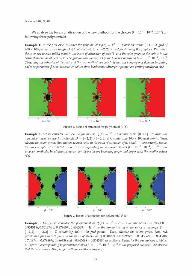
Symmetry 2019, 11, 891

We analyze the basins of attraction of the new method (for the choices β = 10−2, 10−4, 10−8) onfollowing three polynomials:

Example 1. In the first case, consider the polynomial P1(z) = z2 − 1 which has zeros {±1}. A grid of400× 400 points in a rectangle D ∈ C of size [−2, 2]× [−2, 2] is used for drawing the graphics. We assignthe color red to each initial point in the basin of attraction of zero ‘1’ and the color green to the points in thebasin of attraction of zero ‘−1’. The graphics are shown in Figure 1 corresponding to β = 10−2, 10−4, 10−8.Observing the behavior of the basins of the new method, we conclude that the convergence domain becomingwider as parameter β assumes smaller values since black zones (divergent points) are getting smaller in size.

� �

�

β = 10−2� �

�

β = 10−4� �

�

�

β = 10−8

Figure 1. Basins of attraction for polynomial P1(z).

Example 2. Let us consider the next polynomial as P2(z) = z3 − z having zeros {0,±1}. To draw thedynamical view, we select a rectangle D = [−2, 2]× [−2, 2] ∈ C containing 400× 400 grid points. Then,allocate the colors green, blue and red to each point in the basin of attraction of 0, 1 and −1, respectively. Basinsfor this example are exhibited in Figure 2 corresponding to parameter choices β = 10−2, 10−4, 10−8 in theproposed methods. In addition, observe that the basins are becoming larger and larger with the smaller valuesof β.

� �

�

�

β = 10−2� �

�

�

β = 10−4� �

�

�

β = 10−8

Figure 2. Basins of attraction for polynomial P2(z).

Example 3. Lastly, we consider the polynomial as P3(z) = z5 + 2z − 1 having zeros {−0.945068 ±0.854518i, 0.701874 ± 0.879697i, 0.486389}. To draw the dynamical view, we select a rectangle D =

[−2, 2] × [−2, 2] ∈ C containing 400 × 400 grid points. Then, allocate the colors green, blue, red,yellow and pink to each point in the basin of attraction of 0.701874 + 0.879697i, −0.945068− 0.854518i,0.701874− 0.879697i, 0.486389 and−0.945068+ 0.854518i, respectively. Basins for this example are exhibitedin Figure 3 corresponding to parameter choices β = 10−2, 10−4, 10−8 in the proposed methods. We observethat the basins are getting larger with the smaller values of β.

148

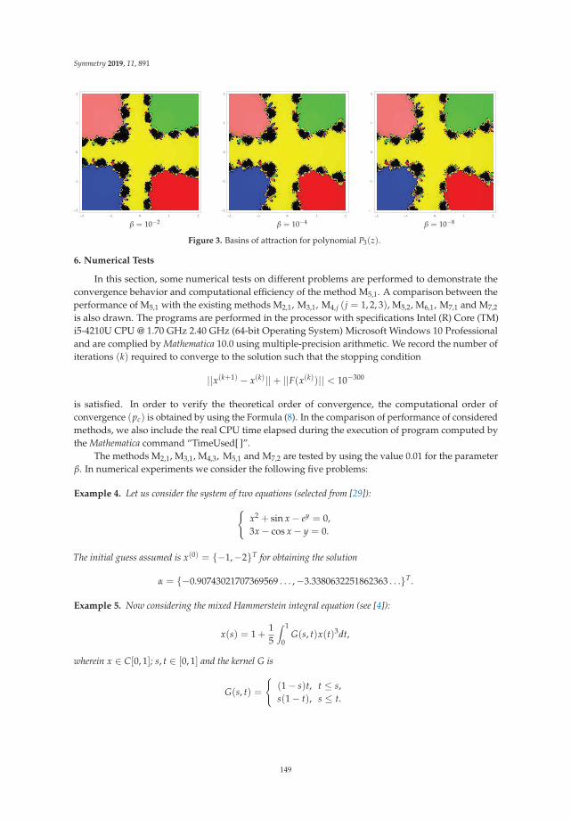
Symmetry 2019, 11, 891

� �

�

�

β = 10−2� �

�

�

β = 10−4� �

�

�

β = 10−8

Figure 3. Basins of attraction for polynomial P3(z).

6. Numerical Tests

In this section, some numerical tests on different problems are performed to demonstrate theconvergence behavior and computational efficiency of the method M5,1. A comparison between theperformance of M5,1 with the existing methods M2,1, M3,1, M4,j (j = 1, 2, 3), M5,2, M6,1, M7,1 and M7,2

is also drawn. The programs are performed in the processor with specifications Intel (R) Core (TM)i5-4210U CPU @ 1.70 GHz 2.40 GHz (64-bit Operating System) Microsoft Windows 10 Professionaland are complied by Mathematica 10.0 using multiple-precision arithmetic. We record the number ofiterations (k) required to converge to the solution such that the stopping condition

||x(k+1) − x(k)||+ ||F(x(k))|| < 10−300

is satisfied. In order to verify the theoretical order of convergence, the computational order ofconvergence (pc) is obtained by using the Formula (8). In the comparison of performance of consideredmethods, we also include the real CPU time elapsed during the execution of program computed bythe Mathematica command “TimeUsed[ ]”.

The methods M2,1, M3,1, M4,3, M5,1 and M7,2 are tested by using the value 0.01 for the parameterβ. In numerical experiments we consider the following five problems:

Example 4. Let us consider the system of two equations (selected from [29]):{x2 + sin x− ey = 0,3x− cos x− y = 0.

The initial guess assumed is x(0) = {−1,−2}T for obtaining the solution

α = {−0.90743021707369569 . . . ,−3.3380632251862363 . . .}T .

Example 5. Now considering the mixed Hammerstein integral equation (see [4]):

x(s) = 1 +15

∫ 1

0G(s, t)x(t)3dt,

wherein x ∈ C[0, 1]; s, t ∈ [0, 1] and the kernel G is

G(s, t) =

{(1− s)t, t ≤ s,s(1− t), s ≤ t.

149

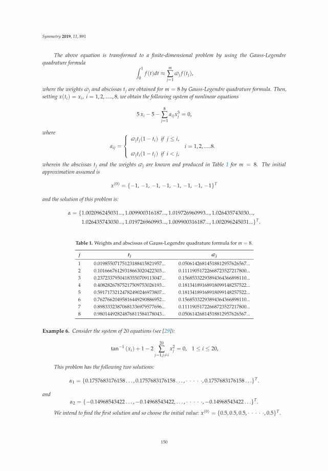
Symmetry 2019, 11, 891

The above equation is transformed to a finite-dimensional problem by using the Gauss-Legendrequadrature formula ∫ 1

0f (t)dt ≈

m

∑j=1

�j f (tj),

where the weights �j and abscissas tj are obtained for m = 8 by Gauss-Legendre quadrature formula. Then,setting x(ti) = xi, i = 1, 2, ....., 8, we obtain the following system of nonlinear equations

5 xi − 5−8

∑j=1

aijx3j = 0,

where

aij =

⎧⎪⎨⎪⎩�jtj(1− ti) if j ≤ i,

i = 1, 2, .....8.�jti(1− tj) if i < j,

wherein the abscissas tj and the weights �j are known and produced in Table 1 for m = 8. The initialapproximation assumed is

x(0) = {−1, −1, −1, −1, −1, −1, −1, −1}T

and the solution of this problem is:

α = {1.002096245031..., 1.009900316187..., 1.019726960993..., 1.026435743030...,

1.026435743030..., 1.019726960993..., 1.009900316187..., 1.002096245031...}T .

Table 1. Weights and abscissas of Gauss-Legendre quadrature formula for m = 8.

j tj �j

1 0.01985507175123188415821957... 0.05061426814518812957626567...2 0.10166676129318663020422303... 0.11119051722668723527217800...3 0.23723379504183550709113047... 0.15685332293894364366898110...4 0.40828267875217509753026193... 0.18134189168918099148257522...5 0.59171732124782490246973807... 0.18134189168918099148257522...6 0.76276620495816449290886952... 0.15685332293894364366898110...7 0.89833323870681336979577696... 0.11119051722668723527217800...8 0.98014492824876811584178043... 0.05061426814518812957626567...

Example 6. Consider the system of 20 equations (see [29]):

tan−1 (xi) + 1− 220

∑j=1,j �=i

x2j = 0, 1 ≤ i ≤ 20,

This problem has the following two solutions:

α1 = {0.1757683176158 . . . , 0.1757683176158 . . . , · · · · ·, 0.1757683176158 . . .}T .

andα2 = {−0.14968543422 . . . ,−0.14968543422, . . . , · · · · ·,−0.14968543422 . . .}T .

We intend to find the first solution and so choose the initial value: x(0) = {0.5, 0.5, 0.5, · · · · ·, 0.5}T.

150

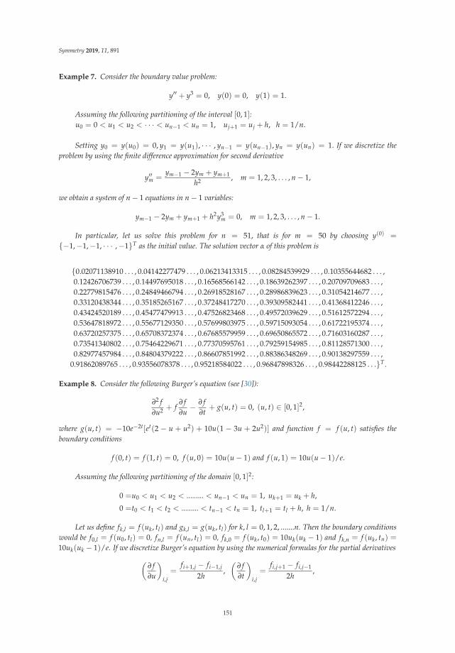
Symmetry 2019, 11, 891

Example 7. Consider the boundary value problem:

y′′ + y3 = 0, y(0) = 0, y(1) = 1.

Assuming the following partitioning of the interval [0, 1]:u0 = 0 < u1 < u2 < · · · < un−1 < un = 1, uj+1 = uj + h, h = 1/n.

Setting y0 = y(u0) = 0, y1 = y(u1), · · · , yn−1 = y(un−1), yn = y(un) = 1. If we discretize theproblem by using the finite difference approximation for second derivative

y′′m =ym−1 − 2ym + ym+1

h2 , m = 1, 2, 3, . . . , n− 1,

we obtain a system of n− 1 equations in n− 1 variables:

ym−1 − 2ym + ym+1 + h2y3m = 0, m = 1, 2, 3, . . . , n− 1.

In particular, let us solve this problem for n = 51, that is for m = 50 by choosing y(0) =

{−1,−1,−1, · · · ,−1}T as the initial value. The solution vector α of this problem is

{0.02071138910 . . . , 0.04142277479 . . . , 0.06213413315 . . . , 0.08284539929 . . . , 0.10355644682 . . . ,0.12426706739 . . . , 0.14497695018 . . . , 0.16568566142 . . . , 0.18639262397 . . . , 0.20709709683 . . . ,0.22779815476 . . . , 0.24849466794 . . . , 0.26918528167 . . . , 0.28986839623 . . . , 0.31054214677 . . . ,0.33120438344 . . . , 0.35185265167 . . . , 0.37248417270 . . . , 0.39309582441 . . . , 0.41368412246 . . . ,0.43424520189 . . . , 0.45477479913 . . . , 0.47526823468 . . . , 0.49572039629 . . . , 0.51612572294 . . . ,0.53647818972 . . . , 0.55677129350 . . . , 0.57699803975 . . . , 0.59715093054 . . . , 0.61722195374 . . . ,0.63720257375 . . . , 0.65708372374 . . . , 0.67685579959 . . . , 0.69650865572 . . . , 0.71603160287 . . . ,0.73541340802 . . . , 0.75464229671 . . . , 0.77370595761 . . . , 0.79259154985 . . . , 0.81128571300 . . . ,0.82977457984 . . . , 0.84804379222 . . . , 0.86607851992 . . . , 0.88386348269 . . . , 0.90138297559 . . . ,

0.91862089765 . . . , 0.93556078378 . . . , 0.95218584022 . . . , 0.96847898326 . . . , 0.98442288125 . . .}T .

Example 8. Consider the following Burger’s equation (see [30]):

∂2 f∂u2 + f

∂ f∂u− ∂ f

∂t+ g(u, t) = 0, (u, t) ∈ [0, 1]2,

where g(u, t) = −10e−2t[et(2 − u + u2) + 10u(1 − 3u + 2u2)] and function f = f (u, t) satisfies theboundary conditions

f (0, t) = f (1, t) = 0, f (u, 0) = 10u(u− 1) and f (u, 1) = 10u(u− 1)/e.

Assuming the following partitioning of the domain [0, 1]2:

0 =u0 < u1 < u2 < ......... < un−1 < un = 1, uk+1 = uk + h,

0 =t0 < t1 < t2 < ......... < tn−1 < tn = 1, tl+1 = tl + h, h = 1/n.

Let us define fk,l = f (uk, tl) and gk,l = g(uk, tl) for k, l = 0, 1, 2, .......n. Then the boundary conditionswould be f0,l = f (u0, tl) = 0, fn,l = f (un, tl) = 0, fk,0 = f (uk, t0) = 10uk(uk − 1) and fk,n = f (uk, tn) =

10uk(uk − 1)/e. If we discretize Burger’s equation by using the numerical formulas for the partial derivatives(∂ f∂u

)i,j=

fi+1,j − fi−1,j

2h,(

∂ f∂t

)i,j=

fi,j+1 − fi,j−1

2h,

151

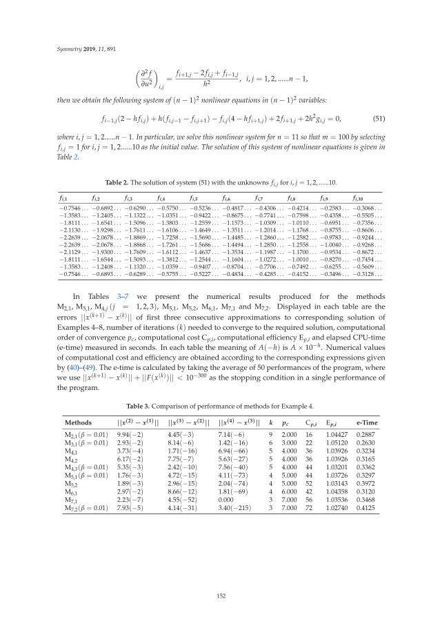
Symmetry 2019, 11, 891

(∂2 f∂u2

)i,j=

fi+1,j − 2 fi,j + fi−1,j

h2 , i, j = 1, 2, ......n− 1,

then we obtain the following system of (n− 1)2 nonlinear equations in (n− 1)2 variables:

fi−1,j(2− h fi,j) + h( fi,j−1 − fi,j+1)− fi,j(4− h fi+1,j) + 2 fi+1,j + 2h2gi,j = 0, (51)

where i, j = 1, 2......n− 1. In particular, we solve this nonlinear system for n = 11 so that m = 100 by selectingfi,j = 1 for i, j = 1, 2......10 as the initial value. The solution of this system of nonlinear equations is given inTable 2.

Table 2. The solution of system (51) with the unknowns fi,j for i, j = 1, 2, ......10.

fi,1 fi,2 fi,3 fi,4 fi,5 fi,6 fi,7 fi,8 fi,9 fi,10

−0.7546 . . . −0.6892 . . . −0.6290 . . . −0.5750 . . . −0.5236 . . . −0.4817 . . . −0.4306 . . . −0.4214 . . . −0.2583 . . . −0.3068 . . .−1.3583 . . . −1.2405 . . . −1.1322 . . . −1.0351 . . . −0.9422 . . . −0.8675 . . . −0.7741 . . . −0.7598 . . . −0.4358 . . . −0.5505 . . .−1.8111 . . . −1.6541 . . . −1.5096 . . . −1.3803 . . . −1.2559 . . . −1.1573 . . . −1.0309 . . . −1.0110 . . . −0.6951 . . . −0.7356 . . .−2.1130 . . . −1.9298 . . . −1.7611 . . . −1.6106 . . . −1.4649 . . . −1.3511 . . . −1.2014 . . . −1.1768 . . . −0.8755 . . . −0.8606 . . .−2.2639 . . . −2.0678 . . . −1.8869 . . . −1.7258 . . . −1.5690 . . . −1.4485 . . . −1.2860 . . . −1.2582 . . . −0.9783 . . . −0.9244 . . .−2.2639 . . . −2.0678 . . . −1.8868 . . . −1.7261 . . . −1.5686 . . . −1.4494 . . . −1.2850 . . . −1.2558 . . . −1.0040 . . . −0.9268 . . .−2.1129 . . . −1.9300 . . . −1.7609 . . . −1.6112 . . . −1.4637 . . . −1.3534 . . . −1.1987 . . . −1.1700 . . . −0.9534 . . . −0.8672 . . .−1.8111 . . . −1.6544 . . . −1.5093 . . . −1.3812 . . . −1.2544 . . . −1.1604 . . . −1.0272 . . . −1.0010 . . . −0.8270 . . . −0.7454 . . .−1.3583 . . . −1.2408 . . . −1.1320 . . . −1.0359 . . . −0.9407 . . . −0.8704 . . . −0.7706 . . . −0.7492 . . . −0.6255 . . . −0.5609 . . .−0.7546 . . . −0.6893 . . . −0.6289 . . . −0.5755 . . . −0.5227 . . . −0.4834 . . . −0.4285 . . . −0.4152 . . . −0.3496 . . . −0.3128 . . .

In Tables 3–7 we present the numerical results produced for the methodsM2,1, M3,1, M4,j (j = 1, 2, 3), M5,1, M5,2, M6,1, M7,1 and M7,2. Displayed in each table are theerrors ||x(k+1) − x(k)|| of first three consecutive approximations to corresponding solution ofExamples 4–8, number of iterations (k) needed to converge to the required solution, computationalorder of convergence pc, computational cost Cp,i, computational efficiency Ep,i and elapsed CPU-time(e-time) measured in seconds. In each table the meaning of A(−h) is A× 10−h. Numerical valuesof computational cost and efficiency are obtained according to the corresponding expressions givenby (40)–(49). The e-time is calculated by taking the average of 50 performances of the program, wherewe use ||x(k+1) − x(k)||+ ||F(x(k))|| < 10−300 as the stopping condition in a single performance ofthe program.

Table 3. Comparison of performance of methods for Example 4.

Methods ||x(2) − x(1)|| ||x(3) − x(2)|| ||x(4) − x(3)|| k pc Cp,i Ep,i e-Time

M2,1(β = 0.01) 9.94(−2) 4.45(−3) 7.14(−6) 9 2.000 16 1.04427 0.2887M3,1(β = 0.01) 2.93(−2) 8.14(−6) 1.42(−16) 6 3.000 22 1.05120 0.2630M4,1 3.73(−4) 1.71(−16) 6.94(−66) 5 4.000 36 1.03926 0.3234M4,2 6.17(−2) 7.75(−7) 5.63(−27) 5 4.000 36 1.03926 0.3165M4,3(β = 0.01) 5.35(−3) 2.42(−10) 7.56(−40) 5 4.000 44 1.03201 0.3362M5,1(β = 0.01) 1.76(−3) 4.72(−15) 4.11(−73) 4 5.000 44 1.03726 0.3297M5,2 1.89(−3) 2.96(−15) 2.04(−74) 4 5.000 52 1.03143 0.3972M6,1 2.97(−2) 8.66(−12) 1.81(−69) 4 6.000 42 1.04358 0.3120M7,1 2.23(−7) 4.55(−52) 0.000 3 7.000 56 1.03536 0.3468M7,2(β = 0.01) 7.93(−5) 4.14(−31) 3.40(−215) 3 7.000 72 1.02740 0.4125

152

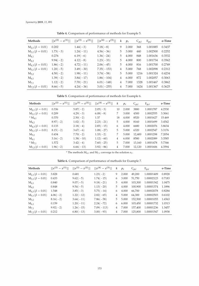
Symmetry 2019, 11, 891

Table 4. Comparison of performance of methods for Example 5.

Methods ||x(2) − x(1)|| ||x(3) − x(2)|| ||x(4) − x(3)|| k pc Cp,i Ep,i e-Time

M2,1(β = 0.01) 0.202 1.44(−3) 7.18(−8) 9 2.000 368 1.001885 0.3437M3,1(β = 0.01) 1.73(−3) 1.24(−11) 4.56(−36) 5 3.000 440 1.002500 0.2252M4,1 0.276 6.19(−6) 1.36(−24) 5 4.000 848 1.001636 0.3532M4,2 9.94(−2) 4.12(−8) 1.23(−33) 5 4.000 800 1.001734 0.3562M4,3(β = 0.01) 1.86(−2) 4.72(−11) 2.06(−45) 5 4.000 816 1.001700 0.2749M5,1(β = 0.01) 1.20(−5) 3.49(−30) 7.35(−153) 4 5.000 768 1.002098 0.2312M5,2 4.50(−2) 1.98(−11) 3.74(−58) 5 5.000 1216 1.001324 0.4234M6,1 1.39(−2) 3.84(−17) 1.86(−104) 4 6.000 872 1.002057 0.3063M7,1 1.12(−2) 7.70(−21) 6.01(−148) 4 7.000 1328 1.001467 0.3862M7,2(β = 0.01) 8.66(−5) 4.24(−36) 3.01(−255) 4 7.000 1424 1.001367 0.3625

Table 5. Comparison of performance of methods for Example 6.

Methods ||x(2) − x(1)|| ||x(3) − x(2)|| ||x(4) − x(3)|| k pc Cp,i Ep,i e-Time

M2,1(β = 0.01) 0.336 5.87(−2) 2.05(−3) 10 2.000 3880 1.0001787 4.2530M3,1(β = 0.01) 0.209 4.29(−3) 6.08(−8) 7 3.000 4300 1.0002555 3.3061* M4,1 0.370 2.50(−2) 1.37 18 4.000 8520 1.0001627 15.469M4,2 8.97(−2) 1.02(−5) 2.23(−21) 5 4.000 8160 1.0001699 3.4542M4,3(β = 0.01) 0.133 2.18(−4) 2.85(−15) 6 4.000 6680 1.0002076 3.8634M5,1(β = 0.01) 8.15(−2) 3.67(−6) 1.08(−27) 5 5.000 6320 1.0002547 3.3176M5,2 0.434 7.70(−2) 1.33(−2) 7 5.000 12,400 1.0001298 7.2054M6,1 3.16(−2) 1.38(−10) 1.12(−60) 4 6.000 8580 1.0002089 3.3585* M7,1 1.572 3.42(−4) 7.60(−25) 5 7.000 13,160 1.0001478 5.7346M7,2(β = 0.01) 1.96(−2) 6.66(−13) 3.92(−86) 4 7.000 12,120 1.0001606 4.3594

* The methods M4,1 and M7,1 converge to the solution α2.

Table 6. Comparison of performance of methods for Example 7.

Methods ||x(2) − x(1)|| ||x(3) − x(2)|| ||x(4) − x(3)|| k pc Cp,i Ep,i e-Time

M2,1(β = 0.01) 3.828 0.681 1.23(−2) 9 2.000 49,200 1.00001409 0.8928M3,1(β = 0.01) 0.433 9.62(−5) 1.74(−15) 6 3.000 51,750 1.00002123 0.7183M4,1 0.840 9.07(−5) 9.18(−21) 5 4.000 103,300 1.00001342 1.0475M4,2 0.848 9.54(−5) 1.13(−20) 5 4.000 100,900 1.00001374 1.1896M4,3(β = 0.01) 1.548 3.85(−3) 5.75(−14) 6 4.000 66,700 1.00002078 0.8284M5,1(β = 0.01) 4.06(−2) 1.22(−12) 2.82(−65) 4 5.000 64,300 1.00002503 0.6102M5,2 8.16(−2) 3.64(−11) 7.86(−58) 5 5.000 152,500 1.00001055 1.6563M6,1 0.159 1.20(−11) 2.24(−72) 6 6.000 103,450 1.00001732 1.0313M7,1 9.92(−2) 1.26(−15) 7.09(−113) 4 7.000 157,400 1.00001236 1.3457M7,2(β = 0.01) 0.212 6.80(−13) 3.00(−93) 4 7.000 125,800 1.00001547 1.0938

153

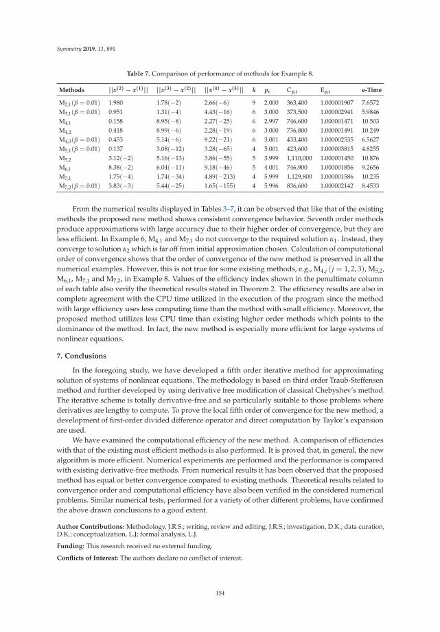
Symmetry 2019, 11, 891

Table 7. Comparison of performance of methods for Example 8.

Methods ||x(2) − x(1)|| ||x(3) − x(2)|| ||x(4) − x(3)|| k pc Cp,i Ep,i e-Time

M2,1(β = 0.01) 1.980 1.78(−2) 2.66(−6) 9 2.000 363,400 1.000001907 7.6572M3,1(β = 0.01) 0.951 1.31(−4) 4.43(−16) 6 3.000 373,500 1.000002941 5.9846M4,1 0.158 8.95(−8) 2.27(−25) 6 2.997 746,600 1.000001471 10.503M4,2 0.418 8.99(−6) 2.28(−19) 6 3.000 736,800 1.000001491 10.249M4,3(β = 0.01) 0.453 5.14(−6) 9.22(−21) 6 3.001 433,400 1.000002535 6.5627M5,1(β = 0.01) 0.137 3.08(−12) 3.28(−65) 4 5.001 423,600 1.000003815 4.8255M5,2 3.12(−2) 5.16(−13) 3.86(−55) 5 3.999 1,110,000 1.000001450 10.876M6,1 8.38(−2) 6.04(−11) 9.18(−46) 5 4.001 746,900 1.000001856 9.2656M7,1 1.75(−4) 1.74(−34) 4.89(−213) 4 5.999 1,129,800 1.000001586 10.235M7,2(β = 0.01) 3.83(−3) 5.44(−25) 1.65(−155) 4 5.996 836,600 1.000002142 8.4533

From the numerical results displayed in Tables 3–7, it can be observed that like that of the existingmethods the proposed new method shows consistent convergence behavior. Seventh order methodsproduce approximations with large accuracy due to their higher order of convergence, but they areless efficient. In Example 6, M4,1 and M7,1 do not converge to the required solution α1. Instead, theyconverge to solution α2 which is far off from initial approximation chosen. Calculation of computationalorder of convergence shows that the order of convergence of the new method is preserved in all thenumerical examples. However, this is not true for some existing methods, e.g., M4,j (j = 1, 2, 3), M5,2,M6,1, M7,1 and M7,2, in Example 8. Values of the efficiency index shown in the penultimate columnof each table also verify the theoretical results stated in Theorem 2. The efficiency results are also incomplete agreement with the CPU time utilized in the execution of the program since the methodwith large efficiency uses less computing time than the method with small efficiency. Moreover, theproposed method utilizes less CPU time than existing higher order methods which points to thedominance of the method. In fact, the new method is especially more efficient for large systems ofnonlinear equations.

7. Conclusions

In the foregoing study, we have developed a fifth order iterative method for approximatingsolution of systems of nonlinear equations. The methodology is based on third order Traub-Steffensenmethod and further developed by using derivative free modification of classical Chebyshev’s method.The iterative scheme is totally derivative-free and so particularly suitable to those problems wherederivatives are lengthy to compute. To prove the local fifth order of convergence for the new method, adevelopment of first-order divided difference operator and direct computation by Taylor’s expansionare used.

We have examined the computational efficiency of the new method. A comparison of efficiencieswith that of the existing most efficient methods is also performed. It is proved that, in general, the newalgorithm is more efficient. Numerical experiments are performed and the performance is comparedwith existing derivative-free methods. From numerical results it has been observed that the proposedmethod has equal or better convergence compared to existing methods. Theoretical results related toconvergence order and computational efficiency have also been verified in the considered numericalproblems. Similar numerical tests, performed for a variety of other different problems, have confirmedthe above drawn conclusions to a good extent.

Author Contributions: Methodology, J.R.S.; writing, review and editing, J.R.S.; investigation, D.K.; data curation,D.K.; conceptualization, L.J; formal analysis, L.J.

Funding: This research received no external funding.

Conflicts of Interest: The authors declare no conflict of interest.

154

Symmetry 2019, 11, 891

References

1. Argyros, I.K. Quadratic equations and applications to Chandrasekhar’s and related equations. Bull. Aust.Math. Soc. 1985, 32, 275–292. [CrossRef]

2. Kelley, C.T. Iterative Methods for Linear and Nonlinear Equations; SIAM: Philadelphia, PA, USA, 1995.3. Ostrowski, A.M. Solution of Equations and Systems of Equations; Academic Press: New York, NY, USA, 1960.4. Ortega, J.M.; Rheinboldt, W.C. Iterative Solution of Nonlinear Equations in Several Variables; Academic Press:

New York, NY, USA, 1970.5. Potra, F.-A.; Pták, V. Nondiscrete Induction and Iterarive Processes; Pitman Publishing: Boston, MA, USA, 1984.6. Traub, J.F. Iterative Methods for the Solution of Equations; Prentice-Hall: Englewood Cliffs, NJ, USA, 1964.7. Ezquerro, J.A.; Hernández, M.A. An optimization of Chebyshev’s method. J. Complex. 2009, 25, 343–361.

[CrossRef]8. Argyros, I.K.; Ezquerro, J.A.; Gutiérrez, J.M.; Hernández, M.A.; Hilout, S. On the semilocal convergence of

efficient Chebyshev-Secant-type methods. J. Comput. Appl. Math. 2011, 235, 3195–3206. [CrossRef]9. Argyros, I.K.; Ren, H. Efficient Steffensen-type algorithms for solving nonlinear equations. Int. J.

Comput. Math. 2013, 90, 691–704. [CrossRef]10. Steffensen, J.F. Remarks on iteration. Skand. Aktuar Tidskr. 1933, 16, 64–72. [CrossRef]11. Ren, H.; Wu, Q.; Bi, W. A class of two-step Steffensen type methods with fourth-order convergence.

Appl. Math. Comput. 2009, 209, 206–210. [CrossRef]12. Zheng, Q.; Zhao, P.; Huang, F. A family of fourth-order Steffensen-type methods with the applications on

solving nonlinear ODEs. Appl. Math. Comput. 2011, 217, 8196–8203. [CrossRef]13. Grau-Sánchez, M.; Noguera, M.; Amat, S. On the approximation of derivatives using divided difference

operators preserving the local convergence order of iterative methods. J. Comput. Appl. Math. 2013,237, 363–372. [CrossRef]

14. Sharma, J.R.; Arora, H. An efficient derivative free iterative method for solving systems of nonlinearequations. Appl. Anal. Discrete Math. 2013, 7, 390–403. [CrossRef]

15. Sharma, J.R.; Arora, H. A novel derivative free algorithm with seventh order convergence for solving systemsof nonlinear equations. Numer. Algorithms 2014, 67, 917–933. [CrossRef]

16. Wang, X.; Zhang, T. A family of Steffensen type methods with seventh-order convergence. Numer. Algorithms2013, 62, 429–444. [CrossRef]

17. Sharma, J.R.; Arora, H. Efficient higher order derivative-free multipoint methods with and without memoryfor systems of nonlinear equations. Int. J. Comput. Math. 2018, 95, 920–938. [CrossRef]

18. Ahmad, F.; Soleymani, F.; Haghani, F.K.; Serra-Capizzano, S. Higher order derivative-free iterative methodswith and without memory for systems of nonlinear equations. Appl. Math. Comput. 2017, 314, 199–211.[CrossRef]

19. Cordero, A.; Torregrosa, J.R. Variants of Newton’s method for functions of several variables.Appl. Math. Comput. 2006, 183, 199–208. [CrossRef]

20. Genocchi, A. Relation entre la différence et la dérivée d’un même ordre quelconque. Arch. Math. Phys. I1869, 49, 342–345.

21. Cordero, A.; Hueso, J.L.; Martínez, E.; Torregrosa, J.R. A modified Newton-Jarratt’s composition.Numer. Algorithms 2010, 55, 87–99. [CrossRef]

22. Lotfi, T.; Bakhtiari, P.; Cordero, A.; Mahdiani, K.; Torregrosa, J.R. Some new efficient multipoint iterativemethods for solving nonlinear systems of equations. Int. J. Comput. Math. 2015, 92, 1921–1934. [CrossRef]

23. Krasnoselsky, M.A.; Vainikko, G.M.; Zabreiko, P.P.; Rutitskii, J.B.; Stetsenko, V. J. Approximate Solution ofOperator Equations; Nauka: Moscow, Russia, 1969. (In Russian)

24. Madhu, K.; Babajee, D.K.R.; Jayaraman, J. An improvement to double-step Newton method and its multi-stepversion for solving system of nonlinear equations and its applications. Numer. Algorithms 2017, 74, 593–607.[CrossRef]

25. Kumar, M.; Singh, A.K.; Srivastava, A. A new fifth order derivative free Newton-type method for solvingnonlinear equations. Appl. Math. Inf. Sci. 2015, 9, 1507–1513.

26. Vrscay, E.R.; Gilbert, W.J. Extraneous fixed points, basin boundaries and chaotic dynamics for Schröder andKönig rational iteration functions. Numer. Math. 1988, 52, 1–16. [CrossRef]

155

Symmetry 2019, 11, 891

27. Varona, J.L. Graphic and numerical comparison between iterative methods. Math. Intell. 2002, 24, 37–46.[CrossRef]

28. Scott, M.; Neta, B.; Chun, C. Basin attractors for various methods. Appl. Math. Comput. 2011, 218, 2584–2599.[CrossRef]

29. Xiao, X.Y.; Yin, H.W. Increasing the order of convergence for iterative methods to solve nonlinear systems.Calcolo 2016, 53, 285–300. [CrossRef]

30. Sauer, T. Numerical Analysis, 2nd ed.; Pearson Education, Inc.: Boston, MA, USA, 2012.

c© 2019 by the authors. Licensee MDPI, Basel, Switzerland. This article is an open accessarticle distributed under the terms and conditions of the Creative Commons Attribution(CC BY) license (http://creativecommons.org/licenses/by/4.0/).

156

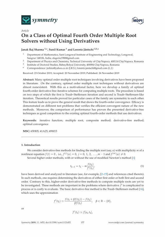
symmetryS SArticle

On a Class of Optimal Fourth Order Multiple RootSolvers without Using Derivatives

Janak Raj Sharma 1,*, Sunil Kumar 1 and Lorentz Jäntschi 2,3,*

1 Department of Mathematics, Sant Longowal Institute of Engineering and Technology, Longowal,Sangrur 148106, India; sfageria1988@gmail.com

2 Department of Physics and Chemistry, Technical University of Cluj-Napoca, 400114 Cluj-Napoca, Romania3 Institute of Doctoral Studies, Babes-Bolyai University, 400084 Cluj-Napoca, Romania* Correspondence: jrshira@yahoo.co.in (J.R.S.); lorentz.jantschi@gmail.com (L.J.)

Received: 23 October 2019; Accepted: 20 November 2019; Published: 26 November 2019

Abstract: Many optimal order multiple root techniques involving derivatives have been proposedin literature. On the contrary, optimal order multiple root techniques without derivatives arealmost nonexistent. With this as a motivational factor, here we develop a family of optimalfourth-order derivative-free iterative schemes for computing multiple roots. The procedure is basedon two steps of which the first is Traub–Steffensen iteration and second is Traub–Steffensen-likeiteration. Theoretical results proved for particular cases of the family are symmetric to each other.This feature leads us to prove the general result that shows the fourth-order convergence. Efficacy isdemonstrated on different test problems that verifies the efficient convergent nature of the newmethods. Moreover, the comparison of performance has proven the presented derivative-freetechniques as good competitors to the existing optimal fourth-order methods that use derivatives.

Keywords: iterative function; multiple root; composite method; derivative-free method;optimal convergence

MSC: 65H05; 41A25; 49M15

1. Introduction

We consider derivative-free methods for finding the multiple root (say, α) with multiplicity m of anonlinear equation f (t) = 0 , i.e., f (j)(α) = 0, j = 0, 1, 2, . . . , m− 1 and f (m)(α) �= 0.

Several higher order methods, with or without the use of modified Newton’s method [1]

tk+1 = tk −mf (tk)

f ′(tk), (1)

have been derived and analyzed in literature (see, for example, [2–15] and references cited therein).In such methods, one requires determining the derivatives of either first order or both first and secondorder. Contrary to this, higher-order derivative-free methods to compute multiple roots are yet tobe investigated. These methods are important in the problems where derivative f ′ is complicated toprocess or is costly to evaluate. The basic derivative-free method is the Traub–Steffensen method [16],which uses the approximation

f ′(tk) "f (tk + β f (tk))− f (tk)

β f (tk), β ∈ R− {0},

orf ′(tk) " f [sk, tk],

Symmetry 2019, 11, 1452; doi:10.3390/sym11121452 www.mdpi.com/journal/symmetry157

Symmetry 2019, 11, 1452

for the derivative f ′ in the classical Newton method in Equation (1). Here, sk = tk + β f (tk) andf [s, t] = f (s)− f (t)

s−t is a divided difference of first order. In this way, the modified Newton method inEquation (1) transforms to the modified Traub–Steffensen derivative free method

tk+1 = tk −mf (tk)

f [sk, tk]. (2)

The modified Traub–Steffensen method in Equation (2) is a noticeable improvement over theNewton method, because it preserves the convergence of order two without using any derivative.

In this work, we aim to design derivative-free multiple root methods of high efficient quality,i.e., the methods of higher convergence order that use the computations as small as we please.Proceeding in this way, we introduce a class of derivative-free fourth-order methods that requirethree new pieces of information of the function f per iteration, and hence possess optimal fourth-orderconvergence in the terminology of Kung–Traub conjecture [17]. This conjecture states that multi-pointiterative functions without memory based on n function evaluations may attain the convergence order2n−1, which is maximum. The methods achieving this convergence order are usually called optimalmethods. The new iterative scheme uses the modified Traub–Steffensen iteration in Equation (2)in the first step and Traub–Steffensen-like iteration in the second step. The methods are examinednumerically on many practical problems of different kind. The comparison of performance withexisting techniques requiring derivative evaluations verifies the efficient character of the new methodsin terms of accuracy and executed CPU time.

The rest of the paper is summarized as follows. In Section 2, the scheme of fourth-order methodis proposed and its convergence order is studied for particular cases. The main result for the generalcase is studied in Section 3. Numerical tests to demonstrate applicability and efficiency of the methodsare presented in Section 4. In this section, a comparison of performance with already establishedmethods is also shown. In Section 5, a conclusion of the main points is drawn.

2. Formulation of Method

To compute a multiple root with multiplicity m ≥ 1, consider the following two-stepiterative scheme:

zk = tk −mf (tk)

f [sk, tk],

tk+1 = zk − H(xk, yk)f (tk)

f [sk, tk], (3)

where xk =m

√f (zk)f (tk)

, yk =m

√f (zk)f (sk)

and H : C2 → C is analytic in a neighborhood of (0, 0). Notice that

this is a two-step scheme with first step as the Traub–Steffensen iteration in Equation (2) and the nextstep as the Traub–Steffensen-like iteration. The second step is weighted by the factor H(x, y), thus wecan call it weight factor or more appropriately weight function.

In the sequel, we study the convergence results of proposed iterative scheme in Equation (3).For clarity, the results are obtained separately for different cases based on the multiplicity m. Firstly,for the case m = 1, the following theorem is proved:

Theorem 1. Assume that f : C→ C is an analytic function in a domain containing a multiple zero (say, α)with multiplicity m = 1. Suppose that the initial point t0 is close enough to α, then the convergence order ofEquation (3) is at least 4, provided that H00 = 0, H10 = 1, H01 = 0, H20 = 2, H11 = 11 and H02 = 0, whereHij =

∂i+j

∂xi∂yj H(xk, yk)|(xk=0,yk=0), for 0 ≤ i, j ≤ 2.

158

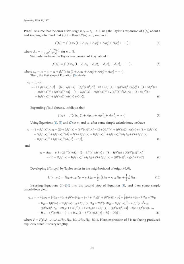
Symmetry 2019, 11, 1452

Proof. Assume that the error at kth stage is ek = tk − α. Using the Taylor’s expansion of f (tk) about α

and keeping into mind that f (α) = 0 and f ′(α) �= 0, we have

f (tk) = f ′(α)ek(1 + A1ek + A2e2

k + A3e3k + A4e4

k + · · ·), (4)

where An = 1(1+n)!

f (1+n)(α)f ′(α) for n ∈ N.

Similarly we have the Taylor’s expansion of f (sk) about α

f (sk) = f ′(α)esk

(1 + A1esk + A2e2

sk+ A3e3

sk+ A4e4

sk+ · · ·

), (5)

where esk = sk − α = ek + β f ′(α)ek(1 + A1ek + A2e2

k + A3e3k + A4e4

k + · · ·).

Then, the first step of Equation (3) yields

ezk = zk − α

= (1 + β f ′(α))A1e2k −

((2 + 2β f ′(α) + (β f ′(α))2)A2

1 − (2 + 3β f ′(α) + (β f ′(α))2)A2)e3

k +((4 + 5β f ′(α)

+ 3(β f ′(α))2 + (β f ′(α))3)A31 − (7 + 10β f ′(α) + 7(β f ′(α))2 + 2(β f ′(α))3)A1 A2 + (3 + 6β f ′(α)

+ 4(β f ′(α))2 + (β f ′(α))3)A3)e4

k + O(e5k). (6)

Expanding f (zk) about α, it follows that

f (zk) = f ′(α)ezk

(1 + A1ezk + A2e2

zk+ A3e3

zk+ · · ·

). (7)

Using Equations (4), (5) and (7) in xk and yk, after some simple calculations, we have

xk = (1 + β f ′(α))A1ek −((3 + 3β f ′(α) + (β f ′(α))2)A2

1 − (2 + 3β f ′(α) + (β f ′(α))2)A2)e2

k +((8 + 10β f ′(α)

+ 5(β f ′(α))2 + (β f ′(α))3)A31 − 2(5 + 7β f ′(α) + 4(β f ′(α))2 + (β f ′(α))3)A1 A2 + (3 + 6β f ′(α)

+ 4(β f ′(α))2 + (β f ′(α))3)A3)e3

k + O(e4k) (8)

and

yk = A1ek −((3 + 2β f ′(α))A2

1 − (2 + β f ′(α))

A2)e2k +

((8 + 8β f ′(α) + 3(β f ′(α))2)A3

1

− (10 + 11β f ′(α) + 4(β f ′(α))2)A1 A2 + (3 + 3β f ′(α) + (β f ′(α))2)A3)e3

k + O(e4k). (9)

Developing H(xk, yk) by Taylor series in the neighborhood of origin (0, 0),

H(xk, yk) ≈ H00 + xk H10 + yk H01 +12

x2k H20 + xkyk H11 +

12

y2k H02. (10)

Inserting Equations (4)–(10) into the second step of Equation (3), and then some simplecalculations yield

ek+1 = − H00 ek +(

H00 − H01 + β f ′(α)H00 − (−1 + H10)(1 + β f ′(α)))

A1e2k −

12((4 + H02 − 8H10 + 2H11

+ H20 + 4β f ′(α)− 10β f ′(α)H10 + 2β f ′(α)H11 + 2β f ′(α)H20 + 2(β f ′(α))2 − 4(β f ′(α))2H10

+ (β f ′(α))2H20 − 2H01(4 + 3β f ′(α)) + 2H00(2 + 2β f ′(α) + (β f ′(α))2))A21 − 2(2 + β f ′(α))(H00

− H01 + β f ′(α)H00 − (−1 + H10)(1 + β f ′(α)))A2)e3

k + δe4k + O(e5

k), (11)

where δ = δ(β, A1, A2, A3, H00, H10, H01, H20, H11, H02). Here, expression of δ is not being producedexplicitly since it is very lengthy.

159

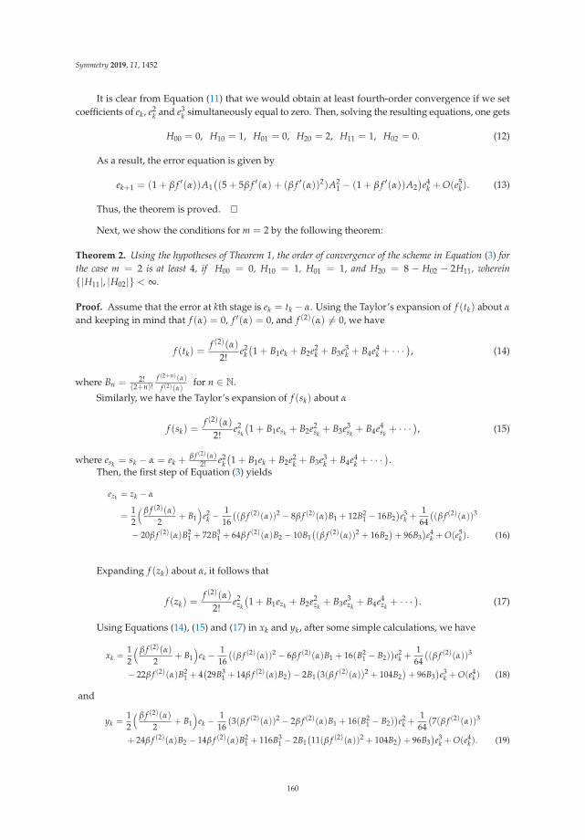
Symmetry 2019, 11, 1452

It is clear from Equation (11) that we would obtain at least fourth-order convergence if we setcoefficients of ek, e2

k and e3k simultaneously equal to zero. Then, solving the resulting equations, one gets

H00 = 0, H10 = 1, H01 = 0, H20 = 2, H11 = 1, H02 = 0. (12)

As a result, the error equation is given by

ek+1 = (1 + β f ′(α))A1((5 + 5β f ′(α) + (β f ′(α))2)A2

1 − (1 + β f ′(α))A2)e4

k + O(e5k). (13)

Thus, the theorem is proved.

Next, we show the conditions for m = 2 by the following theorem:

Theorem 2. Using the hypotheses of Theorem 1, the order of convergence of the scheme in Equation (3) forthe case m = 2 is at least 4, if H00 = 0, H10 = 1, H01 = 1, and H20 = 8 − H02 − 2H11, wherein{|H11|, |H02|} < ∞.

Proof. Assume that the error at kth stage is ek = tk − α. Using the Taylor’s expansion of f (tk) about α

and keeping in mind that f (α) = 0, f ′(α) = 0, and f (2)(α) �= 0, we have

f (tk) =f (2)(α)

2!e2

k(1 + B1ek + B2e2

k + B3e3k + B4e4

k + · · ·), (14)

where Bn = 2!(2+n)!

f (2+n)(α)

f (2)(α)for n ∈ N.

Similarly, we have the Taylor’s expansion of f (sk) about α

f (sk) =f (2)(α)

2!e2

sk

(1 + B1esk + B2e2

sk+ B3e3

sk+ B4e4

sk+ · · ·

), (15)

where esk = sk − α = ek +β f (2)(α)

2! e2k(1 + B1ek + B2e2

k + B3e3k + B4e4

k + · · ·).

Then, the first step of Equation (3) yields

ezk = zk − α

=12

( β f (2)(α)2

+ B1

)e2

k −1

16((β f (2)(α))2 − 8β f (2)(α)B1 + 12B2

1 − 16B2)e3

k +164((β f (2)(α))3

− 20β f (2)(α)B21 + 72B3

1 + 64β f (2)(α)B2 − 10B1((β f (2)(α))2 + 16B2

)+ 96B3

)e4

k + O(e5k). (16)

Expanding f (zk) about α, it follows that

f (zk) =f (2)(α)

2!e2

zk

(1 + B1ezk + B2e2

zk+ B3e3

zk+ B4e4

zk+ · · ·

). (17)

Using Equations (14), (15) and (17) in xk and yk, after some simple calculations, we have

xk =12

( β f (2)(α)2

+ B1

)ek −

116((β f (2)(α))2 − 6β f (2)(α)B1 + 16(B2

1 − B2))e2

k +164((β f (2)(α))3

− 22β f (2)(α)B21 + 4

(29B3

1 + 14β f (2)(α)B2)− 2B1

(3(β f (2)(α))2 + 104B2

)+ 96B3

)e3

k + O(e4k) (18)

and

yk =12

( β f (2)(α)2

+ B1

)ek −

116(3(β f (2)(α))2 − 2β f (2)(α)B1 + 16(B2

1 − B2))e2

k +164(7(β f (2)(α))3

+ 24β f (2)(α)B2 − 14β f (2)(α)B21 + 116B3

1 − 2B1(11(β f (2)(α))2 + 104B2

)+ 96B3

)e3

k + O(e4k). (19)

160

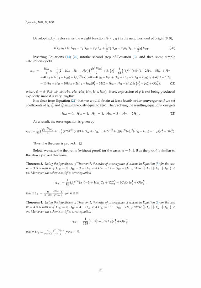
Symmetry 2019, 11, 1452

Developing by Taylor series the weight function H(xk, yk) in the neighborhood of origin (0, 0),

H(xk, yk) ≈ H00 + xk H10 + yk H01 +12

x2k H20 + xkyk H11 +

12

y2k H02. (20)

Inserting Equations (14)–(20) intothe second step of Equation (3), and then some simplecalculations yield

ek+1 = − H002

ek +14(2 + H00 − H01 − H10

)( β f (2)(α)2

+ B1

)e2

k −1

64

((β f (2)(α))2(4 + 2H00 − 8H01 + H02

− 4H10 + 2H11 + H20) + 4β f (2)(α)(−8− 4H00 − H01 + H02 + H10 + 2H11 + H20)B1 + 4(12 + 6H00

− 10H01 + H02 − 10H10 + 2H11 + H20)B21 − 32(2 + H00 − H01 − H10)B2

)e3

k + φ e4k + O(e5

k), (21)

where φ = φ(β, B1, B2, B3, H00, H10, H01, H20, H11, H02). Here, expression of φ is not being producedexplicitly since it is very lengthy.

It is clear from Equation (21) that we would obtain at least fourth-order convergence if we setcoefficients of ek, e2

k and e3k simultaneously equal to zero. Then, solving the resulting equations, one gets

H00 = 0, H10 = 1, H01 = 1, H20 = 8− H02 − 2H11. (22)

As a result, the error equation is given by

ek+1 =1

32

( β f (2)(α)2

+ B1

)((2β f (2)(α)(3 + H02 + H11)B1 + 22B2

1 + ((β f (2)(α))2(H02 + H11)− 8B2))e4

k + O(e5k).

Thus, the theorem is proved.

Below, we state the theorems (without proof) for the cases m = 3, 4, 5 as the proof is similar tothe above proved theorems.

Theorem 3. Using the hypotheses of Theorem 1, the order of convergence of scheme in Equation (3) for the casem = 3 is at least 4, if H00 = 0, H10 = 3− H01, and H20 = 12− H02 − 2H11, where {|H01|, |H02|, |H11|} <∞. Moreover, the scheme satisfies error equation

ek+1 =154(

β f (3)(α)(−3 + H01)C1 + 12C31 − 6C1C2

)e4

k + O(e5k),

where Cn = 3!(3+n)!

f (3+n)(α)

f (3)(α)for n ∈ N.

Theorem 4. Using the hypotheses of Theorem 1, the order of convergence of scheme in Equation (3) for the casem = 4 is at least 4, if H00 = 0, H10 = 4− H01, and H20 = 16− H02 − 2H11, where {|H01|, |H02|, |H11|} <∞. Moreover, the scheme satisfies error equation

ek+1 =1

128(13D3

1 − 8D1D2)e4

k + O(e5k),

where Dn = 4!(4+n)!

f (4+n)(α)

f (4)(α)for n ∈ N.

161

Symmetry 2019, 11, 1452

Theorem 5. Using the hypotheses of Theorem 1, the order of convergence of scheme in Equation (3) for the casem = 5 is at least 4, if H00 = 0, H10 = 5− H01, and H20 = 20− H02 − 2H11, where {|H01|, |H02|, |H11|} <∞. Moreover, the scheme satisfies error equation

ek+1 =1

125(7E3

1 − 5E1E2)e4

k + O(e5k),

where En = 5!(5+n)!

f (5+n)(α)

f (5)(α)for n ∈ N.

Remark 1. We can observe from the above results that the number of conditions on Hij is 6, 4, 3, 3, 3corresponding to cases m = 1, 2, 3, 4, 5 to attain the fourth-order convergence of the method in Equation (3).The cases m = 3, 4, 5 satisfy the common conditions, H00 = 0, H10 = m−H01, and H20 = 4m−H02− 2H11.Nevertheless, their error equations differ from each other as the parameter β does not appear in the equations form = 4, 5. It has been seen that when m ≥ 4 the conditions on Hij are always three in number and the errorequation in each such case does not contain β term. This type of symmetry in the results helps us to prove thegeneral result, which is presented in next section.

3. Main Result

For the multiplicity m ≥ 4, we prove the order of convergence of the scheme in Equation (3) bythe following theorem:

Theorem 6. Assume that the function f : C → C is an analytic in a domain containing zero α havingmultiplicity m ≥ 4. Further, suppose that the initial estimation t0 is close enough to α. Then, the convergenceof the iteration scheme in Equation (3) is of order four, provided that H00 = 0, H10 = m− H01, and H20 =

4m− H02 − 2H11, wherein {|H01|, |H11|, |H02|} < ∞. Moreover, the error in the scheme is given by

ek+1 =1

2m3

((9 + m)K3

1 − 2mK1K2)e4

k + O(e5k).

Proof. Taking into account that f (j)(α) = 0, j = 0, 1, 2, . . . , m− 1 and f m(α) �= 0, then, developingf (tk) about α in the Taylor’s series,

f (tk) =f m(α)

m!em

k(1 + K1ek + K2e2

k + K3e3k + K4e4

k + · · ·), (23)

where Kn = m!(m+n)!

f (m+n)(α)

f (m)(α)for n ∈ N.

In addition, from the expansion of f (sk) about α, it follows that

f (sk) =f m(α)

m!em

sk

(1 + K1esk + K2e2

sk+ K3e3

sk+ K4e4

sk+ · · ·

), (24)

where esk = sk − α = ek +β f m(α)

m! emk(1 + K1ek + K2e2

k + K3e3k + K4e4

k + · · ·). From the first step of

Equation (3),

ezk = zk − α

=K1m

e2k +

1m2

(2mK2 − (1 + m)K2

1)e3

k +1

m3

((1 + m)2K3

1 −m(4 + 3m)K1K2 + 3m2K3)e4

k + O(e5k). (25)

Expansion of f (zk) around α yields

f (zk) =f m(α)

m!e2

zk

(1 + K1ezk + K2e2

zk+ K3e3

zk+ K4e4

zk+ · · ·

). (26)

162

Symmetry 2019, 11, 1452

Using Equations (23), (24) and (26) in the expressions of xk and yk, we have that

xk =K1m

ek +1

m2

(2mK2 − (2 + m)K2

1)e2

k +1

2m3

((7 + 7m + 2m2)K3

1 − 2m(7 + 3m)K1K2 + 6m2K3)e3

k +O(e4k) (27)

and

yk =K1m

ek +1

m2

(mK2 − (2 + m)K2

1)e2

k +1

2m3

((6 + 7m + 2m2)K3

1 − 2m(6 + 3m)K1K2 + 6m2K3)e3

k + O(e4k). (28)

Developing H(xk, yk) in Taylor’s series in the neighborhood of origin (0, 0),

H(xk, yk) ≈ H00 + xk H10 + yk H01 +12

x2k H20 + xkyk H11 +

12

y2k H02. (29)

Inserting Equations (23)–(29) into the second step of Equation (3), it follows that

ek+1 =− H00m

ek +1

m2 (H00 − H01 − H10 + m)K1e2k −

12m3

((H02 − 6H10 + 2H11 + H20 + 2m− 2mH10 + 2m2

+ 2(1 + m)H00 − 2(3 + m)H01)K21 − 4m(H00 − H01 − H10 + m)K2

)e3

k +1

2m4

((5H02 − 13H10 + 10H11

+ 5H20 + 2m + 2mH02 − 11mH10 + 4mH11 + 2mH20 + 4m2 − 2m2H10 + 2m3 + 2(1 + m)2H00

− (13 + 11m + 2m2)H01)K31 − 2m(2H02 − 11H10 + 4H11 + 2H20 + 4m− 3mH10 + 3m2 + (4 + 3m)H00

− (11 + 3m)H01)K1K2 + 6m2(H00 − H01 − H10 + m)K3)e4

k + O(e5k). (30)

It is clear that we can obtain at least fourth-order convergence if the coefficients of ek, e2k , and e3

kvanish. On solving the resulting equations, we get

H00 = 0, H10 = m− H01, H20 = 4m− H02 − 2 H11. (31)

Then, error of Equation (30) is given by

ek+1 =1

2m3

((9 + m)K3

1 − 2mK1K2)e4

k + O(e5k). (32)

Thus, the theorem is proved.

Remark 2. The proposed scheme in Equation (3) reaches fourth-order convergence provided that the conditionsof Theorems 1–3 and 6 are satisfied. This convergence rate is achieved by using only three function evaluations,viz. f (tn), f (sn), and f (zn), per iteration. Therefore, the scheme in Equation (3) is optimal by the Kung–Traubhypothesis [17].

Remark 3. It is important to note that parameter β, which is used in sk, appears only in the error equations of thecases m = 1, 2, 3 but not for m ≥ 4. For m ≥ 4, we have observed that this parameter appears in the coefficientsof e5

k and higher order. However, we do not need such terms to show the required fourth-order convergence.

Some Special Cases

We can generate many iterative schemes as the special cases of the family in Equation (3) basedon the forms of function H(x, y) that satisfy the conditions of Theorems 1, 2 and 6. However, werestrict ourselves to the choices of low-degree polynomials or simple rational functions. These choicesshould be such that the resulting methods may converge to the root with order four for m ≥ 1.Accordingly, the following simple forms are considered:

163

Symmetry 2019, 11, 1452

(1) Let us choose the function

H(xk, yk) = xk + m x2k + (m− 1)yk + m xk yk,

which satisfies the conditions of Theorems 1, 2 and 6. Then, the corresponding fourth-orderiterative scheme is given by

tk+1 = zk −(xk + m x2

k + (m− 1)yk + m xk yk) f (tk)

f [sk, tk]. (33)

(2) Next, consider the rational function

H(xk, yk) = −xk + m x2

k − (m− 1)yk(m yk − 1)m yk − 1

,

satisfying the conditions of Theorems 1, 2 and 6. Then, corresponding fourth-order iterativescheme is given by

tk+1 = zk +xk + m x2

k − (m− 1)yk(m yk − 1)m yk − 1

f (tk)

f [sk, tk]. (34)

(3) Consider another rational function satisfying the conditions of Theorems 1, 2 and 6, which isgiven by

H(xk, yk) =xk − yk + m yk + 2m xk yk −m2 xk yk

1−m xk + x2k

.

The corresponding fourth-order iterative scheme is given by

tk+1 = zk −xk − yk + m yk + 2m xk yk −m2 xk yk

1−m xk + x2k

f (tk)

f [sk, tk]. (35)

For each of the above cases, zk = tk −m f (tk)f [sk ,tk ]

. For future reference, the proposed methods inEquations (33)–(35) are denoted by NM1, NM2, and NM3, respectively.

4. Numerical Results

To validate the theoretical results proven in previous sections, the special cases NM1, NM2,and NM3 of new family were tested numerically by implementing them on some nonlinear equations.Moreover, their comparison was also performed with some existing optimal fourth-order methods thatuse derivatives in the formulas. We considered, for example, the methods by Li et al. [7,8], Sharma andSharma [9], Zhou et al. [10], Soleymani et al. [12], and Kansal et al. [14]. The methods are expressedas follows:

Li–Liao–Cheng method (LLC):

zk = tk −2m

m + 2f (tk)

f ′(tk),

tk+1 = tk −m(m− 2)

( mm+2

)−m f ′(zk)−m2 f ′(tk)

f ′(tk)−( m

m+2)−m f ′(zk)

f (tk)

2 f ′(tk).

164

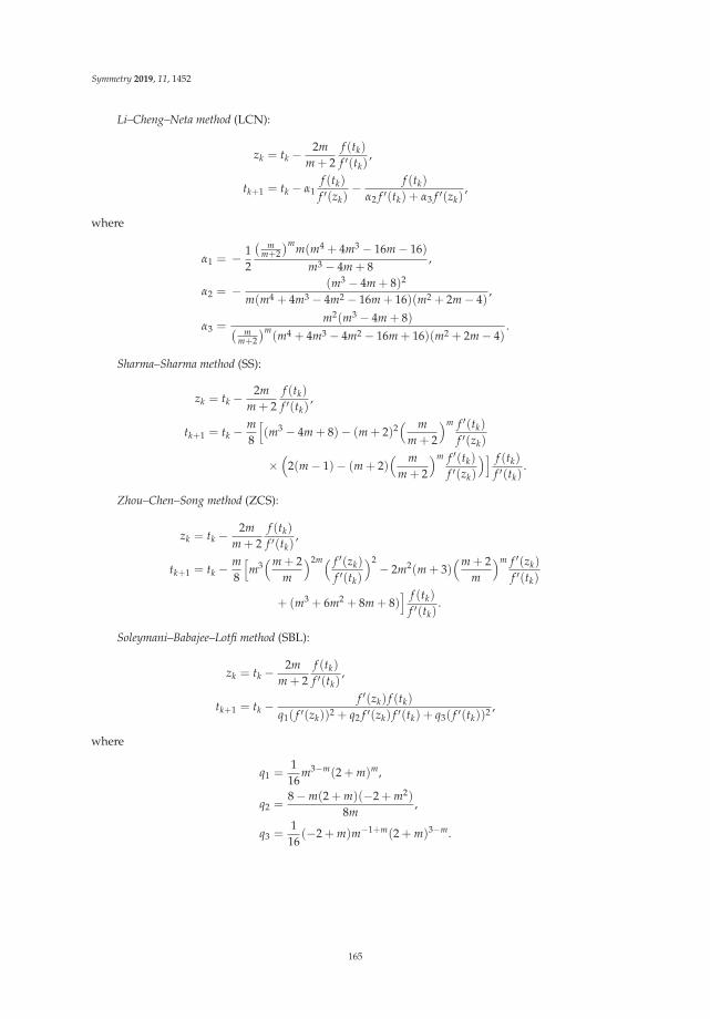
Symmetry 2019, 11, 1452

Li–Cheng–Neta method (LCN):

zk = tk −2m

m + 2f (tk)

f ′(tk),

tk+1 = tk − α1f (tk)

f ′(zk)− f (tk)

α2 f ′(tk) + α3 f ′(zk),

where

α1 = − 12

( mm+2

)mm(m4 + 4m3 − 16m− 16)m3 − 4m + 8

,

α2 = − (m3 − 4m + 8)2

m(m4 + 4m3 − 4m2 − 16m + 16)(m2 + 2m− 4),

α3 =m2(m3 − 4m + 8)( m

m+2)m

(m4 + 4m3 − 4m2 − 16m + 16)(m2 + 2m− 4).

Sharma–Sharma method (SS):

zk = tk −2m

m + 2f (tk)

f ′(tk),

tk+1 = tk −m8

[(m3 − 4m + 8)− (m + 2)2

( mm + 2

)m f ′(tk)

f ′(zk)

×(

2(m− 1)− (m + 2)( m

m + 2

)m f ′(tk)

f ′(zk)

)] f (tk)

f ′(tk).

Zhou–Chen–Song method (ZCS):

zk = tk −2m

m + 2f (tk)

f ′(tk),

tk+1 = tk −m8

[m3(m + 2

m

)2m( f ′(zk)

f ′(tk)

)2− 2m2(m + 3)

(m + 2m

)m f ′(zk)

f ′(tk)

+ (m3 + 6m2 + 8m + 8)] f (tk)

f ′(tk).

Soleymani–Babajee–Lotfi method (SBL):

zk = tk −2m

m + 2f (tk)

f ′(tk),

tk+1 = tk −f ′(zk) f (tk)

q1( f ′(zk))2 + q2 f ′(zk) f ′(tk) + q3( f ′(tk))2 ,

where

q1 =116

m3−m(2 + m)m,

q2 =8−m(2 + m)(−2 + m2)

8m,

q3 =116

(−2 + m)m−1+m(2 + m)3−m.

165

Symmetry 2019, 11, 1452

Kansal–Kanwar–Bhatia method (KKB):

zk = tk −2m

m + 2f (tk)

f ′(tk),

tk+1 = tk −m4

f (tk)

(1 +

m4 p−2m(− f ′(zk)

f ′(tk)+ p−1+m

)2(−1 + pm)

8(2pm + m(−1 + pm))

)

×(4− 2m + m2(−1 + p−m)

f ′(tk)− p−m(2pm + m(−1 + pm))2

f ′(tk)− f ′(zk)

),

where p = mm+2 .

Computational work was compiled in the programming package of Mathematica software [18] ina PC with Intel(R) Pentium(R) CPU B960 @ 2.20 GHz, 2.20 GHz (32-bit Operating System) MicrosoftWindows 7 Professional and 4 GB RAM. Performance of the new methods was tested by choosingvalue of the parameter β = 0.01. The tabulated results obtained by the methods for each probleminclude: (a) the number of iterations (k) required to obtain the solution using the stopping criterion|tk+1 − tk| + | f (tk)| < 10−100; (b) the estimated error |tk+1 − tk| in the first three iterations; (c) thecalculated convergence order (CCO); and (d) the elapsed time (CPU time in seconds) in execution of aprogram, which was measured by the command “TimeUsed[ ]”. The calculated convergence order(CCO) to confirm the theoretical convergence order was calculated by the formula (see [19])

CCO =log |(tk+2 − α)/(tk+1 − α)|

log |(tk+1 − α)/(tk − α)| , for each k = 1, 2, . . . (36)

The following numerical examples were chosen for experimentation:

Example 1. Planck law of radiation to calculate the energy density in an isothermal black body [20] is stated as

φ(λ) =8πchλ−5

ech/λkT − 1. (37)

where λ is wavelength of the radiation, c is speed of light, T is absolute temperature of the black body, k isBoltzmann’s constant, and h is Planck’s constant. The problem is to determine the wavelength λ correspondingto maximum energy density φ(λ). Thus, Equation (37) leads to

φ′(λ) =( 8πchλ−6

ech/λkT − 1

)( (ch/λkT)ech/λkT

ech/λkT − 1− 5

)= A.B. (say)

Note that a maxima for φ will occur when B = 0, that is when

(ch/λkT)ech/λkT

ech/λkT − 1= 5.

Setting t = ch/λkT, the above equation assumes the form

1− t5= e−t. (38)

Define

f1(t) = e−t − 1 +t5

. (39)

The root t = 0 is trivial and thus is not taken for discussion. Observe that for t = 5 the left-hand side ofEquation (38) is zero and the right-hand side is e−5 ≈ 6.74× 10−3. Thus, we guess that another root might occur

166

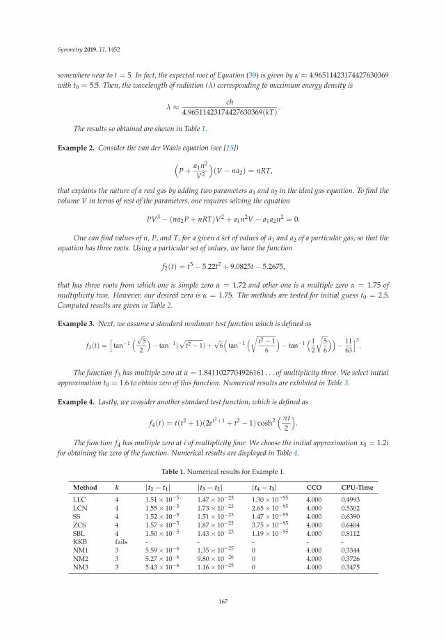
Symmetry 2019, 11, 1452

somewhere near to t = 5. In fact, the expected root of Equation (39) is given by α ≈ 4.96511423174427630369with t0 = 5.5. Then, the wavelength of radiation (λ) corresponding to maximum energy density is

λ ≈ ch4.96511423174427630369(kT)

.

The results so obtained are shown in Table 1.

Example 2. Consider the van der Waals equation (see [15])

(P +

a1n2

V2

)(V − na2) = nRT,

that explains the nature of a real gas by adding two parameters a1 and a2 in the ideal gas equation. To find thevolume V in terms of rest of the parameters, one requires solving the equation

PV3 − (na2P + nRT)V2 + a1n2V − a1a2n2 = 0.

One can find values of n, P, and T, for a given a set of values of a1 and a2 of a particular gas, so that theequation has three roots. Using a particular set of values, we have the function

f2(t) = t3 − 5.22t2 + 9.0825t− 5.2675,

that has three roots from which one is simple zero α = 1.72 and other one is a multiple zero α = 1.75 ofmultiplicity two. However, our desired zero is α = 1.75. The methods are tested for initial guess t0 = 2.5.Computed results are given in Table 2.

Example 3. Next, we assume a standard nonlinear test function which is defined as

f3(t) =[

tan−1(√5

2

)− tan−1(

√t2 − 1) +

√6(

tan−1(√ t2 − 1

6

)− tan−1

(12

√56

))− 11

63

]3.

The function f3 has multiple zero at α = 1.8411027704926161 . . . of multiplicity three. We select initialapproximation t0 = 1.6 to obtain zero of this function. Numerical results are exhibited in Table 3.

Example 4. Lastly, we consider another standard test function, which is defined as

f4(t) = t(t2 + 1)(2et2+1 + t2 − 1) cosh2(πt

2

).

The function f4 has multiple zero at i of multiplicity four. We choose the initial approximation x0 = 1.2ifor obtaining the zero of the function. Numerical results are displayed in Table 4.

Table 1. Numerical results for Example 1.

Method k |t2 − t1| |t3 − t2| |t4 − t3| CCO CPU-Time

LLC 4 1.51× 10−5 1.47× 10−23 1.30× 10−95 4.000 0.4993LCN 4 1.55× 10−5 1.73× 10−23 2.65× 10−95 4.000 0.5302SS 4 1.52× 10−5 1.51× 10−23 1.47× 10−95 4.000 0.6390ZCS 4 1.57× 10−5 1.87× 10−23 3.75× 10−95 4.000 0.6404SBL 4 1.50× 10−5 1.43× 10−23 1.19× 10−95 4.000 0.8112KKB fails - - - - -NM1 3 5.59× 10−6 1.35× 10−25 0 4.000 0.3344NM2 3 5.27× 10−6 9.80× 10−26 0 4.000 0.3726NM3 3 5.43× 10−6 1.16× 10−25 0 4.000 0.3475

167

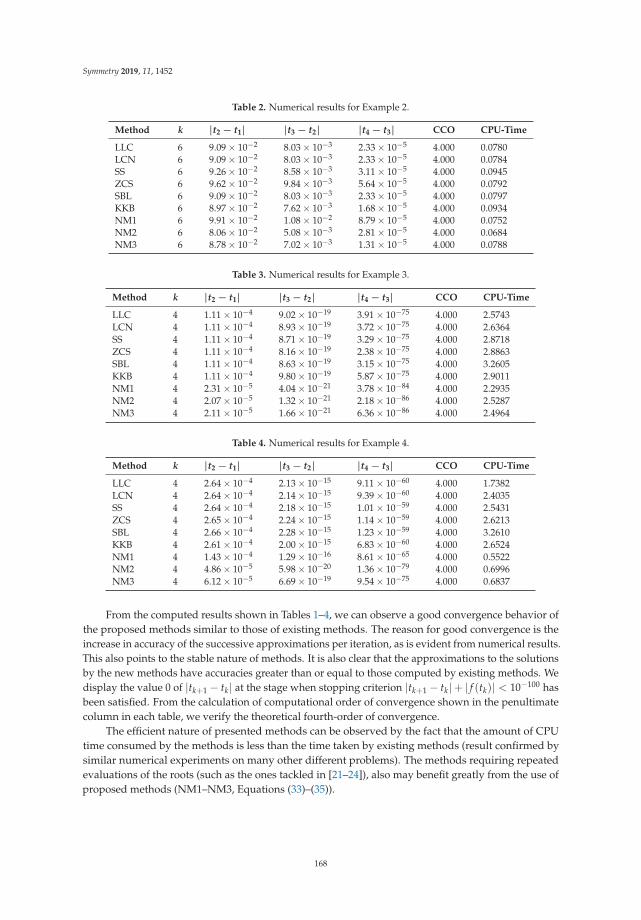
Symmetry 2019, 11, 1452

Table 2. Numerical results for Example 2.

Method k |t2 − t1| |t3 − t2| |t4 − t3| CCO CPU-Time

LLC 6 9.09× 10−2 8.03× 10−3 2.33× 10−5 4.000 0.0780LCN 6 9.09× 10−2 8.03× 10−3 2.33× 10−5 4.000 0.0784SS 6 9.26× 10−2 8.58× 10−3 3.11× 10−5 4.000 0.0945ZCS 6 9.62× 10−2 9.84× 10−3 5.64× 10−5 4.000 0.0792SBL 6 9.09× 10−2 8.03× 10−3 2.33× 10−5 4.000 0.0797KKB 6 8.97× 10−2 7.62× 10−3 1.68× 10−5 4.000 0.0934NM1 6 9.91× 10−2 1.08× 10−2 8.79× 10−5 4.000 0.0752NM2 6 8.06× 10−2 5.08× 10−3 2.81× 10−5 4.000 0.0684NM3 6 8.78× 10−2 7.02× 10−3 1.31× 10−5 4.000 0.0788

Table 3. Numerical results for Example 3.

Method k |t2 − t1| |t3 − t2| |t4 − t3| CCO CPU-Time

LLC 4 1.11× 10−4 9.02× 10−19 3.91× 10−75 4.000 2.5743LCN 4 1.11× 10−4 8.93× 10−19 3.72× 10−75 4.000 2.6364SS 4 1.11× 10−4 8.71× 10−19 3.29× 10−75 4.000 2.8718ZCS 4 1.11× 10−4 8.16× 10−19 2.38× 10−75 4.000 2.8863SBL 4 1.11× 10−4 8.63× 10−19 3.15× 10−75 4.000 3.2605KKB 4 1.11× 10−4 9.80× 10−19 5.87× 10−75 4.000 2.9011NM1 4 2.31× 10−5 4.04× 10−21 3.78× 10−84 4.000 2.2935NM2 4 2.07× 10−5 1.32× 10−21 2.18× 10−86 4.000 2.5287NM3 4 2.11× 10−5 1.66× 10−21 6.36× 10−86 4.000 2.4964

Table 4. Numerical results for Example 4.

Method k |t2 − t1| |t3 − t2| |t4 − t3| CCO CPU-Time

LLC 4 2.64× 10−4 2.13× 10−15 9.11× 10−60 4.000 1.7382LCN 4 2.64× 10−4 2.14× 10−15 9.39× 10−60 4.000 2.4035SS 4 2.64× 10−4 2.18× 10−15 1.01× 10−59 4.000 2.5431ZCS 4 2.65× 10−4 2.24× 10−15 1.14× 10−59 4.000 2.6213SBL 4 2.66× 10−4 2.28× 10−15 1.23× 10−59 4.000 3.2610KKB 4 2.61× 10−4 2.00× 10−15 6.83× 10−60 4.000 2.6524NM1 4 1.43× 10−4 1.29× 10−16 8.61× 10−65 4.000 0.5522NM2 4 4.86× 10−5 5.98× 10−20 1.36× 10−79 4.000 0.6996NM3 4 6.12× 10−5 6.69× 10−19 9.54× 10−75 4.000 0.6837

From the computed results shown in Tables 1–4, we can observe a good convergence behavior ofthe proposed methods similar to those of existing methods. The reason for good convergence is theincrease in accuracy of the successive approximations per iteration, as is evident from numerical results.This also points to the stable nature of methods. It is also clear that the approximations to the solutionsby the new methods have accuracies greater than or equal to those computed by existing methods. Wedisplay the value 0 of |tk+1 − tk| at the stage when stopping criterion |tk+1 − tk|+ | f (tk)| < 10−100 hasbeen satisfied. From the calculation of computational order of convergence shown in the penultimatecolumn in each table, we verify the theoretical fourth-order of convergence.

The efficient nature of presented methods can be observed by the fact that the amount of CPUtime consumed by the methods is less than the time taken by existing methods (result confirmed bysimilar numerical experiments on many other different problems). The methods requiring repeatedevaluations of the roots (such as the ones tackled in [21–24]), also may benefit greatly from the use ofproposed methods (NM1–NM3, Equations (33)–(35)).

168

Symmetry 2019, 11, 1452

5. Conclusions

In this paper, we propose a family of fourth-order derivative-free numerical methods for obtainingmultiple roots of nonlinear equations. Analysis of the convergence was carried out, which proved theorder four under standard assumptions of the function whose zeros we are looking for. In addition,our designed scheme also satisfies the Kung–Traub hypothesis of optimal order of convergence.Some special cases are established. These are employed to solve nonlinear equations including thosearising in practical problems. The new methods are compared with existing techniques of sameorder. Testing of the numerical results shows that the presented derivative-free methods are goodcompetitors to the existing optimal fourth-order techniques that require derivative evaluations in thealgorithm. We conclude the work with a remark that derivative-free methods are good alternatives toNewton-type schemes in the cases when derivatives are expensive to compute or difficult to obtain.

Author Contributions: Methodology, J.R.S.; writing, review and editing, J.R.S.; investigation, S.K.; data curation,S.K.; conceptualization, L.J.; formal analysis, L.J.

Funding: This research received no external funding.

Conflicts of Interest: The authors declare no conflict of interest.

References

1. Schröder, E. Über unendlich viele Algorithmen zur Auflösung der Gleichungen. Math. Ann. 1870, 2, 317–365.[CrossRef]

2. Hansen E.; Patrick, M. A family of root finding methods. Numer. Math. 1977, 27, 257–269. [CrossRef]3. Victory, H.D.; Neta, B. A higher order method for multiple zeros of nonlinear functions. Int. J. Comput. Math.

1983, 12, 329–335. [CrossRef]4. Dong, C. A family of multipoint iterative functions for finding multiple roots of equations. Int. J.

Comput. Math. 1987, 21, 363–367. [CrossRef]5. Osada, N. An optimal multiple root-finding method of order three. J. Comput. Appl. Math. 1994, 51, 131–133.

[CrossRef]6. Neta, B. New third order nonlinear solvers for multiple roots. App. Math. Comput. 2008, 202, 162–170.

[CrossRef]7. Li, S.; Liao, X.; Cheng, L. A new fourth-order iterative method for finding multiple roots of nonlinear

equations. Appl. Math. Comput. 2009, 215, 1288–1292.8. Li, S.G.; Cheng, L.Z.; Neta, B. Some fourth-order nonlinear solvers with closed formulae for multiple roots.

Comput Math. Appl. 2010, 59, 126–135. [CrossRef]9. Sharma, J.R.; Sharma, R. Modified Jarratt method for computing multiple roots. Appl. Math. Comput.

2010, 217, 878–881. [CrossRef]10. Zhou, X.; Chen, X.; Song, Y. Constructing higher-order methods for obtaining the multiple roots of nonlinear

equations. J. Comput. Appl. Math. 2011, 235, 4199–4206. [CrossRef]11. Sharifi, M.; Babajee, D.K.R.; Soleymani, F. Finding the solution of nonlinear equations by a class of optimal

methods. Comput. Math. Appl. 2012, 63, 764–774. [CrossRef]12. Soleymani, F.; Babajee, D.K.R.; Lotfi, T. On a numerical technique for finding multiple zeros and its dynamics.

J. Egypt. Math. Soc. 2013, 21, 346–353. [CrossRef]13. Geum, Y.H.; Kim Y.I.; Neta, B. A class of two-point sixth-order multiple-zero finders of modified

double-Newton type and their dynamics. Appl. Math. Comput. 2015, 270, 387–400. [CrossRef]14. Kansal, M.; Kanwar, V.; Bhatia, S. On some optimal multiple root-finding methods and their dynamics.

Appl. Appl. Math. 2015, 10, 349–367.15. Behl, R.; Zafar, F.; Alshormani, A.S.; Junjua, M.U.D.; Yasmin, N. An optimal eighth-order scheme for multiple

zeros of unvariate functions. Int. J. Comput. Meth. 2019, 16, 1843002. [CrossRef]16. Traub, J.F. Iterative Methods for the Solution of Equations; Chelsea Publishing Company: New York, NY,

USA, 1982.17. Kung, H.T.; Traub, J.F. Optimal order of one-point and multipoint iteration. J. Assoc. Comput. Mach. 1974,

21, 643–651. [CrossRef]

169

Symmetry 2019, 11, 1452

18. Wolfram, S. The Mathematica Book, 5th ed.; Wolfram Media: Bengaluru, India, 2003.19. Weerakoon, S.; Fernando, T.G.I. A variant of Newton’s method with accelerated third-order convergence.

Appl. Math. Lett. 2000, 13, 87–93. [CrossRef]20. Bradie, B. A Friendly Introduction to Numerical Analysis; Pearson Education Inc.: New Delhi, India, 2006.21. Jäntschi L.; Bolboaca S.D. Conformational study of C24 cyclic polyyne clusters. Int. J. Quantum Chem.

2018, 118, e25614. [CrossRef]22. Azad H.; Anaya K.; Al-Dweik A. Y.; Mustafa M. T. Invariant solutions of the wave equation on static

spherically symmetric spacetimes admitting G7 isometry algebra. Symmetry 2018, 10, 665. [CrossRef]23. Matko, V.; Brezovec, B. Improved data center energy efficiency and availability with multilayer node event

processing. Energies 2018, 11, 2478. [CrossRef]24. Jäntschi L. The eigenproblem translated for alignment of molecules. Symmetry 2019, 11, 1027. [CrossRef]

c© 2019 by the authors. Licensee MDPI, Basel, Switzerland. This article is an open accessarticle distributed under the terms and conditions of the Creative Commons Attribution(CC BY) license (http://creativecommons.org/licenses/by/4.0/).

170

symmetryS SArticle

Facility Location Problem Approach forDistributed Drones

Jared Lynskey, Kyi Thar, Thant Zin Oo and Choong Seon Hong *

Department of Computer Science and Engineering, Kyung Hee University, Yongin-si, Gyeonggi-do 17104,Korea; jared@khu.ac.kr (J.L.); kyithar@khu.ac.kr (K.T.); tzoo@khu.ac.kr (T.Z.O.)* Correspondence: cshong@khu.ac.kr

Received: 2 January 2019; Accepted: 15 January 2019; Published: 20 January 2019

Abstract: Currently, industry and academia are undergoing an evolution in developing the nextgeneration of drone applications. Including the development of autonomous drones that can carryout tasks without the assistance of a human operator. In spite of this, there are still problems leftunanswered related to the placement of drone take-off, landing and charging areas. Future policies bygovernments and aviation agencies are inevitably going to restrict the operational area where dronescan take-off and land. Hence, there is a need to develop a system to manage landing and take-offareas for drones. Additionally, we proposed this approach due to the lack of justification for theinitial location of drones in current research. Therefore, to provide a foundation for future research,we give a justified reason that allows predetermined location of drones with the use of drone ports.Furthermore, we propose an algorithm to optimally place these drone ports to minimize the averagedistance drones must travel based on a set of potential drone port locations and tasks generatedin a given area. Our approach is derived from the Facility Location problem which produces anefficient near optimal solution to place drone ports that reduces the overall drone energy consumption.Secondly, we apply various traveling salesman algorithms to determine the shortest route the dronemust travel to visit all the tasks.

Keywords: drone deployment; drone port; traveling salesman; facility location problem

1. Introduction

Recent reports from the Federal Aviation Agency state that there will be an increase from 2.75 to4.47 million small drones operating in the United States by 2021. Since the end of May 2017, more than772,000 owners have already registered with the Federal Aviation Administration (FAA) [1]. The mainreason for the sudden increase in drone ownership is due to consumers purchasing drones for theirhigh mobility and applications in the field of computer vision [2]. Thus, a shift in vision related jobs(building inspection, traffic monitoring and temporary cellular coverage extension) slowly being takenover by drones to perform these tasks. This is because drones can provide the required perspectivefor jobs such as bird’s eye view. Additionally, by using machines to take pictures in hazardous areas,we can minimize the risk to human safety. However, there is still no proposal on the initial deploymentof drones which do not include random placement. Furthermore, the cost of privately owning dronescan be far too expensive for companies who may only require drones for a single task, in comparisonto renting drones [3]. In the case of a rental system, companies and users are not required to purchase adrone allowing the cost to be fairly distributed amongst them. Although the cost to rent can reduce theoverall cost when compared to owning a drone. Typically, users must visit a rental center to collect thedrone. Otherwise, the drone must fly from the shop to the task, reducing the total energy available forcompleting tasks. Therefore, to overcome these foreseen issues, an unmanned drone rental service that

Symmetry 2019, 11, 118; doi:10.3390/sym11010118 www.mdpi.com/journal/symmetry171

Symmetry 2019, 11, 118

utilizes drones placed at distributed drone ports is necessary. By providing a public service that allowsthe rental of distributed autonomous drones waiting at drone ports, this can reduce the total numberof drones in the sky and the total cost of utilizing drones to complete tasks requested by the user.Thus, we propose an algorithm that can be applied to a shared drone service to reduce the excessiveutilization to increase the efficiency by intelligently placing drone ports in respect to the demand andlimitations of drones.

1.1. Motivation for Distributed Drone Ports

In this paper, we assume that drones will return to the drone port and charge after each cycle sincethere are already companies creating landing pads, including Skysense (San Francisco, CA, USA) [4].We imagine that drones must land, take off and be stored at the base of the drone port to charge droneswhile they are not completing tasks in the air to remove the risk of users being injured by rotatingblades and electrical components that charge the drone. Multiple charging pads can be distributedover an area to reduce the average distance drones must travel to recharge. By doing so, we believethe cost of operating a fleet of drones located at distributed drone ports will be less than the cost ofoperating a central drone port because miniature drones don’t require a large drone and can be locatedfrom small areas such as building tops to open fields closer to tasks. Finally, the introduction of droneports will give future research a foundation to justify their initial placement of drones.

1.2. Related Work

This section encompasses the work done by researchers who look at the problem of optimallyplacing drones in the sky. However, from our research, we noticed that none of their work justified thereason for the initial and final location of drones in their work. Thus, we proposed an idea to justifyfurther work’s reasoning of the initial and final location of drones. The authors in paper [5] propose adiscrete and continuous environment to determine the location of drones based on the users. However,they fail to consider where these drones will begin and end their mission. Related work in the field ofdeploying drones to provide coverage has been growing in interest. In Ref. [6], authors proposed anoptimal transport approach to minimize the energy consumption to gather data from moving clustersof IoT (Internet of Things) devices. Works related to a rental system outline the challenges of providingenough assets to satisfy the number of users in the area.

1.3. Challenges

One challenge faced with proposing a rental system is the finite number of combinations possiblebetween the number of drone ports, the location of drone ports and the association between tasks anddrones located at drone ports. Thus, we require an efficient mixed integer problem approach to solveour facility location framework. To complement our facility location framework, we apply a subfieldof machine learning, clustering, to quickly identify the most efficient central points as drone ports.

Using the original facility location framework to solve the problem is a complex procedure that doesnot guarantee an optimal solution because it only considers the average distance between the drone portsand facilities. We also need to find the round-trip path to ensure that the drone can complete all the tasksin its cluster.

Drones come in a variety of classes as outlined in Table 1. However, previous research shows,among the available class of drones, the outlook looks the most promising for mini drones. This is dueto the fact that mini drones are expected to reach a level of autonomous control within the next fiveyears that meets FAA requirements. Despite the current legal roadblocks imposed by the FAA, there islikely still going to be an increasing demand for mini drones in civilian. Mostly due to their small sizecompared with larger drones, mini drones have a much greater intrinsic safety rating [7]. Furthermore,the reason for choosing mini drones to complete tasks is due to their high mobility and much lowercost compared with larger drones. Academics are already working to implement vision systems toallow drones to land [8].

172

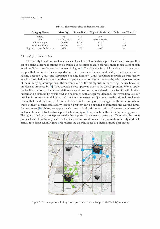
Symmetry 2019, 11, 118

Table 1. The various class of drones available.

Category Name Mass [kg] Range [km] Flight Altitude [m] Endurance [Hours]

Micro <5 <10 250 1Mini <20/30/150 <10 150/250/300 <2

Close Range 25–150 10–30 3000 2–4Medium Range 50–250 30–70 3000 3–6

High Alt. Long Endurance >250 >70 >3000 >6

1.4. Facility Location Problem

The Facility Location problem consists of a set of potential drone port locations L. We use thisset of potential drone locations to discretize our solution space. Secondly, there is also a set of tasklocations D that must be serviced, as seen in Figure 1. The objective is to pick a subset l of drone portsto open that minimizes the average distance between each customer and facility. The UncapacitatedFacility Location (UFLP) and Capacitated Facility Location (CFLP) constitute the basic discrete facilitylocation formulation with an abundance of papers based on their extensions by relaxing one or moreof the underlying assumptions. The current state-of-the-art algorithm for solving Facility Locationproblems is proposed by [9]. They provide a close approximation to the global optimum. We can applythe facility location problem formulation since a drone port is considered to be a facility with limitedoutput and a task can be considered as a customer, with a required demand. However, because ourproblem is not related to delivery trucks, we must make some adjustments to the original problem toensure that the drones can perform the task without running out of energy. For the situation wherethere is delay, a congested facility location problem can be applied to minimize the waiting timesfor customers [10]. Next, we apply the shortest path algorithm to confirm if a generated cluster oftasks can be served by the drone port facility. In Figure 1, we illustrate the decision-making process.The light shaded gray drone ports are the drone ports that were not constructed. Otherwise, the droneports selected to optimally serve tasks based on information such the population density and taskarrival rate. Each cell in Figure 1 represents the discrete space of potential drone port places.

Figure 1. An example of selecting drone ports based on a set of potential ’facility’ locations.

173

Symmetry 2019, 11, 118

1.5. K-Means Clustering Algorithms

Papers that utilize drones to provide coverage to a cluster of users such as [11] attempt to maximizethe ground users’ battery life by deploying drones in areas where existing macro base stations can notprovide sufficient coverage. Their numerical analysis showed promising results due to the fact thattheir algorithm was able to position drones so that over 60% of users fell within a drone’s coverage.However, they did not benchmark their algorithm with other clustering methods, therefore making itdifficult to truly understand if their approach was any better than other methods including exhaustivesearch. One interesting point was their data was based on real Beijing downtown trajectory data.The authors who proposed a k-means stochastic approach gave promising results with a level ofcomplexity O( 1

t ) under general conditions [12] with mini batches improving the speed of convergenceeven more.

2. Materials and Methods

We envision that multiple drone ports will be managed by a central controller that is responsiblefor assigning autonomous grounded drones waiting at a drone port to tasks located within the dronesoperational coverage, removing the need for users to privately own a drone. A drone port is designedto be a small designated take-off, landing and charging area for autonomous drones. Our method tosolve this is based on a facility location problem. Furthermore, our tasks only include those related tocomputers, which just requires the drone to visit the task location, take a photo, and then return tothe base or move on to the next task. The tasks considered in this paper assumed that the drone iscapable of completing the digital task at the requested location without the need to adjust its path todeliver a physical object, such as a delivery service. We apply k-means to reduce the complexity byimplementing a clusters subject to our framework based on the facility problem. Once the model ismatured, it allows us to determine the optimal location to install drone ports based on task demand.Then, for additional tasks, we can immediately assign tasks to their respective drone port, thusreducing the computational time to optimally associate drone port and tasks. Lastly, we distributedthe drone ports over an area to increase the average number of tasks a drone can complete in onecharge compared to a centralized drone port approach. In this section, we explain our system modeland justify our approach to solve the issue of placing drones efficiently in an area. Finding the optimalsolution for a Facility location problem is NP-Hard, it is not therefore advisable to use an exhaustivemethod to determine the optimal number of drones. Our algorithm utilizes clustering to reduce theinitial search space of possible paths, thus improving the efficiency of our algorithm while giving anear optimal route for drones. We also perform heuristic analysis to find the point at which each dronecan complete all of its tasks assigned to it during the cluster phase.

2.1. Central Controller

In our model, we consider a central controller that is responsible for a set of drone ports that eachhave one drone. By using a central controller, we can assume that information containing the dronestate, drone port and task state is available. Therefore, giving a large advantage over a completelydistributed systems since information is accessible in a single place and can be used to increase theco-operation between drones waiting at drone ports.

2.2. Drone Port

We propose the idea of a drone port that is connected via existing infrastructure to a centralcontroller then controls the drone and dispatches it to a job. Our model will consider a drone’s initialposition (x, y) at a drone port as well as the energy consumption e to fly to and from the task, and theenergy consumed while completing a task, and the distance flown before it can perform a task τ.

174

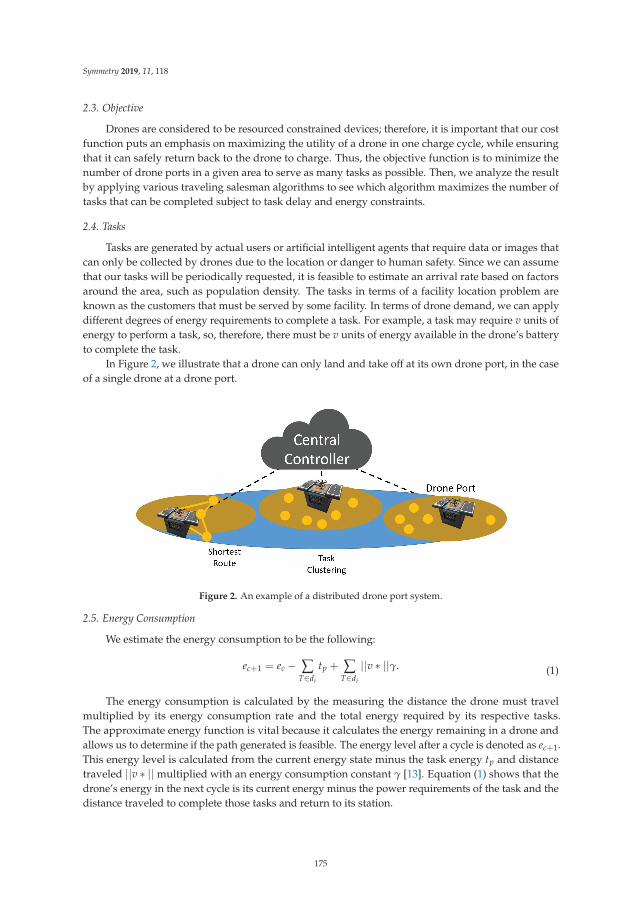
Symmetry 2019, 11, 118

2.3. Objective

Drones are considered to be resourced constrained devices; therefore, it is important that our costfunction puts an emphasis on maximizing the utility of a drone in one charge cycle, while ensuringthat it can safely return back to the drone to charge. Thus, the objective function is to minimize thenumber of drone ports in a given area to serve as many tasks as possible. Then, we analyze the resultby applying various traveling salesman algorithms to see which algorithm maximizes the number oftasks that can be completed subject to task delay and energy constraints.

2.4. Tasks

Tasks are generated by actual users or artificial intelligent agents that require data or images thatcan only be collected by drones due to the location or danger to human safety. Since we can assumethat our tasks will be periodically requested, it is feasible to estimate an arrival rate based on factorsaround the area, such as population density. The tasks in terms of a facility location problem areknown as the customers that must be served by some facility. In terms of drone demand, we can applydifferent degrees of energy requirements to complete a task. For example, a task may require v units ofenergy to perform a task, so, therefore, there must be v units of energy available in the drone’s batteryto complete the task.

In Figure 2, we illustrate that a drone can only land and take off at its own drone port, in the caseof a single drone at a drone port.

Figure 2. An example of a distributed drone port system.

2.5. Energy Consumption

We estimate the energy consumption to be the following:

ec+1 = ec − ∑T∈di

tp + ∑T∈di

||v ∗ ||γ. (1)

The energy consumption is calculated by the measuring the distance the drone must travelmultiplied by its energy consumption rate and the total energy required by its respective tasks.The approximate energy function is vital because it calculates the energy remaining in a drone andallows us to determine if the path generated is feasible. The energy level after a cycle is denoted as ec+1.This energy level is calculated from the current energy state minus the task energy tp and distancetraveled ||v ∗ ||multiplied with an energy consumption constant γ [13]. Equation (1) shows that thedrone’s energy in the next cycle is its current energy minus the power requirements of the task and thedistance traveled to complete those tasks and return to its station.

175

Symmetry 2019, 11, 118

2.6. Facility Location Problem

The objective of an capacitated facility location is to minimize the distance between the tasks andcentral drone port. We use this technique in combination with a shortest route algorithm to ensurethat the coverage size and the number of drones is suitable to satisfy all the tasks generated near thedrone port. In our initial formulation, introduce variable xi, xj containing the co-ordinates of potentialdrone ports and tasks, respectively, where zi = 1, . . . , n where xi = 1 if drone port i is built, and xi = 0,otherwise. We can treat the drone port acts as a facility because it contains the service subject to theenergy constraint, known as the supply.

2.7. Capital Expenditure

In respect to capital expenditure, our objective is to minimize the total monetary cost of buildingnew infrastructure. In the below cost function, our goal is to reduce the total distance between thedrone port xi and tasks xj. Since we are limited by the budget F, it is impossible to build every potentialdrone port i:

minimize ∑di

dij,

subject to ∑i∈A

cizi ≤ F, i = 1, ..., n,

xj ∈ {0, 1}, j = 1, ..., m,dij = ||xi − xj||2.

(2)

2.8. Operational Expenditure

In respect to operational expenditure, our objective is to maximize the number of jobs denotedas yij the index of a job while satisfying constraints such as τj delay for every job. Furthermore, eachdrone must return back to its drone port. Lastly, the path generated must not exceed the drone’s energycapacity denoted as the function f (dij)

maximize ∑i

∑j

yij,

subject to ∑j

yij f (dij) ≤ Bi i = 1, ..., n,

x0 = x fac ,x f inal = x fac ,τj ≤ τj,f (dij) = P ∗ dij + η,τj = tcomplete − tarrival .

(3)

2.9. Drone Port Placement Algorithm

Algorithm 1 is an overview of our proposed algorithm to efficiently place drones in a distributedarea. We develop a heuristic approach by implementing a clustering and traveling salesman problemensemble to determine the feasibility our algorithm’s output data. We continue to increase the numberof drone ports until each drone has enough energy to perform all of the tasks in its coverage.

176

Symmetry 2019, 11, 118

Algorithm 1 Facility Location Problem for Drones

procedure DRONE PORT PLACEMENT AND SHORTEST ROUTEi ← max number of droneportsT ← Task Locations arrayP ← Set of drone ports arrayPmax ← max number of droneportsp ← Initial number of droneportswhile p ≤ Pmax do

clusters ← GenerateCluster(Tasks, p)shortestroute ← TSP(tasks, droneport)e ← f (di j)if e ≥ θ then

Breakelse

p ← p + 1

return Drone Port locationreturn Shortest Routes

2.10. Traveling Salesman Problem

After creating the clusters, we apply a shortest route algorithm to ensure that the drone canperform all of the tasks allocated to it while completing a round-trip back to its original drone port.It is denoted as the Traveling Salesman Problem (TSP) below.

3. Performance Evaluation

Our simulation was conducted on a PC with the operating system Ubuntu 16.04. We applied thealgorithms in Table 2 written in Python 3.5 to conduct our simulations. The area size for our simulationis 1000 × 1000 units.

Table 2. Algorithms we compared.

Algorithm Type Author

2-opt Shortest Path [14]

Genetic Algorithm Shortest Path [15]

Exhaustive Search Shortest Path

Ant Colony Shortest Path [16]

k-means Clustering [17]

3.1. Coverage Size effect on the Combinatorial Search Space

In Figure 3, we analyzed the combination space size in log units if clustering was not applied.Increasing the potential coverage size and the number of potential drone ports exponentially increasesthe search space. The average complexity is given by O(knT), where n is the number of combinationsand T is the maximum number of iterations. In practice, the k-means algorithm is fast, but it tends toreturn a local minima. To avoid this, we used a bottom up approach to avoid falling in to any localminima [18]. This means we can effectively reduce the number of combinations greatly by applyingk-means instead of using a naive approach such as a fixed coverage area. The constraints in ourproposal ensure that no task appears outside a drone port’s range due to improper clustering.

177

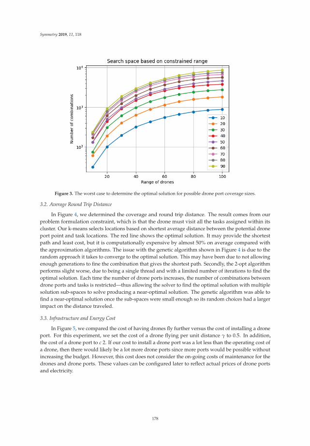
Symmetry 2019, 11, 118

Figure 3. The worst case to determine the optimal solution for possible drone port coverage sizes.

3.2. Average Round Trip Distance

In Figure 4, we determined the coverage and round trip distance. The result comes from ourproblem formulation constraint, which is that the drone must visit all the tasks assigned within itscluster. Our k-means selects locations based on shortest average distance between the potential droneport point and task locations. The red line shows the optimal solution. It may provide the shortestpath and least cost, but it is computationally expensive by almost 50% on average compared withthe approximation algorithms. The issue with the genetic algorithm shown in Figure 4 is due to therandom approach it takes to converge to the optimal solution. This may have been due to not allowingenough generations to fine the combination that gives the shortest path. Secondly, the 2-opt algorithmperforms slight worse, due to being a single thread and with a limited number of iterations to find theoptimal solution. Each time the number of drone ports increases, the number of combinations betweendrone ports and tasks is restricted—thus allowing the solver to find the optimal solution with multiplesolution sub-spaces to solve producing a near-optimal solution. The genetic algorithm was able tofind a near-optimal solution once the sub-spaces were small enough so its random choices had a largerimpact on the distance traveled.

3.3. Infrastructure and Energy Cost

In Figure 5, we compared the cost of having drones fly further versus the cost of installing a droneport. For this experiment, we set the cost of a drone flying per unit distance γ to 0.5. In addition,the cost of a drone port to c 2. If our cost to install a drone port was a lot less than the operating cost ofa drone, then there would likely be a lot more drone ports since more ports would be possible withoutincreasing the budget. However, this cost does not consider the on-going costs of maintenance for thedrones and drone ports. These values can be configured later to reflect actual prices of drone portsand electricity.

178

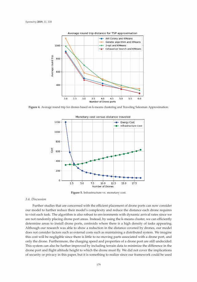
Symmetry 2019, 11, 118

Figure 4. Average round trip for drones based on k-means clustering and Traveling Salesman Approximation.

Figure 5. Infrastructure vs. monetary cost.

3.4. Discussion

Further studies that are concerned with the efficient placement of drone ports can now considerour model to further reduce their model’s complexity and reduce the distance each drone requiresto visit each task. The algorithm is also robust to environments with dynamic arrival rates since weare not randomly placing drone port areas. Instead, by using the k-means cluster, we can efficientlydetermine areas to install drone ports, centroids where there is a high density of tasks appearing.Although our research was able to show a reduction in the distance covered by drones, our modeldoes not consider factors such as external costs such as maintaining a distributed system. We imaginethis cost will be negligible since there is little to no moving parts associated with a drone port, andonly the drone. Furthermore, the charging speed and properties of a drone port are still undecided.This system can also be further improved by including terrain data to minimize the difference in thedrone port and flight altitude height to which the drone must fly. We did not cover the implicationsof security or privacy in this paper, but it is something to realize since our framework could be used

179

Symmetry 2019, 11, 118

to spy as noted in [19], therefore identifying rouge tasks is important. Several additional avenues fordrone port include the following—firstly, considering information such as buildings or landmarks toinclude in the final decision-making to create a path that the drone can follow to complete the task;secondly, adding more capacity at drone ports to allow multiple drones to land and take off; thirdly,optimizing the coverage in a way that maximizes co-operation between drones such as a chain linkdeliver system; and, fourthly, creating boundaries for partitions between two central controllers wouldallow for a hybrid solution with each sub-space of an area having its own controller. Lastly, we alsowish to work on improving the computational efficiency of our proposed algorithm.

4. Conclusions

We proposed a novel algorithm to manage distributed drone ports with a centralized controller toensure maximum co-operation between drones and fair allocation of tasks. The main goal of this systemis to efficiently assign grounded drones at drone ports with their respective tasks. Our combination ofapproximation algorithms ensures that the cluster of tasks belonging to each drone port are withinthe drone’s coverage. Second, the drone can perform the maximum number before returning to thedrone port to recharge. We show that utilizing the Ant algorithm for our cluster round trip for dronesminimizes the distance traveled for each drone. By utilizing this approach, further tasks assigned to anarea can be immediately be assigned without the need to recalculate the entire environment.

Author Contributions: Conceptualization, J.L.; Methodology, J.K., K.T., T.Z.O.; Software, J.L.; Validation, J.L.,Y.Y. and Z.Z.; Formal Analysis, J.L., K.T., T.Z.O.; Investigation, J.K., K.T.; Resources, X.X.; Data Curation,J.K.; Writing—Original Draft Preparation, J.K., K.T.; Writing—Review and Editing, J.L.; Visualization, J.K.;Supervision, C.S.H.

Funding: This research was supported by the MSIT(Ministry of Science and ICT), Korea, under the Grand InformationTechnology Research Center support program (IITP-2018-2015-0-00742) supervised by the IITP(Institute for Informationand communications Technology Promotion).

Conflicts of Interest: The authors declare no conflict of interest.

Abbreviations

Notation used in this article

Notation Explanationec Set of drone portstp Set of dronesdi Drone iv∗ Vectorγ Drone energy leveldij Distance between task j and drone port ici Cost to build drone portzi Decision variable to build drone portxj Decision variable for drone i to complete task jyij Task completion state {0, 1}x0 Drone initial positionx0 Drone final positionτj Calculated task completion delayτj Earliest deadline first constraintf (dij) Power Functionτcomplete Drone energy functionτarrival Minimum drone energyη Task’s drone energy consumptionη Task’s drone energy consumption

180

Symmetry 2019, 11, 118

References

1. FAA. Unmanned Aircraft System. FAA Aerosp. Forecast. 2018. Available online: https://www.faa.gov/data_research/aviation/aerospace_forecasts/media/Unmanned_Aircraft_Systems.pdf (accessed on12 November 2018).

2. Kanellakis, C.; Nikolakopoulos, G. Survey on Computer Vision for UAVs: Current Developments andTrends. J. Intell. Robot. Syst. 2017, 87, 141–168. [CrossRef]

3. Purwanda, I.G.; Adiono, T.; Situmorang, S.; Dawani, F.; Samhany, H.A.; Fuada, S. Prototyping design of alow-cost bike sharing system for smart city application. In Proceedings of the 2017 International Conferenceon ICT For Smart Society (ICISS), Tangerang, Indonesia, 18–19 September 2017; pp. 1–6. [CrossRef]

4. Puiatti, A. Dronesense: Drone Charging Pad. 2014. Available online: https://www.skysense.co/ (accessed on3 April 2018).

5. Sharafeddine, S.; Islambouli, R. On-Demand Deployment of Multiple Aerial Base Stations for TrafficOffloading and Network Recovery. arXiv 2018, arXiv:1807.02009.

6. Chen, M.; Mozaffari, M.; Saad, W.; Yin, C.; Debbah, M.; Hong, C.S. Caching in the sky: Proactive deploymentof cache-enabled unmanned aerial vehicles for optimized quality-of-experience. IEEE J. Sel. Areas Commun.2017, 35, 1046–1061. [CrossRef]

7. Floreano, D.; Wood, R.J. Science, technology and the future of small autonomous drones. Nature 2015,521, 460. [CrossRef] [PubMed]

8. Cesetti, A.; Frontoni, E.; Mancini, A.; Zingaretti, P.; Longhi, S. A Vision-Based Guidance System for UAVNavigation and Safe Landing Using Natural Landmarks. J. Intell. Robot. Syst. 2010, 57, 233–257. [CrossRef]

9. Ahmadian, S.; Swamy, C. Improved approximation guarantees for lower-bounded facility location.In Proceedings of the International Workshop on Approximation and Online Algorithms, Ljubljana, Slovenia,13–14 September 2012; pp. 257–271.

10. Desrochers, M.; Marcotte, P.; Stan, M. The congested facility location problem. Locat. Sci. 1995, 3, 9–23.[CrossRef]

11. Iellamo, S.; Lehtomaki, J.J.; Khan, Z. Placement of 5G Drone Base Stations by Data Field Clustering.In Proceedings of the 2017 IEEE 85th Vehicular Technology Conference (VTC Spring), Sydney, Australia,4–7 June 2017; pp. 1–5. [CrossRef]

12. Tang, C.; Monteleoni, C. Convergence rate of stochastic k-means. arXiv 2016, arXiv:1610.04900.13. Geng, Q.; Zhao, Z. A kind of route planning method for UAV based on improved PSO algorithm.

In Proceedings of the 2013 25th Chinese Control and Decision Conference (CCDC), Guiyang, China, 25–27May 2013; pp. 2328–2331. [CrossRef]

14. Croes, G.A. A method for solving traveling-salesman problems. Oper. Res. 1958, 6, 791–812. [CrossRef]15. Mitchell, M. An Introduction to Genetic Algorithms; MIT Press: Cambridge, MA, USA, 1998.16. Dorigo, M.; Birattari, M.; Blum, C.; Clerc, M.; Stützle, T.; Winfield, A. In Ant Colony Optimization and Swarm

Intelligence, Proceedings of the 6th International Conference, ANTS 2008, Brussels, Belgium, 22–24 September 2008;Springer: Berlin/Heidelberg, Germany, 2008; Volume 5217.

17. Kanungo, T.; Mount, D.M.; Netanyahu, N.S.; Piatko, C.D.; Silverman, R.; Wu, A.Y. An efficient k-meansclustering algorithm: Analysis and implementation. IEEE Trans. Pattern Anal. Mach. Intell. 2002, 27, 881–892.[CrossRef]

18. Arthur, D.; Vassilvitskii, S. k-means++: The advantages of careful seeding. In Proceedings of the EighteenthAnnual ACM-SIAM Symposium on Discrete Algorithms. Society for Industrial and Applied Mathematics,Philadelphia, PA, USA, 7–9 January 2007; pp. 1027–1035.

19. Gonzalez, G. Autonomous Vehicles, Drones Offer New Insurer Risks and Opportunities. Available online:https://www.businessinsurance.com/article/20171207/NEWS06/912317799/Autonomous-vehicles,-drones-offer-new-insurer-risks-and-opportunities(accessed on 12 June 2018).

c© 2019 by the authors. Licensee MDPI, Basel, Switzerland. This article is an open accessarticle distributed under the terms and conditions of the Creative Commons Attribution(CC BY) license (http://creativecommons.org/licenses/by/4.0/).

181

symmetryS SArticle

Parametric Jensen-Shannon Statistical Complexityand Its Applications on Full-Scale CompartmentFire Data

Flavia-Corina Mitroi-Symeonidis 1,2, Ion Anghel 2 and Nicus, or Minculete 3,*

1 Academy of Economic Studies, Department of Applied Mathematics, Calea Dorobantilor 15-17, Sector 1,RO-010552 Bucharest, Romania; fcmitroi@yahoo.com

2 Police Academy “Alexandru Ioan Cuza”, Fire Officers Faculty, Str. Morarilor 3, Sector 2,RO-022451 Bucharest, Romania; ion.anghel@academiadepolitie.ro

3 Faculty of Mathematics and Computer Science, Transilvania University of Bras, ov, Str. Iuliu Maniu50,500091 Bras, ov, Romania

* Correspondence: minculete.nicusor@unitbv.ro

Received: 12 November 2019; Accepted: 19 December 2019; Published: 20 December 2019

Abstract: The order/disorder characteristics of a compartment fire are researched based onexperimental data. From our analysis performed by new, pioneering methods, we claim thatthe parametric Jensen-Shannon complexity can be successfully used to detect unusual data, andthat one can use it also as a means to perform relevant analysis of fire experiments. Thoroughlycomparing the performance of different algorithms (known as permutation entropy and two-lengthpermutation entropy) to extract the probability distribution is an essential step. We discuss some ofthe theoretical assumptions behind each step and stress that the role of the parameter is to fine-tunethe results of the Jensen-Shannon statistical complexity. Note that the Jensen-Shannon statisticalcomplexity is symmetric, while its parametric version displays a symmetric duality due to the a prioriprobabilities used.

Keywords: full-scale fire experiment; compartment fire; permutation entropy; two length permutationentropy; time series analysis; parametric Jensen-Shannon statistical complexity; symmetric duality

1. Introduction

We aim to perform a local entropic analysis of the evolution of the temperature during a full-scalefire experiment and seek a straightforward, general, and process-based model of the compartment fire.We propose a new statistical complexity and compare known algorithms dedicated to the extraction ofthe underlying probabilities, checking their suitability to point out the abnormal values and structureof the experimental time series. For recent research on the fire phenomena performed using entropictools, see Takagi, Gotoda, Tokuda and Miyano [1] and Murayama, Kaku, Funatsu, and Gotoda [2].

The experimental data was collected during a full-scale fire experiment conducted at the FireOfficers Faculty in Bucharest. We briefly include here the description of the experimental setup(Materials and Methods). Details can be found in [3].

The experiment has been carried out using a container (single-room compartment) having thefollowing dimensions: 12 m × 2.2 m × 2.6 m. A single ventilation opening was available, namely thefront door of the container, which remained open during the experiment. Parts of the walls and theceiling of the container were furnished with oriented strand boards (OSB). The fire source has been awooden crib made of 36 pieces of wood strips 2.5 cm × 2.5 cm × 30 cm, on which has been poured500 mL ethanol shortly before ignition. The fire bed was situated in a corner of the compartment,at 1.2 m below the ceiling. The measurement devices consisted of six built-in K-type thermocouples,

Symmetry 2020, 12, 22; doi:10.3390/sym12010022 www.mdpi.com/journal/symmetry183

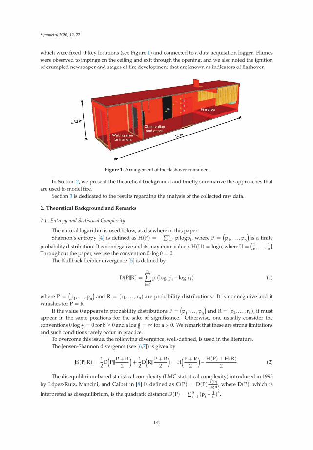
Symmetry 2020, 12, 22

which were fixed at key locations (see Figure 1) and connected to a data acquisition logger. Flameswere observed to impinge on the ceiling and exit through the opening, and we also noted the ignitionof crumpled newspaper and stages of fire development that are known as indicators of flashover.

Figure 1. Arrangement of the flashover container.

In Section 2, we present the theoretical background and briefly summarize the approaches thatare used to model fire.

Section 3 is dedicated to the results regarding the analysis of the collected raw data.

2. Theoretical Background and Remarks

2.1. Entropy and Statistical Complexity

The natural logarithm is used below, as elsewhere in this paper.Shannon’s entropy [4] is defined as H(P) = −∑n

i=1 pilogpi, where P =(p1, . . . , pn

)is a finite

probability distribution. It is nonnegative and its maximum value is H(U) = logn, where U =(

1n , . . . , 1

n

).

Throughout the paper, we use the convention 0· log 0 = 0.The Kullback-Leibler divergence [5] is defined by

D(P‖R) =n∑

i=1

pi(log pi − log ri) (1)

where P =(p1, . . . , pn

)and R = (r1, . . . , rn) are probability distributions. It is nonnegative and it

vanishes for P = R.If the value 0 appears in probability distributions P =

(p1, . . . , pn

)and R = (r1, . . . , rn), it must

appear in the same positions for the sake of significance. Otherwise, one usually consider theconventions 0 log 0

b = 0 for b ≥ 0 and a log a0 = ∞ for a > 0. We remark that these are strong limitations

and such conditions rarely occur in practice.To overcome this issue, the following divergence, well-defined, is used in the literature.The Jensen-Shannon divergence (see [6,7]) is given by

JS(P‖R) = 12

D(P‖P + R

2

)+

12

D(R‖P + R

2

)= H

(P + R2

)− H(P) + H(R)

2. (2)

The disequilibrium-based statistical complexity (LMC statistical complexity) introduced in 1995

by López-Ruiz, Mancini, and Calbet in [8] is defined as C(P) = D(P)H(P)log n , where D(P), which is

interpreted as disequilibrium, is the quadratic distance D(P) =∑n

i=1 (pi − 1n )

2.

184

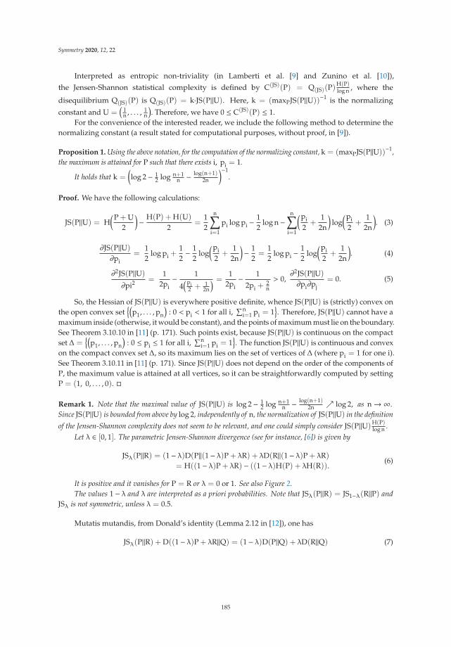
Symmetry 2020, 12, 22

Interpreted as entropic non-triviality (in Lamberti et al. [9] and Zunino et al. [10]),

the Jensen-Shannon statistical complexity is defined by C(JS)(P) = Q(JS)(P)H(P)log n , where the

disequilibrium Q(JS)(P) is Q(JS)(P) = k·JS(P‖U). Here, k = (maxPJS(P‖U))−1 is the normalizing

constant and U =(

1n , . . . , 1

n

). Therefore, we have 0 ≤ C(JS)(P) ≤ 1.

For the convenience of the interested reader, we include the following method to determine thenormalizing constant (a result stated for computational purposes, without proof, in [9]).

Proposition 1. Using the above notation, for the computation of the normalizing constant, k = (maxPJS(P‖U))−1,the maximum is attained for P such that there exists i, pi = 1.

It holds that k =(log 2− 1

2 log n+1n − log(n+1)

2n

)−1.

Proof. We have the following calculations:

JS(P‖U) = H(P + U

2

)− H(P) + H(U)

2=

12

n∑i=1

pi log pi −12

log n−n∑

i=1

(pi

2+

12n

)log

(pi

2+

12n

). (3)

∂JS(P‖U)

∂pi=

12

log pi +12− 1

2log

(pi

2+

12n

)− 1

2=

12

log pi −12

log(pi

2+

12n

). (4)

∂2JS(P‖U)

∂pi2=

12pi− 1

4(pi

2 + 12n

) =1

2pi− 1

2pi +2n

> 0,∂2JS(P‖U)

∂pi∂pj= 0. (5)

So, the Hessian of JS(P‖U) is everywhere positive definite, whence JS(P‖U) is (strictly) convex onthe open convex set

{(p1, . . . , pn

): 0 < pi < 1 for all i,

∑ni=1 pi = 1

}. Therefore, JS(P‖U) cannot have a

maximum inside (otherwise, it would be constant), and the points of maximum must lie on the boundary.See Theorem 3.10.10 in [11] (p. 171). Such points exist, because JS(P‖U) is continuous on the compactset Δ =

{(p1, . . . , pn

): 0 ≤ pi ≤ 1 for all i,

∑ni=1 pi = 1

}. The function JS(P‖U) is continuous and convex

on the compact convex set Δ, so its maximum lies on the set of vertices of Δ (where pi = 1 for one i).See Theorem 3.10.11 in [11] (p. 171). Since JS(P‖U) does not depend on the order of the components ofP, the maximum value is attained at all vertices, so it can be straightforwardly computed by settingP = (1, 0, . . . , 0). �

Remark 1. Note that the maximal value of JS(P‖U) is log 2− 12 log n+1

n − log(n+1)2n ↗ log 2, as n→∞.

Since JS(P‖U) is bounded from above by log 2, independently of n, the normalization of JS(P‖U) in the definitionof the Jensen-Shannon complexity does not seem to be relevant, and one could simply consider JS(P‖U)

H(P)log n .

Let λ ∈ [0, 1]. The parametric Jensen-Shannon divergence (see for instance, [6]) is given by

JSλ(P‖R) = (1− λ)D(P‖(1− λ)P + λR) + λD(R‖(1− λ)P + λR)= H((1− λ)P + λR) − ((1− λ)H(P) + λH(R)).

(6)

It is positive and it vanishes for P = R or λ = 0 or 1. See also Figure 2.The values 1− λ and λ are interpreted as a priori probabilities. Note that JSλ(P‖R) = JS1−λ(R‖P) and

JSλ is not symmetric, unless λ = 0.5.

Mutatis mutandis, from Donald’s identity (Lemma 2.12 in [12]), one has

JSλ(P‖R) + D((1− λ)P + λR‖Q) = (1− λ)D(P‖Q) + λD(R‖Q) (7)

185

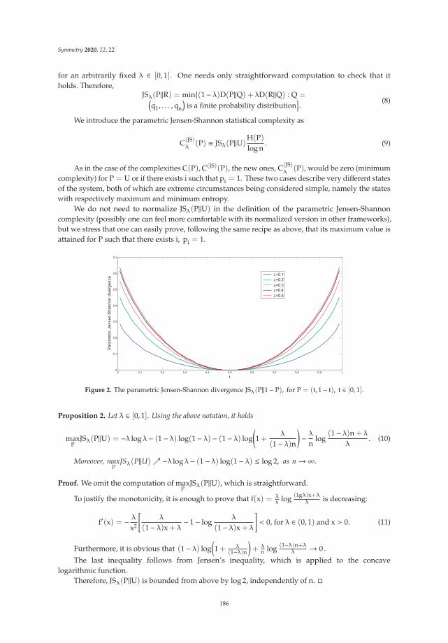
Symmetry 2020, 12, 22

for an arbitrarily fixed λ ∈ [0, 1]. One needs only straightforward computation to check that itholds. Therefore,

JSλ(P‖R) = min{(1− λ)D(P‖Q) + λD(R‖Q) : Q =(

q1, . . . , qn

)is a finite probability distribution

}.

(8)

We introduce the parametric Jensen-Shannon statistical complexity as

C(JS)λ

(P) ≡ JSλ(P‖U)H(P)log n

. (9)

As in the case of the complexities C(P), C(JS)(P), the new ones, C(JS)λ

(P), would be zero (minimumcomplexity) for P = U or if there exists i such that pi = 1. These two cases describe very different statesof the system, both of which are extreme circumstances being considered simple, namely the stateswith respectively maximum and minimum entropy.

We do not need to normalize JSλ(P‖U) in the definition of the parametric Jensen-Shannoncomplexity (possibly one can feel more comfortable with its normalized version in other frameworks),but we stress that one can easily prove, following the same recipe as above, that its maximum value isattained for P such that there exists i, pi = 1.

λλλλλ

Figure 2. The parametric Jensen-Shannon divergence JSλ(P‖1− P), for P = (t, 1− t), t ∈ [0, 1].

Proposition 2. Let λ ∈ [0, 1]. Using the above notation, it holds

maxP

JSλ(P‖U) = −λ log λ− (1− λ) log(1− λ) − (1− λ) log(1 +

λ

(1− λ)n)− λ

nlog

(1− λ)n + λ

λ. (10)

Moreover, maxP

JSλ(P‖U)↗ −λ log λ− (1− λ) log(1− λ) ≤ log 2, as n→∞.

Proof. We omit the computation of maxP

JSλ(P‖U), which is straightforward.

To justify the monotonicity, it is enough to prove that f(x) = λx log (1gλ)x+λ

λ is decreasing:

f′(x) = − λ

x2

[λ

(1− λ)x + λ− 1− log

λ

(1− λ)x + λ

]< 0, for λ ∈ (0, 1) and x > 0. (11)

Furthermore, it is obvious that (1− λ) log(1 + λ

(1−λ)n)+ λ

n log (1−λ)n+λλ → 0 .

The last inequality follows from Jensen’s inequality, which is applied to the concavelogarithmic function.

Therefore, JSλ(P‖U) is bounded from above by log 2, independently of n. �

186

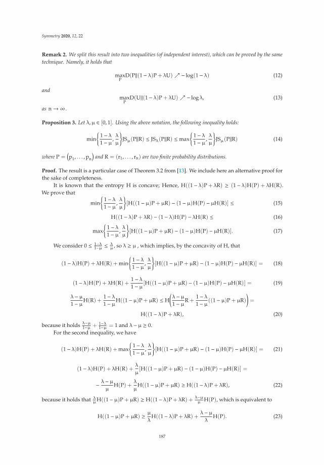
Symmetry 2020, 12, 22

Remark 2. We split this result into two inequalities (of independent interest), which can be proved by the sametechnique. Namely, it holds that

maxP

D(P‖(1− λ)P + λU)↗ − log(1− λ) (12)

andmax

PD(U‖(1− λ)P + λU)↗ − log λ, (13)

as n→∞ .

Proposition 3. Let λ,μ ∈ [0, 1]. Using the above notation, the following inequality holds:

min{

1− λ1− μ ,

λ

μ

}JSμ(P‖R) ≤ JSλ(P‖R) ≤ max

{1− λ1− μ ,

λ

μ

}JSμ(P‖R) (14)

where P =(p1, . . . , pn

)and R = (r1, . . . , rn) are two finite probability distributions.

Proof. The result is a particular case of Theorem 3.2 from [13]. We include here an alternative proof forthe sake of completeness.

It is known that the entropy H is concave; Hence, H((1− λ)P + λR) ≥ (1− λ)H(P) + λH(R).We prove that

min{

1− λ1− μ ,

λ

μ

}[H((1− μ)P + μR) − (1− μ)H(P) − μH(R)] ≤ (15)

H((1− λ)P + λR) − (1− λ)H(P) − λH(R) ≤ (16)

max{

1− λ1− μ ,

λ

μ

}[H((1− μ)P + μR) − (1− μ)H(P) − μH(R)]. (17)

We consider 0 ≤ 1−λ1−μ ≤ λ

μ , so λ ≥ μ , which implies, by the concavity of H, that

(1− λ)H(P) + λH(R) + min{

1− λ1− μ ,

λ

μ

}[H((1− μ)P + μR) − (1− μ)H(P) − μH(R)] = (18)

(1− λ)H(P) + λH(R) +1− λ1− μ [H((1− μ)P + μR) − (1− μ)H(P) − μH(R)] = (19)

λ− μ1− μH(R) +

1− λ1− μH((1− μ)P + μR) ≤ H

(λ− μ1− μR +

1− λ1− μ ((1− μ)P + μR)

)=

H((1− λ)P + λR), (20)

because it holds λ−μ1−μ + 1−λ

1−μ = 1 and λ− μ ≥ 0.For the second inequality, we have

(1− λ)H(P) + λH(R) + max{

1− λ1− μ ,

λ

μ

}[H((1− μ)P + μR) − (1− μ)H(P) − μH(R)] = (21)

(1− λ)H(P) + λH(R) +λ

μ[H((1− μ)P + μR) − (1− μ)H(P) − μH(R)] =

− λ− μμ

H(P) +λ

μH((1− μ)P + μR) ≥ H((1− λ)P + λR), (22)

because it holds that λμH((1− μ)P + μR) ≥ H((1− λ)P + λR) + λ−μ

μ H(P), which is equivalent to

H((1− μ)P + μR) ≥ μ

λH((1− λ)P + λR) +

λ− μλ

H(P). (23)

187

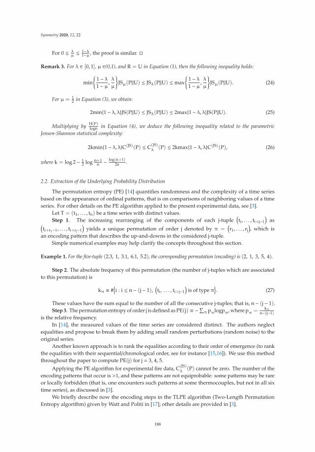
Symmetry 2020, 12, 22

For 0 ≤ λμ ≤ 1−λ

1−μ , the proof is similar. �

Remark 3. For λ ∈ [0, 1], μ ∈(0,1), and R = U in Equation (1), then the following inequality holds:

min{

1− λ1− μ ,

λ

μ

}JSμ(P‖U) ≤ JSλ(P‖U) ≤ max

{1− λ1− μ ,

λ

μ

}JSμ(P‖U). (24)

For μ = 12 in Equation (3), we obtain:

2min{1− λ, λ}JS(P‖U) ≤ JSλ(P‖U) ≤ 2max{1− λ, λ}JS(P‖U). (25)

Multiplying by H(P)logn in Equation (4), we deduce the following inequality related to the parametric

Jensen-Shannon statistical complexity:

2kmin{1− λ, λ}C(JS)(P) ≤ C(JS)λ

(P) ≤ 2kmax{1− λ, λ}C(JS)(P), (26)

where k = log 2− 12 log n+1

n − log(n+1)2n .

2.2. Extraction of the Underlying Probability Distribution

The permutation entropy (PE) [14] quantifies randomness and the complexity of a time seriesbased on the appearance of ordinal patterns, that is on comparisons of neighboring values of a timeseries. For other details on the PE algorithm applied to the present experimental data, see [3].

Let T = (t1, . . . , tn) be a time series with distinct values.Step 1. The increasing rearranging of the components of each j-tuple

(ti, . . . , ti+j−1

)as(

ti+r1−1, . . . , ti+rj−1)

yields a unique permutation of order j denoted by π =(r1, . . . , rj

), which is

an encoding pattern that describes the up-and-downs in the considered j-tuple.Simple numerical examples may help clarify the concepts throughout this section.

Example 1. For the five-tuple (2.3, 1, 3.1, 6.1, 5.2), the corresponding permutation (encoding) is (2, 1, 3, 5, 4).

Step 2. The absolute frequency of this permutation (the number of j-tuples which are associatedto this permutation) is

kπ ≡ #{i : i ≤ n− (j− 1),

(ti, . . . , ti+j−1

)is of type π

}. (27)

These values have the sum equal to the number of all the consecutive j-tuples; that is, n− (j− 1).Step 3. The permutation entropy of order j is defined as PE(j) ≡ −∑

π pπlogpπ, where pπ = kπ

n−(j−1)is the relative frequency.

In [14], the measured values of the time series are considered distinct. The authors neglectequalities and propose to break them by adding small random perturbations (random noise) to theoriginal series.

Another known approach is to rank the equalities according to their order of emergence (to rankthe equalities with their sequential/chronological order, see for instance [15,16]). We use this methodthroughout the paper to compute PE(j) for j = 3, 4, 5.

Applying the PE algorithm for experimental fire data, C(JS)λ

(P) cannot be zero. The number of theencoding patterns that occur is >1, and these patterns are not equiprobable: some patterns may be rareor locally forbidden (that is, one encounters such patterns at some thermocouples, but not in all sixtime series), as discussed in [3].

We briefly describe now the encoding steps in the TLPE algorithm (Two-Length PermutationEntropy algorithm) given by Watt and Politi in [17]; other details are provided in [3].

188

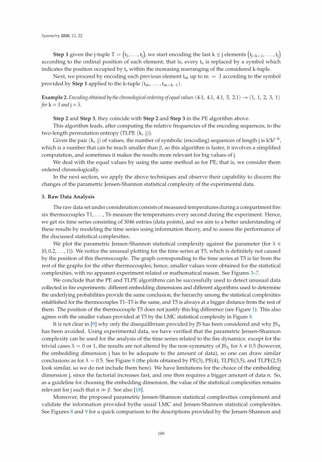
Symmetry 2020, 12, 22

Step 1 given the j-tuple T =(t1, . . . , tj

), we start encoding the last k ≤ j elements

(tj−k+1, . . . , tj

)according to the ordinal position of each element; that is, every ts is replaced by a symbol whichindicates the position occupied by ts within the increasing rearranging of the considered k-tuple.

Next, we proceed by encoding each previous element tm up to m = 1 according to the symbolprovided by Step 1 applied to the k-tuple (tm, . . . , tm+k−1).

Example 2. Encoding obtained by the chronological ordering of equal values (4.1, 4.1, 4.1, 5, 2.1)→ (1, 1, 2, 3, 1)for k = 3 and j = 5.

Step 2 and Step 3, they coincide with Step 2 and Step 3 in the PE algorithm above.This algorithm leads, after computing the relative frequencies of the encoding sequences, to the

two-length permutation entropy (TLPE (k, j)).Given the pair (k, j) of values, the number of symbolic (encoding) sequences of length j is k!kj−k,

which is a number that can be much smaller than j!, so this algorithm is faster, it involves a simplifiedcomputation, and sometimes it makes the results more relevant for big values of j.

We deal with the equal values by using the same method as for PE; that is, we consider themordered chronologically.

In the next section, we apply the above techniques and observe their capability to discern thechanges of the parametric Jensen-Shannon statistical complexity of the experimental data.

3. Raw Data Analysis

The raw data set under consideration consists of measured temperatures during a compartment fire:six thermocouples T1, . . . , T6 measure the temperatures every second during the experiment. Hence,we get six time series consisting of 3046 entries (data points), and we aim to a better understanding ofthese results by modeling the time series using information theory, and to assess the performance ofthe discussed statistical complexities.

We plot the parametric Jensen-Shannon statistical complexity against the parameter (for λ ∈{0, 0.2, . . . , 1}). We notice the unusual plotting for the time series at T5, which is definitely not causedby the position of this thermocouple. The graph corresponding to the time series at T5 is far from therest of the graphs for the other thermocouples; hence, smaller values were obtained for the statisticalcomplexities, with no apparent experiment related or mathematical reason. See Figures 3–7.

We conclude that the PE and TLPE algorithms can be successfully used to detect unusual datacollected in fire experiments: different embedding dimensions and different algorithms used to determinethe underlying probabilities provide the same conclusion, the hierarchy among the statistical complexitiesestablished for the thermocouples T1–T5 is the same, and T5 is always at a bigger distance from the rest ofthem. The position of the thermocouple T5 does not justify this big difference (see Figure 1). This alsoagrees with the smaller values provided at T5 by the LMC statistical complexity in Figure 8.

It is not clear in [9] why only the disequilibrium provided by JS has been considered and why JSλhas been avoided. Using experimental data, we have verified that the parametric Jensen-Shannoncomplexity can be used for the analysis of the time series related to the fire dynamics: except for thetrivial cases λ = 0 or 1, the results are not altered by the non-symmetry of JSλ for λ � 0.5 (however,the embedding dimension j has to be adequate to the amount of data), so one can draw similarconclusions as for λ = 0.5. See Figure 8 (the plots obtained by PE(3), PE(4), TLPE(3,5), and TLPE(2,5)look similar, so we do not include them here). We have limitations for the choice of the embeddingdimension j, since the factorial increases fast, and one then requires a bigger amount of data n. So,as a guideline for choosing the embedding dimension, the value of the statistical complexities remainsrelevant for j such that n� j!. See also [18].

Moreover, the proposed parametric Jensen-Shannon statistical complexities complement andvalidate the information provided bythe usual LMC and Jensen-Shannon statistical complexities.See Figures 8 and 9 for a quick comparison to the descriptions provided by the Jensen-Shannon and

189

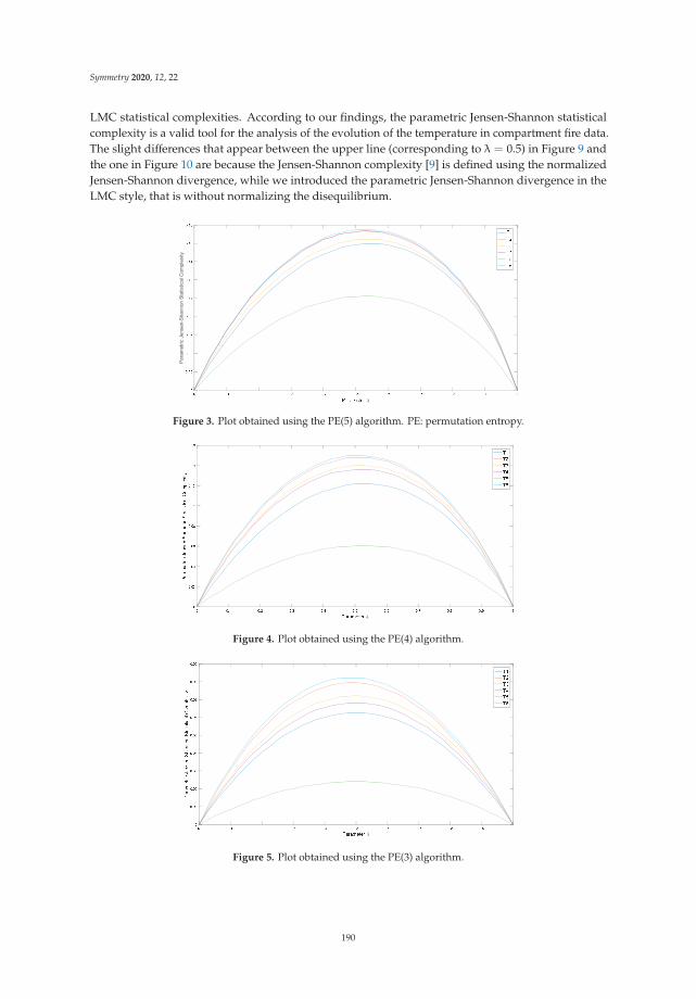
Symmetry 2020, 12, 22

LMC statistical complexities. According to our findings, the parametric Jensen-Shannon statisticalcomplexity is a valid tool for the analysis of the evolution of the temperature in compartment fire data.The slight differences that appear between the upper line (corresponding to λ = 0.5) in Figure 9 andthe one in Figure 10 are because the Jensen-Shannon complexity [9] is defined using the normalizedJensen-Shannon divergence, while we introduced the parametric Jensen-Shannon divergence in theLMC style, that is without normalizing the disequilibrium.

Figure 3. Plot obtained using the PE(5) algorithm. PE: permutation entropy.

Figure 4. Plot obtained using the PE(4) algorithm.

Figure 5. Plot obtained using the PE(3) algorithm.

190

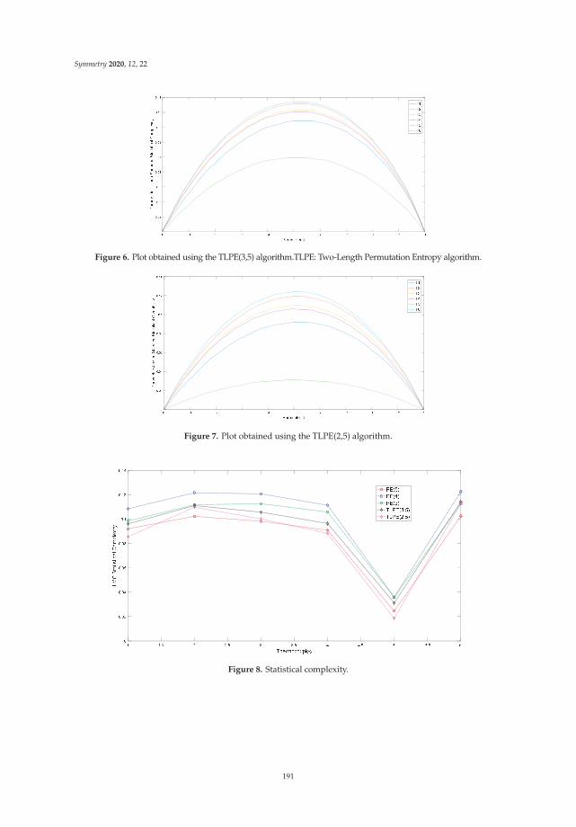
Symmetry 2020, 12, 22

Figure 6. Plot obtained using the TLPE(3,5) algorithm.TLPE: Two-Length Permutation Entropy algorithm.

Figure 7. Plot obtained using the TLPE(2,5) algorithm.

Figure 8. Statistical complexity.

191

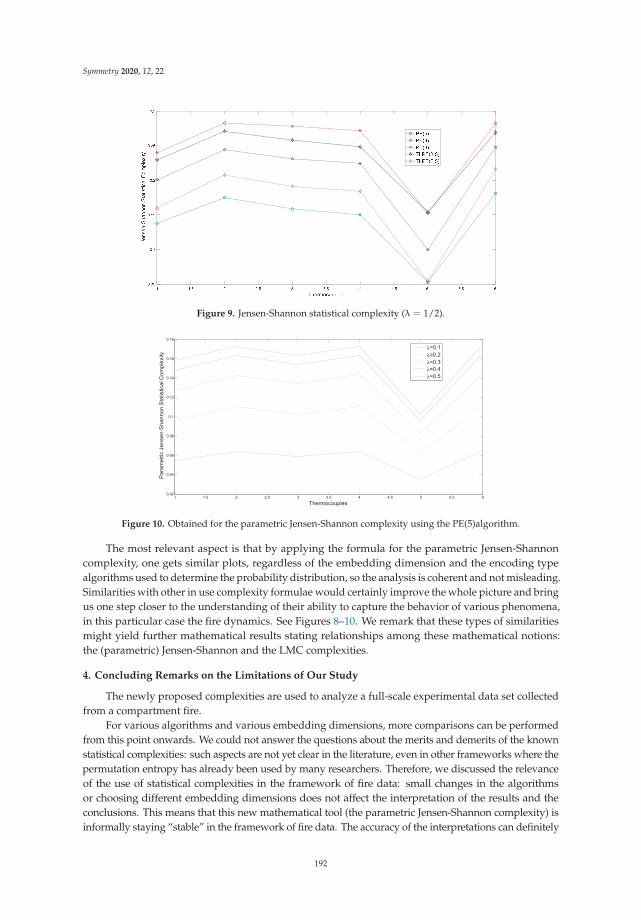
Symmetry 2020, 12, 22

Figure 9. Jensen-Shannon statistical complexity (λ = 1/2).

λλλλλ

Figure 10. Obtained for the parametric Jensen-Shannon complexity using the PE(5)algorithm.

The most relevant aspect is that by applying the formula for the parametric Jensen-Shannoncomplexity, one gets similar plots, regardless of the embedding dimension and the encoding typealgorithms used to determine the probability distribution, so the analysis is coherent and not misleading.Similarities with other in use complexity formulae would certainly improve the whole picture and bringus one step closer to the understanding of their ability to capture the behavior of various phenomena,in this particular case the fire dynamics. See Figures 8–10. We remark that these types of similaritiesmight yield further mathematical results stating relationships among these mathematical notions:the (parametric) Jensen-Shannon and the LMC complexities.

4. Concluding Remarks on the Limitations of Our Study

The newly proposed complexities are used to analyze a full-scale experimental data set collectedfrom a compartment fire.

For various algorithms and various embedding dimensions, more comparisons can be performedfrom this point onwards. We could not answer the questions about the merits and demerits of the knownstatistical complexities: such aspects are not yet clear in the literature, even in other frameworks where thepermutation entropy has already been used by many researchers. Therefore, we discussed the relevanceof the use of statistical complexities in the framework of fire data: small changes in the algorithmsor choosing different embedding dimensions does not affect the interpretation of the results and theconclusions. This means that this new mathematical tool (the parametric Jensen-Shannon complexity) isinformally staying “stable” in the framework of fire data. The accuracy of the interpretations can definitely

192

Symmetry 2020, 12, 22

be improved by the choice of the parameters, but the degree of its change cannot be estimated out of thedata gathered in just one experiment: further research is required.

Other recent results on the analysis of this data set can be found in [19]. To understand this materialthe reader is referred to [20]. For the use of the permutation entropy in another framework see [21,22].

Our results might also indicate a turbulenceor a malfunction of the thermocouple T5 (an improperlycalibrated scale); however, it is beyond the scope of the present paper to discuss it in detail.

Author Contributions: The work presented here was carried out in collaboration between all authors. All authorscontributed equally and significantly in writing this article. All authors have contributed to the manuscript.All authors have read and agreed to the published version of the manuscript.

Funding: This work was supported by a grant of the Romanian Ministry of Research and Innovation, CCCDI-UEFISCDI,project number PN-III-P1-1.2-PCCDI-2017-0350/38PCCDI within PNCDI III.

Acknowledgments: The authors thank Eleutherius Symeonidis for the argumentation of the proof of Proposition 1.

Conflicts of Interest: The authors declare no conflict of interest.

References

1. Takagi, K.; Gotoda, H.; Tokuda, I.T.; Miyano, T. Dynamic behavior of temperature field in a buoyancy-driventurbulent fire. Phys. Lett. A 2018, 382, 3181–3186. [CrossRef]

2. Murayama, S.; Kaku, K.; Funatsu, M.; Gotoda, H. Characterization of dynamic behavior of combustion noiseand detection of blowout in a laboratory-scale gas-turbine model combustor. Proc. Combust. Inst. 2019, 37,5271–5278. [CrossRef]

3. Mitroi-Symeonidis, F.-C.; Anghel, I.; Lalu, O.; Popa, C. The permutation entropy and its applications on firetests data. arXiv 2019, arXiv:1908.04274.

4. Shannon, C.E. A mathematical theory of communication. Bell Syst. Tech. J. 1948, 27, 379–423. [CrossRef]5. Kullback, S.; Leibler, L.A. On information and sufficiency. Ann. Math. Stat. 1951, 22, 79–86. [CrossRef]6. Lin, J. Divergence measures based on the Shannon entropy. IEEE-Trans. Inf. Theory 1991, 37, 145–151. [CrossRef]7. Rao, C.R.; Nayak, T.K. Cross entropy, dissimilarity measures, and characterizations of quadratic entropy.

IEEE Trans. Inform. Theory 1985, 31, 589–593. [CrossRef]8. López-Ruiz, R.; Mancini, H.L.; Calbet, X. A statistical measure of complexity. Phys. Lett. A 1995, 209, 321–326.

[CrossRef]9. Lamberti, P.W.; Martin, M.T.; Plastino, A.; Rosso, O.A. Intensive entropic non-triviality measure. Phys. A Stat.

Mech. Appl. 2004, 334, 119–131. [CrossRef]10. Zunino, L.; Soriano, M.C.; Rosso, O.A. Distinguishing chaotic and stochastic dynamics from time series by

using a multiscale symbolic approach. Phys. Rev. E 2012, 86, 046210. [CrossRef]11. Niculescu, C.P.; Persson, L.-E. Convex Functions and their Applications. A Contemporary Approach, 2nd ed.;

CMS Books in Mathematics; Springer-Verlag: New York, NY, USA, 2018; Volume 23.12. Donald, M.J. Further results on the relative entropy. Math. Proc. Camb. Philos. Soc. 1987, 101, 363–373. [CrossRef]13. Mitroi-Symeonidis, F.-C. About the precision in Jensen-Steffensen inequality. Ann. Univ. Craiova Ser. Mat.

Inform. 2010, 37, 73–84.14. Bandt, C.; Pompe, B. Permutation entropy: A natural complexity measure for time series. Phys. Rev. Lett.

2002, 88, 174102. [CrossRef] [PubMed]15. Cao, T.; Tung, W.W.; Gao, J.B.; Protopopescu, V.A.; Hively, L.M. Detecting dynamical changes in time series

using the permutation entropy. Phys. Rev. E 2004, 70, 046217. [CrossRef]16. Duan, S.; Wang, F.; Zhang, Y. Research on the biophoton emission of wheat kernels based on permutation

entropy. Optik 2019, 178, 723–730. [CrossRef]17. Watt, S.J.; Politi, A. Permutation entropy revisited. Chaos Solitons Fractals 2019, 120, 95–99. [CrossRef]18. Riedl, M.; Müller, A.; Wessel, N. Practical considerations of permutation entropy. Eur. Phys. J. Spec. Top.

2013, 222, 249–262. [CrossRef]19. Mitroi-Symeonidis, F.-C.; Anghel, I.; Furuichi, S. Encodings for the calculation of the permutation hypoentropy

and their applications on full-scale compartment fire data. Acta Tech. Napoc. Ser. Appl. Math. Mech. Eng.2019, 62, 607–616.

193

Symmetry 2020, 12, 22

20. Furuichi, S.; Mitroi-Symeonidis, F.-C.; Symeonidis, E. On some properties of Tsallis hypoentropies andhypodivergences. Entropy 2014, 16, 5377–5399. [CrossRef]

21. Araujo, F.H.A.; Bejan, L.; Rosso, O.A.; Stosic, T. Permutation entropy and statistical complexity analysis ofBrazilian agricultural commodities. Entropy 2019, 21, 1220. [CrossRef]

22. Song, Y.; Ju, Y.; Du, K.; Liu, W.; Song, J. Online road detection under a shadowy traffic image using alearning-based illumination-independent image. Symmetry 2018, 10, 707. [CrossRef]

© 2019 by the authors. Licensee MDPI, Basel, Switzerland. This article is an open accessarticle distributed under the terms and conditions of the Creative Commons Attribution(CC BY) license (http://creativecommons.org/licenses/by/4.0/).

194

symmetryS SArticle

The Asymmetric Alpha-Power Skew-t Distribution

Roger Tovar-Falón 1,*, Heleno Bolfarine 2 and Guillermo Martínez-Flórez 1

1 Departamento de Matemáticas y Estadística, Facultad de Ciencias Básicas, Universidad de Córdoba,Montería 230027, Colombia; guillermomartinez@correo.unicordoba.edu.co

2 Departamento de Estatística, IME, Universidade de São Paulo, São Paulo 1010, Brazil; hbolfar@ime.usp.br* Correspondence: rjtovar@correo.unicordoba.edu.co

Received: 13 November 2019; Accepted: 25 December 2019; Published: 2 January 2020

Abstract: In this paper, we propose a new asymmetric and heavy-tail model that generalizes both theskew-t and power-t models. Properties of the model are studied in detail. The score functions andthe elements of the observed information matrix are given. The process to estimate the parametersin model is discussed by using the maximum likelihood approach. Also, the observed informationmatrix is shown to be non-singular at the whole parametric space. Two applications to real data setsare reported to demonstrate the usefulness of this new model.

Keywords: alpha-power skew-t distribution; skew-t distribution; power-t distribution; asymmetry;Fisher information matrix; maximum likelihood estimation

1. Introduction

In recent years, there has been considerable interest in the statistical literature related to flexiblefamilies of distributions able of modeling data that present high degree of asymmetry, with kurtosisindex greater or smaller than the captured by normal model. In this context, two proposals thathave shown a promising behavior in this type of situations are the skew-normal (SN) distributionof Azzalini [1] and the power-normal (PN) distribution of Durrans [2]. The SN distribution hasbeen widely studied by many authors, and its main drawback is that it presents singular Fisherinformation matrix, implying the inference is useless from the theory of large samples using themaximum likelihood (ML) approach. Although the PN model has a shorter asymmetry range thanSN distribution, it presents non-singular information matrix and can easily be extended to censoredscenarios, as it has a simple distribution function, see, for example, in Martínez-Flórez et al. [3].

The PN model is part of a wide family of distributions known as alpha-power, which has beenwidely studied by many authors. In addition to the normal distribution, the Birnbaum–Saunders (BS)distribution [4] has also been considered, see, for example, in Martínez-Flórez et al. [5], who proposean extension of the BS distribution based on the asymmetric alpha-power family of distributions toillustrate the applicability of the new proposal with a data set is related to the lifetimes in cycles ×10−3

n = 101 aluminum 6061− T6 pieces cut in parallel angle to the rotation direction of rolling at the rateof 18 cycles per second and maximum stress of 21.000 psi. More details of the PN distribution can befound in Gupta and Gupta [6] and Pewsey et al. [7].

An alternative propose for modeling asymmetric data that unifies the two previous approacheswas introduced by Martínez-Flórez et al. [8]. The proposed model, which is called alpha-powerskew-normal (APSN), has non-singular Fisher information matrix, and it can fit data with much moreasymmetry than PN models it can handle. In addition, symmetry can be tested by using the likelihoodratio statistic, as the properties of large samples are satisfied for the ML estimator.

Another set of distributions with non-singular information matrices, useful for modelingasymmetric and heavy-tailed data, are based on generalizations of the Student-t distribution, see,for example, in [9–13]. Azzalini and Capitanio [9] for example, introduced a skew-t (ST) distribution as

Symmetry 2020, 12, 82; doi:10.3390/sym12010082 www.mdpi.com/journal/symmetry195

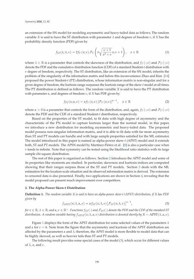
Symmetry 2020, 12, 82

an extension of the SN model for modeling asymmetric and heavy-tailed data as follows; The randomvariable X is said to have the ST distribution with parameter λ and degrees of freedom ν, if X has theprobability density function (PDF) given by

fST(x; λ, ν) = 2 fT (x; ν)FT

(λ

√ν + 1x2 + ν

x; ν + 1

), x ∈ R (1)

where λ ∈ R is a parameter that controls the skewness of the distribution, and fT (·; ν) and FT (·; ν)

denote the PDF and the cumulative distribution function (CDF) of a standard Student-t distribution withν degree of freedom, respectively. The ST distribution, like an extension of the SN model, inherits theproblem of the singularity of the information matrix and before this inconvenience Zhao and Kim [14]proposed the power Student-t (PT) distribution, whose information matrix is non-singular and for agiven degree of freedom, the kurtosis range surpasses the kurtosis range of the skew-t model at all times.The PT distribution is defined as follows. The random variable X is said to have the PT distributionwith parameter α, and degrees of freedom ν, if X has PDF given by

fPT(x; α, ν) = α fT (x; ν) [FT (x; ν)]α−1 , x ∈ R (2)

where α > 0 is a parameter that controls the form of the distribution, and, again, fT (·; ν) and FT (·; ν)

denote the PDF and the CDF of a standard Student-t distribution, respectively.Based on the properties of the ST model, to fit data with high degree of asymmetry and the

characteristic of the PN model to capture kurtosis larger than the normal model, in this paper,we introduce a new distribution for modeling asymmetric and heavy-tailed data. The proposedmodel possess non-singular information matrix, and it is able to fit data with far more asymmetrythan ST and PT models can handle and with large sample properties satisfied for the ML estimator.The model introduced in this paper is named as alpha-power skew-t (APST) model and it extendsboth, ST and PT models. The APSN model by Martínez-Flórez et al. [8] is also a particular case whenν tends to infinite. Note that symmetry can be tested using the likelihood ratio statistics with its largesample chi-square distribution.

The rest of this paper is organized as follows. Section 2 introduces the APST model and some ofits properties like moments are studied. In particular, skewness and kurtosis indices are computedshowing that their ranges surpass those of the ST and PT models. Section 3 deals with the MLestimation for the location-scale situation and its observed information matrix is derived. The extensionto censored data is also presented. Finally, two applications are shown in Section 4, revealing that themodel proposed can present much improvement over competitors.

2. The Alpha-Power Skew-t Distribution

Definition 1. The random variable X is said to have an alpha-power skew-t (APST) distribution, if X has PDFgiven by

fAPST(x; λ, α, ν) = α fST(x; λ, ν)[FST(x; λ, ν)

]α−1, (3)

for x ∈ R, λ ∈ R, and α, ν ∈ R+. Functions fST(·) andFST(·) denote the PDF and the CDF of the standard STdistribution. A random variable having fAPST(x; λ, α, ν) distribution is denoted shortly by X ∼ APST(λ, α, ν).

Figure 1 displays the form of the APST distribution for some selected values of the parameters λ

and α for ν = 6. Note from the figure that the asymmetry and kurtosis of the APST distribution areaffected by the parameters α and λ; therefore, the APST model is more flexible to model data that canbe highly skewed, as well as heavier tails than ST and PT models.

The following result provides some special cases of the model (3), which occur for different valuesof λ, α, and ν.

196

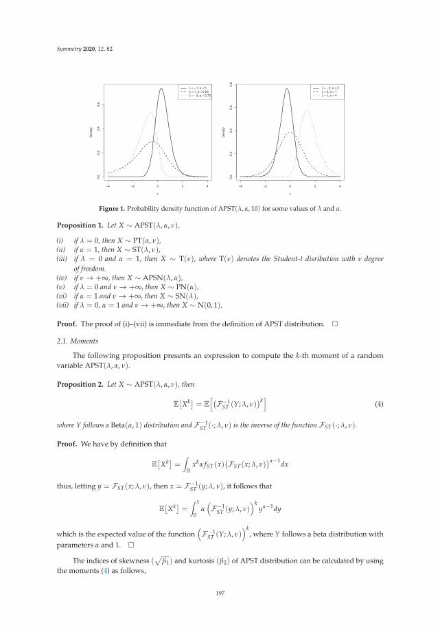
Symmetry 2020, 12, 82

−4 −2 0 2 4

0.0

0.2

0.4

0.6

x

Den

sity

λ = − 1, α = 5λ = 1, α = 0.25λ = − 3, α = 0.75

−4 −2 0 2 4

0.0

0.2

0.4

0.6

0.8

x

Den

sity

λ = − 2, α = 2λ = 0, α = 1λ = 1, α = 4

Figure 1. Probability density function of APST(λ, α, 10) for some values of λ and α.

Proposition 1. Let X ∼ APST(λ, α, ν),

(i) if λ = 0, then X ∼ PT(α, ν),(ii) if α = 1, then X ∼ ST(λ, ν),(iii) if λ = 0 and α = 1, then X ∼ T(ν), where T(ν) denotes the Student-t disribution with ν degree

of freedom.(iv) if ν → +∞, then X ∼ APSN(λ, α),(v) if λ = 0 and ν → +∞, then X ∼ PN(α),(vi) if α = 1 and ν → +∞, then X ∼ SN(λ),(vii) if λ = 0, α = 1 and ν → +∞, then X ∼ N(0, 1),

Proof. The proof of (i)–(vii) is immediate from the definition of APST distribution.

2.1. Moments

The following proposition presents an expression to compute the k-th moment of a randomvariable APST(λ, α, ν).

Proposition 2. Let X ∼ APST(λ, α, ν), then

E[Xk] = E

[(F−1

ST (Y; λ, ν))k]

(4)

where Y follows a Beta(α, 1) distribution and F−1ST (·; λ, ν) is the inverse of the function FST(·; λ, ν).

Proof. We have by definition that

E[Xk] = ∫

R

xkα fST(x)(FST(x; λ, ν)

)α−1dx

thus, letting y = FST(x; λ, ν), then x = F−1ST (y; λ, ν), it follows that

E[Xk] = ∫ 1

0α(F−1

ST (y; λ, ν))k

yα−1dy

which is the expected value of the function(F−1

ST (Y; λ, ν))k

, where Y follows a beta distribution withparameters α and 1.

The indices of skewness (√

β1) and kurtosis (β2) of APST distribution can be calculated by usingthe moments (4) as follows,

197

Symmetry 2020, 12, 82

√β1 =

μ3 − 3μ1μ2 + 2μ31

(μ2 − μ21)

3/2and β2 =

μ4 − 4μ1μ3 + 6μ2μ21 − 3μ4

1(μ2 − μ2

1)2

where μk = E[Xk] for k = 1, . . . , 4. Table 1 presents the ranges of possible values for the indices ofasymmetry and kurtosis for ST(λ, ν), PT(α, ν), and APST(λ, α, ν) distributions, for values of λ between−40 and 40, values of α between 0.5 and 50, and for values of ν = 2, 3, 4, 5, 6, 7. It can seen from Table 1that the length of the admissible intervals for the skewness and the kurtosis parameters of the APSTdistribution are larger than the corresponding intervals of the ST and PT distributions. This is an indicatorthat the APST model is more flexible in terms of asymmetry and kurtosis than the ST and PT models.

Table 1. Skewness and kurtosis for the models ST(λ, ν), PT(α, ν), and APST(λ, α, ν), for λ ∈ (−40, 40),α ∈ (0.5, 50) and ν = 2, . . . 7.

Skew−t Power−t Alpha−Power Skew−t

ν Skewness Kurtosis Skewness Kurtosis Skewness Kurtosis

2 (−0.963, 0.963) (3.170, 3.489) (−0.119, 3.040) (1.552, 10.436) (−2.452, 14.314) (1.395, 864.385)

3 (−0.950, 0.950) (3.146, 3.357) (−0.086, 1.362) (1.325, 3.223) (−2.130, 4.902) (1.628, 114.098)

4 (−1.853, 1.853) (5.099, 7.824) (−0.530, 1.178) (3.461, 5.299) (−1.898, 3.215) (3.153, 29.874)

5 (−0.947, 0.947) (3.051, 3.327) (−0.475, 0.271) (1.176, 3.130) (−1.968, 3.046) (3.862, 19.925)

6 (−1.681, 1.681) (4.554, 7.279) (−0.533, 1.118) (3.974, 5.173) (−1.681, 2.145) (3.892, 11.893)

7 (−0.944, 0.944) (3.007, 3.367) (−0.710, 0.243) (1.264, 3.082) (−1.535, 2.536) (3.136, 15.924)

2.2. Distribution Function

Proposition 3. Let X ∼ APST(λ, α, ν), then the CDF of X, namely, FAPST(x; λ, α, ν) is

FAPST(x; λ, α, ν) =[FST(x; λ, ν)

]α, x ∈ R. (5)

Proof. The proof is immediate and it follows from results of Durrans [2].

The inversion method can be used to generate a random variable with APST distribution.Thus, taking λ ∈ R, α, ν ∈ R+ and a random variable with uniform distribution, namely, U ∼ U(0, 1),random variable X with APST(λ, α, ν) distribution is generated by taking

X = F−1ST

(U1/α; λ, ν

).

Remark 1. We consider a truncated APST(λ, α) distribution to obtain a new and useful lifetime distribution.A random variable T has a truncated alpha-power skew-t distribution (at zero), denoted by TAPST(λ, α, ν), ifits PDF is given by

f (t) =α fST(t, λ, ν)

[FST(t, λ, ν)

]α−1

1−[FST(0, λ, ν)

]α ; t > 0 (6)

The survival and hazard rate functions of a random variable T following a TAPST(λ, α, ν) distribution aregiven by

ST(t) = P(T > t) =1−

[FST(0, λ, ν)

]α −[FST(t, λ, ν)

]α

1−[FST(0, λ, ν)

]α ; t > 0 (7)

and

hT(t) =α fST(t, λ, ν)

[fST(t, λ, ν)

]α−1

1−[FST(0, λ, ν)

]α −[FST(t, λ, ν)

]α ; t > 0 (8)

respectively.

198

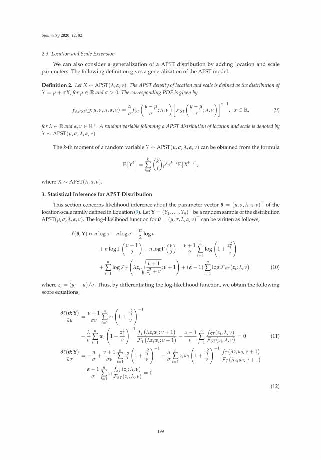
Symmetry 2020, 12, 82

2.3. Location and Scale Extension

We can also consider a generalization of a APST distribution by adding location and scaleparameters. The following definition gives a generalization of the APST model.

Definition 2. Let X ∼ APST(λ, α, ν). The APST density of location and scale is defined as the distribution ofY = μ + σX, for μ ∈ R and σ > 0. The corresponding PDF is given by

fAPST(y; μ, σ, λ, α, ν) =α

σfST

(y− μ

σ; λ, ν

)[FST

(y− μ

σ; λ, ν

)]α−1

, x ∈ R, (9)

for λ ∈ R and α, ν ∈ R+. A random variable following a APST distribution of location and scale is denoted byY ∼ APST(μ, σ, λ, α, ν).

The k-th moment of a random variable Y ∼ APST(μ, σ, λ, α, ν) can be obtained from the formula

E[Yk] = k

∑i=0

(ki

)μiσk−i

E[Xk−i],

where X ∼ APST(λ, α, ν).

3. Statistical Inference for APST Distribution

This section concerns likelihood inference about the parameter vector θ = (μ, σ, λ, α, ν)# of thelocation-scale family defined in Equation (9). Let Y = (Y1, . . . , Yn)# be a random sample of the distributionAPST(μ, σ, λ, α, ν). The log-likelihood function for θ = (μ, σ, λ, α, ν)# can be written as follows,

�(θ; Y) ∝ n log α− n log σ− n2

log ν

+ n log Γ(

ν + 12

)− n log Γ

(ν

2

)− ν + 1

2

n

∑i=1

log

(1 +

z2i

ν

)

+n

∑i=1

logFT

(λzi

√ν + 1z2

i + ν; ν + 1

)+ (α− 1)

n

∑i=1

logFST(zi; λ, ν

)(10)

where zi = (yi − μ)/σ. Thus, by differentiating the log-likelihood function, we obtain the followingscore equations,

∂�(θ; Y)

∂μ=

ν + 1σν

n

∑i=1

zi

(1 +

z2i

ν

)−1

− λ

σ

n

∑i=1

wi

(1 +

z2i

ν

)−1fT(λziwi; ν + 1

)FT

(λziwi; ν + 1

) − α− 1σ

n

∑i=1

fST(zi; λ, ν)

FST(zi; λ, ν)= 0 (11)

∂�(θ; Y)

∂σ= −n

σ+

ν + 1σν

n

∑i=1

z2i

(1 +

z2i

ν

)−1

− λ

σ

n

∑i=1

ziwi

(1 +

z2i

ν

)−1fT(λziwi; ν + 1

)FT

(λziwi; ν + 1

)− α− 1

σ

n

∑i=1

zifST(zi; λ, ν)

FST(zi; λ, ν)= 0

(12)

199

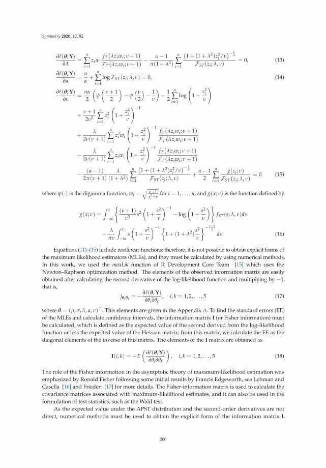
Symmetry 2020, 12, 82

∂�(θ; Y)

∂λ=

n

∑i=1

ziwifT(λziwi; ν + 1

)FT

(λziwi; ν + 1

) − α− 1π(1 + λ2)

n

∑i=1

(1 + (1 + λ2)z2

i /ν)− ν

2

FST(zi; λ, ν)= 0, (13)

∂�(θ; Y)

∂α=

nα+

n

∑i=1

logFST(zi; λ, ν) = 0, (14)

∂�(θ; Y)

∂ν=

nα

2

(ψ

(ν + 1

2

)− ψ

(ν

2

)− 1

ν

)− 1

2

n

∑i=1

log

(1 +

z2i

ν

)

+ν + 12ν2

n

∑i=1

z2i

(1 +

z2i

ν

)−1

+λ

2ν(ν + 1)

n

∑i=1

z3i wi

(1 +

z2i

ν

)−1fT(λziwi; ν + 1

)FT

(λziwi; ν + 1

)− λ

2ν(ν + 1)

n

∑i=1

ziwi

(1 +

z2i

ν

)−1fT(λziwi; ν + 1

)FT

(λziwi; ν + 1

)− (α− 1)

2π(ν + 1)λ

(1 + λ2)

n

∑i=1

(1 + (1 + λ2)z2

i /ν)− ν

2

FST(zi; λ, ν)+

α− 12

n

∑i=1

g(zi; ν)

FST(zi; λ, ν

) = 0 (15)

where ψ(·) is the digamma function, wi =√

ν+1x2

i +νfor i = 1, . . . , n, and g(x; ν) is the function defined by

g(x; ν) =∫ x

−∞

{(ν + 1)

ν2 s2(

1 +s2

ν

)−1

− log(

1 +s2

ν

)}fST(s; λ, ν)ds

− λ

πν

∫ x

−∞s(

1 +s2

ν

)−1 {1 + (1 + λ2)

s2

ν

}− ν+22

ds (16)

Equations (11)–(15) include nonlinear functions; therefore, it is not possible to obtain explicit forms ofthe maximum likelihood estimators (MLEs), and they must be calculated by using numerical methods.In this work, we used the maxLik function of R Development Core Team [15] which uses theNewton–Raphson optimization method. The elements of the observed information matrix are easilyobtained after calculating the second derivative of the log-likelihood function and multiplying by −1,that is,

jθiθk = −∂�(θ; Y)

∂θi∂θk, i, k = 1, 2, . . . , 5 (17)

where θ = (μ, σ, λ, α, ν)#. This elements are given in the Appendix A. To find the standard errors (EE)of the MLEs and calculate confidence intervals, the information matrix I (or Fisher information) mustbe calculated, which is defined as the expected value of the second derived from the log-likelihoodfunction or less the expected value of the Hessian matrix; from this matrix, we calculate the EE as thediagonal elements of the inverse of this matrix. The elements of the I matrix are obtained as

I(i, k) = −E(

∂�(θ; Y)

∂θi∂θk

), i, k = 1, 2, . . . , 5 (18)

The role of the Fisher information in the asymptotic theory of maximum-likelihood estimation wasemphasized by Ronald Fisher following some initial results by Francis Edgeworth, see Lehman andCasella [16] and Frieden [17] for more details. The Fisher-information matrix is used to calculate thecovariance matrices associated with maximum-likelihood estimates, and it can also be used in theformulation of test statistics, such as the Wald test.

As the expected value under the APST distribution and the second-order derivatives are notdirect, numerical methods must be used to obtain the explicit form of the information matrix I.

200

Symmetry 2020, 12, 82

Therefore, we use the observed information matrix to calculate the standard errors in the rest of thedocument.

When ν tends to infinite the ST distribution converges to the SN distribution and we recall thatthe information matrix of a random variable X ∼ SN(μ, σ, λ) which is denoted by Iλ(ϕ), where ϕ =

(μ, σ, λ)#, is singular for λ = 0. Therefore, it is convenient to use a centered parameterization of the STdistribution proposed by Arellano-Valle and Azzalini [18].

The centered parameterization of the SN distribution was proposed as an alternative to the problemof singularity of the information matrix of the SN when λ = 0. Arellano-Valle and Azzalini [19] proposeda second representation of the SN by defining a new random variable X as

X = μ + σ

(Z−E[Z]√

Var[Z]

),

where μ ∈ R and σ > 0 are parameters of the random variable X and Z ∼ SN(λ). This representationis called centered parameterization, as E[X] = μ and Var[X] = σ2 and it is denoted by CSN(μ, σ, γ1),where −0.9953 < γ1 < 0.9953. Under the centered parameterization model, μ, σ, and γ1 =

√β1

represent the mean, the standard deviation and the skewness index of X, respectively. If Z ∼ SN(λ)

then E[Z] = bδ and Var[Z] = 1− (bδ)2, where b =√

2/π and δ = λ/√

1 + λ2; it has that the randomvariable X can be written as X = μ + σZ which has SN(λ1, λ2, λ) distribution, where

λ1 = μ− cσγ1/31 , λ2 = σ

√1 + c2γ2/3

1 , λ =cγ1/3

1√b2 + c2(b2 − 1)γ2/3

1

(19)

with c = {2/(4 − π)}1/3. Under this denomination, the information matrix can be written asIγ1 = D#IλD, where D is a matrix that represents the derivative of the parameters of the standardrepresentation (λ1, λ2 and λ) regarding to the new parameters (μ, σ and γ1). It also follows thatthe information matrix converges to a diagonal matrix Σ−1

c = diag(σ2, σ2/2, 6) when λ → 0.This guarantees the existence and uniqueness of the MLEs of λ1 and λ2 for each fixed value of λ.

Following this same line of thought, we suppose that Y follows the model (1) with locationparameter μ ∈ R and scale parameter σ > 0, that is,

fST(y; μ, σ, λ, ν) =2σ

fT

(y− μ

σ; ν

)FT

(λ

√ν + 1

Qy + ν

(y− μ

σ

); ν + 1

), y ∈ R (20)

where λ ∈ R and Qy = ((y− μ)/σ)2. This representation relates to the direct parameterization of theST distribution with parameter vector ρ = (μ, σ, λ, ν)#. It follows that ZT = (Y − μ)/σ ∼ ST(λ, ν),and by the stochastic representation of the ST distribution is given by ZT = Z/

√V, where Z ∼ SN(λ)

and V ∼ χ2ν/ν. This entails to compute the first four cumulants of ZT denoted by μ1(δ, ν), μ2(δ, ν),

μ3(δ, ν) and μ4(δ, ν), see [18]. The centered parameterization of the ST distribution of a randomvariable Y comes by defining

μt = E[Y] = μ + σμ1(δ, ν) = μ + σbνδ

σ2t = Var[Y] = σ2μ2(δ, ν) = η2

{ν

ν− 2− b2

νδ2}

,

201

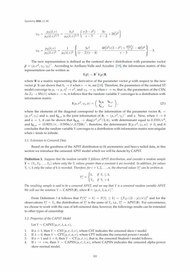
Symmetry 2020, 12, 82

γ1t =μ3(δ, ν)

μ2(δ, ν)3/2 =bνδ

μ2(δ, ν)3/2

{ν(3− δ2)

ν− 3− 3ν

ν− 2+ 2b2

νδ2}

γ2t =μ4(δ, ν)

μ2(δ, ν)2 =1

μ2(δ, ν)2

⎧⎨⎩ 3ν2

(ν− 2)(ν− 4)−

4b2νδ2ν(3− δ2) + 6b2

νδ2νν−2 − 4b4

νδ4

ν− 3

⎫⎬⎭− 3.

The new representation is defined as the centered skew-t distribution with parameter vectorρ = (μ, σ2, γ1, γ2)

#. According to Arellano-Valle and Azzalini [18], the information matrix of thisrepresentation can be written as

I(ρ) = B#I(ρ)B,

where B is a matrix representing the derivative of the parameter vector ρ with respect to the newvector ρ. It can shown that bν → b when ν → ∞, see [18]. Therefore, the parameters of the centered STmodel converge to μt → μ, σ2

t → σ2, and γ1t → γ1 when ν → ∞, that is, the parameters of the CSN.As ZT → SN(λ) when ν → ∞, it follows that the random variable Y converges to a distribution withinformation matrix

I(μ, σ2, γ1, α) =

(Iθ1θ1 Iθ1,αI#θ1,α Iα,α

), (21)

where the elements of the diagonal correspond to the information of the parameter vector θ1 =

(μ, σ2, γ1) and α, and Iθ1,α is the joint information of θ1 = (μ, σ2, γ1)# and α. Now, when λ → 0

and α = 1, it can be shown that Iθ1θ1 → diag(σ2, σ2/2, 6), with determinant equal to 0.3333/σ4,and Iθ1,α = (0.9031/σ,−0.5956/σ, 0.7206)#; therefore, the determinant |I(μ, σ2, γ1, α)| �= 0, and itconcludes that the random variable Y converges to a distribution with information matrix non-singularwhen ν tends to infinite.

3.1. Extension to Censored Data

Based on the goodness of the APST distribution to fit asymmetric and heavy-tailed data, in thissection we introduce the censored APST model which we will be denote by CAPST.

Definition 3. Suppose that the random variable Y follows APST distribution, and consider a random sampleY = (Y1, Y2, . . . , Yn) where only the Yi values greater than a constant k are recorded. In addition, for valuesYi ≤ k only the value of k is recorded. Therefore, for i = 1, 2, . . . , n, the observed values Yo

i can be written as

Yoi =

{k, if Yi ≤ k,

Yi, if Yi > k.

The resulting sample is said to be a censored APST, and we say that Y is a censored random variable APST.We will use the notation Y ∼ CAPST(θ), where θ = (μ, σ, λ, α, ν)#.

From Definition 3 it follows that P(Yoi = k) = P(Yi ≤ k) = {FST ((k− μ)/σ)}α and for the

observations Yoi = Yi, the distribution of Yo

i is the same of Yi, i.e., Yoi ∼ APST(θ). For convenience,

we choose to work with the case of left-censored data; however, the followings results can be extendedto other types of censorship.

3.2. Properties of the CAPST Model

Let Y ∼ CAPST(μ, σ, λ, α, ν),

1. If α = 1, then Y ∼ CST(μ, σ, λ, ν), where CST indicates the censored skew-t model.2. If λ = 0, then Y ∼ CPT(μ, σ, α, ν), where CPT indicates the censored power-t model.3. If α = 1 and λ = 0, then Y ∼ CT(μ, σ, ν), that is, the censored Student-t model follows.4. If ν → +∞, then Y ∼ CAPSN(μ, σ, λ, α), where CAPSN indicates the censored alpha-power

skew-normal model.

202

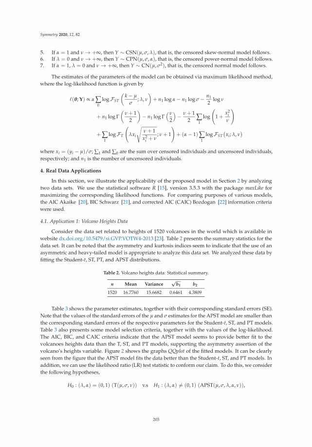
Symmetry 2020, 12, 82

5. If α = 1 and ν → +∞, then Y ∼ CSN(μ, σ, λ), that is, the censored skew-normal model follows.6. If λ = 0 and ν → +∞, then Y ∼ CPN(μ, σ, α), that is, the censored power-normal model follows.7. If α = 1, λ = 0 and ν → +∞, then Y ∼ CN(μ, σ2), that is, the censored normal model follows.

The estimates of the parameters of the model can be obtained via maximum likelihood method,where the log-likelihood function is given by

�(θ; Y) ∝ α ∑0

logFST

(k− μ

σ; λ, ν

)+ n1 log α− n1 log σ− n1

2log ν

+ n1 log Γ(

ν + 12

)− n1 log Γ

(ν

2

)− ν + 1

2 ∑1

log

(1 +

x2i

ν

)

+ ∑1

logFT

(λxi

√ν + 1x2

i + ν; ν + 1

)+ (α− 1)∑

1logFST

(xi; λ, ν

)where xi = (yi − μ)/σ; ∑1 and ∑0 are the sum over censored individuals and uncensored individuals,respectively; and n1 is the number of uncensored individuals.

4. Real Data Applications

In this section, we illustrate the applicability of the proposed model in Section 2 by analyzingtwo data sets. We use the statistical software R [15], version 3.5.3 with the package maxLike formaximizing the corresponding likelihood functions. For comparing purposes of various models,the AIC Akaike [20], BIC Schwarz [21], and corrected AIC (CAIC) Bozdogan [22] information criteriawere used.

4.1. Application 1: Volcano Heights Data

Consider the data set related to heights of 1520 volcanoes in the world which is available inwebsite dx.doi.org/10.5479/si.GVP.VOTW4-2013 [23]. Table 2 presents the summary statistics for thedata set. It can be noted that the asymmetry and kurtosis indices seem to indicate that the use of anasymmetric and heavy-tailed model is appropriate to analyze this data set. We analyzed these data byfitting the Student-t, ST, PT, and APST distributions.

Table 2. Volcano heights data: Statistical summary.

n Mean Variance√

b1 b2

1520 16.7760 15.6682 0.6461 4.3809

Table 3 shows the parameter estimates, together with their corresponding standard errors (SE).Note that the values of the standard errors of the μ and σ estimates for the APST model are smaller thanthe corresponding standard errors of the respective parameters for the Student-t, ST, and PT models.Table 3 also presents some model selection criteria, together with the values of the log-likelihood.The AIC, BIC, and CAIC criteria indicate that the APST model seems to provide better fit to thevolcanoes heights data than the T, ST, and PT models, supporting the asymmetry assertion of thevolcano’s heights variable. Figure 2 shows the graphs QQplot of the fitted models. It can be clearlyseen from the figure that the APST model fits the data better than the Student-t, ST, and PT models. Inaddition, we can use the likelihood ratio (LR) test statistic to conform our claim. To do this, we considerthe following hypotheses,

H0 : (λ, α) = (0, 1) (T(μ, σ, ν)) v.s H1 : (λ, α) �= (0, 1) (APST(μ, σ, λ, α, ν)),

203

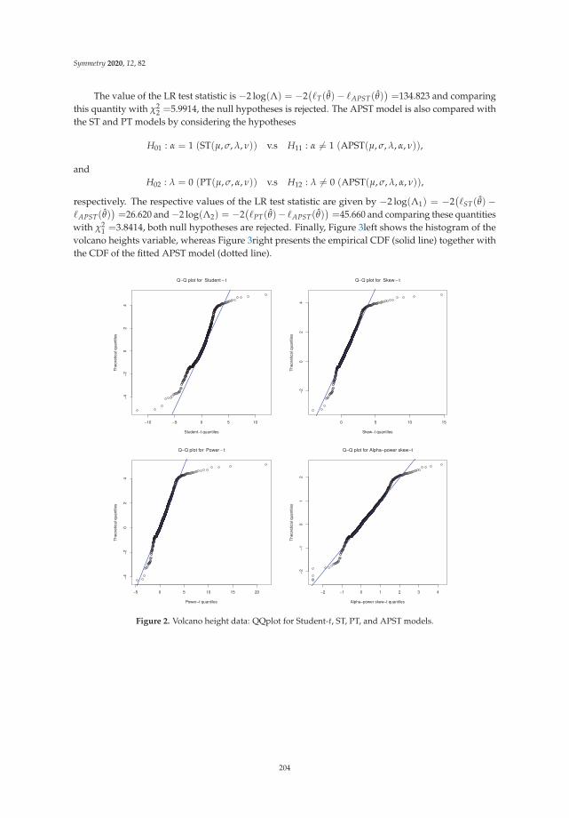
Symmetry 2020, 12, 82

The value of the LR test statistic is −2 log(Λ) = −2(�T(θ)− �APST(θ)

)=134.823 and comparing

this quantity with χ22 =5.9914, the null hypotheses is rejected. The APST model is also compared with

the ST and PT models by considering the hypotheses

H01 : α = 1 (ST(μ, σ, λ, ν)) v.s H11 : α �= 1 (APST(μ, σ, λ, α, ν)),

andH02 : λ = 0 (PT(μ, σ, α, ν)) v.s H12 : λ �= 0 (APST(μ, σ, λ, α, ν)),

respectively. The respective values of the LR test statistic are given by −2 log(Λ1) = −2(�ST(θ)−

�APST(θ))=26.620 and−2 log(Λ2) = −2

(�PT(θ)− �APST(θ)

)=45.660 and comparing these quantities

with χ21 =3.8414, both null hypotheses are rejected. Finally, Figure 3left shows the histogram of the

volcano heights variable, whereas Figure 3right presents the empirical CDF (solid line) together withthe CDF of the fitted APST model (dotted line).

−10 −5 0 5 10

−4

−2

02

4

Q−Q plot for Student − t

Student−t quantiles

The

oret

ical

qua

ntile

s

0 5 10 15

−2

02

4

Q−Q plot for Skew − t

Skew−t quantiles

The

oret

ical

qua

ntile

s

−5 0 5 10 15 20

−4

−2

02

4

Q−Q plot for Power − t

Power−t quantiles

The

oret

ical

qua

ntile

s

−2 −1 0 1 2 3 4

−2

−1

01

2

Q−Q plot for Alpha−power skew−t

Alpha−power skew−t quantiles

The

oret

ical

qua

ntile

s

Figure 2. Volcano height data: QQplot for Student-t, ST, PT, and APST models.

204

Symmetry 2020, 12, 82

y

Den

sity

−40 −20 0 20 40 60

0.00

0.01

0.02

0.03

0.04 Student−t

STPTAPST

−40 −20 0 20 40 60 80

0.0

0.2

0.4

0.6

0.8

1.0

y

Fn(

y)

Empirical CDFFitted CDF

Figure 3. (Left) Graph of fitted densities to volcano height data. (Right) Empirical CDF and CDF offitted APST model.

Table 3. Parameter estimates (SE) for the fitted models to the volcano height data.

Distribution

Estimates Student-t ST PT APST

μ 14.7835(0.3615 ) 4.7469(0.6892) 8.4027(0.7923) 11.5509(0.1337)σ 11.0045(0.3975) 14.1532(0.7237) 11.8146(0.4707) 22.6885(0.0792)λ – 1.5673(0.1838) – 5.2347(0.2870)α – – 1.7912(0.1147) 0.3205(0.0347)ν 3.4156(0.3601) 3.4075(0.3454) 2.7473(0.2566) 12.8734(2.9729)� −6273.35 −6219.25 −6228.77 −6205.94AIC 12,552.70 12,446.49 12,465.53 12,421.87BIC 12,568.68 12,467.79 12,486.53 12,448.50CAIC 12,571.68 12,471.79 12,490.83 12,453.50

4.2. Application 2: Stellar Abundances Data

The second data set is related to measurements for 68 solar-type stars, which are availablein the package astrodatR of the software R [24] under the name Stellar abundances. These data werepreviously analyzed Mattos et al. [25] by using the Scale Mixture of Skew Normal Censored Regression(SMSNCR) models. We take only the response variable: log N(Be), which represents the log of theabundance of beryllium scaled to Sun’s abundance (i.e., the Sun has log N(Be) = 0.0)

In astronomical research, a previously identified sample of objects (stars, galaxies, quasars, X-raysources, etc.) is observed at some new wavebands. According to Feigelson [24], due to limitedsensitivities, some objects may be undetected, leading to upper limits in their derived luminosities.For this dataset we have 12 left-censored data points, i.e., 12 undetected beryllium measurement,that represents 19.35% of observations. Table 4 presents the ML estimates for the parameters of thecensored Studen-t (CT), censored skew-t (CST), censored power-t (CPT), and censored alpha-powerskew-t (CAPST) models, together with their corresponding standard errors. Table 4 also comparesthe fit of the four models using the model selection criteria (AIC, CAIC and BIC). Note that, again,the CAPST model with heavy tails have better fit than the CT, CST, and CPT models.

To identify atypical observations and/or model mispecification, we analyzed the transformationof the martingale residual, rMTi , proposed in Barros et al. [26]. These residuals are defined by

rMTi = sign(rMi)√−2[rMi + δi log(δi − rMi )], i = 1, . . . , n

where rMi = δi + log S(yi; θ) is the martingal residual proposed by Ortega et al. [27], where δi = 0, 1indicates whether the i-th observation is censored or not, respectively; sign(rMi) denotes the sign of

205

Symmetry 2020, 12, 82

rMi; and S(yi; θ) = Pθ(Yi > yi) represents the survival function evaluated at yi, where θ are the MLEfor θ. The plots of rMTi with generated confidence envelopes are presented in Figure 4. From thisfigure, we can see clearly that the CST, CPT, and CAPST models fit better the data than the CT model,since, in that cases, there are not observations which lie outside the envelopes. The Figure 5 shows thegraph of the densities of the different models fitted to the stellar abundances data. From the figure, theCAPST model seems to fit better the stellar abundances data than CT, CST and CPT models.

Table 4. Parameter estimates (SE) for the fitted models to the stellar abundances data.

Distribution

Estimates CT CST CPT CAPST

μ 1.0314(0.0010) 1.2306(0.0018) 1.2098(0.0052) 1.1761(0.0054)σ 0.1596(0.0012) 0.2712(0.0058) 0.0818(0.0008) 0.0905(0.0020)λ – −3.5655(3.7748) – 0.6580(0.5031)α – – 0.1705(0.0208) 0.1518(0.0251)ν 0.9974(0.0884) 1.2501(0.1774) 6.0927(0.7501) 6.0999(0.7326)� −29.50743 −18.87016 −17.67113 −14.80241AIC 65.01487 45.74033 43.34227 39.60482BIC 71.67339 54.61836 52.22030 50.70236CAIC 59.38987 38.37525 35.97719 30.57256

Censored Studen − t

Standard normal quantile

r MT

i

−2 −1 0 1 2

−0.

50.

00.

51.

01.

5

Censored Skew − t

Standard normal quantile

r MT

i

−2 −1 0 1 2

−1.

5−

1.0

−0.

50.

00.

51.

01.

5

Censored Power − t

Standard normal quantile

r MT

i

−2 −1 0 1 2

−2.

0−

1.5

−1.

0−

0.5

0.0

0.5

1.0

Censored Alpha − power skew − t

Standard normal quantile

r MT

i

−2 −1 0 1 2

−2.

0−

1.5

−1.

0−

0.5

0.0

0.5

1.0

Figure 4. Stellar abundances data. Envelopes of transformed martingale residuals for CT, CST, CPT,and CAPST models.

206

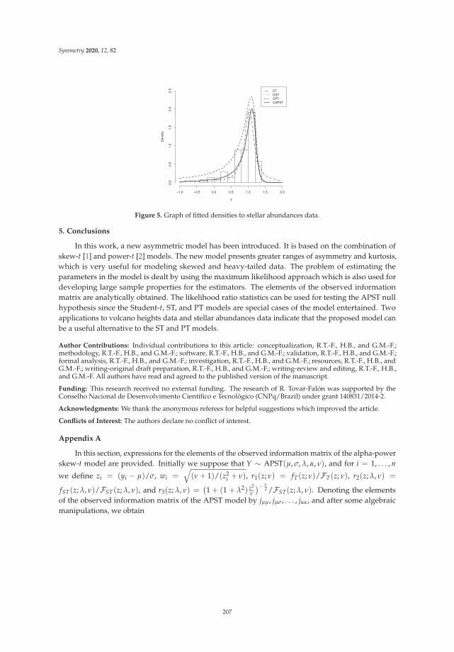
Symmetry 2020, 12, 82

Y

Den

sity

−1.0 −0.5 0.0 0.5 1.0 1.5 2.0

0.0

0.5

1.0

1.5

2.0

2.5 CT

CSTCPTCAPST

Figure 5. Graph of fitted densities to stellar abundances data.

5. Conclusions

In this work, a new asymmetric model has been introduced. It is based on the combination ofskew-t [1] and power-t [2] models. The new model presents greater ranges of asymmetry and kurtosis,which is very useful for modeling skewed and heavy-tailed data. The problem of estimating theparameters in the model is dealt by using the maximum likelihood approach which is also used fordeveloping large sample properties for the estimators. The elements of the observed informationmatrix are analytically obtained. The likelihood ratio statistics can be used for testing the APST nullhypothesis since the Student-t, ST, and PT models are special cases of the model entertained. Twoapplications to volcano heights data and stellar abundances data indicate that the proposed model canbe a useful alternative to the ST and PT models.

Author Contributions: Individual contributions to this article: conceptualization, R.T.-F., H.B., and G.M.-F.;methodology, R.T.-F., H.B., and G.M.-F.; software, R.T.-F., H.B., and G.M.-F.; validation, R.T.-F., H.B., and G.M.-F.;formal analysis, R.T.-F., H.B., and G.M.-F.; investigation, R.T.-F., H.B., and G.M.-F.; resources, R.T.-F., H.B., andG.M.-F.; writing-original draft preparation, R.T.-F., H.B., and G.M.-F.; writing-review and editing, R.T.-F., H.B.,and G.M.-F. All authors have read and agreed to the published version of the manuscript.

Funding: This research received no external funding. The research of R. Tovar-Falón was supported by theConselho Nacional de Desenvolvimento Científico e Tecnológico (CNPq/Brazil) under grant 140831/2014-2.

Acknowledgments: We thank the anonymous referees for helpful suggestions which improved the article.

Conflicts of Interest: The authors declare no conflict of interest.

Appendix A

In this section, expressions for the elements of the observed information matrix of the alpha-powerskew-t model are provided. Initially we suppose that Y ∼ APST(μ, σ, λ, α, ν), and for i = 1, . . . , n

we define zi = (yi − μ)/σ, wi =√(ν + 1)/(z2

i + ν), r1(z; ν) = fT(z; ν)/FT(z; ν), r2(z; λ, ν) =

fST(z; λ, ν)/FST(z; λ, ν), and r3(z; λ, ν) =(1 + (1 + λ2) z2

ν

)− ν2 /FST(z; λ, ν). Denoting the elements

of the observed information matrix of the APST model by jμμ, jμσ, . . . , jαα, and after some algebraicmanipulations, we obtain

207

Symmetry 2020, 12, 82

jμμ =− 1σ2

ν + 1ν2

n

∑i=1

z2i

(1 +

z2i

ν

)−2+

1σ2

ν + 1ν

n

∑i=1

(1 +

z2i

ν

)−2

+λ

σ2

n

∑i=1

ziwi

(1 +

z2i

ν

)−1r1(λziwi; ν + 1)

+2σ2

λ

ν

n

∑i=1

ziwi

(1 +

z2i

ν

)−2r1(λziwi; ν + 1)

+λ3

σ2ν + 2

ν

n

∑i=1

ziwi

(1 +

z2i

ν

)−2(1 +

(1 + λ2) z2

iν

)−1r1(λziwi; ν + 1)

+λ2

σ2ν + 1

ν

n

∑i=1

(1 +

z2i

ν

)−3[r1(λziwi; ν + 1)

]2

jμσ =− λ

σ2α− 1

π

n

∑i=1

(1 +

z2i

ν

)−1(1 +

(1 + λ2) z2

iν

)−1r3(zi; λ, ν)

+α− 1

σ2ν + 1

ν

n

∑i=1

zi

(1 +

z2i

ν

)−1r2(zi; λ, ν) +

α− 1σ2

n

∑i=1

[r2(zi; λ, ν)

]2

2σ2

ν + 1ν

n

∑i=1

zi

(1 +

z2i

ν

)−2

+λ3

σ2ν + 2

ν

n

∑i=1

z2i wi

(1 +

z2i

ν

)−2(1 +

(1 + λ2) z2

iν

)−1r1(λziwi; ν + 1)

+2σ2

λ

ν

n

∑i=1

z2i wi

(1 +

z2i

ν

)−2r1(λziwi; ν + 1)

− λ

σ2

n

∑i=1

wi

(1 +

z2i

ν

)−2r1(λziwi; ν + 1)

+λ2

σ2ν + 1

ν

n

∑i=1

zi

(1 +

z2i

ν

)−3[r1(λziwi; ν + 1)

]2

− λ

σ2α− 1

π

n

∑i=1

zi

(1 +

z2i

ν

)−1(1 +

(1 + λ2) z2

iν

)−1r3(zi; λ, ν)

− α− 1σ2

n

∑i=1

r2(zi; λ, ν) +α− 1

σ2ν + 1

ν

n

∑i=1

z2i

(1 +

z2i

ν

)−1r2(zi; λ, ν)

+α− 1

σ2

n

∑i=1

zi[r2(zi; λ, ν)

]2

208

Symmetry 2020, 12, 82

jμλ =− λ2

σ

ν + 2ν

n

∑i=1

z2i wi

(1 +

z2i

ν

)−1(1 +

(1 + λ2) z2

iν

)−1r1(λziwi; ν + 1)

+1σ

n

∑i=1

wi

(1 +

z2i

ν

)−1r1(λziwi; ν + 1)

− λ

σ

ν + 1ν

n

∑i=1

zi

(1 +

z2i

ν

)−2[r1(λziwi; ν + 1)

]2

+α− 1πσ

n

∑i=1

z2i

(1 +

z2i

ν

)−1r3(zi; λ, ν)

+α− 1πσ

11 + λ2

n

∑i=1

r2(zi; λ, ν)r3(zi; λ, ν)

jμα =1σ

n

∑i=1

r2(zi; λ, ν)

jμν =− 1σν

n

∑i=1

zi

(1 +

z2i

ν

)−1+

ν + 1σν2

n

∑i=1

zi

(1 +

z2i

ν

)−2

+λ

σν2

n

∑i=1

z2i wi

(1 +

z2i

ν

)−2r1(λziwi; ν + 1)

+λ

2σ

1ν(ν + 1)

n

∑i=1

(z2i − 1)wi

(1 +

z2i

ν

)−2r1(λziwi; ν + 1)

+λ3

2σ

ν + 2ν2(ν + 1)

n

∑i=1

z2i (z

2i − 1)wi

(1 +

z2i

ν

)−2(1 +

(1 + λ2) z2

iν

)−1r1(λziwi; ν + 1)

− λ2

2σ

1ν2

n

∑i=1

zi(z2i − 1)

(1 +

z2i

ν

)−3[r1(λziwi; ν + 1)

]2

+λ

2πσ

α− 1ν + 1

n

∑i=1

zi

(1 +

(1 + λ2) z2

iν

)−1r3(zi; λ, ν)

+α− 1

2πσ(ν + 1)λ

1 + λ2

n

∑i=1

r2(zi; λ, ν)r3(zi; λ, ν) +α− 1

2σ

ν + 1ν2

n

∑i=1

z2i

(1 +

z2i

ν

)−1r2(zi; λ, ν)

− α− 12σ

n

∑i=1

log(

1 +z2

iν

)r2(zi; λ, ν)− α− 1

2σ

n

∑i=1

g(zi, ν)

FST(zi; λ, ν)r2(zi; λ, ν)

+λ

2πσ

α− 1ν

n

∑i=1

zi

(1 +

z2i

ν

)−1(1 +

(1 + λ2) z2

iν

)−1r3(zi; λ, ν)

209

Symmetry 2020, 12, 82

jσσ =− nσ2 +

1σ2

ν + 1ν

n

∑i=1

z2i

(1 +

z2i

ν

)−1+

2σ2

ν + 1ν

n

∑i=1

z2i

(1 +

z2i

ν

)−2

− 2λ

σ2

n

∑i=1

ziwi

(1 +

z2i

ν

)−2r1(λziwi; ν + 1)

− λ

σ2ν

n

∑i=1

z3i wi

(1 +

z2i

ν

)−2r1(λziwi; ν + 1)

+λ3

σ2ν + 2

ν

n

∑i=1

z3i wi

(1 +

z2i

ν

)−2(1 +

(1 + λ2) z2

iν

)−1r1(λziwi; ν + 1)

+λ2

σ2ν + 1

ν

n

∑i=1

z2i

(1 +

z2i

ν

)−3r1(λziwi; ν + 1)

− λ

σ2α− 1

π

n

∑i=1

z2i

(1 +

z2i

ν

)−1(1 +

(1 + λ2) z2

iν

)−1r3(zi; λ, ν)

− 2(α− 1)σ2

n

∑i=1

zir2(zi; λ, ν)− α− 1σ2

ν + 1ν

n

∑i=1

z3i

(1 +

z2i

ν

)−1r2(zi; λ, ν)

+α− 1

σ2

n

∑i=1

z2i r2(zi; λ, ν)

jσλ =1σ

n

∑i=1

ziwi

(1 +

z2i

ν

)−1r1(λziwi; ν + 1)

+λ2

σ

ν + 2ν

n

∑i=1

z3i wi

(1 +

z2i

ν

)−1(1 +

(1 + λ2) z2

iν

)−1r1(λziwi; ν + 1)

+λ

σ

ν + 1ν

n

∑i=1

zi

(1 +

z2i

ν

)−2[r1(λziwi; ν + 1)

]2

− α− 1πσ

n

∑i=1

z2i

(1 +

z2i

ν

)−1r3(zi; λ, ν)

+α− 1πσ

11 + λ2

n

∑i=1

r2(zi; λ, ν)r3(zi; λ, ν)

jσα =1σ

n

∑i=1

zir2(zi; λ, ν)

210

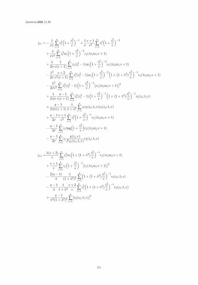
Symmetry 2020, 12, 82

jσν =− 1σν

n

∑i=1

z2i

(1 +

z2i

ν

)−1+

1σ

ν + 1ν2

n

∑i=1

z2i

(1 +

z2i

ν

)−2

+λ

σν2

n

∑i=1

z3i wi

(1 +

z2i

ν

)−2r1(λziwi; ν + 1)

+λ

2σ

1ν(ν + 1)

n

∑i=1

zi(z2i − 1)wi

(1 +

z2i

ν

)−2r1(λziwi; ν + 1)

− λ3

2σ

ν + 2ν2(ν + 1)

n

∑i=1

z3i (z

2i − 1)wi

(1 +

z2i

ν

)−2(1 +

(1 + λ2) z2

iν

)−1r1(λziwi; ν + 1)

− λ2

2σν2

n

∑i=1

z2i (z

2i − 1)

(1 +

z2i

ν

)−3[r1(λziwi; ν + 1)

]2

+λ

2πσ

α− 1ν(ν + 1)

n

∑i=1

z2i (z

2i − 1)

(1 +

z2i

ν

)−1(1 +

(1 + λ2) z2

iν

)−1r3(zi; λ, ν)

+α− 1

2πσ(ν + 1)λ

1 + λ2

n

∑i=1

zir2(zi; λ, ν)r3(zi; λ, ν)

+α− 1

2σ

ν + 1ν2

n

∑i=1

z3i

(1 +

z2i

ν

)−1r1(λziwi; ν + 1)

− α− 12σ

n

∑i=1

zi log(

1 +z2

iν

)r1(λziwi; ν + 1)

− α− 12σ

n

∑i=1

zig(zi, ν)

FST(zi, λ, ν)r2(zi; λ, ν)

jλλ =λ(ν + 2)

ν

n

∑i=1

z3i wi

(1 +

(1 + λ2) z2

iν

)−1r1(λziwi; ν + 1)

+ν + 1

ν

n

∑i=1

zi

(1 +

z2i

ν

)−1[r1(λziwi; ν + 1)

]2

− 2(α− 1)π

λ

(1 + λ2)2

n

∑i=1

(1 +

(1 + λ2) z2

iν

)−1r3(zi; λ, ν)

− α− 1π

λ

1 + λ2ν + 2

ν

n

∑i=1

z2i

(1 +

(1 + λ2) z2

iν

)−1r3(zi; λ, ν)

+α− 1

π2(1 + λ2)2

n

∑i=1

[r3(zi; λ, ν)

]2

211

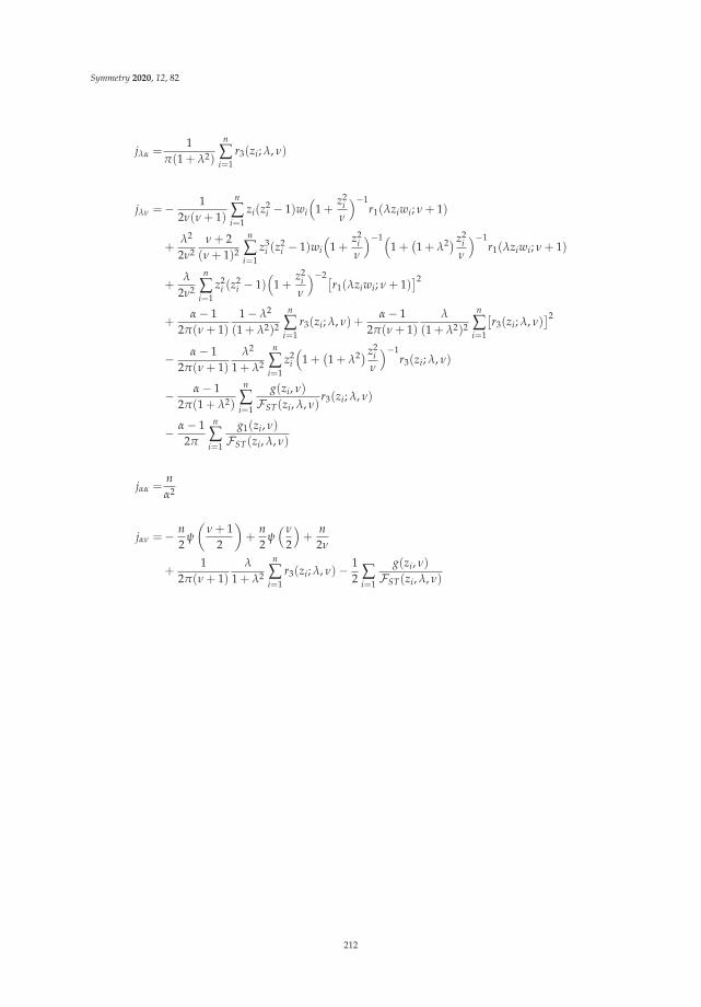
Symmetry 2020, 12, 82

jλα =1

π(1 + λ2)

n

∑i=1

r3(zi; λ, ν)

jλν =− 12ν(ν + 1)

n

∑i=1

zi(z2i − 1)wi

(1 +

z2i

ν

)−1r1(λziwi; ν + 1)

+λ2

2ν2ν + 2

(ν + 1)2

n

∑i=1

z3i (z

2i − 1)wi

(1 +

z2i

ν

)−1(1 +

(1 + λ2) z2

iν

)−1r1(λziwi; ν + 1)

+λ

2ν2

n

∑i=1

z2i (z

2i − 1)

(1 +

z2i

ν

)−2[r1(λziwi; ν + 1)

]2

+α− 1

2π(ν + 1)1− λ2

(1 + λ2)2

n

∑i=1

r3(zi; λ, ν) +α− 1

2π(ν + 1)λ

(1 + λ2)2

n

∑i=1

[r3(zi; λ, ν)

]2

− α− 12π(ν + 1)

λ2

1 + λ2

n

∑i=1

z2i

(1 +

(1 + λ2) z2

iν

)−1r3(zi; λ, ν)

− α− 12π(1 + λ2)

n

∑i=1

g(zi, ν)

FST(zi, λ, ν)r3(zi; λ, ν)

− α− 12π

n

∑i=1

g1(zi, ν)

FST(zi, λ, ν)

jαα =nα2

jαν =− n2

ψ

(ν + 1

2

)+

n2

ψ(ν

2

)+

n2ν

+1

2π(ν + 1)λ

1 + λ2

n

∑i=1

r3(zi; λ, ν)− 12 ∑

i=1

g(zi, ν)

FST(zi, λ, ν)

212

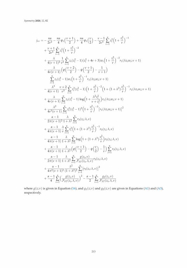
Symmetry 2020, 12, 82

jνν =− nα

2ν2 −nα

4ψ1

(ν + 12

)+

nα

4ψ1

(ν

2

)− ν− 1

2ν3

n

∑i=1

z2i

(1 +

z2i

ν

)−1

+ν + 12ν3

n

∑i=1

z2i

(1 +

z2i

ν

)−2

+λ

4(ν + 1)21ν2

n

∑i=1

zi(z2i − 1)(z2

i + 4ν + 3)wi

(1 +

z2i

ν

)−2r1(λziwi; ν + 1)

− λ

4ν(ν + 1)

(ψ(ν + 2

2

)− ψ

(ν + 12

)− 1

ν + 1

)n

∑i=1

zi(z2i − 1)wi

(1 +

z2i

ν

)−1r1(λziwi; ν + 1)

− λ3

4(ν + 1)ν + 2

ν3

n

∑i=1

z3i (z

2i − 1)

(1 +

z2i

ν

)−2(1 +

(1 + λ2) z2

iν

)−1r1(λziwi; ν + 1)

+λ

4ν(ν + 1)

n

∑i=1

zi(z2i − 1) log

(1 +

λ2z2i

ν + z2i

)r1(λziwi; ν + 1)

+λ2

4ν3(ν + 1)

n

∑i=1

z2i (z

2i − 1)2

(1 +

z2i

ν

)−3[r1(λziwi; ν + 1)

]2

− α− 12π(ν + 1)2

λ

1 + λ2

n

∑i=1

r3(zi; λ, ν)

+α− 1

4π(ν + 1)λ

ν

n

∑i=1

z2i

(1 +

(1 + λ2) z2

iν

)−1r3(zi; λ, ν)

− α− 14π(ν + 1)

λ

1 + λ2

n

∑i=1

log(

1 +(1 + λ2) z2

iν

)r3(zi; λ, ν)

+α− 1

4π(ν + 1)λ

1 + λ2

(ψ(ν + 1

2

)− ψ

(ν

2

)− 1

ν

) n

∑i=1

r3(zi; λ, ν)

− α− 12π(ν + 1)

λ

1 + λ2

n

∑i=1

g(zi, ν)

FST(zi, λ, ν)r3(zi; λ, ν)

+α− 1

4π2(ν + 1)2λ2

(1 + λ2)2

n

∑i=1

[r3(zi; λ, ν)

]2

+α− 1

4

n

∑i=1

( g(zi, ν)

FST(zi, λ, ν)

)2− α− 1

2

n

∑i=1

g2(zi, ν)

FST(zi, λ, ν)

where g(z; ν) is given in Equation (16), and g1(z; ν) and g2(z; ν) are given in Equations (A1) and (A3),respectively.

213

Symmetry 2020, 12, 82

g1(x; ν) =∫ x

−∞

{(ν + 1)s2

ν(s2 + ν)− log

(1 +

s2

ν

)}{1 +

(1 + λ2)s2

ν

}− ν+22

sds

−∫ x

−∞

ss2 + ν

{1 +

(1 + λ2)s2

ν

}− ν+22

ds

+∫ x

−∞

λ2(ν + 2)s3

(s2 + ν)(ν + (1 + λ2)s2)

{1 +

(1 + λ2)s2

ν

}− ν+22

ds (A1)

g2(x; ν) =∫ x

−∞

{s2(s2ν− 2ν− s2)

ν2(s2 + ν)2 +12

[(ν + 1)s2

ν(s2 + ν)− log

(1 +

s2

ν

)]2}fST(s; λ, ν)ds

+λ

2π(ν + 1)

∫ x

−∞

s(s2 − 1)(s2 + ν)

{(ν + 1)s2

ν(s2 + ν)− log

(1 +

s2

ν

)}

×{

1 +(1 + λ2)s2

ν

}− ν+22

ds

+λ

π

∫ x

−∞

s(s + ν)2

{1 +

(1 + λ2)s2

ν

}− ν+22

ds (A2)

+λ

2π

(ψ

(ν + 1

2

)− ψ

(ν

2

)− 1

ν

) ∫ x

−∞

ss2 + ν

{1 +

(1 + λ2)s2

ν

}− ν+22

ds

− λ

2π

∫ x

−∞

ss2 + ν

{(ν + 2)(1 + λ2)s2

ν(ν + (1 + λ2)s2)− log

(1 +

(1 + λ2)s2

ν

)}

×{

1 +(1 + λ2)s2

ν

}− ν+22

ds (A3)

References

1. Azzalini, A. A class of distributions which includes the normal ones. Scand. J. Stat. 1985, 12, 171–178.2. Durrans, S.R. Distributions of fractional order statistics in hydrology. Water Resour. Res. 1992, 28, 1649–1655.

[CrossRef]3. Martínez-Flórez, G.; Bolfarine, H.; Gómez, H.W. The alpha–power tobit model. Commun. Stat. Theory Methods

2013, 42, 633–643. [CrossRef]4. Birnbaum, Z.W.; Saunders, S.C. A new family of life distributions. J. Appl. Probab. 1969, 6, 319–327. [CrossRef]5. Martínez-Flórez, G.; Bolfarine, H.; Gómez, H.W. An alpha-power extension for the Birnbaum-Saunders

distribution. Statistics 2014, 48, 896–912. [CrossRef]6. Gupta, R.D.; Gupta, R.C. Analyzing skewed data by power-normal model. Test 2008, 17, 197–210. [CrossRef]7. Pewsey, A.; Gómez, H. W.; Bolfarine, H. Likelihood–based inference for power distributions. Test 2012, 21,

775–789. [CrossRef]8. Martínez-Flórez, G.; Bolfarine, H.; Gómez, H.W. Skew-normal alpha-power model. Stat. J. Theor. Appl. Stat.

2014, 48, 1414–1428. [CrossRef]9. Azzalini, A.; Capitanio, A. Distributions generated by perturbation of symmetry with emphasis on a

multivariate skew-t distribution. J. R. Stat. Soc. Ser. B (Stat. Methodol.) 2003, 65, 367–389. [CrossRef]10. Branco, M.D.; Dey, D.K. General class of multivariate skew-elliptical distributions. J. Multivar. Anal. 2001, 79,

99–113. [CrossRef]11. Durrans, S.R. Multivariate skew t-distribution. Stat. J. Theor. Appl. Stat. 2003, 37, 359–363.12. Sahu, S.K.; Dey, D.K.; Branco, M.D. A new class of multivariate skew distributions with applications to

Bayesian regression models. Can. J. Stat. 2003, 31, 129–150. [CrossRef]13. Jones, M.C.; Faddy, M.J. A skew extension of the t-distribution, with Applications. J. R. Stat. Soc. Ser. B

(Stat. Methodol.) 2003, 65, 159–174. [CrossRef]

214

Symmetry 2020, 12, 82

14. Zhao, J.; Kim, H.M. Power t distributions. Commun. Stat. Appl. Methods 2016, 23, 321–334.15. R Development Core Team. R: A Language and Environment for Statistical Computing; R Foundation for

Statistical Computing: Vienna, Austria, 2018. Available online: http://www.R-project.org (accessed on 10October 2019).

16. Lehman, E.L.; Casella, G. Theory of Point Estimation, 2nd ed.; Springer: New York, NY, USA, 1998.17. Frieden, B.R. Science from Fisher Information: A Unification; Cambridge Univerisity Press:

Cambridge, UK, 2004.18. Arellano-Valle, R.B.; Azzalini, A. The centered parameterization and related quantities of the

skew–t distribution. J. Multivar. Anal. 2013, 113, 73–90. [CrossRef]19. Arellano-Valle, R.B.; Azzalini, A. The centered parametrization for the multivariate skew-normal distribution.

J. Multivar. Anal. 2008, 99, 1362–1382. [CrossRef]20. Akaike, H. A new look at statistical model identification. IEEE Trans. Autom. Contr. 1974, 19, 716–722.

[CrossRef]21. Schwarz, G. Estimating the dimension of a model. Ann. Stat. 1978, 6, 461–464. [CrossRef]22. Bozdogan, H. Model selection and akaike’s information criterion (AIC): The general theory and its analytical

extensions. Psychometrika 2010, 52, 345–370. [CrossRef]23. Siebert, L.; Simkin, T.; Kimberly, P. Global Volcanism Program. In Volcanoes of the World; v. 4.6.0.;

Venzke, E., Ed.; Smithsonian Institution: Washington, DC, USA, 2013. Available online: https://doi.org/10.5479/si.GVP.VOTW4-2013 (accessed on 10 October 2019).

24. Feigelson, E.D. astrodatR: Astronomical Data. R Package v. 0.1. Available online: http://CRAN.R-project.org/package=astrodatR (accessed on 10 October 2019).

25. Mattos, T.; Garay, A.M.; Lachos, V.H. Likelihood-based inference for censored linear regression models withscale mixtures of skew-normal distributions. J. Appl. Stat. 2018, 45, 2019–2066. [CrossRef]

26. Barros, M.; Galea, M.; González, M.; Leiva, V. Influence diagnostics in the tobit censored response model.Stat. Methods Appl. 2010, 19, 379–397. [CrossRef]

27. Ortega, E.M.; Bolfarine, H.; Paula, G.A. Influence diagnostics in generalized log-gamma regression models.Comput. Stat. Data Anal. 2003, 42, 165–186. [CrossRef]

c© 2020 by the authors. Licensee MDPI, Basel, Switzerland. This article is an open accessarticle distributed under the terms and conditions of the Creative Commons Attribution(CC BY) license (http://creativecommons.org/licenses/by/4.0/).

215

symmetryS SArticle

A Test Detecting the Outliers for ContinuousDistributions Based on the Cumulative DistributionFunction of the Data Being Tested

Lorentz Jäntschi 1,2

1 Department of Physics and Chemistry, Technical University of Cluj-Napoca, 400641 Cluj, Romania;lorentz.jantschi@chem.utcluj.ro or lorentz.jantschi@gmail.com

2 Chemical Doctoral School, Babes, -Bolyai University, 400084 Cluj-Napoca, Romania

Received: 12 June 2019; Accepted: 24 June 2019; Published: 25 June 2019

Abstract: One of the pillars of experimental science is sampling. Based on the analysis of samples,estimations for populations are made. There is an entire science based on sampling. Distribution ofthe population, of the sample, and the connection among those two (including sampling distribution)provides rich information for any estimation to be made. Distributions are split into two main groups:continuous and discrete. The present study applies to continuous distributions. One of the challengesof sampling is its accuracy, or, in other words, how representative the sample is of the population fromwhich it was drawn. To answer this question, a series of statistics have been developed to measurethe agreement between the theoretical (the population) and observed (the sample) distributions.Another challenge, connected to this, is the presence of outliers - regarded here as observationswrongly collected, that is, not belonging to the population subjected to study. To detect outliers,a series of tests have been proposed, but mainly for normal (Gauss) distributions—the most frequentlyencountered distribution. The present study proposes a statistic (and a test) intended to be usedfor any continuous distribution to detect outliers by constructing the confidence interval for theextreme value in the sample, at a certain (preselected) risk of being in error, and depending on thesample size. The proposed statistic is operational for known distributions (with a known probabilitydensity function) and is also dependent on the statistical parameters of the population—here it isdiscussed in connection with estimating those parameters by the maximum likelihood estimationmethod operating on a uniform U(0,1) continuous symmetrical distribution.

Keywords: test for outliers; order statistics; extreme values; confidence intervals; Monte-Carlo simulation

1. Introduction

Many statistical techniques are sensitive to the presence of outliers and all calculations, includingthe mean and standard deviation can be distorted by a single grossly inaccurate data point. Therefore,checking for outliers should be a routine part of any data analysis.

To date, several tests have been developed for the purpose of identifying outliers of certaindistributions. Most of the studies are connected with the Normal (or Gauss) distribution [1]. The firstpaper that attracted attention on this matter is [2] and this was followed by studies that identified thederivation of the distribution of the extreme values in samples taken from Normal distributions [3].Then, a series of tests were developed by Thompson in 1935 [4], these were subjected to evaluation [5],and revised [6,7].

For other distributions such as the Gamma distribution, procedures for detecting outliers wereproposed [8], revised [9], and unfortunately proved to be inefficient [10].

The first attempt to generalize the criterion for detecting outliers for any distribution can be found in [11],but further research on this subject is scarce apart from a notable recent attempt by Bardet and Dimby [12].

Symmetry 2019, 11, 835; doi:10.3390/sym11060835 www.mdpi.com/journal/symmetry217

Symmetry 2019, 11, 835

The Grubbs test is a frequently used test for detecting the outliers of a Normal distribution [7].For a sample (x), the Grubbs’ test statistic takes the largest absolute deviation from the sample mean (x)in units of the sample standard deviation (s) in order to calculate the risk of being in error (αG) whenstating that the most departed values from the mean (min(x), max(x) or both) are not outliers (see Table 1).The associated probabilities of the observed (pG) are obtained from the Student t distribution [13].

Table 1. The Grubbs statistic.

Sample statistic (G) Associated probability (pG = 1-αG) Equation

G“min” =x−min(x)

s αG = n·CDF“Student t”

(−

√n(n−2)

( n−1G )

2−n, n− 2

)(1)

G“max” =max(x)−x

s

G“all” = max(G“min”, G“max”) αG = 2n·CDF“Student t”

(−

√n(n−2)

( n−1G )

2−n, n− 2

)(2)

One should note that the Grubbs test statistic produces a symmetrical confidence interval(see Equations (1) and (2)). The Grubbs statistic as given in Table 1, is intended to be used with theparameters of the population (μ and σ), which are determined using the central moments (CM) method

(μ = x =∑

x/n; σ = s = (∑(x− x)2)

1/2/n).

Here, a method is proposed for constructing the confidence intervals for the extreme values of anycontinuous distribution for which the cumulative distribution function is also obtainable. The methodinvolves the direct application of a simple test for detecting the outliers. The proposed method isbased on deriving the statistic for the extreme values for the uniform distribution. Also, the proposedmethod provides a symmetrical confidence interval in the probability space.

2. Materials and Methods

The Grubbs test (Table 1) is based on the fact that if outliers exist, then these are “localized” as themaximum value and/or the minimum value in the dataset. Thus, the Grubbs test is essentially a sort oforder statistic [14].

Some introductory elements are required for describing the proposed procedure. When a sampleof data is tested under the null hypothesis that it follows a certain distribution, it is intrinsicallyassumed that the distribution is known. The usual assumption is that we possess its probabilitydensity function (PDF, for a continuous distribution) or its probability distribution function (PDFfor a discrete distribution). The discussion below relates to continuous distributions, although thetreatment of discrete distributions are similar to certain degree. Nevertheless, a major distinctionbetween continuous and discrete distributions in the treatment of data is made here; that is, a continuousdistribution is “dense”, e.g., between any two distinct observations it is possible to observe anotherwhile in the case of a discrete distribution, this is generally not true.

Even when the PDF is known (possibly intrinsically), its (statistical) parameters may not necessarilybe known, and this raises the complex problem of estimating the parameters of the (population)distribution from the sample; however, this issue is outside the scope of this paper. In general,the estimation of the parameters of the distribution of the data is biased by the presence of theoutliers in the data, and thus, identifying the outliers along with the estimation of the parametersof the distribution is a difficult task because two statistical hypotheses are operating. Assumingthat the parameters (“parameters”) of the distribution (of the PDF) are obtained using the maximumlikelihood estimation method (MLE, Equation (3); see [15]), there is some suggestion that the uncertaintyaccompanying this estimation is transmitted to the process of detecting the outliers.∏

PDF(X; “parameters”)→ max. ⇒∑

ln (PDF(X; “parameters”))→ min. (3)

218

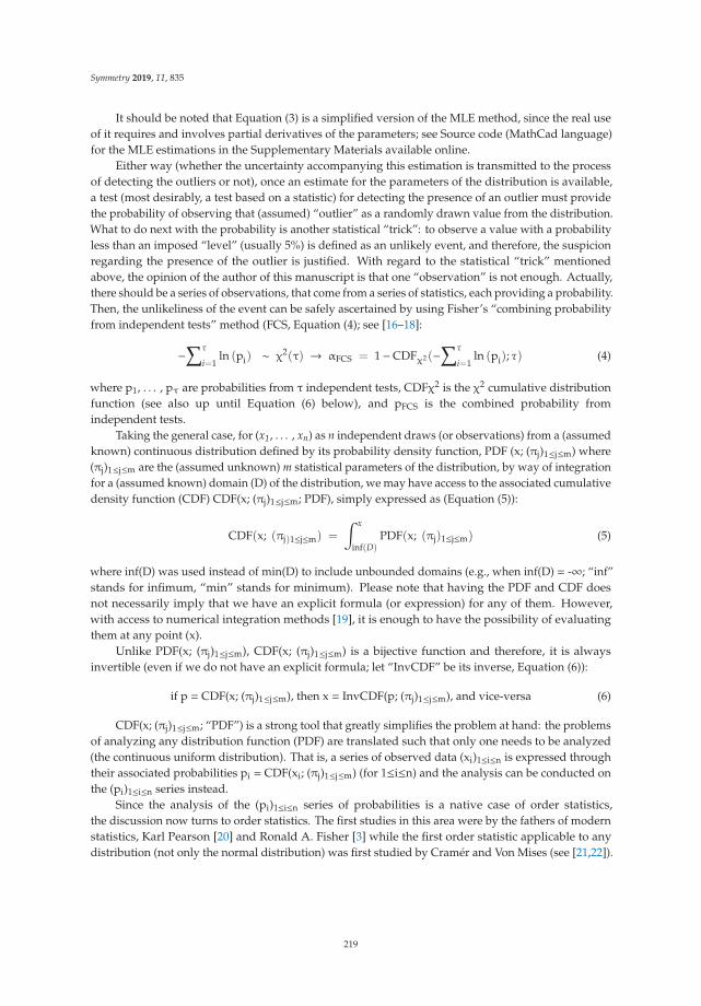
Symmetry 2019, 11, 835

It should be noted that Equation (3) is a simplified version of the MLE method, since the real useof it requires and involves partial derivatives of the parameters; see Source code (MathCad language)for the MLE estimations in the Supplementary Materials available online.

Either way (whether the uncertainty accompanying this estimation is transmitted to the processof detecting the outliers or not), once an estimate for the parameters of the distribution is available,a test (most desirably, a test based on a statistic) for detecting the presence of an outlier must providethe probability of observing that (assumed) “outlier” as a randomly drawn value from the distribution.What to do next with the probability is another statistical “trick”: to observe a value with a probabilityless than an imposed “level” (usually 5%) is defined as an unlikely event, and therefore, the suspicionregarding the presence of the outlier is justified. With regard to the statistical “trick” mentionedabove, the opinion of the author of this manuscript is that one “observation” is not enough. Actually,there should be a series of observations, that come from a series of statistics, each providing a probability.Then, the unlikeliness of the event can be safely ascertained by using Fisher’s “combining probabilityfrom independent tests” method (FCS, Equation (4); see [16–18]:

−∑τ

i=1ln (pi) ∼ χ2(τ) → αFCS = 1−CDFχ2(−

∑τ

i=1ln (pi); τ) (4)

where p1, . . . , pτ are probabilities from τ independent tests, CDFχ2 is the χ2 cumulative distributionfunction (see also up until Equation (6) below), and pFCS is the combined probability fromindependent tests.

Taking the general case, for (x1, . . . , xn) as n independent draws (or observations) from a (assumedknown) continuous distribution defined by its probability density function, PDF (x; (πj)1≤j≤m) where(πj)1≤j≤m are the (assumed unknown) m statistical parameters of the distribution, by way of integrationfor a (assumed known) domain (D) of the distribution, we may have access to the associated cumulativedensity function (CDF) CDF(x; (πj)1≤j≤m; PDF), simply expressed as (Equation (5)):

CDF(x; (πj)1≤j≤m) =

∫ x

inf(D)PDF(x; (πj)1≤j≤m) (5)

where inf(D) was used instead of min(D) to include unbounded domains (e.g., when inf(D) = -∞; “inf”stands for infimum, “min” stands for minimum). Please note that having the PDF and CDF doesnot necessarily imply that we have an explicit formula (or expression) for any of them. However,with access to numerical integration methods [19], it is enough to have the possibility of evaluatingthem at any point (x).

Unlike PDF(x; (πj)1≤j≤m), CDF(x; (πj)1≤j≤m) is a bijective function and therefore, it is alwaysinvertible (even if we do not have an explicit formula; let “InvCDF” be its inverse, Equation (6)):

if p = CDF(x; (πj)1≤j≤m), then x = InvCDF(p; (πj)1≤j≤m), and vice-versa (6)

CDF(x; (πj)1≤j≤m; “PDF”) is a strong tool that greatly simplifies the problem at hand: the problemsof analyzing any distribution function (PDF) are translated such that only one needs to be analyzed(the continuous uniform distribution). That is, a series of observed data (xi)1≤i≤n is expressed throughtheir associated probabilities pi = CDF(xi; (πj)1≤j≤m) (for 1≤i≤n) and the analysis can be conducted onthe (pi)1≤i≤n series instead.

Since the analysis of the (pi)1≤i≤n series of probabilities is a native case of order statistics,the discussion now turns to order statistics. The first studies in this area were by the fathers of modernstatistics, Karl Pearson [20] and Ronald A. Fisher [3] while the first order statistic applicable to anydistribution (not only the normal distribution) was first studied by Cramér and Von Mises (see [21,22]).

219

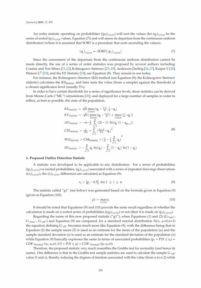
Symmetry 2019, 11, 835

An order statistic operating on probabilities ((pi)1≤i≤n) will sort the values (let (qi)1≤i≤n be theseries of sorted (pi)1≤i≤n values, Equation (7)) and will assess its departure from the continuous uniformdistribution (where it is assumed that SORT is a procedure that sorts ascending the values).

(qi)1≤i≤n ← SORT((pi)1≤i≤n) (7)

Since the assessment of the departure from the continuous uniform distribution cannot bemade directly, the use of a series of order statistics was proposed by several authors including:Cramér and Von Mises [21,22], Kolmogorov-Smirnov [23–25], Anderson-Darling [26,27], Kuiper V [28],Watson U2 [29], and the H1 Statistic [18]; see Equation (8). They remain in use today.

For instance, the Kolmogorov-Smirnov (KS) method (see Equation (8); the Kolmogorov-Smirnovstatistic) calculates the KSStatistic and later tests the value (from a sample) against the threshold ofa chosen significance level (usually 5%).

In order to have certain thresholds for a series of significance levels, these statistics can be derivedfrom Monte-Carlo (“MC”) simulations [30], and deployed for a large number of samples in order toreflect, as best as possible, the state of the population.

KSStatistic =√

n·max1≤i≤n

(qi − i−1n , i

n−qi)

KVStatistic =√

n·(max1≤i≤n

(qi − i−1n ) + max

1≤i≤n( i

n−qi))

ADStatistic = −n− 1n ·

n∑i=1

(2i− 1)· ln(qi·(1− qn−i))

CMStatistic =1

12n +n∑

i=1( 2·i−1

2·n −qi)2

WUStatistic = CMStatistic + ( 12 − 1

n

n∑i=1

qi)2

H1Statistic = −n∑

i=1qi· ln(qi) −

n∑i=1

(1− qi)· ln(1− qi)

(8)

3. Proposed Outlier Detection Statistic

A statistic was developed to be applicable to any distribution. For a series of probabilities((pi)1≤i≤n) or (sorted probabilities, (qi)1≤i≤n) associated with a series of (repeated drawing) observations((xi)1≤i≤n), the (ri)1≤i≤n differences are calculated as Equation (9):

ri =∣∣∣pi − 0.5

∣∣∣, for 1 ≤ i ≤ n (9)

The statistic called “g1” (see below) was generated based on the formula given in Equation (9)(given as Equation (10)).

g1 = max1≤i≤n

ri (10)

It should be noted that Equations (9) and (10) provide the same result regardless of whether thecalculation is made on a sorted series of probabilities ((qi)1≤i≤n) or not (then it is made on (pi)1≤i≤n).

Regarding the name of this new proposed statistic (“g1”), when Equations (1) and (2) (G“min”,G“max”, G“all”) and Equation (9) are compared, for a standard normal distribution N(x; μ=0,σ=1)the equation defining G“all” becomes much more like Equation (9), with the difference being that inEquation (2) the sample mean (x) is used as an estimate for the mean of the population (μ) and thesample standard deviation (s) is used as an estimate for the standard deviation of the population (σ)while Equation (9) basically expresses the same in terms of associated probabilities (pi = P(X ≤ xi) =CDF“Normal”(xi; μ,σ), 0.5 = P(X ≤ μ) = CDF“Normal”(μ; μ,σ)).

Therefore, the proposed statistic very much resembles the Grubbs test for normality (and hence itsname). One difference is that in the Grubbs test sample statistics are used to calculate the sample G“all”

value (x and s), thereby reducing the degrees of freedom associated with the value (from n to n-2) while

220

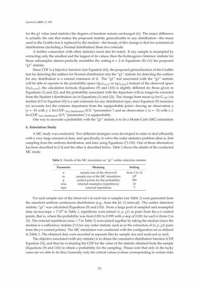
Symmetry 2019, 11, 835

for the g1 value (and statistic) the degrees of freedom remain unchanged (n). The major differenceis actually the one that makes the proposed statistic generalizable to any distribution—the meanused in the Grubbs test is replaced by the median—the beauty of this change is that for symmetricaldistributions (including a Normal distribution) these two coincide.

A further connection with other statistics must also be noted. If any sample is resampled byextracting only the smallest and the largest of its values, then the Kolmogorov-Smirnov statistic forthose subsamples almost perfectly resembles (by setting n = 2 in Equations (8)–(1)) the proposed“g1” statistic.

Since CDF is a bijective function (see Equation (6)), the proposed generalization of the Grubbstest for detecting the outliers for Normal distribution into the “g1” statistic for detecting the outliersfor any distribution is a natural extension of it. The “g1” test associated with the “g1” statisticwill be able to operate in the probability space ((pi)1≤i≤n or (qi)1≤i≤n) instead of the observed space((xi)1≤i≤n), the calculation formula (Equations (9) and (10)) is slightly different (to those given inEquations (1) and (2)), and the probability associated with the departure will no longer be extractedfrom the Student t distribution (as in Equations (1) and (2)). The change from mean (μ for G“all”) tomedian (0.5 in Equation (9)) is a safe extension for any distribution type, since Equation (9) measures(or accounts for) the extreme departures from the equiprobable point—having an observation y(y← X) with y ≤ InvCDF“Any distribution”(0.5; “parameters”) and an observation z (z← X) with z ≥InvCDF“Any distribution”(0.5; “parameters”) is equiprobable.

One way to associate a probability with the “g1” statistic is to do a Monte-Carlo (MC) simulation.

4. Simulation Study

A MC study was conducted. Two different strategies were developed in order to deal efficientlywith a very large amount of data, and specifically, to solve the order statistics problem (that is, firstsampling from the uniform distribution, and later using Equations (7)–(10). One of those alternativeshas been described in [14] and the other is described below. Table 2 shows the details of the conductedMC study.

Table 2. Details of the MC simulation on “g1” outlier detection statistic.

Parameter Meaning Setting

n sample size of the observed from 2 to 12m sample size of the MC simulation 108

p control points for the probability 999resa internal resamples (repetitions) 10repe external repetitions 7

For each sample size of the observed n in each run m samples (see Table 2) were generated fromthe standard uniform continuous distribution (e.g., from the [0, 1] interval). The outlier detectionstatistic “g1” was calculated (Equations (9) and (10)). From a large pool of sampled and resampleddata (m·resa·repe = 7·109 in Table 2, repetitions were joined (n, p, g1) as pairs from the p·n controlpoints, that is, where the probability was from 0.001 to 0.999 with a step of 0.001 for each n (from 2 to12). The external repetitions (resa = 7 in Table 2) were joined together by taking the median (since themedian is a sufficiency statistic [31] for any order statistic such as in the extraction of (n, p, g1) pairsfrom the p·n control points). The MC simulation was conducted with the configuration set as definedin Table 2. The obtained data were recorded in separate files by sample size and analyzed as such.

The objective associated (with any statistic) is to obtain the cumulative distribution function (CDF,Equation (5)), and thus by evaluating the CDF for the value of the statistic obtained from the sample(Equations (9) and (10)) to obtain a probability for the sampling. Please note that only in the luckycases are we able to do this; Generally only the critical values (values corresponding to certain risks

221

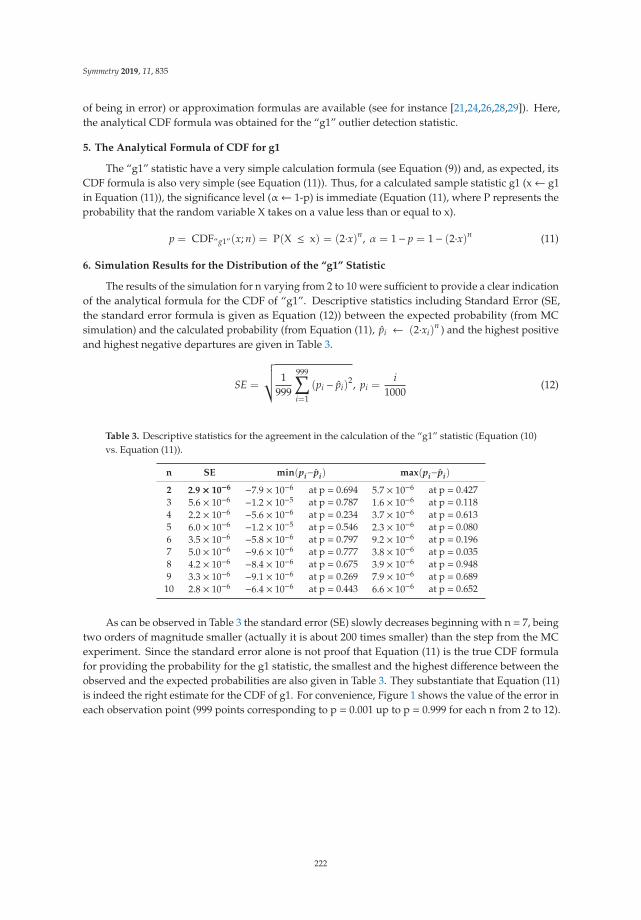
Symmetry 2019, 11, 835

of being in error) or approximation formulas are available (see for instance [21,24,26,28,29]). Here,the analytical CDF formula was obtained for the “g1” outlier detection statistic.

5. The Analytical Formula of CDF for g1

The “g1” statistic have a very simple calculation formula (see Equation (9)) and, as expected, itsCDF formula is also very simple (see Equation (11)). Thus, for a calculated sample statistic g1 (x← g1in Equation (11)), the significance level (α← 1-p) is immediate (Equation (11), where P represents theprobability that the random variable X takes on a value less than or equal to x).

p = CDF“g1”(x; n) = P(X ≤ x) = (2·x)n, α = 1− p = 1− (2·x)n (11)

6. Simulation Results for the Distribution of the “g1” Statistic

The results of the simulation for n varying from 2 to 10 were sufficient to provide a clear indicationof the analytical formula for the CDF of “g1”. Descriptive statistics including Standard Error (SE,the standard error formula is given as Equation (12)) between the expected probability (from MCsimulation) and the calculated probability (from Equation (11), pi ← (2·xi)

n ) and the highest positiveand highest negative departures are given in Table 3.

SE =

√√√1

999

999∑i=1

(pi − pi)2, pi =

i1000

(12)

Table 3. Descriptive statistics for the agreement in the calculation of the “g1” statistic (Equation (10)vs. Equation (11)).

n SE min(pi−pi) max(pi−pi)

2 2.9 × 10−6 −7.9 × 10−6 at p = 0.694 5.7 × 10−6 at p = 0.4273 5.6 × 10−6 −1.2 × 10−5 at p = 0.787 1.6 × 10−6 at p = 0.1184 2.2 × 10−6 −5.6 × 10−6 at p = 0.234 3.7 × 10−6 at p = 0.6135 6.0 × 10−6 −1.2 × 10−5 at p = 0.546 2.3 × 10−6 at p = 0.0806 3.5 × 10−6 −5.8 × 10−6 at p = 0.797 9.2 × 10−6 at p = 0.1967 5.0 × 10−6 −9.6 × 10−6 at p = 0.777 3.8 × 10−6 at p = 0.0358 4.2 × 10−6 −8.4 × 10−6 at p = 0.675 3.9 × 10−6 at p = 0.9489 3.3 × 10−6 −9.1 × 10−6 at p = 0.269 7.9 × 10−6 at p = 0.68910 2.8 × 10−6 −6.4 × 10−6 at p = 0.443 6.6 × 10−6 at p = 0.652

As can be observed in Table 3 the standard error (SE) slowly decreases beginning with n = 7, beingtwo orders of magnitude smaller (actually it is about 200 times smaller) than the step from the MCexperiment. Since the standard error alone is not proof that Equation (11) is the true CDF formulafor providing the probability for the g1 statistic, the smallest and the highest difference between theobserved and the expected probabilities are also given in Table 3. They substantiate that Equation (11)is indeed the right estimate for the CDF of g1. For convenience, Figure 1 shows the value of the error ineach observation point (999 points corresponding to p = 0.001 up to p = 0.999 for each n from 2 to 12).

222

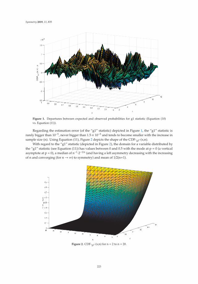
Symmetry 2019, 11, 835

Figure 1. Departures between expected and observed probabilities for g1 statistic (Equation (10)vs. Equation (11)).

Regarding the estimation error (of the “g1” statistic) depicted in Figure 1, the “g1” statistic israrely bigger than 10−5, never bigger than 1.5·× 10−5 and tends to become smaller with the increase insample size (n). Using Equation (11), Figure 2 depicts the shape of the CDF“g1”(x;n).

With regard to the “g1” statistic (depicted in Figure 2), the domain for a variable distributed bythe “g1” statistic (see Equation (11)) has values between 0 and 0.5 with the mode at p = 0 (a verticalasymptote at p = 0), a median of n−1·2−1/n (and having a left asymmetry decreasing with the increasingof n and converging (for n→∞) to symmetry) and mean of 1/2(n+1).

Figure 2. CDF“g1”(x;n) for n = 2 to n = 20.

223

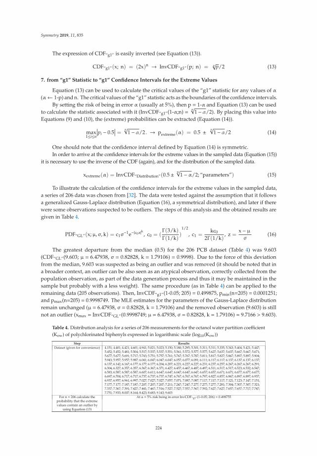
Symmetry 2019, 11, 835

The expression of CDF“g1” is easily inverted (see Equation (13)).

CDF“g1”(x; n) = (2x)n → InvCDF“g1”(p; n) = n√p/2 (13)

7. from “g1” Statistic to “g1” Confidence Intervals for the Extreme Values

Equation (13) can be used to calculate the critical values of the “g1” statistic for any values of α(α← 1-p) and n. The critical values of the “g1” statistic acts as the boundaries of the confidence intervals.

By setting the risk of being in error α (usually at 5%), then p = 1-α and Equation (13) can be usedto calculate the statistic associated with it (InvCDF“g1”(1-α;n) = n√1− α/2). By placing this value intoEquations (9) and (10), the (extreme) probabilities can be extracted (Equation (14)).

max1≤i≤n

∣∣∣pi − 0.5∣∣∣ = n√

1− α/2. → pextreme(α) = 0.5 ± n√1− α/2 (14)

One should note that the confidence interval defined by Equation (14) is symmetric.In order to arrive at the confidence intervals for the extreme values in the sampled data (Equation (15))

it is necessary to use the inverse of the CDF (again), and for the distribution of the sampled data.

xextreme(α) = InvCDF“Distribution”(0.5± n√1−α/2; “parameters”) (15)

To illustrate the calculation of the confidence intervals for the extreme values in the sampled data,a series of 206 data was chosen from [32]. The data were tested against the assumption that it followsa generalized Gauss-Laplace distribution (Equation (16), a symmetrical distribution), and later if therewere some observations suspected to be outliers. The steps of this analysis and the obtained results aregiven in Table 4.

PDF“GL”(x;μ,σ, k) = c1σ−1e−|c0z|k , c0 = (

Γ(3/k)Γ(1/k)

)1/2

, c1 =kc0

2Γ(1/k), z =

x− μσ

(16)

The greatest departure from the median (0.5) for the 206 PCB dataset (Table 4) was 9.603(CDF“GL”(9.603; μ = 6.47938, σ = 0.82828, k = 1.79106) = 0.9998). Due to the force of this deviationfrom the median, 9.603 was suspected as being an outlier and was removed (it should be noted that ina broader context, an outlier can be also seen as an atypical observation, correctly collected from thepopulation observation, as part of the data generation process and thus it may be maintained in thesample but probably with a less weight). The same procedure (as in Table 4) can be applied to theremaining data (205 observations). Then, InvCDF“g1”(1-0.05; 205) = 0.499875, pmin(n=205) = 0.0001251;and pmax(n=205) = 0.9998749. The MLE estimates for the parameters of the Gauss-Laplace distributionremain unchanged (μ = 6.47938, σ = 0.82828, k = 1.79106) and the removed observation (9.603) is stillnot an outlier (xmax = InvCDF“GL”(0.9998749; μ = 6.47938, σ = 0.82828, k = 1.79106) = 9.7166 > 9.603).

Table 4. Distribution analysis for a series of 206 measurements for the octanol water partition coefficient(Kow) of polychlorinated biphenyls expressed in logarithmic scale (log10(Kow))

Step Results

Dataset (given for convenience) 4.151; 4.401; 4.421; 4.601; 4.941; 5.021; 5.023; 5.150; 5.180; 5.295; 5.301; 5.311; 5.311; 5.335; 5.343; 5.404; 5.421; 5.447;5.452; 5.452; 5.481; 5.504; 5.517; 5.537; 5.537; 5.551; 5.561; 5.572; 5.577; 5.577; 5.627; 5.637; 5.637; 5.667; 5.667; 5.671;5.677; 5.677; 5.691; 5.717; 5.743; 5.751; 5.757; 5.761; 5.767; 5.767; 5.787; 5.811; 5.817; 5.827; 5.867; 5.897; 5.897; 5.904;5.943; 5.957; 5.957; 5.987; 6.041; 6.047; 6.047; 6.047; 6.057; 6.077; 6.091; 6.111; 6.117; 6.117; 6.137; 6.137; 6.137; 6.137;6.137; 6.142; 6.167; 6.177; 6.177; 6.177; 6.204; 6.207; 6.221; 6.227; 6.227; 6.231; 6.237; 6.257; 6.267; 6.267; 6.267; 6.291;6.304; 6.327; 6.357; 6.357; 6.367; 6.367; 6.371; 6.427; 6.457; 6.467; 6.487; 6.497; 6.511; 6.517; 6.517; 6.523; 6.532; 6.547;6.583; 6.587; 6.587; 6.587; 6.607; 6.611; 6.647; 6.647; 6.647; 6.647; 6.647; 6.657; 6.657; 6.671; 6.671; 6.677; 6.677; 6.677;6.697; 6.704; 6.717; 6.717; 6.737; 6.737; 6.737; 6.747; 6.767; 6.767; 6.767; 6.797; 6.827; 6.857; 6.867; 6.897; 6.897; 6.937;6.937; 6.957; 6.961; 6.997; 7.027; 7.027; 7.027; 7.057; 7.071; 7.087; 7.087; 7.117; 7.117; 7.117; 7.121; 7.123; 7.147; 7.151;7.177; 7.177; 7.187; 7.187; 7.207; 7.207; 7.207; 7.211; 7.247; 7.247; 7.277; 7.277; 7.277; 7.281; 7.304; 7.307; 7.307; 7.321;7.337; 7.367; 7.391; 7.427; 7.441; 7.467; 7.516; 7.527; 7.527; 7.557; 7.567; 7.592; 7.627; 7.627; 7.657; 7.657; 7.717; 7.747;7.751; 7.933; 8.007; 8.164; 8.423; 8.683; 9.143; 9.603

For n = 206 calculate theprobability that the extremevalues contain an outlier by

using Equation (13)

At α = 5% risk being in error InvCDF“g1”(1-0.05; 206) = 0.498755

224

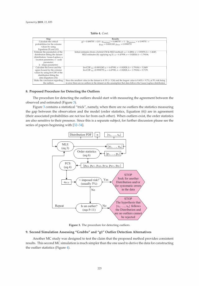
Symmetry 2019, 11, 835

Table 4. Cont.

Step Results

Calculate the criticalprobabilities for the extreme

values by usingEquations (9) and (10)

g1 = 0.498755→ |0.5 - pmin/max| = 0.498755→ 1 - 2pmin/max = ± 0.99751→pmin = 0.0001245; pmax = 0.9998755

Estimate the parameters of thedistribution fitting the dataset

(distribution: Gauss-Laplace; μ- location parameter; σ - scale

parameter;k - shape parameter)

Initial estimates (from a hybrid CM & MLE method): μ = 6.4806; σ = 0.83076; k = 1.4645;MLE estimates (by applying eq.3): μ = 6.47938; σ = 0.82828; k = 1.79106;

Calculate the lower and theupper bound for the extreme

values by using InvCDF of thedistribution fitting the

data (Equation (15))

InvCDF“GL”(0.0001245; μ = 6.47938, σ = 0.82828, k = 1.79106) = 3.2409InvCDF“GL”(0.9998755; μ = 6.47938, σ = 0.82828, k = 1.79106) = 9.7178

Make the conclusion regardingthe outliers

Since the smallest value in the dataset is 4.151 (> 3.24) and the largest value is 9.603 (< 9.71), at 5% risk beingin error there are no outliers in the dataset on the assumption that data follows the Gauss-Laplace distribution

8. Proposed Procedure for Detecting the Outliers

The procedure for detecting the outliers should start with measuring the agreement between theobserved and estimated (Figure 3).

Figure 3 contains a statistical “trick”, namely, when there are no outliers the statistics measuringthe gap between the observation and the model (order statistics, Equation (6)) are in agreement(their associated probabilities are not too far from each other). When outliers exist, the order statisticsare also sensitive to their presence. Since this is a separate subject, for further discussion please see theseries of papers beginning with [32–34].

Figure 3. The procedure for detecting outliers.

9. Second Simulation Assessing “Grubbs” and “g1” Outlier Detection Alternatives

Another MC study was designed to test the claim that the proposed method provides consistentresults. This second MC simulation is much simpler than the one used to derive the data for constructingthe outlier statistics (Figure 4).

225

Symmetry 2019, 11, 835

Figure 4. The procedure for testing the outlier statistics.

The data used here as a proof of the facts are from [7] and all cases involve a Normal distribution(Distribution = Normal in Equation (15); PDF and CDF for Normal distribution in Equation (18);a symmetrical distribution) with α = 5% risk being in error. The parameters of the Normal distribution(μ and σ) are determined for each case, as well as the sample size (Equation (17)).

xextreme(α) = InvCDF“Normal”(0.5± 0.5· n√1−α;μ, σ) (17)

PDF“Normal”(x;μ, σ) =e−

(x−μ)2σ2

σ√

2π, CDF“Normal”(x;μ, σ) =

∫ x

−∞PDF“Normal”(t;μ, σ)dt (18)

For comparison, the same strategy for calculating the confidence intervals of the extreme valuesfor the Normal distribution with the Grubbs test statistic (Equation (2)) was used to provide an alternateresult (Equation (19)).

xcrit(α) = x±Gcrit(α) · s, Gcrit(α) =n− 1√

n

√√t2G(α)

n− 2 + t2G(α)

, tG = InvCDF“Student t”(α2n

, n− 2) (19)

The steps followed in this analysis are given in the Table 5.

Table 5. Comparison of the steps of the analysis and simulation for extreme values confidence intervals(proposed method vs. Grubbs test)

Step Action (step 0 is setting the dataset; α← 0.05)

1 Estimate (with MLE, Equation (3)) parameters (μ, σ) of the Normal distribution; calculate the associated CDFs (Equation (18))

2 Calculate the order statistics, their associated risks being in error, FCS and pFCS (Equations (6) and (4))

3 For n and α calculate the confidence intervals for the extreme values by using (a) Equation (6) and (17) and (b) Equation (19)

4Run the MC experiment (Figure 4) for K = 10000 (and then the expected number of outliers is 500) samples and count thesamples containing outliers for the existing method (Grubbs, Equation (19); with μ and σ from CM method) and for the

proposed method (g1, Equations (13)–(15) and (17); with μ and σ from the MLE method)

Results of the analysis using the steps given in Table 5 for the first dataset are given in Table 6.

226

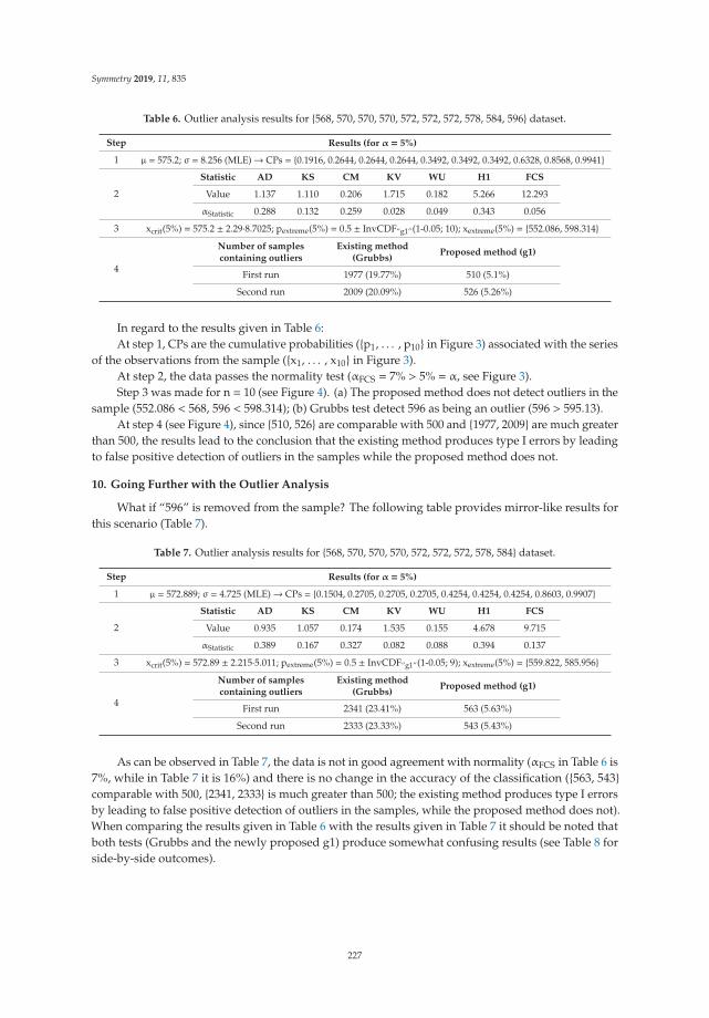
Symmetry 2019, 11, 835

Table 6. Outlier analysis results for {568, 570, 570, 570, 572, 572, 572, 578, 584, 596} dataset.

Step Results (for α = 5%)

1 μ = 575.2; σ = 8.256 (MLE)→ CPs = {0.1916, 0.2644, 0.2644, 0.2644, 0.3492, 0.3492, 0.3492, 0.6328, 0.8568, 0.9941}

2

Statistic AD KS CM KV WU H1 FCS

Value 1.137 1.110 0.206 1.715 0.182 5.266 12.293

αStatistic 0.288 0.132 0.259 0.028 0.049 0.343 0.056

3 xcrit(5%) = 575.2 ± 2.29·8.7025; pextreme(5%) = 0.5 ± InvCDF“g1”(1-0.05; 10); xextreme(5%) = {552.086, 598.314}

4

Number of samplescontaining outliers

Existing method(Grubbs)

Proposed method (g1)

First run 1977 (19.77%) 510 (5.1%)

Second run 2009 (20.09%) 526 (5.26%)

In regard to the results given in Table 6:At step 1, CPs are the cumulative probabilities ({p1, . . . , p10} in Figure 3) associated with the series

of the observations from the sample ({x1, . . . , x10} in Figure 3).At step 2, the data passes the normality test (αFCS = 7% > 5% = α, see Figure 3).Step 3 was made for n = 10 (see Figure 4). (a) The proposed method does not detect outliers in the

sample (552.086 < 568, 596 < 598.314); (b) Grubbs test detect 596 as being an outlier (596 > 595.13).At step 4 (see Figure 4), since {510, 526} are comparable with 500 and {1977, 2009} are much greater

than 500, the results lead to the conclusion that the existing method produces type I errors by leadingto false positive detection of outliers in the samples while the proposed method does not.

10. Going Further with the Outlier Analysis

What if “596” is removed from the sample? The following table provides mirror-like results forthis scenario (Table 7).

Table 7. Outlier analysis results for {568, 570, 570, 570, 572, 572, 572, 578, 584} dataset.

Step Results (for α = 5%)

1 μ = 572.889; σ = 4.725 (MLE)→ CPs = {0.1504, 0.2705, 0.2705, 0.2705, 0.4254, 0.4254, 0.4254, 0.8603, 0.9907}

2

Statistic AD KS CM KV WU H1 FCS

Value 0.935 1.057 0.174 1.535 0.155 4.678 9.715

αStatistic 0.389 0.167 0.327 0.082 0.088 0.394 0.137

3 xcrit(5%) = 572.89 ± 2.215·5.011; pextreme(5%) = 0.5 ± InvCDF“g1”(1-0.05; 9); xextreme(5%) = {559.822, 585.956}

4

Number of samplescontaining outliers

Existing method(Grubbs)

Proposed method (g1)

First run 2341 (23.41%) 563 (5.63%)

Second run 2333 (23.33%) 543 (5.43%)

As can be observed in Table 7, the data is not in good agreement with normality (αFCS in Table 6 is7%, while in Table 7 it is 16%) and there is no change in the accuracy of the classification ({563, 543}comparable with 500, {2341, 2333} is much greater than 500; the existing method produces type I errorsby leading to false positive detection of outliers in the samples, while the proposed method does not).When comparing the results given in Table 6 with the results given in Table 7 it should be noted thatboth tests (Grubbs and the newly proposed g1) produce somewhat confusing results (see Table 8 forside-by-side outcomes).

227

Symmetry 2019, 11, 835

Table 8. Side-by-side comparison of the analysis of the samples.

Sample{568, 570, 570, 570, 572, 572,

572, 578, 584, 596}{568, 570, 570, 570, 572, 572,

572, 578, 584}

At 5% risk being in error can thehypothesis that the sample was drawnfrom a normal distribution be rejected?

No (αFCS = 7%) No (αFCS = 15.8%)

Grubbs confidence interval for ‘nooutliers’ at 5% risk being in error

(555.27, 595.13)596 is detected as being outlier

(561.79, 583.99)584 is detected as being outlier

g1 confidence interval for ‘no outliers’ at5% risk being in error

(552.08, 598.32)no outliers

(559.82, 585.96)no outliers

Table 8 highlights the fact that based on the {568, 570, 570, 570, 572, 572, 572, 578, 584} sample,the g1 test may be interpreted as identifying 596 as being an outlier. This is not quite true because theg1 test was not intended to be used in this way. That is, 596 is outside of the dataset, so at the time ofconstructing the confidence intervals for the extreme values, the information regarding its observationwas missing.

Another trial was done, this time with 601 replacing 596 in the initial dataset (Table 9).

Table 9. Outlier analysis results for the {568, 570, 570, 570, 572, 572, 572, 578, 584, 601} dataset.

Step Results (for α = 5%)

1 From the CM method: μ = 575.7; σ = 10.067; from MLE method: μ = 575.7; σ = 9.550

2

Statistic AD KS CM KV WU H1 FCS

Value 1.267 1.109 0.225 1.774 0.198 5.411 13.652

αStatistic 0.241 0.132 0.226 0.018 0.035 0.254 0.034

3 Grubbs confidence interval for ’no outliers’ at 5% risk being in error: (552.647,598.753); 601 is an outlierg1 confidence interval for ’no outliers’ at 5% risk being in error: (548.963, 602.437); no outliers

In a further trial, 604 replaced 596 in the initial dataset (Table 10).

Table 10. Outlier analysis results for the {568, 570, 570, 570, 572, 572, 572, 578, 584, 604} dataset.

Step Results (for α = 5%)

1 From the CM method: μ = 576.0; σ = 10.914; from MLE method: μ = 576.0; σ = 10.354

2

Statistic AD KS CM KV WU H1 FCS

Value 1.348 1.108 0.238 1.803 0.209 5.481 14.468

αStatistic 0.216 0.133 0.206 0.015 0.028 0.215 0.025

3 Grubbs confidence interval for ’no outliers’ at 5% risk being in error: (551.00, 601.00); 604 is an outlierg1 confidence interval for ’no outliers’ at 5% risk being in error: (547.01, 604.99); no outliers

The conclusion is simple (see the results in the Tables 6, 7, 9 and 10): A test will hardly ever detectan outlier for a small sample; it is more likely to reject the hypothesis of the sample drawn from thedistribution itself!

The same trick was used on a bigger sample and the results are shown in Table 11 (the dataset isfrom Table 4).

228

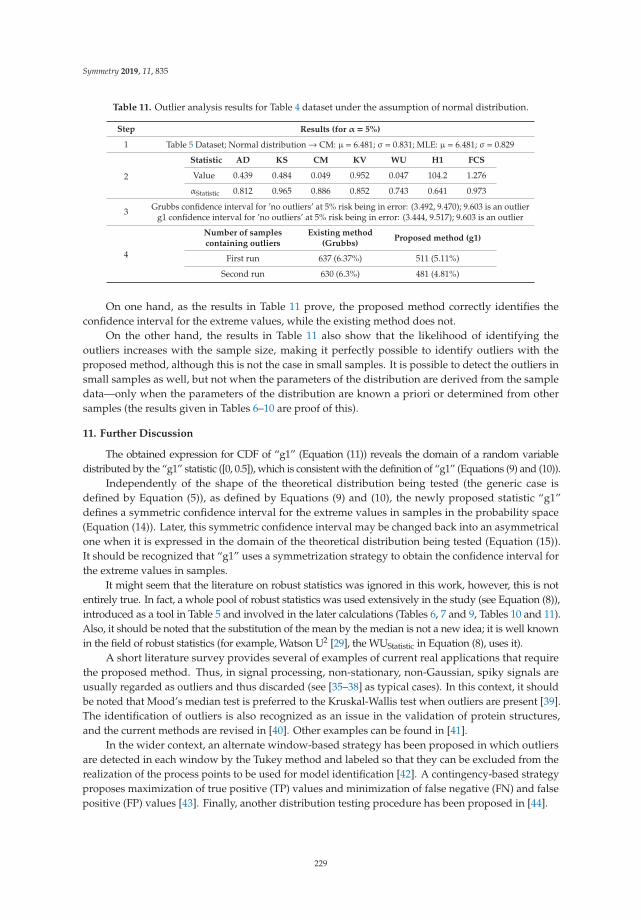
Symmetry 2019, 11, 835

Table 11. Outlier analysis results for Table 4 dataset under the assumption of normal distribution.

Step Results (for α = 5%)

1 Table 5 Dataset; Normal distribution→ CM: μ = 6.481; σ = 0.831; MLE: μ = 6.481; σ = 0.829

2

Statistic AD KS CM KV WU H1 FCS

Value 0.439 0.484 0.049 0.952 0.047 104.2 1.276

αStatistic 0.812 0.965 0.886 0.852 0.743 0.641 0.973

3 Grubbs confidence interval for ’no outliers’ at 5% risk being in error: (3.492, 9.470); 9.603 is an outlierg1 confidence interval for ’no outliers’ at 5% risk being in error: (3.444, 9.517); 9.603 is an outlier

4

Number of samplescontaining outliers

Existing method(Grubbs)

Proposed method (g1)

First run 637 (6.37%) 511 (5.11%)

Second run 630 (6.3%) 481 (4.81%)

On one hand, as the results in Table 11 prove, the proposed method correctly identifies theconfidence interval for the extreme values, while the existing method does not.

On the other hand, the results in Table 11 also show that the likelihood of identifying theoutliers increases with the sample size, making it perfectly possible to identify outliers with theproposed method, although this is not the case in small samples. It is possible to detect the outliers insmall samples as well, but not when the parameters of the distribution are derived from the sampledata—only when the parameters of the distribution are known a priori or determined from othersamples (the results given in Tables 6–10 are proof of this).

11. Further Discussion

The obtained expression for CDF of “g1” (Equation (11)) reveals the domain of a random variabledistributed by the “g1” statistic ([0, 0.5]), which is consistent with the definition of “g1” (Equations (9) and (10)).

Independently of the shape of the theoretical distribution being tested (the generic case isdefined by Equation (5)), as defined by Equations (9) and (10), the newly proposed statistic “g1”defines a symmetric confidence interval for the extreme values in samples in the probability space(Equation (14)). Later, this symmetric confidence interval may be changed back into an asymmetricalone when it is expressed in the domain of the theoretical distribution being tested (Equation (15)).It should be recognized that “g1” uses a symmetrization strategy to obtain the confidence interval forthe extreme values in samples.

It might seem that the literature on robust statistics was ignored in this work, however, this is notentirely true. In fact, a whole pool of robust statistics was used extensively in the study (see Equation (8)),introduced as a tool in Table 5 and involved in the later calculations (Tables 6, 7 and 9, Tables 10 and 11).Also, it should be noted that the substitution of the mean by the median is not a new idea; it is well knownin the field of robust statistics (for example, Watson U2 [29], the WUStatistic in Equation (8), uses it).

A short literature survey provides several of examples of current real applications that requirethe proposed method. Thus, in signal processing, non-stationary, non-Gaussian, spiky signals areusually regarded as outliers and thus discarded (see [35–38] as typical cases). In this context, it shouldbe noted that Mood’s median test is preferred to the Kruskal-Wallis test when outliers are present [39].The identification of outliers is also recognized as an issue in the validation of protein structures,and the current methods are revised in [40]. Other examples can be found in [41].

In the wider context, an alternate window-based strategy has been proposed in which outliersare detected in each window by the Tukey method and labeled so that they can be excluded from therealization of the process points to be used for model identification [42]. A contingency-based strategyproposes maximization of true positive (TP) values and minimization of false negative (FN) and falsepositive (FP) values [43]. Finally, another distribution testing procedure has been proposed in [44].

229

Symmetry 2019, 11, 835

12. Conclusions

A new method for detecting outliers was proposed in this paper. The method is applicable toany continuous distribution at any risk being in error. It was proved that the method correctly detectsthe outliers. For a normal distribution at 5% risk being in error, it was also shown that the proposedmethod outperforms the classical Grubbs test for detecting the outliers.

Supplementary Materials: Details of the software used for deriving the results given in the figures and tables, algorithmsand source codes are given as supplementary material available online at http://www.mdpi.com/2073-8994/11/6/835/s1.

Funding: This research received no external funding.

Acknowledgments: Thanks to my colleague S.D. Bolboacă and for our fruitful discussions during the developmentstage of the study, which helped and motivated the author to complete the study.

Conflicts of Interest: The author declares no conflict of interest.

References

1. Gauss, C.F. Theoria Motus Corporum Coelestium; (Translated in 1857 as “Theory of Motion of the HeavenlyBodies Moving about the Sun in Conic Sections” by C. H. Davis. Little, Brown: Boston. Reprinted in 1963 byDover: New York); Perthes et Besser: Hamburg, Germany, 1809; pp. 249–259.

2. Tippett, L.H.C. The extreme individuals and the range of samples taken from a normal population. Biometrika1925, 17, 151–164. [CrossRef]

3. Fisher, R.A.; Tippett, L.H.C. Limiting forms of the frequency distribution of the largest and smallest memberof a sample. Proc. Camb. Philos. Soc. 1928, 24, 180–190. [CrossRef]

4. Thompson, W.R. On a criterion for the rejection of observations and the distribution of the ratio of thedeviation to the sample standard deviation. Ann. Math. Stat. 1935, 6, 214–219. [CrossRef]

5. Pearson, E.; Sekar, C.C. The efficiency of the statistical tools and a criterion for the rejection of outlyingobservations. Biometrika 1936, 28, 308–320. [CrossRef]

6. Grubbs, F.E. Sample criteria for testing outlying observations. Ann. Math. Stat. 1950, 21, 27–58. [CrossRef]7. Grubbs, F.E. Procedures for detecting outlying observations in samples. Technometrics 1969, 11, 1–21.

[CrossRef]8. Nooghabi, M.; Nooghabi, H.; Nasiri, P. Detecting outliers in gamma distribution. Commun. Stat. Theory Methods

2010, 39, 698–706. [CrossRef]9. Kumar, N.; Lalitha, S. Testing for upper outliers in gamma sample. Commun. Stat. Theory Methods 2012, 41,

820–828. [CrossRef]10. Lucini, M.; Frery, A. Comments on “Detecting Outliers in Gamma Distribution” by M. Jabbari Nooghabi et al.

(2010). Commun. Stat. Theory Methods 2017, 46, 5223–5227. [CrossRef]11. Hartley, H. The range in random samples. Biometrika 1942, 32, 334–348. [CrossRef]12. Bardet, J.-M.; Dimby, S.-F. A new non-parametric detector of univariate outliers for distributions with

unbounded support. Extremes 2017, 20, 751–775. [CrossRef]13. Gosset, W. The probable error of a mean. Biometrika 1908, 6, 1–25.14. Jäntschi, L.; Bolboacă, S.-D. Computation of probability associated with Anderson-Darling statistic.

Mathematics 2018, 6, 88. [CrossRef]15. Fisher, R. On an Absolute Criterion for Fitting Frequency Curves. Messenger Math. 1912, 41, 155–160.16. Fisher, R. Questions and answers #14. Am. Stat. 1948, 2, 30–31.17. Bolboacă, S.D.; Jäntschi, L.; Sestras, , A.F.; Sestras, , R.E.; Pamfil, D.C. Supplementary material of ’Pearson-Fisher

chi-square statistic revisited’. Information 2011, 2, 528–545. [CrossRef]18. Jäntschi, L.; Bolboacă, S.D. Performances of Shannon’s Entropy Statistic in Assessment of Distribution of

Data. Ovidius Univ. Ann. Chem. 2017, 28, 30–42. [CrossRef]19. Davis, P.; Rabinowitz, P. Methods of Numerical Integration; Academic Press: New York, NY, USA, 1975;

pp. 51–198.20. Pearson, K. Note on Francis Gallon’s problem. Biometrika 1902, 1, 390–399.21. Cramér, H. On the composition of elementary errors. Scand. Actuar. J. 1928, 1, 13–74. [CrossRef]22. Von Mises, R.E. Wahrscheinlichkeit, Statistik und Wahrheit; Julius Springer: Berlin, Germany, 1928; pp. 100–138.

230

Symmetry 2019, 11, 835

23. Kolmogorov, A. Sulla determinazione empirica di una legge di distribuzione. Giornale dell’Istituto Italianodegli Attuari 1933, 4, 83–91.

24. Kolmogorov, A. Confidence Limits for an Unknown Distribution Function. Ann. Math. Stat. 1941, 12,461–463. [CrossRef]

25. Smirnov, N. Table for estimating the goodness of fit of empirical distributions. Ann. Math. Stat. 1948, 19,279–281. [CrossRef]

26. Anderson, T.W.; Darling, D.A. Asymptotic theory of certain “goodness-of-fit” criteria based on stochasticprocesses. Ann. Math. Stat. 1952, 23, 193–212. [CrossRef]

27. Anderson, T.W.; Darling, D.A. A Test of Goodness-of-Fit. J. Am. Stat. Assoc. 1954, 49, 765–769. [CrossRef]28. Kuiper, N.H. Tests concerning random points on a circle. Proc. Koninklijke Nederlandse Akademie van Wetenschappen

Series A 1960, 63, 38–47. [CrossRef]29. Watson, G.S. Goodness-Of-Fit Tests on a Circle. Biometrika 1961, 48, 109–114. [CrossRef]30. Metropolis, N.; Ulam, S. The Monte Carlo Method. J. Am. Stat. Assoc. 1949, 44, 335–341. [CrossRef] [PubMed]31. Fisher, R.A. On the mathematical foundations of theoretical statistics. Philos. Trans. R. Soc. A 1922, 222,

309–368. [CrossRef]32. Jäntschi, L. Distribution fitting 1. Parameters estimation under assumption of agreement between observation

and model. Bull. UASVM Hortic. 2009, 66, 684–690.33. Jäntschi, L.; Bolboacă, S.D. Distribution fitting 2. Pearson-Fisher, Kolmogorov-Smirnov, Anderson-Darling,

Wilks-Shapiro, Kramer-von-Misses and Jarque-Bera statistics. Bull. UASVM Hortic. 2009, 66, 691–697.34. Bolboacă, S.D.; Jäntschi, L. Distribution fitting 3. Analysis under normality assumption. Bull. UASVM Hortic.

2009, 66, 698–705.35. Liu, K.; Chen, Y.Q.; Domanski, P.D.; Zhang, X. A novel method for control performance assessment with

fractional order signal processing and its application to semiconductor manufacturing. Algorithms 2018, 11,90. [CrossRef]

36. Paiva, J.S.; Ribeiro, R.S.R.; Cunha, J.P.S.; Rosa, C.C.; Jorge, P.A.S. Single particle differentiation through 2Doptical fiber trapping and back-scattered signal statistical analysis: An exploratory approach. Sensors 2018,18, 710. [CrossRef] [PubMed]

37. Teunissen, P.J.G.; Imparato, D.; Tiberius, C.C.J.M. Does RAIM with correct exclusion produce unbiasedpositions? Sensors 2017, 17, 1508. [CrossRef] [PubMed]

38. Pan, Z.; Liu, L.; Qiu, X.; Lei, B. Fast vessel detection in Gaofen-3 SAR images with ultrafine strip-map mode.Sensors 2017, 17, 1578. [CrossRef] [PubMed]

39. Vergura, S.; Carpentieri, M. Statistics to detect low-intensity anomalies in PV systems. Energies 2018, 11, 30.[CrossRef]

40. Chen, L.; He, J.; Sazzed, S.; Walker, R. An investigation of atomic structures derived from X-ray crystallographyand cryo-electron microscopy using distal blocks of side-chains. Molecules 2018, 23, 610. [CrossRef] [PubMed]

41. Bolboacă, S.D.; Jäntschi, L. The effect of leverage and influential on structure-activity relationships.Comb. Chem. High Throughput Screen. 2013, 16, 288–297. [CrossRef] [PubMed]

42. Faes, L.; Porta, A.; Nollo, G.; Javorka, M. Information decomposition in multivariate systems: Definitions,implementation and application to cardiovascular networks. Entropy 2017, 19, 5. [CrossRef]

43. Li, G.; Wang, J.; Liang, J.; Yue, C. Application of sliding nest window control chart in data stream anomalydetection. Symmetry 2018, 10, 113. [CrossRef]

44. Paolella, M.S. Stable-GARCH models for financial returns: Fast estimation and tests for stability. Econometrics2016, 4, 25. [CrossRef]

© 2019 by the author. Licensee MDPI, Basel, Switzerland. This article is an open accessarticle distributed under the terms and conditions of the Creative Commons Attribution(CC BY) license (http://creativecommons.org/licenses/by/4.0/).

231

MDPISt. Alban-Anlage 66

4052 BaselSwitzerland

Tel. +41 61 683 77 34Fax +41 61 302 89 18

www.mdpi.com

Symmetry Editorial OfficeE-mail: symmetry@mdpi.com

www.mdpi.com/journal/symmetry

MDPI St. Alban-Anlage 66 4052 Basel Switzerland

Tel: +41 61 683 77 34 Fax: +41 61 302 89 18

www.mdpi.com ISBN 978-3-03943-792-4