APPLIED MATHEMATICS - World Radio History
348
-
Upload
khangminh22 -
Category
Documents
-
view
0 -
download
0
Transcript of APPLIED MATHEMATICS - World Radio History
1;)e z/97-
APPLIED
MATHEMATICS for Radio and Communication
Engineers
by CARL E. SMITH, B.s.,m.s.,E.E. Vice President in Charge of Engineering, United Broadcasting Company, and President, Cleveland Institute of Radio Electronics, Cleveland, Ohio; ,Formerly Assistant Director, Operational Research Staff, Office of the Chief Signal Officer, War Depart-ment, Washington, D.C., and President, Smith Prac-tical Radio Institute, Cleveland, Ohio; Member, American Institute of Electrical Engineers; Senior Member, Member of the Board of Editors, Institute of
Radio Engineers
FIRST EDITION
THIRD IMPRESSION
McGRAW-HILL BOOK COMPANY, INC. NEW YORK AND LONDON
1945
APPLIED MATHEMATICS
COPYRIGHT, 1945, BY THE MCGRAW-HILL BOOK COMPANY, INC.
COPYRIGHT, 1935, 1937, 1939, 1943, 1944
BY Carl E. Smith
PRINTED IN THE UNITED STATES OF AMERICA
All rights reserved. This book, or parts thereof, may not be reproduced in any form without permission of
the publishers.
THE MAPLE PRESS COMPANY, YORK, Pit.

APPLIED MATHEMATICS
The quality of the materials used in the manufacture of this book is gov-
erned by continued postwar shortages.


To
My Students
• WHEREVER THEY ARE

*
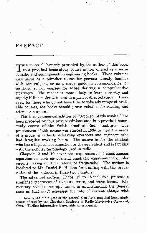
PREFACE
r-In HE material formerly presented by the author of this book as a practical home-study course is now offered as a series
of radio and communication engineering books. These volumes may serve as a refresher course for persons already familiar with the subject, or as a study guide in correspondence' or residence school courses for those desiring a comprehensive treatment. The reader is more likely to learn correctly and rapidly if this material is used in a plan of directed study. How-ever, for those who do not have time to take advantage of avail-able courses, the books should prove valuable for reading and reference purposes.
This first commercial edition of "Applied Mathematics" has been preceded by four private editions used in a practical home-study course of the Smith Practical Radio In,stitute. The preparation of this course was started in 1934 to meet the needs of a group of radio broadcasting operators and engineers who had irregular working hours. The course is for the student who has a high-school education or the equivalent and is familiar with the popular terminology used in radio.
Chapters 9 and 10 cover the requirements of simultaneous equations in mesh circuits and quadratic equations in• complex circuits having multiple resonance frequencies. The author is indebted to Mr. Daniel B. Hutton for assisting with the prepa-ration of the material in these two chapters. The advanced section, Chaps. 12 to 15 inclusive, presents a
simplified treatment of calculus, series, and wave forms. Ele-mentary calculus concepts assist in understanding the theory, such as that di/dt expresses the rate of current change with
These books are a part of the general plan for a practical home study course offered by the Cleveland Institute of Radio Electronics Cleveland, Ohio. Further information is available upon .request.
vii
, viii PREFACE
respect to time. Another illustration is the determination of impedance matching by maximizing the power transfer. The material on series is given because of their use in evaluating functions and making simple engineering approximations. The treatment of wave forms gives the underlying mathematics for analyzing and synthesizing wave shapes found in television and pulse techniques. The section devoted to tables and formulas is included to
make this mathematics handbook self-contained. The other books of this series will refer to this material whenever it is needed. The author wishes to acknowledge the helpful cooperation
which has been received from all sides. In particular, he wishes to thank the many students who by their constructive criticisms have helped to mold this course into its present form, and Beverly Dudley for his careful reading of the manuscript and for the suggestions that he has made for the improvement of the text in a number of places.
CARL E. SMITH. THE PENTAGON, WASHINGTON, D.C., July, 1945.
ACKNOWLEDGMENT
The table of Bessel functions on pages 285-293 has been taken from pages 171-179 of "Funktionentafeln mit Formeln und Kurven" by Jahnke and Emde, and the sine and cosine integral tables on pages 295-298 are from pages 6-9 of the same work. Copyright, 1933, by B. G. Teubner, in Leipzig. Copyright vested in the U. S. Alien Property Custodian, 1943, pursuant to law. Reproduced by permission of the Alien Property Custodian in the public interest, under license number A-963.
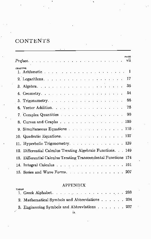
CONTENTS
PAGE
Preface vii
CHAPTER
1. Arithmetic 1
2. Logarithms 17
3. Algebra 35
4. Geometry 54
5. Trigonometry 66
6. Vector Addition 76
7. Complex Quantities 90
8. Curves and Graphs 100
9. Simultaneous Equations 110
10. Quadratic Equations 127
11. Hyperbolic Trigonometry 139
12. Differential Calculus Treating Algebraic Functions. . . 149
13. Differential Calculus Treating Transcendental Functions 174
14. Integral Calculus 191
15. Series and Wave Forms 207
APPENDIX TABLE
1. Greek Alphabet 233
2. Mathematical Symbols and Abbreviations 234
3, Engineering Symbols and Abbreviations 237 ix
CONTENTS TABLE PAGE
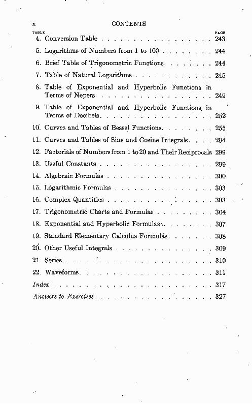
4. Conversion Table 243
5. Logarithms of Numbers from 1 to 100 . . . 244
6. Brief Table of Trigonometric Functions 244
7. Table of Natural Logarithms 245
8. Table of Exponential and Hyperbolic Functions in Terms of Nepers 249
9. Table of Exponential and Hyperbolic Functions, in Terms of Decibels 252
10. Curves and Tables of Bessel Functions 255
11. Curves and Tables of Sine and Cosine Integrals. . . 294
12. Factorials of Numbers from 1 to 20 and Their Reciprocals 299
13. Useful Constants 299
14. Algebraic Formulas 300
15. Logarithmic Formulas 303
16. Complex Quantities 303
17. Trigonometric Charts and Formulas 304
18. Exponential and Hyperbolic Formulas \ 307
19. Standard Elementary Calculus Formulas 308
26. Other Useful Integrals 309
21. Series 310
22. Waveforms 311
Index 317
Answers to Exercises 327
APPLIED MATHEMATICS
CHAPTER 1
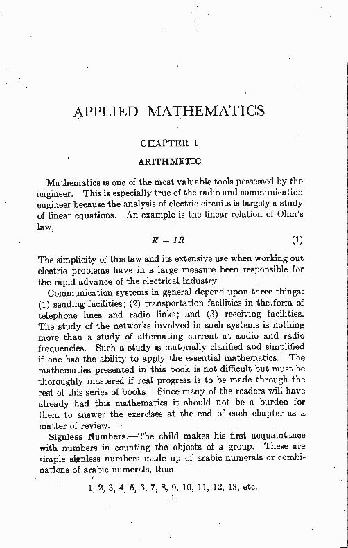
ARITHMETIC
Mathematics is one of the most valuable tools possessed by the engineer. This is especially true of the radio and communication engineer because the analysis of electric circuits is largely a study of linear equations. An example is the linear relation of Ohm's
law,
E = IR (1)
The simplicity of this law and its extensive use when working out electric problems have in a large measure been responsible for the rapid advance of the electrical industry. Communication systems in general depend upon three things:
(1) sending facilities; (2) transportation facilities in the. form of telephone lines and radio links; and (3) receiving facilities. The study of the networks involved in such systems is nothing more than a study of alternating current at audio and radio frequencies. Such a study is materially clarified and simplified if one has the ability to apply the essential mathematics. The mathematics presented in this book is not difficult but must be thoroughly mastered if real progress is to be made through the rest of this series of books. Since many of the readers will have already had this mathematics it should not be a burden for them to answer the exercises at the end of each chapter as a
matter of review. Signless Numbers.—The child makes his first acquaintance
with numbers in counting the objects of a group. These are simple signless numbers made up of arabic numerals or combi-nations of arabic numerals, thus
1, 2, 3, 4, 5, 6, 7, 8, 9, 10, 11, 12, 13, etc. 1
2 APPLIED MATHEMATICS.
These signless numbers obey the arithmetic processes of addition and multiplication.
Example 1. Add 3 to 6. Solution. 3 + 6 = 9. Ans. Example 2. Multiply 2 by 6. Solution. 2 X 6 = 12. Ans.
Real Numbers.----As the child's experience increases he will soon desire to use the arithmetic processes of subtraction and division. Occasionally the result cannot be expressed in the simple system of signless numbers. For instance, if the mercury in the thermometer drops below zero, or if he wishes to subtract a large number from a small number, the result is no longer in the simple system of signless numbers. To expand the number system to take care of all four arith-
metic processes, it is necessary to include a zero and negative numbers. The signless numbers will then be considered posi-tive numbers even though no sign is used. This system of real numbers considered thus far is one of whole numbers called "integers" or "integral numbers." Whole numbers are called "even numbers" when exactly divisible by 2 and " odd numbers" when not exactly divisible by 2. The real number system consists of zero; all whole numbers;
all rational numbers, which can be expressed as whole numbers in fraction form; and all irrational numbers, which cannot be expressed as simple fractions. For instance, the diagonal of a square having sides one unit in length can be expressed as .the
square root of 2, thus; -0. The Vi is an irrational number which cannot be expressed as a simple fraction.
Example 3. Harry has $9 but owes Tom $12. What is Harry's financial status?
Solution. $9 — $12. = —$3. Ans. This means that he is $3 in debt. Harry actually owns less than nothing. Example 4. Divide 6 by. 2 and state the kind of number that results. Solution. 6 ÷ 2 = 3. Ans. The answer is a rational odd integral number. In this example, 6 is
the dividend, 2 is the divisor, and 3 is the quotient.
Example 5. Divide 4 by 6 and state the kind of number that results. 2
Solution. 3.! —2- Ans. er 3 3 •
The answer is a rational number expressed in fraction form.
ARITHMETIC 3
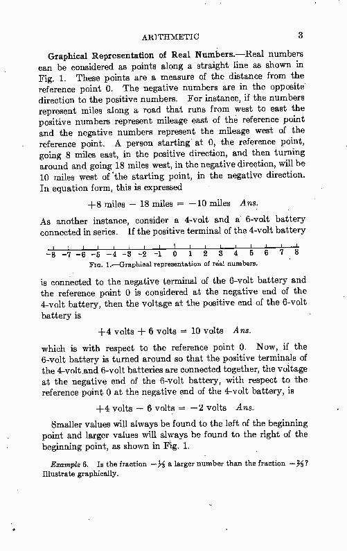
Graphical Representation of Real Numbers.—Real numbers can be considered as points along a straight line as shown in Fig. 1. These points are a measure of the distance from the reference point O. The negative numbers are in the opposite direction to the positive numbers. For instance, if the numbers represent miles along a road that runs from west to east the positive numbers represent mileage east of the reference point and the negative numbers represent the mileage west of the reference point. A person starting at 0, the reference point, going 8 miles east, in the positive direction, and then turning around and going 18 miles west, in the negative direction, will be 10 miles west of the starting point, in the negative direction. In equation form, this is expressed
+8 miles — 18 miles = —10 miles Ans.
As another instance, consider a 4-volt and a 6-volt battery connected in series. If the positive terminal of the 4-volt battery
I I I I I I I 11111 -8 -7 -6 -5 -4 -3 -2 -1 0 1 2 3 4 5 6 7 8
Fro. 1.—Graphical representation of real numbers.
is connected to the negative terminal of the 6-volt battery and the reference point 0 is considered at the negative end of the 4-volt battery, then the voltage at the positive end of the 6-volt battery is
+4 volts + 6 volts = 10 volts Ans.
which is with respect to the reference point O. Now, if the 6-volt battery is turned around so that the positive terminals of the 4-volt .and 6-volt batteries are connected together, the voltage at the negative end of the 6-volt battery, with respect to the reference point 0 at the negative end of the 4-volt battery, is
+4 volts — 6 volts = —2 volts Ans.
Smaller values will always be found to the left of the beginning point and larger values will always be found to the right of the beginning point, as shown in Fig. 1.
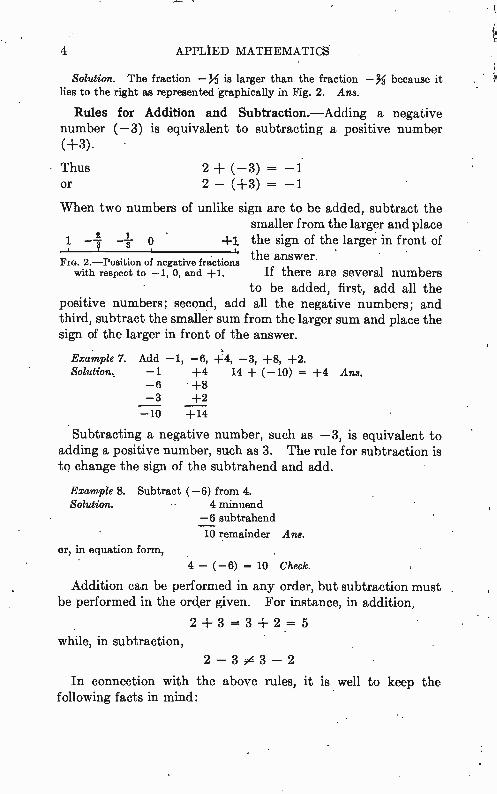
Example 6. Is the fraction —h a larger number than the fraction -%? Illustrate graphically.
4 APPLIED MATHEMATICS
Solution. The fraction —% is larger than the fraction —% because it lies to the right as represented graphically in Fig. 2. Ans.
Rules for Addition and Subtraction.—Adding a negative number (-3) is equivalent to subtracting a positive number
(+3).
Thus or
2 + ( —3) = —1 2 — (+3) = —1
When two numbers of unlike sign are to be added, subtract the smaller from the larger and place
1 —4 . p o 4.1 the sign of the larger in front of the answer. Fm. 2.—Position of negative fractions
with respect to —1, 0, and +1. If there are several numbers to be added, first, add all the
positive numbers; second, add all the negative numbers; and third, subtract the smaller sum from the larger sum and place the sign of the larger in front of the answer.
Example 7. Add —1, —6, +4, —3, +8, +2. Solution, —1 +4 14 + ( —10) = +4 Ans.
—6 +8 —3 +2
—10 +14
• Subtracting a negative number, such as —3, is equivalent to adding a positive number, such as 3. The rule for subtraction is to change the sign of the subtrahend and add.
Example 8. Subtract ( —6) from 4. Solution. 4 minuend
—6 subtrahend
10 remainder Ans.
or, in equation form,
4 — ( —6) -= 10 Check.
Addition can be performed in any order, but subtraction must be performed in the order given. For instance, in addition,
2 + 3 = 3 + 2 = 5
while, in subtraction,
2 — 3 3 — 2
In connection with the above rules, it is well to keep the following facts in mind:
4 ARITHMETIC 5
1. Adding a positive number gives a larger value. 2. Subtracting a positive number gives a smaller value. 3. Adding a negative number gives a smaller value. 4. Subtracting a negative number gives a larger value. Rules for Multiplication and Division.—l. The product or
quotient of two positive numbers is always a positive number. For instance, in multiplication, 2 X 4 = 8, and, in division, 12 4- 3 = 4.
2. The product or quotient of two negative numbers is always a positive number. For instance, in multiplication,
—2 X —4 = 8,
and, in division, —12 ÷ —3 = 4. 3. The product or quotient of a positive and negative number
is always a negative number. For instance, in multiplication, —2 X 4 = —8, and, in division, —12 ÷ 3 = —4.
4. Multiplication can be performed in any order while division must be performed in the order written. For instance, in multiplication, 2 X 4 = 4 X 2 = 8, but, in division,
12 ÷ 3 0 3 ÷ 12.
5. In a series of different operations, the multiplications are performed first, the divisions second, the additions third, and the subtractions fourth. Terms of a grouping, such as between parentheses, should be solved before performing the operation on the grouping.
Example 9. Solve: 12 ÷ 3 — 2 X 9 ÷ 3 ± 10 X 2 — 2. Solution. Performing the multiplications, 12 4- 3 — 18 4- 3 + 20 — 2
Performing the divisions, 4 — 6 ± 20 — 2 Performing the additions, 24 — 6 — 2 Performing the subtractions, 16 Ans. Example 10. Solve: [(2 X 6) — (5 — 8)] ÷ (3 ± 2). Solution. Performing the operations within the parenthesis groupings,
[(12) — ( —3)] 4- (5)
Combining terms in the bracket, 15 ÷ 5 Performing the division, 3 Ans. .
Cancellation.—Cancellation is a process used to shorten mathematical problems involving a series of multiplications and divisions. The following are rules for cancellation:
1. Any factor below the line can be divided into any factor above the line, or any factor above the line can be divided into any factor below the line.
6 APPLIED MATHEMATICS
2. Any factor common to factors of a term above and factors of a term below the line can be divided into each.
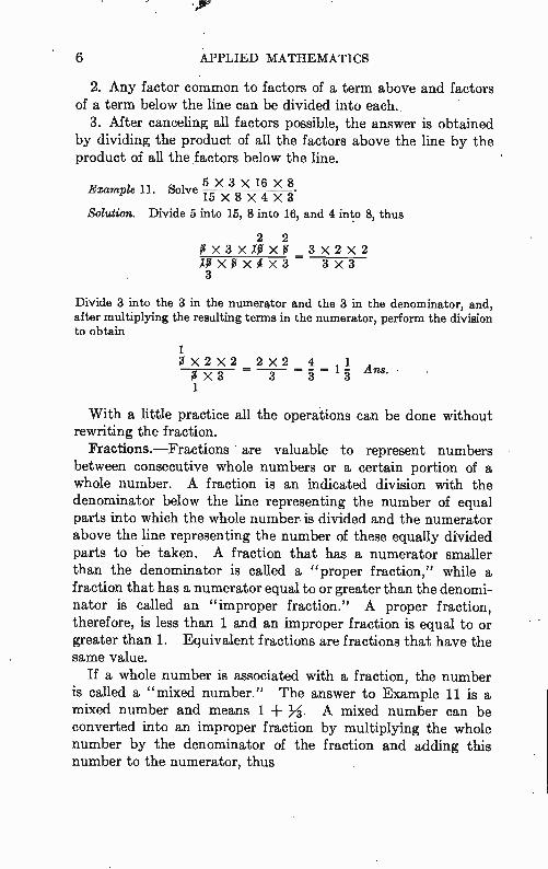
3. After canceling all factors possible, the answer is obtained by dividing the product of all the factors above the line by the product of all the factors below the line.
5 X 3 X 16 X 8 Example 11. Solve
15 X 8 X 4 X 3
Solution. Divide 5 into 15, 8 into 16, and 4 into 8, thus
2 2 gx3xXfix$ 3x2x2 JOxgx0x3 = 3x3 3
Divide 3 into the 3 in the numerator and the 3 in the denominator, and, after multiplying the resulting terms in the numerator, perform the division to obtain
1 g X 2 X 2 2 X 2 4 1 g X 3 3 3 3 1
Ans.
With a little practice all the operations can be done without rewriting the fraction.
Fractions.—Fractions are valuable to represent numbers between consecutive whole numbers or a certain portion of a whole number. A fraction is an indicated division with the denominator below the line representing the number of equal parts into which the whole number is divided and the numerator above the line representing the number of these equally divided parts to be taken. A fraction that has a numerator smaller than the denominator is called a "proper fraction," while a fraction that has a numerator equal to or greater than the denomi-nator is called an "improper fraction." A proper fraction, therefore, is less than 1 and an improper fraction is equal to or greater than I. Equivalent fractions are fractions that have the same value.
If a whole number is associated with a fraction, the number is called a "mixed number." The answer to Example 11 is a mixed number and means 1 ± %. A mixed number can be converted into an improper fraction by multiplying the whole number by the denominator of the fraction and adding this number to the numerator, thus
ARITHMETIC 7
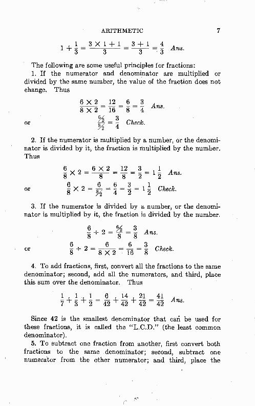
1 3 X 1 + 1 3 -F 1 4 1 — 3 3 3 -- 3 Ans.
The following are some useful principles for fractions: 1. If the numerator and denominator are multiplied or
divided by the same number, the value of the fraction does not change. Thus
6 X 2 12 6 3 A
8 X 2 — 16 8 — `'n8.
3 or = Check.
2. If the numerator is multiplied by a number, or the denomi-nator is divided by it, the fraction is multiplied by the number. Thus
6 —s 6 X 2 12 3 — — _ 1 X 2 = 8 A 8 2 -ans.
Or 6 u X 2 = z= 6 3 Check.
3. If the numerator is divided by a number, or the denomi-nator is multiplied by it, the fraction is divided by the number.
6 ÷ 2 = U = 3 Ans g 8 g --- .
6 6 6 3 • or -g ÷ 2 Check.
8 X 2 16 g
4. To add fractions, first, convert all the fractions to the same denominator; second, add all the numerators, and third, place this sum over the denominator. Thus
1 1 1 6 14 21 41 -42 + U +-42 = 42.
Ans.
Since 42 is the smallest denominator that caii be used for these fractions, it is called the "L.C.D." (the least common denominator).
5. To subtract one fraction from another, first convert both fractions to the same denominator; second, subtract one numerator from the other numerator; and third, place the
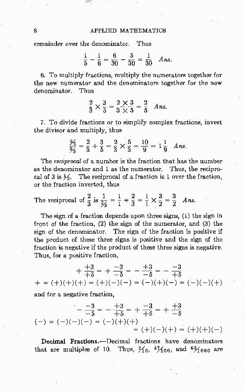
8 APPLIED MATHEMATICS
remainder over the denominator. Thus
1 1 6 5 1 5 630 3030
Ans.
6. To multiply fractions, multiply the numerators together for the new numerator and the denominators together for the new denominator. Thus
2 \, 3 2 X 3 2 A
—ns.
7. To divide fractions or to simplify complex fractions, invert the divisor and multiply, thus
• h_ 2 3 2 ,,. 5 10 , 1 A %
The reciprocal of a number is the fraction that has the number as the denominator and 1 as the numerator. Thus, the recipro-cal of 3 is X. The reciprocal of a fraction is 1 over the fraction, or the fraction inverted, thus
The reciprocal of is 1 12133 = Ans. 3 1 3 1 2 2
• The sign of a fraction depends upon three signs, (1) the sign in
front of the fraction, (2) the sign of the numerator, and (3) the sign of the denominator. The sign of the fraction is positive if the product of these three signs is positive and the sign of the fraction is negative if the product of these three signs is negative. Thus, for a positive fraction,
+3 —3 +3 —3 = = +5 —5 —5 +5
= (+)(±)(±) = (+)(—)(—) = (—)(±)(—) = (—)(—)(±)
and for a negative fraction,
— 3 = 3 = 3 = 3
—5 +5 +5 — 5
(—) = (—)(—)(—) = (—)(±)(+) = (+)(—)(+) =
Decimal Fractions.—Decimal fractions have denominators that are multiples of 10. Thus, -f (), 4% 00, and 6,f000 are
ARITHMETIC 9
decimal fractions. For convenience, they can be written omitting the denominator if a decimal point is placed in the numerator so that there will be as many digits to the right of the decimal point as there are zeros in the denominator, thus
a 47 63 —2 = 0.2, — = 0.47, — — 0.063 10 100 1,000
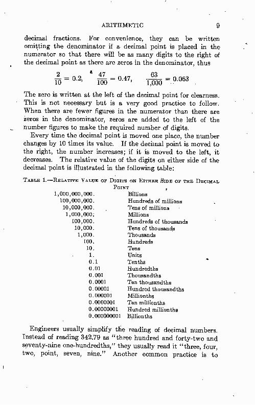
The zero is written at the left of the decimal point for clearness. This is not necessary but is a very good practice to follow. When there are fewer figures in the numerator than there are zeros in the denominator, zeros are added to the left of the number figures to make the required number of digits. Every time the decimal point is moved one place, the number
changes by 10 times its value. If the decimal point is moved to the right, the number increases; if it is moved to the left, it decreases. The relative value of the digits on either side of the decimal point is illustrated in the following table:
TABLE 1.—RELATIVE VALUE
1,000,000,000 100,000 , 000 10,000 , 000 1,000 , 000
100,000 10,000 1,000
100 10 1. o. o. o. o. o. o. o. o. o.
1 01 001 0001 00001 000001 0000001 00000001 000000001
OF DIGITS ON EITHER SIDE OF THE DECIMAL POINT
Billions Hundreds of millions Tens of millions Millions Hundreds of thousands Tens of thousands Thousands Hundreds Tens Units Tenths Hundredths Thousandths Ten thousandths Hundred thousandths Millionths Ten millionths Hundred millionths Billionths
Engineers usually simplify the reading of decimal numbers. Instead of reading 342.79 as "three hundred and forty-two and seventy-nine one-hundredths," they usually read it "three, four, two, point, seven, nine." Another common practice is to
10 APPLIED MATHEMATICS
express small numbers less than unity up to hundredths in per cent of unity by moving the decimal point to the right two digits, thus, 0.79 may be written 79 per cent of unity. Exponents.—The exponent of a number is a small figure placed
to the right and above the number and mewls that the number is to be taken that many times as a factor, hence the square of the
number 10 is
102 = 10 X 10 = 100 Similarly, 108 = 10 X 10 X 10 = 1,000
102 is read "10 cube," or "10 raised to the third power." When no exponent is written, it is understood to be 1; hence, 10' = 10. Positive exponents give results greater than unity, if the number raised to the power is greater than unity. A number raised to a negative power is equivalent to the
reciprocal of the number (1 over the number) raised to a positive power, hence
1 _ (7:11 x 61 x T(51 1 108 —
Negative exponents give results between zero and unity when the number raised to the negative power is greater than unity.
Since positive exponents are for results greater than unity and negative exponents are for results less than unity, the system can be made complete if the exponent zero always gives unity. Hence, any number raised to the zero power is defined to be unity; thus, 10° = 1. IR order to state general laws for exponents, it is convenient
to substitute letters for the numbers as is done in algebra, thus
A. = (A multiplied by itself n times)
Hence, when n= 4, we have A4=A•A•A•A. Using this notation, we can write the following laws of exponents:
1. Addition of Exponents. Am An = Am-Fre (2)
This means that (A multiplied by itself m times) (A multiplied by itself n times) = (A multiplied by itself m n times).
• Example 12. 23 X 24 = 23+4 = 23. Ans. Example 13. 6-8 x 66 x 6-8 x 6-6 = 6-13. Ans.
ARITHMETIC 11
It should be noted that this law is for like numbers raised to the same or different powers. If unlike numbers are raised to powers, it is necessary to raise the respective numbers to the power of their respective exponent before multiplying.
Example 14. 42 X 23 = 4 X4 X2 X2 X2= 16 X8= 128. Ans.
2. Subtraction of Exponents.
Am 1
An = Am—n — An—m
A. 1 when m = n; , , T. „ = A n—n = A° = Tio = 1.
23 Example 15. —22 = 23-2 = 22 = 2. Ans.
116 Example 16. = 11 6 X 112 = 11". Ans.
11-7 54 1 1
Example 17. - 56 X 5-4 - 52 - 5-2. Ans. 56
(3)
These examples show that a number in the numerator can be moved to the denominator if the sign of the exponent is changed. Likewise, a number in the denominator can be moved to the numerator if the sign of the exponent is changed.
3. Multiplication of Exponents. To find the power of a power, we multiply the exponents, thus
(Am)n = Amn
Example 18. (36)3 = 36 X 36 X 36 = 3". Ans. Example 19. (2-3)-4 = 222. Ans. Example 20. (4-4)2 = 4-6. Ans. , Example 21. (62)-2 = 6-14. Ans.
(4)
4. Power of a Product. The power of a product can be written as the product of the various factors raised to that power, thus
(ABC • • •)m = AmBmCm , • • (5)
Example 22. (3 • 4 • 5)2 = 32 • 42 • 52 = 3600. Ans.
5. Power of a Fraction. The power of a fraction can be written as the power of the numerator divided by the power of the denominator, thus
(A)m Am BBm (6)
12 APPLIED MATHEMATICS
3 \ 2 32 g Ans.
Scientific
23. G) = = -s.
Scientific Notation.---Any number can be expressed by, scien-tific notation if it is written as a decimal number between 1 and 10 multiplied by 10 raised to the proper exponent. The use of scientific notation materially simplifies the writing of many num-bers used in electrical engineering. It is recommended that the student use scientific notation wherever it will simplify the numbers.
Example 24. Write the following numbers in scientific notation:
6,000,000 = 6 X 10⁶ Ans. 0.000 000 34 = 3.4 X 10⁻⁷ Ans.
This example shows that the decimal point can be shifted as many places as necessary if the new quantity, or answer, is multi-plied by 10 raised to a power equal to the number of places the decimal point is shifted. The power of 10 in the answer is posi-tive if the decimal point is moved to the left and negative if the decimal point is moved to the right.
Example 25. Simplify the following fraction and express the answer in scientific notation:
4,000 X 5 X 10-12 X 2 X 106 4 X 5 X 2 X 101-'2+6 0.0000005 X 4 X 1016 — 5 X 4 X 10"-1
2 X 10-8 = 2 X 10⁻¹-1 = 2 X 10-12 Ans.
109
ARITHMETIC 13
quite commonly on typewritere not having et and even in printed matter to stand for microfarad.
Inductance values in radio and communication engineering are usually expressed in micromicrohenrys (»ph), microhenrys (.th), or millihenrys (mh). One millihenry is one thousandth of a henry, that is
1 mh = 0.001h = 10-3h
Resistance values are usually larger than unity and may be very large. ka is often used for kilohms, meaning "thousands of ohms," while MO is used for megohms, meaning "millions of ohms." • High voltage or wattage is ordinarily expressed as kilovolt
(kv) or kilowatt (kw). A kilovolt or kilowatt is one thousand times greater than the volt or watt. When changing from one size of unit to another, the conversion
table on page 243 is very convenient to use. The table on page 239 gives other useful quantitative electrical abbreviations.
Radicals.—If a quantity is divided into n equal factors, then one of the factors is said to . be the n" root of the quantity. In other words,
1 (A/s multiplied by itself n times) = A (7)
The nth root of the quantity A can be written as a fractional exponent or as the nth root of the radical A, thus
(8)
Example 26. e= = 3. An..
In Eq. (8), A = 9, n = 2; hence, by Eq. (7),
1+1 (91/2 X 91/2) = 9 2 = 9 or 3 X 3 = 9.
When expressing square root, the 2 is usually omitted; hence
= (9)
but for other roots it must be indicated. The number under the radical sign is called the "radicand."
14 APPLIED MATHEMATICS
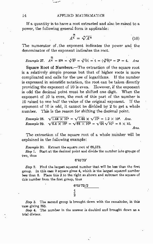
If a quantity is to have a root extracted and also be raised to a power, the following general form is applicable:
A '7 = •Y74.7's (10)
The numerator of , the exponent indicates the power and the denominator of the exponent indicates the root.
Example 27. A; = = \VP = NY7t1 =" 4 = (,e)2 = 22 = 4. Ans
Square Root of Numbers.—The extraction of the square root is a relatively simple process but that of higher roots is more complicated and calls for the use of logarithms. If the number is expressed in scientific notation, the root can be taken directly providing the exponent of 10 is even. However, if the exponent is odd the decimal point must be shifted one digit. When the exponent of 10 is even, the root of this part of the number is 10 raised to one half the value of the original exponent. If the exponent of 10 is odd, it cannot be divided by 2 to get a whole number. This is the reason for shifting the decimal point.
Example 28. -V1.44 X 104 = Vr..r4 X = 1.2 X 10². Ans.
Example 29. -V6.4 X 10' = V64 X 102 = N/64 = 8 x 10. Ans.
The extraction cf the square root of a whole number will be explained in the following example:
Example 30. Extract the square root of 69,573. Step 1. Start at the decimal point and divide the number into groups of
two, thus
6'95'73'
Step 2. Find the largest squared number that will be less than the first group. In this case 2 square gives 4, which is the largest squared number less than 6. Place this 2 to the right as shown and subtract the square of this number from the first group, thus
6'95'73/2
4
Step 3. The second group is brought down with the remainder, in this case giving 295.
Step 4. The number in the answer is doubled and brought down as a trial divisor.
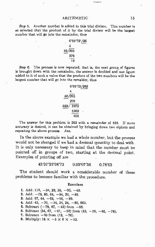
ARITHMETIC 15
Step 5. Another number is added to this trial divisor. This number is so selected that• the product of it by the trial divisor will be the largest number that will go into the remainder, thus
6'95'73'/26
4
46/295
— 276
19
Step 6. The process is now repeated, that is, the next group. of figures is brought down with the remainder, the aniwer is doubled and one figure added to it of such a value that the product of the two numbers will be the largest number that will go into the remaider, thus
6'95'73/263
4
46/295
276
523/ 1973
1569 •
404
The answer for this problem is 263 with a remainder of 404. If more accuracy is desired, it can be obtained by bringing down two ciphers and repeating the above process. Ans.
In the above example we had a whole number, but the process would not be changed if we had a decimal quantity to deal with. It is only necessary to keep in mind that the number must be pointed off in groups of two, starting at the decimal point. Examples of pointing off are
43'97'32'98'73 0.00'07'56 0.78'03
The student should work a considerable number of these problems to become familiar with the procedure.
Exercises
1. Add: 119, —34, 23, 56, —90, —43. 2. Add: —78, 89, 64, —34, 20, —85. 3. Add: 97, 44, —63, —56, —89. 4. Add: 45, —70, —54, 34, 24, —89, 865. 5. Subtract (-78, 87, —43) from —98. 6. Subtract (34, 67, —91, —52) from (45, —19, —65, —78). 7. Subtract —89 from (13, —76). 8. Multiply: 18 X —5 X 6 X —13.
16 APPLIED MATHEMATICS
9. Solve 18 X 103 6 X 10²
10. Solve 8 X —6 X 10-43 X 10-4 —4 X 10" X 32
6» X 6-6 x 6-18 11. Solve
6" X 6-46 12. Express the following in scientific notation: 987,000; 76.456; 0.0007;
9,000.00; 8,976,500.01; ,12,000,000,000,000,000,000.
18. Solve 0.0000006 X 106 X 100,000.00 0.48 X 10-1 X 0.0000004
14. Express each of the following in units, micro units and in mteromicro units: 0.0000009 farad; 1,000 mh; 6mf; 67gpf; 104ph; 0.0003pf; Old; 0.008 farad.
15. Find the square root of the following numbers: 889,635; 9,976; 9,940.09; 5.890331; 0.0000000009; 0.00047; 0.004978.
CHAPTER 2
LOGARITHMS
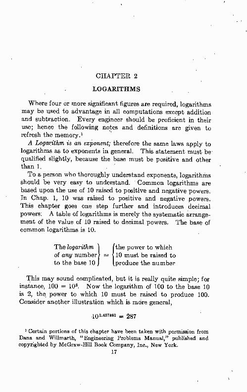
Where four or more significant figures are required, logarithms may be used to advantage in all computations except addition and subtraction. Every engineer should be proficient in their use; hence the following notes and definitions are given to refresh the memory.' A Logarithm is an exponent; therefore the same laws apply to
logarithms as to exponents in general. This statement must be• qualified slightly, because the base must be positive and other than 1. To a person who thoroughly understand exponents, logarithms
should be very easy to understand. Common logarithms are based upon the use of 10 raised to positive and negative powers. In Chap. 1, 10 was raised to positive and negative powers. This chapter goes one step further and introduces decimal powers. A table of logarithms is merely the systematic arrange-ment of the value of 10 raised to decimal powers. The base of common logarithms is 10.
The logarithm the power to which of any number = 10 must be raised to to the base 10 produce the number
This may sound complicated, but it is really quite simple; for instance, 100 = 102. Now the logarithm of 100 to the base 10 is 2, the, power to which 10 must be raised to produce 100. Consider another illustration which is more general,
102.457882 = 287
Certain portions of this chapter have been taken with permission from Dana and Willmarth, "Engineering Problems Manual," published and copyrighted by McGraw-Hill Book Company, Inc., New York.
17
18 APPLIED MATHEMATIÇS
This equation says that the logarithm of 287 is written
log 287 = 2.457882,
which means that 10 must be raised to the 2.457882 power to produce 287; this was obtained from the logarithm tables.
If 10 is raised to the third power, the result is 1,000. • From this it is seen that the logarithm of any number between 100 and 1,000 will be a decimal number between 2 and 3. If 10 is raised to the first power, the answer is 10, so that log 10 = 1, and the logarithm of any number from 10 to 100 will be decimal numbers between 1 and 2.
10° = 1; not 0, which is a common mistake. This says in terms of logarithms that log 1 =-. 0, so numbers between 1 and 10 have logarithms between 0 and 1. The discussion so far has dealt with positive exponents of 10.
That is, all numbers greater than 1 have positive logarithms. Now consider 10-1. From the theory of exponents this can be
written 10-1 = 1/101 = 0.1. This says that log 0.1 = —1. Likewise, 10-2 = 1/102 = 0.01, or log 0.01 = — 2. A more general casç. is 10-1+•55145° = 0.356, or log 0.356 = —1.1-.551450. This was taken from the logarithm table. It is seen from the above illustrations that any number between 0.1 and 1 will have a logarithm of —1+. decimal. Between 0.01 and 0.1 the logarithm will be —2+. decimal; between 0.001 and 0.01 the logarithm will be —3+. decimal. The logarithm of a number is made up of two parts; a decimal,
called the "mantissa," and a whole number (which may be positive, negative, or zero), called the "characteristic." The mantissa determines the sequence of digits, and is all that
is given in logarithm tables. It is always positive. The characteristic determines the position of the decimal
point. Consider the illustration given above, log 287 = 2.457882.
Here 2 is the characteristic and 0.457882 is the mantissa. In the other illustration log 0.356 = —1 +.551450 where —1 is the characteristic and +.551450 is the mantissa. The following simple computations may serve to clear up some
confusion regarding the meaning of logarithms and the character-istic numbers:
LOGARITHMS 19
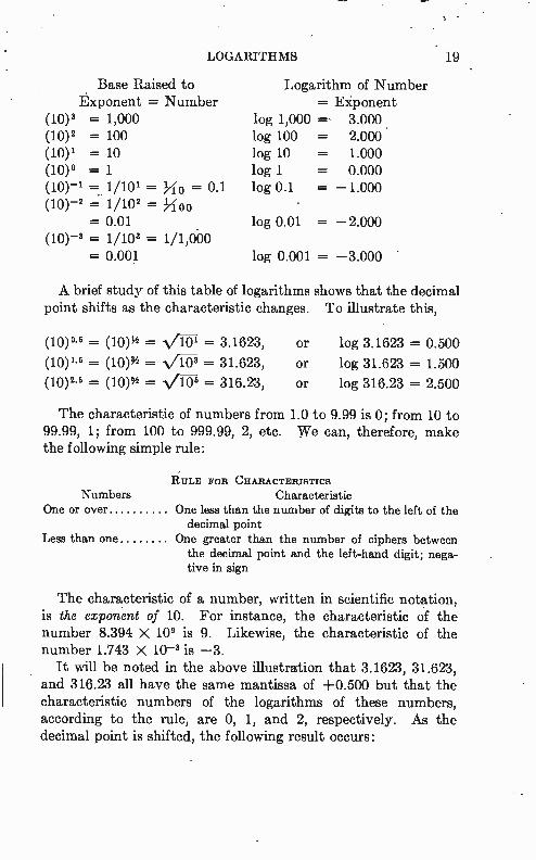
Base Raised to Logarithm of Number Exponent = Number = Exponent
(10) 3 = 1,000 log 1,000 = 3.000 (10) 2 = 100 log 100 = 2.000 (10)' = 10 log 10 = 1.000 (10)° = 1 log 1 = 0.000 (10)-' =_ 1/10' = 31.0 = 0.1 log 0.1 = —1.000 (10)-2 = 1/102 =
= 0.01 log 0.01 = —2.000 (10)-3 = 1/102 = 1/1,600
= 0.001 log 0.001 = —3.000
A brief study of this table of logarithms shows that the decimal point shifts as the characteristic changes. To illustrate this,
(10)" = (10)% = \AP = 3.1623,
(10)" = (10)% = = 31.623,
(10)2.5 = (10)% = NAP = 316.23,
or log 3.1623 = 0.500
or log 31.623 = 1.500
or log 316.23 = 2.500
The characteristic of numbers from 1.0 to 9.99 is 0; from 10 to 99.99, 1; from 100 to 999.99, 2, etc. We can, therefore, make the following simple rule:
RULE FOR CHARACTERISTICS Numbers Characteristic
One or over One less than the number of digits to the left of the decimal point
Less than one One greater than the number of ciphers between the decimal point and the left-hand digit; nega-tive in sign
The characteristic of a number, written in scientific notation, is the exponent of 10. For instance, the characteristic of the number 8.394 X 10° is 9. Likewise, the characteristic of the number 1.743 X 10⁻² is —3.
It will be noted in the above illustration that 3.1623, 31.623, and 316.23 all have the same mantissa of +0.500 but that the characteristic numbers of the logarithms of these numbers, according to the rule, are 0, 1, and 2, respectively. As the decimal point is shifted, the following result occurs:
20 APPLIED MATHEMATICS
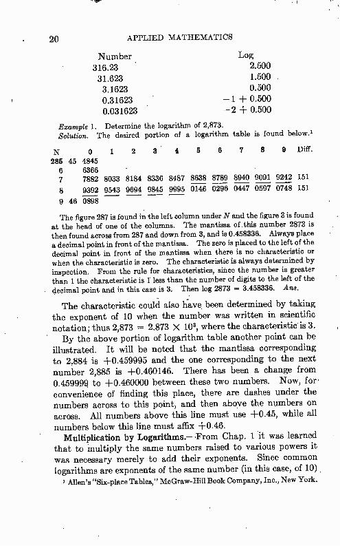
Number Log 316.23 2.500 31.623 1.500 3.1623 0.500 0.31623 —1 + 0.500 0.031623 —2 + 0.500
Example 1. Determine the logarithm of 2,873. Solution. The desired portion of a logarithm table is found below.'
N 0 1 2 3 4 5 6 7 8 9 Diff.
286 45 4845 6 6366 7 7882 8033 8184 8336 8487 8638 8789 8940 9091 9242 151
8 9392 9543 9694 9845 9995 0146 0296 0447 0597 0748 151
9 46 0898
The figure 287 is found in the left column under N and the figure 3 is found at the head of one of the columns. The mantissa of this number 2873 is then found across from 287 and down from 3, and is 0.458336. Always place a decimal point in front of the mantissa. The zero is placed to the left of the decimal point in front of the mantissa when there is no characteristic or when the characteristic is zero. The characteristic is always determined by inspection. From the rule for characteristics, ewe the number is greater than 1 the characteristic is I less than the number of digits to the left of the decimal point and in this case is 3. Then log 2873 = 3.458336. Ans.
The characteristic could also have been determined by taking the exponent of 10 when the number was written in scientific notation; thus 2,873 = 2.873 X 10³, where the characteristic is 3. By the above portion of logarithm table another point can be
illustrated. It will be noted that the mantissa corresponding to 2,884 is +0.459995 and the one corresponding to the next number 2,885 is +0.460146. There has been a change from 0.459999 to +0.460000 between these two numbers. Now, for. convenience of finding this place, there are dashes under the numbers across to this point, and then above the numbers on across. All numbers above this line must use +0.45, while all numbers below this line must affix +0.46.
Multiplication by Logarithms.—From Chap. 1 it was learned that to multiply the same numbers raised to various powers it was necessary merely to add their exponents. Since common logarithms are exponents of the same number (in this case, of 10)
Allen's "Six-place Tables," McGraw-Hill Book Company, Inc., New York.

LOGARITHMS 21
it is necessary only to add the logarithms of the numbers to multiply them. To find the product after the logarithms have been added, it is necessary to determine the number that has a logarithm equal to this sum. This reverse process is called "taking the antilogarithm." To take an antilogarithm, first look up the mantissa of the logarithm in the logarithm table and find the number that gives it. The characteristic of the loga-rithm merely tells where to place the decimal point.
Example 2. Multiply 6 X 48. Solution. log 6 = 0.778151 mantissa from logarithm tables
log 48 = 1.681241 characteristic by inspection
Adding, log (6 X 48) -= 2.459392
Look up the mantissa + 0.459392 in the logarithm table (this mantissa can be found in the portion of logarithm table given above). The number having this mantissa is 2880. Since 2 is the characteristic, point the number off and get 288.0. Ans.
Logarithms are useful in multiplying large numbers, where accuracy to four or five places is sufficient.
Example 3. Multiply 7,864,591 X 198,642. Solution. log 7,864,591 = 6.895644+ mantissa from table
log 198,642 = 5. 297979+ with characteristic affixed
log (7,864,591 X 198,642) = 12.193623+ antilog 12.193623 = 1,562,000,000,000
= 1.562 X 10 12 Ans.
The 'student should check all these examples to familiarize himself with the method of using the logarithm table. It will be noted in working the above problems that no interpolation was made. When looking up the antilogrithm, the number giving the nearest to the mantissa was used. Logarithms are useful in multiplying very small numbers,
as illustrated in Example 4.
Example 4. Multiply 0.000000946 X 0.00087. Solution. log 0.000000946 = —7+0.975891 = 3.975891 — 10
log 0.00087 = —4 + 0.939519 = 6.939519 — 10
log (0.000000946 X 0.00087) -= —11 + 1.915410 = 10.915410 — 20
= 0.915410 — 10 antilog (0.915410 — 10) = 8.2302 X 10⁻²° Ans.
It will be noted in this example that instead of using a negative characteristic with the mantissa, it is more desirable to use a
22 APPLIED MATHEMATICS
positive characteristic with the smallest available multiple of ( —10) placed on the right-hand side. Since the mantissa is always positive, it is confusing to associate with it a negative characteristic and then always have to remember this detail.
If several numbers are to be multiplied, one addition of their logarithms is sufficient. The antilogarithm of this sum gives their product.
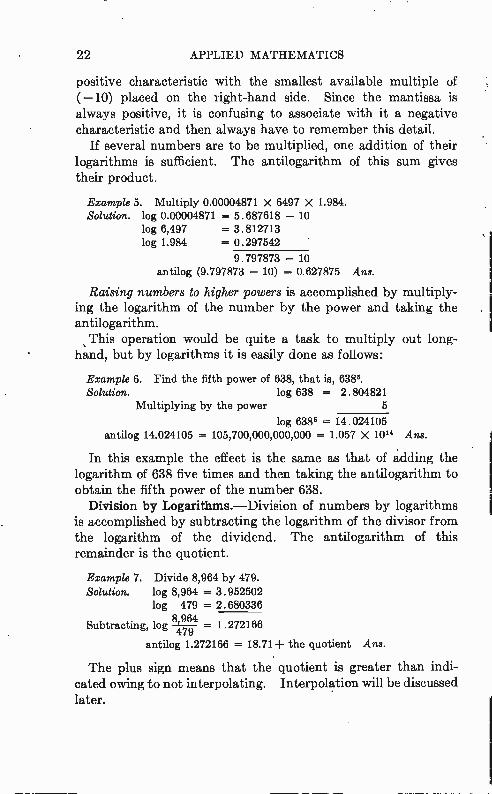
Example 5. Multiply 0.00004871 X 6497 X 1.984. Solution. log 0.00004871 = 5.687618 — 10
log 6,497 = 3.812713 log 1.984 = 0.297542
9.797873 — 10 antilog (9.797873 — 10) = 0.627875 Ans.
Raising numbers to higher powers is accomplished by multiply-ing the logarithm of the number by the power and taking the antilogarithm.
This operation would be quite a task to multiply out long-hand, but by logarithms it is easily done as follows:
Example 6. Find the fifth power of 638, that is, 6384. Solution. log 638 = 2.804821
Multiplying by the power 5
log 6385 = 14.024105 antilog 14.024105 = 105,700,000,000,000 = 1.057 X 10¹⁴ Ans.
In this example the effect is the same as that of adding the logarithm of 638 five times and then taking the antilogarithm to obtain the fifth power of the number 638.
Division by Logarithms.—Division of numbers by logarithms is accomplished by subtracting the logarithm of the divisor from the logarithm of the dividend. The antilogarithm of this remainder is the quotient.
Example 7. Divide 8,964 by 479. Solution. log 8,964 = 3.952502
log 479 = 2.680336 8,964
Subtracting, log —479 = 1.272166
antilog 1.272166 = 18.71+ the quotient Ans.
The plus sign means that the quotient is greater than indi-cated owing to not interpolating. Interpolation will be discussed later.

LOGARITHMS 23
Example 8. Divide 0.000371 by 791. Solution. log 0.000371 = 6.569374 — 10
log 791 = 2.898176
Subtracting, log 0.000371 791 — 3.671198 — 10
antilog (3.671198 — 10) = 4.69027 X 10-' Ans.
Extracting the root of a number is accomplished by dividing the logarithm of the number by the root and taking the antilogarithm.
Example 9. Solve NY976. Solution. log 976 = 2.989450
Dividing, 3)2.989450
log N'ffl = 0.996483
antiiog 0.996483 = 9.919 Ans.
After the student thoroughly understands the use of positive and negative exponents, logarithms become a convenient tool in solving many problems. Only practice is then needed to make the solution of these problems rapid. Logarithms can be used to save considerable time in multiplying and dividing large numbers and the use of logarithms offers the only practical way to raise numbers to high powers and extract roots larger than 2.
Interpolation.—In order to increase the accuracy to more significant figures, beyond the values read directly from th È table, resort is made to interpolation. Interpolation is used in many types of work and should be familiar to the student. Interpo-lation can be used with logarithm tables because the small difference between numbers is approximately proportional to the difference between their logarithms. A practical illustration of interpolation is to find the capacity
of a variable capacitor when set at 53 degrees. Since the capacity at 50 degrees is 278 micromicrofarad and at 55 degrees is 284 micromicrofarad, the capacity change from 50 degrees to 55 degrees is 284 -- 278 = 6 micromicrofarad or % = 1.2 micro-microfarad per degree change of the capacitor dial. Then the capacity for 3 degrees is 3.6 micromicrofarad and is added to the capacity 278 micromicrofarad at 50 degrees to get 281.6 micro-microfarad, the capacity at 53 degrees. This applies only to straight-line variable capacity capacitors.
Applying this principle of interpolation to logarithms, consider the log 78,634. The mantissa of 7863 from the logarithm table is 0.895588, but it is still necessary to obtain the 4 by interpo-
24 APPLIED MATHEMATICS
lation. The figure 56 will be found as the "duff" in the right-hand column. At the bottom of the page will be found a table of proportional parts and going across from the "diff" 56 in the left-hand column to the column headed 4. Therefore 22.4 is the proportional part to be added to the above mantissa giving log 78,634 = 4.8956104. Some logarithm tables do not have proportional parts, so
in such cases it will have to be figured out each time. Consider-ing the above illustration,
log 78,630 = 4.895588 (from log tables) log 78,634 = 4.8956104 (by interpolation) log 78,640 = 4.895644 (from log tables)
Here the logarithms of 30 and 40 are given in the last two digits of the number but it is desired to secure the logarithm of 34 in these last two digits. The corresponding mantissas for 30 and 40 are 0.895588 and 0.895644 respectively. The differ-ence between 30 and 40 is 10, while the difference in the corre-sponding mantissa is 56. This is the way to secure the number in the right-hand column under "diff." Corresponding to 34 take 0.4 of 56, which is 22.4 and is the proportional part worked out at the bottom of the page.' The logarithm by interpolation is log 87,634 = 4.8956104. To find the antilogarithm, the above process must be reversed.
For illustration, find the antilogarithm of 3.657488. From the
logarithm tables,
antilog 3.657438 -- 4,544 antilog 3.657488 = 4,544.521 (by interpolation) antilog 3.657534 = 4,545
Subtract 3.657438 from 3.657488, giving 50, the proportional part. The difference in this case, as noted in the right-hand column, is 96. Across from 96 on the next page find under 5, not 50 but 48, the nearest number to 50, so the answer will not be exact. To make it exact, take the ratio
9506 _x IT) Solving for x,
500 x = —9-é- = 5.21
1 See Allen's "Six-place Tables," McGraw-Hill Book Company, Inc., New York.
LOGARITHMS 25
Now antilog 3.657488 = 4,544.521, while if the 48 from the table was used, the result would be 4,544.5. Ordinarily the accuracy of the proportional parts table is sufficient, but it can be seen that greater accuracy sometimes can be obtained by using exact proportion. The student with a thorough understanding of exponents
should find that what has been presented on logarithms here is sufficient to enable him to handle any ordinary problem in logarithms. However, it may be well to illustrate by example how to handle the characteristic in extracting the root of small numbers.
Example 10. Extract the fifth root of 0.0004466. Solution. log 0.0004466 = 6.649919 — 10
Dividing by 5, log NV0.0004466 = 1.3299838 — 2 = 9.3299838 — 10
antilog (9.3299838 — 10) = 0.213788 Ans.
It should be pointed out that the negative characteristic placed on the right-hand side (-10 in this case) should always be divisible by the root to be extracted. This number is usually made 10 for convenience in routine work.
Example 11. Extract the fourth root of 0.0004466. Solution. log 0.0004466 = 0.649919 — 4
Dividing by 4, log N4/0.0004466 = 0.1624797 — 1 = 9.1624797 — 10
antilog (9.1624797 — 10) = 0.145372 Ans.
Operating the Slide Rule.—The slide rule is a graphic logarithm table. Many users of the instrument do not realize this and as a result are not able to make full use of its possibilities. To multiply numbers, simply add their logarithms. To do it
graphically on the slide rule, add the distances that are marked off proportional to the logarithm. To divide, subtract distance corresponding to the dividend. The resulting distance corre-sponds to the quotient. The accuracy of a slide rule depends upon the precision with
which it is made. A longer slide rule will give better accuracy than a short one, but the accuracy does not increase in direct proportion to the length of the scale. Common 10-inch slide rules will give an accuracy to three significant figures, and on the lower end of the scale it is possible to estimate to the fourth digit.
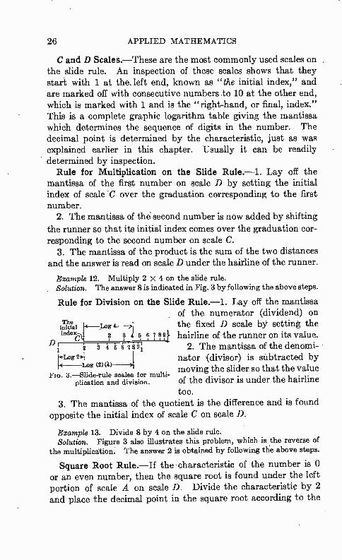
The initial t--Log 4 inde l 2 g K ig7”1
D 1 .1).
i à 4 5 6 789 1
tc(-Log 244 Log (2) (.4 )-->1
3.—Slide-rule scales for plication and division.
26 APPLIED MATHEMATICS
C and D Scales.—These are the most commonly used scales on the slide rule. An inspection of these scales shows that they start with 1 at the, left end, known as "the initial index," and are marked off with consecutive numbers to 10 at the other end, which is marked with 1 and is the "right-hand, or final, index." This is a complete graphic logarithm table giving the mantissa which determines the sequence of digits in the number. The decimal point is determined by the characteristic, just as was explained earlier in this chapter. Usually it can be readily determined by inspection. Rule for Multiplication on the Slide Rule.-1. Lay off the
mantissa of the first number on scale D by setting the initial index of scale *C over the graduation corresponding to the first number.
2. The mantissa of the second number is now added by shifting the runner so that its initial index comes over the graduation cor-responding to the second number on scale C.
3. The mantissa of the product is the sum of the two distances and the answer is read on scale D under the hairline of the runner.
Example 12. Multiply 2 X 4 on the slide rule. Solution. The answer 8 is indicated in Fig. 3 by following the above steps.
Rule for Division on the Slide Rule.-1. Lay off the mantissa of the numerator (dividend) on the fixed D scale by- setting the hairline of the runner on its value.
2. The mantissa of the denomi-nator (divisor) is subtracted by moving the slider so that the value of the divisor is under the hairline too.
3. The mantissa of the quotient is the difference and is found opposite the initial index of scale C on scale D.
Example 13. Divide 8 by 4 on the slide rule. Solution. Figure 3 also illustrates this problem, which is the reverse of
the multiplication. The answer 2 is obtained by following the above steps.
Square Root Rule.—If the characteristic of the number is 0 or an even number, then the square root is found under the left portion of scale A on scale D. Divide the characteristic by 2 and place the decimal point in the square root according to the
multi-
LOGARITHMS 27
result. If the number was originally written in scientific notation, then the exponent of 10 is divided by 2 and the answer is still in scientific notation.
Example 14. Find the square root of 97,969. Solution. Since the characteristic 4 of this number is even, place the
hairline over 97,969 to the left of the center on scale A and read 313 the answer on scale D. The characteristic of the answer is 2, just half that of the original number. Actually only the first three digits of the original number can be read on scale A of the slide rule.
If the characteristic of the number is an odd number, then the square root is found under the right-hand portion of the A scale on the D scale. Subtract 1 from the characteristic of the number and divide by 2 to find the characteristic of the root.
Example 15. Find the square root of 1.56816 X 10⁶. Solution. Below 1.56816 on the right-hand side of scale A find the answer
3.96 X 10⁷. The characteristic 2 was found by subtracting 1 from 5 and dividing by 2.
Square Rule.—When the hairline is to the left of the middle of the A and B scales (roots less than 3.1623), the square of the number on the D scale is found on the A scale. The character-istic of the squared number is twice that of the original number. If the original number is written in scientific notation, then the answer will also be in scientific notation.
Example 16. Square 240. Solution. Above 240 on scale D read the answer 57,600 on scale A. The
characteristic doubled since the answer was on the left-hand side.
When the hairline is to the right of the middle on scale A and B, the characteristic is found by multiplying the characteristic of the original number by 2 and adding 1. Again, if the original number was in scientific notation, then the answer will also be in scientific notation.
Example 17. Square 6.2 X 10⁷.
Solution. Above 6.2 on scale D read the answer 3.844 X 10⁷ on scale A. The characteristic 7 was obtained by multiplying 3 by 2 and adding 1.
The student must use the slide rule at every opportunity if he wishes to become familiar with its operation and feel confidence in its results.
28 APPLIED MATHEMATICS
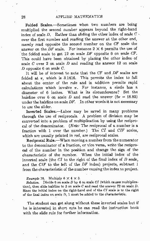
Folded Scales.—Sometimes when two numbers are being multiplied the second number appears beyond the right-hand index of scale D. Rather than sliding the other index of scale C - over the first number and reading the answer at the other end, merely read opposite the second number on the CF scale the answer on the DF scale. For instance 2 X 6 permits the use of the folded scale to get 12 on scale DF opposite 6 on scale CF. This could have been obtained by placing the other index of scale C over 2 on scale D and reading the answer 12 on scale D opposite 6 on scale C.
It will be of interest to note that the CF and DF scales are folded at ir, which is 3.1416. This permits the index to fall about the center of the rule and in addition permits rapid calculations which involve ir.. For instance, a circle has a diameter of 6 inches. What is its circumference? Set the hairline over 6 on scale D and read the answer (67r = 18.85) under the hairline on scale DF. In other words it is not necessary to use the slider.
Inverted Scales.—Labor may be saved in many problems through the use of reciprocals. A problem of division may be converted into a problem of multiplication by using the recipro-cal of the denominator. (Note: The reciprocal of a number is a fraction with 1 over the number.) Thé CI and CIF scales, which are usually printed in red, are reciprocal scales.
Reciprocal Rule.—When moving a number from the numerator to the denominator of a fraction, or vice versa, write the recipro-cal of the number in the position and change the sign of the characteristic of the number. When the initial index of the inverted scale (the CI to the right of the final index of D scale, and the CIF to the left of the DF index) projects, subtract 1 from the characteristic of the number causing the index to project.
Example 18. Multiply 6 X 4 X 3. Solution. Divide 6 on scale D by 4 on scale CI (which causes multiplica-
tion), then slide hairline to 3 on scale C and read the answer 72 on scale D. Since the initial index on the right-hand end of the CI scale is to the right of the final index on scale D, 1 must be added to the characteristic.
The student can get along without these inverted scales but if he is interested in short cuts he can read the instruction book with the slide rule for further information.

LOGARITHMS 29
A and B Scales.—The A and B- scales consist of two complete logarithm scales, each half as long as scale D. Since the values of the logarithm increase twice as fast on scale A as on scale D, the means of securing square roots and square powers is pro-vided. Opposite a number on scale D the square is found on scale A. Conversely, a number on scale A will have its square root opposite it on the D scale.
K Scale.—The K scale consists of three complete logarithm scales, each one third as long as scale D. The K scale gives cubes and cube roots in the same manner as scale A gives squares and square roots.
L Scale.—This scale is a complete logarithm table. To take the logarithm of a number, place the hairline of the slider over the number on scale D and read the mantissa under the hairline on scale L.
The following facts are important to keep in mind when using a slide rule:
1. The slide rule is a graphic logarithn\table. 2. The mantissa only is determined from any logarithm table,
including the slide rule which is a graphic one. 3. The mateissa determines only the sequence of digits. 4. Characteristics are not given in any logarithm tables. 5. The characteristic is determined by inspection. It is the
exponent of 10 when the number is written in scientific notation. 6. The characteristic determines the decimal point. When multiplying very large or very small numbers on the
slide rule, it is convenient to use 10 to some power and place the decimal point after the first digit.
Example 19. Multiply 0.00000027 X 96000. Rewrite 2.7 X 10-7 X 9.6 X 104 Rewrite and multiply 2.7 X 9.6 X 10-8 = 25.92 X 10⁻⁷ Ans.
This makes it easy to keep track of the decimal point by inspection when scientific notation is employed. Decimal Point and the Slide Rule.—The last example illus-
trates how the decimal point can be easily found by inspection. A definite procedure will now be given for keeping track of the decimal point when using the slide rule. When using numerical logarithms the characteristic is added
to the mantissa, but when using the slide rule this cannot be
30 APPLIED MATHEMATICS
done. However, keeping track of the characteristic is the eaâest• way of determining the decimal point when using a slide rule. When multiplying by means of numerical logarithms the sum
of the mantissas is often more than 1.0 and so 1 must be carried over into the column of the characteristics. If this same problem is solved with a slide rule, it is found that there is an exact parallel between the numerical and graphic methods. The distances representing the mantissas will add to one full scale length or more. This corresponds to carrying 1 into the char-acteristic column; hence a note should be made each time this
occurs. There is a simple, quickly applied, and absolutely accurate
rule for decimal points based upon the foregoing facts. This Method completely does away with the need of longhand check-
The Initial Index
iI 2 I 1,1'1,1,1,1 3 4 5 6 7 8 9 1
C a I 1 e I I I " 1 , 1 .1 ,1
2 3 I 4 5 6 7
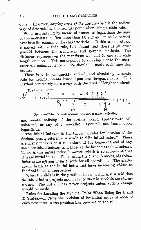
144 36 FIG. 4.—Slide-rule scale showing the initial index projecting.
ing, mental shifting of the decimal point, approximate cal-culation, or any other so-called "system" not based upon logarithms. The Initial Index.—In the following rules for location of the
decimal point, reference is made to "the initial index." There are many indexes on a rule; those at the beginning end of any scale are initial indexes, and those at the far end are final indexes. There is one initial index, however, which is so important that it is the initial index. When using the C and D scales, the initial index is the left end of the C scale for all operations. The gradu-ations begin at the initial index and have increasing values as the final index is approached. When the slide is in the position shown in Fig. 4, it is said that
the initial index projects and a change must be made in the charac-teristic. The initial index never projects unless such a change should be made.
Rules for Locating the Decimal Point When Using the C and D Scales.-1. Note the position of the initial index as soon as each new term in the problem has been set on the rule

LOGARITHMS 31
2. If the initial index projects, add 1 to the logarithmic characteristic of the term which caused the index to project. Thus, for multiplication, add 1 to the logarithmic characteristic of the multiplier which caused the index to project. The characteristic of the answer is the algebraic sum of the character-istics of the terms plus the "added characteristics." For division, add 1 to the logarithmic characteristic of the divisor which caused the index to project. The characteristic of the answer is the algebraic difference of the characteristics of • the divisor and dividend.
3. When the initial index does not project, make no changes in the characteristics.
4. For continued operations, note the position of the initial index as soon as each new term is set on the rule, and record any necessary addition to the characteristics at once.
Sequence of Operations.—While becoming familiar with this method, the beginner should form the habit of going through the following steps in his slide-rule work:
1. Set the work up in a suitable form for a slide-rule compu-tation. (See examples below.)
2. Indicate the logarithmic characteristic of each term some-where close by. (Just above the multipliers and below the divisors is convenient.)
3. Note the position of the initial index as soon as each new factor is set on the rule.
4. Record the "added characteristic" if the initial index projects.
5. Determine the characteristic of the answer.
Multiplication.
Example 20. Multiply 36 by 0.0004. 1. Set the work up in a suitable form. 2. Indicate the logarithmic characteristic above each multiplier.
+1 +1 —4 +1 — 4 + 1 = —2 (36)(0.0004) = 0.0144 = 1.44 X 10⁻² Ans.
3. Referring to Fig. 4, it is seen that the initial index projects. 4. Hence 1 must be added to the characteristics. 5. Adding the characteristics gives 1 — 4 ± 1 = —2 as the charac-
teristic of the answer. The answer is now pointed off according to this characteristic.
32 APPLIED MATHEMATICS
Division.
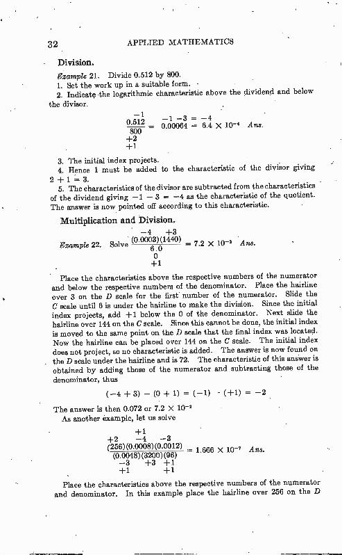
Example 21. Divide 0.512 by 800. 1. Set the work up in a suitable form. • 2. Indicate the logarithmic characteristic above the dividend and below
the divisor.
—1 0.512 —1 — 3 = —4
0.00064 = 6.4 X 10⁻⁴ Ans. 800 +2 +1
3. The initial index projects. 4. Hence 1 must be added to the characteristic of the divisor giving
2 + 1 = 3. 5. The characteristics of the divisor are subtracted from the characteristics
of the dividend giving —1 — 3 = —4 as the characteristic of the quotient. The answer is now pointed off according to this characteristic.
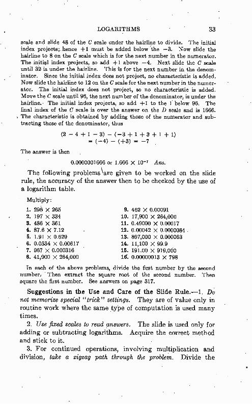
Multiplication and Division. —4 +3
Example 22. solve (0.0003X1440) — 7.2 X 10⁻² Ans
o 6 .0
+1
Place the characteristics above the respective numbers of the numerator and below the respective numbers of the denominator. Place the hairline over 3 on the D scale for the first number of the numerator. Slide the C scale until 6 is under the hairline to make the division. Since the initial index projects, add +1 below the 0 of the denominator. Next slide the hairline over 144 on the C scale. Since this cannot be done, the initial index is moved to the same point on the D scale that the final index was located. Now the hairline can be placed over 144 on the C scale. The initial index does not project, so no characteristic is added. The answer is now found on the D scale under the hairline and is 72. The characteristic of this answer is obtained by adding those of the numerator and subtracting those of the
denominator, thus
(-4 + 3) — (0 + 1) = ( —1) — (+1) = —2
The answer is then 0.072 or 7.2 x 10⁻² As another example, let us solve
+1 +2 —4 —3 (256)(0.0008)(0.0012) (0.0048)(3200)(96) —3 +3 +1 +1 +1
Place the characteristics above the respective numbers of the numerator and denominator. In this example place the hairline over 256 on the D
= 1.666 X 10⁻⁷ Ans.
LOGARITHMS 33
scale and slide 48 of the C scale under the hairline to divide. The initial index projects;. hence +1 must be added below the -3. Now slide the hairline to 8 on the C scale which is for the next number in the numerator. The initial index projects, so add +1 above -4. Next slide the C scale until 32 is under the hairline. This is for the next number in the denom-inator. Since the initial index does not project, no characteristic is added. Now slide the hairline to 12 on the C scale for the next number in the numer-ator. The initial index does not project, so no characteristic is added. Move the C scale until 96, the next number of the denominator, is under the hairline. The initial index projects, so add +1 to the 1 below 96. The final index of the C scale is over the answer on the D scale and is 1666. The characteristic is obtained by adding those of the numerator and sub-tracting those of the denominator, thus
(2 - 4 + 1 - 3) - ( -3 1 + 3 + 1 + 1)
The answer is then
0.0000001666 or 1.666 X 10⁻⁷ Ans.
The following problems \ are given to be worked on the slide rule, the accuracy of the answer then to be checked by the use of a logarithm table.
Multiply:
1. 296 X 265 9. 462 X 0.00091 2. 197 X 334 10. 17,900 X 264,000 3. 486 X 361 11. 0.49000 X 0.00017 4. 87.6 X 7.12 12. 0.00042 X 0.0000084 5. 1.91 X 0.629 13. 897,000 X 0.000063 6. 0.0534 X 0.00617 14. 11,100 X 99.9 7. 967 X 0.000316 15. 191.00 X 919,0® 8. 41,900 X 264,000 16: 0.00000013 X 798
In each of the above problems, divide the first number by the second number. Then extract the square mot of the second number. Then square the first number. See answers on page 317.
Suggestions in the Use and Care of the Slide Rule.-1. Do not memorize special "trick" settings. They are of value only in routine work where the same type of computation is used many times.
2. Use fixed scales to read answers. The slide is used only for adding or subtracting logarithms. Acquire the correct method and stick to it.
3. For continued operations, involving multiplication and division, take a zigzag path through the problem. Divide the
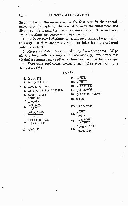
34 APPLIED MATHEMATICS
first number in the numerator by the first term in the denomi-nator, then multiply by the second term in the numerator and divide by the second term in the denominator. This will save several settings and lessen chances to error.
4. Avoid longhand checking, as confidence cannot be gained in this way. If there are several numbers, take them in a different order as a check.
5. Keep your slide rule clean and away from dampness. Wipe off the face with a damp cloth occasionally, but never use alcohol or strong soap, as either of these may remove the markings.
6. Keep scales and runner properly adjusted as accurate results depend on this.
Exercises
1. 961 x 378 11. 2. 14.7 X 7.917 12. -11.
3. 0.00049 X 7,411 13. V0.0001392
4. 9,376 X 1,375 X 0.0006134 14. -‘3/0.0027965
5. 8,761 ÷ 1,942 15. ./0.00039 X 6972 1,918,000 16. 8,9673.
6. 0.0002834
0.0002978 17. 4922 X 7893 1,162
962 X 6,443 •N/763 8. 18. 248 4,9674
0.00092 X 7,134 19. R10.0067] 3 9. 345 X 0.71 476
. [ 0.0034 1' 10. -0T(,ei 20 0.0004962
CHAPTER 3
ALGEBRA
We must study the fundamentals of algebra if we are to get anywhere with radio and communication principles. This review of algebra will consider only the fundamental principles met in everyday engineering work. Nearly all radio engineering involves algebra in some form. Enough of the subject will be treated here to enable the student to handle circuit theory and vacuum tube operation. The work presented will be as simple as ordinary arithmetic and should not baffle any student desiring to take the subject.
In this book algebra will be used to show derivations of useful radio equations. By this means, the student should be better prepared to use such equations than if he were simply given them to memorize. Equations can often be rearranged and solved for a desired term.
In arithmetic figures are used in equations, while in algebra letters are used in order to express more general conditions.
For, instance, in algebra we can write Ohm's law by the expression
E = IR (I)
By simple algebra this same law can be written in the fractional equations
E =
E R =
In some problems one expression will be more desirable than the others. When studying tuned circuits, we deal algebraically with
XL = Xe, where XL is the inductive reactance and X c is the capacitive reactance. The following equation is true for resonance no matter what the numerical values happen to be. It is
35
36 APPLIED MATHEMATICS
f - 2r \FCC (4)
This is the familiar equation used to determine the frequency of resonance. If we know the inductance L and the capacity C, we can determine f, the frequency at which the circuit will freely oscillate. Equations.—We have so far cited several equations, which are
merely expressions of equality between two quantities. This equality is denoted by (=), the sign of equality. In Ohm's law E = IR states that the voltage E has the same numerical value as the current multiplied by the resistance. An equation is an expression having the same value on both sides of the sign of equality. If this is not true, we do not have an equation but an inequality. The value of one side of an equation may be changed or varied if the other side is changed the same amount. Such quantities are called "variables." In this case we are changing the numerical value on both sides but maintaining equality; hence, we still have an equation. We can apply multiplication, division, addition, or subtraction to one side of the equation if we do the same thing to the other side.
Illustration of Addition.
Given Then
x + y = z 1+x+y=l+z
If x = 4, y = 3, and z = 7, the above equations read respec-tively, "Each side is equal to 7, or (4 ± 3 = 7)," and, "Each side is equal to 8 or (1 + 4 + 3 = 1 + 7)."
Illustration of Subtraction.
Given x y — 3 = z — 3 Substituting values 4 + 3 — 3 = 7 — 3 Each side is equal to 4.
Illustration of Multiplication.
Given 2(x + y) = (z)2 Substituting values, 2(4 -I- 3) = 7 X 2 Each side is equal to 14.
ALGEBRA 37
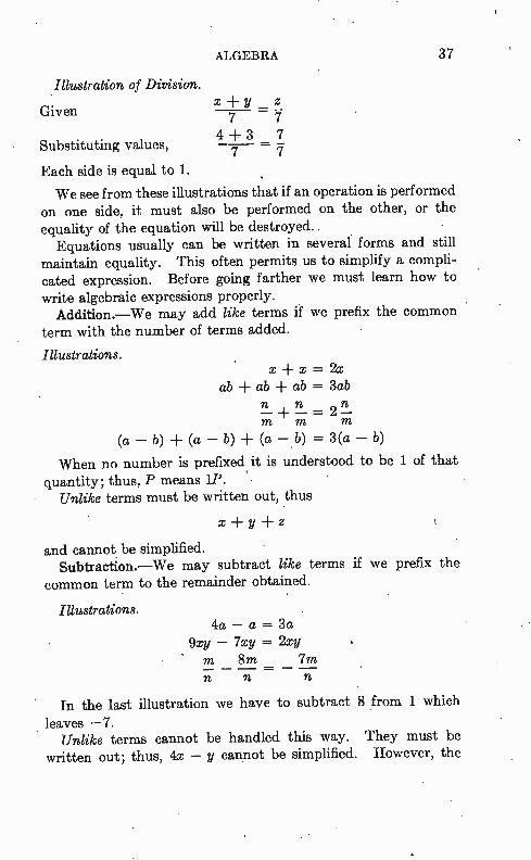
Illustration of Division.
Given
Substituting values,
Each side is equal to 1.
We see from these illustrations that if an operation is performed on one side, it must also be performed on the other, or the equality of the equation will be destroyed..
Equations usually can be written in several forms and still maintain equality. This often permits us to simplify a compli-cated expression. Before going farther we must learn how to write algebraic expressions properly. Addition.—We may add like terms if we prefix the common
term with the number of terms added.
Illustrations. x x = 2x
ab + ab + ab = 3ab n n 711. + n 2 —m = m—
(a — b) + (a — b) + (a — b) = 3(a — b)
When no number is prefixed it is understood to be 1 of that quantity; thus, P means 1P.
Unlike terms must be written out, thus
x -F y + z
x y _ z 7 7
4 + 3 7 7 —
and cannot be simplified. Subtraction.—We may subtract like terms if we prefix the
common term to the remainder obtained.
Illustrations. 4a — a = 3a
9xy — 7xy = 2xy • m 8m 7m —n — -71-1 n
In the last illustration we have to subtract 8 from 1 which
leaves —7. Unlike terms cannot be handled this way. They must be
written out; thus, 4x — y cannot be simplified. However, the
38 APPLIED MATHEMATICS
expression can be rearranged, giving — y + 4x, without changing its value.
Positive and negative number rules, as already given, will always hold true in algebra. What is called " algebraic addition" takes into account all signs and may in some cases actually involve subtraction. As an illustration, the impedance of a circuit can be expressed
D.= R2 + X2 (5)
where R is the resistance, X is the reactance, and Z is the imped-ance. Extracting the square root of both sides, we get
z .= .VR2 ± x2 (6)
In this form we can solve for the impedance, while in the original equation we had to deal with the square of the impedance.
If this circuit contained inductive reactance, XL, and capaci-tive reactance Xe, this expression can be written
z = vR2 (XL _ Ife)2 (7)
In this case the capacitive reactance must be subtracted from the inductive reactance and then the quantity squared before being added to the square of the resistance to obtain the square of the impedance. We see that the algebraic language in the above equation is
very clear and simple in comparison with the expression of the relationship in a sentence. The exact and simple statement of relationships is one of the main objectives in mathematics.
Multiplication.—We may multiply like terms by raising the like term to the power corresponding to the number of terms multiplied.
Illustrations. NXNXN=N3
ab X ab = (ab) 2
We may indicate the multiplication of unlike terms by simply writing the terms to be multiplied in succession with no sign between terms.
Illustrations.—To multiply /, the current, by R, the resistance, to obtain the voltage, E, we write
E = IR
ALGEBRA 39
As another illustration, for resonance,
XL = Xc
but XL = cuL, where w is the angular velocity in radians per second and L is the inductance in henrys, and Xc = 1/c0C where C is the capacity in farads. Since things equal to the same thing are equal to each other, we can write
1 wL =
coC
or, multiplying both sides of the equation by w, we get
Now, if we multiply both sides by 1/L, we get
1 2 -
- Lc but w=2rf
so (Id) 2 =
1 Multiplying through by (2702 we get
1
•
e (2ar) 2le
Now, if we take the square root of both sides, we have
1 f -
2ir N/LC
which is the familiar equation to determine the resonant fre-quency of a circuit.
In this development we have had several occasions to multiply unlike terms such as co X L, written simply caL. Several times we have multiplied both sides of the equation by the same thing so the equation must still hold true. Then in the last step we took the square root of both sides to get the answer in a familiar form.
40 APPLIED MATHEMATICS
Let us now apply the above rules to some more problems. As, an illustration,
2adc X 3abc = 6a2bdc2
Here we note that the numerical coefficients 2 and 3 are multiplied to get. 6. Then we have a X a = a2 and c X c = e2. The d and b must appear in the answer because they are unlike terms, and hence the multiplication can only be indicated.
This same type of reasoning is applied to the following illus-tration:
(4x2e)(5xyz) = 20xxxyyyyzz = 20x 4z2
It will be noted that the theory of exponents comes into play here; that is, when like terms are multiplied their exponents are added.
pair of parentheses indicates one quantity. If we should have (4a2b)3 it weld mean that every unlike term in the quantity must be raised to the third power, thus getting
43(a2)3b2 = 64a6b2
An exponent foil—owing a letter refers to that letter only. For example, xy2 means that only the y is raised to the second power. If we want the x also raised to second power we must write x2y2 or (xy) 2, which are the same and mean xxyy. So far we have dealt with single terms. We must learn how
to deal with quantities with more than one term.
Illustrations. abc (single term) a — be . (two terms) a + b — c • (three terms)
This illustration shows that several terms in a quantity are grouped together by plus and minus signs. One quantity multiplied by another quantity, as (a -F b) multiplied by c, can be expressed e(a b) and if multiplied out gives ca cb. This shows that each term in the quantity must be multiplied individually. To multiply more complicated quantities where the answer is not so evident, the following method is suggested:
ALGEBRA 41
a ± b c multiplier
ac bc answer
As another illustration,
c(ab + cd — e2) = abc ± c2d — ce2
To show this ab + cd — e2
abc ± c2d — ce2
•
After the multiplication has been performed there are still three terms, but the parentheses have been removed, and the multiplication by c has been indicated in each term.
Careful attention must be given to the signs when multiplying. The following rules are, therefore, important to keep in mind.
1. Multiplication of terms with like signs gives a plus product. 2. Terms with unlike signs give a minus product.
Illustrations.
z(x + y) = Zr yz —z(x + y) = —Zr — yz
z(x — y) = Zr — yz —z(x — y) = —xz yz
The application of these rules can be extended to expressions having more than• one term, as illustrated by the following:
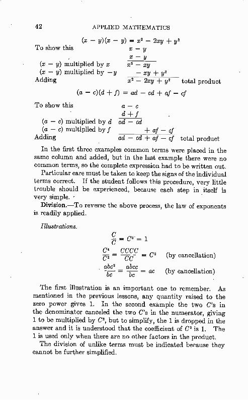
(x + y)(x + y) = x2 ± 2xy + y2
To show this x + y x + y
(x + y) multiplied by x x2 + xy (x ± y) multiplied by y + xy + y2
Adding x2 -I- 2xy ± y2 total product
(x y)(x — y) = x2" — y2
To show this x y x — y
(x ± y) multiplied by x x2 ± xy (x + y) multiplied by —y — xy — y2
Adding . x2 - y2 total product
42 APPLIED MATHEMATICS
To show this
(x — y) multiplied by x (x — y) multiplied by —
Adding
(x — y)(x — y) = x' — 2xy y' x — y x — y
x 2 x y
x y + y2
X 2 - 2xy y' total product
•(a — c)(d f) = ad — cd af — cf
To show this a — c • d f
(a — c) multiplied by d ad — cd (a — c) multiplied by f af — cf
Adding ad — cd ± af — cf total product
In the first three examples common terms were placed in the same column and added, but in the last example there were no common terms, so the complete expression had to be written out.
Particular care must be taken to keep the signs of the individual terms correct. If the student follows this procedure, very little trouble should be experienced, because each step in itself is very simple. -
Division.—To reverse the above process, the law of exponents is readily applied.
Illustrations.
-û = C ° = 1
C 4 CCCC ry2
2 = CC =
abc2 abcc • = — = ac
bc be
(by cancellation)
(by cancellation)
The first illustration is an important one to remember. As mentioned in the previous lessons, any quantity raised to the zero power gives 1. In the second example the two C's in the denominator canceled the two C's in the numerator, giving 1 to be multiplied by C', but to simplify, the 1 is dropped in the answer and it is understood that the coefficient of C' is 1. The 1 is used only when there are no other factors in the product. The division of unlike terms must be indicated because they
cannot be further simplified.
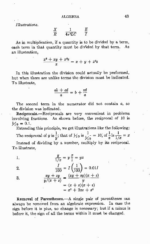
ALGEBRA 43
Illustrations. X 1 E Ti 472Lc
As in multiplication, if a quantity is to be divided by a term, each term in that quantity must be divided by that term. As an illustration,
x2 + xy + x3z= ± y ± x2z
In this illustration the division could actually be performed, but when there are unlike terms the division must be indicated. To illustrate,
ab + ccl = b + —ccl a a
The second term in the numerator did not contain a, so the division was indicated.
Reciprocals.—Reciprocals are very convenient in problems involving fractions. As shown before, the reciprocal of 10 is
= 0.1. Extending this principle, we get illustrations like the following:
. 1 . 1 1. 1 The reciprocal of y -; that of ho — = 10' of - —1/x = x fo x Instead of dividing by a number, multiply by its reciprocal.
To illustrate,
1.
2.
3.
= 1 y - = yx 1 1 x
1-00 I = I (—) = 0.011 100 xy zy _ (xy + zy)(x + z) y/(x z)
= (x + z)(x + = x2 ± 2xz z2
Removal of Parentheses.—A single pair of parentheses can always be removed from an algebraic expression. In case the sign before it is plus, no change is necessary; but if a minus is before it, the sign of all the terms within it must be changed.
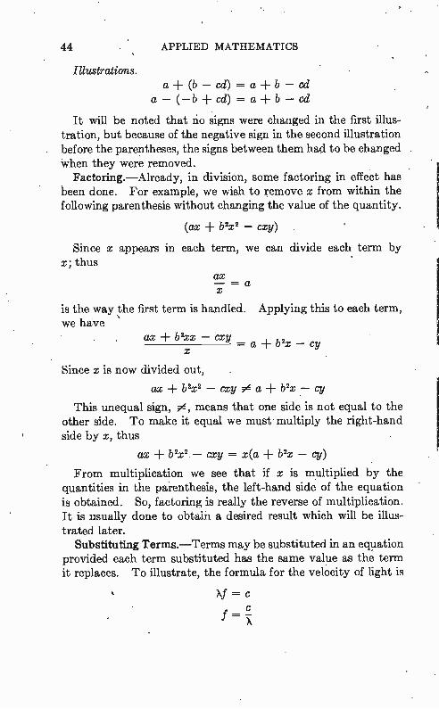
44 APPLIED MATHEMATICS
Illustrations. a + (b — cd) = a + b — cd
a— (—b+cd) = a+b— cd
It will be noted that rio signs were changed in the first illus-tration, but because of the negative sign in the second illustration before the parentheses, the signs between them had to be changed when they were removed.
Factoring.—Already, in division, some factoring in effect has been done. For example, we wish to remove x from within the following parenthesis without changing the value of the quantity.
(ax b2x2 _ axy)
Since x appears in each term, we can divide each term by x; thus
ax a
is the way the first term is handled. Applying this to each term, we have
ax + b2xx — x
Y = a + b2x — cy
Since x is now divided out,
ax + b2x2 — cxy a + b2x — cy
This unequal sign, 0 , means that one side is not equal to the other side. To make it equal we must multiply the right-hand side by x, thus
ax + b2x2 — cxy = x(a + b2x — cy)
From multiplication we see that if x is multiplied by the quantities in the parenthesis, the left-hand side of the equation is obtained. So, factoring is really the reverse of multiplication. It is usually done to obtain a desired result which will be illus-trated later.
Substituting Terms.—Terms may be substituted in an equation provided each term substituted has the same value as the term it replaces. To illustrate, the formula for the velocity of light is
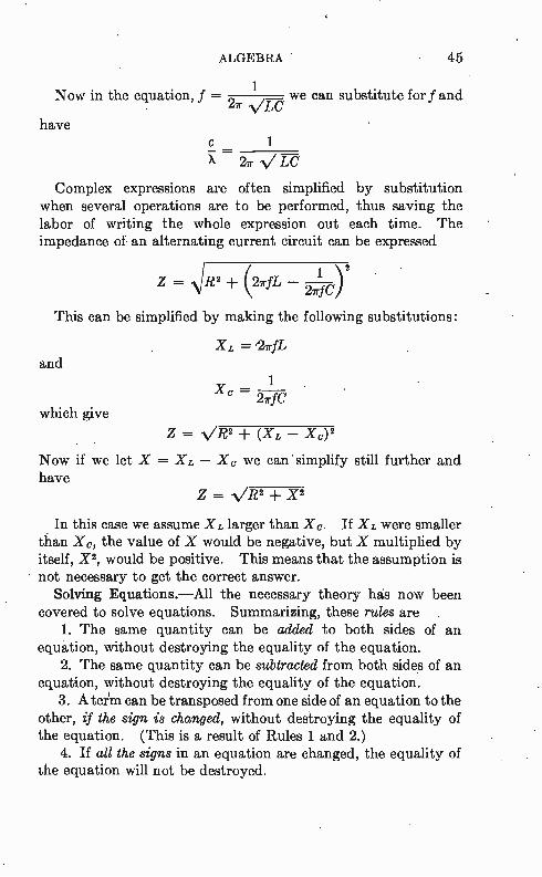
ALGEBRA 45
1 Now in the equation, f — we can substitute for/and
21r.N/LC have
Complex expressions are often simplified by substitution when several operations are to be performed, thus saving the labor of writing the whole expression out each time. The impedance of an alternating current circuit can be expressed
Z = ± (2irfL — 1 2 2irfC)
This can be simplified by making the following substitutions:
XL = '27rfL and
1 Xe —
2/rfC which give
Z = N/R2 ± (XL — X0)2 Now if we let X = XL — Xe we can simplify still further and have
Z =- -VR2 -I- X2
In this case we assume XL larger than Xc. If XL were smaller than X0, the value of X would be negative, but X multiplied by itself, X2, would be positive. This means that the assumption is not necessary to get the correct answer.
Solving Equations.—All the necessary theory has now been covered to solve equations. Summarizing, these rules are
1. The same quantity can be added to both sides of an equation, without destroying the equality of the equation.
2. The same quantity can be subtracted from both sides of an equation, without destroying the equality of the equation.
3. A teijm can be transposed from one side of an equation to the other, if the sign is changed, without destroying the equality of the equation. (This is a result of Rules 1 and 2.)
4. If all the signs in an equation are changed, the equality of the equation will not be destroyed.
46 APPLIED MATHEMATICS
5. Both sides of an equation can be multiplied by the same quantity without destroying the equality of the equation.
6. The same quantity can be divided into both sides of an equation, without destroying the equality of the equation. In other words, terms can be canceled.
7. Both sides of an equation can be raised to the same power without destroying the equality of the equation.
8. The reciprocal of one side of an equation is equal to the reciprocal of the other side.
9. Both sides of an equation can have the same root extracted, without destroying the equality of the equation.
10. Terms in an equation can be replaced by terms that are equal in value. To solve or evaluate an equation we use the above rules in
order that the term for which we are solving can be placed on only one side of the equation. With all other terms of known value on the opposite side, we have a solution and thus know the value of the unknown quantity in terms of known quantities. The usual practice is to arrange unknown terms on the left-hand side of the equation and all known terms on the right-hand side.
For example, E = IR is an expression of Ohm's law. If / = 8 and R = 6, we can replace / and R by the values they equal and then solve for the unknown value of E, thus
E = (8)(6) = 48
Sometimes an algebraic equation is indeterminate; that is, it cannot be solved as explained above. To illustrate,
/XL = where L = 30.
f = 60. 1r --= 6.28. XL = 11,300.
Substituting 11,3001 = (6.28)(60)(30)/ 11,3001 = 11,3001
/ = / 1 = 1
on
ALGEBRA 47
Illustrations of the Use of Above Ten Rules.
Given add
x — y =-. z + y = + y (Rules 1 and 3)
X = z y
To make this perfectly clear, let x = 10, y = 8, and z = 2. Then, substituting,
10 — 8 = 2 or 10 = 2 + 8
Now, use Rule 2 and subtract x from each side of the equation.
Given x — y = z Subtract +x =+x giving —y z — x Substituting, —8 .= 2 — 10
This is seen to be true. Changing all signs,
or y= —z -F x 8 = —2 -I- 10
(Rule 4)
This also is true. Even though the value of both sides of the equation is changed
in each of these cases, the equality is not destroyed. For an example in multiplication and division we have the
general form of Ohm's law,
E =
It is desired to solve for the voltage E. Multiply both sides by Z, giving
E I Z = 7 (Z) (Rule 5)
EzZ On the right-hand side, (Z) = = E
But we want E on the left-hand side so we turn the equation around and have
E = IZ (the solution)
48 APPLIED MATHEMATICS
Now let us solve this equation f or Z. Dividing both sides by / gives
By canceling /,
As above, turning the equation around gives
E Z
(Rule 6)
(the solution)
As another illustration, the Q of a circuit is given by the equation
27rfL = R
If we know the figure of merit Q, the frequency f, and the resist-ance R, we can solve for the inductance L as follows:
27fL Q = R
Multiplying both sides by R removes the denominator on the right-hand side, thus
RQ = 2,7rfL
Dividing both sides by 27f transfers the 27f from the right side of the equation to the left. Thus
2arf —
Then, by turning the equation around,
RQ L = (the solution)
27f
Suppose we wish to find the plate resistance (Rn) in a vacuum tube from the following equation:
A R R2,
Clearing of fractions, by multiplying both sides by the denomi-nator on the right side, gives
ALGEBRA 49
Removing the parentheses and multiplying each term inside them by A, we get
AR ± = ihR
Subtracting AR frém both sides,
AR,, = — AR
Dividing both sides by A,
—A AR
This is the required solution for R,,. The procedure of removing the denominator and clearing of
fractions, shown above, is one of the most useful in solving equations. When any equation with fractions is to be solved they should be removed by this means. The last step is also important, for the desired term is often
multiplied by other known factors. In such cases dividing both sides of the equation by this known term will leave the unknown alone on the left-hand side and give the desired answer.
Solve the above equation for R.
A _ R R,,
Clearing of fractions,
(R = 1.tit
Removing the parentheses,
AR + = IÁR
Subtracting AR from both sides,
AR?, = — AR
Factoring the right-hand side by dividing through by R and multiplying by R,
AR?, — R(ee Aitl) - R(.t — A) .8
Turning the equation around to get R on the left-hand side,
50 APPLIED MATHEMATICS
Dividing both sides by (it — A),
A, R - R - A
Solving for R was slightly more complicated but each step in itself was quite simple. The student should write out each step when solving problems until the procedure is thoroughly under-stood. If the steps are written out in detail, mistakes will be less likely to occur. In an alternating current circuit,
i E
— VR2 + X2 To solve this equation for X, proceed as follows:
Clearing of fractions and turning the equation around,
E = I N/ R2 + X2 Dividing by I,
E = -VR2 + X2
Squaring both sides (Rule 7) and turning the equation around,
R2 -I- X2 =
Transposing R2 (subtracting R2 from both sides), E2
X2 = - - R2 12 Reducing to a common denominator,
E2 R212 E2 X2 = - - - /2 /2 /2
R2I2
Extracting the square root of both sides (Rule 8),
x = \ IE2 - R212 VE2 - R2I2 N/E2 - R2I2 or X
Nfri
The student should become familiar with these proçesses and be able to prove such problems. To prove this problem, take the answer and solve for I.
ALGEBRA 51
X --VE2 - R2/2
Clearing of fractions,
/X = -VE2 - R2/2 Squaring both sides to remove the radical,
Transposing /2R2,
Factoring /2,
I2X2 = E2 - R2I2
PX2 I2R2 = E2
/2(X2 + R2) = E2 Dividing by (X2 + R2),
/2 - E2 X2 + R2 Extracting the square root of both sides by rule 9,
NÍR2 ± x-2 — .vR2 ± x-2 .vR2 x-2
Which is the original equation and indicates that the solution is correct. Another help is to substitute known values in the equation
and prove the answer is correct for a particular case. If it is true for a particular case, it will likely hold in the general solution. Thus, let E = 100 volts, R = 8 ohms resistance, and X = 6 ohms reactance. Then
E2 _ E I -
/ - E 100 100 100 — — = 10 amp yR2 X2 .V82 62 v64 36 10
Substituting these values in the answer and solving for X give
X .i/E2 _ /2R2 = .y1002 _ (10à 2 = 2(8, ) -00,000 — 6,400
= " " I 10 10 -V3 600 60 = ' = - = 6 ohms reactance
10 10
This checks the value given above.
52 APPLIED MATHEMATICS
In case the student may not know when to square or when to extract a square root, it may be helpful to 'remember that X = 2 so if X2 is given, extract the square root to get X and if V.—X is given, square the quantity to get X. Of course rules 7 and 8 must be remembered when performing these operations on equations. Both sides of the equation must be treated alike.
In the equation, = lc°
we know that 1
X/ = 27rfL and X. — zric
Therefore, by substituting as pointed out in rule 10, we can write
1 2efL — 27,fc
Exercises
1. x + y = a — b. Find y, b. 2. ax + by — ez = R. Find b, z. 3. RST XY — JQ. Find S, Q.
4. -12 -= ab. Find z, y.
x + y 5. — a + bz. Find x, b.
6. = az + e. Find y, a. — y
7. X + — PQ. Find M, Y. M — N
8. 0-1-P _R —S Find 7,, a X T
a T2 R — SP T Find T, P.
10. xy2 z N/a ± b. Find a, y.
11. I = E R + ix Find R.
4. 1 1 , 1 -r Find C, CI.
a2n2 13. L — 9a + 10b Find a, n.
N 14. e = Find t.
t X 108
15. W = 70-g-7/2Rt • Find /.
ALGEBRA 53
16. F 2rr 1-1- Find r.
17. T = 2T NU. Find H.
18. K — Find Le. Níreer;
1.9. Re = R.(1 ± at). Find t.
20. X = 1884 -VTLUi. Find C.
CHAPTER 4
GEOMETRY
This lesson will be concerned with the study of the right triangle. Conventional geometry as given in high school is not touched upon in this lesson. All the student need remember from high-school geometry is how to find the hypotenuse of a right triangle if the two legs are given.
In studying electrical engineering, it is often desirable to add voltages and currents that are not alvkays in phase. These voltages and currents can be represented by means of vectors and added by means of geometric addition.
Arithmetic addition concerns itself with adding positive num-bers only. Graphically, this means that only numbers from the origin out along a positive axis can be considered. This permits the addition of vectors in only one direction.
Algebraic addition concerns itself with adding both positive and negative numbers. Graphically, this means that all num-bers on a straight line through the origin can be handled. This number system is twice as large as that of arithmetic addition. This permits the addition of vectors acting in the same direction or in exact opposition.
Geometric addition concerns itself with adding vectors in a plane and hence has generalized algebraic addition much as algebraic addition has generalized arithmetic addition. A vector is a quantity which has both magnitude and direction.
Quantities such as dimensions, weight, and temperature have magnitude only. Quantities with magnitude only are called "scalar quantities." Quantities such as displacement, velocity, force, voltage, current, and impedance have direction in addition to magnitude. These quantities are called "vector quantities"; they are represented by directed lines called "vectors." The length of the line represents the magnitude, and the line is drawn in the direction of the vector. An arrow on the end of the line indicates its sense.
54
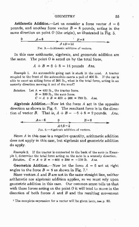
GEOMETRY 55
Arithmetic Addition.—Let us consider a force vector A = 6 pounds, and another force vector B = 8 pounds, acting in the same direction on point 0 (the origin), as illustrated in Fig. 5.
O A=6 ' B=8
AB =14 FIG. 5.—Arithmetic addition of vectors.
In this case arithmetic, algebraic, and geometric addition are the same. The point 0 is acted on by the total force,
A B = 6 + 8 = 14 pounds Ans.
Example 1. An automobile going east is stuck in the mud. A tractor coupled to the front of the automobile exerts a pull of 400 lb. If the car is able to exert an aiding force of 300 lb., what is the total force, acting in an easterly direction moving it out of the mud?
Solution. Let A = 400 lb., the tractor force. B = 300 lb., the auto force. C = A + B = 400 + 300 = 700 lb. Ans.
Algebraic Addition.—Now let the force A act in the opposite direction as shown in Fig. 6. The resultant force is in the direc-tion of vector B. That is, A + B = -6 + 8 = 2 pounds. Ans.
A=-6 O B=8
A-E= 2 FIG. 6.—Algebraic addition of vectors.
"a.
Since A in this case is a negative quantity, arithmetic addition does not apply in this case, but algebraic and geometric addition do apply.
Example 2. If the tractor is connected to the back of the auto in Exam-ple 1, determine the total force acting on the auto in a westerly direction.
Solution. C = A B = —400 + 300 = —100 lb. Ans.
Geometric Addition.—Now let the force A = 6 act at right angles to the force B = 8 as shown in Fig. 7. 1
Since vectors A and B are not in the same straight line, neither arithmetic nor algebraic addition applies, so we must rely upon geometric addition in this case. Our common sense tells us that with these forces acting on the point 0 it will tend to move in the direction of both forces A and B and the resulting movement
1 The complete expression for a vector will be given later, see p. 80.
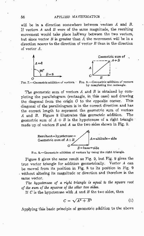
56 APPLIED MATHEMATICS
will be in a direction somewhere between vectors A and B. If vectors A and B were of the same magnitude, the resulting movement would take place halfway between the two vectors, but since vector B is greater than A the movement will be in a direction nearer to the direction of vector B than in the direction of vector A.
o FIG. 7.—Geometric addition of vectors.
Geometric sum of +B
A
Fro. 8.—Geometric addition of vectors by completing the rectangle.
The geometric sum of vectors A and B is obtained by com-pleting the parallelogram (rectangle, in this case) and drawing the diagonal from the origin 0 to the opposite corner. This diagonal of the parallelogram is in the correct direction and has the correct length to represent the geometric sum of vectors A and B. Figure 8 illustrates this geometric addition. The geometric sum of A + B is the hypotenuse of a right triangle made up of vèctors B and A as the two sides shown in Fig. 9.
Resultant =hypotenuse = Geometric sum of A+B
o A= altitude-. side
B= base= side
FIG. 9.—Geometric addition of vectors by using the right triangle.
Figure 8 gives the same result as Fig. 9, but Fig. 9 gives the true vector triangle for addition geometrically. Vector A can be moved from its position in Fig. 8 to its position in Fig. 9 without altering its magnitude or direction and therefore is the
same vector. The hypotenuse of a right triangle is equal to the square root
of the sum of the squares of the other two sides. If C is the hypotenuse with A and B the two sides, then
C = .VA 2 ± B2 (1)
Applying this basic principle of geometric addition to the above
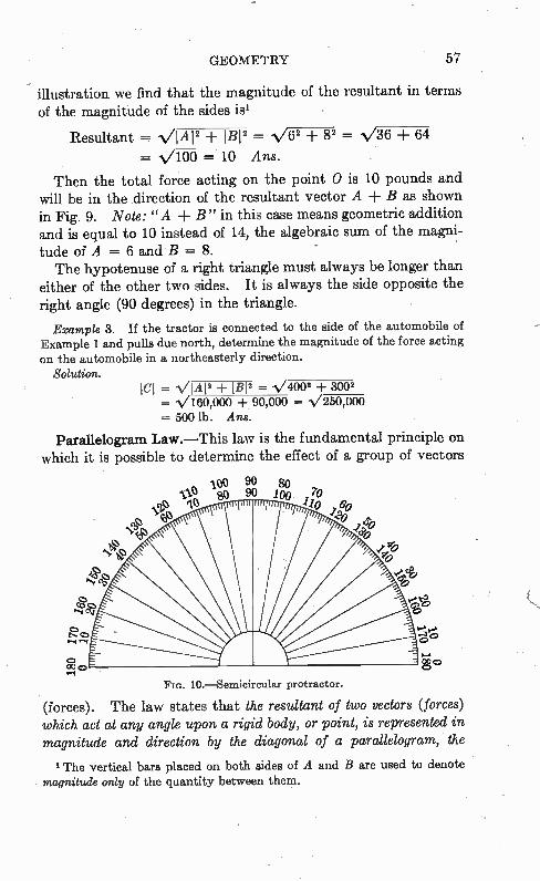
GEOMETRY 57
illustration we find that the magnitude of the resultant in terms of the magnitude of the sides is'
Resultant = viAi2 igi2 = .v82 ± 82 .= V36 64
N/100 = 10 Ans.
Then the total force acting on the point 0 is 10 pounds and will be in the direction of the resultant vector A B as shown in Fig. 9. Note: "A ±B" in this case means geometric addition and is equal to 10 instead of 14, the algebraic sum of the magni-tude of A = 6 and B = 8. The hypotenuse of a right triangle must always be longer than
either of the other two sides. It is always the side opposite the right angle (90 degrees) in the triangle.
Example 3. If the tractor is connected to the side of the automobile of Example 1 and pulls due north, determine the magnitude of the force acting on the automobile in a northeasterly direction.
Solution. ICI = 'OAP + IBI2 = N/4002 ± 3002 = N/160,000 + 90,000 = V250,000 = 500 lb. Ans,.
Parallelogram Law.—This law is the fundamental principle on which it is possible to determine the effect of a group of vectors
no. 10.—Semicircular protractor.
(forces). The law states that the resultant of two vectors (forces) which act at any angle upon a rigid body, or point, is represented in magnitude and direction by the diagonal of a parallelogram, the
1 The vertical bars placed on both sides of A and B are used to denote magnitude only of the quantity between them.
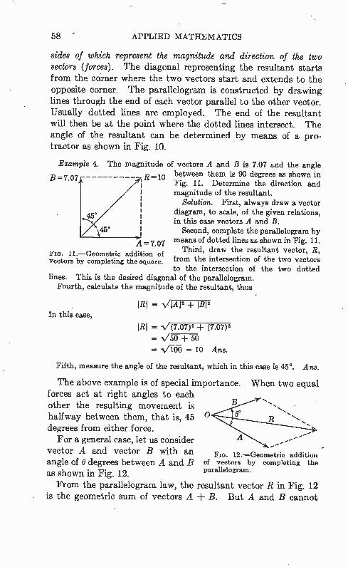
58 " APPLIED MATHEMATICS
sides of which represent the magnitude and direction of the two vectors (forces). The diagonal representing the resultant starts from the corner where the two vectors start and extends to the opposite corner. The parallelogram is constructed by drawing lines through the end of each vector parallel to the other vector. Usually dotted lines are employed. The end of the resultant will then be at the point where the dotted lines intersect. The angle of the resultant can be determined by means of a pro-tractor as shown in Fig. 10.
Example
B=7.07
4. The magnitude
.R — 10
of vectors A and B is 7.07 and the angle between them is 90 degrees as shown in Fig. 11. Determine the direction and magnitude of the resultant.
Solution. First, always draw a vector diagram, to scale, of the given relations, in this case vectors A and B.
Second, complete the parallelogram by A=7.07 means of dotted lines as shown in Fig. 11.
Third, draw the resultant vector, R, from the intersection of the two vectors to the intersection of the two dotted
lines. This is the desired diagonal of the parallelogram. Fourth, calculate the magnitude of the resultant, thus
Fro. 11.—Geometric addition of vectors by completing the square.
In this case, IR1 = -VIA12 + IR12
IRI = V(7.07)2 ± (7.07)2
= V50 ± 50
= V1.970 = 10 Ans.
Fifth, measure the angle of the resultant, which in this case is 45°. Ans.
The above example is of special importance. forces act at right angles to each other the resulting movement is halfway between them, that is, 45 degrees from either force. For a general case, let us consider
vector A and vector B with an angle of O degrees between A and B as shown in Fig. 12. From the parallelogram law, the resultant vector R in Fig. 12
is the geometric sum of vectors A + B. But A and B cannot
When two equal
0 10°
A
•••
FIG. 12.—Geometric addition of vectors by completing the parallelogram.
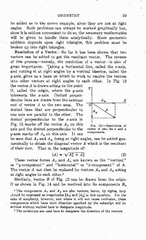
GEOMETRY 59
be added as in the above example, since they are not at right angles. Such problems can always• be worked graphically but, since it is seldom convenient to do so, the necessary mathematics will be given to handle them analytically. Since geometric addition depends upon right triangles, this problem must be broken up into right triangles.
Resolution of a Vector.—So far it has been shown that two vectors can be added to get the resultant vector. The reverse of this process—namely, the resolution of a vector—is also of great importance. taking a horizontal line, called the x-axis, and cutting it at right angles by a vertical bisector, called the y-axis, gives us a basis on which to work to resolve the vectors into other vectors at right angles to each other. In Fig. 12 the vector A is drawn acting on the point 0, called the origin, where the y-axis intersects the x-axis. Dotted perpen-dicular lines are drawn from the extreme A x X
end of vector A to the two axes. The dotted lines that are perpendicular to one axis are parallel to the other. The dotted perpendicular to the x-axis in Fig. 13 marks off the vector A x on this FIG. 13.—Resolution of axis and the dotted perpendicular to the vector A into its x and y
y-axis marks off At, on this axis. It can components. be seen that A. and A„, being at right angles, can be added geo-metrically to obtain the diagonal vector A which is the resultant of their sum. That is, the magnitude of'
iAi = / + (2) These vector forces A. and At, are known as the "vertical"
or "y-component" and "horizontal" or "x-component" of A. The vector A can then be replaced by vectors Ax and Ay acting at right angles to each other.2
Similarly, vector B of Fig. 12 can be drawn from the origin 0 as shown in Fig. 14 and be resolved into its components B.
The components A. and A v are also vectors; hence, by rights, they ..hould be expressed as magnitudes IA xi and !Ail in this equation. For the sake of simplicity, however, and where it will not cause confusion, these components which have their direction specified by the subscript will be written without vertical bars to designate magnitude. 2 The subscripts are used here to designate the direction of the vectors.
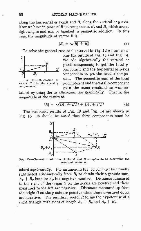
60 APPLIED MATHEMATICS
along the horizontal or x-axis and By along the vertical or y-axis. Now we have in place of B its components B. and B„ which are at right angles and can be handled in geometric addition. In this case, the magnitude of vector B is
IBI = (3)
To solve the general case as illustrated in Fig. 12 we can corn-bine the results of Fig. 13 and Fig. 14. We add algebraically the vertical or y-axis component § to get the total y-
By x component and the horizontal or x-axis O B, components to get the total x-compo-
FIG. 14.—Resolution of nent. The geometric sum of the total vector B into its x and y y-component and the total x-component components. gives the same resultant as was ob-
tained by using the parallelogram law graphically. That is, the magnitude of the resultant
IRI = (A. ± B.)2 -I- (24,, B„)2 (4)
The combinéd results of Fig. 13 and Fig. 14 are shown in Fig. 15. It should be noted that these components must be
Fro. 15.—Geometric addition of the A and B components to determine the resultant vector R.
added algebraically. For instance, in Fig. 15, A„ must be actually subtracted arithmetically from By to obtain their algebraic sum, A„ + By because 21„ is a negative number. Distances measured to the right of the origin 0 on the x-axis are positive and those measured to the left are negative. Distances measured up fróm the origin 0 on the y-axis are positive while those measured down are negative. The resultant vector R forms the hypotenuse of a right triangle with sides of length Az + B. and A„ B„.
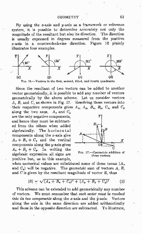
GEOMETRY 61
By using the x-axis and y-axis as a framework or reference system, it is possible to determine accurately not only the magnitude of the resultant but also its direction. The direction is usually expressed in degrees measured from the positive x-axis in a counterclockwise direction. Figure 16 plainly illustrates four examples.
Y
X
Y
(a) (b) (e) (d) 16.—Vectors in the first, second, third, and fourth quadrants.
Since the resultant of two vectors can be added to another vector geometrically, it is possible to add any number of vectors geometrically by the above scheme. Let us consider vectors A, B, and C, as shown in Fig. 17. Resolving these vectors into their respective components gives A, A5, B, B„, C, and C,„ along the two axes. A. and C„ are the only negative components, and hence they must be subtract-ed from the others when added algebraically. The horizontal components along the x-axis give A 1 A. + Br -F C. and the vertical components along the y-axis give A„ By C„. In writing the algebraic expression all signs are positive but, as in this example, when numerical values are substituted some of these terms (A r and Cy) will be negative. The geometric sum of vectors A, B, and C is given by the resultant magnitude of vector R, thus
+ B. + C.) 2 + (Ay + Bv Cy)2 (5)
This scheme can be extended to add geometrically any number of vectors. We must remember that each vector must be resolved into its two components along the x-axis and the ji-axis. Vectors along the axis in the same direction are added arithmetically and those in the opposite direction are subtracted. To illustrate,
FIG. 17.—Geometric addition of three vectors.
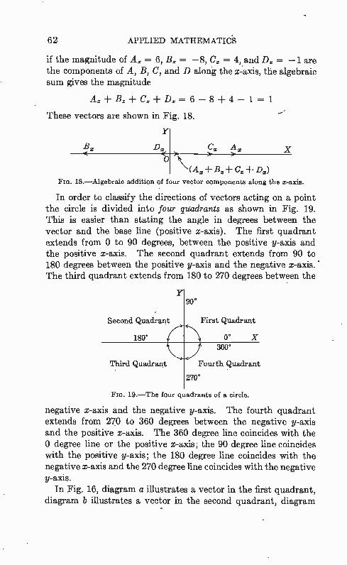
62 APPLIED MATHEMATIC'S
if the magnitude of A. = 6, B. = —8, C. = 4, and D. = —1 are the components of A, B, C, and D along the x-axis, the algebraic sum gives the magnitude
A. B. + C. + D. = 6 — 8 -F 4 — 1 = 1
These vectors are shown in Fg. 18.
Y
B. D, C, A,
)')t >
FIG. 18.—Algebraic addition of four vector components along the x-axis.
In order to classify the directions of vectors acting on a point the circle is divided into four quadrants as shown in Fig. 19. This is easier than stating the angle in degrees between the vector and the base line (positive x-axis). The first quadrant extends from 0 to 90 degrees, between the positive y-axis and the positive x-axis. The second quadrant extends from 90 to 180 degrees between the positive y-axis and the negative x-axis. The third quadrant extends from 180 to 270 degrees between the
Y o
Second Quadrant First Quadrant
1800 0° X 360°
Third Quadrant Fourth Quadrant
2700
X
19.—The four quadrants of a circle.
negative x-axis and the negative y-axis. The fourth quadrant extends from 270 to 360 degrees between the negative y-axis and the positive x-axis. The 360 degree line coincides with the 0 degree line or the positive x-axis; the 90 degree line coincides with the positive y-axis; the 180 degree line coincides with the negative x-axis and the 270 degree line coincides with the negative y-axis.
In Fig. 16, diagram a illustrates a vector in the first quadrant, diagram b illustrates a vector in the second quadrant, diagram
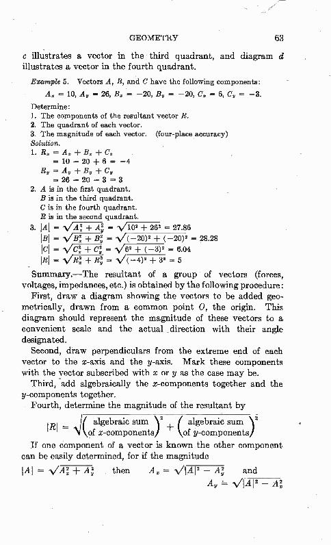
GEOMETRY 63
c illustrates a vector in the third quadrant, and diagram d illustrates a vector in the fourth quadrant.
Example 5. Vectors A, B, and C have the following components:
A. = 10, A.„ = 26, B. = —20, B,,, = —20, C. = 6, Cv = —3.
Determine: 1. The components of the resultant vector R. 2. The quadrant of each vector. 3. The magnitude of each vector. (four-place accuracy) Solution. 1.R,xAx+Bx+Cx
.= 10 — 20 -I- 6 = —4 R,, = Ai, •+ By + C. = 26 — 20 — 3 = 3
2. A is in the first quadrant. B is in the third quadrant. C is in the fourth quadrant. R is in the second quadrant.
3. IAI -- VA! +Az = Vur + 262 -- 27.86 IBI = B: = (-20)2 ± (-20)2 = 28.28 ICI = "s,/C1 C:, = N/62 ( —3)2 = 6.04
IRI = R: R12, = / (- 4)2 + 32 = 5
Summary.—The resultant of a group• of vectors (forces, voltages, impedances, etc.) is obtained by the following procedure:
First, draw a diagram showing the vectors to be added geo-metrically, drawn from a common point 0, the origin. This diagram should represent the magnitude of these vectors to a convenient scale and the actual _direction with their angle designated.
Second, draw perpendiculars from the extreme end of each vector to the x-axis and the y-axis. Mark these components with the vector subscribed with x or y as the case may be.
Third, "add algebraically the x-components together and the y-components together.
Fourth, determine the magnitude of the resultant by
1R/ = ,‘/( algebraic sum algebraic sum \ 2
\of x-components)2 ( of y-components/
If one component of a vector is known the other component can be easily determined, for if the magnitude
IAl = VA! + A: then = VIA12 At2/ and
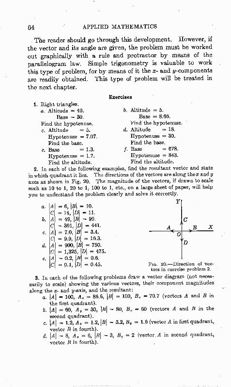
64 APPLIED MATHEMATICS
The reader should go through this development. However, if the vector and its angle are given, the problem must be worked out graphically with a rule and protractor by means of the parallelogram law. Simple trigonometry is valuable to work this type of problem, for by means of it the x- and y-components are readily obtained. This type of problem will be treated in the next chapter.
Exercises
1. Right triangles. a. Altitude -- 40. b. Altitude = 5.
Base -- 30. Base = 8.66. Find the hypotenuse. Find the hypotenuse. c. Altitude = 5. d. Altitude -- 18.
Hypotenuse = 7.07. Hypotenuse = 30. Find the base. Find the base.
e. Base = 1.3. f. Base = 678. Hypotenuse = 1.7. Hypotenuse = 843. Find the altitude. Find the altitude.
2. In each of the following examples, find the resultant vector and state in which quadrant it lies. The directions of the vectors are along the x and y axes as shown in Fig. 20. The magnitude of the vectors, if drawn to scale such as 10 to 1, 20 to 1, 100 to 1, etc., on a large sheet of paper, will help you to understand the problem clearly and solve it correctly.
a. Al = 6, IBI = 10. CI = 14, IDI = 11.
b. A = 49, IBI = 99. C -- 391, IDI = 441. A< >B X
c. A =- 7.0, = 3.4. 0 C = 9.9, IDI = 16.3.
d. A = 900, IBI = 750. C = 1,325, DI = 475.
e. A = 0.2, IB = 0.6. C = 0.1, ID = 0.45. Fm. 20.—Direction of vec-
tors in exercise problem 2.
3. In each of the following problems draw a vector diagram (not neces-sarily to scale) showing the various vectors, their component magnitudes along the x- and y-axis, and the resultant:
a. IA = 100, A. = 86.6, = 100, B. = 70.7 (vectors A and B in the first quadrant).
b. IA = 60, A,, = 30, IBI = 80, B. = 60 (vectors A and B in the second quadrant).
c. IAI = 1.2, A. = 1.2, IBI = 3.2, By = 1.6 (vector A in first quadrant, vector B in fourth).
d. lAi = 8, A. = 6, IBI = 3, B,, = 2 (vector .A in second quadrant vector B in fourth).
Y
D
GEOMETRY 65
e. IAI 340, A, = 100, IBI = 180, B. = 80 (vector A in third quad-rant, vector B in first).
f. IAI = 400, A. = 150, IBI = 500, B. = 250, ICI 300, C. = 200 (vector A in first quadrant, vector B in second, and vector C in
third). Note: All the x- and y-components are expressed as positive numbers in
the problems above. The actual sign is to be determined by the student from a knowledge of the quadrant in which the vector lies.
CHAPTER 5
TRIGONOMETRY
In the last chapter we learned how to resolve a vector or force into its horizontal component along the x-axis and its vertical component along the y-axis. After this operation had been performed to each vector to be added, the algebraic sum of the x-components gave a resultant x-component and the algebraic sum of the y-components gave a resultant y-component. The hypotenuse of the triangle formed by the resultant x-component and the resultant y-component is called the geometric or vector sum of all the vectors or forces added. But this gives us no information concerning the value of the angles in this triangle. We also mentioned in the last chapter a problem that had an angle given, but we could not solve it with the tools we then had.
Trigonometry is the tool that deals with the angles of a right triangle and their relationship to the sides of the triangle. If we have one angle and one side of a right triangle given, we can determine the other two sides and angle by using simple trigo-nometry. We can now appreciate the value of this new tool and how by its use we can solve practical vector problems involving forces, impedances, voltages, currents, etc.
Trigonometric Functions.—Trigonometry deals with what are known as "trigonometric functions" of the angle. Such a function is a ratio between two sides of the right triangle.
In Fig. 21, a line is drawn through the point 0 at an angle a (alpha) with the horizontal line the x-axis. At some point R1 on this line drop a perpendicular to X1 on the x-axis. This perpendicular of course, cuts the x-axis at right angles, and we
have the right triangle with sides a, b, and c. In this right triangle it is possible to make three different ratios of the sides, that is, a/b, c/b, and c/a. Now, let us take some other point R2 on this line and drop
another perpendicular to X2 on the x-axis. In this case we have formed another right triangle with sides A., B, and C. It is
66
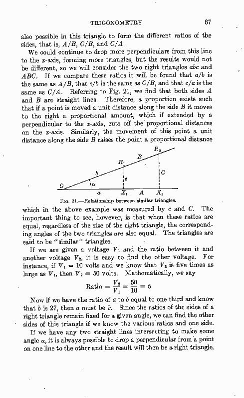
TRIGONOMETRY 67
also possible in this triangle to form the different ratios of the sides, that is, AIB, C/B, and C/A. We could continue to drop more perpendiculars from this line
to the x-axis, forming more triangles, but the results would not be different, so we will consider the two right triangles abc and ABC. If we compare these ratios it will be found that a/b is the same as A/B, that c/b is the same as C/B, and that c/a is the same as C/A. Referring to Fig. 21, we find that both sides A and B are straight lines. Therefore, a proportion exists such that if a point is moved a unit distance along the side B it moves to the right a proportional amount, which if extended by a perpendicular to the x-axis, cuts off the proportional distances on the x-axis. Similarly, the movement of this point a unit distance along the side B raises the point a proportional distance
R2
a X1 A X 2
Fro. 21.—Relationship between similar triangles.
which in the above example was measured by c and C. The important thing to see, however, is that when these ratios are equal, regardless of the size of the right triangle, the correspond-ing angles of the two triangles are also equal. The triangles are said to be "similar" triangles.
If we are given a voltage Vi and the ratio between it and another voltage V2, it is easy to find the other voltage. For instance, if Vi = 10 volts and we know that y2 is five times as large as Vi, then V2 = 50 volts. Mathematically, we say
,. V2 50 nauo Vi— = — =
10
Now if we have the ratio of a to b equal to one third and know that b is 27, then a must be 9. Since the ratios of the sides of a right triangle remain fixed for a given angle, we can find the other sides of this triangle if we know the various ratios and one side.
If we have any two straight lines intersecting to make some angle a, it is always possible to drop a perpendicular from a point on one line to the other and the result will then be a right triangle.
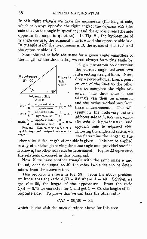
68 APPLIED MATHEMATICS
In this right triangle we have the hypotenuse (the longest side, which is always opposite the right angle) ; the adjacent side (the side next to the angle in question); and the opposite side (the side opposite the angle in question). In Fig. 21, the hypotenuse of triangle abc is b, the adjacent side is a and the opposite side is c. In triangle ABC the hypotenuse is B, the adjacent side is A and the opposite side is C.
Since the ratios hold the same for a given angle regardless of the length of the three sides, we can always form this angle by
using a protractor to determine the correct angle between two . intersecting straight lines. Now,
Hypotenuse Opposite B=10 Side drop a perpendicular from a point
C-= 6 on one of the lines to the other line to complete the right tri-angle. The three sides of the triangle can then be measured and the ratios worked out from
0.8 10 these measurements. This will 6 0 6 result in the following ratios: . 10 adjacent side to hypotenuse, oppo-
Adjacent Side 4= 8
A adjacent side Ratio B hypotenuse
Ratio C opposite side B hypotenuse
C opposite side 6 Ratio . . — — 0.75 site side to hypotenuse, and
A adjacent aide 8 Pm. 22.—Names of the sides of a opposite side to adjacent side.
right triangle with respect to the acute Knowing the angle and ratios, we angle a.
can determine the length GI the other sides if the length of one side is given. This can be applied to any other triangle having the same angle and, provided one side is known, the other sides can be determined. Figure 22 represents the relations discussed in this paragraph. Now, if we have another triangle with the same angle a and
the adjacent side equal to 40, the other two sides can be deter-mined from the above ratios.
This problem is shown in Fig. 23. From the above problem we know that the ratio A / B = 0.8 where A = 40. Solving, we get B = 50, the length of the hypotenuse. From the ratio C/A = 0.75 we can solve for C and get C = 30, the length of the opposite side. To prove this we can take the other ratio
C/B = 30/50 = 0.6
which checks with the ratio obtained above for this case.
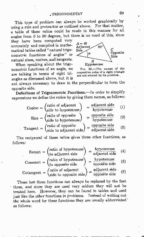
TRIGONOMETRY 69
This type of problem can always be worked graphically by using a rule and protractor as outlined above. For that matter, a table of these ratios could be made in this manner for all angles from 0 to 90 degrees, but there is no need of this, since
they have been computed very accurately and compiled in mathe-matical tables called "natural trigo-nometric functions of angles" or natural sines, cosines, and tangents. When speaking about the trigo-
nometric functions of an angle, we are talking in terms of right tri-angles as discussed above, but it is not always necessary to draw in the perpendicular to form the opposite side.
Definitions of Trigonometric Functions.—In order to simplify expressions we define the ratios by giving them names, as follows:
Cosine =
Sine =
Tangent =
The reciprocal follows:
A= 40 Adjacent Side
Hypotenuse 23.—The names of the
respective sides of a right triangle are not altered by its position.
Opposite Side
(ratio of adjacent ) adjacent side \side to hypotenuse = hypotenuse
(ratio of opposite _ opposite side side to hypotenuse — hypotenuse
(ratio of opposite _ opposite side \side to adjacent side) — adjacent side
of these ratios gives three other functions, as
Secant =
Cosecant =
Cotangent =
(ratio of hypotenuse) _ hypotenuse to adjacent side adjacent side
(ratio of hypotenuse) _ hypotenuse \to opposite side — opposite side
(ratio of adjacent \ _ adjacent side \side to opposite side) opposite side
(1)
(2)
(3)
(4)
(5)
(6)
These last three functions can always be replaced by the first • three, and since they are used very seldom they will not be treated here. However, they can be found in tables and used just like the other functions in problems. Instead of writing out the whole word for these functions they are usually abbreviated as follows:
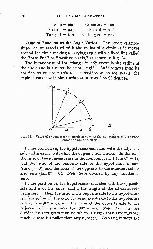
70 APPLIED MATHEMATICS
Sine = sin Cosine = cos
Tangent = tan
Cosecant = csc Secant = sec
Cotangent = cot
Value of Function as the Angle Varies.—The above relation-ships can be associated with the radius of a circle as it moves around the circle making a varying angle with a fixed line called the " base line" or "positive x-axis," as shown in Fig. 24. The hypotenuse of the triangle in any event is the radius of
the circle and is always the same length. As it rotates from its position oa on the x-axis to the position oe on the y-axis, the angle it makes with the x-axis varies from 0 to 90 degrees.
FIG. 24.—Value of tr.gonometric functions vary as the hypotenuse of a triangle traces the arc of a circle.
In the position oa, the hypotenuse coincides with the adjacent side and is equal to it, while the opposite side is zero. In this case the ratio of the adjacent side to the hypotenuse is 1 (cos 0° = 1), and the ratio of the opposite side to the hypotenuse is zero (sin 0°= 0), and the ratio of the opposite to the adjacent side is also zero (tan 0° = 0). Note: Zero divided by any number is zero.
In the position ce, the hypotenuse coincides with the opposite side and is of the same length, the length of the adjacent side being zero. Then the ratio of the opposite side to the hypotenuse is 1 (sin 90° = 1), the ratio of the adjacent side to the hypotenuse is zero (cos 90° = 0), and the ratio of the opposite side to the adjacent side is infinity (tan 90° = co). Note: Any number divided by zero gives infinity, which is larger than any number, much as zero is smaller than any number. Zero and infinity are
TRIGONOMETRY 71
really not numbers and hence must not be handled as numbers in mathematical operations.
If the hypotenuse (radius) is made of unit length, the ratio of the adjacent side to the hypotenuse is equal to the length of the adjacent side and the ratio of the opposite side to the hypotenuse is equal to the length of the opposite side.
Referring to Fig. 24, we can see that the adjacent side decreases from oa, which is 1, to os when the hypotenuse is in the position ob. As the hypotenuse takes on the positions oc, od, and lastly oe the adjacent side decreases from no to mo and then finally becomes of zero length. This means that the cosine of the angle varies from unity for 0 degrees to zero for 90 degrees, decreasing as the angle increases. The opposite side is of zero length when the hypotenuse is in
position oa and increases to be when the hypotenuse takes on the position ob. As the hypotenuse takes on the positions oc, od, and finally oe, the opposite side increases in length from en to dm and lastly is of unit length oe. This shows that the sine of the angle varies from zero at 0 degrees to unity at 90 degrees, increasing as the angle increases.
Consider the ratio of the opposite side to the adjacent side as the angle varies from 0 to 90 degrees. This ratio varies from 0 when the hypotenuse is in position oa to 00 (infinity) when the hypotenuse is in position oe. When the hypotenuse makes an angle of 45 degrees with the x-axis this ratio is unity, so the tangent of the angle varies from zero to unity in the first 45 degrees and from unity to infinity in the next 45 degrees. The tangent of the angle increases as the angle increases.
It is of interest to note that the sine and cosine, opposite and adjacent sides in Fig. 24, never grow larger than the hypotenuse, which is 1, but the tangent, which is the ratio of the opposite side to the adjacent side, or sine to cosine, has both terms in the ratio varying. The opposite side grows larger while the adjacent side grow smaller. The result is that the tangent grows larger rather slowly up to 45 degrees but then grows larger rapidly as the angle increases to 90 degrees. In the case of the sine and cosine, only one term in the ratio varied. The student should now inspect a table of trigonometric
functions (a brief table is at the back of this book). These functions may be listed as natural sines and cosines in one table
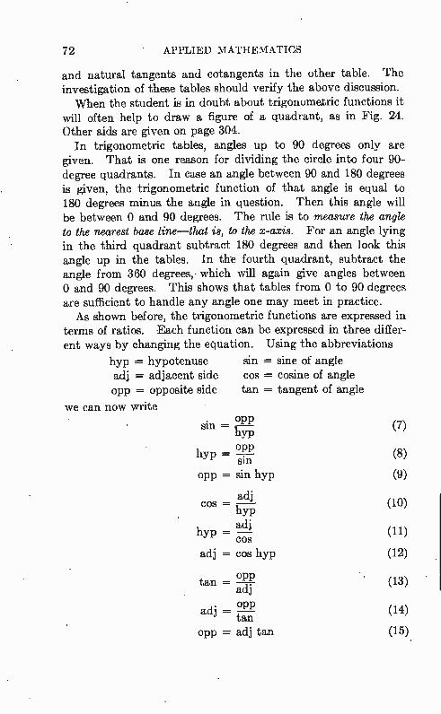
72 APPLIED MATHEMATICS
and natural tangents and cotangents in the other table. The investigation of these tables should verify the above discussion. When the student is in doubt about trigonometric functions it
will often help to draw a figure of a quadrant, as in Fig. 24. Other aids are given on page 304.
In trigonometric tables, angles up to 90 degrees only are given. That is one reason for dividing the circle into four 90-degree quadrants. In case an angle between 90 and 180 degrees is given, the trigonometric function of that angle is equal to 180 degrees minus the angle in question. Then this angle will be between 0 and 90 degrees. The rule is to measure the angle to the nearest base line—that is, to the x-axis. For an angle lying in the third quadrant subtract 180 degrees and then look this angle up in the tables. In the fourth quadrant, subtract the angle from 360 degrees, which will again give angles between 0 and 90 degrees. This shows that tables from 0 to 90 degrees are sufficient to handle any angle one may meet in practice. As shown before, the trigonometric functions are expressed in
terms of ratios. Each function can be expressed in three differ-ent ways by changing the equation. Using the abbreviations
hyp = hypotenuse sin = sine of angle adj = adjacent side cos = cosine of angle opp = opposite side tan = tangent of angle
we can now write
sin = opp (7) hyp
hyp = °P. P (8)
opp = sslinn hyp (9)
adj cos = (10)
hyp hyp = adj (11)
cos adj = cos hyp (12)
opp tan = (13)
adj
oPP adj = (14) tan
opp = adj tan (15).
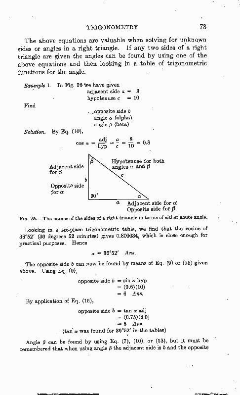
TRIGONOMETRY 73
The above equations are valuable when solving for unknown sides or angles in a right triangle. If any two sides of a right triangle are given the angles can be found by using one of the above equations and then looking in a table of trigonometric functions for the angle.
Example 1. In Fig. 25 iffe have given adjacent side a = 8 hypotenuse c = 10
Find _opposite side b angle a (alpha) angle p (beta)
Solution. By Eq. (10),
adj a 8 cos a - _ - — = u.o
hyp c 10
Adjacent side for 13
Opposite side for st
Irypotenuse for both angles a and e
a Adjacent side for Opposite side forl3
Fm. 25.—The names of the sides of a right triangle in terms of either acute angle.
Looking in a six-place trigonometric table, we find that the cosine of 36°52' (36 degrees 52 minutes) gives 0.800034, which is close enough for practical purposes. Hence
a 36°52' Ans.
The opposite side b can now be found by means of Eq. (9) or (15) given above. Using Eq. (9),
opposite side b = sin « hyp = (0.6)(10) = 6 Ans.
By application of Eq. (15),
opposite side b = tan a adj = (0.75)(8.0) = 6 Ans.
(tari a was found for 36°52' in the tables)
Angle 13 can be found by using Eq. (7), (10), or (13), but it must be remembered that when using angle 13 the adjacent side is b and the opposite
74 APPLIED MATHEMATICS
side is a. Using Eq. (7),
sin/3 = 131). •— 8 — 0.8 hyp 71) —
Then, from the table, = 53°08' (nearly) Ans.
Note: This must be read up from the bottom of the page. The minutes are given on the right-hand side instead of the left-hand side when the angles at the top are used. (See Allen's "Six-place Tables.")
It will be noted that cos « = 0.8 and sin fi = 0.8. This is due to the fact that the sum of the interior angles of a triangle is 180 degrees. Since we are using right triangles, one of these angles equals 90° and hence the sum of the other two angles equals 180° — 90° = 90°. This says that a ± p = 90°, so if « = 36°52', fl = 90° — « = 90° — 36°52' = 53°08'. Since the sum of a and fi is 90° they are called "complementary angles." That is, if one angle increases a certain amount the other angle must decrease the same amount and vice versa.
If one side and an angle of a right triangle are given it is possible to find the value of the other sides and angles by means of trigonometry.
Example 2. In Fig. 25, let b = 20 and = 30°. Find a, c, and 13.
Solution.
Angle 19 = 90° — « = 90° — 30° = 60° Ans.
By Eq. (11) and the use of the trigonometric tables,
= —h _ adj = b cos cos s
20 20 cos 60° — 0.5 — 40 Ans.
By Eq. (15),
a = opp = adj tan = 20 tan 13 = (20)(1.732) = (20)(1.732) = 34.64 Ans.
The work can easily be checked by using other equations such as Eq. (12), as follows:
Substituting,
/ adj = hyp cos «
34.64 = (40)(cos 30°) = (40)(0.866) = 34.64 Check.
TRIGONOMETRY 75
Applying this knowledge of trigonometry, we are able to work the problems mentioned in the preceding chapter. In other words, if we have a vector or force with magnitude and direction given, it is a simple matter to find its components along the x-axis and the y-axis. This type of problem will be handled in the next chapter on vector addition.
Inverse Trigonómetric Functions.—In logarithms we used the antilogarithm, which is the number corresponding to a certain logarithm. In trigonometry it is advantageous to use similar expressions. The angle corresponding to a given ratio can be expressed in three ways, as follows:
tan-1 0.5 = 26°34' sin-1 0.5 = 30° cos-1 0.5 = 60°
These equations can be rewritten in the familiar form as follows:
tan 26°34' = 0.5 sin 30° = 0.5 cos 60° = 0.5
The student should not confuse the above forms tan-1, sin-1, and cos-1 with negative exponents—they are merely abbrevi-ations to simplify the mathématics.
Logarithms of Trigonometric Functions.—Also, the student should not confuse logarithmic sin, cos, tan, and cot with the natural functions. This table (such as found in Allen's "Six-place Tables") of logarithmic trigonometric functions is merely a table of logarithms of ratios for use in problems when dealing with logarithms and will not be referred to in this book unless so specified.
Exercises
In each of the following problems, construct the triangle, showing values of all the sides and angles. In solving them, use the equations on page 72 and the fact that the sum of the angles of a triangle equals 180°.
1. Hypotenuse = 60, angle = 40°. 2. Opposite side = 35, angle = 25°. 8. Adjacent side •=-- 7.07, angle = 45°. 4. Adjacent side = 10, opposite side = 20. 5. Hypotenuse = 15, adjacent side = 5. 6. Opposite side = 50, hypotenuse = 90. Each of the above problems should be checked by several other'equations
until he student is positive that he is familiar with each type of problem.
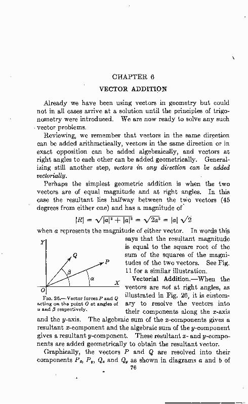
CHAPTER 6
VECTOR ADDITION
Already we have been using vectors in geometry but could not in all cases arrive at a solution until the principles of trigo-nometry were introduced. We are now ready to solve any such vector problems.
Reviewing, we remember that vectors in the same direction can be added arithmetically, vectors in the same direction or in exact opposition can be added algebraically, and vectors at right angles to each other can be added geometrically. General-izing still another step, vectors in any direction can be added vectorially.
Perhaps the simplest geometric addition is when the two vectors are of equal magnitude and at right angles. In this case the resultant lies halfway between the two vectors (45 degrees from either one) and has a magnitude of
IR1 + 'al' = V2a2 = lal
when a represents the magnitude of either vector. In words this says that the resultant magnitude
Y is equal to the square root of the sum of the squares of the magni-tudes of the two vectors. See Fig. 11 for a similar illustration.
Vectorial Addition.—When the X
0 vectors are not at right angles, as
26.—Vector forces P and Q illustrated in Fig. 26, it is ciistom-acting on the point 0 at angles of ary to resolve the vectors into is and p respectively, their components along the x-axis
and the y-axis. The algebraic sum of the x-components gives a resultant x-component and the algebraic sum of the y-component gives a resultant y-component. These resultant x- and y-compo-nents are added geometrically to obtain the resultant vector.
Graphically, the vectors P and Q are resolved into their components P., P., Q. and Q5 as shown in diagrams a and b of
76
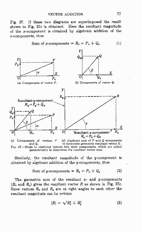
VECTOR ADDITION 77
Fig. 27. If these two diagrams are superimposed the result shown in Fig. 27e is obtained. Here the resultant magnitude of the x-component is obtained by algebraic addition of the x-components, thus
Sum of x-components = R. = P. ± Q. (1)
Y
o (a Components of vector P.
Resultant y -component
= Pv+
Y
Y
Y
Qv
(b) Components of -vector Q.
7 X
Resultant x-component Rz
Rx=Px+Qz (c) Components of vectors P (d) Algebraic sum of P and Q components
and Q. to determine geometric resultant vector R. 27.—Steps in resolving vectors into their components, which are added
geometrically to determine the resultant vector sum.
Similarly, the resultant magnitude of the y-component is obtained by algebraic addition of the y-components, thus
Sum of y-components = R5 = P5 ± Qy (2)
The geometric sum of the resultant x- and y-components (R. and R) gives the resultant vector R as shown in Fig. 27e. Since vectors Rx and R,, are at right angles to each other the resultant magnitude can be written
RI = 1/RI 42, (3)
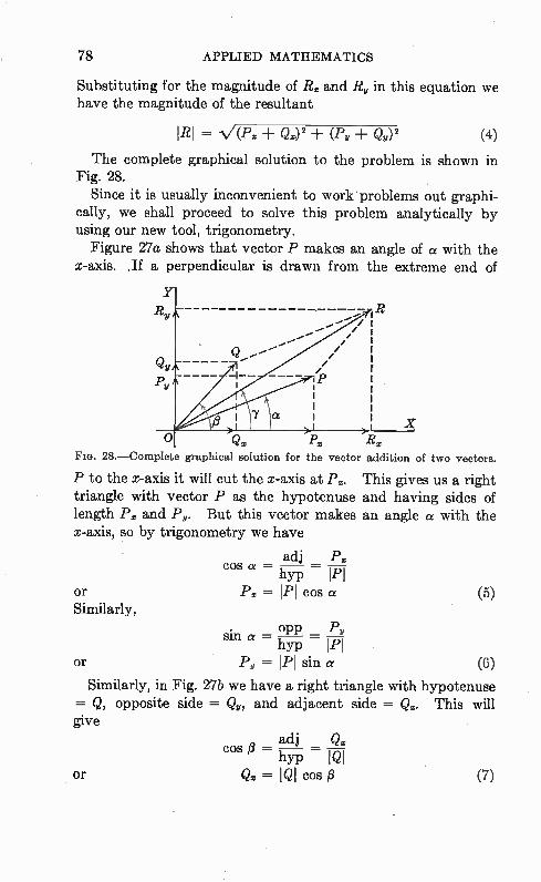
78 APPLIED MATHEMATICS
Substituting for the magnitude of R. and Rs, in this equation we have the magnitude of the resultant
¡RI = ± (2.)2 ± (Ps, Q„) 2 (4)
The complete graphical solution to the problem is shown in Fig. 28.
Since it is usually inconvenient to work problems out graphi-cally, we shall proceed to solve this problem analytically by using our new tool, trigonometry.
Figure 27a shows that vector P makes an angle of a with the x-axis. ,If a perpendicular is drawn from the extreme end of
o 28.—Complete graphical solution for the vector addition of two vectors.
P to the x-axis it will cut the x-axis at P. This gives us a right triangle with vector P as the hypotenuse and having sides of length P. and Ps,. But this vector makes an angle a with the x-axis, so by trigonometry we have
cos a adj = P. hyp I
or P. = IPI cos a Similarly,
sin a = oPP hyp 1/3
or Ps, = ¡PI sin a (6)
Similarly, in Fig. 27b we have a right triangle with hypotenuse = Q, opposite side = Q„, and adjacent side = Q. This will give
(5)
or
„ adj Qx cos p = 71 - _ 17) —
Q. = IQI cos 0 (7)
and
or
VECTOR ADDITION
sin = c-21)- = 911 hYP IQ! = IQ! sin
Substituting Eqs. (5) and (7) in Eq. (1) gives
R. = P. + Q. =PI cos « IQI cos #
Substituting Eqs. (6) and (8) in Eq. (2) gives
R, = Pi, + Qu = IPI sin a -I- IQ! sin #
Now, by substituting Eqs. (9) and (10) in (3), we get the resultant magnitude of the vector R in terms of the magnitude of vectors P, Q and trigonometric functions of the angles a and 13, that is,
'RI = VP' cos a ± IQ' cos + (IPI sin a ± IQI sin 13)2 (11)
This equation is perfectly general for finding the magnitude of the vector R, which is the sum of any two vectors, P and Q, making angles a and 13 respectively with the positive x-axis.
It is of interest to note that in Fig. 27 we have a right triangle with the magnitude of vector R the hypotenuse, the magnitude Ru the opposite side equal to PI sin a + IQI sin 0, and R. the adjacent side equal to !PI cos a ± IQ! cos 0. If we call the angle that vector R makes with the positive x-axis "7" (gamma), we have
tan = opp = R, (12) sin a ± IQ! sin /3 'y
adj R. = IPI cos a.+ IQI cos 13
Since we know the length of the opposite and adjacent side, the angle 7 can be found by referring to any trigonometry table.
Equation (11) gives the magnitude of the resultant vector and Eq. (12) gives the angle; therefore, the resultant vector is com-pletely determined.
Example 1. Referring to Fig. 26 we have given
IF1 = 10 = 5
Determine the resultant vector R.
a = 30° = 60°
80 APPLIED MATHEMATICS
Solution. Since P and Q are not at right angles with each other, we must use the above method to determine the resultant, that is, find the x-and y-components, which will be at right angles and hence can be added by geometric addition to obtain the final resultant. The x-component of P by Eq. (5) is
= IPI cos a= 10 cos 30° -- 10(0.866) = 8.66
The x-component of Q by Eq. (7) is
Q. = IQI cos tit = 5 cos 60° = 5(0.5) = 2.5
The resultant x-component by Eq. (1) is
R. = P. -I- Q. .= 8.66 -F 2.5 = 11.16
Now, the y-component of P by Eq. (6) is
P,, = IPI sin a -= 10 sin 30° = 10(0.5) = 5
and the y-component of Q by Eq. (8) is
(20 = IQI sin = 5 sin 60° -- 5(0.866) = 4.33
The resultant y-component by Eq. (2) is then
R„ = Pi, = 5 -I- 4.33 = 9.33
Equation (3) will now give us the magnitude of the resultant, thus
IRI = N/R! = N/(11.16)2 (9.33)2
= N/124.6 -I- 87.04 = NP2T.F.6 = 14.54 Ans.
Now that we have the magnitude we will solve for y (gamma), the angle the resultant vector R makes with the positive x-axis. From Eq. (12) we have
R„ 9.33 tarfhy = rFit3 = 0'836
From trigonometric tables, y 39°54' Ans.
This gives the complete solution of the resultant vector R which is often written in engineering form as follows:'
R = IRII-y
= 14.54/39°54' Ans.
This answer is read, "magnitude R at an angle of gamma," or "14.55 at an angle of 39 degrees 54 minutes."
This form of notation is adopted here because of its common use in engineering. Furthermore, it lends itself readily to handwriting. Some-times vectors are noted by boldface type or by a dot or bar placed above the
VECTOR ADDITION 81
Since a vector has both magnitude and direction, the above way of writing vectors is very convenient; it gives the magnitude (14.55) and the direction with respect to the positive x-axis (39°54'). This problem was worked on the slide rule and hence the
answer is not absolutely correct, but for ordinary engineering work it is entirely satisfactory.
It could have been solved by substituting directly in Eqs. (11) and (12) thus
IR1 = V(IPI cos a + cos i3)2 + (IPI sin a + pi sin 0)2 Substituting the numerical values,
¡RI = V(10 cos 30° + 5 cos 600)2 + (10 sin 30° ± 5 sin 600)2
Looking up the trigonometric functions,
I RI = V[10(0.866) + 5(0.5)]2 + [10(0.5) + 5(0.866)12
Performing the indicated multiplication,
IRI = 1/(8.6,6 ± 2.5)2 + (5 + 4.33)2
Adding inside the parentheses and squaring,
'RI = V(11.16)2 + (9.33)2 = V124.6 + 87.04
Adding under the radical and extracting the square root,
IRI = V211.6 = 14.54 Ans.
This answer is the same as was obtained above. Now, substituting in Eq. (12) we have
'PI sin a + pi sin (3 tan -y —
WI Cos a +1Q1 cos 0 symbol. Then the equation can be written without vertical bars to denote. magnitude, thus
R=É=R=R/7
Using this notation requires boldface type, a dot, or a bar to denote every vector quantity. With such a system, the boldface type could be used in print and the dot or bar placed above the vector symbol when written longhand. From the standpoint of making the system consistent in both print and script, and in order to save time and effort, it is more convenient to use the vertical bars the few times that they are needed to denote the absolute value or magnitude only.
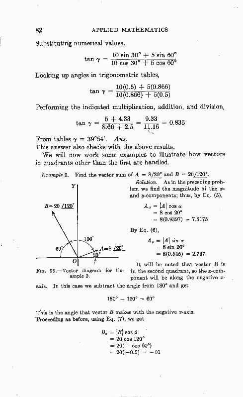
82 APPLIED MATHEMATICS
Substituting numerical values,
10 sin 30° ± 5 sin 60° tan -y —
10 cos 30° ± 5 cos 60°
Looking up angles in trigonometric tables,
10(0.5) ± 5(0.866) tan y = 10(0.866) + 5(0.5)
Performing the indicated multiplication, addition, and division,
5 + 4.33 9.33 tan -y =- 8.66 + 2.5 — = 0.836
From tables y = 39°54'. Ans. This answer also checks with the above results. We will now work some examples to illustrate how vectors
in quadrants other than the first are handled.
Example 2. Find the vector sum of A = 8/20° and B = 20/120°. Solution. As in the preceding prob-
Y lem we find the magnitude of the x-and y-components; thus, by Eq. (5),
A. lAl cos = 8 cos 20° = 8(0.9397) = 7.5175
By Eq. (6),
= lAl sin « = 8 sin 20° = 8(0.545) = 2.737
It will be noted that vector B is in the second quadrant, so the x-com-ponent will be along the negative x-
B= 20 /120°
Era. 29.—Vector diagram for Ex-ample 2.
axis. In this case we subtract the angle from 180° and get
180° — 120° = 60°
This is the angle that vector B makes with the negative x-axis. 'Proceeding as before, using Eq. (7), we get
B=IBj cos 5 • = 20 cos 120° = 20( — cos 60°) = 20( —0.5) = —10
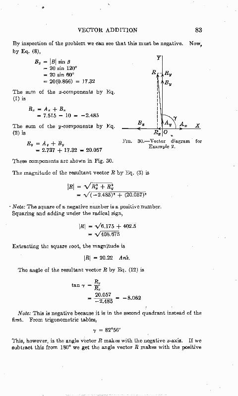
VECTOR ADDITION 83
By inspection of the problem we can see that this must be negative. Now,
by Eq. (8),
BY = IBI sin = 20 sin 120° = 20 sin 60° = 20(0.866) = 17.32
The sum of the x-components by Eq. (1) is
R. = A. ± B. = 7.515 — 10 = —2.485
The sum of the y-components by Eq. (2) is
= AY + BF = 2.737 -I- 17.32 = 20.057
These components are shown in Fig. 30.
The magnitude of the resultant vector R by Eq. (3) is
IRI = VR:
FIG. 30.—Vector diagram for Example 2.
= —2.485)2 (20.057)2
• Note: The square of a negative number is a positive number. Squaring and adding under the radical sign,
IRI = V6.175 402.5
V408.675
Extracting the square root, the magnitude is
IRI = 20.22 Ans'.
The angle of the resultant vector R by Eq. (12) is
tan 7
20.057 = —2.485 — "62
Note: This is negative because it is in the second quadrant instead of the first. From trigonometric tables,
= 82°56'
This, however, is the angle vector R makes with the negative x-axis. If we subtract this from 180° we get the angle vector R makes with the positive
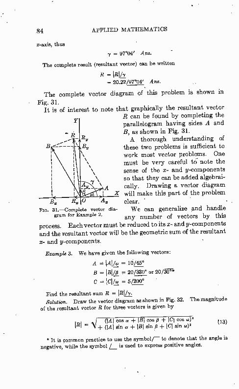
84 APPLIED MATHEMATICS
x-axis, thus
-y = 97°04' Ans.
The complete result (resultant vector) can be written
R = = 20.22/97°04' Ans.
The complete vector diagram of this problem is shown in
Fig. 31. It is of interest to note that graphically the resultant vector
R can be found by completing the Y parallelogram having sides A and
B, as shown in Fig. 31. A thorough understanding of
B By these two problems is sufficient to work most vector problems. One must be very careful tó note the sense of the x- and y-components so that they can be added algebrai-
\ A cally. Drawing a vector diagram X will make this part of the problem
Bo Ego O A. clear. " We can generalize and handle
any number of vectors by this process. Each vector must be reduced to its x- and y-components and the resultant vector will be the geometric sum of the resultant
x- and y-components.
Example 3. We have given the following vectors:
A = IAIL = 16/45°
B = !BIM = 20/330° or 20/30°*
C = ICl/w = 5/200°
Find the resultant sum R = 1R/'y. Solution. Draw the vector diagram as shown in Fig. 32. The magnitude
of the resultant vector R for three vectors is given by
FIG. 31.—Complete vector gram for Example 2.
dia-
(IAI cos a + IBI cos 13 + ICI cos (.0)2 IBI = ± (IA' gjn a IBI sin d + ICI sin co)2
* It is common practice to use the symbol/ — to denote that the angle is negative, while the symbol is used to express positive angles.
03)
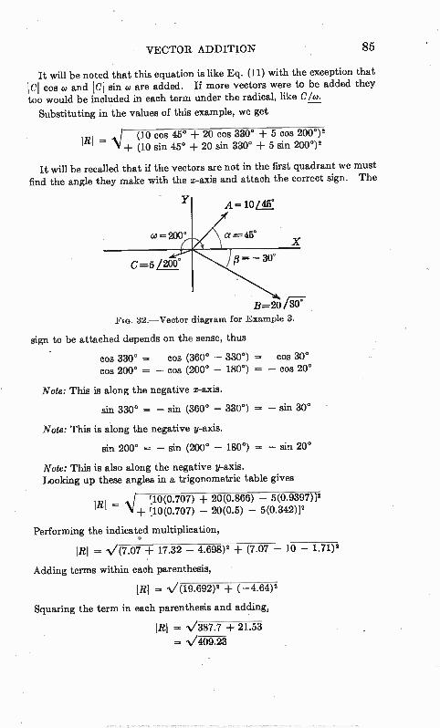
VECTOR ADDITION 85
It will be noted that this equation is like Eq. (11) with the exception that ICI cos co and ICI sin Co are added. If more vectors were to be added they too would be included in each term under the radical, like C/c0.
Substituting in the values of this example, we get
IRI (10 cos 45° ± 20 cos 330° 5 cos 2000)2 NI -I- -1- (10 sin 45° ± 20 sin 330° -I- 5 sin 2000)2
It will be recalled that if the vectors are not in the first quadrant we must find the angle they make with the x-axis and attach the correct sign. The
Y
200°
C / 200°
A =, IOLA°,
a = 45°
— 30°
13=20 F3F
FIG. 32.—Vector diagram for Example 3.
sign to be attached depends on the sense, thus
cos 330° = cos (360° — 330°) = cos 30° cos 200° = — cos (200° — 180°) = — cos 20°
Note: This is along the negative x-axis.
sin 330° = — sin (360° — 330°) = — sin 30°
Note: This is along the negative y-axis.
sin 200° = — sin (200° — 180°) = — sin 20°
Note: This is also along the negative y-axis. Looking up these angles in a trigonometric table gives
IRI = [10(0.707) ± 20(0.866) — 5(0-.9397)12 \I+ [10(0.707) — 20(0.5) — 5(0.342)12
Performing the indicated multiplication, •
I RI = / (7.07 -I- 17.32 — 4.698)2 + (7.07 — 10 — 1.71)2
Adding terms within each parenthesis,
IRI = N/(19.692)2 ± (-4.64)2
Squaring the term in each parenthesis and adding,
I RI = 1/387.7 ± 21.53 = VV:1-9.23
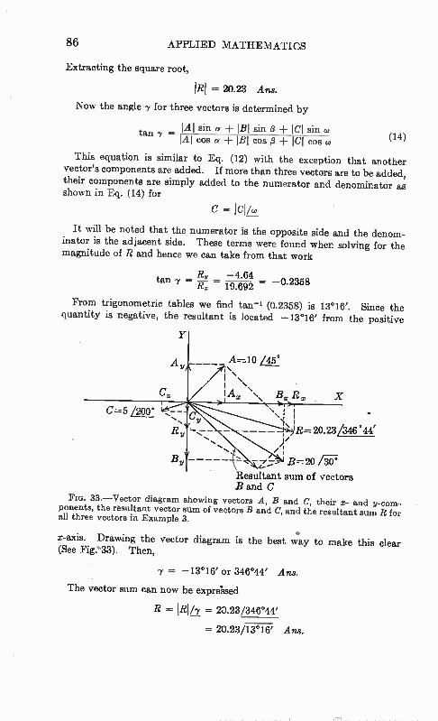
86 APPLIED MATHEMATICS
Extracting the square root,
= 20.23 Ans.
Now the angle -y for three vectors is determined by
ta 1A1 sin a 1/31 sin -F ICI sin co n -y = 1A1 cos « 1/31 cos /3 + ICI cos w (14)
This equation is similar to Eq. (12) with the exception that another vector's components are added. If more than three vectors are to be added, their components are simply added to the numerator and denominator as shown in Eq. (14) for
C = IcIA0
It will be noted that the numerator is the opposite side and the denom-inator is the adjacent side. These terms were found when solving for the magnitude of R and hence we can take from that work
R„ -4.64 tan y - = = -0.2358
R. 19.692
From trigonometric tables we find tan-1 (0.2358) is 13°16'. Since the quantity is negative, the resultant is located -13°16' from the positive
Y
Cx
A=10 /45°
I \'• I lAz \
C=5 /200° • • • • •
R=20.23/346 °44'
B=20 /IF
Resultant sum of vectors B and C
33.—Vector diagram showing vectors A, B and C, their x- and y-com-ponents, the resultant vector sum of vectors B and C, and the resultant sum R for all three vectors in Example 3.
• x-axis. Drawing the vector diagram is the best way to make this clear (See Fig.°33). Then,
= -13°16' or 346°44' Ans.
The vector sum can now be exprelsed
R = IRI/7 = 20.23/346°44'
= 20.23/13°16' Ans.
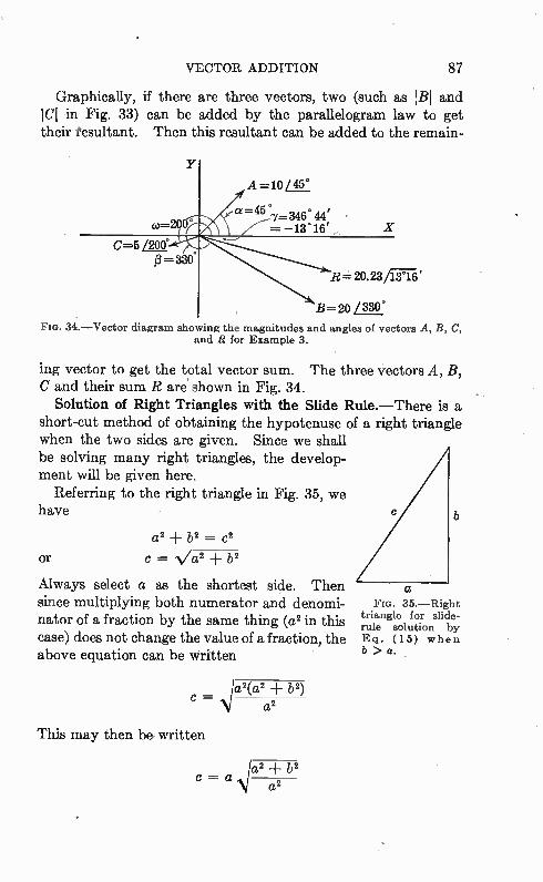
VECTOR ADDITION 87
Graphically, if there are three vectors, two (such as (BI and ICI in Fig. 33) can be added by the parallelogram law to get their tesultant. Then this resultant can be added to the remain-
FIG. 34.—Vector diagram showing the magnitudes and angles of vectors A, B, C, and R for Example 3.
ing vector to get the total vector sum. The three vectors A, B, C and their sum R are' shown in Fig. 34.
Solution of Right Triangles with the Slide Rule.—There is a short-cut method of obtaining the hypotenuse of a right triangle when the two sides are given. Since we shall be solving many right triangles, the develop-ment will be given here.
Referring to the right triangle in Fig. 35, we have
a2 b2 = 62
or c = -Va2 b2
Always select a as the shortest side. Then since multiplying both numerator and denomi-nator of a fraction by the same thing (a2 in this case) does not change the value of a fraction, the above equation can be written
c =
This may then be. written
c=a
V a2(a2 b2) a2
\ /a 2 b2
az
a FIG. 35.—Right
triangle for slide-rule solution by Eq. (15) when b > a.
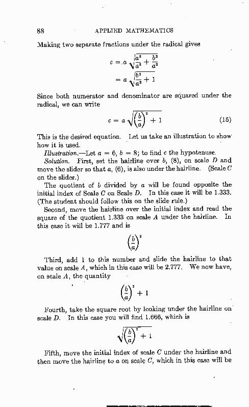
88 APPLIED MATHEMATICS
Making two separate fractions under the radical gives
\la2 b2
c = Ft2 Ft2 b2 = a \ri + 1 a
Since both numerator and denominator are squared under the radical, we can write
b)2 c = a NK—a ± 1 (15)
This is the desired equation. Let us take an illustration to show how it is used.
Illustration.—Let a = 6, b = 8; to find c the hypotenuse. Solution. First, set the hairline over b, (8), on scale D and
move the slider so that a, (6), is also under the hairline. (Scale C on the slider.) The quotient of b divided by a will be found opposite the
initial index of Scale C on Scale D. In this case it will be 1.333. (The student should follow this on the slide rule.)
Second, move the hairline over the initial index and read the square of the quotient 1.333 on scale A under the hairline. In this case it will be 1.777 and is
( ab) 2
Third, add 1 to this number and slide the hairline to that value on scale A, which in this case will be 2.777. We now have, on scale A, the quantity
(!)-)2 + 1 a
Fourth, take the square root by looking under the hairline on •
scale D. In this case you will find 1.666, which is
Fifth, move the initial index of scale C under the hairline and then move the hairline to a on scale C, which in this case will be
VECTOR ADDITION 89
6. The answer will be found on scale D under the hairline and in this case will be 10. We then have the complete expression solved for c, that is,
c = a j -i2t)2 ± = 6.\1() =
10 Ans. ct
Note: In the development a was the shortest side, while in some of the above examples this is not true. Therefore, the a and b will have to be interchanged in these cases.
Exercises
In each of the following problems, draw a vector diagram approximately to scale and solve for the resultant vector sum (magnitude and angle):
1. Voltage vector V1 = 110/0° (110 volts at an angle of 0° with positive
x-axis). Voltage vector V2 = 115/75° (115 volts at an angle of 75° with posi-
tive x-axis). 2. Impedance vector Z1 = 100/40°.
Impedance vector Z2 = 50/15° or 50/345°.
3. Current vector II = 3/215°.
Current vector /2 = 4/300°.
4. Voltage vector V1 = 150/60°.
Voltage vector V2 = 100/180°.
Voltage vector V3 = 50/300°.
5. Force vector F1 = 17/110°.
Force vector F2 = 15/320°.
Force vector F2 = 10/190°.
Work each of the following exercises by the slide-rule method and check for the resultant hypotenuse by the kinger method:
6. a = 3, b = 4. Find c. 7. a = 5, b = 5. Find c. 8. a = 14, b 11. Find c. 9. a = 76, b = 21. Find c.
10. a = 1.28, b = 0.91. Find c.
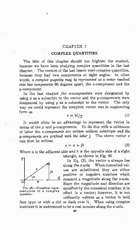
CHAPTER 7
COMPLEX QUANTITIES
The title of this chapter should not frighten the student, because we have been studying complex quantities in the last chapter. The vectors of the last lesson were complex quantities, because they had two components at right angles. In other words, a complex qugntity may be represented as a vector resolved into two components 90 degrees apart, the x-component and the y-component.
In the last chapter ,the x-components were designated by using x as a subscript to the vector and the y-components were designated by using y as a subscript to the vector. The only way we could represent the complete vector was in engineering form as
c =_ icl ia (1)
It would often be an advantage to represent the vector in terms of the x and y-components. To do this with a minimum of labor the x-components are written without subscripts and the y-components are prefixed with the letter j. The above vector c can then be written
c = a ± jb (2)
Where a is the adjacent side and b is the opposite side of a right triangle, as shown in Fig. 36.
Y In Eq. (2), the vector a always lies along the x-axis. When numerical val-ues are substituted they are either positive or negative numbers which measure a magnitude along the x-axis. Since the magnitude and direction are specified by the numerical number, it in effect is a vector; however, it is not ordinarily written as a vector in bold
face type or with a dot or dash over it. When using complex numbers it is understood to be a real number along the x-axis.
90
o Fro. 38.—Graphical repre-
sentation of a complex quantity.
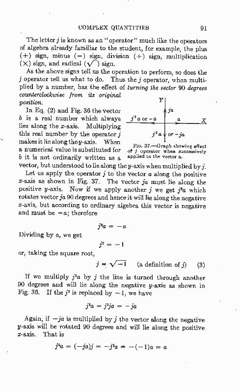
COMPLEX QUANTITIES 91
The letter jis known as an "operator" much like the operators of algebra already familiar to the student, for example, the plus (+) sign, minus ( — ) sign, division (÷) sign, multiplication (X) sign, and radical (V-) sign. As the above signs tell us the operation to perform, so does the
j operator tell us what to do. Thus the j operator, when multi-plied by a number, has the effect of turning the vector 90 degrees counterclockwise from its original
Y position. In Eq. (2) and Fig. 36 the vector
b is a real number which always j 2 a or - a a
lies along the x-axis. Multiplying this real number by the operator j .1. 3 a or - ja.
makes it lie along the y-axis. When FIG. 37.—Graph showing effect
a numerical value is substituted for of j operator when successively
b it is not ordinarily written as a applied to the vector a.
vector, but understood to lie along the y-axis when multiplied by j. Let us apply the operator j to the vector a along the positive
x-axis as shown in Fig. 37. The vector ja must lie along the positive y-axis. Now if we apply another j we get j'a which rotates vector ja 90 degrees and hence it will lie along the negative x-axis, but according to ordinary algebra this vector is negative and must be — a; therefore
i2a = _a
Dividing by a, we get j2 = _
or, taking the square root,
j = V -1-1. (a definition of j) (3)
If we multiply j'a by j the line is turned through another 90 degrees and will lie along the negative y-axis as shown in Fig. 36. If the j2 is replaced by —1, we have
= j2ja = — ja
Again, if — ja is multiplied by j the vector along the negative y-axis will be rotated 90 degrees and will lie along the positive x-axis. That is
j'a = (— ja)j = —j'a = — (-1)a = a
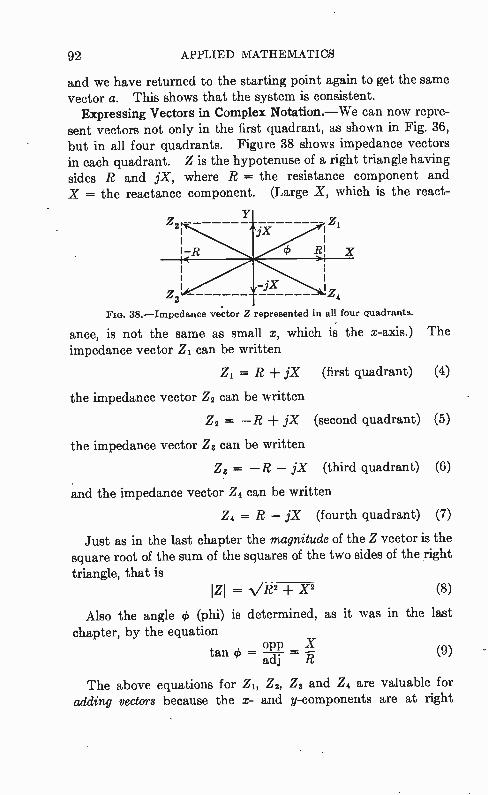
92 APPLIED MATHEMATICS
and we have returned to the starting point again to get the same vector a. This shows that the system is consistent.
Expressing Vectors in Complex Notation.—We can now repre-sent vectors not only in the first quadrant, as shown in Fig. 36, but in all four quadrants. Figure 38 shows impedance vectors in each quadrant. Z is the hypotenuse of a right triangle having sides R and jX, where R = the resistance component and X -= the reactance component. (Large X, which is the react-
38.—Impedance vector Z represented in all four quadrants.
ance, is not the same as small x, which is the x-axis.) The impedance vector Zi can be written
Z1 = R jX (first quadrant) (4)
the impedance vector Z2 can be written
Z2 = —R jX (second quadrant) (5)
the impedance vector Z3 can be written
Z3 = —R — jX (third quadrant) (6)
and the impedance vector Z4 can be written
Z4 = R — jX (fourth quadrant) (7)
Just as in the last chapter the magnitude of the Z vector is the square root of the sum of the squares of the two sides of the right
triangle, that is IZI = N/R2 + X2 (8)
Also the angle 41 (phi) is determined, as it was in the last
chapter, by the equation opp X
tan = a7lf = R
The above equations for Zi, Z2, Z3 and Z4 are valuable for adding vectors because the x- and y-components are at right
(9)
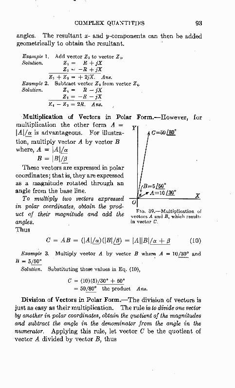
COMPLEX QUANTITIES 93
angles. The resultant x- and y-components can then be added geometrically to obtain the resultant.
Example 1. Add vector Z4 to vector Z2. Solution. Zi = R + iX
Z2 = —R + jX
Z1 + Z2 = 2jX. Ans. Example 2. Subtract vector Z3 from vector Z4. Solution. Z4 = R — iX
Z3 = —R — jX
Z4 — Z3 = 2R. Ans.
•Multiplication of Vectors in Polar multiplication the other form A = IAI/a is advantageous. For illustra-
tion, multiply vector A by vector B where, A = AI
B = 1./31/t3
These vectors are expressed in polar coordinates; that is, they are expressed as a magnitude rotated through an angle from the base line.
To multiply two vectors expressed in polar coordinates, obtain the prod-uct of their magnitude and add the angles. Thus
Y
Form.—However,
C=50/80°
B=5LLO° A=I0
for
X o FIG. 39.—Multiplication of
vectors A and B, which result,. in vector C.
C = AB = (IAI/ a)(1B1/13) = ± 13 (10)
Example 3. Multiply vector A by vector B where A = 10/30° and B = 5/50°
Solution. Substituting these values in Eq. (10),
C = (10)(5)/30° ± 50° = 50/80° the product Ans.
Division of Vectors in Polar Form.—The division of vectors is just as easy as their multiplication. The rule is to divide one vector by another in polar coordinates, obtain the quotient of the magnitudes and subtract the angle in the denominator from the angle in the numerator. Applying this rule, let vector C be the quotient of vector A divided by vector B, thus
94 APPLIED MATHEMATICS
A IAI/a IAl C = = —
B 1B1/13 iBi / a 13
Example 4. Divide vector E by vector Z where E = 100/60° and Z -= 5/5°
Solution. Substituting these values in Eq. (11),
iE — 1001600
= Z 5/5°
Dividing the magnitudes 10% = 20 and subtracting the denominator angle from the numerator angle gives
60°— 5° = 55°
Hence I = E = — 100/60° 100 /60° — 5° Z 5/5° 5
= 20/55° the quotient. Ans.
Example 5. Divide vector E by vector I when E = 8/10° and / = 16/40°
Solution. Substituting these values in Eq. (11),
E 8/10° 8 Z — 16 /10° — 40° I — 16/40°
= 0.5/30° or 0.5/330° the quotient Ans.
Trigonometry Applied to Complex Numbers.—According to what we learned in the last chapter, the magnitude of the x-component of c is Ici cos a and the magnitude of the y-com-ponent of c is Ici sin a. In complex numbers we write
c -= a ± jb
but a is the x-component ici cos a and b is the y-component Ici sin a; therefore, we can write
c = ici cos a + jici sin a
Factoring out the ici on the right-hand side gives
c = Ici (cos a j sin a) (12)
In this equation ici is the magnitude of the vector and
(cos a ± j sin a)
is the trigonometric operator which rotates the vector through the angle a in a counterclockwise direction from the positive x-axis.
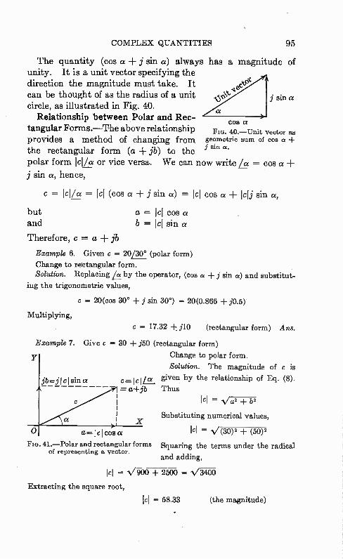
COMPLEX QUANTITIES 95
The quantity (cos j sin a) always has a magnitude of unity. It is a unit vector specifying the direction the magnitude must take. It 4e.e. can be thought of as the radius of a unit sin
circle, as illustrated in Fig. 40. Relationship between Polar and Rec-
tangular Forms.—The above relationship FIG. 40.—Unit vector as provides a method of changing from geometric sum of cos a -I-
j sin a. the rectangular form (a jb) to the polar form ici/a or vice versa. We can now write /« = cos « j sin «, hence,
cos
= ici/a = ici (cos « j sin a) = Ici cos « icij sin «,
but a = ici cos and b icl sin a
Therefore, c = a ± jb
Example 6. Given c = 20/30° (polar form)
Change to rectangular form. Solution. Replacing by the operator, (cos a j sin a) and substitut-
ing the trigonometric values,
c = 20(cos 30° j sin 30°) = 20(0.866 -I- j0.5)
Multiplying,
Example 7.
c = 17.32 j10 (rectangular form) Ans.
Give c = 30 ± j50 (rectangular form)
Change to polar form.
Solution. The magnitude of c is
c= given by the relationship of Eq. (8). IcILL(e. = a+ jb Thus
O a=icicos a
FIG. 41.—Polar and rectangular forms of representing a vector.
Ici = V al 52
Substituting numerical values,
Ici = N/(30)2 + (50)2
Squaring the terms under the radical
and adding,
Ici = N/900 + 2500 = -V3400
Extracting the square root,
Ici = 58.33 (the magnitude)
az a4 Cos a = — — — • • •
1_2 ILI
96 APPLIED MATHEMATICS
The angle is obtained by Eq. (9), thus
opp b 50 tan « — — = — = 1.666
adj a 30 From trigonometric tables,
a = 59°02' (approx.) (the angle)
Then the complete answer in polar form. is
o = ici/ce = 58.33/59°02' Ans.
It is important to note that the magnitude
cos a= cos 59°02' = 0.514539 sin « = sin 59°02' = 0.857467
Hence, a = Ici cos « Substituting numerical values,
a = 58.33(0.514539) --- 30, which checks Check.
and, b = ici sin « Substituting numerical values,
b = 58.33 (0.857467) = 50, which also checks Check.
This process of changing from polar to rectangular form and vice versa will be used to advantage later in the study of alter-nating current circuit theory. True Mathematical Polar Form.—The polar form c = ici/ct
has been adopted because of its convenience in expressing a vector which has a magnitude ici and makes an angle a with the reference axes. From pure mathematics it is easy to develop the exact character of this quantity. The magnitude of ex, sin x, and cos x can be defined by the
following series:
(13)
(,14)
(15)
In these equations the three dots at the end indicate that only a few terms of the series are written. Enough terms are usually written to indicate how the rest of the series can be written.
COMPLEX QUANTITIES 97
The expressions 12, 13, etc., in the denominator mean factorial, thus
12 = 2 • 1 = 2, 13 = 3 • 2 • 1 = 6, 14 = 4 • 3 • 2 • 1 = 24, etc.
Now if ja is substituted for x in Eq. (13), it can be written
, • , (ia) 2 I ( ja) g ja) 4 = -r — -r — -r — -r • • • (16)
12 13 14 but,
j = j2 = 1
ja = —
j4 = 1
j6
j6 = 1
Substituting these values in (16) gives
2 3 ± °* 4 C5 • •
Separating the j terms; gives
ja = (1 — + É — 12 14
(17)
(18)
But the two series of (18) are the same.as those of (14) and (15), hence,
= cos a j sin a (191
This shows that the true mathematical polar form of c is Icleice where e = 2.718 • • • the base of natural logarithms. This establishes the exponential character of the angle, showing why the angles are added when vectors are multiplied. The vector c can be written in several forms, as follows:
c = Ici /a = = Ici (cos a j sin a)
= 1cl cos a + ilel sin ce (20)
Multiplication of Vectors in Rectangular Form.—The multi-plication of vectors in rectangular form is more cumbersome than the multiplication of vectors in polar form. Usually it is easier to change from rectangular to polar form for multiplication than to perform the multiplication in rectangular form. However, in some cases, such as certain theoretical developments, multi-plication in rectangular form is valuable, and it should therefore be understood by the student.
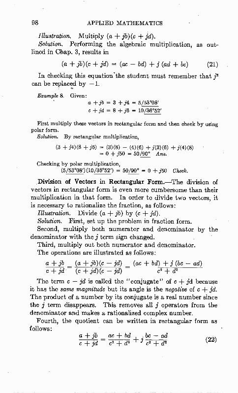
98 APPLIED MATHEMATICS
Illustration. Multiply (a + jb)(c jd). Solution. Performing the algebraic multiplication, as out-
lined in Chap. 3, results in
(a ± jb)(c jd) = (ac — bd) + j (ad ± be) (21)
In checking this equation the student must remember that j2 can be replaced by —1.
Example 8. Given: a +16 = 3 + 14 = 5/53°08'
c + jd = 8 +16 = 10/36°52'
First multiply these vectors in rectangular form and then check by using polar form.
Solution. By rectangular multiplication,
(3 +14)(8 +16) = (3)(8) — (4)(6) +1(3)(6) +1(4)(8) = 0 +150 = 50/90° Ans.
Checking by polar multiplication, (5/53°08')(10/36°52') = 50/90° = 0 -1- j50 Check.
Division of Vectors in Rectangular Form.—The division of vectors in rectangular form is even more cumbersome than their multiplication in that form. In order to divide two vectors, it is necessary to rationalize the fraction, as follows:
Illustration. Divide (a + jb) by (c jd). Solution. First, set up the problem in fraction form. Second, multiply both numerator and denominator by the
denominator with the j term sign changed. Third, multiply out both numerator and denominator. The operations are illustrated as follows:
a ± jb _ (a ± jb) (e — jd) _ (ac ± bd) + j (be — ad) jd - (c jd) (e — jd) e2 cl2
The term c — jd is called the "conjugate" of c jd because it has the same magnitude but its angle is the negative of c jd. The product of a number by its conjugate is a real number since the j term disappears. This removes all j operators from the denominator and makes a rationalized complex number.
Fourth, the quotient can be written in rectangular form as follows:
a + jb _ ac bd be—ad c jd c2 d2 3 c2 d2
(22)
COMPLEX QUANTITIES 99
Example 9. Given: a ± jb = 3 ± j4 = 5/53°08'
c + jd = 8 + j6 = 10/36°52'
First divide these vectors in rectangular form and then check by using polar form.
Solution.
3 + j4 _ (3 +j4)(8 — j6) _ 24 ± 24 + 1(32 — 18) 48 + 114
8 + (8 +16)(8 — 16) (64) + (36) — 100 = 0.48 + 10.14 = 0.50/16°16' Ans.
Checking by polar division,
5/53°08' — 0.5/1t°16' = 0.48 j0.14 Check.
10/36°52'
Exercises
1. Write c = jell_o_e = 50/30° in rectangular form, (a + jb).
2. Write c = jcj La = 10/300° in rectangular form. 3. Write c = a + 16 = — 20 +j30 in polar form. 4. Multiply A = 25/15° by B = 60/80°.
5. Divide A = 25/15° by B = 60/80° and express in rectangular form.
CHAPTER 8
CURVES AND GRAPHS
Curves and graphs are widely used to show relationships clearly. They bring together the principles of both algebra and geometry in a pictorial way that greedy increases their utility. A curve is a smooth line representing the relationship between
two or more variables. Such curves are often used by engineers for visualizing design relationships. A common procedure to obtain a curve is to vary one quantity and note the simul-taneous values of the other quantities. After sufficient data have been obtained, the points are plotted on appropriate graph paper and a smooth line is drawn through them to show the relationship. Algebraic equations can also be solved by plotting curves. These methods are not so readily adapted to high accuracy as pure algebraic methods, yet they often permit the solution of problems so difficult that pure algebraic methods become impractical. A curve is a special type of graph. A graph is a pictorial representation showing the• relationship between two or more quantities. Graphs are used extensively by newspapers, magazines, technical journals, engineers, and busi-ness people concerned with relative values. In one of the most common types of graphs, the adjacent points are joined by straight lines. This should be done unless there is a good reason for drawing a smooth curve through them. Common graphs of this type are those that show temperature plotted against time, stock market values plotted daily, and volume of business plotted monthly. Business men often base important decisions upon information obtained from graphs.
Engineering curves are usually plotted on cross-section paper. Cross-section paper comes in a variety of forms to meet various needs. Some of the more common forms are rectangular . coordinate paper, logarithmic paper, and polar coordinate paper.
System of Rectangular Coordinates.—We have already been using a system of coordinates. Such a system is shown in
loo
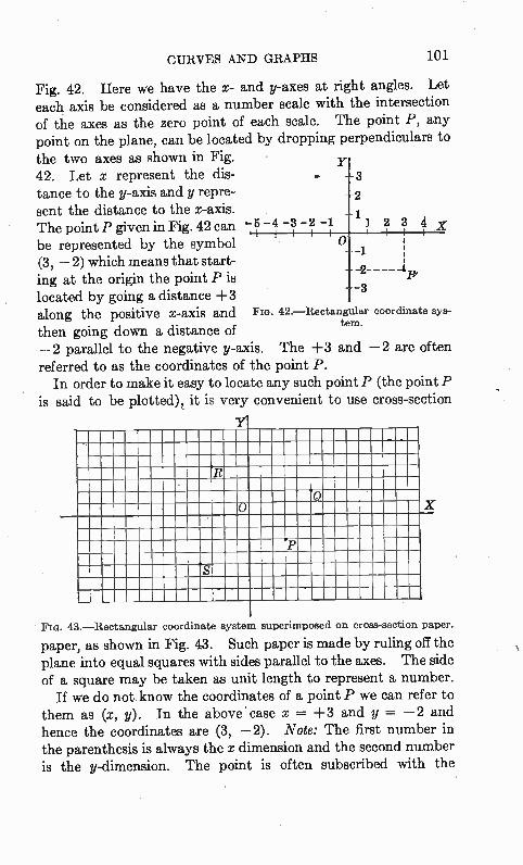
CURVES AND GRAPHS 101
Fig. 42. Here we have the x- and y-axes at right angles. Let each axis be considered as a number scale with the intersection of the axes as the zero point of each scale. The point P, any point on the plane, can be located by dropping perpendiculars to
the two axes as shown in Fig. Y 42. Let x represent the dis- -3
tance to the y-axis and y repre- -2
sent the distance to the x-axis. -1 The point P given in Fig. 42 can -4 -3 -2 -1 1 2 8 4 x 11111 1 I t be represented by the symbol 0 - (3, — 2) which means that start-ing at the origin the point P is
--3 located by going a distance +3 along the positive x-axis and FIG. 42.—Rectangular coordinate sys-
then going down a distance of tem.
— 2 parallel to the negative y-axis. The +3 and —2 are often referred to as the coordinates of the point P.
In order to make it easy to locate any such point P (the point P is said to be plotted), it is very convenient to use cross-section
43.—Rectangular coordinate system superimposed on cross-section paper.
paper, as shown in Fig. 43. Such paper is made by ruling off the plane into equal squares with sides parallel to the axes. The side of a square may be taken as unit length to represent a number.
If we do not know the coordinates of a point P we can refer to them as (x, y). In the above • case x = +3 and y = — 2 and hence the coordinates are (3, —2). Note: The first number in the parenthesis is always the x dimension and the second number is the y-dimension. The point is often subscribed with the
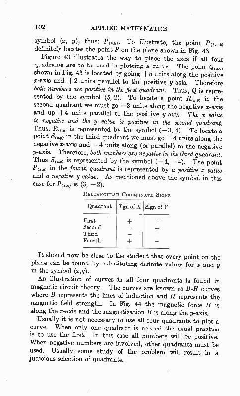
102 APPLIED MATHEMATICS
symbol (x, y), thus: P(.,„). To illustrate, the point P(3,-2)
definitely locates the point P on the plane shown in Fig. 43. Figure 43 illustrates the way to place the axes if all four
quadrants are to be used in plotting a curve. The point Q(.4,) shown in Fig. 43 is located by going +5 units along the positive x-axis and +2 units parallel to the positive y-axis. Therefore both numbers are positive in the first quadrant. Thus, Q is repre-sented by the symbol (5, 2). To locate a point R(.) in the second quadrant we must go —3 units along the negative x-axis and up +4 units parallel to the positive y-asis. The .x value is negative and the y value is positive in the second quadrant. Thus, R(.,„) is represented by the symbol ( —3, 4). To locate a point S(x,y) in the third quadrant we must go —4 units along the negative x-axis and —4 units along (or parallel) to the negative y-axis. Therefore, both numbers are negative in the third quadrant. Thus S(x.„) is represented by the symbol (-4, —4). The point P(.,5) in the fourth quadrant is represented by a positive x value and a negative y value. As mentioned above the symbol in this case for P(.,5) is (3, —2).
RECTANGULAR COORDINATE SIGNS
Quadrant Sign of X
First Second Third Fourth
Sign of Y
It should now be clear to the student that every point on the plane can be found by substituting definite values for x and y in the symbol (x,y).
An illustration of curves in all four quadrants is found in magnetic circuit theory. The curves are known as B-H curves where B represents the lines of induction and H represents the magnetic field strength. In Fig. 44 the magnetic force H is along the x-axis and the magnetization B is along the y-axis.
Usually it is not necessary to ase all four quadrants to plot a curve. When only one quadrant is needed the usual practice is to use the first. In this case all numbers will be positive. When negative numbers are involved, other quadrants must be used. Usually some study of the problem will result in a judicious selection of quadrants.
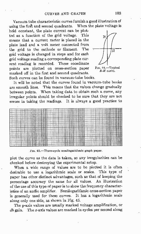
CURVES AND GRAPHS 103
Vacuum tube characteristic curves furnish a good illustration of using the first and second quadrants. When the plate voltage is held constant, the plate current can be plot-ted as a function of the grid voltage. This means that a current meter is placed in the plate lead and a volt meter connected from the grid to the cathode or filament. The grid voltage is changed in steps and for each grid voltage reading a corresponding plate cur-rent reading is recorded. These coordinate points are plotted on cross-section paper marked off in the first and second quadrants. Such curves can be found in vacuum-tube books.
It will be noted that the curves found in vacuum-tube books are smooth lines. This means that the values change gradually between points. When taking data to obtain such a curve, any irregular points should be checked to be sure that they are not errors in taking the readings. It is always a good practice to
FIG. 44.—Typical B-H curve.
1111111111M11111111 1111 IW10.1110111 1 lib Ill 111111111111 IWIIII1 1 11111 1 1 .01111111111 I BIM RRRRR 11 1111011N 1 1111 III 11111 11 111 I II 111111111111111H111111 I I ffir .110 H 1 IÈ1113111111111 1 11111111 11111 1,1111111 1 11 111 'MI.1111111 111111111 II 11 mumiun 111111 11 MI 11111111111111 111111111 II 111 :h11111 Ill 1111111MIIIIII1111 111111111 HI MI HIII 1111 1 11 liZI'MI.1111111 1 1 1 1111111111 1 1101 1 1111111110111 I 01 1111111111 111111110H 1 Ill 11111 HUI 11 1 111111MIII1111 111111 1111 111911 MINIM 1 11,1 IL '1111111111111 1111111111111 W1111111111111111 III 111111.11111111111111111/ 11tl11, 1 1111111 1 1 HUH-11MM llllll 1111111111 11 II 1 1111 I I 1111.113111H111111111 11111111E 11111 11' 11 11111110 MI I 111111111111 111111111 He II I 1111 1 I H11 C flIMMIIIIIIII 1 1111111 1111 I 1P 11 I 11111 1 114 11' 'MIII111111111111 1 Willi 1 n el 11111111 II nu :e UE1111111 11111111 10 1111111 111 III 1 II III 1111111111 11 11111111 1 X111 , 1111 1 II I 1 I Plan
1111111111 111111111 1 I I.1MT: 1 111 1 1 111 1.113.1111111 111111111111 I 1 I 11 1.11..11111 I I , 111 alli.111111111 I Z11E11111111111110 11 1'1 I '1.11 I 11 I MI 1111111111111 III 1111 NI 1 III ll'IL11111 :11,,I.1111111g111111 111111111 1 11 Il I II I
11" 11111" 11 111 1 111 11111111 III 111111 I WV HI 11 Ill H II :31111131111111111111111111 I 1 11111.11 11111 I 1 1 1 lgLMNIIIIIIIIIIIIIIII 1 I III 110 I II II I III zumigiiinn II 1 nui i I III II n p ffilionlogiiii! III 111111 1 1 1 1 11 111111 I 111511111111111111 111111 I 111111 1 I I I I 1 11111111111111 I II U III 1 1 II Ill 1211111111111111H1 1111 I HI 11 11111111 II I '11. IIIMIIIIIIIIII 11111 1 1 1 1 11 111 Ill I 1 in 1 ...milniumuu I 111îi I 11111 I III 1111111111111111111 1111 11 1111,1141111 11111 III 1 'F IMMilifillniiiIIII I II I I Ill 1 1 311.11111111111111111 11 11 1111 1 II 11 1 1 11111•1111•11111 111111111 II I I VH1'11111111 I 111111 11111111111 1110111111111 II 1 1 II Ill II Ill 1 III 11111111 II 111111 I 101 11 II 11111 1 1 II I 1 IIIIIMMI1111111E1111111 ill I I 1 H 11111111 Ill II 111111 IMIIIII 1111111111111 1 1 1 111111 I II 11111111111111111111111 1 mill 1 I II I 11 II I IIMMMIIIIIIIII 1111111 1 1 1 I 1'1111 11 11 II II 1111•1113111111111 111111111 m pimp urn 1 III 11.111111111 1111111111 1 1111 11 1111 Ill 111111 II 11111111MMIIIIIIII 11111111111 11 1 1H 11 11 1111 III I 11101 varummiluni mum I nu 11 II 111 11 IIIIIIIIII II 1111111 11111111111 111111 11111 MI II II 11111.11111111 11111 111 11.1 11 11 III I I II III EMIIIIIIIIIIIII 11 Ilh 1 1 1 11 HI MI 1 II IIMIIIIIIIII 1111111 III _11 III III MU 11 11 I II 1 II 1111111.11111111 111111111 11 III . II 11 1 I Ill II 111 1.11111111111 1111 III HIP 1 1 I , 11 pu 1'Ill 111111111111111 1111111 111111 111 III 111111 111001 111111 111111 I 111 11 141111 1 1111111 111111111.111111111 1111111111111 I I II . 11 1 1 II I III
Fro. 45.—Three-cycle semi ogarithmic graph paper.
plot the curve as the data is taken, so any irregularities can be checked before destroying the experimental setup. When a wide range of values are to be plotted it is often
desirable to use a logarithmic scale or scales. This type of paper has other distinct advantages, such as that of keeping the percentage accuracy the same for all values. An illustration of the use of this type of paper is to show the frequency character-istics of an audio amplifier. Semilogarithmic cross-section paper is generally used for these curves. It has a logarithmic scale along only one side, as shown in Fig. 45. The y-axis values are usually marked voltage amplification, or
db gain. The x-axis values are marked in cycles per second along
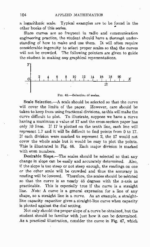
104 APPLIED MATHEMATICS
a logarithmic scale. Typical examples are to be found in the other books of this series.
Since curves are so frequent in radio and communication engineering practice, the student should have a thorough under-standing of how to make and use them. It will often require considerable ingenuity to select proper scales so that the curves will not be crowded. The following pointers are given to guide the student in making any graphical representations.
Y
o 12 14 16 18 20
II I I II X
46.—Selection of scales.
17
Scale Selection.—A scare should be selected so that the curve will cover the limits of the paper. However, care should be taken to keep from using fractional divisions, as this will make the curve difficult to plot. To illustrate, suppose we have a curve having a maximum x value of 17 and the cross-section paper has only 10 lines. If 17 is plotted on the tenth line, each line will represent 1.7 and it will be difficult to find points from 0 to 17. If each division were marked to represent 2, the 17 would not cover the whole scale but it would be easy to plot the points. This is illustrated in Fig. 46. Each major division is marked with even numbers.
Desirable Slope.—The scales should be selected so that any change in slope can be easily and accurately determined. Also, if the slope is too steep or not steep enough, the readings on one or the other scale will be crowded and thus the accuracy in reading will be lowered. Therefore, the scales should be selected so that the curve is as nearly 45 degrees with the x-axis as practicable. This is especially true if the curve is a straight line. Note: A curve is a general expression for a line of any shape, so a straight line is a curve. As an example, a straight-line capacity capacitor gives a straight-line curve when capacity is plotted against the dial setting. Not only should the proper slope of a curve be obtained, but the
student should be familiar with just how it can be determined. As a practical illustration, consider the curve in Fig. 47, which
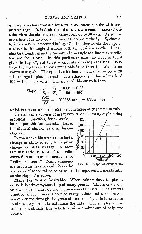
CURVES AND GRAPHS 105
is the plate characteristic for a type 250 vacuum tube with zero grid voltage. It is desired to find the plate conductance of th tube when the plate current varies from 60 to 80 mils. As will be given later, the plate conductance is the slope of the 1„— E„ charac-teristic curve as presented in Fig. 47. In other words, the slope of a curve is the angle it makes with the positive x-axis. It can also be thought of as the tangent of the angle the line makes with the positive x-axis. In this particular case the slope is tan O given in Fig. 47, but tan O = opposite side/adjacent side. Per-haps the best way to determine this is to form the triangle as shown in Fig. 47. The opposite side has a length of 80 — 60 = 20 mils change in plate current. The adjacent side has a length of 190 — 160 =- 30 volts. The slope of this curve is then
12 - I 0.08 — 0.06 Slope —
E2 E1 - 190 — 160
"2 — 0• 000666 mho, = 666 g mho — 30 —
which is a measure of the plate conductance of the vacuum tube. The slope of a curve is of great importance in many engineering
problems. Calculus, for example, is 120
based upon this fundamental idea, so e100 the student should learn all he can
In the above illustration we had a 60 (k.
02 80 about it.
change in plate current for a given .52 40
change in plate voltage. A -in. ore 1: 20 familiar ratio is that of the miles covered in an hour, commonly called "miles per hour." Many engineer-ing problems have to deal with ratios and each of these ratios or rates can be represented graphically as the slope of a curve. Many Points Are Desirable.—When taking data to plot a
curve it is advantageous to plot many points. This is especially true when the values do not fall on a smooth curve. The general practice in such cases is to plot many points and then draw a smooth curve through the greatest number of points in order to minimize any errors in obtaining the data. The simplest curve to plot j straight line, which requires a minimum of only two
points, '
O
100 200 300 Volts Ep
Fro. 47.—Slope determination.
400
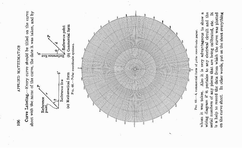
' e \t, 'es\ ‘``,tee% %edieeee'
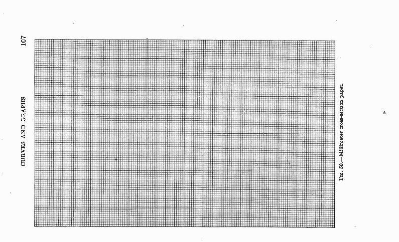
CURVES AND GRAPHS
::::::::::: "E. NM.
n ▪ ::: ..... hiLiPMEC:= .............. -1:1 .L...misicamernha: .. unuku eal ••••••••••••
:....!! ....... miesuluvuesuadmie: 112:::LEF91111111111i:. .
eithen.r2.2.1 n.
;IMUMININtr.- . mdf:1:11111:1"ju;:111.z1;1111b;:_eimbillittillililigrel:iPrelliiiLiiMILIFF:1.11111::9i41.111,11 • . :.....1!:. .. ........ :IL.. • :T.,rompinurengihnuip::
12171:1"1"r::::r74119; .. Rédrinbel neillnidnelireinimujgralleilmoraimun u—mou -19:nlnererFPunnn* :In:Lad:me" yisciumeml
nal ..... un. . "Jueur .." 1.» ... . :1;91411. 1: 1:1::::::.1::
▪ :!' --J iiie ll!!!!!!!11101-0111111111114 4111:eit e-
......... . et .1
..... «. 1. ..... ......
CZEOPMET . 1:1811125 1:171:11 ................. : ..............
111111!!!!!iilldra.:191: 1 k: ..
te ::1... " . . :•::. " ::..1 u
::::::::::11:.::::
• nun
: .......... au:
: ::::::::::: err:e. • e
e •••••••••••••
• •
:
.:: •Ole.
ng ng ..... •••
... .....
r EllE ....... e
::::111 a n.
!La: ........... •••• •••:
a. : EifP P
... 3.• ••••
.. a
•• .11
el••••••••••••••••••••••••••• ...
FIG. 50.—Millimeter c
ross-section paper.

108 APPLIED MATHEMATICS
that will help to convey a complete picture of the conditions and the results of the experiment. System of Polar Coordinates.—Some data are best presented
on polar coordinate paper. Common illustrations are field patterns of microphones, loud-speakers, and directional antennas. To specify a point P by polar coordinates it is necessary to
know the distance from the reference point to the point P and the angle this line makes with the reference line. In the mathematical form, as shown in Fig. 48a, the reference point corresponds to the origin used in rectangular coordinates and the reference line corresponds to the positive x-axis. To each the point P the distance r is laid off along the x-axis and then the line is rotated counterclockwise through the positive angle O. The same point could be reached by rotating the line clockwise through a negative tingle which would be equal to — (360° — 0).
In commercial practice, such as navigation and directional antenna design, the reference line is north and the angles are measured clockwise. Figure 48b illustrates a commercial form of polar coordinate system. The true azimuth of the point is measured by 4, and its distance from the reference point is d. A sample of polar coordinate paper for commercial applications is shown in Fig. 49. The point P can be represented in polar coordinates by the
symbol (r, 0) or (d, iliuserated in Fig. 48. To make it easy to locate any such point, um polar coordinate paper can be printed with many radial lines along which the distance can be measured and many circles around which the angle can be measured.
Exercises
1. Experimental data give the following information in regard to a sample of transformer steel:
H B H
0 1.0 0 —1.0 2,000 1.3 —2,000 —1.3 4,000 1.7 —4,000 —1.7 6,000 2.2 —6,000 —2.2 8,000 3.4 —8,000 —3.4 8,300 4.0 —8,300 —4.0 8,000 2.2 —8,000 —2.2 6,000 0.0 —6,000 0.0 4,000 —0.6 —4,000 0.6 2,000 —0.8 —2,000 0.8
0 —1.0 0 1.0

CURVES AND GRAPHS 109
Plot the B-H curve on cross-section paper, as shown in Fig. 50. 2. Field intensity measurements on a radio broadcasting station are
made by going due north of the transmitter. Plot the ground wave field intensity on log-log paper' from the following data:
Millivolts Millivolts Miles per Meter Miles per Meter
1 94 1.5 61 12 5.0 2 45 14 3.9 3 28.5 16.5 3.0 4 20.5 20 2.1 5 15.5 25 1.4 6 12.5 30 1.0 8 8.6 40 0.55 10 6.4 60 0.26
80 0.12
What is the distance to the 25, 10, 5, 2.5, and 0.5 mv per m contours? Draw the inverse distance curve through the point 100 mv per m at 1 mile.
3. The computation of field intensity measurements at 1 mile for a 1-kw broadcast transmitter using a three-tower directional antenna system results in the following data:
Azi-muth
Millivolts Azi-per Meter muth
o 10 20 30 40 50 so 70 so
369.5 90 337.5 100 288.3 110 228.5 120 175.0 130 126.6 140 88.1 150 65.9 160 33.7 170
Millivolts flo5i-per Meter muth
33.3 180 58.6 190 87.3 200 108.1 210 113.6 220 100.2 230 64.5 240 27.0 250 67.5 260
Millivolts Azi-per Meter muth
129.6 270 182.6 280 220.0 290 229.3 300 222.2 310 194.3 320 157.4 330 116.0 340 76.6 350
Millivolts per Meter
29.2 61.5 99.5 150.2 208.4 268.5 320.6 361.4 378.1
Plot these data on polar coordinate paper. Draw the root-mean-square field intensity circle at 191 mv per m. The area of this circle is the same as the area within the irregular pattern. This value can be checked by squar-ing the thirty-six readings of millivolts per meter, dividing their sum by 36, and extracting the square root. A sample of suitable polar coordinate paper is shown in Fig. 49.
' To plot such data, the Federal Communications Commission normally uses Logarithmic, 7 X 2.2 cycles, No. 358-127, printed by Keuffel and Esser Co., N.Y.
CHAPTER 9
SIMULTANEOUS EQUATIONS
In radio and communication engineering, problems often arise in which two desired unknown quantities can be determined when two sets of conditions are known. This method of attack is very powerful and can be expanded to find an n number of desired unknowns if a set of n independent conditions are known.
Sets of Two Linear Equations.—The following illustration shows how a problem may lead to a set of two linear equations, sometimes called "simultaneous equations." Let us consider the formula
Rk — at = 1 (1)
where R = resistance of a metal after being heated through t. k = constant, the reciprocal of the resistance at the
initial temperature. a = constant, the temperature coefficient of the resist-
ance. t = temperature change in degrees centigrade.
It is found by trial that R = 108 when t = 20 and that R = 128 when t = 70. With these two sets of conditions, it is desired to find the constants k and a. Substituting the two sets of information in Eq. (1) results in
108k — 20a = 1 (using first set of conditions) (2) 128k — 70a = 1 .(using second set of conditions) (3)
It is easy to find numbers for k and a that will satisfy Eq. (2) but not Eq. (3), and to find other numbers for k and a that will satisfy Eq. (3) but not Eq. (2). There is only one pair of numbers for k and a that will satisfy both equations at the same time and this pair is the solution of the set of two equations. There are three methods of finding these values of k and a and these methods will be given later. The solution to this problem is
k = 0.01 Ans. a = 0.004 Ans.
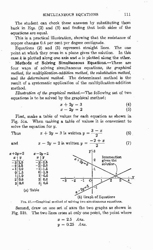
x 1-2y=3 x y - 3 - 2 -1 o 1 2 3
3.0 2.5 2.0 1.5 1.0 0.6 0.0
SIMULTANEOUS EQUATIONS 111
The student can check these answers by substituting them back in Eqs. (2) and (3) and finding that both sides of the equations are equal.
This is a practical illustration, showing that the resistance of copper changes 0.4 per cent per degree centigrade.
Equations (2) and (3) represent straight lines. The one point at which they cross in a plane gives the solution. In this case k is plotted along one axis and a is plotted along the other. Methods of Solving Simultaneous Equations.—There are
four ways of solving simultaneous equations, the graphical method, the multiplication-addition method, the substitution method, and the determinant method. The determinant method is the result of a systematic application of the multiplication-addition method.
Illustration of the graphical method.—The following set of two equations is to be solved by the graphical method:
x + 2y = 3 (4) x — 2y = 2 (5)
First, make a table of values for each equation as shown in Fig. 51a. When making a table of values it is convenient to solve the equation for y.
3 — x Thus x 2y = 3 is written y — 2
— 2 + x and x — 2y = 2 is written y = 2
Y 3 x -2y=2 x y -3 -2 -1 o 2 3
(a) Table
-2.5 -2.0 -1.6 -1.0 -0.6 0.0 0.6
(6)
(7)
Intersection 2 gives the
8 solution
(b) Graph of Equations FIG. 51.—Graphical method of solving two shnultaneous equations.
Second, draw on one set of axes the two graphs as shown in Fig. 51b. The two lines cross at only one point, the point where
x = 2.5 Ans. y = 0.25 Ans.
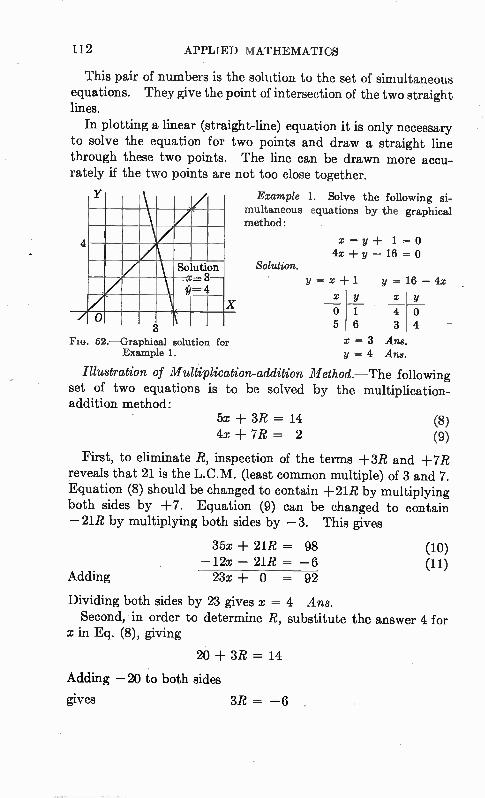
112 APPLIED MATHEMATICS
This pair of numbers is the solution to the set of simultaneous equations. They give the point of intersection of the two straight lines.
In plotting a linear (straight-line) equation it is only necessary to solve the equation for two points and draw a straight line through these two points. The line can be drawn more accu-rately if the two points are not too close together.
Example 1. Solve the following si-multaneous equations by the graphical method:
x — y + 1 = 0 4x -F y — 16 =
Solution. y = x + 1
o 5
1 6
y = 16 — 4x
x y
4 0 3 4
52.—Graphical solution for x = 3 Ans Example 1. y = 4 Ans
Illustration of Multiplication-addition. Method.—The following set of two equations is to be solved by the multiplication-addition method:
5x + 3R = 14 4x + 7R = 2
(8) (9)
First, to eliminate R, inspection of the terms +3R and +7R reveals that 21 is the L.C.M. (least common multiple) of 3 and 7. Equation (8) should be changed to contain +21R by multiplying both sides by +7. Equation (9) can be changed to contain —21R by multiplying both sides by —3. This gives
35x + 21R = 98 (10) —12x — 21R = —6 (11)
Adding 23x+ O = 92
Dividing both sides by 23 gives x = 4 Ans. Second, in order to determine R, substitute the answer 4 for
x in Eq. (8), giving
20 + 3R = 14
Adding — 20 to both sides
gives 3R = —6
SIMULTANEOUS EQUATIONS 113
Dividing both sides by 3
gives R = —2 Ans.
Check: Substitute 4 for x and —2 for R in both Eqs. (8) and (9), thus
5x + 3R = 14 20 — 6 = 14
14 = 14
4x + 7R = 2 16 — 14 = 2
2 = 2
Hence, the solution x = 4 and R = —2 has just been proved correct.
Example 2. Solve the following simultaneous equations by the multi-plication-:addition method:
5x + 7y = 3 3x + 14y = 6
Multiplying the first equation by —2 and adding the second gives
—10x — 14y = —6 3x + 14y = 6
gives Hence,
— 7x = x = 0 Ans.
Substituting x = 0 in the first equation, y = ,¡ Ans.
Illustration of the Substitution Method.—The following set of two equations is to be solved by the substitution method:
4x + 3? = 5 (12) 6x — 7R = 19
First, solve Eq. (12) for R, obtaining
R= 5— 5 — 4x
(13)
(14)
Second, copy Eq. (13) but in the place of R write the fraction as given in Eq. (14). This is permissible because R is equal to this fraction. The result of this substitution is then
7(5 — 4x) 6x — 19 (15)
3
This equation contains only one unknown number, x. The unknown number R has been eliminated by substitution. Multi-ply both sides of the equation by 3, giving
18x — 7(5 — 4x) = 57
114 APPLIED MATHEMATICS
Removing the parentheses
gives 18x — 35 ± 28x = 57 Collecting terms, 46x = 92 Hence, x = 2 Ans.
Third, substitute 2 for x in Eq. (14), giving
R = 5 — 4x 5 — 8 3 = 3
= —1 Ans.
Check: Substitute x = 2 and R = —1 in Eqs. (12) and (13), thus
4x + 3R = 5 8 — 3 = 5
5 = 5
6x — 7R = 19 12 + 7 = 19
19 = 19
Hence, x = 2 and R = --1 is the one and only solution to this set of simultaneous equations. The -substitution method, just shown, can be used in more
difficult situations than the multiplication-addition method. This can be illustrated by noting the following pair of equations:
3x + 2R = 4 x2 + R2 5
(16) (17)
Equation (16) is a linear equation (of the first degree, since x and R appear to the first power). Equation (17) is a quadratic equation (of the, second degree, since x. and R appear to the second power).
First, solve Eq. (16) for R, obtaining
R = (18) 2
Second, substitute this value of R in Eq. (17) to obtain
x2 + (4 - 31 = 5 or \ 2 4
Multiplying both sides by 4,
4x2 + 16 — 24x -F 9x2 = 20 Collecting terms, 13x2 — 24x — 4 = 0 (19)
This is an equation in x only and can be solved for x very easily by the methods of the next chapter. The above set of
SIMULTANEOUS EQUATIONS 115
simultaneous equations could not be solved by the multiplication-addition method.
Example 3. Solve by the substitution method the following problem: The sum of the three angles of a triangle is 180°. If one acute angle of
the right triangle is four times the size of the other, determine the size of the two acute angles.
Solution. From the first statement let a and t3 be the two acute angles to get
« +13 + 90° = 180° or a -I- p = 90°
From the second statement, « = 40
Substituting this value of « in the first equation gives
4r9 + = 90 a = 18° Ans.
and « = 4$ = 4(18)° = 72° Ans.
Classification of Linear Simultaneous Equations.—Some sets of equations have no solution. To illustrate, the equations
2x ± 3R = 5 2x ± 3R = 7
contradict each other, and are inconsistent. The graphical method shows that they are parallel lines and hence do not meet to give a solution. Some sets of equations are dependent, because one equation
can be made exactly like the other by multiplying by some number. To illustrate, the first equation of the set,
3x ± 6R = 7.5 2x + 4R =. 5
becomes the second when it is multiplied by h. The graphical method shows that both equations represent the same straight line, hence they have an infinite number of solutions. Such equations are sometimes called "indeterminate equations."
All sets of equations that are neither inconsistent nor dependent are called "independent." Their graphs are distinct nonparallel lines and they always have a single solution. That is, they cross at only one point. If the equations are written in general form, we have
bly = ci (20) ct2x b2y = c2 (21)
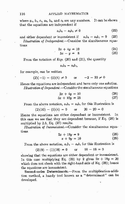
116 APPLIED MATHEMATICS
where al, b1, c, a2, b2, and c2 are any numbers. It can be shown that the equations are independent if
aib2 — a2bi 0 0 (22)
and either dependent or inconsistent if aib2 — a2bi = 0 (23) Illustration of Independent.—Consider the simultaneous equa-
tions 2x + 4y = 10 (24) 5x — y = 8 (25)
From the notation of Eqs. (20) and (21), the quantity
alb2 — a2bi,
for example, can be written
(2)( —1) — (5)(4) 0 0 or — 2 — 20 0 0
Hence the equations are independent and have only one solution. Illustration of Dependent.—Consider the simultaneous equations
2x ± 4y = 10 5x ± by = 25
(26) (27)
From the above notation, aib2 — a2bi for this illustration is
(2)(10) — (5)(4) = 0 or 20 — 20 =
Hence the equations are either dependent or inconsistent. In this case we see that they are dependent because, if Eq. (26) is multiplied by 2.5, Eq. (27) results.
Illustration of Inconsistent.—Consider the simultaneous equa-tions
2x ± 18y = 9 X 9y = 10
(28) (29)
From the above notation, aib2 — a2bi for this illustration is
(2)(9) — (1)(18) = 0 or 18 — 18 =
showing that the equations are either dependent or inconsistent. In this case multiplying Eq. (29) by 2 gives 2x ± 18y = 20 which does not check with the right-hand side of Eq. (28); hence the equations are inconsistent.
Second-order Determinants.—From the multiplication-addi-tion method, a handy tool known as a "determinant" can be developed.
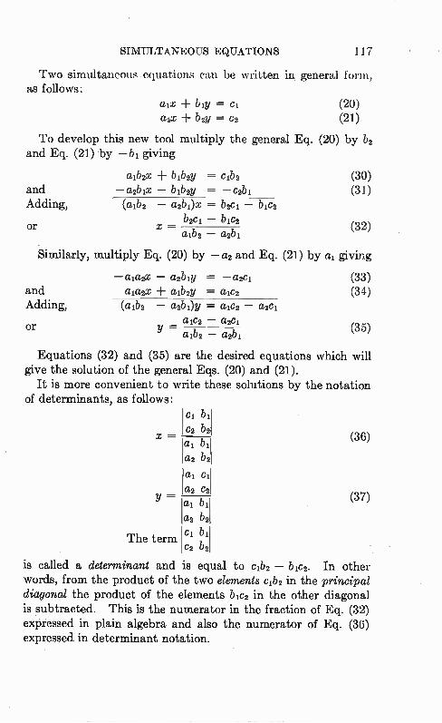
SIMULTANEOUS EQUATIONS 117
Two simultaneous equations can be written in general form, as follows:
aix biy = ci (20) b2y = c2 (21)
To develop this new tool multiply the general Eq. (20) by b2 and Eq. (21) by —b1 giving
aib2x bib2y = ci.b2 (30) and Adding,
or
—a2bg — bibe = —c2bi (aib2 — a2bi)x = b2ci — bic2
— b2ci — bic2 x
alb2 a2b1
(31)
(32)
Similarly, multiply Eq. (20) by — a2 and Eq. (21) by al giving
—alazx — azbiy = —azci and alazx aibzy aicz Adding, (aib2 — a2b1)Y = ctic2 — a2ci
alc2 — a2ci or = aibz — azbi
(33) (34)
(35)
Equations (32) and (35) are the desired equations which will give the solution of the general Eqs. (20) and (21).
It is more convenient to write these solutions by the notation of determinants, as follows:
Y —
The term
c1 bli
C2 b2
al 611 az b21
al cl az c2
bi az bz c1 bl
c2 b2
(36)
(37)
is called a determinant and is equal to cib2 — bic2. In other words, from the product of the two elements cib2 in the principal diagonal the product of the elements be2 in the other diagonal is subtracted. This is the numerator in the fraction of Eq. (32) expressed in plain algebra and also the numerator of Eq. (36) expressed in determinant notation.
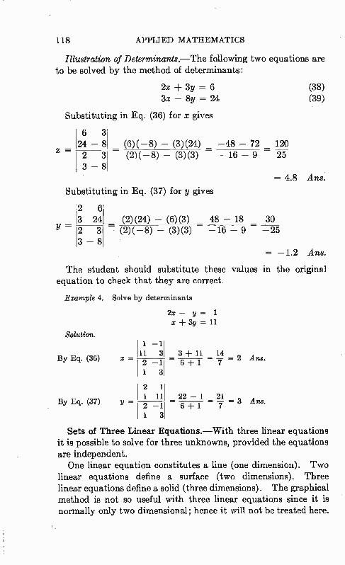
118 APPLIED MATHEMATICS
Illustration of Determinants.—The following two equations are to be solved by the method of determinants:
2x + 3y = 6 (38) 3x — 8y = 24 (39)
Substituting in Eq. (36) for x gives
I 6 3 124 — 8 _ (6)( —8) — (3)(24) = —48 — 72 120
x = 2 3 (2)( —8) — (3)(3) —16 — 9 — 25 3 — 8
= 4.8 Ans.
Substituting in Eq. (37) for y gives
2 6 3 24 (2)(24) — (6)(3) _ 48 — 18 30
Y = 2 3 (2)( — 8) — (3)(3) —16 — 9 —25 3 — 8
= —1.2 Ans.
The student should substitute these values in the original equation to check that they are correct.
Example 4. Solve by determinants
2x — y = 1 X 3y = 11
Solution.
By Eq. (36) x
By Eq. (37) Y
1 —11 11 31 3 11 14 2 —11 6 + 1 7 1 31
2 1 1 11 22 — 1 21 2-1 — 6 + 1 7 1 3
— 2 Ans.
— 3 Ans.
Sets of Three Linear Equations.—With three linear equations it is possible to solve for three unknowns, provided the equations are independent. One linear equation constitutes a line (one dimension). Two
linear equations define a surface (two dimensions). Three linear equations define a solid (three dimensions). The graphical method is not so useful with three linear equations since it is normally only two dimensional; hence it will not be treated here.
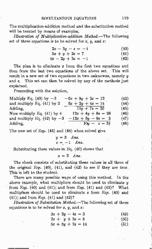
SIMULTANEOUS EQUATIONS 119
The multiplication-addition method and the substitution method will be treated by means of examples.
Illustration of Multiplication-addition Method.—The following set of three equations is to be solved for x, y, and z:
2x — 3y z = —4 (40) 3x + y + 2z = 7 (41)
4x — 2y + 3z = —1 (42)
The plan is to eliminate x from the first two equations and then from the last two equations of the above set. This will result in a new set of two equations in two unknowns, namely y and z. This set can then be solved by any of the methods just explained.
Proceeding with the solution,
Multiply Eq. (40) by —3 —6x + 9y + 3z = 12 (43) and multiply Eq. (41) by 2 6x + 2y + 4z = 14 (44) Adding, 11y + 7z = 26 (45) Now multiply Eq. (41) by 4 12x + 4y + 8z = 28 (46) and multiply Eq. (42) by —3 —12x + 6y — 9z = 3 (47) Adding, lOy — z = 31 (48)
The new set of Eqs. (45) and (48) when solved give
y = 3 Ans. z=-1 Ans.
Substituting these values in Eq. (40) shows that
x = 2 Ans.
The check consists of substituting these values in all three of the original Eqs. (40), (41), and (42) to see if they are true. This is left to the student. There are many possible ways of using this method. In the
above example, what multipliers should be used to eliminate y from Eqs. (40) and (41); and from Eqs. (41) and (42)? What multipliers should be used to eliminate z from Eqs. (40) and (41); and from Eqs. (41) and (42)?
Illustration of Substitution Method.—The following set of three equations is to be solved for x, y, and z:
3x + 2y — 4z = 3 (49) 2x + y + 3z = 8 ' (50) 5x + 3y + 2z = 14 (51)
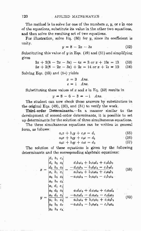
120 APPLIED MATHEMATICS
The method is to solve for one of the numbers x, y, or z in one of the equations, substitute its value in the other two equations, and then solve the resulting set of two equations.
For illustration, solve Eq. (50) for y, since its coefficient is unity.
y = 8 — 2x — 3z (52)
Substituting this value of y in Eqs. (49) and (51) and simplifying gives
3x + 2(8 — 2x — 3z) — 4z = 3 or x 10z = 13 (53) 5x + 3(8 — 2x — 3z) + 2z = 14 or x + 7z 10 (54)
Solving Eqs. (53) and (54) yields
x = 3 Ans. z = 1 Ans.
Substituting these values of x and z in Eq. (52) results in
y = 8 — 6 — 3 = —1 Ans.
The student can now check these answers by substitution in the original Eqs. (49), (50), and (51) to verify the work.
Third-order Determinants.—In a manner similar to the development of second-order determinants, it is possible to set up determinants for the solution of three simultaneous equations. The three simultaneous equations c'an be written in general
form, as follows: aix bly + ciz = dl (55) azx + b2y + c2z = d2 (56) a3x + b3y + c3z = d3 (57)
The solution of these equations is given by the following determinants and the corresponding algebraic equations:
x —
dl b1 ci d2 b2 c2 d3 b3 Cs
b1 cl a2 b2* e2 as b3 c3 ai dl cl a2 d2 e2 a3 d3 c3
b1 cl a2 b2 c2 a3 b3 c3
dib2c3 + bic2d3 + cid2b3 —dic2b3 — bid2c3 — cib2d3
aib2c3 + bic2a3 + cla2b3 —alc2b3 — bla2c3 — cib2a3
ald2c3 HF dic2a3 HF cla2d3 —aic2d3 — dia2c3 — cid2a3
a4b2c3 blc2a3 HF cla/b8 —alc2b3 — bet2c3 — cib2a3
(58)
(59)
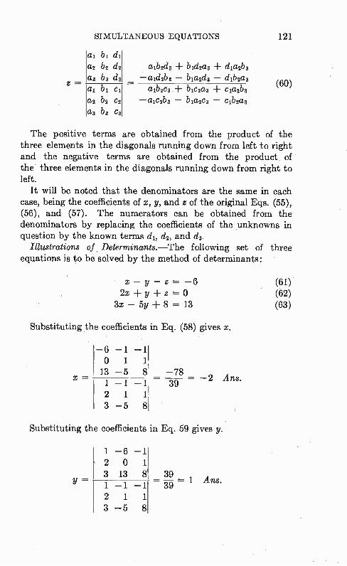
SIMULTANEOUS EQUATIONS 121
z —
al bi d1 az bz dz ailhd3 bidza3 dia2b3 a3 b3 d3 —aid2b3 — biazd3 — dib2a3 al b1 c1 - althea ± bicza3 cia2b3 az bz _2 —aiczb3 — bia2c3 — cib2a3 a3 b3 c3
(60)
The positive terms are obtained from the product of the three elements in the diagonals running down from left to right and the negative terms are obtained from the product of the• three elements in the diagonals running down from right to left.
It will be noted that the denominators are the same in each case, being the coefficients of x, y, and z of the original Eqs. (55), (56), and (57). The numerators can be obtained from the denominators by replacing the coefficients of the unknowns in question by the known terms dl, dz, and da.
Illustrations of . Determinants.—The following set of three equations is to be solved by the method of determinants:
• x — y — z = —6 (61) 2x + y + z 0 (62)
3x — 5y + 8 = 13 (63)
Substituting the coefficients in Eq. (58) gives x.
x =
—6 —1 —1 0 1 1 13-5 8 —78 1 —1 —1 39 2 1 11 3 — 5 81
= —2 Ans.
Substituting the coefficients in Eq. 59 gives y.
Y=
1 —6 —1 2 0 1 3 13 8 1 —1 —1 2 1 1 3-5 8
39 — — 39 1 Ans.
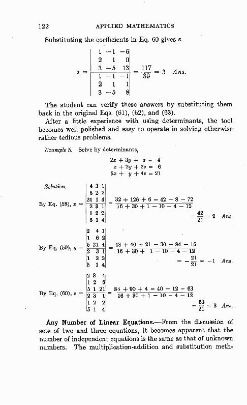
122 APPLIED MATHEMATICS
Substituting the coefficients in Eq. 60 gives z.
1 — 1 — 6 2 1 0 3 — 5 13 117
z = 1 — 1 —1 — 9 = 3 Ans.
2 1 1 3 — 5 8
The student can verify these answers by substituting them back in the original Eqs. (61), (62), and (63).
After a little experience with using determinants, the tool becomes well polished and easy to operate in solving otherwise rather tedious problems.
Example 5. Solve by determinants,
2x + 3y + z = 4 x + 2y + 2z = 6
5x + y + 4z = 21
Solution.
BY Eq. (58), ec —
By Eq. (59), y =
By Eq. (60), z —
4 3 1 6 2 2 211 4 2 3 1 1 2 2 5 1 4
2 4 1 1 62 5 21 4 2 31 1 22 5 14
23 4 12 6 5 1 21 23 1 12 2 51 4
32 + 126 + 6 — 42 — 8 — 72 16 + 30 + 1 — 10 — 4 — 12
42 = 2 Ans.
21
48 + 40 + 21 — 30 — 84 — 16 16 + 30 + 1 — 10 — 4 — 12
21 — — = —1 Ans.
21
84 + 90 + 4 — 40 — 12 — 63 — 16 + 30 + 1 — 10 — 4 — 12
63 = 2-1 = 3 Ans.
Any Number of Linear Equations.—From the discussion of sets of two and three equations, it becomes apparent that the number of independent equations is the same as that of unknown numbers. The multiplication-addition and substitution meth-
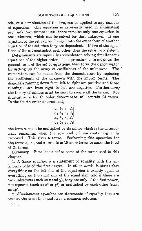
SIMULTANEOUS EQUATIONS 123
als, or a combination of the two, can be applied to any number of equations. One equation is necessarily used in eliminating each unknown number until there remains only one equation in one unknown, which can be solved for that unknown. If one equation of the set can be changed into the exact form of another equation of the set, then they are dependent. If two of the equa-tions of the set contradict each other, then the set is inconsistent.
Determinants are especially convenient in solving simultaneous equations of the higher order. The procedure is to set down the general form of the set of equations, then form the denominator by setting up the array of coefficients of the unknowns. The numerators can be made from the denominators by replacing the coefficients of the unknown with the known terms. The diagonals running down from left to right are positive and those running down from right to left are negative. Furthermore, the theory of minors must be used to secure all the terms. For illustration a fourth order determinant will contain 24 terms. In the fourth order determinant,
al bl c,. dl
a2 b2 C2 d2
as bit eg ds a4 b4 e4 d4
the term al must be multiplied by its minor which is the determi-nant remaining when the row and column containing al is removed. This gives 6 terms. Performing this operation for the terms b1, cl, and d1 results in 18 more terms to make the total of 24 terms. Summary.—First let us define some of the terms used in this
chapter. 1. A linear equation is a statement of equality with the un-
knowns only of the first degree. In other words, it states that everything on the left side of the equal sign is exactly equal to everything on the right side of the equal sign; and if there are two unknowns (such as x and y), they are only of the first power, not squared (such as x2 or y2) or multiplied by each other (such as xy).
2. Simultaneous equations are statements of equality that are true at the same time and have a common solution.
124 APPLIED MATHEMATICS
3. Independent equations are statements of equality that are all different, but have a single common solution.
4. Dependent equations are statements of equality that are alike and therefore have an infinite number of solutions.
5. Inconsistent equations are statements of equality that cannot both be true at the same time, and therefore do not have a common solution. Now, with these five definitions clearly in mind, you can see
what the problems at the end of this chapter are like. For example, suppose you have two equations that are not alike and do not disagree. Then they fit definitions 1, 2, and 3 above and are called "independent linear simultaneous equations." If both of them have x and y and there are no other unknowns, then the two equations can be solved for x and y. You will be able to find one and only one value of x and one and only one value of y that will make both equations true at the same time.
If the equations are dependent you will fini that any set of values for x and y that suit one equation will also suit the other equation. This means that you really have only one equation and not two. But if the equations are inconsistent you cannot find one set of
values for x and y that will suit both equations at the same time. Hence you do not have a problem that you can solve. Many students have trouble trying to solve dependent and
inconsistent sets of equations. The fact is that they are not to be solved. The student must understand this or he will be held back in his later work. The only kind of simultaneous equations that can be solved are independent ones. The exer-cises of this chapter are made to help you pick out the inde-pendent sets of equations from the dependent and inconsistent ones. Students and teachers are often called upon to solve practical
problems. In doing so they might be required to set up a set of simultaneous equations. As an illustration, the currents of a network can be found if the voltages and impedances are known. What is to be done if the equations made up turn out to be dependent or inconsistent? If they are dependent, it means that the student has not obtained enough independent equations. Hence he will have to set up more equations until he has as many independent equations as he has currents (or unknowns)
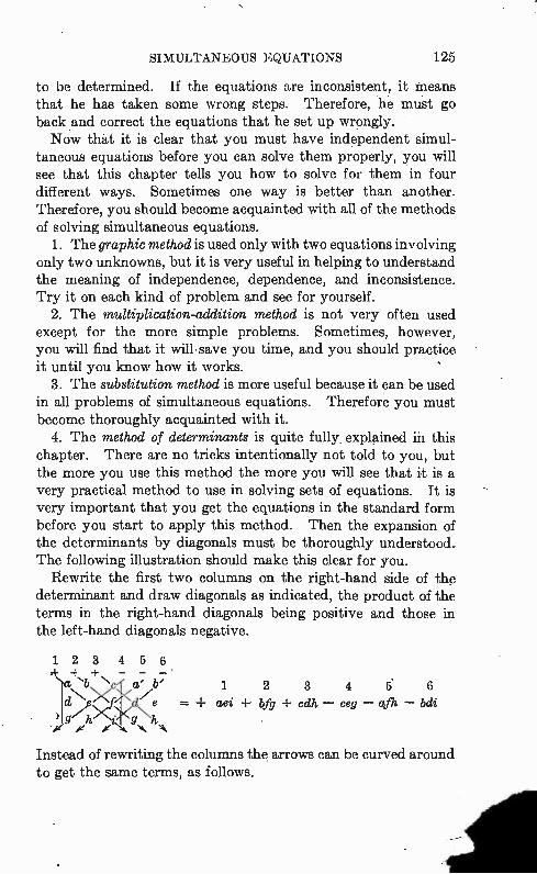
SIMULTANEOUS EQUATIONS 125
to be determined. If the equations are inconsistent, it means that he has taken some wrong steps. Therefore, he must go back and correct the equations that he set up wrongly. Now that it is clear that you must have independent simul-
taneous equations before you can solve them properly, you will see that this chapter tells you how to solve for them in four different ways. Sometimes one way is better than another. Therefore, you should become acquainted with all of the methods of solving simultaneous equations.
1. The graphic method is used only with two equations involving only two unknowns, but it is very useful in helping to understand the meaning of independence, dependence, and inconsistence. Try it on each kind of problem and see for yourself.
2. The multiplication-addition method is not very often used except for the more simple problems. Sometimes, however, you will find that it will.save you time, and you should practice it until you know how it works.
3. The substitution method is more useful because it can be used in all problems of simultaneous equations. Therefore you must become thoroughly acquainted with it.
4. The method of determinants is quite fully , explained in this chapter. There are no tricks intentionally not told to you, but the more you use this method the more you will see that it is a very practical method to use in solving sets of equations. It is very important that you get the equations in the standard form before you start to apply this method. Then the expansion of the determinants by diagonals must be thoroughly understood. The following illustration should make this clear for you.
Rewrite the first two columns on the right-hand side of the determinant and draw diagonals as indicated, the product of the terms in the right-hand diagonals being positive and those in the left-hand diagonals negative.
1 2 3 4 5 6 -F + — — •-•
a' b' 1 2 3 4 È 6
e = + aei 4- bfg + cdh ceg — afh — bdi
Instead of rewriting the columns the arrows can be curved around to get the same terms, as follows.
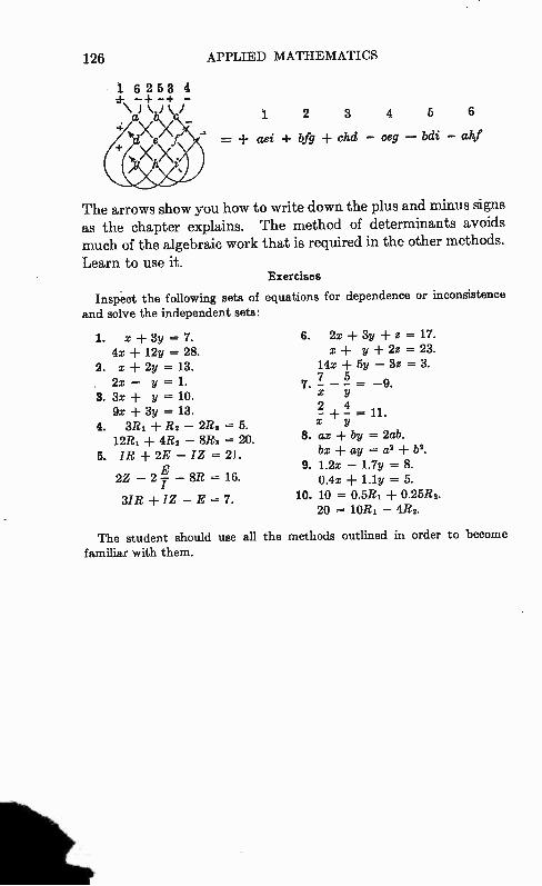
126 APPLIED MATHEMATICS
1 2 3 4 5 6
= + aei + bfg + chd - ceg - bdi - ah!
The arrows show you how to write down the plus and minus signs as the chapter explains. The method of determinants avoids much of the algebraic work that is required in the other methods. Learn to use it.
Exercises
Inspect the following sets of equations for dependence or inconsistence and solve the independent sets:
1. x + 3y = 7. 4x + 12y = 28.
2. x -I- 2y = 13. 2x - y = 1.
3. 3x + y = 10. 9x + 3y = 13.
4. 3R1 4- R2 2R8 = 5. 12R8 + 4E2 - 8E8 = 20.
5. IR + 2E - IZ = 21. E
2Z - 2 - - 8E = 16.
31E + IZ -, E =7.
6. 2x + 3y + z = 17. x + y + 2z = 23.
14x + 5y - 3z = 3. 5
7. 7 - - - = X y 2 4 - + - = 11. X y
8. ax + by = 2ab. bx + ay = a2 + b2.
9. 1.2x - 1.7y = 8. 0.4x + 1.1y = 5.
10. 10 = 0.5E1 + 0.25E2. 20 = 10E1 - 4E2.
The student should use all the methods outlined in order to become familiar with them.
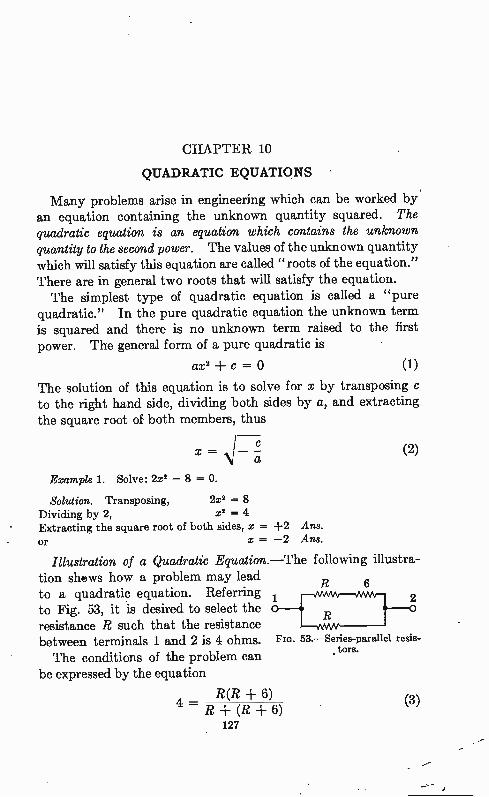
CHAPTER 10
QUADRATIC EQUATIONS
Many problems arise in engineering which can be worked by an equation containing the unknown quantity squared. The quadratic equation is an equation which contains the unknown quantity to the second power. The values of the unknown quantity which will satisfy this equation are called " roots of the equation." There are in general two roots that will satisfy the equation. The simplest type of quadratic equation is called a "pure
quadratic." In the pure quadratic equation the unknown term is squared and there is no unknown term raised to the first power. The general form of a pure quadratic is
ax2 c = 0 (1)
The solution of this equation is to solve for x by transposing c to the right hand side, dividing both sides by a, and extracting the square root of both members, thus
Example 1. Solve: 2x2 — 8 = O.
Solution. Transposing, 2x2 = 8 Dividing by 2, x2 = 4 Extracting the square root of both sides, x = or x =
Illustration of a Quadratic Equation. tion shows how a problem may lead to a quadratic equation. Referring to Fig. 53, it is desired to select the resistance R such that the resistance between terminals 1 and 2 is 4 ohms. The conditions of the problem can
be expressed by the equation
+2 Ans. —2 Ans.
—The following illustra-
6 1 —vvvvvv—vvm— 2 o
FIG. 53.—Series-parallel resis-. tors.
R(R + 6) 4 — R (R + 6)
127
(3)
128 APPLIED MATHEMATICS
Multiplying both sides of the equation by 2R -I- 6, to clear the equation of fractions,
4(2R + 6) = R2 + 6R
Transposing all terms to the left-hand side,
R2 — 2R — 24 =
(4)
(5)
This is a quadratic equation in R. If factored, it can be written
(R — 6)(R + 4) -- 0 (6)
This equation is true if R = 6, hence (6 — 6) = 0 or if R = — 4 so that ( —4 ± 4) = O. The resistance R can then be either 6 ohms or —4 ohms. The value normally selected would be 6 ohms, because it is easier to obtain than a —4 ohm resistance device. The two answers are the two roots of the equation.
Example 2. Solve the following equation by factoring.
x2 — 4x — 21 = 0
The product of the two factors must equal —21 and their sum must equal —4. It is soon discovered that +3 and —7 are factors that meet this condition, hence the equation can be factored and written
The solutions, then, are
or
(x + 3)(x — 7) =
x = —3 Ans. x = 7 Ans.
Methods of Solution.—Quadratic equations can be solved by the methods of graphing, factoring, completing the square, or using the quadratic formula. The most useful method is the quadratic formula. The factoring method is illustrated above. The other methods
will be illustrated below. Illustration of the Graphic Method.—Solve the quadratic
equation, x2 — 2x — 3 = 0 by graphing the curve
y x2 — 2x — 3.
Since the zero is replaced by y, the solutions of x will be the value of x when y = O. To draw the graph of y = x2 — 2e- 3 the values of y are
obtained when x is given values as shown in Fig. 54a. The solution will be the values of x when y = O. In this case x = —1
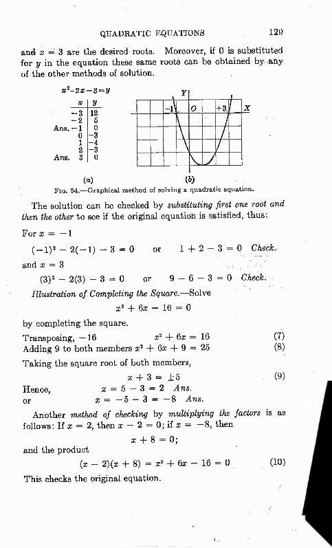
QUADRATIC EQUATIONS 129
and x = 3 are the desired roots. Moreover, if 0 is substituted for y in the equation these same roots can be obtained by .any of the other methods of solution.
x2-2x-3=y
x y
-3 12 -2 5
Ans.-1 0 0 -3 1 -4 2 -3
Ans. 3 0
o +3 X
(a) (b) 54.—Graphical method of solving a quadratic equation.
The solution can be checked by substituting first one root and then the other to see if the original equation is satisfied, thus:
For x = —1
(-1)2 — 2( —1) — 3 = 0 or 1 + 2 — = 0 Check.
and x = 3
(3)2 — 2(3) — 3 = 0 or 9 — 6 — 3 = 0 Check.
Illustration of Completing the Square.—Solve
x2 + 6x — 16 ----
by completing the square.
Transposing, —16 x2 + 6x = 16 (7) Adding 9 to both members x2 ± 6x ± 9 = 25 (8)
Taking the square root of both members,
x + 3 = +5 (9) Hence, x = 5 — 3 = 2 Ans. Or x = —5 — 3 = —8 Ans.
Another method of checking by multiplying the factors is as follows: If x = 2, then x — 2 = 0; if x = —8, then
x + 8 = 0; and the product
(x — 2)(x + 8) = x2 + 6x — 16 = 0 (10)
This checks the original equation.
130 APPLIED MATHEMATICS
Quadratic Formula.—The general form of the quadratic equation can be expressed
ax2 bx c (11)
In the above illustration, x2 -F 6x - 16 = 0, we have a = 1, b = 6, and c = -16. Dividing the general quadratic equation by a,
x2 + -a x + -a = 0 (12)
Transposing c/a
x2 -I- a- x = - -a (13)
This corresponds to Eq. (7) in the above illustration. Adding to both members the square of b/2a,
, b b2 c b2 x- -r- - x , — = - - + —
a 4a2 a 4a2 (14)
In the above illustration note that 34 of 6 when squared gives 9. See Eq. (8).
Find the square root of both members of the equation, using both + and - roots of the right-hand member, thus
-r , b i , b2 c
= — "N4a2 - a
(15)
This corresponds to Eq. (9) of the illustration. Using first the positive value and then the negative one results in two new equations of x,
and
-b Ib2 c x =
2a 4a2 a
-b b2 c x =
2a 4a2 a
These equations correspond to x = 5 - 3 = 2 and
x = -5 - 3 = - 8
(16)
(17)
in the above illustration. If the b/2a of Eq. (15) is transposed to the other side, the
c/a term multiplied by 4a in both numerator and denominator,
QUADRATIC EQUATIONS 131
and the two terms under the radical reduced to a common denominator, then
—b , \ib2 — 4ac x =
2a — 4a2 (18)
Since the square root of 4a2 is 2a, it can be written outside the 'radical as a common denominator, thus
—b + b2 — 4ac X — (19)
2a
This is the quadratic formula, which should be memorized. In words it is usually stated "x equals minus b plus or minus the square root of b squared minus four ac, all divided by two a."
Example 3. Solve the following equation by means of the quadratic
formula: 3R2 - 7R + 4 = 0
In applying the formula it is noted that a is +3, b is —7, and c is +4, the unknown number being R instead of x. Making these substitutions in Eq. (19), the formula gives
— (- 7) R — ± *V( — 7)2 — 4(3)(4) 2 (3)
Simplifying further,
Hence
and
R — 6
7 + 1 4 R = — — Ans.
6 3 7 — 1
Ans. 6
7 ± V49 — 48
Check by the sum and product of the roots method is done as follows: Adding the two roots as given in Eqs. (16) and (17),
—b —b —b 2a 2a = a
Adding the two roots in the answers,
or
4 7
— ( — 7) — b 3 a
Multiplying the two roots as given in Eqs. (16) and (17) by the method as illustrated on page 41 for (x + y) (x — y) = x2 — y2,
2 b2 !N2 =
'-;:i 4a2 a) ei (20)
132 APPLIED MATHEMATICS
In this example the product of the two roots is (%)(1) = which should. and does equal c/a.
The quadratic equation will now be explained in more detail. The general form of the quadratic equation is
ax2 bx c = 0 (11)
The first term ax2 is made up of a product of a known number a and the unknown number x raised to the second power, (x2). The second term is also a product of a known number, b, and the unknown number, x. The third term is simply another known number, c. It might be asked why these terms, added together, make a quadratic quantity that is equal to zero. That will be seen to be true when a, b, c, and x are explained. First, a is a known. jiinmber. It can be a positive number (greater than zero) or a negative number (less than zero). It can never be zero (see definition at end of the chapter). Second, b can also be a positive or negative number, but it can also be zero. Third, c can be a positive or negative number or zero. Now if a, b, and c are integer numbers it is easy to find a value of x that will make the quadratic quantity
022 bx c
equal to zero. To illustrate, if a = 2, b = —5, and c = 3, then ax2 bx c will be the quadratic quantity 2x2 — 5x ± 3. Hence it is plainly possible to find a value for x that will make this quadratic quantity in x equal to zero. In fact there are two values of x that will make 2x2 — 5x + 3 equal to zero. But instead of going into the methods of finding these values
of x it is more important at this point of the discussion to under-stand what the problem is. These coefficients a, b, and c, even though they are known numbers, might cause the student con-siderable trouble unless he realized what they meant. Instead of being numerals, each of them might be a quantity, so we should really consider them as expressions. Just as a stands for the whole thing by which x2 is multiplied, b stands for the whole thing by which x is multiplied, and c stands for the whole thing by which unity (1) is multiplied. Since c is made up of the constant terms, it is often referred to as the constant of the equation. If the quadratic equation is not arranged so that the coefficient of x2, which is a, can be seen and dealt with as a term or quantity,
QUADRATIC EQUATIONS 133
it must be rearranged. Likewise the coefficient of x, namely b, must be rearranged and collected into a quantity. When a, b, and c can be written down and the equation is arranged according to the descending powers of x with the right side of the equation zero, then the quadratic equation is in its standard form and is ready to solve. To illustrate, the quadratic equation
7 kx 9x2 k = 17x ± 8 kx2 6
is rearranged as follows:
(9 — 8k)x2 -F (k — 17)x (k 1) =
This rearranged equation is the same as the other quadratic equation but is in its standard form with a equal to (9 — 8k), b equal to (k — 17) and c equal to (k 1). When the student is able to rearrange any kind of quadratic equation so that it will be in its standard form, which is the general form
ax2 -F bx c = 0,
then he is ready to solve any quadratic equation he may encounter. Use of the Discriminant b2 — 4ac.—The quantity b2 — 4ac
under the radical in the quadratic formula is called the dis-criminant because its value decides whether the roots are equal or unequal, real or complex, rational or irrational.
Case I. If b2 — 4ac is zero the roots are equal and real. For illustration, in the equation
4x2 — 12x -F 9 = •
a = 4, b = —12, c = 9 and b2 — 4ac = 144 — 144 = 0. The usual solution is written
12 -F 12—VO x — and x —
8 8
both of which reduce to 1.5. Hence the roots are equal and real. Case IL. If b2 — 4ac is positive (greater than zero) the roots
are unequal and real. For illustration, in the equation
3x2 — 7x — 20
a = 3, b = —7, c = —20 and b2 — 4ac = 49 -I- 240 = 289. The roots are
134 APPLIED MATHEMATICS
7 + V289 7 + 17 x = — 4
6 6
7 — Vig 7 — 17 = — and x = 6 6
which are unequal and real. Case III. If b2 — 4ac is negative (less than zero) the roots are
unequal and complex numbers. For illustration, in the equation
3x2 — 2x + 1 =
a = 3, b = —2, c 1, and b2 — 4o,c = 4 — 12 = —8. The roots are
and
— 2 + -V-8 1 j x
6 3
2 — 1 — j x —
6 3
where j2 = —1 or, taking the square root, j = These roots are unequal and complex numbers. Case IV. If b2 — 4ac is an exact square or zero the roots are
rational, otherwise they are irrational. For illustration, in the equation
x2 — 5x + 4 =
a = 1, b = —5, c = 4 and b2 — 4ac = 25 — 16 = 9. The roots are
and
x — 2
5 — X = = 1
2
These roots are rational numbers. But in the illustration of the equation
x2 — 5x — 3 =
a = 1, b = —5, c = —3, and b2 — 4ac = 25 + 12 = 37 The roots are
and
5 -I-- x = 2
5 — Nrs-7 x - 2
QUADRATIC EQUATIONS 135
These roots are irrational numbers, because N/-3-77 cannot be expressed as a fraction.
It is very important to have a clear understanding of what the solution of a quadratic equation means. A further discussion of the discriminant should assist in giving a clear meaning of the solution. A quadratic equation in one unknown number has two values
of that unknown that will make it true. If x is the unknown number, there will always be two values of x that will satisfy the equation, but they don't have to be integers. They can be fractions, irrational numbers, or complex numbers. There is only one case in which the two values of x are equal and that is when the quadratic in x, namely, ax2 bx c, is a perfect square. Probably the best way for the student to understand the meaning of all these different situations is by graphing the quadratic as illustrated in this chapter. Then the student will see for himself that the curve of the quadratic function y (y being the value of ax2 bx c) crosses the x-axis twice in all cases but two. One is when the two values of x are equal and in this case the curve just touches the x-axis. The other case is when the curve does not touch or cross the x-axis. In this case both values of x that make y equal zero are complex numbers. One way of expressing the meaning of this solution is to say that the curve crosses the x-axis in two imaginary places, because the complex numbers involve the imaginary number -V —1.
Example 4. Solve the following equations by the quadratic formula:
X2 - 8x + 15 = 0 (a) x2 — 8x + 16 = 0 (b) x2 — 8x + 17 = 0 (c)
Determine from the value of the discriminant the case number. Plot a graph of the equations.
Solution. By the quadratic formula the solutions are
8 ± N/64 — 60 — 4 ± 1 = 3 or 5 Ans. For Eq. (a), 2
8 ± N/64 — 64 For Eq. (b), x = — 4 Ans.
2
8 ± N/64 — 68 For Eq. (e), x = — 4 ± /1 Ans.
2
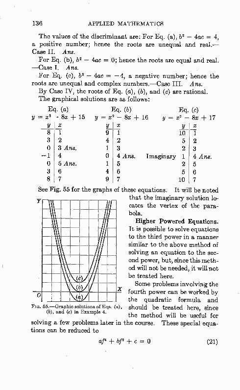
136 APPLIED MATHEMATICS
The values of the discriminant are: For Eq. (a), 52 — 4ac = 4, a positive number; hence the roots are unequal and real.— Case II. Ans. For Eq. (b), b2 — 4ac = 0; hence the roots are equal and real.
—Case I. Ans. For Eq. (c), b2 — 4ac = —4, a negative number; hence the
roots are unequal and complex numbers.—Case III. Ans. By Case IV, the roots of Eq. (a), (b), and (c) are rational. The graphical solutions are as follows:
Eq. (a) Eq. (b) Eq. (c) y x2 — 8x + 15 y = x2 — 8x + 16 y = x2 — 8x + 17
O the quadratic formula and should be treated here, since the method will be useful for
solving a few problems later in the course. These special equa-tions can be reduced to
af4 + bf2 + c = 0 (21)
y 8 3 o
—1 O 3 8
2 3 Ans. 4 5 Ans. 6 7
F 4
1
0
1
4
9
y 10
2 5 3 2 4 Ans. Imaginary 1 5 2 6 5 7 10
2 3 4 Ans. 5 6 7
See Fig. 55 for the graphs of these equations. It will be noted that the imaginary solution lo-cates the vertex of the para-bola. Higher Powered Equations.
It is possible to solve equations to the third power in a manner similar to the above method of solving an equation to the sec-ond power, but, since this meth-od will not be needed, it will not be treated here. Some problems involving the
X fourth power can be worked by
(c)
FIG. 55.—Graphic solutions of Eqs. (a), (b), and (c) in Examp e 4.
QUADRATIC EQUATIONS 137
In this type of problem let x = f2 and the general form of the quadratic formula results, that is,
ax2 + bx + c = (11)
Example 5. In a certain series parallel circuit it is found that the fre-quency f can be expressed as
2 2 X 10⁻¹ j,4 _ 6f2 ± 4 X 1012 = 0
It is desired to solve this equation for f since this solution will give the frequency at which the circuit is resonant. At present we are interested only in the method; later in the course we shall be interested in the results of such a solution.
Solution. Applying the quadratic formula,
/2 6 ± V62 — 4(2 x 10-12)(4 X 10¹²) 2(2 X 10-12)
6 + N/36 — 32 6 + 2 = — 4 X 10-12 4 X 10-12
f2 = 2 X 10¹² or f2 = 1 X 10¹² Then, f = 1.414 X 10⁸ or f = 1 X 10⁶ Ans.
Some Useful Definitions.
1. A quadratic equation is an equation of the second order. In other words, it is an equation in which the unknown number is raised to the second power (squared) and no higher power. The first power of the unknown can also be present in the equa-tion but it doesn't have to be present. The second power must be present; if only the first power of the unknown is present, the equation is linear and not quadratic.
2. A quantity is a product or sum of numbers. These numbers may be known or unknown. Notice that a quantity is not an equation because it is not a statement of equality, and that it therefore does not have an equal sign in it.
3. A term is a product of numbers. These numbers may be known or unknown. Notice that a term can be a quantity, but that a quantity that is a sum is not a term.
4. An expression is a term or quantity, except that we think of an expression as a symbol that stands for something else or possibly for a class of things.
Exercises
1. x2 — 6x — 7 = 0. Solve by the factoring method. 2. x2 12x = 28. Solve by completing the square.
138 APPLIED MATHEMATICS
3. x2 — 6x — 4 = O. Solve by using the quadratic formula. 4. 5x2 — 3x — 4 = O. Solve by any method. 5. x 1/x = 1/. Solve by any method. 6. 2x2 — (V-27* V)x = O. Solve by any method. 7. rsx2 rs = x(r2 s2). Solve by any method. 8. Solve the following equation for x by using the quadratic formula:
kx2 — 3kx + 9 = O. Then find the value of k that will make the roots equal. This is done by setting the discriminant equal to zero and solving for k.
9. z2 — (2 k)x ± 4 = O. Follow the procedure used in Exercise 8. 10. Solve the following equation for the resonant frequencies f.
2f4 + 4608 = 200f2.
•
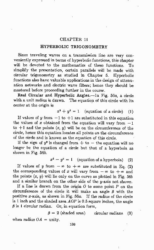
CHAPTER 11
HYPERBOLIC TRIGONOMETRY
Since traveling waves on a transmission line are very con-veniently expressed in terms of hyperbolic functions, this chapter will be devoted to the mathematics of these functions. To simplify the presentation, certain parallels will be made with circular trigonometry as studied in Chapter 5. Hyperbolic functions also have valuable applications in the design of attenu-ation networks and electric wave filters; hence they should be mastered before proceeding further in the course.
Real Circular and Hyperbolic Angles.—In Fig. 56a, a circle with a unit radius is drawn. The equation of this circle with its center at the origin is
x 2 + y2 = 1 (equation of a circle) (1)
If values of y from —1 to +1 are substituted in this equation the values of x obtained from the equation will vary from —1 to +1 and the points (x, y) will be on the circumference of the circle, hence this equation locates all points on the circumference of the circle and is known as the equation of this circle.
If the sign of y2 is changed from ± to — the equation will no longer be the equation of a circle but that of a hyperbola as shown in Fig. 565.
x2 — y' = 1 (equation of a hyperbola) (2)
If values of y from — co to ± co are substituted in Eq. (2) the corresponding values of x will vary from — 00 to ± co and the points (x, y) will lie only on the curve as plotted in Fig. 565 and a similar branch on the other side of the y-axis not shown.
If a line is drawn from the origin 0 to some point P on the circumference of the circle it will make an angle /3 with the positive x-axis, as shown in Fig. 56a, If the radius of the circle is 1 inch and the shaded area AOP is 0.5 square inches, the angle /3 is 1 circular radian. Or, in equation form,
p = 2 (shaded area) circular radians (3)
when radius OA = unity. 139
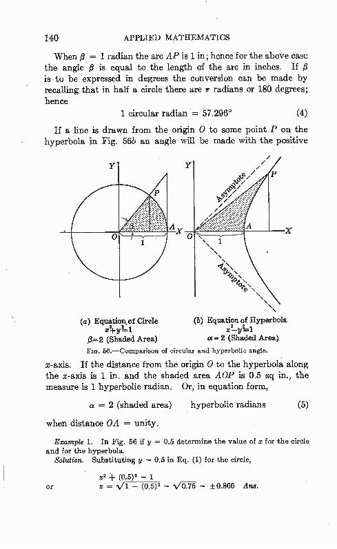
140 APPLIED MATHEMATICS
When p = 1 radian the arc AP is 1 in; hence for the above case the angle p is equal to the length of the arc in inches. If 13 is to be expressed in degrees the conversion can be made by recalling that in half a circle there are ir radians or 180 degrees; hence
1 circular radian = 57.296° (4)
If a line is drawn from the origin 0 to some point P on the hyperbola in Fig. 565 an angle will be made with the positive
•••••
(a) Equation of Circle (b) Equation of Hyperbola x2-1-y2=1 2 2
13=2 (Shaded Area) a= 2 (Shaded Area)
FIG. 56.—Comparison of circular and hyperbolic angle.
x-axis. If the distance from the origin 0 to the hyperbola along the x-axis is 1 in. and the shaded area AOP is 0.5 sq in., the measure is 1 hyperbolic radian. Or, in equation form,
a = 2 (shaded area) hyperbolic radians (5)
when distance OA = unity.
Example 1. In Fig. 56 if y = 0.5 determine the value of x for the circle and for the hyperbola.
Solution. Substituting y = 0.5 in Eq. (1) for the circle,
(0.5)2 = 1 or z = Vi — (03)2 = N/0.75 -= +0.866 Ans.
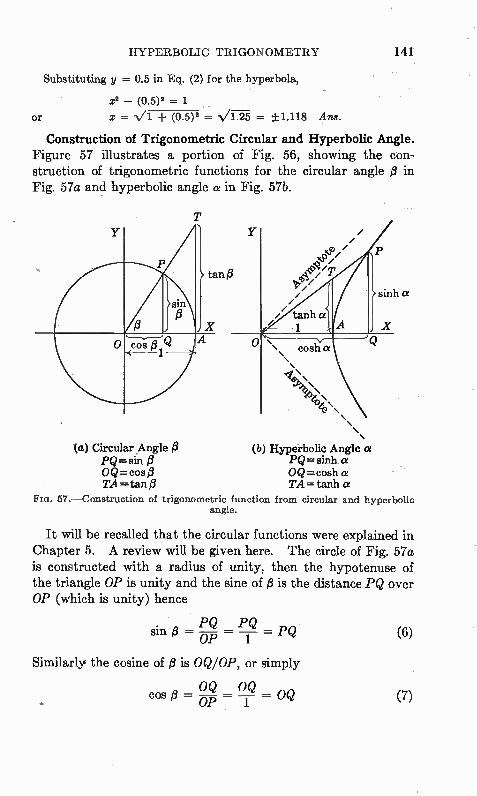
HYPERBOLIC TRIGONOMETRY 141
Substituting y = 0.5 in Eq. (2) for the hyperbola,
x2 _ (0.5)2 = 1
or X = + (0.5) 2 = = ±1.118 Ans. Construction of Trigonometric Circular and Hyperbolic Angle.
Figure 57 illustrates a portion of Fig. 56, showing the con-struction of trigonometric functions for the circular angle p in Fig. 57a and hyperbolic angle a in Fig. 57b.
(a) Circular _Angle f3 PQ=sin OQ = cos fi TA=tan
e
sinh a
\\ cosh a •
\ ex • ,o45•\
eoec,\ • • • • •
(b) Hyperbolic Angle a PQ= sinh a OQ = cosh a TA= tanh a
Fro. 57.—Construction of trigonometric function from circular and hyperbolic angle.
It will be recalled that the circular functions were explained in Chapter 5. A review will be given here. The circle of Fig. 57a is constructed with a radius of unity, then the hypotenuse of the triangle OP is unity and the sine of f3 is the distance PQ over OP (which is unity) hence
PQ PQ
Similarly the cosine of pis 0Q/OP, or simply
OQ OQ COS/3_p_ _ = o--p- = T. - = OQ
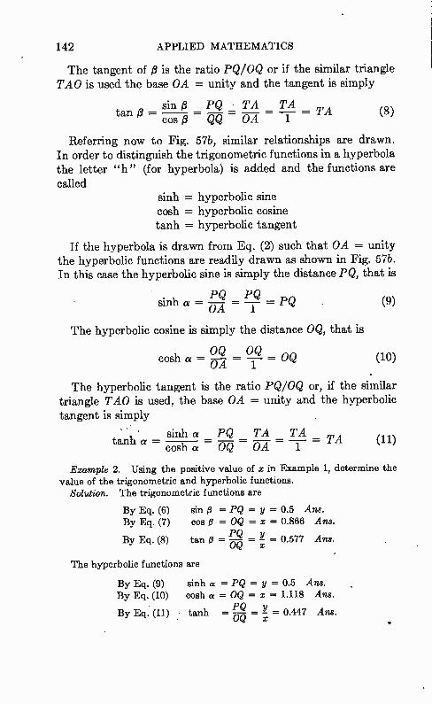
142 APPLIED MATHEMATICS
The tangent of 13 is the ratio PQ/OQ or if the similar triangle TAO is used the base OA = unity and the tangent is simply
sin 13 PQ • TA TA _ tan /3 = — = = _ TA (8)
cos a QQ OA 1
Referring now to Fig. 57b, similar relationships are drawn. In order to distinguish the trigonometric functions in a hyperbola the letter "h" (for hyperbola) is added and the functions are called
sinh = hyperbolic sine cosh = hyperbolic cosine tanh = hyperbolic tangent
If the hyperbola is drawn from Eq. (2) such that OA = unity the hyperbolic functions are readily drawn as shown in Fig. 57b. In this case the hyperbolic sine is simply the distance PQ, that is
PQ PQ sinh a = = = PQ (9)
OA 1
The hyperbolic cosine is simply the distance OQ, that is
OQ OQ cosh a = = = °Q (10)
The hyperbolic tangent is the ratio PQ/OQ or, if the similar triangle TAO is used, the base OA = unity and the hyperbolic tangent is simply
• sinha PQ TA TA tanh a = — — = TA (11)
cosh a OQ OA 1
Example 2. Using the positive value of x in Example 1, determine the value of the trigonometric and hyperbolic functions.
Solution. The trigonometric functions are
By Eq. (6) By Eq. (7)
By Eq. (8)
sin 13 = PQ = y = 0.5 Ans. cos t1 = OQ = x = 0.866 Ans.
PQ Y tan 13 = (..72 = 7 = 0.577 Ans.
The hyperbolic functions are
By Eq. (9) sinh a = PQ = y = 0.5 Ans. By Eq. (10) cosh a = OQ = x = 1.118 Ans.
By Eq. (11) tanh = ' PQ — — 0 447 Ans. OQ x
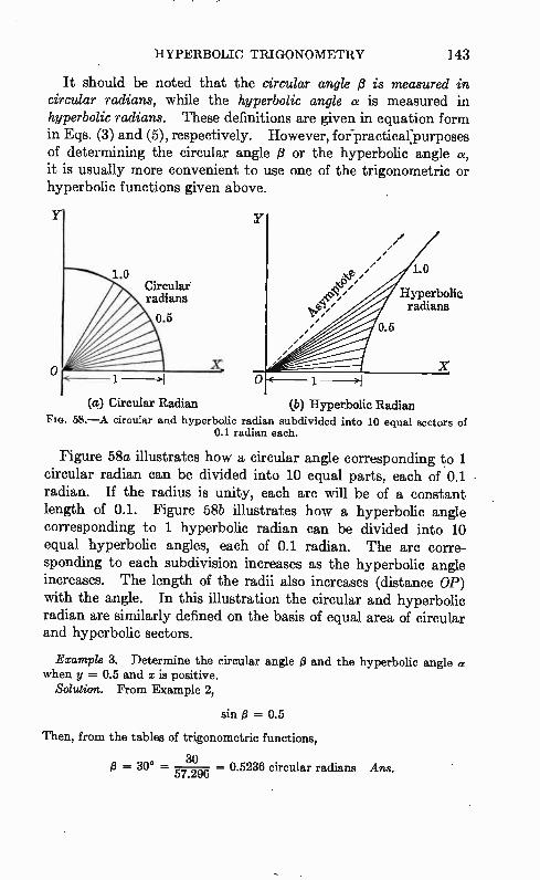
HYPERBOLIC TRIGONOMETRY 143
It should be noted that the circular angle is measured in circular radians, while the hyperbolic angle a is measured in hyperbolic radians. These definitions are given in equation form in Eqs. (3) and (5), respectively. However, forepractical:purposes of determining the circular angle or the hyperbolic angle a, it is usually more convenient to use one of the trigonometric or hyperbolic functions given above.
Y
1.0
(a) Circular Radian
1.0
Hyperbolic radians
0.5
(b) Hyperbolic Radian FIG. 58.—A circular and hyperbolic radian subdivided into 10 equal sectors of
0.1 radian each.
Figure 58a illustrates how a circular angle corresponding to 1 circular radian can be divided into 10 equal parts, each of 0.1 radian. If the radius is unity, each arc will be of a constant length of 0.1. Figure 58b illustrates how a hyperbolic angle corresponding to 1 hyperbolic radian can be divided into 10 equal hyperbolic angles, each of 0.1 radian. The arc corre-sponding to each subdivision increases as the hyperbolic angle increases. The length of the radii also increases (distance OP) with the angle. In this illustration the circular and hyperbolic radian are similarly defined on the basis of equal area of circular and hyperbolic sectors.
Example 3. Determine the circular angle 13 and the hyperbolic angle « when y = 0.5 and x is positive.
Solution. From Example 2,
sin fi = 0.5
Then, from the tables of trigonometric functions,
30 13 30° — — 0.5236 circular radians Ans.
57.296
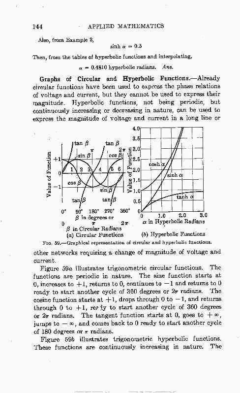
sin f3
tan f3 tan
144 APPLIED MATHEMATICS
Also, from Example 2, sinh a = 0.5
Then, from the tables of hyperbolic functions and interpolating,
= 0.4810 hyperbolic radians. Ans.
Graphs of Circular and Hyperbolic Functions.—Already circular functions have been used to express the phase relations of voltage and current, but they cannot be used to express their magnitude. Hyperbolic functions, not being periodic, but continuously increasing or decreasing in nature, can be used to express the magnitude of voltage and current in a long line or
4.0
3.6 tan ti tan fi
ir 27 g 3.0 sin 13 COS /32
8° 2.5
2.0 o 00 1.5
1.0
0.5
0° 90° 180° 270° 360° 0 /3 in degrees or O 1 0 2 0 3 0
O 2 /I. a in Hyperbolic Radians $ in Circular Radians (a) Circular Functions (b) Hyperbolic Functions
FIG. 59.—Graphical representation of circular and hyperbolic functions.
other networks requiring .a change of magnitude of voltage and current.
Figure 59a illustrates trigonometric circular functions. The functions are periodic in nature. The sine function starts at 0, increases to +1, returns to 0, continues to —1 and returns to 0 ready to start another cycle of 360 degrees or 2./r radians. The cosine function starts at +1, drops through 0 to —1, and returns through 0 to +1, re? dy to start another cycle of 360 degrees or 2« radians. The tangent function starts at 0, goes to + 00, jumps to — 00, and comes back to 0 ready to start another cycle of 180 degrees or ir radians.
Figure 59b illustrates trigonometric hyperbolic functions. These functions are continuously increasing in nature. The
cosh a
tanh a
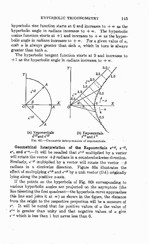
HYPERBOLIC TRIGONOMETRY 145
hyperbolic sine function starts at 0 and increases to ± 00 as the hyperbolic angle in radians increases to 00. The hyperbolic cosine function starts at +1 and increases to ± 00 as the hyper-bolic angle in radians increases to ± 00. For a given value of «, cosh « is always greater than sinh «, which in turn is always greater than tanh «. The hyperbolic tangent function starts at 0 and increases to
+1 as the hyperbolic angle in radians increases to ± 00
(a) Exponentials (b) Exponentials Maud e-ji3 di..« and ia PIG. 60.—Geometric interpretation of exponentials.
Geometrical Interpretation of the Exponentials e, and will be recalled that e-HP multiplied by a vector will rotate the vector -FP radians in a counterclockwise direction. Similarly, E-ifi multiplied by a vector will rotate the vector . —13 radians in a clockwise direction. Figure 60a illustrates the effect of multiplying e-Flo and e-in by a unit vector (OA) originally lying along the positive x-axis.
If the points on the hyperbola of Fig. 60b corresponding to various hyperbolic angles are projected on the asymptote (the line bisecting the first quadrant—the hyperbola curve approaches this line and joins it at 00) as shown in the figure, the distance from the origin to the respective projection will be a measure of Ea . It will be noted that for positive values of a the value of e+a is greater than unity and that negative values of a give E—a which is less than 1 but never less than O.
146 APPLIED MATHEMATICS
Exponentials Applied to Circular Functions.—For our use, trigonometric functions do not need to be given a geometrical interpretation. In fact, they are sometimes defined by an alge-braic exponential form. For example, the identity for changing from polar to rectangular form, which is
e+e = cos j sin e (12)
is added to the form when the sign of 13 is made negative, thus
= cos (-0) + j sin (--e) = cos e - j sin e (13)
the result is eFio
(Ho + -= 2 cos e or cos fi - 2 (14)
cos fi is sometimes defined by this equation. Now, if Eq. (13) is subtracted from Eq. (12),
e+is - -- 2j sin e or sin fi - (15) 2j
sin e is sometimes defined by this equation. Tan e can be defined by the ratio, thus
el-or e-itc sin e tan /3 - cos /3 - 3 €4113 _ (16) ± E-10
Also, cot fe can be defined as 1 cos A
cot 13 = (17) tan si . n e — Exponentials Applied to Hyperbolic Functions.—From analogy
with the circular trigonometric functions, the hyperbolic functions
can be defined as follows:
= cosh « + sinh « (18) e-a = cosh a - sinh « (19)
Subtracting Eq. (19) from Eq. (18) gives
- 6-« sinh « - 2 (20)
sinh a can be defined by this equation. Adding Eq. (18) and Eq. (19) gives
± cosh a = 2
(21)

HYPERBOLIC TRIGONOMETRY 147
cosh « can be defined by this equation. Tanh a can be defined by the ratio
sinh « _ tanh « - cosh « e ±
Ea E—« (22)
In some equations it is more convenient to use the reciprocal of tanh a which is known as "hyperbolic cotangent" and can be defined as follows:
1 cosh a ea + E—a coth « = - tanh a s., -
mn a ea — 6-« (23)
Example 4. Determine the values of the exponentials for circular and hyperbolic functions when y = 0.5 and x is positive.
Solution. From Examples 2 and 3 and the use of Eq. (12),
cos /3 + j sin (i0.6236 = 0.866 ± j0.5 = 1/30° Ans.
From Examples 2 and 3 and the use of Eq. (18),
Ea = cosh a sinh ,0.4812 = 1.118 + 0.5 = 1.618 Ans.
Circular and Hyperbolic Identities.—These identities are tabulated on page 307, primarily for reference purposes. The proof of many of these identities can be made by substitution of the exponential forms given above. In these equations a is not necessarily a hyperbolic radian nor is 13 necessarily a circular radian. In general they can be considered as two different angles measured in radians.
Example 5. Develop the equation
cosh' 5 — sinh2 5= 1
from the circular function identity
sin213 = 1
Solution. In the circular function.identity, replace 5 with jet to get
sin' jfl + cos2 ji3 = 1 But, sinj5 = j sinh ift and cos jti = cosh /3 Hence, j2 sinh2 5 + cosh' 5 = 1 or cosh' _5inh25 = 1 Ans.
Example 6. Determine the circular sine and hyperbolic sine of the complex quantity
= a + /13 = 0.4812 -I- /0.5236
148 APPLIED MATHEMATICS
• ...Solution. Referring to the list of identities,
sin y = sin (a +i) --- sin a cosh # + j cos a sinh = sin (0.4812) cosh (0.5236) j cos (0.4812) sinh (0.5236)
Converting from radians to degrees,
sin y = sin (27.57°) cosh (0.5236) + j cos (27.57°) sinh (0.5236)
Finding the values from the tables,
sin y-= (0.4628)(1.14025) + j(0.8865)(0.54786) = 0.5277 + j0.4857 = 0.7172/42°38' Ans.
From the list of identities,
sinh y = sinh (« +j) = sinh a cos 13 + j cosh a sin # sinh (0.4812) cos (0.5236) + j cosh (0.4812) sin (0.5236)
= (0.5) (0.866) +1 (1.118) (0.5) = 0.433 + j0.559 = 0.7071/52°15' Ans.
Exercises
1. If a circle has a radius of 1 in. and the vector OP (Fig. 56) is rotated so that the shaded area is 2 sq. in., what is the value of f3 ?
2. If a hyperbola measures 1 in. from 0 to A and the vector OP is turned clockwise so that the shaded area is 3 sq in., what is the value of « and Ea
(see Fig. 56)? 3. In Eq. (1) if x -= 0.707 what are the possible values of y? 4. In Eq. (2) if x = 2.0 what are the possible values of y? 5. How does the value of cosh « compare with sink « as « is varied?
What are the corresponding values of tanh a? 6. Between what limits do sin 13 and cos # vary? What are the limits
of tan 13? 7. What valuable property does eel have when multiplied by a vector?
How is this property different from eu multiplied by the same vector? 8. If tanh « = 0.76159, determine sinh «, cosh «, coth «, and «.
CHAPTER 12
DIFFERENTIAL CALCULUS TREATING ALGEBRAIC FUNCTIONS
Arithmetic deals with the use of numbers, which are constant quantities, while algebra deals with the use of symbols repre-senting either constant or variable quantities. Calculus, going one step farther, deals with the nature and variation of these quantities. Since calculus uses both arithmetic and algebra, it is studied last. The basic ideas of calculus are simple and fascinating when one
has a good working knowledge of such subjects as algebra and trigonometry. However, the large amount of detail and the abstract approach that is often made lead to disinterest and to a false notion that the subject is extremely difficult.
Calculus in its elementary forms can be divided into differential calculus and integral calculus, much as arithmetic processes can be divided into subtraction and addition. In both the calculus and the arithmetic the processes are inverse operations. The purpose of studying calculus at this time is to become
familiar with the nature of changing electrical quantities. Not that the student will be able to work out all calculus problems, because even the best mathematicians cannot do this, but that the student can work simple problems and be able to understand the meaning of calculus terms when they are found in the litera-ture. This chapter will deal with differential calculus in ele-mentary and graphical forms which treat algebraic functions, while the next chapter will deal with transcendental functions in a similar fashion. Then a treatment of elementary and graphical forms of integral calculus will be presented.
All algebraic functions of x are rational functions, while all other functions of x are transcendental or irrational functions of x: An algebraic function of x can in its most complicated form be expressed as a fraction with values of x in both the numerator and denominator.
149
150 APPLIED MATHEMATICS
Calculus Symbols.—The letter d is used in differential calculus to mean "a little bit of," hence "dx" means "a little bit of x." This little bit of x is a difference quantity, commonly called the "differential" or "element" of x. d can be remembered as the first letter of "difference" or "differential." "dx" is actually of indefinitely small size. Differential calculus cau be simply explained as a mathematics of making and using indefinitely small difference calculation. The symbol f as used in integral calculus is merely an elongated
letter S which means "the sum of." This symbol which stands f or the first letter of sum is usually called "the integral of," which means the whole or total. Integral calculus can be simply explained as the mathematics of making and using large sum calculations.
Integral and differential calculus symbols are often used in combination to express a quantity, thus f dx means "the sum of all the little bits of x." In other words, the whole quantity can be found by adding up all the indefinitely small little bits of x.
Limits.—In reality quantities must be finite or zero. In other words, we have something or we have nothing. This concept seems simple. The mathematician, however, has complicated the matter by devising two fictitious quantities, as it were, which are used to aid him in his reasoning processes. One is called "infinity," and is greater than any number or quantity. The other is called "an infinitesimal" and is smaller than any number or quantity. How do we arrive at these fictitious quantities of infinity and
an infinitesimal? The answer to this question is found in the use of limits. A variable quantity, if it increases indefinitely in size, is said to reach infinity in the limit. Likewise, if a variable quantity decreases indefinitely in size it becomes an infinitesimal and is said to reach zero in the limit. In the precise language of the mathematician, a variable is said to approach a limit when its value becodes and remains arbitrarily close to the limit. " Arbi-trarily close" means that we can assign a number as close as we please to the limit and the variable will ultimately become and remain closer to the limit than this arbitrary or assigned number.
If the variable x approaches infinity as the limit, the fact is stated mathematically as
lim x = co X-) 00
DIFFERENT.IAL CALCULUS: ALGEBRAIC 151
This states in words that the limit of the variable x equals infinity as x approaches infinity. On the other hand if the variable x approaches zero as the
limit it is called an "infinitesimal." This means that the variable becomes and remains as close as you please to zero. In mathematical language,
hm x =
This says in words that the limit of x equals zero as x approaches zero. The quantity dx is known as an infinitesimal, because in the
calculus process of differentiation it approaches zero as the limit. By this limiting method the calculus process becomes an exact process. For illustration, the ratio dy/dx pronounced "dee-wy by dee-ex" is made up of two differential quantities each of which approaches zero in the limit to give 0/0, which as such cannot be evaluated. Here is where the mathematician's reasoning process with infinitesimals comes to the rescue. The value of y is related to the value of x so long as values can be assigned to either one. For illustration, y may always be twice the value of x no matter how small x is made. In this case the ratio is 2 right up to the limit 0/0, so it is reasonable to believe the value of 0/0 for this case is 2. In other words, the indeter-minate 0/0 is evaluated by this limiting process.. The idea of limits is often useful, as illustrated by the following
mathematical statement:
lim x2 = 4
This states in words that the limit of the variable x2 equals 4 as x approaches 2. It is easy to see that x2 = 2' = 4 in the limit. The differential sign d is closely related to the incremental
sign A (the Greek letter delta). The basic difference is that .à.x stands for a finite increment of x while dx stands for an infini-tesimal increment of x. •
Relative Smallness.—Our calculations will deal with small quantities having various degrees of smallness. It is, therefore, important to know what degrees of smallness we can omit and still arrive at an answer with the required accuracy.
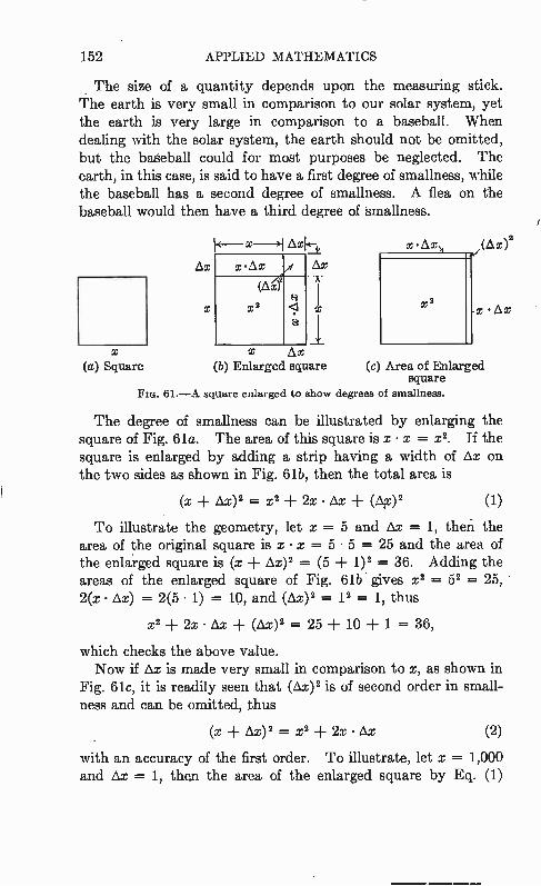
152 APPLIED MATHEMATICS
The size of a quantity depends upon the measuring stick. The earth is very small in comparison to our solar system, yet the earth is very large in comparison to a baseball. When dealing with the solar system, the earth should not be omitted, but the baseball could for most purposes be neglected. The earth, in this case, is said to have a first degree of smallness, while the baseball has a second degree of smallness. A flea on the baseball would then have a third degree of smallness.
Ax
(a) Square
[loci<It.
Ax
1 -
x x (b) Enlarged square
x•Ax
X 2
(o) Area of Enlarged square
FIG. 61.—A square enlarged to show degrees of smallness.
The degree of smallness can be illustrated by enlarging the square of Fig. 61a. The area of this square is x • x = x2. If the square is enlarged by adding a strip having a width of Ax on the two sides as shown in Fig. 61b, then the total area is
(x Ax)2 = x2 + 2x • Ax (A:z)2 (1)
To illustrate the geometry, let x = 5 and Ax = 1, then the area of the original square is x • x = 5 • 5 = 25 and the area of the enlarged square is (x Ax)2 = (5 ± 1) 2 = 36. Adding the areas of the enlarged square of Fig. 61b gives x2 = 52 = 25, 2(x • Ax) = 2(5 • 1) = 10, and (Ax)2 = 12 = 1, thus
x2 ± 2x • 3,x ± (àx) 2 = 25 ± 10 ± 1 = 36,
which checks the above value. Now if Ax is made very small in comparison to x, as shown in
Fig. 61c, it is readily seen that (Ax)2 is of second order in small-ness and can be omitted, thus
(x Ax) 2 = x2 ± 2x • Ax (2)
with an accuracy of the first order. To illustrate, let x = 1,000 and Ax = 1, then the area of the enlarged square by Eq. (1)
DIFFERENTIAL CALCULUS: ALGEBRAIC 153
with accuracy to the second order is
(x ,e.x)2 = (1,001)2 = 1,002,001
and by Eq. (2), the accuracy to the first order is
x2 ± 2x ,à.x = 1,000,000 ± 2,000 = 1,002,000
By neglecting the second-order term (Ó.x) 2, the answer has changed approximately one part in a million. This makes it clear that if ha is made small enough, by approaching the value of dx, the second, third, and higher order terms can be omitted. Rates.—One of the most familiar illustrations of rate is the
movement of an object which takes a certain amount of time. An automobile, for example, travels at a rate of 60 miles per hour. If the automobile has a uniform speed the whole distance, x = 60 miles, and the total time, t = 1 hr, can be used to express the rate mathematically, thus
x distance Rate = — . (3)
t time
Using the above values, Eq. (3) gives
60 miles Rate = — 60 mph
1 hr
Since it is unusual to have a constant rate of speed for such a long period of time, it is logical to look for a way to express this rate at any particular instant. By writing dx as an incremental distance corresponding to an incremental interval of time, dt, the rate at any instant can be expressed by
dx Rate = (4)
dt
where dx = differential of x, pronounced "dee-ex." • dt =- differential of t, pronounced "dee-tee."
This equation states that the mathematical rate of x at the particular instant is the ratio of the differentials dx divided by dt. The differential of any variable quantity is indicated by writing the letter d before the quantity, thus in this equation the symbol dx is not the product of d and x but represents an incremental difference quantity. . This difference quantity dx known as a differential corresponds to the distance covered during the corresponding incremental difference quantity dt the time
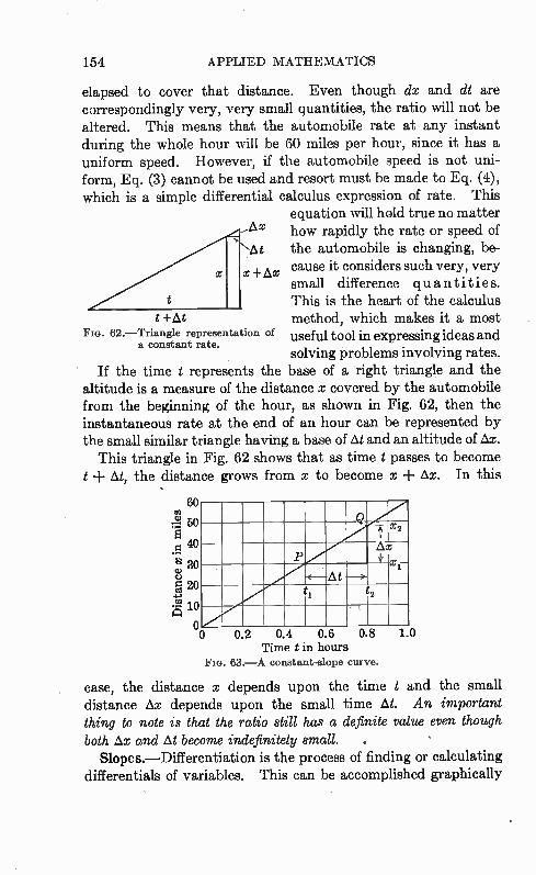
154 APPLIED MATHEMATICS
elapsed to cover that distance. Even though dx and dt are correspondingly very, very small quantities, the ratio will not be altered. This means that the automobile rate at any instant during the whole hour will be 60 miles per hour, since it has a uniform speed. However, if the automobile speed is not uni-form, Eq. (3) cannot be used and resort must be made to Eq. (4), which is a simple differential calculus expression of rate. This
equation will hold true no matter Ax how rapidly the rate or speed of A t the automobile is changing, be--I-Ax cause it considers such very, very x
small difference quantities. This is the heart of the calculus method, which makes it a most
F/G. 62.—Triangle representation of useful tool in expressing ideas and a constant rate.
solving problems involving rates. If the time t represents the base of a right triangle and the
altitude is a measure of the distance x covered by the automobile from the beginning of the hour, as shown in Fig. 62, then the instantaneous rate at the end of an hour can be represented by the small similar triangle having a base of At and an altitude of Ax.
This triangle in Fig. 62 shows that as time t passes to become t + At, the distance grows from x to become x Ax. In this
t -1-At
60
so e e 40
el 30
20
ga 10 0 02 0.4 0.6
Time t in hours no. 63.—A constant-slope curve.
case, the distance x depends upon the time t and the small distance Ax depends upon the small time At. An important thing to note is that the ratio still has a definite value even though both Ax and At become indefinitely small. .
Slopes.—Differentiation is the process of finding or calculating differentials of variables. This can be accomplished graphically
o
At
T x2
1̀' x
ti 2
0.8 1.0
DIFFERENTIAL CALCULUS: ALGEBRAIC 155
by plotting the curve of the variable and then determining the slope of the curve. Consider the above illustration of an auto-mobile traveling 60 miles per hour. This information if plotted will give the straight line curve shown in Fig. 63. By substituting in Eq. (3), the slope of this curve is found to be 60 miles per hour. Now, instead of considering all of the graph, use the portion of the curve between points P and Q. The slope of this portion of the curve is the change in distance Ax = x2 — x1 divided by the corresponding change in time At = t2 - ti, or, in equation form,
Ax X2 Xj— Slope — — At t2 — ti
where .à.x = the change in x, pronounced "delta ex." At = the change in t, pronounced "delta tee."
If the values on the curve are substituted in Eq. (5), the result is
48 — 30 18 Slope — — = 60 mph
0.8 — 0.5 0.3
• (5)
This checks with the solution obtained by using Eq. (3) for the whole curve.
If the quantity Ax is made smaller and smaller, it can be .made to approach the differential d,x. Similarly At can be made to approach the differential dt. For illustration move the point Q closer and closer to the point P and the triangle will become smaller and smaller with the result that the slope or rate at the point P can be expressed in differential form by Eq. (4). This reveals that there are two types of rates, an average rate which is computed over a definite interval, such as from P to Q in the above illustration, and an instantaneous rate which is computed at one particular point such as P in the above illustration. For a curve that is not a straight line the ratio of Ax to At
as illustrated in Fig. 63 will not always give the slope at the point P. The slope of the curve, at the point P, is called the "tangent" to the curve. Hence, to find the derivative dx by dt at the point P, draw a tangent to the curve at that point and find the slope of this tangent.
Slope = tangent = derivative
The slope can also be expressed in terms of the limiting process as follows: es'
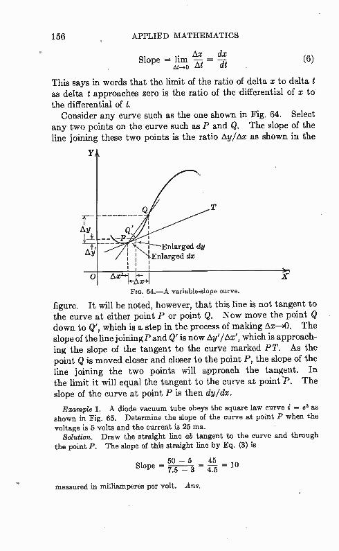
156 APPLIED MATHEMATICS
. àx c/x Slope = hm —AA =
at CLG (6)
This says in words that the limit of the ratio of delta x to delta t as delta t approaches zero is the ratio of the differential of x to the differential of t.
Consider any curve such as the one shown in Fig. 64. Select any two points on the curve such as P and Q. The slope of the line joining these two points is the ratio ày/Ax as shown in the
Y
I Enlarged dy Enlarged dx
FIG. 64.—A variable-slope curve.
figure. It will be noted, however, that this line is not tangent to the curve at either point P or point Q. Now move the point Q down to Q', which is a step in the process of making ix—O. The slope of the line j oining P and Q' is now ày'/x', which is approach-ing the slope of the tangent to the curve marked PT. As the point Q is moved closer and closer to the point P, the slope of the line joining the two points will approach the tangent. In the limit it will equal the tangent to the curve at point P. The slope of the curve at point P is then dy/dx.
Example 1. A diode vacuum tube obeys the square law curve i = e2 as shown in Fig. 65. Determine the slope of the curve at point P when the voltage is 5 volts and the current is 25 ma.
Solution. Draw the straight line ab tangent to the curve and through the point P. The slope of this straight line by Eq. (3) is
50-5 45 Slope = 7.5 _ 3 = 4.5 = 10
measured in milliamperes per volt. Ans.
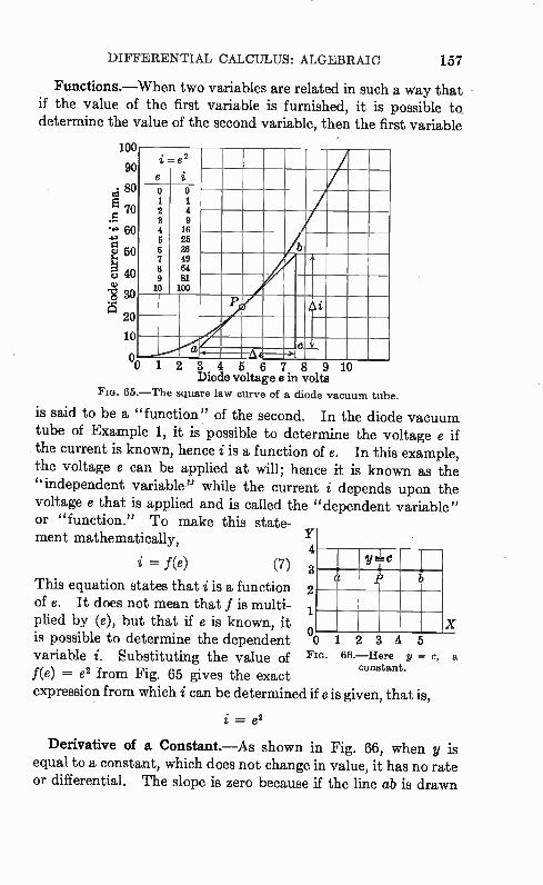
DIFFERENTIAL CALCULUS: ALGEBRAIC 157
Function s.—When two variables are related in such a way that if the value of the first variable is furnished, it is possible to determine the value of the second variable, then the first variable
4.1
tio 50
eq 40
'<i) 30
20
10
i=e2
e i 0 1 2 3 4 5 6 7 8 9 10
0 1 4 9
16 28 36 49 64 81 100
b -
P Ai
_ a lc - A 6 7 8 9 10
Diode voltage e in volts FIG. 65.—The square law curve of a diode vacuum tube.
is said to be a "function" of the second. In the diode vacuum tube of Example 1, it is possible to determine the voltage e if the current is known, hence i is a function of e. In this example, the voltage e can be applied at will; hence it is known as the "independent variable" while the current i depends upon the voltage e that is applied and is called the "dependent variable" or "function." To make this state-ment mathematically, Y
4
= f(e) (7) 3
This equation states that i is a function 2
of e. It does not mean that f is multi-plied by (e), but that if e is known, it X
0 is possible to determine the dependent 0 1 2 3 variable i. Substituting the value of FIG. 66.—Here y = c, a
f(e) = e2 from Fig. 65 gives the exact expression from which i can be determined if e is given, that is,
i = e2
Derivative of a Constant.—As shown in Fig. 66, when y is equal to a constant, which does not change in value, it has no rate or differential. The slope is zero because if the line ab is drawn
yc
4
constant.
6
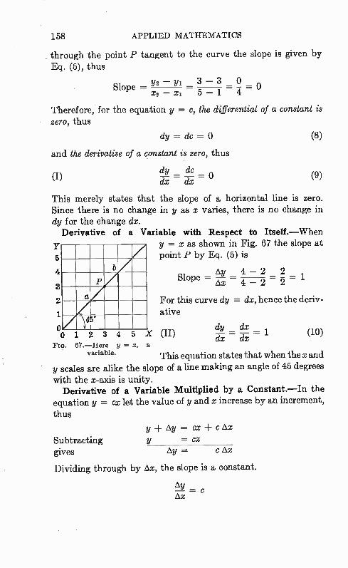
158 APPLIED MATHEMATICS
, through the point P tangent to the curve the slope is given by Eq. (5), thus
Slope — y2 — yi _ 3 — 3 _ _ o x2 — x1 5 — 1 4
Therefore, for the equation y = c, the differential of a constant is zero, thus
dy = dc =
and the derivative of a constant is zero, thus
dx dy _ de c17 = ° (I)
(8)
(9)
This merely states that the slope of a horizontal line is zero. Since there is no change in y as x varies, there is no change in dy for the change c/x.
Derivative of a
Y
6
4
a 2
1
oo
Variable with Respect to Itself .—When y = x as shown in Fig. 67 the slope at point P by Eq. (5) is
Ay 4 — 2 2 Slope — — — — 1 Ax 4 — 2 2
a
45,
1 2 3 4 5 X
For this curve dy = dx, hence the deriv-ative
(II) FIG. 67.—Here y x, a
This equation states that when the x and y scales are alike the slope of a line making an angle of 45 degrees
with the x-axis is unity. Derivative of a Variable Multiplied by a Constant.—In the
equation y = cx let the value of y and x increase by an increment,
thus
variable.
(10)
y Ay = cx -F c
Subtracting y --= cx gives Ay = c Ax
Dividing through by Ax, the slope is a constant.
Ax
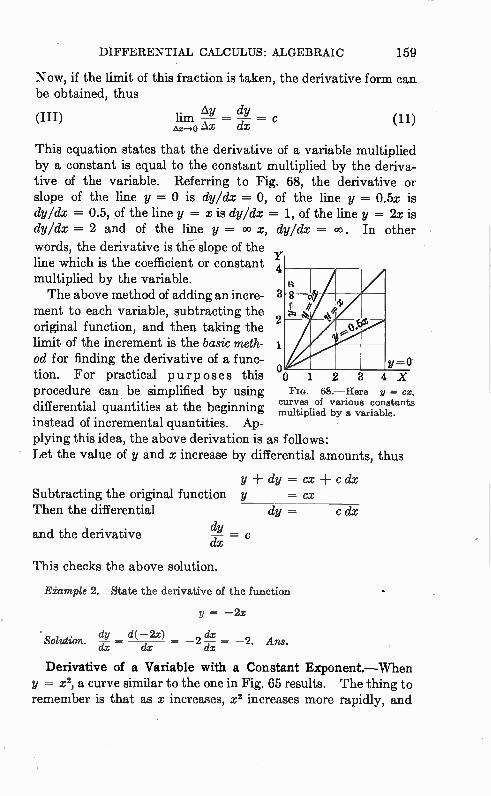
DIFFERENTIAL CALCULUS: ALGEBRAIC 159
Now, if the limit of this fraction is taken, the derivative form can be obtained, thus
(III) lim = d=Y c (11) ax—> 0 3.2 dx
This equation states that the derivative of a variable multiplied by a constant is equal to the constant multiplied by the deriva-tive of the variable. Referring to Fig. 68, the derivative or slope of the line y = 0 is dy/dx = 0, of the line y = 0.5x is dy/dx = 0.5, of the line y = xis dy/dx -= I, of the line y = 2x is dy/dx = 2 and of the line y = CO x, dy/dx = co. In other
words, the derivative is the slope of the Y line which is the coefficient or constant 4
multiplied by the variable. The above method of adding an More- 3
ment to each variable, subtracting the 2 original function, and then taking the
limit of the increment is the basic meth-od for finding the derivative of a func- y =0
tion. For practical purposes this 00
procedure can be simplified by using FIG. 68.—Here y = cx, curves of various constants
differential quantities at the beginning multiplied by a variable. instead of incremental quantities. Ap-plying this idea, the above derivation is as follows: Let the value of y and x increase by differential amounts, thus
y ± dy = cx c dx Subtracting the original function y = cx Then the differential dy = c dx
and the derivative dy dx c
This checks the above solution.
Eiample 2. State the derivative of the function
y -= —2x
Solution. dy _ d( —2x) _ 2 dx dx 2. Ans. dx dx
Derivative of a Variable with a Constant Exponent—When y = x2, a curve similar to the one in Fig. 65 results. The thing to remember is that as x increases, x2 increases more rapidly, and
1 2 3 4 X
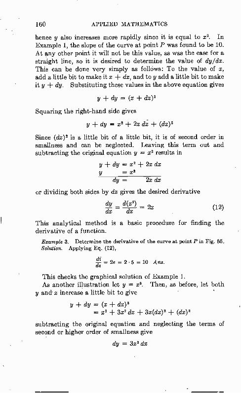
160 APPLIED MATHEMATICS
hence y also increases more rapidly since it is equal to x2. In Example 1, the slope of the curve at point P was found to be 10. At any other point it will not be this value, as was the case for a straight line, so it is desired to determine the value of dy/dx. This can be done very simply as follows: To the value of x, add a little bit to make it x dx, and to y add a little bit to make it y -I- dy. Substituting these values in the above equation gives
y + dy = (x dx)2
Squaring the right-hand side gives
y + dy = x2 ± 2x dx (dx)2
Since (dx)2 is a little bit of a little bit, it is of second order in smallness and can be neglected. Leaving this term out and subtracting the original equation y = x2 results in
y ± dy = x2 ± 2x dx y = x2
dy = 2x dx
or dividing both sides by dx gives the desired derivative
dy _ d(x2) _ dx dx
(12)
This analytical method is a basic procedure for finding the derivative of a function.
Example 3. Determine the derivative of the curve at point P in Fig. 65. Solution. Applying Eq. (12),
di c• = 2e = 2 • 5 = 10 Ans.
This checks the graphical solution of Example 1. As another illustration let y -= x2. Then, as before, let both
y and x increase a little bit to give •
y ± dy = (x dx) 3 = x3 3x2 dx 3x(dx)2 (dx)3
subtracting the original equation and neglecting the terms of second or higher order of smallness give
dy = 3x2 dx
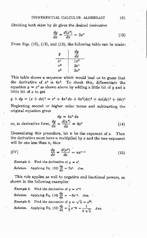
DIFFERENTIAL CALCULUS: ALGEBRAIC 161
Dividing both sides by dx gives the desired derivative
dy _ d(x3) _ 2 (13) dx dx °x
From Eqs. (10), (12), and (13), the following table can be made:
dy
lx° x 2 2x1
3x2
This table shows a sequence which would lead us to guess that the derivative of x4 is 4x'. To check this, differentiate the equation y = x4 as shown above by adding a little bit of y and a little bit of x to get
y ± dy = dx)4 = x4 + 4x3 dx 6x2(dx)2 4x(dx) 8 (dx)4
Neglecting second or higher order terms and subtracting the original equation gives
dy = 4x2 dx dy d(x4)
or, in derivative form, crx- _ — c—T—T = 4x3 (14)
Generalizing this procedure, let n be the exponent of x. Then the derivative must have n multiplied by x and the new exponent will be one less than n, thus
dy _ d(xn) dx dx
(IV) = nxn—i 05)
Example 4. Find the derivative of y = x7.
Solution. Applying Eq. (15) 2= 7x6. Ans.
This rule applies as well to negative and fractional powers, as shown in the following examples:
Example 5. Find the derivative of y = dy
Solution. Applying Eq. (15) (T-x —2x-3. Ans. -
Example O. Find the derivative of y = •‘/ = dy 1 1
Solution. Applying Eq. (15) d—x = -2 orki = Ans. 2 •\/
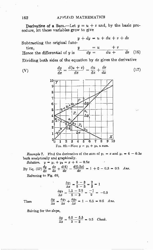
162 APPLIED MATHEMATICS
Derivative of a Sum.—Let y = u ± y and, by the basic pro-cedure, let these variables grow to give
y -F dy = u + du + y ± dv Subtracting the original func-
tion, y = u + v Hence the differential of y is dy = du + dv (16)
Dividing both sides of the equation by dx gives the derivative
(V)
10
9
8
7
6
5
4
3
2
1 o
dy _ d(u v) _ du , dv dx dx dx
Y
LyV
It
al AVI
• e a,
P
ti (S, ,C S2
ax _
X 2 3 4 5 7
69.—Here y = yi -I- y2, a sum.
(17)
Example 7. Find the derivative of the sum of yt = x and y2 = 4 — 0.5x bctth analytically and graphically.
Solution. y = y + y2 -= x -I- 4 — 0.5x dy dx d(4) d(0.5x)
By Eq. (17) c-u = (Tx ± dx dx = 1 + — 0.5 = 0.5 Ans.
Referring to Fig. 69,
Then Ay
Ax
Ay, 5 — 3 2 _ 1 = 5 — 3 2
Ay2 1.5 — 2.5 _ —1 _ 0.5 Ax 5 — 3 2
Ans. Ax Ax
Solving for the slope,
AY 6'5 — 53 — 0.5 Check. Ax = 5 — 3
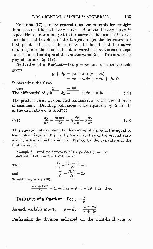
DIFFERENTIAL CALCULUS: ALGEBRAIC 163
Equation (17) is more general than the example for straight lines because it holds for any curve. However, for any curve, it is possible to draw a tangent to the curve at the point of interest and then find the slope of the tangent to get the derivative for that point. If this is done, it will be found that the curve resulting from the sum of the other variables has the same slope as the sum of the slopes of the various variables. This is another way of stating Eq. (17).
Derivative of a Product.—Let y = uy and as each variable grows
y + dy = (u + du) (v dv) = uy udv v du ± du dv
Subtracting the func-tion, • Y = Uy
The differential of y is dy = u dv du (18)
The product du dv was omitted because it is of the second order of smallness. Dividing both sides of the equation by dx results in the derivative of a product
dy _ d(uv) dv du (VI) u — , v — (19)
dx dx dx dx
This equation states that the derivative of a product is equal to the first variable multiplied by the derivative of the second vari-able plus the second variable multiplied by the derivative of the first variable.
Example 8. Find the derivative of the product (x + 1)x2. Solution. Let u x -I- 1 and v = x2
Then du _ d(x 1) _ dx dx
and dv _ d(x2) 2x dx dx
Substituting in Eq. (19),
d(x + 1)x2 — (x + 1)2x + x2. 1 = 3x2 + 2x Ans.
cis
Derivative of a Quotient.—Let y =
As each variable grows, u+ du
y+dy — v+dv
Performing the division indicated on the right-hand side to
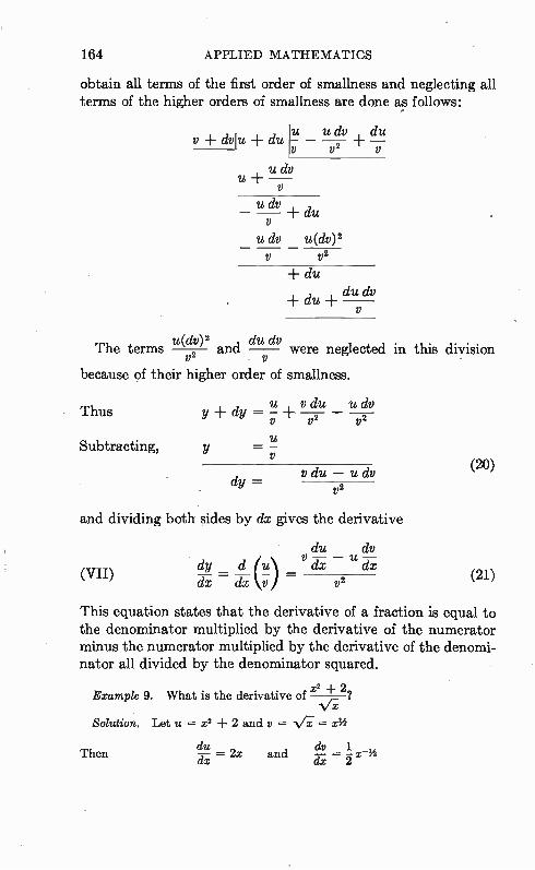
164 APPLIED MATHEMATICS
obtain all terms of the first order of smallness and neglecting all terms of the higher orders of smallness are done as follows:
y ± dylu ± du -u "1". — u dv , du 1,2 7
u + u dv
u dv —-+ du
u dv u(dv)2 V V2
+ du
+ du + du dv
u(dv)2 du dv The terms and were neglected in this division y2 y
because of their higher order of smallness.
Thus
Subtracting,
u , v du u dv v v2
u =
dy = V du — u dv
1,2
and dividing both sides by dx gives the derivative
(VII)
du dv
dx dx v2
This equation states that the derivative of a fraction is equal to the denominator multiplied by the derivative of the numerator minus the numerator multiplied by the derivative of the denomi-nator all divided by the denominator squared.
x2 + 2 Example 9. What is the derivative of _ ?
•1/4 Solution. Let u =z2 + 2 and y = = x1/2
(20)
Then du dx
and dv 1 _ (-Tx = x
(21)
DIFFERENTIAL CALCULUS: ALGEBRAIC 165
Substituting in Eq. (21),
d (Z2 + 2) Vi • 2x — (x2 + 2) 3 17; 1 Ans.
dx Nfx. z 2 x
Thus far we have developed the important derivatives for algebraic functions. In most cases graphs have been furnished to illustrate more clearly what happens. Now, to make use of this knowledge, some practical applications will be treated along with some more ideas about differential calculus. In other words, we have the tools; let's learn how to make good use of them.
Successive Derivatives.—The idea that a derivative may represent a rate of change has already been given. It is the ratio of the little bit of space covered in the corresponding little bit of time. Let us apply this idea to a freely falling object. From physics, the equation for a freely falling body is
s = 16t2 (22)
where s = space covered by the freely falling body, in feet. t = time after the body begins to fall, in seconds.
This curve is plotted in Fig. 70 for a time period of 8 seconds. As time increases the space is covered more rapidly. This means that the velocity must be increasing. The velocity, if scientifically expressed, is the derivative of space with respect to :time. If applied to Eq. (22), it gives
ds v = 32f (23) dt
where y = velocity in feet per second. When this curve is plotted, as shown in Fig. 70, it is noted that
the velocity is steadily increasing. Now the rate at which the velocity is increasing is called the "acceleration." Taking the derivative of Eq. (23), which is the second successive derivative, results in
dv a = = — = 04 (24) dt dt2
where a = acceleration in feet per second per second, and d2s/dt2 = the second derivative of s with respect to t. It can also be read "dee squared ess over dee-tee squared." This equation shows that the acceleration, due to the force of gravity,
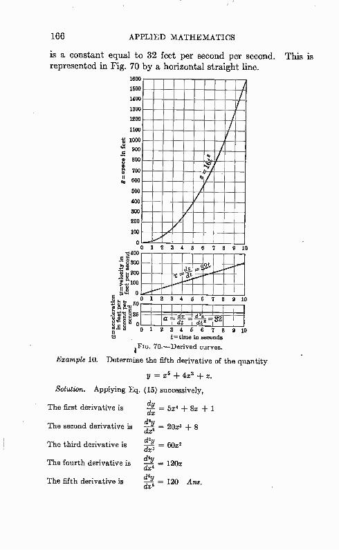
166 APPLIED MATHEMATICS
is a constant equal to 32 feet per second per second. This is represented in Fig. 70 by a horizontal straight line.
S =space in feet
1600
1500
1400
1300
1200
1100
1000
900
800
700
600
500
400
300
200
100
o o .0 400 e 300 p I
2e) 100
II $ aN-• o 0 s. iiRKqe 60
4 1 125 § Op
1 2 3 4 6 6 7 8 10
11 t
1 2 3 4 5 6 7 9 10
a = dv = de8-1--_ 32 dt 7c 1
2 8 4 5 6 7 8 t= time in seconds
&FIG. 70.—Derived curves.
9 10
Example 10. Determine the fifth derivative of the quantity
y = x5 + 42 x.
Solution. Applying Eq. (15) successively,
dy The first derivative is — = 5x4 + 8x ± 1 dx da,
The second derivative is = 20x3 ± 8 dx2 d3y
The third derivative is 37,3 = sox=
d'y The fourth derivative is --= 120x
dx" dsy
The fifth derivative is = 120 Ans. clx5
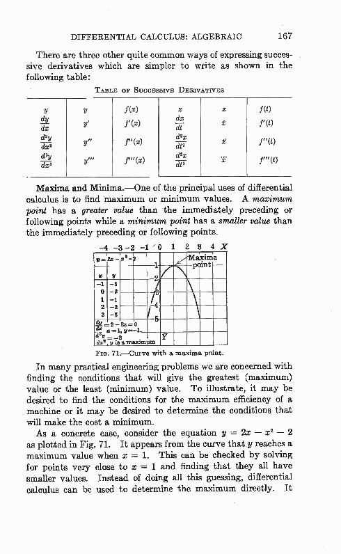
DIFFERENTIAL CALCULUS: ALGEBRAIC 167
There are three other quite common ways of expressing succes-sive derivatives which are simpler to write as shown in the following table:
TABLE or SUCCESSIVE DERIVATIVES
y y f(x) x x f(t) dy 71X d'y de d'y
yi
et
f (x)
f" (x)
(z)
dx Tc d'x dt2 d3x
i
z
.i.
f' (t)
f"(t)
rii(t)
de yin fill
dt 3
Maxima and Minima.—One of the principal uses of differential calculus is to find maximum or minimum values. A maximum point has a greater value than the immediately preceding or following points while a minimum point has a smaller value than the immediately preceding or following points.
-4 -8-2 -1'0 1 2 3 4 X v '2x_'x2_2 Mnxinia
point
e ti -1 0
1 2
3
-6 -2 -1 -2 -5
At _2
' 2
de,
_2,,_ I y - e- -
y is a maximum
0 -1
5
FIG. 71.—Curve with a maxima point.
In many practical engineering problems we are concerned with finding the conditions that will give the greatest (maximum) value or the least (minimum) value. To illustrate, it may be desired to find the conditions for the maximum efficiency of a machine or it may be desired to determine the conditions that will make the cost a minimum. As a concrete case, consider the equation y -= 2x — x2 — 2
as plotted in Fig. 71. It appears from the curve that y reaches a maximum value when x = 1. This can be checked by solving for points very close to x = 1 and finding that they all have smaller values. Instead of doing all this guessing, differential calculus can be used to determine the maximum directly. It
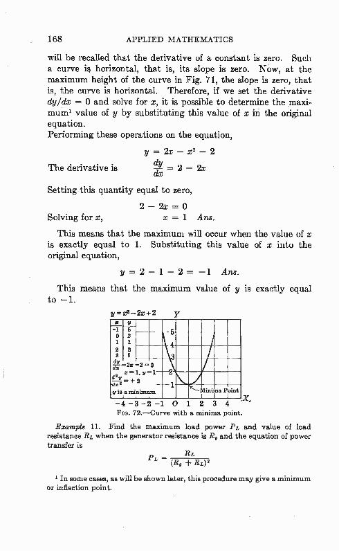
168 APPLIED MATHEMATICS
will be recalled that the derivative of a constant is zero. Such a curve is horizontal, that is, its slope is zero. Now, at the maximum height of the curve in Fig. 71, the slope is zero, that is, the curve is horizontal. Therefore, if we set the derivative dy/dx = 0 and solve for x, it is possible to determine the maxi-mum' value of y by substituting this value of x in the original equation. Performing these operations on the equation,
y = 2x — x2 — 2 dy
The derivative is = 2 — 2x
Setting this quantity equal to zero,
2 — 2x = Solving for x, x = 1 Ans.
This means that the maximum will occur when the value of x is exactly equal to 1. Substituting this value of x into the original equation,
y = 2 — 1 — 2 = — 1 Ans.
This means that the maximum value of y is exactly equal to —1.
y =•. x2 — 2x + 2 w y
5 -1 0 1
5 2 1 4
2 2 3 5 3 e=2,2 =0
x=1, y-1 d 2v 2
•az2 =-1-2 1 Minima Point y is a minimum
Y
—4-3-2-1 0 1 2 3 4 FIG. 72.—Curve with a minima point.
Example 11. Find the maximum load power PL and value of load resistance Rx, when the generator resistance is Ito and the equation of power transfer is
R1' PL — (14 +14)2
In some cases, as will be shown later, this procedure may give a minimum or inflection point.
DIFFERENTIAL CALCULUS: ALGEBRAIC 169
Solving this equation,
Solution. Since this equation is a fraction, let u = RL and y = (R, R.L) 2 in Eq. (21). The derivatives are then
du dR.L and dv d(R, RL)2 dRz, dRL = 2(R, + RL)
Now, substituting these values into Eq. (21) results in
d/I'L (Rg Rz)2 — RL2(Rg RL) _ ± — 214 — 0
dRL, = (R, RL)4 (R, RL) 8
This equatior. is true when the numerator is zero, hence
R, — = 0 or RL = R, Ans.
As another case, consider the equation y = x2 — 2x ± 2 which is plotted in Fig. 72. The curve appears to reach a minimum value of y = 1 when x -= 1. To check this, take the first derivative and equate it to zero, thus
du = 2x — 2 =
dx Hence, x = 1 Ans.
Substituting this value in the original equation.
y = 1 — 2 + 2 = 1 Ans.
Example 12. The cost C of handling vacuum tubes in a factory varies with the output N per day according to the relation
C=a-1- 17.-1-cN
where a, b, and c are constants. For what output will the cost be least? Solution. Taking the first derivative and equating to zero,
de —b -
dN = N2
N _ rb c
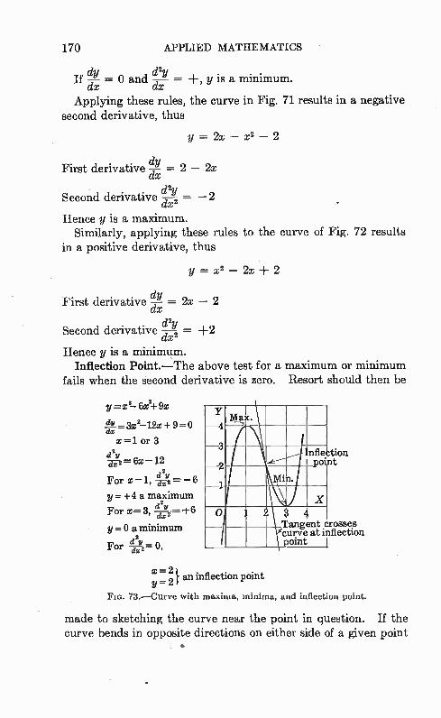
170 APPLIED MATHEMATICS
If di. d2Y = 0 and =' y is a minimum. dx dx
Applying these rules, the curve in Fig. 71 results in a negative second derivative, thus
y = 2x — x2 — 2
First derivative dy = 2 — 2x dx d2y
Second derivative = —2 dx2
Hence y is a maximum. Similarly, applying these rules to the curve of Fig. 72 results
in a positive derivative, thus
y = X2 — 2x + 2
First derivative dy = 2x — 2 dx d2y
Second derivative dx- 2 = +2
Hence y is a minimum. Inflection Point.—The above test for a maximum or minimum
fails when the second derivative is zero. Resort should then be
6x2+ 9x
A=3x2-12x+ 9=0 (Ix x=1 or 3
d2y cyx2= 6x-12
For x-1, e s — 6
y = +4 a maximum
For x=3, d<2-e2.= +6
y = 0 a minimum
For e= 0,
Max.
—3 Infle Po
—2 il X
Il 2 3 4 I Tangent c curve at il point
tion it
rosses fleetion
x=2) i y = 2 an nflection point
FIG. 73.—Curve with maxima, minima, and inflection point.
made to sketching the curve near the point in question. If the curve bends in opposite directions on either side of a given point
-
DIFFERENTIAL CALCULUS: ALGEBRAIC • 171
that point is called an "inflection point." In other words, an inflection point separates an upward concave portion of a curve (---) from a downward concave portion of the curve At an inflection point a tangent to the curve will cross the curve. The rule can be stated as follows:
d2y If cd--111-=Oand Ei = 0, y is an inflection point, a maximum, or
a minimum. In this case, the curve should be plotted to deter-mine its exact nature.
Example 13. Find the maximum, minimum, and inflection-point values and plot the curve
y = x3 - 6x2 + Dx
dy Solution. The first derivative - 3x2 - 12x + 9 =
dx - By the quadratic formula, x = 1 or 3
The second derivative is — = 6x - 12 d,x2
If x = 1' _ -6, hence a maximum at dx2
y = 1 - 6 + 9 = +4 Ans.
d'y H _ = 3, — - +6, hence a minimum at dx2
Let
Then and
y = 27 - 54 + 27 = 0 Ans. d'y
= 6x - 12 = dx2
x = 2 y = 8 - 24 + 18 = +2 Ans.
From the plotted curve as shown in Fig. 73, we see that the last point is an inflection point.
y = x3 - 6x2 + 9x du -Y- = 3x2 - 12x -F 9 = dx x = 1 or 3 =
c " "
For x = 1, ds- 2 = -y = + 4 a maximum
city For x = 3, die- 2 = +y = 0 a minimum
d2y For
dx2 = x = 2 y = 2 } an inflection point
172 APPLIED MATHEMATICS
Summary.
1. Algebraic differentiation formulas: dc
° dx dx
(II) dx = 1
(I)
d (III) -d—x (cx) = c
(IV) —d (xn) = nxn-1 dx d du dv
(V) T(x (u v) = +
d dv du (VI) c-F (uv) =u c-rx +v ci-x
du dv
(VII) dx \vl v2
2. Successive differentiation is the process of repeating the operation of differentiating a function. These successive oper-ations result in the "first derivative," "second derivative," and so on to the "nth derivative."
3 .If—=Oand—dd—x'y' =, y is a maximum. dy dx dy d'y
4. If dx = 0 and — = , y is a minimum.
5. If = 0 and d--1/ = 0, y is an inflection point, a maximuln, dx de
or a minimum. In this case, the curve should be plotted to determine its nature.
Exercises
Differentiate the following five equations: 1. y = ax2 bx c 2. y 3. y = (a + x) 2 4. y = x •Va bx
a — 5. y x— a + x
6. What is the second derivative of y = VFc? 7. The current I depends upon the temperature t of an incandescent
lamp by the equation I = a ± bt Ce
DIFFERENTIAL CALCULUS: ALGEBRAIC 173
What is the expression for the variation of the current corresponding to a variation of the temperature?
8. If the space covered is given by the equation •
8 = 412 — 6
find the velocity and acceleration when t = 2. 9. Find the value of x and the value of y for the maximum and minimum
values of the curve y = x3 — 3x + 4 10. If the current i = 16 •Vi 8 is expressed in amperes and the time t
in seconds, what is the time when the current changes at the rate of 2 amp per sec?
CHAPTER 13
DIFFERENTIAL CALCULUS TREATING TRANSCENDENTAL FUNCTIONS
As pointed out in the last chapter, a transcendental function is any function that is not a simple algebraic function. Transcen-dental functions are irrational functions such as Ez, sin x, and log x. The Law of Natural Growth.—The law of natural growth
results when the increase in size of a quantity is always propor-tional to the size of the quantity. This is illustrated by nature when an organism's growth is proportional to the size of the organism. This could also be called a "logarithmic rate" of growing because the percentage increase is always proportional to the magnitude at that instant.
Studying two cases will help to clarify this law. Consider the difference between constant and natural growth as illustrated in simple and compound interest. With simple interest, the capital grows arithmetically at unit rate while with compound interest the capital grows logarithmetically at unit rate.
Simple Interest.—Start with a capital of $1 and let the interest rate be 3'ío or 10 per cent per year. The owner will then make 10 cents on this dollar each year. By saving this interest each year he will have a total capital of $2 at the end of 10 years, to double his property.
Stating this problem in general terms, let / be the original capital and 1/n be the yearly interest rate, then it will take n years to double his property, that is
x + n () = 2x (1)
For the first year the owner has $1. At the end of the year he receives 10 cents in interest. He saves this 10 cents during the following year and collects another 10 cents at the end of the second year. This process is shown graphically in Fig. 74 for
174
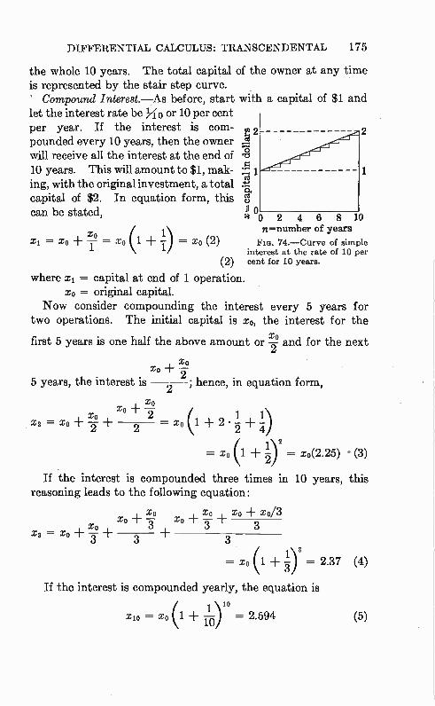
DIFFERENTIAL CALCULUS: TRANSCENDENTAL 175
the whole 10 years. The total capital of the owner at any time is represented by the stair step curve. ' Compound Interest.—As before, start with a capital of $1 and let the interest rate be Yio or 10 per cent per year. If the interest is corn- pounded every 10 years, then the owner
-8 will receive all the interest at the end of me 10 years. This will amount to $1, mak- 9. .., e• 1 ing, with the original investment, a total P
El. capital of $2. In equation form, this g can be stated, II a o 2 4 6 8 10
( n=number of years xi = xo + = xo 1 + —1 = xo (2) Fie. 74.—Curve of simple
interest at the rate of 10 per (2) cent for 10 years.
where x1 = capital at end of 1 operation. xo = original capital.
Now consider compounding the interest every 5 years for two operations. The initial capital is xo, the interest for the
first 5 years is one half the above amount or Xi and for the next
, X0 X0 -t- •-i
5 years, the interest is — 2--; hence, in equation form,
xo x2 = xo -I- x2° ± 2 2 — xo (1 ± 2 • ±
2 4
(1 + 1)2 = xo(2.25) • (3)
If the interest is compounded three times in 10 years, this reasoning leads to the following equation;
xo xo , xo xo/3 , -r -r xo xo
X0 ° 3 3 X3 = X3 + 3 , 3 3
= xo (1 -F = 2.37 (4) 3
If the interest is compounded yearly, the equation is
xio = xo (1 -I- = 2.594 (5)
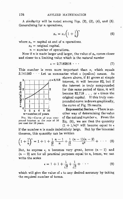
176 APPLIED MATHEMATICS
A similarity will be noted among Eqs. (2), (3), (4), and (5). Generalizing for n operations,
= xo (1 + —1)n (6)
where x„ = capital at end of n operations. x = original capital. n = number of operations.
Now if n is made larger and larger, the value of x„ comes closer and closer to a limiting value which is the natural number
E = 2.7182818 • • • (7)
This number is even more important than ir, which equals 3.141592 • Let us summarize what e (epsilon) means. As
shown above, if $1 grows at simple 3 e —2.718 • interest, it will become $2, but if
7f) ^c 2 e
Tçi
1 e
0 0 2 4 6 8 10 n=number_of years
Fm. 75.—Curve of true com-pound interest at the rate of 10 per cent for 10 years.
the interest is truly compounded 2 for this same period of time, it will
become $2.718 . . . or e times the original capital. If this truly com-pounded curve is drawn graphically, the curve of Fig. 75 results.
Exponential Series.—There is an-other way of determining the value of the natural number e. From the Eq. (6), we see that the quantity (1 + 1/n). will become equal to e
if the number n is made indefinitely large. But by the binomial theorem, this quantity can be written
1
1 n — 1 1 (n — 1)(n — 2) + (8) (1 =ii -I- o +la
- n'
But, to express e, n becomes very great, hence (n — 1) and (n — 2) are for all practical purposes equal to n, hence, we can write the series
E =- 1 + 1 — — -r • • • L2_ L3_
which will give the value of e to any desired accuracy by taking the required number of terms.
(9)
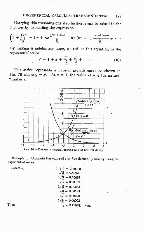
DIFFERENTIAL CALCULUS: TRANSCENDENTAL 177
Carrying this reasoning one step farther, e can be raised to the x power by expanding the expression
(1 + .10 nx + nx ifix-i (1/n) nX (nx \ . 1"e-2 (1/n) 2
IL "
By making n indefinitely large, we reduce this equation to the exponential series
X 2 X 3 Ex = 1 -I- X — — + • • • (10)
This series represents a natural growth curve as shown in Fig. 76 where y = e. At x = 1, the value of y is the natural number e.
y or dy
dx
4 Natural
curve growth
3 in ii=x
2 çu a e Vt„4, Natural
curve V= e
decay
- —2 à
FIG. 76.—Curves of natural growth and of natural decay
X
Example 1. Compute the value of e to five decimal places by using the exponential series.
Solution.
Then
1 ± 1 = 2.00000
1/132 = 0.50000 1/ = 0.16667
1/4— = 0.04167
1/ 5— = 0.00833
= 0.00139
1/ 7— = 0.00020
1/ 8— = 0.00002
e = 2.71828. Ans.
I 78 APPLIED MATHEMATICS
The Law of Natural Decay.—Since the reverse process of growth is decay, consideration will now be given to natural decay or die-away curves. Just as e is the measure of natural growth, so 1/E or e-1 is the measure of natural decay. Applying this reasoning to the exponential series by changing the sign of x
results in
= 1 - X - - --r • • • 12 13
Then, making x = 1, the value of 6-1 becomes
1 , 1 1 - = E-1 = 1 - 1 -r — — ,—
12 13 • • • = 0.36788 • • • (12)
Now, just as a quantity of unit size naturally grows to 2.71828, so does a quantity of unit size naturally die-away to 0.36788. As a practical illustration, the natural cooling of a hot body
obeys the law y = ae-bi (13)
where y is the temperature at any given time t while a and b are
constants. To illustrate the nature of this natural decay curve, it has been
plotted in Fig. 76. Both the natural growth and decay curves have very important
electrical engineering applications. As for example, the change in signal strength along a telephone line obeys these natural laws, and the natural time constant of circuits also can be
explained by them. Derivative of the Exponential Function ex.—When y = ex, the
curve of Fig. 76 results. It will be noted that this is simply an extension of the curve of Fig. 75. A further study will reveal that this curve has very special properties. Using the expo-nential series as given in Eq. (10), it is found that the derivative is the same as the original value.
d 2x 3x2 4x3 Thus (ex) = 0 ± 1 — — — -I- • • •
dx 12 13 14
= 1 x -Ê -I- • • • (14) 12
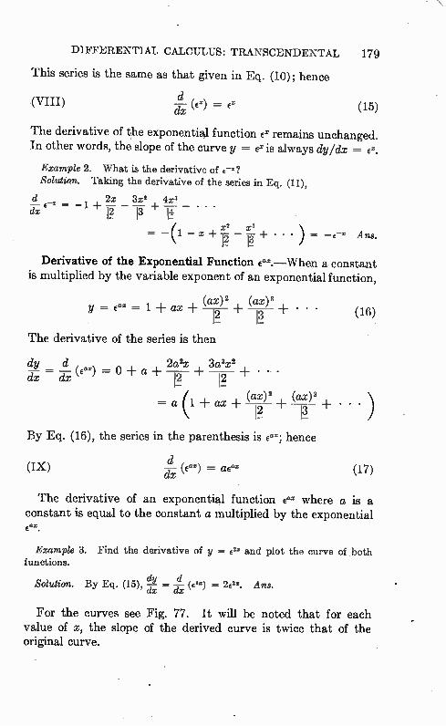
DIFFERENTIAL CALCULUS: TRANSCENDENTAL 179
This series is the same as that given in Eq. (10); hence
d „ (VIII) = EX (15) dx
The derivative of the exponential function e remains unchanged. In other words, the slope of the curve y = e is always dy/dx = ex.
Example 2. What is the derivative of e--"? Solution. Taking the derivative of the series in Eq. (11),
d 2x 3x2 4x3 = + dXe
= (1 — x + — + • • • ) = —6-. Ans.
Derivative of the Exponential Function ex.—When a constant is multiplied by the variable exponent of an exponential function,
y =ea x + ax + (ax)2 ()3
The derivative of the series is then
2 . = 2a2x 3a3x2 (Eae) = o + a + + 12 +
(ax)2 (ax) 3 = a (1 ax 12 + ±
By Eq. (16), the series in the parenthesis is ea"; hence
(IX) d (ex) = a fax
(16)
(17)
The derivative of an exponential function ex where a is a constant is equal to the constant a multiplied by the exponential ¿cm.
Example 3. Find the derivative of y = €2z and plot the curve of both functions.
dy d Solution. By Eq. (15), — — (es") = 2E2e. Ans.
dx dx
For the curves see Fig. 77. It will be noted that for each value of x, the slope of the derived curve is twice that of the original curve.
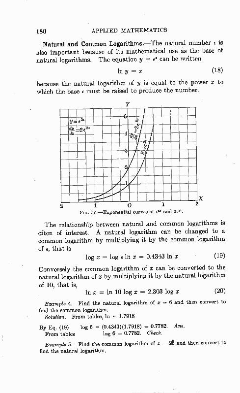
180 APPLIED MATHEMATICS
Natural and Common Logarithms.—The natural number e is also important because of its mathematical use as the base of natural logarithms. The equation y = Ex can be written
ln y = x (18)
because the natural logarithm of y is equal to the power x to which the base e must be raised to produce the number.
Y
Y = E 2x ____5
du =.2e 2x dx
N 74 4
3
2
1
0 1 n 1 «4' X
Fro. 77.—Exponential curves of e" and 2e".
The relationship between natural and common logarithms is often of interest. A natural logarithm can be changed to a common logarithm by multiplying it by the common logarithm of e, that is
log x = log e ln x = 0.4343 ln x • (19)
Conversely the common logarithm of x can be converted to the natural logarithm of x by multiplying it by the natural logarithm
of 10, that is, ln x = ln 10 log x = 2.303 log x (20)
Example 4. Find the natural logarithm of x = 6 and then convert to
find the common logarithm. Solution. From tables, In = 1.7918
By Eq. (19) log 6 = (0.4343)(1.7918) = 0.7782. Ans. From tables log 6 = 0.7782. Check.
Example 5. Find the common logarithm of x e and then convert to find the natural logarithm.
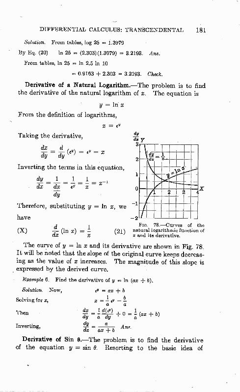
DIFFERENTIAL CALCULUS: TRANSCENDENTAL 181
Solution. From tables, log 25 = 1.3979
By Eq. (20) ln 25 = (2.303)(1.3979) = 3.2193. Amt.
From tables, ln 25 = in 2.5 ln 10
= 0.9163 ± 2.303 = 3.2193. Check.
Derivative of a Natural Logarithm.—The problem is to find the derivative of the natural logarithm of x. The equation is
y in x
From the definition of logarithms,
X -= EY
Taking the derivative,
dx d = (0) = Ev = dy dy
Inverting the terms in this equation,
dy _ 1 = 1 _ 1 x-i -
dy
Therefore, substituting y = ln x, we
have 2
(X) d (In x) = -1 Fro. 78.—Curves of the CTX (21) natural logarithmic function of x and its derivative.
The curve of y = In x and its derivative are shown in Fig. 78. It will be noted that the slope of the original curve keeps decreas-ing as the value of x increases. The magnitude of this slope is • expressed by the derived curve.
• Example 6. Find the derivative of y = ln (ax b).
Solution. Now, ev= ax b
1 b Solving for x,
dx 1 d(o) 1 Then _ ± O = (ax b)
dy dy dy a dx ax +b Ane.
dy dx y 3
2
Inverting,
Derivative of Sin 0.—The problem is to find the derivative of the equation y = sin O. Resorting to the basic idea of
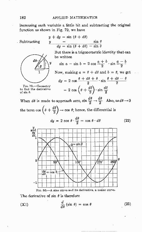
. Subtracting
182 APPLIED MATHEMATICS
increasing each variable a little bit and subtracting the original function as shown in Fig. 79, we have
y ± dy = sin (0 + dO) y = sin 0
Fm. 79.—Geometry to find the derivative of sin O.
dy = sin (0 dO) — sin 0
But there is a trigonometric identity that can be written
sin a — sin b -- 2 cos 2 a ± b • si.n a —2 b
Now, making a = 0 ± dO and b = 0, we get
0 + dO -I- 0 0 ± dO — O dy = 2 cos sin
2 2 ( = 2 cos 0 ± -y • sin T
dO) . dO
dO dO When dO is made to approach zero, sin 7 ---> 7 - Also, as dO —*I)
the term cos ( 0 + -c-1:2) —> cos O; hence, the differential is
de dy --- 2 cos 0 • .7 = cos 0 • dO (22)
and dv de
o
1
y= sin 9
90° 180° 270° 360°
dv dB = cos
Fro. 80 —A sine curve and its derivative, a cosine curve.
The derivative of sin 0 is therefore
d (XI) (To- (sin 0) = cos 0
O
(23)
DIFFERENTIAL CALCULUS: TRANSCENDENTAL 183
The curve of sin O with its derived curve cos O is shown in Fig. 80.
Example 7. A sinusoidal voltage in a circuit can be expressed by the equation E -= sin cot where the constant co is the angular velocity of a vector and t is the time. Determine the expression for the rate at which the voltage E changes
with respect to time. Solution. Applying the above procedure,
E -I- dE = sin (cot + co dt)
Subtracting dE = sin (cot + w dt) — sin cot
Letting a = cot + co dt and b = cot
and using trigonometric identities, we get
dE = 2 cos cot + co& wt sin cut codt — wt 2 2
E sin cot
In this expression the cosine term approaches cos cot as dt —› 0 and the sine w dt
term approaches as dt O.
Hence,
dE = 2 cos cot • writ = cos t dt "
d jé (sin cot) = w cos cot Ans.
Derivative of cos O.—Following a procedure similar to that used for finding the derivative of sin 0, we have
y dy = cos (0 ± dO) Subtracting y = cos
dy = cos (0 + dO) — cos O
From the trigonometric identity,
a+b .sin a—b cos a — cos b = —2 sin
2 2
let a = O ± dO and b = 0; then
—2 sin ° + d° + 0.+ 0 dO — 0 dy = • sin 2 2
( = —2 sin 0 + -ce • sin cl-
dO dO . dO Neglecting in comparison to O and making sin result in
184 APPLIED MATHEMATICS
the differential de
dy = —2 sin 0 —2 = — sin O dO
The derivative of cos O is therefore
(XII) d
(cos 0) = — sin 0
(24)
(25)
Successive Derivatives of sin O and cos 0.—By using Eqs. (23) and (25), it is possible to take successive derivatives of these functions, thus
Original function y = sin
dy First derivative — _ — cos 0 de
• d'y Second derivative —d02 = — sin 0
day Third derivative — = — cos 0
d03 d4v
Fourth derivative = sin e, the original function
The second derivative of sin 0 or cos O is equal to the original function but of opposite sign.
Example 8. Find the values of y = sin e when sin O is a maximum and a minimum.
Solution. Setting the first derivative equal to zero gives the requiréd values of e. Thus
= (sin 0) = cos e = de de
cos e is zero when e = 90° and 270°. For these values of e the second derivative will indicate maximum or minimum values.
d2y d c-ffi (cos 0) = —sin e
d2y When O = 90° ' = —1; hence, a maximum. (102
d2y When O = 270°, _ — +1; hence, a minimum.
The maximum value of y = sin 90° = +1. Ans. and the minimum value of y = sin 270° = —1. Ans.
sin 0 Derivative of tan 0.—Let y = tan 0 =
cos El
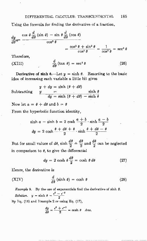
DIFFERENTIAL CALCULUS: TRANSCENDENTAL 185
Using the formula for finding the derivative of a fraction,
d d cos O — (sin 0) - 0 — (cos 0) dy de . de
cos2 cos2 O ± sin2 0 1
— sec2 0082 0 cos2
Therefore, d
(XIII) a (tan 0) = sec2 0 (26)
Derivative of sinh 0.—Let y = sinh B. Resorting to the basic idea of increasing each variable a little bit gives
y ± dy = sinh (0 ± de) Subtracting y = sinh O
dy = sinh (0 ± de) - sinh
Now let a = e + de and b = 0
From the hyperbolic function identity,
a ± b • sinh a - b sinh a - sinh b 2 cosh 2 2
0 + de ± 0 inh O + dO - 0 dy = 2 cosh • s 2 2
de de de But for small values of dO, sinh -2- = -2- and can be neglected
in comparison to 0, to give the differential
dy = 2 cosh 0de —2 = cosh 0 dO (27)
Hence, the derivative is
d (XIV) (sinh 0) = cosh 0 (28)
Example 9. By the use of exponentials find the derivative of sinh O. Co — 6-0
Solution. y = sinh O — 2
By Eq. (15) and Example 2 or using Eq. (17),
dy e° e-te — cosh 0 Ans.
de 2
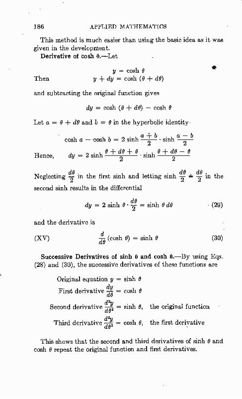
186 APPLIED MATHEMATICS
This method is much easier than using the basic idea as it was given in the development.
Derivative of cosh 0.—Let
y = cosh 0 Then y + dy = cosh (0 ± de)
and subtracting the original function gives
dy = cosh (0 + de) — cosh 0
Let a = O dO and b = O in the hyperbolic identity
cosh a — cosh b = 2 sinh a + 2 b • sinh a —2 b
0 + d ± 0 sinh ± dO — 0 Hence, dy = 2 sinh 2 2
dO de de . Neglecting 7 in the first sinh and letting sinh 7 7 in the
second sinh results in the differential
dy = 2 sinh O• = sinh O dO (29)
and the derivative is
d (XV) cTé (cash °) = sinh O (30)
Successive Derivatives of sinh O and cosh 0.—By using Eqs. (28) and (30), the successive derivatives of these functions are
Original equation y = sinh dy
First derivative = cosh 0
. el/ . sinh derivative — =inh 0, the original function
de2 . day
Third derivative — = cosh 0, the first derivative dea
This shows that the second and third derivatives of sinh 0 and cosh 0 repeat the original function and first derivatives.
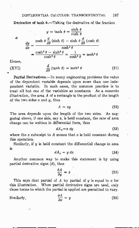
DIFFERENTIAL CALCULUS: TRANSCENDENTAL 187
Derivative of tanh 0.—Taking the derivative of the fraction
sinh y = tanh O =
cosh O d .
cosh —B (sinh 0) — sinh O —d (cosh 0) d dy . dO
dx cosh2 O cosh2 0 — sinh20 1
— sech2 cosh2 O cosh' O
Hence, d
(XVI) (tanh 0) = sech2 (31)
Partial Derivatives.—In many engineering problems the value of the dependent variable depends upon more than one inde-pendent variable. In such cases, the common practice is to treat all but one of the variables as constants. As a concrete illustration, the area A of a rectangle is the product of the length id the two sides x and y, thus
= xy (32)
The area depends upon the length of the two sides. As sug-gested above, if one side, say x, is held constant, the rate of area change can be written in differential form, thus
dAx=x dy (33)
where the x subscript to A means that x is held constant during this operation.
Similarly, if y is held constant the differential change in area is
dA„ y dx (34)
Another common way to make this statement is by using partial derivative signs (a), thus
aA (35)= x
This says that partial of A by partial of y is equal to x for this illustration. When partial derivative signs are used, only those terms to which the partial is applied are permitted to vary.
ax Y Similarly, (36)
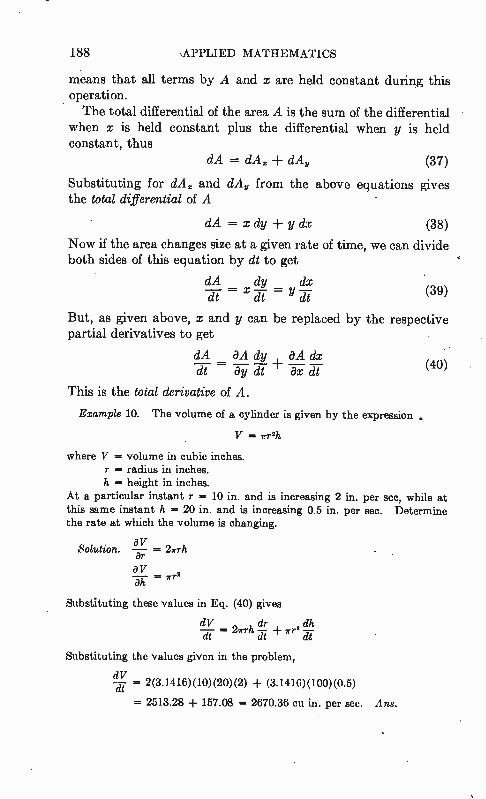
188 ,APPLIED MATHEMATICS
means that all terms by A and x are held constant during this operation. The total differential of the area A is the sum of the differential
when x is held constant plus the differential when y is held constant, thus
dA = dA. dA y (37)
Substituting for dA. and dA y from the above equations gives the total differential of A
dA = x dy + y dx (38)
Now if the area changes size at a given rate of time, we can divide both sides of this equation by dt to get
dA dy (ix dt x dt Y dt (39)
But, as given above, x and y can be replaced by the respective partial derivatives to get
dA aA dy aA dx dl = ay CV axdt
This is the total derivative of A.
Example 10. The volume of a cylinder is given by the expression
V = irr2h
where V = volume in cubic inches. r = radius in inches. h = height in inches.
At a particular instant r -- 10 in. and is increasing 2 in. per sec, while at this same instant h = 20 in. and is increasing 0.5 in. per sec. Determine the rate at which the volume is changing.
Solution. —8V = Irrh ar av ah
Substituting these values in Eq. (40) gives
dV n 7.dt dr , dt dh = erra — -r 7rr - — dt
Substituting the values given in the problem,
dV --d-t- = 2(3.1416)(10)(20)(2) -F (3.1416)(100)(0.5)
= 2513.28 157.08 = 2670.36 cu in. per sec. Ans.
(40)
r r 2
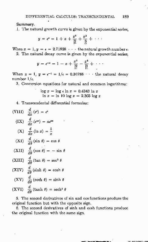
DIFFERENTIAL CALCULUS: TRANSCENDENTAL 189 •
Summary. 1. The natural growth curve is given by the exponential series,
x2 X3 y =ex=1+x+ T2- - + + • • •
When x = 1, y = E = 2.71828 • • • the natural growth number e. 2. The natural decay curve is given by the exponential series,
x2 x3 y = E—e = 1 — z + — Tg- • •
When x --= 1, y = = 1/e = 0.36788 • • • the natural decay number 1/e.
3. Conversion equations for natural and common logarithms:
log x = log e In x = 0.4343 ln x ln x = In 10 log x = 2.303 log x
4. Transcendental differential formulas:
d (es) =
d (IX) d7x (Eae)= ClEae
d (X) c-rx d
(XI) Fié (sin 0) = cos O
d « (XII) (cos 0) = — sin
d (XIII) -d-à (tan 0) = sec2 O
d (XIV) c-ré (sinh 0) = cosh
d (Xy) a (cosh 0) = sinh O d
(XVI) (tanh 0) = sech2
5. The second derivatives of sin and cos functions produce the original function but with the opposite sign.
6. The second derivatives of sinh and cosh functions produce the original function with the same sign.
(VIII)
190 APPLIED MATHEMATICS
7. Partial derivatives are useful in treating engineering prob-lems having more than one independent variable.
Exercises
1. Determine the value of et to five decimal places when x = 2. 2. Find the derivative of y = eae+fie.
3. Find the derivative of y = ln x2. eix — e-i2
4. Find the derivative of y = sin x — 2i by using exponentials.
5. Find the natural logarithm of 8 and then convert to find the common logarithm.
6. In an electrical circuit, the voltage
di E = L —dt
Where i = I sin cot, determine the value of the voltage E. 7. Find the derivative of y -= cos' O.
cos e 8. Find the derivative of y = cot 0 = sal 0 9. What is the second derivative of y = cosh ax?
10. Find the maximum or minimum of the function F = x 2xy y.
CHAPTER 14
INTEGRAL CALCULUS
The word "integral" means the whole or sum of all the little bits. Therefore, integral calculus is the mathematics of calcu-lating the sum of all the little bits. The integral sign f, as already explained, is an elongated letter S, meaning "the sum of." Mathematicians usually prefer to read this sign "the integral of." Thus, f dx means the sum of all the little bits of x but is usually read "the integral of dx." It may be written in the form
of an integral equation, thus
y f dx (1)
This equation states that y is equal to the sum of a vast number of very small quantities dx. In fact, these dx quantities are so indefinitely small that it requires the sum of an indefinitely large number of them to make up the total or integral quantity y. The integral sign is quite closely related to the summation
sign (the Greek letter sigma). The basic difference is that stands for the sum of a few or finite number of terms, while f stands for the sum of an indefinitely large number or infinite number of terme. It may be written in the form of a summation equation, thus
y = Zyk (2)
where y is the sum of all the yk terms that are to be added together. Integration as used in integral calculus can be thought of as
the inverse operation of differentiation as used in differential calculus. This can be compared to division as the inverse operation of multiplication. Integration is more difficult than differentiation, much as division is more difficult than multi-plication. In general, integration of a variable cannot be performed unless the variable has already been found by the process of differentiation. For differentiation, the symbol of
operation is —d ( ) where the quantity to be operated on is dx
191
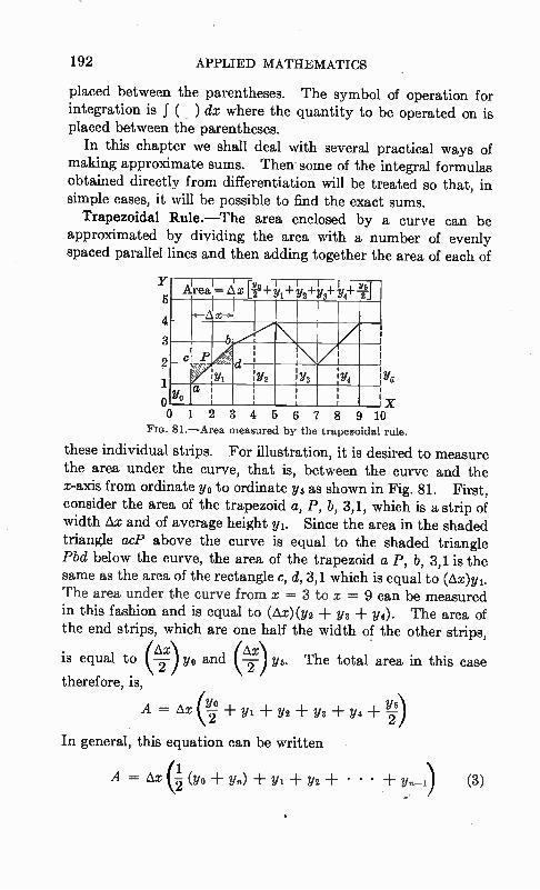
192 APPLIED MATHEMATICS
placed between the parentheses. The symbol of operation for integration is f ( ) dx where the quantity to be operated on is placed between the parentheses.
In this chapter we shall deal with several practical ways of making approximate sums. Then some of the integral formulas obtained directly from differentiation will be treated so that, in simple cases, it will be possible to find the exact sums.
Trapezoidal Rule.—The area enclosed by a curve can be approximated by dividing the area with a number of evenly spaced parallel lines and then adding together the area of each of
Y 5
4
3
2
1
Area = ax [Ye + y1+ iy2+y3+ /4+!J
<-4(X x—•
b ri, 4
d i
Y2 ' Ys . Y4 7'`‘ 111
y a : . ; ,
I
) 1 2 3 4 5 6 7 R gi 11
y5
o . X
Fn. 81.—Area measured by the trapezoidal rule.
these individual strips. For illustration, it is desired to measure the area under the curve, that is, between the curve and the x-axis from ordinate yo to ordinate y6 as shown in Fig. 81. First, consider the area of the trapezoid a, P, b, 3,1, which is a strip of width àx and of average height ya. Since the area in the shaded triangle acP above the curve is equal to the shaded triangle Pbd below the curve, the area of the trapezoid a P, b, 3,1 is the same as the area of the rectangle c, d, 3,1 which is equal to (Ax)y1. The area under the curve from x = 3 to x = 9 can be measured in this fashion and is equal to (ax) (y2 ya y4). The area of the end strips, which are one half the width of the other strips,
is equal to (-2 yo and (—tix) y6. 2 The total area in this case àx)
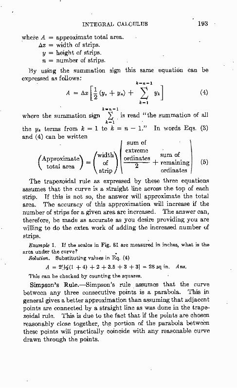
INTEGRAL CALCULUS 193
where A = approximate total area. = width of strips.
y = height of strips. n = number of strips.
By using the summation sign this same equation can be expressed as follows:
k=n-1
A = Az (Y. + yo) + Yki (4) 1
k=1
k=n-1
where the summation sign S is read "the summation of all k=1
the yk terms from k = 1 to k = n — 1." In words Eqs. and (4) can be written
sum of extreme
(Approximate) (width \ total area = of
) ordinates sum of
strip 2 + remaining (5)
ordinates
The trapezoidal rule as expressed by these three equations assumes that the curve is a straight line across the top of each strip. If this is not so, the answer will approximate the total area. The accuracy of this approximation will increase if the number of strips for a given area are increased. The answer can, therefore, be made as accurate as you desire providing you are willing to do the extra work of adding the increased number of strips. Example 1. If the scales in Fig. 81 are measured in inches, what is the
area under the curve? Solution. Substituting values in Eq. (4)
A = 2[%(1 ± 4) + 2 ± 3.5 -I- 3 + 3] = 28 sq in. Ans.
This can be checked by counting the squares.
Simpson's Rule.—Simpson's rule assumes that the curve between any three consecutive points is a parabola. This in general gives a better approximation than assuming that adjacent points are connected by a straight line as was done in the trape-zoidal rule. This is due to the fact that if the points are chosen reasonably close together, the portion of the parabola between these points will practically coincide with any reasonable curve drawn through the points.
(3)

194 APPLIED MATHEMATICS
The area under any portion of a parabola is exactly 3 of the enclosing rectangle as illustrated in Fig. 82. The area under
any three points on a parabola is Y y =1 —x2
Area = (ye 4y1+ y2) given by
1 Area = —3 (y,, + 4y ± Y*2)
If these are the first three points 0.5 giving the area in the first two
strips, then the area in the second two strips is
o 0.5 1 Area = —1 Ax (y2 + 4y8 ± 114)
x 3
FIG. 82.—Area under a parabola In general, these areas can be measured by Simpson's rule, added together to give the total
area under the curve, thus
1 A = —3 Ax (Y0 ± 4y1 2y2 4y$ 24 ± • • • + yn) (6)
where A = approximate total area. = width of strips.
y = height of strips. n = number of strips (n being even).
Equation (6) may be expressed by using the summation sign, as follows:
k= n k= ta —1
A = 3 + Yn) 4 E Y(2k-1) + 2 y2ki ,
k=11.
(7)
In words, this equation can be expressed
À = 1 [wid,1 [(orclinates sum of extreme sum of remaining ) -à °I + 4 odd-numbered
strip ordinates
sum of remaining -I- 2 ( even-numbered (8)
ordinates
Example 2. Determine the area under the parabola of Fig. 82 if the scales are in inches.
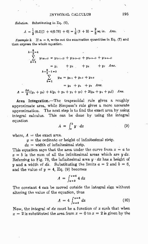
INTEGRAL CALCULUS 195
Solution. Substituting in Eq. (6),
1 1 2 A = - (0.5)[1 + 4(0.75) + 0] - (1 + 3) = - sq in. Ans.
3 6 3
Example 3. If n = 8, write out the summation quantities in Eq. (7) and then express the whole equation.
8 k=--4 2
y(75-7) = Y(2.1-7) + Y(2.2-7) + y(2. 3-1) + y(2.4-1) k 1
+ Y3 + Ys + y7 Ans.
Y2k, = Y2.1 + Y2.2 + Y2.2
= Y2 + Y4 + ye Ans. Ax
A = —3 (Yo + y8) + 4(yi + ya + y, + y7) + 2(fix ± 114 + 116)) Ans.
Area Integration.—The trapezoidal rule gives a roughly approximate area, while Simpson's rule gives a more accurate approximation. The next step is to find the exact area by using integral calculus. This can be done by using the integral equation
= j: y • dx (9)
where, A = the exact area. y = the ordinate or height of infinitesimal strip.
dx = width of infinitesimal strip. This equation says that the area under the curve from x = a to x = b is the sum of all the infinitesimal areas which are y dx. Referring to Fig. 78, the infinitesimal area y • dx has a height of y and a width of dx. Substituting the limits a = 2 and b = 6, and the value of y = 4, Eq. (9) becomes
A = fe".6 4 dx x=2
The constant 4 can be moved outside the integral sign without altering the value of the equation, thus
= 4 dx J =2
Now, the integral of dx must be a function of x such that when x = 2 is substituted the area from x = 0 to x = 2 is given by the
(10)
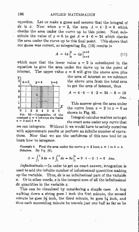
196 APPLIED MATHEMATICS
equation. Let us make a guess and assume that the integral of dx is x. Now when x = 2, the area A = 4 2 = 8 which checks the area under the curve up to this point. Next sub-stitute the value of x = 6 to get A = 4 • 6 = 24 which checks the area under the curve up to this final point. This shows that our guess was correct, so integrating Eq. (10) results in
A = 4x lb = 4x lx=6 a x=2
(11)
which says that the lower value x = 2 is substituted in the equation to give the area under the curve up to the point of interest. The upper value x = 6 will give the above area plus Y the area of interest so we subtract 5 a=2 y=4 b=6 the above area from the total area 4 to get the area of interest, thus
3
2 A = 4 • 6 — 4 • 2 = 24 — 8 = 16
Ans.
1 This answer gives the area under X the curve from x = 2 to x = 6 as 0 1 2
shown in Fig. 83. Fro. 83.—Integration of the constant y = 4 between the limits Integral calculus enables us to get a = 2 and b = 6. the exact area under any curve that we can integrate. Without it we would have to satisfy ourselves with approximate results or perform an infinite number of opera-tions. Now that we see the usefulness of this new tool let us learn how to integrate.
Example 4. Find the area under the curve y = 2 from a = 1 to b = 4. Solution. By Eq. (9),
3 4 5 6 7
4 4 4 A = 2 clx 21 dx 2x = 2 • 4 — 2 • 1 = 6 Ans.
Infinitesimals.—In order to get an exact answer, integration is used to add the infinite number of infinitesimal quantities making up the variable. Thus, dx is an infinitesimal part of the variable x. Or in other words, x is the integral sum of all the infinitesimal dx quantities in the variable x.
This can be visualized by considering a simple case. A bug walking down a string goes 1 inch the first minute, the second minute he goes AI inch, the third minute, he goes inch, and thus each succeeding minute he travels just one half as far as he
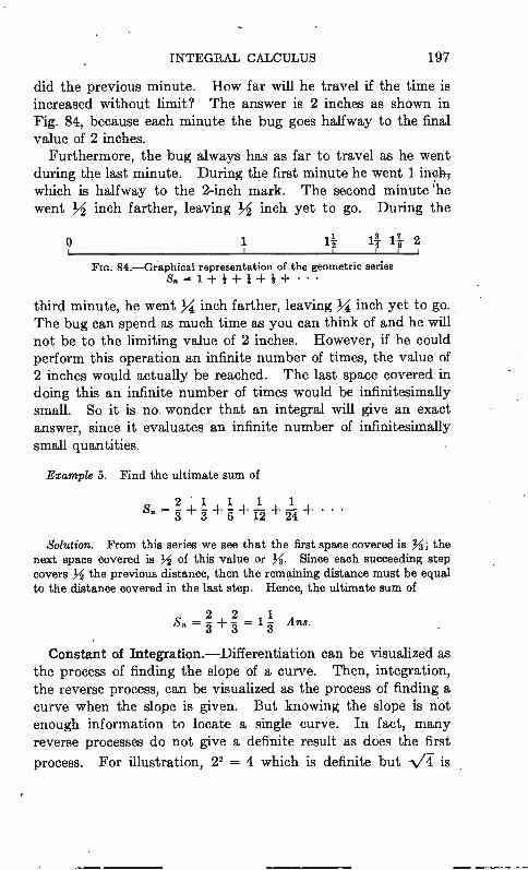
INTEGRAL CALCULUS 197
did the previous minute. How far will he travel if the time is increased without limit? The answer is 2 inches as shown in Fig. 84, because each minute the bug goes halfway to the final value of 2 inches.
Furthermore, the bug always has as far to travel as he went during the last minute. During the first minute he went 1 file, which is halfway to the 2-inch mark. The second minute 'he went AI inch farther, leaving 14 inch yet to go. During the
o 1-1
FIG. 84.—Graphical representation of the geometric series S. = 1 ± + I ± • • •
third minute, he went AI inch farther, leaving Yi inch yet to go. The bug can spend as much time as you can think of and he will not be to the limiting value of 2 inches. However, if he could perform this operation an infinite number of times, the value of 2 inches would actually be reached. The last space covered in doing this an infinite number of times would be infinitesimally small. So it is no wonder that an integral will give an exact answer, since it evaluates an infinite number of infinitesimally small quantities.
Example 5. Find the ultimate sum of
2 . 1 1 1 1 Sn=u+u -Ful-i-g-1-ii+ • • •
Solution. From this series we see that the first space covered is h; the next space covered is 34 of this value or h. Since each succeeding step covers 34 the previous distance, then the remaining distance must be equal to the distance covered in the last step. Hence, the ultimate sum of
Constant of Integration.—Differentiation can be visualized as the process of finding the slope of a curve. Then, integration, the reverse process, can be visualized as the process of finding a curve when the slope is given. But knowing the slope is not enough information to locate a single curve. In fact, many reverse processes do not give a definite result as does the first
process. For illustration, 22 = 4 which is definite but Vi is
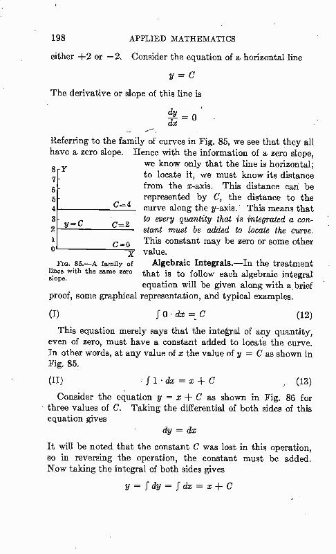
198 APPLIED MATHEMATICS
either +2 or —2. Consider the equation of a horizontal line
= C
The derivative or slope of this line is
dy _ o dx
Referring to the family of curves in Fig. 85, we see that they all have a zero slope. Hence with the information of a zero slope,
we know only that the line is horizontal; to locate it, we must know its distance from the x-axis. This distance can be
5 represented by C, the distance to the 4 C 4 curve along the y-axis. This means that 3 — =2 to every quantity that is integrated a con- y C c
2 stant must be added to locate the curve. 1 C-0 This constant may be zero or some other
x value. Algebraic Integrals.—In the treatment
that is to follow each algebraic integral equation will be given along with a brief
proof, some graphical representation, and typical examples.
8-Y
6
FIG. 85.—A family of lines with the same zero slope.
(I) f 0 • dx =_ C (12)
This equation merely says that the integral of any quantity, even of zero, must have a constant added to locate the curve. In other words, at any value of x the value of y = C as shown in Fig. 85.
(II) • f I • dx x C (13)
Consider the equation y=x-FC as shown in Fig. 86 for three values of C. Taking the differential of both sides of this equation gives
dy = dx
It will be noted that the constant C was lost in this operation, so in reversing the operation, the constant must be added. Now taking the integral of both sides gives
y = f dy = f dx = x C
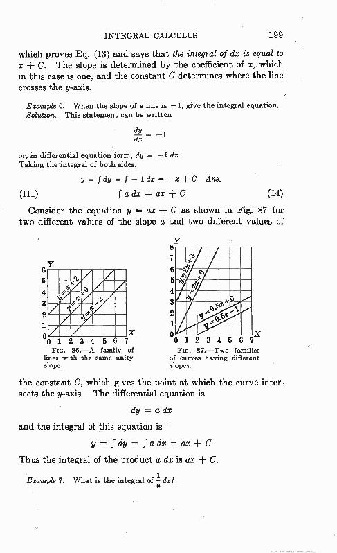
INTEGRAL CALCULUS 199
which proves Eq. (13) and says that the integral of dx is equal to x + C. The slope is determined by the coefficient of x, which in this case is one, and the constant C determines where the line crosses the y-axis.
Example 6. When the slope of a line is —1, give the integral equation. Solution. This statement can be written
dy _ dx
or, in differential equation form, dy = —1 dx. Taking the integral of both sides,
y dy = f — 1 d,x = — x C Ans.
(III) fadx=ax+C (14)
Consider the equation y -= ax +C as shown in Fig. 87 for two different values of the slope a and two different values of
SY
7
6 6
e x xel, o x
ct, ei, e
5 5
4 4
3 3
2 2
1 1 X 0 X
0 4 5 6 7 °O 1 2 3 4 5 6 7 Fm. 86.—A family of
lines with the same unity slope.
FIG. 87.—Two famil'es of curves having different slopes.
the constant C, which gives the point at which the curve inter-sects the y-axis. The differential equation is
dy = a dx
and the integral of this equation is
y = f dy = f a dx = ax + C
Thus the integral of the product a dx is ax + C.
Example 7. What is the integral of dx?
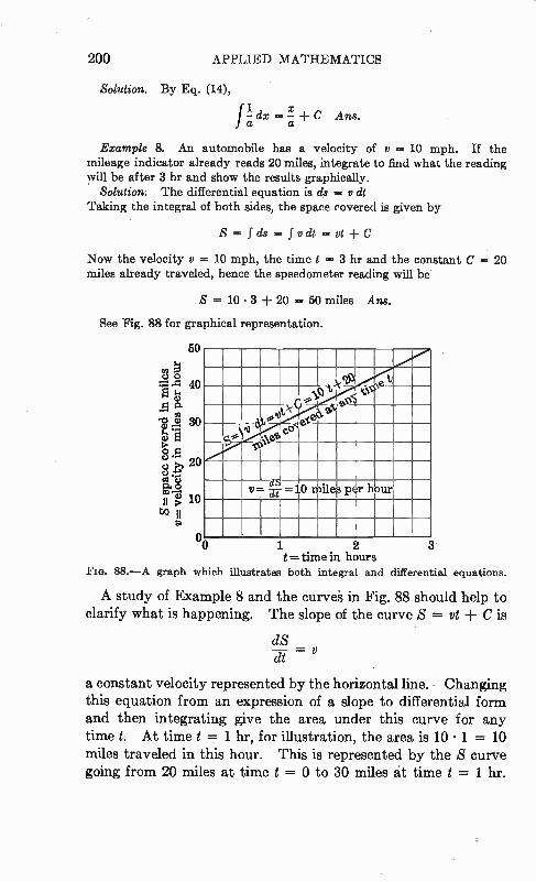
200 APPLIED MATHEMATICS
Solution. By Eq. (14),
fdx = + C Ans. a a
Example 8. An automobile has a velocity of y = 10 mph. If the mileage indicator already reads 20 miles, integrate to find what the reading will be after 3 hr and show the results graphically.
Solution. The differential equation is de =y dt Taking the integral of both sides, the space covered is given by
S= fds= fyd,t=et+C
Now the velocity y = 10 mph, the time t = 3 hr and the constant C = 20 miles already traveled, hence the speedometer reading will be
S = 10 • 3 -I- 20 = 50 miles Ans.
See Fig. 88 for graphical representation.
n
5 .'otk e
el0
0
al v= zi• =10 mile1 p r hour
0 0 1
t = time in hours FIG. 88.— A graph which illustrates both integral and differential equations.
A study of Example 8 and the curve's in Fig. 88 should help to clarify what is happening. The slope of the curve S = vt C is
dS = v
a constant velocity represented by the horizontal line. Changing this equation from an expression of a slope to differential form and then integrating give the area under this curve for any time t. At time t = 1 hr, for illustration, the area is 10 • 1 = 10 miles traveled in this hour. This is represented by the S curve going from 20 miles at time t = 0 to 30 miles at time t = 1 hr.
INTEGRAL CALCULUS 201
This S curve starts at 20 because the mileage indicator originally had that reading.
(IV) 1
f x dx = -2 x2 ± C (15)
Integral equations can be solved only if some function is known which yields the desired differential equation. The process is then to determine the differential equations for all known functions. Reversing the process and adding a constant will then give the desired integral equation. This we have done, giving the answer first, and then checking it by differentiation. Thus, let
Hence,
y = -1 x2 + C 2
dy = 2 (1) x dx = x dx Check. 2
1 y = f dy = f x dx =.5 x2 + C
Example 9. Solve f ax dx. Solution. Moving the constant a outside the integral sign and using
Eq. (15),
1 ax dx = a xdx = i o,x2 C Ans.
(V) xn dx - 1 xn+1 C n + 1 1
Let, y - n xn+1 +
Then, dy = xn dx
This checks the integral.
Hence, y = f dy = f xn dx n +1 i xn+' C
Example 10. Solve f x2 dx.
1 Solution. By Eq. (16) f x2 dx = 5 x3 ± C. Ans.
dx (VI) f x- dx = f — = ln x + C
(16)
(17)
202 APPLIED MATHEMATICS
This is an exceptional case to Rule V, because here we deal with infinite values for which Rule V does not apply. A search of derivatives will give a function, y = in x C the differential of which is
dy = -1 dx
so the problem is solved, and
y = f dy = f x-i dx = ln x C
This solution is a striking example of a problem that cannot be solved until the corresponding differentiation is found. This can be further illustrated by the differential equation
dy = a--x' dx
which even today has not been integrated because no one has found a-z2 when differentiating some other. function.
(VII) f (u v) dx = f u dx f y dx (18)
This merely states that the integral of an algebraic sum (u v) is the same as the sum of the integrals of u and v. This is a useful equation to reduce equations to standard forms which can be recognized and integrated.
Example 11. Find the integral of f(x ± 1)(x 2) dx. Solution. Multiplying, (x 1)(x + 2) = x2 + 3x + 2
Then, by Eq. (18),
f (x2 + 3x + 2) dx f x2 dx f3x dx f2 dx
(VIII)
1 3 - x' + C Ans. 3 2
fu dx = ux — fx du + C (19)
This is one of the most useful algebraic integrals and is known as "integration by parts." It says that if x du can be found then u dx can also be found. The equation can be derived as follows: The differential of a product is
d(uv) = u dv y du
Rearranging this equation,
u dv = d(uv) — v du
and integrating both sides of the equation results in
fu dv = uy — fv du -I- C (20)
INTEGRAL CALCULUS 203
This is the same as Eq. (19) but with y instead of x as the variable.
Example 12. Find fxex dx.
Solution. Let u = x dv = ex dx du = dx v =
Making these substitutions in Eq. (20) gives
Ans.
(IX) Eax dx = 1 -a eax C
Differentiating, d (7t 1 5ax _
Hence the above equation must be correct.
Example 13. The current in a circuit is given by the equation
. z = Tz (1 — e L )
What charge of electricity Q = fi, dt has passed through the circuit in t
seconds? Solution. Substituting for i,
Q = lEz- (1 — leg) dt
Q = fd — fe1tdt
Et EL — let + L +C Ans.
To make this a useful engineering answer, other information is needed to evaluate C.
Applying Eq. (18),
(21)
(X) flnxdx=x(lnx-1)+C (22)
To prove this, take the derivative
d (x ln x - 1) = x • x- 1 +ln x - 1 = in x Check.
(XI) f sin ax dx = 1 cos ax a
(23)
204 APPLIED MATHEMATICS
Taking the derivative of the answer,
d( _ _cos ax = _ -(1 1 , __ a) sin ax = sin ax Check. dx a a
Making a = 1 gives the answer for f sin x = - cos x -I- C
(XII) f cos ax dx = -1 sin ax + C (24) a
d 1 Similarly, ( -it sin ax) = COS ax Check.
(XIII) f tan ax dx = - -1 ln (cos ax) ± C (25) a
To prove this, write
sin ax 1 d(cos ax) f ax dx = — dx - cos ax aj cos ax
Now, by applying Eq. (17),
1 d(cos ax) 1 - ln (cos ax) C Check. aj cos ax a
Multiple Integrals.—We have already discussed partial differentiation when there were several variables. The inverse process is called partial integration. When making a partial integration all variables but one are held constant for the first integration and then in the second integration only one other variable is allowed to vary. This is continued until all the variables are allowed to vary during tlie integration. When performing multiple integration there are as many integral signs as there are variables to be integrated.
Consider the multiple integral
z = ff (x2 + Y2) dx dY (26)
Holding y2 and dy constant while integrating with respect to x,
z = f [f (x2 + y2) dx] dy = f [fx2 dx f y2 dx] dy = f [h x8 + y2x] dy
Now, holding xs and x constant while integrating with respect to y,
1 z = -1 xay + -3 ysx C
3 (27)
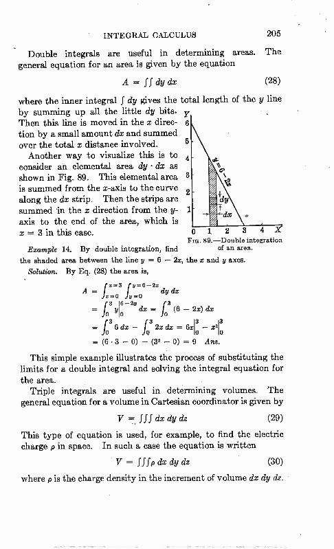
INTEGRAL CALCULUS 205
Double integrals are useful in determining areas. The general equation for an area is given by the equation
A = f f dy dx (28)
where the inner integral f dy gives the total length of the y line by summing up all the little dy bits. Y Then this line is moved in the x direc- 6 tion by a small amount dx and summed over the total x distance involved. 5
Another way to visualize this is to 4 consider an elemental area dy • dx as cP shown in Fig. 89. This elemental area 3 c-D is summed from the x-axis to the curve along the dx strip. Then the strips are summed in the x direction from the y-axis to the end of the area, which is x = 3 in this case.
Example 14. By double integration, find
the shaded area between the line y = 6 - 2x, the x and y axes.
Solution. By Eq. (28) the area is,
(x=3 ry = 6 — 2x A x=o iv-o dy dx
f3 16-2x 3 o dx fo (6 - 2x) dx
f r 3 6 dx - 2x dx 6x - x213 JO o o
= (6 • 3 - 0) - (32 - 0) = 9 Ans
This simple example illustrates the process of substituting the limits for a double integral and solving the integral equation for the area.
Triple integrals are useful in determining volumes. The general equation for a volume in Cartesian coordinator is given by
V =7. fff dx dy dz (29)
This type of equation is used, for example, to find the electric charge p in space. In such a case the equation is written
V --- fffp dx dy dz (30)
where p is the charge density in the increment of volume dx dy dz.
0 1 2 3 4 X Fio. 89.-.-Double integration
of an area.
206 APPLIED MATHEMATICS
Some of the more elementary ideas of calculus have been presented, to enable the reader to follow better the reasoning of authors who resort to calculus in their technical articles or books. Calculus can be considered as an art that is acquired only by continued study and by solving many problems. It is used as a practical tool by many research and desitn engineers. To those desiring to pursue the subject further, a few references are given along with a well known table of integrals. A short table of derivative and integral tables for ready reference will be found on page 308 in the appendix.
References
"Practical Calculus for Home Study," by Palmer, McGraw-Hill Book Company, Inc., New York.
"Differential and Integral Calculus," by Granville, Smith and Longley, Ginn and Company, Boston.
"A Short fable of Integrals," by B. O. Peirce, Ginn and Company, Boston. "Mathematical Tables;" by H. B. Dwight, McGraw-Hill Book Company,
Inc. • Exercises
1. Determine the average current of the sine curve i = sin cot by taking values every 10° up to 90° and using the trapezoidal rule.
2. Determine the average current I., of the sine curve i = sin cot by taking values every 15° up to 90° and using Simpson's rule.
8. Integrate the sine curve i = sin cot from cot = 0 to cot = ; radians
to determine the average current I a„. Compare the accuracy of the three methods used above to four decimal places.
4. Find the value of the series
Sn = 1 — + h — 31. + • • to eight terms.i
dx 5. Integrate 1— and fax dx.
x2
6. Integrate f2(x + 1) dx and f4(x2 ± 2)(x — 1) dx.
dx 7. Integrate i a2 —•
X 8. Integrate fx2ez dx
9. Integrate f cos 6cot d(£01) and 1162° dx.
10. Integrate fa ln (10x) dz.
CHAPTER 15
SERIES AND WAVE FORMS
The use of series makes possible the numerical solution of many problems that would otherwise be extremely difficult.
This chapter will deal with some of the more useful series and wave forms encountered in engineering work. Particular attention will be given to practical applications of power series and the use of Fourier's series to express wave forms.
Definitions.—A series is the sum of a sequence of terms. "Sequence" means that the terms are formed according to some fixed rule. Thus, the sequence of terms
1, 2, 3, 4, etc.
can be written into the series k=n
Sn = 1 + 2 + 3 + 4 + • • • ±k+ • • +n= k (I) k=1.
where S. -= a series of n terms. . k = a general or representative term in the series.
n = the last term. A. finite series has a limited number of terms. For illustration,
the series (a + b)3 = a' + 3a2b + 3ab2 + b3 (2)
is a finite series containing only four terms. An infinite series has an unlimited number of terms. The
fraction = 0.3 + 0.03 + 0.003 + 0.0003 + • • • (3)
is a good illustration of an infinite series when the fraction is expressed decimally because no matter how many decimal terms you add the sum will never quite reach the value of %. In other words, an infinite number of terms must be added to give the desired answer. A convergent series approaches a finite value as the number of
terms are increased. Equations (2) and (3) are convergent 207
208 APPLIED MATHEMATICS
series. Equation (2) reaches the final finite value with only four terms. A divergent series approaches an infinite value as the number of
terms is increased. Equation (1) is a divergent series because the sum of terms becomes increasingly large as the number n is made larger.
Example L Write down three more terms and the kth term, and also express as a summation, the series
S„ = 2 + 4 + 8 -I- 16 + • • •
Solution. It is noted that each succeeding term doubles. The second term is the square of the first term and the third term is the cube of the first term. Hence the desired series is
S„ = 2 + 4 + 8 + 16 + 32 + 64 + 128 + • • • k=n
± 2k ± • • • + 2k = E 2k Ans. k
Comparison Test for Convergence or Divergence.—Since .a converging series has a definite value, it is of far more practical importance than a diverging series. It is therefore important to know if the series is convergent or divergent. One of the simplest ways to test this is to compare the given series with a series that is known to converge. Two series are frequently used to apply this test. The geometric (or power) series
S„ --= a+ ax ax2 + • • • -I- ax.-1 a(1 — xn) a(xn — 1) 1 — x x — 1 (4)
converges when x is less than 1 and diverges when x is equal to or greater than 1. If x is less than 1, then x. will become very small as n is increased, hence xn can be neglected, with the result that the series converges to the value
Sn — a 1 — x
when x < 1 (5)
When x is greater than 1, the term xn in the last fraction of Eq. (4) becomes increasingly large as n is increased, with the result that no definite value can be given to the fraction. This means that the series is divergent for x > 1.
SERIES AND WAVE FORMS 209
When x equals 1, the series reduces to a sum of a terms. Hence as n is increased the sum will continue to increase. There-fore, the series is divergent when x = 1. The p series which is frequently used in the comparison test is
k=n
1 1 1 1 Sn = 1 + + • • • ± + • • • ± — = 1 (6) 2P 3P nP kP
k=1
which is convergent for p > 1 and divergent for p 1. The comparison test states that a given series converges if
corresponding terms are smaller than those of a converging series. Likewise, a given series diverges if corresponding terms are larger than those of a diverging series. Applying these rules and Eq. (4), let us see if the following
series is convergent:
9 = ± ( 9 \) 2
f(e) 1 F)" + • Then S„ = 1 x + x2 + • • • is the value of Eq. (4) when a = 1. Equating corresponding terms, x = % 0; hence x <.1 and the series converges by the comparison test.
Example 2. Test the following series for convergence or divergence.
k=
f(k) = 2 ()k
Solution. Comparing this series with Eq. (4) when a = 2 and x is less
than 1, we have
test series S. = 2 + 2x + 2x2 + 2x3 + • • • + 2x.
and given series f(k) = 2 + 2 ()2 + 2 (02 + 2 (1)2 + • • • + 2 ‘in" n
Comparing term by term, the first terms are equal, the second term of the given series is less than the second term of the test series when x is slightly less than 1, and so on for the rest of the terms, hence the series converges.
Ans. • Note: The given series could be shifted to the right one place so the
exponents would be similar; then the terms of the given series would all be less than corresponding terms of the test series with the exception of the first term of the given series. Since the first term is finte, the series must converge, because the rest of the series converges.
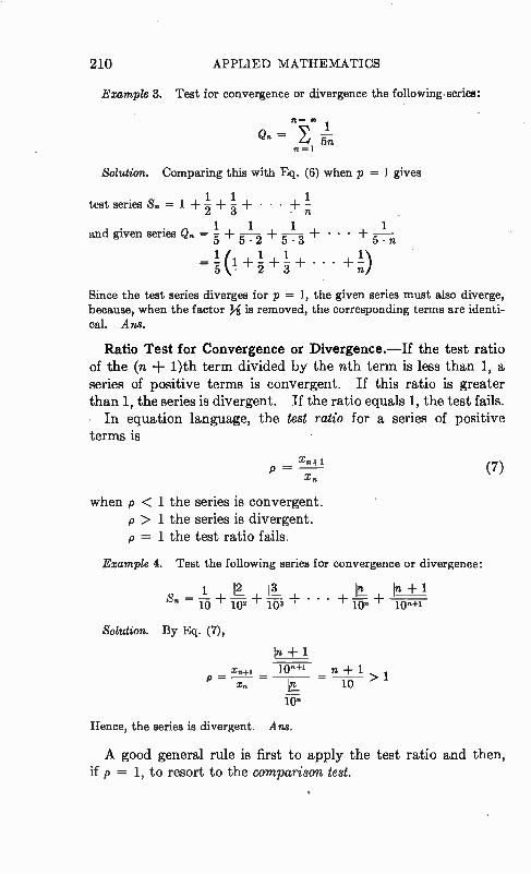
210 APPLIED MATHEMATICS
Example 3. Test for convergence or divergence the following•series:
Q. = n=1
Solution. Comparing this with Eq. (6) when p = 1 gives
1 1 1 test series S.=1±i-1-5+ • • • 7I-•
1 1 1 and given series Q. = + • • • +
Since the test series diverges for p = 1, the given series must also diverge, because, when the factor X is removed, the corresponding terms are identi-cal. Ans.
Ratio Test for Convergence or Divergence.—If the test ratio of the (n + 1)th term divided by the nth term is less than 1, a series of positive terms is convergent. If this ratio is greater than 1, the series is divergent. If the ratio equals 1, the test fails. • In equation language, the test ratio for a series of positive terms is
X18+1 p =
xn
when p < 1 the series is convergent. p > 1 the series is divergent. p = 1 the test ratio fails.
Example 4. Test the following series for convergence or divergence:
1 11 13 11 -F 1 S' Îö +i+103+ • • • + + 10"41
Solution. By Eq. (7),
fri + 1
x,.+L 10" 1-1 n 1 X. 10 > 1
'on
(7)
Hence, the series is divergent. Ans.
A good general rule is first to apply the test ratio and then, if p = 1, to resort to the comparison test.
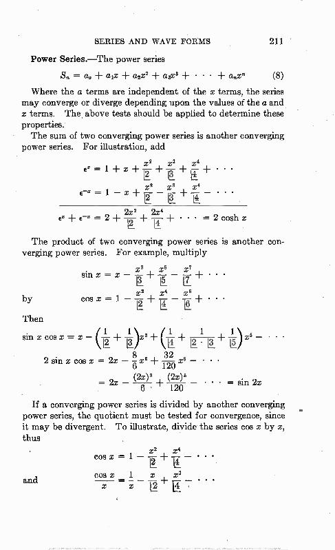
SERIES AND WAVE FORMS
Power Series.—The power series
Sn, = ac, aix a2x2 a8x3 + • • • -I- ccen
211
(8)
Where the a terms are independent of the x terms, the series may converge or diverge depending upon the values of the a and x terms. The above tests should be applied to determine these properties. The sum of two converging power series is another converging
power series. For illustration, add
2 X3 X4 ± e [4: ex=1-Fx+ 2- 11 2 8 x4
E-x = 1 — z + — v_t 2x2 21:4x: ,
2 cosh x
The product of two converging power series is another con-verging power series. For example, multiply
by
Then
X5 X5 X7 Sill X = X — — — — — ± • • •
11 É C_7_ X2 , x4 x6 ,
cos x 1 — — - - - • • • 1±
1 1 1 1 ± 1) _ sin x cos x = x — eg= -F — -F n •
8 32 2 sin x cos x = 2x — x3 wo x5 — • • •
(2x)8 (2x)5 = 2x — • • 120 • = sin 2x 6 •
If a converging power series is divided by another converging power series, the quotient must be tested for convergence, since it may be divergent. To illustrate, divide the series cos x by x, thus
and
cos x = 1 — —x2 -1-• -x4 - • • • [2_ cos x 1 x x3 X X E
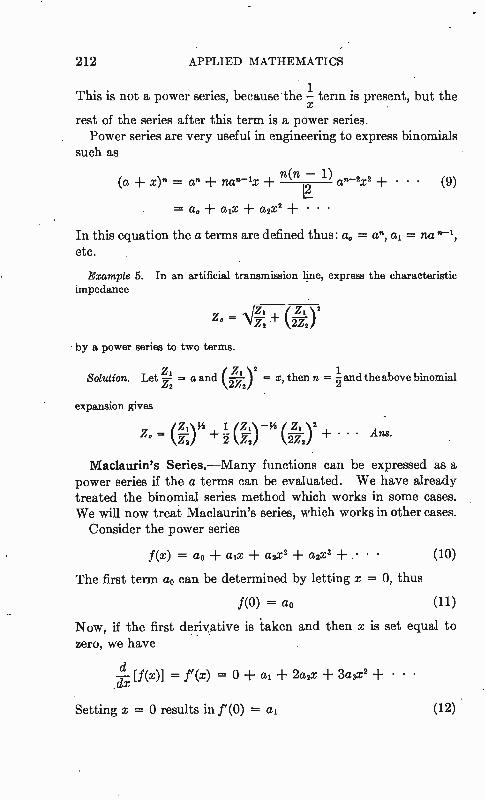
212 APPLIED MATHEMATICS
This is not a power series, because the !7 term is present, but the
rest of the series after this term is a power series. Power series are very useful in engineering to express binomials
such as
(a -I- x)n = -I- nan-le n(n — 1) an-2x2 . . . (9)
= a. + alx a2x2 + • • •
In this equation the a terms are defined thus: a. = a", al = na n-1, etc.
Example 5. In an artificial transmission line, express the characteristic impedance
Z. = 'Ne2• +'Z"
• by a power series to two terms.
Zi Z 1 Solution. Let — = a and k 7)2 n s, then - the above binomial
Z2 AZ,2 2
expansion gives
Z. (pyi (2Zziy . Ans.
Maclaurin's Series.—Many functions can be expressed as a power series if the a terms can be evaluated. We have already treated the binomial series method which works in some cases. We will now treat Maclaurin's series, which works in other cases.
Consider the power series
f(x) = ao aix a2x2 (ha' + • • • (10)
The first term ao can be determined by letting x = 0, thus
1(0) = ao (11)
Now, if the first derivative is taken and then x is set equal to zero, we have
d [f(x)] = (x) = O + a1 -F 2a2x 3a2x2 + • • •
Setting x = 0 results in f (0) = a (12)
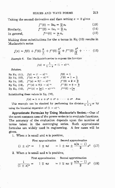
SERIES AND WAVE FORMS 213
'raking the second derivative and then setting x = 0 gives
f"(0) = 2a2 = 12 a2 (13)
Similarly, f"(0) = 6a3 =13_a3 (14)
In general, P.)(0) = Éan (15)
Making these substitutions for the a terms in Eq (10) results in Maclaurin's series
f(x) = f(0) + (0) x2 + f"(0) —12 + fm (0)
Example 6. Use Maclaurin's series to express the function
1 f(x)
Solution.
By Eq. (11), f(x) = (1 — x) -3 By Eq. (12), f (a) = (1 — x) -2
By Eq. (13), f"(x) = 2(1 — x)-3
By Eq. (14), f"(x) = 6(1 — x)-4
By Eq. (15), foo(x) = 1Li(1 —
- (1 _ x)-1.
f(0) = 1 f'(0) = 1 = 11
f"(0) = 2 =T2
ru(0) = 6 =
f (4) (0) .11
• (16)
Substituting these values in Eq. (16),
f(x) = 1 +x + x3 + • • • + een Ans. 1
This example can be checked by performing the division _ x or by
using the binomial expansion of (1 —
Approximate Formulas by Using Maclaurin's Series.—One of the most common uses of the power series is to evaluate functions. The accuracy of the evaluation depends upon the number of terms taken in the converging series. Such approximate formulas are widely used in engineering. A few cases will be given.
1. When x is small and n is positive,
First approximation Second approximation
(1 ± x). 1 + ni = 1 + nx + n(n — 1) x2 (17) 2
2. When x is small and n is positive,
First approximation Second approximation
1 n(n — 1) — 1 nx — 1 nx -T- 2 x2 (18)
(1 + x).
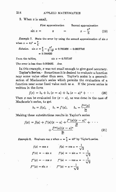
214 APPLIED MATHEMATICS
3. When x is small,
First approximation Second approximation
x3 sin x = x = x — (19)
Example 7. State the error by using the second approximation of sin x
when x = 45° = '-r•• 4
Solution. sin x = — = 0.785368 — 0.0807746 4 6 • 43
= 0.704622
From the tables, sin x = 0.707107
The error is less than 0.002485. Ans.
In this example, x was not small enough to give good accuracy. Taylor's Series.—Sometimes it is desired to evaluate a function
near some value other than zero. Taylor's series is a generali-zation of Maclaurin's series which permits the evaluation of a function near some fixed value such as a. If the power series is written in the form
f(x) = bo -F b1 (x — a) + b2 (x — a)2 + • • • (20)
Then x can be evaluated for (x — a), as was done in the case of Maclaurin's series, to get
bo = f(a), ,bi = f' (a), b„ —
Making these substitutions results in Taylor's series
f" (a)(x — a) 2 f(x) = f(a) f'(a)(x — a) -I- , + • • •
Le-f(n) (a)(x — a)n
f (n) (a)
Example 8. Evaluate cos x when a = = 45° by Taylor's series.
1 f(x) = cos x f(a) = cos a = vi-
f'(x) = — sin x f'(a) = — sin « = —
1 f"(re) — — cos x f"(a) = — cos a = — :ji
f"(x) = sin x .f"' (a) = ce = ..--./i•
(21)
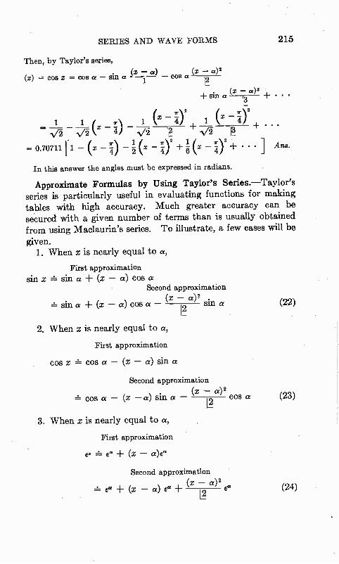
SERIES AND WAVE FORMS
Then, by Taylor's series,
(x) = cos x = cos a — sin a S-EL-- cos a
+ sin a — a)3
P.
1 1 1 tx—i) + 1 +
r 2 r 3
Vi V2.
= 0.70711 — — — — — 70 3 + • • I
In this answer the angles must be expressed in radians.
Approximate Formulas by Using Taylor's Series.— Taylor's series is particularly useful in evaluating functions for making tables with high accuracy. Much greater accuracy can be secured with a given number of terms than is usually obtained from using Maclaurin's series. To illustrate, a few cases will be
given. 1. When x is nearly equal to «,
First approximation sin x -A sin a ± (x — «) cos «
Second approximation
A sin a (x — a) cos a (x — a)2 . (22) 12 Sill a
215
2. When x is nearly equal to a,
First approximation
cos x COS a — (X — a) Sill a
Second approximation
cos a — (x —«) sin « (x — «)2
L? 3. When x is nearly equal to a,
First approximation
exa + (x - «)e
Second approximation
ea (x — a)2 ± — a) + L?.
cos a
Ans.
(23)
(24)
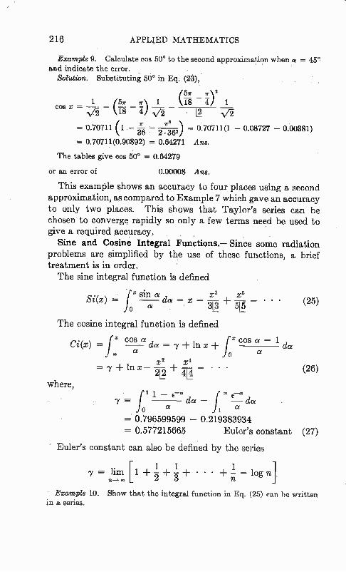
216 APPLIED MATHEMATICS
Example 9. Calculate cos 50° to the second approximation when a 45° and indicate the error. _ •
Solution. Substituting 50° in Eq. (28):
(571-,. \2
1 (57 \ 1 — 4) 1 COS =
•‘/Î ‘18 4/ Nr2 • )2 •‘/Î
= 0.70711 (1 - •-• 2 -;7-2) - 0.70711(1 - 0.08727 - 0.00381)
= 0.70711(0.90892) = 0.64271 Ans.
The tables give cos 50° = 0.64279
or an error of 0.00008 Ans.
This example shows an accuracy to four places using a second approximation, as compared to Example 7 which gave an accuracy to only two places. This shows that Taylor's series can be chosen to converge rapidly so only a few terms need be used to give a required accuracy.
Sine and Cosine Integral Functions.—Since some radiation problems are simplified by the use of these functions, a brief treatment is in order. The sine integral function is defined
l' a e sin a x3 x6 si(x) = da --= x — ug + 75, _ • • • (25) J°
cosine integral function is defined
ci(x) f e = e" a a da — 7 + ln x + f oe COS
X2 x 4 =- 7 ± x - — — - • • •
212 411 where,
a —
a
1 da
(26)
• f o u 1 — 5-« da — f " da 'Y = a a
• = 0.796599599 — 0.219383934 = 0.577215665 Euler's constant (27)
Euler's constant can also be defined by the series
1 1 1 -y [1 -Pid-u+ • • • + - log ni
n-+
Example 10. Show that the integral function in Eq. (25) can be written in a series.
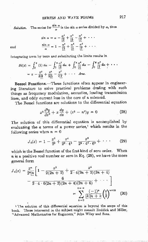
SERIES AND WAVE FORMS 217
sin a Solution. The series for — is the sin a series divided by a, thus a
and
sin a = a -5+5-5+.- sin a « 4 « 6
— 1 73 +5-77 4 . ..•
Integrating term by term and substituting the limits results in
x «4 x ce6 fet22, a • f —clot f — dct+ •
8i(x) = fox (1) deg r§a Jo IA Oil .
— X3 + 1-3 5 7 — - + • • • 21/28. 313 51_ . 7117.
Bessel Functions.—These functions often appear in engineer-ing literature to solve practical problems dealing with such things as frequency modulation, acoustics, loading transmission lines, and eddy current loss in the core of a solenoid. The Bessel functions are solutions to the differential equation
d2y dy x 2 ± (x 2 n2)y = O (28)
dx2 dx
The solution of this differential equation is accomplished by evaluating the a terms of a power series,' which results in the following series when n =
x2 x4 x6 Jo(x) — 1 22 ± 22 . 42 22 . 42 . 62 ± • • • (29)
which is the Bessel function of the first kind of zero order. When n. is a positive real number or zero in Eq. (28), we have the more general form
J(x) = [1 X2 x4
2(2n + 2) + 2 • 4(2n + 2)(2n + 4)
6 2 • 4 • 6(2n + 2)(2n + 4)(2n + 6)
k= — 1)k (er
= e ̀ 4 ik In k 2 k = 0
(30)
The solution of this differential equation is beyond the scope of this book. Those interested in the subject might consult Reddick and Miller, "Advanced Mathematics for, Engineers," John Wiley and Sons.
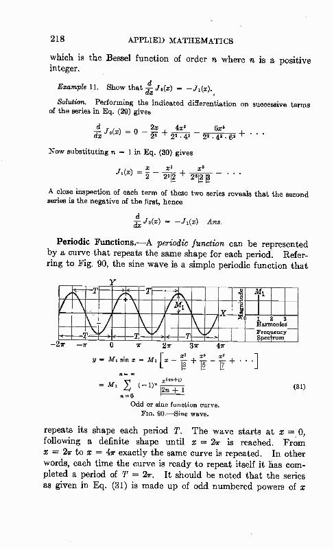
218 APPLIED MATHEMATICS
which is the Bessel function of order n where n is a positive integer.
d Example Jo(x) 11. Show that — J(x) —J1(x).
dx
Solution. Performing the indicated differentiation on successive terms of the series in Eq. (29) gives
d 2x 4x3 f3x3 — o(x) = O — 22 ± 22 • 42 22 • 42 • 62 + d,x
Now substituting n = lin Eq. (30) gives
x x3 , x5 2512 [?.
A close inspection of each term of these two series reveals that the second series is the negative of the first, hence
d —o (x) = — 11(x) Ans. dx
Periodic Functions.—A periodic function can be represented by a curve that repeats the same shape for each period. Refer-ring to Fig. 90, the sine wave is a simple periodic function that
M1 +
y —
—
(5 1 2 3 Harmonics_ Frequency ppectrum. >< >
— ir 27r 3v 47r
y = MI sin x = MI [x — — — — — + • xs xs xs
1.1
= M (-1)* pn + 1
n=0 Odd or sine function curve. FIG. 90.—Sine wave.
o
(31)
repeats its shape each period T. The wave starts at x = 0, following a definite shape until x = 2r is reached. From x = Zr to x = 47 exactly the same curve is repeated. In other words, each time the curve is ready to repeat itself it fias com-pleted a period of T = 2ir. It should be noted that the series as given in Eq. (31) is made up of odd numbered powers of x
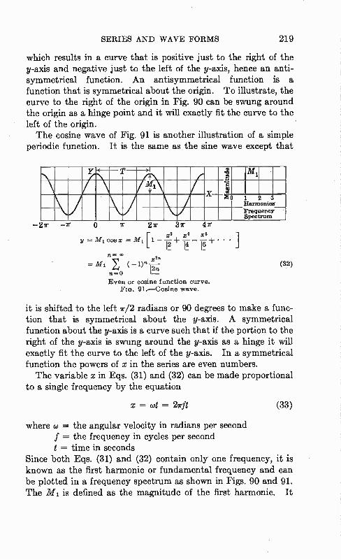
SERIES AND WAVE FORMS 219
which results in a curve that is positive just to the right of the y-axis and negative just to the left of the y-axis, hence an anti-symmetrical function. An antisymmetrical function is a function that is symmetrical about the origin. To illustrate, the curve to the right of the origin in Fig. 90 can be swung around the origin as a hinge point and it will exactly fit the curve to the left of the origin. The cosine wave of Fig. 91 is another illustration of a simple
periodic function. It is the same as the sine wave except that
Y T ---*1 41j a -e---
1111
x e.l. g e0 1
Harmonics' Frequency Spectrum
2 .
-
—ir o ir 2ir Sir 4r
X4 X6 y =Micosx = [1— Í1 2 +14 + • • • 2 lo
n=
M1 E (-1)" n —0
Even or cosine function curve. FIG. 91.— Cosine wave.
(3)
it is shifted to the left ir/2 radians or 90 degrees to make a func-tion that is symmetrical about the y-axis. A symmetrical function about the y-axis is a curve such that if the portion to the right of the y-axis is swung around the y-axis as a hinge it will exactly fit the curve to the left of the y-axis. In a symmetrical function the powers of x in the series are even numbers. The variable x in Eqs. (31) and (32) can be made proportional
to a single frequency by the equation
x = cut = Irft (33)
where co = the angular velocity in radians per second f = the frequency in cycles per second t = time in seconds
Since both Eqs. (31) and (32) contain only one frequency, it is known as the first harmonic or fundamental frequency and can be plotted in a frequency spectrum as shown in Figs. 90 and 91. The M 1 is defined as the magnitude of the first harmonic. It
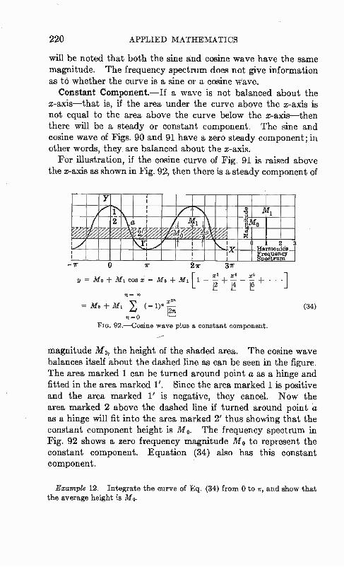
220 APPLIED MATHEMATICS
will be noted that both the sine and cosine wave have the same magnitude. The frequency spectrum does not give information as .6:5 whether the curve is a sine or a cosine wave.
Constant Component.—If a wave is not balanced about the x-axis—that is, if the area under the curve above the x-axis is not equal to the area above the curve below the x-axis--then there will be a steady or constant component. The sine and cosine wave of Figs. 90 and 91 have a zero steady component; in other words, they, are balanced about the x-axis. For illustration, if the cosine curve of Fig. 91 is raised above
the x-axis as shown in Fig. 92, then there is a steady component of
Y r r
1 0 31 .0 1 -t 1 eivi 0
i r 1 t X. Harmon
2 8 Cal 1
t 1 1 Frequency Spectrum
ir 27r 3/r x2 x4 x,
y = Mo MI cos x = Mo MI [1 — — + • • • É F.
91.. 0.
X" = MO + MI 1)" —
I2n 5000
no. 92.—Cosine wave plus a constant component.
(34)
magnitude M o, the height of the shaded area. The cosine wave balances itself about the dashed line as can be seen in the figure. The area marked 1 can be turned around point a as a hinge and fitted in the area marked 1'. Since the area marked 1 is positive and the area marked 1' is negative, they cancel. Now the area marked 2 above the dashed line if turned around point *a as a hinge will fit into the area marked 2' thus showing that the constant component height is M o. The frequency spectrum in Fig. 92 shows a zero frequency magnitude M o to represent the constant component. Equation (34) also has this constant component.
Example 12. Integrate the curve of Eq. (34) from 0 to ir, and show that the average height is Mo.
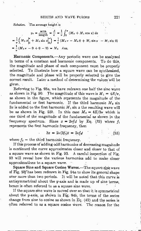
SERIES AND WAVE FORMS 221
Solution. The average height-is
area A 1 fir Yo length _ _ir Jo ° C°8 x) dx
= — (Mo X + M 1 sin an (Mo — Mo + M1 sin — sin CO ir ir 1
= — (Mo + — 0) = Mo Ans.
Harmonic Components.—Any periodic wave can be analyzed in terms of a constant and harmonic components. To do this, the magnitude and phase of each component must be properly selected. To illustrate how a square wave can be synthesized, the magnitude and phase will be properly selected to give the correct result. Later a method of determining the values will be given. .
Referring to Fig. 93a, we have redrawn one half the sine wave as shown in Fig. 90. The magnitude of this wave is 3/1 = 4E/7, as shown in the figure, which represents the magnitude of the fundamental or first harmonic. If the third harmonic M 3 sin 3x is added to the first harmonic M1 sin x the resulting wave will be as shown in Fig. 93b. In this case M 3 --= 4E/37 which is one third of the magnitude of the fundamental as shown in the •frequency spectrum. Since x = 27fit by Eq. (33) where h. represents the first harmonic frequency, then
3x = 27(3fi)t = 27f31 (35)
where fa = the third harmonic frequency. , If this process of adding odd harmonics of decreasing magnitude
is continued the curve approximates closer and closer to that of a square wave as shown in Fig. 93. A careful inspection of Fig. 93 will reveal how the various harmonics add to make closer approximations to a square wave. -
Square Sine and Square Cosine Waves.—The square sine wave of Fig. 93f has been redrawn in Fig. 94a to show its general shape over more than two periods. It will be noted that this curve is antisymmetrical about the y-axis and is made up of sine terms, hence is often referred to as a square sine wave.
If the square sine wave is moved over so that it is symmetrical about the y-axis, as shnwn in Fig. 94b-, the terms of the series change from sine to cosine as shown in Eq. (42) and the series is often referred to as a square cosine *ave. The reason for the
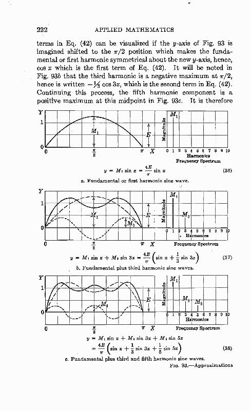
222 APPLIED MATHEMATICS
terms in Eq. (42) can be visualized if the y-axis of Fig. 93 is imagined shifted to the 7/2 position which makes the funda-mental or first harmonic symmetrical about the new y-axis, hence, cos x which is the first term of Eq. (42). It will be noted in Fig. 93b that the third harmonic is a negative maximum at ir/2, hence is written —% cos 3; which is the second term in Eq. (42). Continuing this process, the fifth harmonic component is a positive maximum at this midpoint in Fig. 93c. • It is therefore
Y
1
o o
Y
1
o
Y
1
o
M1
ir
fs;
r X 0 1 2 8 4 6 6 7 8 9 10 Harmonics
Frequency Spectrum
4E y = MI sin x = — sin x
a. Fundamental or first harmonic sine wave.
(36)
. a M1
.... . •..
‘ \ t ] §— MI
4'" ----, „. / /
/- ••••\8 3"
i 1 2 8Bil 5017 91
o X tir Frequency Spectrum
4E 1 y = MI sin x + Ms sin 3x — (sin x + —3 sin 3x)
b. Fundamental plus third harmonic sine waves.
(37)
0 1 2 8 4 5 6 7 8 9 1) Harmonics
0 .i. T X Frequency Spectrum 2
y = M1 sin z + Ma sin 3z + Ms sin 5x 1
= 4- (sin x + —3 sin 3x + 1 sin 5x) (38) r 5 e. Fundamental plus third and fifth harmonic sine waves.
Fie. 93.—Approximations
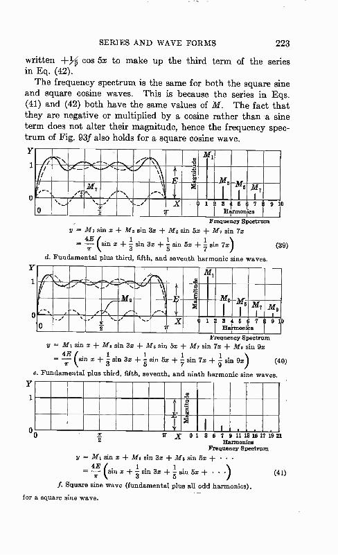
SERIES AND WAVE FORMS 223
written +h cos 5x to make up the third term of the series in Eq. (42). The frequency spectrum is the same for both the square sine
and square cosine waves. This is because the series in Eqs. (41) and (42) both have the same values of M. The fact that they are negative or multiplied by a cosine rather than a sine term does not alter their magnitude, hence the frequency spec-trum of Fig. 93f also holds for a square cosine wave.
Y
1
o
• ..-.„ ./ •ri
/ \ ‘
E
o ....
03g M 3
,"...\,
me
0 \../ .._,
\
X 2
, ,...... ,x
f
o 1 2 8 4 Harmonics
6 6 7 8 9 1
Y
1
o
Frequency Spectrum y = Mt sin x + Ma s n 3x + Ms sin 5x + M7 sin 7x + /1/9 sin 9x
1 1 1 1 = l!' . (sin x -I- - sin 3x + - sin 5x + - sin 7x + - sin 9x) (40) r 3 5 7 9
e. Fundamental plus third, fifth, seventh, and ninth harmonic sine waves.
Y
1
Frequency Spectrum , y --= Mt sin x + Mt sin 3x + Mt sin 5x + Mt sin 7x
4E1 . 1 1 1 = —ir (sin x -I- -3 sin 3x + - sin 5x + -7 sin 7x)
5 d. Fundamental plus third, fifth, and seventh harmonic sine waves.
(39)
• e •ts M 1
t _. .._/ .......
M9
\ \ E
:1.5.
.f.ç,. e
M 3_31-
.1 I 6 l
Mi I
M 9 I
0 ir 2
X f
0 1 2 8 4 Harmonics 1
5 6 7 8
1
9 1i
4
0 o 2E r X 0 1 8 5 7 9 11 13 15 17 19 21 2 Harmonics
Frequency Spectrum
y= Mt sin x + Mt sin 3x + Mt sin 5x + • • •
= (sin x + - sin 3x + - sin 5x + • • .) 3 5
4E 1
f. Square sine wave (fundamental plus all odd harmonics).
for a square sine wave.
(41)
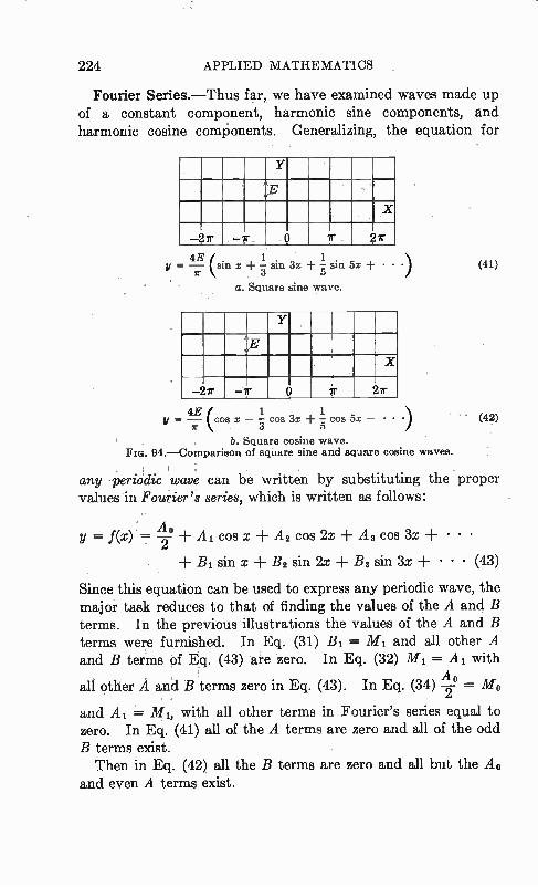
224 APPLIED MATHEMATICS
Fourier Series.—Thus far, we have examined waves made up of a constant component, harmonic sine components, and harmonic cosine components. Generalizing, the equation for
Y
A.E X
o ir ?ir 4 1 1
= E — sin x — sin 3x — sin 5x + • • .) 11- 3 5
a. Square sine wave.
Y
X
—27r —7r o 7r 2r
4E, V (COS — — COS 3x — cos 5x — • ")
r • 3 5 b. Square cosine wave.
94.—Comparison of square sine and square cosine waves.
(41)
' (42)
any periódic wave can be written by substituting the proper values in Fourier 's series, which is written as follows:
' Y = f(x) . = A —o + Ai cos x + A2 cos 2x + As cos 3x + • • • - 2
+ B1 sin x + B2 sin 2x + B3 sin 3x + • • • (43)
Since this equation can be used to express any periodic wave, the major task reduces to that of finding the values of the A and B terms. In the previous illustrations the values of the A and B terms were furnished. In Eq. (31) B1 = M 1 and all other A and B terms of Eq. (43) are zero. In Eq. (32) M 1 = A1 with
all other A and B terms zero in Eq. (43). In Eq. (34) A° = Mo 2
and A1 = M I, with all other terms in Fourier's series equal to zero. In Eq. (41) all of the A terms are zero and all of the odd B terms exist. Then in Eq. (42) all the B terms are zero and all but the 44.0
and even A terms exist.
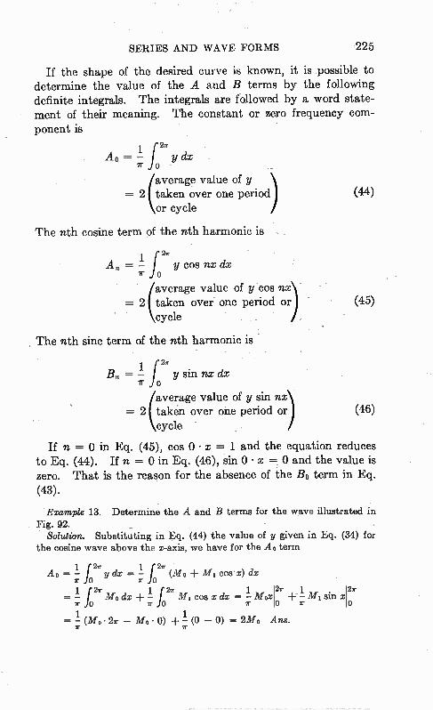
SERIES AND WAVE FORMS 225
If the shape of the desired curve is known, it is possible to determine the value of the A and B terms by the following definite integrals. The integrals are followed by a word state-ment of their meaning. The constant or zero frequency com-
ponent is
1 2e AO = f — y dx 71" o
/average value of y = 2 taken over one period
or cycle
The nth cosine term of the nth harmonic is
(44)
1 f 21. A. = — y cos nx dx
ir o
/average value of y cos nx = 2 taken over one period or . (45)
cycle
, The nth sine term of the nth harmonic is •
1 f 2r B. = — y sin nx dx
ir o
( in average value of y s nx = 2 taken over one period or (46)
cycle
If n = 0 in Eq. (45), cos 0 • x = 1 and the equation reduces to Eq. (44). If n = 0 in Eq. (46), sin 0 • x -= 0 and the value is zero. That is the reason for the absence of the Bo term in Eq. (43).
Example 13. Determine the A and B terms for the wave illustrated in Fig. 92. _
Solution. Substituting in Eq. (44) the value of y given in Eq. (34) for the cosine wave above the x-axis, we have for the A. 0 term
Ao = 21. dx "f lr (Mo ± M1 cos- x) dx r o o
= 1.2w Mo dx f Mit COO x dx = Moxl2r + -I- M 1 sin xi . e ir ir 0 ir 0
1 1 = — (Mo• 27r — M o • 0) — (0 — 0) = 2Mo Ans.
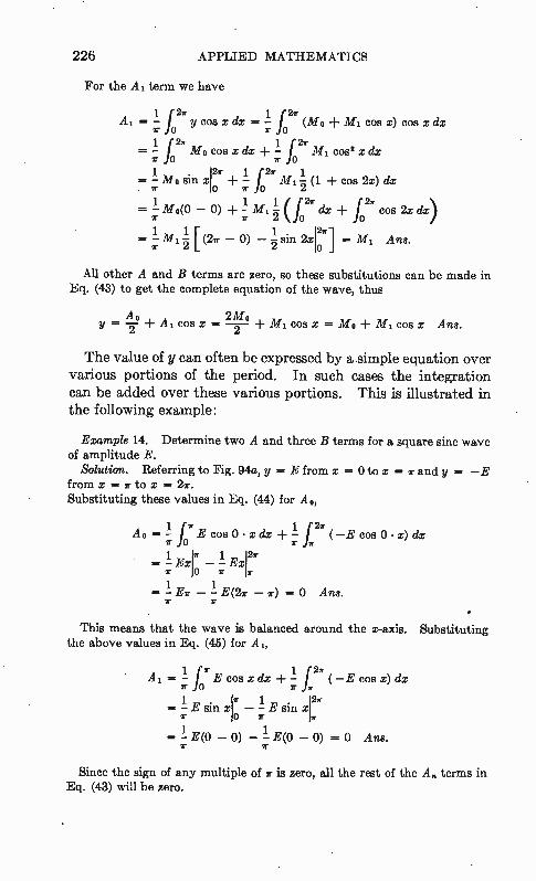
226 APPLIED MATHEMATICS
For the A1 term we have
j2 w Al = 1 - y cos x dx = -1 f 27 (Mo + M 1 cos x) cos x dx
w w o 11 2or
= - Mo cos x dx + -1 f M I COS2 x dx Ir 0 7 0
.= 1 mo sin x12. i +_1 . 2. mi 1 o ir 2 (1 -F cos 2x) dx r
= 1 mo _ 0\ '- _L _1 m 1 1 i pr dx + f h 2w cos 2x dx) r ' T 2 vh 1 - M I 1 - [ (27 - 0) - -l oin 2x1221 = M I Ans. Ir 2 2
AR other A and B terms are zero, so these substitutions can be made in Eq. (43) to get the complete equation of the wave, thus
Ao 2M0 y = — .41. 1 COS X = — M I COS X = o ± Mi. CO8 x Ans.
2 2
The value of y can often be expressed by a simple equation over various portions of the period. In such cases the integration can be added over these various portions. This is illustrated in the following example:
Example 14. Determine two A and three B terms for a square sine wave of amplitude E.
Solution. Referring to Fig. 94a, y = E from x = 0 to x = ir and y = -E from x = ir to x Substituting these values in Eq. (44) for Ao,
Ao= 1 F T ECOSO•XdX+ 1 1 2 (-E cos 0 • x) dx ir 71"
= — Ex — Exl2e r Or
1 1 = - Er - - E(2r - 7) = 0 Ans.
7r
• This means that the wave is balanced around the x-axis. Substituting
the above values in Eq. (45) for A1,
1 jar 1 12ir A1 = - E cos x dx + - (-E cos x) dx
7r 0 7 T
e 1 127 .... —1 E sin xi - - E sin x y 0 ir .-
= 1 E(0 - 0) - -1 E(0 - 0) = 0 Ans. Ir 7r
Since the sign of any multiple of ir is zero, all the rest of the A» terms in Eq. (43) will be zero.
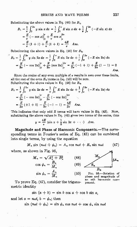
SERIES AND WAVE FORMS 227
Substituting the above values in Eq. (46) for B1,
1 E l =•• 127 ysm . xdx = - 1 7 - f E sin x dx + -1 f lr ( -E sin z) dx w o 7r o ir ir
y E 2ir = -E (- cos x)i + - cos x
ir 0 ir lir 4E
Ans. 7 ir y
Substituting the above values in Eq. (46) for Bs,
By = 1 21. II Sin 2x dx = E sin 2x dx + V 22. (-E sin 2x) dx r o 70 T
E w E 21r E E = (- cos 2x)10 + 27i. (cos 2x)I = — (-1 + 1) + rr (1 - 1) = 0
24r Ans.
Since the cosine of any even multiple of 7 results in zero over these limits, all the rest of the even B. terms in Eq. (43) will be zero. Substituting the above values in Eq. (46) for By,
By = 1 12r y sin 3x de = 1 17 .E sin 3x dx + -11 21. ( - E sin 3x) dx r 0 7 0 ir E — (- cos 3x)lw - —E (- cos 3x) 122. 37r o 32- E 4E = Fr (+1 + 1) - —E (-1 - 1) = — Ans.
3r
This indicates that only odd B terms will have values in Eq. (43). Now, substituting the above values in Eq. (43) gives two terms of the series, thus
4E 1 y = — (sin x + -3 sin 3x + • • .) Ans.
Magnitude and Phase of Harmonic Components.—The corre-sponding terms in Fourier's series of Eq. (43) can be combined into single terms, by using the equation
ilf„ sin (nwt + = An cos net ± B. sin nod (47)
where, as shown in Fig. 95,
= VA! ± Be, (48) B.
cos = (49)
An sin in = (50) FIG. 95.—Relation of
phase and magnitude of an nth harmonic corn-
To prove Eq. (47), consider the trigono- ponent.
metric identity
sin (a + b) = sin b cos a + cos b sin a,
and let a = not, b = 1P„; then
sin (nwt -I- en) = sin gin cos ned + 008 ifrn sin not
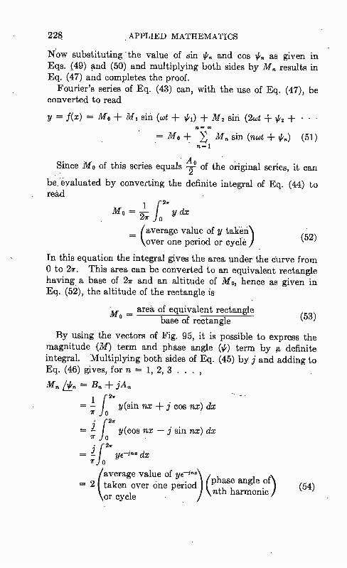
228 APPLIED MATHEMATICS
Now substituting the value of sin tii„ and cos 1/4, as given in Eqs. (49) and (50) and multiplying both sides by Mn results in Eq. (47) and completes the proof.
Fourier's series of Eq. (43) can, with the use of Eq. (47), be converted to read
= Ax) = Mo M1 sin (cot ± %Pi) + M2 sin (2wt + 4/2 + • • • n =
= M o Mn sin (mot ip„) (51)
Since M o of this series equals 4 9 of the original series, it can
be. evaluated by converting the definite integral of Eq. (44) to read
Mo = 1 f 2'r y dx 27r o
(average value of y takén\ (52) over one period or cycle
In this equation the integral gives the area under the curve from 0 to 27. This area can be converted to an equivalent rectangle having a base of 27 and an altitude of M o, hence as given in Eq. (52), the altitude of the rectangle is
area of equivalent rectangle Mo — (53) base of rectangle
By using the vectors of Fig. 95, it is possible to express the magnitude (M) term and phase angle (#) term by definite integral. Multiplying both sides of Eq. (45) by j and adding to Eq. (46) gives, for n --- 1, 2, 3 . .
Ms = B. ± jAn
1 = — f y(sin nx j cos nx) dx
11 Jo
f 27 y(cos nx — j sin nx) dx 1r 0
...= i 2. 7 fo ye-inz dx
( average value of ye-in. taken over one period) ( nilsee angle of\ = 2
nth harmonic ) or cycle (54)
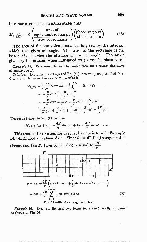
SERIES AND WAVE FORMS 229
In other words, this equation states that
( area of ¡¡ii,,,,My, = 2 equivalent rectangle) (phase angle of\ (55) nth harmonic ;
base of rectangle
The area of the equivalent rectangle is given by the integral, which also gives an angle. The base of the rectangle is 2er, hence M„ is twice the altitude of the rectangle. The angle given by the integral when multiplied by j gives the phase term.
Example 15. Determine the first harmonic term for a square sine wave of amplitude E.
Solution. Dividing the integral of Eq. (54) into two parts, the first from 0 to or and the second from ir to 2w, results in
T • 2. mibpi =4 EE— ie dx + 1 — Eei. dx o
— — C-11 — ir 10 ir e
r 7
E 4E
The second term in Eq. (51) is then
4E 4E M I sin (ait #,) = — sin (wt ± 0) = — sin oit Ans.
11"
This checks the s^lution for the first harmonic term in Example 14, which used x in place of wt. Since = 00, the j component is
4E absent and the B„ term of Eq. (54) is equal to —
Y
2irk E
X
2r
y = kE (sin irk cos x —1 sin 2rk cos 2x 4- • • .) 2
n =
kE + 1 sin nrk cos nx ir z n
n-1 FIG. 96.—Short rectangular pulse.
(56)
Example 16. Evaluate the first two terms for a short rectangular pulse as shown in Fig. 96.
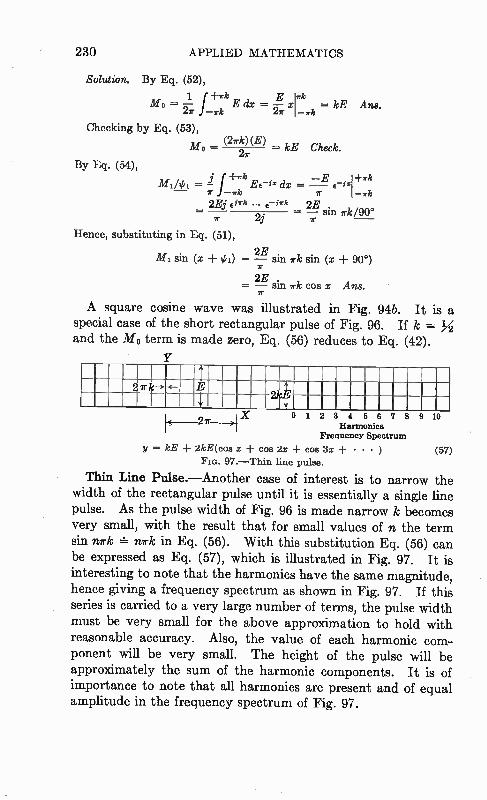
230 APPLIED MATHEMATICS
Solution. By Eq. (52),
1 f +irk E Irk Mo = E = 27; x kE Ans.
Checking by Eq. (53), ark)(E)
0 = = kE Check. 27r
By Eq. (54),
M del = f +7k Ee-tx dx = -E e —ir 1 7k
2Ej eivk - 2jeirk - 2E sin irk/90°
Hence, substituting in Eq. (51),
MI sin (x #i) = sin irk sin (x + 90°) I. 2E — sin irk cos x Ans. ir
A square cosine wave was illustrated in Fig. 94b. It is a special case of the short rectangular pulse of Fig. 96. If k = and the M o term is made zero, Eq. (56) reduces to Eq. (42).
Y
E I +
1 X 0 1 2 3 4 5 6 7 8 *---27r > Harmonics
Frequency Spectrum y = kE 2kE(cos X -I- cos 2x + cos 3x + • • • ) (57)
FIG. 97.—Thin line pulse.
Thin Line Pulse.—Another case of interest is to narrow the width of the rectangular pulse until it is essentially a single line pulse. As the pulse width of Fig. 96 is made narrow k becomes very small, with the result that for small values of n, the term sin nrk nrk in Eq. (56). With this substitution Eq. (56) can be expressed as Eq. (57), which is illustrated in Fig. 97. It is interesting to note that the harmonics have the same magnitude, hence giving a frequency spectrum as shown in Fig. 97. If this series is carried to a very large number of terms, the pulse width must be very small for the above approximation to hold with reasonable accuracy. Also, the value of each harmonic com-ponent will be very small. The height of the pulse will be approximately the sum of the harmonic components. It is of importance to note that all harmonics are present and of equal amplitude in the frequency spectrum of Fig. 97.
9 10

SERIES AND WAVE FORMS 231
Exercises
1. Write the nth term for the series
and test the series for convergence or divergence. 1 1 1
2. Test the series S. = (yip ± (op +
for convergence or divergence and write the nth term. 1 1 1
3. Test ratio the series S. = 1 -I- g -I- g + • • •
4. Find the approximate value of V .87 by applying the binomial series. 5. Expand the function sin x into a series.
•
sin x 6. What is the third approximation value of 1 — x?
7. Give the second approximation value of e2.1 when e2 .= 7.3891 and note the error.
8. Determine the third harmonic term for a square sine wave of ampli-tude E.
9. Evaluate the second harmonic of a scanning voltage when the wave form is
E y = — x from to -Hr.
ir
10. An antisymmetrieal sawtooth wave has the following wave form:
2E ir y — x from — +11 22E ir 2
y = .2E — x from to 1;.
Determine the first harmonic term in the series.

I
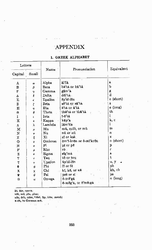
APPENDIX
1. GREEK ALPHABET
Letters Name Pronunciation Equivalent
Capital Small
A « Alpha tillà a
B 13 Beta betis. or Wtá b
r -y Gamma Om% g A 8 Delta déPtit d
E e Epsilon épielén e (short)
Z r Zeta zetà or MU. z
H n Eta é'tà, or AU e (long)
e O Theta theta or thA'tà, th
I t Iota 1-ietà i
K k Kappa kgp'à k, 0
A X Lambda litm'dà 1
M N
ii V
Mu Nu
mn, mc7), or mtl nù or nü
m n •
Z. E xi zI or ksé x
0 0 Omicron 6m1-krÔn or 23-mIltrÔn o (short)
II ir Pi pi or pé p P p Rho ri5 r
Z cr Sigma sIg'init s
T r Tau tó or t,ou t
T u Upsilon tip's1-1,5n u, y ..
.1> e Phi fl or fé ph
X X Chi kI, ké, or ICA kh, ch
‘I, n
Ifr 0
Psi Omega
psé or Ed te-megà
>Ps o (long)
6-még'à, or erne...et
At, OM, opera; 'At, me, pin, pine; Mg, Orb, náte, f cród, up, lute, menit; s-oh, in German act: •
233
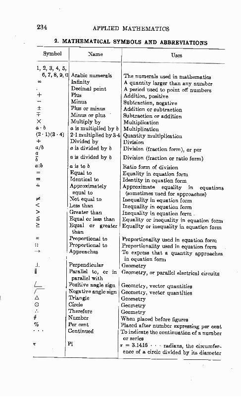
234 APPLIED MATHEMATICS
2. MATHEMATICAL SYMBOLS AND ABBREVIATIONS
Symbol Name Uses
1, 2, 3, 4, 5, 6, 7, 8, 9, 0
00
•
X a • b (2 • 1)(3 • 4)
a/b a
a:b
Arabic numerals Infinity Decimal point Plus Minus Plus or minus Minus or plus Multiply by a is multiplied by b 2.1 multiplied by 3.4 Divided by a is divided by b
a is divided by b
a is to b Equal to Identical to Approximately equal to Not equal to Less than Greater than Equal or less than Equal or greater than
Proportional to Proportional to Approaches
Perpendicular II Parallel to, or in
parallel with Positive angle sign Negative angle sign Triangle
0 Circle Therefore Number Per cent
. . . Continued
Pi
The numerals used in mathematics A quantity larger than any number A period used to point off numbers Addition, positive Subtraction, negative Addition or subtraction Subtraction or addition Multiplication Multiplication Quantity multiplication Division Division (fraction form), or per
Division (fraction or ratio form)
Ratio form of division Equality in equation form Identity in equation form Approximate equality in equations (sometimes used for approaches)
Inequality in equation form Inequality in equation form Inequality in equation form. Equality or inequality in equation form Equality or inequality in equation form
Proportionality used in equation form Proportionality used in equation form To express that a quantity approaches in equation form Geometry Geometry, or parallel electrical circuits
Geometry, vector quantities Geometry, vector quantities Geometry Geometry Geometry When placed before figures Placed after number expressing per cent To indicate the continuation of a number or series r = 3.1416 • • • radians, the circumfer-ence of a circle divided by its diameter
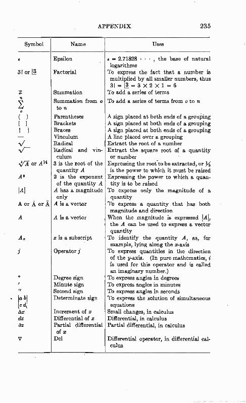
APPENDIX 235
Symbol Name Uses
e
3! or 11
1±
( ) [ 1 1
NY-A- or tei
A2
IA!
A or A or ji
A
A.
a
a b cd Ax dx ax
V
Epsilon
Factorial
Summation
Summation from o ton
Parentheses Brackets Braces Vinculum Radical Radical and vin-culum 3 is the root of the quantity A 2 is the exponent of the quantity A A has a magnitude only A is a vector
A is a vector
x is a subscript
Operator j
Degree sign Minute sign Second sign Determinate sign
Increment of x Differential of x Partial differential of x Del
6 = 2.71828 • • • , the base of natural logarithms To express the fact that a number is multiplied by all smaller numbers, thus = = 3 X 2 X 1 = 6
To add a series of terms
To add a series of terms from o to n
A sign placed at both ends of a grouping A sign placed at both ends of a grouping A sign placed at both ends of a grouping A line placed over a grouping Extract the root of a number Extract the square root of a quantity or number Expressing the root to be extracted, or is the power to which it must be raised Expressing the power to which a quan-tity is to be raised To express only the magnitude of a quantity To express a quantity that has both magnitude and direction When the magnitude is expressed !Alt the A can be used to express a vector quantity To identify the quantity A, as, for example, lying along the x-axis To express quantities in the direction of the y-axis. (In pure mathematics, i is used for this operator and is called an imaginary number.) To express angles in degrees To express angles in minutes To express angles in seconds To express the solution of simultaneous equations
Small changes, in calculus Differential, in calculus Partial differential, in calculus
Differential operator, in differential cal-culus
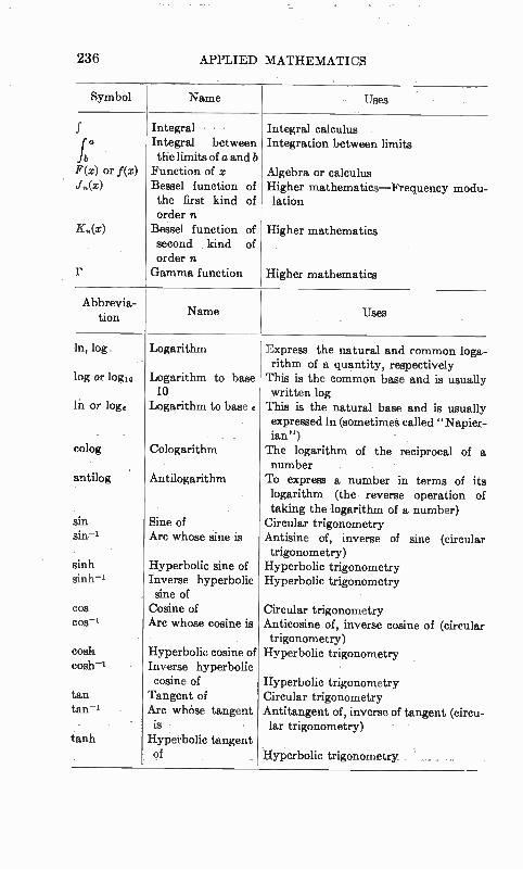
236 APPLIED MATHEMATICS
Symbol
K(x)
Name Uses
Integral Integral between the limits of a and b Function of x Bessel function of the first kind of order n
Bessel function of second . kind of order n Gamma function
Integral calculus Integration between limits
Algebra or calculus Higher mathematics—Frequency modu-lation
Higher mathematics
Higher mathematics
Abbrevia-tion
ln, log
log or log ic
in or log6
colog
antilog
sin sin-1
sinh sinh-1
cos
cos-1
cosh cosh-1
tan tan-1
ianh
Name Uses
Logarithm
Logarithm to base 10
Logarithm to base E
Cologarithm
Antilogarithm
Sine of Arc whose sine is
Hyperbolic sine of inverse hyperbolic sine of Cosine of Arc whose cosine is
Hyperbolic cosine of Inverse hyperbolic cosine of Tangent of Arc wheese tangent is Hyperbolic tangent
of
Express the natural and common loga-rithm of a quantity, respectively This is the common base and is usually written log This is the natural base and is usually expressed ln (sometimes called " Napier-ian") The logarithm of the reciprocal of a number To express a number in terms of its logarithm (the reverse operation of taking the logarithm of a number)
Circular trigonometry Antisine of, inverse of sine (circular trigonometry) Hyperbolic trigonometry Hyperbolic trigonometry
Circular trigonometry Anticosine of, inverse cosine of (circular trigonometry) Hyperbolic trigonometry
Hyperbolic trigonometry Circular trigonometry Antitangent of, inverse of tangent (circu-lar trigonometry)
Hyperbolic trigonometry
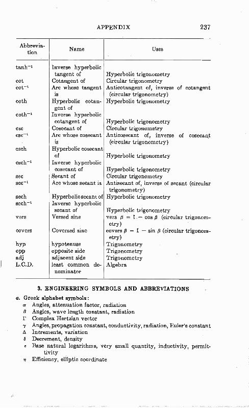
Abbrevia-tion
tanh-1
cot cot-1
coth
coth-1
ese
ese-1
csch
csch-1
sec sec-1
sech sech-1
vers
covers
hYP oPP adj L. C.D.
APPENDIX
Name
Inverse hyperbolic tangent of Cotangent of Arc whose tangent is Hyperbolic cotan-gent of
Inverse hyperbolic cotangent of Cosecant of Arc whose cosecant is
Hyperbolic cosecant of Inverse hyperbolic cosecant of Secant of Arc whose secant is
Hyperbolic secant of Inverse hyperbolic secant of Versed sine
Coversed sine
hypotenuse opposite side adjacent side least common de-nominator
237
Uses
Hyperbolic trigonometry Circular trigonometry Anticotangent of, inverse of cotangent (circular trigonometry)
Hyperbolic trigonometry
Hyperbolic trigonometry Circular trigonometry Anticosecant of, inverse of cosecant (circular trigonometry)
Hyperbolic trigonometry
Hyperbolic trigonometry Circular trigonometry Antisecant of, inverse of secant (circular trigonometry) Hyperbolic trigonometry
Hyperbolic trigonometry vers /3 = 1 — cos /3 (circular trigonom-etry)
covers p = 1 - sin e (circular trigonom-etry) Trigonometry Trigonometry Trigonometry Algebra
3. ENGINEERING SYMBOLS AND ABBREVIATIONS
a. Greek alphabet symbols: « Angles, attenuation factor, radiation 13 Angles, wave length constant, radiation I' Complex Hertzian vector y Angles, propagation constant, conductivity, radiation, Euler's constant à Increments, variation
Decrement, density e Base natural logarithms, very small quantity, inductivity, permit-
tivity n Efficiency, elliptic coordinate
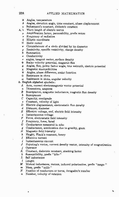
238 APPLIED MATHEMATICS
• Angles, temperature O Angles, elevation angle, time constant, phase displacement K Boltzmann's constant, dielectric constant
A, X Wave length of electric waves • Amplification factor, permeability, prefix micro le Frequency of radiation k Elliptic coordinate II Hertz vector y Circumference of a circle divided by its diameter p Resistivity, specific resistivity, charge density Z Summation • Conductivity T angles, tangent vector, surface density • Scalar velocity potential, magnetic flux ft. Angles, flux, power factor angle, true azimuth, electric potential • Magnetic susceptibilities * Angles, phase difference, scalar function • Resistance in ohms co Resistance in ohms, angular velocity
b. English alphabet symbols: A Area, current electromagnetic vector potential a Dimensions, amperes B Susceptance, magnetic inductance, magnetic flux density b Susceptance C Capacity, centigrade c Constant, velocity of light D Electric displacement, electrostatic flux density d Distance, diameter E Effective voltage, emf, electric field intensity e Instantaneous voltage F Force, electrostatic field intensity f Frequency, force, farad G Conductance measured in mho g Conductance, acceleration due to gravity, gram H Magnetic field intensity h Height, Plank's constant, henry I Effective current i Instantaneous current • Poynting's vector, current density vector, intensity of magnetization j Operator K Constant, dielectric constant, stacking factor k Susceptibility, prefix "kilo-" L Self inductance 1 Length M Mutual inductance, meters, induced polarization, prefix "mega-" m Mass, prefix "milli-" N Number of conductors or turns, Avogadro's number n Number, velocity of rotation
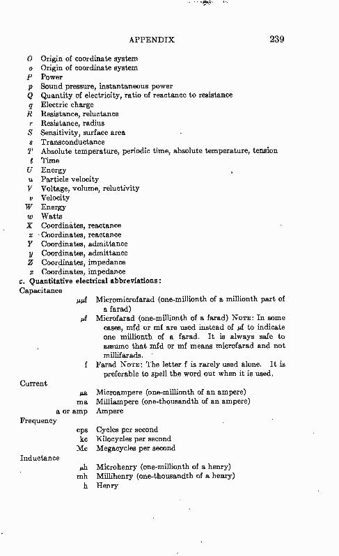
APPENDIX 239
O Origin of coordinate system o Origin of coordinate system P Power p Sound pressure, instantaneous power Q Quantity of electricity, ratio of reactance to resistance q Electric charge R Resistance, reluctance ✓ Resistance, radius S Sensitivity, surface area s Transconductance T Absolute temperature, periodic time, absolute temperature, tension t Time U Energy u Particle velocity ✓ Voltage, volume, reluctivity • Velocity W Energy w Watts X Coordinates, reactance • Coordinates, reactance Y Coordinates, admittance y Coordinates, admittance Z Coordinates, impedance z Coordinates, impedance
c. Quantitative electrical abbreviations: Capacitance
ppf Micromicrofarad (one-millionth of a millionth part of a farad)
,if Microfarad (one-millionth of a farad) Nom: In some cases, mf d or mf are used instead of if to indicate one millionth of a farad. It is always safe to assume that mfd or mf means microfarad and not millifarads.
f Farad Nom: The letter f is rarely used alone. It is preferable to spell the word out when it is used.
Current aa Microampere (one-millionth of an ampere) ma Milliampere (one-thousandth of an ampere)
a or amp Ampere Frequency
cps Cycles per second kc Kilocycles per second Mc Megacycles per second
Inductance ph Microhenry (one-millionth of a henry) mh Millihenry (one-thousandth of a henry) h Henry
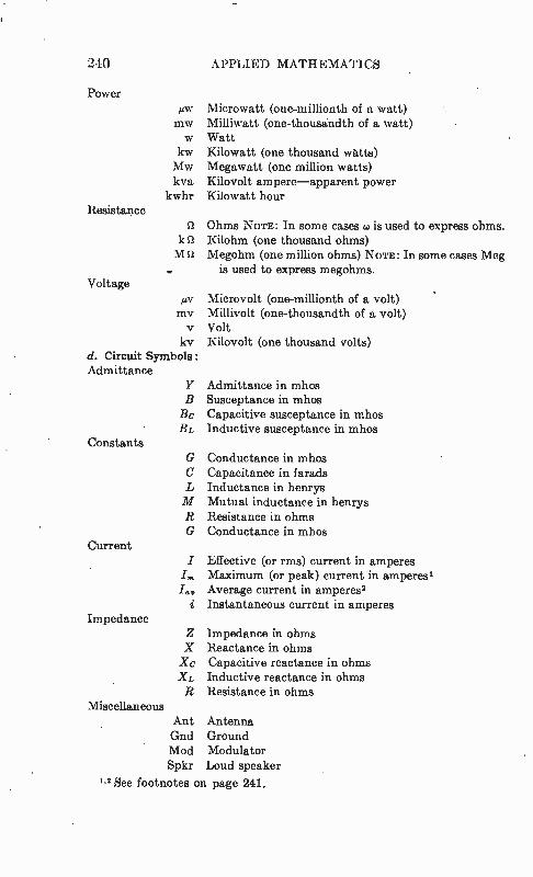
240 APPLIED MATHEMATICS
Power itw Microwatt (one-millionth of a watt) mw Milliwatt (one-thousandth of a watt) w Watt kw Kilowatt (one thousand watts) Mw Megawatt (one million watts) kva Kilovolt ampere—apparent power
kwhr Kilowatt hour Resistance
n Ohms NOTE: In some cases co is used to express ohms. k fl Kilohm (one thousand ohms) M11 Megohm (one million ohms) NOTE: In some cases Meg
is used to express megohms. Voltage
/.4v Microvolt (one-millionth of a volt) mv Millivolt (one-thousandth of a volt) ▪ Volt kv Kilovolt (one thousand volts)
d. Circuit Symbols: Admittance
Y Admittance in mhos B Suseeptance in mhos Bc Capacitive susceptance in mhos BL Inductive susceptance in mhos
Constants G Conductance in mhos C Capacitance in farads L Inductance in henrys M Mutual inductance in henrys R Resistance in ohms G Conductance in mhos
Current Effective (or rms) current in amperes Maximum (or peak) current in amperes' Average current in amperes2 Instantaneous current in amperes
Impedance Z Impedance in ohms X Reactance in ohms Xe Capacitive reactance in ohms Xr, Inductive reactance in ohms R Resistance in ohms
Miscellaneous Ant Antenna Gnd Ground Mod Modulator Spkr Loud speaker
" See footnotes on page 241.
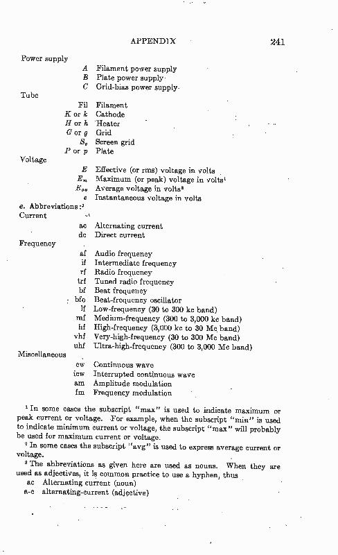
APPENDIX 241
Power supply A Filament power supply B Plate power supply• C Grid-bias power supply
Tube Fil Filament
K or k Cathode H or h Heater G or g Grid
S, Screen grid P or p Plate
Voltage
E Effective (or rms) voltage in volts E. Maximum (or peak) voltage in volts' Ea. Average voltage in volts' e Instantaneous voltage in volts
e. Abbreviations:' Current .%
ac Alternating current de Direct current
Frequency
af Audio frequency if Intermediate frequency rf Radio frequency
trf Tuned radio frequency bf Beat frequency
bfo Beat-frequency oscillator lf Low-frequency (30 to 300 ke band) mf Medium-frequency (300 to 3,000 ke band) hf High-frequency (3,000 kc to 30 Mc band)
vhf Very-high-frequency (30 to 300 Mc band) uhf Ultra-high-frequency (300 to 3,000 Mc band)
Miscellaneous ow Continuous wave icw Interrupted continuous wave am Amplitude modulation fm Frequency modulation
In some cases the subscript "max" is used to indicate maximum or peak current or voltage. For example, when the subscript "min" is used to indicate minimum current or voltage, the subscript "max" will probably be used for maximum current or voltage.
2 In some cases the subscript "avg" is used to express average current or voltage.
3 The abbreviations as given here are used as nouns. When they are used as adjectives, it is common practice to use a hyphen, thus
ac Alternating current (noun) a-c alternating-current (adjective)
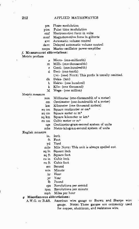
242 APPLIED MATHEMATICS
pm Phase modulation ptm Pulse time modulation emf Electromotive force in volte mmf Magnetomotive force in gilberts aye Automatic volume control
davc Delayed automatic volume control mopa Master-oscillator power-amplifier
f. Measurement abbreviations: Metric prefixes
ei Micro.- (one-millionth) Milli- (one-thousandth)
c Centi- (one-hundredth) d Deci- (one-tenth)
Uni- (one) NOTE: This prefix is usually omitted. dk Deka, (ten) h Hekto- (one hundred) k Kilo- (one thousand) M Mega- (one million)
Metric measure mm Millimeter (one-thousandth of a meter) cm Centimeter (one-hundredth of a meter) km Kilometer (one thousand meters)
sq cm Square centimeter or cm2 sq cm Square meter or m2 sq km Square kilometer or km3 Cu cm Cubic meter or m3
cgs Centimeter-gram-second system of units mks Meter-kilogram-second system of units
English measure in. Inch ft Foot yd Yard
mile Mile NOTE: This unit is always spelled out. sq in Square inch sq ft Square foot en in Cubic inch eu ft Cubic foot sec Second min Minute hr Hour yr Year lb Pound
rps Revolutions per second rpm Revolutions per minute mph Miles per hour
g Miscellaneous abbreviations: A.W.G. or B.&S. American wire gauge or Brown and Sharpe wire
gauge. NOTE: These gauges are commonly used for copper, aluminum, and resistance wire.
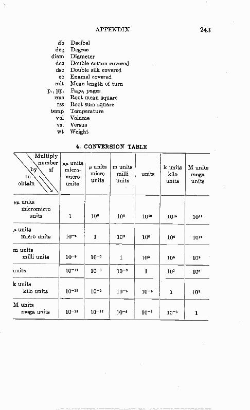
APPENDIX 243
db Decibel deg Degree
diam Diameter dcc Double cotton covered dsc Double silk covered ec Enamel covered
mlt Mean length of turn p., pp. Page, pages
rms Root mean square rss Root sum square
temp Temperature vol Volume vs. Versus wt Weight
4. CONVERSION TABLE
Multiply number
by of
to\\ obtain
pp units micro-
micro units
µ units micro units
m units milli units
units k units kilo units
M units mega units
pp units micromicro
units 1 106 109 1012 10 16 10is
p units micro units
m units milli units
10-6 1 103 10 6 102 10 1'
10-2 10-3
10-6
10-2
1 10 , 106 102
units 10-12 10-3 1 103 106
k units kilo units
M units mega units
10-16 10-6 10-3 1 103
10-18 10-12 10-3 10-6 10-3 1
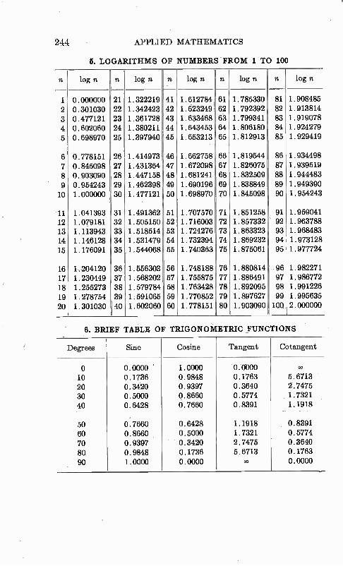
244 APPLIED MATHEMATICS
5. LOGARITHMS OF NUMBERS .FP.OM 1 TO 100
n lop; n n kg n n 14 n n kg n n 4n
1 0.000000 21 1.322219 41 1.612784 61 1.785330 81 1.908485
2 0.301030 22 1.342423 42 1.623249 62 1.792392 82 1.913814
3 0.477121 23 1.361728 43 1.633468 63 1.799341 83 1.919078
4 0.602060 24 1.380211 44 1.643453 64 1.806180 84 1.924279
5 0.698970 25 1.397940 45 1.653213 65 1.812913 85 1.929419
6 0.778151 26 1.414973 46 1.662758 66 1.819544 86 1.934498
7 0.845098 27 1.431364 47 1.672098 67 1.826075 87 1.939519
8 0.903090 28 1.447158 48 1.681241 68 1.832509 88 1.944483
9 0.954243 29 1.462398 49 1.690196 69 1.838849 89 1.949390
10 1.000000 30 1.477121 50 1.698970 70 1.845098 90 1.954243
-11 1.041393 31 1.491362 51 1.707570 71 1.851258 91 1.959041
12 1.079181 32 1.505150 52 1.716003 72 1.857332 92 1.963788 13 1.113943 33 1.518514 53 1.724276 73 1.863323 93 1.968483
14 1.146128 34 1.531479 54 1.732394 74 1.869232 94 1.973128
15 1.176091 35 1.544068 55 1.740363 75 1.875061 95 1.977724
16 1,204120 36 1,556303 56 1.748188 76 1.880814 96 1.982271
17 1.230449 37 1.568202 57 1.755875 77 1.886491 97 1.986772
18 1.255273 38 1.579784 58 1.763428 78 1.892095 98 1.991226
19 1.278754 39 1591065 59 1.770852 79 1.897627 99 1.995635
20 1.301030 40 1.602060 60 1-778151 80 1.903090 100 2.000000
6. BRIEF TABLE OF TRIGONOMETRIC FUNCTIONS
Degrees Sine Cosine Tangent Cotangent
C) o.0000 - 1.0000 0.0000 co
10 0.1736 0.9848 0.1763 5.6713
20 0.3420 0.9397 0.3640 2.7475
30 0.5000 0.8660 0.5774 . 1.7321
40 0.6428 0.7660 0.8391 1.1918 _ .
, 50 0.7660 0.6428 1.1918 . 0.8391
60 0.8660 0.5000 1.7321 0.5774
70 0.9397 0.3420 2.7475 0:3640
80 0.9848 0.1736 5.6713 0.1763
90 Loom 0.0000 e 0.0000
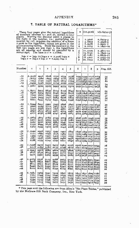
APPENDIX 245
7. TABLE OF NATURAL LOGARITHMS*
These four pages give the natural logarithms of numbers between 0.2 and 20, correct to four places. Moving the decimal point n places to the right in the number, i.e, multiplying the number by Ion, requires the addition of n times 2.3026 to the logarithm; values are given in the accompanying tables. SincetfœnumberSinthe first two pages are less than 2, the logarithms are all negative and should be preceded by a minus sign. The baseise = 2.72828.
loge x = log, so logis x = 2.3026 logo x logs, x = logo e log. x 0.4343 log. x
2
3 4
5 6 7 8 9
(52.3026)
2.3026 4.6052 6.9078 9.2103
5(0.6974-3)
0.6974-3 0.3948-5 0.0022-7 0.7897-10
11.5129 13.8155 16.1181 18.4207 20.7233
0.4871-12 0.1848-14 0.8829-27 0.5793-10 0.2767-22
Number o 2 2 3 4 5 6 7 8 0 Avg. duff.
• .20 2.3026 2926 2828 2730 2634 2538 2443 234922562164 95 .12 .2073 2082 2893 2804 2726 1628 2542 24561372 2280 87 .22 .1203 1120 2037 0956 0875 0794 0715063605570479 80 .13 .0402 0326 0250 0174 0099 0025 095298789805 9733 74
1.9661 9590 9529 9449 9379 9310 .24 9241 917392059038 69
.15 2.8971 8905 8839 8773 8708 8643 8579851584528389 65
.26 8326 8264 8202 8240 8079 8028 7958 7898 7838 7779 62
.27 7720 7662 7603 7545 7487 7430 7373 732672607204 57
.28 7248 7093 7037 6983 6928 6874 6820 6766 6713 6660 54 .19 0007 6555 6503 6451 6309 6348 6296 6246 6195 6145 52
.20 1.6094 6045 5995 5945 5896 5847 5799 5750 5702 5654 49 .22 5600 5559 5512 5465 5418 5371 5325 52795233 5187 47
.22 5141 5096 5051 5006 4961 4917 4872 4828 4784 4740 44.
.23 4697 4653 4610 4567 4524 4482 4439 4397 4355 4313 4.3 .24 4271 4230 4/88 4147 4100 4065 4024 3984 3943 3903 4r
.25
.26 1.3863 3471
3823 34.32
3783 3394
3744 3350
3704 3313
3665 3280
3626 3243
3587 3205
3548 3/68
3509 3230
39 38
.27 3093 3056 3020 2083 2946 2910 2874 2837 2802 2765 36
.28 2730 2694 2658 2623 2588 2553 252824832448 2413 35 .20 2379 2344 2310 2276 2242 2208 2174214021072073 34
.30
.31 2.2040
1722 2006 2680
2973 2648
1940 2616
2907 1584
2874 1552
1842 1520
28092777 1489 1457
1744 1426
33 32
.32 1394 2363 1332 2302 2270 2239 2209 22782147 1127 32
.33 1087 2056 2026 0996 006 0036 00060877084708/8 30
.34 0788 0759 0729 0700 0672 0642 0623058405560527 29
.35 1.0498 0470 0442 0423 0385 0356 0328030002720244 28
.36 0217 0189 0161 0134 0106 0079 0051 002499979970 27
.37 0.9943 9916 9889 9862 983576i 9782 975597299702 27
.38 9676 9650 9623 9597 9571 9545 9519 9493 9467 9442 26
.39 9416 9390 9365 9339 9314 9289 9263 9238 9223 9288 25
.40 0.0163 9238 9223 9088 9063 9039 9024898989658940 25 •41 8910 8892 8867 884,3 8829 8795 8771874787238699 24 .42 8675 8652 8627 8604 8580 8337 8533851084868463 23 .43 8440 8416 8393 8370 8347 8324 8302 8278 8255 8233 23 .44 8220 8187 8264 8142 8229 8097 8074805280308007 22
.43 0.7985 7963 7941 7929 7897 7875 7853 7832 7809 7787 22
.46 7765 7744 7722 7700 7679 7657 7636761475937572 21
.47 7550 7529 7508 7487 7465 7444 7423 7402 7381 7361 21
.48 7340 7319 7298 7277 7257 7230 7225719571747154 20
.49 7133 7113 7093 7072 7052 7032 7012 6992 6972 6951 20
*This page and the following are from Allen's "Six-Place Tables," published by the McGraw-Hill Book Company, Inc., New York,
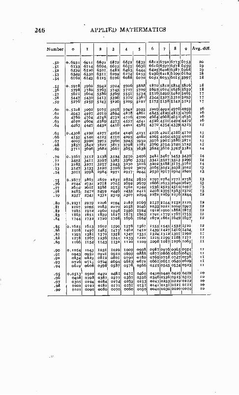
246 - APPLIED MATHEMATICS
Number o z 2 3 4 5 6 7 8 9
,
Avg. dig,
.50
.51
.52
.53
.54
.55
.56
.57
.58
0.6931 6733 6539 619 61 2
0 .5978 5798 5621 5447
6921 6724 6520 6330 6143
5960 5780 5604 5430
6892 6694 65or 6312 6125
5942 5703 5550 5413
6872 6675 6482 6292 6106
5924 5745 5569 5396
6852 6655 6463 6274 6o88
5906 5727 5551 5379
6832 6636 6444 6255 6070
5888 5709 5534 5361
6812679267736753 6616 6425 6236 6051
58705852583458/6 5692 5516549954825465 53445327532125293
6597 6406 6228 603360155997
5674
6578 6387 6199
5656
6559 6368 6180
5639
20 29 19 28 28
28 18 17 27
.59 5276 5259 5243 5226 5209 5192 5175 515851425125 27
.6o 0.5208 5092 5075 5038 5042 5025 5009 4992 4976 4959 26
.61 4943 4927 4910 4894 4878 4861 4845 4829 4813 4796 26
.62 4780 4764 4748 4732 4716 4700 4684 4668 4652 4636 26
.63 4620 4604 4589 4573 4557 4541 4526451044944479 26
.64 4463 4447 4432 4416 4401 4385 4370435443394323 25
.65 0.4308 4292 4277 .4262 4246 4231 42164201 41864170 1$
.66 4155 4.140 4225 4210 4095 4080 4065 405040354020 IS
.67 4005 3990 3975 3960 3945 3930 3916 3901 3886387x zs
.68 3857 3842 3827 3813 3798 3783 3769375437493725 Is
.69 3721 3696 3682 3667 3653 3638 3624361035953581 14
.7o .2.3567 3552 3538 3524 3510 3496 3481 346734533439 14
.71 3425 3411 3397 3383 3369 3355 3341 332733/33299 14
.72 3285 3272 3257 3243 3230 3226 320232883175 3161 14
.73 3247 3233 3220 3206 3092 3079 3065 305230383025 23
.74 3021 2998 2984 2971 2957 3944 2930 2927 2904 2890 23
.75 0.2877 2863 2850 2837 2824 2820 2797 2784277/ 2758 23
.76 2744 2732 2728 2705 2692 2679 2666265326402627 x3
.77 2614 2601 2588 2575 2562 2549 2536 2523 2510 2497 :3
.78 2485 2472 2459 2446 2433 2421 2408 2395 2383 2370 23
.79 2357 2345 2332 23/9 2307 2294 2282 2269 2256 2244 12
.8o 0.2232 22/9 22426 2194 2182 2169 2257 21442/32 2120 12
.81 2107 2095 2083 2070 2058 2.246 2033 2021 2009 1997 12
.82 1985 2972 196o 2948 2936 2924 1912 1900 1888 2875 12
.83 1863 1851 1839 2827 1815 1803 1792 1779 2767 2755 12
.84 1744 1732 1720 1708 1696 1684 2672 166/ 16492637 12
.85 0.2625 1613 1602 1590 1578 /567 1555 1543 1532 1520 12
.86 1508 2497 1485 1473 1462 1450 1439 2427 1416 1404 12
.87 1393 1381 1370 x358 1347 2335 13241322 1302 1290 zx
.88 1278 1267 1256 2244 1233 1222 1210 2299 1188 1177 22
.89 2166 1154 1143 1132 II20 1109 1098 1087 1076 1065 II
.90 0.1054 1043 1031 1020 1009 0998 098709760965 0954 II
.92 0943 0932 0921 0920 0899 0888 0877 0866 0856 0845 21
.92 0834 0823 0812 0801 0790 0780 0769 0758 0747 0736 Ir
.93 0726 0715 0704 0694 0683 0672 066, 065, 0640 0629 II
.94 0629 o6o8 0598 0587 0576 0566 0555 0545 0534 0523 II
.95 0.0513 0502 0492 0481 0471 0460 0450044004290419 zo
.96 0408 0398 0387 0377 0367 0356 034603360325 0325 io
.97 0305 0294 0284 0274 0263 0253 0243 0233 02220212 IO
.98 0202 0192 0182 0171 0161 OISI 0141 013101210/11 ro
.99 0102 0090 0080 0070 oo6o 0050 004 003000200010 IO
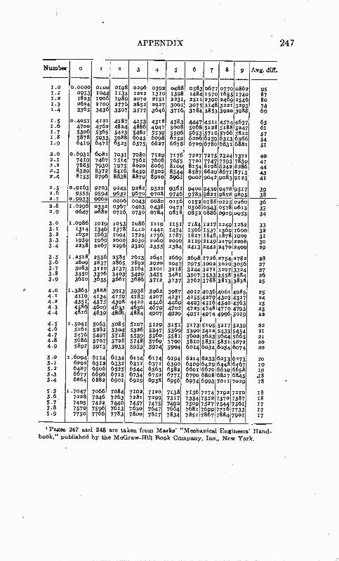
APPENDIX
Number o z 1 3 4 5 6 7 8 9 Avg. diff.
1.o o.0000 ozoo 0298 0296 0392 0488 0583 0677 0770 0862 95 z.z 0953 1044 1133 1222 13/0 1398 1484 1370 1655 1740 87 I.2 1823 I906 1989 2070 2151 2231 2311 2390 2469 2546 80 2.3 2624 2700 2776 2852 2927 3002 3075 3148 3222 3293 74 1.4 3365 3436 3507 3577 3646 3726 3784 3853 3920 3988 69
2.5 0.4055 4121 4287 4253 4318 4383 4447 45114574 4637 65 2.6 4700 4762 4824 4886 4947 5008 5068 5228 5288 5247 62 2.7 530 5365 5423 5481 5539 sue 5653 5720 5766 5822 57 1.8 5878 5933 5988 604,3 6098 6/52 6206 6259 6313 6366 54 1.9 64/9 6472 6523 6575 6627 6678 6729 6780 6831 6581 51
2.0 0.6931 6982 7032 7080 7229 7178 72277275 73247372 49 2.1 7419 7467 7514 7562 7608 7655 7701 7747 7793 7839 47 2.2 7885 7930 7975 8o2o 8065 8209 8254829882428286 44 2.3 8329 8372 8416 8459 8502 8544 8587 8629 8672 8713 43 2.4 8755 8796 8838 8879 8920 8962 9002 9042 9083 9123 42
2.5 0.9163 9203 9243 9282 9322 9361 9400 9439 9478 9527 39 2.6 9555 9594 9632 9670 9708 9746 97839822 9858 9895 38 2.7 o •9933 9969 0006 0043 oo8o 6226 0152 0188 0225 0260 36 2.8 1.0296 0332 0367 0403 0438 0473 0508 0543 0578 0623 35 2.9 0647 0682 0716 0750 0784 0828 0852 0886 0919 0953 34
3.0 2.0986 2019 2053 2086 1219 1131 zIgt 2217 1249 1282 33 3.2 1324 2346 2378 2410 1442 2474 15 1537 1569 2600 32 3.2 1632 1663 1694 2725 2756 2787 2827 2848 2878 2909 31 3.3 1939 2969 2000 2030 2060 2090 2119 2149 2179 2208 30 3.4 2238 2267 2296 2326 2355 2384 2413 2442 2470 2499 29
3.5 1.2528 2556 2585 2623 2642 2669 2698272627542782 28 3.6 2809 2837 2865 2892 2920 2947 2975300230293056 27 3.7 3083 31Io 3137 3164 3192 3228 32443272 32973324 27 3.8 3350 3376 3403 3429 3455 3481 3507 3533 3558 3584 26 3.9 3620 3635 3062 3086 3712 3737 3762 3788 3813 3838 25
4.0 1.3863 3888 39/3 3938 3962 3987 4012 4036 40624085 25 4. 1 4.2
4110 4351
4134 4.375
4159 4.398
4183 4422
4207 4.446
4231 4469
4255 44934526 4540
4279 4303 4327 4563
24 23
4.3 4580 4609 4643 4656 4679 4702 47254748 4770 4793 23 4.4 4816 4839 48l 4884 4907 4929 495/ 49744996 5019 22
4.5 2.5041 5063 5085 5207 5129 5251 52735195 52275239 22 4.6 5261 5282 5304 5326 3347 3369 5390 5412 5433 5454 22 4.7 5476 5497 3518 5539 5500 5581 5602 5023 5644 5065 21 4.8 5686 5707 5728 574 5769 5790 58zo 5832 5852 5872 20 4.9 5892 3913 5933 5953 5974 5994 6014 6034 6034 6074 20
5.0 2.6094 6114 6134 6154 6174 6294 6214 233 6253 6273 20 5.2 6292 6312 6332 6351 6371 6390 6409 429 6448 6467 29 5.2 6487 6596 6525 6544 6563 6582 6602 620 6639 0058 19 5.3 6677 6696 6725 6734 6752 6772 6790 808 6827 6845 g8 5.4 6864 6882 6901 6919 6938 6956 6974 6993 7021 7029 18
5.5 1.7047 7066 7084 7102 7220 7238 725672747192 722o 18 5.6 7228 7246 7263 7282 7299 7317 7334 7352 7370 7387 28 5.7 7405 7422 7440 7457 7475 7492 7509 7527 75447562 17 5•8 7579 7596 7013 7030 7647 7664 7682 7699 7716 7733 17 5.9 7750 7766 7783 7800 7817 7834 7852 7867 7884 7901 27
'Pages 247 and 248 are taken from Marks' 'Mechanical Engineers' Hand-book," published by the McGraw-Hill Book Company, Inc., New York.
247
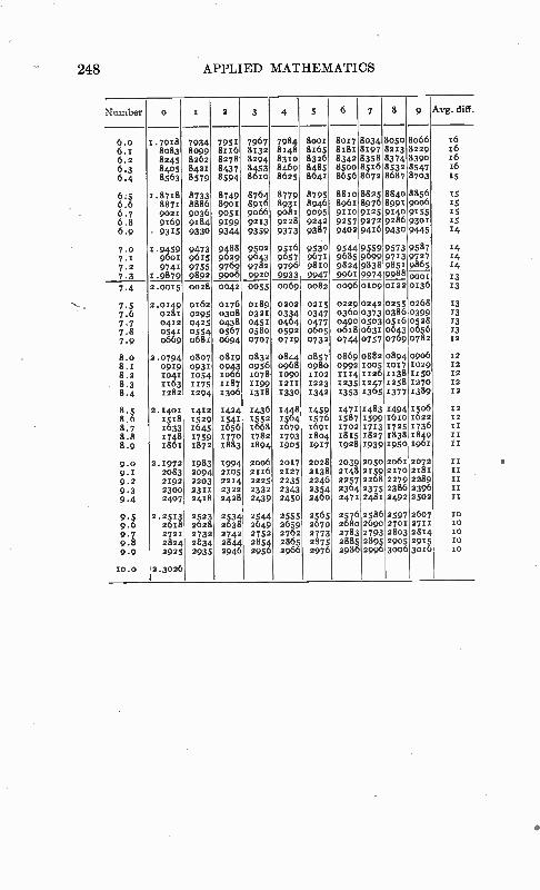
248 APPLIED MATHEMATICS
Number o 1 2 3 4 5 6 7 8 g Aorg.diff.
6.o 2.7928 7934 7951 7967 7984 8001 8017803480508°66 26 6.2 8o83 8099 8126 8132 8148 8265 8182 8197 8223 8229 26 6.2 8245 8262 8278 8294 8310 8326 8342 8358 8374 8390 26 6.3 8405 8421 8437 8453 8469 8485 8soo 85268532 8547 26 6.4 8563 8579 8594 8620 8625 8642 865686728687 8703 zs
6;5 2.8728 8733 8749 8764 8779 8795 8820 8825 88408856 25 6.6 8872 8886 8902 8926 8931 8946 8962 8976899 9oo6 25 6.7 9021 51036 9052 9066 9081 9095 9220 9125 914 9155 15 6.8 9269 9184 9199 9213 9228 9242 9257 9272 928 9501 IS
6.9 - 9315 9330 9344 9359 9373 9387 9402 9426 943 9445 14
7.0 1.9459 9473 9488 9502 9526 9530 9544 9559 9573 9587 14 7.2 9601 9615 9629 9643 9657 9671 9685 9699 9713 9727 14 7.2 9741 9755 9769 9782 9796 9820 98249838 985 9865 14 7.3 2.9879 9892 9906 9920 9933 9947 9961 9974 998 000i 23
1
•
ó
,oeeee
soe,o
,o,o eeeee
corneae**
..3.4.4
..x•
C>
çoe..-4.0•
in
4›.Wie;«:3
:oe:.44,
2.0015 0028 0042 0055 0069 0082 00960,090x220136 13
2.6249 0262 6176 6189 0202 0215 0229024202550268 13
0281 0295 0308 0321 0334 0347 0360037303860399 23 .2412 0425 0448 0451 0464 0477 0490050305260528 23 0541 0609
0554 0681
0507 0694
0580 0707
0592 0719
oóos 0732
0618663206430656 0744075707690782
23 12
2.0794 0807 0819 0852 0844 0857 08696882089409126 22 0929 0931 0943 0956 0968 0980 0992 /oos 2017 1029 12
1041 1054 1006 107 1090 1102 21242226 2138 1250 12
2163 2175 2187 1199 1211 1225 1255 1247 1258 1270 12
1282 1294 1306 1518 1530 1542 /353 1365 1377 1589 12
2.1401 1412 1424 1436 2448 1459 2471 2483 14942506 12
1518 1529 1541 1552 1564 1576 1587 15992620 2622 II
1653 1645 /656 2668 2679 1692 2702 1713 1725 2736 Ix 17g8 1759 1770 1782 1793 1804 2815 2827 1838 2U zt 281 2872 2883 2894 1905 1917 2928 1939 1950 1 ix
2.1972 2983 2994 2006 2027 2028 2039 2050 2061 2072 II
2083 2094 2205 2116 2127 2158 2148215921702181 Ix 2192 2203 2214 2225 2255 2246 2257 2268 2279 2289 II
2300 2311 2322 2332 2343 2354 2364 2375 2386 2396 II 2407 2418 2428 2439 2450 2460 2471 2481 2492 2502 xx
2.2523 2523 2534 2544 2555 2565 2576 2586 2597 2607 xo 2628 2628 2638 2649 2659 2670 268026902702 2711 xo 2721 2732 2742 2752 2762 2773 2783 2793 2803 2814 IO
2824 2834 2844 2854 2865 2375 2885 2895 2905 2915 10
2925 2935 2946 2956 3966 2976 2986299630063.226 io
2.3026
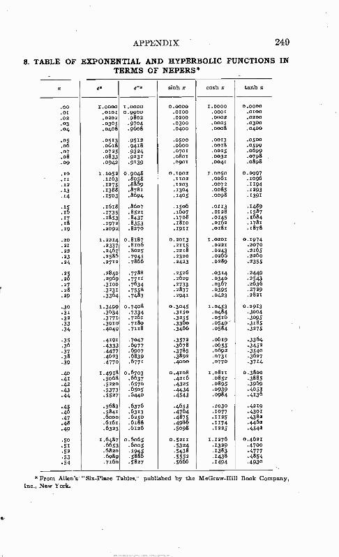
APPENDIX 249
8. TABLE OF EXPONENTIAL AND HYPERBOLIC FUNCTIONS IN
TERMS OF NEPERS*
x e. e-. sinh x cosh x tanh x
.00 1.0000 x.0000 o.0000 Iffloo 0.0000
.01( .010I 0.9900 .0100 .0001 .0100
.02 .0202 .9802 .0200 .0002 .0200
.03 .0355 .9704 .0300 .0005 .0300
.04 .0408 .96o8 .0400 .0008 .0400
.05 .0513 .9512 .0500 .0013 .0500
.o6 .0628 .9428 .o600 .0028 .0 599
.07 .0725 .9324 .0702 .0025 .0699
.08 .0833 .923/ .080x .0032 .0798
.o9 .0942 .9 139 .0902 .0041 .0898
.xo 1.1052 0.9048 0./002 1.0050 0.0997
.11 .1163 .8958 .1102 .0061 .1096
.12 .1275 .8869 .2203 .0072 .1194
.13 .1388 .8782 .1304 .0085 .1293
.14 .2503 .8694 .1405 .0098 .1391
.1s .2628 .8607 .2506 .0113 .1489
.26 .2735 .8522 .2607 .01/8 .1587
.27 .1853 .8437 .2708 .024s .2684
.28 .1972 .8353 .1810 .0162 .1781
.19 .2092 .827o .2912 .0181 .1878
.20 1.2214 0.8187 0.2013 1.0201 0.1974
.21 .2337 .8106 .211$ .0221 .2070
.22 .2461 .8025 .2218 .0243 .2155
.23 .2586 .7945 .2320 .0266 .2260
.24 .271 .7856 .2423 .0289 .23$$
.2$ .2840 .7788 .2526 .0314 .2449
.26 .2969 .7711 .2629 .9849 .2543
.27 .3200
.7634 .2733 .0367 .2636
.28 .3231 .7558 .2837 .039s .2729
.29 .3364 .7483 .2941 .04/3 .2822
.30 1 .3499 0 .7408 0 .3045 2.0453 0.2923
.3 1 .3034 .7334 .3Iso .0484 .3004
.32 .3772 .7261 .32ss .0526 .3095
.33 .3910 .7189 .336o .0549 .3 185
.34 .4049 .7218 .3466 .0584 .3275
.35 .4191 .7047 .3572 .0629 .3364
.36 .4333 .6977 .3678 .0655 4452
.37 77 ..1g23
.6907 .3785 .0692 .3540 .38 .6839 .3892 .0732 .3627
.39 .4770 .6771 .4000 .0770 .37 14
.40 2.4918 0.6703 0.4208 2.0812 0.3800
.41 .5068 .6637 .4226 .0852 .388s
.42 .5220 .6570 .432s .0895 .3969
.43 .5373 .6505 .4434 .0939 .4053
.44 .5527 .6440 .4543 .0984 .4 136
.45 .5683 .6376 .4653 .103o .4229
.46 .5841 .6323 .4764 .2077 .43ox
.47 .6000 .62so .4875 .1125 .4382
.48 .6261 .6,88 .4986 .1174 .4462
.49 .63/3 .6126 .5098 .2225 .4542
.50 2.6487 0.6065 0.5221 1.1276 0.4622
.51 .6653 .60os .5324 .13/9 .4700
.52 .682o .5945 .5438 .2383 .4777
.53 .6989 .5886 .5552 .1438 .4854
.54 .7260 .58/7 .5666 .1494 .4930
*From Allen's "Six-Place Tables,- published by the McGraw-Hill Book Company, Inc., New York.
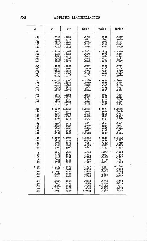
250 APPLIED MATHEMATICS
x e e-. shah x cosh x Utah x
.55 .7333 .5769 .5782 .255x .5005
.56 .7507 .5722 .5897 .1609 .5080
.57 .7683 .5655 .6014 .1669 .5254
.58 .786o .5599 .6131 .1730 .5227
.59 .8040 .5543 .6248 .1792 .5299
.6o 1.8221 0.5488 0.6367 x.1855 0.5370
.6r .8404 .5434 .6485 .1919 .5441
.62 .8589 .5379 .6605 .2984 .5511
.63 .8776 .5326 .6725 .2051 .5581
.64 .8965 .5273 .6846 .2219 .5649
.65 .9155 .5220 .6967 .2288 .5727
.66 .9348 .5169 .7o90 .2258 .5784
.67 .9542 .5117 .7223 .2330 .5850
.68 .9739 .5066 .7336 .2402 .5918
.69 .9937 .5016 .746x .2476 .5980
.70 2.0138 0.4966 0.7586 1.2552 0.6044
.71 .0340 .4916 .7722 .2628 .6107
.72 .0544 .4868 .7838 .2706 .6169
.73 .0751 .4819 .7966 .2785 .6231
.74 .0959 .4771 .8094 .2865 .629x
75 : 76
.1170
.1383 .4724 .4677
.8223
.8353 .2947 .3030
.6352 .64rx
.77 .2598 .463o 1 84 .3 224 .6469
.78 .1815 .4584 .8 Is .3199 .6527
.79 .2034 .4538 .8748 .3286 .6584
.8o 2.2288 0.4493 0.888r 1.3374 0.6640
.81 .2479 .4449 .9025 .3464 .6696
.82 .27435 .4404 .9250 .3585 .675x
.83 .2933 .436o .9286 .3647 .6805
.84 .3264 .43 17 .9423 .3740 .6858
.85 .3396 .4274 .956r .3835 .6911
.86 .3632 .4232 .9700 .3932 .6965
.87 .3869 .4190 .9840 .4029 .7024
.88 .4209 .4248 .998x .4228 .7064
.89 .4352 .4107 1.0122 .4229 .7114
.90 2.4596 0.4066 2.0265 2 .4332 0.7163
.91 .4843 .4025 .0409 .4434 .7211
.92 .5093 .3985 .0554 .4539 .7259
.93 .5345 .3946 .07.20 .4645 .7306
.94 .5600 .3906 .0847 .4753 .7352
.95 .5857 .3867 .0995 .4862 .7398
.96 .6117 .3829 .1144 .4973 .7443
.97 '6379 .379x .2294 .so8s .7457
.98 .6645 .3753 .1449 .5199 .7531
.99 .6912 .3726 .2598 .5314 .7574
r.00 2.7283 0.3679 2./752 2.543r 0.76,6 .05 .8577 .3499 .2539 .6038 .7815 ace 3.0042 .3329 .3356 .6685 .8005 .15 .z582 .3266 .4208 .7374 .8178 .20 .3201 .3012 .5093 .8107 .8337
.25 .4903 .2865 .6019 .8884 .8483
.3o .6693 .2725 .6984 .9709 .8617
.35 .8574 .2592 .7991 2.0583 .8742
.40 4.0552 .2466 .9043 .1509 .8854
.45 .2631 .2346 2.0143 .2488 .8957
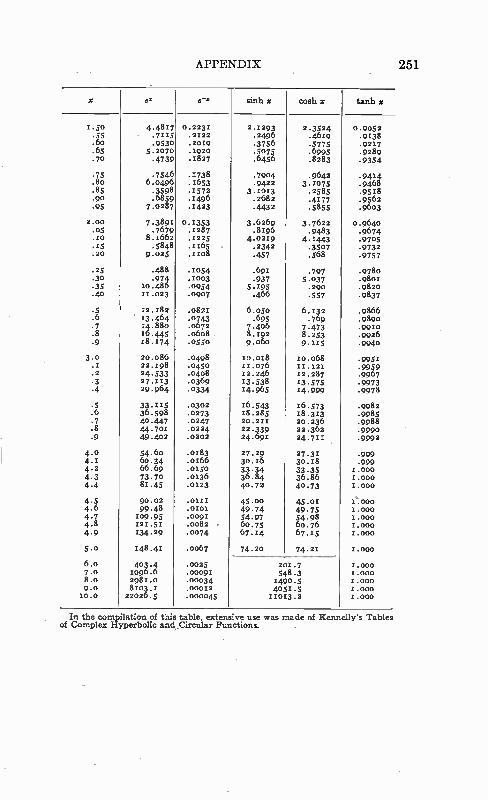
APPENDIX
x e e-. sinh x cosh x tanh x
1.50 4.4817 0.2231 2.1293 2.3524 0.9052 .55 .7115 .2122 .2496 .4619 .9138 .6o .9530 .2029 .3756 .5775 .9227 .65 5.2070 .1920 .5075 .6995 .9289 .70 .4739 .1827 .6456 .8283 .9354
.75 .7546 .1738 .7904 .9642 .9414
.8o 6.0496 .1653 .9422 3.1075 .9468
.85 .3598 .1572 3.1023 .2585 .9528
.90 .6859 .1496 .2682 .4177 .9562
.95 7.0287 .1423 .4432 .5855 .9603
2.00 7.3891 0.1353 3.6269 3.7622 0.9640 .05 .7679 .2287 .8296 .9483 .9674 .20 8.2662 .2225 4.0229 4.1443 .9705 .25 .5848 .2265 .2342 .3507 .9732 .20 9.025 .1108 .457 .568 .9757
.25 .488 .1054 .692 .797 .9780
.30 .974 .2003 .937 5.037 .9802
.35 10.486 .0954 5.195 .290 .9820
.40 11.023 .0907 .466 .557 .9837
.5 22.282 .0821 6.050 6.132 .9866
.6 ' 13.464 .0743 .695 .769 .9890
.7 14.880 .0672 7.406 7.473 .9920
.8 16.445 .0608- 8.192 8.253 .9926
.9 18.174 .0550 9.060 9.125 .9940
3.0 20.086 .0498 20.018 10.068 .9951 .2 22.198 .0450 11.076 11.121 .9959 .2 24.533 .0408 12.246 22.287 .9967 .3 27.223 .0369 13.538 13.575 .9973 .4 29.964 .0334 14.965 14.999 .9978
.5 33.115 .0302 16.543 16.573 .9982
.6 36.598 .0273 28.285 28.313 .9985
.7 40.447 .0247 20.211 2.2.236 .9988
.8 44.701 .0224 22.339 22.362 .9990
.9 49.402 .0202 24.691 24.722 .9992
4. 0 54.60 .0183 27.29 27.32 .999 4.1 60.34 .0266 30.16 30.18 .999 4.2 66.69 .0250 33.34 33.35 r.000 4.3 73.70 .0136 36.84 36.86 2.000 4.4 81.45 .0223 40.72 40.73 2.000
4.5 90.02 .0222 45.00 45.01 e.000 4.6 99.48 .oxox 49.74 49.75 2.000 4.7 209.95 .0092 54.97 54.98 2.000 4.8 121.51 .0082 • 60.75 60.76 1.000 4.9 234.29 .0074 67. 14 67.15 2.000
5.0 148.41 .0067 74.20 74.21 Ifflo
6.o 403.4 .0025 201.7 1.000 7.0 1096.6 .00091 548.3 2.000 8.o 2981.0 .00034 1490.5 1.000 9.0 8103.1 .00012 4051.5 r.000 20.0 22026.5 .0004345 21023.2 2.000
In the compilation of this table, extensive use was made of Kennelly's Tables of Complex Hyperbolic and Circular Functions.
251
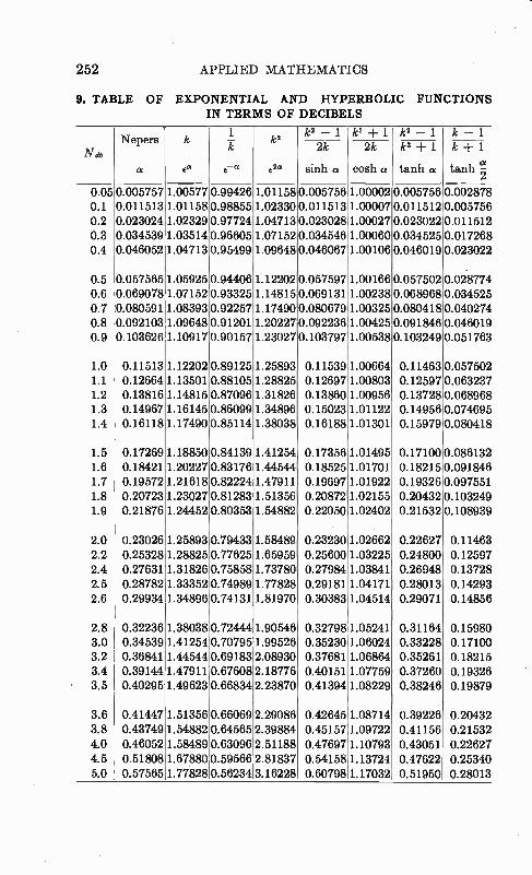
252 APPLIED MATHEMATICS
9. TABLE OF EXPONENTIAL AND HYPERBOLIC FUNCTIONS IN TERMS OF DECIBELS
Ne N epers
ot
k
,a
1 Tc
,-a
k2
,2a
k2 - 1 le + 1 k2 - 1 k - 1 k + 1
tanh 2 2
2k
sinh a
2k
cosh a
k2 -1- 1
tanh a
0.05 0.005757 1.00577 0.99426 1.01158 0.005756 1.00002 0.005756 0.002878 0.1 0.011513 1.01158 0.98855 1.02330 0.011513 1.00007 0.011512 0.005756 0.2 0.023024 1.02329 0.97724 1.04713 0.023028 1.00027 0.023022 0.011512 0.3 0.034539 1.03514 0.96605 1.07152 0.034546 1.00060 0.034525 0.017268 0.4 0.046052 1.04713 0.95499 1.09648 0.046067 1.00106 0.046019 0.023022
0.5 0.057565 1.05925 0.94406 1.12202 0.057597 1.00166 0.057502 0.028774 0.6 0.069078 1.07152 0.93325 1.14815 0.069131 1.00238 0.068968 0.034525 0.7 0.080591 1.08393 0.92257 1.17490 0.080679 1.00325 0.080418 0.040274 0.8 0.092103 1.09648 0.91201 1.20227 0.092236 1.00425 0.091846 0.046019 0.9 0.103626 1.10917 0.90157 1.23027 0.103797 1.00538 0.103249 0.051763
1.0 0.11513 1.12202 0.89125 1.25893 0.11539 1.00664 0.11463 0.057502 1.1 0.12664 1.13501 0.88105 1.28825 0.12697 1.00803 0.12597 0.063237 1.2 0.13816 1.14815 0.87096 1.31826 0.13860 1.00956 0.13728 0.068968 1.3 0.14967 1.16145 0.86099 1.34896 0.15023 1.01122 0.14956 0.074695 1.4 0.16118 1.17490 0.85114 1.38038 0.16188 1.01301 0.15979 0.080418
1.5 0.17269 1.18850 0.84139 1.41254 0.17356 1.01495 0.17100 0.086132 1.6 0.18421 1.20227 0.83176 1.44544 0.18525 1.01701 0.18215 0.091846 1.7 0.19572 1.21618 0.82224 1.47911 0.19697 1.01922 0.19326 0.097551 1.8 0.20723 1.23027 0.81283 1.51356 0.20872 1.02155 0.20432 0.103249 1.9 0.21876 1.24452 0.80353 1.54882 0.22050 1.02402 0.21532 0.108939
2.0 0.23026 1.25893 0.79433 1.58489 0.23230 1.02662 0.22627 0.11463 2.2 0.25328 1.28825 0.77625 1.65959 0.25600 1.03225 0.24800 0.12597 2.4 0.27631 1.31826 0.75858 1.73780 0.27984 1.03841 0.26948 0.13728 2.5 0.28782 1.33352 0.74989 1.77828 0.29181 1.04171 0.28013 0.14293 2.6 0.29934 1.34896 0.74131 1.81970 0.30383 1.04514 0.29071 0.14856
2.8 0.32236 1.38038 0.72444 1.90546 0.32798 1.05241 0.31164 0.15980 3.0 0.34539 1.41254 0.70795 1.99526 0.35230 1.06024 0.33228 0.17100 3.2 0.36841 1.44544 0.69183 2.08930 0.37681 1.06864 0.35261 0.18215 3.4 0.39144 1.47911 0.67608 2.18776 0.40151 1.07759 0.37260 0.19326 3.5 0.40295 1.49623 0.66834 2.23870 0.41394 1.08229 0.38246 0.19879
3.6 0.41447 1.51356 0.66069 2.29086 0.42645 1.08714 0.39226 0.20432 3.8 0.43749 1.54882 0.64565 2.39884 0.45157 1.09722 0.41156 0.21532 4.0 0.46052 1.58489 0.63096 2.51188 0.47697 1.10793 0.43051 0.22627 4.5 0.51808 1.67880 0.59566 2.81837 0.54158 1.13724 0.47622 0.25340 5.0 0.57565 1.77828 0,56234 3.16228 0.60798 1.17032 0.51950 0.28013
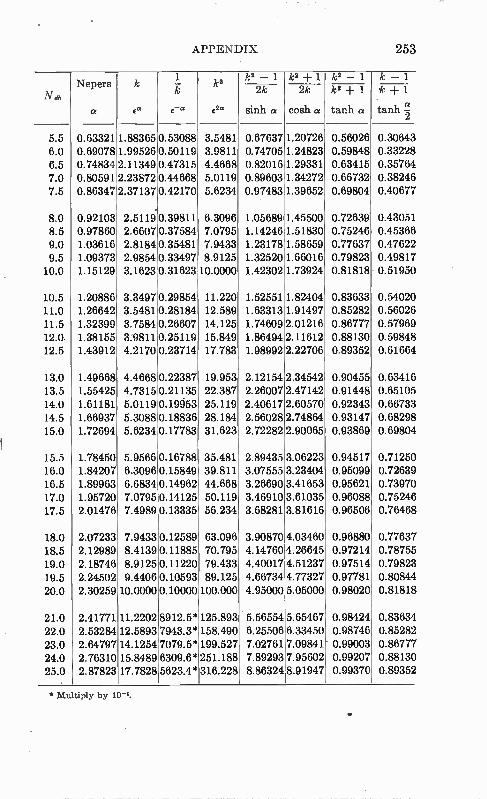
APPENDIX 253
Na, Nepers
«
k
e
1 ; IT
,-a
k2
êa
k2 - 1 k2 -I- 1 k2 - 1 k - 1 2k
sinh «
2k
cosh «
k2 +1
tanh a
k+ 1
tanh -c! 2
5.5 0.63321 1.88365 0.53088 3.5481 0.67637 1.20726 0.56026 0.30643 6.0 0.69078 1.99526 0.50119 3.9811 0.74705 1.24823 0.59848 0.33228 6.5 0.74834 2.11349 0.47315 4.4668 0.82016 1.29331 0.63415 0.35764 7.0 0.80591 2.23872 0.44668 5.0119 0.89603 1.34272 0.66732 0.38246 7.5 0.86347 2.37137 0.42170 5.6234 0.97483 1.39652 0.69804 0.40677
8.0 0.92103 2.51190.39811 6.3096 1.05689 1.45500 0.72639 0.43051 8.5 0.97860 2.6607 0.37584 7.0795 1.14246 1.51830 0.75246 0.45366 9.0 1.03616 2.8184 0.35481 7.9433 1.23178 1.58659 0.77637 0.47622 9.5 1.09373 2.9854 0.33497 8.9125 1.32520 1.66016 0.79823 0.49817
10.0 1.15129 3.1623 0.31623 10.0000 1.42302 1.73924 0.81818 0.51950
10.5 1.20886 3.3497 0.29854 11.220 1.52551 1.82404 0.83633 0.54020 11.0 1.26642 3.5481 0.28184 12.589 1.63313 1.91497 0.85282 0.56026 11.5 1.32399 3.7584 0.26607 14.125 1.74609 2.01216 0.86777 0.57969 12.o. 1.38155 3.9811 0.25119 15.849 1.86494 2.11612 0.88130 0.59848 12.5 1.43912 4.2170 0.23714 17.783 1.98992 2.22706 0.89352 0.61664
13.0 1.49668 4.4668 0.22387 19.953 2.12154 2.34542 0.90455 0.63416 13.5 1.55425 4.7315 0.21135 22.387 2.26007 2.47142 0.91448 0.65105 14.0 1.61181 5.0119 0.19953 25.119 2.40617 2.60570 0.92343 0.66733 14.5 1.66937 5.3088 0.18836 28.184 2.56028 2.74864 0.93147 0.68298 15.0 1.72694 5.6234 0.17783 31.623 2.72282 2.90065 0.93869 0.69804
15.5 1.78450 5.9566 0.16788 35.481 2.89435 3.06223 0.94517 0.71250 16.0 1.84207 6.3096 0.15849 39.811 3.07555 3.23404 0.95099 0.72639 16.5 1.89963 6.6834 0.14962 44.668 3.26690 3.41653 0.95621 0.73970 17.0 1.95720 7.0795 0.14125 50.119 3.46910 3.61035 0.96088 0.75246 17.5 2.01476 7.4989 0.13335 56.234 3.68281 3.81616 0.96506 0.76468
18.0 2.07233 7.9433 0.12589 63.096 3.90870 4.03460 0.96880 0.77637 18.5 2.12989 8.4139 0.11885 70.795 4.14760 4.26645 0.97214 0.78755
19.0 2.18746 8.9125 0.11220 79.433 4.40017 4.51237 0.97514 0.79823 19.5 2.24502 9.4406 0.10593 89.125 4.66734 4.77327 0.97781 0.80844
20.0 2.30259 10.0000 0.10000 100.000 4.95000 5.05000 0.98020 0.81818
21.0 2.41771 11.2202 8912.5* 125.893 5.56554 5.65467 0.98424 0.83634 22.0 2.53284 12.5893 7943.3* 158.490 6.25506 6.33450 0.98746 0.85282 23.0 2.64797 14.1254 7079.5* 199.527 7.02761 7.09841 0.99003 0.86777 24.0 2.76310 15.8489 6309.6* 251.188 7.89293 7.95602 0.99207 0.88130 25.0 2.87823 17.7828 5623.4* 316.228 8.86324 8.91947 0.99370 0.89352
*Multiply by 10-5.
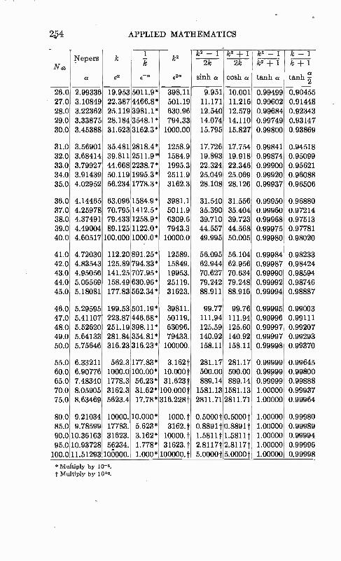
4 APPLIED MATHEMATICS
N ab 1•T epers
«
k
e
1 le
ea
k2
êa
k2 - 1 k2 + 1 k2 - 1 k2 + 1
tanh a
k - 1 2k
sinh a
2k
cosh a
k + 1
tanh cl 2
26.0 2.99336 19.953 5011.9* 398.11 9.951 10.001 0.99499 0.90455 27.0 3.10849 22.3874466.8* 501.19 11.171 11.216 0.99602 0.91448 28.0 3.22362 25.119 3981.1* 630.96 12.540 12.579 0.99684 0.92343 29.0 3.33875 28.184 3548.1* 794.33 14.074 14.110 0.99749 0.93147 30.0 3.45388 31.623 3162.3* 1000.00 15.795 15.827 0.99800 0.93869
31.0 3.56901 35.481 2818.4* 1258.9 17.726 17.754 0.99841 0.94518 32.0 3.68414 39.811 2511.9* 1584.9 19.893 19.918 0.99874 0.95099 33.0 3.79927 44.668 2238.7* 1995.3 22.324 22.346 0.99900 0.95621 34.0 3.91439 50.119 1995.3* 2511.9 25.049 25.069 0.99920 0.96088 35.0 4.02952 56.234 1778.3* 3162.3 28.108 28.126 0.99937 0.96506
36.0 4.14465 63.096 1584.9* 3981.1 31.540 31.556 0.99950 0.96880 37.0 4.25978 70.795 1412.5* 5011.9 35.390 35.404 0.99960 0.97214 38.0 4.37491 79.433 1258.9* 6309.6 39.710 39.723 0.99968 0.97513 39.0 4.49004 89.125 1122.0* 7943.3 44.557 44.568 0.99975 0.97781 40.0 4.60517 100.000 1000.0* 10000.0 49.995 50.005 0.99980 0.98020
41.0 4.72030 112.20 891.25* 12589. 56.095 56.104 0.99984 0.98233 42.0 4.83543 125.89 794.33* 15849. 62.944 62.956 0.99987 0.98424 43.0 4.95056 141.25 707.95* 19953. 70.627 70.634 0.99990 0.98594 44.0 5.06569 158.49 630.96* 25119. 79.242 79.248 0.99992 0.98746 45.0 5.18081 177.83 562.34* 31623. 88.911 88.916 0.99994 0.98887
46.0 5.29595 199.53 501.19* 39811. 99.77 99.76 0.99995 0.99003 47.0 5.41107 223.87 446.68* 50119. 111.94 111.94 0.99996 0.99111 48.0 5.52620 251.19 398.11* 63096. 125.59 125.60 0.99997 0.99207 49.0 5.64133 281.84 354.81* 79433. 140.92 140.92 0.99997 0.99293 50.0 5.75646 316.23 316.23* 100000. 158.11 158.11 0.99998 0.99370
55.0 6.33211 562.3 177.83* 3.162f 281.17 281.17 0.99999 0.99645 60.0 6.90776 1000.0 100.00* 10.000f 500.00 500.00 0.99999 0.99800 65.0 7.48340 1778.3 56.23* 31.623f 889.14 889.14 0.99999 0.99888 70.0 8.05905 3162.3 31.62* 100.000t 1581.13 1581.13 1.00000 0.99937 75.0 8.63469 5623.4 17.78* 316.228f 2811.71 2811.71 1.00000 0.99964
80.0 9.21034 10000. 10.000* 1000. t 0.5000 t 05000f 1.00000 0.99980 85.0 9.78599 17783. 5.623* 3162. t 0.8891t 0.8891 t 1.00000 0.99989 90.0 10.36163 31623. 3.162* 10000. t 1.5811 t 1.5811 t 1.00000 0.99994 95.0 10.93728 56234. 1.778* 31623. t 2.8117t 2.81171* 1.00000 0.99996 100.0 11.51293 106000. 1.000* 100000. t 5.0000 t 5.0000.1. 1.00000 0.99998
*Muitiply by 10-5. t Multiply by 10+5.
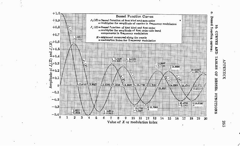
+1.0
+0.9
+0.8
+0.7
••+0.6
0+0.2 a>
E
oa
o
—0.1
—0.2
0.3
0.4 0 1
•..i
BRIM
Mai
IMP
11
1.8412 4-0 581
Bessel Function Curves Jo (Z= Bessel function of first kind and zero order
= multiplier for amplitude of carrier in frequency modulation
.7-1 (X) =Bessel function of first kind and first order =multiplier for amplitude of first order side band components in frequency, modulation
X= argument measured along the x-axis =modulation index for frequency modulation
I/
BB:
mum mom
Mk' BMW
N▪ MI l
II Il
• 11
1
II •
.1 1aBIMI
lel3211111 •
a
2.4048
»IMP À.1111.1M BUM
311111111111
6.6201 LIB
• LI
Meng ll I/
RIM
LIMMErrEVIIMPLIMIWI
PLnum '.
11
I/
13.8T.di
ll
II?' may
19.61591 0.1801,
•Plak IMBEELI BRIM
BBBrAMIBM
14.9309
•
,e, IC pi.. .BBN
VA
3.83171 0.402.8 f
2 1111 n 19
3
AMf 6.3314 1-0.8461
10.1736 -0.2497
• IPZ BIM
{ 11.7060
16.4706 l-0 965
BM a. I.
{155 18.
0
4
5
6
78
910
1112
31
14
15
16
17
81
1920
Vaue l
of Xro ation odulm
xinde
: SOA.M3 uopoun; Tassag -a
SKODLLM1I3 TSaS'all 10 STIIVIE IN(V sammo
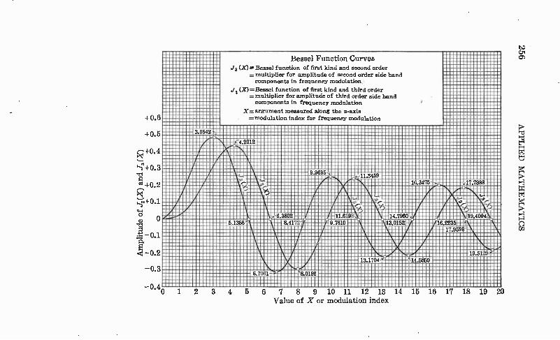
+0.6
-4-0.5
+0.4
+0.2
o 0
e
—0.3
:Una
Male
Bessel Function Curves J2(X)— Bessel function of first kind and second order
. multiplier for amplitude of second order side band components in frequency modulation.
J3CM — Bessel function of first kind and third order =multiplier for amplitude 02 third order side band components in frequency modulation
X— argument measured along the x-axis . ..modulation index for frequency modulation
0I'lere321. !.131»là,
'ABM
.ti
1/BABBII
nommeri
MA, ABU WI%
1t Mann
9.9695 e
14
11.3469 • M 16.3475 se
WAWA fl
6.1366
6.3802 moan no amp MMMMM laiLEXŒF M À
71 MMMMMMMMMMMM BRIM Mae MI»
A Mae Man\ M.M•0111111
\BMA WWI
:»1111
à MMM
muumuu
MM nano,
I 'll
I 16.2235 Inn M Ann
00
MIL
19.4094 4 , 1 .9598 BA
ri 1BI
¡rat
Ll MUNI
6.7061
44 MMMM MM gre lga
EMU 14.5859
— 0.40 1 2 3 4 5 6 7 8 9 10 11 12 13 14 15 16 17 18 19 20 Value of X or modulation index
SOLI
VN'3
1:11
,VM1
CUaIlddV
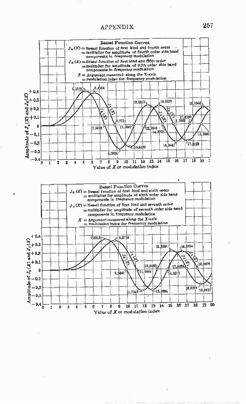
APPENDIX 257
Bessel Function Curves
.74 (X) =- Bessel function of first kind and fourth order =multiplier for amplitude of fourth order side band
components in frequency modulation
J s (X) =Bessel function of first kind and fifth order =multiplier for amplitude of fifth order side band
components in frequency modulation
X = Argument measured along the X-axis .,-_- modulation index for frequency modulation
J.3175 1
6.4156
2.6819 13.9872 1.1960
c... a
,- IA ..... e (-"te•
0 8.7714 `l.) 15.7002
17.6160 gr 7.58f 11. 647 2.3386
14 1725 18 9801
0.5199 16 9641 17.3128
l
I
9.2824
o
-I 0.4
-I-0.3
,o•-1- 0.2 e o
o 0
o 0.1 o
0.2
0.4 0 1
1 2 3 4 5 6 7 8 o 14
Value of X or modulation index
Bessel Function Curves
J6 (X) = Bessel function of first kind and sixth order ,-... multiplier for amplitude of sixth order side band components in frequency modulation
j 7 (X) =- Bessel function of first kind and seventh order =multiplier for amplitude of seventh order side band
components in frequency modulation
X = Argument measured along the X-axis = modulation index for frequency modulation
7 5013 • 8.5778
15.2682 16.5294
ir c....
9.9361
13.5893
14.8213
17.003 18.2878
0864
-t-- 9419 11.7349 12.324
18.637419
2 3 4 5 6 7 8 9 10 11
Value of X or modo ation index
lb 10 20
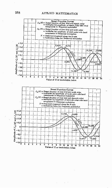
258 APPLIED MATHEMATICS
Bessel Function Curves jg (X)= Bessel function of first kind and eighth order
=multiplier for, amplitude of eighth.order side band components in frequency modulation
Jg (X)= Bessel function of first kind and ninth order = multiplier for amplitude of ninth order side band
components in frequency modulation X = Argument measured along the X-axis
=modulation index for frequency modulation
+ 0.4
•—•40.3
0 —0.1
e -0.2 m. A —0.3
•9 —O. 4o
R +0.41
+0.2
+OA
k °
o —0.1
e —0.2 en —0.8
sl
0
1 2 3 4 5 6 7 8 9 10 11 12 13
9.64 4
14.:
17.7,0
156 f 15 2868
14 Value of X or modulation index
15 16
Bessel Function Curves jiex) =-- Bessel function of first kind and tenth order
= multiplier for amplitude of tenth order side band components in frequency modulation
J11(I) =Bessel function of first kind and eleventh order = multiplier for amplitude of eleventh order side band
components in frequency modulation
X =Argument measured along the X-axis =modulation index for frequency modulation
1 2.2266
17
17.
19
.412
18
0045
19.1%45
19 20
À 19 6160
'6.4479 17.
1 2 3 4 5 6 7 8 9 10 11 12 13 14 15 16
Value of X or modulation index 17 18 19 20
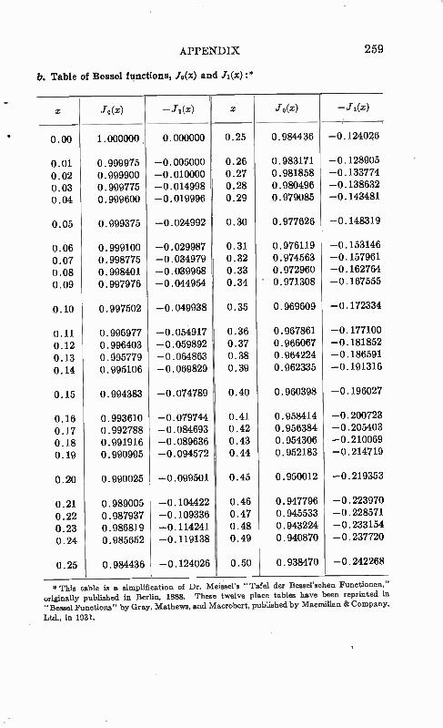
APPENDIX
b. Table of Bessel functions, Jo(x) and Ji(x) :*
259
x .1. o(x) -.1- i(x) x 10(x) --.1.1(x)
0.00 1.000000 0.000000 0.25 0.984436 -0.124026
0.01 0.999975 -0.005000 0.26 0.983171 -0. 128905
0.02 0.999900 -0.010000 0.27 0.981858 -0. 133774
0.03 0.999775 -0.014998 0.28 0.980496 -0. 138632
0.04 0.999600 -0.019996 0.29 0.979085 -0. 143481
0.05 0.999375 -0.024992 0.30 0.977626 -0. 148319
0.06 0.999100 -0.029987 0.31 0.976119 -0. 153146
0.07 0.998775 -0.034979 0.32 0.974563 -0. 157961
0.08 0.998401 -0.039968 0.33 0.972960 -0. 162764
0.09 0.997976 -0.044954 0.34 0.971308 -0. 167555
0.10 0.997502 -0.049938 0.35 0.969609 -0. 172334
0.11 0.996977 -0.054917 0.36 0.967861 -0. 177100
0.12 0.996403 -0.059892 0.37 0.966067 -0.181852
0.13 0.4)95779 -0.064863 0.38 0.964224 -0. 186591
0.14 0.995106 -0.069829 0.39 0.962335 -0. 191316
0.15 0.994383 -0.074789 0.40 0.960398 -0. 196027
0.16 0.993610 -0.079744 0.41 0.958414 -0.200723
0.17 0.992788 -0.084693 0.42 0.956384 -0.205403
0.18 0.991916 -0.089636 0.43 0.954306 -0.210069
0.19 0.990995 -0.094572 0.44 0.952183 -0.214719
0.20 0.990025 -0.099501 0.45 0.950012 -0.219353
0.21 0.989005 -0. 104422 0.46 0.947796 -0.223970
0.22 0.987937 -0. 109336 0.47 0.945533 -0. 228571
0.23 0.986819 -0. 114241 0.48 0.943224 -0.233154
0.24 0.985652 -0. 119138 0.49 0.940870 -0.237720
0.25 0.984436 -0. 124026 0.50 0.938470 -0. 242268
* This table is a simplification of Dr. Meissel's "Tafel der Bessel'schen Functionen," originally published in Berlin, 1888. These twelve place tables have been reprinted in " Bessel Functions" by Gray, Mathews, and Macrobert, published by Macmillan 4r Company,
Ltd., in 1931.
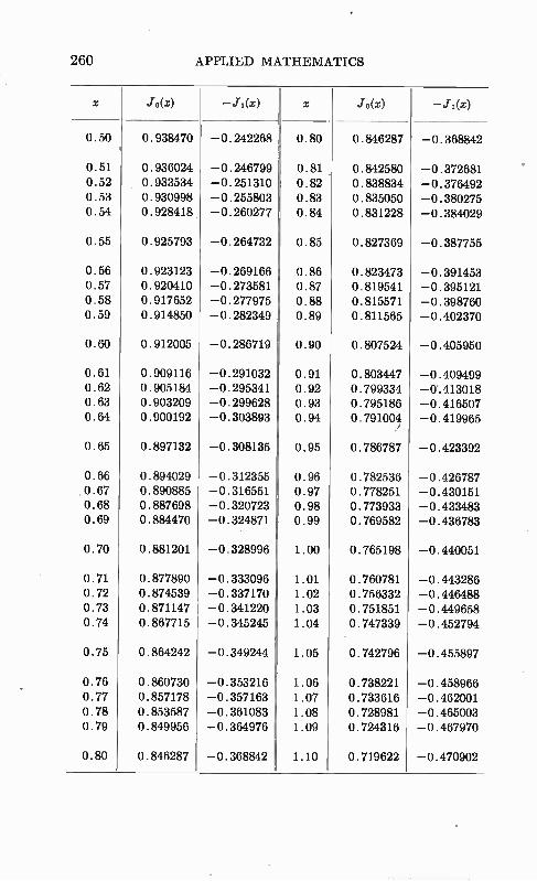
260 APPLIED MATHEMATICS
x Jo(x) -Ji(x) x jo(x) --.11(x)
0.50 0.938470 --0.242268 0.80 0.846287 --0.368842
0.51 0.936024 --0.246799 0.81 0.842580 -0.372681 0.52 0.933534 --0.251310 0.82 0.838834 --0.376492 0.53 0.930998 --0.255803 0.83 0.835050 --0.380275 0.54 0.928418 --0.260277 0.84 0.831228 --0.384029
0.55 0.925793 --0.264732 0.85 0.827369 --0.387755
0.56 0.923123 --0.269166 0.86 0.823473 --0.391453 0.57 0.920410 -0.273581 0.87 0.819541 --0.395121 0.58 0.917652 --0.277975 0.88 0.815571 -0.398760 0.59 0.914850 --0.282349 0.89 0.811565 --0.402370
0.60 0.912005 --0.286719 0.90 0.807524 -0.405950
0.61 0.909116 --0.291032 0.91 0.803447 --0.409499 0.62 0.905184 --0.295341 0.92 0.799334 --0.413018 0.63 0.903209 --0.299628 0.93 0.795186 --0.416507 0.64 0.900192 -0.303893 0.94 0.791004 --0.419965
/
0.65 0.897132 --0.308135 0.95 0.786787 --0.423392
0.66 0.894029 --0.312355 0.96 0.782536 --0.426787 0.67 0.890885 --0.316551 0.97 0.778251 --0.430151 0.68 0.887698 -0.320723 0.98 0.773933 --0.433483 0.69 0.884470 --0.324871 0.99 0.769582 --0.436783
0.70 0.881201 --0.328996 1.00 0.765198 --0.440051
0.71 0.877890 -0.333096 1.01 0.760781 -0.443286 0.72 0.874539 --0.337170 1.02 0.756332 --0.446488 0.73 0.871147 -0.341220 1.03 0.751851 --0.449658 0.74 0.867715 --0.345245 1.04 0.747339 -0.452794
0.75 0.864242 --0.349244 1.05 0.742796 -0.455897
0.76 0.860730 --0.353216 1.06 0.738221 -0.458966 0.77 0.857178 -0.357163 1.07 0.733616 --0.462001 0.78 0.853587 -0.361083 1.08 0.728981 -0.465003 0.79 0.849956 --0.364976 1.09 0.724316 --0.467970
0.80 0.846287 --0.368842 1.10 0.719622 --0.470902
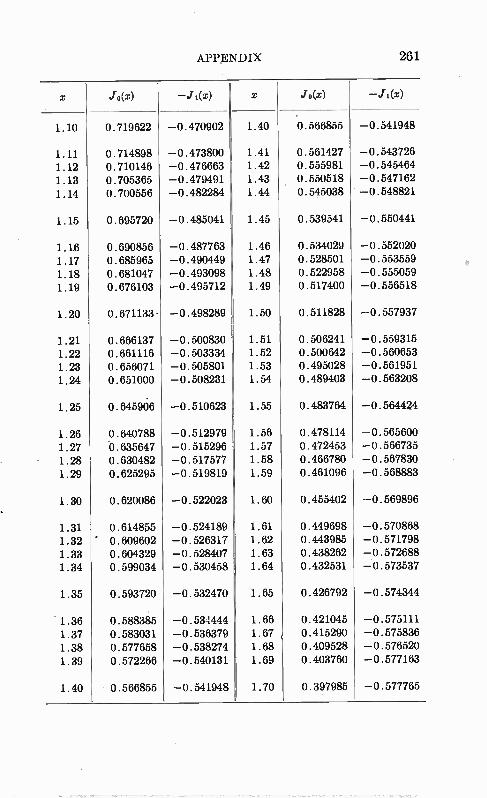
APPENDIX 261
x Jo(x) - Ji(x) x jo(x) -./.1(x)
1.10 0.719622 --0.470902 1.40 0.566855 --0.541948
1.11 0.714898 --0.473800 1.41 0.561427 --0.543726
1.12 0.710146 -0.476663 1.42 0.555981 -43.545464
1.13 0.705365 --0.479491 1.43 0.550518 --0.547162
1.14 0.700556 --0.482284 1.44 0.545038 --0.548821
1.15 0.695720 -4).485041 1.45 0.539541 -0.550441
1.16 0.690856 -0.487763 1.46 0.534029 -4).552020
1.17 0.685965 --0.490449 1.47 0.528501 --0.553559
1.18 0.681047 --0.493098 1.48 0.522958 -0.555059
1.19 0.676103 -4).495712 1.49 0.517400 --0.556518
1.20 0.671133. -0.498289 1.50 0.511828 --0.557937
1.21 0.666137 -0.500830 1.51 0.506241 --0.559315
1.22 0.661116 --0.503334 1.52 0.500642 --0.560653
1.23 0.656071 --0.505801 1.53 0.495028 --0.561951
1.24 0.651000 --0.508231 1.54 0.489403 --0.563208
1.25 0.645906 -0.510623 1.55 0.483764 -4).564424
1.26 0.640788 -4).512979 1.56 0.478114 --0.565600
1.27 6.635647 --0.515296 1.57 0.472453 -4).566735
1.28 0.630482 -4).517577 1.58 0.466780 -0.567830
1.29 0.625295 -0.519819 1.59 0.461096 --0.568883
1.30 0.620086 -4).522023 1.60 0.455402 --0.569896
1.31 0.614855 --0.524189 1.61 0.449698 --0.570868
1.32 ' 0.609602 --0.526317 1.62 0.443985 --0.571798
1.33 0.604329 --0.528407 1.63 0.438262 --0.572688
1.34 0.599034 -0.530458 1.64 0.432531 --0.573537
1.35 0.593720 --0.532470 1.65 0.426792 -4).574344
-1.36 0.588385 --0.534444 1.66 0.421045 --0.575111
1.37 0.583031 --0.536379 1.67 0.415290 --0.575836
1.38 0.577658 --0.538274 1.68 0.409528 --0.576520
1.39 0.572266 --0.540131 1.69 0.403760 --0.577163
1.40 0.566855 --0.541948 1.70 0.397985 --0.577765
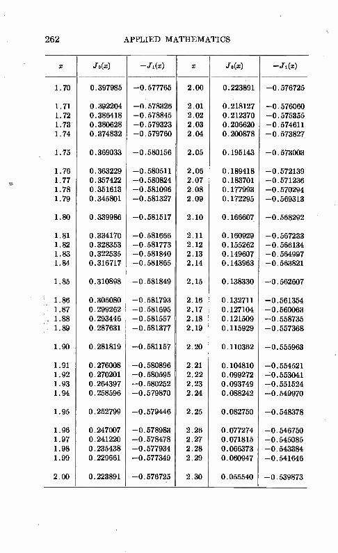
262 APPLIED MATHEMATICS
x jo(x) --ji(x) x jo(x) --.1.1(x)
1.70 0.397985 --0.577765 2.00 0.223891 --0.576725
1.71 0.392204 --0.578326 2.01 0.218127 --0.576060 1.72 0.386418 --0.578845 2.02 0.212370 --0.575355 1.73 0.380628 -0.579323 2.03 0.206620 --0.574611 1.74 0.374832 --0.579760 2.04 0.200878 -0.573827
1.75 0.369033 --0.580156 2.05 0.195143 --0.573003
1.76 0.363229 -0.580511 2.06 0.189418 -0.572139 1.77 0.357422 --0.580824 2.07 0.183701 --0.571236 1.78 0.351613 -0.581096 2.08 0.177993 --0.570294 1.79 0.345801 -0.581327 2.09 0.172295 --0.569313
1.80 0.339986 --0.581517 2.10 0.166607 -0.568292
1.81 0.334170 --0.581666 2.11 0.160929 --0.567233 1.82 0.328353 --0.581773 2.12 0.155262 --0.566134 1.83 0.322535 --0.581840 2.13 0.149607 --0.564997 1.84 0.316717 --0.581865 2.14 0.143963 --0.563821
1.85 0.310898 --0.581849 2.15 0.138330 --0.562607
1.86 0.305080 --0.581793 2.16 0.132711 -0.561354 . 1.87
.. 0.299262 --0.581695 2.17 0.127104 -0.560063
1.88 0.293446 -0.581557 2.18 0.121509 --0.558735 1.89 0.287631 -0.581377 2.19 0.115929 --0.557368
1.90 0.281819 --0.581157 2.20 0.110362 --0.555963
1.91 0.276008 --0.580896 2.21 0.104810 --0.554521 1.92 0.270201 --0.580595 2.22 0.099272 -0.553041 1.93 0.264397 --0.580252 2.23 0.093749 --0.551524 1.94 0.258596 --0.579870 2.24 0.088242 -0.549970
1.95 0.252799 --0.579446 2.25 0.082750 -0.548378
1.96 0.247007 --0.578983 2.26 0.077274 --0.546750 1.97 0.241220 --0.578478 2.27 0.071815 --0.545085 1.98 0.235438 --0.577934 2.28 0.066373 -0.543384 1.99 0.229661 --0.577349 2.29 0.060947 --0.541646
2.00 0.223891 --0.576725 2.30 0.055540 --0.539873
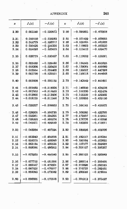
APPENDIX 263
X Jo(x) -./1(x) Jo(x) - .11(x)
2.30 0.055540 --0.539873 2.60 --0.096805 -4).470818
2.31 0.050150 --0.538063 2.61 --0.101499 --0.468025 2.32 0.044779 --0.536217 2.62 --0.106165 --0.465202 2.33 0.039426 -0.§34336 2.63 -0.110803 --0.462350 2.34 0.034092 --0.532419 2.64 --0.115412 --0.459470
2.35 0.028778 --0.530467 2.65 --0.119992 --0.456561
2.36 0.023483 -43.528480 2.66 --0.124543 --0.453625 2.37 0.018208 --0.526458 2.67 --0.129064 --0.450660 2.38 0.012954 -0.524402 2.68 -43.133557. --0.447668 .2.39 0.007720 -0.522311 2.69 --0.138018 --0.444648
240 0.002508 -0.520185 2.70 --0.142449 --0.441601
2.41 --0.002683 -4).518026 2.71 --0.146850 --0.438528 2.42 --0.007853 --0.515833 2.72 --0.151220 -0.435428 2.43 --0.013000 -43.513606 2.73 -43.155559 -43.432302 2.44 --0.018125 --0.511346 2.74 -43.159866 -0.429150
2.45 -43.023227 --0.509052 2.75 --0.164141 -0.425972
2.46 --0.028306 -0.506726 2.76 --0.168385 --0.422769 2.47 --0.033361 --0.504366 2.77 -0.172597 --0.419541 2.48 --0.038393 --0.501974 2.78 --0.176776 --0.416288 2.49 --0.043401 --0.499550 2.79 --0.180922 --0.413011
2.50 --0.048384 -0.497094 2.80 --0.185036 --0.409709
2.51 --0.053342 -0.494606 2.81 -0.189117 --0.406384 2.52 --0.058276 --0.492086 2.82 -43.193164 -43.403035 2.53 --0.063184 --0.489535 2.83 -43.197177 --0.399662 2.54 -0.068066 --0.486953 2.84 --0.201157 --0.396267
2.55 --0.072923 -0.484340 2.85 --0.205102 --0.392849
2.56 --0.077753 --0.481696 2.86 --0.209014 --0.389408 2.57 -0.082557 --0.479021 2.87 --0.212890 --0.385945 2.58 --0.087333 --0.476317 2.88 --9.216732 --0.382461 2.59 --0.092083 --0.473582 2.89 --0.220540 --0.378955
2.60 -0.096805 --0.470818 2.90 --0.224312 --0.375427
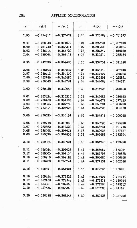
264 APPLIED MATHEMATICS
Jo(z)
2.90
2.91 2.92 2.93 2.94
2.95
2.96 2.97 2.98 2.99
3.00
3.01 3.02 3.03 3.04
3.05
3.06 3.07 3.08 3.09
3.10
3.11 3.12 3.13 3.14
3.15
3.16 3.17 3.18 3.19
3.20
--0.224312 --0.375427 3.20 -4).320188
--0.228048 --0.371879 3.21 --0.322781 --0.231749 --0.368311 3.22 --0.325335 --0.235414 --0.364722 3.23 --0.327847 --0.239043 --0.361113 3.24 --0.330319
--0.242636 --0.357485 3.25 --0.332751
-43.246193 --0.353837 3.26 --0.335142 -4).249713 --0.350170 3.27 --0.337492 -4).253196 --0.346485 3.28 --0.339801 -4).256643 --0.342781 3.29 --0.342069
-4).260052 --0.339059 3.30 --0.344296
-4).263424 --0.3à5319 3.31 --0.346482 --0.266758 -0.331563 3.32 --0.348627 --0.270055 --0.327789 3.33 --0.350731 --0.273314 --0.323998 3.34 --0.352793
--0.276535 --0.320191 3.35 --0.354814
--0.279718 --0.316368 3.36 --0.356793 --0.282862 -4).312529 3.37 --0.358731 --0.285968 -4).308675 3.38 --0.360628 --0.289036 -43.304805 3.39 --0.362482
--0.292064 -4).300921 3.40 -4).364296
--0.295054 --0.297023 3.41 --0.366067 --0.298005 --0.293110 3.42 --0.367797 --0.300916 --0.289184 3.43 -1).369485 --0.303788 --0.285244 3.44 -4).371131
-0.306621 --0.281291 3.45 --0.372735
--0.309414 -1).277326 3.46 --0.374297 -4).312168 -0.273348 3.47 --0.375818 -1).314881 -1).269358 3.48 --0.377296 --0.317555 -4).265356 3.49 -0.378733
-0.320188 -0.261343 3.50 --0.380128
--0.261343
--0.257319 --0.253284 --0.249239 --0.245184
--0.241120
--0.237046 --0.232963 --0.228871 --0.224771
--0.220663
--0.216548 --0.212425 --0.208296 --0.204160
-41200018
--0.195870 --0.191716 --0.187557 --0.183394
--0.179226
-0.175054 -0.170878 -0.166699 -0.162516
-0.158331
--0.154144 --0.149954 --0.145763 --0.141571
--0.137378
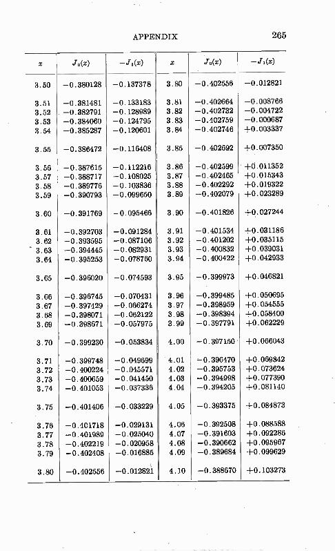
APPENDIX 265
X jo(x) --.1.1(x) x jo(x) -41(x)
3.50 -0.380128 --0.137378 3.80 -4).402556 -4).012821
3.51 -0.381481 --0.133183 3.81 -0.402664 --0.008766
3.52 . --0.382791 --0.128989 3.82 --0.402732 --0.004722
3.53 --0.384060 --0.124795 3.83 --0.402759 --0.000687
3.54 --0.385287 --0.120601 3.84 --0.402746 +0.003337
3.55 --0.386472 --0.116408 3.85 --0.402692 14).007350
3.56 --0.387615 --0.112216 3.86 --0.402599 1-0.011352
3.57 --0.388717 --0.108025 3.87 -0.402465 +0.015343
3.58 --0.389776 --0.103836 3.88 --0.402292 +0.019322
3.59 -40.390793 --0.099650 3.89 --0.402079 1-0.023289
3.60 -4).391769 --0.095466 3.90 --0.401826 +0.027244
3.61 --0.392703 --0.091284 3.91 --0.401534 +0.031186
3.62 -43.393595 --0.087106 3.92 --0.401202 1-0.035115
- 3.63 --0.394445 --0.082931 3.93 -0.400832 14).039031
3.64 -4).395253 --0.078760 3.94 --0.400422 +0.042933
3.65 --0.396020 -4).074593 3.95 --0.399973 14).046821
3.66 --0.396745 -0.070431 3.96 -4).399485 14).050695
3.67 --0.397429 --0.066274 3.97 --0.398959 1-0.054555
3.68 --0.398071 --0.062122 3.98 -43.398394 +0.058400
3.69 -4).398671 --0.057975 3.99 --0.397791 143.062229
3.70 --0.399230 -40.053834 4.00 --0.397150 14).066043
3.71 --0.399748 --0.049699 4.01 --0.396470 1-0.069842
3.72 --0.400224 --0.045571 4.02 --0.395753 14).073624
3.73 --0.400659 --0.041450 4.03 --0.394998 14).077390
3.74 --0.401053 --0.037336 4.04 --0.394205 14).081140
3.75 -10.401406 -4).033229 4.05 --0.393375 140.084873
3.76 -4).401718 --0.029131 4.06 --0.392508 +0.088588
3.77 -4).401989 --0.025040 4.07 --0.391603 1-0.092286
3.78 --0.402219 -4).020958 4.08 --0.390662 +0.095967
3.79 -4).402408 --0.016885 4.09 --0.389684 14).099629
3.80 -4).402556 --0.012821 4.10 --0.388670 14).103273
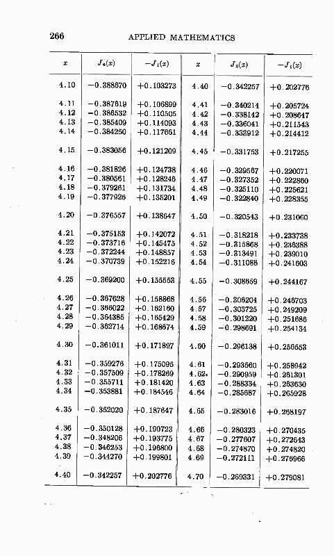
266 APPLIED MATHEMATICS
Jo(x)
4.10
4.11 4.12 4.13 4.14
4.15
4.16 4.17 4.18 4.19
4.20
4.21 4.22 4.23 4.24
4.25
4.26 4.27 4.28 4.29
4.30
4.31 4.32 4.33 4.34
4.35
4.36 4.37 4.38 4.39
4.40
-0.388670 +0.103273 4.40 -0.342257
-0.387619 +0.106899 4.41 -0.340214 -0.386532 +0.110505 4.42 -0.338142 -0.385409 +0.114093 4.43 -0.336041 -0.384250 +0.117661 4.44 -0.333912
-0.383056 +0.121209
-0.381826 +0.124738 -0.380561 +0.128246 -0.379261 +0.131734 -0.377926 +0.135201
-0.376557 +0.138647
-0.375153 +0.142072 -0.373716 +0.145475 -0.372244 +0.148857 -0.370739 +0.152216
-0.369200 +0.155553
4.45 -0.331753
4.46 -0.329567 4.47 -0.327352 4.48 -0.325110 4.49 -0.322840
4.50 -0.320543
4.51 -0.318218 4.52 -0.315868 4.53 -0.313491 4.54 -0.311088
4.55 -0.308659
-0.367628 +0.158868 4.56 -0.306204 -0.366022 +0.162160 4.57 -0.303725 -0.364385 +0.165429 4.58 -0.301220 -0.362714 +0.168674 4.59 -0.298691
-0.361011 +0.171897 4.60 -0.296138
-0.359276 +0.175095 4.61 -0.293560 -0.357509 +0.178269 4.62. -0.290959 -0.355711 +0.181420 4.63 -0.288334 -0.353881 +0.184546 4.64 -0.285687
-0.352020 +0.187647 4.65 -0.283016
-0.350128 +0A90723 4.66 -0.280323 -0.348206 +0.193775 4.67 -0.277607 -0.346253 +0.196800 4.68 -0.274870 -0.344270 +0A99801 4.69 -0.272111
-0.342257 14).202776 4.70 -4).269331
+0. 202776
+0.205724 +0.208647 +0.211543 +0.214412
+0.217255
+0.220071 +0.222860 +0.225621 +0.228355
+0.231060
+0.233738 +0.236388 +0.239010 +0.241603
+0.244167
+0.246703 +0.249209 +0.251686 +0.254134
+0.256553
+0.258942 +0.261301 +0.263630 +0.265928
+0.268197
+0.270435 +0.272643 +0.274820 +0.276966
+0.279081
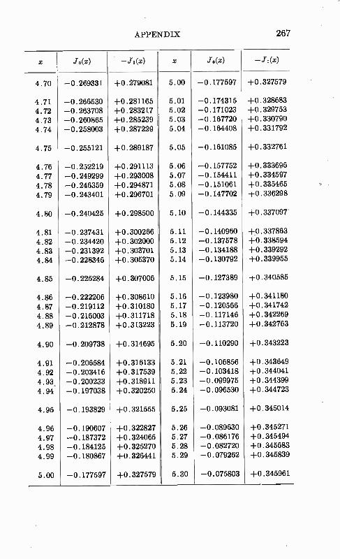
APPENDIX 267
x Jo(x) -J1(z) x jo(x) - J i(x)
4.70 --0.269331 1-0.279081 5.00 --0.177597 1-0.327579
4.71 --0.266530 14).281165 5.01 --0.174315 140.328683
4.72 --0.263708 14).283217 5.02 -40.171023 +0.329753
4.73 --0.260865 +0.285239 5.03 --0.167720 140.330790
4.74 --0.258003 44).287229 5.04 --0.164408 1-0.331792
4.75 --0.255121 14).289187 5.05 --0.161085 140.332761
4.76 --0.252219 14).291113 5.06 --0.157752 14).333696
4.77 --0.249299 14).293008 5.07 --0.154411 14).334597
4.78 --0.246359 1-0.294871 5.08 -0.151061 A-0.335465
4.79 --0.243401 14).296701 5.09 -43.147702 +0.336298
4.80 --0.240425 14).298500 5.10 --0.144335 140.337097
4.81 --0.237431 14).300266 5.11 --0.140960 +0.337863
4.82 -0.234420 +0.302000 5.12 --0.137578 A-0.338594
4.83 -4).231392 14).303701 5.13 --0.134188 A-0.339292
4.84 --0.228346 A-0.305370 5.14 --0.130792 +0.339955
4.85 -0.225284 +0.307006 5.15 --0.127389 +0.340535
4.86 -4).222206 1-0.308610 5.16 --0.123980 140.341180
4.87 --0.219112 140.310180 5.17 --0.120566 +0.341742
4.88 -4).216003 14).311718 5.18 --0.117146 +0.342269
4.89 --0.212878 14).313223 5.19 --0.113720 A-0.342763
4.90 --0.209738 14).314695 5.20 --0.110290 140.343223
4.91 --0.206584 A4).316133 5.21 -4).106856 A43.343649
4.92 --0.203416 14).317539 5.22 --0.103418 A4).344041
4.93. --0.200233 1-0.318911 5.23 --0.099975 140.344399
4.94 --0.197038 14).320250 5.24 --0.096530 A40.344723
4.95 -43.193829 140.321555 5.25 -4).093081 143.345014
4.96 --0.190607 A-0.322827 5.26 --0.089630 14).345271
4.97 -4).187372 140.324065 5.27 --0.086176 A40.345494
4.98 --0.184125 143.325270 5.28 --0.082720 143.345683
4.99 --0.180867 14).326441 5.29 --0.079262 -F0.345839
5.00 -4).177597 +0.327579 5.30 --0.075803 14).345961
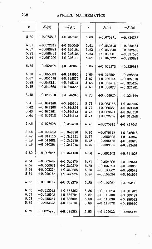
268 APPLIED MATHEMATICS
x Jo(s) -Ji(x) x Jo(x) - Ji(r)
5.30 --0.075803 +0.345961 5.60 -F0.026971 +0.334333
5.31 -0.072343 +0.346049 5.61 +0.030310 +0.333451 5.32 -40.068882 +0.346104 5.62 +0.033640 140.332538 5.33 -40.065421 +0.346126 5.63 +0.036961 -F0.331595 5.34 --0.061960 +0.346114 5.64 140.040272 140.330621
5.35 -40.058499 -F0.346069 5.65 140.043573 -F0.329617
5.36 --0.055039 +0.345990 5.66 140.046864 +0.328583 5.37 --0.051579 +0.345879 5.67 +0.050144 143.327518 5.38 -40.048121 +0.345734 5.68 +0.053414 +0.326424 5.39 -40.044665 140.345556 5.69 +0.056673 -F0.325301
5.40 --0.041210 +0.345345 5.70 +0.059920 140.324148
5.41 --0.037758 +0.345101 5.71 140.063156 +0.322965 5.42 -0.034308 +0.344824 5.72 +0.066380 +0.321753 5.43 -0.030861 140.344515 5.73 +0.069591 140.320513 5.44 -0.027418 143.344173 5.74 +0.072789 14).319243
5.45 --0.023978 140.343798 5.75 140.075975 +0.317945
5.46 --0.020542 +0.343390 5.76 +0.079148 +0.316618 5.47 --0.017110 +0.342951 5.77 +0.082308 +1).315262 5.48 --0.013683 +0.342479 5.78 +0.085453 140.313879 5.49 -40.010261 14).341975 5.79 140.088585 14).312467
5.50 --0.006844 14).341438 5.80 +0.091703 140.311028
5.51 --0.003432 +0.340870 5.81 +0.094806 143.309561 5.52 --0.000027 +0.340270 5.82 143.097894 +0.308066 5.53 +0.003373 +0.339638 5.83 143.100967 140.306544 5.54 +0.006766 +0.338974 5.84 +0.104024 140.304995
5.55 +0.010152 +0.338279 5.85 143.107067 14).303419
5.56 +0.013532 143.337552 5.86 +0.110093 140.301817 5.57 +0.016903 +0.336794 5.87 14).113103 140.300187 5.58 +0.020267 140.336004 5.88 140.116096 14).298532 5.59 +0.023623 140.335184 5.89 -FO.119073 +0.296850
5.60 -F0.026971 -F0.334333 5.90 -FO.122033 140.295142
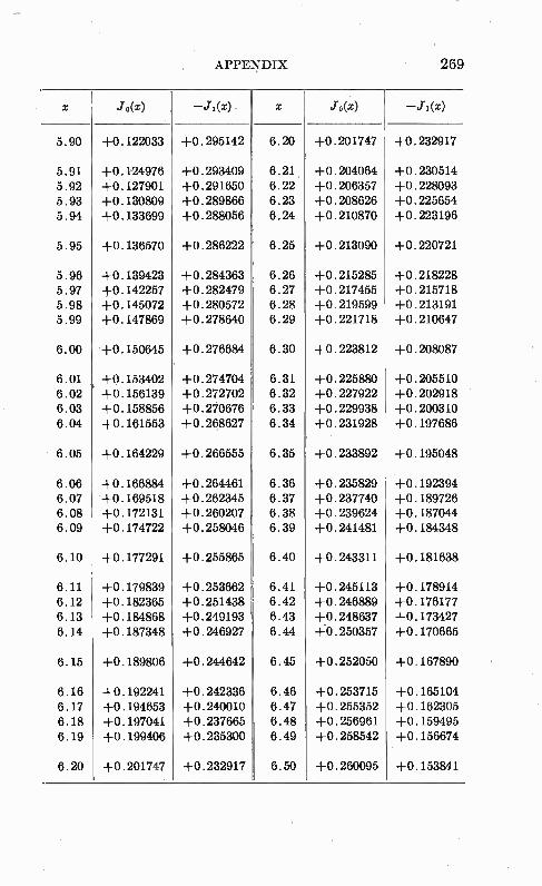
APPEI%,TDIX 269
x Jo(x) -J1(x) x jo(x) --J i(x)
5.90 14).122033 1-0.295142 6.20 1-0.201747 143.232917
5.91 -F0.124976 +0.293409 6.21 14).204064 +0.230514 5.92 +0.127901 14).291650 6.22 1-0.206357 +0.228093 5.95 1-0.130800 1-0.289866 6.23 +0.208626 +0.225654 5.94 +0.133699 140.288056 6.24 1-0.210870 14).223196
5.95 1-0.136570 1-0.286222 6.25 1-0.213090 A4).220721
5.96 +0.139423 140.284363 6.26 1-0.215285 140.218228 5.97 14).142257 A-0.282479 6.27 A-0.217455 1-0.215718 5.98 +0.145072 +0.280572 6.28 +0.219599 +0.213191 5.99 143.147869 1-0.278640 6.29 1-0.221718 14).210647
6.00 -F0.150645 14).276684 6.30 14).223812 14).208087
6.01 140.153402 +0.274704 6.31 +0.225880 1-0.205510 6.02 +0.156139 140.272702 6.32 14).227922 +0.202918 6.03 +0.158856 +0.270676 6.33 143.229938 140.200310 6.04 140.161553 +0.268627 6.34 A-0.231928 14).197686
6.05 +0.164229 +0.266555 6.35 14).233892 -FO.195048
5.05 1-0.166884 A-0.264461 6.36 +0.235829 1-0.192394 6.07 -FO.169518 143.262345 6.37 1-0.237740 14).189726 6.08 +0.172131 143.260207 6.38 +0.239624 -FO.187044 6.09 14).174722 +0.258046 6.39 +0.241481 14).184348
6.10 14).177291 A-0.255865 6.40 14).243311 A-0.181638
6.11 14).179839 A-0.253662 6.41 +0.245113 -FO.178914 6.12 A-0.182365 140.251438 6.42 14).246889 14).176177 6.13 A-0.184868 14).249193 6.43 1-0.248637 140.173427 6.14 A-0.187348 140.246927 6.44 A:0.250357 14).170665
6.15 14).189806 14).244642 6.45 14).252050 +0.167890
6.16 +0.192241 1-0.242336 6.46 44).253715 +0.165104 6.17 +0.194653 14).240010 6.47 145.255352 1-0.162305 6.18 +0.197041 145.237665 6.48 +0.256961 145.159495 6.19 4-0.199406 14).235300 6.49 +0.258542 145.156674
6.20 14).201747 44).232917 6.50 14).260095 14).153841
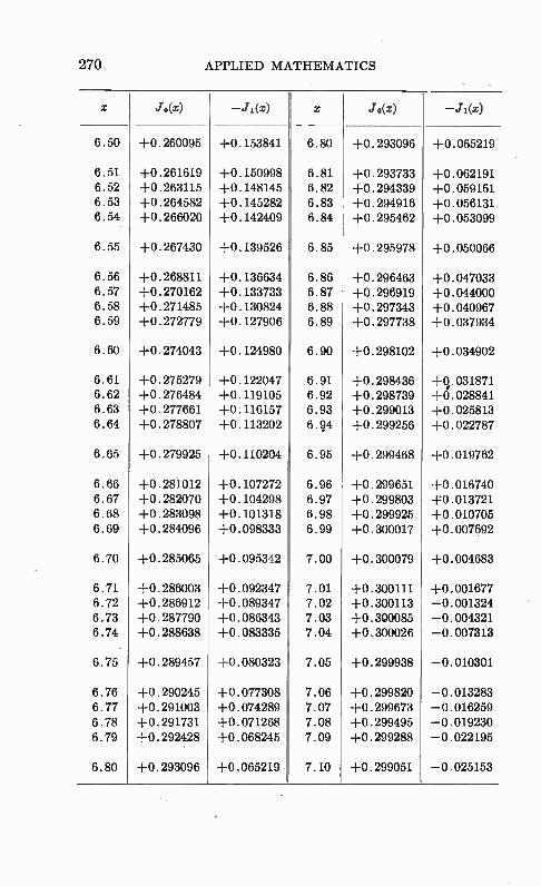
270 APPLIED MATHEMATICS
6.50
6.51 6.52 6.53 6.54
6.55
6.56 6.57 6.58 6.59
6.60
6.61 6.62 6.63 6.64
6.65
6.66 6.67 6.68 6.69
6.70
6.71 6.72 6.73 6.74
6.75
6.76 6.77 6.78 6.79
6.80
Jo(x) -.T1(z) Jo(x)
1-0.260095 +0.153841 6.80 +0.293096
+0.261619 -F0.150998 6.81 143.293733 A-0.263115 A-0.148145 6.82 +0.294339 +0.264582 A4).145282 6.83 A43.294916 +0.266020 143.142409 6.84 143.295462
+0.267430 +0.139526 6.85 +0.295978
+FO.268811 +0.136634 6.86 A-0.296463 +0.270162 -FO.133733 6.87 +0.296919 +0.271485 A-0.130824 6.88 +0.297343 A-0.272779 -FO.127906 6.89 A4).297738
+0.274043 +0.124980 6.90 +0.298102
+0.275279 143.122047 6.91 +0.298436 143.276484 A4).119105 6.92 14).298739 14).277661 A43.116157 6.93 14).299013 +0.278807 +0.113202 6.$4 A-0.299256
+0.279925 +0.110204 6.95 +0.299468
+0.281012 +0.107272 6.96 143.299651 44).282070 141104298 6.97 +0.299803 14).283098 140.101318 6.98 +0.299925 14).284096 A-0.098333 6.99 A-0.300017
+0.285065 -0.095342 7.00
1-0.286003 -F0.092347 +0.286912 +0.089347 +0.287790 +0.086343 +0.288638 +0.083335
+0.289457 +0.080323
-F0.290245 +0.077308 A4).291003 +0.074289 A-0.291731 +0.071268 +0.292428 +0.068245
+0.293096 +0.065219
+0.300079
7.01 +0.300111 7.02 +0.300113 7.03 A-0.300085 7.04 +0.300026
7.05 1-0.299938
7.06 +0.299820 7.07 A-0.299673 7.08 A-0.299495 7.09 +0.299288
7.10 -F0.299051
+0.065219
+0.062191 +0.059161 i43.056131 A-0.053099
+0.050066
A-0.047033 A-0.044000 A-0.040967 +0.037934
+0.034902
+q. 031871 143.028841 +0.025813 A-0.022787
1-0.019762
+0.016740 +0.013721 +0.010705 +0.007692
+0.004683
A-0.001677 --0.001324 --0.004321 --0.007313
--0.010301
--0.013283 --0.016259 --0.019230 --0.022195
-0.025153
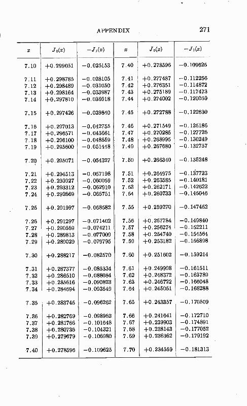
APPENDIX 271
x jo(x) -JI (x) x Jo (x) --ji(x)
7.10 +0.299051 -0.025153 7.40 14).278596 --0.109625
7.11 A-0.298785 --0.028105 7.41 1-0.277487 --0.112256
7.12 A4).298489 --0.031050 7.42 14).276351 --0.114872
7.13 -143.298164 --0.033987 7.43 A4).275189 --0.117473
7.14 14).297810 --0.036918 7.44 1-0.274002 --0.120059
7.15 -F0.297426 --0.039840 7.45 14).272788 -0.122630
7.16 14).297013 --0.042755 7.46 14).271549 --0.125186
7.17 14).296571 --0.045661 7.47 +0.270285 -4).127726
7.18 14).296100 --0.048559 7.48 +0.268995 --0.130249
7.19 1-0.295600 --0.051448 7.49 +0.267680 --0.132757
7.29 14).295071 --0.054327 7.50 14).266340 --0.135248
7.21 A-0.294513 --0.057198 7.51 A43.264975 -0.1i7723
7.22 1-0.293927 --0.060059 7.52 14).263585 --0.140181
7.23 A-0.293312 --0.062910 7.53 A-0.262171 --0.142622
7.24 -F0.292669 --0.065751 7.54 1-0.260733 --0.145046
7.25 14).291997 --0.068582 7.55 +0.259270 --0.147452
7.26 14).291297 --0.071402 7.56 +0.257784 --0.149840
7.27 +0.290569 --0.074211 7.57 A-0.256274 --0.152211
7.28 +0.289813 --0.077009 7.58 14).254740 --0.154564
7.29 14).289029 --0.079795 7.59 A-0.253182 --0.156898
7.30 14).288217 --0.082570 7.60 14).251602 --0.159214
7.31 14).287377 --0.085334 7.61 +0.249998 -0.161511
7.32 A-0.286510 --0.088084 7.62 1-0.248372 -0.163789
7.33 +0.285616 --0.090823 7.63 +0.246722 --0.166048
7.34 A-0.284694 --0.093549 7.64 14).245051 --0.168288
7.35 A4).283745 --0.096262 7.65 14).243357 --0.170509
7.36 14).282769 --0.098962 7.66 +0.241641 --0.172710
7.37 14).281766 --0.101648 7.67 14).239903 --0.174891
7.38 A-0.280736 --0.104321 7.68 14).238143 --0.177052
7.39 14).279679 --0.106980 7.69 A40.236362 --0.179192
7.40 A-0.278596 --0.109625 7.70 140.234559 --0.181313
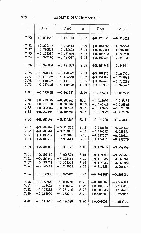
272 APPLIED MATHEMATICS
7.70
7.71 7.72 7.73 7.74
7.75
7.76 7.77 7.78 7.79
7.80
7.1 7.82 7.83 7.84
7.85
7.86 7.87 7.88 7.89
7.90
7.91 7.92 7.93 7.94
7.95
7.96 7.97 7.98 7.99
8.00
10(x) -Ji(z) Jo(x)
+0.234559 -4).181313 0 8.00 +0.171651
1-0.232735 --0.183413 8.01 +0.169297 14).230891 --0.185492 8.02 14).166930 +0.229026 -0.187550 8.03 1-0.164549 14).227140 --0.189587 8.04 1-0.162154
+0. 225234 -0.191603 8.05 14).159746
1-0.223308 --0.193597 8.06 1-0.157325 14).221362 --0.195570 8.07 1-0.154892 140.219397 --0.197521 8.08 +0.152446 1-0.217412 --0.199450 8.09 1-0.149988
14).215408
+0. 213385 +0.211343 +0. 209283 +0. 207204
1-0.205108
--0.201357 II 8.10
--0.203242 --0.205104 --0.206944 --0.208761
8.11 8.12 8.13 8.14
1-0.147517
1-0.145036 1-0.142542 +0.140038 i-0.137522
-4).210555 8.15 1-0.134996
14).202993 --0.212327 8.16 1-0.132460 140.200861 -0.214015 8.17 +0.129913 140.198712 --0.215800 8.18 1-0.127357 141196545 -4).217501 8.19 140.124791
+0.194362 --0.219179 8.20 I 14).122215
1-0.192162 --0.220834 8.21 14).119631 A-0.189945 --0.222464 8.22 1-0.117038 1-0.187713 --0.224071 8.23 +0.114436 14).185464 --0.225653 8.24 14).111826
+0.183200 -0.227212 8.25 II +0.109207
1-0.180920 --0.228746 8.26 1-0.106582 14).178625 --0.230255 8.27 14).103948 14).176315 -0.231740 •8.28 14).101308 14).173990 -0.233201 8.29 14).098660
+0.171651 -0.234636 8.30 I 14).096006
-0. 234636
--0.236047 --0.237433 --0.238794 --0.240129
--0.241439
--0.242724 --0.243983 --0.245217 --0.246425
--0.247608
--0.248764 --0.249895 --0.251000 --0.252078
--0.253131
--0.254157 --0.255157 --0.256131 --0.257078
--0.257999
--0.258893 --0.259761 --0.260602 --0.261416 .
--0.262204
--0.262964 --0.263698 --0.264406 --0.265086
--0.265739
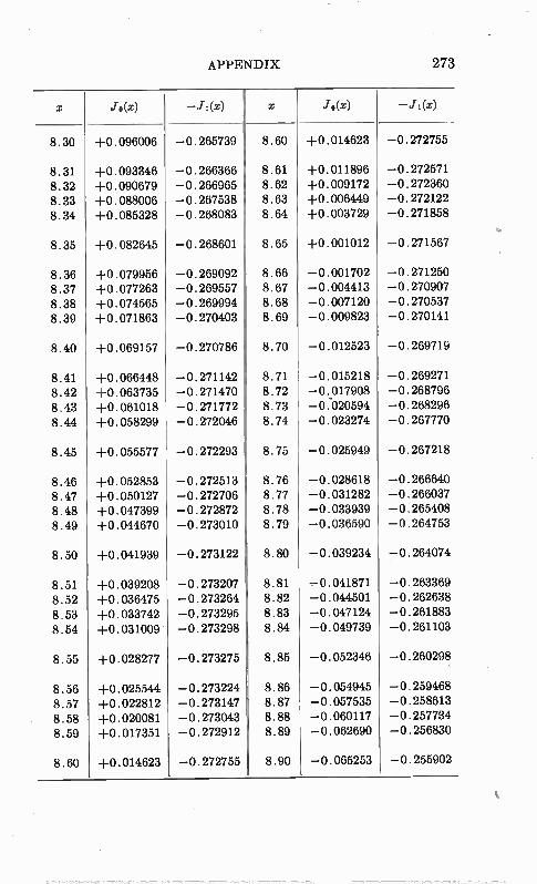
APPENDIX 273
x jo(x) -.11(x) x jo(x) - .11(x)
8.30 +0.096006 --0.265739 8.60 14).014623 -4).272755
8.31 1-0.093346 --0.266366 8.61 14).011896 --0.272571
8.32 +0.090679 --0.266965 8.62 +0.009172 --0.272360
8.33 14).088006 --0.267538 8.63 A4D.006449 --0.272122
8.34 +0.085328 --0.268083 8.64 1-0.003729 --0.271858
8.35 1-0.082645 --0.268601 8.65 1-0.001012 --0.271567
8.36 14).079956 --0.269092 8.66 --0.001702 --0.271250
8.37 +0.077263 --0.269557 8.67 --0.004413 --0.270907
8.38 14).074565 --0.269994 8.68 --0.007120 --0.270537
8.39 +0.071863 --0.270403 8.69 --0.009823 --0.270141
8.40 A-0.069157 --0.270786 8.70 --0.012523 --0.269719
8.41 14).066448 -0.271142 8.71 --0.015218 --0.269271
8.42 A4).063735 --0.271470 8.72 --0.017908 --0.268796
8.43 14).061018 --0.271772 8.73 -0:020594 --0.268296
8.44 A4).058299 --0.272046 8.74 --0.023274 --0.267770
8.45 +0.055577 --0.272293 8.75 --0.025949 --0.267218
8.46 +0.052853 -0.272513 8.76 -0.028618 --0.266640
8.47 +0.050127 --0.272706 8.77 -0.031282 --0.266037
8.48 14).047399 --0.272872 8.78 --0.033939 --0.265408
8.49 14).044670 --0.273010 8.79 --0.036590 --0.264753
8.50 140.041939 --0.273122 8.80 --0.039234 --0.264074
8.51 +0.039208 --0.273207 8.81 --0.041871 --0.263369
8.52 140.036475 --0.273264 8.82 --0.044501 --0.262638
8.53 14).033742 --0.273295 8.83 --0.047124 --0.261883
8.54 A40.031009 --0.273298 8.84 --0.049739 --0.261103
8.55 A-0.028277 --0.273275 8.85 -4).052346 --0.260298
8.56 14).025544 --0.273224 8.86 --0.054945 --0.259468
8.57 -F0.022812 --0.273147 8.87 --0.057535 --0.258613
8.58 1-0.020081 --0.273043 8.88 -40.060117 -0.257784
8.59 140.017351 --0.272912 8.89 --0.062690 --0.256830
8.60 A4).014623 --0.272755 8.90 --0.065253 --0.255902
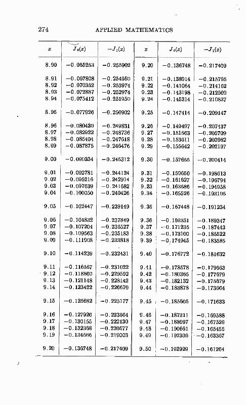
274 APPLIED MATHEMATICS
Jo(x) -Ji(x) Jo(x)
8.90 --0.065253 --0.255902 9.20 --0.136748
8.91 --0.067808 --0.254950 9.21 --0.138914 8.92 --0.070352 -4).253974 9.22 -4).141064 8.93 --0.072887 --0.252974 9.23 -40.143198 8.94 --0.075412 --0.251950 9.24 --0.145314
8.95 --0.077926 --0.250902 9.25 -4).147414
8.96 --0.080430 --0.249831 9.26 -0.149497 8.97 --0.082922 --0.248736 9.27 --0.151563 8.98 --0.085404 --0.247618 9.28 --0.153611 8.99 --0.087875 --0.246476 9.29 -43.155642
9.00 --0.090334 --0.245312 9.30 --0.157655
9.01 --0.092781 --0.244124 9.31 -4).159650 9.02 --0.095216 --0.242914 9.32 --0.161627 9.03 --0.097639 --0.241682 9.33 -0.163586 9.04 -4).100050 --0.240426 9.34 --0.165526
9.05 --0.102447 -4).239149 9.35 -4).167448
9.06 --0.104832 --0.237849 9.36 --0.169351 9.07 --0.107204 --0.236527 9.37 --0.171235 9.08 --0.109563 --0.235183 9.38 --0.173100 9.09 --0.111908 --0.233818 9.39 -4).174945
9.10 --0.114239 --0.232431 9.40 -4).176772
9.11 -49.116557 -40.231022 9.41 --0.178578 9.12 --0.118860 --0.229592 9.42 --0.180365 9.13 --0.121148 --0.228142 9.43 --0.182132 9.14 -40.123422 -0.226670 9.44 --0.183878
9.15 --0.125682 -0.225177 9.45 --0.185605
9.16 --0.127926 --0.223664 9.46 -41187311 9.17 --0.130155 --0.222130 9.47 --0.188997 9.18 --0.132368 --0.220577 9.48 --0.190661 9.19 --0.134566 --0.219003 9.49 -4).192306
9.20 --0.136748 -0.217409 9.50 -0.193929
--0.217409
--0.215795 -4).214162 --0.212509 --0.210837
--0.209147
--0.207437 --0.205709 --0.203962 --0.202197
--0.200414
--0.198613 --0.196794 -4).194958 --0.193105
-4).191234
--0.189347 --0.187443 --0.185522 --0.183585
--0.181632
--0.179663 --0.177679 --0.175679 --0.173664
--0.171633
-43.169588 -4).167529 -0.165455 -4).163367
-0.161264
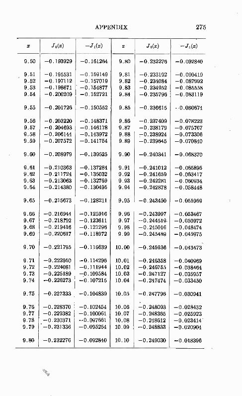
APPENDIX 275
x Jo(x) -Ji(x) x Jo(x) --ji(x)
9.50 --0.193929 --0.161264 9.80 --0.232276 --0.092840
9.51 '
--0.195531 --0.159149 9.81 --0.233192 --0.090419 9.52 -0.197112 --0.157019 9.82 --0.234084 --0.087992 9.53 --0.198671 --0.154877 9.83 --0.234952 --0.085558 9.54 --0.200209 --0.152721 9.84 --0.235796 --0.083119
9.55 --0.201726 --0.150552 9.85 --0.236615 --0.080674
9.56 --0.203220 --0.148371 9.86 --0.237409 --0.078223 9.57 --0.204693 --0.146178 9.87 --0.238179 --0.075767 9.58 --0.206144 -43.143972 9.88 743.238924 --0.073306 9.59 --0.207572 --0.141754 9.89 --0.239645 --0.070840
9.60 -43.208979 -43.139525 9.90 -4).240341 --0.068370
9.61 --0.210363 --0.137284 9.91 --0.241012 --0.065895 9.62 --0.211724 --0.135032 9.92 --0.241659 --0.063417 9.63 --0.213063 --0.132769 9.93 --0.242281 --0.060934 9.64 --0.214380 --0.130495 9.94 --0.242878 --0.058448
9.65 --0.215673 -43.128211 9.95 --0.243450 -43.055959
9.66 -43.216944 --0.125916 9.96 --0.243997 --0.053467 9.67 -0.2181'92 --0.123611 9.97 -0.244519. --0.050972 9.68 --0.219416 --0.121296 9.98 --0.245016 --0.048474 9.69 --0.220617 --0.118972 9.99 --0.245489 -0.045975
9.70 --0.221795 --0.116639 10.00 --0.245936 --0.043473:
9.71 -43.222950 --0.114296 10.01 --0.246358 --0.040969 9.72 --0.224081 -40.111944 10.02 --0.246755 --0.038464 9.73 --0.225189 -70.109584 10.03 -0.247127 --0.035957 9.74 --0.226273 --0.107215 10.04 --0.247474 --0.033450
9.75 -43.227333 -0.104839 10.05 --0.247796 --0.030941
9.76 --0.228370 -43.102454 10.06 -0.248093 --0.028432 9. ;77 -0.229382 --0.100061 10.07 --0.248365 --0.025923 9.78 --0.230371 -43.097661 10.08 -4).248612 --0.023414 9.79 ' -0.231336 --0.095254 10.09 --0.248833 --0.020904
9.80 -4).232276 -0.092840 10.10 -0.249030 --0.018396
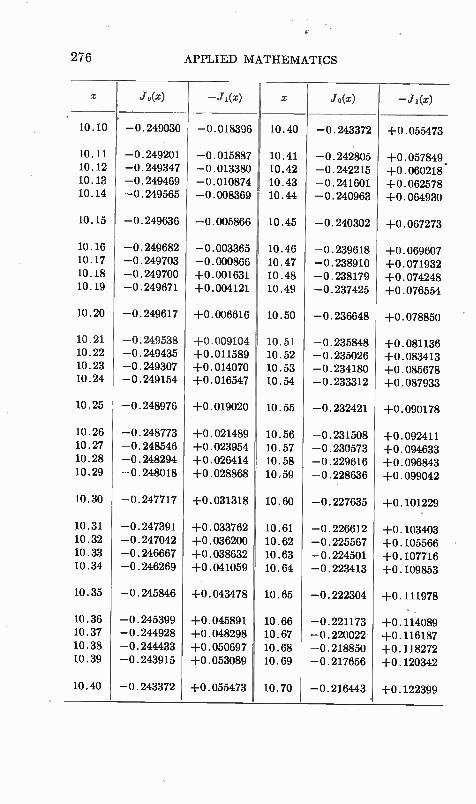
276 APPLIED MATHEMATICS
oe Jo(x) -Ji(x) x 10(x)
10.10 --0.249030 -0.018396 10.40 --0.243372 +0.055473
10.11 -0.249201 -0.015887 10.41 --0.242805 +0.057849 . 10.12 --0.249347 -0.013380 10.42 --0.242215 +0.060218 10.13 --0.249469 -0.010874 10.43 --0.241601 +0.062578 10.14 --0.249565 -0.008369 10.44 --0.240963 +0.064930
10.15 --0.249636 --0.005866 10.45 --0.240302 +0.067273
10.16 -0.249682 --0.003365 10.46 --0.239618 A-0.069607 10.17 --0.249703 --0.000866 10.47 --0.238910 +0.071932 10.18 -0.249700 +0.001631 10.48 --0.238179 +0.074248 10.19 --0.249671 +0.004121 10.49 --0.237425 A4).076554
10.20 -0.249617 +0.006616 10.50 --0.236648 +0.078850
10.21 -0.249538 +0.009104 10.51 -0.235848 +0.081136 10.22 -0.249435 A-0.011589 10.52 --0.235026 +0.083413 10.23 --0.249307 +0.014070 10.53 --0.234180 +0.085078 10.24 -0.249154 +0.016547 10.54 -0.233312 +0.087933
10.25 --0.248976 +0.019020 10.55 -0.232421 +0.090178
10.26 -0.248773 -14).021489 10.56 --0.231508 +0.092411 10.27 --0.248546 -F0.023954 10.57 -0.230573 +0.094633 10.28 --0.248294 +0.026414 10.58 --0.229616 +0.096843 10.29 --0.248018 +0.028868 10.59 --0.228636 +0.099042
10.30 --0.247717 +0.031318 10.60 -0.227635 -F0.101229
10.31 -0.247391 +0.033762 10.61 --0.226612 -14).103403 10.32 --0.247042 +0.036200 10.62 --0.225567 +0.105566 10.33 --0.246667 +0.038632 10.63 --0.224501 +0.107716 10.34 --0.246269 +0.041059 10.64 -0.223413 +0.109853
10.35 -0.245846 +0.043478 10.65 -0.222304 +0.111978
10.36 -4).245399 -14).045891 10.66 --0.221173 +0.114089 10.37 --0.244928 +0.048298 10.67 --0.220022 +0.116187 10.38 --0.244433 +0.050697 10.68 -0.218850 +0.118272 10.39 --0.243915 A-0.053089 10.69 -0.217656 -F0.120342
10.40 --0.243372 1-0.055473 10.70 --0.216443 +0.122399
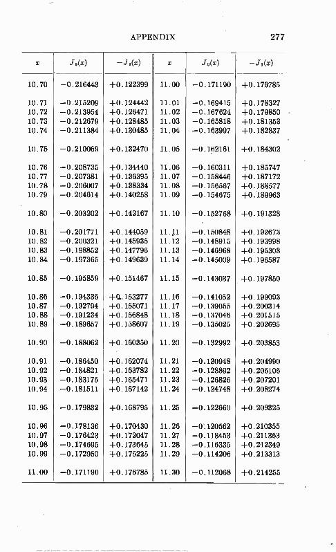
APPENDIX 277
x .10(x) -‘1 i(x) x Jo(x) --ji(x)
10,70 -0.216443 A-0.122399 11.00 --0.171190 1-0.176785
10.71 --0.215209 141124442 11.01 --0.169415 14).178327 10.72 --0.213954 1-0.126471 11.02 --0.167624 143.179850 10.73 --0.212679 44).128485 11.03 --0.165818 143.181353 10.74 --0.211384 143.130485 11.04 --0.163997 14).182837
10.75 --0.210069 1-0.132470 11.05 --0.162161 +0.184302
10.76 --0.208735 44).134440 11.06 --0.160311 44).185747 10.77 -0.207381 143.136395 11.07 --0.158446 1-0.187172 10.78 --0.206007 44).138334 11.08 -0.156567 44).188577 10.79 -0.204614 44).140258 11.09 --0.154675 14).189963
10.80 --0.203202 443.142167 11.10 --0.152768 1-0.191328
10.81 --0.201771 44).144059 11.j1 --0.150848 443.192673 10.82 --0.200321 A4).145935 11.12 --0.148915 +0.193998 10.83 --0.198852 4-0.147796 11.13 --0.146968 440.195303 10.84 --0.197365 1-0.149639 11.14 --0.145009 4-0.196587
10.85 --0.195859 4-0.151467 11.15 --0.143037 44).197850
10.86 --0.194336 141.153277 11.16 --0.141052 14).199093 10.87 -4).192794 +0.155071 11.17 --0.139055 +0.200314 10.88 --0.191234 14).156848 11.18 --0.137046 44).201515 10.89 -43.189657 4-0.158607 11.19 --0.135025 4-0.202695
10.90 -43.188062 A-0.160350 11.20 --0.132992 443.203853
10.91 --0.186450 +0.162074 11.21 --0.130948 443.204990 10.92 --0.184821 44).163782 11.22 --0.128892 A-0.206106 10.93 --0.183175 +0.165471 11.23 --0.126826 14).207201 10.94 --0.181511 143.167142 11.24 --0.124748 4-0.208274
10.95 --0.179832 1-0.168795 11.25 --0.122660 14).209325
10.96 --0.178136 14).170430 11.26 -(1120562 1-0.210355 10.97 --0.176423 44).172047 11.27 --0.118453 140.211363 10.98 --0.174695 143.173645 11.28 --0.116335 4-0.212349 10.99 --0.172950 14).175225 11.29 -4).114206 +0.213313
11.00 -4).171190 4-0.176785 11.30 -4).112068 14).214255
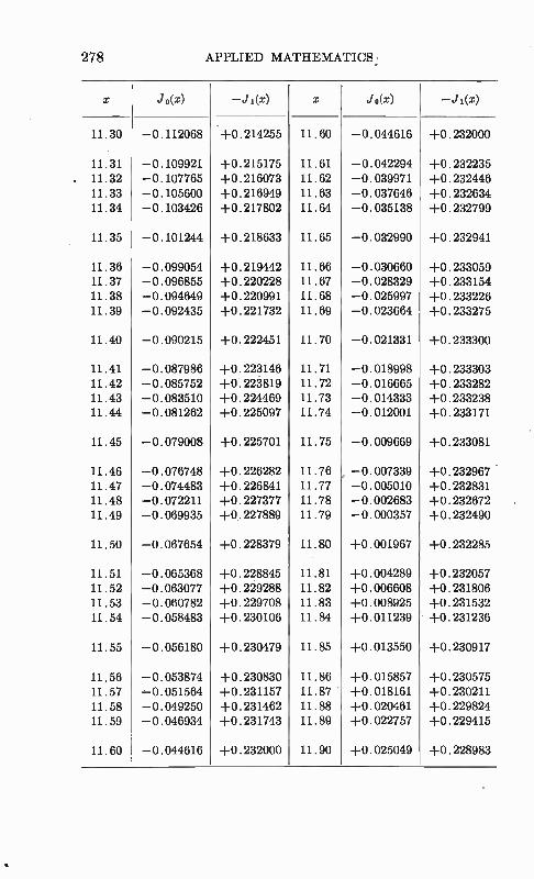
278 APPLIED MATHEMATICS
x Jo(x) -Ji(x) x Jo(x) - J1(x)
11.30 --0.112068 40.214255 11.60 --0.044616 14).232000
11.31 --0.109921 14).215175 11.61 --0.042294 14).232235 11.32 --0.107765 14).216073 11.62 --0.039971 14).232446 11.33 -4).105600 14).216949 11.63 --0.037646 +0.232634 11.34 --0.103426 1-0.217802 11.64 --0.035138 +0.232799
11.35 --0.101244 +0.218633 11.65 -0.032990 1-0.232941
11.36 --0.099054 1-0.219442 11.66 --0.030660 -F0.233059 11.37 --0.096855 14).220228 11.67 --0.028329 143.233154 11.38 --0.094649 +0.220991 11.68 --0.025997 A-0.233226 11.39 --0.092435 14).221732 11.69 --0.023664 443.233275
11.40 --0.090215 +0.222451 11.70 --0.021331 14).233300
11.41 --0.087986 1-0.223146 11.71 --0.018998 1-0.233303 11.42 --0.085752 1-0.22à819 11.72 --0.016665 +0.233282 11.43 --0.083510 140.224469 11.73 --0.014333 +0.233238 11.44 --0.081262 14).225097 11.74 --0.012001 +0.233171
11.45 --0.079008 +0.225701 11.75 --0.009669 A-0.233081
11.46 --0.076748 +0.226282 11.76 --0.007339 1-0.232967 • 11.47 --0.074483 A-0.226841 11.77 --0.005010 1-0.232831 11.48 --0.072211 A-0.227377 11.78 --0.002683 +0.232672 11.49 --0.069935 4-0.227889 11.79 --0.000357 14).232490
11.50 --0.067654 143.228379 11.80 +0.001967 143.232285
11.51 --0.065368 14).228845 11.81 -F0.004289 14).232057 11.52 --0.063077 +0.229288 11.82 4-0.006608 A-0.231806 11.53 --0.060782 140.229708 11.83 1-0.008925 A-0.231532 11.54 --0.058483 +0.230106 11.84 +0.011239 14).231236
11.55 --0.056180 14).230479 11.85 14).013550 +0.230917
11.56 --0.053874 +0.230830 11.86 44).015857 44).230575 11.57 --0.051564 +0.231157 11.87 +0.018161 +0.230211 11.58 --0.049250 1-0.231462 11.88 140.020461 +0.229824 11.59 --0.046934 A-0.231743 11.89 140.022757 140.229415
11.60 --0.044616 +0.232000 11.90 +0.025049 +0.228983
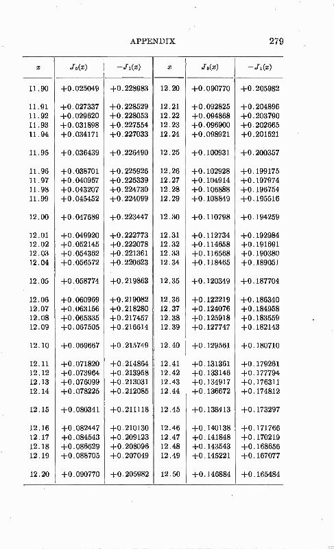
APPENDIX 279
X Jo(z) -Ji(x) x To(x) - Ji(x)
11.90 149.025049 +0.228983 12.20 1-0.090770 149.205982
11.91 +0.027337 1-0.228529 12.21 14).092825 1-0.204896 11.92 -F0.029620 +0.228053 12.22 14).094868 14).203790 11.93 143.031898 1-0.227554 12.23 1-0.096900 14).202665 11.94 149.034171 140.227033 12.24 +0.098921 1-0.201521
11.95 +0.036439 -F0.226490 12.25 14).100931 +0.200357
11.96 +0.038701 14).225926 12.26 14).102928 +0.199175 11.97 149.040957 14).225339 12.27 14).104914 14).197974 11.98 +0.043207 +0.224730 12.28 1-0.106888 +0.196754 11.99 141045452 +0.224099 12.29 14).108849 +0.195516
12.00 +0.047689 +0.223447 12.30 14).110798 +0.194259
12.01 1-0.049920 1-0.222773 12.31 1-0.112734 140.192984 12.02 14).052145 14).222078 12.32 1-0.114658 -FO.191691 12.03 +0.054362 1-0.221361 12.33 +0.116568 149.190380 12.04 14).056572 14).220623 12.34 14).118465 14).189051
12.05 143.058774 14).219863 12.35 +0.120349 1-0.187704
12.06 1-0.060969 +0.219082 12.36 149.122219 +0.186340 12.07 +0.063156 1-0.218280 12.37 +0.124076 14).184958 12.08 +0.065335 +0.217457 12.38 +0.125918 +0.183559 12.09 141067505 14).216614 12.39 14).127747 +0.182143
12.10 +0.069667 +0.215749 12.40 +0.129561 1-0.180710
12.11 1-0.071820 +0,214864 12.41 141131361 143.179261 12.12 149.073964 14).213958 12.42 +0.133146 +0.177794 12.13 14).076099 1-0.213031 12.43 14).134917 149.176311 12.14 +0.078225 1-0.212085 12.44 149.136672 1-0.174812
12.15 14).080341 +0.211118 12.45 1-0.138413 +0.173297
12.16 1-0.082447 +0.210130 12.46 14).140138 14).171766 12.17 14).084543 1-0.209123 12.47 141141848 -14).170219 12.18 +0.080029 14).208096 12.48 14).143543 1-0.168656 12.19 +0.088705 14).207049 12.49 +0.145221 1-0.167077
12.20 14).090770 1-0.205982 12.50 1-0.146884 14).165484
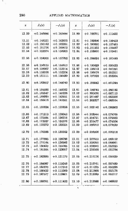
280 APPLIED MATHEMATICS
Jo(x)
12.50 A-0.146884
-Ji(x)
12.51 +0.148531 12.52 +0.150162 12.53 +0.151776 12.54 +0.153374
12.55 +0.154955
12.56 +0.156519 12.57 +0.158067 12.58 +0.159598 12.59 A-0.161111
12.60 +0.162607
12.61 +0.164086 12.62 +0.165547 12.63 +0.166990 12.64 +0.168416
12.65 +0.169824
12.66 +0.171213 12.67 -F0.172584 12.68 +0.173937 12.69 +0.175272
12.70 +0.176588
12.71 +0.177885 12.72 +0.179164 12.73 +0.180423 12.74 +0.181664
12.75 -F0.182885
12.76 +0.184087 12.77 +0.185270 12.78 +0.186433 12.79 +0.187577
12.80 +0.188701
+0.165484
+0.163875 +0.162251 A-0.160613 -FO.158959
+0.157292
12.80
12.81 12.82 12.83 12.84
12.85
Jo(x) -Ji(z)
+0.188701
+0.189806 +0.190890 -F0.191955 A-0.193000
+0.194024
+0.155610 12.86 +0.195029 +0.153914 12.87 +0.196013 -F0.152204 12.88 H-0.196976 +0.150480 12.89 A-0.197920
+0.148742 12.90 +0.198842
+0.146992 12.91 +0.199745 1-0.145228 12.92 +0.200626 A-0.143451 12.93 A-0.201487 +0.141661 12.94 A-0.202327
+0.139858 12.95 +0.203146
+0.138043 12.96 A-0.203944 +0.136216 12.97 A-0.204721 +0.134376 12.98 +0.205477 -F0.132525 12.99 +0.206212
+0.130662 13.00 +0.206926
1-0.128788 13.01 A-0.207619 +0.126902 13.02 +0.208290 +0.125005 13.03 +0.208940 -FO.123097 13.04 +0.209568
+0.121179 13.05 +0.210176
A-0.119249 13.06 +0.210761 +0.117310 13.07 +0.211325 +0.115360 13.08 -F0.211868 -F0.113401 13.09 +0.212389
+0.111432 13.10 A-0.212888
+0.111432
+0.109453 +0.107465 +0. 105467 +0.103461
+0.101446
+0.099423 +0.097391 +0.095351 +0.093304
+0.091248
+0.089185 +0.087115 +0.085038 +0.082954
+0.080863
+0.078766 A-0.076663 +0.074554 +0.072439
+0.070318
+0.068192 A-0.066061 +0.063925 A-0.061784
+0.059639
+0.057489 +0.055336 +0.053178 +0.051017
+0.048852
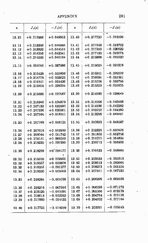
APPENDIX 281
x Jo(x) - Ji(x) x Jo(x) -Ji(x)
e
13.10 14).212888 A-0.048852 13.40 140.217725 -0.016599.
13.11 1-0.213366 1-0.046685 13.41 -F0.217548 --0.018762
13.12 140.213822 140.044514 13.42 14).217350 --0.020922
13.13 +0.214256 140.042341 13.43 14).217130 -0.023078
13.14 A4).214669 140.040164 13.44 +0.216888 --0.025230
13.15 140.215059 143.037986 13.45 143.216625 --0.027378
13.16 1-0.215428 140.035806 13.46 140.216341 --0.029522
13.17 143.215776 1-0.033623 13.47 140.216035 --0.031661 13.18 -F0.216101 140.031439 13.48 143.215708 0.033795
13.19 .1-0.216404 1-0.029254 13.49 140.215359 --0.035925
13.20 +0.216686 1-0.027067 13.50 14).214989 --0.038049
13.21 1-0.216946 +0.024879 13.51 141214598 --0.040168
13.22 14).217183 +0.022690 13.52 140.214186 --0.042282
13.23 +0.217399 1-0.020501 13.53 +0.213752 --0.044389
13.24 1-0.217594 14).018311 13.54 1-0.213298 --0.046491
13.25 1-0.217766 1-0.016121 13.55 140.212823 --0.0485g7
13.26 14).217916 1-0.013932 13.56 14).212326 --0.050676
13.27 1-0.218044 +0.011742 13.57 14).211809 --0.052758
13.28 140.218151 +0.009553 13.58 +0.211271 --0.054834
13.29 143.218235 +0.007365 13.59 1-0.210713 --0.056903 •
13.30 140.218298 1-0..005177 13.60 1-0.210133 --0.058965 •
13.31 14).218339 +0.002991 13.61 +0.209533 --0.061019
13.32 44).218357 14).000806 13.62 +0.208913 --0.063065
13.33 14).218355 --0.001377 13.63 14).208272 --0.065104
13.34 1-0.218330 --0.003559 13.64 1-0.207611 -0.067135
13.35 14).218284 --0.005738 13.65 140.206929 --0.069158
13.36 4-0.218216 --0.007916 13.66 1-0.206228 --0.071173
13.37 14).218126 --0.010091 13.67 14).205506 --0.073178
13.38 14).218014 --0.012263 13.68 +0.204764 --0.075176
13.39 14).217880 -0.014433 13.69 44).204002 --0.077164
13.40 14).217725 --0.016599 13.70 143.203221 --0.079143
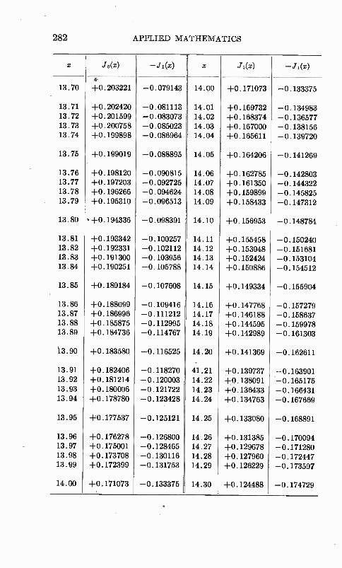
282 APPLIED MATHEMATICS
x Jo(z) -J1(x) x jo(x) --.1.1(x)
ii 13.70 +0.203221 --0.079143 14.00 1-0.171073 --0.133375
13.71 44).202420 --0.081113 14.01 +0.169732 --0.134983 13.72 14).201599 --0.083073 14.02 A40.168374 --0.136577 13.73 4-0.200758 --0.085023 14.03 -F0.167000 --0.138156 13.74 1-0.199898 --0.086964 14.04 14).165611 --0.139720
13.75 A-0.199019 --0.088895 14.05 1-0.164206 -0.141269
13.76 14).198120 --0.090815 14.06 +0.162785 -43.142803 13.77 140.197203 --0.092725 14.07 140.161350 --0.144322 13.78 +0.196266 --0.094624 14.08 +0.159899 -0.145825 13.79 +0.195310 --0.096513 14.09 +0.158433 --0.147312
13.80 ,-F0.194336 --0.098391 14.10 A-0.156953 --0.148784
13.81 A-0.193342 --0.100257 14.11 14).155458 --0.150240 13.82 1-0.192331 --0.102112 14.12 143.153948 --0.151681 13.83 14).191300 --0.103956 14.13 +0.152424 -0.153104 13.84 140.190251 --0.105788 14.14 14).150886 --0.154512
13.85 143.189184 -4).107608 14.15 A-0.149334 --0.155904
13.86 +0.188099 --0.109416 14.16 -F0.147768 --0.157279 13.87 +0.186996 --0.111212 14.17 14).146188 --0.158637 13.88 +0.185875 --0.112995 14.18 14).144595 --0.159978 13.89 +0.184736 --0.114767 14.19 +0.142989 --0.161303
13.00 14).183580 --0.116525 14.20 A-0.141369 --0.162611
13.91 A-0.182406 --0.118270 41.21 +0.139737 --0.163901 13.92 14).181214 --0.120003 14.22 143.138091 --0.165175 13.93 +0.180006 --0.121722 14.23 -F0.136433 --0.166431 13.94 +0.178780 -4).123428 14.24 A40.134763 --0.167669
13.95 14).177537 --0.125121 14.25 A-0.133080 --0.168891
13.96 1-0.176278 -0.126800 14.26 A4).131385 --0.170094 13.97 +0.175001 --0.128465 14.27 +0.129678 --0.171280 13.98 -F0.173708 -4).130116 14.28 +0.127960 -4).172447 13.99 +0.172399 -0.131753 14.29 -FO.126229 --0.173597
14.00 A40.171073 -4).133375 14.30 140.124488 -0.174729
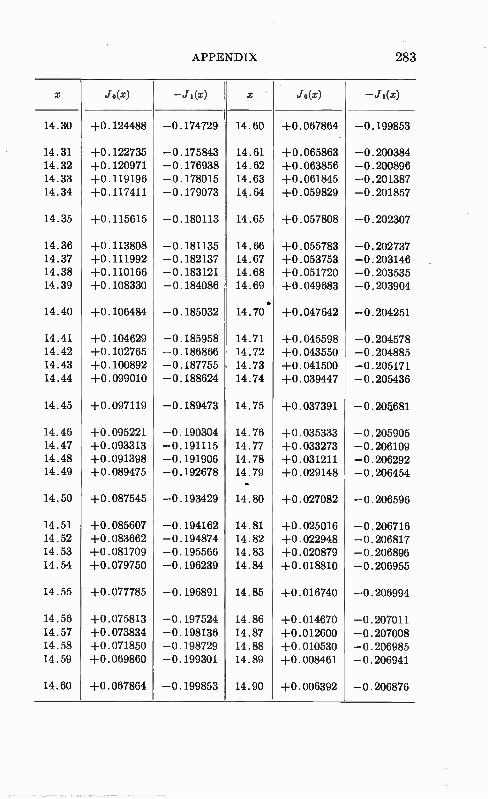
APPENDIX 283
x jo(x) - .11(x) x I o(x) -.11(x)
14.30 14).124488 -4).174729 14.60 +0.067864 --0.199853
14.31 14).122735 --0.175843 14.61 143.065863 --0.200384 14.32 +0.120971 --0.176938 14.62 14).063856 --0.200896 14.33 +0.119196 --0.178015 14.63 +0.061845 --0.201387 14.34 1-0.117411 --0.179073 14.64 -F0.059829 --0.201857
14.35 14).115615 --0.180113 14.65 +0.057808 --0.202307
14.36 1-0.113808 --0.181135 14.66 +0.055783 --0.202737 14.37 143.111992 --0.182137 14.67 1-0.053753 --0.203146 14.38 14).110166 --0.183121 14.68 +0.051720 --0.203535 14.39 14).108330 --0.184086 14.69 +0.049683 --0.203904
e 14.40 +0.106484 -0.185032 14.70 140.047642 --0.204251
14.41 +0.104629 --0.185958 14.71 140.045598 --0.204578 14.42 14).102765 --0.186866 14.72 +0.043550 --0.204885 14.43 14).100892 --0.187755 14.73 +0.041500 --0.205171 14.44 +0.099010 --0.188624 14.74 143.039447 --0.205436
14.45 14).097119 --0.189473 14.75 140.037391 -0.204681
14.46 +0.095221 --0.190304 14.76 +0.035333 --0.205905 14.47 +0.093313 -0.191115 14.77 -F0.033273 --0.206109 14.48 +0.091398 -0.191906 14.78 +0.031211 -40.206292 14.49 +0.089475 --0.192678 14.79 +0.029148 -43.206454
14.50 +0.087545 --0.193429 14.80 -F0.027082 --0.206596
14.51 +0.085607 --0.194162 14.81 140.025016 --0.206716 14.52 140.083662 --0.194874 14.82 -F0.022948 --0.206817 14.53 +0.081709 -4).195566 14.83 140.020879 --0.206896 14.54 +0.079750 --0.196239 14.84 +0.018810 --0.206955
14.55 +0.077785 --0.196891 14.85 +0.016740 --0.206994
14.56 140.075813 -0.197524 14.86 +0.014670 --0.207011 14.57 +0.073834 --0.198136 14.87 +0.012600 --0.207008 14.58 143.071850 --0.198729 14.88 143.010530 --0.206985 14.59 +0.069860 --0.199301 14.89 +0.008461 --0.206941
14.60 +0.067864 --0.199853 14.90 14).006392 --0.206876
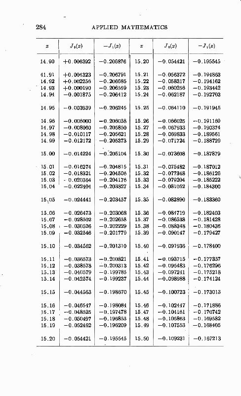
284 APPLIED MATHEMATICS
x Jo(x) - Ji(x) x Jo(x) -.71(x)
14.90 +0.006392 --0.206876 15.20 -0.054421 -4).195545
41.91 14).004323 --0.206791 15.21 --0.056372 --0.194863 14.92 +0.002256 -0.206685 15.22 --0.058317 --0.194162 ' 14.93 143.000190 --0.206559 15.23 -4).060256 --0.193442 14.94 --0.001875 --0.206412 15.24 --0.062187 --0.192703
14.95 --0.003939 --0.206245 15.25 --0.064110 --0.191945
14.96 --0.006000 --0.206058 15.26 --0.066025 --0.191169 14.97 -0.008060 --0.205850 15.27 --0.067933 --0.190374 14.98 -0.010117 --0.205621 15.28 --0.069833 --0.189561 14.99 --0.012172 --0.205373 15.29 --0.071724 --0.188729
15.00 --0.014224 -0205104 15.30 --0.073608 --0.187879
15.01 --0.016274 --0.204815 15.31 --0.075482 --0.187012 15.02 --0.018321 --0.204506 15.32 -4).077348 -0.186126 15.03 --0.020364 -0.204176 15.33 --0.079204 --0.185222 15.04 --0.022404 -4).203827 15.34 --0.081052 --0.184300
15,05 --0.024441 --0.203457 15.35 -4).082890 --0.183360
15.06 -0.026473 -0.203068 15.36 --0.084719 --0.182403 15.07 --0.028502 --0.202658 15.37 --0.086538 -0.181428 15.08 --0.030526 --0.W32229 15.38 --0.088348 --0.180436 15.09 --0.032546 --0.201779 15.39 --0.090147 --0.179427
15.10 --0.034562 --0.201310 15.40 --0.091936 --0.178400
15.11 --0.036573 --0.200821 15.41 --0.093715 --0.177357 15.12 --0.038578 --0.200313 15.42 --0.095483 --0.176296 15.13 --0.040579 --0.199785 15.43 --0.097241 -0.175218 15.14 --0.042574 --0.199237 15.44 --0.098988 -4).174124
15.15 --0.044563 -0.198670 15.45 -4).100723 -43.173013
15.16 --0.046547 --0.198084 15.46 --0.102447 -0.171886 15.17 --0.048525 --0.197478 15.47 --0.104161 --0.170742 15.18 -0.050497 --0.196853 15.48 -0.105863 -0.169582 15.19 --0.052462 -43.196209 15.49 --0.107553 --0.168405
15.20 --0.054421 --0.195545 15.50 -0.109231 --0.167213
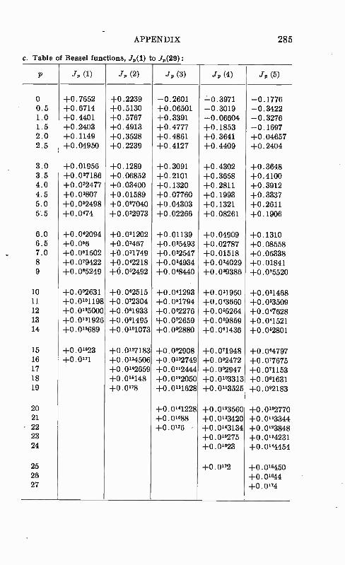
APPENDIX
c. Table of Bessel functions, .12,(1) to .4(29):
P Ji, (1) tip (2) JP (3) Ji, (4) fp (5)
o +0.7652 +0.2239 -0.2601 -0.3971 -0.1776 0.5 +0.6714 +0.5130 +0.06501 -0.3019 -0.3422 1.0 +0.4401 +0.5767 +0.3391 -0.06604 -0.3276 1.5 +0.2403 +0.4913 +0.4777 +0.1853 -0.1697 2.0 +0.1149 +0.3528 +0.4861 +0.3641 +0.04657 2.5 +0.04950 +0.2239 +0.4127 +0.4409 +0.2404
3.0 +0.01956 +0.1289 +0.3091 +0.4302 +0.3648 3.5 +0.027186 +0.06852 +0.2101 +0.3658 +0.4100 4.0 +0.022477 +0.03400 +0.1320 +0.2811 +0.3912 4.5 +0.03807 +0.01589 +0.07760 +0.1993 +0.3337 5.0 +0.032498 +0.027040 +0.04303 +0.1321 +0.2611 5.5 +0.014 +0.022973 +0.02266 +0.08261 +0.1906
6.0 +0.042094 +0.021202 +0.01139 +0.04909 +0.1310 6.5 +0.066 +0.03467 +0.025493 +0.02787 +0.08558 7.0 +0.061502 +0.031749 +0.022547 +0.01518 +0.05338 8 +0.079422 +0.042218 +0.034934 +0.024029 +0.01841 9 +0.085249 +1).062492 +0.048440 +0.039386 +0.025520
10 +0.0°2631 +0.062515 +0.041293 +0.031950 +0.021468 11 +0.01°1198 +0.072304 +0.061794 +0.043660 +0.033509 12 +0.0 125000 +0.081933 +0.062276 +0.066264 +0.0/628 13 +0.0'31926 +0.0°1495 +0.072659 +0.069859 +0.041521 14 +0.016689 +0.01°1073 +0.082880 +0.061436 +0.062801
15 +0.0 1623 +0.0127183 +0.0°2908 +0.071948 +0.064797 16 +0.0771 +0.0134506 +0.01°2749 +0.082472 +0.077675 17 +0.0142659 +0.0 712444 +0.0°2947 +0.071153 18 +0.0 16148 +0.0'22050 +0.07°3313 +0.031631 19 +0.0778 +0.0131628 +0.0113525 +0.0°2183
20 +0.01'1228 +0.0 123560 +0.01°2770 21 +0.01688 +0.0133420 +0.0 113344
, 22 +0.0176 , +0.013134 +0.0123848 23 +0.016275 +0.0134231 24 +0.0 1623 +0.01'4454
25 +0.0'2 +0.016450 26 +0.01644 27 +0.0174
285
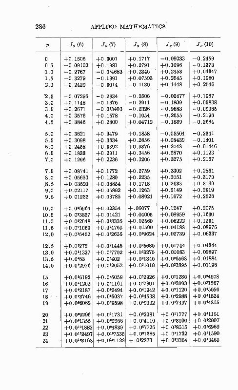
286 APPLIED MATHEMATICS
P Jp (6) JP (7) JP (8) JP (9) JP (10)
0 +0.1506 +0.3001 +0.1717 -0.09033 -0.2459 0.5 -0.09102 +0.1981 +0.2791 +0.1096 -0.1373 1.0 -0.2767 -0.024683 +0.2346 +0.2453 +0.04347 1.5 -0.3279 --0.1991 +0.07593 +0.2545 +0.1980 2.0 -0.2429 0.3014 -0.1130 +0.1448 +0.2546
'2.5 0.07295 -0.2834 -0.2506 -0.02477 +0.1967 3.0 +0.1148 -.0.1676 -0.2911 -0.1809 +0.05838 3.5 +0.2671 -0.023403 -0.2326 -0.2683 -0.09965 4.0 +0.3576 +0.1578 -0.1054 -0.2655 -0.2196 4.5 +0.3846 +0.2800 +0.04712 -0.1839 -0.2664
5.0 +0.3621 +0.3479 +0.1858 •-0.05504 .•-0.2341 5.5 +0.3098 +0.3634 +0.2856 +0.08439 -0.1401 6.0 +0.2458 +0.3392 +0.3376 +0.2043 -0.01446 6.5 +0.1833 +0.2911 +0.3456 +0.2870 +0.1123 . 7.0 +0.1296 +0.2236 +0.3206 +0.3275 +0.2167
7.5 +0.08741 +0.1772 +0.2759 +0.3302 +0.2861 8.0 +0.05653 +0.1280 +0.2235 +0.3051 +0.3179
8.5 +0.03520 +0.08854 +0.1718 +0.2633 +0.3169 9.0 +0.02117 +0.05892 +0.1263 +0.2149 +0.2919 9.5 +0.01232 +0.03785 +0.08921 +0.1672 +0.2526
10.0 +0.026964 +0.02354 +.06077 +0.1247 +0.2075
10.5 +0.023827 +0.01421 +0,04005 +0.08959 +0.1630
11.0 +0.022048 +0.028335 +0.02560 +0.06222 +0.1231
11.5 +0.021069 +0.024763 +0.01590 +0.04188 +0.08976 12.0 +0.035452 +0.022656 +0.029624 +0.02739 +0.06337
12.5 +0.03272 +0.021446 +0.025680 +0.01744 +0.04344
13.0 +0.031327 +0.037702 +0.023275 +0.01083 +0.02897 13.5 +0.0463 +0.03402 +0.021846 +0.026568 +0.01884
14.0 +0.042976 +0.032052 +0.021019 +0.023895 +0.01196
15 +0.0%192 +0.045059 +0.032926 +0.021286 +0.024508 16 +0.061202 +0.041161 +0.047801 +0.033993 +0.021567
17 +0.062187 +0.062494 +0.041942 +0.031120 +0.035056
18 +0.073746 +0.065037 +0.064538 +0.042988 +0.081524
19 +0.086062 +0.079598 +0.069992 +0.067497 +0.044315
20 +0.099296 +0.071731 +0.062081 +0.061777 +0.041151 21 +0.091355 +0.082966 +0.074110 +0.063990 +0.062907
22 +0.0'01882 +0.094839 +0.087725 +0.078515 +0.066969
23 +0.0"2497 +0.0107535 +0.081385 +0.071732 +0.061590 24 +0.0123168 +0.01°1122 +.092373 +0.083364 +0.073463
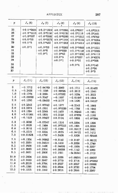
APPENDIX 287
- P J1, (6) JP (7) JP (8) •
.r, (9) JP (10)
25 +0.0'33855 +0.0"1602 +0.01°3895 +0.0°6257 +0.087215 26 +0.0'44415 +0.01°2195 +0.01'6135 +0.0°1116 +0.081441 27 +0.016507 +0.0'32893 +0.0 129289 +0.01°1913 +0.082762 28 +0.01655 +0.01°3673 +0.0 121354 +0.0"3154 +0.01°5094 29 +0.0176 +0.016450 +0.0'31903 +0.0125014 +0.01'9050
30 +0.0171 +0.01653 +0.0'42583 +0.0'1692 +0.0111551 31 +0.0'76 +0.0'6339 +0.0131140 +0.0122568 32 +0.0'71 +0.01643 +0.0"1636 +0.0'84112 33 +0.0175 +0.0'6227 +0.01°6376 34 +0.0 171 +0.01631 +0.018958
35 +0.0'74 +0.0'6140 36 +0.01620 37 +0.0'73
p ji, (11) .1", (12) Jp (13) Jp (14) J, (15)
0 -0.1712 +0.04769 +0.2069 +0.1711 -0.01422 0.5 -0.2406 -0.1236 +0.09298 +0.2112 +0.1340 1.0 -0.1768 -0.2234 -0.07032 +0.1334 +0.2051 1.5 -0.02293 -0.2047 -0.1937 -0.01407 +0.1654 2.0 +0.1390 -0.08493 -0.2177 -0.1520 +0.04157
2.5 +0.2343 +0.07242 +0.1377 -0.2143 -0.1009 3.0 +0.2273 +0.1951 +0.0°3320 -0.1768 -0.1940 3.5 +0.1294 +0.2348 +0.1407 -0.06245 -0.1991 4.0 -0.01504 +0.1825 +0.2193 +0.07624 -0.1192 4.5 -0.1519 +0.06457 +0.2134 +0.1830 +0 .027984 5.0 -0.2383 -0.07347 +0.1316 +0.2204 +0.1305 5.5 -0.2538 -0.1864 +0.087055 +0.1801 +0.2039 6.0 -0.2016 -0.2437 -0.1180 +0.08117 +0.2061 6.5 -0.1018 -0.2354 -0.2075 -0.04151 +0.1415 7.0 +0.01838 -0.1703 -0.2406 -0.1508 +0.03446 7.5 +0.1334 -0.06865 -0.2145 -0.2187 -0.08121 8.0 +0.2250 +0.04510 -0.1410 -0.2320 -0.1740 8.5 +0.2838 +0.1496 -0.04006 -0.1928 -0.2227 9.0 +0.3089 +0.2304 +0.06698 -0.1143 -0.2200 • 9.5 +0.3051 +0.2806 +0.1621 -0..01541 -0.1712
10.0 +0.2804 +0.3005 +0.2338 +0.08501 +0.09007 10.5 +0.2433 +0.2947 +0.2770 +0.1718 +0.05862 11.0 +0.2010 +0.2704 +0.2927 +0.2357 +0.09995 11.5 +0.1593 +0.2351 •+0.2854 +0.2732 +0.1794 12.0 +0.1216 +0.1953 +0.2615 +0.2855 +0.2367
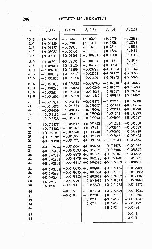
288 APPLIED MATHEMATICS
P J, (11) J, (12) J„ (13) Jp (14) Jp (15)
12.5 +0.08978 +0.1559 +0.2279 +0.2770 +0.2692
13.0 +0.06429 +0.1201 +0.1901 +0.2536 +0.2787
13.5 +0.04477 +0.08970 +0.1528 +0.2214 +0.2693
14.0 +0.03037 +0.06504 +0.1188 +0.1855 +0.2464
14.5 +0.02011 +0.04591 +0.08953 +0.1500 +0.2155
15.0 +0.01301 +0.03161 +0.06564 +0.1174 +0.1813
15.5 +0.028237 +0.02126 +0.04691 +0.08931 +0.1474
16.0 +0.025110 +0.01399 +0.03272 +0.06613 +0.1162
16.5 +0.023108 +0.029017 +0.02232 +0.04777 +0.08905
17.0 +0.021856 +0.025698 +0.01491 +0.03372 +0.06653
17.5 +0.021086 +0.023532 +0.029760 +0.02330 +0.04853
18.0 +0.036280 +0.022152 +0.026269 +0.01577 +0.03463
18.5 +0.03366 +0.021288 +0.023955 +0.01047 +0.02419
19.0 +0.031990 +0.0/590 +0.022452 +0.026824 +0.01657
20 +0.045931 +0.032512 +0.038971 +0.022753 +0.027360
21 +0.041670 +0.01839 +0.033087 +0.021041 +0.023054
22 +0.064458 +0.042315 +0.031004 +0.033711 +0.021190
23 +0.051132 +0.066491 +0.043092 +0.031251 +0.034379
24 +0.062738 +0.051733 +0.069060 +0.044006 +0.04527
25 +0.076333 +0.064418 +0.062532 +0.041221 +0.045060
26 +0.071403 +0.061078 +0.066761 +0.063555 +0.041599
27 +0.082981 +0.072521 +0.061730 +0.069902 +0.04829
28 +0.046092 +0.085665 +0.074249 +0.062645 +0.061398
29 +0.091198 +0.081225 +0.04004 +0.076790 +0.063883
30 +0.0102274 +0.092552 +0.082283 +0.071678 +0.061037
31 +0.0'4165 +0.0105133 +0.095009 +0.083995 +0.072670
32 +0.0127375 +0.01'9976 +0.091062 +0.099187 +0.086632
33 +0.0121264 +0.0"1876 +0.01°2176 +0.092042 +0.081591
34 +0.0132100 +0.0123417 +0.0114320 +0.01°4392 +0.093693
35 +0 .0143383 +0.0 136035 +0.0 128310 +0.0119155 +0.0"8301
36 +0.012529 +0.0'31035 +0.0121551 +0.0"1851 +0.010/809
37 +0.0 1680 +0.0 141723 +0.0132812 +0.0'23632 +0.0113827
38 +0.01612 +0.0'6279 +0.0144956 +0.0136928 +0.0127863
39 +0.0"2 +0.01644 +0.016850 +0.0131285 +0.0 121571
40 +0.011 +0.016142 +0.0 142320 +0.0133054
41 +0.0171 +0.0 1623 +0.016408 +0.0145781
42 +0.0174 +0.01670 +0.0141067
43 +0.0171 +0.01612 +0.0'6192
44 +Q.0172 +0.0 1634
45 +0.0176
46 +0.0171

APPENDIX 289
p Jp (16) Jp (17) Jp (18) Jp (19) jp (20)
0 --0.1749 --0.1699 --0.01336 +0.1466 140.1670 0.5 --0.05743 --0.1860 --0.1412 14).02744 1-0.1629 1.0 14).09040 --0.09767 --0.1880 --0.1057 +0.06683 1.5 1-0.1874 +0.04231 --0.1320 --0.1795 -0.06466 2.0 +0.1862 -FO.1584 -0.027533 --0.1578 --0.1603
2.5 1-0.09257 143.1935 A-0.1192 --0.05578 --0.1726 3.0 -4).04385 -FO.1349 +0.1863 14).07249 --0.09890 3.5 -4).1585 143.01461 +0.1651 1411649 +0.02152
4.0 --0.2026 --0.1107 14106964 14).1806 +0.1307
4.5 --0.1619 --0.1875 --0.05501 +0.1165 A-0.1801
5.0 --0.05747 --0.1870 --0.1554 140.023572 -F0.1512 5.5 +0.06743 --0.1139 -4).1926 --0.1097 1-0.05953 6.0 140.1667 A-0.027153 --0.1560 --0.1788 --0.05509 6.5 14).2083 +0.1138 --0.06273 --0.1800 --0.1474 7.0 1-0.1825 +0.1875 1-0.05140 --0.1165 --0.1842
7.5 +0.1018 14).2009 14).1473 --0.01350 --0.1553 8.0 --0.027021 14).1537 -FO.1959 14109294 --0.07387 8.5 --0.1128 14).06346 1-0.1855 1-0.1694 143.03088 9.0 --0.1895 --0.04286 -0.1228 +0.1947 1-0.1251 9.5 --0.2217 --0.1374 140.02786 +0.1650 1-0.1816
10.0 --0.2062 --0.1991 -4).07317 1-0.09155 1-0.1865 10.5 --0.1504 --0.2171 --0.1561 -0.024326 140.1416 11.0 --0.06822 --0.1914 --0.2041 --0.09837 +0.06136 11.5 14).02427 --0.1307 --0.2100 --0.1698 --0.03288 12.0 +0.1124 --0.04857 --0.1762 --0.2055 --0.1190
12.5 1-0.1853 1-0.04024 --0.1122 --0.2012 --0.1794 13.0 140.2368 14).1228 --0.03092 --0.1612 --0.2041 13.5 143.2653 +0.1899 14105414 --0.09497 -0.1914 14.0 +0.2724 +0.2364 14).1316 --0.01507 -0.1464 14.5 A-0.2623 1-0.2613 140.1934 143.06627 --0.07897
15.0 140.2399 140.2666 14).2356 140.1389 -0.038121 15.5 +0.2102 143.2559 +0.2575 1-0.1961 +0.07689 16.0 143.1775 140.2340 +0.2611 140.2345 14).1452 16.5 1411450 +0.2054 +0.2500 140.2537 14).1982 17.0 +0.1150 A-0.1739 1412286 14).2559 +0.2331
17.5 +0.08876 +0.1427 1-0.2009 14).2445 +0.2501 18.0 +0.06685 14).1138 14).1706 140.2235 1-0.2511 18.5 +0.04920 14).08844 143.1406 140.1968 14).2395 19.0 1-0.03544 140.06710 +0.1127 14).1676 143.2189
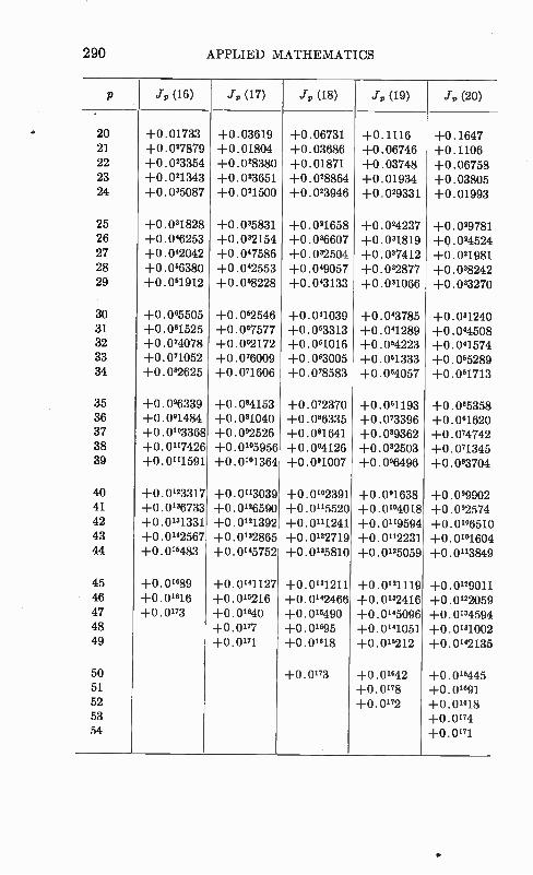
290 APPLIED MATHEMATICS
P J, (16) 4 (17) J, (18) J, (19) erp (20)
20 +0.01733 +0.03619 +0.06731 +0.1116 +0.1647 21 +0.027879 +0.01804 +0.03686 +0.06746 +0.1106 22 +0.023354 +0.028380 +0.01871 +0.03748 +0.06758 23 +0.021343 +0.023651 +0.028864 +0.01934 +0.03805 24 +0.035087 +0.021500 +0.023946 +0.029331 +0.01993
25 +0.031828 +0.035831 +0.021658 +0.024237 +0.029781 26 +0.046253 +0.032154 +0.036607 +0.031819 +0.024524 27 +0.0%042 +0.01586 +0.032504 +0.04412 +0.021981 28 +0.026380 +0.042553 +0.09057 +0.032877 +0.038242 29 +0.051912 +0.068228 +0.03133 +0.081066 +0.033270
30 +0.065505 +0.062546 +0.041039 +0.043785 +0.031240 31 +0.061525 +0.067577 +0.023313 +0.041289 +0.044508 32 +0.074078 +0.062172 +0.061016 +0.064223 +0.01574 33 +0.071052 +0.076009 +0.063005 +0.021333 +0.065289 34 +0.082625 +0.071606 +0.078583 +0.064057 +0.021713
35 +0.096339 +0.084153 +0.072370 +0.061193 +0.065358 36 +0.091484 +0.081040 +0.086335 +0.073396 +0.061620 37 +0.01°3368 +0.0°2526 +0.081641 +0.0%362 +0.04742 38 +0.0117426 +0.01°5956 +0.0°4126 +0.082503 +0.071345 39 +0.0111591 +0.01°1364 +0.0°1007 +0.0°6496 +0.083704
40 +0.0123317 +0.0113039 +0.01°2391 +0.0°1638 +0.099902 41 +0.0136733 +0.0126590 +0.0 115520 +0.01°4018 +0.092574 42 +0.0131331 +0.0121392 +0.0111241 +0.0 119594 +0.01°6510 43 +0.0'42567 +0.0132865 +0.0122719 +0.0112231 +0.01°1604 44 +0.016483 +0.0145752 +0.0135810 +0.0125059 +0.0113849
45 +0.01689 +0.0"1127 +0.0131211 +0.0121119 +0.0129011 46 +0.01616 +0.016216 +0.0142466 +0.0132416 +0.0122059 47 +0.0'73 +0.01640 +0.016490 +0.0'45096 +0.0134594 48 +0.0177 +0.01695 +0.0141051 +0.0131002 49 +0.0171 +0.01618 +0.016212 +0.0"2135
50 +0.0173 +0.01642 +0.016445 51 +0.0178 +0.01691 52 +0.0172 +0.01618 53 +0.0174 54 +0.0171
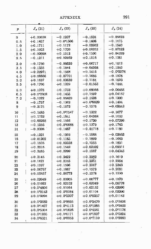
APPENDIX 291
P J„ (21) Jp (22) J„ (23) Jp (24)
0 140.03658 --0.1207 --0.1624 --0.05623
0.5 +0.1457 --0.021506 --0.1408 --0.1475
1.0 +0.1711 +0.1172 --0.03952 --0.1540
1.5 -FO.1023 +0.1700 14).08253 --0.07523
2.0 -40.02028 14).1313 +0.1590 44).04339
2.5 -4).1311 140.02469 +0.1516 +0.1381
3.0 --0.1750 --0.09330 1-0.06717 AD.1613
3.5 --0.1335 --0.1644 --0.04958 A-0.1040
4.0 --0.02971 --0.1568 --0.1415 --0.023076 4.5 140.08656 --0.07701 --0.1666 --0.1078 5.0 14).1637 +0.03630 --0.1164 --0.1623
5.5 140.1706 44).1329 --0.01563 --0.1444
6.0 14).1076 4-0.1733 14).09086 -.0.06455
6.5 140.022808 +0.1435 -F0.1592 +0.04157
7.0 --0.1022 -F0.05820 +0.1638 +0.1300 8 --0.1757 --0.1362 +0.028829 -FO.1404
9 --0.3175 --0.1573 --0.1576 -4).03643
10 14).1485 14).027547 --0.1322 --0.1677 11 140.1732 +0.1641 +0.04268 -4).1033
12 14).03293 14).1566 -FO.1730 14).07299 13 --0.1356 14).026688 +0.1379 -F0.1763 14 --0.2008 -411487 --0.01718 +0.1180
15 --0.1321 --0.1959 --0.1588 --0.03863 16 14).01202 --0.1185 --0.1899 --0.1663 17 140.1505 +0.02358 --0.1055 --0.1831 18 140.2316 4).1549 +0.03402 --0.09311 19 +0.2465 14).2299 A-0.1587 +0.04345
20 A-0.2145 A-0.2422 14).2282 140.1619 21 +0.1621 +0.2105 1-0.23i1 140.2264 22 -P0.1097 +0.1596 +0.2067 A-0.2343 23 +0.06767 +0.1087 1-0.1573 +0.2031 24 44).03857 +0.06773 4-0.1078 +0.1550
25 -F0.02049 1-0.03905 44).06777 A4).1070
26 140.01022 140.02102 4D.03949 A4).06778 27 1-0.024806 +0.01064 +0.02152 1-0.03990 28 +0.022143 +0.025084 44).01104 140.02200
29 +0.029094 +0.022307 1-0.025357 14).01143
30 +0.023682 +0.029965 +0.0D2470 +0.025626 31 +0.021427 44).024113 44).021085 +0.022633 32 +0.045304 +0.021626 +0.024561 A40.021176 33 4-0.041895 140.046171 -F0.021837 +0.025024 34 +0.026521 440.042253 440.047110 +0.022060
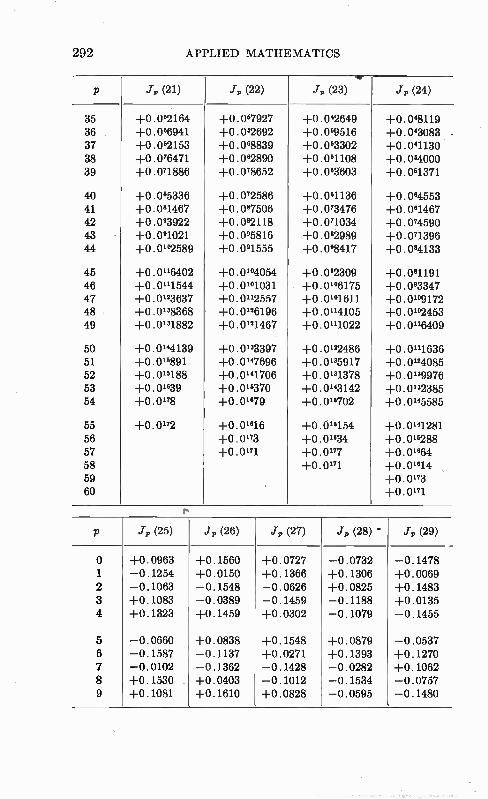
292 APPLIED MATHEMATICS
P fp (21) Jp (22) ..,
..Tp (23) JP (24)
35 +0.052164 +0.057927 +0.042649 +0.048119 36 +0.026941 +0.052692 +0.059516 +0.03083 - 37 +0.082153 +0.0°8839 +0.053302 +0.041130 38 +0.076471 +0.042890 +0.051108 +0.054000 39 +0.071886 +0.078652 +0.043603 +0.051371
40 +0.085336 +0.072586 +0.0°1136 +0.044553 41 +0.081467 +0.087506 +0.073476 +0.0°1467 42 +0.023922 +0.082118 +0.071034 +0.074590 43 +0.021021 +0.025816 +0.082989 +0.071396 44 +0.01°2589 +0.021555 +0.028417 +0.084133
45 +0.0116402 +0.01°4054 +0.022309 +0.081191 46 +0.0 111544 +0.01°1031 +0.01°6175 +0.023347 47 +0.0123637 +0.0112557 +0.0 121611 +0.01°9172 48 +0.0128368 +0.0126196 +0.0114105 +0.01°2453 49 +0.0181882 +0.0121467 +0.0"1022 +0.0"6409
50 +0.0 144139 +0.0"3397 +0.0122486 +0.0111636 51 +0.015891 +0.0 147696 +0.0 185917 +0.0124085 52 +0.015188 +0.0141706 +0.0"1378 +0.0189976 53 +0 .01639 +0.015370 +0.0'43142 +0.0 132385 54 +0.0'78 +0.01°79 +0.015702 +0.0145585
55 +0.0172 +0.01°16 +0.0'5154 +0.0"1281 56 +0.0'73 +0.01°34 +0.015288 57 +0.0"1 +0.0'77 +0.01°64 58 +0.0171 +0.01°14 59 +0.0'73 60 . +0.0171
P 4 (25) Ji, (26) .4 (27) tip (28) ' 4 (29)
CO
GA
+0.0963 +0.1560 +0.0727 -0.0732 -0.1478 -0.1254 +0.0150 +0.1366 +0.1306 +0.0069 -0.1063 -0.1548 -0.0626 +0.0825 +0.1483 +0.1083 -0.0389 -0.1459 -0.1188 +0.0135 +0.1323 +0.1459 +0.0302 -0.1079 -0.1455
-0.0660 +0.0838 +0.1548 +0.0879 -0.0537 -0.1587 -0.1137 +0.0271 +0.1393 +0.1270 -0.0102 -0.1362 -0.1428 -0.0282 +0.1062 +0.1530 +0.0403 -0.1012 -0.1534 -0.0757 +0.1081 +0.1610 +0.0828 -0.0595 -0.1480
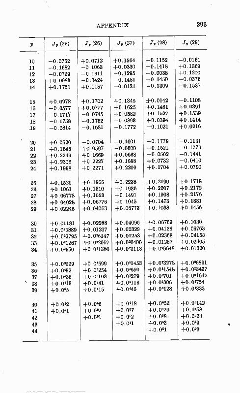
APPENDIX 293
p ' J, (25) Jp (26) Jp (27) J, (28) Jp (29)
10 -0.0752 +0.0712 +0.1564 +0.1152 -0.0161
11 -0.1682 -0.1063 +0.0330 +0.1418 +0.1369
12 -0.0729 -0.1611 -0.1295 -0.0038 +0.1200
13 +0.0983 -0.0424 -0.1481 -0.1450 -0.0376
14 +0.1751 +0.1187 -0.0131 -0.1309 -0.1537
15 +0.0978 +0.1702 +0.1345 +0.0142 -0.1108
16 -0.0577 +0.0777 +0.1625 +0.1461 +0.0391
17 -0.1717 -0.0745 +0.0582 +0.1527 +0.1539
18 -0.1758 -0.1752 -0.0893 +0.0394 +0.1414
.19 -0.0814 -0.1681 -0.1772 -0.1021 +0.0216
20 +0.0520 -0.0704 -0.1601 -0.1779 -0.1131
21 +0.1646 +0.0597 -0.0600 -0.1521 -0.1776
22 +0.2246 +0.1669 +0.0668 -0.0502 -0.1441
23 +0.2306 +0.2227 +0.1688 +0.0732 -0.0410
24 +0.1998 +0.2271 +0.2209 +0.1704 +0.0790
25 +0.1529 +0.1966 +0.2238 +0.2190 +0.1718
26 +0.1061 +0.1510 +0.1936 +0.2207 +0.2172
27 +0.06778 +0.1053 +0.1491 +0.1908 +0.2176
28 +0.04028 +0.06776 +0.1045 +0.1473 +0.1881
29 +0.02245 +0.04063 +0.06773 +0.1038 +0.1456
30 +0.01181 +0.02288 +0.04096 +0.06769 +0.1030
31 +0.025889 +0.01217 +0.02329 +0.04126 +0.06763
32 +0.022795 +0.026147 +0.01253 +0.02368 +0.04155
33 +0.021267 +0.022957 +0.026400 +0.01287 +0.02405
34 +0.03550 +0.021360 +0.023118 +0.026648 +0.01320
35 +0.03229 +0.03599 +0.021453 +0.023278 +0.026891
36 +0.0492 +0.032M +0.03650 +0.021548 +0.023437
37 +0.0436 +0.08103 +0.03279 +0.08701 +0.021642
\ 38 +0.0413 +0.0441 +0.03116 +0.03306 +0.03754
39 +0.055 +0.0415 +0.0446 +0.03128 +0.03333
40 +0.052 +0.056 +0.0418 +0.0452 +0.03142
41 +0.051 +0.052 +0.057 +0.0420 +0.0458
42 +0.051 +0.052 +0.058 +0.0423
43 +0.051 +0.053 +0.069
44 +0.051 +0.053
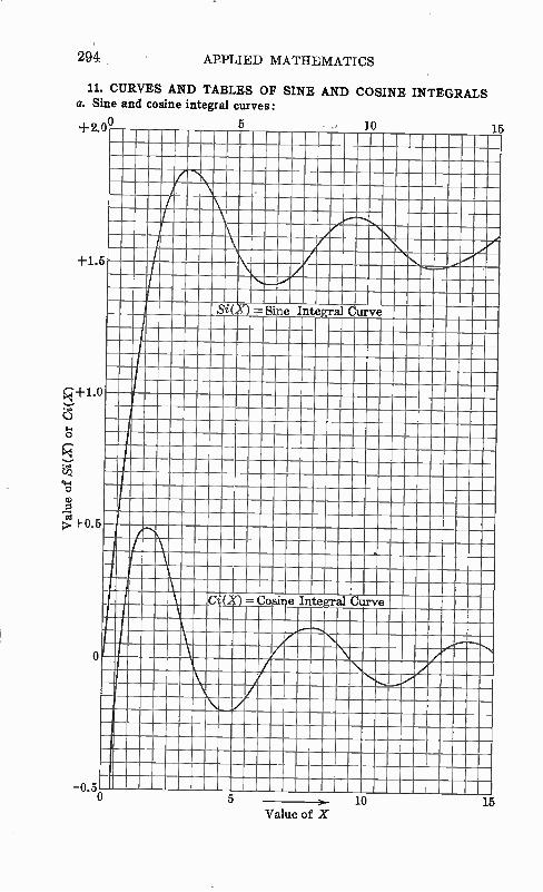

APPENDIX 95
b. Sine and cosine integral tables:
.r Si(z) Ci(x) MW Ei(-x)
0.00 +0.000000 - co - co - cc,
0.01 +0.010000 -4.0280 -4.0179 -4.0379
0.02 •+0.019999 -3.3349 -3.3147 -3.3547
0.03 +0.029998 -2.9296 -2.8991 -2.9591
0.04 +0.039996 -2.6421 -2.6013 -2.6813
0.05 +0.04999 -2.4191 -S.3679 -2.4679
0.06 +0.05999 -2.2371 -2.1753 -2.2953
0.07 +0.06998 -2.0833 -2.0108 -2.1508
0.08 +0.07997 -1.9501 -1.8669 -2.0269
0.09 +0.08996 -1.8328 -1.7387 -1.9187
0.10 +0.09994 -1.7279 -1.6228 -1.8229
0.11 +0. 10993 -1.6331 -1.5170 -1.7371
0.12 +0.11990 -1.5466 -1.4193 -1.6595
0.13 +0. 12988 -1.4672 -1.3287 -1.5889
0.14 +0. 13985 -1.3938 -1.2438 -1.5241
0.16 +0.14981 -1.3255 -1.1641 -1.4645
0.16 +0.15977 -1.2618 -1.0887 -1.4092
0.17 +0.16973 -1.2020 -1.0172 -1.3578
0.18 +0.1797 -1.1457 -0.9491 -1.3098
0.19 +0.1896 -1.0925 -0.8841 -1.2649
0.20 +0.1996 -1.0422 -0.8218 -1.2227
0.21 +0.2095 -0.9944 -0.7619 -1.1829
0.22 +0.2194 -0.9490 -0.7042 -1.1454
0.23 +0.2293 -0.9057 -0.6485 -1.1099
0.24 +0.2392 -0.8643 -0.5947 -1.0762
0.25 +0.2491 -0.8247 -0.5425 -1.0443
0.26 +0.2590 -0.7867 -0.4919 -1.0139
0.27 +0.2689 -0.7503 -0.4427 -0.9849
0.28 +0.2788 -0.7153 -0.3949 -0.9573
0.29 +0.2886 -0.6816 -0.3482 -0.9309
0.30 +0.2985 -0.6492 -0.3027 -0.9057
0.31 +0.3083 -0.6179 -0.2582 -0.8815
0.32 +0.3182 -0.5877 -0.2147 -0.8583
0.33 +0.3280 -0.5585 -0.17210 -0.8361
0.34 +0.3378 -0.5304 -0.13036 -0.8147
0.35 +0.3476 -0.5031 -0.08943 -0.7942
0.36 +0.3574 -0.4787 -0.04926 • -0.7745
0.37 +0.3672 -0.4511 -0.00979 -0.7554
0.38 +0.3770 -0.4263 +0.02901 -0.7371
0.39 +0.3867 -0.4022 +0.06718 -0.7194
0.40 +0.3965 -0.3788 +0.10477 -0.7024
0.41 +0.4062 -0.3561 +0. 14179 -0.6859
0.42 +0.4159 -0.3341 +0. 17828 -0.6700
0.43 +0.4256 -0.3126 +0.2143 -0.6546
0.44 +0.4353 -0.2918 +0.2498 -0.6397
0.45 +0.4450 -0.2715 +0.2849 -0.6253
0.46 +0.4548 -0.2517 +0.3195 -0.6114
0.47 +0.4643 -0.2325 +0.3537 -0.5979
0.48 - +0.4739 -0.2138 +0.3878 -0.5848
0.49 +0.4835 -0.1956 +0.4211 -0.5721
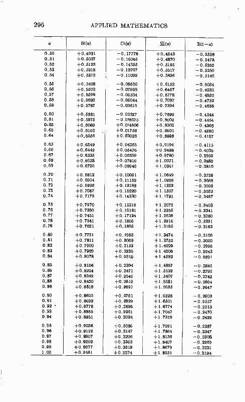
296 APPLIED MATHEMATICS
x Si(x) Ci (x) E(x) Ei( -x)
0.50 +0.4931 -0.17778 +0.4542 -0.5598 0.51 +0.5027 -0.16045 +0.4870 -0.5478 0.52 +0.5123 -0.14355 +0.5195 -0.5362 0.53 +0.5218 -0.12707 +0.5517 -0.5250 0.54 +0.5313 -0.11099 +0.5838 -0.5140
0.55 +0.5408 -0.09530 4 0.8153 -0.5034 0.56 +0.5503 -0.07999 +0.6467 -0.4930 0.57 +0.5598 -0.06504 +0.6778 -0.4830 0.58 +0.5693 -0.05044 +0.7087 -0.4732 0.59 +0.5787 -0.03619 +0.7394 -0.4636
0.60 +0.5881 -0.02227 +0.7699 -0.4544 0.61 +0.5975 -0.028675 +0.8002 - 0.4454 0.62 +0.6069 +0.024606 +0.8302 -0.4366 0.63 +0.6163 . +0.01758 +0.8601 -0.4280 0.64 +0.6256 +0.63026 +0.8898 -0.4197
0.65 +0.6349 +0.04265 +0.9194 -0.4115 0.66 +0.6442 +0.05476 +0.9488 -0.4038 0.67 +0.8535 +0.06659 +0.9780 -0.3959 0.68 +0.6628 +0.07816 +1.0071 -0.3883 0.69 +0.6720 +0.08946 +1.0361 -0.3810
0.70 +0.6812 +0.10051 +1.0649 -0.3738 0.71 +0.6904 +0.11132 +1.0936 -0.3668 0.72 +0.6996 +0.12188 +1.1222 - 0.3599 0.73 +0.7087 +0. 13220 +1.1507 -0.3532 0.74 +0.7179 +0.14230 +1.1791 - 0.3467
0.75 +0.7270 +0.15216 +1.2073 -0.3403 0.76 +0.7360 +0.16181 +1.2355 -0.3341 0.77 +0.7451 +0.17124 +1.2636 -0.3280 0.78 +0.7541 +0.1805 +1.2916 -0.3221 0.79 +0.7631 +0.1895 +1.3195 -0.3163
0.80 +0.7721 +0.1983 +1.3474 -0.3106 0.81 +0.7811 +0.2069 +1.3752 -0.8050 0.82 +0.7900 +0.2153 +1.4029 -0.2996 0.83 +0.7989 +0.2235 +1.4306 -0.2943 0.84 +0.8078 +0.2318 +1.4582 -0.2891
0.85 +0.8166 +0.2394 +1.4857 - 0.2840 0.86 +0.8254 +0.2471 +1.5132 -0.2790 0.87 +0.8342 +0.2546 +1.5407 - -0.2742 0.88 +0.8430 +0.2619 +1.5681 - 0.2694 0.89 +0.8518 +0.2691 +1.5955 -0.2647
0.90 +0.8605 +0.2761 +1.6228 -0.2602 0.91 +0.8692 +0.2829 +1.6501 -0.2557 0.92 ' +0.8778 +0.2896 +1.6774 -0.2513 0.93 +0.8865 • +0.2961 +1.7047 -0.2470 0.94 +0.8951 +0.3024 +1.7319 -0.2429
0.95 +0.9036 +0.3086 +1.7591 -0.2387 0.96 +0.9122 +0.3147 +1.7864 -0.2347 0.97 +0.9207 +0.3206 +1.8136 -0.2308 0.98 +0.9292 +0.3263 +1.8407 -0.2269 0.99 +0.9377 +0.3319 +1.8679 -0.2231 1.00 +0.9461 +0.3374 +1.8951 -0.2194
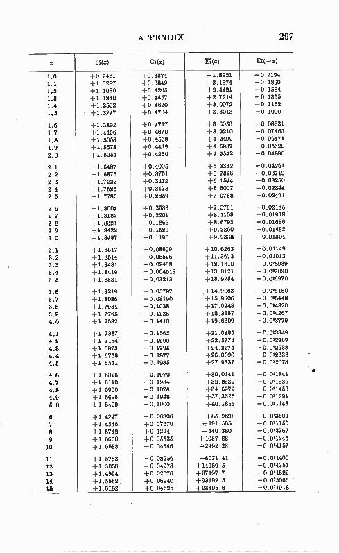
APPENDIX 297
x Si(x) Ci(x) ri(x) Ei(- x)
1.0 +0.9461 +0.3374 +1.8951 -0.2194
1.1 +1.0287 +0.3849 +2.1674 -0.1880
1.2 +1.1080 +0.4205 +2.4421 -0.1584
1.3 +1.1840 +0.4457 +2.7214 -0.1355
1.4 +1.2562 +0.4620 +3.0072 -0.1162
1.5 +1.3247 +0.4704 +3.3013 -0.1000
1.6 +1.3892 +0.4717 +3.6053 -0.08631
1.7 +1.4496 +0.4670 +3.9210 -0.07465
1.8 +1.5058 +0.4568 +4.2499 -0.06471
1.9 +1.5578 +0.4419 +4.5937 -0.05620
2.0 +1.6054 +0.4230 +4.9542 -0.04890
2.1 +1.6487 +0.4005 +5.3332 -0.04261
2.2 +1.6876 +0.3751 +5.7326 -0.03719
2.3 +1.7222 +0.3472 +6.1544 -0.03250
2.4 +1.7525 +0.3173 +6.6007 -0.02844
2.5 +1.7785 +0.2859 +7.0738 -0.02491
2.6 +1.8004 +0.2533 +7.5761 -0.02185
2.7 +1.8182 +0.2201 +8.1103 -0.01918
2.8 +1.8321 +0.1865 . +8.6793 -0.01686
2.9 +1.8422 +0.1529 +9.2860 -0.01482
3.0 +1.8487 +0.1196 +9.9338 -0.01304
3.1 +1.8517 +0.08699 +10.6263 -0.01149
3.2 +1.8514 +0.05526 +11.3873 -0.01013
3.3 +1.8481 +0.02468 +12.1610 -0.028939
3.4 +1.8419 -0.004518 +13.0121 -0.027890
3.5 +1.8331 -0.03213 +13.9254 -0.026970
3.6 +1.8219 -0.05797 +14.9063 -0.026160
3.7 +1.8086 -0.08190 +15.9606 -0.025448
3.8 +1.7934 -0.1038 +17.0948 -0.024820
3.9 +1.7765 -0.1235 +18.3157 -0.024267
4.0 +1.7582 -0.1410 +19.6309 -0.023779
4.1 +1.7387 -0.1562 +21.0485 -0.023349
4.2 +1.7184 -0.1690 +22.5774 -0.022969
4.3 +1.6973 -0.1795 +24.2274 -0.022633
4.4 +1.6758 -0.1877 +26.0090 -0.022336
4.5 +1.6541 -0.1935 +27.9337 -0.022073
4.6 +1.6325 -0.1970 +30.0141 -0.021841
4.7 +1.8110 -0.1984 +32.2639 -0.021635
4.8 +1.5900 -0.1976 +34.6979 -0.021453
4.9 +1.5696 -0.1948 +37.3325 -0.021291
5.0 +1.5499 -0.1900 +40.1853 -0.021148
8 +1.4247 -0.06806 +85.9898 -0.023601
7 +1.4546 +0.07670 +191.505 -0.021155
8 +1.5742 +0.1224 +440.380 -0.043767
9 +1.6650 +0.05535 +1037.88 -0.041245
10 +1.6583 -0.04546 +2492.23 -0.054157
11 +1.5783 -0.08956 +6071.41 -0.051400
12 +1.5050 -0.04978 +14959.5 -0.054751
13 +1.4994 +0.02676 +37197.7 -0.051622
14 +1.5562 +0.06940 +93192.5 -0.0,5566 --
15 +1.8182 +0.04628 +23495.6 -0.0,1918
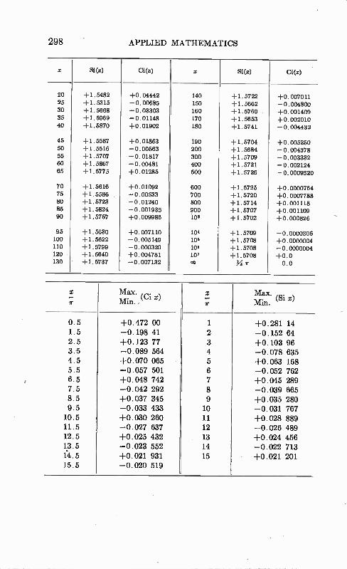
298 APPLIED MATHEMATICS
x Si(x) Ci(x) x Si(x) Ci(x)
20 +1.5482 +0.04442 140 +1.5722 +0.007011 25 +1.5315 -0.00685 150 +1.5862 -0.004800 30 +1.5668 -0.03303 160 +1.5769 +0.001409 35 +1.5969 -0.01148 170 +1.5653 +0.002010 40 +1.5870 +0.01902 180 +1.5741 -0.004432
45 +1.5587 +0.01863 190 +1.5704 +0.005250 50 +1.5516 -0.00563 200 +1.5684 -0.004378 55 +1.5707 -0.01817 300 +1.5709 -0.003332 60 +1.5867 -0.00481 400 +1.5721 -0.002124 65 +1.5775 +0.01285 500 +1.5726 -0.0009320
70 +1.5616 +0.01092 600 +1.5725 +0.0000764 75 +1.5586 -0.00533 700 +1.5720 +0.0007788 80 +1.5723 -0.01240 800 +1.5714 +0.001118 85 +1.5824 -0.001935 900 +1.5707 +0.001109 90 +1.5757 +0.009986 108 +1.5702 +0.000826
95 +1.5630 +0.007110 104 +1.5709 -0.0000306 100 +1.5822 -0.005149 108 +1.5708 +0.0000004 110 +1.5799 -0.000320 108 +1.5708 -0.0000004 120 +1.5640 +0.004781 107 +1.5708 +0.0 130 +1.5737 -0.007132 oo X *8" 0.0
X
ir
Max. Min. (Ci x) .
Max. Min. (Si x)
0.5 1.5 2.5 3.5 4.5 5.5 6.5 7.5 8.5 9.5 10.5 11.5 12.5 13.5 174.5 15.5
1-0.472 00 1 -0.198 41 2 1-0.123 77 3 --0.089 564 4 1-0.070 065 5 -0.057 501 6 1-0.048 742 7 -0.042 292 8 1-0.037 345 9 --0.033 433 10 +0.030 260 11 --0.027 637 12 A-0.025 432 13 --0.023 552 14 1-0.021 931 15 --0.020 519
+0.281 14 --0.152 64 1-0.103 96 -0.078 635 +0.063 168 --0.052 762 +0.045 289 --0.039 665 +0.035 280 --0.031 767 +0.028 889 --0.026 489 +0.024 456 --0.022 713 +0.021 201
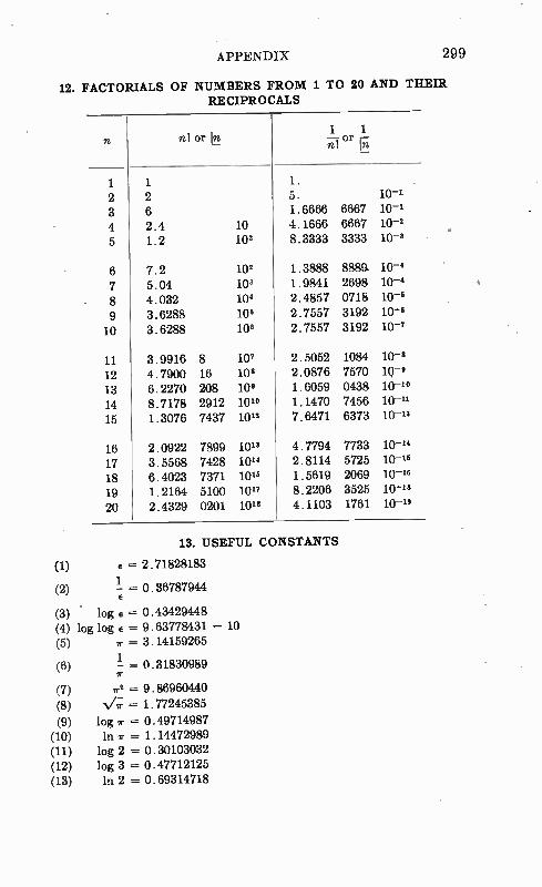
APPENDIX 299
12. FACTORIALS OF NUMBERS FROM 1 TO 20 AND THEIR RECIPROCALS
1 2 3 4 5
6 7 8 9 10
11 12 13 14 15
16 17 18 19 20
n! or
1 2 6 2.4 1.2
10 102
7.2 102 5.04 102 4.032 106 3.6288 109 3.6288 106
3.9916 8 107 4.7900 16 106 6.2270 208 109 8.7178 2912 101° 1.3076 7437 1012
2.0922 7899 10" 3.5568 7428 10" 6.4023 7371 10" 1.2164 5100 10" 2.4329 0201 10"
1 1 or Ft
1. 5. 10-1
1.6666 6667 10-1 4.1666 6667 10-2 8.3333 3333 10-2
1.3888 SS&D. 10-6 1.9841 2698 10-6 2.4857 0718 10-9 2.7557 3192 10-6 2.7557 3192 10-7
2.5052 1084 10-6 2.0876 7570 10-9 1.6059 0438 10-1° 1.1470 7456 10-11 7.6471 6373 10-12
4.7794 7733 10-" 2.8114 5725 10-16 1.5619 2069 10-16 8.2206 3525 10-16 4.1103 1761 10-19
13. USEFUL CONSTANTS
(1) e = 2.71828183 1
(2) - = 0.36787944 e
(3) h)ge= 0.43429448 (4) logloge = 9.63778431 - 10 (5) ir= 3.14159265
1 (6) - = 0.31830989
(7) e2 -= 9.86960440 (8) NAT- = 1.77245385 (9) log ir = 0.49714987
(10) lnir = 1.14472989 (11) log2 = 0.30103032 (12) log3 = 0.47712125 (13) 1112 = 0.69314718
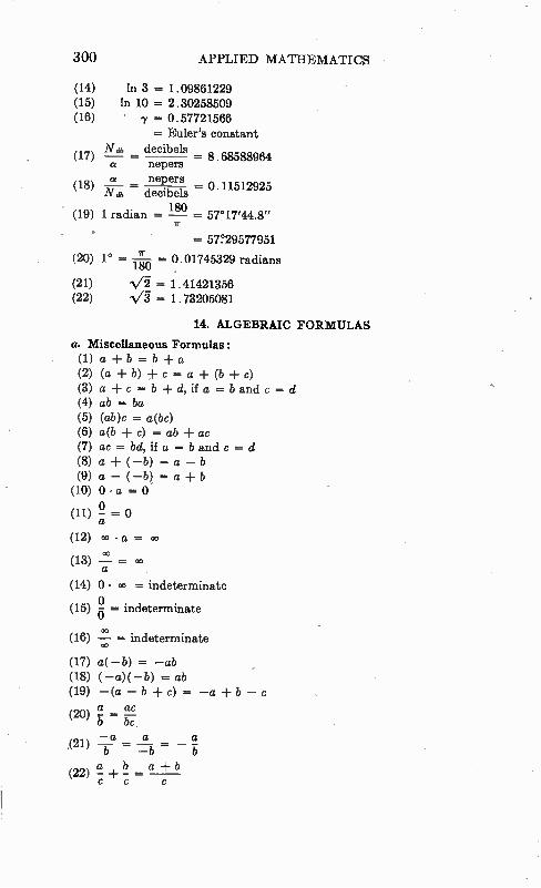
300 APPLIED MATHEMATICS
(14) In 3 = 1.09861229 (15) In 10 = 2.30258509 (16) • = 0.57721566
= Euler's constant Ndb decibels
(17) - - 8.68588964 nepers
a nepers (18) - 0.11512925
Nab decibels 180
(19) 1 radian = — = 57°17'44.8"
57?295'77951
(20) 1° = ir = 0.01745329 radians 180
(21) = 1.41421356 (22) 1/U = 1.73205081
14. ALGEBRAIC FORMULAS
a. Miscellaneous Formulas: (1)a+b=b+a (2) (a + b) -F c = a c) (3) a + c = b + d, if a = b and c = d (4) ab = Sa (5) (ab)c = a(bc) (6) a(b + c) = ab + ac (7) ac = bd, if a = b and c = d (8) a + (-b) = a - b (9) a - (-b) = a -F b
(10) 0 • a -=
0 (11) a- =
(12) co • a = co aco
(13) __
(14) 0 • co = indeterminate
(15) t(!ii = indeterminate
(16) = indeterminate co
(17) a( -b) = -ab
(18) (- a)(--b) = ab (19) -(a - b c) = -a -I- b - c
(20) ( -46 •Ice•
-a a a .(21) = -b =
(22) (1 + 1, _a-Fb
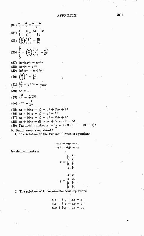
APPENDIX 301
a (23) b a b - - - = c c
(24) ab = ad bd
(25) (feb)(â) =
a
(26) ((i)(c ad c.!)
(27) (am)(a") = (28) (a"')" = am. (29) (abc)". = amb".cm
(30) (16)'
_ (31) -i- = a'^ ^ =
(32) a° = 1 tn
(33) a = •V7c.
(34) c‘-'" =
a"-m
(35) (a + b)(a b) = a2 2ab 1,2 (36) (a b)(a - b) = a2 - (37) (a - b)(a - b) = a2 - 2ab b2 (38) (a b) (e - d) = ac be - ad - bd (39) Factorial number n! = 1 • 2 • 3 •
b. Simultaneous equations: 1. The solution of the two simultaneous equations
by determinants is
aix bly =cl asx ± b2y= c2
e, ill
C2 b2 ai bl a2 1)2
CI
1:2 C2
a z bz az bz
2. The solution of three simultaneous equations
(n - 1)n
eta ± be + ciz = dl a2x + be + c2z= (12 a3x be c3z = d3
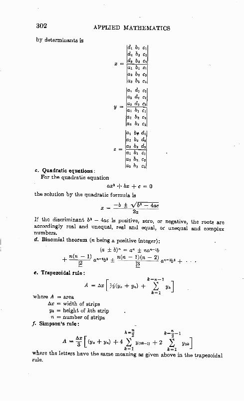
302 APPLIED MATHEMATICS
by determinants is
X =
Y =
c. Quadratic equations: For the quadratic equation
-Fbx + c = the solution by the quadratic formula is
-b ± -Vb2 - 4ac x - 2a
If the discriminant b2 - 4ac is positive, zero, or negative, the roots are accordingly real and unequal, real and equal, or unequal and complex numbers.
d. Binomial theorem (n being a positive integer):
(a + b) n = an + na"-lb
+ n(n 1) a,.-2b2 ± n(n - 1)(n - 2) a"-3bs ± • • • 12 13
d1 b1 e1 d2 its c2 d3 b, C3
al b1 Ci
a2 b2 c2
a3 b3
a, di. ci 2 C12 C2
3 d3 C3
al bi a2 b3 C2
b3 Ca
al bp dl a2 b3 (12 a3 b3 d3 at b1 Ci
a3 b,, C2 3 14 C3
e. Trapezoidal rule:
where A -= area = width of strips
yk = height of kth strip n = number of strips
f. Simpson's rule:
k =n-1
A = [h(y. yn) Yk] k =1
k=- k=--1 2 2
A = [(y. + y.) + 4 / y(2k-i) -I- 2 / 112k]k = 1 k-1
where the letters have the same meaning as given above in the trapezoidal rule.
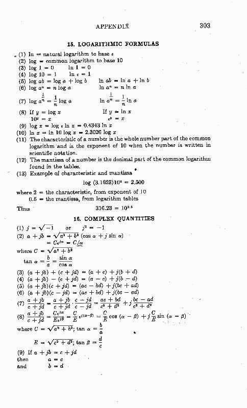
APPENDEt 303
15. LOGARITHMIC FORMULAS
(1) In = natural logarithm to base E (2) log = common logarithm to base 10 (3) log 1 = 0 ln 1 = 0 (4) log 10 = 1 in E = 1 (5) log ab = log a -I- log b In ab = ln a ± in b (6) log a's n log a in = n in a
1 —1 1
(7) log an = ie log a in an —n In a
(8) If y = log x If y = ln x 10v = X
(9) log x = log e in x = 0.4343 in x (10) ln x = ln 10 log x = 2.3026 log x (11) The characteristic of a number is the whole number part of the common
logarithm and is the exponent of 10 when the number is written in
scientific notation. (12) The mantissa of a number is the decimal part of the common logarithm
found in the tables. (13) Example of characteristic and mantissa
log (3.1623)102 = 2.500
where 2 = the characteristic, from exponent of 10 0.5 = the mantissa, from logarithm tables
Thus 316.23 = 102.5
16. COMPLEX QUANTITIES
(1) j = Nr--1. or
(2) a -1- jb = Va2 + b2 (cos « j sin «) = CEi« = C/a
where C = N/a2 b2 b sin a
tan « — = a cos a
(3) (a -I- jb) + (c - - jd) = (a -I- c) j(b d) (4) (a + jb) — (c -1- jd) = (a — c) + j(b d) (5) (a ± jb)(c jd) = (ac — bd) + j(bc + ced) (6) (a -1- fb)(c — jd) = (ac -1- bd) +j(bc — ad)
(7) a jb a + c — jd ac + bd .bc — ad c + jd c + jd c — jd c2 + d2 c2 d2 —
a + jb Ceja C . C . C E (8) = _ 1(a-0) _ 8 113 E e E" (3)+JE sin
c j e
where C = Va2 1)2; tan « = a
E = c2 + d2; tan 13 = cic
(9) If a + jb c jd then a= c and b=d
- 0)
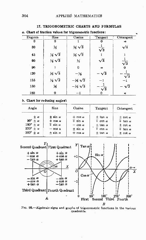
304 APPLIED MATHEMATICS
17. TRIGONOMETRIC CHARTS AND FORMULAS
a. Chart of fraction values for trigonometric functions:
Degrees Sine Cosine Tangent Cotangent 0 0 1 0 co
30 1
1/
45 1/i 1/i 1 1 1
-‘7à 90 1 0 ce 0
120 i'N/à —IA — 1/-3. 1
1/3 135 *1/-j — 1/i —1 —1
1/3 180 0 —1 0 c.0
b. Chart for reducing angles
Angle Sine Cosine Tangent Cotangent
+ a ± sin a + COS a + tan a -H cot a 90° + a + cos a ---i-- sin a ItI etn a IH- tan a
180° + a +- sin a — cos a + tan a ± cot a 270° + a — cos a + sin a - + ctn a + tan a 360° + a + sin a ± cos a + tan a + cot a
Y Second Quadrant First Quadrant
4- sin a 4- sin a —cosa + cos a +1 — tan a + tan a
—sna — cos a +tan a
X
—sna + cos a —tan a
Third Quadrant Fourth Quadrant
A
a
O 90 ° 180° 270° 360° First Second Third Fourth
FIG. 98.—Algebraic signs and graphs of trigonometric functions in the various quadrants.
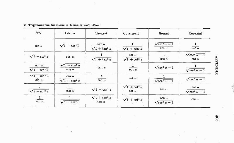
c. Trigonometric functions in terms of each other:
Sine Cosine Tangent Cotangent Secant Cosecant
sin a tan « 1 1 Vsec2 a — 1 Vi COS2 — a
Vi ± tan2 « -V1 + cote a sec a
1
CSC a
cosa 1 cot a VCSC2 a — 1 S "Vi — W a
Vi + tan2 a -Vi + cot2 « sec a C8C a
sin « V1 — cos2 « tan a
1 1 Vsec2 « 1
V1 — sin2 « cos a Cot a VCSC2 a — 1
V1 — sin2 a CO8 a 1 Cot a
1
sin a -V1 — cos2 a tan « Vsec2 a — 1 -Vesc2 a — 1
1 1 -V1 ± cote a sec a
CSC a
—cota V1 sm2 a cos a N/1 ± tan2 « N/C8C2 a — 1
1 1 N/1 -I- tan2 a sec a CSC a V1 + COP a sin a N/I. — COS2 a tan a Vsec2 a — 1
XIGNaddV
o Ca
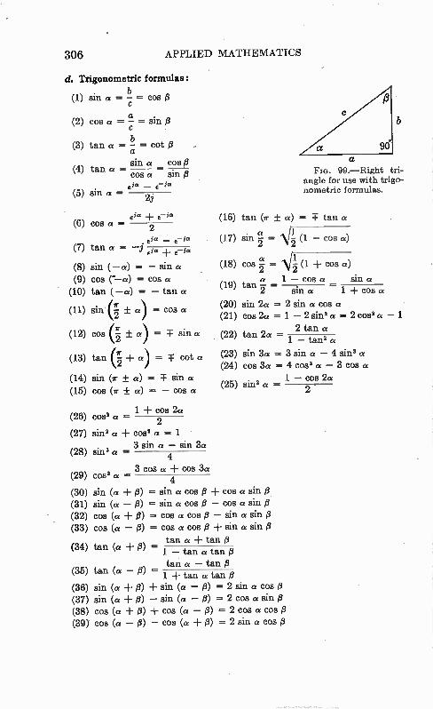
306 APPLIED MATHEMATICS
d. Trigonometric formulas:
(1) sin a = - cos 0
a (2) cos a = - = sin 0
e
(3) tan a = a-b = cot ft
Sin a cos 13 tan a = — =
cos a sin 0 Sa -
sin « 2j
(4)
(5)
(6) COIS a = 2 . éa L cja (17) sin cl = "V-1 (1 - COS a)
(7) tan a = 2 2 2 - eia + (-va
(18) cos i = \fi (8) sin ( - a) = - sin « (1 ± cos a)« 1
(9) cos (--a) = cos a a 1 - COS a sin a (19) tan 2 -
sin a = 1 ± COS a (10) tan ( -«) = - tan a
()11 sin ( ± a) = cos a (20) sin 2a = 2 sin a cos « 1-r-2 (21) COE1 2« = 1 - 2 sina a = 2 cos2 a - 1
(12) cos (-2 ± a) = :F. ain a (22) tan 2« - 2 tan « 1 - tana a
r
cot « (23) sin 3a = 3 sin a - 4 Bina a (13) tan (-2 ± a) = T- (24) cos 3a = 4 cosa a - 3 cos a
7
(14) sin (w- ± a) =F sin « 1 - cos 2« (25) Sin2 a -
(15) cos (Ir ± a) = - cos a 2 '
1 ± cos 2« (26) cosa a - 2 (27) sina ce + cosa a = 1
3 sin a - sin 3« (28) sin; a = 4
3 cos « ± cos 3« (29) cosa « - 4
(30) sin (« -I- 0) = sin « cos 0 + cos « sin 0 (31) sin (a - 0) --= sin a cos fi - cos a sin # (32) cos (a -I- 0) = cos a cos 0 - sin a sin 0 (33) cos (a - p) = cos a cos e + sin a sin 0
tan a ± tan 0 (34) tan (« + p) - 1 - tan a tan 0
tan « - tan e (35) tan (a - 0) = 1 ± tan a tan p (36) sin (a -I- 0) -I- sin (a - (3) = 2 sin a cos 0 (37) sin (a + 0) - sin (a - 13) = 2 cos a sin # (38) cos (« -I- p) + cos (« - 0) = 2 cos a cos 0 (39) cos (a - 0) - cos (a + p) = 2 sin a cos p
Sa ±
a Fio. 99.—Right tri-
angle for use with trigo-nometric formulas.
(16) tan (7i- ± a) = tan «
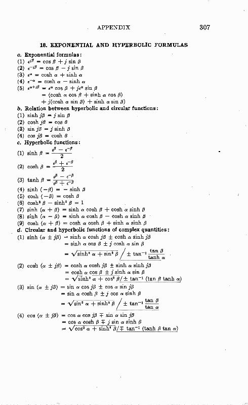
APPENDIX 307
18. EXPONENTIAL AND HYPERBOLIC FORMULAS
a. Exponential formulas: (1) eifi = cos a ± j sin a (2) e-ile = cos - j sin fi (3) ect = cosh « sinh « (4) e-a = cosh « - sinh a (5) ea+i13 cos 13 + je* sin
= (cosh a cos a sinh a cos a) i(cosh « sin e) + sinh « sin a)
b. Relation between hyperbolic and circular functions: (1) sinh jii = j sin /3 (2) cosh je = cos 13 (3) sin 113 = j sinh (4) cos j13 = cosh a c. Hyperbolic functions:
- E-0 (1) sinh -
2 €15 e--0
(2) cosh a 2 -
(3) tanh /3 = o
(4) sinh ( -0) - sinh a (5) cosh ( -a) = cosh # (6) cosh2 - sinh2 13 = 1 (7) sinh (« + 13) = sinh a cosh /3 -{- cosh « sinh e (8) sinh (« - 13) sinh a cosh 13 - cosh a sinh (9) cosh (« /3) = cosh a cosh 13 sinh « sinh d. Circular and hyperbolic functions of complex quantities: (1) sinh (a ± j13) = sinh a cosh ja ± cosh « sinh je
= sinh « cos e ± j cosh « sin = •Vennh2 « sin2 /3 ± tan-, tan a
tanh «
(2) cosh (a ± ja) = cosh a cosh ja ± sinh a sinh je = cosh a cos /3 ± j sinh a sin /3 = N/sinh2 « 0082 a/ ± tan-2 (tan 13 tanh a)
(3) sin (« ±j) = sin « cos ja ± cos a sin je = sin « cosh e ± j cos a sinh #
= N/sin2 « sinh2 a ± tan-2 tan 8 tan a"
(4) cos (« ± = cos a cos ja T- sin a sin ja = cos a cosh a j sin a sinh
N/cos2 a + sinh2 eiT- tan-1 (tanh a tan «)
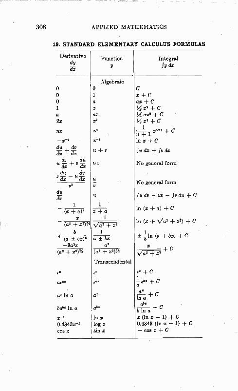
308 APPLIED MATHEMATICS
19. STANDARD ELEMENTARY CALCULUS FORMULAS
Derivative dy dx
Function Integral
fY dx
o o o 1 a 2x
nx
du dv Tx + crx dv , du
.1 -ry Tcz
du dv v — ud7x
du dv
+ a)2
(a2 + x2)% _ b
(a ± bx)2 —3a2x
(a2 + x2)%
aye'
ax in a
babx ln a
x-1 0.4343x-i CO8 X
Algebraic
o
a
ax x2
x^
x-1
+
uy
V
Va2 + x2 1
a + bx a2
(al + x2)%
Transcendental
ax
abz
ln x log x sin z
z + C ax + C
+ C axs _FC
1 n
x' 11 + 1
In x + C
fu dx 1.11 dx
No general form
No general form
u dv uy — fv du ± C
ln (x + a) + C
ln (x ..Vc --x2) C
1 ± In (a + bx) C
N/a2 + x2 ± e
bina C
x (ln x — 1) + C 0.4343 (In x — 1) + C — cos x + C
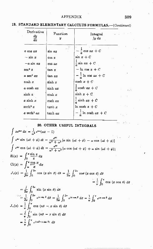
APPENDIX 309
19. STANDARD ELEMENTARY CALCULUS FORMULAS.—(Continued)
Derivative dy dx
Function Integral
.1.1/ dx
a cos ax
- sin x
-a sin ax
sec2 x
a sec2 ax
cosh x
a cosh ax
sinh x
a sinh x
sech2 x
a sech2 ax
sin ax
cos x
cos ax
tan x
tan ax
sinh x
sinh ax
cosh x
cosh ax
tanh x
tanh ax
- -1 cos ax C a
sin x C 1 -a in ax C
- in cos x C 1
- - In cos as C a
cosh x
-1 cosh ax C a sinh x C 1 -sinh ax C a in cosh x C 1
- - In cosh ax C a
20. OTHER USEFUL INTEGRALS 1
xeax dx = ea '(Crx — 1)
at sin (cut + 1k) dt = a2 e±at (02 [a sin (tot + ‘,) - co cos (Wt #)]
at cos (Cut + 1,1") dt - a2 e: co2 [a cos ((et +1,0 ± co sin (cut +1,)1
Si(s) = foe Sije dx
Ci(x) = f e x J 0(x) = 2'r cos (x sin 0) clO = f02 cos, (x cos 0) do
1 r cos (x cos 0) de
ir o
= j- f 2w sin (x sin 0) do 27 o
= 1 FT i 1 I . e z 6 de - 1 1 21. ei' ece ° de = - ez» coo 8 de
2ir o - 2or o ' r o
.1.(x) = -1 IT cos (nO -, x sin 0) do r 0
= jrsin (n0 - x sin 0) dO ir o
= 1 fr 2i(.8-x sin 8) do ir o
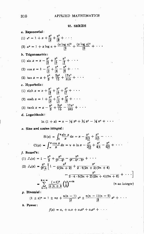
310 APPLIED MATHEMATICS
21. SERIES
a. Exponential: 2 X3 (1) e = 1 + x + + • • 7
(x log a)2 (x log a)3 (2) a = 1 + x log a + 13. + +
b. Trigonometric: X3 X6 X7
(1)sinx.---x
(2) cos x
x6 2x5 17x7 (3) tan x x + -17 +
c. Hyperbolic:
(1) sinh x x + + + 5+••• (2) cosh x = 1 erei2- + +N+•••
X3 2x5 17x2 (3) tanh x x — + -f-5- — 315 -F
d. Logarithmic:
ln (1 + x) = x — x2 + xs — x4 + • •
e. Sine and cosine integral:
si(x) = fox suix dx x 3T!.x2 3x2
x2 x4 xe cj(z) ro cc.--3xx dx = 7 ± ln x — -F — e + • • •
f. BessePs: X
(1) J°(x) -1 ' 1« + 2:•442 22 • 42 • 62 -I-e r, xf x.
(2) jn(e) 2'In L` 2(2n ± 2) ± 2 • 4(2n -1- 2)(2n -1- 4)
X6 2 • 4 6(2n + 2)(2n + 4)(2n + 6) +
g •
k= (-1)k An+2k
k - S 'kin +k k2f
—
Binomial:
(n an integer)
n(n — 1) n(n — 1)(n — 2) (1 ± x)n = 1 ± nx x2 + x3 + • •
12
h. Power:
f(x) = a. + a2x2 -1- a3x3 + • • •
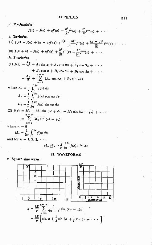
j. Taylor's:
APPENDIX 311
i. Maclaurin's:
f(x) = fie)) e(0) + 21"(o) + fm(o) + • • • 12
(1) f(x) = f(a) + (x — a)f'(a) + (x —a)2 f"(a) + f"'(a) +
h' h3 (2) f(x + h) = .f(x) (x) ± f"(x) + —13 ,f"(x)
k. Fourier's: Ao
(1) f(x) = —2 + Ai sin x + 142 cos 2x + A 3 COS 3x
+ B1 cos x + B2 cos 2x + B3 cos 3x
Ao nv= ' = ± 4 (A, cos nx + B. sin nx)
n =
where Ao = 1 1.2' f(x) dx ir
A„ = f f(x) cos nx dx ir
B. = f f(x) sin nx dx ir
(2) f(x) = Mo + M I sin (cot ± 1,1,1) ± M2 sin (cot ih) n =
/ M. sin (cot + tk.) n = o
where n =
= fo f(x) dx 1
and for n = 1, 2, 3, • • •
M. Lk„ = 1 f f(x)E—i"' dx 7r 0
22. WAVEFORMS
a. Square sine wave:
E 0 •0 o
1
Q 7r 2r X O Z 4
Harmonics 6 8 . 10
= 4E n 1 .
y = 2n — 1 —r sin (2n — 1)x n = 1
= 4E rsin x 1 sin 3x + É sin 5x + • • • 3
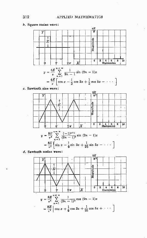
3 I 2 APPLIED MATHEMATICS
b. Square cosine wave: 4E
Y ir
t E
I I
1,
0 7 ?ir X 0 2 4 6
Harmonics 8 10
nr--4E 1
Y 2 1 sin (2n — 1)x = n — n 1
4E 1 , 1 = — [cos x — COS OX I- -5- COS 5X • • •
c. Sawtooth sine wave: sÉ
Y e t E
0 .0 A g
.
e
Q 7r ? 71" X 0 2 4 6 8
Harmonics 10
n 8E ( —1)"+1
Y = 72 Lw (2n — 1)2 sin (2n — 1)x n 1
1 . = [sin x — sin 3x + 2-5 sin 5x — • • •
d. Sawtooth cosine wave: 8E
Y e
t 0 .0 E
1, ; >I
\
0 •:r 2ir X 0 2 4
?arir 6
°nice 8 10
8E n 'e 1 = 7r2 Li (2n 1)2 cos (2n — 1)x
n =- 1
= 81 1 [cos 1- cos 3x + 1 cos 5x + • • • 9 25 72
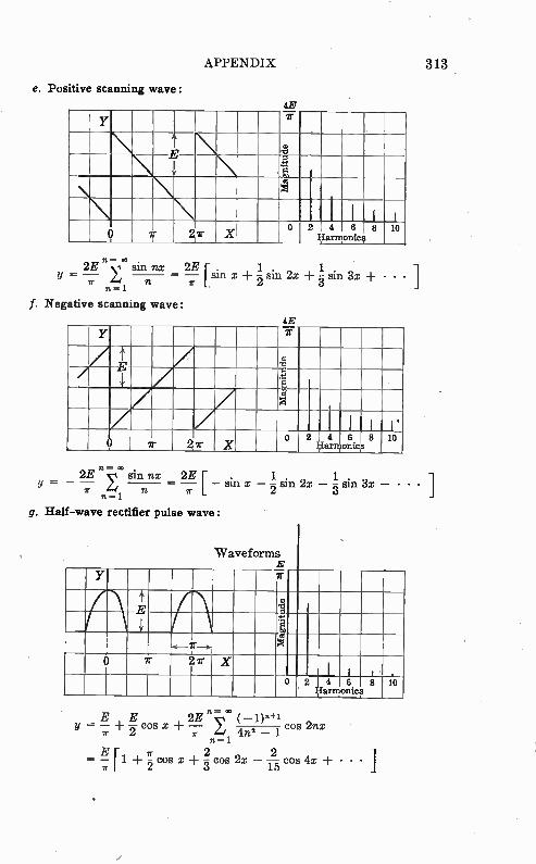
APPENDIX
e. Positive scanning wave:
4E
Y 7
..
5 x I I i
0 r 2 ir X o 2
Harmonica 4 6 8 10
n = 2E s sin nx 2E [
± -1 sin 2x + sin 3x + • • • y — sin x ir n 7r 2 3 n
f. Negative scanning wave:
4E Y Y
t o E 4
-0 0 e
5 x / I I 1 i.
Q r 2.1* X 0 2 4
Ham 6 8
onics 10
313
it- 00 2E ssin nu 2E i 1 . 1 . — - — [ - sn x - - sin eX — — 8111 ôX - • • • I n 2 3 n = I
g. Half-wave rectifier pulse wave:
Waveforms
Y r
n Et 0 ni
4. :..-1.
5 -,,----7-). X
0 'Tr 27r X
0 2 4 6 8 ' Harmonics
10
E E 2E n= os —1)a41 cos 2nx y = -1-5- cos x — S
ir 7 n=1 4n2 -
E 2 = - [1 + cos x + -3 cos 2x - —2 cos 4x + • • •
r 2 15
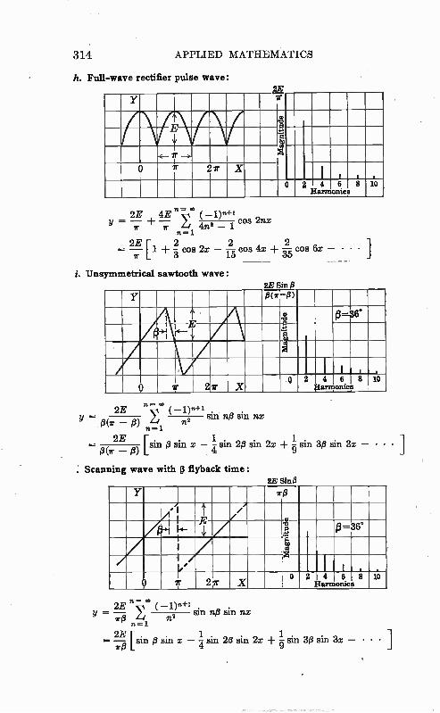
314 APPLIED MATHEMATICS
h. Full-wave rectifier pulse wave: 2E
Y 71'
o ne e
la
-(--- r --› r 27r X
0 2 4 Harmonics
6 8 10
n = -2—E + (-1)n+1 cos 2nx
4n 2 — 1 " n = 1
[ 1 + cos 2x — A- cos 4x + â = cos 6x — • • •
i. Unsymmetrical sawtooth wave: 2E Sin
Y
H =36 1 .
ffri
E
r"— • .12
_I , o
0 ir 2 7r X 0 2 4
Harmonics 6 8 10
n = 2E (-1)"+1 Y s. n
(.1 sin nx (ir e) nL1=1 n2
1 2E — 3) [sin /3 sin x — sin 20 sin 2x + -9 sin 30 sin 3x — • • • 1
Scanning wave with LI flyback time: 2E Sin 0
Y re
'1 I
t , /
o' i 1. 'd
5' 0=36°
I I t4 e i , i . .
9 ir 2 ir X 0 2 4 6 8
Harmonics 10
y --- n1 ' sin n0 sin nx n
= LE [sin 0 sin x — -4 sin 20 sin 2x + -1 sin 3e sin 3x — • • • 7T13 9
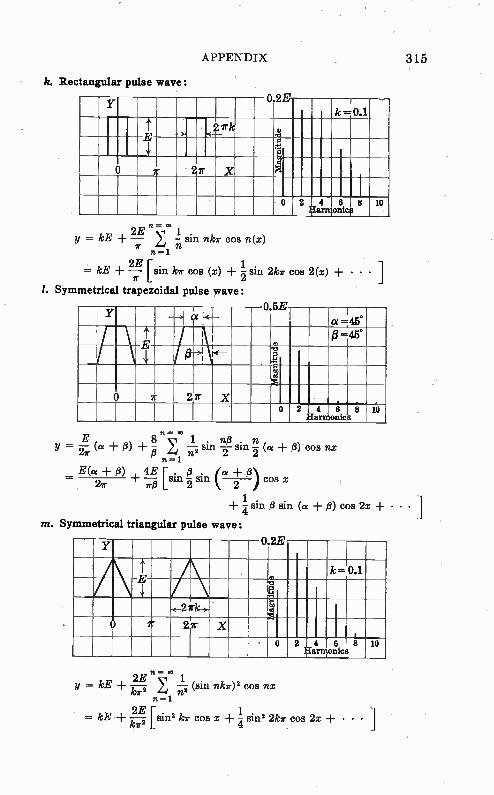
APPENDIX
k. Rectangular pulse wave:
Y v zz,
0.1
t 2 Irk . -0 E
1, .e
O ir 2r X 1
0 2 4 Harmonics
6 8 10
2E n --- ' 1 . y = kE ± — - sin nkr cos n(x)
r n=i n 2E 1
= kE + — [ sin kw cos (x) + - sin 21cr cos 2(x) + • /I* 2
1. Symmetrica trapezoidal pulse wave:
Y cx ..(--U. U4,
ce=45°
\ t E I
1 1 . i3 - 45°
0...÷1 ..0 e •E
z
o ir 27r X 0 2 4 6
Harmonics 8 10
315
n = 00 E
Y 8 (.(cï s) s (a e) cos nx in sin 7 .-i n =1
= E(a + 0) 4E + [. . (a + 0) sin - sin cos x 7/3 2 2
± -I sin 0 sin (a ± 0) cos 2x • • • 1 4 m. Symmetrical triangular pulse wave:
Y
--A -1 ,I,
0 'CS e •E
-(-2irk-0. cl S
0 r 27r X 1
0 2 4 6 Harmonics
8 10
2E n 1 y = kE —kr2 —n2 (sin nicir) 2 cos nx n =1
2E = kE +
W 2 [sini2 kir cos x+ - s n2 2kr cos 2x + • • • k 4
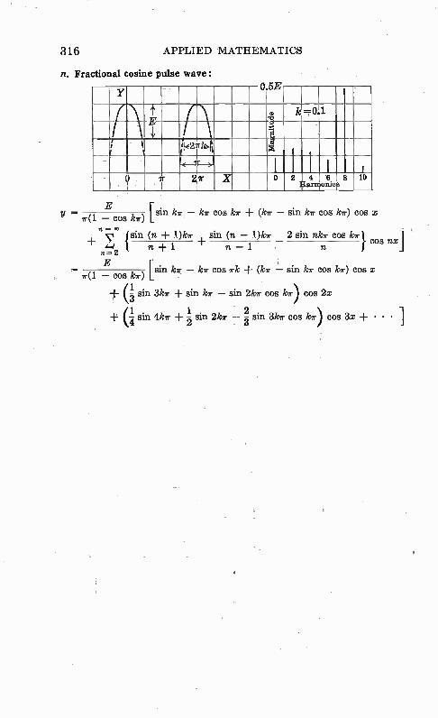
316 APPLIED MATHEMATICS
n. Fractional cosine pulse wave: V Cl.Ei
t n -,, , ;
I i
1424,a'; / î 1.< Ir
IIII / )1
? Ir 21- X o 2 4
Harmonie 6 8 a
10
E [sin kir — kw cos kir + (kir — sin kw cos ken-) cos x
Y = ( 1 — cos kir) n = ce
s Isin (n 1)lor sin (n — 1)kir 2 sin nkir cos kir } cos nx] 1 n + 1 n — 1 n= 2
E = cos kr) [sin — kir cos irk + (kir — sin kir cos kir) cos x
sin 3kor ± sin Ir4r — sin 2kir cos kir) cos 2x
+ (1. sin 4kir sin 21er — sin 31or cos kir) cos 3x + •
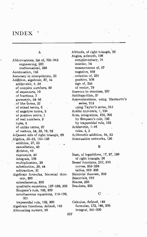
INDEX '
A
Abbreviations, list of, 234-243 engineering, 239 mathematical, 236
Acceleration, 165 Accuracy in interpolation, 23 Addition, algebraic, 37, 54
arithmetic, 4, 54 of complex numbers, 92 of exponents, 10 of fractions, 7 geometric, 54-56 of like terms, 37 of mixed terms, 6 . of negative terms, 3 of positive terms, 1 of real numbers, 2 rules, 4 of unlike terms, 37 of vectors, 54, 58, 76, 92
Adjacent side of right triangle, 68 Algebra, 35-53, 110-138
addition, 37, 55 cancellation, 42 division, 42 exponents, 40 integrals, 198 multiplication, 38 substitution, 39, 44 subtraction, 37
Algebraic formulas, binomial theo-rem, 302
miscellaneous, 300 quadratic equations, 127-138, 302 Simpson's rule, 193, 302 simultaneous equations, 110-126,
301 trapezoidal rule, 192, 302
Algebraic functions, defined, 149 Alternating current, 50
Altitude, of right triangle, 56 Angles, azimuth, 108
complimentary, 74 interior, 74 measurement of, 57 negative, 108 notation of, 234 positive, 108 sign of, 234 of vector, 79
Answers to exercises, 327 Antilogarithm, 21 Approximations, using Maclaurin's
series, 213 using Taylor's series, 215
Arabic numerals, 1, 234 Area, integration, 195, 205 by Simpson's rule, 193 by trapezoidal rule, 192
Arithmetic, 1-16 rules, 4, 5
Arithmetic addition, 54, 55 Attenuation networks, 139
Base, of logarithms, 17, 97, 180 of right triangle, 56
Bessel functions, 217, 310 curves, 255-258 tables, 259-293
Binomial theorem, 302 Binomials, 212 Braces, 235 Brackets, 235
Calculus, defined, 149 formulas, 172, 189, 308 integral, 191-206
317
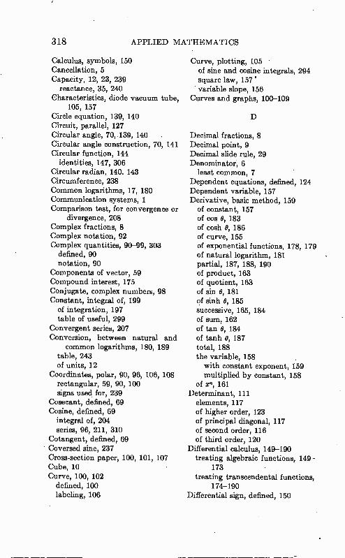
318 APPLIED MATHEMATICS
Calculus, symbols, 150 Cancellation, 5 Capacity, 12, 23, 239
reactance, 35, 240 Characteristics, diode vacuum tube,
105, 157 Circle equation, 139, 140 Circuit, parallel, 127 Circular angle, 70, 139, 140 Circular angle construction, 70, 141 Circular function, 144
identities, 147, 306 Circular radian, 140. 143 Circumference, 238 Common logarithms, 17, 180 Communication systems, 1 Comparison test, for convergence or
divergence, 208 Complex fractions, 8 Complex notation, 92 Complex quantities, 90-99, 303
defined, 90 notation, 90
Components of vector, 59 Compound interest, 175 Conjugate, complex numbers, 98 Constant, integral of, 199
of integration, 197 table of useful, 299
Convergent series, 207 Conversion, between natural and
common logarithms, 180, 189 table, 243 of units, 12
Coordinates, polar, 90, 96, 106, 108 rectangular, 59, 90, 100 signs used for, 239
Cosecant, defined, 69 Cosine, defined, 69
integral of, 204 series, 96, 211, 310
Cotangent, defined, 69 Coversed sine, 237 Cross-section paper, 100, 101, 107 Cube, 10 Curve, 100, 102
defined, 100 labeling, 106
Curve, plotting, 105 - of sine and cosine integrals, 294
square law, 157• ' variable slope, 156
Curves and graphs, 100-109
D
Decimal fractions, 8 Decimal point, 9 Decimal slide rule, 29 Denominator, 6
least common, 7 Dependent equations, defined, 124 Dependent variable, 157 Derivative, basic method, 159
of constant, 157 of cos 0, 183 of cosh 0, 186 of curve, 155 of exponential functions, 178, 179 of natural logarithm, 181 partial, 187, 188, 190 of product, 163 of quotient, 163 of sin 0, 181 of sinh 0, 185 successive, 165, 184 of sum, 162 of tan 0, 184 of tanh 0, 187 total, 188 the variable, 158 with constant exponent, 159 multiplied by constant, 158
of xn, 161 Determinant, 111
elements, 117 of higher order, 123 of principal diagonal, 117 of second order, 116 of third order, 120
Differential calculus, 149-190 treating algebraic functions, 149-
173 treating transcendental functions,
174-190 Differential sign, defined, 150
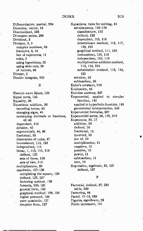
INDEX 319
Differentiation, partial, 204 Direction, vector, 54 Discriminant, 133 Divergent series, 208 Dividend, 2 Division, 2, 5 complex numbers, 93 fractions, 8, 42 law of exponents, 11 rules, 5 using logarithms, 22 using slide rule, 26 of vectors, 93
Divisor, 2 Double integrals, 205
E
Electric wave filters, 139 Equal roots, 133 Equality, 36 Equations, addition, 36
canceling terms, 45 changing signs, 45 containing decimals or fractions,
42-43 dependent, 115 division, 42 exponentials, 46, 96 fractional, 35 illustration of rules, 47 inconsistent, 115, 124 independent, 115 linear, 1, 110, 115, 118
defined, 123 sets of three, 118 sets of two, 110
multiplication, 36 quadratic, 127-138
completing the square, 129 defined, 127, 137 factoring method, 128 formula, 130, 131 general form, 132 graphical method, 128, higher powered, 136 pure quadratic, 127 simplest form, 127
Equations, rules for solving, 45 simultaneous, 110-126
classification, 115 defined, 123 dependent, 115, 116 determinant method, 116, 117,
120, 122 graphical method, 111, 125 inconsistent, 115, 116 independent, 115, 116 multiplication-addition method,
112, 119, 125 substitution method, 113, 119,
125 solution, 45 subtraction, 36
Euler's constant, 216 Evaluation, 46 Exercise answers, 327 Exponential, applied to circular
function, 146 applied to hyperbolic function, 146 geometrical interpretation, 145
Exponential formulas, 307 Exponential series, 96, 176, 310 Exponents, 10, 17
addition, 10 defined, 10 fractional, 13 inverted, 13 law of, 10 multiplication, 11 negative, 10 positive, 10 power, 11 subtraction, 11 zero, 10
Expression, algebraic, 35, 137 defined, 137
Factorial, defined, 97, 235 table, 299
129 Factoring, 44 Farad, 12-13, 239 Figures, significant, 23 Finite increment, 151
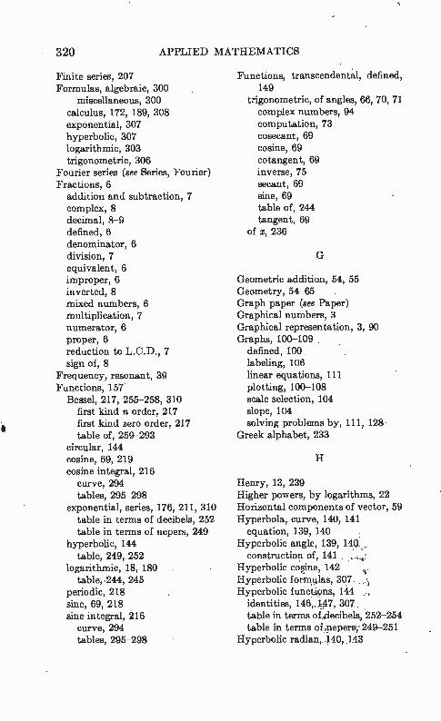
320 APPLIED MATHEMATICS
Finite series, 207 Formulas, algebraic, 300
miscellaneous, 300 calculus, 172, 189, 308 exponential, 307 hyperbolic, 307 logarithmic, 303 trigonometric, 306
Fourier series (see Series, Fourier) Fractions, 6
addition and subtraction, 7 complex, 8 decimal, 8-9 defined, 6 denominator, 6 division, 7 equivalent, 6 improper, 6 inverted, 8 mixed numbers, 6 multiplication, 7 numerator, 6 proper, 6 reduction to L.C.D., 7 sign of, 8
Frequency, resonant, 39 Functions, 157
Bessel, 217, 255-258, 310 first kind n order, 217 first kind zero order, 217 table of, 259-293
circular, 144 cosine, 69, 219 cosine integral, 216
curve, 294 tables, 295-298
exponential, series, 176, 211, 310 table in terms of decibels, 252 table in terms of nepers, 249
hyperbolic, 144 table, 249, 252
logarithmic, 18, 180 table, .244, 245
periodic, 218 sine, 69, 218 sine integral, 216
curve, 294 tables, 295-298
Functions, transcendental, defined, 149
trigonometric, of angles, 66, 70, 71 complex numbers, 94 computation, 73 cosecant, 69 cosine, 69 cotangent, 69 inverse, 75 secant, 69 sine, 69 table of, 244 tangent, 69
of x, 236
G
Geometric addition, 54, 55 Geometry, 54-65 . Graph paper (see Paper) Graphical numbers, 3 Graphical representation, 3, 90 Graphs, 100-109 .
defined, 100 labeling, 106 linear equations, 111 plotting, 100-108 scale selection, 104 slope, 104 solving problems by, 111, 128
Greek alphabet, 233
H
Henry, 13, 239 Higher powers, by logarithms, 22 Horizontal components of vector, 59 Hyperbola, curve, 140, 141
equation, 139, 140 Hyperbolic angle, 139> 140
construction of, 141 . Hyperbolic copine, 142 Hyperbolic formulas, 307 Hyperbolic functkes, 144 .,
identities, 146i .147, 307 table in terms of4lecibels, 252-254 table in terms of eepers, 249-251
Hyperbolic radian, 140, 143

INDEX 321
Hyperbolic sine, 142 Hyperbolic tangent, 142 Hyperbolic trigonometry, 139-148 Hypotenuse of right triangle, 56 Hysteresis (or B-H cürve), 102, 103,
322
Identities, circular and hyperbolic, 306, 307
circular function, 147, 306 hyperbolic function, 147, 307 trigonometric, 305, 306
Imaginary numbers, 235 representation of, 90
Impedance, 38 Impedance vector, 92 Improper fraction, 6 Inconsistent equations, 115, 124 Incremental sign, 151 Independent equation, defined, 124 Independent variable, 157 Infinite series, 207, 310 Infinitesimal increment, 151 Infinitesimals, 151, 196 Index, initial, on slide rule, 30 Inductance, 13 Inductive reactance, 35, 92 Inflection point, 170 Integrals, 308, 309
algebraic, 198, 308 of algebraic sum, 202 calculus, 191-206
defined, 191 of constant, 199 of cosine, 204 multiple, 204 of natural logarithm, 203 of one, 198 sign, 191, 236
defined, 150 of sine, 203 of tangent, 204 transcendental, 203, 308 triple, 205 of variable, 201 of zero, 198
Integration, partial, 204 by parts, 202 volume, 205
Interest, simple, 174 Interior angle, of triangle, 74 Interpolation, 23 Inverse trigonometric functions, 75 Irrational numbers, 2
j, operator, 90
Kilohm, 13, 240 Kilovolt, 13, 240 Kilowatt, 13, 240
Law, of natural decay, 178 of natural growth, 174
Least common denominator, 7, 237 Less than, sign, 234 Limits, 150 Linear equation, 1, 110 any number of, 122 defined, 123 sets of three, 118 sets of two, 110
Logarithm, 17-34 base of, 17, 97, 180, 236 characteristics for, 18
rules for, 19 cologarithm, 236 common system, 17 defined, 17 division by, 22 extracting roots by, 23 fractional exponents, 19 graphical, paper, 103, 109, 322
slide rule, 25 interpolation, 23 mantissa, defined, 18
rules, 19 multiplication by, 20 napierian, 236 natural, 97, 180, 236
table of, 245-248 of numbers from 1 to 100, 244
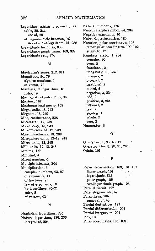
322 APPLIED MATHEMATICS
Logarithm, raising to power by, 22 table, 20, 244
use of, 20 of trigonometric function, 75
See also Antilogarithm, 21, 236 Logarithmic formulas, 303 Logarithmic graph paper, 103, 322 Logarithmic rate, 174
Maclaurin's series, 212, 311 Magnitude, 54, 79
signlesa numbers, 1 of vector, 79
Mantissa, of logarithms, 18 rules, 19
Mathematical polar form, 96 Maxima, 167 Maximum load power, 168 Mega, units, 13, 243 Megohm, 13, 240 Mho, conductance, 238 Microfarad, 12, 239 Microhenry, 13, 239 Micromicrofarad, 12, 239 Micromicrohenry, 13, 239 Micromicro units, 12-13, 243 Micro units, 12, 243 Milli units, 12-13, 243 Minima, 167 Minuend, 4 Mixed number, 6 Multiple integrals, 204 Multiplication, 5 complex numbers, 93, 97 of exponents, 11 of fractions, 7 law of exponents, 10 by logarithms, 20-21 rules, 5 of vectors, 93
N
Napierian, logarithms, 236 Natural logarithms, 180, 236
integral of, 203
Natural number e, 176 Negative angle symbol, 84, 234 Negative exponents, 10 Networks, attenuation, 139 Notation, polar coordinates, 108
rectangular coordinates, 100-102 scientific, 12
Numbers, arabic, 1, 234 complex, 90 even, 2 fractional, 2 imaginary, 90, 235 integers, 2 integral, 2 irrational, 2 mixed, 6 negative, 3, 234 odd, 2 positive, 3, 234 rational, 2 real, 2 signless, 1 whole, 2 zero, 2
Numerator, 6
O
Ohm's law, 1, 35, 46, 47 Operator j (or i), 90, 91, 235 Origin, 101
Paper, cross section, 100, 101, 107 linear graph, 107 logarithmic, 322 polar graph, 106 semilogarithmic graph, 103
Parallel circuit, 127 Parallelogram law, 57 Parenthesis, 235 removal of, 43
Partial derivatives, 187 Partial differentiation, 204 Partial integration, 204 Plot, 100 Polar coordinates, 106, 108
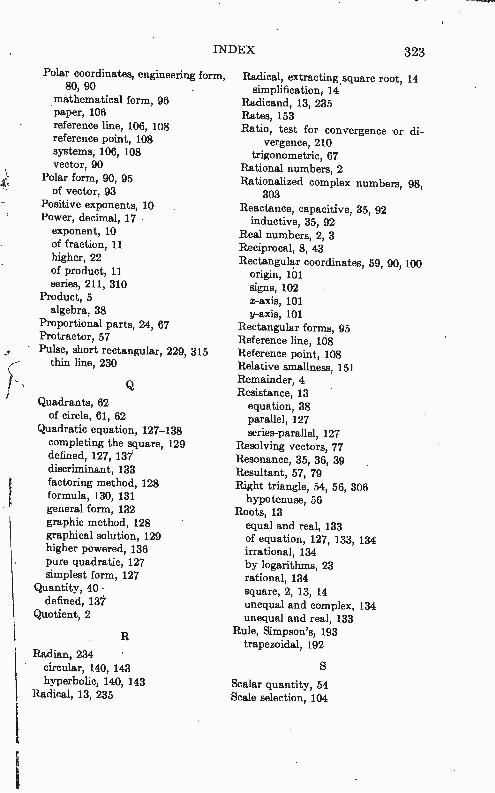
INDEX 323
Polar coordinates, engineering form, 80, 90
mathematical form, 96 paper, 106 reference line, 106, 108 reference point, 108 systems, 106, 108 vector, 90
Polar form, 90, 95 of vector, 93
Positive exponents, 10 Power, decimal, 17 •
exponent, 10 of fraction, 11 higher, 22 of product, 11 series, 211, 310
Product, 5 algebra, 38
Proportional parts, 24, 67 Protractor, 57 Pulse, short rectangular, 229, 315
thin line, 230
Quadrants, 62 of circle, 61, 62
Quadratic equation, 127-138 completing the square, 129 defined, 127, 137 discriminant, 133 factoring method, 128 formula, 130, 131 general form, 132 graphic method, 128 graphical solution, 129 higher powered, 136 pure quadratic, 127 simplest form, 127
Quantity, 40 defined, 137
Quotient, 2
Radian, 234 circular, 140, 143 hyperbolic, 140, 143
Radical, 13, 235
Radical, extracting square root, 14 simplification, 14
Radicand, 13, 235 Rates, 153 Ratio, test for convergence or di-
vergence, 210 trigonometric, 67
Rational numbers, 2 Rationalized complex numbers, 98,
303 Reactance, capacitive, 35, 92
inductive, 35, 92 Real numbers, 2, 3 Reciprocal, 8, 43
Rectangular coordinates, 59, 90, 100 origin, 101 signs, 102 x-axis, 101 y-axis, 101
Rectangular forms, 95 Reference line, 108 Reference point, 108 Relative smallness, 151 Remainder, 4 Resistance, 13
equation, 38 parallel, 127 series-parallel, 127
Resolving vectors, 77 Resonance, 35, 36, 39 Resultant, 57, 79 Right triangle, 54, 56, 306 hypotenuse, 56
Roots, 13 equal and real, 133 of equation, 127, 133, 134 irrational, 134 by logarithms, 23 rational, 134 square, 2, 13, 14 unequal and complex, 134 unequal and real, 133
Rule, Simpson's, 193 trapezoidal, 192
S
Scalar quantity, 54 Scale selection, 104
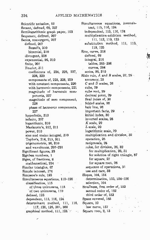
324 APPLIED MATHEMATICS
Scientific notation, 12 Secant, defined, 69, 237 Semilogaiithmic graph paper, 103 Sequence, defined, 207 Series, convergent, 207
defined, 207 Bessel's, 310 binomial, 310
divergent, 208 exponential, 96, 310 finite, 207 Fourier, 311
coefficients of, 224, 225, 227, 228, 229
components of, 225, 228, 229 with constant components, 220 with harmonic components, 221 magnitude of harmonic com-
ponents, 227 magnitude of zero component,
228 phase of harmonic components,
227 hyperbolic, 310 infinite, 207 logarithmic, 310 Maclaurin's, 212, 311 power, 310 sine and cosine integral, 310 Taylor's, 214, 215, 311 trigonometric, 96, 310 and waveforms, 207-231
Significant figures, 23 Signless numbers, 1 Signs, of fractions, 8
mathematical, 234 Similar triangles, 67 Simple interest, 174 Simpson's rule, 193 Simultaneous equations, 110-126
classification, 115 of three unknowns, 118 •of two unknowns, 110
defined, 123 dependent, 115, 116, 124 determinant method, 111, 116,
117, 120, 125, 301, 302 graphical method, 111, 125, -
Simultaneous equations, inconsis-tent, 115, 116, 124
independent, 115, 116, 124 multiplication-addition method,
111, 112, 119, 125 substitution method, 111, 113,
119, 125 Sine, curve, 218
defined, 69 integral, 216
tables, 295-298 curves, 294
series, 96, 310 Slide rule, A and B scales, 27, 29
accura cy, 25 C and D scales, 26 cube, 29 cube root, 29 decimal point, 29 final index of, 30 folded scales, 28 hair line, 26 important facts, 29 initial index, 30 inverted scales, 28 K scale, 29 L scale, 29 logarithmic scale, 29 multiplication and division, 32 operation, 25 reciprocals, 28 rules, for division, 26, 32
for multiplication, 26, 31 for solution of right triangle, 87 for square, 27 for square root, 26
sequence of operations, 31 use and care, 33
Slopes, 104, 154 determination, 105, 154-156 selection, 104
Smallness, first order of, 152 second order of, 152 third order of, 152
Space covered, 165 Square, 10
law curve, 157 Square root, 2, 13
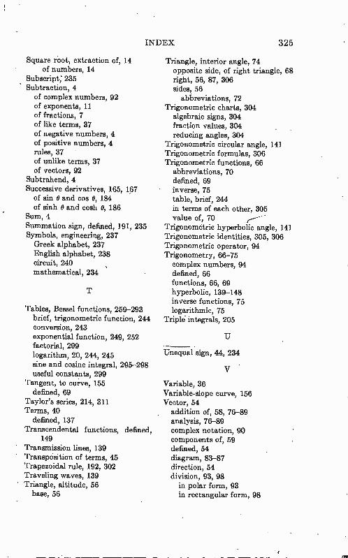
INDEX 325
Square root, extraction of, 14 of numbers, 14
Subscript; 235 Subtraction, 4
of complex numbers, 92 of exponents, 11 of fractions, 7 of like terms, 37 of negative numbers, 4 of positive numbers, 4 rules, 37 of unlike terms, 37 of vectors, 92
Subtrahend, 4 Successive derivatives, 165, 167
of sin 0 and cos 0, 184 of sinh 0 and cosh 0, 186
Sum, 4 Summation sign, defined, 191, 235 Symbols, engineering, 237 Greek alphabet, 237 English alphabet, 238 circuit, 240 mathematical, 234
Tables, Bessel functions, 259-293 brief, trigonometric function, 244 conversion, 243 exponential function, 249, 252 factorial, 299 logarithm, 20, 244, 245 sine and cosine integral, 295-298 useful constants, 299
Tangent, to curve, 155 defined, 69
Taylor's series, 214, 311 Terms, 40
defined, 137 Transcendental functions, defined,
149 Transmission lines, 139 Transposition of terms, 45 Trapezoidal rule, 192, 302 Traveling waves, 139 Triangle, altitude, 56
base, 56
Triangle, interior angle, 74 opposite side, of right triangle, 68 right, 56, 87, 306 sides, 56
abbreviations, 72 Trigonometric charts, 304
algebraic signs, 304 fraction values, 304 reducing angles, 304
Trigonometric circular angle, 141 Trigonometric formulas, 306 Trigonometric functions, 66
abbreviations, 70 defined, 69 inverse, 75 table, brief, 244 in terms of each other, 305 value of, 70
Trigonometric hyperbolic angle, 141 Trigonometric identities, 305, 306 Trigonometric operator, 94 Trigonometry, 66-75 complex numbers, 94 defined, 66 functions, 66, 69 hyperbolic, 139-148 inverse functions, 75 logarithmic, 75
Triplé integrals, 205
U
Unequal sign, 44, 234
V
Variable, 36 Variable-slope curve, 156 Vector, 54
addition of, 58, 76-89 analysis, 76-89 complex notation, 90 components of, 59 defined, 54 diagram, 83-87 direction, 54 division, 93, 98
in polar form, 93 in rectangular form, 98
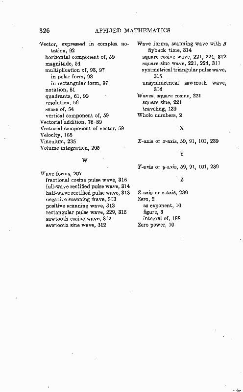
326 APPLIED MATHEMATICS
Vector, expressed in complex no-tation, 92
horizontal component of, 59 magnitude, 54 multiplication of, 93, 97
in polar form, 93 in rectangular form, 97
notation, 81 quadrants, 61, 92 resolution, 59 sense of, 54 vertical component of, 59
Vectorial addition, 76-89 Vectorial component of vector, 59 Velocity, 165 Vinculum, 235 Volume integration, 205
Wave forms, 207 fractional cosine pulse wave, 316 full-wave rectified pulse wave, 314 half-wave rectified pulse wave, 313 negative scanning wave, 313 positive scanning wave, 313 rectangular pulse wave, 229, 315 sawtooth cosine wave, 312 sawtooth sine wave, 312
Wave forms, scanning wave with p flyback time, 314
square cosine wave, 221, 224, 312 square sine wave, 221, 224, 311 symmetrical triangular pulse wave,
315 unsymmetrical sawtooth wave,
314 Waves, square cosine, 221
square sine, 221 traveling, 139
Whole numbers, 2
X-axis or x-axis, 59, 91, 101, 239
Y
Y-axis or y-axis, 59, 91, 101, 239
Z-axis or z-axis, 239 Zero, 2
as exponent, 10 figure, 3 integral of, 198
Zero power, 10
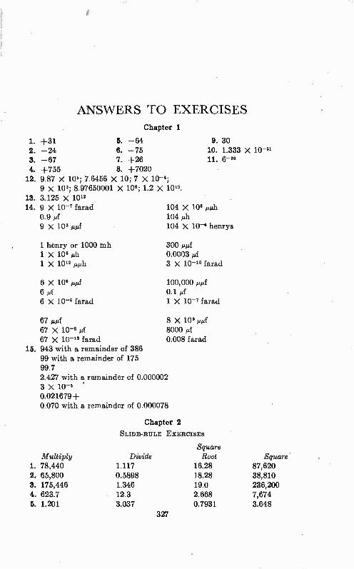
ANSWERS TO EXERCISES Chapter 1
1. +31 5. -64 2. -24 6. -75 3. -67 7. +26 4. +755 8. +7020
12. 9.87 X 10⁶; 7.6456 X 10; 7 X 10⁻⁶; 9 X 10²; 8.97650001 X 10⁶; 1.2 X 10¹⁶.
13. 3.125 X 10¹² 14. 9 X 10⁻⁷ farad
0.9 9 X 10⁶ ¡Ltd
1 henry or 1000 mh 1 X 10⁶ ph 1 X 10¹² pph
6 X 10⁶ ppf 6 id 6 X 10⁻⁶ farad
9. 30 10. 1.333 X 10⁻²¹ 11. 6-26
104 X 106 i.g.th 104 ph 104 X 10-6 henrys
300 muf 0.0003 I.tf 3 X 10⁻¹° farad
100,000 gpf 0.1 d 1 x 10⁻⁷ farad
67 f 8 X 10⁹ ppf 67 X 10-6 pf 8000 mf 67 X 10-12 farad 0.008 farad
15. 943 with a remainder of 386 99 with a remainder of 175 99.7 2.427 with a remainder of 0.000002 3 X 10⁻⁶ 0.021679+ 0.070 with a remainder of 0.000078
Chapter 2
SLIDE-RULE EXERCISES
Square Multiply Divide Root Square
1. 78,440 1.117 16.28 87,620 2. 65,800 0.5898 18.28 38,810 3. 175,446 1.346 19.0 236,200 4. 623.7 12.3 2.668 7,674 5. 1.201 3.037 0.7931 3.648
327
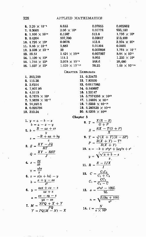
328 APPLIED MATHEMATICS
6. 3.29 X 10⁻⁶ 7. 0.3056 8. 1.106 X 10¹⁰ 9. 0.4204
10. 4.726 X 100 11. 8.33 X 10⁻⁶ 12. 3.528 X 10⁻² 13. 56.51 14. 1.109 X 10⁸ 15. 1.755 X 10⁸ 16. 1.037 X 10⁶
1. 363,250 2. 116.38 3. 3.6314 4. 7,907.96 5. 4.5113 6. 6.7678 X 10° 7. 2.5628 X 10⁻² 8. 24,992.6 9. 0.026794
10. 310.54
1. y=a -b-x b=a-x-y
2. b - R - ax cz
- -R ax 4- by z
XY - JQ RT
XV - RST = j
xY 4. z _ - ab
abz =
= z(a bz) - y X -F y - as
zz azz cx - z
as ± c cx - Cy - z
yz - xz
7 M NPQ X Y . = PQ
Y = PQ(M - N) - X
5. x
6. y -
a -
8.655 3.06 X 10⁶ 0.1587 507,700 0.0678 2,882 50 1.424 X 101° 111.1 2.078 X 10⁻⁶ 1.629 X 10⁻¹⁰
0.07855 0.002852 0.01778 935,100 513.8 1.756 X 10² 0.03017 213,400 513.8 3.204 X 10⁸ 0.01304 0.2401 0.002898 1.764 X 10⁻⁷ 0.007937 8.04 X 10¹¹ 9.995 1.232 X 10⁸ 958.6 36,480 28.25 1.69 X 10⁻¹⁴
CHAPTER EXERCISES
11. 0.35475 12. 7.82520 13. 0.0117985 14. 0.140887 15. 1.22147 16. 5.7974266 X 10" 17. 1.18894 X 10" 18. 7.5333 X 10⁻¹² 19. 5.280829 X 10⁻⁸ 20. 8.5306 X 1028
Chapter 3
8. T - X(R - S) o + RX - T(0 P)
X
9. T = NV(X Y)(R - SP) R(X -I- Y) - T°
S(X ± Y) 10. a = -b z2y4 2xy2z z'
NiVa b - z
P -
a2n6 - 10bL 13. a
9L
= .\IL(9a 10b) 71
N 14. t -
e X108
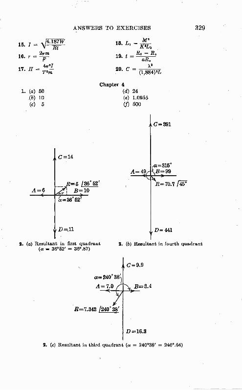
ANSWERS TO EXERCISES 329
_ , V/clew M 2 15. I 18. LI = Rt K2L2
2rna 16. r = 19. t —
F aR. 41.21 X2
17. H =- 20. C = T2m (1,884)2L
1. (a) 50 (b) 10
(c) 5
A=6
Chapter 4 (d) 24 (e) 1.0955 (f) 500
C=14
R=5 /3652' B=10 o
a=36 52'
D =11
A= 49
C=391
ot = 315° B= 99
R= 70.7
D= 441
2. (a) Resultant in first quadrant 2. (b) Resultant in fourth quadrant (a = 36°52' = 36°.87)
C=9.9
a= 24038
A=7.0 B=3.4
R=7.343 /240°38'
D=16.3
2. (c) Resultant in third quadrant (a = 240°38' = 240°.64)
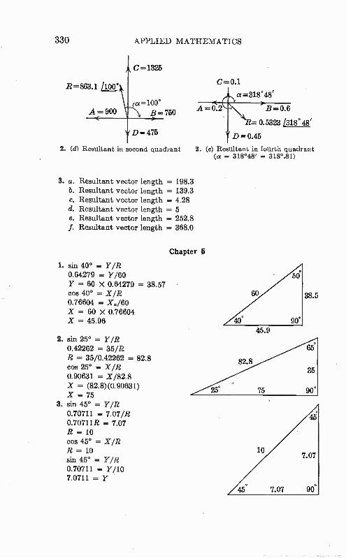
A = 900 B=750
D- 475
330 APPLIED MATHEMATICS
C=1325
R=863.1 /100 'C=0.1 a=318°48'
(a=100° A=0.2 B=0.6
R= 0.5323 /318°48'
D -= 0.45
2. (d) Resultant in second quadrant 2. (e) Resultant in fourth quadrant (a = 318°48' = 318°.81)
3. a. Resultant vector length = 198.3 b. Resultant vector length = 139.3 c. Resultant vector length = 4.28 d. Resultant vector length = 5 e. Resultant vector length = 252.8 f. Resultant vector length =- 368.0
Chapter 5
1. sin 40° -= Y/R 0.64279 = Y/60 Y = 60 X 0.64279 = 38.57 cos 40° = X /R 0.76604 = X./60 X = 60 X 0.76604 X = 45.96
2. sin 25° = Y/R 0.42262 -= 35/R R = 35/0.42262 = 82.8 cos 25° = X/R 0.90631 = 1/82.8 X = (82.8)(0.90631) X = 75
3. sin 45° = Y/R 0.70711 = 7.07/R 0.70711R = 7.07 R = 10 cos 45° = X /R R = 10 sin 45° = Y/R 0.70711 = Y/10 7.0711 = Y
45.9
38.5
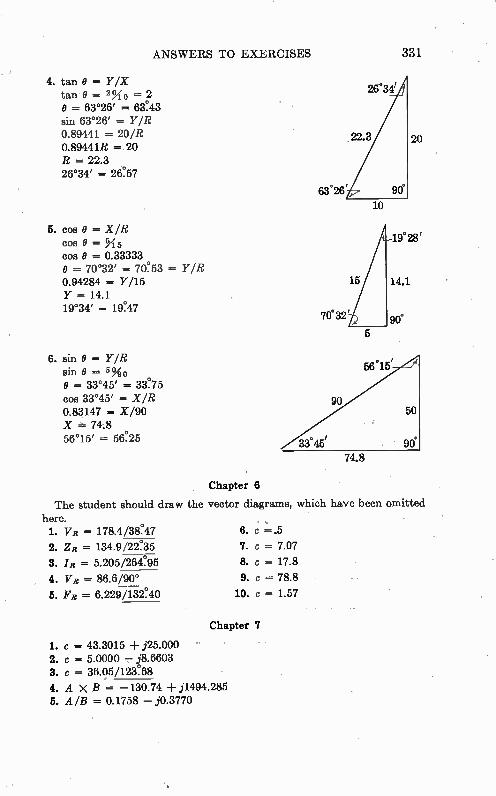
ANSWERS TO EXERCISES 331
4. tan 8 = Y/X tan 0 = 2% 0 = 2 26°31'
= 63°26' = 6e43 sin 63°26' = Y/R 0.89441 = 20/R 22.3 20 0.89441R = 20 R = 22.3 26°34' = 26%7
5. cos O = X/R cos = '1 5 1928'
cos O = 0.33333 o = 70°32' = 70%3 = Y/R 0.94284 = Y/15 16 14.1 Y = 14.1 19°34' = 1e47
70°32'
5
10
6. sin O = Y/R sin O = 5%0 56'15'
9 = 33°45' = 3e75 cos 33°45' = XIR 90 0.83147 = X/90 50 X = 74.8
56°15' = 5625 33 45' 90°
74.8
Chapter 6
The student should draw the vector diagrams, which have been omitted
here. , 1. VI? = 178.4/3e47 6. c =.5
2. ZR = 134.9/22%5 7. c = 7.07
3. IR = 5.205/264%5 8. c = 17.8
4. VR = 86.6/90° 9. c = 78.8
5. FR = 6.229/13240 10. c = 1.57
Chapter 7
1. c = 43.3015 + j25.000 2. c = 5.0000 0.6603 3. c = 36.05/123.68
4. A X B = -130.74 + j1494.285 5. A/B = 0.1758 - j0.3770
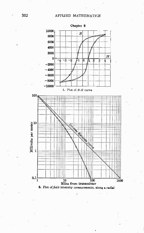
332 APPLIED MATHEMATICS
Chapter 8
10000
8000
6000
4000
2000
o —2000
—4000
—6000
—8000
—10000
H 12 3 « 4 —4 —3 —2 1 o
1. Plot of B-H curve
10 100 Miles from transmitter
2. Plot of field intensity measurements, along a radial
1000
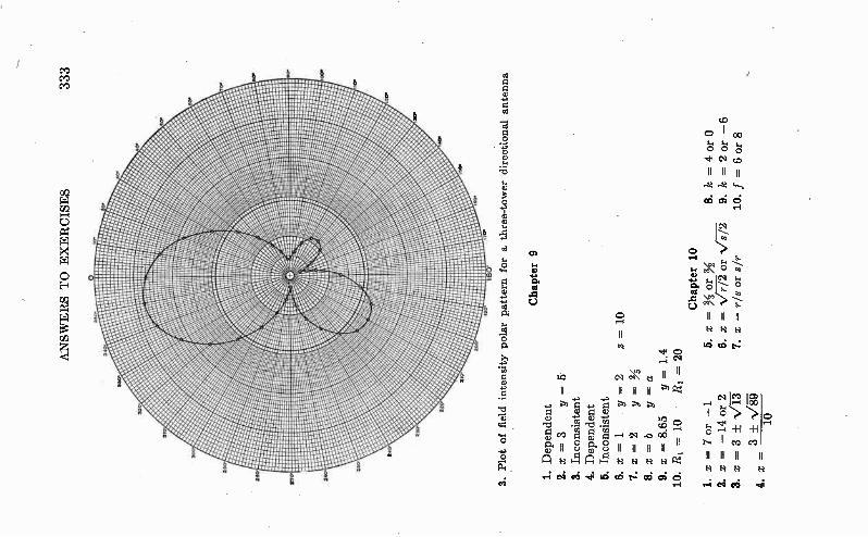
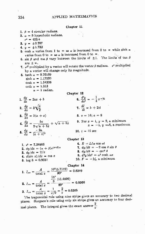
334 APPLIED MATHEMATICS
Chapter 11
1. )3 = 4 circular radians. 2. « = 6 hyperbolic radians.
= 403.4 3. y = ±0.707 4. y = +1.732 5. cosh « varies from 1 to co as « is increased from 0 to co while sinh
varies from 0 to co as a is increased from 0 to co. 6. sin 13 and cos 13 vary between the limits of ±1. The limits'of tan 13
are 7. e0 multiplied by a vector will rotate the vector 13 radians. Ea multiplied
by a vector will change only its magnitude. 8. tanh a = 0.76159
sinh « = 1.17520 cosh a = 1.54308 coth « = 1.313
= 1 radian.
dy 1. = 2ax b
dx
\fr-dx 2 dy
3. -dx 2(a x)
bx
dx 2Va bx dy = -2a
5. dx (a + x)2
1. e2 = 7.38905 2. dyldx = (a ± /3)e<"+0)' 3. dyldx =21x 4. d(sin x)/dx -= cos x 5. log 8 = 0.9031
Chapter 12 1
6. -d2Y = - dx2 4 •
dl 7. Tit = b 2ct
8. y = 16; a = 8
9. For x = 1, y = 2, a minimum x -1, y =.6, a maximum
= 16 sec
Chapter 13 6. E = Llw cos cut 7. dylde = -2 cos O sin 8. dy/d0 = - cse° 9. d2y1dx2 = a2 cosh «a;
10. F = a minimum
Chapter 14 A 10°(5.7149)
- = 0.6349 av = total x 90°
15° -F (11.4592) A
----- - 0.6366 total x 90° A 1 2
3. = - = - =. - 0.6366 total x r/2
The trapezoidal rule using nine strips gives an accuracy to two decimal places. Simpson's rule using only six strips gives an accuracy to four deci-
mal places. The integral gives the exact answer --
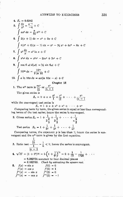
ANSWERS TO EXERCISES 335
4. S. = 0.6345
5. 15 C
faxa dx = xio
6. f 2(x + 1) dx = ± 2x C
f4(x2 + 2)(x — 1) dx = x4 — + 4x2
7. f a2 = a2 ln + C
8. f X2 Ez de = Xi e — 2xe' + 2ex + C
9. f cos 6 cot d(wt) = it¡ sin 6f.ot + C
162e f 162' dx — C
2 ln 16
10. f a ln 10x dx = ax(ln 10x — x) C
Chapter 15 xn
1. The nu. term is ne" or 11, In — 1
The given series is x2 =0-Fx-FT+r,
while the convergent test series is —
S. = 1 x + x2 + xa -I- • • • ± nn Comparing term by term, the given series is equal or less than correspond-
ing terms of the test series; hence the series is convergent. 1 1 1
2. Given series S. = 1 ± ± • • • ± 2 — 3 — n — 3 3 3
Test series S. = 1 ± I + + • • • + n—P 2P 3P 1
Comparing terms, the exponent p is less than 1; hence the series is con-vergent and the nth term is given by the first equation.
3. Ratio test
1
+ '
1 — < 1; hence the series is convergent.
1
4.
= 6.082754 accurate to four decimal places . = 6.082763. Check by extracting the square root.
5. f(x) = sin x f(0) = f'(x) = cos x f (0) = 1 f'(x) = — sin x f"(0) = f" (x) = — cos x f"(0) = —1
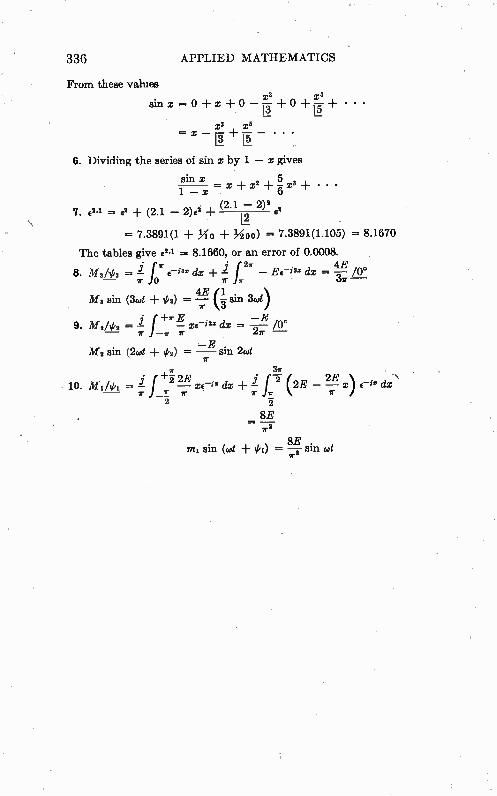
336 APPLIED MATHEMATICS
From these values x3 x'
sinx=
xs x' = x - r3..4. 11 - • • •
6. Dividing the series of sin x by 1 - x gives
sin x - x + x2 ± x3 ± • • •
1 + (2.1 - 2)2 o
7. e2.1 = ê -I- (2.1 - 2)e2
= 7.3891(1 + 310 + hoo) = 7.3891(1.105) = 8.1670
The tables give Oa = 8.1660, or an error of 0.0008.
8. m ai,p8 dr f 2T E«-j3,e dx T e —
31. sin (3i.ot ± 4,3) = 1411. sin 3,d)
9. M2/4,3 ir f -Eir "! XE-i2e dx = /0° 71"
-E M g sin (2Kut ± #2) — sin lot
ir ir
+- 2E .... LE x 10. mi/ei - i I. 2 — ze— i» d., + i f;-'r (2E -i. d,' . it ir 2r jir r
- i 8E
... r2 8E
mi sin (wt = —,2 sin cot

•

.