ADVANCES in APPLIED and PURE MATHEMATICS - inase

ADVANCES in APPLIED and PURE MATHEMATICS

Proceedings of the 2014 International Conference on Pure Mathematics, Applied Mathematics, Computational Methods

(PMAMCM 2014)

Santorini Island, Greece July 17-21, 2014

ADVANCES in APPLIED and PURE MATHEMATICS Proceedings of the 2014 International Conference on Pure Mathematics, Applied Mathematics, Computational Methods (PMAMCM 2014) Santorini Island, Greece July 17-21, 2014 Copyright © 2014, by the editors All the copyright of the present book belongs to the editors. All rights reserved. No part of this publication may be reproduced, stored in a retrieval system, or transmitted in any form or by any means, electronic, mechanical, photocopying, recording, or otherwise, without the prior written permission of the editors. All papers of the present volume were peer reviewed by no less than two independent reviewers. Acceptance was granted when both reviewers' recommendations were positive.

Series: Mathematics and Computers in Science and Engineering Series | 29 ISSN: 2227-4588 ISBN: 978-1-61804-240-8

ADVANCES in APPLIED and PURE MATHEMATICS

Proceedings of the 2014 International Conference on Pure Mathematics, Applied Mathematics, Computational Methods

(PMAMCM 2014)

Santorini Island, Greece July 17-21, 2014

Organizing Committee General Chairs (EDITORS) • Prof. Nikos E. Mastorakis

Industrial Eng.Department Technical University of Sofia, Bulgaria

• Prof. Panos M. Pardalos, Distinguished Prof. of Industrial and Systems Engineering, University of Florida, USA

• Professor Ravi P. Agarwal Department of Mathematics Texas A&M University – Kingsville 700 University Blvd. Kingsville, TX 78363-8202, USA

• Prof. Ljubiša Kočinac, University of Nis, Nis, Serbia

Senior Program Chair • Prof. Valery Y. Glizer,

Ort Braude College, Karmiel, Israel Program Chairs • Prof. Filippo Neri

Dipartimento di Informatica e Sistemistica University of Naples "Federico II" Naples, Italy

• Prof. Constantin Udriste, University Politehnica of Bucharest, Bucharest Romania

• Prof. Marcia Cristina A. B. Federson, Universidade de São Paulo, São Paulo, Brazil

Tutorials Chair • Prof. Pradip Majumdar

Department of Mechanical Engineering Northern Illinois University Dekalb, Illinois, USA

Special Session Chair • Prof. Pavel Varacha

Tomas Bata University in Zlin Faculty of Applied Informatics Department of Informatics and Artificial Intelligence Zlin, Czech Republic

Workshops Chair • Prof. Sehie Park,

The National Academy of Sciences, Republic of Korea

Local Organizing Chair • Prof. Klimis Ntalianis,

Tech. Educ. Inst. of Athens (TEI), Athens, Greece Publication Chair • Prof. Gen Qi Xu

Department of Mathematics Tianjin University Tianjin, China

Publicity Committee • Prof. Vjacheslav Yurko,

Saratov State University, Astrakhanskaya, Russia

• Prof. Myriam Lazard Institut Superieur d' Ingenierie de la Conception Saint Die, France

International Liaisons • Professor Jinhu Lu, IEEE Fellow

Institute of Systems Science Academy of Mathematics and Systems Science Chinese Academy of Sciences Beijing 100190, P. R. China

• Prof. Olga Martin Applied Sciences Faculty Politehnica University of Bucharest Romania

• Prof. Vincenzo Niola Departement of Mechanical Engineering for Energetics University of Naples "Federico II" Naples, Italy

• Prof. Eduardo Mario Dias Electrical Energy and Automation Engineering Department Escola Politecnica da Universidade de Sao Paulo Brazil

Steering Committee • Prof. Stefan Siegmund, Technische Universitaet Dresden, Germany • Prof. Zoran Bojkovic, Univ. of Belgrade, Serbia • Prof. Metin Demiralp, Istanbul Technical University, Turkey • Prof. Imre Rudas, Obuda University, Budapest, Hungary

Program Committee for PURE MATHEMATICS Prof. Ferhan M. Atici, Western KentuckyUniversity, Bowling Green, KY 42101, USA Prof. Ravi P. Agarwal, Texas A&M University - Kingsville, Kingsville, TX, USA Prof. Martin Bohner, Missouri University of Science and Technology, Rolla, Missouri, USA Prof. Dashan Fan, University of Wisconsin-Milwaukee, Milwaukee, WI, USA Prof. Paolo Marcellini. University of Firenze, Firenze, Italy Prof. Xiaodong Yan, University of Connecticut, Connecticut, USA Prof. Ming Mei, McGill University, Montreal, Quebec, Canada Prof. Enrique Llorens, University of Valencia, Valencia, Spain Prof. Yuriy V. Rogovchenko, University of Agder, Kristiansand, Norway Prof. Yong Hong Wu, Curtin University of Technology, Perth, WA, Australia Prof. Angelo Favini, University of Bologna, Bologna, Italy Prof. Andrew Pickering, Universidad Rey Juan Carlos, Mostoles, Madrid, Spain Prof. Guozhen Lu, Wayne state university, Detroit, MI 48202, USA Prof. Gerd Teschke, Hochschule Neubrandenburg - University of Applied Sciences, Germany Prof. Michel Chipot, University of Zurich, Switzerland Prof. Juan Carlos Cortes Lopez, Universidad Politecnica de Valencia, Spain Prof. Julian Lopez-Gomez, Universitad Complutense de Madrid, Madrid, Spain Prof. Jozef Banas, Rzeszow University of Technology, Rzeszow, Poland Prof. Ivan G. Avramidi, New Mexico Tech, Socorro, New Mexico, USA Prof. Kevin R. Payne, Universita' degli Studi di Milano, Milan, Italy Prof. Juan Pablo Rincon-Zapatero, Universidad Carlos III De Madrid, Madrid, Spain Prof. Valery Y. Glizer, ORT Braude College, Karmiel, Israel Prof. Norio Yoshida, University of Toyama, Toyama, Japan Prof. Feliz Minhos, Universidade de Evora, Evora, Portugal Prof. Mihai Mihailescu, University of Craiova, Craiova, Romania Prof. Lucas Jodar, Universitat Politecnica de Valencia, Valencia, Spain Prof. Dumitru Baleanu, Cankaya University, Ankara, Turkey Prof. Jianming Zhan, Hubei University for Nationalities, Enshi, Hubei Province, China Prof. Zhenya Yan, Institute of Systems Science, AMSS, Chinese Academy of Sciences, Beijing, China Prof. Nasser-Eddine Mohamed Ali Tatar, King Fahd University of Petroleum and Mineral, Saudi Arabia Prof. Jianqing Chen, Fujian Normal University, Cangshan, Fuzhou, Fujian, China Prof. Josef Diblik, Brno University of Technology, Brno, Czech Republic Prof. Stanislaw Migorski, Jagiellonian University in Krakow, Krakow, Poland Prof. Qing-Wen Wang, Shanghai University, Shanghai, China Prof. Luis Castro, University of Aveiro, Aveiro, Portugal Prof. Alberto Fiorenza, Universita' di Napoli "Federico II", Napoli (Naples), Italy Prof. Patricia J. Y. Wong, Nanyang Technological University, Singapore Prof. Salvatore A. Marano, Universita degli Studi di Catania, Catania, Italy Prof. Sung Guen Kim, Kyungpook National University, Daegu, South Korea Prof. Maria Alessandra Ragusa, Universita di Catania, Catania, Italy Prof. Gerassimos Barbatis, University of Athens, Athens, Greece Prof. Jinde Cao, Distinguished Prof., Southeast University, Nanjing 210096, China Prof. Kailash C. Patidar, University of the Western Cape, 7535 Bellville, South Africa Prof. Mitsuharu Otani, Waseda University, Japan Prof. Luigi Rodino, University of Torino, Torino, Italy Prof. Carlos Lizama, Universidad de Santiago de Chile, Santiago, Chile Prof. Jinhu Lu, Chinese Academy of Sciences, Beijing, China Prof. Narcisa C. Apreutesei, Technical University of Iasi, Iasi, Romania Prof. Sining Zheng, Dalian University of Technology, Dalian, China Prof. Daoyi Xu, Sichuan University, Chengdu, China Prof. Zili Wu, Xi'an Jiaotong-Liverpool University, Suzhou, Jiangsu, China Prof. Wei-Shih Du, National Kaohsiung Normal University, Kaohsiung City, Taiwan Prof. Khalil Ezzinbi, Universite Cadi Ayyad, Marrakesh, Morocco

Prof. Youyu Wang, Tianjin University of Finance and Economics, Tianjin, China Prof. Satit Saejung, Khon Kaen University, Thailand Prof. Chun-Gang Zhu, Dalian University of Technology, Dalian, China Prof. Mohamed Kamal Aouf, Mansoura University, Mansoura City, Egypt Prof. Yansheng Liu, Shandong Normal University, Jinan, Shandong, China Prof. Naseer Shahzad, King Abdulaziz University, Jeddah, Saudi Arabia Prof. Janusz Brzdek, Pedagogical University of Cracow, Poland Prof. Mohammad T. Darvishi, Razi University, Kermanshah, Iran Prof. Ahmed El-Sayed, Alexandria University, Alexandria, Egypt

Program Committee for APPLIED MATHEMATICS and COMPUTATIONAL METHODS Prof. Martin Bohner, Missouri University of Science and Technology, Rolla, Missouri, USA Prof. Martin Schechter, University of California, Irvine, USA Prof. Ivan G. Avramidi, New Mexico Tech, Socorro, New Mexico, USA Prof. Michel Chipot, University of Zurich, Zurich, Switzerland Prof. Xiaodong Yan, University of Connecticut, Connecticut USA Prof. Ravi P. Agarwal, Texas A&M University - Kingsville, Kingsville, TX, USA Prof. Yushun Wang, Nanjing Normal university, Nanjing, China Prof. Detlev Buchholz, Universitaet Goettingen, Goettingen, Germany Prof. Patricia J. Y. Wong, Nanyang Technological University, Singapore Prof. Andrei Korobeinikov, Centre de Recerca Matematica, Barcelona, Spain Prof. Jim Zhu, Western Michigan University, Kalamazoo, MI, USA Prof. Ferhan M. Atici, Department of Mathematics, Western Kentucky University, USA Prof. Gerd Teschke, Institute for Computational Mathematics in Science and Technology, Germany Prof. Meirong Zhang, Tsinghua University, Beijing, China Prof. Lucio Boccardo, Universita degli Studi di Roma "La Sapienza", Roma, Italy Prof. Shanhe Wu, Longyan University, Longyan, Fujian, China Prof. Natig M. Atakishiyev, National Autonomous University of Mexico, Mexico Prof. Jianming Zhan, Hubei University for Nationalities, Enshi, Hubei Province, China Prof. Narcisa C. Apreutesei, Technical University of Iasi, Iasi, Romania Prof. Chun-Gang Zhu, Dalian University of Technology, Dalian, China Prof. Abdelghani Bellouquid, University Cadi Ayyad, Morocco Prof. Jinde Cao, Southeast University/ King Abdulaziz University, China Prof. Josef Diblik, Brno University of Technology, Brno, Czech Republic Prof. Jianqing Chen, Fujian Normal University, Fuzhou, Fujian, China Prof. Naseer Shahzad, King Abdulaziz University, Jeddah, Saudi Arabia Prof. Sining Zheng, Dalian University of Technology, Dalian, China Prof. Leszek Gasinski, Uniwersytet Jagielloński, Krakowie, Poland Prof. Satit Saejung, Khon Kaen University, Muang District, Khon Kaen, Thailand Prof. Juan J. Trujillo, Universidad de La Laguna, La Laguna, Tenerife, Spain Prof. Tiecheng Xia, Department of Mathematics, Shanghai University, China Prof. Stevo Stevic, Mathematical Institute Serbian Academy of Sciences and Arts, Beogrand, Serbia Prof. Lucas Jodar, Universitat Politecnica de Valencia, Valencia, Spain Prof. Noemi Wolanski, Universidad de Buenos Aires, Buenos Aires, Argentina Prof. Zhenya Yan, Chinese Academy of Sciences, Beijing, China Prof. Juan Carlos Cortes Lopez, Universidad Politecnica de Valencia, Spain Prof. Wei-Shih Du, National Kaohsiung Normal University, Kaohsiung City, Taiwan Prof. Kailash C. Patidar, University of the Western Cape, Cape Town, South Africa Prof. Hossein Jafari, University of Mazandaran, Babolsar, Iran Prof. Abdel-Maksoud A Soliman, Suez Canal University, Egypt Prof. Janusz Brzdek, Pedagogical University of Cracow, Cracow, Poland Dr. Fasma Diele, Italian National Research Council (C.N.R.), Bari, Italy

Additional Reviewers Santoso Wibowo CQ University, Australia Lesley Farmer California State University Long Beach, CA, USA Xiang Bai Huazhong University of Science and Technology, China Jon Burley Michigan State University, MI, USA Genqi Xu Tianjin University, China Zhong-Jie Han Tianjin University, China Kazuhiko Natori Toho University, Japan João Bastos Instituto Superior de Engenharia do Porto, Portugal José Carlos Metrôlho Instituto Politecnico de Castelo Branco, Portugal Hessam Ghasemnejad Kingston University London, UK Matthias Buyle Artesis Hogeschool Antwerpen, Belgium Minhui Yan Shanghai Maritime University, China Takuya Yamano Kanagawa University, Japan Yamagishi Hiromitsu Ehime University, Japan Francesco Zirilli Sapienza Universita di Roma, Italy Sorinel Oprisan College of Charleston, CA, USA Ole Christian Boe Norwegian Military Academy, Norway Deolinda Rasteiro Coimbra Institute of Engineering, Portugal James Vance The University of Virginia's College at Wise, VA, USA Valeri Mladenov Technical University of Sofia, Bulgaria Angel F. Tenorio Universidad Pablo de Olavide, Spain Bazil Taha Ahmed Universidad Autonoma de Madrid, Spain Francesco Rotondo Polytechnic of Bari University, Italy Jose Flores The University of South Dakota, SD, USA Masaji Tanaka Okayama University of Science, Japan M. Javed Khan Tuskegee University, AL, USA Frederic Kuznik National Institute of Applied Sciences, Lyon, France Shinji Osada Gifu University School of Medicine, Japan Dmitrijs Serdjuks Riga Technical University, Latvia Philippe Dondon Institut polytechnique de Bordeaux, France Abelha Antonio Universidade do Minho, Portugal Konstantin Volkov Kingston University London, UK Manoj K. Jha Morgan State University in Baltimore, USA Eleazar Jimenez Serrano Kyushu University, Japan Imre Rudas Obuda University, Budapest, Hungary Andrey Dmitriev Russian Academy of Sciences, Russia Tetsuya Yoshida Hokkaido University, Japan Alejandro Fuentes-Penna Universidad Autónoma del Estado de Hidalgo, Mexico Stavros Ponis National Technical University of Athens, Greece Moran Wang Tsinghua University, China Kei Eguchi Fukuoka Institute of Technology, Japan Miguel Carriegos Universidad de Leon, Spain George Barreto Pontificia Universidad Javeriana, Colombia Tetsuya Shimamura Saitama University, Japan

Table of Contents

Keynote Lecture 1: New Developments in Clifford Fourier Transforms 14 Eckhard Hitzer Keynote Lecture 2: Robust Adaptive Control of Linear Infinite Dimensional Symmetric Hyperbolic Systems with Application to Quantum Information Systems

15

Mark J. Balas Keynote Lecture 3: Multidimensional Optimization Methods with Fewer Steps Than the Dimension: A Case of "Insider Trading" in Chemical Physics

16

Paul G. Mezey Keynote Lecture 4: MvStudium_Group: A Family of Tools for Modeling and Simulation of Complex Dynamical Systems

17

Yuri B. Senichenkov New Developments in Clifford Fourier Transforms 19 Eckhard Hitzer Computing the Distribution Function via Adaptive Multilevel Splitting 26 Ioannis Phinikettos, Ioannis Demetriou, Axel Gandy Recovering of Secrets using the BCJR Algorithm 33 Marcel Fernandez Efficient Numerical Method in the High-Frequency Anti-Plane Diffraction by an Interface Crack

43

Michael Remizov, Mezhlum Sumbatyan Robust Adaptive Control with Disturbance Rejection for Symmetric Hyperbolic Systems of Partial Differential Equations

48

Mark J. Balas, Susan A. Frost Mathematical Modeling of Crown Forest Fires Spread Taking Account Firebreaks 55 Valeriy Perminov Analytical Solution for Some MHD Problems on a Flow of Conducting Liquid in the Initial Part of a Channel in the Case of Rotational Symmetry

61

Elena Ligere, Ilona Dzenite Some Properties of Operators with Non-Analytic Functional Calculus 68 Cristina Şerbănescu, Ioan Bacalu Pulsatile Non-Newtonian Flows in a Dilated Vessel 79 Iqbal Husain, Christian R Langdon, Justin Schwark

Advances in Applied and Pure Mathematics

ISBN: 978-1-61804-240-8 11

Permutation Codes: A Branch and Bound Approach 86 Roberto Montemanni, Janos Barta, Derek H. Smith Unary Operators 91 József Dombi MHD Mixed Convection Flow of a Second-Grade Fluid on a Vertical Surface 98 Fotini Labropulu, Daiming Li, Ioan Pop Workflow Analysis - A Task Model Approach 103 Gloria Cravo Degrees of Freedom and Advantages of Different Rule-Based Fuzzy Systems 107 Marco Pota, Massimo Esposito Research Method of Energy-Optimal Spacecraft Control during Interorbital Maneuvers 115 N. L. Sokolov Keywords Extraction from Articles’ Title for Ontological Purposes 120 Sylvia Poulimenou, Sofia Stamou, Sozon Papavlasopoulos, Marios Poulos Architecture of an Agents-Based Model for Pulmonary Tuberculosis 126 M. A. Gabriel Moreno Sandoval Flanged Wide Reinforced Concrete Beam Subjected to Fire - Numerical Investigations 132 A. Puskás, A. Chira A New Open Source Project for Modeling and Simulation of Complex Dynamical Systems 138 A. A. Isakov, Y. B. Senichenkov Timed Ignition of Separated Charge 142 Michal Kovarik Analysis of Physical Health Index and Children Obesity or Overweight in Western China 148 Jingya Bai, Ye He, Xiangjun Hai, Yutang Wang, Jinquan He, Shen Li New Tuning Method of the Wavelet Function for Inertial Sensor Signals Denoising 153 Ioana-Raluca Edu, Felix-Constantin Adochiei, Radu Obreja, Constantin Rotaru, Teodor Lucian Grigorie

An Exploratory Crossover Operator for Improving the Performance of MOEAs 158 K. Metaxiotis, K. Liagkouras Modelling of High-Temperature Behaviour of Cementitious Composites 163 Jirı Vala, Anna Kucerova, Petra Rozehnalova


ISBN: 978-1-61804-240-8 12

Gaussian Mixture Models Approach for Multiple Fault Detection - DAMADICS Benchmark 167 Erika Torres, Edwin Villareal Analytical and Experimental Modeling of the Drivers Spine 172 Veronica Argesanu, Raul Miklos Kulcsar, Ion Silviu Borozan, Mihaela Jula, Saša Ćuković, Eugen Bota

Exponentially Scaled Point Processes and Data Classification 179 Marcel Jirina A Comparative Study on Principal Component Analysis and Factor Analysis for the Formation of Association Rule in Data Mining Domain

187

Dharmpal Singh, J. Pal Choudhary, Malika De Complex Probability and Markov Stochastic Process 198 Bijan Bidabad, Behrouz Bidabad, Nikos Mastorakis Comparison of Homotopy Perturbation Sumudu Transform Method and Homotopy Decomposition Method for Solving Nonlinear Fractional Partial Differential Equations

202

Rodrigue Batogna Gnitchogna, Abdon Atangana Noise Studies in Measurements and Estimates of Stepwise Changes in Genome DNA Chromosomal Structures

212

Jorge Munoz-Minjares, Yuriy S. Shmaliy, Jesus Cabal-Aragon Fundamentals of a Fuzzy Inference System for Educational Evaluation 222 M. A. Luis Gabriel Moreno Sandoval, William David Peña Peña The Movement Equation oh the Drivers Spine 227 Raul Miklos Kulcsar, Veronica Argesanu, Ion Silviu Borozan, Inocentiu Maniu, Mihaela Jula, Adrian Nagel

Authors Index 232


ISBN: 978-1-61804-240-8 13

Keynote Lecture 1

New Developments in Clifford Fourier Transforms

Sen. Ass. Prof. Dr. rer. nat. Eckhard Hitzer Department of Material Science

International Christian University Tokyo, Japan

E-mail: [email protected]

Abstract: We show how real and complex Fourier transforms are extended to W.R. Hamilton's algebra of quaternions and to W.K. Clifford's geometric algebras. This was initially motivated by applications in nuclear magnetic resonance and electric engineering. Followed by an ever wider range of applications in color image and signal processing. Clifford's geometric algebras are complete algebras, algebraically encoding a vector space and all its subspace elements, including Grassmannians (a vector space and all its subspaces of given dimension k). Applications include electromagnetism, and the processing of images, color images, vector field and climate data. Further developments of Clifford Fourier Transforms include operator exponential representations, and extensions to wider classes of integral transforms, like Clifford algebra versions of linear canonical transforms and wavelets. Brief Biography of the Speaker: http://erkenntnis.icu.ac.jp/


ISBN: 978-1-61804-240-8 14

Keynote Lecture 2

Robust Adaptive Control of Linear Infinite Dimensional Symmetric Hyperbolic Systems with Application to Quantum Information Systems

Prof. Mark J. Balas Distinguished Faculty

Aerospace Engineering Department & Electrical Engineering Department

Embry-Riddle Aeronautical University Daytona Beach, Florida

USA E-mail: [email protected]

Abstract: Symmetric Hyperbolic Systems of partial differential equations describe many physical phenomena such as wave behavior, electromagnetic fields, and quantum fields. To illustrate the utility of the adaptive control law, we apply the results to control of symmetric hyperbolic systems with coercive boundary conditions. Given a Symmetric Hyperbolic continuous-time infinite-dimensional plant on a Hilbert space and disturbances of known and unknown waveform, we show that there exists a stabilizing direct model reference adaptive control law with certain disturbance rejection and robustness properties. The closed loop system is shown to be exponentially convergent to a neighborhood with radius proportional to bounds on the size of the disturbance. The plant is described by a closed densely defined linear operator that generates a continuous semigroup of bounded operators on the Hilbert space of states. We will discuss the need and use of this kind of direct adaptive control in quantum information systems. Brief Biography of the Speaker: Mark Balas is presently distinguished faculty in Aerospace Engineering at Embry-Riddle Aeronautical University. He was the Guthrie Nicholson Professor of Electrical Engineering and Head of the Electrical and Computer Engineering Department at the University of Wyoming. He has the following technical degrees: PhD in Mathematics, MS Electrical Engineering, MA Mathematics, and BS Electrical Engineering. He has held various positions in industry, academia, and government. Among his careers, he has been a university professor for over 35 years with RPI, MIT, University of Colorado-Boulder, and University of Wyoming, and has mentored 42 doctoral students. He has over 300 publications in archive journals, refereed conference proceedings and technical book chapters. He has been visiting faculty with the Institute for Quantum Information and the Control and Dynamics Division at the California Institute of Technology, the US Air Force Research Laboratory-Kirtland AFB, the NASA-Jet Propulsion Laboratory, the NASA Ames Research Center, and was the Associate Director of the University of Wyoming Wind Energy Research Center and adjunct faculty with the School of Energy Resources. He is a life fellow of the AIAA and a life fellow of the IEEE.


ISBN: 978-1-61804-240-8 15

Keynote Lecture 3

Multidimensional Optimization Methods with Fewer Steps Than the Dimension: A Case of "Insider Trading" in Chemical Physics

Prof. Paul G. Mezey Canada Research Chair in Scientific Modeling and Simulation

Department of Chemistry and Department of Physics and Physical Oceanography Memorial University of Newfoundland

Canada E-mail: [email protected]

Abstract: "Insider trading" in commerce takes advantage of information that is not commonly available, and a somewhat similar advantage plays a role in some specific, very high-dimensional optimization problems of chemical physics, in particular, molecular quantum mechanics. Using a specific application of the Variational Theorem for the expectation value of molecular Hamiltonians, an optimization problem of thousands of unknowns does often converge in fewer than hundred steps. The search for optimum, however, is typically starting from highly specific initial choices for the values of these unknowns, where the conditions imposed by physics, not formally included in the optimization algorithms, are taken into account in an implicit way. This rapid convergence also provides compatible choices for "hybrid optimization strategies", such as those applied in macromolecular quantum chemistry [1]. The efficiency of these approaches, although highly specific for the given problems, nevertheless, provides motivation for a similar, implicit use of side conditions for a better choice of approximate initial values of the unknowns to be determined. [1]. P.G. Mezey, "On the Inherited "Purity" of Certain Extrapolated Density Matrices", Computational and Theoretical Chemistry, 1003, 130-133 (2013). Brief Biography of the Speaker: http://www.mun.ca/research/explore/chairs/mezey.php


ISBN: 978-1-61804-240-8 16

Keynote Lecture 4

MvStudium_Group: A Family of Tools for Modeling and Simulation of Complex Dynamical Systems

Professor Yuri B. Senichenkov co-author: Professor Yu. B. Kolesov

Distributed Computing and Networking Department St. Petersburg State Polytechnical University

Russia E-mail: [email protected]

Abstract: Designing of new version of Rand Model Designing under the name RMD 7 is coming to an end. It will be possible using dynamic objects, dynamic connections (bonds), and arrays of objects in the new version. These types are used for Simulation Modeling, and Agent Based Modeling. The first trial version will be available at year-end. The tools developed by MvStudium_Group are considered by authors as universal tools for automation modeling and simulation of complex dynamical systems. We are feeling strongly that at least nitty-gritty real system is multi-component, hierarchical, and event-driven system. Modeling of such systems requires using object-oriented technologies, expressive graphical languages and various mathematical models for event-driven systems. The last versions of Model Vision Modeling Language are intended for multi-component models with variable structure and event-driven behavior. Brief Biography of the Speaker: PhD degree in Numerical Analysis from St. Petersburg State University (1984). Dr. Sci. degree (Computer Science) from St. Petersburg Polytechnic University (2005). Author of 125 scientific publications-conference papers, articles, monographs and textbooks. A board member of National Simulation Society - NSS (http://simulation.su/en.html), and Federation of European Simulation Societies- EuroSim (http://www.eurosim.info/). A member of Scientific Editorial Board of "Simulation Notes Europe" Journal (http://www.sne-journal.org/), and "Computer Tools in Education" Journal(http://ipo.spb.ru/journal/). Chairman and Chief-Editor of COMOD 2001-2014 conferences (https://dcn.icc.spbstu.ru/).


ISBN: 978-1-61804-240-8 17


ISBN: 978-1-61804-240-8 18

New Developments in Clifford Fourier TransformsEckhard Hitzer

Abstract—We show how real and complex Fourier transformsare extended to W.R. Hamiltons algebra of quaternions and toW.K. Clifford’s geometric algebras. This was initially motivated byapplications in nuclear magnetic resonance and electric engineering.Followed by an ever wider range of applications in color image andsignal processing. Cliffords geometric algebras are complete algebras,algebraically encoding a vector space and all its subspace elements.Applications include electromagnetism, and the processing of images,color images, vector field and climate data. Further developments ofClifford Fourier Transforms include operator exponential represen-tations, and extensions to wider classes of integral transforms, likeClifford algebra versions of linear canonical transforms and wavelets.

Keywords—Fourier transform, Clifford algebra, geometric algebra,quaternions, signal processing, linear canonical transform

I. INTRODUCTION

We begin by introducing Clifford Fourier transforms, in-cluding the important class of quaternion Fourier transformsmainly along the lines of [31] and [5], adding further detail,emphasize and new developments.

There is the alternative operator exponential Clifford Fouriertransform (CFT) approach, mainly pursued by the CliffordAnalysis Group at the university of Ghent (Belgium) [5].New work in this direction closely related to the roots of −1approach explained below is in preparation [11].

We mainly provide an overview of research based on theholistic investigation [28] of real geometric square roots of−1 in Clifford algebras Cl(p, q) over real vector spaces Rp,q .These algebras include real and complex numbers, quater-nions, Pauli- and Dirac algebra, space time algebra, spinoralgebra, Lie algebras, conformal geometric algebra and manymore. The resulting CFTs are therefore perfectly tailored towork on functions valued in these algebras. In general thecontinuous manifolds of

√−1 in Cl(p, q) consist of several

conjugacy classes and their connected components. Simpleexamples are shown in Fig. 1.

A CFT analyzes scalar, vector and multivector signals interms of sine and cosine waves with multivector coefficients.Basically, the imaginary unit i ∈ C in the transformationkernel eiφ = cosφ+ i sinφ is replaced by a

√−1 in Cl(p, q).

This produces a host of CFTs, an incomplete brief overviewis sketched in Fig. 2, see also the historical overview in [5].Additionally the

√−1 in Cl(p, q) allow to construct further

types of integral transformations, notably Clifford wavelets[21], [37].

E. Hitzer is with the Department of Material Science, International ChristianUniversity, Mitaka, Tokyo, 181-8585 Japan e-mail: [email protected].

thanksManuscript received May 31, 2014; revised ...

II. CLIFFORD’S GEOMETRIC ALGEBRA

Definition 1 (Clifford’s geometric algebra [15], [36]). Lete1, e2, . . . , ep, ep+1, . . ., en, with n = p + q, e2k = εk,εk = +1 for k = 1, . . . , p, εk = −1 for k = p+ 1, . . . , n, bean orthonormal base of the inner product vector space Rp,qwith a geometric product according to the multiplication rules

ekel + elek = 2εkδk,l, k, l = 1, . . . n, (1)

where δk,l is the Kronecker symbol with δk,l = 1 for k = l,and δk,l = 0 for k 6= l. This non-commutative product and theadditional axiom of associativity generate the 2n-dimensionalClifford geometric algebra Cl(p, q) = Cl(Rp,q) = Clp,q =Gp,q = Rp,q over R. The set eA : A ⊆ 1, . . . , nwith eA = eh1eh2 . . . ehk

, 1 ≤ h1 < . . . < hk ≤ n,e∅ = 1, forms a graded (blade) basis of Cl(p, q). The gradesk range from 0 for scalars, 1 for vectors, 2 for bivectors, sfor s-vectors, up to n for pseudoscalars. The vector spaceRp,q is included in Cl(p, q) as the subset of 1-vectors. Thegeneral elements of Cl(p, q) are real linear combinationsof basis blades eA, called Clifford numbers, multivectors orhypercomplex numbers.

In general 〈A〉k denotes the grade k part of A ∈ Cl(p, q).The parts of grade 0 and k+ s, respectively, of the geometricproduct of a k-vector Ak ∈ Cl(p, q) with an s-vector Bs ∈Cl(p, q)

Ak ∗Bs := 〈AkBs〉0, Ak ∧Bs := 〈AkBs〉k+s, (2)

are called scalar product and outer product, respectively.For Euclidean vector spaces (n = p) we use Rn = Rn,0

and Cl(n) = Cl(n, 0). Every k-vector B that can be writtenas the outer product B = b1 ∧ b2 ∧ . . . ∧ bk of k vectorsb1, b2, . . . , bk ∈ Rp,q is called a simple k-vector or blade.

Multivectors M ∈ Cl(p, q) have k-vector parts (0 ≤ k ≤n): scalar part Sc(M) = 〈M〉 = 〈M〉0 = M0 ∈ R, vectorpart 〈M〉1 ∈ Rp,q , bi-vector part 〈M〉2, . . . , and pseudoscalarpart 〈M〉n ∈

∧n Rp,qM =

∑A

MAeA = 〈M〉+ 〈M〉1 + 〈M〉2 + . . .+ 〈M〉n . (3)

The principal reverse of M ∈ Cl(p, q) defined as

M =n∑k=0

(−1)k(k−1)

2 〈M〉k, (4)

often replaces complex conjugation and quaternion conjuga-tion. Taking the reverse is equivalent to reversing the orderof products of basis vectors in the basis blades eA. Theoperation M means to change in the basis decompositionof M the sign of every vector of negative square eA =εh1eh1εh2eh2 . . . εhk

ehk, 1 ≤ h1 < . . . < hk ≤ n. Reversion,

M , and principal reversion are all involutions.


ISBN: 978-1-61804-240-8 19

For M,N ∈ Cl(p, q) we get M ∗ N =∑AMANA. Two

multivectors M,N ∈ Cl(p, q) are orthogonal if and only ifM ∗ N = 0. The modulus |M | of a multivector M ∈ Cl(p, q)is defined as

|M |2 =M ∗ M =∑A

M2A. (5)

A. Multivector signal functions

A multivector valued function f : Rp,q → Cl(p, q), has 2n

blade components (fA : Rp,q → R)

f(x) =∑A

fA(x)eA. (6)

We define the inner product of two functions f, g : Rp,q →Cl(p, q) by

(f, g) =

∫Rp,q

f(x)g(x) dnx

=∑A,B

eAeB∫Rp,q

fA(x)gB(x) dnx, (7)

with the symmetric scalar part

〈f, g〉 =∫Rp,q

f(x) ∗ g(x) dnx =∑A

∫Rp,q

fA(x)gA(x) dnx,

(8)

and the L2(Rp,q;Cl(p, q))-norm

‖f‖2 = 〈(f, f)〉 =∫Rp,q

|f(x)|2dnx =∑A

∫Rp,q

f2A(x) dnx,

(9)

L2(Rp,q;Cl(p, q)) = f : Rp,q → Cl(p, q) | ‖f‖ <∞.(10)

B. Square roots of −1 in Clifford algebras

Every Clifford algebra Cl(p, q), s8 = (p − q) mod 8, isisomorphic to one of the following (square) matrix algebras1

M(2d,R), M(d,H), M(2d,R2), M(d,H2) or M(2d,C).The first argument of M is the dimension, the second theassociated ring2 R for s8 = 0, 2, R2 for s8 = 1, C fors8 = 3, 7, H for s8 = 4, 6, and H2 for s8 = 5. For evenn: d = 2(n−2)/2, for odd n: d = 2(n−3)/2.

It has been shown [27], [28] that Sc(f) = 0 for everysquare root of −1 in every matrix algebra A isomorphic toCl(p, q). One can distinguish ordinary square roots of −1,and exceptional ones. All square roots of −1 in Cl(p, q) canbe computed using the package CLIFFORD for Maple [1],[3], [29], [38].

In all cases the ordinary square roots f of −1 constitute aunique conjugacy class of dimension dim(A)/2, which has asmany connected components as the group G(A) of invertibleelements in A. Furthermore, we have Spec(f) = 0 (zeropseudoscalar part) if the associated ring is R2, H2, or C. Theexceptional square roots of −1 only exist if A ∼=M(2d,C).

1Compare chapter 16 on matrix representations and periodicity of 8, aswell as Table 1 on p. 217 of [36].

2Associated ring means, that the matrix elements are from the respectivering R, R2, C, H or H2.

For A = M(2d,R), the centralizer (set of all elementsin Cl(p, q) commuting with f ) and the conjugacy class of asquare root f of −1 both have R-dimension 2d2 with twoconnected components. For the simplest case d = 1 we havethe algebra Cl(2, 0) isomorphic to M(2,R).

For A =M(2d,R2) =M(2d,R)×M(2d,R), the squareroots of (−1,−1) are pairs of two square roots of −1 inM(2d,R). They constitute a unique conjugacy class with fourconnected components, each of dimension 4d2. Regarding thefour connected components, the group of inner automorphismsInn(A) induces the permutations of the Klein group, whereasthe quotient group Aut(A)/Inn(A) is isomorphic to the groupof isometries of a Euclidean square in 2D. The simplestexample with d = 1 is Cl(2, 1) isomorphic to M(2,R2) =M(2,R)×M(2,R).

For A =M(d,H), the submanifold of the square roots fof −1 is a single connected conjugacy class of R-dimension2d2 equal to the R-dimension of the centralizer of every f .The easiest example is H itself for d = 1.

For A = M(d,H2) = M(d,H) × M(d,H), the squareroots of (−1,−1) are pairs of two square roots (f, f ′) of −1inM(d,H) and constitute a unique connected conjugacy classof R-dimension 4d2. The group Aut(A) has two connectedcomponents: the neutral component Inn(A) connected tothe identity and the second component containing the swapautomorphism (f, f ′) 7→ (f ′, f). The simplest case for d = 1is H2 isomorphic to Cl(0, 3).

For A =M(2d,C), the square roots of −1 are in bijectionto the idempotents [2]. First, the ordinary square roots of −1(with k = 0) constitute a conjugacy class of R-dimension4d2 of a single connected component which is invariant underAut(A). Second, there are 2d conjugacy classes of exceptionalsquare roots of −1, each composed of a single connectedcomponent, characterized by the equality Spec(f) = k/d (thepseudoscalar coefficient) with ±k ∈ 1, 2, . . . , d, and theirR-dimensions are 4(d2 − k2). The group Aut(A) includesconjugation of the pseudoscalar ω 7→ −ω which maps theconjugacy class associated with k to the class associated with−k. The simplest case for d = 1 is the Pauli matrix algebraisomorphic to the geometric algebra Cl(3, 0) of 3D Euclideanspace R3, and to complex biquaternions [42].

C. Quaternions

Quaternions are a special Clifford algebra, because thealgebra of quaternions H is isomorphic to Cl(0, 2), and tothe even grade subalgebra of the Clifford algebra of three-dimensional Euclidean space Cl+(3, 0). But quaternions wereinitially known independently of Clifford algebras and havetheir own specific notation, which we briefly introduce here.

Gauss, Rodrigues and Hamilton’s four-dimensional (4D)quaternion algebra H is defined over R with three imaginaryunits:

ij = −ji = k, jk = −kj = i, ki = −ik = j,

i2 = j2 = k2 = ijk = −1. (11)


ISBN: 978-1-61804-240-8 20

Every quaternion can be written explicitly as

q = qr + qii+ qjj + qkk ∈ H, qr, qi, qj , qk ∈ R, (12)

and has a quaternion conjugate (equivalent3 to Clifford con-jugation in Cl+(3, 0) and Cl(0, 2))

q = qr − qii− qjj − qkk, pq = q p, (13)

which leaves the scalar part qr unchanged. This leads to thenorm of q ∈ H

|q| =√qq =

√q2r + q2i + q2j + q2k, |pq| = |p||q|. (14)

The part V (q) = q − qr = 12 (q − q) = qii + qjj + qkk is

called a pure quaternion, and it squares to the negative number−(q2i + q2j + q2k). Every unit quaternion (i.e. |q| = 1) can bewritten as:

q = qr + qii+ qjj + qkk = qr +√q2i + q2j + q2k µ(q)

= cosα+ µ(q) sinα = eαµ(q), (15)

where

cosα = qr, sinα =√q2i + q2j + q2k,

µ(q) =V (q)

|q|=qii+ qjj + qkk√q2i + q2j + q2k

, and µ(q)2= −1.

(16)

The inverse of a non-zero quaternion is

q−1 =q

|q|2=

q

qq. (17)

The scalar part of a quaternion is defined as

Sc(q) = qr =1

2(q + q), (18)

with symmetries

Sc(pq) = Sc(qp) = prqr − piqi − pjqj − pkqk,Sc(q) = Sc(q), ∀p, q ∈ H, (19)

and linearity

Sc(αp+ βq) = αSc(p) + βSc(q) = αpr + βqr,

∀p, q ∈ H, α, β ∈ R. (20)

The scalar part and the quaternion conjugate allow the defini-tion of the R4 inner product4 of two quaternions p, q as

Sc(pq) = prqr + piqi + pjqj + pkqk ∈ R. (21)

Definition 2 (Orthogonality of quaternions). Two quaternionsp, q ∈ H are orthogonal p ⊥ q, if and only if the inner productSc(pq) = 0.

3This may be important in generalisations of the QFT, such as to aspace-time Fourier transform in [19], or a general two-sided Clifford Fouriertransform in [24].

4Note that we do not use the notation p · q, which is unconventional forfull quaternions.

III. INVENTORY OF CLIFFORD FOURIER TRANSFORMS

A. General geometric Fourier transform

Recently a rigorous effort was made in [8] to design ageneral geometric Fourier transform, that incorporates mostof the previously known CFTs with the help of very generalsets of left and right kernel factor products

FGFT h(ω) =∫Rp′,q′

L(x, ω)h(x)R(x, ω)dn′x,

L(x, ω) =∏s∈FL

e−s(x,ω), (22)

with p′ + q′ = n′, FL = s1(x, ω), . . . , sL(x, ω) a set ofmappings Rp′,q′ × Rp′,q′ → Ip,q into the manifold of realmultiples of

√−1 in Cl(p, q). R(x, ω) is defined similarly,

and h : Rp′,q′ → Cl(p, q) is the multivector signal function.

B. CFT due to Sommen and Buelow

This clearly subsumes the CFT due to Sommen and Buelow[7]

FSBh(ω) =∫Rn

h(x)n∏k=1

e−2πxkωkekdnx, (23)

where x, ω ∈ Rn with components xk, ωk, and e1, . . . ek isan orthonormal basis of R0,n, h : Rn → Cl(0, n).

C. Color image CFT

It is further possible [16] to only pick strictly mutually com-muting sets of

√−1 in Cl(p, q), e.g. e1e2, e3e4 ∈ Cl(4, 0)

and construct CFTs with therefore commuting kernel factorsin analogy to (23). Also contained in (22) is the color imageCFT of [40]

FCIh(ω) =∫R2

e12ω·xI4Be

12ω·xBh(x)

e−12ω·xBe−

12ω·xI4Bd2x, (24)

where B ∈ Cl(4, 0) is a bivector and I4B ∈ Cl(4, 0) itsdual complementary bivector. It is especially useful for theintroduction of efficient non-marginal generalized color imageFourier descriptors.

D. Two-sided CFT

The main type of CFT, which we will review here is thegeneral two sided CFT [24] with only one kernel factor oneach side

Ff,gh(ω) =∫Rp′,q′

e−fu(x,ω)h(x)e−gv(x,ω)dn′x, (25)

with f, g two√−1 in Cl(p, q), u, v : Rp′,q′ × Rp′,q′ → R

and often Rp′,q′ = Rp,q . In the following we will discuss afamily of transforms, which belong to this class of CFTs, seethe lower half of Fig. 2.


ISBN: 978-1-61804-240-8 21

E. Quaternion Fourier Transform (QFT)

One of the nowadays most widely applied CFTs is thequaternion Fourier transform (QFT) [19], [26]

Ff,gh(ω) =∫R2

e−fx1ω1h(x)e−gx2ω2d2x, (26)

which also has variants were one of the left or right kernelfactors is dropped, or both are placed together at the right orleft side. It was first described by Ernst, et al, [14, pp. 307-308] (with f = i, g = j) for spectral analysis in two-dimensional nuclear magnetic resonance, suggesting to usethe QFT as a method to independently adjust phase angleswith respect to two frequency variables in two-dimensionalspectroscopy. Later Ell [12] independently formulated andexplored the QFT for the analysis of linear time-invariantsystems of PDEs. The QFT was further applied by Buelow,et al [6] for image, video and texture analysis, by Sangwineet al [43], [5] for color image analysis and analysis of non-stationary improper complex signals, vector image processing,and quaternion polar signal representations. It is possible tosplit every quaternion-valued signal and its QFT into twoquasi-complex components [26], which allow the applicationof complex discretization and fast FT methods. The split canbe generalized to the general CFT (25) [24] in the form

x± =1

2(x± fxg), x ∈ Cl(p, q). (27)

In the case of quaternions the quaternion coefficient spaceR4 is thereby split into two steerable (by the choice of twopure quaternions f, g) orthogonal two-dimensional planes [26].The geometry of this split appears closely related to thequaternion geometry of rotations [39]. For colors expressedby quaternions, these two planes become chrominance andluminance when f = g = gray line [13].

F. Quaternion Fourier Stieltjes transform

Georgiev and Morais have modified the QFT to a quaternionFourier Stieltjes transform [18].

FStj(σ1, σ2) =

∫R2

e−fx1ω1dσ1(x1)dσ2(x2)e

−gx2ω2 , (28)

with f = −i, g = −j, σk : R→ H, |σk| ≤ δk for real numbers0 < δk <∞, k = 1, 2.

G. Quaternion Fourier Mellin transform, Clifford FourierMellin transform

Introducing polar coordinates in R2 allows to establish aquaternion Fourier Mellin transform (QFMT) [30]

FQMh(ν, k) =1

2π

∫ ∞0

∫ 2π

0

r−fνh(r, θ)e−gkθdθdr/r,

∀(ν, k) ∈ R× Z, (29)

which can characterize 2D shapes rotation, translation andscale invariant, possibly including color encoded in the quater-nion valued signal h : R2 → H such that |h| is summable overR∗+ × S1 under the measure dθdr/r, R∗ the multiplicativegroup of positive non-zero numbers, and f, g ∈ H two

√−1. The QFMT can be generalized straightforward to a

Clifford Fourier Mellin transform applied to signals h : R2 →Cl(p, q), p+ q = 2 [23], with f, g ∈ Cl(p, q), p+ q = 2.

H. Volume-time CFT and spacetime CFT

The spacetime algebra Cl(3, 1) of Minkowski space with or-thonormal vector basis et, e1, e2, e3, −e2t = e21 = e22 = e33,has three blades et, i3, ist of time vector, unit space volume3-vector and unit hyperspace volume 4-vector, which areisomorphic to Hamilton’s three quaternion units

e2t = −1, i3 = e1e2e3 = e∗t = eti−13 , i23 = −1,

ist = eti3, i2st = −1. (30)

The Cl(3, 1) subalgebra with basis 1, et, i3, ist is thereforeisomorphic to quaternions and allows to generalize the two-sided QFT to a volume-time Fourier transform

FV T h(ω) =∫R3,1

e−etωth(x)e−~x·~ωd4x, (31)

with x = tet + ~x ∈ R3,1, ~x = x1e1 + x2e2 + x3e3, ω =ωtet + ~ω ∈ R3,1, ~ω = ω1e1 + ω2e2 + ω3e3. The split (27)with f = et, g = i3 = e∗t becomes the spacetime split ofspecial relativity

h± =1

2(1± ethe

∗t ). (32)

It is most interesting to observe, that the volume-time Fouriertransform can indeed be applied to multivector signal functionsvalued in the whole spacetime algebra h : R3,1 → Cl(3, 1)without changing its form [19], [22]

FST h(ω) =∫R3,1

e−etωth(x)e−i3~x·~ωd4x. (33)

The split (32) applied to spacetime Fourier transform (33)leads to a multivector wavepacket analysis

FST h(ω) =∫R3,1

h+(x)e−i3(~x·~ω−tωt)d4x

+

∫R3,1

h−(x)e−i3(~x·~ω+tωt)d4x, (34)

in terms of right and left propagating spacetime multivectorwave packets.

I. One-sided CFTs

Finally, we turn to one-sided CFTs [25], which are obtainedby setting the phase function u = 0 in (25). A recent discretespinor CFT used for edge and texture detection is given in[4], where the signal is represented as a spinor and the

√−1

is a local tangent bivector B ∈ Cl(3, 0) to the image intensitysurface (e3 is the intensity axis).


ISBN: 978-1-61804-240-8 22

J. Pseudoscalar kernel CFTs

The following class of one-sided CFTs which uses a singlepseudoscalar

√−1 has been well studied and applied [20]

FPSh(ω) =∫Rn

h(x)e−inx·ωdnx,

in = e1e2 . . . en, n = 2, 3(mod 4), (35)

where h : Rn → Cl(n, 0), and e1, e2, . . . , en is theorthonormal basis of Rn. Historically the special case of(35), n = 3, was already introduced in 1990 [32] for theprocessing of electromagnetic fields. This same transform waslater applied [17] to two-dimensional images embedded inCl(3, 0) to yield a two-dimensional analytic signal, and inimage structure processing. Moreover, the pseudoscalar CFT(35), n = 3, was successfully applied to three-dimensionalvector field processing in [10], [9] with vector signal convo-lution based on Clifford’s full geometric product of vectors.The theory of the transform has been thoroughly studied in[20].

For embedding one-dimensional signals in R2, [17] consid-ered in (35) the special case of n = 2, and in [10], [9] thiswas also applied to the processing of two-dimensional vectorfields.

Recent applications of (35) with n = 2, 3, to geographicinformation systems and climate data can be found in [47],[46], [35].

K. Quaternion and Clifford linear canonical transforms

Real and complex linear canonical transforms parametrizea continuum of transforms, which include the Fourier, frac-tional Fourier, Laplace, fractional Laplace, Gauss-Weierstrass,Bargmann, Fresnel, and Lorentz transforms, as well as scalingoperations. A Fourier transform transforms multiplication withthe space argument x into differentiation with respect to thefrequency argument ω. In Schroedinger quantum mechancisthis constitutes a rotation in position-momentum phase space.A linear canonical transform transforms the position andmomentum operators into linear combinations (with a two-by-two real or complex parameter matrix), preserving thefundamental position-momentum commutator relationship, atthe core of the uncertainty principle. The transform operatorcan be made to act on appropriate spaces of functions, and canbe realized in the form of integral transforms, parametrized interms of the four real (or complex) matrix parameters [44].

KitIan Kou et al [34] introduce the quaternionic linearcanonical transform (QLCT). They consider a pair of unitdeterminant two-by-two matrices

A1 =

(a1 b1c1 d1

), A2 =

(a2 b2c2 d2

), (36)

with entries a1, a2, b1, b2, c1, c2, d1, d2 ∈ R, a1d1 − c1b1 = 1,a2d2 − c2b2 = 1, where they disregard the cases b1 = 0,b2 = 0, for which the LCT is essentially a chirp multiplication.

We now generalize the definitions of [34] using the fol-lowing two kernel functions with two pure unit quaternions

f, g ∈ H, f2 = g2 = −1, including the cases f = ±g,

KfA1

(x1, ω1) =1√f2πb1

ef(a1x21−2x1ω1+d1ω

21)/(2b1),

KgA2

(x2, ω2) =1√g2πb2

eg(a2x22−2x2ω1+d2ω

22)/(2b2). (37)

The two-sided QLCT of signals h ∈ L1(R2,H) can nowgenerally be defined as

Lf,g(ω) =∫R2

KfA1

(x1, ω1)h(x)KgA2

(x2, ω2)d2x. (38)

The left-sided and right-sided QLCTs can be defined corre-spondingly by placing the two kernel factors both on the leftor on the right5, respectively. For a1 = d1 = a2 = d2 = 0,b1 = b2 = 1, the conventional two-sided (left-sided, right-sided) QFT is recovered. We note that it will be of interest to”complexify” the matrices A1 and A2, by including replacinga1 → a1r + fa1f , a2 → a2r + ga2g , etc. In [34] for f = iand g = j the right-sided QLCT and its properties, includingan uncertainty principle are studied in some detail.

In [45] a complex Clifford linear canonical transform isdefined and studied for signals f ∈ L1(Rm, Cm+1), whereCm+1 = span1, e1, . . . , em ⊂ Cl(0,m) is the subspace ofparavectors in Cl(0,m). This includes uncertainty principles.Motivated by Remark 2.2 in [45], we now modify this defini-tion to generalize the one-sided CFT of [25] for real Cliffordalgebras Cl(n, 0) to a general real Clifford linear canonicaltransform (CLNT). We define the parameter matrix

A =

(a bc d

), a, b, c, d ∈ R, ad− cb = 1. (39)

We again omit the case b = 0 and define the kernel

Kf (x,ω) =1√

f(2π)nbef(ax

2−2x·ω+dω2)/(2b), (40)

with the general square root of −1: f ∈ Cl(n, 0), f2 = −1.Then the general real CLNT can be defined for signals h ∈L1(Rn;Cl(n, 0)) as

Lfh(ω) =∫Rn

h(x)Kf (x,ω)dnx. (41)

For a = d = 0, b = 1, the conventional one-sided CFT of [25]in Cl(n, 0) is recovered. It is again of interest to modify theentries of the parameter matrix to a→ a0+faf , b→ b0+fbf ,etc.

Similarly in [33] a Clifford version of a linear canonicaltransform (CLCT) for signals h ∈ L1(Rm;Rm+1) is formu-lated using two-by-two parameter matrices A1, . . . , Am, whichmaps Rm → Cl(0,m). The Sommen Bulow CFT (23) isrecovered for parameter matrix entries ak = dk = 0, bk = 1,1 ≤ k ≤ m.

5In [34] the possibility of a more general pair of unit quaternions f, g ∈ H,f2 = g2 = −1, is only indicated for the case of the right-sided QLCT,but with the restriction that f, g should be an orthonormal pair of purequaternions, i.e. Sc(fg) = 0. Otherwise [34] always strictly sets f = iand g = j.


ISBN: 978-1-61804-240-8 23

Fig. 1. Manifolds [28] of square roots f of−1 in Cl(2, 0) (left), Cl(1, 1) (center), and Cl(0, 2) ∼= H (right). The square roots are f = α+b1e1+b2e2+βe12,with α, b1, b2, β ∈ R, α = 0, and β2 = b21e

22 + b22e

21 + e21e

22.

Clifford Fourier Transformations (CFT)

Clifford Algebra √−1

2-sided CFT

2-sided (1-sided)quaternion FT (QFT)

1-sided CFTpolar

Quaternion Fourier Mellin Transform

Clifford Fourier Mellin Transform

pseudoscalar CFTn=2,3(mod 4)

Spacetime FTMultivector Wavepackets

Volume-time FT

Plane CFT i2 = e

1e

2

3D CFT i3 = e

1e

2e

3

Spinorial CFTisomorphism

Cl(0,n) basis vector CFT

CommutativeCFT

Operator exponentialCFT

pola

r

Quaternion Fourier Stieltjes Transform

Clifford Wavelets

General geometric FT

Color image CFT

fract. QFTQuat. Lin.Can. Transf.

(fi) Cliff. Lin.Can. Transf.

Hyp.-compl. Lin.Can. Transf.

Fig. 2. Family tree of Clifford Fourier transformations.

IV. CONCLUSION

We have reviewed Clifford Fourier transforms which applythe manifolds of

√−1 ∈ Cl(p, q) in order to create a

rich variety of new Clifford valued Fourier transformations.The history of these transforms spans just over 30 years.Major steps in the development were: Cl(0, n) CFTs, thenpseudoscalar CFTs, and Quaternion FTs. In the 1990ies es-pecially applications to electromagnetic fields/electronics andin signal/image processing dominated. This was followed byby color image processing and most recently applications inGeographic Information Systems (GIS). This paper could onlyfeature a part of the approaches in CFT research, and onlya part of the applications. Omitted were details on opera-tor exponential CFT approach [5], and CFT for conformalgeometric algebra. Regarding applications, e.g. CFT Fourierdescriptor representations of shape [41] of B. Rosenhahn, etal was omitted. Note that there are further types of Cliffordalgebra/analysis related integral transforms: Clifford wavelets,Clifford radon transforms, Clifford Hilbert transforms, ...which we did not discuss.

ACKNOWLEDGMENT

Soli deo gloria. I do thank my dear family, and the organiz-ers of the PMAMCM 2014 conference in Santorini, Greece.

REFERENCES

[1] R. Abłamowicz, Computations with Clifford and Grassmann Algebras,Adv. Appl. Clifford Algebras 19, No. 3–4 (2009), 499–545.

[2] R. Abłamowicz, B. Fauser, K. Podlaski, J. Rembielinski, Idempotentsof Clifford Algebras. Czechoslovak Journal of Physics, 53 (11) (2003),949–954.

[3] R. Abłamowicz and B. Fauser, CLIFFORD with Bigebra – A MaplePackage for Computations with Clifford and Grassmann Algebras,http://math.tntech.edu/rafal/ ( c©1996-2012).

[4] T. Batard, M. Berthier, CliffordFourier Transf. and Spinor Repr. of Images,in: E. Hitzer, S.J. Sangwine (eds.), ”Quaternion and Clifford FourierTransf. and Wavelets”, TIM 27, Birkhauser, Basel, 2013, 177–195.

[5] F. Brackx, et al, History of Quaternion and Clifford-Fourier Transf., in:E. Hitzer, S.J. Sangwine (eds.), ”Quaternion and Clifford Fourier Transf.and Wavelets”, TIM 27, Birkhauser, Basel, 2013, xi–xxvii.

[6] T. Buelow, Hypercomplex Spectral Signal Repr. for the Proc. and Analysisof Images, PhD thesis, Univ. of Kiel, Germany, Inst. fuer Informatik undPrakt. Math., Aug. 1999.

[7] T. Buelow, et al, Non-comm. Hypercomplex Fourier Transf. of Multidim.Signals, in G. Sommer (ed.), ”Geom. Comp. with Cliff. Algebras”,Springer 2001, 187–207.

[8] R. Bujack, et al, A General Geom. Fourier Transf., in: E. Hitzer, S.J.Sangwine (eds.), ”Quaternion and Clifford Fourier Transf. and Wavelets”,TIM 27, Birkhauser, Basel, 2013, 155–176.


ISBN: 978-1-61804-240-8 24

[9] J. Ebling, G. Scheuermann, Clifford convolution and pattern matchingon vector fields, In Proc. IEEE Vis., 3, IEEE Computer Society, LosAlamitos, 2003. 193–200,

[10] J. Ebling, G. Scheuermann, Cliff. Four. transf. on vector fields, IEEETrans. on Vis. and Comp. Graph., 11(4), (2005), 469–479.

[11] D. Eelbode, E. Hitzer, Operator Exponentials for the Clifford FourierTransform on Multivector Fields, in preparation, 18 pages. Preprint: http://vixra.org/abs/1403.0310.

[12] T. A. Ell, Quaternionic Fourier Transform for Analysis of Two-dimensional Linear Time-Invariant Partial Differential Systems. in Pro-ceedings of the 32nd IEEE Conference on Decision and Control, Decem-ber 15-17, 2 (1993), 1830–1841.

[13] T.A. Ell, S.J. Sangwine, Hypercomplex Fourier transforms of colorimages, IEEE Trans. Image Process., 16(1) (2007), 22–35.

[14] R. R. Ernst, et al, Princ. of NMR in One and Two Dim., Int. Ser. ofMonogr. on Chem., Oxford Univ. Press, 1987.

[15] M.I. Falcao, H.R. Malonek, Generalized Exponentials through Appellsets in Rn+1 and Bessel functions, AIP Conference Proceedings, Vol.936, pp. 738–741 (2007).

[16] M. Felsberg, et al, Comm. Hypercomplex Fourier Transf. of Multidim.Signals, in G. Sommer (ed.), ”Geom. Comp. with Cliff. Algebras”,Springer 2001, 209–229.

[17] M. Felsberg, Low-Level Img. Proc. with the Struct. Multivec., PhD thesis,Univ. of Kiel, Inst. fuer Inf. & Prakt. Math., 2002.

[18] S. Georgiev, J. Morais, Bochner’s Theorems in the Framework ofQuaternion Analysis in: E. Hitzer, S.J. Sangwine (eds.), ”Quaternion andClifford Fourier Transf. and Wavelets”, TIM 27, Birkhauser, Basel, 2013,85–104.

[19] E. Hitzer, Quaternion Fourier Transform on Quaternion Fields andGeneralizations, AACA, 17 (2007), 497–517.

[20] E. Hitzer, B. Mawardi, Clifford Fourier Transf. on Multivector Fieldsand Unc. Princ. for Dim. n = 2 (mod 4) and n = 3 (mod 4), P. Angles(ed.), AACA, 18(S3,4), (2008), 715–736.

[21] E. Hitzer, Cliff. (Geom.) Alg. Wavel. Transf., in V. Skala, D. Hildenbrand(eds.), Proc. GraVisMa 2009, Plzen, 2009, 94–101.

[22] E. Hitzer, Directional Uncertainty Principle for Quaternion FourierTransforms, AACA, 20(2) (2010), 271–284.

[23] E. Hitzer, Clifford Fourier-Mellin transform with two real square rootsof −1 in Cl(p, q), p+q = 2, 9th ICNPAA 2012, AIP Conf. Proc., 1493,(2012), 480–485.

[24] E. Hitzer, Two-sided Clifford Fourier transf. with two square roots of −1in Cl(p, q), Advances in Applied Clifford Algebras, 2014, 20 pages, DOI:10.1007/s00006-014-0441-9. First published in M. Berthier, L. Fuchs, C.Saint-Jean (eds.) electronic Proceedings of AGACSE 2012, La Rochelle,France, 2-4 July 2012. Preprint: http://arxiv.org/abs/1306.2092 .

[25] E. Hitzer, The Clifford Fourier transform in real Clifford algebras, in E.H., K. Tachibana (eds.), ”Session on Geometric Algebra and Applications,IKM 2012”, Special Issue of Clifford Analysis, Clifford Algebras andtheir Applications, Vol. 2, No. 3, pp. 227-240, (2013). First published inK. Guerlebeck, T. Lahmer and F. Werner (eds.), electronic Proc. of 19thInternational Conference on the Application of Computer Science andMathematics in Architecture and Civil Engineering, IKM 2012, Weimar,Germany, 0406 July 2012. Preprint: http://vixra.org/abs/1306.0130 .

[26] E. Hitzer, S. J. Sangwine, The Orthogonal 2D Planes Split of Quater-nions and Steerable Quaternion Fourier Transf., in: E. Hitzer, S.J.Sangwine (eds.), ”Quaternion and Clifford Fourier Transf. and Wavelets”,TIM 27, Birkhauser, Basel, 2013, 15–39.

[27] E. Hitzer, R. Abłamowicz, Geometric Roots of −1 in Clifford AlgebrasCl(p, q) with p + q ≤ 4. Adv. Appl. Clifford Algebras, 21(1), (2011)121–144, DOI: 10.1007/s00006-010-0240-x.

[28] E. Hitzer, J. Helmstetter, and R. Abłamowicz, Square roots of -1 in realClifford algebras, in: E. Hitzer, S.J. Sangwine (eds.), ”Quaternion andClifford Fourier Transf. and Wavelets”, TIM 27, Birkhauser, Basel, 2013,123–153.

[29] E. Hitzer, J. Helmstetter, and R. Abłamowicz, Maple work-sheets created with CLIFFORD for a verification of results in [28],http://math.tntech.edu/rafal/publications.html ( c©2012).

[30] E. Hitzer, Quaternionic Fourier-Mellin Transf., in T. Sugawa (ed.),Proc. of ICFIDCAA 2011, Hiroshima, Japan, Tohoku Univ. Press, Sendai(2013), ii, 123–131.

[31] E. Hitzer, Extending Fourier transformations to Hamiltons quater-nions and Cliffords geometric algebras, In T. Simos, G. Psihoyiosand C. Tsitouras (eds.), Numerical Analysis and Applied MathematicsICNAAM 2013, AIP Conf. Proc. 1558, pp. 529–532 (2013). DOI:10.1063/1.4825544, Preprint: http://viXra.org/abs/1310.0249

[32] B. Jancewicz. Trivector Fourier transf. and electromag. Field, J. of Math.Phys., 31(8), (1990), 1847–1852.

[33] K. Kou, J. Morais, Y. Zhang, Generalized prolate spheroidal wavefunctions for offset linear canonical transform in Clifford Analysis, Math.Meth. Appl. Sci. 2013, 36 pp. 1028-1041. DOI: 10.1002/mma.2657.

[34] K. Kou, J-Y. Ou, J. Morais, On Uncertainty Principle for QuaternionicLinear Canonical Transform, Abs. and App. Anal., Vol. 2013, IC 72592,14 pp.

[35] Linwang Yuan, et al, Geom. Alg. for Multidim.-Unified Geogr. Inf.System, AACA, 23 (2013), 497–518.

[36] P. Lounesto, Clifford Algebras and Spinors, CUP, Cambridge (UK),2001.

[37] B. Mawardi, E. Hitzer, Clifford Algebra Cl(3,0)-valued Wavelet Transf.,Clifford Wavelet Uncertainty Inequality and Clifford Gabor Wavelets, Int.J. of Wavelets, Multiresolution and Inf. Proc., 5(6) (2007), 997–1019.

[38] Waterloo Maple Incorporated, Maple, a general purpose computeralgebra system. Waterloo, http://www.maplesoft.com ( c©2012).

[39] L. Meister, H. Schaeben, A concise quaternion geometry of rotations,Mathematical Methods in the Applied Sciences 2005; 28(1): pp. 101–126.

[40] J. Mennesson, et al, Color Obj. Recogn. Based on a Clifford FourierTransf., in L. Dorst, J. Lasenby, ”Guide to Geom. Algebra in Pract.”,Springer 2011, 175–191.

[41] B. Rosenhahn, G. Sommer Pose estimation of free-form objects, Euro-pean Conference on Computer Vision, Springer-Verlag, Berlin, 127, pp.414–427, Prague, 2004, edited by Pajdla, T.; Matas, J.

[42] S. J. Sangwine, Biquaternion (Complexified Quaternion) Roots of −1.Adv. Appl. Clifford Algebras 16(1) (2006), 63–68.

[43] S. J. Sangwine, Fourier transforms of colour images using quaternion, orhypercomplex, numbers, Electronics Letters, 32(21) (1996), 1979–1980.

[44] K.B. Wolf, Integral Transforms in Science and Engineering, Chapters9&10, New York, Plenum Press, 1979. http://www.fis.unam.mx/∼bwolf/integral.html

[45] Y. Yang, K. Kou, Uncertainty principles for hypercomplex signals inthe linear canoncial transform domains, Signal Proc., Vol. 95 (2014), pp.67–75.

[46] Yuan Linwang, et al, Pattern Forced Geophys. Vec. Field Segm. basedon Clifford FFT, To appear in Computer & Geoscience.

[47] Yu Zhaoyuan, et al, Clifford Algebra for Geophys. Vector Fields, Toappear in Nonlinear Process in Geophysics.

Eckhard Hitzer Eckhard Hitzer is Senior Asso-ciate Professor at the Department of Material Sci-ence at the International Christian University inMitaka/Tokyo, Japan. His special interests are theo-retical and applied Clifford geometric algebras andClifford analysis, including applications to crystalsymmetry visualization, neural networks, signal andimage processing. Additionally he is interested inenvironmental radiation measurements, renewableenergy and energy efficient buildings.


ISBN: 978-1-61804-240-8 25

Computing the distribution function via adaptivemultilevel splitting

Ioannis Phinikettos, Ioannis Demetriou and Axel Gandy

Abstract—The method of adaptive multilevel splitting is extendedby estimating the whole distribution function and not only theprobability over some point. An asymptotic result is proved that isused to construct confidenc bands inside a closed interval in the tailof the distribution function. A simulation study is performed givingempirical evidence to the theory. Confidenc bands are constructedusing as an example the infinit norm of a multivariate normalrandom vector.

I. INTRODUCTIONA powerful method for rare event simulation, is multilevel

splitting. Multilevel splitting, introduced in [8] and [11], hasbecome very popular the last decades. The main principle ofmultilevel splitting, is to split the state space into a sequenceof sub-levels that decrease to a rarer set. Then the probabilityof this rarer set is estimated by using all the subsequentconditional probabilities of the sub-levels.One of the main problems of multilevel splitting is how to

fi the sub-levels in advance. Several adaptive methods wereintroduced by [3], [4], and [7]. The difference to this articleis that we are reporting all the hitting probabilities up to acertain threshold i.e. constructing the distribution function.[7] have shown that several properties for their probability

estimator hold. They have shown that their estimator follows acertain discrete distribution. Using this distribution, they haveconstructed appropriate confidenc intervals, shown that theestimator is unbiased and have given an explicit form of thevariance. We extend their results by showing that the estimateddistribution function follows a certain stochastic process andgiven this process, we construct appropriate confidenc bands.We will apply adaptive multilevel splitting to construct the

confidenc bands for the infinit norm of a multivariate normalrandom vector. The multivariate normal distribution is animportant tool in the statistical community. The most importantalgorithm that is used for the computation of multivariatenormal probabilities is given in [5]. Another method, that isdesigned to exploit the infinit norm is given in [9].The article is structured as follows. In Section II, we

state and prove the main theorem and give the form of theconfidenc bands. In Section III, we apply the method to themultivariate normal distribution and construct the appropriateconfidenc bands. A discussion is contained in Section IV.

II. METHODOLOGY

Suppose we want to estimate the hitting probability pc =P(φ(X) > c), where X is a random element on somea probability space (Ω,F ,P) with distribution function µ,together with some measurable real function φ(X) : Ω → R

and c ∈ R. We apply adaptive multilevel splitting for theestimation of the whole distribution function of φ(X) up toa certain threshold and not only of the probability over thatpoint.

A. Algorithm

In this section, we present the algorithm for computing theCDF of φ(X) via adaptive multilevel splitting using the ideaof [7]. The algorithm is given below:

Algorithm II.1 (Computing the CDF via adaptive multilevelsplitting).1) Inputc ∈ R andN ∈ N. Setp = 1−1/N andc0 = −∞.2) GenerateN i.i.d. random elementsX(1)

1 , . . . , X(1)N ∼

X. Setj := 1.3) Let cj = mini φ(X

(j)i ).

4) If cj ≥ c setcj = c and GOTO 7.5) Let

X(j+1)i =

X

(j)i if φ(X

(j)i ) > cj

Xi ∼ L(X|φ(X) > cj) if φ(X(j)i ) ≤ cj ,

where theXi are independent and also independent ofX(j)

1 , . . . , X(j)N .

6) Setj := j + 1 and GOTO 3.7) The CDF is given by the step function

F (k) =

j−1∑

i=0

(1− pi)Ici ≤ k < ci+1, k ≤ c. (1)

The critical part of this algorithm is the updating Step 5.At each iteration the paths have to be independent and drawnfrom the conditional law. Those particles that were over thethreshold cause no problem. The ones that were below haveto be killed and regenerate new particles, keeping the samplesize at each iteration constant.Efficien ways to regenerate the particles have been studied

in [3], [4] and [7] . In [4] adaptive multilevel splitting wasconsidered for the estimation of very small entrance probabil-ities in strong Markov processes using an almost surely finitstopping time. The particles that were below the thresholdin Step 5 were killed. For each killed particle, a new particlefrom the conditional law was generated by choosing uniformlya survived particle and extending it from the firs point itcrossed the threshold until the stopping time. [3] and [7]considered adaptive multilevel splitting in static distributions.In this setting the particles could not be extended and sometransition kernel (e.g. a Metropolis kernel) was constructed to


ISBN: 978-1-61804-240-8 26

overcome this difficult . The new transition was accepted ifits corresponding value was over the threshold.Before we move to the next section, let us introduce some

notation. We denote the random variable Mc = maxm ∈ N :cm ≤ c, which depends on the number of particles N. Theadaptive multilevel splitting estimator for P(φ(X) > c) = 1−F (c), using the idea of [7], is then given by pc = (1−1/N)Mc .Since we are interested in estimating the distribution functionF , we consider the stochastic process Mcc∈IF , where IFdenotes the support of F.

B. Construction of the confidence bands

We assume that the distribution function F of φ(X) is con-tinuous and in addition that F is strictly increasing over someclosed interval I = [cmin, cmax], such that 0 ≤ F (cmin) <F (cmax) < 1. The reason for introducing the interval I, isthat we want to construct confidenc bands over I in the tailof the distribution function F.We denote the survivor function and the integrated hazard

function of φ(X) by S(x) = 1−F (x) and Λ(x) = − logS(x),respectively. We also defin the set I = Λ(c) : c ∈ I, whichis also a closed interval given by I = [Λ(cmin),Λ(cmax)].The next proposition proves that Mcc∈IF is a Poisson

process of rate N, subject to the time transformation c →Λ(c).

Proposition II.1. Mcc∈IFd= MΛ(c)c∈IF , where

Mtt∈R≥0is a Poisson process of rateN.

Proof: The proof is exactly the same as Corollary 1 of[7], but with a different conclusion. The random variable Mc

can be written as

Mc = maxm : cm ≤ c

= maxm : S(cm) ≥ S(c)

= maxm : Λ(cm) ≤ Λ(c).

The random variables Λ(c1), . . .Λ(cm), . . . can be viewed asthe successive arrival times of a Poisson process of rate N,as it has been proved in Theorem 1 of [7]. If we consider thestochastic process Mcc∈IF , this is just the definitio of aPoisson process subject to the time transformation c→ Λ(c).

Note that since Λ : IF → R≥0 might not be injective,the process MΛ(c)c∈IF might not be a Poisson process ofstandard form. But inside the interval I ⊂ IF it is injectiveand as Λ(x) is continuous, MΛ(c)c∈I is a Poisson processrestricted to I subject to the time transformation c → Λ(c).First, let us defin the stochastic process Acc∈I , with

Ac = aN (log pc−log pcmin−N log(1−1/N)[Λ(c)−Λ(cmin)]),(2)

where aN = 1√N log(1−1/N)

. Also let Btt∈R≥0be a standard

Brownian motion. Convergence in distribution ( d→) always beas N →∞. The next theorem proves an asymptotic result forAc, which can be used to construct confidenc bands for thedistribution function of φ(X)|φ(X) > cmin over the intervalI .

0 500 1000 1500

0.7

00

.75

0.8

00

.85

0.9

00

.95

1.0

0

σ = 0.1

update step

acce

pta

nce

pro

ba

bility

0 500 1000 1500

0.4

0.5

0.6

0.7

0.8

0.9

1.0

σ = 0.3

update step

acce

pta

nce

pro

ba

bility

0 500 1000 1500

0.2

0.4

0.6

0.8

1.0

σ = 0.5

update step

acce

pta

nce

pro

ba

bility

0 500 1000 1500

0.2

0.4

0.6

0.8

1.0

σ = 0.7

update step

acce

pta

nce

pro

ba

bility

Fig. 1. Plots of the acceptance probability of the transition kernel for eachstep of the algorithm. We use a sample size N = 100, t = 1000 with c = 20and for covariance matrix Σ2.

Theorem II.1. Let b = log(pcmin)− log(pcmax

). Then

supc∈I |Ac|√b

d→ sup

0≤t≤1|Bt|.

The proof of the theorem is based on the followinglemma. For the next lemma, the symbol d

→ denote conver-gence in distribution in the set of cadlag functions endowedwith the Skorohod topology [?, ]Chapters 1 and 3]billings-ley1999convergence.

Lemma 1. Define the processZtt∈R≥0by Zt = 1√

N(Mt−

Nt), whereMt is a Poisson process of rateN. The followingis true

Ztt∈R≥0

d→ Btt∈R≥0

.

Proof: To prove this lemma, we need to show the 3 sufficient conditions of Proposition 1 of [10]. A brief introductionto Poisson process and martingale theory can be found in [1,Section 2.2].Firstly, we need to show that Zt is a local martingale. As

Nt is the compensator of Mt, then Zt is a martingale andtherefore a local martingale.Secondly, we have to show that the maximum of the jumps

of Zt converges to 0 as N →∞. As a Poisson process attains


ISBN: 978-1-61804-240-8 27

jumps of size 1, then Zt attains jumps of size 1/√N which

turns to 0 as N →∞.Finally, we need the predictable variation process < . > of

Zt to converge in probability to an increasing function H. Inour case we must have H(t) = t.We have < Mt−Nt >= Ntand as < βDt >= β2 < Dt > for β ∈ R and any stochasticprocess Dt, the third property holds. As the three sufficienconditions hold, the result follows.

Using this lemma, we are now able to prove the theorem.Proof of Theorem II.1: As log pc = Mc log(1− 1/N),

the process Acc∈I is transformed to

Ac =1√N

(Mc −Mcmin−N(Λ(c)− Λ(cmin)))

d=

1√N

(MΛ(c) − MΛ(cmin) −N(Λ(c)− Λ(cmin))), c ∈ I.

Consider the continuous time transformation c → Λ−1(t +Λ(cmin)). We get the transformed process Att∈I , with

At =1√N

(Mt+Λ(cmin) − MΛ(cmin) −Nt),

where I = [0,Λ(cmax) − Λ(cmin)]. Since a Poisson processis a Levy process, the process Mt+Λ(cmin) − MΛ(cmin) is alsoa Poisson process of rate N. So we can use Lemma 1 to sayAtt∈I

d→ Btt∈I .

As the map sup |.|, where the supremum runs over someclosed interval, is continuous between the set of cadlag func-tions to the set of real numbers, by the continuous mappingtheorem [2, Theorem 2.7], we get the convergence

supt∈I

|At|d→ sup

t∈I

|Bt|. (3)

Next, we use the result that Bt0≤t≤t/√t is the same as

a standard Brownian motion on [0, 1] and also use Slutsky’slemma. [7] have proved that pc is an unbiased estimator ofS(c) for all c and also proved that var(pc) = p2

c(p−1/Nc −

1). As var(pc) → 0 as N → ∞, by a standard result, weget consistency i.e. pc

d→ S(c). As the function log(x) is

continuous for all 0 < x < 1, we get − log(pc)d→ Λ(c) for

all c. We have that

supt∈I |Bt|√b

=supt∈I |Bt|√

Λ(cmax)− Λ(cmin)

√Λ(cmax)− Λ(cmin)

√− log(pcmax) + log(pcmin)

d→ sup

0≤t≤1|Bt|.

As supc∈I |Ac|d= supt∈I |At|, we get the required result

supc∈I |Ac|√b

d→ sup

0≤t≤1|Bt|.

Next, we construct the confidenc bands for the conditionalintegrated hazard function Y (c) = Λ(c) − Λ(cmin) and theconditional survivor function W (c) = S(c)/S(cmin). Theircorresponding estimators are given by Y (c) = Λ(c)− Λ(cmin)

4.0 4.1 4.2 4.3 4.4 4.5

0.0

00

05

0.0

00

10

0.0

00

15

N=100

c

S(c)

S(c)

4.0 4.1 4.2 4.3 4.4 4.5

0.0

00

05

0.0

00

10

0.0

00

15

N=1000

c

S(c)

S(c)

4.0 4.1 4.2 4.3 4.4 4.5

0.0

00

05

0.0

00

10

0.0

00

15

N=5000

c

S(c)

S(c)

4.0 4.1 4.2 4.3 4.4 4.5

0.0

00

05

0.0

00

10

0.0

00

15

N=10000

c

S(c)

S(c)

Fig. 2. Plots of the survivor function S(c) and the its estimate S(c) usingdifferent sample sizes N and c ∈ [4, 4.5] for covariance matrix Σ1.

and W (c) = S(c)/S(cmin), where S(k) = pk and Λ(k) =− log(pk).

Corollary 1. The conditionalintegrated hazard functionY (c),with c ∈ I, hasα - confidence bands given by

Y ±(c) =Y (c)

zN±hα√

b

aNzN, c ∈ I, (4)

where zN = −N log(1 − 1/N) and hα is the α -quantilefor the distribution function ofsupt∈[0,1] |B(t)|. Equivalently,we get confidence for the the conditional survivor distributionW (c) by

W±(c) = exp(−Y ±(c)), c ∈ I. (5)

Proof: Use Theorem II.1 and solve appropriately.

III. COMPUTING THE DISTRIBUTION FUNCTION OF THEINFINITY NORM OF A MULTIVARIATE NORMAL RANDOM

VECTOR

In this section, we apply Algorithm II.1 and constructappropriate confidenc bands for both the integrated hazardfunction and the distribution function together with theirconditional versions. As an example, we use the multivariatenormal distribution.


ISBN: 978-1-61804-240-8 28

14.0 14.2 14.4 14.6 14.8 15.00.0

00

05

0.0

00

15

N=100

c

S(c)

S(c)

14.0 14.2 14.4 14.6 14.8 15.0

0.0

00

10

0.0

00

20

N=1000

c

S(c)

S(c)

14.0 14.2 14.4 14.6 14.8 15.0

0.0

00

10

0.0

00

20

N=5000

c

S(c)

S(c)

14.0 14.2 14.4 14.6 14.8 15.0

0.0

00

10

0.0

00

20

N=10000

c

S(c)

S(c)

Fig. 3. Plots of the survivor function S(c) and the its estimate S(c) usingdifferent sample sizes N and c ∈ [14, 15] for covariance matrix Σ2.

Let X denote a zero mean multivariate normal randomvector with covariance matrix Σ. We want to estimate thedistribution function of ‖X‖∞, i.e. φ ≡ ‖.‖∞. This formsatisfie all of our assumptions from Section II-B. Actuallythe distribution function is strictly increasing everywhere in[0,∞). Of course, we can writeX = BZ where Σ = BBt andZ is a standard multivariate normal random vector. There areseveral choices for the matrix B i.e. one can use the Choleskydecomposition or the singular value decomposition.We have discussed in Section II-A several methods to

regenerate new paths in Step 5 of Algorithm II.1. For thecurrent example we use the transition kernel for the standardmultivariate normal distribution from [7] with a slightly mod-ification Suppose the chain is at state xn. Then the proposedtransition is given by

xn+1 =xn + σBZn√

1 + σ2,

where Zn denotes a standard normal random vector. Then thetransition kernel of the algorithm is completed by accepting theproposed transition if its infinit norm exceeds the thresholdof the corresponding step.We test this algorithm in situations where we know the ex-

plicit solution of the distribution function. We use covariance

19.0 19.2 19.4 19.6 19.8 20.0

1e

-06

3e

-06

5e

-06

N=100

c

W(c)

W(c)

19.0 19.2 19.4 19.6 19.8 20.0

1e

-06

3e

-06

5e

-06

N=1000

c

W(c)

W(c)

19.0 19.2 19.4 19.6 19.8 20.0

1e

-06

3e

-06

5e

-06

N=5000

c

W(c)

W(c)

19.0 19.2 19.4 19.6 19.8 20.0

1e

-06

3e

-06

5e

-06

N=10000

c

W(c)

W(c)

Fig. 4. Plots of the conditional survivor function W (c) and the its estimateW (c) using different sample sizes N with cmin = 10 and c ∈ [19, 20] forcovariance matrix Σ2.

matrices Σ of the following diagonal form:• Σ1 = diag(1, 1, 1),• Σ2 = diag(7, 12, 11, 11, 12, 9, 11, 7, 10, 11).

Before we move to simulation results, we evaluate the ad-hoc choice for the transition parameter σ. Figure 1 plotsthe acceptance probability of the transition kernel for eachsubsequent updating step of the algorithm for different valuesof σ, using the covariance matrix Σ2 and t = 1000 transitions.The usual rule of thumb for acceptance probabilities is around0.3. Considering the plots, we notice that at the start, theparameter σ should be higher and gradually decreased withrarer events. We are not investigating this point further butrather choose σ = 0.3 and continue with this value onwards.We also use t = 50 kernel transitions.We begin with Figures 2 - 4. These figure contain the

plots of the survivor function S(c) or the conditional survivorfunction W (c) together with their corresponding estimatesS(c) and W (c) respectively. For convenience, we have usedcertain closed intervals over their support. We have used bothcovariance matrices Σ1 and Σ2 with different samples sizesN. As the sample size increases, we notice the convergence ofthe estimate to the true quantity. For N = 10000, the estimateis mimicking the true quantity with high accuracy. But even


ISBN: 978-1-61804-240-8 29

14.0 14.5 15.0 15.5 16.0

0.0

0.5

1.0

1.5

2.0

2.5

N=100

c

Y(c)

Y(c)

14.0 14.5 15.0 15.5 16.0

0.2

0.4

0.6

0.8

1.0

N=100

c

W(c)

W(c)

14.0 14.5 15.0 15.5 16.0

0.0

0.5

1.0

1.5

2.0

2.5

N=1000

c

Y(c)

Y(c)

14.0 14.5 15.0 15.5 16.0

0.2

0.4

0.6

0.8

1.0

N=1000

c

W(c)

W(c)

Fig. 5. Confidenc bands for the conditional integrated hazard function Y (c)and the conditional survivor function W (c) with covariance matrix Σ2. Wehave different sample sizes N together with cmin = 14 and cmax = 16.

with a choice of the very small sample size N = 100, theadaptive multilevel splitting estimator seems to outperform theusual empirical distribution estimator. We also notice that theestimator is most likely to be on one side of the true quantityand especially for lower sample sizes.We continue by testing the coverage probability of the confi

dence bands given in (4), i.e. we are estimating the probabilitythat the conditional integrated hazard function Y (c) lies insidethe confidenc bands Y ±(c), where c lies in the closed intervalI = [cmin, cmax]. We are using α = 0.95 - quantile of thedistribution function of supt∈[0,1] |B(t)| which is hα ≈ 2.24.Each estimation is based on 1000 replications using differentsample sizes N ∈ 102, 103, 104. For covariance matrix Σ1,we have used I = [4, 6] and got the coverage probabilities0.946, 0.946 and 0.955 for N = 102, 103, 104 respectively.For the covariance matrix Σ2, we have taken I = [14, 20] andwe got 0.894, 0.916 and 0.942 respectively. In both cases, thecoverage probability seems to converge to the true value 0.95,giving empirical evidence to the Theorem II.1.In the remaining Figures 5 - 8, we are plotting confidenc

bands for the integrated hazard function and the survivorfunction or their conditional versions. Each plot is based onone run for sample sizes N ∈ 100, 1000. As expected, the

0 2 4 6 8 10 12

01

23

45

6

N=100

c

Λ(c)

Λ(c)

0 2 4 6 8 10 12

0.0

0.2

0.4

0.6

0.8

1.0

N=100

c

S(c)

S(c)

0 2 4 6 8 10 12

01

23

45

6

N=1000

c

Λ(c)

Λ(c)

0 2 4 6 8 10 12

0.0

0.2

0.4

0.6

0.8

1.0

N=1000

c

S(c)

S(c)

Fig. 6. Confidenc bands for the integrated hazard function Λ(c) and thesurvivor function S(c) for c ∈ [0, 12] with covariance matrix Σ2. We haveused different sample sizes N.

confidenc bands get narrower with increasing sample size. Inall figures we notice that the true quantity always lies insidethe confidenc bands. The confidenc bands also mimics thetrue quantity.

Remark 1. One can apply Algorithm II.1 for the estimation ofthe multivariate t distribution. There are different versions ofthe t distribution. One such form is given in [12]. [6] describethis form and in their Section 2.1 construct a crude MonteCarlo estimator. Considering the form of the estimator, it canbe seen, given some transition kernel for the variables, thatour algorithm can be easily fit to this example.

IV. DISCUSSION

We have extended the results of [7] by applying adaptivemultilevel splitting for the estimation of the whole distributionfunction and not only for the probability over some point.A simulation study was performed, using as an example

the infinit norm of a multivariate normal random vector.Confidenc bands were constructed for both the distributionfunction and the integrated hazard function together with theirconditional versions. A test for the coverage probability of the


ISBN: 978-1-61804-240-8 30

18.0 18.5 19.0 19.5 20.0

6.0

6.5

7.0

7.5

8.0

8.5

9.0

N=100

c

Y(c)

Y(c)

18.0 18.5 19.0 19.5 20.0

0.0

00

00

.00

10

0.0

02

00

.00

30 N=100

c

W(c)

W(c)

18.0 18.5 19.0 19.5 20.0

6.0

6.5

7.0

7.5

8.0

8.5

9.0

N=1000

c

Y(c)

Y(c)

18.0 18.5 19.0 19.5 20.0

0.0

00

00

.00

10

0.0

02

00

.00

30

N=1000

c

W(c)

W(c)

Fig. 7. Confidenc bands for the conditional integrated hazard function Y (c)and the conditional survivor function W (c) with covariance matrix Σ2. Wehave different sample sizes N and cmin = 14 with c ∈ [18, 20].

conditional distribution function, showed that the theoreticalresults were consistent in practice.In Theorem II.1 we got convergence in distribution of

(3) using the continuous functional sup |.|. Other continuousfunctionals can be used that result to known distributions andthis is a topic for further research.

18.0 18.5 19.0 19.5 20.0

14

.51

5.5

16

.51

7.5

N=100

c

Λ(c)

Λ(c)

18.0 18.5 19.0 19.5 20.0

0e

+0

02

e-0

74

e-0

76

e-0

7

N=100

c

S(c)

S(c)

18.0 18.5 19.0 19.5 20.0

14

.51

5.5

16

.51

7.5

N=1000

c

Λ(c)

Λ(c)

18.0 18.5 19.0 19.5 20.0

0e

+0

02

e-0

74

e-0

76

e-0

7

N=1000

c

S(c)

S(c)

Fig. 8. Confidenc bands for the integrated hazard function Λ(c) and thesurvivor function S(c) for c ∈ [18, 20] with covariance matrix Σ2. We haveused different sample sizes N.


ISBN: 978-1-61804-240-8 31

REFERENCES

[1] Aalen, O., Borgan, Ø., and Gjessing, H.: Survival and event historyanalysis: a process point of view. Springer Verlag (2008).

[2] Billingsley, P.: Convergence of probability measures. Wiley New York(1999).

[3] Cerou, F., Del Moral, P., Furon, T., and Guyader, A.: Rare eventsimulation for a static distribution. INRIA-00350762(2009).

[4] Cerou, F. and Guyader, A.: Adaptive multilevel splitting for rare eventanalysis. Stochastic Analysis and Applications, 25(2):417–443 (2007).

[5] Genz, A.: Numerical computation of multivariate normal probabilities.Journal of Computational and Graphical Statistics, 1:141–149 (1992).

[6] Genz, A. and Bretz, F.: Comparison of methods for the computation ofmultivariate t probabilities. Journal of Computational and GraphicalStatistics, 11(4):950–971 (2002).

[7] Guyader, A., Hengartner, N., and Matzner-Lber, E.: Simulation andestimation of extreme quantiles and extreme probabilities. Preprint(2011).

[8] Kahn, H. and Harris, T.: Estimation of particle transmission by randomsampling. National Bureau of Standards Applied Mathematics Series,12:27–30 (1951).

[9] Phinikettos, I. and Gandy, A.: Fast computation of high dimensionalmultivariate normal probabilities. Computational Statistics and DataAnalysis(2010).

[10] Rebolledo, R.: Central limit theorems for local martingales. ProbabilityTheory and Related Fields, 51(3):269–286 (1980).

[11] Rosenbluth, M. and Rosenbluth, A.: Monte Carlo calculation of theaverage extension of molecular chains. The Journal of ChemicalPhysics, 23(2):356–359 (1955).

[12] Tong, Y.: Multivariate normal distribution (1990).


ISBN: 978-1-61804-240-8 32

Recovering of Secrets using the BCJR algorithmMarcel Fernandez

Abstract—Chung, Graham and Leighton defined the guess-ing secrets game in [1]. In this game, player B has to guess aset of c > 1 secrets that player A has choosen from a set of Nsecrets. To unveil the secrets, player B is allowed to ask a seriesof boolean questions. For each question, A can adversariallyselect one of the secrets but once his choice is made he mustanswer truthfully. In this paper we present a solution to thec = 2 guessing secrets problem consisting in an error correctingcode equipped with a tracing algorithm that, using the Bahl,Cocke, Jelinek and Raviv algorithm as its underlying routine,efficiently recovers the secrets.

Keywords—BCJR algorithm, coding theory, guessing secrets,separating codes.

I. Introduction

In the original “I’ve got a secret” TV game show [2] acontestant with a secret was questioned by four panelists.The questions were directed towards guessing the secret. Aprize money was given to the contestant if the secret couldnot be guessed by the panel. In this paper we consider avariant of the game, as defined by Chung, Graham andLeighton [1]. In this variant, called “guessing secrets”,there are two players A and B. Player A draws a subsetof c ≥ 2 secrets from a set Π of N secrets. Player B asksa series of questions in order discover the secrets. We willfollow the approach of Alon, Guruswami, Kaufman andSudan discussed in [3].

The game of guessing secrets is related to many differenttopics in communications and security such as separatingsystems [4], efficient delivery of Internet content [1] andthe construction of schemes for the copyright protectionof digital data [3]. As a matter of fact, our results canbe used as a tracing algorithm for the fingerprinting codein [5].

A. Our contributionWe present a solution to the guessing secrets problem

consisting in a (2,2)-separating linear block code. Wealso design a tracing algorithm that, from the trellisrepresentation of the code, recovers the secrets using theBahl, Cocke, Jelinek and Raviv (BCJR) algorithm [6] asits underlying routine. The algorithm discussed consists ofseveral iterations of the BCJR algorithm that “corrects”(in a list decoding flavor) ⌊ d−1

2 ⌋ + 1 errors, which is onemore error than the error correcting bound of the code.

This work has been supported in part by the Spanish Governmentthrough project Consolider Ingenio 2007 CSD2007-00004 “ARES”and TEC2011-26491 “COPPI”.

Marcel Fernandez is with the Department of Telematics Engineer-ing. Universitat Politecnica de Catalunya. C/ Jordi Girona 1 i 3.Campus Nord, Mod C3, UPC. 08034 Barcelona. Spain.

This result might be of independent interest.

The paper is organized as follows. Section II gives anoverview of the coding theory concepts used throughoutthe paper. Section III presents a formal description ofthe game of guessing secrets for the case of c = 2secrets. In Section IV we show that dual binary Hammingcodes give a solution to the game of guessing secrets. Wepresent a new analysis of the Bahl, Cocke, Jelinek andRaviv algorithm in Section V. In Section VI, a tracingalgorithm that allows to recover the secrets, using theBCJR algorithm as its underlying routine, is discussed.Finally, our conclusions are given in Section VII.

II. Background on coding theoryA. Binary (2,2)-separating codes

In this section we give a description of binary (2,2)-separating codes.

Let IFn2 be the vector space over IF2, then C ⊆ IFn

2 iscalled a code. The field, IF2 is called the code alphabet. Acode C is called a linear code if it forms a subspace ofIFn

2 . The number of nonzero coordinates in x is called theweight of x and is commonly denoted by w(x). The Ham-ming distance d(a, b) between two words a, b ∈ IFn

q is thenumber of positions where a and b differ. The minimumdistance d of C, is defined as the smallest distance betweentwo different code words. If the dimension of the subspaceis k, and its minimum Hamming distance is d, then we callC an [n,k,d]-code. An error correcting code of minimumdistance d can correct up to can correct

⌊d−1

2⌋

errors.A (n − k) × n matrix H, is a parity check matrix for the

code C, if C is the set of code words c for which Hc =0, where 0 is the all-zero (n − k) tuple. Each row of thematrix is called a parity check equation. A code whose codewords satisfy all the parity check equations of a paritycheck matrix is called a parity check code.

For any two words a, b in IFnq we define the set of

descendants D(a, b) as D(a, b) := x ∈ IFnq : xi ∈

ai, bi, 1 ≤ i ≤ n. For a code C, the descendant codeC∗ is defined as: C∗ :=

∪a∈C,b∈C D(a, b).

If c ∈ C∗ is a descendant of a and b, then we call a andb parents of c.

A code C is (2, 2)-separating [4], if for any two disjointsubsets of code words of size two, a, b and c, d, wherea, b∩c, d = ∅, their respective sets of descendants arealso disjoint, D(a, b) ∩ D(c, d) = ∅.

Next corollary from [7] gives a sufficient condition for alinear code to be (2,2)-separating.

Corollary 1 ([7]): All linear, equidistant codes are (2,2)-separating.


ISBN: 978-1-61804-240-8 33

B. Dual binary Hamming codesIn this paper we will make extensive use of dual binary

Hamming codes.Dual binary Hammming codes are codes with param-

eters [n = 2k − 1, k, d = 2k−1], where n represents thecode length, k its dimension and d its minimum distance.Moreover, N = 2k denotes the number of code words. Dualbinary Hamming codes are (2, 2)-separating, equidistantcodes. All code words except the all zero code words havethe same Hamming weight.

C. Trellis representation of block codesThe contents of this section are based on [8]. For a

binary linear block code, a trellis is defined as a graph inwhich the nodes represent states, and the edges representtransitions between these states. The nodes are groupedinto sets St, indexed by a “time” parameter t, 0 ≤ t ≤ n.The parameter t indicates the depth of the node. The edgesare unidirectional, with the direction of the edge goingfrom the node at depth t, to the node at depth t+1. Eachedge is labeled using an element of IF2.

In any depth t, the number of states in the set St is atmost 2(n−k). The states at depth t are denoted by si

t, forcertain values of i, i ∈ 0, 1, . . . , 2(n−k) − 1. The stateswill be identified by binary (n − k)-tuples.

In the trellis representation of a code C, each distinctpath corresponds to a different code word, in which thelabels of the edges in the path are precisely the codeword symbols. The correspondence between paths andcode words is one to one, and it is readily seen from theconstruction process of the trellis, that we now present.

The construction algorithm of the trellis of a linear blockcode, uses the fact that every code word of C must satisfyall the parity check equations imposed by the parity checkmatrix H. In this case, the code words are precisely thecoefficients c1, c2, . . . , cn of the linear combinations of thecolumns hi of H, that satisfy

c1h1 + c2h2 + · · · + cnhn = 0, (1)

where 0 is the all zero (n − k)-tuple.Intuitively, the algorithm first constructs a graph, in

which all linear combinations of the columns of H arerepresented by a distinct path. Then removes all pathscorresponding to the linear combinations that do not notsatisfy (1).

1) Initialization (depth t = 0):S0 = s0

0, where s00 = (0, . . . , 0).

2) Iterate for each depth t = 0, 1, . . . , (n − 1).a) Construct St+1 = s0

t+1, . . . , s|It+1|t+1 , using

sjt+1 = si

t + clht+1∀i ∈ It and l = 0, 1.

b) For every i ∈ It, according to 2a:• Draw a connecting edge between the node si

t

and the 2 nodes it generates at depth (t+1),according to 2a.

• Label each edge θi,jt , with the value of cj ∈

IF2 that generated sjt+1 from si

t.

0 0 0 0 0 0 0 A0 0 1 1 1 0 1 B0 1 0 1 0 1 1 C0 1 1 0 1 1 0 D1 0 0 0 1 1 1 E1 0 1 1 0 1 0 F1 1 0 1 1 0 0 G1 1 1 0 0 0 1 H

Fig. 1. The dual binary Hamming [7,3,4] code

0 0 0 0 0 0 0

0 0 0 1

1

1

1

11

0

0

0

0

1

1

1

1

1

1

1

111

1 1

0 0

0

0

(0000)

(0001)

(0010)

(0011)

(0100)

(0101)

(0110)

(0111)

(1000)

(1001)

(1010)

(1011)

(1100)

(1101)

(1110)

(1111)

t=0 t=1 t=2 t=3 t=4 t=5 t=6 t=7

Fig. 2. Trellis for the dual binary Hamming [7,3,4] code

3) Remove all nodes that do not have a path to theall-zero state at depth n, and also remove all edgesincident to these nodes.

According to the convention in 2b, for every edge θi,jt , we

can define the function label of(θi,jt ) that, given a code

word c = (c1, c2, . . . , cn), returns the cj that generatedsj

t+1 from sit

There are 2k different paths in the trellis starting atdepth 0 and ending at depth n, each path correspondingto a code word. Since the nodes (states) are generated byadding linear combinations of (n − k)-tuples of elementsof IF2, the number of nodes (states) at each depth is atmost 2(n−k). As an example, and because we will use itbelow, we take the dual binary Hamming [7,3,4] code. Forthis code, we show in Figures 1 and 2, the complete setof code words and the trellis representation respectively.Note that there is a one-to-one correspondence betweenboth figures.

D. The Bahl, Cocke, Jelinek and Raviv AlgorithmWe provide the basic facts of the Bahl, Cocke, Jelinek

and Raviv algorithm.Given the trellis of a code, the BCJR algorithm outputs

the reliability of each symbol of the received word. More


ISBN: 978-1-61804-240-8 34

precisely it helps to compute the a posteriori probability(APP) functions:

1) P (St = m|rn1 ) (associated with each node in the

trellis) that indicates the conditional probability ofbeing in state m at time instant t given that thereceived bit sequence is rn

1 .2) P (St−1 = m′; St = m|rn

1 ) (associated with eachbranch in the trellis) that indicates the jointprobability of being in state m′ at time t − 1 and instate m at time t given that the received bit sequenceis rn

1 .However it is simpler to obtain the joint probabilities1) The function λt(m) is defined as the joint probability

of being in state m at time instant t and that thereceived bit sequence (word) is rn

1 .

λt(m) = P (St = m; rn1 )

2) The function σt(m′, m) is defined as the joint prob-ability of being in state m′ at time instant t−1, andin state m at time instant t, and that the receivedbit sequence is rn

1 .

σt(m′, m) = P (St−1 = m′; St = m; rn1 )

Note that since P (rn1 ) = λn(0) the APP probabilities

are easily obtained through the following expressions

P (St = m|rn1 ) = P (St = m; rn

1 )P (rn

1 )= λt(m)

λn(0)(2)

P (St−1 = m′; St = m|rn1 ) = P (St−1 = m′; St = m; rn

1 )P (rn

1 )

= σt(m′, m)λn(0)

(3)

III. Guessing two secrets with binary answersIn this section we present a formal description of the

game of guessing secrets for the case of c = 2 secrets.In the first part of the game, player A draws exactly

two secrets S = s1, s2, from a set Π of N secrets.Then, player B asks a series of boolean questions inorder discover the secrets. For each question asked, A canadversarially choose a secret among the 2 secrets, but oncethe choice is made he must answer truthfully.

We first note that there’s no way to guarantee thatplayer B can learn both secrets, since if all replies arerelated to just one of the two secrets, then B cannot learnnothing about the other.

Note also, that B can never assert that a certain secretis one of A’s secrets, since A can always take three secretss1, s2, s3 and answer using a majority strategy. In thiscase, the answer that A provides will be feasible for thethree sets of secrets s1, s2, s1, s3 and s2, s3.

Using the above reasoning, we see that for a givenanswer we have the following possible configurations forthe sets of secrets: A star configuration, when all pairsof secrets share a common element. A degenerated star

configuration, when there is a single pair of secrets. Anda triangle configuration, when there are three possibledisjoint pairs secrets.

The solution for the c = 2 secrets problem will thenconsist, in finding the appropriate star or triangle config-uration for a given sequence of answers. Also, we requirethe strategy to be invertible [1], which means that, givena sequence of answers, there exists an efficient algorithmcapable of recovering the secrets.

A. Explicit construction of the strategyFollowing the discussion in [3], we denote the questions

in an oblivious strategy as a sequence G of n booleanfunctions gi : 1, . . . , N → 0, 1. For a given secret xthe sequence of answers to the questions gi will then beC(x) = ⟨g1(x), g2(x), . . . , gn(x)⟩.

Without loss of generality we suppose that log2 N isan integer. In this case, using the binary representationfor 1, . . . , N we can redefine C as the mapping C :0, 1log2 N → 0, 1n. From this point of view C can beseen as an error-correcting code. From now on we willrefer to a given strategy G using its associated code C,and to the sequence of answers to a given secret using itsassociated code word.

The question now is: which properties an error-correcting code must possess in order to solve the guessingsecrets problem?. Depending on the sequence of answers,player B needs to recover a triangle or a star configuration.In either case, he can use the following strategy. Use theN = |Π| secrets as vertices to construct a complete graphKN . The pair of secrets (s1, s2) can then be seen as anedge of KN . Since we are considering each question asfunction gi : 1, . . . , N → 0, 1, the answer induces apartition Π = g−1

i (0) ∪ g−1i (1). If the answer of player A

to question gi is a ∈ 0, 1 and the pair of secrets chosenby A is (s1, s2), we have that (s1, s2) ∩ g−1

i (a) = ∅. Nowplayer B can remove all edges within the subgraph of KN

spanned by g−1i (1 − a). It follows that from the questions

gi (1 ≤ i ≤ n), that B asks, he must be able to removeall edges until he is left with a subgraph “that contains nopair of disjoint edges” [3].

We now show how the strategy described in the previousparagraph can be accomplished using a certain code C. LetC(s1), C(s2), C(s3) and C(s4) be the sequence of answersassociated with four distinct secrets s1, s2, s3 and s4. Notethat each sequence will correspond to a code word ofC. The questions that B asks, should have the followingproperty: for every two disjoint pairs of secrets, there isa question gi that allows to rule out at least one of thepairs. This implies that there should exist at least onevalue i, i ∈ 1, . . . , n, called the discriminating index forwhich C(s1)i = C(s2)i = C(s3)i = C(s4)i. A code witha discriminating index for every two disjoint pairs of codewords, is called a (2,2)-separating code [4] and was definedabove in Section II. Moreover, such a code gives a strategythat solves the c = 2 guessing secrets game. Thus, we haveproved the following lema.


ISBN: 978-1-61804-240-8 35

Lemma 1: [3] A (2,2)-separating code solves the c = 2guessing secrets game.

IV. Solution to the Guessing Secrets Game.Dual binary Hamming codes

We begin to discuss our work in this section.

Using Lemma 1 and the reasoning above we have thefollowing lemma whose proof is immediate.

Lemma 2: Let N be the number of secrets in the set ofsecrets. Without loss of generality suppose that N = 2k

for a given k. Then a [n = 2k − 1, k, d = 2k−1] dual binaryHamming code solves the c = 2 guessing secrets game.

Remark 1: Note that for a (2,2)-separating [n, k, d]code solving the c = 2 guessing secrets game, n is thenumber of questions, 2k is the number of secrets in theset. Moreover, a descendant as defined in Section II is thesequence of answers given by player B, and the parentsof this descendant are the secrets chosen by player A.

We now obtain some results on dual binary Hammingcodes related to the guessing secrets problem. For lack ofspace we do not provide the proofs.

We first show that considering a dual binary Hammingcode C, a 2-coalition Γ cannot generate any descendantthat is closer (in the Hamming sense) to a code word w ∈C − Γ than is to the coalition’s own code words, that is

mind(x, y)|x ∈ Γ ≤ (w, y), ∀w ∈ C − Γ.

According to Remark 1 this means that the code word ofone of the secrets chosen by player A, will as close to thesequence of answers given by player B as any other codeword.

Proposition 1: Let C be a dual binary Hamming [n =2k − 1, k, d = 2k−1] code. Let Γ = u, v ⊂ C be acoalition, and let y be a descendant generated by Γ.

Then, we always have that

d(w, y) ≥ d

2and mind(x, y)|x ∈ Γ ≤ d

2,

where w is any code word, w ∈ C − Γ.From Proposition 1 it follows that the worst situation

is whend(y, w) = d(y, u) = d(y, v) = d

2, (4)

for some w ∈ C − Γ.Note that the (2, 2)-separability of the dual binary

Hamming codes, determines that there can only exista single code word w with this property. Moreover, forthis to happen, the descendant y must have exactly d/2symbols from u and d/2 symbols from v where u and vare different.

Next proposition gives the necessary conditions, for (4)to be satisfied. This is precisely the triangle configurationas defined in Section III.

Proposition 2: Let C be a dual binary [n = 2k−1, k, d =2k−1] Hamming code. Let Γ = u, v ⊂ C be a coalition

and let y be a descendant generated by the coalition Γ.Then

d(y, w) = d(y, u) = d(y, v) = d

2, (5)

only if

d(y, u) = d(y, v) = d

2,

where u and v are different, and therefore the Hammingweight of the descendant y, denoted by w(y), satisfies w(y)mod 2 = 0.

Note that in this case, in order to recover the secrets,we exceed the correcting capacity of the code and we willhave to use tailor made decoding algorithms such as theones discussed below in Section VI.

V. The Bahl, Cocke, Jelinek and RavivAlgorithm

We continue to present our work in this section whereprovide a new analysis of the Bahl, Cocke, Jelinek andRaviv algorithm described in Section II-D.

A. Computation of the joint probability function σt(m′, m)

For our purposes we will need the σt(m′, m) function.From the definitions in Section II-D, and the analysis inthe Appendix, the σt(m′, m) function gives informationabout the transitions (symbols) in the trellis at time t.This transition information can be obtained by checkingwhat happens in the trellis before, after and at time t.Intuitively σ gives us the probability of a given symbol ina given position.

Therefore, if t represents each position in the code, 1 ≤t ≤ n, we have that

Symbol 0∑branch(m,m′)=0

σt(m, m′) =

12k

∑c:ct=0

P (r1|c1) · · · P (rt|ct = 0) · · · P (rn|cn) (6)

Symbol 1∑branch(m,m′)=1

σt(m, m′) =

12k

∑c:ct=1

P (r1|c1) · · · P (rt|ct = 1) · · · P (rn|cn) (7)

Remark 2: We also note, that a for a given position,say t = j, a code word indicates us to make a decision fora given symbol if this symbol is precisely the label of theedge of the path in the trellis corresponding to this codeword in t = j.


ISBN: 978-1-61804-240-8 36

B. Correcting 1 error

As a warmup, first suppose we are transmitting the all-zero code word through a noisy channel, and that one erroroccurs in the first bit, so rt

1 = (1, 0, 0, 0, 0, 0, 0).Since the code is equidistant d = 4, by comparing rt

1 =(1, 0, 0, 0, 0, 0, 0) with each code word (see Figure 1) wehave that there is 1 code word at exactly distance 1 (A),4 code words at distance 3 (E, F, G, H) and 3 code wordsat distance 5 (B, C, D).

We will use the following notation. Let rn1 =

(r1, r2, . . . , r7) be the ‘received’ word. By using the labelsin Figure 1 and Figure 2, we can express P (rn

1 |A) as

P (rn1 |A) := P (r1|0)P (r2|0)P (r3|0) · · · P (r6|0)P (r7|0)

Without loss of generality, we now turn our attention tothe 4th position. Then, for t = 4, we can express (6)and (7) as:

Symbol 0

σ4(0, 0) + σ4(1, 1) + σ4(6, 6) + σ4(7, 7) =18

(P (rn1 |A) + P (rn

1 |D) + P (rn1 |E) + P (rn

1 |H))

Symbol 1

σ4(0, 2) + σ4(11, 3) + σ4(12, 4) + σ4(13, 5) =18

(P (rn1 |B) + P (rn

1 |C) + P (rn1 |F ) + P (rn

1 |G))

In this position, we have that code words A, D, E, Hpoint us towards making a decision in favor of symbol ‘0’whereas code words B, C, F, G lead us to decide in favor ofsymbol ‘1’. Since we are assuming that we have transmittedthe all-zero code word and that we have received rt

1 =(1, 0, 0, 0, 0, 0, 0), we note that:

1) The closest code word to rt1 = (1, 0, 0, 0, 0, 0, 0),

which is code word A leads us to decide in favor of a‘0’, that intuitively says that there is NOT an errorin this position. The rest of the code words confirmthis intuition.

2) The code words that indicate us to go for a ‘0’ arethe ones that the label of the edges that the path ofthese code words pass through is a ‘0’.

Now let

P (ri|s) =

1 + ϵ

2if ri = s

1 − ϵ

2if ri = s

(8)

This is a reasonable assumption, since in fact we are sayingthat there is a higher probability that the received symbolis the one that has been sent.

By taking rt1 = (1, 0, 0, 0, 0, 0, 0) and using (8), the

σ4(m′, m) expressions are:

Symbol 0

σ4(0, 0) + σ4(1, 1) + σ4(6, 6) + σ4(7, 7) =18

P (r1|0)P (r2|0)P (r3|0)P(r4|0)P (r5|0)P (r6|0)P (r7|0)

+18

P (r1|1)P (r2|0)P (r3|0)P(r4|0)P (r5|1)P (r6|1)P (r7|1)

+18

P (r1|0)P (r2|1)P (r3|1)P(r4|0)P (r5|1)P (r6|1)P (r7|0)

+18

P (r1|1)P (r2|1)P (r3|1)P(r4|0)P (r5|0)P (r6|0)P (r7|1)

(8)=

18

127 ((1 + ϵ)6(1 − ϵ) + 2(1 + ϵ)4(1 − ϵ)3 + (1 + ϵ)2(1 − ϵ)5)

Symbol 1

σ4(0, 2) + σ4(11, 3) + σ4(12, 4) + σ4(13, 5) =18

P (r1|1)P (r2|0)P (r3|1)P(r4|1)P (r5|0)P (r6|1)P (r7|0)

+18

P (r1|0)P (r2|0)P (r3|1)P(r4|1)P (r5|1)P (r6|0)P (r7|1)

+18

P (r1|1)P (r2|1)P (r3|0)P(r4|1)P (r5|1)P (r6|0)P (r7|0)

+18

P (r1|0)P (r2|1)P (r3|0)P(r4|1)P (r5|0)P (r6|1)P (r7|1)

(8)=

18

127

(2(1 + ϵ)4(1 − ϵ)3 + 2(1 + ϵ)2(1 − ϵ)5

)Therefore,Pr 0Pr 1

∣∣∣∣t=4

= σ4(0, 0) + σ4(1, 1) + σ4(6, 6) + σ4(7, 7)σ4(0, 2) + σ4(11, 3) + σ4(12, 4) + σ4(13, 5)

= 1 + ϵ2

(1 − ϵ)2 ≥ 1 for 0 ≤ ϵ ≤ 1 (9)

So the algorithm points us to the correct decision ofa ‘0’ in the 4th position. Note that the same reasoningapplies to positions 2, 3, 5, 6, 7.

We now evaluate the 1st position, which is the positionwhere the error has occurred.

Symbol 0

σ1(0, 0) =18

(P (rn1 |A) + P (rn

1 |B) + P (rn1 |C) + P (rn

1 |D))

Symbol 1

σ1(0, 7) =18

(P (rn1 |E) + P (rn

1 |F ) + P (rn1 |G) + P (rn

1 |H))

Again, since we are assuming that we have transmittedthe all-zero code word and that we have received rt

1 =(1, 0, 0, 0, 0, 0, 0), we note that A, the closest code word tort

1 = (1, 0, 0, 0, 0, 0, 0), leads to a decision in favor of a ‘0’.By taking rt

1 = (1, 0, 0, 0, 0, 0, 0) and using (8) again, theσ1(m′, m) expressions are:Symbol 0

σ1(0, 0) (8)= 18

127

((1 + ϵ)6(1 − ϵ) + 3(1 + ϵ)2(1 − ϵ)5)

Symbol 1

σ1(0, 7) (8)= 18

127 4(1 + ϵ)4(1 − ϵ)3

Therefore,


ISBN: 978-1-61804-240-8 37

Pr 0Pr 1

∣∣∣∣t=1

= σ1(0, 0)σ1(0, 7)

= 1 − 2ϵ + 6ϵ2 − 2ϵ3 + ϵ4

(−1 + ϵ)2(1 + ϵ)2

≥ 1 for 0.3 ≤ ϵ ≤ 1 (10)

So the algorithm points us to the correct decision of a‘0’ in the 1st position, and the error can be corrected.

C. Correcting beyond the error correcting bound. Identify-ing the parents of a descendant

In this section we discuss a key property of the BCJRalgorithm. This property is essential for the results in thispaper. Intuitively, this property consists of the followingfact. Suppose we run the BCJR algorithm using as input adescendant z of a certain coalition u, v. In the symbolsof the descendant z where the parents u and v agree theBCJR algorithm returns a higher reliability.

This is better illustrated with an example. Suppose nowthat we have the descendant rt

2 = (1, 1, 0, 0, 0, 0, 0). Notethat rt

2 can only be generated by the coalitions of codewords A, G, A, H and G, H (see Figure 1). Notealso that in the 6th position all three code words A, G, Hhave a 0. On the other hand in the 4th position A and Hhave a 0 and G has a 1. We will see that for the 0 in the 6thposition the BCJR algorithm outputs a higher reliabilitythan for the 0 in the 4th position. In other words we willprove the following proposition.

Proposition 3: Let Γ = u, v be two code words of adual binary Hamming code. Let z be a descendant createdby u, v. Then:

1) For a star configuration (see Section III), the outputreliabilities of the symbols of z given by the BCJRalgorithm will correspond to u if d(u, z) ≤ d

2−1 and

to v otherwise.2) For a degenerated star configuration (see Sec-

tion III), the output reliabilities of the symbols ofz given by the BCJR algorithm will be larger forsymbols in which u and v agree, than in symbolswhere they differ.

3) In case another code word say w forms a triangleconfiguration with u and v (see Section III) then theoutput reliabilities of the symbols of z given by theBCJR algorithm are largest in the positions whereu, v and w agree.

For clarity, we prove Proposition 3 using an example.1) Example. Proof of Proposition 3: Since the code is

equidistant d = 4. By by comparing rt2 = (1, 1, 0, 0, 0, 0, 0)

with each code word we have that there are 3 code wordsat exactly distance 2 (A, G, H), 4 code words at distance4 (C, D, E, F ) and 1 code word at distance 6 (B)

Again without loss of generality, we turn our attentionto the 4th position. We have seen that in this positionSymbol 0

σ4(0, 0) + σ4(1, 1) + σ4(6, 6) + σ4(7, 7) =18

(P (rn1 |A) + P (rn

1 |D) + P (rn1 |E) + P (rn

1 |H))

Symbol 1

σ4(0, 2) + σ4(11, 3) + σ4(12, 4) + σ4(13, 5) =18

(P (rn1 |B) + P (rn

1 |C) + P (rn1 |F ) + P (rn

1 |G))

We have that code words A, D, E, H point us towardsmaking a decision in favor of symbol ‘0’ whereas codewords B, C, F, G lead us to decide in favor of symbol‘1’. Since we are assuming that the descendant is rt

2 =(1, 1, 0, 0, 0, 0, 0):

1) The closest code words to rt2 = (1, 1, 0, 0, 0, 0, 0) are

A, G, H. A and H lead us to decide in favor of a ‘0’while G leads us towards a ‘1’. This intuitively saysthat the symbol in this position should be a ‘0’.

2) The other 2 code words that indicate us to makea decision for a ‘0’, are D, E. They are at distance4 of rt

2 = (1, 1, 0, 0, 0, 0, 0), which is the minimumdistance of the code.

By taking rt2 = (1, 1, 0, 0, 0, 0, 0) and again using (8), the

σ4(m′, m) expressions are:Symbol 0

σ4(0, 0) + σ4(1, 1) + σ4(6, 6) + σ4(7, 7) =(8)=

18

127

(2(1 + ϵ)5(1 − ϵ)2 + 2(1 + ϵ)3(1 − ϵ)4

)Symbol 1

σ4(0, 2) + σ4(11, 3) + σ4(12, 4) + σ4(13, 5) =(8)=

18

127

(2(1 + ϵ)3(1 − ϵ)4 + (1 + ϵ)(1 − ϵ)6 + (1 + ϵ)5(1 − ϵ)2

)Therefore,

Pr 0Pr 1

∣∣∣∣t=4

= σ4(0, 0) + σ4(1, 1) + σ4(6, 6) + σ4(7, 7)σ4(0, 2) + σ4(11, 3) + σ4(12, 4) + σ4(13, 5)

= (1 + ϵ)2

1 + ϵ2 > 1 (11)

So the algorithm points us for a decision of a ‘0’ inthe 4th position. Note that the same reasoning applies topositions 1, 2, 3, 5, 7.

We now evaluate the 6th position (which is the onlyposition where the 3 parents A, G, H have the same symbol(‘0’)).Symbol 0

σ6(0, 0) + σ6(1, 1) =18

(P (rn1 |A) + P (rn

1 |B) + P (rn1 |G) + P (rn

1 |H))

Symbol 1

σ6(2, 0) + σ6(3, 1) =18

(P (rn1 |C) + P (rn

1 |D) + P (rn1 |E) + P (rn

1 |F ))

In this position, we have that code words A, B, G, H pointus towards making a decision in favor of symbol ‘0’ whereascode words C, D, E, F lead us to decide in favor of symbol‘1’. Again, since we are assuming that the descendant isrt

2 = (1, 1, 0, 0, 0, 0, 0), we note that:


ISBN: 978-1-61804-240-8 38

1) Now A, G, H, the closest code words to rt2 =

(1, 1, 0, 0, 0, 0, 0), lead to a decision in favor of a‘0’. Intuitively this indicates that the symbol in thisposition is ‘strong’.

2) The other code word that indicates a ‘0’ decision isB, which is the code word at a larger distance fromrt

2 = (1, 1, 0, 0, 0, 0, 0). This is a consequence of thefollowing:We start with code words A and G

0 0 0 0 0 0 0 A1 1 0 1 1 0 0 G

0 (*)0 (**)

There exists a code word with a ‘0’ in the 6thposition at distance 4 from both A and G. Since Aand G disagree in 4 positions and the 6th positionis fixed, the only possibility is that this code wordis different from A and G where A and G agree,and in the remaining 4 positions, agrees in two ofthem with A and in two of them with G. We takeH to be this code word.

0 0 0 0 0 0 0 A1 1 0 1 1 0 0 G1 1 1 0 0 0 1 H

0 (**)

Now the also must exist a code word with a ‘0’in the 6th position at distance 4 from A, G andH. Since again the 6th position is fixed, there 6available positions and this code word must agreein two of them with A (and be different from Ain the remaining 4), in two of them with B (andbe different from B in the remaining 4) and in twoof them with C(and again be different from C inthe remaining 4). This is the same as saying thatit must be equal to A in the positions in with thesymbol of A is the minority of the symbols of A, Gand H.

0 0 0 0 0 0 0 A1 1 0 1 1 0 0 G1 1 1 0 0 0 1 H0 0 1 1 1 0 1 B

1 1 0 0 0 0 0 rt2

Summarizing, for the [7, 3, 4] dual binary Hammingcode a descendant rt

2 = (1, 1, 0, 0, 0, 0, 0) contains anequal number of symbols from both A and G, andforms a triangle configuration with code word H.Moreover, if we take A, G and H then the descendantcan be seen as constructed according to a majoritydecision. Since we found B according to a minoritydecision, rt

2 = (1, 1, 0, 0, 0, 0, 0) and B only agreein one position.

By taking rt2 = (1, 1, 0, 0, 0, 0, 0) and using (8) again, the

σ6(m′, m) expressions are:

Symbol 0

σ6(0, 0) + σ6(1, 1)(8)=

18

127

((1 + ϵ)(1 − ϵ)6 + 3(1 + ϵ)5(1 − ϵ)2

)

Fig. 3. Symbol reliabilities

Symbol 1

σ6(2, 0) + σ6(3, 1)(8)=

18

127 4(1 + ϵ)3(1 − ϵ)4

Therefore,

Pr 0Pr 1

∣∣∣∣t=6

= σ1(0, 0)σ1(0, 7)

= 1 + 2ϵ + 6ϵ2 + 2ϵ3 + ϵ4

(−1 + ϵ)2(1 + ϵ)2 > 1

for 0 ≤ ϵ ≤ 1 (12)

Finally, we compare (11) and(12). We note that alwaysPr 0Pr 1

∣∣∣∣t=6

>Pr 0Pr 1

∣∣∣∣t=4

(13)

This can also be shown in Figure 3. Therefore, the BCJRalgorithm returns a larger reliability for a symbol in aposition in which the parents of a descendant agree. Thisproves Proposition 3.

VI. Efficient recovery of the secretsWe now approach the problem of how to efficiently

recover the secrets, when the strategy used is a dual binaryHamming code. To recover the secrets we first need a wayto relate the word associated to a sequence of answersgiven by A, with the code words corresponding to thesesecrets. This was done in Remark 1. Now, if we denote byz the word corresponding to the sequence of answers givenby player A, then according to Section III, Proposition 1and Proposition 2 we have that:

1) In a star configuration, for the common secret, sayu, we have that d(u, z) ≤ d

2− 1.

2) In a “degenerated” star configuration, for the singlepair of secrets, say u, v, we have that d(u, z) =d(v, z) = d

2.

3) In a triangle configuration, for the three possiblepairs of secrets, say u, v, u, w and v, w, wehave that d(u, z) = d(v, z) = d(w, z) = d

2.

Therefore, we need an algorithm that outputs all codewords of a (2,2)-separating code within distance d/2 of z.Since the error correcting bound of the code is ⌊ d−1

2 ⌋ wehave that in both cases, “degenerated” star and triangle,


ISBN: 978-1-61804-240-8 39

we need to correct one more than the error correctingbound of the code. As it is shown below, this can bedone by modifying the Bahl, Cocke, Jelinek and Ravivalgorithm.

A. Recovering secrets with the BCJR algorithmIn this section we use Proposition 3, to efficiently recover

secrets using the BCJR algorithm.We first give an intuitive description of the algorithm.

Recall that given a sequence of answers z we need to find,either the unique code word at a distance less or equalthan d

2 −1 of z, or the code word, or the two or three codewords at a distance d

2 of z.Let z = (z1, z2, . . . , zn) be a descendant. We run the

BCJR algorithm with input z. Let Pr 0Pr 1

∣∣∣∣t=j

, 1 ≤ j ≤ n,

the output of the BCJR algorithm. According to Proposi-tion 3 we know that in the positions where the parentsof z agree we will obtain a larger reliability towards agiven symbol. Since we wish to obtain the parents ofz we set the probability of these symbols to 1. In theremaining positions the symbols of the parents differ fromeach other. Note that if in one of these positions weset the probability of one of the symbols to 1, we willmake the descendant ‘closer’ in Hamming sense to oneof the parents. Running again the BCJR algorithm withthese modified probabilities will yield this parent. Oncewe obtain a parent, we search for a position in which thisparent and the descendant are different. By setting, in thisposition, the probability of the symbol of the descendantto 1, and running again the BCJR algorithm we will obtainanother parent.

In the following algorithm we will have occasion to usethe following rules.Rule 1:

Symbol|t=j =

0 if Pr 0

Pr 1

∣∣∣∣t=j

> 1

1 if Pr 0Pr 1

∣∣∣∣t=j

< 1

Rule 2:1) Pr(rj |cj = 0) = 1 and Pr(rj |cj = 1) = 0 if

Pr 0Pr 1

∣∣∣∣t=j

> 1

2) Pr(rj |cj = 0) = 0 and Pr(rj |cj = 1) = 1 ifPr 0Pr 1

∣∣∣∣t=j

< 1

Tracing BCJR Algorithm. (TBCJRA)

Input:Dual binary Hammming code [n = 2k − 1, k, d = 2k−1]A descendant z = (z1, z2, . . . , zn).

Output:A list L containing the parents of z

Initialization: L := ∅

1) First Steps: Run the BCJR algorithm using z andobtain Pr 0

Pr 1

∣∣∣∣t=j

, 1 ≤ j ≤ n.

a) t1 := Apply Rule 1 to Pr 0Pr 1

∣∣∣∣t=j

, 1 ≤ j ≤ n

b) if d(t1, z) < d/2 add t1 to L and exit.c) else go to Iteration

2) Iteration:a) Find the positions j1, . . . , js in which the

values of Pr 0Pr 1

∣∣∣∣t=j

, 1 ≤ j ≤ n are maximum.

b) Apply Rule 2 to these positions and run theBCJR algoritm to obtain Pr 0

Pr 1

∣∣∣∣t=j

, 1 ≤ j ≤ n,

j /∈ j1, . . . , js.c) t2 := Apply Rule 1 to Pr 0

Pr 1

∣∣∣∣t=j

, 1 ≤ j ≤ n

d) add t2 to Le) Find a position jl, jl /∈ j1, . . . , js, in which

t2 and z disagree and set Pr(zjl|cjl

= zjl) = 1

and Pr(zjl|cjl

! = zjl) = 0

f) Run the BCJR algoritm to obtain Pr 0Pr 1

∣∣∣∣t=j

,

1 ≤ j ≤ n, j /∈ j1, . . . , js ∪ jl.g) t3 := Apply Rule 1 to Pr 0

Pr 1

∣∣∣∣t=j

, 1 ≤ j ≤ n

h) add t3 to Li) Find a position jm, jm /∈ j1, . . . , js ∪ jl, in

which t3 and z disagree and set Pr(zjm |cjm =zjm) = 1 and Pr(zjm |cjm ! = zjm) = 0

j) Run the BCJR algoritm to obtain Pr 0Pr 1

∣∣∣∣t=j

,

1 ≤ j ≤ n, j /∈ j1, . . . , js ∪ jl.k) t4 := Apply Rule 1 to Pr 0

Pr 1

∣∣∣∣t=j

, 1 ≤ j ≤ n

l) if t4 is different from both t2 and t3, then addt4 to L

m) Output L and exit

B. Correctness of the algorithmWe have to show that the code words in the list L are the

parents of the descendant z. We first show the correctnessof Step 1b. If the output at Step 1b is not empty isbecause all “errors” in the descendant have been corrected.This means that one of the parents was at a distance lessthan d/2 − 1 from the descendant. By Proposition 1 andProposition 3 this is the only traceable parent, and thisparent is precisely t1.

We now show that the output at Step 2m, containsall the parents of z. In this case, this is true again fromProposition 3 and Proposition 2. If the configuration isa degenerated star configuration then t2 and t3 are theparents of z. In the remaining case t2, t3 and t4 form atriangle.

VII. ConclusionsIn this paper we present an explicit set of questions that

solves the c = 2 guessing secrets problem together with


ISBN: 978-1-61804-240-8 40

an efficient algorithm to recover the secrets. The explicitset of questions is based on a dual binary Hamming code.The recovery of the secrets consists in the decoding of ablock code beyond its error correction bound. In order toperform this decoding efficiently we present a modificationof the BCJR algorithm, that passing through the trellisrepresenting the block code, returns all the code words ofthe code within distance d/2 of a given word.

Appendix

Given a trellis, to compute the joint probability func-tions λt(m) and σt(m′, m) the following auxiliary func-tions are used:

1) The before function αt(m)

αt(m) = P (St = m; rt1)

that denotes the joint probability of being in state mat time instant t and that the received bit sequencebefore (up to) time t is rt

1.2) The after function βt(m)

βt(m) = P (rnt+1|St = m)

that denotes the probability of receiving the bitsequence rn

t+1 after time t conditioned on being instate m at time t.

3) The transition function γt(m′, m)

γt(m′, m) = P (St = m; rt|St−1 = m′)

that denotes the joint probability of being at statem at time t and that the received bit at time t is rt

conditioned on being in state m′ at time t − 1.

A. Computation of the auxiliary functions αt(m), βt(m)and γt(m′, m)

1) The transition function γt(m′, m): In the most gen-eral case the transition function γt(m′, m), is computedaccording to the following expression

γt(m′, m) =∑x∈IF2

P (St = m|St−1 = m′) · P (x|St−1 = m′, St = m) · P (rt|x)

where• P (St = m|St−1 = m′) is the probability of being in

state m at time t given that the state at time t − 1 ism′.

• P (x|St−1 = m′, St = m) is the probability that thecode word symbol is x given that the transition is fromstate m′ at time t − 1 to state m at time t.

• P (rt|x) is the transition probability of the discretememoryless channel, that is, the probability that thesymbol at the symbol at the channel output is rt giventhat the symbol at the input is x.

2) The before function αt(m): The function αt(m) =P (St = m; rt

1) denotes the joint probability of being instate m at time instant t and that the received bit sequencebefore (up to) time t is rt

1.Therefore,

αt(m) =∑m′

αt−1(m′) · γt(m′, m)

Since we will always assume that at time t = 0 the stateof the trellis is m = 0, that is S0 = 0, then the boundaryconditions on alpha are

α0(0) = 1 (14)α0(m) = 0 for m = 0

3) The after function βt(m): The after functionβt(m) = P (rn

t+1|St = m) denotes the probability ofreceiving the bit sequence rn

t+1 after time t conditionedon being in state m at time t.

Therefore,

βt(m) =∑m′

βt+1(m′) · γt+1(m, m′)

Since we will always assume that at time t = n the stateof the trellis is m = 0, that is Sn = 0, then the boundaryconditions on beta are

βn(0) = 1 (15)βn(m) = 0 for m = 0

B. Computation of the joint probability functions λt(m)and σt(m′, m)

1) Obtaining of λt(m): We first recall that λt(m) =P (St = m; rn

1 ) indicates the joint probability of being instate m at time instant t and that the received bit sequence(word) is rn

1 .Therefore,

P (St = m; rn1 ) = P (St = m; rt

1) · P (rnt+1|St = m) (16)

which is the same as

λt(m) = αt(m) · βt(m) (17)

Intuitively this says that λ gives information about thestates (nodes in the trellis) at time t, and that this in-formation can be obtanided by watching what happens inthe trellis before and after time t.

2) Obtaining of σt(m′, m): We recall that theσt(m′, m) = P (St−1 = m′; St = m; rn

1 ) function isdefined as the joint probability of being in state m′ attime instant t − 1, and in state m at time instant t, andthat the received bit sequence is rn

1 .Therefore,

P (St−1 = m′; St = m; rn1 ) =

P (St−1 = m′; rt−11 ) · P (St = m; rt|St−1 = m′) · P (rn

t+1|St = m)

that again is the same asσt(m′, m) = αt−1(m′) · γt(m′, m) · βt(m) (18)


ISBN: 978-1-61804-240-8 41

As an intuitive explanation we can say that σt(m′, m)gives information about the transitions (symbols) in thetrellis at time t, and that this transition information canbe obtained by checking what happens in the trellis before,after and at time t.

C. Graphical interpretation of the auxiliary functionsαt(m), βt(m) and γt(m′, m)

In Section VII-A1 we discussed the computation of theprobability function γt(m′, m) = P (St = m; rt|St−1 =m′), obtaining the expression

γt(m′, m) =∑x∈IF2

P (St = m|St−1 = m′) · P (x|St−1 = m′, St = m) · P (rt|x)

In the case that the trellis corresponds to the dualHamming binary code, we have that

• The probability P (St = m|St−1 = m′) is

P (St = m|St−1 = m′) =

1/2 if 2 edges depart m’1 if 1 edge departs m’

• The probability P (x|St−1 = m′, St = m) is

P (x|St−1 = m′, St = m)

1 if edge from m’ to m = x0 otherwise

This implies that

γt(m′, m) =

12

P (rt|x) if edge from m’ to m = xand 2 edges depart from state m’

P (rt|x) if edge from m’ to m = xand 1 edges departs from state m’

(19)

In Section VII-A2 we saw that the before functionαt(m) = P (St = m; rt

1) can be computed from the trellisrecursively using

αt(m) =∑m′

αt−1(m′) · γt(m′, m)

with the boundary conditions

α0(0) = 1 (20)α0(m) = 0 for m = 0

The value of γt(m′, m) is readily obtained from (19), andtherefore to obtain αt(m) we need αt−1(m′) so we will bemoving through the trellis from left to right, i.e. in theforward direction.

In Section VII-A2 we saw that the after functionβt(m) = P (rn

t+1|St = m) can be computed from the trellisrecursively using

βt(m) =∑m′

βt+1(m′) · γt+1(m, m′)

with the boundary conditions

βn(0) = 1 (21)βn(m) = 0 for m = 0

Again, the value of γt(m′, m) is readily obtainedfrom (19), and therefore to obtain βt(m) we need βt+1(m′)so we will be moving through the trellis from right to left,i.e. in the backward direction.

AcknowledgementThis work has been supported in part by the Span-

ish Government through project Consolider Ingenio 2007CSD2007-00004 “ARES” and TEC2011-26491 “COPPI”.

References[1] F. Chung, R. Graham, and T. Leighton, “Guessing secrets,” The

Electronic Journal of Combinatorics, vol. 8, p. R13, 2001.[2] “I’ve got a secret. A classic tv gameshow.”

http://www.timvp.com/ivegotse.html.[3] N. Alon, V. Guruswami, T. Kaufman, and M. Sudan, “Guessing

secrets efficiently via list-decoding,” in Proc. of the 13th AnnualACM-SIAM SODA, 2002, pp. 254–262.

[4] Y. L. Sagalovich, “Separating systems,” Probl. Inform. Trans.,vol. 30, no. 2, pp. 14–35, 1994.

[5] J. Domingo-Ferrer and J. Herrera-Joancomartı, “Simplecollusion-secure fingerprinting schemes for images,” inProceedings of the Information Technology: Coding andComputing–ITCC’00. IEEE Computer Society, 2000, pp.128–132.

[6] L. R. Bahl, J. Cocke, F. Jelinek, and J. Raviv, “Optimal decodingof linear codes for minimizing symbol error rate (corresp.),” IEEETransactions on Information Theory, vol. 20, no. 2, pp. 284–287,1974.

[7] G. Cohen, S. Encheva, and H. G. Schaathun, “On separatingcodes,” ENST, Paris, Tech. Rep., 2001.

[8] J. K. Wolf, “Efficient maximum likelihood decoding of linearblock codes using a trellis,” IEEE Trans. Inform. Theory, vol. 24,pp. 76–80, 1978.


ISBN: 978-1-61804-240-8 42

Efficient Numerical Method in the High-FrequencyAnti-Plane Diffraction by an Interface Crack

Michael Remizov and Mezhlum Sumbatyan

Abstract—In the problem of high-frequency diffraction byinterface cracks in linear elastic materials we propose a numericalmethod which is based on a separation of the oscillating solutionand a certain slowly varying function. New effective approximatefactorization of the symbolic function is offered while using ofthe Wiener-Hopf method for high-frequency asymptotic solution.This technique described in literature for regular (Fredholm)integral equations is applied here to hyper-singular equationsarising in diffraction by thin cracks on the boarder between twodifferent elastic media. The algorithm proposed is efficient forboth high and moderate frequencies.

Index Terms—diffraction, integral equation, high frequency,numerical method.

I. INTRODUCTION

THE high-frequency regime is a field of the diffractiontheory where standard numerical methods encounter sig-

nificant obstacles since these require too huge discrete grids.Various approaches have been proposed to overcome thisdifficulty. Schematically, they may be classifies as analytical(or purely asymptotic) and semi-analytical (i.e. combiningnumerical treatments with some asymptotic properties of thesolution). The key ideas of asymptotic theories, well furtherreferences, can be found in recent works [1]-[6]. Only fewworks are devoted to semi-analytical approaches, and a goodrepresentation of respective ideas is given in [7]. For volumet-ric obstacles this is applied to the Fredholm boundary integralequation. The main goal of the present work is to proposea new numerical method in the anti-plane diffraction problemfor an interface crack, which is efficient for high and moderatefrequencies and based principally on the constructed explicithigh-frequency asymptotics.

II. ANTI-PLANE DIFFRACTION PROBLEM

Let us consider the SH- (anti-plane) problem on diffractionof a plane incident wave by a straight finite-length crackx ∈ (−a, a), y = 0 located on the boarder between twodifferent linear elastic isotropic spaces. The plane incidenttransverse wave arrives from infinity in the upper (first)medium, forming angle θ with respect to vertical axis y:winc(x, y) = exp[−ik1s(x sin θ + y cos θ)], where k1s is thetransverse wave number for the upper half-plane (y ≥ 0)and the time-dependent factor exp(−iωt) is hidden. Notethat in the anti-plane problem the displacement vector isuj(x, y, z) = 0, 0, wj(x, y), j = 1, 2 where functions wj

M. Yu. Remizov and M. A. Sumbatyan are with the Faculty of Mathematics,Mechanics and Computer Science, Southern Federal University, Rostov-on-Don, Russia e-mail: [email protected], [email protected]

Manuscript received May 31, 2014; revised January 11, 2014.

satisfy the Helmholtz equations for the upper (j = 1) andlower (j = 2) half-planes respectively:

∂2wj

∂x2+

∂2wj

∂y2+ k2

j w = 0, kj = ω

√ρj

µj, (2.1)

where µj and ρj designate elastic shear modulus and massdensity for respective medium.

The boundary conditions correspond to stress-free faces ofthe crack, and the continuity of the displacement and the stresson the interface outside the crack. This implies:

y = 0 :∂w1

∂y=

∂w2

∂y= 0 , |x| ≤ a ;

w1 = w2 , µ1∂w1

∂y= µ2

∂w2

∂y, |x| > a . (2.2)

Let us represent the wave field in the upper mediumas the sum of the incident and the scattered ones: w1 =e−ik1(x sin θ+y cos θ) + wsc

1 . By applying the Fourier transformalong x-axis: w1(x, y) =⇒ W1(s, y), w2(x, y) =⇒ W2(s, y),one easily obtains from (2.1):

W1 =A1(s)e−γ1y + 2πδ(s− k1 sin θ)e−ik1y cos θ,

W2 = A2(s)eγ2y, γj =√

s2−k2j , (2.3)

where the following obvious relation (δ is Dirac’s delta-function):

∞∫

−∞e−ik1x sin θ eixs dx = 2πδ(s− k1 sin θ) (2.4)

has been used, and A1, A2 are two arbitrary functions ofFourier parameter s. It should be noted that expressions (2.3)automatically satisfy the radiation condition at infinity.

It follows from (2.2) that µ1∂w1/∂y = µ2∂w2/∂y, y = 0for all |x| < ∞. This implies:

−µ1[γ1A1 + 2πik1 cos θ δ(s− k1 sin θ)] = γ2µ2A2. (2.5)

In order to obtain a second relation between two quantitiesA1 and A2, let us introduce the new unknown function q(x),as follows:

y = 0 : w1 − w2 = q(x), |x| < ∞ ;

q(x) = 0, |x| > a, (2.6)

where the trivial value of q(x) outside the crack follows fromthe continuity of the displacement over the interface, see (2.2).Therefore, if q(x) =⇒ Q(s), then

Q(s) = W1(s, 0)−W2(s, 0) = A1+2πδ(s−k1 sin θ)−A2 =


ISBN: 978-1-61804-240-8 43

=(

1− ik1

γ1cos θ

)δ(s−k1 sin θ)−

(1 +

µ2γ2

µ1γ1

)A2, (2.7)

where the value of A1 in terms of A2 has been used, seeEq. (2.5). Now, Eqs. (2.3) and (2.7) imply:

W2(s, y) = µ1

[2π

γ1 − ik1 cos θ

µ1γ1 + µ2γ2δ(s− k1 sin θ)−

− γ1Q(s)µ1γ1 + µ2γ2

]eγ2y ,

(2.8)

and the remaining still unused boundary condition in (2.2),namely ∂w2(x, 0)/∂y = 0, |x| ≤ a, by applying the inverseFourier transform to Eq. (2.8), results in the basic integralequation for the unknown function q(x):

ak1∫

−ak1

q(ξ)K(x−ξ)dξ=f(x), |x|≤ak1; (2.9)

K(x)=12π

∞∫

−∞L(s)e−ixsds=

1π

∞∫

0

L(s)cos(xs)ds,

L(s) =√

s2 − 1√

s2 − k2

µ√

s2 − 1 +√

s2 − k2, µ =

µ1

µ2, k2 =

k22

k21

=µ1ρ2

µ2ρ1,

f(x)=

[(√

s2−1−icos θ)√

s2−k2

µ√

s2−1 +√

s2−k2e−ixs

]

s=sin θ

=Ae−ix sin θ,

A=−2icos θ

√sin2 θ−k2

√sin2 θ−k2−iµcos θ

written in a dimensionless form.First of all, let us notice that the denominator of the fraction

in function L(s) does not vanish. This follows from theconsideration of the three possible cases: (i) Both square roots√

s2 − 1 and√

s2 − k2 are real-valued. In this case they bothare positive, hence the sum of two positive quantities cannotpossess the zero value; (ii) One of them is real-valued andthe other one is imaginary. In this case the sum of these twosquare roots may vanish if and only if they both are trivialthat is impossible; (iii) Both these square roots are imaginary.This case can be reduced to case (i), since the denominator isthe same quantity as in (i) multiplied by −i.

It is clear that kernel K(x) is even: K(x) = K(|x|).Besides, the kernel is smooth: K(|x|) ∈ C1(0, 2ak1] outsidethe origin. In order to estimate its behavior as x → 0, let usextract explicitly the leading asymptotic term of function L(s)at infinity: L(s) = |s|/(µ+1)+O(1/|s|), s →∞. Therefore,

K(x) =1

π(µ + 1)

∞∫

0

s cos(xs) ds + K0(x) =

= − 1π(µ + 1)x2

+ K0(x), (2.10)

K0(x)=1π

∞∫

0

[ √s2 − 1

√s2 − k2

µ√

s2−1 +√

s2−k2− s

µ + 1

]cos(xs) ds =

= O(ln |x|), x → 0.

It thus can be seen that the leading term of the kernel’sexpansion for small x is hyper-singular, and kernel K0(x) hasthe weak (integrable) logarithmic singularity only. A stabledirect numerical algorithm to solve integral equations withsuch kernels is described in [8].

III. ASYMPTOTIC ANALYSIS OF THE BASIC INTEGRALEQUATION

In the high-frequency regime the numerical treatment ofequation (2.9) becomes inefficient, because it is necessary tokeep a fixed number of nodes per wave length. As a result, thisleads to a huge size of the discrete mesh. For this reason, letus construct an asymptotic solution of integral equation (2.9),as ak1 → ∞. The method we use is allied to the classical”Edge Waves” technique [4]. Let us represent the solution ofequation (2.9) as a combination of three functions:

q(x) = q1 (ak1 + x) + q2 (ak1 − x)− q0(x), (3.1)

satisfying, respectively, the following three equations:∞∫

−ak1

q1(ak1+ ξ)K(x− ξ)dξ = f(x)+

+

−ak1∫

−∞[q2(ak1− ξ)−q0(ξ)]K(x− ξ)dξ, −ak1 <x<∞, (3.2a)

ak1∫

−∞q2(ak1− ξ)K(x− ξ) dξ = f(x)+

+

∞∫

ak1

[q1(ak1+ξ)−q0(ξ)]K(x−ξ) dξ, −∞<x<ak1, (3.2b)

∞∫

−∞q0(ξ)K(x− ξ) dξ = f(x), −∞ < x < ∞ . (3.2c)

The equivalence of equation (2.9) and the system of threeequations (3.2) is easily proved if one applies the combination(3.2a)+(3.2b)–(3.2c).

The leading asymptotic term of the solution can be con-structed by rejecting the residual integrals in the right-handsides of (3.2a) and (3.2b). Under such a treatment, thesetwo equations contain integral operators only in their left-hand sides, becoming the Wiener-Hopf equations on semi-infinite intervals. As soon as they are solved, the correctnessof the hypothesis, that the rejected right-hand-side tails areasymptotically small, can be checked by substituting the foundsolutions into those tail integrals. Physically, this means thatthe reciprocal wave influence of the edges to each other isasymptotically small, in the first approximation.

It should be noted that the third equation (3.2c) is a simpleconvolution integral equation on the infinite axis, and itssolution is easily obtained by the Fourier transform (f(x) =⇒F (s)):

q0(x)=12π

∞∫

−∞

F (s)L(s)

e−ixsds = a

∞∫

−∞

δ(s−sin θ)L(s)

e−ixsds =


ISBN: 978-1-61804-240-8 44

=Ae−ix sin θ

L(sin θ)=2 e−ix sin θ . (3.3)

It is very interesting to notice that q0(x) is the same as it couldbe predicted by Kirchhoff’s physical diffraction theory [4].

The Wiener-Hopf equations (3.2a), (3.2b) discussed above,after evident change of variables x′ = ak1 ± x, ξ′ = ak1 ± ξ,can be rewritten in a more standard form, holding over interval(0,∞):

∞∫

0

q1,2(ξ′)K(x′ − ξ′) dξ′ = f1,2(x′), 0 ≤ x′ < ∞ ;

f1,2(x′) = f [±(x′ − ak1)]. (3.4)

As usually, in solving the Wiener-Hopf equations let us des-ignate for any function ϕ+(x′) = ϕ(x′), x′ ≥ 0; ϕ+(x′) = 0,x′ < 0; ϕ−(x′) = ϕ(x′), x′ ≤ 0; ϕ−(x′) = 0, x′ > 0;and Φ+(x′) (Φ−(x′)) are the values on the real axes of Φ(z),analytic in upper (lower) half-planes of complex variable z.Then (3.4) is rewritten as follows

Q+j (s)L(s) = F+

j (s) + D−(s), (j = 1, 2);

F+1,2(s) =

Ae± iak1 sin θ

i (± sin θ − s), (3.5)

where D−(s) is an unknown function.The next step is a factorization of the symbolic function [9]:

L(s) = L+(s)L−(s). After that eq. (3.5) reads as follows:

Q+j (s)L+(s) =

F+j (s)

L−(s)+ E−(s) , (3.6)

where E−(s) is another unknown function. Now, after theobvious decomposition

F+1,2(s)

L−(s)=

Ae± iak1 sin θ

i (± sin θ−s)L−(s)=

=

Ae± iak1 sin θ

i (± sin θ − s)

[1

L−(s)− 1

L−(± sin θ)

]

−+

+[

Ae± iak1 sin θ

iL−(± sin θ)(± sin θ − s)

]

+

=

= H−(s) + H+(s) , (3.7)

relation (3.6) can be rewritten as follows:

Q+j (s)L+(s)−H+(s) = H−(s) + E−(s) . (3.8)

Since the left-hand side here contains only functions analyticalin the upper half-plane and the right-hand side – only functionsanalytical in the lower one, these two functions are in fact thesame unique entire function. The physical condition claimsthat the solution, which is an opening of the crack faces, shouldvanish when approaching the crack’s edges: q1,2 → 0, x →0. A simple analysis shows that this implies that the entirefunction above must identically be trivial. This defines thesolution of the Wiener-Hopf equation (3.4) in the form

Q+1,2(s) =

H+(s)L+(s)

=

=Ae± iak1 sin θ

iL−(± sin θ)(± sin θ − s)L+(s), (3.9)

which after application of the inverse Fourier transform givesthe solution to equation (3.4) and, as a consequence, theleading term (3.1) of the high-frequency analytical solutionto the whole problem.

IV. EFFICIENT FACTORIZATION OF FUNCTION L(S) ANDA CLOSED-FORM SOLUTION

It is obvious from the previous section that the key point ofthe method proposed is the factorization of the symbolic func-tion L(s). The representation of this function in its exact form(2.9) unlikely admits any explicit-form factorization. Thereare known some complex analytical formulas for factorizationof arbitrary function, expressed in quadratures [9], howeverin practice calculation of such integrals turns out very hardproblem.

In the present work we give an efficient approximation offunction L(s) which admits an evident simple factorization.Let us notice that the structure of L(s) (2.9) is a combinationof four square roots (

√s + 1 )+ , (

√s + k )+ , (

√s− 1 )− ,

(√

s− k )− , two of them being analytical in the upper half-plane, and the other two – in the lower half-plane (for moredetail, see [9]). obviously, the factorization of the numeratorin (2.9) is attained in a simple way:

√s2 − 1

√s2 − k2 =(√

s + 1√

s + k)+

(√s− 1

√s− k

)−.

Let us approximate the denominator of L(s) as follows:

µ√

s2−1 +√

s2−k2 ≈ (4.1)

≈ µ + 1(B + 1)2

(B√

s + 1 +√

s + k)

+·(B√

s−1 +√

s−k)−

.

It is obvious that the approximating function has the sameasymptotic behavior as s → ∞. Besides, this keeps allqualitative properties of the initial function, having the samebranching points s = ±1, ±k. The introduced parameterB = B(µ, k) > 0 may be chosen, for given values ofparameters µ and k, to provide better approximation uniformlyover all finite real-valued values of variable s ∈ (−∞,∞).It is also obvious that in the case when µ1/µ2 = ρ1/ρ2

parameter k = 1, hence the approximation is absolutelyprecise with B = 0. By calculating the maximum relative errorε, between exact and approximating complex-valued functions,for s ∈ (−∞,∞), a numerical investigation shows that theworst precision takes place for opposite values of relationsµ1/µ2 and ρ1/ρ2, i.e. when the former is extremely large (orsmall) and at the same time the latter is extremely small (orlarge). For example, in the case µ1/µ2 = 1/10, ρ1/ρ2 = 10the relative error can be attained ε = 7% only, with B = 0.2.in the case µ1/µ2 = 1/5, ρ1/ρ2 = 5 the value ε = 4% canbe attained with B = 0.31.

However, it should be noted that the cases with rough ap-proximation described above are not realistic from the physicalpoint of view. Indeed, if one material is more rigid than theother one, then in practice its both elastic modulus and massdensity are greater than respective parameters of the secondmaterial. If we leave such unrealistic cases aside, keepingonly the cases when both the relations are simultaneously


ISBN: 978-1-61804-240-8 45

less or greater than the unit value, then the precision of theapproximation becomes considerably better. By allowing thematerials’ parameters to differ maximum by one order only:1/10 ≤ µ1/µ2, ρ1/ρ2 ≤ 1, the worst case is µ1/µ2 = 1,ρ1/ρ2 = 1/10 with ε = 2% attained for B = 0.77. Inpractice, staying far from the extremal values of the physicalparameters, the maximum relative error is always less than1–2%.

With the introduced approximation (4.1) the efficient fac-torization of symbolic function L(s) is taken in the form

L(s) =[

(B + 1)√

s + 1√

s + k√µ + 1 (B

√s + 1 +

√s + k)

]

+

×

×[

(B + 1)√

s− 1√

s− k√µ + 1 (B

√s− 1 +

√s− k)

]

−= L+(s)L−(s). (4.2)

Omitting some transformations, one comes to the followingexpression of Fourier transforms Q+

1,2(s)

Q+1,2(s) =

A(µ + 1)e± iak1 sin θ

(B + 1)2(± sin θ − s)× (4.3)

×(

1√1∓ sin θ

+B√

k ∓ sin θ

)(1√

s + 1+

B√s + k

).

The Fourier inversion of this function may be performedby passing to inverse Laplace transform, with the changeis = −p, s = ip, where p is the Laplace parameter. Expression(4.3) contains elementary functions with tabulated Laplaceinversions [10]:

1(α− s)

√s + β

=eπi/4

(p + iα)√

p− iβ

⇐=ie−iαx′

√α + β

Erf[e−πi/4

√(α + β)x′

], (4.4)

where Erf(z) is the probability integral. Since x′ = ak1 ± x,the inversion of (4.3) gives

q(1,2)(ak1 ± x) =A(µ + 1)i(B + 1)2

×

×(

1√1∓ sin θ

+B√

k ∓ sin θ

)e∓ix sin θ×

×

Erf[e−πi/4

√(1± sin θ)(ak1 ± x)

]√

1± sin θ+

+B Erf

[e−πi/4

√(k ± sin θ)(ak1 ± x)

]√

k ± sin θ

. (4.5)

For large argument the probability integral tends to 1, thenone can see that

q+1,2(ak1 ± x) ∼ A(µ + 1)i

(B + 1)2e∓ix sin θ(

1√1∓ sin θ

+

+B√

k ∓ sin θ)×

(1√

1± sin θ+

B√k ± sin θ

)=

=Ae−ix sin θ

L(sin θ)=2 e−ix sin θ = q0(x), x → ±∞ . (4.6)

The second term of this asymptotic estimate (not writ-ten here for the sake of brevity) shows that the differenceq+1,2(ak1± x)− q0(x) not only tends to zero as x → ±∞ but

also is integrable at infinity. This guarantees the right-hand-side tails in Eq. (3.2) to be asymptotically small as ak1 →∞,that justifies the basic hypothesis permitting rejection of thetails.

Finally, we note that similar problems have been studied in[11] where a polynomial approximation form is applied to thefactorization problem, and in [12] where a numerical treatmentof factorization is performed. The principal distinctive featureof the factorization proposed in the present work is thatit catches all qualitative properties of the basic branchingcomplex-valued symbolic function, in the way permitting theexplicit-form solution of the posed problem. It also providesany desired level of precision, by obvious combination of theproposed factorization (4.1) with the ideas presented in [11].

V. THE ESSENCE OF THE PROPOSED NUMERICAL METHOD

The basic idea of the proposed method is to seek the basicunknown function q(x) as a product of the high-frequencyasymptotic representation (3.1) and a certain slowly varyingfunction G(x), namely

q(x) = [q1 (ak1 + x) + q2 (ak1 − x)− q0(x)] G(x),

ak1 →∞. (5.1)

Physically, for extremely high frequencies function G musttend to an identically unit value. For moderately high fre-quencies the new unknown function G(x) is a certain slowlyvarying one, playing the role of modulating amplitude forthe rapidly oscillating component. One thus may take a smallnumber of nodes, to find this function from the main integralequation, uniformly for all high frequencies. The substitutionof (5.1) into Eqs. (2.9) rewrites it in the form

12π

∫ ak1

−ak1

[q1 (ak1 + ξ) + q2 (ak1 − ξ)− q0(ξ)]G(ξ) dξ×

×∫ ∞

−∞L(s)eis(ξ−x) ds = f(x), |x| ≤ ak1. (5.2)

It should be noted that functions q(1,2)(x) in (4.5) can berewritten in terms of Fresnel integrals S2(x), C2(x) of real-valued arguments:

q(1,2)(x) = D1,2e∓ix sin θ[C2(a1,2x) + iS2(a1,2x)]+

+E1,2e∓ix sin θ[C2(b1,2x) + iS2(b1,2x)];

D1,2 =B1,2e

−i 3π4√

2√a1,2

; a1,2 = ks ± sin θ;

E1,2 =b1,2e

− 3π4√

2√b1,2

; b1,2 = 1± sin θ. (5.3)

In discretization of Eq. (5.2) let us choose N equal sub-intervals over full interval (−a, a), where N is the same forall large values of parameter ak1. Then, assuming that the


ISBN: 978-1-61804-240-8 46

unknown function G(ξ) is almost constant over each smallsub-interval, we deduce (Gm = G(ξm)):

I =12π

∫ ak1

−ak1

G(ξ)[q1 (ak1 + ξ)+ (5.4)

+q2 (ak1 − ξ)− q0(ξ)]dξ

∫ ∞

−∞L(s)eis(ξ−x) ≈

≈ 12π

N1∑m=1

Gm

∫ (xm+

hk12

)(xm−hk1

2

) [q1 (ak1 + ξ)+

+q2 (ak1 − ξ)− q0(ξ)]dξ

∫ ∞

−∞L(s) eis(ξ−xn) ds;

N∑m=1

GmInm = fn, (5.5)

Inm =12π

∫ (xm+

hk12

)(xm−hk1

2

) [D1e−i(ak1+ξ) sin θ×

×C2 (a1 [ak1 + ξ]) + iS2 (a1 [ak1 + ξ])+

+E1e−i(ak1+ξ) sin θ×

×C2 (b1 [ak1 + ξ]) + iS2 (b1 [ak1 + ξ])+

+D2ei(ak1−ξ) sin θ(C2 (a2 [ak1 − ξ])+

+iS2 (a2 [ak1 − ξ])) + E2ei(ak1−ξ) sin θ ×

×C2 (b2 [ak1 − ξ]) + iS2 (b2 [ak1 + ξ])−

−2e−iξ sin θ]dξ

∫ ∞

−∞L(s)eis(ξ−xn) ds;

fn = f(xn) = Ae−ixn sin θ, h = 2a/N, n = 1, N.

Let us estimate the efficiency of the proposed algorithm,say for ak1 = 200. The standard numerical treatment meansto solve a certain 1200× 1200 LAS (linear algebraic system).The proposed method requires to find slowly varying functionG(x), hence it is quite sufficient to take N = 120 nodes,i.e a certain 120 × 120 LAS, whose dimension is smaller in10 times. Since the number of arithmetic operations in thestandard Gauss elimination algorithm is proportional to thethird power of dimension, the gain is 103 = 1000 times. Ob-viously, for larger N the gain becomes even more significant.

It should be noted that the algorithm proposed works wellfor all high, moderate, and low frequencies. Really, in thecases of high and moderate frequencies it is discussed above.In the case of low frequencies the full solution as wellas extracted oscillating exponential function become slowlyvarying functions, hence a small quantity of nodes is againrequired in this case for the numerical treatment.

REFERENCES

[1] L.B. Felsen, N. Marcuvitz, Radiation and Scattering of Waves, Prentice-Hall: Englewood Cliffs, New Jersey, 1973.

[2] V.M. Babich, V.S. Buldyrev, Asymptotic Methods in Short-WavelengthDiffraction Theory, Springer-Verlag: Berlin / Heidelberg, 1989.

[3] D.A.M. McNamara, C.W.I. Pistorius, J.A.G. Malherbe, Introduction tothe Uniform Geometrical Theory of Diffraction, Artech House: Nor-wood, 1990.

[4] P.Ya. Ufimtsev, Fundamentals of the Physical Theory of Diffraction, JohnWiley: Hoboken, New Jersey, 2007.

[5] E. Scarpetta, M.A. Sumbatyan, Explicit analytical representations in themultiple high-frequency reflection of acoustic waves from curved sur-faces: the leading asymptotic term, Acta Acust. Acust., 2011, 97, 115–127.

[6] E. Scarpetta, M.A. Sumbatyan, An asymptotic estimate of the edge ef-fects in the high-frequency Kirchhoff diffraction theory for 3d problems,Wave Motion, 2011, 48, 408–422.

[7] M.Yu. Remizov, M.A. Sumbatyan, A semi-analytical method of solvingproblems of the high-frequency diffraction of elastic waves by cracks,J. Appl. Math. Mech., 2013, 77, 452-456.

[8] G. Iovane, I.K. Lifanov, M.A. Sumbatyan, On direct numerical treatmentof hypersingular integral equations arising in mechanics and acoustics,Acta Mech., 2003, 162, 99–110. H. Bateman, A. Erdelyi, Tables ofIntegral Transforms. V.1, McGraw-Hill: New York, 1954.

[9] R. Mittra, S.W. Lee, Analytical Techniques in the Theory of GuidedWaves, Macmillan: New York, 1971.

[10] H. Bateman, A. Erdelyi, Tables of Integral Transforms. V.1, McGraw-Hill: New York, 1954.

[11] D. Abrahams, On the solution of Wiener-Hopf problems involvingnoncommutative matrix kernel decompositions, SIAM J. Appl. Math.,1997, 57, 541–567.

[12] S.C. Pal, M.L. Ghosh, High frequency scattering of anti-plane shearwaves by an interface crack, Indian J. Pure Appl. Math., 1990, 21,1107–1124.


ISBN: 978-1-61804-240-8 47

Abstract— Given a linear continuous-time infinite-

dimensional plant on a Hilbert space and disturbances of known

and unknown waveform, we show that there exists a stabilizing

direct model reference adaptive control law with certain

disturbance rejection and robustness properties. The closed

loop system is shown to be exponentially convergent to a

neighborhood with radius proportional to bounds on the size of

the disturbance. The plant is described by a closed densely

defined linear operator that generates a continuous semigroup

of bounded operators on the Hilbert space of states.

Symmetric Hyperbolic Systems of partial differential

equations describe many physical phenomena such as wave

behavior, electromagnetic fields, and quantum fields. To

illustrate the utility of the adaptive control law, we apply the

results to control of symmetric hyperbolic systems with coercive

boundary conditions.

Keywords: infinite dimensional systems, partial differential

equations, adaptive control.

I. INTRODUCTION

Many control systems are inherently infinite dimensional when they are described by partial differential equations. Currently there is renewed interest in the control of these kinds of systems especially in flexible aerospace structures and the quantum control field [1]-[2]. It is especially of interest to control these systems adaptively via finite-dimensional controllers. In our work [3]-[6] we have accomplished direct model reference adaptive control and disturbance rejection with very low order adaptive gain laws for MIMO finite dimensional systems. When systems are subjected to an unknown internal delay, these systems are also infinite dimensional in nature. The adaptive control theory can be modified to handle this situation [7]. However, this approach does not handle the situation when partial differential equations describe the open loop system.

This paper considers the effect of infinite dimensionality on the adaptive control approach of [4]-[6]. We will show that the adaptively controlled system is globally stable, but the adaptive error is no longer guaranteed to approach the origin. However, exponential convergence to a neighborhood can be achieved as a result of the control design. We will prove a robustness result for the adaptive control which extends the results of [4].

M.J. Balas is with the Aerospace Engineering Department, Embry-

Riddle Aeronautical University , Daytona Beach, FL 32119

([email protected]).

S.A. Frost is with the Intelligent Systems Division, NASA Ames

Research Center, Moffett Field, CA 94035([email protected]).

Our focus will be on applying our results to Symmetric Hyperbolic Systems of partial differential equations. Such systems, originated by K.O. Friedrichs and P. D. Lax, describe many physical phenomena such as wave behavior, electromagnetic fields, and the theory of relativistic quantum fields; for example, see [15]-[18]. To illustrate the utility of the adaptive control law, we apply the results to control of symmetric hyperbolic systems with coercive boundary conditions. Other closely related work on compensators for infinite dimensions from a different viewpoint can be found in [21].

II. ROBUSTNESS OF THE ERROR SYSTEM

We begin by considering the definition of Strict Dissipativity for infinite-dimensional systems and the general form of the “adaptive error system” to later prove stability. The main theorem of this section will be utilized in the following section to assess the stability of the adaptive controller with disturbance rejection for linear diffusion systems.

Noting that there can be some ambiguity in the literature with the definition of strictly dissipative systems, we modify the suggestion of Wen in [8] for finite dimensional systems and expand it to include infinite dimensional systems.

Definition 1: The triple (Ac, B, C) is said to be Strictly

Dissipative if cA is a densely defined ,closed operator on

XAD c )( a complex Hilbert space with inner product

),( yx and corresponding norm ),( xxx and

generates a 0C semigroup of bounded operators )(tU ,

and ),( CB are bounded finite rank input/output operators

with rank M where mm RXCXRB : and : . In

addition there exist symmetric positive bounded operator P

on X such that 2

max

2

min ),( xpxPxxp , i.e. P is

bounded and coercive, and

2

*

1Re( , ) [( , ) ( , )]

2c c cPA e e PA e e e PA e

e

PB C

(1)

where 0 and ( )ce D A .

Robust Adaptive Control with Disturbance Rejection

for Symmetric Hyperbolic Systems of Partial Differential Equations

Mark J. Balas and Susan A. Frost


ISBN: 978-1-61804-240-8 48

mailto:[email protected]

We also say that ( , , )A B C is Almost Strictly

Dissipative (ASD) when there exists a *

mxmG such that

( , , )cA B C is strictly dissipative with CBGAAc * .

Note that if P I in (1),by the Lumer-Phillips Theorem

[11], p405, we would have ( ) ; 0t

cU t e t .

The following theorem shows that convergence to a neighborhood with radius determined by the supremum norm

of is possible for a specific type of adaptive error system.

In the following, we denote 1

2tr( )TM M M as

the trace norm of a matrix M where 0 .

Theorem 2: Consider the coupled system of differential equations

T

( )

( ) ( )

c

G

y

y

eA e B G t G z

t

e Ce

G t e z aG t

(2)

where , ( ), m

Ce v D A z R and mxmXxRX

G

e

is a Hilbert space with

inner product 1 2 1

1 2 1 2

1 2

, ( , ) tre e

e e G GG G

,

norm 1

2 1 2tr( )e

e G GG

and where )(tG is

the mxm adaptive gain matrix and is any positive definite

constant matrix, each of appropriate dimension. Assume the

following:

i.) ( , , )A B C is ASD with CBGAAc *

ii.) there exists 0GM such that

* *tr( )T

GG G M

iii.) there exists 0M such that

Mtt

)(sup0

iv.) there exists 0 such that

max

ap

, where

maxp is defined in Definition 1

v.) the positive definite matrix satisfies

2

1tr( )G

M

aM

,

then the gain matrix, G(t), is bounded, and the state, e(t)

exponentially with rate ate

approaches the ball of radius

M

pa

pR

min

max

*

1

Proof of Theorem 2:

First we note that if see [10] Theo 8.8 p 151. Consider the positive definite function,

T1tr2

1),(

2

1GGePeV

(3)

where GtGtG )()( and P satisfies (1). Taking the

time derivative of (3) (we assume this can be done in X ) and substituting (2) into the result yields

1 T

1[( , ) ( , )] ( , )

2

tr ( , )

c cV PA e e e PA e PBw e

G G Pe v

where w Gz . Invoking the equalities in the definition of

Strict Dissipativity in (1), using xTy = tr[yx

T], and

substituting (2) into the last expression (with

weweCewePBw yy

*,),(),( ), we obtain

1 T

,

2 1 T

2 1 T

1 T

min

1 T

Re( , ) ,

tr

( ) ( , )

tr ( )

( , )

tr

tr ( , )

2 1( , )

2

12 tr

2

tr

y

c y

T T

y

e w

V PA e e e w

a G G

tr e z G Pe v

e a G G G

Pe v

e a G G

a G G Pe v

Pe ep

a G G

a G

1 T

1 T

( , )

2 tr ( , )

G Pe v

aV a G G Pe v

Now, using the Cauchy-Schwartz Inequality

tr22

*T1 GGGG


ISBN: 978-1-61804-240-8 49

And

),(),( ),( 2

1

2

1

ePevPePPvPe

We have

1

2

*

max22

*

max22

1

22*

max 22

2 ( , )

( ) ( , )

1 12 ( , )

2 2

V

V aV a G G p ν Pe e

a G G p M Pe e

a G p M Pe e G

Therefore,

*

max1 22

22

V aVa G p M

V

Now, using the identity CABABC trtr ,

1

2

1 1

* * 1 * * * 12 2

2

1

21* * * * 1 1 2

1 1* * 12 2

tr ( ) tr ( )

tr ( ) ( ) tr( )

tr ( ) tr( )

T T

T T

T

G

G

G G G G G

G G G G

G G

M MM

aM a

which implies

max1

2

21 2

V aVp M

V

(4)

From

1

21

2

max

2(2 )

1 2

at at

at

d V aVe V e

dtV

e p M

Integrating this expression we have:

11)0()(

max2/12/1

atat ea

MpVtVe

Therefore,

max1/2 1/21

( ) (0) 1at atp M

V t V e ea

(5)

The function ( )V t is a norm function of the state ( )e t and

matrix ( )G t . So, since 1/2( )V t is bounded for all t , then

( )e t and ( )G t are bounded. We also obtain the following

inequality:

2/1

min )()( tVtep

Substitution of this into (5) gives us an exponential bound on

state e():

1/2

min

max

min

( ) (0)

11

at

at

ee t V

p

p Me

a p

(6)

Taking the limit superior of (6), we have

*

min

max1)(lim RM

pa

pte

(7)

End of Proof.

III. ROBUST ADAPTIVE REGULATION WITH DISTURBANCE REJECTION

In order to accomplish some degree of disturbance rejection in a MRAC system, we shall make use of a definition, given in [7], for the persistent disturbance:

Definition 2: A disturbance vector q

D Ru is said to be

persistent if it satisfies the disturbance generator equations:

)()(

)()(or

)()(

)()(

tLtz

tztu

tFztz

tztu

DD

DD

DD

DD

where F is a marginally stable matrix and )(tD is a

vector of known functions forming a basis for all the possible disturbances. This is known as “disturbances with known waveforms but unknown amplitudes”.

Consider the Linear Infinite Dimensional Plant with Persistent Disturbances given by:

( ) ( ) ( ) ( )D

xt Ax t Bu t u t

t

(8a)

m

i

iiubBu1

(8b)

mitxcytCxty ii ...1)),(,(),()( (8c)

where 0(0) ( )x x D A , )(ADx is the plant state,

)(ADbi are actuator influence functions, )(ADci

are sensor influence functions, , mu y are the control

input and plant output m-vectors respectively, Du is a


ISBN: 978-1-61804-240-8 50

disturbance with known basis functions D . We assume the

columns of are linear combinations of the columns of B

(denoted Span( ) Span(B)). This can be relaxed a bit by using ideal trajectories, but we will leave that to another time.

The above system must have output regulation to a

neighborhood:

),0( RNyt (9)

Since the plant is subjected to unknown bounded signals, we cannot expect better regulation than (9). The adaptive controller will have the form:

DD

T

DD

ee

T

e

DDe

aGyG

aGyyG

GyGu

(10)

Using Theorem 1, we have the following corollary about the corresponding direct adaptive control strategy:

Corollary 1: Assume the following:

i.) There exists a gain, *

eG such that the triple

),,( * CBCBGAA eC is SD, i.e.

ASD, is ),,( CBA

ii.) A is a densely defined ,closed operator on

XAD )( and generates a 0C semigroup of

bounded operators )(tU ,

iii.) Span( ) Span(B)

Then the output ( )y t exponentially approaches a

neighborhood with radius proportional to the magnitude of

the disturbance, , for sufficiently small and i .

Furthermore, each adaptive gain matrix is bounded.

Proof:Since Span()Span(B), there exists a transformation *

DG such that 0* DBGL

Let, e DG G G , * * *

e DG G G , and

*G G G . Then GGyGGu DDe **

where,

D

y

. The error differential equation becomes

* *

0

( ) ( )

bounded signal

c

e D D

A

C

xA BG C x BG L

t

A x Bw

w G

Since B, C are finite rank operators, so is *

eBG C .

Therefore, *

c eA A BG C with ( )cD A D(A) generates

a 0C semigroup ( )cU t because A does; see [9] Theo. 2.1

p. 497. Using equations (10), we have

*

T

G G G

G

y aG

where 0

00

e

D

. By Theorem 1, the corollary

follows for and i sufficiently small.

End of Proof.

Corollary 1 provides a control law that is robust with respect to persistent disturbances and unknown bounded

disturbances, and, exponentially with rateate

, produces:

vMB

pa

pty

min

max1)(lim

.

IV. SYMMETRIC HYPERBOLIC SYSTEMS

We will illustrate the above robust adaptive controller on the following m input, m output Symmetric Hyperbolic Problem:

1

2

3

( )

( , )

( , )

( , )

...

( , )

D

m

xAx B u u v

t

c x

c x

y Cx c x

c x

(11)

with inner product ( , ) ( )Tv w v w dz

and is a

bounded open set with smooth boundary, and where

1

2

3 : linear; ( )

...

T

m

i

m

b

b

B b X b D A

b

,

2

0(0) ( ) ( )Nx x D A X L , and

: linear; ( )m

iC X c D A .

For this application we will assume the disturbances are step functions. Note that the disturbance functions can be any


ISBN: 978-1-61804-240-8 51

basis function as long as D is bounded, in particular

sinusoidal disturbances are often applicable. So we have

1D and (1)

(0)

D D

D D

u z

z z

which implies 0F and

1D .

Let the adaptive control law be e Du G y G with

T

e e e

D D D

G yy G

G y G

.

Now we define the closed linear operator A with domain

( )D A dense in the Hilbert space 2 ( )X L with inner

product 1 2 1 2( , ) T

Ωv v (v v )dz as:

0

1

N

i

i i

xAx A A x

z

where iA are NxN symmetric constant matrices,

0A is a real

NxN constant matrix, and x is an Nx1 column vector of functions.

Thus (11) is a symmetric Hyperbolic System of first order partial differential equations with

N

i

ii AA1

)(

which is an NxN symmetric matrix [15]. The Boundary

Conditions which define the operator domain )(AD will be

coercive, i.e. 0nhT where

1 2 3

1( ) ...

2

T T T T

Nh x x A x x A x x A x x A x and

( )n z is the outward normal vector on boundary of the

domain N .

Now use * *

D

e D D e D D D

u w

u G y G G y G G where

D

y

which implies *[ ]

c

t e

A x

x Ax BG Cx Bw v

which implies *

c eA A BG C .

Since the boundary conditions are coercive, we use the Divergence Theorem to obtain

*

*

0

1

*

0

( )

*

0

0

*

0

( , ) ( , ) ( , )

( ) ( , ) ( , )

1( ) ( , ) ( , )

2

1( ) ( , ) ( , )

2

( , ) ( , )

c e

NT

i e

i i

e

Div h

T

e

e

A x x Ax x BG Cx x

xx A dz A x x BG Cx x

z

h dz A x x BG Cx x

h n dz A x x BG Cx x

A x x BG Cx x

Assume i ib c or *B C and 0* *

e eG -g .

Then we have *

0

*

0

2

0

( , ) ( , ) ( , )

( , ) ( , )

( , )

0

c e

*

e

*

e

A x x A x x BG Cx x

A x x - g Cx B x

A x x - g Cx

which implies 2

0Re ( , ) *

c e(A x,x) A x x - g Cx and *B C

which is not quite strictly dissipative.

But we have the following result:

Theorem 2: cA has compact resolvent; hence it has

discrete spectrum, in the sense that it consists only of isolated eigenvalues with finite multiplicity.

Proof: See Appendix I.

Consider that

s uX E E where sE is the stable eigenspace and uE

is the unstable eigenspace with corresponding projections

,s uP P . Assume that

dim u uE N and uE E . This implies that

,s uP P are bounded self adjoint operators.

Choose uPC ; this is possible when the unstable subspace

is finite-dimensional.

Then we have the following result:

Theorem 3:

2

0Re( , ) sA x x P x for all ( )x D A

implies that ( , , )A B C is almost strictly dissipative (ASD).

Proof:


ISBN: 978-1-61804-240-8 52

2*

2*

0

2 2*

2 2

2

Re( , ) Re( , )

Re( , )

c e

e

s e u

s u

A x x Ax x g Cx

A x x g Cx

P x g P x

P x P x

x

by choosing *

eg .

Therefore, 2

Re( , )cA x x x and *C B implies

that there exists * * 0e eG g such that

*( , , ) c eA A BG C B C is strictly dissipative with

P I .

Here is a simple first order symmetric hyperbolic system example to illustrate some of the above:

1 0

1 0 0

1 0 0 0 1

0 1

t z D

BA A

C

x x x u u

y x

where 0 is small.

If we use *

* 0eG g

this implies that

2

0

2 2

1 * 2

2 2

* 1 2

0

2

Re ( , )

min( , )

*

c eA x,x A x x - g Cx

q g q

g q q

x

where 1

2

qx

q

.

Then *( , , )c eA A BG C B C is strictly dissipative with

P I and we can apply Theo. 1 and Cor. 1.

V. CONCLUSIONS

In Theorem 1 we proved a robustness result for adaptive control under the hypothesis of almost strict dissipativity for infinite dimensional systems. This idea is an extension of the concept of m-accretivity for infinite dimensional systems; see [9] pp278-280. In Cor 1, we showed that adaptive regulation to a neighborhood was possible with an adaptive controller modified with a leakage term. This controller could also mitigate persistent disturbances. The results in

Theo. 1 can be easily extended to cause model tracking instead of regulation. Also we can relax the requirement that the disturbance enters through the same channels as the control.

We applied these results to general symmetric hyperbolic systems using m actuator and m sensors and adaptive output feedback.We showed that under some limitations on operator spectrum that we can accomplish robust adaptive control. This allows the possibility of rather simple direct adaptive control which also mitigates persistent disturbances for a large class of applications in wave behavior, electromagnetic fields, and some quantum fields.

APPENDIX

Proof of Theorem 2.

We will assume the operator A is closed. If not we can work with the closure of A. It is easy to see that A is skew

self-adjoint, i.e. ( , ) ( , )Af g f Ag for all

, ( )f g D A . Therefore the spectrum of A must lie on the

imaginery axis and any complex )(A if it has nonzero

real part.

With coercive boundary conditions, it can be shown that

for all ( )x D A , we have

2

2 22

1

N

i i

xK Ax x

z

and so 1D(A) H .

Let ( )A , the resolvent set of A and consider the

resolvent operator

)()(:)()( 21 ADLXAIR .

We want to show that this resolvent operator is (sequentially) compact:

Take a bounded sequence

1 k kx X

and define (1) ( )k kh R x D A .

Then 2

2 22

1

Nk

k k

i i

hK Ah h

z

.

But k k kh Ah x or k k kAh h x

which implies

22 2

k k k k kAh h x h x .

Therefore


ISBN: 978-1-61804-240-8 53

2

2 2

11

2 2 22

22 22

222 2(1 )

Nk

k k

i i

k k k

k k k k

k k k

hh h

z

h K Ah h

h K h x h

K h K h x

Now kx is bounded by assumption and

(1)k kh R x is bounded because (1)R is a bounded

operator.

Therefore, 1kh is a bounded and so k 1

hk

is a bounded

sequence in 1H .

Consequently by the Rellich Compactness Theorem ( see e.g [19]Theo. 8.38 p175 or [20] Theo. 2 p246),

1H is compactly embedded in 2( )X L because is

a bounded open set with smooth boundary.

Therefore there exists a convergent subsequence of 1k k

h

in 2 )X L ( and the resolvent operator

1)()1( AIR is a compact operator. Then, by Theo.

6.29 [9]p187, )(R is compact for all )(A and the

spectrum is discrete, in the sense that it consists only of isolated eigenvalues with finite multiplicities.

End of Proof.

REFERENCES

[1] A. Pazy,Semigroups of Linear Operators and Applications to partial

Differential Equations,Springer 1983.

[2] D. D’Alessandro, Introduction to Quantum Control and Dynamics,

Chapman &Hall, 2008.

[3] Balas, M., R. S. Erwin, and R. Fuentes, “Adaptive control of

persistent disturbances for aerospace structures”, AIAA GNC,

Denver, 2000.

[4] R. Fuentes and M. Balas, "Direct Adaptive Rejection of Persistent

Disturbances", Journal of Mathematical Analysis and Applications,

Vol 251, pp 28-39, 2000

[5] Fuentes, R and M. Balas, “Disturbance accommodation for a class of

tracking control systems”, AIAA GNC, Denver, Colorado, 2000.

[6] Fuentes, R. and M. Balas, “Robust Model Reference Adaptive

Control with Disturbance Rejection”, Proc. ACC, 2002.

[7] M. Balas, S. Gajendar, and L. Robertson, “Adaptive Tracking Control

of Linear Systems with Unknown Delays and Persistent Disturbances

(or Who You Callin’ Retarded?)”, Proceedings of the AIAA

Guidance, Navigation and Control Conference, Chicago, IL,Aug

2009.

[8] Wen, J., “Time domain and frequency domain conditions for strict

positive realness”, IEEE Trans Automat. Contr., vol. 33, no. 10,

pp.988-992, 1988.

[9] T. Kato, Perturbation Theory for Linear Operators ,corrected 2nd

edition, Springer, 1980.

[10] R. Curtain and A. Pritchard, Functional Analysis in Modern Applied

Mathematics, Academic Press, 1977.

[11] M. Renardy and R. Rogers, An Introduction to Partial Differential

Equations,Springer, 1993.

[12] M. Balas, “Trends in Large Space Structure Control Theory: Fondest

Hopes, Wildest Dreams”, IEEE Trans Automatic Control, AC-27, No.

3, 1982.

[13] M.Balas and R. Fuentes, “A Non-Orthogonal Projection Approach to

Characterization of Almost Positive Real Systems with an Application

to Adaptive Control”, Proc of American Control Conference, 2004.

[14] P. Antsaklis and A. Michel, A Linear Systems Primer,Birkhauser,

2007.

[15] L. Bers, F. John, and M. Schecter, Partial Differential Equations, J.

Wiley and Sons, New York, 1964.

[16] F. Treves, Basic Linear partial Differential Equations, Academic

Press, New York, 1975.

[17] M. Taylor, Partial Differential Equations: Basic Theory, Springer,

New York, 1996.

[18] S. Schweber, An Introduction to Relativistic Quantum Field Theory,

Dover, Mineola, NY, 1989.

[19] A. Bressan, Lecture Notes on Functional Analysis with Applications

to Linear Partial Differential Equations, American Mathematical

Society, Vol 143, providence, RI, 2013.

[20] P. Lax, Functional Analysis, J. Wilet and Sons, NY, 2002.

[21] R. Curtain, M. Demetriou, and K. Ito, “Adaptive Compensators for

perturbed positive Real Infinite Dimensional Systems”,AFOSR

Report, 03 June 1998.


ISBN: 978-1-61804-240-8 54

Mathematical modeling of crown forest fires spread taking account firebreaks

Valeriy Perminov National Research Tomsk Polytechnic University, e-mail: [email protected]

Abstract It is developed mathematical model of heat and mass transfer processes at crown forest fire spread which takes into account fire breaks. The paper gives a new mathematical setting and method of numerical solution of this problem. It is based on numerical solution of two dimensional Reynolds equations for turbulent flow taking into account diffusion equations for chemical components and equations of energy conservation for gaseous and condensed phases. To obtain discrete analogies a method of finite volume was used. Numerical solutions of crown forest fire propagation taking account breaks and glades were found. It possible to obtain a detailed picture of the change in the temperature and component concentration fields with time, and determine as well as the limiting condition of fire propagation in forest with these firebreaks. Keywords— control volume, crown fire, fire spread, forest fire, mathematical model, numerical method.

1. INTRODUCTION Many mathematical models have been developed to

calculate forward rates of spread for various fuel complexes. A detailed list is given Grishin A.M.[1]. Crown fires are initiated by convective and radiative heat transfer from surface fires. However, convection is the main heat transfer mechanism [2]. The theory proposed by Van Wagner depends on three simple crown properties: crown base height, bulk density of forest combustible materials and moisture content of forest fuel. Also, crown fire initiation and hazard have been studied and modelled in details later by another authors [3-9]. The more complete discussion of the problem of crown forest fires is provided by co-workers at Tomsk University [1,10]. In particular, a mathematical model of forest fires was obtained by Grishin [1] based on an analysis of known and original experimental data Konev [11], and using concepts and methods from reactive media mechanics. The physical two-phase models used by Morvan and Dupuy [12, 13] may be considered as a continuation and extension of the formulation proposed by A.M. Grishin[1].

This study gives a two dimensional averaged mathematical setting and method of numerical solution of a problem of a forest fire spread. The boundary-value problem is solved numerically using the method of splitting according to physical processes. It was based on numerical solution of two dimensional Reynolds equations for the description of turbulent flow taking into account for diffusion equations chemical components and equations of energy conservation for gaseous and condensed phases, volume of fraction of condensed phase (dry organic substance, moisture, condensed pyrolysis products, mineral part of forest fuel). One aspect of this research is to study of the conditions when the forest fire spreads through firebreaks and glades. The purpose of this paper is to describe detailed picture of the change in the temperature and component concentration fields with time, and determine as well as the limiting condition of fire propagation in forest with fire breaks.

2. MATHEMATICAL MODEL

It is assumed that the forest during a forest fire can be modeled as 1) a multi-phase, multistoried, spatially heterogeneous medium; 2) in the fire zone the forest is a porous-dispersed, two-temperature, single-velocity, reactive medium; 3) the forest canopy is supposed to be non - deformed medium (trunks, large branches, small twigs and needles), which affects only the magnitude of the force of resistance in the equation of conservation of momentum in the gas phase, i.e., the medium is assumed to be quasi-solid (almost non-deformable during wind gusts); 4) let there be a so-called “ventilated” forest massif, in which the volume of fractions of condensed forest fuel phases, consisting of dry organic matter, water in liquid state, solid pyrolysis products, and ash, can be neglected compared to the volume fraction of gas phase (components of air and gaseous pyrolysis products); 5) the flow has a developed turbulent nature and molecular transfer is neglected; 6) gaseous phase density doesn’t depend on the pressure because of the low velocities of the flow in comparison with the velocity of the sound. Let the point x1, x2 , x3= 0 is situated at the centre of the surface forest fire source at the height of the roughness level, axis 0x1 directed parallel to the Earth’s surface to the right in the direction of the unperturbed wind speed, axis 0x2 directed perpendicular to 0x1 and axis 0x3 directed upward (Fig. 1).

Fig.1. Scheme of the domain. Because of the horizontal sizes of forest massif more than height of forest, system of equations of general mathematical model of forest fire was integrated between


ISBN: 978-1-61804-240-8 55

the limits from height of the roughness level - 0 to top boundary of forest crown.

;3,2,1,/)()( =−−=+ +− jhmmQvxt j

j

ρ∂∂

∂ρ∂ (1)

;3,2,1,/)(

||)(

=−+−

−−−′′−+−=

+− ihQv

gvvscvvxx

pdtdv

iii

iidjijj

i

ττ

ρρρ∂∂

∂∂

ρ

(2)

;/)(

)()( 55

hqq

TTRqTvcxdt

dTc

TT

svjpj

p

+− −−

+−−+′′−= αρ∂∂ρ

(3)

;5,1,/)(

)( 5

=−+

+−+′′−=

+− α

ρ∂∂ρ

αα

αααα

hJJ

QcRcvxdt

dcj

j(4)

;0/)()4(3

4 =−+−−

+− hqqTcUkx

Ukc

x RRSRj

R

jσ

∂∂

∂∂ (5)

;)(

)4( 42233

4

1

SV

SRi

Siipi

TT

TcUkRqRqt

Tc

−+

−+−=∑=

α

σ∂∂

ϕρ (6)

.1,),0,0(,,15

1

5

1

5

1∑∑∑===

====i

ie ggMc

RTPc ϕρα α

α

αα

The system of equations (1)–(6) must be solved taking into account the initial and boundary conditions

1 2 3 10 : 0, 0, 0, , , , ;e e s e iet v v v T T c c T Tα α ϕ ϕ= = = = = = = = (7)

31 1 1 2

1

1

: , 0 , 0, , ,

/ 2 0 ;3

e e e e

RR

vx x v V v T T c c

xUc cU

k x

α α∂∂

∂∂

= − = = = = =

− + = (8)

31 21 1

1 1 1 1

1 1

: 0, 0, 0, 0,

0, 0 ;3 2

e

RR

v cv vx xx x x x

UT c c Ux k x

α∂ ∂∂ ∂∂ ∂ ∂ ∂

∂∂∂ ∂

= = = = =

= + =

(9)

31 22 20

2 2 2 2

2 2

: 0, 0, 0, 0,

0, 0 ;3 2

RR

v cv vx xx x x x

UT c c Ux k x

α∂ ∂∂ ∂∂ ∂ ∂ ∂

∂∂∂ ∂

= = = = =

= − + =

(10)

31 22 2

2 2 2 2

2 2

: 0, 0, 0, 0,

0, 0 .3 2

e

RR

v cv vx xx x x x

UT c c Ux k x

α∂ ∂∂ ∂∂ ∂ ∂ ∂

∂∂∂ ∂

= = = = =

= + =

(11)

3 1 23 3

3 30 1 2

3 1 2

0 : 0, 0, 0, 0 ,3 2

, , ,

0, , , ;

RR

g

e

c Uc cx v v Ux k x

v v T T x x

v T T x x

α∂ ∂∂ ∂

= = = = − + =

= = ≤ ∆ ≤ ∆

= = > ∆ > ∆

(12)

31 23 3

3 3 3 3

3 3

: 0, 0, 0, 0,

0, 0 .3 2

e

RR

v cv vx xx x x x

UT c c Ux k x

α∂ ∂∂ ∂∂ ∂ ∂ ∂

∂∂∂ ∂

= = = = =

= + =

(13)

Here and above td

d is the symbol of the total

(substantial) derivative; αv is the coefficient of phase exchange; ρ - density of gas – dispersed phase, t is time; vi - the velocity components; T, TS, - temperatures of gas and solid phases, UR - density of radiation energy, k - coefficient of radiation attenuation, P - pressure; cp – constant pressure specific heat of the gas phase, cpi, ρi, ϕi – specific heat, density and volume of fraction of condensed phase (1 – dry organic substance, 2 – moisture, 3 – condensed pyrolysis products, 4 – mineral part of forest fuel, 5 – gas phase), Ri – the mass rates of chemical reactions, qi – thermal effects of chemical reactions; kg , kS - radiation absorption coefficients for gas and condensed phases; eT - the ambient temperature; cα - mass concentrations of α - component of gas - dispersed medium, index α=1,2,3, where 1 corresponds to the density of oxygen, 2 - to carbon monoxide CO, 3 - to carbon dioxide and inert components of air, 4 - to particles of black, 5 - to particles of smoke; R – universal gas constant; Mα , MC, and M molecular mass of α -components of the gas phase, carbon and air mixture; g is the gravity acceleration; cd is an empirical coefficient of the resistance of the vegetation, s is the specific surface of the forest fuel in the given forest stratum. In system of equations (1)-(6) are introduced the next designations:

TvJcvJvvvm Tii ′′−=′′−=′′−== 3333 ,,, ρρρτρ αα

Upper indexes “+” and “-” designate values of functions at x3=h and x3=0 correspondingly. It is assumed that heat and mass exchange of fire front and boundary layer of atmosphere are governed by Newton law and written using the formulas

./)(/)(

,/)(/)(

pe

eTT

hccchJJhTThqq

ααα α

α

−−=−

−−=−+−

+−

To define source terms which characterize inflow (outflow of mass) in a volume unit of the gas-dispersed phase, the following formulae were used for the rate of formulation of the gas-dispersed mixture m , outflow of oxygen 51R , changing carbon monoxide 52R

.0,)1(

,2

,)1(

535152

52

13513

121

=−−=

−−=++−=

RRRR

RMM

RRRMM

RRQ

cg

cc

αν

α

Here νg – mass fraction of gas combustible products of pyrolysis, α4 and α5 – empirical constants. Reaction rates


ISBN: 978-1-61804-240-8 56

of these various contributions (pyrolysis, evaporation, combustion of coke and volatile combustible products of pyrolysis) are approximated by Arrhenius laws whose parameters (pre-exponential constant ki and activation energy Ei) are evaluated using data for mathematical models [1].

0.51 21 1 1 1 2 2 2 2

0.252.253 51 2

3 3 3 1 5 5 21 2

exp , exp ,

exp , exp .

ss s

s

E ER k R k TRT RT

E Ec M c MR k s c R k M TRT M M RTσ

ρ ϕ ρ ϕ

ρϕ

−

−

= − = −

= − = −

The initial values for volume of fractions of condensed phases are determined using the expressions:

1 11 2 3

1 2 3

(1 ) , , c eze e e

d Wd α ϕ ρνϕ ϕ ϕρ ρ ρ−

= = =

where d -bulk density for surface layer, νz – coefficient of ashes of forest fuel, W – forest fuel moisture content. It is supposed that the optical properties of a medium are independent of radiation wavelength (the assumption that the medium is “grey”), and the so-called diffusion approximation for radiation flux density were used for a mathematical description of radiation transport during forest fires. To close the system (1)–(6), the components of the tensor of turbulent stresses, and the turbulent heat and mass fluxes are determined using the local-equilibrium model of turbulence [1]. The system of equations (1)–(6) contains terms associated with turbulent diffusion, thermal conduction, and convection, and needs to be closed. The components of the tensor of turbulent stresses jivv ′′ρ , as well as the turbulent fluxes of heat and mass

j pv c Tρ ′ ′ , jv cαρ ′ ′ are written in terms of the gradients of the average flow properties using the formulas

,32

jii

j

j

itji K

xv

xv

vv δ∂∂

∂∂

µρ −

+=′′−

, ,j p t j tj j

cTv c T v c Dx x

αα

∂∂ρ λ ρ ρ∂ ∂

′ ′− = − =

,/,/,Pr/ 2 ερµµρµλ µ KcScDc tttttptt ===

where µt, λt, Dt are the coefficients of turbulent viscosity, thermal conductivity, and diffusion, respectively; Prt, Sct are the turbulent Prandtl and Schmidt numbers, which were assumed to be equal to 1. In dimensional form, the coefficient of dynamic turbulent viscosity is determined using local equilibrium model of turbulence [1]. The thermodynamic, thermophysical and structural characteristics correspond to the forest fuels in the canopy of a different (for example pine) type of forest. The system of equations (1)–(6) must be solved taking into account the initial and boundary conditions.

3. NUMERICAL METHOD AND RESULTS The boundary-value problem (1)–(6) is solved numerically using the method of splitting according to

physical processes. In the first stage, the hydrodynamic pattern of flow and distribution of scalar functions was calculated. The system of ordinary differential equations of chemical kinetics obtained as a result of splitting was then integrated. A discrete analog was obtained by means of the control volume method using the SIMPLE like algorithm [15]. The accuracy of the program was checked by the method of inserted analytical solutions. Analytical expressions for the unknown functions were substituted in (1)–(6) and the closure of the equations were calculated. This was then treated as the source in each equation. Next, with the aid of the algorithm described above, the values of the functions used were inferred with an accuracy of not less than 1%. The effect of the dimensions of the control volumes on the solution was studied by diminishing them. The time step was selected automatically.

Fields of temperature, velocity, component mass fractions, and volume fractions of phases were obtained numerically. The distribution of basic functions shows that the process of crown forest fire initiation goes through the next stages. The first stage is related to increasing maximum temperature in the fire source. At this process stage the fire source a thermal wind is formed a zone of heated forest fire pyrolysis products which are mixed with air, float up and penetrate into the crowns of trees. As a result, forest fuels in the tree crowns are heated, moisture evaporates and gaseous and dispersed pyrolysis products are generated. Ignition of gaseous pyrolysis products of the ground cover occurs at the next stage, and that of gaseous pyrolysis products in the forest canopy occurs at the last stage. As a result of heating of forest fuel elements of crown, moisture evaporates, and pyrolysis occurs accompanied by the release of gaseous products, which then ignite and burn away in the forest canopy. At the moment of ignition the gas combustible products of pyrolysis burns away, and the concentration of oxygen is rapidly reduced. The temperatures of both phases reach a maximum value at the point of ignition. The ignition processes is of a gas - phase nature. Note also that the transfer of energy from the fire source takes place due to radiation; the value of radiation heat flux density is small compared to that of the convective heat flux. At Ve ≠ 0, the wind field in the forest canopy interacts with the gas-jet obstacle that forms from the forest fire source and from the ignited forest canopy and burn away in the forest canopy. Figures 2 - 5 present the distribution of temperature

)300,/( KTTTTT ee == (1- 2., 2 – 2.6, 3 – 3, 4 – 3.5,

5 – 4.) for gas phase, concentrations of oxygen 1c (1 – 0.1, 2 – 0.5, 3 – 0.6, 4 – 0.7, 5 – 0.8, 6 – 0.9) and volatile combustible products of pyrolysis 2c (1 – 1., 2- 0.1, 3 – 0.05, 4 – 0.01) ( 23.0,/ 11 == ee сcсc αα ) and temperature of condensed phase

)300,/( KTTTTT eeSSS == (1- 2., 2 – 2.6, 3 – 3, 4 – 3.5, 5 – 4.) for wind velocity Ve= 10 m/s at h=10 m: 1) t=3 sec., 2) t=10 sec, 3) t=18 sec., 4) t= 24 sec. The boundary-value problem is solved numerically using the


ISBN: 978-1-61804-240-8 57

method of splitting according to physical processes. Fields of temperature, velocity, component mass fractions, and volume fractions of phases were obtained numerically. As a result of heating of forest fuel elements of crown, moisture evaporates, and pyrolysis occurs accompanied by the release of gaseous products, which then ignite and burn away in the forest canopy. At the moment of ignition the gas combustible products of pyrolysis burns away, and the concentration of oxygen is rapidly reduced. The temperatures of both phases reach a maximum value at the point of ignition. The ignition processes is of a gas - phase nature. Note also that the transfer of energy from the fire source takes place due to radiation; the value of radiation heat flux density is small compared to that of the convective heat flux. At Ve ≠ 0, the wind field in the forest canopy interacts with the gas-jet obstacle that forms from the forest fire source and from the ignited forest canopy and burn away in the forest canopy. The isotherms and lines of equal levels of gas phase components concentrations were deformed and moved in the forest canopy by the action of wind. It is concluded that the forest fire begins to spread. Mathematical model and the result of the calculation give an opportunity to consider forest fire spread for different wind velocity, canopy bulk densities and moisture forest fuel. The results obtained in this papers show the decrease of the wind induces a decrease of the rate of fire spread.

One of the objectives of this paper could be to develop modeling means to reduce forest fire hazard in forest or near towns. In this paper it presents numerical results to study forest fire propagation through fire breaks and around glades. The results of numerical calculation present the forest fire front movement using distributions of temperature at different instants of time for various sizes of firebreaks. The fire break is situated in the middle of domain. In the first case the fire could not spread through this fire break. If the fire break reduces to 4 meters the fire continue to spread but the isotherms of forest fire is decreased after overcoming of fire break. The dependence of critical fire break value for different wind velocities is presented in paper. Of course the size of safe distance depends not only of wind velocity, but type and quality of forest combustible materials, its moisture, height of trees and others conditions. This model allows studying an influence all these main factors. The isotherms and lines of equal levels are moved in the forest canopy and deformed by the action of wind. Similarly, the fields of component concentrations are deformed. It is concluded that the forest fire begins to spread.

Fig.2. Field of isotherms of the forest fire spread (gas phase).

Fig.3. The distribution of oxygen 1c

Mathematical model and the result of the calculation give an opportunity to consider forest fire spread for different wind velocity. Figures 6 (a, b, c, d) present the distribution of temperature for gas phase, concentration of oxygen and volatile combustible products of pyrolysis

2c concentrations and temperature of condensed phase for wind velocity Ve= 5 m/s at h=10 m: 1) t=3 sec., 2) t=10 sec, 3) t=18 sec., 4) t= 20 sec., 5) t=31 sec., 6) t= 40 sec.

Fig.4 The distribution of 2c

Fig.5 Field of isotherms of the forest fire spread (solid phase).

The results reported in Fig. 6 show the decrease of the wind induces a decrease of the rate of fire spread. One of the objectives of this paper could be to develop modeling means to reduce forest fire hazard in forest or near towns. In this paper it presents numerical results to study forest fire propagation through firebreak. This problem was considered by Zverev [16] in one dimensional mathematical model approach.


ISBN: 978-1-61804-240-8 58

Fig.6 Fields of isotherms of gas (a) and solid phase (d), isolines

of oxygen(b) and gas products of pyrolysis(c).

Figures 7 and 8 (Figure 8 b is a continuation of Figure 8 a) present the forest fire front movement using distributions of temperature at different instants of time for two sizes of firebreaks (4.5 and 4 meters). The fire break is situated in the middle of domain (x1 =100 m). In the first case the fire could not spread through this fire break.

Fig.7 Fields of isotherms for firebreak equals 4.5 m.

If the fire break reduces to 4 meters (Figure 8) the fire continue to spread but the isotherm (isotherm 5) of forest fire is decreased after overcoming of fire break. In the Figure 9. the dependence of critical fire break value for different wind velocities is presented. Of course the size of safe distance depends not only of wind velocity, but type and quality of forest combustible materials, its moisture, height of trees and others conditions. This model allows to study an influence all these main factors.

Fig.8 Field of isotherms. Firebreak equals 4 m.

Fig.9 The influence of wind velocity at the size of firebreak.

Figure 10(a, b, c) show the results of numerical simulation of a forest fire spreading around the glade under the action of wind blowing through it at a speed 5 m/s in the direction of the Ox1-axis. Initially, the source of the fire has the shape of a rectangular. Then isotherms are deformed under the action of wind and the contour of forest fire is look as crescent (Fig. 10 a, curves I). When the fire (isotherms II in Fig.10 a) moves around the forest glade it is divided in two parts. But after that two fire fronts were joined in united fire (isotherms III in Fig.10 a). Figures 10 (b, c) present the distribution of concentration of oxygen and volatile combustible products of pyrolysis 2c for this case.


ISBN: 978-1-61804-240-8 59

Fig.10 Fields of isotherms of gas phase (a), isolines of

oxygen(b) and gas products of pyrolysis(c).

Using the model proposed in this paper it is possible to estimate the sizes of firebreaks which look likes as glades.

4. CONCLUSION

The results of calculation give an opportunity to evaluate critical condition of the forest fire spread, which allows applying the given model for preventing fires. The model proposed there gives a detailed picture of the change in the temperature and component concentration fields with time, and determine as well as the influence of different conditions on the crown forest fire initiation. It allows to investigate dynamics of forest fire initiation and spread under influence of various external conditions: a) meteorology conditions (air temperature, wind velocity etc.), b) type (various kinds of forest combustible materials) and their state(load, moisture etc.). The results obtained agree with the laws of physics and experimental data [1,11].

REFERENCES [1] Grishin A.M., Mathematical Modeling Forest Fire and New

Methods Fighting Them, Tomsk: Publishing House of Tomsk University (Russia), 1997.

[2] Van Wagner C.E., Conditions for the start and spread of crown fire, Canadian Journal of Forest Research 7, 1977, pp. 23-34.

[3] Alexander V.E., Crown fire thresholds in exotic pine plantations of Australasia, PhD diss., Australian National University, 1998.

[4] Van Wagner C.E., Prediction of crown fire behavior in conifer stands, In Proceedings of 10th conference on fire and forest meteorology. Ottawa, Ontario. (Eds D. C. MacIver, H. Auld and R. Whitewood), 1989.

[5] Xanthopoulos, G., Development of a wildland crown fire initiation model,. Ph.D diss., University of Montana, 1990.

[6] Rothermel R.C., Crown fire analysis and interpretation, In Proceedings of 11th International conference on fire and forest meteorology, Missoula, Montana (USA), 1991.

[7] Cruz M.G. et al., Predicting crown fire behavior to support forest fire management decision-making, In Proceedings of IV International conference on forest fire research. Luso-Coimbra, Portugal. (Ed. D. X. Viegas), 11 [CD-ROM]. (Millpress), 2002.

[8] Albini F.A. et al,. Modeling ignition and burning rate of large woody natural fuels, Int. Journal of Wildland fire, 5, 1995, pp 81-91.

[9] Scott J.H. et al, Assessing crown fire potential by linking models of surface and crown fire behavior, USDA Forest Service, Rocky Mountain Forest and Range Experiment Station. Fort Collins: RMRS-RP-29, (Colorado, USA), 2001.

[10] Grishin A.M., Perminov V.A., Mathematical modeling of the ignition of tree crowns, Combustion, Explosion, and Shock Waves, 34, 1998, pp. 378-386.

[11] Konev E.V., The physical foundation of vegetative materials combustion, Novosibirsk: Nauka, 1977.

[12] Morvan D., Dupuy J.L., Modeling of fire spread through a forest fuel bed using a multiphase formulation, Combustion and Flame. 127, 2001, pp. 1981-1994.

[13] Morvan D., Dupuy J.L., Modeling the propagation of wildfire through a Mediterranean shrub using a multiphase formulation. Combustion and Flame, 138, 2004, pp. 199-210.

[14] Perminov V.A., Mathematical modeling of crown forest fire initiation, In Proceedings of III International conference on forest fire research and 14th conference on fire and forest meteorology. Luso, Portugal. (Ed. D.X.Viegas), 1998, pp. 419-431.

[15] Patankar S.V., Numerical Heat Transfer and Fluid Flow. New York, Hemisphere Publishing Corporation, 1981.

[16] Zverev V.G., Mathematical modeling of aerodynamics and heat and mass transfer at crown forest fire spread, Ph.D. diss, Tomsk State University, 1985.

Valeriy A. Perminov obtained his PhD at Tomsk University for a thesis on the mathematical modeling of forest fires. In 2011 he became a Doctor of Physical and Mathematical Sciences. Since 2011 he is an Associate Professor of Tomsk Polytechnic University, Department of Ecology and Basic Safety. His scientific interest is connected with mathematical and computational models for physical processes and their applications to ecology and forest fires initiation and development and environmental pollution. Dr. Perminov is a member in Council on combustion and explosion of Siberian Department of Russian Academy of Science and a member of American Chemical Society. He is an Editor-in-Chief of “Open Journal of Forestry”.


ISBN: 978-1-61804-240-8 60

Abstract—This paper presents the analytical solution of

magnetohydrodynamical (MHD) problems on a developing flow of

conducting liquid in the initial part of a channel for the case, when

conducting fluid flows into the channel through its wall in the

presence of the rotational symmetry in the geometry of the flow. The

problems are solved in Stokes and inductionless approximation, and

on using integral transforms. The velocity field of the flow is

analyzed numerically by means of the obtained solutions.

Keywords— Magnetohydrodynamics, Navier-Stokes equations,

analytical solution, channel flow.

I. INTRODUCTION

AGNETOHYDRODYNAMICS (MHD) is a separate

discipline combining the classical fluid mechanics and

electrodynamics. The flow of a conducting fluid in the external

magnetic field produces new effects, absent in the ordinary

hydrodynamics, and which arise due to the electromagnetic

Lorenz force generated by the interaction of the moving fluid

with electromagnetic field. MHD analyzes these phenomena

and it also studies a flow of a conducting fluid caused by the

current passing through the fluid.

Nowadays MHD effects are widely exploited both in

technical devices (e.g., in pumps, flow meters, generators) and

industrial processes in metallurgy, material processing,

chemical industry, industrial power engineering and nuclear

engineering. Channels, in particular narrow and circular

channels, are common parts of many MHD devices. Therefore,

investigation of MHD phenomena in channels with conducting

fluids is quite important.

The motion of conducting fluid in external magnetic field is

described by the system of MHD equations, containing

Navier-Stokes equation for the motion of incompressible

viscous fluid with the additional term corresponding to the

Lorentz force (see [3], [4]).

In magnetohydrodinamics the number of exact solutions,

obtained analytically, is limited due to the nonlinearity of the

Navier-Stokes equation. The exact solutions have been

obtained only for very specific problems. Therefore, numerical

Elena Ligere is with the Department of Engineering Mathematics, Riga

Technical University, Riga, Latvia (e-mail: [email protected]).

Ilona Dzenite with the Department of Engineering Mathematics, Riga

Technical University, Riga, Latvia (e-mail: [email protected]).

methods are widely used for solving these problems.

Analytical solutions are mostly obtained for the simplified

flow models and on using some approximations. In the present

paper the following two approximations are used. These are

the Stokes approximation, when the nonlinear term is

neglected in the Navier-Stokes equations, and the

inductionless approximation, for which the induced currents

are taken into account, but the magnetic field created by these

currents is neglected.

In this paper two problems on a flow of conducting liquid in

the initial part of a channel are considered for the case, when

conducting fluid flows into the channel through its wall in the

presence of rotational symmetry in the geometry of the flow.

These problems are solved analytically by using integral

transforms.

The first problem is the problem on an inflow of a

conducting fluid in the plane channel through a round hole of

finite radius in its lateral side. In the authors’ work [5], this

problem was considered for the longitudinal magnetic field,

but the case of the strong transverse magnetic field was just

briefly mentioned. In the present paper, the case of the strong

transverse magnetic field is considered in detail and some new

numerical results are also presented.

Additionally, the problem on an inflow of a conducting

liquid into a circular channel through a split of finite length in

its lateral side is briefly considered. This problem was

considered in the author’s work [2] and its solution was

obtained in the form of convergent improper integrals on using

Stokes and inductionless approximation. In [2] on obtaining

the solution, the Fourier transform was used together with the

assumption that the velocity and pressure gradient are equal to

zero in channel at the sufficient distance from the entrance

region. But this assumption is not correct, since in longitudinal

magnetic field in a round channel the Poiseuille flow appears

far away from the entrance region. In the present paper the

correct way of obtaining the analytical solution of the problem

is considered, although it is shown that the final results

obtained in [2] are the same and correct.

II. PROBLEM FORMULATION

A plane channel with conducting fluid is located in region

0 , 0 2 , D r h z h , where , ,r z are

cylindrical coordinates. There is a round hole of finite radius

Analytical solution for some MHD problems on

a flow of conducting liquid in the initial part of

a channel in the case of rotational symmetry

Elena Ligere, Ilona Dzenite

M


ISBN: 978-1-61804-240-8 61

R in the channel later side, through which a conducting fluid

flows into the channel with the constant velocity 0 zV e (see

Fig.1).

0

zhz

eVV

0

~

z

e e=BB

0

~ -h

hD

R~

r~

z~

R~

Fig. 1. The geometry of the flow.

The case of transverse magnetic field is considered, i.e.,

when the external magnetic field z

e eB

0B is parallel to the

z~ axis. It is also assumed that the channel walls z h are

non-conducting and induced streams do not flow through the

hole hz ~ , Rr~~0 .

On introducing the dimensionless variables, when the half-

width of channel h is used as a length scale, the magnitude of

the velocity of fluid in the entrance region V0 - as a velocity

scale, and B0, V0B0 , 0 /V h - as scales of magnetic field,

electrical field and pressure, respectively, where is the

conductivity, is the density and is the viscosity of the

fluid, and on using Stokes and inductionless approximations,

the dimensionless MHD equations in cylindrical coordinates

take the form

PeeVEHaV BB

)(2 , (1)

0Vdiv

, (2)

where Be is the unit vector of external magnetic field,

( , ) ( , )r r z zV V r z e V r z e is the velocity of the fluid,

)()( 020 zzr

rr VLer

VVLeV

,

2

2

2

2

0

1

zrrrL

.

P is the pressure, /0hBHa is the Hartmann

number, characterizing the ratio of electromagnetic force to

viscous one.

Projecting (1) and (2) onto the r and z axes, and taking into

account that B ze e and the intensity of electrical field 0E

for this problem (see [3],[4]), the problem takes the form

02

1 rr VHaVLr

P

, (3)

00 zVLz

P

, (4)

0)(1

rz Vr

rrz

V

. (5)

with the following boundary conditions

1z : 0rV ,

Rr

RrVz

,0

0,1 (6)

1z : 0rV , 0zV , (7)

: 0rr V , / 0P r , (8)

where 2

01 / rffLfL , hRR /~

.

III. PROBLEM SOLVING

Due to the rotational symmetry of the problem with respect

to r, the Hankel transform (see [1]) is used for the problem

solving. The Hankel transform of order 1 with respect to r is

applied to the functions r

V and rP / , but the Hankel

transform of order 0 is applied to the functions z

V and zP / :

rdrrJVzV rr )(),(ˆ1

0

, drrrJVzV zz )(),(ˆ

0

0

,

drrrPJzP )(),(ˆ

0

0

, (9)

where ( )J r is the Bessel functions of order .

On applying the Hankel transform to the system (3)-(5), one

gets the system of ordinary differential equations for the

Hankel transforms ),(ˆ zVr , ),(ˆ zVz , ),(ˆ zP :

0ˆˆ

ˆˆ 2

2

22 r

rr VHa

dz

VdVP , (10)

0ˆ

ˆˆ

2

22

dz

VdV

zd

Pd zz , (11)

0ˆˆ

rz V

dz

Vd (12)

with the boundary conditions:

1z : 0ˆ rV , /)(ˆ1 RRJVz (13)

1z : 0ˆ rV , 0ˆ zV . (14)

On eliminating rV and P from (10)-(12), the following

differential equation is obtained for zV .

0ˆˆ2ˆ 422)4(

zzz VVHaV . (15)

The general solution of (15) has the form

zkCzkCzkCzkCVz 24132211 coshcoshsinhsinhˆ , (16)

where 22

1 k , 22

2 k , (17)

2/Ha , C1 - C4 are arbitrary constants.


ISBN: 978-1-61804-240-8 62

In order to reduce the number of the constants C1-C4 in (16)

and simplify the problem solving, the problem is divided into

two sub-problems: an odd and even problem with respect to z,

on considering a plane channel with two holes in its lateral

sides z h in the region 0 r R .

In the odd problem with respect to z the fluid with

velocities 2/0 zeV

flows into the channel through the both

holes at z h . The geometry of the flow for this problem is

presented in Fig. 2.

In the even problem with respect to z the fluid with velocity

2/0 zeV

flows into the channel through the hole at hz ~

and flows out with the same velocity through the hole at

hz ~ . The geometry of the flow is presented in Fig. 3.

Then the solution of the general problem is equal to

the sum of solutions of the odd end even problems.

A. Solution of the Odd Problem

The odd problem with respect to z is the problem on an

inflow of fluid into the channel through both holes at z h .

0

zhz

eVV

02

1~

z

e e=BB

0~

R~

h

h

z~

r~

R~

zhz

eVV

02

1~

Fig. 2. The odd problem with respect to z.

The dimensionless boundary conditions for the problem are

1z : 0rV ,

Rr

RrVz

,0

0,2/1 (18)

0: xVr , 0/ xP . (19)

On applying the Hankel transforms (9) to the boundary

conditions (18)-(19), one gets

1z : 0ˆ rV , )2/()(ˆ1 RJRVz (20)

For the odd problem, zV is the odd function with

respect to z and, therefore, 043 CC in (16), i.e.

zkCzkCzVz 2211 sinhsinh),(ˆ (21)

In order to determine 1C and

2C , the boundary

condition (20) are used together with the additional

boundary condition obtained from (12), i.e.,

1z : )2/()(ˆ1 RJRVz and 0/ˆ dzVd z . (22)

As a result, one obtains

1

122211 sinhcoshsinhcoshˆ zkkkzkkkVz , (23)

where 21, kk are given by (17),

2111221 sinhcoshsinhcosh kkkkkk . (24)

2/)()( 1 RRJ (25)

The function rV is determined from (12):

1

1221 coshcoshcoshcoshˆ zkkzkkVr (26)

Functions P and dzPd /ˆ are determined from (10)-(11):

1

2111222 coshcoshcoshcoshˆ zkkkzkkkHaP (27)

1

2112 sinhcoshsinhcoshˆ zkkzkkHa

zd

Pd (28)

Then on using the inverse complex Hankel transform,

the solution of the problem (3)–(5) with boundary conditions

(18)-(19) is obtained in the form of the convergent improper

integrals:

0

1

1

1221 )(coshcoshcoshcosh

drJzkkzkk

Vr, (29)

0

0

1

122211 )(sinhcoshsinhcosh

drJzkkkzkkk

Vz (30)

0

1

1

2111222 )(coshcoshcoshcosh

drJzkkkzkkk

Har

P

(31)

0

0

2

1

2112 )(sinhcoshsinhcosh

drJ

zkkzkkHa

z

P (32)

B. Solution of the Even Problem

The geometry of the flow for the even problem with

respect to z is shown in Fig. 3.

0

ze e=BB

0

~R~

h

h

z~

r~

R~

zhz

eVV

02

1~

zhz

eVV

02

1~

Fig. 3. The even problem with respect to z.


ISBN: 978-1-61804-240-8 63

The dimensionless boundary conditions for this

problem are

1z : 0rV ,

Rr

RrVz

,0

0,2/1 (33)

0: xVr , 0/ xP . (34)

On applying the Hankel transform (9) to boundary

conditions (32)-(33), one gets

1z : 0ˆ rV , )2/()(ˆ1 RRJVz (35)

For the even problem, the function zV is even with

respect to z, therefore, 021 CC in (16), i.e.,

zkCzkCzVz 2413 coshcosh),(ˆ . (36)

In order to determine 3C and

4C , the boundary

condition (35) and (12) are used, as a result, one gets

2

211122 coshsinhcoshsinhˆ zkkkzkkkVz (37)

where 21, kk are given by (17), is given by (25) and

1212122 sinhcoshsinhcosh kkkkkk .

The function rV is determined from (12):

2

1221 sinhsinhsinhsinhˆ zkkzkkVr (38)

The functions P and dzPd /ˆ are determined from (10)-

(11):

2

211122 sinhsinhsinhsinhˆ zkkkzkkkHaP (39)

2

1221 coshsinhcoshsinhˆ zkkzkkHa

zd

Pd (40)

On applying the inverse complex Hankel transform to

(37)-(40), the solution to the problem (3)–(5) with boundary

conditions (33), (34) is obtained in the form of convergent

improper integrals:

0

1

2

2112 )(sinhsinhsinhsinh

drzkkzkk

Vr , (41)

0

0

2

211122 )(coshsinhcoshsinh

drJzkkkzkkk

Vz (42)

drJzkkkzkkk

Har

P)(

sinhsinhsinhsinh1

0 2

122211

(43)

drJ

zkkzkkHa

z

P)(

coshsinhcoshsinh0

2

0 2

1221

(44)

where 21, kk are given by (17) and by (25) .

IV. NUMERICAL RESULTS

A. Numerical Results for the Odd Problem

On the base of obtained solution, the velocity field is

studied numerically. Results of calculations of the

velocity radial component rV for the odd problem at

the Hartmann numbers Ha=10 and Ha=50 are presented

graphically in Fig. 4. The component rV is an odd

function with respect to z. It can be seen from Fig.4

that rV has the M-shaped profiles only near the

entrance hole ( 1.11 r at На=10 and 1.11 r

На=50). Even at a small distance from the entrance, the

profiles of rV take the shape peculiar to the Hartmann

flow in a plane channel in transverse magnetic field.

The magnitude of the velocity is inversely proportional to

the distance from the hole.

0.2 0.4 0.6 0.8 1

0.05

0.1

0.15

0.2

0.25

Ha=10Vr

z

r=1.01

r=1.1

r=1.5

r=2

r=3

r=6r=4

0.2 0.4 0.6 0.8 1

0.05

0.1

0.15

0.2

0.25

0.3Ha=50Vr

z

r=1.01

r=1.1

r=1.5

r=2

r=3

r=6r=4

Fig. 4. Profiles of the velocity radial component rV for the odd

problem at R=1.

B. Numerical Results for the Even Problem

Fig. 5 presents the results of calculation of rV by means of

formula (41). One can see that rV differs from zero only near

the entrance region. Additionally, in Fig. 5 rV is positive for

some values of r, e.g., for 10 r and Ha=10. However,

since the fluid flows out through the hole at 1z , the r-

component of the velocity must be negative for 10 r at

Ha=0. It means that in the transverse magnetic field in the

region 10 z there exists an opposite flow, which occurs due

to vortices generated in the channel (see Fig. 6). The vector


ISBN: 978-1-61804-240-8 64

field of the velocity for Ha=10 is shown in Fig. 6.

-1 -0.5 0.5 1

-0.1

-0.05

0.05

0.1

Ha=10

z

Vr

r=1.01

r=1.1

r=1.5

r=2

-0.1

-1 -0.5 0.5 1

-0.05

0.05

0.1 Ha=50

z

Vr

r=1.01

r=1.1

Fig. 5. Profiles of rV for the even problem at R=1.

0.8 1.2 1.4 1.6 1.8 2r

-1

-0.5

0.5

1

z

Fig. 6. Velocity field for the even problem at R=1 and Ha=10.

C. Numerical Results for the General Problem

The solution of the general problem is equal to the sum of

solutions to the odd and even problems with respect to z.

Results of calculation of rV for the general problem at the

Hartmann numbers Ha=10 and Ha=50 are presented in Fig. 7

and Fig. 8.

-1 -0.5 0.5 1

0.05

0.1

0.15

0.2

0.25

0.3

0.35 Ha=10Vr

z

r=1.01

r=1.1

r=1.5

r=2

r=4

r=3

Fig. 7. Profiles of rV for the general problem at R=1 and Ha=10.

One can see that as in the previous case, the profiles of the

velocity component rV differ from the Hartmann flow profiles

only near the entrance region. The magnitude of the velocity is

inversely proportional to the distance from the hole.

-1 -0.5 0.5 1

0.05

0.1

0.15

0.2

0.25

0.3

0.35

Ha=50Vr

z

r=1.01

r=1.1

r=1.5

r=2

Fig. 8. Profiles of rV for the general problem at R=1 and Ha=50.

V. REMARKS TO THE SOLUTION OF MHD PROBLEM ON AN

INFLOW OF CONDUCTING FLUID INTO A CIRCULAR CHANNEL

THROUGH THE CHANNEL’S LATERAL SIDE

A. Formulation of the Problem

A circular channel is located in the region

D = zRr ~,2~0,~0 . There is a split

in the channel lateral surface in the region

dzdRr~~~

,~ , through which a conducting fluid flows

into the channel with the constant velocity reVV

0

~ (see

Fig.9). The case of longitudinal magnetic field is considered,

i.e., when the external magnetic field z

e eBB

0 is parallel to

the z~ axis.

0

r~

z~R

reVVRr

0

~

zeBB

0

~

d~

d~

Fig. 9. The geometry of the flow in the circular channel.

It is supposed that walls Rr ~ are nonconducting and

induced streams do not flow through the split Rr ~ ,

dzd~~~

in the region rR ~ . In this problem

0E

(see [3]). The dimensionless variables are introduced

similarly as it was done for the first problem, but the chanel

radius R is used as the length scale.

The problem is described by the system of equations

(3)-(5) with the boundary conditions:

1r : 0zV ,

),(,0

),(,1

ddz

ddzVr (45)


ISBN: 978-1-61804-240-8 65

)sign()(: zrVVz z ,

( ) ( )PP

sign z A sign zz z

, (46)

where Rdd /~

, constA . The functions )(rV and

dzdP / are the velocity of the flow and the pressure gradient

in the channel at the sufficient distance from the entrance

region, and which satisfy the following equation (see [3], [4]):

0)(1

dr

dVr

rd

d

rdz

dP (47)

with the boundary condition: 1r : 0)( rV .

B. Solution of the Problem.

On solving the problem, the symmetry of the problem with

respect to z is used, i.e., the velocity component ),( zrVr and

pressure ),( zrP are even functions with respect to z, but the

component ),( zrVz is the odd function with respect to z. It

means that the functions ),( zrVr and ),( zrVz satisfy

additional boundary conditions:

10,0 rz : .0/,0 zVV rz (48)

The problem can be solved by the Fourier cosine and

Fourier sine transforms, but since zV and zP / do not

tends to zero at z , the new functions for the velocity

and pressure gradient are to be introduced before using these

transforms:

z

new erVzVV )()arctan(

2

(49)

Azz

P

z

Pnew

)arctan(

2

(50)

As a result, the problem has the form:

0)( 2

1 r

new

VHaLr

P

, (51)

0

1

2)(

222

0

z

zrVVL

z

P new

z

new

, (52)

01

1)(

2)(

12

zrVrV

rrz

Vr

new

z

. (53)

Boundary conditions are

1r : 0new

zV , 1, ( , )

0, ( , )r

z d dV

z d d

(54)

0: new

zVz , 0/ zPnew. (55)

The Fourier cosine transform with respect to z is applied to

(51), (53) and to Vr in boundary conditions (54), but the

Fourier sine transform is applied to (52) and to Vz in boundary

conditions (54):

dzzzrVzrVFrV rr

cc

r

cos),(2

)],([),(

0

,

dzzzrVzrVFrVnew

z

new

z

ss

z

sin),(2

),(),(

0

,

dzzzrPzrPFrP newnewcc

cos),(2

),(),(

0

.

It is also used that

222 1

1

1

2

zF

z

zF cs . (56)

As a result, the following system of ordinary differential

equations for the unknown functions c

rV , s

zV , cP is obtained:

0)( 2

1 c

rr

c

VHaLdr

dP, (57)

0)()(2

0

cs

zr

c FrVVLP , (58)

0)()(21

cc

r

s

z FrVrVdr

d

rV , (59)

were 2

2

2

0

1

dr

d

rdr

dL r

, 201

1

rLL rr ,

un

21

1)(

zFF cc .

The boundary conditions are

r=1:

LrV c

r

sin2),( , 0

s

zV (60)

On eliminating the functions s

zV , cP from system (57)-

(59), the equation for c

rV is obtained in the form

.0)(~

2)~

( 222

1

2

0 c

r

c

rr

c

rrr VHaVLVLLrd

d (61)

where rd

d

rL r

1~0 ,

dr

d

rdr

dLr

12

2

, 21

1~

rLL rr . (2.67)

Differential equation (61) completely coincides with

differential equation for c

rV obtained in [2], therefore, the

solution of this equation is the same as in [2], i.e.,

))())( 212111 rkIcrkIc)λ(r,V с

r (62)

where

1 2 0 2 2 1 0 1( ) ( ) ( ) / , ( ) ( ) ( ) /c A k I k c A k I k , (63)


ISBN: 978-1-61804-240-8 66

iHakiHak 2

2

2

1 , , (64)

)()()()(,sin2

)( 1120221101 kIkIkkIkIkL

A

.

The function s

zV is determined from (59):

)()(2))

1)(r, 20221011

rVFrkIkCrkIkCV

cs

z

(65)

The functions cP and drdPc / are determined from (57)

and (58) on taking into account the following formulas

)()(~

1

2

11 rkIkrkILr

un )()( 0

2

0 rkIkrkILr .

Then

)()(~)()(~212111 rkIcrkIc

rd

dPc

, (66)

AFrkIkcrkIkciHaP

cc )(2

)()( 10112022 . (67)

Note, that s

zV and cP differ from result obtained in [2] by

only last terms. On applying the inverse cosine and sine

Fourier transforms to the functions c

rV , s

zV , drdPc / and

cP , the solution of the problem is obtained and it has the

form of convergent improper integrals, which coincide with

the solution of the problem obtained in [2]:

dzrkIcrkIcVr cos)()()()(2

0

212111

, (68)

d

zrkIkcrkIkcVz

sin)()()()(

2

0

20221011

, (69)

dzrkIcrkIc

r

Pcos)()(~)()(~2

0

212111

, (70)

dzrkIkcrkIkciHa

z

Psin)()()()(

2

0

10112022

,

(71)

where ),()()(~11 cHaiHac

)()()(~22 cHaiHac

and )(),( 21 cc are given by (63).

REFERENCES

[1] Antimirov M.Ya., Kolyshkin A.A., Vaillancourt R. Applied Integral

Transforms.- Rhole Island USA: American Mathematical Society, 1993.

[2] Antimirov M., Ligere E. “Analytical solution for

magnetohydrodynamical problems at flow of conducting fluid in the

initial part of round and plane channels”, Magnetohydrodynamics.

vol.36, no.3.,pp. 241-250, 2000.

[3] Bojarevich V.B, Freiberg Ja.G., Shilova E.I., Shcherbinin E.V.

Electrically indjused vortical flows. Dordreht; Boston; London:

KLUWER Acad. Publ. 1989

[4] Davidson P.A. An Introduction to Magnetohydrodynamics, New York:

Cambridge university press, 2001.

[5] Ligere E., Dzenite I. “Application of Integral Transforms for Solving

Some MHD Problems” in Proc 14th WSEAS Int. Conf. on

Mathematical and Computational Methods in Science and

Engineering.- Advances in Mathematical and Computational Methods,

Sliema (Malta), September 7-9, 2012, pp. 286.-291.


ISBN: 978-1-61804-240-8 67

Abstract— This paper is dedicated to the study of some properties of the operators which admit residually non-analytic functional

calculus initiated in [14]. The concepts of SA -spectral function,

respectively SA -decomposable and SA -spectral operators are introduced and characterized here and several elementary properties concerning them are studied. These operators are natural

generalizations of the notions of A -scalar, A -decomposable and

A -spectral operators studied in [8] and appear, in generally, as restrictions or quotients of the last one.

Keywords— A -spectral ( SA -spectral) function; A -scalar

( SA -scalar); A -decomposable ( SA -decomposable); A -spectral

( SA -spectral); restrictions and quotients of operators.

I. INTRODUCTION

Let X be a Banach space, let XB be the algebra

of all linear bounded operators on X and let be the

complex plane. If T XB and Y X is a (closed)

invariant subspace to T , let us denote by |T Y the restriction

of T to Y , respectively by T the operator induced by T in

the quotient space /X X Y . In what follows, by subspace

of X we understand a closed linear manifold of X . Recall

that Y is a spectral maximal space of T if it is an invariant

subspace such that for any other subspace Z X also

invariant to T , the inclusion | |T Z T Y implies

Z Y ([8]). A family of open sets 1n

S i iG G

is an

S -covering of the closed set if

1

n

S ii

G G S

and iG S 1, 2,...,i n

(where S is also closed) ([12]).

The operator T XB is S -decomposable

(where S T is compact) if for any finite open S -

covering 1n

S i iG G

of T , there is a system

1n

S i iY Y

of spectral maximal spaces of T such that

| S ST Y G , | i iT Y G 1, 2,...,i n and

1

n

S ii

X Y Y

([4]). If dim 0S , then S and T

is decomposable ([8]). An open set is said to be a set

of analytic uniqueness for T XB if for any open set

and any analytic function 0 :f X satisfying

the equation 0 0I T f it follows that

0 0f in ([12]). For T XB there is a unique

maximal open set T of analytic uniqueness ([12]). We shall

denote by \T T TS and call it the analytic

spectral residuum of T . For x X , a point is in

T x if in a neighborhood V of , there is at least an

analytic X -valued function xf (called T -associated to x )

such that xI T f x , for V . We shall put

\ ,

\ and

;

T T T T T T

T T T T T

T T

x x x x x

x x x x S

X F x X x F

where TS F ([12], [13]).

An operator T XB is said to have the single-

valued extension property if for any analytic function

:f X (where is an open set), with

0I T f , it follows that 0f ([10]). T

Some Properties of Operators with Non-Analytic Functional Calculus

Cristina Şerbănescu and Ioan Bacalu Faculty of Applied Sciences, University Politehnica of Bucharest, Romania


ISBN: 978-1-61804-240-8 68

has the single-valued extension property if and only if

TS ; then we have T Tx x and there is in

T Tx x a unique analytic function x , T -

associated to x , for any x X . We shall recall that if

T XB , TS , TS F and TX F is closed,

for F closed, then TX F is a spectral maximal

space of T ([12]).

We say that two operators 1 2,T T XB are

quasinilpotent equivalent if

1 1

1 2 2 1lim lim 0n nn n

n nT T T T

where

1 2 1 2

0

1

nn n k k n k

k

nT T T T

k

([8]).

Definition 1.1. ([14]) Let be a set of the complex plane

and let S be a compact subset. An algebra SA of -

valued functions defined on is called S -normal if for any

finite open S -covering 1n

S i iG G

of , there are the

functions, ,S i Sf f A 1 i n such that:

1) 0, 1 , 0, 1S if f

1 i n ;

2) supp , suppS S i if G f G

1 i n ;

3)

1

1n

S ii

f f

on

where the support of Sf A is defined as:

supp ; 0f f .

Definition 1.2. ([14]) An algebra SA of -valued functions

defined on is called S -admissible if:

1) , 1S S A A (where and 1 denote the

functions f and 1f );

2) SA is S -normal;

3) for any Sf A and any supp f , the

function

, for \

0, for

f

f

belongs to SA .

Definition 1.3. ([14]) An operator T XB is said to be

SA -scalar if there are an S -admissible algebra SA and an

algebraic homomorphism : SU XA B such that

1U I and U T (where 1 is the function 1f

and is the function f ). The mapping U is called

SA -spectral homomorphism ( SA -spectral function or

SA -functional calculus) for T .

If S , then we put A A and we obtain an A -

spectral function and an A -scalar operator ([8]).

The support of an SA -spectral function U

is denoted by supp U and it is defined as the

smallest closed set F such that 0fU for

Sf A with supp f F .

A subspace Y of X is said to be invariant with respect to an SA -spectral function

: SU XA B if fU Y Y , for any Sf A .

We recall several important properties of an A -

spectral function U ([8]), because we want to obtain similar

properties for an SA -spectral function:

1. U has the single-valued extension property,

where is the identical function f ;

2. suppU fU x f

, for any f A and

x X ;

3.If suppU x f

,then

0fU x , for any f A and x X ;

4.

; 0U U fx X F x X x F U x

, for any f A with property supp f F ,

F closed;

5. supp U U ;

6. U is decomposable.

Theorem 1.4. Let T XB be an SA -scalar operator

and let U be an SA -spectral function for T . Then we

have:

supp U T S and suppT U S .


ISBN: 978-1-61804-240-8 69

Proof. Let us consider Sf A such that

supp f T S . If supp f and

is the identical function f , then we have

f ffI U U U U

hence

,f fU U U , for suppU f .

The function

, , for

, for supp

f

f

T U UF

U f

is entire and lim 0F

, therefore 0F . It

follows that 0fU

on supp f and 0fU , hence

supp U T S .

Let now 0 supp U S , let 0

V be an open

neighborhood of 0 and let W be an open neighborhood of

supp U S such that 0

V W . Because the

algebra SA is S -normal, then there is a function Sf A

with 1f on W and 0f for 0

V .

Consequently

supp 1 suppf U S

hence

1 0fU , i.e. fU I .

Whence

0 0

0 0f f fU I U I U U U I

therefore we finally have 0 U T and

hence suppT U S .

Theorem 1.5. (Properties of SA -spectral functions)

Let U be an SA -spectral function (particularly, U is an

SA -spectral function for an SA -scalar operator

T XB , T U ). Then we have the following

properties:

(1) The spectral analytic residuum TS has the

property: TS S ; when TS (particularly, S ),

then T has the single-valued extension property;

(2) If 0 0 0I U x , with 0 0x and

Sf A with f c , for G , where G is a

neighborhood of 0 , then 0 0fU x c x ;

(3) If Sf A and x X , then

suppT fU x f ; moreover, if supp f S , then

suppT fU x f ;

(4) If Sf A such that

suppU x f

and TS , then

0fU x ;

(5) If F closed, with F S , x X and

TS , then Ux X F

if and only if 0fU x , for

any Sf A with the property supp f F ;

(6) U is S -decomposable.

Proof. The assertions (1) and (2) are proved in [14], Theorem 3.2, respectively Lemma 3.1.

(3) We observe that for any supp f we have

Sf A and the X -valued function fU x

is

analytic. Consequently,

f f fI T U x I U U x U x ,

therefore T fU x , hence suppT fU x f .

Furthermore, for Sf A with supp f S , we

deduce

suppT f T T f T fU x S U x S U x f

(4) Let x be the unique analytic X -valued function

defined on U x

which satisfies the equality

I U x x on U x

.

It results that

f f fI U U x U I U x U x

on U x

hence the following inclusions are obtained

U U fx U x

and

U f UU x x

.

From assertion (3),

supp

U f T f T T f

T f

U x U x S U x

U x f

,

hence


ISBN: 978-1-61804-240-8 70

suppU f UU x f x

,

therefore according to Proposition 1.1.2, [8], it follows that

0fU x .

The property (5) can be obtained by using (4), as in the proof of Proposition 3.1.17, [8] and will be omitted.

The proof of (6) is presented in [14], Theorem 3.3.

Lemma 1.6. Let U be an SA -spectral function. If 1G is an

open neighborhood of supp U , 1 suppG U and 2G

is an open set such that 1 2G G ,

2 suppG U (i.e. 1 2,G G is an open covering

of ), then by S -normality of the algebra SA it results

that there are tow functions 1 2, Sf f A such that:

1 20 1, 0 1,f f ,

1 1supp f G , 2 2supp f G and

1 2 1f f on .

With these conditions we have:

a) 1fU I ,

20fU

b) For Sf A having the property that 1f on

a neighborhood of supp U , it results that fU I .

Proof. We have

1 2 2

1

supp 1 supp

supp 1 supp

f f G

f U

hence

1 11 10 f fU U U

therefore

1 1fU U I and 2

0fU .

Moreover, for Sf A with the property that

1f on a neighborhood of supp U we have

fU I

because it can be chosen in this case: 1 2,f f f g , with

supp suppg U , hence 0gU and

accordingly

1f g f gU U I U U , whence fU I .

Remark 1.7. From Lemma 1.6, it results that if Sf A and

1f in a neighborhood of supp U , then fU I . If

we denote by

0f

fU Y

A

the linear subspace of X

generated by fU Y , where Y X and 0A is the set of all

functions in SA with compact support, then we have:

0f

fU X X

A.

Definition 1.8. Let U be an SA -spectral function. For any

open set SG G we denote

supp

fUX G U Xf G

and for any closed set SF we put

U UG F

X F X G

.

where S (respectively, SG ) is the family of all closed

(respectively, open) subsets F (respectively, G ) having the property: either F S or

F S (respectively, G S or G S ).

Theorem 1.9. Let U be an SA -spectral function. Then

;U UUX F X F x X x F

, for

,SF F S .

Proof. If U x F

, for SF , with F S , let us

consider SG G an open set with G F S . Then by

S -normality of SA there is a function Sf A such that

1, for in a neighborhood of

0, for in a neighborhood of \

Ff

G

and therefore supp f G , whence

supp 1 supp 1Uf x f F

.

According to Theorem 1.5, 1 0fU x , hence

f Ux U x X G .

SG G being an arbitrary open set with , SG F F ,

we have

Ux X F , i.e. U UX F X F

.

Conversely, let us show that

UUX F X F

, for any SF , F S .

Let U Ux X F X G , for any open set

SG G , G F S , and let 1 SG G be an arbitrary


ISBN: 978-1-61804-240-8 71

open set containing G . By S -normality of SA , there is a

function 1 Sf A such that

11

1, for

0, for \

Gf

G

hence 11supp f G . Therefore for any Sf A with

supp f G we have 1f f f , so that

1f f fU U U , i.e. 1

| |f U UU X G I X G

whence

1fU x x .

According to Theorem 1.5 it follows that

1 1 1

11suppU U f U f U U fx U x U x S U x f G

and hence

1

1

1

S

UG

G G

x G G

G

.

SG G being an arbitrary open set, G F S , we

obtain

S

UG

G F S

x G F

G

, hence Ux X F

.

Corollary 1.10. If U is an SA -spectral function, then for

any SF with F S , UX F is a maximal

spectral space for U .

Proof. It results easily from the previous theorem.

Theorem 1.11. Let 1 2,T T XB . If 1T is S -

decomposable (in particular, decomposable) and 1 2,T T are

spectral equivalent, then 2T is also S -decomposable (in

particular, decomposable) and

1 2T TX F X F ,

for any F closed, F S (when S , for any

F closed).

If 1T and 2T are decomposable, then 1T is spectral

equivalent to 2T if and only if their spectral spaces

1TX F and

2TX F are equal, i.e.

1 2T TX F X F , for any F closed ([8], 2.2.1,

2.2.2).

If 1T and 2T are S -decomposable and spectral equivalent,

then their spectral spaces are equal, i.e.

1 2T TX F X F , for any F closed, F S ,

but conversely is not true.

II. SPECTRAL EQUIVALENCE OF SA -SCALAR OPERATORS.

SA -DECOMPOSABLE AND SA -SPECTRAL OPERATORS

For decomposable (respectively, spectral, S -

decomposable, S -spectral) operators, we have several important results with respect to spectral equivalence property.

Thus if 1 2,T T XB , 1T is decomposable (respectively,

spectral, S -decomposable, S -spectral) and 1 2,T T are

spectral equivalent, then 2T is also decomposable

(respectively, spectral, S -decomposable, S -spectral).

Furthermore, if 1T and 2T are decomposable (respectively,

spectral), then 1 2,T T are spectral equivalent if and only if

the spectral maximal spaces 1 2

,T TX F X F of 1T

and 2T , corresponding to any closed set F , are equal

(respectively, the spectral measures 1 2,E E of 1T and 2T

are equal) ([8], 2.2.1, 2.2.2, 2.2.4). For S -decomposable

(respectively, S -spectral) operators, the equality of the

spectral spaces (respectively, the equality of S -spectral measures) does not induce the spectral equivalence of the

operators, but only their S -spectral equivalence.

The behaviour of A -scalar and SA -scalar

operators with respect to spectral equivalence is completely

different. If 1T XB is A -scalar (respectively, SA -

scalar) and 2T XB is spectral equivalent to 1T , then

2T is not A -scalar (respectively, SA -scalar), in general; in

this situation, we still know that 2T is decomposable

(respectively, S -decomposable) and then 2T is said to be

A -decomposable (respectively, SA -decomposable). If in

addition T commutes with one of its A -spectral

(respectively, SA -spectral) functions U , i.e.

f fT U U T , for any f A (respectively, for any

Sf A ), then T is said to be A -spectral

(respectively, SA -spectral).

Definition 2.1. An operator T XB is called SA -

decomposable if there is an SA -spectral function U such

that T is spectral equivalent to U .


ISBN: 978-1-61804-240-8 72

In case that S , we have A A , A -spectral

function is A -spectral function, A -decomposable operator

is A -decomposable operator ([8]).

Theorem 2.2. Let T XB such that we consider the

following two assertions:

(I) There is an SA -spectral function U such that T is

spectral equivalent to U (i.e. T is SA -decomposable);

(II) There is an SA -spectral function U such that for any

closed set F , F S , we have:

(a) U UT X F X F

(b) UT X F F

.

Then the assertion (I) implies the assertion (II), and for case

S , the assertions (I) and (II) are equivalent.

Proof. Let us suppose that there is an SA -spectral function

U such that T and U are spectral equivalent. Since U

is S -decomposable (Theorem 1.5), then, according to

Theorem 1.11, it results that T is S -decomposable and we have

T UX F X F

(1)

for any F closed, F S . But TX F is invariant

to T and TT X F F (Theorem 2.1.3, [6]),

whence it follows (by (1)) that

U UT X F X F

and

UT X F F

.

In case S , if the assertion (II) is fulfilled, according to

Theorem 2.2.6, [8], we deduce that T is decomposable and

that the equality (1) holds for any closed set F . Then T

is spectral equivalent to U (Theorem 2.2.2, [8]) and

therefore (I) is verified.

Remark 2.3. If T XB is SA -decomposable and U is

one of its SA -spectral functions, then:

1) T is S -decomposable;

2) T UX F X F

, for any F

closed, F S ;

3) If V is another SA -spectral function of T ,

then U and V are spectral equivalent (in particular, V

is spectral equivalent to T );

4) For S , if A is an inverse closed algebra of

continuous functions defined on a closed subset of and V

is another A -spectral function of T , then fU and fV are

spectral equivalent, for any f A (see [8]).

Definition 2.4. An operator T XB is called SA -

spectral if it is SA -decomposable and commutes with one of

its SA -spectral functions, hence T is SA -spectral if there

is an SA -spectral function U commuting with T such that

T is spectral equivalent to U .

For S , we have that an A -spectral operator is an A -

spectral operator ([8]).

Theorem 2.5. For an operator T XB we consider the

following four assertions:

I T is SA -decomposable and commutes with one of its

SA -spectral functions (i.e. T is SA -spectral);

II II1 T is S -decomposable;

II2 There is an SA -spectral function U

commuting with T , i.e. f fU T T U , for any

Sf A ;

II3 T UX F X F

, for any F

closed, F S ;

III III1 There is an SA -spectral function U

commuting with T ;

III2 | UT X F F

, for any F

closed, F S ;

IV T S Q , where S is an SA -scalar operator and

Q is a quasinilpotent operator commuting with an SA -

spectral function of S (not to be confused the compact subset

S with the operator S from the equality T S Q , S

being the scalar part of T and Q the radical part of T ).

Then the assertions I and IV , respectively II and

III are equivalent, I implies II , respectively III ,

and finally IV implies II .

Proof. I II , III . Assuming (I) fulfilled, we prove

that the assertions (II) and (III) are verified. If T is SA -

decomposable and commutes with one of its SA -spectral

functions U , then U is spectral-equivalent to T .


ISBN: 978-1-61804-240-8 73

Furthermore, U being S -decomposable (Theorem 1.5),

then T is S -decomposable (Theorem 1.12) and we have the equality:

T UX F X F

for any F closed, F S , hence II is fulfilled.

From Theorem 2.2, it follows that

U TT X F T X F F

for any F closed, F S , hence III is also

verified.

I IV T being SA -spectral, there is an SA -

spectral function U commuting with T , i.e.

f fT U U T , for any Sf A (in particular,

T U U T ) such that T is spectral equivalent to U .

But the operator U is S -decomposable (Theorem 1.5),

hence by Theorem 1.12, T is also S -decomposable and the following equality is verified

T UX F X F

, for any F closed, F S .

Using the fact that T and U commute, it follows that

T U is a quasinilpotent operator commuting with U ,

because

0

1

nn nn k k n k

k

T U T U T U

and the quasinilpotent equivalence of T and U is given by

1 1

lim lim 0n nn n

n nT U U T

(we remember that an operator T is quasinilpotent

if

1

lim 0n n

nT

or, equivalently, 0T ). We

remark that if U is an SA -spectral function, then U is an

SA -scalar operator. Putting S U and Q T U , we

have

T S Q

where S is SA -scalar and Q is quasinilpotent ( S is the

scalar part of T and Q is the radical part of T ).

IV I By the hypothesis of assertion IV , since

S is an SA -scalar operator, we deduce that there is at least

one SA -spectral function U of S such that: S U , the

quasinilpotent operator Q commutes with U and S is S -

decomposable (Theorem 1.5). It also results that T S Q

commutes with U (since we obviously have

f fU U U U fU ) and since Q T S is

quasinilpotent, then T is spectral equivalent to S ,

consequently T is SA -spectral.

III II Assume that there is an SA -spectral function

U commuting with T such that | UT X F F

,

for F closed, F S . On account of the definition and

the properties of an SA -spectral function and of an SA -

scalar operator, we remark that U is an SA -scalar

operator, hence U is S -decomposable (Theorem 1.5) and

we have U UX F X F

, F closed, F S

(Theorem 1.9). But UX F

is a spectral maximal space of

U (Theorem 2.1.3, [6]), hence it is ultrainvariant to U

(Proposition 1.3.2, [8]); therefore UX F

is invariant to

T and then the restriction | UT X F

makes sense and

| UT X F F

.

II III The operator T being S -decomposable,

according to Theorem 2.1.3, [6], we have that TX F is a

spectral maximal space of T , for any F closed,

F S and

| TT X F F T

hence (by ( II3 )

U TT X F T X F F

.

IV II S being SA -scalar, there is an SA -

spectral function U such that S U . But from Theorem

1.5, S is S -decomposable and applying Theorem 1.11 to T

and S , we get that T is S -decomposable and

T S UX F X F X F

for any F closed, F S .

The function U commutes with the quasinilpotent

operator Q , i.e. f fQ U U Q , for Sf A , hence

T S Q commutes with U .

Remark 2.6. With the same conditions as in Theorem 2.4, if

S , then the four assertions above are equivalent (see [8]).

Remark 2.7. Let 1 2,T T XB be two spectral

equivalent operators. Then we have:


ISBN: 978-1-61804-240-8 74

1) If 1T XB is SA -scalar (respectively, A -

scalar), then 2T is not SA -scalar (respectively, A -scalar).

2) If 1T XB is SA -decomposable

(respectively, A -decomposable), then 2T is SA -

decomposable (respectively, A -decomposable).

3) If 1T XB is SA -spectral (respectively,

A -spectral), then 2T is not SA -spectral (respectively, A -

spectral).

III. SEVERAL PROPERTIES OF SA -SCALAR, SA -

DECOMPOSABLE AND SA -SPECTRAL OPERATORS.

In this section we study the behaviour of these three

classes of operators with respect to direct sums, to restrictions and quotients with regard to an invariant subspace and to continuous algebraic homomorphisms, respectively.

Lemma 3.1.

1 Let ,i i iA B XB such that iA is quasinilpotent

equivalent to , 1,2iB i . Then 1 2A A is quasinilpotent

equivalent to 1 2B B ;

2 Let ,A B XB such that A is quasinilpotent

equivalent to B and let Y be a closed linear subspace of X

invariant to both A and B . Then the restrictions A Y and

B Y are quasinilpotent equivalent;

3 If ,A B XB are two quasinilpotent equivalent

operators and :h X YB B is a continuous

homomorphism, then h A is quasinilpotent equivalent to

h B . Similarly, if h is an antihomomorphism.

Proof. We remind that the multiplication between two

operators A and B means here the composition of A with

B . In general, A and B are not permutable, and the definition of quasinilpotent equivalence is reminded in

Preliminaries; if A and B commute, the spectral equivalence

is equivalent to the fact that the operator A B is

quasinilpotent (i.e. 1

lim 0n n

nA B

).

We also remember that

1 2 1 2 1 1 2 2

1 2 1 2

1 2 1 2 1 1 2 2

A A B B A B A B

A A A A

A A B B A B A B

hence 1 2 1 2n n nA A A A .

If we use the

notation 0

1

nn n k k n k

k

nA B A B

k

, for

any ,A B XB then we have

1 2 1 2

1 2 1 2

0

1 2 1 2

0

1 1 2 2

0

1

1

1

n

nn k k n k

k

nn k k k n k n k

k

nn k k n k k n k

k

A A B B

nA A B B

k

nA A B B

k

nA B A B

k

1 1 2 2

0 0

1 1 2 2

1 1

n nn k n kk n k k n k

k k

n n

n nA B A B

k k

A B A B

therefore

1 2 1 2 1 1 2 2

n n nA A B B A B A B

By the last equality and from the definition of the norm in

the space 1 2X X

2 2 21 2 1 2x x x x

we deduce that

12

1 2 1 2

12 2

1 1 2 2

nn

nn n

A A B B

A B A B

and therefore assertion 1 is established.

2 For ,A B XB and Y X a closed subspace

invariant to both A and B , we obviously


ISBN: 978-1-61804-240-8 75

have

0

0

0

0

1

1

1

1

nn n k k n k

k

nn k k n k

k

nn k k n k

k

nk n kn k

k

n

nA B Y A B Y

k

nA B Y

k

nA Y B Y

k

nA Y B Y

k

A Y B Y

and applying the inequality T Y T and the fact that

A and B are quasinilpotent equivalent, it follows that A Y

is spectral equivalent to B Y .

3 If ,A B XB and :h X YB B is a

continuous homomorphism (respectively, antihomomorphism), then we obtain

0

0

0

1

1

1

nn n k k n k

k

nn k k n k

k

nk n kn k

k

n

nh A B h A B

k

nh A h B

k

nh A h B

k

h A h B

(respectively,

1

nn nh A B h A h B ) and

n nh A h B h A B

hence if A and B are quasinilpotent equivalent, it results that

h A is spectral equivalent to h B .

Proposition 3.2. Let SA be an S -admissible algebra and

let 1X and 2X be two Banach spaces. If 1 1T XB and

2 2T XB are SA -scalar (respectively, SA -

decomposable or SA -spectral) operators, then

1 2 1 2T T X X B is also SA -scalar (respectively,

SA -decomposable or SA -spectral).

Proof. If 1T and 2T are SA -scalar, then there are two SA -

spectral functions 1U and

2U such that

1

1 11 1, XU T U I and

2

2 22 1, XU T U I

(where and 1 are the functions f and

1f ).

The mapping

1 21 2: SU U X X BA ,

1 2f ff U U ,

is evidently an SA -spectral function for 1 2T T , because

we have:

1 2 1 2

1 2 1 21 2

1 2 1 21 1

1X X X X

U U U U T T

U U U U I I I

1 2f f

U U

is analytic on supp f ,

since 1f

U

2f

U

are analytic on supp f ,

hence 1 2T T is SA -scalar.

If 1T and 2T are SA -decomposable, then there are

two SA -spectral functions 1U and

2U such that 1T is

spectral equivalent to 1U , respectively 2T is spectral

equivalent to 2U . According to Lemma 3.1, we have that

1 2T T is spectral equivalent to1 2U U , hence

1 2T T is SA -decomposable.

If 1T and 2T are SA -spectral, then there are two

SA -spectral functions 1U and

2U such that 1U

commutes with 1T and 1T is spectral equivalent to 1U ,

respectively 2U commutes with 2T and 2T is spectral

equivalent to 2U .

It is obvious that 1 2U U commutes with

1 2T T :


ISBN: 978-1-61804-240-8 76

1 2 1 21 2 1 2

1 2 1 21 2 1 2

1 2 1 21 2 1 2 ,

.

f ff

f f f f

f ff

S

U U T T U U T T

U T U T T U T U

T T U U T T U U

f

A

From Lemma 3.1, 1 2T T is spectral equivalent

to1 2U U , hence 1 2T T is SA -spectral.

Proposition 3.3. Let T XB be an SA -scalar

(respectively, SA -decomposable or SA -spectral) operators

and let Y be a closed linear subspace of X which is

invariant to T and to one of its SA -spectral functions. Then

the restriction T Y is 1SA -scalar (respectively,

1SA -

decomposable or 1SA -spectral), where

1S S T Y .

Proof. Let us suppose that T is SA -scalar and let U be an

SA -spectral function for T such

that Y is invariant to both T and U . Then the restrictions

, , ,f ST Y U Y U Y f A make sense. Putting

f fV U Y we obtain a YB -valued function V which

is an 1SA -spectral function for T Y , since:

1 1

|

| Y

V U Y T Y

V U Y I

hence the operator T Y is 1SA -scalar, where

1S S T Y .

If T is SA -decomposable, then T is spectral

equivalent to U and according to Lemma 3.1, it results that

T Y is spectral equivalent to |U Y V , therefore T Y

is 1SA -decomposable.

If T is SA -spectral, then T commutes with U

and T is spectral equivalent to U . It is clear that T Y

commutes with V and according to Lemma 3.1, T Y is

spectral equivalent to V , hence T Y is 1SA -spectral.

Proposition 3.4. Let X and Y be two Banach spaces, let

T XB be an SA -scalar (respectively, SA -

decomposable or SA -spectral) and let

:h X YB B be a continuous homomorphism or

antihomomorphism. Then h T is also SA -scalar

(respectively, SA -decomposable or SA -spectral).

Proof. We remark that the SA -spectral functions U and

h U are defined using the same S -admissible algebra

SA . The S -admissible algebra SA with which it is defined

the SA -spectral function U is also the same for the SA -

spectral function h U with the same S .

If : SU XBA is an SA -spectral function,

then the mapping : Sh U Y BA defined by

,f Sfh U h U f A is also an SA -spectral

function.

Let us suppose that T is an SA -scalar operator and

let U be an SA -spectral function for T , i.e. U T ,

1 XU I . Then h U is an SA -spectral function for

h T :

11 X Y

h U h U h T

h U h U h I I

hence h T is SA -scalar.

If T is SA -decomposable, then T is spectral

equivalent to U and according to Lemma 3.1, it results that

h T is spectral equivalent to h U h U ,

therefore h T is SA -decomposable.

If T is SA -spectral, then T commutes with U

and T is spectral equivalent to U . It is obvious that h T

commutes with h U and according to Lemma 3.1, h T

is spectral equivalent to h U

, hence T Y is SA -

spectral.

Corollary 3.5. If T XB is an SA -scalar (respectively,

SA -decomposable or SA -spectral), U is one of its SA -

spectral functions and Y is a closed linear subspace of X

invariant to both T and U , then T X B , defined by

,T x T x x X

, the quotient operator induced by T in


ISBN: 978-1-61804-240-8 77

the quotient space /X X Y , is also an SA -scalar

(respectively, SA -decomposable or SA -spectral) operator.

Proof. This is an immediate consequence of the previous proposition.

IV. CONCLUSIONS

We will underline the relevance, importance and

necessity of studying the SA -scalar (respectively, SA -

decomposable or SA -spectral) operators, showing the

consistence of this class, in the sense of how many and how substantial its subfamilies are.

These operators are natural generalizations of the notions of

A -scalar, A -decomposable and A -spectral operators studied in [8] and appear, in general, as restrictions or quotients of the last one.

We demonstrated some of their properties, leaving the challenge to proof and generalize many others.

REFERENCES

[1] ALBRECHT, E.J., ESCHMEIER, J., Analytic functional models and local spectral theory, Proc. London Math. Soc., 75, 323-348, 1997.

[2] APOSTOL, C., Spectral decompositions and functional calculus, Rev. Roum. Math. Putes et Appl., 13, 1481-1528 1968.

[3] BACALU, I., On restrictions and quotients of decomposable operators, Rev. Roum. Math. Pures et Appl., 18, 809-813, 1973.

[4] BACALU, I., S decomposable operators in Banach spaces, Rev.

Roum. Math. Pures et Appl., 20, 1101-1107, 1975. [5] BACALU, I., Some properties of decomposable operators, Rev. Roum.

Math. Pures et Appl., 21, 177-194, 1976. [6] BACALU, I., Descompuneri spectrale reziduale (Residually spectral

decompositions), St. Cerc. Mat. I (1980), II (1980), III (1981).

[7] BACALU, I., S Spectral Decompositions, Ed. Politehnica Press,

Bucharest, 2008. [8] COLOJOARĂ, I., FOIAŞ, C., Theory of generalized spectral operators,

Gordon Breach, Science Publ., New York-London-Paris, 1968. [9] DOWSON, H.R., Restrictions of spectral operators, Proc. London

Math. Soc., 15, 437-457, 1965. [10] DUNFORD, N., SCHWARTZ, J.T., Linear operators, Interscience

Publishers, New York, I (1958), II (1963), III (1971). [11] LAURSEN, K.B., NEUMANN, M.M., An Introduction to Local

Spectral Theory, London Math. Soc. Monographs New Series, Oxford Univ. Press., New-York, 2000.

[12] VASILESCU, F.H., Residually decomposable operators in Banach spaces, Tôhoku Math. Journ., 21, 509-522, 1969.

[13] VASILESCU F.H., Analytic Functional Calculus and Spectral Decompositions, D. Reidel Publishing Co., Dordrecht, Editura Academiei, Bucharest, 1982.

[14] ZAMFIR, M., BACALU, I., S A -scalar operators, U.P.B. Sci.

Bull., Series A, 74, 89-98, 2012.


ISBN: 978-1-61804-240-8 78

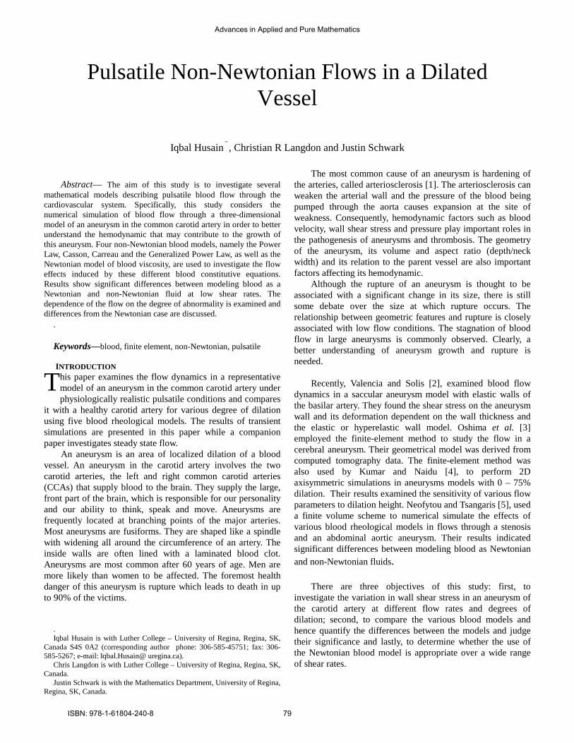
Keywords—blood, finite element, non-Newtonian, pulsatile INTRODUCTION

Abstract— The aim of this study is to investigate several

mathematical models describing pulsatile blood flow through the cardiovascular system. Specifically, this study considers the numerical simulation of blood flow through a three-dimensional model of an aneurysm in the common carotid artery in order to better understand the hemodynamic that may contribute to the growth of this aneurysm. Four non-Newtonian blood models, namely the Power Law, Casson, Carreau and the Generalized Power Law, as well as the Newtonian model of blood viscosity, are used to investigate the flow effects induced by these different blood constitutive equations. Results show significant differences between modeling blood as a Newtonian and non-Newtonian fluid at low shear rates. The dependence of the flow on the degree of abnormality is examined and differences from the Newtonian case are discussed.

.

his paper examines the flow dynamics in a representative model of an aneurysm in the common carotid artery under physiologically realistic pulsatile conditions and compares

it with a healthy carotid artery for various degree of dilation using five blood rheological models. The results of transient simulations are presented in this paper while a companion paper investigates steady state flow.

An aneurysm is an area of localized dilation of a blood vessel. An aneurysm in the carotid artery involves the two carotid arteries, the left and right common carotid arteries (CCAs) that supply blood to the brain. They supply the large, front part of the brain, which is responsible for our personality and our ability to think, speak and move. Aneurysms are frequently located at branching points of the major arteries. Most aneurysms are fusiforms. They are shaped like a spindle with widening all around the circumference of an artery. The inside walls are often lined with a laminated blood clot. Aneurysms are most common after 60 years of age. Men are more likely than women to be affected. The foremost health danger of this aneurysm is rupture which leads to death in up to 90% of the victims.

. Iqbal Husain is with Luther College – University of Regina, Regina, SK,

Canada S4S 0A2 (corresponding author phone: 306-585-45751; fax: 306-585-5267; e-mail: Iqbal.Husain@ uregina.ca).

Chris Langdon is with Luther College – University of Regina, Regina, SK, Canada.

Justin Schwark is with the Mathematics Department, University of Regina, Regina, SK, Canada.

The most common cause of an aneurysm is hardening of the arteries, called arteriosclerosis [1]. The arteriosclerosis can weaken the arterial wall and the pressure of the blood being pumped through the aorta causes expansion at the site of weakness. Consequently, hemodynamic factors such as blood velocity, wall shear stress and pressure play important roles in the pathogenesis of aneurysms and thrombosis. The geometry of the aneurysm, its volume and aspect ratio (depth/neck width) and its relation to the parent vessel are also important factors affecting its hemodynamic.

Although the rupture of an aneurysm is thought to be associated with a significant change in its size, there is still some debate over the size at which rupture occurs. The relationship between geometric features and rupture is closely associated with low flow conditions. The stagnation of blood flow in large aneurysms is commonly observed. Clearly, a better understanding of aneurysm growth and rupture is needed.

Recently, Valencia and Solis [2], examined blood flow

dynamics in a saccular aneurysm model with elastic walls of the basilar artery. They found the shear stress on the aneurysm wall and its deformation dependent on the wall thickness and the elastic or hyperelastic wall model. Oshima et al. [3] employed the finite-element method to study the flow in a cerebral aneurysm. Their geometrical model was derived from computed tomography data. The finite-element method was also used by Kumar and Naidu [4], to perform 2D axisymmetric simulations in aneurysms models with 0 – 75% dilation. Their results examined the sensitivity of various flow parameters to dilation height. Neofytou and Tsangaris [5], used a finite volume scheme to numerical simulate the effects of various blood rheological models in flows through a stenosis and an abdominal aortic aneurysm. Their results indicated significant differences between modeling blood as Newtonian and non-Newtonian fluids.

There are three objectives of this study: first, to

investigate the variation in wall shear stress in an aneurysm of the carotid artery at different flow rates and degrees of dilation; second, to compare the various blood models and hence quantify the differences between the models and judge their significance and lastly, to determine whether the use of the Newtonian blood model is appropriate over a wide range of shear rates.

Pulsatile Non-Newtonian Flows in a Dilated Vessel

Iqbal Husain*, Christian R Langdon and Justin Schwark

T


ISBN: 978-1-61804-240-8 79

2 MATHEMATICAL MODELLING

2.1 Governing equations We assumed the blood flow to be laminar and

incompressible and therefore the governing Navier-Stokes equations for such flows are given by

0=⋅∇ V (1)

pVVtV

∇−−∇=

∇+

∂∂ τρ ..

(2)

where V is the three-dimensional velocity vector, p pressure, ρ density and τ the shear stress term.

We considered four different non-Newtonian blood flow models and compared the results obtained with that from the simple Newtonian model in this study. The effects of these models on the flow field and the wall shear stress in the vicinity of the aneurysm are examined. These models are given below [6].

Blood Models

1. Newtonian model

00345.0=µ sPa ⋅ (3) 2. Power Law Model

10 )( −= nγµµ

(4) where =0.01467 and . 3. Casson Model

γ

γητµ

2][ +=

y

(5) where and = with = 0.0012 Pa·s and . 4. Carreau Model

( ) ( )[ ] 2/)1(20 1

−

∞∞ +−+=n

γλµµµµ

(6) where Pa·s, Pa·s,

s and . 5. Generalized Power Law Model

1−= nγλµ

(7)

where

,exp1exp)(

−

+−∆+= ∞ γ

γµµγλ

ba

−

+−∆−= ∞ γ

γγ

dc

nnn exp1exp)(

and .

These models have been created by various researchers Walburn and Schneck [7], Cho and Kensey [8], Fung [9], Ballyk et al. [10]and Johnston et al. [11], by fitting the input parameters in these models to experimental data for blood viscosity measured at certain shear rates. 2.2 Geometry

The diameters of the left and right common carotid artery

show a significant amount of variation. A study of 17 healthy subjects [12] produced diameters in the range of 0.52 to 0.75 cm with an average diameter of 0.64 cm. In this study, two different model of the abdominal aortic aneurysm are used to investigate blood flow in the initial stages of its development. The carotid artery before and after the dilation is idealized as a straight rigid tube without any branching arteries.

The flow geometry then consists of straight rigid tube of diameter d and is divided into three regions, the inlet, the dilation and the outlet region. The lengths of these regions are 4d, 4d and 18d, respectively. The radius of the undeformed inlet and outlet is . Two different values of the diameter were used to model the carotid artery, namely,

cm and cm. The radius of the diseased region [12] is given by

( ) ( ) ( ) bxxbaba

abaarr ≤≤

−−

++

+−+= 02

22

22 2

2222

0 (8)

where x is the distance from the start of the aneurysm, a is the degree of dilation, and b is the overall length of the diseased area as shown in Figure 1. Each model had an aspect ratio

which is typical of fusiform aneurysms.

Fig. 1. Aneurysm Geometry Three different degrees of dilation, 25%, 40% and 55% were used in this study.


ISBN: 978-1-61804-240-8 80

2.3 Assumptions and boundary conditions

We assume the arterial walls to be rigid and apply the no-

slip condition at the walls. At the outlet, stress-free conditions are applied and the pressure is set to zero. Symmetry is assumed at the centerline. Finally, the velocity profile at the inlet is regarded to be that of fully developed flow in a straight tube and is given by

0

2

0

01 rrrruu ≤≤

−= (9)

where u is the velocity component in the −x direction and is the centerline velocity specified at the inlet.

Fig. 2. Physiological flow waveform in the carotid artery used to drive the inlet velocity boundary condition as a function of time.

In transient flow, the pulsatile flow prescribed at the inlet of the artery is given by a time varying forcing function given in Figure 2. This physiological profile was obtained by averaging the pulsed Doppler spectra data collected from the left and right common carotid arteries of 17 normal volunteers [12]. The data was acquired over approximately 50 cardiac cycles and analyzed in both the time and frequency domains to determine the average properties and variability of human carotid waveform. In this study, this forcing function was scaled to yield a maximum inflow velocity of with a heart rate of approximately 60 beats per minute.

2.4 Solution methodology

The governing equations are highly nonlinear and are solved numerically using techniques of computational fluid dynamics. In this study, these equations are solved using the finite element method as implemented by COMSOL (COMSOL Inc., Los Angeles, CA). The flow geometry for the aneurysm was first created using Matlab. Then a finite element mesh was placed on this geometry. Briefly, an inlet plane of the artery is meshed in 2D using triangles and this mesh is extruded along the centerline of the artery to create a 3D mesh consisting of hexadrel elements. The mesh used for all computations consisted of 17,696 elements and 27,132 nodes for the aneurysm.

Grid independence was determined by performing additional simulations using a greater number of nodes. A mesh size of 107, 350 nodes for the aneurysm was used and the results obtained differed from those on the original mesh by less than 1%.

3. RESULTS AND DISCUSSION

Pulsatile inflow simulations were performed using all five models given above. As stated, three different degrees of dilation of the aneurysm were examined namely 25%, 40% and 55%. Several flow rates )(u were used in these simulations, from 0.04 m/sec to 0.22 m/sec, corresponding to the lower range of the average maximum systolic velocity of 1.08 m/sec in the common carotid artery as reported in [12].

A comparison of the streamlines patterns from various models in pulsatile flow simulation shows that the flow follows the contour of the wall (attached flow) throughout the aneurysm during the early systolic phase. During late systole, a vortex begins to form at the proximal end of the aneurysm. By the late diastolic stage, the flow becomes vortex dominated with the vortex filling the entire aneurysm. This flow pattern is similar in larger aneurysm except that the vortex strength and the translational speed increases. There exists minor differences in the recirculation regions shown by each model and these differences become more prominent at 55% dilation and higher flow rates, specifically the growth of the recirculation region and the vortex length. The Newtonian model shows the largest recirculation region and the Power law model, the smallest.

Fig. 3. Pressure difference distribution as a function of flow rate. The distribution of maximum pressure with the flow rate

is shown in Figure 3. This figure shows that all of the non-Newtonian models considered here produce a lower pressure difference than the Newtonian model at low flow rates.


ISBN: 978-1-61804-240-8 81

Specifically, the lowest pressure drop is induced by the Generalized Power Law model. At higher flow rates, greater than 0.16 m/s, the Generalized Power Law model comes in close agreement with the Newtonian model whilst the Careau model begins to deviate, giving pressure differences that are significantly less than the Newtonian fluid. It is not clear why this is the case and further study is required to explain this behaviour. Also, at flow rates greater than 0.18 m/s, the Power Law model begins to breakdown, producing pressure differences significantly higher than the Newtonian model. The other non-Newtonian models show good agreement in pressure differences with the Newtonian case for various degrees of severity and as the flow rate increases. This result agrees well with that of [5] in the transient non-pulsatile case.

Fig. 4. Wall shear stress distribution for various degrees of dilation.

Fig. 5. Wall shear stress vs shear rate. The distribution of the wall shear stress (WSS) is one of

the most important hemodynamic parameter due to its direct relevance in artherosclerosis formation. The distribution of wall shear stress with the size of the aneurysm for the 0.64 cm diameter artery is shown in Figure 4. It is evident that WSS increases with increasing dilation. All of the non-Newtonian models give values that are higher than the Newtonian case for various flow rates, especially, the Power Law model. At all degrees of dilations, the WSS values predicted by this model are significantly higher than that of the Newtonian model. Figure 5 displays the distribution of maximum WSS with shear rate. Again, WSS increases with increasing shear rate with the Power Law model deviating significantly from the rest at higher shear rates. The Casson and the Carreau models produce higher WSS values compared to the Newtonian model at high shear rates but are in good agreement with the Newtonian values at low shear rates. The Generalized Power Law model compares very well with the Newtonian model at both high and low shear rates.


ISBN: 978-1-61804-240-8 82

Fig. 6. Wall shear stress distribution for an artery with a 55% aneurysm using the generalized power law.

Fig. 7. Shear rate distribution in an artery containing a 55% aneurysm. Figure 6 show the distributions of shear stress for a 55%

aneurysm obtained from the Generalized Power Law at various times in a cardiac cycle. As can be seen, the shear stress drops abruptly as the flow enters the aneurysm. The magnitude of this drop increases with higher flow rates. This is followed by a sharp rise at the end of the aneurysm. Further downstream, the WSS rapidly regains its undisturbed value. The maximum wall shear stress occurs in the middle of the cycle corresponding to the maximum inflow velocity. The distribution of shear rates in a 55% dilated artery is shown in Figure 7. The high shear rates are confined to the small areas at the entrance and exit to the aneurysm and immediately downstream.

The maximum and minimum WSS values are in good agreement for the Generalized Power Law and the Newtonian models. The Power Law model gives a much lower value because it exhibits a lower viscosity at the entrance and exit of the aneurysm where the shear stress is high. As the flow rate increases, these WSS differences from the first two models become less prominent indicating insignificant differences in model behaviour at high shear rates.

Similar result are obtained when the diameter of the common carotid artery is assumed to be as large as 2.0 cm. The maximum wall shear stress and shear rates values are lower when compared to the 0.64 cm diameter artery but the differences in model behaviour are analogous.

It is evident from these results that the Power Law model tends to break down at higher shear rates in that it reduces the viscosity of the blood to levels below the Newtonian level which theoretically is not possible. This is clearly evident in the 55 % dilated model. The pressure difference predicted by this model is less than the Newtonian model, indicating a lower than Newtonian viscosity. This model also produces very low wall shear stress levels, dropping below Newtonian levels at fairly low shear rates, for example at the medium flow rate at 55% dilation, the WSS levels are less than Newtonian levels. This Power Law model is relatively easy to use but predict decreasing viscosity at higher strain, contrary to the generally accepted observation that blood behaves as a Newtonian fluid for strains above .

At low shear rates the Casson model shows near Newtonian behavior. As the shear rate increases, this model begins deviating from the Newtonian case by producing higher WSS. This model takes the haematocrit factor H (the volume fraction of red blood cells in whole blood) into account, with the parameters given (obtained from data fitting) suggesting a value of H of 37%. However, it is reported that this yields a limiting viscosity at high shear slightly above the usual Newtonian value. The results obtained here suggest the same with WSS values above the Newtonian values at very high shear rates. This model appears to breakdown in the aneurysm at high shear rates, but is accurate at low shear rates.

The Carreau model generally produces values that are in close agreement with that of the Newtonian model at shear rates well above 1100 −s . Our results do not indicate this to be the case. Both the WSS and the pressure difference deviate significantly from the Newtonian values at shear rates in excess of 11000 −s . This model by design reverts to Newtonian numbers as shear rates approach infinity. The basis for this model is the constant Newtonian viscosity, modified to non-Newtonian such that the modification tends to zero as the limit of the shear rate goes to infinity.

Finally, the Generalized Power Law model gave results

that are in closest agreement with the Newtonian values at mid-range and high shear rates. At low shear rates, this model gives values that are close to that of the Power Law and the Carreau models. While the Power Law model breaks down at high shear, our results show a close agreement between the Generalized Power Law and the Newtonian models even at


ISBN: 978-1-61804-240-8 83

high shear rates as shown in Figure 5. The Generalized Power Law model is widely accepted as a general model for non-Newtonian blood viscosity. It includes the Power Law model at low shear rate and the Newtonian model at mid-range and high shear rates. There is also good agreement between the Generalized Power Law and the Carreau model for low shear rates.

4. CONCLUSIONS

A study of the effects of modeling blood flow through an aneurysm using five different blood rheological models is presented. The flow field and wall shear stress distributions produced by each model are investigated for various flow rates and degrees of abnormality. In a specific dilated artery with a particular inlet velocity, the pattern of the WSS was found to be the same for all models studied. The only difference was in the magnitude of the WSS predicted by each model. These differences were significant at low shear rates and, in the case of the Power Law, the Carreau and the Casson model, at high shear rates. At mid-range to high shear rates, the Generalized Power Law and the Newtonian models produced almost identical results. The differences in magnitude of the WSS can be explained by the differences in the models themselves as discussed above. The results show that there are significant differences between simulating blood as a Newtonian or non- Newtonian fluid at low shear rates. In particular, the Power Law model overestimates WSS at low shear rates and underestimates it at high shear. The Newtonian model under estimates WSS at low shear while the Generalized Power Law models provide a better approximation of WSS at low shear rates. The distribution of shear rates in the dilated artery in Figure 7 shows a small region in the vicinity of the aneurysm where the shear rate is high. The shear rate in the rest of the artery is relatively low, indicating that non-Newtonian behavior is important. However, these simulations correspond to a heart rate of only 60 beats per minute and low inlet velocities (maximum of 0.225 m/s for the dilated artery). If the heart rate were increased to 100 beats per minute and/or the inlet velocities increased, the region (and periods in a cardiac cycle) over which the non-Newtonian behavior was important would decrease.

0 2 4 6 8 10 12

Generalized Power Law

Power Law

Careau

Casson

Newtonian

Mo

del

Wall Shear Stress (N/m^2)

Fig. 8. Wall shear stress chart. In a healthy left or right common carotid artery, the average maximum systolic velocity is 1.08 m/s [13]. In modeling the aneurysm, our simulation could only reach velocities as high as 0.375 m/s. We were successful in simulating a healthy artery at the maximum velocity and the results obtained from the various models are shown in Figure 8. The WSS values from all models are in good agreement except for the Power Law model. As in the dilated artery, the Generalized Power Law model gave the closest value to that of the Newtonian model. In conclusion, in terms of the wall shear stress distribution, we found that the Newtonian model is a good approximation in regions of mid-range to high shear but the Generalized Power Law model provides a better approximation of wall shear stress at low shear. Whether the fact that the Newtonian model underestimates the WSS in regions of low shear is biologically significant is open to debate. A prudent approach would be to use the Generalized Power Law model since it predicts WSS better than the Newtonian model for low inlet velocities and regions of low shear and is effectively Newtonian at midrange to high shear. These conclusions are presented under the assumption that the arterial walls are rigid and zero pressure is assumed at the outlet. A more realistic simulation would include elastic walls and incorporate the effects of upstream and downstream parts of the circulatory system into the boundary conditions. Simulations incorporating elastic walls are currently in progress. References [1] D.N. Ku, Blood flow in arteries, Annual Review of

Fluid Mechanics (1997), Vol. 29 pp. 399-434.


ISBN: 978-1-61804-240-8 84

[2] A. Valencia, F. Solis (2006), Blood flow dynamics and arterial wall interaction in a saccular aneurysm model of the basilar artery, Comp. Struc., Vol. 84 , pp.1326-1337.

[3] Oshima et al. (2001), Finite element simulation of

blood flow in the cerebral artery, Comp. Meth. App. Mech. Eng., Vol. 191, pp. 661 – 671.

[4] B.V. Rathish Kumar and K.B. Naidu (1996),

Hemodynamics in aneurysm, Comp. Biomed. Res., Vol. 2 , pp. 119 – 139.

[5] P. Neofytou, S. Tsangaris (2005), Flow effects of blood

constitutive equations in 3D models of vascular anomalies, Int. J. Numer. Meth. Fluids, Vol. 51, pp. 489-510.

[6] T.J. Pedley (1980), The fluid mechanics of large blood

vessels, Cambridge University Press Cambridge. [7] F.J. Walburn, D.J. Schneck (1976), A constitutive

equation for whole human blood, Biorheology Vol.13, pp. 201- 210.

[8] Y.I. Cho, K.R. Kensey (1991), Effects of the non-

Newtonian viscosity of blood on flows in a diseased arterial vessel, Part I: steady flows, Biorheology, Vol. 28, pp. 241-262.

[9] Y.C. Fung (1993), Biomechanics: Mechanical

properties of living tissue, 2nd Edition, Springer Berlin.. [10] P.D. Ballyk, D.A. Steinman, C.R. Ethier (1994),

Simulations of non-Newtonian blood flow in an end-to-end anastomosis, Biorheology, Vol. 31 (5), pp. 565-586.

[11] B.M. Johnston et al (2004)., Non-Newtonian blood

flow in human right coronary arteries: steady state simulations, J. Biomechanics, Vol. 37, pp. 709-720.

[12] D.W. Holdsworth et al. (1998), Characterization of

common carotid artery blood-flow waveforms in normal human subjects, Physiol. Meas., Vol. 20, pp. 219-240.


ISBN: 978-1-61804-240-8 85

Permutation codes: a branch and bound approachRoberto Montemanni, Janos Barta and Derek H. Smith

Abstract—This paper presents a new approach for retrievinglargest possible permutation codes. These have applications inerror correction for telecommunication purposes. The methodpresented is based on combinatorial optimization concepts suchas branch and bound techniques and incorporates new ad-hoc theoretical results. It is shown how the method can beapplied to obtain new results for subproblems. These results forsubproblems can be combined with other theoretical results toobtain new results for complete instances. It is shown how thenew improved upper bound M(7,5)≤ 124 can be obtained withsuch techniques.

Index Terms—Permutation codes; Branch and bound algo-rithms; Upper bounds.

I. INTRODUCTION

THIS paper considers the application of branch and boundtechniques to the construction of permutation codes. Per-

mutation codes (sometimes referred to as permutation array)have received considerable attention in the literature [1], [2],[3], [4], [5], [6], [7]. This has been motivated by an applicationto powerline communications when M-ary Frequency-ShiftKeying (FSK) modulation is used [3], [8], [9], [10], [11]. Inthis application permutations are used to ensure that poweroutput remains as constant as possible while combattingimpulsive noise permanent, narrow band noise from electricalequipment or magnetic fields, as well as the more commonwhite Gaussian noise.

A permutation code is a set of permutations in the symmet-ric group Sn of all permutations on n elements. The codewordsare the permutations and the code length is n. The error-correcting capability of a permutation code is related to theminimum Hamming distance of the code. The Hamming dis-tance δ between two codewords is the number of elements thatdiffer in the two permutations. Alternatively, two permutationsσ1 and σ2 are at distance δ if σ1σ

−12 has exactly n−δ fixed

points. The minimum distance d is then the minimum δ takenover all pairs of distinct permutations. Such a code is thendenoted an (n,d) permutation code.

Redundancy in an encoding is minimized if the number ofcodewords is as large as possible. Thus if M(n,d) denotesthe maximum number of codewords in an (n,d) permutationcode it is important to determine M(n,d), or if this is notpossible to find good lower and upper bounds. The mostcomplete contributions to lower bounds can be found is in [3],[12]. Recently, some improvements based on similar searchtechniques have been presented in [13], while in [14] a study

R. Montemanni and J. Barta are with the Dalle Molle Institute forArtificial Intelligence, University of Applied Sciences of Southern Switzer-land, Galleria 2, 6928 Manno, Switzerland. Emails: roberto.montemanni,[email protected].

D.H. Smith is with the Division of Mathematics and Statistics, Uni-versity of South Wales, Pontypridd, CF37 1DL, Wales, UK. Email:[email protected].

Γ = [012345], [021453], [034512],[045231], [102534], [130425],[153240], [205143], [243015],[251304], [310254], [324105],[341520], [425310], [432051],[450132], [504321], [513402].

Fig. 1. An optimal (6, 5) code.

on the structure of optimal codes has been presented. Resultson a similar problem using a metric different from the onetreated in this paper can be found in [15].

II. PROBLEM DESCRIPTION

A permutation of the n-tuple x0 = [0,1, ...,n−1] ∈ Nn is acodeword of length n and the set of all codewords of lengthn is denoted by Ωn. From an algebraic point of view the setΩn is the single orbit of the symmetric group of permutationsSn , i.e.

Ωn = x ∈ Nn|x = gx0, g ∈Sn

Any subset Γ of Ωn is a permutation code of length n. Themain problem can now be stated as:

Definition 1. Given a code length n and a Hamming distanced, the maximum permutation code problem (MPCP) consistsof the determination of a code Γ⊆Ωn with minimum distanced and the maximum possible number of codewords.

Example 1. The problem (6,5) is to determine a maximalcode of length n= 6 with minimum distance d = 5. As reportedin [14], [3], [12] the optimal solution of this problem isM(6,5) = 18. One of the many possible optimal (6,5) codesis shown in Figure 1.

III. A BRANCH AND BOUND ALGORITHM

Branch and bound approaches work by building a search-tree that covers all possible assignments of permutations tosolutions, but with most of the branches of the tree pruned byinferring information from lower and upper bounds. The mainelements of the algorithm proposed here are described in thissection.

A. Structure of the search-tree node

From now on, the set of nodes of the search tree will bedenoted S, and the subtree of the search-tree rooted at node twill be denoted as SubT (t). Each node t of the search-tree isthen identified by the following elements:


ISBN: 978-1-61804-240-8 86

• in(t): a list of permutations that are forced in the solutionsassociated with the search-tree nodes of SubT (t);

• f eas(t): a list of permutations that are feasible accordingto the list of forced permutations in(t), and to reductionrules (see Section III-D2);

• lb(t): a lower bound for the number of permutations in theoptimal solutions associated with the search-tree nodes inSubT (t). The calculation of the lower bound is describedin Section III-F.

• ub(t): an upper bound for the number of permutationsin the optimal solutions associated with the search-treenodes in SubT (t). The calculation of the upper bound isdescribed in Section III-E.

From these four items all the information required by domi-nance rules and pruning can be derived.

B. Initialization and branching strategy

Initial lower and upper bounds BestLB and BestUB areprovided as input to the algorithm (they can be 0 and +∞,respectively). These initial values will be updated during theexecution of the algorithm in case improved values are ob-tained. A permutation p is selected and the root r of the search-tree is the node initialized with in(r) = p, lb(r) = BestLB,ub(r) = BestUB and f eas(r) = i∈Ωn : δ (i, p)≥ d. Initially,r will be the only node contained in S (S := r), the set ofthe nodes to be examined, referred to as open nodes in theremainder of the paper. Due to the symmetry of the problem,the first permutation included in in(r) can be chosen arbitrarily.The set of closed nodes C is initialized as empty (C := /0). Thisset will contain nodes already examined by the algorithm, andwill be used by pruning and reduction techniques described inSection III-D.

At each iteration of the branch and bound algorithm, anopen node t from the set S is expanded (see Section III-Cfor more details about the strategy used to select node t, andthe rationale behind it), which means that node t is expandedby decomposing it into the associated subproblems. One newsearch-tree node tp is created for each permutation p of f eas(t)in such a way that in(tp)= in(t)∪p and the new set f eas(tp)is determined, also taking into account the reduction andpruning rules described in Section III-D. Sets S and C arefinally updated: S = S\t, C = C∪t. For each new nodetp the values of lb(tp) and ub(tp) are calculated, as describedin Sections III-F and III-E respectively. In the case that thepruning test is positive (see Section III-D) the new node tp ispruned and C :=C∪tp, otherwise the set S of open node isincremented: S := S∪tp.

In case mint∈S ub(t) ≤ BestUB, the global upper boundof the residual open problems has been improved, and theupdating BestUB := mint∈S ub(t) can take place. Also thevalue of BestLB can be updated in case a new incumbentheuristic solution is found (in general BestLB :=maxt∈S lb(t)).All the open nodes u of the search tree are examined andpruned in case ub(u) ≤ BestLB, since no improving solutioncan exist in the search-tree node rooted in u. In such a caseS := S\u and S := S∪u.

The branch and bound algorithm stops when the set Sis empty (all the search-tree nodes have been processed orlabelled as dominated).

C. Selection of the node to expand

Nodes are expanded in the same order they have previouslybeen created. This strategy allows the best exploitation of thereduction and pruning rules described in Section III-D.

D. Reduction and pruning rules

This section discusses some rules useful to prune dominatedsearch-tree nodes and to reduce the size of f eas(t) whilegenerating a new search-tree node t. These results are basedon the concept of isomorphism for graphs [16].

1) Pruning rule: Two graphs G and H are said to beisomorphic if a bijection between the vertex sets of G andH f : V (G)→ V (H) exists, such that any two vertices u andv of G are adjacent in G if and only if f (u) and f (v) areadjacent in H.

Definition 2. The graph induced by search-tree node t isdefined as GI

t = V It ,E

It , with V I

t = V\in(t) and EIt =

i, j|i, j ∈V It ,δ (i, j)≥ d)

.

Remark 1. The graph induced by search-tree node t isconsidered instead of the subgraph of G with vertices setf eas(t) because f eas(t) might have already have benefitedfrom reduction rules in previous iterations, and thereforeisomorphisms could be more difficult to identify.

Definition 3. If the graph GIt induced by search-tree node t

is isomorphic to the graph GIu induced by another search-tree

node u, it will be said (for short) that node t is isomorphic tonode u and written t ∼= u.

The following result allows one of two isomorphic nodesto be pruned from the branch and bound tree.

Theorem 1. If a new search-tree node t is such that t ∼= u withu ∈ S∪C, |in(t)|= |in(u)| then the node t can be classified asdominated and moved to set C (S = S\t and C =C∪t).

Proof: The search-tree subtree associated with node twill provide an optimal solution with the same number ofpermutations of that of node u, that has been already expanded(u ∈C), or is scheduled to be expanded (u ∈ S).

2) Reduction rule: During the branching of a search-tree node t, all potential new search-tree nodes obtained byexpanding the set f eas(t) with each possible permutation willbe considered.

Proposition 1. While creating a new search-tree node uobtained by adding pu ∈ f eas(t) into in(u), permutationpk ∈ f eas(u), with k ∼= v, v ∈ S∪C, |in(k)| = |in(v)| (nodesalready expanded at the same level) can be taken out off eas(u): f eas(u) = f eas(u)\pk

Proof: The best possible solution including permutationspk and the permutations of in(u) is equivalent to that ofthe problem v, that has been already expanded (u ∈ C), oris scheduled to be expanded (u ∈ S). Therefore all solutions


ISBN: 978-1-61804-240-8 87

including permutation pk are not of interest while solving theproblem associated with f eas(u).

Remark 2. When applying the reduction rule described inProposition 1 it is necessary to expand search-tree nodesaccording to the basic strategy described in Section III-C, inorder to avoid situations where the permutations isomorphic tothat associated with node ui are taken out from f eas(vi) as aresult of Proposition 1 at level i of the search-tree, but then thepermutations associated with a descendant v j of vi are takenout of a descendant u j of ui at a level j, with j > i, of thetree. Such a situation would clearly lead to infeasible solutionssince some regions of the search space are left unvisited bythe search-tree.

In the implementation described here the routines of Nauty2.5 described in [17] are used to identify graph isomorphisms.

E. Upper bound

The set of codewords Ωn can be split into n subsetsW0, ...,Wn−1, in such a way that for a fixed value k ∈ 0, ...,n−1 the subset Wi is defined as Wi = x ∈ Ωn|x(k) = i. Inother words, the subset Wi contains all codewords with the k-thcomponent having the value i. Since the partition is obtainedby fixing the value of one component of the codewords, it isclear that the sets Wi are isomorphic to Ωn−1. Furthermore,as the sets Wi form a partition of Ωn it is well-known that anupper bound of M(n,d) can be obtained by adding the upperbounds on the subsets Wi:

Theorem 2 (Deza and Vanstone [18]).

M(n,d)≤ n ·M(n−1,d) (1)

The partitioning procedure described in Theorem 2 can becarried out on any subset of Ωn. At each search-tree nodet the algorithm generates a partition T0, ...,Tn−1 of the setf eas(t), such that Ti = x ∈ f eas(t)|x(k) = i and a partitionQ0, ...,Qn−1 of the set in(t), such that Qi = x ∈ in(t)|x(k) =i. For each subset Ti an upper bound UB(Ti) is calculatedusing the Maximum Clique Problem (MCP) solver proposedin [19] (see also [20]), which is run for 10 seconds on everysubproblem. The choice of this solver is motivated by itsability of proving optimality extremely fast on small/mediumproblems. From preliminary experiments the solver describedin [19] is significantly faster than the one presented in [21](see Section III-F) on the instances treated.

The new upper bound for the search tree node t can beexpressed as follows.

Proposition 2.n−1

∑i=0|Qi|+minUB(Ti);M(n−1,d)−|Qi| (2)

is a valid upper bound for the search-subtree rooted at thesearch-tree node t.

Proof: In case it can be shown that in a partition Tiof f eas(t) the maximum clique has size smaller than M(n−1,d)−|Qi| a tighter upper bound for that partition is available.

Combining the n partitions together, gives the global upperbound provided by (2).

Remark 3. The result of Proposition 2 can be seen as arefinement of a previous result originally presented in [14].

Remark 4. As the index k of the fixed component in thecodewords can be varied, there are n different partitions thatcan be generated. The algorithm computes for each partitionan upper bound and finally chooses the lowest one.

F. Lower bounds

The methods used to provide lower bounds for the optimalsolution cost of the problem associated with the search-treenode t are based on MCP algorithms [21]. In detail, whenexamining node t, it is possible to associate a graph Gt =Vt ,Et such that the set of vertices Vt = f eas(t) (where eachvertex is associated with a permutation) and the set of edgesEt = i, j|i, j ∈Vt ,δ (i, j)≥ d). Notice that this graph is asubgraph of that induced by node t (see Section III-D). Theproblem is then equivalent to solving a MCP on graph Gt .This transformation usually has the side-effect that possiblestructure and information coming from group theory (and thepossibility to exploit these) is lost. On the other hand, thevery efficient methods developed for the MCP over the yearscan be used directly. In the remainder of this section it will beshown how to modify a general-purpose method to the currentcontext, in order to insert permutation codes related conceptsinto its logic.

The original MCP method works as follows, according tothe description provided in [21]. The algorithm considers thevertices of Vt in a given order v1,v2, ...,v|Vt |. Initially, themethod finds the largest clique C1 that contains the vertex v1.Then it finds C2, the largest clique in Gt\v1 that containsv2 and so on. Applying heuristics and pruning techniques,the search space can, however, be reduced dramatically. Thenotion of the depth is crucial for the algorithm. Supposevertex v1 is under investigation. At depth 2, all verticesadjacent to v1 are considered. At depth 3, all vertices (that arealready in depth 2) adjacent to the first vertex in depth 2 areconsidered and so on. When there are no more vertices left ata certain depth, a clique has been identified, and backtrackingis activated. Pruning rules based on the number of vertices leftat each level are triggered to have early backtracking. Theserules are very quick to check but very effective. When theentire search-tree created by the method has been visited (ordeclared dominated) the computation is stopped and the largestclique has been retrieved.

Some context-dependent modifications of the general algo-rithm previously described were implemented. The modifica-tions to the original method are introduced to anticipate thepruning in the branch and bound framework running internallyin the MCP algorithm. In detail, during the execution a 2-dimension array PosVal is kept in memory, defined as follows.

Definition 4. PosVal[i][ j] contains at any time during theexecution of the MCP algorithm [21] the current number ofpermutations with value j in position i that are still feasible


ISBN: 978-1-61804-240-8 88

according to the partial assignment under investigation, or arepart of such a partial assignment.

Notice that the structure is dynamically updated during theexecution of the algorithm, depending on the partial solutioncurrently under investigation. The pruning is based on thefollowing theoretical results.

Proposition 3. Whenn

∑j=1

minM(n−1,d),PosVal[i][ j] ≤ BestLB (3)

for some i,1 ≤ i ≤ n the partial solution under investigationwill not lead to any improving result, it can be pruned and itis possible to backtrack.

Proof: It is known ([18]) that if a position i of the code-words of a code (n,d) is fixed to a value j then there cannotbe more that M(n− 1,d) permutations with this property.This is valid for each value of i and j. During the executionof the MCP algorithm PosVal[i][ j] can become smaller thanM(n−1,d) for some i or j. In such a case the best upper boundfor the corresponding subproblem is no longer M(n− 1,d),and the global upper bound is updated according to (3) bysumming over all possible values j for position i. Whenthe global upper bound is not greater than the cost of thebest solution currently available (BestLB) there is no hope offinding an incumbent improved solution, and backtracking canbe activated.

Proposition 4. Whenn

∑i=1

minM(n−1,d),PosVal[i][ j] ≤ BestLB

for some j,1≤ j ≤ n the partial solution under investigationwill not lead to any improving result, it can be pruned and itis possible to backtrack.

Proof: The proof is based on the same principles of thatof Proposition 3 but now the sum is over all possible positionsi for value j (by columns of PosVal instead of by rows).

Remark 5. The results of Propositions 3 and 4 can be seenas the adaptation of the upper bound of Proposition 2 to thecontext of the MCP algorithm, where it is preferable to havea less precise but much faster upper bound.

In the context of the current permutation codes algorithm,the main target is to have the MCP algorithm complete thecomputation in order to prove optimality for the problem underinvestigation in the given time available (see Section IV). Forthis reason, to have pruning as early as possible, at eachiteration one of the permutations with value j in position iis expanded such that

PosVal[i][ j] = min1≤k≤n,1≤l≤n

PosVal[k][l] (4)

The strategy described in (4) allows the anticipation of theapplication of Propositions 3 and 4 as much as possible.Different strategies might however be used in order to makeit more likely to have heuristic solutions instead of earlybacktracking, if the algorithm is used in a different perspective.

The modified version of the algorithm originally proposedin [21] described previously is executed each time a new non-dominated search-tree node (of the external branch and boundmethod) is generated, and it is run for a maximum of 720seconds.

IV. EXPERIMENTAL RESULTS

The approach discussed in Section III can be applied tosubproblems to prevent ths size of the search tree increasingtoo much for large instances. Results on subproblems canthen be propagated to full problems in order to obtain newtheoretical results, as will be shown later in this section. Allthe experiments presented have been carried out on a computerequipped with a 2.3GHz AMD Quad Opteron processor (onlyone core has been used at a time), while the algorithm hasbeen coded in ANSI C.

In the study presented here two subproblems of (7,5) areconsidered, where a position of the permutations is restrictedto values from a given set F ⊂ 0,1, ...,n− 1. The largestpossible code fulfilling the requirements with all permutationswith the given position strictly from F is sought. Notice thateither the position fixed or the values of F are not importantdue to the symmetry of the problem. The cardinality of F is theonly important factor. Therefore subproblems can be definedas follows.

Definition 5. Refer to the problem (n,d)||F | as the subproblemof (n,d) where a position of the code is restricted to valuesfrom set F.

Such a problem with |F | = 1 is equivalent to the problem(6,5) since the largest possible set with a common symbolin the first position is sought. According to [18] this amountsto looking for the largest possible code of length n−1. Moreinteresting are the cases when 2 ≤ |F | ≤ n− 1. Notice thatfor these problems a trivial upper bound, coming from thegeneralization of that described in (1), is the following one:

M(n,d)||F | ≤ |F | ·M(n−1,d) (5)

For |F |= 2 equation (5) returns an upper bound of 36. Thebranch and bound described in Section III has been able toretrieve a solution with 36 permutations, matching the upperbound. This result is not as obvious as it could appear, sincetraditional methods based on maximum clique solvers (e.g.[19], [21]) are not able to retrieve such a solution in a weekof computation, while the method described here was able toclose the problem in 15 382 seconds. The optimal solutionretrieved is presented in Figure 2. It might turn out to beuseful for future studies by other researcher, since inspectingsuch a solution might bring new insights about the generalcharacteristics of solutions.

For |F |= 3 the branch and bound described in Section IIIhas been used to obtain a new upper bound, which improvesthe one given by (5). The algorithm itself is not able to findsignificantly large heuristic solutions (and consequently lowerbounds), but if it is run with a hypothetical initial lower boundof BestLB = 53, the algorithm is able to prove in 922 450seconds that no solution with 54 permutations exists, leadingto the following new result.


ISBN: 978-1-61804-240-8 89

Γ = [0123456], [0134562], [0162345],[0214635], [0236154], [0265413],[0342516], [0351642], [0364251],[0415326], [0426531], [0452163],[0516243], [0521364], [0543621],[0631425], [0645132], [0653214],[1025634], [1043265], [1056423],[1203546], [1240653], [1254360],[1305462], [1326045], [1360524],[1432605], [1450236], [1463052],[1534026], [1546302], [1562430],[1602354], [1624503], [1635240].

Fig. 2. An optimal (7, 5)|2 code.

Proposition 5.M(7,5)|3 ≤ 53

The result of Proposition 5 has a remarkable implication: itallows us to improve the lower bound for the general problem(7,5).

Proposition 6.M(7,5)≤ 124

Proof: Partition the code in three parts, each part coveringsome possible values for a given position. The first and thesecond parts cover 3 possible distinct values each, while thethird part covers the remaining value. By combining the resultson subproblems the new global upper bound is obtained:M(7,5)≤M(7,5)|3 ·2+M(7,5)|1 ≤ 53 ·2+18 = 124

The result of Proposition 6 improves the previously bestknown upper bound of 126 that can be obtained with equation(5). It is interesting to mention that the best result reported inthe literature so far was 140 instead of 126 (see, for example,[12]).

The results previously presented show that a novel approachlike the one proposed has potential. Further refinement tothe current branch and bound method could lead to newimprovements.

V. CONCLUSIONS

A novel approach based on combinatorial optimization andbranch and bound has been proposed to attack permutationcodes. It is based on some ad-hoc new theoretical results thatmake the technique practical for real problems. Experimentalresults have been presented, aiming at clarifying the currentpotential of the method. New results on subproblems of per-mutation code instances have been described, and it has beenshown how such results can be used to derive new theoreticalresults (upper bounds in this case) for full permutation codeinstances.

The technique appears to be capable of further improve-ments to handle larger problem instances. New theoreticalresults could be used to speed up computation and to make

pruning even more effective. There is also a clear potentialfor such techniques to be adapted to other types of codes (e.g.binary codes). Such adaptions represent an important area forfuture work.

REFERENCES

[1] I.F. Blake, Permutation codes for discrete channels, IEEE Transactionson Informormation Theory 20(1) 138–140, 1974.

[2] M. Bogaerts, New upper bounds for the size of permutation codes via lin-ear programming, The Electronic Journal of Combinatorics 17(#R135),2010.

[3] W. Chu, C.J. Colbourn and P. Dukes, Constructions for permutationcodes in powerline communications, Designs, Codes and Cryptography32, 51–64, 2004.

[4] P. Dukes and N. Sawchuck, Bounds on permutation codes of distancefour, Journal of Algebraic Combinatorics 31 143–158, 2010.

[5] P. Frankl and M. Deza, On maximal numbers of permutations with givenmaximal or minimal distance, Journal of Combinatorial Theory SeriesA 22, 352–260, 1977.

[6] I. Janiszczak and R. Staszewski, An improved bound for permuta-tion arrays of length 10, http://www.iem.uni-due.de/preprints/IJRS.pdf(downloaded 17th March 2011).

[7] H. Tarnanen, Upper bounds on permutation codes via linear program-ming, European Journal of Combinatorics 20 101–114, 1999.

[8] C.J. Colbourn, T. Kløve and A.C.H. Ling, Permutation arrays forpowerline communication and mutually orthogonal latin squares, IEEETransactions on Information Theory 50, 1289–1291, 2004.

[9] A.J. Han Vinck, Coded modulation for power line communications,A.E.U. International Journal Electronics and Communications 54(1), 45–49, 2000.

[10] S. Huczynska, Powerline communications and the 36 officers problem,Philosophical Transactions of the Royal Socicety A. 364, 3199–3214,2006.

[11] N. Pavlidou, A.J. Han Vinck, J. Yazdani and B. Honary, Power line com-munications: state of the art and future trends, IEEE CommunicationsMagazine 41(4), 34–40, 2003.

[12] D.H. Smith and R. Montemanni, A new table of permutation codes,Design, Codes and Cryptography 63(2), 241–253, 2012.

[13] I. Janiszczak, W. Lempken, P.R.J. Ostergard and R. Staszewski, Permuta-tion codes invariant under isometries, Designs, Codes and Cryptography,to appear.

[14] J. Barta, R. Montemanni and D.H. Smith, A branch and bound ap-proach to permutation codes, Proceedings of the IEEE 2nd InternationalConference of Information and Communication Technology - ICOICT,187–192, 2014.

[15] D.H. Smith and R. Montemanni, Permutation codes with specifiedpacking radius, Design, Codes and Cryptography 69, 95–106, 2013.

[16] B.D. McKay, Practical graph isomorphism, Congressum Numerantium.30 45–87, 1981.

[17] B.D. McKay and A. Piperno, Practical graph isomorphism, II, Journalof Symbolic Computation 60 94–112, 2014.

[18] M. Deza and S.A. Vanstone, Bounds for permutation arrays, Journal ofStatistical Planning and Inference 2 197–209, 1978.

[19] P.R.J. Ostergard, A fast algorithm for the maximum clique problem,Discrete Applied Mathematics 120, 197–207, 2002.

[20] P.R.J. Ostergard, A new algorithm for the maximum-weight cliqueproblem, Nordic Journal of Computing 8(4), 424–436, 2001.

[21] R. Carraghan and P.M. Pardalos, An exact algorithm for the maximumclique problem, Operations Research Letters, 9 375–382, 1990.


ISBN: 978-1-61804-240-8 90

Unary operatorsJózsef Dombi

(Invited Paper)

Abstract—Modal operators play an important role in fuzzytheory, and in recent years researchers have devoted more efforton this topic. In our study, we will construct modal operators.We give a common form of all types of unary operators. Wewill characterise them using differential equations, Bayesianinference, and a functional equation. We will show that a specialclass of the kappa function is related to the sigmoid function, itand can be characterised by odds.

Keywords—negation, modalities, hedges, sharpness operator, Pli-ant system

I. INTRODUCTION

In logic theory, modal operators have a variety of applica-tions and even from a theoretical perspective they are inter-esting to study. Here, we will present different approaches forobtaining the form of the necessity and possibility operators.These have a simple parametrical form. By changing theparameter value, we get different modalities. Cintula et al[1] made a study on fuzzy logic with an additive involutivenegation operator. In Hájek’s paper [2], the basic logic (BL)was defined. In a recent paper [3], we can find a survey paperthat discusses the state-of-art of BL.

In standard modal systems, the basic modalities are callednecessity (denoted by ) and possibility (denoted by ♦).They satisfy basic properties such as their interdefinability vianegation p = ¬♦¬p, and distributivity of over conjunction(p ∧ q) = p ∧ q and distributivity of ♦ over disjunction♦(p ∧ q) = ♦p ∧ ♦q. Now consider a De Morgan operatorsystem augmented with unary operators that represent thedistributive modalities.

II. NEGATION

Definition 1: We say that η(x) is a negation ifη : [0, 1]→ [0, 1] satisfies the following conditions:

C1: η : [0, 1]→ [0, 1] is continuous (Continuity)C2: η(0) = 1, η(1) = 0 (Boundary conditions)C3: η(x) < η(y) for x > y (Monotonicity)C4: η(η(x)) = x (Involution)

From C1, C2 and C3, it follows that there exists a fix pointν∗ ∈ [0, 1] of the negation where

η(ν∗) = ν∗ (1)

So another possible characterisation of negation is when weassign a so-called decision value ν for a given ν0, i.e. a point

J. Dombi is with the Institute of Informatics, University of Szeged, Hungarye-mail: [email protected]

Manuscript received June 19, 2014; revised July 04, 2014.

(ν, ν0) can be specified such that the curve must intersect. Thistells us something about how strong the negation operator is.

η(ν) = ν0 (2)

If η(x) has a fix point ν∗, we use the notation ην∗(x) andif the decision value is ν, then we use the notation ην(x). Ifη(x) is employed without a suffix, then the parameter has noimportance in the proofs. Later on we will characterise thenegation operator in terms of the ν∗, ν0 and ν parameters.

For the strong negation operator case, two representationtheorems are known. Trillas [4] has shown that every involu-tive negation operator has the following form

η(x) = f−1(1− f(x)), (3)

where f : [0, 1] → [0, 1] is a continuous strictly increasing(or decreasing) function. This generator function correspondsto the nilpotent operators (nilpontent t-norms). For the strictlymonotonously increasing t-norms, another form of the negationoperator is given in [5]:

η(x) = f−1

(1

f(x)

),

where f : [0, 1] → [0,∞] is a continuous, increasing (ordecreasing) function and f is the generator function of thestrict monotone t-norm or t-conorm.

We can express these negation operators in terms of theirneutral values and we get a new form of the negation operator.

For the strict monotone operators,

ην∗(x) = f−1

(f2(ν∗)

f(x)

)(4)

The other form of the negation operator in terms of ν0, andν, and corresponding to (II), is

ην(x) = f−1

(f(ν0)

f(ν)

f(x)

)(5)

In the following we will use (4) and (5) to represent thenegation operator because here we are just considering strictmonotone operators and we sketch the shape of the negationfunction.

Definition 2: If ν1 < ν2, then ην1(x) is a stricter negationthan ην2(x).

Definition 3 (Drastic negation): We call η1(x) and η2(x) adrastic negation when

η1(x) =

1 if x 6= 10 if x = 1

η0(x) =

1 if x = 00 if x 6= 0


ISBN: 978-1-61804-240-8 91

Theorem 4: The negation operators

ην(x) = f−1

(f(ν0)

f(ν)

f(x)

),

ην∗(x) = f−1

(f2(ν∗)

f(x)

)have the following properties:

a. They are continuous.b. They are strictly monotonous decreasing.c. The correspondence principle is valid:

ην(0) = 1, ην(1) = 0, ην∗(0) = 1, ην∗(1) = 0

d) The involutive property is valid:

ην(ην(x)) = x, ην∗(ην∗(x)) = x.

e) The neutral value property holds:

ην(ν) = ν0, ην∗(ν∗) = ν∗.

Proof: Using the representation form of the negationoperator, this is trivial.

In fuzzy theory, we utilise two types of negation operator.These are

Yager: ηm(x) = m√

1− xm (6)

andHamacher, Sugeno: ηa(x) =

1− x1 + ax

(7)

We can express the parameters of the negation operator interms of its neutral values n(ν∗) = ν∗. So we have

ν∗ = η(ν∗) = m√

1− νm∗ and m = − ln(2)

ln(ν∗)

Then the Yager negation operator has the form

ην∗(x) =(

1− x−ln 2lnν∗

)− ln ν∗ln2

(8)

In a similar way, for the Hamacher negation operator,

ην(x) =1

1 + 1−ν0

ν0

1−νν

x1−x

, ην∗(x) =1

1 + ( 1−ν∗ν∗

)2 x1−x

(9)This form of the negation operator can be found in [6].Definition 5: A negation ην1

(x) is stricter than ην2(x), if

ν1 < ν2.

III. MODALITIES INDUCED BY TWO NEGATIONOPERATORS

The linguistic hedge “very” always expresses a tightinterval, whereas ”more or less” expresses a looser interval(less tight). In this sense, "very" corresponds to the necessityoperator and "‘more or less"’ the possibility operator.With this starting point, the necessity and possibility operatorsused in fuzzy logic are based on an extension of modal logicto the continuous case. We begin with the negation operator

and we make use of two types of this operator; one that isstrict, and one that is less strict. We will show that with thesetwo negation operators we can define the modal hedges.

Modal logic, which is an area of mathematical logic,can be viewed as a logical system obtained by adding logicalsymbols and inference rules.

We will construct linguistic modal hedges called necessityand possibility hedges. The construction is based on the factthat modal operators can be realised by combining two kindsof negation operators.

In intuitionistic logic, another kind of negation operator alsohas to be taken into account. Here ∼x means the negatedvalue of x. ∼1 x and ∼2 x are two negation operators.

In modal logic, ∼1 x means "x" is impossible. In otherwords, ∼1 is a stronger negation than not "x", i.e. ∼2 x.Because ∼1 x in modal logic, it means "x is impossible".We can write

impossible x = necessity(not x)

∼1 x := impossible x

∼2 x := not x

∼1 x = ∼2 x

We will show that both operators belong to the same classof unary operators, and also show that because they havea common form in the Pliant system, we will denote bothof them by τν(x). Depending on the ν value, we get thenecessity hedge or the possibility hedge.

As we mentioned above, in modal logic we have two moreoperators than in the classical logic case, namely necessity andpossibility; and in modal logic there are two basic identities.These are

∼1 x = impossible(x) = necessity(not(x)) = ∼2 x(10)

♦x = possible(x) = not(impossible(x)) =∼2 (∼1 x) (11)

In our context, we model impossible(x) with a stricternegation operator than not(x). Eq.(11) serves as a definitionof the possibility operator.

If in Eq.(10) we replace x by ∼2 x and using the fact that∼2 x is involutive, we get

x =∼1 (∼2 x),

and with Eq.(11), we have

♦x =∼2 (∼1 x).

Definition 6: The general form of the modal operators is


ISBN: 978-1-61804-240-8 92

τν1,ν2(x) = ην1

(ην2(x)) ,

where ν1 and ν2 are neutral values. If ν1 < ν2, then τν1,ν2(x)is a necessity operator and if ν2 < ν1, then τν1,ν2(x) is apossibility operator.From the above definition, we get

τν1,ν2(x) = f−1

(f(ν1)

f(x)

f(ν2)

),

This can be rewritten as

τν,ν0(x) = f−1

(f(ν0)

f(x)

f(ν)

).

Dombi operator case:

fc(x) =

(1− xx

)αand fd(x) =

(x

1− x

)ατνc(x) =

1

1 + 1−ν0

ν0

(νc

1−νc1−xx

)τνd(x) =

1

1 + 1−ν0

ν0

(νd

1−νd1−xx

)IV. BAYESIAN INFERENCE AND MODALITIES

Theorem 7: Here, we show that Bayes’ theorem can bereformulated so we have the modal operator of the Pliantsystem.

Proof: Bayes’ theorem modifies a probability value, givennew evidence, in the following way

P (H|E) =P (E|H)P (H)

P (E)

P (E|H) is called the conditional probability. It is alsoknown as a likelihood function when it is regarded as afunction of H for fixed E (P (E|Hx)). P (H) is called an apriori probability, P (E) is called a marginal probability andP (H|E) is called an a posterior probability. Because P (E)can be rewritten as

P (E) = P (E|H)P (H) + P (E|H)P (H),

where H is the complementer event (H ∪ H = X (H, H spanover all possibilities) and H ∩ H = ∅). We can employ theidentity P (H) = 1 − P (H). Hence, we can rewrite Bayes’formula as

P (H|E) =P (E|H)P (H)

P (E|H)P (H) + P (E|H)P (H)

=1

1 + P (E|H)P (E|H)

1−P (H)P (H)

=1

1 + ν1−ν

1−xx

= τν(x) (12)

where P (H) = x, ν = 1

1+P (E|H)

P (E|H)

and τν(x) is modal

operator in the Pliant system. The ratio of two likelihoodfunctions is called the likelihood ratio. So

∧E =P (E|H)

P (E|H)

and we get

ν =1

1 + ∧Eor P (H|E) =

1

1 + 1∧E

1−P (H)P (H)

P (H|E) can be expressed in terms of ∧E . From Eq. 12, weget

P (H|E)

1− P (H|E)= ∧E

P (H)

1− P (H)or odd(H|E) = ∧Eodd(H),

(13)where odd(H) and odd(H|E) are called the odds of the apriori probability and a posteriori probability. That is, theposteriori probability is a linear function of the odds of priorprobability.

With two pieces of evidence E1 and E2 that are marginallyand conditionally independent of each other, successivelyapplying Bayes’ theorem yields

P (H|E1 ∧ E2)

= P (E1|H)P (E2|H)P (H)P (E1|H)P (E2|H)P (H)+P (E1|H)P (E2|H)P (H)

Thus, we get

P (H|E1 ∧ E2) =1

1 + 1∧1∧2

1−P (H)P (H)

=1

1 + ν1−ν

1−P (H)P (H)

= τν(P (H))

So we get again the modal operator of the Pliant system, where

∧1 =P (E1|H)

P (E1|H), ∧2 =

P (E2|H)

P (E2|H), ν =

1

1 + 1∧1∧2

More generally, we can infer that

odd

(H|

n⋂i=1

Ei

)= odd(H)

n∏i=1

∧i, where ∧i =P (Ei|H)

P (Ei|H)

andn∏i=1

∧i = ∧ is called Bayes’ factor

odd

(H|

n⋂i=1

Ei

)= τν(P (H))

and

ν =1

1 +∏∧i.


ISBN: 978-1-61804-240-8 93

V. INTRODUCTION: HEDGES IN THE ZADEH’S SENSE

In the early 1970s, Zadeh [7] introduced a class of poweringmodifiers that defined the concept of linguistic variables andhedges. He proposed computing with words as an extensionof fuzzy sets and logic theory (Zadeh [8], [9]). The linguistichedges (LHs) change the meaning of primary term values.Many theoretical studies have contributed to the computa-tion with words and to the LH concepts (see De Cock andKerre [10]; Huynh, Ho, and Nakamori [11]; Rubin [12];Türksen [13]).

As pointed out by Zadeh [14], [15], [16], linguistic variablesand terms are closer to human thinking (which emphasiseimportance more than certainty) and are used in everyday life.For this reason, words and linguistic terms can be used tomodel human thinking systems (Liu et al. [17]; Zadeh [18]).

1) General form of modifiers: Three types of modifiers wereintroduced earlier. These are the

1) Negation operator:

ην,ν0(x) = f−1

(f(ν0)

f(ν)

f(x)

)2) Hedge operators, necessity and possibility operators:

τν,ν0(x) = f−1

(f(ν0)

f(x)

f(ν)

)(14)

3) Sharpness operator:

χ(λ)(x) = f−1(fλ(x)

)(15)

These three types of operators can be represented in acommon form.

Definition 8: The general form of the modifier operators is

κ(λ)ν,ν0

(x) = f−1

(f(ν0)

(f(x)

f(ν)

)λ)(16)

Theorem 9: Negation (1), hedge (14) and sharpness (15) arespecial cases of this modifier.

Proof:

λ = −1 is the negation operatorλ = 1 is the hedge operator

f(ν0) = f(ν) = 1 is the sharpness operator

VI. CHARACTERIZATION OF THE MODIFIERS BY ADIFFERENTIAL EQUATION

We saw previously that κ(x) is closely related to thegenerator function. Namely, it is an isomorphic mapping of theabstract space of objects onto the real line. If we have differenttypes of mapping, then we will have different operators. Ifwe change the isomorphic function f we get conjunctive,disjunctive or aggregation operators. See Figure 1.We will characterize κ(x) by this f function.

Let us introduce the effectiveness notion for f(x) by definingthe following

r(x) =f ′(x)

f(x)

Fig. 1. Interpretation of x y = f−1(f(x) + f(y))

Definition 10: We say that the effectiveness of κ(x) isnormal if

r(κ(x)) = λr(x)

and the boundary condition holds

ν0 = κ(ν)

Theorem 11: Let κ(x) be an arbitrary, continuous and dif-ferentiable modifier on [0, 1] with the property

κ(ν) = ν0.

κ(x) is normal iff

κ(x) = f−1

(f(ν0)

(f(x)

f(ν)

)λ),

where λ 6= 0. This is the general form of the modifier operator.Proof: Let f be a strictly monotonous transformation of

κ(x). Then

r(κ(x)) =f(κ(x))′

f(κ(x))= λ

f ′(x)

f(x)= r(x) (17)

or, rewriting this equation, we have

f(κ(x))′

f ′(x)= λ

f(κ(x))

f(x),

That is, the ratio of the speed of the transformed value κ(x)and the speed of x are the same as the ratio of the transformedvalue and the value x multiplied by a constant λ.

Recall that

(ln(f(x)))′ =f ′(x)

f(x),

so Eq.(17) can be written in the following form:

(ln(f(κ(x))))′ = (λ ln(f(x)))′


ISBN: 978-1-61804-240-8 94

Integrating both sides, we get

ln(f(κ(x))) = λ ln(f(x)) + C

andf(κ(x)) = Cfλ(x)

Expressing this in terms of κ(x), we find that

κ(x) = f−1(Cfλ(x)

)Using the boundary condition κ(ν) = ν0,

f(ν0) = Cfλ(ν) ⇒ C =f(ν0)

fλ(ν),

which is the desired result.Corollary 12: From (17), we see that

f ′(κ(x))κ′(x)

f(κ(x))= λ

f ′(x)

f(x)

and soκ′(x) = λ

f(κ(x))

f ′(κ(x))

f ′(x)

f(x)

is related to negation operators

VII. SIGMOID AND KAPPA FUNCTION

The sigmoid function plays an role in economics, biology,chemistry and other sciences. A key feature of the sigmoidfunction is that the solution of the differential equationσ′(x) = λσ(x)(1− σ(x)) is the sigmoid function.

Let us replace σ(x) function by κ(x)x and 1 − σ(x) by

1−κ(x)1−x , then with this substitution, we can characterize the

kappa function. Here, σ(x) is the value and κ(x)x is the relative

value; and similarly 1 − σ(x) is the value and 1−κ(x)1−x is the

relative value.Theorem 13: Let κ(x) be an arbitrary continuous and dif-

ferentiable function on [0, 1] with the properties

κ(ν) = ν0 and κ′(x) = λκ(x)(1− κ(x))

x(1− x).

If the above conditions hold, then the κ(x) function is

κ(x) =1

1 + 1−ν0

ν0

(1−νν

x1−x

)λ (18)

Proof: Making use of (18), we can write

y′ = κ′(x) = λ1

x(1− x)

11

κ(x)(1− κ(x))

= λ1

x(1− x)

11

y(1− y)

=f1(x)

f2(y)

where

f1(x) =λ

x(1− x)f2(x) =

1

y(1− y)

The differential equation

y′ =f1(x)

f2(y)

is separable, so the solution is:∫f2(y)dy =

∫f1(x)dx+ c

In our case∫1

y(1− y)dy = λ

∫1

x(1− x)dx+ c

so

ln(y)− ln(y − 1) = λ ln(x)− ln(x− 1) + ln(a)

We gety

1− y= a

(x

1− x

)λ,

so the unary operator is

y =1

1 + a(

1−xx

)λ

VIII. CHARACTERIZATION OF THE KAPPA FUNCTION BYODDS

Let us denote the odds of the input variable by X , i.e.

X =x

1− x(19)

and the odds of the output (transformed) value by Y, i.e.

Y =κ(x)

1− κ(x). (20)

Let F (X) be the corresponding function between the inputand output odds

Y = F (X). (21)

It is natural to assume that

F (X1X2) = C1F (X1)F (X2) (22)

orF

(X1

X2

)= C2

F (X1)

F (X2), (23)

where Ci > 0, i = 1, 2.Theorem 14: The general solution of (21) and (23) is

F (X1, X2) =1

C1Xλ (24)

F (X1, X2) = C2Xλ (25)


ISBN: 978-1-61804-240-8 95

Then (24) and (25) have the same form, i.e. C1 = 1C2

.

Proof: See [19].Theorem 15: If (22) (or (23)) is true, then κ(x) has the form

κ(x) =1

1 + C(

1−xx

)Proof: Using (19), (20) and (24), we get

κ(x)

1− κ(x)=

1

C

(x

1− x

)λ. (26)

A. Extension of κλν (x) to [a, b] intervalWe can extend K on the [a, b] interval. K : [a, b]→ [0, 1]Here, κ(x) is defined on [0, 1]. We can extend it to the [a, b]

interval by applying a linear transformation. That is,

x :=x− ab− a

and

ν :=xν − ab− a

Then we get

K(λ)a,b (x) =

1

1 + 1−ν0

ν0

(xν − ab− xν

b− xx− a

)λK

(λ)a,b (x) has the following properties:

K(λ)a,b (xν) = ν0,

K(λ)a,b (a) = 0 and Ka,b(b) = 1

Ka,b has the same form as that in [20], where we showedthat this is the general form for a certain class of membershipfunction.

We can extend K such that K∗ : [a, b] → [A,B]. ThisK∗(x) function can be written in the following implicit form:

K∗(x)−K∗(a)

K∗(b)−K∗(x)

K∗(b)−K∗(xν)

K∗(xν)−K∗(a)=

(x− ab− x

)λ(b− xνxν − a

)λ(27)

Now let

X :=

(x− ab− x

)λ(b− xνxν − a

)λK∗(xν)−K∗(a)

K∗(b)−K∗(xν)(28)

Then we get the explicit form of K(x)

K∗(x) =XK∗(b) +K∗(a)

1 +X(29)

IX. CONCLUSIONS

In this study, we provided a general and theoretical basisfor modalities. Here, we defined necessity and possibilityoperators, then we defined them via using a generator functionof the Pliant operators. We gave a theoretical basis for hedgesand the main result is a unified formula for unary operators.The subroutine can be downloaded from the following website:http://www.inf.u-szeged.hu/~dombi/.

ACKNOWLEDGEMENTS

This work was partially supported by the European Unionand the European Social Fund through project FuturICT.hu(grant no.: TÁMOP-4.2.2.C-11/1/KONV-2012-0013).

REFERENCES

[1] P. Cintula, E. Klement, R. Mesiar, and M. Navara, “Fuzzy logics withan additional involutive negation,” Fuzzy Sets and Systems, vol. 161,pp. 390–411, 2010.

[2] P. Hájek, Metamathematics of fuzzy logic. Kluwer Academic Publish-ers, Dordrecht, 1998.

[3] S. Gottwald and P. Hájek, “Triangular norm-based mathematical fuzzylogics,” Logical Algebraic, Analytic and Probabilistic Aspects of Trian-gular Norms, pp. 275–299, 2005.

[4] E. Trillas, “Sobre functiones de negacion en la teoria de conjuntasdifusos,” Stochastica, vol. 3, pp. 47–60, 1979.

[5] J. Dombi., “De Morgan systems with an infinitely many negations inthe strict monotone operator case,” Information Sciences, vol. 181, pp.1440–1453, 2011.

[6] ——, “Towards a general class of operators for fuzzy systems,” IEEETransactions on Fuzzy Systems, vol. 16, pp. 477–484, 2008.

[7] L. A. Zadeh, “A fuzzy-set - theoretic interpretation of linguistic hedges.”Journal of Cybernetics, vol. 2(3), pp. 4–34, 1972.

[8] ——, “Fuzzy logic = computing with words,” IEEE Transactions onFuzzy Systems, vol. 4, pp. 103–111, 1996.

[9] ——, “From computing with numbers to computing with words-Frommanipulation of measurements to manipulation of perceptions.” IEEETransactions on Circuits and Systems-I: Fundamental Theory andApplications, vol. 45(1), pp. 105–119, 1999.

[10] M. D. Cock and E. E. Kerre., “Fuzzy modifiers based on fuzzyrelations.” Information Sciences, vol. 160, pp. 173–199, 2004.

[11] V. N. Huynh, T. B. Ho, and Y. Nakamori., “A parametric representationof linguistic hedges in Zadeh’s fuzzy logic.” International Journal ofApproximate Reasoning, vol. 30, pp. 203–223, 2002.

[12] S. H. Rubin, “Computing with words.” IEEE Systems, Man and Cyber-netics, Part B, vol. 29(4), pp. 518–524, 1999.

[13] I. B. Turksen., “A foundation for CWW: Meta-linguistic axioms.” IEEEFuzzy Information, vol. Processing NAFIPS’04, pp. 395–400, 2004.

[14] L. A. Zadeh., “The concept of a linguistic variable and its applicationto approximate reasoning, part 1.” Information Sciences, vol. 8, pp.199–249, 1975.

[15] ——, “The concept of a linguistic variable and its application toapproximate reasoning, part 2.” Information Sciences, vol. 8, pp. 301–357, 1975.

[16] ——, “The concept of a linguistic variable and its application toapproximate reasoning, part 3.” Information Sciences, vol. 9, pp. 43–80,1975.

[17] B. D. Liu, C. Y. Chen, and J. Y. Tsao., “Design of adaptive fuzzy logiccontroller based on linguistic-hedge concepts and genetic algorithms.”IEEE Systems, Man and Cybernetics, Part B, vol. 31(1), pp. 32–53,2001.


ISBN: 978-1-61804-240-8 96

[18] L. A. Zadeh., “Quantitative fuzzy semantics.” Information Sciences,vol. 3, pp. 159–176, 1971.

[19] J. Aczél, “Lectures on functional equations and their applications, acad,”Press, New York, vol. 1966, 1966.

[20] J. Dombi, “Membership function as an evaluation,” Fuzzy Sets andSystems, vol. 35, pp. 1–21, 1990.

József Dombi degrees earned at University of Szeged. Academic degrees:University doctor’s degree (1977, Summa cum laude), Candidate mathematicalsciences (1994, CSc, Title of dissertation: Fuzzy sets’ structure from the aspectof multicriteria decision aid.). Visiting positions: Leningrad (1971, 6 months),Leipzig (1974, 6 months), Bukarest (1978, 1 month), DAAD Scholarship,Aachen (1978, 12 months), Alexander von Humboldt Scholarship, Aachen(1986, 12 months), European Scholarship, Bristol (1987, 3 months), Academicresearch exchange (Paris, Helsinki, Turku, Tampere), CEEPUS guest professor,Linz (2000 and 2009, 1 month), and Klagenfurt (2008, 1 month). Awards:1991 Minister of Education award, 1997 Pro Sciencia award for student, 1998László Kalmár award, in 1997 DataScope won Information Technology awardin Brussels, won the Best Software of the Year award in 2000 at COMDEX,Las Vegas. Editorial membership: editorial boardâs member of the Foundationsof Computing and Decision Sciences magazine until 1997, editorial boardâsmember of the International Journal of Systems Sciences and editorial boardâsmember of the International Journal of Advanced Intelligence Paradigms.Membership in international organizations: IFSA (International Fuzzy SystemAssociation), Member of European COST Action on Multicriteria DecisionMaking, ESIGMA (European Special Interest Group on Multicriteria Analy-sis), European Working Group on Multiple Criteria Decision Aid, MTA PublicBody (Operational Research), MOT (Hungarian Association of OperationalResearch), Hungarian Humboldt Association. Business: 1993 founder and headof Cygron Research Ltd., 2000 scientific consultant of Mindmaker Ltd., 2002founder and head of Dopti research and development Ltd. Research interest:computational intelligence, theory of fuzzy sets, multicriteria decision making,genetic and evolutional algorithms, operation research.


ISBN: 978-1-61804-240-8 97

Keywords—non -Newtonian; mixed convection; incompressible; stagnation-point; spectral method.

Abstract—An analysis of the steady magnetohydrodynamis

(MHD) mixed convection flow of a viscoelastic fluid stagnating orthogonally on a heated or cooled vertical flat plate has been studied. Using similarity variables, the governing equations are transformed into a system of two coupled non-linear ordinary differential equations which then are solved numerically using the spectral method.

I. INTRODUCTION NTEREST in the study of non-Newtonian fluids has become more evident over the past decades due to the

occurrence of these fluids in many engineering and industrial applications. Non-Newtonian fluids is a broad class of fluids in which the relation between the shear stress and the shear rate is nonlinear and hence there exist many constitutive relations. One such relation describes the so-called second-grade fluid. The equations of motion of second-grade fluid are highly non-linear and one order higher than the Navier-Stokes equations.

The mixed convection flow is encountered in many industrial and technological applications which include electronic devices cooled by fans, solar central receivers exposed to wind currents, etc. (Seshadri et al. [1]). The mixed convection in stagnation flow is important when the buoyancy forces due to the temperature difference between the surface and the free stream become large. Consequently, both the flow and thermal fields are significantly affected by the buoyancy forces. Hiemenz [2] derived an exact solution of the Navier-Stokes equations which describes the steady flow of a viscous and incompressible fluid directed perpendicularly (orthogonally) to an infinite flat plate. An analytic technique, namely the homotopy analysis method (HAM), has been recently used by Hayat et al. [3] to study the steady mixed

F. Labropulu is with Luther College, University of Regina, Regina, SK,

Canada S4S 0A2 (phone: 306-585-5040; fax: 306-585-5267; e-mail: [email protected]).

D. Li , was with University of Regina, Regina, SK Canada. He is now with the Department of Petroleum Engineering, University of Calgary, Calgary, AB, Canada (e-mail: [email protected]).

I. Pop is with the Faculty of Mathematics, University of Cluj, R-3400 Cluj, CP 253, Romania (e-mail: [email protected]).

convection in two-dimensional stagnation flows of a viscoelastic fluid around a heated vertical surface for the case when the temperature of the wall varies linearly with the distance from the stagnation point.

The aim of this paper is to analyze the steady two-dimensional mixed convection flow of a second grade fluid stagnating orthogonally on a heated or cooled vertical flat plate. The governing equations are transformed into a system of two coupled non-linear ordinary differential equations using similarity variables. Employing the spectral method (Canuto et al. [4]), the resulting equations are then solved numerically.

II. BASIC EQUATIONS Consider the steady orthogonal mixed convection flow of

a second grade fluid close to the stagnation point on a vertical surface. The oblique velocity of the inviscid (potential) fluid is

),( eee vuv and it is assumed that the temperature of the plate

is )(xTw , while the uniform temperature of the ambient fluid

is ∞T , where ∞> TxTw )( corresponds to a heated plate

(assisting flow) and ∞< TxTw )( corresponds to a cooled

plate (opposing flow), respectively. The potential velocity ev

has the components eu a x b y= + and ev a y= − , where ba and are positive constants. It is also assumed that

the wall temperature )(xTw varies linearly with x being of

the form xcTxTw += ∞)( , where c is positive or negative constant. The bar on a variable denotes its dimensional form. Under these assumptions along with the Boussinesq approximation, the steady two-dimensional mixed convection flow of a second grade fluid can be written in dimensionless form as follows:

0=∂∂

+∂∂

yv

xu

(1)

MHD mixed convection flow of a second-grade fluid on a vertical surface

Fotini Labropulu, Daiming Li and Ioan Pop

I


ISBN: 978-1-61804-240-8 98

22

2

22

22

1

2

2 4 2

2

2

eu u p uu v u W ux y x x x

u u v v uvx y x x x y

v u u uu vy x y x y x y

v v u v ux y x x x y

Mu T

λ

λ

∂ ∂ ∂ ∂ ∂+ = − + ∇ + ∂ ∂ ∂ ∂ ∂

∂ ∂ ∂ ∂ ∂ + + + + ∂ ∂ ∂ ∂ ∂ ∂ ∂ ∂ ∂ ∂ ∂ ∂ ∂ + + + + ∂ ∂ ∂ ∂ ∂ ∂ ∂

∂ ∂ ∂ ∂ ∂ ∂ + + + + ∂ ∂ ∂ ∂ ∂ ∂ − ±

(2)

2

22

2 22

12

2

2

2 4 2

2

ev v p u uu v v Wx y y x x y

v u v vu vx y x y x y

v v u v uuy x y y y x y

v v v uvy y x yy

λ

∂ ∂ ∂ ∂ ∂ ∂+ = − + ∇ + ∂ ∂ ∂ ∂ ∂ ∂∂ ∂ ∂ ∂ ∂ ∂ + + + ∂ ∂ ∂ ∂ ∂ ∂ ∂ ∂ ∂ ∂ ∂ ∂ + + + + ∂ ∂ ∂ ∂ ∂ ∂ ∂

∂ ∂ ∂ ∂ ∂ + + + + ∂ ∂ ∂ ∂∂

(3)

TyTv

xTu 2

Pr1

∇=∂∂

+∂∂

(4)

and the boundary conditions in dimensionless form are

0, 0, ( ) at 0, , 0, as

w

e e e

v u T T x x yu x v y T p p y

= = = = == = − = = → ∞

(5)

where Pr is the Prandtl number, eW is the Weissenberg

number, M is the Hartmann number, 1λ is a viscoelastic parameter and λ is the constant mixed convection parameter. It should be mentioned that 0>λ (heated plate) corresponds to assisting flow and 0<λ (cooled plate) corresponds to opposing flow, while 0=λ corresponds to forced convection flow, respectively. Using Eqs. (2) and (3), and boundary conditions (5), the non-dimensional pressure ep p= of the inviscid or far flow can be expressed as

.)(21 22 Constyxpp e ++−== (6)

The physical quantity of interest are the shear stress or skin friction at the wall and the local heat flux from the flat plate, which can be easily shown that in dimensionless form are given by

2 2

2

2 2

20

2 2

w e

y

u v u vW uy x x y x

u v v u v vvx y y y x yy

τ

=

∂ ∂ ∂ ∂= + + + ∂ ∂ ∂ ∂ ∂

∂ ∂ ∂ ∂ ∂ ∂+ + − + ∂ ∂ ∂ ∂ ∂ ∂ ∂ ∂

(7)

0w

y

Tqy =

∂ = − ∂ (8)

The boundary conditions (5) suggest that Eqs. (1) to (4) have a solution of the form ( ) , ( ), ( )u x F y v F y T x yθ= = − =′ (9) where prime denotes differentiation with respect to y . Substituting (9) into Eqs. (2) to (4) and eliminating the pressure p by cross differentiation of Eqs. (2) and (3) it results in, after one integration of the resulting equation, the following ordinary differential equations

( )2 2

1

2

0

ivF F F F We F F F F F

MF Cλθ

+ − − − +′′′ ′′ ′ ′ ′′′ ′′

− ± + =′

(10)

0''''Pr1

=−+ θθθ FF (11)

where 1C is a constant of integration. The boundary conditions (5) become

(0) 0, '(0) 0, '( ) 1(0) 1, ( ) 0

F F Fθ θ

= = ∞ == ∞ =

(12)

Taking the limit ∞→y in Eq. (10) and using the boundary

conditions 1)(' =∞F and 0)( =∞θ , we get 11 =C . Further, from an analysis of the boundary layer equation (10) it results in that )(yF behaves as ( ) as F y y A y= + → ∞ (13) where )(WeAA = is a constant accounts for the boundary layer displacement

Employing (9), the dimensionless skin friction and the local heat transfer given by equations (7) and (8) can now be written as

''(0)w x Fτ = (14)

(0)wq xθ= − ′ (15) where the values of (0)F ′′ and (0)θ′ can be calculated from equations (10) to (11) with the boundary conditions (12) for various values of the parameters , ,We Mλ and Pr .


ISBN: 978-1-61804-240-8 99

III. METHOD OF SOLUTION, RESULTS AND DISCUSSION

The coupled equations (10) and (11) subject to boundary conditions (12) has been solved numerically for various values of , ,We Mλ and Pr using the highly accurate and at the same time stable spectral method (Canuto et al., [4]).

Numerical values of (0)F ′′ and (0)θ− ′ for assisting

flows are shown in Tables 1 to 2 for various values of Pr when 0.0We = , 1λ = and 0.M = These values are in good agreement with previously reported values of Ramachandran et a. [5], Lok et al. [6] and Ishak et al. [7]. Numerical values of (0)F ′′ and (0)θ− ′ for assisting and opposing flows are shown in Tables 3 to 4 for various values of Pr and We when 0.2λ = and 0.M = It is observed from Tables 3 and 4 that the skin friction coefficient and the local heat transfer are decreasing when the Weissenberg number We is increasing in both the assisting and opposing flows. On the other hand, the skin friction is decreasing and the local heat transfer is increasing when Pr is increasing in the case of assisting flow. In the case of opposing flow, the skin friction and the local heat transfer are increasing as Pr is increasing. The variation of ( )F y′ for various values of λ when

0.3We = and Pr 1= for assisted flow is shown in Figure 1. Figure 2 depicts the variation of ( )F y′ for various values of λ when 0.3We = and Pr 1= for opposed flow. Figure 3 illustrates the variation of ( )yθ for various values of λ when 0.3We = and Pr 1= for assisted flow. The variation of ( )yθ for various values of λ when 0.3We = and Pr 1= for opposed flow are shown in Figure 4.

REFERENCES [1] R. Seshadri, N. Sreeshylan and G. Nath, “Unsteady mixed

convection flow in the stagnation region of a heated vertical plate due to impulsive motion”, Int. J. Heat Mass Transfer, 45 (2002), pp. 1345-1352.

[2] K. Hiemenz, “Die Grenzschicht an einem in den gleichförmigen Flüssigkeitsstrom eingetauchten geraden Kreiszylinder”, Dingler Polytech, J. 326 (1911), pp. 321-324.

[3] T. Hayat, Z. Abbas and I. Pop, “Mixed convection in the stagnation point flow adjacent to a vertical surface in a viscoelastic fluid”, Int. J. Heat Mass Transfer 51 (2008), pp. 3200-3206.

[4] C. Canuto, M.Y. Hossaini, A.Quartcroni and T.A. Zang, “Spectral Methods in Fluid Dynamics”, Springer, Berlin, 1987.

[5] N. Ramachandran, T.S. Chen and B.F. Armaly, “Mixed convection in stagnation flows adjacent to vertical surfaces”, J. Heat Transfer 110 (1988), pp. 373-377.

[6] Y.Y. Lok, . Amin, D. Campean, I. Pop, “Steady mixed convection flow of a micropolar fluid near the stagnation point on a vertical surface”, Int. J. Num. Meth. Heat Fluid Flow 15 (2005), pp. 654-670.

[7] A. Ishak, R. Nazar and I. Pop, “Mixed convection boundary layer flow adjacent to a vertical surface embedded in a stable stratified medium”, Int. J. Heat Mass Transfer 51 (2008), pp. 3693-3695.

Table 1. Numerical values of (0)F ′′ for various values of Pr for assisting flow when 1, 0Weλ = = and 0.M =

Pr Ramachandran et al. [12]

Lok et al. [13]

Ishak et al. [14]

Present Results

0.7 1.7063 1.706376 1.7063 1.7063 1 - - 1.6754 1.6754 7 1.1579 1.517952 1.5179 1.5179 10 - - 1.4928 1.4928 20 1.4485 1.448520 1.4485 1.4485 40 1.4101 1.410094 1.4101 1.4101 60 1.3903 1.390311 1.3903 1.3903 80 1.3774 1.377429 1.3774 1.3774

Table 2. Numerical values of (0)θ− ′ for various values of Pr for assisting flow when 1, 0Weλ = = and 0.M =

Pr Ramachandran et al. [12]

Lok et al. [13]

Ishak et al. [14]

Present Results

0.7 0.7641 0.764087 0.7641 0.7641 1 - - 0.8708 0.8708 7 1.7224 1.722775 1.7224 1.7224 10 - - 1.9446 1.9446 20 2.4576 2.458836 2.4576 2.4576 40 3.1011 3.103703 3.1011 3.1011 60 3.5514 3.555404 3.5514 3.5514 80 3.9095 3.194882 3.9095 3.9095


ISBN: 978-1-61804-240-8 100

Table 3. Numerical values of (0)F ′′ for various values of Pr and We when 0.2λ = and 0.M = We

Pr Assisting Flow

Opposing flow

0.0 0.2 1.35426 1.10711 0.2 0.2 1.15591 0.95607 0.5 0.2 0.98230 0.81854 0.7 0.2 0.90441 0.75554 1.0 0.2 0.81738 0.68434 1.5 0.2 0.71694 0.60129 2.0 0.2 0.64713 0.54310 0.2 0.0 1.19920 0.92091 0.5 1.14411 0.96893 0.7 1.13961 0.97378 1.0 1.13482 0.97892 Table 4. Numerical values of (0)θ− ′ for various values of Pr and We when 0.2λ = and 0.M = We

Pr Assisting Flow

Opposing flow

0.0 0.2 0.44198 0.42351 0.2 0.2 0.42606 0.40958 0.5 0.2 0.40990 0.39499 0.7 0.2 0.40177 0.38753 1.0 0.2 0.39189 0.37837 1.5 0.2 0.37922 0.36652 2.0 0.2 0.36944 0.35729 0.2 0.0 0.03221 0.03221 0.5 0.60841 0.58753 0.7 0.69073 0.66820 1.0 0.78862 0.76435

Figure 1: Variation of ( )F y′ for various values of λ when

0.3We = and Pr 1= for assisted flow.


ISBN: 978-1-61804-240-8 101

Figure 2: Variation of ( )F y′ for various values of λ when 0.3We = and Pr 1= for opposed flow.

Figure 3: Variation of ( )yθ for various values of λ when

0.3We = and Pr 1= for assisted flow.

Figure 4: Variation of ( )yθ for various values of λ when

0.3We = and Pr 1= for opposed flow.


ISBN: 978-1-61804-240-8 102

Workflow Analysis - A Task Model ApproachGloria Cravo, Member of Center for Linear Structures and Combinatorics, University of Lisbon

Abstract—In this paper we describe the structure of a workflowas a graph whose vertices represent tasks and the arcs areassociated to workflow transitions. To each task an input/outputlogic operator is associated and this logic operator can be thelogical AND (•), the OR (⊗), or the XOR -exclusive-or - (⊕).Furthermore, we associate a Boolean term to each transitionpresent in the workflow.

The main contribution of this paper is the analysis of aworkflow through its tasks which allows us to describe thedynamism of the workflow in a very simple way.

Finally, we describe the logical termination of workflows andwe present conditions under which this property is valid.

Index Terms—Graphs, Propositional Logic, Workflows, Busi-ness Processes.

I. INTRODUCTION

AWorkflow is an abstraction of a business process thatconsists on the execution of a set of tasks to complete

a process (for example, hiring process, loan application, salesorder processing, etc.). Tasks represent unities of work to beexecuted that can be processed by a combination of resources,such as a computer program, an external system, or humanactivity. In the literature several papers are devoted to thestudy of workflows, see for example [1], [2], [3], [4], [8], [9],[10], [11], [12], [13], [14], [15], [16], [17] and the referencestherein. In general, these approaches contemplate the use ofPetri Nets, State and Activity Charts, Event-Condition-Actionrules, Temporal Logic and Markov Chains.

In this paper we present a formalism to describe and analysethe structure of workflows based on the concept of graph andPropositional Logic. An important highlight of this paper is theemphasis on the tasks present in the workflow, which allowsus to identify easily the dynamism present in the workflow.Finally, we describe the logical termination in a very intuitiveform and we present conditions under which this property isvalid.

II. WORKFLOW STRUCTURE

In this Section we provide a complete description of thestructure of workflows. We start by introducing the formalconcept of a workflow. This workflow structure can be alsofound in [5], [6], [7]. Notice this type of graphs has andinput/output logic operator associated with each vertex.

Definition 2.1: [5], [6], [7] A workflow is a tri-logicacylic directed graph WG = (T,A,A′,M), where T =t1, t2, . . . , tn is a finite nonempty set of vertices representingworkflow tasks. Each task ti (i.e., a vertex) has attributedan input logic operator (represented by ti) and an output

Gloria Cravo is with the Center of Exact Sciences and Engineering, Univer-sity of Madeira, 9020-105 Funchal, Madeira, Portugal, e-mail: [email protected](see http://www.uma.pt).

logic operator (represented by ti ≺). An input/output logicoperator can be the logical AND (•), the OR (⊗), or the XOR-exclusive-or - (⊕). The set A = at, au, a1, a2, . . . , am is afinite nonempty set of arcs representing workflow transitions.The transition at is the tuple (t, t1) and transition au isthe tuple (tn,u), where the symbols t and u representabstract tasks which indicate the entry and ending point ofthe workflow, respectively. Every transition ai, i ∈ 1, . . . , ncorresponds to a tuple of the form (tk, tl), where tk, tl ∈ T.

We use the symbol ′ to reference the label of a transition,i.e., a′i references transition ai, ai ∈ A. The elements a′i arecalled Boolean terms and form the set A′.

Given ti ∈ T, the incoming transitions for task ti are thetuples of the form (tl, ti), tl ∈ T, and the outgoing transitionsare the tuples of the form (ti, tl), tl ∈ T.

The incoming/outgoing condition of task ti is theBoolean expression a′k1

ϕ . . . ϕa′kl, where ϕ ∈ •,⊗,⊕,

a′k1, . . . , a′kl

∈ A′ and ak1 , . . . , aklare the incoming/outgoing

transitions of task ti. The terms a′k1, . . . , a′kl

are connectedwith the logic operator ti, ti ≺, respectively. If task tihas only one incoming/outgoing transition we assume that thecondition does not have logic operator.

An Event-Action (EA) model for task ti is an implication ofthe form ti : fE fC , where fE and fC are the incoming andoutgoing conditions of task ti, respectively. An EA model hasthe behavior with two distinct modes: when fE is evaluated totrue, fC is also evaluated to true; when fE is evaluated tofalse, fC is always false. And the EA model ti : fE fC

is true if both fE , fC are true, otherwise it is false. We saythat the EA model ti : fE fC is positive if its Booleanvalue is true, otherwise it is said to be negative.

We denote by M the set of all EA models present in WG.Task ti is said to be executed if the EA model ti : fE fC

is positive. In this case, task ti has attributed the Boolean valuetrue.

Remark 1: Given an expression whose Boolean value is true(respectively, false), we simply can represent this fact by 1,(respectively, 0).

Remark 2: Given an EA model ti : fE fC , if fE is false,then task ti disables all its outgoing transitions. ConsequentlyfC is also false.

Notice the workflow starts its execution by enabling transi-tion at, i.e., by asserting a′t to be true. In other words, theworkflow starts its execution by executing task t1.

Notice that a′i is true if transition ai is enabled, otherwise ai

is false. Transitions can be enabled by a user or by an externalevent. If the EA model ti : fE fC is negative, then bothfE , fC are false. In this case, all the transitions of fC aredisabled.


ISBN: 978-1-61804-240-8 103

JOURNAL OF LATEX CLASS FILES, VOL. 6, NO. 1, JANUARY 2007 2

Fig. 1. Example of a workflow.

Example 1: In Figure 1 we present a workflow WG =(T,A,A′,M), where T = t1, t2, . . . , t9, A = at,au, a1, a2, . . . , a11, A′ = a′t, a′u, a′1, a′2, . . . , a′11, M =t1 : a′t a′1 • a′2, t2 : a′1 a′3 ⊕ a′4, t3 : a′2 a′8,t4 : a′3 a′5⊕ a′6, t5 : a′4 a′7, t6 : a′5 a′9, t7 : a′6 a′10,t8 : a′7 ⊕ a′9 ⊕ a′10 a′11, t9 : a′8 • a′11 a′u.

The output logic operator of task t2 (t2 ≺) is a XOR (⊕),while the input logic operator of task t9 ( t9) is an AND(•).

The incoming transition for task t2 is a1 = (t1, t2) and itsoutgoing transitions are a3 = (t2, t4) and a4 = (t2, t5). Hencethe incoming condition for task t2 is a′1, while its outgoingcondition is a′3 ⊕ a′4.

Task t2 is executed if the EA model t2 : a′1 a′3 ⊕ a′4 ispositive, i.e., if a′1 is true and only one of the Boolean termsa′3, a

′4 is true.

Proposition 2.2: Let WG = (T,A,A′,M) be a workflow.Let al = (ti, tj) ∈ A, ti, tj ∈ T. If a′l is true, then ti isnecessarily executed.

Proof 1: Let us assume that a′l is true. Let ti : fEi fCi

bethe EA model associated to task ti. If task ti is not executed,then the EA model ti : fEi fCi is negative. Since theEA model is negative, all outgoing transitions of task ti aredisabled, in particular al is disabled, i.e., a′l is false, wich isa contradiction. Hence task ti is executed.

Remark 3: The condition of Proposition 2.2 is not sufficient.For example in the workflow from Figure 1, if task t2 isexecuted, then the EA model t2 : a′1 a′3 ⊕ a′4 is positive.For a′1 = true, a′3 = true, a′4 = false, a4 = (t2, t5), t2 isexecuted, but a′4 is false.

Remark 4: Let us consider the Boolean term a′l where al =(ti, tj) ∈ A, ti, tj ∈ T. If a′l is true, task tj is not necessarilyexecuted. For example, in the workflow from Figure 2, let usassume that a′t = true, a′1 = true, a′2 = false, a′3 = true,a′4 = true, a′5 = true, a′6 = true, a′7 = true, a′8 = true,a′u = false. Hence, for this assignment the EA model t7 :a′6 ⊕ a′8 a′u is negative, which means that task t7 is notexecuted. Nevertheless, a8 = (t6, t7) and a′8 is true.

Next we introduce the concept of logical termination. Thisis a very important structural property, since its analysis will

Fig. 2. Example of a workflow.

allow to verify if a workflow will eventually finish, accordingto the initial specifications.

Definition 2.3: Let WG = (T,A,A′,M) be a workflow.We say that WG logically terminates if task tn is executedwhenever task t1 is executed.

In the following result we establish a necessary and suffi-cient condition for the logical termination.

Theorem 2.4: Let WG = (T,A,A′,M) be a workflow.Then WG logically terminates if and only if a′u is truewhenever a′t is true.

Proof 2: Let us assume that WG logically terminates, i.e.,task tn is executed whenever task t1 is executed. This meansthat the EA model tn : fEn a′u is positive whenever theEA model t1 : a′t fC1 is positive. Bearing in mind thatWG starts its execution by executing task t1, then the EAmodel t1 : a′t fC1 is positive. Hence the EA model tn :fEn a′u is also positive. Consequently, a′t, fC1 , fEn , a

′u

are true. Thus, a′u is true whenever a′t is true.Conversely, let us assume that a′u is true whenever a′t is

true. Let us assume that task t1 is executed. This means thatthe EA model t1 : a′t fC1 is positive. Bearing in mindthat a′u is true, according to the behavior of the EA models,necessarily fEn is true. Hence the EA model tn : fEn a′uis positive, which means that task tn is executed. So we canconclude that task tn is executed whenever task t1 is executed,which means that WG logically terminates.

Example 2: It is not hard to check that in the workflow fromFigure 1, a′u is true whenever a′t is true. Thus, the workflowlogically terminates.

Next we address our study on the dynamism present ina workflow. Obviously the dynamism is associated to thesequencial execution of its tasks. In the workflow from Figure1 the execution of task t1 implies the execution of both taskst2, t3; the execution of task t2 implies the execution of onlyone of the tasks t4, t5; the execution of task t4 implies theexecution of only one of the tasks t6, t7; the execution of onlyone of the tasks t5, t6, t7 implies the execution of task t8.Finally, the execution of both tasks t3, t8 implies the executionof taks t9. Hence, we can state the execution of task t1 impliesthe execution of t2 • t3; the execution of task t2 implies theexecution of t4 ⊕ t5; the execution of task t4 implies theexecution of t6 ⊕ t7; the execution of t5 ⊕ t6 ⊕ t7 impliesthe execution of task t8; the execution of t3 • t8 implies the


ISBN: 978-1-61804-240-8 104


execution of taks t9. Notice that when we consider t2 • t3, theoperator • is the output logic operator of task t1,while whenwe consider t5⊕ t6⊕ t7, ⊕ is the input logic operator of taskt8.

These remarks led us to introduce the following concept.

Definition 2.5: Let WG = (T,A,A′,M) be a workflow.The compound tasks of WG are the elements of the followingform: ti1ϕti2ϕ . . . ϕtik

, ti1 , ti2 , . . . tik∈ T, ϕ ∈ •,⊗,⊕.

The set of all compound tasks of WG is denoted by T ′, i.e.:

T ′ = ti1ϕti2ϕ . . . ϕtik: ti1 , ti2 , . . . tik

∈ T, ϕ ∈ •,⊗,⊕.

Example 3: In the workflow from Figure 1, T ′ = t2 • t3,t4 ⊕ t5, t6 ⊕ t7, t5 ⊕ t6 ⊕ t7, t3 • t8.

Remark 5: Since every task ti has associated a Booleanvalue, according to its execution, it is also natural to attributea Boolean value to the compound tasks of WG. The naturalattribution is the following. Given any compound task of WG,ti1ϕti2ϕ . . . ϕtik

, ϕ ∈ •,⊗,⊕:If ϕ = •, then the Boolean value of ti1ϕti2ϕ . . . ϕtik

is 1if and only if the Boolean value of all tasks ti1 , ti2 , . . . , tik

isequal to 1;

If ϕ = ⊗, then the Boolean value of ti1ϕti2ϕ . . . ϕtikis 1 if

and only if there exists at least one of the tasks ti1 , ti2 , . . . , tik

whose Boolean value is equal to 1;If ϕ = ⊕, then the Boolean value of ti1ϕti2ϕ . . . ϕtik

is 1if and only if there exists only one of the tasks ti1 , ti2 , . . . , tik

with Boolean value equal to 1.Naturally, we can state that a compound task

ti1ϕti2ϕ . . . ϕtikis executed if and only if its Boolean

value is equal to 1, which means that the compound taskti1ϕti2ϕ . . . ϕtik

is positive. In other words, ti1ϕti2ϕ . . . ϕtik

is executed if and only if:If ϕ = •, all tasks ti1 , ti2 , . . . , tik

are executed;If ϕ = ⊗, at least one of the tasks ti1 , ti2 , . . . , tik

isexecuted;

If ϕ = ⊕, only one of the tasks ti1 , ti2 , . . . , tikis executed.

Definition 2.6: Let WG = (T,A,A′,M) be a workflow. Letti, tj , ti1 , ti2 , . . . , tik

, tj1 , tj2 , . . . , tjl∈ T, ϕ, ψ•,⊗,⊕.

A compound task model is an implication with one of thefollowing forms:

(1) ti → tj1ψtj2ψ . . . ψtjl;

(2) ti1ϕti2ϕ . . . ϕtik→ tj ;

(3) ti1ϕti2ϕ . . . ϕtik→ tj1ψtj2ψ . . . ψtjl

.Usually we represent a compound task model by tIi

→ tOi,

where tIi is called the incoming task and tOi is called theoutgoing task. We say that a compound task model tIi → tOi

is positive if both incoming and outgoing tasks are positive,i.e., if both tasks tIi

, tOiare executed.

In particular, the implication of the form ti → tj is calleda simple task model. Clearly, it is positive if both tasks ti, tjare executed.

The set of all simple and compound task models present inWG is called the set of task models of WG and is denotedby TM.

The task models have the behavior with two distinct modes:if its incoming task is true, necessarily its outgoing task is

true; if the incoming task is false, the outgoing task is false.In other words, if tIi

→ tOiis a compound task model, then

tIiis executed if and only if tOi

is executed.

Notice that in a compound task model tIi→ tOi

, at leastone of the tasks tIi

, tOiis compound.

Example 4: In the workflow from Figure 1, the set of its taskmodels is: TM = t1 → t2 • t3, t2 → t4 ⊕ t5, t4 → t6 ⊕ t7,t5 ⊕ t6 ⊕ t7 → t8, t3 • t8 → t9.

From now on, we use the symbol ←→ with the followingmeaning: X ←→ Y means that the compound statements Xand Y are logically equivalent.

According to simple rules of Logic and taking into accountthe behavior of the task models, we can infer the followingrules that allow us to identify new task models present in theworkflow.

Remark 6: Let WG = (T,A,A′,M) be a workflow.(a) If both tasks models tIi

→ tOiand tIj

→ tOjbelong

to TM and tOi←→ tIj

then the model tIi→ tOj

still holdsin WG.

(b) If both task models tIi→ tOi

and tIj→ tOj

belongto TM , where tOi

←→ tLϕtIj, ϕ ∈ •,⊗,⊕ then the task

model tIi → tLϕtOj still holds in WG.(c) If both task models tIi

→ tOiand tOj

→ tIjbelong

to TM , where tOi←→ tLϕtIj

, ϕ ∈ •,⊗,⊕ then the taskmodel tIi → tLϕtOj still holds in WG.

(d) If both task models tIi→ tOi

and tIj→ tOj

belongto TM , where tIi

←→ tLϕtIj, ϕ ∈ •,⊗,⊕ then the task

model tLϕtOj → tOi still holds in WG.(e) If both task models tIi

→ tOiand tOj

→ tIjbelong

to TM , where tIi←→ tLϕtIj

, ϕ ∈ •,⊗,⊕ then the taskmodel tLϕtOj → tOi still holds in WG.

The previous remark allow us to identify new task models,as it is described below.

Definition 2.7: Let WG = (T,A,A′,M) be a workflow.An extended task model is a model obtained by applying afinite sequence of some of the rules presented in Remark 6.We denote by TM ′ the set of all extended task models ofWG.

Example 5: In the workflow From Figure 1, bearing in mindthat t1 → t2 • t3, t2 → t4⊕ t5 ∈ TM, according to Remark 6we can conclude that the model t1 → (t4⊕ t5) • t3 still holdsin WG. Therefore, we can state that t1 → (t4⊕ t5) • t3 is anextended task model of WG.

Notice we adopt the same notation of the task models torepresent the extended task models. Furthermore, the extendedtask models verify the same properties of the task models. Inparticular, given an extended task model B → C, necessarilyboth B, C have the same Boolean value.

Definition 2.8: Let WG = (T,A,A′,M) be a workflow. Wedefine the closure of TM as the set of all task models andextended task models in WG. This set is denoted by TM∗.In other words, TM∗ = TM ∪ TM ′.


ISBN: 978-1-61804-240-8 105


Example 6: As we saw in Example 4 in the workflow fromFigure 1, TM = t1 → t2 • t3, t2 → t4 ⊕ t5, t4 → t6 ⊕ t7,t5 ⊕ t6 ⊕ t7 → t8, t3 • t8 → t9. Since t1 → t2 • t3, t2 →t4 ⊕ t5 ∈ TM , according to Remark 6 we can deduce thatt1 → (t4⊕ t5) • t3 ∈ TM∗. Now bearing in mind that t4 →t6⊕ t7 ∈ TM, applying again Remark 6 we can conclude thatt1 → ((t6⊕t7)⊕t5)•t3 ∈ TM∗. As (t6⊕t7)⊕t5 ←→ t5⊕t6⊕t7 we can state that t1 → (t5⊕ t6⊕ t7) • t3 ∈ TM∗. Bearingin mind that t5 ⊕ t6 ⊕ t7 → t8, applying once more Remark6 we infer that t1 → t8 • t3 ∈ TM∗. As t8 • t3 ←→ t3 • t8,applying again Remark 6 we conclude that t1 → t9 ∈ TM∗.

Notice the workflow from Figure 1 logically terminates andt1 → t9 ∈ TM∗. Furthermore, we studied many other exam-ples of workflows that logically terminates and simultaneouslyt1 → tn ∈ TM∗. The analysis of these different cases led usto formulate the following conjecture.

Conjecture 1: Given a workflow WG = (T,A,A′,M), thenWG logically terminates if and only if t1 → tn ∈ TM∗.

III. CONCLUSION

In this paper we develop a formalism to describe and analysethe structure of workflows. Furthermore, our analysis allowsus to study the logical termination of workflows. In particularwe present conditions under which this property is valid.

It is important to point out that our main emphasis isthe analysis of a workflow through the study of its tasks.Another relevant aspect of our approach is the introductionof the concept of compound tasks. This concept allows us toidentify new task models based on the existing ones. Throughthese new task models we are able to describe the dynamismpresent in a workflow. Clearly, the study of the dynamism ofa workflow is equivalent to analyse the sequential executionof its tasks.

Finally, we conjecture that a workflow (WG) logicallyterminates if and only if t1 → tn is in the closure of WG.

REFERENCES

[1] W. V. M. P. v. d. Aalst. The application of petri nets to workflowmanagement. Journal of Circuits, Systems and Computers, 8(1):21–66,1998.

[2] W. V. M. P. v. d. Aalst. Workflow verification: Finding control-flowerrors using petri-net-based techniques. In W. V. M. P. v. d. Aalst,J. Desel, and A. Oberweis, editors, Business Process Management:Models, Techniques, and Empirical Studies, pages 161–183. Springer-Verlag, Berlin, 2000.

[3] P. Attie, M. Singh, A. Sheth, and M. Rusinkiewicz. Specifying andenforcing intertask dependencies. In Proceedings of 19th InternationalConference on Very Large Data Bases, pages 134–145, Dublin, Ireland,1993. Morgan Kaufman.

[4] J. Cao, C. Chan, and K. Chan. Workflow analysis for web publishingusing a state-activity process model. Journal of Systems and Software,76(3):221–235, 2005.

[5] G. Cravo. Applications of propositional logic to workflow analysis.Applied Mathematics Letters, 23:272–276, 2010.

[6] G. Cravo. Logical termination of workflows: An interdisciplinaryapproach. Journal of Numerical Analysis, Industrial and AppliedMathematics, 5(3-4):153–161, 2011.

[7] G. Cravo and J. Cardoso. Termination of workflows: A snapshot-basedapproach. Mathematica Balkanica, 21(3-4):233–243, 2007.

[8] U. Dayal, M. Hsu, and R. Ladin. Organizing long-running activities withtriggers and transactions. In ACM SIGMOD International Conferenceon Management of Data Table of Contents, pages 204–214, AtlanticCity, New Jersey, 1990. ACM Press, New York, NY, USA.

[9] J. Eder, H. Groiss, and H. Nekvasil. A workflow system based on activedatabases. In G. Chroust and A. Benczur, editors, Proceedings of CON’94, Workflow Management: Challenges, Paradigms and Products, pages249–265, Linz, Austria, 1994.

[10] F. Gottschalk, W. V. M. P. v. d. Aalst, M. H. Jansen-Vullers, andM. La Rosa. Configurable workflow models. International Journalof Cooperative Information Systems, 17(2):223–255, 2008.

[11] F. Gottschalk, W. V. M. P. v. d. Aalst, M. H. Jasen-Vullers, and H. M. W.Verbeek. Protor2CPN: Using colored petri nets for configuring andtesting business processes. International Journal on Software Tools forTechnology Transfer, 10(1):95–111, 2008.

[12] A. H. M. t. Hofstede and E. R. Nieuwland. Task structure semanticsthrough process algebra. Software Engineering Journal, 8(1):14–20,1993.

[13] J. Klingemann, J. Wasch, and K. Aberer. Deriving service models incross-organizational workflows. In Proceedings of RIDE-InformationTechnology for Virtual Enterprises (RIDE-VE’ 99), pages 100–107,Sydney, Australia, 1999.

[14] P. Muth, D. Wodtke, J. Weissenfels, G. Weikum, and K. Dittrich.Enterprise-wide workflow management based on state and activitycharts. In A. Dogac, L. Kalinichenko, T. Ozsu, and A. Sheth, editors,Proceedings NATO Advanced Study Institute on Workflow ManagementSystems and Interoperability. Springer-Verlag, 1998.

[15] A. Rozinat, R. S. Mans, M. Song, and W. V. M. P. v. d. Aalst.Discovering colored petri nets from event logs. International Journalon Software Tools for Technology Transfer, 10(1):57–74, 2008.

[16] M. P. Singh and K. van Hee. Semantical considerations on workflows:An algebra for intertask dependencies. In Fifth International Workshopon Database Programming Languages, Umbria, Italy, 1995. Springer.

[17] H. M. W. Verbeek, W. V. M. P. v. d. Aalst, and A. H. M. Hofstede.Verifying workflows with cancellation regions and OR-joins: An ap-proach based on relaxed soundness and invariants. Computer Journal,50(3):294–314, 2007.

Gloria Cravo holds a first degree in Mathematics from the Universityof Lisbon, Portugal (1992), and a MSc. Degree in Mathematics from theUniversity of Lisbon, Portugal (1997). In 2003 she obtained her PhD inMathematics, from University of Lisbon, Portugal. The main contribution ofher PhD thesis is in the area of the so-called Matrix Completion Problems.Between 1992 and 1997, she worked at the Department of Mathematicsof the University of Madeira as auxiliary teacher. From 1997 to 2003 sheworked at the Department of Mathematics of the University of Madeira asteaching assistant. Since 2003 she works at the Department of Mathematicsand Engineering of the University of Madeira as assistant professor. Her mainareas of research are Matrix Completion Problems, Graph Theory, ControlTheory, Logic, Computer Science and Wireless Sensor Networks. She is anactive research member of the Center for Linear Structures and Combinatorics.


ISBN: 978-1-61804-240-8 106

Abstract—Rule-based fuzzy systems are gaining increasing

importance for classification in many fields of application. Various

degrees of freedom for the construction of rule-based fuzzy models

are analyzed here, comprising fuzzy sets shape, different types of

norms, axes rotation, and weights for antecedents and consequents of

each rule and for different rules. Results of application on an example

dataset are discussed in terms of classification performances, taking

into account interpretability at the same time.

Keywords—classification, norms, rule-based fuzzy systems,

fuzzy set shapes, weights.

I. INTRODUCTION

ULE-BASED fuzzy systems are gaining increasing

importance in a widening variety of fields of application.

In particular, classification problems can be tackled by using

fuzzy systems, basically constituted by a fuzzy partition of

influencing variables, and a rule base connecting them to

different classes to which each data sample should be

associated. However, some structural decisions to be made in

designing this type of systems have not been extensively

considered yet. For example, at the best of our knowledge, the

choices of the shape of fuzzy sets, often triangular or Gaussian,

and of the type of T-norm and S-norm used for inference, have

been studied only few times with rationale motivations [1-4].

Moreover, while a simple fuzzy system could be promptly

interpretable by the user, many complications can be added to

the system, making it gradually more similar to a neural

network, aiming at improving performances, but returning the

drawback of hindering the overall transparency and

interpretability.

In this work, the classification performances of different

rule-based fuzzy systems are studied, starting from a simple

system, and going towards a more complicated one. A recently

developed method [5] is used to extract knowledge from data,

and to obtain a reference fuzzy system.

Firstly, on the simplified version of the reference system, the

choice of the shape of MFs is evaluated, by considering the

differences among a crisp system, a fuzzy system with linear

M. Pota is with the Institute for High Performance Computing and

Networking (ICAR) of National Research Council of Italy (CNR), Napoli,

80131 Italy (corresponding author to provide phone: +39 3384174424; fax:

+39 0816139531; e-mail: [email protected]).

M. Esposito is with the Institute for High Performance Computing and

Networking (ICAR) of National Research Council of Italy (CNR), Napoli,

80131 Italy (e-mail:[email protected]).

membership functions (MFs), and the substitution with

smoothed MFs. Then, using a family of T-norms and S-norms,

and their soft couterparts, the types of norm which are more

appropriate for different uses in the inference process are

individuated. Moreover, possible complications added to the

simplified system, such as the use of linear combinations of the

original variables, the use of weights for different antecedents

of each rule, weights for different rules, and the definition of

rule consequents as a set of classes with respective

probabilities instead of a single class, are evaluated in terms of

their power of improving performances, and the results are

discussed in order to decide whether such improvements could

be great enough to justify the associated loss of system

interpretability.

A well-known dataset, i.e. the Wisconsin Breast Cancer

Dataset [6], is used as a proof of concepts. In particular, only a

couple of independent variables is considered, in order to

allow the 3D visualization of surfaces representing the

posterior probabilities of different classes, and thus discuss the

changes in the results while structural changes are disposed.

This paper is organized as follows. In Section II, some

possible improvements to a simple fuzzy system for

classification are listed, and followed by an example of a

recently developed system. In Section III, the results of a

comparison among different systems are given and discussed.

Finally, Section IV concludes the work.

II. VARIANTS OF A FUZZY SYSTEM

A. A Simple Fuzzy System for Classification

A fuzzy system is basically made of the fuzzy partitions of

the variables of interest (once these have been selected), and of

a rule base.

Each fuzzy partition is made of a collection of fuzzy sets,

representing the terms of the associated linguistic variable.

Suppose that n variables are considered. Then, suppose that

the range of the j-th variable is partitioned into Tj fuzzy sets

( )

j

j

tF , with 1,...,j jt T= . Each of the N data samples

( ) ( ) 1,...,

ni i ix x=x , 1,...,i N= , belongs to the fuzzy set

( )

j

j

tF

with the membership grade ( ) ( )j

j j

itxµ

.

A complete rule base [7] is made of a set of 1 ... nT T⋅ ⋅ rules

Degrees of Freedom and Advantages of

Different Rule-Based Fuzzy Systems

Marco Pota, and Massimo Esposito

R


ISBN: 978-1-61804-240-8 107

1,..., nt tr , with 1 1,..., 1,..., ... 1,...,n nt t T T∈ × × , of the type:

( ) ( ) ( ) ( )

( ) ( ) ( ) ( ) 11

111,...,11 1

11,...,

...

...

...nn

nn

nnT TT T

if x is F and and x is F then C

if x is F and and x is F then C

, (1)

where antecedents are all possible combinations of fuzzy sets

of the partitions, and consequents are fuzzy sets [8,9].

Each data sample ix fires the rule 1,..., nt tr with a strength

( ) ( )

1,...1,...,n j

j j

it t tj n

FS T xµ=

= , (2)

while the implication of the consequence is usually modeled

as:

1 1 1,..., ,..., ,...,,n n nt t t t t tIMP T FS C =

, (3)

and different implications are aggregated as:

11 1

,...,,..., 1,..., ... 1,..., n

n n

t tt t T T

AGG S IMP∈ × ×

= , (4)

where T is a T-norm and S is an S-norm.

Note that FS in (2) is a number, while IMP in (3) and

AGG in (4) are fuzzy sets. Suppose that there are K possible

classes 1,..., KC C , then the fuzzy set AGG assume a set of

values 1,..., KAGG AGG in correspondence of different

classes. Therefore, a defuzzification step is required, which

can be accomplished in different ways: usually, the class k

which takes the greatest kAGG is chosen (winner-takes-all

strategy); however, since a result constituted by different

classes with respective confidence grades should be preferred

[10], then the defuzzification can be implemented as a

normalization [4]:

1

/

K

k kDEF AGG AGGκκ =

= ∑ . (5)

B. Shape of Membership Functions

Only few works have discussed on the opportunity of using

a certain shape for MFs [1-3], however, results seem to be

application-dependent. In general, the following considerations

could be made.

First of all, the difference between crisp intervals (binary

MFs) and fuzzy intervals (trapezoidal MFs) can be studied,

even if the advantages of fuzzy logic [11] are widely

recognized [12,13].

Fuzzy numbers (triangular MFs) can be viewed as particular

cases of fuzzy intervals. Even if they are used very often, their

advantage with respect to fuzzy intervals can be ascribed only

to a lower number of parameters (3 instead of 4), which

reflects the difference between a number and an interval.

However, intervals are generally more appropriate to model

the terms of a linguistic variable. On the other hand, intervals

of the type Ax x< or Bx x> cannot be fuzzified with

increasing and then decreasing MFs, like triangular and

Gaussian ones, but “shoulders” (only decreasing or only

increasing MFs) are required to model extreme linguistic terms

instead. Therefore, triangular, Gaussian and bell-shaped MFs

will not be considered here, even if Gaussian MFs require a

lower number of parameters.

Trapezoidal MFs can be provided with some improvements,

in order to reach: i) derivability, i.e. to obtain MFs smoothly

going from the plateaus to the increasing/decreasing segments;

ii) non-linearity, i.e. to obtain MFs overcoming the limits of

linear models between input and output variables. These issues

can be settled by considering sigmoidal MFs.

A trapezoidal or a sigmoidal MF can be represented by 4

parameters a, b, c, d, while a “shoulder” by 2 parameters. A

whole partition with T MFs can be described by ( )2 1T −

parameters. Binary MFs are represented here with the same

number of parameters. Therefore, the MFs are modeled here as

follows: right “shoulders” [ ]; ,R x c dµ are binary

[ ]( )

( )

0 / 2; ,

1 / 2RB

, x c dx c d

, c d xµ

≤ +=

+ ≤ , (6)

trapezoidal

[ ]

0

; ,

1

RT

, x c

x cx c d , c x d

d c

, d x

µ

≤

−= < <

−≤

, (7)

or sigmoidal

[ ]2

1; ,

1

RS d c xt t

d c d c

x c d

e

µ+

⋅ − ⋅ ⋅ − −

=

+

, (8)

respective left “shoulders” are

[ ] [ ]; , 1 ; ,L Rx a b x a bµ µ= − , (9)

while internal MFs are

[ ] [ ] [ ]; , , , 1 ; , ; ,I L Rx a b c d x a b x c dµ µ µ= − − , (10)

with a b c d≤ ≤ ≤ and [ ]1/ 1t Log ε= − , where 1ε (in the

following 0.01ε = ) is a positive constant fixed to approximate

sigmoidal MFs to normal, i.e. [ ] 1xε µ ε≤ ≤ − . Using these

settings, binary sets divide the variable range in intervals,

trapezoids fuzzify these intervals, and trapezoidal and

sigmoidal MFs with the same parameters result very similar,

the latter being smoother.

In the following, a comparison of performances will be

made among binary, trapezoidal and sigmoidal MFs. In Fig. 1,

the three types of partition are shown, all with a number of

terms 3T = and the same parameters.

Fig. 1 Binary, trapezoidal, and sigmoidal fuzzy partitions.


ISBN: 978-1-61804-240-8 108

C. A Family of (Soft) T-norms and S-norms

Many types of T-norms and S-norms were developed. In

particular, Mamdani, Product, Łukasiewicz and Drastic T-

norms are the most used. However, very few attempts [4] were

done on deciding which type is the most suitable for different

applications. At the same time, some parameterized families of

norms were developed, which smoothly changes one norm into

the others by varying just one parameter p. Here, the Frank T-

norm family [14] is considered:

( )

1

1

1 1

1

min ,..., 0

1

max 1,0,..., ;

1

log 11

d

d

d

d

da

p

a a , p

a , p

a d , pT a a p

p

, otherwisep

δ

δ

δ

δ

δ

δ

=

=

=

=

=

− + = +∞ =

−

+ −

∏

∑

∏

, (11)

with 0p ≥ . The corresponding S-norm is calculated as:

1 1,..., ; 1 1 ,...,1 ;d dS a a p T a a p= − − − . (12)

Moreover, following [15], a soft version of both norms,

which is a middle way between each norm and the arithmetic

mean, can be defined as follows:

( )1 1

1

1,..., ; , 1 ,..., ;

d

d dT a a p a T a a pd

δδ

α α α

=

= − + ∑ , (13)

( )1 1

1

1,..., ; , 1 ,..., ;

d

d dS a a p a S a a pd

δδ

α α α

=

= − + ∑ . (14)

In the following, the dependence of system performances on

both p and α parameters will be evaluated. In particular,

their use for different T-norms and S-norms, i.e. Fp and Fα

in (2), Ip and Iα in (3), Ap and Aα in (4), is investigated,

and different optimal values of them can be found.

D. Preferred Directions

Some of the best regression [16,17] or classification [18,19]

systems are based on the observation that there exist a set of

directions in the variables space, which is better than others in

explaining the behavior of the system. E.g., in [16] these

preferential directions are those which maximize the variance

and result more useful to study the output variable, while in

[18,19] they define a hyperplane which divides the space

where the samples of one class are situated from the other

where there is the other class. Generally, these directions do

not correspond to the original variables of the dataset, but are

linear combinations of them. They can be viewed as a possible

reduction of dimensionality and axes rotation.

On the one hand, preferred directions could be surely useful

to improve the system performances. On the other hand, they

are scarcely used in fuzzy systems where interpretability is a

main objective, since their use undoubtedly complicates the

comprehensibility of the system.

In the following, the advantages of axes rotation will be

studied by substituting a couple of original variables 1x and

2x with another orthogonal couple obtained by linearly

combining them through a parameter D, i.e.

1 2 1 2 2 1, ,x x x Dx x Dx⇒ + − . (15)

E. Weights

Different importance can be assigned to antecedents of each

rule, and to different rules of a rule base.

In the case of rule antecedents, assigning them different

weights 1w ,..., nw corresponds to giving different importance

to the variables, and can be modeled [4] by substituting in (2)

the T-norm with a weighted T-norm:

( ) ( )1 1 1 1, ..., ; , ..., 1 1 ,...,1 1n n n nWT a a w w T w a w a = − − − − . (16)

In case of R different rules, their different impact on the

result can be modeled [4] by substituting in (4) the S-norm

with a weighted S-norm:

[ ] [ ]1 1 1 1,..., ; ,..., ,...,R R R RWS a a W W S W a W a= . (17)

All 1w ,..., nw and 1W ,..., RW must be in the interval [ ]0,1

[4].

The dependence on the system performances on the use of

weights will be studied in the following by comparing

weighted and non-weighted firing strength and aggregation.

F. Consequent definition

In case of regression, each consequent of (1) can be a

singleton (i.e. a fuzzy set whose support is a single value with

a membership grade of 1) or a proper fuzzy set [8], or a

function [9]. In case of a classifier, which is examined in this

work, each consequent can be a singleton whose support is a

class [8], or a fuzzy set defined on different classes [8].

Suppose that there are K possible classes 1,..., KC C . In the

simplified model, each consequent is a singleton whose

support is a class. Deeper knowledge can be modeled by a

more complicated system. For example, if one knows that, in

the space restriction modeled by antecedents of a rule

1,..., nt tr , different classes have respective probabilities

1,..., 1nt tp − ,..., 1,..., nt t Kp − , then these can be assigned to the

rule consequent, which can be regarded as a fuzzy sets with

different non-zero membership grades in correspondence of

different classes. In this case, the result of defuzzification (5)

can be viewed as the posterior probability [5]:

1

| /

K

k kP C AGG AGGκκ =

= ∑x . (18)

G. A Reference Method for Knowledge Extraction

The method [5], which was recently developed by authors,

is considered as a reference one. It can be summarized as

follows.


ISBN: 978-1-61804-240-8 109

Each range of the original variables is partitioned into a

collection of Tj fuzzy sets described by sigmoidal MFs,

( ) ( )j

j j

txµ

, 1,...,j jt T= , such that:

( ) ( ) ( )

1

|

j

j j

j

Tjj j

k t k tt

P C x xλ µ−

=

⋅ ∑ , (19)

with 1,...,k K= and 1,...,j n= .

Note that parameters of MFs and the number of fuzzy sets

constituting each partition are optimized at the same time.

Then, a rule base as (1) is constructed, by considering a

complete set of rules 1,..., nt tr , each one having a weight

1,..., nt tW and different probabilities of classes 1,..., nt t kp − .

Weights and probabilities are calculated as follows:

1

1 1

1

1

,...,

1,...,

,...,

1 1 1

...

n

n n

n

n

K

t t k

kt t TT K

k

k

w

W

w τ ττ τ

−=

−= = =

=

∑

∑ ∑∑ (20)

1

1

1

,...,

,...,

,...,

1

n

n

n

t t k

t t k K

t t k

k

wp

w

−

−

−=

=

∑ , (21)

where

1

1,..., 1

...n

n

t k t k

t t k nk

wP C

λ λ− −− −

⋅ ⋅=

, (22)

and kP C are prior probabilities of classes.

The types of norms used are product T-norm in (2), product

T-norm in (3), and weighted sum for S-norm in (4). After

normalization (5), it is demonstrated that the results

approximate posterior probabilities as in (18).

In the following, this method will be used to calculate

parameters of membership functions, rule weights and rule

consequents. Its results will be compared with those of the

systems obtained by simplifying it and then: i) substituting

different shapes of MFs; ii) modifying types of T-norms and S-

norms; iii) using soft T-norms and S-norms; iv) rotating axes;

v) adding weights to antecedents; vi) adding weights to rules;

vii) substituting singletons with fuzzy consequents.

III. RESULTS AND DISCUSSION

In this section, the Wisconsin Breast Cancer Dataset [6] is

used as a proof of concepts. 699 samples are classified into

benign (CB) and malignant (CM). Two input variables of the

dataset are used here, which are Uniformity of Cell Shape

(UCS) and Bland Chromatin (BC).

The choice of only two variables derives from the need of

showing the behavior of 3D surfaces representing the functions

of the posterior probabilities of classes (CPPFs). In the

following (see Figs 3-7, 9), the surface representing the

probability of BC , given different values of UCS and BC, i.e.

[ ]|BP C x , in red, and that representing [ ]|MP C x in green,

are showed together. The lateral view of the images is given

when the height of the surfaces is to be shown, while the top

view is preferred to emphasize the separation of the variables

space into regions associated to different classes (e.g., if

[ ] [ ]| |B MP C P C>x x , then the point x of the space is

assigned to the class BC and in the top view it is red).

Results of different systems are evaluated in terms of

classification error (CE) and squared classification error

(SCE):

1

1 ˆ1 ,0

N

i i

i

CE if C C otherwiseN

=

= ⋅ = ∑ , (23)

( )2

1 1

1 1N K

k ki i

i k

SCEN K

α δ= =

= −∑∑ , (24)

where ˆiC is the predicted class, iC the real one, k

iα the

activation of k-th class for the i-th data sample, and kiδ is 1 if

the correct class for the i-th data sample is the k-th one, 0

otherwise. In particular, while CE is simply the fraction of

wrongly classified data items, SCE takes into account that high

(low) confidence should be assigned to right (wrong)

solutions. Both should be minimized.

The method described in Section II.G is used to determine

parameters of membership functions and the number of terms

of each partition. In particular, only two fuzzy sets constitute

each of the two partitions, and the parameters of the MFs (8)

and (9) results: 1.09 and 5.37 for UCS, 1.34 and 6.01 for BC.

The obtained partitions are shown in Fig.2.

Moreover, the reference method is used to determine

optimal rule weights (20) and rule consequents (21), of a rule

base as (1), which are listed in the first column of Table I.A,

together with the resulting performances.

In order to evaluate the usefulness of system complications,

let us begin by considering a simple system, as described in

Section II.A, where parameters p and α of norms are set as

follows: 0F I Ap p p= = = and 1F I Aα α α= = = . Original

variables are used, no weights are assigned to rule antecedents

nor to different rules, and consequents are defined as

singletons, obtained by substituting the highest probability

found by (21) with 1, the others with 0.

Fig. 2 Fuzzy partitions of two variables calculated by the reference

method.


ISBN: 978-1-61804-240-8 110

The first comparison can be made among different shapes of

MFs, going from binary, through trapezoidal, to sigmoidal

MFs. CPPFs given by the simple system in these three cases

are shown in Fig.3, where CPPFs reflect the shape chosen for

MFs, and the observations given in Section II.B can be

repeated. Measures of performance are listed in Table I.A,

where it can be seen that in all three cases the same CE is

obtained, while an improvement of SCE is obtained with fuzzy

systems with respect to crisp one. Using trapezoidal or

sigmoidal MFs gives very similar results, therefore for the

following runs the sigmoidal shape is chosen, in order to

ensure derivability.

If the type of norms (11) and (12) is changed by varying

Fp and Ip , as explained in Section II.C, then the CPPFs

result very similar. If Ap is varied (see Fig. 4), then the first

difference can be detected by comparing the case of 0Ap =

with others: in the null case, the separation between regions in

which different classes are associated can be drawn by

orthogonal segments connected by an angle, while in the other

cases, the segments are connected by a curve, as can be seen

by comparing Fig. 4 (a) and (c) (top views). Another

significant variation happens for values of 2Ap < , different

from 0 and 1, i.e. CPPFs flatten around the probability of 0.5,

as can be seen in Fig. 4 (b). The evaluation of performances

reveals that only varying Ap has significant influence on

results, and in particular, if it assumes values of 0, 1 and +∞

the best results are obtained, as can be seen by Table I.A.

Therefore, since Fp and Ip can be chosen equal to 0, 1 or

+∞ , in order to have simple norms, the choices of 1 or +∞

can be done for Ap in order to improve performances and

obtain curve class separation. For the following runs, the same

settings of the reference method are chosen.

If soft norms are used as in (13) and (14), by varying

parameters Fα , Iα and Aα as explained in Section II.C, then

the class posterior probabilities are mainly influenced by the

variation of Fα and Iα , as can be seen in Fig. 5. In

particular, surfaces flatten when these two parameters

decrease. On the other hand, in Table I.A it can be seen that

the best performances are obtained when soft norms are not

used. If a soft norm is used for aggregation, no significant

effect is gained, but a complication is added. Therefore, for the

following runs, 1F I Aα α α= = = .

In Fig. 6 (top views), the axes rotation due to the variation

of D in (15) from 0.2− to 0.2 is shown. From the analysis of

results, a value of 0.12D = − was found to minimize CE,

while a value of 0.08D = − minimizes SCE, as reported in

Table I.B. This is in accordance with the observation that

original variables are not necessarily the best, and the use of

their linear combination can often improve system

performances. However, in this case the improvements are not

great enough to justify the great loss of comprehensibility due

to the use of linear combination of variables in the rule base,

especially for applications like medicine, where interpretability

has fundamental importance. In the following, original

variables are kept.

Fig. 3 Functions of class posterior probabilities by using (a) binary,

(b) trapezoidal and (c) sigmoidal MFs.

\

Fig. 4 Functions of class posterior probabilities by using (a) 0Ap = ,

(b) 0.5Ap = and (c) 1Ap = .

Fig. 5 Functions of class posterior probabilities by using soft norms:

(a) 0Fα = , 1Iα = , 1Aα = , (b) 1Fα = , 0Iα = , 1Aα = , (c) 1Fα = ,

1Iα = , 0Aα = , (d) 1Fα = , 1Iα = , 1Aα = .


ISBN: 978-1-61804-240-8 111

Fig. 6 Axes rotation: (a) 0D = , (b) 0.2D = − , (c) 0.2D = .

If different weights are assigned to the antecedents of the

rules, the CPPFs change the amount of dependence from

different variables, as can be seen in Fig. 7: at the limit of

some weight equal to 0, the dependence from the

corresponding variable disappears; in this case, the surfaces

approach the value of 0.5 in the region where there are two

different rules in which the antecedent with weight 0 changes,

the antecedent with weight 1 is the same, and the conclusions

are opposite. Even if the use of these weights adds a

meaningful complication to the interpretability of the system, it

could be an advantage for performances in some applications.

However, in the examined case, the optimal settings

correspond to not applying them, as can be seen in Fig. 8.

Therefore, antecedent weights are not applied in the following.

TABLE I.A

PERFORMANCES OF DIFFERENT SYSTEMS Settings

Reference Shapes Norm types Soft norms

Shape:

Binary=B

Trapezoidal=T

Sigmoidal=S

S B T S S S S S S S S

pF 1 0 0 0 0,2 +∞ 1 1 1 1 1

pI 1 0 0 0 0, +∞ 0 1 1 1 1 1

pA +∞ 0 0 0 0,1 0 0,2 +∞ +∞ +∞ +∞

αF 1 1 1 1 1 1 1 1 0 1 1

αI 1 1 1 1 1 1 1 1 1 0 1

αA 1 1 1 1 1 1 1 1 1 1 0

D 0 0 0 0 0 0 0 0 0 0 0

UCSw 1 1 1 1 1 1 1 1 1 1 1

BCw 1 1 1 1 1 1 1 1 1 1 1

,low lowW 0.35 1 1 1 1 1 1 1 1 1 1

.low highW 0.02 1 1 1 1 1 1 1 1 1 1

,high lowW 0.04 1 1 1 1 1 1 1 1 1 1

,high highW 0.59 1 1 1 1 1 1 1 1 1 1

,low low Bp −

1 1 1 1 1 1 1 1 1 1 1

,low low Mp −

0 0 0 0 0 0 0 0 0 0 0

,low high Bp −

1 1 1 1 1 1 1 1 1 1 1

,low high Mp −

0 0 0 0 0 0 0 0 0 0 0

,high low Bp −

0.66 1 1 1 1 1 1 1 1 1 1

,high low Mp −

0.34 0 0 0 0 0 0 0 0 0 0

,high high Bp − 0 0 0 0 0 0 0 0 0 0 0

,high high Mp −

1 1 1 1 1 1 1 1 1 1 1

Performances

CE 0.047 0.112 0.112 0.112 0.112 0.112 0.112 0.112 0.345 - 0.112

SCE 0.039 0.112 0.069 0.077 0.077,0.079 0.084 0.079,0.248 0.080 0.117 0.250 0.080


ISBN: 978-1-61804-240-8 112

Fig. 7 Antecedent weights: (a) 0UCSw = and 1BCw = , (b) 1UCSw =

and 0BCw = .

Rule weights and conclusions have been already optimized

by means of the reference method. The influence on CPPFs of

each one and both of them is shown in Fig. 9. Starting with

parameters described above, it can be noticed that the

application of optimized rule conclusions scales the CPPFs,

therefore the interclass separation only slightly changes, but

the height of CPPFs changes instead; on the other hand, if rule

weights are applied, then the regions ascribed to different

classes are significantly changed. As a consequence, as can be

seen in Table I.B, the use of optimized rule conclusions does

not improve much CE, but improves SCE significantly if rule

weights are not applied. The application of rule weights

significantly improves both CE and SCE, and in this case using

optimized conclusions gives a further improvement. Therefore,

the use of rule weights and conclusions in the form of different

classes with respective probabilities, in particular of rule

weights, can be very advantageous; however, the choice

depends on the relative importance given to performances and

interpretability.

TABLE I.B

PERFORMANCES OF DIFFERENT SYSTEMS Settings

Axes rotation Antecedent weights Rule weights Rule conclusions Reference

Shape:

Binary=B

Trapezoidal=T

Sigmoidal=S

S S S S S S S S

pF 1 1 1 1 1 1 1 1

pI 1 1 1 1 1 1 1 1

pA +∞ +∞ +∞ +∞ +∞ +∞ +∞ +∞

αF 1 1 1 1 1 1 1 1

αI 1 1 1 1 1 1 1 1

αA 1 1 1 1 1 1 1 1

D 0 -0.12 -0.08 0 0 0 0 0

UCSw 1 1 1 0 1 1 1 1

BCw 1 1 1 1 0 1 1 1

,low lowW 1 1 1 1 1 0.35 1 0.35

,low highW 1 1 1 1 1 0.02 1 0.02

,high lowW 1 1 1 1 1 0.04 1 0.04

,high highW 1 1 1 1 1 0.59 1 0.59

,low low Bp −

1 1 1 1 1 1 1 1

,low low Mp −

0 0 0 0 0 0 0 0

,low high Bp −

1 1 1 1 1 1 1 1

,low high Mp −

0 0 0 0 0 0 0 0

,high low Bp −

1 1 1 1 1 1 0.66 0.66

,high low Mp −

0 0 0 0 0 0 0.34 0.34

,high high Bp −

0 0 0 0 0 0 0 0

,high high Mp − 1 1 1 1 1 1 1 1

Performances

CE 0.112 0.102 0.103 0.345 0.345 0.052 0.112 0.047

SCE 0.080 0.077 0.076 0.135 0.117 0.041 0.060 0.039


ISBN: 978-1-61804-240-8 113

Fig. 8 (a) CE and (b) SCE as antecedent weights are varied.

Fig. 9 (a) No rule weights and single class conclusions; (b) optimized

rule weights; (c) optimized rule conclusions; (d) reference method.

IV. CONCLUSION

Various degrees of freedom which characterize the

modeling of a rule-based fuzzy system for classification were

analyzed, with the aim of individuating the possible settings

and complications of a simple system which can improve the

classification performances, taking into account the loss of

interpretability connected with them. The following

conclusions can be drawn: i) the trapezoidal shape of fuzzy

sets is preferable with respect to others frequently used, such

as triangular and Gaussian, and the sigmoidal shape adds

derivability with the same number of parameters; ii) simple

norms, like Mamdani (not for aggregation), Product, and

Łukasiewicz ones can be adopted, while the use of soft norms

should be avoided; iii) axes rotation can be advantageous, but

the performance improvement can be small with respect to the

loss of comprehensibility; iv) using weights for rule

antecedents can be advantageous, but not in the examined

case, however the associated loss of interpretability is

significant; v) the use of rule weights strongly improves the

system performances, therefore it is recommended, even if

interpretability somehow decreases at the same time; vi) the

definition of rule conclusions in the form of different classes

with respective probabilities furnishes an improvement with

respect to single class conclusions, with an associated slight

increase of complexity. A recently developed method [5]

results in accordance with these conclusions, and allows to

obtain the best performances with respect to all the other

cases.

REFERENCES

[1] N. Gupta, S. K. Jain, “Comparative analysis of fuzzy power system

stabilizer using different membership functions,” International Journal

of Computer and Electrical Engineering, vol. 2 (2), pp. 262-267, 2010.

[2] J. G. Monicka, N. Sekhar, K. R. Kumar, “Performance evaluation of

membership functions on fuzzy logic controlled AC voltage controller

for speed control of induction motor drive,” International Journal of

Computer Applications, vol. 13 (5), 2011.

[3] J. Zhao, B. Bose, “Evaluation of membership functions for fuzzy logic

controlled induction motor drive,” in Proc. 28th IEEE Annual

Conference of the Industrial Electronics Society, Svilla, Spain,

November 2002, pp. 229-234.

[4] L. Rutkowski, K. Cpalka, Flexible Neuro-fuzzy systems, IEEE

Transactions on Neural Networks, vol. 14 (3), pp. 554-574, 2003.

[5] M. Pota, M. Esposito, G. De Pietro, “Combination of Interpretable

Fuzzy Models and Probabilistic Inference in Medical DSSs,” in Proc.

8th International Conference on Knowledge, In-formation and

Creativity Support Systems, Krakow, Poland, 2013, pp. 541-552.

[6] K. Bache, M. Lichman, UCI Machine Learning Repository, 2013.

<http://archive.ics.uci.edu/ml>. Irvine, CA: University of California,

School of Information and Computer Science.

[7] P. Y. Glorennec, Algorithmes d’apprentissage pour systèmes

d’inférence floue, Editions Hermès, Paris, 1999.

[8] E. H. Mamdani, S. Assilian, “An experiment in linguistic synthesis with

a fuzzy logic controller,” International Journal of Man-Machine

Studies, vol. 7 (1), pp. 1-13, 1975.

[9] M. Sugeno, Industrial applications of fuzzy control, Elsevier Science

Pub. Co., 1985.

[10] M. Pota, M. Esposito, G. De Pietro, “Fuzzy partitioning for clinical

DSSs using statistical information transformed into possibility-based

knowledge,” Knowledge-Based Systems, 2014,

http://dx.doi.org/10.1016/j.knosys.2014.06.021

[11] L. Zadeh, “Fuzzy sets,” Information and Control, vol. 8, pp. 338-353,

1965.

[12] T. E. Rothenfluh, K. Bögl, K.-P. Adlassnig, “Representation and

Acquisition of Knowledge for a Fuzzy Medical Consultation System,”

in Studies in Fuzziness and Soft Computing, P. S. Szczepaniak, P. J. G.

Lisboa, J. Kacprzyk, Eds., vol. 41, Fuzzy systems in Medicine, Physica-

Verlag HD, 2000, pp. 636-651.

[13] J .M. Alonso, C. Castiello, M. Lucarelli, C. Mencar, “Modelling

interpretable fuzzy rule-based classifiers for Medical Decision Support,”

in Medical Applications of Intelligent Data Analysis: Research

advancements, R. Magdalena, E. Soria, J. Guerrero, J. Gómez-Sanchis,

A.J. Serrano, Eds., IGI Global, 2012, pp. 255-272.

[14] M. Frank, “On the simultaneous associativity of F(x,y) and x+y–F(x,y),”

Aequationes Math., vol. 19, pp. 141-160, 1979.

[15] R. R. Yager, D. P. Filev, Essentials of Fuzzy Modeling and Control,

New York: Wiley, 1994.

[16] M. G. Kendall, A course in Multivariate Analysis, London: Griffin,

1957.

[17] A. Hōskuldsson, “PLS regression methods,” Journal of Chemometrics,

vol. 2 (3), pp. 211-228, 1988.

[18] R. A. Fisher, “The use of multiple measurements in taxonomic

problems,” Annals of Eugenics, vol. 7 (2), pp. 179-188, 1936.

[19] R. C. Rao, “The utilization of multiple measurements in problems of

biological classification,” Journal of the Royal Statistical Society, Series

B (Methodological), vol. 10 (2), pp. 159-203, 1948.


ISBN: 978-1-61804-240-8 114

Research method of energy-optimal spacecraft

control during interorbital maneuvers

Sokolov N.L.

Mission Control Centre

Central Research Institute of Machine Building (FSUE/TSNIIMASH)

4, Pionerskaya St., Korolev, Moscow region, 141070

RUSSIAN FEDERATION

[email protected]

Abstract - This work is focused on the research of energy

optimal scheme of SC thrust vector control during the

interorbital maneuvers.

The methodological novelty of the proposed decision is

development of transformation algorithms for initial systems

of differential equations and connection formulae between

the unknown parameters of SC motion and conjugate

variables. It helps to avoid the above-mentioned difficulties.

Thus, the algorithm is proposed for analytical decision of

differential equations for the conjugate variables which

provides the possibility to determine the structure of optimal

control avoiding the complicated calculation procedures.

Besides the proof is given of the Hamiltonian identical

equality to zero and the conjugate variable corresponding to

a subsatellite-point longitude along all the flightpath. It

makes possible to elaborate additional dependencies,

connecting the unknown parameters in the initial point of

trajectory. Along with the use of transversality conditions in

the boundary points of trajectories these transformations

also allow reducing the multi-parameter boundary problem

of the SC optimal trajectory search to the two-parameter

one, which provides high level of efficiency during

calculation.

The structure of thrust vector optimal control is

determined. The fact is proved that for a wide range of

boundary conditions, weight and power characteristics of

SC the maximum number of SC engine burns equals two. At

the first burn the SC is transferred from the initial orbit to

the interim one, which has a cross point with the final orbit,

where velocity and radius-vector of SC are respectively

equal to the specified values. At the second burn, in the

cross-point of orbits, the trajectory angle is adjusted.

On the whole the proposed methodological approach can

be used as the basis of wide range of tasks aimed at

optimization of interorbital flights and corrections and it can

be introduced for the planning of perspective missions of

near and outer space.

Key words-Spacecraft, interorbital maneuvers,

minimization of energy consumption, transform algorithms,

accelerated calculation algorithm.

Sokolov Nikolay Leonidovich, Candidate of Science (Engineering),

senior researcher, Deputy Head of the Mission Control Centre of Federal

State Unitary Enterprise “The Central Research Institute of Machine Building”. E-mail: [email protected]. Research interests: optimal

control, flight dynamics, ballistics, probability theory, mathematical

modelling.

I. INTRODUCTION

The control process of spacecraft quite often requires the

conducting of dynamic operations. Basing on the SC

operation experience one can see the need for the space

debris avoidance maneuvers from time to time and

correction for maintaining of orbital parameters. Besides,

the powered maneuvers are conducted during SC deorbiting

which is the final stage for the most SC.

At the same time, all the mentioned tasks connected with

conducting of powered maneuvers are focused on the

research for energy optimal schemes of SC control.

The task solution of SC optimal control entails

considerable estimate time and difficulties of computational

architecture. That’s why it would be reasonable to use

quasioptimal algorithms of variational task solution which

meet the requirements due to their effective operation speed:

the limit of errors of the algorithm output must not exceed

several per cent with the total qualitative coincidence with

the results of optimal control tasks.

II. STATEMENT OF THE PROBLEM

The motion of SC is described by differential equations,

which is a special case of the system, described in the works

[1,2], without regard to aerodynamic forces, enabling the SC

to maneuver in the atmosphere, as well as centrifugal and

Coriolis forces: 2

2sin cos cos ,

2 x

dV V P

dt P r m

2cos cos sin cos , (1)

d V P

dt r V r mV

cos cos sin ,cos

d V Ptg

dt r mV

cos cossin , ,

cos

dr d VV

dt dt r

cos sin , ,gspec E

d V dm P

dt r dt P

where V– spacecraft velocity, θ– burnout angle, ε– angle

between projection of velocity onto the local horizon and

local parallel, r– radius vector connecting Earth’s centre and

spacecraft centre of mass, λ and φ – geographic longitude

and latitude respectively, m – spacecraft mass, ρ –

atmospheric density, μ – product of gravitational constant by

Earth’s mass, Px – front surface reduced load, Cx –

aerodynamic drag coefficient, P – engine thrust, Pspec –


ISBN: 978-1-61804-240-8 115


specific thrust, gE – gravitational acceleration on earth’s

surface, α – angle between thrust vector projection on a

motion plane and spacecraft velocity vector, β – angle

between thrust vector and SC motion plane.

Besides, in case of SC unperturbed motion with the

switched off engine the correlation is true between the

course angle ε and latitude φ

cos cos . (2)C

The SC was controlled by change of propulsive efforts,

characterized by the thrust value P and its orientation

relative to SC velocity vector α and β:

, 0 , . (3)mixP P

The SC initial state was determined by the orbital

parameters of earth satellite vehicle and it’s mass in the

fixed moment of time to:

0 0 0 0 0

0 0 0 0

0 0 0 0

( ), 0, ,

, ,

, . (4)

V V t t

r r t t

t m m t

End of trajectory is the point on the earth surface (hR=0)

with the specified geographic coordinates

, . (5)R R R Rh h

The intermediate conditions were also taken into account:

velocity and burnout angle at the moment when SC reaches

the atmospheric conditional boundary were set (hend=100

km):

( ), . (6)ent ent e entV V h h

The research for the development of approximately

optimal control algorithms for SC were based on the optimal

control theory: for a SC which motion is described by the

equations system (1) and the relation (2), it is necessary to

find the control laws P(t), α(t), β(t), providing extremum of

functional 0 minF fJ m m m with the

constraints (3), edge (4), (5) and intermediate (6) conditions.

The peculiarity of the given problem solution as

compared to the SC maneuver tasks in the atmosphere is

that the control process finishes before SC re-entry, i.e. the

landing point deviation from the specified one is fully

determined by the SC state vector at the moment of engines’

closedown. It allows performing the optimal control task

only in the extra-atmospheric phase, considering that the

propulsion system is switched on at the initial moment of

time: Po=Pmax, and the end point is determined by the

conditions (6) and lateral displacement of the re-entry point

Lent in relation to the plane of initial orbit. The value Lent is

calculated depending on the orbital parameters (4) and

geographic coordinates λR and φR.

III. OPTIMALITY CONDITIONS

We used maximum principle of Pontryagin in order to

solve the variational task [3].

We introduce the Hamiltonian

1 2, (7)H PF F

where

1 21

3 7

cos sin

sin ,gspec E

F cos cosm mV

mVcos P

2 1 22 2

2 3

4 5 6.

cos cos

sin cos sincos

F sin cosr r V

V Vcos tg

r r

V cos cos VV

r r

The conjugate variables φi (i=1,2,…,7) are determined by

the following relations:

1 12 22 2

2 32

3 4 52

6,

1cos cos

1sin cos

1 cos cossin sin

cos

1cos sin

x

d VH

dt V P r V r

Pcos cos tg

mV r

P

mV cos r

r

21 2 22 2

3 32

4 5 6,

sin sin

sin cos sin sin

sin coscos sin sin (8)

cos

d H Vcos

dt r r V r

V Ptg

r mVcos

V VV

r r

33

5 6

cos sin

cos sincos cos ,

cos

d H Vtg

dt r

V V

r r

41 23 3

2 32 2

5 62 2

2 2sin cos

cos cos cos

cos coscos si ,n

cos

d H

dt r r r V

V Vtg

r r

V V

r r

5

632

5 ,2

0 ,

cos cos

cos cos sin

d H

dt

d H V

dt r cos

V

r cos


ISBN: 978-1-61804-240-8 116

712

2 3 .2 2

cos cos

sin cos sincos

d H P

dt m m

P P

m V m V

The laws of parameter variation α, β and Ρ with optimal

control are determined from the Hamiltonian maximization

condition. The relations for calculation of optimal values α

and β are obtained from the conditions / 0H

and / 0 :H

2

1

, (9) tgV

3 3

1 2 1

cos . (10)

cos sin costg

V V cos

With a help of inequation 2 2 2 2/ 0, / 0H H we will establish the

membership of angles and to one of the two quadrants:

1cos , (11)sign

21

1

cos cos sin

. (12)cos

signV

sign

The engine thrust possesses the boundary values:

1 with 0maxP P F and

1 0 with 0 13P F

Let’s prove that there are no more than two powered

flight phases.

The expression has a switchover function in the thrust

optimal control. In order to determine the number of burns it

is necessary to examine the function F1, which, according to

[4], is calculated from the equation Vent and Lent,

21 1

3

1( cos cos sin

sin )cos

F cosm V

V

Considering the formulae (9) and (10) we get

11

1. (14)

cos cosF

m

IV. ANALYTIC ALGORITHM OF OPTIMAL MANEUVER

CALCULATION

In order to investigate the behavior of curve F1 we

transform the mathematical model of SC motion, as the

equation (14) cannot be solved analytically. Let’s consider

that SC flight with the running engine is determined only by

active forces and during the coast flight – only by

gravitational forces. Suppose that angles α and β, as well as

trajectory angle θ change insignificantly during the powered

flight. Then the differential equations for conjugate variable

ψ1, influencing the function F1, take the form:

122

32

sin cos

sin with 0,

d P

dt mV

PP

mV

12 22 2

1 with 0.

dP

dt r V r

In contexts of the made assumptions in both cases ˙

*

2 20, that is .С

We show that ˙

1 0 .0 with Rt t t t The

equation for 1 with 0P considering (9) and (10) is

transformed in the following way:

2 2 21 1 .cos cos

d Psin cos sin

dt mV

As the expression 1 / cos has the same sign as

cos (q. v. (12)), the inequality is true ψ1≥0 with P≠0.

The sign of the variable ψ1 with P=0 depends on the sign

of the constant ψ2 =C*, which is determined from the

following considerations. In order to transfer SC from earth

satellite orbit to a descending trajectory, angle α in the

process of powered flight should be in the range of

/ 2 . Then from the equation (11) we obtain

that ψ1 ≤0, and with the help of equation (9) determine that

ψ2=C*≤0 Hence, ψ1≥0 during the coast flight. At that, the

analysis of dependence ψ1 showed that the conjugate

variable ψ1 jumps at the moment of engine thrust P

switching. Hence we can conclude that the variable ψ1

during all the considered flight phase of SC changes its sign

no more than two times.

Thus, considering the condition (14) we may conclude

that the maximum number of zeros of function F1, as well as

the number of SC engine thrust switchings, equals two.

Besides in this case the switchings are made from P=Pmax to

P=0, and then to P=Pmax again.

Thus, the laws of thrust vector optimal control are

characterized by the dependencies (9), (10), (13). In order to

obtain the numerical evaluation of optimal trajectory it’s

necessary to solve the boundary value problem which

consists in iteration of 10 N(=10) parameters at the

beginning of a trajectory (seven-parameters vector of

conjugate variables ψi0 and values of control functions (P0,

α0, β0), with which the final edge conditions are fulfilled.

Some boundary values of conjugate variables can be

obtained on account of transversability condition [4]:

0

1 3

5 6

[ 1

] 0. 15kt

t

m H t

As the variations δε and δφ with t=t0 are interdependent

ones, the transversality condition is fulfilled in case if the

following equality occurs

30 60 0. (16)

On the other hand, the variations δε and δφ are related by

0q q

where cos cos .q C


ISBN: 978-1-61804-240-8 117

Therefore the condition (16) will be achieved if the initial

values ψ30 and ψ60 are chosen to realize the relation

30 60

00

60 0 0 30

or

. (17)

q q

tg ctg

With t=tR the equation (15) due to arbitrariness of

variations δm, δt, δλ is possible only if

7 51, 0, 0.R RH

As the variables t and λ do not constitute in an explicit

form the right parts of the system (1), we can conclude that,

the Hamiltonian H and the conjugate variable ψ5 are

identically equal to zero:

50, 0. (18)H

The equations (9), (10), (17), (18) and the equality

defined in the problem statement P(t0) =Pmax provide six

constraint equations between ten initial parameters. The

deficient four equations necessary for initial estimate of

boundary problem solution can be got introducing the

assumptions about vanishing of switching function at the

initial instant and impulse character of engines’ operation.

From the first assumption follows:

10 200 0 0 0

0 0 0

30 700

0 0 0

cos sin

0. (19) cos gspec E

cos cosm m V

sinm V P

In view of equation (18) and (19) we get:

00 10 0 20 0 202 2

0 0 0 0

00 0 0 30 0 0 40

0

0 0 0 050 0 0 60

0 0 0

sin cos cos

sin

coscos 0. (20)

cos

V

r r V r

Vcos cos tg V

r

V cos Vsin

r r

Using the second equation and solving the Keplerian

motion equations [5], we may determine initial orientation

angles of thrust vector α0 and β0 at the moment of SC

reentry:

10 1arcsin sin . (21)V

V

where

2

0 1

0 0

0 1 0,

2 2, ,

ent

ent

E

V V Vr r r

r r R h

1

1 1

2 2

0 1 0 1 1

,

cos cos ,

2 cos ,

ent ent ent

ent E ent

r V

rV

V V V V V

r R h

0

0

, 22arcsin ( ) arcsin ( )

ent

E ent

Larctg

R A r A r

where

2

2

1 2

/( ) ,

C C

C rA r

2 2 2 2

1 2

2, .ent ent ent ent

ent

C V C r V cosr

If the single-burn SC transfer to the finite point with the

coordinates r=rent, V=Vent, θ=θent and LL=Lent the two-burn

transfer is considered. The first burn of the value V1 with

α0=π provides SC reentry with the specified values Vent and

Lent, and with the help of the second burn , given with

the final value θ is adjusted. At that the initial

value of angle is always determined by the formula (22).

Thus, the mentioned analytical dependencies enable us to

find the first approximation for the boundary task solution.

V. PERFORMANCE ANALYSIS OF MANEUVER SCHEMES

The conducted analysis of numerical results reveals the

structure of thrust vector optimal control with minimum of

active mass. The calculations were made with variation of

altitude h0 and inclinations i0 of earth satellite circular orbits,

initial SC mass m0, reduced frontal surface load Px, thrust P

and specific thrust Pspec of the propulsion device, spacecraft

reentry conditions Vent, θent, Lent in the range: 0 0

0 0

0 2

300 700 km, 40 80 ,

kg 500 2500 kg, 500 200 ,

mx

h i

m P

0 0

1000 5000 kg, 250 450 s,

6,5 8 km / s, 15 5 ,

spec

ent ent

P P

V

0 800 km. 23entL

The following values were used as nominal values of

varied parameters: 0

0 0 0

2

500 km, 55 , 2000 kg,

1000 kg / m , 2000 kg, 320 s,x spec

h i m

P P P

0 7,4 / , 11 . 24ent entV km s

It is showed that for all the variation range of parameters

the optimal control consists in two- burn ignition: at the 1st

burn the SC is transferred from the satellite orbit to the

descending trajectory, at the 2nd

burn the reentry parameters

are corrected. The thrust vector orientation at the 1st burn

consists in the following: angle α is constant and equals ~

1800, angle β slightly changes from the initial value β0, lying

in the range from 1200 to 180

0, depending on the value of

lateral displacement Lent, by±1÷20.

The analysis of results provides opportunity to establish

general principles of optimal control and derive a non-

iterative algorithm on their basis. It involves the use of

control programs with the constant thrust vector orientation

at 1st burn: β=β0, where β0 is calculated by the formula (23).

The finish of 1st burn corresponds to SC velocity to the

value providing during the further coasting flight the reentry

with the specified velocity Vent. At the 2nd

burn, angle β ≈ 0,

and angle either equals 900 if there’s a need to reduce


ISBN: 978-1-61804-240-8 118

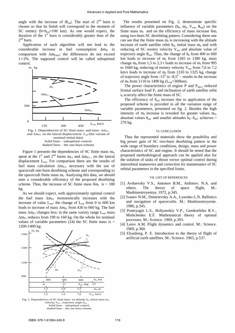
angle with the increase of |θent|. The start of 2nd

burn is

chosen so that its finish will correspond to the moment of

SC reentry (h=hent=100 km). As one would expect, the

duration of the 1st burn is considerably greater than of the

2nd

burn.

Application of such algorithm will not lead to the

considerable increase in fuel consumption in

comparison with mFmin: the differences do not exceed

1÷2%. The supposed control will be called suboptimal

control.

0

500

150 300 450

m, kg

Fig. 1. Dependencies of SC final mass and mass ΔmF1

and ΔmF2 on the lateral displacement Lent (the variant of

nominal initial data)

Solid lines – suboptimal control;

dashed lines – the one-burn scheme

ΔmF1

ΔmF2

mf

Lent, km/s

Figure 1 presents the dependencies of SC finite mass mf,

spent at the 1st and 2

nd burns mF1 and mF2 , on the lateral

displacement Lent. For comparison there are the results of

fuel mass calculation mF1, necessary with the use of

spacecraft one-burn deorbiting scheme and corresponding to

the spacecraft finite mass mf. Analyzing this data, we should

note a considerable efficiency of the proposed deorbiting

scheme. Thus, the increase of SC finite mass δmf is ~ 180

kg.

As we should expect, with approximately optimal control

the fuel mass mF1 monotonically increases with the

increase of value Lent: the change of Lent from 0 to 600 km

leads to increase of mass mF1 from 430 to 660 kg. The fuel

mass mF2 changes less: in the same variety range Lent mass

mF1 reduces from 190 to 160 kg. On the whole for nominal

values of variable parameters (24) the SC finite mass is ~

1200-1400 kg.

900

1100

1300

1500

400 500 600

-8 -11 -15

Fig. 2. Dependencies of SC final mass on altitude h0, initial mass m0,

velocity Vent , trajectory angle θent

Solid lines – suboptimal control;

dashed lines – the one-burn scheme

mf, kg

h0

m0

Vent

h0, km

θent, deg

1,5 2,0 2,5 m0 ,m

7,2 7,4 7,6 Vent, km/s

θent

The results presented on Fig. 2, demonstrate specific

influence of variable parameters (h0, m0, Vent, θent) on the

finite mass mf and on the efficiency of mass increase δmf

using two-burn SC deorbiting pattern. Considering them one

can see that the finite mass mf is increasing with the altitude

increase of earth satellite orbit h0, initial mass m0 and with

reducing of SC reentry velocity Vent and absolute value of

trajectory angle θent. Thus, the change of h0 from 400 to 600

km leads to increase of mf from 1265 to 1380 kg, mass

change m0 from 1,5 to 2,3 t leads to increase of mf from 995

to 1660 kg, reducing of reentry velocity Vent from 7,6 to 7,2

km/s leads to increase of mf from 1310 to 1325 kg, change

of trajectory angle from -150 to -8,5

0 – results in the increase

of mf from 1110 to 1490 kg (Lent=300km).

The power characteristics of engine P and Pspec, reduced

frontal surface load Px and inclination of earth satellite orbit

i0 scarcely affect the finite mass of SC.

The efficiency of δmf increase due to application of the

proposed scheme is provided in all the variation range of

variable parameters, presented on fig. 2. Besides the high

intensity of mf increase is revealed for greater values m0,

absolute values θent and smaller altitudes h0: δmf achieves ~

270 kg.

VI. CONCLUSION

Thus the represented materials show the possibility and

big power gain of SC two-burn deorbiting pattern in the

wide range of boundary conditions, design, mass and power

characteristics of SC and engine. It should be noted that the

proposed methodological approach can be applied also for

the solution of tasks of thrust vector optimal control during

interorbital maneuvers and correction for maintenance of SC

orbital parameters in the specified limits.

VII. LIST OF REFERENCES

[1] Avduevsky V.S., Antonov B.M., Anfimov. N.A. and

others. The theory of space flight, M.:

Mashinostroyeniye, 1972, p.345.

[2] Ivanov N.M., Dmitrievsky A.A., Lysenko L.N. Ballistics

and navigation of spacecrafts. M.: Mashinostroyenie.

1986, p.345.

[3] Pontryagin L.S., Boltyanskiy V.P., Gamkrelidze R.V.,

Mishchenko E.F. Mathematical theory of optimal

processes. M.: Science. 1969, p.393.

[4] Letov A.M. Flight dynamics and control. M.: Science.

1969, p.360.

[5] Elyasberg, P. E. Introduction to the theory of flight of

artificial earth satellites. M.: Science. 1965, p.537.


ISBN: 978-1-61804-240-8 119

Keywords— TFIDF, Vector Space Model, Data Mining, Text Analysis, Distance Measure.

Abstract— in this paper, we introduce a novel keyword

extraction algorithm, which identifies text descriptive terms in the titles of scientific articles. The identified terms can serve as search keywords for retrieving research articles form digital scientific databases and/or repositories. Our algorithm relies on the vector space model to represent the article titles and treats every term in a title as a vector with each vector containing three features namely, the number of characters a term has, the importance or else the strength of the term in the title and the relative order or else the position of the term in the title. Based on the weight our algorithm computes for each of the above features it assigns every term in the article’s title with a score indicating the suitability of that term as search keyword that could retrieve its corresponding article in the top ranking position. The experimental evaluation of our proposed algorithm on real scientific data proves its effectiveness in detecting text descriptive keywords and verifies our assumption that in the case of scientific publications title terms are expressive of the articles’.

I. INTRODUCTION

eyword-based approach is user friendly and easy to apply with an acceptable retrieval precision, while semantically rich ontology addresses the need for complete descriptions of text

retrieval and improves the precision of retrieval [1]. Keyword extraction is a significant technique for text retrieval, Web page retrieval, text clustering, summarization, text mining, and so on. By extracting appropriate keywords, we can easily choose which document to read to learn the relationship among documents [2]. A trivial algorithm for indexing is the unsupervised Term Frequency Inverse Document Frequency (TFIDF) measure [3], which extracts keywords that perform frequently in a text, but that don’t perform frequently in the rest of the corpus [4,5]. It is computationally efficient and performs reasonably well [6]. The term “keyword extraction” is used in the context of text mining [3]. Keyword extraction has also been treated as a supervised learning problem [4, 5, 7], where a classifier is used to classify candidate words into positive or negative instances using a set of features. Other research for keyword extraction has also taken advantage of semantic resources [8], Web-based metric, such as PMI score (point-wise mutual information) [7], or graph-based algorithms (e.g., [9] that attempted to use a reinforcement approach to do keyword extraction and summarization simultaneously) [6]. Relative scientific work has been carried out, where Frequent Terms (FT) are considered crucial [10], thus are extracted first, in order to extract keywords from a single document. Another interesting research has been carried out, where an alternative approach occurs.

A proposed algorithm [11], where not only term frequency is measured or other statistics, but in addition the usage of professional indexers is implemented. Furthermore, TFIDF weighting measure is combined with the vector space method for this purpose [12]. The TFIDF very relevant for the document is commonly used in IR to compare a query vector with a document vector using a similarity or distance function such as the cosine similarity function. However, the problem focuses on the disharmony with the Shannon-like theory [13]. More details are given in section II.A. The algorithm proposed in this paper can be considered novel, since it is not based not on the frequency where a term occurs (TF/IDF) which considers every word in a document equally weighted, but it inserts 3 variables that constitute each word uniquely identified. In a correlation between the two algorithms, in TF/IDF algorithm the angle of a word vector and the component vector represents the term frequency when in the proposed angle it represents 3 unique variables that provide a unique vector identity for each word. It is known, that the Ontologies are related to a model of knowledge, and knowledge in turn to information. Thus, it makes sense to introduce the concept of entropy and mutual information, as defined by Shannon for information theory in [14], on ontologies. Entropy and mutual information in turn enables us to define a distance measure formally. With this distance a sound foundation is given for the capturing of the inherent structure of ontology. Consequently, in our work, we attempt to use a new algorithm which is creating in the philosophy of TFIDF algorithm giving simultaneously a solution to Shannon-like model disharmony. This paper is organized as follows:

• Section II provides the theoretical and practical implications of this study which includes the related TF/IDF algorithm, the basis of the algorithm and the ranking criterion.

• Section III describes the experimental design analyzed the data collection part, the implementation of the algorithm as well as the retrieval and evaluation results

• Section IV presents the discussion and the future plan.

II. METHODOLOGY

A. Vector Space Model The TF/IDF algorithm is the best known weighting scheme for terms in information retrieval until know. This is based on three components

• Document Frequency (DF) • Inverse Document Frequency (IDF) • Term Frequency (TF)

And is implemented by the formula

Keywords Extraction from Articles’ Title for Ontological Purposes

Sylvia Poulimenou, Sofia Stamou, Sozon Papavlasopoulos, and Marios Poulos

K


ISBN: 978-1-61804-240-8 120

/ _ _ _ _ _TF IDF Term Frequency X Inverse Document Frequency= Or via the equation 1.

( ), , 101 log *logt d t dt

wNtfdf

= +

(1)

A characterization of algorithm is that the TF/IDF score (or, weight) for a term increases with the number of occurrences in a document (TF component). Moreover it increases when considering how rare the term is across the entire collection (IDF component). However, this is based on a continuously dynamic training procedure. Furthermore, this technique demands multi relationships between the terms and texts. The most significant problems are referred in the searching procedure using weighted terms [12, 13]. In particular, the core of the problem is that it is difficult to identify a single event space and probability measure within which all the related random variables can be determined. Without such a unifying event space, any procedure that contains matching and/or mixing different measures local and global that may well be unacceptable in terms of a Shannon-like theory [13]. A more serious problem occurs, when we search using weighted terms, we typically take the query terms ignoring all the other terms in the vocabulary. It is difficult to realize how such a practice could make sense in a Shannon-like model: every term in the document must be supposed to transmit information as well as any other. That is, the existence of a term ki would carry. Then an amount of information log P (ki) is produced irrespective of whether or not it is in the query. There is not any connect for the amount of information to the specific query. So we would have no explanation for leaving it out of the estimation [13]. However, the similarity of the typical IDF formulation to a component of entropy has inspired other researchers [14] to make connections, sometimes somewhat differently from the connection suggested above.

B. The Basis of the Algorithm The feature extraction is based on vector space model

theory. In more details, we considered that the title of a published document depicts a determined vector (vs) which is unique. This technique creates an auto-correlation mechanism which is unique from each document and this practice gives a solution to Shannon-like model because each document is downgraded in term locally. Thus, a stable-single event space is created for each document with computing probability measure. Taking into account this consideration, we assume that each word of a specific title represents of a vector (vw) which consists of three (3) features namely, the number of characters (w), the strength (s), and the order in the title (n) (see equation 2).

( ) [ ]0

niw i ii

V i s w=

=

(2)

Where, 0 00 0s w= ∧ =

For this reason, we normalized the vector (vw) and we

obtained the equivalent vector

00

0

nin wi i

we ni iw i

VV

V=

=

=

=

(3)

As strength (s) we use an encoding measure and for simplification reason we defined the ASCII encoding [15], more details of this procedure is given in the experimental part.

Furthermore, the vector (vs) depicted as the resultant vector (vs), see equation 3.

( )

0

ni

s wei

V V=

= ∑

(4)

C. The Ranking criterion The proximity rankings of documents in a keyword search

can be estimated, by using the assumptions of document similarities theory [16], by comparing the deviation of angles between each document vector and the original query vector is the resultant vector (vs) which represents the dominant orientation vector of the title. The calculation of the cosine of the angle between the vectors, is defined by equation (5).

( )

( )( )cos

ii we s

iwe s

V VV V

θ =

(5)

The new ranking of

0

( )1 0min cos

j

n

jr rιθ=

+ = − (6)

Where ( )0 min cos ir θ =

D. The novelty of the Algorithm Taking into account the sections II.A and II.B the

calculation of documents vectors can be calculated into two different techniques.

In the classical vector space model theory using the TF/IDF algorithm the document vector is extracted using multivariate components i.

1 2,, ...,s iU w w w = (7)

In the proposed method the document vector vs is extracted using the three aforementioned components[ ]i ii s w . In

other words the proposed method uses stable size of document vector (dimension 3).

In the same way, the query vector of the proposed vector has the same dimensionality while the classical vector has i dimensionality.

A vector space model iV

is adopted instead of vector sU

where the i variable is replaced by variable r (see equation 6).


ISBN: 978-1-61804-240-8 121

http://en.wikipedia.org/wiki/Relevance_%28information_retrieval%29

http://en.wikipedia.org/wiki/Ranking

http://en.wikipedia.org/wiki/Semantic_similarity



http://en.wikipedia.org/wiki/Cosine

The reason of this replacement took place because variable r is considered as a very important factor in the semantic theory

[17]. The replacement was made deliberately since vector iV

represents the influence’s degree through variable r because this will lead in a new ranking procedure according to its influence.

[ ]i i i iU r s w=

(8)

Finally, in both cases the relevance rankings of documents in a keyword search can be calculated, using the assumptions of document similarities theory, by comparing the deviation of angles between each document vector and the original query vector where the query is represented as the same kind of vector as the documents (see fig. 1).

Fig. 1. The query procedure between query vector and document

vector The matching calculation is implemented via the cosine of

the angles (θ,φ example see fig. 1) between the vectors, instead of the angle itself, see equations (5,6).

III. EXPERIMENTAL PART

A. The Data Collection The next step of the experiment lies in using an internet browser to visit Google Scholar in order to gather titles from 3 different Classes from Dewey Classification. In detail, from each Class we choose 10 titles from 10 different subclasses, that way we gather a sample of 181 titles totally from 3 different Dewey Classes. These Titles are: knowledge, systems, bibliographies, catalogs, libraries, biographies, topology, publishing, manuscripts and Algebra. Therefore our total title sample is approximately 181 titles. Continuing with the methodology steps followed, after already explaining the algorithm that extracts the 3 most dominant keywords and before inserting the title to the algorithm for processing, the step that needs to be done is a preprocessing of the title. The title is filtered in an automatic way in order to remove words considered as “non keywords”, such as stop words. In this paper we consider as a valid keyword, words that belong to the part of speech noun or compound noun. After the title is filtered, the next step is to apply the algorithm to each title. All the results for each separate title are being registered. The

output that is generated every time returns the three most dominant words that are considered as keywords for every title. In the next step we test the output in order to measure our experiment success rate. We search in Google Scholar (in title) using the exact output of the algorithm and carry out a statistical research of the total results. In order to be more precise we will present in detail an example/sample taken from our research. The whole process begins once we have selected a title of an article, which was obtained by using Google Scholar. Our search term was “Knowledge” and the title obtained “Advances in knowledge discovery and data mining”. Now, the obtained title must be preprocessed, before applying the algorithm. By using POS software, we keep words that based on the part of speech they belong they can be considered as valid keywords. All stop words must be cleared and also part of speech that for the purposes of this research must be excluded. Therefore, from the original title what is left is “Advances knowledge discovery data mining”. At this point we can apply the algorithm to the title that is left in order to export the three most dominant keywords of the sentence. After the algorithm is applied, we continue the experiment by testing whether our results are successful. To do so, we must visit Google Scholar again and by searching only in title, with the three most dominant keywords we check the results. The first result we find out of 181 results is the original title.

B. Implementation of the Algorithm

According to sections (II.A, II.B, III.A) we implement the proposed procedure using the aforementioned example according to the following steps:

Step 1. In the pre-processing procedure the title “Advances in knowledge discovery and data mining” is filtered in the eliminated one “Advances knowledge discovery data mining” using the rule of section (III.A) Step 2. We applied the algorithm by using the equations 1& 2 for the extraction of the vw features. This implemented by the following code of Matlab and the results are presented in Table I: num1=double(‘Advances knowledge discovery data mining’); k1=find (num1==32); k2=length(k1); sol1=[]; for i=2:1:k2; j=i-1; t=num1(k1(j)+1:k1(j+1)-1); sol=[i,length(t),sum(t)]; sol1=[sol1;sol]; end t=num1(1:k1(1)-1); solbeg=[1,length(t),sum(t)]; t=num1(k1(k2)+1:length(num1)); sollast=[k2+1,length(t),sum(t)]; sol1=[solbeg;sol1;sollast]; % sol1=Vw word vector % word normalization vector Vwe d1=sol1/norm(sol1);


ISBN: 978-1-61804-240-8 122

http://en.wikipedia.org/wiki/Relevance_%28information_retrieval%29

http://en.wikipedia.org/wiki/Ranking


http://en.wikipedia.org/wiki/Cosine

Table I. The Features of Vw

Words Order No. Characters

Strength

Advances 1 8 805 knowledge 2 9 960

discovery 3 9 984

data 4 4 410

mining 5 6 642

Step 3. We applied the algorithm by using the equation 3 for the extraction of the resultant vector (vs) features. This implemented by the following code of Matlab “ u=sum(d1)” and the results are presented in equation 7:

( ) ( ) [ ]55

0 0

0.0085 0.0204 2.1524i is we s

i i

V V V= =

= =∑ (7)

Step 4. This implementation according to equations 4 and 5 give the following results in Table II.

Table II. The angle between the resultant (vs) and the word (vw) Words Cosθ Ranking Advances 0.1572 3 knowledge 0.1069 2

discovery 0.0547 1

data 0.3332 5

mining 0.2202 4

As result of this procedure the words “discovery, knowledge and Advances” are selected as the optimum triple keywords.

C. The Retrieval Results According to previous stage, 181 triple keywords are extracted from corresponding Scholar Google titles. In the retrieval procedure each of the 181 triple keywords are given as queries in Scholar Google machine in order to obtain the corresponding answers. Furthermore, we investigate if the primary keyword for collection of the articles contains in the extracted triple keywords. More details, about the order of this answers regarding the score of the successful trial of retrieval the correct title is given in Table III.

Table III. Retrieval Results regarding to 181 triple words Order of success Queries

Present of primary Keyword

1 156 155

2 14 12

3 3 2

4 0 0

5 1 1

6 0 0

7 0 0

8 0 0

9 0 0

10 1 0

11 2 0

12 1 0

13 1 0

14 0 0

15 0 0

16 0

17 1

Furthermore, if we considered that x is the order of the successful retrieval using the triple words and y is number of queries. Then there is a polynomial n degree

11 2 1( ) ...n n

n np x p x p x p x p−+= + + + + (8)

Where ( )2min ( )i ii

p x y − ∑ (9)

Then using the following code of Matlab c = polyfit(x,y,5); xfit = linspace(min(x),max(x),length(x)); yfit = polyval(c,xfit); plot(x,y,'o',xfit,yfit,'--') we calculate that the robust fit polyonym is n=5 degree (see fig. 2)

0 2 4 6 8 10 12 14 16 18-20

0

20

40

60

80

100

120

140

160R2 = 0.92192

Fig. 2. The polynomial fit regression with r2=0.9219

Then the polynomial of this experiment is determined by equation (8)

5 4 3 2( ) -0.0071 0.3566 -6.7615 +59.1588 -233.5057 323.0271p x x x x x x= + + (8)

D. Evaluation of the Results For the evaluation of the collected data the probability density function (pdf) is used. The aim of this adoption focuses on the determination of the maximum width of the interval (window)


ISBN: 978-1-61804-240-8 123

x=[1,…,17] values. These values correspond to the order of successful article retrieval in Scholar Google search. In this way, we ask to found the robust interval window of values with the highest probability of searching scores. We typically proceed by investigating at a diagram (see fig. 2) of our data, and demanding to match it to the form of a smooth probability Gaussian density function, and rather one that is easy to work with. The Gaussian distribution is normally useful when the values a random variable takes are grouped near its mean, with the probability that the value falls below the mean corresponding to the probability that it falls above the mean [18]-[19]. In this stage we depict the density probability of integer values of polynomial with x=[1,…,17] which are presented in Table IV:

Table IV. Polynomial Values Calculation

x values P values

1 142.2682

2 44.0373

3 -0.4620

4 -13.1717

5 -10.0314

6 -1.8303

7 4.9408

8 7.2375

9 4.6098

10 -1.6499

11 -9.3588

12 -16.2957

13 -21.0530

14 -23.8887

15 -27.5784

16 -38.2673

17 -66.3222

If ( )f x is the normal distribution 1 2,..., 17,p p pχ ∈ then we

calculated the normal density probability function (see equation 10)

[ ]Pr ( )b

Xa

a X b f x dx≤ ≤ = ∫ (10)

a=1 and b=17 (see fig. 3), then we ascertain that the most probable value of x is 3.

Fig. 3. The probability density function of p values

As an interpretation of this result is that the proposed method for a triple keyword query gives an accurate retrieval ranking into the first 3 positions.

Furthermore, in order to evaluate the sensitivity and specificity of our method [20] we consider that the success scores are ranged between 1 and 3 interval space, as obtained by the probability density function (see fig. 2). In our case, we considered as true positive scores, all the articles which retrieved in the first second and third order via the triple query vector. As false positives scores are considered the articles which the primary keyword does not present in the triple keywords. Finally, true negative scores consider the rest scores (beyond of the three first orders). Then, the Table III is transformed into Table IV.

Table V. Retrieval Success Results regarding to 181 triple words

True Positive False Positive True Negative

151 11 8

sensitivity 0.90

specificity 0.58

The Sensitivity relates to the test's ability to identify positive results.

This can also be written as:

_ _ _ 1510.90

_ _ _ _ _ _ 168

number of true positivessensitivity

number of true positives number of false positives= = =

+

Specificity relates to the test's ability to identify negative results. This can also be written as:

_ _ _ 110.58

_ _ _ _ _ _ 19

number of true negativesspecificity

number of true negatives number of false positives= = =

+

IV. CONCLUSIONS We have presented a new keyword extraction algorithm that

detects the most important terms in the titles of scientific papers, which are then employed as search keywords for retrieving articles form digital scientific online resources. In particular, the core of the problem lies in the fact that it is


ISBN: 978-1-61804-240-8 124

rather difficult to identify a single event space and probability measure within which all the related random variables can be determined. Our algorithm is based on the vector space model to represent the article titles and treats every term in a title as a vector, with each vector containing three features namely, the number of characters a term has, the importance of the term in the title and the relative order of the term in the title. In the classical vector space model theory, using the TF/IDF algorithm, the document vector is extracted by using multivariate components j, while the classical vector has j dimensionality.

Based on the weight our algorithm computes for each of the above features it assigns every term in the article’s title with a score indicating the suitability of that term as a search keyword that could retrieve its corresponding article in the top ranking position. The experimental evaluation of our proposed algorithm regarding real data proves its effectiveness in detecting the most suitable keywords in the articles' title and indicates that title terms may be sufficient for representing the article semantics, when it comes to scientific publications, which is to be investigated in the future. Currently, we are in the process of enriching our algorithm with additional features from the articles' contents such as the abstract and the keywords authors indicated for their articles. Moreover, to address the issue of synonyms and polysemy, that are not included in this experiment. In addition, we plan to employ the identified keywords for building an ontology that could be employed as a repository of search term for conducting text retrieval tasks in scientific online repositories.

Furthermore, in order to evaluate the sensitivity of our method we consider that the success scores are ranged between 1 and 3 interval space, such as obtained by the probability density function.

Finally, we intend to release the ontology that will be developed so that it could be employed by other researchers for performing semantic retrieval tasks. Entropy and mutual information in turn enables us to define a distance measure formally. With this distance a sound foundation is given for the capturing of the inherent structure of ontology. Consequently, in our work, we attempt to use a new algorithm which will be created in the philosophy of TFIDF algorithm giving simultaneously a solution to Shannon-like model disharmony.

REFERENCES [1] H. Wang, S. Liu, L.T. Chia. “Does ontology help in image retrieval? A

comparison between keyword, text ontology and multi-modality ontology approaches”. In Proceedings of the 14th Annual ACM International Conference on Multimedia. 2006. pp. 109–112.

[2] Y. Matsuo, M. Ishizuka, “Keyword extraction from a single document using word co-occurrence statistical information”. International Journal on Artificial Intelligence Tools. 2004. Vol. 13, pp. 157–169.

[3] M. Rajman, R. Besancon “Text mining – knowledge extraction from unstructured textual data”. In Proceedings of the 6th Conference of International Federation of Classification Societies. 1998.

[4] E. Frank, G.W. Paynter, I.H. Witten, C. Gutwin, C.G. Nevill-Manning. “Domain-specific keyphrase extraction”. In Proceedings of IJCAI, 1999, pp. 688–673.

[5] Y.H. Kerner, Z. Gross, A. Masa, “Automatic extraction and learning of keyphrases from scientific articles”. Computational Linguistics and Intelligent Text Processing, 2005, pp. 657–669.

[6] Liu F. Liu, Y Liu. “Automatic keyword extraction for the meeting corpus using supervised approach and bigram expansion”. In Proceedings of IEEE SLT.

[7] P. Turney, “Coherent keyphrase extraction via web mining”. In Proceedings of IJCAI, 2003, pp. 434–439.

[8] G. Carenini, R.T. Ng, X. Zhou, “Summarizing emails with conversational cohesion and subjectivity,” in Proceedings of ACL/HLT, 2008.

[9] A. Janin, D. Baron, J. Edwards, D. Ellis, G. Gelbart, N. Norgan, B. Pe- skin, T. Pfau, E. Shriberg, A. Stolcke, and C. Wooters, “The icsi meeting corpus,” in Proceedings of ICASSP, 2003.

[10] Matsuo, Y., Ishizuka, M. “Keyword extraction from a single document using word co-occurrence statistical information”. International Journal on Artificial Intelligence Tools. 2004. Vol 13, pp. 157–169.

[11] Hulth, A., “Improved automatic keyword extraction given more linguistic knowledge”. In Proceedings of the 2003 Conference on Empirical Methods in Natural Language Processing. 2003. Association for Computational Linguistics, pp. 216–223

[12] P. Soucy και G. W. Mineau, ‘Beyond TFIDF weighting for text categorization in the vector space model’. IJCAI, 2005, Vol. 5, pp 1130–1135.

[13] Robertson, S. “Understanding Inverse Document Frequency: On theoretical arguments for IDF”. Journal of Documentation, 2004, Vol. 60 (5), pp. 503–520.

[14] C. Blake, ‘A comparison of document, sentence, and term event spaces’, In Proceedings of the 21st International Conference on Computational Linguistics and the 44th annual meeting of the Association for Computational Linguistics, 2006, pp. 601–608.

[15] M. Poulos, S. Papavlasopoulos, V. Chrissikopoulos, “A text categorization technique based on a numerical conversion of a symbolic expression and an onion layers algorithm”. Journal of Digital Information, 2006, Vol. 1 (6).

[16] Salton, G., Wong, A., Yang, C. S. “A vector space model for automatic indexing”. Communications of the ACM. 1975. Vol. 18, pp. 613–620.

[17] Harispe S. et al. “Semantic measures for the comparison of units of language, concepts or entities from text and knowledge base analysis”. Arxiv. 2013. Vol. 1310, 1285. pp. 1-159.

[18] Parzen, E. “On estimation of a probability density function and mode”. The annals of mathematical statics. 1962. Vol. 33, pp. 1065-1076

[19] Abramowitz, M., Stegun, I. A. (Eds.). "Probability Functions." Ch. 26 in Handbook of Mathematical Functions with Formulas, Graphs, and Mathematical Tables, 9th printing. New York: Dover, 1972, pp. 925-964,

[20] M. Poulos, G. Bokos, N. Kanellopoulos, S. Papavlasopoulos and M. Avlonitis. “Specific selection of FFT amplitudes from audio sports and news broadcasting for classification purposes”. Journal of Graph Algorithms and Applications. 2007. Vol. 11(1). pp. 277–307


ISBN: 978-1-61804-240-8 125

http://www.amazon.com/exec/obidos/ASIN/0486612724/ref=nosim/weisstein-20

http://www.amazon.com/exec/obidos/ASIN/0486612724/ref=nosim/weisstein-20

http://scholar.google.gr/citations?view_op=view_citation&hl=el&user=b1O4PYcAAAAJ&citation_for_view=b1O4PYcAAAAJ:LkGwnXOMwfcC



Abstract- This text generally describes the architecture of

an agent-based model for pulmonary tuberculosis in the zone of Usme (Bogotá, Colombia), product of a master's thesis in Information Sciences and Computing of District University "Francisco José de Caldas" [1]. First comes the introduction, then the tools and concepts that allow the simulation, then the model is exposed from a conceptual approach to technology-society relationship, and finally it is disclosed the author’s findings.

Key words: Agents-Based Models, Geographic Automata System (GAS), Epidemiologic simulation, complex Systems.

I. INTRODUCTION

The technological edge thinks forward, looking for ways to understand it, study and intervene in the world over time towards a particular purpose. So it makes models that attempt to reproduce actual facts and allows a better understanding of the relationship of humans with them, appearing technologies with that purpose as Agent-Based Models and Geographic Automata System, among others [2].

But the future is thought from the uncertainty, because the world is complex and multiple, set of systems with the general characteristics of not to be reversible, not to be accurately predicted, to develop nonlinear interdependent relationships, and to have appearance of order (emergency), being necessary to go beyond the deterministic mathematical formal schemes [3, 4].

The bio-social systems, being complex, cannot be predicted with accuracy nor are reversible, so they have a constitution order from the simple to the complex, allowing the passage from chaos to order at the time called edge of chaos, where self-organization emerges, which is the coordination of the parts’ behaviors of a system without any central power or external coercion that lead them. Jhon Stwart Kauffman formulated a hypothesis of a global connection between all parts of a physical system, that after a certain time, due to the energy accumulated between these, by inertia was that these associated themselves synergistically and generate patterns (self- adaptive systems) [3, 4].

1Department of Academic Research, “Manuela Beltran” University.

[email protected] 2 Department of Academic Research, UNIMINUTO.

[email protected]

Current knowledge have the task of describing the

complexity of the world we inhabit, so in this case it is intended to represent the nonlinear and interdependent relationships of a community in the middle of a tuberculosis epidemic, in order to predict the scenarios of this complex system [4, 5], explaining the construction of a Agent-Based Model for Tuberculosis in Usme’s zone, and thinking about the origin and social horizon of technology.

II. TOOL AND BASIC CONCEPTS FOR THE MODEL

A. Geographic Automata System (GAS)

Between 1999 and 2001, Paul M. Torrens and Itzhak Benenson created Geographic Automata System (GAS) for modeling phenomena on real spaces, from individual computer entities within the system: agents. On the one hand, they modified the classical Cellular Automata (CA), which is a system in one, two or three dimensions, consisting of partitions called cells, which acquire ways to present: states, from a default set of them, ranging from relations with its neighboring cells, their neighborhood (Figure 1), through pre-established transition- state rules, in a sequence of moments called evolution system [6, 7].

And on the other hand, they placed those entities that change over time (A. Figure 2) on a Geographic Information System (GIS), which is a set of layers that describe the geographic characteristics of a place, from the general to the specific (Figure 2 B). Thus, agents are related to real spaces, preserving the neighborhood concept in his role for the change of state (Figure 1), but not only on generic objects such as cells, but sometimes on entities with own characteristics and mobility: specific sites , people, vehicles, etc. (C. Figure 2) [2, 6].

Fig 1. Types of neighborhood in cellular automata which allows the

evolution of the system. Neighborhood A: Von Newman neighborhood, with octagonal neighbor cells. Neighborhood B: Moore neighborhood, with

octagonal and diagonal neighbor cells [5].

A Geographic Automata System (G), is defined as the set of automatas (K), which vary from state (S) over time, through transition rules (Ts), developed at specific locations (L), from

Architecture of an Agents-Based Model for pulmonary tuberculosis

M.A. Gabriel Moreno Sandoval1

William David Peña Peña

2


ISBN: 978-1-61804-240-8 126


mobility rules (if any) of each one (ML), considering its neighborhood (N) at every time, called Tick, and the criteria of relationship they have with this (RN) (Figure 3) [7, 8]. Where, thanks to this set, It is able to see the interdependent relationships between the conditions of each area (population density, healthiness, etc.), and each agent (location, nutrition, origin, economic status, etc.) [9].

Fig 2. Integration of CA and GIS in the constitution of GAS.

Fig 3. Representation of a Geographic Automata System (GAS) [8].

First, the geographic information of Usme Central zone, was

registered with ArgGis, application that allows to enter raster data type of a land, generating a GIS shapefiles (.shp) [10]. And then again, as Framework it was used Repast, which is a set of Java classes and methods linking agents with a GIS, allowing focusing on the modeling of the relevant attributes of the phenomenon, because this program already contains the multi-threaded programming, where in pseudo-parallel way for each Tick, transition rules are executed for all agents run, and also it provides a graphical interface of the simulation [11].

B. Usme zone

Usme is a local and administrative subdivision of Bogotá, which was incorporated into the city in 1990, because before that it was a town. So today some rural practices persist (agriculture, small farms, artisanal slaughtering), where according to figures consulted (data from 1999 to 2007 that varied in the study of late 2011, the same year it was supported the thesis on the model), 84.9% of its land (18,306.52 hectares) was rural and 15% urban, preserving some natural resources (now damaged by mining, urbanization and the tanning of leather) as water sources (21 in urban sector, 23 in rural sector, 11 rivers, 2 dams and 3 ponds.) [12].

Its population consisted of 51% female and 49% male, 34.8% of the population was under 15 years and 2.5% over 60, there being a high economic dependence, where on average 100 people were dependent of every 59, workers

mostly with low levels of schooling and informal jobs. In addition, from 1995 to 2005, amidst the paramilitary phenomenon nationwide, this zone received 8.2% of the displaced population that came to Bogotá by the violence [12].

Thus, according to the Unsatisfied Basic Needs Indicator

(NBI, by the Spanish acronym), which considers the shortages at home: a) housing with physical or structural defects, b) lack of basic services or deficiencies in drinking water and feces disposal, c) overcrowding (2 persons/5m2), d) high economic dependence (1 productive person / 3 or more dependents), e) truancy (at least one child between 7 and 11 do not regularly attend a school), and f) Misery, when the home has two or more of the above conditions, it was found that Usme was 9, 1% of homes in NBI, with 1% in misery. Fact also reflected in the 51% of the population below the "poverty line" indicator that arises from considering the minimum subsistence income for a person [13].

C. Tuberculosis Pulmonar (TB)

Illness from the bacteria Mycobacterium tuberculosis, native bovine and adapted to the human (zoonoses), which attacks places rich in mucous membranes (such as the lungs) and develops according to: the strength of the micro-organism to survive and be transmitted (virulence), the opposition that the body makes to the micro-organism (resistance), ease that people have to acquire and develop the disease (hypersensitivity) and the morphology of the affected tissues (genesis of the pattern infectious) being vulnerable to ultra-violet rays. It manifests in cough with coughing up phlegm or blood, evening sweating, fever, fatigue and unintentional weight loss.. Phases of development are: the attack or the arrival of bacillus in the body, then its logarithmic growth and the progressive activation of cells infected into other tissues, then there is an immunity, delayed as the body's inadequate response to disease, thus leading to the destruction of tissue and the transmission of new one [14].

Diagnosis is made by biochemical reaction of cultivated samples. To eradicate it is used treatment shortened supervised (DOTS), the antibiotic rifampicin, isoniazid, Pyrazinamide, and Ethambutol, over a period of 48 weeks, extending in the case of a relapse to 63, and whose success or failure (even fatal), depend on conditions of life of the infected as food, hygiene, wholesomeness in the habitat and permanence in the treatment, since deaths from TB are commonly associated with poverty and undernutrition [15].

III. AGENT-BASED MODEL FOR TUBERCULOSIS IN USME

A. Simulation’s time and space

In architecture model time and space simulation, as the first condition for the interdependence between agents is carried out in the middle of tuberculosis outbreak as a complex system were established. On the one hand TimeProject whose TimeProject constructor class is created generated internal time model, allowing the passage of the method step(). And moreover the Global class, entering shape files and generates graphical output interface was created, also it determines the


ISBN: 978-1-61804-240-8 127

amount of Tick equivalent to every hour (1 hour = 1 Tick) , the number of initial agents in each state, that the epidemiological model of pulmonary tuberculosis (SIR model) are: Susceptible (which could be infected), infected (disease carrier) and Recovered (who overcomes the infection), and the amount of each type of agent , which under Usme socioeconomic conditions are: Housewife, Worker, Student, Deplaced and Homeless, which enter as parameters via setValuesFromParameters() method of that class [1] (A. Figure 4).

Therefore, States and agents that is different in the middle of

a space and a time shared, determine that the Organization of the information in a complex system should be a dynamic structure that contains the particularity of the elements and their no-lineal relationships, and don’t simply a collection of attributes.

B. Contexts

Contexts are joint that grouped the agents of a system and the relationships between them. Thus, MainContext class is the generic context that through the build() method, load the global timeline, originates and controls the contexts of spaces and people, and is the time and the particular space of these agents. Subsequently determined the context of each place: Home (HomeContext), workstation (WorkPlaceContext), study location (StudyPlaceContext) and entertainment venue (EntertainmentPlaceContext), dynamically created by reflection (in the execution of the program), through the method createSubContext() in the class CityContext, referencing their positions from the tract (class RoadContext), the intersections of these and the boundaries between places (class JunctionContext). In the same way, with the class PersonContext was created the possibility of dynamically generating the contexts of agents -sets of sites and other agents-: HousewifeContext, WorkerContext, StudentContext, DeplacedContext, HomellessContext (B. Figure 4).

The location of the agents was determined by the rules of

movement (ML) of each, using for this parametric class AgentContext and getGeography() method. And the location of the sites was performed using the same method name PlaceContext parametric class (C. Figure 4).

Due to the needed for information on the TB outbreak

(major focus of infection, more infected population trend of spread of the disease, etc.), which would act on this, the dynamic generation of contexts allowed the development of the non-linear relationships between the different agents in a period of time, loading and processing the increased volume of information in the model thanks to the architecture of the program, through reflection, extended the possibilities of development of the system.

C. Places

Parametric classes system can evolve on the geographical

conditions of Usme, which is very important for the relationship between the demographic conditions of a region and the spread of an epidemic (TB in this case), where the different types of places and their characteristics were determined and verified with the abstract class Place, with the

attribute listPerson created an arrangement for certain amount of agents inside, regardless of their type, verify with the method getOvercrowdingCondition() the overpopulation (boolean data), on the basis of the capacity of the place (method getPeople Capacity()), and the number of people in it (method getAmountPerson()) [1].

Fig 4. Time and space model, and training contexts through parametric

classes.

The specific locations and attributes were defined with HomePlace classes (households), WorkPlace (work sites), StudyPlace (study sites), EntertainmentPlace (entertainment venues) and Route (tracks), which inherit of the class Place attributes as the maximum area place (MaxArea...), high capacity (MaxAmount...), many people (amountPersons), capacity (peopleCapacity), use, management, geometry, number of people per state (amountSusceptible, amountInfected, amountRecovered), among others.

Calculation of amounts by State was performed on the method step() -different class TimeProject step() method, and later exposed the Person class step() method-, and the distribution of agents by States was random from classes of each place: Work Place, Study Place, Home Place,


ISBN: 978-1-61804-240-8 128

Entertainment Place, trough the method getRandomStudyPlace, getRandomHomePlace, getRandomWorkPlace, and getRandom EntertainmentPlace, respectfully (A. Figure 5).

The description of Usme geography through Shape files and their inclusion in the system, allowed to generate scenarios appropriate for studying the TB epidemic in the actual conditions of this place, as a requirement of a model oriented to care for the life of the population, through the generation and the study of patterns in the spread of this disease.

Fig. 5. Architecture of sites Agents model.

D. Agents

It determined each agent-specific property so that they can evolve relationship tailored to the reality of the TB outbreak: daily places of movement, origin in the case of displaced persons, etc. Why the particular agents were created 'Worker',

'Housewife', 'Student', 'Deplaced for violence' and 'Street people', through classes, Worker, Housewife, Student, Deplace and Homeless, respectively.

Previous classes inherit from the Person class attributes of localization in each place (currentLocalization), routes of movement (route), location at every moment of the system (currentTick), identification (id), employment status, medical service, stratum, previous infection by HIV and TB, type of person, State of health (healthFactor) and number of health (numberHealthFactor), which is verified by the verifyHealthFactor() method According to the infections activate method infect(), which passes the person State Susceptible to infected (first passive, then contagious).

Although it must be clarified that home and the places of development of each agent are attributes in each particular class (Worker, Student, Housewife, Homeless, Deplaced etc.), and is thus allowing you to determine routines on different types of agent through parameters that are entered as Schedule (specific cases) in the classes of every kind of person (B. Figure 5).

E. Rules of transition

Rules of transition between the States of SIR epidemiological model are identical for all agents (TABLE I.): susceptible to passive infected, and hence a contagious agent, then be recovered, however the times varied considering multiple living conditions of Usme (TABLE II.), where the method infect() of class Person activated particular rules contained in the classes of each type of agent making it easier in some cases to the acquisition of disease, and likewise, hampering its recovery (average increase of vulnerability, TABLE II) [1].

TABLE I: TRANSITION RULES.

State change

Susceptible to Infected liability

Infected liability. From Infected Contagious

Infected to Recovered

Time (1 Tick = actual 1 hour).

12 Tick 96 Tick Tick 4032 (24 weeks): Assuming

completion of treatment of 48

weeks.

According to the conditions of life in each agent, for

example, the time 12 Tick in the vicinity of a contagious, necessary to move from Susceptible to passive infected, agent reduced by the average decrease in 1/8, 1/6, or 1/4 of the number healht Factor attribute, as there was an average delay of 1/8, 1/6, or 1/4 in raising that attribute according to the conditions of table 2, to move from infected to retrieved, for a population chosen randomly according to the percentage of population affected, with the following conditions: 1 in every 4 people in overcrowded housing was inadequate, 1 in 3 people in destitution was in misery by NBI, 1 in 4 people with poor nutrition in the NBI1 in 3 people with chronic malnutrition was on the same indicator, as gaps in living conditions have problems shared, setting such conditions through schedule in each type of agent [9].


ISBN: 978-1-61804-240-8 129

TABLE II.: IMPACT ON VULNERABILITY FACTORS ATTRIBUTE PERCENTAGE WITH POPULATION AFFECTED

NUMBERHEALHTFACTOR.

Vulnerability Factor Average increase in vulnerability. Attribute numberHealhtFactor ()

<= 0.2 = infected.

Scale of 0-1.

% Affected Population 3

Poor nutrition

1/8 30%

Chronic malnutrition 1/6 15%

Overcrowding 1/4 5%

Housing inadequate 1/6 2%

Households with NBI (1 Home = Average of 4 People)

1/8 9.1% households =

36.4% population

Misery as NBI ¼ 1% of households =

4% population

Homelessness ¼ 6%

F. A CASE

With a total amount of 500 agents, 20% love House, workers 25%, 25%, 15% and 15% displaced students of street, 5% initial of infected, recovered 20% and 75% susceptible, were obtained data from Table III.

TABLE III: AGENT TYPES OF INFECTION BY TICK.

Agents Infected% (of the

total) for Tick. T= 1 T= 200 T= 528 T=

4032 Housewife

1% 1.2% 3.8% 0.2%

Worker 1% 1.8% 4.2% 0.4%

Student 1% 1.4% 3.4% 0.2%

Displaced 1% 2% 3.6% 0.8%

Homeless 1% 1.6% 4.2% 0.6%

TOTAL INFECTION

5% 8% 19.2% 2.2%

The resulting data is inferred that infection levels rise first in

patients with immune deficiencies related to bad nutrition, poverty, and inadequate conditions of habitat (housing overcrowding or free services: NBI), nothing that although the highest proportion of agents corresponded to a type (workers and students), harder those infected in that eradicating the disease, they are those who described under very poor conditions of existence (Street and displaced inhabitants), which, if they had not taken into account would have caused a uniform tendency in the simulation behavior, without allowing to see the auto-organising patterns of the disease from the actual conditions to be able to act on this.

3 Estimated figures weighting of survey data quality of life and

social diagnosis of the town, considering older vulnerabilities for IDPs and resident street [9, 10].

IV. CONCLUSIONS

1) The dynamic construction of contexts from parametric classes (T:Microsoft.VisualStudio.Test Tools. execution. agent context and Place Context) in the architecture of the model allowed a greater volume of information loaded and processed, reducing the lines of code and optimizing the performance of the machine, but projecting a greater precision of the simulation to the real conditions of the phenomenon in Usme (special agents(: street people, displaced persons, and specific conditions: NBI, nutrition, overcrowding) at all times, making this program as a support tool that could be used by local health authorities.

2) The creation of Time Project and Global classes with their respective methods, and the union coherent types of agent to these, incorporating in a single set all elements of the simulation, is the architecture of the system as a Framework for the creation of models of epidemics-targeting GAS, regardless specific geography in which develops and simulated disease now that the creation of common space and time, and the possibility of agents to act is through these by means of dynamic contexts, create the basic conditions for any model can develop.

3) The model is created for the study of infection and the spread of tuberculosis taking into account the social dynamics, adopt to different fields and learn behaviors and theoretical but reliable of a possible epidemic statistics without ethical implications, and allowing the application of preventive methods and control large scale.

REFERENCES

[1] Moreno Sandoval, L. G. Epidemiological model of the tuberculosis based on agents in Usme, Bogota, Colombia. Thesis of mastery in Sciences of the Information and the Communication. University Distrital " Francisco Jose of Caldas ". June, 2007 - March, 2012. [2] Benenson I., Torrens P. M. Geographic Automata Systems: A New Paradigm for Integrating GIS and Geographic Simulation. In Proceedings of the AGILE 2003 Conference on Geographic Information Science, Pages 367-384 (Lyon, France). April 24th- 26th, 2003. [3] Lucas C. Self-Organization. In Magazine Thinking the complexity, 3(6): 5-15, 2009. [4] S. M. Manson., S. Sun., D. Bonsal, “Agent-Based Modeling and Complexity” in Agent-Based Models of Geographical Systems A.J. Heppenstall, A.T. Crooks, L.M. See, M. Batty, Eds. Dordrecht, Heidelberg, London, New York, Springer, 2012, ch, 4, pp. 125-140. [5] Perez Martínez A. Stuart Kauffman's work. The problem of the complex order and his philosophical implications. In Magazine Thinking the complexity, 3(6): 21-38, 2009. [6] Benenson I., Torrens P. M. Geographic Automata Systems. In International Journal of Geographical Information Science. 19 (4): 385–412, April 2005. [7] Kari J. Cellular Automata. Technical Report. University of Turku, Finland, 2013. [8] I. Benenson, V. Kharbash. Geographic Automata Systems: From The Paradigm to the Urban Modeling Software. In: Proceedings of the 8th International Conference on Geocomputation University of Michigan. United States of America. July 31 to August 3, 2005. [9] M. Parvin, “Agent-based Modeling of Urban Phenomena in GIS” Capstone Project, thesis submitted in fulfillment of Masters in Urban Spatial Analytics, University of Pennsylvania, CA, 2007 [10] Autonomous university of Madrid. Manual (basic level) for the production of maps with ArcGis. December, 2011. [11] Malleson N. Repast Simphony Tutorial. Technical Report. May 7, 2008.


ISBN: 978-1-61804-240-8 130

[12] Secretariat of estate of the District. Crossing Usme 2004. In: physical Physical and socioeconomic Diagnosis of the localities of Bogota, D.C. Major mayoralty of Bogota. Bogota DC, Colombia. 2004. [13] Secretariat of Health of the District. The health and the quality of life. Locality 5 - Usme. Major mayoralty of Bogota DC. 2009. [14] Dr. S. Invertrz. Pathogeny of the tuberculosis. University of Buenos Aires. Buenos Aires, Argentina. 2008. [15] Dr. Ospina S. The tuberculosis, a historical - epidemiological perspective. Magazine Infectio. Vol.5 no. 4 pp. 241-250, Bogota October - December, 2001. Authors Luis Gabriel Moreno Sandoval: He was born on March 8, 1986 in Bogotá, Colombia. System Engineer, Master of Science in Information and Communication of the University District "Francisco Jose de Caldas" (Bogota). Researcher tecnolgías vanguard as agent-based models and natural language processing, manager and director of leading academics and business groups on innovation and technology. Currently he is finishing his master's degree in administration from the University "Shown of Colombia". William David Peña Peña: He was born on February 12, 1987, Philosopher (University "Free" Colombia) and transdisciplinary research. Manager various academic areas in the humanities and speaker at international events (Scientific Convention CUJAE, Cuba, 2012. Innoed 2013, Cuba. CLEI2014 And soon, Uruguay. Among others) on the application of technology to solve social problems related to education and health. Currently he is doing based on developments in the particular cognitive processes educational technologies.


ISBN: 978-1-61804-240-8 131

Keywords—non-linear analysis, transient coupled temperature-displacement, wide pre-stressed reinforced concrete beams

Abstract—When using wide pre-stressed reinforced concrete

beams for realization of prefabricated concrete slabs beside their mechanical disadvantages with respect to the regular ones, their increased risk of brittle failure and other uncertainty in their behavior have to be considered. Since in structural design structural height might be imposed, wide beams with all their disadvantages become the right solution. But how the mechanical behavior of the prefabricated floor system can be influenced in case of fire? The paper presents numerical modeling for prefabricated floor system using wide reinforced concrete beams considered together with the corresponding double floor with precast slab and concrete topping, subjected to fire in different fire scenarios, establishing the scenario with the highest risk on the structural stability.

I. INTRODUCTION N practice of precast concrete structures several structural solutions are widely spread. Double floor systems are

assuring the necessary speed in structure realization as well as the structural flexibility, which, in combination with use of wide pre-stressed reinforced concrete beams, presents countless benefits, but at the same time raises questions with respect to their mechanical behavior when subjected to loadings. Provisions of existing design codes are not clearly covering all the possible load situations according to [1], neither use of wide pre-stressed reinforced concrete since either code provisions are not covering or the structural system used [1] has no or limited references in codes and practice. From fire resistance point of view the degree of fire resistance is established according to [3], which is establishing the necessary fire resistance of each structural element. According to provisions of [2] fire resistance is assured by foreseeing specific concrete cover of reinforcement. Use of pre-stressed

This work was realized as consequence of the research concerns of the

Technical University of Cluj-Napoca, Faculty of Civil Engineering. A. Puskás is now with the Department of Structures, Faculty of Civil

Engineering, Technical University of Cluj-Napoca, G. Baritiu street no. 25, 400027, Cluj-Napoca, Romania (phone:+40-264-401545, e-mail: [email protected]).

A. Chira is working at the Department of Structural Mechanics, Faculty of Civil Engineering, Technical University of Cluj-Napoca, G. Baritiu street no. 25, 400027, Cluj-Napoca, Romania. He is now postdoctoral researcher of the Department of Building Structures, Faculty of Civil Engineering, Department of Building Structures, Thákurova 7, 166 29 Praha 6, Czech Republic (e-mail: alexandru.chira@ fsv.cvut.cz).

slab elements can avoid excessive deformations and postpone the appearance of cracks [4], and as consequence the excessive exposure of reinforcement to fire. Due to the decreased structural height of wide beam floor systems their sensibility to fire is crucial. Studies on wide reinforced concrete beams subjected to fire shows that in numerical analysis the beam supposed to different fire scenarios has an adequate behavior for the imposed fire resistance degree [5], but their behavior as part of the floor system needs further investigations.

II. PROBLEM FORMULATION For studying the behavior of the wide pre-stressed reinforced concrete beam subjected to different fire scenarios a floor system using this type of beam is considered [6], as presented in Fig. 1.

Fig. 1 floor system layout

For the modeling the floor system effective width of the beam has been considered (Fig. 2) according to the clause 5.3.2.1 of [1], taking into consideration the used concrete and reinforcement quantity, quality and disposal.

Flanged wide reinforced concrete beam subjected to fire - numerical investigations

A. Puskás and A. Chira

I


ISBN: 978-1-61804-240-8 132


Fig. 2 effective width of the beam

The total double floor thickness is 17 cm, build up by a 8 cm precast floor of C40/50 class concrete and a 8 cm topping of C25/30. The main wide beam reinforcement is presented on Fig. 3. Its total length is 7.86 a, while the cross-section is 25x120 cm. The concrete quality used is C30/37, with longitudinal and transversal reinforcements PC52 type and active reinforcements of St1660 type having 12.9 mm diameter. For the analysis Abaqus FEM code [7] has been used, with different material law for both concrete and steel, for every change of temperature. For concrete it has been used the C3D8T solid elements: an 8-node thermally coupled brick, tri-linear displacement and temperature and for the reinforcements the T3D2T elements: a 2-node 3-D thermally coupled truss. The analysis was done in three steps: in the first one the pre-tensioning was done and in the second one the gravity loads were applied for both a static general analysis being used. In the third step a transient coupled temperature-displacement analysis have been used [8][9][10][11][12].

Fig. 3: main wide beam reinforcement

For the analysis of the beam taking into account the effective width of the beam three different fire scenarios have been used [5],considering two hours from the curve presented in figure 4.

Fig. 4: ISO 834 standard fire curve [2]

III. MODELING OF THE BEAM ON FIRE In order to investigate the flanged wide reinforced concrete

beam subjected to fire analyses have been performed using Abaqus finite element analysis. Results for the three scenarios are presented in the followings:

A. Scenario I The first scenario of fire takes into consideration acting of

the fire along the whole length and aside the whole width of the flanged beam (Fig. 5).

Fig. 5: Scenario I of fire action

Fig. 6: Displacement after two hours of fire, d=10.96 cm

Fig. 7: Concrete plastic equivalent strain from compression,

PEEQ=7.61E-3

Fig. 8: Concrete plastic equivalent strain from tension,

PEEQT=9.59 E-3


ISBN: 978-1-61804-240-8 133

Fig. 9: Steel plastic equivalent strain, PEEQ=9.50E-3

Fig. 10: Temperature distribution on concrete after two hours of fire,

Tmax=1052ºC

Fig. 11: Temperature distribution on steel after two hours of fire,

Tmax=981.6 ºC

Fig. 12: Time versus maximum temperature curve on concrete

Fig. 13: Displacement – maximum temperature diagram

B. Scenario II The second scenario of fire considers the fire acting in the

middle of the opening on a strip of 0.50 m wide, aside the whole width of the flanged beam (Fig. 14).

Fig. 14: Scenario II of fire action



PEEQ=1.90E-3


ISBN: 978-1-61804-240-8 134


PEEQT=3.71E-3



Tmax=978.7ºC


Tmax=913.9 ºC



C. Scenario III In the third scenario of fire it have been considered acting

on a strip of 0.50 m wide near the support, aside the whole width of the flanged beam (Fig. 23).

Fig. 23: Scenario III of fire action



ISBN: 978-1-61804-240-8 135


PEEQ=4.39E-3


PEEQT=5.14E-3



Tmax=969.4ºC


Tmax=908.4 ºC



IV. DISCUSSION The three scenarios taken into consideration in the investigation presents possible situation of fire acting on the beam. When comparing results obtained for flanged wide reinforced concrete beam with respect to the independent wide reinforced concrete beam [5] one can remark similar behavior of the beams under the same external load, but deflection of the beam, internal stresses in concrete and reinforcements as well as internal temperature are of more reduced values.

Comparison of the results for the three scenarios is unnecessary since the load given by the fire in the first scenario is incomparable with the other two scenarios. Even so we can remark the increased risk for the stability of the element for scenario I since after one hour it reaches excessive deformation (beyond l/100), where the concrete cover of the tensioned reinforcements is already inexistent. For scenarios II and III the deformation occurred is almost negligible under the external and fire loads.


ISBN: 978-1-61804-240-8 136

V. CONCLUSION The behavior of the flanged wide reinforced concrete beam

subjected to fire according to the presented numerical investigation can be considered highly satisfying, taking in consideration the designed concrete cover and the imposed fire resistance of the element of 15 minutes. Fire resistance of the beam is improved when joint with the flanges is considered and pre-stressing for the beam is applied, avoiding excessive deflection even after one hour of fire load. Temperature in the reinforcements reaches dangerous values after one hour of fire load.

The displacements after two hours of fire are less for the wide beam interacting with the precast slab then the results only on the wide beam alone [5], 3 times less for the first and second scenario and almost 8 times less for the third scenario.

Modeling the interaction of the precast slab with the prestressed wide beam gives a more accurate representation on the behavior of the beam subjected to gravity and fire loads. For a better understanding of the mechanical behavior the authors will have to do some experimental investigations in order to see if the numerical model is close to reality.

REFERENCES [1] *** SR EN 1992-1-1-2004, Eurocode 2, Design of concrete structures.

Part 1-1: General rules and rules for buildings, 2004. [2] *** SR EN 1992-1-2-2004, Eurocode 2, Design of concrete structures.

Part 1-2: General rules – structural fire design, 2004. [3] ***. (1999). P118-99: Normativ de siguranță la foc a construcțiilor [4] A. Puskas, Z. Kiss, “Testing of a wide reinforced concrete beam”, The

7th Central European Congress on Concrete Engineering, Balatonfüred, Hungary, 22-23 September 2011, pp. 315-318

[5] A. Puskas, A. Chira, “Numerical Investigations on a Wide Reinforced Concrete Beam Subjected to Fire”, Proceedings of the 4th International Conference on Mathematical Models for Engineering Science - MMES '13, Brasov, Romania, June 1-3, 2013, pp. 169-174, ISBN: 978-1-61804-194-4

[6] Z. Kiss, K. Bálint, A. Puskás, “Steel or concrete structure – prefabricated or cast in situ? The design of a multistory building in Bucharest for Kika”, III, Medunarodna Savetovanke, Subotica, 8-9. Octobar 2009, p. 79-93.

[7] Abaqus. Abaqus Analysis User's Manual. [8] I. Moga, L. Moga, “Heat flow simulation through the window together

with the wall in which is fitted in”, IASTED conference “Applied Simulation and Modeling” Palma de Mallorca, Spain, 29 – 31 August, 2007, ISBN: 978-0-88986-687-4

[9] A. Faris, A. Nadjai, S. Choi, “Numerical and experimental investigations of the behavior of high strength concrete columns in fire”, Elsevier, Engineering structures, 2010.

[10] K. Venkatesh, R. Nikhil, “A simplified approach for predicting fire resistance of reinforced concrete columns under biaxial bending”, Elsevier, Engineering structures, 2012.

[11] Qing-Hua Tan,Lin-HaiHan n, Hong-XiaYu, Fire performance of concrete filled steel tubular (CFST) column to RC beam joint, Fire Safety Journal, 2012

[12] Anil Agarwal , Lisa Choe , Amit H. Varma ,,Fire design of steel columns: Effects of thermal gradients’’ Elsevier, Journal of Constructional Steel Research, 2014.

A. Puskás is Assistant Professor at Faculty of Civil Engineering of Technical University of Cluj-Napoca, Romania, since 2007. He received the B.S. and Ph.D. degrees in civil engineering in 1995 and 2012, respectively, from Technical University of Cluj-Napoca, Romania, and M.S. degree in Business Administration from Faculty of Business of Babes-Bolyai University, Cluj-Napoca, Romania, in 2005. In 2013 he graduated a Postgraduate Course in

Sustainable Urbanization at Technical University of Cluj-Napoca, Romania and participated in a short course in Sustainability: Principles and Practice at Massachusetts Institute of Technology, Cambridge, United States.

He joined Technical University of Cluj-Napoca, Romania in 2003 as Teaching Assistant. From 2000 he have also worked as Structural Designer, leading or participating in design of several steel, concrete, masonry or wooden structured industrial and public buildings. Since 2005 he is also Technical Director of a privately owned construction company, with extensive activity in industrial and public building design and realization. He has authored more than 30 Journal and Conference papers. His current interests include pre-stressed concrete design, sustainable structural solutions, sustainability of structures and their environmental impact as well as waste recycling in construction industry.

Dr. Puskás is member of The International Federation for Structural Concrete, The American Concrete Institute, Association of Environmental Engineering and Science Professors, Romanian Green Building Council and Association of Structural Designer Civil Engineers. A. Chira is Assistant Professor at Faculty of Civil Engineering of Technical University of Cluj-Napoca, Romania, since 2014. He received the B.S. and Ph.D. degrees in civil engineering in 2008 and 2011, respectively, from Technical University of Cluj-Napoca, Romania,

He joined Technical University of Cluj-Napoca, Romania in 2010 as Teaching Assistant. In 2007 he started to work as Structural Designer, being involved in the design of concrete, steel or masonry both industrial and public buildings.

Dr. Chira is member of research team ,,Computational Modeling and Advanced Simulation in Structural and Geotechnical Engineering’’.


ISBN: 978-1-61804-240-8 137

Keywords— complex dynamical systems, modeling languages, equation-based models, hybrid systems.

Abstract— OpenMVL project is a research project devoted to

mathematical problems of equation-based modelling and simulation of complex dynamical systems. Open source tool OpenMVLSHELL developed by A.A. Isakov is presented. OpenMVLSHELL transforms a model written in Model Vision Language to a system of algebraic-differential equations. Hereby OpenMVLSHELL automatically builds, analyzes, reduces, and solves systems of algebraic-differential equations. The numerical software of OpenMVLSHEL is available for augmenting by users. User can test and compere effectiveness of his own methods with OpenMVLSHELL’s methods using built-in set of test problems.

I. INTRODUCTION Visual tools for modeling and simulation of complex dynamical systems are used in research, industry, and education. Simulink (StateFlow, Simmechanics, SimPowerSystems, etc. - MathWorks), Dymola, Ptolemy are only a few well-known names of such tools [1]. It is possible marking out universal and unified tools among them. Universality assumes ability of building a model of any needed type using universal tool only. Commonality requires using unified modeling language for model specification and its well-defined interpretation (See Unified Modeling Language (UML) for example). Modeling and simulation of complex dynamical systems using universal and unified tools may be disjoint on stages:

• Specification of an equation-based model. • Building a system of equations using component

equations and connection equations. • Reducing of a system. • Numerical solution of current equations. • Visualizing of solution (behavior of model).

Modules of tools for modeling and simulation of complex dynamical systems answerable for Building, Reducing, and Numerical Solution may be considered as special kind of numerical software. Numerical software and numerical libraries are generally accessible and have open source usually (Netlib for example).

Open source tool OpenMVLSHELL developed by A.A. Isakov deals with mathematical and numerical problems of modeling and simulation of complex dynamical systems. OpenMVL Project (http://dcn.ftk.spbstu.ru/) opens for Users numerical software of universal and unified visual tools MvStudium and Rand Model Designer (www.mvstudim.com; www.rand-service.com), developed by MvStudium Group.

II. OPEN SOURCE TOOLS FOR MODELING AND SIMULATION OF COMPLEX DYNAMICAL SYSTEMS

Modern tools automatize modeling and simulation of physical or technical, real or projectible complex objects. Complex objects demand complex models: classical dynamical and hybrid systems are among them. They keep on key role in equation-based modeling. Traditional problems of numerical solution of large scale and sparse hybrid algebraic-differential equations are supplemented by problems of their building, analyzing, and reducing. This is specific character and main distinction of numerical software for modeling and simulation of complex dynamical systems from traditional numerical libraries for solving algebraic, differential, and algebraic-differential equations. OpenMVL project is a research project devoted to mathematical problems of equation-based modelling and simulation of complex dynamical systems. The OpenModelica Project [5, 6] has been choosing as prototype of OpenMVL [7]. OpenModelica:

• is open source and free of charge tool, • provides users object-oriented technology of modeling

(without graphical interface), • allows playing with the model and carry out complex

computational experiments.

If OpenModelica Project draws user’s attention and demonstrates possibilities of object-oriented modeling, then OpenMVL deals with problems of numerical software needed for object-oriented modeling of complex dynamical systems only. A hybrid system with local continuous behavior in the form of sparse and large scale algebraic-differential equations is the main mathematical model for complex dynamical systems. Blocks with «contacts-flows» connection equations («acausal» blocks [5]) and hybrid systems as their component model may

A new open source project for modeling and simulation of complex dynamical systems

Isakov A. A., Senichenkov Yu. B., Distributed Computing and Networking Department, Saint Petersburg state Polytechnical University, [email protected], SPBSTU, Polytehnicheskaj 29,

St. Petersburg,195251, Russia


ISBN: 978-1-61804-240-8 138

http://www.mvstudim.com/

http://www.rand-service.com/


cause difficulties if we want building executable code for all permissible current systems of equations for whole model beforehand (Fig.1).

Fig. 1. «Acasual» blocks with «contacts-flows» and hybrid component equations. Tools used Modelica overcome this problem restricting local behavior equations in hybrid system. Model Vision Language (MVL) has no such limitations. This is only one distinction between Modelica, MVL, and other Modeling Languages [1]. There are many others, and it is important starting discussion about Standard for tools of modeling and simulation of complex dynamical systems. Open source tools such as OpenModelica or OpenMVLSHELL may be considered as prototypes for workable Standard. Any Standard fixes progress and issues the challenges. Standard implies reproducibility

modeling and simulation results for different tools if they follow Standard. Standard should touch on classification of permissible:

• model types (systems of algebraic equations, system of ordinarily differential equations, systems of algebraic-differential equation),

• methods of decomposition and aggregation of component models (causal, «acausal» blocks, «agents» and so on) ,

• methods of analyzing, reducing and approximation of models,

from the point of view of numerical software for modeling and simulation of complex dynamical systems. Standard is able to prescribe compulsory list of

• numerical methods, • and instruments for computational experiments

for comparison results of simulation.

We are going argues only classification of models and list on numerical methods used in MvStudium Group’s tools in this paper. Component «Analyzer» recognizes a model types and component «Solver» suggests and calls acceptable numerical method in OpenMVLSHELL.

III. OPENMVL PROJECT OpenMVL Project with OpenMVLShell (Fig. 2) tool:

• is open source project, • based on Model Vision object-oriented modeling

Language with UML-based diagrams for hybrid systems (Behavior-Charts or for short B-Charts) for specification of a model under consideration (Fig. 3.).

Fig 2. OpenMVLShell structure diagram

OpenMVLShell:

• has Editor for model specification;


ISBN: 978-1-61804-240-8 139

• build executable code interacting with User; • has Test-bench for plying with model and plotting

results (Fig.4).

Fig 3. Modelling in OpenMVLShell.

For building and playing with Model:

• download a Model written in MVL (any Model Vision tool can save graphical specification of a model as MVL-text);

• build executable Model with help of OpenMVLShell; • call executable Model.

Fig 4. A numerical experiment in OpenMVLShell. Component «Solver» calls numerical methods in compliance with results of syntactic analysis of equations written by User. In the rest of the paper:

. ,;:

);(:)();();(1

vectorsandmatricesreal

onssubstitutiSubunknownstimet

km

nn

n

−ℜ→ℜ

ℜ→ℜ

ℜ∈ℜ∈

bBA,GF,

xx

«Analyzer» distinguishes between:

1. Systems of nonlinear algebraic equations (NAE) begin by substitutions ()Sub .

NAE:

==

0),,()(

21

11

txxFxSubx

.

2. Systems of linear algebraic equations (LAE):

LAE:

+=⋅=

)()()(

112

11

xGbxAxSubxt

.

3. Systems of ordinary differential equations:

ODE_general:

=

=

0),,,(

)(

2

21

11

tdt

dx

xxF

xSubx

ODE_normal:

=

=

),,(

)(

2

21

11

tdt

dxxF

xxSubx

ODE_linear:

++⋅=

=

)(

)(

12

11

2 xGbxAx

xSubx

dtd

4. Systems of algebraic-differential equations:

DAE_semi-explicit:

=

=

=

),,(0

),,(

)(

32

32

2

1

1

11

t

tdt

d

xxxG

xxxFx

xSubx

DAE_semi-explicit_1:

+=⋅

=

=

),(

),,(

)(

2113

1

11

32

2

xxGbxA

xxxFx

xSubx

tdt

d

DAE_semi-explicit_2:

++⋅=⋅

=

bxFxAx

B

xSubx

),(

)(

12

11

2 tdt

d


ISBN: 978-1-61804-240-8 140

Fig 5. Possible structures of solved systems. Effectiveness depends on structure of solved system. OpenMVLShell distinguishes between sparse and non-sparse systems, and systems with the special structure (Fig. 5). Solvers of systems of linear algebraic equations take into account their sparseness. «Solver» for NAE, ODE, and DAE can call «automaton», standard (built-in), users’, and debugging methods (Fig. 6). «Automaton» is used on default. The goal of «Automaton» is to find solution at any cost. It may be a set of sequentially executable software implementation of numerical methods.

Fig. 6. Structure of a «Solver». OpenMVLShell and all MvStudium Group tools have two-level numerical library. Lower level contains software implementation of numerical methods for NAE, LAE, ODE, DAE written in Fortran. NAE: Newton and Powell methods. LAE: LINPACK solvers for non-sparse systems and systems with special structure (band and so on); Sparse Solvers. ODE: Solvers from ODEPACK [9]; Hairer and Wanner Solvers from [8]. DAE: ODEPACK, DASSL [10], DASPK [11].

IV. CONCLUSION Number and complexity of tools for modeling and simulation of complex dynamical systems increases permanently. They

should be standardized. OpenMVL is open project used now for research and education [2, 3, 4] (http://dcn.ftk.spbstu.ru/). We suggest using it as start point for future Standard. Joint us!

REFERENCES

[1] Popper N., Breitenecker F., Extended and Structural Features of Simulators. Simulation News Europe, 2008 - Dec., pp.27-38. [2] Isakov A.A., Senichenkov Yu. B. OpenMVL is a tool for modelling and simulation. //Computing, measuring, and control systems, St. Petersburg: SPBSPU. - 2010 - pp. 84-89. [3] Isakov A.A., Senichenkov Yu. B. Program Complex OpenMVL for Modeling Complex Dynamical Systems // «Differential equations and control processes» Journal, Mathematics and Mechanics Faculty of Saint-Petersburg State University, St. Petersburg - 2011. [4] Isakov A.A., OpenMVLShell – research tool for modeling and simulation. // All-Russian competition for students and post-graduate students "Innovation technologies in Education", Belgorod state National University - 2011 - pp. 11-15. [5] Fritzson P. Principles of Object-Oriented Modeling and Simulation with Modelica 2.1, Wiley-IEEE Press, 939 pages. [6] Fritzson. P. Introduction to Modeling and Simulation of Technical and Physical Systems with Modelica 2011. Wiley-IEEE Press , 232 pages.

[7] https://www.modelica.org/publications [8] Hairer E., Wanner G. (1996), Solving oridinary differential equations II. Stiff and differential-algebraic problems, Springer-Verlag, Berlin. [9] A. C. Hindmarsh, "ODEPACK, A Systematized Collection of ODE Solvers," in Scientific Computing, R. S. Stepleman et al. (eds.), North-Holland, Amsterdam, 1983 (vol. 1 of IMACS Transactions on Scientific Computation), pp. 55-64. [10] [11]

http://www.netlib.org/ode/ddassl.

http:/www-users.cs.umn.edu/~petzold/DASPK

Isakov Alexander A. -- MPhil (Computer Science, 2012, SPBSTU), postgraduate student of Distributed Computing and Networking Computing department, Saint Petersburg state Polythecnical University. Senichenkov Yuri B. – DPhil (Numerical software, 2005, SPBSTU), Professor of Distributed Computing and Networking Computing department, Saint Petersburg state Polythecnical University.


ISBN: 978-1-61804-240-8 141

http://eu.wiley.com/WileyCDA/Section/id-302479.html?query=Peter+Fritzson

https://www.modelica.org/publications

http://www.netlib.org/ode/ddassl

Abstract—The typical design of the weapon system using

separated propellant charge is not beneficial enough to the muzzle

velocity because of the ignition delay of additional charge. The new

method of the precisely timed electric ignition has been developed.

Contributions of the timed ignition to the ballistic output of weapon

have been modelled and model has been supported by experimental

shootings results. The muzzle energy of the projectile fired with

timed ignition has been increased by more than 25 percent compared

to the projectile fired from typical weapon.

Keywords—Interior ballistics, gun, separated charge, muzzle

velocity, timed ignition, electric ignition.

I. INTRODUCTION

HE concept of gun using separated propellant charge is

described in [1,4,6,7], it is a weapon system designed to

produce high muzzle velocity alongside preserving the

maximum pressure limit. The design of the weapon is

distinguished with the use of at least one additional chamber

placed alongside the barrel bore. The additional propellant

charge is placed inside the additional chamber and ignited

during the shot. The only method of ignition of the additional

propellant had been the way of utilization of hot powder gases

from barrel bore produced during the shot by burning of basic

charge. This method does inflict ignition delay. The ballistic

efficiency does drop as a result of any delay of ignition. If the

new method of electronically driven timed ignition is used,

the ballistic performance of the system is increased

significantly, whereas the main advantage of not breaking the

maximal ballistic pressure limit is maintained.

Fig. 1 – Historical concept of weapon system using separated

propellant charge with ignition by hot gases (by Lyman and

Haskell in 1883).

M. Kovarik is with the Weapons and Ammunition Department, Faculty of

Military Technology, University of Defence, Brno, Czech Republic (e-mail:

[email protected]).

II. PROBLEM FORMULATION

The ballistic performance of the weapon could be measured

by the kinetic energy of the projectile. If the energy

conservation equation (1) is observed and the work done by

propellant gases is expressed, the weapon performance could

be enhanced by increasing the ballistic pressure of propellant

gases accelerating the projectile:

2

0

1d

2

úl

q ús p l m v , (1)

where cross-section surface is represented by s, ballistic

pressure by p, the l does stand for projectile travel, lú for

barrel length, mq is mass of projectile and vú is projectile’s

muzzle velocity. However the high pressures inside the barrel

are limited to the highest value of pressure pmax, because of

the barrel strength limitation. This fact does lead to pressure

development optimization resulting in the ideal rectangular

pressure course illustrated in the following figure.

Fig. 2 – Ideal pressure course.

Typical pressure courses are not closed enough to the ideal

one, it could be refined by the way of placing additional

charges alongside the barrel (see Fig.1) to help reduce the

effect of the pressure curve decreasing branch.

The process of shot evolution does begin ordinary, starting

with initiation of basic propellant charge placed inside the

main cartridge chamber. After the certain amount of time

projectile is moving inside the barrel bore, being accelerated

by the propellant gases of the basic charge. While the

projectile does travel, it releases volume in which the basic

propellant charge does burn and does enable propellant gases

to expand and ballistic pressure to drop. At this time

projectile should pass the flash hole and should connect the

volume of burning gases to the volume of additional chamber

with additional propellant. Hot gases intrude the additional

chamber through flash hole and ignite additional propellant

in order to produce more gases and reverse the pressure drop

behind the projectile.

Timed ignition of separated charge

Michal Kovarik

T


ISBN: 978-1-61804-240-8 142

The described process of ignition of additional propellant is

significantly time-consuming and does impede full utilization

of system with separated propellant charge (see Fig.4). If the

ignition of additional propellant charge could be timed

precisely to the moment when projectile does pass the flash

hole, the obstacle of ignition delay would be removed.

Therefore the pressure course should be improved and higher

muzzle velocity should be produced.

III. MODEL

Following the objective of physical action description the

mathematical model was assessed. The core of the model of is

based on the thermodynamical description of geometrical

theory of propellant combustion consisting of following

equations:

2 3z z z , (2)

21

2q

z

f m v

p ps l l

, (3)

d

dq z

vm s p p

t , (4)

1d

d

z

k

u m p pz

t I

, (5)

0

11l l

, (6)

d

d

lv

t , (7)

2

lim

11

V

vT T

v

, (8)

where ψ stands for the relative quantity of burnt-out

powder, κ, λ, μ are geometric characteristics of the powder

grain, z is the relative burnt thickness of the powder grain, p

is the ballistic pressure and pz is the primer pressure, f is the

specific energy of propellant, ω is the mass of the propellant

charge, mq is the mass of the projectile, φ is the fictivity

coefficient of the projectile, s is the cross-section area of bore,

m, u1, ν are rate of burning coefficients, Ik is the pressure

impulse of ballistic pressure, l is the projectile travel as lψ is

the relative length of initial combustion volume, Θ is the heat

parameter of powder expansion, Δ stands for the loading

density, δ for the powder mass density and α is the covolume

of powder gases.

This model of the interior ballistics has to be modified in

order to description of the weapon utilizing additional serial

chambers. In the case of system with additional propellant

charge, every combustion space has to be described

separately. The main issue is mathematical description of the

propellant gases flow between the chamber and barrel bore,

the problem is mainly represented by the assuming the flow

rate of the propellant gases through the ignition channel and

the generation of the propellant gases mixtures.

The flow rate of the propellant gases mpr is dependent on

the difference in the internal pressure in barrel bore p and

internal pressure in the additional chamber p1. If the

condition

1

1

2

2p p

(9)

is met, the propellant gases will flow by the critical velocity

and flow rate will be

pr k

v

pm

Tf

T

, (10)

where the outflow coefficient ξ* is given by

2

221

2

. (11)

If the condition (9) is not met, the coefficient ξ* is

substituted by the outflow coefficient ξ given by

2 2

1 11 1

2 1 p p

p p

. (12)

The coefficient κk defines local flow conditions of the

particular channel design, it has been assessed according to

the Cibulevky theory.

The equations for mathematical description of the

propellant gases mixture are based on the Dalton’s law

p = ∑pi, the total pressure exerted by the mixture of non-

reactive gases is equal to the sum of the partial pressures of

individual gases. When βi represents partial mass of i-th

portion

i

i

, (13)

then the mixture could be characterized by the quantities:

1i i i

f f

, (14)

ii i

i

f

f

, (15)

1i i i

, (16)

and

1i i i iT r T

r

, (17)

where gas constant r is equal to r = ψ-1∑βi·ψi·ri.

Described mathematical model conforms the preconditions

and simplifications of no heat transfer between barrel and

propellant gases, uniform dispersion of the propellant burning

products inside the barrel bore, neglect of wave process in the

gases, merely simplification of the influence of the primer,


ISBN: 978-1-61804-240-8 143

quantification of energetic losses are by means of the

fictiveness coefficient, minimization of the gases leakage,

constant the heat capacity ratio during the shot generation

and others which are perceptible from the equations notation

itself, for example combustion rate law u = u1(m+pν).

The solution of the presented system could be found by the

numerical method only. The Runge-Kutta 4th order method

has been used and the appropriate procedures were built

under the environment of Matrix Laboratory software.

Parameters and constant values were given by

characteristics and properties of the gun and ammunition

used during following experimental shootings. The calculated

pressure course of chosen gun fired as an ordinary weapon

(with basic propellant charge only) is illustrated in following

figure.

0 0.5 1 1.5 2 2.5 3 3.5 4 4.5 50

10

20

30

40

50

60

70

80

time [ms]

pre

ssure

[M

Pa]

Fig.3 – Pressure course of chosen gun.

The comparison of the numerical model results for the

chosen case of weapon system designed as a weapon system

with one additional propellant charge utilizing the ‘gas

ignition’ and the same weapon system with the precisely

timed ignition are depicted in the next figures (the safe

reduced experimental additional propellant charge was

modelled for correspondence between the computation and

the experiment).

0 0.5 1 1.5 2 2.5 3 3.5 4 4.5 50

10

20

30

40

50

60

70

80

time [ms]

pre

ssure

[M

Pa]

Fig.4 – Pressure course in the case of ‘gas ignition’.

0 0.5 1 1.5 2 2.5 3 3.5 4 4.50

10

20

30

40

50

60

70

80

time [ms]

pre

ssure

[M

Pa]

Fig.5 – Pressure course in the case of timed ignition.

The numerical analysis of the mass of additional propellant

charge and time of ignition for the chosen weapon system was

made and the resulting pressure course for the most profitable

feasible solution is shown in the Fig. 6.

0 0.5 1 1.5 2 2.5 3 3.5 4 4.50

10

20

30

40

50

60

70

80

time [ms]

pre

ssure

[M

Pa]

Fig.6 – The best feasible pressure course.

Numerical values of the calculated maximum pressures and

relevant muzzle velocities are summarized in the following

table.

Table I. – Calculated values of velocities and maximal pressures.


ISBN: 978-1-61804-240-8 144

IV. EXPERIMENT

A. Weapon

The experimental weapon was the modified smooth-bored

barrel of calibre 12.7×107 and length of 100 bores. The three

additional chamber were placed alongside the bore, just first

was utilized.

Fig.7 – The best feasible pressure course.

The additional chamber was designed as a hollow volume

inside the screw and placed into the first position. Flash holes

were drilled to the barrel and inclined to the barrel bore axis.

The barrel was supported at the placement of additional

chamber by the steel rings and the additional chamber was

mechanically sealed. The electric ignition wire passage

opening in the screw’s head was left.

Fig.8 – The additional chamber.

The barrel was fit to the universal breech UZ-2000 and gun

carriage STZA providing remote initiation.

B. Ammunition

The experimental ammunition consist of projectile, basic

charge and additional charge. Monolithic brass projectiles

were used instead of the common line production because of

the mass variation.

Fig.9 – The experimental projectile.

The basic charge was placed inside the brass case adjusted

to the pressure measurement according to C.I.P. standards.

The propellant was 7-hole single based deterred powder. The

mass of the basic charge was set to constant 9 g. Every charge

was reweighted.

The additional propellant charge was integrated into the

screw of additional chamber. It consist of electric initiator F3

(EMS PATVAG) in the hollow volume of the support casing,

composite contact casing of crezol-formaldehyde resin, and

the assembly of contact screw placed inside the composite

pin. In the case of ‘gas ignition’ the assembly without electric

equipment was used.

Fig.10 – The additional charge assembly.

The double-based small-grained spherical powder with the

high vivacity was used as the additional propellant. Because

of the manipulation reasons it was placed inside the micro-

foil pre-perforated bag.

C. Arrangement

The arrangement of the measuring chain is depicted in the

Fig. 12. The action started by the time delay setup on the

timing unit from personal computer by the means of the

developed digital interface. Then the sufficient electric charge

was stored in the capacitive high-voltage unit. The

mechanical initiation of the basic propellant charge caused

the rise of the ballistic pressure. The value of the pressure was

measured by the piezoelectric sensor. The charge signal was

transformed to voltage signal and observed by the timing unit

in real-time. After the pressure threshold had been reached,

the timing unit counted delay and sent the control signal to

the switch unit. The high-voltage circuit was closed and

initiator ignited the additional propellant. The laser gates

were used to measure projectile velocity and ballistic analyzer

recorded signals.


ISBN: 978-1-61804-240-8 145

Fig.12 – The measuring chain (PC-personal computers, BA-ballistic

analyzer, NZ-charge-voltage transducer, ČJ-timing unit, SJ-switch

unit, VN-high voltage unit, LH-laser gates, arrows-signal lines).

D. Results

The experimental comparison between systems of typical

gun, ‘gas ignition’ and ‘timed ignition’ has been made. The

same types and amounts of propellants were used. The

pressure courses are compared in the Fig. 13 (refers to

Fig.3-5). Analogously the ‘best solution’ pressure course was

measured (Fig.14 does relate to Fig.6).

Fig.13 – The comparison of measured pressure courses.

Fig.14 – The measured best feasible solution pressure course.

Numerical values of the measured maximum pressures and

relevant muzzle velocities are summarized in the following

table.

Table II. – Measured values of velocities and maximal pressures.

V. CONCLUSION

The timed ignition of separated propellant charge does

result in the muzzle velocity increase compared both to the

typical gun and to the gun utilizing the gas ignition of the

separated propellant charge. Although the reliability of the

model is limited, the effect to pressure curves is in

accordance. If the more detailed description of the weapon

system with separated propellant charge was focused, it

should incorporate the hydrodynamic theory, though the

solution would become complicated due to its demands for

values acquaintance of considerable amount of unknown

quantities. The utilization of one additional chamber with

timed ignition does produce equivalent increase in muzzle

velocity compared to use of three additional chambers ignited

by hot gases [13].


ISBN: 978-1-61804-240-8 146

REFERENCES

[1] M. Kovarik, “Serial chamber gun (Published Conference Proceedings

style)”, in Proceedings of the 17th International Conference New Trends

and Research of Energetic Materials, Pardubice, 2014.

[2] M. Kovarik, “Projectile velocity increase by the use of separated propellant

charge (Published Conference Proceedings style)”, in Proceedings of the

4th International Conference on Fluid Mechanics and Heat & Mass

Transfer). World Scientific and Engineering Academy and Society,

Dubrovnik, 2013.

[3] E. Davis, “Advanced propulsion study”, Warp Drive Metrics, Las Vegas,

2004.

[4] L. Stiefel, “Gun propulsion technology (Book style), New Jersey,

AIAA,1997.

[5] A. Horst, “Brief Journey Through The History of Gun Propulsion (Book

style)”, Army Research Lab, Aberdeen proving ground MD, 2005.

[6] A. Siegel, Theory of high-muzzle-velocity guns, AGARDogograph

Vol 91, US Naval Ordnance Laboratory, Silver Spring, 1965.

[7] А. Златин, “Баллистические установки и их примениние в

экспериментальных исследованниях (Book style),” Наука, 1974.

[8] P. Oosthuisen, “Compressible fluid flow (Book style)”, New York,

McGraw-Hill, 1997.

[9] E. Hairer, The numerical solution of differential-algebraic systems by

Runge-Kutta methods. Berlin, Springer, 1989.

[10] J. Kusák, Thermodynamical devices of high velocity of ejected body

(Study style)”, Prototypa ZM, Brno, 2007.

[11] L. Jedlička, “Modelling of pressure gradient in the space behind the

projectile”, In: Proceedings of the 7th WSEAS international conference

on System science and simulation in engineering. World Scientific and

Engineering Academy and Society, 2008.

[12] M. Hajn, “Possible advantages of the weapon system using separated

propellant charge (Published Conference Proceedings style)”, in Proc.

Armament and Equipment of Land Forces, Lipt. Mikuláš, 2012.

[13] M. Hajn, “Projectile velocity increase by the use of separated propellant

charge (Published Conference Proceedings style)”, in Proceedings of the

4th International Conference on Fluid Mechanics and Heat & Mass

Transfer). World Scientific and Engineering Academy and Society,

Dubrovnik, 2013.

[14] S. Ying, “The mechanism analysis of interior ballistics of serial chamber

gun (Report style)”, Ballistic Laboratory of China, 2008.


ISBN: 978-1-61804-240-8 147

Analysis of physical health index and Children obesity or overweight in Western China

Jingya Bai, Ye He*, Xiangjun Hai, Yutang Wang, Jinquan He, Shen Li Faulty of Medicine, Northwest University for Nationalities, China

(*Corresponding Author: [email protected])

Abstract—To investigate and analyze the obesity or overweight situation among 7 to 12 year old children in 2013 and its relation to blood pressure, pulse, vital capacity index. To provide scientific evidence for different level governments to make corresponding preventative strategies and intervention measures. This paper take 7 to 12 year old children in 11 primary schools as investigation objects; measure their height, weight, blood pressure, pulse and vital capacity index and screen the overweight and obesity according to the standard made by WGOC. The overweight rate of 7 to 12 city boys, city girls, country boys, country girls in 2013 is respectively 14.54%,7.06%,7.35%,1.97%. The obesity or overweight rate of them is respectively 23.85%,13.02%,11.38%,3.82%. The overweight rate and the obesity rate have different trends as the age grows. The overweight rate and the obesity rate at different ages are different in genders and town-country difference. The overweight children’s and obesity children’s blood pressure, pulse of are higher than the normal children’s, but their vital capacity index is lower than the normal children’s. BMI is very positively related to the diastolic blood pressure and systolic blood pressure (except girls), while BMI is obviously negatively related to vital capacity index. The school and the children’s parents cooperate to strengthen the food management of obesity or overweight children, train them good dietary habits, do exercise to build their physique, improve their health level.

Keywords: Children obesity or overweight, physical health index, Western China

I. INTRODUCTION In recent years, as the dietary pattern and life style changes

and the living standards improves, Childhood obesity is developing in Children, which seriously influences the children’s health, and it has been an important public health matter. According to the survey, childhood obesity cannot only cause social psychological problems to the children [1], but also increase the risk of obesity to them in their adulthood and blood pressure, diabetes, dyslipidemia and other diseases related to obesity which often happen in adulthood occur in their childhood [2-5].

In [11], in comparisons among age–sex–BMI percentile groups, systolic and diastolic blood pressure values were higher in obese and overweight groups than in normal weight groups for both sexes. Although BMI among girls was higher than among boys in all three percentile groups, there were no significant differences between sexes with respect to blood pressure values. The present findings emphasize the importance of the prevention of obesity in order to prevent future related problems such as hypertension in children and

adolescents. In [12], this paper aimed to investigate the ability of BMI and waist circumference, single and combined, in identifying children who are at risk of hypertension and in influencing absolute blood pressure values. High blood pressure is strongly associated with excess weight. Waist circumference improves the ability of BMI to identify hypertension in obese children. Waist circumference is related to absolute blood pressure values in all weight classes. In [13], this paper aimed to determine the prevalence of overweight in US children using the most recent national data with measured weights and heights and to examine trends in overweight prevalence. The prevalence of overweight among children in the United States is continuing to increase, especially among Mexican-American and non-Hispanic black adolescents. In [14], this paper aimed to examine the extent of blood lipid abnormalities in overweight children and to determine whether the prevalence of dyslipidemia is different in overweight children with elevated blood pressure (BP) compared with overweight children with normal BP (NBP). The high prevalence of dyslipidemia found in this overweight sample supports recent recommendations to collect plasma lipid levels in not only overweight children with BP ≥90th percentile but also in all overweight children. In [15], this paper aimed to examine tracking and predictiveness of childhood lipid levels, blood pressure, and body mass index for risk profile in adulthood and the best age to measure the childhood risk factor levels. Childhood blood pressure, serum lipid levels, and body mass index correlate strongly with values measured in middle age. These associations seemed to be stronger with increased age at measurements. In [16], although the influence of obesity on ventilatory function has long been recognized, the nature of the relationship and the mechanisms are not yet clear. The purpose of this report was to examine the effects of overall obesity and fat distribution on ventilatory function. Body fat distribution has independent effects on ventilatory function after adjustment for overall obesity in men. The finding that age modifies this association has implications for future research.

The paper analyzed the 7-12 year old children’s physical health monitoring data in Lanzhou, gained the children’s overweight, obesity popularity situation among different economic social groups in Lanzhou cities and countries, analyzes the relation between childhood obesity and blood pressure, pulse, vital capacity index and then provide scientific evidence for different level government to make corresponding preventative strategies and intervention measures.


ISBN: 978-1-61804-240-8 148

II. 2. RESEARCH OBJECTS AND METHODS

A. Research objects Through taking whole group at random as sample, classify

Lanzhou according to the town and the country. According to the social economic and cultural development level, divide them into up, middle and low level. According to the requirements of National Student Physique and Health Research Group, it choose 4188 students at 7 to 12 years old in 11 schools as researching objects, among which are 1279 city boys, 991 city girls, 1116 country boys and 812 country girls.

B. Investigation Methods The age of children is full age according to the birthdates

and the measure dates. It strictly obeys the National Student Physics and Health Monitoring Implementing Rules to measure their heights, weight, blood pressure, pulse and vital capacity. The survey screws are professional medical personnel who have taken uniform training, and they use the same mode measuring apparatus. Before being used, the apparatuses has been checked and corrected in uniform, and the site quality control measures all meet the demand. They applies vertical height and weight complex measurement apparatus, the unit of height being m (meter) and being precise to 0.01m and the unit of weight being kg (kilogram) and being precise to 0.1 kg. When measuring the blood pressure, the children tested should sit down and be quiet with the up arm at the same level as the heart, measure the brachial artery on right up arm for twice, and take the mean value of the two continuous tests as the tested children’s blood pressure (kpa).It applies cylinder vital capacity measurement apparatus to measure vital capacity. Before being used, the cylinder vital capacity measurement apparatus should be checked and corrected, measure it for three times and take the largest vital capacity value as the vital capacity value, finally account the vital capacity index[vital capacity (mL)/(kg)]. When measuring the pulse, the checkers put their fore-fingers and middle fingers onto the cross stripes in wrist of the children and near the thumbs. Normal pulse is in regular rhythm and uniform force, the fingers are flexible.

C. Diagnostic Criteria Count the index (BMI) by using height and weight. BMI=

Weight/height2 ( /). Screen the overweight and obesity according to the standard made by Working Group of Obesity in China ,WGOC. In order to get rid of the interference caused by malnutrition, they set up a comparison between the malnutrition children and the normal children according to the Students’ Standard Height and Weight Table.

D. Statistical Method Input the data by using Excel software and analyze the data

by using SPSS19.0 software. The measurement data shall be shown in mean data±s. The comparison of rateχ2 to check and exact probabilities in fourhold table. T check will be used to analyze when comparison between two groups is made, but one-way ANOVA T Test is will be used to analyze between more than two groups. BMI and blood pressure, pulse, vital capacity index will be used as Pearson to analyze.

III. 3. RESULTS

A. Overweight and obesity situation 1) General situation

As shown in Table 1, the city boys’ overweight rate, obesity rate and overweight+ obesity rate are highest, while the country girls’ are lowest. By comparison, we learn that the city boys overweight rate, obesity rate, overweight + obesity rate is respectively higher than the city girls’ (P<0.01) and the country boys’ (P<0.01). The city girls’ and the country boys’ overweight rate, obesity rate, overweight+ obesity possible rate are higher than the country girls (P<0.01).

2) The overweight, obesity possible rate in different gender children

As shown in table 1, by comparing the city boys’ and the city girls’, the boys’ overweight rate at different age groups are higher than the girls, among which the 7 year old boys’ overweight rate is a bit higher than the 7 year old girls; the 8 to 12 year old boys’ overweight rage is obviously higher than girls (more than doubled.) The boys’ obesity rate at different ages are higher than the girls, among which 9 year old boys’ obesity rate is close to the girls’, boys’ obesity rate at other ages are 2 to 7 percent higher than the girls’. The boys’ overweight+ obesity possible rates at different ages are higher than the girls’, among which the difference at 11-year-old reaches 15.77 percent. By comparing the city boys and city girls in the same ages, city boys overweight rate, overweight + obesity possible rate (except 7 year-old group) at the same ages are significantly different, and the 10-year-old group boys obesity rate is very different from the city girls(P<0.05 or P<0.01).

Through comparison between the country boys’ and country girls’, the country girls’ overweight rate, obesity rate, overweight + obesity rate is very low, in detail, the 8 to 10 year-old group country girls’ possible rate is 0, 11 to 12 year old country girls’ possible rate is higher than the country boys’. By comparing the country boys’ and country girls’ at the same age, 8 to 11 year-old group country boys’ overweight rate, 7-year old and 9-year old groups obesity rate, 7 to 11 year old group overweight + obesity possible rate is significantly different from the country girls’.

3) The city children’s and the country children’s overweight, obesity possible rate

As shown in table 1, the city boys’ overweight rate, obesity rate, overweight + obesity rate at different ages are higher than country boys’, among which the differences in 10-year old group overweight rate, overweight + obesity rate and 7-year old group obesity rate are largest, they respectively are 11.68 percent, 18.16 percent, 8.26 percent. By comparing the boys at the same age group, 8 to 10-year old group city boys’ overweight rate, 7 to 8-year old group and 10-year old group overweight + obesity rate are obviously different from the country boys ( P<0.05 or P<0.01).

By comparing the city girls and country girls, the 11-year old group country girls’ obesity rate and 12-year old group overweight rate, obesity rate, overweight + obesity rate are higher than the city girls’; the overweight rate, obesity rate,


ISBN: 978-1-61804-240-8 149

overweight + obesity rate at other ages group are higher in the city girls. By comparing the city girls and country girls at the same age group, the 7-year old group city girls’ overweight rate,

overweight + obesity rate , 7 to 9-year old group obesity rate is greatly different from the country girls’(P<0.05 or P<0.01).

TABLE I. 7 TO 12 YEAR OLD TOWN AND COUNTRYSIDE CHILDREN’S OVERWEIGHT AND OBESITY POSITIVE RATE IN LANZHOU (2013)

Area Age Boy Girl

Testing Person Overweight obesity

Overweight and obesity

Testing Person

Overweight obesity Overweight

and obesity

City 7 216 20(9.26) 26(12.04) 46(21.30) 189 16(8.47)

15(7.94) 31(16.40)

8 237 29(12.24)* 22(9.28) 51(21.52)** 169 10(5.92)

8(4.73) 18(10.65)

9 236 31(13.14)** 19(8.05) 50(21.19)* 197 11(5.58)

15(7.61) 26(13.20)

10 226 44(19.47)* 25(11.06)* 69(30.53)** 161 18(11.18) 7(4.35) 25(15.53)

11 188 34(18.09)** 16(8.51) 50(26.60)** 120 6(5.00) 7(5.83) 13(10.83)

12 176 28(15.91)** 11(6.25) 39(22.16)** 155 9(5.81) 7(4.52) 16(10.32)

Total 1279 186(14.54)** 119(9.30)** 305(23.85)** 991 70(7.06)

59(5.95) 129(13.02)

Countryside 7 238 15(6.30) 9(3.78)* 24(10.08)** 190 5(2.63) 0(0) 5(2.63)

8 211 9(4.27)* 8(3.79) 17(8.06)** 137 0(0) 0(0) 0(0)

9 189 8(4.23)* 8(4.23)* 16(8.47)** 139 0(0) 0(0) 0(0)

10 186 15(8.06) ** 8(4.30) 23(12.37)** 112 0(0) 0(0) 0(0)

11 145 17(11.72)** 6(4.14) 23(15.86)* 102 0(0) 7(6.86) 7(6.86)

12 147 18(12.24) 6(4.08) 24(16.33) 132 11(8.33) 8(6.06) 19(14.39)

Total 1116 82(7.35)** 45(4.03)** 127(11.38)** 812 16(1.97) 15(1.85) 31(3.82)

Note: the number in ( ) is the possible rate/%. Comparison between children in different genders: Comparison between children in town and in country: Δ means P,0.05; ΔΔ means P<0.01.

4) Children’s overweight, obesity possible rate at different age groups

Boys’ overweight rate grows as the age increases. City boys’ obesity rate falls as the age increases. The country boys’ obesity rate stays at about 4 percent. City boys’ overweight + obesity possible rate first grows and then falls. The country boys overweight + obesity possible rate first falls and then grows. Through inspection, the city (F= 12.82, P=0.025), the country (F=15.42, P=0.009) boys’ overweight rate at different ages are greatly different.

The city girls’ overweight, obesity, overweight + obesity possible rate all falls as the age grows. The country girls’ overweight, obesity, overweight + obesity possible rate grows as the age grows. Through inspection, the country girls’ overweight rate (F=37.95, P=0.0000), obesity rate (F=37.95, P=0.0000), overweight + obesity rate (F=58.91, P= 0.0000) at different age groups are greatly different.

B. Comparison of Obesity-or-overweigh children’s and normal children’s blood pressure, vital capacity index The boys’ and girls’ diastolic blood pressure, systolic blood

pressure and pulse: the obesity group > the overweight group> the normal weight group. Vital capacity index: the normal group > overweight group > obesity group. Through comparison, the boys’ and the girls’ overweight group, obesity group and the normal weight group’s diastolic blood pressure, systolic blood pressure, pulse ( except girls), vital capacity index is statistically different (P<0.05 or P< 0.01).

TABLE II. TABLE 2 COMPARISON OF LANZHOU OVERWEIGHT GROUP, OBESITY GROUP AND NORMAL WEIGHT GROUP CHILDREN’S BLOOD PRESSURE, PULSE, VITAL CAPACITY INDEX (±S)


ISBN: 978-1-61804-240-8 150

Type

Boy Girl

Testing Person

diastolic blood pressure (kPa)

systolic blood pressure (kPa)

Pulse (time/min)

Vital capacity index (mL)/(kg)

Testing Person

diastolic blood pressure (kPa)

systolic blood pressure (kPa)

Pulse (time/min)

Vital capacity index (mL)/(kg)

comparison 1703 69.32±7.61** 107.92±9.68** 86.18±7.37 48.95±11.68** 1408 69.34±7.14 106.66±8.96** 86.59±7.19 43.45±11.32**

Overweight 268 72.17±9.04** 112.54±10.13** 87.63±7.62* 40.29±8.47** 86 72.38±7.79** 111.63±9.01** 87.23±7.81 35.69±7.93**

obesity 164 75.36±8.46** 117.44±10.09** 88.99±8.04** 34.48±7.98** 74 74.63±8.25** 115.27±9.53* 88.47±10.52 29.12±4.93**

Note: * means P<0.05, ** means P<0.01.

C. 3.3. Correlation analysis between BMI and blood pressure, pulse, vital capacity index

TABLE III. CORRELATION ANALYSIS BETWEEN CHILDREN’S BMI AND BLOOD PRESSURE, PULSE, VITAL CAPACITY INDEX IN LANZHOU

Gender Index R value P value Boy diastolic blood

pressure 0.194 0.000

systolic blood pressure

0.190 0.000

Pulse -0.020 0.475 Vital capacity

index -0.365 0.000

Girl diastolic blood pressure

0.046 0.161

systolic blood pressure

0.055 0.097

Pulse -0.002 0.939 Vital capacity

index -0.270 0.000

It applies Pearson to analyze the correlation of BMI and diastolic blood pressure, systolic blood pressure, pulse and vital capacity. BMI is positively related to the diastolic blood pressure and systolic blood pressure (except girls); BMI is negatively related to vital capacity index.

IV. 4. DISCUSSION

A. Current situation of Children obesity or overweight in Lanzhou 2013 and the causes The overweight rate announces the early popular trend, the

obesity or overweight rate reflects the popular situation, the obesity rate reflects the popular level [6].The thesis shows that 7 to 12 –year old city boys’ , city girls’, country boys’ an country girls’ overweight rate is respectively 14.54 percent, 7.06 percent, 7.35 percent and 1.97 percent. The obesity rate is respectively 9.30 percent, 5.95 percent, 4.03 percent and 1.85 percent. The obesity or overweight possible rate is respectively 23.85 percent, 13.02 percent, 11.38 percent, 3.82 percent. The boys’ is higher than the girls’ and the city’s is higher than the country’s, which is in accordance with the reported results [7]. The city boys are the most easy to join the group of obesity-or- overweight, so measures should be taken. The overweight and obesity possible rate differs in genders and city-country at all the age groups, among which the city and country boys’ overweight rate at 10 to 12-year old group is higher than those at other age groups; country girls’ overweight rate, obesity rate at 11 to 12 –year old grows sharply, and they are the most

dangerous group to get obesity or overweight. The latest American report shows that the childhood obesity rate in 2009 to 2010 is 16.9 percent [8]. In cities of Guangdong province, 7 to 14-year old students’ overweight rate is 11.1 percent, the obesity rate is 7.2 percent [9]. In Zhangjiakou city, 7 to 12-year old children’s overweight rate is 13.01 percent, obesity rate is 14.25 percent [10]. By comparison, Lanzhou- children overweight rate, obesity rate in 2013 are lower than that in developed countries and the large or medium cities in China. Compared with the Lanzhou (2013) city boys’, city girls’ and country boys’ overweight rate, obesity rate grows, while the country girls’ overweight rate and obesity rate falls.

B. The relation between childhood obesity and blood pressure, pulse, vital capacity The human beings’ cardio system and breath system is a

symbol of a person’s health and they also influence the human beings’ lifespan, working duration and working efficiency. Blood pressure, pulse and vital capacity is a key physical index of the heart, vessels and lungs, thus they mean a lot to the body and the health.

Obesity is an important factor to cause high blood pressure. The gradually increasing blood pressure rate coexists with the sharply growing obesity or overweight. The research shows, the overweight children and the obesity children’s diastolic blood pressure, systolic blood pressure are higher than normal weight children. BMI is positively related to the diastolic blood pressure, systolic blood pressure, which is in accordance with the research results in recent years[11-13]: prove that overweight and obesity is an important factor to cause the children blood pressure to be higher. Obesity children’s growing blood pressure may be a compensatory mechanism. As the adipose tissue increases, the vascular bed increases, then the capacity increases, thus the output per pulse and the output from the heart increases. As the heart contains a larger capacity in a long time, the chambers of the heart grow, the myocardium grows thicker and the weight of myocardium increases. Meanwhile, as the adipose tissue in and out of the myocardium is easy to cause damage to the myocardium, the diastolic function of left chamber falls[14]. It’s reported that the blood pressure has tracks. The original high blood pressure at adulthood can date back to the childhood. As the blood pressure in childhood grows, the blood pressure in adulthood and the risk of high blood pressure at adulthood rise greatly [15]. Therefore, to conduct children blood pressure and prevent the children from high blood pressure is very important.


ISBN: 978-1-61804-240-8 151

Vital capacity is one of the most important indexes to reflect the human beings’ lung function. The vital capacity is not only related to the anatomy capacity of the lungs, but also related to the ventilator function and the contractility of the lungs. Obesity causes the ventilator function to fall, thus the blood circulation property becomes abnormal and the hypoxemia forms, which finally damages the ventilator function. The research founds that overweight, obesity children’s vital capacity index is lower than the normal weight children’s. BMI is negatively related to the vital capacity index. Note: the obesity children’s ventilator functions grows far behind the normal children’s, because the extra fat accumulating in the chest and the belly can take mechanism action to the chest and the belly, action of the chest and the diaphragm is limited, then the ventilator block grows causing the ventilator function to fall, finally the vital capacity and the ventilator adjustment changes [16]. The research has not found the relation between pulse and BMI, but the close relation between pulse and individual action may influence the relation between pulse and BMI.

Childhood obesity mainly is a kind of pure obesity. The parents and the school should strengths the health education onto their children or students; help them to believe in the conception that health is the most important. They should take some necessary long-term interfere actions to control the dietary habit of “high energy, high fat”, increase their exercise strength, change their bad lifestyle to prevent or control obesity and other complications.

ACKNOWLEDGMENT Chengguan of Lanzhou of Science and Technology Project:

Application of bioelectrical impedance measuring body composition feasibility study in the diagnosis of childhood obesity (2012-1-11).

REFERENCE [1] DANIELS SR.Complications ofobesity in children and adolescents.Int

JObes(Lond), 2009,33(Suppl1):S60-S65. [2] Christodoulos AD, Douda HT, Tokmakidis SP, Cardiorespiratory

fitness, metabolic risk and inflammation in children.INT J Pediatr,2012,2012:270515

[3] Chen X, Wang Y, T racking of blood pressure from childhood to adulthood: a systematic review and met aregression analysis[J].Circulation,2008,117(25):3171-3180

[4] Weiss R, Dziura J, Burgert TS, et al. Obesity and the Metabolic Syndrome in Children and Adolescents.N Engl J Med, 2004, 350:2362-2374.

[5] DANIELSSR. The consequences of childhood overweight and obesity. Future Child, 2006, 16(1):47-67.

[6] Working Group on Obesity in China (WGOC). Guidelines for prevention and control of overweight and obesity in Chinese adults. Biom Environ Sci，2004，17(Suppl):1-36.

[7] OGDEN CL,CARROLL MD,CURTIN LR,et al. Prevalence of overweight and obesity in the United States,1999-2004[J].JAMA,2006,295(13):1549-1555

[8] Ogden CL, Carroll MD, Kit BK, et al．Prevalence of obesity and trends in body mass index Among US children and adolescents, 1999-2010[J].JAMA,2012,307(5):483-490.

[9] Liu W, Lin R, Lin U, et al．Prevalence and association between obesity and metabolic syndrome Among Chinese elementary school children: a school-based survey. BMC Public Health, 2010,10:780-785

[10] Christodoulos, A. D., Douda, H. T., & Tokmakidis, S. P. (2012). Cardiorespiratory fitness, metabolic risk, and inflammation in children.International journal of pediatrics, 2012.

[11] Gundogdu Z. Relationship between BMI and blood pressure in girls and boys.Public Health Nutr, 2008,11(10):1085-1088.

[12] Genovesi S, Antolini L, Giussani M, et al. Usefulness of waist circumference for the identification of childhood hypertension. J Hypertens, 2008,26(8):1563-1570.

[13] Ogden CL, Flegal KM, Carroll M, et al. Prevalence and trends in overweight among US children and adolescents 1999-2000[J].JAMA,2002,288(14):1728-1732.

[14] Boyd, G. S., Koenigsberg, J., Falkner, B., Gidding, S., & Hassink, S. (2005). Effect of obesity and high blood pressure on plasma lipid levels in children and adolescents. Pediatrics, 116(2), 442-446.

[15] Juhola J, Magnussen CG, Viikari JS, et al, Tracking of serum lipid levels, blood pressure, and body mass index from childhood to adulthood ： the cardiovascular risk in young finns Study. J Pediatr,2011,159(4):584-590

[16] Lazarus, R., Sparrow, D., & Weiss, S. T. (1997). Effects of obesity and fat distribution on ventilatory function the normative aging study. CHEST Journal,111(4), 891-898.


ISBN: 978-1-61804-240-8 152

New Tuning Method of the Wavelet Function for Inertial Sensor Signals Denoising

Ioana-Raluca Edu1,*,

Felix-Constantin Adochiei2, Radu Obreja2,

Constantin Rotaru1, Teodor Lucian Grigorie2

1Military Technical Academy, Faculty of Mechatronics and Armament Integrated Systems, Bucharest, Romania

2University of Craiova, Faculty of Electrical Engineering, Department of Electric, Energetic and Aerospace Engineering *Corresponding author (E-mail: [email protected])

Abstract — The current research is aimed at implementing and

validating software procedures by proposing new algorithms that receive data from inertial navigation systems/sensors (data acquisition equipment) and provide accurate navigation information. In the first phase, our concern was to implement a real-time evaluation criterion with the intention of achieving real-time data from an accelerometer. It is well known that most errors in the detection of position, velocity and attitude in inertial navigation occur due to difficult numerical integration of noise. The main goal of this study was to propose a signal processing algorithm, based on the Wavelet filter, used along with a criterion for evaluating and updating the Wavelet’s optimal level of decomposition, for reducing the noise component. We performed numerical simulations using signals received from an accelerometer and analyzed the numerical results to see whether the improved Wavelet (proposed method) can be used to achieve more precise information on a vehicle.

Keywords — signal processing; wavelet transform, partial directed

coherence method.

I. INTRODUCTION

The aim of the our scientific research is to develop advanced algorithms able to determine the optimal level of decomposition for the Wavelet method and to implement these algorithms in a miniaturized inertial measurement units in order to obtain accurate data regarding the vehicle displacement.

Apart from the indisputable benefits of size reduction, reliability, manufacturing costs and power consumption, the miniaturization of sensors and by default of inertial measurement systems (INS) caused a number of problems related to their performance degradation. As a result of miniaturization, stochastic (noise of the system) and deterministic errors occurred [1-4].

The inertial sensors noise, major source of errors for inertial navigation systems, is characterized by a constant power throughout the frequency spectrum, that reflects the dynamics of mobile systems - which are intended to be monitored (generally in the range 0-100 Hz). Therefore, this type of noise filtering in the 0-100 Hz band is not recommended.

This noise component that overlaps over the output of the sensors, cannot be totally eliminated but it can be influenced by stochastic processes [5].

The development and also the optimization of advanced algorithms for improving the performances of miniaturized inertial sensor and inertial measurement units are extremely important topics in the field of aerospace navigation systems.

The practical challenge of the study under discussion was to develop and validate a complex algorithm that would process the signals received from accelerometers, and later from INS, remove the noise and offer precise information regarding the vehicle displacement.

Therefore, an improved wavelet filter was proposed, used to remove the noise detected during measurements, in order to obtain a better accuracy of the measurements. The optimal order of the wavelet filter (the optimal decomposition level) was calculated using a correlation analysis function applied to the signals achieved from the accelerometers and the real speed signals applied to the accelerometers (considered as reference signals).

II. PROPOSED METHOD

The Wavelet transform is a very powerful tool for the signal feature extraction and noise reduction and offers effective localization in time and frequency domains.

In order to analyze signals, the continuous Wavelet transform (CWT) can be considered as a tree decomposition of the signal (the Wavelet decomposition tree), a combination of a set of basic functions, obtained by means of dilation and translation of a single prototype Wavelet function )(tψ called the mother Wavelet, as illustrated in Fig. 1 [6].

In practice, the dual tree consists of two discrete Wavelet transforms working in parallel. The branches of the tree are interpreted as the real part, respectively, the imaginary one of a complex wavelet. Thus the complex wavelet transform is obtained.

The continuous Wavelet transform ),)(( τψ sfW , of the signal )()( 2 RLtf ∈ can be determined as:


ISBN: 978-1-61804-240-8 153

( )( ) ∫ ⋅⎟⎠⎞

⎜⎝⎛ −⋅⋅=

∞+

∞−dt

st

stfsfW τψτψ

1)(, (1)

where, ψ denote the complex conjugate of ψ .

Fig.1- Wavelet decomposition tree

A wavelet filter acts as an averaging filter or a filter that

detects details when a signal is decomposed with wavelets. A part of the consequent wavelet coefficients match with details in the data set. The detail significance is proportional with the amplitude of the waves - if they are small, they can be left out, without essentially influencing the data set main features [7]. The main idea of thresholding is to set all coefficients that are below a specific threshold at zero value. In order to rebuild the data set these coefficients are utilized in an inverse wavelet transform [8]. Deficiencies and design issues of such decomposition lead to the development of new processing methods.

We decided to propose a new method for estimating the optimal level of decomposing for the wavelet filter.

We are introducing a new time frequency approach, an extension of the Partial Directed Coherence (PDC) method, to assess coupling dynamics information in multivariate dynamic systems [9].

PDC approach is able to detect direct and indirect couplings between two time series. PDC is based on an m-dimensional multichannel autoregressive model (MAR) and uses an MAR process with order p:

∑ (2)

Where the w vector is the white noise and Ar matrices are expressed by means of the next formulation:

11 , 1 ,,1 , , (3)

with r=1,.., p model order. parameters represent the linear interaction effect of onto . They are estimated by means of an adaptive autoregressive approach [10], the main advantage of which is the possibility of analyzing time-varying signals by updating the calculations for each time sample under investigation.

By calculating the Fourier transform of Ar(n) matrix, more specific by calculating A(n, t) coefficient matrix in frequency domain:

, ∑ | (4) where I is the identity matrix, a number of time-varying measurements of connectivity can be established.

The PDC coupling estimation between two time series (Xi and Xj) was defined by Baccala et al. [11] as:

),(),(

),()(

fnafna

fnAn

jHj

ijij

Δ=π (5)

where )(nijπ is the correlation parameter, (.)H the Hermitian transpose, Aij(n,f) the Ar(n) ,the Fourier transform of the matrix in the frequency domain, aj(n,f) the j’th column number of the matrix A(n,f), n the number of windows and f, the frequency.

The ijπ parameter normalization conditions in the frequency

domain ( )( fijπ ) were defined as:

∑ =≤≤ =mi ijij ff 1 1)(,1)(0 ππ (6)

for all 1 values. These measures were considered to provide information

on the presence and level of causal correlation between two time series (Xi and Xj) as follows:

a) high values reflecting a directionally linear influence from Xj to Xi, meaning that, for values equal to 1, all the causal influences originating from Xj are directed towards Xi,

b) low values (≈0) suggesting the absence of any causal correlation from Xj to Xi, meaning that Xj does not influence Xi.

In order to estimate the coupling level (CL) between two time series belonging to the same system and to estimate the optimal level of the wavelet filter, the calculation of a new parameter was proposed, by employing the following equations: 1 1 1, 0 , 01 , 0 (7)

where, is the Wavelet’s actual level and

is the Wavelet’s optimal level of decomposition. These measures provide information on wavelet coefficient as follows: a) if the previous value is lower than the current value then the order of the wavelet decomposition is equal to the previous value plus 1. b) if the previous value is higher than or equal to the current value, then the optimal order of decomposition is equal to the previous value.

The main idea of the optimization algorithm is illustrated in Fig. 2, where a signal received from an accelerometer is processed and analyzed by using the Wavelet transform until an optimal level of decomposition is established and the useful signal is achieved [10]. This elementary structure was proposed and studied in order to obtain a further general tuning method for the inertial sensor denoising, with the wavelet


ISBN: 978-1-61804-240-8 154

method. In this new general structure, the reference signals will be provided by a GPS, while the disrupted input signals in PDC are the outputs of the inertial navigation system (INS) (Fig. 3).

Filtered signal Signal from accelerometer

Wavelet Denoising PDC

Optimal level of decompozition

Reference signal

Fig.2 - The logical scheme/mathematical algorithm proposed for improving

the signals acquired from an accelerometer

Filtered signalInertial sensors signals INSWavelet

Denoising PDC

Optimal level of decompozition

GPS

Fig. 3 – The architecture of the general tuning method for the inertial sensor

denoising with wavelet method

For the here-presented study we simulated noisy and noiseless (clean) signals received from a miniaturized accelerometer in order to acknowledge an offline tuning of the wavelet function used in the denoising process of the accelerometer. The noiseless signals were used as reference signals (equivalent to the signals received from a GPS device) to correct the errors of the accelerometer. The noisy signals were correlated with the noiseless signals, by applying equation 7, in order to achieve the optimal level of decomposition of the wavelet filter leading to - after the accelerometer calibration - the achievement of more accurate acceleration data.

In simulations, a sinusoidal signal, generated by using the wnoise Matlab function for “Noisy wavelet test data”, Fig. 4, was considered as a reference signal. This signal was corrupted by different types of noise (additive Gaussian white noise) as it may be seen in Fig. 5.

The method was implemented in Matlab for testing and validation after the mathematical problem was established.

Fig 4 - Original signal

Fig. 5 - Signal corrupted with additive Gaussian white noise

III. RESULTS AND DISCUSSIONS

By applying the proposed algorithm to the corrupted signal, using as reference the original signal (equivalent to the GPS signal), the and CL achieved values were recorded in Table 1. According to equation 7, we can observe that the optimal level of decomposition is 10 for CL = 0.851520.

Table 1.

2 0.142700 3 0.289110 4 0.552780 5 0.795460 6 0.811420 7 0.811610 8 0.812420 9 0.835450

10 0.851520 11 0.811660 12 0.793500 13 0.778150 14 0.770220

For a visual comparison of the coupling level between the

corrupted and the original signals, the coupling level diagrams for five different coupling levels were plotted by means of a short time implementation, with a window of 300 sample length, Figures 6 and 7. In both figures, y-axis represents the number of windows and the x-axis represents the normalized frequency between 0 and 1.

As it can be seen in all coupling diagrams, transitions from coupling to uncoupling, from strong level of couplings (represented in red color and shades of red) towards the absence of coupling (represented in blue color and shades of blue) are visible; an absence of coupling – a predominantly blue color is visible in Figure 6 suggesting that for 0.289110 , the investigated signals are uncorrelated or the level of correlation is very low and the achieved data corresponds in a limited propotion with the real data (the original signal). We are interested in achieving the highest level of coupling between the signals, CL values ≈ 1. A higher level of coupling can be seen in figure 8, for CL = 0.851520, where the predominantly red color suggests the presence of a strong level of coupling between the two signals. This level of coupling indicates that, for 0.851520 10 is the .

200 400 600 800 1000 1200 1400 1600 1800 2000-10

-8

-6

-4

-2

0

2

4

6

8

10Original signal

200 400 600 800 1000 1200 1400 1600 1800 2000-10

-8

-6

-4

-2

0

2

4

6

8

10Noisy signal - Signal to noise ratio = 3


ISBN: 978-1-61804-240-8 155

Fig 6 - Signal achieved for =3

Fig. 7 – The coupling level diagram for 0.811420 , 6

Fig. 8 – The coupling level diagram for 0.851520, for which 10

Fig. 9 - Signal achieved for =14

The sinusoidal signals achieved for different were displayed in figures 10, 11, 12, 13 and 14. After a careful visual inspection of figures 10 - 14 one

can see that as the CL level increases, the signal achieved is more similar to the original signal but when/after CL = 14, the signal shape changes and turns into a sinusoidal signal, which loses the characteristics of the original signal. Also from

the visual inspection we concluded that sinusoidal signal achieved for =10, which may be seen in Fig. 11 is/ was the optimum level of decomposition - .



Fig. 12 - Signal achieved for = 6


Ch1 <-- Ch 2

0 0.2 0.4 0.6 0.8 10

5

10

15

20

25

30

0

0.1

0.2

0.3

0.4

0.5

0.6

0.7

0.8

0.9

1

Ch1 <-- Ch 2

0 0.2 0.4 0.6 0.8 10

5

10

15

20

25

30

0

0.1

0.2

0.3

0.4

0.5

0.6

0.7

0.8

0.9

1

Ch1 <-- Ch 2

0 0.2 0.4 0.6 0.8 10

5

10

15

20

25

30

0

0.1

0.2

0.3

0.4

0.5

0.6

0.7

0.8

0.9

1

Ch1 <-- Ch 2

0 0.2 0.4 0.6 0.8 10

5

10

15

20

25

30

0

0.1

0.2

0.3

0.4

0.5

0.6

0.7

0.8

0.9

1

200 400 600 800 1000 1200 1400 1600 1800 2000-10

-8

-6

-4

-2

0

2

4

6

8

10

200 400 600 800 1000 1200 1400 1600 1800 2000-10

-8

-6

-4

-2

0

2

4

6

8

10

200 400 600 800 1000 1200 1400 1600 1800 2000-10

-8

-6

-4

-2

0

2

4

6

8

10

200 400 600 800 1000 1200 1400 1600 1800 2000-10

-8

-6

-4

-2

0

2

4

6

8

10


ISBN: 978-1-61804-240-8 156


By using the proposed configuration from Figure 3, the

correlation between useful signals, signals received from an accelerometer or an inertial measurement unit/INS can be tracked and corrected by using signals received from a GPS device (in a pre-calibration phase of the INS). This correlation becomes less clear when the signals achieved from the INS become correlated with the signals received from GPS, the correlation level reaches values close to 1, resulting in reduced errors of the navigation system (caused by the noise).

IV. CONCLUSIONS This is a topical issue which brings significant

improvement in the inertial navigation systems signal processing having a clear-cut role in positioning investigations.

The purpose of this research was to improve the performance of inertial navigation systems and their level of accuracy for situations when the GPS becomes unavailable. An improved version of the Wavelet filter was proposed for filtering/denoising the signals received from an accelerometer.

We intend to implement this algorithm for pre-calibrating a two-dimensional navigation system in the horizontal plan in order to improve its accuracy in positioning. By establishing the best coupling level of signals received from INS and GPS, using the GPS signal as reference, the optimal level of decomposition of the wavelet transform can be established and the proposed algorithm can be implemented in the inertial measurement unit as a real-time evaluation criterion with the purpose of achieving real-time data.

REFERENCES [1] A. Lawrence, "Modern inertial technology:

navigation, guidance and control.," Springer Verlag, New York, 1993.

[2] R. Ramalingam, G. Anitha, and J. Shanmugam, "Microelectromechnical Systems Inertial Measurement Unit Error Modelling and Error Analysis for Low-cost Strapdown Inertial Navigation System," Defence Science Journal, Vol. 59, No. 6, Nov. , pp. 650-658, 2009.

[3] T. D. Tan, L. M. Ha, N. T. Long, N. P. Thuy, and H. H. Tue, "Performance Improvement of MEMS-Based

Sensor Applying in Inertial Navigation Systems," Research - Development and Application on Electronics, Telecommunications and Information Technology, No. 2 , Posts, Telematics & Information Technology Journal, pp. 19-24, 2007.

[4] D. G. Eqziabher, "Design and Performance Analysis of a Low-Cost Aided Dead Reckoning Navigator," A Dissertation submitted to the Department of Aeronautics and Astronautics and the committee on graduate studies of Stanford University in partial fulfillment of the requirements for the degree of doctor of philosophy, Stanford University, February, 2004.

[5] H. Haiying, " Modeling inertial sensors errors using Allan variance," UCEGE reports number 20201, Master’s thesis, University of Calgary, September, 2004.

[6] T. Chan and C. J. Kuo, "Texture Analysis and Classification with Tree-Structured Wavelet Transform," IEEE Transactions on Image Processing, Vol. 2, No. 4, October, 1993.

[7] H. Khorrami and M. Moavenian, "A comparative study of DWT, CWT and DCT transforms in ECG arrhythmias classification " Expert Systems with Applications, 2010.

[8] M. Alfaouri and K. Daqrouq, "ECG Signal Denoising By Wavelet Transform Thresholding," in American Journal of Applied Sciences 5 (3): pp: 276 – 281, 2008.

[9] F.-C. Adochiei, S. Schulz, I.-R. Edu, H. Costin, and A. Voss, "A new normalised short time pdc for dynamic coupling analyses in hypertensive pregnant women.," BMT 2013, GRAZ, 19-21 September, 2013.

[10] T. Milde, L. Leistritz, L. Astolfi, W. H. R. Miltner, T. Weiss, F. Babiloni, and H. Witte, "A new Kalman filter approach for the estimation of high-dimensional time-variant multivariate AR models and its application in analysis of laser-evoked brain potentials " Neuroimage 50 960-9, 2010.

[11] L. A. Baccala and K. Sameshima, "Partial directed coherence: a new concept in neural structure determination.," Biol. Cybern., 84, 463-474.

200 400 600 800 1000 1200 1400 1600 1800 2000-10

-8

-6

-4

-2

0

2

4

6

8

10


ISBN: 978-1-61804-240-8 157

Abstract—In evolutionary algorithms the recombination operator

considered to be one of the key operators that allows the population to progress towards higher fitness solutions. In this paper we re-examine the Simulated Binary Crossover (SBX) operator and propose an exploratory version of the SBX operator that allows the Multiobjective Evolutionary Algorithms (MOEAs) to search large landscapes efficiently. The proposed Exploratory Crossover Operator (ECO) is applied to the Non‐dominated Sorting Genetic Algorithm II (NSGAII), under the Zitzler-Deb-Thiele’s (ZDT) set of test functions. The relevant results are compared with the results derived by the same MOEA by using its typical configuration with the SBX operator. The experimental results show that the proposed Exploratory Crossover Operator outperforms the classical Simulated Binary Crossover operator, based on two performance metrics that evaluate the proximity of the solutions to the Pareto front. Keywords—Multiobjective optimization; evolutionary algori-

thms; crossover.

I. INTRODUCTION ECOMBINATION or crossover operators are being used by the Evolutionary Algorithms along with the selection

and mutation operators in order to evolve a set of solutions towards higher fitness regions of the search space. Each one of the aforementioned operators is designed in order to facilitate different needs, for instance the crossover operator is responsible for the search process while the mutation acts as a diversity preserving mechanism. Further, the various recombination techniques can be divided into distinct categories based on the selected representation. For instance, there is a substantial number of recombination operators that use binary encoding for the representation of chromosome, to name just a few recombination operators that belong to this category, one-point crossover, n-point crossover, uniform crossover and arithmetic crossover. Binary representation, however, can be problematic in tasks that require a high numerical precision [1]. Real coding is more suitable representation for continuous domain problems, where each gene represents a variable of the problem. One of the most popular real coded crossover operators that has been applied to

K. Metaxiotis is an Associate Professor at the Decision Support Systems

Laboratory, Department of Informatics, University of Piraeus, 80, Karaoli & Dimitriou Str., 18534 Piraeus, Greece (phone: +30210 4142378; fax: +30210 4142264; e-mail: [email protected]).

K. Liagkouras is a PhD Candidate at the Decision Support Systems Laboratory, Department of Informatics, University of Piraeus, 80, Karaoli & Dimitriou Str., 18534 Piraeus, Greece (e-mail: [email protected]).

a considerable number of multiobjective evolutionary algorithms (MOEAs), is the Simulated Binary Crossover (SBX) [2]. In this work we propose a new strategy to improve the performance of SBX operator by introducing an exploratory version of the SBX operator that allows the more efficient exploration of the search space.

The rest of the paper is structure as follows. In section II, a description of the Simulated Binary Crossover (SBX) is given and in section III the proposed Exploratory Crossover Operator (ECO) is presented. The experimental environment is presented in section IV. Section V presents the performance metrics. In section VI we test the performance of the proposed ECO by using the Zitzler-Deb-Thiele’s (ZDT) set of test functions. Finally, section VII analyzes the results and concludes the paper.

II. SIMULATED BINARY CROSSOVER (SBX) The simulated binary crossover (SBX) operator was introduced by Deb and Agrawal [2] in 1995. It uses a probability distribution around two parents to create two children solutions. Unlike other real-parameter crossover operators, SBX uses a probability distribution which is similar in principle to the probability of creating children solutions in crossover operators used in binary-coded algorithms. In SBX as introduced by [2] each decision variable xi, can take values in the interval: 푥( ) ≤ 푥 ≤ 푥( ), 푖 = 1, 2, … , 푛. Where 푥( ) and 푥( ) stand respectively for the lower and upper bounds for the decision variable i. In SBX, two parent solutions 푦( ) and 푦( ) generate two children solutions 푐( ) and 푐( ) as follows:

1. Calculate the spread factor β:

훽 = 1 + 2

푦 ( ) − 푦( ) 푚푖푛 (푦( ) − 푦( )), (푦( ) − 푦 ( ))

2. Calculate parameter a :

훼 = 2 − 훽 ( )

3. Create a random number u between 0 and 1. u [0, 1];

An exploratory crossover operator for improving the performance of MOEAs

K. Metaxiotis, K. Liagkouras

R


ISBN: 978-1-61804-240-8 158

4. Find a parameter 훽 with the assistance of the following polynomial probability distribution:

훽 =

⎩⎪⎨

⎪⎧

(푎푢) ( )⁄ 푖푓 푢 ≤ 1

푎 ,

12 − 푎푢

( )⁄

표푡ℎ푒푟푤푖푠푒

The above procedure allows a zero probability of creating any children solutions outside the prescribed range 푥( ), 푥( ) . Where ηc is the distribution index for SBX and can take any nonnegative value. In particular, small values of ηc allow children solutions to be created far away from parents and large values of ηc allow children solutions to be created near the parent solutions.

5. The children solutions are then calculated as follows: 푐( ) = 0.5 푦( ) + 푦( ) − 훽 |푦( ) − 푦( )| 푐( ) = 0.5 푦( ) + 푦( ) + 훽 |푦( ) − 푦( )|

The probability distributions as shown in step 4, do not create any solution outside the given bounds 푥( ), 푥( ) instead they scale up the probability for solutions inside the bounds, as shown by the solid line in Fig. 1.

Fig. 1 Probabilities distributions for bounded and unbounded cases

III. EXPLORATORY CROSSOVER OPERATOR (ECO) The Evolutionary Algorithms (EAs) in order to be able to maintain a satisfactory level of progression towards higher fitness regions of the search space is necessary to exploit and explore efficiently the search space. The exploitation of the search space is done mainly through the selection operator and the exploration through the crossover operator. In this study we propose a new crossover operator named Exploratory Crossover Operator (ECO) due to its ability to explore efficiently the search space. We will start analyzing ECO

mechanism by recalling the simulated binary crossover (SBX) as shown in section II, as the first two steps are common for both methods. Indeed as shown below first we calculate the spread factor β and then the parameter α in the same manner as the SBX. However, in step 3 we follow a different strategy. As shown in section II that illustrates the SBX operator, a random number u ∈ [0, 1] is generated. If u ≤ 1/a, it samples to the left hand side (region between 푦( )

and 푦( ), otherwise if u > 1/a it samples to the right hand side (region between 푦( )

and 푦( ), where 푦( )is the ith parent solution. In ECO at this particular point as shown below we follow a different methodology. Specifically, instead of generating a random number 푢 ∈ [0, 1], we generate two random numbers, u ∈ [0, 1/푎] to sample the left hand side and a random number u ∈ (1/푎, 1] to sample the right hand side of the probability distribution. From the aforementioned process emerge two values of 훽 , the 훽 that samples the left hand side of the polynomial probability distribution and the 훽 that samples the right hand side of the polynomial probability distribution. Next, as shown below in step 5 with the assistance of 훽 and 훽 are formulated two variants for each child solution. Specifically, c( ) and c( ) are the two variants that emerge by substituting the β and β to c( ). Respectively c( ) and c( ) are the two variants that emerge by substituting the 훽 and 훽 to c( ). Then, by substituting to the parent solution vector at the position of the selected variable to be crossovered, respectively the c( )and c( ) we create two different child solution vectors (csv), the csv( )and csv( ). Thanks to the generated csv( )and csv( ) we are able to perform fitness evaluation for each one of the corresponding cases. As soon as we complete the fitness evaluation process, we select the best child solution between the two variants c( )and c( ) with the assistance of the Pareto optimality framework. The same procedure is followed for c( )and c( ). The proposed methodology allows us to explore more efficiently the search space and move progressively towards higher fitness solutions. Whenever, there is not a clear winner i.e. strong or weak dominance, between the c( )and c( ) , or respectively between the c( )and c( ) the generation of a random number allows the random choice of one of the two alternative child solutions. The procedure of computing children solutions c( ) and c( ) from two parent solutions 푦( ) and 푦( ) under the Exploratory Crossover Operator (ECO) is as follows:

1. Calculate the spread factor β:

훽 = 1 + 2

푦 ( ) − 푦( ) 푚푖푛 (푦( ) − 푦( )), (푦( ) − 푦 ( ))

2. Calculate parameter a :


ISBN: 978-1-61804-240-8 159

훼 = 2 − 훽 ( )

3. Create 2 random numbers u ∈ [0, 1/푎] and u ∈ (1/푎, 1]. uL [0, 1/α]; uR (1/α, 1];

4. Find 2 parameters β and β with the assistance of

the following polynomial probability distribution:

β = 푎푢( )⁄

, u ∈ [0, 1/푎],

β =1

2 − 푎푢

( )⁄

, u ∈ (1/푎, 1]

5. Thus, instead of a unique value for 푐( ) and 푐( ), we

obtain two evaluations for each child solution that correspond to β and β respectivelly:

c( ) = 0.5 푦( ) + 푦( ) − β |푦( ) − 푦( )|

c( ) = 0.5 푦( ) + 푦( ) − β |푦( ) − 푦( )| c( ) = 0.5 푦( ) + 푦( ) + β |푦( ) − 푦( )|

c( ) = 0.5 푦( ) + 푦( ) + β |푦( ) − 푦( )|

6. We perform fitness evaluation for each variant child

solution, by substituting the candidate solutions into the parent solution vector.

7. We select the best variant between the c( )and c( ), based on the Pareto optimality framework. The same procedure is followed for c( )and c( ).

Whenever, there is not a clear winner i.e. strong or weak dominance, between the c( )and c( ) , or respectively between the c( )and c( ) the generation of a random number allows the random choice of one of the two alternative child solutions.

IV. EXPERIMENTAL ENVIRONMENT All algorithms have been implemented in Java and run on a personal computer Core 2 Duo at 1.83 GHz. The jMetal [3] framework has been used to compare the performance of the proposed, Exploratory Crossover Operator (ECO) against the

Simulated Binary Crossover (SBX) operator with the assistance of NSGAII. In all tests we use, binary tournament and polynomial mutation (PLM) [2] as, selection and mutation operator, respectively. The crossover probability is Pc = 0.9 and mutation probability is Pm = 1/n, where n is the number of decision variables. The distribution indices for the crossover and mutation operators are ηc = 20 and ηm = 20, respectively. Population size is set to 100, using 25,000 function evaluations with 100 independent runs.

V. PERFORMANCE METRICS

A. Hypervolume Hypervolume [4], is an indicator of both the convergence and diversity of an approximation set. Thus, given a set S containing m points in n objectives, the hypervolume of S is the size of the portion of objective space that is dominated by at least one point in S. The hypervolume of S is calculated relative to a reference point which is worse than (or equal to) every point in S in every objective. The greater the hypervolume of a solution the better considered the solution.

B. Epsilon Indicator Iε Zitzler et al. [5] introduced the epsilon indicator (Iε). There are two versions of epsilon indicator the multiplicative and the additive. In this study we use the unary additive epsilon indicator. The basic usefulness of epsilon indicator of an approximation set A (Iε+) is that it provides the minimum factor ε by which each point in the real front R can be added such that the resulting transformed approximation set is dominated by A. The additive epsilon indicator is a good measure of diversity, since it focuses on the worst case distance and reveals whether or not the approximation set has gaps in its trade-off solution set.

VI. EXPERIMENTAL RESULTS A number of computational experiments were performed to

test the performance of the proposed Exploratory Crossover Operator (ECO) for the solution of the ZDT1-4, 6 set of test functions [6]. The performance of the proposed ECO operator is assessed in comparison with the Simulated Binary Crossover (SBX) operator with the assistance of a well-known MOEA, namely the Non-dominated Sorting Genetic Algorithm II (NSGAII). The evaluation of the performance is based on two performance metrics that assess both the proximity of the solutions to the Pareto front.

A. The Zitzler-Deb-Theile (ZDT) test suite The Zitzler-Deb-Theile (ZDT) test suite [6] is widely used

for evaluating algorithms solving MOPs. The following five bi-objective MOPs named ZDT1, ZDT2, ZDT3, ZDT4 and ZDT6 were used for comparing the proposed Exploratory Crossover Operator (ECO) against the Simulated Binary Crossover (SBX). They have been used extensively for testing MOEAs and their Pareto front shapes are convex, nonconvex, disconnected, multimodal and non-uniform. ZDT1, ZDT2 and


ISBN: 978-1-61804-240-8 160

ZDT3 use 30 decision variables and ZDT4 and ZDT6 use 10 decision variables respectively. Zitzler-Deb-Thiele’s function N.1 ( ZDT1) problem:

푀푖푛 =

⎩⎪⎪⎨

⎪⎪⎧

푓 (푥) = 푥 푓 (푥) = 푔(푥)ℎ(푓 (푥), 푔(푥))

푔(푥) = 1 + 929 ∑ 푥

ℎ 푓 (푥), 푔(푥) = 1 − 푓 (푥)푔(푥)

푓표푟 0 ≤ 푥 ≤ 1 푎푛푑 1 ≤ 푖 ≤ 30

Zitzler-Deb-Thiele’s function N.2 ( ZDT2) problem:

푀푖푛 =

⎩⎪⎪⎨

⎪⎪⎧

푓 (푥) = 푥 푓 (푥) = 푔(푥)ℎ(푓 (푥), 푔(푥))

푔(푥) = 1 + 929 ∑ 푥

ℎ 푓 (푥), 푔(푥) = 1 − 푓 (푥)푔(푥)

푓표푟 0 ≤ 푥 ≤ 1 푎푛푑 1 ≤ 푖 ≤ 30

Zitzler-Deb-Thiele’s function N.3 ( ZDT3) problem

푀푖푛 =

⎩⎪⎪⎨

⎪⎪⎧

푓 (푥) = 푥 푓 (푥) = 푔(푥)ℎ(푓 (푥), 푔(푥))

푔(푥) = 1 + 929 ∑ 푥

ℎ 푓 (푥), 푔(푥) = 1 − 푓 (푥)푔(푥) −

푓 (푥)푔(푥) sin 10휋푓 (푥)

푓표푟 0 ≤ 푥 ≤ 1 푎푛푑 1 ≤ 푖 ≤ 30


푀푖푛 =

⎩⎪⎪⎨

⎪⎪⎧

푓 (푥) = 푓 (푥) = 푔(푥)ℎ(푓 (푥), 푔(푥))

푔(푥) = 91 + ∑ ( 푥 − 10 cos(4휋푥 ))

ℎ 푓 (푥), 푔(푥) = 1 − 푓 (푥)푔(푥)

푓표푟 0 ≤ 푥 ≤ 1, − 5 ≤ 푥 ≤ 5, 2 ≤ 푖 ≤ 10


푀푖푛 =

⎩⎪⎪⎨

⎪⎪⎧ 푓 (푥) = 1 − exp (−4푥 )푠푖푛 (6휋푥 )

푓 (푥) = 푔(푥)ℎ(푓 (푥), 푔(푥))

푔(푥) = 1 + 9∑ 푥

9

.

ℎ 푓 (푥), 푔(푥) = 1 − 푓 (푥)푔(푥)

푓표푟 0 ≤ 푥 ≤ 1 푎푛푑 1 ≤ 푖 ≤ 10

The results in the Tables I and II have been produced by using JMetal [3] framework. Table I presents the results of ZDT1-4, 6 test functions. Specifically, it presents the mean, standard deviation (STD), median and interquartile range (IQR) of all the independent runs carried out for Hypervolume (HV) and Epsilon indicator respectively.

Clearly, regarding the HV [4], [7] indicator the higher the value (i.e. the greater the hypervolume) the better the computed front. HV is able of capturing in a single number both the closeness of the solutions to the optimal set and to a certain degree, the spread of the solutions across the objective space [8]. The second indicator, the Epsilon [5] is a measure of the smaller distance that a solution set A, needs to be changed in such a way that it dominates the optimal Pareto front of this problem. Obviously the smaller the value of this indicator, the better the derived solution set.

Table II use boxplots to present graphically the performance of NSGAII under two different configurations, ECO and SBX respectively, for HV and Epsilon performance indicators. Boxplot is a convenient way of graphically depicting groups of numerical data through their quartiles.

TABLE I MEAN, STD, MEDIAN AND IQR FOR HV AND EPSILON

Problem: ZDT1 NSGAII ECO SBX

HV. Mean and Std 6.60e-012.9e-04 6.59e-013.2e-04 HV. Median and IQR 6.60e-013.5e-04 6.59e-014.8e-04 EPSILON. Mean and Std 1.26e-022.0e-03 1.35e-022.4e-03 EPSILON. Median and IQR 1.25e-023.0e-03 1.29e-022.5e-03










ISBN: 978-1-61804-240-8 161

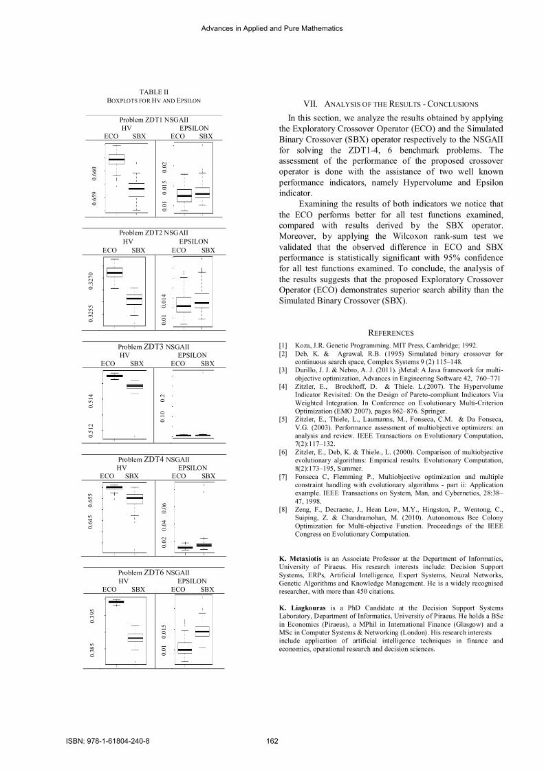
TABLE II

BOXPLOTS FOR HV AND EPSILON

Problem ZDT1 NSGAII HV EPSILON

ECO SBX ECO SBX

0

.659

0.6

60

0.01

0

.015

0

.02


ECO SBX ECO SBX

0.3

255

0.

3270

0.01

0

.014


ECO SBX ECO SBX

0.51

2

0.51

4

0

.10

0

.2


ECO SBX ECO SBX

0.6

45

0.6

55

0.0

2

0.04

0

.06


ECO SBX ECO SBX

0

.385

0.3

95

0

.01

0.

015

VII. ANALYSIS OF THE RESULTS - CONCLUSIONS In this section, we analyze the results obtained by applying

the Exploratory Crossover Operator (ECO) and the Simulated Binary Crossover (SBX) operator respectively to the NSGAII for solving the ZDT1-4, 6 benchmark problems. The assessment of the performance of the proposed crossover operator is done with the assistance of two well known performance indicators, namely Hypervolume and Epsilon indicator.

Examining the results of both indicators we notice that the ECO performs better for all test functions examined, compared with results derived by the SBX operator. Moreover, by applying the Wilcoxon rank-sum test we validated that the observed difference in ECO and SBX performance is statistically significant with 95% confidence for all test functions examined. To conclude, the analysis of the results suggests that the proposed Exploratory Crossover Operator (ECO) demonstrates superior search ability than the Simulated Binary Crossover (SBX).

REFERENCES [1] Koza, J.R. Genetic Programming. MIT Press, Cambridge; 1992. [2] Deb, K. & Agrawal, R.B. (1995) Simulated binary crossover for

continuous search space, Complex Systems 9 (2) 115–148. [3] Durillo, J. J. & Nebro, A. J. (2011). jMetal: A Java framework for multi-

objective optimization, Advances in Engineering Software 42, 760–771 [4] Zitzler, E., Brockhoff, D. & Thiele. L.(2007). The Hypervolume

Indicator Revisited: On the Design of Pareto-compliant Indicators Via Weighted Integration. In Conference on Evolutionary Multi-Criterion Optimization (EMO 2007), pages 862–876. Springer.

[5] Zitzler, E., Thiele, L., Laumanns, M., Fonseca, C.M. & Da Fonseca, V.G. (2003). Performance assessment of multiobjective optimizers: an analysis and review. IEEE Transactions on Evolutionary Computation, 7(2):117–132.

[6] Zitzler, E., Deb, K. & Thiele., L. (2000). Comparison of multiobjective evolutionary algorithms: Empirical results. Evolutionary Computation, 8(2):173–195, Summer.

[7] Fonseca C, Flemming P., Multiobjective optimization and multiple constraint handling with evolutionary algorithms - part ii: Application example. IEEE Transactions on System, Man, and Cybernetics, 28:38–47, 1998.

[8] Zeng, F., Decraene, J., Hean Low, M.Y., Hingston, P., Wentong, C., Suiping, Z. & Chandramohan, M. (2010). Autonomous Bee Colony Optimization for Multi-objective Function. Proceedings of the IEEE Congress on Evolutionary Computation.

K. Metaxiotis is an Associate Professor at the Department of Informatics, University of Piraeus. His research interests include: Decision Support Systems, ERPs, Αrtificial Ιntelligence, Expert Systems, Neural Networks, Genetic Algorithms and Knowledge Management. He is a widely recognised researcher, with more than 450 citations. K. Liagkouras is a PhD Candidate at the Decision Support Systems Laboratory, Department of Informatics, University of Piraeus. He holds a BSc in Economics (Piraeus), a MPhil in International Finance (Glasgow) and a MSc in Computer Systems & Networking (London). His research interests include application of artificial intelligence techniques in finance and economics, operational research and decision sciences.


ISBN: 978-1-61804-240-8 162

Modelling of high-temperature behaviourof cementitious composites

Jirı Vala, Anna Kucerova and Petra Rozehnalova

Abstract—The computational prediction of non-stationary be-haviour of cementitious composites exposed to high temperature,supported by proper physical and mathematical formulations, isa rather complicated analysis, dealing with the coupled heat and(liquid and vapour) mass transfer and related mechanical effects.The macroscopic mass, momentum and energy conservationequations need to exploit available information from micro-structural considerations. The derivation and implementationof a computational model is always a compromise between themodel complexity and the reasonable possibility of identificationof material characteristics of all components and their changes.The paper presents a possible approach to such analysis, suppliedby an illustrative example, confronting computational resultsfrom a simplified model (taking only dominant physical pro-cesses into account), with experimental ones, performed in thespecialized laboratory at the Brno University of Technology.

Index Terms—Cementitious composites, high temperature be-haviour, poro-mechanics of multi-phase media, computationalsimulation.

I. INTRODUCTION

PROBLEMS concerning cementitions composites, espe-cially concrete both in its regular and more advanced

forms, as high-strength, stamped, (ultra-)high-performance,self-consolidating, pervious or vacuum concrete, limecrete,shotcrete, etc., exposed to elevated temperatures are significantand wide ranging. The increasing interest of designers ofbuilding structures in this field in several last decades has beendriven by the exploitation of advanced materials, structuresand technologies, reducing the external energy consumption,whose thermal, mechanical, etc. time-dependent behaviourcannot be predicted using the simplified semi-empirical formu-lae from most valid European and national technical standards.Such models as that of one-dimensional heat conduction with(nearly) constant thermal conductivity and capacity, give nopractically relevant results for refractory or phase changematerials, thermal storage equipments, etc. – cf. [11]. Fortu-nately, in such cases the correlation between the predicted andmeasured quantities, e. g. of the annual energy consumption ofa building, can be available, to help to optimize the design ofboth new and reconstructed building structures. This is nottrue for high temperatures leading to partial or total collapseof a structure, as those caused by thermal radiation during afire.

A lot of historical remarks and relevant references for theanalysis of structures exposed to fire can be found in [5].The physical background for the evaluation of simultaneoustemperature and moisture redistributions under such conditions

J. Vala, A. Kucerova and P. Rozehnalova are with the Brno Universityof Technology, Faculty of Civil Engineering, Czech Republic, 602 00 Brno,Veverı 95.

is based on the balance law of classical thermodynamics.However, it is not trivial to supply a resulting system ofevolution by reasonable effective constitutive relations, validat the microstructural level, despite of the complicated (typi-cally porous) material structures. Most classical approaches toevaluate temperature and moisture redistributions rely on the(semi-)empirical relations from [1]. The attempts to improvethem can be seen in various directions, with still open prob-lems and difficulties everywhere. The physical and/or math-ematical homogenization approaches applied to a referencevolume element seem to be useful. The process of cementhydration, distinguishing between anhydrous cement scale,cement-paste scale, mortar scale and macro-scale, handledby specific physical and mathematical formulations, with aposteriori scale bridging applying least squares arguments, hasbeen described in details, evaluating the hydration of particularclinker phases, in [14]. However, the thermal gains and lossesfrom chemical reactions cannot be considered as deterministicones, moreover corresponding computations just in the case ofdehydration must suffer from the lack of relevant data at somescales. The formal mathematical two-scale or similar homog-enization, introduced in [4], needs to remove assumptions ofperiodicity using stochastic or abstract deterministic homog-enization structures; this leads to physically non-transparentand mathematically very complicated formulations, whoseapplicability to the construction of practical algorithms for theanalysis of engineering problems is not clear. From such pointof view, the most promising approach of the last years seemsto be that of [9] and (in a substantially generalized version) of[8], replacing the proper homogenization by some argumentsfrom the mixture theory; this will be the principal idea evenin our following considerations in this short paper.

II. PHYSICAL AND MATHEMATICAL BACKGROUND

Following [8] (unlike [14]), for the quantification of the de-hydration process we shall work with the hydration degree Γ,a number between 0 and 1, as the part of hydrated (chemicallycombined) water mw in its standard mass, constituted usuallyduring the early-age treatment of a cementitious composite.Although the evaluation of Γ from a simple algebraic formulais not available because it must take into account the chemicalaffinity and the fact that the accessibility of water for chemicalreactions is controlled by the water content ηw inside the poresunder certain temperature T , we shall apply Γ as a knownfunction of such (or slightly transformed) variables.

The multiphase medium at the macroscopic level can beconsidered as the superposition of 4 phases: solid material,liquid water, water vapour and dry air, identified by their in-dices ε ∈ s, w, v, a. In the Lagrangian description of motion,


ISBN: 978-1-61804-240-8 163

following [16], the deformation tensor F s can be derived usingthe derivatives of displacements of particular points with re-spect to Cartesian coordinate system x = (x1, x2, x3) in the 3-dimensional Euclidean space. If ωε is a source correspondingto certain scalar quantity φε then the conservation of suchquantity can be expressed by [3], p. 4, and [6], p. 9, as

φε + (φεvεi ),i = ωε ; (1)

this formula contains the dot notation for the derivative withrespect to any positive time t, (. . .),i means the derivativewith respect to xi where i ∈ 1, 2, 3, vε

i = uεi , with uε

i

referring to displacements related to the initial geometricalconfiguration x0 = (x01, x02, x03) (for t = 0) and later alsoai = ui; the Einstein summation is applied to i and j from1, 2, 3 everywhere. For the brevity, φε will be moreover usedinstead of φεηε where ηε(n, S) is the volume fraction of thephase ε, a function of the material porosity n and the saturationS. Clearly detF s = (1−n)/(1−n0) with n0 corresponding tox0. The saturation S is an experimentally identified functionof the absolute temperature T and of the capillary pressurepc, needed later; the assumption of local thermal equilibriumyields the same values of T for all phases.

In addition to T , we have 4 a priori unknown materialdensities ρε and 12 velocity components vε

i . Assuming thatvapour and dry air are perfect gases, we are able to evaluatetheir pressures pv(ρv, T ) and pa(ρa, T ) from the Clapeyronlaw; the capillary pressure is then pc = pv + pa − pw, withthe liquid water pressure pw, or alternatively just with pc,as an additional unknown variable. In the deterioration of acomposite structure 2 crucial quantities occur: the mass mw

of liquid water lost from the skeleton and the vapour mass mv

caused by evaporation and desorption. The time evolution ofmass mw can be determined from the formally simple formulamw = Γmw

0 , with m0 related to t = 0. The vapour fraction ζremains to be calculated from the system of balance equationsof the type (1), supplied by appropriate constitutive relations.

The mass balance works withφε = ρε ,

ωs = −mw , ωw = mw − mv , ωv = mv , ωa = 0in (1). No additional algebraic relations are necessary.

Since all phases are considered as microscopically non-polar, the angular momentum balance forces only the symme-try of the partial Cauchy stress tensor τ , i. e. τij = τji for suchstress components. The formulation of the linear momentumbalance in 3 direction is more delicate. Introducing wε

i = ρεvεi

and choosing (for particular i)φε = wε

i ,

we can evaluate, using the Kronecker symbol δ, the totalCauchy stress σ in the form σij = τijδ

sε and finally setωε = σε

ij,j + ρε(gi − aεi + tεi )

in (1) where gi denotes the gravity accelerations and tεithe additional accelerations caused by interactions with otherphases, whose evaluation is possible from the Darcy law,as explained lower. The constitutive relationships for thesolid phase, e. g. those between τ and us, vs, etc., need themultiplicative decomposition into a finite number m of matrixcomponents F s = F s1 . . . F sm (elasticity, creep, damage, etc.ones) to express τ(F s1 . . . F sm, F s1 . . . F sm, . . .). For ε 6= s,

Fig. 1. Fire simulation at the Brno University of Technology: laboratorysetting (upper photo), detail of real experiment (lower photo).

introducing the dynamical viscosity µε and the permeabilitymatrix Kε

ij , depending on ρε again, we can formulate theDarcy law as

µερε(vεi − vs

i ) = Kεij(ρε(gj − aε

j + tεj)− pε,j) . (2)The energy balance inserts

φε =12wε

i vεi + ρεκ

ε

with κε usually defined as cεT , using the thermal capacitiescε, in general functions of T and pc again, and some internalheat fluxes qε

i , and alsoωε = (σε

ij,j + qεi ),j + (gi − aε

i + tεi ) +$ε ,

$s = −mwhw , $w = mwhw − mvhv , $v = mvhv ,

$a = 0into (1); two new characteristics here are the specific enthalpiesof cement dehydration hw and evaporation hv . The internalheat fluxes qε

i come from the constitutive relationqεi = −λε

ijT,j − ξεijp

c,j ; (3)

the first (typically dominant) additive term corresponds to thewell-known Fourier law of thermal conduction, the second oneto the Dufour effect, with some material characteristics λε

ij

and ξεij dependent on T and pc. Similarly to (3), it is possible

derive the diffusive fluxes rεi = ρε(vε

i − vsi ) with i ∈ v, w

in the formrεi = −ςεijT,j − γε

ijpc,j , (4)

due to the Fick law (the second additive term), respecting theSoret effect (the first one), with some material characteristicsςεij and γε

ij dependent on T and pc.Now we have 4 mass balance equations, 3×4=12 momen-

tum ones and 4 energy ones, in total 20 partial differentialequations of evolution for 3 groups of variables:

R = (ρs, ρw, ρv, ρa) ,V = (vs

1, vs2, v

s3, v

w1 , v

w2 , v

w3 , v

v1 , v

v2 , v

v3 , v

a1 , v

a2 , v

a3 ) ,

T = (T, pc,mv, ζ) ,


ISBN: 978-1-61804-240-8 164

Fig. 2. Time development of temperature T .

supplied by appropriate initial and boundary conditions,e. g. for a priori known values of all variables for t = 0 ofthe Dirichlet, Cauchy, Neumann, Robin, etc. types, for localunit boundary outward normals n(x) = (n1(x), n2(x), n3(x))in particular• σijnj = ti with imposed tractions ti,• (ρa(va

i − vsi ) + ra

i )ni = ra with imposed air fluxes ra,• (ρw(vw

i −vsi )+rw

i +ρv(vvi −vs

i )+rvi )ni = rw+rv+β(ρv)

with imposed liquid water and vapour fluxes rw, rv andsome mass exchange function β,

• (ρw(vwi − vs

i )hv − λijT,j − ξεijp

c,j)ni = q + α(T ) with

imposed heat fluxes and some heat exchange function α,e. g. by the Stefan - Boltzmann law, proportional to T 4.

This seems to be a correct and complete formulation for theanalysis of time development of R, V and T .

III. COMPUTATIONAL PREDICTION

Unfortunately, a lot of serious difficulties is hidden in theabove presented formulation, e. g. the still missing “MilleniumPrize” existence result on the solvability of Navier - Stokesequations (cf. the “mysteriously difficult problem” of [15],p. 257), the physical and mathematical incompatibilities like[7], as well the absence of sufficiently robust, efficient andreliable numerical algorithms based on the intuitive time-discretized computational scheme:

1. set R, V and T by the initial conditions for t = 0,2. go to the next time step, preserving R, V and T ,3. solve some linearized version of (1) with the mass

balance choice, evaluate and perform the correction εR,4. solve some linearized version of (1) with the momentum

balance choice, evaluate and perform the correction εV ,5. solve some linearized version of (1) with the energy

balance choice, evaluate and perform the correction εT ,

Fig. 3. Time development of pressure pc.

6. if εR, εV and εT are sufficiently small, return to 3,7. stop the computation if the final time is reached, other-

wise return to 2.

Consequently all practical computational tools make use ofstrong simplifications. The rather general approach of [8] in-troduces the additive linearized strain decomposition instead ofthe multiplicative finite strain one, ignores some less importantterms, as the kinetic energy (the first additive term in φε) inthe energy balance interpretation of (1), as well as the Dufourand Soret effects in (3) and (4), and reduces the number ofvariables, comparing (2) with the differences vε

i −vsi with ε ∈

v, w, a from the momentum balance interpretation of (1),and presents a computational scheme of the above sketchedtype, applying the Galerkin formulation and the finite elementtechnique. Nevertheless, most engineering approaches, as [2]or [12], endeavour to obtain a system of 2 equations ofevolution for T and pc (or some equivalent quantity) only, pre-eliminating or neglecting all remaining ones, using argumentsof various levels: from micro-mechanically motivated physicalconsiderations to formal simplification tricks.

The reliability of computational results depends on thequality and precision of input data, including the designand identification of all material characteristics. Probably allauthors take some of them from the literature, not from theirextensive original experimental work; the variability of formsof such characteristics and generated values, accenting thosefrom (2), including the formulae from [8], has been discussedin [5]. Nevertheless, the proper analysis of uncertainty andsignificance of particular physical processes lead to even morecomplicated formulations, analyzed (for much easier directmodel problems) in [17] using the spectral stochastic finiteelement technique, or in [10] the Sobol sensitivity indices, inboth cases together with the Monte Carlo simulations.


ISBN: 978-1-61804-240-8 165

Fig. 4. Time development of moisture content ρw + ρv .

Unlike most experiments in civil and material engineering inlaboratories and in situ, nearly no relevant results for advancednumerical simulations are available from real unexpected fires,as the most dangerous conditions for building structures,crucial for the reliable prediction of behaviour of concreteand similar structures. Since also laboratory experiments withcementitious composites under the conditions close to a realfire, as that documented on Figure 1, performed at the BrnoUniversity of Technology, are expensive, producing incom-plete and uncertain quantitative data anyway, the reasonablegoal of numerical simulation is to test simple numericalmodels with acceptable correlation with real data, as the firststep for the development of more advanced multi-physicalmodels.

Figures 2, 3 and 4 are the outputs from a rather simpletwo-dimensional isotropic model, neglecting mechanical loads,strains and stresses, compatible with the slightly modified andrevisited approach of [2], combining the finite element andvolume techniques together with the iterated time discretiza-tion scheme (the numerical construction of Rothe sequences),implemented in the MATLAB environment. The fire is consid-ered as the boundary thermal radiation on the left and upperedges of the rectangle. Surprisingly some phenomena observedin situ can be explained from the deeper analysis of results ofsuch seemingly simple calculations.

IV. CONCLUSION

Development of reasonable models and computational algo-rithms for the prediction of thermal, mechanical, etc. behaviourof cementitious composites and whole building structures, isstrongly required by the applied research in civil engineering,which cannot be ignored, although the formal mathematicalverification of such models is not available and the practicalvalidation suffers from the lack of data from observations

in situ, as well as of large databases from relevant (veryexpensive) experiments. The first steps, both in the sufficientlygeneral formulation of the problem, containing most prac-tical computational approaches as special ones, as well asthe methodology of computational and experimental work,sketched in this paper, should be a motivation for furtherextensive research.

ACKNOWLEDGMENT

This research has been supported by the research projectFAST-S-14-2490 at Brno University of Technology, in collab-oration with the research project FAST-S-14-2346.

REFERENCES

[1] Z. P. Bazant, W. Thonguthai, Pore pressure and drying of concrete athigh temperature. Journal of the Engineering Mechanics Division 104,1978, pp. 1059–1079.

[2] M. Benes, R. Stefan and J. Zeman, Analysis of coupled transportphenomena in concrete at elevated temperatures. Applied Mathematicsand Computation 219, 2013, pp. 7262–7274.

[3] A. Bermudez de Castro, Continuum Thermomechanics. Birkhauser,2005.

[4] D. Cioranescu and P. Donato, An Introduction to Homogenization.Oxford University Press, 1999.

[5] C. T. Davie, C. J. Pearce and N. Bicanic, Aspects of permeability inmodelling of concrete exposed to high temperatures. Transport in PorousMedia 95, 2012, pp. 627–646.

[6] J. H. Ferziger and M. Peric, Computational Methods for Fluid Dynamics.Springer, 2002.

[7] T. Furst, R. Vodak, M. Sır and M. Bıl, On the incompatibility ofRichards’ equation and finger-like infiltration in unsaturated homoge-neous porous media. Water Resource Research 45, 2009, W0340, 12 pp.

[8] D. Gawin and F. Pesavento, An overview of modeling cement basedmaterials at elevated temperatures with mechanics of multi-phase porousmedia. Fire Technology 48, 2012, pp. 753-793.

[9] D. Gawin, F. Pesavento and B. A. Schrefler, Simulation of damageperme-ability coupling in hygro-thermo-mechanical analysis of concrete at hightemperature. Communications in Numerical Methods and Engineering18, 2002, pp. 113-119.

[10] J. Gottvald and Z. Kala, Sensitivity analysis of tangential digging forcesof the bucket wheel excavator SchRs 1320 for different terraces. Journalof Civil Engineering and Management 18, 2012, pp. 609–620.

[11] P. Jarosova and S. Stastnık, Modelling of thermal transfer for energysaving buildings. International Conference on Numerical Analysis andApplied Mathematics 2013 – Proceedings, American Institute of Physics,2013, pp. 1000–1003.

[12] V. Kocı, J. Madera, T. Korecky, M. Jerman and R. Cerny, Computationalanalysis of coupled heat and moisture transport in building envelopes:the effect of moisture content. Thermophysics 2013 – Conference Pro-ceedings in Podkylava (Slovak Republic). Slovak Academy of Sciencesin Bratislava, 2013, pp. 62–71.

[13] G. Nguetseng and N. Svanstedt, σ-convergence. Banach Journal ofMathematical Analysis, 5, 2011, pp. 101–135.

[14] Ch. Pichler, R. Lackner and H. A. Mang, Multiscale model of creep ofshotcrete – from logarithmic type viscous behaviour of CSH at the µ-m scale to macroscopic tunnel analysis. Journal of Advanced ConcreteTechnology 6, 2008, pp. 91–110.

[15] T. Roubıcek, Nonlinear Partial Differential Equations with Applications.Birkhauser, 2005.

[16] L. Sanavia, B. A. Schrefler and P. Steinmann, A formulation for an unsat-urated porous medium undergoing large inelastic strains. ComputationalMechanics 1, 2002, pp. 137–151.

[17] N. Zabaras, Inverse problems in heat transfer. In: Handbook on Numer-ical Heat Transfer (W. J. Minkowycz, E. M. Sparrow and J. S. Murthy,eds.), Chap. 17. John Wiley & Sons, 2004.

Jirı Vala (*1956) is professor of the Institute of Mathematics and DescriptiveGeometry at the Brno University of Technology, Faculty of Civil Engineering.Anna Kucerova (*1985) and Petra Rozehnalova (*1984) are Ph.D. studentsat the same university.


ISBN: 978-1-61804-240-8 166

Gaussian Mixture Models Approach for Multiple Fault Detection -DAMADICS Benchmark

Erika Torres, Edwin Villareal

Abstract—In fault detection, data-driven methods are limitedby the lack of knowledge about faults. This paper presents anapproach based in statistical modeling, which uses normal oper-ation information for training a Gaussian Mixture Model. Suchmodel has been widely used in speaker verification, because iscapable of mapping the observations into a multidimensionalmembership function, this feature makes this algorithm veryconvenient because works in a unsupervised way. This techniqueuses the normal behavior data to estimate the parameters andthen classify future data according to the model. The proposedapproach consists of two stages: an offline stage, where theGaussian model is trained by using Expectation-Maximizationalgorithm; and the online stage, where the readings likelihoodis evaluated according to the normal operation model. If thelikelihood is found to be inferior to a certain threshold, afault is detected. This approach may be extended to multipleprocesses in science and engineering; for instance, a case studyis presented using the DAMADICS benchmark, where thisapproach was validated.

Keywords—Fault Detection, Gaussian Mixture Models, Indus-trial Processes

I. INTRODUCTION

AS the industrial processes complexity keeps increasing,fault detection has become a critical issue in order to

meet safety, enviromental and productivity requirements.In this regard, several approaches have been proposed,particularly, being artificial intelligence methods the currenttrend. However, one of the main drawbacks of thesemethods is the implementation complexity for a realindustrial environment, which limits its appeal for mostindustrial applications. Hence, approaches that may incurin a lower complexity while keeping acceptable results arehighly favored. The approach presented in this paper aimsat this paradigm.

Computer-based solutions have been proposed to meetthe aforementioned requirements, for instance, machinelearning methods, see [1], like Bayesian Learning methods[2], Self-Organizing Maps [3], or PCA [4],etc. The mainobjective of these methods is to transform the monitoringdata (usually sensors) into statistical models, in order toclassify and detect anomalies. Since the analytical modelis not taken into account, the method remains flexible forimplementation in different environments.

However, a shortcoming of artificial intelligence methodsis the need of data from different anomalies or failures totrain the model. Some systems have low on-site failure rate,and as a consequence, the amount of failure data availableis limited, see [5]. In this paper, a GMM approach for faultdetection is proposed, to overcome the lack of failure data, asthis method can be trained using only normal operation data.

Regarding industrial processes, failures usually occurin sensors, actuators or processes. The main purpose offault detection is to evaluate symptoms, which indicate thedifference between normal and faulty states. As such, andtaking into account the performed observation, the methodsof failure detection are divided into three categories:signal threshold, signal model and process model basedapproaches, see [6].

From the taxonomy of failure detection presentedpreviously, the proposed approach in this paper falls withinthe signal model-based category, as it extracts the statisticalfeatures of the process from the sensor readings, where thetraining is taking place off-line. As such, this approach issuitable for real-time applications, because the operationsrequired for classification can be calculated in small batcheswhile new data is being read.

This paper is organized as follows. Firstly, A brief re-view of GMM is presented, fault detection by using GMMis described in Section 3. The proposed scheme is vali-dated by simulation examples of Chemical Plant Benchmark(DAMADICS) in Section 4. Finally, we present the conclu-sions obtained from the implementation and discuss futurework.

II. GAUSSIAN MIXTURE MODELS

Gaussian mixture models are commonly used instatistical analysis. In most applications, its parameters aredetermined by using Maximum Likelihood and ExpectationMaximization algorithm.

As industrial processes are influenced by multiple facts,like temperature, noise and environmental conditions, it isrequired to include adequate modelling to these variables.The GMM has the capability of representing a large classof sample distributions, which is a very useful tool forthe characterization of multiple problems, like speakerrecognition, see [7].

In the context of fault detection systems, the usage of aGMM for representing features distributions, is motivatedby the notion that the individual component densities canmodel a set of hidden classes. In the same context, weassume that the features in the normal operation spacecorrespond to different hidden classes. We assume that if welearn a Gaussian Mixture Model with sufficient variability ofnormal operation behavior, then the model will be capableof distinguish between any state different than the normalone. Because all the features used to train the GMM areunlabeled, the healthy state classes are hidden in a class ofan observation that is unknown.


ISBN: 978-1-61804-240-8 167

MAY 2014 2

The mixture model is a convex combination of unimodalgaussian functions:

p(x|λ) =M∑i=1

wig(x|µi,Σi) (1)

M∑i=1

wi = 1 (2)

where wi are the mixing coefficients and the parameters ofthe of the component density functions p(x|λ) which usuallyvary with i.

g(x|µi,Σi) =1

(2π)D/2|Σi|1/2exp

(− (x− µi)

T (x− µi)

2Σi

)(3)

where g(x|µi,Σi) are the component Gaussian densities. Theset of parameters is λi = (wi, µi,Σi), where i = 1, . . . ,M ,M is the GMM model size, µi and Σi are the mean andcovariance matrix of the ith GMM component, respectively:Finally, D is the dimension of vector x.

To determine the ”membership” of the data point x to theith GMM component, the loglikelihood of the data point,of each individual model distribution is calculated using theEquation 4 . An implementation of this algorithm for Matlabcan be found at [8].

log p(x|λ) =T∑

t=1

log p(xt|λ) (4)

A. Expectation Maximization Algorithm for Gaussian Mix-tures

Given a set of training vectors and a GMM configura-tion (model size, minimum variance, which are determinedheuristically),the parameters of the GMM λ are left to beestimated. These parameters, should lead to the best match(in the maximum likelihood sense) for the distribution ofthe training features vectors. There are several techniquesavailable for estimating the parameters of the GMM, beingMaximum Likelihood (ML) the most used method. The aimof ML estimation is to find the model parameters whichmaximize the likelihood of the GMM given the training data.For a sequence of T training vectors X = x1, . . . , xT ,the GMM likelihood, assuming independence between thevectors, can be written as

p(X|λ) =T∏

t=1

p(xi|λ) (5)

Unfortunately, for this expression direct maximization is notpossible. This equation, however, can be solved iterativelyusing a special case of the EM algorithm. The goal of thisalgorithm is to maximize the likelihood function (Equation4) according to the parameters: means, covariances and themixing coefficients for all the components. The process isdivided in the following stages:

1) Initialize the means µi , covariances σi and mixingcoefficients wi, and evaluate the initial value of thelikelihood.

GMM (λ)Observation Vector -logP(O|λ)

Feature adquisition Model Training Scoring and Thresholding

Off-line Stage On-line Stage

Fig. 1. Block diagram for fault detection by using GMM

2) Evaluate probabilistic distance using the current pa-rameter values

wi =1

T

T∑t=1

Pr(i|xt, λ) (6)

µi =

∑Tt=1 Pr(i|xt, λ)xt∑Tt=1 Pr(i|xt, λ)

(7)

σ2i =

∑Tt=1 Pr(i|xt, λ)x2t∑Tt=1 Pr(i|xt, λ)

− µi (8)

3) Calcule the aposteriori data probabilities.

Pr(i|xt, λ) =wig(xt|µi,Σi)∑M

k=1 wkg(xt|µk,Σk)(9)

4) Calcule the error, which is the negative of the likeli-hood function.

5) Go back to step 2 until the error change is very smallor the number of iterations is reached (usually 15-20).

where σ2,xt, and µi, refer to arbitrary elements of the vectorsσ2, xt, and µi respectively.

III. FAULT DETECTION USING GMMThe main advantage of using Gaussian Mixture Models,

is that the model can be trained with normal operation data,without further information about the multiple failure states,which can be unknown at the moment. This advantage,allows the detection of multiple failure states even if aparticular failure is happening for the very first time.

The signals can be used directly or transformed to extractmore interesting features for the detection task. In this articlewe use the raw signals to learn the model.

The principle of this method consists of two phases: afirst phase during which an statistical model is learned usingthe Expectation Maximization algorithm; and a secondphase where the learned model is used to score the currentsystem condition, as it is shown in Figure 1. If the maximumlikelihood score exceeds certain threshold, then the detectionsystem triggers a failure alarm.

The proposed method described in the Algorithm 1, isa data-based technique which mainly uses the sensor data(consisting as well of normal operating data called xtr )gathered during a significant period of time to adjust theparameters of a Gaussian mixture model called λ of sizeM . The threshold is obtained using validation data (alsonormal operation data), called xv . The obtained model useslog Likelihood to distinguish between data that is ”normal”,and the data that is ”anomalous”, the data set for testing


ISBN: 978-1-61804-240-8 168

MAY 2014 3

is called xt. In the algorithm the testing data is fed to themodel through a window of time, in order calculate theloglikelihood when sufficient data is gathered.

Algorithm 1 Fault detection by using Gaussian MixtureModels

1: procedure FDGMM(train data)2: Organize train data in a matrix called xtr.3: Set the parameters for the algorithm.4: λ0=kmeans(xtr).5: λ=gmmEM(xtr,M ,λ0)6: l=loglikelihood(xv ,λ).7: Set the likelihood threshold ε according to l,to detect

a failure.8: for xt(1:window:end) do9: l=loglikelihood(xt,λ)

10: if l< ε then11: Hey, something is really wrong.12: else13: Everything is cool14: end if15: end for16: end procedure

IV. THE TESTING BENCHMARK DAMADICSThis benchmark was proposed in 2003 [9] to help the

development of fault detection methods in a industry environ-ment. The process has multiple sensors and actuators whichcan present different types of failure, abrupt and incipient.From the repository we use the normal behavior data to trainthe model, and the failure data to test the results. The faultydata is scarce, but we simulated 30 cases to test our approachwith the simulink tool available in the repository.

V. EXPERIMENTS

To validate the functionality of the algorithm we use theDAMADICS benchmark. This database was created to testfault detection algorithms with real data and simulations.The authors provided libraries to simulate 19 types offaults from three actuators with two different degreesof ocurrence (Abrupt, Incipient). In this experiment wemonitor three signals: controller output, upstream pressureand downstream pressure.

In Table I, the analysed fault types are presented, andthe fault scenarios that are derived from them. As themonitoring of root causes for a faulty event is a verydifficult task for the operators, it follows to infer the stateof the process, from key variables belonging to it.

A. Data generationThe actuator model is simulated using Matlab Simulink

and the libraries provided in DAMADICS webpage. Theavailable data is separated into three sets, one for training(1 st to 4th of November), a second for validation (5th ofNovember) and other for testing (October 30th, November9th and November 17th). The observation sequences are

0 10 20 30 40 50 60 70 80 90 1000

0.1

0.2

0.3

0.4

0.5

0.6

0.7

0.8

0.9

1

Time (Window of 1000 secs)

Nor

mal

ized

Log

like

lihoo

d

Fig. 2. Normalized Loglikelihood for fault 16, corresponding to November30th. This picture indicates that the failure occurred near to the time windownumber 60.

10 20 30 40 50 60 70

0.1

0.2

0.3

0.4

0.5

0.6

0.7

0.8

0.9

1

Time (Window of 1000 secs)

Nor

mal

ized

Log

like

lihoo

d

Fault 16

Fault Threshold

Fault 18

Fig. 3. Normalized Loglikelihood for data set, corresponding to November17th, where multiple types of faults occurred. In this picture we can see thatthree faults occurred after the time window number 50.

sensors and valves readings, whose size depends on thefailure mode, for this article we only consider the 16, 17 and18 faults, which are general external failures. The model sizewas determined heuristically, as well the minimum varianceand detection threshold.

B. Model identification

The goal of this stage is to obtain a GMM for normaloperation data. The data set concerning the failures is usedonly in the testing stage. The first step uses the k-meansalgorithm to locate the centroids for the initial parameters.The second step relies in the EM algorithm to estimate

TABLE I. FAULTS UNDER ANALYSIS

Date Fault type Description

October 30th 18 Partially opened bypassvalve

November 9th 16 Positioner supply pressuredrop

November 17th 17 Unexpected pressure dropacross the valve


ISBN: 978-1-61804-240-8 169

25 30 35 40 45 50 55

2

4

6

8

10

12

14

x 104 Frequency Distribution Normal Operation Data (Three variables case)

Fre

quen

cy

25 30 35 40 45 50 55

2

4

6

8

10

12

14

x 104 Estimated Gaussian Mixture Model Normal Operation Data (Three variables case)

seconds

Fre

quen

cy

LC5103CV

LC5103X

LC5103PV

Fig. 4. Upper: Histogram of Normal operation data set corresponding to November 1st to 5th for training purposes. Below: Histogram of learned GaussianMixture model.

the GMM parameters, where the covariance matrices areset to be diagonal. The appropriate size of the model isdetermined, in order to obtain trustworthy results. Also, thebest minimum covariance threshold is found, to ensure thatthe model converges and remains sensitive to variances indata. The model selection is based on the likelihood functionevaluated over the validation set. The result is a model forthe normal operation data which detects anomalies in theprocess by using loglikelihood function.

C. Testing the ModelA data set representing an operating condition as shown

in Figure 4 is fed to the GMM model. This data set iscomposed by data of the three previously mentioned signals,between November 1st-4th. The whole data set has 345600data points for each signal, which is equivalent to 4 days ofoperation.

From the data set, we calculate the loglikelihood score andnormalize it by the number of samples in the window (set to1000 secs). If the data set score is lower than the threshold ε,the algorithm detects an anomaly. The model is tested withdifferent types of faults, being important to note that the userhas to set the threshold according to the sensibility desired.

VI. RESULTS AND DISCUSSION

A set of observation sequences belonging to a particularfault scenario are fed to the model. The results for bothmonitoring tasks and detection, are shown in the Figures 2and 3. These figure show how the score decreases drasticallywhen a fault is detected. The fault scenario corresponds toOctober 30th, and 17th of November. We set the threshold

to 0.82 for normalized likelihood. Every one of the faultsexpected in every day, was detected by the algorithm. Toprove the robustness of the algorithm, we use simulateddata, for normal behavior data we use 100 tests and forfaulty behavior we use 30 test. The results for false alarmwas 6% and false rejection was 1%. This numbers changeaccording to the threshold but these were the best found inthe experiments.

VII. CONCLUSION

A fault detection system based on GMM was developed.Using the DAMADICS benchmark actuator system it waspossible to verify its capabilites regarding monitoring tasks.With a model of normal operations was able to detectfault events immediately after its occurrence. This patternrecognition tool plays an important role when fault eventdata is scarce, and we have plenty of normal operation data.Besides, by using a temporal sequence of observations asmodel input, the model may be trained again if there are anychanges in the behavior of the process, with the posibilityof adding even more signals, which can be a daunting taskwith model based methods.

The results are very promising concerning to theapplication of GMM in chemical process monitoring. In thefuture, these results can be used along with decision treesto include a fault diagnosis stage, as a complement for theproposed system. It follows from the results obtained, thatthe proposed approach may have further applications in themonitoring of other industrial procesess as well, leading toprospective opportunities for research and development.


ISBN: 978-1-61804-240-8 170

MAY 2014 5

In real world fault detection is important the aplicabilityof the solutions, in this article we aim to solve some issuesthat are common in data-based methods. Such as the lackof failure information, and the training of multiple modelswhich can be very expensive and impractical. The resultsshow that with only normal operation data is possible tolearn a model that is capable of detect anomalies in multiplesignals. This solution is very flexible, can be applied to manysituations and only requires be trained once, this fact makesthis solution ideal for real time applications. In the futurethis solution can be improved if is combined with MaximumAposteriori adaptation and decision trees for diagnosis tasks.

REFERENCES

[1] Y. Guo, J. Wall, and J. L. andSam West, “A machine learning approachfor fault detection in multi-variable systems,” in ATES in conjunctionwith Tenth Conference on Autonomous Agents and Multi-Agent Systems(AAMAS) AAMAS 2011, 2011.

[2] J. P. Matsuura, A. Iees, P. Marechal, E. Gomes, T. Yoneyama,R. Kawakami, and H. Galvo, “Learning bayesian networks for faultdetection,” in In Proceedings of the IEEE Signal Processing SocietyWorkshop, 2004, pp. 133–142.

[3] T. Chopra and J. Vajpai, “Classification of faults in damadics bench-mark process control system using self organizing maps,” InternationalJournal of Soft Computing and Engineering (IJSCE) ISSN: 2231-2307,Volume-1, Issue-3, July 2011, vol. 1 (3), pp. 85–90, 2011.

[4] J. Sun, Y. Li, and C. Wen, “Fault diagnosis and detection based on com-bination with gaussian mixture models and variable reconstruction,” inInnovative Computing, Information and Control (ICICIC), 2009 FourthInternational Conference on, 2009, pp. 227–230.

[5] F. Nelwamondo and T. Marwala, “Faults detection using gaussianmixture models, mel-frequency cepstral coefficients and kurtosis,” inSystems, Man and Cybernetics, 2006. SMC ’06. IEEE InternationalConference on, vol. 1, 2006, pp. 290–295.

[6] A. Shui, W. Chen, P. Zhang, S. Hu, and X. Huang, “Reviewof fault diagnosis in control systems,” in Proceedings ofthe 21st annual international conference on Chinese controland decision conference, ser. CCDC’09. Piscataway, NJ,USA: IEEE Press, 2009, pp. 5360–5369. [Online]. Available:http://dl.acm.org/citation.cfm?id=1714810.1715162

[7] D. A. Reynolds, T. F. Quatieri, and R. B. Dunn, “Speaker verificationusing adapted gaussian mixture models,” in Digital Signal Processing,2000, p. 2000.

[8] I. Nabney, NETLAB: Algorithms for Pattern Recognition, ser. Advancesin Computer Vision and Pattern Recognition. Springer, 2002. [Online].Available: http://books.google.com.co/books?id=LaAAJP1ZxBsC

[9] M. Syfert, R. Patton, M. Bartys, and J. Quevedo, “Development andapplication of methods for actuator diagnosis in industrial controlsystems (damadics): A benchmark study.” Proceedings of the IFACSymposium Safe Process, pp. 939–950, 2003.


ISBN: 978-1-61804-240-8 171

Keywords—Spine, ergonomics, vehicle, musculoskeletal affections.

Abstract—The aim of this study is to determine a analytical

expression in the coronal plane of the drivers spine while driving along curved roads and also to determine ergonomic parameters for the car seat design. To determine the analytical expression and the ergonomic parameters, an experiment was developed to monitor the position variation in time of the vertebras in the coronal plane. The result lead to three sinusoidal equations. The amplitude values of the sinusoidal functions describing the variation in time of angles between the vertebras gives an image regarding the deformation degree of the intervertebral discs.

I. INTRODUCTION HE possibility to drive in complete healthy and safety conditions not only for the professional drivers but also

for the rest of the population which uses vehicles as frequent transportation means leads to efficiency by improving the quality of life.

In this context it is noted the following objectives and research directions: the development of modern mathematical models and principles to be included in a design or control algorithm.

The present study is based on the egronomical research regarding the spine’s behavior while driving along curved roads.

II. ANALYTICAL EXPRESSION OF THE SPINE IN THE CORONAL PLANE

The optimal ergonomic body posture of the driver sitting in the car seat is influenced by the structural characteristics of the seat. The body has to be constrained to the seat such way so that the spine’s form is an ideal anatomical or ergonomic optimal shape. Therefore to design and construct the car seat, it is proposed to start from the ideal anatomical shape of the spine in the coronal plane (Fig. 1). [2, 3]

To determine the design parameters of the car seat is necessary to know the analytical form of the spine’s shape in the coronal plane.

In the coronal plane, the shape of the spine can be expressed mathematically by the equation of a straight vertical line. Vertebrae centers are collinear. Considering a reference

system as in figure 2, the vertical line’s equation containing vertebras centers is considered to be x = 0.

Fig. 1- Anatomical planes.

Point O, the origin of the coordinate system coincides with the lowest point of the coccyx.

The analytical expression x = 0 of the spine’s shape in the coronal plane is only valid if the vehicle is at rest, or the vehicle travels on a rectilinear continuous road (unreal case).

Due to the centrifugal force acting on the human body while the vehicle is traveling along a, the human body changes its posture in the coronal plane in the opposite direction of the centrifugal force, to maintain the balance in the car seat. Thus the spine’s shape changes depending on the vehicle’s traveling speed and the curved path’s radius, causing the spine shape mathematical expression in the coronal plane to be a motion law.

The spine shape is the line containing the centers of the vertebras. Anatomically, the shape and movement of the spinal column are shown by the relative rotational movement between the vertebras. According to anatomy and kinematic studies of the human spine, it is concluded that the center of rotation between two vertebras is the center of the intervertebral disc that connects the two vertebras. Thus

Analytical and experimental modeling of the drivers spine

Veronica Argesanu, Raul Miklos Kulcsar, Ion Silviu Borozan, Mihaela Jula, Saša Ćuković, Eugen Bota

T


ISBN: 978-1-61804-240-8 172

https://www.facebook.com/profile.php?id=1409907364

intervertebral disc can be considered a ball joint with three degrees of freedom corresponding to rotation after three axes.

In figure 3 are shown as an example, L3 and L4 vertebras centers as CL3 and CL4 points, and the rotation centers of the L2, L3, L4 and L5 vertebras, as CrL2-L3-L4 and CrL4 CrL3-L5.

Fig. 2. – The spine in the coronal plane related to the coordinate

system xOy.

Fig. 3 - L3 and L4 vertebras centers (CL3 and CL4), and the rotation

centers of the L2, L3, L4 and L5 vertebras (CrL2-L3-L4 and CrL4 CrL3-L5).

Considering the vertebras in the coronal plane as represented by segments connecting the rotation centers, the shape of the spine may be given by the angles αi of these segments.

Figure 4 represents the lumbar segment in the coronal plane. The L1, L2 ... L5 vertebras are the CrT12-L1CrL2-L3-L3 CRL1-L2CrL2, CrL2-L3CrL3-L4-S1 ... CrL4-L5CrL5 segments. The relative rotation between two vertebras is given by the angle αi between the segments representing the two vertebras.

Fig. 4 – The lumbar spine with the segments representing L1, L2 ...

L5 vertebras.

The motion law of the spine in the coronal plane can be expressed as a function of the vehicle speed (va), the curved trajectory radius (rtr) and the upper body mass (mcs), function that returns the values of the αi angles.

(1)

To determine the function given by relation (1), we created an experiment that for a given route and a constant driving speed, the upper body movements in the coronal plane were monitored.

Fig. 5 - The route used in the experiment.


ISBN: 978-1-61804-240-8 173

The track used in the experiment is the same track used to determine the dynamic cornering ability of the vehicles (fig. 5).[29]

In the experiment we used the motion sensor manufactured by PASCO scientific and the PASCO CI-6400 Science Workshop 500 Interface (fig. 7).

The motion sensor MotionSensor II (fig. 6) operates on the sonar principle. The sensor can measure distances between 0.15m and 8m, between it and the object of interest (fig. 6).

Fig. 6 – Motion Sensor II.

Fig. 7 - PASCO CI-6400 Science Workshop 500 Interface.

Before measurements, the motion sensor must be calibrated. In this experiment the driver's upper body sideway

movements in the coronal plane were monitored. To monitor the movements in the coronal plane the motion sensor was used to determine the positions in time of three points on the driver's body right side. In figure 8 is shown the positioning of the sensor. The first point is on the right side of the C1 vertebra, located at a distance of dC = 0.477m from the sensor. The second point is placed on the right shoulder on the T4 vertebra’s right side, located at a distance of dT = 0.39m from the sensor. The third point is located next to the L1 vertebra located at a distance of dL = 0.419m from the sensor.

In figure 9 is shown the sensor in the first position for determining the C1 vertebra movements. The rC, rT and rL distances from the seat surface, were determined by anthropometric measurements of the driver’s body in seated position. Thus rC = 0.8m, rT = 0.585m and rL = 0.4m.

The experiment was carried out in three stages. In each

stage the position in time of one of the three points is determined. In each stage the vehicle is traveling with a constant speed of 15km/h according to the vehicle dynamic steering ability tests. [5]

Fig. 8 - Points of interest for sensor positioning.

Fig. 9 - The sensor in the first position for determining the C1

vertebra movements.

III. THE EXPERIMENTAL RESULTS AND DATA PROCESSING The traveling time in one direction and performing a series

of measurements, is about 15s. Figures 10, 11 and 12 are presented graphically the results

of series of measurements for the three points. At each step corresponding to a point were performed seven series of measurements.

For each point were averaged seven sets of measurements. Thus the results of processing experimental data are presented graphically in figure 13.

As a first analysis of the results obtained, it can be seen that the variation in time of the position of the three points can be expressed as a sinusoidal function with the same frequency but


ISBN: 978-1-61804-240-8 174

different amplitudes.

Fig. 10 - The series of measurements for the C1 vertebra.

Fig. 11 - The series of measurements the T4 vertebra.

Fig. 12 - The series of measurements for the L1 vertebra.

Fig. 13 – Graphical representation of the positions in time of the

three points.

IV. DETERMINATION OF THE SINUSOIDAL FUNCTIONS DESCRIBING THE VARIATION IN TIME OF THE C1, T4 AND L1

VERTEBRAS POSITIONS Using the Mathcad software the position in time values for

the three points were introduced as the following strings:

cp0

01

2

3

4

5

6

7

8

9

10

11

12

13

14

15

0.4770.476

0.479

0.478

0.482

0.479

0.474

0.48

0.473

0.473

0.475

0.48

0.469

0.476

0.485

...

:= um0

01

2

3

4

5

6

7

8

9

10

11

12

13

14

15

0.390.399

0.401

0.403

0.405

0.407

0.409

0.411

0.411

0.411

0.411

0.411

0.41

0.412

0.413

...

:= lb0

01

2

3

4

5

6

7

8

9

10

11

12

13

14

15

0.4180.418

0.418

0.419

0.419

0.419

0.419

0.42

0.42

0.42

0.42

0.421

0.422

0.424

0.425

...

:=

The cp string corresponds to the C1 point, um string

corresponds to the T4 point and lb string corresponds to the L1 point.

The next step is to determine the frequency of each string.

tcpmaxi i max cp( ) cpiif

0 otherwise

:=

max tcpmax( ) 98=


ISBN: 978-1-61804-240-8 175

tcpmini i min cp( ) cpiif

0 otherwise

:=

max tcpmin( ) 83=

tummaxi i max um( ) umiif

0 otherwise

:=

max tummax( ) 99=

tummini i min um( ) umiif

0 otherwise

:=

max tummin( ) 117=

tlbmaxi i max lb( ) lbiif

0 otherwise

:=

max tlbmax( ) 70=

tlbmini i min lb( ) lbiif

0 otherwise

:=

max tlbmin( ) 86=

The time interval between the maximum and minimum for each string is determined:

(2)

(3)

(4)

In order to determine the single frequency in all three strings, the average of the three time periods is determined:

(5)

Thus, the frequency will be:

(6)

The amplitude of each string is determined as follows:

(7)

(8)

(9)

The cp string amplitude is noted acp, the um string amplitude is noted with aum, and the amplitude of the lb string is noted alb.

The sinusoidal functions describing the position variation in time of the C1, T4 and L1 vertebraes points are the following:

(10)

(11)

(12)

In the figures 14, 15 and 16 the sinusoidal functions are represented in comparison to the cp, um and lb strings graphic form. For each case can be seen that the sinusoidal functions allure is very close to the allure of the strings measured values.

In conclusion it can be considered that these sinusoidal functions can describe the position variation in time of the C1, T4 and L1 vertebra’s points, while driving on a sinusoidal trajectory.

Fig. 14 - Graphical representation of the ycp sinusoidal function

compared with the cp string.


ISBN: 978-1-61804-240-8 176

Fig. 15 - Graphical representation of the yum sinusoidal function

compared with the um string.

Fig. 16 - Graphical representation of the ylb sinusoidal function

compared with the lb string.

Fig. 17 – The sinusoidal functions describing the position variation in

time of the C1, T4 and L1 vertebras points.

Fig. 18 – The sinusoidal functions describing the position variation in

time of the C1, T4 and L1 vertebras.

The sinusoidal functions describing the position variation in time of the C1, T4 and L1 vertebras in the coronal plane are:

(13)

(14)

(15)

V. CONCLUSIONS The amplitude values of the sinusoidal functions describing

the variation in time of angles between the vertebras gives an image regarding the deformation degree of the intervertebral discs.

A nonergonomic posture of the driver’s body seated in the vehicle’s seat implies the spine to be in a shape that subjects the intervertebral discs to uneven tensions causing deformations that in some cases can exceed the limits at which the musculoskeletal affections of the spine can be avoided or treated by physiotherapy.

REFERENCES [1] Adams M. ; Bogduk N. ; Burton K. ; Dolan P. (2006). The

Biomechanics of Back Pain Second Edition, Churchill Livingstone Elsevier.

[2] Borozan I. S.; Maniu I.; Kulcsar R. M.; „Ergonomic analysis on driving an Automatic Gearbox equipped vehicle”, SACI 2012 IEEE 7th International Symposium on Applied Computational Intelligence and Informatics, May 24-26, 2012, Timisoara, Romania.

[3] Borozan I. S.; Kulcsar R. M.; “Vertebral column bioengineering analysis at bending and torsion”, International Conference on Human-Machine Systems, Cyborgs and Enhancing Devices HUMASCEND, Iasi, Romania, June 14-17, 2012.

[4] Goran Devedžić, Saša Ćuković, Vanja Luković, Danijela Milošević, K. Subburaj, Tanja Luković, "ScolioMedIS: web-oriented information system for idiopathic scoliosis visualization and monitoring", Journal of Computer Methods and Programs in Biomedicine, Vol.108, No.-, pp. 736-749, ISSN -, Doi 10.1016/j.cmpb.2012.04.008, 2012.

[5] Hilohi C., Untaru M., Soare I., Druţa Gh., „Metode si mijloace de incercare a automobilelor”, Editura Tehnică București, 1982.

[6] Hinza B., Seidel H., „The significance of using anthropometric parameters and postures of European drivers as a database for finite-


ISBN: 978-1-61804-240-8 177

element models when calculating spinal forces during whole-body vibration exposure”, International Journal of Industrial Ergonomics, Elsevier, 2008.

[7] Kolich M., „A conceptual framework proposed to formalize the scientific investigation of automobile seat comfort”, Applied Ergonomics, Elsevier, 2008.

[8] Kulcsar R. M.; Madaras L.; “Ergonomical study regarding the effects of the inertia and centrifugal forces on the driver”, MTM & Robotics 2012, The Joint International Conference of the XI International Conference on Mechanisms and Mechanical Transmissions (MTM) and the International Conference on Robotics (Robotics’12), Clermont-Ferrand, France, June 6-8, 2012 Applied Mechanics and Materials, Vol. 162, Mechanisms, Mechanical Transmissions and Robotics, ISBN-13:978-3-03785-395-5, pp. 84-91.

[9] Muksian R., Nash C.D.Jr. “A model for the response of seated humans to sinusoidal displacements of the seat”, J. Biomechanics, vol.7, pp 209-215, Pergamon Press, 1974.

[10] Tae-Yun Koo1, Kee-Jun Park, „A Study on Driver’s Workload of Telematics Using a Driving Simulator: A Comparison among Information Modalities”, International journal of precision engineering and manufacturing vol. 10, no. 3, pp. 59-63, 2009.


ISBN: 978-1-61804-240-8 178

http://www.scientific.net/AMM

http://www.scientific.net/AMM.162

CSCC14 1

Exponentially scaled point processesand data classification

Marcel Jirina

Abstract—We use a measure for distances of neighbors’ of agiven point that is based on lp metrics and a scaling exponent. Weshow that if the measure scales with scaling exponent mentioned,then distribution function of this measure converges to Erlangdistribution. The scaling of distances is used for design of aclassifier. Three variants of classifier are described. The localapproach uses local value of scaling exponent. The global methoduses the correlation dimension as the scaling exponent. In theIINC method indexes of neighbors of the query point are essential.Results of some experiments are shown and open problems ofclassification with scaling are dicussed.

Keywords—Multivariate data, nearest neighbor, Erlang distribu-tion, multifractal, scaling exponent, classification, IINC.

I. INTRODUCTION

In this paper we use a model that there is some underlyingprocess and in the process some events occur. We supposethat events occur randomly and independently one of another.The only information we have is d-dimensional data arisingfrom events, i.e. by (often rather approximate) measurementor sampling.

Important notion is a scaling characterized by scalingexponent denoted also as fractal dimension. This dimension qis lesser than space dimension d, and usually is not an integer.The space dimension d is often called embedding dimensionusing concept that fractal is a q-dimensional formation plungedinto larger d-dimensional space [16]. This concept can beapplied to volume V of a ball of radius r. There is V = cqr

q

for q-dimensional ball in d-dimensional space; cq is a constantdependent on q and metrics used. Usually q = d but the sameholds for integer q < d, e.g. two dimensional circle in threedimensional Euclidean space. Keeping the concept consistent,q need not be an integer but there is no intuition how, say,2.57-dimensional ball looks like.

The goal of this study is to analyze the distances of nearestneighbors from given point (location) in a multidimensionalspatial point process in Rd with exponential scaling [5]. Theresult is that when using scaled measure for distance of thek-th neighbor, the distance can have the Erlang distribution oforder k. We show here that scaling leads to simple polynomialtransformation z = rq . With the use of this transformation aclassifier can be designed.

The work was supported by Ministry of Education of the Czech Republicunder INGO project No. LG 12020.

M. Jirina is with the Institute of Computer Science AS CR, Pod Vodarenskouvezi 2, 182 07 Praha 8, Czech Republic (e-mail: [email protected])

II. MULTIDIMENSIONAL POINT PROCESSES AND FRACTALBEHAVIOR

A. Point processes

Let there be an ,,underlying process“ UP . This processis sampled randomly and independently so that random d-dimensional data

P = x1, x2, . . ., xi ∈ X ⊂ Rd (1)

arose. This data (without respect to time or order in whichindividual samples xi was taken) forms spatial point process inRd and individual samples xi are called points, in applicationsoften events [6], samples, patterns or so.

We are interested in distances from one selected fixed pointx to others; especially distance to the k-th nearest neighbor.From now we use numbering of points according to their orderas neighbors of point x; xk being the k-th nearest neighbor ofpoint x. To distance lk from x to its k-th nearest neighbor aprobability is assigned. There is introduced

Sk(l) = Prl < lk = PrN(lk) < k

i.e. probability that a distance to the k-th nearest neighboris larger than l that is equal to probability of finding k-1points within distance lk [4]. For k = 1 it is called avoidanceprobability and often denoted P0. Function

Fk(l) = 1− Sk(l)

is the distribution function of distance l to the k-th neighbor.A scaling function is a real-valued function c : Rd →

R+, that satisfies a self-similarity property with respect to agroup of affine transformations [20]. There are several typesof scaling functions, shifting, scaling, eventually reflections.General equation for scaling can have form

µ(~x+ ~a) = cθ(~x)

and in less general (fractal) case of exponential scaling

µ(~x+ ~a) = ah(~x)

Here θ is l-dimensional parameter vector. When the scalingis location dependent, we speak about locally dependent pointprocess.


ISBN: 978-1-61804-240-8 179

CSCC14 2

B. Fractal behaviorWe admitt that an ,,underlying process“ UP shows expo-

nentially scaled characteristics. Let there be data in Rd, see(1).

One can introduce a distance between two points of P usinglp metrics, lij = ||xi - xj ||p, xi, xj ∈ P . In a bounded regionW ∈ Rd a cumulative distribution function of lij

CI(l) = limN→∞

1

N(N − 1)

N∑i=1

N−1∑j=1

h(l − lij) ,

is denoted as correlation integral; h(.) is the Heaviside stepfunction. Grassberger and Procaccia [10] introduced correla-tion dimension ν as limit

ν = liml→0

CI(l)

l.

Having empirical data on P , distances between any twopoints of P is the only information yelded exactly with theuse a relatively simple computation.

It is apparent that scaling of distances between any twopoints of P also holds for near neighbors’ distances distri-bution. Let Fk(l) be the distribution function of distance fromsome point x to the k-th neighbor. Let us define anotherfunction, the function D(x, l) of neighbors’ distances fromone particular point x as follows [13], [14].

DefinitionProbability distribution mapping function D(x, l) of the

neighborhood of the query point x is function D(x, l) =∫B(x,l)

p(z)dz, where l is the distance from the query point

and B(x, l) is the ball with center x and radius l.In bounded region W ⊂ P when using a proper rescaling,

the DMF is, in fact, a cumulative distribution function ofdistances from given location x ∈ W ⊂ P to all other pointsof P in W . We call it also near neighbors’ distance distributionfunction. We use D(x, r) mostly in this sense. It is easily seenthat DMF can be written in form

D(x, l) = limN→∞

1

N − 1

N−1∑j=1

h(l − lj).

The correlation integral can be decomposed into set of DMFseach corresponding to particular point x0i ∈W ⊂ P as follows[14]

CI(r) = limN→∞

1

N

N∑i=1

1

N − 1

N−1∑j=1

h(r − lij)

that means

CI(l) = limN→∞

1

N

N∑i=1

D(x0i, l) .

Thus the correlation integral is a mean of probability distribu-tion mapping functions for all points of W ⊂ P .

We introduce a local scaling exponent q according to thefollowing definition.

DefinitionLet there be a positive q such that D(x,l)

lq →const for l → 0 + .We call function

z(l) = lq

a power approximation of the probability distribution mappingfunction and q is a distribution mapping exponent.

C. Common interesting behaviorIt is common that measure l(A) on Rd is usually a

Lebesgue measure or based on it. Thus l(A) depends on integerdimensionality d. Our intention is to deal with some q, d ≥ q >0 not necessary an integer.

Here we contract metric space (X , ρ) to (Rd, lp), wherelp is Lebesgue p-norm. Let q ∈ (0, d]. We define measureµ(.) of neighbors distances so that for S = (a line between xiand xj) there is µ(S) = lqp(xi − x) − lqp(xj − x) ,lp(xi − x) ≥ lp(xj − x) , µ(O) = 0 , µ(S1 ∪ S2) =µ(S1) + µ(S2); S1 ∩ S2 = O a.s.

It is easily seen that µ(.) is a measure; it is nonnegative,it equals to zero for the empty set and for xi = xj , and iscountable additive.

Then it holds a theorem that is a special but useful case ofmore general results about point processes [4], [5], [20].

Theorem 1: Let there be a point process P and boundedregion x ⊂ Rd, where there is given point x and Nnearestneighbors of x. Let D(x, l) scales with exponent q. Let processP in bounded region W ⊂ Rd be mapped (by mappingMPpx) to process p in bounded interval w ⊂ R+. Then one-dimensional point process p in w ⊂ R+ is a homogenousPoisson process with intensity λ = lim

N→∞N/zN .

Proof: It is omitted here.Theorem 1 can be applied to all points x0 ∈ P . Supposing

monofractal underlying process UP and by point process Pinduced measure µpν(.) with correlation dimension ν as oneif its parameters, the ν scales also the DMF of all points of Pand then q = ν.

Corollary 1: Let there be a point process P and boundedregion W , where there are given location x and N nearestneighbors of x. Let DMF D(x, l) scales with exponent q.Then probability distribution of µk = µpq(xk – x) of the k-thnearest neighbor xk of given location x is Erlang distributionErl(µk, k, λ), i.e.

F (µk) = 1− exp(−λµk)k−1∑j=0

(λµk)j

j!

f(µk) =λk

k!(µk)

k−1 exp(−λµk) .

Proof: It is omitted here.We found that when one can find a scaling of neighbors’

distances measure, in form z = rq , q is the distributionmapping exponent, then one can find a “Poisson process-like” behavior, i.e. Erlang distribution of neighbors’ distancesmeasure. Usually, a measure is considered that may depend


ISBN: 978-1-61804-240-8 180

CSCC14 3

on the embedding space dimension d (integer), while we usemore general distribution mapping exponent q that is a positivereal number.

III. CLASSIFICATION USING SCALING

Here we show basic idea of multidimensional data classifi-cation using scaling and three variants of this approach.

A. Data

Let the learning set U of total N samples be given. Eachsample xt = xt1, xt2, xtd; t = 1, 2, ...N, xtk ∈ R; k =1, 2, ..., d corresponds to a point in d-dimensional metric spaceMd, where d is the sample space dimension. For each xt ∈ Ua class function T : Rd → 1, 2, ...C : T (xt) = c isintroduced. With the class function the learning set U isdecomposed into disjoint classes Uc = xt ∈ U |T (xt) =

c; c ∈ 1, 2, ..., C,C⋃c=1

Uc,∩Ub = ∅; c, b ∈ 1, 2, ..., C; c 6= b.

Cardinality of set Uc let be Nc. As we need to expresswhich sample is closer or further from some given point x,we can rank points of the learning set according to distanceri of point xi from point x. Therefore, let points of U beindexed (ranked) so that for any two points xi, xj ∈ Uthere is i < j if ri < rj ; i, j = 1, 2, ...N , and classUc = xi ∈ U |T (xi) = c. Of course, the ranking depends onpoint x and eventually metrics of Md. We use Euclidean (L2)and absolute (Manhattan, L1) metrics here. In the followingindexing by i means ranking just introduced.

B. The DME method

This classifier uses the distribution mapping exponent al-ready introduced.

1) Intuitive explanation: Let us consider the partial influ-ences of the individual points to the probability that point x isof class c. Each point of class c in the neighborhood of point xadds a little to the probability that point x is of class c, wherec = 0, 1 is the class mark. Suppose that this contribution is thelarger the closer the point considered is to point x and viceversa. Let p(c|x, i) be a partial contribution of the i-th nearestpoint to the probability that point x is of class c. Then:

For the first (nearest) point i = 1 and ther is p(c|x, 1) '1

Sqrq1

, where we use the distribution mapping exponent q in-stead of the data space dimensionality d; Sq is proportionalityconstant dependent on the dimensionality and metrics used.For the second point i = 2 there is p(c|x, 2) ' 1

Sqrq2

... Andso on; generally for point No. i p(c|x, i) ' 1

Sqrqi.

We add the partial contributions of individual points togetherby summing up

p(c|x) '∑xi∈Uc

p(c|x, i) = 1

Sq

∑xi∈Uc

1/rqi

(The sum goes over the indexes i for which the correspondingsamples of the learning set are of class c). For both classes

there is p(0|x) + p(1|x) = 1 and from it Sq =N∑i=1

1/rqi Thus

we get the form suitable for practical computation

p(c|x) =

∑xi∈Uc

1/rqi

N∑i=1

1/rqi

(2)

(The upper sum goes over the indexes i for which thecorresponding samples of the learning set are of class c). At thesame time all N points of the learning set are used instead ofsome finite number as in the k-NN method. Moreover, we donot use the nearest point (i = 1) usually. It can be found thatits influence is more negative than positive on the probabilityestimate here.

2) Theory: Here we come from an assumption that the bestapproximation of the probability distribution of the data isclosely related to the uniformity of the data space around thequery point x. In cases of uniform distribution - at least in theneighborhood of the query point - the best results are usuallyobtained. Therefore we approximate (polynomially expand)the true distribution so that at least in the neighborhood ofthe query point the distribution density function appears to beconstant.

Now a question arises why influences of individual points ofa given class to the final probability that point x is of the classare inversely proportional to the z = rqi . Let there be Z, thelargest of all z for a given class. We have shown that variablez = rq has uniform distribution with some density pz . Itholds Zpz = 1 because the integral of the distribution densityfunction over its support (0, Z) equals to one. If supportwould be (0, Z1), Z1 < Z, then the density must be largerproportionally to Z/Z1. It means that shift of each point closerto point x will enlarge the density so that it will be inverselyproportional to the distance of a point from point x.

Theorem 2: Let the task of classification into two classesbe a given. Let the size of the learning set be N and let bothclasses have the same number of samples. Let q , 1 < q < dbe the distribution mapping exponent, let i be the index of thei-th nearest neighbor of point x (without respect to class), andri > 0 its distance from point x. Then

p(c|x) = limN→∞

∑xi∈Uc

1/rqi

N∑i=1

1/rqi

(3)

(the upper sum goes for all points of class c only) is probabilitythat point x belongs to class c.

Proof: can be found in [13]3) Generalization: Up to now we suposed two classes only

and the same number of samples of both classes in the learningset. For general number of C classes and of the differentnumber of the samples N1, N2, ...NC of individual classesformula (3) must be completed. In fact, the last is only arecalculation of the relative representation of the differentnumber of the samples in classes.


ISBN: 978-1-61804-240-8 181

CSCC14 4

p(c|x) =limN→∞

(1/Nc∑

xi∈Uc

1/rqi )

C∑k=1

limN→∞

(1/Nk∑

xi∈Uk

1/rqi )

(4)

4) The DME classifier construction: This method representsa direct use of formula (2) eventually formula (4) in form

p(c|x) =1/Nc

∑xi∈Uc

1/rqi

C∑k=1

(1/Nk∑

xi∈Uk

1/rqi )

(5)

Note that the convergence of sums above is faster the largerDME q is. Usually, for multivariate real-life data the DMEis also large (and the correlation dimension as well). Figs. 1and 2 illustrate the convergence of the sum in the numeratorabove for one query point for the well-known ”vote” data,see [1]. The task is to find whether a president elected willbe republican or democrat. The data is 15-dimensional of twoclasses that have a different number of samples. In the learningset, there are 116 times republican and 184 times democrat.The distribution mapping exponent q varies between 4.52 and14 with the mean value 10.22.

Fig. 1. Sample contribution to the sum in the numerator of (5) for the 15dimensional data vote and one particular query point; q = 7.22. The upperline corresponds to the republican, the lower line to the democrat. Samplesare sorted according to the distance r, i.e. also to the size of the samplecontribution to the sum for one class. There are different numbers of samplesof one and the other class in the learning set.

The classification procedure is rather straightforward. First,compute the distribution mapping exponent q for the querypoint x by standard linear regression, see the next section.Then, we simply sum up all the components excluding thenearest point.

In our approach, a true distribution is mapped to the uniformdistribution. For uniform distribution, it holds that the i-thneighbor distance from a given point has an Erlang distributionof i-th order. For an Erlang distribution of i-th order, therelative statistical deviation, i.e. the statistical deviation dividedby the mean, is equal to 1/

√i. Then the relative statistical

Fig. 2. The size of the total sum in the numerator of (5) for the 15-dimensional data ”vote” and one particular query point; q = 7.22. The upperline corresponds to the republican, the lower line to the democrat. The samplesare sorted according to the distance r, i.e. also to the size of the samplecontribution to the sum for one class.

deviation diminishes with the index of the neighbor and forthe nearest neighbor is equal to 1 which also follows from thefact that Erlang(1) distribution is exponential distribution. So,there is a large relative spread in the positions of the nearestneighbor and, at the same time, its influence is the largest. Inpractice, it appears better to eliminate the influence of the firstnearest neighbor. Theorems for DME as well for CD methodremains valid.

This is made for classes, simultaneously getting C sums forall classes. Then we can get the Bayes ratio or a probabilityestimate that point x belongs to class. The class that has largestprobability estimate is taken as an estimated class of querypoint x. Eventually these probabilities can be weighted in thesame way as in other classifiers.

5) Distribution mapping exponent estimation: Importantissue of this method is a procedure how to determine thedistribution mapping exponent.

To estimate the distribution mapping exponent q we usea similar approach, nearly identical, to the approach ofGrassberger and Procaccia [10] for the correlation dimensionestimation.

This is a task of estimating the slope of a straight linelinearly approximating the graph of the dependence of theneighbor’s index as a function of distance in log-log scale.Grassberger and Procaccia [10] proposed a solution by linearregression. Dvorak and Klaschka [7], Guerrero and Smith[11], Osborne and Provenzale [18] later proposed differentmodifications and heuristics. Many of these approaches andheuristics can be used for the distribution mapping exponentestimation, e.g. use of the square root of Nc nearest neighborsinstead of Nc to eliminate the influence of a limited number ofthe points of the learning set. The accuracy of the distributionmapping exponent estimation is the same problem as theaccuracy of the correlation dimension estimation. On the otherhand, one can find that a small change of q does not essentiallyinfluence the classification results.

The approach described here has two other variants.


ISBN: 978-1-61804-240-8 182

CSCC14 5

C. CD method - correlation dimension based approach

In this method it is supposed that distribution mappingexponents for individual query points differ only slightly andthat one can use the value of correlation dimension ν instead.Computation has then two steps, in the first step the estimate ofcorrelation dimension ν is computed using any known suitablemethod and then one uses formulas (2) or (5) where ν insteadof q is used.

Again, as in Section III-B we exclude the first nearestneighbor of the query point. The convergence of sums isequally fast as in the DME method.

A relative advantage of this approach is that estimate ofthe correlation dimension is more exact than estimate of thedistribution mapping exponent and that computation of thecorrelation dimension is done once only in difference of theDME that must be computed for each query point anew.

1) Correlation dimension estimation: For the approximationof probability of class at a given point and classificationdescribed above, a fast and reliable method for correlationdimension estimation is needed. Methods for the estimationof correlation dimension differ by approaches used and alsoby some kind of heuristics that usually optimize the size ofradius r to get a realistic estimation of correlation dimension[17], [3], [25] as mentioned above.

Averaging methodThe basic problem of correlation dimension estimation is the

large number of pairs that arise even for a moderate learningset size. The idea of the correlation dimension estimationdescribed below is based on the observation that distancesbetween all pairs of points can be divided into groups, eachgroup associated with one (fixed) point of the learning set.

Theorem 3: Let there be a learning set of N points (sam-ples). Let the correlation integral be CI(r) and let D(x, r) bethe distribution mapping function corresponding to point x.Then, CI(r) is a mean of D(x, r) for all points of U

Proof: For proof see [15].We have found that for sufficiently good estimation of the

correlation dimension one can use part of the data set only, foreach point to estimate the distribution mapping exponent, andtake the average. The part of the data set may be some numberof points randomly selected from the data set. It suffice to use100 points. The method of averaging need not be limited tothe Grassberger-Procaccia algorithm. We use it analogicallyfor Takens’ algorithm [25] as well.

D. IINC method - the inverted indexes of neighbors classifier

1) Intuitive basis: Similar way as in Section III-B1 let usassume that the influence on the probability that point x is ofclass c of the nearest neighbor of class c is 1, the influence ofthe second nearest neighbor is 1/2, the influence of the thirdnearest neighbor is 1/3 etc. Again we add the partial influencesof individual points together by summing up

p(c|x) =∑xi∈Uc

p1(c|x, ri) = K∑xi∈Uc

1/i.

The sum goes over indexes i for which the correspondingsamples of the learning set are of class c. The estimation ofthe probability that the query point x belongs to class c is

p(c|x) =

∑xi∈Uc

1/i

N∑i=1

1/i

.

In the denominator is the so-called harmonic number HN ,the sum of truncated harmonic series. The hypothesis aboveis equivalent to the assumption that the influence of individualpoints of the learning set is governed by Zipfian distribution(Zipf’s law) [27], [23]. There is an interesting fact that the useof 1/i has a close connection to the correlation integral andcorrelation dimension and thus to the dynamics and true datadimensionality of processes that generate the data we wish toseparate.

2) Theory:Theorem 4: Let the task of classification into two classes

be given. Let the size of the learning set be N and let bothclasses have the same number of samples. Let i be the indexof the i-th nearest neighbor of point x (without consideringthe neighbor’s class) and ri be its distance from point x. Then

p(c|x) = limN→∞

∑xi∈Uc

1/i

N∑i=1

1/i

(6)

(the upper sum goes over indexes i for which the correspondingsamples are of class c) is the probability that point x belongsto class c.

Proof: For proof see [15].In the formula above it is seen that the approach is, in the

end a kernel approach with rather strange kernel in differenceto kernels usually used [12], [22].

It is easily seen that

C∑c=1

p(c|x) =C∑c=1

limN→∞

∑xi∈Uc

1/i

HN= 1

and p(c|x) is a ”sum of relative frequencies of occurrence” ofpoints of a given class c. A ”relative frequencies of occurrence”of point i , i.e. of the i-th neighbor of query point x, is

f(i; 1, N) =1/i

HN

In fact, f(i; 1, N) is a probability mass function of Zipfiandistribution (Zipf’s law). In our case p(c|x) is a sum ofprobability mass functions for all appearances of class c.

From these considerations Theorem 4 above was formulated.3) The Classifier construction: Let samples of the learning

set (i.e. all samples regardless of the class) be sorted accordingto their distances from the query point x. Let indexes beassigned to these points so that 1 is assigned to the nearestneighbor, 2 to the second nearest neighbor etc. This sortingis important difference to both methods described before


ISBN: 978-1-61804-240-8 183

CSCC14 6

that need no sorting when distribution mapping exponentor cortrelation dimension are known. Let us compute sumsS0(x) = 1

N0

∑xi∈U0

1/i and S1(x) = 1N1

∑xi∈U1

1/i, i.e. the

sums of the reciprocals of the indexes of samples from classc = 0 and from class c = 1. N0 and N1 are the numbers ofsamples of class 0 and class 1, respectively, N0 + N1 = N .The probability that point x belongs to class 0 is

p(c = 0|x) = S0(x)

S0(x) + S1(x)(7)

and similarly the probability that point x belongs to class 1 is

p(c = 1|x) = S1(x)

S0(x) + S1(x)(8)

When some discriminant threshold θ is chosen then if p(c =1|x) > θ point x is of class 1 else it is of class 0. This is thesame procedure as in other classification approaches where theoutput is an estimation of probability (naive Bayes) or any realvalued variable (neural networks). The value of threshold canbe optimized with respect to minimal classification error. Thedefault value of the discriminant threshold here is θ = 0.5.

4) Generalization: Formulas above hold for two class prob-lem with equal number of samples of both classes in thelearning set. For larger number of classes and a differentnumber of samples of classes formula has the form similarto (5):

p(c|x) =1/Nc

∑xi∈Uc

1/i

C∑k=1

(1/Nk∑

xi∈Uk

1/i)

(9)

It is only a recalculation of the relative representation ofdifferent numbers of samples of one and the other class. Forclassification into more than two classes we use this formulafor all classes and we assign to the query point x a class c forwhich p(c|x) is the largest.

IV. EXPERIMENTS

We demonstrate the features and the power of the classifierboth on synthetic and real-life data.

A. Synthetic DataSynthetic data according to Paredes and Vidal [19] is two-

dimensional and consists of three two-dimensional normaldistributions with identical a-priori probabilities. If µ denotesthe vector of the means and Cm is the covariance matrix, thereis

Class A : µ = (2, 0.5)t, Cm = (1, 0; 0, 1) (identity matrix)Class B : µ = (0, 2)t, Cm = (1, 0.5; 0.5, 1)Class C : µ = (0,−1)t, Cm = (1,−0.5;−0.5, 1).Fig. 3 shows the results obtained by the different methods

for the different learning sets sizes from 8 to 256 samples anda testing set of 5000 samples all from the same distributionsand independent. Each point in the figure was obtained by

averaging over 100 different runs. It is seen that in thissynthetic experiment, the DME based method presented herereliably outperforms all other methods shown and for a largenumber of samples fast approaches to the Bayes limit.

Fig. 3. Comparison of the classification errors of the synthetic data for thedifferent approaches in dependence on the size of the learning set. In thelegend, 1-NN(L2) means the 1-NN method with Euclidean metrics, CW, PW,and CPW are three variants of the method by Paredes and Vidal [19]; thepoints are estimated from this reference. Bayes means the Bayes limit, DMEmeans the basic method presented here.

Note that in this test, the error of the DME estimation iscombined with numerical errors, and with a negative influenceof the low number of the samples giving the results presentedin Fig. 3.

B. Data from Machine Learning RepositoryThe classification ability of the algorithm (DME) was

tested using real-life tasks from the UCI Machine LearningRepository; see [1]. Seven databases have been used for theclassification task, see Table 1.

TABLE 1. Classification mean square errors for four different meth-ods including DME.

For the Shuttle data, the learning and testing sets are directlyat hand and were used as they are. For smaller data sets across validation of 10 or 9 was used. The Iris data set was


ISBN: 978-1-61804-240-8 184

CSCC14 7

modified into a two-class problem excluding the iris-setozaclass according to Friedman [9]. The methods for comparisonare• 1-NN - standard nearest neighbor method• Sqrt-NN - the k-NN method with k equal to the square

root of the number of samples of the learning set• Bayes - the naive Bayes method using ten bins his-

togramsFor the k-NN, Bayes, and our method the discriminant

thresholds were tuned accordingly. All procedures are deter-ministic (even Bayes algorithm) and then no repeated runsare needed. The testing shows the classification ability of theDME method for some tasks compared to the other publishedmethods and results for the same data sets.

Fig. 4. Comparison of the classification errors for four different methodsincluding the DME. Note that for the Mushroom data, both the 1-NN andDME algorithms give zero error. For the Shuttle data, the errors are ten timesenlarged.

V. OPEN PROBLEMS

We have shown the use of scaling for data classification. Thethree classifiers presented here were tested and can be used asthey are similarly as one sometimes uses the 1-NN or k-NNmethods. On the other hand, preprocessing like data editingor some kind of learning may essentially enhance classifier‘sbehavior.

A. EditingThis is a way of learning data set modification that tries

enhance especially borders between classes to make classrecognition easier. Original idea of editing (or preclassification)[26] is to classify a sample of the learning set by the methodfor which edited learning data will be used. If classificationresult does not correspond to the sample class, remove thissample from the learning set else leave it there. After thisis done, use the edited learning set for data classificationby standard way. There are another ingenious methods thatmodify originally simple methods with help of learning, e.g.the learning weigting method [19] modifies the learning setby weighting classes and features and then uses simple 1-NNmethod similarly as [26].

B. Crossing phenomenonThe basic notion used here is the distribution mapping func-

tion. Depicted in the log-log coordinates it is approximatelylinearly growing function. When there are two classes we mayhave two such lines in one graph for a point x. If one line liesunder the other, point x belongs to class of the lower line. Butwhat if lines cross? And is the crossing point essential issue?

C. Scaled point processes but not exactly exponentiallyThe exponential scaling used here is a special case of more

complex scaling functions. Transformation z = rq may haveanother form depending on the scaling function used. Mainproblem is scaling function identification [20], [21]. One cansuppose that with the use of more realistic scaling function thanexponential, may lead to modification of methods presentedhere and improving their behavior.

VI. DISCUSSION

We found that when one can find a scaling of neighbors’distances measure, in form z = rq , q is the distributionmapping exponent, then one can find a “Poisson process-like” behavior, i.e. Erlang distribution of neighbors’ distancesmeasure. Usually, a measure is considered that may dependon the embedding space dimension d (integer), while we usemore general distribution mapping exponent q that is a positivereal number.

Because the Erlang distribution converges to Gaussian dis-tribution for index k → ∞, the result according to Theorem1 also relates to some results of e.g. [2], [8], [24] aboutconvergence of near-neighbor distances.

The correlation dimension, eventually multifractal dimen-sion, singularity (or Holder) exponent or singularity strength,is often used for characterization of one dimensional or two-dimensional data, i.e. for signals and pictures. Our results arevalid for multidimensional data that need not form a seriesbecause in this respect data is considered as individual pointsin a multidimensional space with proper metrics.

Our model of the polynomial expansion of the data spacecomes from the demand to have a uniform distribution ofpoints, at least locally. There is an interesting relationship be-tween the correlation dimension and the distribution mappingexponent. The former is a global feature of the fractal or datagenerating process; the latter is a local feature of the dataset and is closely related to a particular query point. On theother hand, if linear regression were used, the computationalprocedure is almost the same in both cases. Moreover, it canbe found that the values of the distribution mapping exponentlie sometimes in a narrow, sometimes in a rather wide intervalaround its mean value. Not surprisingly, the mean value ofthe distribution mapping exponent over all samples is not farfrom the correlation dimension. Introducing the notion of thedistribution mapping exponent and the polynomial expansionof the distances may be a starting point for a more detaileddescription of the local behavior of the multivariate data andfor the development of new approaches to the data analysis,including classification problems.


ISBN: 978-1-61804-240-8 185

CSCC14 8

Our experiments demonstrate that the simplest classifierbased on the ideas introduced here can outperform othermethods for some data sets. In all the tasks presented here,the distribution-mapping-exponent-based method outperformsor is comparable to the 1-NN algorithm and in six of the seventasks, outperforms naive Bayes algorithm being only a littlebit worse for the Splice data. All of these comparisons includean uncertainty in the computation of the distribution mappingexponent. By the use of the notion of distance, i.e. a simpletransformation En → E1, the problems with dimensionalityare easily eliminated at a loss of information on the truedistribution of the points in the neighborhood of the querypoint which does not seem to be fundamental.

VII. CONCLUSION

This work was motivated by observation that near neighborsdistances in homogenous Poisson processes in Rd have, in fact,the Erlang distribution modified so, that independent variableis substituted by term Krd, where K is a constant, r thedistance of the neighbor and d the space dimension. This isthe scaling function in exponential form. Here we answer aquestion, what if point process has arisen from underlyingprocess with scaling exponent lesser than space dimension d.

This problem is solved by introduction of a distributionmapping function and its power approximation. It has beenshown that the distribution mapping exponent of the powerapproximation is very close to the scaling exponent knownfrom the theory of fractals and multifractals. It leads simplified,in the end, to strange scale measured by scaling exponent-power of neighbors’ distances. It was then found that whenusing thus scaled measure for distance of the k-th neighbor onecan construct simple and effective classifier; we have presentedhere three its variants and discussed some open problems.

REFERENCES

[1] BACHE, K., LICHMAN, M.(2013) UCI Machine Learning Repository.Irvine, CA: University of California, School of Information and ComputerScience, [online], 2013. Available: ¡http://archive.ics.uci.edu/ml¿.

[2] BONETTI M, PAGANO M. (2005) The interpoint distance distributionas a descriptor of point patterns, with an application to spatial diseaseclustering. Stat. Med. Vol. 24, No. 5, pp. 753-773.

[3] CAMASTRA, F. (2003) Data dimensionality estimation methods: asurvey. Pattern Recognition, Vol. 6, pp. 2945-2954.

[4] DALEY, D. J., VERE-JONES, D. (2005) An Introduction to the Theoryof Point Processes. Volume I, Elementary theory and methods. Secondedition, Springer.

[5] DALEY, D.J., VERRE-JONES, D. (2008) An Introduction to the Theory ofPoint Processes. Volume II, General Theory and Structure. Second Edition,Springer.

[6] DIGGLE, P.J. (2003) A statistical Analysis of Spatial Point Processes.Arnold, London.

[7] DVORAK,I., KLASCHKA,J. (1990) Modification of the Grassberger-Procaccia algorithm for estimating the correlation exponent of chaoticsystems with high embedding dimension. Physics Letters A, Vol. 145,No. 5, pp. 225-231.

[8] EVANS, D. (2008) A law of large numbers for nearest neighbourstatistics. Proc. R. Soc. A. Vol. 464, pp. 3175–3192.

[9] FRIEDMANN,J. H. (1994) Flexible Metric Nearest Neighbor Classifica-tion. Technical Report, Dept. of Statistics, Stanford University, 32 p.

[10] GRASSBERGER, P., PROCACCIA, I. (1983) Measuring the strangenessof strange attractors, Physica, Vol. 9D, pp. 189-208.

[11] GUERRERO, A., SMITH, L.A. (2003) Towards coherent estimation ofcorrelation dimension. Physics letters A, Vol. 318, pp. 373-379.

[12] HERBRICH, R. (2002) Learning Kernel Classifiers. Theory and Algo-rithms. The MIT Press, Cambridge, Mass., London, England.

[13] JIRINA, M. (2013) Utilization of singularity exponent in nearestneighbor based classifier. Journal of Classification (Springer) Vol. 30, No.1, pp. 3-29.

[14] JIRINA, M. (2014) Correlation Dimension-Based Classifier. IEEETransaction on Cybernetics Vol. 44, in print.

[15] JIRINA, M., JIRINA, M., JR. (2014) Classification Using the ZipfianKernel. Journal of Classification (Springer). Vol. 31, in print.

[16] MANDELBROT, B. B. (1982) The Fractal Geometry of Nature. W. H.Freeman & Co; ISBN 0-7167-1186-9.

[17] MO, D., HUANG, S.H. (2012) Fractal-Based Intrinsic DimensionEstimation and Its Application in Dimensionality Reduction. IEEE Transon Knowledge and Data Engineering. Vol. 24 no. 1, pp. 59-71.

[18] OSBORNE,A. R., PROVENZALE,A.(1989) Finite correlation dimensionfor stochastic systems with power-law spectra. Physica D, Vol. 35, pp.357-381, (1989).

[19] R. PAREDES,R., VIDAL,E.(2006) Learning Weighted Metrics to Mini-mize Nearest Neighbor Classification Error. IEEE Transactions on PatternAnalysis and Machine Intelligence, Vol. 20, No. 7, pp. 1100-1110.

[20] PROKESOVA, M., HAHN, U., AND JENSEN, E. B. V. (2006) Statisticsfor locally scaled point processes. In Baddeley, A., Gregori, P., Mateu, J.,Stoica, R., and Stoyan, D. (editors), Case Studies in Spatial Point ProcessModelling, Lecture Notes in Statistics, Springer, New York, Vol. 185, pp.99-123.

[21] PROKESOVA, M. (2010) Inhomogeneity in spatisal Cox point processes- location dependent thinning is not the only option. Image Anal StereolVol.29, pp. 133-141.

[22] SCHLKOPF, B., SMOLA, A.J. (2002) Learning with Kernels. SupportVector Machines, Regularization, Optimization, and Beyond. The MITPress, Cambridge, Mass., London, England.

[23] SCHMULAND, B.(2003) Random Harmonic Series. American Mathe-matical Monthly Vol 110, pp. 407-416, May 2003.

[24] SILVERMAN, B. W. (1976) Limit theorems for dissociated randomvariables. Advances in Applied Probability, Vol. 8, pp.806-819.

[25] TAKENS, F. (1985) On the Numerical Determination of the Dimensionof the Attractor. In: Dynamical Systems and Bifurcations, in: LectureNotes in Mathematics, Vol. 1125, Springer, Berlin, p. 99-106.

[26] WILSON,D.L. (1972) Asymptotic properties of nearest neighbor rulesusing edited data. IEEE Trans on System Man and Cybernetics, Vol. SMC-2, No. 3, pp. 408-421. (July 1972)

[27] ZIPF, G.K.(1968) The Psycho-Biology of Language. An Introductionto Dynamic Philology . The MIT Press, 1968.


ISBN: 978-1-61804-240-8 186

A comparative study on principal component analysis and factor analysis for the formation of association rule

in data mining domain

Dharmpal Singh1, J.Pal Choudhary2, Malika De3 1Department of Computer Sc. & Engineering, JIS College of Engineering

Block ‘A’ Phase III, Kalyani, Nadia-741235, West Bengal, INDIA [email protected]

2Department of Information Technology, Kalyani Govt. Engineering College, Kalyani, Nadia-741235, West Bengal, INDIA

[email protected] 3Department of Engineering & Technological Studies, University of Kalyani

Kalyani, Nadia-741235, West Bengal, INDIA [email protected]

Abstract: Association rule plays an important role in data mining. It aims to extract interesting correlations, frequent patterns, associations or casual structures among sets of items in the transaction databases or other data warehouse. Several authors have proposed different techniques to form the associations rule in data mining. But it has been observed that the said techniques have some problem. Therefore, in this paper an effort has been made to form the association using principal component analysis and factor analysis. A comparative study on the performance of principal component analysis and factor analysis has also been made to select the preferable model for the formation of association rule in data mining. A clustering technique with distance measure function has been used to compare the result of both the techniques. A new distance measure function named as Bit equal has been proposed for clustering and result has been compared with other exiting distance measure function. Keywords: Data mining, Association rule, Factor analysis, Principal component analysis, Cluster, K-means and Euclidian distance, Hamming distance. Introduction: Data mining [1] is the process of extracting interesting (non-trivial, implicit, previously unknown and potentially useful) information or patterns from large information repositories such as: relational database, data warehouses, XML repository, etc. Also data mining is known as one of the core processes of Knowledge Discovery in Database (KDD). Association rule mining, one of the most important and well researched techniques of data mining, was first introduced in [2]. It aims to extract interesting correlations, frequent patterns, associations or casual structures among sets of items in the transaction databases or other data repositories. Association rules are widely used in various areas such as telecommunication networks, market and risk management, inventory control etc. Association rule mining has also been applied to e-learning systems for traditionally association analysis (finding correlations between items in a dataset), including, e.g., the following tasks: building recommender agents for on-line learning activities or 14 Enrique García, Cristóbal Romero, Sebastián Ventura and Toon Calders shortcuts [3], automatically guiding the learner’s activities and intelligently generate and recommend learning materials [4], identifying attributes characterizing patterns of performance disparity between various groups of students [5], discovering interesting relationships from student’s usage information in order to

provide feedback to course author [6], finding out the relationships between each pattern of learner’s behavior [7], finding students’ mistakes that are often occurring together [8], guiding the search for best fitting transfer model of student learning [9], optimizing the content of an e-learning portal by determining the content of most interest to the user [10], extracting useful patterns to help educators and web masters evaluating and interpreting on-line course activities [3], and personalizing e-learning based on aggregate usage profiles and a domain ontology [11]. Association rule mining algorithms need to be configured before to be executed. So, the user has to give appropriate values for the parameters in advance (often leading to too many or too few rules) in order to obtain a good number of rules. A comparative study between the main algorithms that are currently used to discover association rules can be found in: Apriori [12], FP-Growth [13], MagnumOpus [14], and Closet [15]. Most of these algorithms require the user to set two thresholds, the minimal support and the minimal confidence, and find all the rules that exceed the thresholds specified by the user. Therefore, the user must possess a certain amount of expertise in order to find the right settings for support and confidence to obtain the best rules. Therefore an effort has been made to


ISBN: 978-1-61804-240-8 187

form the association rule using the principal component analysis and factor analysis. Markus Z¨oller[16] has discussed the ideas, assumptions and purposes of PCA (Principal component analysis) and FA. A comprehension and the ability to differ between PCA and FA have also been established. Hee-Ju Kim [17] has examined the differences between common factor analysis (CFA) and principal component analysis (PCA). Further the author has opined that CFA (Common factor analysis) provided a more accurate result as compared to the PCA (Principal component analysis). Diana D. Suhr [18] has discussed similarities and differences between PCA (Principal component analysis) and EFA. Examples of PCA (Principal component analysis) and EFA with PRINCOMP and FACTOR have also been illustrated and discussed.

Several authors have used data mining techniques [2-15] for association rule generation and the selection of best rules among the extracted rule. Certain authors have made a comparative study regarding the performance principal component analysis [16]-[18] and factor analysis [16]-[18].

During the extraction of association rule, it has been observed that some of rules have been ignored. In many cases, the algorithms generate an extremely large number of association rules, often in thousands or even in millions. Further, the component of association rule is sometimes very large. It is nearly impossible for the end users to comprehend or validate such large number of complex association rules, thereby limiting the usefulness of the data mining results. Several strategies have been proposed to reduce the number of association rules, such as generating only “interesting” rules, generating only “nonredundant” rules, or generating only those rules satisfying certain other criteria such as coverage, leverage, lift or strength.

In order to eliminate the problems, the technique of factor analysis and principal component analysis has been applied on the available data to reduce the number of variables in the rules. Further it has been observed that if data are not in clean form poor result may be achieved. Therefore the data mining preprocessing techniques like data cleansing, data integration, data transformation and data reduction have to be applied on the available data to clean it in proper form to form the association rule in data mining. Thereafter, method of factor analysis and principal component analysis has been applied on the dataset. The comparative study of factor analysis and principal component analysis has been made by forming the different number of clusters on the total effect value as formed using factor analysis and principal component analysis. The distance measure function has been applied on the different number of cluster as formed using factor analysis and principal component analysis to select the preferable model. The bit equal distance measure function has been proposed to select the clustering elements based on the same number of bit of two elements. Here Iris Flower data set has been used as data set.

In first section, abstract and introduction have been furnished. In second section, brief methodologies of the models have been furnished. In third section, implementation has been furnished in detail. In fourth section, result and conclusion have been furnished. 2. Methodology: 2.1 Data Mining A formal definition of data mining (DM) is also known as data fishing, data dredging (1960), knowledge discovery in databases (1990), or depending on the domain, as business intelligence, information discovery, information harvesting or data pattern processing. Knowledge Discovery in Databases (KDD) is the non-trivial process of identifying valid, novel, potentially useful, and ultimately understandable patterns in data. By data the definition refers to a set of facts (e.g. records in a database), whereas pattern represents an expression which describes a subset of the data, i.e. any structured representation or higher level description of a subset of the data. The term process designates a complex activity, comprised of several steps, while non-trivial implies that some search or inference is necessary, the straightforward derivation of the patterns is not possible. The resulting models or patterns should be valid on new data, with a certain level of confidence. The patterns have to be novel for the system and that have to be potentially useful, i.e. bring some kind of benefit to the analyst or the task. Ultimately, these should be interpretable, even if this requires some kind of result transformation. An important concept is that of interestingness, which normally quantifies the added value of a pattern which combines validity, novelty, utility and simplicity. This can be expressed either explicitly, or implicitly, through the ranking performed by the DM (Data Mining) system on the returned patterns. Initially DM (Data Mining) has represented a component in the KDD (Knowledge Discovery in Databases) process which is responsible for finding the patterns in data. 2.2 Data Preprocessing Data preprocessing is an important step in the data mining process. The phrase "garbage in, garbage out" is particularly applicable to data mining. Data gathering methods handle resultant in out-of-range values (e.g., Income: 100), impossible data combinations (e.g., Gender: Male, Pregnant: Yes), missing values, etc. Analyzing data that has not been carefully screened for such problems can produce misleading results. Thus, the representation and quality of data is necessary to be reviewed before running an analysis. If there exits irrelevant and redundant information or noisy and unreliable data, knowledge discovery during the training phase becomes difficult. Data preparation and filtering steps can take considerable amount of processing time. Data cleaning (or data cleansing) routines attempt to fill in missing values, smooth out noise while identifying outliers, and correct inconsistencies in the data. The data processing and data post processing depends on the user to form and represent the knowledge of data mining.


ISBN: 978-1-61804-240-8 188

Data preprocessing includes the following techniques: (1) Data cleaning: This technique includes fill in missing values, smooth noisy data, identify or remove outliers and resolve inconsistencies. (2) Data integration: This technique includes integration of multiple databases, data cubes, or files. (3) Data transformation: This technique includes normalization and aggregation. (4) Data reduction: This technique is used to obtain reduced representation in volume but to produce the same or similar analytical results (5) Data discretization: This is the part of data reduction but it is importance especially for numerical data. 2.3 Association Rule The formal statement of association rule mining problem has been discussed by Agrawal et al. [18] in the year 1993. Let I= I1, I2. … Im be a set of m distinct attributes, T be transaction that contains a set of items such that T ⊆ I, D be a database with different transaction records Ts. An association rule is an implication in the form of X ⇒Y, where X, Y⊂ I are sets of items called item sets, and X ∩ Y = ɸ . X is called antecedent while Y is called consequent, X implies Y has formed as rule. There are two important basic measures for association rules, support(s) and confidence(c). Since the database is large and users concern only those frequently used items, usually thresholds of support and confidence are predefined by the users to drop those rules that are not so important or useful. The two thresholds are called minimal support and minimal confidence respectively, additional constraints of interesting rules also can be specified by the users. Support(s) of an association rule is defined as the percentage/fraction of records that contain X Y to the total number of records in the database. The count for each item is increased by one in every time when the item is encountered in different transaction T in database D during the scanning process. It means the support count does not take the quantity of the item into account. For example in a transaction a customer buys three bottles of beers but the support count number of beeris increased by one, in another word if a transaction contains an item then the support count of this item is increased by one. Support(s) is calculated by the following formula:

From the definition it can be mentioned that the support of an item is a statistical significance of an association rule. Suppose the support of an item is 0.1%, it means only 0.1 percent of the transaction contains purchasing of this item. The retailer will not pay much attention to such kind of items that are not bought so frequently, obviously a high support is desired for more interesting association rules. Before the mining process, users can specify the minimum support as a threshold, which means the user are only interested in certain association rules that are generated from those item sets whose support value exceeds that threshold value. However, sometimes even the item sets are not as frequent as defined by the threshold, the association rules generated from them are still important. For example in the supermarket some items are very expensive,

consequently these are not purchased so often as the threshold required, but association rules between those expensive items are as important as other frequently bought items to the retailer. Confidence of an association rule is defined as the percentage/fraction of the number of transactions that contain X Y to the total number of records that contain X, where if the percentage exceeds the threshold of confidence an interesting association rule X ⇒Y can be generated.

Confidence is a measure of strength of the association rules, suppose the confidence of the association rule X⇒Y is 80%, it means that 80% of the transactions that contain X and Y together, similarly to ensure the interestingness of the rules specified by minimum confidence is also pre-defined by users. Association rule mining is to find out association rules that satisfy the pre-defined minimum support and confidence from a given database. The problem is usually decomposed into two sub problems. One is to find those item sets whose occurrences exceed a predefined threshold in the database, those item sets are called frequent or large item sets. The second problem is to generate association rules from those large item sets with the constraints of minimal confidence. Suppose one of the large item sets is Lk. Lk = I1, I2,…, Ik-1, Ik association rules with this item sets are generated in the following way, the first rule is = I1, I2,…, Ik-1⇒ Ik, by checking the confidence this rule can be determined as important or not. Then other rules are generated by deleting the last items in the antecedent and inserting it into the consequent item, further the confidence of the new rules are checked to determine the importance of them. Those processes are iterated until the antecedent item becomes empty. 2.4 Factor Analysis Factor analysis is a statistical method used to describe variability among observed, correlated variables in terms of a potentially lower number of unobserved variables called factors. In other words, it is possible, that variations in fewer observed variables mainly reflect the variations in total effect. Factor analysis searches for such joint variations in response to unobserved latent variables. The observed variables are modeled as linear combinations of the potential factors, plus "error" terms. The information gained about the interdependencies between observed variables can be used later to reduce the set of variables in a dataset. Computationally this technique is equivalent to low rank approximation of the matrix of observed variables. Factor analysis originated in psychometrics, and is used in behavioral sciences, social sciences, marketing, product management, operations research, and other applied sciences that deal with large quantities of data. 2.5 Principal component analysis (PCA) is a statistical procedure that uses orthogonal transformation to convert a set of observations of possibly correlated variables into a set of values of linearly uncorrelated variables called principal components. The number of principal components is less than or equal to the number of original variables. This


ISBN: 978-1-61804-240-8 189

transformation is defined in such a way that the first principal component has the largest possible variance (that is, accounts for as much of the variability in the data as possible), and each succeeding component in turn has the highest variance possible under the constraint that it be orthogonal to (i.e., uncorrelated with) the preceding components. Principal components are guaranteed to be independent if the data set is jointly normally distributed. PCA is sensitive to the relative scaling of the original variables. 2.6 Clustering The Clustering method deals with finding a structure in a collection of unlabeled data. A loose definition of clustering could be “the process of organizing objects into groups whose members are similar in some way”. A cluster is therefore a collection of objects which are “similar” between them and are “dissimilar” to the objects belonging to other clusters. The graphical example of cluster has shown in figure 1.9. In this case it is easily identified the 4 clusters into which the data can be divided, the similarity criterion is that two or more objects belong to the same cluster if they are “close” according to a given distance (in this case geometrical distance). This is called distance-based clustering. 2.6.1 K-Means Clustering K-Means (MacQueen, 1967) clustering algorithm is one of the simplest unsupervised learning algorithms that solve the well known clustering problem. The procedure follows a simple and easy way to classify a given data set through a certain number of clusters (assume k clusters) with a priori. The main idea is to define k centroids, one for each cluster. These centroids should be placed in a cunning way because different location causes different result. So, the better choice is to place them as much as possible far away from each other. The next step is to take each point belonging to a given data set and associate it to the nearest centroid. When no point is pending, the first step is completed and an early groupage is done. At this point it is needed to re-calculate k new centroids as barycenters of the clusters resulting from the previous step. After these k new centroids have been obtained a new binding has to be done between the same data set points and the nearest new centroid. A loop has been formed. As a result of this loop it may be noticed that the k centroids change their location step by step until no more changes are done. In other words centroids do not move any more. Finally, this algorithm aims at minimizing an objective function, generally a squared error function. The objective function as

where is a chosen distance measure between a data point and the cluster centre . 2.6.1.2 K-Means Algorithm

1. Place K points into the space represented by the objects that are being clustered. These points represent initial group of centroids.

2. Assign each object to the group that has the closest centroid.

3. When all objects have been assigned, recalculate the positions of the K centroids.

4. Repeat Steps 2 and 3 until the centroids no longer move. This produces a separation of the objects into groups from which the metric to be minimized can be calculated.

Although it can be proved that the procedure will always terminate, the k-means algorithm does not necessarily find the most optimal configuration, corresponding to the global objective function minimum. The algorithm is also significantly sensitive to the initial randomly selected cluster centers. The k-means algorithm can be run multiple times to reduce this effect. K-means algorithm is a simple algorithm that has been adapted to many problem domains. 2.6.3 Distance Measure An important component of a clustering algorithm is the distance measure between data points. If the components of the data instance vectors are in the same physical units it is possible that the simple successfully group similar data instances. However, even in this case the Euclidean distance can sometimes be misleading. 2.6.3.1 Euclidean Distance According to the Euclidean distance formula, the distance between two points in the plane with coordinates (x, y) and (a, b) is given by

dist ((x, y), (a, b)) = √(x - a)² + (y - b)² 2.6.3.2 Hamming Distance The Hamming distance between two strings of equal length is the number of positions at which the corresponding symbols are different. In another way, it measures the minimum number of substitutions required to change one string into the other, or the minimum number of errors that could have transformed one string into the other. The Hamming distance between: • 1011101 and 1001001 is 2. • 2173896 and 2233796 is 3. 2.6.3.3 Proposed Bit equal It has been observed that hamming distance based on the minimum number of errors that could have transformed one string into the other. But clustering techniques based on grouping of object of similar types therefore here an effort has been made to group the object of similar type rather than based on the dissimilarity of strings (hamming distance). The bit equal distance measure function has been proposed to count the same number of bit of two elements. For an example, consider the strings 1011101 and 1001001, the hamming distance is 2, but in bit equal (Consider the strings have equal number bit) the similarity is 5. Here we can say


ISBN: 978-1-61804-240-8 190

http://www.cut-the-knot.org/do_you_know/far_near.shtml#euclidean

that five bits of the elements are same based the similarity properties of clustering. 3. Implementation: The available data contains the information of Iris flowers with various items which have been furnished column wise in table 1. The data related to iris flower containing 40 data values which have been shown in table 2. It is to note that the quality of flower depends on the sepal length of the flower. If the sepal length of a particular flower is known, the quality of flower can be ascertained. Therefore the sepal length of flower (D) has been chosen as the objective item (consequent item) of the flowers. The other parameters i.e. sepal width (A), petal length (B) and petal width (C) have been chosen as the depending items (antecedent items). The purpose of this work is to correlate the items A, B and C with D, so that based on any value of A, B and C, the value of D can be estimated. From the value of D the quality of that type of flower can be ascertained.

Table 1 Flower Characteristics

Item Name Item description A Sepal width B Petal length C Petal width D Sepal length

Now it is necessary to check whether the data items are proper or not. If the data items are proper, extraction of information is possible otherwise the data items are not suitable for the extraction of knowledge. In that case preprocessing of data is necessary for getting the proper data. The set of 40 data elements has been taken which have been furnished in table 2.

Table 2 Available Data

Serial Number A B C D

1 3.5 1.4 0.2 5.1 2 3 1.4 0.2 4.9 3 3.2 1.3 0.2 4.7 4 3.1 1.5 0.2 4.6 5 3.6 1.4 0.2 5 6 3.9 1.7 0.4 5.4 7 3.4 1.4 0.3 4.6 8 3.4 1.5 0.2 5 9 2.9 1.4 0.2 4.4

10 3.1 1.5 0.1 4.9 11 3.7 1.5 0.2 5.4 12 3.4 1.6 0.2 4.8 13 3 1.4 0.1 4.8 14 3.2 4.7 1.4 7 15 3.2 4.5 1.5 6.4 16 3.1 4.9 1.5 6.9 17 2.3 4 1.3 5.5 18 2.8 4.6 1.5 6.5 19 2.8 4.5 1.3 5.7 20 3.3 4.7 1.6 6.3

21 2.4 3.3 1 4.9 22 2.9 4.6 1.3 6.6 23 2.7 3.9 1.4 5.2 24 2 3.5 1 5 25 3 4.2 1.5 5.9 26 2.2 4 1 6 27 3.3 6 2.5 6.3 28 2.7 5.1 1.9 5.8 29 3 5.9 2.1 7.1 30 2.9 5.6 1.8 6.3 31 3 5.8 2.2 6.5 32 3 6.6 2.1 7.6 33 2.5 4.5 1.7 4.9 34 2.9 6.3 1.8 7.3 35 2.5 5.8 1.8 6.7 36 3.6 6.1 2.5 7.2 37 3.2 5.1 2 6.5 38 2.7 5.3 1.9 6.4 39 3 5.5 2.1 6.8 40 2.5 5 2 5.7

The data mining preprocessing techniques like data cleansing, data integration, data transformation and data reduction have been applied on the available data as follows: Data Cleansing The data cleansing techniques include the filling in the missing value, correct or rectify the inconsistent data and identify the outlier of the data which have been applied on the available data. It has been observed that each data set does not contain any missing value. The said data item does not contain any inconsistent data i.e. any abnormally low or any abnormally high value. All the data values are regularly distributed within the range of that data items. Therefore the data cleansing techniques are not applicable for the available data. Data Integration The data integration technique has to be applied if data has been collected from different sources. The available data have been taken from a single source therefore the said technique is not applicable here. Data transformation The data transformation techniques such as smoothing, aggregation, normalization, decimal scaling have to be applied to get the data in proper form. Smoothing technique has to be applied on the data to remove the noise from the data. Aggregation technique has to be applied to summarize the data. To make the data within specific range smoothing and normalization technique have to be applied. Decimal scaling technique has to be applied to move the decimal point to particular position of all data values. Out of these data transformation techniques, smoothing and decimal scaling techniques have been applied on the data as furnished in table 2 to get the revised data as furnished in table 3.

Table 3 Revised Data

Serial Number A B C

D


ISBN: 978-1-61804-240-8 191

1 3500 1400 200 5100 2 3000 1400 200 4900 3 3200 1300 200 4700 4 3100 1500 200 4600 5 3600 1400 200 5000 6 3900 1700 400 5400 7 3400 1400 300 4600 8 3400 1500 200 5000 9 2900 1400 200 4400

10 3100 1500 100 4900 11 3700 1500 200 5400 12 3400 1600 200 4800 13 3000 1400 100 4800 14 3200 4700 1400 7000 15 3200 4500 1500 6400 16 3100 4900 1500 6900 17 2300 4000 1300 5500 18 2800 4600 1500 6500 19 2800 4500 1300 5700 20 3300 4700 1600 6300 21 2400 3300 1000 4900 22 2900 4600 1300 6600 23 2700 3900 1400 5200 24 2000 3500 1000 5000 25 3000 4200 1500 5900 26 2200 4000 1000 6000 27 3300 6000 2500 6300 28 2700 5100 1900 5800 29 3000 5900 2100 7100 30 2900 5600 1800 6300 31 3000 5800 2200 6500 32 3000 6600 2100 7600 33 2500 4500 1700 4900 34 2900 6300 1800 7300 35 2500 5800 1800 6700 36 3600 6100 2500 7200 37 3200 5100 2000 6500 38 2700 5300 1900 6400 39 3000 5500 2100 6800 40 2500 5000 2000 5700

Data Reduction The data reduction method has to be applied on huge amount of data (tetra byte) to get the certain portion of data. Since here the amount of data is not large, the said technique has not been applied. Association Rule Formation The association rule has been formed using the data items as furnished in table 2 with attribute description as present in table 1 as follows: Step 1 Rule 1 IF A = 3500 AND B = 1400 AND C = 200 THEN D = 5100 Rule 2 IF A = 3000 AND B = 1400 AND C = 200 THEN D = 4900 Rule 3 IF A = 3200 AND B = 1300 AND C = 200 THEN D = 4700 . . . . . .

. . . . . .

. . . . . . Rule 40 IF A = 2500 AND B = 5000 AND C = 2000 THEN D = 5700 It is to mention that each rule has been formed on the basis of the value of each data item. In table 3, the first row contains the value of A, B, C, D as 3500, 1400, 200, 5100 respectively. On the basis of values of data items, the rule1 has been formed. Accordingly all rules have been set up. Here the item D has been chosen as objective item ( consequent item) and other items A, B, C have been taken as depending items (antecedent items). Since there are 40 data items, 40 rules have been formed based on different values of data items. Step 2 The numerical values have been assigned to the attribute of the each rule which has been furnished in table 4. Here the range of A, B, C and D have been divided in three equal part. As for example, the numerical value as 100 has been assigned to attribute A if the value of A lies between 2000 to 2633.33. The value 100 has been termed as A1. The numerical value as 150 has been assigned to attribute A if the value of A lies between 2633.33 to 3266.66. The value as 150 has been termed as A2. Accordingly the numerical values have been assigned to all data items.

Table 4 Numerical Values for the Range

Item/ Range A A1(2000-2633.33) =

100 A2(2633.33-3266.66) = 150

A3(3266.66-3900) = 200

B B1(1300-3066.67) = 201

B2(3066.67-4833.34) = 251

B3(4833.34-6600) = 301

C C1(100-900) = 302 C2(900-1700) = 352 C3(1700-2500) = 402 D D1(4400-5466.67) =

600 D2(5466.67-6533.34) = 650

D3(6533.34-7600) = 700

Step 3 Numerical values have been assigned to each antecedent item (A, B, C) and consequent item (D). For rule number 1, the values of A, B, C and D are 3500, 1400, 200 and 5100 respectively. Using the values, numerical values have been assigned to the rule based on the range of values as specified in table 4. For the rule number one, the numerical value of A, B and C are 200, 201 and 302 respectively ( from table 3) therefore the sum of all antecedent numerical values are = 200 + 201 + 302 = 703 which has been termed as cumulative antecedent item. Using the range of the values as furnished in table 4, the numerical value for D has been assigned as 600. This procedure has been repeated for all set of rules. The cumulative antecedent item and consequent item for all rules have been furnished in table 5.

Table 5 Antecedent and Consequent Item Serial Number

Antecedent Item

Consequent Item

1 703 600 2 653 600


ISBN: 978-1-61804-240-8 192

3 653 600 4 653 600 5 703 600 6 703 600 7 703 600 8 703 600 9 653 600

10 653 600 11 703 600 12 703 600 13 653 600 14 753 700 15 753 650 16 803 700 17 703 650 18 753 650 19 753 650 20 803 650 21 753 600 22 753 700 23 753 600 24 703 600 25 753 650 26 703 650 27 903 650 28 853 650 29 853 700 30 853 650 31 853 650 32 853 700 33 753 600 34 853 700 35 803 700 36 903 700 37 853 650 38 853 650 39 853 700 40 803 650

Step 4 It is to note that numerical values have been assigned to each item by dividing the items values into certain range of values. Here the items A, B, C and D have been divided into three ranges of values. Further it is to note that it may happen that each item may have to divide into unequal range of values. In that case it may be difficult to handle range of values. Apart from that, it may happen that a particular consequent item may be related to a number of cumulative antecedent items with huge difference in data values. The support and confidence has to be found on Iris data for the application of Apriori algorithm. In case of Iris flower data all the data in numeric form where it is not possible to calculate the confidence and support using Apriori algorithm method mentioned by Agrawal et al. [18] in the year 1993. Therefore an effort has to be made to calculate the confidence and support in following ways. To calculate the support and confidence all the data have to be converted into range which has been furnished in table 4. Base on the table 6 the all data

have been assigned a range which has been furnished in table 6.

Table 6 Assigned Range of the Data Element

Serial Number

A B C D Range of Data

1 3500 1400 200 5100 A3 B1 C1 D1 2 3000 1400 200 4900 A2 B1 C1 D1 3 3200 1300 200 4700 A2 B1 C1 D1 4 3100 1500 200 4600 A2 B1 C1 D1 5 3600 1400 200 5000 A3 B1 C1 D1 6 3900 1700 400 5400 A3 B1 C1 D1 7 3400 1400 300 4600 A3 B1 C1 D1 8 3400 1500 200 5000 A3 B1 C1 D1 9 2900 1400 200 4400 A2 B1 C1 D1 10 3100 1500 100 4900 A2 B1 C1 D1 11 3700 1500 200 5400 A3 B1 C1 D1 12 3400 1600 200 4800 A3 B1 C1 D1 13 3000 1400 100 4800 A2 B1 C1 D1 14 3200 4700 1400 7000 A2 B1 C2 D3 15 3200 4500 1500 6400 A2 B1 C2 D2 16 3100 4900 1500 6900 A2 B2 C2 D3 17 2300 4000 1300 5500 A1 B2 C2 D2 18 2800 4600 1500 6500 A2 B2 C2 D2 19 2800 4500 1300 5700 A2 B2 C2 D2 20 3300 4700 1600 6300 A3 B2 C2 D2 21 2400 3300 1000 4900 A1 B2 C2 D1 22 2900 4600 1300 6600 A3 B2 C2 D3 23 2700 3900 1400 5200 A2 B2 C2 D1 24 2000 3500 1000 5000 A1 B2 C2 D1 25 3000 4200 1500 5900 A2 B2 C2 D2 26 2200 4000 1000 6000 A1 B2 C2 D2 27 3300 6000 2500 6300 A3 B3 C3 D2 28 2700 5100 1900 5800 A2 B3 C3 D2 29 3000 5900 2100 7100 A2 B3 C3 D3 30 2900 5600 1800 6300 A2 B3 C3 D2 31 3000 5800 2200 6500 A2 B3 C3 D2 32 3000 6600 2100 7600 A2 B3 C3 D3 33 2500 4500 1700 4900 A1 B3 C3 D1 34 2900 6300 1800 7300 A2 B3 C3 D3 35 2500 5800 1800 6700 A1 B3 C3 D2 36 3600 6100 2500 7200 A3 B3 C3 D3 37 3200 5100 2000 6500 A2 B3 C3 D2 38 2700 5300 1900 6400 A2 B3 C3 D2 39 3000 5500 2100 6800 A2 B3 C3 D3 40 2500 5000 2000 5700 A1 B3 C3 D2

Here A1, A2 and A3 occurred 11, 22 and 7 times respectively. Similarly B1, B2, B3, C1, C2, C3, D1, D2 and D3 have been occurred 15, 12, 13, 13, 13, 14, 17, 15 and 8 respectively. According to Apriori algorithm support of A1 will be 11/40 (27.5%), A2=22/40 (55%), A3=7/40 (17.5%), B1=15/40 (37.5%), B2=12/40, (30%) B3=13/40, (32.5%) C1=13/40 (32.5), D1= (42.5%), D2=15/40(37.5%) and D3=8/15(20%). If support is less than 30% then ignore the rule. Here A3 will be ignored from the set of rule. Therefore it is necessary to ignore the rule where A3 has occurred. Therefore, seven rules have to be ignored from the rule set. This action further ignored the rules which are associated with A3. For an


ISBN: 978-1-61804-240-8 193

example in step 1 A3 has occurred seven places out of 40 rules (as shown in table 7. If the A3 will be ignored therefore other values which have been associated with it has to be ignored to make the rule consistent. It has been seen that if rule has been ignored in this ways then almost all rule will be ignored. In order to eliminate the problems, the techniques of factor analysis and principal component analysis have been applied on the available data which have been described as follows: 3.1 Multivariate Data Analysis The methods of factor analysis and principal component analysis have been applied on the available input data to make a decision to select the optimal model for the formation of association rule. 3.1.1 Factor Analysis Step 1 Using the values of A, B and C as furnished in table 2, the correlation of coefficient of the items A and B, A and C, B and C, A and A, B and B, C and C have been computed and these coefficients have been stored in table 7 termed as correlation matrix.

Table 7 Correlation matrix

1.0000 -0.3395 -0.2858 -0.3395 1.0000 0.9740 -0.2858 0.9740 1.0000

Step 2 The eigen value and eigen vectors of the elements A, B and C using the above correlation matrix have been calculated using Matlab Tools. The contributions of eigen value of each item among all other items has been calculated and it has been observed that percentage contribution of the item A (0.81%) is less as compared to other items (B (27.61%), C (71.49%)) therefore it has been ignored. The major factors have been calculated as per the formula (√eigen value × eigen vector) using the selected eigen value and eigen vector The major factors have been furnished in table 8.

Table 8 Contribution of Eigen Vector Corresponding Eigen Value

Data Attribute /Eigen Value

0.8308 2.1448

A 0.8479 -0.5263 B 0.2037 0.9696 C 0.2602 0.9563

Step 3 The cumulative effect value for all these data items have been calculated by adding the values row wise corresponding to each element of table 7. The cumulative values for all items have been calculating and furnished in table 9.

Table 9

Cumulative Effect Value of Items Data

Attribute Cumulative

Effect

A 0.32 B 1.17

C 1.22 Step 4 Now a relation has been formed by using the cumulative effect value of all the elements to produce total effect value. Total effect value = (0.32) × A + (1.17) × B + (1.22) × C. Now using the relation, a resultant total effect value has been furnished in table 10.

Table 10 Total Effect Value

Serial Number A B C

Total Effect Value

1 3500 1400 200 3002 2 3000 1400 200 2842 3 3200 1300 200 2789 4 3100 1500 200 2991 5 3600 1400 200 3034 6 3900 1700 400 3725 7 3400 1400 300 3092 8 3400 1500 200 3087 9 2900 1400 200 2810 10 3100 1500 100 2869 11 3700 1500 200 3183 12 3400 1600 200 3204 13 3000 1400 100 2720 14 3200 4700 1400 8231 15 3200 4500 1500 8119 16 3100 4900 1500 8555 17 2300 4000 1300 7002 18 2800 4600 1500 8108 19 2800 4500 1300 7747 20 3300 4700 1600 8507 21 2400 3300 1000 5849 22 2900 4600 1300 7896 23 2700 3900 1400 7135 24 2000 3500 1000 5955 25 3000 4200 1500 7704 26 2200 4000 1000 6604 27 3300 6000 2500 11126 28 2700 5100 1900 9149 29 3000 5900 2100 10425 30 2900 5600 1800 9676 31 3000 5800 2200 10430 32 3000 6600 2100 11244 33 2500 4500 1700 8139 34 2900 6300 1800 10495 35 2500 5800 1800 9782 36 3600 6100 2500 11339 37 3200 5100 2000 9431 38 2700 5300 1900 9383 39 3000 5500 2100 9957 40 2500 5000 2000 9090

Step 5 The total effect value has been formed using the value of the items A, B and C. This total effect value has been related to the value of D. The distribution of sorted total effect value and the corresponding value of D have been furnished in figure 1. The total effect value has been named as cumulative antecedent item and values of D has been named as consequent item.


ISBN: 978-1-61804-240-8 194

3.1.2 Principal Component Analysis Step 1 Using the values of A, B and C as furnished in table 2, the covariance coefficient of the items A and B, A and C, B and C, A and A, B and B, C and C have been computed and these coefficients have been stored in table 11 termed as covariance matrix.

Table 11 Covariance Matrix

0.1731 -0.2551 -0.0933 -0.2551 3.2614 1.3803 -0.0933 1.3803 0.6158

Step 2 The eigen value and eigen vectors of the elements A, B and C using above covariance matrix have been calculated using Matlab Tools, it has been observed that percentage contribution of the item A (0.62%) is less as compared to other (B (3.82%), C (95.55%)) therefore it has been ignored. The major factors have been calculated as per the formula (√eigen value × eigen vector) using the selected eigen value eigen vector. The major factors have been furnished in table 12.

Table 12 Contribution of Eigen Vector Corresponding Eigen Value

Data Attribute/ Eigen Value

0.1548 3.8703

A 0.3866 -0.1442 B 0.0092 1.8073 C 0.0508 0.7707

Step 3 The cumulative effect value for all these data items have been calculated by adding the values row wise corresponding to each element of table 11. The cumulative value for all items has been furnished in table 13.

Table 13 Cumulative Effect Value of Items

Data Attribute

Cumulative Effect

A 0.24 B 1.82 C 0.82

Step4 Now a relation has been formed by using the cumulative effect value of all the elements to produce total effect value. Total effect value = (0.24) × A + (1.82) × B + (0.82) × C. Now using the relation, a resultant total effect value has been computed which has been furnished in table 14.

Table 14 Total Effect Value

Serial Number A B C

Total Effect Value

1 3500 1400 200 3552 2 3000 1400 200 3432 3 3200 1300 200 3298 4 3100 1500 200 3638 5 3600 1400 200 3576

6 3900 1700 400 4358 7 3400 1400 300 3610 8 3400 1500 200 3710 9 2900 1400 200 3408

10 3100 1500 100 3556 11 3700 1500 200 3782 12 3400 1600 200 3892 13 3000 1400 100 3350 14 3200 4700 1400 10470 15 3200 4500 1500 10188 16 3100 4900 1500 10892 17 2300 4000 1300 8898 18 2800 4600 1500 10274 19 2800 4500 1300 9928 20 3300 4700 1600 10658 21 2400 3300 1000 7402 22 2900 4600 1300 10134 23 2700 3900 1400 8894 24 2000 3500 1000 7670 25 3000 4200 1500 9594 26 2200 4000 1000 8628 27 3300 6000 2500 13762 28 2700 5100 1900 11488 29 3000 5900 2100 13180 30 2900 5600 1800 12364 31 3000 5800 2200 13080 32 3000 6600 2100 14454 33 2500 4500 1700 10184 34 2900 6300 1800 13638 35 2500 5800 1800 12632 36 3600 6100 2500 14016 37 3200 5100 2000 11690 38 2700 5300 1900 11852 39 3000 5500 2100 12452 40 2500 5000 2000 11340

Step 5 The total effect value has been formed using the value of the items A, B and C. This total effect value has been related to the value of D. The sorted total effect value and the corresponding value of D have been furnished in figure 1. The total effect value has been named as cumulative antecedent item and values of D has been named as consequent item.


ISBN: 978-1-61804-240-8 195

Figure 1: Antecedent vs. Consequent item of PCA and FA

Step 6 K-means clustering has been applied on the total effect value using factor analysis and principal component analysis with a number of clusters (2, 3, 4, and 12). Step 7 Several distance function have been used to calculate the cumulative distance value for the total cluster cumulative distance value has been calculated by summing the distance values of individual elements within the cluster from respective cluster. Step 8 The cumulative distance value for different clusters have been furnished in table 15 using Iris Flower data set and Wine Data set and Boston city data set have been furnished in table 16 and table 17 respectively.

Table 15 Data used Iris data set

PCA vs. Factor Analysis Using Different Clusters Factor Analysis Principal Component Analysis

No. of cluster/ Distanc

e Functio

n

(Two Cluste

r)

(Three Cluste

r)

(Four Cluste

r)

(Twelve

Cluster)

(Two Cluste

r)

(Three

Cluster)

(Four Cluster)

(Twelve

Cluster)

Euclidean

10577.91

6847.881

1858.28

555.77 13588.59

8419.52

6951.631 2779.303

Hamming

269 237 228 169 279 259 254 199

Bit Equal

192 181 176 129 219 233 238 169

Table 16

Data used Wine Data Set PCA vs. Factor Analysis Using Different Clusters

Factor Analysis Principal Component Analysis No. of cluster

/ Distan

ce Functi

on

(Two Clust

er)

(Three

Cluster)

(Four

Cluster)

(Twelve

Cluster)

(Two Clust

er)

(Three

Cluster)

(Four Cluste

r)

(Twelve

Cluster)

Euclidean

145889.2

118276

83136.7

29373.85

220367.5

178716.2

126225.7

53575.41

Hamming

369 347 314 269 403 399 366 292

Bit Equal

282 266 246 229 319 303 288 217

Table 17

Data used Boston city Data Set PCA vs. Factor Analysis Using Different Clusters

Factor Analysis Principal Component Analysis No. of cluster

/ Distan

ce Functi

on

(Two Clust

er)

(Three

Cluster)

(Four

Cluster)

(Twelve

Cluster)

(Two Clust

er)

(Three

Cluster)

(Four Cluste

r)

(Twelve

Cluster)

Euclidean

14637.05

11507.74

8696.66

2187.659

149111.2

119149.6

103823.9

30728.32

Hamming

267 247 214 198 303 289 256 196

Bit Equal

182 166 146 129 219 203 188 157

Step 9 The objective of the formation of cluster is to separate samples of distinct group by transforming them to space which minimizes their within class variability. From table 15, 16 and table 17 it has been observed that the factor analysis is more effective as compared to principal component analysis after the formation of clusters using data items i.e. Iris Flower, Wine Data set and Boston city data set. Therefore factor analysis method is suitable multivariate analysis method using Iris data, Wine Data set and Boston city data set for the formation of association rule. 4. Result The methods of multivariate analysis (factor analysis and principal component analysis) have been applied on the available input data to make a decision to select the optimal model for the formation of association rule. The cumulative antecedent item has been formed using these methods. . From table 15, 16 and table 17 it has been observed that the factor analysis is more effective as compared to principal component analysis after the formation of clusters using data items i.e. Iris Flower, Wine Data set and Boston city data set. Conclusion: It has been observed that AND methodology and Apriori algorithm were not useful to form the association rule for the Iris Flower data set, Wine Data set and Boston city data set. In order to eliminate the problems, the techniques of factor analysis and principal component analysis have been applied on the available data. From the table 15, 16 and 17 it has been observed that the cumulative distance value within the cluster is less in case of factor analysis as compared to principal component analysis using two, three, four and twelve clusters. Therefore cumulative antecedent value using factor analysis has to be used to from the association rule in data mining. In future, initially the same number of clusters has been formed using the objective item value as D. Thereafter, a relation has been formed using total effect value and objective item value of the data sets.

0

5000

10000

15000

20000

1 4 7 10 13 16 19 22 25 28 31 34 37 40

Rang

e of

dat

a

Antecedent vs Consequent item of PCA and FA

Cumulative Antecedent Item (FA)Cumulative Antecedent Item (PCA)Consequent Item (FA)

Consequent Item (PCA)


ISBN: 978-1-61804-240-8 196

Reference: [1] Chen, M.-S., Han, J., and Yu, P. S, “Data mining: an overview from a database perspective”, IEEE Transaction on Knowledge and Data Engineering 8, pp. 866-883, 1996. [2] Agrawal, R., Imielinski, T., and Swami, A. N., “Mining association rules between sets of items in large databases”, Proceedings of the 1993 ACM SIGMOD International Conference on Management of Data, 207-216, 1993. [3]. Zaiane, O., “Building a Recommender Agent for e-Learning Systems” Proc. of the Int.Conf. in Education, pp. 55-59, 2002. [4] Lu, J.” Personalized e-learning material recommender system”, In: Proc. of the Int. Conf. on Information Technology for Application, pp. 374–379, 2004 [5] Minaei-Bidgoli, B., Tan, P., Punch, W., “Mining interesting contrast rules for a web-based educational system” In: Proc. of the Int. Conf. on Machine Learning Applications, pp. 1-8, 2004. [6]. Romero, C., Ventura, S., Bra, P. D., “Knowledge discovery with genetic programming for providing feedback to courseware author: User Modeling and User-Adapted Interaction:” The Journal of Personalization Research, Vol. 14, No. 5, pp.425–464, 2004. [7]. Yu, P., Own, C., Lin, L. “On learning behavior analysis of web based interactive Environment”, In: Proc. of the Int. Conf. on Implementing Curricular Change in Engineering Education, pp. 1-10, 2001. [8]. Merceron, A., & Yacef, K, “Mining student data captured from a web-based tutoring tool”, Journal of Interactive Learning Research, Vol.15, No.4, pp.319–346, 2004. [9]. Freyberger, J., Heffernan, N., Ruiz, C “Using association rules to guide a search for best fitting transfer models of student learning” In: Workshop on Analyzing Student-Tutor Interactions Logs to Improve Educational Outcomes at ITS Conference , pp. 1-10, 2004. [10]. Ramli, A.A., “Web usage mining using apriori algorithm: UUM learning care portal case”, In: Proc. of the Int. Conf. on Knowledge Management , pp.1-19, 2005. [11] Markellou, P., Mousourouli, I., Spiros, S., Tsakalidis, A,”Using Semantic Web Mining Technologies for Personalized e-Learning Experiences”, In: Proc. of the Int. Conference on Web-based Education pp. 1-10, 2005 [12]Agrawal, R. and Srikant, R., “Fast algorithms for mining association rules”, In: Proc. of Int. Conf. on Very Large Data Bases, pp. 487-499, 1996. [13]. Han, J., Pei, J., and Yin, Y., “Mining frequent patterns without candidate generation” In: Proc. of ACM-SIGMOD Int. Conf. on Management of Data , pp.1-12, 1999. [14]. Webb, G.I.: OPUS, “An efficient admissible algorithm for unordered search”, Journal of Artificial Intelligence Research Vol. 3, pp. 431-465, 1995. [15] Pei, J., Han, J., Mao, R., “CLOSET: An efficient algorithm for mining frequent closed itemsets”, In Proc. of ACM_SIGMOD Int. DMKD, pp. 21-30, 2000.

[16]Markus Z¨oller “A Comparison between Principal Component Analysis and Factor Analysis”, University Of Applied Sciences W¨Urzburg-Schweinfurt, pp 1-4, 2012. [17] Hee-Ju Kim “Common Factor Analysis Versus Principal Component Analysis: Choice for Symptom Cluster Research”, Asian Nursing Research, Vol. 2, No. 1, pp.17–24, 2000. [18] Diana D. Suhr “Principal Component Analysis vs. Exploratory Factor Analysis”, University of Northern Colorado, pp. 203-230. [19] D. P. Singh and J. P. Choudhury, “Assessment of Exported Mango Quantity By Soft Computing Model,” in IJITKM-09 International Journal, Kurukshetra University, pp. 393-395, June-July 2009. [20] D. P. Singh, J. P. Choudhury and Mallika De, “Performance Measurement of Neural Network Model Considering Various Membership Functions under Fuzzy Logic,” International Journal of Computer and Engineering, vol. 1, no. 2, pp.1-5, 2010. [21] D. P. Singh, J. P. Choudhury and Mallika De, “Performance measurement of Soft Computing models based on Residual Analysis,” in International Journal for Applied Engineering and Research, Kurukshetra University, vol.5, pp 823-832, Jan-July, 2011. [22] D. P. Singh, J. P. Choudhury and Mallika De, “A comparative study on the performance of Fuzzy Logic, Bayesian Logic and neural network towards Decision Making,” in International Journal of Data Analysis Techniques and Strategies, vol.4, no.2, pp. 205-216, March, 2012. [23] D. P. Singh, J. P. Choudhury and Mallika De, “Optimization of Fruit Quantity by different types of cluster techniques,” in PCTE Journal Of Computer Sciences., vol.8, no.2, pp .90-96 , June-July, 2011. [24] D. P. Singh, J. P. Choudhury and Mallika De, “ A Comparative Study on the performance of Soft Computing models in the domain of Data Mining,” International Journal of Advancements in Computer Science and Information Technology, vol. 1, no. 1, pp. 35-49, September, 2011. [25] D. P. Singh, J. P. Choudhury and Mallika De,” A Comparative Study to Select a Soft Computing Model for Knowledge Discovery in Data Mining,” in International Journal of Artificial Intelligence and Knowledge Discovery, Vol. 2, no. 2, pp. 6-19, April, 2012. Bibliography: Dharmpal Singh has received Bachelor of Computer Science & Engineering from West Bengal University of Technology and Master of Computer Science & Engineering also from West Bengal University of Technology. He has about six years of experience in teaching and research. At present he is with JIS College of Engineering, Kalyani, West Bengal, India as Assistant Professor. Now he is pursuing PhD in University of Kalyani. He has about 15 publications in National and International Journals and Conference Proceedings.


ISBN: 978-1-61804-240-8 197

Abstract—This paper discusses the existence of "complex

probability" in the real world sensible problems. By defining a measure more general than conventional definition of probability, the transition probability matrix of discrete Markov chain is broken to the periods shorter than a complete step of transition. In this regard, the complex probability is implied.

Keywords— Probability, Markov Chain, Stochastic Process.

I. INTRODUCTION OMTIMES analytic numbers coincide with the mathematical modeling of real world and make the real analysis of problems complex. All the measures in our

everyday problems belong to R, and mostly to R+. Probability of occurrence of an event always belongs to the range [0,1]. In this paper, it is discussed that to solve a special class of Markov chain which should have solution in real world, we are confronted with "analytic probabilities"!. Though the name probability applies to the values between zero and one, we define a special analogue measure of probability as complex probability where the conventional probability is a subclass of this newly defined measure.

Now define the well-known discrete time Markov chain nY a Markov stochastic process whose state space is

Ns ,...,2,1= for which 0,1,2,...T = . Refer to the value

of Yn as the outcome of the nth trial. We say Yn being in state i if Yn = i. The probability of Yn+1 being in state j, given that Yn is in state i (called a one–step transition probability) is denoted by 1, +nn

ijP , i.e.,

, 11Prn n

ij ij n nP P Y j Y i++= = = = (1)

Therefore, the Markov or transition probability matrix of the process is defined by

Bijan Bidabad is WSEAS Post Doctorate Researcher, (No. 2, 12th St.,

Mahestan Ave., Shahrak Gharb, Tehran, 14658, IRAN. (Tel.: +98-21-88360810, Mobile: +98-912-1090164, Fax: +98-21-88369336, email: [email protected] , web: http://www.bidabad.com )

Behrouz Bidabad, Faculty of mathematics, Polytechnics University, Hafez Ave., Tehran, 15914, IRAN (email: [email protected], web: http://www.aut.ac.ir/official/main.asp?uid=bidabad)

Nikos Mastorakis, Technical University of Sofia, Bulgaria, Department of Industrial Engineering, Sofia, 1000, BULGARIA (email: [email protected], web: http://elfe.tu-sofia.bg/mastorakis)

(2) The n-step transition probability matrix ( ) ,n n

ijP=P whichn

ijP denotes the probability that the

process goes from state i to state j in n transitions. Formally,

Pr ,nij n m mP Y j Y i i j S+= = = ∀ ∈ (3)

According to Chapman – Kolmogorov relation for discrete Markov matrices (Karlin and Taylor (1975)), it can be proved that

(4) Pn that is P to the power n is a Markov matrix if P is

Markov. Now, suppose that we intend to derive the t-step transition

probability matrix P(t) where t≥0 from the above (3) and (4) definition of n-step transition probability matrix P. That is, to find the transition probability matrix for incomplete steps. On the other hand, we are interested to find the transition matrix P(t) when t is between two sequential integers. This case is not just a tatonnement example. To clarify the application of this phenomenon, consider the following example.

Example 1. Usually in population census of societies with N distinct regions, migration information is collected in an NxN migration matrix for a period of ten years. Denote this matrix

by M. Any element of M, mij is the population who leaved region i and went to region j through the last ten years. By deviding each mij to sum of the ith row of M, a value of Pij is computed as an estimate of probability of transition from ith to jth regions. Thus, the stochastic matrix P gives the probabilities of going from region i to region j in ten years (which is one–step transition probability matrix). The question is: how we can compute the transition probability matrix for one year or one-tenth step and so on.

If we knew the generic function of probabilities in very small period of time we would be able to solve problems similar to example 1. But the generic function (5) is not obtainable. If it were, we would apply the continous time Markov procedure using the generic NxN matrix A as:

Complex Probability and Markov Stochastic Process

Bijan Bidabad, Behrouz Bidabad, Nikos Mastorakis0F1

S


ISBN: 978-1-61804-240-8 198



http://www.aut.ac.ir/official/main.asp?uid=bidabad


http://elfe.tu-sofia.bg/mastorakis

(5) Where P(h) denotes transition probability matrix at time h.

Then the transition probability matrix at any time 0≥t might be computed as follows. (Karlin and Taylor (1975)). P(t) = e At

(6) Therefore a special procedure should be adopted to find the

transition probability matrix P(t) at any time t from discrete Markov chain information. As it will be show later the adopted procedure coincides with transition probability matrix with complex elements.

II. BREAKING THE TIME IN DISCRETE MARKOV CHAIN Consider again matrix P defined in (2). Also, assume P is of

full rank. Assumption 1: P is of full rank. This assumption assures that all eigenvalues of P are

nonzero and P is diagnalizable, Searle (1982), Dhrymes (1978). This assumption is not very restrictive, since; actually, most of Markov matrices have dominant diagonals. That is probability of transition from state i to itself is more than the sum of probabilities from state i to all other states. The matrices having dominant diagonals are non-singular, Takayama (1974). Threfore, P can be decomposed as follows (Searle (1982), Klein (1973)).

1−=P XΛX (7) Where X is an NxN matrix of eigenvectors 1,..., ,, i Ni =x

1[ ,...., ]N=X x x (8)

and Λ the NxN diagonal matrix of corresponding eigenvalues,

1 ,..., Ndiag λ λ=Λ (9)

Using (7), (8) and (9) to break n-step transition probability matrix P to any smaller period of time t≥ 0, we do as follows. If 0≤it for all iЄ1,…,Kare fractions of n–step period and

1

k

ii

t n=

=∑ for any n belonging to natural numbers then,

1

1

k

ikn i

j

tit =

== =Π

∑P P P (10)

On the other hand, transition probability matrix of n-step can be broken to fractions of n, if sum of them is equal to n. Therefore, any 0≥t fraction of one-step transition probability matrix can be written as,

1t t −=P XΛ X (11) where,

1 ,....,t t tNdiag λ λ=Λ

(12)

Before discussing on the nature of eigenvalues of P let us define the generalized Markov matrix.

Definition 1. Matrix Q is a generalized Markov matrix if the

following conditions are fulfilled:

[ ][ ]

1

1

1) ,

2) Re ( ) 0,1 ,

3) Im( ) 1,1 ,

4) Re ( ) 1

5) Im( ) 0

ij

ij

ij

N

ijj

N

ijj

q C i j S

q i j S

q i j S

q i S

q i S

=

=

∈ ∀ ∈

∈ ∀ ∈

∈ − ∀ ∈

= ∀ ∈∑

= ∀ ∈∑

Remark 1. According to definition 1, matrix Q can be

written as: i= +Q U V (13)

Where U and V are NxN matrices of real and imaginary

parts of Q with .1−=i Remark 2. Matrix U has all Properties of P defined by (2),

thus, P⊂ Q. Treorem 1. If P is a Markov matrix then Pt also satisfies

Markovian properties. Proof: According to Chapman–Kolmogorov relation for

continuous Markov chain (Karlin and Taylor (1975)), we have ( ) ( ) ( ) , 0t s t s t s+ = ≥P P P (14) That is, if P(t) and P(s), transition probability matrices at

times t and s are Markovs, then the product of them P(t+s) is also Markov. Let t=1, then P(1) is a one-step transition probability matrix which is equivalent to (2). Hence, our discrete Markov matrix P is equivalent to its continuous analogue P(1). So

(1)=P P (15) If we show that

( )t t=P P (16) Then according to (14) t s t s+ =P P P (17) We can conclude that if P is Markov then Pt, Ps and Pt+s are

also Markovs for 0, ≥st and the theorem is proved. Rewrite P(t) in (6) as (18).

1( ) ( )t t −=P XΛ X (18)

Where ,i i Sλ ∈ are the eigenvalues of A defined by (5), and

1( ) exp( ),...,exp(t tNt diag λ λ=Λ (19)

And X is the corresponding eigenmatrix of A. Take the natural logarithm of (18),

1( ) ( )ln t t −=P XΦ X (20)


ISBN: 978-1-61804-240-8 199

Where,

1( ) ,..., Nt t diag λ λΦ = (21)

So, 1( )ln t t −=P XψX (22)

where

1 ,..., Ndiag λ λ=ψ (23)

Write (22) for t=1 and multiply both side by t, 1(1)t ln t −=P XψX (24)

By comparison of (22) and (24) conclude that ( ) (1)ln t t ln=P P (25)

or, ( ) (1)tt =P P (26) Given (15), equation (26) is the same as (16) Q.E.D.

Result 1. Matrix Pt fulfils definition 1. Thus, t ⊆P Q . This comes from the following remarks.

Remark 3. Sum of each row of Pt is equal to one. Since Pt

satisfies Markovian properties (theorem 1). Remark 4. Sum of imaginary parts of each row is equal to

zero. This immediately comes from remark 3. Remark 5. If qij denotes the ijth element of Pt for 0,t ≥

then 1ijq ≤ for all i and j belonging to S. This remark can be

concluded form theorem 1.

Remark 6. If , 0t t= ≥Q P equals to the complex matrix

defined by (13), then 1 , .jkV j k S≤ ∀ ∈ Since,

2 2

2 2

1 1

1 1 .

jk jk jk jk jk

jk jk jk

q u iv u iv

u v v

≥ = + ⇒ ≥ +

≥ + ⇒ ≥

Remark 7. Given Q as in remark 6, then ujk∈[0,1]. This also

comes immediately from theorem 1.

III. DISCUSSION ON BROKEN TIMES The broken time discrete Markov chain is not always a

complex probability matrix defined by definition 1. Matrix Pt has different properties with respect to t and eigenvalues. iλ may be real (positive or negative) or complex depending on the characteristic polynomial of P.

Since P is a non–negative matrix, Forbenius theorem (Takayama (1974), Nikaido (1970)) assures that P has a positive dominant eigenvalue

01 λ (Frobenius root) (27) and

1 2, ...,i i Nλ λ≤ ∀ ∈ (28)

Furthermore, if P is also a Markov matrix then its Frobenius root is equal to one, (Bellman (1970), Takayama (1974)). Therefore,

1 1λ = (29)

1i i Sλ ≤ ∀ ∈ (30)

With the above information, consider the following discussions.

) (0,1]ia i Sλ ∈ ∀ ∈

In this case all 0≥tiλ for 0≥t and no imaginary part

occurs in matrix Pt. iλ are all positive for i belonging to S if we can decompose the matrix P to two positive semi-definite and positive definite matrices B and C of the same size (Mardia, Kent, Bibby (1982)) as

1−=P C B [ ]) 1,1 , 0,i ib i Sλ λ∈ − ≠ ∀ ∈

0, ≥ttiλ belongs to sets of real and imaginary numbers

based on the value of t. In this case Pt belongs to the class of generalized stochastic matrix Q of definition 1. For i Rλ ∈ , it is sufficient that P be positive definite.

) , (0,1]i ic C i Sλ λ∈ ∈ ∀ ∈ Pt in this case for 0≥t and t N∉ belongs to the class of

generalized Markov matrices of definition 1. Ntd ∈) (Natural numbers)

In all cases of a, b, and c we never coincide with complex probabilities. Since Pt can be drived by simply multiplying P, t times.

)e t Z∈ (Integer numbers) In this case, Pt is a real matrix but does not always satisfy

condition 2 of definition 1.

)f t R −∈ Pt is a complex matrix but does always satisfy conditions 2

and 3 of definition 1.

IV. COMPLEX PROBABILITY JUSTIFICATION Interpretation of the "Complex probability" as defined by

definition 1 is not very simple and needs more elaborations. The interesting problem is that, it exists in operational works of statistics as the example 1 discussed. Many similar examples like the cited may be gathered.

With this definition of probability, the moments of a real random variable are complex. Although the t–step distribution

tπ of initial distribution 0π with respect to Pt may be

complex, they have the same total as .0π That is, if


ISBN: 978-1-61804-240-8 200

0 01 0( ,..., )Nπ π=π (32)

Then, t

t o o o oi= = = +π π P π Q π U π V (33)

And we have the following remark accordingly, Remark 8. Sum of t-step distribution is equal to sum of

initial distribution. That is,

1 1

N N

oj tjj j

π π= =

=∑ ∑ (34)

This can be derived based on (32) and (33) as

(35) And, sum of t–step distribution is

1 11 1 1

( ... ) ( ,..., )N N N

tj oj j jN oj j jnj j j

u u i v vπ π π= = =

= + + +∑ ∑ ∑ (36)

The two parentheses in (36) are one and zero respectively based on conditions 4 and 5 of definition 1. Thus, (36) and (34) are the same.

The above remark 8 states that though there exists imaginary transition probabilities to move from state j to k, the total sum of “imaginary transitions” is equal to zero. On the other hand, after tth step transition, the total distribution has no imaginary part.

V. SUMMARY By summarizing the discrete and continuous times Markov

stochastic processes a class of real world problems was introduced which cannot be solved by each of the procedures. The solutions of these problems coincide with “Complex probabilities” of transitions that are inherent in mathematical formulation of the model. Complex probability is defined and some of its properties with respect to the cited class are examined. Justification of the idea of complex probability needs more work and is left for further research.

ACKNOWLEDGEMENTS The authors are indebted to Dr. A. Monajemi who read the

manuscript and gave valuable remarks.

REFERENCES [1] R. Bellman (1970), Introduction to matrix analysis, McGraw–

Hill. [2] P.J. Dhrymes (1978), Mathematics for econometrics. Springer-

Verlag. [3] W. Feller (1970, 1971), An Introduction to probability theory

and its applications, vols. 1,2, Wiley, New York. [4] P.G. Hoel, S.C. Port, C. J. Stone (1972), Introduction to

stochastic processes. Houghton Mifflin, New York. [5] S. Karlin, H.M.Taylor (1975), A first course in stochastic

processes. Academic Press.

[6] E. Klein (1973), Mathematical methods in theoretical economics, topological and vector space foundations of equilibrium analysis, Academic Press.

[7] K.V. Mardia, J.T. Kent, J.M. Bibby (1982), Multivariate analysis, Academic Press.

[8] H. Nikaido (1970), Introduction to sets and mapping in modern economics. North Holland Publishing Co.

[9] S.S. Searle (1982), Matrix algebra useful for statistics. Wiley. [10] A.Takayama (1974) Mathematical economics. Dyrden Press,

Illinois. [11] E. Wentzel, L. Ovcharov (1986) Applied problems in

probability theory. Mir, Moscow.


ISBN: 978-1-61804-240-8 201

Abstract—We paid attention to the methodology of two integral

transform methods for solving nonlinear fractional partial differential

equations. On one hand, the Homotopy Perturbation Sumudu

Transform Method (HPSTM) is the coupling of the Sumudu

transform and the HPM using He’s polynomials. On the other hand,

the Homotopy Decomposition Method (HDM) is the coupling of

Adomian Decomposition Method and Perturbation Method. Both

methods are very powerful and efficient techniques for solving

different kinds of linear and nonlinear fractional differential

equations arising in different fields of science and engineering.

However, the HDM has an advantage over the HPSTM which is that

it solves the nonlinear problems using only the inverse operator

which is basically the fractional integral. Additionally there is no

need to use any other inverse transform to find the components of the

series solutions as in the case of HPSTM. As a consequence the

calculations involved in HDM are very simple and straightforward.

. Keywords—Homotopy decomposition method,Integral

transforms,nonlinear fractional differential equation, Sumudu transform.

I. INTRODUCTION

Fractional Calculus has been used to model physical and engineering processes, which are found to be best described by fractional differential equations. It is worth nothing that the standard mathematical models of integer-order derivatives, including nonlinear models, do not work adequately in many cases. In the recent years, fractional calculus has played a very important role in various fields an excellent literature of this can be found in [1-10]. However, analytical solutions of these equations are quickly difficult to find. One can find in the literature a wide class of methods dealing with approximate solutions to problems described by

1Department of Pure and Applied Mathematics University of Namibia Bag 13301,340 MandumeNdemufayo Ave Windhoek, Namibia, E-mail: [email protected]

2Institute for Groundwater Studies, University of the Free State, P0 Box 399, Bloemfontein, South Africa, Email address: [email protected]

nonlinear fractional differential equations, asymptotic and perturbation methods for instance. Perturbation methods carry among others the inconvenient that approximate solutions engage series of small parameters which cause difficulties since most nonlinear problems have no small parameters at all. Even though a suitable choice of small parameters occasionally lead to ideal solution, in most cases unsuitable choices lead to serious effects in the solutions. Therefore, an analytical method which does not require a small parameter in the equation modelling the phenomenon is welcome. To deal with the pitfall presented by perturbation methods for solving nonlinear equations, we present a literature review in some new asymptotic methods aiming for the search of solitary solutions of nonlinear differential equations, nonlinear differential-difference equations, and nonlinear fractional differential equations; see in [11]. The homotopy perturbation method (HPM) was first initiated by He [12]. The HPM was also studied by many authors to present approximate and exact solution of linear and nonlinear equations arising in various scientific and technological fields [13–23]. The Adomian decomposition method (ADM) [24] and variational iteration method (VIM) [25] have also been applied to study the various physical problems. The Homotopy decomposition method (HDM) was recently proposed by [26-27] to solve the groundwater flow equation and the modified fractional KDV equation [26-27]. The Homotopy decomposition method is actually the combination of perturbation method and Adomian decomposition method. Singh et al. [28] studied solutions of linear and nonlinear partial differential equations by using the homotopy perturbation Sumudu transform method (HPSTM). The HPSTM is a combination of Sumudu transform, HPM, and He’s polynomials.

II. SUMUDU TRANSFORM The Sumudu transform, is an integral transform similar to

the Laplace transform, introduced in the early 1990s by Gamage K. Watugala [29] to solve differential equations and control engineering problems. It is equivalent to the Laplace-Carson transform with the substitution . Sumudu is a Sinhala word, meaning “smooth”. The Sumudu transform of a function defined for all real numbers , is the function defined by: (2.1).

Comparison of Homotopy Perturbation Sumudu Transform method and Homotopy

Decomposition method for solving nonlinear Fractional Partial Differential Equations

1Rodrigue Batogna Gnitchogna, 2Abdon Atangana,


ISBN: 978-1-61804-240-8 202



A. Properties of Sumudu Transform [30-33]

• The transform of a Heaviside unit step function is a Heaviside unit step function in the transformed domain.

• The transform of a Heaviside unit ramp function is a Heaviside unit ramp function in the transformed domain.

• The transform of a monomial is the called monomial .

• If is a monotonically increasing function, so is and the converse is true for decreasing

functions.

• The Sumudu transform can be defined for functions which are discontinuous at the origin. In that case the two branches of the function should be transformed separately.

• If is continuous at the origin, so is the transformation

• The limit of as tends to zero is equal to the limit of as tends to zero provided both limits exist.

• The limit of as tends to infinity is equal to the limit of as tends to infinity provided both limits exist.

• Scaling of the function by a factor to form the function gives a transform which is the result of scaling by the same factor.

.

III. BASIC DEFINITION OF FRACTIONAL CALCULUS Definition 1 A real function , is said to be in the

space , µ ϵℝ if there exists a real number p > µ, such that

f(x) = h(x), where and it is said to be in

space if , m∈ℕ

Definition 2 The Riemann-Liouville fractional integral

operator of order α≥0, of a function , μ≥-1, is defined as

(3.1)

Properties of the operator can be found in [1-4] we mention

only the following:

For and

(3.2)

,

.

Lemma 1 If

then

and,

(3.3)

Definition 3: Partial Derivatives of Fractional order

Assume now that is a function of n variables

also of class on . As an extension of

definition 3 we define partial derivative of order for

respect to the function

(3.4)

If it exists, where is the usual partial derivative of integer

order m.

Definition 4: The Sumudu transform of the Caputo fractional

derivative is defined as follows [30-33]:

(3.5)

IV. SOLUTION BY (HPSTM) AND (HDM)

V.I. Basic Idea of HPSTM

We illustrate the basic idea of this method, by considering a

general fractional nonlinear non-homogeneous partial

differential equation with the initial condition of the form of

general form:

(4.1)

subject to the initial condition


ISBN: 978-1-61804-240-8 203

where, denotes without loss of generality the Caputo

fraction derivative operator, is a known function, is the

general nonlinear fractional differential operator and

represents a linear fractional differential operator.

Applying the Sumudu Transform on Both sides of equation

(4.1), we obtain:

(4.2)

Using the property of the Sumudu transform, we have

(4.3)

Now applying the Sumudu inverse on both sides of (4.3) we

obtain:

(4.4) represents the term arising from the known function

and the initial conditions.

Now we apply the HPM: (4.5)

The nonlinear tern can be decomposed (4.6)

using the He’s polynomial [22] given as: (4.7)

Substituting (4.5) and (4.6)

(4.8)

which is the coupling of the Sumudu transform and the HPM

using He’s polynomials. Comparing the coefficients of like

powers of , the following approximations are obtained.

,

,

,

(4.9)

,

,

Finally, we approximate the analytical solution by the truncated series: (4.10)

The above series solution generally converges very rapidly

[33]

V.II. Basic Idea of HDM [26-27] The method first step here is to transform the fractional partial

differential equation to the fractional partial integral equation

by applying the inverse operator of on both sides of

equation (4.1) to obtain: (4.11)

Or in general by putting

We obtain:

(4.12)


ISBN: 978-1-61804-240-8 204

In the homotopy decomposition method, the basic assumption

is that the solutions can be written as a power series in

(4.13)

(4.14)

and the nonlinear term can be decomposed as

(4.14)

where is an embedding parameter. [22] is

the He’s polynomials that can be generated by

(4.16)

The homotopy decomposition method is obtained by the

graceful coupling of homotopy technique with Abel integral

and is given by (4.17)

Comparing the terms of same powers of gives solutions of

various orders with the first term:

(4.18)

It is worth noting that, the term is the Taylor series of

the exact solution of equation (4.1) of order .

V. APPLICATIONS In this section we solve some popular nonlinear partial

differential equation with both methods.

Example 1:

Let consider the following one-dimensional fractional heat-

like problem: (5.1)

Subject to the boundary condition:

and initial condition

Example 2 Consider the following time-fractional derivative in

plane as (5.2)

subject to the initial conditions (5.3)

Example 3 Consider the following nonlinear time-fractional gas dynamics equations [Kilicman]

(5.4) with the initial conditions

(5.5) Example 4: Consider the following three-dimensional

fractional heat-like equation

(5.6)

Subject to the initial condition:

(5.7)

V.I. Solution via HPSTM

Example1: Apply the steps involved in HPSTM as presented

in section 4.1 to equation (5.1) we obtain the following:

,

(5.8)

,

,

(5.9)

,

(5.10)

,

Therefore the series solution is given as:

(5.11)


ISBN: 978-1-61804-240-8 205

This equivalent to the exact solution in closed form:

(5.12)

where is the Mittag-Leffler function.

Example 2: Applying the steps involved in HPSTM as

presented in section 4.1 to equation (5.2) we obtain:

,

,

, Therefore the series solution is given as:

(5.13)

It is important to point out that if the above solution takes the form: (5.14)

which is the first four terms of the series expansion of the exact solution

Example 3: Apply the steps involved in HPSTM as presented

in section 4.1 to equation (5.4) Kilicman et al [ 33] obtained

the following:

,

,

,

,

(5.15)

,


(5.16)

Example 4: Applying the steps involved in HPSTM as

presented in section 4.1 to equation (5.2) we obtain:

(5.17)

Therefore the approximate solution of equation for the first is given below as:

. (5.18)


ISBN: 978-1-61804-240-8 206

V.II. Solution via HDM

Example 1: Apply the steps involved in HDM as presented in section 4.2 to equation (5.1) we obtain the following (5.19)

Comparing the terms of the same powers of p we obtain:

(5.20)

The asymptotic solution is given by

(5.20)

This is the exact solution of (5.1) when .

Example 2 Following the discussion presented earlier, applying the initial conditions and comparing the terms of the same power of p, integrating, we obtain the following solutions:

(5.21)

Using the package Mathematica, in the same manner one can obtain the rest of the components. But for four terms were computed and the asymptotic solution is given by: (5. 22)

It is important to point out that if the above solution takes the form:

Which are the first four terms of the series expansion of the exact solution Example 3:

,

,

,

,

(5.23)

.


ISBN: 978-1-61804-240-8 207

,


(5.24)

Example 4: Following carefully the steps involved in the

HDM, we arrive at the following equations

(5.25)

Now comparing the terms of the same power of yields:

(5.26)

Thus the following components are obtained as results of the above integrals

(5.27) Therefore the approximate solution of equation for the first is given below as:

Now when we obtained the follow solution (5.28)

Where is the generalized Mittag-Leffler function. Note that in the case

(5.29)

This is the exact solution for this case.

VI. COMPARISON OF METHODS This section is devoted to the comparison between the two

integral transform methods.

The two methods are very powerful and efficient techniques

for solving different kinds of linear and nonlinear fractional

differential equations arising in different fields of science and

engineering. However, it can be noted that the HDM has an

advantage over the HPSTM which is that it solves the

nonlinear problems using only the inverse operator which is

simply the fractional integral. There is no need to use any

other inverse transform to find the components of the series

solutions as in the case of HPSTM. In addition the calculations

involved in HDM are very simple and straightforward. In

conclusion, the HDM and the HPSTM may be considered as a

nice refinement in existing numerical techniques and might

find wide applications.


ISBN: 978-1-61804-240-8 208

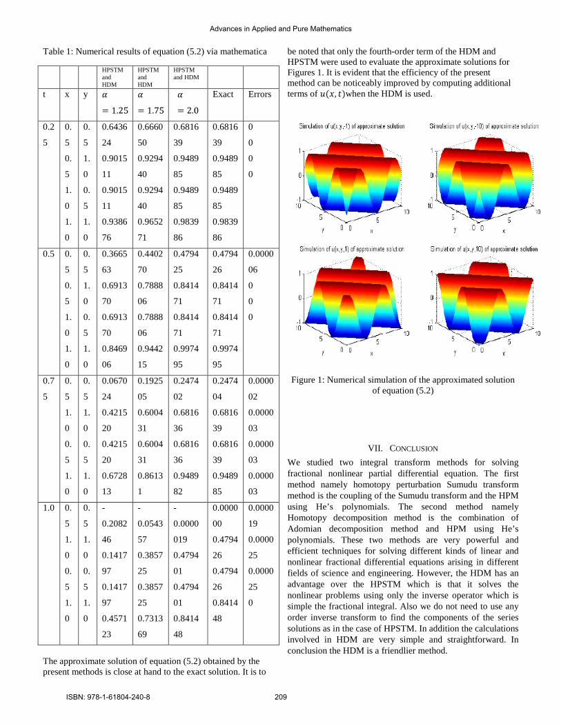
Table 1: Numerical results of equation (5.2) via mathematica

HPSTM and HDM

HPSTM and HDM

HPSTM and HDM

t x y

Exact Errors

0.2

5

0.

5

0.

5

1.

0

1.

0

0.

5

1.

0

0.

5

1.

0

0.6436

24

0.9015

11

0.9015

11

0.9386

76

0.6660

50

0.9294

40

0.9294

40

0.9652

71

0.6816

39

0.9489

85

0.9489

85

0.9839

86

0.6816

39

0.9489

85

0.9489

85

0.9839

86

0

0

0

0

0.5 0.

5

0.

5

1.

0

1.

0

0.

5

1.

0

0.

5

1.

0

0.3665

63

0.6913

70

0.6913

70

0.8469

06

0.4402

70

0.7888

06

0.7888

06

0.9442

15

0.4794

25

0.8414

71

0.8414

71

0.9974

95

0.4794

26

0.8414

71

0.8414

71

0.9974

95

0.0000

06

0

0

0

0.7

5

0.

5

1.

0

0.

5

1.

0

0.

5

1.

0

0.

5

1.

0

0.0670

24

0.4215

20

0.4215

20

0.6728

13

0.1925

05

0.6004

31

0.6004

31

0.8613

1

0.2474

02

0.6816

36

0.6816

36

0.9489

82

0.2474

04

0.6816

39

0.6816

39

0.9489

85

0.0000

02

0.0000

03

0.0000

03

0.0000

03

1.0 0.

5

1.

0

0.

5

1.

0

0.

5

1.

0

0.

5

1.

0

-

0.2082

46

0.1417

97

0.1417

97

0.4571

23

-

0.0543

57

0.3857

25

0.3857

25

0.7313

69

-

0.0000

019

0.4794

01

0.4794

01

0.8414

48

0.0000

00

0.4794

26

0.4794

26

0.8414

48

0.0000

19

0.0000

25

0.0000

25

0

The approximate solution of equation (5.2) obtained by the present methods is close at hand to the exact solution. It is to

be noted that only the fourth-order term of the HDM and HPSTM were used to evaluate the approximate solutions for Figures 1. It is evident that the efficiency of the present method can be noticeably improved by computing additional terms of when the HDM is used.

Figure 1: Numerical simulation of the approximated solution of equation (5.2)

VII. CONCLUSION We studied two integral transform methods for solving fractional nonlinear partial differential equation. The first method namely homotopy perturbation Sumudu transform method is the coupling of the Sumudu transform and the HPM using He’s polynomials. The second method namely Homotopy decomposition method is the combination of Adomian decomposition method and HPM using He’s polynomials. These two methods are very powerful and efficient techniques for solving different kinds of linear and nonlinear fractional differential equations arising in different fields of science and engineering. However, the HDM has an advantage over the HPSTM which is that it solves the nonlinear problems using only the inverse operator which is simple the fractional integral. Also we do not need to use any order inverse transform to find the components of the series solutions as in the case of HPSTM. In addition the calculations involved in HDM are very simple and straightforward. In conclusion the HDM is a friendlier method.


ISBN: 978-1-61804-240-8 209

REFERENCES [1] K. B. Oldham and J. Spanier, “The Fractional Calculus”, Academic Press, New York, NY, USA, (1974). [2] I. Podlubny, “Fractional Differential Equations”, Academic Press, New York, NY, USA, (1999). [3] A. A. Kilbas, H. M. Srivastava, and J. J. Trujillo, “Theory and Applications of Fractional Differential Equations”, Elsevier, Amsterdam, The Netherlands, (2006).

[4] I. Podlubny, “Fractional Differential Equations”, Academic Press, San Diego, Calif, USA, (1999). [5] M. Caputo, “Linear models of dissipation whose Q is almost frequency independent, part II,” Geophysical Journal International, vol. 13, no. 5, pp. 529–539, (1967). [6] A. A. Kilbas, H. H. Srivastava, and J. J. Trujillo, “Theory and Applications of Fractional Differential Equations”, Elsevier, Amsterdam, The Netherlands, (2006). [7] K. S. Miller and B. Ross, “An Introduction to the Fractional Calculus and Fractional Differential Equations”, Wiley, New York, NY, USA, (1993). [8] S. G. Samko, A. A. Kilbas, and O. I. Marichev, “Fractional Integrals and Derivatives: Theory and Applications”, Gordon and Breach, Yverdon, Switzerland, (1993). [9] G. M. Zaslavsky, “Hamiltonian Chaos and Fractional Dynamics”, Oxford University Press, (2005). [10] A. Yildirim, “An algorithm for solving the fractional nonlinear Schrödinger equation by means of the homotopy perturbation method,” International Journal of Nonlinear Sciences andNumerical Simulation, vol. 10, no. 4, (2009). pp. 445–450, [11] J. H. He, “Asymptotic methods for solitary solutions and compactons,” Abstract and Applied Analysis, vol. 2012, (2012). Article ID 916793, 130 pages, [12] J.-H. He, “Homotopy perturbation technique,” Computer Methods in Applied Mechanics and Engineering, vol. 178, no. 3-4, (1999), pp.257–262. [13] J.-H. He, “Homotopy perturbation method: a new nonlinear analytical technique,” Applied Mathematics and Computation, vol. 135, no. 1, (2003). pp. 73–79. [14] J.-H. He, “New interpretation of homotopy perturbation method. Addendum: ‘some asymptotic methods for strongly nonlinear equations’,” International Journal of Modern PhysicsB, vol. 20, no. 18, (2006). pp. 2561–2568. [15] D. D. Ganji, “The application of He’s homotopy perturbation method to nonlinear equations arising in heat transfer,” PhysicsLetters A, vol. 355, no. 4-5, (2006). pp. 337–341.

[16] A. Yildirim, “An algorithm for solving the fractional nonlinear Schrödinger equation by means of the homotopy perturbation method,” International Journal of Nonlinear Sciences andNumerical Simulation, vol. 10, no. 4, (2009), pp. 445–450. [17] D. D. Ganji and M. Rafei, “Solitary wave solutions for a generalized Hirota-Satsuma coupled KdV equation by homotopy perturbation method,” Physics Letters A, vol. 356, no. 2, (2006)., pp. 131– 137. [18] M. M. Rashidi, D. D. Ganji, and S. Dinarvand, “Explicit analytical solutions of the generalized Burger and Burger-Fisher equations by homotopy perturbation method,” Numerical Methodsfor Partial Differential Equations, vol. 25, no. 2, (2009). pp. 409–417 [19] H. Aminikhah and M. Hemmatnezhad, “An efficient method for quadratic Riccati differential equation,” Communications inNonlinear Science and Numerical Simulation, vol. 15, no. 4, (2010). pp. 835–839. [20] S. H. Kachapi and D. D. Ganji, Nonlinear Equations: Analytical Methods and Applications, Springer, (2012). [21] Atangana Abdon. ”New Class of Boundary Value Problems”, Inf. Sci. Lett. Vol 1 no. 2, (2012) pp 67-76 [22] Y. M. Qin and D.Q. Zeng, “Homotopy perturbation method for the q-diffusion equation with a source term,” Communicationsin Fractional Calculus, vol. 3, no. 1, (2012). pp. 34–37, [23] M. Javidi and M. A. Raji, “Combination of Laplace transform and homotopy perturbation method to solve the parabolic partial differential equations,” Communications in FractionalCalculus, vol. 3, no. 1, , (2012).pp. 10–19. [24] J. S. Duan, R. Rach, D. Buleanu, and A. M. Wazwaz, “A review of the Adomian decomposition method and its applications to fractional differential equations,” Communications in FractionalCalculus, vol. 3, no. 2, (2012). pp. 73–99. [25] D.D. Ganji, “Asemi-Analytical technique for non-linear settling particle equation of motion,” Journal of Hydro-EnvironmentResearch, vol. 6, no. 4, (2012). pp. 323–327, [26] A. Atangana and Aydin Secer. “Time-fractional Coupled- the Korteweg-de Vries Equations” Abstract Applied Analysis, In press (2013) [27] Atangana A., Botha J.F. “Analytical solution of groundwater flow equation via Homotopy Decomposition Method, J Earth Sci Climate Change, vol 3, (2012) pp 115. doi:10.4172/2157-7617.1000115 [28] J. Singh, D. Kumar, and Sushila, “Homotopy perturbation Sumudu transform method for nonlinear equations,”


ISBN: 978-1-61804-240-8 210

Advancesin Applied Mathematics and Mechanics, vol. 4, (2011), pp. pp 165–175.

[29] Watugala, G. K., “Sumudu transform: a new integral transform to solve differential equations and control engineering problems.” International Journal of Mathematical Education in Science and Technology vol 24, (1993), pp 35–43.

[30] Weerakoon, S., “Application of Sumudu transform to partial differential equations” International Journal of Mathematical Education in Science and Technology, vol 25 (1994), pp 277–283.

31-Asiru, M.A. “Classroom note: Application of the Sumudu transform to discrete dynamic systems” International Journal of Mathematical Education in Science and Technology, vol 34 no 6, (2003) , pages. 944-949 [32] Airu, M.A. “Further properties of the Sumudu transform and its applications” International Journal of Mathematical Education in Science and Technology, vol 33 no 3, (2002), pp. 441-449 [33] Jagdev Singh, Devendra Kumar, and A. Kılıçman “Homotopy Perturbation Method for Fractional Gas Dynamics Equation Using Sumudu Transform”. Abstract and Applied Analysis Volume 2013 (2013), pp 8


ISBN: 978-1-61804-240-8 211

Noise Studies in Measurements and Estimates of Stepwise Changesin Genome DNA Chromosomal Structures

JORGE MUNOZ-MINJARES, YURIY S. SHMALIY, JESUS CABAL-ARAGONUniversidad de Guanajuato

Department of Electronics EngineeringCtra. Salamanca-Valle, 3.5+1.8km, 36885, Salamanca

MEXICOj.ulises−[email protected], [email protected]

Abstract: Measurements using the high resolution array-comparative genomic hybridization (HR-CGH) array areaccompanied with large noise which strongly affects the estimates of the copy number variations (CNVs) and re-sults in segmental errors as well as in jitter in the breakpoints. Based on the probabilistic analysis and algorithmdesigned, we show that jitter in the breakpoints can be well approximated with the discrete skew Laplace distri-bution if the local signal-to-noise ratios (SNRs) exceed unity. Using this distribution, we propose an algorithmfor computing the estimate upper and lower bounds. Some measurements and estimates tested using these boundsshow that the higher probe resolution is provided the more segmental accuracy can be achieved and that largersegmental SNRs cause smaller jitter in the breakpoints. Estimates of the CNVs combined with the bounds pro-posed may play a crucial role for medical experts to make decisions about true chromosomal changes and eventheir existence.

Key–Words: Genome copy number, estimate, jitter, breakpoint, error bound

1 Introduction

The deoxyribonucleic acid (DNA) of a genome es-sential for human life often demonstrates structuralchanges called copy-number variations (CNVs) asso-ciated with disease such as cancer [1]. The sell withthe DNA typically has a number of copies of one ormore sections of the DNA that results in the struc-tural chromosomal rearrangements - deletions, dupli-cations, inversions and translocations of certain parts[2]. Small such CNVs are present in many forms inthe human genome, including single-nucleotide poly-morphisms, small insertion-deletion polymorphisms,variable numbers of repetitive sequences, and ge-nomic structural alterations [3]. If genomic aberra-tions involve large CNVs, the process was shown tobe directly coupled with cancer and the relevant struc-tural changes were called copy-number alterations(CNAs) [4]. A brief survey of types of chromosomealterations involving copy number changes is givenin [5]. The copy number represents the number ofDNA molecules in a cell and can be defined as thenumber of times a given segment of DNA is present ina cell. Because the DNA is usually double-stranded,the size of a gene or chromosome is often measuredin base pairs. A commonly accepted unit of measure-ment in molecular biology is kilobase (kb) equal to

1000 base pairs of DNA [6]. The human genome with23 chromosomes is estimated to be about 3.2 billionbase pairs long and to contain 20000− 25000 distinctgenes [1]. Each CNV may range from about one kb toseveral megabases (Mbs) in size [2].

One of the techniques employing chromosomalmicroarray analysis to detect the CNVs at a resolutionlevel of 5–10 kbs is the array-comparative genomichybridization (aCGH) [7]. It was reported in [8] thatthe high-resolution CGH (HR-CGH) arrays are accu-rate to detect structural variations (SV) at resolution of200 bp. In microarray technique, the CNVs are oftennormalized and plotted as log2 R/G = log2 Ratio,where R and G are the fluorescent Red and Greenintensities, respectively [9]. An annoying feature ofsuch measurements is that the Ratio is highly contam-inated by noise which intensity does not always al-low for correct visual identification of the breakpointsand copy numbers and makes most of the estimationtechniques poor efficient if the number of segmentalreadings is small. It was shown in [10] that sufficientquality in the CNVs mapping can be achieved withtens of millions of paired reads of 29–36 bases at each.Deletions as small as 300 bp should also be detectedin some cases. For instance, arrays with a 9-bp tilingpath were used in [8] to map a 622-bp heterozygousdeletion. So, further progress in the probe resolution


ISBN: 978-1-61804-240-8 212

of the CNVs measurements is desirable.Typically, a chromosome section is observed with

some average resolution r, bp and M readings in thegenomic location scale. The following distinct prop-erties of the CNVs function were recognized [2, 5]:

1) It is piecewise constant (PWC) and sparse witha small number L of the breakpoints (edges) il, l ∈[1, L], on a long base-pair length. The breakpoints areplaces as 0 < i1 < · · · < iL < rM and can be unitedin a vector

I = [i1 i2 . . . iL]T ∈ RL . (1)

Sometimes, the genomic location scale is repre-sented in the number of readings n ∈ [1,M ] witha unit step ignoring “bad” or empty measurements,where n represents the nth reading. In such a scale,the nlth discrete point corresponds to the ilth break-point in the genomic location scale and the pointsplaced as 0 < n1 < · · · < nL < M can be unitedin a vector

N = [n1 n2 . . . nL]T ∈ RL . (2)

An advantage of N against I is that it facilitates thealgorithm design. However, the final estimates arecommonly represented in the genomic location scale.

2) Its segments with constant copy numbers aj ,j ∈ [1, L+1], are integer, although this property is notsurvived in the log2 Ratio. The segmental constantchanges can also be united in a vector

a = [a1 a2 . . . aL+1]T ∈ RL+1 , (3)

in which aj characterizes a segment between ij−1 andij on an interval [ij−1, ij − 1].

3) The measurement noise in the log2 Ratio ishighly intensive and can be modeled as additive whiteGaussian.

The estimation theory offers several useful ap-proaches for piecewise signals such as those generatedby the chromosomal changes. One can employ thewavelet-based [11, 12] filters, robust estimators [12],adaptive kernel smoothers [13, 14], maximum likeli-hood (ML) based on Gauss’s ordinary least squares(OLS), penalized bridge estimator [15] and ridge re-gression [16] (also known as Tikhonov regulariza-tion), fussed least-absolute shrinkage and selectionoperator (Lasso) [17], the Schwarz information crite-rion-based estimator [18, 19], and forward-backwardsmoothers [20–22].

We also find a number of solutions developed es-pecially for needs of bioinformatics. Efficient algo-rithms for filtering, smoothing and detection were pro-posed in [11,12,19,23–28]. Methods for segmentationand modeling were developed in [10, 18, 24, 29–32].

Figure 1: Simulated genome segmental changes with asingle breakpoint at nl = 50 and segmental variances σ2

l =0.333 and σ2

l+1 = 0.083 corresponding to segmental SNRsγl = 1.47 and γl+1 = 5.88: (a) measurement and (b) jitterpdf. The jitter pdf was found by applying a ML estimatorvia a histogram over 104 runs.

Sparse representation based on penalized optimiza-tion and Bayesian learning were provided in [33–38].These results show that a small number of readings Nj

per a segment aj in line with large measurement noiseremain the main limiters of accuracy in the estimationof CNVs. Picard et al. have shown experimentallyin [29] that each segmental estimate is accompaniedwith errors and each breakpoint has jitter which can-not be overcome by any estimator.

For clarity, we generalize an experiment con-ducted in [29] in Fig. 1. Here, a chromosomal parthaving two constant segments al = 0.7 and al+1 = 0and a breakpoint nl = 50 is simulated in the pres-ence of discrete white Gaussian noise having segmen-tal variances σ2

l = 0.333 and σ2l+1 = 0.083 (Fig. 1a).

For the local segmental signal-to-noise ratios (SNRs)

γ−l =∆2

l

σ2l

, γ+l =

∆2l

σ2l+1

, (4)

where ∆l = al+1 − al is a local segmental change, itcorresponds to γ−l = 1.47 and γ+

l = 5.88.The breakpoint location nl was detected in Fig. 1

using a ML estimator [22] (one can employ any otherestimator). Measurements and estimations were re-peated 104 times with different realization of noise.Then the histogram was plotted for the detected break-point locations and normalized to have a unit area.The jitter probability density function (pdf) obtainedin such a way is sketched in Fig. 1b. Even a quick


ISBN: 978-1-61804-240-8 213

look at this figure assures that jitter at a level of 0.01(jitter probability of 1%) has 10 points to the left (leftjitter) and 2 points to the right (right jitter). In otherwords, with the probability of 99%, the breakpoint nl

can be found at any point between n = 40 and n = 52that may be too rough for medical conclusions, espe-cially if r is large. Let us add that simple averagingwhich is optimal for the estimation of PWC changesbetween the breakpoints is able to reduce the noisevariance by the factor of Nl. Noise reduction maythus also be insufficient for medical applications if Nl

is small. So, effect of noise needs more investigationsand the CNVs estimate bounds are required.

2 Jitter in the Breakpoints

In follows from the experiment conducted in [29] andsupported by Fig. 1 that jitter in the breakpoints playsa critical role in the estimation of the CNVs. Large jit-ter may cause wrong conclusions about the breakpointlocations. On the other hand, it may cause extra errorsin the determination of segmental changes especiallyif Nl and segmental SNRs occur to be small.

2.1 Laplace-Based Approximation

The results published in [29] and our own investiga-tions provided in [39] and generalized in Fig. 1b showthat jitter in the breakpoints has approximately theskew Laplace distribution. The discrete skew Laplacedistribution was recently derived in [40],

p(k|dl, ql) =(1− dl)(1− ql)

1− dlql

dk

l , k > 0 ,

q|k|l , k 6 0 ,

(5)

where dl = e−κl

νl ∈ (0, 1) and ql = e− 1

κlνl ∈ (0, 1)and in which κl > 0 and νl > 0 are coefficients de-fined by the process. Below, we shall show that (5) canserve as a reasonably good approximation for jitter inthe breakpoints of PWC signals such as that shown inFig. 1a if the segmental SNRs exceed unity.

Let us consider N neighboring to nl readings ineach segment. We may assign an event Alj meaningthat all measurements at points nl − N 6 j < nl

belong to lth segment. Another event Blj means thatall measurements at nl 6 j < nl + N − 1 belong to(l+1)th segment. We think that a measured value be-longs to one segment if the probability is larger thanif it belongs to another segment. Because noise isGaussian and the segmental variances are different,the Gaussian pdfs cross each other in two points, αl

and βl. The events Alj and Blj can thus be specified

as follows:

Alj is

(αl < xj) ∧ (xj < βl) , σ2l > σ2

l+1 ,

xj > αl , σ2l = σ2

l+1 ,αl < xj < βl , σ2

l < σ2l+1 ,

(6)

Blj is

βl < xj < αl , σ2l < σ2

l+1 ,

xj < αl , σ2l = σ2

l+1 ,(xj < αl) ∧ (xj > βl) , σ2

l > σ2l+1 .

(7)

The inverse events meaning that at least one of thepoints do not belong to the relevant interval are Alj =1−Alj and Blj = 1−Blj .

Both Alj and Blj can be united into two blocks

Al = Al(il−N)Al(il−N+1) . . . Al(il−1) ,

Bl = Bl(il)Bl(il+1) . . . Bl(il+N−1) .

We think that if Al and Bl occur simultaneously thenthe breakpoint nl will be jitter-free. However, theremay be found some other events which do not obliga-torily lead to jitter. We ignore such events and defineapproximately the probability P (AlBl) of the jitter-free breakpoint as

P (AlBl) = P (Ail−N . . . Ail−1Bil . . . Bil+N−1) .(8)

The inverse event P (AlBl) = 1−P (AlBl) meaningthat at least one point belongs to another event can becalled the jitter probability.

In white Gaussian noise, all the events are inde-pendent and (8) thus can be rewritten as

P (AlBl) = PN (Al)PN (Bl) , (9)

where, following (6) and (7), the probabilities P (Al)and P (Bl) can be specified as, respectively,

P (Al) =

1−αl∫βl

pl(x)dx , σ2l > σ2

l+1 ,

∞∫αl

pl(x)dx , σ2l = σ2

l+1 ,

βl∫αl

pl(x)dx , σ2l < σ2

l+1 ,

(10)

P (Bl) =

αl∫βl

pl+1(x)dx , σ2l > σ2

l+1 ,

αl∫−∞

pl+1(x)dx , σ2l = σ2

l+1 ,

1−βl∫αl

pl+1(x)dx , σ2l < σ2

l+1 ,

(11)

where pl(x) = 1√2πσ2

l

e− (x−al)

2

σ2l is Gaussian density.


ISBN: 978-1-61804-240-8 214

Let us now think that jitter occurs at some pointnl ± k, 0 6 k 6 N , and assign two additional blocksof events

Alk = Ail−N . . . Ail−1−k ,

Blk = Bil+k . . . Bil+N−1 .

The probability P−k , P−

k (AlkAl(il−k) . . . Ail−1Bl)that jitter occurs at kth point to the leftfrom nl (left jitter) and the probabilityP+

k , P+k (AlBl(il+1) . . . Bl(il+k−1)Blk) that

jitter occurs at kth point to the right from nl (rightjitter) can thus be written as, respectively,

P−k = PN−k(Al)[1− P (Al)]kPN (Bl) , (12)

P+k = PN (Al)[1− P (Bl)]kPN−k(Bl) . (13)

By normalizing (12) and (13) with (9), we arriveat a function that turns out to be independent on N :

fl(k) =

[P−1(Al)− 1]|k| , k < 0 , (left)1 , k = 0 ,

[P−1(Bl)− 1]k , k > 0 . (right)(14)

Further normalization of fl(k) to have a unit arealeads to the pdf pl(k) = 1

φlfl(k), where φl is the sum

of the values of fl(k) for all k,

φl = 1 +∞∑

k=1

[ϕAl (k) + ϕB

l (k)] , (15)

where ϕAl (k) = [P−1(Al) − 1]k and ϕB

l (k) =[P−1(Bl) − 1]k. Now observe that, in the approxi-mation accepted, fl(k) converges with k only if 0.5 <

P = P (A), P (B) < 1. Otherwise, if P < 0.5,the sum φl is infinite, fl(k) cannot be transformed topl(k), and the lth breakpoint cannot be detected. Con-sidering the case of 0.5 < P = P (A), P (B) < 1,we conclude that ln P < 0, ln(1 − P ) < 0, andln(1 − P ) < ln P . Next, using a standard relation∞∑

k=1

xk = 1x−1−1

, where x < 1, and after little trans-

formations we bring (15) to

φl =P (Al) + P (Bl)− 1

[1− 2P (Al)][1− 2P (Bl)]. (16)

The jitter pdf pl(k) associated with the lth break-point can finally be found to be

pl(k) =1φl

[P−1(Al)− 1]|k| , k < 0 ,1 , k = 0 ,

[P−1(Bl)− 1]k , k > 0 ,

(17)

where φl is specified by (16) and 0.5 <P (Al), P (Bl) < 1. By substituting ql =P−1(Al)−1 and dl = P−1(Bl)−1, we find P (Al) =1/(1 + ql) and P (Bl) = 1/(1 + dl), provide thetransformations, and finally go from (17) to the dis-crete skew Laplace distribution (5) in which κl andνl still need to be connected to (17). To find κl andνl, below we consider three points k = −1, k = 0,and k = 1. By equating (5) and (17), we firstobtain (1−dl)(1−ql)dl

1−dlql= 1

φl

1−P (Bl)P (Bl)

for k = 1 and(1−dl)(1−ql)ql

1−dlql= 1

φl

1−P (Al)P (Al)

for k = −1 that gives us

νl = 1−κ2l

κl ln µl, where

µl =P (Al)[1− P (Bl)]P (Bl)[1− P (Al)]

. (18)

For k = 0, we have (1−dl)(1−ql)1−dlql

= 1φl

and trans-

form it to an equation x2l − φl(1+µl)

1+φlx − 1−φl

1+φlµl = 0,

which proper solution is

xl =φl(1 + µl)2(1 + φl)

(1−

√1 +

4µl(1− φ2l )

φ2l (1 + µl)2

)(19)

and which xl = µ− κ2

l1−κ2

ll gives us

κl =

√ln xl

ln(xl/µl). (20)

By combining νl with (19), we also provide a simplerform for νl, namely

νl = − κl

ln xl. (21)

The discrete skew Laplace distribution (5) canthus be used to represent jitter in the breakpoints sta-tistically.

Now substitute the Gaussian pdf to (10) and (11),provide the transformations, and find

P (Al) =

1 + 12 [erf(gβ

l )− erf(gαl )] , γ−l < γ+

l ,12erfc(gα

1 ) , γ−l = γ+l ,

12 [erf(gβ

l )− erf(gαl )] , γ−l > γ+

l ,(22)

P (Bl) =

12 [erf(hα

l )− erf(hβl )] , γ−l < γ+

l ,1− 1

2erfc(hαl ) , γ−l = γ+

l ,

1 + 12 [erf(hα

l )− erf(hβl )] , γ−l > γ+

l ,(23)

where gβl = βl−∆l

|∆l|

√γ−l2 , gα

l = αl−∆l|∆l|

√γ−l2 , hβ

l =

βl|∆l|

√γ+

l2 , hα

l = αl|∆l|

√γ+

l2 , erf(x) is the error func-

tion, erfc(x) is the complementary error function. If


ISBN: 978-1-61804-240-8 215

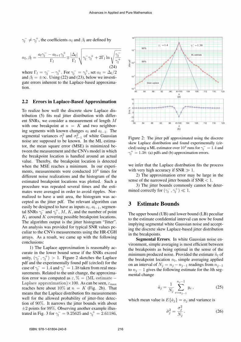
γ−l 6= γ+l , the coefficients αl and βl are defined by

αl, βl =alγ

−l − al+1γ

+l

Γl∓|∆l|

Γl

√√√√γ−l γ+l + 2Γl ln

√γ−lγ+

l

(24)where Γl = γ−l − γ+

l . For γ−l = γ+l , set αl = ∆l/2

and βl = ±∞. Using (22) and (23), below we investi-gate errors inherent to the Laplace-based approxima-tion.

2.2 Errors in Laplace-Based Approximation

To realize how well the discrete skew Laplace dis-tribution (5) fits real jitter distribution with differ-ent SNRs, we consider a measurement of length Mwith one breakpoint at n = K and two neighbor-ing segments with known changes al and al−1. Thesegmental variances σ2

l and σ2l−1 of white Gaussian

noise are supposed to be known. In the ML estima-tor, the mean square error (MSE) is minimized be-tween the measurement and the CNVs model in whichthe breakpoint location is handled around an actualvalue. Thereby, the breakpoint location is detectedwhen the MSE reaches a minimum. In our experi-ments, measurements were conducted 104 times fordifferent noise realizations and the histogram of theestimated breakpoint locations was plotted. Such aprocedure was repeated several times and the esti-mates were averaged in order to avoid ripples. Nor-malized to have a unit area, the histogram was ac-cepted as the jitter pdf. The relevant algorithm caneasily be designed to have as inputs al, al−1, segmen-tal SNRs γ−l and γ+

l , M , K, and the number of pointK1 around K covering possible breakpoint locations.The algorithm output is the jitter histogram “Jitter”.An analysis was provided for typical SNR values pe-culiar to the CNVs measurements using the HR-CGHarrays. As a result, we came up with the followingconclusions:

1) The Laplace approximation is reasonably ac-curate in the lower bound sense if the SNRs exceedunity, (γ−l , γ+

l ) > 1. Figure 2 sketches the Laplacepdf and the experimentally found pdf (circled) for thecase of γ−l = 1.4 and γ+

l = 1.38 taken from real mea-surements. Related to the unit change, the approxima-tion error was computed as ε,% = (ML estimate −Laplace approximation)×100. As can be seen, εmax

reaches here about 10% at n = K (Fig. 2b). Thatmeans that the Laplace distribution fits measurementswell for the allowed probability of jitter-free detec-tion of 90%. It narrows the jitter bounds with about±2 points for 99%. Observing another example illus-trated in Fig. 3 for γ−l = 9.25625 and γ+

l = 2.61186,

Figure 2: The jitter pdf approximated using the discreteskew Laplace distribution and found experimentally (cir-cled) using a ML estimator over 104 runs for γ−l = 1.4 andγ+

l = 1.38: (a) pdfs and (b) approximation errors.

we infer that the Laplace distribution fits the processwith very high accuracy if SNR À 1.

2) The approximation error may be large in thesense of the narrowed jitter bounds if SNR < 1.

3) The jitter bounds commonly cannot be deter-mined correctly for (γ−l , γ+

l ) ¿ 1.

3 Estimate Bounds

The upper bound (UB) and lower bound (LB) peculiarto the estimate confidential interval can now be foundimplying segmental white Gaussian noise and accept-ing the discrete skew Laplace-based jitter distributionin the breakpoints.

Segmental Errors. In white Gaussian noise en-vironment, simple averaging is most efficient betweenthe breakpoints as being optimal in the sense of theminimum produced noise. Provided the estimate nl ofthe breakpoint location nl, simple averaging appliedon an interval of Nj = nj −nj−1 readings from nj−1

to nj − 1 gives the following estimate for the lth seg-mental change

aj =1

Nj

nj−1∑v=nj−1

yv , (25)

which mean value is Eaj = aj and variance is

σ2j =

σ2j

Nj. (26)


ISBN: 978-1-61804-240-8 216

Figure 3: The jitter pdf approximated using the discreteskew Laplace distribution and found experimentally (cir-cled) using a ML estimator over 104 runs for γ−l = 9.25625and γ+

l = 2.61186: (a) pdfs and (b) approximation errors.

The UB for segmental estimates can be formed in

the θ-sigma sense as aUBj = Eaj + θ

√σ2

j

Nj, where

θ > 1 is commonly integer. However, neither an ac-tual aj = Eaj nor multiple measurements neces-sary to approach aj by averaging are available. Wethus specify UB and LB approximately as

aUBj

∼= aj + θ

√σ2

j

Nj, (27)

aLBj

∼= aj − θ

√σ2

j

Nj. (28)

where θ = 1 guarantees an existence of true changesbetween UB and LB with the probability of 68.27% orerror probability of κ = 0.3173 that is 31.73%; θ = 2of 95.45% or κ = 0.0555 that is 5.55% and θ = 3 of99.73% or κ = 0.0027 that is 0.27%.

Jitter Bounds. The jitter left bound (JLB) JLl

and the jitter right bound (JRB) JRl can be determined

with respect to nl as follows. Because a step is unitywith integer k, we specify the jitter probability at thekth point using (5) as

Pk(γ−l , γ+l ) = p[k|d(γ−l , γ+

l ), q(γ−l , γ+l )] . (29)

We then equate (29) to κ and solve it for the right and

left jitter to have, respectively,

kRl =

⌊νl

κlln

(1− dl)(1− ql)κ(1− dlql)

⌋, (30)

kLl =

⌊νlκlln

(1− dl)(1− ql)κ(1− dlql)

⌋, (31)

where bxc means the maximum integer equal to orlower than x. The JLB and JRB can be defined withrespect to nl as JL

l = nl−kLl and JR

l = nl+kRl . Now

observe that nl is unknown and use the estimate nl. Ifit happens that nl lies at the right bound, then the truenl can be found kR

l points to the left. Otherwise, if nl

lies at the left bound, then il can be found kLl points

to the right. Approximate JLB and JRB are thus thefollowing

JLl

∼= nl − kRl , (32)

JRl

∼= nl + kLl . (33)

Note that κ in (30) and (31) should be specifiedin the θ-sense as in (27) and (28).

UB and LB Masks and Algorithm. By combin-ing (27), (28), (32), and (33), the UB mask BU

n andthe LB mask BL

n can now be formed to outline theregion for true genomic changes. The relevant algo-rithm was designed in [41]. Its inputs are measure-ments yn, breakpoints estimates nl, tolerance param-eter θ, number L of the breakpoints, and number ofreadings M . At the output, the algorithms producestwo masks: BU

n and BLn .

The UB and LB masks have the following basicapplied properties:

• The true CNVs exist between BUn and BL

n withthe probability determined in the θ-sigma sense.

• If BUn or BL

n covering two or more breakpoints isuniform, then there is a probability of no changesin this region.

• If both BUn and BL

n covering two or more break-points are uniform, then there is a high probabil-ity of no changes in this region.

We notice again that the jitter bounds in BUn and

BLn may have enough accuracy if (γ−l , γ+

l ) > 1.They may be considered in the lower bound sense if(γ−l , γ+

l ) < 1. However, the approximation error iscommonly large if (γ−l , γ+

l ) < 0.5. For details, seeSection 2.2.

4 Applications

In this section, we test some CNVs measurementsand estimates by the UB and LB masks computed


ISBN: 978-1-61804-240-8 217

in the three-sigma sense, θ = 3, using the algorithm[41–43]. Because the algorithm can be applied to anyCNVs data with supposedly known breakpoints, wechoose the 1st chromosome measured using the HR-CGH array in [28] and available from [44].

The CNVs structure has 34 segments and 33breakpoints. Most of the segments have the SNRsexceeding unity meaning that the UB and LB maskswill have enough accuracy. The SNRs in segmentsa18 and a21 range between 0.5 and unity which meansthat real jitter can be here about twice larger. The re-maining segments a23, a28, a31 and a32 demonstratethe SNR below 0.5 that means that the jitter boundscannot be estimated with sufficient accuracy. We justmay say that jitter can be much larger in the relevantbreakpoints.

Let us consider the CNVs measurements and esti-mates in more detail following Fig. 4. As can be seen,there are two intervals with no measurements betweenthe breakpoints i15 and i16 and the breakpoints i28 andi29. A part of measurements covering the breakpointsfrom i5 to i14 is shown in Fig. 5a. Its specific is thatthe segmental SNRs are all larger than unity and themasks thus can be used directly for practical appli-cations. The masks suggest that errors in all of thesegmental estimates reach tens of percents. In fact, a5

and a10 are estimated with error of about 50%. Errorexceeds 30% in the estimates a7, a9, a12, and a13. Asimilar problem can be observed in the estimates ofalmost all of the breakpoints in which left and rightjitter reaches several points.

A situation even worse with a part of the chromo-some covering the breakpoints from i17 to i26. Thesegmental errors exceed 50% here over almost allsegments. Furthermore, the UB is placed above LBaround i17, i20, and i22. That means that there is aprobability that these breakpoints do not exist. On theother hand, estimates in the part covering i24–i26 arenot reliable. Thus there is a probability of no changesin this region as well.

5 Conclusions

Effect of measurement noise on the HR-CGH array-based estimates of the CNVs naturally results in seg-mental errors and jitter in the breakpoints due to typ-ically low SNRs. Errors can be so large that medicalexpert would hardly be able to arrive at correct con-clusions about real CNVs structures irrespective of theestimator used. Two rules of thumb for designers ofmeasurement equipment are thus the following: thehigher probe resolution the more segmental accuracyand the larger segmental SNRs the lower jitter in thebreakpoints.

Because of large noise, estimates of the CNVsmay bring insufficient information to experts and mustbe tested by UB and LB masks. To form such masks,the jitter distribution must be known. We have shownthat jitter in the breakpoints can be modeled usingthe discrete skew Laplace distribution if the segmen-tal SNRs exceed unity. Otherwise, the approximationerrors can be large and more profound investigationsof jitter will be required. The UB and LB masks pro-posed in this paper in the θ-sigma sense outline theregion within which the true changes exist with a highprobability (99.73% in the three-sigma sense). Pro-vided the masks, information about CNVs is morecomplete and sometimes can be crucial for medicalexperts to make a correct decision about true struc-ture. Testing some measurements and estimates bythe UB and LB masks has revealed large errors ex-ceeding (30...50)% in many segments. It was alsodemonstrated that jitter in some breakpoints is redun-dantly large for making any decision about their truelocations. We finally notice that further investigationsmust be focused on the jitter statistics at low SNR val-ues that is required to sketch a more correct proba-bilistic picture of the CNVs.

References:[1] International Human Genome Sequencing Consor-

tium, “Finishing the euchromatic sequence of thehuman genome,” Nature, vol. 431, pp. 931-945,Oct. 2004.

[2] P. Stankiewicz and J. R. Lupski, “Structural Varia-tion in the Human Genome and its Role in Disease,”Annual Review of Medicine, vol. 61, pp. 437-455,Feb. 2010.

[3] A. J. Iafrate, L. Feuk, M. N. Rivera, M. L. Lis-tewnik, P. K. Donahoe, Y. Qi, S. W. Scherer, and C.Lee, “Detection of large-scale variation in the hu-man genome,” Nature Genetics, vol. 36, no. 9, pp.949-951, Sep. 2004.

[4] J. R. Pollack, T. Sorlie, C. M. Perou, C. A. Rees, S.S. Jeffrey, P. E. Lonning, R. Tibshirani, D. Botstein,A. L. Borresen-Dale, and P. O. Brown, “Microarrayanalysis reveals a major direct role of DNA copynumber alteration in the transcriptional program ofhuman breast tumors,” Proc. Natl Acad. Sci (PNAS),vol. 99, no. 20, pp. 12963-12968, Oct. 2002.

[5] R. Pique-Regi, A. Ortega, A. Tewfik, and S. As-gharzadeh, “Detection changes in the DNA copynumber,” IEEE Signal Process. Mgn., vol. 29, no.1, pp. 98-107, Jan. 2012.

[6] A. F. Cockburn, M. J. Newkirk, and R. A. Fir-tel, “Organization of the ribosomal RNA genes ofdictyostelium discoideum: mapping of the non-trascribed spacer regions,” Cell, vol. 9, no. 4, pp.605-613, Dec 1976.


ISBN: 978-1-61804-240-8 218

Figure 4: Measurements and estimates of the 1st chromosome changes taken from archive “159A–vs–159D–cut” availablein [44].

Figure 5: Parts of chromosomal changes (Fig. 4) tested byUB and LB masks: (a) genomic location from about 97Mbto 120Mb and (b) genomic location from 143Mb to 159Mb.Jitter in i5, i6, i9, and i10 is moderate and these breakpointsare well detectable. Breakpoints i17, i22, i27, i30, and i31cannot be estimated correctly owing to low SNRs. There isa probability that the breakpoints i17, i19, i20, i22, and i24do not exist.

[7] H. Ren, W. Francis, A. Boys, A. C. Chueh, N.Wong, P. La, L. H. Wong, J. Ryan, H. R. Slater,and K. H. Choo, “BAC-based PCR fragment mi-croarray: high-resolution detection of chromosomaldeletion and duplication breakpoints,” Human Mu-tation, vol. 25, no. 5, pp. 476-482, May 2005.

[8] A. E. Urban, J. O. Korbel, R. Selzer, T. Richmond,A. Hacker, G. V. Popescu, J. F. Cubells, R. Green,B. S. Emanuel, M. B. Gerstein, S. M. Weissman,and M. Snyder, “High-resolution mapping of DNAcopy alterations in human chromosome 22 usinghigh-density tiling oligonucleotide arrays,” Proc.Natl. Acad. Sci. (PNAS), vol. 103, no. 12, pp. 4534-4539, Mar. 2006.

[9] Y. H. Yang, S. Dudoit, P. Luu, D. M. Lin, V. Peng,J. Ngai, and T. P. Speed, “Normalization for cDNAmicroarray data: a robust composite method ad-dressing single and multiple slide systematic vari-ation,” Nucleic Acids Research, vol. 30, no. 4, pp.1–10, Feb 2002.

[10] P.J. Campbell, P.J. Stephens, E.D. Pleasance, S.OMeara, H. Li, T. Santarius, L.A Stebbings, C.Leroy, S. Edkins, C. Hardy, J.W. Teague, A. Men-zies, I. Goodhead, D.J. Turner, C.M. Clee, M.A.Quail, A. Cox, C. Brown, R. Durbin, M.E. Hurles,P.A.W Edwards, G.R. Bignell, M.R. Stratton, andP.A. Futreal, “Identification of somatically acquiredrearrangements in cancer using genome-wide mas-sively parallel paired-end sequencing”, Nature Ge-netics, vol. 40, no. 6, pp. 722-729, Jun. 2008.

[11] L. Hsu, S.G. Self, D. Grove, T. Randolph, K. Wang,J.J. Delrow, L. Loo, and P. Porter, “Denoising array-based comparative genomic hybridization data us-ing wavelets”, Biostatistics, vol. 6, no. 2, pp. 211–226, 2005.


ISBN: 978-1-61804-240-8 219

[12] E. Ben-Yaacov and Y.C. Eldar, “A fast and flexiblemethod for the segmentation of aCGH data”, Bio-statistics, vol. 24, no. 16, pp. i139–i145, 2008.

[13] V. Katkovnik and V.G. Spokoiny, “Spatial adaptiveestimation via fitted local likelihood techniques,”IEEE Trans. Signal Process., vol. 56, no. 3, pp.873–886, 2008.

[14] A. Goldenshluger and A. Nemirovski, “Adaptivede-noising of signals satisfying differential inequal-ities,” IEEE Trans. Inf. Theory, vol. 43, no. 3, pp.872–889, 1997.

[15] I.E. Frank and J.H. Friedman, “A Statistical Viewof Some Chemometrics Regression Tools,” Techno-metrics, vol. 35, pp. 109-148, 1993.

[16] A.E. Hoerl and R.W. Kennard, R.W., “Ridge re-gression: biased estimation for nonorthogonal prob-lems,” Technometrics, vol. 12, pp. 55-67, 1970.

[17] R. Tibshirani, “Regression Shrinkage and Selectionvia the Lasso,” Journal of Royal Statist. Soc., ser. B,vol. 58, pp. 267-288, 1996.

[18] J. Fridlyand, A.M. Snijders, D. Pinkel, D.G. Albert-son, and A.N. Jain, “Hidden Markov models ap-proach to the analysis of array CGH data”, Journalof Multivariate Analysis, vol. 90, no. 1, pp. 132-153,2004.

[19] J. Chen and Y.-P. Wang, “A statistical change pointmodel approach for the detection of DNA copynumber variations in array CGH data”, IEEE/ACMTrans. on Comput. Biology and Bioinform., vol. 6,no. 4, pp. 529–541, 2009.

[20] S. H. Chung and R. A. Kennedy, “Forward-backward non-linear filtering technique for extract-ing small biological signal from noise,” J Neuro-science Meth, vol. 40, no. 1, pp. 71–86, Nov 1991.

[21] O. Vite-Chavez, R. Olivera-Reyna, O. Ibarra-Manzano, Y. S. Shmaliy, and L. Morales-Mendoza,“Time-variant forward-backward FIR denoising ofpiecewise-smooth signals,” Int. J. Electron. Com-mun. (AEU), vol. 67, no. 5, pp. 406–413, May 2013.

[22] J. Munoz-Minjares, O. Ibarra-Manzano, and Y. S.Shmaliy, “Maximum likelihood estimation of DNAcopy number variations in HR-CGH arrays data,”In Proc. 12th WSEAS Int. Conf. on Signal Process.,Comput. Geometry and Artif. Vision (ISCGAV’12),Proc. 12th WSEAS Int. Conf. on Systems Theoryand Sc. Comput. (ISTASC’12), Istanbul (Turkey),pp. 45-50, 2012.

[23] J. Huang, W. Wei, J. Zhang, G. Liu, G. R. Bignell,M. R. Stratton, P. A. Futreal, R. Wooster, K. W.Jones, and M. H. Shapero, “Whole genome DNAcopy number changes identified by high densityoligonucleotide arrays,” Hum. Genomics, vol. 1, no.4, pp. 287–299, May 2004.

[24] C. Xie and M. T. Tammi, “CNV-seq, a new methodto detect copy number variantion using high-throughput sequencing,” BMC Bioinform., vol. 10,no. 80, pp. 1–9, Mar 2009.

[25] A. K. Alqallaf and A. H. Teqfik, “DNA copy num-ber detection and Sigma filter,” In Proc. GENSIPS,pp. 1–4, 2007.

[26] S. Ivakhno, T. Royce, A. J. Cox, D. J. Evers, R. K.Cheetham, and S. Tavare, “CNAseg–A novel frame-work for identification of copy number changes incancer from second-generation sequencing data,”Bioinform., vol. 26, no. 24, pp. 3051–3058, Dec.2010.

[27] J. Chen and A. K. Gupta, Parametric StatisticalChange Point Analysis with Applications to Ge-netics, Medicine, and Finance, 2nd Ed., Springer,2012.

[28] R. Lucito, J. Healy, J. Alexander, A. Reiner, D.Esposito, M. Chi, L. Rodgers, A. Brady, J. Sebat,J. Troge, J. A. West, S. Rostan, K. C. Nquyen,S. Powers, K. Q. Ye, A. Olshen, E. Venkatra-man, L. Norton, and M. Wigler, “Representa-tional oligonucleotide microarray analysis: a high-resolution method to detect genome copy numbervariation,” Genome Research, vol. 13, no. 10, pp.2291–2305, Oct. 2003.

[29] F. Picard, S. Robin, M. Lavielle, C. Vaisse, and J.-J.Daudin, “A statistical approach for array CGH dataanalysis,” BMC Bioinformatics, vol. 6, no. 1, pp.27–37, 2005.

[30] A. B. Olshen, E. S. Venkatraman, R. Lucito, M.Wigner, “Circular binary segmentation for the anal-ysis of array-based DNA copy number data,” Bio-statistics, vol. 5, no. 4, pp. 557–572, Oct. 2004.

[31] J. T. Simpson, R. E. Mclntyre, D. J. Adams, and R.Durbin, “Copy number variant detection in inbredstrains from short read sequence data,” Bioinformat-ics, vol. 26, no. 4, pp. 565–567, Feb. 2010.

[32] L. Wang, A. Abyzov, J. O. Korbel, M. Snyder,and M. Gerstein, “MSB: A mean-shift-based ap-proach for the analysis of structural variation in thegenome,” Genomic Res., vol. 19, no. 1, pp. 106–117, Jan 2009.

[33] V. Boeva, A. Zinovyev, K. Bleakley, J. P. Vert,I. Janoueix-Lerosey, O. Delattre, and E. Barillot,“Control-free calling of copy number alterations indeep-sequencing data using GC-content normaliza-tion,” Bioinformatics, vol. 27, no. 2, pp. 268–269,Jan. 2011.

[34] R. Tibshirani and P. Wang, “Spatial smoothing andhot spot detection for CGH data using the fusedlasso,” Biostatistics, vol. 9, no. 1, pp. 18–29, Jan.2008.

[35] R. Pique-Regi, J. Monso-Varona, A. Ortega, R. C.Seeger, T. J. Triche, and S. Asgharzadeh, “Sparserepresentation and Bayesian detection of genomecopy number alterations from microarray data,”Bioinformatics, vol. 24, no. 3, pp. 309–318, Mar.2008.


ISBN: 978-1-61804-240-8 220

[36] X. Gao and J. Huang, “A robust penalized methodfor the analysis of noisy DNA copy number data,”BMC Genomics, vol. 11, no. 517, pp. 1–10, Sep.2010.

[37] O. M. Rueda and R. Diaz-Uriante, “RJaCGH:Bayesian analysis of a aCGH arrays for detectingcopy number changes and recurrent regions,” Bioin-formatics, vol. 25, no. 15, pp. 1959–1960, Aug.2009.

[38] Y. Yuan, C. Curtis, C. Caldas, and F. Markowetz, “Asparse regulatory network of copy-number drivengene expression reveals putative breast cancer onco-genes,” IEEE Trans. Comput. Biology and Bioinfor-matics, vol. 9, no. 4, pp. 947–954, Jul.-Aug. 2012.

[39] J. Munoz-Minjares, J. Cabal-Aragon, and Y. S.Shmaliy, “Jitter probability in the breakpoints ofdiscrete sparse piecewise-constant signals,” Proc.21st European Signal Process. Conf. (EUSIPCO-2013), 2013.

[40] T. J. Kozubowski and S. Inusah, “A skew Laplacedistribution on integers,” Annals of the Inst. ofStatist. Math., vol. 58, no. 3, pp. 555-571, Sep.2006.

[41] J. Munoz-Minjares, J. Cabal-Aragon, Y. S. Shmaliy,“Probabilistic bounds for estimates of genome DNAcopy number variations using HR-CGH microar-rays,” Proc. 21st European Signal Process. Conf.(EUSIPCO-2013), 2013.

[42] J. Munoz-Minjares, Y. S. Shmaliy, J. Cabal-Aragon,“Confidence limits for genome DNA copy num-ber variations in HR-CGH array measurements,”Biomedical Signal Processing & Control, vol. 10,pp. 166–173, Mar. 2014.

[43] J. Munoz-Minjares, J. Cabal-Aragon, Y. S. Shmaliy,“Effect of noise on estimate bounds for genomeDNA structural changes,” WSEAS Trans. on Biologyand Biomedicine, vol. 11, pp. 52–61, Apr. 2014.

[44] Representational oligonucleotide microarray analy-sis (ROMA), http://Roma.cshl.org.


ISBN: 978-1-61804-240-8 221

Fundamentals of a fuzzy inference system for educational evaluation

M.A. Luis Gabriel Moreno Sandoval William David Peña Peña

Abstract—This paper exposes features a fuzzy inference system

General focused on educational evaluation, constructed from a data base relational, with the objectives of, first, generate discussion about fuzzy logic as a new tool to interpret the educational process through information technologies and communication, and second, exposing the virtues and drawbacks of these data structures in the development of models of complex phenomena. First is the introduction with the theoretical bases is exposed, Later, the technical characteristics of the application with the successes and difficulties rose by this, and finally presents the conclusions of the authors.

Keywords—Fuzzy Logic, Fuzzy Inference System, decision making with Multicriteria, alternative assessment in education.

I. Introduction Education is a system based on the particular properties of its elements and non-linear and interdependent relationships that they have with non-reversible dynamics in time and that remain without any outside control, presenting patterns of order at various scales [1, 2]. That is why education is a complex phenomenon, where training and learning process cannot be weighted from a scale standardized for all contexts and experiences, since the only knowledge can be appropriate, understood and applied in all their dimensions, when each person internalizing it from in their everyday practice. Current education and its ways of assessment is based in the classical world modern vision as machine, which dismembered the reality in its parts and reset it from a logical order, on the one hand, this has caused that the educational evaluation is developed under a same logical scheme regardless of the person who studies [3]. And on the other hand It has led to underestimate, and even at times ignored, the particularity of student and its context, and the possibilities it offers to exercise and develop studied knowledge, putting the topics above its actual application, where the students are overwhelmed and concealed by concepts, diagrams and formulas that do not relate to its existence [4].

M.A. Luis Gabriel Moreno Sandoval University “Manuela Beltran” Bogotá, Colombia [email protected]

William David Peña Peña UniversityCorporation UNIMINUTO Cundinamarca, Colombia [email protected]

The problem suggests a solution that enables you to relate the specific content with daily practice and perception of personal realization that knowledge gives to each person. Why is proposed an evaluation system with fuzzy logic, that not only focuses on themes, concepts and theories, they represent the connection of multiple variables within the educational process, allowing study it, understand it to improve it permanently, from the reading of each student.

A. Education: A product and a right at the same time

This project is mainly geared towards the educational evaluation for distance mode of studies in higher education, because in this case the tutor, for sharing with the student less than in face-to-face mode, requires greater predictive and assertive, to update and improve permanently their contents and methodologies, projecting to a more personal realization and knowledge to a higher yield in the working life of the students. The document “Opens and distance learning. Considerations on trends, policies and strategies" of the UNESCO [5], it exposes education distance and open as a product provided by suppliers, but at the time defines the mode of studies as a possibility that all persons have access to the right to education, the academic to the student the broadest spectrum of possibilities through knowledge purposes providing education to isolated populations or with difficulties to access to traditional education methods, and offer academic programs oriented to the training for work [5]. The educational spectrum in Colombian society is characterized by difficulties of access to higher education, economic dependence, segregation, and in some cases violence (social, economic and political) [6], and that requires evaluation methods not only considered the interpretation of a specific subject, but the way in which this subject can contribute to the personal, social and productive development of the person, and not just one of these aspects.

B. Fuzzy logic Fuzzy logic is a knowledge originated from mathematical statistics, giving an element a weighting of non-deterministic as the one used in the classical logic, because in this one, an element belongs or not to a set, but in the fuzzy logic that element has different ranges of belonging. Loty Admeh Sadeh (1972), creator of fuzzy logic, for example, proposes the case of a classical group called "Tall people", to which belong the people with stature greater than or equal to 1.8 meters, where a person with stature of 1,79 m not belonged to this, however, in fuzzy logic, by means of mathematical functions, pre-


ISBN: 978-1-61804-240-8 222

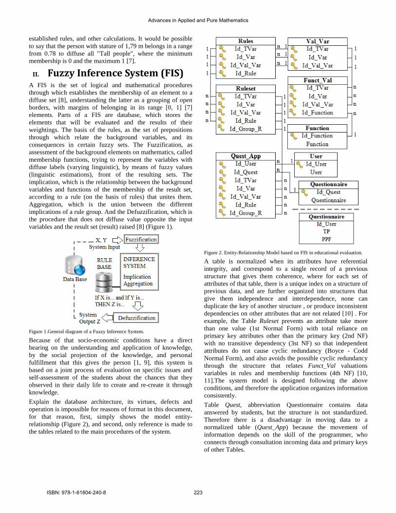
established rules, and other calculations. It would be possible to say that the person with stature of 1,79 m belongs in a range from 0.78 to diffuse all "Tall people", where the minimum membership is 0 and the maximum 1 [7].

II. Fuzzy Inference System (FIS) A FIS is the set of logical and mathematical procedures through which establishes the membership of an element to a diffuse set [8], understanding the latter as a grouping of open borders, with margins of belonging in its range [0, 1] [7] elements. Parts of a FIS are database, which stores the elements that will be evaluated and the results of their weightings. The basis of the rules, as the set of prepositions through which relate the background variables, and its consequences in certain fuzzy sets. The Fuzzification, as assessment of the background elements on mathematics, called membership functions, trying to represent the variables with diffuse labels (varying linguistic), by means of fuzzy values (linguistic estimations), front of the resulting sets. The implication, which is the relationship between the background variables and functions of the membership of the result set, according to a rule (on the basis of rules) that unites them. Aggregation, which is the union between the different implications of a rule group. And the Defuzzification, which is the procedure that does not diffuse value opposite the input variables and the result set (result) raised [8] (Figure 1).

Figure 1.General diagram of a Fuzzy Inference System.

Because of that socio-economic conditions have a direct bearing on the understanding and application of knowledge, by the social projection of the knowledge, and personal fulfillment that this gives the person [1, 9], this system is based on a joint process of evaluation on specific issues and self-assessment of the students about the chances that they observed in their daily life to create and re-create it through knowledge. Explain the database architecture, its virtues, defects and operation is impossible for reasons of format in this document, for that reason, first, simply shows the model entity-relationship (Figure 2), and second, only reference is made to the tables related to the main procedures of the system.

Figure 2. Entity-Relationship Model based on FIS in educational evaluation.

A table is normalized when its attributes have referential integrity, and correspond to a single record of a previous structure that gives them coherence, where for each set of attributes of that table, there is a unique index on a structure of previous data, and are further organized into structures that give them independence and interdependence, none can duplicate the key of another structure , or produce inconsistent dependencies on other attributes that are not related [10] . For example, the Table Ruleset prevents an attribute take more than one value (1st Normal Form) with total reliance on primary key attributes other than the primary key (2nd NF) with no transitive dependency (3st NF) so that independent attributes do not cause cyclic redundancy (Boyce - Codd Normal Form), and also avoids the possible cyclic redundancy through the structure that relates Funct_Val valuations variables in rules and membership functions (4th NF) [10, 11].The system model is designed following the above conditions, and therefore the application organizes information consistently. Table Quest, abbreviation Questionnaire contains data answered by students, but the structure is not standardized. Therefore there is a disadvantage in moving data to a normalized table (Quest_App) because the movement of information depends on the skill of the programmer, who connects through consultation incoming data and primary keys of other Tables.


ISBN: 978-1-61804-240-8 223

Table Quest_App, short for Applied Questionnaire, stores the responses of students in a standard from its relationship with the User Id (User Table), Id Questionnaire (Id_Quest), Id Type Variable (Id_TVar) structure, Id Variable (Id_Var), Id valuation variable (Id_Val_Var) and Rule Id (Id_Rule) from the input data (Table Ruleset fields) (Figure 3). Table Ruleset contains all relationships between the antecedent variables and consequences, it inherits all the attributes of the Rules Table, and also records the group to which each rule belongs, used in the processes of involvement and aggregation explained later. These relationships are called rules of Implication, and in this case are of the form IF A is a' and IF B is b' THEN C is c' (Mamdani type) which are the most used, unlike the rules type Takagi-Sugeno: IF a is a' and IF B is b' THEN C is f(x) [12].

Figure 3. Scheme of hand building through consultation (Questionnaire_App_0) Table Questionnaire_App.

As this is a pilot project, for now the interest is to generate a relationship between evaluation of issues and the perception of personal realization of the student through such content, that is why the background variables considered are theoretical precision (TP), which gets an average rating on a specific topic, with ratings by using tags, and perception of personal fulfillment (PPF), which is obtained from the auto-evaluation question to the student: in what measure do you think these skills have served to engage more fully and learn about yourself? And the resulting consequence of the involvement of these variables is called Staff-academic achievement (SAA). Although each variable has its own identity, its ratings labels are the same for all: low (1), medium-low (2), medium (3), medium-high, (4), high (5), creating the matrix of involvement from these rules. For example in table in., the rule in the position (1,1), reads: IF TP is Low (1) and IF PPF is Low (1) THEN SAA is Low (1) (Table I). Table Val_Var is also the basis of the referential integrity of the structure Funct_Val short for Valuation Function, wherein the data of the membership functions that correspond to each evaluation of the background variables and the consequences are stored. The membership functions for the antecedent variables (TP, PPF) are sigmoidal, because this function has an inflection point at which growth accelerates, from representing that the person has given valuation closer to the

issues or more likely to relate their personal fulfillment with knowledge (A. Figure 4.). And the membership function of the consequence (SAA) is trapezoidal, because it represents a transition (in belonged = 1), a momentary stage of the relationship between knowledge and perception of embodiment through this (B. Figure 4.).

TABLE I. RULES OF IMPLICATION FOR “SAA”.

TP

PPF

1 2 3 4 5

1 1 2 2 3 3

2 1 2 3 3 4

3 1 2 3 4 4

4 1 2 3 4 5

5 2 3 4 5 5 Note: Rules temporary transition, subject to review by experts.

Figure 4. A. Membership sigmoidal function for background variables (TP, PPF), B. Trapezoidal Membership Function for the SAA accordingly (Based in [12]).

A. Fuzzification Each of the data recorded by the students (made from a query in the Table Quest_App), must be assessed in accordance with the membership functions (Table Funct_Val). This created a query with SQL's union with each of the sections of the sigmoidal function, and if one wanted the Fuzzification to dynamically generate, should join each of the sections of all types of membership (A. figure 5) function.


ISBN: 978-1-61804-240-8 224

Figure 5. Fuzzification (A) and implication (B)Schemein the FIS by querying.

B. Implication Held a consultation to assess the results of the Fuzzification from a logical condition called involvement. In this case using the involvement of Mamdani [13] (1).

μRc (x, y)= min [μA(x), μB(y)](1)

Consists in taking the lesser of the two values (for each variable TP and PPF) fusificados, and assess them as f(x)in each membership function of conclusions, according to the rules of involvement (table I.), to find the values of "X" in each one, joining the segments of the membership of the conclusions functions. This consultation generated enough workload to the machine, so it was used a query of inclusion of data of the inquiry of involvement in a new table, to reduce the cost of memory in the following processes (B. Figure 5).

C. Aggregation Once obtained the ordered pairs built a single geometric shape (from the top), uniting the implications of the entire rule group to which belongs the rule evaluated. This was done through consultation of segregation of rule sets, which generates couples sorted by Group (corresponding to a set, in this case SAA) and not by individual rule, by means of a comparison with the ruleset data structure (A. Figure 6).

Figure 6. Aggregation (A) and Defuzzification (B) Scheme in FIS by querying

D. Defuzzification Finally, it is necessary to apply a mathematical procedure to generate a non-diffuse value from the ordered pairs. The most common and used in this application method is the centroid, consistent in finding an average of the area of the figure (B. Figure 5), through the operation [13]:

y= (∑i yiμB (y)dy)/ (∑iμB (y)dy)(2)

III. Conclusions 1) SQL language has the limitation not to be parameterizable dynamically according to the requirements of the user, in the Fuzzification, the involvement, the aggregation or the Defuzzification, each of the evaluated function segments or each of the mathematical procedures should be performed as a query apart, with which generated great expense of memory


ISBN: 978-1-61804-240-8 225

on the machine. However, this application proposes as a solution the moving of data from these complex queries joining new tables, releasing the burden of memory of the above procedures. 2) Referential integrity and standardization remain the basis of coherence, strength and operation of data bases. Hence the need to keep in mind these conditions regardless of the type of information structure, since the combination of paradigms in a single computer system, allows to take elements suitable of each, allowing a deeper conceptual, with more ownership and social knowledge, such as which intends to consider this alternative (a pioneer in Colombia) educational evaluation system, from the own perception of the student (in remote mode). That is why that as work to a near future arises the union's database with a JAVA program that supplements the procedures with enough memory load, and even provides a GUI based, to make this program a full framework for Fuzzy Systems. 3) The relational databases, have gradually tended to be replaced by object-oriented database, however this application, checks that the effectiveness of these technologies lies in the ability of abstraction on a problem, coming to represent complex phenomena such as those described by means of fuzzy logic. Taking the most valuable elements of each technology, as for example, some SQL queries of few lines of instruction that can replace many lines of code in advanced programming languages. Sometimes technology makes us see both the future that we seem to wonder traveling on a plane, forgetting the importance of having learned to walk.

References

[1] López, V. “Education as a complex system”. Journal ISLAS, 44 (132). pp. 113-127. April-June 2002.

[2] Perez Martínez A. Stuart Kauffman's work. The problem of the complex order and his philosophical implications. In:Journal Thinking the complexity, 3(6): 21-38, 2009.

[3] Ballester, B. L., Colom, C. A. J. Fuzzy logic: A new epistemology for Education Sciences. Journal of Education, Spain. 340. May-August 2006, pp . 995-1008.

[4] Castro-Gómez, S. Decolonizing the university. The hubris of the zero point knowledge and dialogue. In: The decolonial rotation. Refl ections for epistemic diversity beyond global capitalism. Bogotá, Man Century Publishers. 2007. pp. 79-92.

[5] UNESCO. Open and distance learning . Considerations trends policies and strategies. Division of Higher Education. pp. 11-78. 2002.

[6] Colombian Commission of Jurists.The enjoyment of the right to education in Colombia . Alternate Report to the UN Special Rapporteur on the Right to Education. pp. 23-43, July 2007.

[7] L., Zadeh. Fuzzy sets. Information and Control, 8. pp. 338-353, 1965. [8] Arango S. D., Conrado A., Serna U. A., Pérez O. G. Business

management indicators with fuzzy logic to make decisions.Journal Lámpsakos. “Luis Amigo” University. No. 8. pp. 47-54. July-December, 2012.

[9] Alvarez H., Peña M. Modeling Fuzzy Inference Systems Takagi- Sugeno type.In: Advances in Computer Systems and No. 1. pp. 1–11, Medellíın, July 2004.

[10] S. Jorge. Principles of Relational Databases. Technical and theoretical report. pp. 23-29. 2004.

[11] Date C.J. An Introduction to Database Systems. Pearson Education. Mexico , 2001.

[12] F. Dernoncourt. Introduction to fuzzy logic. Technical and theoretical report.MIT, January 2013.

[13] MSc. Supo H. R. Fuzzy Logic. Technical and theoretical report.Jorge Basadre Grohmann National University. Tacna, Perú, 2003.

About Author (s): • M.A. Luis Gabriel Moreno Sandoval: Systems Engineer, Master of

Science in Information and Communication are the University District "Francisco José de Caldas" (Bogotá, Colombia). Manager and participant in many academic and business initiatives in information science and communication with agent-based applications, natural language processing, and other cutting-edge technologies models.

• William David Peña Peña: Philosopher, researcher in Computer Science. Participant important international events on human and Sciences to technology (Argentina, Uruguay and Cuba). Currently teaching at the university corporation UNIMINUTO in the area of research and developer of multiple p'royectos for academic lasd application of ICT.


ISBN: 978-1-61804-240-8 226

Keywords—Ergonomics, spine, vehicle, simulation.

Abstract—The aim of this study is to determine the movement

equation of the drivers spine and to simulate the spine’s movements in the coronal plane by using the MathCAD and CATIA software. On this line was proposed a methodology to approach the interaction between driver and the vehicle to allow accurate conclusions for the driving activity.

I. INTRODUCTION ECENT years have brought the current general trend in the design, construction and operation of motor vehicles

(research centers of companies producing curricula of universities / departments field, masters that include ergonomics and comfort of road vehicles, European legislation, etc. .), namely the transformation of the interior components of passive elements with uncontrolled reaction to changing human factor elements able to adapt continuously.

In the current scientific and technological conditions is required reconsideration of the research, analysis and design optics of the working places by applying outstanding results obtained recently in some new areas of human activity such as systems theory, cybernetics, information theory, operational research , computer science and ergonomics.

It should be noted that if the configuration of the safety, ventilation, lighting, heating, etc..., interior equipment is analyzed and properly carried out, in terms of scientific evidence (evidence based) on the behavior of the driver's body, especially the spine with associated muscles, still requires further study which continually preoccupied car manufacturing companies.

II. DETERMINING THE MOVEMENT EQUATION OF THE SPINAL COLUMN IN THE CORONAL PLANE

Using the coordinate system shown in figure 1 it is considered that the center of each vertebra is moving along the arch of circle with center the origin of the coordinate sistem, and radius equal to the height above the x-axis, the seat surface. The length of each arc of circle is depending on the vehicle traveling speed and the radius of the trajectory.

In the coordinate system shown in figure 1, the sinusoidal functions are variations on the x-axis:

(1) (2)

(3)

Fig. 1. – The spine in the coronal plane related to the coordinate system xOy.

The equations of the arch on what the C1, T4 and L1 vertebras are moving are given by the relations:

(4)

(5)

(6)

In the coronal plane and the coordinate system (fig. 1), the spine shape is a curved line given by the following equation:

The movement equation oh the drivers spine Raul Miklos Kulcsar, Veronica Argesanu, Ion Silviu Borozan, Inocentiu Maniu, Mihaela Jula, Adrian

Nagel

R


ISBN: 978-1-61804-240-8 227

(7)

In this equation the unknowns are: ai, bi, ci, and di. Knowing the coordinates of four points, the unknowns ai, bi, ci, and di are determined with the Cramer method:

(8)

Due to the fact that the origin is one of the four points results that di is equal to 0. So the system of equations (8) is transformed into a system of three equations with three unknowns:

(9)

Using the Mathcad software has created a program sequence which limits the curve given by the equation (7), that describes the shape of the spine in the coronal plane, between the origin and the center of C1 vertebra. The program sequence is:

Fig. 2– The shape of spinal colum in coronal plane at the

maximum right lateral tilt.

In figure 2 is shown the graph obtained with the Mathcad

software in which is represented the shape of the spinal column in coronal plane at the maximum right lateral tilt, given by the equation (7). Also in this graph are the corresponding trajectory arch centers of the C1, T4, and L1 vertebras.

III. SPINE MOTION SIMULATION USING MATHCAD SOFTWARE Through Animation function, Mathcad software allows

changes to a graphic animation using software integrated FRAME variable.

Starting from the equation (7), which describes the shape of the spine in the coronal plane between the origin and the center of C1 vertebra, was created the following sequence of program that animates the graph in figure 2.

In figure 3 are shown some frames from the created animation in Mathcad software.


ISBN: 978-1-61804-240-8 228

Fig. 3 – Extracted frames from Mathcad simulation.

IV. SPINE MOTION SIMULATION USING CAD SOFTWARE CATIA

To achieve spine motion simulation with CAD software CATIA, the DMU Kinematics module is selected. Because the simulation of the spine movement is only in the coronal plane, spine assembly is such that the motion of each vertebra is restricted in the rotation joint at the center of rotation.

Using DMU Kinematics module, the simulation is done with the function Simulation with Laws. The laws of motion are given by the time variation of angle αi.

The angle αi is determined by the difference between the two slopes to the curve given by equation (7) in the centers of two consecutive vertebrae. To determine the slope in the center of the vertebrae we should know that center of coordinates must be reported to the reference system. From the 3D model of the whole spine created in CAD software CATIA V5, we extract the values of the distances between the centers of the vertebrae. The values of the distances between the centers of the vertebrae are given in Table 1.

Table. 1 – Distances between the centers of the vertebrae. Nr. crt. Vertebras Distance [mm]

1. C2 – C3 15,7 2. C3 – C4 14 3. C4 – C5 14,9 4. C5 – C6 14,5 5. C6 – C7 15 6. C7 – T1 16 7. T1 – T2 18,48 8. T2 – T3 21 9. T3 – T4 21,5

10. T4 – T5 21,5 11. T5 – T6 22,46 12. T6 – T7 23,46 13. T7 – T8 24,47 14. T8 – T9 25,49 15. T9 – T10 27 16. T10 – T11 28 17. T11 – T12 29,5 18. T12 – L1 30,98 19. L1 – L2 31,49 20. L2 – L3 31,92 21. L3 – L4 32,45 22. L4 – L5 32,47

These values will be introduced in Mathcad software under

the string of numbers with the note dv. Knowing the center of each vertebra is moving in an arc of a circle with its center at the origin of the coordinate system, we determine the radius of these arcs with the relationship:


ISBN: 978-1-61804-240-8 229

Where u is a counter for determining the number of orders according to Table 1.

Each of the vertebrae is moving under a center of an arc of a circle with a time variation given by the sinusoidal function similar to those given by the relations (1), (2) and (3). The amplitude of movement is determined by the intersection of the arc corresponding to each center of the vertebrae, and the curve that describes the shape of the spine extreme point side slope.

To determine the coordinates of these points, the following sequence was created using the software program Mathcad:

Where , .

Knowing the coordinates of the center vertebrae in the coronal plane, the shape of the spine side slope extreme point, can be determined from the slopes of the curve (7) in these points with the following relationship:

Thus the angle α will be:

The values of the angles αamp and γ are returned in radians by the Mathcad calculation software. The values of the angle αamp represent the amplitude of the sinusoidal function given by the following relationship (10). The functions describing the variation in time of the angle between the vertebras.

(10)

Fig. 4 – Extracted frames realized with CAD software CATIA V5.

V. CONCLUSION The amplitude values of the sinusoidal functions describing

the variation in time of angles between vertebrae gives an insight into the degree of deformation of intervertebral discs.

According to the literature the maximum tilt in the coronal plane of the lumbar vertebrae are 5 ° for L1-L2; 5 ° for L2-L3; 4.5 ° for L3-L4; 2.2 ° for L4-L5; 1 degrees for L1-S1.


ISBN: 978-1-61804-240-8 230

This sort of ergonomic analysis over the driver spine involves a study of the effects of vibration on the human body.

As reported above it is evident that we have a maximum interest for understanding the pathogenesis of diseases caused by vibration, to determine the hygienic conditions of operation of vehicles. Such research should focus on framing all operation of machinery, especially motor vehicles, in parameters corresponding to operator health insurance, in this analysis of driver and passengers.

On this line was proposed a methodology to approach the interaction between driver and the vehicle to allow accurate conclusions for the driving activity.

REFERENCES [1] Adams M. ; Bogduk N. ; Burton K. ; Dolan P. (2006). The

Biomechanics of Back Pain Second Edition, Churchill Livingstone Elsevier.

[2] Borozan I. S.; Maniu I.; Kulcsar R. M.; „Ergonomic analysis on driving an Automatic Gearbox equipped vehicle”, SACI 2012 IEEE 7th International Symposium on Applied Computational Intelligence and Informatics, May 24-26, 2012, Timisoara, Romania.

[3] Borozan I. S.; Kulcsar R. M.; “Vertebral column bioengineering analysis at bending and torsion”, International Conference on Human-Machine Systems, Cyborgs and Enhancing Devices HUMASCEND, Iasi, Romania, June 14-17, 2012.

[4] Goran Devedžić, Saša Ćuković, Vanja Luković, Danijela Milošević, K. Subburaj, Tanja Luković, "ScolioMedIS: web-oriented information system for idiopathic scoliosis visualization and monitoring", Journal of Computer Methods and Programs in Biomedicine, Vol.108, No.-, pp. 736-749, ISSN -, Doi 10.1016/j.cmpb.2012.04.008, 2012.

[5] Hilohi C., Untaru M., Soare I., Druţa Gh., „Metode si mijloace de incercare a automobilelor”, Editura Tehnică București, 1982.

[6] Hinza B., Seidel H., „The significance of using anthropometric parameters and postures of European drivers as a database for finite-element models when calculating spinal forces during whole-body vibration exposure”, International Journal of Industrial Ergonomics, Elsevier, 2008.

[7] Kolich M., „A conceptual framework proposed to formalize the scientific investigation of automobile seat comfort”, Applied Ergonomics, Elsevier, 2008.

[8] Kulcsar R. M.; Madaras L.; “Ergonomical study regarding the effects of the inertia and centrifugal forces on the driver”, MTM & Robotics 2012, The Joint International Conference of the XI International Conference on Mechanisms and Mechanical Transmissions (MTM) and the International Conference on Robotics (Robotics’12), Clermont-Ferrand, France, June 6-8, 2012 Applied Mechanics and Materials, Vol. 162, Mechanisms, Mechanical Transmissions and Robotics, ISBN-13:978-3-03785-395-5, pp. 84-91.

[9] Muksian R., Nash C.D.Jr. “A model for the response of seated humans to sinusoidal displacements of the seat”, J. Biomechanics, vol.7, pp 209-215, Pergamon Press, 1974.

[10] Tae-Yun Koo1, Kee-Jun Park, „A Study on Driver’s Workload of Telematics Using a Driving Simulator: A Comparison among Information Modalities”, International journal of precision engineering and manufacturing vol. 10, no. 3, pp. 59-63, 2009.


ISBN: 978-1-61804-240-8 231

Authors Index

Adochiei, F.-C. 153 Grigorie, T. L. 153 Peña, W. D. P. 222 Argesanu, V. 172, 227 Hai, X. 148 Perminov, V. 55 Atangana, A. 202 He, J. 148 Phinikettos, I. 26 Bacalu, I. 68 He, Y. 148 Pop, I. 98 Bai, J. 148 Hitzer, E. 19 Pota, M. 107 Balas, M. J. 48 Husain, I. 79 Poulimenou, S. 120 Barta, J. 86 Isakov, A. A. 138 Poulos, M. 120 Bidabad, Be. 198 Jirina, M. 179 Puskás, A. 132 Bidabad, Bi. 198 Jula, M. 172, 227 Remizov, M. 43 Borozan, I. S. 172, 227 Kovarik, M. 142 Rotaru, C. 153 Bota, E. 172 Kucerova, A. 163 Rozehnalova, P. 163 Cabal-Aragon, J. 212 Kulcsar, R. M. 172, 227 Sandoval, M. A. L. G. M. 126, 222Chira, A. 132 Labropulu, F. 98 Schwark, J. 79 Choudhary, J. P. 187 Langdon, C. R. 79 Senichenkov, Y. B. 138 Cravo, G. 103 Li, D. 98 Şerbănescu, C. 68 Ćuković, S. 172 Li, S. 148 Shmaliy, Y. S. 212 De, M. 187 Liagkouras, K. 158 Singh, D. 187 Demetriou, I. 26 Ligere, E. 61 Smith, D. H. 86 Dombi, J. 91 Maniu, I. 227 Sokolov, N. L. 115 Dzenite, I. 61 Mastorakis, N. 198 Stamou, S. 120 Edu, I.-R. 153 Metaxiotis, K. 158 Sumbatyan, M. 43 Esposito, M. 107 Montemanni, R. 86 Torres, E. 167 Fernandez, M. 33 Munoz-Minjares, J. 212 Vala, J. 163 Frost, S. A. 48 Nagel, A. 227 Villareal, E. 167 Gandy, A. 26 Obreja, R. 153 Wang, Y. 148 Gnitchogna, R. B. 202 Papavlasopoulos, S. 120


ISBN: 978-1-61804-240-8 232

ADVANCES in APPLIED and PURE MATHEMATICS - inase

Documents

Transcript of ADVANCES in APPLIED and PURE MATHEMATICS - inase