Pure and Applied Geophysics

Visibility graph analysis of 2003-2012 earthquake sequence in Kachchh region,Western India

--Manuscript Draft--

Manuscript Number: PAAG-D-14-00279R1

Full Title: Visibility graph analysis of 2003-2012 earthquake sequence in Kachchh region,Western India

Article Type: Report -Top. Vol. Current challenges in statistical seismology

Keywords: Visibility graph, Seismicity, Kachchh

Corresponding Author: Luciano Telesca

Tito, ITALY

Corresponding Author SecondaryInformation:

Corresponding Author's Institution:

Corresponding Author's SecondaryInstitution:

First Author: Luciano Telesca

First Author Secondary Information:

Order of Authors: Luciano Telesca

Michele Lovallo

S. K. Aggarwal

P. K. Khan

B. K. Rastogi

Order of Authors Secondary Information:

Abstract: The Visibility Graph (VG) is a rather novel statistical method in earthquake sequenceanalysis; it maps time series into networks or graphs, converting dynamical propertiesof time series in topological properties of networks. By using the VG approach, wedefined the parameter window mean interval connectivity time <Tc>, which informsabout the mean linkage time between earthquakes. We analysed the time variation of<Tc> in the aftershock depleted catalogue of the Kachchh Gujarat (Western India)seismicity from 2003 to 2012, and we found that <Tc>: i) changes through timeindicating that the topological properties of the earthquake network are not stationary;ii) appeared to significantly decrease before the largest shock (M5.7) occurred on 7thMarch 2006, near the Gedi fault, an active fault in Kachchh area.

Powered by Editorial Manager® and ProduXion Manager® from Aries Systems Corporation

Reviewer #1

This paper by Telesca et al. applies the novel method of Visibility Graph (VG) in the analysis of the

2003-2012 earthquake sequence in Kachchh region, Western India. The first author is a pioneer in

the application of the VG method to seismicity. The paper clearly presents conclusive evidence

supporting the finding that the mean interval connectivity time <Tc> (defined for the first time)

exhibits a significant decrease before the largest shock (M5.7) that occurred in the examined region.

The statistical analysis is convincing and the presentation easy to follow. The above stated main

finding of the paper is compatible with results obtained by other methods and may be useful in

future for earthquake prediction. Hence, the paper presents original, scientifically sound and

interesting results that fall within the scope of Pure and Applied Geophysics. Thus, I consider that it

certainly merits publication in Pure and Applied Geophysics.

We really thank the referee.

1) p.4, ll. 39, 41, "Ma": For the readers convenience please explain geo-historical date Million years

ago

Done

2)p.5 l.19 (Fig.2) -> , the epicenters of which are shown in Fig.2

Done

3)p.6 l.35 marked point processes, -> marked point processes (e.g., Daley and Vere-Jones, 2003,

2008),

Done

4)p.6 l.38 directly the magnitude. -> directly the magnitude (cf. a method focused on the

consecutive emitted energies of earthquakes, and hence magnitude, is natural time analysis, e.g.,

Varotsos et al., 2006, 2011, Sarlis et al., 2009, Sarlis, 2011, Sarlis and Christopoulos, 2012).

Done

5)p.8 l.3, large earthquakes. -> large earthquakes. The decrease of <Tc> is also compatible with the

recent observation that the fluctuations of the seismicity order parameter in natural time exhibits

remarkable minima before the strongest earthquakes (Varotsos et al., 2011, 2013, Sarlis et al.,

2013).

Done

Reviewer #2

The paper by L. Telesca et al., entitled "Visibility graph analysis of 2003-2012 earthquake sequence

in Kachchh region, Western India" applied the VG method and defined a new parameter <Tc> to

detected the potential seismicity precursor before the M5.7 earthquake in Kachchh area, they found

a significant decrease of <Tc> before the M5.7 earthquake, which outside the 95% confidence band

and the selection of the time windows length also be considered. The manuscript was well written.

We really thank the referee.

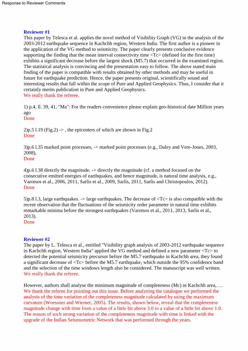
However, authors shall analyse the minimum magnitude of completeness (Mc) in Kachchh area,….

We thank the referee for pointing out this issue. Before analyzing the catalogue we performed the

analysis of the time variation of the completeness magnitude calculated by using the maximum

curvature (Woessner and Wiemer, 2005). The results, shown below, reveal that the completeness

magnitude change with time from a value of a little bit above 3.0 to a value of a little bit above 1.0.

The reason of such strong variation of the completeness magnitude with time is linked with the

upgrade of the Indian Seismometric Network that was performed through the years.

Response to Reviewer Comments

On the base of such results, we preferred to be very conservative and considered all the earthquakes

with magnitude larger than 3.0.

We added this further analysis and figure in the revised paper.

2002 2004 2006 2008 2010 2012 2014

1.0

1.5

2.0

2.5

3.0

3.5

Mc

years

……and check the robustness of the results with the different cut-off magnitude selection.

We checked the robustness of the results with magnitude thresholds of 3.2 and 3.5. The results are

shown in Figs. 7 and 8 of the revised paper.

Furthermore, authors also need to discuss whether the declustering procedures could affect the

reliability of the result.

We applied the method to the earthquake catalog declustered by using the Reasenberg’s method.

The results shown in Fig. 9 indicate the robustness of the method with different declustering

techniques.

Finally, several references appeared in the content but cannot be listed, such as "Tyupkin and Di

Giovambattista (2005)" and "Stiphout et al., 2012".

Done

1

Visibility graph analysis of 2003-2012 earthquake sequence in Kachchh region,

Western India

LUCIANO TELESCA1(*)

, MICHELE LOVALLO2, S. K. AGGARWAL

3, P. K. KHAN

4, B. K. RASTOGI

3

1 National Research Council, Institute of Methodologies for Environmental Analysis – C.da S.Loja,

85050 Tito, Italy

2 ARPAB - 85100, Potenza, Italy

3 Institute of Seismological Research,Gandhinagar, India

4 Indian School of Mines, Dhanbad, India

* Corresponding author

Abstract –The Visibility Graph (VG) is a rather novel statistical method in earthquake sequence

analysis; it maps time series into networks or graphs, converting dynamical properties of time series

in topological properties of networks. By using the VG approach, we defined the parameter window

mean interval connectivity time <Tc>, which informs about the mean linkage time between

earthquakes. We analysed the time variation of <Tc> in the aftershock depleted catalogue of the

Kachchh Gujarat (Western India) seismicity from 2003 to 2012, and we found that <Tc>: i) changes

through time indicating that the topological properties of the earthquake network are not stationary;

ii) appeared to significantly decrease before the largest shock (M5.7) that occurred on 7th

March

2006, near the Gedi fault, an active fault in Kachchh area.

Keywords: Visibility graph, Seismicity, Kachchh

Introduction

ManuscriptClick here to download Manuscript: VG_TN_revised.doc

1 2 3 4 5 6 7 8 9 10 11 12 13 14 15 16 17 18 19 20 21 22 23 24 25 26 27 28 29 30 31 32 33 34 35 36 37 38 39 40 41 42 43 44 45 46 47 48 49 50 51 52 53 54 55 56 57 58 59 60 61 62 63 64 65

2

Recently, the Visibility Graph (VG) method has been representing a novel approach in describing

the statistical characteristics of earthquakes by focusing on its topological properties. The VG

method was developed by Lacasa et al. (2008), who proposed a way to map time series into

networks or graphs. They showed that such mapping converts dynamical properties of time series

into topological properties of networks and vice versa, and the features of networks can be

informative of the characteristics of the associated time series. In particular, periodic time series are

mapped in regular networks, in random time series into random graphs, and fractal time series into

scale-free networks (Lacasa et al., 2008; Donner et al., 2011; Campanharo et al., 2011).

In the VG approach a segment connects any two values of the series visible by each other, meaning

that such segment is not broken by any other intermediate value of the series. In terms of graph

theory, each value of the time series represents a node, and two nodes are connected if there exists

visibility between them. The mathematical definition of the visibility criterion (Lacasa et al., 2008)

is the following: two arbitrary data values (ta, ya) and (tb, yb) are visible to each other if any other

data (tc, yc) placed between them fulfils the following constrain:

ab

cbbabc

tt

ttyyyy

. (1)

Let’s indicate with ki the connectivity degree, which is the number of connections of each node i.

The following properties always hold (Lacasa et al., 2008): 1. Connection: each node is visible at

least by its nearest neighbors (left and right); 2. Absence of directionality: no direction is defined in

the links; 3. Invariance under affine transformations (rescaling of both axes and horizontal and

vertical translations) of the time series.

The VG method was mainly applied to investigate the dynamical properties of continuous signals.

Pierini et al. (2012) demonstrate, by using the VG method the time series of hourly means of wind

speed recorded at two wind stations in central Argentina (one inland and the other coastal) finding

1 2 3 4 5 6 7 8 9 10 11 12 13 14 15 16 17 18 19 20 21 22 23 24 25 26 27 28 29 30 31 32 33 34 35 36 37 38 39 40 41 42 43 44 45 46 47 48 49 50 51 52 53 54 55 56 57 58 59 60 61 62 63 64 65

3

that the topological properties of the two series are similar and do not depend by the characteristics

of the two sites. The analysis of the v–k (sample value – connectivity degree) plots also suggested

that higher values of a series are not necessarily ‘‘hubs’’, that is values characterized by large

connectivity. Telesca et al. (2012) analysed ocean tide records by the VG method in central

Argentina and discriminated local (linked with the coastal conditions) from global (linked to more

general and common atmospheric forcing and ocean current conditions) effects just analysing the

properties of the connectivity degree distribution curve.

Recently the VG method was applied also to point processes (sequence of events randomly

occurring on time) (see Fig. 1 for a visual sketch). Telesca and Lovallo (2012) applied the VG

method to the seismicity of the whole Italy, finding the presence of power-law behavior in the

distribution of the connectivity degree independent of the time-clustering structure and of the

increase of the magnitude threshold. Telesca et al. (2013) performed the VG analysis of the

sequences of earthquakes occurred in the sub-duction zone of Mexico and found that the k-M plots

(which is the relationship between the magnitude M of each event and its connectivity degree k)

were characterized by increasing trend of k with the increase of M, revealing, thus, the property of

hub as typical of the higher magnitude events.

In the present paper, we investigate the earthquake series which occurred in Kachchh region,

Gujarat (Western India) between the year 2003 to 2012. This area has been raising a great interest in

the seismological community because it was struck by a strong Mw 7.7 Bhuj earthquake on 26th

January 2001, and causing more than 160,000 injured and more than 20,000 people killed, and,

thus, making the search of earthquake precursory signatures challenging. After that, the moderate

seismicity still prolongs making the region like a natural seismic laboratory for seismologists in

term of moderate earthquakes of magnitude up to 5.7 and extending to several nearby faults, like

Allah Band fault (ABF), Island belt fault (IBF), Gedi fault (GF), North Wagad fault (NWF), South

Wagad fault (SWF), Kachchh Mainland fault (KMF), Katrol Hill faults (KHF) (Fig. 2).

1 2 3 4 5 6 7 8 9 10 11 12 13 14 15 16 17 18 19 20 21 22 23 24 25 26 27 28 29 30 31 32 33 34 35 36 37 38 39 40 41 42 43 44 45 46 47 48 49 50 51 52 53 54 55 56 57 58 59 60 61 62 63 64 65

4

Seismotectonic settings

According to Rastogi et al. (2012), the Kachchh region is considered one of the seismically most active

intraplate regions worldwide, as it was known to have high hazard due to the occurrences of several great

historical damaging earthquakes until the 2001 Bhuj earthquake that occurred along the south dipping

NWF, a blind dip-slip fault system in Kachchh, which slips in reverse sense of motion in response

to the prevailing north-south compressional forces due to northward motion of Indian plate (Mandal

et al. 2004a; Bordin and Horton, 2004). Until today this event produces a continued aftershock

activity on the same fault and triggers the seismicity on several other nearby faults. Further, the

presence of inter-connected rupture nucleated trends suggest a possible link between these faults

(Mishra and Zhao, 2003; Talwani and Gangopadhyay, 2001).

The Kachchh region is an example of a tectonically controlled landscape whose physiographic

feature are the manifestation of the earth movement along the tectonic lineament of the pre-

Mesozoic basinal configuration that was produced by primordial fault pattern in the pre-Cambrian

basement (Biswas and Deshpande, 1970; 1987). The lithosphere of the epicentral region of the 2001

earthquake is inferred to be hot and thin (only 70 km as compared to normal 100 km) and its crustal

thickness is also small (34 km as compared to 40 km in the surrounding region) caused due to

rifting at around 184 million years ago. The restructuring of this warm and thin lithosphere might

have occurred due to thermal plume at 65 million years ago (Mandal and Pandey 2010). The KMF

is the major fault along rift axis and become the active principle fault, which presently shows right

lateral strike slip fault as overstep by SWF in eastern part of the basin (Biswas, 2005). The

overstepped zone between the two wrench faults is a convergent transfer zone undergone

transpressional stress in the strained eastern part of the basin.

Results

1 2 3 4 5 6 7 8 9 10 11 12 13 14 15 16 17 18 19 20 21 22 23 24 25 26 27 28 29 30 31 32 33 34 35 36 37 38 39 40 41 42 43 44 45 46 47 48 49 50 51 52 53 54 55 56 57 58 59 60 61 62 63 64 65

5

We analysed the seismicity of Kachchh area for the period from 2003 to 2012. The Indian

Seismometric Network has gone through a continuous upgrade that has led to a progressive

decrease of the completeness magnitude of the seismic catalogue with the time. Fig. 3 shows the

time variation of the comleteness magnitude calculated by using the method of the maximum

curvature (Woessner and Wiemer, 2005). As it can be seen, the completeness magnitude strongly

changes with time. In our study, we preferred to be very conservative and considered the sequence

of the events with magnitude equal or larger than 3.0. Before analysing the seismic catalog by

means of the VG method, we removed the aftershocks by using the Gardner and Knopoff (1974)

technique jointly with the Uhrhammer space-time window (van Stiphout et al., 2012): for each

earthquake in the catalog with magnitude M, the successive events are identified as aftershocks if

they occur within a specified time interval and within a distance interval defined by the Uhrhammer

relations (van Stiphout et al., 2012) from respectively the occurrence time and epicenter of the first

earthquake. The obtained declustered catalogue contains 865 events with magnitude larger or equal

to 3.0 (the epicentres of which are shown in Fig. 2). We applied the VG method to the declustered

seismic catalogue. In particular the time variation of the VG window mean interval connectivity

time <Tc>, defined below, was analysed. Considering a sliding window of N events with a shift of 1

event between two successive windows, for each event in the window we computed the interval

connectivity time tc as the time interval between two visible events (events that satisfy the visibility

condition of Eq. 1), for each event we calculated the mean interval connectivity time < tc >, that is

the average of all the intervals tc corresponding to that event. Now, for each window we calculated

the average of all the < tc >, obtaining the window mean interval connectivity time < Tc >. Each

calculated value of < Tc > was associated with the time of occurrence of the last event in the sliding

window. Fig. 4 shows the time variation of < Tc > (red curve) along with the largest earthquake

occurred on 7th

March 2006 with magnitude 5.7 within the same time span of the variability of

<Tc>. We used a window length N=100 events We can observe that before the occurrence of the

largest shock, <Tc> decreases almost suddenly, while, after it, starts to increase; the rate of the

1 2 3 4 5 6 7 8 9 10 11 12 13 14 15 16 17 18 19 20 21 22 23 24 25 26 27 28 29 30 31 32 33 34 35 36 37 38 39 40 41 42 43 44 45 46 47 48 49 50 51 52 53 54 55 56 57 58 59 60 61 62 63 64 65

6

increase after the earthquake is lower than that of the decrease before that event. After such

increasing phase, the <Tc> recovers to its initial conditions, evolving in a more or less stable

behavior. In order to check that the behavior shown by <Tc> is not due by chance, we applied the

same analysis on the 100 shuffled seismic sequences. Each shuffle is obtained, maintaining fixed

the order of the magnitudes but shuffling the occurrence times; in this way, a random earthquake

sequence is obtained that shares with the original one the same probability density function of the

inter-event times and the same magnitude distribution. For each shuffle, we calculated the time

variation of the parameter <Tc>shuf considering a sliding window of 100 events, similarly to the

original sequence. Therefore, at each time, 100 values of <Tc>shuf are obtained. The 95% confidence

band was estimated as the 2.5th

and the 97.5th

quantiles of the distribution of the <Tc>shuf at that

time. Fig. 4 shows that the decrease of <Tc> before the occurrence of the M5.7 earthquake is outside

the 95% confidence band of <Tc>shuf (black dotted lines) indicating that this decrease is significant.

In order to check the robustness of the obtained results with respect to the length of the sliding

window, we repeated the analysis with a moving window of 50 events and 150 events. The results,

shown in Figs. 5 and 6, are similar to those obtained with 100 event window, and this reinforces the

significance of the decrease of <Tc> before the occurrence of the largest shock of March 2006.

In order to check the robustness of the results with different threshold magnitudes and declustering

techniques, we applied the VG method for sliding windows of 100 events to the Uhmhammer-based

declustered catalogue with cut-off magnitudes of 3.2 (Fig. 7) and 3.5 (Fig. 8) and to the

Reasenberg-based (Reasenberg, 1985) declustered catalog with cut-off magnitude of 3.0 (Fig. 9).

The results show that the method could reliably identify anomalous decreasing behaviour of the

parameter <Tc> before the occurrence of the largest shock.

Discussion

It is well known that earthquakes are correlated in time. Several studies applying time-correlation

methods revealed that earthquakes are correlated among them (Telesca et al., 2003; Telesca et al.,

1 2 3 4 5 6 7 8 9 10 11 12 13 14 15 16 17 18 19 20 21 22 23 24 25 26 27 28 29 30 31 32 33 34 35 36 37 38 39 40 41 42 43 44 45 46 47 48 49 50 51 52 53 54 55 56 57 58 59 60 61 62 63 64 65

7

2007). However, earthquakes are magnitude-marked point processes (e.g., Daley and Vere-Jones,

2003; 2008), and most of the methods used to investigate the time properties of seismicity do not

involve directly the magnitude (a method focused on the consecutive emitted energies of

earthquakes, and hence magnitude, is natural time analysis, e.g., Varotsos et al., 2006, 2011, Sarlis

et al., 2009, Sarlis, 2011, Sarlis and Christopoulos, 2012). The VG approach could be viewed as a

topological method able to capture correlation in earthquake sequences involving both the

magnitude and the occurrence time. Linking the earthquakes with each other based on the visibility

criterion (Eq. 1) that takes into account both the occurrence time and the magnitude of each event,

converts the earthquake sequence in a clustered network. In this network the smaller and more

frequent events are linked with the nearest larger events that, having a better visibility contact with

more neighbors than other events, play the role of hubs of the network. The larger events,

furthermore, more infrequent, tend to inter-connect also each other, linking clusters with clusters,

leading to an interdependence in the occurrence of major earthquakes (Romanowicz, 1993; Mega et

al., 2003).

The VG procedure seems not so different from the idea behind the Single Link Cluster (SLC)

method (Frohlich and Davis, 1990), on the basis of which the analysis of spatial correlation length

was proposed as a precursor of large earthquakes (Zoeller et al., 2001; Zoeller et al., 2002); the

difference relies in the domain, that is in the SLC approach the link between two earthquakes is

space-type, in the VG is time-type.

What does the VG parameter <Tc> means? On the basis of its definition, the parameter <Tc> relies,

substantially, to the mean inter-event time between one earthquake and all those that are “visible” to

it in the VG domain. Two earthquakes that are “visible” to each other could also be not consecutive;

in fact it’s the magnitude of the events that governs the “visibility” and, thus, the linkage between

the earthquakes. Therefore, <Tc> averages all these means over a group of earthquakes (those

included in the moving window). If <Tc> is high, this means that, on average, more time has to pass

1 2 3 4 5 6 7 8 9 10 11 12 13 14 15 16 17 18 19 20 21 22 23 24 25 26 27 28 29 30 31 32 33 34 35 36 37 38 39 40 41 42 43 44 45 46 47 48 49 50 51 52 53 54 55 56 57 58 59 60 61 62 63 64 65

8

so that two earthquakes will be linked to each other, while if it is low, this means that less time has

to pass so that two earthquakes will be visibly connected.

In our case, we observe a decrease of the VG parameter <Tc> before the occurrence of the largest

shock of the analysed sequence; this indicates that before its occurrence, the average linkage time

between “visible” earthquakes lowers. This behaviour could suggest also that before the largest

shock the time-clustering of the events occurred before is enhancing, and could be considered

consistent to what observed by Tyupkin and Di Giovambattista (2005). Even though these authors

analysed the decrease of the spatial correlation length before a large earthquake, indicating the

approaching to a critical point behaviour, they have reported a relationship between the

characteristic time interval between events involved in the correlation length estimation and the

linear dimension of the domain where the spatial correlation length is evaluated. From this

relationship it is possible, then, deduced that the characteristic time should be low in order that the

decrease in the spatial correlation length could be observed. This lowering of the VG parameter

<Tc> before the largest event could be thought as related to such characteristic time and its decrease

would be considered consistent with the decrease in the correlation length observed by Tyupkin and

Di Giovambatista (2005) before some large earthquakes.

The decrease of <Tc> is also compatible with the recent observation that the fluctuations of the

seismicity order parameter in natural time exhibits remarkable minima before the strongest

earthquakes (Varotsos et al., 2011, 2013, Sarlis et al., 2013)

Conclusions

The VG method represents a novel approach in investigating the time dynamics of the seismicity.

Of course, it should not be considered as better than the standard statistical methods that are well

known and well assessed in getting information about the time dynamics of earthquake sequences.

However, the VG could be viewed as an alternative method that allows to investigate an earthquake

1 2 3 4 5 6 7 8 9 10 11 12 13 14 15 16 17 18 19 20 21 22 23 24 25 26 27 28 29 30 31 32 33 34 35 36 37 38 39 40 41 42 43 44 45 46 47 48 49 50 51 52 53 54 55 56 57 58 59 60 61 62 63 64 65

9

sequence focusing on their topological properties and inter-connectivity. The application of the VG

method to the seismicity of Kachchh area has revealed that a decrease in the connectivity time

between (also non consecutive) earthquakes appears before the largest shock of the sequence; and

such decrease is significant at 95% and also robust with respect to the length of the event window.

This result strengthens the reliability of the VG approach in detecting precursory signatures in

earthquake sequences.

Acknowledgements

The present study was supported by the ISR project “Statistical Seismic data Analysis of Gujarat

Region, Western India”. The authors from Institute of Seismological Research are thankful to the

Department of Science and Technology, Gujarat for providing all necessary facilities to carry out

this research.

References

Aki K., 1965, Maximum likelihood estimate of b in the formula log N = a-bM and its confidence

limits, Bull. Earthquake Res. Inst. Tokyo Univ., 43, 237–239.

Bada G, Grenerczy Gy, Tóth L, Horváth F, Stein S, Cloetingh S, Windhoffer G, Fodor L. Pinter N,

Fejes I, 2007. Motion of Adria and ongoing inversion of the Pannonian basin: Seismicity, GPS

velocities and stress transfer. In: Stein, S., Mazzotti, S., (Eds.), Continental Intraplate Earthquakes:

Science, Hazard, and Policy Issues. Geological Society of America Special Paper 425, p. 243-262,

doi: 10.1130/2007.2425(16).

Biswas, S. K., and Deshpande, S. V., 1970. Geological and Tectonic maps of Kutch. In: Bull. Oil.

Nat. Gas Commn., vol.7, 115-116.

1 2 3 4 5 6 7 8 9 10 11 12 13 14 15 16 17 18 19 20 21 22 23 24 25 26 27 28 29 30 31 32 33 34 35 36 37 38 39 40 41 42 43 44 45 46 47 48 49 50 51 52 53 54 55 56 57 58 59 60 61 62 63 64 65

10

Biswas, S. K., 1987. Regional tectonic framework structure and evolution of western marginal basin

of India. Tectonophysics, vol.135, 307-327.

Biswas, S.K., 2005. A review of structure and tectonics of Kutch basin, western India, with special

reference to earthquakes. Current Science, vol. 88, No.10, Pp. 1592-1600.

Bodin, P. and Horton, S., 2004. Source parameter and tectonic implication of aftershocks of the

Mw7.6 Bhuj earthquake of January 26, 2001. Bull. Seism. Soc. Am., vol94, 818-827.

Campanharo A. S. L. O., Sirer M. I., Malmgren R. D., Ramos F. M., Amaral L. A. N., 2011, Duality

between Time Series and Networks, PLoS ONE, 6, e23378.

Daley, D.J., Vere-Jones, D., 2003. An Introduction to the Theory of Point Processes Volume I:

Elementary Theory and Methods. Springer, New York, 471p.

Daley, D.J., Vere-Jones, D., 2008. An Introduction to the Theory of Point Processes Volume II:

General Theory and Structure. Springer, New York, 573p.

Donner R. V., Donges J. F., 2011, Visibility graph analysis of geophysical time series: Potentials and

possible pitfalls, Acta Geophysica, 60, 589-623.

Lacasa L., Luque B., Ballesteros F., Luque J., Nuño J. C., 2008, From time series to complex

networks: The visibility graph, Proceedings of the National Academy of Sciences, 105, 4972-4975.

1 2 3 4 5 6 7 8 9 10 11 12 13 14 15 16 17 18 19 20 21 22 23 24 25 26 27 28 29 30 31 32 33 34 35 36 37 38 39 40 41 42 43 44 45 46 47 48 49 50 51 52 53 54 55 56 57 58 59 60 61 62 63 64 65

11

Mishra, O. P., and Zhao, D., 2003. Crack density, saturation rate and porosity at the 2001 Bhuj,

India earthquake hypocenter: a fluid-driven earthquake?, Earth Planet Science Letter, vol 212, 393-

405.

Mandal, P., Rastogi, B. K., Satyanarayana, H. V. S., Kousaliya, M., Vijayraghavan, C., Satyamurthy,

C., Raju, I. P., Sharma, A. N. S., and Kumar, N. 2004a. Characterization of the causative fault

system for the 2001 Bhuj earthquake of Mw7.7. Tectonophysics, vol.378, 105-121.

Mandal, P., and Pandey, O. P., 2010. Relocation of aftershocks of the 2001 Bhuj earthquake: a new

insight into seismotectonics of the Kachchh seismic zone, Gujarat, India. Journal of Geodynamics,

vol.49, 254-260.

Mega, M. S., Allegroni, P., Grignolini, P., Latora, V., Palatela, L., Rapisarda, A., Vinciguerra, S.,

2003, Power-law time distribution of large earthquakes, Phys. Rev. Lett., 90, 188501.

Michas, G., Vallianatos, F., Sammonds, P., 2013, Non-extensivity and long-range correlations in the

earthquake activity at the West Corinth rift (Greece), Nonlinear Proc. Geophys., 20, 713-724.

Pierini, J. O., Lovallo, M., Telesca, L., 2012. Visibility graph analysis of wind speed records

measured in central Argentina, Physica A, 391, 5041–5048.

Rastogi, B. K., Kumar, S., Aggrawal, S. K., 2012. Seismicity of Gujarat, Nat Hazard, DOI

10.1007/s11069-011-0077-1.

Reasenberg, P.A., 1985, Second-order moment of Central California Seismicity. Journal of

Geophysical Research, B, Solid Earth and Planets 90, 5479–5495.

1 2 3 4 5 6 7 8 9 10 11 12 13 14 15 16 17 18 19 20 21 22 23 24 25 26 27 28 29 30 31 32 33 34 35 36 37 38 39 40 41 42 43 44 45 46 47 48 49 50 51 52 53 54 55 56 57 58 59 60 61 62 63 64 65

12

Romanowicz, B., 1993, Spatiotemporal patterns in the energy-release of great earthquakes, Science,

260,1923-1926.

Talwani, P. and Gangopadhyay A., 2001, Tectonic framework of the Kachchh earthquake of 26

January 2001, Seismological Research Letters, vol. 72, No.3, 336-345.

Telesca L., Lovallo M., 2012, Analysis of seismic sequences by using the method of visibility

graph, Europhysics Lett., 97, 50002.

Telesca L., Lovallo M., Ramirez-Rojas A., Flores-Marquez L., 2013, Investigating the time

dynamics of seismicity by using the visibility graph approach: Application to seismicity of Mexican

subduction zone, Physica A 392, 6571–6577, 2013.

Telesca, L., Lapenna, V., Macchiato, M., 2003, Spatial variability of time-correlated behaviour in

Italian seismicity, Earth Planet. Sci. Lett., 212, 279-290.

Telesca, L., Lovallo, M., Lapenna, V., Macchiato, M., 2007, Long-range correlations in 2-

dimensional spatio-temporal seismic fluctuations, Physica A, 377, 279-284.

Telesca, L., Lovallo, M., 2012. Analysis of seismic sequences by using the method of visibility

graph, Europhysics Lett., 97, 50002.

Tyupkin, Y. S., Di Giovambattista, R., 2005. Correlation length a san indicator of critical point

bhevior prior to a large earthquake, Earth Planet. Sci. Lett., 230, 85–96.

1 2 3 4 5 6 7 8 9 10 11 12 13 14 15 16 17 18 19 20 21 22 23 24 25 26 27 28 29 30 31 32 33 34 35 36 37 38 39 40 41 42 43 44 45 46 47 48 49 50 51 52 53 54 55 56 57 58 59 60 61 62 63 64 65

13

Varotsos, P., Sarlis, N., Skordas, E., Lazaridou, M., 2006. Attempt to distinguish

long-range temporal correlations from the statistics of the increments by natural time analysis,

Phys. Rev. E, 74, 021123.

Varotsos, P. A., Sarlis, N. V., Skordas, E. S., 2011. Scale-specific order parameter fluctuations of

seismicity in natural time before mainshocks, Europhys. Lett., 96, 59002.

Varotsos, P. A., Sarlis, N. V., Skordas, E. S., Lazaridou, M. S., 2013. Seismic Electric Signals: An

additional fact showing their physical interconnection with seismicity, Tectonophysics, 589, 116-

125.

Sarlis, N.V., Skordas, E. S., Varotsos, P. A., Nagao, T., Kamogawa, M., Tanaka, H., Uyeda, S.,

2013. Minimum of the order parameter fluctuations of seismicity before major earthquakes in

Japan, Proc. Natl. Acad. Sci. U. S. A., 110, 13734-13738.

Sarlis, N., Skordas, E., Varotsos, P., 2009. Multiplicative cascades and seismicity in natural time,

Phys. Rev. E, 80, 022102.

Sarlis, N. V., 2011. Magnitude correlations in global seismicity, Phys. Rev. E, 84, 022101.

Sarlis, N.V., Christopoulos, S.-R.G., 2012. Natural time analysis of the Centennial

Earthquake Catalog, CHAOS, 22, 023123.

Wiemer, S., Wyss, M., 2002. Spatial and temporal variability of the b-value in seismogenic

volumes: an overview. Adv. Geophys. 45, 259–302.

1 2 3 4 5 6 7 8 9 10 11 12 13 14 15 16 17 18 19 20 21 22 23 24 25 26 27 28 29 30 31 32 33 34 35 36 37 38 39 40 41 42 43 44 45 46 47 48 49 50 51 52 53 54 55 56 57 58 59 60 61 62 63 64 65

14

Woessner, J., Wiemer, S., 2005. Assessing the quality of earthquake catalogues: estimating the

magnitude of completeness and its uncertainty. Bull. Seismol. Soc. Am., 95, 684–698, doi:

10.1785/0120040007.

Zoeller G., Hainzl S., 2002. A systematic spatiotemporal test of the critical point hypothesis for

large earthquakes. Geophys. Res. Lett. 29, 53/1–4.

Zoeller G., Hainzl S., Kurths J., 2001. Observation of growing correlation length as an indicator for

critical point behavior prior to large earthquakes. J. Geophys. Res. 106, 2167–2176.

van Stiphout, T., Zhuang, J., Marsan, D., 2012. Seismicity declustering, Community Online

Resource for Statistical Seismicity Analysis, doi:10.5078/corssa-52382934. Available at

http://www.corssa.org.

1 2 3 4 5 6 7 8 9 10 11 12 13 14 15 16 17 18 19 20 21 22 23 24 25 26 27 28 29 30 31 32 33 34 35 36 37 38 39 40 41 42 43 44 45 46 47 48 49 50 51 52 53 54 55 56 57 58 59 60 61 62 63 64 65

1200 1400 1600 1800 2000 2200 2400 2600 2800

1.0

1.2

1.4

1.6

1.8

2.0

2.2

2.4

2.6

2.8

3.0

Ma

gn

itu

de

time

Fig. 1. Sketch of the VG applied to a synthetic seismic sequence.

Fig. 2. Spatial distribution of the declustered Kachaah seismicity from 2003 to 2012.

FigureClick here to download Figure: Figsrev.doc

2002 2004 2006 2008 2010 2012 2014

1.0

1.5

2.0

2.5

3.0

3.5

Mc

years

Fig. 3. Time variation of the completeness magnitudo calculated by using the maximum curvature

method (Woessner and Wiemer, 2005).

0 1x106

2x106

3x106

4x106

5x106

6x106

5.0x103

1.0x104

1.5x104

2.0x104

2.5x104

3.0x104

3.5x104

4.0x104

6

<T

c>

time (min)

Window length=100 events

95%

Ma

gn

itu

de

Fig. 4. Time variation of <Tc> (red) and the 95% confidence band (black dotted), using a window

length of 100 events. The largest earthquakes occurred on 7th

March 2006 (M=5.7) is indicated by

the blue vertical arrow.

0 1x106

2x106

3x106

4x106

5x106

6x106

0.0

5.0x103

1.0x104

1.5x104

2.0x104

2.5x104

3.0x104

3.5x104

4.0x104

6

<T

c>

time (min)

Window length=50 events

95%

Ma

gn

itu

de

Fig. 5. Time variation of <Tc> (red) and the 95% confidence band (black dotted) using a window

length of 50 events. The largest earthquakes occurred on 7th

March 2006 (M=5.7) is indicated by

the blue vertical arrow.

.

1x106

2x106

3x106

4x106

5x106

6x106

5.0x103

1.0x104

1.5x104

2.0x104

2.5x104

3.0x104

3.5x104

4.0x104

4.5x104

6

<T

c>

time (min)

Window length=150 events

95%

Ma

gn

itu

de

Fig. 6. Time variation of <Tc> (red) and the 95% confidence band (black dotted) using a window

length of 150 events. The largest earthquakes occurred on 7th

March 2006 (M=5.7) is indicated by

the blue vertical arrow

0 1x106

2x106

3x106

4x106

5x106

6x106

10000

20000

30000

40000

50000

60000

70000

6

<T

c>

time (min)

95%

Window length=100 events

Minimum magnitude=3.2

Ma

gn

itu

de

Fig. 7. Time variation of <Tc> (red) and the 95% confidence band (black dotted) using a window

length of 100 events and minimum magnitude of 3.2. The largest earthquakes occurred on 7th

March

2006 (M=5.7) is indicated by the blue vertical arrow

1.0x106

1.5x106

2.0x106

2.5x106

3.0x106

3.5x106

4.0x106

4.5x106

5.0x106

5.5x106

20000

40000

60000

80000

100000

120000

6

<T

c>

time (min)

Window length=100 events

Minimum magnitude=3.5

95%

Ma

gn

itu

de

Fig. 8. Time variation of <Tc> (red) and the 95% confidence band (black dotted) using a window

length of 100 events and minimum magnitude of 3.5. The largest earthquakes occurred on 7th

March

2006 (M=5.7) is indicated by the blue vertical arrow

0 1x106

2x106

3x106

4x106

5x106

6x106

0

5000

10000

15000

20000

25000

30000

35000

40000

6

<T

c>

time (min)

Window length=100 events

Reasenberg's declustering method

95% Ma

gn

itu

de

Fig. 9. Time variation of <Tc> (red) and the 95% confidence band (black dotted) using a window

length of 100 events and minimum magnitude of 3.0. The catalogue was declustyered by using the

Reasenberg’s method. The largest earthquakes occurred on 7th

March 2006 (M=5.7) is indicated by

the blue vertical arrow