Eindhoven University of Technology

MASTER

Dynamic range and radiometer improvements made to a beacon receiver through the use ofDSP techniques

Snijders, R.M.G.

Award date:2001

Link to publication

DisclaimerThis document contains a student thesis (bachelor's or master's), as authored by a student at Eindhoven University of Technology. Studenttheses are made available in the TU/e repository upon obtaining the required degree. The grade received is not published on the documentas presented in the repository. The required complexity or quality of research of student theses may vary by program, and the requiredminimum study period may vary in duration.

General rightsCopyright and moral rights for the publications made accessible in the public portal are retained by the authors and/or other copyright ownersand it is a condition of accessing publications that users recognise and abide by the legal requirements associated with these rights.

• Users may download and print one copy of any publication from the public portal for the purpose of private study or research. • You may not further distribute the material or use it for any profit-making activity or commercial gain

Eindhoven University of TechnologyFaculty of Electrical Engineering

Division of Telecommunication Technologyand Electromagnetics, Radiosystems Group

TTEDynamic range and radiometer improvements

made to a beacon receiver through the useof DSP techniques.

by: R.M.G. Snijders

Master of Science Thesis,Carried out from April 2000 to March 2001

Supervisors: Prof. c.J. Kikkert of the James Cook University in Townsville 1(t!!Prof.dr.ir. G. Brussaard ofthe Eindhoven University of Technology in Eindhoven

, "','

Thefamky ifElectricalEn~ ifthe Eindhowz Unil:ersity ofT~ disclaims all respon.sibiliryfor the contents oftraineeship andgraduation reports.

Summary

Propagation experiments are one of the many activities done by the James CookUniversity (JCU). The project for these measurements is called "Satellite TransmissionRain Attenuation Project" or simply STRAP. As part of this project, engineers of JCU,department Electrical Engineering had developed and built a beacon receiver which isnow called the STRAP4 beacon receiver. The first version of the beacon receiver(STRAP1) was fully analog and the second beacon receiver (STRAP2) was the firstdigital receiver. Mter using both receivers for many years, it became clear that thedynamic range was not large enough for the Northern Queensland climate. To improvethe dynamic range of the STRAP2 beacon receiver, the hardware of the local oscillatorwas changed. These hardware changes had already been made by a student of JCU, butthe successor of the STRAP2 beacon receiver (STRAP3) with the new synthesizer wasnever tested.

The first task of this project was to get the STRAP3 beacon receiver to work. Mterfinishing the prototype of the STRAP3 receiver, it became clear that the synthesizer hadto be changed again, because there were close-in spurii around the beacon signal and thesystem noise floor was not homogeneous and was too high. By changing the synthesizerloopfilter and the synthesizer reference frequency, these disadvantages where gone andthis is what made the STRAP4 beacon receiver.

The STRAP4 beacon receiver is logging the signal and noise power of the AustralianOptus B3 satellite beacon. The dynamic range of the STRAP4 receiver, logging at JCU inTownsville is approximately 45 dB, and the receiver can stay in lock onto signals thatare 50 dB lower then the signal power at clear-sky. Where the dynamic range is definedas: "The ratio between clear-sky signal power and the minimum signal power, where thereceiver still can track the signal, and give correct results within 1 dB". The dynamicrange of the STRAP4 beacon receiver is very close to the calculated theoretical value andtherefore this beacon receiver is almost at its theoretical maximum. The improvementsin the dynamic range were accomplished by changing the hardware of the synthesizer,adding video-averaging on the spectrum data, better peak detection and by reorganizingthe software programflow.

The other aim of this project was to improve the radiometer of the STRAP beaconreceiver. The radiometer makes it possible to calculate the signal attenuation out of themeasured noise power. By increasing the noise bandwidth and by adding 1.5 Hz videofiltering on the noise power, the measured noise power has a spread of 1 dB, instead of5 dB for the STRAP2 receiver. Unfortunately it was not possible to use the radiometeroptimally, because of an interference signal that was coming into satellite-dish, andwhich could not been removed at that time.

More features/improvements to the STRAP4 beacon receiver were added apart from thedynamic range and radiometer improvements, such as: video-filtering on the signalpower, faster data output rate for the logger and a spectrum transfer option foranalyzing the beacon frequency spectrum. All these improvements and extra optionsmade the STRAP4 receiver the best of all the STRAP receivers made at the James CookUniversity so far.

Acknowledgements

I wish to thank all colleagues of the James Cook University, department Electricaland Computer Engineering, for answering all my questions that I have had about theproject and lots of other things and I want to thank them for the wonderful time that I

have had at JCD.

I also want to thank my roommates and the friendly roomkeeper that I have hadduring the stay in Townsville as well all the friendly backpackers that I met during

the seven months in Australia, because they were given me a wonderful time, withoutany worries.

Especially I want to thank two persons:

Professor C.J. Kikkert for all his guidance during my research and tutoring inTownsville, as well guiding me in writing this thesis.

Prof.Dr.Ir. G. Brussaard who helped me to make contact with the James CookUniversity and for all his guidance during the project, inclusive guiding me in writing

this thesis.

Contents

Summary

Acknowledgements

Contents

Abbreviations

1. Introduction

2. The existing STRAP receiver2.1. STRAP12.2. STRAP2

2.2.1. The DSP software of the STRAP2 beacon receiver2.3. Results of the STRAPI and STRAP2 beacon receiver2.4. Hardware improvements to the STRAP2 beacon receiver

3. Changes made to the STRAP receiver3.1. STRAP3 hardware configuration3.2. Software for the STRAP3 beacon receiver3.3. Results of the STRAP3 beacon receiver3.4. Hardware difference between STRAP3 and STRAP43.5. Software of the STRAP4 beacon receiver

3.5.1. Better noise measurements3.5.2. Program is interrupt base3.5.3. Video filtering on the FFT3.5.4. Better peak detection3.5.5. Video filtering on the noise power3.5.6 Video filtering on the signal power

3.6. Results ofthe STRAP4 beacon receiver

4. Dynamic range of the STRAP beacon receiver4.1. Dynamic range measurement of the STRAP44.2 Dynamic range of the different STRAP receivers

5. Theoretical dynamic range5.1 Signal power calculation5.2 Noise power calculation5.3 "Stay in lock" and dynamic range calculation

6. Radiometer6.1 Basic theory of the radiometer6.2 Explanation of the STRAP4 radiometer6.3 Calculation and results of the STRAP4 radiometer

6.3.1 Calculate the antenna temperature with clear sky6.3.2. Calculate the signal attenuation out the noise at clear sky6.3.3. Calculate the attenuation out the noise during a rain fade6.3.4. Conclusion of the radiometer measurements

1

55681010

13141616172020212324242525

292931

33333437

3939424343444447

7. Conclusion7.1 Conclusion of the dynamic range (1st aim)7.2 Conclusion of the radiometer (2nd aim)7.3 End conclusion

8. Recommendations

References

AppendicesAppendix A Datasheet beacon receiver STRAP2 & STRAP4Appendix B Datasheet DSPAppendix C Datasheet LNCAppendix D Datasheet DDCAppendix E Datasheet Front-end coax cable lossAppendix F Hardware changes made to the PLL/synthesizerAppendix G Compiler guideAppendix H Flowchart main programAppendix I Flowchart search_peakAppendix J Video filtering FFT spectrumAppendix K Video filtering signal powerAppendix L Video filtering noise powerAppendix M Result of video filtering the frequency spectrumAppendix N Analyze the best bin sizeAppendix 0 Receiver output formatAppendix P Software timingAppendix Q Satellite path length calculationAppendix R Excel worksheet of the CINAppendix S Rain data of the STRAP2Appendix T FFT spectrum ofthe STRAP3 and STRAP4Appendix U Beacon spectrum with interference signalAppendix V Rain data of the STRAP4AppendixW FFT Windowing

49494950

51

53

5557596163656769717375778183858789919799101103105

Abbreviations

ADCDACDCDDCDFTDIFDSPFFTFIRHHFIIFIIRITUJCULOLNCNCOPLLQSTRAPUHFULPCVCOVHFSNRTU/eX-tal

Analogue to Digital ConverterDigital to Analog ConverterDirect CurrentDigital Down ConverterDiscreet Fourier TransformationDecimation In FrequencyDigital Signal ProcessorFast Fourier TransformationFinite Impulse Response (filter)HertzHigh FrequencyIn-phaseIntermediate FrequencyInfinite Impulse Response (filter)International Telecommunication UnionJames Cook UniversityLocal OscillatorLow Noise ConverterNumerical Controlled OscillatorPhase Lock LoopQuadratureSatellite Transmission Rain Attenuation ProjectUltra High FrequencyUp Link Power ControlVoltage Controlled OscillatorVery High FrequencySignal to Noise RatioEindhoven University of TechnologyCrystal

Chapter 1

Introduction

Attenuation of satellite signals due to rain is very significant for frequencies above5 GHz. As the spectrum becomes more crowded, users are forced to use higherfrequencies. When the frequencies are going higher and higher, the question is whatis happening with the signal in different weather conditions and climates. To have agood perception of the attenuation due to rain and under clear-sky conditions,attenuation models are often used. Figure 1.1 is a plot from the International TelecomUnion (lTD) where the attenuation versus the frequencies is plotted. This plot gives avery good idea of what the rain is doing to the signal attenuation. For example, ifthere is a C-band signal of 4 GHz transmitting from a satellite to earth in very heavyrainfall of 150 mm/hr (10 January 1998 in Townsville), the attenuation is 0.12 dBlkm.But for the same rainfall with a Ku-band signal of for example 12.75 GHz theattenuation is 5 dBlkm, this is about 40 times as much as the 4 GHz signal.

0.01 L--L------L..-'-----__.L..L--L-_-'-----__.L...-__-'-----_-----'

100 r-------,-----,.-----,---.....,....--....,...-TT1~

0.1 1----+----f-+--+--'r~rH_-_+_--_+--__1

3 10 30 100 300 1000

Frequency in GHzFigure 1.1: lTV Rain attenuation data plot

The most effective technique used to measure rain attenuation is to conduct anexperiment, which monitors the received signal strength of a satellite beacon. Asatellite beacon is a low-power signal, that is sent out by a satellite for research or fortracking and control purpose. By doing research on the signal strength in variousweather conditions, it is possible to make more accurate signal strength models. Theused Optus B3 beacon signal is mostly used for Up Link Power Control (ULPC), whichis used to control the signal power of the earth station. By calculating the signalattenuation, the sent out signal power of the earth station will be set to the rightlevel, so that the satellite front-end will not be damaged, under any weathercondition.

Due to the small power of most satellite beacons it can be difficult to measure rainattenuation with sufficient dynamic range. For measurements on rain attenuation agreat dynamic range is preferred. This means that a receiver must "look" very deepinto the noise to detect the low-power beacon signal.

JCD has been doing these measurements for many of years, the project is called"Satellite Transmission Rain Attenuation Project" (STRAP). JCD can use the beaconfrom the Intelsat satellite (11.198GHz and 11.451GHz) and from the AustralianOptus B3 satellite (12.75GHz). However for this project we only used the Optus B3satellite.

Because the rainfall in North Queensland is so intense comparing to other places, thedynamic range of the receiver must be large to satisfy the measurements. In the last10 years there was done a lot of research on improving the STRAP receiver, becausethe current system still loses lock during a huge rainstorm. This means that thesystem could not track the beacon signal anymore, which results in an inaccuratemeasurement. It is possible to increase the antenna surface, but this is very costly.Therefore, one of the aims of this project, was to improve the system by improving thereceiver only.

The first receiver was totally analog but in 1999 C.J. Kikkert and B. Bowthorpe builta Digital Signal Processor (DSP) in the receiver to improve the whole system. Byusing a DSP, the signal and the noise power can be measured simultaneously, whichgives the ability to calculate the attenuation of the beacon signal in two differentways. The easiest way is to calculate the attenuation by using the ratio between theclear-sky signal power and the current signal power. The other method is to calculatethe attenuation out of the noise power, by using the radiometer equation; this ispossible, because there is a relationship between the noise power and the signalattenuation. The spread of the measured noise power must be low to give satisfactoryresults, especially when there is a rain fade. Hard- and software changes were madeto the beacon receiver to improve the noise measurement of the receiver and thus toimprove the radiometer.

In this thesis the following subjects will be discussed:

Chapter 2: The hardware of the STRAPI and STRAP2 receiver is explained, as wellthe software made for the STRAP2. The phase noise of the STRAP2local oscillator was too high, therefore a JCD student made somechanges, the measurement results of these changes are described at theend of this chapter.

Chapter 3: The STRAP2 beacon receiver with the new local oscillator (STRAP3)should give better performance, and will be described in this chapter.After analyzing the STRAP3 receiver, it became clear that there whereclose-in spurii around the beacon, therefore the hardware had to bechanged to the STRAP4 receiver. The hardware changes and thesoftware made during this project will be explained in this chapter.

2

Chapter 4: The dynamic range and the "stay in lock" range are defined in thischapter. The dynamic range of the STRAP4 beacon receiver, softwareversion 2 and software version 27 is measured and plotted. Theseresults are compared with each other, together with the results from theSTRAPI and STRAP2 receiver. At the end of this chapter there is ashort conclusion of these dynamic range results.

Chapter 5: The Carrier to Noise ratio (CIN) is theoretical calculated, which after itis used to analyze the maximum dynamic range for this beacon receiver.The calculated value is compared with the measured dynamic range ofthe final STRAP4 receiver at the end of chapter 5.

Chapter 6: The radiometer of the STRAP receiver is explained in this 6th chapter.First the basics of the radiometer is described and than it is used tocalculate the attenuation out of the noise power. At the end of thischapter there is a short conclusion of the STRAP4 radiometer

Chapter 7: The conclusion of the whole research is described in this chapter, whichis divided in 3 sections; global conclusion of the improvements made tothe receiver, and the conclusion of the radiometer and dynamic range.

Chapter 8: Recommends are given in this chapter, to possibly improve the STRAPbeacon receiver (more).

3

Chapter 2

The existing STRAP receiver

In December 1990 the STRAP1 receiver was installed at Bukit Timah Earth Stationin Singapore for Singapore Telecom. This beacon receiver was fully analog and wasthe second beacon receiver built and developed by JCD.

In 1997, JCD developed a new frequency tracking system for the beacon receiver. Theanalog frequency tracking system of the STRAP1 receiver was replaced by a DSPenvironment (STRAP2). This allows an improvement of the dynamic range andpermits logging digital data containing the measured signal and noise power at thesame time. Such a receiver has been running successfully at Bukit Timah EarthStation since it was installed in September 1998.

The dynamic range of the STRAP2 was not significantly bigger than that of theSTRAP 1 receiver, however the STRAP2 receiver was more powerful, because of theextra functions that were included. In addition the STRAP2 receiver locked onto thesatellite beacon in about one second, compared with one minute for the STRAP1receiver. In this chapter the hardware of the STRAP1 and STRAP2 beacon receiversis described, as is the software that is used for the STRAP2 receiver.

2.1. STRAPl

The first version of the STRAP beacon receiver (STRAP 1) was fully analog and couldmeasure a modulated or unmodulated signal. The power of the carrier, or mean signalis sent to a logger that collects the data. The simplified block diagram of the STRAP1is shown below in figure 2.1.

Satellite beacon signal12.75G~

Detect Beaconf-------------I Frequency

Analog datato data logger

12755.2 MHz

PLL10.7 MHz

Detect Beacon\----><.....!.""'--"!-"--------1 Amplitude

HF to audioconverter &final IF filter

Figure 2.1: Block diagram of STRAP1

5

As can be seen in the block diagram of figure 2.1, the 12.75 GHz beacon signal iscoming in at an 3 meter parabolic dish, where it will be down converted from12.75 GHz to 1.4 GHz with a Low Noise Converter (LNC) uses a dielectric resonatoroscillator. The second down conversion is done using a low noise and very stable fixedfrequency oscillator, to produce an Intermediate Frequency (IF) signal at 137 MHz.The third down conversion is done with a PLL to 5.5 MHz. Mter several further downconversions the final IF frequency of 3.18 kHz is obtained. Peak detecting that signalproduces a DC signal which indicates the signal power. Because the received signal isso small, an IF bandwidth of less than 100 Hz is required, in order to obtain adynamic range of more than 35 dB [5]. The down converted signal should thus bewithin 50 Hz of the final IF filter center frequency of 3.18 kHz. The frequency drift offront-end oscillators and especially the used oscillator of the LNC is far more than theused detection bandwidth, therefor frequency control must be used to compensatethese frequency variations.

The frequency control for the beacon receiver consists of injecting a signal 5.2 MHzabove the 12.75 GHz beacon signal into the receiver dish. The down conversionprocess places this injected signal at 10.7 MHz and the beacon at 5.5 MHz. Theinjected signal is then used in the PLL to cancel the drift due to the dielectricoscillator. A frequency locked loop controls the spacing between the injected signaland the beacon signal to ensure that the beacon signal is placed exactly at the centerof the 3.18 kHz final IF filter.

The STRAP1 receiver located in Townsville, logging on the Intelsat beacon, could staylocked to signals 35 dB lower than clear-sky condition [5] [6] (see chapter 4.2).

2.2. STRAP2

The second hardware version of the STRAP receiver (STRAP2) is the successor of thefirst STRAP receiver (STRAP1). The simplified block diagram of the STRAP2 receiveris shown in figure 2.2.

veo

Satellite beacon signal12.75GY

evaluationdi ital control EZUTE· kit Digital serial data

to data logger

Figure 2.2: Block diagram of STRAP2

HF digitaldown converte

&decimation

filter

di ital dats AD2181DSP board

6

The signal tracking system of the STRAP2 receiver is done with a DSP, which byapplying an FFT to the input signal gives the ability to improve the dynamic range bydigital signal processing techniques. The LNC that was used with the STRAP1receiver is now replaced by a commercial LNC from Norsat (Appendix C), which has acrystal locked oscillator instead of a dielectric oscillator for better noise performanceand a smaller frequency drift. The Norsat LNC has a performance specificationsufficient for this system and shifts the 12.75 GHz signal down to 1.4 GHz. Just likethe STRAP1 receiver, the received beacon signal is shifted down in three stages,resulting in a 5.5 MHz signal at the output of the VHF IF module. This 5.5 MHzsignal is filtered with a standard bandpass-filter of approximately 150 kHz, and is theinput of the DDC board ("HF digital down converter & decimation filter") where thesignal will be digitized.

The beacon signal at the 5.5 MHz IF in figure 2.2, is digitized using a 10 bit Analog toDigital Converter (ADC), with a sampling frequency of 20 MSPS to satisfy theNyquist rate and avoids any harmonic aliasing. The last down conversion to DC isdone digitally with a Digital Down Converter (DDC) from Intersil (formerly Harrissemiconductors, Appendix D). This high performance DDC generates an In phase (I)and Quadrature (Q) component that is used by the DSP to calculate a complex FFT.The simplified block diagram of the DDC and ADC is shown in figure 2.3, where NCOstands for a Numerical Controlled Oscillator used in the DDC.

Q Data156 , 39 or 9.8kSPS

NCO:cos(2TI In t)

I Data156 , 39 or 9.8kSPS

NCO':sin(ZIt In t)

In = NCO frequency 015.5 MHz

Figure 2.3: Block diagram of the ADC and the DDC

The DSP will track the beacon signal and when the program finds it necessary it canre-adjust the NCO (figure 2.3), the Very High Frequency Voltage Controlled Oscillator(VHF-VCO, figure 2.2) or change the decimation-factor of the decimation filter inDDC. The adjustment will shift the frequency of the digitized beacon signal very closeto 0 Hz, so that the beacon always stays within the FFT spectrum. The decimationfactor determines the resolution of the FFT and the size of the frequency "bins". Whenthe beacon is within the FFT frequency spectrum the DSP will calculate the signaland the noise power and send this data by a serial RS-232 connection to the logger.(The features of the STRAP2 can be found in Appendix A). The receiver therefore is aFrequency Lock Loop (FLL) receiver.

7

2.2.1. The DSP software ofthe STRAP2 beacon receiver.

The software for the STRAP2 receiver was written by B.J. Bowthorpe [1] as part ofhis Ph.D. in 1998, in an assembly language for the Analog Devices, ADSP-2181 DSP(Appendix B). The DSP is a part of the EZ-LITE-kit evaluation-board which is used inthe STRAP2 beacon receiver. The advantage of this evaluation kit is that the monitorprogram and the communication hard- and software is already implemented. Thesoftware for the STRAP2 receiver is written using a normal text-editor and can beassembled, complied and linked under MS-DOS to an .exe file. This .exe file can beuploaded by a MS-Windows 3.11 program to the DSP evaluation-board in the receiverfor testing purpose. Once the STRAP software program is finished, it can beprogrammed in an Erasable Programmable Read Only Memory (EPROM, 27C512) tomake the beacon receiver a stand alone system.

The basic idea of the STRAP2-program is:1. Search for the strongest signal in a bandwidth of 1.4 MHz.2. Zoom in, by changing the DDC decimation factor.3. Keep tracking the signal under any weather condition.

A very simplified flowchart of this STRAP2 program is shown in figure 2.4.

YesIs there 1rrinul

past

No

YesOut lock Yes

Out of lock more then 20 seconds

NoNo

NCO adjusted Yes No Yesmore than peak found last

+/·100kH 5min

No No

Figure 2.4: Flowchart of the STRAP2 program.

How to find the strongest signal in an 1.4 MHz bandwidth:When the program starts, it will search for the strongest signal in a bandwidth of1.4 MHz by calculating a FFT over 32 VHF-VCO slots (VHF-VCO makes a sweep from130.8 MHz to 132.2 MHz with a step size of 50 kHz). Because the DDC decimationfactor at startup is set to 128, the bandwidth of the FFT is approximately 78 kHz, andthe bin size is 152.6 Hzlbin, while the calculated FFT spectrum contains 1024 bins.The FFT bandwidth is calculated by dividing the sample frequency by the decimationfactor and then multiplying this by a half (Nyquists theory).

8

FFT bandwidth for a decimation factor of 128 is: 20.106

•~ =78.125 kHz128 2

The bin with the highest energy in the FFT is the peak-power. The DSP is searchingfor the VHF-VCO slot with the highest peak power and will select this frequency slot.After setting the VHF-VCO to the right slot, the NCO will be used for fine tuning thebeacon close to 0 Hz, where after the decimation factor will be set to 2048. Mostly thesearch routine can find the beacon signal in one sweep of 1.4 MHz and can do this inless than one second.

Zooming in and tracking the beacon:When the receiver is locked onto the beacon signal the decimation factor of the DDC ischanging from 128 to 2048 to get a better Signal to Noise Ratio (SNR). Because thebeacon signal, receiver oscillators and the LNC will drift in frequency the NCO canbe adjusted to set the beacon signal close to 0 Hz in the FFT spectrum. When theNCO of the STRAP2 receiver is adjusted more than +/- 100 kHz from the 5.5 MHzbecause of drifting, then the DSP software will change the output voltage of theDigital Analog Converter (DAC) to change the frequency of the VHF-VCO. After theVHF-VCO is stabilized the beacon signal should be within 200 kHz of the centre of the5.5 MHz IF filter. The final frequency adjustment is done using the NCO to sweepthough the 200 kHz bandwidth and then setting the NCO to produce the satellitebeacon output within +/- 20 kHz of 0 Hz.

To make sure that the beacon receiver does not lock on another signal such as aspurious, it does a 200 kHz search every minute. This is done only by adjusting theNCO. When the program cannot find a signal, it is either out of lock, or there is ahuge rain fade. When there is still no signal after 20 seconds, it will do a 200 kHzNCO search, to make sure that the beacon has not drifted outside this range. If thebeacon has not been found within 5 minutes, by using the 200 kHz bandwidth NCOsearch, a complete 1.4 MHz bandwidth search is initiated to re-lock onto the beacon.

When the receiver is tracking the beacon signal, the DSP calculates the power of thesignal and the noise around the signal at 8 times per second and send thisinformation to the logger using a serial RS232 connection.

Signal and noise power calculation:Since the beacon signal energy is spread out over several bins of the FFT, the beaconsignal is evaluated by summing the signal power over a number of bins. To make surethat at least 95% of the power is included, the signal power is calculated by addingthe power of the 41 bins around the peak-power (bin size = 9.54 Hz/bin). The noisepower is calculated by taking a total of 82 bins, 110 bins away from 0 Hz of the FFTand this value is divided by two, to get the same bandwidth as the signal power.

9

2.3. Results of STRAPl and STRAP2 beacon receiver

JCD and Singapore Telecom have done years of measurements with both systems(STRAP1, STRAP2) located at the Bukit Timah Earth Station. In addition STRAP1and STRAP2 receivers have been operating for several years in a dual site, dualfrequencyexperiment[l].

On 30 August 1998 there was heavy rainfall in Townsville when the prototype of theSTRAP2 receiver was logging, these results can be found in Appendix T. Theprototype STRAP2 receiver based in Townsville did not include the sky noise powermeasurement, but the receiver located at the Bukit Timah Earth Station is capable ofmeasuring the signal and the noise power simultaneously.

Figure 2.5 shows a rain fade obtained from the STRAP2 beacon receiver at BukitTimah. As can be seen, the received signal power decreases during a rain fade and atthe same time the noise power increases. By using the radiometer equation, whichwill be discussed in Chapter 6, the attenuation of the beacon signal can be calculatedfrom the noise power. The received signal power can be simply calculated bysubtracting the signal attenuation from the beacon power at clear-sky. However,when the noise is spreading out over a range of 5 dB, the radiometer results will beinaccurate, especially in a rain fade. Therefore, there had to be done some post loggerfiltering to the data, to get a smaller noise spread of approximately 1 dB (figure 2.5).

~ rseacor Attenuation

l~ oJ'"Rain Fade at ~

I- Bukit Timah3 Sep 98 ~ Radiometer Attenuation

¥~

I

easured NoisE -

5

o

-5

~ -10

.=!5 -15+:l'CI

E-20

~0:( -25'tlcl'CIQl -30III'02 -35

-402000 2500 3000 3500 4000 4500

Time in Seconds

Figure 2.5: Signal attenuation and radiometer measurements

More STRAP2 rain data can be found in Appendix S.

2.4. Hardware improvements to the STRAP2 beacon receiver

The STRAP1 receiver was replaced by the STRAP2 receiver but the dynamic rangewas not significantly increased. The limitations of the dynamic range is caused by thehigher phase noise ofthe VHF-VCO in the STRAP2 receiver. The VCO in the STRAP2receiver was a VCO, whose frequency was controlled by a DC signal from the 8 bit

10

DAe. Because the veo of the STRAP2 receiver was not placed in a PLL, with a wideloop filter bandwidth, the phase noise performance was poor. By placing the veo in aPLL (see simplified block diagram of STRAP3 and STRAP4, figure 3.1), the phasenoise performance should increase, which means, that the system noise and thereforethe dynamic range should improve.

Figure 2.6 shows the spectrum of the Optus B3 satellite beacon, received inTownsville using the STRAP2 receiver with the free-running Yeo. This spectrum isobtained by shifting the 5.5 MHz signal to 10 kHz and using a computer sound-card todigitize the data. A similar spectrum can be found in figure 2.7, which is the 5.5 MHzbeacon signal using the veo in a PLL. The reduced phase noise can clearly be seen.Having a lower phase noise, permits the total beacon signal energy to be determinedby summing the power of the small number of FFT bins. For the free-running VHF­YeO, the power of the satellite beacon is determined by adding the energy over41 bins centered around the peak signal.

Measured beacon signal bandwidth is:power over the number of bins . bin size =41 . 9.54 =391 Hz

An analysis of the data used to produce figure 2.6 shows, that the frequencycomponents within 20 dB of the maximum signal are contained within an 350 Hzbandwidth. The 391 Hz measuring bandwidth will thus cover much more than 95% ofthe beacon signal power. The same analysis of the data used from figure 2.7 shows,that the frequency components within 20 dB of the maximum signal are containedwith in an 80 Hz bandwidth.

j5i1GtHteW,jftfii-:ntM'W!t!@ijiii@1lI!·wn,,,,,,,uhiF€P :lgl)(;' immm'IMI'M''tfftffl''diidl.d§ liii.@ilIi,*1&MkjPf'fil'eAw9kHz 10kHz

DdB

10 dB

ZO dB

30 dB

.tIO dB

50 dB

&0 dB

70 dB

80 dB

11kHz 12kHz 13kHl '4kHzDdB

10 dB

20 dB

30 dB

40 dB

50 dB

70 dB

80 dB

...., ...., 1. 2kHz 13kHz

90 dB

100 dB

110 dB

12U dBBucDn Slonal, DC eontrDlh:d yeo. 0192 bin RcalFFTSianel PClwcr ·12.83 dBls, Samplinq Frequency 40.00UD kHz. OedmR.tiu =1Slonel1= -1 2.83 dB at 11.3137 kHzSNR 1VIII dB SSR -1.92 dB THO 208.80 dB SINAD -1.96 dB SFDR 14.63 deftMus. Noise ·31.24 dBts -57.53 dBlBin• .fi8.Z2 dBfs/Hz UCFDR ' ....63 dBfsIdeal Noise -68.79 dBts-9S.0B dB/Bin. -105.77 dBfs/Hl Res. fJlN 11.719 Hz

Figure 2.6: STRAP2 beacon signal

90 dB

100 dB

110 dB

120 dB

Bncon Sianai. PU.. Yeo. 8192 bin RealfFTSianal Power -5.62 dBls. Salhplll,a Frequency 48.0000 kHz. Oec;IIhRalio ., 1Sional1= -5.52 dB al 10.1934 kHzSNR 25.75 dB SSR 36.32 dB THD 200.00 dB SINAD 25.39 dB SFDR 043.94 dBh.Wees. Nalae -31.37 dBls -57.66 dBlBln. -68.35 dBlalHz UeFOR 43.904 dBfsIdeal Noise -68.79 dBls -95.08 dBtBin. -105.77 dBfaIHz Res. fJlN 11.719 Hz

Figure 2.7: STRAP3 beacon signal

Because of the phase noise improvement, the signal bandwidth can be decreased witha factor 4.4, and therefore the dynamic range should increase approximately 6.6 dB.This was not tested by the student that made these changes to the STRAP2 receiver,therefor the first task of this master project was to get the STRAP2 receiver with thehardware changes (STRAP3) to work.

11

Chapter 3

Changes made to the STRAP receiver

After a month of preparation at the Eindhoven University of Technology (TU/e) , Ispend a period of 6 month at JCU to carry out the project to improve the dynamicrange and the radiometer of the STRAP beacon receiver. The project was undersupervision of Prof. C.J. Kikkert, head of JCU, Department Electrical Engineering. Alist of activities carried out during the stay at JCU is shown below and will bediscussed in detail in the rest of this chapter.

Make software for the STRAP3:This was the first task. The hardware of STRAP2 receiver had already been changedto the STRAP3 by a JCU student [3], but the prototype-software for the STRAP3receiver did not work yet.

Make a MSDOS data logger, that can receive FFT data from the DSP:The beacon receiver in normal operation will send a signal and noise power to thelogger, but it was necessary to analyze the spectrum and other parameters as well.Because the signal and the noise power is so small, it was not possible use a spectrumanalyzer to make an accurate analysis. Therefore a logger was made, that displaysthe signal power, noise power and possibly a third parameter, which could also receivethe beacon frequency spectrum data for analysis purposes.

Make hardware changes to STRAP3 beacon receiver, to get rid of the spurii:Mter analyzing the FFT spectrum, it showed many close-in spurii at the mains powerfrequency and its harmonics (Appendix U). This was traced to inadequate powersupply of the new PLL unit (synthesizer). Therefore a few hardware changes had to bemade to STRAP3 beacon receiver, resulting into STRAP4.

Make software for the STRAP4:27 software versions have been made for the STRAP4 beacon receiver. This latestversion has a higher data output rate, has video averaging on the FFT-data, and hasvideo averaging on the signal and noise power, that made the improvements on thedynamic range and the radiometer of the STRAP receiver.

Get the whole system running before 19 December 2000:The STRAP beacon receiver had to be operational before the end of the project atJCU. This meant that the EPROM with the latest software version of the STRAP4,had to work without any problems as a stand alone system.

Make a conversion program for the Linux data logger:Because the Linux logger is more reliable and has the ability to log data for manymonths without doing anything to the logger, this logger was used to log data afterfinishing this project at JCU. To have the ability of reading and analyzing the logger­file, there had to be made a conversion program, that gives the ability to plot thelogger data in a program like Excel, GNU-plot or Matlab. This was also interesting,when more rain fade data could be added to this thesis.

13

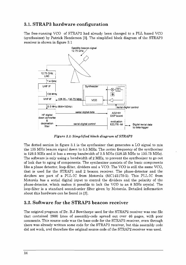
3.1. STRAP3 hardware configuration

The free-running VCO of STRAP2 had already been changed to a PLL based VCO(synthesizer) by Patrick Henderson [3]. The simplified block diagram of the STRAP3receiver is shown in figure 3.1

Satellite beacon signal12.75GY

r··SyntFi"e·s'zer······································ .

veo

serial-digital control,--------'L-------,

HF digitaldown converte

&decimation

filter

serial di ital data

serial-digital control

AD2181DSP board

evaluationEZLlTE- kit Digital serial data

to data logger

Figure 3.1: Simplified bloch diagram of STRAP3

The dotted section in figure 3.1 is the synthesizer that generates a La signal to mixthe 135 MHz beacon signal down to 5.5 MHz. The center frequency of the synthesizeris 129.5 MHz and it has a sweep bandwidth of 2.5 MHz (128.25 MHz to 130.75 MHz).The software is only using a bandwidth of 2 MHz, to prevent the synthesizer to go outof lock due to aging of components. The synthesizer consists of the basic componentslike a phase detector, loop-filter, dividers and a VCO. The VCO is still the same VCO,that is used for the STRAP1 and 2 beacon receiver. The phase-detector and thedividers are part of a PLL-IC from Motorola (MC145170-2). This PLL-IC fromMotorola has a serial digital input to control the dividers and the polarity of thephase-detector, which makes it possible to lock the VCO to an 8 MHz crystal. Theloop-filter is a standard second-order filter given by Motorola. Detailed informationabout this hardware can be found in [3].

3.2. Software for the STRAP3 beacon receiver

The original program of Dr. B.J Bowthorpe used for the STRAP2 receiver was one filethat contained 2800 lines of assembly-code spread out over 46 pages, with poorcomments. This source code was the base-code for the STRAP3 receiver, even throughthere was already written some code for the STRAP3 receiver, but this assembly codedid not work, and therefore the original source code of the STRAP2 receiver was used.

14

To improve the readability and arrange the original STRAP2 code in a more orderlyfashion program, the file had to be splitted up into 10 files, and more comments had toadded to the source code. The 10 filenames with an explanation are:

1. main.asmThis source-code contains the main structure of the whole program and has a listedinformation of the changes that have been made to the program.

2. intvec.asmThis source code contains the interrupt vector table and the interrupt routines

3. info.asmThis file contains information in ASCII code, that can be easy recognize in theEPROM code with the information of the author, version-number and date of compile.

4. uart.asmThis is a standard Analog Device library, with added self-made sub-routines to controlthe serial port in the DSP for the RS-232 protocol.

5. math.asmThis file contains mathematical sub-routines such as square-roots and the logarithmfunction, used in the STRAP software.

6. f4n1024.asmThis is a standard Analog Device library, with added self-made sub-routines tocalculate a frequency spectrum by means of a FFT and windowing.

7. average.asmThis file is only used in the STRAP4 and contains all the video filtering routines.Videlicet for the FFT, signal power and noise power.

8. ddc.asmThis file contains all the control sub-routines for the DDC.

9. delay.asmThis file contains all the delay sub-routines, which have been used in the STRAPreceiver program.

10. pll.asmThis file contains all the sub-routines for controlling the synthesizer.

The 10 listed files will be compiled and linked together to a file called strap3xx.exe,were "xx" stands for the version number. A short description of the assembler, linker,simulator, splitter and EPROM programmer can be found in Appendix G. The latestsoftware program (strap307.exe) works properly on the STRAP3 receiver, and has thesame program structure as the STRAP2 receiver (figure 2.4 for the flowchart). Theonly difference in the flowchart is that the STRAP3 program controls a synthesizerand the STRAP2 controls a VCO.

The existing logger could not handle extra test data, that was now coming from theSTRAP3 receiver, therefore it was necessary to develop a new data logger, that could

15

analyze more than only the signal and the noise power. The new data logger andother test programs in combination with the STRAP3 receiver allows to analyze thedata coming from the beacon receiver. This makes it possible to analyze, for examplethe DDC data, calculated FFT data and the frequency drift of the 5.5 MHz beaconsignal. This information was very useful to show, that the system was workingproperly and later on it was used to see, what the effect was of video averaging on thecalculated FFT.

3.3. Results of the STRAP3 beacon receiver

Figure 3.2 shows a plot of the signal and noise power, when the signal and the noisepower are still added over 41 bins, the same as the STRAP2 receiver.

5

0

·5

·10m2-:;; -15~Q..,If> ·20'0z~

"'" -250;

"C>(7j

·30

'0091. AT' using 1'3 --

-35

·40

...Inoise spread = 5dB

- --.,

-45 '---_---L__--'-__-'--_----'-__----'-__-'--_----'__---'-__-'--_----l

50600 pm 0.02:40 am 65920 am 15600 pm 85240 pm 349.20 am 1046'00 am 54240 pm 03920 am 7.3900 am 2.3240 pm1818100 19/8100 19/8100 19/8100 1918100 2018100 2018!J0 2018100 2118100 2118100 2118100

Figure 3.2: Rain attenuation measured with the STRAP307 software

The new logger program was written in Borland C for use with MS-DOS and readsthe signal and the noise power and possibly extra data from a serial port. Only whenthe signal or the noise power is changed by more than a certain threshold the signalpower, noise power and sample-number will be written to the hard-disk. Thisdifferential logging reduces the amount of data to be stored, without sacrificingaccuracy. There is also a time threshold, which means that the program writes thedata after a certain time to the hard-disk even if the data values are not changing.The logger-file for one weekend logging with the new MS-DOS logger was plottedusing the freeware program GNU-plot and can be seen in figure 3.2. The data shows adaily variation in the signal and noise power, and also shows a noise power spread ofapproximately 5 dB, which is too big for useful radiometer measurements. The powervalues are measured in dB related to a certain power-offset that can be adjust, so thatthe signal power at clear-sky is 0 dB.

16

3.4. Hardware difference between STRAP3 and STRAP4

To investigate the spectrum of the 5.5 MHz signal, data was transferred from theDDC via the DSP to the PC, to analyze this with an FFT program. As can be seen inAppendix T and also figure 3.3 there are spurii around the beacon signal, which areharmonics of the 50 Hz power supply.

odB10 dB

20 dB

30 dB

<10 dB

50 dB

60 dB

70 dB

80 dB

90 dB

100 dB

110 dB

120 dB

130 dB

1<10 dB

150 dB160 dB

Figure 3.3: Beacon frequency spectrum of the STRAP3 beacon receiver

Hardware changes had to be made to the synthesizer of STRAP3 receiver (AppendixF), to improve the beacon frequency spectrum, because the power supply of thesynthesizer was filtered to suppress high frequencies, but the 50 Hz component wasnot suppressed well enough. After better filtering, the power of the 50 Hz harmonicswhere decreased, however a good enough performance could not yet be obtained.

Because of the narrow synthesizer loopbandwidth, the system noise around thecarrier was not flat and not far enough below the expected sky-noise, this means thatthe system noise will affect the measurements. With a loopbandwidth ofapproximately 250 Hz, the phase noise of the VHF-VCO will cause an increase in thenoise floor at approximately 250 Hz from the beacon signal (figure 3.3). By increasingthe loopbandwidth, it is possible to have the bad phase noise of the VHF-VCO outsidethe measured beacon spectrum and the low phase noise of the crystal, whichgenerates the reference frequency, inside the beacon spectrum. The largeloopbandwidth will result in a flat noise floor, which improves the radiometerperformance because the measured noise bandwidth can be increased.

By increasing the loopbandwidth to approximately 2.5 kHz the VCO phase noise willstill cause an increase of noise power in the measured spectrum (Appendix T, figureT2). To make the noise floor flat, that is far below the expected sky-noise, it isnecessary to use a loop-bandwidth of 3 kHz or larger. A beacon frequency spectrumwith a synthesizer loop-bandwidth of 3 kHz, that is used in the STRAP4 receiver,locked on the Optus B3 satellite is shown in figure 3.4.

17

5.495MHzodB10 dB

20 dB

30 dB

40 dB

50 dB

60 dB

70 dB

80 dB

90 dB

100 dB

110 dB

120 dB

130 dB

140 dB

150 dB160 dB

5.497MHz 5.499MHz 5.501 1004Hz 5.503MHz 5.505MHz

Figure 3.4: Beacon frequency spectrum of the STRAP4 beacon receiver

Mter suppressing the close-in spurii and increasing the loopbandwidth of thesynthesizer the power of phase detector reference frequency was increased at theoutput of the synthesizer. A synthesizer reference frequency of 25 kHz was used inthe STRAP3 receiver and is generated from a 8 MHz crystal that is divided by 320 toget 25 kHz (R divider). This reference frequency was used to have the specified stepsize of 25 kHz when doing a full sweep by only changing the N divider. Figure 3.5shows a block diagram of the synthesizer used in the STRAP3 and 4 receiver.

Outputlrequency: 128.25 MHz -130.75 MHz

Figure 3.5: Block diagram of the used synthesizer in the STRAP3 and 4 receiver

Increasing the loopbandwidth also increases the amplitude of the 25 kHz referencefrequency components passing through the loop filter. This can cause false lockingand tracking. By changing the 2nd order loop-filter into a higher order loop-filter, itsuppress the reference frequency more, but it also makes the synthesizer unstableand causes oscillations at the output of the synthesizer. An other option is to makethe reference frequency higher but this will affect the step size of the synthesizer,unless the Rand N dividers are changing simultaneously.

To find out if there was a possibility to have a step size of approximately 25 kHz andat the same time to have a reference frequency higher than 100 kHz, a C program waswritten. The program was called pll03.exe and calculate all the Rand N values thatsatisfies the input specification. Mter calculating all the values, the program willoptimize the step size and makes a lookup table. The following system values wereused in the program:

18

Frequency of the crystalFrequency range of the referenceOutput frequency range

===

8 MHz100 kHz...300 kHz128.5 MHz... 130.5 MHz

The result is a calculated lookup-table with 190 Nand R values, which allows thesynthesizer sweep though a range of 2 MHz with step sizes between 18.144 kHz and28.568 kHz. The lookup-table can be automatically compiled into the STRAP program.By changing the synthesizer hardware, the lookup-table with the calculated valueshad to be used, because the 'old' STRAP3 program will cause oscillations incombination with the 'new' synthesizer. The hardware changes together with the newsoftware, improves noise measurement and will have less power in the comingthrough reference frequency. This new configuration is used in the STRAP4 beaconreceiver

The results of the beacon frequency spectrum, before and after the changes are shownin figure 3.6 and figure 3.7 respectively.

OdS10dS20dS30dS40dS50dSSOdS70dSBOdSSOdS100dSHOdS120dS130dS140dS150dS1S0dS'-------- -----'

? ? ? ? ? ? ? ? ? ? ?~ ~ ~ ~ ~ ~ ~ ~ ~ ~ ~

Frequency difference with respect to 5.5 MHz

Figure 3.6: STRAP3 frequency spectrum

OdS10dS20dS30dS40dS50dSSOdS70dSBOdSSOdS100dS110dS120dS130dS140dS150dS1S0dS,L...--------'----------------.J

? ? ? ? ? ? ? ? ? ? ?~ ~ ~ ~ ~ ~ ~ f ~ ~ ~

Frequency difference w~h respect to 5.5 MHz

Figure 3.7: STRAP4 frequency spectrum

As can be seen in figures 3.6 and 3.7, the Low Pass FIR filter bandwidth(-3 dB) of theDigital Down-conversion process is 2684 Hz. This is in agreement with the DDC datasheet (Appendix D). After allowing for the satellite beacon, only a relative smallbandwidth is thus available for the radiometric noise measurements. This is howeverstill wide enough to produce useful results. [7]

Curve 1 is the original beacon signal from the Optus B3 satellite, where at least 95%of the beacon power is in 5 bins around the bin with the highest energy. The addedpower in 5 bins is approximately 0 dB and the noise power in one bins isapproximately -60 dB, which result -53 dB over 5 bins.

Curve 2 is a generated signal, generated by a Marconi 2041 signal generatorconnected to the input of the STRAP receiver at approximately 1.4 GHz. Thefrequency and the amplitude of the generator is set to the same values as curve 1, theonly difference is that the noise floor of this generator is much lower. The noise floorof the signal generator is at least 20 dB lower than the noise floor of curve 1, whatmeans that the system noise of the receiver is at least 20 dB below the sky-noise atclear-sky condition. This also means that the system noise of the receiver can beneglected compared to the sky noise and noise of the LNC.

Curve 3 is the noise floor measured, when there is no signal, but there is a resistor of50 Ohms connected to the input of the receiver with a temperature of approximately290 K. Curve 3 is even a few dB lower than curve 2, which means the system noise isdefinitely more than 20 dB below the sky-noise and therefore the system noise of thereceiver can be neglected, when measuring the sky-noise.

19

3.5. Software of the STRAP4 beacon receiver

The global structure of the STRAP4 program is still the same as that of the STRAP2and STRAP3, however the features and performances are much better and can beseen in Appendix A. A detailed flowchart with explanation of the STRAP4 programcan be found in Appendix H and I, but the major difference between the STRAP3 andSTRAP4 program are listed below:

• Better noise measurements• Program is interrupt based• Video filtering on the FFT-data• Better peak detection• Video filtering on the noise power

Each of these will now be discussed in turn.

3.5.1. Better noise measurements

By knowing what the spectrum of the beacon at 5.5 MHz looks like, it is possible tofind a method to measure the noise around the beacon. Because the radiometermeasurements require a stable noise level with a small spread (for the meaning ofnoise spread see figure 3.2), it is recommendable to have as much noise data aspossible, that is averaged over a number of bins. The noise is calculated by having thepower in the 512 bins around the center of the FFT, subtracted by 41 bins around thebeacon, see figure 3.8. This is then converted to the equivalent value of the noise in 5bins, because the signal power is also in 5 bins.

~--------.--------~------_._----------· . .· , .· . .· ,, .·10 --------------------~---------------------r

-20

·90

·80 -lhr ~IO ~lI- ft •• - - .~ •••••••• - - ••••••• - - • - ~ -~~ ~ - - • - - - ••:••••• - •• ~ ••••. . .: ....::----1- ---------.--.-----..:t:-...---oj' . -..... :- -. -. -

.100 -1----------'--------'-'-'-"'------'-----'---------'

___________________ ~----------------------- e· • • _

, , .· . ., , ., , .

-30 - •••••• 0 •••••• __ ••• ~. 0 •••• - - 0 •• _ ••••••••• ~ _ _: •• _;_ • _ ••••• ~ •• _

: :,:::. .,.·40 - - - - . - - - -- - - - - •• - - - ~. - 0 • - - • - • - - - 0 __ •••• - • -; - , -; - -- - -- - -;- - - - - - - -;- - - - - - - - - __ - __ - __ - - -

OJ' . . .~: ~., -50~a.

-60

-70

52 103 154 205 256 307 358 409 460 511 562 613 664 715 766 617 868 919 970 1021Bin

Figure 3.8: Number of bins used for signal and noise power measurement

20

3.5.2. Program is interrupt based

The advantage, having the STRAP program interrupt based, is that there will be nolost samples and therefore the receiver has a higher data output-rate.

The STRAP2 receiver copies 1024 I and 1024 Q values into a buffer, which is used tocalculated a window and a FFT. After calculating the FFT, the DSP has to calculatethe signal and noise power and send this to the data logger. All this processing takestime, approximately 21 ms. The data transfer of I and Q samples from the DDC to theDSP will take 104 ms, together this is 125 ms. This means, that the STRAP2 couldsent 8 frames/sec to the data-logger, where a frame consist of signal and noise power(Appendix 0).

The STRAP4 has a better way to do this. The to be processed data from the DDC willbe place in a circular buffer, by a interrupt routine. In the mean time the DSP iscalculating the FFT, signal and noise power and send this to the data logger. Thismeans, that the DSP send a frame of data every 104 ms to the data logger, which are9.54 frames/sec.

A circular buffer is a buffer that has virtually the same begin address as the endaddress, which means that the buffer can be filled continuously, but the data will stayin the buffer a certain time.

An other advantage of an interrupt based I1Q-data transfer is, that it is possible tocalculate an FFT any time, because there should be always enough data in thecircular buffer. The STRAP4 program will calculate a 1024 points FFT and send noiseand signal power in approximately 21 ms, just like the STRAP2 receiver. This means,that after every 256 new I1Q samples, the signal and noise power can be calculatedand send away. By doing these calculations after each 256 I1Q samples, the dataoutput of the FFT-calculation is 4 times as high, which gives better performance tothe video filtering, even through these FFT's are correlated. Because of the signal andnoise power correlation, it is not necessary to send this data after every FFT­calculation, which means, that the receiver data output rate stays the same (9.54frames/sec). The data-flow from the DDC to the data logger is shown in figure 3.9 andgives a good representations how the data from the circular buffer is used for the FFTcalculation The software timing of the FFT and some other software routines, can befound in Appendix P.

As can be seen in figure 3.9 there will be data-transfer of I1Q-data every 102.4 IlS,from the DDC to the DSP. When all the 32 bits (16 bits I and 16 bits Q) aretransferred to the DSP, it will generate an internal interrupt, so that the DSP jumpsfrom the main program into the interrupt service routine to store the I1Q-data into thecircular buffer. Because this interrupt service routine is so small, it will almost notaffect the total processing time of the FFT, signal and noise power calculations. Thismeans, that the calculations done in the main program will be done within 21 ms,after which the DSP goes into idle state to save DSP power and live-time. After each26 ms there is enough data in the circular buffer to do a new FFT-calculation. Thedata will be copied from the circular buffer into a normal buffer, which is used by theFFT sub-routine to calculate the frequency spectrum. The frequency spectrum datawill be video filtered every 26 ms, that is used for frequency tracking and to calculate

21

the signal and the noise power. The calculated signal and noise power will be videofiltered every 26 ms. as well.

DIGITAL DOWN CONVERTER

serial data transfer of I and QDSP interrupt routine will place data in the circular buffer

Circular buffer

BMI~~~~~~~I~~' __

m>U;EEN(OLtlN

~~

copy1 024 I and 1024 Q words fromcircular buffer to temporary buffer

1024 I and 1024 Q words of data

1024 long words of bin power data32 bits =16 bits Low, 16 bits High

frequency spectrum video filter (fc = 1.5 Hz)calculate signal and noise powernoise and signal power video filter (fc = 0.5 Hz)

I~>·

~ ••.•,.•,,'%••.••C,

.u)

send signal and noise power to logger

DATA LOGGER

Figure 3.9: Data flow from DDC to data logger

The DSP has signal and noise power data available every 26 ms, but because thesevalues are correlated they will be send every 104 ms, just like it was done in theSTRAP3 program, this saves processing time and lower the DSP load, which savesDSP-power and life-time.

22

3.5.3. Video filtering on the FFT-data

The filter that is used to process the FFT data is a 1.5 Hz first-order Low Pass Filter.This filter is used, because it is fast and simple to calculate the 1024-samples perFFT, which saves processing time and memory compared to a second- or higher-orderfilter (see Appendix J). Filtering of the spectrum data will decrease the highest noisepower in a bin, therefore the threshold for signal detection can be decreased as well,which will increase the "stay in lock" range. As can be seen in Appendix M, the FFTnoise floor power spread is decreasing, when filtering this data, the noise powerspread is at its minimum after less than 64 samples. This is also the minimumnumber of samples, that has to be taken before the DSP makes a decision, whetherthere is a signal or not. Figure 3.10 shows a beacon frequency spectrum with filteredand unfiltered data. By doing filtering on the FFT-data the improvement in thedynamic range is approximately 6 dB, which can be seen in figure 3.10 with -45.77 dBas highest unfiltered noise power and -51.64 dB as highest filtered noise power.

-- FFT data not filtered-- FFTdata filtered0

-10

-20

-30

m-40"C---Ci3-50==0c..-60

-70

-80

-90

-1001 67 133 199 265 331 397 463 529 595 661 7Z1 793 859 925 991

Bin

Figure 3.10: Spectrum of filtered and unfiltered FFT-data

It is possible to decrease the noise floor power spread, by decreasing the corner filterfrequency, but this has a disadvantage as well. Because the beacon signal is driftingand is not fixed to one frequency, the power of the signal will spread out over anumber of bins. This means, that if the FFT filtering is too slow the powermeasurements and the peak detection are not correct any more, which gives falsereadings. The overall drifting of the signal is not more than one bin per one FFTcalculation, according to one week of logging data with the STRAP4 receiver on theOptus satellite beacon, in Townsville. Table 3.1 shows the calculated results, byhaving the unfiltered FFT data and the filtered FFT data, which is shifted only onebin at Time=O from bin 988 to 989.

23

Time Peak (avg. FFT) Peak (real FFT) Power in 5bins Power in 7 bins0 988 988 -6.59862 -6.592361 988 989 -6.67592 -6.605332 988 989 -6.66618 -6.603713 989 989 -6.65768 -6.60229

Table 3.1: Results of shifting the processed signal one bin.

According to table 3.1, the power of the signal will have an error of 0.08 dB if thesignal is shifting one bin, where the power is measured in 5 bins (see also AppendixN). Because the error is so small, even this is only one step of one bin, this error canbe neglected compare to the spread in the received signal power itself. The signal andthe noise power will be calculated from the filtered FFT-data, so that these powers arefilter as well, but they will also be filtered individually with an 0.5 Hz filter, whichwill be explained in another section.

3.5.4 Better peak detection

The STRAP2 beacon receiver calculate the signal and noise power around the bin withthe highest energy in the frequency spectrum. This will work as long there is not aspurious signal in the spectrum. But if there is a spurious signal, the STRAP2receiver could lock on the wrong signal and give false signal and noise power results,or even worse, it could lose lock.

To prevent these actions, the STRAP4 receiver determines how many signals thereare in the beacon frequency spectrum. If there are more or less signals than expected,the program will refresh the FFT-data and filter for at least 64 new samples to makesure that there are no spurn in the frequency spectrum. The threshold of detectingspurii is 6 dB above the bin-average( bin-average with clear-sky = approx.-31 dB), thiswill be approximately 25 dB lower than the signal power with clear-sky. Because theuse of the bin-average as threshold, the spurious detection is variable. For clear-skythe receiver detects spurn of >-25 dB and in a rain-fade with an attenuation of 40 dBthe bin-average is approximately the same as the noise, which gives a spurn detectionof> -48 dB. (-54 dB + 6 dB)

3.5.5. Video filtering on the noise power

The noise power video filter was specified by JeD. The digital fIlter used to be inagreement with this specification and is an 6th-order Butterworth fIlter with a cornerfrequency of 0.5 Hz. A corner frequency of 0.5 Hz was used, because weather changesare much slower than 2 seconds and all the changes in the measured data faster than2 seconds are not relevant and will be suppressed.

Because an 6th-order Butterworth filter can easily oscillate, the filter is split up into 3second-order filters, with the same poles as used in the 6th-order filter. This willmake the filter more stable. The calculated gain for these second-order filters is about1/625, which makes the noise power so small, that there are inaccurate calculations.

For example:The lowest measured noise power would be -50 dB. The logger reads a value from aserial port and convert this like: (value*10) - 38.6, this is done having a decibel scale,where the signal power at clear sky is about 0 dB. The sent noise value by the receiver

24

is 0.072. This value is generated by a log-function from a standard library, therefore itis an 4.12 format. (4 bits integers, 12 bits decimals), which also means, that the senthexadecimal value is: 0126.

The data from the frequency spectrum is in a 16.16 format (see figure 3.9), whichmeans that the value before the log-function is more accurate and is 0000.126Ehexadecimal. This value of 0000. 126E hexadecimal is used for the video filter. Whenthe video filter divide 0000.126E by a gain of 625, it will be very small, namely0000.0007 hexadecimal. This results in an 32 bit value with a poor resolution, and byusing the 0000.126E value in the filter and gain it at the end there is no overflow inthe calculation and the resolution is 625 times better. (The realized filter can be foundin Appendix L.)

3.5.6. Video filtering on the signal power

The signal power video filter is a simple first-order filter. The signal power does notneed an 6th-order filter, because this is not part of the radiometer specification. Thefirst-order filtering determines the output bandwidth, that is equal to the noise powerbandwidth. The noise power filter has a delay of six samples and the signal powerfilter has a delay of one sample, the difference in the time delay (0.13 seconds) can betaken care of in the signal analysis. (The realized filter can be found in Appendix K.)

3.6. Results of the STRAP4 beacon receiver

On 15 December 2000 the STRAP4 receiver with software version 27 started loggingdata and the result is shown in figure 3.11.

noise spread < 1dB

'D427·3.DAT' using 1'2 --

'D427-3.DAT' using 13 --

rr T . r -or

! ......... .LA ~'r-' .....

't

10 -10:E.

~0c-O>

'" ·20'0z"0C

'"-;;c

'"i:fj ·30

·5020415 pm 4:58:57 pm 7:53:39 pm 10:58:21 pm 14303 am 4:37:45 am 732:27 am 10:27:09 pm 1:2151 pm 4:16:33 pm 711'15 pm15/12r1X1 15/12ilJO 15/12ilJ0 15112ilJ0 16112/00 16/12100 16112.00 16/12.00 16/12/00 16/12/00 16/12100

10

·40

o

Figure 3.11: Logger data of the STRAP4 started on 15 December 2000

25

As can be seen in figure 3.11 the signal and the noise spread is about 1 dB, howeverthe noise power is sometimes changing approximately 1 dB. After a night of recordingspectrum data, it became clear, that there was a second signal close to the 12.75 GHzbeacon. This interference signal, probably another satellite beacon, was driftingthrough the spectrum, and was drifting in- and outside the measured noise and signalrange (see Appendix U). There is more rain fade data, but this was logged with someearlier software versions, 19 and 20, and can be found in Appendix V.

As can be seen in figure 3.12 the interference signal has a peak power of -37.89 dBand is located in the noise measuring range.

-1.72

-37.89

131 196 261 326 391 456 521 586 651 716 781 846 911 976Bin

Figure 3.12: Beacon frequency spectrum with interference signal

When the interference signal is not in the measured noise range, the logged noisepower will be approximately -47 dB, with the assumption that the average noisepower in one bin is -54 dB, see equation 3.1.

Noise power in 5 bins = Noise power in 1 bin· a [Equation 3.1]

where: Noise power in 5 bins =Noise power in 1 bin =a=

the logged noise power in dBdisplayed in figure 3.12 in dB10 . log(5) =6.989 dB

When there is an interference signal in the measured noise range, just like figure3.12, the logged noise power will increase to -46.18 dB, with the assumption that theinterference signal power is within 5 bins, and this is -33.8 dB according to figure3.12. The logged noise power will now be:

Noise power in 5 bins =10·log(Pnoisein466bins + Pinterference signal in5 bins) + f3 [Equation 3.2]

26

where: Noise power in 5 bins =Pnoise in 466 bins =

Pinterference signal in 5 bins =

~=

the logged noise power in dBthe added power in 466 bins around theinterference signal, and will beapproximately 1.855 E-3the added power of the interference signalin 5 bins and is approximately -33.8 dB =0.412 E-3.10 ·log(5/471) = -19.74 dB

The difference between equation 3.1 and 3.2 will be the change of noise power infigure 3.11 and is 0.82 dB. This problem with the interference signal in the measuredbeacon frequency spectrum, could not be fixed in time and its resolution was not partof the aim of the project.

As can be seen in figure 3.11 there was at approximately 11 PM, 15 December 2000rain fade that caused a signal attenuation of more than 10 dB, unfortunately this wasthe largest rain fade during the research in Australia with this receiver. Thereforethis logged data had to be used for analyzing the radiometer, even though it has aninterference signal drifting inside and outside the noise measuring range during thefade. This data will be used in Chapter 6, after making corrections to the noise power.

The total logger time of the plot shown in figure 3.11 is 27 hours and 38 minutes. Ascan be seen the signal has a daily variation, which has its maximum around 4 AMand its minimum around 4 PM. This means that when the sky temperature is at itsminimum, the signal attenuation is at its minimum as well and therefore the loggedsignal power has its maximum around 4 AM.

After finishing the project in Australia, the STRAP4 beacon receiver was logging datawith a new Linux data logger that was made by a JCU student [4]. This data logger isnow part of the whole logging environment used by the JCU. The new Linux datalogger is made for Linux, X-windows and uses differential logging just like the MS­DOS logger. Because the stored data of the new Linux logger was different, then thatof the MS-DOS logger, there had to be made a conversion program. This conversionprogram is made in Borland C and converts data from a Linux logger to a readablefile, that can be used by a spreadsheet or mathematics program. The advantage of theLinux logger data file is that it stores real time, instead of samples in the logger file,this made it easier to analyze, when there was a rain fade. More information aboutthe Linux data file can be found in [1] and [4]

Unfortunately the conversion program did not have to been used, because there wasno rain fade while writing this thesis, that should give better data to analyze.

27

Chapter 4

Dynamic range of the STRAP beacon receiver

The mean reason for improving the beacon receiver was to increase the dynamicrange. The common definition of a dynamic range according to [2, p. 454] and [9, p.56] is:

The dynamic range is the ratio between maximum signal and basic noiselevel. Usually the dynamic range is expressed in decibels.

The more precise definition for the beacon receiver, used in this thesis is:

The dynamic range is the ratio between clear-sky signal power and theminimum signal power, where the receiver still can track the signal and give

correct results within IdE.

4.1. Dynamic range measurement of the STRAP4

Knowing what the definition of the dynamic range is, it is possible to measure thedynamic range by using the following steps:

1. Measure the noise and the signal power, of the "real" beacon signal comingfrom the receiver antenna.

2. Disconnect the "real" beacon signal from the beacon receiver input and connectthe receiver as done in figure 4.1. (This will replace the receiver antenna, LNCand the coax cable of 80 meters)

3. Decrease the power of the signal until the receiver gets out of lock.

Measuring of the signal power and the noise power under clear-sky conditions, is doneby looking at the biggest difference between the signal and noise power over 24 hoursof time. The maximum signal power on an ordinary day as figure 3.11 is 2.0 dB andthe noise power at that same time is -47.2 dB if the interference signal was not there.

After knowing the signal and noise power at clear sky conditions, the artificial beacongets the same signal power and noise power at the right frequency by connecting it uplike the setup in figure 4.1.

Marconi 20411448MHz, f-----_+{+8dBm

~-t-----'---==-l-------1Marconi 20232MHz, -BdBm

SOdBattenuation

HP33120'----------1 Noise,+13dBm

To the input of beacon receiver (to = approx. 1.4 GHz)

Figure 4.1 : Setup for dynamic range measurements

29

The noise of the noise-generator is centered around the 2 MHz signal, generated bythe Marconi 2023 signal generator, this is the beacon plus the noise. By up-convertingthis signal to a frequency of approx. 1.4 GHz, the beacon frequency spectrum is thesame as that of the "real" Optus B3 beacon. By changing the power of the Marconi2023 signal generator and the power of the HP33120 noise generator, it is possible toget the exact same numbers on the logger that were found in step 1; this is the startcondition.

By decreasing the signal power of the Marconi 2023 signal generator only, the signal­to-noise ratio would be decreasing as well. Figure 4.2 shows a plot of the beaconreceiver input power versus the measured power shown on the logger.

10o-10-20-30-40-50-60-70-80

Beacon receiver goes~to saturatfn

./~('"

.//'

/'V

1dB difference at -118 dBm receiver input power/'

VClear sky signal power- 2.0 dEA Clear sky noise power = -47.2 dE

.. .. .. .. .. .. .. .............. .. ............ .. .. .. .. ... .. .. .... -.-:A/'.. .. .. .. .. .. .. .. ............ ............. .. ............ -:'-:f

.STRAP4 beacon receiver indicates that it can't.... find a signal at -123 dBm receiver input power...

........

-60

-110

-120

-80

-90

-130

-160-90

-140

-150

ECD~ -70NJ:c:>'V

xec..li -100iii....

~iiic0>.iii-::Jc..

.5:

~.~

&

Measured logger signal power (dB).

Figure 4.2: Receiver input power versus measured power by the receiver it self

As can be seen in figure 4.2 the measured signal level will be within 1 dB of the truelevel, with a receiver input signal that is equal to, or larger than -118 dBm, or also ameasured logger signal power that is equal to, or larger than -43 dB. This means,that the dynamic range of this receiver (STRAP4, software version 27) is 45 dB (2 dB+ 43 dB).

Once the receiver is locked onto the beacon, it will stay in lock with signals largerthan -123 dBm. If the beacon power is more than clear sky power, then it willmeasure the right beacon power level as well, unless the receiver input power islarger than -69.5 dBm. Signals larger than -69.5 dBm will cause a saturation in thereceiver and this results in inaccurate measurements, because the measured loggerpower is falling of rapidly, when the power gets larger than this level, which can beseen in figure 4.2.

30

4.2. Dynamic range of the different STRAP receivers

There were done two dynamic range test for this project, namely a dynamic range testwith the STRAP402 receiver and a dynamic range test with the STRAP427 receiver.The dynamic range measurements, on the STRAP402 and STRAP427 together withthe measurements from earlier work on the STRAP1 and 2 receiver, are processedwith a spreadsheet program, MS-Excel, and is shown in figure 4.3. Because the LNCof the STRAP1 is different than that of the other STRAP receivers, the receiver dishoutput power is plotted versus the measured logger power to make a good comparison.

-55

-100

-45 -35 -25 -15 -5 5

-110

_ -120ElD"'C-~ -130a.:5a.:50

..c:en -140'6....a>>

"ij)ua>

0:::-150

-160

-170

,/

Measured logger signal power (dB)

• STRAP1 - - - - ref11 • STRAP2 - - - - ref2 lIE STRAP402 • STRAP427

Figure 4.3: Plot of the four different STRAP receivers

To compare the different STRAP receivers, the dynamic range and the "stay in lock"range are listed in table 4.1, where the "stay in lock" is defined as:

The "stay in lock" range is the ratio between clear sky signal and theminimum signal power, where the receiver is locked to a signal and stays in

lock.

31

Remark: The "stay in lock" range is not the same as lock range, because when thereceiver is locked, the decimation factor of the DDC is 2048. When starting-up thereceiver, the DDC decimation factor is 128, which means that the lock range isapproximately 12 dB less than the "stay in lock" range, because the SNR.

·ynamic rangewithin2dB

STRAP1 Inielsai 7 dBW 34.2 dB 35 dBSTRAP2 0 ius B3 17.6 dBW 36 dB 36 dBSTRAP402 0 ius B3 17.6 dBW 40 dB 40 dBSTRAP427 0 ius B3 17.6 dBW 45 dB 47.5 dB 50 dBTable 4.1: Dynamic range and "stay in lock" range for different STRAP receivers.

The STRAP receivers in table 4.1 are STAPl, 2, 402 and 427, and will are discussedin a short conclusion in the next section.

4.2.1 Conclusion of the dynamic range

STRAPl receiver, this is the first, fully analog STRAP beacon receiver, that waslogging at the Intesat beacon, which has approximately 10 dB less power than thenewer Optus B3 satellite beacon. This means that the sensitivity of the STRAPI isabout 10 dB better than the STRAP2 beacon receiver according to figure 4.3 and table4.1.

STRAP2 receiver, this is the first digital STRAP receiver, with a dynamic range and"stay in lock" range that is almost the same as the STRAPI receiver, however thesensitivity of the STRAP2 is about 10 dB worse than the STRAP1.

STRAP402 receiver, this is the first STRAP receiver that was tested during thisproject. STRAP402 means, that it is a STRAP4 receiver with software version 2. Thedynamic range and "stay in lock" range are much better and are only responsible forthe hardware changes that where made to the STRAP2. This means that by onlychanging the hardware, the dynamic range was improved with 7 dB and the "stay inlock" range was improved with 4 dB. This is what was excepted and discussed inparagraph 2.3.

STRAP427 receiver, this is the last and final version of the STRAP receiver so far.The dynamic range, as defined on page 27, is 45 dB which is 24.3 dB better than thefirst STRAP receiver (STRAPl) and 14 dB better than the STRAP2 receiver. Thesensitivity ofthe STRAPI and STRAP427 receiver is almost the same (figure 4.3), butthe STRAP427 has a larger "stay in lock" range and dynamic range, because of thedifferent beacon power.

32

Chapter 5

Theoretical dynamic range

The dynamic range that is measured in the previous chapter, is theoretical analyzedin this chapter.

Satellite:Type:Position:Frequency:Power:

Satellite dishPosition:Diameter:Type:Antenna cons.:Antenna into factor:

LNCType:Conversion gain:Noise figure:

Optus B3 satellite1560 East12.75 GHz, unmodulated uplink power control (DLPC) beacon17.6 dBW EIRP (=Ps·Gs)

Townsville, 1460 45" Longitude, 190 18" Latitude3 meterParabolic with the LNC in the focal point0.550.9

Norsat PLV-82060 dB0.8 to 1.0 dB

Cable between LNC and the ReceiverType: RG-6 5730 TVRO General InstrumentFrequency: 1450 MHzLength: Approx. 80 m.Attenuation: 21.04 dB (Calculation see Appendix E)

Beacon receiverType:FFT:Windowing:Decimation factor:

STRAP4271024 points radix-4 DIFMinimum 4-sample Blackman Harris (appendix W)2048 (when locked onto beacon)

To calculate the theoretical dynamic range, the signal and noise power has to becalculated first, this is done in the next two paragraphs. In the third and also the lastparagraph, the "stay in lock" range and the dynamic range is calculated. (The exactMS-Excel calculations can be found in appendix R.)

5.1. Signal power calculation

Appendix Q gives a representation of the link between the satellite and the receiverantenna in Townsville, where the distance between the satellite and JCD iscalculated. By knowing the exact pathlength that is found in Appendix Q (pathlenght= 36,339,437 m),'the path loss can be calculated for clear-sky condition.

33

I =(4ff' pathlength)2 =3 78851E 20 =205 78dBpath A . + . [equation 5.1]

where: lpath =pathlength =A =

path loss36,339,437 melf with c = 2.9979 .108 mls and f = 12.75 GHz

The gain of the Receiver antenna is:

( )

2ff·D

GR = ----;:- .y =88464 =49.47dB [equation 5.2]

where: GR

yD

===

Satellite dish gain factorAntenna constant (0.55 used by JCU)The diameter of the receiver antenna-dish (3 m)

The calculated beacon power at the input of the receiver is:

==

Pr+ lpath + GR + GLNC -lee

-71.8 dBm[equation 5.3]

With PR the power in dB's at the input of the beacon receiver and lee the loss of thecable and the connectors used between the beacon receiver and the LNC. The loss ofthe coaxcable is specified in Appendix L, and the extra loss is approximately 2 dBwhich gives a total loss of: lee = 23.1 dB.

5.2. Noise power calculation

To calculate the received noise at clear-sky, the external noise has to be defined first.The external noise sources are:

• The sun

• The moon

• The earth

• Galactic noise

• Cosmic noise

• Sky noise

• Atmospheric noise

• Man-made noise

The noise temperature of the sun is normally between 1,000 and 10,000 oK for12.75 GHz, but the satellite dish of the beacon receiver is not pointing to the sun, thisis why this noise source may be neglect under the most circumstances. However thesatellite is moving compared to the sun during the year, which means that theincoming sun-noise can be so high that it may not be neglect at all times.

34

An other important noise source is the earthnoise, which will be received because ofthe non ideal antenna, which has spillover and so it is getting noise from the earthinto the receiver antenna dish. The average earth noise temperature is 254 oK,however for Townsville as receiver-site, the earth temperature may be slightly morethan 254 oK.

Galactic noise and cosmic noise are falling off rapidly at higher frequencies. Thegalactic noise can be neglect above 1 GHz and the cosmic noise has a temperature ofapproximately 2.7 K for 12.75 GHz.

Atmospheric noise originates mainly from the oxygen and water vapor moleculeswhich absorb radiation; this is described in Chapter 6.

It is difficult to say what the antenna noise temperature is because it is changing allthe time and it depends on so many factors, however it is possible to make a goodapproximation with equation 5.4.

TA =(H . Ts,e) + Tcosmic + [(1-B) . Tg] [equation 5.4]

where: TAHTs,eTCOSIILic

==

=

Antenna noise temperatureAntenna integration factor (0.9 used by JCD)Sky temperature at given elevation angleCosmic temperature (2.7 K)Earth temperature (290 K)

The unknown sky noise temperature can be estimated by usmg an lTDrecommendation plot (figure 5.1).

Brightness temperature of clear air for 7.5 g/m 3 of water vapour concentration(expansion of abscissa scale of Fig. 4): 8 is the elevation angle

1000

500

200g~ 100.a!!!Q)

~ 50.2lIIIIII

~1: 20Cl

~10

5

2

8 =0°

./ioo"" ...~ ~ -~ 'q'

V /' '- 10-"" l/ zV ioo"" J /'~

....... rf' -......V

..- "/' ~Jf./10°

I" " .... ~ '"", ,'" ...... 20°

_........ i'V

V V /30

6 ....... ~

-........... / / "/W r-\. .-~V,....1-' V 1'-' ~ Rn' .-

.--.-' ...... /' V V/ 90c

# "'.-.- ./. .r,..~V'

....-.:::: -;:::..- i"'"

r

o 5 10 15 20 25 30 35 40 45 50 55Frequency (GHz)

Figure 5.1: lTV plot of clear air, brightness temperature

60

35

The sky noise temperature for an elevation angle of 64 degrees is approximately5.5 K. This means, that the antenna-noise (TA) should be 37 oK @ 12.75 GHz, howeverthis is only a tribute value. The exact value can only be measured and is changing intime. Unfortunately the beacon receiver is not only measuring the antenna noise, butalso internal noise, such as the equivalent noise temperature of the beacon receiver,cable and LNC. The mean noise sources are shown in figure 5.2.

Tground

T cable+conneetors T beacon receiver

Figure 5.2: Simplified diagram of the "Noise sources" at clear sky

The equivalent noise power at the input of the system (receiver antenna) is defined as:

NAE k . Tetet·B [equation 5.5]

where: kTetot =

B =

Boltzmanns constant, 1.38 x 10-23 watt-seconds/oKEquivalent noise temperature oKBandwidth in Hertz.

The used Tetet in equation 5.5 can be calculated with the equation for a number ofstages in cascade, like:

[equation 5.6]

After filling in the number in equation 5.6, the total equivalent noise temperature willbe: Tetet = 114.35 oK.

Now there is only one last value unknown in equation 5.5, the noise bandwidth (B).The logger noise power is the equivalent noise power in 5 bins, with a bin size of9.54 Hz, this together with the window function multiplication factor of two will give anoise bandwidth of 95.37 Hz. (see appendix W for the used window function).

The equivalent noise power at the input of the system, can be calculated withequation 5.5 and is: NAE= -152.22 dBm

36

Because the theoretically calculated signal power is the power at the input of thereceiver instead of the input of the receiver antenna, this NAE has to be multipliedwith the gain factor of the LNC and the loss of the coax cable and connectors. Thenoise power at the input of the receiver (N) is:

N = NAE + GLNC - lee= -158.22 dBm + 60 dB - 23.1 dB

N = -121.32 dBm

[equation 5.7]

The exact calculation of the signal and noise power can be found in Appendix R.

5.3. "Stay in lock" and dynamic range cacluation

The calculated Signal to Noise Ratio (SNR) or also Carrier to Noise ratio (CIN) at theinput of the receiver is: 49.52 dB (-71.80 + 121.32). This is a trustful value because itis very close to the measured SNR by the logger, which is: 49.2 dB (2 + 47.2).

The "stay in lock" range is approximately the same as the SNR, this resulted out ofmany experiments, therefore:

The theoretically "stay in lock" range is: 49.52 dB.

When the signal is getting smaller, in a rain fade, the signal power is getting closer tothe noise power, this will affecting the measured signal power. The measured signalpower may have an error of less then 1 dB. This means that the signal has to be5.87 dB higher then the noise, according to the calculation below.

(Signal + Noise) / Signal =1 + Noise/Signal =Noise/Signal =SNR =

1.2589 (= 1 dB)1.25890.25895.87 dB

Therefore the dynamic range is: 46.65 dB.

37

Chapter 6

Radiometer

In this chapter the radiometer of the STRAP4 is described. A radiometer is nothingnew, there are already several existing radiometers, and can be divided in threetypes:

• The Total power radiometer (TPR)• The Dicke radiometer (DR)• The Noise-injection radiometer (NIR)

These type of radiometers are widely used for sensing the properties of the earth(weather conditions). The radiometer of the STRAP4 is of the type "Total powerradiometer" and its simplified block diagram can be found in figure 6.1.

TA -.....-----1

rTN

B

f--_Vout

Figure 6.1: Simplified block diagram of a Total power radiometer

The gaining (G) is done by the hardware, and the rest is done by the software of theSTRAP4 receiver, which is discussed in the second paragraph after the basic theory ofa radiometer. The third and also last paragraph will be used to discuss the radiometerresults of the STRAP4 receiver, which will be followed by a short conclusion of thedata that is taken on December the 15th of 2000.

6.1. Basic theory of the radiometer

The theory is already explained in many books [1][8][10][11], but in this paragraphyou will find a short summary of the distraction, and will give values of theparameters. In the previous chapter was already discussed that the received noise isnot only coming from one noise source, infect there are many noise sources. The onethat is not discussed yet, is the atmospheric noise, which is significant by rain. Figure6.2 gives a representation of the noise sources, when there is rain between thesatellite dish and the satellite.

39

Figure 6.2: Representation of the extra noise coming into the dish by rain

The rain is an absorbing medium, that will have a transmissivity t. When the mediumtemperature (rain) in equilibrium is Tm, then the absorbed energy corresponds to(l-t)Tm and hence the energy radiated as noise from the absorbing medium causes anincrease in noise temperature equal to (l-t)Tm.

Therefore the noise caused by rain is:

( 1 JT 1--m A

rain

with A . =~rain t

[equation 6.1]

where: Tmt

==

Medium temperature (K)The transmissivity

And the noise from the background is:

Tcosmic with A . =~rain t

[equation 6.2]

The received noise (Tr) from the cosmic and the rain can be calculated as:

Tr = (1- t)Tm+ t . Tcosmic

The attenuation(A), can be solved by re-arranging the equations to:

A = ~osmic - TmT -Tr m

[equation 6.3]

[equation 6.4]

As can be seen in figure 6.2 there is also ground noise coming into a not ideal antennadish, this is because an antenna will have side lobes, that pick up ground noise. Theantenna output noise temperature, TA, can be represented by:

40

Kelvin [equation 6.5]

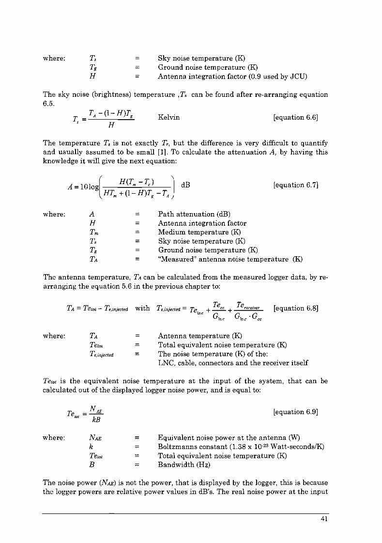
where: TsTg

H

===

Sky noise temperature (K)Ground noise temperature (K)Antenna integration factor (0.9 used by JCD)

The sky noise (brightness) temperature, Ts can be found after re-arranging equation6.5.

T -(l-H)TT = A g

S HKelvin [equation 6.6]

The temperature Ts is not exactly Tr, but the difference is very difficult to quantifyand usually assumed to be small [1]. To calculate the attenuation A, by having thisknowledge it will give the next equation:

A =lOIOg( H(Tm- TJ J dBHTm + (1- H)Tg - TA

[equation 6.7]

where: AH

=

===

Path attenuation (dB)Antenna integration factorMedium temperature (K)Sky noise temperature (K)Ground noise temperature (K)"Measured" antenna noise temperature (K)

The antenna temperature, TA can be calculated from the measured logger data, by re­arranging the equation 5.6 in the previous chapter to:

TA =Tetot - Te,injeeted with Te,injeeted = Te + Teee + TereeeiverInc G

1neG

1ne• Gee

[equation 6.8]

where: TATetotTe,injeeted

=

=

Antenna temperature (K)Total equivalent noise temperature (K)The noise temperature (K) of the:LNC, cable, connectors and the receiver itself

Tetot is the equivalent noise temperature at the input of the system, that can becalculated out of the displayed logger noise power, and is equal to:

N AETetot =--kB

where: NAE =kTetot =B =

[equation 6.9]

Equivalent noise power at the antenna (W)Boltzmanns constant (1.38 x 10.23 Watt-secondslK)Total equivalent noise temperature (K)Bandwidth (Hz)

The noise power (NAE) is not the power, that is displayed by the logger, this is becausethe logger powers are relative power values in dB's. The real noise power at the input

41

of the receiver at clear sky is -72 dB, which is displayed by the logger as 2 dB. Thismeans that the displayed value has to be added with -74 dBm to get the real noisepower at the input of the receiver. There is a gain between the receiver and theantenna, made by the LNC, coax cable and the connectors as well, which is needed tocalculated the equivalent noise temperature at the antenna.

NAE =Ndisplayed/dBJ - Roffset - Cine + lee [equation 6.10]

where: NAE =Ndisplayed/dBJ =Roffset =Cine =lee =

Equivalent noise power at antenna (dBm)Displayed logger value (dB)Receiver power offset (74 dBm)Gain of the LNC (60 dB)Loss of the coax cable and the connectors (23.1 dB)

The equations 6.7 to 6.10 can be re-arranged to:

A =lOiogH(Tm-TJ dB

HT +(l-H)T _[(NdiSPIOed[dBJ -Roffset -G1ne +lecJ-T.. Jm g kB e,lnJeeled

[equation 6.11]

where: A =H =Trn =Ts =T g =Te,injeeted =Roffset =Ndisplayed[dBJ =k =B =

Path attenuation (dB)Antenna integration factorMedium temperature (K)Sky noise temperature (K)Ground noise temperature (K)The injected noise by the hardware (K)Reciever power offset (108 dBm)Displayed logger value (dB)Boltzmanns constant (1.38 x 10.23 Watt-seconds/K)Bandwidth (Hz)

The equations will be used in another section to calculate the antenna temperatureand the signal attenuation out of the noise.

6.2. Explanation of the STRAP4 radiometer

The gaining of the radiometer is done by the hardware, and the rest of the blocks isdone by the software, such as; band pass filter (B), converter (x2) and an integrator('t).In the STRAP4 receiver the converter and the main band pass filter for theradiometer are swapped, because the STRAP4 receiver is calculating the FFT andmakes directly a power spectrum of the voltage spectrum. After the conversion, thereare 471 bins added together and subsequently converted to the equivalent noise powerin 5 bins, which means that the bandwidth of 471 bins is 4492 Hz. Because of theBlackman Harris window-function that is used, the noise resolution bandwidth istwice as much.

42

Therefore the radiometer measuring bandwidth is 8984 Hz.

To have a more reliable and accurate measurement, there is an integration done onthe radiometer power. The integration time and the bandwidth of a standardradiometer together with the STRAP2 and STRAP4 radiometer are reflected in table6.1.

Type .. ~ ... ~ . . ~ W .....,--~.

Standard 12 GHz radiometer 1E+9 4,8,16,32,64 ms.STRAP2 beacon receiver 1564 NoneSTRAP4 beacon receiver 8984 0.5 Hz, 2 s.

Table 6.1: Table of radiometer properties

As can be seen in table 6.1 the bandwidth of the STRAP4 is increased with a factor5.74 compared to the STRAP2, but is still smaller than a standard radiometer. Thebandwidth of the STRAP4 receiver is still more than a hundred thousand timessmaller than a standard radiometer. This explains that the noise power spread of theSTRAP4 receiver is larger than a standard radiometer. To compensate this largenoise spread level, the radiometer data will be processed by a low pass filter with aintegration time of 2 seconds. This integration time can be this large, because thenoise power changes will never be that fast, that there will be thrown away importantdata.

6.3. Calculation and results of the STRAP4 radiometer

By knowing the noise bandwidth and the basics of the radiometer, the antennatemperature and the signal attenuation can be calculated out of the noise. This isdescribed in the next three sections of this paragraph, and at the end there is a shortconclusion of the radiometer results.

6.3.1. Calculate the antenna temperature with clear sky

The equivalent total noise power at the antenna with clear sky can be calculated withequation 6.10 and is:

NAE =-47.2 dB -74 dB - 60 dB + 23.1 dB =158.1 dBm.

By using equation 6.9. the total equivalent temperature can be calculated:

Tetat = 117.63 K

The temperature injected by the hardware (Te,injected) can be found in Appendix Randis 77.35 K. This means that the antenna temperature with clear sky condition can becalculated by using equation 6.8. and is:

TA = 117.63 - 77.35 = 40.28 K

The "measured" value is about 3 Kelvin larger than the estimated value of theantenna temperature, which was 37 Kelvin. There are many ways to explain the

43

difference, but most likely there is a small error in the lee, especially because the valueof lee is calculated and not measured, and has a great impact on the answer of TA.

6.3.2. Calculate the signal attenuation out of the noise at clear sky.

When calculating the attenuation out of the noise power, equation 6.7 and 6.11 can beused. Because the antenna temperature (TA) has already been calculated in theprevious section, it is recommendable to use equation 6.7. The parameters used forthis equation 6.7 will now be discussed in turn:

Tcosmic:This is the noise temperature of the universe, where the satellite dish is pointing to.The temperature is small and pretty constant and is about 2.7 Kelvin.

Tm:The medium temperature, that is also the temperature of the rain is very difficult tomeasure, because it is not homogenous, and its a function of frequency, rain rate, rainheight, elevation angle, could cover and ambient temperature. Therefore the mediumtemperature is usually be chosen to be constant, and is 290 K, according to theresearch of B.J. Bowthorpe [1].

Tg:

It is possible to measure the ground temperature (Tg) very accurate, but unfortunatelyit was not done by JCU at that time. The value that is used in the calculations is Tg =290K

H:This value is taken from a paper of C.J. Kikkert [5] and is H =0.9. The integrationfactor is the factor of sky temperature, that is received by the antenna. The factor(i-H) is the factor of received ground noise by the antenna.

When using these values in equation 6.7, the attenuation, for clear sky, will be:

A = 1.41 dB

6.3.3. Calculate the attenuation out of the noise during a rain fade.

To calculate the attenuation during a rain fade the same equation 6.7 or 6.11 is used.Unfortunately, the only data taken during a rain fade with the final STRAP4 beaconreceiver was an 10 dB rain fade with an inference signal close to the beacon signalitself. It is possible to receive data from JCU, during the making of this thesis, butthere was almost no rain and therefore this rain data had to been used.

As already been said in the previous chapters the interference signal causes avariation of approximately 0.82 dB in the noise power. When using this data thevariation has to be removed and this is done manually. The result of the measurednoise with the interference signal and the modified noise can be found in figure 6.3.

44

I\bise -- ~s. I\bise

-43.5 ,..----------,--------,--------r---------,.--------,

25:0020:0015:0010:0005:00

-47.5 ..1.- ----l --'- -'- --'- ---'

00:00

-44.5 +----------j-------+---.--:--fL--------'~.t-~-----__+-------__j

-46.5 +--+-----t---/---~"'-------+----~~+__-----___f~---~~__l

-44 +--------/-------+----t.iI(IJl--l\--+__------+------__l

co -45:'2- +----------j-------;;H-------t--f'------'----=1"'---__+------__j

~ -45.5 +----------j------+-,"+--------+----+--__+----~~__ja.(l)

'"'0 -46 +---------/-------,jr---+------~+__-----'t--...___.~--+------__lz

Tirre (rrinutes:secondes)

Figure 6.3: Noise correction on the 10dB rain fade of 15 December 2000

When using the modified noise power data of the rain fade in equation 6.11 theattenuation plot can be calculated, this is done with a datasheet program MS-Excel(figure 6.4).

-Radiometer power --Meas. Signal --Noise

.~

~(~<b="

CD~ -10

~a.Q)

.~ -20z'0C",

~ -30Oliii

10

o

-40

-50

00:00 05:00 10:00 15:00 20:00 25:00

Tirre (rrinutes:secondes)

Figure 6.4: Beacon and radiometer attenuation o/the used values in 6.3.1 and 6.3.2

As can be seen in figure 6.4 the radiometer attenuation is not enough compared to themeasured signal attenuation. Because the signal attenuation is much more accuratethan the radiometer attenuation, the radiometer attenuation should be wrong. Thereare many parameters in equation 6.11 that can have an error. The parameters fromequation 6.11 will be discussed in turn, by changing them to a value that gives asatisfied radiometer attenuation:

45

Antenna integration factor H:This value is copied out of a paper [5] and is 0.9. By changing only the parameter H toany value between 0 and 1, will not result in a better plot.

Medium temperature Tm:The medium or also rain temperature was copied from a book [1], and was assumed tobe constant (290 K). By changing only the parameter Tm to 178 K, it will result in aplot that can be seen in figure 6.5. This is highly unlikely because the receiver-site islocated in tropical Townsville and the medium temperature would be -95 degreesCelsius.

Cosmic temperature Tc:The cosmic temperature is definitely between 2.7 K and 3 K at 12.75 GHz. Bychanging the cosmic temperature from 2.7 K to 10 K there is no visual difference inthe radiometer attenuation plot.

Ground Temperature Tg:

The ground temperature was not measured, but the value was copied from a book [1].The value that is used is 290 K, by changing this value between 100 K and 600 K theplot itself is not getting better, however the clear sky attenuation is changing.

Gain between the antenna and the receiver:The gain between the antenna and what the receiver displayed was 110.9 dB. Bychanging the gain only to 109.5 dB (1.4 dB less) it will have good plot results of therain fade. Probably the calculated and measured gain is not accurate enough for theradiometer measurements. The plot of the radiometer attenuation, with a gain of109.5 dB can be seen in figure 6.5.

--Radiometer power --Meas. Signal --Noise

10 ,---------,----------,-------,-------...,------------,

oF~~~=~~!Ilotl!o.~~~----+--~-_+-==-=-__l

~ .10 +------__+_------'~-_+~-.,..-'__c:w~:(rl'__-+__-----_+_------___j~ pc­al

~ ·20

"Cc::CIl

~ ·30 +---------+----------+~~~---t_-----+_-----___ICl

CiS

·40 +-~----__+_-----___l_~~----+__~~---_+_------___j

25:0020:0015:0010:0005:00.50 -'----------'---------'-------'---------'----------'

00:00

Tirre (ninutes:secondes)

Figure 6.5: Beacon and radiometer attenuation with 1.4 dB less gain.

46

The radiometer result of figure 6.5 can only be used as an indication of theattenuation, because the fluctuation is getting bigger when the attenuation increases,this is because some parameter will be more significant in a fade. Possibly significantparameters, that could cause these fluctuations, are:

• The ground temperature, which can be measured, but is not done in thismeasurement.

• The medium temperature, which can not be measured. However themedium temperature can be estimated from the outdoor temperature,which can be measured, but is unfortunately not measured in thismeasurement.

• The gain between the receiver antenna and the receiver. It is possible thatby changing the temperature, for example the LNC temperature, the gainis changing, this will have a great affect on this radiometer measurement.Probably the LNC is the most sensitive component that could beresponsible for gain fluctuations. Therefore it is recommendable to have aLNC temperature measurement. This temperature was not been loggedduring this measurement, but is definitely feasible.

6.3.4. Conclusion of the radiometer measurement.

The radiometer can be used, however it is recommend to use the radiometer strictlyas an indication tool, because of the large inaccuracy during a rain fade. Theinaccurate radiometer attenuation, is caused by many parameters, that become moresignificant in a rain fade. The only measured parameter in the radiometer equation isthe noise power, but this is not the only parameter, that is changing during a rainfade.

From earlier research on the STRAP2 radiometer, it became clear that during therain fade on 3 September 1998 in Bukit Timah (figure 2.5), the ambient temperaturewas changing nearly 5 degrees. Probably the LNC temperature, LNC-gain, groundtemperature and the receiver temperature are changing as well in a rain fade. Byimproving the radiometer, it can be used as a good device for analyzing signalattenuation, or to improve the radiometer model. The radiometer can be improved bylogging more than only the noise power, such as; the ambient temperature, groundtemperature, LNC temperature and maybe away to log the gain between the antennaand the receiver.

47

Chapter 7

Conclusion

The first aim for this project was to improve the dynamic range of the beacon receiverand the second aim was to improve the radiometer of the receiver.

7.1. Conclusion of the dynamic range (1st aim)

To improve the STRAP2 beacon receiver, the free running veo was replaced by asynthesizer. The receiver (STRAP3), with the new synthesizer was never been tested,because the software was not working. The synthesizer with the new STRAP3program should improve the dynamic range of the receiver with approximately 6 dB,after measuring it seems to be 7 dB, but the "stay in lock" range was improved with 4dB.

There were made more software changes to the STRAP program to improve thedynamic range and "stay in lock" range. For example the programflow of the STRAP2program had some "bugs", which has been fixed in the new STRAP4 program. Thisresulted in a further increase of the dynamic range and "stay in lock" range withapproximately 1 dB and 4 dB respectively.

An other improvement was made to the dynamic range by adding video filtering onthe spectrum data, which gives a flatter noise floor. The improvement wasapproximately 6 dB, which results in an overall improvement of approximately 14 dBfor the dynamic range and also the "stay in lock" range. The final STRAP4 beaconreceiver has a dynamic range of 45 dB, and a "stay in lock" range of 50 dB.

To make sure that the maximum performance was reached the dynamic range wastheoretically calculated. The calculated result and the measured result did not havemore than 1 dB difference, which means that the STRAP4 receiver is almost at themaximum performance, when talking about the "stay in lock range" and the "dynamicrange".

7.2. Conclusion of the radiometer (2nd aim)

By changing the hardware and software of the receiver, it was possible to improve theradiometer of the STRAP receiver as well. The main software changes are, increasethe noise bandwidth and filter the noise data with an 0.5 Hz video filter. Mter makingthese changes, the noise power spread was decreasing from 5 dB to less than 1 dB.The radiometer should work better than the STRAP2 radiometer, however it was notpossible to compare these two radiometers, because they were not loggingsimultaneously at the same location. An other problem was, an interference signaldrifting though the noise measurement spectrum, which causes unwanted variationsin the noise.

The unwanted noise variations had to be removed from the data manually, before thenoise data could be used for the radiometer equation. Mter using the modified data

49

for the radiometer, it became clear, that some parameters were getting moresignificant, when the noise power was increasing. This means, if the noise power isincreasing, caused by a rain fade, the fluctuations in the radiometer attenuation isincreasing as welL To decrease these fluctuations, it is recommend, to measure notonly the noise power, but also different temperatures and the gain between antennaand the receiver, which could result in a more powerful radiometer.

7.3. End conclusion

The two aims for this project have been researched. Still it is possible to improve theSTRAP beacon receiver, but this can only be done by making significant changes inthe hardware. In chapter 8 some improvements will be suggested.

50

Chapter 8

Recommendations

To improve the STRAP beacon receiver the following actions can be taken:

Locate where the interference signal is coming from and remove it.This must be done before the data of the receiver is valid.

Measure the ground-, LNC-, cable- and receiver temperature, as well thegain between the antenna and the receiver.This will probably improve the radiometer and maybe it can be used as a realpowerful instrument.

Test the STRAP4 beacon receiver by rain fades of more than 10 dB.Because there was nobig rain fade so far, the STRAP4 beacon receiver could not betested in practice with a huge rain fade.

Remove the 59th harmonic of the 20 MHz DDC clock frequency.The 59th harmonic of 20 MHz will inject a frequency of 1180.23 MHz in a mixer,which is mixed down to 134.77 MHz with the 1315 MHz LO. This 134.77 MHz isapproximately 20 kHz away from the expected beacon frequency, which could causefalse locking. When the receiver is locked on the Optus B3 beacon, it will not "see" thisinterference signal, because it is outside the bandwidth of the FFT. However it couldlock onto this interference signal in a huge rain fade.

Use a larger noise bandwidth for better radiometer performances.Try to find out or it is possible to use a larger bandwidth for improving the accuracy ofthe noise power, without decreasing the dynamic range of the receiver.

Using a better LNCThe noise temperature, which is added to the antenna noise, is mainly coming fromthe LNC. Today there are better LNC's, which reduces the received noise and havealso better stability. This could improve the radiometer.

Using a better antennaIt might be possible to make a better trade off between gain and antenna sidelobelevel.

Do research on the windowing functionIt may be possible to have a better dynamic range by using another window functionfor the FFT.

Use a DSP with watchdog timerWhen using a watchdog timer, it makes the beacon receiver program more reliable.

51

References

[1] Bowthore, B.J.Microwave propagation impairments in tropical rainJames Cook University, Department school of engineering.Ph.D. Thesis, October 1999

[2] Daniel, N.McGraw-Hill dictionary of scientific and technical termsPhilippines, McGraw-Hill Inc.Dictionary, 1974

[3] Henderson, P.STRAP receiver improvementBachlor Thesis, James Cook University, Electrical and Computer Engineering.October 1999

[4] Christie, B.A.JCUSTRAP 2000 single site multi purpose data loggerBachlor Thesis, James Cook University, Electrical and Computer Engineering.October 2000

[5] Kikkert C.J., Bowthorpe B.A Satellite Beacon Receiver using digital Signal Processing TechniquesAustralian Microelectronics conference, MICR097.Melbourne, September 29 - October 1 1997, Proceedings pp 12-17.ISBN: 0909394-43-1

[6] Kikkert C.J., Bowthorpe B. and Ong Jin TeongA DSP based Satellite Beacon Receiver and Radiometer1998 Asia Pacific Microwave Conference (APMC98).Yokohama, Japan, 8-11 December 1998, pp 443-446

[7] Kikkert C.J., Bowthorpe B. and Ong Jin TeongImprovements to a DSP based Satellite Beacon Receiver and RadiometerSecond International conference on information, communications and signalprocessing. (ICICS99)Singapore, December 7-10 1999, Proceedings: paper 274 on CD, pub NTU

[8] Martin, J.Communications satellite systemsUnited States of America, Prentice-Hall Inc, 1978ISBN: 0-13-153163-8

[8] Oldfield, R.The practical dictionary of electricity and electronicsChicago, American Technical Society, 1958

53

[10] Roddy, D.Satellite CommunicationsUnited States of America, Prentice-Hall Inc, 1995ISBN: 0-07-053370-9

[11] Skou, N.Microwave radiometer systems: design and analysisNorwood, Artech House Inc., 1989ISBN: 0-89006-368-0

Interesting Website pages:

[12] Keith Kikkert's Home Pagehttp://www.;cu.edu.au/-eec;k/research/home.html

[13] IIR filter design based on low-pass RC circuithttp://www.intersrv.com/-dcross/rc1.html

[14] Filter designhttp://www-users.cs.york.ac. uk/-fisher/mkfilter

[15] Blackman windowhttp://www-ccrma.stanford.edu/-jos/examples/Example 4 Blackman.html

54

Appendices

Appendix A. (Datasheet beacon receiver STRAP2 &STRAP4)

AI. Features and specifications of the STRAP2

• Measurement of L band, C band, Ku band and Ka band beacon signal strength,even for modulated beacons.

• Analog down converted to 5.5 MHz, and then digitally sampled at 20 MSPS, 16bits.

• Digital down-conversion, and filtered at very high frequency resolution.• 1024 points Radix-4 DIF Fast Fourier Transformation (FFT) and Minimum 4-sample

Blackman Harris windowing done with DSP running at 33 MIPS.• Rapid search and highly reliable acquisition of signal, faster than 1 second.• Digital tracking of signal to compensate the drift of the beacon frequency.• Dynamic range of 31 dB, with in 1 dB* error, using a Optus B3 satellite beacon

received with a 3 meter dish diameter in Townsville.• Dynamic range of 36 dB, with in 2 dB** error, using a Optus B3 satellite beacon

received with a 3 meter dish diameter in Townsville.• "Stay in lock" range of 36 dB, that is indicated by the receiver.• Signal and noise power measured simultaneously measured along the same path.• A radiometer and a beacon receiver in one instrument.• Signal power is added power in 41 bins around the peak, and has a bandwidth of

390 Hz, which contains more than 95% of the Optus B3 satellite, beacon power.• Noise power is measured in a bandwidth of 1564 Hz close to the beacon, this

power is converted to an equivalent power in 41 bins.• 9600 bit/s serial output data by use of a RS-232 connection, with every 125

millisecond a data frame that contains signal and noise power.• Signal and noise power display with analog instruments on the beacon receiver

itself.

• The dynamic range is the ratio between clear-sky signal power and the minimum signal power where the receiver stillcan track the signal, and give correct results within 1 dB."The dynamic range is the ratio between clear-sky signal power and the minimum signal power where the receiver stillcan track the signal, and give correct results within 2 dB.

55

A2. Features and specifications of the STRAP4

• Measurement of L band, C band, Ku band and Ka band beacon signal strength,even for modulated beacons.

• Analog down converted to 5.5 MHz, and then digitally sampled at 20 MSPS, 16bits.

• Digital down-conversion, and filtered at very high frequency resolution.• 1024 points Radix-4 DIF Fast Fourier Transformation (FFT) and Minimum 4-sample

Blackman Harris windowing done with DSP running at 33 MIPS.• Rapid search and highly reliable acquisition of signal, faster than 3 seconds.• Digital tracking of signal to compensate the drift of the beacon frequency.• Video filtering on the spectrum data (l.5 Hz first order low pass filter), to

improve the dynamic range and "stay in lock" range.• Dynamic range of 45 dB, with in 1 dB* error, using a Optus B3 satellite beacon

received with a 3 meter dish diameter in Townsville.• Dynamic range of 47.5 dB, with in 2 dB** error, using a Optus B3 satellite beacon

received with a 3 meter dish diameter in Townsville.• "Stay in lock" range of 50 dB, this is indicated by the receiver.• Signal and noise power measured simultaneously measured along the same path.• A radiometer and a beacon receiver in one instrument.• Signal power is added power in 5 bins around the peak, and has a bandwidth of

47.7 Hz, which contains more than 95% of the Optus B3 satellite, beacon power.• Video filtering on the signal power (0.5 Hz first order low pass butterworth

filter), to filter out high frequencies.• Noise power is measured in a bandwidth of 8984 Hz around the beacon, this

power is converted to a equivalent power in 5 bins.• Video filter on the noise power (0.5 Hz 6th order low pass butterworth

filter), to decrease the noise spread less than 1 dB.• 9600 bit/s serial output data by use of a RS-232 connection, with every 104

millisecond a data frame that contains signal and noise power.• Signal and noise power display with digital instrument on the beacon receiver

itself.

• The dynamic range is the ratio between clear-sky signal power and the minimum signal power where the receiver stillcan track the signal, and give correct results within 1 dB.-The dynamic range is the ra.tio between clear-sky signal power and the minimum signal power where the receiver stillcan track the signal, and give correct results within 2 dB.

56

Appendix B. (Datasheet 2181 ADSP)

-",ANALOGW DEVICES DSP Microcomputer

1 A_DS_P_-21_81_1FEATURESPERFORMANCE25 ns Instruction Cycle Time from 20 MHz Crystal

@ 5.0 Volts40 MIPS Sustained PerformanceSingle-Cycle Instruction ExecutionSingle·Cycle Context Switch3-Bus Architecture Allows Dual Operand Fetches in

Every Instruction CycleMultifunction InstructionsPower-Down Mode Featuring Low CMOS Standby

Power Dissipation with 100 Cycle Recovery fromPower-Down Condition

Low Power Dissipation in Idle Mode

INTEGRATIONADSP·2100 Family Code Compatible, with Instruction

Set Extensions80K Bytes of On-Chip RAM. Configured as

16K Words On-Chip Program Memory RAM16K Words On-Chip Data Memory RAM

Dual Purpose Program Memory for Both Instructionand Data Storage

Independent AlU. MultiplierlAccumulator, and BarrelShifter Computational Units

Two Independent Data Address GeneratorsPowerful Program Sequencer Provides

Zero Overhead loopingConditional Instruction Execution

Programmable 16-Bit Interval Timer with Prescaler128-lead TQFP/128·Lead PQFPSYSTEM INTERFACE16-Bit Internal DMA Port for High Speed Access to

On-Chip Memory4 MByte Memory Interface for Storage of Data Tables

and Program Overlays8-Bit DMA to Byte Memory for Transparent

Program and Data Memory Transfers1/0 Memory Interface with 2048 Locations Supports

Parallel PeripheralsProgrammable Memory Strobe and Separate 1/0 Memory

Space Permits "Glueless" System DesignProgrammable Wait State GenerationTwo Double-Buffered Serial Ports with Companding

Hardware and Automatic Data BufferingAutomatic Booting of On.Chip Program Memory from

Byte-Wide External Memory, e.g., EPROM, orThrough Internal DMA Port

Six External Interrupts13 Programmable Flag Pins Provide Flexible System

SignalingICE·PortlM Emulator Interface Supports Debugging

in Final SystemsICE- Port is a trademark of Analog Devices, Inc.

REV. DInformation furnished by Analog Devices is believed to be accurate andreliable. However. no responsibility is assumed by Analog Devices for itsuse, nor for any infringements of patents or other rights of third partieswhich may result from its use. No license is granted by implication orotherwise under any patent or patent rights of Analog Devices.

FUNCTIONAL BLOCK DIAGRAM

~ARITH"ETIC UNITS

~~~

ADSP·2'OO BASE-",ARCHITECTURE

GENERAL DESCRIPTIONThe ADSP-2181 is a single-chip microcomputer optimized fordigital signal processing (DSP) and other high speed numericprocessing applications.

The ADSP-2181 combines the ADSP-2IOD family base archi­tecture (three computational units, data address generators anda program sequencer) with two serial ports, a 16-bit internalDMA port, a byte DMA port, a programmable timer. Flag lJO.extensive interrupt capabilities, and on-chip program and datamemory.

The ADSP-2181 integrates 8DK bytes of on-chip memory con­figured as 16K words (24-bit) of program RAM, and 16K words(16-bit) of data RAM. Power-down circuitry is also provided tomeet the low power needs of battery operated portable equip­ment. The ADSP-2181 is available in 128-lead TQFP and 128­lead PQFP packages.

In addition, the ADSP-2181 supports new instructions. whichinclude bit manipulations-bit set, bit clear, bit toggle. bit test­new ALU constants. new multiplication instruction (x squared).biased rounding, result free ALU operations. I/O memory trans­fers and global interrupt masking for increased flexibility.

Fabricated in a high speed. double metal, low power, CMOSprocess. the ADSP-2181 operates with a 25 ns instruction cycletime. Every instruction can execute in a single processor cycle.

The ADSP-2l8 I's flexible architecture and comprehensiveinstruction set allow the processor to perform multiple opera­tions in parallel. In one processor cycle the ADSP-2181 can:

• Generate the next program address• Fetch the next instruction

• Perform one or two data moves• Update one or two data address pointers

• Perform a computational operation

One Technology Way, P.O. Box 9106. Norwood, MA 02062.9106, U.S.A.Tel: 7811329·4700 World Wide Web Site: http://www.analog.comFax: 7811326-8703 tI:l Analog Devices, Inc., 1998

57

Appendix C. (Datasheet LNC)The Norsat 1000LB is the successor of the Norsat PLV-820. The datasheet of the PLV­820 is not available anymore, but the 1000LB LNC has the same specifications.

1000LSeriesFrequency bands available

1000LA 7000LS 100DLe

Typica I service N. Amer Aussat Europe

Input frequelKy (GHz) 11.7 - 12.2 12.25 - 12.75 10.95 - 11.7

L.O. frequency (GHz) 10.75 11.30 10.00

Output frequency (MHz) 950 - 1450 950 - 1450 950 - 1700

Typical specifications

1000l SeriesData Ku-bandPll LNB

Applications

Low cost PLL LNBs exhibit all of the

characteristics, including the low

phase noise, of the standard PLL

LN Bs. The lower cost is achieved

through slightly reduced L.a. stability

• Video Low data rate digital video• Audio SCPC digital or analog

audio• Data Low speed SCPC data from

128 Kbps to -20 Mbps, orany higher data rate

Noise figure options

La stability options (over temperature)

L.a. phase nOise

Conversion gain

Output level (1dB compression)

Power requirements

Input VSWR

Dimensions

Weight

Output connector

08 to 1.0 dB

- 50 kHz to -100 kHz

-75 dBclHz @ 1 kHz

60 dB (±05 dB/25 MHz segment)

+6 dBm

+15 to +24 VDC, 150 mA

2.2:1

4" x 1.6" x 1.6" (11 x 4 x 4mm)

14 ounces (400 g)

Standard 75 ohm Fconnector

IOOOL Typical Phase Noise IOOOL Series Block Diagram

·'10

·100

·30

·40

·50

·00

·110

- -..............

IFWI

100 IK

Hz10K lOOt

\Jorsat Intertlctlon~1 Inc

59

Appendix D. (Datasheet DOC)

intersil HSP50016

Features

Applications

• 75 MSPS Input Data Rate

• 16-Bit Data Input; Offset Binary or 2's ComplementFormat

• Spurious Free Dynamic Range Through Modulator>102dB

• Frequency Selectivity: <0.006Hz

• Identical Lowpass Filters for I and Q

• Passband Ripple: <0.04dB

• Stopband Attenuation: >104dB

• Filter -3dB to -1 02dB Shape Factor: <1.5

• Decimation Factors from 32 to 131,072

• IEEE 1149.1 Test Access Port

• HSP50016-EV Evaluation Board Available

• Cellular Base Stations

• Smart Antennas

• Channelized Receivers

• Spectrum Analysis

• Related Products: H15703, H15746, HI5766 AIDs

Ordering InformationPKG.NO.

N44.65

N44.65

G48.A

PACKAGE

44 Ld PLCC

44 Ld PLCC

48 Ld CPGAoto 70

oto 70

oto 70

TEMP. RANGE(oC)

PARTNUMBER

HSP50016JC-52

HSP50016JC-75

HSP50016GC-52

Digital Down ConverterThe Digital Down Converter (DDC) is a single chipsynthesizer, quadrature mixer and lowpass IiIter. Its input

data is a sampled data stream of up to 16 bits in width andup to a 75 MSPS data rate. The DDC performs downconversion, narrowband low pass filtering and decimation to

produce a baseband signal.

The internal synthesizer can produce a variety of signalformats. They are: CW, frequency hopped, linear FM upchirp, and linear FM down chirp. The complex result of themodulation process is lowpass filtered and decimated withidentical real filters in the in-phase (I) and quadrature (Q)processing chains.

Lowpass filtering is accomplished via a High Decimation

Filter (HDF) followed by a fixed Finite Impulse Response(FIR) filter. The combined response of the two stage filter

results in a -3dB to -1 02dB shape factor of better than 1.5.The stopband attenuation is greater than 106dB. Thecomposite passband ripple is less than 0.04dB. Thesynthesizer and mixer can be bypassed so that the chipoperates as a single narrow band low pass filter.

The chip receives forty bit serial commands as a controlinput. This interface is compatible with the serial I/O port

available on most microprocessors.

The output data can be configured in fixed point or singleprecision floating point. The fixed point formats are 16,

24, 32, or 38-bit, two's complement, signed magnitude, oroffset binary.

The circuit provides an IEEE 1149.1 Test Access Port.

Block Diagram

IQClK

IQSTRB

III

L. -+ ClKSER

Q

OUTPUT

lOW PASS FIRFilTER

lOW PASS FIRFilTER

...._---_... ,,,L.-+ClK4ROR

ClK2R

L.-+ClKR

L.-+ClK

COMPLEXSINUSOID

GENERATOR

cos SIN

'----+--+{)()-II--+I HIGH DECIMATIONFilTER

-1 TEST ACCESSPORT

------'

CONTROL _

TEST ACCESS

PORT/CTRl

ClK _

DATA ......,,L---1~l-+()(}- ......---~ HIGH DECIMATIONFilTER

16

3-198 CAUTION: These devices are sensitive to electrostatic discharge: follow proper IC Handling Procedures.http://www.intersil.com or 407·727-9207 I Copyright © Intelllil Corporation 1999

61

Appendix E. (Front-end coax cable loss)The coax cable between the LNC and the beacon receiver is approximately 80 m andis a "General Instrument" cable of the type RG6 5730. When the cable is used at 1450MHz the attenuation will be 26.3 dB/lOO m, this can be seen in table L1 and figureL1. The attenuation for 80 meters of cable should be: 21.04 dB.

FlameRetardant

PVC.030/.76

Table £1: loss of the RG6 coaxcable

11050

100200400700900

100014502200

0.260.811.462.052.834.05

5.66.236.598.04

9.7

0.842.664.796.729.28

13.2818.3720.4321.6226.3731.81

RG6 5730 TVRO 1450MHz Coax cable I-+-AttenuatiOOJ

35

30

25

20

15

10

5

oo 500 1000 1500 2000 2500

Figure £1: loss of the RG6 coax-cable

63

Appendix F (Hardware changes made to the PLL/synthesizer)

The PLL (synthesizer) loop filter of the STRAP3 can be found in [3]. The synthesizerloop-bandwidth was to small, after increasing the bandwidth; the reference frequencyhad to be changed. The reference frequency lies between 100 and 300 kHz. The loopfilter component values are changed and are shown in figure Flo

Figure Fl: Loop filter and a part of the veo of the STRAP4

0R

0F

110nF

=r0nF

LM741

Loopfilter veo

The 50 Hz power-supply frequency and its harmonics, were not suppressed enough,this is why the power-supply filter was improved as well, by increasing the capacitorsand adding a resistor in serie.

65

Appendix G. (Compiler guide)

Assembler:The assembler, assembles the .dsp files to a .obj file, which then can be used by thelinker.

asm21 strap427 -2181 -I

This command assembles the strap427-file, which means that the program is forSTRAP hardware version4 and the software version 27. The example command shownabove creates the file: strap427.obj.

LinkerThe linker creates an executable file (.exe) from the object modules created by theassembler. The following example creates a file called strap.exe

Id21 strap427 -a adsp2181 -e strap

SimulatorThe simulator lets you run your code in a simulation environment to test yoursoftware without using an actual hardware system. The simulator does not run underwindows95/98 i.e. you have to run it under MS-DOS. The simulator is invoked asfollows:

sim2181 -a adsp2181 -e strap

SplitterOnce you have verified that your software works, you can format the executable sothat it can be programmed into en EPROM. The Prom Splitter can be invoked withthe following command:

spl21 strap strap -loader -2181

This will take the executable file strap.exe and create a PROM-file called strap.bnm,this is a Motorola S record format.

Program EPROMAt JeD they use an EXTRAPRO programmer. The programmer has to be started upby typing C:\ROM\SUNSHINE\EPP512.EXE. Once the program is running there mustbe the following settings present:

MFR: 27/27CTYPE: x512VPP: 12.5V

BLANKBIT: 1PGMSPEED: NORMALVCP: 5.QV

To read the Motorola format file, press 2 for loading a file. It is possible to read threedifferent kind of file, the M stands for reading a Motorola file format. If the file is on afloppy-disk then type: A:\strap.bnm. To check or the STRAP program is in the bufferuse 7. To check or the EPROM is blank B. If the EPROM is blank and the settings

67

and the program are correct, then use P to program the STRAP-program in theEPROM.

The Make fileBecause the STRAP program consists of more than one .dsp file it is good to use abatch file. The batch file is called MAKE.BAT and is presented below.

asm21 main -2181 -c-Iasm21 intvec -2181 -c-Iasm21 info-2181-c-1asm21 uart -2181 -c-Iasm21 math-2181-c-1asm21 f4n1 024 -2181 -c-Iasm21 average -2181 -c-Iasm21 ddc -2181 -c-Iasm21 delay -2181 -c-Iasm21 pI! -2181 -c-IId21 -i linklist -a adsp2181 -e strap -g -xspl21 strap strap -loader -2181@echo ----Ready----

The linker uses multiple-files, and the files are defined in a linker file, called:L1NKLIST.

MAININTVECINFOPLLAVERAGEUARTF4N1024MATHDELAYDOC

68

Appendix H. (Flowchart main-program)

N samplBS

IRQEbutton

time> % hour y

Inlockout of lock

time < 2mln

y

out of locktime <5min

y

Figure H 1: Flowchart of the main program

69

Start: The DSP starts here with the main program of the STRAP4.

Delay 1 second: This delay is necessary to settle the hardware of the STRAP4receIver.

IniCsystem: Initialize the system settings.

Init_calc: Calculate parameters used by the program.

Init_pH: Initialize the PLL and set the frequency to lowest freqeuncy.

Init_ddc: Initialize the DDC.

Sync iqdata: DSP is synchronizing the I and Q data from the DDC

Search_peak: The mean routine for searching the beacon with the actual PLLand NCO settings. This first "search_peak" routine is a dummyroutine for settling the system.

PH_search: The DSP is sweeping the PLL from the lowest frequency to thehighest frequency to find the strongest signal in 2 MHz.(DDC decimation =128)

Wide_search: Mter setting the PLL, the DSP will do a NCO sweep over 200kHz to find the strongest signal. (DDC decimation =512)

Search_peak: The main routine for searching the beacon with the actual PLLand NCO settings. (DDC decimation =2048) (see Appendix I)

N Samples? Mter N=1024 samples there is enough data to send out, and theprogram can go on.

IRQE button? If IRQE button is pressed, the DSP will send the FFT data to thelogger by a RS232 connection (extra option)

Send FFT data: This subroutine will send de FFT data out over RS232 betweenthe start and stop character (#)

Sync Iqdata: Re-synchronies the I and Q data coming from the DDC

Time> Y2 hour? When the receiver is tracking the signal for half an hour and thesignal is not attenuated more than 25 dB it will reset itself toprevent false locking.

In lock? When the system is in lock, it will re-adjust the NCO if necessaryand toggle the led, to indicate that the system is in lock.

Out of lock time < 2min?When there is no signal less than 2 minutes, don't adjust NCO orPLL, just search for a signal

Out oflock time < 5min?When there is no signal for more than 2 minutes and less than 5minutes, then do a narrow_search. (Search in adjacent NCOslots). When the receiver is out of lock more than 5 min than itwill restart itself.

70

Appendix I. (Flowchart Search_peak)The subroutine "search_peak" is an important subroutine of the main program(appendix H). This subroutine will calculate the noise power and the signal power ofthe signal that the program finds in the FFT spectrum.

1 peak

RTS

Figure I1: Flowchart of subroutine seachJJeak

Comments over the flowchart please turn over the page.

71

Search_peak: The beginning of the subroutine.

Wait_points_ok: The program is Idle till it can process 1024 points.

Copyiq: Copy the data from the receiver-buffer in an FFT-input-buffer.The receiver-buffer is filled with I and Q data by an interruptservice routine.

Windowing: Scale the data with a Minimurn 4-sample Blackman Harriswindow function. (See Appendix W)

Fft: Calculate a 1024 points Radix-4 DIF FFT.

Blk_exp_corr: Make from all the data an absolute 16-bit value.

Output2power: Convert the output data in power data.

Avg_value: Video averaging routine.

Bin_average: Calculate the average bin power of all the bins inside thedecimation filter of the DDC.

Peakdetect: Detect the peak of the signal over the average FFT data

IPeak? When there are more peaks then expected, the program will domore averaging. (It maybe spurii)When the number of peaks is equal to the expected number ofpeaks (example 1) the program will continue.

Sig_pow_calc: Calculate the power of the beacon by adding the power over 5bins around the peak-value.

Noise_pow_calc: Calculate the noise power around the beacon signal bysubtracting 41 bins around the beacon from the total power in512 bins.

Rts: Return from subroutine.

72

Appendix J. (Video filtering FFT spectrum)

The filter that is used to calculate the averaged FFT spectrum is a first order filter.The filter has a corner frequency of 1.5 Hz at a sampling frequency of 38.16 Hz tosatisfy good frequency tracking. To make a low calculation-time for calculating theaveraged FFT spectrum, the filter in figure J1 is used.

0.125-1

Z

0.875

Figure Jl: Digital filter for the FFT data

The used values of this filter are calculated with the help of an Internet websitecalled: "IIR filter design based on low-pass RC circuit" [2]. The theory for calculatingIIR filter parameters can be found in appendix L.

73

Appendix K. (Video filtering signal power)

The type of filter used for filtering the signal power is a Lowpass butterworth filter,this is the same as used for filtering the noise power. The corner frequency for thisfilter is 0.5 Hz at a sampling rate of 38.16 Hz. A block diagram of this filter can befound in Figure Kl.

X[1]

0.0395

y[1 ]

·1Z

-1Z

X[O]

y[O]

Figure Kl: Digital filter for the signal power

The used values of this filter are calculated with the help of an Internet websitecalled: "Filter design" [3]. The theory for calculating IIR filter parameters can befound in appendix L.

75

Appendix L. (Video filtering noise power)

Video filtering is used on the FFT spectrum data for better frequency trackingperformance, and filtering is also used on signal and noise power to decrease thespread. All the filters have the same principle, but the noise filter is far the mostcomplex one and so, only the noise filter will be explained. The noise filter is a 6thorder Low Pass Butterworth filter, and is designed with Matlab 5, with an accuracy oflO·n (however the values in this Appendix are displayed with a accuracy of 10·4).Thefirst step is: Find the polynomial roots the 6 order filter, by using the buttap command.

» [Z,P,K]=buttap(6)Z=

oP=

-0.2588 + 0.9659i-0.2588 - 0.9659i-0.7071 + 0.7071 i-0.7071 - 0.7071 i-0.9659 + 0.2588i-0.9659 - 0.2588i

K=1

The polynomial can be calculated with the poly command.

» poly(P)ans =

1.0000 3.8637 7.4641 9.1416 7.4641 3.8637 1.0000

Because an 6th order digital filter can oscillate very easy, the filter is split up in 3,2nd order filters with the following roots:

filter1 =

filter2=

filter3=

-0.2588 + 0.9659i-0.2588 - 0.9659i-0.7071 + 0.7071 i-0.7071 - 0.7071 i-0.9659 + 0.2588i-0.9659 - 0.2588i

The corner frequency is: 1 r/s, because it is normalized. The global expression is:

G(s) ~ ( "';l.:J1+2~m;l.:J + (m;l.:J 2

This means that the poles and the zeros have to be multiplied. The zeros and the thirdterm of the pole-polynomial have to be multiply with (roc)2 and the second term of thepole-polynomial has to be multiplied with roc.

77

This will give the following roots for the poles:

filter1 =

filter2 =

filter3 =

-0.8131 + 3.0345i-0.8131 - 3.0345i-2.2214 + 2.2214i-2.2214 - 2.2214i-3.0345 + 0.8131i-3.0345 - 0.8131 i

The Gain of each of the three filters is (coc)2 and they do not have zeros. The Bilinear Ztransformation will transform a S-domein-function into a Z-domain-function. TheMatlab function is:

[Zd1,Pd1 ,Kd1]=bilinear(z1 ,p1,k1,Fs)[Zd2,Pd2,Kd2]=bilinear(z2,p2,k2,Fs)[Zd3,Pd3,Kd3]=bilinear(z3,p3,k3,Fs)

With z1, p1, k1 and the sample frequency Fs, the s-domain function will betransformed to:

Zd1 = Zd2 = Zd3 =-1 -1 -1-1 -1 -1

Pd1 = Pd2 = Pd3 =0.9759 + 0.0777i 0.9419 + 0.0549i 0.9233 + 0.0197i0.9759 - 0.0777i 0.9419 - 0.0549i 0.9233 - 0.0197i

Kd1 = Kd2 = Kd3 =0.0017 0.0016 0.0016

The used equations can be found by using the following Matlab command:

A1=poly(Zd1)*Kd 181=poly(Pd1)A2=poly(Zd2)*Kd282=poly(Pd2)A3=poly(Zd3)*Kd383=poly(Pd3)

Which gives the following results:

Filter 1:A1 = 0.0017 0.0033 0.001781 = 1.0000 -1.9517 0.9583

What means:Y[n]= 0.0017 X[n] + 0.0033 X[n-1] + 0.0017 X[n-2] + 1.9517 Y[n-1] - 0.9583 Y[n-2]

Filter2:A2 = 0.0016 0.0032 0.001682 = 1.0000 -1.8838 0.8902

What means:Y[n]= 0.0016 X[n] + 0.0032 X[n-1] + 0.0016 X[n-2] + 1.8838 Y[n-1] - 0.8902 Y[n-2]

78

Filter3:A3 = 0.0016 0.0031 0.001683 = 1.0000 -1.8466 0.8529

What means:Y[n]= 0.0016 X[n] + 0.0031 X[n-1] + 0.0016 X[n-2] + 1.8466 Y[n-1] - 0.8529 Y[n-2]

The block diagram of this filter is shown in figure Ll.

X1[2]

y3[2]

Filter1

Filter2

Filter3

Figure L1: Blockdiagram of the digital 6th order butterworth filter

79

The whole filter in Matlab can be made with the following commands:

A=conv(A1,A2)A=conv(A,A3)B=conv(B1,B2)B=conv(B,B3)

And can be plotted with the Matlab command:

freqz(A,B,512,38.16)

The result can be found in plot below (figure L2).

I1 I 1 I 1 I 1 I 1_____~ ~ ! L ~ J 1 L ~ _

1 1 1 1 1 1 I 1 1I 1 I 1 I 1 I 1 1

"1--..... 1 I I , 1 I I 1

- - - - - - -1- - -~~- - - - _ ~ __ - - - - - • __ - - - - -1- - - - - - - ~ - - - - - - - ~ - - - - - - -I- - - - - - - -1- - - - - - -

1 I ---~ I 1 1 1 I I1 1 I ~~I 1 I I 1I 1 I 1 -----r----....L I 1 1

-------,- ------., -------, -------r------ -1- - - - - - - ,';""=""-~- - r ------ -1- - - - - - -

1 I 1 I 1 I -J... II 1 I I I I 1-............, I

1 1 1 1 I 1 1 ~----------------_._------_._------------------------- ---._----------~------I 1 I 1 1 1 I' '\I I I I I I I I \1 1 I I 1 1 I I

----·--~----·-1--·----t-------~-------~------1------- -------~------~---\---I I , 1 I' 'I

1

1 1 1 1 1 1 I 1 1______~ ~ ! L ~ J 1 L .~ _

1 I I I 1 I 1 I I1 1 I I 1 I 1 I II 1 I 1 1 I 1 , I

-------~--·---~-------,-------~-------~------1-------t-------~------~-------1 I 1 1 I 1 I 1 11 1 , 1 I 1 1 , 1

1 1 I I 1 1 1 I I

- -----r------.,-------,-------r-------r------,-------,-------r------~-------I 1 I 1 I 1 1

I 'I 1 I 'I

I 'I 'I 1 I{---r------,-------i------- -------r------1------- -------r------~-------

\ 1 1 1 I 1 I'

_____~: l__._____ .: ._~ ________ ~ : ._I t==-! I I I I, 1 I I iI 'I 1 I

20

Figure L2: Bodediagram of the digital 6th order butterworth filterused for filtering the noise power

80

Appendix M. (Result of video filtering the frequency spectrum)

Video filtering on the FFT data is used to increase the "stay in lock" and dynamicrange. By using video filtering on the spectrum data the noise spread will bedecreasing, which means that the ratio between the maximum noise bin power andthe maximum signal bin power is increasing. After starting-up, or after re-adjust anoscillator, the filter data will be refreshed, which means that the filter data need sometime to settle. The next five plots in figure M1 to M5, shows the spectrum after 2, 4, 8,16 and 32 samples of filtering. To make sure to have maximum performance, therehas to be a maximum of 64 samples, unless the receiver detect the signal out of thenoise before taking 64 samples of filtering. Once the system is running the number ofsamples is not important anymore, because it is more than 64 samples.

0

-10

-20

-30

[D -40EQ; -50~

c.. -60

-70

-80

-90

-100 requency (Hz)

Figure Ml: Spectrum data, 2 samples after refreshing the filter data

0-,--------------------------------------,

-10 +--------------------1-------------------1

-20 +------------------ft-----------------1

-30 +------------------tt-----------------1

[D -40 +------------------f+------------------1EQ; -50 +-----------,r---.lr-:---.,-----.---~h_t-+.-.____.__I____co,.._,.......'__t-------_____1~

c.. -60 -1---------iH1A.fIf!i!~~~M~~~U~~eM~U&.~l__----~

-70 +-------+~---------------------'-~Ftr_----_____1

-80 +------lfi-I-L----------------------"I-I------_____1

-90

-100 ...l..- ---:: ---;:-:----:-- ----'

Frequency (Hz)

Figure M2: Spectrum data, 4 samples after refreshing the filter data

The. marks the highest bin noise power of the spectrum. As can seen in the five plots thehighest noise bin power is approximately 5 dB lower after 32 samples compared to 2 samplesof filtering, and will be approximately 6 dB lower compared to no filtering. This means thatfiltering the FFT data, will improve the "stay in lock" range with 6dB compared to no videofiltering

81

0,-----------------------------------...,-10 +-----------------------I-----------------j

-20 +---------------------tI,---------------------1

-30 +--------------------+1--------------------\

-70 +------,------/tt---------------------------"--trr--------j

-90 _lUUI:_-80 +----++------t-------------------------IjIH----r----+--Jrl

CD -40 +-------------------+t-----------------\~Qi -50 +-------------.--------++.-----.8r:;---------------\

~a. -60 +------------,r!II""-'Jt--.:L..J-f'-'-I----"'..!..L....:...:..--UIL-"'--'-''--~.l.!I-JIf---''_''_t--'---4-_I'__'_1f_'_'!\_.Ir:_--------j

-100 ..L-..------------------,=-::r::'"eq=:u":':e:'::n::'"c:":'"y"7i(HT.z=")--------------...J

Figure M3: Spectrum data, 8 samples after refreshing the filter data

0

-10

-20

-30

CD -40~

Qi -50~a. -60

-70

-80

-90

-100

.AMI-.Nt. IIt.I • It ~ \ 01 Fe ...~t\~2.6". "'VY "'T If'" "'f" "'J -.r'j l' '~"\II'I

I '\lr ",r II

Frequency (Hz)

Figure M4: Spectrum data, 16 samples after refreshing the filter data

o

-10

-20

-30

CD -40~Qi -50~a. -60

-70

-80

-90

-52.16..... ,A J.AIL.. 1 ,1- .f ~II~. .t...A ..~ ,.ur•_tl.,,- ., .... ' 'j --.,. ,." .. ' V'\n.

f '\l \

nl ~

-100Frequency (Hz)

Figure M5: Spectrum data, 32 samples after refreshing the filter data

82

Appendix N. (Analyze the best bin size)

To calculate the signal power a number of bins are added, so that >95% of the signalpower is in those bins. By having a look at the results the non video filtered signalpower(N-l), also the power in 19 bins around the peak, is: 0.6939dB. This meansthat the measured power must be equal to or larger than 0.659 dB (0.659 = 95% of0.6939) and this corresponds with a signal bandwidth that is equal to or larger thanthe added power in 5 bins.( see table Nl, first column)

Signal Power (N*1) Signal avgpowerrN~1) SignalavggpowedN)3 bins 3.493E-01 3.433E-01 1.121E-015 bins 6.813E-01 6.121 E-01 5.830E-017 bins 6.874E-01 6.334E-01 6.374E-019 bins 6.911 E-01 6.377E-01 6.434E-0111 bins 6.930E-01 6.391 E-01 6.456E-01

Table N 1: non-filtered Signal power, filtered signal powerand filtered signal power when peak is shifted 1 bin

On the other hand the number of bins must be as small as possible to have themaximum dynamic range. Because the beacon signal is not steady, but is drifting (notmore than 1 bin per sample) the beacon signal is spreading out over the spectrum, ascan seen in figure N 1. When the signal is moving 1 bin, the peak power is changing,these changes can been seen in table Nl, column 3. The signal power for 3, 5, 7, 9 and11 bins are shown in table N1. The error for 3 bins is 0.5 dB and this will giveproblems in the stability of the signal power measurement. The power in 5 bins willgive a stable measuring result and give a small error that is acceptable. Therefor theoptimal signal bandwidth is 5 bins

Shift 1 B in

1-.._-POWER(N-1) - ..--AVG_POWER(N-1) __AVG.POWER(N) I

0

~r? ~

\\-10

/ I \\III \ \

-20, \

1/ \~I\ \

I \~\iD ..; I

-30:2- I ,Ir . ~

~\..GO t~ I0 ·40 I I 'i~~

""'" - I ::-0:r ;~

'\-50')1 I

.. "- ~r""l~ I I .... ... 1.-\",. ~

, I \ I I ~I' , I \

-60 " \ \ ,~ I I

I ..... ~

-70

Bins

Figure N 1: Spectrum of the averaged power before and after adding a signal that isshifted 1 bin to the right

83

Table N2 gives the result of figure Nl in the form of a table. The first column showsthe power bins around the peak at a certain moment. The second column gives thedata when the power was filtered for a long time. The third column shows the resultof filtered data from column two, that is shifted over 1 bin.

POWE~tN+1~ <4 1"j',I,· AVGPOWER(N~1)!!!!'t':,i!, "~I' 'i AVG POWE~(N)

-55.52 2.805E-06 -56.09991947 2.455E-06

-53.89 4.083E-06 -53.95 4.027E-06 -53.94245451 4.034E-06

-54 3.981E-06 -53.28 4.699E-06 -53.36373748 4.609E-06

-51.8 6.607E-06 -53.74 4.227E-06 -53.44456555 4.524E-06

-50.04 9.908E-06 -53.91 4.064E-06 -53.19218719 4.795E-06

-52.92 5. 105E-06 -54.08 3.908E-06 -53.91689125 4.058E-06

-54.98 3.177E-06 -53.72 4.246E-06 -53.85890874 4.113E-06

-50.78 8.356E-06 -51.84 6.546E-06 -51.69246479 6.773E-06

-52.33 5.848E-06 -51.19 7.603E-06 -51.31717574 7.384E-06

-49.6 1.096E-05 -51.12 7.727E-06 -50.8982651 8.132E-06

-46.08 2.466E-05 -51.01 7.925E-06 -49.99265109 1.002E-05

-48.53 1.403E-05 -46.87 2.056E-05 -47.04596537 1.974E-05

-61 7.943E-07 -43.2 4.786E-05 -43.76963524 4.198E-05

-46.42 2.280E-05 -44.3 3.715E-05 -44.5149069 3.536E-05

-44.42 3.614E-05 -43.76 4.207E-05 -43.83721951 4.133E-05

-45.7 2.692E-05 -35.68 2.704E-04 -36.19859743 2.400E-04

-38.85 1.303E-04 -31.12 7.727E-04 -31.59652289 6.924E-04

-33.26 4.721E-04 -27.81 1.656E-03 -28.21654361 1.508E-03

-32.45 5.689E-04 -17.14 1.932E-02 -17.70168998 1.698E-02

-22.55 5.559E-03 -6.99 2.000E-01 -7.552707705 1.757E-01

-9.14 1.219E-01 -2.68 5.395E~01 -3.121954209 4.873E-01

-2:96 5.058E-01 -4.65 3.428E-01 -4.399140759 3.631 E-01

-3.41 4.560E-01 -13.03 4.977E-02 -9.975893786 1.006E-01

-10.94 8.054E-02 -24.9 3.236E-03 -18.89454899 1.290E-02

-29.69 1.074E-03 -30.54 8.831E-04 -30.42419725 9.069E-04

-32.79 5.260E-04 -34.94 3.206E-04 -34.605466 3.463E-04

-34.15 3.846E-04 -39.81 1.045E-04 -38.55466291 1.395E-04

-41.81 6.592E-05 -43.19 4.797E-05 -42.99154854 5.022E-05

-45.82 2.618E-05 -43.25 4.732E-05 -43.49950372 4.467E-05

-43.15 4.842E-05 -45.28 2.965E-05 -44.94925633 3.199E-05

-49.03 1.250E-05 -50.68 8.551E-06 -50.43607873 9.045E-06

-66.12 2.443E-07 -51.21 7.568E-06 -51.76993527 6.653E-06

-63.59 4.375E-07 -50.3 9.333E-06 -50.85093028 8.221E-06

-52.14 6.109E-06 -51.29 7.430E-06 -51.38758703 7.265E-06

-51.02 7.907E-06 -54.02 3.963E-06 -53.51076154 4.456E-06

-50.89 8.147E-06 -54.05 3.936E-06 -53.50475932 4.462E-06

-53.4 4.571E-06 -53.74 4.227E-06 -53.69601559 4.270E-06

-52.54 5.572E-06 -53.57 4.395E-06 -53.42707806 4.542E-06

-62.53 5.585E-07 -54.27 3.741 E-06 -54.75827715 3.343E-06

-55.56 2.780E-06 -54.34 3.681 E-06 -54.4750302 3.569E-06

-47.55 1.758E-05 -54.86 3.266E-06 -52.96274712 5.055E-06

-45.85 2.600E-05

Table 1.1: Numbers of 41 Bins around the peak, of the unfiltered signal and of thefiltered power before and after adding the 1 bin shifted signal.

84

Appendix O. (Receiver output format)

The STRAP receiver is sending data to a logger by a RS232 serial port. The serialprotocol settings are shown below and also shown in figure 01:

9600 bits/sec1 startbit8 bits of data1 stopbitno parityno ere-check.

Start Data Data Data Data Data Data Data Data Stopbit bitO bit1 bit2 bit3 bit4 bit5 bit6 bit7 bit

105us

1.05ms

Figure 01: Representation ofthe RS232 bits, send by the receiver

This means that sending 1 character (8bits) takes about 1.05 ms. After calculating thesignal en noise power the receiver is sending the following (ASCII) characters, where40Dl is the signal power and F4D8 is the noise power.

Character:[4] [0] [D]

Byte-values:52 48 68

[1]

49

[space]

32

[F]

70

[4]

52

[D]

68

[8]

56

[enter]

13, 10

The receiver is normally sending this frame of characters every 104 ms to the logger,this means that the receiver is sending 11.55 ms of data every 104 ms, which is 11% ofthe total processing time. (See also Appendix P)

STRAP4 has a special feature, that can send the FFT data when the /IRQE button ispressed. The start and stop character of this option is defined as '#' en between thesecharacters the data will be transmit, see below:

'#' 'signal power' 'noise power' 'bin average' 'peak bin' 'peaks' 'enter''bin power in dB' 'video filtered bin power in dB"enter''bin power in dB' 'video filtered bin power in dB"enter''bin power in dB' 'video filtered bin power in dB"enter''bin power in dB' 'video filtered bin power in dB"enter''#'

85

Appendix P. (Software timing)

ISin(5.5MHz t)

DecimationFilter

DecimationFilter

Q Data156 , 39 or 9.8kSPS

I Data156 , 39 or 9.8kSPS

Figure P 1: Block Diagram of Digital Down Converter

Sample frequencySample period

Decimation ofDDC

Output sample frequency

Output period

Time for 1024 samples

Bin size

Logger output data rate

Video filter sample frequency

20 MHz1I20E+6= 50ns

2048

20E+6/2048= 9.77 kHz

1/9.77E+3= 102.4fls

1024*102.4fls= 104.86ms

1I104.86E-3= 9.54 Hz

1I104.86E-3= 9.54 Hz

4*9.54 Hz=38.16 Hz

87

The data from the DDC is continuously stored in a circular buffer, to prevent datawriting into the buffer before the previous stored data is used, the buffer has to belonger than 1024 samples. The timing in of the hard- and software makes it possibleto use a buffer of 5/4 * 1024 I and Q samples.The timing of the all the main routines can be seen in figure P2.

5/4" 1024Samples = 1280Samples" 102.4 us =131 ms

26.215ms

52.43 ms

78.645 ms

104.86 ms

m 1024 points complex FFT every 256 samples of new data

ilde, only processing incoming I and Q data from DOC

frequency check, sync check, calculate signal and niose power

send logger data by RS232 to logger

Figure P2: Timing of the software

Mter starting-up, the receiver fills the circular buffer with data, when the buffer hasat least 1024 I and Q samples, it can do a 1024 points FFT (AI). To calculate a FFT itwill need 1024 data samples, which means that for FFT (A2) data from block 3,4,5and 1 will be used.

The data from the FFT will go through a video filter, and after every 4 FFT's thefiltered data will be analyzed on several things like:

• Check where the beacon is in the FFT spectrum to re-adjust an oscillator ifnecessary.

• Check the I and Q data coming from the DDC or it is still in synchronization.• Calculate the signal and noise power, and check or there is still a signal

When this is done successfully, the data is sent out to the logger, which will takeabout 11.55 ms according to the previous appendix O.

88

Appendix Q. (Satellite path length calculation)

The satellite using for this calculation is positioned at 156° East, and the receiver at146° 45" longitude and 19° 18" latitude (South). Figure Ql shows the positions on aglobe.

. ... R==6 3710················ ... ·:.3Km

O°f-------

19.3°f----~-

.. .. .~?r.earth SUrfac·........e.tosate/lite is 35 784'"

············ · ',m

Figure Ql: Positions of Townsville and the satellite

Figure Q2 is zoomed in around the Townsville, which shows the three angles.

Figure Q2: Zoomed version of Q1

hv

By working in the gray surface, it is possible to calculate the angle ~3 betweenTownsville and the satellite.

hh = tan(9.3°)· r = 1,037,588m

hv = tan(19.25°). r = 2,231,102m

The distance between T and S in the gray surface is:

hs =~hV2 + hh 2 =2,460,571m

89

The angle <1>3 is calculated by:

,/,3 2 . (O.5hS) 2227°r = . arcsm -- = .r

Figure Q3 shows the signal path from Sand T, which will help to calculate thedistance between Townsville and the satellite.

h1s

h2

Figure Q3: The look of surface T,S and the center of the earth

The height h2 can be calculated from

h2 + r = (hI + r). cos(¢3) , h2 =32,640,076m

And length 11 is:

11 == (hI + r)· sin(¢3) = 15,974,357m

The path length for the beacon signal, from the Optus B3 satellite to Townsville is:

path =.Jn 2 + h2 2 == 36,339,437 m

Elevation angle is:

¢4 == arctan( ~~) == 63.92°

Azimuth angle is:

¢5 == arctan( ~~) == 24.94°

90

Appendix R. (Excel worksheets)

Rl. Satellite path length

Receiver location =

Satellite =

phi1=phi2=

h.satr=

hh =hv =

hs=

phi3=

h2=

11 =

path length =

146.00 degrees19.00 degrees

146.75 degrees Longitude19.30 degrees Latitude (south)

156.00 degrees East

19.30 degrees9.25 degrees

35,784,000.00 m6,371,030.00 m

1,037,588.12 m2,231,102.98 m

2,460,570.99 m

22.27 degrees

32,640,076.96 m

15,974,357.19 m

36,339,437.42 m

45.00 minutes Longitude18 minuets Latitude (south)

Elevation =

Azimuth =

63.92 degrees1----~--

F- 24=.=94-!degrees

91

R2. Signal calculation

path length

cfreqLambda

sqrt(pathloss)pathloss

Gain LNCGain atten =

Lcable (80m)Lconnectors

Pt =Pt =

P at dish =Pout LNC =Pin Receiver =

92

36,339,437.42:

2.9979E+0811.275E+10i

2.3513E-02j

19421425636:3.77192E+20!=

6°ldB88367.18686 l=

21.09~1~~;

17.6ldBW47.6!dBm

-108.7027118!dBm-48.70271183idBm-71.79871183idBm

!display power=

205.7656 dB

49.46291 dB

1.6 dB

R3. Noise calculation

1...... ......~ ........

1 Ix11x

303.151 Kelvin

1.25892541x298.151Kelvin

1000000lx

.f L.i

1..""... ~........... j. j37iKeivinTantenne=.., _ .

Noise Figure LNCTempTe(lnc)=(Flnc-1 )*ToGain LNC

!

Feedloss O!dBF=loss oldB i=Temp 30[Degrees C !-

I~(!~~.~I~~.~.t==.(~.I~~.=~t..T.~ ; 0;!.~!=:.I."'-i.~................,

1/dB25!Degrees C '=

77.198611Kelvin i!60idB 1=

f ..·· ..· · ·· · · · + · ; ····..·······..· ·.. ·..··· ..···· 1 , .

..l ......._... _.......

..........~ ..

-151.32 IdBW-121.32!dBm

323.295751x293.15iKelvin

1.58489321X

293.15iKelvin

!j=

1=Loss calble+connectors=F=LossTemp

I~(~~):.(E=~):.I? _.._ _ _..... J

23.096 dB23.096,dB

20IDegrees C '=

59?9?:~J~~ ly!J1_ _ ..l,i .. ........................"\".....

1=F(beacon receiver)= 21dB;Temp 20!Degrees C !=Te(rec)=(F-1 )*To '171.4614'Kelvin

•••••••••••• , ••••••" M _ , •••••••••••••• _ __ __._••..1 1. __ _1 1.Te(feedloss) +[Te(lne)/g(feedloss)]+[Te(ee)/g(feedloss) *g(lne)]+[Te(ree)/g(feedloss) *g(lne) *g(ee)]=

= 77 .34853 KelvinTe(tot)=Tantenne+ Te(feedloss)+[Te(Ine)/g(feedloss)]+[Te(ee)/g(feedloss) *g(lne)]+[Te(ree)/g(feedloss) *g(lne) *g(ee)]

+:~~);;....... _ __ , ·1·1·4·:29~·~l~:~:::~· ..~·· ..[= ·.._· ·~~~·.15IKelvin

F(tot)=[Te(tot)/To]+1 = 1.263664!x 1= 1.0169659'dBk= 1.38E-23!BW I bin= 19.07349!Hz/BinB= 95.367431HzNout=k*Tout*B*G(lnc-cc)= 7.38E-16Ix

R4. Carrier to Noise calculation

C/N = 49.52 dB displayed value on the logger

Theoretical Dynamic range = 43.65 dB

93

R5. Radiometer calculation, part!Start value's used for radiometer calculations.

Nclearsky==

47.20-idB =186.70-!dBW =

-156.70 dBm2.14E-19 x

Te(tot)= 114.29!KeIVinTcclnc= 77.35!KelvinTa (clear sky)=Te(tot)-Tcclnc 36.94 Kelvin

H=Tm=Tc=Tg=

k=B=G=extra gain + ;

0.90290.00 Kelvin

2.70 Kelvin290.00 Kelvin

0.0095.37 Hz

109.50 89125093813 <-----------------­1.40-

ratio between signalpowerat satellite dish anddisplayed power

Clear skyA=

H(Tm-Tc)H*Tm+(1-H)Tg-Ta

H(Tm-Tc)H*Tm+(1-H)Tg+TcclnckBG

StartsignalRadiometer start attStart radiometerNoise offset factor

94

1.021773492 0.09354632 dB

258.57 Kelvin253.06 Kelvin Ta=(N/kBG)-Tcclnc

258.57 Kelvin367.35 Kelvin

1.17E-10

0.75181.17E+001.92E+00

o

R6. Radiometer calculation, part2The radiometer attenuation is calculated using the values from previous part(radiometer calculations part 1). The logged noise data is from a rain fade on 15thDecember 2000 and is analyzed in this thesis Chapter 6. (Displayed only 10 samplesjust before the rain fade). The measured signal power in column2 must be very closeto the value in the last column, which is the power calculated out of the noise powerby use of the radiometer equation.

302009 0.61 01 -47.02 -47.02302022 0.82 1 1.57718E-05i -47.04 -47.04302034 0.57! 3.03304E-05! -46.95 -46.95302046 0.821 4.4889E-05! -47.06 -47.06302049 1.05! 4.85286E-051 -47.07 -47.07

0.81 1

I

302062 6.43004E-05! -47 -47302067 0.61 7.03665E-05i -46.94 -46.94302095 0.81 ! 0.0001043371 -46.93 -46.93302142 0.61 i 0.0001613581 -46.92 -46.92

0.82[I

302150 0.0001710631 -46.9 -46.9•• ! i

'·1

-47.02 1.98609E-08! 1.17E-10 169.3 367.35-47.04 1.97697E-081 1.17E-10 168.5 367.35-46.95 2.01837E-08! 1.17E-10 172.1 367.35

I

-47.06 1.96789E-08! 1.17E-10 167.8 367.35-47.07 1.96336E-081 1.17E-10 167.4 367.35

-47 1.99526E-08i 1.17E-10 170.1 367.35-46.94 2.02302E-08! 1.17E-10 172.5 367.35-46.93 2.02768E-08! 1.17E-10 172.9 367.35-46.92 2.03236E-081 1.17E-1O 173.3 367.35

-46.9 2.04174E-08! 1.17E-10 174.1 367.35.. 1

198.03 258.57 1.31 1.16 1.92 0.76198.80 258.57 1.30 1.14 1.92 0.78195.27 258.57 1.32 1.22 1.92 0.70199.58 258.57 1.30 1.12 1.92 0.80199.96 258.57 1.29 1.12 1.92 0.81197.24 258.57 1.31 1.18 1.92 0.75194.88 258.57 1.33 1.23 1.92 0.69194.48 258.57 1.33 1.24 1.92 0.69194.08 258.57 1.33 1.25 1.92 0.68193.28 258.57 1.34 1.26 1.92 0.66

95

Appendix S. (Rain data of the STRAP2)

On 30 August 1999 the 8TRAP2 was logging data during a rain fade shown in figure81 that covers an 27-hour period of that event

o

-10ID"C

.!:Q.l

"C::l~ -200.E«

-30

'J. " ,.:"I' '7 ~.".,~

~ ~~,..-.

~ ..-, ...-..IiIll 'J ~','" r- 1"""" ~

-40o 0.2x105 0.4x105 0.6x105 0.8x105 1,Ox105

Time in Seconds

Figure 81: Rain fade of the whole event

610006050060000

01----------+-----------+------------1

-40 L....-.---l._---'--_-'-_--'----_--'-_.L...----l._----'-_-'-_--'--_--'----_.l....-_L----l._----'

59500

-10ID"C

.!:t::0

~::l -20t::Q.l

~

-30

Time in Seconds

Figure 82: Close-up of the rain fade

97

As can seen in the figures S 1 and S2 the receiver looses lock when the fade becomesmore than 34 dB. When the rain attenuation is decreasing the beacon receiver willlock again on the signal. With the STRAP2 beacon receiver it will re-lock in less thenone second when the signal is more than 6 dB above the noise. The STRAP4 will dothis in 3 seconds. The STRAP1 receiver would take more than one minute to reacquirelock, so that an important part of the event would be lost. The prototype beaconSTRAP2 receiver that is used for this measurement shown in figure Sl and figure S2,did not have a noise measurement in the program, this is why only the signal hasbeen plotted.

The STRAP4 beacon receiver will probably stay in lock with a rain fade this big,because the "stay in lock" range is 14 dB bigger (50 dB) than the STRAP2 receiver.

98

Appendix T. (FFT spectrum of the STRAP3 and STRAP4)

The measurements on the FFT beacon spectrum, were done by collecting the time­data from the DDC and transform this with a FFT-program used by JCD. Figure Tlshows an 1 k beacon spectrum of the first working STRAP3 beacon receiver. As canseen there are spurii components around the beacon.

5.501MHz5.499MHz5.497MHz5.495MHzodB10 dB

20 dB

30 dB

40 dB

50 dB

60 dB

70 dB

00 dB

90 dB

100 dB

110 dB

120 dB

130 dB

140 dB

150 dB160 dB

# 16 BIT analoae data comina from DDC, 1024 bin ComplexFFTSianal Power -6.32 dBfs. Samplina Frequency 20.0000 MHz. DecimRatio =2040Sional 1= -6.32 dB at 5.4999 MHzSNR 52.52 dB SSR 16.76 dB THD 200.00 dB SINAD 16.76 dB SFDR 30.11 dBfsMeas. Noise -50.03 dBfs -05.92 dB/Bin. -90.72 dBfs/Hz UCFDR 30.11 dBfsIdeal Noise -95.09 dBfs -122.10 dB/Bin. -160.09 dBfs/Hz Res. BW 19.073 Hz

Figure Tl: Beacon spectrum of the first working STRAP3 receiver, LoopBW= 250 kHz

Mter filtering the power-supply (more), and increasing the PLL (synthesizer) loop­bandwidth, the beacon spectrum contained less spurii, see figure T2.

5.505MHz5.503MHz-,,, .. '.". <,'.'.'.'.'_.-,--- ,-

5.501MHz5,499MHz5.497MHz~-- ¥ '. " ,-,

5.495MHzodB10 dB

20 dB

30 dB

40 dB

50 dB

60 dB

70 dB

00 dB

90 dB

100 dB

110 dB

120 dB

130 dB

140 dB

150 dB160 dB

# 16 BIT analoae data comina from DDC. 1024 bin ComplexFFTSianal Power -6.73 dBfs. Samplina Frequency 20.0000 MHz. DecimRatio =2040Sionall = -6.73 dB at 5,4990 MHzSNR 49.74 dB SSR 20.06 dB THD 200.00 dB SINAD 20.03 dB SFDR 49.46 dBfsMeas. Noise -56.47 dBfs -03.56 dB/Bin. -96.36 dBfslHz UCFDR 49.46 dBfsIdeal Noise -95.09 dBfs -122.10 dB/Bin. -160.09 dBfs/Hz Res. BW 19.073 Hz

Figure T2: Beacon spectrum of the STRAP3 receiver with a biggerPLL loop-bandwidth, LoopBW = 2 kHz

99

The loop-bandwidth of the synthesizer was not big enough yet. By making a softwaremodification, the bandwidth could be made larger without oscillation problems. Theresult of the beacon spectrum after all the hardware and software changes can beseen in figure T3. Figure T4 shows a spectrum when a low noise signal generator wasconnected to the receiver, to compare the noise floor level. The noise floor level offigure T3 and T4 is still more than 20 dB, which means that the system noise of thereceiver is at least 20 dB lower than the sky noise coming from the antenna.

5.495MHz 5.497MHz 5.499MHz 5.501MHz 5.503MHz 5.505MHzodB10 dB

20 dB

30 dB

40 dB

50 dB

60 dB

70 dB

80 dB

90 dB

100 dB

11 0 dB

120 dB

130 dB

140 dB

150 dB160 dB

# 16 BIT lInaloqe data comino from DOC. 102011 bin ComplexFFTSional Power -7.68 dBfs. Samplinq Frequency 20.0000 MHz. DecimRatio =2048Sionall = -7.68 dB at 5.4996 MHzSNR 52,23 dB SSR 32,76 dB THO 200.00 dB SINAD 32.71 dB SFDR 57,13 dBfsMeas, Noise -59.91 dBfs -87.00 dB/Bin. -99.80 dBfs/Hz UCFDR 57.13 dBfsIdeal Noise -95.09 dBfs -122.18 dB/Bin. -168.09 dBfs/Hz Res. BW 19.073 Hz

Figure T3: Beacon spectrum of the STRAP4, final result, LoopBW =3kHz

5.505MHz5.503MHz5.501MHz5.499MHz5.497MHz5.495MHzodB10 dB

20 dB

30 dB

40 dB

50 dB

60 dB

10 dB

80 dB

90 dB

100 dB

110 dB

120 dB

130 dB

140 dB

150 dB160 dB

# 16 BIT analooe data cominq from DOC. 1024 bin ComplexFFTSiqnal Power -6.27 dBfs. Samplinq Frequency 20.0000 MHz. DecimRatio =2048Sionall = -6.21 dB at 5.5002 MHzSNR 65,18 dB SSR 50.36 dB THO 200.00 dB SINAD 50.22 dB SFDR 67.38 dBfsMeas. Noise -71.45 dBfs -98.53 dB/Bin. -111.33 dBfs/Hz UCFDR 67.38 dBfsIdeal Noise -95.09 dBfs -122.18 dB/Bin. -168.09 dBfs/Hz Res. BW 19.073 Hz

Figure T4: Low noise generator spectrum measured with the STRAP4

100

Appendix U. (Beacon spectrum with interference signal)

The noise power had 1 dB variations in the logged data. Mter recording FFrspectrum data for 14 hours, it became clear that there was a interference signaldrifting though the spectrum, that affects the noise power. Because there was no timeleft during this project and it was no part of the projects aim, the interference signalcould not been removed.The signal is coming from space, or is generated in the LNC. It is not possible, thatthe interference signal is generated by the receiver, because there is no interference inthe spectrum when connecting a signal generator to the receiver. There is also nointerference signal when blocking the LNC, which suggest that the interference signalis coming from another satellite. On 11 December 2000 the recording of FFT datastarted, every 30 minutes FFT data was stored onto a computer. Figure U1 to U5shows the spectrums of the beacon between 10:28 PM and 2:30 AM each hour, wherecan seen that the interference signal is drifting through the spectrum.

0'PWl12228.DAT' using 2 --

·10

·20

Q; ·30;s:0

0- ·40Q)(f>

'0z -50-ccos

-60(ijcOl

i1.i -70

-80

·90

·100 '----~~--~---~---~---~------'o 200 400 600 800 1000 1200

Figure U1: Beacon spectrum 10:28 pm, December the 11th 2000

0

-10

-20

Q; -30;s:0

0- ·40Q)(f>

'0z -50-ccos

·60(ijcOl

i1.i -70

-80

·90

'PW112328.DAT' using 2 --

-100 '----~---~---~---~---~-----'o 200 400 600 800 1000 1200

Figure U2: Beacon spectrum 11:28 pm, December the 11th 2000

101

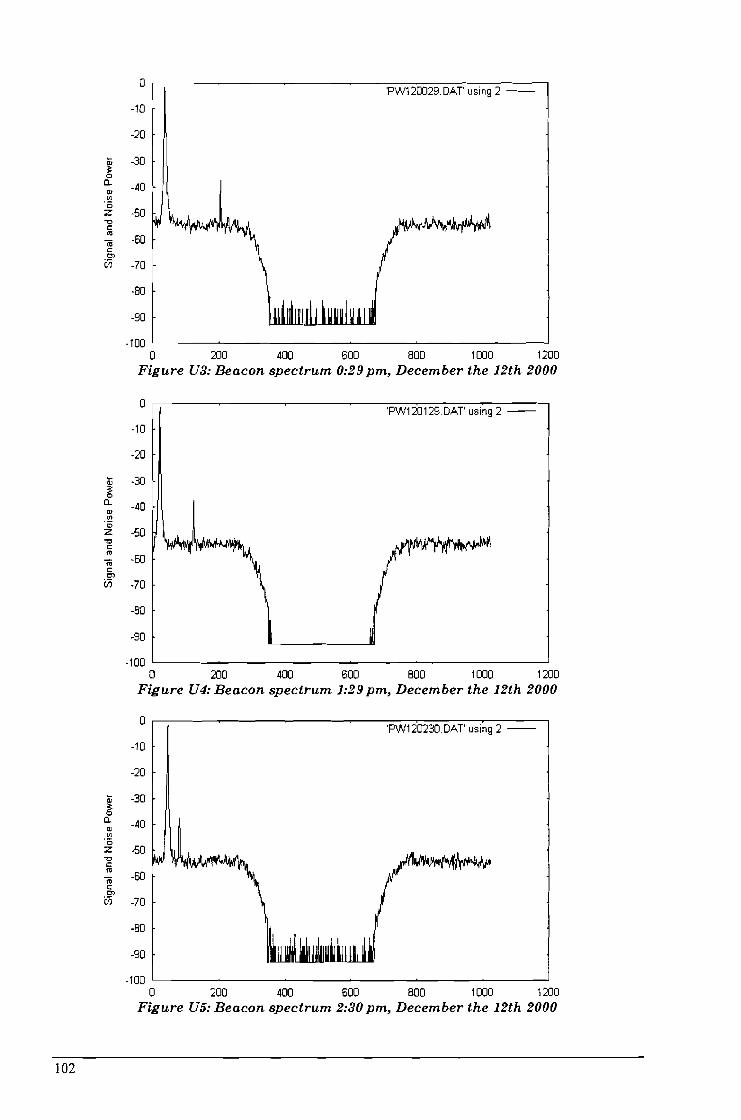
0

-10

-20

~ -300)

~0

CL -400)

'"'0-50z

"'"c:

'" -60(ijc:Olen -70

-80

-90

'PW120029.DAT' using 2 --

,~~

-100 1 1

o 200 400 600 800 1000 1200Figure V3: Beacon spectrum 0:29 pm, December the 12th 2000

I~

0

-10

·20

:;; -30~0

CL -400)

'"'0-50z

"'"c:

'" -50(ijc:Ol

~'i -70

-80

·90

'PW120129DAT' using 2 --

-100 LI ~ ~ ~ ~ ~__---...J

o 200 400 600 800 1000 1200Figure V4: Beacon spectrum 1:29 pm, December the 12th 2000

0

-10

-20

:;; -30~0

CL -400)

'"'0-50z

"'"c:

'" -60(ijc:Ol

en -70

-80

·90

'PW120230 DAT' using 2 --

I~fr~

102

-100 LI---~---~---~----~---~-_-.I

o 200 400 600 800 1000 1200Figure V5: Beacon spectrum 2:30 pm, December the 12th 2000

Appendix V. (Rain data of the STRAP4)

The rain fade that toke place on 15 December 2000, is already discussed anddisplayed in this thesis, however there was logged more data during this project. Infigure VI, V2 and V3 you can find plots that were recorded with respectivelySTRAP419, STRAP420 and STRAP427. Figure V3 was already discussed in Chapter3, but this plot is bigger and is plotted versus samples instead of time.

10

o

-10

~-20L-

a>:;:0-30a...

-40

\ r\ ., (

~1fT ~~

---50

-60915000 917000 919000 921000 923000 925000 927000 929000 931000 933000 935000

Samples (1samples=104 ms)

Figure VI: Rain fade on November the 21th, logged with STRAP419

10.,-------------------------------,

-10 +--------------------------------l

.........CO~ -20 +-------------------------------jL-

a>~ -30 +-------------------------------j

a...

-40 +-------------------------------j

-50 l=:::::::::::::::~=====:::=:::::::~===============~

1000009000050000 60000 70000 80000Samples (1 sample=104 ms)

Figure V2: Rain fade on November the 22th, logged with STRAP420

-60 -'-- -----.J

40000

103

10

o

m -10::3-"-0)

:s:0G-O)(f)

-200z-0c:roroc:0"1

i:i5 -30

-40

'0427-3. OAT' using 1:2

'0427-3. OAT' using 1:3

I

-50

o 100000 200000 300000 400000 500000 600000 700000 800000 900000 1e+06

Samples (approx. 9.54 per second)

Figure V3: Rain fade on December the 16th, logged with STRAP427

Appendix W. (FFT windowing)

The used window-function for the STRAP2 is the minimum 4-sample BlackmanHarris function. This window-function was also specified to be used in STRAP3 andSTRAP4.

Overall advantage is:First side-lob down to 92 dB

Overall disadvantages are:3 dB signal bandwidth spread out over: 1.9 binsNoise bandwidth spread out over: 2 bins

The window-function can be analyzed in Matlab, with the following m-file:

N=64zpf=64nfft=N*zpffni=0:(N*zpf)-1 ;fni=fni/(N*(zpf-1 ));

theta = 2*pi/(N-1);w=(0.35875 - 0.48829*cos(theta*(0:N-1)) +0.14128*cos(2*theta*(0:N-1 ))-0.01168*cos(3*theta*(0:N-1 )));

figure(1 );sUbplot(3, 1, 1); plot(w,'*'); title(The minimum 4-sample Blackman Harris Blackman Window');xlabel(Time (samples)') ; ylabel('Amplitude');text(-8,1,'a)');

% Also show the window transform:xw = [w,zeros(1,(zpf-1 )*N)]; % zero-padded window (col vector)Xw = fft(xw); % Blackman window transformspec = 20*log10(abs(Xw)); % Spectral magnitude in dBspec = spec - max(spec); % Usually we normalize to 0 db maxspec = max(spec,-150*ones(1,nfft)); % clip to -100 dBsubplot(3,1 ,2); plot(fni,spec,'-'); axis([O, 1,-150,10]); grid;xlabel('Normalized Frequency (cycles per sample)');ylabel('Magnitude (dB)');text(-.12,20, 'b)');

% Replot interpreting upper bin numbers as negative frequencies:nh = nfft/2;specnf = [spec(nh+1 :nfft),spec(1 :nh)]; % see also Matlab's fftshiftOfninf = fni - 0.5;subplot(3,1,3);plot(fninf,specnf,'-'); aXis([-0.5,0.5,-150,1 0]); grid;xlabel('Normalized Frequency (cycles per sample)');ylabel('Magnitude (dB)');text(-.6,20,'c)');

105

The plot of the minimum 4-sample Blackman Harris function will be generatedby the m-file and can be seen in figure WI.

Figure Wl: minimum 4-sample Blackman Harris window function

106