arX

iv:s

ubm

it/25

8975

7 [

q-bi

o.PE

] 2

5 Fe

b 20

19

Meeting yield and conservation objectives by balancing

harvesting of juveniles and adults

Niklas L.P. Lundstrom 1, Nicolas Loeuille 2, Xinzhu Meng 1,3, Mats Bodin 1,4, Ake Brannstrom 1,6

1 Department of Mathematics and Mathematical Statistics, Umea University, 90187 Umea, Sweden, 2 Sorbonne Universites,

UPMC Univ Paris 6, UPEC, Univ Paris Diderot, Univ Paris-Est Creteil, CNRS, INRA, IRD, Institute of Ecology and Environ-

mental Sciences-Paris (IEES Paris), place jussieu, 75005 Paris, France, 3 College of Mathematics and Systems Science, Shandong

University of Science and Technology, Qingdao 266590, China, 4 Department of Ecology and Environmental Science, Umea Uni-

versity, 90187 Umea, Sweden, 6 Evolution and Ecology Program, International Institute for Applied Systems Analysis, 2361

Laxenburg, Austria.

Keywords: fisheries management; maximum sustainable yield; pretty good yield; Pareto fron-tier; resilience; size-structure

Abstract

Sustainable yields that are at least 80% of the maximum sustainable yield are sometimes re-ferred to as pretty good yield (PGY). The range of PGY harvesting strategies is generally broadand thus leaves room to account for additional objectives besides high yield. Here, we analyzestage-dependent harvesting strategies that realize PGY with conservation as a second objective.We show that (1) PGY harvesting strategies can give large conservation benefits and (2) equalharvesting rates of juveniles and adults is often a good strategy. These conclusions are based ontrade-off curves between yield and four measures of conservation that form in two establishedpopulation models, one age-structured and one stage-structured model, when considering dif-ferent harvesting rates of juveniles and adults. These conclusions hold for a broad range ofparameter settings, though our investigation of robustness also reveals that (3) predictions ofthe age-structured model are more sensitive to variations in parameter values than those ofthe stage-structured model. Finally, we find that (4) measures of stability that are often quitedifficult to assess in the field (e.g. basic reproduction ratio and resilience) are systematicallynegatively correlated with impacts on biomass and impact on size structure, so that these laterquantities can provide integrative signals to detect possible collapses.

Introduction

Almost one third of the world’s fished marine stocks are currently overexploited (FAO 2016).Some fish stocks have even collapsed, with examples including the Californian sardine (Sardinops

1

sagax, Clupeidae) fishery in the 1950s (Radovich 1982), the Atlanto-Scandian herring (Clupeaharengus, Clupeidae) fishery in the late 1960s (Krovnin and Rodionov 1992), the Peruvian an-chovy (Engraulis ringens, Engraulidae) fishery in the 1970s (Clark 1977), and the Northern cod(Gadus morhua, Gadidae) fishery off the east coast of Canada in the 1990s (Hannesson 1996;Olsen et al. 2004). The large proportion of overexploited marine fish stocks underscore theimportance of implementing sustainable harvesting practices and for further improving modernfisheries-management methods.

Maximum sustainable yield (MSY) has long been a central concept in population ecology(Smith and Punt 2001; Hilborn 2007; Mesnil 2012). While maximization of yield from har-vested populations is economically desirable, there is a rich scientific literature that criticizesthe MSY concept and highlights its shortcomings, including the difficulty of correctly estimatingMSY, the inappropriateness of long-term yield maximization as the single management objec-tive, and the practical difficulty of accurately implementing the required level of harvestingeffort (Smith and Punt 2001). MSY has further been criticized for its inability to prevent thecollapse of important fisheries (Beverton and Holt 1957; Larkin 1977; Mangel and Levin 2005;Hilborn 2010). As an example, Alaska’s Bering Sea Pollock fishery declined in 2009, and de-spite being known as a sustainable fishery which implements scientific recommendations, themanagement has been criticized for considering mainly MSY (Morell 2009).

MacCall and Hilborn have introduced the concept pretty good yield (PGY; Hilborn 2010) forsustainable yields that are at least 80% of the MSY. In contrast to MSY harvesting-managementobjectives, PGY can be realized by a range of harvesting strategies and therefore leaves roomto account for other desirable objectives in addition to the maximization of yield. The addedvalue that PGY offers will depend on the extent to which the implemented harvesting strategiescan successfully account for other desirable objectives beyond yield.

The aim of this paper is to investigate to which extent PGY harvesting strategies can simul-taneously account for high yield and large conservation benefits. To increase the chances thatour conclusions are valid over a broad range of circumstances, we base our study on two estab-lished population models. The first is an age-structured model (henceforth age model) that iscommonly used for modeling fish populations and evaluating fishing strategies (Francis 1992;Punt 1994; Punt et al. 1995; Punt and Hilborn 1997; Hilborn 2010). The second is a stage-structured consumer-resource population model (henceforth stage model) that has been intro-duced by de Roos et al. (2008). Both models are capable of describing a range of aquatic andterrestrial animal populations. The age model belongs to a class of models that have a long his-tory in fisheries science and that incorporates age-dependent fecundity, age-dependent survival,and density-dependent recruitment. The stage model is derived from a fully size-structuredcounterpart with food-dependent growth, fecundity and maturation, and accounts for feedbacksfrom resource depletion. In particular, it accounts for ontogenetic asymmetry, i.e., differentialabilities of juveniles and adults to utilize available resources (de Roos and Persson 2013). Withthe age-model and stage-model being two fairly distinct representatives of contemporary pop-ulation models, results on which they agree are likely to be fairly robust and results on whichthey differ are likely to be ones where careful description of the population ecology is impor-tant and may therefore differ from species to species. Using separate independently developedmodels to investigate robustness of findings should be a reasonable strategy (Levins 1966).

We extend both models by introducing selective harvesting of juveniles and adults, givingwide ranges of possible harvesting strategies with different consequences for yield and conserva-tion. While it is straightforward to quantify the yield of a harvesting strategy, it is less obvioushow the conservations benefits should be measured. Here, we consider four different measures

2

of conservation benefits: two measures that capture the direct impacts on the harvested pop-ulation (the impact on population biomass and the impact on the population size structure)and two measures that capture the indirect risks of collapse due to changes in population dy-namics (resilience and the basic reproduction ratio). We determine trade-offs between yieldand conservation benefits by finding the so-called Pareto-efficient front; the set of strategiesthat cannot simultaneously be improved upon in both yield and conservation benefit. Thesetrade-off curves allow us to assess how large conservation benefits can be gained while preserv-ing PGY. Finally, we determine the relationship between the direct impact measures and theindirect risk measures, with the idea that the former are likely to be more easily observable inthe field while the latter better reflect the risks of collapse. Taken together, our results showthat there are large potential gains of using specific PGY harvesting strategies over traditionalMSY strategies. Moreover, among PGY strategies, the ones that include equal harvesting ofadults and juveniles often allow the best compromises between conservation and yield.

Methods

In this section we first present the two population models, one age-structured and one stage-structured. We extend both models by introducing selective harvesting of juveniles and adults,giving wide ranges of possible harvesting strategies with different consequences for the realizedyield and for conservation. We next present our methods of stability analysis involving theimpact measures and risk measures that we will use to evaluate different harvesting strategies.Finally, we recall the concept of maximum sustainable yield (MSY) and the economic concept ofPareto-efficiency which we will use to determine trade off curves between yield and conservation.

The age model

We adopt an age-structured population model that in different guises has been widely usedwhen modeling fish populations and evaluating fishing strategies (Francis 1992; Punt 1994;Punt et al. 1995; Punt and Hilborn 1997; Hilborn 2010). The model incorporates density-dependent recruitment in the form of a Beverton-Holt stock-recruitment relationship with atunable degree of random recruitment variability. Natural mortality is assumed to be indepen-dent of age and time, and age-specific harvesting is assumed constant over time. The centralelements of the model, which are mainly derived from Hilborn (2010), are described below.

We denote by Na,t the number of individuals of age a in year t and assume that individualsmature at age amature after which they reproduce at an age-dependent rate proportional totheir body size. Individuals younger than amature are considered juveniles, while individualsolder than or with age equal to amature are considered adults. For simplicity, we assume thatthe population is made up entirely of female individuals, but as we show in the Appendix, ourresults are unchanged with a standard Fisherian sex-ratio of 50% females. The age-dependentfraction of mature females (ma) and their corresponding egg production (fa) are given by

ma =

{

0 if a ≤ amature

1 if a > amaturefa = c sa, (1)

where c is a positive constant that scales the fecundity rate and sa is the mass of an individualat age a. We adopt a von Bertalanffy (1957) growth curve to describe individual length as afunction of age, and assume that individual mass sa is proportional to the cube of individual

3

length, i.e.

sa = smax

(

1− e−K(a−a0))3

, (2)

where smax is the asymptotic maximum body mass, K is a growth rate parameter and a0 is ahypothetical negative age at which the individual has zero length. In Appendix Fig A 3 weillustrate von Bertalanffy growth curves for some parameter values.

The total egg production in a year t = 0, 1, 2, . . . is found by summing over the offspringproduced by mature females of different ages,

Et =amax∑

a=0

mafaNa,t, (3)

where amax is the maximum age of individuals and Na,t is the number of individuals, per unitof volume, of age a in year t.

The number of individuals in each age class changes from year to year according to

N0,t = Rt, and

Na,t = Na−1,t−1S(1− γa−1) for 1 ≤ a, (4)

where Rt is the recruitment of newborn individuals in year t, t = 1, 2, 3, . . . , as describedfurther below, and S(1− γa−1) is the probability that an individual survives from one year tothe next. This survival probability is decomposed in survival from natural mortality S andfrom harvesting mortality (1 − γa−1). Note that, as probabilities, these variables always takevalues from 0 to 1.

We incorporate stage-selective harvesting by allowing separate constant fractions harvestedof juveniles (FJ) and adults (FA) and setting the vulnerability of individuals to

γa =

{

FJ if a < amature

FA if a ≥ amature.(5)

We assume Beverton-Holt recruitment (Beverton and Holt 1957),

Rt+1 =Et

α + βEtexp

(

ut −σ2u

2

)

, (6)

where ut are independent and normally distributed random variables with mean 0 and standarddeviation σu. The factor −σ2

u/2 ensures that the expected number of recruits remains the samewith varying σ2

u because the lognormal random variable represented by the exponential hasalways mean 1. The parameters α and β are not used directly as they lack a direct ecologicalinterpretation. Instead, they are determined from the expected total egg production at equilib-rium in absence of harvesting (E0) and from the steepness parameter (h) setting the sensitivityof the recruitment to the total egg production. The steepness is defined as the ratio of re-cruitment when egg production equals 20% of E0 to recruitment at E0 (Mace and Doonan 1988;Hilborn 2010) and may take values between 0.2 and 1. If h is close to 1, recruitment is almostindependent of the egg production, and if h is close to 0.2, recruitment is almost proportionalto the egg production. In Appendix Fig. A 1 we illustrate how recruitment depends on E0 andh and state their exact mathematical relationship with α and β.

4

For the age model, we use

R0 = smax = c = 1, amax = 100, K = 0.23, a0 = −2,

amature = 8, h = 0.7, S = 0.8, σu = 0, (7)

as our default parameters values, with substantial motivations given in the Appendix. Here, R0

is measured in number of individuals per unit of volume, smax and c−1 have an arbitrary massunit, while amax, a0, amature and K−1 are measured in years. However, after a rescaling of theequations, R0, smax and c (as well as sa, Et, Rt and Na,t) can be considered as non-dimensionaland we can take R0 = smax = c = 1 without loss of generality. See the Appendix for details.While we believe that the parametrization in (7) is a reasonable choice, we have consideredsubstantial variations and present how our results from the age model depend on parametervalues in the result section. A systematic investigation of the robustness of our results withrespect to variations of the parameter values in (7) are given in the Appendix.

The stage model

We adopt an archetypal consumer-resource model that has been introduced by de Roos etal. (2008) as a reliable approximation of a fully size-structured population model. Themodel is stage-structured and incorporates key aspects of individual life history such as food-dependent growth, maturation, and fecundity. In contrast to the age-model, the population-level feedback that results from resource depletion induces competition between life-historystages whenever juveniles and adults have differential abilities to utilize available resources.Competition under such ontogenetic asymmetry can strongly influence the ecological dynam-ics (de Roos and Persson 2013) and may thus effect how harvesting affects population sizestructure. The central elements of this model are described below, with the detailed modelformulation given in de Roos et al. (2008).

Individuals are composed into two stages, juveniles and adults, depending only on theirsize. Both juveniles and adults forage on a shared resource R = R(t). The juvenile biomassis denoted by J = J(t) while adult biomass is denoted by A = A(t). Juveniles are born withsize sborn and grow until they reach the size smax at which point they cease to grow, mature,and become adults. Juveniles use all available energy for growth and maturation, while adultsdo not grow and instead invest all their energy in reproduction. The juvenile growth rateand adult reproduction rate depend on resource abundance. In accordance with metabolictheory of ecology, foraging ability and metabolic requirements increase with individual bodysize (Brown et al. 2004). Juveniles and adults do not produce biomass when the energy intakeis insufficient to cover maintenance requirements.

The rate at which the biomass of juveniles, adults, and available resources changes are givenby three differential equations:

dJ

dt= (wJ(R)− v(wJ(R))−M − FJ)J + wA(R)A,

dA

dt= v(wJ(R))J − (M + FA)A, (8)

dR

dt= r(Rmax − R)− Imax

R

H +R(J + qA) .

Here, wJ(R) and wA(R) are the net biomass production, per unit body mass, of juveniles andadults, respectively. The natural mortality is denoted by M while FJ and FA are the respective

5

stage-dependent harvesting rates of juveniles and adults. Continuing, v(wJ(R)) is the resource-dependent rate at which juveniles mature and become adults, r is the resource turnover rate,and Rmax is the maximum resource density.

The net biomass production rates for juveniles and adults are assumed to equal the balancebetween ingestion and mass-specific metabolic rate T according to

wJ(R) = max

{

0, σImaxR

H +R− T

}

and wA(R) = max

{

0, σqImaxR

H +R− T

}

.

Here, σ represents the efficiency of resource ingestion, and the maximum juvenile and adultingestion rates per unit biomass equal Imax and qImax, respectively, H is the half-saturationconstant of consumers, and the factor q describes the difference in ingestion rates betweenjuveniles and adults. The juvenile maturation rate depends on the net biomass ingestion andthus also on the resource density. It is derived from the fully size-structured counterpart byassuming that the population size structure is at equilibrium and by determining the rate atwhich juvenile individuals reach the maturation size smax. In the stage model, the juvenilematuration rate is given by

v(wJ(R)) =wJ(R)−M − FJ

1− (sborn/smax)1−(M+FJ)/wJ(R)

The function v(wJ(R)) results from a mathematical derivation and lacks a clear biologicallyinterpretable form. When wJ(R) = M + FJ the function is undefined, and at this value itis defined by v(M + FJ) = −(M + FJ)/ log(sborn/smax). In Appendix Fig. A 7 we illustratethe maturation function v(wJ(R)) as well as the net biomass production functions wJ(R) andwA(R). Noting that the size at birth sborn and the size at maturation smax appears only as thefraction sborn/smax we can reduce the numbers of parameters by letting z = sborn/smax.

For the stage model, we use

H = T = r = 1, Rmax = 2, σ = 0.5, Imax = 10, M = 0.1, z = 0.01, q = 0.85, (9)

as our default parameters values. Here, H and Rmax are measured in biomass per unit ofvolume while T, r, Imax and M are expressed per unit of time. However, after a rescaling ofthe equations all parameters, as well as the biomass densities J , A and R, can be consideredas non-dimensional and we can take H = T = 1 without loss of generality. See the Appendixfor details. The parameter values in (9) are inspired by de Roos et al. (2008) and may beconsidered as archetypal. We show in the Appendix that our results are largely robust withrespect to variations of these default values.

Model dynamics

Both the age model and the stage model are nonlinear dynamical systems and therefore com-plicated dynamics can not be ruled out a priori. However, extensive numerical investigations ofbasin of attractions indicate that solution trajectories end up, after sufficient time, at a glob-ally stable equilibrium in both models. This equilibrium is therefore the only attractor whichis either an interior (positive) equilibrium or an extinction equilibrium depending on the har-vesting rates. Indeed, our nonlocal approach to resilience (presented below) tests the dynamicsin both models for a large number of perturbations (inferred through initial conditions) andwould detect any coexisting attractor with a high probability. We refer the reader to Meng etal. (2013) and Roos et al. (2008) for more on dynamic properties, mathematical analysis aswell as numerical investigations of the stage model.

6

Stability analysis: measures of conservation

Stability of ecological systems is important for both conservation and harvesting purposes. Inunstable systems, population dynamics may transiently go to low biomass values where thepopulations become vulnerable to demographic stochasticity or other factors. Hence, lack ofstability promotes extinction. Stability is desirable also for harvest managers as it ensuresstable yield. There are many definitions of stability, see e.g. McCann (2000), and we proposehere to study the consequences of harvesting on stability through four different measures ofconservation. The first two are impact measures; impact of harvesting on the populationbiomass and impact of harvesting on the population size structure. The second two measureshave a natural link to the risk of extinction and will be referred to as risk measures. Theseare the resilience and the basic reproduction ratio (the recovery potential in case of the stagemodel). We define the resilience as the reciprocal of the time needed for the population torecover from a perturbation, and we consider here both small and large perturbations. Thebasic reproduction ratio/recovery potential describes the population’s rate of increase from verylow abundances, and thus could be construed as the likelihood of population rebound, followinga crash (e.g. due to a large disturbance).

Measures of impact on biomass and size structure

Let J∗ = J∗(FJ, FA) and A∗ = A∗(FJ, FA) denote the juvenile and adult biomass at equilibrium,respectively, of the harvested population. In case of the stage model J∗ and A∗ are given directlyby the state variables at equilibrium. For the age model, J∗ and A∗ are obtained through theformulas

J∗ =

amature−1∑

a=0

N∗

asa and A∗ =

amax∑

a=amature

N∗

asa,

where N∗

a denotes the number of individuals of age a at equilibrium. Furthermore, let J∗

u

and A∗

u denote the juvenile and adult biomass at equilibrium in the absence of harvesting, i.e.J∗

u = J∗(0, 0) and A∗

u = A∗(0, 0). Moreover, let B∗ = J∗ + A∗ and B∗

u = J∗

u + A∗

u. We measureimpact on biomass of harvesting through the expression

Impact on biomass = 1−B∗

B∗

u

.

Similarly, we consider impact on size-structure through the expression

Impact on size-structure =J∗

J∗ + A∗

[

J∗

u

J∗

u + A∗

u

]

−1

− 1,

which equals the relative change in the fraction of juvenile biomass following harvesting. If theimpact on size-structure is positive (negative), then harvesting has increased (decreased) thefraction of juveniles in the population.

Resilience, basic reproduction ratio and recovery potential as risk measures

Resilience as a risk measure is increasingly used in ecology (Pimm and Lawton 1977; Loreauand Behera 1999; Petchey et al. 2002; Montoya et al. 2006; Loeuille 2010; Valdovinos et al.

7

2010). Resilience is now also increasingly discussed in a fishery management context (Hsieh etal. 2006; Law et al. 2012; Fung et al. 2013). The higher the resilience, the smaller the risk ofextinction due to random drift.

We consider resilience of the population by measuring the reciprocal of the time needed forthe population to recover the positive equilibrium given a random perturbation. We do thisby considering a large number of initial conditions. From each initial condition, we measurethe time until the population (and also the resource in case of the stage model) returns to asmall neighborhood of the equilibrium. The average value of this return time over the numberof trials are then used to quantify the resilience:

Resilience =1

Average value of the return times.

Our resilience measure estimates the population’s expected rate of return, given a randomperturbation. In contrast to many other studies on resilience that assess resilience based oneigenvalues of the Jacobian matrix, our approach is not limited to the immediate neighborhoodof the equilibrium, but can also tackle large disturbances, a point we will return to in the dis-cussion section. The precise procedure by which we determine the resilience is described in theAppendix where we also present an alternative resilience measure, estimating the population’sprobability to return within a time limit, and reproduce some of our results using differentmagnitudes of disturbances.

We also consider the basic reproduction ratio as a risk measure, which represents the averagenumber of offspring produced over the lifetime of an individual in the absence of density-dependent competition, i.e., when the population abundance is very low. For the age model,we derive the following expression for the basic reproduction ratio as functions of the harvestingrates FJ and FA:

Basic reproduction ratio =(1− FJ)

amature ×∑amax

a=amature+1 sa Sa (1− FA)

a−amature

(

1− h−0.20.8h

)

×∑amax

a=amature+1 sa Sa

. (10)

A basic reproduction ratio larger than one ensures that the biomass of an initially small pop-ulation increases on average, while a basic reproduction ratio less than one implies that thepopulation will eventually become extinct. The derivation of expression (10) can be found inthe Appendix.

In case of the stage model we use the recovery potential introduced in Meng et al. 2013,

Recovery potential =wA(Rmax)

M + FA×

v(wJ(Rmax))

v(wJ(Rmax))− wJ(Rmax) +M + FJ.

The recovery potential is the generational net biomass production (per unit body mass) in apristine environment (free from density-dependent mortality) and is therefore closely related tothe basic reproduction ratio. Similar as for the basic reproduction ratio, a recovery potentiallarger than one ensures that the biomass of an initially small population increases on average,while a recovery potential less than one implies that the population will eventually becomeextinct. The basic reproduction ratio, as well as the recovery potential, are directly linked tothe probability of surviving a period of low population abundance during which random driftcaused by demographic stochasticity can lead to extinction. We further discuss this fact, as wellas giving overall motivations of our choices of conservation measures, in the discussion section.

8

Maximum sustainable yield and trade-off through Pareto efficiency

Recalling that J∗ and A∗ denote the juvenile and adult biomass at equilibrium, for any givenharvesting rates FJ ≥ 0, FA ≥ 0, the yield objective function is given by

Yield = FJJ∗ + FAA

∗. (11)

Moreover, the maximum sustainable yield (MSY) is obtained by taking the maximum of theyield objective function across all harvesting strategies (FJ, FA). In addition to the yield func-tion we are, in case of both the age model and the stage model, armed with four measures ofconservation as functions of the harvesting rates (FJ, FA). Using these objective functions wecan calculate both the yield and the conservation for given harvesting strategies, see Fig. 1 inthe Results section.

To determine the trade-off between the two objectives yield and conservation, we plot theyield as a function of each conservation measure in the results section and apply the economicconcept of Pareto efficiency to evaluate different harvesting strategies. A harvesting strategyis Pareto efficient if it cannot be improved upon without trading off one of the consideredobjectives against the other, see e.g. Karpagam (1999, page 11). The Pareto front is the set ofall Pareto efficient harvesting strategies. Hence, managers can restrict the choice of harvestingstrategy to this set, rather than considering the full range of possible harvesting strategies. Thecloser a strategy is to the Pareto front, the more efficient it is.

Results

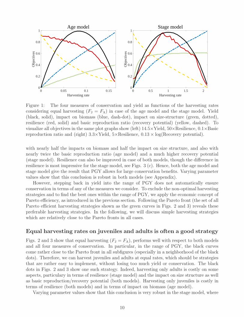
Figure 1 shows how the four measures of conservation and the yield changes with harvest-ing intensity for equal harvesting rates of juveniles and adults (henceforth equal harvesting),i.e. FJ = FA. As harvesting pressure increases, the yield first increases after which it decreasesas the population becomes “overexploited”. The impact on biomass and the impact on size-structure increase with harvesting pressure, while the basic reproduction ratio and the recoverypotential decrease. The resilience decreases with harvest pressure in case of the age model, butfirst increases to a maximum and then decreases in case of the stage model. Note that due tothe different nature of the age model and the stage model, the values of the harvesting rates inthe two models may not be immediately compared.

We are now ready to present the trade-offs between yield and the four measures of conser-vation. Figure 2 represents results from the age model, while Fig. 3 gives the correspondingresults for the stage model.

Pretty good yield allows large conservation benefits

Focusing on the age model, Figs. 2 (b)-(d) show that the basic reproduction ratio is relativelylow and the impact on size structure is also relatively large at MSY, while the resilience isrelatively high at MSY. Focusing on the stage model, Figs. 3 (c) and (d) show slightly differentresults; harvesting for MSY (which is obtained by harvesting only adults) gives a resilience anda recovery potential that is only a tiny fraction of the unexploited state and is close to theboundary of extinction. Hence, harvesting for MSY may substantially increase the risk of stockcollapse. Fig. 3 (b) shows also that the impact on size structure is at a maximum at MSY.

Common for both models and all four measures is, see Figs. 2 (a)-(d) and Figs. 3 (a)-(d),that by stepping back in yield by 20% into the range of PGY, we can find harvesting strategies

9

0 0.05 0.1 0.15Harvesting rate

0

0.2

0.4

0.6

0.8

1O

bjec

tive

s

Age model

0 0.5 1 1.5 2Harvesting rate

0

0.2

0.4

0.6

0.8

1

Obj

ecti

ves

Stage model

Figure 1: The four measures of conservation and yield as functions of the harvesting ratesconsidering equal harvesting (FJ = FA) in case of the age model and the stage model. Yield(black, solid), impact on biomass (blue, dash-dot), impact on size-structure (green, dotted),resilience (red, solid) and basic reproduction ratio (recovery potential) (yellow, dashed). Tovisualize all objectives in the same plot graphs show (left) 14.5×Yield, 50×Resilience, 0.1×Basicreproduction ratio and (right) 3.3×Yield, 5×Resilience, 0.13× log(Recovery potential).

with nearly half the impacts on biomass and half the impact on size structure, and also withnearly twice the basic reproduction ratio (age model) and a much higher recovery potential(stage model). Resilience can also be improved in case of both models, though the difference inresilience is most impressive for the stage model, see Figs. 3 (c). Hence, both the age model andstage model give the result that PGY allows for large conservation benefits. Varying parametervalues show that this conclusion is robust in both models (see Appendix).

However, stepping back in yield into the range of PGY does not automatically ensureconservation in terms of any of the measures we consider. To exclude the non-optimal harvestingstrategies and to find the best ones within the range of PGY, we apply the economic concept ofPareto efficiency, as introduced in the previous section. Following the Pareto front (the set of allPareto efficient harvesting strategies shown as the green curves in Figs. 2 and 3) reveals thesepreferable harvesting strategies. In the following, we will discuss simple harvesting strategieswhich are relatively close to the Pareto fronts in all cases.

Equal harvesting rates on juveniles and adults is often a good strategy

Figs. 2 and 3 show that equal harvesting (FJ = FA), performs well with respect to both modelsand all four measures of conservation. In particular, in the range of PGY, the black curvescome rather close to the Pareto front in all subfigures (especially in a neighborhood of the blackdots). Therefore, we can harvest juveniles and adults at equal rates, which should be strategiesthat are rather easy to implement, without losing too much yield or conservation. The blackdots in Figs. 2 and 3 show one such strategy. Indeed, harvesting only adults is costly on someaspects, particulary in terms of resilience (stage model) and the impact on size structure as wellas basic reproduction/recovery potential (both models). Harvesting only juveniles is costly interms of resilience (both models) and in terms of impact on biomass (age model).

Varying parameter values show that this conclusion is very robust in the stage model, where

10

10.5010.50

Impact on biomass

0

0.2

0.4

0.6

0.8

1

Yie

ld

(a)

0 0.1 0.2 0.3 0.4

Impact on size-structure

0

0.2

0.4

0.6

0.8

1

Yie

ld

(b)

0 0.005 0.01 0.015 0.02

Resilience

0

0.2

0.4

0.6

0.8

1

Yie

ld

(c)

2 4 6 8

Basic reproduction ratio

0

0.2

0.4

0.6

0.8

1

Yie

ld

(d)

Age model

Figure 2: Trade-offs between yield and the four conservation measures in the age model. Thegray regions show “all possible” combinations that can be realized when varying the harvestingrates on juveniles and adults. The solid green curves represent the Pareto front, while thedotted grey lines give the border for PGY, i.e. 80% of MSY. The yellow dots represent MSYand the green squares give the unfished state. We observe that within the range of PGY, equalharvesting performs well with respect to all measures. The black dots represent a suggestedharvesting strategy, within the range of PGY, produced by FA = FJ = 0.06. Parameter valuesare as in (7) and yield normalization is as in Figure 1.

11

10.5010.50

Impact on biomass

0

0.2

0.4

0.6

0.8

1

Yie

ld

(a)

0 0.2 0.4 0.6 0.8 1

Impact on size-structure

0

0.2

0.4

0.6

0.8

1

Yie

ld

(b)

0 0.05 0.1 0.15 0.2

Resilience

0

0.2

0.4

0.6

0.8

1

Yie

ld

(c)

100

101

102

103

Recovery potential

0

0.2

0.4

0.6

0.8

1

Yie

ld

(d)

Stage model

Figure 3: Trade-offs between yield and the four conservation measures in the stage model.The gray region, curves, dots, and squares are as in Fig. 2. We observe that within the range ofPGY, equal harvesting performs well with respect to all measures. The black dots represent asuggested harvesting strategy, within the range of PGY, produced by FA = FJ = 0.8. Parametervalues are as in (9) and yield is normalized as in Fig. 1.

12

it seems to remain in the wide ranges M ∈ [0, 0.5], z ∈ [0.0001, 0.2], σImax ∈ [3, 100], q ∈

[0.6, 2], Rmax ∈ [0.5, 100]. We refer the reader to the Appendix for substantial investigations(both numerical and analytical) of robustness with respect to variations of parameter values.Additional trade-off curves, as those presented in Fig. 3, are given for six different parametriza-tions in Figs. A 8, A 9 and A 10.

However, equal harvesting is often but not always suggested by the age model. Here, theefficient strategies seem to depend on the fraction of juveniles at the unharvested equilibrium,J∗

u/(A∗

u+J∗

u), as well as on the survival from natural mortality, S. We proceed by investigatingthis dependence by comparing pure adult harvesting (henceforth adult harvesting), equal har-vesting and pure juvenile harvesting (henceforth juvenile harvesting) for a wide range of param-eter values in the age model. Figure 4 gives an approximation of regions in which the age modelsuggest adult harvesting, equal harvesting and juvenile harvesting. Juvenile or adult harvestingis suggested only if such strategies are the most Pareto-efficient once, within the range of PGY,with respect to all four conservation measures. The borders in Figure 4 are approximationswhich are produced by examining a large number of variants of Figure 2 for parameter values inthe intervals a0 ∈ [−3,−0.2], K ∈ [0.1, 1], amature ∈ [3, 15], h ∈ [0.3, 0.9], σu ∈ [0, 0.5].Indeed, we varied each parameter at a time, keeping the others at the default values givenin (7), and tested at least 10 values in each interval. Further parameter combinations havealso been tested in order to refine the borders in Figure 4. Points P0 − P8 in Fig. 4 corre-spond to different parametrizations of the age model. The default parametrization in (7) givesJ∗

u/(A∗

u + J∗

u) ≈ 0.6, S = 0.8 and is marked with P0. In Appendix Figs A 2, A 4, A 5 and A6 we present trade-off curves, similar to those in Fig. 2, for different parametrizations corre-sponding to the remaining eight points P1 − P8. The Appendix also contains motivations andexplanations for the dependence shown in Fig. 4.

It turns out that if it is possible to obtain PGY for a wide range of harvesting strategies(including adult, juvenile and equal harvesting), then our conservation measures are in favor ofequal harvesting. When adult or juvenile harvesting performs better than equal harvesting, itis usually because equal harvesting can not give a yield in the range of PGY.

The age model is more sensitive to variations in parameter values

than the stage model

Focusing on the age model we first note that for the parameter values used in Figs. 1 and2 we have a survival from natural mortality of S = 0.8 (Mills et al. 2002) and the fraction ofjuveniles in an unharvested population, J∗

u/(A∗

u+J∗

u) ≈ 0.6. We conclude that in this case equalharvesting is a good strategy. Varying the parameter values, it turns out that an increase in thefraction of juveniles implies an increase in the yield obtained when harvesting only juveniles, i.e.the blue curves will be lifted in Fig. 2. Similarly, a decrease in the fraction of juveniles impliesan increase in the yield obtained when harvesting only adults, i.e. the red curves will be lifted inFig. 2. This dependence, which is expected and natural, can be observed in both models, but itis much stronger in the age model. While Fig. 4 gives an approximation of the borders betweenadult harvesting, equal harvesting and juvenile harvesting, a similar investigation on the stagemodel gives a much larger region suggesting equal harvesting. In particular, in the stage model,the most Pareto-efficient strategies, within the range of PGY, seems to be dominated by equalharvesting as long as 0.1 < J∗

u/(A∗

u + J∗

u) < 0.9. (For the parameter values used in Figs. 1 and3, we have J∗

u/(A∗

u + J∗

u) ≈ 0.5.)In conclusion, for populations in the region where the age model suggests equal harvesting,

13

20 30 40 50 60 70 80 90 100Precentage of juvenile biomass, J∗

u/(A∗

u + J∗

u)

0.6

0.65

0.7

0.75

0.8

0.85

0.9

0.95

Survivalfrom

naturalmortality,S

Sensitivity to parameter values in the age model

P8

P5

P0= P

1= P

2

P7

P3

P6

P4

Juvenile

harvesting

Equal

harvesting

Adult

harvesting

Figure 4: The harvesting strategy suggested by the results of the age model depends on Sand the fraction of juveniles in the unharvested population. In the dark-grey region, equalharvesting is suggested by the age model, while adult harvesting is better for low fraction ofjuveniles and juvenile harvesting is to recommend when the fraction of juveniles is high. Thelight-grey regions refer to borderline cases. Juvenile or adult harvesting is suggested only ifsuch strategies are the most Pareto-efficient once, within the range of PGY, with respect to allfour conservation measures. Point P0 corresponds to the default parametrization, while pointsP1 − P8 correspond to parametrizations considered in the Appendix.

14

the age model and the stage model agree on similar results. For populations outside of thisregion the age model suggests adult harvesting, or, for some rare parameter settings, juvenileharvesting.

Impact on size structure and impact on biomass serve as warning

signals

As neither the resilience nor the basic reproduction ratio (recovery potential) can be directlymeasured in the field, it is important to identify reliable proxies for conservation managementthat can be measured in field surveys. Figs 5 and 6 show that a harvesting strategy with ahigh impact on population size structure, or a high impact on biomass, implies a low basicreproduction ratio (recovery potential) and a low resilience and hence a high risk of collapse.Indeed, we find that resilience and basic reproduction ratio (recovery potential) are system-atically negatively correlated with impacts on biomass and size structure, so that these laterquantities, which should be relatively easy to measure in field surveys, can provide integrativesignals to detect possible collapses.

Discussion

We have investigated how well stage-dependent harvesting strategies that qualify for pretty goodyield (PGY) can account for conservation as a second objective. To increase the chances thatour results apply to a broad range of populations, we have studied two established populationmodels and reported conclusions that are common to both. We have also investigated a widerange of parameter values for both models. To incorporate conservation as a second objectivefor our optimization procedure, we have used four different measures of conservation appliedto both the age model and the stage model. First, this extended analysis allows us to concludestrong robustness of the results when all measures agree for both models; e.g., that there arelarge potential gains of using specific PGY harvesting strategies that often, but not always,correspond to equal harvesting rates of juveniles and adults. Second, we are able to discuss andcompare both the two models as well as the four measures of conservation with each other.

Implications for management of harvested populations

Our study supports the implementation of PGY. Furthermore, our results support implementa-tion through equal harvesting of juveniles and adults, in conjunction with regular surveys thataim to detect changes in population biomass and size structure. Managers aiming to imple-ment optimal regulations may want to parameterize the age and stage model (or other suitablepopulation models) for the specific species in question. A similar analysis as the one presentedhere can then be carried out and will give the specific harvesting strategy that maximizes con-servation benefits, e.g. as described by the four conservation measures considered here, for agiven target-value of sustainable yield.

Managers relying on other approaches may still be interested in assessing changes in thesize structure of a population, as well as changes in biomass, as these are strongly linked toour risk measures and may thus serve as warning signals for an impending collapse. In fisheriesmanagement, changes in size structure and biomass can be measured through trial fishing,reinforcing our conclusion that size-structure and biomass are appropriate proxies for the riskof collapse and possible extinction.

15

0

0����

0.01

�����

0.02

R�� ����

1���01���0

I����� �� � !"#$%

(a)

0

&'()*

0.01

+,-./

0.02

123456789:

0 0.1 0.2 ;<= 0.4

>?@ABC DE FGHJKLMNOPQSTU

(c)

2

4

6

8

VWXYZ[\]^_`abcdefghijk

1lmn01opq0

rstuvw xy z{|}~��

(b)

2

4

6

8

����������������������

0 0.1 0.2 ��� 0.4

������  ¡ ¢£¤¥¦§¨©ª«¬­®¯

(d)

°±² ³´µ¶·

Figure 5: The relation between impact measures and risk measures for the age model. We ob-serve that a large impact on biomass implies a low basic reproduction ratio (recovery potential)and also a low resilience. The same is true for impact on size structure. Curves, green squaresand parameters are as in Fig. 2.

16

0

¸¹º»

0.1

¼½¾¿

0.2

ÀÁÂÃÄÅÆÇÈÉ

1ÊËÌ01ÍÎÏ0

ÐÑÒÓÔÕ Ö× ØÙÚÛÜÝÞ

(a)

0

ßàáâ

0.1

ãäåæ

0.2

çèéêëìíîïð

0 0.2 0.4 0.6 0.8 1

ñòóôõö ÷ø ùúûüýþÿI������

(c)

100

101

102

103

Recovery

pote

nti

al

10��01�0

�� ��� �� �������

(b)

100

101

102

103

Recovery

pote

nti

al

0 0.2 0.4 0.6 0.8 1

������ ! "#$%&'()*+,-./

(d)

Stage model

Figure 6: The relation between impact measures and risk measures for the stage model.We observe that a large impact on biomass implies a low basic reproduction ratio (recoverypotential) and also a low resilience. The same is true for impact on size structure. Curves,green squares and parameters are as in Fig. 3.

17

One should note that equal harvesting should be relatively easy to implement. Indeed,in a single-species setting an equal harvesting strategy is implemented by setting the sameharvesting rate over all sizes of individuals. This joint rate should then be tuned against thesmallest value giving the desired yield. In a multi-species setting, the harvesting rate should stillbe the same over all ages/sizes within each species, but the preferable rate may differ betweenspecies. Naturally, the rate should be higher for species with a higher productivity, and lower forspecies having lower productivity. Related to this is the concept of balanced harvesting, whichhas attracted considerable attention recently, and aims to distribute “a moderate mortalityfrom fishing across the widest possible range of species, stocks, and sizes in an ecosystem, inproportion to their natural productivity, so that the relative size and species composition ismaintained” (Garcia et al., 2012). While implementing balanced harvesting is difficult sincesuch strategy may be selective within each species as well (since productivity may depend onage/size), see e.g. Reid et al. (2016), our results show that size-structure can be preservedfairly well by implementing the simple strategy of equal harvesting.

We have optimized for yield and conservation, not for economic yield. Therefore, dependingon the market (price of small fish versus price of large fish), managers may obtain differentpreferable harvesting strategies if aiming for economic yield.

Why harvest juveniles? Differences and similarities between the age

model and the stage model

While harvesting individuals before they mature is a debated topic, we have seen that boththe age model and the stage model give arguments for equal harvesting rates of juveniles andadults. Indeed, relying on the stage model this argument is robust with respect to variationsin parameters values. The age model is more sensitive and the suggested harvesting strategyvaries between mainly equal harvesting and adult harvesting as a function of parameter values.To understand these results we first recall (see Results) that if it is possible to obtain PGYfor a wide range of harvesting strategies, then our conservation measures are in favor of equalharvesting. Therefore, we can focus the following discussion on when and why the models allowfor such wide range of harvesting strategies.

By extensive numerical experiments we illustrate this dependence for the age model in Figure4. Varying the parameters values in the age model, it turns out that an increase in the fractionJ∗

u/(A∗

u+J∗

u) of juveniles implies an increase in the yield obtained when harvesting only juveniles,and that a decrease in the fraction of juveniles implies an increase in the yield obtained whenharvesting only adults. This is natural; when considering harvesting of a population consistingof mainly juveniles it is not possible to obtain a good yield by harvesting only adults. From Fig.4 we also see that as the survival from natural mortality S increases, the recommendation goestowards including more juveniles in the harvesting strategy. A reason for this is that for small Sadditional mortality through harvesting on young individuals implies that too few individualssurvive and become adults and the population declines.

A corresponding parameter dependence, as described in Fig. 4, is much weaker in case ofthe stage model. Indeed, as mentioned in the results section, the stage model suggest equalharvesting for wide ranges of parameter values, see the Appendix for more on this. One reasonfor this difference in sensitivity of the recommended harvesting strategies between the twomodels, with respect to parameter values, is as follows. The stage model explicitly modelsthe resource R(t) through the third equation in (8), and reproduction, growth and maturityare assumed to be increasing functions of the resource. Therefore, removing adult or juvenile

18

biomass through harvesting results in more resource available for the remaining population,which in turn increases biomass production through all three mechanisms reproduction, growthand maturity of juveniles. This feedback implies that the dynamics of the stage model allowsfor wide ranges of efficient harvesting strategies.

On the other hand, the age model incorporates the Beverton-Holt spawner recruit curvein (6) for reproduction, and, independent of the recruitment, individuals are assumed to growfollowing the Bertalanffy growth curve in (2). Growth and recruitment are thus assumed tobe independent in the age model, while they are dependent through the resource in the stagemodel. This means that if some juveniles are removed by harvesting it will not be in favorof the recruitment of newborns in case of the age model, as it would be in case of the stagemodel. Thus, it is more costly to harvest juveniles in the age model than in the stage model,and therefore the age model more often suggests to leave small individuals, let them grow, andcatch them as adults.

In conclusion, the more extensive population-level feedbacks in the stage model makes thepopulation productive for a wider range of harvesting strategies than the age model does, andthe age model is more restrictive to juvenile harvesting than the stage model. This explains whyequal harvesting performs well through wider ranges of parameter values in the stage model,than in the age model.

Importance of preserving population size structure

Our advice is based on our finding that large impacts on size-structure generally implies a highrisk of collapse as captured by our risk measures, see Fig. 5 and 6. To reduce the impactof harvesting on population size structure, it seems advisable to harvest juveniles as well asadults, see Fig. 2 and 3. Thus, equal harvesting is more likely to preserve the size structurethan single-stage harvesting. (A similar conclusion was reached by Jacobsen et al. 2014.) Wehave shown that large impacts on size structure typically indicate unfavorable readings of ourrisk measures. Our work thus reinforces the conclusions from a large and growing number ofstudies (considering both ecological and evolutionary aspects) that argue for the importanceof preserving the size structure of harvested populations. These studies, which we discussbelow, reinforce the importance of including impact on size structure explicitly as an importantconservation measure when discussing harvesting strategies. In fact, not accounting for theimpact on size structure explicitly in our analysis means that we should find the recommendedharvesting strategies from Figs. 2 and 3 (a), (c) and (d) only, not including the Pareto efficiencyin Figs. 2 (b) and 3 (b). This would result in a shift towards recommending adult harvesting,especially in case of the age model.

From an ecological point of view, our analysis that size structure largely impacts thestructure and functioning of the system is in agreement with previous works. Anderson etal. (2008) show that populations with a larger fraction of juveniles have less stable popula-tion dynamics because of changes in demographic parameters, and, therefore, suffers a largerrisk of extinction. (In this context, see also Wikstrom et al. 2012.) Moreover, changes inthe size-structure of the population affect the balance of intra- and interspecific competition(Loreau and Mazancourt 2013).

From an evolutionary point of view, affecting the size-structure of a population can poten-tially induce changes in biological traits such as size-at-age and age-at-maturation. One reasonis that harvesting only large individuals creates a large mortality selective pressure so that onlyadults that reproduce early, and at small size, pass their genes (Dunlop et al. 2015). A conse-

19

quence may be evolution toward small individuals reproducing early, which is generally not de-sirable from an ecological (low reproduction) nor from an economical (too small to be valuable)point of view (Grift et al 2003; Olsen et al. 2004). Evolutionary changes may have large impacton economic profit and future management (Conover and Munch 2002; Jorgensen et al. 2007;Belgrano and Fowler 2013), and may be difficult to reverse. Studying the collapse of the north-ern cod (Gadus morhua, Gadidae), it has been shown that, before government imposed amoratorium, the life history shifted towards maturation at earlier ages and at smaller sizes(Olsen et al. 2004), suggesting fisheries-induced evolution of maturation patterns. Moreover, arecent study provides experimental evidence for rapid evolution induced by changes in the popu-lation size-structure of a fished population (van Wijk et al. 2013). Significant genetic variationfor production-related traits is also present in fished populations (Law 2000), and Cameron etal. (2013) experimentally demonstrate evolutionary changes, in response to harvesting juvenilesor adults. In Kuparinen and Merila (2007) the authors argue that we should stop targetingonly large individuals to avoid evolutionary impact on fisheries. See also Garcia et al. (2012)and Law et al. (2012) for more arguments for harvesting preserving population size structure.In conclusion, we recommend that managers consider the impact on size structure and thatthey avoid large deviations from the size structure of a pristine, unharvested population.

Relations between the four measures of conservation

We have considered conservation as a second objective, beyond yield, in our optimization pro-cedure. To quantify conservation we have chosen two impact measures; impact on biomassand impact on size structure, and two “risk” measures; resilience and basic reproduction ratio(recovery potential). It is not obviously true, even though it is expected, that the impact mea-sures relate simply to the risk measures. Therefore, we present Figs 5 and 6 which show thata large impact on biomass, or size structure, implies a low basic reproduction ratio (recoverypotential) and also a low resilience. From this fact we concluded that it is important to preservesize structure and biomass in order to preserve stability of the population, and that impact onbiomass and impact on size structure work as warning signals for a collapse.

From Figs. 5 and 6 it is clear that the relations between the four measures of conservationare not simple. This is clearest from Fig. 6 (a) and (c) representing the stage model; resiliencecan vastly differ from the other measures by increasing with harvest pressure for some har-vesting strategies. This phenomena, which bears resemblances to the paradox of enrichment(Rosenzweig 1971; Rip and McCann 2011), deserves attention since it is very strong in thestage model under equal harvesting, but not present at all under adult harvesting. This thusprovides a substantial argument in favour of equal harvesting. Using an alternative resiliencemeasure, we give further illustrations and explanations of this behaviour of the stage model inthe Appendix, see Figs. A 11 and A 12.

Comparing resilience simulations in Figs. 2 (c) and 3 (c) we conclude that harvesting of onlyadults is among the best strategies in the age model, while such strategy is among the worstusing the stage model (considering resilience only). The resilience in the stage model insteadsuggest equal harvesting rates. This is because in the age model, the population will returnfast to the equilibrium when harvesting only adults, after a given perturbation. In the stagemodel however, the population returns very slowly when harvesting only adults, compared tothe case of equal harvesting. Hence, transient behavior, and therefore the resilience, behavesdifferent in the models.

Concepts of stability are numerous in ecology (McCann 2000), and how the different stability

20

measures relate to one another is considered a timely and important question (Donohue et al.2013). Indeed, measures of stability in ecological systems is today an active research area,see e.g. Neubert and Caswell (1997) for alternatives to resilience, Nimmo et al. (2015) fordiscussions of resistance and resilience, and Isbell et al. (2015) as well as Dunne et al. (2002)for stability and its relations to biodiversity. Importantly, our model suggests that our differentconservation measures covary, and may be usefully assessed through changes in biomass andsize structure.

Motivations of our choice of conservation measures

As our results may depend on our chosen conservation measures, we consider here additionalmotivations and discussions concerning this topic. First, the measures impact on biomass andimpact on size structure are important to consider simply since they can be measured in reality.Second, these measures are natural, simple and easy to interpret and a large impact on biomasswould certainly imply impact on the surrounding ecosystem. Moreover, in the subsectionImportance of preserving population size structure, we further motivated the impact on sizestructure as a central measure, based on the fact that population size structure is important topreserve from both an ecological and evolutionary point of view.

To motivate the basic reproduction ratio and the recovery potential as a risk measure, wenote that, as already mentioned in the methods section, these measures are directly linked to theprobability of surviving a period of low population abundance during which random drift causedby demographic stochasticity can lead to extinction. To see this, consider a small populationin a pristine environment in which all individuals are, for simplicity, assumed to be identical.In this case, the basic reproduction ratio (or the recovery potential) is simply the ratio betweenbirth-rate b and death-rate d, that is Θ = b/d. As proved by Grimmett and Stirzaker (1992,page 272), the probability of avoiding extinction through random drift is given by 1 − 1/Θ ifΘ > 1, and zero if Θ ≤ 1. Hence, there is a direct link between the basic reproduction ratio(recovery potential) and the probability of surviving a period of low population abundance;a high basic reproduction ratio (recovery potential) ensures a high probability of surviving.To justify the investigation of the effects of large disturbances that bring the population tosmall numbers, so that density dependence can be ignored, placing individuals in a pristineenvironment, we mention mass mortality events (Fey et al. 2015), drastic climate variabilitysuch as heat waves, storms, and floods (Reusch et al. 2005), and heavily exploited ecosystems(Jones and Schmitz 2009).

To motivate our choice of resilience as a risk measure we first note that, when dealingwith nonlinear models, many works considers only local stability and local resilience measures(based on eigenvalues of the Jacobian matrix). However, such approach gives only informationarbitrarily close to the equilibrium, saying little about the basin of attraction (the set of initialconditions attracted by the equilibrium). If the equilibrium is locally stable but the basin ofattraction is small, then even a small perturbation can force the dynamics to jump to anotherattractor, having possibly dangerous behaviour. A large and convex basin of attraction, withthe equilibrium in the middle, ensures that the population recovers a perturbation with ahigh probability. Therefore, it is natural to use both the size and the shape of the basinof attraction as stability/risk measures (Lundstrom and Aidanpaa 2007, Menck et al. 2013,Lundstrom 2018). However, such “nonlocal” stability measure does not deliver any informationin our case because for both models the equilibrium is the unique globally stable attractor (Thebasin of attraction is the whole positive space, see Methods). We proceed toward a nonlocal

21

resilience measure by invoking the next natural candidate, the return time to equilibrium givena perturbation, and define resilience as the reciprocal of the expected time needed for thepopulation to retain the equilibrium (see Methods). In contrary to many works on resilience,our nonlocal approach can invoke effects from small as well as from large perturbations whichis in line with classical definitions of ecological resilience (Walker et al. 1969, Holling 1973).Our resilience measure estimates the population’s expected rate of return, given a randomperturbation. In the Appendix we present an alternative nonlocal resilience measure, the basin-time resilience, which is based on the size of a subset of the basin of attraction from whichtrajectories return fast. Basin-time resilience estimates the probability that the populationrecovers the equilibrium within a time limit. Results from this measure strengthen our previousconclusions and are illustrated in Appendix Figs. A 11 and A 12.

In general, our approach to resilience is applicable to advanced nonlinear models (withcomplicated dynamics involving multiple attractors) as well as to simple linear models withone unique stable equilibrium. We have chosen to impose perturbations by random samplingfrom a uniform distribution, but any set of perturbations may be considered, e.g. normallydistributed from equilibrium or a deterministic choice. One may also consider perturbationsonly in the juvenile-, adult- or the resource dimension. Our resilience measures link the widelyused local approach (analyzed through eigenvalues) with the nonlocal one that is usually con-sidered relevant by ecologists (accounting for basins of attraction and large disturbances) aswe may consider various ranges of disturbances. We refer the reader to Lundstrom (2018) forfurther discussions and constructions of nonlocal stability and resilience measures as well astheir relations to local measures. For discussion on the use of local resilience in ecology andthe fact that it can be difficult to assess from an empirical point of view, see Haegeman et al.(2016).

Topics for future research

In both the age model and the stage model we considered individuals in only two stages, asjuveniles or as adults. We then considered harvesting strategies that allow for different mortalityrates in these two stages. Using slightly generalized versions of the age model and the stagemodel, many more possible harvesting strategies can be explored. A natural first step is toconsider harvesting on a size interval, and this can later be extended to include several sizeintervals as well as more realistic descriptions of harvesting mortality as a function of size.Classical works of Beverton and Holt (1957) and Holt (1958) consider separate harvesting rateson each year/size class and show that given a fixed harvesting effort, the yield is maximized iffish are caught at the size or age where cohort biomass is maximum. Extending our modelingto allow for different harvesting rates on each year/size class would allow for evaluating suchresult with respect to our suggested measures of conservation.

We point out that even though the stage model is purely deterministic, one strength of ourwork is to tackle, through the nonlocal resilience measure and the recovery potential, how thepopulation recover from small as well as large stochastic perturbations, and how the populationmay survive demographic stochasticity at low density levels. To account for more stochasticeffects, a possible direction would be to expand the modeling towards demographic and envi-ronmental stochasticity, since the interplay between stochasticity of demographic parametersand deterministic nonlinearity is important (Sugihara et al. 2011). A study in this direction byEngen et al. (2018) has found that adding environmental stochasticity may change predictionsof which harvesting strategy (adult, juvenile, or mixed harvesting) that gives the highest yield.

22

They show that even when a deterministic model gave the highest yield from adult or juve-nile harvesting, adding environmental stochasticity caused mixed harvesting to give the highestyield in many cases. This indicates that our result “equal harvesting is often a good strategy”might be further strengthened when environmental stochasticity is given further account.

Another promising extension of the work presented here is to move beyond single-speciesmanagement towards ecosystem-based management. We believe in a trend from single-objectivetowards multi-objective approaches (i.e. optimizing for yield and conservation, not only yield),strengthened by the present paper. This trend may evolve towards multi-objective approachesusing multi-species population models, that is, towards ecosystem management. Studies in thisdirection already exists, see e.g. White et al. (2012), Tromeur and Loeuille (2017) and Jacobsenet al. (2017). Our four measures of conservation can be extended to more general multi-species settings, and the present method using Pareto frontiers to find sustainable harvestingstrategies can then be applied also in such general settings. For example, harvesting on a set ofk species in a food web with respective harvesting rates (F1, F2, ..., Fk), we can for any desiredyield determine the harvesting strategy that offers the highest conservation benefits. Hence,the methods presented here open a door for reconciling economic and conservation issues inecosystem management and can be extended to more complex scenarios including for examplemanagement of multiple fisheries and maintaining species diversity.

A concept which has attracted considerable attention recently is balanced harvesting (see e.g.Garcia et al., 2012), see also the beginning of Discussion. Balanced harvesting strategies shouldpreserve ecosystems’ relative size and species composition, and thus harvesting rates may needto be adjusted in proportion to the productivity of individuals. As productivity differs amongspecies, and also within a single species, a balanced harvesting strategy is probably selectiveand nontrivial to find and implement. Law et al. (2015) argue that switching from size-at-entryregulations to balanced harvesting can increase both yield and conservation. Noting that equalharvesting is a more balanced strategy than adult harvesting, their result is in line with thepresent paper. As our approach can potentially be extended to a general multi-species settingsit can also be applied to evaluate general balanced harvesting strategies in the framework ofadvanced population models.

Appendix–supporting research for the manuscript

Meeting yield and conservation objectives by harvesting

of both juveniles and adults

The appendix gives additional motivations, explanations and details on the main manuscript,as well as additional numerical and analytical results which strengthen the main findings of themain text. We begin by motivating parameter values as well as investigating robustness withrespect to variations of parameter values in the age model, and proceed with a similar sectionfor the stage model. Next, we describe our resilience measure in detail and give some additionalresilience investigations of the stage model using an alternative resilience measure. We end byderiving the analytical expression for the basic reproduction ratio for the age model.

23

Motivations and variations of parameter values in the age

model

Concerning the parametrization of the age model, we have used

R0 = smax = c = 1, amax = 100, K = 0.23, a0 = −2, (A1)

amature = 8, h = 0.7, S = 0.8, σu = 0,

as default values in the main text, and we have considered substantial variations from these par-ticular values. When varying parameter values in the age model, we have seen that the prefer-able harvesting strategies depend on the parametrization in a way that can be well-explainedby Fig. 4 in the main text. That is, the suggested harvesting strategy (when comparing adultharvesting, equal harvesting and juvenile harvesting) depends on the survival from naturalmortality, S, as well as on the fraction of juveniles in the unharvested case, J∗

u/(J∗

u +A∗

u). Theresults in Fig. 4 seem to be robust whenever parameters take on values in the wide intervals

K ∈ [0.1, 1], a0 ∈ [−3,−0.2], amature ∈ [3, 15], h ∈ [0.3, 0.9], σu ∈ [0, 0.5]. (A2)

Indeed, we have varied each parameter at a time, keeping the others at the values given in (A1)and tested at least 10 values in each interval. Further parameter combinations in the aboveintervals have also been tested.

In the following we will give motivations for the parameter values in (A1) as well as for theconsidered intervals in (A2). We will also give some explanations of how and why our resultsdepend, or not depend, on the parameter values. Finally, we present additional trade-off curves(similar to those in Fig. 2 in the main text) but for parametrizations corresponding to pointsP1 − P8 in Fig. 4 in the main text. These curves are given in Figs. A 2, A 4, A 5 and A 6.Careful reading of these figures should convince the reader that our main findings are robustwith respect to variations of parameter values. We do not present additional versions of maintext Fig. 5 (showing relation between measures). However, the correlation can be seen fromthe trade-off figures by first focusing on the MSY point and then follow curves, for differentmeasures, in the direction of either increasing or decreasing harvesting pressure.

Reduction of parameters

We begin by motivating that without loss of generality we can choose R0 = smax = c = 1, aswell as amax = 100, and we will therefore not consider variations of these parameter values. Inparticular, by careful investigation of the equations in the main text we see that if we dividefa = csa in eq. (1) by c, eq. (2) by smax and eq. (4) by R0, then R0, smax, c, sa, Et, Rt and Na,t

can be considered as non-dimensional. We obtain non-dimensional equations, similar to the oldonce but with R0 = smax = c = 1. This shows why these parameters can be set to 1 withoutloss of generality. Indeed, the results for arbitrary R0 and smax can be obtained by multiplyingthe yield obtained for R0 = smax = 1, given by main text eq. (11), by arbitrary values ofthese parameters. The parameter R0 scales the number of individuals in the population, perunit volume, while smax scales the mass of each individual. The constant c sets the numberof eggs per individual, and the assumed Beverton-Holt recruitment relation (A3), giving therelation between egg production and offspring, saturates in relation to the number of eggs atthe unharvested equilibrium. As our results are independent of the number of eggs in the lake,the value of the constant c is unimportant. This explains also that we can take ma = 1/2 in

24

place of ma = 1 and consider half the population as adults; that would only correspond toconsidering half the number of eggs per individual, i.e. c = 1/2.

Finally, we will take the maximum age of an individual to be so large that it only cut awaya negligible amount of biomass, i.e., very old fish. For our needs, amax = 100 is enough.

Steepness h in the Beverton-Holt recruitment, points P1 and P2

We recall the assumed Beverton-Holt recruitment

Rt+1 =Et

α + βEtexp

(

ut −σ2u

2

)

, (A3)

in which ut are independent and normally distributed random variables with mean 0 and stan-dard deviation σu. The parameters α and β are given by

α =E0

R0

(

1−h− 0.2

0.8h

)

, β =h− 0.2

0.8hR0,

where E0 and R0 are, respectively, the average egg production and recruitment at equilibriumin the absence of harvesting mortality. The parameter h is the steepness which sets the sensi-tivity of recruitment with respect to egg production and may take values between 0.2 and 1.The steepness is defined as the ratio of recruitment when egg production equals 20% of E0 torecruitment at E0 (Mace and Doonan 1988; Hilborn 2010).

The relation between E0 and R0 yields

E0 = R0

amax∑

a=0

mafaSa. (A4)

To derive this relation, put Rt = R0 and γa−1 = 0 in main text eq. (4). It then follows thatnumbers of individuals at equilibrium, in the absence of harvesting, are

N0,t = R0, N1,t = R0S, N2,t = R0S2, . . . , Namax,t = R0S

amax.

By summing up these individuals total egg production (recall main text eq. (3)) we obtainrelation (A4).

We have already chosen R0 = 1 and the value of E0 follows from ma, fa, sa via (A4).Moreover, by numerical investigations we have convinced ourselves that there is little effect ofvarying σu. Therefore, in the following we focus on the steepness parameter h.

Myers et al. (1999) reviewed the steepness of 244 stocks of fish and found that steepnessvalues varies mainly in the range from 0.3 and 0.9. An intermediate value of 0.7 and slightlygreater steepness values are common (Myers et al. 1999, Table 1). We have considered variationsof steepness in the range h ∈ [0.3, 0.9], and to clarify the dependence of steepness we presentadditional trade-off curves in Fig. A 2 for h = 0.5 (point P1 in Fig. 4) and h = 0.9 (point P2

in Fig. 4). It turns out that our main results are not sensitive to the steepness. We can seein Fig. A 2 that (i) our conclusion that PGY allows large conservation benefits becomes moreclear when steepness increases, and that (ii) equal harvesting performs well rather independentof steepness.

To understand why (i) and (ii) should hold in general, and how our conservation measuresdepend on the steepness, we proceed by noting the following. If h = 1 then α = 0, β = 1/R0

25

E0Egg production, Et

R0

Recruitment,

Rt

h = 1

h = 0.9

h = 0.7

h = 0.5

h = 0.2

Beverton-Holt recruitment curves

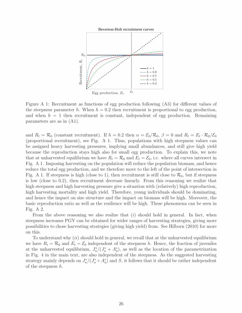
Figure A 1: Recruitment as functions of egg production following (A3) for different values ofthe steepness parameter h. When h = 0.2 then recruitment is proportional to egg production,and when h = 1 then recruitment is constant, independent of egg production. Remainingparameters are as in (A1).

and Rt = R0 (constant recruitment). If h = 0.2 then α = E0/R0, β = 0 and Rt = Et · R0/E0(proportional recruitment), see Fig. A 1. Thus, populations with high steepness values canbe assigned heavy harvesting pressures, implying small abundances, and still give high yieldbecause the reproduction stays high also for small egg production. To explain this, we notethat at unharvested equilibrium we have Rt = R0 and Et = E0, i.e. where all curves intersect inFig. A 1. Imposing harvesting on the population will reduce the population biomass, and hencereduce the total egg production, and we therefore move to the left of the point of intersection inFig. A 1. If steepness is high (close to 1), then recruitment is still close to R0, but if steepnessis low (close to 0.2), then recruitment decrease linearly. From this reasoning we realize thathigh steepness and high harvesting pressure give a situation with (relatively) high reproduction,high harvesting mortality and high yield. Therefore, young individuals should be dominating,and hence the impact on size structure and the impact on biomass will be high. Moreover, thebasic reproduction ratio as well as the resilience will be high. These phenomena can be seen inFig. A 2.

From the above reasoning we also realize that (i) should hold in general. In fact, whensteepness increases PGY can be obtained for wider ranges of harvesting strategies, giving morepossibilities to chose harvesting strategies (giving high yield) from. See Hilborn (2010) for moreon this.

To understand why (ii) should hold in general, we recall that at the unharvested equilibriumwe have Rt = R0 and Et = E0 independent of the steepness h. Hence, the fraction of juvenilesat the unharvested equilibrium, J∗

u/(J∗

u + A∗

u), as well as the location of the parametrizationin Fig. 4 in the main text, are also independent of the steepness. As the suggested harvestingstrategy mainly depends on J∗

u/(J∗

u +A∗

u) and S, it follows that it should be rather independentof the steepness h.

26

10.5010.50

Impact on biomass

0

0.5

1

1.5

Yie

ld

Variation of steepness, h

0 0.1 0.2 0.3 0.4 0.5

123456 78 9:;<=>?@ABCDEF

0

0.5

1

1.5

Yie

ld

0 0.005 0.01 0.015 0.02 0.025

Resilience

0

0.5

1

1.5

Yie

ld

5 10 15 20

GHJKL MNOPQRSTUVWX YZ[\]

0

0.5

1

1.5

Yie

ld

Figure A 2: Age model for h = 0.5 (thin curves) giving point P1 in Fig. 4 and h = 0.9 (thickcurves) giving point P2. Juvenile harvesting (blue, dashed), equal harvesting (black, solid),adult harvesting (red, dash-dot). Remaining parameters are as in (A1) and yield is normalizedas in Fig. 2 in the main text.

27

0 5 10 15Age, a

0

0.2

0.4

0.6

0.8

1

Biomass

per

individual,s a

(a)

a0 = −3

a0 = −2

a0 = −1

a0 = −0.2

0 5 10 15Age, a

0

0.2

0.4

0.6

0.8

1

Biomass

per

individual,s a

(b)

K = 0.1

K = 0.23

K = 0.5

K = 1

Figure A 3: Growth of an individual as functions of age following the von Bertalanffy growthcurves (A5) for different values of the parameters a0 and K. (a) variation of a0, (b) variationof K. Remaining parameters are as in (A1).

Parameters a0 and K in the von Bertalanffy growth, points P3 and P4

We have assumed von Bertalanffy (1957) growth to describe individual length as a function ofage, and that individual mass is proportional to the cube of individual length, i.e.

sa = smax

(

1− e−K(a−a0))3

, (A5)

where sa is the mass of an individual at age a, smax is the asymptotic maximum body mass, Kis a growth rate parameter and a0 is the hypothetical negative age at which the individual haszero length. We have already motivated smax = 1. Punt et al. (1995, page 290) studying thealbacore (Thunnus alalunga, Scombridae) motivate us to take a0 = −1 and K = 0.23. However,the value of a0 may be decreased to −2 as well since the age model is discrete and calculates thesize of all individuals in the beginning of the year, but harvesting and egg production naturallyoccur continuously during the year. We have considered variations in the ranges a0 ∈ [−3,−0.2]and K ∈ [0.1, 1]. Figure A 3 shows the corresponding growth curves for some values of a0 andK.

We present additional trade-off curves in Fig. A 4 for a0 = −3 (point P3 in Fig. 4) anda0 = −1 (point P4 in Fig. 4). When a0 = −1 then especially young individuals will have lowerbiomass and therefore the fraction of juveniles in the population will be small, J∗

u/(J∗

u +A∗

u) ≈53%. As a result, adult harvesting performs better, with respect to all conservation measures,than equal harvesting and juvenile harvesting. When a0 = −3 then especially young individualswill be of more biomass and therefore the fraction of juveniles in the population will be larger,J∗

u/(J∗

u + A∗

u) ≈ 66%. In this case equal harvesting is on the Pareto front within the range ofPGY for impact on biomass and resilience, and, therefore we recommend equal harvesting.

Considering variations in the growth parameter K gives a similar effect: A large K impliesthat individuals grow fast and this affects especially young individuals. If K = 1 then J∗

u/(J∗

u +A∗

u) ≈ 81% and juvenile harvesting is the only strategy on the Pareto front, in the range ofPGY, for all conservation measures. If K = 0.1 then J∗

u/(J∗

u +A∗

u) ≈ 41% and adult harvestingis the only strategy on the Pareto front, in the range of PGY, for all conservation measures.

28

10.5010.50

Impact on biomass

0

0.5

1

1.5

Yie

ld

Variation of parameter a0

0 0.1 0.2 0.3 0.4 0.5

^_`abc de fghijklmnopqrs

0

0.5

1

1.5

Yie

ld

0 0.005 0.01 0.015 0.02

Resilience

0

0.5

1

1.5

Yie

ld

2 4 6 8 10

tuvwx yz{|}~������ �����

0

0.5

1

1.5

Yie

ld

Figure A 4: Age model for a0 = −3 (thin curves) giving point P3 in Fig. 4, and a0 = −1(thick curves) giving point P4. Remaining description is as in Fig. A 2.

29

10.5010.50

Impact on biomass

0

0.5

1

1.5Y

ield

Variation of ageat mat rit amat�re

0 0.2 0.4 0.6 0.8 1

������ �� ������������� 

0

0.5

1

1.5

Yie

ld

0 0.005 0.01 0.015 0.02

Resilience

0

0.5

1

1.5

Yie

ld

2 4 6 8 10

¡¢£¤¥ ¦§¨©ª«¬­®¯°± ²³´µ¶

0

0.5

1

1.5Y

ield

Figure A 5: Age model for amature = 5 (thin curves) giving point P5 in Fig. 4, and amature = 11(thick curves) giving point P6. Remaining description is as in Fig. A 2.

Age at maturity amature, point P5 and P6

The quotient of length of first maturity to maximum length of fish may vary in the widerange from 0.2 to 1, but most species seem to be in the range 0.3 to 0.9 (Fishbase Fig. 43,http://www.fishbase.org/manual). Recalling the von Bertalanffy growth curves in Fig. A3, we realize that it is satisfactory that our results hold for age at maturity in the intervalamature ∈ [3, 15].

We present additional trade-off curves in Fig. A 5 for amature = 5 (point P5 in Fig. 4)and amature = 11 (point P6 in Fig. 4). If amature = 5 then J∗

u/(J∗

u + A∗

u) ≈ 35% and adultharvesting is the only strategy on the Pareto front, in the range of PGY, for all conservationmeasures. If amature = 11 then J∗

u/(J∗

u + A∗

u) ≈ 78% and we are at the border where equalharvesting and juvenile harvesting perform rather equally. Thus, amature has a large effect onthe fraction of juveniles in the population, and, therefore, a large impact on the preferableharvesting strategies.

30

10.80.60.40.20

Impact on biomass

0

0.5

1

1.5

2

2.5Y

ield

0 0.2 0.4 0.6 0.8 1

Impact on size-structure

0

0.5

1

1.5

2

2.5

Yie

ld

0 0.005 0.01 0.015 0.02 0.025

Resilience

0

0.5

1

1.5

2

2.5

Yie

ld

2 4 6 8 10

Basic reproduction ratio

0

0.5

1

1.5

2

2.5

Yie

ld

Variation of natural mortality, S

Figure A 6: Age model for S = 0.65 (thin curves) giving point P7 in Fig. 4, and S = 0.9(thick curves) giving point P8. Remaining description is as in Fig. A 2.

Survival from natural mortality S, points P7 and P8

Motivated by e.g. Mills et al. (2002) we used the default value S = 0.8 for the survival fromnatural mortality. We have seen that results from the age model are rather dependent of S,and this dependence has been investigated and presented in Fig. 4 in the main text. Fig. A 6shows additional trade-off curves for S = 0.65 (point P7 in Fig. 4) and S = 0.9 (point P8 inFig. 4). If S = 0.65 then J∗

u/(J∗

u +A∗

u) ≈ 88% and we are at the border where equal harvestingand juvenile harvesting perform rather equally. If S = 0.9 then J∗

u/(J∗

u +A∗

u) ≈ 32% and adultharvesting is the only strategy on the Pareto front, in the range of PGY, for all conservationmeasures.

31

Motivations and variations of parameter values in the

stage model

We adopt the following values of the model parameters,

H = T = r = 1, Rmax = 2, σ = 0.5, Imax = 10, M = 0.1, z = 0.01, q = 0.85. (A6)

These values may be considered as archetypal, and motivations can be found in de Roos et al.(2008). However, these values were derived in the Roos et al. (2008) using not only data onfish species. To ensure the validity of results in the setting of fisheries, we give below a ratherlengthy section concerning motivations and sensitivity of our results with respect to parametervalues.

First, we recall that we have considered substantial variations of these values and concluded,by numerically calculating trade-off curves, that our results from the stage model are robustfor the wide ranges of parameter values given by

M ∈ [0, 0.5], z ∈ [0.0001, 0.2], σImax ∈ [3, 100], q ∈ [0.6, 2], Rmax ∈ [0.5, 100]. (A7)

Indeed, we varied each parameter at a time, keeping the others at the values given in (A6)and tested at least 10 values in each interval. Several further parameter combinations havealso been tested, e.g. letting each parameter take on values at the boundary of the intervals in(A7). The upper bound of 100 on the intervals for Rmax and σImax does not seem necessary;the structures of the population, relevant for our study, seem to remain for much larger valuesas well. The lower limits of these intervals ensure that the population has a positive stableequilibrium.

In the following we will give, in addition to the motivations in de Roos et al. (2008),discussions and motivations for the parameter values in (A6) as well as for the consideredintervals in (A7). We will also give some explanations of how and why our results depend, ornot depend, on the parameter values. Finally, we present additional trade-off curves (similar tothose in Fig. 3 in the main text) but for other parametrizations. These curves are given in Figs.A 8, A 9 and A 10. Careful reading of these figures should convince the reader that our mainfindings are robust with respect to variations of parameter values. We do not present additionalversions of main text Fig. 6 (showing relation between measures). However, the correlation canbe seen from the trade-off figures by first focusing on the MSY point and then follow curves,for different measures, in the direction of either increasing or decreasing harvesting pressure.

Reduction of parameters

We begin by motivating that we can take H = T = 1 without loss of generality. The half-saturation constantH represents a resource density and is measured in biomass per unit volume.Changing its value can be considered as changes in the volume in which we express the densitiesR, J and A. Without loss of generality we can choose H = 1. This fixes the environmentalvolume in which the population is assumed to live and thus scales the biomass densities R,J and A. Mathematically, we rescale the stage model by introducing the new dimensionlessvariables J ′ = J/H , A′ = A/H , R′ = R/H and R′

max = R′

max/H , resulting in that H goesaway from the set of equations. We also rescale the time variable t with the mass-specificmetabolic rate parameter T , measured per unit of time, by introducing the dimensionless timet′ = tT and expressing the dynamics of the resource and the consumers as functions of this

32

new time variable. Moreover, we introduce the new dimensionless rate parameters r′ = r/T ,I ′max = Imax/T , M

′ = M/T , F ′

J = FJ/T and F ′

A = FA/T , resulting in that T goes away fromthe set of equations. This shows that we can choose H = T = 1 without loss of generality,and that results for other values of the parameters H and T can be obtained by multiplicationsfrom the results for H = T = 1. We therefore omit further investigations in H and T and putfocus on the remaining parameters. For simplicity, we will omit the “prime”-notation in thefollowing even though we work with the dimensionless quantities. The rescaled stage modelequations are identical to main text eqs. (8) but with H = T = 1. In particular,

dJ

dt= (wJ(R)− v(wJ(R))−M − FJ)J + wA(R)A, (A8)

dA

dt= v(wJ(R))J − (M + FA)A,

dR

dt= r(Rmax − R)− Imax

R

1 +R(J + qA) ,

where the net biomass production by a juvenile and an adult are, respectively,

wJ(R) = max

{

0, σImaxR

1 +R− 1

}

and wA(R) = max

{

0, σqImaxR

1 +R− 1

}

, (A9)

and the maturation is given by

v(x) =x−M − FJ

1− z1−(M+FJ)/x, (A10)

for x 6= M + FJ and v(M + FJ) = −(M + FJ)/ log(z).For clarity we plot the net biomass production functions for juveniles and adults, wJ(R)

and wA(R), as well as the maturation function v(wJ(R)), in Fig. A 7. All functions arezero (juveniles and adults do not produce biomass, and juveniles do not mature) until energyintake is sufficient to cover maintenance requirements, after which they increase with resourceabundance.

Resource parameters r and Rmax

Numerical investigations strongly indicate that our results are very robust with respect tovariations of the resource parameters r and Rmax. We will now give a theoretical explanationof this. Let J∗, A∗ and R∗ denote the juvenile, adult and resource biomass at equilibrium,respectively. Let also J∗

u , A∗

u and R∗

u denote these quantities in case of no harvesting pressure,i.e. when FJ = FA = 0. Setting derivatives to zero in the stage model (A8) and solving thecorresponding set of equations for equilibria we find that

J∗ =r(Rmax − R∗)(1 +R∗)(M + FA)

ImaxR∗(M + FA + qv(wJ(R∗))), A∗ =

r(Rmax − R∗)(1 +R∗)v(wJ(R∗))

ImaxR∗(M + FA + qv(wJ(R∗))), (A11)

where R∗ is given as the unique root of the equation

wA(R∗)v(wJ(R

∗))

(M + FA)[v(wJ(R∗))− wJ(R∗) +M + FJ]= 1. (A12)

33

0 0.5 1 1.5 2Resource, R

0

0.5

1

1.5

2

2.5Biomass production functions

wJ(R)

wA(R)

v(wJ(R))

v(wJ(R))

Figure A 7: Biomass production function for juveniles, wJ(R), and for adults, wA(R). Thematuration function v(wJ(R)) for M + FJ = 0.1 (blue, dashed) and for M + FJ = 1 (green,dotted). Remaining parameters are as in (A6).

From (A12) we note that the root R∗ will be independent of both r and Rmax, and from (A11)we see that both the juvenile and adult biomass, J∗ and A∗, increase linearly with both r andRmax, and so is the yield. Moreover, from the expressions in (A11) we see that

J∗

J∗ + A∗=

M + FA

M + FA + v(wJ(R∗))and (A13)

Impact on size-structure =M + FA

M + FA + v(wJ(R∗))

[

M

M + v(wJ(R∗

u))

]

−1

− 1.

Therefore, the fraction of juveniles in the population, as well as the population size structure, areindependent of r and Rmax (because R∗ is). We can also conclude, from the expressions for therecovery potential and the impact on biomass given in the main text, that both these measuresare independent of r. We may also note that the recovery potential becomes independent ofRmax as Rmax becomes very large as the ingestion for a single individual saturates for very largeresource densities.

These arguments clarifies why our results are more or less independent of r and Rmax

(whenever these parameters take on values giving a non-extinct population at equilibrium).Therefore, we feel comfortable with letting r = 1 and Rmax = 2 and put focus on the remainingparameters.

Ingestion parameters σ and Imax

Numerical investigations strongly indicate that our results are very robust with respect tovariations of the ingestion parameters σ and Imax. To understand why this is the case, weexpand on the above analytical reasoning and prove that at equilibrium, the fraction of juvenilebiomass in the population and the impact on size structure, see (A13), as well as wA(R

∗),wJ(R

∗) and v(wJ(R∗)) are in fact independent of r, Rmax, σ and Imax. Indeed, they depend

only on the parameters M +FJ, M +FA, q, and z. To prove this, consider equation (A12) fromwhich we solve the resource equilibrium biomass. In this equation, R∗, σ and Imax appear only

34

implicitly in the functions wA(R∗) and wJ(R

∗), see expressions (A9). Thus, by setting

α∗ = σImaxR∗

1 +R∗

we can solve (A12) for α∗, independent of the parameters σ and Imax. Therefore, varying σand Imax will not change wA(R

∗), wJ(R∗) and v(wJ(R

∗)), and thus not change the fraction ofjuvenile biomass in the population nor the impact on size structure. This shows why our resultsare very robust with respect to σ and Imax, and from here we fix σ = 0.5 and Imax = 10 andfocus on the remaining parameters.

Ratio of size at birth to maximum size z

De Roos et al. (2008) use the value z = 0.01 for the ratio of size at birth to maximum size,z = sborn/smax. To further motivate this value in a fisheries context, we note that Punt etal. (1995, page 290) studying the albacore (Thunnus alalunga, Scombridae) use K = 0.23 anda0 = −1 in the von Bertalanffy growth growth curves, recall Fig. A 3. This gives a value ofz ≈ 0.009 which is very close to 0.01. (Changing a0 to −3 gives z ≈ 0.12, and a0 = −0.2 givesz ≈ 0.00009.)

By numerically calculating trade-off curves as those in Fig. 3 in the main text, we have seenthat our results are robust with respect to variations of z in the wide interval z ∈ [0.0001, 0.2].Indeed, results from the stage model suggest that equal harvesting performs well rather inde-pendent of z as long as it takes on reasonable values. We present additional trade-off curves inFig. A 8 for the values z = 0.001 and z = 0.1. Here, we clearly see that the value of z has littleeffect on how juvenile-, adult- and equal harvesting performs.

Difference in ingestion between juveniles and adults q

It seems hard to motivate a specific value for the parameter q describing the difference iningestion rates between juveniles and adults: “An estimate for this parameter can hardly bederived from experimental data as it is only a phenomenological representation of stage-specificdifferences in resource availability and resource use between juveniles and adults.” (De Rooset al. 2008). By substantial numerical investigations we have seen that our results hold atleast as long as q ∈ [0.6, 2]. We present additional trade-off curves in Fig. A 9 for q = 0.6and q = 1.5, showing that our main findings hold for these parametrizations as well. Theconservation measures stays rather stable also when q is goes out of the bounds 0.6 and 2, butthen the difference in yield between the harvesting strategies increase. Indeed, smaller q impliesthat adult harvesting is better, and larger q implies that juvenile harvesting is better.

Natural mortality rate M

Following De Roos et al. (2008) we have adopted the default value of M = 0.1 for the naturalmortality rate. Fig. A 10 shows additional trade-off curves for the values M = 0.05 andM = 0.4. The main structure of the curves remains and thus our main results are robust alsoto changes in M . Let us note that M is simply added to the harvesting rates FJ and FA inthe stage model, recall (A8). Therefore, an increase in M should force the trade-off curves forjuvenile harvesting and adult harvesting toward the trade-off curves for equal harvesting (if Mis high, then there is then always high mortality on both juveniles and adults). This can be

35

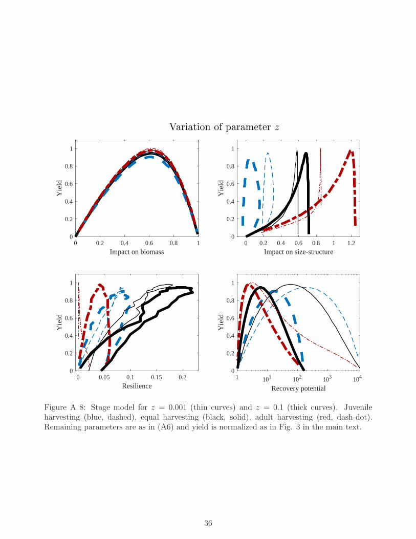
10.80.60.40.20

Impact on biomass

0

0.2

0.4

0.6

0.8

1

Yie

ld

0 0.05 0.1 0.15 0.2

Resilience

0

0.2

0.4

0.6

0.8

1

Yie

ld

1 101 102 103 104

Recovery potential

0

0.2

0.4

0.6

0.8

1

Yie

ld

0 0.2 0.4 0.6 0.8 1 1.2

Impact on size-structure

0

0.2

0.4

0.6

0.8

1

Yie

ld

Variation of parameter z

Figure A 8: Stage model for z = 0.001 (thin curves) and z = 0.1 (thick curves). Juvenileharvesting (blue, dashed), equal harvesting (black, solid), adult harvesting (red, dash-dot).Remaining parameters are as in (A6) and yield is normalized as in Fig. 3 in the main text.

36

10.80.60.40.20

Impact on biomass

0

0.2

0.4

0.6

0.8

1

1.2

Yie

ld

0 1 2 3 4 5 6

Impact on size-structure

0

0.2

0.4

0.6

0.8

1

1.2

Yie

ld

0 0.05 0.1 0.15 0.2 0.25

Resilience

0

0.2

0.4

0.6

0.8

1

1.2

Yie

ld

1 101 102 103

Recovery potential

0

0.2

0.4

0.6

0.8

1

1.2

Yie

ld

Variation of parameter q

Figure A 9: Stage model for q = 0.6 (thin curves) and q = 1.5 (thick curves), remainingdescription is as in Fig. A 8.

37

10.80.60.40.20

Impact on biomass

0

0.2

0.4

0.6

0.8

1

Yie

ld

0 0.5 1 1.5 2 2.5

Impact on size-structure

0

0.2

0.4

0.6

0.8

1

Yie

ld

0 0.05 0.1 0.15 0.2

Resilience

0

0.2

0.4

0.6

0.8

1

Yie

ld

100 101 102 103

Recovery potential

0

0.2

0.4

0.6

0.8

1

Yie

ld

Variation of natural mortality, M

Figure A 10: Stage model for M = 0.05 (thin curves) and M = 0.4 (thick curves), remainingdescription is as in Fig. A 8.

observed in Fig. A 10. We can also see that the impact on size structure is much smaller forhigher M , which may be understood by the fact that now the unharvested state already has ahigh death rate. We can also observe the expected decrease in yield when death rate increasesfrom M = 0.05 to M = 0.4.

Detailed description of our resilience measure

We have considered resilience of the population by measuring the reciprocal of the time neededfor the population to recover the positive equilibrium given a random perturbation. To describethe procedure in detail, let (J∗, A∗, R∗) denote the equilibrium of biomass in the stage model,and let N∗

a , a = 0, 1, 2, . . . , amax denote the equilibrium of number of individuals in the agemodel. For a given constant κ > 0 that scales the maximum displacement of the populationfrom the equilibrium, we start a trajectory from a random point uniformly distributed in the

38

cube

(0, κJ∗)× (0, κA∗)× (0, κR∗) (stage model), (A14)

(0, κN∗

0 )× (0, κN∗

1 )× (0, κN∗

2 )× · · · × (0, κN∗

amax) (age model).

We then find the return time as the time needed for this trajectory to be close enough to theequilibrium in the sense that

{

(

J∗ − J(t)

J∗

)2

+

(

A∗ −A(t)

A∗

)2

+

(

R∗ − R(t)

R∗

)2}1/2

≤ ǫ (stage model), (A15)

{

amax∑

a=0

(

N∗

a −Na,t

N∗

a

)2}1/2

≤ ǫ (age model),

for some small ǫ > 0. After repeating this procedure n times we find the resilience, as a functionof the harvesting rates FJ and FA, by taking the reciprocal of the average of the correspondingreturn times, i.e.

Resilience =1

Average of the n return times.

Our resilience measure estimates the population’s expected rate of return, given a randomperturbation. We have used the parameter values κ = 2, ǫ = 0.01 and n = 100 as defaultvalues, but main results are not very sensitive to the magnitude of the imposed perturbations(κ) nor the size of the small neighborhood (ǫ) as long as κ >> ǫ take on reasonable values.We present some results on κ = 1 in Fig. A 12 below, which means that we consider onlyperturbations that remove biomass.

It is worth noting that when implementing our approach to resilience, one tests the modelfor a large number of initial conditions. Therefore, one may find out if the system is bistable,i.e. if other attractors (e.g. stable states or periodic solutions) are present, which is valuableinformation. Indeed, if this is the case, a tested initial condition may produce a trajectory thatnever return to the equilibrium. This will be revealed by our simulation procedure. If applyingour approach to bistable systems, one should define another stopping criteria for the otherattractors. The resilience can then be defined as the average of the reciprocal of the returntimes, setting the reciprocal to zero whenever an initial condition reached another attractor.In that way initial conditions (perturbations) that escape to another states contributes withresilience zero, c.f. measure R in Lundstrom (2018).

Basin-time resilience and further investigations of the stage

model

From our results on the stage model we have seen that resilience, in contrary to the other con-servation measures, may vastly increase with harvesting pressure for some harvesting strategies.This is true for equal harvesting and juvenile harvesting, but not at all for adult harvesting,recall Fig. 3 in the main text as well as Figs. A 8, A 9 and A 10. Indeed, adult harvestinggives the worst resilience while equal harvesting gives the best resilience (which can be up to20 times higher in the range of PGY). As this phenomenon provides a substantial argument in

39

favour of equal harvesting compared to adult harvesting, we investigate it further here in orderto increase the credibility of our results.

Each dot in Figs. A 11 (a)-(c) show an imposed perturbation as an initial condition fromwhich we integrated the trajectory until it reached the small neighborhood of the equilibriumgiven by (A15) with ǫ = 0.1. Tested initial conditions are distributed uniformly in (0, κJ∗) ×(0, κA∗) with R = R∗ and κ = 2. Grey dots return to the equilibrium within a time limitwhich we set to t ≤ 5, while red dots need more time to recover the equilibrium. There isno harvesting pressure in Fig. A 11 (a), adult harvesting FJ = 0, FA = 35 in (b) and equalharvesting FJ = FA = 0.8 in (c). The harvesting strategies in (b) and (c) give similar yields(close to the maximum possible yield). The fraction of grey dots is largest in case of equalharvesting, while it is smallest in case of adult harvesting, which means that the populationreturns fast from more perturbations (initial conditions) in case of equal harvesting than foradult harvesting. This reflects the higher resilience in case of equal harvesting. Indeed, thefraction of grey dots estimates the probability that the population recover the equilibrium ina time limit, given a random perturbation, and constitutes a natural candidate for measuringresilience.

In general, let basin-time be a subset of the basin of attraction from which trajectoriesreturn to (a small neighborhood of) the attractor within a time limit, t ≤ τ . A large and convexbasin-time set should then reflect high resilience. Therefore, both the size and the shape of thebasin-time constitute natural candidates for measuring resilience (Lundstrom 2018). We willconsider the size of the basin-time set as a resilience measure. To do so we impose perturbationsas described in (A14) and integrate each trajectory until it reaches the neighborhood definedby (A15). We further let N τ

return denote the number of initial conditions from which trajectoriesreturn in time τ , and Ntot denote the total number of tested initial conditions. We measureresilience as the size of the basin-time set through the estimate

Basin-time resilience =N τ

return

Ntot.

Figure A 11 (d) shows trade-off curves between basin-time resilience and yield. (parametersare κ = 2, n = 1000, ǫ = 0.1 and τ = 5.) It is clear that also the basin-time resilience measurestrengthen the result of the stage model saying that equal harvesting performs best while adultharvesting gives the worst resilience; these trade-off curves are very similar to those in Fig. 3(c) in the main text.

Figs. A 11 (a), (b) and (c) may indicate that the higher resilience in case of equal harvestingis due to fast return of trajectories starting at high biomass. Indeed, the basin-time, estimatedby the fraction of grey dots, is largest in Fig. A 11 (c) and includes all points correspondingto larger initial biomass than at equilibrium. Therefore, we complement the given resilienceestimations by a simulation in which we consider only perturbations that remove biomass. Inparticular, we take κ = 1 and reproduce the trade-off curves between resilience (both measures)and yield, see Fig. A 12. We can observe that equal harvesting is now challenged by juvenileharvesting, but both resilience measures still agree on the result that equal harvesting is muchbetter than adult harvesting.

In addition to the above resilience estimations, we have also considered normally distributedperturbations (centered at the equilibrium) as well as the “standard” local resilience measuregiven by the real part of the eigenvalue of the Jacobian matrix at equilibrium with largest realpart. Results from these investigations also agree very well with our findings.

For further ideas on how to use the basin of attraction, the basin-time as well as the return

40

0 0.1 0.2 0.3 0.4 0.5 0.6 0.7Juvenile biomass, J

0

0.1

0.2

0.3

0.4

0.5

0.6

0.7

Adult

biomass,A

(a)

0 0.2 0.4 0.6Juvenile biomass, J

0

0.002

0.004

0.006

0.008

0.01

0.012

0.014

0.016

Adult

biomass,A

(b)

0 0.1 0.2 0.3 0.4 0.5Juvenile biomass, J

0

0.02

0.04

0.06

0.08

0.1

0.12

0.14

Adult

biomass,A

(c)

0 0.2 0.4 0.6 0.8 1Basin-time resilience

0

0.5

1

Yie

ld

(d)

Figure A 11: (a)-(c): Population recover fast from most perturbations in case of equal harvesting(c) and from fewest perturbations in case of adult harvesting (b). The grey dots represent initialconditions that return to the equilibrium within time 5, while the red dots need more time torecover the equilibrium. There is no harvesting pressure in (a). (d): Trade-off between basin-time resilience and yield. Juvenile harvesting (blue, dashed), equal harvesting (black, solid),adult harvesting (red, dash-dot). Model parameters are as in (A6) and yield is normalized asin Fig. 3 in the main text.

41

0 0.2 0.4 0.6 0.8 1Basin-time resilience

0

0.5

1

Yie

ld

(a)

0 0.05 0.1 0.15Resilience

0

0.5

1

Yie

ld

(b)

Figure A 12: Trade-off between yield and resilience considering κ = 1, i.e. perturbationsonly remove population and resource biomass. (a) basin-time resilience and (b) the resiliencemeasure used in the main text. Remaining descriptions are as in Fig. A 11.

time to measure stability and resilience, we refer the reader to Lundstrom (2018) and referencestherein.

Derivation of the basic reproduction ratio for the age

model

The basic reproduction ratio represents the average number of offsprings produced over thelifetime of an individual in the absence of density-dependent competition. We consider an indi-vidual satisfying the dynamics of the age model and calculate an expression for this individualsexpected offsprings during its lifetime. For this purpose, we let Et denote the egg productionand Rt the recruitment from this individual, at time t. That no density-dependent competitionis present lead us to assume that the Beverton-Holt recruitment is completely unsaturated.Such situation is achieved by taking β = 0 (or R0 = ∞) in (A3), giving

Rt+1 =Et

αexp

(

ut −σ2u

2

)

in which α =

(

1−h− 0.2

0.8h

) amax∑

a=0

mafaSa, (A16)

where we used relation (A4) to find the expression for α. Now, since ut − σ2u/2 is normally dis-

tributed with mean −σ2u/2 and standard deviation σu, we obtain, where E denotes expectation,

E

{

exp

(

ut −σ2u

2

)}

= 1.

Therefore, the expected number of offsprings in year t becomes

E{

Rt+1

}

=Et

α

42

and hence the expected total number of offsprings from the single individual during its lifetime,i.e. the basic reproduction ratio R0(FJ, FA), becomes

R0(FJ, FA) = E

{

amax∑

t=0

Rt+1

}

=amax∑

t=0

E{

Rt+1

}

=1

α

amax∑

t=0

Et, (A17)

where α is given in (A16).It remains to calculate the total number of eggs produced, i.e. the sum in the right hand

side of (A17). Indeed, following (3) and (4) in the main text we conclude that

amax∑

t=0

Et = m0f0 +m1f1S(1− γ0) +m2f2S2(1− γ0)(1− γ1) + . . .

= m0f0 +amax∑

a=1

mafaSaa−1∏

i=0

(1− γi).

By the expression for ma in (1) in the main text and by γa in (5) in the main text we find thatthe above expression yields

amax∑

t=0

Et = m0f0 +amax∑

a=1

mafaSaa−1∏

i=0

(1− γi) =amax∑

a=amature+1

faSaa−1∏

i=0

(1− γi)

= (1− FJ)amature ×

amax∑

a=amature+1

faSa (1− FA)

a−amature .

We next use the relation fa = csa given in (1) in the main text to derive

amax∑

t=0

Et = c (1− FJ)amature ×

amax∑

a=amature+1

sa Sa (1− FA)

a−amature .

Using (1) in the main text once more we see that α can be written

α = c

(

1−h− 0.2

0.8h

) amax∑

a=amature+1

sa Sa. (A18)

Inserting main text eq. (3) and (A18) into (A17) and simplifying yield

R0(FJ, FA) =(1− FJ)

amature ×∑amax

a=amature+1 sa Sa (1− FA)

a−amature

(

1− h−0.20.8h

)

×∑amax

a=amature+1 sa Sa

.

This expression is identical to eq. (10) in the main text which gives the basic reproductionratio for the age model.

References

Anderson C.N.K., Hsieh C., Sandin S.A. et al. (2008) Why fishing magnifies fluctuations in fishabundance. Nature 452:835–839.

43

Belgrano A., Fowler C.W. (2013) How fisheries affect evolution. Science 342:1176–1177.

von Bertalanffy L. (1957) Quantitative laws in metabolism and growth. Quarterly Review ofBiology 32:217–231 .

Beverton R.J.H., Holt S.J. (1957) On the dynamics of exploited fish populations. U.K. Min.Agr. and Fish. Fish. Invest. (Ser. 2) 19.

Brown J.H., Gillooly J.F., Allen A.P., Savage V.M., West G.B. (2004) Toward a metabolictheory of ecology. Ecology 85:1771–1789.

Cameron T.C., Sullivan D.O., Reynolds A., Piertney S.B., Benton T.G. (2013) Eco-evolutionarydynamics in response to selection on life-history. Ecology Letters 16:754–763.

Clark W.G. (1977) The lessons of the Peruvian anchoveta fishery. California CooperativeOceanic Fisheries Investigations 19:57–63.

Conover D.O., Munch S.B. (2002) Sustaining fisheries yields over evolutionary time scales.Science 297:94–96.

Donohue I., Petchey O.L., Montoya J.M., Jackson A.L., McNally L., Viana M., Healy K., LurgiM., O’Connor N.E., Emmerson M.C. (2013) On the dimensionality of ecological stability.Ecology Letters 16:421–429.

Dunlop E.S., Eikeset A.M., Stenseth N.C. (2015) From genes to populations: how fisheries-induced evolution alters stock productivity. Ecological Applications 25:1860–1868.

Dunne J.A., Williams R.J., Martinez N.D. (2002) Network structure and biodiversity loss infood webs: robustness increases with connectance. Ecology Letters 5:558–567.

Engen S., Lee A. M., Saether B-E. Spatial distribution and optimal harvesting of an age-structured population in a fluctuating environment. Mathematical biosciences 296 (2018):36–44.

FAO (2016) The state of world fisheries and aquaculture 2014, Vol. Food and AgricultureOrganization of the United Nations, Rome. http://www.fao.org/fishery/sofia/en

Fey S.B., Siepielski A.M., Nussle S., et al. (2015) Recent shifts in the occurrence, cause, andmagnitude of animal mass mortality events. Proceedings of the National Academy of Sciencesof the USA 112:1083–1088.

Francis R.I.C.C. (1992) Use of risk analysis to assess fishery management strategies: a casestudy using orange roughy (Hoplostethus atlanticus) on the Chatham Rise, New Zealand.Canadian Journal of Fisheries and Aquatic Sciences 49:922–30.

Fung T., Farnsworth K.D., Shephard S., Reid D.G., Rossberg A.G. (2013) Why the size struc-ture of marine communities can require decades to recover from fishing. Marine EcologyProgress Series 484:155–171.

Garcia S.M., Kolding J., Rice J. et al. (2012) Reconsidering the consequences of selectivefisheries. Science 335:1045–1047.

44

Grift R.E., Rijnsdorp A.D., Barot S., Heino M., Dieckmann U. (2003) Fisheries-inducedtrends in reaction norms for maturation in North Sea plaice. Marine Ecology Progress Series257:247–257.

Grimmett G.R., Stirzaker D.R. (1992) Probability and Random Processes, 2nd edn. The Claren-don Press Oxford University Press, New York.

Haegeman B., Arnoldi J.F., Wang S., de Mazancourt C., Montoya J.M., Loreau M. (2016).Resilience, invariability, and ecological stability across levels of organization. bioRxiv, 085852.

Hannesson R. (1996) Fisheries Mismanagement: the case of the North Atlantic cod. FishingNews Books, London.

Hilborn R. (2007) Defining success in fisheries and conflicts in objectives. Marine Policy 31:153–158.

Hilborn R. (2010) Pretty good yield and exploited fishes. Marine Policy 34:193–196.

Holling C.S. (1973) Resilience and stability of ecological systems. Annual review of ecology andsystematics, 4(1), 1–23.

Holt R. (1958) The evaluation of fisheries resources by the dynamic analysis of stocks, and noteson the time factors involved. International commission for the northwest atlantic fisheries,special publication 1:77–95.

Hsieh C., Reiss C.S., Hunter J.R., Beddington J.R., May R.M., Sugihara G. (2006) Fishingelevates variability in the abundance of exploited species. Nature 443:859–862.

Isbell F., Craven D., Connolly J. et al. (2015) Biodiversity increases the resistance of ecosystemproductivity to climate extremes. Nature 526:574–577.

Jacobsen N.S., Gislason H., Andersen K.H. (2014) The consequences of balanced harvest-ing of fish communities. Proceedings of the Royal Society of London B: Biological Sciences281:20132701.

Jacobsen N.S., Burgess M.G., Andersen K.H. (2017) Efficiency of fisheries is increasing at theecosystem level. Fish and Fisheries 18.2:199–211.

Jones H.P., Schmitz O.J. (2009) Rapid recovery of damaged ecosystems. PloS one 4:e5653

Jorgensen C., Enberg K., Dunlop E.S. et al. (2007) Managing evolving fish stocks. Science318:1247–1248.

Karpagam M. (1999) Environmental Economics: A Textbook. Sterling PublishersPvt. Ltd.

Krovnin A.S., Rodionov S.N. (1992) Atlanto-Scandian herring: a case study. In Climate Vari-ability, Climate Change and Fisheries, eds Glantz M., Cambridge University Press UK, pp231–260.

Kuparinen A., Merila J. (2007) Detecting and managing fisheries-induced evolution. Trends inEcology and Evolution 22:652–659.

45

Larkin P.A. (1977) An epitaph for the concept of maximum sustained yield. Transactions ofthe American Fisheries Society 106:1–11.

Law R. (2000) Fishing, selection, and phenotypic evolution. ICES Journal of Marine Science57:659–668.

Law R., Plank M.J., Kolding J. (2012) On balanced exploitation of marine ecosystems: resultsfrom dynamic size spectra. ICES Journal of Marine Science 69:602–614.

Law R., Kolding J., Plank M.J. (2015) Squaring the circle: reconciling fishing and conservationof aquatic ecosystems. Fish and Fisheries 16.1: 160–174.

Levins R. (1966) The strategy of model building in population biology. American Scientist 54.4:421–431.

Loeuille, N. (2010) Influence of evolution on the stability of ecological communities. EcologyLetters 13:1536–1545.

Loreau M., Behera N. (1999) Phenotypic diversity and stability of ecosystem processes. Theo-retical Population Biology 56:29–47.

Loreau M., Mazancourt C. (2013) Biodiversity and ecosystem stability: a synthesis of underly-ing mechanisms. Ecology Letters 16:106–115.

Lundstrom N. L. P. (2018) How to find simple nonlocal stability and resilience measures. Non-linear Dynamics, 93:887–908.

Lundstrom, N. L. P., Aidanpaa, J-O. Dynamic consequences of electromagnetic pull due todeviations in generator shape. Journal of Sound and Vibration 301:207–225.

Mace P.M., Doonan I.J. (1988) A generalised bioeconomic simulation model for fish populationdynamics. MAFFish, NZ Ministry of Agriculture and Fisheries, 1988.

Mangel M., Levin P.S. (2005) Regime, phase and paradigm shifts: making community ecologythe basic science for fisheries. Philosophical Transactions of the Royal Society B 360:95–105.

Myers R.A., Bowen K.G., Barrowman N.J. (1999) Maximum reproductive rate of fish at lowpopulation sizes. Canadian Journal of Fisheries and Aquatic Sciences 56:2404-2419.

McCann K. (2000) The diversity-stability debate. Nature, 405:228-233.

Menck P.J., Heitzig J., Marwan N., Kurths J. (2013) How basin stability complements thelinear-stability paradigm. Nature Physics 9:89-92.

Meng X., Lundstrom N.L.P., Bodin M., Brannstrom A. (2013) Dynamics and management ofstage-structured fish stocks. Bulleting of Mathematical Biology 75:1–23.

Mesnil B. (2012) The hesitant emergence of maximum sustainable yield (MSY) in fisheriespolicies in Europe. Marine Policy 36:473–480.

Montoya J.M., Pimm S.L., Sole R.V. (2006) Ecological networks and their fragility. Nature442:259–264.

46

Morell V. (2009) Can science keep Alaska’s Bering sea pollock fishery healthy? Science326:1340–1341.

Mills K.H., Chalanchuk S.M., Allan D.J. (2002) Abundance, annual survival, and recruitment ofunexploited and exploited lake charr, Salvelinus namaycush, populations at the ExperimentalLakes Area, northwestern Ontario. Environmental Biology of Fishes 64:281–292.

Neubert M.G., Caswell H. (1997) Alternatives to resilience for measuring the responses ofecological systems to perturbations. Ecology 78:653–665.

Nimmo D.G., Mac Nally R., Cunningham S.C., Haslem A., Bennett A.F. (2015) Vive laresistance: reviving resistance for 21st century conservation. Trends in Ecology and Evo-lution 30:516–523.

Olsen E.M., Heino M., Lilly G.R. et al. (2004) Maturation trends indicative of rapid evolutionpreceded the collapse of northern cod. Nature 428:932–935.

Petchey O.L., Casey T., Jiang L., McPhearson P.T., Price J. (2002) Species richness, environ-mental fluctuations, and temporal change in total community biomass. Oikos 99:231–240.

Pimm S.L., Lawton J.H. (1977) Number of Trophic Levels in Ecological Communities. Nature268:329–331.

Punt A.E. (1994) Assessments of the stocks of Cape hake Merluccius spp. off South Africa.South African Journal of Marine Science 14:159–86.

Punt A.E., Butterworth D.S. and Penney A.J. (1995) Stock assessment and risk analysis for thesouth Atlantic population of albacore Thunnus alalunga using an age-structured productionmodel. South African Journal of Marine Science 16:361–71.

Punt A.E., Hilborn R. (1997) Fisheries stock assessment and decision analysis: the Bayesianapproach. Reviews in Fish Biology and Fisheries 7:35–63.

Radovich J. (1982) The collapse of the California sardine fishery – what have we learned?California Cooperative Oceanic Fisheries Investigations Report 23:56–78.

Reid D. G., Graham N., Suuronen P., He P., Pol M. (2016) Implementing balanced harvesting:practical challenges and other implications. ICES Journal of Marine Science, 73(6), 1690-1696.

Reusch T.B.H., Ehlers A., Hammerli A., Worm B. (2005) Ecosystem recovery after climaticextremes enhanced by genotypic diversity. Proceedings of the National Academy of Sciencesof the USA, 102:2826-2831.

Rip J.M.K., McCann K.S. (2011) Cross-ecosystem differences in stability and the principle ofenergy flux. Ecology Letters 14:733–740.

de Roos A.M., Persson L. (2013) Population and Community Ecology of Ontogenetic Develop-ment. Princeton University Press.

de Roos A.M., Schellekens T., van Kooten T., DeWolfshaar K.V., Claessen D., Persson L. (2008)Simplifying a physiologically structured population model to a stage-structured biomassmodel. Theoretical Population Biology 73:47–62.

47

Rosenzweig M.L. (1971) Paradox of enrichment: destabilization of exploitation ecosystems inecological time. Science 171:385–387.

Smith T., Punt A.E. (2001) The gospel of maximum sustainable yield in fisheries manage-ment: birth, crucifixion and reincarnation. In Conservation of Exploited Species. Edited byJD Reynolds, GM Mace, KH Redford, and JG Robinson. Cambridge University Press, Cam-bridge, UK, 41–66.

Sugihara G., Beddington J., Hsieh C., Deyle E., Fogarty M., Glaser S.M., Hewitt R., Hol-lowed A., May R.M., Munch S.B., Perretti C., Rosenberg A.A., Sandin S., Ye H. (2011) Areexploited fish populations stable? Proc Natl Acad Sci USA 108(48):1224–1225.

Tromeur E., Loeuille N. (2017) Balancing yield with resilience and conservation objectives inharvested predator-prey communities. Oikos 126.12: 1780–1789.

Valdovinos F.S., Ramos-Jiliberto R., Garay-Narvaez L., Urbani P., Dunne J.A. (2010) Conse-quences of adaptive behaviour for the structure and dynamics of food webs. Ecology Letters13:1546–1559.

Walker B.H., Ludwig D., Holling C.S., Peterman R.M. (1969). Stability of semi–arid savannagrazing systems. Ecology 69, 473–498.

White C., Costello C., Kendall B.E., Brown C.J. (2012) The value of coordinated managementof interacting ecosystem services. Ecology Letters 15:509–519.

van Wijk S.J., Taylor M.I., Creer S. et al. (2013) Experimental harvesting of fish populationsdrives genetically based shifts in body size and maturation. Frontiers in Ecology and theEnvironment 11:181–187.

Wikstrom A., Ripa J., Jonzen N. (2012) The role of harvesting in age-structured populations:Disentangling dynamic and age truncation effects. Theoretical Population Biology 82:348–354.

48