
Master's Thesis - Pure
117
Eindhoven University of Technology MASTER Artifact-centric log extraction and process discovery Lu, X. Award date: 2013 Link to publication Disclaimer This document contains a student thesis (bachelor's or master's), as authored by a student at Eindhoven University of Technology. Student theses are made available in the TU/e repository upon obtaining the required degree. The grade received is not published on the document as presented in the repository. The required complexity or quality of research of student theses may vary by program, and the required minimum study period may vary in duration. General rights Copyright and moral rights for the publications made accessible in the public portal are retained by the authors and/or other copyright owners and it is a condition of accessing publications that users recognise and abide by the legal requirements associated with these rights. • Users may download and print one copy of any publication from the public portal for the purpose of private study or research. • You may not further distribute the material or use it for any profit-making activity or commercial gain
-
Upload
khangminh22 -
Category
Documents
-
view
3 -
download
0
Transcript of Master's Thesis - Pure

Eindhoven University of Technology
MASTER
Artifact-centric log extraction and process discovery
Lu, X.
Award date:2013
Link to publication
DisclaimerThis document contains a student thesis (bachelor's or master's), as authored by a student at Eindhoven University of Technology. Studenttheses are made available in the TU/e repository upon obtaining the required degree. The grade received is not published on the documentas presented in the repository. The required complexity or quality of research of student theses may vary by program, and the requiredminimum study period may vary in duration.
General rightsCopyright and moral rights for the publications made accessible in the public portal are retained by the authors and/or other copyright ownersand it is a condition of accessing publications that users recognise and abide by the legal requirements associated with these rights.
• Users may download and print one copy of any publication from the public portal for the purpose of private study or research. • You may not further distribute the material or use it for any profit-making activity or commercial gain

Artifact-Centric Log Extractionand Process Discovery
Master Thesis
Xixi Lu
Department of Mathematics and Computer ScienceArchitecture of Information Systems Research Group
Supervisors:Dr. ir. Dirk Fahland
ir. Marijn Nagelkerke (KPMG)ir. Dennis van de Wiel (KPMG)
Dr. ir. Irene Vanderfeesten
Final version
Eindhoven, September 2013


Abstract
The omnipresence of using Enterprise Resource Planning (ERP) systems to support business pro-cesses has enabled recording a great amount of (relational) data which indicates the behaviors ofthese processes. However, to allow classic process mining techniques to be applied on this data todiscover process models and gain new insight, approaches have been proposed to convert this datainto an event log, which is generally required by process mining techniques. These traditional con-version approaches tend to assume an isolated process with a clear notion of a case and a unique caseidentifier. This assumption has caused issues such as the known Data Convergence and Divergenceproblems in an ERP system setting, due to the fact that these processes comprise the life-cycles ofvarious interrelated data objects, also known as artifacts, instead of a single object. In this thesis, anew semi-automatic artifact-oriented approach is presented which is extended from the XTract ap-proach proposed by E.H.J.Nooijen et al. [21][22]. The new approach identifies various artifacts anddiscovers the life-cycle of each of these artifacts and their interrelated relations both on the artifacttype level and on the event type level. An artifact-centric model in the proclet language [4] anddiverse statistics for business analyses are obtained by using our approach. The presented approachis implemented and evaluated on multiple processes of ERP systems through case studies.
Keywords: Process Mining, Artifact-Centric Process Discovery, Relational Data to Event logs Con-version, ERP Systems


Preface
This master thesis is the result of my graduation project which completes my Business InformationSystems study at Eindhoven University of Technology. The project was conducted in cooperationwith KPMG IT Advisory and the Architecture of Information Systems group of the Mathematicsand Computer Science department of Eindhoven University of Technology.
First of all I would like to thank my graduation supervisor, Dirk Fahland, for his guidance duringmy master project. I would like to thank Dirk for the weekly discussions, extensive reviews, and thefast and constructive feedback. Furthermore my thanks go out to Irene Vanderfeesten for being myreviewer.
Secondly, I would like to thank KPMG IT Advisory N.V. for allowing me to join the team. KPMGhas given me the opportunity to work with experts in the field of data analytics, SAP, and Oracle andfreely use the available resources in the organization. My colleagues have made my internship a reallyvaluable experience where I learned to think about problems in a business perspective and where wehad a lot of fun. Special gratitude goes to Marijn Nagelkerke and Dennis van de Wiel, my supervisors,who have helped me to apply my research in practice and conduct case studies. Moreover, I wouldlike to thank Ruud who has provided me the opportunity and helped me conducting the case study.
I would like to thank Boudewijn van Dongen, Mike Bussel, and Rob Reijnders, without who Iwould not have come into contact with KPMG and thus would not have had the opportunity todo this project in the first place. I would especially like to thank Boudewijn who has been a greatmentor and helped me to get started with this master project. I would like to express my gratitudeto Erik Nooijen, whose thesis forms the fundamentals of this project.
Finally, I would like to thank my mother, my friends and my class mates. Without their support,I would never have come this far. This project concludes my five years study at Eindhoven Universityof Technology, during which I have met so many people such as Maikel, Han, Paul, Pim, Janot,Quirijn, Sander, Alex, Qian, Qinrui, Xiyuan, Ruben, Thomas, Kosmas, Tatiana, Twan, Zheyi andmany others who have helped me grow so much. Thank you.
v


Contents
Abstract iii
Preface v
1 Introduction 1
1.1 Thesis Context . . . . . . . . . . . . . . . . . . . . . . . . . . . . . . . . . . . . . . 1
1.2 Research Problem . . . . . . . . . . . . . . . . . . . . . . . . . . . . . . . . . . . . 7
1.3 Research Scope . . . . . . . . . . . . . . . . . . . . . . . . . . . . . . . . . . . . . 9
1.4 Outline - Artifact Centric Approach . . . . . . . . . . . . . . . . . . . . . . . . . . . 10
2 Preliminaries 13
2.1 Process Mining . . . . . . . . . . . . . . . . . . . . . . . . . . . . . . . . . . . . . 13
2.1.1 Event logs and the XES Event Log Format . . . . . . . . . . . . . . . . . . 14
2.1.2 Process Discovery and ProM framework . . . . . . . . . . . . . . . . . . . . 16
2.1.3 Process Models and Artifact-Centric Model . . . . . . . . . . . . . . . . . . 17
2.1.4 Relational Databases and ERP systems . . . . . . . . . . . . . . . . . . . . 17
2.2 Literature Study - Traditional Log Extraction Approaches . . . . . . . . . . . . . . . 18
2.3 Literature Study - Artifact-Centric Log Extraction Approach . . . . . . . . . . . . . 20
2.3.1 Open Issues of XTract . . . . . . . . . . . . . . . . . . . . . . . . . . . . . . 21
3 Artifact Type Identification 27
3.1 Data Schema Identification . . . . . . . . . . . . . . . . . . . . . . . . . . . . . . . 28
3.2 Artifact Schema Identification . . . . . . . . . . . . . . . . . . . . . . . . . . . . . 30
3.3 Artifact Identification . . . . . . . . . . . . . . . . . . . . . . . . . . . . . . . . . . 32
4 Interaction Identification 37
4.1 Artifact Type Level and Instance Level Interactions . . . . . . . . . . . . . . . . . . 39
4.1.1 Direct Artifact Type level and Instance Level Interactions . . . . . . . . . . . 39
4.1.2 Indirect Artifact level Interactions . . . . . . . . . . . . . . . . . . . . . . . 41
4.1.3 Possibility of Identifying Event Level Interactions . . . . . . . . . . . . . . . 44
4.2 Type Level Interaction Identification . . . . . . . . . . . . . . . . . . . . . . . . . . 44
4.2.1 Artifact Interaction Graph and Direct Interactions . . . . . . . . . . . . . . . 45
4.2.2 Direct to Indirect Interactions . . . . . . . . . . . . . . . . . . . . . . . . . . 46
4.3 Mapping Creation and Log Extraction . . . . . . . . . . . . . . . . . . . . . . . . . 48
vii

CONTENTS
5 Artifact-Centric Process Discovery and Analyses 515.1 Logs and Life-cycle Discovery . . . . . . . . . . . . . . . . . . . . . . . . . . . . . . 52
5.1.1 Event logs with trace level interactions . . . . . . . . . . . . . . . . . . . . . 525.1.2 Life-cycle Miners . . . . . . . . . . . . . . . . . . . . . . . . . . . . . . . . 54
5.2 Event Type Level Interaction Identification . . . . . . . . . . . . . . . . . . . . . . . 545.2.1 Interaction Discovery by Merging Logs . . . . . . . . . . . . . . . . . . . . . 545.2.2 Interaction Discovery by using Criteria . . . . . . . . . . . . . . . . . . . . . 565.2.3 Limitations . . . . . . . . . . . . . . . . . . . . . . . . . . . . . . . . . . . . 58
5.3 Artifact-Centric Model Discovery . . . . . . . . . . . . . . . . . . . . . . . . . . . . 585.3.1 Proclet System Creation . . . . . . . . . . . . . . . . . . . . . . . . . . . . 595.3.2 Simple representation . . . . . . . . . . . . . . . . . . . . . . . . . . . . . . 59
5.4 Artifact-Centric Process Analyses . . . . . . . . . . . . . . . . . . . . . . . . . . . . 605.4.1 Traceability . . . . . . . . . . . . . . . . . . . . . . . . . . . . . . . . . . . 60
6 Implementation 636.1 XTract2 . . . . . . . . . . . . . . . . . . . . . . . . . . . . . . . . . . . . . . . . . 636.2 InteractionMiner . . . . . . . . . . . . . . . . . . . . . . . . . . . . . . . . . . . . 66
7 Case Studies 697.1 Case I - SAP Order To Cash Process . . . . . . . . . . . . . . . . . . . . . . . . . . 69
7.1.1 SAP OTC process and data structure . . . . . . . . . . . . . . . . . . . . . 697.1.2 SAP OTC - Extraction and Discovery . . . . . . . . . . . . . . . . . . . . . 707.1.3 SAP OTC - Process Analyses and Discussion . . . . . . . . . . . . . . . . . 75
7.2 Case II - Oracle Project Administration Process . . . . . . . . . . . . . . . . . . . . 787.2.1 Oracle PA Process and Data source . . . . . . . . . . . . . . . . . . . . . . 787.2.2 Oracle PA - Extraction and Discovery . . . . . . . . . . . . . . . . . . . . . 797.2.3 Process Analyses Result and Discussion . . . . . . . . . . . . . . . . . . . . 82
8 Conclusion 898.1 Limitations and Future Work . . . . . . . . . . . . . . . . . . . . . . . . . . . . . . 90
Bibliography 92
A OTC Example 97
B Mapping Creation and Log Extraction 99
C Case Studies 101C.1 Case I - SAP OTC process . . . . . . . . . . . . . . . . . . . . . . . . . . . . . . . 101
viii

List of Figures
1.1 The tables of the simplified OTC example . . . . . . . . . . . . . . . . . . . . . . . 2
1.2 A time-line regarding the creation of documents of the OTC example . . . . . . . . 3
1.3 An conceptual event log of the OTC example . . . . . . . . . . . . . . . . . . . . . 4
1.4 A simple sequential causal graph of Sales Order S1. . . . . . . . . . . . . . . . . . . 5
1.5 A simple sequential causal graph of the OTC example. . . . . . . . . . . . . . . . . 5
1.6 An proclet system of the OTC example regarding the creation event type . . . . . . 7
1.7 A simple representation of the proclet system of the OTC example . . . . . . . . . . 7
1.8 The research scope of the thesis . . . . . . . . . . . . . . . . . . . . . . . . . . . . 9
1.9 The research outline of this thesis . . . . . . . . . . . . . . . . . . . . . . . . . . . 11
2.1 Process Mining scope . . . . . . . . . . . . . . . . . . . . . . . . . . . . . . . . . . 14
2.2 Event logs structure . . . . . . . . . . . . . . . . . . . . . . . . . . . . . . . . . . . 15
2.3 XES meta model . . . . . . . . . . . . . . . . . . . . . . . . . . . . . . . . . . . . 16
2.4 The overall method of the original XTract . . . . . . . . . . . . . . . . . . . . . . . 21
2.5 The foreign key of OTC example that is identified automatically . . . . . . . . . . . 22
2.6 The artifact Sales Documents . . . . . . . . . . . . . . . . . . . . . . . . . . . . . . 24
3.1 Method Artifact Identification . . . . . . . . . . . . . . . . . . . . . . . . . . . . . 28
3.2 The counterexample OTC for references . . . . . . . . . . . . . . . . . . . . . . . . 29
3.3 Comparing the artifact schemas obtained using the XTract approach and our ap-proach with respect to tables T and the main table Tm . . . . . . . . . . . . . . . . 32
3.4 Comparing the artifacts obtained using the XTract approach and our approach . . . 34
3.5 Artifact Type Identification . . . . . . . . . . . . . . . . . . . . . . . . . . . . . . . 36
4.1 Interactions levels . . . . . . . . . . . . . . . . . . . . . . . . . . . . . . . . . . . . 38
4.2 Method Interaction Identification. . . . . . . . . . . . . . . . . . . . . . . . . . . . 39
4.3 The artifact type level interactions of the example. . . . . . . . . . . . . . . . . . . 41
4.4 Indirect Interactions . . . . . . . . . . . . . . . . . . . . . . . . . . . . . . . . . . . 42
4.5 Type level interactions . . . . . . . . . . . . . . . . . . . . . . . . . . . . . . . . . . 44
4.6 Mapping Creation and Log Extraction . . . . . . . . . . . . . . . . . . . . . . . . . 50
5.1 Method Artifact-Centric Process Discovery and Analysis . . . . . . . . . . . . . . . 52
5.2 An artifact centric model of the OTC example . . . . . . . . . . . . . . . . . . . . . 62
6.1 Architecture of XTract2 . . . . . . . . . . . . . . . . . . . . . . . . . . . . . . . . 64
6.2 Architecture of InteractionMiner . . . . . . . . . . . . . . . . . . . . . . . . . . . . 64
6.3 XTract2 - (A1) Import Data schema . . . . . . . . . . . . . . . . . . . . . . . . . . 64
ix
LIST OF FIGURES
6.4 XTract2 - (A2) Artifact schema identification and (A3) Artifact identification . . . . 656.5 XTract2 - (B) Interaction Identification and Interaction Graph . . . . . . . . . . . . 656.6 XTract2 - (C) Log extraction : mapping with interactions and an example of event
log with interactions . . . . . . . . . . . . . . . . . . . . . . . . . . . . . . . . . . . 666.7 Selecting event logs for InteractionMiner . . . . . . . . . . . . . . . . . . . . . . . 676.8 The dialog to select the life-cycle miner and the merged log miner . . . . . . . . . . 676.9 The proclet system view of the artifact model in the visualizer . . . . . . . . . . . . 676.10 The simple representation view in the visualizer . . . . . . . . . . . . . . . . . . . . 67
7.1 SAP OTC process - relational structure . . . . . . . . . . . . . . . . . . . . . . . . 707.2 SAP OTC process - tables and record counts . . . . . . . . . . . . . . . . . . . . . 717.3 SAP OTC process - sales order lifecycle including the changes of lines . . . . . . . . 727.4 SAP OTC process - artifacts . . . . . . . . . . . . . . . . . . . . . . . . . . . . . . 727.5 SAP OTC process - interaction graph . . . . . . . . . . . . . . . . . . . . . . . . . 737.6 SAP OTC process - artifacts with type level interactions extracted . . . . . . . . . . 747.7 SAP OTC process - artifact-centric model with simple representation . . . . . . . . . 747.8 SAP OTC process - the Orders artifact with change event types . . . . . . . . . . . 757.9 SAP OTC process - artifact-centric model with outliers . . . . . . . . . . . . . . . . 757.10 SAP OTC process - artifact-centric model with the discovered interactions . . . . . . 767.11 SAP OTC process - artifact-centric model with interactions . . . . . . . . . . . . . . 777.12 SAP OTC process - artifact-centric model with outliers . . . . . . . . . . . . . . . . 777.13 Oracle PA process table record counts . . . . . . . . . . . . . . . . . . . . . . . . . 787.14 Interaction graph of PA artifacts . . . . . . . . . . . . . . . . . . . . . . . . . . . . 797.15 The artifacts created for Oracle PA process . . . . . . . . . . . . . . . . . . . . . . 807.16 Three event logs extracted . . . . . . . . . . . . . . . . . . . . . . . . . . . . . . . 807.17 A proclet system discovered using merging logs method . . . . . . . . . . . . . . . . 817.18 A proclet system discovered by using the max number of event level interactions
criterion . . . . . . . . . . . . . . . . . . . . . . . . . . . . . . . . . . . . . . . . . 817.19 A proclet system discovered by using the existing precedence criterion . . . . . . . . 827.20 A proclet system discovered by using the existing precedence criterion . . . . . . . . 837.21 A proclet system discovered by using the existing precedence criterion . . . . . . . . 847.22 Expenditures created after projects closed . . . . . . . . . . . . . . . . . . . . . . . 857.23 Expenditures created after projects closed in database . . . . . . . . . . . . . . . . . 857.24 Four projects of which the closed date is more than one day earlier than its last update 867.25 Eight artifacts obtained from expenditure items . . . . . . . . . . . . . . . . . . . . 877.26 Interactions between the eight expenditure artifacts and the project life cycle . . . . 88
A.1 Data schema of the OTC example . . . . . . . . . . . . . . . . . . . . . . . . . . . 98
B.1 Mapping . . . . . . . . . . . . . . . . . . . . . . . . . . . . . . . . . . . . . . . . . 99B.2 Mapping data structure . . . . . . . . . . . . . . . . . . . . . . . . . . . . . . . . . 100
C.1 SAP OTC tables - primary keys . . . . . . . . . . . . . . . . . . . . . . . . . . . . . 101C.2 SAP OTC tables - foreign keys . . . . . . . . . . . . . . . . . . . . . . . . . . . . . 102
x

List of Tables
3.1 Reference keys . . . . . . . . . . . . . . . . . . . . . . . . . . . . . . . . . . . . . . 303.2 An example of the Sales Order artifact . . . . . . . . . . . . . . . . . . . . . . . . . 33
4.1 Direct interactions (ASalesOrder, F2, AReturnOrder) instances . . . . . . . . . . . . . 414.2 Direct interactions (AReturnOrder, F2, AReturnDelivery) instances . . . . . . . . . . . 41
xi


Listings
4.1 Interaction Count Selection Query . . . . . . . . . . . . . . . . . . . . . . . . . . . 404.2 Interaction Instances Selection Query . . . . . . . . . . . . . . . . . . . . . . . . . . 407.1 A query verifying payments received date ealier than invoice placed in AR . . . . . . 76
xiii


Chapter 1
Introduction
This master thesis, completed as part of the Business Information System master at Eindhoven Uni-versity of Technology, is carried out within the KPMG Advisory N.V. (KPMG)1 and the Architectureof Information Systems (AIS) group of the Mathematics and Computer Science department of TU/e.
In this chapter, we start with introducing the current state of business process analyses andexplaining the main difficulties that obstruct process mining techniques from being applied withinbusiness information systems using an example in Section 1.1. Then, we list the current approachesfound in the literature that address these difficulties and discuss the issues found related to theseapproaches. Next, we present the artifact-centric approach found in the literature that addressesthese issues. We shortly motivate why the artifact-centric approach is more suitable, followed bythe open issues related to the current artifact-centric approach, which form the basis of our researchproblem defined in Section 1.2 and the research scope defined in Section 1.3. An outline of ourartifact centric approach and of this thesis is given in Section 1.4
1.1 Thesis Context
The omnipresence of using information systems, such as Enterprise Resource Planning (ERP) sys-tems, Work flow management systems (WfMS), Customer Relation Management (CRM) systems,within corporations to support business processes has enabled the recording of a great amount ofdigital data describing the tasks done for the cases handled by corporations. Analyzing this data toretrieve useful information to gain insight into the occurrences in reality and to improve processesis currently a major topic in information technology. A new emerging type of data analysis tech-niques known as Process Mining [3] has proven its usefulness by offering a new insight into businessprocesses. The focus of these techniques is analyzing and visualizing continuous, concurrent data.One of the goals of process mining techniques is to discover a process model when given an eventlog, denoted as process discovery. As process discovery techniques mature, business users also tendto use the discovered model exploratively to detect deviating flows in business processes since themodels obtained illustrate the real executions of processes rather than wishful thinking documentedin a hand-made model.
1http://www.kpmg.com/nl/en/services/advisory/pages/default.aspx
1
CHAPTER 1. INTRODUCTION
Documents Changes
Change id Date changed Reference id Table name Change type Old Value New Value
1 13-5-2020 S1 SD Price updated 100 80
2 30-5-2020 S1 SD Delivery block released X -
3 10-6-2020 S1 SD Billing block released X -
4 10-6-2020 B1 BD Invoice date updated 20-6-2020 20-6-2020
PAGE 36
Billing documents (BD)
BD id Date created Document type Clearing date
B1 20-5-2020 Invoice 31-5-2020
B2 24-5-2020 Invoice 5-6-2020
Delivery documents (DD)
DD id Date created Reference SD id Reference BD Document type Picking date
D1 18-5-2020 S1 B1 Delivery 31-5-2020
D2 22-5-2020 S1 B2 Delivery 5-6-2020
D3 25-5-2020 S2 B2 Delivery 5-6-2020
D4 12-6-2020 S3 null Return Delivery NULL
Sales documents (SD)
SD id Date created Reference id Document type Value Last change
S1 16-5-2020 null Sales Order 100 30-5-2020
S2 17-5-2020 null Sales Order 200 31-5-2020
S3 10-6-2020 S1 Return Order 10 NULL
parent
table
child
table
F1
F4
F3 F2
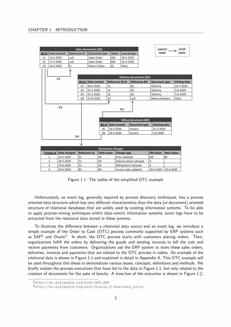
Figure 1.1: The tables of the simplified OTC example
Unfortunately, an event log, generally required by process discovery techniques, has a processoriented data structure which has very different characteristics than the data (or document) orientedstructure of relational databases that are widely used by existing information systems. To be ableto apply process mining techniques within data-centric information systems, event logs have to beextracted from the relational data stored in these systems.
To illustrate the difference between a relational data source and an event log, we introduce asimple example of the Order to Cash (OTC) process commonly supported by ERP systems suchas SAP2 and Oracle3. In short, the OTC process starts with customers placing orders. Then,organizations fulfill the orders by delivering the goods and sending invoices to bill the cost andreceive payments from customers. Organizations use the ERP system to store these sales orders,deliveries, invoices and payments that are related to the OTC process in tables. An example of therelational data is shown in Figure 1.1 and explained in detail in Appendix A. This OTC example willbe used throughout this thesis to demonstrate various issues, concepts, definitions and methods. Webriefly explain the process executions that have led to the data in Figure 1.1, but only related to thecreation of documents for the sake of brevity. A time-line of the execution is shown in Figure 1.2,
2http://en.wikipedia.org/wiki/SAP_ERP3http://en.wikipedia.org/wiki/Oracle_E-Business_Suite
2
CHAPTER 1. INTRODUCTION
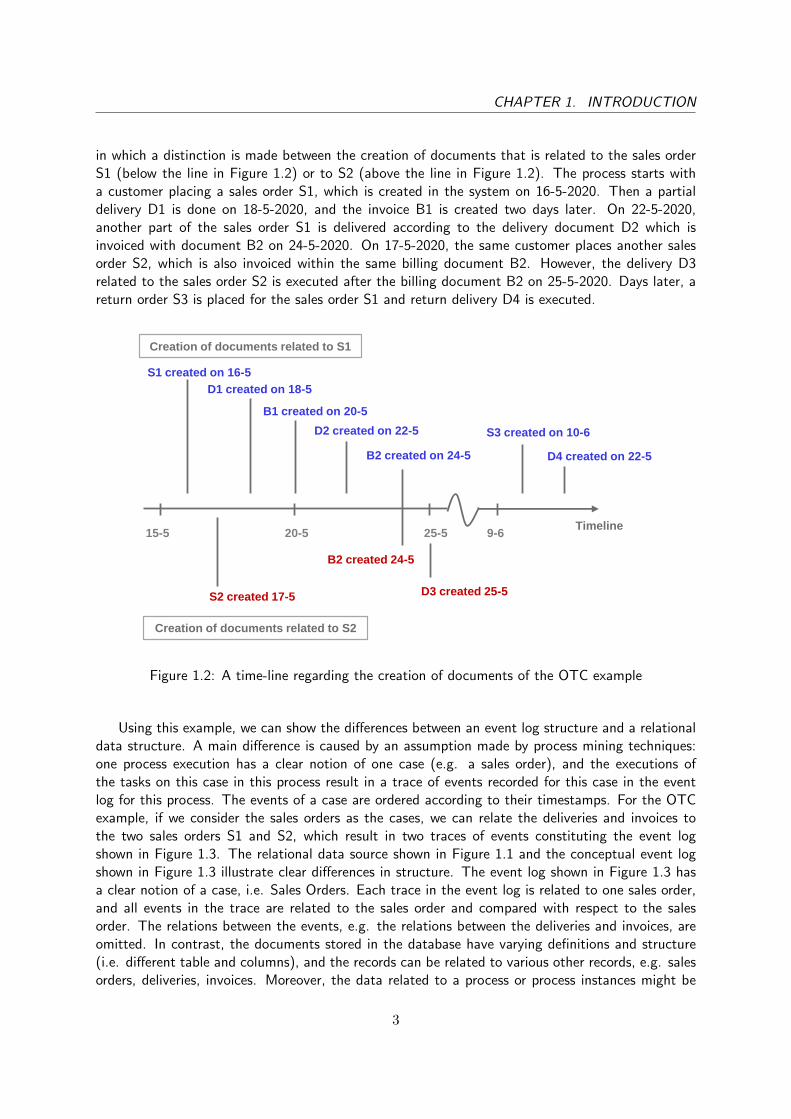
in which a distinction is made between the creation of documents that is related to the sales orderS1 (below the line in Figure 1.2) or to S2 (above the line in Figure 1.2). The process starts witha customer placing a sales order S1, which is created in the system on 16-5-2020. Then a partialdelivery D1 is done on 18-5-2020, and the invoice B1 is created two days later. On 22-5-2020,another part of the sales order S1 is delivered according to the delivery document D2 which isinvoiced with document B2 on 24-5-2020. On 17-5-2020, the same customer places another salesorder S2, which is also invoiced within the same billing document B2. However, the delivery D3related to the sales order S2 is executed after the billing document B2 on 25-5-2020. Days later, areturn order S3 is placed for the sales order S1 and return delivery D4 is executed.
PAGE 34
15-5 20-5 25-5 9-6
S1 created on 16-5
D1 created on 18-5
D2 created on 22-5
B1 created on 20-5
B2 created on 24-5
S2 created 17-5 D3 created 25-5
B2 created 24-5
S3 created on 10-6
D4 created on 22-5
Creation of documents related to S1
Creation of documents related to S2
Timeline
Figure 1.2: A time-line regarding the creation of documents of the OTC example
Using this example, we can show the differences between an event log structure and a relationaldata structure. A main difference is caused by an assumption made by process mining techniques:one process execution has a clear notion of one case (e.g. a sales order), and the executions ofthe tasks on this case in this process result in a trace of events recorded for this case in the eventlog for this process. The events of a case are ordered according to their timestamps. For the OTCexample, if we consider the sales orders as the cases, we can relate the deliveries and invoices tothe two sales orders S1 and S2, which result in two traces of events constituting the event logshown in Figure 1.3. The relational data source shown in Figure 1.1 and the conceptual event logshown in Figure 1.3 illustrate clear differences in structure. The event log shown in Figure 1.3 hasa clear notion of a case, i.e. Sales Orders. Each trace in the event log is related to one sales order,and all events in the trace are related to the sales order and compared with respect to the salesorder. The relations between the events, e.g. the relations between the deliveries and invoices, areomitted. In contrast, the documents stored in the database have varying definitions and structure(i.e. different table and columns), and the records can be related to various other records, e.g. salesorders, deliveries, invoices. Moreover, the data related to a process or process instances might be
3

CHAPTER 1. INTRODUCTION
spread over the tables. Thus, the relational data related to the execution of a process has to becollected and converted to an event log. A conversion definition between a relational database ofrelational data and an event log, also known as a (log) mapping, is a specification which indicatesspecific part of the relational data should be converted to a specific part in the event log.
Event log
PAGE 33
Trace 1 : Sales Order S1
Event Id Event type Event timestamp Resource
S1 Order Created 16-5-2001 Dirk
D1 Delivery Created 18-5-2001 Dirk
B1 Invoice Created 20-5-2001 Dirk
D2 Delivery Created 22-5-2001 Marijn
B2 Invoice Created 24-5-2001 Marijn
S3 Return Order Created 10-6-2001 Xixi
D4 Return Delivery created 12-6-2001 Xixi
Trace 2 : Sales Order S2
Event Id Event type Event timestamp Resource
S2 Order Created 17-5-2001 Dirk
B2 Invoice Created 24-5-2001 Dirk
D3 Delivery Created 15-5-2001 Dirk
Figure 1.3: An conceptual event log of the OTC example
During the literature study, various approaches have been found to support the conversion fromrelational data to event logs. The goal of most approaches, proposed by several studies such as M.van Giessels [13], I.E.A. Segers [26], J. Buijs [9], D. Piessens [24], and A. Roest [25], is to extract oneevent log which describes a single, isolated process. We categorize these approach as the traditionallog extraction approaches (also refer to as the traditional approaches). Many issues have beenfound regarding the traditional log extraction approaches. For instance, no clear definition of a casecould be found in a data centric system since there are many different definitions of cases such assales orders, deliveries and invoices identified in the OTC example. This lack of a clear notion of acase has lead to two well known problems: data divergence and data convergence.
The data divergence problem is defined as the situation when a case is related to multiple eventsof the same event type. Figure 1.3 shows that the case sales order S1 has two Delivery Createdevents D1 and D2 and two Invoice Created events B1 and B2. If we draw a simple causality netby only using the trace S1, we obtain the model shown in Figure 1.4. Business users immediatelynotice the edge from Invoice to Delivery and find this edge strange as they think the edge indicatesthat there are invoices created before the related deliveries. However, this edge actually means thatthere is an invoice B1 created before a delivery D2, both of which are related to the sales order S1but not related to each other. This complexity and ambiguity of the process model increaseswhen more deliveries and invoices are linked to the case, as the divergence problem also introducesloops. Now, if we include the trace S2, a similar model shown in Figure 1.5 is obtained with thesame strange edge from Invoice Created to Delivery Created. However, this time there really is an
4

CHAPTER 1. INTRODUCTION
Figure 1.4: A simple sequential causalgraph of Sales Order S1.
Figure 1.5: A simple sequential causalgraph of the OTC example.
invoice B2 created before its related delivery document D3, which is an outlier and might indicaterisks or faulty configurations in the process. Identifying these strange but true positive sequentialdependencies between related invoices and deliveries is the aim of business users, which is disturbedby the divergence problem. Solving divergence should eliminate the false positives.
The problem of data convergence is defined as the situation when one event is related tomultiple cases. For example, when considering the sales orders as the notion of a case and thecreation of invoices as events, the Invoice Created event of the invoice B2, which is related totwo different sales orders S1 and S2, will be extracted twice, as illustrated by the event log inFigure 1.3. Traditional process mining techniques consider the event Invoice Created B2 as twodifferent events. Together with the creation of invoice B1, we obtain three Invoice Created eventsas shown in Figure 1.5, whereas there are only two invoices B1 and B2. Thus, the data convergenceproblem leads to extracting duplicate events and biased statistics.
Choosing different notions of a case for the process definition is proposed in different literatureas a solution to the divergence and convergence problem. However, this solution might solve thedivergence and convergence partially but not completely. Take the OTC example, choosing theinvoices as the case definition, the many-to-many relation between the invoices and sales orderscauses the event log obtained to still suffers from divergence and convergence. Choosing the deliveriesas case definition solves the divergence problem, but worsens the convergence problem, e.g. also thesales order created S1 is extracted as an event for D1 and D2. Furthermore, it is also very difficult forthe traditional approaches to define or to retrieve an optimal definition of a case from all possible case
5

CHAPTER 1. INTRODUCTION
definitions found in relational data. As ERP systems store various documents related to a businessprocess execution, and the relational structure allows each document to have its own execution whichmay or may not be related to other documents, business processes supported by such an ERP systemcan be generally viewed as a set of documents and each has its own lifecycle. Moreover, as ERPsystems support the operation of an entire organization which has dozens large processes, it is almostimpossible to describe the behavior of a system using only one process definition. These issues haveled to another type of log extraction approach and process mining techniques: the artifact-centricapproach.
Artifacts are business entities described by both an information model and a lifecycle. For theOTC example, we can consider sales orders, deliveries and invoices as different artifacts, each hasits own life cycle and interactions with each other. The relations between artifacts can be viewedas interactions between artifacts during their lifecycles, in which the data divergence and dataconvergence between artifacts are allowed. For example, the creation of sales orders might lead tothe creation of multiple deliveries. This concept of artifacts is first introduced by A. Nigam and N.Caswell [20] and put into practice by D. Cohn and R. Hull [10]. An artifact-centric process modelsdescribes a process as multiple collaborative artifacts, each with its own life cycle and interactionswith each other. A formal notation for an artifact-centric model is the proclet system proposed byW. van der Aalst et al. [4], which will be explained in Section 2.1.3. An example of a proclet systemof the OTC example is shown in Figure 1.6. For each document type found in the OTC example,we consider it as an artifact (type) with it own life-cycle, illustrated by the large gray rectangle. Theinteractions are represented by the edges between the artifacts. Since the proclet system might bedifficult to be explained to business users, a more abstract representation like Figure 1.7 might bemore suitable.
Traditionally, users conducted interviews to manually construct artifact-centric process models forbusiness process management. However, this approach is very time consuming, since an organizationmight have thousands of artifacts. E. Nooijen et al. [21][22] were the first and the only one whoproposed an automatic approach to identify artifacts from a given relational data and extract artifactsas event logs for applying process mining techniques. E. Nooijen has implemented the approach asa tool named XTract.
Based on the result of literature study, we believe that the artifact-centric approach is a moresuitable way for conducting process mining within data-centric systems such as ERP systems. First,the notion of interactions in an artifact-centric model allows the model to express one-to-manyand many-to-one causalities between cases, which can solve the data divergence and convergenceproblems and obtain a simpler process model. Moreover, the notion of artifacts allows us to de-compose a large process into smaller collaborative processes (i.e. life-cycles) of different cases. Thisdecomposition further decreases the complexity of individual life-cycles and improves the scalabilityof applying process mining within data-centric systems. Furthermore, the artifact-centric approachis actually a generalization of the traditional log extraction approach because we can also considerthe large process as one artifact and still obtain the same complex life-cycle of this artifact. Forexample, considering the sales orders of the OTC example as one artifact, and the creation events ofdeliveries, invoices, return order and return delivery constitute the sales orders’ life cycle, we obtainthe same life-cycle as the process model shown in Figure 1.5.
Compared to the single case definition view of traditional log extraction approaches, the notionof artifacts gives a “conceptual lens” that allows us to interpret relational data differently. Unfor-tunately, the original XTract approach (or the tool) introduced by E. Nooijen et al. [21][22] is still
6

CHAPTER 1. INTRODUCTION
Sales Order
Artifact
Created C:1
Return Order Artifact
Created C:1C:1
Return Delivery
Artifact
CreatedC:1
Delivery Artifact
Created C:*C:*
Invoice Artifact
CreatedC:1
C:1
Input ports Output ports
proclet (class)
Channel
Figure 1.6: An proclet system of the OTCexample regarding the creation event type
Figure 1.7: A simple representation of theproclet system of the OTC example
incomplete indicating a low practical value. We list here some issues and will discuss them in detailin Section 2.3. First, no interactions between artifacts were identified nor extracted by the originalXTract approach, which left the artifacts’ life cycles as single, isolated processes. This incomplete-ness indicates that no complete artifact-centric model can be created (semi-) automaticallyyet from a given data source. Moreover, the XTract approach was unable to identify multipleartifacts sharing the main table: the XTract can only consider the Sales Documents (SD) table ofthe OTC example as one artifact and is unable to distinguish the artifacts Sales Order and ReturnOrder based on the document types from the SD table. The XTract tool also does not supportany changes of artifacts identified. In addition, the XTract approach has not addressed the dataconvergence and data divergence explicitly.
As it is useful to apply process mining techniques within ERP systems, and the artifact-centricapproach is a more intuitive way to perform this compared to the traditional log extraction ap-proaches, the existing artifact-centric approach has to be extended for artifact identification, andnew methods have to be developed for interaction identification and artifact-centric process modeldiscovery.
1.2 Research Problem
In section 1.1, we have briefly introduce the thesis context and issues related to traditional logextraction approaches as well as the artifact-centric log extraction approach. In this section, we givethe problem definition of this thesis and divide the problem into three sub problems.
We have argued that the artifact-centric approach is a more suitable way for conducting processmining within data-centric systems than the traditional log extraction approach. First, we can usethe notion of interactions to express one-to-many and many-to-one causalities between artifacts,
7

CHAPTER 1. INTRODUCTION
solve the data divergence and convergence problems, and obtain a more intuitive model. Second,the notion of artifacts allows us to decompose a large process into smaller collaborative processes(i.e. life-cycles) of different cases and therefore improving the scalability of log extraction and processmining. Third, because we can also consider a large process also as one artifact, the artifact-centricapproach is actually a generalization of the traditional log extraction approach.
We have also discussed the current artifact-centric approach is incomplete. For example, nomethod has been found in the literature which can identify interactions between different processdefinitions (i.e. between artifacts if in an artifact-centric context) or between cases or betweenevents, neither on the database level nor on the event log level. Thus, no approach supports the(semi-) automatic discovery of an artifact-centric model yet, when given a data source. Due to thebusiness context of this thesis, it also is important that the identified artifact-centric model can beused by business analysts to analyze processes. Therefore, we define the research problem as follows:
Given a relational data source, we would like to support business analysts to (semi-) au-tomatically discover an artifact-centric model, which describes the process of severalcollaborative processes (or life cycles of artifacts), each of which has it own life cycle, andinteractions with each other, and to be able to use this discovered model to perform processanalyses.
We assume that the relational data source contains information about the documents in theprocess, their relations to each other and timestamps of the tasks performed on these documentsthat are relevant for the process analyses. An example of the relational data source is the OTC tablesshown in Figure 1.1. In addition, if the data schema is too complex to be identified automatically,we assume that there is knowledge available of the data schema (i.e. primary keys and foreign keys).
Since many existing technologies provide partial solutions, we can divide the research probleminto sub problems to use as many existing techniques as possible to (partially) solve the problem.Especially, XTract approach provides a prototype which allows users to connect to different typesof relational databases and provides functions to identify simple, isolated artifacts and to createevent logs. Consequently, each event log that is created based on an artifact can be used as inputfor existing process discovery techniques to obtain a process model (or a life cycle in an artifact-centric context). In addition, since the event log format has been standardized using the XESformat, creating event logs with interactions will allow more artifact centric discovery techniques tobe developed and applied independent of the method proposed in this thesis. The artifact-centricmodel obtained should have formal definitions to allow researchers to further investigate issues in anacademic context. In addition, due to the business context of this thesis, the artifact-centric modelthat is shown to the analysts should be simple and understandable, and allow analysts to identifyoutliers. The analysts should be able to retrieve cases (or case identifiers) and statistic informationto verify and assess the process. For aforementioned reasons, we divide the research problem intoto three sub problems:
(I) Given a relational data source, we would like to support business analysts to (semi-) automat-ically extract event logs, where each event log describes the life cycle of an artifact as wellas the interactions of this artifact with other artifacts.
(II) Given a set of event logs which also contains data of interactions with each other, we wouldlike to discover a formal artifact-centric model including interactions among the life cycles.
8

CHAPTER 1. INTRODUCTION
(III) Given a formal artifact-centric model together with the corresponding set of event logs, wewould like to be able to visualize a model that is intuitive for business users and to obtaininformation about outliers and statistics.
Due to the large scope and the interest of the business analysts involved in this thesis, the primarygoal of this thesis is to be able to obtain an artifact-centric model that supports the business analystsperforming process analyses (III). The usability of the GUI of the prototype is of secondary concern.Therefore, case studies are conducted to evaluate the artifact-centric models obtained instead of theusability of the tools.
1.3 Research Scope
We have defined the research problem. To solve the problem, we need an approach that supportsanalysts to extract event logs including the interactions between the logs, and an approach thatdiscovers an artifact centric model, outliers and statistics from these event logs. Furthermore, themodel obtained is evaluated via case studies to improve the understandability. In this section, wedefine the research scope of this thesis.
PAGE
22
Data
sources ? ? Artifact-centric
Models
extraction mining
Information
system
Digital world
Physic world Processes
Executions
Manual
selections
and changes
Manual
selections
Information,
understanding and
interpretation
XES Event
logs with
interactions
Figure 1.8: The research scope of the thesis
A high level overview of the research scope (and the solution approach) is demonstrated inFigure 1.8. We briefly explain each element and the reason why it is included. First, the data sourcesobtained is generally derived from interactions between human users and information systems forbusiness process executions. Since the recording of process executions is done by information systems,some knowledge of the information systems to be mined is desired. In this thesis, the knowledge ofthe relevant information systems is provided by the system experts at KPMG or obtained during theinterviews with advisors.
The data sources recorded by information systems can be considered as input for the log extrac-tion method. KPMG has extensive experience with data analysis and has developed a data analysis
9

CHAPTER 1. INTRODUCTION
platform (Facts2Value) that supports extracting, analyzing and reporting data from the client’s infor-mation systems for audit and advisory purposes. Currently, over two hundred Facts2Value analysesengagements are performed annually. Facts2Value is still being expanded and improved. Becausethe data downloaded by KPMG were uploaded to the data warehouse on Microsoft SQL servers tomake them available for performing Business Intelligence analysis, we also used these data as inputin this thesis to conduct case studies and test our artifact-centric process analysis approach.
Using the relational data sources as input, the log extraction method, denoted by the first blackbox (with a question mark), is the solution that supports analysts to extract event logs including theinteractions between the logs (i.e. problem (I)). In addition, the log extraction method should supportanalysts to select, change or construct the artifacts (i.e. process definitions) and interactions desired.A list of event logs with interactions in XES format is then obtained and used for the discovery of anartifact-centric model. The mining method, denoted by the second black box, returns an artifact-centric model including interactions among the life cycles (which aims to address problem (II)). Theartifact-centric model discovered should be intuitive and easy to understand.
It is important to include the human element, since the goal of process mining is to provideuseful information for business analysts. Specifically, due to the business context of this thesis, thebusiness advisors should be able to use our approach (i.e. the prototype built for support), and themodel discovered should be easy to understand by business users. Therefore, case studies have beenconducted with both business analysts and clients to evaluate the process models obtained (whichaims to address problem (III)).
1.4 Outline - Artifact Centric Approach
In the previous sections, we have defined the research problem and scope to semi-automaticallydiscover an artifact-centric model from a given data source. In this section, we outline the reportby briefly introducing our artifact-centric approach for the thesis problem including sub methods tothe sub problems. An overview of the approach is shown in Figure 1.9.
First, in Chapter 2, the preliminary concepts that are related to the research scope illustrated inFigure 1.8 are investigated by conducting literature study: event log format in Section 2.1.1, processdiscovery techniques (i.e. the “mining” element) in Section 2.1.2, process models in Section 2.1.3,information systems (also data sources) in Section 2.1.4, and the traditional log extraction methodsin Section 2.2. In addition, the artifact-centric log extraction approach XTract is also investigatedin detail in Section 2.3, since we use the XTract approach as a start point of our approach. We alsodiscuss the open issues of the XTract approach in detail and introduce our solution to the issue byreferring to the specific section describing the solution.
In Chapters 3 and 4, we present our artifact-centric approach to the log extraction problem (I).We divide the log extraction problem (I) into three phases: (A) artifact type level identification, (B)type level interaction identification, and (C) log extraction.
In the first phase (A) artifact type identification explained in Chapter 3, we would like toidentify a set of stand-alone artifacts from the given data sources. Each artifact contains all datarelated to the life cycle of the artifact. We consider the artifact type identification as a separatephase since the artifacts obtained (without interactions) can already be extracted as event logs whichcan be used to identify the life cycles. Moreover, the existing XTract approach can be used and
10

CHAPTER 1. INTRODUCTION
PAGE
22
Data
sources ? ? Artifact-centric
Models
extraction mining
Information
system
Digital world
Physic world Processes
Executions
Support
selections
and changes
Support
selections
XES Event
logs with
interactions
Evaluation and
assessment of
Information and
understanding
(I) (II)
(III)
Data Schema
identification
Artifact
Schemas
Identification
Artifacts
Identification
Artifact type
identification
Type level
Interactions
identification
(direct)
Interaction
graph creation
Indirect
interactions
identification
Log
Extraction
Artifact-Log
Mapping
creation
Cache
Database
creation
Event log
generations
Artifact
life cycle
discovery
Event type
level
discovery
Visualizations
and
Information
Processes
Discovery
(A) (B) (C)
(A3)
(A2)
(A1)
(Chap 3) (Chap 4) (Chap 5)
(B1)
(B2)
(C1)
(C2)
(C3)
(Chap 7)
Figure 1.9: The research outline of this thesis
extended to solve this sub problem. Our approach to identify artifact types consists of three steps:(A1) given data sources, we generalize the definition of foreign keys (named references) and allowanalysts to import schema information to obtain the data schema in Section 3.1; (A2) given thedata schema, we identify the artifact schemas to discover similar artifacts while explicitly addressingthe convergence and divergence problems in Section 3.2; (A3) we allow identifying multiple artifactsfrom a given artifact schema, explained in Section 3.3.
In the second phase (B) type level interaction identification, we identify the (type level)interactions between artifacts. These interactions are necessary to relate different artifacts to eachother and to investigate the causal relations between the life-cycles of artifacts, e.g. the Creation ofthe Sales Order artifact has led to the Creation of the Delivery artifact. Furthermore, interactionsbetween artifacts can be used to express the one-to-many, many-to-one, and many-to-many rela-tions, which solve the data divergence and convergence problem and help to create a more intuitivemodel. In this phase (B), we first define the interactions and investigate the possibility of extractinginteractions on the database level in Section 4.1. Then, we propose our approach to identify (B1)direct and (B2) indirect interactions between artifacts in Section 4.2.
After identifying the (type level) interactions, the artifacts are complete. In the third phase(C) Log Extraction, we use the artifacts to create log mappings (i.e. conversion definitions) forextracting the relational data of each artifact (type) as an event log. This phase (C) is necessary toobtain the event logs, which can be imported into process mining tools to discover process models.It is logical to divide the interaction identification and the log extraction into two phases, since one
11

CHAPTER 1. INTRODUCTION
can skip the interaction identification if they are not interesting. Moreover, one can propose differentmethods for interaction identification or log extraction. In this thesis, the log extraction functionprovided by the original XTract approach is mainly reused with minor changes. Our extensionsare explained in Section 4.3. One can implement new methods for writing logs since the existingfunctions show some performance issues. Both phases are illustrated in Chapter 4.
Our approach to address the mining problem, explained in Chapter 5, is necessary to obtainan artifact-centric process model from the set of event logs (with interactions). After solving theextraction problem, we obtain a set of event logs, each of which describes the life cycle of an artifacttype (e.g. Sales Order), and each trace in this event log represents the life cycle of an artifactinstance (e.g. S1). This set of event logs is used by our approach to discover an artifact-centricmodel and other information such as outliers and statistics, which addresses the second problem(II) and the third problem (III). We first show how to identify individual life-cycles of artifacts inSection 5.1. Then, we show two different methods to identify interactions between event types ofdifferent life-cycles in Section 5.2, in which we also illustrate how to identify unusual interactions.Finally, we create an artifact-centric model by using the life-cycles and the interactions between theirevent types, explained in Section 5.3. For business users, it is important to be able to retrieve casesfrom a given causal relation, and this is shown in Section 5.4.
In Chapter 6, the two implementations XTract2 and InteractionMiner for, respectively, the ex-traction and mining problem are explained in Sections 6.1 and 6.2. The architectures of the twoimplementations together with a set of screen shots explaining the functions of the tools are alsoshown.
Case studies have been conducted using the data provided by KPMG to evaluate our approachand whether the third problem (III) is addressed. The case studies were performed for two differentprocesses of two different types of ERP systems, Oracle and SAP: the Order to Cash (OTC) processof SAP and the Project Administration (PA) process of Oracle. The SAP - OTC process was chosenby the company supervisors. The PA process was chosen by an available customer. The result ofthe case studies are included and discussed in Chapter 7.
Finally, this thesis is concluded by Chapter 8 in which a summary of the thesis is given, andlimitations of the approach are discussed. We also include a list of future work to discuss thepossibility to overcome the limitations and further improve the artifact-centric approach in general.
In the following chapters, we use the words ‘XTract approach’ when referring to the originalXTract approach, whereas the words ‘our approach’ or ‘our method’ are used when referring to themethod that is newly designed to solve the specific problem within the given context.
12

Chapter 2
Preliminaries
We have defined our research scope and goal in the previous chapter. Before going into the details ofour approach, the preliminary concept of each component in the research scope shown in Figure 1.8,i.e. process mining, event logs, process models, ERP systems and log extraction approaches, areintroduced in this chapter since these concepts will be used throughout this thesis. First, we brieflydescribe process mining and its scope in Section 2.1. Within Section 2.1, we further explain thecomponents of the thesis scope which are also related to the process mining scope: (Section 2.1.1)event logs and the XES format, which is extracted from the data sources; (Section 2.1.2) processdiscovery techniques which are used to mining the event logs; (Section 2.1.3) the process modelsreturned by the discovery techniques; (Section 2.1.4) the relational data sources and ERP systemsused as the source of event log extraction. Finally, the traditional approaches extracting theevent logs and the original artifact oriented XTract approach are discussed in Sections 2.2 and 2.3,respectively.
2.1 Process Mining
In this section, we briefly introduce the goal and scope of process mining as illustrated in Figure 2.1and relate the elements of process mining to an artifact-centric context. Process mining is a setof techniques to “discover, monitor and improve real processes (i.e., not assumed processes) byextracting knowledge from event logs” [3]. Note that the research scope of this thesis shown inFigure 1.8 is aligned with the process mining scope: the data sources component is similar to theinformation systems component. However, the log extraction is out of the process mining scopesince traditional mining techniques assumed the existence of event logs. Therefore, the problem oflog extraction was explicitly added to Figure 2.1 to show its position in the classic process miningscope and to help readers compare the classic process mining scope to our research scope. Whenapplying process mining techniques on the event logs recorded from processes, insight into controlflow dependencies, data usage, resource utilization and various performance related statistics of theprocesses can be obtained.
13

CHAPTER 2. PRELIMINARIES
PAGE 31
Process
Mining
Log
Extraction
Data
sources
Figure 2.1: Process Mining scope
2.1.1 Event logs and the XES Event Log Format
Most process mining techniques require an event log as input. In this section, a general eventlog (structure) is first explained. Then, since we have introduced our artifact centric approach inSection 1.4, we would like to give a comparison between the terminologies used in the traditionalprocess mining context and the terminologies in the artifact centric context on a conceptual level.Next, a formal definition of an event log used for reasoning is given. This section is concluded byintroducing the event log format XES which is used in this thesis.
In general, an event log comprises lists of events. Each list of events is called a trace or aprocess instance and is recorded from the tasks executed on a certain case instance going throughthe process. A common structure of an event log, drawn by J. Buijs [9], is shown in Figure 2.2 onthe right hand side. On the model level (or process definition level), a process specifies the acitiviesthat should be executed in a certain order. A process can be instantiated to the case instances goingthrough this process, also called process instances. The event types, instantiated from the activities,are performed on the case instances of the process which are recoded as events on the log levelcontaining the data such as the time when the event is executed (i.e. timestamp), the resource whoexecuted the event, and other attributes. An ordered list of events performed on a case instance iscalled a trace.
Figure 2.2 on the left hand side compares the definitions of event logs in a traditional miningcontext to the notions used in the artifact-centric context. An artifact (type) is equivalent to thenotion of a process definition, in which the event type definitions are specified. An artifact instanceis instantiated from an artifact type. The artifact instances that share the same artifact type havesimilar event types. When extracting an event log based on a definition of an artifact type, each
14

CHAPTER 2. PRELIMINARIES
PAGE 32
Log level
Instantiation
Model
Artifact -
centric
context
Traditional
Mining
context
equivalent
equivalent
equivalent
Specifies
Performed on
Of
instantiate instantiates instantiates
creates creates create
Ordered
Attributes
Event
types
Process/
Case
instances
Traces Events
Artifact
instances
Activities Process Artifact
(type)
Traces
Timestamp
Event type
Resource
…
Figure 2.2: Event logs structure
artifact instance is similar to a process instance (or a case) which results in a trace of events.
To be able to reason about logs and to precisely specify the requirements for event logs, we usethe formal definition of event log introduced by W. van der Aalst in the Process Mining book [2].
Let E be the event universe, i.e. the set of all possible event identifiers. Events may becharacterized by various attributes, e.g., an event may have a timestamp, correspond to an activity,is executed by a particular person, has associated costs, etc. Let AN be a set of attribute names.For any event e ∈ E and name n ∈ AN : #n(e) is the value of attribute n for event e. If event edoes not have an attribute named n, then #n(e) = ⊥ (null value).
The following standard attributes are used in this thesis: #eventType(e) is the event type associ-ated to event e. #time(e) is the timestamp of event e (also denoted by T (e)). #resource(e) is theresource associated to event e.
Let L be the case universe, i.e. the set of all possible case identifiers. A case also has attributes.For any case c ∈ L and name n ∈ AN : #n(c) is the value of attribute n for case c. If case c doesnot have an attribute named n, then #n(c) = ⊥ (null value).
Each case has a special mandatory attribute trace: #trace(c) ∈ E∗. We assume traces in a logcontain at least one event, i.e. #trace(c) 6= 〈〉.
A trace is a finite sequence of events σ ∈ E∗ such that each event appears only once, i.e., for1 ≤ i < j ≤ |σ| : σ(i) 6= σ(j). Thus, we also use σc to denote #trace(c).
An event log is a set of cases L ⊆ L such that each event appears at most once in the entirelog. We use AL to denote the set of all event types appearing in log L, i.e. AL = {#eventType(e) |c ∈ L ∧ e ∈ #trace(c)}.
A format for event logs is the XML based format XES1, which is selected as the standard format
1http://www.xes-standard.org/
15

CHAPTER 2. PRELIMINARIES
for event logs by the IEEE Task Force on Process Mining. The complete meta model of the XESformat is shown in Figure 2.3. The elements Trace, Event, and Attribute are comparable to the sameelement in the general event log structure introduced by Figure 2.2. For further detailed explanation,we refer to the official website of the standard. Both J. Buijs [9] and H. Verbeek et al. [28] havediscussed the difference between the MXML event log format and the XES event log format. Sincethe XES format is an improved version based on the MXML event log format, well supported andchosen as the standard format, we use the XES event log in this thesis.Technische Universiteit Eindhoven University of Technology
Log
Trace
Event
ID
Boolean
Float
Int
Date
String
Attribute
Classifier
Extension name
prefix
URI
Key
Value
<declares>
<defines> <defines>
<defines><trace-global>
<event-global>
<contains>
<contains>
<contains>
<contains>
Figure 2.1: The UML 2.0 class diagram for the complete meta-model for the XES standard
• One examination in which the x-ray machine is employed
• One visit of the website, by one specific user
Tag name for the trace object in the XML serialization of XES: <trace>
No XML attributes are defined for the <trace> tag.
2.1.3 Event
Every trace contains an arbitrary number of event objects. Events represent atomic granules ofactivity that have been observed during the execution of a process. As such, an event has noduration. Examples of an event are:
• Recording the client’s personal information in the database has been completed
• One picture is taken by the x-ray machine
• An image has been downloaded by the web browser
3 XES / Version 1.4
Figure 2.3: XES meta modelDrawn using the UML 2.0 class diagram
2.1.2 Process Discovery and ProM framework
A specific type of techniques in the process mining domain is Process Discovery, which use anevent log as input and discover a process model as output. Some well known process discoverytechniques are Alpha algorithm [5], (Flexible) Heuristic miner [29][30], Genetic process mining [18],ILP mining [31], and Fuzzy mining [14]. Note that the model discovered from a given event logvaries depending on which mining algorithm is used. This phenomenon is due to the fact thateach discovery algorithm has its own definition to determine the causality between the event types.Another characteristic of discovery algorithms is that the algorithms are mainly aimed to identifythe main flow and eliminate the outliers, whereas business users tend to use the discovered modelto identify outliers. These aspects have to be taken into account for this thesis.
ProM is a generic open-source framework for implementing process mining tools in a standardenvironment [27][28]. The framework provides researchers an extensive base to implement newalgorithms in the form of plug-ins. The framework provides an easy-to-use user interface functionality,a variety of model type implementations (e.g. Petri nets, EPCs) and common functionality like
16

CHAPTER 2. PRELIMINARIES
reading and writing files. Each plug-in can be applied to any (compatible) object in the commonobject pool allowing the chaining of plug-ins to come to the desired result. ProM can read eventlogs stored in the new event log format XES (as explained in Section 2.1.1). Furthermore, it canalso load process model definitions in a wide variety of formats. In this thesis, ProM 6 is chosen toimplement the approach for the mining problem (II).
2.1.3 Process Models and Artifact-Centric Model
The process models discovered by process mining techniques describe the behaviors and the execu-tions of real processes at an abstract level. Various process model notations are used to visualizethese process models in various aspects such as the control flow aspect, or the organizational aspect.To describe the control flow aspect of processes, one can visualize the order of tasks to be executedby using model notations such as Transition Systems [6], Business Process Model and Notation(BPMN) [32], Petri nets [19], Event Driven Process Chains (EPC) [1], and Declaire models [23]. Todescribe the organizational aspect of processes, one can visualize the hand-overs of tasks based onthe categorization of resources using simple causal nets.
Within this thesis, we use the proclet system to describe the control flow aspects of a setof collaborative processes (denoted as artifacts) [4]. A proclet system consists of proclets andinteractions found between the proclets. Each proclet describes the life cycle (i.e. control flow)of an artifact as a Petri net and its possible interactions with other artifacts, denoted by ports andchannels. Each channel describes a uni-directional message flow from one proclet to another. Achannel connects two proclets through ports of the two proclets. Each port of a proclet has acardinality (C) indicating the number of other artifacts to which a message is sent or received fromvia the port. A value of a cardinality could be 1 (exactly once), ? (zero or once), * (zero or more)and + (once or more). An output port sends messages, and an input port receives messages whichcan be processed by a transition.
An example proclet system of the OTC example is shown in Figure 1.6. From left to right, eachlarge rectangle represents a proclet showing the life-cycles of the artifacts Sales Order, Return Order,Delivery, Return Delivery and Invoice, respectively. The event type Created of the artifact Sales Orderhas an output port, which is connected via a channel with the input port of the event type Createdof the artifact Delivery, whereas the event type Last Change of the artifact Sales Order has both aninput port and an output port.
An event type level interaction between two artifacts is described by two ports and a channelconnecting the two proclets. The event level interactions can be compared to the messages whichare sent via the channel.
2.1.4 Relational Databases and ERP systems
The data sources in the research scope of this thesis are the relational data stored in relationaldatabases by information systems. Relational databases are a shared collection of logically relateddata (tables) described by a relational model (e.g. the OTC example illustrated in Figure 1.1). Inother words, software systems which store the transactional data related to business executions in arelational database can be used as input. For example, Enterprise Resource Planning (ERP) systems,known as software systems that support the optimal usage of all resources in an organization, or the
17

CHAPTER 2. PRELIMINARIES
work flow management systems (WfMS), which already have clear definitions of processes supportedby the system, or Customer Relational Management (CRM) systems, which manage the data relatedto customers. Moreover, we assumed that the input data source contains information about thedocuments in a process, their relations to each other and timestamps of the tasks performed onthese documents that are relevant for the process analysis.
Within this thesis, the data sources used to evaluate the new proposed approach are relationaldata created and used by ERP systems: the Order To Cash (OTC) process supported by SAP, andthe Purchase to Pay (PTP) and Project Administration (PA) processes supported by the OracleERP system.
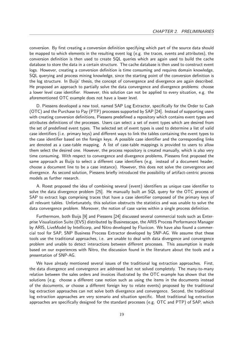
2.2 Literature Study - Traditional Log Extraction Approaches
The introduction to event logs and relational data has shown that both data structures differ fromeach other fundamentally. One of the main differences is that a process definition has a clear notionof a case, whereas the relational data contains several notions of “cases” (i.e. different objectsor documents). Therefore, before process mining techniques can be applied, the relational datahas to be converted to an event log or multiple event logs. In this section, we first explain thecharacteristics of traditional event log extraction approaches. Then, several traditional approachesfound in the literature are discussed briefly. Finally, we will summarize the issues related to thetraditional approaches in general which led to the new artifact-oriented approach.
Traditional log extraction approaches are approaches which extract event logs from data-centric systems based only on one notion of a case. These approaches first (try to) identify or defineone notion of a case. After specifying or selecting the event types (manually), the approaches collectthe events found in the data source that are associated with the cases found for the defined casenotion, e.g. the way we created the event log shown in Figure 1.3. Having all relevant data collected,the approaches rewrite the data as one event log in a log format such as XES. These approachesonly extract one log for one process definition at a time, while assuming the process is isolated andhas no interaction with other processes or its system environment.
M. van Giessel is the first who investigated the applicability of process mining in ERP systems [13].He proposed a manual approach for applying process mining on SAP which consists of three stepsand uses the SAP reference model as a guide: (1) find relevant tables containing the data for theevent log; (2) find the relationships between the relevant tables; (3) find event types related to thedocument identifiers found in the relevant tables. The event log is then created by hand which isvery laborious for a large number of events.
I.E.A. Segers used ProM 5 and the ProM import framework to create an event log from SAPR/3 system for auditing purposes, which still requires a great amount of manual work [26]. Theevent log was created in an MXML log format. According to D. Piessens, Segers was one of the firstwho pointed out the covergence and divergence problems. The convergence issue is defined as thesituation when an event is linked to multiple process instances (or cases). The divergence issue isdefined as the situation when multiple events of the same event type are linked to one case. Thesetwo known issues are caused by the lack of a clear notion of a case.
J. Buijs was the first one who proposed a general approach to extract event logs in the XES formatfrom various data sources [9]. Moreover, Buijs has built a tool, named XESame, to support the
18
CHAPTER 2. PRELIMINARIES
conversion. By first creating a conversion definition specifying which part of the source data shouldbe mapped to which elements in the resulting event log (e.g. the traces, events and attributes), theconversion definition is then used to create SQL queries which are again used to build the cachedatabase to store the data in a certain structure. The cache database is then used to construct eventlogs. However, creating a conversion definition is time consuming and requires domain knowledge,SQL querying and process mining knowledge, since the starting point of the conversion definition isthe log structure. In Buijs’ thesis, the concept of convergence and divergence are again described.He proposed an approach to partially solve the data convergence and divergence problems: choosea lower level case identifier. However, this solution can not be applied to every situation, e.g. theaforementioned OTC example does not have a lower level.
D. Piessens developed a new tool, named SAP Log Extractor, specifically for the Order to Cash(OTC) and the Purchase to Pay (PTP) processes supported by SAP [24]. Instead of supporting userswith creating conversion definitions, Piessens predefined a repository which contains event types andattributes definitions of the processes. Users can select a set of event types which are desired fromthe set of predefined event types. The selected set of event types is used to determine a list of validcase identifiers (i.e. primary keys) and different ways to link the tables containing the event types tothe case identifier based on the foreign keys. A possible case identifier and the corresponding linksare denoted as a case-table mapping. A list of case-table mappings is provided to users to allowthem select the desired one. However, the process repository is created manually, which is also verytime consuming. With respect to convergence and divergence problems, Piessens first proposed thesame approach as Buijs to select a different case identifiers (e.g. instead of a document header,choose a document line to be a case instance). However, this does not solve the convergence anddivergence. As second solution, Piessens briefly introduced the possibility of artifact-centric processmodels as further research.
A. Roest proposed the idea of combining several (event) identifiers as unique case identifier tosolve the data divergence problem [25]. He manually built an SQL query for the OTC process ofSAP to extract logs comprising traces that have a case identifier composed of the primary keys ofall relevant tables. Unfortunately, this solution obstructs the statistics and was unable to solve thedata convergence problem. Moreover, the notion of case varies within a single process definition.
Furthermore, both Buijs [9] and Piessens [24] discussed several commercial tools such as Enter-prise Visualization Suite (EVS) distributed by Businesscape, the ARIS Process Performance Managerby ARIS, LiveModel by Intellicorp, and Nitro developed by Fluxicon. We have also found a commer-cial tool for SAP, SNP Business Process Extractor developed by SNP-AG. We assume that thesetools use the traditional approaches, i.e. are unable to deal with data divergence and convergenceproblem and unable to detect interactions between different processes. This assumption is madebased on our experiences with Nitro, the discussion found in the literature about the tools and apresentation of SNP-AG.
We have already mentioned several issues of the traditional log extraction approaches. First,the data divergence and convergence are addressed but not solved completely. The many-to-manyrelation between the sales orders and invoices illustrated by the OTC example has shown that thesolutions (e.g. choose a different case notion such as using the items in the documents insteadof the documents, or choose a different foreign key to relate events) proposed by the traditionallog extraction approaches can not solve both divergence and convergence. Second, the traditionallog extraction approaches are very scenario and situation specific. Most traditional log extractionapproaches are specifically designed for the standard processes (e.g. OTC and PTP) of SAP, which
19

CHAPTER 2. PRELIMINARIES
means extending these approaches to other systems or processes will require a great amount ofwork. J.Buijs [9] is the only one who has implemented a general solution to support log extractionsfrom data sources. However, users still have to manually define the conversion definition (i.e. amapping definition between the data source and the event log). Based on the experience of theOTC process of SAP, it is observed that the ‘hard’ foreign keys between the tables of large ERPsystem may remain the same, but the ‘soft’ relations vary between different system instances. Thisvariety means the relation between the event types and the case might change for each instance ofSAP, which means that the conversion definition has to be redefined. For instance, we consider thesales orders as cases, and the creation of return deliveries as events. Now, without changing theforeign keys, we can propose a new example, in which the return delivery has a foreign key to salesorders instead of return orders, thus changing the reference SD id of the return delivery D4 from S3to S1. Now, the mapping definition of the return delivery events have to be changed. These issueshave led to the development of another type of approach: the artifact-centric approach.
2.3 Literature Study - Artifact-Centric Log Extraction Approach
We have discussed that the traditional log extraction approaches have encountered many problemssuch as data convergence and divergence when applied within ERP systems, since many informationsystems use relational databases which are data-centric and document-centric causing ambiguouscase definition. Therefore, a different type of log extraction approach, named artifact-centric ap-proach, is proposed by E. Nooijen et al. [21][22] to model a process as the life cycles of severalobjects and interactions between the objects. In this section, we first recall the motivation to ap-ply artifact-centric approach. Then, we give a brief overview of the original XTract approach. InSection 2.3.1, we discuss each step of the original XTract approach in more detail with the issuesidentified when applying the XTract approach on real ERP systems, which are also the reasons forextending the XTract approach.
We have argued that the artifact-centric approach is a more suitable way for extracting event logswithin data-centric systems than the traditional log extraction approach. The new conceptual viewprovided by the artifact-centric approach allows us to consider a process as several collaborativeartifacts with their own life-cycles, instead of fixed to the assumption (also made by traditionallog extraction approaches) that a process is only related to a single notion of a case, and it isisolated and has no interaction with its environment. This view is more suitable for data-centricsystems, since in data-centric systems, we have also various interrelated objects, e.g. sales orders,deliveries, invoices, and each has its own life-cycles. Furthermore, the notion of interactions betweenartifacts introduced by the artifact-centric approach allows us to express one-to-many and many-to-one causalities between artifacts that caused the data divergence and convergence problems inthe traditional log extraction approach. Solving the data divergence and convergence problems helpus to obtain a simpler and more intuitive model and thus increase the possibility to discover true-positive unusual flows. Finally, the artifact-centric approach actually generalizes the traditional logextraction approach because we can also consider a large process also as one artifact.
The concept of artifacts is first introduced by A. Nigam and N. Caswell [20] and put into practiceby D. Cohn and R. Hull [10]. However, artifacts were created manually and based on interviews,which is time-consuming. E. Nooijen et al. [21][22] were the first who proposed an artifact centriclog extraction approach, named XTract, to fully automatically extract the event logs from a given
20

CHAPTER 2. PRELIMINARIES
PAGE 25
1
2
3
4
5
Figure 2.4: The overall method of the original XTract
data source. The XTract approach was tested using the developed prototype and conducting casestudies.
The overall method of the XTract approach consists of two phases, Artifact Schema Identificationand Artifact Lifecycle Discovery, which are divided in five steps, as shown in Figure 2.4. First, (1)given a relational data source, the schema of the source is automatically extracted. Second, Nooijen(2) uses the schema extracted to identify artifact schema(s). Third, (3) a schema log mapping isautomatically created for an artifact schema representing one single isolated artifact which is selectedby users. Fourth, (4) the schema-log mapping (which is similar to a conversion definition used byJ. Buijs) is then used to create SQL queries. The queries are used to build a cache database totemporarily store the data of event log, which is then used to automatically generate event logs. Asthe last step, (5) the XTract reused existing process discovery techniques to mine the life cycles ofan artifact.
Since the XTract approach is the only general approach found in the literature and the sourcecode is made available. We used the XTract approach as the start point of our research. Weinvestigated the XTract approach in detail by applying the XTract tool on the available data.
2.3.1 Open Issues of XTract
By applying the XTract approach to the OTC example of Figure 1.1, we can highlight the openissues in XTract that make it currently inapplicable in practice. In this section, we discuss theseopen issues in detail regarding each step of the XTract approach, introduce our solution to the issueand refer to the specific section in which our approach is discussed more in detail.
21

CHAPTER 2. PRELIMINARIES
Given a relational source, the XTract approach assumes that no knowledge about this relationalsource is available. Therefore, the first step is to (1) automatically identify the data schema consistingof primary keys, foreign keys, column domains and a function assigning a column to a domain.Nooijen used existing schema identification techniques such as MIND [16][17] and SPIDER [8][7]for the foreign key identification. However, as the literature shows, these methods can only identifyhard foreign key dependencies, i.e. each tuple value in the child columns should match to a valuetuple in the parent columns such as the foreign key between (the SD id column of) the SD tableand (the Reference SD id column of) the DD table (i.e. F2 in Figure 1.1) of the OTC example.
Unable to Identify Complex Foreign Keys
The XTract approach was unable to automatically identify all foreign keys. Applying the first step(1) of the XTract approach on the OTC example, the result in Figure 2.5 shows that the XTractapproach is only able to identify the foreign key between (the SD id column of) the SD table and(the Reference SD id column of) the DD table (i.e. F2 in Figure 1.1). The other three foreignkeys are omitted. E. Nooijen has also indicated that the schema identification is an NP-completeproblem, and available solutions take exponential time in the number of columns for identifyingthe schema. The case studies of Nooijen have also shown that there are severe run-time issues,e.g. unable to terminate when identifying 2 column foreign keys for large ERP systems. Since theXTract tool did not provide any support for adding foreign keys or importing foreign keys, we hadto manually add the other foreign keys in the database to perform the subsequent steps. During thecollaboration with KPMG advisers, it had been noticed that the advisers already have knowledgeof the schema of the databases including foreign keys, or the foreign keys might be documentedfor large ERP systems. Therefore, it might be faster and easier to support users by importing andreusing the schemas. This solution is used in our approach and further explained in Section 3.1.
We have also noticed that the data structure used by the XTract approach for foreign keys doesnot allow to express the foreign key between the Document Changes and other three tables (i.e. F4
in Figure 1.1) of the OTC example, where the column Table name should have a certain value. Wealso solved this limitation by extending the definition of reference which is explained in Section 3.1.
Convergence and Divergence Problems
Having the schema of the data source identified, the XTract approach performed the second step (2)artifact schema(s) identification as follows. Based on the importance of the table (i.e. entropy [11])
Figure 2.5: The foreign key of OTC example that is identified automatically
22

CHAPTER 2. PRELIMINARIES
and the distance of the references (i.e. the matched average fraction [33]), k-clustering is applied tocluster tables into different artifact schemas. The number k denotes the number of artifact schemaand is specified by users. The ‘center’ (according to the defined distance) is automatically returnedas the main table of the artifact schema containing the case instances. As the calculation of distanceof the references have not taken into account that relations other than one-to-one (i.e. the matchedaverage fraction is greater than 1) should be infinite, two tables linked by relations other than one-to-one are not explicitly clustered into two artifacts schemas. Using the OTC example, we obtainthe following artifact schemas.
• For k = 1, the XTract approach returned an artifact schema consisting all four tables with themain table as the Document Changes table.• For k = 2, the XTract approach returned two artifact schemas, one consists of the BD table
(as main table), and the other consists of the SD, DD and the changes table with the maintable as the Document Changes table.• For k = 3, three artifact schemas were returned. One consists of the BD table (as main table);
One consists of the Changes table (as main table); and the other consists of the SD and DDtables and the main table is unknown.• For k = 4, four artifact schemas were returned. One consists of the BD table (as main table);
One consists of the Changes table (as main table); one consists of the SD and DD tables andthe main table is unknown; and the fourth is an empty artifact schema.
The results show that the k-clustering approach leaves the convergence and divergence within anartifact schema unaddressed. Moreover, the results also show that it is very unintuitive to cluster thetables of OTC to the artifact schemas this way. It is more logical to obtain three artifact schemasfor the OTC example: one with table SD in (and table Changes), one with table DD (and tableChanges), and one with table BD (and table Changes) to indicate the sales documents artifacts,delivery documents artifacts and billing documents artifacts, respectively. Therefore, to be able toperform the next step, the three artifact schema are manually inserted in the database. In ourapproach, we present a new algorithm to identify the artifact schemas, which does solve the dataconvergence and data divergence problem. Moreover, we allow users to change the artifacts schemasidentified, which is explained in Section 3.2.
Unable to Identify Artifacts within One Table and Event Types within One Column
During the third step (3) schema-log mapping creation, an artifact schema that is identified duringthe previous step is automatically mapped to one artifact, based on which a log mapping (i.e.one conversion definition) is created. The primary key of the main table of an artifact schema ismapped to the artifact instance identifier and is mapped to the traceID of the TraceMapping; themain table of the artifact (schema) is the fromTable of the TraceMapping; each time column inthe artifact schema is automatically mapped to an event type of the artifact, which is mapped toan EventMapping in the mapping; an attribute is either mapped to an AttributeMapping if it hasonly one value or mapped to an ListAttribute if it has multiple values. Note each column used hasalready defined the XesAttribute key, type and extension during the domain calculation. For theartifact Sales Documents, we obtain the following mapping shown in Figure 2.6.
For the third step (3) schema-log mapping creation, we have noticed the following limitations.First, as the OTC example shows, the sales document Sales Order and the sales document Return
23
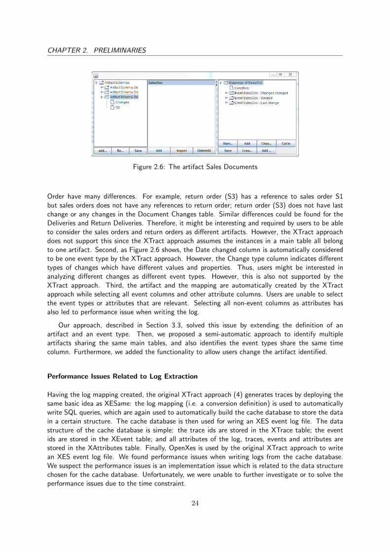
CHAPTER 2. PRELIMINARIES
Figure 2.6: The artifact Sales Documents
Order have many differences. For example, return order (S3) has a reference to sales order S1but sales orders does not have any references to return order; return order (S3) does not have lastchange or any changes in the Document Changes table. Similar differences could be found for theDeliveries and Return Deliveries. Therefore, it might be interesting and required by users to be ableto consider the sales orders and return orders as different artifacts. However, the XTract approachdoes not support this since the XTract approach assumes the instances in a main table all belongto one artifact. Second, as Figure 2.6 shows, the Date changed column is automatically consideredto be one event type by the XTract approach. However, the Change type column indicates differenttypes of changes which have different values and properties. Thus, users might be interested inanalyzing different changes as different event types. However, this is also not supported by theXTract approach. Third, the artifact and the mapping are automatically created by the XTractapproach while selecting all event columns and other attribute columns. Users are unable to selectthe event types or attributes that are relevant. Selecting all non-event columns as attributes hasalso led to performance issue when writing the log.
Our approach, described in Section 3.3, solved this issue by extending the definition of anartifact and an event type. Then, we proposed a semi-automatic approach to identify multipleartifacts sharing the same main tables, and also identifies the event types share the same timecolumn. Furthermore, we added the functionality to allow users change the artifact identified.
Performance Issues Related to Log Extraction
Having the log mapping created, the original XTract approach (4) generates traces by deploying thesame basic idea as XESame: the log mapping (i.e. a conversion definition) is used to automaticallywrite SQL queries, which are again used to automatically build the cache database to store the datain a certain structure. The cache database is then used for wring an XES event log file. The datastructure of the cache database is simple: the trace ids are stored in the XTrace table; the eventids are stored in the XEvent table; and all attributes of the log, traces, events and attributes arestored in the XAttributes table. Finally, OpenXes is used by the original XTract approach to writean XES event log file. We found performance issues when writing logs from the cache database.We suspect the performance issues is an implementation issue which is related to the data structurechosen for the cache database. Unfortunately, we were unable to further investigate or to solve theperformance issues due to the time constraint.
24

CHAPTER 2. PRELIMINARIES
No Interaction Identified and Other Issues
Another issue found is that the method used by the XTract approach for creating the SQL querieswas unable to deal with foreign keys with self loops, e.g. the foreign key from the SD table to theSD table (i.e. F1 in Figure 1.1) in the OTC example. Assume in the OTC example, we have changesin the Document changes table that refer to previous changes of a sales document but not directlinked to the sales document, these change events will not be able to be identified.
No interactions are identified between the different artifacts by the XTract approach. Themissing interactions are one of the most interesting aspects of applying artifact-centric approachsince otherwise, the artifact-centric approach only returns a set of single isolated trivial processes.For example, no information about the relations between the sales orders and deliveries can beobtained. Our approach addresses the identification of interactions between artifacts in Chapter 4.
Nooijen uses the existing process discovery techniques to discover the life-cycles of artifacts.However, no interaction between (the event types of) the life-cycles is discovered by XTract. Weproposed two solutions to identify interactions between event types and thus discovering the artifact-centric model, discussed in Chapter 5.
25


Chapter 3
Artifact Type Identification
In Chapter 1, we have defined our research problem and research scope as obtaining an artifactcentric model from a data source. We have divided the problem into three phases, (I) extraction,(II) mining and (III) evaluation. In this chapter, we shall introduce our solution to the first step ofthe extraction phase: (A) artifact type identification. In other words, given a data source, we wouldlike to be able to identify a set of artifacts which divide the data source into collections of data,each of which contains complete information of an artifact. Each of the returned artifacts has a setof trace id columns, event type columns and attribute columns, which is aligned with the structureof an event log. For now, we do not consider any interactions between artifacts. We first recall thereason why the original XTract approach is not applicable in practice, followed by a short overviewof our approach, in which we will also introduce the rest sections of this chapter.
The original XTract approach is not suitable for creating the desired artifacts in practice. First,the complex foreign keys can not be expressed with the current data structure and can not beidentified automatically (or identified within an acceptable time frame). Moreover, the way in whichXTract creates artifacts does not explicitly exclude one-to-many and many-to-one relations withinan artifact, and thus leaving the convergence and divergences problems unsolved. Furthermore, wefound that instances within a table can belong to separate artifacts, whereas the XTract approachassumes that a main table only contains instances of one artifact. Also, events of different eventtypes could share the same event column, which is not supported by XTract. Finally, the XTractprototype does not support manually changing artifacts which automatically includes all event typeand attribute columns.
To create desired artifacts for real-life ERP systems, we proposed a new approach extendedbased on the XTract approach. Our approach follows three steps using the same numbering as inSection 1.4: (A1) data schema identification, (A2) artifact schema identification, and (A3) artifactidentification, of which an overview is shown in Figure 3.1. In the following sections, we shallemphasize the functions added and using examples to illustrate the difference between the XTractapproach and our approach. First, given a data source, we now also allow to selectively import a partof the tables of the data source (1.1). While in the original XTract one can not import the primarykeys and foreign keys separately, we now also allow to import this partial schema information (1.2)to be able to identify complex data schemas, described in Section 3.1. Second, in Section 3.2, wepresent our algorithm which identifies artifact schemas by fully splitting the tables based on referencesto explicitly avoid the convergence and divergence problem (2.1). In contrast to the original XTract
27

CHAPTER 3. ARTIFACT TYPE IDENTIFICATION
1.Artifacts Identification
Import Fully auto detection
(1,1) Selective Import
(1.2) Import
K-clustering
(2.1) Full Split
(2.2) Support changes
One artifact creation
(3.1) Multiple artifacts creation
(3.2) Support changes
Primary keysForeign keys
Data sources Tables Data schema
Artifact schemas
Artifacts with
conditions
NameObject existed
Name Object
with changes
methodFunctions existed
methodFunctions added
Figure 3.1: Method Artifact IdentificationThe black arcs show the existing functions of the XTract approach, whereas the red arcs show the
methods added.
approach, we also support users to add tables to or remove tables from a specific artifact schemato adjust which data is considered during the artifact identification (2.2). In Section 3.3, havingidentified the artifact schemas, we extended the definition of an artifact to an artifact with conditionto allow identifying multiple artifacts sharing the same main table (also known as instance table)(3.1), instead of mapping an artifact schema to only one artifact, which is done by the originalXTract. In addition, our method provides users support to add, change and remove each artifactidentified (3.2).
3.1 Data Schema Identification
In this section, we introduce the step (A1), data schema identification, of the artifact identificationto discover the data schema including primary keys, foreign keys, and column domains from a givendata source. We first illustrate the issues of the reference definition used by the XTract approach.Then, we generalized the definition of references to express complex foreign keys, followed a formaldefinition of the data schema identification problem. Finally, we present our solution which identifiesdata schemas by allowing users to import primary keys and reference. The data schema can be usedto later identify event types, case identifiers and other elements to create event logs.
The fully automatic (data) schema identification used by the XTract approach has encounteredseveral issues such as being unable to identify complex reference keys and long computation time.During the collaboration with KPMG advisers, it had been noticed that the advisers already haveknowledge of the schema of the databases including reference keys, or the reference keys might bedocumented for large ERP systems. Therefore, the method should allow users to express the schemaand be able to export and import the schema to reuse it for ERP systems which share the samestructure and tables. However, we notice the reference definition Foriginal = 〈Tp,Cp, Tc,Cc〉 usedby the original XTract is unable to express complex references. For instance, if the SD, DD andBD tables of Chapter 1 overlap in primary key values such as when the first letter is removed fromthe identifiers shown in Figure 3.2, then the condition that the Table name in the CHANGES table
28
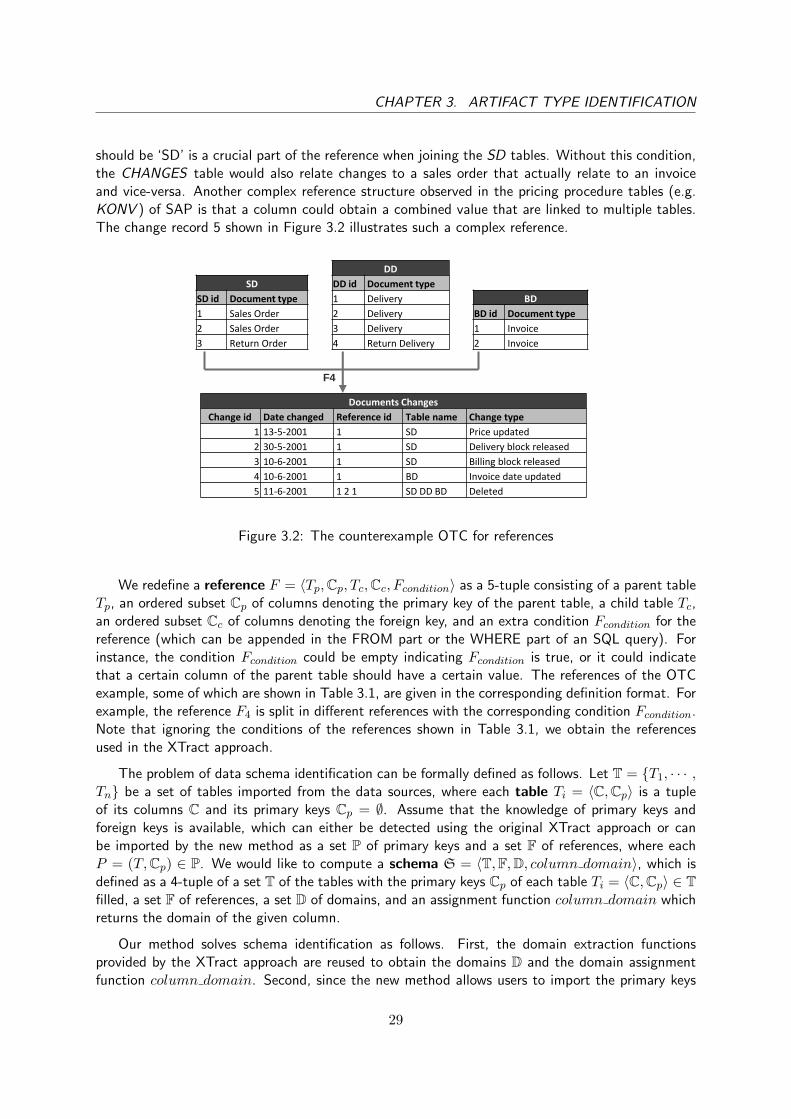
CHAPTER 3. ARTIFACT TYPE IDENTIFICATION
should be ‘SD’ is a crucial part of the reference when joining the SD tables. Without this condition,the CHANGES table would also relate changes to a sales order that actually relate to an invoiceand vice-versa. Another complex reference structure observed in the pricing procedure tables (e.g.KONV ) of SAP is that a column could obtain a combined value that are linked to multiple tables.The change record 5 shown in Figure 3.2 illustrates such a complex reference.
Documents Changes
Change id Date changed Reference id Table name Change type
1 13-5-2001 1 SD Price updated
2 30-5-2001 1 SD Delivery block released
3 10-6-2001 1 SD Billing block released
4 10-6-2001 1 BD Invoice date updated
5 11-6-2001 1 2 1 SD DD BD Deleted
PAGE 32
BD
BD id Document type
1 Invoice
2 Invoice
DD
DD id Document type
1 Delivery
2 Delivery
3 Delivery
4 Return Delivery
SD
SD id Document type
1 Sales Order
2 Sales Order
3 Return Order
F4
Figure 3.2: The counterexample OTC for references
We redefine a reference F = 〈Tp,Cp, Tc,Cc, Fcondition〉 as a 5-tuple consisting of a parent tableTp, an ordered subset Cp of columns denoting the primary key of the parent table, a child table Tc,an ordered subset Cc of columns denoting the foreign key, and an extra condition Fcondition for thereference (which can be appended in the FROM part or the WHERE part of an SQL query). Forinstance, the condition Fcondition could be empty indicating Fcondition is true, or it could indicatethat a certain column of the parent table should have a certain value. The references of the OTCexample, some of which are shown in Table 3.1, are given in the corresponding definition format. Forexample, the reference F4 is split in different references with the corresponding condition Fcondition.Note that ignoring the conditions of the references shown in Table 3.1, we obtain the referencesused in the XTract approach.
The problem of data schema identification can be formally defined as follows. Let T = {T1, · · · ,Tn} be a set of tables imported from the data sources, where each table Ti = 〈C,Cp〉 is a tupleof its columns C and its primary keys Cp = ∅. Assume that the knowledge of primary keys andforeign keys is available, which can either be detected using the original XTract approach or canbe imported by the new method as a set P of primary keys and a set F of references, where eachP = (T,Cp) ∈ P. We would like to compute a schema S = 〈T,F,D, column domain〉, which isdefined as a 4-tuple of a set T of the tables with the primary keys Cp of each table Ti = 〈C,Cp〉 ∈ Tfilled, a set F of references, a set D of domains, and an assignment function column domain whichreturns the domain of the given column.
Our method solves schema identification as follows. First, the domain extraction functionsprovided by the XTract approach are reused to obtain the domains D and the domain assignmentfunction column domain. Second, since the new method allows users to import the primary keys
29
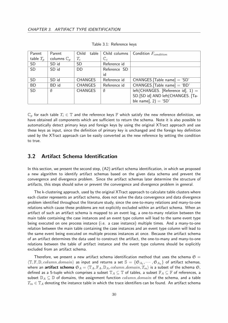
CHAPTER 3. ARTIFACT TYPE IDENTIFICATION
Table 3.1: Reference keys
Parenttable Tp
Parentcolumns Cp
Child tableTc
Child columnsCc
Condition Fcondition
SD SD id SD Reference id
SD SD id DD Reference SDid
SD SD id CHANGES Reference id CHANGES.[Table name] = ‘SD’
BD BD id CHANGES Reference id CHANGES.[Table name] = ‘BD’
SD ∅ CHANGES ∅ left(CHANGES. [Reference id], 1) =SD.[SD id] AND left(CHANGES. [Ta-ble name], 2) = ‘SD’
Cp for each table Ti ∈ T and the reference keys F which satisfy the new reference definition, wehave obtained all components which are sufficient to return the schema. Note it is also possible toautomatically detect primary keys and foreign keys by using the original XTract approach and usethese keys as input, since the definition of primary key is unchanged and the foreign key definitionused by the XTract approach can be easily converted as the new reference by setting the conditionto true.
3.2 Artifact Schema Identification
In this section, we present the second step, (A2) artifact schema identification, in which we proposeda new algorithm to identify artifact schemas based on the given data schema and prevent theconvergence and divergence problem. Since the artifact schemas later determine the structure ofartifacts, this steps should solve or prevent the convergence and divergence problem in general.
The k-clustering approach, used by the original XTract approach to calculate table clusters whereeach cluster represents an artifact schema, does not solve the data convergence and data divergenceproblem identified throughout the literature study, since the one-to-many relations and many-to-onerelations which cause these problems are not explicitly excluded within an artifact schema. When anartifact of such an artifact schema is mapped to an event log, a one-to-many relation between themain table containing the case instances and an event type column will lead to the same event typebeing executed on one process instance (i.e. a case instance) multiple times. And a many-to-onerelation between the main table containing the case instances and an event type column will lead tothe same event being executed on multiple process instances at once. Because the artifact schemaof an artifact determines the data used to construct the artifact, the one-to-many and many-to-onerelations between the table of artifact instance and the event type columns should be explicitlyexcluded from an artifact schema.
Therefore, we present a new artifact schema identification method that uses the schema S =〈T,F,D, column domain〉 as input and returns a set S = {SA1 , · · · ,SAn} of artifact schemas,where an artifact schema SA = 〈TA,FA,DA, column domain, Tm〉 is a subset of the schema S,defined as a 5-tuple which comprises a subset TA ⊆ T of tables, a subset FA ⊆ F of references, asubset DA ⊆ D of domains, the assignment function column domain of the schema, and a tableTm ∈ TA denoting the instance table in which the trace identifiers can be found. An artifact schema
30

CHAPTER 3. ARTIFACT TYPE IDENTIFICATION
comprises complete information related to its artifact(s). Note the definition of an artifact schemais unchanged from the original XTract approach, which means the original XTract approach can stillbe used to detect artifact schemas.
The new simple algorithm ComputeArtifactSchemas(S) shown below identifies artifact schemaswhile preventing the data divergence and convergence problem. Since the one to many and many toone references cause the divergence and convergence problem, these references are not desired withinan artifact schema. Therefore, if we construct a schema graph where each table is a node, and eachreference is an edge from the parent table to the child table, then we can remove the references whichare not one to one, thus resulting in a graph only connected by one to one reference. The sub graphswhich are still connected can be considered as valid artifact schemas as it only contains tables whichare linked by one to one references. The main table Tm can be selected as a table which has no parentin the set TA of the selected tables. The set DA of domains is the union set of all domains of columnsof the tables in TA. We can obtain an artifact schema SA = 〈TA,FA,DA,S.column domain, Tm〉and add it to the set S to be returned.
Algorithm ComputeArtifactSchemas(S)1. Let a graph G = (TG,FG)← (S.T,S.F)2. for F ∈ FG3. do if (F is not one to one)4. then remove F from FG5. for a connected sub graph g = (Tg,Fg) ⊆ G6. do TA ← Tg, FA ← Fg,7. select a table Tm ∈ TA which has no parent table in TA8. DA ← the union set of domains of columns of the tables in TA9. create a new artifact schema SA = 〈TA,FA,DA,S.column domain, Tm〉10. add artifact schema SA to S11. return S
The algorithm ComputeArtifactSchemas presented, which is a simple brute-force way of splittingtables to exclude one-to-many relations, also faces some issues. For example, in SAP, the changetables CDHDR and CDPOS contain all change records of the sales documents stored in the tableVBAK . It might be more logical to consider the changes as a part of the life-cycle of the Sales Orderartifact, instead of as a separate artifact. However, the change tables are returned as a separateartifact schema by the algorithm because the sales document table is linked to the change tables bya one-to-many reference, which means a sales document could be linked to multiple change records(i.e. data divergence). However, a ‘perfect’ artifact (schema) has not been defined. The tablesassigned to an artifact schema influence the data contained in the event log. Therefore, our methodallows users to add tables to or delete tables from the artifact schemas to construct an entity oftables containing all information related to an artifact which shall be subsequently converted to anevent log that satisfy the requirements of users. Thus, users can decide whether to consider thechanges as a separate artifact (then there are interactions between sales order and changes whichsolves the divergence problem) or as a part of the Sales Order artifact’s life-cycle by adding theChanges table to the artifact schema of SD (which cause the divergence problem). Furthermore,users can construct artifact schemas which overlap in tables.
We shall illustrate the different between the XTract approach and our artifact schema identi-fication. Given the OTC example, the XTract approach returns the three artifact schemas shown
31

CHAPTER 3. ARTIFACT TYPE IDENTIFICATION
in the left table of Figure 3.3 when given k = 3 (as discussed in Section 2.3). Our approach shallfirst return three artifact schemas SD, BD, and DD as shown by the black tables in the right tableof Figure 3.3. Since only one invoice has a change, the document changes table is assigned to theBD artifact schema. The SD artifact schema returned only contains the SD table, similar for theDD artifact schema. Now if users desire to include changes for the SD artifact, they can add thechanges table to the SD artifact schema. This comparison shows that it is more intuitive and easierto apply the new approach.
PAGE 33
XTract: Artifact Schemas (k = 3)
Name Main table Tables
BD BD BD
Changes Changes Changes
Changes ? SD, DD
Our Approach: Artifact schemas
Name Main table Tables
BD BD BD, Changes
SD SD SD (, Changes)
DD DD DD
Figure 3.3: Comparing the artifact schemas obtained using the XTract approach and ourapproach with respect to tables T and the main table Tm
3.3 Artifact Identification
In this section, we present the third step, (A3) artifact identification, in which we have extendedthe definition of artifacts and event types to be able to identify multiple artifacts of which the caseinstances share the same main table and multiple event types of which the events share the sametime column. Furthermore, we present a semi-automatic method to help users identify these artifactsand event types, when given a set of artifact schemas.
Our artifact identification method should be able to identify multiple artifacts sharing the sameartifact schema, since the assumption made by the original XTract approach that a main tabletable Tm of an artifact schema SA only contains the instance information of one specific artifact isunrealistic. We use the OTC example as a counterexample. In the SD table shown in Figure 1.1,multiple document types that share the same data structure are stored: two sales orders and onereturn order. The return order has a reference to the first sales order with id S1, whereas the salesorders have no reference to previous documents. In addition, the return order S3 has a referencewith the return delivery and no reference with the deliveries in the DD table, whereas the salesorder do have references with the deliveries and no direct reference with the return delivery. Thisinformation already indicates the sales order and the return order have different interactions withthe system. Therefore it is important to be able to distinguish the two document types as differentartifacts having separate life cycles, such that the interactions could also be identified separately.
After the artifact schemas SA are identified, the artifact identification method, which uses eachof these artifact schemas to obtain one or multiple artifacts, is defined as follows. Given an artifactschema SA = 〈TA,FA,DA, column domain, Tm〉, the method returns a set of artifacts, whereeach artifact A = 〈Aname,CAid,E,Cattrs, I,SA, Acondition〉 denotes a 7-tuple which comprises aname Aname, a set CAid of columns denoting the case identifier of the artifact, a set E of eventtypes, a set Cattrs of columns denoting the case attributes, a set I of interactions between thisartifact A and other artifacts (which is an empty set for now), the corresponding artifact schemaSA, and an artifact condition Acondition which is an extra condition (which can be appended in
32

CHAPTER 3. ARTIFACT TYPE IDENTIFICATION
Table 3.2: An example of the Sales Order artifact
Artifact’s component Value
Aname Sales Order
CAid { SD id }
E1 ∈ E
〈Ename = date created,CEid = {SD id},Ctime = [date created],CEattrs = {},Econdition = ∅〉
E2 ∈ E
〈Ename = last change,CEid = {SD id},Ctime = [latest change],CEattrs = {},Econdition = ∅〉
Cattrs { [Document type], [Value]}I ∅Acondition Tm.[Document type] = ‘Sales Order’
the FROM part or the WHERE part of an SQL query) that is used to distinguish various artifactshaving the same instance table Tm (or having the same artifact schema). Each event type Ei =〈Ename,CEid, Ctime,CEattrs, Econdition〉 in the set E of the event types is constituted by a nameEname of the event type, a set CEid of columns defining the event identifier, a column Ctimeindicating the ordering (or the timestamps) of events of this event type, a set CEattrs of columnsdenoting the attributes of the event type, and a condition Econdition to distinguish various eventtypes having the same time column Ctime.
Using the SD table of the OTC example, we would like to show a concrete example of theartifact definition. Consider the artifact schema SA = 〈TA,FA,DA, column domain, Tm〉, wherethe tables TA = {SD} and the references FA = {〈SD, {SD id}, SD, {Reference id}〉}, we wouldlike to identify two artifacts, the Sales Order and the Return Order. Both artifacts may havethe same artifact schema, but they could have different events, attributes, and interactions. Forexample, the artifact Sales Order ASalesOrder = 〈Aname,CAid,E,Cattrs, I,SA, Acondition〉 couldhave the structure shown in Table 3.2, in which each component of the artifact is given a value.
To be able to semi-automatically construct artifacts based on an artifact schema and a column(or columns) indicating the artifact, we define two functions. The first function constructs a singleartifact, whereas the second function constructs multiple artifacts by calling the first function multipletimes. The first function createArtifact(SA, Aname, Acondition) takes an artifact schema SA, anartifact name Aname, and an artifact condition Acondition as input. Then, this function uses afunction provided by the existing XTract approach to obtain a set CAid of case identifiers, a set Eof event types and a set Cattrs of case attribute columns (the details of this existing function canbe found in the thesis of E.Nooijen [21]). These components suffice for returning an artifact. Thesecond function createArtifactsByColumnValues(SA, Ce) takes an artifact schema SA and a list Ceof columns as input. For each distinct tuple value v = (v1, · · · , vn) found for Ce = (C1, · · · , Cn),an artifact is created by calling the first function createArtifact with the artifact schema SA, theartifact name Aname = v, and the condition Acondition equal to
∧ni=1Ci = vi (i.e.‘C1 = v1 AND
33

CHAPTER 3. ARTIFACT TYPE IDENTIFICATION
... AND Cn = vn’). In addition, for the columns in C which are not in the main table SA.Tm, thetables of these columns should be selected to be joined with the main table such that the conditioncan be tested on these columns. In this case, the shortest path algorithm can be used to selectreferences and the tables. As a result, a set of complete artifacts without interactions is constructedby createArtifactsByColumnValues.
It is also possible to import a predefined list of artifacts using the function importArtifact(T ′m,Aname, Acondition). For each artifact schema SA retrieved where the main table Tm of SA isequal to T ′m, the function constructs an artifact by calling the function createArtifact(SA, Aname,Acondition).
Figure 3.4 demonstrates the difference in artifacts returned by the XTract approach and ourapproach. Given the artifact schema SD containing the table SD as the main table and tableChanges, the XTract approach returns one artifact SD shown on the left hand side in Figure 3.4. Incontrast, the user can indicate the document type column as a condition column constituting Ce inthe function createArtifactsByColumnValues(SA, Ce). Two artifacts Sales Order and Return Orderare then identified, as shown on the right hand side in Figure 3.4.
PAGE 34
Given Artifact schema SD
Name Main table Tables
SD SD SD, Changes
Artifact SD
Artifact name SalesDocuments
Artifact Identifier {[SD id]}
Event type DateCreated
name "Created"
Event id {[SD id]}
Timestamp {[date created]}
Event type LastChange
name "last change"
Event id {[SD id]}
Timestamp {[last change]}
Event type ChangesChanged
name "Changed"
Event id {[Change id]}
Timestamp {[Date changed]}
Artifact Sales Order
Artifact name Sales Order
Artifact Identifier {[SD id]}
Condition SD.[Document type] = 'Sales Order'
Event type DateCreated
name "Created"
Event id {[SD id]}
Timestamp {[date created]}
Condition
Event type LastChange
name "last change"
Event id {[SD id]}
Timestamp {[last change]}
Condition
Event type PriceUpdated
name "Price updated"
Event id {[Change id]}
Timestamp {[Date changed]}
Condition Changes.[Change type] = 'Price updated'
Event type DeliveryBlockReleased
name "Delivery block released"
Event id {[Change id]}
Timestamp {[Date changed]}
Condition
Changes.[Change type] = 'Delivery block released'
Event type BillingBlockReleased
name "Billing block released"
Event id {[Change id]}
Timestamp {[Date changed]}
Condition Changes.[Change type] = 'Billing block released'
Artifact Return Order
Artifact name Return Order
Artifact Identifier {[SD id]}
Condition SD.[Document type] = 'Return Order'
Event type DateCreated
name "Created"
Event id {[SD id]}
Timestamp {[date created]}
Condition
The original Xtract approach Our approach
one Tm one artifact one Tm multiple artifacts
one Ctime one event type one Ctime multiple event types
Figure 3.4: Comparing the artifacts obtained using the XTract approach and our approach
To be able to identify multiple event types sharing the same timestamp column, similar cus-
34

CHAPTER 3. ARTIFACT TYPE IDENTIFICATION
tomization (as for the artifact identification) is also added because the original XTract approachwhich assigns a time stamp column entirely to one event types has its limitation. We illustrate thislimitation with the DOCUMENT CHANGES table shown in Figure 1.1 which is a simplified versionof the SAP change tables CDHDR and CDPOS . Three change records (with id 1, 2 and 3) of thesales order S1 are found, and one change record (with id 4) of the invoice B1 is found. The columnDate changed can be automatically identified as one event type date changed using the XTract ap-proach, which aggregates different changes. However, the table also shows different event types thatare distinguished by the value in column change type. Since considering different changes as differ-ent event types reveals the relation between different change types in time aspect, it is required to beable to identify different event types based on the column Change type. We present two functions(similar to the two functions of artifacts creation): the first function createEventType(Ctime, Ename,Econdition) calls the existing XTract approach to obtain the event identifier and the event attributeswhich results in components that are sufficient for returning an event type; the second function cre-ateEventTypesByColumnValues(C ′time, Ce) calls the first function createEventType(Ctime, Ename,Econdition) with Ctime = C ′time, Ename = v, and Econdition =
∧ni=1Ci = vi, for each distinct tuple
value v = (v1, · · · , vn) found for Ce = (C1, · · · , Cn) (and similarly, if the columns in Ce belongsto different tables than the time column Ctime, tables can be selected and joined using the shortestpath algorithm).
Identifying multiple event types is also illustrated in Figure 3.4. The artifact Sales Order shows thethree different event types, PriceUpdated, DeliveryBlockReleased and BillingBlockReleased, identi-fied from the time column Date Changed using the second function createEventTypesByColumn-Values(C ′time, Ce). In contrast, the XTract approach automatically considers the time column DateChanged as one event type ChangesChanged.
Furthermore, the approach presented allows users to change the name Anameand conditionAcondition of an artifact and the event type names Ename and event type conditions Econdition ofthis artifact. It is also possible to change the event type identifier columns CEid and the timestampcolumn Ctime of an event type. Moreover, users can easily delete and add event types, event typeattributes and case attributes.
We conclude this chapter by giving an overview of the achievements shown in Figure 3.5. First,we reconstruct the data schemas from a given data source. Then, we identify artifact schemas andprevent the data divergence and convergence problem. Finally, we are able to semi automaticallyidentify multiple artifacts from a given artifact schema.
35

CHAPTER 3. ARTIFACT TYPE IDENTIFICATION
Data
sch
em
as
Art
ifact
Sch
em
as
Art
ifacts
Fig
ure
3.5:
Art
ifac
tT
ype
Iden
tifi
cati
on
36

Chapter 4
Interaction Identification
In Chapter 3, we have discussed the first step (A) the identification of complete stand-alone artifactsof the extraction phase, without considering any interactions between artifacts. In this chapter, wewill introduce the second step, (B) interaction identification (between the artifacts), in which we areable to define interactions and discover both direct and indirect interactions between artifacts on thedatabase level. Moreover, we will show our approach to (C) extract logs including interactions byextending the XTract approach. We first recall our current findings in the literature of interactionidentification. Then, we introduce the four levels of interactions to clarify the concepts of interac-tions. Finally, we give an overview of our approach, in which the remaining sections of this chapterare also introduced.
No interaction identification techniques are discussed in the literature. Traditional log conversionapproaches assume a single, isolated process, in which the notion of interactions with other processesare not considered. The XTract approach only has identified the artifacts without considering theinteractions between the artifacts. Although the XTract approach can extract an event log basedon an artifact, no information of interactions are included. Thus, unfortunately, due to the noveltyof the notion of artifacts, no approach has yet been found in the literature which can automaticallyand specifically identify the interactions between artifacts (or between different event log conversiondefinitions). This also indicates that interactions between the artifacts have no clear definitionor categorization yet. Moreover, the possibility of whether interactions can be identified on thedatabase level has not been investigated. Therefore, we have conducted research into (1) defininginteractions, and (2) designing a new approach to be able to automatically identify interactionsand more importantly, (3) being able to extract event logs with interactions which can be used todiscover process models that have interactions with each other.
Interactions between the artifacts should be discovered. For instance, take the SD table shown inFigure 1.1 and the artifact Return Order shown in Table 3.2. Without interactions, the Return Orderartifact will only have two events, Date Created and Latest Change and have no reference at all tothe related Return Order. This limitation leads to a great loss of important information, sincethe relation between artifacts do exist and are interesting to investigate. Furthermore, it is almostimpossible to describe the behavior of an ERP system in a single process, whereas allowing to expressinteractions between processes also allows users to model the system as a collection of collaborativeprocesses. In addition, an interaction between artifacts allows to express other relations than aone-to-one relation, which solves the data divergence and convergence problems.
37

CHAPTER 4. INTERACTION IDENTIFICATION
To be clear about which interactions are discussed, the interactions are categorized into fourlevels based on the objects between which the interactions taken place. The categorization is shownin Figure 4.1. (a) The artifact instance level interactions denotes interactions between twoartifact instances such as the sales order S1 and the return order S3. The existence of artifactinstance level interactions between two artifacts also indicates, to some extent, the existence of anartifact type level interaction between the two artifacts. (b) The artifact type level interactionsrefer to interactions between two artifacts such as the Sales Order and the Return Order. (c) Theevent level interactions are interactions between two events such as the Latest Change event withid S1 and timestamp ‘1-6-2001’ of the sales order S1 and the Date Created event with id S3 andtimestamp ‘10-6-2001’ of the return order S3. Similar to the artifact instance level interactions, theevent level interactions between the two events also indicate, to some extent, the existence of anevent type level interactions between the two event types of the two events. Thus, (d) the eventtype level interactions denote interactions between two event types such as the Latest Changeevent type of the sales order artifact and the Date Created event type of the return order artifact. Forthe sake of brevity, we also refer to artifact instance level interactions as instance level interactionsand refer to artifact type level interactions as type level interactions.
PAGE 27
Artifacts Event types
Artifact instances Events
Specifies
Performed
Instantiation Instantiation
Event type level interactions
Events level interactions Artifact instance level interactions
Artifact type level interactions
Definition
Recording
Indicate
DB level Log level
Artifact LogMapping
Event Log
CacheDB
Indicate
Figure 4.1: Interactions levelsThe four levels of interactions
In this chapter, we introduce a new approach to identify type level interactions and extract eventlogs with instance level interactions (instantiated from the type level interactions). In Chapter 5, wewill consider event level and event type level interactions. An overview of our approach is shown inFigure 4.2. In Section 4.1, we first illustrate the concept of type level interactions and instancelevel interactions and give these two concepts clear formal definitions used in this approach, alongwith the reason why only these two types of interactions are identified on the database level. Then,in Section 4.2, a new method ’type level interaction identification’ (1.1), which identifies interactionson the type level between artifacts with conditions, is described. The method ’type level interactionidentification’ also provides support to allow users to change ‘Artifact with type level interactions’and select the interactions desired (1.2). In Section 4.3, we will illustrate the method ‘MappingCreation’ which creates mappings for type level interactions (2.2), and extend the artifact mappingcreation method provided by the XTract approach (2.1) to create a mapping with type levelinteractions for each artifact. Finally, based on a mapping with type level interactions, an artifactis converted to an event log with artifact instance level interactions by using and extending theconversion method provided by the XTract approach to be able to extract artifact instance level
38

CHAPTER 4. INTERACTION IDENTIFICATION
XTract2 Approach
2.Artifact type level interactions Identification
1.Artifacts Identification
(1.1) Artifact typ level Interactions identification
(2.1) Artifact mapping creation
(1.2) Support changes
(3) Log extraction:
Build CacheDB
and SQL queries
(2.2) Interaction mapping creation
Artifacts with
conditions
Artifact with type level
interaction
Mappings with artifact
references
Event logs with
interactions
NameObject existed
Name Object
with changes
methodFunctions existed
methodFunctions added
Figure 4.2: Method Interaction Identification.Each rectangle represents an object used, and each arc represents a method used. The black arcsindicates reusing a method provided by the XTract approach, whereas the red arcs indicates a new
designed method
interactions as attributes of traces (3).
4.1 Artifact Type Level and Instance Level Interactions
The aim of this section is to clarify the definition of type level and instance level interactions. Wefirst define the direct interactions both on type level and instance level in Sections 4.1.1. Next, weextend the direct interactions to indirect interactions in Sections 4.1.2. Based on the definition andexamples shown, we argue why only the type level and instance level interactions are identified onthe database level, whereas the discovery of event type level and event level interactions is done onthe log level in Section 4.1.3.
4.1.1 Direct Artifact Type level and Instance Level Interactions
In this section, we first discuss how we use a reference between two main tables (of two artifacts)to define a direct interaction. Next, the formal definition of direct interactions and of an interactiongraph is given.
To be able to automatically identify interactions between artifacts, the notion of interactionsshould be formally defined. Since a main table of an artifact contains the instances of this artifact,a reference F found between two main tables may also indicate a direct relation between the twoartifacts. For example, the reference F2 between the main tables (SD and DD) of Sales Order andDelivery artifacts could be a direct interaction. But this combination of two artifacts and a referencebetween the main tables of these two artifact is not always a direct interaction. For example, themain tables of the artifacts Sales Order and Return Delivery is also related by reference F2, but noreal relations (i.e. no related instances) are found. This uncertainty is due to the fact that theinstances of an artifact might only be a subset of the records in its main table Tm, which have no
39

CHAPTER 4. INTERACTION IDENTIFICATION
reference to the instances of other artifacts. In other words, even if a foreign key of a table exists inthe data structure, the foreign key might not be used by every record in this table.
To verify the existence of a direct relation between two artifacts inherited from a reference, thereshould be a record of one artifact referring to a record in the main table of the other artifact. Theexistence of such a direct relation between two artifacts is the concept of a type level interaction. Thedefinition of a direct type level interaction d = (AS , F,AT ) ∈ A×F×A between two artifacts ASand AT is a 3-tuple comprising the two artifacts and a reference F = 〈Tp,Cp, Tc,Cc, Scondition〉 ∈ F,where the main table AS .Tm = Tp and the main table AT .Tm = Tc, thus the reference F = 〈AS .Tm,AS .CAid, AT .Tm,Cc, Scondition〉. We denote the artifact AS as the parent artifact and the artifactAT as the child artifact. More importantly, there has to be a record s in AS .Tm referring to a recordt in AT .Tm that s satisfies the condition AS .Acondition, and t satisfy the condition AT .Acondition.To be concrete, an example of relational algebra and an SQL query which select the number n giventwo artifacts is shown in Listing 4.1.
The direct instance level interactions are instantiated from the interactions on the type levelby joining the main tables based on direct type level interactions. To be concrete, an example ofan SQL query which select the interaction instances between the sales orders and the return orderis shown in Listing 4.2. The resulting instance level interactions between the sales orders and thereturn orders are shown in Table 4.1. Table 4.2 shows the instance level interactions between thereturn orders and the return deliveries.
Listing 4.1: Interaction Count Selection Query
/* Select the count of an direct type level interaction d = (AS , F,AT ) *//* In relational algebra:
#(π(AS .CAid,AT .CAid)(AS .Tm ./(Cp1=Cc1∧···∧Cpn=Ccn∧AS .Acondition∧AT .Acondition) AT .Tm)) > 0
*/SELECT COUNT(DISTINCT AS .CAid, AT .CAid)FROM AS .TM INNER JOIN AT .TM ON F.Cp1 = F.Cc1 AND ... AND F.Cpn = F.Ccn
AND F.Scondition IS TRUE AND AS .Acondition IS TRUE AND AT .Acondition IS TRUE
Listing 4.2: Interaction Instances Selection Query
/* Select the interaction instances of a type level interaction */SELECT DISTINCT SALESORDER.[SD ID] AS [Sales Order SD id],
RETURNORDER.[SD ID] AS [Return Order SD id]FROM SD AS SALESORDER INNER JOIN SD AS RETURNORDER
ON SALESORDER.[SD ID] = RETURNORDER.[REFERENCE ID]AND SALESORDER.[DOCUMENT TYPE] = ‘Sales Order’AND RETURNORDER.[DOCUMENT TYPE] = ‘Return Order’
We shall illustrate the direct type level and instance level interactions with the OTC example.A reference F2 = 〈SD, {SD id},DD, {Reference SD id}〉 between the SD table and the DD tableis found (i.e. the foreign key column Reference SD id in the DD table refers to the primary keycolumn SD id of the SD table). Joining the two tables based on the reference F2, the result showstwo direct instance level interactions between the two delivery documents D1 and D2 and the salesorder S1 and a direct instance level interaction instance between the return delivery D3 and thereturn order S3 is found, which indicate the existence of a direct type level interactions betweenthe sales order and the delivery, and between the return order and the return delivery, respectively.However, there is no direct interactions found between the sales order and the return delivery, or
40

CHAPTER 4. INTERACTION IDENTIFICATION
between the return order and the delivery. The result confirms our claim above: a reference betweentwo artifacts does not always imply the existence of a direct type level interaction between thetwo artifacts. We obtained two direct type level interactions (ASalesOrder, F2, AReturnOrder) and(AReturnOrder, F2, AReturnDelivery), respectively, with their direct instance level interactions shownin Tables 4.1 and 4.2.
An interaction graph for the OTC example shown in Figure 4.3 indicates the direct interactions(i.e. arcs) between the artifacts (i.e. elliptic nodes). Formally, we define an interaction graphG = (Asub, D), where Asub ⊆ A and D ⊆ Asub × Fselected × Asub, where Fselected ⊆ F. Each nodeA ∈ Asub represents an unique artifact A (i.e. no two nodes represents the same artifact), andeach edge e = (As, F,At) ∈ D represents the existence of a direct type level interaction (As, F,At)between the parent artifact As and the child artifact At, where F is the reference between themain tables of artifacts. The two subsets Asub and Fselected is to allow a user to limit the scopeof the interaction graph and interaction identification if desired. Note that this definition explicitlyallows multiple edges (thus multiple direct type level interactions) between two artifacts becausethere could be different references linking the artifacts. Moreover, we define the outgoing edges ofartifact AS as outEdges(AS) = {(AS , Fi, x) ∈ D | AS , x ∈ Asub}. Similarly, the incoming edgesof artifact AS is defined as inEdges(AS) = {(x, Fi, AS) ∈ D | AS , x ∈ Asub}.
Table 4.1: Direct interactions (ASalesOrder, F2, AReturnOrder) instances
Sales Order SD id Return Order SD id
S1 S3
Table 4.2: Direct interactions (AReturnOrder, F2, AReturnDelivery) instances
Return Order SD id Return Delivery DD id
S3 D4
PAGE 22
Sales Documents
Table
Deliveries Documents
Table
Sales
Documents
table
Deliveries
Documents
table
Billing
Documents
table
Billing Documents
Table
Sales Order Delivery
Return order Return delivery
Invoice
Figure 4.3: The artifact type level interactions of the example.Each eclipse underneath a table represents an artifact found in this table, and an arc represents the existing of a
direct interaction between the two artifacts (i.e. there are reference instances).
4.1.2 Indirect Artifact level Interactions
In the previous section, we have defined direct interactions. In this section, we discuss the motiva-tion for identifying indirect interactions. Then, we investigate different indirect interactions basedon the direct interaction and define valid indirect interactions. Finally, we define the set of type
41

CHAPTER 4. INTERACTION IDENTIFICATION
level interactions, which is constituted of the valid indirect interactions together with the directinteractions.
Identifying indirect interactions is required, since it should be possible to retrieve interactionsbetween two artifacts when the interactions go through artifacts of which the logs will not beextracted. For instance, if the return orders shown in Figure 4.3 can be ignored, we would still liketo be able to identify the interactions between the Sales Order and the Return Delivery. Another real-life situation encountered is that ERP systems in general have a document header and document linesstructure. For example, the sales document table VBAK and the sales line table VBAP. Differenttypes of documents are usually connected by lines. Typically, advisors are not interested in the linesbut only at the header level. Since the document headers are connected through lines, it should bepossible to identify interactions between header tables through the line tables, without extract anyinformation of lines. However, it is still questionable whether each indirect interaction is possibleand valid, e.g. the possibility of an indirect interaction between delivery and return order.
Indirect interactions can be defined using the direct interactions, similar to joining multiple tableslinked by references. An important property which is used to determine the validness of indirect typelevel interaction is that, when given a reference, a record in the parent table is linked to zero ormultiple records in the child table, whereas a record in the child table is only linked to zero or onerecords in the parent table. This property also indicates, given a direct type level interaction, aninstance in the parent artifact can be linked to zero or multiple instances of the child artifact, whereasan instance in the child artifact can only be linked to zero or one instance of the parent artifact.We denote this property as Reference property. Similar to an inductive step, we can considereach possible case of an indirect interaction extended from two direct interactions and define thisvalidness of this indirect type level interaction. Three possible cases of an indirect interaction aredisplayed in Figure 4.4.
Sales Order
Return order Return delivery
Sales Order Delivery Invoice
Sales Order Delivery
Return order
S1
S3 D4
S1
S2
D1
D2
B1
B2
D3
S1
S3
D1
D2
(a)
(b)
(c)
Figure 4.4: Indirect InteractionsThe three possible cases of indirect interactions extended from two direct interactions
The first case (a) is a valid interaction, which is when two direct interactions (ASi , Fi, ATi) and(ATi , Fj , ATj ) are linked as a chain and have the same direction, thus Fi.Tc = Fj .Tp. For example,the two direct interactions (ASalesOrder, Fi, AReturnOrder) and (AReturnOrder, Fj , AReturnDelivery)are linked this way. Since both interactions share the return order artifact, it is possible to join thethree main tables based on the two direct interactions. As the references are joined in the samedirection, we have the guarantee that an instance of the artifact ATi is only linked to zero or one
42

CHAPTER 4. INTERACTION IDENTIFICATION
instance of the artifact ASi , based on the reference property. This property also indicates that aninstance of the artifact ASi is linked to all instances of the artifact ATj , and these instances ofATj are not linked to any other instances of the artifact ASi . We denote this indirect type levelinteractions which is obtained from two direct interactions (ASi , Fi, ATi) and (ATi , Fj , ATj ) of thesame direction as a strong indirect interaction between the artifacts ASi and ATj .
The second case (b) is a valid interaction but over-approximates the actual interactions, whichis when two direct interactions (ASi , Fi, ATi) and (ASj , Fj , ATi) link to the same child artifact,thus Fi.Tc = Fj .Tc. For example, the two direct interactions (ASalesOrder, Fi, ADelivery) and(AInvoice, Fj , ADelivery) are linked this way. An instance of the artifact Sales Order can be ex-plicitly linked to an instance of the artifact Invoice via one instance of the artifact Delivery, asshown by the graph in Figure 4.4(b) on the right-hand side (e.g. (S1, B2), (S1, B2), (S2, B2)).This explicitness is because an instance of the artifact Delivery can only be linked to one instanceof Sales Order and one instance of Invoice (e.g. (S1, D1, B1)) based on the reference property.However, also based on the reference property, there is the possibility that an instance of the artifactInvoice are linked to multiple sales order (e.g. B2). As result, when the invoices B1 and B2 areselected as the indirect instance level interactions for the sales order S1, we have also included apart of B2 that is not related to S1 but related to S2. Therefore, all these type level interactionswhich contains two direct interactions (ASi , Fi, ATi) and (ASj , Fj , ATi) of the same child artifactsas a weak indirect interaction between the artifacts ASi and ASj .
The third case (c) involves invalid indirect type level interactions which include two directinteractions (ASi , Fi, ATi) and (ASi , Fj , ATj ) that have the same parent artifact ASi and dif-ferent target artifacts. For example, the two direct interactions (ASalesOrder, Fi, ADelivery) and(ASalesOrder, Fj , AReturnOrder) are linked this way. Since an instance of the artifact Sales Order canbe linked to multiple instances of the artifact Delivery and multiple instances of the Return Order(e.g. (S1, {D1, D2}, {S3})), it is impossible to determine the exact relations between the instancesonly based on the references. Therefore, we classify this case as invalid indirect type level interac-tions.
The validness of indirect interactions consisting of two direct interactions can be applied tothe indirect interactions of any length. If an indirect interaction includes case (c), then it is aninvalid interaction. Else if it includes a case (b), then it is a weak interaction which has a notion ofover-approximation. Otherwise, it only consists of case (a), which is a strong interaction.
The definition of a valid type level interaction IS,T = 〈d1, · · · , dn〉 ∈ (A × F × A)∗ betweenartifacts AS and AT is a sequence of direct interactions di = (APi , Fi, ACi) ∈ A × F × A and1 ≤ i ≤ n, which satisfy one of the following property shown in Figure 4.5: (1) the parent artifactAP1 of first direct interaction d1 is the artifact AS , and the child artifact APn of the last directinteraction dn is the artifact AT , and for 1 ≤ i < n, ACi = APi+1 ; or (2) the child artifact AC1 offirst direct interaction d1 is the artifact AS , and the parent artifact APn of the last direct interactiondn is the artifact AT , and for 1 ≤ i < n, APi = ACi+1 ; or (3) there is a number k and 1 ≤ k ≤ n,for 1 ≤ i < k, ACi = APi+1 , and ACk = ACk+1
, and for k < i < n, APi = ACi+1 , and the parentartifact AP1 of first direct interaction d1 is the artifact AS , and the parent artifact APn of the lastdirect interaction dn is the artifact AT . In addition, the number of interaction instances is greaterthan zero. The length of strong joins of this interaction is defined as k, and the length of weakjoins is defined as m = n−k. When the length m of weak joins is greater than zero, the interactioninstances could be an over-approximation.
43

CHAPTER 4. INTERACTION IDENTIFICATION
PAGE 31
S T d1 dn
S T d1 dn AP1 ACn Ac1
Apn
S d1 dk AP1
ACk = AC(k+1)
T dk+1 dn Apn
(1) (2)
(3)
Figure 4.5: Type level interactions
Given a set A of artifacts, a set D of direct interactions where for each di ∈ D the parentartifact APi ∈ A and the child artifact ACi ∈ A, and an artifact AS ∈ A, we define a full set IfSof valid type level interactions of artifact AS as {(IS,T , AT ) | AT ∈ A and IS,T is a valid type level
interaction from AS to AT }. For example, the full set IfReturnOrder of the artifact Return Orderis {(〈(ReturnOrder, F2, ReturnDelivery)〉, AReturnDelivery), (〈(SalesOrder, F1, ReturnOrder)〉,ASalesOrder)}.
4.1.3 Possibility of Identifying Event Level Interactions
The definition and the examples have demonstrated that the type level interactions and instance levelinteractions between two artifacts are possible and relatively easy to be identified on the databaselevel. In contrast, studying the OTC example has also revealed that to automatically identify theinteractions between event types of two artifacts is much more difficult to do at the database level,since there might not be any explicit indication of a relation between two event types except thetimestamps. For example, the direct interaction between the Sales Order and the Return Orderdoes not indicate whether the Date Created event type of Return Order is (causally) related to theDate Created event type of Sales Order or to the Latest Change event type of the Sales Order.Similarly, the interaction on the event level, for which comparison in time might be needed, is alsodifficult to be identified in relational databases. For this purpose, the event log structure and processmining techniques are much more suitable. Therefore, we identified the type level interactions ondatabases and extract event logs with the instance level interactions. Then, we can use these eventlogs with instance level interactions to identify the interactions on event type level and event level.
4.2 Type Level Interaction Identification
In Section 4.1, we have introduced different kinds of interaction and formalized the type levelinteractions. In this section, we will present our approach to first automatically identify a set of typelevel interactions, and then allow users to select the type level interactions which they are interestedin. A set of artifacts with type level interactions to each other are returned for log extraction.
Formally, given a set of artifacts A = {A1, · · · , An} as input, where each artifact A = 〈Aname,CAid,E,Cattrs, I = ∅,SA, Acondition〉, a number r > 0, a number k ≥ 1 and a number m ≥ 0, the
algorithm should return the set A of artifacts, where for each artifact AS ∈ A, the set IS ⊆ IfS isfilled, and for each interaction IS ∈ IS , the length of strong joins is less than or equal to k, the length
44

CHAPTER 4. INTERACTION IDENTIFICATION
of weak joins is less then or equal to m and the number of distinct instance level of interactions isgreater or equal to r.
We made the following design decision explicitly. To restrict the identification of distinct inter-actions on the parent artifact, we constrain the number of strong joins greater than zero and thenumber of weak joins less than or equal to the number of strong joins, i.e. k ≥ 1 and m ≤ k.In other words, recalling the three situations of type level interaction shown in Figure 4.5, we onlyobtain interactions of the parent artifact AS that satisfy (1), or (3) with m ≤ k. The interactionsthat satisfy (2) or (3) with m > k will only be extracted as the interactions of artifact AT . Notethat this decision will also effect the event logs we extract. An instance level interaction will onlybe extracted from the parent artifact.
There are several advantages to only identify interactions on the one side. First, limiting theinteractions to the parent artifact can prevent duplicated attributes to be extracted to improvethe performance of log extraction. Furthermore, this decision also limits the number of discoveredinteractions to decrease the number of manual selections that are needed by users. Moreover, weobtain the parent and child structure and the reference property which can be reused during theprocess discovery. We have only observed one disadvantage. For example, when a child artifactinstance has an interaction with a parent artifact instance but this parent instance is not extractedin the event log, then we miss the information that the child instance has an interaction in the eventlog. Note that we only restricted the numbers k and m, thus it is very easy to change our solutionto extract interactions on both side.
We divide the method into two parts. The first part takes a set of artifacts A = {A1, · · · , An}as input, calculates a complete set of direct interactions between the artifacts, and returns aninteraction graph G = (Asub, D), where each node Ai ∈ Asub represents an artifact Ai , and eachedge d = (As, F,At) ∈ D represents the existence of a direct interaction (As, F,At) between theartifact As and artifact At. Having an interaction graph G created, the second part of this methoduse the interaction graph G as input and returns a set of artifacts, each of which includes a set ofvalid type level interactions I (direct and indirect).
4.2.1 Artifact Interaction Graph and Direct Interactions
In this section, we present our algorithm to construct an interaction graph G and calculate all directinteractions which satisfy the following criteria. Given a set of artifacts A = {A1, · · · , An} as input,a complete set of direct interactions between the artifacts should be calculated, and an interactiongraph G = (Asub, D) should be returned, where each node Ai ∈ Asub represents an artifact Ai, andeach edge d = (As, F,At) ∈ D represents the existence of a direct interaction (As, F,At) betweenthe artifact As and artifact At where the number of instances of the direct interaction (As, F,At)should be greater than 0.
Each direct type level interaction with the number of instance level interactions greater thanzero is added to the interaction graph, but this number does not have to be greater than or equalto r. The reason for this is because a number of instance level interactions do not have a monotonedecreasing property. For example, a sales order is linked to one return order, but this return ordercould be linked to hundred return deliveries. For r = 10, this interaction d between sales order andreturn order does not satisfy countSelect(d) ≥ r, but the indirect interaction d′ between sales orderand return delivery does satisfy countSelect(d′) ≥ r. Since we use the interaction graph to compute
45

CHAPTER 4. INTERACTION IDENTIFICATION
the indirect interactions, all direct interaction with the number of instance level interaction greaterthan zero should be added.
Algorithm ConstructInteractionGraph(Asub,Fselection)1. D ← ∅2. for F = 〈Tp,Cp, Tc,Cc, Scondition〉 ∈ Fselection3. do for Ap ∈ Artifacts(TP ), Ac ∈ Artifacts(Tc)4. do if countSelect(Ap, F,Ac) ≥ 05. then D ← D ∪ (Ap, F,Ac)6. return G = (Asub, D)
The algorithm ConstructInteractionGraph(A,Fselection) solves this problem. First, we initializethe set D. Second, for each reference F ∈ Fselection ⊆ F, we retrieve the artifacts Ap of its parenttable and the artifacts Ac of its child table. We define the function Artifacts(T ) = {A ∈ Asub |A.Tm = T} to retrieve the artifacts of which their main table is T (see Line 3). For each combinationof Ap and Ac with the reference F between them, we select the count using the countSelect querydefined in Listing 4.1 to verify whether it is a direct interaction (see Lines 3 and 4). If the count isgreater than 0, then an edge (Ap, F,Ac) is added to D as an edge in the interaction graph G.
Note that for a reference F ∈ F\Fselection, this reference is not used to obtain any type level orinstance level interactions. Another remark is that, when there is overlapping between the instancesof artifacts in the same table, this overlapping is not considered as a direct interaction and no edgeis added because the related reference is not given. Nevertheless, it is possible to add the referencesF = 〈Tp,Cp, Tp,Cp, null〉 to the reference selection to solve this constraint.
4.2.2 Direct to Indirect Interactions
Having the interaction graph constructed, we present, in this section, our approach to identify typelevel interactions. The problem definition of the second part of the type level interaction identificationis described as follows. Given a set A of artifacts, an interaction graph G = (Asub, D), a numberr > 0, a number k ≥ 1 and a number m ≥ 0, the algorithm should return, for each artifact A ∈ A,a set I of valid interactions with other artifacts, where for each interaction I ∈ I, the number ofinteraction instances is greater than or equal to r, the length of strong joins is less than or equal tok and the length of weak joins is less than or equal to m.
We present the algorithm CalculatesInteractions(A, G, r, k,m), which solves this problem. First,for each artifact AS , the algorithm initializes the set I of interactions as empty set. For each outgoingedge d = (AS , F,At) ∈ D of AS , the (direct) interaction Icurrent = 〈d〉 is created. If the numberof instance level interaction of Icurrent is greater than or equal to r, then Icurrent is added to theinteraction set I of artifact AS . Next, algorithm calls the recursive algorithm calculateJoins(AS , At,Icurrent, IA, r, k − 1, m) to select all valid indirect interactions.
Algorithm CalculatesInteractions(A, G, r, k,m)1. for AS ∈ A2. do I← ∅3. for (AS , F,At) ∈ outEdges(A)
46
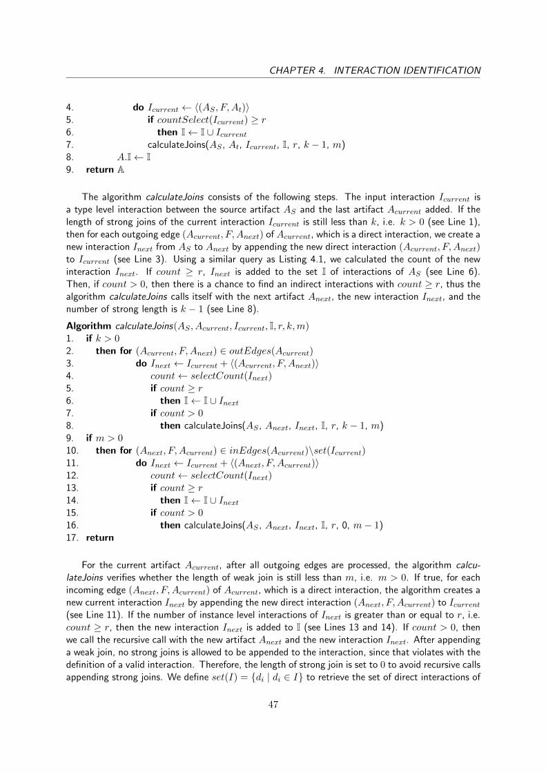
CHAPTER 4. INTERACTION IDENTIFICATION
4. do Icurrent ← 〈(AS , F,At)〉5. if countSelect(Icurrent) ≥ r6. then I← I ∪ Icurrent7. calculateJoins(AS , At, Icurrent, I, r, k − 1, m)8. A.I← I9. return A
The algorithm calculateJoins consists of the following steps. The input interaction Icurrent isa type level interaction between the source artifact AS and the last artifact Acurrent added. If thelength of strong joins of the current interaction Icurrent is still less than k, i.e. k > 0 (see Line 1),then for each outgoing edge (Acurrent, F,Anext) of Acurrent, which is a direct interaction, we create anew interaction Inext from AS to Anext by appending the new direct interaction (Acurrent, F,Anext)to Icurrent (see Line 3). Using a similar query as Listing 4.1, we calculated the count of the newinteraction Inext. If count ≥ r, Inext is added to the set I of interactions of AS (see Line 6).Then, if count > 0, then there is a chance to find an indirect interactions with count ≥ r, thus thealgorithm calculateJoins calls itself with the next artifact Anext, the new interaction Inext, and thenumber of strong length is k − 1 (see Line 8).
Algorithm calculateJoins(AS , Acurrent, Icurrent, I, r, k,m)1. if k > 02. then for (Acurrent, F,Anext) ∈ outEdges(Acurrent)3. do Inext ← Icurrent + 〈(Acurrent, F,Anext)〉4. count← selectCount(Inext)5. if count ≥ r6. then I← I ∪ Inext7. if count > 08. then calculateJoins(AS , Anext, Inext, I, r, k − 1, m)9. if m > 010. then for (Anext, F,Acurrent) ∈ inEdges(Acurrent)\set(Icurrent)11. do Inext ← Icurrent + 〈(Anext, F,Acurrent)〉12. count← selectCount(Inext)13. if count ≥ r14. then I← I ∪ Inext15. if count > 016. then calculateJoins(AS , Anext, Inext, I, r, 0, m− 1)17. return
For the current artifact Acurrent, after all outgoing edges are processed, the algorithm calcu-lateJoins verifies whether the length of weak join is still less than m, i.e. m > 0. If true, for eachincoming edge (Anext, F,Acurrent) of Acurrent, which is a direct interaction, the algorithm creates anew current interaction Inext by appending the new direct interaction (Anext, F,Acurrent) to Icurrent(see Line 11). If the number of instance level interactions of Inext is greater than or equal to r, i.e.count ≥ r, then the new interaction Inext is added to I (see Lines 13 and 14). If count > 0, thenwe call the recursive call with the new artifact Anext and the new interaction Inext. After appendinga weak join, no strong joins is allowed to be appended to the interaction, since that violates with thedefinition of a valid interaction. Therefore, the length of strong join is set to 0 to avoid recursive callsappending strong joins. We define set(I) = {di | di ∈ I} to retrieve the set of direct interactions of
47

CHAPTER 4. INTERACTION IDENTIFICATION
a type level interaction I, where I = 〈d1, · · · , dn〉. To avoid the weak join taking the same directinteractions and creating too complex weak join, we remove the direct interactions that is alreadyin the current interaction Icurrent (see Line 10).
After the algorithm CalculatesInteractions(A, G, r, k,m) terminates, we have, for each artifactA ∈ A, the set A.I of interactions calculated and returned. Users can now select a set of desiredtype level interactions from the set A.I.
4.3 Mapping Creation and Log Extraction
In Section 4.2, we have presented our approach for identifying type level interactions which returnsa set of artifacts, each of which has a set of type level interactions to other artifacts. In this section,given an artifact with type level interactions to other artifacts, we would like to (C) extract anevent log for the artifact including the instance level interactions. We first give a short problemdescription of extracting event logs of artifacts. Then, we present an overview of our solution tothe log extraction (C) problem. Next, we highlight the extensions that is added to the mappingstructure. Finally, an overview of this chapter is given.
We have argued that it is more logical to identify the interactions between events and betweenevent types on the event log level. Therefore, the type level interactions and instance level inter-actions should be extracted in the event log of an artifact. The XTract approach already providedmethods which create a mapping (also known as conversion definition) between an artifact and anevent log structure definition and use the mapping to convert artifact data to an event log. However,no mapping definition existed for the type level interactions yet. Furthermore, the new definition ofartifacts and event types, which are extended with conditions, are not supported by the mappingstructure of XTract. The aim is thus to extend the mapping structure of the XTract approach suchthat a mapping can be created for the extended artifact with type level interactions. Moreover, anevent log with instance level interactions can be extracted from the artifact based on the mapping.
The solution proposed for (C) the LogExtraction follows the steps done by the original XTractapproach and is demonstrated in Figure 4.6. First, an artifact (e.g. artifact sales order shown inFigure 4.6) is used to create a log mapping. The type level interactions are mapped as a ListAttributewhere the links are direct interactions (e.g. the LogMapping of sales order is shown in Figures 4.6and B.1). Having the log mapping created, the new ‘LogExtraction’ method extends the XTractapproach to be able to append conditions to the queries and use direct interactions in the joins.Using the new queries, the cache database is created and the data structure of the cache databaseis unchanged from the XTract approach. The interactions are stored as attributes of traces.
The new mapping structure is illustrated in Figure B.2, where the uncolored classes are alreadydefined by the XTract approach. A class GeneralMappingProperty as an attribute of the Gen-eralMappingItem, which contains two attributes, a condition and the artifact identifier, is added. Byadding this class, the condition attribute of the extended definition of artifact and event types canbe mapped to the condition of the GeneralMappingProperty. Moreover, the ListAttribute is used tomap interactions. An inheritance class DirectInteraction is added to the class Reference to be usedby ListAttribute to specify interactions. This way a mapping for the interaction can be created aslistAttribute: key is ‘interaction ’ concatenated with the interacting artifact name because XES doesnot allow the same key to be used multiple times. The attributeId is the set At.CAid of identifier
48

CHAPTER 4. INTERACTION IDENTIFICATION
columns. The from table is the main table As.Tm of the source artifact. The link is equal to theinteraction.
An important design decision we made is that, from an artifact to each of the other artifacts, weonly allow one type level interactions to be extracted between these two artifacts. This is mainly dueto the ambiguity when mining different type level interactions between two artifacts in the miningphase (II). We shall discuss this more in detail in Section 5.1.1.
We conclude this chapter by giving an overview of the achievements shown in Figure 3.5. InSection 4.2, we have shown how to compute, for each of the artifacts obtained in Chapter 3, a set oftype level interactions from itself to other artifacts. In this section, we have discussed that for eachof these complete artifacts such as the Sales Order artifact shown in Figure 3.5 on the left hand side,we create a log mapping including information about type level interactions. Next, we translate thelog mapping to SQL queries to build a cache database to store the event log data. Instance levelinteractions are retrieved by queries as case attributes. Finally, using OpenXes, we write an eventlog from the case database. Now, we have a list of event logs with instance level interactions.
49

CHAPTER 4. INTERACTION IDENTIFICATION
LogM
app
ing(
LM)
nam
e
"Sal
es
Ord
er l
og"
Trac
eM
app
ing
trac
eID
fro
mTa
ble
lin
k
[SD
id]
SD
Att
rib
ute
Map
pin
g
key
typ
eso
urc
eC
olu
mn
Exte
nsi
on
Stri
ng_
Clu
ste
r_0
Stri
ng
[SD
id]
nu
ll
Ge
ne
ralM
app
ingP
rop
ery
con
dit
ion
arti
fact
Id
<m
ain
tab
le>
.[D
ocu
men
t typ
e] =
'Sal
es
Ord
er'
19
List
Att
rib
ute
s
attr
ibu
teID
key
fro
mTa
ble
[DD
id]
"In
tera
ctio
n_
Re
turn
De
live
ry"
SD
Lin
ks
lin
kNu
mb
er
fro
mA
rtif
act
toA
rtif
act
Re
fere
nce
119
(Sa
les
Ord
er)
20 (
Re
turn
Ord
er)
F1
220
(R
etu
rn O
rde
r)17
(R
etu
rn D
eliv
ery
)F2
Eve
ntM
app
ing
eve
ntI
Dn
ame
eve
ntC
olu
mn
fro
mTa
ble
lin
k
[SD
id]
Last
ch
ange
[Las
t ch
ange
]SD
[SD
id]
Cre
ate
d[D
ate
Cre
ate
d]
SD
Ge
ne
ralM
app
ingP
rop
ery
con
dit
ion
arti
fact
Id
<m
ain
tab
le>
.[D
ocu
men
t typ
e] =
'Re
turn
De
live
ry'
17
Exte
nsi
on
(EX
)
nam
ep
refi
xU
RI
Tim
eti
me
htt
p:/
/ww
w.x
es-s
tand
ard
.org
/tim
e.xe
sext
Co
nce
pt
con
cep
th
ttp
://w
ww
.xes
-sta
ndar
d.o
rg/c
onc
ep
t.xe
sext
Cla
ssif
ier (
CL)
nam
eke
ys
Un
iqu
e c
lass
ifie
rsco
nce
pt:
nam
e e
vent
_id
Act
ivit
y cl
assi
fie
rsco
nce
pt:
nam
e
Trac
eG
rob
alA
ttri
bu
te
key
typ
eva
lue
ext
en
sio
n
trac
e_
idSt
rin
gn
ull
Inte
ract
ion
_R
etu
rn D
eliv
ery
Stri
ng
MU
LTIP
LEn
ull
Stri
ng_
Clu
ste
r_0
Stri
ng
nu
ll
con
cep
t:n
ame
Stri
ng
con
cep
t.xe
sext
Eve
ntG
lob
alA
ttri
bu
te
key
typ
eva
lue
ext
en
sio
n
tim
e:t
ime
stam
pD
ate
1-1-
1970
tim
e.x
ese
xt
eve
nt_
idSt
rin
gn
ull
con
cep
t:n
ame
Stri
ng
con
cep
t.xe
sext
Art
ifact
Sale
sO
rder
Art
ifact
Nam
e A
nam
e=
‘Sale
s o
rder’
Even
t ty
pe E
da
teC
reate
d
Att
rib
ute
Ccatt
r=
{[S
D i
d]}
Art
ifact
Iden
tifi
er
CA
id=
{[S
D i
d]}
Inte
racti
on
I
Art
ifact
co
nd
itio
n A
co
nd
itio
n=
[do
cu
men
t ty
pe]
= ‘
Sale
s o
rder’
nam
e E
nam
e=
‘C
reate
d’
Even
t id
CE
id=
{[S
D i
d]}
Tim
esta
mp
Cti
me=
{[d
ate
cre
ate
d]}
Even
t ty
pe E
lastC
ha
ng
e
nam
e E
na
me
= ‘
last
ch
an
ge’
Even
t id
CE
id=
{[S
D i
d]}
Tim
esta
mp
Cti
me=
{[l
ast
ch
an
ge]}
d1
= (A
sale
sO
rde
r, F
1, A
Re
turn
Ord
er)
d2
= (A
Re
turn
Ord
er,
F2, A
Re
turn
De
liv
ery
)
Ch
ild
art
ifact
As=
AR
etu
rnD
eli
very
Cach
eD
B
Even
t L
og
Art
ifact
(wit
h c
on
dit
ion
)
Art
ifact
(wit
h t
yp
e
level in
tera
cti
on
s)
(Lo
g)
Map
pin
g (
wit
h
art
ifact
refe
ren
ces
Art
ifact
Sale
sO
rder
Art
ifact
Nam
e A
na
me
= ‘S
ale
s o
rder’
Even
t ty
pe E
date
Cre
ate
d
Att
rib
ute
Ccatt
r=
{[S
D i
d]}
Art
ifact
Iden
tifi
er
CA
id=
{[S
D i
d]}
Art
ifact
co
nd
itio
n A
co
nd
itio
n=
[do
cu
men
t ty
pe]
= ‘
Sale
s o
rder’
nam
e E
na
me
= ‘
Cre
ate
d’
Even
t id
CE
id=
{[S
D i
d]}
Tim
esta
mp
Cti
me=
{[d
ate
cre
ate
d]}
Even
t ty
pe E
lastC
han
ge
nam
e E
na
me
= ‘
last
ch
an
ge’
Even
t id
CE
id=
{[S
D i
d]}
Tim
esta
mp
Cti
me=
{[l
ast
ch
an
ge]}
Fig
ure
4.6:
Map
pin
gC
reat
ion
and
Log
Ext
ract
ion
An
arti
fact
isu
sed
tocr
eate
alo
gm
app
ing,
wh
ich
isu
sed
tocr
eate
aca
che
dat
abas
e,w
hic
his
use
dto
crea
teth
eev
ent
log.
50

Chapter 5
Artifact-Centric Process Discovery andAnalyses
In Chapter 4, we have presented our approach to extract event logs with artifact instance levelinteractions for artifacts with type level interactions. In this chapter, we illustrate how the logs areused to identify life cycles for each artifact and the interactions between the event types of artifacts.Moreover, we present our method to create a proclet system given these life cycles and event typelevel interactions and visualizing the proclet system using a simple representation which can be moreeasily explained to business users. Finally, we provide several analyses to allow users to assess theprocess discovered. But first, we discuss the motivation for event type level interaction identificationand give an overview of our approach.
No previous work has been found on (semi-)automated interactions discovery for event logs.Classic process discovery algorithms assume a single event log as input and return a discoveredprocess model as output. Since no interactions have been identified for the artifacts and the eventlogs by the original XTract approach, the XTract approach has also limited its scope to only applyexisting discovery algorithms and return a single, isolated control flow model (also referred to as life-cycle) per artifact. As result of the previous chapter, a set of event logs with trace level interactions(i.e. artifact instance level interaction) are available, which indicate the possibility of identifyingevent level interactions and event type level interactions. We argue that being able to identify eventtype level interactions is one of the most valuable steps of the artifact-oriented approach, since theartifact type level and artifact instance level interactions might already be known and relatively easyto identify. In contrast, the interactions on event type level not only have the implication of muchdetailed dependencies but also new information for users which is not easy to detect using databasetechnology or data mining technology. Furthermore, due to the business context of this thesis, thediscovered model should be intuitive and understandable. Additional information should be providedfor business users to analyze the discovered model.
We have formulated the problem as follows. Given a set of event logs with trace level interactions(i.e. artifact instance level interaction), the approach should return a process model describing thelife cycle of each log as well as the interactions between the life cycles. Moreover, the returnedmodel should be informative and understandable. Figure 5.1 shows an overview of the approach.Starting from the logs with interactions, the existing process discovery miners are used to discovera life-cycle for each event log (1), which is described in Section 5.1.2. To identify event type level
51

CHAPTER 5. ARTIFACT-CENTRIC PROCESS DISCOVERY AND ANALYSES
interactions, two methods are proposed and presented in Section 5.2. The first method merges thelogs and applies discovery miners to extract interactions (2), whereas the second method defines acriterion of a valid event type level interaction and finds the event type level interactions based onthe criterion (3). The retrieved event type level interactions are added to the life-cycle models tocreate a proclet model (4). Using the proclet model as a formal underlying data model, a simplerepresentation and more detailed information are visualized for business users. Before describing theevent type level interaction identification in detail, we would like to first clarify the input, event logswith trace level interactions, and briefly introduce the discovery of life-cycles of artifacts.
InteractionVisualizerInteractionMiner
ProcletLife-cycles
Event level
interactions
Logs with
interactions
(1) Process Discovery
Miners
Merged Logs
(2.2) Process Discovery
Miners and
Extract Interaction
(2.1) Merge Logs
(4) Create
(3) Define interactions and
filter invalid combinations based on statistics
(5) visualize
Simple
represen-
tations
Information
Proclet
represen-
tation
Filters
Name Object used Method existed Method addedmethodmethod
Figure 5.1: Method Artifact-Centric Process Discovery and AnalysisEach rectangle represent an object, and each arc represents a method used.
5.1 Logs and Life-cycle Discovery
In this section, we shall first introduce the concept of event logs with trace level interactions anddefine several functions used to retrieve interactions. Then, we illustrate the discovery of life-cyclesfrom a given event log using the existing process discovery techniques.
5.1.1 Event logs with trace level interactions
In Section 2.1.1, we have defined an event log as a set of cases L ⊆ L, where #trace(c) = σc ∈ E∗returns the trace of events of this case to be able to reason about event logs. A list of definitionsregarding trace level interactions are defined in this section and used in this chapter. In Chapter 4.3,we have illustrate how to extract artifact instance level interactions of an artifact as attributes ofthe traces. Therefore, given an event log L and another log T , we can use I T ∈ AN : #I T (c)to retrieve the set of cases of log T to which the case c ∈ L has an interaction with, where theartifact of the log L is the parent artifact. We recall an important design decision discussed inSection 4.2: the interactions between two artifacts are only extracted for the parent artifact to avoidextract duplicate attribute and improve the performance of log extraction. Thus, the definitions andfunctions given below have taken this decision into account.
52

CHAPTER 5. ARTIFACT-CENTRIC PROCESS DISCOVERY AND ANALYSES
We define the functions I, IP and IC to retrieve the trace level interactions. We defineI(LS , LT ) = {(cs, ct) | cs ∈ LS ∧ ct ∈ LT ∧ ct ∈ #I T (cs)} ⊆ LS × LT as the combination ori-ented set of trace level interactions between the logs LS and LT , where each (cs, ct) ∈ I(LS , LT )indicates that there is a trace level interaction between the two traces cs and ct. Note that the condi-tion ‘ct ∈ LT ’ in the definition indicates that the combination oriented set of trace level interactionsI(LS , LT ) is different than the set of all interaction case attributes of log LS . The difference is dueto the possibility that a case of artifact T , to which a case of artifact S has interaction with, is notextracted in the log LT (e.g. not in the extraction time frame). If one has extracted the trace levelinteractions between two artifacts on both artifacts, then the condition ‘cs ∈ #I S(ct)’ should beincluded in the definition.
In addition, we define a parent oriented set of trace level interactions as follows. IP (LS , LT ) ={(cs, {ct1 · · · ctn}) | cs ∈ LS ∧ ∀1≤i≤n(cti ∈ LT ∧ (cs, cti) ∈ I(LS , LT ))} ⊆ LS × P(LT ) betweenthe logs LS and LT , which is simply group the I(LS , LT ) by parent traces cs. We define a childoriented set of trace level interactions as follows. IC(LS , LT ) = {({cs1 · · · csn}, ct) | ct ∈LT ∧ ∀1≤i≤n(csi ∈ LS ∧ (csi , ct) ∈ I(LS , LT ))} ⊆ P(LS)× LT between the logs LS and LT .
We illustrate the functions I, IP and IC with the OTC example shown in Figure 4.4(b). Assumewe have extracted an event log of the artifact Sales Order with trace level interactions to the artifactInvoice and an event log of the artifact Invoice (i.e. the artifact Sales Order is the parent artifact). Weuse the trace id to represent the trace. Thus the combination oriented set of trace level interactionsI(LSalesOrder, LInvoice) = {(S1, B1), (S1, B2), (S2, B2)}. The parent oriented set of trace levelinteractions IP (LSalesOrder, LInvoice) = {(S1, {B1, B2}), (S2, {B2})}. The child oriented set oftrace level interactions IC(LSalesOrder, LInvoice) = {({S1}, B1), ({S1, S2}, B2)}.
Note that we assume that the trace level interactions are only based on one artifact type levelinteraction between two different event logs LS and LT (also discussed in Section 4.3). In otherwords, an event log LS has only one attribute with the name I T ∈ AN . This constraint is dueto that the event type level interaction identification are based on I(LS , LT ). When there is morethan one artifact type level interaction, it is difficult to decide which one of the artifact type levelinteractions should be used, or if multiple artifact type level interactions should be used. Due tothe time scope, we left the possibility of identifying event type level interactions based on multipleartifact type level interactions as future work.
To be able to filter a trace of log L such that, given an even type E ∈ AL, only events withevent type E are retained, we define the project function FE . For example, the trace sales orderσS1 consists of two events, i.e. 〈(S1, created, 13− 5− 2001), (S1, latestchange, 1− 6− 2001)〉. Ifwe apply the project function on the trace σS1 with E = created, then we will have Fcreated(σS1) =〈(S1, created, 13− 5− 2001)〉.
For later use, we define the following notations. The symbol σs <T σt between two sequencesσs and σt means that for each event es ∈ σs, its timestamp #time(es) is before the timestamps#time(et) of each event et ∈ σt. For example, FE(σs) <T FE(σt) means that each event es ∈ σswhich has the event type E is executed earlier than each event et ∈ σt which has the event typeE. In the same way, the symbol σs =T σt denotes that all events of the two traces happened onthe same time, and the symbol σs >T σt is the opposite of σs <T σt, which means the same asσt <T σs. In addition, σs ≤T σt and σs ≥T σt are also used.
53

CHAPTER 5. ARTIFACT-CENTRIC PROCESS DISCOVERY AND ANALYSES
5.1.2 Life-cycle Miners
In this section, we give a general definition of the algorithms that discover the life cycle of anartifact from a given event log. Many existing process discovery algorithms can already automaticallydiscover a control flow model when given an event log. Within this thesis, the control flow modelis considered to be the life-cycle of the given event log which described the behavior of an artifact.Therefore, we can simply use the existing discovery techniques. We generally define the life-cyclediscovery problem, without discovering interfaces and channels, as follows. Given an event log L, thealgorithm returns a petri net model PN = (P, T, F, Tv) describing the life-cycle of the log L, and weuse the term life-cycle miner Miner(L) to denote any such a process discovery algorithm. We canreuse any existing process discovery algorithm that returns a Petri Net as implementations of thelife-cycle miner Miner. For instance, Alpha miner [5], Genetic miner [18], and ILP miner [31] canbe used directly. The Flexible Heuristic miner [30] returns a heuristic net which can be converted toa petri net using the HeuristicsNetToPetriNetConverter plug-in provided in the same HeuristicMinerpackage. Additionally, the ProM package Murata1 provided by ProM can be used to reduce thesilent transitions in the returned petri net.
5.2 Event Type Level Interaction Identification
In Section 5.1.2, we have shown how to identify a life cycle for each event log. In this section, weillustrate two new methods that are proposed to identify interactions between the event types ofevent logs. More formally, for each two event logs LS and LT in the given set of logs, we would liketo identify the set X ⊆ (ALS ×ALT ) ∪ (ALT ×ALS ) of event type level interactions, where ALSand ALT are the sets of all event types appearing in logs LS and LT , respectively. Note that thisdefinition only defines the form of event type level interactions, but does not give any meanings tothe event type level interactions, since the meaning of event type level interactions varies dependingon the method we deploy to discover them.
5.2.1 Interaction Discovery by Merging Logs
In this section, we propose our first method to discover event type level interactions, which is mergingthe logs based on trace level interactions. We apply a process discovery miner on the merged log toidentify dependencies between event types of the two artifacts, which can be translated as an eventtype level interaction.
We present the CalculatesETLInteractionsByMergingLogs algorithm below. First in Lines 1and 2, if there is no trace level interactions found between the logs LS and LT , i.e. I(LS , LT ) = ∅,then the algorithm returns an empty set as the event type level interactions. Else, for each (σs, σt) ∈I(LS , LT ), we merge the two traces to a new trace using the merge function M (see Line 5).
The merge function M ∈ (E∗S × E∗T ) → (ES ∪ ET )∗ merges the events of two input traces σsand σt recursively and ordered by the timestamps: (a) σs = 〈〉 and σt = 〈〉, M(〈〉, 〈〉) = 〈〉. (b)For σs ∈ E∗S and σt = 〈〉, M(σs, 〈〉) = σs. (c) For σt ∈ E∗T and σs = 〈〉, M(〈〉, σt) = σt. (d) For
1https://svn.win.tue.nl/trac/prom/browser/Documentation/PackageMurata.pdf
54

CHAPTER 5. ARTIFACT-CENTRIC PROCESS DISCOVERY AND ANALYSES
σs ∈ E∗S ∧ s ∈ ES , and for σt ∈ E∗T ∧ t ∈ ET :
M(〈s〉+ σs, 〈t〉+ σt) =
{〈s〉+M(σs, 〈t〉+ σt) if T (s) ≤ T (t)〈t〉+M(〈s〉+ σs, σt) if T (s) > T (t)
The merged log Lnew from the trace level interactions I(LS , LT ) consists of all merged tracesσnew, of which the number of events is greater than zero (see Line 6). Now, a process discoveryalgorithm can be applied on the merged log Lnew to discover dependencies between the two setsALS and ALT of event types. We use Miner(L) to denote a process mining algorithm which takesa (merged) log and returns a new process model PNnew (see Line 7). For each direct succession(Ei, Ej) between the two event types Ei and Ej indicated by the model PNnew, we verify whetherthe direct succession satisfies the event type level interaction form. Thus, if the two event typesbelong to different original sets ALS and ALT , then this direct succession is considered to be anevent type level interaction between Ei and Ej and added to the set X (see Lines 8-10).
Algorithm CalculatesETLInteractionsByMergingLogs(LS , LT )1. if I(LS , LT ) = ∅2. then return ∅3. else Lnew ← [], X ← ∅4. for (σs, σt) ∈ I(LS , LT )5. do σnew ←M(σs, σt)6. if σnew 6= 〈〉 then add σnew to Lnew7. PNnew ←Miner(Lnew)8. for (Ei, Ej) where Ej is a direct successor of Ei in the model PNnew,9. and (Ei, Ej) ∈ ALS ×ALT or (Ei, Ej) ∈ ALT ×ALS10. do add (Ei, Ej) to X.11. return (Lnew, X)
We illustrate here an example of how to translate direct successors as even type level interactions.For instance, if we use the heuristic miner as the Miner(Lnew), a simple causality net DG =(ALnew , E), in which E ⊆ ALnew × ALnew indicates the direct succession between event types, isobtained from the log Lnew. Since this log Lnew is merged from the two logs LS and LT , i.e.ALnew = ALS ∪ ALT , which implies that E ⊆ (ALS ∪ ALT )× (ALS ∪ ALT ). Thus, a dependency(s, t) ∈ E and more importantly (s, t) ∈ (ALS ×ALT )∪ (ALT ×ALS ) is returned as an event typelevel interaction because (s, t) ∈ (ALS × ALT ) ∪ (ALT × ALS ) ⇔ ((s ∈ ALS ∧ t ∈ ALT ) ∨ (t ∈ALS ∧ s ∈ ALT )), thus satisfying the form of an event type level interaction. Similarly, if we useda miner which returns a labeled Petri net PN = (P, T, F, Tv) as Miner(L), then we can constructa simple causality net DG to obtain direct successors and event type level interactions.
An important remark is that different process discovery techniques return a different set ofevent type level interactions. The meaning of an event type level interactions identified also variesdepending on the discovery miner chosen as Miner(L). For example, the interactions (dependencies)between two event types identified by the alpha miner are absolute precedence, thus event type Aalways before event type B, and no B is found before A in the log. In contrast, the event-type levelinteractions returned by the flexible heuristic miner have a different meaning, i.e. event type A ismainly before event type B, and B before A is much less frequent (or lower than the threshold) inthe log.
55
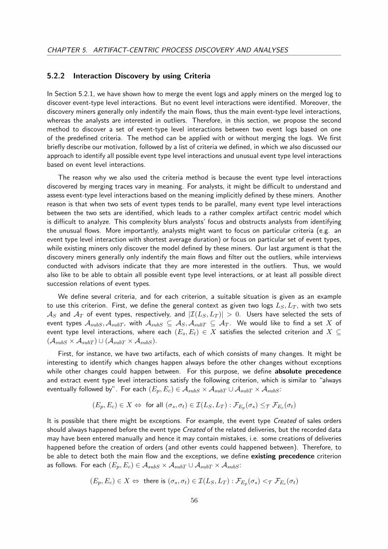
CHAPTER 5. ARTIFACT-CENTRIC PROCESS DISCOVERY AND ANALYSES
5.2.2 Interaction Discovery by using Criteria
In Section 5.2.1, we have shown how to merge the event logs and apply miners on the merged log todiscover event-type level interactions. But no event level interactions were identified. Moreover, thediscovery miners generally only indentify the main flows, thus the main event-type level interactions,whereas the analysts are interested in outliers. Therefore, in this section, we propose the secondmethod to discover a set of event-type level interactions between two event logs based on oneof the predefined criteria. The method can be applied with or without merging the logs. We firstbriefly describe our motivation, followed by a list of criteria we defined, in which we also discussed ourapproach to identify all possible event type level interactions and unusual event type level interactionsbased on event level interactions.
The reason why we also used the criteria method is because the event type level interactionsdiscovered by merging traces vary in meaning. For analysts, it might be difficult to understand andassess event-type level interactions based on the meaning implicitly defined by these miners. Anotherreason is that when two sets of event types tends to be parallel, many event type level interactionsbetween the two sets are identified, which leads to a rather complex artifact centric model whichis difficult to analyze. This complexity blurs analysts’ focus and obstructs analysts from identifyingthe unusual flows. More importantly, analysts might want to focus on particular criteria (e.g. anevent type level interaction with shortest average duration) or focus on particular set of event types,while existing miners only discover the model defined by these miners. Our last argument is that thediscovery miners generally only indentify the main flows and filter out the outliers, while interviewsconducted with advisors indicate that they are more interested in the outliers. Thus, we wouldalso like to be able to obtain all possible event type level interactions, or at least all possible directsuccession relations of event types.
We define several criteria, and for each criterion, a suitable situation is given as an exampleto use this criterion. First, we define the general context as given two logs LS , LT , with two setsAS and AT of event types, respectively, and |I(LS , LT )| > 0. Users have selected the sets ofevent types AsubS ,AsubT , with AsubS ⊆ AS ,AsubT ⊆ AT . We would like to find a set X ofevent type level interactions, where each (Es, Et) ∈ X satisfies the selected criterion and X ⊆(AsubS ×AsubT ) ∪ (AsubT ×AsubS).
First, for instance, we have two artifacts, each of which consists of many changes. It might beinteresting to identify which changes happen always before the other changes without exceptionswhile other changes could happen between. For this purpose, we define absolute precedenceand extract event type level interactions satisfy the following criterion, which is similar to “alwayseventually followed by”. For each (Ep, Ec) ∈ AsubS ×AsubT ∪ AsubT ×AsubS :
(Ep, Ec) ∈ X ⇔ for all (σs, σt) ∈ I(LS , LT ) : FEp(σs) ≤T FEc(σt)
It is possible that there might be exceptions. For example, the event type Created of sales ordersshould always happened before the event type Created of the related deliveries, but the recorded datamay have been entered manually and hence it may contain mistakes, i.e. some creations of deliverieshappened before the creation of orders (and other events could happened between). Therefore, tobe able to detect both the main flow and the exceptions, we define existing precedence criterionas follows. For each (Ep, Ec) ∈ AsubS ×AsubT ∪ AsubT ×AsubS :
(Ep, Ec) ∈ X ⇔ there is (σs, σt) ∈ I(LS , LT ) : FEp(σs) <T FEc(σt)
56

CHAPTER 5. ARTIFACT-CENTRIC PROCESS DISCOVERY AND ANALYSES
We might say that when one event type always happens shortly after another event type, i.e. thetime duration between the events of the two event types are shortest, then there might be a causalrelation. We define this as another criterion shortest time which select only two event type levelinteractions:
(Ep, Ec) ∈ X ⇔(min(Ep,Ec)∈AsubS×AsubT (
∑(σs,σt)∈I(LS,LT ) AvgT imeDur(FEp (σs),FEc (σt))
|I(LS ,LT )| ) ∨
min(Ep,Ec)∈AsubT×AsubS
∑(σs,σt)∈I(LS,LT ) AvgT imeDur(FEp (σs),FEc (σt))
|I(LS ,LT )| )
Note, for the above three criteria, we could also used the parent oriented interactions set IP (LS , LT )or the child oriented interactions set IC(LS , LT ). However, when the merged log is used, the criteriashould based on the combination oriented interactions.
Event Level Interaction and Outlier Identification
We have argued that discovery miners only identify main flows (i.e. only main event type levelinteractions), and analysts would like to identify outliers. Therefore, we propose a criterion usingthe merged log to identify all possible event-type level interactions based on event level interactions.First we define an event level interaction as follows. For a direct succession of two events (ei, ei+1) ina merged trace, if they belong to different original event sets (of the two log), then there is an eventlevel interaction between them. Formally, if (ei, ei+1) ∈ M(σs, σt) ∧ (σs, σt) ∈ I(LS , LT ) ∧ ((ei ∈ES ∧ ei+1 ∈ ET ) ∨ (ei ∈ ET ∧ ei+1 ∈ ES)), then (ei, ei+1) is an event level interaction.
An important remark here is that the event level interactions we defined is totally unrelated tothe set XminerOnMergedLog of event type level interactions we identified by applying a miner on themerged log. Thus, event level interactions (defined here) are not instantiated from these event typelevel interactions. However, the merged log can be used to identify these event level interactionsbetween the logs LS and LT . Moreover, we can use these event level interactions, to identify allpossible combination of a direct succession of two event types, for which an event level interactionexisted. We define this condition as the existence of an event level interactions criterion:
(Ep, Ec) ∈ X ⇔
∃(σs, σt) ∈ I(LS , LT ) : ∃(ei, ei+1) ∈M(σs, σt) :#eventType(ei) = Ep ∧#eventType(ei+1) = Ec ∧ ((ei ∈ ES ∧ ei+1 ∈ ET ) ∨ (ei ∈ ET ∧ ei+1 ∈ ES))
We can use the set XexistenceEventLevelI of event type level interactions identified based on the theexistence of an event level interactions criterion to illustrate the possible event type level interactions(i.e. possible combination of direct succession of two event types) that is not discovered by applyinga miner on the merged log. Since we assume the miners identify the main flows, we considerXexistenceEventLevelI\XminerOnMergedLog as the set of unusual event type level interactions (i.e.outliers).
To only retrieve the event type level interaction in XexistenceEventLevelI that has the maximalnumber of event level interactions found in the merged log, we define the last criterion max numberof event level interactions as:
57

CHAPTER 5. ARTIFACT-CENTRIC PROCESS DISCOVERY AND ANALYSES
(Ep, Ec) ∈ X ⇔
max(Ep,Ec)∈AsubS×AsubT⋃
(σs,σt)∈I(LS ,LT ){(ei, ei+1) | (ei, ei+1) ∈ σ ∧ σ ∈M(σs, σt) ∧#eventType(ei) = Ep ∧#eventType(ei+1) = Ec}
∨max(Ep,Ec)∈AsubT×AsubS
⋃(σs,σt)∈I(LS ,LT )
{(ei, ei+1) | (ei, ei+1) ∈ σ ∧ σ ∈M(σs, σt) ∧#eventType(ei) = Ep ∧#eventType(ei+1) = Ec}
For this thesis, we have only defined and implemented the aforementioned criteria and used thesein the case studies. Investigating and implementing other criteria is listed as future work.
5.2.3 Limitations
One of the main limitations of these event type level interaction identification is that the interactionsare limited to two artifacts only. For example, we have three event logs, sales order, deliveries, andinvoices. The sales orders have interactions towards deliveries, and the deliveries have interactionstowards invoices. When we have identified the creation of invoices has lead to the creation ofdeliveries, and the creation of orders has also lead to the creation of deliveries, but no informationrelating the creation of orders and the creation of invoices can be obtained.
For the above mentioned limitation, two solutions can be applied. One can identify the artifacttype level interactions between the sales orders and invoices, and then use the artifact instance levelinteractions extracted to identify interactions between sales orders and invoices. Another solutionis proposed but not realized due to the time scope of this thesis. One can merge multiple logs toovercome this limitation of event type level interactions. We can again create an interaction graphfor the event logs, and the validness we defined for type level interactions might be reused. Thenthe logs can be merged using the interaction links.
Conducting case studies has found another limitation of this method which is also mentionedbefore. Assume there is a trace with an event ea, and the trace interacts with another trace withtwo events eb and ec. All three events happened on the same time. Since the ordering of eventswhich has the same timestamps are not deterministic, we could have different traces merged fromthe two traces, which leads to different interactions even using the same Miner(L), or differentevent level interactions identified using the the existence of an event level interactions criterion. Ifthere are multiple similar traces merged differently, the complexity of the resulting model increasesunnecessarily.
5.3 Artifact-Centric Model Discovery
In Sections 5.1.2 and 5.2, we have presented the discovery of life cycles and interactions betweenevent types. In this section, we use the life cycles and the interactions discovered to create anartifact-centric process model. Due to the academic background of this thesis, the formal modellanguage proclet system (explained in Section 2.1.3) is used to describe the processes discoveredsuch that formal constructions such as AND-splits, XOR-splits and silent transitions can be usedto illustrate and analyze the model behavior. In Section 5.3.1, we show how we create a procletsystem. However, since the thesis also has a business context and interests, the model viewed by
58

CHAPTER 5. ARTIFACT-CENTRIC PROCESS DISCOVERY AND ANALYSES
users should be easy to understand, which means as simple as possible. Therefore, it is decided toalso visualize a simple representation from a proclet system which is introduced in Section 5.3.2.
5.3.1 Proclet System Creation
Let a set PN of Petri nets be given, each PNi ∈ PN describes the life cycle of artifact Ai. Moreover, amapping function Q ⊆ (PN×PN)→ A×A is available, which returns a set X ⊆ AS×AT∪AT×ASof event type level interactions between two petrinets when given the two petri nets PNS , PNT ∈PN. In addition, for each petri net PNi, we have a function ATi : Ai → Tiv that maps an eventtype to the corresponding labeled transition in the Petri net. We present a method which creates acorresponding proclet system (introduced in Section 2.1.3) by mapping each Petri net to a procletand creating the ports for each petrinet and channels between the proclets.
We define the constraint (according to the definition of ports) that every port is connect toone transition, and each transition is only connect to one input port and one output port. Thisconstraint is due to the fact that when a transition is connected to two output ports, there is noexplicit expressiveness (identifiable) to distinguish whether a message is sent via both output ports(AND-splits), or it is only sent via one output port depending on a condition.
First, we create ports for each petri net PNs ∈ PN as follows. Given a petri net PNs representingthe life cycle of artifact As, we return a union set Xs of all its event type level interactions towards anyother net PNi ∈ PN, i.e. Xs =
⋃PNi∈PNQ(PNs, PNi). For each event type EsOutput of the artifact
As, if there is an event type level interaction (EsOutput, Ei) ∈ Xs and (EsOutput, Ei) ∈ As×Ai, wecreate an output port for the labeled transition ATs(EsOutput) of event type EsOutput in petri netPNs. For each event types EsInput of PNs, if there is an event type level interaction (Ei, EsInput) ∈Xs and (Ei, EsInput) ∈ Ai ×As, we create an input port for the transition ATs(EsInput) of eventtype EsInput in petri net PNs.
Now that we have the ports created for the transitions (representing the event types), we connectthe output port of transition AT (Ei) to the input port of transition AT (Ej) for each distinct eventtype level interaction (Ei, Ej) ∈ X =
⋃PNi∈PN,PNj∈PNQ(PNi, PNj).
5.3.2 Simple representation
Due to the business context of this thesis, interviews have be conducted with advisors of KPMGto investigate the requirements of clients for the process model. The result of the investigationhas indicated that the proclet system will be too difficult to be understood by the clients or tootime-consuming to be explained to the clients. One of the customers involved in the case study alsoindicates that he is less interested in the notions of places, tokens, silent transitions, AND-splits andOR-splits and finds the sequential relations containing adequate information. Therefore, a simplerepresentation is used to visualize the proclet system, which is similar to a simple dependency graph.
Given a proclet system, we visualize a simple representation as follows. For each proclet, first,each place found is removed by connecting each input transition to each output transition of thisplace, which results in a graph only consisting of transitions and arcs between transitions. Then,each silent transition found is removed by directly connecting each of its input transitions with eachof its output transitions. Having all silent transitions removed, we obtain a graph with only labeledvisible transitions and arcs between the visible transitions indicating sequential dependencies. Then,
59

CHAPTER 5. ARTIFACT-CENTRIC PROCESS DISCOVERY AND ANALYSES
for each channel found between two ports, we draw an arc from the transition which is connected tothe input port of the channel to the transition which is connected to the output port of the channel.
The simple representation of the OTC example visualizing the proclet system is shown in Fig-ure 1.7. Each large gray rectangle represents the life-cycle of an artifact visualizing the underlyingproclet (class). An arc within the large gray rectangle represents a sequential dependency betweenthe event types of the artifact. An arc connecting two transitions crossing over two large rectanglesrepresents an event type level interaction between the two transitions.
5.4 Artifact-Centric Process Analyses
Business users tend to compare a process model returned by discovery techniques to a process modelthey are familiar with in order to detect unusual flows. For example, when a model is discoveredin which an arc is found from the Delivery Created event type to the Sales Order Created eventtype, which indicates the deliveries is created before the related sales order, business users shallimmediately spot this unusual arcs and consider this arc as a risk or an outlier. As the meaning ofan arc is ambiguous and depends on the specific discovery technique applied, more information ofthe model should be given for users to assess the model.
In this section, we first illustrate several functions to retrieve information when given an eventtype level interaction in Section 5.4.1.
5.4.1 Traceability
One of the requirements is that it should be possible to retrieve traces from a given element of themodel. In this section, we first illustrate the information that we can highlight for a chosen eventtype level interaction, followed by the information we can highlight for a chosen proclet.
Given an event type level interaction (ES , ET ), we categorize each combination oriented tracelevel interaction (σS , σT ) ∈ I(LS , LT ) into one of the following four types. We assume, the traceσS contains at least one event with event type ES and the trace σT contains at least one event withevent type ET :
(1) parent trace σS is restrictively equal to child trace σT on this interaction: for each es ∈FES (σS), for each et ∈ FET (σT ), with timestamp T (es) = T (et).
(2) parent trace σS is restrictively eventually before child trace σT on this interaction: for eaches ∈ FES (σS), for each et ∈ FET (σT ), with timestamp T (es) ≤ T (et), And there is es ∈ FES (σS),et ∈ FET (σT ), with timestamp T (es) < T (et).
(3) parent trace σS is restrictively eventually after child trace σT on this interaction: for eaches ∈ FES (σS), for each et ∈ FET (σT ), with timestamp T (es) ≥ T (et), and there is es ∈ FES (σS),et ∈ FET (σT ), with timestamp T (es) > T (et).
(4) parent trace σS is parallel to child trace σT on this interaction: there is es1, es2 ∈ FES (σS),et1, et2 ∈ FET (σT ), with timestamp T (es1) < T (et1), and T (et2) < T (es2)
Similarly, it is also possible to categorize a parent oriented trace level interaction (σS , {σT1 · · ·σTn}) ∈IP (LS , LT ) into the four categories, given an event type level interaction (ES , ET ). For example,
60

CHAPTER 5. ARTIFACT-CENTRIC PROCESS DISCOVERY AND ANALYSES
parent trace σS is restrictively equal to child trace(s) {σT1 · · ·σTn} on this interaction: for eaches ∈ FES (σS) if and only if for each et ∈
⋃1≤i≤nFET (σT i), with timestamp T (es) = T (et).
In addition, if the merging method is used, we will also be able to give information about the eventlevel interactions found in the merged log using the event level interactions defined in Section 5.2.2.Since the merging method is combination-oriented, the event level interactions are also combinationoriented.
When users selecting an event type level interaction (arc), we can retrieve the parent traceswhich restrictively before, equal to, after of parallel to the child traces of the interaction (ES , ET )based on the orientation of interactions to allow users further interpreting, reasoning, and assessingthis interactions self.
When selecting a proclet, we illustrate the artifact type level interactions of the artifact repre-sented by this proclet, where the artifact is the parent artifact thus containing the interactions inthe log. In addition, we also categorize the trace level interactions (i.e. the artifact instance levelinteractions of the artifact type level interaction) into four options. (1) the traces of this artifactthat have an interaction with the traces which are found in the child artifact log. (2) the tracesof this artifact having interactions with the case of the child artifact but not founded in the childlog. (3) the traces of this artifact that have no trace level interactions. (4) the traces of the childartifact that have no interactions with the parent traces (i.e. the child traces do not appear in theinteraction attribute of the parent traces). When verifying these four types, it was noticed that dueto the single parent side trace level interactions extraction, there might be false positives in thefourth option, which means the child trace had a reference, however, the referred parent trace iseither not extracted or is not in the data source download. This issue is solvable by extracting theinteraction on both sides.
We conclude this chapter by giving an overview of the achievements. Figure 5.2 shows a simplerepresentation of the artifact centric model of the OTC example. In Section 5.1.2, we have shownhow to discovery life cycles of artifact by using an existing discovery miner. In Section 5.2, wehave presented two different method to discover event type level interactions: one (described inSection 5.2.1) merges trace level interrelated event logs and applies an existing discovery minerto identify the direct successors that are originating from different artifacts as event type levelinteractions. The second method (described in Section 5.2.2) uses one of the predefined criteriato identify event type level interactions. By using the second method, we have also shown howto identify the set of all possible event type level interactions based on direct succession of eventswhich are found in the merged log and belong to different artifacts (i.e. event level interaction). Weused this set to discover unusual flows that are found in this set but not discovered by applying aminer on the merged log (e.g. shown by the red arcs in Figure 5.2). Finally, in Section 5.4, we haveshown how to create a proclet system and visualize the proclet system with a simple representationfor process analyses, followed by how we highlight the information for analysts to retrieve cases andassess the model.
61

Figure 5.2: An artifact centric model of the OTC examplethe red arcs represent unusual flows

Chapter 6
Implementation
In Chapters 3-5, we have shown our approach that addresses (I) the extraction of event logs (withinteractions) and (II) automatically mining a proclets system, shown in Figure 1.9. For each part,a prototype is built to implement and test the approach. In this chapter, we shall briefly explainthe architecture of the two implementations and the important design decisions. Moreover, screen-shots are given to illustrate the execution of the approach. Since the first part of the approachcan reuse the functions of the previous implemented XTract application, it is decided to reuse theimplementation and extend the data model and structures to achieve the requirements. The newXTract approach is called XTract2 , which is discussed in Section 6.1. The second part is consideredto be a mining algorithm. ProM has provided a framework for handling the import of event logsand visualization. Therefore, we decide to implement the mining algorithm as a plug-in for ProM inJava, we called the InteractionMiner .
6.1 XTract2
We have realized our approach regarding the three phases, (A) artifact type identification, (B) typelevel interaction identification and (C) Log extraction, of (I) the extraction problem (discussed inChapters 3 and 4) in the XTract2 tool. In this section, we first give an architecture overview of theXTract2 tool and the functionality of each component. Then, examples are given to illustrate theflow of calls. Finally, we show some screen-shots of the tool.
The architecture of the XTract2 tool, illustrated in Figure 6.1, follows in general the model-view-controller architectural pattern. We shall briefly describe the function of each componentby going through a flow of calls. The GUI component consists of an UI package which handlesall human-machine interactions between users and the XTract2 application. For example, userscan specify the internal cache database which should be used, select the source database, canimport the schema and change the artifacts and interactions. The GUI component handles theuser inputs by calling the packages in the Controller component, i.e. Algorithms, ArtifactController,Data.dataImport and Data.datapersistence. The Algorithms package of the XTract application isunchanged and reused for calculations such as automatic schema identification, artifact (withoutinteractions) creation, and column domain identifications. The ArtifactController handles variouschanges on the artifacts and their type level interactions. The Data.dataImport package uses the
63

CHAPTER 6. IMPLEMENTATION
JDBC connector to processes various types of source data, import the data and relational datastructure and pass through the Data.persistence package. The Data.persistence package also usesthe JDBC connector to handle data insertion, extraction and deletion in the cache database. Andboth GUI and Controller components uses the data models in the Models component to transferdata within the application.
For example, users specified the data source and the internal cache databases via the UI package,the UI package calls the Data.dataImport package to import the tables, columns and schemas fromthe source databases and calls the Data.persistence package to create a schema and insert data intothe cache database. By calling the functions in the Algorithm package via UI, users can identifyartifact schemas and create artifacts. When users modify the artifacts, the UI package calls theArtifactController to temporarily change the structure of the artifact. Both objects can be storedpersistently in the cache database via the Data.persistence package. To recall the artifacts identified,the Data.persistence package extracts data from cache database and uses the Models package tocreate models which can be demonstrated to users by GUI. When users indicate to extract theartifact via the UI, the UI calls the functions in the Algorithms package, which create a mappingmodel and used this mapping to create a cache for the OpenXES to write the event log.
XTract2
GUI Models
Controller
PAGE
23
Artifact &
interactions
Mappings
XES model
XES
Event
log
UI
Data.
persistence
Algorithms Artifact
Controller
Data.
dataImport
Source
Database Cache
Database
XES
Event
log
Figure 6.1: Architecture of XTract2
ProM framework
InteractionMiner
PAGE
23
Vizualizer
Merger
Miners
Lifecycle
Miners
Miner
Plugin
Proclets
system
XES
Event
logs
Merged
log
Figure 6.2: Architecture ofInteractionMiner
Figure 6.3: XTract2 - (A1) Import Data schema
We will illustrate the XTract2 tool based on the three phases of the extraction approach explainedin Section 1.4 by emphasizing on the new functionality. The same numbering is used. As the
64

CHAPTER 6. IMPLEMENTATION
‘import data schema’ button in Figure 6.3 shows, we have added the functionality to allow importdata schema (A1). The ‘Artifact schema identification by splitting tables’ button calls the newimplemented the ComputeArtifactSchemas(S) algorithm to identify artifact schemas. Figure 6.4shows the interface where users can perform the following tasks:
• add and remove tables of artifact schemas;• construct artifacts with conditions;• construct event types with conditions;• add and remove event types, attributes and interactions;• calculate type level interactions;• extract event logs;
Figure 6.4: XTract2 - (A2) Artifact schema identification and (A3) Artifact identification
Figure 6.5: XTract2 - (B) Interaction Identification and Interaction Graph
The interaction graph is shown in a separate frame illustrated by Figure 6.5. Users can selectan interaction in Figure 6.4 to highlight the links of this interactions with red color in the interfaceshown in Figure 6.5. By clicking the ‘Create Log’ button, the XTract2 tool automatically createsthe log mapping (with type level interactions) and an event log for the selected artifact. Figure 6.6shows a part of the mapping and the event log of the artifact Sales Order.
65

CHAPTER 6. IMPLEMENTATION
Figure 6.6: XTract2 - (C) Log extraction : mapping with interactions and an example of eventlog with interactions
6.2 InteractionMiner
In this section, an overview of the architecture of the InteractionMiner plugin is first shown. Then,we demonstrate some screen shots of the plugin to illustrate some functionalities.
The architecture of the InteractionMiner application, illustrated in Figure 6.2, follows a generalProM plug-in pattern, which has a MinerPlugin package, a Visualizer package, a LifecycleMinersand a MergerMiners package. Given a set of XES event logs (with artifact instance level interactions)as input of the MinerPlugin package, the MinerPlugin package calls the specified lifecycle minerfrom the LifecycleMiners package to construct a proclet for each log, then the MinerPlugin mergesthe logs, exports the merged log as an object to the ProM framework and creates a connectionto be able to retrieve the merged log. The MinerPlugin calls the specified MergedLogMiner in theMergedLogMiners to apply it on the merged log which returns event type level interactions identified.The MinerPlugin then returns a proclets system (called artifactModel) to the ProM framework, whichwill automatically call the corresponding visualizer to visualize the proclets system. Users can interactwith the visualizer package to retrieve information or select different interactions.
We illustrate our mining approach by going through the screen shots of the InteractionMinerplugin. First, users can load a set of event logs into ProM and select the logs for applying theInteractionMiner plugin, as shown in Figure 6.7. Then, users can specify the life cycle miningalgorithm and the merged log mining algorithm in the dialog shown in Figure 6.8. If the selectedalgorithm has other settings (e.g. heuristic miner has a dialog to set parameters), these will also beshown. After the miner is finished, we obtain an artifact centric model. Users can select the procletview shown in Figure 6.9 or the simplified representation shown in Figure 6.10 in the visualizer.Furthermore, the right hand side of the visualizer allows users to select a subset of the transitions,to select a criterion for event type level interaction identification, to obtain more information of anelement selected in the model, and to view different flows between two artifacts that have interactionwith each other.
66

Figure 6.7: Selecting event logs forInteractionMiner
Figure 6.8: The dialog to select thelife-cycle miner and the merged logminer
Figure 6.9: The proclet system view of theartifact model in the visualizer
Figure 6.10: The simple representation viewin the visualizer


Chapter 7
Case Studies
We have defined our approach and shown the tools within previous chapters. To verify and vali-date our approach and to use the process models obtained to perform analyses, two case studieswere conducted. In this chapter, for each case study, we shall (1) introduce the process and thedata source, (2) explain the execution of our approach including decisions made, and (3) discussobservations and results we have obtained.
The first case study was performed in the OTC process of SAP. In this case study, we emphasizeon the execution of our approach (such as decisions about the artifact selection and interactionselection) since no customer was involved. The second case study was conducted in the PA processof Oracle. Since customers were involved, we emphasize the discussion of the result of analyses. Forboth case studies, we are guided by the advisors of KPMG, who are the experts in ERP systems anddata analytic and have rich experience of conducting advisory projects for clients.
7.1 Case I - SAP Order To Cash Process
The first case study was performed for the Order to Cash (OTC) process supported by SAP systems.The data is provided by KPMG. Since no specific customer was involved, the requirements of thecase study for the OTC process of SAP were provided by the advisors of KPMG, who are the expertsin SAP systems and have rich experience of conducting advisory projects for clients. Therefore, theresult obtained is also validated and discussed with the advisors. In this section, we first give ashort introduction to the OTC process and the relational data structure that is used by SAP. Then,we emphasize the approach in which we obtain event logs and artifact models of the OTC process.Finally, we discuss some observations about the models obtained.
7.1.1 SAP OTC process and data structure
A simple OTC process in the system starts with creating a sales order. After the order is delivered, adelivery document is created. Then, an invoice document is created in the system, sent to customerand posted in the account receivable (table). After receiving the payment, this simple process ends.However, there are many complex variations of this process. For example, the orders could be linkedto a contract document, or return orders could be placed and return deliveries are made. Credit
69

CHAPTER 7. CASE STUDIES
memo requests might be received from customers when the goods are incomplete or damaged.Invoices might also be canceled.
The data structure used to support the OTC process allows flexibility to deal with the afore-mentioned variance, but it is also very complex. The relational data structure of SAP regardingthe relevant tables of this case study is shown in Figure 7.1. The VBAK table stores various salesdocuments such as sales orders, inquiries, contracts, return orders, credit memo requests and debitmemo requests. As these documents share similar structure, they are put into one table, and thevalue in the column vbtyp indicates the type of a document. Similarly, the delivery documents suchas deliveries, return deliveries and delivery shipping notifications are stored in the LIKP table, and theinvoice documents such as invoices, invoice cancellations, inter-company invoices, and credit memosare stored in the VBRK table. Each document has lines stored separately. For example, a salesorder of a web-shop might have included different products, where each line represents a product(or material) with the ordered quantities. The lines of the sales documents (in VBAK ), the deliverydocuments (in LIKP), and the invoice documents (in VBRK ) are stored in the tables VBAP, LIPS ,and VBRK , respectively. Documents are linked through lines. For example, a delivery (document)could combine various lines from various sales orders which are in the stock. Invoice documentsare then placed in the account receivable tables BKPF and BSID as invoices with open payments.When payments are received, the open payment in the BSID table is deleted and added to the closedpayment table BSAD. Each document and each line could have separate changes performed andstored in the change tables CDHDR and CDPOS . For example, a billing block release is a changeof sales documents, whereas price changes are related to the sales lines.
VBAK
(Sales
documents)
LIKP
(Delivery
documents)
VBRK
(Invoice
documents)
VBAP
(Sales lines)
LIPS
(Delivery
lines)
VBRP
(Invoice lines)
BKPF
(Payment
documents)
CDHDR
(Changes
Header)
One to
many
name Table
BSID
(Open
Payment
documents)
BSAD
(Closed
Payment
documents)
CDPOS
(Changes
LINES)
Figure 7.1: SAP OTC process - relational structure
7.1.2 SAP OTC - Extraction and Discovery
In this section, we emphasize the steps taken and decisions made to obtain an artifact centric modelfor the SAP - OTC process.
70
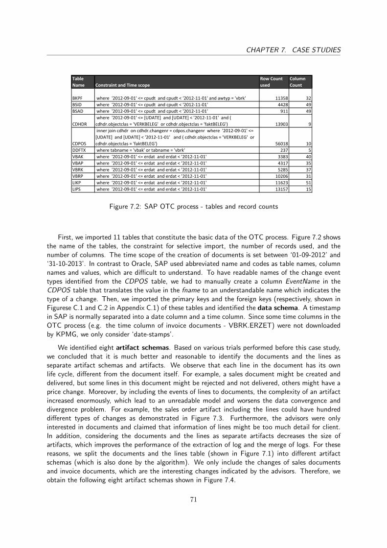
CHAPTER 7. CASE STUDIES
Table
Name Constraint and Time scope
Row Count
used
Column
Count
BKPF where '2012-09-01' <= cpudt and cpudt < '2012-11-01' and awtyp = 'vbrk' 11358 32
BSID where '2012-09-01' <= cpudt and cpudt < '2012-11-01' 4428 49
BSAD where '2012-09-01' <= cpudt and cpudt < '2012-11-01' 911 49
CDHDR
where '2012-09-01' <= [UDATE] and [UDATE] < '2012-11-01' and (
cdhdr.objectclas = 'VERKBELEG' or cdhdr.objectclas = 'faktBELEG') 13903 9
CDPOS
inner join cdhdr on cdhdr.changenr = cdpos.changenr where '2012-09-01' <=
[UDATE] and [UDATE] < '2012-11-01' and ( cdhdr.objectclas = 'VERKBELEG' or
cdhdr.objectclas = 'faktBELEG') 56018 10
DDFTX where tabname = 'vbak' or tabname = 'vbrk' 237 5
VBAK where '2012-09-01' <= erdat and erdat < '2012-11-01' 3383 40
VBAP where '2012-09-01' <= erdat and erdat < '2012-11-01' 4317 35
VBRK where '2012-09-01' <= erdat and erdat < '2012-11-01' 5285 37
VBRP where '2012-09-01' <= erdat and erdat < '2012-11-01' 10206 31
LIKP where '2012-09-01' <= erdat and erdat < '2012-11-01' 11623 51
LIPS where '2012-09-01' <= erdat and erdat < '2012-11-01' 13157 15
Figure 7.2: SAP OTC process - tables and record counts
First, we imported 11 tables that constitute the basic data of the OTC process. Figure 7.2 showsthe name of the tables, the constraint for selective import, the number of records used, and thenumber of columns. The time scope of the creation of documents is set between ‘01-09-2012’ and‘31-10-2013’. In contrast to Oracle, SAP used abbreviated name and codes as table names, columnnames and values, which are difficult to understand. To have readable names of the change eventtypes identified from the CDPOS table, we had to manually create a column EventName in theCDPOS table that translates the value in the fname to an understandable name which indicates thetype of a change. Then, we imported the primary keys and the foreign keys (respectively, shown inFigurese C.1 and C.2 in Appendix C.1) of these tables and identified the data schema. A timestampin SAP is normally separated into a date column and a time column. Since some time columns in theOTC process (e.g. the time column of invoice documents - VBRK.ERZET) were not downloadedby KPMG, we only consider ‘date-stamps’.
We identified eight artifact schemas. Based on various trials performed before this case study,we concluded that it is much better and reasonable to identify the documents and the lines asseparate artifact schemas and artifacts. We observe that each line in the document has its ownlife cycle, different from the document itself. For example, a sales document might be created anddelivered, but some lines in this document might be rejected and not delivered, others might have aprice change. Moreover, by including the events of lines to documents, the complexity of an artifactincreased enormously, which lead to an unreadable model and worsens the data convergence anddivergence problem. For example, the sales order artifact including the lines could have hundreddifferent types of changes as demonstrated in Figure 7.3. Furthermore, the advisors were onlyinterested in documents and claimed that information of lines might be too much detail for client.In addition, considering the documents and the lines as separate artifacts decreases the size ofartifacts, which improves the performance of the extraction of log and the merge of logs. For thesereasons, we split the documents and the lines table (shown in Figure 7.1) into different artifactschemas (which is also done by the algorithm). We only include the changes of sales documentsand invoice documents, which are the interesting changes indicated by the advisors. Therefore, weobtain the following eight artifact schemas shown in Figure 7.4.
71

CHAPTER 7. CASE STUDIES
14
3
5
95
30
10
1
3
1
2
1
40
96
30
4
1
6
20
234
110
5
74
18
2
7
531
90
1
1
11
64
4
37
108
4
64
2
16
3
66
2
1
1
5
71
3
24
21
5
41
63
3
6
12
1
36
156
2
3
9
49
1
7
66
1
12
13
3
1
1
8
3
25
5
4
1
136
57
13
3
144
1
5
5
71
5
35
85
1
6
1
4
1
1
3
1
164
4
1
2
6
116
312
1
62
2
1
80
27
58
1
15
4
30
6613
127
41
33
3
2
75
35
1
38
5
54
210
1
11
22
148
48
35
16
8
51
2
56
6
245
6
5 4
72
1
71
19
1
2
136
4
2
870
9
75
1
141
24
177
18
21
1
37
1
54
3 7
2
1
67
1
2
63
11
6
6
1974
1
2
1291
Delivery blockU177
Customer group 1U109
Matl Staging TimeU75
Transp. Plan. TimeU64
Order created2581
Rel. credit valueU240
Loading TimeU64
Overall CreditStatusU462
Release dateU242
Goods Issue TimeU62
Shipping Point/Receiving PtU167
Confirmation statusU167
Confirmed QuantityU1362
Sales Document: PartnerKEY I7730
Goods Issue DateU617
Requested deliv.dateU145
Next dateU536
Billing DateU246
Sales Document: Schedule Line DataKEY D213
Transptn Plang DateU617
Incoterms (Part 2)U313
Pricing dateU199
Loading DateU617
Material Avail. DateU646
Order quantityU317
Delivery DateU577
Net priceU564
Credit priceU1342
RouteU284
Shipping ConditionsU51
Item delivery data..U125
Overall statusU305
Underdel. ToleranceU27
Unlimited toleranceU7
Manual priceU130
Overdeliv. ToleranceU27
Terms of PaymentU42
Partner DescriptionU28
Billing blockU177
Invoicing datesU9
Transportation zoneU93
CustomerU120
Sales Document: Business DataKEY D1
Sales Document: Item DataKEY D23
Sales Document: Item DataKEY I465
PO numberU170
Next checkU111
Sales Document: Schedule Line DataKEY I649
Delivery PriorityU1
Purchase order dateU20
Oldest open itemsU25
Country KeyU70
Sales Document: PartnerKEY D30
Risk categoryU2
Customer groupU1
Credit accountU7
Storage LocationU72
Fixed date and qtyU81
Complete deliveryU27
Sold-to partyU1
MRP AreaU104
PlantU104
Translation DateU46
Exchange RateU17
Reason for rejectionU38
Special proc. indicatorU29
Item of RequisitionU22
Purchase RequisitionU20
Profit CenterU80
MaterialU95
Planning plantU12
Dynamic checkU188
Availability checkU7
Arrival timeU5
BatchU12
Sched.line categoryU39
IncotermsU153
Requirements typeU10
DescriptionU9
Material GroupU5
Order reasonU4
Lett.-of-credit crcyU1
Personnel NumberU4
Unit of measureU6
Financial documentU1
Shipping typeU2
Ex.rate-LettOfCreditU1
Financial doc. no.U8
Means-of-Trans. TypeU7
Part.dlv./itemU6
Header delivery dataU7
Serv.rendered dateU3
Bus.transaction typeU2
Means of transportU8
Item categoryU7
Purch. Doc. CategoryU8
EU triangular dealU1
VendorU5
Material freight grpU3
Header dataU7
Tax depart. countryU2
Figure 7.3: SAP OTC process - sales order lifecycle including the changes of lines
Artifact Schema Maintable Artifact Artifact condition Extracted
BKPF BKPF PostInAR <maintable>.awtyp = 'VBRK' Yes
Payment05or15 (<maintable>.bschl = '05' or <maintable>.bschl = '15') Yes
Payment01or11 (<maintable>.bschl = '01' or <maintable>.bschl = '11')
Delivery H <maintable>.vbtyp = 'J' Yes
DeliveryShippingNotification H <maintable>.vbtyp = '7' Yes
ReturnDelivery H <maintable>.vbtyp = 'T' Yes
Delivery L inner join tableLIKP y1 on <maintable>.vbeln = y1.vbeln and y1.vbtyp = 'J'
DeliveryShippingNotification L inner join tableLIKP y2 on <maintable>.vbeln = y2.vbeln and y2.vbtyp = '7'
ReturnDelivery L inner join tableLIKP y3 on <maintable>.vbeln = y3.vbeln and y3.vbtyp = 'T'
Contract H <maintable>.vbtyp = 'G' Yes
ReturnOrder H <maintable>.vbtyp = 'H' Yes
DebitMemoRequest H <maintable>.vbtyp = 'L' Yes
Order H <maintable>.vbtyp = 'C' Yes
CreditMemoRequest H <maintable>.vbtyp = 'K' Yes
Contract L inner join tableVBAK s1 on <maintable>.vbeln = s1.vbeln and s1.vbtyp = 'G'
ReturnOrder L inner join tableVBAK s2 on <maintable>.vbeln = s2.vbeln and s2.vbtyp = 'H'
DebitMemoRequest L inner join tableVBAK s3 on <maintable>.vbeln = s3.vbeln and s3.vbtyp = 'L'
Order L inner join tableVBAK s4 on <maintable>.vbeln = s4.vbeln and s4.vbtyp = 'C'
CreditMemoRequest L inner join tableVBAK s5 on <maintable>.vbeln = s5.vbeln and s5.vbtyp = 'K'
Invoice H <maintable>.vbtyp = 'M' Yes
ProFormaInvoice H <maintable>.vbtyp = 'U' Yes
IntercompanyCreditMemo H <maintable>.vbtyp = '6' Yes
CreditMemo H <maintable>.vbtyp = 'O' Yes
DebitMemo H <maintable>.vbtyp = 'P' Yes
CreditMemoCancellation H <maintable>.vbtyp = 'S' Yes
IntercompanyInvoice H <maintable>.vbtyp = '5' Yes
InvoiceCancellation H <maintable>.vbtyp = 'N' Yes
Invoice L inner join tableVBRK t1 on <maintable>.vbeln = t1.vbeln and t1.vbtyp = 'M'
ProFormaInvoice L inner join tableVBRK t2 on <maintable>.vbeln = t2.vbeln and t2.vbtyp = 'U'
IntercompanyCreditMemo L inner join tableVBRK t3 on <maintable>.vbeln = t3.vbeln and t3.vbtyp = '6'
CreditMemo L inner join tableVBRK t4 on <maintable>.vbeln = t4.vbeln and t4.vbtyp = 'O'
DebitMemo L inner join tableVBRK t5 on <maintable>.vbeln = t5.vbeln and t5.vbtyp = 'P'
CreditMemoCancellation L inner join tableVBRK t6 on <maintable>.vbeln = t6.vbeln and t6.vbtyp = 'S'
IntercompanyInvoice L inner join tableVBRK t7 on <maintable>.vbeln = t7.vbeln and t7.vbtyp = '5'
InvoiceCancellation L inner join tableVBRK t8 on <maintable>.vbeln = t8.vbeln and t8.vbtyp = 'N'VBRPVBRP
VBAK
VBAP
VBAK
VBAP
VBRKVBRK
BSAD BSAD
LIKP LIKP
LIPS LIPS
Figure 7.4: SAP OTC process - artifacts
72

CHAPTER 7. CASE STUDIES
We identify one or multiple artifacts for each artifact schema as illustrated by the third columnin Figure 7.4. For the BKPF artifact schema which describes payment documents, only one artifactis identified. The advisors indicates that the value in the bschl column of the closed payment table(BSAD) refers to the type of payment. When the value in the bschl column is 05 or 15, it indicatesthat the record is a real payment received. Therefore, a separate artifact type is created. For thesales documents (VBAK ) and lines (VBAP), delivery documents (LIKP) and lines (LIPS), andinvoice documents (VBRK ) and lines (VBRP), there is a column vbtyp in the document tables thatindicate the type of documents. Therefore, we created the artifacts of documents and lines basedon the values found in this column. In total, we have identified 35 artifacts.
To identify and select the artifact type level interactions, several decisions were made basedon the interviews with advisors. First, only the documents were interesting for the advisors, thus lineartifacts and their interactions were omitted. This requirement and the OTC table structure shownin Figure 7.1 indicates that a weak join has to be included. For example, a sales document must firstjoin the sales lines, then join the delivery lines, to join the delivery document, in which the last joinis an over-approximation. Second, there is a type of foreign keys in the sales, delivery and invoicedocuments that indicate the previous document(s) of a record, i.e. the vgbel and vgpos columns.This previous document relation is very interesting since the relation indicates the transformation(or causality) between different type of documents. Therefore, if this foreign key existed, we selectthe interactions that are based on this reference. Furthermore, since the main goal is to identifyoutliers, any interaction with at least one record is selected. Thus, we have set the least number ofrecord r = 1, the number of strong joins k = 2 and the number of weak joins m = 1. Figure 7.5shows a screen shot of the interaction graph that is constructed. The type level interactions thatare selected and extracted are shown in Figure 7.6.
Figure 7.5: SAP OTC process - interaction graph
For each artifact shown in Figure 7.6, we obtain an event log with trace level interaction. Intotal, 18 event logs are extracted and imported into ProM. Using the heuristic miner as the life-cycleminer and the merged log miner, we obtain the artifact-centric system shown in Figure 7.7. Eachlife cycle only contains one event type to first have a simple helicopter view. Thus, for all artifactsexcept artifact ‘payment05or15’, we first only considered extracting the Creation event type. Forthe artifact ‘payment05or15’, we only considered the clearing date (i.e. the column augdt). This
73
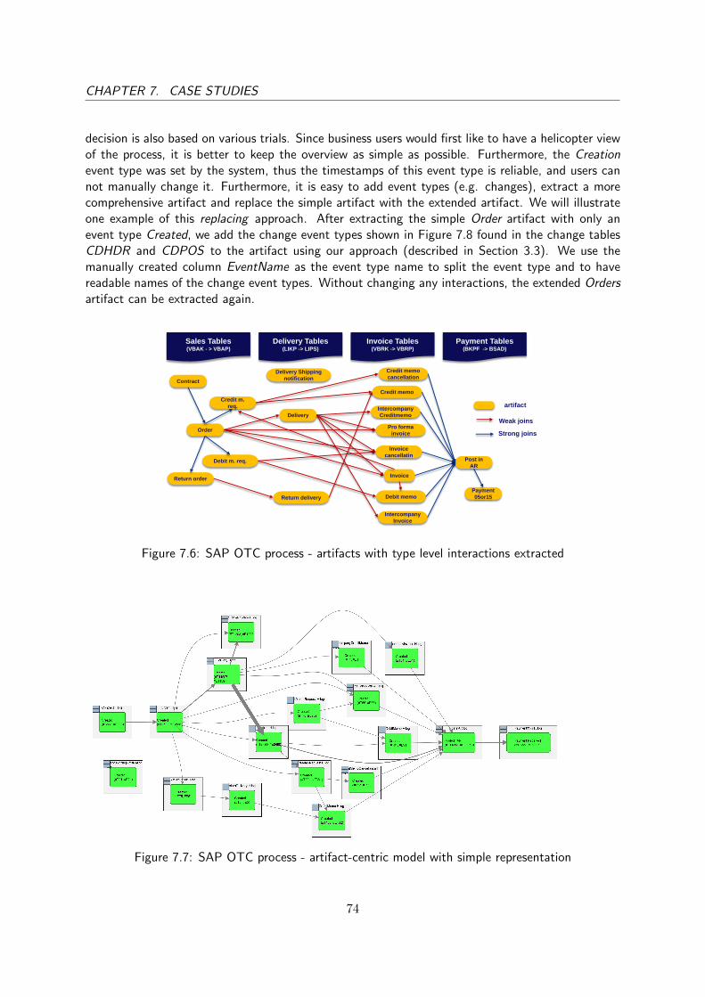
CHAPTER 7. CASE STUDIES
decision is also based on various trials. Since business users would first like to have a helicopter viewof the process, it is better to keep the overview as simple as possible. Furthermore, the Creationevent type was set by the system, thus the timestamps of this event type is reliable, and users cannot manually change it. Furthermore, it is easy to add event types (e.g. changes), extract a morecomprehensive artifact and replace the simple artifact with the extended artifact. We will illustrateone example of this replacing approach. After extracting the simple Order artifact with only anevent type Created, we add the change event types shown in Figure 7.8 found in the change tablesCDHDR and CDPOS to the artifact using our approach (described in Section 3.3). We use themanually created column EventName as the event type name to split the event type and to havereadable names of the change event types. Without changing any interactions, the extended Ordersartifact can be extracted again.Motivation - Complexity
PAGE 4
Sales Tables (VBAK - > VBAP)
Delivery Tables (LIKP -> LIPS)
Invoice Tables (VBRK -> VBRP)
Payment Tables (BKPF -> BSAD)
Order
Delivery
Invoice Return order
Return delivery
Credit memo
Payment
05or15
Contract
Credit m.
req.
Debit m. req.
Credit memo
cancellation
Post in
AR
Pro forma
invoice
Debit memo
Invoice
cancellatin
Context – Artifacts– Interactions - Discovery & Analyses – Case Studies - Conclusion
Strong joins
Intercompany
Invoice
Intercompany
Creditmemo
Delivery Shipping
notification
Weak joins
artifact
Figure 7.6: SAP OTC process - artifacts with type level interactions extracted
Figure 7.7: SAP OTC process - artifact-centric model with simple representation
74

CHAPTER 7. CASE STUDIES
Figure 7.8: SAP OTC process - the Orders artifact with change event types
7.1.3 SAP OTC - Process Analyses and Discussion
In this section, we discuss three observations: identifying unusual flows, extending and replacingartifacts and the complexity of interactions.
One of the analyses is to identify unusual flows. In the “Interaction Filter” tabbed panel on theright hand side of the InteractionMiner visualizer, we can select the ‘show all interactions’ optionand obtain all event type level interactions using the existence of an event level interactions criterion(described in Section 5.2.2). Moreover, the unusual event type level interactions which are obtainedby using this criterion but not discovered by the miner (also described in Section 5.2.2) are coloredred. The model shown in Figure 7.9 demonstrate only one unusual flow (indicated by the red arc):there were payments received before the invoices were created in the account receivable.
Figure 7.9: SAP OTC process - artifact-centric model with outliers
Verifying the cases retrieved via this unexpected flow in the database with the query in Listing 7.1has shown that the Payment Received date is indeed earlier than the Posted In AR event. Advisors
75

CHAPTER 7. CASE STUDIES
have also validated that this flow is strange and can not be explained other than the date weremanually changed. Further investigation conducted by advisors has proved that the cases wasindeed manually changed by someone using the transaction code FB05, which is not a usual action(which has real financial risks). In other words, we have successfully and exploratively discovered atrue-positive unusual action.
Listing 7.1: A query verifying payments received date ealier than invoice placed in AR
SELECT a.BELNR, a.CPUDT, a.AWKEY, b.BELNR, b.BSCHL, b.AUGBL, b.CPUDT, b.AUGDT, c.BELNR, c.cpudt, c.AUGDT, c.BSCHL
FROM bkpf aINNER JOIN BSAD b ON b.BELNR = a.BELNR and b.gjahr = a.gjahr and b.bukrs = a.
bukrs and b.mandt = a.mandtINNER JOIN BSAD c ON c.belnr = b.AUGBL and b.gjahr = c.gjahr and b.bukrs = c.
bukrs and b.mandt = c.mandtWHERE a.CPUDT > c.AUGDT and (b.bschl = ’01’ or b.bschl = ’11’) and (c.BSCHL =
’05’ or c.BSCHL = ’15’) and a.awtyp = ’vbrk’ and a.belnr = ’x’ -- x = caseID
The second observation is that, after creating the artifact centric model shown in Figure 7.7which is simple and easy to analyze, we can now replace simple artifacts with extended artifactsto show more detail of the process. For example, we have created a more comprehensive artifactOrder by adding all change event types found in the change tables (described in Section 7.1.2).Since the trace identifiers have not changed, and interactions have not changed, there is no needto reconstruct other event logs. We replace the simple event log of Order with the comprehensiveevent log of Order, and obtain an artifact centric model shown in Figure 7.10.
Figure 7.10: SAP OTC process - artifact-centric model with the discovered interactions
Note that we can now identify some difference in event type level interactions between the salesorder artifact and other artifacts.
To show this difference more clearly, we obtain a more simplified model shown in Figure 7.11 byusing the max number of event level interactions criterion, that is, we only highlight type levelinteractions where the number of event level interactions is maximal between two artifact types.
76

CHAPTER 7. CASE STUDIES
Figure 7.11: SAP OTC process - artifact-centric model with interactions
The red circles indicate an interesting difference. For example, most artifacts, e.g. delivery,credit memo request, debit memo request are generally created directly after the creation of salesorder, whereas the invoices (that are directly related to a sales order via vgbel and vgpos) are createdafter the Release Date change event type of this sales order. Similar for the invoice cancellationartifact, of which the creation generally takes place after the Next Date of the sales order changes.
Only to illustrate the complexity, we have included the model with all direct interactions shownin Figure 7.12. The red arcs are the unusual event type level interactions which are obtained by usingthe existence of an event level interactions criterion but not discovered by the applying the mineron the merged log (described in Section 5.2.2). As this model is also almost impossible to analyze,further simplification techniques have to be developed. For example, visualization techniques mighthelp improve the understandability of the model such as the edge bundling techniques proposed byD. Holten and J. van Wijk [15].
Figure 7.12: SAP OTC process - artifact-centric model with outliers
77

CHAPTER 7. CASE STUDIES
7.2 Case II - Oracle Project Administration Process
The second case study is performed for the project administration (PA) process supported by theOracle information system of an educational organization. The data is downloaded from the educa-tional organization provided by KPMG. This case study is done based on the request of the client,i.e. the educational organization. Therefore, feedback received from the client is also discussed.First, a brief introduction to the project administration process is given, together with an overviewof the tables that were downloaded and available for analysis.
7.2.1 Oracle PA Process and Data source
An educational organization has thousands of projects running, e.g. different research projects. Theproject administration process supported by Oracle starts with creating projects in the system. At themoment of creating a project in the system, it is usually definitive that the project will be executed.It is possible that the project has already started. After the project is created in the system, onecan specify relevant information of the project such as its starting date. During the execution ofthe project, tasks are created for the project to declare different expenditures related to a task, e.g.personnel, materials. Interviews with advisors have indicated that, for assessing financial risks, it isimportant that the ending date of expenditures is before the the complete date of tasks. Moreover,all tasks should be completed before the completion date of a project. When a project is completed,it means that the main activities, such as the research itself, are finished. When the administrationwork is completed, such as financial checks, the project is closed.
For this case study, 18 tables were downloaded, and 7 tables were used in the actual analysisas shown in Figure 7.13. Due to the time constraint, we have limited our data scope between01-06-2012 and 31-12-2012. The number of the records of each table used in the process analysisis also shown in the fourth column of Figure 7.13.
Table Name
Row Count
downloaded Used
Row Count
used
Column
Count
FND_USER 905 905 27
HR_ALL_ORGANIZATION_UNITS 1053 1053 43
MTL_SYSTEM_ITEMS_B 0
OE_ORDER_HEADERS_ALL 0
PA_COST_DISTRIBUTION_LINES_ALL 95943 x 5543 15
PA_EXPENDITURE_COMMENTS 55149 30511 7
PA_EXPENDITURE_ITEMS_ALL 96978 x 5620 32
PA_EXPENDITURE_TYPES 94 x 94 10
PA_EXPENDITURES_ALL 682590 x 3100 24
PA_PROJECT_CUSTOMERS_V 16238 16238 17
PA_PROJECT_STATUSES 80 x 80 23
PA_PROJECTS_ALL 5364 x 1132 29
PA_TASKS 2416 x 1236 31
PA_TRANSACTION_SOURCES 48 48 4
PAY_COST_ALLOCATION_KEYFLEX 1694 1694 11
PO_HEADERS_ALL 5186 5186 139
PO_LINE_LOCATIONS_ALL 7700 7700 148
PO_LINES_ALL 7700 7700 135
Figure 7.13: Oracle PA process table record counts
78

CHAPTER 7. CASE STUDIES
We briefly describe the eight tables used. Each project corresponds to a record in the PA PRO-JECTS ALL table. The timestamp of the creation of a project is stored in the CREATION DATEcolumn. The starting date, completion date, and closed date of a project are stored in theSTART DATE, COMPLETION DATE and CLOSED DATE columns, respectively. Each task isstored as a record in the PA TASKS table, which has a foreign key to the PA PROJECTS ALLtable. Expenditure documents are stored in the PA EXPENDITURES ALL table, and expendi-ture items of an expenditure document are stored in the PA EXPENDITURE ITEMS ALL. Theexpenditures are linked to the tasks via the PA EXPENDITURE ITEMS ALL table directly. ThePA COST DISTRIBUTION LINES ALL table also provides a link between the tasks and the ex-penditure items. Each expenditure item has an expenditure type which can be categorized intoeight different expenditure category, e.g. ‘Third-party services’, ‘Equipment, Inventory and Soft-ware’, ‘Housing Expenses’. Information of expenditure types and categories are stored in thePA EXPENDITURE TYPES. Each project has a current status (e.g. rejected, approved, closed),and information of the status are stored in the PA PROJECT STATUSES table.
Figure 7.14: Interaction graph of PA artifacts
A document of the tables was provided by advisors of KPMG, which includes information of theprimary keys and foreign keys of the tables, helping us to obtain the data schema. Other tablescontain more informative date and are less relevant for the core PA process.
7.2.2 Oracle PA - Extraction and Discovery
We first have identified 6 artifacts. Since the information stored in the PA PROJECT STATUSEStable and the PA EXPENDITURE TYPES table are only informative and not related to a specificstep of the process, we only considered the other six tables. Each of the six tables is then consideredas an artifact schema and is mapped to one artifact, respectively. The six artifacts are shown in
79

CHAPTER 7. CASE STUDIES
Figure 7.15. Applying the approach described in Section 4.2.1, seven direct type level interactionsare found between the artifacts which are shown in Figure 7.14.
Artifacts Maintable Extracted
Interaction
From To via
Project PA_PROJECTS_ALL x Project Tasks
ExpAll PA_EXPENDITURES_ALL x Tasks ExpAll ExpItem
Tasks PA_TASKS x
CostDistr PA_COST_DISTRIBUTION_LINES_ALL
ExpItem PA_EXPENDITURE_ITEMS_ALL
ExpTypes PA_EXPENDITURE_TYPES
Figure 7.15: The artifacts created for Oracle PA process
Projects Log
Occurrences
(absolute)
Occurrences
(relative)
Trace count 1132
Total event count 5329
Last update 1132 21,2%
Creation 1132 21,2%
Start 1111 20,8%
Program update 757 14,2%
Completion 715 13,4%
Closed 482 9,0%
Tasks Log
Occurrences
(absolute)
Occurrences
(relative)
Trace count 1236
Total event count 4383
Last update 1236 28,2%
Creation 1236 28,2%
Start 1216 27,7%
Completion 695 15,9%
ExpAll Log
Occurrences
(absolute)
Occurrences
(relative)
Trace count 3100
Total event count 9300
Last update 3100 33,3%
Creation 3100 33,3%
Expenditure ending 3100 33,3%
Figure 7.16: Three event logs extracted
For the log extraction step, since the project administration (PA) process mainly consists of theprojects, tasks and expenditures, we extract these three artifacts and type level interactions betweenthem, demonstrated by Figure 7.15. The three event logs are imported into ProM. Figure 7.16 showsthe number of occurrences of traces and events of the three logs. We observe that each number oftraces (or cases) of an event log confirms the number of the row count of the corresponding maintable.
80

CHAPTER 7. CASE STUDIES
For the artifact-centric process discovery, the heuristic miner is used as the life cycle miner andas the merged log miner. We obtain the following proclet model in simple representation shown inFigure 7.17. Using the max number of event level interactions criterion defined in Section 5.2.2to identify the event type level interactions, we obtain a simpler model shown in Figure 7.18 whichcan be more easily explained to business users.
Figure 7.17: A proclet system discovered using merging logs method
Figure 7.18: A proclet system discovered by using the max number of event level interactionscriterion
81

CHAPTER 7. CASE STUDIES
7.2.3 Process Analyses Result and Discussion
As a goal of the thesis is to perform process analysis using the artifact centric approach, the resultsobtained are discussed and validated with advisors. We have found a set of unusual flows usingthe artifact-centric model. We were able to retrieve the cases for each unusual flow we found andverified them in the original database. Then, an interview with the client was conducted, duringwhich the clients gave explanations for these unusual flows.
In this section, we first discuss the unusual flows found between the artifacts. Then, we shortlydiscuss the unusual flows found within the artifact life cycle. Finally, additional questions askedby the client and feedback given by the client regarding the model are presented. We discover thefollowing unusual flows between the artifacts, noted using a unique numbering that corresponds withthe numbering shown in models:
• First, projects must be created in the system before tasks, and tasks should be created beforeexpenditures. Therefore, we select the creation event types of three artifacts and use theexisting precedence criterion (explained in Section 5.2.2) to see if any unusual flow can beobserved regarding the creation time. As the model obtained in Figure 7.19 shows, no taskswere created before the creation of the related project (1). However, there are expenditurescreated before the creation of the related task (2).
Figure 7.19: A proclet system discovered by using the existing precedence criterion
Both the advisors and the client indicate that this unexpected flow is possible in the followingsituation: when a project has started, and expenditures have already been made during theinitial phase of the project and have to be declared but no specific tasks are created yet. Thesame explanation is given when we observed that there are expenditures created before tasksstarted. This result indicates that our approach is able to identify various ordering of eventtypes via the event type level interactions.
82

CHAPTER 7. CASE STUDIES
• Some unusual flows were observed by advisors between the Start Date and Creation Date ofprojects and tasks. Therefore, we have included the Start Date of projects and tasks (3) andobtained the model shown in Figure 7.20.
Figure 7.20: A proclet system discovered by using the existing precedence criterion
The client, who is also the business expert, indicated that it is normal to have a project createdbefore or after the project is started. For example, they might have waited with creating aproject in the system until the funding of project is received whereas the research project hasalready started. The same reason holds for the tasks. However, the Start Date of tasks shouldalways be after or equal to the Start Date of project, which is true as the model shows (4).This observation has also led to the next question from the client.
• The creation of projects and tasks in the system are administrative work. The client indicatesthat when creating a project in the system, the specification of all tasks related to this projectare known, thus the creation time of tasks should happen shortly after the creation of theproject. If not, it may indicate that double administrative work have been done. Since theaverage time of different event type level interactions is calculated for the shortest timecriterion defined in Section 5.2.2, we were able to retrieve this the average time between thecreation of project and tasks (5) easily, which is 1.088 day. However, the average time mightbe an inaccurate indication. Therefore, we asked the client to indicate a maximal threshold.The client indicates the time between the creation of project and the creation of related tasksshould be less than or equal to two weeks. We had to verify this property manually in thedatabase. Of the 1236 tasks, we found 1197 tasks which were created less than a day afterthe project was created; 8 tasks which were created between a day and 14 days after theproject was created; and 31 tasks which were created greater than 14 days. We found notask was created before the creation of its project (5). This result show that our approach
83

CHAPTER 7. CASE STUDIES
has correctly shown the flows. However, more details and data might be necessary to helpusers assess a certain interaction. We consider the visualization of the more detailed data ofa certain interaction as future research.
• Both the advisors and the client indicate the closing of project process should follow thisordering: expenditure ending, task completed, project completed and finally project closed.As the model in Figure 7.21 shows, we have found one task which is completed before the twoexpenditures that are related to this task (6).
Figure 7.21: A proclet system discovered by using the existing precedence criterion
Consulting the Oracle website1 by advisors, the expenditure could end in the weekend of thesame week that the task is completed. Verifying this constraint in the original database, itindeed shows that the expenditure is created at Sunday, two days after the task is completed.Thus, this case is allowed. Our artifact centric approach has identified this unusual flow purelybased on the data. However, to understand that this unusual case is allowed, more domainknowledge might have to be built into the model.
• One observation which can not be explained by advisors and client is that there are manyprojects closed before the related tasks are completed (7). This ordering of events indicatesthe risk that expenditures can be booked on the tasks while the project is already closed.Therefore, the client has asked us to further investigate whether there are expenditures createdafter the projects are closed or completed. We replace the event log of projects which has tracelevel interactions to tasks with another event log of projects which has trace level interactionsto expenditures and obtained the model shown in Figure 7.22.
1http://docs.oracle.com/cd/A60725_05/html/comnls/us/pa/dates06.htm
84

CHAPTER 7. CASE STUDIES
Figure 7.22: Expenditures created after projects closed
We found two projects that are created in parallel with the creation of the expenditures(8). The definition of parallel (given in Section 5.4.1) indicates that there are expenditureswhich are created after the two projects are closed. Verifying in the database, we retrieved fiveexpenditures that were indeed created after the two projects were closed, shown in Figure 7.23.This result again shows that our approach is able to illustrate true positive unusual flows.
Figure 7.23: Expenditures created after projects closed in database
Also, unusual flows have been found within an artifact life cycle. During the validation withadvisors, we have found some limitations about the information shown within an artifact. Onelimitation found is that the Creation and Last Update timestamps recorded by Oracle have the timeinformation, whereas the other timestamps such as start, complete and closed only have the dateinformation. This difference has led to unusual ordering of the events, which led to false positiveunusual flows. For example, the Creation of a project is at 2012-08-01 10:26:34.000, and theClosed Date of the project is at 2012-08-01 00:00:00.000. This problem is caused by the limitationof the data source. One could build the functionality to categorize cases into two categories, ofwhich the time duration between the two sequential event types is within a day or longer than aday. Note that this limitation is also relevant for the information shown for the interactions. Weconsider this limitation as future work.
Another problem found is also related to timestamps. To assess the risk, it is important to
85

CHAPTER 7. CASE STUDIES
distinguish between the situation that an event really happens before another event and the situationthat an event happens at the same time as another event. We have added the functionality todistinguish this situation. However, this functionality has led to another problem observed. Whena user selects a sequential relation (i.e. arc) between two event types, we only display the caseswhich contains two events direct followed by each other, and not the cases in which two events iseventually followed by each other:
• For example, we have only found one project which is closed before the project is completed.However, when verifying this observation in the database, we have found more projects whichare closed before the projects are completed. This example illustrate what we have discussed,we have not displayed the cases, of which projects are first closed, then other event(s) hap-pened, followed by the Completed event. Assessing the impact of the unusual flow whena project is closed before completed, the false negative cases have to be included, which isconsidered as future research.
• We have observed one task which is created after the task was started and closed, but noexpenditure is declared for this task. Verifying the task in the database, we have found thatthe Closed Date is more than one day before the creation of the task. We have verified thatthere are no false negative cases that are not detected due to the same aforementioned reason.However, both advisors and client can not explain this observation with valid reasons. Thisresult again shows that our approach is able to illustrate true positive unusual flows. Since itis only one task and no related expenditure is found in the database, the client indicates thatthis observation was less relevant.
• A unusual flow, not indicated by the advisors but observed by the client, was that there isa sequential dependency between the Closed Date and the Last Update of project, i.e. thereare updates on projects after the projects are closed. The client indicates that no changeshould be found after projects are closed. This unusual flow might be due to the limitationthat the timestamps of closed events only have a date and no time. We verified this on thedatabase. We found that all projects have the last update later than the closed date, butonly four projects of which the closed date is more than one day earlier than its last update,shown in Figure 7.24. The result and the verification in the database actually indicates thatour approach purely illustrated the data, whereas the quality of the data has an impact on themodel discovered. Missing the time element in some timestamps causes unusual flows.
Figure 7.24: Four projects of which the closed date is more than one day earlier than its lastupdate
We have received the following feedback to refine and extend the model.
• It had been possible to relate purchase orders (which can be found in the Purchase Order(PO) tables) and accounts payable invoices (which can be found in the Accounts Payable(AP) tables) to the expenditures, indicated by advisors. This linkage may have been very
86
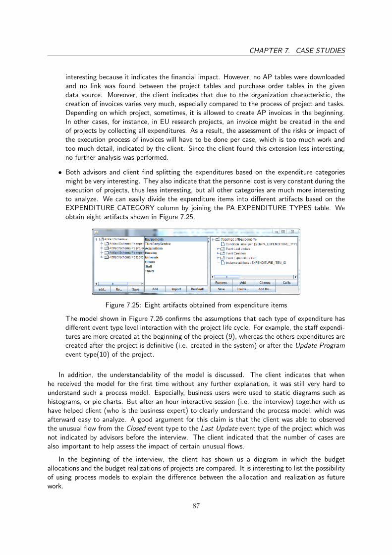
CHAPTER 7. CASE STUDIES
interesting because it indicates the financial impact. However, no AP tables were downloadedand no link was found between the project tables and purchase order tables in the givendata source. Moreover, the client indicates that due to the organization characteristic, thecreation of invoices varies very much, especially compared to the process of project and tasks.Depending on which project, sometimes, it is allowed to create AP invoices in the beginning.In other cases, for instance, in EU research projects, an invoice might be created in the endof projects by collecting all expenditures. As a result, the assessment of the risks or impact ofthe execution process of invoices will have to be done per case, which is too much work andtoo much detail, indicated by the client. Since the client found this extension less interesting,no further analysis was performed.
• Both advisors and client find splitting the expenditures based on the expenditure categoriesmight be very interesting. They also indicate that the personnel cost is very constant during theexecution of projects, thus less interesting, but all other categories are much more interestingto analyze. We can easily divide the expenditure items into different artifacts based on theEXPENDITURE CATEGORY column by joining the PA EXPENDITURE TYPES table. Weobtain eight artifacts shown in Figure 7.25.
Figure 7.25: Eight artifacts obtained from expenditure items
The model shown in Figure 7.26 confirms the assumptions that each type of expenditure hasdifferent event type level interaction with the project life cycle. For example, the staff expendi-tures are more created at the beginning of the project (9), whereas the others expenditures arecreated after the project is definitive (i.e. created in the system) or after the Update Programevent type(10) of the project.
In addition, the understandability of the model is discussed. The client indicates that whenhe received the model for the first time without any further explanation, it was still very hard tounderstand such a process model. Especially, business users were used to static diagrams such ashistograms, or pie charts. But after an hour interactive session (i.e. the interview) together with ushave helped client (who is the business expert) to clearly understand the process model, which wasafterward easy to analyze. A good argument for this claim is that the client was able to observedthe unusual flow from the Closed event type to the Last Update event type of the project which wasnot indicated by advisors before the interview. The client indicated that the number of cases arealso important to help assess the impact of certain unusual flows.
In the beginning of the interview, the client has shown us a diagram in which the budgetallocations and the budget realizations of projects are compared. It is interesting to list the possibilityof using process models to explain the difference between the allocation and realization as futurework.
87

CHAPTER 7. CASE STUDIES
Figure 7.26: Interactions between the eight expenditure artifacts and the project life cycle
We conclude this chapter by summarizing the the results of the two case studies. For both casestudies, we were able to successfully create the desired artifacts and identify the desired type levelinteractions. We were able to use the event logs which were extracted from these artifacts andinteractions to successfully discover an artifact-centric model. Moreover, for both case studies, wewere able to use the discovered model to identify true-positive unusual flows validated by the advisorsand client. However, there were also some limitations. In some cases, domain knowledge might berequired to distinguish the “allowed” flows from the real unusual flows identified. Moreover, theunderstandability of the model can be further improved. Furthermore, the InteractionMiner toolshould visualize more data of a certain flow to help users assess the flow accurately.
88

Chapter 8
Conclusion
Within this master thesis, we have analyzed, using an artifact-centric approach, the extraction ofevent logs with trace level interactions from relational data sources and the mining of artifact-centricmodels from these event logs. We recall the goal of this master thesis and the research outline shownin Figure 1.9:
Given a relational data source, we would like to support business analysts to (semi-) au-tomatically discover an artifact-centric model, which describes the process of severalcollaborative processes (or life cycles of artifacts), each of which has it own life cycle, andinteractions with each other, and to be able to use this discovered model to perform processanalyses.
Before presenting our approach, we have investigated each element in the research scope: eventlogs, process models, relational data sources, and more importantly, the traditional approach oflog extraction and the original XTract approach of artifact-centric log extraction. Emphasizing thelimitations of traditional approaches, we have shown that the data convergence and divergenceproblem was unsolved, and that these approaches were less suitable for data- (or document-) centricsystems by considering the lifecycle of various documents as one process definition. We have alsoshown the limitations of the original XTract approach such as run-time issues and inability to identifythe desired artifacts. Furthermore, no interactions were identified, thus no artifact-centric processmodel is discovered.
Our first contribution is the extension of the data structure of the original XTract approach andfunctionality added to allow users to identify the desired artifacts from a given data source. Usersare now able to (1) import primary keys and (complex) foreign keys, (2) change artifact schemas,(3) identify various artifacts that share the same artifact schema, and (4) change artifacts by addingor removing event types and attributes.
The major contribution we made is categorizing the interactions, identifying type level inter-actions on the database level and extracting instance level interactions from event logs. We havedivided the interactions into four types: type level interactions, instance (or trace) level interactions,event type level interactions and event level interactions. We have formally defined valid artifacttype level interactions and developed a method to identify these interactions. Furthermore, wehave extended the original XTract implementation to support (1) identifying type level interactions,
89

CHAPTER 8. CONCLUSION
(2) allowing users to select the desired interactions for each artifact, and (3) extract an event logwith instance level interactions for an artifact. Event logs with instance level interactions can allowmore general process mining techniques to be applied and developed, independent of the discoverytechniques we proposed.
The last achievement is the artifact-centric process discovery algorithm we proposed and imple-mented as the InteractionMiner plug-in in ProM. We were able to automatically discover an artifact-centric model in the proclet language by: (1) identifying the life cycle of each artifact using existingdiscovery algorithms and (2) identifying the event type level interactions through merging the inter-acting logs and applying existing discovery algorithms. Furthermore, the InteractionMiner visualizerallows users to select criteria and the desired transitions to further explore the artifact-centric model.Also detailed information are provided for users to assess and verify the unusual behavioral patternsidentified.
To verify and validate our approach and the artifact-centric models we obtained, two case studieshave been performed on two different process of two different ERP systems. The first case study,performed within the OTC process of SAP, has shown that our approach is able to deal with complexdata structure and identify complex artifacts and type level interactions. The second case study,performed within the PA process of Oracle, has shown that the customers were able to understandthe model and discover a unusual behavioral pattern by themselves. Both case studies have shownthat the approach was able to successfully discover the desired artifacts and the artifact-centricprocess model.
We believe that we have developed an artifact-centric approach. Our prototypes support businessanalysts to (semi-)automatically discover an artifact-centric model from a given relational datasource. We also believe that we have shown that the artifact-centric model discovered is moreintuitive than the old approaches for business users and can be used to perform process analyses.
8.1 Limitations and Future Work
In this section, we discuss the limitations and future work with respect to the following four aspects:(1) artifact identification, (2) interaction discovery, (3) process analyses and visualization, and (4)functionality of the tools.
Artifact Identification
For the (A) artifact type identification phase of the extraction problem, we list the following limita-tions and possible extensions. First, we are still unable to automatically identify the “perfect” artifact(schema). For example, it is more logical to include the change tables (CDHDR and CDPOS) ofSAP in artifacts, instead of considering them as a separate artifact. However, this solution causes thedata divergence problem. We allow users to change the artifact (schema) identified by our approachbut this also increased the burden on users. Domain knowledge is really necessary to create thedesired artifacts for conducting process analyses. Therefore, more support should be provided forusers.
A possible solution could be using pattern recognition/matching techniques, which build a pat-tern repository of (im)possible structures of an artifact and use these structures to automatically
90

CHAPTER 8. CONCLUSION
identify (possible) artifacts. Another solution could be implementing more heuristic rules. For ex-ample, the columns which has a certain amount of values (e.g. ≥ 1∧ ≤ 10) can be used for splittingthe artifacts or the event types.
We notice that both SAP and Oracle systems have a document (header) and document linestructure. For example, the sales documents and the sales lines. The advisors are typically interestedin the document (header) level. It might be possible to introduce an approach to level the (main)tables (thus the artifacts) based on the type of relations. For example, the parent table of a one-to-many relation has higher level than the child table of this relation, and all tables without parents areassigned to the highest level. We can allow a user to limit the scope to a certain level of artifacts.
It is also very interesting to investigate and allow hierarchy within an artifact and within anartifact-centric model. Thus, we can use sub-artifacts to model document lines which can be includedwithin the artifacts. For example, the artifact Sales Order can include the sub artifact Sales Lineswithin its life-cycle. We can group several artifacts and aggregate the interactions between artifactsinto the interactions between the groups of artifacts. Having such a hierarchy might allow us tocreate an overview of an entire ERP system, while still be able to zoom into the details of life cycleof each artifact.
Interaction Discovery
Regarding the interaction identification, several improvements can be done. First, we can extractmultiple type level interactions between two artifacts (by simply assigning each of these interactionsa different key in the XES event log), while adding the functionality in the InteractionMiner to selectthe specific type level interactions to investigate. This extension will increase the usability of theapproach and allow users and researchers to investigate multiple type level interactions at the sametime without re-extract event logs.
Another very interesting extension is to merge the event logs of multiple artifacts to overcomethe limitation of the current interactions which only express the (possible) causal relations betweentwo artifacts. Take the OTC example and the model shown in Figure 1.7, if an invoice is createdbefore a related delivery and also before the creation of the order related to the delivery, we willonly be able to identify the unusual flow from the creation of invoice to the creation of delivery. Wewill not be able to identify this ordering between the three artifacts: first the creation of invoice,then the creation of order, followed by the creation of delivery. Therefore, we can merge the orders,deliveries and invoice based on the interactions to obtain the event log, which has a notion of a caseas the combination of these three documents.
An important remark is that it is also possible to merge merge multiple event logs to obtain anevent log of a large artifact, which is usually obtained by using the traditional log. For example,we can use the trace level interactions to merge the (multiple) related Delivery traces with theSales Order trace.
Process Analyses and Visualization
The artifact-centric models we visualized in ProM used the default functions (e.g. regarding layout)provided by the ProM framework. One can use more sophisticated visualization techniques such asthe edge bundling techniques [15] to improve the understandability of the model. The interviews
91

CHAPTER 8. CONCLUSION
conducted with the advisors have also shown that using message sequence chart to visualize individualcases and their related interactions might be interesting.
As the results of the case studies have shown, to really use the discovered artifact-centric modelfor detecting unusual flow, more filters based on domain knowledge might be necessary to distinguishthe real unusual flows from the allowed unusual flows. For example, in the case study of the Oracle- PA process, we found a task which was completed before two related expenditures were ended.However, this unusual flow from Expenditure Ending to Task Completed is allowed if they are withinthe same week. Thus, to distinguish these cases from the the not allowed cases, domain knowledgeand logic might have to be build into the model.
So far, we used the discovered model to identify unusual flows. It would be interesting to applythe conformance checking techniques proposed by D. Fahland et al. [12] on the artifact-centric modeldiscovered by our approach.
Functionality of the Tools
A limitation of the XTract 2 tool is still the performance of log extraction, which is also discussedby E. Nooijen [21] since we reused the XTract approach.
For the SAP case study, we had to extract two version of event logs of the same artifact: a simpleversion and a comprehensive version. We used the simple version to obtain a better overview. How-ever, this can also be realized by providing transition filtering function in the InteractionMiner tool.Also, being able to modeling, filtering, highlighting or comparing artifact-centric models based onattributes (e.g. different business units, different time frame) would be very useful for conductingprocess analyses.
92

Bibliography
[1] W.M.P. van der Aalst. Formalization and verification of event-driven process chains. Informationand Software technology, 41(10):639–650, 1999. (see 17)
[2] W.M.P. van der Aalst. Process Mining: Discovery, Conformance and Enhancement of BusinessProcesses. Springer, 2011. (see 15)
[3] W.M.P. van der Aalst, A. Adriansyah, A.K.A. de Medeiros, F. Arcieri, T. Baier, T. Blickle, J.C.Bose, P. van den Brand, R. Brandtjen, J. Buijs, et al. Process Mining Manifesto. In Businessprocess management workshops, pages 169–194. Springer, 2012. (see 1, 13)
[4] W.M.P. van der Aalst, R.S. Mans, and N.C. Russell. Workflow Support Using Proclets: Divide,Interact, and Conquer. IEEE Data Eng. Bull., 32(3):16–22, 2009. (see iii, 6, 17)
[5] W.M.P. van der Aalst, A.J.M.M. Weijters, and L. Maruster. Workflow mining: Discoveringprocess models from event logs. Knowledge and Data Engineering, IEEE Transactions on,16(9):1128–1142, 2004. (see 16, 54)
[6] A. Arnold and J. Plaice. Finite transition systems: semantics of communicating systems.Prentice Hall International (UK) Ltd., 1994. (see 17)
[7] J. Bauckmann, U. Leser, and F. Naumann. Efficient and exact computation of inclusion de-pendencies for data integration. Number 34. Universitatsverlag Potsdam, 2010. (see 22)
[8] J. Bauckmann, U. Leser, F. Naumann, and V. Tietz. Efficiently detecting inclusion dependen-cies. In Data Engineering, 2007. ICDE 2007. IEEE 23rd International Conference on, pages1448–1450. IEEE, 2007. (see 22)
[9] J.C.A.M. Buijs. Mapping data sources to xes in a generic way. Master’s thesis, EindhovenUniversity of Technology, 2010. (see 4, 14, 16, 18, 19, 20)
[10] D. Cohn and R. Hull. Business artifacts: A data-centric approach to modeling business oper-ations and processes. Bulletin of the IEEE Computer Society Technical Committee on DataEngineering, 32(3):3–9, 2009. (see 6, 20)
[11] T.M. Cover and J.A. Thomas. Entropy, relative entropy and mutual information. Elements ofInformation Theory, pages 12–49, 1991. (see 22)
[12] D. Fahland, M. de Leoni, B.F. van Dongen, and W.M.P. van der Aalst. Behavioral conformanceof artifact-centric process models. In Business Information Systems, pages 37–49. Springer,2011. (see 92)
93

BIBLIOGRAPHY
[13] M. van Giessel. Process Mining in SAP R/3: A method for applying process mining to SAPR/3. Master’s thesis, Eindhoven University of Technology, 2004. (see 4, 18)
[14] C.W. Gunther and W.M.P. van der Aalst. Fuzzy mining–adaptive process simplification basedon multi-perspective metrics. In Business Process Management, pages 328–343. Springer, 2007.(see 16)
[15] D. Holten and J.J. van Wijk. Force-directed edge bundling for graph visualization. In ComputerGraphics Forum, volume 28, pages 983–990. Wiley Online Library, 2009. (see 77, 91)
[16] F. de Marchi, S. Lopes, and J.-M. Petit. Efficient algorithms for mining inclusion dependencies.In Advances in Database TechnologyEDBT 2002, pages 464–476. Springer, 2002. (see 22)
[17] F. de Marchi, S. Lopes, and J.-M. Petit. Unary and n-ary inclusion dependency discovery inrelational databases. Journal of Intelligent Information Systems, 32(1):53–73, 2009. (see 22)
[18] A.K.A. de Medeiros, A.J.M.M. Weijters, and W.M.P. van der Aalst. Genetic process mining: anexperimental evaluation. Data Mining and Knowledge Discovery, 14(2):245–304, 2007. (see 16,54)
[19] T. Murata. Petri nets: Properties, analysis and applications. Proceedings of the IEEE,77(4):541–580, 1989. (see 17)
[20] A. Nigam and N.S. Caswell. Business artifacts: An approach to operational specification. IBMSystems Journal, 42(3):428–445, 2003. (see 6, 20)
[21] E.H.J. Nooijen. Artifact-Centric Process Analysis–Process discovery in ERP systems. Master’sthesis, Eindhoven University of Technology, 2012. (see iii, 6, 20, 33, 92)
[22] E.H.J. Nooijen, B.F. van Dongen, and D. Fahland. Automatic Discovery of Data-Centricand Artifact-Centric Processes. In Business Process Management Workshops, pages 316–327.Springer, 2013. (see iii, 6, 20)
[23] M. Pesic, M.H. Schonenberg, N. Sidorova, and W.M.P. van der Aalst. Constraint-based work-flow models: Change made easy. In On the Move to Meaningful Internet Systems 2007: CoopIS,DOA, ODBASE, GADA, and IS, pages 77–94. Springer, 2007. (see 17)
[24] D.A.M. Piessens. Event Log Extraction from SAP ECC 6.0. Master’s thesis, Eindhoven Uni-versity of Technology, 2011. (see 4, 19)
[25] A. Roest. A practitioners guide towards process mining on erp systems implemented and testedfor sap order to cash. Master’s thesis, Eindhoven University of Technology, 2012. (see 4, 19)
[26] I.E.A. Segers. Investigating the application of process mining for auditing purposes. Master’sthesis, Eindhoven University of Technology, 2007. (see 4, 18)
[27] H.M.W. Verbeek, J.C.A.M. Buijs, B.F. van Dongen, and W.M.P. van der Aalst. Prom 6: Theprocess mining toolkit. Proc. of BPM Demonstration Track, 615:34–39, 2010. (see 16)
[28] H.M.W. Verbeek, J.C.A.M. Buijs, B.F. van Dongen, and W.M.P. van der Aalst. XES, xESame,and proM 6. In Information Systems Evolution, pages 60–75. Springer, 2011. (see 16)
94

BIBLIOGRAPHY
[29] A.J.M.M. Weijters, W.M.P. van der Aalst, and A.K.A. de Medeiros. Process mining with theheuristics miner-algorithm. Technische Universiteit Eindhoven, Tech. Rep. WP, 166, 2006.(see 16)
[30] A.J.M.M. Weijters and J.T.S. Ribeiro. Flexible heuristics miner (fhm). In ComputationalIntelligence and Data Mining (CIDM), 2011 IEEE Symposium on, pages 310–317. IEEE, 2011.(see 16, 54)
[31] J.M.E.M. van der Werf, B.F. van Dongen, C.A.J. Hurkens, and A. Serebrenik. Process discoveryusing integer linear programming. In Applications and Theory of Petri Nets, pages 368–387.Springer, 2008. (see 16, 54)
[32] S.A. White. Introduction to bpmn. IBM Cooperation, pages 2008–029, 2004. (see 17)
[33] X.Y. Yang, C.M. Procopiuc, and D. Srivastava. Summarizing relational databases. Proceedingsof the VLDB Endowment, 2(1):634–645, 2009. (see 23)
95


Appendix A
OTC Example
In this appendix, we introduce the OTC example which is simplified from the table structure usedby the SAP Order to Cash (OTC) process. The example is named the OTC example and usedthroughout this thesis. The relational data structure shown in Figure A.1 consists of four tables,Sales Documents(SD), Deliveries Document(DD), Billing Document(BD) and the Document Changes.The content of the four tables are shown in Figure 1.1 with references.
• The SD table contains two sales orders (i.e. S1 and S2) and a return order (i.e. S3), and theDocument type column indicates two types of documents, Sales Order and Return order. TheSD table is a simple version of the sales documents table VBAK within SAP.• The DD table contains three delivery documents (i.e. D1, D2, D3) and a return delivery doc-
ument (i.e. D4), and the Document type column indicates two types of documents, Deliveryand Return delivery.• The BD table contains two invoice documents (i.e. B1, B2), and the Document type column
indicates one type of documents, Invoice.• The DOCUMENT CHANGES table (Changes) store all changes related to different document
(the column Reference id is a foreign key referring to the other three tables). The firstthree records is related to the sales order S1, and the fourth record is related to the invoiceB2. The column Date changed indicates the date when the change is done, and the columnChange type indicates the type of the change.
The four references between the tables SD, DD, BD, and changes are displayed in Figures A.1and 1.1.
• The SD table has a reference F1 with itself, i.e. the foreign key column Reference id in theSD table refers to the primary key column SD id in the SD table.• A reference F2 between the SD table and the DD table is found, i.e. the foreign key column
Reference SD id in the DD table refers to the primary key column SD id in the SD table.• There is a reference F3 found between the BD table and the DD table, i.e. the foreign key
column Reference BD id in the DD table refers to the primary key column BD id in the BDtable.• The reference F4 is found between the table CHANGES and the other three documents tables.
The column Reference id is a foreign key referring to the column SD id , the column DD id orthe column BD id depending on the value in the column Table name of the table CHANGES .
97
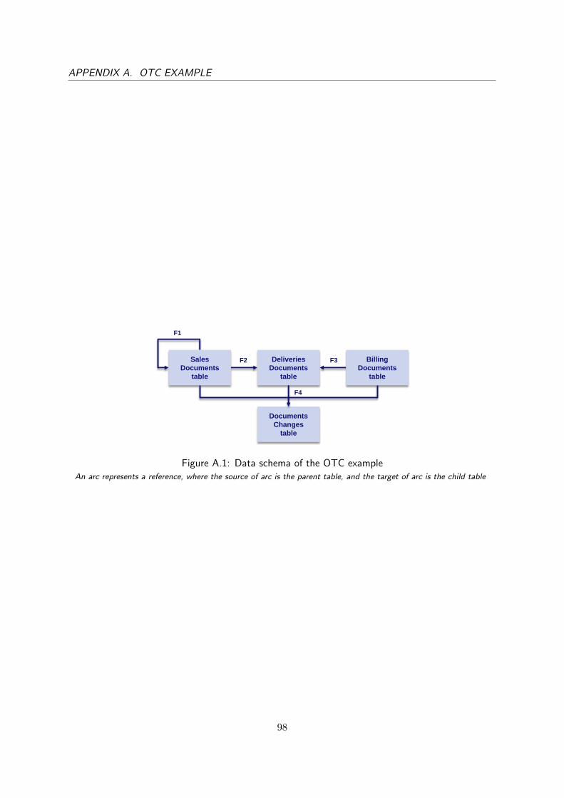
APPENDIX A. OTC EXAMPLE
PAGE 26
Sales Documents
Table
Deliveries Documents
Table
Sales
Documents
table
Deliveries
Documents
table
Billing
Documents
table
Billing Documents
Table
Sales Order Delivery
Return order Return delivery
Invoice
F1
F2 F3
Documents
Changes
table
F4
Figure A.1: Data schema of the OTC exampleAn arc represents a reference, where the source of arc is the parent table, and the target of arc is the child table
98

Appendix B
Mapping Creation and Log Extraction
In this appendix, we show an example of a (log) mapping created based on the artifact Sales Orderin Figure B.1. The new data structure with respect of the mapping is shown in Figure B.2.
LogMapping(LM)
name
"Sales Order log"
TraceMapping
traceID fromTable link
[SD id] SD
AttributeMapping
key type sourceColumn Extension
String_Cluster_0 String [SD id] null
GeneralMappingPropery
condition artifactId
<maintable>.[Document type] = 'Sales Order' 19
ListAttributes
attributeID key fromTable
[DD id] "Interaction_Return Delivery" SD
Links
linkNumber fromArtifact toArtifact Reference
1 19 (Sales Order) 20 (Return Order) F1
2 20 (Return Order) 17 (Return Delivery) F2
EventMapping
eventID name eventColumn fromTable link
[SD id] Last change [Last change] SD
[SD id] Created [Date Created] SD
GeneralMappingPropery
condition artifactId
<maintable>.[Document type] = 'Return Delivery' 17
Extension (EX)
name prefix URI
Time time http://www.xes-standard.org/time.xesext
Concept concept http://www.xes-standard.org/concept.xesext
Classifier (CL)
name keys
Unique classifiers concept:name event_id
Activity classifiers concept:name
TraceGrobalAttribute
key type value extension
trace_id String null
Interaction_Return Delivery String MULTIPLE null
String_Cluster_0 String null
concept:name String concept.xesext
EventGlobalAttribute
key type value extension
time:timestamp Date 1-1-1970 time.xesext
event_id String null
concept:name String concept.xesext
Figure B.1: MappingMapping of artifact sales order
99

APPENDIX B. MAPPING CREATION AND LOG EXTRACTION
-condition : String
-artifactId : Int
GeneralMappingProperty
1
1
-parentTable : Table
-parentColumns : List<Column>
-childTable: Table
-childColumns : List<Column>
-condition: String
Reference-link: list of
+*
-parentArtifact : Artifact
-childArtifact : Artifact
DirectInteraction
Figure B.2: Mapping data structureReused the mapping data structure of XTract and extended with the class
GeneralMappingProperty (colored blue)
100

Appendix C
Case Studies
C.1 Case I - SAP OTC process
In this appendix, we show the result related to the SAP case study. Figure C.1 shows the primarykeys we used for the SAP Order to Cash process, and Figure C.2 shows the foreign keys we used.
Table Primary keys
BKPF Mandt,BUKRS,BELNR,GJAHR
bsad MANDT,BUKRS,KUNNR,UMSKS,UMSKZ,AUGDT,AUGBL,ZUONR,GJAHR,BELNR,BUZEI
cdhdr MANDANT,OBJECTCLAS,OBJECTID,CHANGENR
bsid MANDT,BUKRS,KUNNR,UMSKS,UMSKZ,AUGDT,AUGBL,ZUONR,GJAHR,BELNR,BUZEI
cdpossmall MANDANT,OBJECTCLAS,OBJECTID,CHANGENR,TABNAME,TABKEY,FNAME,CHNGIND
LIKP MANDT,VBELN
LIPS MANDT,VBELN,POSNR
VBAK MANDT,VBELN
VBAP MANDT,VBELN,POSNR
VBRK MANDT,VBELN
VBRP MANDT,VBELN,POSNR
cdpos MANDANT,OBJECTCLAS,OBJECTID,CHANGENR,TABNAME,TABKEY,FNAME,CHNGIND
Figure C.1: SAP OTC tables - primary keys
101

APPENDIX C. CASE STUDIES
Parent table Parent columns Child table Child columns Condition
VBAK mandt,vbeln VBAK mandt,vgbel NULL
VBAK mandt,vbeln VBAP mandt,vbeln NULL
VBAP mandt,vbeln,posnr VBAP mandt,vgbel,vgpos NULL
VBAP mandt,vbeln,posnr LIPS mandt,vgbel,vgpos NULL
VBAP mandt,vbeln,posnr VBRP mandt,vgbel,vgpos NULL
VBAP mandt,vbeln,posnr VBRP mandt,aubel,aupos NULL
LIKP mandt,vbeln LIPS mandt,vbeln NULL
LIPS mandt,vbeln,posnr VBRP mandt,vgbel,vgpos NULL
LIPS mandt,vbeln,posnr VBAP mandt,vgbel,vgpos NULL
LIPS mandt,vbeln,posnr LIPS mandt,vgbel,vgpos NULL
VBRP mandt,vbeln,posnr VBRP mandt,vgbel,vgpos NULL
VBRK mandt,vbeln VBRP mandt,vbeln NULL
VBRP mandt,vbeln,posnr VBAP mandt,vgbel,vgpos NULL
CDHDR mandant,objectclas,objectid,changenr CDPOS mandant,objectclas,objectid,changenr NULL
VBRK mandt,vbeln CDHDR mandant,objectid <child>.objectclas = 'FAKTBELEG'
VBRP mandt,vbeln CDHDR mandant,objectid <child>.objectclas = 'FAKTBELEG'
VBAK mandt,vbeln CDHDR mandant,objectid <child>.objectclas = 'VERKBELEG'
VBAP mandt,vbeln CDHDR mandant,objectid <child>.objectclas = 'VERKBELEG'
VBRK mandt,vbeln BKPF mandt,awkey <child>.awtyp = 'VBRK'
BKPF mandt,BUKRS,BELNR,GJAHR BSAD mandt,BUKRS,BELNR,GJAHR NULL
VBRK mandt,vbeln CDPOS mandant,objectid
<child>.objectclas = 'FAKTBELEG' and <child>.tabname =
'VBRK' and <child>.tabkey = <parent>.mandt+<parent>.vbeln
VBRP mandt,vbeln CDPOS mandant,objectid
<child>.objectclas = 'FAKTBELEG' and <child>.tabname =
'VBRP' and <child>.tabkey =
<parent>.mandt+<parent>.vbeln+<parent>.posnr
VBAK mandt,vbeln CDPOS mandant,objectid
<child>.objectclas = 'VERKBELEG' and <child>.tabname =
'VBAK' and <child>.tabkey = <parent>.mandt+<parent>.vbeln
VBAP mandt,vbeln CDPOS mandant,objectid
<child>.objectclas = 'VERKBELEG' and <child>.tabname =
'VBAP' and <child>.tabkey = <parent>.mandt+<parent>.vbeln
+ <parent>.posnr
BSAD mandt,belnr,BUKRS,GJAHR BSAD mandt,augbl,BUKRS,GJAHR NULL
Figure C.2: SAP OTC tables - foreign keys
102