Master’s thesis Geology

Petrology and Economic Geology

GEOCHEMICAL AND PALEOMAGNETIC CONSTRAINTS ON MID-PROTEROZOIC MAFIC DYKE EMPLACEMENT EVENTS IN SOUTHERN FINLAND

Katja Bohm

2018

Supervisors: Arto Luttinen, Johanna Salminen

UNIVERSITY OF HELSINKI FACULTY OF SCIENCE

DEPARTMENT OF GEOSCIENCES AND GEOGRAPHY

PL 64 (Gustaf Hällströmin katu 2) 00014 Helsingin yliopisto

Tiedekunta/Osasto – Fakultet/Sektion – Faculty Faculty of Science

Laitos/Institution– Department Department of Geosciences and Geography

Tekijä/Författare – Author Katja Bohm

Työn nimi / Arbetets titel – Title Geochemical and paleomagnetic constraints on mid-Proterozoic mafic dyke emplacement events in southern Finland

Oppiaine /Läroämne – Subject

Geology

Työn laji/Arbetets art – Level

Master’s Thesis

Aika/Datum – Month and year

10/2018

Sivumäärä/ Sidoantal – Number of pages

86

Tiivistelmä/Referat – Abstract

Mid-Proterozoic mafic dyke swarms in southern Finland are associated with rapakivi magmatism. The dyke swarms are commonly referred to as “Subjotnian” (1.64–1.54 Ga), being older than the rift-filling Jotnian sandstones. Mafic rocks from five dyke swarms located in Åland, Satakunta, Häme, Suomenniemi and Sipoo were studied in this thesis.

An X-ray fluorescence (XRF) analysis was made of 110 rock samples from 101 mafic dykes and one mafic intrusion. The analyses were made of the same rock samples as previous paleomagnetic studies.

Overall, the Subjotnian mafic dykes in southern Finland are hyperstene-normative tholeiitic basalts or basaltic andesites with varying MgO contents (3–15 wt%). Some dykes show alkaline features with higher total alkali and/or Nb/Y values. They vary from

quartz- to olivine-normative types. The dykes of the Åland swarm form two geohemical groups. The division is accompanied with a switch in magnetic polarity and distinct virtual geomagnetic pole positions. These observations imply that two separate magmatic events/pulses that have an age difference have taken place in Åland. The Satakunta dykes form two geochemical groups of which

the other includes presumably Svecofennian dykes that show high Nb/Y values at given Zr/Y ratios. The dykes of the Häme swarm form three geochemical groups. Although some Suomenniemi dykes show geochemical and paleomagnetic affinities to Häme dykes, they probably represent a distinct igneous event of the event that formed the nearby Häme swarm. The Sipoo dykes are

very homogeneous in their geochemistry and can be distinguished from the emplacement events that formed the other Subjotnian swarms.

The Subjotnian dyke swarms in southern Finland that are believed to have emplacement ages of >1.63 Ga (Häme, Suomenniemi and Sipoo swarms in S-SE Finland) generally have higher Nb/Y (and Zr/Y) values than the dyke swarms that are believed to record younger magmatic events at <1.58 Ga (Åland and Satakunta swarms in SW Finland). Some Satakunta dykes, however, have

geochemical and/or paleomagnetic implications that suggest they have an older Subjotnian age than the dated 1.57 Ga dyke in Satakunta. Further chronological work on the Satakunta dyke swarm is needed to verify the age of the dykes.

Many of the Subjotnian dykes show a secondary magnetization component, called the “B-component”, whose direction is always close to, but distinct of, the Present Earth Field (PEF) at the sampling location. There was no correlation between the B-component and the magma types of the dykes. The B-component occurs mostly in dykes that are very altered. Thus, the results support

previous suggestions that the B-component formed due to hydrothermal alteration of the rocks and the subsequent formation of new magnetic minerals.

Avainsanat – Nyckelord – Keywords Mid-Proterozoic, Subjotnian, Åland, Satakunta, Häme, Suomenniemi, Sipoo, Dyke swarm, Mafic dyke, Diabase, Rapakivi, Geochemistry, XRF, Paleomagnetism, Virtual geomagnetic pole

Säilytyspaikka – Förvaringställe – Where deposited

University of Helsinki

Muita tietoja – Övriga uppgifter – Additional information

Tiedekunta/Osasto – Fakultet/Sektion – Faculty Matemaattis-luonnontieteellinen tiedekunta

Laitos/Institution– Department Geotieteiden ja maantieteen laitos

Tekijä/Författare – Author Katja Bohm

Työn nimi / Arbetets titel – Title Geokemiallisia ja paleomagneettisia todisteita eteläisen Suomen keskiproterotsooisten mafisten juonien syntyvaiheisiin

Oppiaine /Läroämne – Subject Geologia

Työn laji/Arbetets art – Level Pro Gradu

Aika/Datum – Month and year 10/2018

Sivumäärä/ Sidoantal – Number of pages 86

Tiivistelmä/Referat – Abstract

Keskiproterotsooiset mafiset juoniparvet eteläisessä Suomessa liittyvät rapakivimagmatismiin. Näitä juoniparvia kutsutaan ”subjotunisiksi” (1,64–1,54 Ga), koska ne edeltävät jotunisia hiekkakiviä. Tässä työssä tutkittiin mafisia juonia viidestä eri juoniparvesta, jotka sijaitsevat Ahvenanmaalla, Satakunnassa, Hämeessä, Suomenniemellä ja Sipoossa.

Yhteensä 110 kivinäytteelle, jotka oli aiemmin kerätty 101 mafisesta juonesta ja yhdestä mafisesta intruusiosta, tehtiin röntgenfluoresenssianalyysi (XRF). Samoja näytteitä oli aiemmin käytetty paleomagneettisissa tutkimuksissa.

Yleistäen eteläisen Suomen subjotuniset mafiset juonet ovat hypersteeni-normatiivisia tholeiittisia basaltteia ja basalttisia andesiitteja. Joillakin juonilla on alkalisia piirteitä, jotka ilmenevät kohonneina alkalipitoisuuksina ja/tai Nb/Y-arvoina. Juonien MgO

pitoisuudet ovat vaihtelevia (3–15 wt%), ja niiden normatiivinen koostumus vaihtelee kvartsinormatiivisista oliviininormatiivisiin tyyppeihin. Ahvenanmaan juonet jakautuvat kahteen geokemialliseen ryhmään, joilla on pääsääntöisesti myös erilaiset magneettiset polariteetit ja virtuaalisten geomagneettisten napojen sijainnit. Nämä havainnot viittaavat kahteen eri-ikäiseen

magmaattiseen tapahtumaan Ahvenanmaalla. Satakunnan juonet muodostavat kaksi geokemiallista ryhmää. Toiseen ryhmään kuuluu oletettavasti svekofennisiä juonia, joilla on selkeästi korkeammat Nb/Y-arvot tietyillä Zr/Y-arvoilla kuin subjotunisilla juonilla. Hämeen juonet muodostavat kolme geokemiallista ryhmää. Joillakin Suomenniemen juonilla on geokemiallisia ja

paleomagneettisia yhteneväisyyksiä Hämeen juonien kanssa, mutta todennäköisesti Suomenniemen juonet edustavat läheisen Hämeen juoniparven synnyttäneestä tapahtumasta erillistä magmaattista tapahtumaa. Sipoon juonet muodostavat hyvin homogeenisen geokemiallisen ryhmän, joka erottuu selkeästi muiden subjotunisten juonien geokemiasta. Sipoon juonien voidaan

tässä mielessä ajatella edustavan magmaattista intruusiota, joka on erillinen niistä tapahtumista, jotka muodostivat muut tämän tutkimuksen juoniparvet.

Niillä eteläisen Suomen subjotunisilla juonilla, joiden on ajateltu muodostuneen >1,63 Ga (Hämeen, Suomenniemen ja Sipoon parvet Etelä- ja Kaakkois-Suomessa), on yleisesti ottaen korkeammat Nb/Y- ja Zr/Y-arvot kuin niillä juonilla, joiden on ajateltu kuuluvan nuorempiin, <1,58 Ga muodostuneisiin parviin (Ahvenanmaan ja Satakunnan juoniparvet Lounais-Suomessa). Osalla

Satakunnan juonista on kuitenkin geokemiallisia ja/tai paleomagneettisia ominaisuuksia, jotka viittaavat niiden olevan vanhempia subjotunisia kuin Satakunnan iätetty 1,57 Ga juoni. Näiden juonien ikien varmistamiseksi tulisi kuitenkin tehdä uusia tarkkoja iänmäärityksiä Satakunnan juoniparvelle.

Monilla tämän tutkimuksen juonilla on havaittu sekundäärisen magnetoituman komponentti, ”B-komponentti”, jonka suunta on aina lähellä (mutta selkeästi eriävä) Maan magneettikentän tämänhetkistä suuntaa kullakin näytteenottopaikalla. Tässä tutkimuksessa

ei havaittu yhteneväisyyksiä B-komponentin ja tietyn magmatyypin välillä. Sen sijaan B-komponentin havaittiin esiintyvän erityisesti hyvin muuttuneilla juonilla. Tämä tutkimus tukee aiempien tutkimusten havaintoja siitä, että B-komponentin synty liittyy kivien hydrotermiseen muuttumiseen ja siitä johtuvaan uusien magneettisten mineraalien syntyyn.

Avainsanat – Nyckelord – Keywords Keskiproterotsooinen, Subjotuninen, Ahvenanmaa, Satakunta, Häme, Suomenniemi, Sipoo, Juoniparvi, Mafinen juoni, Diabaasi, Rapakivi, Geokemia, XRF, Paleomagnetismi, Virtuaalinen geomagneettinen napa

Säilytyspaikka – Förvaringställe – Where deposited Helsingin yliopisto

Muita tietoja – Övriga uppgifter – Additional information

Table of contents

1. INTRODUCTION ..................................................................................................... 4

2. MAFIC DYKES ........................................................................................................ 6

2.1. Large igneous provinces and continental flood basalts .............................. 6

2.2. Geochemical research of mafic dykes ....................................................... 7

2.3. Paleomagnetic research of mafic dykes ..................................................... 9

3. GEOLOGICAL SETTING AND BACKGROUND ................................................. 11

3.1. Mesoproterozoic rapakivi magmatism in southern Finland ...................... 11

3.2. Geochemical and paleomagnetic features of the Subjotnian dykes ........... 13

3.2.1. Geochemical features ............................................................. 13

3.2.2. Paleomagnetic features .......................................................... 15

3.3. The Åland dyke swarm ........................................................................... 19

3.4. The Satakunta dyke swarm ...................................................................... 21

3.5. The Häme dyke swarm............................................................................ 22

3.6. The Suomenniemi dyke swarm ............................................................... 24

3.7. The Sipoo dyke swarm ............................................................................ 25

4. MATERIALS AND METHODS ............................................................................. 27

4.1. Materials ................................................................................................. 27

4.2. Geochemical and petrographical methods ............................................... 28

5. RESULTS ............................................................................................................... 29

5.1. Petrography............................................................................................. 29

5.2. Geochemistry .......................................................................................... 32

5.2.1. Subjotnian dykes in general .................................................... 32

5.2.2. Geochemistry of the Åland dyke swarm................................... 36

5.2.3. Geochemistry of the Satakunta dyke swarm ............................ 36

5.2.4. Geochemistry of the Häme dyke swarm................................... 37

5.2.5. Geochemistry of the Suomenniemi dyke swarm ....................... 37

5.2.6. Geochemistry of the Sipoo dyke swarm ................................... 38

5.2.7. Geochemical grouping of the dykes ........................................ 38

6. DISCUSSION ........................................................................................................ 43

6.1. Geochemistry vs. magnetic polarity records in the dykes ......................... 43

6.2. Comparison between VGPs and geochemistry ........................................ 45

6.2.1. The Åland dyke swarm ............................................................ 47

6.2.2. The Satakunta dyke swarm...................................................... 48

6.2.3. The Häme dyke swarm ............................................................ 51

6.2.4. The Suomenniemi dyke swarm ................................................ 53

6.2.5. The Sipoo dyke swarm ............................................................ 55

6.3. Comparison with previous geochemical data ........................................... 57

6.4. Geochemistry of the dykes with pervasive overprint ............................... 58

7. CONCLUSIONS ..................................................................................................... 60

8. ACKNOWLEDGEMENTS ..................................................................................... 61

9. REFERENCES ........................................................................................................ 61

10. APPENDICES ....................................................................................................... 66

Appendix I. The coordinates of the dykes and other information.

Appendix II. The XRF results and C.I.P.W. norms.

Appendix III. Petrographic observations.

4

1. INTRODUCTION

Precambrian mafic dyke swarms are important sources of information when studying

continental drift and magma systems related to crustal extension, mantle plumes and

breakup of continents (e.g. Ernst and Buchan 1997; Bleeker and Ernst 2006). Mafic dyke

swarms represent the plumbing system for the voluminous mantle-derived magmas that

produce large igneous provinces (LIPs) (e.g. Ernst and Buchan 1997). LIPs are targets of

multidisciplinary research by paleomagnetic, geochemical and geochronological

methods. They can provide essential information not only on mantle plumes and mantle

behaviour through Earth history but also on breakup of continents and supercontinent

cycles (i.e. the cycles of continental crust aggregation and dispersal) (Courtillot et al.

1999; Ernst and Buchan 2001; Bleeker 2004; Bryan and Ernst 2008; Ernst et al. 2008).

LIPs can also be used in constraining paleocontinental reconstructions (e.g. Bleeker and

Ernst 2006). Furthermore, research on LIPs is necessary because they involve economic

mineral deposits and have had a catastrophic impact on the climate and the biosphere

(Bryan and Ernst 2008). Mafic dyke swarms are sometimes the only major remnants of

LIPs of pre-Mesozoic age since erosion and tectonics have commonly removed most of

the volcanic rocks of these events (Ernst and Buchan 1997). Mafic dyke swarms are thus

essential components of the research on LIPs and their origin.

Mid-Proterozoic mafic dyke swarms in southern Finland from five different localities are

studied in this thesis: the Åland, Satakunta, Häme, Suomenniemi and Sipoo swarms.

These dyke swarms are associated with rapakivi granites (Laitakari 1969; Ehlers and

Ehlers 1977; Laitala 1984; Pihlaja 1987; Rämö 1991) and they may be the early

manifestations of rifting related to the attempted breakup of the 1.8–1.3 Ga Nuna

(Columbia, Hudsonland; Meert 2002; Rogers and Santosh 2002; Zhao et al. 2004; Meert

2012; Evans 2013 and references therein) supercontinent (Salminen et al. 2014; 2016;

2017; 2018).

According to published age data, the five dyke swarms in southern Finland split into two

age groups, so that the U-Pb ages of the Åland and Satakunta swarms in SW Finland

range between 1576–1565 Ma (Lehtonen et al. 2003; Salminen et al. 2016 and references

therein) and the U-Pb ages of the swarms in SE Finland, the Häme, Suomenniemi and

Sipoo swarms, range between 1646–1633 Ma (Törnroos 1984; Laitakari 1987; Siivola

5

1987; Salminen et al. 2017). The recent paleomagnetic results of these dyke swarms

challenge this chronological division, however, as one of the two paleomagnetic poles

obtained from the Satakunta dykes (pole SK2; Salminen et al. 2014) shows a similar

magnetization age to the Häme pole (Salminen et al. 2017). The other paleomagnetic pole

from Satakunta (pole SK1; Salminen et al. 2014) is similar to paleomagnetic pole of

Åland (Salminen et al. 2016) as is expected for the nearly coeval poles.

Among the dyke swarms in SE Finland, the roughly coeval paleomagnetic poles of Häme,

Suomenniemi and Sipoo swarms are distinct (Mertanen and Pesonen 1995; Salminen et

al. 2017; 2018). Possible explanations are age differences accompanied with continental

drift and/or problems with the paleomagnetic data (Salminen et al. 2018).

Many paleomagnetic records of Precambrian Baltica also show a secondary

paleomagnetic component (Mertanen and Pesonen 1995; Elming et al. 2009; Preeden et

al. 2009; Lubnina et al. 2010; Salminen et al. 2014; 2016; 2017; 2018), which is always

nearly parallel to the Present Earth Field direction (PEF) in the sampling area and which

seems to come from the most altered dykes (e.g. Salminen et al. 2014). Later in this text,

this component will be referred to as ‘B-component’ (Mertanen and Pesonen 1995) to

distinguish it from other secondary components, such as PEF.

One aim of this work is to use geochemical analyses of the five mafic dyke swarms in

southern Finland to recognize chemically different magma types that may represent

distinct magmatic events. The geochemical data can enhance the interpretation of

paleomagnetic data if some dykes can be added to or removed from paleomagnetic pole

calculations. Distinguishing magmatic events by using the geochemical data can be done

by critically evaluating the chemical compositions of the mafic dykes, especially their

trace element ratios. Magmatic differentiation has a relatively strong effect on the major

element contents of mafic dykes, but the ratios of incompatible elements remain relatively

unchanged after these processes and can thus be used as geochemical fingerprints of the

original magmas.

Rather few detailed studies on the geochemistry of the Finnish mid-Proterozoic mafic

dyke swarms have been published (Rämö 1991; Eklund et al. 1994; Lehtonen et al. 2003;

Lindholm 2010), and only one study (Salminen et al. 2014) has combined geochemical

6

and paleomagnetic data. Reliable high-precision geochronological data are also sparse.

In this study, an X-ray fluorescence (XRF) analysis was made of 110 samples from 101

mafic dykes and one mafic intrusion of the five dyke swarms. The geochemistry was

compared with the previously published paleomagnetic data (Mertanen and Pesonen

1995; Salminen et al. 2014; 2016; 2017; 2018) of the dyke swarms. The same rock

samples were used for the geochemical (this study) and paleomagnetic (previous studies)

studies.

There are several questions this study aims to address by using geochemical analyses:

Does the variation in paleomagnetic data manifest itself also in geochemistry? Why the

paleomagnetic pole of Häme dyke swarm is distinct from the roughly coeval poles of

Sipoo and Suomenniemi dyke swarms? Are the Åland and Satakunta mafic dykes part of

the same swarm with similar geochemical fingerprints? Are the Satakunta dyke swarm

and the Häme dyke swarm consanguineous? Is the geographical division of the five dyke

swarms thus also valid petrogenetically and/or chronologically? What is the reason for

the pervasive overprinted magnetization component (the B-component) for some of the

mafic dykes of these swarms?

2. MAFIC DYKES

2.1. Large igneous provinces and continental flood basalts

Continental flood basalts (CFBs) are one type of continental LIPs (Bryan and Ernst 2008).

The definition of LIPs, according to Bryan and Ernst (2008), is as follows: LIPs “are

magmatic provinces with areal extents >0.1 Mkm2, igneous volumes >0.1 Mkm3 and

maximum lifespans of ~50 Myr that have intraplate tectonic settings or geochemical

affinities, and are characterised by igneous pulse(s) of short duration (~1–5 Myr), during

which a large proportion (>75%) of the total igneous volume has been emplaced.” The

Proterozoic LIPs are commonly deeply eroded, consisting of the plumbing system

manifested by dyke swarms, sill provinces and layered intrusions and showing only minor

remnants of the actual flood basalts (Ernst et al. 2008).

7

CFBs exist on every continent and form typically in extensional tectonic settings and by

continental rifting (Winter 2001). While oceanic LIPs are often quite homogenic in their

geochemistry, continental LIPs have more varieties (e.g. Bryan and Ernst 2008). Most

continental LIPs are compositionally bimodal with mafic and silicic igneous rock

occurrences that range from low-Ti to high-Ti magma types (e.g. Bryan and Ernst 2008).

CFBs are commonly tholeiitic basalts, but alkaline types and evolved differentiates are

also represented (Winter 2001). Generalized, CFBs are evolved with high Si, Fe, Ti and

K contents, low (<60) Mg numbers [atomic 100*Mg/(Mg+Fe2+)] and low contents of

compatible elements (Ni, Cr) relative to primary mantle-derived magmas (e.g. Winter

2001; Bryan and Ernst 2008).

The origin of CFBs is problematic. Variable isotope and trace element geochemistry

suggests a diverse range of mantle sources for CFBs. Some CFBs have trace element

geochemistry that resembles ocean island basalts (OIB) or enriched mid-ocean ridge

basalts (E-MORB). They have relatively high concentrations of incompatible elements,

such as large-ion lithophile elements (LIL) and light rare earth elements (LREE), and

resemble plume-related magmatism in this respect (e.g. Winter 2001). Other CFBs have

incompatible trace element ratios notably similar to those of island arc basalts (IAB) with,

for example, low Nb and Ti and high La contents that could be due to crustal

contamination (Heinonen et al. 2016; Luttinen 2018). Commonly observed enriched

isotopic signatures point to crustal contamination (Arndt et al. 1993), subcontinental

lithospheric mantle (SCLM) sources (Gallagher and Hawkesworth 1992) or subduction-

modified mantle sources (Merle et al. 2014; Wang et al. 2015).

2.2. Geochemical research of mafic dykes

The chemical composition of magma differentiates as it goes through processes in the

mantle and in the crust. Partial melting of the mantle peridotite generates primary

magmas. The primary magmas subsequently evolve due to crystallization of some

minerals (e.g. olivine), and the separation of these crystals from the melt. The process

leads to the formation of evolved magmas that have differentiated chemical compositions

when compared to the primary magma. Fractional crystallization of olivine for example,

enriches the melt in K and Na and depletes it in Mg (e.g. Cox et al. 1981). Furthermore,

8

some elements (e.g. Sr, Rb, Nb, Zr, Ce, La) are more incompatible and prefer to stay in

the liquid phase during crystallization, while some are compatible (e.g. Ni, Cr) and prefer

the crystal structures of certain minerals (e.g. Cox et al. 1981). Thus, lower concentrations

of compatible elements, for example, imply the magma has gone through fractional

crystallization and is not a primary magma. Incompatible elements however are not

affected by this differentiation as much as the compatible ones, although some

incompatible elements may change to compatible during the magmatic evolution (Cox et

al. 1981). The ratios of incompatible elements (such as Nb/Y or Zr/Y), however, are rather

stable in the process of fractional crystallization.

Besides fractional crystallization and resultant accumulation of minerals, crustal

contamination and hydrothermal alteration can also affect the composition of mafic

magmas. Accumulation of e.g. olivine through gravitational settling produces a cumulate

rock that is not representative of the original melt. Magmatic differentiation through

crystallization does not significantly change the ratios of incompatible elements, which

is why these ratios are commonly used when evaluating the mantle sources of mafic

magmas. Crustal contamination in basalts on the other hand commonly changes the

chemical element ratios so that, for example, La/Nb becomes higher and Ti/Zr becomes

lower (Heinonen et al. 2016; Luttinen 2018). Hydrothermal alteration is indicated usually

by the mobility of e.g. Na, K, Rb, Cs, Sr, Ba and P, but elements such as Ti, Zr, Nb, Y

and the heavy rare earths are not affected by it (e.g. Pearce and Cann 1973; Winchester

and Floyd 1976; Cox et al. 1981). Hydrothermal alteration depends not only on the

mineralogy of the rocks, but also on the physical properties of the rock, such as

vesicularity and volatile content.

Mafic dykes are good targets for geochemical studies because they are typically well-

preserved compared to mafic lavas and have not been as strongly altered by subsolidus

hydrothermal alteration as lavas due to lower vesicularity. The magmatic evolution of

mafic dykes also tends to be relatively simple compared to felsic igneous rocks.

A combined set of major element, trace element, and isotopic data comprises a unique

geochemical fingerprint of mafic dykes. By using geochemical fingerprints, it is

theoretically possible to identify individual batches of magmas that have been derived

from a magma plumbing system and that represent distinctive magmatic events of a single

9

period of intrusive activity. Geochemical fingerprinting is therefore a relatively economic

method of grouping of numerous and widespread mafic dykes into provisional coeval

magmatic suites. Such grouping is a prerequisite to petrological research of mafic dyke

swarms and it can provide essential supportive information for geochronological and

paleomagnetic research.

2.3. Paleomagnetic research of mafic dykes

The paleomagnetism of mafic dykes is based on 1) the magnetic minerals that block the

direction of the Earth’s magnetic field during the cooling of the magma and 2) the stable

nature of the direction obtained from the dykes and its persistence through prolonged

geological time. The primary magnetic minerals in mafic dykes often have small grain

sizes which enhances the stability of the magnetization over big grain sizes (e.g.

McElhinny 1973 and references therein). For mafic dykes, the direction of the Earth’s

magnetic field is locked in the magnetic minerals when their temperature decreases below

the Curie point of each mineral (e.g. McElhinny 1973). This is called the primary

magnetization component of the rock and it forms by thermoremanent magnetization

(TRM). The primary component can last in the rocks over the geological time-scale if no

extensive heating (TRM) or metamorphosis (chemical remanent magnetization, CRM;

thermochemical remanent magnetization, TCRM) occurs (e.g. McElhinny 1973). Later

geological events can overprint the primary magnetization direction.

Rocks are often partially remagnetized and show secondary magnetization components

that form by CRM. By using adequate demagnetization methods, the magnetization

components can be separated from the rock sample. Their primary nature can be verified

with field tests. Commonly used field test in the case of mafic dykes is the baked contact

test (Everitt and Clegg 1962). The contact zone of the host rock is heated (baked) by the

mafic dyke near or above the Curie temperature of the magnetic minerals, which results

in a similar magnetization direction for both the dyke and the contact zone of the host

rock. Further away from the contact, the magnetization direction of the host rocks is

different as these rocks were not heated by the dyke intrusion (TRM) (Everitt and Clegg

1962).

10

By using the direction of the remanent magnetization in addition to the coordinates of the

sampling site, the location of a virtual geomagnetic pole (VGP) can be obtained. A pole

calculated for one cooling unit (=one dyke) is called a virtual geomagnetic pole, because

it does not average out the secular variation of the geomagnetic field (e.g. McElhinny

1973). A VGP shows the position of the pole of a geocentric dipole and its corresponding

magnetic field direction at one location at one point in time (Butler 1992). Secular

variation is the change in magnetic field with time and it occurs dominantly during ≤105

years intervals, although any cyclicity cannot be assumed nor any predictions made

(Butler 1992). If the secular variation is averaged out, the geocentric dipole coincides

with the Earth’s rotation axis, which is the basis of the Geocentric Axial Dipole (GAD)

hypothesis (Hospers 1954) and the calculations of paleomagnetic poles. Paleomagnetic

poles are calculated from the mean of VGPs.

VGPs can differ from the paleomagnetic poles as much as 15°–20° (e.g. McElhinny and

McFadden 2000). Paleosecular variation during the last 5 m.y. shows that the amount of

dispersion of VGPs depends on the site latitude, increasing from equator towards pole by

almost a factor of two (Butler 1992). During the early Mesoproterozoic, Baltica was

located in equatorial latitudes (e.g. Salminen et al. 2016).

Paleomagnetism is the only quantitative tool for paleocontinental reconstructions.

Essential for the reconstructions is the concept of key paleomagnetic poles (Buchan et al.

2000; Buchan 2013). Key poles are the paleomagnetic poles that are precisely dated and

the magnetization is proven primary by field tests (Buchan 2013). Only good quality

poles, preferably key poles, should be used when constructing apparent polar wander

paths (APWPs) and drift of continents.

The dipolar geomagnetic field also switches its polarity in unpredictable time intervals

(e.g. Butler 1992). In Northern Hemisphere, normal (N) polarity is conventionally

referred to as the downward north-seeking magnetization direction and reversed (R)

polarity as the upward south-seeking direction. The time-averaged geomagnetic field

direction differs by 180° between the two different polarities. The average duration of

polarity intervals has been ~0.25 m.y. during the last 5 m.y., but there is much variation

in the duration and the intervals are randomly distributed in the geological time scale

11

(Butler 1992). The duration of a transition is usually quick (probably <5000 years; Butler

1992).

Mafic dyke swarms comprise a target for the multidisciplinary research of

paleocontinents and their reconstructions. Paleomagnetic data are essential for

quantifying the ancient positions of continents and chronological data gives the absolute

time frame for the reconstructions. Additional geochemical data can then enhance the

interpretation of paleomagnetic data by allowing individual igneous events to be

distinguished from others.

3. GEOLOGICAL SETTING AND BACKGROUND

3.1. Mid-Proterozoic rapakivi magmatism in southern Finland

Rapakivi granites occur on every continent (Rämö and Haapala 1995) and their temporal

distribution worldwide may be coeval with supercontinent cycles (e.g. Rämö and Haapala

1995; Åhäll et al. 2000). In southern Finland, mid-Proterozoic mafic dyke swarms are

associated with rapakivi granite batholiths in various places (Figure 1). The bimodal

intrusions crosscut Paleoproterozoic (1.9–1.8 Ga) Svecofennian bedrock (Rämö and

Haapala 2005). There are four large rapakivi batholiths (Wiborg, Åland, Laitila and

Vehmaa) and a group of smaller plutons (e.g. Ahvenisto, Suomenniemi, Onas, Bodom,

Obbnäs, Eurajoki) in Finland (e.g. Rämö and Haapala 2005).

The Finnish occurrences are part of a larger province of rapakivi granites that extends

from central Sweden to the Salmi rapakivi intrusion in Russian Karelia and to Poland in

the south. Available chronological data suggest that the Finnish rapakivi granites can be

divided into two groups, where the older 1.65–1.62 Ga group is positioned between the

younger 1.58–1.54 Ga group in SW Finland and the 1.54 Ma old (Neymark et al. 1994)

Salmi batholith in Russian Karelia (Rämö and Haapala 2005). A study from the Vehmaa

rapakivi batholith (Shebanov et al. 2000), however, suggests that the core of the ovoids

typical of rapakivi granites has a U-Pb (zircon) age of 1630 Ma (error limits unavailable),

while the matrix has a U-Pb (zircon) age of 1573 Ma (error limits unavailable). This

connects the intrusive suite of SW Finland to the intrusions in SE Finland

12

geochronologically by indicating that magmatic activity existed also in SW Finland at

roughly the same time as in SE Finland.

Figure 1. Generalized geological map of southern Finland and adjacent areas with the locations of the dyke swarms of this study. See text for age references.

The Finnish rapakivi granites occur as sheet-like bodies (Luosto et al. 1990) that have

formed in several emplacement events (Rämö and Haapala 2005). According to the

prevailing model, rapakivi magmatism in Finland was generated by the heating and

melting of the Paleoproterozoic crust by underplating of partial melts from the mantle

(e.g. Rämö and Haapala 2005). This mantle material is now manifested by the mafic

dykes, plutons and minor volcanics of the bimodal association. The rapakivi granites were

emplaced in an extensional tectonic environment where the associated dykes mostly

intruded into previously formed cracks (Laitakari and Leino 1989). Mafic dykes are

observed to cut the rapakivi granites in Åland (Bergman 1981) and in Suomenniemi

(Rämö 1991), but this is not observed in the other dyke swarms of this study. Felsic dykes

are also commonly present which, together with the rapakivi granites, mark the melting

13

of the Paleoproterozoic Svecofennian crust (e.g. Rämö 1991) with possible minor

contribution from mantle-derived melts (Heinonen et al. 2010a). Based on Hf-isotopes,

Heinonen et al. (2010a) suggest the primary origin for the gabbro-anorthositic rocks

associated with southern Finnish rapakivi granites was an ambient depleted upper mantle

and that the mafic magmas were modified by considerable crustal and/or sub-continental

lithospheric mantle (SCLM) contamination.

3.2. Geochemical and paleomagnetic features of the Subjotnian dykes

The mid-Proterozoic dyke swarms in Fennoscandia are usually referred to as

“Subjotnian” (ca. 1.65–1.54 Ga), being older than the rift-filling Jotnian sandstones in

Satakunta. In this study, samples from five Subjotnian dyke swarms are analysed: the

Åland, Satakunta, Häme, Suomenniemi and Sipoo swarms (Figure 1). The ages for the

Satakunta and Åland mafic swarms range between 1576–1565 Ma (Lehtonen et al. 2003;

Salminen et al. 2016 and references therein) and the ages for the Häme, Suomenniemi

and Sipoo swarms between 1646–1633 Ma (Törnroos 1984; Laitakari 1987; Siivola 1987;

Salminen et al. 2017).

3.2.1. Geochemical features

The Häme swarm is the largest and most studied of the Subjotnian dyke swarms (e.g.

Laitakari 1969; 1987; Laitakari and Leino 1989; Lindholm 2010; Salminen et al. 2017).

The geochemistry of the Suomenniemi swarm is also reported in considerable detail

(Rämö 1991). In the case of the other swarms, geochemical studies are sparse. In Åland,

the geochemical studies by Suominen (1991) and Eklund et al. (1994) are focused on the

SW part of the dyke swarm around the island of Föglö (Figure 6). Older studies of the

Åland swarm are limited to major element geochemistry (e.g. Ehlers and Ehlers 1977).

One study of the Satakunta swarm focuses on the major elements (Pihlaja 1987).

Lehtonen et al. (2003) reported also trace element geochemistry for Satakunta and

Salminen et al. (2014) showed the Nb, Y and Pb-isotope compositions for the mafic dykes

of Satakunta and Sipoo swarms.

14

The earlier geochemical studies show the Subjotnian mafic dykes in southern Finland are

tholeiitic, subalkaline to alkaline basalts, basaltic andesites or andesites (Laitakari 1969;

1987; Pihlaja 1987; Rämö 1991; Eklund et al. 1994; Lehtonen et al. 2003; Lindholm

2010). They range from quartz tholeiites to olivine tholeiites in their normative

composition and their MgO contents also vary. The Satakunta, Häme and Suomenniemi

dykes are relatively Fe-rich for tholeiitic basalts (Rämö 1991; Lehtonen et al. 2003;

Lindholm 2010).

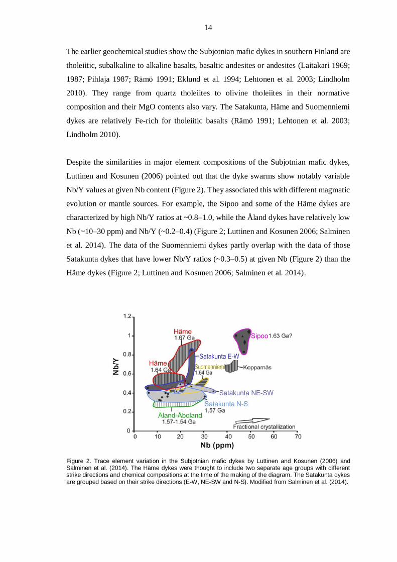
Despite the similarities in major element compositions of the Subjotnian mafic dykes,

Luttinen and Kosunen (2006) pointed out that the dyke swarms show notably variable

Nb/Y values at given Nb content (Figure 2). They associated this with different magmatic

evolution or mantle sources. For example, the Sipoo and some of the Häme dykes are

characterized by high Nb/Y ratios at ~0.8–1.0, while the Åland dykes have relatively low

Nb (~10–30 ppm) and Nb/Y (~0.2–0.4) (Figure 2; Luttinen and Kosunen 2006; Salminen

et al. 2014). The data of the Suomenniemi dykes partly overlap with the data of those

Satakunta dykes that have lower Nb/Y ratios (~0.3–0.5) at given Nb (Figure 2) than the

Häme dykes (Figure 2; Luttinen and Kosunen 2006; Salminen et al. 2014).

Figure 2. Trace element variation in the Subjotnian mafic dykes by Luttinen and Kosunen (2006) and Salminen et al. (2014). The Häme dykes were thought to include two separate age groups with different strike directions and chemical compositions at the time of the making of the diagram. The Satakunta dykes are grouped based on their strike directions (E-W, NE-SW and N-S). Modified from Salminen et al. (2014).

15

The area that covers the mid-Proterozoic dyke swarms in southern Finland (~0.14 Mkm2)

can readily be thought as a scene of one or several CFB events. The separate swarms may

represent fragmented continental LIPs (Bryan and Ernst 2008) that have been separated

by erosion. According to current knowledge, however, the time span for the formation of

the mafic dyke swarms in Finland is ~80 Ma which is longer than the definition of LIPs

(~50 Ma; Bryan and Ernst 2008) permits. The pulsed character stated in the definition of

LIPs (Bryan and Ernst 2008) has, however, been proven either by geochemical (e.g.

Lindholm 2010), mineralogical (e.g. Lehtonen et al. 2003) or other petrological

observations for the southern Finnish Subjotnian dyke swarms. For example, composite

dykes consisting of two mafic dykes are found at least in Åland (Ehlers and Ehlers 1977;

Eklund et al. 1994). In Suomenniemi, two kinds of composite bimodal dykes are found:

1) dykes where the mafic dyke is younger than its felsic counterpart and 2) where the

felsic dyke is younger than its mafic counterpart (Rämö 1991).

3.2.2. Paleomagnetic features

Figure 3 shows some of the paleomagnetic poles of Proterozoic Baltica, including the

Subjotnian poles. The Subjotnian poles include data not only from the mafic dykes that

are the targets of this study, but also from felsic rocks. The Satakunta paleomagnetic pole

SK1 was calculated from the data of the N-S and NE-SW trending dykes and the

paleomagnetic pole SK2 from the E-W trending dykes of Satakunta (Salminen et al.

2014). Salminen et al. (2014) suggested the pole SK2 is older than the SK1 pole due to

its position near older (1.9–1.8 Ga Svecofennian aged) paleomagnetic key poles. A

previous petrological study has also suggested that some of the E-W trending dykes in

Satakunta are continuations of the (~1.64 Ga) Häme dyke swarm based on their strike

directions and locations on the continuation of the Häme fracture zone (Pihlaja 1987).

The presumably younger SK1 pole of Satakunta is similar to the pole of the Åland dykes

(Salminen et al. 2014; 2016), which implies they may belong to the same swarm or simply

that they are coeval. They can also be of different age if the continent has not moved. One

dyke in Satakunta (dyke S11SL in this study) showed a Svecofennian paleomagnetic

direction and was not included in the Subjotnian pole calculations by Salminen et al.

(2014).

16

As shown in Figure 3, the roughly coeval (~1.63–1.64 Ga) Häme, Suomenniemi and

Sipoo poles are distinct, which is unexpected since coeval [in the range of <±20 Ma;

Buchan (2013)] paleomagnetic poles from the same craton should have the same position.

The position of the poles of Suomenniemi and Sipoo swarms show younger

magnetization ages than the pole of Häme swarm (Salminen et al. 2018) (Figure 3).

However, the data from the combined felsic and mafic N polarity dykes of Suomenniemi,

Sipoo and Häme overlap, indicating a coeval magnetization age (Salminen et al. 2018).

According to Salminen et al. (2018) the asymmetry between N and R polarity could imply

problems in the quality of the paleomagnetic data, possibly due to an unremoved

secondary component.

Figure 3. Some Proterozoic paleomagnetic poles for Baltica with A95 error circles. Baltica is at its present-day location. The poles of the dyke swarms in this study are indicated with colours. SK=Satakunta. The references of the poles: 1776 Ma Småland intrusion: Pisarevsky and Bylund (2010); 1750 Ma Hoting gabbro: Elming et al. (2009); 1642 Ma Häme dykes: Salminen et al. (2017); 1643 Ma Suomenniemi dykes: Salminen et al. (2018); 1633 Ma Sipoo dykes: Mertanen and Pesonen (1995); 1576 Ma Åland dykes: Salminen et al. (2016); SK1 1565 Ma Satakunta N-S and NE-SW trending dykes: Salminen et al. (2014); SK2 Satakunta E-W trending dykes: Salminen et al. (2014); 1469 Ma Bunkris-Glysjön-Öje dykes: Pisarevsky et al. (2014); 1457 Ma Lake Ladoga mafic rocks: Salminen and Pesonen (2007); Lubnina et al. (2010); 1384 Ma Mashak suite: Lubnina (2009); 1265 Ma Postjotnian intrusions: Pesonen et al. (2003); 1258 Ma Postjotnian intrusions: Pisarevsky et al. (2014).

17

For some of the Subjotnian dyke swarms, it is possible to define relative ages of the N

and R polarity magnetization directions. In Åland archipelago, the R polarity dykes,

which always occur on different islands or islets than the N polarity dykes, might be older

than the N polarity dykes based on paleomagnetism (Salminen et al. 2016). The actual

age difference, if present, is however unknown. In Sipoo, the R polarity mafic dykes are

interpreted to be older than the N polarity quartz-porphyry dykes based on petrological

studies by Laitala (1984) and Törnroos (1984) and on the paleomagnetic results by

Mertanen and Pesonen (1995). According to Mertanen and Pesonen (1995), the R polarity

mafic dykes showed secondary magnetization components of N polarity as

thermochemical overprints that were produced by the hydrothermal fluids from the felsic

intrusions. This has resulted in almost total remagnetization of one dyke (dyke SF in this

study; Figure 9) (Mertanen and Pesonen 1995). In the Häme swarm, the N and R polarity

dykes are coeval (J. Salminen, unpublished data). The geochronological resolution may

not, however, be high enough to separate the different magma intrusions of different

polarities. The polarity intervals can have durations of only some tens of thousands of

years and the polarity transitions also happen in relatively short time intervals, probably

<5000 years (Butler 1992).

Between the N and R polarity magnetization directions, an asymmetry in declination is

observed in Häme (Salminen et al. 2017) and in inclination in Satakunta (Salminen et al.

2014) and Åland (Salminen et al. 2016) (Figure 4). The possible reasons for the

asymmetry can be an unremoved secondary component, an unusual behaviour of the

geomagnetic field in the Mesoproterozoic, crustal tilting or an age difference between the

N and R polarity dykes associated with continental drift. For Åland and Satakunta, the

symmetry enhanced after a secondary component (B-component) with an adjusted

intensity was subtracted from the primary component (Salminen et al. 2017). For the

Häme data, however, the asymmetry is in declination and the subtraction of an unremoved

secondary component (B-component) did not enhance the symmetry (Salminen et al.

2017).

Many of the Subjotnian dykes as well as other Precambrian dykes in Baltica show a

secondary magnetization component, the B-component, which in some dykes has

completely overprinted the primary magnetization component (Mertanen and Pesonen

1995; Elming et al. 2009; Lubnina et al. 2010; Salminen et al. 2014; 2016; 2017; 2018).

18

Its direction is always close to the Present Earth Field direction (PEF) at the sampling

area (Figure 5). Based on its paleomagnetic pole position, it is thought to be early

Mesozoic and thus it may represent hydrothermal alteration (and the formation of new

magnetic minerals such as hematite, maghemite or magnetite) related to the break-up of

Pangea (Preeden et al. 2009; Salminen et al. 2014).

Figure 4. The normal (blue) and reversed (red) polarity magnetization components of the Subjotnian dykes shown in stereographic projections. Open (closed) symbol denotes downward (upward) directions. Modified from Salminen et al. (2014; 2016; 2017; 2018) and J. Salminen, personal communication (2018).

Figure 5. Site mean directions for the B-component in the Satakunta dyke swarm as reported by Salminen et al. (2014). Blue dot represents mean value. Closed symbols represent downward directions. Green star represents Present Earth’s Field direction on the sampling area. Modified from Salminen et al. (2014).

19

3.3. The Åland dyke swarm

Åland archipelago is located in the southwestern Finland and the crystalline basement of

the main island consists mainly of Mesoproterozoic rapakivi granite (Figures 1 and 6).

The archipelago east of the Åland rapakivi intrusion consists of Paleoproterozoic

Svecofennian rocks that are cut by Paleo- and Mesoproterozoic dykes. The U-Pb (zircon)

ages of the Åland rapakivi granite units are between 1568 ± 10 Ma and 1579 ± 13 Ma

(Suominen 1991).

Figure 6. Generalized geological map of Åland. The sampling sites of this study are indicated.

The Subjotnian mafic dykes are spread around the SW part of the Åland rapakivi to the

SE part and continue ~80 km to NE towards the Vehmaa rapakivi intrusion on the

mainland Finland (Figure 6). However, mafic dykes do not occur in the vicinity of the

Vehmaa intrusion, whereas quartz-porphyry dykes do (Karell et al. 2009). Additionally,

the Åland and Vehmaa rapakivi granites are clearly separated from each other based on

the steep structures that separate the Vehmaa rapakivi from the host rocks (Karell et al.

20

2009). This suggests the Åland rapakivi and associated dykes may have formed separately

from those in mainland Finland. One U-Pb (zircon) age of Vehmaa rapakivi granite is

1590 ± 15 Ma (Vaasjoki 1977), although, as mentioned before, a study by Shebanov et

al. (2000) showed that the core of the ovoid crystals has a U-Pb (zircon) age of 1630 Ma,

while the matrix has a U-Pb (zircon) age of 1573 Ma. Since the prevailing model of

rapakivi magmatism requires mafic underplating, the mafic magmatism may have

occurred also in SW Finland as early as 1630 Ma.

The Åland dyke swarm is typified by vertically or subvertically dipping dykes with strikes

generally in the SSW-NNE direction (e.g. Eklund et al. 1994). Their widths vary from a

few millimetres to over 100 m (Salminen et al. 2016). In his study, Suominen (1991)

divided the dykes in the SW part of the Åland swarm into three sets: the pyroxene diabase

dykes of the Föglö island to the SE of Åland (Figure 6), the anorthositic varieties of these

pyroxene diabase dykes on the islands to the SW of Åland (Västersten, Danten and

Östersten; Figure 6), and the hornblende diabase dykes of the Kumlinge island (Figure

6). On the island of Föglö, the dykes show U-Pb (zircon) ages of 1577 ± 12 Ma and 1540

± 12 Ma (Suominen 1991), although, according to Suominen (1991), the younger age

may have been disturbed by tectonic movements along a fracture line near the site. To the

SW of the Åland rapakivi area, the dykes are most likely of same age as the Föglö dykes

(Suominen 1991). No U-Pb age was obtained from the dykes in Kumlinge by Suominen

(1991).

In addition to the above-mentioned ages, a U-Pb (zircon) age of 1575.9 ± 3.0 Ma has been

reported by Salminen et al. (2016) from a quartz-monzonitic part of a compositionally

heterogeneous bimodal dyke (with width of ~200 m) on Korsö island (Figure 6). There

is, however, evidence of mafic dykes of different ages, and the magmatic activity in Åland

can be considered to have happened during 1570–1580 Ma ago. Evidence of magma

mixing and mingling between basaltic and granitic magmas (Lindberg and Eklund 1992;

Eklund et al. 1994) proves the rapakivi granites and mafic magmas are at least in some

locations coeval. In Kungsholm, Jomala, one mafic dyke cuts the Åland rapakivi granite

(Bergman 1981), proving some dykes are younger than the rapakivi granites. Ehlers and

Ehlers (1977) also describe multiple intrusions in some of the mafic dykes, forming

composite dykes. It remains speculative whether the possible 1630 Ma magmatism in

Vehmaa (Shebanov et al. 2000) reached to Åland.

21

3.4. Satakunta dyke swarm

The Mesoproterozoic suite in the Satakunta area in SW Finland is located on the west

coast of Finland, north of the Laitila and Eurajoki rapakivi batholiths (Figures 1 and 7).

In the southern part of the area (Figure 7a), the Jotnian Satakunta sandstone and the

Postjotnian mafic dykes separate the Subjotnian dykes from the 1573 ± 8 Ma [U-Pb

(zircon); Vaasjoki (1977)] Laitila batholith. The Satakunta sandstone was deposited at ca.

1600–1270 Ma in an intracratonic rift basin during several stages (Pokki et al. 2013). The

younger limit of this timeline is constrained by the intrusion of the Postjotnian olivine

diabase dykes and sills that cut the sandstones and the Laitila rapakivi batholith.

Figure 7. a) Generalized geological map of the Satakunta dyke swarm and adjacent areas. b) The sampling sites of this study. The Laitila rapakivi intrusion is indicated in a).

22

In the northern part of the Satakunta swarm area (Figure 7a), ~150 km to north of the

Laitila batholith, there are smaller rapakivi or rapakivi-type intrusions (Lehtonen et al.

2003): Böle [U-Pb (zircon) age 1568 ± 6 Ma; Lehtonen et al. (2003)], Siipyy [U-Pb

(zircon) age 1562 ± 14 Ma; Idman (1989)], Käräjävuori and Orisberg. In the Kainasto

area (Figure 7a), there are also anorthositic leucogabbros/leucomonzogabbros, medium-

grained gabbros and plagioclase porphyrites of which the plagioclase porphyrites

resemble the Subjotnian mafic dykes in terms of texture, occurrence and chemical

composition (Lehtonen et al. 2003). Postjotnian mafic dykes are also present (Lehtonen

et al. 2003).

Lehtonen et al. (2003) divide the Subjotnian mafic dykes of Satakunta into N-S and E-W

trending dykes that sometimes occur as swarms. Salminen et al. (2014) have additionally

a NE-SW trending group. Pihlaja (1987) suggested the E-W trending dykes in the Pori

area (Figure 7a) may belong to the same en echelon fracture system as the Häme dykes

based on their strike direction and their location that seems to be on a continuous path

from the Häme fracture zone.

According to Lehtonen et al. (2003), coarse-grained types of the Satakunta mafic dykes

are gabbro-like with shorter and wider dimensions than fine-grained types. A U-Pb

(baddeleyite) age of 1565 Ma (error limits unavailable) has been reported by Lehtonen et

al. (2003) for a N-S trending coarse-grained dyke in Härkmeri (in this study, dyke

S11LS). According to Lehtonen et al. (2003), the presence of spherical 1–2 cm sized

quartz inclusions in one dyke is indicative of coeval felsic magmas (or crustal

contamination).

3.5. The Häme dyke swarm

The Häme swarm is the most extensive of the Subjotnian dyke swarms, as it starts from

the Ahvenisto complex near the city of Heinola and continues ~150 km to the ~NW

direction to Kuru (Figures 1 and 8) (Laitakari 1969). The 1644–1629 Ma (Heinonen 2010)

Ahvenisto complex that lies to the NW of the large Wiborg (1642–1622 Ma; Rämö et al.

2014) rapakivi batholith, is a anorthosite-mangerite-charnokite-granite complex that has

23

a rapakivi core partially surrounded by mafic rocks in a horseshoe-shaped zone (e.g.

Heinonen et al. 2010b). The main mafic rock types in Ahvenisto are leucogabbronorite

and olivine-bearing leucogabbro (Heinonen et al. 2010b). According to Laitakari and

Leino (1989), the Ahvenisto gabbro-anorthosite may have been the magma chamber of

the mafic dykes of Häme.

Figure 8. Generalized geological map of the areas of the Häme and Suomenniemi dyke swarms. The sampling sites of this study are indicated. The Ahvenisto, Suomenniemi and Wiborg rapakivi intrusions are also indicated.

The widths of the Subjotnian dykes of Häme swarm vary from a few centimetres possibly

up to 250 m (Laitakari 1969). The widths get narrower the longer the distance is from the

Ahvenisto complex (Laitakari 1969). The dykes dip vertically or subvertically with

typically sharp contacts with the host rock (Laitakari 1969). In three locations, mafic

dykes cut other mafic dykes (Laitakari 1969) which records multiple magma injections.

Laitakari (1969) reports two strike direction maxima; 120°–135° and 095° plus several

other dykes with trends between these limits (095°–120°). Previously the two main strike

directions have been interpreted to correspond to compositionally and chronologically

24

distinctive phases (Laitakari 1969; 1987; Vaasjoki and Sakko 1989; Luttinen and

Kosunen 2006), but a detailed geochemical study by Lindholm (2010) does not support

this idea and suggests the major element variability is mainly caused by different cooling

histories. Instead, Lindholm (2010) identifies three geochemically distinct groups that are

independent of strike directions based on incompatible element ratios.

Based on the most reliable age determinations, the mafic dykes of Häme swarm intruded

at 1635–1646 Ma. The precise ages are: a U-Pb (zircon) age of 1646 ± 6 Ma (Ansio;

Laitakari 1987), a U-Pb (baddeleyite) age of 1642 ± 2 Ma (Virmaila; Salminen et al.

2017) and a U-Pb (zircon) age of 1640 ± 2 Ma (Ahvenisto; Heinonen et al. 2010b).

Additionally, a U-Pb (baddeleyite) age of 1647 ± 14 Ma is obtained from Torittu

(Salminen et al. 2017; site H17 in this study; Figure 8). Unpublished data (J. Salminen)

from the dykes in this study (Figure 8: sites H12, H13, H14 and H25) give U-Pb

(baddeleyite) ages of 1635–1640 Ma. A quartz porphyritic dyke from Ahvenisto complex

has a U-Pb (zircon) age of 1636 ± 2 Ma (Heinonen et al. 2010b), suggesting a younger

age for the felsic dykes.

3.6. The Suomenniemi dyke swarm

The Suomenniemi swarm lies ~60 km to the NE of the Häme swarm and is associated

with the Suomenniemi rapakivi pluton to the north of the Wiborg rapakivi batholith

(Figure 8). The main rapakivi granite series in Suomenniemi crystallized from a single

parental magma at 1644 ± 4 Ma (U-Pb, zircon) and another granitic intrusion occurred

some millions of years later (Rämö 1991; Rämö and Mänttäri 2015). Even later, at 1634

± 4 Ma (U-Pb, zircon), the felsic dykes intruded the rapakivi granites and the

Svecofennian bedrock (Rämö and Mänttäri 2015).

The ~40 mafic dykes that have been studied in the Suomenniemi swarm are vertical,

trending towards NW, and cut sharply the surrounding bedrock (Rämö 1991). The mafic

and felsic dykes have widths of a few centimetres to 50 m but are commonly 5–20 m wide

(Rämö 1991).

25

The mafic dykes of Suomenniemi swarm are approximately the same age than the main

rapakivi series: a U-Pb (zircon) age of 1643 ± 5 Ma (Siivola 1987) has been obtained

from the Lovasjärvi intrusion (Figure 8). Vaasjoki et al. (1991) report that the intrusion

of the mafic dykes in Suomenniemi continued until 1635 Ma, based on the U-Pb data

from the felsic dykes in Suomenniemi and an observation of a composite dyke where the

mafic part is younger than the felsic part. Composite dykes, where a felsic dyke has

intruded the mafic dyke are also present (Rämö 1991 and references therein). Three mafic

dykes are found to cut the rapakivi batholith, while the majority surrounds it (Rämö

1991). According to Haapala and Rämö (1990), the rapakivi granites in Suomenniemi

originate from the Svecofennian crust based on Nd-isotopes. According to Rämö (1991),

the mafic dykes as well as gabbroic and anorthositic rocks in Suomenniemi were derived

from LREE-depleted mantle source and were contaminated by the Svecofennian crust,

based on varying Nd isotopic compositions.

The Lovasjärvi intrusion (Figure 8; site S04 in this study) is a sheet-like, 5 km long and

800 m wide, NW trending and vertically dipping intrusion that is cut by rapakivi granites

at both ends (Siivola 1987). The intrusion consists of melatroctolite and olivine diabase

in the NW part, and medium- to coarse-grained olivine-free diabase in the middle and SE

parts (Siivola 1987; Rämö 1991). Siivola (1987), Laitakari (1987) and Vaasjoki and

Sakko (1989) group the intrusion as part of the Häme dyke swarm, while Rämö (1991)

and Salminen et al. (2018) consider it to belong to the Suomenniemi complex. This study

follows the latter way.

3.7. The Sipoo dyke swarm

The Sipoo dykes are associated with Onas rapakivi stock that lies ~20 km to the west

from the large Wiborg rapakivi batholith (Figure 9). The age of the Onas rapakivi is 1630

± 10 Ma [U-Pb (zircon); Laitala 1984]. Further to the west, there are two other smaller

rapakivi complexes in Bodom and Obbnäs with associated dyke swarms (Figure 9). Both

of these rapakivi granites have a U-Pb (zircon) age of 1645 ± 5 Ma (Vaasjoki 1977).

According to Mertanen and Pesonen (1995), the Sipoo dyke swarm consists of mafic and

felsic dykes with vertical or subvertical dips. The width of the swarm is ~80 km and

26

length ~20 km. The mafic dykes seem to be striking in E-W directions while the felsic

dykes strike mostly in NW-SE directions (Mertanen and Pesonen 1995). The widths of

the mafic dykes range from a few centimetres to 3 m.

Figure 9. Generalized geological map of the Sipoo dyke swarm and adjacent areas. The sampling sites of this study are indicated (no geochemistry was made of the dyke SD).

A felsic dyke in Östersundbom has been dated 1633 Ma [error limits unavailable; U-Pb

(zircon); Törnroos 1984]. The felsic dykes are older than the Onas granite (Törnroos

1984), but younger than the mafic dykes since composite dykes, where a felsic dyke cuts

a mafic dyke, are present (Laitala 1984). The felsic dykes are altered, which may be

related to the crystallization of the Onas granite (Törnroos 1984). The mafic dykes, on

the other hand, are altered possibly due to the hydrothermal fluids from the felsic dykes

and the Onas granite (Mertanen and Pesonen 1995).

27

4. MATERIALS AND METHODS

4.1. Materials

A total of 109 samples from 101 mafic dykes and one sample from a sheet-like mafic

intrusion (site S04 from Lovasjärvi in Suomenniemi; Figure 8) were prepared for

geochemical analysis. The sample collection was done previously for the purposes of

paleomagnetic research (Mertanen and Pesonen 1995; Salminen et al. 2014; 2016; 2017;

2018). The sampling locations are plotted in Figures 6–9. The majority of the samples

were collected by a portable water-cooled gasoline drill. Some samples from Sipoo were

collected as block samples with a hammer. The diameters of the drill core samples are

2.54 cm and lengths vary (Figure 10). Most of the specimens used for this work have a

mass of ~30 g. Sample selection was made, when possible, by avoiding weathered and

fractured samples as well as samples containing phenocrysts. A table showing the

coordinates of the dykes and other features of the samples is in Appendix I.

Figure 10. Some drill core samples from the dyke A8 from Åland. The sample A8C-2 was used for geochemical analysis and, in terms of its size that is standard for paleomagnetism, represents a typical sample for geochemistry in this study.

28

4.2. Geochemical and petrographical methods

The sample preparation for the geochemical analysis was done at the mineralogy

laboratory at the Department of Geosciences and Geography, University of Helsinki. For

the wavelength dispersive X-ray fluorescence (WD-XRF) analysis, the samples were first

polished with a coarse (120 mm) diamond abrasive disc to remove ink marks, glue, paint

(Sipoo samples), graphite pencil marks and fingerprints on the surfaces. Subsequently,

they were crushed inside a plastic bag with additional tough packing plastic material using

a rock splitting press and a hammer. The rock chips were then pulverized using a tungsten

carbide ball mill (Fritsch Pulverisette 6). To produce a glass bead by fusing (Claisse M4

fluxer), 0.600 g of the sample powder was mixed with 6.000 g of flux mixture of lithium

tetraborate (49.75%), lithium metaborate (49.75%) and lithium bromide (0.5%). The

beads were analysed using PANalytical Axios mAX 4 kw WD-XRF spectrometer for the

major (Si, Ti, Al, Fe, Mn, Mg, Ca, Na, K and P) and trace elements (Ba, Ce, Cr, Cu, La,

Nb, Ni, Rb, Sr, U, V, Y, Zn and Zr).

At present, there are neither published accuracy nor precision estimates for the analyses

performed at the mineralogy laboratory. Based on experiments with different calibrations

of the XRF instrument, the detection limits have been obtained for each element

(indicated in the Appendix II if the result was below the limit) (Pasi Heikkilä, personal

communication 2018). The precision (2σ) for the major oxides was <0.1 wt.% and for the

trace elements <10 ppm, except for Ce <20 ppm (Pasi Heikkilä, personal communication

2018).

Some samples showed low total values of the major oxides (down to 90.87 wt.%). A

second bead was made of the powder for one sample (A9A-2, dyke A9 from Åland) to

verify the results. The results of the second bead were similar to the first one (Table 1),

which indicates the low values are due to other reasons than the sample preparation

practice. The reasons for the low values are discussed in Chapter 5.1. and Section 5.2.1.

29

Table 1. Comparison of the results of sample A9A-2 (Åland) obtained from the beads fused from the same sample powder. The results of La and U for the original bead (A9A-2) are below detection limits (10 ppm for La and 2 ppm for U).

Major oxides Sum

SiO2, wt.% TiO2 Al2O3 FeO MnO MgO CaO Na2O K2O P2O5

A9A-2 90.87 46.10 1.98 13.94 13.33 0.17 6.53 4.76 1.38 2.23 0.45 A9A-2, new 91.88 46.43 1.98 14.06 13.39 0.17 6.99 4.80 1.38 2.24 0.44

Trace elements

Ba, ppm Cu Cr Ni Sr Zn Zr Rb Nb Y Ce La V U

A9A-2 254 35 159 70 56 270 168 171 9 50 44 7 188 0 A9A-2, new 243 35 157 74 57 270 171 170 11 48 46 12 188 2

Fifty-two thin sections were examined using polarization microscope Nikon

LABOPHOT2-POL. Samples for petrography were selected based on a preliminary

geochemical grouping of the dykes and their previously reported paleomagnetic

properties (Mertanen and Pesonen 1995; Salminen et al. 2014; 2016; 2017; 2018). Their

textural and mineralogical features and their possible chemical alteration features were

observed.

5. RESULTS

5.1. Petrography

Generalizing, most of the samples show nesophitic, subophitic or ophitic textures

depending on the size of the interstitial clinopyroxene relative to the euhedral plagioclase

laths. Twelve of the 52 samples are porphyritic with plagioclase microphenocrysts

(<3mm). One sample (from dyke A5 from Åland) showed also clinopyroxene

microphenocrysts (<1mm), which form glomerophyric clusters with plagioclase

microphenocrysts (<2mm). Plagioclase (An30-60) is mostly lath-shaped and less than 1 mm

long. Largest plagioclase grains are up to 2 cm long in the sheet-like intrusion S04 from

Lovasjärvi in Suomenniemi. Fifteen of the 52 samples include olivine, which occurs as

subhedral grains and/or anhedral and interstitial between plagioclase laths. Primary

opaque minerals are commonly anhedral and interstitial but occur also as euhedral

30

elongated or cubic grains. Sometimes they have been crystallized before clinopyroxene,

which is indicated by euhedral opaque inclusions in clinopyroxene. Secondary opaque

minerals are also present. A few samples have orthopyroxene as an interstitial mineral.

Apatite is a common accessory mineral and zircons occur in some samples. Some dykes

show rapid cooling with swallow tails and skeletal crystal shapes in plagioclase and the

presence of vesicles (filled with carbonate, quartz, biotite, chlorite and occasional

opaques) are suggestive of near-surface emplacement environment (Figures 11b–c).

Preferred orientation of plagioclase and spherulitic textures are common in these cases

(Figures 11b–c).

Figure 11. Photomicrographs of three thin sections showing different textures observed in the samples (plane polarized light). a) ophitic texture in dyke H24 (sample JS14-H24B-2; Häme), b) spherulitic texture in dyke H15 (Häme) and c) preferred orientation of plagioclase with vesicles in dyke A13 (Åland). ol=olivine, plg=plagioclase, cpx=clinopyroxene.

Secondary biotite is always present and occurs as an alteration product of opaque minerals

and olivine. Biotite is often further altered to chlorite. Clinopyroxene has altered to

chlorite and possibly metamorphosed to amphibole, in some cases almost completely.

Olivine is in some cases altered to “iddingsite” and its cleavage spaces are often filled

with opaque minerals, biotite and serpentine. Plagioclase shows variable alteration to

sericite and saussurite but is generally the least altered primary mineral. In this study, the

overall alteration level of the samples was described using a four-stage scale: low = very

little alteration, moderate = some alteration, high = very altered, very high = totally altered

(Figure 12). The low total %-values of the XRF analysis for some samples is explained

by the high level or complete alteration of the samples which has increased the amount

of volatiles in them.

31

Figure 12. Photomicrographs of four thin sections showing degrees of alteration (plane polarized light). a) low degree alteration: dyke H13 (sample H13; Häme), b) moderate degree alteration: dyke S02 (Suomenniemi), c) high degree alteration: sample dyke H11 (Häme) and d) very high degree alteration: dyke SF (Sipoo).

The dykes H13 and H14 from Häme had anhedral and interstitial-type of plagioclase, that

had formed from an adcumulus-type of crystal growth. The dyke S13 from Suomenniemi

had a quartz-xenocryst and the dyke A3 from Åland a metasedimentary xenolith.

Examination of the samples which contain the overprinted paleomagnetic B-component

shows them to exhibit mainly a “high” degree of alteration. Many of them contain vesicles

and/or fractures. In these samples, the opaque minerals often occur in two varieties,

indicating crystallization of magnetic minerals in at least two separate stages. This degree

of alteration is compatible with previous studies (Preeden et al. 2009; Salminen et al.

2014).

Three of the thin section samples differ from igneous mafic intrusions in terms of

mineralogy and/or texture. The sample A2F-3 (dyke A2) from Åland is andesitic which

is also indicated by the geochemistry (Section 5.2.1; Figure 13). This sample is from a

fine-grained dyke cutting a coarser-grained dyke. The sample A2G-1 is from the coarser-

32

grained part and is a somewhat typical (although altered) diabase with subophitic texture.

Satakunta dykes NI and NO are totally recrystallized, metamorphosed at amphibolite

facies and are amphibolites with foliated textures and abundant hornblende, biotite and

plagioclase. The petrographical features are summarised in Appendix III.

5.2. Geochemistry

5.2.1. Subjotnian dykes in general

The results of the XRF analyses with C.I.P.W. norms are listed in Appendix II. The

processing and interpretation of the data are done using major oxide normalization to

100% (i.e. volatile-free) whereas trace element data are not normalized. Solubility of

water is low in tholeiitic basalts and normalized data probably correspond closely to the

original magma compositions. As discussed in Chapter 5.1. (Appendix III), many of the

samples contain abundant secondary water-bearing minerals. Thus, it can be assumed that

the low totals in some samples result from alteration.

The dykes are grouped according to their locations in the geochemistry diagrams of

Figures 13–16. All the dykes are hyperstene-normative (i.e. tholeiitic), which is typical

of continental flood basalts. They vary from quartz- to olivine-normative types. In the

total alkali vs. silica (TAS) diagram, the dykes plot mainly in the fields of basalts, basaltic

andesites and basaltic trachyandesites (Le Bas et al. 1986; Figure 13). Sub-alkaline

compositions are dominant, but many (31%) have alkaline affinity in Figure 13. Total

alkalis are in the range of 2–6 wt.% and SiO2 content between 46–55 wt.% for most of

the samples. The Åland dykes and some of the Satakunta dykes plot at lower total alkali

contents than most of the other dykes.

Many of the studied Subjotnian dykes have been altered. Classification diagram based on

immobile Nb, Zr, Ti and Y is well-suited for altered samples (Figure 14). Generalizing,

classification of the dykes based on Nb/Y and Zr/Ti is compatible with TAS

classification. The data points group on the basalt field accompanied by groups of

andesites/basaltic andesites and alkali basalts. Accumulation of phenocrysts (e.g. olivine)

does not significantly affect the ratios of incompatible elements, so the picrobasalt dykes

33

JS16-A05 (Häme) and FF (Satakunta) (Figure 13) are classified as basalt and alkali basalt

in Figure 14, respectively. However, while JS16-A05 seems to be fitting well among the

other Häme dykes, FF is part of a minor group of Satakunta dykes that plot in the alkali

basalt field. Sipoo, Åland and Häme dykes all form distinctive, relatively coherent groups,

while the Suomenniemi dykes are scattered and the Satakunta dykes seem to form at least

two groups. Dykes S11SG (Satakunta), SO (Satakunta) and FF (Satakunta) and sample

A2F-2 from dyke A2 (Åland) are exceptional in Figures 13 and 14. These are interpreted

as unrepresentative rock samples and are no longer discussed in this study.

Figure 13. Total alkali–silica diagram for the classification of volcanic rocks (Le Bas et al. 1986). The diagram includes all the samples of this study (n=110). Exceptional dykes and sample are identified (see text).

Figure 14. Classification diagram of basaltic rocks after Pearce (1996). The diagram includes all the samples of this study (n=110). Exceptional dykes and sample are identified (see text).

34

The Subjotnian dykes of this study exhibit a very wide range of MgO (3.1–15.4 wt.%)

(Appendix II). Figures 15 and 16 show variations in major oxides and trace elements

relative to Mg number [molar 100*Mg/(Mg+Fe2+), where Fe2+=0.9*total Fe], which is a

widely used index of fractional crystallization. The dykes are all evolved to varying

degree from a primary magma. The great majority of the dykes represent evolved magmas

typified by high TiO2 (0.7–4.5 wt.%) and lower Ni contents (12–249 ppm). A positive

correlation can be seen in Al2O3 and CaO, while a negative correlation is seen in TiO2,

FeO, K2O and P2O5 (Figure 15). The trace elements also show correlation with Mg

number: the compatible elements Ni and Cu show positive correlation while the

incompatible elements (Ba, Sr, Zn, Zr, Rb, Nb, Y, Ce and La) show negative correlation

(Figure 16).

Figure 15. Mg number (Mg#) vs. major elements (in wt. %) variation diagrams for the Subjotnian dykes (n= 106).

35

Figure 16. Mg number (Mg#) vs. trace elements (in ppm) variation diagrams for the Subjotnian dykes (n= 106).

36

5.2.2. Geochemistry of Åland dyke swarm

Fifteen of the 23 hyperstene-normative dykes of Åland are olivine-normative, while eight

are quartz-normative. The Åland dykes are mainly subalkaline basalts in TAS diagram

with low total alkalis (~3–4 wt.%.) (Figure 13). Dykes A10, A11, A12 and A13 are

basaltic andesites and dyke A1, which is situated on a different island than other sampled

dykes in Åland swarm (Figure 6), is a trachybasalt in TAS diagram (Figure 13) with a

high total alkali value at ~5 wt.%.

Most of the Åland dykes in Figures 15 and 16 form a homogeneous group that is

characterized by relatively low contents of incompatible elements (e.g. K2O, P2O5, Ba,

Zr, Rb, Nb, Ce and La) and high contents of CaO and Ni at Mg numbers of 42–51. Dykes

A1 and A8–A13 differ from this group with slightly lower Mg numbers that range from

37 to 50, and with their generally higher K2O, P2O5, Ba, Zr, Rb, Ce and La contents.

5.2.3. Geochemistry of Satakunta dyke swarm

Ten Satakunta samples (n=43) are olivine-normative while 33 are quartz-normative.

Sample AM1-1AB/2AB (dyke AM) lacks normative diopside, was sampled close to

chilled margin, and is discarded from further examination due to possible contamination

from host rock (see Appendix I: sample AM7-1B is from the same dyke, 3 m from the

dyke margin, and AM1-1AB/2AB is from close to contact.). The dyke OJ has a relatively

high amount of normative olivine (24.40) compared to the other samples of Satakunta.

The presumably Svecofennian aged dyke S11SL does not significantly differ from the

whole Subjotnian assemblage in diagrams in Figures 13–16.

The majority of the Satakunta dykes plot in the subalkaline basalt and basaltic andesite

fields in Figures 13 and 14 forming a coherent group with total alkalis at ~3.0–4.6 wt.%.

Dykes OJ and AT plot in the alkaline basalt field in TAS diagram due to lower silica

contents (Figure 13). Dyke AT is also different from the rest of the Satakunta dykes with

its distinctively higher Ti, Zr, Y and Ce contents at the Mg number of 45. Most of the

Satakunta dykes have Mg numbers between 31–50.

37

There is a group of four dykes (NO, NE, NI and NM) that have lower total alkalis (~2–3

wt.%) than the rest of the Satakunta dykes (Figure 13), plot in or near the alkaline basalt

field in Figure 14, have high Mg numbers (58–65) and high contents of incompatible

elements (TiO2, K2O, P2O5, Ba, Sr, Zr, Rb, Nb, Ce and La) as well as low Na2O and FeO

contents (Figures 15–16). The high contents of compatible elements (Ni, Cu) and high

Mg numbers (59.5 and 64.7, respectively) suggest dykes AO and OJ might be part of this

group. At least two dykes (NI and NO) in the group are metamorphic (Chapter 5.1;

Appendix III).

5.2.4. Geochemistry of Häme dyke swarm

Twelve of the Häme dykes (n=29) are quartz-normative and 17 olivine-normative. In the

TAS diagram (Figure 13), the Häme dykes plot on both sides of the alkaline-subalkaline

boundary. They are characterized by relatively high contents of total alkali (~4.0–5.5

wt.%). Most of the Häme dykes are basalts, but a group of basaltic trachyandesites is also

present. Apart from the picrobasalt dyke JS16-A05 (Mg number 62), the Häme dykes

have Mg numbers between 31–50. Dyke JS16-A05 has a very high amount of normative

olivine (40.99) and its magnetite norm is higher than ilmenite norm while the opposite

occurs in the other Subjotnian dykes. It also shows a high content of olivine grains

(Appendix III). The low-Mg Häme dykes are among the most incompatible element-

enriched Subjotnian mafic intrusions. Dyke H21 is a basaltic andesite, highly anomalous

relative to the other Häme dykes and has also a distinct strike direction and mode of

occurrence (see Appendix I). This sample is therefore no longer discussed in this study.

5.2.5. Geochemistry of Suomenniemi dyke swarm

Four of the Suomenniemi dykes (n=10) are quartz-normative and six olivine-normative.

The compositions of the Suomenniemi dykes are relatively scattered in all diagrams in

Figures 13–16. In TAS diagram, they straddle the alkaline-subalkaline boundary and are

basalts and basaltic andesites with total alkali contents in the range of ~3–5 wt.%. Their

Mg numbers range between 30–50. Some of the Suomenniemi samples have slightly

lower contents of incompatible elements at given Mg number than the rest of the

Subjotnian samples.

38

5.2.6. Geochemistry of Sipoo dyke swarm

The samples (n=5) from the Sipoo dykes (n=4) show all olivine-normative compositions.

The Sipoo dykes are geochemically homogeneous. In the TAS diagram (Figure 13), they

plot in the alkaline basalt field with relatively high contents of total alkalis at ~4.6 wt.%.

They are among the most evolved dykes with low Mg numbers (~35). The Sipoo dykes

have slightly higher TiO2, P2O5, Zr and Nb at given Mg numbers than the other Subjotnian

dykes.

5.2.7. Geochemical grouping of the dykes

Geochemical compositions of mafic rocks reflect the net effect of several processes,

including partial melting, fractional crystallization and crystal accumulation, magma

mixing and contamination, degassing and secondary alteration. Nb/Y vs. Zr/Y diagram

(Figure 17) eliminates the effects of fractional crystallization of mafic magmas and the

ratios of the incompatible elements in this diagram are not affected by secondary

alteration. The distribution coefficients of Nb, Zr and Y for the predominant mineral

phases of mafic magmas, i.e. plagioclase, olivine and clinopyroxene, are similar (e.g.

Aigner-Torres et al. 2007; Earthref.org, GERM Partition Coefficient (Kd) Database, site

visited 02.10.2018). Thus, the ratios of these elements during fractional crystallization

stay somewhat constant. Higher degree of partial melting results in decreasing Nb/Y and

Zr/Y, because the distribution coefficients of Nb and Zr are similar, but they are lower

than that of Y for the mantle peridotite minerals (olivine, orthopyroxene, clinopyroxene,

garnet/spinel) (e.g. Salters and Longhi 1999; Earthref.org, GERM Partition Coefficient

(Kd) Database, site visited 02.10.2018). Thus, variations in Nb/Y at given Zr/Y are very

likely to indicate mantle source heterogeneity, because variable partial melting is typified

by coupled variations in Nb/Y and Zr/Y (e.g. Luttinen 2018). Overall, the Nb/Y vs. Zr/Y

plot (Figure 17) effectively summarises petrogenetically significant geochemical

variation in the studied Subjotnian dykes. The same elements, Nb, Zr and Y were first

used as a diagnostic feature of the Subjotnian dykes by Luttinen and Kosunen (2006) and

were later also used by Salminen et al. (2014).

39

Figure 17. Variation of Nb/Y vs. Zr/Y for the Subjotnian dyke swarms (n=104). Exceptional dykes are indicated (see text). H1, H2 and H3 (Häme swarm), SK1 and SK2 (Satakunta swarm) and Å1 and Å2 (Åland swarm) refer to geochemical groups defined in this study. Dashed lines indicate compositional fields of older (>1.63 Ga) and younger (<1.58 Ga) swarms.

Table 2. Grouping of the Åland dykes according to their geochemistry as in Figure 17. N=normal polarity magnetization. R=reversed polarity magnetization.

ÅLAND SAMPLE/DYKE

LOCATION POLARITY OF VGP

WIDTH OF DYKE (m)

STRIKE/ DIP (°)

GROUP Å1:

A2G-2/A2 Korsö R 100-300 170/- A3C-2/A3 Korsö R >100 170/- A4D-2/A4 Brändö-s-tip R 0.2 045/60 A5C-2/A5 Brändö-s-tip R 0.3 045/90 A6A-2/A6 Brändö-s-tip R 0.05-0.1 045/90 A7C-2/A7 Brändö-s-tip R 0.15 045/90 A14F-2/A14 Torsholma-

Barkholm R 1.5 040/85

A15F-2/A15 -‘’- R 0.8 040/80 A16D-2/A16 -‘’- R 0.5 040/80 A17B-2/A17 -‘’- R 1.5 025/80 A18B-2/A18 -‘’- R 1 040/90 A19C-2/A19 -‘’- R 1.5 030/90 A20A-2/A20 -‘’- R 1.5 025/85 A21C-2/A21 -‘’- R 1.5 035/80 A22A-2/A22 Brändö-s-tip R >5 GROUP Å2: A1E-2/A1 Enklinge N 3 045/80 A8C-2/A8 Brändö-s-tip R 0.3 045/90 A9A-2/A9 Keistiö N 0.12 020/80 A10A-2/A10 Keistiö - 0.1-0.6 A11B-2/A11 Keistiö N 0.35 035/ 80 A12C-2/A12 Keistiö - 0.3 030/75 A13E-2/A13 Keistiö N 5 025/ 85

40

The Åland dykes form two groups (Å1 and Å2; Figure 17; Table 2). Although its Zr/Y

value is similar to Group Å1 (~3–4), dyke A9 is assigned to Group Å2 based on the

geochemistry described in Section 5.2.2.

The Satakunta samples also form two groups (SK1 and SK2; Figure 17; Table 3), of

which the Group SK1 includes most of the samples. Group SK1 is geochemically

Table 3. Grouping of the Satakunta dykes according to their geochemistry as in Figure 17. N=normal polarity magnetization. R=reversed polarity magnetization. SVF=Svecofennian.

SATAKUNTA SAMPLE/DYKE

LOCATION POLARITY OF VGP

WIDTH OF DYKE (m)

STRIKE/ DIP (°)

GROUP SK1:

AM7-1B/AM Ämttöö N >20 000/90 S11HJ 10.1/S11HJ Heikinjärvi N >6-10 020/90 S11HJ 14.1/S11HJ Heikinjärvi N 10 020/90 IV6-1A/IV Ilvesmäki-Pori-Toukari N >20 170/90 IV15-1A/IV Ilvesmäki-Pori-Toukari N >20 170/90 S11GR 4.1/S11GR Grötgrund R 1.5 000/60 S11LS 5.1/S11LS Lillsund N >60 000/- HH2-1B/HH Holmberginhaka -

005/80

S11KA 4.1/S11KA Karlstrand - 1.5 145/60 S11VA 1.1/S11VA Västerängen - 10-15 160/90 S11PL 1.1/S11PL Powerline-

Kristiinankaupunki - ~4 165/70

S11VR 2.1/S11VR Vargöskatan - 0.5 160/- S11OV 3.1/S11OV Överträsket R <0.15 010/60 MA1-1D/MA Mäntymäki N 15 170/90 MA9-1D/MA Mäntymäki N 15 170/90 AT2-1B/AT Ämttöö-Riisivilja N 0.1 035/90 FB5-1B/FB Fiskee - ~1 060/- FE-1AB/1B/FE Fiskee N 0.3 060/72 FI1-1B/FI Fiskee - <0.3 040/90 FK2-3C/FK Fiskee - 0.7 058/90 FS3-1B/FS Fiskee - 0.35 050/ 90 FT10-1A/FT Fiskee -

047/90

FC1-1D/FC Fiskee - ~7 060/90 FC5-1A/FC Fiskee - ~7 060/90 FD6-1D/FD Fiskee - <0.3 060/50 FH7-1AB/FH Fiskee - 0.3 060/ 80 LK8-1B/LK Fläksholma -

055/90

SA8-1B/SA Salmela - 090/75 FA9-1C/FA Fiskee R 0.35 090/90 NR6-1A/NR Söörrmarkuntie - 0.2 095/85 S11BR 5.1/S11BR Brändön - <0.5 075/90 JS16-A01B-1/JS16-A01 Karlstrand - <2 130/90 GROUP SK2: NE1-1B/NE Niemi -

NI6-1B/NI Niemi -

100/75 NM1-1C/NM Niemi -

OJ2-2B/OJ Ojala N 0.1 090/90 NO2-1B/NO Söörrmarkuntie N 0.6 150/65 S11SL 5.1/S11SL Strandlund N (SVF) 1.5 090/90 AO3-1A/AO Ämttöö-Riisivilja N 0.25 115/60

41

relatively uniform and is typified by low Nb/Y at given Zr/Y. Based on the overall

geochemistry, dykes S11BR and S11OV were assigned to Group SK1 despite their

relatively low Zr/Y ratios when compared to the other dykes in Group SK1 (Figure 17).

Satakunta Group SK2 shows variable Zr/Y and Nb/Y and is distinguished from most of

the Subjotnian dykes by high Nb/Y at given Zr/Y. Several dykes belonging to Group SK2

(NI, NO, AO, OJ) show evidence of metamorphism or very strong alteration (including

low total values). Group SK2 includes also the presumably Svecofennian dyke S11SL. It

is possible the dykes NE and NM in Group SK2 are metamorphosed since their chemistry

is similar to that of the metamorphosed dyke NI (Figure 17).

The Häme dykes also show wide ranges of Zr/Y and they can be divided into three groups

(Table 4). Group H1 includes the majority of the Häme dykes and shows the lowest Nb/Y

(~0.4–0.5) and Zr/Y ratios (~5–6). Group H3 has the highest Nb/Y (~0.6–0.8) and Zr/Y

ratios (~9) while Group H2 has Nb/Y in the range of ~0.4–0.6 and Zr/Y at ~7. Group H1

partly coincides with the Suomenniemi dykes and Group H2 with one dyke (S08) from

Suomenniemi (Figure 17). Dyke H23 could not be assigned to these groups. This study

supports the conclusion of Lindholm (2010) that the geochemical groups of Häme dykes

do not correlate with the strike direction of the dykes (Table 4) as was earlier proposed

by Laitakari (1969; 1987) and Vaasjoki and Sakko (1989).

The Suomenniemi samples cluster near the Häme Group H1 in Figure 17, but there is

also variation within the swarm. Sample S04 of the Lovasjärvi intrusion has relatively

high Nb/Y (~0.65) at Zr/Y of ~6, and dyke S10 relatively high Zr/Y (~8) at Nb/Y of ~0.5.

The scatter in the Suomenniemi data implicates that the sample set may not be sufficient

for a comprehensive picture of the compositional variability in the Suomenniemi swarm.

As in the previous diagrams in Chapter 5.2., the Sipoo dykes form their own,

homogeneous geochemical group (Figure 17). They are characterized by relatively high

Nb/Y (~0.5–0.6) and Zr/Y (~8).

42

Table 4. Grouping of the Häme dykes according to their geochemistry as in Figure 17. N=normal polarity magnetization. R=reversed polarity magnetization.

HÄME SAMPLE/DYKE

LOCATION POLARITY OF VGP

WIDTH OF DYKE (m)

STRIKE/ DIP (°)

GROUP H1: JS16-A03F-1/JS16-A03F Soidinkallio - 8 125/- JS16-A04A-1/JS16-A04 Kurjeniemi N 24 140/90 JS16-A05C-1/JS16-A05 Heinola N >250 135/- JS14-H3A-1/H3 Kasiniemi - 20 120/- JS14-H4B-1/2/H4 Kasiniemi/Ansio - 30 120/- JS14-H6C-1/H6 Karivuori - >70 100/- JS14-H12A/H12 Hirtniemi N 12 095/90 JS14-H13A1/H13 Hirtniemi R >60 135/90 JS14-H18A-1/H18 Tuomasvuori N ~50 135/- JS14-H18C-1/2/H18 Tuomasvuori N ~50 135/- JS14-H24A1/H24 Romo R >50 130/- JS14-H25B/E-1/H25 Muorinkallio N >80 130/- GROUP H2: JS16-A02C/D-1/JS16-A02 Iso Niinilammi N 1.9 135/75 JS14-H1B-1/2/H1 Orivesi: Tre-Jklä

road N 5 090/90

JS14-H1E-1/2/H1 Orivesi: Tre-Jklä road

N 5 090/90

JS14-H2F-1/H2 Orivesi: Tre-Jklä road

- 1.5 100/-

JS14-H7B-1/H7 Vehkajärvi - 3.1 100/90 JS14-H7L-1/H7 Vehkajärvi - 3.1 100/90 JS14-H11A/H11 Hirtniemi - 6-8 135/90 JS14-H14C-1/H14 Myllylahti - >40 140/ 00 JS14-H15C-1/2/H15 Harmoistenkaivo N 45 140/90 JS14-H17A-1/H17 Torittu R ~60 090/90 GROUP H3: JS14-H16E-1/2/H16 Torittu - 0.6 100/90 JS14-H19A-3/H19 Koukkujärvi - 24 130/- JS14-H19H-2/H19 Koukkujärvi - 24 130/- JS14-H20F-1/2/H20 Koukkujärvi R 2.5-3 110/90 JS14-H22B-1a/1d/H22 Koukkujärvi - >12 110/90 OTHER: JS14-H23A1/H23 Partakorpi R 30 110/-

It is interesting to notice that the dyke swarms that are believed to have emplacement ages

of >1.63 Ga plot almost exclusively at high Nb/Y (and Zr/Y) values in Figure 17. In

contrast, the dyke swarms that probably record younger magmatic events at <1.58 Ga are

typified by low Nb/Y and Zr/Y. This apparent transition from high Nb/Y to low Nb/Y

compositions during Subjotnian magmatism is discussed in Chapter 6.3.

43

6. DISCUSSION

6.1. Geochemistry vs. magnetic polarity records in the dykes

The reversal of the geomagnetic field is manifested in the studied dykes by the existence

of both N and R polarity magnetization directions. Mafic rocks with different polarity

must have at least marginally different ages. Bearing in mind that the precision of even

the best isotopic ages is on the order of 1% and that polarity intervals can be relatively

short (>104 years; Butler 1992), comparison between magnetic polarity and geochemical

variations can provide useful constraints for assessing the magmatic-tectonic evolution

of mafic dyke swarms. Figure 18 shows the variation of Nb/Y vs. Zr/Y of all the dykes

compared with the polarity of the primary magnetization direction. Most dyke swarms

have formed slowly enough for the magnetic field reversal to have occurred at least once.

The geochemistry of the N polarity dykes is different from that of the R polarity dykes

within the Åland swarm and within Satakunta Group SK1.

Figure 18. Variation of Nb/Y vs. Zr/Y of the studied dykes (n=104) compared with the magnetic polarity of the dykes. The geochemical groups (as in Figure 17) of Åland (Å1 and Å2), Satakunta (SK1 and SK2) and Häme (H1-H3) are indicated. N=normal polarity magnetization. R=reversed polarity magnetization. OP=overprinted (no primary component obtained).

44

The geochemical division of the Åland dykes is in line with the polarity directions (Figure

19). This correlation is clearly visible in the Nb/Y vs. Nb plot in Figure 19b. Group Å1

includes only dykes that show R polarity. Group Å2 includes the N polarity dykes and

one R polarity dyke. The dykes that did not show a primary paleomagnetic component

(dykes A10 and A12) are located in the same area as the N polarity dykes (Figure 6) and

show geochemical affinity to Group Å2. Group Å2 differs from Group Å1 by higher Zr/Y

ratios (Figure 19a). As reported in Section 5.2.2. for the dykes in Group Å2, they also

have higher SiO2, K2O, P2O5, Ba, Zr, Nb, Rb, Ce and La contents and slightly lower Mg

numbers than the dykes in Group Å1. The different magnetic polarities in the

geochemically defined groups of mafic dykes in Åland imply there were two separate

magmatic events/pulses that have an age difference.

Figure 19. Variation of Nb/Y vs. a) Zr/Y and b) Nb of the normal and reversed polarity Åland dykes.

In Satakunta, Group SK1 shows mainly N polarity. Three dykes show R polarity. Within

the Satakunta Group SK1, the N and R polarity dykes show a clear division in their Nb/Y

ratios (Figure 20). The Nb/Y ratios of the R polarity dykes are higher at given Zr/Y ratios

than those of the N polarity dykes. As in Åland, this could mean they have different

magma sources that represent different magmatic events. However, the small number of

R polarity dykes in Group SK1 may not be sufficient enough to reliably verify this

conclusion.

45

Figure 20. Variation of Nb/Y vs. Zr/Y for the normal and reversed polarity Group SK1 dykes (Satakunta).

In Häme, Groups H1 and H2 contain both N and R polarity dykes (Figure 18). Group H3

only has one dyke with a primary (R polarity) magnetization component (dyke H20). The

Suomenniemi dykes do not show correlation between the magnetic polarity and

geochemistry either (Figure 18). This means the mafic intrusions have emplaced during

a long enough time period for the magnetic field reversal to have occurred at least once

in Häme and in Suomenniemi. However, the data do not facilitate assessment of possible

age differences between Groups H1, H2 and H3 in the Häme swarm.

As described by Mertanen and Pesonen (1995), the only N polarity dyke in Sipoo (the

dyke SF) has probably obtained its N polarity magnetization direction as an overprint by

the felsic intrusions in the area. It possibly originally contained also the R polarity

magnetization direction. Thus, the Sipoo dykes are homogeneous in geochemistry and

most likely have the same magnetic polarity (Figure 18), which implies they formed

during the same magmatic event.

6.2. Comparison between VGPs and geochemistry

If the secular changes of the Earth’s magnetic field are averaged out, coeval VGPs from

same sampling site should be overlapping. Thus, dykes that record distinct VGPs

46

probably have an age difference. Within the studied dykes there is geochemical variation

that could indicate age differences between the dykes. Therefore, the VGPs are compared

with the geochemistry of the dykes.

Figure 21. The virtual geomagnetic poles of the Subjotnian mafic dykes used in this study. VGP data from Mertanen and Pesonen (1995) and Salminen et al. (2014; 2016; 2017; 2018). Baltica is at its present-day location. The reversed polarity poles have been inverted. The grey squares with error circles and ages in Ma are paleomagnetic poles for Proterozoic Baltica: see references in Figure 3. The APWP for Proterozoic Baltica (green dashed line) is drawn after Salminen et al. (2017). Å = Åland, SK = Satakunta, H = Häme, SN = Suomenniemi, SI = Sipoo. The Satakunta dykes are divided into three groups based on their strike directions (N-S, NE-SW and E-W). The VGP of the dyke S11SL was interpreted to be of Svecofennian age by Salminen et al. (2014) based on its position.

47

This study uses the VGPs from the previous publications by Mertanen and Pesonen

(1995) and Salminen et al. (2014; 2016; 2017; 2018). The VGPs are plotted in Figure 21.

The geochemical analyses of this study are made from the same samples from which the

paleomagnetic studies were made. The number of dykes showing primary magnetization

(and a VGP) in this study is lower than the number of dykes used for geochemical

analyses due to weak remanent magnetization components and/or strong secondary

components, or due to scattered paleomagnetic results. In general, the R polarity VGPs

seem to plot at lower latitudes than the N polarity VGPs, which reflects the geomagnetic

reversal asymmetry observed in some Subjotnian paleomagnetic results (Salminen et al.

2014; 2016; 2017).

6.2.1. The Åland dyke swarm

Figure 22 highlights the positions of the VGPs of the Åland dykes. The geochemistry of

the Åland dykes correlates with the polarity of VGPs as discussed in Chapter 6.1. The N

polarity VGPs of Åland comprise a scattered group at higher latitudes than the R polarity

VGPs that form a coherent group near the Häme 1642 Ma mean pole (Figure 22). This

may imply a possible age difference between the N and R polarity dykes as suggested in

previous studies (Salminen et al. 2016). The geochemistry supports this as the dykes with

N polarity VGPs have slightly different ratios of incompatible elements than the dykes

with R polarity VGPs. This suggests that the N polarity and R polarity dykes represent

separate magmatic events.

The Åland Group Å2 has similar Zr/Y and Nb/Y values to Satakunta Group SK1 (Figure

17), which raises the question whether these two dyke swarms are at least partially co-

magmatic. Generalizing, the VGPs of Åland Group Å2 are also near the VGPs of

Satakunta (Figures 21–22). On the other hand, this is expected for nearly coeval poles

and does not mean they are co-magmatic. The VGP of the R polarity dyke A8 from Group

Å2 also plots together with the other R polarity VGPs of Åland (i.e. Group Å1) (Figure

22). Based on these data, it cannot be said that the Åland swarm continues to Satakunta

region.

48

Figure 22. The highlighted normal and reversed polarity VGPs of Åland dykes. Other VGPs are shown for comparison (cf. Figure 21). The geochemical groups Å1 and Å2 are indicated. The paleomagnetic pole of the Åland swarm by Salminen et al. (2016) is indicated by black colour. Paleomagnetic data from Mertanen and Pesonen (1995) and Salminen et al. (2014; 2016; 2017; 2018).

6.2.2. The Satakunta dyke swarm

The variation of Nb/Y vs. Zr/Y and the VGPs of the Satakunta dykes are shown in Figure

23. For paleomagnetic studies, the Satakunta dykes were divided by Salminen et al.

(2014) into three groups based on their strike directions (E-W, NE-SW and N-S).

Salminen et al. (2014) obtained two paleomagnetic poles from Satakunta: Pole SK1 from

the NE-SW and N-S trending dykes and Pole SK2 from the E-W trending dykes of

Satakunta (Figures 3 and 23a). These poles are hereby referred to as “Pole SK1” and

“Pole SK2” to separate them from the geochemical groups “Group SK1” and “Group

SK2” defined in this study. Pole SK2 was interpreted to be older than Pole SK1 (but still

Subjotnian) by Salminen et al. (2014). Additionally, one E-W trending dyke (dyke S11SL

in this study) was interpreted to be Svecofennian (and was thus excluded from the

Subjotnian pole calculations) by Salminen et al. (2014) based on its VGP position

(Figures 21 and 23a).

49

Figure 23. The highlighted a) positions of the VGPs (cf. Figure 21) and b) the variation of Nb/Y vs. Zr/Y of the Satakunta dykes (cf. Figure 17). The geochemical groups SK1 and SK2 of the Satakunta dykes (cf. Figure 17) are indicated in both figures. The paleomagnetic poles (SK1 and SK2) of Satakunta by Salminen et al. (2014) are indicated by black colour in a). N=normal polarity magnetization. R=reversed polarity magnetization. OP=overprinted (no primary component obtained). Paleomagnetic data from Mertanen and Pesonen (1995) and Salminen et al. (2014; 2016; 2017; 2018).

50

The geochemistry of this study mostly agrees with the division of the Satakunta dykes by

Salminen et al. (2014) as Group SK2 consists only of E-W trending dykes (Table 4). In

Group SK1, there is one E-W trending dyke that has a VGP (dyke FA). Group SK2 is

discussed here first.

Based on petrography (Chapter 5.1.; Appendix III), dykes NI and NO from Group SK2

are metamorphic. The geochemical similarity (high Nb/Y) between the metamorphic

dykes and other dykes belonging to Group SK2 suggests five Satakunta dykes (NO,

S11SL, NI, NE, NM) are Svecofennian or at least older than Subjotnian (Figure 23b).

Despite its similar geochemistry, dyke AO is not considered to be part of this presumably

Svecofennian group, because it yielded a positive baked contact test (Salminen et al.

2014) and can be regarded as Subjotnian.

The VGP of the metamorphic dyke NO is located on the older side of the APWP for

Baltica (Figure 23a), implying an older Subjotnian age than the 1.57 Ga Satakunta dykes

[as suggested by Salminen et al. (2014) for the Pole SK2]. It is possible the Subjotnian

magnetization component in dyke NO is a secondary component that has overprinted the

possible Svecofennian primary magnetization direction.

Following the observations described above, the only dykes in Group SK2 that can be

regarded as Subjotnian are dykes AO and OJ. They both have high Nb/Y at given Zr/Y

and a high or a very high level of alteration (Appendix III). Additionally, the VGP of dyke

OJ is on the older side of the APWP for Baltica (Figure 23a). Combined, the geochemical

and paleomagnetic features imply that dykes AO and OJ have an older Subjotnian age

than the 1.57 Ga age of Group SK1.

In Group SK1, there are three dykes that show VGPs on the older side of the APWP for

Baltica (dykes FA, S11GR and AT; Figure 23a). The VGPs of these three dykes from

Group SK1 thus imply they could belong to the presumably older group of Subjotnian

dykes in Satakunta. One of them (dyke FA) has an E-W strike direction and was included

in the calculation of the presumably older Pole SK2 by Salminen et al. (2014). Dyke FA

is very altered (Appendix III) which supports it having an old age. It has also relatively

high Nb/Y (0.4), connecting it with the >1.63 Ga dykes in Figure 17. The N-S trending

dyke S11GR, however, apart from the differences related to the magnetic polarity of the

51

dykes (Chapter 6.1.), does not differ from the rest of the dykes of the Satakunta Group

SK1 geochemically. The NE-SW trending dyke AT, on the other hand, has distinctively

higher Ti, Zr, Y and Ce contents than all the other Satakunta dykes at the Mg number of

44.8 (Section 5.2.3.), but it does not stand out from Group SK1 dykes in Figure 23b. Dyke

AT is also very altered (Appendix III). Although it cannot be concluded reliably without

detailed chronological studies, dykes FA and AT have geochemical and paleomagnetic

implications that they are part of the presumably older Subjotnian dykes of Satakunta.

The positions of the N and R polarity VGPs of Group SK1 (Figure 23a) do not support

the speculation that the dykes of different polarities represent different magmatic events

(as was discussed in Chapter 6.1). N and R polarity VGPs occur on both older and

younger sides of the APWP for Baltica (Figure 23a).

6.2.3. The Häme dyke swarm

The VGPs of Häme swarm show a dispersion of VGPs comparable to that observed in

the Satakunta swarm (Figures 23 and 24). The VGPs of the R polarity dykes of Häme

plot near the older side of the APWP for Baltica, while the majority of the dykes with N

polarity VGPs plot closer to the younger side (Figure 24a). Comparison of the three

geochemical groups H1–H3 does not reveal correlation between geochemistry and VGPs

(Figure 24). Häme Groups H1 and H2 show both N and R polarity and Group H3 only

has one dyke with a primary magnetization component (dyke H20). Dyke H23 shows R

polarity VGP but could not be assigned to any of the geochemical groups of Häme.

Several dykes from Häme have been dated, but only those age determinations that have

error limits less than ±10 Ma are discussed in this section. The dated dykes that have N

polarity VGPs are H12 and H25, and they show similar 1.64 Ga ages (J. Salminen,

unpublished data). A dyke with a R polarity VGP (dyke H13) gives also an age of 1.64

Ga (J. Salminen, unpublished data). All these dated dykes belong to Group H1. These

most reliable age determinations prove that some N polarity dykes are of same age as

some R polarity dykes, but it does not necessarily mean that this applies to all the dykes

of Häme. There is a ~60° difference in longitude between the VGPs of the nearly coeval

dykes H12 (and H25) and H13 (Figure 24a). Therefore, it is likely that an age difference

52

Figure 24. The highlighted a) positions of the VGPs (cf. Figure 21) and b) the variation of Nb/Y vs. Zr/Y of the Häme dykes (cf. Figure 17). The geochemical groups of the Häme dykes H1, H2 and H3 (as in Figure 17) are indicated in both figures. The paleomagnetic pole of the Häme swarm by Salminen et al. (2017) is indicated by black colour in a). N=normal polarity magnetization. R=reversed polarity magnetization, OP=overprinted (no primary component obtained). Paleomagnetic data from Mertanen and Pesonen (1995) and Salminen et al. (2014; 2016; 2017; 2018).

53

between the N and R polarity dykes does not explain the distinct VGPs of different

polarities and the scatter in Häme paleomagnetic data.

There are no well-defined ages for the dykes of Häme Groups H2 and H3. However,

dykes H17 and H20 from Groups H2 and H3 respectively, have VGPs near the dated dyke

H13 (Figure 24a). This implies their ages are also similar to that of dyke H13 and that all

the geochemical groups in Häme have roughly the same age: 1635–1640 Ma (J. Salminen,

unpublished data). Geochemical variation can occur rapidly, and the differences observed

between the geochemical groups of Häme can be explained with the age range of 5 Ma.

There is however no reason for the purposes of paleomagnetism to separate different

magma pulses if they are roughly the same age.

There are no implications in geochemistry that would explain the scattered VGPs of the

Häme dykes. Thus, the VGPs may show scatter due to paleosecular variation of the

geomagnetic field or due to other problems in paleomagnetic data that are beyond the

scope of this study.

6.2.4. The Suomenniemi dyke swarm

The Suomenniemi VGPs are relatively scattered, but they tend to settle near the younger

side of the APWP for Baltica (Figures 21 and 25a). The Suomenniemi dykes are also

geochemically relatively variable. Some dykes resemble the Häme dykes while others

resemble the Satakunta dykes (Figure 25b). One dyke (S10) from Suomenniemi has

similar Zr/Y and Nb/Y values to the Sipoo dykes (Figure 25b). Dyke S13 from

Suomenniemi shows similarity in geochemistry with the Häme Group H1 dykes and has

a VGP near them (Figure 25). Dykes S02 and S08 have also geochemical affinities to the

Häme dykes, but their VGPs are a bit off from the Häme VGPs (Figure 25). The positions

of the R polarity VGPs of Suomenniemi near the younger side of the APWP for Baltica,

however, imply that the Suomenniemi dykes were emplaced during an igneous event

distinct from the Häme event(s).

Based on the presence of composite dykes as well as mafic dykes cutting 1644–1640 Ma

rapakivi granites, Rämö (1991) and Vaasjoki et al. (1991) suggested that some of the

Suomenniemi dykes are ~10 Ma younger than the 1643 Ma intrusion in Lovasjärvi (sheet-

54

Figure 25. The highlighted a) positions of the VGPs and the paleomagnetic pole for the Suomenniemi swarm (cf. Figure 21) and b) the variation of Nb/Y vs. Zr/Y of the Suomenniemi dykes (cf. Figure 17). The paleomagnetic pole of the Suomenniemi swarm by Salminen et al. (2018) is indicated by black colour in a). N=normal polarity magnetization. R=reversed polarity magnetization. OP=overprinted (no primary component obtained). Paleomagnetic data from Mertanen and Pesonen (1995) and Salminen et al. (2014; 2016; 2017; 2018).

55

like intrusion S04 in this study). The intrusion S04 has a distinctively higher Nb/Y at

given Zr/Y than the dykes of Suomenniemi in this study (Figure 25b). This feature cannot

be explained by an accumulation of minerals, since the intrusion was petrographically

observed to have a subophitic texture (Appendix III). The distinct Nb/Y values at given

Zr/Y imply that the dykes in Suomenniemi formed in a different magmatic pulse than the

Lovasjärvi intrusion (S04). The VGPs of dykes S02 and S08 are of different polarity and

~20°S from the VGP of intrusion S04. This could support the idea of younger ages at

least for the dykes S02 and S08. It should, however, be noted that the quality of the

paleomagnetic data from Suomenniemi is relatively poor due to scattered data and low

number of samples.

6.2.5. The Sipoo dyke swarm

The Sipoo dykes are very homogenic in their geochemistry but their VGPs are very

scattered (Figure 26). The number of samples is small, which makes the interpretation of

the scattered data challenging. Based on their distinctive geochemistry, especially their

higher TiO2 contents at given Mg numbers (Figure 15), the Sipoo swarm represents a

separate igneous event from those that generated the roughly coeval Häme and

Suomenniemi swarms. This, however, does not mean that the emplacement ages are

significantly different. The reason for the distinct paleomagnetic poles of the coeval

swarms of Häme, Suomenniemi and Sipoo cannot be explained by the geochemical data.

56

Figure 26. The highlighted a) positions of the VGPs (cf. Figure 21) and b) the variation of Nb/Y vs. Zr/Y (cf. Figure 17) of the Sipoo dykes. The paleomagnetic pole of the Sipoo swarm by Mertanen and Pesonen (1995) is indicated by black colour in a). N=normal polarity magnetization. R=reversed polarity magnetization. Geochemical data for dyke SD [VGP indicated in a)] are not available. Paleomagnetic data from Mertanen and Pesonen (1995) and Salminen et al. (2014; 2016; 2017; 2018).

57

6.3. Comparison with previous geochemical data

Comparison with previously published geochemical data (Figure 27) shows that the data

of this study are generally compatible with the data from previous studies. The Åland-

Åboland data from Lindberg et al. (1991) support the geochemical division defined in

this study for the Åland dykes (Figure 27a). The Satakunta Group SK1 data of this study

have some differences with the data of Salminen et al. (2014), but both show relatively

low Nb/Y values for the dykes of Group SK1 (Figure 27a). It remains speculative whether

the possibly older Subjotnian dykes (AO and OJ) of Satakunta Group SK2 have formed

later than the 1.57 Ga Satakunta dykes. The dyke AO of Salminen et al. (2014) shows

similar Nb/Y and Nb values to dyke OJ of this study (Figure 27b).

Figure 27. Variation of Nb/Y vs. Nb of a) Åland and Group SK1 Satakunta dykes and b) Group SK2 Satakunta (excluding the presumably Svecofennian dykes), Häme, Suomenniemi and Sipoo dykes. The geochemical groups (cf. Figure 17) of Åland (Å1 and Å2), Satakunta (SK1 and SK2) and Häme (H1–H3) are indicated. Data from previous studies are shown for comparison. Data without reference are from this study. Grouping of the Satakunta dykes from Salminen et al. (2014) is according to the grouping defined in this study of the Satakunta dykes. Data sources: Lindberg et al. (1991), Rämö (1991), Lindholm (2010), Salminen et al. (2014), this study.

The Häme data of this study show similar Nb/Y and Nb values to those of Lindholm

(2010) (Figure 27b). Dyke H23 of this study and the data from Lindholm (2010),

however, imply there is a set of high Nb/Y dykes in the Häme swarm which is not well

represented by the data of this study (Figure 27b). Comparison with geochemical data of

58

Rämö (1991) shows that the sample material of this study also lacks examples of Nb-rich

intrusions of the Suomenniemi swarm (Figure 27b). The Sipoo data of this study show

lower Nb/Y values and Nb contents than the Sipoo data from Salminen et al. (2014) but

they show overlap with the field of Häme dykes reported by Lindholm (2010) (Figure

27b). These features could imply that there is a connection between the roughly coeval

Häme and Sipoo events.

The transition from high Nb/Y to low Nb/Y compositions during Subjotnian magmatism

was briefly mentioned in Section 5.2.7. and shown in Figure 17. This transition is also

seen in Figure 27, as the dyke swarms that are believed to have emplacement ages of

<1.58 Ga plot at low Nb/Y values (Figure 27a) and those that probably intruded before

1.63 Ga show high Nb/Y values (Figure 27b).

There are no clear geochemical indicators that some of the Satakunta dykes would be part

of, or the same age as the Häme swarm as has been discussed in previous studies (Pihlaja

1987; Salminen et al. 2014). Some of the Satakunta dykes in this study have, however,

shown geochemical and paleomagnetic features that imply those dykes may have an older

Subjotnian age than the 1.57 Ga age defined for the Satakunta swarm. The extension of

the ~1.6 Ga magmatism to SW Finland is supported by the dating of the Vehmaa rapakivi

granite at 1.63 Ga (Shebanov et al. 2000). The data of this study suggests that younger,

possibly <1.58 Ga, emplacement events produced magmas with low Nb/Y (and Zr/Y)

values showing higher degrees of partial melting or different mantle sources than the older

events. Possibly due to the structural separation of Åland from the Vehmaa batholith in

mainland Finland (Karell et al. 2009), the igneous activity did not manifest itself in Åland

before ~1.58 Ga. Further, high-precision geochronological work at least on the Satakunta

swarm is required to verify the regional scale of the ~1.6 Ga Subjotnian magmatism.

6.4. Geochemistry of the dykes with pervasive overprint

The B-component is thought to originate from hydrothermal alteration and crystallization

of secondary magnetic minerals. To study if the B-component is related to the

composition of the melt of which the dykes were crystallized, the Nb/Y vs. Zr/Y diagram

was examined in the light of the B-component in the paleomagnetic data. Four groups

59

were assigned based on the possible existence of the B-component in the dyke (Figure

28): 1) “B” (n=16): dykes that show the B-component (B), but they do not show a primary

component (P); 2) “P+B” (n=41): dykes that show a primary component and the B-

component; 3) “P+S” (n=23): dykes that show a primary component and a secondary (S)

component(s) other than the B-component; 4) “S” (n=30): dykes that show only a

secondary component(s) other than the B-component.

Figure 28. The variation of Nb/Y vs. Zr/Y in terms of the existence of the paleomagnetic B-component in the dykes (n=104). The geochemical groups (cf. Figure 17) of Åland (Å1 and Å2), Satakunta (SK1 and SK2) and Häme (H1–H3) are indicated as well as the areas where Suomenniemi and Sipoo samples are plotted. P=primary magnetization component. B=B-component. S=secondary component other than the B-component.

There is no correlation between the existence of a B-component and the source magma:

the B-component occurs in dykes of all types of magmas (Figure 28). Therefore, it does

not seem to be related to a specific composition of the melt from which the rocks were

crystallized, i.e. the origin of the rock. The low total % -values and petrography (Chapter

5.1.) indicate the rocks with the B-component are usually more altered than the rocks

without it, although alteration is not limited only to the processes that formed the B-

60

component. The physical properties, such as vesicularity, cracks and volatile content as

well as mineralogy may have a bigger impact on the alteration of the rock than the

geochemical composition of the rock. Indeed, most samples that were observed to contain

vesicles and/or cracks (Appendix III), also showed the B-component. The results support

the previous conclusions by Preeden et al. (2009) and Salminen et al. (2014), that the B-

component overprint was formed by hydrothermal alteration of the rocks. The

geochemistry does not explain what was the event that caused the B-component.

7. CONCLUSIONS

This study indicates variability in the geochemistry of Åland, Satakunta and Häme dyke

swarms. The data are, however, compatible with previous data and are thus representative

for the Subjotnian mafic dykes in southern Finland.

Within the Åland swarm, there is a geochemical division into two groups accompanied

with a switch in magnetic polarity. This implies that two separate magmatic events/pulses

that have an age difference have taken place in Åland. The geochemistry indicates that

the Åland and Satakunta swarms are separate igneous events and that the Åland swarm

does not continue to Satakunta region.

The Satakunta dykes form two geochemical groups. Group SK1 is dated to be <1.58 Ga

and shows low Nb/Y (and Zr/Y) values. Group SK2 includes five presumably

Svecofennian dykes and two Subjotnian dykes.

The geochemical data of this study from the Häme swarm forms three groups (H1–H3).

The combined geochemical and paleomagnetic data as well as unpublished chronological

data indicate the Groups H1–H3 are roughly coeval.

Although some Suomenniemi dykes show geochemical affinities to the Häme dykes, they

probably represent a distinct igneous event of Häme.

The Sipoo dykes are very homogeneous in their geochemistry and can be distinguished

from the emplacement event that formed the Häme and Suomenniemi swarms.

61

The Subjotnian dyke swarms in southern Finland that are believed to have emplacement

ages of >1.63 Ga (Häme, Suomenniemi and Sipoo swarms) generally have higher Nb/Y

(and Zr/Y) values than the dyke swarms that are believed to record younger magmatic

events at <1.58 Ga (Åland and Satakunta swarms). Some Satakunta dykes, however, show

geochemical and/or paleomagnetic implications that suggest these dykes could have an

older Subjotnian age than the dated 1.57 Ga dyke in Satakunta. Further, high-precision

chronological work on the Satakunta swarm is required to verify the ages of the dykes.

The origin of the paleomagnetic B-component is related to the alteration of rocks and is

not associated with a certain magma type. The high level of alteration of the dykes that

contain the B-component supports previous assumptions that it forms by hydrothermal

alteration of the rocks.

8. ACKNOWLEDGEMENTS

I want to thank my supervisor Johanna Salminen for providing the thesis topic and

samples, supporting and commenting the work in an encouraging way and for introducing

me to the world of paleomagnetism. I also want to thank my other supervisor, Arto

Luttinen for sharing his expertise in geochemistry and his valuable comments which

greatly improved the quality of the thesis. I am thankful for Satu Mertanen for providing

the Sipoo samples. I also want to acknowledge Pasi Heikkilä for instructing and teaching

me the XRF method from scratch. The laboratory personnel and other staff at the

University of Helsinki, Department of Geosciences and Geography were always very

helpful which is greatly appreciated. Lastly, I would like to thank my family for support

and my partner Hassan Blasim for his patience, support and cooking services during the

busy stages of the work.

9. REFERENCES

Åhäll, K.-I., Brewer, T.S. and Connelly, J.N. 2000. Episodic rapakivi magmatism due to distal orogenesis?: Correlation of 1.69–1.50 Ga orogenic and inboard, “anorogenic” events in the

Baltic Shield. Geology 28: 823–826.

62

Aigner-Torres, M., Blundy, J., Ulmer, P. and Pettke, T., 2007. Laser Ablation ICPMS study of

trace element partitioning between plagioclase and basaltic melts: an experimental approach.

Contributions to Mineralogy and Petrology, 153: 647–667. Arndt, N.T. Czamanske, G.K., Wooden, J.L. and Fedorenko, V.A., 1993. Mantle and crustal

contributions to continental flood volcanism. Tectonophysics, 223: 39–52.

Bergman, L. 1981. Berggrunden inom Signilskär, Mariehamn och Geta kartblad. Summary: Pre-Quaternary rocks of the Signilskär, Mariehamn and Geta map-sheet areas. Geological map of

Finland 1:100 000; Sheets 0034+0043, 1012 and 1021. Explanation to the maps of Pre-

Quaternary rocks, 72 p. Bleeker, W. 2004. Taking the Pulse of Planet Earth: A Proposal for a New Multi-disciplinary

Flagship Project in Canadian Solid Earth Sciences. Geoscience Canada 31, 179–190.

Bleeker, W. and Ernst, R. 2006. Short-lived mantle generated magmatic events and their dyke

swarms: the key unlocking Earth’s paleogeographic record back to 2.6 Ga. In: Hanski, E., Mertanen, S., Rämö, O.T., and Vuollo, J. (Eds.) Dyke Swarms - Time Markers of Crustal

Evolution. Taylor and Francis Group, London, 3–26.

Bryan, S.E. and Ernst, R.E. 2008. Revised definition of Large Igneous Provinces (LIPs). Earth-Science Reviews 86: 175–202.

Buchan, K., Mertanen, S., Park, R., Pesonen, L., Elming, S.-Å., Abrahamsen, N. and Bylund, G.

2000. Comparing the drift of Laurentia and Baltica in the Proterozoic: the importance of key palaeomagnetic poles. Tectonophysics 319: 167–198.

Buchan, K.L. 2013. Key paleomagnetic poles and their use in Proterozoic continent and

supercontinent reconstructions: A review. Precambrian Researc, 238: 93–110.

Butler, R.F. 1992. Paleomagnetism: Magnetic domains to geologic terranes. Blackwell Scientific Publications cop., Boston, 319 p.

Courtillot, V., Jaupart, C., Manighetti, I., Tapponnier, P. and Besse, J. 1999. On causal links

between flood basalts and continental breakup. Earth and Planetary Science Letters, 166: 177–195.

Cox, K.G., Bell, J.D. and Pankhurst, R.J. 1981. The interpretation of igneous rocks. George Allen

& Unwin Ltd, London, 450 p.

Earthref.org, GERM Partition coefficient (Kd) Database, site visited 02.10.2018. https://earthref.org/KDD/

Ehlers, C. and Ehlers, M. 1977. Shearing and multiple intrusion in the diabases of Åland

archipelago, SW Finland. Geological Survey of Finland Bulletin 289: 42 p. Eklund, O., Fröjdö, S. and Lindberg, B. 1994. Magma mixing, the petrogenetic link between

anorthositic suites and rapakivi granites, Åland, SW Finland. Mineralogy and Petrology 50:

3–19. Elming, S., Moakhar, M., Layer, P. and Donadini, F. 2009. Uplift deduced from remanent

magnetization of a proterozoic basic dyke and the baked country rock in the Hoting area,

Central Sweden: a palaeomagnetic and 40Ar/39Ar study. Geophysical Journal International

179: 59–78. Ernst, R.E. and Buchan, K.L. 1997. Giant radiating dyke swarms: their use in identifying pre-

Mesozoic large igneous provinces and mantle plumes. Geophysical Monograph -American

Geophysical Union 100: 297–334. Ernst, R.E. and Buchan, K.L. 2001. Large mafic magmatic events through time and links to

mantle-plume heads. In: R.E. Ernst and K.L. Buchan (Eds.), Mantle plumes: Their

identification through time, Geological Society of America Special Paper, pp. 483–575. Ernst, R.E., Wingate, M.T.D., Buchan, K.L. and Li, Z.X. 2008. Global record of 1600–700Ma

Large Igneous Provinces (LIPs): Implications for the reconstruction of the proposed Nuna

(Columbia) and Rodinia supercontinents. Precambrian Research 160: 159–178.

Evans, D.A.D. 2013. Reconstructing pre-Pangean supercontinents. GSA Bulletin 125: 1735–1751.

Everitt, C.W.F. and Clegg, J.A. 1962. A Field Test of Palaeomagnetic Stability. Geophysical

Journal of the Royal Astronomical Society 6: 312–319. Gallagher, K. and Hawkesworth, C. 1992. Dehydration melting and the generation of continental

flood basalts. Nature 358: 57–59.

63

Haapala, I. and Rämö, O.T. 1990. Petrogenesis of the Proterozoic rapakivi granites of Finland.

Geological Society of America Special Paper 246: 275–286.

Heinonen, A. 2010. Ahvenisto AMCG complex - updates and recent discoveries. In: A. Heinonen, S. Lukkari and T. Rämö (Eds.) Guide to the IGCP-510 (A-type Granites and Related Rocks

Through Time) Field Trip, Southeastern Finland, August 14-18, 2010. Department of

Geosciences and Geology, University of Helsinki C3, pp. 18–21. Heinonen, A.P., Andersen, T. and Rämö, O.T. 2010a. Re-evaluation of Rapakivi Petrogenesis:

Source Constraints from the Hf Isotope Composition of Zircon in the Rapakivi Granites and

Associated Mafic Rocks of Southern Finland. Journal of Petrology 51: 1687–1709. Heinonen, A.P., Ramo, O.T., Manttari, I., Johanson, B. and Alviola, R. 2010b. Formation and

fractionation of high-Al tholeiitic magmas in the Ahvenisto rapakivi granite massif-type

anorthosite complex, southeastern Finland. The Canadian Mineralogist 48: 969–990.

Heinonen, J.S., Luttinen, A.V. and Bohrson, W.A. 2016. Enriched continental flood basalts from depleted mantle melts: modeling the lithospheric contamination of Karoo lavas from

Antarctica. Contributions to Mineralogy and Petrology, 171: 9.

Hospers, J. 1954. Rock Magnetism and Polar Wandering. Nature 173: 1183–1184. Idman, H. 1989. The Siipyy granite-a new rapakivi occurrence in Finland. Bulletin of the

Geological Society of Finland 61: 123–127.

Karell, F., Ehlers, C., Airo, M.-L. and Selonen, O. 2009. Intrusion mechanisms and magnetic fabrics of the Vehmaa rapakivi granite batholith in SW Finland. Geotectonic Research 96: 53–

68.

Laitakari, I. 1969. On the set of olivine diabase dikes in Häme, Finland. Bulletin de la Commission

Géologique de Finlande 241, 65 pp. Laitakari, I. 1987. Hämeen subjotuninen diabaasijuoniparvi. In: K. Aro and I. Laitakari (Eds.),

Suomen diabaasit ja muut mafiset kivilajit. Geological Survey of Finland Report of

Investigation 76., pp. 99–116. Laitakari, I. and Leino, H. 1989. A New Model for the Emplacement of the Häme Diabase Dyke

Swarm, Central Finland. In: S. Autio (Ed.), Current Research 1988. Geological Survey of

Finland, Special Paper 10, pp. 7–8.

Laitala, M. 1984. Pellingin ja Porvoon kartta-alueiden kallioperä. Summary: Pre-Quaternary rocks of the Pellinki and Porvoo map-sheet areas. Geological map of Finland 1:100 000:

Sheets 3012 and 3021. Explanation to the maps of pre-Quaternary rocks. Geological Survey

of Finland, Espoo, 53 p. Le Bas, M.J., Le Maitre, R.W., Streckeisen, A. and Zanettin, B. 1986. IUGS Subcommission on

the Systematics of Igneous Rocks; A Chemical Classification of Volcanic Rocks Based on the

Total Alkali-Silica Diagram. Journal of Petrology 27: 745–750. Lehtonen, M., Kujala, H., Kärkkäinen, N., Lehtonen, A., Mäkitie, H., Mänttäri, I., Virransalo, P.

and Vuokko, J. 2003. Etelä-Pohjanmaan liuskealueen kallioperä. Summary: Pre-Quaternary

rocks of the South Osthrobothnia Schist Belt. Geological Survey of Finland, Report of

Investigation 158: 1–125. Lindberg, B., Eklund, O. and Suominen, V. 1991. Middle Proterozoic Subjotnian diabases and

related mafic rocks in the archipelago of southwestern Finland. In: I. Laitakari (Ed.),

Fennoscandian meeting and excursion on Precambrian dyke swarms, June 10-15, 1991, Finland. IGCP Technical Report 4, 18–30.

Lindberg, B. and Eklund, O. 1992. Mixing between basaltic and granitic magmas in a rapakivi

related quartz-feldspar porphyry, Åland, SW Finland. Geologiska Föreningen i Stockholm Förhandlingar 114: 103–112.

Lindholm, T. 2010. Hämeen diabaasijuonien geokemia. Master's Thesis, University of Helsinki,

50 p.

Lubnina, N. 2009. The East European Craton in the Mesoproterozoic: new key paleomagnetic poles. Doklady Earth Sciences 428: 1174–1178.

Lubnina, N.V., Mertanen, S., Söderlund, U., Bogdanova, S., Vasilieva, T.I. and Frank-

Kamenetsky, D. 2010. A new key pole for the East European Craton at 1452 Ma: Palaeomagnetic and geochronological constraints from mafic rocks in the Lake Ladoga region

(Russian Karelia). Precambrian Research 183: 442–462.

64

Luosto, U., Tiira, T., Korhonen, H., Azbel, I., Burmin, V., Buyanov, A., Kosminskaya, I., Ionkis,

V. and Sharov, N. 1990. Crust and upper mantle structure along the DSS Baltic profile in SE

Finland. Geophysical Journal International 101: 89–110. Luttinen, A.V. 2018. Bilateral geochemical asymmetry in the Karoo large igneous province.

Scientific Reports 8: 5223.

Luttinen, A.V. and Kosunen, P.J. 2006. The Kopparnäs dyke swarm in Inkoo, southern Finland: New evidence for Jotnian magmatism in the SE Fennoscandian Shield. In: Hanski, E.,

Mertanen, S., Rämö, O.T., and Vuollo, J. (Eds.) Dyke Swarms - Time Markers of Crustal

Evolution. Taylor and Francis Group, London, pp. 85–98. McElhinny, M.W. 1973. Palaeomagnetism and plate tectonics. Cambridge University Press, New

York, 358 p.

McElhinny, M.W. and McFadden, P.L. 2000. Paleomagnetism: Continents and Oceans.

International Geophysics Series. Academic Press, San Diego, 386 p. Meert, J.G. 2002. Paleomagnetic Evidence for a Paleo-Mesoproterozoic Supercontinent

Columbia. Gondwana Research 5: 207–215.

Meert, J.G. 2012. What's in a name? The Columbia (Paleopangaea/Nuna) supercontinent. Gondwana Research 21: 987–993.

Merle, R., Marzoli, A., Reisberg, L., Bertrand, H., Nemchin, A., Chiaradia, M., Callegaro, S.,

Jourdan, F., Bellieni, G., Kontak, D., Puffer, J. and McHone, J.G. 2014. Sr, Nd, Pb and Os Isotope Systematics of CAMP Tholeiites from Eastern North America (ENA): Evidence of a

Subduction-enriched Mantle Source. Journal of Petrology 55: 133–180.

Merrill, R.T. and McElhinny, M.W. 1983. The Earth's Magnetic Field: Its History, Origin, and

Planetary Perspective. International Geophysics Series. Academic Press, London, 401 p. Mertanen, S. and Pesonen, L.J. 1995. Palaeomagnetic and rock magnetic investigations of the

Sipoo Subjotnian quartz porphyry and diabase dykes, southern Fennoscandia. Physics of the

Earth and Planetary Interiors 88: 145–175. Neymark, L.A., Yu. Amelin, V. and Larin, A.M. 1994. Pb-Nd-Sr isotopic and geochemical

constraints on the origin of the 1.54–1.56 Ga Salmi rapakivi granite—Anorthosite batholith

(Karelia, Russia). Mineralogy and Petrology 50: 173–193.

Pearce, J.A. and Cann, J. 1973. Tectonic setting of basic volcanic rocks determined using trace element analyses. Earth and planetary science letters 19: 290–300.

Pearce, J.A. 1996. A user’s guide to basalt discrimination diagrams. Trace element geochemistry

of volcanic rocks: applications for massive sulphide exploration. Geological Association of Canada, Short Course Notes 12: pp. 79–113.

Pesonen, L., Elming, S.-Å., Mertanen, S., Pisarevsky, S., D'Agrella-Filho, M., Meert, J., Schmidt,

P., Abrahamsen, N. and Bylund, G. 2003. Palaeomagnetic configuration of continents during the Proterozoic. Tectonophysics 375: 289–324.

Pihlaja, P. 1987. The Subjotnian diabases of the Pori region, southwestern Finland. Geological

Survey of Finland, Report of Investigation 76: 133–150.

Pisarevsky, S. and Bylund, G. 2010. Paleomagnetism of 1780–1770 Ma mafic and composite intrusions of Småland (Sweden): implications for the Mesoproterozoic supercontinent.

American Journal of Science 310: 1168–1186.

Pisarevsky, S.A., Elming, S.-Å., Pesonen, L.J. and Li, Z.-X. 2014. Mesoproterozoic paleogeography: supercontinent and beyond. Precambrian Research 244: 207–225.

Pokki, J., Kohonen, J., Lahtinen, R., Rämö, T.O. and Andersen, T. 2013. Petrology and

provenance of the Mesoproterozoic Satakunta formation, SW Finland, 204. Geological Survey of Finland, Report of Investigation 204: 61 p.

Preeden, U., Mertanen, S., Elminen, T. and Plado, J. 2009. Secondary magnetizations in shear

and fault zones in southern Finland. Tectonophysics 479: 203–213.

Rämö, O.T. 1991. Petrogenesis of the Proterozoic rapakivi granites and related basic rocks of southeastern Fennoscandia: Nd and Pb isotopic and general geochemical constraints.

Geological Survey of Finland Bulletin 355: 1–161.

Rämö, O.T. and Haapala, I. 1995. One hundred years of rapakivi granite. Mineralogy and Petrology 52: 129–185.

65

Rämö, O.T. and Haapala, I. 2005. Rapakivi Granites. In: M. Lehtinen, P.A. Nurmi and O.T. Rämö

(Eds.), Precambrian Geology of Finland - Key to the Evolution of the Fennoscandian Shield.

Elsevier, pp. 533–562. Rämö, O.T. and Mänttäri, I. 2015. Geochronology of the Suomenniemi rapakivi granite complex

revisited: Implications of point-specific errors on zircon U-Pb and refined λ87 on whole-rock

Rb-Sr. Bulletin of the Geological Society of Finland 87: 25–45. Rämö, O. T., Heinonen, A., Lahaye, Y., Larjamo, K., Mänttäri, I. and Turkki, V. 2014. Age and

isotopic fingerprints of some plutonic rocks in the Wiborg rapakivi granite batholith with

special reference to the dark wiborgite of the Ristisaari Island. Bulletin of the Geological Society of Finland 86, 71–91.

Rogers, J.J.W. and Santosh, M. 2002. Configuration of Columbia, a Mesoproterozoic

Supercontinent. Gondwana Research 5: 5–22.

Salminen, J. and Pesonen, L.J. 2007. Paleomagnetic and rock magnetic study of the Mesoproterozoic sill, Valaam island, Russian Karelia. Precambrian Research 159: 212–230.

Salminen, J., Mertanen, S., Evans, D.A.D. and Wang, Z. 2014. Paleomagnetic and geochemical

studies of the Mesoproterozoic Satakunta dyke swarms, Finland, with implications for a Northern Europe – North America (NENA) connection within Nuna supercontinent.

Precambrian Research 244: 170–191.

Salminen, J., Klein, R., Mertanen, S., Pesonen, L.J., Fröjdö, S., Mänttäri, I. and Eklund, O. 2016. Palaeomagnetism and U–Pb geochronology of c. 1570 Ma intrusives from Åland archipelago,

SW Finland – implications for Nuna. Geological Society, London, Special Publications 424:

95–118.

Salminen, J., Klein, R., Veikkolainen, T., Mertanen, S. and Mänttäri, I. 2017. Mesoproterozoic geomagnetic reversal asymmetry in light of new paleomagnetic and geochronological data for

the Häme dyke swarm, Finland: Implications for the Nuna supercontinent. Precambrian

Research 288: 1–22. Salminen, J., Klein, R. and Mertanen, S. 2018. New rock magnetic and paleomagnetic results for

the 1.64 Ga Suomenniemi dyke swarm, SE Finland. Precambrian Research, in press.

Salters, V.J.M. and Longhi, J., 1999. Trace element partitioning during the initial stages of

melting beneath mid-ocean ridges. Earth and Planetary Science Letters, 166: 15–30. Shebanov, A.D., Savatenkov, V., Eklund, O., Andersson, U.B., Annersten, H. and Claesson, S.

2000. Regional mineralogical correlation linking post- and anorogenic magmatic events:

evidences from unusual barian biotites in the Järppilä rapakivi porphyries, Vehmaa batholith (s. Finland), In: Advances On Micas - Problems, Methods, Application in Geodynamics. Rome

2.-3.11.2000.

Siivola, J. 1987. The mafic intrusion of Lovasjarvi. Geological Survey of Finland, Report of Investigation 76: 121–128.

Suominen, V. 1991. The Chronostratigraphy of South-Western Finland with Special Reference

to Postjotnian and Subjotnian Diabases. Geological Survey of Finland Bulletin 356: 100 p.

Törnroos, R. 1984. Petrography, mineral chemistry and petrochemistry of granite porphyry dykes from Sibbo, southern Finland. Geological Survey of Finland Bulletin 326: 1–43.

Vaasjoki, M. 1977. Rapakivi granites and other postorogenic rocks in Finland: their age and the

lead isotopic composition of certain associated galena mineralizations. PhD Thesis, Geological Survey of Finland, Espoo, 74 p.

Vaasjoki, M. and Sakko, M. 1989. The radiometric age of the Virmaila diabase dyke: Evidence

for 20 Ma of continental rifting in Padasjoki, southern Finland. Geological Survey of Finland, Special Paper 10: 43–44.

Vaasjoki, M., Rämö, O. T. and Sakko, M. 1991. New U-Pb ages from the Wiborg rapakivi area:

constraints on the temporal evolution of the rapakivi granite-anorthosite-diabase dyke

association of southeastern Finland. Precambrian Research 51: 227–243. Wang, X.-C., Wilde, S.A., Li, Q.-L. and Yang, Y.-N. 2015. Continental flood basalts derived

from the hydrous mantle transition zone. Nature Communications 6: 7700.

Winchester, J.A. and Floyd, P.A. 1976. Geochemical magma type discrimination: application to altered and metamorphosed basic igneous rocks. Earth and Planetary Science Letters 28: 459–

469.

66

Winter, J.D. 2001. An Introduction to Igneous and Metamorphic Petrology. Prentice Hall, New

Jersey, 697 p.

Zhao, G., Sun, M., Wilde, S.A. and Li, S. 2004. A Paleo-Mesoproterozoic supercontinent: assembly, growth and breakup. Earth-Science Reviews 67: 91–123.

10. APPENDICES

Appendix I. The coordinates of the dykes and other information.

Appendix II. The XRF results and C.I.P.W. norms.

Appendix III. Petrographic observations.

APPENDIX I. The locations and coordinates of the sampling sites, paleomagnetic polarity (N=normal, R=reversed) of virtual geomagnetic poles (VGPs) and other information on the samples. SVF=Svecofennian. On the “Paleomagnetic components” -column: P=primary magnetization component. B=B-component. S=secondary component other than the B-component.

SAMPLE/DYKE LOCATION LAT (°) LONG (°) POLARITY OF VGP

PALEO-MAGNETIC COMPO-NENTS

WIDTH OF DYKE (m)

STRIKE/ DIP (°)

SAMPLING NOTES

Åland

A1E-2/A1 Enklinge 60.32501 20.73659 N P+B 3 045/80 4 cm to dyke margin A2F-2/A2 Korsö 60.41191 20.98899 R P+B

170/- cutting A2G-2

A2G-2/A2 Korsö 60.41191 20.98899 R P+B 100-300 170/- big dyke cut by narrower, fine-grained dykes (A2F-2), ~5 cm from the contact of the two varieties

A3C-2/A3 Korsö 60.42021 20.99369 R P+B >100 170/-

A4D-2/A4 Brändö-s-tip 60.40367 21.03527 R P+B 0.2 045/60 from margin A5C-2/A5 Brändö-s-tip 60.40352 21.03536 R P+B 0.3 045/90 from margin A6A-2/A6 Brändö-s-tip 60.40349 21.03542 R P+S 0.05-0.1 045/90 from margin A7C-2/A7 Brändö-s-tip 60.40349 21.03542 R P+S 0.15 045/90 from margin A8C-2/A8 Brändö-s-tip 60.42021 20.99397 R P+B 0.3 045/90 from margin A9A-2/A9 Keistiö 60.3678 21.33001 N P+B 0.12 020/80

A10A-2/A10 Keistiö 60.36783 21.32999 - S 0.1-0.6 15 cm from margin A11B-2/A11 Keistiö 60.3741 21.29178 N P+B 0.35 035/ 80

A12C-2/A12 Keistiö 60.3741 21.29178 - S 0.3 030/75 10 cm from margin A13E-2/A13 Keistiö 60.37411 21.29178 N P+B 5 025/ 85 from margin A14F-2/A14 Torsholma-Barkholm 60.35017 21.06314 R P+B 1.5 040/85 4 cm from margin A15F-2/A15 Torsholma-Barkholm 60.35021 21.06291 R P+S 0.8 040/80

A16D-2/A16 Torsholma-Barkholm 60.35018 21.06307 R P+B 0.5 040/80

A17B-2/A17 Torsholma-Barkholm 60.35016 21.06313 R P+S 1.5 025/80

A18B-2/A18 Torsholma-Barkholm 60.35015 21.06316 R P+B 1 040/90

A19C-2/A19 Torsholma-Barkholm 60.35015 21.06316 R P+S 1.5 030/90

A20A-2/A20 Torsholma-Barkholm 60.35015 21.06316 R P+B 1.5 025/85 5 cm from margin A21C-2/A21 Torsholma-Barkholm 60.35011 21.06317 R P+B 1.5 035/80 10 cm from margin A22A-2/A22 Brändö-s-tip 60.42021 20.99397 R P+S >5

Satakunta

AM-1AB/2AB/AM Ämttöö 61.662 21.62 N P+B >20 000/90 close to margin AM7-1B/AM Ämttöö 61.662 21.62 N P+B >20 000/90 3 m from margin S11HJ 10.1/S11HJ Heikinjärvi 62.05921 21.67 N P+S >6-10 020/90 close to margin S11HJ 14.1/S11HJ Heikinjärvi 62.05921 21.67 N P+S 10 020/90 25 cm from margin IV6-1A/IV Ilvesmäki-Pori-Toukari 61.5419 21.7524 N P+B >20 170/90 2.15 m from margin IV15-1A/IV Ilvesmäki-Pori-Toukari 61.5419 21.7524 N P+B >20 170/90 center of dyke S11GR 4.1/S11GR Grötgrund 62.2404 21.37973 R P+S 1.5 000/60 15 cm from margin S11LS 5.1/S11LS Lillsund 62.20588 21.42881 N P+S >60 000/-

HH2-1B/HH Holmberginhaka 61.687 21.594 - S

005/80 sample covers the whole width of the dyke

S11KA 4.1/S11KA Karlstrand 62.30109 21.37854 - S 1.5 145/60 10 cm from margin S11VA 1.1/S11VA Västerängen 62.26948 21.43409 - S 10-15 160/90 3 cm from margin S11PL 1.1/S11PL Powerline-

Kristiinankaupunki 62.27918 21.43138 - S ~4 165/70 4 cm from margin

S11VR 2.1/S11VR Vargöskatan 62.22967 21.38082 - S 0.5 160/- 7 cm from margin S11SG 1.1/S11SG Smultrongrung 62.19736 21.44071 - S 7-10 000/- middle of dyke S11OV 3.1/S11OV Överträsket 62.15448 21.39492 R P+S <0.15 010/60 5 cm from margin MA1-1D/MA Mäntymäki 61.7262 21.6094 N P+B 15 170/90 closer to margin than MA9 MA9-1D/MA Mäntymäki 61.7262 21.6094 N P+B 15 170/90 MA1 is closer to margin than MA9 AT2-1B/AT Ämttöö-Riisivilja 61.644 21.635 N P+S 0.1 035/90 from margin SO3-1A/SO Söörmarkku 61.5681 21.81511 - S

FB5-1B/FB Fiskee 61.683 21.55 - S ~1 060/- 7 cm from margin FE-1AB/1B/FE Fiskee 61.679 21.545 N P+B 0.3 060/72 center of dyke FF3-1B/FF Fiskee 61.687 21.594 - S

040/90 6-8 cm from margin

FI1-1B/FI Fiskee 61.68004 21.54199 - B <0.3 040/90

FK2-3C/FK Fiskee 61.68004 21.54199 - B 0.7 058/90 center of dyke FS3-1B/FS Fiskee 61.68004 21.54199 - B 0.35 050/ 90 center of dyke FT10-1A/FT Fiskee 61.68 21.553 - S

047/90

FC1-1D/FC Fiskee 61.6802 21.5451 - B ~7 060/90 ~3 m from margin FC5-1A/FC Fiskee 61.6802 21.5451 - B ~7 060/90 20 cm from margin FD6-1D/FD Fiskee 61.6804 21.5461 - B <0.3 060/50 ~10 cm from margin FH7-1AB/FH Fiskee 61.6807 21.5462 - B 0.3 060/ 80

LK8-1B/LK Fläksholma 61.687 21.587 - S

055/90 ~12 cm from margin NE1-1B/NE Niemi 61.74803 21.5541 - S

NI6-1B/NI Niemi 61.74803 21.5541 - S

100/75

NM1-1C/NM Niemi 61.74803 21.5541 - S

SA8-1B/SA Salmela 61.744 21.616 - B

090/75

FA9-1C/FA Fiskee 61.679 21.545 R P+B 0.35 090/90 3 cm from margin OJ2-2B/OJ Ojala 61.744 21.616 N P+S 0.1 090/90

NO2-1B/NO Söörrmarkuntie 61.56 21.82 N P+S 0.6 150/65 15 cm from margin NR6-1A/NR Söörrmarkuntie 61.56 21.82 - B 0.2 095/85 center of dyke S11BR 5.1/S11BR Brändön 62.19396 21.44967 - S <0.5 075/90 15 cm from margin S11SL 5.1/S11SL Strandlund 62.19736 21.44071 N (SVF) P+S 1.5 090/90 1 cm from margin AO3-1A/AO Ämttöö-Riisivilja 61.6068 21.7833 N P+B 0.25 115/60 3 cm from margin JS16-A01B-1/JS16-A01 Karlstrand 62.30115 21.37869 - S <2 130/90 ~50 cm from margin Häme

JS16-A02C/D-1/JS16-A02 Iso Niinilammi 61.2969 25.73298 N P+S 1.9 135/75 20-30 cm from margin JS16-A03F-1/JS16-A03 Soidinkallio 61.29261 25.78074 - B 8 125/-

JS16-A04A-1/JS16-A04 Kurjeniemi 61.26891 25.88807 N P+B 24 140/90

JS16-A05C-1/JS16-A05 Heinola 61.2554 25.07348 N P+S >250 135/-

JS14-H1B-1/2/H1 Orivesi: Tre-Jklä road 61.66022 24.2579 N P+B 5 090/90

JS14-H1E-1/2/H1 Orivesi: Tre-Jklä road 61.66022 24.2579 N P+B 5 090/90 close to margin JS14-H2F-1/H2 Orivesi: Tre-Jklä road 61.6633 24.2652 - S 1.5 100/- 10 cm from margin JS14-H3A-1/H3 Kasiniemi 61.45257 24.89912 - S 20 120/-

JS14-H4B-1/2/H4 Kasiniemi/Ansio 61.44028 24.91873 - S 30 120/-

JS14-H6C-1/H6 Karivuori 61.49417 24.78237 - S >70 100/-

JS14-H7B-1/H7 Vehkajärvi 61.50682 24.83713 - S 3.1 100/90 from margin JS14-H7L-1/H7 Vehkajärvi 61.50682 24.83713 - S 3.1 100/90 20 cm from margin JS14-H11A/H11 Hirtniemi 61.3335 25.3992 - B 6-8 135/90

JS14-H12A/H12 Hirtniemi 61.3397 25.3951 N P+B 12 095/90

JS14-H13A1/H13 Hirtniemi 61.3396 25.4095 R P+B >60 135/90 from margin JS14-H14C-1/H14 Myllylahti 61.4781 25.1485 - S >40 140/ 00 from margin JS14-H15C-1/2/H15 Harmoistenkaivo 61.4896 25.125 N P+B 45 140/90 from margin JS14-H16E-1/2/H16 Torittu 61.4515 25.1431 - S 0.6 100/90 5 cm from margin JS14-H17A-1/H17 Torittu 61.4515 25.1431 R P+B ~60 090/90 from margin JS14-H18A-1/H18 Tuomasvuori 61.3605 25.2903 N P+B ~50 135/-

JS14-H18C-1/2/H18 Tuomasvuori 61.3605 25.2903 N P+B ~50 135/-

JS14-H19A-3/H19 Koukkujärvi 61.442 25.2183 - S 24 130/- from margin JS14-H19H-2/H19 Koukkujärvi 61.442 25.2183 - S 24 130/-

JS14-H20F-1/2/H20 Koukkujärvi 61.4411 25.2168 R P+B 2.5-3 110/90

JS14-H21a-1A/2A/H21 Koukkujärvi 61.4419 25.2173 - S 0.5 040/45 forms network with host rock JS14-H22B-1a/1d/H22 Koukkujärvi 61.4409 25.2177 - S >12 110/90 ~2 m from margin JS14-H23A1/H23 Partakorpi 61.4568 25.0548 R P+B 30 110/-

JS14-H24A1/H24 Romo 61.4041 25.0316 R P+B >50 130/-

JS14-H25B/E-1/H25 Muorinkallio 61.4201 24.9873 N P+S >80 130/- from margin Suomenniemi

JS16S02F-1/2/S02 Syväjärvi 61.38741 27.37468 R P+B 10 120/-

JS16S03F-1/2/S03 Kirkkovuori 61.4179 27.24749 - B 15 120/- ~10 cm from margin JS16S04A-1/S04 Lovasjärvi 61.15562 27.14392 N P+B ~800 120/- sheet-like intrusion JS16S08E-2/3/S08 Pellosniemi 61.46265 27.26889 R P+B 3 135/90 ~1m from margin JS16S09E-1/S09 Viiru 61.34045 27.18698 - B 5 120/- ~2m from margin JS16S10I-1/S10 Korpijärvi 61.33423 27.18958 N P+B >20 130/90 diabase and quartz-porphyry mingled

dyke, sample from diabase close to quartz-porphyry

JS16S11D-1/S11 Lehtoniemi/Lehtojärvi 61.33242 27.1269 - B >20 120/-

JS16S12A/B-1/S12 Riippa 61.35487 27.11097 - B <0.2 090/90

JS16S13A/C-1/S13 Hujala 61.35692 27.3414 N P+B 20

JS16S14E-2/S14 Joutsa 61.69276 26.24243 - B

Sipoo

SB10-1B/SB Sipoo, Kerava, Ahjo 60.4 25.15 R P+S <3 ~090/-

SB2-1D/SB Sipoo, Kerava, Ahjo 60.4 25.15 R P+S <3 ~090/-

SC1-1D/SC Sipoo, Hästberget 60.4 25.23 R P+S <3 ~090/-

SD Sipoo, Kalkstrand 60.25 25.4 R P+S

~090/-

SF2-1B/SF Sipoo, railway 60.37 25.38 N P+S ~0.3 ~020/-

SG2-1C/SG Sipoo, Paipis 60.42 25.22 R P+S <3 ~135/-

APPENDIX II. Major and trace element concentrations by XRF at the Department of Geosciences and Geography, University of Helsinki. < denotes result below detection limit. CIPW norm calculated from major elements normalized to 100% with Fe3+/total Fe at 0.1.

ÅLAND A1E-2 A2F-2 A2G-2 A3C-2 A4D-2 A5C-2 A6A-2 A7C-2 A8C-2 A9A-2 A10A-2 A11B-2 A12C-2 A13E-2

SiO2, wt.% 46.41 58.25 47.53 50.53 47.90 48.10 47.54 47.82 46.34 46.10 50.51 50.28 51.04 50.28

TiO2 2.61 1.56 1.14 1.33 1.41 1.41 1.35 1.38 4.45 1.98 1.54 2.82 1.75 2.70

Al2O3 15.82 13.03 20.38 16.26 16.86 16.88 16.90 16.84 13.69 13.94 16.02 15.27 15.33 14.66

FeO 13.17 10.01 9.97 10.90 11.83 11.94 11.61 11.85 15.05 13.33 10.32 10.87 12.13 12.01

MnO 0.17 0.16 0.13 0.22 0.19 0.18 0.18 0.18 0.18 0.17 0.11 0.10 0.14 0.22

MgO 6.69 1.56 4.03 6.44 6.36 6.39 6.26 6.40 4.44 6.53 3.52 5.27 4.68 4.18

CaO 3.80 4.70 9.63 8.68 9.16 9.17 9.27 9.24 8.03 4.76 6.74 5.23 6.63 7.98

Na2O 3.98 2.98 2.99 2.66 2.80 2.81 2.71 2.73 2.33 1.38 2.09 1.99 2.62 2.50

K2O 1.38 3.40 1.26 0.55 0.48 0.47 0.45 0.45 1.59 2.23 2.09 1.53 0.99 0.91

P2O5 0.29 0.50 0.30 0.29 0.23 0.23 0.22 0.22 1.19 0.45 0.36 0.73 0.48 0.70

Sum 94.32 96.15 97.36 97.89 97.22 97.58 96.49 97.11 97.29 90.87 93.30 94.09 95.79 96.14

Ba, ppm 286 846 354 205 245 252 237 239 774 254 492 425 404 440

Ce 38 207 39 34 33 42 33 38 135 44 56 85 85 96

Cu 23 21 29 37 55 52 57 55 45 35 15 28 29 38

Cr 13 11 22 72 74 67 73 70 129 159 27 74 41 74

La 10 99 <10 12 19 <10 15 18 44 <10 20 43 24 40

Nb 7 28 7 6 9 8 10 6 23 9 8 13 7 18

Ni 43 5 43 48 83 84 81 81 45 70 21 28 31 27

Rb 82 142 37 26 14 14 12 12 53 171 51 92 80 31

Sr 156 172 278 243 256 257 256 258 284 56 266 205 355 246

U <2 3 2 <2 <2 4 3 2 2 <2 <2 <2 <2 <2

V 141 76 78 158 192 196 186 188 127 188 254 137 258 150

Y 38 99 27 31 30 29 30 30 84 50 40 59 49 54

Zn 135 232 116 126 113 105 110 109 219 270 66 123 119 132

Zr 179 431 100 116 95 94 91 92 423 168 157 273 217 247

CIPW Q 0.00 13.01 0.00 0.85 0.00 0.00 0.00 0.00 0.82 2.96 6.43 10.75 5.51 6.33

C 1.66 0.00 0.00 0.00 0.00 0.00 0.00 0.00 0.00 1.85 0.00 2.74 0.00 0.00

Or 8.65 20.90 7.65 3.32 2.92 2.85 2.76 2.74 9.66 14.50 13.24 9.61 6.11 5.59

Ab 35.71 26.23 25.99 23.00 24.37 24.37 23.77 23.79 20.27 12.85 18.96 17.90 23.14 22.00

An 17.98 12.62 39.51 31.48 32.93 32.85 33.81 33.33 22.82 22.75 30.18 22.51 28.34 27.14

Di 0.00 7.09 6.32 8.75 10.16 10.14 10.25 10.27 8.51 0.00 2.64 0.00 2.28 7.77

Hy 7.53 14.37 0.52 27.73 13.97 14.33 14.67 14.81 24.18 37.68 22.93 27.34 28.16 22.34

Ol 20.49 0.00 15.61 0.00 10.59 10.42 9.83 10.08 0.00 0.00 0.00 0.00 0.00 0.00

Mt 2.03 1.51 1.49 1.62 1.76 1.77 1.75 1.77 2.24 2.13 1.60 1.68 1.84 1.81

Il 5.26 3.08 2.23 2.58 2.76 2.75 2.66 2.70 8.69 4.14 3.14 5.70 3.47 5.34

Ap 0.73 1.23 0.73 0.70 0.56 0.56 0.54 0.54 2.90 1.17 0.91 1.84 1.19 1.73

Sum 100.03 100.04 100.03 100.03 100.02 100.02 100.02 100.02 100.08 100.04 100.03 100.05 100.04 100.05

ÅLAND, cont. A14F-2 A15F-2 A16D-2 A17B-2 A18B-2 A19C-2 A20A-2 A21C-2 A22A-2

SiO2, wt.% 46.97 46.78 47.29 47.22 47.23 47.23 46.94 47.00 48.15

TiO2 1.76 1.38 1.74 1.80 1.72 1.71 1.72 1.95 1.39

Al2O3 16.00 17.06 16.23 15.92 16.2 16.14 16.05 16.06 16.80

FeO 12.96 12.70 12.31 12.56 12.38 12.52 12.58 12.15 11.90

MnO 0.19 0.18 0.18 0.18 0.18 0.18 0.18 0.16 0.18

MgO 6.82 6.58 6.88 6.86 6.97 7.07 7.00 6.67 6.45

CaO 9.24 9.12 9.59 9.47 9.57 9.53 9.52 9.24 9.33

Na2O 2.45 2.63 2.37 2.37 2.52 2.55 2.50 2.59 2.70

K2O 0.60 0.35 0.58 0.70 0.53 0.52 0.58 0.59 0.45

P2O5 0.29 0.16 0.33 0.33 0.31 0.31 0.30 0.37 0.22

Sum 97.28 96.94 97.50 97.41 97.61 97.76 97.37 96.78 97.57

Ba, ppm 270 191 306 312 295 300 281 322 245

Ce 53 33 49 30 30 39 30 55 20

Cu 67 58 55 61 58 61 70 67 60

Cr 174 46 200 200 195 187 196 215 71

La 11 10 11 11 <10 26 19 19 13

Nb 8 9 9 5 7 5 13 12 8

Ni 91 80 109 104 109 111 107 101 83

Rb 15 12 18 20 13 18 14 20 16

Sr 221 241 226 222 226 225 220 224 268

U <2 <2 2 3 3 2 2 <2 <2

V 230 229 205 218 218 213 217 228 192

Y 38 29 38 38 37 36 37 42 30

Zn 127 111 116 118 122 116 116 128 105

Zr 122 80 130 134 123 124 122 146 96

CIPW

Q 0.00 0.00 0.00 0.00 0.00 0.00 0.00 0.00 0.00

C 0.00 0.00 0.00 0.00 0.00 0.00 0.00 0.00 0.00

Or 3.65 2.13 3.52 4.25 3.21 3.14 3.52 3.60 2.73

Ab 21.31 22.96 20.57 20.59 21.85 22.07 21.73 22.65 23.42

An 31.75 34.78 32.75 31.55 32.09 31.77 31.69 31.47 33.20

Di 11.12 8.98 11.44 11.97 11.97 12.01 12.24 11.08 10.58

Hy 14.56 12.55 16.23 15.26 13.16 12.47 11.84 14.39 15.93

Ol 11.56 13.63 9.50 10.23 11.82 12.63 13.05 10.30 9.17

Mt 1.93 1.90 1.83 1.87 1.84 1.86 1.87 1.82 1.77

Il 3.44 2.71 3.39 3.51 3.35 3.32 3.36 3.83 2.71

Ap 0.71 0.39 0.80 0.80 0.75 0.75 0.73 0.91 0.53

Sum 100.03 100.02 100.03 100.03 100.03 100.03 100.03 100.03 100.02

SATAKUNTA AM1-1AB/2AB

AM7-1B

S11HJ 10.1

S11HJ 14.1

IV15-1A

IV6-1A S11GR

4.1 S11LS

5.1 HH2-

1B S11KA

4.1 S11VA

1.1 S11PL-

1.1 S11VR

2.1 S11SG

1.1 S11OV

3.1 MA9-

1D MA1-

1D

SiO2, wt.% 52.34 50.79 50.09 49.69 51.84 51.99 51.13 50.31 51.93 50.91 51.28 50.34 50.90 57.83 49.24 51.95 52.14

TiO2 2.98 2.85 2.65 2.63 3.03 3.04 2.32 2.63 1.74 2.09 3.19 2.28 2.29 1.90 2.32 3.03 3.04

Al2O3 12.66 13.49 14.02 14.01 13.45 13.24 14.65 14.04 14.56 14.94 13.16 14.48 14.62 14.11 14.68 13.44 13.28

FeO 12.96 13.30 13.20 13.29 12.73 12.85 11.95 12.39 10.95 11.62 13.93 12.89 11.94 7.26 13.25 12.65 12.91

MnO 0.18 0.18 0.18 0.18 0.17 0.17 0.17 0.17 0.15 0.16 0.18 0.18 0.17 0.10 0.18 0.17 0.17

MgO 4.63 3.90 4.45 4.58 3.57 3.52 5.23 5.26 5.00 5.50 3.46 5.17 5.20 2.59 5.78 3.62 3.55

CaO 3.70 6.78 8.18 8.41 7.30 7.54 7.88 7.55 7.42 8.01 7.20 7.96 7.96 5.08 8.42 7.46 7.52

Na2O 3.74 2.30 2.49 2.47 2.38 2.34 2.51 2.32 2.58 2.48 2.31 2.38 2.47 3.57 2.48 2.31 2.29

K2O 0.79 1.66 1.13 0.95 1.76 1.44 1.45 1.47 1.35 1.33 2.26 1.45 1.40 4.02 1.02 1.79 1.78

P2O5 0.74 0.67 0.62 0.60 0.76 0.78 0.58 0.74 0.44 0.50 0.91 0.55 0.58 1.38 0.47 0.75 0.76

Sum 94.72 95.92 97.01 96.81 96.99 96.91 97.87 96.88 96.12 97.54 97.88 97.68 97.53 97.84 97.84 97.17 97.44

Ba, ppm 202 945 655 537 756 744 604 917 605 543 868 598 593 3632 471 773 784

Ce 84 84 65 64 93 95 78 110 89 67 118 70 79 495 55 104 95

Cr 60 55 47 51 57 53 162 170 144 169 49 138 165 32 171 53 55

Cu 19 32 31 32 37 34 44 29 57 46 42 50 50 34 48 31 38

La 34 31 16 25 38 43 33 62 30 26 57 31 25 287 18 54 40

Nb 10 13 12 13 16 17 17 15 13 13 21 15 13 27 16 19 21

Ni 38 37 42 43 33 32 86 61 96 94 42 85 84 15 97 32 34

Rb 32 64 25 22 40 37 37 39 59 36 71 41 38 148 30 44 43

Sr 152 418 453 418 369 326 316 495 358 308 247 282 308 1595 268 327 326

U <2 2 2 3 3 4 3 3 2 <2 4 <2 2 5 4 2 <2

V 223 240 231 239 230 234 202 187 174 194 229 222 207 103 227 233 229

Y 50 50 44 43 57 59 46 47 37 40 64 44 45 36 40 57 60

Zn 146 176 162 164 163 170 138 153 134 132 194 152 141 156 143 168 170

Zr 267 265 250 246 322 338 232 253 215 208 391 230 230 860 169 325 334

CIPW Q 8.07 7.04 4.16 3.89 7.97 9.27 3.42 4.33 5.32 2.97 5.95 2.60 3.52 8.37 0.47 8.12 8.39

C 0.74 0.00 0.00 0.00 0.00 0.00 0.00 0.00 0.00 0.00 0.00 0.00 0.00 0.00 0.00 0.00 0.00

Or 4.93 10.23 6.88 5.80 10.72 8.78 8.76 8.97 8.30 8.06 13.65 8.77 8.48 24.28 6.16 10.89 10.80

Ab 33.41 20.29 21.72 21.59 20.76 20.43 21.70 20.26 22.71 21.51 19.97 20.62 21.43 30.88 21.45 20.12 19.89

An 14.28 22.50 24.47 25.14 21.46 22.05 24.96 24.31 25.14 26.35 19.27 25.13 25.30 10.84 26.48 21.63 21.24

Di 0.00 6.74 11.06 11.66 9.07 9.52 9.25 7.79 8.46 9.16 9.43 9.70 9.41 4.77 10.89 9.61 10.08

Hy 28.82 23.94 23.07 23.34 20.37 20.21 24.29 25.57 23.93 24.96 21.33 25.54 24.26 12.85 26.98 20.05 19.96

Ol 0.00 0.00 0.00 0.00 0.00 0.00 0.00 0.00 0.00 0.00 0.00 0.00 0.00 0.00 0.00 0.00 0.00

Mt 1.98 2.01 1.97 1.99 1.90 1.92 1.77 1.85 1.65 1.73 2.06 1.91 1.78 1.08 1.96 1.89 1.92

Il 5.98 5.65 5.19 5.16 5.94 5.96 4.50 5.16 3.44 4.07 6.19 4.44 4.46 3.69 4.51 5.93 5.93

Ap 1.85 1.65 1.51 1.47 1.86 1.91 1.40 1.81 1.08 1.21 2.20 1.33 1.41 3.34 1.14 1.83 1.85

Sum 100.05 100.05 100.05 100.04 100.05 100.05 100.04 100.05 100.04 100.04 100.06 100.04 100.04 100.08 100.04 100.05 100.05

SATAKUNTA, cont.

AT2-1B SO3-1A FB5-1B FE5-1AB/1B

FF3-1B FI1-1B FK2-3C FS3-1B FT10-1A FC1-1D FC5-1A FD6-1D FH7-1AB LK8-1B

SiO2, wt.% 44.55 60.71 48.85 49.14 39.84 47.05 48.60 47.07 49.22 46.31 46.62 47.36 46.32 48.80

TiO2 4.37 0.88 3.20 3.15 3.95 2.41 3.08 2.34 3.26 3.27 3.17 2.45 3.34 3.12

Al2O3 14.19 13.29 14.39 14.64 10.60 15.36 14.70 15.28 14.92 15.87 15.52 15.34 15.36 14.58

FeO 14.61 8.92 13.64 13.47 12.83 12.88 13.35 12.68 12.54 12.19 12.64 12.93 13.28 13.49

MnO 0.24 0.08 0.18 0.18 0.20 0.18 0.17 0.18 0.15 0.14 0.16 0.18 0.16 0.18

MgO 5.98 5.23 4.25 4.23 9.60 6.13 4.18 6.20 4.48 5.09 5.17 6.19 5.55 4.19

CaO 4.46 1.32 7.97 8.15 12.97 9.28 8.03 9.25 6.97 7.44 7.77 9.29 8.21 7.96

Na2O 1.30 1.28 2.57 2.61 0.49 2.48 2.60 2.37 2.61 2.58 2.59 2.45 2.68 2.60

K2O 2.96 4.28 1.35 1.33 1.94 0.83 1.29 0.75 1.39 1.38 1.27 0.84 1.10 1.34

P2O5 1.35 0.15 1.04 1.02 2.99 0.67 0.99 0.65 1.06 0.84 0.80 0.68 0.86 1.02

Sum 94.01 96.14 97.44 97.92 95.41 97.27 96.99 96.77 96.60 95.11 95.71 97.71 96.86 97.28

Ba, ppm 905 365 802 786 378 485 769 461 807 635 600 486 582 808

Ce 183 34 151 122 370 102 136 86 147 97 119 94 96 137

Cr 78 24 66 62 258 171 66 172 62 244 245 170 227 57

Cu 50 80 40 46 64 46 41 50 45 44 46 54 51 44

La 71 10 67 72 147 46 62 35 66 51 39 49 46 69

Nb 26 11 25 23 35 13 22 15 20 14 14 13 16 18

Ni 60 20 35 40 217 90 36 94 39 87 83 92 93 35

Rb 61 85 44 46 92 29 41 26 43 51 44 32 41 43

Sr 178 70 297 323 646 231 302 222 298 275 271 236 275 303

U <2 <2 3 <2 <2 2 4 4 2 <2 3 <2 <2 4

V 205 143 190 182 247 200 182 206 192 162 159 210 161 185

Y 93 36 61 62 50 49 59 49 65 55 55 51 61 60

Zn 157 278 190 184 163 151 180 143 190 229 172 153 176 184

Zr 561 146 402 407 396 260 381 249 407 344 330 269 359 393

CIPW Q 3.87 21.74 2.78 2.67 0.00 0.00 2.49 0.00 4.20 0.00 0.00 0.00 0.00 2.62

C 4.22 4.69 0.00 0.00 0.00 0.00 0.00 0.00 0.00 0.00 0.00 0.00 0.00 0.00

Or 18.61 26.31 8.19 8.03 12.02 5.04 7.86 4.58 8.50 8.58 7.84 5.08 6.71 8.14

Ab 11.70 11.27 22.32 22.55 4.35 21.57 22.68 20.72 22.86 22.95 22.90 21.22 23.41 22.62

An 14.16 5.79 24.37 24.82 22.00 29.12 25.39 29.80 25.77 29.07 28.18 29.04 27.50 24.83

Di 0.00 0.00 7.76 8.12 20.30 11.37 7.57 10.97 2.39 3.30 5.52 11.26 7.27 7.49

Hy 33.04 26.76 23.86 23.31 9.38 17.86 23.62 21.51 25.46 23.62 23.00 19.33 18.09 23.78

Ol 0.00 0.00 0.00 0.00 14.88 6.81 0.00 4.38 0.00 2.06 2.43 5.79 6.43 0.00

Mt 2.25 1.35 2.03 2.00 1.95 1.92 2.00 1.90 1.88 1.86 1.92 1.92 1.99 2.01

Il 8.83 1.74 6.24 6.11 7.87 4.71 6.03 4.60 6.41 6.53 6.29 4.76 6.55 6.09

Ap 3.40 0.37 2.53 2.47 7.42 1.63 2.42 1.59 2.60 2.09 1.98 1.65 2.10 2.48

Sum 100.09 100.02 100.07 100.07 100.18 100.05 100.06 100.05 100.07 100.06 100.06 100.05 100.06 100.07

SATAKUNTA, cont.

NE1-1B NI6-1B NM1-1C SA8-1B FA9-1C OJ2-2B NO2-1B NR6-1A S11BR 5.1

S11SL 5.1

AO3-1A JS16-A01B-1

SiO2, wt.% 48.37 49.11 49.00 47.79 48.73 42.86 48.73 46.52 46.34 49.06 52.91 50.96

TiO2 2.65 3.05 2.96 1.85 3.14 1.01 1.47 2.07 3.68 3.29 0.73 2.11

Al2O3 12.22 13.45 12.97 14.67 14.74 17.91 14.33 16.27 12.92 13.89 15.68 14.85

FeO 10.58 11.02 10.58 11.97 13.27 10.77 9.52 13.30 16.41 13.44 9.10 11.61

MnO 0.14 0.17 0.18 0.17 0.17 0.21 0.16 0.18 0.29 0.19 0.13 0.16

MgO 9.78 7.64 7.97 6.15 4.15 9.67 9.73 6.14 3.69 4.94 6.74 5.48

CaO 7.61 8.27 8.78 9.31 7.88 4.88 9.42 8.48 7.78 8.81 8.07 8.01

Na2O 0.39 0.52 0.47 2.22 2.67 2.33 0.58 2.91 1.89 2.78 2.98 2.51

K2O 2.26 1.67 1.65 1.63 1.36 1.56 2.10 0.44 2.01 0.89 0.57 1.34

P2O5 1.03 1.42 1.26 0.38 1.02 0.13 0.73 0.32 1.45 0.68 0.11 0.50

Sum 95.03 96.32 95.82 96.14 97.13 91.33 96.77 96.63 96.46 97.97 97.02 97.53

Ba, ppm 567 620 565 454 777 339 553 224 758 420 240 545

Ce 134 180 187 36 138 33 119 27 106 47 21 75

Cr 501 348 405 232 65 340 576 88 16 64 255 172

Cu 26 40 12 86 42 149 44 62 59 36 67 49

La 54 81 80 16 73 13 57 <10 37 25 11 22

Nb 34 42 38 11 25 8 16 7 15 20 10 13

Ni 249 164 205 69 39 219 172 87 12 62 151 92

Rb 88 71 70 52 46 38 86 13 106 28 25 37

Sr 300 903 755 247 301 216 539 296 487 532 375 309

U 3 <2 <2 2 5 2 <2 <2 <2 2 2 2

V 158 146 144 245 184 233 221 176 314 191 149 198

Y 32 37 34 26 60 20 25 36 44 34 15 41

Zn 147 158 168 122 189 100 103 127 233 160 87 135

Zr 265 330 315 175 393 61 140 155 154 184 83 210

CIPW

Q 5.37 9.72 9.20 0.00 2.38 0.00 1.42 0.00 2.24 1.45 2.89 2.95

C 0.00 0.00 0.00 0.00 0.00 4.19 0.00 0.00 0.00 0.00 0.00 0.00

Or 14.05 10.25 10.18 10.02 8.28 10.09 12.83 2.69 12.31 5.37 3.47 8.12

Ab 3.47 4.57 4.15 19.54 23.26 21.59 5.07 25.48 16.58 24.01 25.99 21.78

An 26.22 30.56 29.65 26.26 24.93 25.58 31.31 31.08 21.60 23.27 28.58 25.94

Di 5.21 1.97 5.88 15.91 7.10 0.00 9.78 8.56 7.30 14.04 9.81 9.51

Hy 36.26 31.86 30.44 13.93 23.51 10.03 33.55 12.26 26.79 21.90 26.22 24.69

Ol 0.00 0.00 0.00 7.97 0.00 24.40 0.00 13.10 0.00 0.00 0.00 0.00

Mt 1.61 1.66 1.60 1.81 1.98 1.71 1.43 2.00 2.47 1.99 1.36 1.73

Il 5.30 6.02 5.87 3.66 6.14 2.10 2.89 4.07 7.25 6.38 1.43 4.11

Ap 2.57 3.49 3.12 0.94 2.49 0.34 1.79 0.78 3.56 1.64 0.27 1.21

Sum 100.07 100.09 100.08 100.03 100.07 100.02 100.05 100.03 100.09 100.05 100.02 100.04

HÄME JS16-A02C/D-

1

JS16-A03F-

1

JS16-A04A-

1

JS16-A05C-

1

JS14-H1B-

1/2

JS14-H1E-1/2

JS14-H2F-1

JS14-H3A-1

JS14-H4B-1/2

JS14-H6C-1

JS14-H7B-1

JS14-H7L-1

JS14-H11A

JS14-H12A

JS14-H13A1

SiO2, wt.% 49.51 48.11 48.42 44.11 47.37 47.28 49.34 47.80 48.72 47.99 49.39 49.44 49.53 47.43 47.63

TiO2 3.07 3.07 2.96 1.11 2.68 2.70 3.04 1.76 1.51 2.59 3.03 3.01 3.03 2.69 2.59

Al2O3 14.46 14.24 15.12 11.25 15.13 15.18 14.49 18.19 16.82 16.06 14.44 14.43 14.28 16.01 16.12

FeO 14.06 14.79 14.02 19.01 14.29 14.10 13.86 11.65 12.77 13.64 13.88 13.85 14.02 14.03 13.97

MnO 0.18 0.20 0.18 0.23 0.19 0.18 0.18 0.15 0.16 0.18 0.18 0.18 0.18 0.18 0.18

MgO 3.77 4.73 4.23 15.42 4.20 4.14 3.79 5.55 6.03 5.02 3.76 3.73 3.73 5.16 5.15

CaO 6.89 7.57 7.48 5.31 7.43 7.44 6.89 8.25 7.23 8.20 6.89 6.94 6.71 7.84 7.92

Na2O 2.75 2.68 2.85 1.78 2.93 2.81 2.83 3.01 3.09 2.88 2.83 2.61 2.74 2.87 2.93

K2O 1.85 1.73 1.77 0.80 1.91 1.91 1.97 1.10 1.50 1.43 2.00 2.06 1.92 1.41 1.38

P2O5 0.89 0.74 0.77 0.26 0.87 0.88 0.87 0.40 0.47 0.60 0.87 0.87 0.88 0.59 0.56

Sum 97.43 97.86 97.80 99.28 97.00 96.62 97.26 97.86 98.30 98.59 97.27 97.12 97.02 98.21 98.43

Ba, ppm 837 743 734 373 804 786 868 467 568 599 875 863 829 590 581

Ce 117 101 100 38 107 129 125 38 74 81 107 106 119 78 74

Cr 42 76 60 107 48 43 44 62 40 70 45 50 46 84 67

Cu 38 53 33 20 41 45 37 20 18 43 35 38 37 32 33

La 45 40 41 25 49 39 54 26 37 41 58 46 57 27 32

Nb 21 22 20 10 22 25 28 14 16 18 25 24 26 17 16

Ni 22 40 32 225 32 30 22 49 68 42 23 23 22 46 45

Rb 50 54 51 22 56 58 61 29 41 40 53 56 58 40 36

Sr 366 358 369 272 422 409 361 447 399 402 364 372 354 384 382

U 4 <2 3 2 3 <2 <2 3 3 <2 3 3 2 5 <2

V 190 201 179 78 151 146 195 112 95 167 190 191 191 178 161

Y 51 51 47 19 41 41 48 27 36 44 48 48 49 40 41

Zn 187 180 175 182 164 165 188 122 143 161 190 188 185 163 159

Zr 335 297 278 107 294 294 332 142 210 226 332 333 349 216 216

CIPW Q 2.18 0.00 0.00 0.00 0.00 0.00 1.26 0.00 0.00 0.00 1.27 2.22 2.38 0.00 0.00

C 0.00 0.00 0.00 0.00 0.00 0.00 0.00 0.00 0.00 0.00 0.00 0.00 0.00 0.00 0.00

Or 11.22 10.45 10.70 4.76 11.64 11.68 11.97 6.64 9.02 8.57 12.15 12.54 11.70 8.49 8.29

Ab 23.88 23.17 24.66 15.17 25.56 24.61 24.62 26.03 26.60 24.72 24.62 22.74 23.90 24.73 25.19

An 22.22 22.19 23.76 20.49 23.19 23.98 21.61 33.59 28.07 27.05 21.37 22.21 21.64 27.12 27.18

Di 5.83 9.45 7.61 3.55 7.55 6.98 6.49 4.62 4.41 8.57 6.69 6.24 5.70 7.16 7.55

Hy 24.49 20.86 20.25 9.54 12.93 15.68 23.98 9.47 11.12 12.84 23.85 24.03 24.57 12.61 11.61

Ol 0.00 3.99 3.38 40.99 9.69 7.55 0.00 13.57 14.89 9.86 0.00 0.00 0.00 11.24 11.82

Mt 2.09 2.19 2.08 2.78 2.14 2.12 2.07 1.73 1.88 2.01 2.07 2.07 2.10 2.07 2.06

Il 5.99 5.96 5.75 2.12 5.25 5.31 5.94 3.42 2.92 4.99 5.92 5.89 5.93 5.20 5.00

Ap 2.16 1.79 1.87 0.62 2.12 2.16 2.12 0.97 1.13 1.44 2.12 2.12 2.15 1.42 1.35

Sum 100.06 100.05 100.05 100.03 100.06 100.06 100.06 100.03 100.04 100.04 100.06 100.06 100.06 100.04 100.04

HÄME, cont. JS14-H14C-1

JS14-H15C-

1/2

JS14-H16E-

1/2

JS14-H17A-1

JS14-H18A-1

JS14-H18C-

1/2

JS14-H19A-3

JS14-H19H-2

JS14-H20F-

1/2

JS14- H21a-1A/2A

JS14- H22B-1a/1d

JS14-H23A1

JS14-H24A1

JS14-H25B/E-1

SiO2, wt.% 50.25 50.59 50.30 47.58 47.51 47.43 47.97 49.14 51.14 51.47 52.16 45.56 46.50 48.09 TiO2 3.18 3.13 3.13 2.94 2.55 2.65 3.51 3.17 3.08 1.02 3.03 2.31 2.48 1.66 Al2O3 13.99 13.91 14.19 16.39 16.78 16.24 14.52 14.27 14.01 17.31 13.86 13.93 14.20 18.53 FeO 14.21 13.68 13.96 13.66 13.11 13.67 12.34 13.60 13.71 9.26 13.45 16.19 16.24 11.44 MnO 0.19 0.18 0.18 0.18 0.17 0.18 0.10 0.17 0.17 0.19 0.17 0.20 0.21 0.14 MgO 3.60 3.32 3.22 4.09 4.72 4.90 3.58 3.25 3.17 6.38 3.15 8.22 6.55 5.49 CaO 6.81 6.49 6.16 8.29 8.43 8.33 5.71 6.50 5.99 7.66 5.90 7.13 7.08 8.45 Na2O 2.53 2.81 2.74 3.14 2.99 2.95 3.53 2.64 2.61 0.74 2.62 2.60 2.71 2.99 K2O 2.22 2.50 2.59 1.71 1.34 1.36 2.43 1.86 2.63 2.74 2.71 1.33 1.41 1.07 P2O5 0.92 0.94 0.94 0.68 0.56 0.61 1.06 0.94 0.93 0.14 0.90 0.51 0.58 0.40 Sum 97.90 97.55 97.41 98.66 98.16 98.32 94.75 95.54 97.44 96.91 97.95 97.98 97.96 98.26 Ba, ppm 883 929 1086 749 551 574 816 1071 1158 274 1146 594 578 460 Ce 131 133 139 94 68 81 151 137 122 58 145 47 71 55 Cr 48 40 25 38 57 60 27 31 22 47 22 41 58 50 Cu 40 36 42 36 34 33 30 40 39 14 35 29 35 22 La 59 55 68 34 27 36 73 62 60 11 62 24 34 19 Nb 26 25 32 21 18 19 34 32 29 8 33 23 15 12 Ni 22 19 16 20 41 42 17 17 16 64 18 82 68 59 Rb 68 90 75 44 34 36 67 54 69 153 72 36 39 29 Sr 357 346 395 472 403 389 177 391 395 257 395 383 342 462 U <2 3 <2 <2 4 2 <2 4 <2 <2 <2 <2 <2 2 V 194 186 162 178 161 174 170 163 162 140 162 157 149 104 Y 53 53 43 37 39 42 53 43 42 23 43 28 41 26 Zn 190 184 183 157 152 157 133 191 183 115 182 161 188 124 Zr 350 363 394 265 207 213 467 396 387 90 379 192 221 143 CIPW

Q 3.44 2.71 2.61 0.00 0.00 0.00 0.00 4.23 4.50 5.58 5.54 0.00 0.00 0.00

C 0.00 0.00 0.00 0.00 0.00 0.00 0.00 0.00 0.00 0.00 0.00 0.00 0.00 0.00

Or 13.40 15.15 15.71 10.24 8.07 8.18 15.16 11.51 15.95 16.71 16.35 8.02 8.51 6.44

Ab 21.87 24.38 23.80 26.93 25.78 25.39 31.53 23.38 22.67 6.46 22.63 22.45 23.41 25.75

An 20.69 18.41 19.27 25.92 28.94 27.52 17.52 22.60 19.24 36.96 18.43 22.87 22.88 34.58

Di 6.49 7.03 4.92 9.48 8.32 8.76 4.26 4.00 4.26 1.08 4.62 8.15 7.61 4.51

Hy 23.66 21.98 23.27 4.88 8.89 9.62 14.91 23.65 23.14 29.50 22.44 5.52 11.57 10.08

Ol 0.00 0.00 0.00 13.29 11.82 11.98 5.13 0.00 0.00 0.00 0.00 24.91 17.45 12.82

Mt 2.11 2.03 2.08 2.01 1.94 2.02 1.89 2.06 2.04 1.39 1.99 2.40 2.40 1.69

Il 6.17 6.10 6.11 5.66 4.94 5.12 7.04 6.30 6.01 2.00 5.88 4.48 4.81 3.21

Ap 2.23 2.28 2.29 1.63 1.35 1.47 2.65 2.33 2.26 0.34 2.18 1.23 1.40 0.96

Sum 100.06 100.06 100.06 100.05 100.04 100.04 100.07 100.06 100.06 100.02 100.06 100.04 100.04 100.03

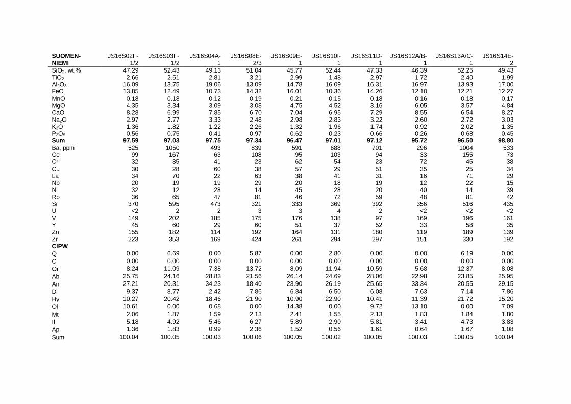
SUOMEN- NIEMI

JS16S02F-1/2

JS16S03F-1/2

JS16S04A-1

JS16S08E-2/3

JS16S09E-1

JS16S10I-1

JS16S11D-1

JS16S12A/B-1

JS16S13A/C-1

JS16S14E-2

SiO2, wt.% 47.29 52.43 49.13 51.04 45.77 52.44 47.33 46.39 52.25 49.43 TiO2 2.66 2.51 2.81 3.21 2.99 1.48 2.97 1.72 2.40 1.99 Al2O3 16.09 13.75 19.06 13.09 14.78 16.09 16.31 16.97 13.93 17.00 FeO 13.85 12.49 10.73 14.32 16.01 10.36 14.26 12.10 12.21 12.27 MnO 0.18 0.18 0.12 0.19 0.21 0.15 0.18 0.16 0.18 0.17 MgO 4.35 3.34 3.09 3.08 4.75 4.52 3.16 6.05 3.57 4.84 CaO 8.28 6.99 7.85 6.70 7.04 6.95 7.29 8.55 6.54 8.27 Na2O 2.97 2.77 3.33 2.48 2.98 2.83 3.22 2.60 2.72 3.03 K2O 1.36 1.82 1.22 2.26 1.32 1.96 1.74 0.92 2.02 1.35 P2O5 0.56 0.75 0.41 0.97 0.62 0.23 0.66 0.26 0.68 0.45 Sum 97.59 97.03 97.75 97.34 96.47 97.01 97.12 95.72 96.50 98.80 Ba, ppm 525 1050 493 839 591 688 701 296 1004 533 Ce 99 167 63 108 95 103 94 33 155 73 Cr 32 35 41 23 62 54 23 72 45 38 Cu 30 28 60 38 57 29 51 35 25 34 La 34 70 22 63 38 41 31 16 71 29 Nb 20 19 19 29 20 18 19 12 22 15 Ni 32 12 28 14 45 28 20 40 14 39 Rb 36 65 47 81 46 72 59 48 81 42 Sr 370 595 473 321 333 369 392 356 516 435 U <2 2 2 3 3 4 2 <2 <2 <2 V 149 202 185 175 176 138 97 169 196 161 Y 45 60 29 60 51 37 52 33 58 35 Zn 155 182 114 192 164 131 180 119 189 139 Zr 223 353 169 424 261 294 297 151 330 192 CIPW Q 0.00 6.69 0.00 5.87 0.00 2.80 0.00 0.00 6.19 0.00

C 0.00 0.00 0.00 0.00 0.00 0.00 0.00 0.00 0.00 0.00

Or 8.24 11.09 7.38 13.72 8.09 11.94 10.59 5.68 12.37 8.08

Ab 25.75 24.16 28.83 21.56 26.14 24.69 28.06 22.98 23.85 25.95

An 27.21 20.31 34.23 18.40 23.90 26.19 25.65 33.34 20.55 29.15

Di 9.37 8.77 2.42 7.86 6.84 6.50 6.08 7.63 7.14 7.86

Hy 10.27 20.42 18.46 21.90 10.90 22.90 10.41 11.39 21.72 15.20

Ol 10.61 0.00 0.68 0.00 14.38 0.00 9.72 13.10 0.00 7.09

Mt 2.06 1.87 1.59 2.13 2.41 1.55 2.13 1.83 1.84 1.80

Il 5.18 4.92 5.46 6.27 5.89 2.90 5.81 3.41 4.73 3.83

Ap 1.36 1.83 0.99 2.36 1.52 0.56 1.61 0.64 1.67 1.08

Sum 100.04 100.05 100.03 100.06 100.05 100.02 100.05 100.03 100.05 100.04

SIPOO SB10-1B SB2-1D SC1-1D SF2-1B SG2-1C

SiO2, wt.% 45.35 45.13 45.24 44.69 45.09 TiO2 4.11 4.07 4.13 4.11 4.08 Al2O3 14.13 14.08 14.13 14.00 14.09 FeO 15.56 15.83 16.14 15.85 15.94 MnO 0.19 0.20 0.20 0.20 0.20 MgO 4.27 4.24 4.33 4.33 4.26 CaO 7.49 7.43 7.62 7.28 7.47 Na2O 2.81 2.86 2.88 2.79 2.90 K2O 1.69 1.63 1.65 1.85 1.67 P2O5 1.16 1.14 1.15 1.13 1.13 Sum 96.76 96.61 97.47 96.23 96.83 Ba, ppm 786 789 780 782 796 Ce 129 143 132 125 131 Cr 44 47 50 36 50 Cu 48 47 43 41 42 La 63 60 57 67 58 Nb 40 32 38 37 35 Ni 32 32 33 33 35 Rb 56 46 50 56 50 Sr 356 356 359 349 353 U 3 2 <2 2 2 V 127 116 125 127 121 Y 62 60 60 60 59 Zn 143 190 201 158 202 Zr 490 482 472 472 480 CIPW Q 0.00 0.00 0.00 0.00 0.00

C 0.00 0.00 0.00 0.00 0.00

Or 10.32 9.97 10.00 11.36 10.19

Ab 24.57 25.05 25.00 24.53 25.34

An 21.65 21.50 21.29 21.00 21.17

Di 7.51 7.55 8.25 7.46 8.00

Hy 13.88 12.71 10.49 10.07 10.52

Ol 8.89 10.13 11.79 12.36 11.70

Mt 2.33 2.38 2.40 2.39 2.39

Il 8.07 8.01 8.05 8.12 8.01

Ap 2.84 2.80 2.80 2.78 2.76

Sum 100.08 100.07 100.07 100.07 100.07

APPENDIX III. Petrographic observations. Percentages are vol.%. ppl=plane polarized light, plg=plagioclase, ol=olivine, cpx=clinopyroxene, hbl=hornblende, bio=biotite, q=quartz, kfs=alkali feldspar, zr=zircon, ap=apatite, carb=carbonate, amp=amphibole, chl=chlorite, opx=orthopyroxene, sil=sillimanite, spi=spinel, serp=serpentine, op=opaque, ser=sericite, gar=garnet, musc=muscovite, saus=saussurite.

SAMPLE/DYKE plg ol cpx Other Accessory minerals

Opaques (Primary) Texture Alteration level (low, moderate, high, very high)

ÅLAND

A2F-3/A2 middle parts are more altered

- - hbl + bio + q not a diabase but

andesitic

kfs + zr + ap + carb

elongated granular, fine-grained

-

A2G-1/A2 60%, An45, <1,5cm

compositional zoning

- - 40% of secondary interstitial minerals

(amp, chl, bio, carb)

ap+q some elongated, some anhedral

interstitial

subophitic moderate

A3F-2/A3 50%, An35, euhedral, <2mm

5%, interstitial,

altered to bio + op

40%, augite, interstitial,

some cpx may be opx

metasedimentary xenolith (sil + spi)

secondary bio + amp + serp +

chl + carb

10%, mainly anhedral

interstitial, some elongated

euhedral grains inside secondary mica (alteration

of ol)

subophitic-ophitic moderate

A5C-1/A5 50%, subhedral, mainly <<1mm,

micro-phenocrysts

<2mm, swallow tails & skeletal

- 5%, subhedral micro-

phenocrysts <1mm

20% microcrystalline

matrix, cracks and vesicles filled with

op + carb + bio

25%, interstitial preferred

orientation of plg, glomerophyric (plg

+ cpx)

moderate

A8C-3/A8 50%, subhedral, mainly <<1mm,

micro-phenocrysts

<1mm, swallow tails

- - 35% microcrystalline matrix + vesicles

(<<1 mm) filled with bio + carb

15%, micro-phenocrysts

(<1mm) + a lot in the matrix (+bio), mostly elongated euhedral grains

(ilmenite)

preferred orientation of plg

moderate

A9A-3/A9 50%, subhedral, mainly <<1mm,

micropheno-crysts <1mm

-

45% matrix of secondary minerals

secondary bio+ carb

5%, anhedral spots

too altered to see very high

A12B-3/A12 40%, mainly <1mm,

micropheno-crysts <4mm, swallow tails & skeletal, altered

- - 40% microcrystalline matrix + vesicles (<1mm) filled with

carb + q (no reaction rims)

20%, mainly

euhedral elongated + in

cracks anhedral reddish

preferred orientation of plg

high

A13E-1/A13 50%, mainly <<1mm,

micropheno-crysts <3mm,

swallow tails and spherulites

- - 45% microcrystalline matrix + vesicles (<1mm) filled with

carb + q + bio + chl (round, no reaction

rims)

5%, mainly euhedral

elongated in matrix + in

cracks

preferred orientation/flow

texture of plg 70% of the thin section +

30% spheluritic

high

A14E-1/A14 45%, An30, subhedral, mainly

<1mm, micropheno-crysts 2mm

- - 35% matrix of secondary minerals

(chl + ser + bio)

20%, anhedral intergranular,

some euhedral elongated

subophitic high

A15E-1/A15 50%, An50, subhedral, mainly

<<1mm, micropheno-crysts <3mm,

spherulites

- - 45% matrix of secondary minerals (chl + amp + ser +

bio)

5%, anhedral

intergranular, a few subhedral

enclosed by plg

ophitic high

A19C-1/A19 50%, mainly <<1mm,

micropheno-crysts <1mm, swallow tails

10%, subhedral <<1mm grains

30%, interstitial, almost

completely altered

secondary bio + chl +

ser

10%, subhedral intergranular

subophitic high

SATAKUNTA

AM7-2AB/AM 50%, subhedral, <3mm, also very

altered

- 40%, almost completely

chloritized (+ possibly amp)

completely altered xenolith (3mm) of

feldspar +op+ bio + chl + q

secondary amp+ chl + ser + carb

+ op

10%, anhedral interstitial +

euhedral elongated

subophitic very high

S11HJ 10.3/ S11HJ

50%, An45, subhedral, <3mm

- 40%, almost completely

chloritized (+ possibly amp)

q +

secondary carb + chl

+ ser

10%, anhedral interstitial +

euhedral elongated

subophitic high

S11HJ 16.1/ S11HJ

40%, subhedral, <1mm,

- - 30% interstitial secondary minerals + 10% completely

chloritized microphenocrysts

(<1mm)

20%, anhedral

interstitial + euhedral cubic &

elongated

preferred orientation of plg

high

IV/IV 50%, An35, subhedral,

<2mm, some are zonal

- 30%, almost completely

chloritized (+ possibly amp)

secondary bio+ser

10%, anhedral interstitial/inter-

granular

subophitic high

S11GR 4.3/ S11GR

40%, mostly <<1mm,

micropheno-crysts ~1mm

- - 30% microcrystalline

matrix + 5% completely altered

phenocrysts (<1mm)

25%, anhedral

interstitial + euhedral cubic &

elongated

preferred orientation of plg

moderate

MA9-1A/MA 55%, An60, subhedral,

<3mm, altered (ser+ saus)

- 30% augite, interstitial and

elongated

three “clots” of q + carb + bio + musc,

reaction rims, vesicle-like

secondary: chl + bio + carb+ ser+

saus

15%, anhedral interstitial +

euhedral cubic & elongated

subophitic, elongated crystal

shapes

high

AT2-1AB/AT 35%, <1mm, subhedral, also

very altered

- - 30%, interstitial secondary matrix, 10% vesicles filled with q (mostly) + carb + secondary

minerals (very round, no reaction

rims)

25%, crack-

filling+ mainly elongated

intergranular

preferred orientation of plg

high

FE1-1B/FE 40%, An45, subhedral, mostly

<1mm, micropheno-crysts <3mm

- - 30% microcrystalline

matrix + 5% opx + 5% vesicles filled with q + carb + bio (no reaction rims)

25%, dendritic could be ophitic high

FK2-2B/FK 50%, An45, subhedral,

<3mm, compositional

zoning in some

- - 10% opx, 10% secondary inter-stitial minerals +

vesicles filled with bio+ carb+ musc

secondary musc +

carb

30%, dendritic mainly between

plg-laths

could be ophitic high

NI6-1AB/NI anhedral

amphibolite: amphibole (hbl)+ bio + plg + q + op

musc + ap 10%, anhedral interstitial

metamorphic: foliated,

recrystallized

FA5-1C/FA 40% mainly <1mm subhedral with swallow tails,

some zonal ~2mm

micropheno-crysts

- - 10% vesicles filled with q + carb + bio + op (no reaction

rims), 30% microcrystalline

matrix

- 20%, dendritic, possibly

crystallized at the same time as

plg

preferred orientation of plg,

spherulitic,

high

OJ4-3AB/OJ 50% <<1mm, micropheno-crysts ~1mm,

almost completely

altered to ser + carb

- - 40% matrix: secondary chl + carb + ser + op + other alteration

products

- 10%, in cracks and in matrix

too altered to see very high

NO2-2B/NO anhedral

amphibolite: amphiboles (hbl+

ortho-amp) + bio+plg

ap + q + cpx + zr

10%, anhedral interstitial

metamorphic: foliated,

recrystallized

NR6-1F/NR 50%, ~An40, euhedral, <2mm

- - 20% microcrystalline

matrix

- 30%, in cracks and in ground

mass

could be primary ophitic

moderate

AO4-1A/AO 30% sub-/euhedral

micropheno-crysts of <1mm,

swallow tails

- - 50% spherulitic matrix, 20% opx- microphenocrysts

op accessory, in cracks and in ground mass

microphenocrysts+ spherulitic/ feathery

matrix

high

HÄME

JS16-A02A-1/ JS16-A02

40%, mainly <<1mm,

micropheno-crysts <1mm, swallow tails, spherulites

- - 35% microcrystalline matrix + vesicles (<1mm) filled with

carb + q + bio

25%,

intergranular, euhedral

elongated and anhedral

spherulitic high

JS16-A05B/ JS16-A05

40%, ~An55, mainly anhedral interstitial bet-ween ol with ol inclusions, also eu-/subhedral

grains

45%, subhedral, forsteritic

10%, interstitial: ol, plg & op inclusions

5%, anhedral

interstitial, crystall. before

cpx

ol cumulate with plg and cpx inter-

cumulus

low

JS14-H1A-1/ H1

55%, An45, mainly <2mm, micropheno-crysts ~5mm

15%, euhedral and

interstitial, very altered to op + serp

20%, interstitial, altered to amp

secondary carb + ser + amp + chl + bio

10%, anhedral interstitial +

euhedral

subophitic-ophitic high

JS14-H11D-2/ H11

40%, An40, subhedral, <2mm

- 40%, interstitial, almost

completely altered

vesicles filled with q + carb + chl (no

reaction rims)

secondary bio,

amp,chl, ser

20%, mainly anhedral

interstitial, also euhedral elongated

subophitic-ophitic high

H12/H12 50%, An50, subhedral, <3mm

25%, anhedral interstitial

15%, anhedral interstitial

ap + zr +

secondary: bio + op + serp + ser

+ chl

10%, anhedral interstitial, before

cpx

nesophitic, subophitic domains

moderate

JS14-H13E-2/ H13

55%, mainly subhedral <1mm,

also euhedral micropheno-

crysts <5mm with ol +op inclusions

and compositional

zoning

20%, eu-/subhedral

and anhedral interstitial

20%, augite

10%, both euhedral

(crystallized before cpx) and interstitial ones

nesophitic, subophitic domains

low

H13/H13 50%, euhedral + interstitial

domains, <3mm

20%, interstitial with plg

inclusions

20%, interstitial, reddish in ppl

secondary ser + bio +

chl

10%, anhedral interstitial

nesophitic, subophitic domains, adcumulus-type plg

growth

low

JS14-H14E-1/ H14

60%, An45, anhedral

interstitial: poikilitic with cpx inclusions, <3mm

- 30%, augite twinning, subhedral

zr + ap +

secondary bio

10%, elongated grains

intergranular dolerite,

adcumulus-type plg growth

low

H14/H14 55%, An45, subhedral,

<4mm, compositional

zoning

15%, subhedral

20%, augite, interstitial

secondary bio + chl +

ser

10%, anhedral interstitial +

some elongated grains

nesophitic, subophitic domains

moderate

JS14-H15A-1/ H15

40%, <2mm, swallow tails and

skeletal, spherulites

- - 40% microcrystalline matrix + vesicles (<1mm) filled with

carb + q + chl + bio (no reaction rims)

secondary carb + chl + bio + ser

20%, mainly elongated

euhedral, also anhedral interstitial

spherulitic high

JS14-H17D-1/ H17

45%, subhedral, <4mm,

compositional zoning

20%, forsteritic, anhedral interstitial

and subhedral, crystallized before cpx

20%, interstitial, possibly pigeonite

ap +

secondary bio + chl,+ serp + op

15%, anhedral interstitial+

inclusions in plg

subophitic domains high

JS14-H18B-1/ H18

55%, An45, subhedral, <2mm

25%, forsteritic, anhedral interstitial

and subhedral , crystallized before cpx

35%, interstitial, reddish in ppl

secondary

bio 10%, anhedral

interstitial, large areas, crystall.

after cpx

nes-/subophitic, ophitic domains

low

JS14-H20F-3/ H20

60%, An35, euhedral, mainly

<<1mm, micropheno-crysts <1mm

- accessory, small spots (<<1mm),

altered

10% vesicles of some kind filled

with q + amp (<2mm)

secondary: amp + ser + chl + bio

30%, sub-/euhedral cubic and elongated, some anhedral

granular (plg + cpx + op), could be

nesophitic

high

JS14-H23B-1/ H23

50%, An45, subhedral, <5mm

25%, forsteritic, anhedral interstitial

and subhedral, crystallized before cpx

20%, interstitial secondary bio + idd + ser

ap 5%, anhedral interstitial, crystallized before cpx

nesophitic low

JS14-H24B-2/ H24

45%, An60, subhedral, up to

7mm

25%, forsteritic, anhedral interstitial

and subhedral , crystallized before cpx

25%, augite, interstitial,

reddish in ppl

secondary bio + ser ap 5%, euhedral inclusions in cpx

+anhedral interst., before

cpx

ophitic low

H24/H24 45%, An55, subhedral, <3mm

10%, subhedral

35%, augite, almost

completely altered to amp,

interstitial

secondary bio + amp + ser + chl +

idd + op

ap 10%, anhedral interstitial +

euhedral elongated(big)

ophitic high

H25/H25 55%, An45, subhedral, up to

8mm, compositional

zoning

20%, interstitial,

also as inclusions in

plg

20%, interstitial

ap, secondary

idd

5%, anhedral interstitial, crystallized before cpx

nesophitic, subophitic domains

low

SUOMENNIEMI

JS16S02G-2/ S02

40%, An55, subhedral,

<5mm, some are zonal, relatively

unaltered

15%, subhedral

granular and anhedral interstitial

30%, reddish in ppl

secondary bio+chl ap 15%, anhedral interstitial + subhedral elongated

nesophitic, subophitic domains

moderate

JS16S04C-3/ S04

50%, subhedral, up to 2cm, also

very altered

- 40% altered cpx (chl + amp)

secondary: amp + chl + bio + ser

10%, anhedral

interstitial subophitic very high

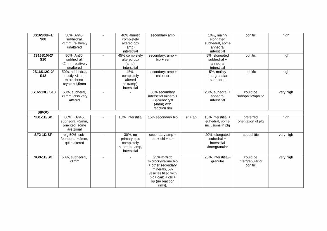
JS16S08F-1/ S08

50%, An45, subhedral,

<1mm, relatively unaltered

- 40% almost completely altered cpx

(amp), interstitial

secondary amp

10%, mainly elongated

subhedral, some anhedral interstitial

ophitic high

JS16S10I-2/ S10

50%, An30, subhedral,

<2mm, relatively unaltered

- 45% completely altered cpx

(amp), interstitial

secondary: amp + bio + ser

5%, elongated subhedral +

anhedral interstitial

ophitic high

JS16S12C-2/ S12

50%, subhedral, mostly <1mm, micropheno-

crysts <1,5mm

- 45%, completely

altered cpx(amp), interstitial

secondary: amp + chl + ser

5%, mainly

intergranular subhedral

ophitic high

JS16S13E/ S13 50%, subheral, <1mm, also very

altered

- - 30% secondary interstitial minerals

+ q-xenocryst (4mm) with reaction rim

20%, euhedral +

anhedral interstitial

could be subophitic/ophitic

very high

SIPOO

SB1-1B/SB 60%, ~An45, subhedral <2mm,

oriented, some are zonal

- 10%, interstitial 15% secondary bio zr + ap 15% interstitial + euhedral, some inclusions in plg

preferred orientation of plg

high

SF2-1D/SF plg 50%, sub-/euhedral, <2mm,

quite altered

- 30%, no primary cpx: completely

altered to amp, interstitial

secondary amp + bio + chl + ser

20%, elongated

euhedral + interstitial

/intergranular

subophitic very high

SG9-1B/SG 50%, subhedral, <1mm

- - 25% matrix: microcrystalline bio + other secondary

minerals, 5% vesicles filled with bio+ carb + chl + op (no reaction

rims),

25%, interstitial/-

granular could be

intergranular or ophitic

very high