MASTER'S THESIS - CORE
147
Faculty of Science and Technology MASTER’S THESIS Study program/ Specialization: Offshore Technology/ Subsea Technology Spring semester, 2013 Open / Restricted access Writer: Se-Hoon Yoon ………………………………………… (Writer’s signature) Faculty supervisor: Prof. Daniel Karunakaran (Ph.D.) (University of Stavanger/ Subsea 7 Norway) External supervisor(s): Dr. Zhengmao Yang (Subsea 7 Norway) Title of thesis: Phenomenon of Pipeline Walking in High Temperature Pipeline Credits (ECTS): 30 Key words: Pipeline walking, Thermal transients, Axial friction coefficient, ANSYS Pages: XIII + 65 + enclosure: 68 Stavanger, 10th June 2013
-
Upload
khangminh22 -
Category
Documents
-
view
1 -
download
0
Transcript of MASTER'S THESIS - CORE

Faculty of Science and Technology
MASTER’S THESIS
Study program/ Specialization:
Offshore Technology/ Subsea Technology
Spring semester, 2013
Open / Restricted access
Writer:
Se-Hoon Yoon
………………………………………… (Writer’s signature)
Faculty supervisor:
Prof. Daniel Karunakaran (Ph.D.) (University of Stavanger/ Subsea 7 Norway)
External supervisor(s):
Dr. Zhengmao Yang (Subsea 7 Norway)
Title of thesis:
Phenomenon of Pipeline Walking in High Temperature Pipeline
Credits (ECTS):
30
Key words:
Pipeline walking, Thermal transients,
Axial friction coefficient, ANSYS
Pages: XIII + 65
+ enclosure: 68
Stavanger, 10th June 2013

Master thesis
Phenomenon of Pipeline Walking in High Temperature Pipeline
Se-Hoon Yoon < I >
University of Stavanger
ABSTRACT
As the offshore oil and gas fields have been exploited in deeper water, subsea pipelines
are increasingly required to operate at high temperatures and pressures. It causes subsea pipelines
to be more susceptible to movements both in lateral and axial directions due to the loads
produced by high temperatures and pressures. Some high temperature pipelines have experienced
the cumulative axial displacement of an overall pipeline length over a number of start-up/shut-in
cycles, which is commonly known as “Pipeline walking”. [2]
The objective of this thesis work is to describe the phenomenon of pipeline walking by
specifically focusing on a short and high temperature pipeline and identify key parameters of it
in terms of the pipeline design. It is because designing to control or mitigate the accumulated
walking over the life of the pipeline system can lead to changing in field layouts and high
installation costs related to mitigation measures. [5] It is therefore important to be able to assess
if the walking is a potential issue in the early design phase.
Moreover, a literature study on contributory mechanisms to cause pipeline walking is
emphasized in the thesis including general pipeline technology in terms of the pipeline expansion
design: [1]
- Sustained tension at the end of the pipeline, associated with a steel catenary riser (SCR);
- Global seabed slope along the pipeline length;
- Thermal transients along the pipeline during shutdown and restart operations.
Understanding an axial movement of short pipelines due to the resultant of the thermal
transient is an important consideration in the pipeline walking assessment. [1] Thus, a numerical
model of pipeline walking based on the thermal transient load is established by the finite element
method in the thesis. It presents the effect of the transient temperature profile on pipeline
walking. In addition to that, it focuses on the effect of axial friction factors related to pipe-soil
interaction as the sensitivity study.
Lastly, the thesis briefly deals with possible mitigation options to prevent pipeline
walking. This global axial movement phenomenon can lead to various pipeline integrity issues
although walking itself is not a limit state in design. [14] It is evident that the possible mitigation
methods are to be taken into account at the design phase depending on consequential effects of
accumulated axial walking. Hence, the pros and cons of possible mitigation measures are
discussed in connection with the sensitivity study results.
Keywords: Pipeline walking, Thermal transients, Axial friction coefficient, ANSYS.

Master thesis
Phenomenon of Pipeline Walking in High Temperature Pipeline
Se-Hoon Yoon < II >
University of Stavanger
ACKNOWLEDGEMENTS
This thesis is made to conclude author’s Master of Science education in Offshore
Technology at University of Stavanger in Norway. The thesis work was mainly performed at
Subsea 7 Norway, started from January 2013 and completed in June 2013. Several people have
supported academically and practically for achieving this master thesis. Thus, it is glad to
express my gratitude to them.
Foremost, I would like to express my deepest appreciation to my supervisor Prof. Daniel
Karunakaran (Ph.D.) who gave me the opportunity to carry out the thesis work not only under his
supervision but also with Subsea 7. His valuable comments and discussions are gratefully
acknowledged.
My sincere gratitude is also given to Dr. Zhengmao Yang who provided me with detailed
instructions on my thesis as well as useful practical tips on analytical calculations in ANSYS.
His excellent guidance helped me in all the time of performing the thesis work.
I would like to thank Mr. Bjørn Lindberg Bjerke who is a Department Engineering
Manager at Subsea 7 in Oslo. His permission for me to stay and carry out the thesis work in
Subsea 7 Oslo office provided me with an excellent atmosphere for doing the thesis work.
Furthermore, I would also like to acknowledge with much appreciation to Mr. Helge
Dykesteen and Ms. Giovanna Fong who welcomed me every visit to Stavanger. I could not have
successfully completed the thesis without their sincere hospitality.
Last but definitely not least, I wish to give special thanks to my wife Jang Mee Hong who
was always cheering me up and gave me big encouragement to complete not only the thesis but
also the entire master degree program. In addition, a special gratitude is also given to my family
in Korea: my parents as well as parent in law. Their sincere supports were directly delivered to
me even long distance and it really encouraged me.
Stavanger, 10th June 2013
Se-Hoon Yoon

Master thesis
Phenomenon of Pipeline Walking in High Temperature Pipeline
Se-Hoon Yoon < III >
University of Stavanger
NOMENCLATURE
1. SYMBOLS
① Roman Symbols Thermal expansion coefficient
Cross sectional area of pipe (OD: ) Cross sectional area of pipe (ID: ) Cross sectional area of pipe wall (ID: ) Cross sectional area of pipe insulation coating ( ) ) Mass of pipe buoyancy per unit length (kg/m)
Pipeline internal diameter (mm) Pipeline outer diameter (mm) E Young’s modulus EA Axial stiffness (N)
Axial friction force (N/m)
Constraint friction force
Thermal gradients force per unit length (N/m)
g Acceleration of gravity
KP Kilometer point L Length of pipeline (m) Mass of pipe concrete coating per unit length (kg/m) Mass of pipe insulation coating per unit length (kg/m) Mass of fluid content in pipe per unit length (kg/m) Mass of pipe steel per unit length (kg/m)
Mass of submerged pipeline (in water) per unit length (kg/m) Total mass of pipeline (in air) per unit length (kg/m) External pressure (Pa) Hydrostatic pressure (Pa)
Internal pressure (Pa) Differential internal pressure across the pipe wall Operating pressure (Pa) Thermal gradient in degrees per unit length ( ) Effective axial force (N) Residual lay tension (N) SCR tension (N) True axial tension (N) Effective pipe diameter (mm) Pipeline wall thickness Pipeline external (insulation) coating thickness (mm)

Master thesis
Phenomenon of Pipeline Walking in High Temperature Pipeline
Se-Hoon Yoon < IV >
University of Stavanger
Pipeline concrete coating thickness (mm) Operating temperature ( ) Shutdown temperature ( ) Distance between two virtual anchors
Weight of pipeline (dry weight) per unit length (N/m) Weight of submerged pipeline per unit length (N/m)
② Greek Symbols Parameter in walking due to thermal transients
Walk per cycle due to SCR Tension (m)
Walk per cycle due to Seabed slope (m)
Walk per cycle due to Thermal Transients (m)
Change in fully constrained force (N)
Change in effective axial force over for SCR (N)
Change in effective axial force over for slope (N) Temperature difference (℃) Inlet temperature difference Thermal strain
Strain due to end cap effect
Strain due to Poisson’s effect
Total strain due to combined thermal and pressure Poisson’s effect
(For the unrestrained condition)
Temperature
Friction coefficient
Poisson’s ratio
Density of pipe steel
Density of pipe insulation coating
Density of pipe concrete coating
Density of fluid content in oil
Density of seawater
SMYS of pipe steel (MPa)
Seabed slope

Master thesis
Phenomenon of Pipeline Walking in High Temperature Pipeline
Se-Hoon Yoon < V >
University of Stavanger
2. ABBREVIATIONS
BE Best Estimate
DISP Displacement
DNV Det Norske Veritas
EAF Effective Axial Force
FE Finite Element
FEA Finite Element Analysis
HP/HT High Pressure / High Temperature
ID Inner Diameter
JIP Joint Industry Project
LB Lower Bound
OD Outer Diameter
OTC Offshore Technology Conference
PLET Pipeline End Terminations
SCR Steel Catenary Riser
SMYS Specified Minimum Yield Stress
THK Thickness
TDP Touchdown Point
UB Upper Bound
VAP Virtual Anchor Point
WD Water Depth

Master thesis
Phenomenon of Pipeline Walking in High Temperature Pipeline
Se-Hoon Yoon < VI >
University of Stavanger
TABLE OF CONTENTS
ABSTRACT ------------------------------------------------------------------------------------------------------------------- I
ACKNOWLEDGEMENTS ---------------------------------------------------------------------------------------------- II
NOMENCLATURE ------------------------------------------------------------------------------------------------------ III
TABLE OF CONTENTS ------------------------------------------------------------------------------------------------ VI
TABLE OF FIGURES ---------------------------------------------------------------------------------------------------- X
TABLE OF TABLES --------------------------------------------------------------------------------------------------- XIII
1. Introduction --------------------------------------------------------------------------------------------------------------- 1
1.1 Background ------------------------------------------------------------------------------------------------------------ 1
1.2 Problem Identification ----------------------------------------------------------------------------------------------- 1
1.3 Purpose and Scope ---------------------------------------------------------------------------------------------------- 2
1.4 Organization of Thesis ----------------------------------------------------------------------------------------------- 3
2. Literature Review -------------------------------------------------------------------------------------------------------- 4
2.1 General ------------------------------------------------------------------------------------------------------------------ 4
2.2 Pipeline Expansion --------------------------------------------------------------------------------------------------- 4
2.2.1 Causes of Expansion [6] --------------------------------------------------------------------------------------- 4
2.2.1.1 Thermal Strain ( ) -------------------------------------------------------------------------------- 4
2.2.1.2 Pressure Effects -------------------------------------------------------------------------------------------- 5
2.2.1.3 Combined Thermal and Pressure ---------------------------------------------------------------------- 5
2.2.2 Effective Axial Force ------------------------------------------------------------------------------------------ 6
2.2.2.1 Fully-Constrained Effective Force --------------------------------------------------------------------- 7
2.2.2.2 Build-up of Effective Axial Force --------------------------------------------------------------------- 8
2.2.3 Virtual Anchor Point (VAP) ---------------------------------------------------------------------------------- 9
2.3 Governing Parameters in Pipeline Walking [1] --------------------------------------------------------------- 10
2.3.1 Fully Mobilized ----------------------------------------------------------------------------------------------- 10

Master thesis
Phenomenon of Pipeline Walking in High Temperature Pipeline
Se-Hoon Yoon < VII >
University of Stavanger
2.3.2 Full Cyclic Constraint ---------------------------------------------------------------------------------------- 11
2.3.3 Cyclic Constraint ---------------------------------------------------------------------------------------------- 11
2.4 Pipeline Walking Mechanisms ----------------------------------------------------------------------------------- 13
2.4.1 Steel Catenary Riser (SCR) Tension ---------------------------------------------------------------------- 13
2.4.1.1 Derivation of Walk per cycle due to SCR Tension [1] ------------------------------------------ 15
2.4.2 Seabed Slope --------------------------------------------------------------------------------------------------- 17
2.4.2.1 Derivation of Walk per cycle due to Seabed Slope [1] ------------------------------------------ 17
2.4.3 Thermal Transients along the Pipeline-------------------------------------------------------------------- 18
2.4.3.1 Thermal loading and transients ----------------------------------------------------------------------- 19
2.4.3.2 Derivation of Walk per cycle due to Thermal Transients [1] ----------------------------------- 21
2.5 Pipe-Soil Interaction ----------------------------------------------------------------------------------------------- 23
2.5.1 Pipeline Embedment ----------------------------------------------------------------------------------------- 23
2.5.2 Axial Pipe-Soil Resistance [30] ---------------------------------------------------------------------------- 24
2.6 Summary ------------------------------------------------------------------------------------------------------------- 25
3. Research Design -------------------------------------------------------------------------------------------------------- 27
3.1 General ---------------------------------------------------------------------------------------------------------------- 27
3.2 Preparation for Research Model [20] --------------------------------------------------------------------------- 27
3.2.1 Modeling a Pipeline ------------------------------------------------------------------------------------------ 27
3.2.2 Temperature Profile Preparation --------------------------------------------------------------------------- 27
3.2.3 Thermal Load Application ---------------------------------------------------------------------------------- 28
3.2.4 Pipe-Soil Interaction Application -------------------------------------------------------------------------- 28
3.3 Element Types Used in Finite Element Analysis Model ---------------------------------------------------- 29
3.3.1 Pipeline Model ------------------------------------------------------------------------------------------------ 29
3.3.2 Seabed Model -------------------------------------------------------------------------------------------------- 30
3.4 Process of Finite Element Analysis (FEA) -------------------------------------------------------------------- 33
4. Case Study Description ----------------------------------------------------------------------------------------------- 35
Master thesis
Phenomenon of Pipeline Walking in High Temperature Pipeline
Se-Hoon Yoon < VIII >
University of Stavanger
4.1 General ---------------------------------------------------------------------------------------------------------------- 35
4.2 Pipeline Model ------------------------------------------------------------------------------------------------------ 35
4.2.1 Pipeline Parameter -------------------------------------------------------------------------------------------- 35
4.2.2 Pipe Material Property --------------------------------------------------------------------------------------- 36
4.3 Input Data ------------------------------------------------------------------------------------------------------------ 37
4.3.1 Operating Data ------------------------------------------------------------------------------------------------ 37
4.3.2 Environmental and Soil Data ------------------------------------------------------------------------------- 38
5. Reasults and Discussion ---------------------------------------------------------------------------------------------- 39
5.1 General ---------------------------------------------------------------------------------------------------------------- 39
5.2 Pipeline Response Analysis Results ---------------------------------------------------------------------------- 39
5.2.1 Effective Axial Force Profile ------------------------------------------------------------------------------- 40
5.2.2 Pipeline Cumulative Displacement ------------------------------------------------------------------------ 43
5.2.3 Axial Displacement: Walking ------------------------------------------------------------------------------ 47
5.2.3.1 Walking at Mid-Point ---------------------------------------------------------------------------------- 47
5.2.3.2 Walking at Two Ends (Hot/Cold) -------------------------------------------------------------------- 48
5.3 Pipeline Response upon Axial Friction Factor ---------------------------------------------------------------- 50
5.3.1 Effective Axial Force Profile ------------------------------------------------------------------------------- 50
5.3.2 Axial Displacement ------------------------------------------------------------------------------------------- 54
5.3.2.1 Mid-Point Axial Displacement ----------------------------------------------------------------------- 54
5.3.2.2 Axial Displacement with Friction Factor 2.0 ------------------------------------------------------ 56
5.4 Mitigation Measures for Pipeline Walking -------------------------------------------------------------------- 57
5.4.1 Anchoring [11] ------------------------------------------------------------------------------------------------ 57
5.4.2 Increase Axial Friction [1] ---------------------------------------------------------------------------------- 58
5.4.2.1 Pipe-Soil Interaction ------------------------------------------------------------------------------------ 58
5.4.2.2 Pipeline Weight Coating ------------------------------------------------------------------------------- 58
5.4.2.3 Trench and Bury ----------------------------------------------------------------------------------------- 58

Master thesis
Phenomenon of Pipeline Walking in High Temperature Pipeline
Se-Hoon Yoon < IX >
University of Stavanger
5.4.2.4 Rock Dumping and Mattress -------------------------------------------------------------------------- 59
5.4.3 Increase Subsea Connection Line Capacity -------------------------------------------------------------- 60
5.5 Summary ------------------------------------------------------------------------------------------------------------- 60
6. Conclusion and Further Study ------------------------------------------------------------------------------------- 61
6.1 General ---------------------------------------------------------------------------------------------------------------- 61
6.2 Conclusions ---------------------------------------------------------------------------------------------------------- 61
6.3 Further Study -------------------------------------------------------------------------------------------------------- 62
REFERENCE -------------------------------------------------------------------------------------------------------------- 63
Appendix I ----------------------------------------------------------------------------------------------------------------- AI-1
Appendix II --------------------------------------------------------------------------------------------------------------AII-1
Appendix III ----------------------------------------------------------------------------------------------------------- AIII-1
Appendix IV-1 --------------------------------------------------------------------------------------------------------- AIV-1
Appendix IV-2 -------------------------------------------------------------------------------------------------------- AIV-26
Appendix V -------------------------------------------------------------------------------------------------------------- AV-1

Master thesis
Phenomenon of Pipeline Walking in High Temperature Pipeline
Se-Hoon Yoon < X >
University of Stavanger
TABLE OF FIGURES
Figure 1.1: Offshore Pipeline System (Yong Bai, 2005) [24] ...................................................................... 2
Figure 2.1: Conventional S-lay Installation (Olav Fyrileiv et al., 2005) [9] ................................................. 6
Figure 2.2: Effective Axial Force for a Range of Friction in a Straight Pipeline (David A.S. Bruton et al.,
2008) [10] ..................................................................................................................................................... 7
Figure 2.3: Typical Virtual Anchor Point for Pipeline (Class note by Qiang Chen) [6] .............................. 9
Figure 2.4: Effective Axial Force in a Short Straight Pipeline (David Bruton et al., 2005) [12] ................. 9
Figure 2.5: A Typical Force Profile for a Fully Mobilized Pipeline (D. Bruton et al., 2006) [1] ............... 10
Figure 2.6: A Typical Force Profile for a Fully Constrained Pipeline (D. Bruton et al., 2006) [1] ............ 11
Figure 2.7: A Typical Force Profile for a Cyclically Constrained Pipeline (D. Bruton et al., 2006) [1] .... 12
Figure 2.8: A Typical Subsea Tieback with SCR, Pipeline and PLET (M. Brunner et al., 2006) [17] ...... 13
Figure 2.9: A Force Profile – SCR at Cold End (D. Bruton et al., 2006) [1] .............................................. 14
Figure 2.10: An Axial Force Profile by Asymmetrical Loading (Gautam Chaudhury, 2010) [11] ............ 15
Figure 2.11: Seabed Slope including its sign convention (D. Bruton et al., 2006) [1] ............................... 17
Figure 2.12: A Force Profile - Seabed Slope (D. Bruton et al., 2006) [1] .................................................. 17
Figure 2.13: A Typical Thermal Transients (D. Bruton et al., 2006) [1] .................................................... 19
Figure 2.14: An Example of Force Profile – First Heat-up (D. Bruton et al., 2006) [1] ............................. 20
Figure 2.15: An Example of Force Profile – Second Heat-up (D. Bruton et al., 2006) [1] ........................ 20
Figure 2.16: Analytical Model (D. Bruton et al., 2006) [1] ........................................................................ 22
Figure 2.17: Initial Pipeline Embedment (D. Bruton et al., 2008) [10] ...................................................... 23
Figure 2.18: Axial Pipe-Soil Resistance Behavior (D. Bruton et al., 2008) [10] ........................................ 24
Figure 3.1: Temperature Transients used in Pipeline Walking Analysis .................................................... 28
Figure 3.2: PIPE288 Geometry (ANSYS Inc. 2009) [21] .......................................................................... 29
Figure 3.3: Pipeline Model of PIPE288 Element ........................................................................................ 30
Figure 3.4: Node-to-Surface Contact Elements (ANSYS Inc. 2009) [23] .................................................. 31
Figure 3.5: Geometry of TARGE170 (ANSYS Inc. 2009) [21] ................................................................. 32
Figure 3.6: Segment Types of TARGE170 (ANSYS Inc. 2009) [21] ........................................................ 32
Figure 3.7: Pipeline and Seabed Modeling in ANSYS ............................................................................... 33
Figure 4.1: Proposed de-rating values for yield stress of C-Mn steel (DNV-OS-F101, 2012) ................... 37

Master thesis
Phenomenon of Pipeline Walking in High Temperature Pipeline
Se-Hoon Yoon < XI >
University of Stavanger
Figure 4.2: Ramberg-Osgood Stress-Strain Curve for API 5L X65 (at 20 & 88 ) ............................... 37
Figure 5.1: Interpolated Temperature Load Profile for 88 ...................................................................... 39
Figure 5.2: Effective Axial Force for 1st Cycle .......................................................................................... 40
Figure 5.3: Effective Axial Force for 2nd Cycle ........................................................................................ 40
Figure 5.4: Effective Axial Force for 3rd Cycle ......................................................................................... 41
Figure 5.5: Effective Axial Force for 4th Cycle ......................................................................................... 41
Figure 5.6: Effective Axial Force for 5th Cycle ......................................................................................... 42
Figure 5.7: Pipeline Displacement for 1st Cycle ........................................................................................ 43
Figure 5.8: Pipeline Displacement for 2nd Cycle ....................................................................................... 43
Figure 5.9: Pipeline Displacement for 3rd Cycle ........................................................................................ 44
Figure 5.10: Pipeline Displacement for 4th Cycle ...................................................................................... 44
Figure 5.11: Pipeline Displacement for 5th Cycle ...................................................................................... 45
Figure 5.12: Axial Walking at Mid-Point ................................................................................................... 47
Figure 5.13: Axial Walking at Hot End ...................................................................................................... 48
Figure 5.14: Axial Walking at Cold End .................................................................................................... 48
Figure 5.15: Axial Walking Displacement ................................................................................................. 49
Figure 5.16: Effective Axial Force for 1st Cycle with Friction factor 0.3 .................................................. 50
Figure 5.17: Effective Axial Force for 1st Cycle with Friction factor 0.5 .................................................. 50
Figure 5.18: Effective Axial Force for 1st Cycle with Friction factor 0.7 .................................................. 51
Figure 5.19: Effective Axial Force for 1st Cycle with Friction factor 2.0 .................................................. 51
Figure 5.20: Effective Axial Force for 4th Cycle with Friction Factor 0.5................................................. 52
Figure 5.21: Effective Axial Force for 5th Cycle with Friction Factor 0.5................................................. 52
Figure 5.22: Effective Axial Force for 4th Cycle with Friction Factor 0.7................................................. 53
Figure 5.23: Effective Axial Force for 5th Cycle with Friction Factor 0.7................................................. 53
Figure 5.24: Axial Walking Displacement at Mid-Point with Friction Factor 0.3, 0.5 & 0.7 .................... 55
Figure 5.25: A Typical Pipeline Restraining Anchor (Ryan Watson et al., 2010) [16] .............................. 57
Figure 5.26: A Trenching Operation (from www.theareofdreging.com) .................................................... 59
Figure 5.27: A Rock Dumping Operation (from www.nordnes.nl) ............................................................ 59
Figure A-II.1 Temperature Transients used in Pipeline Walking Analysis ........................................... AII-2
Figure A-V.1: Effective Axial Force for 2nd Cycle with Friction factor 0.5 ........................................ AV-2

Master thesis
Phenomenon of Pipeline Walking in High Temperature Pipeline
Se-Hoon Yoon < XII >
University of Stavanger
Figure A-V.2: Effective Axial Force for 3rd Cycle with Friction factor 0.5 ......................................... AV-2
Figure A-V.3: Effective Axial Force for 2nd Cycle with Friction factor 0.7 ........................................ AV-3
Figure A-V.4: Effective Axial Force for 3rd Cycle with Friction factor 0.7 ......................................... AV-3
Figure A-V.5: Effective Axial Force for 2nd Cycle with Friction factor 2.0 ........................................ AV-4
Figure A-V.6: Effective Axial Force for 3rd Cycle with Friction factor 2.0 ......................................... AV-4
Figure A-V.7: Effective Axial Force for 4th Cycle with Friction factor 2.0 ......................................... AV-5
Figure A-V.8: Effective Axial Force for 5th Cycle with Friction factor 2.0 ......................................... AV-5
Figure A-V.9: Axial Walking Displacement at Mid-Point .................................................................... AV-6

Master thesis
Phenomenon of Pipeline Walking in High Temperature Pipeline
Se-Hoon Yoon < XIII >
University of Stavanger
TABLE OF TABLES
Table 4.1: Pipeline Design Data and Material Properties ........................................................................... 35
Table 4.2: Coating Parameters .................................................................................................................... 36
Table 4.3: Operating parameters ................................................................................................................. 37
Table 4.4: Environmental Data ................................................................................................................... 38
Table 4.5: Environmental Data (Soil Conditions)....................................................................................... 38
Table 5.1: Hot-End Pipe Displacement ....................................................................................................... 45
Table 5.2: Cold-End Pipe Displacement ..................................................................................................... 46
Table 5.3: Mid-Point Pipe Displacement .................................................................................................... 46
Table 5.4: Mid-Point Axial Displacement with Friction Factor 0.5 ........................................................... 54
Table 5.5: Mid-Point Axial Displacement with Friction Factor 0.7 ........................................................... 55
Table 5.6: Results of Walking Rate ............................................................................................................ 56
Table 5.7: Mid-Point Axial Displacement with Friction Factor 2.0 ........................................................... 56

Master thesis
Phenomenon of Pipeline Walking in High Temperature Pipeline
Se-Hoon Yoon 1 | P a g e
University of Stavanger
1. Introduction
1.1 Background
The instability phenomenon of subsea pipelines associated to high pressures and
temperatures has become a critical aspect for the design of pipelines. As design conditions
become more challenging, primarily due to increasing operating temperatures, much attention
has been focused on controlling thermal expansion. The pipelines particularly are laid down on
the seabed and the capacity of PLETs (pipeline end terminations) and/or in-line structure to
absorb expansion may be limited. [3]
Conventionally, it interprets the design criteria of such structures by calculating the
expansion under maximum operating conditions, and the pipeline is assumed to expand and
contract within the stable limit. However, the real situation shows much more complicated than
that under cyclic loadings. As the operating conditions are cycled the basic expansion and
contraction can be accompanied by axial ratcheting behavior. This behavior is known as
“pipeline walking”. [2]
Pipeline walking is another major design challenge, which has been observed in
operating pipeline systems. This phenomenon occurring in start-up/shut-down cycles cause a
cumulative axial displacement of a high temperature and short pipeline1. It expands and contracts
when it is subjected to different operational conditions: starting from hydro-test to operational
pressure, operational temperature heating, and shut-down cooling to ambient temperature.
The pipeline failure will not happen due to the axial walking itself unless the pipeline is
susceptible to buckling. However, as a result of the accumulated global displacement over a
number of cycles, the axial walking may make an impact on the failure of tie-in jumpers/spools.
It may also lead to localized failure because of the increased loading within a lateral buckle. [3]
Therefore, this issue is worth taking into account at the design stage since its occurrence may
have a major influence on the field layout and development, which can have a huge impact on
the project cost and development.
1.2 Problem Identification
When it comes to the short HT/HP pipeline, i.e. a partially restrained system, a large
transient cumulative expansion is to be considered during the design phase. [5] It is because
when the pipeline undergoes multiple operational cycles (start-up/shutdown) with thermal
gradients, the entire system experiences a global axial displacement (walking) phenomenon.
1 The term ‘short’ related to pipelines that do not reach full constraint, but expand about a virtual anchor point
located at the middle of the pipeline. [1]

Master thesis
Phenomenon of Pipeline Walking in High Temperature Pipeline
Se-Hoon Yoon 2 | P a g e
University of Stavanger
Besides, the presence of a tension due to a steel catenary riser (SCR) connected to the pipeline or
a significant seabed slope also causes the walking.
Figure 1.1: Offshore Pipeline System (Yong Bai, 2005) [24]
Consequently, the walking phenomenon may lead to irreparable damage to the subsea structures
which are shown in Figure 1.1, Moreover, six failures were reported by the end of 2000 in North
Sea due to excessive expansion of the pipeline, and at least one loss of containment failure due to
pipeline walking has been observed. [19]
1.3 Purpose and Scope
The aim of the thesis work is to understand the pipeline walking phenomenon, key
factors that influence on walking and study how to assess the severity of the walking problem
particularly focusing on the pipeline under the high temperature condition.
The scope is to be based on the pipeline walking mechanisms that have been investigated
by SAFEBUCK JIP: [1]
- Sustained tension at the end of the pipeline, associated with a steel catenary riser (SCR);
- Global seabed slope along the pipeline length;
- Thermal transients along the pipeline during shutdown and restart operations.

Master thesis
Phenomenon of Pipeline Walking in High Temperature Pipeline
Se-Hoon Yoon 3 | P a g e
University of Stavanger
The finite element analysis modeling is used to identify and analyze the pipeline walking
phenomenon. The short and high temperature pipeline is demonstrated with asymmetric loads
originated from the thermal transients. In addition to that, it defines a relevant walking scenario
to look into parameters such as axial friction factors that influence on occurring the walking as a
sensitivity study. Based on it, the possible mitigation methods are discussed.
1.4 Organization of Thesis
- Chapter 2: Presents the theoretical background of important parameters related to the
temperature and pressure loadings causing pipeline axial displacements including the
pipe-soil interaction. Furthermore, main mechanisms for the pipeline to walk are dealt
with.
- Chapter 3: Provides the methodology that is used in the thesis work. It presents
preparation of research models such as pipeline/seabed models, and temperature load
profiles in the FEA by using ANSYS 13.0 (Mechanical APDL) software.
- Chapter 4: Describes data in the case study in order to perform the FEA. It gives detailed
values of pipeline modeling information and the environmental conditions for the
pipeline walking analysis.
- Chapter 5: Explains the results of the FEA based on Ch.3 and Ch.4. The sensitivity study
results are also presented considering the interaction between the walking rate and axial
friction factors. Lastly, mitigation measures for pipeline walking are briefly introduced in
connection with the results in the chapter.
- Chapter 6: Presents the conclusions of the thesis work based on Ch.5 and the further
works.

Master thesis
Phenomenon of Pipeline Walking in High Temperature Pipeline
Se-Hoon Yoon 4 | P a g e
University of Stavanger
2. Literature Review
2.1 General
It is to be easy to manage the axial stability of the subsea pipelines if they are under
comparatively low pressures and temperatures because their responses to the loading, by high
axial force distribution along the length of the pipelines, are not the serious problem. In contrast,
a HP/HT pipeline system impacts on the pipeline design since the instability phenomenon such
as end-expansion and potential for high stresses can be severe, which deteriorates the pipeline
integrity.
This chapter presents the theoretical explanation of important subjects and parameters
related to the HP/HT loadings leading to pipeline axial movements, and mechanisms of pipeline
walking. Furthermore, it deals with the pipe-soil interaction to look into the effect of the soil
resistance (parameters) for preparation of the sensitivity study.
2.2 Pipeline Expansion
The pipeline expansion may takes place due to operating pressures and temperatures at its
two ends. As being developed in higher pressure and temperature fields, the pipeline expansion
instability phenomenon such as axial creeping (walking), buckling (upheaval and lateral
movements), or a combination of both is taken into account in the pipeline design. The
substantial movement by expansion, particularly at platforms, is important because it can
overstress risers and elbows, and bring the pipe into contraction with the platform itself. [4]
2.2.1 Causes of Expansion [8]
Three main reasons are contributing to the end force and expansion which are inducing
pipeline walking and lateral/upheaval buckling as follows:
- Temperature (Thermal);
- Pressure (End-cap force);
- Poisson contraction (associated with pressure effects).
2.2.1.1 Thermal Strain ( )
The thermal strain occurs due to temperature difference between installation and
operation. When it is under unrestrained condition, the temperature rise causes an expansion
given by equation 2.1:
(2.1)

Master thesis
Phenomenon of Pipeline Walking in High Temperature Pipeline
Se-Hoon Yoon 5 | P a g e
University of Stavanger
Where,
Thermal expansion coefficient
Temperature difference (℃).
2.2.1.2 Pressure Effects
a) End-Cap effect
It occurs at any curvatures along the pipeline, and the axial loadings take place due to the
differential pressure loading across the pipe, i.e. compression. The strain at the pipeline due
to end cap effect becomes equation 2.2:
Where,
;
E
b) Poisson Effect
The hoop stress and the corresponding circumferential strain are induced by the internal
pressure. The former causes a longitudinal contraction, and the latter gives axial contraction
on pipeline, i.e. the pipe expands in the hoop direction, and the Poisson’s effect results in an
axial contraction (opposite to end cap pressure effect). Under the unrestrained condition, the
expansion/strain due to Poisson’s effect becomes equation 2.3:
Where,
: Poisson's ratio;
Hoop stress.
2.2.1.3 Combined Thermal and Pressure
Consequently, the total strain for the unrestrained condition is given by equation 2.4:

Master thesis
Phenomenon of Pipeline Walking in High Temperature Pipeline
Se-Hoon Yoon 6 | P a g e
University of Stavanger
2.2.2 Effective Axial Force
The concept of the effective axial force can be used to understand the pipeline expansion
phenomenon. It is composed of the true axial force in the pipe wall and the pressure induced
axial force, so it is defined as equation 2.5: [1]
Where,
: Effective axial force (N);
(N);
External pressure (Pa);
Cross sectional area of pipe (OD: ) Cross sectional area of pipe (ID: )
By considering a conventional S-lay installation illustrated in Figure 2.1, the effective
axial force in the pipeline after installation can be estimated, and the concept of residual lay
tension can be used to define the effective axial force after installation as given by equation
2.6: [9]
Where,
(N).
Figure 2.1: Conventional S-lay Installation (Olav Fyrileiv et al., 2005) [9]
As the pipeline operated, the thermal expansion ( takes place and it makes
the true axial force get into compression. At the same time, the hoop stress and Poisson’s effect

Master thesis
Phenomenon of Pipeline Walking in High Temperature Pipeline
Se-Hoon Yoon 7 | P a g e
University of Stavanger
lead to tension in the true axial force. [9] Thus, based on the equation 2.5, the effective
axial force can be shown as equation 2.7 if fully restrained2:
Where,
;
: Cross sectional area of pipe wall (
Moreover, the change in fully constrained force associated with an unload case is given
as equation 2.8 since it considers cyclic loadings of the pipeline: [1]
Where,
Subscript figures (1 & 2) indicate conditions before and after the operating changes.
2.2.2.1 Fully-Constrained Effective Force
The fully-constrained effective force represents the maximum effective axial force that
occurs in the pipeline. Since the ends of the pipeline are usually free to expand, the force at the
ends is zero. However, as the cumulative axial resistance increases with distance from the
pipeline ends, the force can reach to a fully-constrained condition, as presented in Figure 2.2. [10]
Figure 2.2: Effective Axial Force for a Range of Friction in a Straight Pipeline
(David A.S. Bruton et al., 2008) [10]
2 The axial strain in the pipeline is zero is known as the fully constrained – not allows to slide axially. [1]

Master thesis
Phenomenon of Pipeline Walking in High Temperature Pipeline
Se-Hoon Yoon 8 | P a g e
University of Stavanger
The Figure 2.2 also shows that the fully-constrained force is to change (slightly fall) with the
variation of pressure and temperature along the pipeline length.
2.2.2.2 Build-up of Effective Axial Force
The level of the cumulative axial restraint due to the seabed resistance influences on
increments of the effective axial force. As it moves toward the pipeline end, furthermore, the
effective axial force is reduced from the virtual anchor zone due to end expansion as shown in
Figure 2.2. The axial force decrease along the pipeline from anchor point is governed by the
axial friction between the pipeline and soil. Hence, the selection of the pipe-soil axial resistance
factor is important for the load force calculations. [31]
It is defined as “full cyclic constraint” when no axial displacement occurs over a certain
length of pipe, and “fully mobilized” where axial displacement occurs over the full length of the
pipeline. In addition, the slope of the force profile shown in the Figure 2.2 is defined by the axial
resistance (force) per unit length: [11]
Where,
: Axial friction force (N/m);
Regarding a free-ended short pipeline (curved in blue in Figure 2.2, it does not reach the full
constraint, and the maximum axial force can be significantly below the fully constraint force. In
this case the effective axial force is solely produced by friction force. Hence, the effective axial
force can be defined by the axial friction force.
The level of axial friction on the effective force profile in Figure 2.2 is an important
parameter. Depending on either the lower bound friction or the upper bound friction (here
and 0.58 respectively), which are based on lower and upper bound soil responses that
correspond to drained and undrained axial movements, variations in the EAF can be expected.
Thus, the pipe-soil interaction has been importantly taken into account in a real design case. [10]
The operating condition and the axial friction influence on compressive effective axial
forces in the pipeline. Particularly, when the compressive force is large enough, the pipeline may
be susceptible to lateral buckling. However, a deeper investigation and demonstration on the
issue of lateral buckling is not performed in this thesis. Instead, the theoretical research on the
pipe-soil interaction is briefly dealt with at the end of this chapter.

Master thesis
Phenomenon of Pipeline Walking in High Temperature Pipeline
Se-Hoon Yoon 9 | P a g e
University of Stavanger
2.2.3 Virtual Anchor Point (VAP)
The term of VAP is defined that the point where the expansion force (restraining force) is
equivalent to the soil frictional force, so the pipeline becomes fully restrained at this point. [7]
Figure 2.3: Typical Virtual Anchor Point for Pipeline (Class note by Qiang Chen) [6]
For a short pipeline, the overall length may be insufficient to reach full restraint and the
VAP is generally situated at the middle of it where the effective axial force gets the maximum
value. [13]
Figure 2.4: Effective Axial Force in a Short Straight Pipeline (David Bruton et al., 2005) [12]

Master thesis
Phenomenon of Pipeline Walking in High Temperature Pipeline
Se-Hoon Yoon 10 | P a g e
University of Stavanger
2.3 Governing Parameters in Pipeline Walking [1]
As the level of axial friction (constraint) is the important parameter on the effective axial
force, it is also one of the essential parameters to assess pipeline walking since its value varies
during start-up and shutdown cycles. This section deals with parameters and their conditions for
occurring the walking in terms of the constraint friction force and the axial friction force.
2.3.1 Fully Mobilized
Generally, a pipeline is considered as a short pipeline under the fully mobilized condition
which is leading to pipeline walking. The mathematical definition of the fully mobilized
condition in the pipeline is given in terms of the relationship between the constraint friction force
and the axial friction force :
Where,
: Constraint friction force
.
Figure 2.5: A Typical Force Profile for a Fully Mobilized Pipeline (D. Bruton et al., 2006) [1]

Master thesis
Phenomenon of Pipeline Walking in High Temperature Pipeline
Se-Hoon Yoon 11 | P a g e
University of Stavanger
2.3.2 Full Cyclic Constraint
Being fully constrained means no occurrence of axial displacement over a portion of the
pipeline, and it is applied to the long pipeline whose force profiles change considerably, as
illustrated in Figure 2.6:
Figure 2.6: A Typical Force Profile for a Fully Constrained Pipeline (D. Bruton et al., 2006) [1]
According to the Figure 2.6, it shows the relationship between the constraint friction
force and the axial friction force for the pipeline to reach full constraint, and the
relationship is given as equation 2.11:
In addition to that, it indicates the walking phenomenon is to be prevented especially in the fully
constrained section unless the gradient of the thermal transient is tremendously high.
2.3.3 Cyclic Constraint
In some cases, the pipeline becomes cyclically constrained after a certain number of
cycles when the partial restraint is achieved along the pipeline and walking curtailed. [3] The
cyclically constrained case is shown in Figure 2.7. The walking phenomenon is depending on
whether the system is reaching full constraint or not. If the system only just reaches cyclic
constraint then the walking will be similar to that of the short pipeline. However, it will become
constrained as the friction increases, i.e. reducing the walking. It appears when the constraint
friction force and the axial friction force are in the relationship as equation 2.12:

Master thesis
Phenomenon of Pipeline Walking in High Temperature Pipeline
Se-Hoon Yoon 12 | P a g e
University of Stavanger
Figure 2.7: A Typical Force Profile for a Cyclically Constrained Pipeline (D. Bruton et al., 2006) [1]

Master thesis
Phenomenon of Pipeline Walking in High Temperature Pipeline
Se-Hoon Yoon 13 | P a g e
University of Stavanger
2.4 Pipeline Walking Mechanisms
This section presents three main mechanisms in the pipeline walking phenomenon, which
are related to a stepwise ratcheting that occurs during operations (shutdown and restart): [15]
- Steel catenary riser (SCR) tension;
- Seabed slope;
- Thermal transients along the pipeline (during heat-up/cooling cycles).
The recent researches and monitoring have identified a multiphase flow behavior during
shutdown/restart operation as a new mechanism associated with pipeline walking. [16] However,
the impact of multiphase flow on pipeline walking is not dealt with in this study.
2.4.1 Steel Catenary Riser (SCR) Tension
A SCR system is commonly used to tie the subsea pipeline into a floating facility in
deepwater field development shown as Figure 2.8:
Figure 2.8: A Typical Subsea Tieback with SCR, Pipeline and PLET (M. Brunner et al., 2006) [17]
Pipeline walking is to take place in this system. It is not only because the pipeline is short
enough to be considered under the fully mobilized condition but also a tension applied by
the SCR at the touch downpoint (TDP) can cause the short pipeline to walk during the heating
and cooling cycles. This tension is specifically considered as constant since it assumes that a
sufficient axial friction is axially stable in spite of the highest axial riser tension. [1]
SCR TDP
Pipeline
PLET
Tieback Length

Master thesis
Phenomenon of Pipeline Walking in High Temperature Pipeline
Se-Hoon Yoon 14 | P a g e
University of Stavanger
An asymmetric load can occur from the applied tension either at one end or seabed slope
or a combination of both (the seabed slope case is presented in section 2.4.2). It separates virtual
anchors (between the heating and cooling) which are equivalent to net transferred force acting on
the soil [11]. The Figure 2.9 shows the force profile for the fully mobilized pipeline attached to
the SCR at the cold end. It indicates that the pipeline between point A and B expands towards the
SCR during heat-up while contracts when cooling down.
Figure 2.9: A Force Profile – SCR at Cold End (D. Bruton et al., 2006) [1]

Master thesis
Phenomenon of Pipeline Walking in High Temperature Pipeline
Se-Hoon Yoon 15 | P a g e
University of Stavanger
2.4.1.1 Derivation of Walk per cycle due to SCR Tension [1]
The development of the analytical calculation for the pipeline walking rate can be derived
by a typical axial force profile of the pipeline. If it is assumed that the pipeline system is under
uniform heating and cooling cycle conditions during operation, it can be shown as Figure 2.10:
Figure 2.10: An Axial Force Profile by Asymmetrical Loading (Gautam Chaudhury, 2010) [11]
The separation distance between two virtual anchors ( ) can be given by equation 2.13:
Where,
: SCR Tension (N) Axial friction force (N/m).
The lengths given in Figure 2.10 (marked with circle), which is a distance between the
virtual anchor point to pipe end (hot and cold end respectively), can be determined by equation
2.14: [11]
Where,
Length of pipeline (= ) (m).
𝑓
𝑓

Master thesis
Phenomenon of Pipeline Walking in High Temperature Pipeline
Se-Hoon Yoon 16 | P a g e
University of Stavanger
The pipeline walking is the result of irregular strains during heating and cooling
operations, so the analytical solutions of it is to be developed based on such strains. To derive the
change in axial strain, the change in force over the length ( ) of the pipeline is firstly to be
considered as equation 2.15:
Where,
: Change in effective axial force over (N).
Hence, the change in axial strain that is related to the force change can be given by equation 2.16:
Where,
: Change in fully constrained force (N);
EA: Axial stiffness (N).
The walk per cycle ( ) of the pipeline is the strain difference between two lengths: .
It is obtained by equation 2.17 which is based on equation 2.13 and 2.14:
(
) (
)
Where,
: Walk per cycle due to SCR Tension (m).
Finally, the walk per cycle due to the SCR tension is simply derived as equation 2.18 by
combining equations 2.13 to 2.16:
Where,
implies conditions as follows:

Master thesis
Phenomenon of Pipeline Walking in High Temperature Pipeline
Se-Hoon Yoon 17 | P a g e
University of Stavanger
2.4.2 Seabed Slope
The fundamental analysis of a seabed slope condition case is essentially the same as the
SCR tension case. [11] The difference between two cases is the resistance requires correction of
the sine component load since a pipeline is laid on a seabed with a certain angle of slope , as
illustrated in Figure 2.11:
Figure 2.11: Seabed Slope including its sign convention (D. Bruton et al., 2006) [1]
However, the deriving equation of the walking rate in this section is based on a constant
slope . According to SAFEBUCK JIP design guideline, the average slope over the pipeline
can be employed if the slope varies slowly, and a more complex assessment is to be required if
the variation of slope is significant along the length. [15]
2.4.2.1 Derivation of Walk per cycle due to Seabed Slope [1]
The occurrence of the external unbalanced force in the seabed slope case is interpreted
with a component of the pipeline weight which acts in the direction of expansion. Thus,
depending on the position of slope (sloping down from inlet or sloping up from inlet), an
asymmetry force profile can be presented as Figured 2.12, which is similar to the SCR case:
Figure 2.12: A Force Profile - Seabed Slope (D. Bruton et al., 2006) [1]
𝑓
𝑓

Master thesis
Phenomenon of Pipeline Walking in High Temperature Pipeline
Se-Hoon Yoon 18 | P a g e
University of Stavanger
Therefore, the position of the two virtual anchors can be decided depending on a situation
of pipeline sloping. For instance, if a pipeline slopes downwards from the inlet, the hot anchor
(A) is located closer to the hot end and the cold anchor (B’) closer to the cold end. The slope of
the force profile (between A and B) remains the same on heat-up and cool-down. It indicates that
the pipeline expands downhill towards B on heat-up and contracts downhill towards B on cool-
down. As for the SCR case, the overall global displacement of the pipeline is governed by the
central section (AB), which causes the whole pipeline to displace downhill, towards the cold end.
The distance between two virtual anchors ( ) in the seabed slope case can be given by
equation 2.19:
Where,
W (= ): Submerged pipeline weight (N/m).
The change in force over the length of is given by equation 2.20, which is similar to equation
2.15:
Where,
implies the pipeline weight direction in Figure 2.12.
Finally, the derivation of walking rate (per cycle) due to seabed slope can be obtained as
equation 2.21 based on the definitions, which is similar to SCR tension case, and equations both
in section 2.4.1 and 2.4.2:
Where,
: Walk per cycle due to Seabed slope (m).
2.4.3 Thermal Transients along the Pipeline
Earlier two cases of the pipeline walking mechanism (SCR tension and seabed slope) are
basically assumed with no thermal gradient. [11] As heating the pipeline, however, it is always
associated with a temperature gradient. The asymmetric heating process due to the thermal
gradient leads to shifting the virtual anchor points (VAP) during heat-up and cool-down cycles,
and eventually pipeline walking occurs.
This section presents one of important mechanisms for pipeline walking: thermal
transients. To assess pipeline walking when dominated by the thermal loading and transients, it is

Master thesis
Phenomenon of Pipeline Walking in High Temperature Pipeline
Se-Hoon Yoon 19 | P a g e
University of Stavanger
vital to understand and examine the relationship between the transient thermal force profile and
pipeline displacement in each cycle during heating and cooling. [1] Thus, it derives equations
with respect to magnitude of walk from thermal gradient heating and presents relevant force
profiles in the section.
Furthermore, the thesis work is to more focus on the thermal transient case since the main
aim of it is to research the short and high temperature pipeline. It demonstrates the relevant
numerical model to analyze and understand the pipeline walking phenomenon.
2.4.3.1 Thermal Loading and Transients
The thermal transient is defined by changes in fluid temperature and thermal loading
during shutdown and restart operations. The pipe is to walk under this condition, and its direction
generally towards the cold end of the pipeline. Hence, a steep temperature gradient results in a
higher rate of walking. [2]
Figure 2.13: A Typical Thermal Transients (D. Bruton et al., 2006) [1]
When it comes to the heating and cooling cycles in the pipeline, both cycle conditions are
to be different. The cooling, normally occurring after shutting down, gradually moves to ambient
conditions without thermal transient loading. In contrast, the heating takes place non-uniformly
from one side to the other with some gradients with temperature rising. [1] For this reason,
walking generally occurs on heating (start-up) but no reversal of walking on cool down
(shutdown). Consequently, the shape of thermal profile established over time during heating up
in the pipeline is essential for the phenomenon, and its typical profile is presented in Figure 2.13.
Besides, the pipeline behavior in this case is different between the first start up heating
process and the subsequence heating (from 2nd heating). This is because of a near zero axial

Master thesis
Phenomenon of Pipeline Walking in High Temperature Pipeline
Se-Hoon Yoon 20 | P a g e
University of Stavanger
condition along the pipeline length during the first heat operation. [11] The example force
profiles of first heat-up and second heat-up are illustrated in Figure 2.14 and 15 respectively:
Figure 2.14: An Example of Force Profile – First Heat-up (D. Bruton et al., 2006) [1]
Figure 2.15: An Example of Force Profile – Second Heat-up (D. Bruton et al., 2006) [1]
The Figure 2.14 presents that the virtual anchor begins to move from the heat source
towards the mid-line of a pipe because the heat increases the compressive axial force and the
pipeline finally becomes fully mobilized. On the other hand, the pipeline contracts about the
virtual anchor point at the center when cooled overall pipeline.
Due to the occurrence of residual axial tension on cool-down, the force profile in the
pipeline on the second and subsequent heating cycles forms differently from the first cycle.

Master thesis
Phenomenon of Pipeline Walking in High Temperature Pipeline
Se-Hoon Yoon 21 | P a g e
University of Stavanger
These cycles dominate the walking process, so the second loading response is considered to
understand the pipeline walking mechanism. [1]
The process of thermal transients resumes when the pipeline is reheated. It results in the
asymmetric expansion along the pipeline, the mid-point movements towards the cold end, the
occurrence of full mobilization, and the position of virtual anchor in the center of the line.
Afterwards the pipe contracts equally about the midline anchor on cool-down.
2.4.3.2 Derivation of Walk per cycle due to Thermal Transients [1]
The thermal gradients force ( per unit length is given by equation 2.22:
Where,
: Thermal gradients force per unit length (N/m);
: Thermal gradient in degrees per unit length ( .
Besides, the walk per cycle can be expressed by equation 2.23 by following the same principle of
driving strain and resistance as before. It is because the thermal gradient heating causes the pipe
to walk towards the cold end: [11]
∫
Where,
: Walk per cycle due to Thermal transients (m);
: Small segments of the complete pipeline (m).
Consequently, integrating the equation 2.23 is to become equation 2.24:
Based on the equation 2.24, the thermal gradient force is to be 1.5 times more than the frictional
resistance force for pipeline walking to take place:
According to SAFEBUCK JIP design guideline, it presents that a pipeline is not prone to
walking if the axial friction force exceeds the following value as given by equation 2.26: [15]

Master thesis
Phenomenon of Pipeline Walking in High Temperature Pipeline
Se-Hoon Yoon 22 | P a g e
University of Stavanger
Where,
: Parameter in walking due to thermal transients, which is obtained from
[ : Inlet temperature difference]
Additionally, the guideline shows the estimation of walking per cycle due to thermal transient as
equation 2.27: [15]
(√ )
The analytical model demonstrated by SAFEBUCK JIP presents the valid range: the walk
as a function of the axial friction force ( ), shown as Figure 2.16. The result specifically shows
that the walking rate has its highest value when the pipeline becomes fully mobilized. The
maximum rate of walking occurs when: [15]
Figure 2.16: Analytical Model (D. Bruton et al., 2006) [1]

Master thesis
Phenomenon of Pipeline Walking in High Temperature Pipeline
Se-Hoon Yoon 23 | P a g e
University of Stavanger
2.5 Pipe-Soil Interaction
When it comes to pipeline walking, the soil friction is one of important factors for its
occurrence. It is because that the walking phenomenon can happen when the axial restraint,
which is supported by the soil, is insufficient to overcome the loading due to pipeline loading.
[10] Besides, the pipeline walking analyses are tremendously sensitive to pipe-soil interaction
since their response possesses the biggest uncertainty, which is not only applicable to walking
but also to lateral buckling assessment in the design. This section briefly looks into the
theoretical background of pipe-soil interaction and deals with the parameters to predict their
pipe-soil interaction.
Its prediction heavily relies on estimations of uncertain parameters such as soil properties,
and pipeline installation effects. [26] With respect to pipe-soil interaction in the design
methodology, the concepts: Pipeline embedment, Lateral resistance and Axial resistance are
introduced and considered. In the thesis, however, the specific numerical researches are not
presented regarding aforementioned subjects since it is beyond the objective of the thesis work.
Instead, only the pipeline embedment and axial resistance are briefly presented in the following
subsections for the background of the sensitivity study.
2.5.1 Pipeline Embedment
The pipeline embedment is defined as the depth of penetration of the pipe into the seabed
as shown in Figure 2.17. [10] It affects the axial resistance since it is related to the pipe-soil
contact area.
Figure 2.17: Initial Pipeline Embedment (D. Bruton et al., 2008) [10]
Its calculation has been performed by using the SAFEBUCK JIP guideline and the equation
presented by Verley & Lund, which are based on the pipe penetration due to the pipe self-weight
during installation. Additionally, its prediction is made with the upper bound, best bound and
lower bound soil shear strength conditions. [27]

Master thesis
Phenomenon of Pipeline Walking in High Temperature Pipeline
Se-Hoon Yoon 24 | P a g e
University of Stavanger
2.5.2 Axial Pipe-Soil Resistance [30]
The axial resistance is affected by the interface friction factor and the duration of pipeline
loading. [29] Particularly, the former is related to adhesion factor, soil shear strength, and
pipeline embedded surface area, which are based on the pipe-soil interface. Besides, those are
uncertainties and used in the prediction of not only the axial but also the lateral resistance of a
pipe. The adhesion factor is affected by the magnitude of soil shear strength and both are in
inverse proportion relationship. The soil shear strength is relevant to the soil response that can be
bounded by drained and undrained conditions. The definitions of them are directly cited from ref
[28] as follows:
- Drained: the condition under which water is able to flow into or out of a mass of soil in
the length of time that the soil is subjected to some change in load.
- Undrained: the condition under which there is no flow of water into or out of a mass of
soil in the length of time that the soil is subjected to some change in load.
Furthermore, two concepts of axial friction are introduced to define the axial response
(Breakout and Residual), as illustrated in Figure 2.18:
Figure 2.18: Axial Pipe-Soil Resistance Behavior (D. Bruton et al., 2008) [10]
It shows that the frictional resistance is reached at a relatively very small displacement and then
gradually reduced to a residual value at a relatively large displacement.
Depending upon a type of soils, the axial resistance can vary. For instance, a drained
response defines the axial friction in non-cohesive soils (clay). In cohesive soils, in contrast,
undrained (fast) and drained (slow) responses commonly hold different values of axial resistance,
as given by the Brittle and Drained response curves in Figure 2.18. It is because of the pore

Master thesis
Phenomenon of Pipeline Walking in High Temperature Pipeline
Se-Hoon Yoon 25 | P a g e
University of Stavanger
pressure occurred by the vertical load and the pipe velocity. [18] In addition to that, the thermal
expansion is not likely to be affected during the Breakout, so the residual axial resistance should
be used for the pipeline walking analysis.
2.6 Summary
This chapter deals with the theoretical background of the pipeline expansion that takes
place due to operational pressures and temperatures. Plus, the concept of the effective axial force
is discussed. After that, most sections present the concept of pipeline walking.
The pipeline expansion occurs when it is heated (startup), which is opposed by axial
resistance, and it contracts when cooling down (shutdown). The axial resistance prevents the
pipeline from contracting to its original position. Subsequent restart and shutdown cycles in the
pipeline are normally accompanied by steady-state expansion and contraction between
established pipe-end positions. In some cases, however, this cycling can lead to a global axial
movement of the pipeline, which is defined as “pipeline walking”. [10]
Pipeline walking is the phenomenon when the pipeline become fully mobilized during
shutdown and restart operations and normally associated with the short and high temperature
pipeline. It can, of course, take place on long pipelines especially coming along with lateral
buckling by dividing the long line into a series of short lines [12], but it is not to be dealt with in
the thesis.
The SAFEBUCK JIP has researched on pipeline walking and defined the key factors that
affect this phenomenon. The design guidance and analytical expressions for the pipeline walking
assessment have been provided by them as well. Accordingly, the main causes of pipeline
walking (mechanisms) are presented as follows:
Tension at the end of the pipeline, associated with an SCR;
A global seabed slope along the pipeline length;
Thermal gradients along the pipeline during changes in operating conditions.
Particularly, walking can lead to significant global displacement of the pipeline over a number of
thermal cycles. Although walking is not a limit state for the pipeline itself, without careful
consideration can lead to failures as follows: [2]
Overstressing of connections;
Loss of tension in a SCR (steel catenary riser);
Increased loading within a lateral buckle;
The need for anchors to restrain walking;
Route curve pullout of restrained systems.

Master thesis
Phenomenon of Pipeline Walking in High Temperature Pipeline
Se-Hoon Yoon 26 | P a g e
University of Stavanger
Thus, it is important to be aware of contributions from each driving mechanism and proper
analytical performance is to be considered.
Lastly, understanding the pipe-soil interaction is important to analyze the walking
phenomenon. The axial resistance, particularly related to the walking, depends on several factors
that have a wide range of uncertainties due to unpredictable parameters such as soil shear
strength, pipeline embedment, and adhesion factor. Moreover, the selection of axial friction
coefficients is important with respect to pipeline walking in the design. In the thesis work, hence,
the sensitivity study on axial friction factors is considered when creating the simulation model to
analyze pipeline walking in the finite element analysis (FEA).

Master thesis
Phenomenon of Pipeline Walking in High Temperature Pipeline
Se-Hoon Yoon 27 | P a g e
University of Stavanger
3. Research Design
3.1 General
This chapter presents the methodology used in the thesis work to analyze the pipeline
walking phenomenon particularly due to the thermal transients. The methodology is prepared
based on Design guidelines for pipeline walking analysis [20] and OTC technical paper [1]. The
finite element analysis (FEA) is carried out by using ANSYS 13.0 (Mechanical APDL) software.
It consists of several sections that give detail descriptions regarding creating a suitable
model for the analysis such as selections of a pipeline and a seabed model in the FEA, and a
preparation for the temperature profile which is used in the case study. Furthermore, the
modeling for the sensitivity analysis is presented to look into the effects of axial friction factors
on pipeline walking. Its detail discussion is to be given in Ch. 5 (Results and discussion) as well.
3.2 Preparation for Research Model [20]
The objective of this section is to make a brief guidance for generating the research
model. It basically focuses on analyzing the susceptibility of pipeline walking under the effects
of thermal transients during start-ups and shutdowns.
3.2.1 Modeling a Pipeline
Modeling a pipeline for the walking analysis is based on:
a) A 3-D and two-node pipe element from ANSYS;
b) A pipe-seabed contact is created based on the Coulomb friction law;
c) The linear material stress-strain properties of the pipe are used in the model.
3.2.2 Temperature Profile Preparation
a) Temperature profile is developed over time as the pipeline heats up;
b) No pressure variation is applied. [1]
The thermal transient is created by using a typical temperature profile which is shown in Figure
2.13 in Ch. 2. The temperature values are read upon the each temperature load step with a
maximum operating temperature 88 . Consequently, the profile is given as Figure 3.1:

Master thesis
Phenomenon of Pipeline Walking in High Temperature Pipeline
Se-Hoon Yoon 28 | P a g e
University of Stavanger
0
10
20
30
40
50
60
70
80
90
100
0
10
0
20
0
30
0
40
0
50
0
60
0
70
0
80
0
90
0
10
00
11
00
12
00
13
00
14
00
15
00
16
00
17
00
18
00
19
00
20
00
#1
#2
#3
#4
#5
#6
#7
#8
#9
#10
Figure 3.1: Temperature Transients used in Pipeline Walking Analysis
The Mathcad v15 is used to interpolate the temperatures. It generates the temperature
load profiles that are applied to the pipeline model in the FEA, which is composed of 1999
elements. The separate sheets regarding preparation of the temperature load profile are presented
in Appendix II.
3.2.3 Thermal Load Application
In the FEA, it is arranged as the following sequence:
a) The ambient temperature (3.5 ) is applied as an initial condition;
b) The first temperature load step profile is applied;
c) The temperature loads are continuously applied in series order until the 10th load step;
d) For the shutdown condition, the ambient temperature is re-applied, which implies one
cycle is completed.
3.2.4 Pipe-Soil Interaction Application
The pipe-soil interaction possesses the biggest uncertainties in the design of pipeline
walking. [29] It indicates that the pipeline walking analysis is very sensitive to it. Hence, the
measurement uncertainty of soil properties and conditions are one of important factors in this
kind of analysis.
KP (m)
(Figur
e 2.0:
Conve
ntional
S-lay
install
ation
(Olav
Fyrilei
v et al.,
2005)
[9]
Fi
gu
re
2.
0:
C
on
ve
nti
on
al
S-
la
y
in
st
all
ati
on
(O
la
v
Fy
ril
ei
v
et
al.
,
20
05
)
[9]
Load step
2.0:
Conventi
onal S-
lay
installati
on (Olav
Fyrileiv
et al.,
2005) [9]

Master thesis
Phenomenon of Pipeline Walking in High Temperature Pipeline
Se-Hoon Yoon 29 | P a g e
University of Stavanger
However, due to the limited research and literature regarding that topic, different values
of friction coefficients (axial and lateral) are assumed on the basis of factors that are commonly
considered in the pipeline design. Moreover, the pipe-soil frictional model is created based on
the orthotropic friction model for making the stick-slip condition in different directions. [21] The
selected values of the axial friction factor used in the analysis and sensitivity study are presented
in Ch. 4.
3.3 Element Types Used in Finite Element Analysis Model
This section deals with detailed descriptions of the finite element model for the analysis.
All relevant models are based on the software of ANSYS 13.0 (Mechanical APDL) that is used
to perform the FEA.
3.3.1 Pipeline Model
It considers the straight rigid pipeline with a length of 2km and being laid on the flat
seabed. The feature of the pipeline model is selected from the ANSYS (Mechanical APDL)
element of PIPE288 as shown in Figure 3.2. The PIPE288 element is suitable for analyzing a
hollow thin-wall slender pipe structures with external and internal pressure. [22]
Figure 3.2: PIPE288 Geometry (ANSYS Inc. 2009) [21]
Settings of the element condition are accomplished by giving values of “KEYOPT”, and
the followings are vital conditions in the model:
- KEYOPT (0) into 1 for Temperature input (Through wall gradient);
- KEYOPT (4) into 4 for Hoop strain treatment (Thin pipe theory);
- KEYOPT (6) into 0 for End cap loads (Internal and external pressure cause load on
end caps).

Master thesis
Phenomenon of Pipeline Walking in High Temperature Pipeline
Se-Hoon Yoon 30 | P a g e
University of Stavanger
When it comes to the value of the temperature input (KEYOP (0)), the temperature load profile
is defined as element body loads. It implies that the operating temperature varies linearly through
wall gradient.
The pipeline model generated in ANSYS is shown in Figure 3.3. The Cartesian
coordinates in three dimensions indicates the position of the pipeline. It is laid on the XZ-plane
and Y-axis is used to measure the water depth.
Figure 3.3: Pipeline Model of PIPE288 Element
The section of the PIPE288 element is created based on the command “SECDATA” in ANSYS.
The default value of 8 is given for the number of cells along the circumference in the model.
Hence, the section of the pipe is shown as Figure 3.3.
The further specific ANSYS Script (commands) for running ANSYS is separately
presented in Appendix IV-1.
3.3.2 Seabed Model
The data from measurements (survey) of the seabed topography plays a critical role for
constructing the 3-D seabed model. It is to make sure that the FE model is to ensure a realistic
environment during carrying out the analysis of the pipeline behavior. [24]
However, the seabed is assumed as a flat non-deformable area in this study. Based on it,
the Node-to-surface contact is selected for the seabed model. In this contact selection, the
elements of CONTA175 and TARGE170 are used for a contact pair and a 3-D associated target
surface respectively from the ANSYS model. It is because the concept of Contact-Target pair is

Master thesis
Phenomenon of Pipeline Walking in High Temperature Pipeline
Se-Hoon Yoon 31 | P a g e
University of Stavanger
widely used in the finite element modeling of the contact between two bodies [21], and it is
shown as Figure 3.4:
Figure 3.4: Node-to-Surface Contact Elements (ANSYS Inc. 2009) [23]
The followings are the main features of those elements:
- TARGE170 is selected to represent rigid target surface and Figure 3.5 shows its
geometry;
- The selection of the TARGE170 segment type is also applicable. In this thesis “4-
Node Quadrilateral” is used to define the target surface, which is set with commands
of “TSHAP, QUAD”. The Figure 3.6 shows the segment type of TARGE170;
- In the contact pair condition, i.e. Node-to-surface contact, CONTA175 is selected and
established between the seabed (TARGE170) and the pipeline element (PIPE288);
- CONTA175 deals with orthotropic Coulomb friction as the friction model [21]. Axial
and lateral directions are introduced in the pipe-soil (seabed) interaction model by
applying two friction factors (axial and lateral). The command of “TB, FRIC” is used
to set the orthotropic friction command by setting the value of “TBOPT” into
“ORTHO”. The axial and lateral friction factors are defined using “TBDATA”
command.

Master thesis
Phenomenon of Pipeline Walking in High Temperature Pipeline
Se-Hoon Yoon 32 | P a g e
University of Stavanger
Figure 3.5: Geometry of TARGE170 (ANSYS Inc. 2009) [21]
Figure 3.6: Segment Types of TARGE170 (ANSYS Inc. 2009) [21]

Master thesis
Phenomenon of Pipeline Walking in High Temperature Pipeline
Se-Hoon Yoon 33 | P a g e
University of Stavanger
3.4 Process of Finite Element Analysis (FEA)
This section presents the description of an initial condition and the process of the FEA
performance. The pipeline is generated as a 2km length straight pipeline laid on the flat/even
seabed illustrated as Figure 3.7, which is under thermal cyclic loadings. However, the behavior
of the pipeline during installation such as lay-tension and lay angle is not considered, and no
bending moment in the pipeline is assumed in this analysis.
Figure 3.7: Pipeline and Seabed Modeling in ANSYS
The temperature profile created according to section 3.2.2 is applied to the pipeline model. The
following procedures are conducted in the FEA based on the thermal load application presented
in section 3.2.3:
- Initial condition:
It is assumed that the pipeline is initially laid on the seabed under an ambient
temperature (3.5 ) condition.
- Subsequent events to initial condition:
The temperatures are gradually stepped up according to the temperature profiles until
10th temperature load step. The interpolated temperatures are particularly applied to
each node of the pipeline model.
To make a shutdown (cool down) condition, it lets the temperature be the ambient
temperature. After that, it sets a restart condition by re-applying the first temperature
load step and repeats 5 times as operational cycles.

Master thesis
Phenomenon of Pipeline Walking in High Temperature Pipeline
Se-Hoon Yoon 34 | P a g e
University of Stavanger
- Temperature load step application:
It uses the command of “TIME” that is a word to set the time for a load step in
ANSYS. The each interpolated temperature load step is saved as the filename
extension of “Tx.inp”3, and the command of “INPUT” is used for applying the saved
temperature loads.
- Results extraction:
The results of the FEA are extracted by the ANSYS macro function, so the effective
axial force and the axial displacement (x-direction in the case) are consequently
presented and saved as “.txt” files. The ANSYS Script for the extraction is given in
Appendix IV-2.
3 ‘x’ implies the numerical digit: 1 through 10 for the saved each load step.

Master thesis
Phenomenon of Pipeline Walking in High Temperature Pipeline
Se-Hoon Yoon 35 | P a g e
University of Stavanger
4. Case Study Description
4.1 General
This chapter presents the basic data to create the finite element (FE) model in order to
check the walking phenomenon. The analytical model considered is a typical production pipeline
with 2km in length under the thermal transient loadings. Given data and parameters are based on
reasonable assumptions.
4.2 Pipeline Model
4.2.1 Pipeline Parameter
The selected pipeline is based on the API 5L X65, and its properties are presented in
Table 4.1:
Table 4.1: Pipeline Design Data and Material Properties
Parameter Value Unit
Pipe material API 5L X65 -
Production method Seamless -
Outer diameter 323.9 mm
Wall thickness 25.4 mm
Corrosion allowance 6 mm
Density 7850
SMYS 450 MPa (= N/ )
SMTS 535 MPa (= N/ )
Young’s modulus MPa (= N/ )
Thermal expansion coefficient
Poisson’s ratio 0.3 -
De-rating value for yield stress (Max. operating Temp. 88 )
22.8 MPa (= N/ )
Regarding the de-rating value for yield stress is calculated according to DNV-OS-F101 Sec.5
C300 and its relevant graph is shown in Figure 4.1:

Master thesis
Phenomenon of Pipeline Walking in High Temperature Pipeline
Se-Hoon Yoon 36 | P a g e
University of Stavanger
Figure 4.1: Proposed de-rating values for yield stress of C-Mn steel (DNV-OS-F101, 2012)
The properties of insulation coating and concrete coating on the pipeline, which give a realistic
model in the analysis, are shown in Table 4.2:
Table 4.2: Coating Parameters
Parameter Value Unit
Insulation thickness 5 mm
Insulation density 910
Concrete coating thickness 30 mm
Concrete coating density 2400
4.2.2 Pipe Material Property
The material property of the pipeline model is defined by a Ramberg-Osgood stress-strain
curve to take account of exceedance of the pipeline linear elastic limits during operations. [18]
The FE model, therefore, is analyzed based on its stress-strain curve of the pipe material (API 5L
X65). The Figure 4.2 is generated based on calculations of the Ramsberg-Osgood stress-strain
relation. In Figure 4.2, 88 implies the max. operational temperature and 20 refers to room
temperature. Its numerical analysis is separately presented in Appendix III.

Master thesis
Phenomenon of Pipeline Walking in High Temperature Pipeline
Se-Hoon Yoon 37 | P a g e
University of Stavanger
0 0.02 0.04 0.06 0.08 0.1
1.5 108
3 108
4.5 108
6 108
( )
Figure 4.2: Ramberg-Osgood Stress-Strain Curve for API 5L X65 (at 20 & 88 )
4.3 Input Data
This section shows conditions of the subject pipeline used for the walking analysis.
4.3.1 Operating Data
The Table 4.3 gives the summary of the operational conditions and the density of content
in the pipe. It is assumed that the pipe is filled with oil in the analysis.
Table 4.3: Operating parameters
Parameter Value Unit
Content density (Oil) 900
Operating internal pressure 15 MPa
Operating temperature 88
Shutdown (ambient) temperature 3.5
Strain ( )
Stress
(Pa)
( )
Temp.: 20
Temp.: 88

Master thesis
Phenomenon of Pipeline Walking in High Temperature Pipeline
Se-Hoon Yoon 38 | P a g e
University of Stavanger
4.3.2 Environmental and Soil Data
The Table 4.4 and 4.5 gives the data regarding environmental and soil conditions
respectively:
Table 4.4: Environmental Data
Parameter Value Unit
Seawater density 1027
Water depth 100 m
Table 4.5: Environmental Data (Soil Conditions)
Parameter Value
Axial friction
LB 0.3
BE 0.5
UB 0.7
Lateral friction 0.8
Soil mobilization 2mm ~ 4mm
With regards to the pipe-soil interaction, it contains a hardly predictable uncertainty in
the design of pipeline walking. [18] Hence, the performance of the sensitivity analysis is required
to determine the effect of friction on pipeline walking. In the thesis work, the axial friction factor
of 0.3 is initially used for the analysis and then other values of factors are applied. Furthermore,
the value of 2.0 as the friction factor is additionally used for a wider analysis in the effect of
friction factor on the walking phenomenon.

Master thesis
Phenomenon of Pipeline Walking in High Temperature Pipeline
Se-Hoon Yoon 39 | P a g e
University of Stavanger
0
10
20
30
40
50
60
70
80
90
100
0 500 1000 1500 2000
Temp_Load Step 1
Temp_Load Step 2
Temp_Load Step 3
Temp_Load Step 4
Temp_Load Step 5
Temp_Load Step 6
Temp_Load Step 7
Temp_Load Step 8
Temp_Load Step 9
Temp_Load Step 10
5. Results and Discussion
5.1 General
The objective of this chapter is to explicate the results of the thesis work. The
methodology described in Ch. 3 is conducted to analyze the pipeline walking phenomenon under
the transient thermal cycling. Basically, it presents the responses of the pipeline resting on the
seabed described in the analytical FE modeling. The sensitivity study is also discussed in the
chapter to understand the critical parameter for the walking phenomenon. Hence, the results of
different axial friction factor applications are presented. Lastly, the chapter deals with the
necessity of mitigation measures in order to eliminate or prevent pipeline walking in connection
with the sensitivity study results. Moreover, the numerical calculation of the walking rate
according to SAFEBUCK JIP pipeline design guidelines [15] is separately presented in
Appendix I to confirm the validation of the FEA results in the chapter.
5.2 Pipeline Response Analysis Results
This section preferentially deals with the results based on the model conditions as follows:
- Pipe wall thickness: 25.4mm;
- Operating temperature: max. 88 ;
- Axial friction factor: 0.3 (LB).
The interpolated temperature load profile is shown as Figure 5.1:
Figure 5.1: Interpolated Temperature Load Profile for 88
KP (m)
(Figur
e 2.0:
Conve
ntional
S-lay
install
ation
(Olav
Fyrilei
v et
Fi
g
ur
e
2.
0:
C
o
n
ve
nt
io
n
al
S-
la
y
in
st
al
la
ti
o
n

Master thesis
Phenomenon of Pipeline Walking in High Temperature Pipeline
Se-Hoon Yoon 40 | P a g e
University of Stavanger
-800000
-600000
-400000
-200000
0
200000
400000
600000
800000
0 500 1000 1500 2000
load1
load2
load3
load4
load5
load6
load7
load8
load9
load10
load11
5.2.1 Effective Axial Force Profile
The Figures 5.2 through 5.6 show the profiles of the effective axial force developed from
the first to the fifth cycle respectively. The “load1” in the Figure 5.2 indicates the initial
condition in the pipeline (referring to staying in an ambient temperature). While, it implies
restarting the operation in Figures 5.3 through 5.6, which means the first temperature load step is
applied to the pipeline in the FEA. The consecutive load numbers stand for the temperature load
step application in the FEA. The “load12” displays the shut-down condition in the first cycle,
whereas the “load11” refers to that condition in the rest of cycles. Both load numbers are
referring to the pipeline turned to the ambient temperature as shutting-down.
Figure 5.2: Effective Axial Force for 1st Cycle
Figure 5.3: Effective Axial Force for 2nd Cycle
-800000
-600000
-400000
-200000
0
200000
400000
600000
800000
0 500 1000 1500 2000
load1
load2
load3
load4
load5
load6
load7
load8
load9
load10
load11
load12
KP (m)
(Figur
Eff
ecti
ve
ax
ial
forc
e (N
)
KP (m)
(Figur
e 2.0:
Conve
ntiona
l S-lay
install
ation
(Olav
Fyrilei
v et
al.,
2005)
[9]
Eff
ecti
ve
ax
ial
forc
e (N
)

Master thesis
Phenomenon of Pipeline Walking in High Temperature Pipeline
Se-Hoon Yoon 41 | P a g e
University of Stavanger
Figure 5.4: Effective Axial Force for 3rd Cycle
Figure 5.5: Effective Axial Force for 4th Cycle
The Figures 5.2 through 5.6 also indicate that as the pipeline is gradually heated, the
effective axial force (compressive force) builds up until the pipeline is entirely mobilized (it
happens after the 7th load step in this case). Once the pipeline turns to fully mobilized, the
profiles show that there are less variations in force over the length of the pipeline. Moreover, The
VAP (virtual anchor point) is situated in the middle of the pipeline when fully mobilized. On
-800000
-600000
-400000
-200000
0
200000
400000
600000
800000
0 500 1000 1500 2000
load1
load2
load3
load4
load5
load6
load7
load8
load9
load10
load11
-800000
-600000
-400000
-200000
0
200000
400000
600000
800000
0 500 1000 1500 2000
load1
load2
load3
load4
load5
load6
load7
load8
load9
load10
load11
Eff
ecti
ve
ax
ial
forc
e (N
)
KP (m)
(Figur
KP (m)
(Figur
e 2.0:
Conve
ntiona
l S-lay
install
ation
(Olav
Fyrilei
v et
al.,
2005)
[9]
Eff
ecti
ve
ax
ial
forc
e (N
)

Master thesis
Phenomenon of Pipeline Walking in High Temperature Pipeline
Se-Hoon Yoon 42 | P a g e
University of Stavanger
shut-down condition, which is cooled down at a uniform rate, the contraction takes placed about
the VAP.
Figure 5.6: Effective Axial Force for 5th Cycle
The case in the study has the similar aspect of the pipeline behavior that has been
presented in Ch.2.4.3.1. The EAF profile is developed in a different form from the second cycle
compared with the first cycle profile. It is because that the occurrence of residual tension (caused
by friction) when cooling-down. Hence, the pipeline does not return to its original position/size.
According to the Figure 5.3 (2nd cycle), two VAPs are observed when the “load1” is
applied in the pipeline, and both are located at KP 28 and KP 1015 respectively. As the pipeline
gets heated up, the positions of the VAPs move towards the mid-point and the cold-end (here, at
KP 1000 and KP 2000 respectively), specifically it gets the maximum effective axial force at the
mid-point (-5.898x N in the case). Other profiles also show the similar aspects, as illustrated
in Figures 5.4 through 5.6. Due to that phenomenon, i.e. the shift of the VAP, the asymmetrical
expansion from the second heat-up takes place, and the pipeline system in the case study can be
expected to “walk”.
-800000
-600000
-400000
-200000
0
200000
400000
600000
800000
0 500 1000 1500 2000
load1
load2
load3
load4
load5
load6
load7
load8
load9
load10
load11
Eff
ecti
ve
ax
ial
forc
e (N
)
KP (m)
(Figur

Master thesis
Phenomenon of Pipeline Walking in High Temperature Pipeline
Se-Hoon Yoon 43 | P a g e
University of Stavanger
5.2.2 Pipeline Cumulative Displacement
The FEA of the case study presents the occurrence of expansion along the full length of
the pipeline. The following Figures 5.7 through 5.11 show the profiles of the pipeline expansion
developed from the first cycle to the fifth cycle respectively. Similar to the EAF case, the load
numbers in the Figures also imply the temperature load steps and operating conditions in the
FEA.
Figure 5.7: Pipeline Displacement for 1st Cycle
Figure 5.8: Pipeline Displacement for 2nd Cycle
-1
-0,8
-0,6
-0,4
-0,2
0
0,2
0,4
0,6
0,8
1
0 500 1000 1500 2000
load1
load2
load3
load4
load5
load6
load7
load8
load9
load10
load11
load12
-1
-0,8
-0,6
-0,4
-0,2
0
0,2
0,4
0,6
0,8
1
1,2
0 500 1000 1500 2000
load1
load2
load3
load4
load5
load6
load7
load8
load9
load10
load11
KP (m)
(Figur
e 2.0:
Conve
ntiona
l S-lay
install
ation
(Olav
Fyrilei
v et
al.,
2005)
[9]
Dis
pla
cem
en
t (m
)
KP (m)
(Figur
e 2.0:
Conve
ntiona
l S-lay
install
ation
(Olav
Fyrilei
v et
al.,
2005)
[9]
Dis
pla
cem
en
t (m
)

Master thesis
Phenomenon of Pipeline Walking in High Temperature Pipeline
Se-Hoon Yoon 44 | P a g e
University of Stavanger
Figure 5.9: Pipeline Displacement for 3rd Cycle
Figure 5.10: Pipeline Displacement for 4th Cycle
-1
-0,8
-0,6
-0,4
-0,2
0
0,2
0,4
0,6
0,8
1
1,2
0 500 1000 1500 2000
load1
load2
load3
load4
load5
load6
load7
load8
load9
load10
load11
-1
-0,8
-0,6
-0,4
-0,2
0
0,2
0,4
0,6
0,8
1
1,2
0 500 1000 1500 2000
load1
load2
load3
load4
load5
load6
load7
load8
load9
load10
load11
Dis
pla
cem
en
t (m
)
KP (m)
(Figur
Dis
pla
cem
en
t (m
)
KP (m)
(Figur

Master thesis
Phenomenon of Pipeline Walking in High Temperature Pipeline
Se-Hoon Yoon 45 | P a g e
University of Stavanger
Figure 5.11: Pipeline Displacement for 5th Cycle
As the pipeline is progressively hotter, the figures indicate that the non-uniform
expansions take place. When KP is adjacent to zero, i.e. close to the hot end, the pipeline is
prone to expand towards to its end. Other parts of the line, on the other hand, the shift is made
towards the cold end, i.e. KP close to 2000. The figures in Table 5.1 and 5.2 also show
displacement in meter at hot/cold ends of the pipeline in each load step.
Table 5.1: Hot-End Pipe Displacement
1st Cycle 2nd Cycle 3rd Cycle 4th Cycle 5th Cycle
Load No.
DISP
(m)
Load
No.
DISP
(m)
Load
No.
DISP
(m)
Load
No.
DISP
(m)
Load
No.
DISP
(m)
1 0 1 -0.0725 1 -0.0226 1 0.027 1 0.0785
2 -0.0179 2 -0.1099 2 -0.06 2 -0.0104 2 0.0412
3 -0.0661 3 -0.2416 3 -0.1919 3 -0.1424 3 -0.0908
4 -0.2356 4 -0.411 4 -0.3612 4 -0.3119 4 -0.2604
5 -0.4435 5 -0.5965 5 -0.5467 5 -0.496 5 -0.4445
6 -0.6506 6 -0.6351 6 -0.5854 6 -0.5338 6 -0.4823
7 -0.686 7 -0.7746 7 -0.7244 7 -0.6731 7 -0.6216
8 -0.8241 8 -0.8111 8 -0.7614 8 -0.7098 8 -0.6582
9 -0.8607 9 -0.8175 9 -0.7679 9 -0.7162 9 -0.6647
10 -0.8672 10 -0.8579 10 -0.8082 10 -0.7565 10 -0.705
11 -0.9075 11 -0.0066 11 0.043 11 0.0945 11 0.146
12 -0.0565
-0,8
-0,6
-0,4
-0,2
0
0,2
0,4
0,6
0,8
1
1,2
0 500 1000 1500 2000
load1
load2
load3
load4
load5
load6
load7
load8
load9
load10
load11
Dis
pla
cem
en
t (m
)
KP (m)
(Figur
e 2.0:
Conve
ntiona
l S-lay
install
ation
(Olav
Fyrilei
v et
al.,
2005)
[9]

Master thesis
Phenomenon of Pipeline Walking in High Temperature Pipeline
Se-Hoon Yoon 46 | P a g e
University of Stavanger
Table 5.2: Cold-End Pipe Displacement
1st Cycle 2nd Cycle 3rd Cycle 4th Cycle 5th Cycle
Load No.
DISP
(m)
Load
No.
DISP
(m)
Load
No.
DISP
(m)
Load
No.
DISP
(m)
Load
No.
DISP
(m)
1 0 1 0.0654 1 0.1152 1 0.1649 1 0.2164
2 0.0019 2 0.0656 2 0.1154 2 0.1651 2 0.2166
3 0.0033 3 0.0666 3 0.1164 3 0.1661 3 0.2176
4 0.0085 4 0.0693 4 0.1192 4 0.1687 4 0.2202
5 0.0141 5 0.0794 5 0.1293 5 0.1801 5 0.2316
6 0.0211 6 0.11 6 0.1598 6 0.2113 6 0.2628
7 0.059 7 0.373 7 0.4231 7 0.4745 7 0.526
8 0.3235 8 0.671 8 0.7206 8 0.7723 8 0.8238
9 0.6214 9 0.7721 9 0.8217 9 0.8735 9 0.925
10 0.7225 10 0.9419 10 0.9917 10 1.0433 10 1.0949
11 0.8924 11 0.1135 11 0.1632 11 0.2147 11 0.2662
12 0.0637
According to Figures 5.7 through 5.11, the expansion at the cold end (i.e. KP 2000) starts
to sharply increase with the continuous increase in temperature once the pipeline becomes fully
mobilized (in this case, it occurs after “load7”). With regards to the fully mobilized status, it can
also be recognized by the values of the pipeline mid-point (i.e. KP 1000) displacement as given
in Table 5.3. It shows that less variations of the expansion after the 7th load step in each cycle.
Table 5.3: Mid-Point Pipe Displacement
1st Cycle 2nd Cycle 3rd Cycle 4th Cycle 5th Cycle
Load No.
DISP
(m)
Load
No.
DISP
(m)
Load
No.
DISP
(m)
Load
No.
DISP
(m)
Load
No.
DISP
(m)
1 0 1 0.0042 1 0.0541 1 0.1037 1 0.1552
2 0.0001 2 0.0077 2 0.0575 2 0.1071 2 0.1587
3 0.0004 3 0.0232 3 0.073 3 0.1226 3 0.1741
4 0.0026 4 0.0551 4 0.1048 4 0.1539 4 0.2054
5 0.0133 5 0.0628 5 0.1126 5 0.1639 5 0.2154
6 0.0083 6 0.0538 6 0.1036 6 0.1551 6 0.2066
7 0.0029 7 0.0531 7 0.1033 7 0.1546 7 0.2061
8 0.0036 8 0.0532 8 0.1029 8 0.1546 8 0.2061
9 0.0036 9 0.0533 9 0.1028 9 0.1546 9 0.2061
10 0.0036 10 0.0531 10 0.1029 10 0.1546 10 0.2061
11 0.0036 11 0.0534 11 0.103 11 0.1545 11 0.206
12 0.0035

Master thesis
Phenomenon of Pipeline Walking in High Temperature Pipeline
Se-Hoon Yoon 47 | P a g e
University of Stavanger
0
0,05
0,1
0,15
0,2
0,25
0 12 24 36 48 60
Mid-PointAxialDisplacement
5.2.3 Axial Displacement: Walking
The cumulative axial displacement is to be considered to perceive the effect of the
thermal cyclic loading on the movement of the pipeline. [1] This section handles axial walking
results at the mid-point and two ends due to the expansion and contraction with the subject
temperature profiles.
5.2.3.1 Walking at Mid-Point
The Table 5.3 in Ch. 5.2.2 shows the axial displacement at the mid-point of the pipeline
through entire cycles (5-cycle). It also presents that each cycle consists of 11 load steps except
for the first cycle which has 12 load steps due to the initial condition. Hence, totally 56
temperature load steps are applied to the pipeline model in the FEA. Eventually, the graph of the
mid-point displacement under the 5-cycle operation is illustrated as Figure 5.12:
Figure 5.12: Axial Walking at Mid-Point
The Figure 5.12 indicates the walking begins to occur during the second heat-up and
becomes stabilized as the operating cycles continue. It is because the constant growth of the
displacement under the FE model condition. It shows approximate 0.05m walk in every cycle in
the case. The walking rate screening calcuation based on ref. [15] also shows about 0.05m per
cycle. Its numerical calculation sheet is presented in Appendix I.
Therefore, it can be assumed that it will have the same displacement increase (i.e. same
walking rate) in subsequent cycles after the fifth. If the allowable walking distance is 1.0 meter,
it can say that the subject pipeline system will be able to operate 20 startup/shutdown cycles
based on the results of it.
1
0
F
5 (Figure
4 (Figur
3 (Figure
2 (FiNumber of Operating Cycle
Figure 2.0: Conventional
S-lay installation (Olav
Fyrileiv et al., 2005) [9]
Dis
pla
cem
en
t (m
)

Master thesis
Phenomenon of Pipeline Walking in High Temperature Pipeline
Se-Hoon Yoon 48 | P a g e
University of Stavanger
0
0,2
0,4
0,6
0,8
1
1,2
0 10 20 30 40 50 60
Cold End AxialDisplacement
5.2.3.2 Walking at Two Ends (Hot/Cold)
The data based on the Table 5.1 and 5.2 in Ch. 5.2.2 is used to present the graph of the
axial displacement at the two ends (Hot/Cold) of the pipeline over 5 cycles. The temperature load
conditions are the same as the mid-point (totally 56 temperature load steps). Accordingly, both
ends displacement are illustrated as Figure 5.13 and 5.14 respectively:
Figure 5.13: Axial Walking at Hot End
Figure 5.14: Axial Walking at Cold End
-1,2
-1
-0,8
-0,6
-0,4
-0,2
0
0,2
0,4
0 10 20 30 40 50 60
Hot End AxialDisplacement
Dis
pla
cem
en
t (m
)
1 (
0
F
5 (Figure
4 (Figur
3 (Figure
2 (F
Number of Operating Cycle
Figure 2.0: Conventional
S-lay installation (Olav
Fyrileiv et al., 2005) [9]
Dis
pla
cem
en
t (m
)
1 (
0
F
5 (Figure
4 (Figur
3 (Figure
2 (FNumber of Operating Cycle
Figure 2.0: Conventional
S-lay installation (Olav
Fyrileiv et al., 2005) [9]

Master thesis
Phenomenon of Pipeline Walking in High Temperature Pipeline
Se-Hoon Yoon 49 | P a g e
University of Stavanger
Finally, graphs of axial walking results can be plotted together and it is shown as Figure 5.15:
Figure 5.15: Axial Walking Displacement
The Figure 5.15 shows that over the shut-in and restart cycles, i.e. operations after completing
the first cycle, the pipeline has a tendency not to return to the same position/condition. It means
that a relative axial movement is made with those repeated cycles and consequently, the pipeline
in the case study experiences an accumulated walking.
-1
-0,8
-0,6
-0,4
-0,2
0
0,2
0,4
0,6
0,8
1
1,2
0 10 20 30 40 50 60
Mid-Pint
Cold End
Hot End
1 (
0
F
5 (Figure 2.0:
4 (Figur
3 (Figure
2 (FiNumber of Operating Cycle
Figure 2.0: Conventional
S-lay installation (Olav
Fyrileiv et al., 2005) [9]
Dis
pla
cem
en
t (m
)

Master thesis
Phenomenon of Pipeline Walking in High Temperature Pipeline
Se-Hoon Yoon 50 | P a g e
University of Stavanger
-1000000
-800000
-600000
-400000
-200000
0
200000
400000
600000
800000
1000000
0 500 1000 1500 2000
load1
load2
load3
load4
load5
load6
load7
load8
load9
load10
load11
load12
5.3 Pipeline Response upon Axial Friction Factor
This section discusses the analysis results regarding the impact of axial friction factors on
the walking phenomenon. Basically, three models are generated with different friction
coefficients described in Ch.4.3.2, and the additional coefficient value of 2.0 is modeled for the
extensive analysis on the walking.
5.3.1 Effective Axial Force Profile
The graphs of the first cycle effective axial force for each model (LB: 0.3, BE: 0.5, UB:
0.7) are illustrated as Figures 5.16 through 5.18 respectively:
Figure 5.16: Effective Axial Force for 1st Cycle with Friction factor 0.3
Figure 5.17: Effective Axial Force for 1st Cycle with Friction factor 0.5
KP (m)
(Figur
e 2.0:
Conve
ntiona
l S-lay
install
ation
(Olav
Fyrilei
v et
al.,
2005)
[9]
Eff
ecti
ve
ax
ial
forc
e (N
)
-800000
-600000
-400000
-200000
0
200000
400000
600000
800000
0 500 1000 1500 2000
load1
load2
load3
load4
load5
load6
load7
load8
load9
load10
load11
load12
KP (m)
(Figur
Eff
ecti
ve
ax
ial
forc
e (N
)

Master thesis
Phenomenon of Pipeline Walking in High Temperature Pipeline
Se-Hoon Yoon 51 | P a g e
University of Stavanger
-4000000
-3000000
-2000000
-1000000
0
1000000
2000000
3000000
0 500 1000 1500 2000
load1
load2
load3
load4
load5
load6
load7
load8
load9
load10
load11
load12
Figure 5.18: Effective Axial Force for 1st Cycle with Friction factor 0.7
It shows that the EAF increases as the friction factor rises. The VAPs are located in the
middle of the pipeline when the pipeline becomes fully mobilized (after “load7” in all cases), and
the EAFs at the positions are -5.8x N, -9.7x N and -1.3x N respectively. It is because
that the axial resistance (force) per unit length is directly related with the submerged pipeline
weight and the friction factor, which is also presented in Ch.2.2.2.2.
However, it gives the different results when the axial friction coefficient becomes bigger
than aforementioned factors and reaches a certain value (2.0 in the study). The EAF decreases
with that value shown as Figure 5.19. Besides, the force profile is similar to the case of the
cyclically constrained pipeline that is presented in Ch.2.3.3.
Figure 5.19: Effective Axial Force for 1st Cycle with Friction factor 2.0
KP (m)
(Figur
e 2.0:
Conve
ntiona
l S-lay
install
ation
(Olav
Fyrilei
v et
al.,
2005)
[9]
Eff
ecti
ve
ax
ial
forc
e (N
)
-1500000
-1200000
-900000
-600000
-300000
0
300000
600000
900000
1200000
1500000
0 500 1000 1500 2000
load1
load2
load3
load4
load5
load6
load7
load8
load9
load10
load11
load12
KP (m)
(Figur
e 2.0:
Conve
ntiona
l S-lay
install
ation
(Olav
Fyrilei
v et
al.,
2005)
[9]
Eff
ecti
ve
ax
ial
forc
e (N
)

Master thesis
Phenomenon of Pipeline Walking in High Temperature Pipeline
Se-Hoon Yoon 52 | P a g e
University of Stavanger
-1000000
-800000
-600000
-400000
-200000
0
200000
400000
600000
800000
1000000
0 500 1000 1500 2000
load1
load2
load3
load4
load5
load6
load7
load8
load9
load10
load11
-1000000
-800000
-600000
-400000
-200000
0
200000
400000
600000
800000
1000000
0 500 1000 1500 2000
load1
load2
load3
load4
load5
load6
load7
load8
load9
load10
load11
Another observation considering variations in axial friction factor is given from the
developed EAF profiles during subsequent operating cycles. The force profiles particularly for
4th and 5th cycles under the friction factor 0.5 and 0.7 are shown as Figures 5.20 through 5.23
respectively:
Figure 5.20: Effective Axial Force for 4th Cycle with Friction Factor 0.5
Figure 5.21: Effective Axial Force for 5th Cycle with Friction Factor 0.5
The calculated force data and its profile show that the EAF goes constant (less variation) after
certain operating cycles. This case, it begins to happen after the 4th cycle. When the pipeline
becomes fully mobilized, the maximum values of the EAF in each cycle (4th and 5th) are
-9.732x N and -9.728x N respectively with the factor of 0.5. Similarly, it shows
-1.376x N and -1.376x N with the factor of 0.7. Other cases: friction factor 0.3 and 2.0 also
KP (m)
(Figur
e 2.0:
Conve
ntiona
l S-lay
install
ation
(Olav
Fyrilei
v et
al.,
2005)
[9]
Eff
ecti
ve
ax
ial
forc
e (N
)
KP (m)
(Figur
e 2.0:
Conve
ntiona
l S-lay
install
ation
(Olav
Fyrilei
v et
al.,
2005)
[9]
Eff
ecti
ve
ax
ial
forc
e (N
)
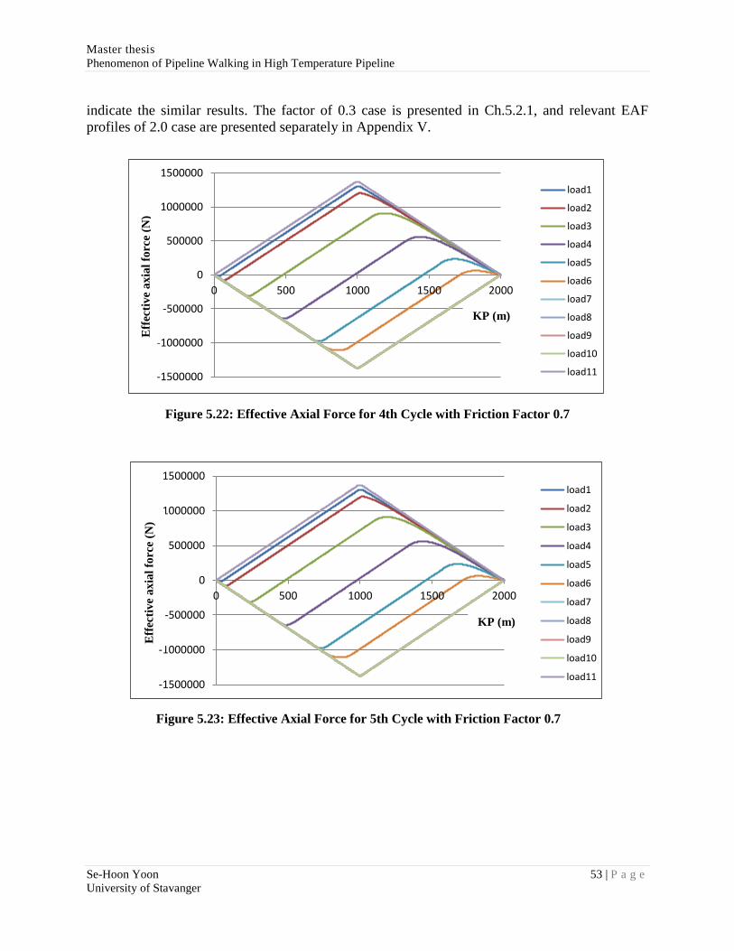
Master thesis
Phenomenon of Pipeline Walking in High Temperature Pipeline
Se-Hoon Yoon 53 | P a g e
University of Stavanger
-1500000
-1000000
-500000
0
500000
1000000
1500000
0 500 1000 1500 2000
load1
load2
load3
load4
load5
load6
load7
load8
load9
load10
load11
-1500000
-1000000
-500000
0
500000
1000000
1500000
0 500 1000 1500 2000
load1
load2
load3
load4
load5
load6
load7
load8
load9
load10
load11
indicate the similar results. The factor of 0.3 case is presented in Ch.5.2.1, and relevant EAF
profiles of 2.0 case are presented separately in Appendix V.
Figure 5.22: Effective Axial Force for 4th Cycle with Friction Factor 0.7
Figure 5.23: Effective Axial Force for 5th Cycle with Friction Factor 0.7
KP (m)
(Figur
e 2.0:
Conve
ntiona
l S-lay
install
ation
(Olav
Fyrilei
v et
al.,
2005)
[9]
Eff
ecti
ve
ax
ial
forc
e (N
)
KP (m)
(Figur
e 2.0:
Conve
ntiona
l S-lay
install
ation
(Olav
Fyrilei
v et
al.,
2005)
[9]
Eff
ecti
ve
ax
ial
forc
e (N
)

Master thesis
Phenomenon of Pipeline Walking in High Temperature Pipeline
Se-Hoon Yoon 54 | P a g e
University of Stavanger
5.3.2 Axial Displacement
This section discusses the axial movements over a range of operating cycles (5-cycle)
under different friction coefficient conditions. The results of the displacement in the section
mainly deal with the axial displacements at Mid-point, Hot end and Cold end of the pipeline.
5.3.2.1 Mid-Point Axial Displacement
The table 5.4 and 5.5 show the axial displacement at the mid-point of the pipeline with
friction factors: 0.5 and 0.7 respectively. Regarding the factor of 0.3 case is presented in Table
5.3 in Ch. 5.2.3.
Table 5.4: Mid-Point Axial Displacement with Friction Factor 0.5
1st Cycle 2nd Cycle 3rd Cycle 4th Cycle 5th Cycle
Load No.
DISP
(m)
Load
No.
DISP
(m)
Load
No.
DISP
(m)
Load
No.
DISP
(m)
Load
No.
DISP
(m)
1 0 1 0.0148 1 0.0964 1 0.1781 1 0.2598
2 0 2 0.0179 2 0.0995 2 0.1812 2 0.263
3 0.0001 3 0.0338 3 0.1154 3 0.1971 3 0.2788
4 0.0009 4 0.0756 4 0.1572 4 0.2388 4 0.3206
5 0.0129 5 0.1021 5 0.1838 5 0.2654 5 0.3472
6 0,0202 6 0.1001 6 0.1817 6 0.2636 6 0.3454
7 0.013 7 0.0952 7 0.1768 7 0.2584 7 0.3404
8 0.0137 8 0.0953 8 0.1769 8 0.2588 8 0.3406
9 0.0136 9 0.0953 9 0.177 9 0.2588 9 0.3406
10 0.0136 10 0.0953 10 0.1769 10 0.2588 10 0.3406
11 0.0136 11 0.0955 11 0.1772 11 0.259 11 0.3408
12 0.0139

Master thesis
Phenomenon of Pipeline Walking in High Temperature Pipeline
Se-Hoon Yoon 55 | P a g e
University of Stavanger
-0,05
0
0,05
0,1
0,15
0,2
0,25
0,3
0,35
0,4
0,45
0,5
Mid-Point AxialDisplacement(0.3)
Mid-Point AxialDisplacement(0.5)
Mid-Point AxialDisplacement(0.7)
Table 5.5: Mid-Point Axial Displacement with Friction Factor 0.7
1st Cycle 2nd Cycle 3rd Cycle 4th Cycle 5th Cycle
Load No.
DISP
(m)
Load
No.
DISP
(m)
Load
No.
DISP
(m)
Load
No.
DISP
(m)
Load
No.
DISP
(m)
1 0 1 0.0218 1 0.1256 1 0.2294 1 0.3332
2 0 2 0.0244 2 0.1283 2 0.232 2 0.3359
3 0 3 0.0407 3 0.1445 3 0.2483 3 0.3521
4 0.0004 4 0.0872 4 0.191 4 0.2948 4 0.3987
5 0.0115 5 0.125 5 0.2288 5 0.3325 5 0.4364
6 0.0255 6 0.129 6 0.2327 6 0.3366 6 0.4404
7 0.0237 7 0.1255 7 0.2293 7 0.3323 7 0.4362
8 0.0211 8 0.1247 8 0.2284 8 0.3323 8 0.4361
9 0.0211 9 0.1247 9 0.2284 9 0.3323 9 0.4361
10 0.0211 10 0.1246 10 0.2284 10 0.3323 10 0.4361
11 0.0211 11 0.1247 11 0.2285 11 0.3323 11 0.4362
12 0.0209
Figure 5.24: Axial Walking Displacement at Mid-Point with Friction Factor 0.3, 0.5 & 0.7
The axial displacements under the given conditions are plotted according to Tables 5.3 through
5.5, and it is shown as Figure 5.24. It indicates that the axial walking rises as the friction
1
0
F
5 (Figure
4 (Figur
3 (Figure
2 (FigNumber of Operating Cycle
Figure 2.0: Conventional
S-lay installation (Olav
Fyrileiv et al., 2005) [9]
Dis
pla
cem
en
t (m
)

Master thesis
Phenomenon of Pipeline Walking in High Temperature Pipeline
Se-Hoon Yoon 56 | P a g e
University of Stavanger
increases in the range of friction factors. The walking rate per operational cycle with different
values of the friction factor is given in Table 5.6:
Table 5.6: Results of Walking Rate
Friction Factor Walking Rate
LB 0.3 Abt. 0.05m/cycle
BE 0.5 Abt. 0.08m/cycle
UB 0.7 Abt. 0.1m/cycle
5.3.2.2 Axial Displacement with Friction Factor 2.0
It can be expected to get the different consequence concerning the walking in accordance
with the results of the EAF with friction factor of 2.0, which is discussed in Ch.5.3.1. The Table
5.7 shows the axial displacement at the mid-point of the pipeline with the factor of 2.0:
Table 5.7: Mid-Point Axial Displacement with Friction Factor 2.0
1st Cycle 2nd Cycle 3rd Cycle 4th Cycle 5th Cycle
Load No.
DISP
(m)
Load
No.
DISP
(m)
Load
No.
DISP
(m)
Load
No.
DISP
(m)
Load
No.
DISP
(m)
1 0 1 0.0117 1 0.0553 1 0.1009 1 0.147
2 0 2 0.0117 2 0.0553 2 0.1009 2 0.147
3 0 3 0.0117 3 0.0553 3 0.101 3 0.147
4 0 4 0.0136 4 0.057 4 0.1034 4 0.1496
5 0.0012 5 0.0521 5 0.098 5 0.144 5 0.1902
6 0.0121 6 0.0565 6 0.1022 6 0.1482 6 0.1936
7 0.0131 7 0.0558 7 0.1015 7 0.1475 7 0.1936
8 0.0123 8 0.0555 8 0.1012 8 0.1472 8 0.1934
9 0.0119 9 0.0555 9 0.1012 9 0.1472 9 0.1934
10 0.0119 10 0.0553 10 0.101 10 0.147 10 0.1932
11 0.0119 11 0.0553 11 0.1009 11 0.147 11 0.1931
12 0.0117
It can be seen that the axial movement (walking) is reduced compared to the results with other
factors (lower values) and gives approximate 0.046m/cycle under the condition. Therefore, the
pipelines can partly response like a long pipeline, which is fully restrained over a fixed length
under operation conditions, when the axial friction is high enough. As it becomes constrained,
the walking phenomenon consequently is to decrease or to disappear.

Master thesis
Phenomenon of Pipeline Walking in High Temperature Pipeline
Se-Hoon Yoon 57 | P a g e
University of Stavanger
5.4 Mitigation Measures for Pipeline Walking
This thesis work mainly focuses on pipeline walking which is resulted by cyclic heating
and cooling operations of a pipeline especially when the pipeline asymmetrically loaded. This is
because the fact that the heating operation is non-uniform, whereas the cooling operation is
nearly uniform. [11] Consequently, the instability of pipeline on the seabed occurred by the
pipeline walking phenomenon is to be taken into account, and mitigation methods can be
discussed by considering the causes of pipeline walking.
This section outlines mitigation measures of pipeline walking based on an understanding
of its mechanisms and the results from the case study. The selection of walking mitigation
method is evidently depends on the consequential effects of accumulated axial displacement due
to pipeline walking. Thus, each mitigation method and its impact on pipeline design are briefly
discussed. However, installation, cost of method and planning are not to be presented since it is
beyond the scope of this study.
5.4.1 Anchoring [11]
The pipeline anchors are the most common method to mitigate pipeline walking. It
controls and limits the maximum axial displacement by inducing additional tension in the
pipeline especially during a shutdown. A typical size of these anchors is in the range of 50 to 350
tons, and its general illustration is shown in Figure 5.25: [1]
Figure 5.25: A Typical Pipeline Restraining Anchor (Ryan Watson et al., 2010) [16]
The pipeline walking phenomenon is associated with the virtual anchor point shifts in the
pipeline during heating and cooling operations under asymmetrical load conditions. This means
the efficient mitigation can be set by correcting the separation between the virtual anchors. Thus,
the end support anchoring can be introduced. It works by way of reducing the separation between
the virtual anchors. Anchoring a pipeline especially in the cases of end tension or seabed slope
gives equal amount of corrective tension at the opposite end. It functions that the asymmetric

Master thesis
Phenomenon of Pipeline Walking in High Temperature Pipeline
Se-Hoon Yoon 58 | P a g e
University of Stavanger
loading is eliminated not to occur walking. Moreover, an anchor can be placed on the pipeline to
force the virtual anchor points to share the same location on the pipe.
The tension induced by an anchor can be sufficient for a pipeline to be susceptible to
lateral instability (buckling) while an anchor is eliminating walking. In addition, the walking
phenomenon can still occur in that buckled region, so walking into a buckle may give over stress
into the pipeline. [3] Consequently, it should ensure that the location of an anchor is to be well
considered in terms of possible buckling in the pipeline.
5.4.2 Increase Axial Friction [1]
The walking phenomenon critically depends on the critical axial force. In some cases
shows that the walking rate is to decrease due to the growth of an axial friction to a certain extent.
[3] Even the sensitivity study in the thesis work also notes that aspect. Hence, increasing axial
friction can be considered to mitigate pipeline walking, and there are several treatments for this
achievement.
5.4.2.1 Pipe-Soil Interaction
By investigating a specific pipe-soil interaction on site, it can improve friction factors for
design since lower values of friction factors can be expected. However, collecting soil data is
quite time consuming activity and costly. Besides, a deep water soil survey is to be one of
challenges to get the accurate analysis. It is not just because of the very low shear strength
exhibited by most deep water seabed top layers, but also because of the very low effective stress
level (a few kPa only). [3] Consequently, it may be impractical to produce such a high axial
resistance especially in a deep water pipeline without additional mitigation to control pipeline
walking.
5.4.2.2 Pipeline Weight Coating
A concrete weight coating can be a possible way to increase axial and lateral friction
resistance which is advantageous to reduce expansion and walking. However, it is likely to
experience lateral buckling due to the higher axial resistance, and the higher localized strains
may also take place because of higher lateral frictions. [3]
5.4.2.3 Trench and Bury
Those can be used to increase the axial friction resistance in the pipeline. However, a
high cost concern and limited equipment for deep water are challenges.

Master thesis
Phenomenon of Pipeline Walking in High Temperature Pipeline
Se-Hoon Yoon 59 | P a g e
University of Stavanger
Figure 5.26: A Trenching Operation (from www.theareofdreging.com)
5.4.2.4 Rock Dumping and Mattress
It gives such a function of additional anchoring, so it can reduce the end expansion and
walking in addition to buckling controls. However, a large amount of materials is to be required
to limit the walking problem. In addition, installation time, cost and recruiting specific vessels
for installation are other challenges.
Figure 5.27: A Rock Dumping Operation (from www.nordnes.nl)

Master thesis
Phenomenon of Pipeline Walking in High Temperature Pipeline
Se-Hoon Yoon 60 | P a g e
University of Stavanger
5.4.3 Increase Subsea Connection Line Capacity
When it comes to a limit sate for the pipeline, the walking phenomenon is not a failure
mode, [2] but it can lead to overstressing on subsea structure connections. Thus, by increasing
the capacity of spools and/or jumpers it can accommodate the axial displacement of pipeline
induced by walking. However, installation and handling limits may be restrictions for increasing
their capacities. [3]
5.5 Summary
This chapter has discussed the results of the FEA on pipeline walking under the thermal
cyclic loadings and dealt with different values of the axial friction factors for the sensitivity
study. There are no variations in the EAF when the pipeline is fully mobilized (after the 7th load
step in this case). From the second heat-up, two VAPs appear and move towards the mid-point
and the cold-end respectively as the pipeline gradually heated-up. With regards to pipeline
expansion, it becomes constant (less variations) when fully mobilized, especially at the mid-point
of the pipeline in the case. Besides, the walking rate per cycle has increased as the value of the
axial friction factor increase. However, the rate was reduced at the certain value of the factor
(here, 2.0), and it showed that the axial movement decreases with further increase in friction
factor.
In addition to that, the chapter has briefly presented the pipeline walking mitigation.
Some measures are introduced and it is to be considered in terms of relevant mechanisms of
pipeline walking: walking towards the tension end, bottom end of the slope, and the cold end
when transient heating is applied. It implies that the direction of walking and the associated
parameters are key factors for it. The increment of the axial friction can be selected as the
mitigation method based on the results of the case study, and increase capacity of the subsea
structures can be another option.

Master thesis
Phenomenon of Pipeline Walking in High Temperature Pipeline
Se-Hoon Yoon 61 | P a g e
University of Stavanger
6. Conclusion and Further Study
6.1 General
This chapter deals with the conclusions of the thesis work based on the analysis results in
Ch. 5. It describes the results briefly regarding the pipeline walking phenomenon under the
thermal cyclic loadings in the FEA. The further study is also to present in connection with the
works in the thesis.
6.2 Conclusions
The objective of the thesis is to study and understand pipeline walking when it is
subjected to the succession of thermal cycles. For the case study, thus, the FE model is generated
and the thermal gradients are modeled to simulate the propagation of temperatures along the
pipeline during operational cycles (5cycles considered in the study). The API 5L X65 grade
pipeline with the length of 2km laid on the flat seabed and the maximum operating temperature
88 are selected for analysis. The followings are conclusions based on the FEA results:
1. The relatively short pipeline is prone to axial walking due to thermal transients. It is
because the overall length of it is not insufficient to reach full restraint, and the VAP
is located at the middle of the pipeline where the EAF gets its max value. Even the
pipeline on the flat seabed with no end tension can experience the walking.
2. The axial movement under the thermal cyclic loadings is to translate from the hot-end
towards the cold-end. The results in Ch.5.2.3 support the conclusion. Hence,
considering the accurate assessment of walking for the reliability/capacity of the end
connectors is important.
3. Once the pipeline is fully mobilized, no variations in the EAF occur. Besides, the
EAF becomes constant after certain operations (after 4 cycles in the case study). Thus,
the walking rate is to be predictable without simulating more cycles.
4. The pipe-soil interaction is one of the important parameters in the walking assessment.
The walking rates grow as the axial friction factor increases according to Ch.5.3.2.
However, It turns to decrease with the certain value of the friction factor (here, 2.0).
Therefore, the increment of the axial friction can be one of possible methods to limit
the walking rate.

Master thesis
Phenomenon of Pipeline Walking in High Temperature Pipeline
Se-Hoon Yoon 62 | P a g e
University of Stavanger
6.3 Further Study
This section presents the further works, and the followings are to be performed:
1. It is quite difficult to predict the accurate axial friction especially in deep water due to
the uncertainties of soil conditions. Hence, more specific parameter studies regarding
soil conditions to be carried out in connection with pipeline walking.
2. Walking can be occurred by each of aforementioned mechanisms, but for many
pipelines more than one mechanism may be active. Thus, effects of combinations are
to be studied. Furthermore, the interaction between pipeline walking and lateral
buckling can be studied especially for a long pipeline. The long pipeline is effectively
split into several short pipelines due to buckling mitigation measures that acting as
pipeline ends.

Master thesis
Phenomenon of Pipeline Walking in High Temperature Pipeline
Se-Hoon Yoon 63 | P a g e
University of Stavanger
REFERENCE
[1] Bruton, D. S., Sinclair, F. and Carr, M., “Pipeline walking – Understanding the Field Layout
Challenges, and Analytical Solutions Developed for the SAFEBUCK JIP”, OTC 17945, Houston,
TX, May 2006.
[2] Bruton, D. A. S., Sinclair, F. and Carr, M., “Lessons Learned From Observing Walking of
Pipeline with Lateral Buckles, Including New Driving Mechanisms and Updated Analysis
Models”, OTC 20750, Huston, TX, May 2010.
[3] Rong, H., Inglis R., Bell G., Huang Z. and Chan, R., “Evaluation and Mitigation of Axial
Walking with a Focus on Deep Water Flowlines”, OTC 19862, Houston, TX, May 2009.
[4] Palmer, Andrew C. and Ling, Michael T.S., “Movement of Submarine Pipelines Close to
Platforms”, OTC 4067, Houston, TX, May 1981.
[5] Kumar, Amitabh and M. Brian, “Global Buckling and Axial Stability for HP/HT flowlines”,
OTC 20126, Houston, TX, May 2009.
[6] Chen, Qiang (2012), “Pipelines and Risers”, Class notes, University of Stavanger
(Unpublished).
[7] Pipeline Encyclopedia, “Pipeline Expansion”, (Cited 11th Feb. 2013), Available from:
<http://pipelineencyclopedia.blogspot.no>.
[8] Karunakaran, D. (2012), “Pipelines and Risers”, Class notes, University of Stavanger
(Unpublished).
[9] Fyrileiv, Olav and Collberg, Leif, “Influence of pressure in pipeline design-effective axial
force”, OMAE2005-67502, Proceedings of OMAE 2005, Halkidiki, Greece, 2005.
[10] Bruton, David A.S., White, David J. and Carr. M., “Pipe-Soil Interaction During Lateral
Buckling and Pipeline walking – The SAFEBUCK JIP”, OTC 19589, Houston, TX, May 2008.
[11] Chaudhury, Gautam, “Managing Unidirectional Movements (Walk) of HP/HT Submarine
Flowlines During Heating and Shutdown Cooling”, IOPF 2010-1003, Houston, TX, Oct. 2010.
[12] Bruton, D., Carr, M., Crawford, M. and Poiate, E. “The Safe Design of Hot On-Bottom
Pipelines with Lateral Buckling using the Design Guideline Developed by the SAFEBUCK Joint
Industry Project”, Deep Offshore Technology Conference, Vitoria, Espirito, Brazil (2005),
(Cited 2nd April 2013), Available from: <http://www.otmdevelopment4.co.uk/DOT2005-
SAFEBUCK_JIP-Overview.pdf>.

Master thesis
Phenomenon of Pipeline Walking in High Temperature Pipeline
Se-Hoon Yoon 64 | P a g e
University of Stavanger
[13] Ommundsen, Marius Loen, “UPHEAVAL BUCKLING OF BURIED PIPELINES” MSc
thesis, University of Stavanger, 2009, p.10.
[14] Watson, R.D., Sinclair, F. and Bruton, D. A. S., “SAFEBUCK JIP: Operational Integrity of
Deepwater Flowlines”, OTC 21724, Houston, TX, May 2011.
[15] SAFEBUCK JIP, “Safe Design of Pipelines with Lateral Buckling Design Guideline”,
Report Number BR02050/SAFEBUCK/B issued Aug. 2004, p. 18~20. (Confidential to JIP
Participants).
[16] Watson, R., Bruton D., Sinclair, F “Influence of Multiphase Flow on Global Displacement
of Deepwater Pipelines – In Design and Operation”, IOPF 2010-6002, Houston, TX, Oct. 2010.
[17] Brunner, M.S., Qi, X., Zheng, J. and Chao, J.C., “Combined Effect of Flowline Walking and
Riser Dynamic Loads on HP/HT Flowline Design”, OTC 17806, Houston, TX, May 2006.
[18] Subsea 7, “Guideline for Pipeline Walking and Lateral Buckling”, Doc. No. GR-DCE-RPL-
018, Feb. 2010 (Confidential to Subsea 7).
[19] AdvancePipeliner, “Global Buckling and Walking in Subsea Pipelines: Consequences and
Mitigation Measures”, (Cited 2nd Feb. 2013), Available from: <http://www.advancepipeliner.c-
om/site/index.php/component/content/article/131-allcategories/61-global-buclking-and-walking-
in-subsea-pipelines-consequences-and-mitigation-measures.html>.
[20] Subsea 7, “Design Guidelines Pipeline walking analysis”, Doc. No. CEO1PD-P-GU-129,
Nov. 2007 (Confidential to Subsea 7).
[21] ANSYS, Inc., “Theory Reference for the Mechanical APDL and Mechanical Applications”,
Release 12.1, Nov. 2009, p.793~8144/ p. 880~885
5.
[22] ANSYS Inc., “ANSYS User Manuals released 13.0”, 2010, (Cited 22nd April 2013),
Available from:
<https://www.sharcnet.ca/Software/Fluent13/help/ans_elem/Hlp_E_PIPE288.html>.
[23] ANSYS, Inc., “Contact Technology Guide”, Release 12.1, Nov. 2009, p. 69~71.
[24] Bai, Yong “Pipelines and risers”, Elsevier Ocean Engineering book series vol.3, p. 101~114.
[25] DNV-OS-F101, DNV Offshore Standard “Submarine Pipeline Systems”, Det Norske
Veritas, August 2012, Sec.4 G400.
4 Ch. 3.2.3/ 3.3.2
5 Ch.3.3.1

Master thesis
Phenomenon of Pipeline Walking in High Temperature Pipeline
Se-Hoon Yoon 65 | P a g e
University of Stavanger
[26] Casola, F., Chayeb, A. E., Greco S., Carlucci, A., “Characteristic of Pipe Soil Interaction
and Influence on HPHT Pipeline Design”, ISBN 978-1-880653-96-8 (Set); ISSN 1098-6189
(Set), Proceedings of ISOPE, Maui, Hawaii, USA 2011.
[27] Subsea 7, “Pipelines Design Centre of Excellence Documentation”, Doc. No. GD-GL-PD-
018, Feb. 2007 (Confidential to Subsea 7).
[28] Duncan, J. M., Wright, Stephen G., “Soil Strength and Slope Stability”, JOHN WILEY &
SONS Inc., Jan. 2005, p. 19.
[29] Oliphant J., Maconochie, A., “Axial Pipeline-Soil Interaction”, ISBN 1-880653-66-4 (Set);
ISSN 1098-6189 (Set), Proceedings of ISOPE, San Francisco, USA 2006.
[30] Mebarkia, S., “Effect of High-Pressure/High Temperature Flowlines and Soil Interaction on
Deepwater Subsea Development”, OTC 18107, Houston, TX, May 2006.
[31] DNV-RP-F110, DNV Recommended Practice “Global Buckling of Submarine Pipelines-
Structural Design due to High Temperature/High Pressure”, Det Norske Veritas, Oct. 2007,
Ch.5.2.2/3.

Master thesis
Phenomenon of Pipeline Walking in High Temperature Pipeline
Se-Hoon Yoon AI-1 | P a g e
University of Stavanger
Appendix I
Pipeline Model Parameter Calculation

Master thesis
Phenomenon of Pipeline Walking in High Temperature Pipeline
Se-Hoon Yoon AI-2 | P a g e
University of Stavanger
1. General
This appendix consists of calculations related to the rigid pipeline model which is
introduced in chapter 4. The objective of the separate sheets is to validate the results of the FE
analysis by ANSYS with respect to pipeline walking. The calculations are carried out according
to ref [15] and [20].
2. Input data
2.1 Pipeline
Length 2000m
Pipeline outer diameter 323.9mm
Wall Thickness 25.4mm
External (insulation) coating thickness 5mm
Concrete coating thickness 30mm
2.2 Material Properties
2.2.1 Pipeline
Density of pipe steel 7850
SMYS of pipe steel 450MPa
Young’s modulus of pipe steel Mpa
Thermal expansion coefficient
Poisson’s ratio of pipe steel
2.2.2 Insulation / Concrete Coating
Density of insulation coating 910
Density of concrete coating 2400
2.3 Operating Data
Operating temperature 88
Shutdown (ambient) temperature
Operating pressure 15Mpa
Density of fluid content in pipe 900

Master thesis
Phenomenon of Pipeline Walking in High Temperature Pipeline
Se-Hoon Yoon AI-3 | P a g e
University of Stavanger
2.3 Environmental and Soil Data
2.3.1 Environmental Data
Density of seawater 1027
Water depth 100m
2.3.2 Soil Data
Axial friction factor 0.3 (Initial value)
3. Calculations
Unit: ; ;
3.1 Parameter Calculations
Effective Pipe Diameter : + 2( + ) = 323.9 + 2(5 + 30) = 393.9mm
Internal diameter : = 323.9 2 25.4 = 273.1mm
Cross sectional area of pipe :
(
)
Cross sectional area of insulation coating :
Cross sectional area of concrete coating :
Mass of pipe steel per unit length :
Mass of insulation coating per unit length :

Master thesis
Phenomenon of Pipeline Walking in High Temperature Pipeline
Se-Hoon Yoon AI-4 | P a g e
University of Stavanger
Mass of concrete coating per unit length :
Mass of content :
(
)
Pipeline total mass per unit length (in air) :
Mass of pipe buoyancy per unit length :
Mass of submerged pipeline per unit length (in water) :
Weight of pipeline per unit length (dry weight) :
Weight of submerged pipeline per unit length :
3.2 Walking Rate
Friction force :
Thermal gradients force :
(
)
Walk per cycle due to Thermal Transients :
√

Master thesis
Phenomenon of Pipeline Walking in High Temperature Pipeline
Se-Hoon Yoon AI-5 | P a g e
University of Stavanger
√
(
)

Master thesis
Phenomenon of Pipeline Walking in High Temperature Pipeline
Se-Hoon Yoon AII-1 | P a g e
University of Stavanger
Appendix II
Temperature Profile Preparation

Master thesis
Phenomenon of Pipeline Walking in High Temperature Pipeline
Se-Hoon Yoon AII-2 | P a g e
University of Stavanger
0
10
20
30
40
50
60
70
80
90
100
0
10
0
20
0
30
0
40
0
50
0
60
0
70
0
80
0
90
0
10
00
11
00
12
00
13
00
14
00
15
00
16
00
17
00
18
00
19
00
20
00
#1
#2
#3
#4
#5
#6
#7
#8
#9
#10
1. General
This appendix presents interpolated temperatures along the pipeline to create the
temperature load profiles. The Mathcad v15 is used and it is created based on the maximum
operating temperature: 88 in the thesis work. The profile is made based on Figure A-II.1 that is
taken from Figure 3.1 in Ch.3.
The body force, which is the thermal load in the thesis work, is applied to the pipeline
model in the FEA. Thus, each element of the model has been taken temperatures based on these
temperature profiles.
Figure A-II.1: Temperature Transients used in Pipeline Walking Analysis
KP (m)
(Figure
2.0:
Conventi
onal S-
lay
installati
on (Olav
Fyrileiv
et al.,
2005) [9]
F
i
g
u
r
e
2
.
0
:
C
o
n
v
e
n
ti
o
n
a
l
S
-
l
a
y
i
n
st
a
ll
a
ti
o
n
(
O
l
a
v
F
y
Load step
2.0:
Conventi
onal S-
lay
installati
on (Olav
Fyrileiv
et al.,
2005) [9]

Master thesis
Phenomenon of Pipeline Walking in High Temperature Pipeline
Se-Hoon Yoon AII-3 | P a g e
University of Stavanger
1. Temperature Load #1 Interpolation
Temp. Load #1 Table (Tin):
Tin
0 1
0
1
2
3
4
5
6
7
8
9
0 24
50 18
100 10
150 6
200 4
250 4
300 4
350 4
400 4
450 ...
0 500 1000 1500 2000
5
10
15
20
25
Temperature profile of temp load step #1
Pipe length in m
Tem
per
ature
(ce
lsiu
s deg
ree)
T0
KP
KP Tin0
T0 Tin1

Master thesis
Phenomenon of Pipeline Walking in High Temperature Pipeline
Se-Hoon Yoon AII-4 | P a g e
University of Stavanger
Number of data points:
Interpolate data:
Tout
0 1
0
1
2
3
4
5
6
7
8
9
1 1
2 2
3 3
4 4
5 5
6 6
7 7
8 8
9 9
10 ...
Element_N Tout0
KPout Tout1
n rows KPout( )
i 0 n 1
Ti
linterp KP T0 KPouti
out WRITEPRN "Interpolated Temperature Load_#1" T ( )

Master thesis
Phenomenon of Pipeline Walking in High Temperature Pipeline
Se-Hoon Yoon AII-5 | P a g e
University of Stavanger
2. Temperature Load #2 Interpolation
Temp. Load #2 Table (Tin):
Tin
0 1
0
1
2
3
4
5
6
7
8
9
0 60
50 47
100 30
150 21
200 10
250 7
300 4
350 4
400 4
450 ...
KP Tin0
T0 Tin1
0 500 1000 1500 2000
20
40
60
Temperature profile of temp load step #2
Pipe length in m
Tem
per
atu
re (
cels
ius
deg
ree)
T0
KP

Master thesis
Phenomenon of Pipeline Walking in High Temperature Pipeline
Se-Hoon Yoon AII-6 | P a g e
University of Stavanger
Number of data points:
Interpolate data:
Tout
0 1
0
1
2
3
4
5
6
7
8
9
1 1
2 2
3 3
4 4
5 5
6 6
7 7
8 8
9 9
10 ...
Element_N Tout0
KPout Tout1
n rows KPout( )
i 0 n 1
Ti
linterp KP T0 KPouti
out WRITEPRN "Interpolated Temperature Load_#2" T ( )

Master thesis
Phenomenon of Pipeline Walking in High Temperature Pipeline
Se-Hoon Yoon AII-7 | P a g e
University of Stavanger
3. Temperature Load #3 Interpolation
Temp. Load #3 Table (Tin):
Tin
0 1
0
1
2
3
4
5
6
7
8
9
0 80
50 77
100 72
150 60
200 55
250 50
300 40
350 31
400 22
450 ...
KP Tin0
T0 Tin1
0 500 1000 1500 2000
20
40
60
80
Temperature profile of temp load step #3
Pipe length in m
Tem
per
atu
re (
cels
ius
deg
ree)
T0
KP

Master thesis
Phenomenon of Pipeline Walking in High Temperature Pipeline
Se-Hoon Yoon AII-8 | P a g e
University of Stavanger
Number of data points:
Interpolate data:
Tout
0 1
0
1
2
3
4
5
6
7
8
9
1 1
2 2
3 3
4 4
5 5
6 6
7 7
8 8
9 9
10 ...
Element_N Tout0
KPout Tout1
n rows KPout( )
i 0 n 1
Ti
linterp KP T0 KPouti
out WRITEPRN "Interpolated Temperature Load_#3" T ( )

Master thesis
Phenomenon of Pipeline Walking in High Temperature Pipeline
Se-Hoon Yoon AII-9 | P a g e
University of Stavanger
4. Temperature Load #4 Interpolation
Temp. Load #4 Table (Tin):
Tin
0 1
0
1
2
3
4
5
6
7
8
9
0 81
50 80
100 79
150 77
200 75
250 73
300 71
350 67
400 59
450 ...
KP Tin0
T0 Tin1
0 500 1000 1500 2000
20
40
60
80
100
Temperature profile of temp load step #4
Pipe length in m
Tem
per
atu
re (
cels
ius
deg
ree)
T0
KP

Master thesis
Phenomenon of Pipeline Walking in High Temperature Pipeline
Se-Hoon Yoon AII-10 | P a g e
University of Stavanger
Number of data points:
Interpolate data:
Tout
0 1
0
1
2
3
4
5
6
7
8
9
1 1
2 2
3 3
4 4
5 5
6 6
7 7
8 8
9 9
10 ...
Element_N Tout0
KPout Tout1
n rows KPout( )
i 0 n 1
Ti
linterp KP T0 KPouti
out WRITEPRN "Interpolated Temperature Load_#4" T ( )

Master thesis
Phenomenon of Pipeline Walking in High Temperature Pipeline
Se-Hoon Yoon AII-11 | P a g e
University of Stavanger
5. Temperature Load #5 Interpolation
Temp. Load #5 Table (Tin):
Tin
0 1
0
1
2
3
4
5
6
7
8
9
0 85
50 84
100 83
150 82
200 81
250 80
300 78
350 78
400 76
450 ...
KP Tin0
T0 Tin1
0 500 1000 1500 2000
20
40
60
80
100
Temperature profile of temp load step #5
Pipe length in m
Tem
per
ature
(ce
lsiu
s deg
ree)
T0
KP

Master thesis
Phenomenon of Pipeline Walking in High Temperature Pipeline
Se-Hoon Yoon AII-12 | P a g e
University of Stavanger
Number of data points:
Interpolate data:
Tout
0 1
0
1
2
3
4
5
6
7
8
9
1 1
2 2
3 3
4 4
5 5
6 6
7 7
8 8
9 9
10 ...
Element_N Tout0
KPout Tout1
n rows KPout( )
i 0 n 1
Ti
linterp KP T0 KPouti
out WRITEPRN "Interpolated Temperature Load_#5" T ( )

Master thesis
Phenomenon of Pipeline Walking in High Temperature Pipeline
Se-Hoon Yoon AII-13 | P a g e
University of Stavanger
6. Temperature Load #6 Interpolation
Temp. Load #6 Table (Tin):
Tin
0 1
0
1
2
3
4
5
6
7
8
9
0 85
50 84
100 83
150 82
200 81
250 80
300 78
350 78
400 76
450 ...
KP Tin0
T0 Tin1
0 500 1000 1500 2000
20
40
60
80
100
Temperature profile of temp load step #6
Pipe length in m
Tem
per
ature
(ce
lsiu
s deg
ree)
T0
KP

Master thesis
Phenomenon of Pipeline Walking in High Temperature Pipeline
Se-Hoon Yoon AII-14 | P a g e
University of Stavanger
Number of data points:
Interpolate data:
Tout
0 1
0
1
2
3
4
5
6
7
8
9
1 1
2 2
3 3
4 4
5 5
6 6
7 7
8 8
9 9
10 ...
Element_N Tout0
KPout Tout1
n rows KPout( )
i 0 n 1
Ti
linterp KP T0 KPouti
out WRITEPRN "Interpolated Temperature Load_#6" T ( )
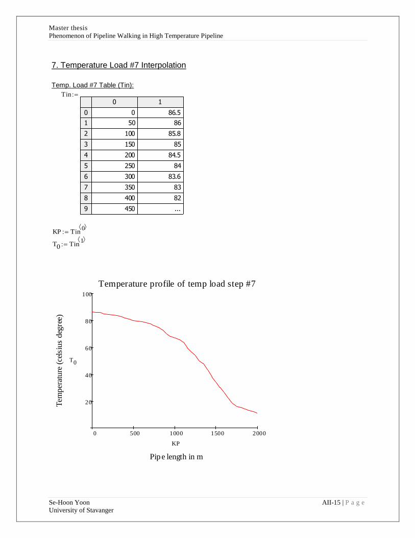
Master thesis
Phenomenon of Pipeline Walking in High Temperature Pipeline
Se-Hoon Yoon AII-15 | P a g e
University of Stavanger
7. Temperature Load #7 Interpolation
Temp. Load #7 Table (Tin):
Tin
0 1
0
1
2
3
4
5
6
7
8
9
0 86.5
50 86
100 85.8
150 85
200 84.5
250 84
300 83.6
350 83
400 82
450 ...
KP Tin0
T0 Tin1
0 500 1000 1500 2000
20
40
60
80
100
Temperature profile of temp load step #7
Pipe length in m
Tem
per
ature
(ce
lsiu
s deg
ree)
T0
KP

Master thesis
Phenomenon of Pipeline Walking in High Temperature Pipeline
Se-Hoon Yoon AII-16 | P a g e
University of Stavanger
Number of data points:
Interpolate data:
Tout
0 1
0
1
2
3
4
5
6
7
8
9
1 1
2 2
3 3
4 4
5 5
6 6
7 7
8 8
9 9
10 ...
Element_N Tout0
KPout Tout1
n rows KPout( )
i 0 n 1
Ti
linterp KP T0 KPouti
out WRITEPRN "Interpolated Temperature Load_#7" T ( )

Master thesis
Phenomenon of Pipeline Walking in High Temperature Pipeline
Se-Hoon Yoon AII-17 | P a g e
University of Stavanger
8. Temperature Load #8 Interpolation
Temp. Load #8 Table (Tin):
Tin
0 1
0
1
2
3
4
5
6
7
8
9
0 87
50 86.6
100 86
150 85.6
200 85.2
250 85
300 84.5
350 84
400 83.5
450 ...
KP Tin0
T0 Tin1
0 500 1000 1500 200040
50
60
70
80
90
Temperature profile of temp load step #8
Pipe length in m
Tem
per
ature
(ce
lsiu
s deg
ree)
T0
KP

Master thesis
Phenomenon of Pipeline Walking in High Temperature Pipeline
Se-Hoon Yoon AII-18 | P a g e
University of Stavanger
Number of data points:
Interpolate data:
Tout
0 1
0
1
2
3
4
5
6
7
8
9
1 1
2 2
3 3
4 4
5 5
6 6
7 7
8 8
9 9
10 ...
Element_N Tout0
KPout Tout1
n rows KPout( )
i 0 n 1
Ti
linterp KP T0 KPouti
out WRITEPRN "Interpolated Temperature Load_#8" T ( )

Master thesis
Phenomenon of Pipeline Walking in High Temperature Pipeline
Se-Hoon Yoon AII-19 | P a g e
University of Stavanger
9. Temperature Load #9 Interpolation
Temp. Load #9 Table (Tin):
Tin
0 1
0
1
2
3
4
5
6
7
8
9
0 87
50 86.6
100 86
150 85.6
200 85.2
250 85
300 84.5
350 84.5
400 83.7
450 ...
KP Tin0
T0 Tin1
0 500 1000 1500 200060
70
80
90
Temperature profile of temp load step #9
Pipe length in m
Tem
per
ature
(ce
lsiu
s deg
ree)
T0
KP

Master thesis
Phenomenon of Pipeline Walking in High Temperature Pipeline
Se-Hoon Yoon AII-20 | P a g e
University of Stavanger
Number of data points:
Interpolate data:
Tout
0 1
0
1
2
3
4
5
6
7
8
9
1 1
2 2
3 3
4 4
5 5
6 6
7 7
8 8
9 9
10 ...
Element_N Tout0
KPout Tout1
n rows KPout( )
i 0 n 1
Ti
linterp KP T0 KPouti
out WRITEPRN "Interpolated Temperature Load_#9" T ( )

Master thesis
Phenomenon of Pipeline Walking in High Temperature Pipeline
Se-Hoon Yoon AII-21 | P a g e
University of Stavanger
10. Temperature Load #10 Interpolation
Temp. Load #10 Table (Tin):
Tin
0 1
0
1
2
3
4
5
6
7
8
9
0 88
50 87.67
100 87.4
150 87.32
200 87.2
250 87.18
300 87
350 86.76
400 86.67
450 ...
KP Tin0
T0 Tin1
0 500 1000 1500 200083
84
85
86
87
88
Temperature profile of temp load step #10
Pipe length in m
Tem
per
ature
(ce
lsiu
s deg
ree)
T0
KP

Master thesis
Phenomenon of Pipeline Walking in High Temperature Pipeline
Se-Hoon Yoon AII-22 | P a g e
University of Stavanger
Number of data points:
Interpolate data:
Tout
0 1
0
1
2
3
4
5
6
7
8
9
1 1
2 2
3 3
4 4
5 5
6 6
7 7
8 8
9 9
10 ...
Element_N Tout0
KPout Tout1
n rows KPout( )
i 0 n 1
Ti
linterp KP T0 KPouti
out WRITEPRN "Interpolated Temperature Load_#10" T ( )

Master thesis
Phenomenon of Pipeline Walking in High Temperature Pipeline
Se-Hoon Yoon AIII-1 | P a g e
University of Stavanger
Appendix III
Pipeline Model Material Property

Master thesis
Phenomenon of Pipeline Walking in High Temperature Pipeline
Se-Hoon Yoon AIII-2 | P a g e
University of Stavanger
2 SMTS 535 MPa
y SMYS 450 MPa
Ramberg-Osgood Stress-Strain Curve
Given parameters:
Youngs Modulus:
Yield Stress:
Tensile Stress:
Elongation at break:
Known points on the stress-strain curve:
Yield point:
Second point:
Ramberg-Osgood material model:
Calculating the Ramberg-Osgood curve parameters:
The 0.7 is also called the Ramberg-Osgood yield parameter, and is sometimes denoted
R or y. It is found by drawing a line in the stress-strain graph with a slope of 0.7E from origin.
The Ramberg-Osgood yield parameter is the corresponding stress where this line intersects
the stress-strain curve.
( )
E1
3
7
0.7
n 1

Master thesis
Phenomenon of Pipeline Walking in High Temperature Pipeline
Se-Hoon Yoon AIII-3 | P a g e
University of Stavanger
n 1 1 2 2
ln1 E 1
2 E 2
ln1
2
Re-arranging equation:
Since 0.7 and n are constants, the following can be used:
Hence:
is cancelled, thus:
Or
Further:
Hence:
Since
and
E1
3
7
0.7
n 1
E 3
7
0.7
n 1
E 3
7
n
0.7n 1
E 3
7
n
0.7n 1
0.7n 1 3
7
n
E
0.7_1
n1 10.7_2
n2 1
3
7
1n
1 E 1
3
7
2n
2 E 2
3
7
1n
2n
1 E 1
2 E 2
1
2
n1 E 1
2 E 2
ln1
2
n
n ln1
2
ln1 E 1
2 E 2

Master thesis
Phenomenon of Pipeline Walking in High Temperature Pipeline
Se-Hoon Yoon AIII-4 | P a g e
University of Stavanger
n n y y 2 2
And:
Remove unit for the calculation
This is true for any and corresponding.
For the current case:
Repeating expression, required for graphing
Setting plot range:
Ramberg-Osgood curve:
E1E
1MPa
E1 2.07 105
0.7 x x n 3
7
xn
x E1 x
1
n 1
n 19.965
0.7 0.7
y
1MPay n
1 MPa
( )
E1
3
7
0.7
n 1
0 0.02 0.04 0.06 0.080
2 108
4 108
6 108
( )
n
0.7 424.426MPa

Master thesis
Phenomenon of Pipeline Walking in High Temperature Pipeline
Se-Hoon Yoon AIV-1 | P a g e
University of Stavanger
Appendix IV-1
Finite Element Analysis
ANSYS Scripts for Modeling

Master thesis
Phenomenon of Pipeline Walking in High Temperature Pipeline
Se-Hoon Yoon AIV-2 | P a g e
University of Stavanger
!*************************************************************************************
!* Title: *
!* *
!* Pipeline walking for high temperature subsea pipeline by thermal transient *
!* *
!* Presented by Se-Hoon Yoon *
!* (Graduate student of Offshore technology in University of Stavanger, Norway) *
!*************************************************************************************
!* Description: *
!* It presents APDL (ANSYS Parametric Design Language) to analyze pipeline walking. *
!* *
!* Status/Comments: *
!* The each temperature load step profile is given as 'inp' filename extension *
!*************************************************************************************
! File Desc.: Model 22in pipeline
FINI
/CLEAR
*SET,LOADCASE,'Test2'
/TITLE,%LOADCASE%
!File Desc.: Pipeline walking by thermal transient
/FILENAM,%LOADCASE%
/UNITS,MKS ! MKS system (m,kg,s,deg C)
!######################################## #############################################
!# Various parameters # # Unit are [m] [N] [Kg] [s] [deg C] #
!######################################## #############################################
pi=4*ATAN(1.0) ! Pi
g=9.81 ! Gravitational Acceleration (m/s^2)
WD=-100 ! Water Depth (m)
/PREP7 ! Enter model creation preprocessor
!ANTYPE,0,NEW ! 0=STATIC
ACEL,,g ! Define gravity
ET,1,PIPE288 ! Pipe elements
SECTYPE,1,PIPE ! Define pipe section type

Master thesis
Phenomenon of Pipeline Walking in High Temperature Pipeline
Se-Hoon Yoon AIV-3 | P a g e
University of Stavanger
SECDATA,323.9E-3,25.4E-3 ! Define pipe section:OD,Tkwall [m]
ET,2,TARGE170 ! Seabed element
ET,3,CONTA175 ! Contact elements
!---------------------------------------------------------------------------------------
! PIPELINE DATA
!---------------------------------------------------------------------------------------
!#DIMENSION FOR WEIGHT CALCULATION
OD=323.9E-3 ! Pipe Outer Diameter (m)
tkwall=25.4E-3 ! Pipe Wall Thickness (m)
DI=OD-2*tkwall ! Pipe Inner Diameter (m)
L=2000 ! Pipeline Length (m)
t_ext=5E-3 ! External Coating Thickness (m)
t_conc=30E-3 ! Concrete Coating Thickness (m)
!#OPERATIONAL DATA
DEN_SW=1027 ! Water Density (Kg/m^3)
DENSFL=900 ! Content Density OIL (Kg/m^3)
Pres_d=15E6 ! Design Pressure (N/m^2)
Pres_op=15E6 ! Operating Pressure (N/m^2)
T_amb=3.5 ! Ambient Temerature (deg C)
T_op=88 ! Operating Temperature (deg C)
!R_lay=0 ! Residual Lay Tension
!#MATERIAL PROPERTIES
!MP,DENS,1,7850 ! Pipe Material density (Kg/m^3)
! defined as equivalent density
MPTEMP,1,0,100 ! Define temperatures for Young's modulus
MP,EX,1,207E9 ! Young's modulus (N/m^2)

Master thesis
Phenomenon of Pipeline Walking in High Temperature Pipeline
Se-Hoon Yoon AIV-4 | P a g e
University of Stavanger
MP,ALPX,1,1.17E-5 ! Thermal expansion coefficient (/deg C)
MP,PRXY,1,0.3 ! Poisson ratio
!#COATING DENSITY
P_EXT=910 ! Insulation or Coating Density (Kg/m^3)
P_CONC=2400 ! Concrete Coating Density (Kg/m^3)
!-------------------------------------------------------------------------------------- -------
! **DEFINE STRESS-PLASTIC STRAIN CURVE**
!---------------------------------------------------------------------------------------------
TB,MISO,1,2,4 !PLASTIC ! Activate a data table
! Hardening using von Misses or Hill plasticity
TBTEMP,20.0 ! Temperature = 20.0deg C
TBPT,,0.0,0.0
TBPT,,0.0019,393.3E6
TBPT,,0.005,450E6
TBPT,,0.092,535E6
TBTEMP,100.0 ! Temperature = 100.0deg C
TBPT,,0.0,0.0
TBPT,,0.0018,372.6E6
TBPT,,0.005,420E6
TBPT,,0.092,505E6
!-----------------------------------------------------------------------------------------------
! SEABED DATA
!-----------------------------------------------------------------------------------------------
!DEFINE SEABED SOIL FRICTION
FRICLAX=0.3 ! Soil friction coefficient in axial direction
FRICLLAT=0.8 ! Soil friction coefficient in lateral direction
TB,FRIC,2,,,ORTHO ! Define orthotropic soil friction
TBDATA,1,FRICLAX,FRICLLAT
igap=0 ! Initial gap between pipeline and seabed
!------------------------------------------------------------------------------------------------------
! PIPE SYSTEM PARAMETER CALCULATION
!------------------------------------------------------------------------------------------------------

Master thesis
Phenomenon of Pipeline Walking in High Temperature Pipeline
Se-Hoon Yoon AIV-5 | P a g e
University of Stavanger
D_EFF=OD+2*(t_ext+t_conc) ! Effective Pipe Diameter (m)
AS=pi*(OD**2-DI**2)/4 ! Cross-sectional Area of Pipe Steel (m^2)
AS_EXT=pi*((OD+2*t_ext)**2-OD**2)/4 ! Cross-sectional Area of External Coating (m^2)
AS_CONC=pi*((OD+2*t_ext+2*t_conc)**2-(OD+2*t_ext)**2)/4 ! Cross-sectional Area of Concrete Coating (m^2)
M_STEEL=AS*7850 ! Pipe Steel Mass (Kg/m)
M_EXT=AS_EXT*P_EXT ! External Coating Mass (Kg/m)
M_CONC=AS_CONC*P_CONC ! Concrete Coating Mass (Kg/m)
M_CONT=pi*(DI**2)*DENSFL/4 ! Content Mass (Kg/m)
M_WATE=pi*(DI**2)*DEN_SW/4 ! Water Mass (Kg/m)
M_BUOY=pi*(D_EFF**2)*DEN_SW/4 ! Buoyancy Mass (Kg/m)
MWALL=M_STEEL+M_EXT+M_CONC ! Pipeline Total Mass (Kg/m) (weight on air)
M_SUB=MWALL-M_BUOY ! Submerged Mass (Kg/m) (weight in water)
W_CONT=M_CONT*g ! Content Weight (N/m)
W_WATE=M_WATE*g ! Flooded Weight (N/m)
W_SUB=M_SUB*g ! Empty Pipe Submerged Weight (N/m)
EQ_DEN=M_SUB/AS ! Submerged pipe Equivalent Density (kg/m^3)
DENSIN=((t_ext*P_EXT)+(t_conc*P_CONC))/(t_ext+t_conc) ! Insulation Eqv. Density (Corr. & Concr. Coat.) (N/m)
TKIN=t_ext+t_conc ! Insulation thickness (Corr. & Concr. Coat.) (m)
AREAIN=AS_EXT+AS_CONC ! Insulation Area (Corrosion coat.& Concrete Coat.) (m^2)
!---------------------------------------------------------------------------------------------------------
! **APPLY WEIGHT ON PIPELINE**
!---------------------------------------------------------------------------------------------------------
MP,DENS,1,EQ_DEN ! Pipe Material density (Kg/m^3)
! Using Equivalent Density for submerged weight
SECCONTROLS,M_CONT ! Added mass: content(kg/m)
!--------------------------------------------------------------------------------------------------------
! ELEMENT REAL CONSTANT
!------------------------------------------------------------------------------------------------------ --
!# FOR PIPELINE !
KEYOPT,1,1,0 ! Temperature Through wall gradient
KEYOPT,1,4,1 ! Thin Pipe Theory

Master thesis
Phenomenon of Pipeline Walking in High Temperature Pipeline
Se-Hoon Yoon AIV-6 | P a g e
University of Stavanger
KEYOPT,1,6,0 ! Internal and External pressure cause loads on end caps
KEYOPT,1,7,0 ! Output control for section forces/moments and strains/curvatures KEYOPT,1,8,0 ! Output control at integration points (1=Maximum and minimum stresses/strains)
KEYOPT,1,9,2
KEYOPT,1,15,0 ! One result for each section integration point
!---------------!
!# SEABED !
!---------------!
R,22,,,0.01,0.5 ! Define Contact Stiffness Factor and Penetration Tolerance Factor
KEYOPT,3,10,2 ! Set option 10 (Contact Stiffness Update) for element type 3 to 2 (Each substep based on mean
! Stress of underlying elements from the previous substep (pair based))
! Update stiffness automatically based on maximum penetration
KEYOPT,3,2,1 ! Penalty method, static stiffness of seabed
KEYOPT,3,4,2 !
KEYOPT,3,10,2 !
KEYOPT,3,12,0 ! Behavior of Contact Surface (0=standard)
!---------------------------------------------------------------------------------------
! PIPELINE MODELING
!---------------------------------------------------------------------------------------
!################################################################################
!# Generate Keypoints (m) #
!################################################################################
K, 1 , 0.0 , WD , 0.0
K, 11 , 2000.0 , WD , 0.0
!**************************************************************
!* Create nodes to describe local coordinate systems for ends *
!**************************************************************
K, 12 , -25.0 , WD , 0.0
K, 13 , 0.0 , WD+25.0 , 0.0
K, 14 , 2025.0 , WD , 0.0
K, 15 , 2000.0 , WD+25.0 , 0.0
!*************************************************
!* Create new coordinate systems for ends (11,12) *
!*************************************************

Master thesis
Phenomenon of Pipeline Walking in High Temperature Pipeline
Se-Hoon Yoon AIV-7 | P a g e
University of Stavanger
CSKP, 11 ,0 ,1 ,12 ,13
CSKP, 12 ,0 ,11 ,14 ,15
CSYS,0 ! Activate the default coordinate system (0)
!######################################
!# Pipe Nodes #
!######################################
EndNode=2000
*DO, I, 1, EndNode
N, I, L/EndNode*I, WD, 0
*ENDDO
!*********************************************
!* Meshing of straight pipe elements *
!*********************************************
TYPE,1 ! Element type, material, constants
MAT,1
SECNUM,1
*DO,I,1,endnode-1
E,I,I+1
*ENDDO
!---------------------------------------------------------------------------------------
! SEABED MODELING
!---------------------------------------------------------------------------------------
!*********************************************
!* Meshing of seabed elements
!*********************************************
! Define nodes for seabed area
N, 3001 , -15.0 , WD-igap , 15.0
N, 3002 , 2015 , WD-igap , 15.0
N, 3003 , 2015 , WD-igap , -15.0
N, 3004 , -15.0 , WD-igap , -15.0

Master thesis
Phenomenon of Pipeline Walking in High Temperature Pipeline
Se-Hoon Yoon AIV-8 | P a g e
University of Stavanger
!#DEFINE TARGET ELEMENT##
!------------------------
TYPE,2 ! Select material and properties for seabed
MAT,2
REAL,22
TSHAPE,QUAD ! SET TARGET SHAPE
NUMSTR,ELEM,30001
E,3001,3002,3003,3004 ! Define Element
NSEL,S,NODE,,1,endnode ! Select pipe nodes
TYPE,3 ! Select element type 3
REAL,22
NUMSTR,ELEM,40001
ESURF
ALLSEL ! - Seabed done
!---------------------------------------------------------------------------------------
! MISC: END LOCAL COORDINATE
!---------------------------------------------------------------------------------------
! Rotate end nodes to local coordinate system
e1=1 ! Identify end node and
CSYS,11 ! Change nodal coordinate system
NROTAT,e1
e2=EndNode ! Identify end node and
CSYS,12 ! Change nodal coordinate system
NROTAT,e2
CSYS,0
GPLOT
!-----------------------------------------------------------------------------------------
! DISPLAY MODEL
!-----------------------------------------------------------------------------------------
/ESHAPE,1 ! Display elements as solids
/TRIAD,rbot ! Display XYZ triad in right bottom corner
/PSYMB,NDIR,1 ! Display nodal coordinate system if other than global

Master thesis
Phenomenon of Pipeline Walking in High Temperature Pipeline
Se-Hoon Yoon AIV-9 | P a g e
University of Stavanger
FINISH ! Exit the preprocessor
!/EOF
!##############################################################################################
!# SOLUTION PROCESSOR #
!##############################################################################################
/CONFIG,NRES,20000
/SOLU ! Enter solution processor
ANTYPE,STATIC ! 0=STATIC
!OUTRES,ALL,ALL
NLGEOM,ON ! Includes large deflection effects in a static or full transient analysis
NEQIT,1000 ! Specifies the maximum number of equilibrium iterations for nonlinear analyses
AUTOTS,ON ! Automatic time stepping
NROPT,UNSYM ! Specifies the Newton-Raphson options in a static or full transient analysis
! (FULL or UNSYM= the stiffness matrix is updated at every equilibrium iteration)
NSUBST,5,20,2 ! Specifies the number of substeps to be taken every load step (nbr this step, maximum number of
! Substeps to be taken (i.e. min. time step), minimum number of step (i.e. max time step)
TREF,T_amb ! Reference Temperature (deg C) for Thermal Strain Calculation
CNCHECK,AUTO ! Adjust the initial status of contact pairs
STABILIZE,CONSTANT,DAMPING,0.1,AnyTime
MONITOR,1,1000,UX
MONITOR,2,1000,UY
!**********************************************************************************************************
!* LOAD STEPS
!**********************************************************************************************************
TIME,1 ! Set the time for the end of the load step
/STITLE,1,PIPELINE LAID ON SEABED-INITIAL CONDITION

Master thesis
Phenomenon of Pipeline Walking in High Temperature Pipeline
Se-Hoon Yoon AIV-10 | P a g e
University of Stavanger
! Set Boundary Condition
NSEL,S,NODE,,1,EndNode
D,ALL,ROTZ
ALLSEL
SOLVE
SAVE
!**********************************************************************************************************
!* LOAD STEP cycle #1
!**********************************************************************************************************
!---------------------------------------------------------------------------------------------------------------------
TIME,2
/STITLE,1,APPLY OPERATING PRESSURE AND TEMPERATURE
NSUBST,10,2000,10
! Surface Loads PIPE288: Pressures -- 1-PINT, 2-PX, 3-PY, 4-PZ, 5-POUT
/Input,T1,inp ! 1st temperature load step
ALLSEL
SOLVE
SAVE
!---------------------------------------------------------------------------------------------------------------------
TIME,3
NSUBST,10,2000,10
! Surface Loads PIPE288: Pressures -- 1-PINT, 2-PX, 3-PY, 4-PZ, 5-POUT
/Input,T2,inp ! 2nd temperature load step
ALLSEL
SOLVE
SAV
!---------------------------------------------------------------------------------------------------------------------
TIME,4
NSUBST,10,2000,10
! Surface Loads PIPE288: Pressures -- 1-PINT, 2-PX, 3-PY, 4-PZ, 5-POUT
/Input,T3,inp ! 3rd temperature load step
ALLSEL

Master thesis
Phenomenon of Pipeline Walking in High Temperature Pipeline
Se-Hoon Yoon AIV-11 | P a g e
University of Stavanger
SOLVE
SAVE
!---------------------------------------------------------------------------------------------------------------------
TIME,5
NSUBST,10,2000,10
! Surface Loads PIPE288: Pressures -- 1-PINT, 2-PX, 3-PY, 4-PZ, 5-POUT
/Input,T4,inp ! 4th temperature load step
ALLSEL
SOLVE
SAVE
!---------------------------------------------------------------------------------------------------------------------
TIME,6
NSUBST,10,2000,10
! Surface Loads PIPE288: Pressures -- 1-PINT, 2-PX, 3-PY, 4-PZ, 5-POUT
/Input,T5,inp ! 5th temperature load step
ALLSEL
SOLVE
SAVE
!---------------------------------------------------------------------------------------------------------------------
TIME,7
NSUBST,10,2000,10
! Surface Loads PIPE288: Pressures -- 1-PINT, 2-PX, 3-PY, 4-PZ, 5-POUT
/Input,T6,inp ! 6th temperature load step
ALLSEL
SOLVE
SAVE
!---------------------------------------------------------------------------------------------------------------------
TIME,8
NSUBST,10,2000,10
! Surface Loads PIPE288: Pressures -- 1-PINT, 2-PX, 3-PY, 4-PZ, 5-POUT
/Input,T7,inp ! 7th temperature load step
ALLSEL

Master thesis
Phenomenon of Pipeline Walking in High Temperature Pipeline
Se-Hoon Yoon AIV-12 | P a g e
University of Stavanger
SOLVE
SAVE
!---------------------------------------------------------------------------------------------------------------------
TIME,9
NSUBST,10,2000,10
! Surface Loads PIPE288: Pressures -- 1-PINT, 2-PX, 3-PY, 4-PZ, 5-POUT
/Input,T8,inp ! 8th temperature load step
ALLSEL
SOLVE
SAVE
!---------------------------------------------------------------------------------------------------------------------
TIME,10
NSUBST,10,2000,10
! Surface Loads PIPE288: Pressures -- 1-PINT, 2-PX, 3-PY, 4-PZ, 5-POUT
/Input,T9,inp ! 9th temperature load step
ALLSEL
SOLVE
SAVE
!---------------------------------------------------------------------------------------------------------------------
TIME,11
NSUBST,10,2000,10
! Surface Loads PIPE288: Pressures -- 1-PINT, 2-PX, 3-PY, 4-PZ, 5-POUT
/Input,T10,inp ! 10th temperature load step
ALLSEL
SOLVE
SAVE
!---------------------------------------------------------------------------------------------------------------------
TIME,12
NSUBST,10,2000,10
! Surface Loads PIPE288: Pressures -- 1-PINT, 2-PX, 3-PY, 4-PZ, 5-POU
ESEL,S,ENAME,,PIPE288 ! Select All lines
BFE,ALL,Temp,1,T_amb ! Shutdown

Master thesis
Phenomenon of Pipeline Walking in High Temperature Pipeline
Se-Hoon Yoon AIV-13 | P a g e
University of Stavanger
ALLSEL
SOLVE
SAVE
!**********************************************************************************************************
!* LOAD STEP cycle #2
!**********************************************************************************************************
!---------------------------------------------------------------------------------------------------------------------
TIME,13
NSUBST,200,2000,10
! Surface Loads PIPE288: Pressures -- 1-PINT, 2-PX, 3-PY, 4-PZ, 5-POUT
/Input,T1,inp ! 1st temperature load step
ALLSEL
SOLVE
SAVE
!---------------------------------------------------------------------------------------------------------------------
TIME,14
NSUBST,10,2000,10
! Surface Loads PIPE288: Pressures -- 1-PINT, 2-PX, 3-PY, 4-PZ, 5-POUT
/Input,T2,inp ! 2nd temperature load step
ALLSEL
SOLVE
SAVE
!---------------------------------------------------------------------------------------------------------------------
TIME,15
NSUBST,10,2000,10
! Surface Loads PIPE288: Pressures -- 1-PINT, 2-PX, 3-PY, 4-PZ, 5-POUT
/Input,T3,inp ! 3rd temperature load step
ALLSEL
SOLVE
SAVE

Master thesis
Phenomenon of Pipeline Walking in High Temperature Pipeline
Se-Hoon Yoon AIV-14 | P a g e
University of Stavanger
!---------------------------------------------------------------------------------------------------------------------
TIME,16
/STITLE,1,APPLY OPERATING PRESSURE AND TEMPERATURE
NSUBST,10,2000,10
! Surface Loads PIPE288: Pressures -- 1-PINT, 2-PX, 3-PY, 4-PZ, 5-POUT
/Input,T4,inp ! 4th temperature load step
ALLSEL
SOLVE
SAVE
!---------------------------------------------------------------------------------------------------------------------
TIME,17
/STITLE,1,APPLY OPERATING PRESSURE AND TEMPERATURE
NSUBST,10,2000,10
! Surface Loads PIPE288: Pressures -- 1-PINT, 2-PX, 3-PY, 4-PZ, 5-POUT
/Input,T5,inp ! 5th temperature load step
ALLSEL
SOLVE
SAVE
!---------------------------------------------------------------------------------------------------------------------
TIME,18
/STITLE,1,APPLY OPERATING PRESSURE AND TEMPERATURE
NSUBST,10,2000,10
! Surface Loads PIPE288: Pressures -- 1-PINT, 2-PX, 3-PY, 4-PZ, 5-POUT
/Input,T6,inp ! 6th temperature load step
ALLSEL
SOLVE
SAVE
!---------------------------------------------------------------------------------------------------------------------
TIME,19
/STITLE,1,APPLY OPERATING PRESSURE AND TEMPERATURE
NSUBST,10,2000,10
! Surface Loads PIPE288: Pressures -- 1-PINT, 2-PX, 3-PY, 4-PZ, 5-POUT
/Input,T7,inp ! 7th temperature load step

Master thesis
Phenomenon of Pipeline Walking in High Temperature Pipeline
Se-Hoon Yoon AIV-15 | P a g e
University of Stavanger
ALLSEL
SOLVE
SAVE
!---------------------------------------------------------------------------------------------------------------------
TIME,20
/STITLE,1,APPLY OPERATING PRESSURE AND TEMPERATURE
NSUBST,10,2000,10
! Surface Loads PIPE288: Pressures -- 1-PINT, 2-PX, 3-PY, 4-PZ, 5-POUT
/Input,T8,inp ! 8th temperature load step
ALLSEL
SOLVE
SAVE
!---------------------------------------------------------------------------------------------------------------------
TIME,21
/STITLE,1,APPLY OPERATING PRESSURE AND TEMPERATURE
NSUBST,10,2000,10
! Surface Loads PIPE288: Pressures -- 1-PINT, 2-PX, 3-PY, 4-PZ, 5-POUT
/Input,T9,inp ! 9th temperature load step
ALLSEL
SOLVE
SAVE
!---------------------------------------------------------------------------------------------------------------------
TIME,22
/STITLE,1,APPLY OPERATING PRESSURE AND TEMPERATURE
NSUBST,10,2000,10
! Surface Loads PIPE288: Pressures -- 1-PINT, 2-PX, 3-PY, 4-PZ, 5-POUT
/Input,T10,inp ! 10th temperature load step
ALLSEL
SOLVE
SAVE
!---------------------------------------------------------------------------------------------------------------------
TIME,23
/STITLE,1,APPLY OPERATING PRESSURE AND TEMPERATURE

Master thesis
Phenomenon of Pipeline Walking in High Temperature Pipeline
Se-Hoon Yoon AIV-16 | P a g e
University of Stavanger
NSUBST,10,2000,10
! Surface Loads PIPE288: Pressures -- 1-PINT, 2-PX, 3-PY, 4-PZ, 5-POUT
ESEL,S,ENAME,,PIPE288
BFE,ALL,Temp,1,T_amb ! Shutdown
ALLSEL
SOLVE
SAVE
!**********************************************************************************************************
!* LOAD STEP cycle #3
!**********************************************************************************************************
!---------------------------------------------------------------------------------------------------------------------
TIME,24
/STITLE,1,APPLY OPERATING PRESSURE AND TEMPERATURE
NSUBST,10,2000,10
! Surface Loads PIPE288: Pressures -- 1-PINT, 2-PX, 3-PY, 4-PZ, 5-POUT
/Input,T1,inp ! 1st temperature load step
ALLSEL
SOLVE
SAVE
!---------------------------------------------------------------------------------------------------------------------
TIME,25
/STITLE,1,APPLY OPERATING PRESSURE AND TEMPERATURE
NSUBST,10,2000,10
! Surface Loads PIPE288: Pressures -- 1-PINT, 2-PX, 3-PY, 4-PZ, 5-POUT
/Input,T2,inp ! 2nd temperature load step
ALLSEL
SOLVE
SAVE
!---------------------------------------------------------------------------------------------------------------------
TIME,26
/STITLE,1,APPLY OPERATING PRESSURE AND TEMPERATURE

Master thesis
Phenomenon of Pipeline Walking in High Temperature Pipeline
Se-Hoon Yoon AIV-17 | P a g e
University of Stavanger
NSUBST,10,2000,10
! Surface Loads PIPE288: Pressures -- 1-PINT, 2-PX, 3-PY, 4-PZ, 5-POUT
/Input,T3,inp ! 3rd temperature load step
ALLSEL
SOLVE
SAVE
!---------------------------------------------------------------------------------------------------------------------
TIME,27
/STITLE,1,APPLY OPERATING PRESSURE AND TEMPERATURE
NSUBST,10,2000,10
! Surface Loads PIPE288: Pressures -- 1-PINT, 2-PX, 3-PY, 4-PZ, 5-POUT
/Input,T4,inp ! 4th temperature load step
ALLSEL
SOLVE
SAVE
!---------------------------------------------------------------------------------------------------------------------
TIME,28
/STITLE,1,APPLY OPERATING PRESSURE AND TEMPERATURE
NSUBST,10,2000,10
! Surface Loads PIPE288: Pressures -- 1-PINT, 2-PX, 3-PY, 4-PZ, 5-POUT
/Input,T5,inp ! 5th temperature load step
ALLSEL
SOLVE
SAVE
!---------------------------------------------------------------------------------------------------------------------
TIME,29
/STITLE,1,APPLY OPERATING PRESSURE AND TEMPERATURE
NSUBST,10,2000,10
! Surface Loads PIPE288: Pressures -- 1-PINT, 2-PX, 3-PY, 4-PZ, 5-POUT
/Input,T6,inp ! 6th temperature load step
ALLSEL
SOLVE
SAVE

Master thesis
Phenomenon of Pipeline Walking in High Temperature Pipeline
Se-Hoon Yoon AIV-18 | P a g e
University of Stavanger
!---------------------------------------------------------------------------------------------------------------------
TIME,30
/STITLE,1,APPLY OPERATING PRESSURE AND TEMPERATURE
NSUBST,10,2000,10
! Surface Loads PIPE288: Pressures -- 1-PINT, 2-PX, 3-PY, 4-PZ, 5-POUT
/Input,T7,inp ! 7th temperature load step
ALLSEL
SOLVE
SAVE
!---------------------------------------------------------------------------------------------------------------------
TIME,31
/STITLE,1,APPLY OPERATING PRESSURE AND TEMPERATURE
NSUBST,10,2000,10
! Surface Loads PIPE288: Pressures -- 1-PINT, 2-PX, 3-PY, 4-PZ, 5-POUT
/Input,T8,inp ! 8th temperature load step
ALLSEL
SOLVE
SAVE
!---------------------------------------------------------------------------------------------------------------------
TIME,32
/STITLE,1,APPLY OPERATING PRESSURE AND TEMPERATURE
NSUBST,10,2000,10
! Surface Loads PIPE288: Pressures -- 1-PINT, 2-PX, 3-PY, 4-PZ, 5-POUT
/Input,T9,inp ! 9th temperature load step
ALLSEL
SOLVE
SAVE
!---------------------------------------------------------------------------------------------------------------------
TIME,33
/STITLE,1,APPLY OPERATING PRESSURE AND TEMPERATURE
NSUBST,10,2000,10
! Surface Loads PIPE288: Pressures -- 1-PINT, 2-PX, 3-PY, 4-PZ, 5-POUT
/Input,T10,inp ! 10th temperature load step

Master thesis
Phenomenon of Pipeline Walking in High Temperature Pipeline
Se-Hoon Yoon AIV-19 | P a g e
University of Stavanger
ALLSEL
SOLVE
SAVE
!---------------------------------------------------------------------------------------------------------------------
TIME,34
/STITLE,1,APPLY OPERATING PRESSURE AND TEMPERATURE
NSUBST,10,2000,10
! Surface Loads PIPE288: Pressures -- 1-PINT, 2-PX, 3-PY, 4-PZ, 5-POUT
ESEL,S,ENAME,,PIPE288 ! Select All lines
BFE,ALL,Temp,1,T_amb ! Shutdown
ALLSEL
SOLVE
SAVE
!**********************************************************************************************************
!* LOAD STEP cycle #4
!**********************************************************************************************************
!---------------------------------------------------------------------------------------------------------------------
TIME,35
/STITLE,1,APPLY OPERATING PRESSURE AND TEMPERATURE
NSUBST,200,2000,10
! Surface Loads PIPE288: Pressures -- 1-PINT, 2-PX, 3-PY, 4-PZ, 5-POUT
/Input,T1,inp ! 1st temperature load step
ALLSEL
SOLVE
SAVE
!---------------------------------------------------------------------------------------------------------------------
TIME,36
/STITLE,1,APPLY OPERATING PRESSURE AND TEMPERATURE
NSUBST,200,2000,10
! Surface Loads PIPE288: Pressures -- 1-PINT, 2-PX, 3-PY, 4-PZ, 5-POUT
/Input,T2,inp ! 2nd temperature load step

Master thesis
Phenomenon of Pipeline Walking in High Temperature Pipeline
Se-Hoon Yoon AIV-20 | P a g e
University of Stavanger
ALLSEL
SOLVE
SAVE
!---------------------------------------------------------------------------------------------------------------------
TIME,37
/STITLE,1,APPLY OPERATING PRESSURE AND TEMPERATURE
NSUBST,200,2000,10
! Surface Loads PIPE288: Pressures -- 1-PINT, 2-PX, 3-PY, 4-PZ, 5-POUT
/Input,T3,inp ! 3rd temperature load step
ALLSEL
SOLVE
SAVE
!---------------------------------------------------------------------------------------------------------------------
TIME,38
/STITLE,1,APPLY OPERATING PRESSURE AND TEMPERATURE
NSUBST,200,2000,10
! Surface Loads PIPE288: Pressures -- 1-PINT, 2-PX, 3-PY, 4-PZ, 5-POUT
/Input,T4,inp ! 4th temperature load step
ALLSEL
SOLVE
SAVE
!---------------------------------------------------------------------------------------------------------------------
TIME,39
/STITLE,1,APPLY OPERATING PRESSURE AND TEMPERATURE
NSUBST,200,2000,10
! Surface Loads PIPE288: Pressures -- 1-PINT, 2-PX, 3-PY, 4-PZ, 5-POUT
/Input,T5,inp ! 5th temperature load step
ALLSEL
SOLVE
SAVE
!---------------------------------------------------------------------------------------------------------------------
TIME,40
/STITLE,1,APPLY OPERATING PRESSURE AND TEMPERATURE
Master thesis
Phenomenon of Pipeline Walking in High Temperature Pipeline
Se-Hoon Yoon AIV-21 | P a g e
University of Stavanger
NSUBST,200,2000,10
! Surface Loads PIPE288: Pressures -- 1-PINT, 2-PX, 3-PY, 4-PZ, 5-POUT
/Input,T6,inp ! 6th temperature load step
ALLSEL
SOLVE
SAVE
!---------------------------------------------------------------------------------------------------------------------
TIME,41
/STITLE,1,APPLY OPERATING PRESSURE AND TEMPERATURE
NSUBST,200,2000,10
! Surface Loads PIPE288: Pressures -- 1-PINT, 2-PX, 3-PY, 4-PZ, 5-POUT
/Input,T7,inp ! 7th temperature load step
ALLSEL
SOLVE
SAVE
!---------------------------------------------------------------------------------------------------------------------
TIME,42
/STITLE,1,APPLY OPERATING PRESSURE AND TEMPERATURE
NSUBST,200,2000,10
! Surface Loads PIPE288: Pressures -- 1-PINT, 2-PX, 3-PY, 4-PZ, 5-POUT
/Input,T8,inp ! 8th temperature load step
ALLSEL
SOLVE
SAVE
!---------------------------------------------------------------------------------------------------------------------
TIME,43
/STITLE,1,APPLY OPERATING PRESSURE AND TEMPERATURE
NSUBST,200,2000,10
! Surface Loads PIPE288: Pressures -- 1-PINT, 2-PX, 3-PY, 4-PZ, 5-POUT
/Input,T9,inp ! 9th temperature load step
ALLSEL
SOLVE
SAVE

Master thesis
Phenomenon of Pipeline Walking in High Temperature Pipeline
Se-Hoon Yoon AIV-22 | P a g e
University of Stavanger
!---------------------------------------------------------------------------------------------------------------------
TIME,44
/STITLE,1,APPLY OPERATING PRESSURE AND TEMPERATURE
NSUBST,200,2000,10
! Surface Loads PIPE288: Pressures -- 1-PINT, 2-PX, 3-PY, 4-PZ, 5-POUT
/Input,T10,inp ! 10th temperature load step
ALLSEL
SOLVE
SAVE
!---------------------------------------------------------------------------------------------------------------------
TIME,45
/STITLE,1,APPLY OPERATING PRESSURE AND TEMPERATURE
NSUBST,200,2000,10
! Surface Loads PIPE288: Pressures -- 1-PINT, 2-PX, 3-PY, 4-PZ, 5-POUT
ESEL,S,ENAME,,PIPE288 ! Select All lines
BFE,ALL,Temp,1,T_amb ! Shutdown
ALLSEL
SOLVE
SAVE
!**********************************************************************************************************
!* LOAD STEP cycle #5
!**********************************************************************************************************
!---------------------------------------------------------------------------------------------------------------------
TIME,46
/STITLE,1,APPLY OPERATING PRESSURE AND TEMPERATURE
NSUBST,200,2000,10
! Surface Loads PIPE288: Pressures -- 1-PINT, 2-PX, 3-PY, 4-PZ, 5-POUT
/Input,T1,inp ! 1st temperature load step
ALLSEL
SOLVE
SAVE

Master thesis
Phenomenon of Pipeline Walking in High Temperature Pipeline
Se-Hoon Yoon AIV-23 | P a g e
University of Stavanger
!---------------------------------------------------------------------------------------------------------------------
TIME,47
/STITLE,1,APPLY OPERATING PRESSURE AND TEMPERATURE
NSUBST,200,2000,10
! Surface Loads PIPE288: Pressures -- 1-PINT, 2-PX, 3-PY, 4-PZ, 5-POUT
/Input,T2,inp ! 2nd temperature load step
ALLSEL
SOLVE
SAVE
!---------------------------------------------------------------------------------------------------------------------
TIME,48
/STITLE,1,APPLY OPERATING PRESSURE AND TEMPERATURE
NSUBST,200,2000,10
! Surface Loads PIPE288: Pressures -- 1-PINT, 2-PX, 3-PY, 4-PZ, 5-POUT
/Input,T3,inp ! 3rd temperature load step
ALLSEL
SOLVE
SAVE
!---------------------------------------------------------------------------------------------------------------------
TIME,49
/STITLE,1,APPLY OPERATING PRESSURE AND TEMPERATURE
NSUBST,200,2000,10
! Surface Loads PIPE288: Pressures -- 1-PINT, 2-PX, 3-PY, 4-PZ, 5-POUT
/Input,T4,inp ! 4th temperature load step
ALLSEL
SOLVE
SAVE
!---------------------------------------------------------------------------------------------------------------------
TIME,50
/STITLE,1,APPLY OPERATING PRESSURE AND TEMPERATURE
NSUBST,200,2000,10
! Surface Loads PIPE288: Pressures -- 1-PINT, 2-PX, 3-PY, 4-PZ, 5-POUT
/Input,T5,inp ! 5th temperature load step

Master thesis
Phenomenon of Pipeline Walking in High Temperature Pipeline
Se-Hoon Yoon AIV-24 | P a g e
University of Stavanger
ALLSEL
SOLVE
SAVE
!---------------------------------------------------------------------------------------------------------------------
TIME,51
/STITLE,1,APPLY OPERATING PRESSURE AND TEMPERATURE
NSUBST,200,2000,10
! Surface Loads PIPE288: Pressures -- 1-PINT, 2-PX, 3-PY, 4-PZ, 5-POUT
/Input,T6,inp ! 6th temperature load step
ALLSEL
SOLVE
SAVE
!---------------------------------------------------------------------------------------------------------------------
TIME,52
/STITLE,1,APPLY OPERATING PRESSURE AND TEMPERATURE
NSUBST,200,2000,10
! Surface Loads PIPE288: Pressures -- 1-PINT, 2-PX, 3-PY, 4-PZ, 5-POUT
/Input,T7,inp ! 7th temperature load step
ALLSEL
SOLVE
SAVE
!---------------------------------------------------------------------------------------------------------------------
TIME,53
/STITLE,1,APPLY OPERATING PRESSURE AND TEMPERATURE
NSUBST,200,2000,10
! Surface Loads PIPE288: Pressures -- 1-PINT, 2-PX, 3-PY, 4-PZ, 5-POUT
/Input,T8,inp ! 8th temperature load step
ALLSEL
SOLVE
SAVE
!---------------------------------------------------------------------------------------------------------------------
TIME,54
/STITLE,1,APPLY OPERATING PRESSURE AND TEMPERATURE

Master thesis
Phenomenon of Pipeline Walking in High Temperature Pipeline
Se-Hoon Yoon AIV-25 | P a g e
University of Stavanger
NSUBST,200,2000,10
! Surface Loads PIPE288: Pressures -- 1-PINT, 2-PX, 3-PY, 4-PZ, 5-POUT
/Input,T9,inp ! 9th temperature load step
ALLSEL
SOLVE
SAVE
!------------------------------------------------------------------------------------------------ ---------------------
TIME,55
/STITLE,1,APPLY OPERATING PRESSURE AND TEMPERATURE
NSUBST,200,2000,10
! Surface Loads PIPE288: Pressures -- 1-PINT, 2-PX, 3-PY, 4-PZ, 5-POUT
/Input,T10,inp ! 10th temperature load step
ALLSEL
SOLVE
SAVE
!---------------------------------------------------------------------------------------------------------------------
TIME,56
/STITLE,1,APPLY OPERATING PRESSURE AND TEMPERATURE
NSUBST,200,2000,10
! Surface Loads PIPE288: Pressures -- 1-PINT, 2-PX, 3-PY, 4-PZ, 5-POUT
ESEL,S,ENAME,,PIPE288 ! Select All lines
BFE,ALL,Temp,1,T_amb
ALLSEL
SOLVE
SAVE
/DSCALE,all,10
FINI
/EOF

Master thesis
Phenomenon of Pipeline Walking in High Temperature Pipeline
Se-Hoon Yoon AIV-26 | P a g e
University of Stavanger
Appendix IV-2
Finite Element Analysis ANSYS Scripts
for Results Extraction

Master thesis
Phenomenon of Pipeline Walking in High Temperature Pipeline
Se-Hoon Yoon AIV-27 | P a g e
University of Stavanger
1. Effective Axial Force:
Finish
/FILNAM,Test2 ! File name used for analysis
resume,Test2,db ! Upload the analysis database
/post1
endElem=1999 ! Number of nodes
StartStep=1 ! Start Step for 1st Cycle
EndStep=2 ! End Step for 1st Cycle
nlcases=EndStep-StartStep+1 ! Maximum 10
*dim,final,array,endElem,nlcases
*do,I,1,nlcases
set,StartStep+I-1
*do,J,1,endElem
*GET,FX_I,ELEM,J,SMISC,63
final(J,I)=FX_I
*enddo
*enddo
*cfopen, Tension1_1, txt ! Write to file tnesion.txt
/INPUT,tstepif,mac ! Read input from file "tstepif.mac"
*cfclose
/EOF
2. Axial Displacement:
Finish
/FILNAM,Test2 ! File name used for analysis
resume,Test2,db ! Upload the analysis database

Master thesis
Phenomenon of Pipeline Walking in High Temperature Pipeline
Se-Hoon Yoon AIV-28 | P a g e
University of Stavanger
/post1
endnode=2000 ! Number of nodes
StartStep=11 ! Start Step for 1st Cycle
EndStep=12 ! End Step for 1st Cycle
nlcases=EndStep-StartStep+1 ! Maximum 10
*dim,final,array,endnode,nlcases
*do,I,1,nlcases
set,StartStep+I-1
*do,J,1,endnode
*GET,DisX,NODE,J,U,X
final(J,I)=DisX
*enddo
*enddo
*cfopen, DX_1st_cyc-1, txt !write to file DX_1st_cyc.txt
/INPUT,tstepif,mac
*cfclose
/EOF
3. “tstepif.mac”:
*IF,nlcases,EQ,1,THEN
*vwrite, final(1,1)
(f16.4) !format
*ELSEIF,nlcases,EQ,2,THEN
*vwrite, final(1,1),',', final(1,2)
(f16.4, a1,f16.4) !format

Master thesis
Phenomenon of Pipeline Walking in High Temperature Pipeline
Se-Hoon Yoon AIV-29 | P a g e
University of Stavanger
*ELSEIF,nlcases,EQ,3,THEN
*vwrite, final(1,1),',', final(1,2),',', final(1,3)
(f16.4, a1,f16.4, a1,f16.4) !format
*ELSEIF,nlcases,EQ,4,THEN
*vwrite, final(1,1),',', final(1,2),',', final(1,3),',', final(1,4)
(f16.4, a1,f16.4, a1,f16.4, a1,f16.4) !format
*ELSEIF,nlcases,EQ,5,THEN
*vwrite, final(1,1),',', final(1,2),',', final(1,3),',', final(1,4),',', final(1,5)
(f16.4, a1,f16.4, a1,f16.4, a1,f16.4, a1,f16.4) !format
*ELSEIF,nlcases,EQ,6,THEN
*vwrite, final(1,1),',', final(1,2),',', final(1,3),',', final(1,4),',', final(1,5),',', final(1,6)
(f16.4, a1,f16.4, a1,f16.4, a1,f16.4, a1,f16.4, a1,f16.4)
*ELSEIF,nlcases,EQ,7,THEN
*vwrite, final(1,1),',', final(1,2),',', final(1,3),',', final(1,4),',', final(1,5),',', final(1,6),',', final(1,7)
(f16.4, a1,f16.4, a1,f16.4, a1,f16.4, a1,f16.4, a1,f16.4, a1,f16.4)
*ELSEIF,nlcases,EQ,8,THEN
*vwrite, final(1,1),',', final(1,2),',', final(1,3),',', final(1,4),',', final(1,5),',', final(1,6),',', final(1,7),',', final(1,8)
(f16.4, a1,f16.4, a1,f16.4, a1,f16.4, a1,f16.4, a1,f16.4, a1,f16.4, a1,f16.4)
*ELSEIF,nlcases,EQ,9,THEN

Master thesis
Phenomenon of Pipeline Walking in High Temperature Pipeline
Se-Hoon Yoon AIV-30 | P a g e
University of Stavanger
*vwrite, final(1,1),',', final(1,2),',', final(1,3),',', final(1,4),',', final(1,5),',', final(1,6),',', final(1,7),',', final(1,8),',', final(1,9)
(f16.4, a1,f16.4, a1,f16.4, a1,f16.4, a1,f16.4, a1,f16.4, a1,f16.4, a1,f16.4, a1,f16.4)
*ELSEIF,nlcases,EQ,10,THEN
*vwrite, final(1,1),',', final(1,2),',', final(1,3),',', final(1,4),',', final(1,5),',', final(1,6),',', final(1,7),',', final(1,8),',', final(1,9),',', final(1,10)
(f16.4, a1,f16.4, a1,f16.4, a1,f16.4, a1,f16.4, a1,f16.4, a1,f16.4, a1,f16.4, a1,f16.4, a1,f16.4)
*ELSEIF,nlcases,EQ,11,THEN
*vwrite, final(1,1),',', final(1,2),',', final(1,3),',', final(1,4),',', final(1,5),',', final(1,6),',', final(1,7),',', final(1,8),',', final(1,9),',', final(1,10),',', final(1,11)
(f16.4, a1,f16.4, a1,f16.4, a1,f16.4, a1,f16.4, a1,f16.4, a1,f16.4, a1,f16.4, a1,f16.4, a1,f16.4, a1,f16.4)
*ELSEIF,nlcases,EQ,12,THEN
*vwrite, final(1,1),',', final(1,2),',', final(1,3),',', final(1,4),',', final(1,5),',', final(1,6),',', final(1,7),',', final(1,8),',', final(1,9),',', final(1,10),',', final(1,11),',',
final(1,12)
(f16.4, a1,f16.4, a1,f16.4, a1,f16.4, a1,f16.4, a1,f16.4, a1,f16.4, a1,f16.4, a1,f16.4, a1,f16.4, a1,f16.4, a1,f16.4)
*ELSEIF,nlcases,EQ,13,THEN
*vwrite, final(1,1),',', final(1,2),',', final(1,3),',', final(1,4),',', final(1,5),',', final(1,6),',', final(1,7),',', final(1,8),',', final(1,9),',', final(1,10),',', final(1,11),',',
final(1,12),',', final(1,13)
(f16.4, a1,f16.4, a1,f16.4, a1,f16.4, a1,f16.4, a1,f16.4, a1,f16.4, a1,f16.4, a1,f16.4, a1,f16.4, a1,f16.4, a1,f16.4, a1,f16.4)
*ELSEIF,nlcases,EQ,14,THEN
*vwrite, final(1,1),',', final(1,2),',', final(1,3),',', final(1,4),',', final(1,5),',', final(1,6),',', final(1,7),',', final(1,8),',', final(1,9),',', final(1,10),',', final(1,11),',',
final(1,12),',', final(1,13),',', final(1,14)
(f16.4, a1,f16.4, a1,f16.4, a1,f16.4, a1,f16.4, a1,f16.4, a1,f16.4, a1,f16.4, a1,f16.4, a1,f16.4, a1,f16.4, a1,f16.4, a1,f16.4, a1,f16.4)
*ELSEIF,nlcases,EQ,15,THEN

Master thesis
Phenomenon of Pipeline Walking in High Temperature Pipeline
Se-Hoon Yoon AIV-31 | P a g e
University of Stavanger
*vwrite, final(1,1),',', final(1,2),',', final(1,3),',', final(1,4),',', final(1,5),',', final(1,6),',', final(1,7),',', final(1,8),',', final(1,9),',', final(1,10),',', final(1,11),', ',
final(1,12),',', final(1,13),',', final(1,14),',', final(1,15)
(f16.4, a1,f16.4, a1,f16.4, a1,f16.4, a1,f16.4, a1,f16.4, a1,f16.4, a1,f16.4, a1,f16.4, a1,f16.4, a1,f16.4, a1,f16.4, a1,f16.4, a1,f16.4, a1,f16.4)
*ELSEIF,nlcases,EQ,16,THEN
*vwrite, final(1,1),',', final(1,2),',', final(1,3),',', final(1,4),',', final(1,5),',', final(1,6),',', final(1,7),',', final(1,8),',', final(1,9),',', final(1,10),',', final(1,11),',',
final(1,12),',', final(1,13),',', final(1,14),',', final(1,15),',', final(1,16)
(f16.4, a1,f16.4, a1,f16.4, a1,f16.4, a1,f16.4, a1,f16.4, a1,f16.4, a1,f16.4, a1,f16.4, a1,f16.4, a1,f16.4, a1,f16.4, a1,f16.4, a1,f16.4, a1,f16.4, a1,f16.4)
*ELSEIF,nlcases,EQ,17,THEN
*vwrite, final(1,1),',', final(1,2),',', final(1,3),',', final(1,4),',', final(1,5),',', final(1,6),',', final(1,7),',', final(1,8),',', final(1,9),',', final(1,10),',', final(1,11),',',
final(1,12),',', final(1,13),',', final(1,14),',', final(1,15),',', final(1,16),',', final(1,17)
(f16.4, a1,f16.4, a1,f16.4, a1,f16.4, a1,f16.4, a1,f16.4, a1,f16.4, a1,f16.4, a1,f16.4, a1,f16.4, a1,f16.4, a1,f16.4, a1,f16.4, a1,f16.4, a1,f16.4, a1,f16.4, a1,f16.4)
*ELSEIF,nlcases,EQ,18,THEN
*vwrite, final(1,1),',', final(1,2),',', final(1,3),',', final(1,4),',', final(1,5),',', final(1,6),',', final(1,7),',', final(1,8),',', final(1,9),',', final(1,10),',', final(1,11),',',
final(1,12),',', final(1,13),',', final(1,14),',', final(1,15),',', final(1,16),',', final(1,17),',', final(1,18)
(f16.4, a1,f16.4, a1,f16.4, a1,f16.4, a1,f16.4, a1,f16.4, a1,f16.4, a1,f16.4, a1,f16.4, a1,f16.4, a1,f16.4, a1,f16.4, a1,f16.4, a1,f16.4, a1,f16.4, a1,f16.4, a1,f16.4,
a1,f16.4)
*ELSEIF,nlcases,EQ,19,THEN
*vwrite, final(1,1),',', final(1,2),',', final(1,3),',', final(1,4),',', final(1,5),',', final(1,6),',', final(1,7),',', final(1,8),',', final(1,9),',', final(1,10),',', final(1,11),',',
final(1,12),',', final(1,13),',', final(1,14),',', final(1,15),',', final(1,16),',', final(1,17),',', final(1,18),',', final(1,19)
(f16.4, a1,f16.4, a1,f16.4, a1,f16.4, a1,f16.4, a1,f16.4, a1,f16.4, a1,f16.4, a1,f16.4, a1,f16.4, a1,f16.4, a1,f16.4, a1,f16.4, a1,f16.4, a1,f16.4, a1,f16.4, a1,f16.4,
a1,f16.4, a1,f16.4)
*ENDIF

Master thesis
Phenomenon of Pipeline Walking in High Temperature Pipeline
Se-Hoon Yoon AV-1 | P a g e
University of Stavanger
Appendix V
EAF with Friction Factor (0.5, 0.7 & 0.2)
including Axial Walking Displacement at
Mid-Point

Master thesis
Phenomenon of Pipeline Walking in High Temperature Pipeline
Se-Hoon Yoon AV-2 | P a g e
University of Stavanger
1. Friction Factor 0.5:
Figure A-V.1: Effective Axial Force for 2nd Cycle with Friction factor 0.5
Figure A-V.2: Effective Axial Force for 3rd Cycle with Friction factor 0.5
-1000000
-800000
-600000
-400000
-200000
0
200000
400000
600000
800000
1000000
0 500 1000 1500 2000
load1
load2
load3
load4
load5
load6
load7
load8
load9
load10
load11
-1000000
-800000
-600000
-400000
-200000
0
200000
400000
600000
800000
1000000
0 500 1000 1500 2000
load1
load2
load3
load4
load5
load6
load7
load8
load9
load10
load11
KP (m)
(FigurEff
ecti
ve
ax
ial
forc
e (N
)
KP (m)
(FigurEff
ecti
ve
ax
ial
forc
e (N
)

Master thesis
Phenomenon of Pipeline Walking in High Temperature Pipeline
Se-Hoon Yoon AV-3 | P a g e
University of Stavanger
2. Friction Factor 0.7:
Figure A-V.3: Effective Axial Force for 2nd Cycle with Friction factor 0.7
Figure A-V.4: Effective Axial Force for 3rd Cycle with Friction factor 0.7
-1500000
-1000000
-500000
0
500000
1000000
1500000
0 500 1000 1500 2000
load1
load2
load3
load4
load5
load6
load7
load8
load9
load10
load11
KP (m)
(FigurEff
ecti
ve
ax
ial
forc
e (N
)
-1500000
-1000000
-500000
0
500000
1000000
1500000
0 500 1000 1500 2000
load1
load2
load3
load4
load5
load6
load7
load8
load9
load10
load11
KP (m)
(FigurEff
ecti
ve
ax
ial
forc
e (N
)

Master thesis
Phenomenon of Pipeline Walking in High Temperature Pipeline
Se-Hoon Yoon AV-4 | P a g e
University of Stavanger
3. Friction Factor 2.0:
Figure A-V.5: Effective Axial Force for 2nd Cycle with Friction factor 2.0
Figure A-V.6: Effective Axial Force for 3rd Cycle with Friction factor 2.0
-4000000
-3000000
-2000000
-1000000
0
1000000
2000000
3000000
0 500 1000 1500 2000
load1
load2
load3
load4
load5
load6
load7
load8
load9
load10
load11
KP (m)
(Figur
Eff
ecti
ve
ax
ial
forc
e (N
)
-4000000
-3000000
-2000000
-1000000
0
1000000
2000000
3000000
0 500 1000 1500 2000
load1
load2
load3
load4
load5
load6
load7
load8
load9
load10
load11
KP (m)
(Figur
Eff
ecti
ve
ax
ial
forc
e (N
)
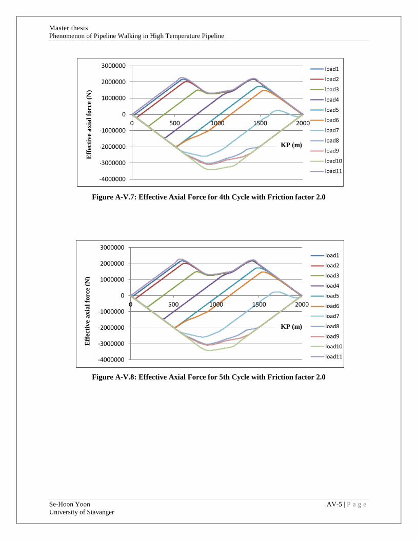
Master thesis
Phenomenon of Pipeline Walking in High Temperature Pipeline
Se-Hoon Yoon AV-5 | P a g e
University of Stavanger
-4000000
-3000000
-2000000
-1000000
0
1000000
2000000
3000000
0 500 1000 1500 2000
load1
load2
load3
load4
load5
load6
load7
load8
load9
load10
load11
Figure A-V.7: Effective Axial Force for 4th Cycle with Friction factor 2.0
Figure A-V.8: Effective Axial Force for 5th Cycle with Friction factor 2.0
-4000000
-3000000
-2000000
-1000000
0
1000000
2000000
3000000
0 500 1000 1500 2000
load1
load2
load3
load4
load5
load6
load7
load8
load9
load10
load11
KP (m)
(Figur
e 2.0:
Conve
ntiona
l S-lay
install
ation
(Olav
Fyrilei
v et
al.,
2005)
[9]
Eff
ecti
ve
ax
ial
forc
e (N
)
KP (m)
(Figur
e 2.0:
Conve
ntiona
l S-lay
install
ation
(Olav
Fyrilei
v et
al.,
2005)
[9]
Eff
ecti
ve
ax
ial
forc
e (N
)

Master thesis
Phenomenon of Pipeline Walking in High Temperature Pipeline
Se-Hoon Yoon AV-6 | P a g e
University of Stavanger
0
0,05
0,1
0,15
0,2
0,25
0,3
0,35
0,4
0,45
0 10 20 30 40 50
Dis_X_MidPoint(frictionfactor: 0.3)
Dis_X_MidPoint(frictionfactor: 0.5)
Dis_X_MidPoint(frictionfactor: 0.7)
Dis_X_MidPoint(frictionfactor: 2.0)
4. Walking at Mid-Point:
Figure A-V.9: Axial Walking Displacement at Mid-Point
1
0
F
5 (Figure
4 (Figure
3 (Figure
2 (FiNumber of Operating Cycle
Figure 2.0: Conventional
S-lay installation (Olav
Fyrileiv et al., 2005) [9]
Dis
pla
cem
en
t (m
)