MASTER'S THESIS - Unit
130
Faculty of Science and Technology MASTER’S THESIS Study program/ Specialization: Department of Mechanical and Structural Engineering And Materials Science Specialization in Offshore Structural Engineering Spring semester, 2013 Open / Restricted access Writer: Redion Kajolli ………………………………………… (Writer’s signature) Faculty supervisor: Title of thesis: A new approach for estimating fatigue life in offshore steel structures Credits (ECTS): 30 Key words: Damage indicator based model Sequential law Full range S-N curve FEM-employed dynamic time history analysis Stress-history evaluation Fatigue life estimation Pages: ………………… + Enclosure: ………… Stavanger, Date/year
-
Upload
khangminh22 -
Category
Documents
-
view
0 -
download
0
Transcript of MASTER'S THESIS - Unit

Faculty of Science and Technology
MASTER’S THESIS
Study program/ Specialization: Department of Mechanical and Structural Engineering And Materials Science Specialization in Offshore Structural Engineering
Spring semester, 2013
Open / Restricted access
Writer: Redion Kajolli
…………………………………………
(Writer’s signature)
Faculty supervisor:
Title of thesis: A new approach for estimating fatigue life in offshore steel structures
Credits (ECTS): 30 Key words: Damage indicator based model Sequential law Full range S-N curve FEM-employed dynamic time history analysis Stress-history evaluation Fatigue life estimation
Pages: ………………… + Enclosure: …………
Stavanger, Date/year


i
A new approach for estimating fatigue life in offshore steel structures
ABSTRACT
Miner’s rule is generally accepted as the fatigue criteria for life estimation of existing offshore steel structures. Similarly, it has always been acknowledged as a simplification that is easy to use in design where detailed loading history is unknown. But in the case of existing structures where the detailed loading history is known, Miner’s rule might provide incorrect results because of its omission of load sequence effect. Recently, a new damage indicator-based sequential law has been proposed to capture the load sequence effect more precisely. However, application of this sequential law to estimate the remaining fatigue life of existing steel structures has not been properly studied. The objective of this study is to estimate the remaining fatigue life of an offshore structure using the sequential law, and introduces a new approach to estimate remaining fatigue life. This approach is specially based on combination of real stress histories, sequential law and fully known Wöhler curves. The obtained fatigue life is compared and conclusions are drawn.

ii
A new approach for estimating fatigue life in offshore steel structures
ACKNOWLEDGEMENTS
I would like to express my sincere gratitude to my supervisor, Professor S.A. Sudath C. Siriwardane for facilitation of the topic, for his academic competence, engagement, and for his ability to motivate and to spark interest. Further, I would also like to express my gratitude to Professor Ove Tobias Gudmestad for academic competence and for constructive conversations. Finally I would like to thank Besmir Kajolli, Pipeline Engineer at IKM Ocean Design. Constructive feedback was very much appreciated.

iii
A new approach for estimating fatigue life in offshore steel structures
TABLE OF CONTENTS
1 INTRODUCTION 1
1.1 BACKGROUND 1 1.2 OBJECTIVE 2 1.3 CONTENT 2 1.4 SYMBOLS 3
2 HYDRODYNAMIC LOADS 4
2.1 INTRODUCTION 4 2.2 LINEAR WAVE THEORY 4 2.3 HYDROSTATICS 5 2.3.1 CROSS-SECTIONAL X-DIRECTION 5 2.3.2 CROSS-SECTIONAL Y-DIRECTION 6 2.3.3 CROSS-SECTIONAL Z-DIRECTION 7 2.4 HYDRODYNAMICS 8 2.4.1 CONTINUITY OF MASS 8 2.4.2 NON-ROTATIONAL FLOW 10 2.4.3 VELOCITY OF WATER PARTICLES 11 2.4.4 BOUNDARY CONDITIONS 12 2.4.5 SOLUTION OF THE TWO-DIMENSIONAL LAPLACE EQUATION 14 2.4.6 WATER DEPTH DEFINITION 15 2.4.7 WATER PARTICLE VELOCITIES AND ACCELERATION 16 2.5 WAVE LOADS ON SLENDER MEMBERS 17 2.5.1 NORMAL FORCE ON A FIXED STRUCTURE IN WAVES 18 2.5.2 HYDRODYNAMIC COEFFICIENTS FOR NORMAL FLOW 19 2.6 CASE DEFINITION 22 2.6.1 WAVE SIMULATION 22 2.6.2 LINEARIZATION OF THE DRAG FORCES IN DYNAMIC ANALYSIS 23 2.6.3 TIME-HISTORY FUNCTIONS 25
3 STRUCTURAL ANALYSIS 27
3.1 INTRODUCTION 27 3.2 FINITE ELEMENT MODELLING 27 3.2.1 AXIS SYSTEM 28 3.2.2 UNITS 28 3.2.3 MATERIAL PROPERTIES 28 3.2.4 STRUCTURAL DETAILS AND SECTION PROPERTIES 29 3.2.5 MEMBER END RELEASES 29 3.2.6 FOUNDATION PLANE 29 3.2.7 MESHING 30 3.2.8 DESIGN CODE 30 3.2.9 PARTIAL ACTION FACTORS 30 3.3 MODAL TIME-HISTORY ANALYSIS 31 3.3.1 MASS SOURCE 31 3.3.2 TIME-HISTORY FUNCTION DEFINITION 31

iv
A new approach for estimating fatigue life in offshore steel structures
3.3.3 LOAD CASES 33 3.4 LOAD ASSIGNS 35 3.4.1 DECK LOADING 35 3.4.2 WAVE LOADING 36 3.5 ANALYSIS 36 3.6 RESULTS 38 3.6.1 STATIC DESIGN-CHECK 38 3.6.2 STATIC DESIGN OVERWRITES 39 3.6.3 TIME-HISTORY ANALYSIS 41
4 CONVENTIONAL FATIGUE LIFE ESTIMATION 42
4.1 INTRODUCTION 42 4.2 BASIC CONCEPTS OF FATIGUE 42 4.2.1 INITIATION OF CRACK 42 4.2.2 CRACK GROWTH 43 4.2.3 FINAL FAILURE 43 4.2.4 DIFFERENT APPROACHES IN FATIGUE ASSESSMENT 43 4.3 FATIGUE STRENGTH BASED ON S-N CURVES 44 4.3.1 S-N CURVES 44 4.3.2 NOMINAL STRESS APPROACH 44 4.3.3 HOT SPOT IN TUBULAR JOINTS 45 4.4 PALMGREN-MINER RULE 46 4.4.1 FATIGUE DESIGN FACTORS 46 4.5 SCF AND SUPERPOSITION OF STRESSES 47 4.6 STRESS-HISTORY EVALUATION OF JOINT 9 48 4.6.1 CHORD 48 4.6.2 BRACE A 50 4.6.3 BRACE B 52 4.6.4 BRACE C 54 4.7 STRESS-HISTORY EVALUATION OF JOINT 13 57 4.7.1 CHORD 57 4.7.2 BRACE A 59 4.7.3 BRACE B 61 4.7.4 BRACE C 63 4.8 FATIGUE LIFE ESTIMATION 66 4.8.1 JOINT 9 66 4.8.2 JOINT 13 66 4.8.3 SUMMARY 66
5 PROPOSED APPROACH FOR FATIGUE LIFE ESTIMATION 67
5.1 INTRODUCTION 67 5.2 SEQUENTIAL LAW 67 5.2.1 FULL RANGE S-N CURVE 68 5.2.2 FULL RANGE T-CURVE IN SEAWATER WITH CATHODIC PROTECTION 69 5.2.3 APPLICATION OF THE SEQUENTIAL LAW 70 5.2.4 VERIFICATION OF THE SEQUENTIAL LAW 72 5.3 FATIGUE LIFE ESTIMATION 74

v
A new approach for estimating fatigue life in offshore steel structures
6 DISCUSSION 75
7 CONCLUSION 76
8 FURTHER STUDIES 77
9 REFERENCES 78

vi
A new approach for estimating fatigue life in offshore steel structures
TABLE OF FIGURES FIGURE 2-1: WATER VOLUME ELEMENT ........................................................................................................................... 5 FIGURE 2-2: FORCES IN X-DIRECTION ............................................................................................................................... 5 FIGURE 2-3: FORCES IN Y-DIRECTION ............................................................................................................................... 6 FIGURE 2-4: FORCES IN Z-DIRECTION ............................................................................................................................... 7 FIGURE 2-5: MASS FLOW INTO THE ELEMENT .................................................................................................................... 8 FIGURE 2-6: ELEMENT DEFORMATION............................................................................................................................ 10 FIGURE 2-7: FORCES ACTING ON A SLENDER MEMBER, REF. [3]. .......................................................................................... 17 FIGURE 2-8: ADDED MASS COEFFICIENT VS. KC-NUMBER, REF. [4]. ..................................................................................... 21 FIGURE 2-9: SCATTER DIAGRAM FOR THE NORTHERN NORTH SEA, 1973 – 2001, REF.[10]. ................................................... 22 FIGURE 2-10: WAVE-STRUCTURE INTERACTION, REF. [11]. ............................................................................................... 23 FIGURE 2-11: DRAG LOAD VS. INERTIA LOAD, HS=1.5M ................................................................................................... 25 FIGURE 2-12: DRAG LOAD VS. INERTIA LOAD, HS=2.0M ................................................................................................... 26 FIGURE 2-13: DRAG LOAD VS. INERTIA LOAD, HS=2.5M ................................................................................................... 26 FIGURE 3-1: CONVENTIONAL STEEL JACKET ..................................................................................................................... 27 FIGURE 3-2: FOUNDATION PLANE VIEW – JOINT SPRINGS ................................................................................................... 29 FIGURE 3-3: MASS SOURCE DEFINITION ......................................................................................................................... 31 FIGURE 3-4: LINEARIZED DRAG LOAD FUNCTION ............................................................................................................... 32 FIGURE 3-5: INERTIA LOAD FUNCTION ............................................................................................................................ 32 FIGURE 3-6: INERTIA AND DRAG LOAD FUNCTIONS COMBINED ............................................................................................ 32 FIGURE 3-7: MODAL LOAD CASE ................................................................................................................................... 33 FIGURE 3-8: TOTAL WAVE LOAD CASE ............................................................................................................................ 34 FIGURE 3-9: DECK MASS LOADING 3D-VIEW ................................................................................................................... 35 FIGURE 3-10: DECK MASS LOADING XZ-PLANE VIEW ......................................................................................................... 35 FIGURE 3-11: WAVE LOADING 3D-VIEW ........................................................................................................................ 36 FIGURE 3-12: WAVE LOADING XZ-PLANE VIEW ............................................................................................................... 36 FIGURE 3-13: LOAD CASES SET TO RUN .......................................................................................................................... 37 FIGURE 3-14: ANALYSIS VS. DESIGN SECTION VERIFICATION ................................................................................................ 37 FIGURE 3-15: MEMBER VERIFICATION ........................................................................................................................... 37 FIGURE 3-16: DESIGN-CHECK OF THE STRUCTURE AND CAPACITY RANGE ............................................................................... 38 FIGURE 3-17: ELEMENT 31 – STRESS CHECK INFORMATION ................................................................................................ 39 FIGURE 3-18: ELEMENT 32 – STRESS CHECK INFORMATION ................................................................................................ 39 FIGURE 3-19: K-FACTOR OVERWRITES ........................................................................................................................... 39 FIGURE 3-20: MODIFIED DESIGN-CHECK OF THE STRUCTURE AND CAPACITY RANGE ................................................................. 40 FIGURE 3-21: ELEMENT 31 – MODIFIED STRESS CHECK INFORMATION ................................................................................. 40 FIGURE 3-22: ELEMENT 32 – MODIFIED STRESS CHECK INFORMATION ................................................................................. 40 FIGURE 3-23: ENVELOPE-STRESS DIAGRAM ..................................................................................................................... 41 FIGURE 3-24: JOINT 9 ................................................................................................................................................ 41 FIGURE 3-25: JOINT 13 .............................................................................................................................................. 41 FIGURE 4-1: S-N CURVE FOR TUBULAR JOINTS IN AIR AND SEAWATER [3] .............................................................................. 45 FIGURE 4-2: ARBITRARY KT-JOINT, REF.[3] .................................................................................................................... 47 FIGURE 4-3: HOT SPOT AROUND THE CIRCUMFERENCE OF THE INTERSECTION, REF.[3] ............................................................ 47 FIGURE 4-4: STRESS-HISTORY SAMPLE FOR HS 1.5M – CHORD IN JOINT 9 ............................................................................. 49 FIGURE 4-5: STRESS-HISTORY SAMPLE FOR HS 2.0M – CHORD IN JOINT 9 ............................................................................. 49 FIGURE 4-6: STRESS-HISTORY SAMPLE FOR HS 2.5M – CHORD IN JOINT 9 ............................................................................. 50 FIGURE 4-7: STRESS-HISTORY SAMPLE FOR HS 1.5M – BRACE A IN JOINT 9 ........................................................................... 51 FIGURE 4-8: STRESS-HISTORY SAMPLE FOR HS 2.0M – BRACE A IN JOINT 9 ........................................................................... 51 FIGURE 4-9: STRESS-HISTORY SAMPLE FOR HS 2.5M – BRACE A IN JOINT 9 ........................................................................... 52 FIGURE 4-10: STRESS-HISTORY SAMPLE FOR HS 1.5M – BRACE B IN JOINT 9 ......................................................................... 53 FIGURE 4-11: STRESS-HISTORY SAMPLE FOR HS 2.0M – BRACE B IN JOINT 9 ......................................................................... 53 FIGURE 4-12: STRESS-HISTORY SAMPLE FOR HS 2.5M – BRACE B IN JOINT 9 ......................................................................... 54 FIGURE 4-13: STRESS-HISTORY SAMPLE FOR HS 1.5M – BRACE C IN JOINT 9 ......................................................................... 55 FIGURE 4-14: STRESS-HISTORY SAMPLE FOR HS 2.0M – BRACE C IN JOINT 9 ......................................................................... 55 FIGURE 4-15: STRESS-HISTORY SAMPLE FOR HS 2.5M – BRACE C IN JOINT 9 ......................................................................... 56 FIGURE 4-16: STRESS-HISTORY SAMPLE FOR HS 1.5M – CHORD IN JOINT 13 ......................................................................... 58

vii
A new approach for estimating fatigue life in offshore steel structures
FIGURE 4-17: STRESS-HISTORY SAMPLE FOR HS 2.0M – CHORD IN JOINT 13 ......................................................................... 58 FIGURE 4-18: STRESS-HISTORY SAMPLE FOR HS 2.5M – CHORD IN JOINT 13 ......................................................................... 59 FIGURE 4-19: STRESS-HISTORY SAMPLE FOR HS 1.5M – BRACE A IN JOINT 13....................................................................... 60 FIGURE 4-20: STRESS-HISTORY SAMPLE FOR HS 2.0M – BRACE A IN JOINT 13....................................................................... 60 FIGURE 4-21: STRESS-HISTORY SAMPLE FOR HS 2.5M – BRACE A IN JOINT 13....................................................................... 61 FIGURE 4-22: STRESS-HISTORY SAMPLE FOR HS 1.5M – BRACE B IN JOINT 13 ....................................................................... 62 FIGURE 4-23: STRESS-HISTORY SAMPLE FOR HS 2.0M – BRACE B IN JOINT 13 ....................................................................... 62 FIGURE 4-24: STRESS-HISTORY SAMPLE FOR HS 2.5M – BRACE B IN JOINT 13 ....................................................................... 63 FIGURE 4-25: STRESS-HISTORY SAMPLE FOR HS 1.5M – BRACE C IN JOINT 13 ....................................................................... 64 FIGURE 4-26: STRESS-HISTORY SAMPLE FOR HS 2.0M – BRACE C IN JOINT 13 ....................................................................... 64 FIGURE 4-27: STRESS-HISTORY SAMPLE FOR HS 2.5M – BRACE C IN JOINT 13 ....................................................................... 65 FIGURE 5-1: STEP-BY-STEP GRAPHICAL REPRESENTATION OF THE FULLY KNOWN S-N CURVE MODELLING TECHNIQUE, REF. [15] ...... 68 FIGURE 5-2: FULL RANGE T-CURVES .............................................................................................................................. 69 FIGURE 5-3: SCHEMATIC PRESENTATION OF NEW DAMAGE INDICATOR-BASED SEQUENTIAL LAW. ............................................... 70 FIGURE 5-4 FLOW CHART FOR THE PROPOSED DAMAGE INDICATOR BASED SEQUENTIAL LAW, REF.[17] ....................................... 71 FIGURE 5-5: PREDICTED S-N CURVE FOR 16MN STEEL VS. EXPERIMENTAL DATA, REF. [17] ...................................................... 72 FIGURE 5-6: PREDICTED S-N CURVE FOR 45 C STEEL VS. EXPERIMENTAL DATA, REF. [17] ........................................................ 72 FIGURE 5-7: COMPARISON OF THE PREDICTED FATIGUE DAMAGE VS. EXPERIMENTAL DATA FOR 16MN STEEL, REF.[17] ................. 73 FIGURE 5-8: COMPARISON OF THE PREDICTED FATIGUE DAMAGE VS. EXPERIMENTAL DATA FOR 45C STEEL, REF. [17] ................... 73

viii
A new approach for estimating fatigue life in offshore steel structures
LIST OF TABLES TABLE 1: WATER DEPTH DEFINITION .............................................................................................................................. 15 TABLE 2: SURFACE ROUGHNESS, REF. [4]. ....................................................................................................................... 19 TABLE 3: MARINE THICKNESS ESTIMATION, REF. [6].......................................................................................................... 19 TABLE 4: DRAG VS. INERTIA DOMINANCE ........................................................................................................................ 20 TABLE 5: AXIS SYSTEM FOR THE JACKET LEGS ................................................................................................................... 28 TABLE 6: MATERIAL PROPERTIES ................................................................................................................................... 28 TABLE 7: CROSS-SECTIONAL DATA OF THE FRAME ELEMENTS ............................................................................................... 29 TABLE 8: SPRING STIFFNESS.......................................................................................................................................... 29 TABLE 9: PARTIAL ACTION FACTORS FOR THE LIMIT STATES, REF. [5] ..................................................................................... 30 TABLE 10: FATIGUE DESIGN FACTORS [7] ........................................................................................................................ 46 TABLE 11: SCFS FOR THE CHORD IN JOINT 9 .................................................................................................................... 48 TABLE 12: HOT SPOT STRESS EVALUATION OF THE CHORD IN JOINT 9 .................................................................................... 48 TABLE 13: STRESS CONCENTRATION FACTORS FOR BRACE A IN JOINT 9 ................................................................................. 50 TABLE 14: HOT SPOT STRESS EVALUATION OF BRACE A IN JOINT 9 ....................................................................................... 50 TABLE 15: STRESS CONCENTRATION FACTORS FOR BRACE B IN JOINT 9 ................................................................................. 52 TABLE 16: HOT SPOT STRESS EVALUATION OF BRACE B IN JOINT 9 ....................................................................................... 52 TABLE 17: STRESS CONCENTRATION FACTORS FOR BRACE C IN JOINT 9 ................................................................................. 54 TABLE 18: HOT SPOT STRESS EVALUATION FOR BRACE C IN JOINT 9 ...................................................................................... 54 TABLE 19: SCFS FOR THE CHORD IN JOINT 13 .................................................................................................................. 57 TABLE 20: HOT SPOT STRESS EVALUATION OF THE CHORD IN JOINT 13 .................................................................................. 57 TABLE 21: SCFS FOR BRACE A IN JOINT 13...................................................................................................................... 59 TABLE 22: HOT SPOT STRESS EVALUATION OF BRACE A IN JOINT 13 ..................................................................................... 59 TABLE 23: SCFS FOR BRACE B IN JOINT 13 ...................................................................................................................... 61 TABLE 24: HOT SPOT STRESS EVALUATION OF BRACE B IN JOINT 13 ..................................................................................... 61 TABLE 25: SCFS FOR BRACE C IN JOINT 13 ...................................................................................................................... 63 TABLE 26: HOT SPOT STRESS EVALUATION OF BRACE C IN JOINT 13...................................................................................... 63 TABLE 27: FATIGUE LIFE ESTIMATION OF JOINT 9 [IN YEARS] ............................................................................................... 66 TABLE 28: FATIGUE LIFE ESTIMATION OF JOINT 13 [IN YEARS] ............................................................................................. 66 TABLE 29: SEQUENTIAL LAW VS. MINER’S FATIGUE LIFE ESTIMATION.................................................................................... 74

Introduction Background
1
A new approach for estimating fatigue life in offshore steel structures
1 Introduction
1.1 Background
The demand for exploration and production of oil and gas has grown ever since the early offshore activities began in the North Sea in the 1960’s. The first steel structures to operate in the North Sea were transferred from the Gulf of Mexico, where exploration and production activities had been on-going since the 1930’s. Shortly after, it became clear that these structures were not adequate when operating in more severe weather conditions such as in the North Sea [1][2]. One of the phenomena that are very likely to occur in any type of offshore structures is fatigue. This phenomenon occurs in all type of structures and structural details subjected to fluctuating loads, causing time-varying stresses in the structure. The nature of this phenomenon was first discovered prior to 1850, where railway axels were failing without any obvious cause. The understanding of fatigue was brought a big step forward by Wöhler’s studies in the 1850’s and has ever since been “rediscovered” for various types of structures [1]. Offshore structures of all types are subjected to environmental loads, occurring in the form of wind, waves, currents and earthquakes, all acting simultaneously. These loads are referred to as cyclic (or repetitive) loads, which during a long period of time can cause significant amount of fatigue damage. Fatigue cracks are therefore likely to evolve as a result of structures being subjected to environmental loads. Among these, waves and earthquakes are considered to be the most important sources of structural excitations. In spite of this, earthquake loads are only taken into consideration when assessing offshore structures close to or in tectonic fields. Wind loads represent a contribution of ~ 5% of the environmental loading, while currents are often of unimportance due to the nature of their frequency - which is not sufficient to excite the considerable bigger structures [12]. However, currents remain an important factor when assessing stability of subsea equipment [18]. It is said that we are able to learn more from failures than success; just over 33 years ago a fatal accident took place on the Alexander L. Kielland platform located in the North Sea. Literature studies prove that the predominant reason for the accident was failure of a brace due to fatigue cracking followed by unstable fracture. The failure of this brace led to a chain effect, causing the other supporting braces in the same column to fail as well. Loss of the column led to flooding and Alexander L. Kielland along with the 212 men on board capsized in the North Sea [1], leading to the loss of 123 human lives. The term fatigue is not something that one comes across on the daily basis, but remains of major importance in terms of structural health monitoring.

2 Introduction Objective
A new approach for estimating fatigue life in offshore steel structures
1.2 Objective
The objective of this study is to introduce the application of the damage indicator-based sequential law to fatigue assessment of offshore structures and assess the validity of the proposed theorem, and to some extent present a new approach for fatigue life estimation. This new approach consists mainly of a new damage-indicator based sequential law that is in previous studies and research proven to capture the loading sequence in variable amplitude loading. Previous research is performed on railway bridges, which have been subjected to railway traffic from the first ever steam-powered locomotives to the modern day electricity-powered: representing a somewhat decreasing loading amplitude. However, the fatigue assessment in this study is based on a deterministic approach, where only the wave actions are taken account for.
1.3 Content
The starting point of this study is the introduction and theoretical appraisal of hydrodynamic load assessment presented in chapter 2. This chapter briefly introduces the main principles in hydrostatics, hydrodynamics and linear wave theory. Hydrodynamic loads are calculated in reference with design codes mainly provided by Det Norske Veritas. The final section of this chapter introduces a case definition. This case definition is based on a deterministic approach. Chapter 3 briefly presents the basics and the procedure for design and analysis of the structure under consideration. A FEM-employed dynamic time history analysis is conducted. Critical members are identified. The main objective in this chapter is to obtain time-history outputs for the critical members. The following chapter covers basic the fatigue mechanisms, characteristics and fatigue life estimation of critical structural components of a steel jacket. Fatigue life estimation is based on code given S-N curves and the acknowledged Palmgren-Miner hypothesis. Another important point at issue is stress-history evaluation. Chapter 5 proposes a new approach for fatigue life estimation of offshore steel structures. A new damage indicator-based sequential law is presented. Verification of this theory is proved by applying and comparing the proposed theory against experimental data. Fatigue life estimations of fatigue governing members are carried out. Results and advantages of this new approach are discussed in chapter 6. The following chapter provides a conclusion, while chapter 7 presents some thoughts on further work.

Introduction Symbols
3
A new approach for estimating fatigue life in offshore steel structures
1.4 Symbols
𝜆 Wave length 𝑇 Wave period 𝐻 Wave height 𝐻𝑠 Significant wave height �⃗� External force per unit volume element 𝑓𝑥 Unit force in the x-direction 𝑓𝑦 Unit force in the y-direction 𝑓𝑧 Unit force in the z-direction 𝜌 Density of sea water 𝜑 Potential function 𝜉 Free surface 𝜉0 Wave amplitude 𝜎𝑌 Yield strength 𝜎𝑈 Ultimate tensile strength Δ𝜎 Stress range 𝑁 Number of cycles until failure for stress range ∆𝜎 𝑚 The negative inverse slope of S-N curve
𝑙𝑜𝑔 𝑎� The intercept of log N-axis

4 Hydrodynamic loads Introduction
A new approach for estimating fatigue life in offshore steel structures
2 Hydrodynamic loads
2.1 Introduction
This chapter covers hydrostatics, hydrodynamics and linear wave theory, which is the core theory of ocean surface waves used in ocean and coastal engineering. This theory takes advantages of the linearized boundary conditions, where waves are considered as regular waves with sinusoidal shape. In reality there is no such thing as a regular sea state because waves come in all shapes with different heights and periods. Hydromechanics of slender cylinders is also implemented. All types of offshore structures other than large floating bodies consist of slender cylinders. A slender cylinder is defined as a cylinder of such geometry, which allows the diameter to be small in comparison with the wavelength. Examples of such cylinders are legs and braces of an offshore structure. It could also be some type of subsea pipeline and umbilical cable. Derivation of the fundamental theory in hydrostatics and hydromechanics is done in reference with Marine Technology and Design [8]. DNV provides recommended practice for assessing the sea state and converting of the ocean characteristics to hydrodynamic loads affecting offshore structures.
2.2 Linear wave theory
If we were to divide the wave conditions in a sea state, we would divide them in two classes: • Wind sea • Swell sea
Wind sea is described as waves generated from local fetching winds, while swell sea is long period waves generated by distant storms. We have previously mentioned that the simplest wave theory is obtained by considering the wave height to be much smaller than both the wavelength and the water depth. This wave theory is approved when assessing swell sea, and is referred to as linear wave theory, sinusoidal wave theory or Airy theory [4]. Based on this theory, the sea state is considered to be consisting of regular waves propagating with a permanent form. Each wave has a distinct wavelength 𝜆, wave period 𝑇, and wave height 𝐻.

Hydrodynamic loads Hydrostatics
5
A new approach for estimating fatigue life in offshore steel structures
2.3 Hydrostatics
Hydrostatics is described as the theory of fluid, which is not in motion. This theory describes the properties of fluid and the activities inside the fluid. External force per unit volume element is derived by considering equilibrium of a water volume element, and expressed by Figure 2-1 gives a visualization of the water volume element.
Figure 2-1: Water volume element
2.3.1 Cross-sectional x-direction
Based on Newton’s third law of motion, for a static condition, the sum of all forces equals to zero. Hence, the sum of all forces on the element in the x-direction should be equal to zero.
Figure 2-2: Forces in x-direction
�⃗� = (𝑓𝑥,𝑓𝑦 ,𝑓𝑧) Eq. 2-1

6 Hydrodynamic loads Hydrostatics
A new approach for estimating fatigue life in offshore steel structures
The unit force acting on the element in the x-direction is thus derived and obtained from Eq. 2-2.
2.3.2 Cross-sectional y-direction
By applying the same theory and the same principles, the unit force in y-direction is derived to be the same as in x-direction. The unit force acting on the element in y-direction is expressed by Eq. 2-3.
Figure 2-3: Forces in y-direction
𝑃 ∗ 𝑑𝑧 ∗ 𝑑𝑦 + 𝑓𝑥𝑑𝑧 ∗ 𝑑𝑦 ∗ 𝑑𝑧 − �𝑃 +𝜕𝑃𝜕𝑥
𝑑𝑥� 𝑑𝑦 ∗ 𝑑𝑧 = 0 Eq. 2-2
𝑓𝑥𝑑𝑧 ∗ 𝑑𝑦 ∗ 𝑑𝑧 − �𝜕𝑃𝜕𝑥
𝑑𝑥� 𝑑𝑦 ∗ 𝑑𝑧 = 0
𝑓𝑥 − 𝜕𝑃𝜕𝑥
= 0 => 𝑓𝑥 = 𝜕𝑃𝜕𝑥
𝑓𝑦 − 𝜕𝑃𝜕𝑦
= 0 => 𝑓𝑦 = 𝜕𝑃𝜕𝑦
Eq. 2-3

Hydrodynamic loads Hydrostatics
7
A new approach for estimating fatigue life in offshore steel structures
2.3.3 Cross-sectional z-direction
Figure 2-4: Forces in z-direction
The unit force acting on the element in the z-direction is derived by Eq. 2-4
Applying Newton’s second law of motion, we derive the following:
Using the fact that pressure change is only depending on the altitude in z-direction, the fundamental hydrostatic equations are summarized by Eq. 2-6.
In order to get a better understanding of these equations and their relation to the space they act in, they are expressed by vector notation.
By integrating and assuming constant density (in water or oil fluids), the pressure at a given point in z-direction is as derived in Eq. 2-8.
Where 𝐶 = 𝑝0 is the atmospheric pressure at the sea surface 𝑧0.
𝑓𝑧 − 𝜕𝑃𝜕𝑧
= 0 => 𝑓𝑧 = 𝜕𝑃𝜕𝑧
Eq. 2-4
𝐹 = 𝑚 ∗ 𝑎 = −𝑚 ∗ 𝑔 = −𝜌 ∗ 𝑉 ∗ 𝑔 = −𝜌 ∗ 𝑔 Eq. 2-5
∆𝑃 =�⃗�=
⎩⎪⎪⎨
⎪⎪⎧𝜕𝑃𝜕𝑥
= 𝑓𝑥 = 0
𝜕𝑃𝜕𝑦
= 𝑓𝑦 = 0
𝜕𝑃𝜕𝑧
= 𝑓𝑧 = −𝜌𝑔
Eq. 2-6
∆𝑃 = 𝜕𝜕𝑥
𝑃𝚤 +𝜕𝜕𝑥
𝑃𝚥 +𝜕𝜕𝑥
𝑃𝑘�⃗ = �⃗� = −𝜌𝑔𝑘�⃗ Eq. 2-7
�𝜕𝑃𝜕𝑧
= −𝜌𝑔𝑧 + 𝐶 Eq. 2-8

8 Hydrodynamic loads Hydrodynamics
A new approach for estimating fatigue life in offshore steel structures
2.4 Hydrodynamics
The objective of studying the sea state is describing the forces acting on an offshore structure. It is of the essence that acceleration and velocity of a water particle is closely studied as these properties determine the force acting on the structure [8]. This section covers mass movement through a volume element of water, and the derivation of elementary, but important principles in hydrodynamics.
2.4.1 Continuity of mass
One of the most important physical principles when assessing hydrodynamics is continuity of mass, which requires that the net mass flow into an element (𝑑𝑉 = 𝑑𝑥𝑑𝑦𝑑𝑧) equals to the mass increase of the element.
Where velocity of flow is expressed in vector notation
𝑈��⃗ = 𝑢𝚤 + 𝑣𝚥 + 𝑤𝑘�⃗
Figure 2-5: Mass flow into the element
Net mass flow into the volume element during a period of time dt, is found by summing up the mass flow in each plane (x, y, z).
�(𝜌𝑢) − �𝜌𝑢 +𝜕𝜕𝑥
(𝜌𝑢)𝑑𝑥�� 𝑑𝑦 ∗ 𝑑𝑧 ∗ 𝑑𝑡
+ �(𝜌𝑣) − �𝜌𝑣 +𝜕𝜕𝑦
(𝜌𝑣)𝑑𝑦�� 𝑑𝑥 ∗ 𝑑𝑧 ∗ 𝑑𝑡
+ �(𝜌𝑤) − �𝜌𝑤 +𝜕𝜕𝑧
(𝜌𝑤)𝑑𝑧�� 𝑑𝑥 ∗ 𝑑𝑦 ∗ 𝑑𝑡
𝑀𝑎𝑠𝑠 𝑓𝑙𝑜𝑤 = 𝑑𝑒𝑛𝑠𝑖𝑡𝑦 ∗ 𝑣𝑒𝑙𝑜𝑐𝑖𝑡𝑦 𝑜𝑓 𝑓𝑙𝑜𝑤 Eq. 2-9

Hydrodynamic loads Hydrodynamics
9
A new approach for estimating fatigue life in offshore steel structures
Continuity of flow is derived and expressed by Eq. 2-10.
Where mass increase during a time dt, is given by:
This gives us the continuity equation:
Furthermore, the continuity equation is simplified and the continuity equation for mass is finally obtained and expressed by Eq. 2-13.
𝜕𝜌𝜕𝑡
+𝜕𝜌𝜕𝑥
𝑢 +𝜕𝜌𝜕𝑦
𝑣 +𝜕𝜌𝜕𝑧
𝑤 + 𝜌 �𝜕𝑢𝜕𝑥
+𝜕𝑣𝜕𝑦
+𝜕𝑤𝜕𝑧� = 0
�𝜕𝜕𝑡
+𝜕𝜕𝑥
𝑢 +𝜕𝜕𝑦
𝑣 +𝜕𝜕𝑧𝑤�𝜌 + 𝜌 �
𝜕𝑢𝜕𝑥
+𝜕𝑣𝜕𝑦
+𝜕𝑤𝜕𝑧� = 0
𝐷𝜌𝐷𝑡
+ 𝜌 �𝜕𝑢𝜕𝑥
+𝜕𝑣𝜕𝑦
+𝜕𝑤𝜕𝑧� = 0
Where 𝐷
𝐷𝑡 is the total differential operator, representing the change in time for a particle in rest
– while the second term represents the particle’s movement [8]. Based on the constant density of the fluid, it is ideal that the fluid is labelled incompressible, thus leading to the following:
𝜕𝜌𝜕𝑡
=𝜕𝜌𝜕𝑥
=𝜕𝜌𝜕𝑦
=𝜕𝜌𝜕𝑧
= 0
𝐷𝜌𝐷𝑡
= 0 Furthermore, the equation for mass flow follows, and proves the fluid to be incompressible. This is one of the three fundamental assumptions made when taking advantage of linearized boundary conditions where waves are considered regular of sinusoidal shape.
−�𝜕𝜕𝑥
(𝜌𝑢) +𝜕𝜕𝑦
(𝜌𝑣) +𝜕𝜕𝑧
(𝜌𝑤)� 𝑑𝑉𝑑𝑡 =𝜕𝜌𝜕𝑡𝑑𝑉𝑑𝑡 Eq. 2-10
𝜕𝜕𝑡
(𝜌𝑑𝑉)𝑑𝑡 ⇔ 𝜕𝜌𝜕𝑡𝑑𝑉𝑑𝑡 Eq. 2-11
𝜕𝜌𝜕𝑡
+𝜕𝜕𝑥
(𝜌𝑢) +𝜕𝜕𝑦
(𝜌𝑣) +𝜕𝜕𝑧
(𝜌𝑤) = 0 Eq. 2-12
𝐷𝜌𝐷𝑡
+ 𝜌∇𝑈��⃗ = 0 Eq. 2-13
∇ ∙ 𝑈��⃗ =𝜕𝑢𝜕𝑥
+𝜕𝑣𝜕𝑦
+𝜕𝑤𝜕𝑧
= 0 (Incompressible) Eq. 2-14

10 Hydrodynamic loads Hydrodynamics
A new approach for estimating fatigue life in offshore steel structures
2.4.2 Non-rotational flow
Another physical principle when assessing hydrodynamics is considering the water to be an ideal fluid where no shear forces occur between the particles, or in other terms consider the fluid to have a frictionless flow [8].
Figure 2-6: Element deformation
Based on the assumption of non-rotational flow, the rotation of a water particle around its COG should be equal to zero. Figure 2-6 shows that the water particle elements deform, but they do not rotate. Using this assumption, we set up the following mathematical relations:
tan𝛼 = −𝑑𝑤𝑑𝑥
= −𝜕𝑤𝜕𝑥
𝑑𝑡
tan𝛽 = 𝑑𝑢𝑑𝑧
= 𝜕𝑢𝜕𝑧
𝑑𝑡
⇓ 𝜕𝑢𝜕𝑧
−𝜕𝑤𝜕𝑥
= 0 Similarly, the following relations go for the y-z and x-y plane, respectively.
𝜕𝑣𝜕𝑧
−𝜕𝑤𝜕𝑦
= 0
𝜕𝑣𝜕𝑥
−𝜕𝑢𝜕𝑦
= 0
tan𝛼 = − tan𝛽 ⇒ tan𝛼 + tan𝛽 = 0 Eq. 2-15

Hydrodynamic loads Hydrodynamics
11
A new approach for estimating fatigue life in offshore steel structures
Considering the cross product of ∇ and 𝑈��⃗ we hence prove the water to be an ideal fluid with no shear forces between the water particles.
2.4.3 Velocity of water particles
Given that the right conditions are present, where the fluid flow is incompressible and non-rotational, a potential function 𝜑 exists, such that the partial derivatives of this function with respect to the directions (x, y, z), give the velocities in each of these directions. If such a function exists, it is referred to as the velocity potential [8].
Further, using the fact that the fluid is incompressible, the equation for the potential flow is obtained and expressed by the partial differential Eq. 2-20.
∇ ∙ 𝑈��⃗ = 0 ⇓
𝜕𝑢𝜕𝑥
+𝜕𝑣𝜕𝑦
+𝜕𝑤𝜕𝑧
= 0
𝜕𝜕𝑥
�𝜕𝜑𝜕𝑥� +
𝜕𝜕𝑦
�𝜕𝜑𝜕𝑦� +
𝜕𝜕𝑧�𝜕𝜑𝜕𝑧� = 0
𝜕𝜕𝑥
�𝜕𝜑𝜕𝑥� +
𝜕𝜕𝑦
�𝜕𝜑𝜕𝑦� +
𝜕𝜕𝑧�𝜕𝜑𝜕𝑧� = 0
𝜕2𝜑𝜕𝑥2
+𝜕2𝜑𝜕𝑦2
+𝜕2𝜑𝜕𝑧2
= 0
Notice that for a real sea state the equation obtained covers a 3-dimentional plane. For a design case where the sea state is considered regular, with waves of sinusoidal shapes, the equation covers a 2-dimentional plane.
∇ × 𝑈��⃗ = �𝚤 𝚥 𝑘�⃗𝜕𝜕𝑥
𝜕𝜕𝑦
𝜕𝜕𝑧
𝑢 𝑣 𝑤
� = 0�⃗ (Non − rotational) Eq. 2-16
𝜑 = 𝜑(𝑥,𝑦, 𝑧, 𝑡) Eq. 2-17
𝑢 =𝜕𝜑𝜕𝑥
, 𝑣 =𝜕𝜑𝜕𝑦
, 𝑤 =𝜕𝜑𝜕𝑧
Eq. 2-18
∇𝜑 =𝜕𝜑𝜕𝑥
𝚤 + 𝜕𝜑𝜕𝑦
𝚤 +𝜕𝜑𝜕𝑧
𝑘�⃗ = 𝑈��⃗ Eq. 2-19
∇2𝜑 = 0 Eq. 2-20
𝜕2𝜑𝜕𝑥2
+𝜕2𝜑𝜕𝑧2
Eq. 2-21

12 Hydrodynamic loads Hydrodynamics
A new approach for estimating fatigue life in offshore steel structures
2.4.4 Boundary conditions
Partial differential equations may have different solutions. We search for a solution of a simple type, expressed by a sinusoidal shape. In order to solve the Laplace equation ∇2𝜑 = 0 we need to set some boundary conditions. These boundary conditions are set from physical principles.
2.4.4.1 Bottom condition
Considering a flat bottom, where the z-direction is expressed by the water depth d, we come to the conclusion that no water can flow through the bottom [8]. Hence, the vertical velocity at the bottom is equal to zero.
2.4.4.2 Wall condition
- No water can flow through a wall. This principle leads to the fact that the horizontal velocity at a given distance x = a, is equal to zero.
2.4.4.3 Kinematic surface condition
Let 𝜉 = 𝜉(𝑥, 𝑡) denote the free surface of a wave. When assessing waves at the surface we assume that no water can flow through the surface. Water particles at the free surface will remain at the surface [8]. Based on this condition the vertical velocity at the surface is as follows:
The equation obtained contains a non-linear term, and in order to find the velocity in vertical direction we need to know the velocity in horizontal direction. This non-linear term is linearized and the velocity 𝑤, at the surface is set to be equal to the velocity at the still water level (where z = 0). This approximation is approved when assuming linearized surface condition [8].
𝑤 =𝜕𝜑𝜕𝑧�𝑧=−𝑑
= 0 Eq. 2-22
𝑢 =𝜕𝜑𝜕𝑥�𝑥=𝑎
= 0 Eq. 2-23
𝑤 =𝜕𝜑𝜕𝑧�𝑧=𝜉(𝑥,𝑡)
=𝜕𝜉𝜕𝑡
+ 𝑢𝜕𝜉𝜕𝑥
Eq. 2-24
⇒ 𝑤 =𝜕𝜑𝜕𝑧�𝑧=0
=𝜕𝜉𝜕𝑡
Eq. 2-25

Hydrodynamic loads Hydrodynamics
13
A new approach for estimating fatigue life in offshore steel structures
2.4.4.4 Dynamical boundary condition
A form of the Bernoulli equation which is valid for incompressible fluid, states that the pressure at the free surface is constant and equal to the atmospheric pressure [8]. The pressure variation in such a fluid is described by Eq. 2-26.
Where right hand side of the equation is equal to an arbitrary constant and is considered to be of less importance. This constant is set to be 𝐶(𝑡) = 𝑃
𝜌.
Further, based on the theory stated above, we set the pressure at the free surface to be equal to the atmospheric pressure (𝑧 = 𝜉(𝑥, 𝑡) ; 𝑃 = 𝑃𝑜).
Furthermore, the free surface is set to be equal to the still water level (𝑧 = 0), and by linearizing the non-linear term we are left with the following equation:
This is an approved approximation because of the fact that the wave deviation from 𝑧 = 0 to 𝑧 = 𝜉 is considered to be relative small in comparison to the wavelength. This is considered to be the best first order approximation available when assessing a “linear” sea state consisting of sinusoidal shape [8].
𝑃𝜌
+ 𝑔 ∙ 𝑧 +𝜕𝜑𝜕𝑡
+12∙ (𝑢2 + 𝑤2) = 𝐶(𝑡) Eq. 2-26
𝑔 ∙ 𝜉 +𝜕𝜑𝜕𝑡�𝑧= 𝜉
+12∙ (𝑢2 + 𝑤2)�
𝑧= 𝜉= 0 Eq. 2-27
𝑔 ∙ 𝜉 +𝜕𝜑𝜕𝑡�𝑧= 0
= 0 ⇒ 𝜉 = −1𝑔∙𝜕𝜑𝜕𝑡�𝑧= 0
Eq. 2-28

14 Hydrodynamic loads Hydrodynamics
A new approach for estimating fatigue life in offshore steel structures
2.4.5 Solution of the two-dimensional Laplace equation
By implementing the boundary conditions stated in section 2.4.4, the following equation is obtained:
⇓
Given the derived boundary conditions, we can now solve the two dimensional Laplace equation.
∇2𝜑 =𝜕2𝜑𝜕𝑥2
+𝜕2𝜑𝜕𝑧2
= 0
−∞ < 𝑥 < ∞ ; –𝑑 < 𝑧 < 𝜉 A solution 𝜑 = 𝜑(𝑥, 𝑧, 𝑡), is found by separating variables and introducing the following functions
𝑋(𝑥) = 𝐴 ∙ sin𝑘𝑥 + 𝐵 ∙ sin 𝑘𝑥 𝑍(𝑧) = 𝐶 ∙ 𝑒𝑘𝑧 + 𝐷 ∙ 𝑒−𝑘𝑧𝑇(𝑡) = 𝐸 ∙ sin𝑤𝑡 + 𝐹 ∙ cos𝑤𝑡 ≠ 0
⇓
𝑑2𝑋𝜕𝑋2
∙ 𝑍(𝑧) ∙ 𝑇(𝑡) +𝑑2𝑍𝜕𝑍2
∙ 𝑋(𝑥) ∙ 𝑇(𝑡)
𝑑2𝑋𝑑𝑋2𝑋(𝑥)
= −𝑑2𝑍𝑑𝑍2𝑍(𝑧)
The variables are now separated and must be equal to a constant (–𝑘)2. The constant has a negative value because we want to define the wave direction as positive and moving along the x-axis [8].
𝑑2𝑋𝑑𝑋2
+ 𝑘2 ∙ 𝑋(𝑥) = 0
𝑑2𝑍𝑑𝑍2
+ 𝑘2 ∙ 𝑍(𝑍) = 0
𝜕𝜑𝜕𝑡�𝑧= 0
=𝜕𝜉𝜕𝑡
=𝜕𝜕𝑡�−
1𝑔∙𝜕𝜑𝜕𝑡�𝑧= 0
� Eq. 2-29
𝜕2𝜑𝜕𝑡2
+ 𝑔 ∙𝜕𝜑𝜕𝑧�𝑧=0
= 0 Eq. 2-30

Hydrodynamic loads Hydrodynamics
15
A new approach for estimating fatigue life in offshore steel structures
We can now set up an expression for the potential function.
𝜑 = 𝜑(𝑥, 𝑧, 𝑡) = 𝑋(𝑥) ∙ 𝑍(𝑧) ∙ 𝑇(𝑡)
𝜑 = [𝐴 ∙ sin𝑘𝑥 + 𝐵 ∙ cos 𝑘𝑥] + [𝐶 ∙ 𝑒𝑘𝑧 + 𝐷 ∙ 𝑒−𝑘𝑧] ∙ 𝑇(𝑡)
… Finally, after taking use of the boundary conditions, the velocity potential is obtained and expressed by Eq. 2-31. We are now able to obtain the particle velocities and accelerations and can further obtain the hydrodynamic loads acting on an offshore structure.
2.4.6 Water depth definition
We divide the water depth into shallow and deep water and the expression for the velocity potential will vary depending on the “water-depth” situation. Each of these situations are depending on the relation between the depth 𝑑, and the wavelength 𝜆, and are defined in Table 1.
Table 1: Water depth definition
Shallow water 𝑑 >𝜆2
Deep water 𝑑𝜆
>1
20
When considering a deep-water situation, we take use of the mathematical relation formulated in Eq. 2-32. Thereafter, the velocity potential for a deep-water situation is expressed by Eq. 2-33.
Further, the velocity potential for a shallow water situation is given by Eq. 2-34.
𝜑 = (𝑥, 𝑧, 𝑡) =𝜉0 ∙ 𝑔𝜔
∙cosh 𝑘(𝑧 + 𝑑)
cosh(𝑘𝑑) ∙ cos(𝜔𝑡 − 𝑘𝑥) Eq. 2-31
cosh 𝑘(𝑧 + 𝑑)cosh(𝑘𝑑) =
𝑒𝑘(𝑧+𝑑)
𝑒𝑘𝑑= 𝑒𝑘𝑧 Eq. 2-32
𝜑𝑑𝑒𝑒𝑝 = (𝑥, 𝑧, 𝑡) =𝜉0 ∙ 𝑔𝜔
∙ 𝑒𝑘𝑧 ∙ cos(𝜔𝑡 − 𝑘𝑥) Eq. 2-33
𝜑𝑠ℎ𝑎𝑙𝑙𝑜𝑤 = (𝑥, 𝑧, 𝑡) =𝜉0 ∙ 𝑔𝜔
∙ cos(𝜔𝑡 − 𝑘𝑥) Eq. 2-34

16 Hydrodynamic loads Hydrodynamics
A new approach for estimating fatigue life in offshore steel structures
2.4.7 Water particle velocities and acceleration
2.4.7.1 Horizontal direction
The horizontal flow velocity is obtained by taking the derivative of the velocity potential with respect to the direction. The horizontal flow acceleration is obtained by taking the derivative of the velocity with respect to time.
Notice that the horizontal velocity has the same function as the surface profile 𝜉 = 𝜉0 sin(𝑤𝑡 − 𝑘𝑥), and has its maximum at the wave crests when sin(𝑤𝑡 − 𝑘𝑥) = 1. The horizontal flow acceleration is obtained by taking the derivative of the velocity with respect to time
2.4.7.2 Vertical direction
The velocities and acceleration in vertical direction are given by the following set of equations (Eq. 2-39 - Eq. 2-42).
𝑢 =𝜕𝜑𝜕𝑥
=𝜉0 ∙ 𝑔 ∙ 𝑘
𝜔∙
cosh 𝑘(𝑧 + 𝑑)cosh (𝑘𝑑)
∙ sin(𝜔𝑡 − 𝑘𝑥) Eq. 2-35
𝑢𝑑𝑒𝑒𝑝 =𝜕𝜑𝑑𝑒𝑒𝑝𝜕𝑥
=𝜉0 ∙ 𝑔 ∙ 𝑘
𝜔∙ 𝑒𝑘𝑧 ∙ sin(𝜔𝑡 − 𝑘𝑥) Eq. 2-36
𝑢𝑠ℎ𝑎𝑙𝑙𝑜𝑤 =𝜕𝜑𝑠ℎ𝑎𝑙𝑙𝑜𝑤
𝜕𝑥=𝜉0 ∙ 𝑔 ∙ 𝑘
𝜔∙ sin(𝜔𝑡 − 𝑘𝑥) Eq. 2-37
�̇� =𝜕𝑢𝜕𝑡
= 𝜉0 ∙ 𝑔 ∙ 𝑘 ∙cosh 𝑘(𝑧 + 𝑑)
cosh(𝑘𝑑) ∙ cos(𝜔𝑡 − 𝑘𝑥) Eq. 2-38
𝑤 =𝜕𝜑𝜕𝑧
=𝜉0 ∙ 𝑔 ∙ 𝑘
𝜔∙
sinh𝑘(𝑧 + 𝑑)cosh (𝑘𝑑)
∙ cos(𝜔𝑡 − 𝑘𝑥) Eq. 2-39
𝑤𝑑𝑒𝑒𝑝 =𝜕𝜑𝑑𝑒𝑒𝑝𝜕𝑧
=𝜉0 ∙ 𝑔 ∙ 𝑘
𝜔∙ 𝑒𝑘𝑧 ∙ cos(𝜔𝑡 − 𝑘𝑥) Eq. 2-40
𝑤𝑠ℎ𝑎𝑙𝑙𝑜𝑤 =𝜕𝜑𝑠ℎ𝑎𝑙𝑙𝑜𝑤
𝜕𝑧=𝜉0 ∙ 𝑔 ∙ 𝑘2
𝜔∙ (𝑧 + 𝑑) cos(𝜔𝑡 − 𝑘𝑥)
Eq. 2-41
�̇� =𝜕𝑤𝜕𝑡
= −𝜉0 ∙ 𝑔 ∙ 𝑘 ∙sinh 𝑘(𝑧 + 𝑑)
cosh(𝑘𝑑) ∙ sin(𝜔𝑡 − 𝑘𝑥) Eq. 2-42

Hydrodynamic loads Wave loads on slender members
17
A new approach for estimating fatigue life in offshore steel structures
2.5 Wave loads on slender members
The hydrodynamic forces acting on a slender structure in general fluid is estimated by summing up all the sectional forces acting on each section of the structure. The force acting on a section is decomposed in a normal force 𝑓𝑁, a tangential force 𝑓𝑇, and in some cases a lift force 𝑓𝐿, as shown in Figure 2-7 [3].
Figure 2-7: Forces acting on a slender member, ref. [3].
A submerged cylinder is subjected to a combination of velocities and accelerations caused by the water particles. For a situation where the structural member cross-section is significantly smaller than the wavelength, the wave loads may be calculated using Morison’s formula [4]. Morison’s load formula is applicable when the following conditions are satisfied:
• When we have a situation of a non-breaking wave (𝐻𝜆
< 0.14). • When the acceleration over the diameter of the structure is constant;
The diameter is small compared to the wavelength (𝜆 > 5𝐷). • When the displacement of the cylinder is restricted (𝜆
𝐷< 0.2).
If these conditions are satisfied, Morison’s load formula states that the wave loads are a sum of the inertia force, which is proportional to the acceleration, and a drag force, which is proportional to the square of the velocity [4].

18 Hydrodynamic loads Wave loads on slender members
A new approach for estimating fatigue life in offshore steel structures
2.5.1 Normal force on a fixed structure in waves
Given that the Morison’s load formula is applicable, the normal force on a fixed slender member in a two-dimensional flow normal to the member is in reference with DNV-RP-C205 given by:
Where the first term takes account for the inertia force, while the second term is an expression for the drag force. The total force acting on the entire cylinder is expressed by Eq. 2-44.
The horizontal flow velocity is largest under the wave crest; hence we integrate from the wave amplitude 𝜉0, all the way down to the sea bottom −𝑑. Given the fact that the acceleration under the crest top is equal to zero (�̇� = 0), causes the inertia force under the crest top to be zero, and the total force is hence:
Further, when the wave crosses the mean water level (𝑧 = 0), the horizontal flow velocity is then equal to zero (𝑢 = 0), which results the drag force to be equal to zero (𝑓𝐷(𝑧, 𝑡) = 0). The total force acting on the cylinder is hence:
𝑓𝑁(𝑡) = 𝜌 ∙ (1 + 𝐶𝐴) ∙ 𝐴 ∙ �̇� + (1/2 ∙ 𝜌 ∙ 𝐶𝐷 ∙ D ∙ 𝑢 ∙ |𝑢|) Eq. 2-43
𝐹(𝑡) = � 𝑓(𝑧, 𝑡)
𝑠𝑢𝑟𝑓𝑎𝑐𝑒
−𝑑
𝑑𝑧 = �𝑓𝑀(𝑧, 𝑡)
𝜉
−𝑑
𝑑𝑧 + �𝑓𝐷
𝜉
−𝑑
(𝑧, 𝑡)𝑑𝑧 Eq. 2-44
𝐹(𝑡) = � 𝑓𝐷
𝜉0
−𝑑
(𝑧, 𝑡)𝑑𝑧 Eq. 2-45
𝐹(𝑡) = �𝑓𝑀
0
−𝑑
(𝑧, 𝑡)𝑑𝑧 Eq. 2-46

Hydrodynamic loads Wave loads on slender members
19
A new approach for estimating fatigue life in offshore steel structures
2.5.2 Hydrodynamic coefficients for normal flow
When calculating the hydrodynamic loads on a structure based on Morison’s load formula, one should take account for the variation of the drag- and mass coefficient. These coefficients are depending on the Reynolds number, the Keulegan-Carpenter number and the surface roughness of the structure [4]. The hydrodynamic coefficients are based on experimental data and the relation between these coefficients and the governing parameters are as follows:
2.5.2.1 Reynolds number
The Reynolds number is a dimensionless parameter depending on the flow velocity, the cross-sectional diameter of the structure, and on the viscosity of the water.
𝑅𝑒 =𝑢𝐷𝜈
=𝑢(𝐷 + 2𝑡𝑚)
𝜈
As guidance for determining the surface roughness of the structure, DNV recommends that the values in Table 2 be used.
Material k (meters) Steel, new uncoated 5 ∙ 10−5 Steel, painted 5 ∙ 10−6 Steel, highly corroded 3 ∙ 10−3 Concrete 3 ∙ 10−3 Marine growth 5 ∙ 10−3 − 5 ∙ 10−2
Table 2: Surface roughness, ref. [4].
If no specific site information is present for the case under consideration, one shall assume that marine growth might occur. Further, the marine thickness is in reference with NORSOK-N003 estimated from the values in Table 3. The effect of marine growth must be considered when determining the effective diameter for the member under consideration.
Table 3: Marine thickness estimation, ref. [6].
56 − 69°𝑁 59 − 72°𝑁 Marine growth density (𝑘𝑔/𝑚3)
Water depth (m) Thickness (mm) Thickness (mm) 1325 +2 – 40 100 60
Below 40 50 30
𝐶𝐷 = 𝐶𝐷(𝑅𝑒,𝐾𝑐,∆)𝐶𝐴 = 𝐶𝐴(𝑅𝑒 ,𝐾𝑐,∆)
20 Hydrodynamic loads Wave loads on slender members
A new approach for estimating fatigue life in offshore steel structures
In reference with DNV-RP-C205, for high Reynolds numbers - the dependence of the drag coefficient on roughness parameter is to be taken as:
𝐶𝐷𝑆(∆) = �0,65
(29 + 4𝑙𝑜𝑔10(1.05
∆))/20:::
∆ < 10−410−4 < ∆ < 10−2
∆ > 10−2
Where ∆= 𝑘𝐷
Further, the drag coefficient is expressed by Eq. 2-47.
Where 𝜓(𝐾𝐶) takes account for the wake amplification factor. Furthermore, the wake amplification factor for different 𝐾𝑐-numbers is to be taken as [4]:
𝜓(𝐾𝐶) = �𝐶𝜋 + 0,1 ∙ (𝐾𝐶 − 12) 2 ≤ 𝐾𝐶 ≤ 12𝐶𝜋 − 1 0,75 ≤ 𝐾𝐶 ≤ 2𝐶𝜋 − 1 − 2(𝐾𝐶 − 0,75) 𝑂𝑡ℎ𝑒𝑟𝑤𝑖𝑠𝑒
Where 𝐶𝜋 is:
𝐶𝜋 = 1,50 − 0,024 ∙ (12
𝐶𝐷𝑆(∆) − 10)
2.5.2.2 Keulegan-Carpenter number
The Keulegan-Carpenter number is a non-dimensional parameter depending on the wave height (𝐻), and the cross-sectional diameter of the structure (𝐷). For sinusoidal flow, the 𝐾𝑐-number is obtained by the following equation:
𝐾𝑐 =2𝜋 ∙ 𝜉𝑜𝐷 + 2𝑡𝑚
The magnitude of the Keulegan-Carpenter number says something about the relation between the drag and inertia term, when determining the hydrodynamic loads based on the Morison’s load formula. Based on this we compute whether the drag or inertia term is dominating, or if both terms should be taken into account. All these three different load cases are defined in Table 4.
Table 4: Drag vs. inertia dominance
Inertia dominance 𝐾𝑐 < 3 Drag term is linearized 3 < 𝐾𝑐 < 15 The full Morison shall be used 15 < 𝐾𝑐 < 45 Drag dominance 𝐾𝑐 > 45
𝐶𝐷 = 𝐶𝐷𝑆(∆) ∙ 𝜓(𝐾𝐶) Eq. 2-47

Hydrodynamic loads Wave loads on slender members
21
A new approach for estimating fatigue life in offshore steel structures
The drag term included in the Morison Load Formula is 90° out of phase with inertia term. This is because the drag term is depending on the velocity while the inertia term is depending on the acceleration of the flow. One tries to avoid using the complete Morison equation unless it is absolutely necessary. A simple way of doing this is by studying the 𝐾𝑐-number for the case under consideration and if possible, neglecting either the drag or inertia term. As previously mentioned, the Keulegan Carpenter number and the roughness of the material will have an impact on the mass coefficient for the case under consideration. The added mass coefficients for smooth and rough structures for large values of 𝐾𝑐-number are in reference with DNV-RP-205 given as:
𝐶𝐴 = 0,6 𝑆𝑚𝑜𝑜𝑡ℎ 𝑐𝑦𝑙𝑖𝑛𝑑𝑒𝑟𝑠0,2 𝑅𝑜𝑢𝑔ℎ 𝑐𝑦𝑙𝑖𝑛𝑑𝑒𝑟𝑠
Further, for small values of 𝐾𝑐 (𝐾𝑐 < 3), the added mass coefficient can be taken as 𝐶𝐴 = 1 for both rough and smooth cylinders. Furthermore, for 𝐾𝑐 >3, the added mass coefficient is found from the following formula:
𝐶𝐴 = 𝑚𝑎𝑥 �1 − 0,044(𝐾𝑐 − 3)
0,6 − (𝐶𝐷𝑆(∆) − 0,65)
The mass coefficient is then defined as
Figure 2-8 shows the relation between the added mass and the Keulegan-Carpenter number for both rough and smooth cylinders.
Figure 2-8: Added mass coefficient vs. KC-number, ref. [4].
𝐶𝑀 = 1 + 𝐶𝐴 Eq. 2-48

22 Hydrodynamic loads Case definition
A new approach for estimating fatigue life in offshore steel structures
2.6 Case definition
This section covers the transformation of the hydrodynamic loads derived in section 2.5 into time history functions, which are to be assigned to the jacket platform legs. Emphasis is put on hydrodynamics and structural dynamics. It is of the essence that one is able to distinguish the presented approach, from the design of offshore steel structures. The design of offshore steel structures is based on wave statistics and a probabilistic methodology where one has to take account for the random nature of the environmental loads [10].
2.6.1 Wave simulation
The idea is to simulate different waves and assign these waves to the jacket platform modelled in Chapter 3. Three waves of different wave heights are chosen in reference with a scatter diagram valid for locations in the Northern North Sea. Further, the chosen waves are simulated and assumed to be consecutively generated during the course of one day. Figure 2-9 shows the selected waves, their corresponding heights and peak periods. Notice how the wave height is labelled as significant wave height while the period is labelled as peak period. The significant wave height 𝐻𝑠 is defined as the average height of the highest one third waves in a short term record length. The peak period 𝑇𝑝 is the wave period at which the wave energy spectrum has its maximum value. In a short-term storm duration, or short term wave conditions, the sea state is assumed to be stationary for an interval of 20 minutes up to 3- or 6-hours [4][10]. Furthermore, for a storm duration of 3 hours, the wave loads acting on the jacket platform leg are to be calculated from the maximum wave height 𝐻𝑚𝑎𝑥. Experimental data show that for a 3-hour storm duration, the maximum wave height is to be taken from Eq. 2-49 [9]. 𝐻𝑚𝑎𝑥 = 1.86 ∗ 𝐻𝑠
Eq. 2-49
Figure 2-9: Scatter diagram for the Northern North Sea, 1973 – 2001, ref.[10].

Hydrodynamic loads Case definition
23
A new approach for estimating fatigue life in offshore steel structures
2.6.2 Linearization of the drag forces in dynamic analysis
Morrison’s formula is applied when evaluating the hydrodynamic forces acting on slender tubular members. The waves are assumed to be unidirectional and linear wave theory is used to obtain the water particle motions at any given elevation. When linearizing the drag force, one must assess whether one should take account for the vibration amplitude of the structural component or not. If the vibration amplitude of the structural component is small in relation to the wave induced water particle motions, it is sufficient that the drag force is calculated without taking account for the velocity of the structural member [6]. Figure 2-10 shows the wave-structure interaction for a simple vertical pile. The drag force for the hatched cross-section is given by Eq. 2-50.
Figure 2-10: Wave-structure interaction, ref. [11].
𝐹𝑑 =12∙ ρ ∙ 𝐶𝐷 ∙ D ∙ Δl ∙ u(t) ∙ |𝑢(𝑡)| Eq. 2-50
Given the linear wave theory extrapolation and its corresponding assumptions, it is further assumed that the wave induced motions are harmonic as well. The water velocity function is hence expressed by a sinusoidal function [11]:
𝑢(𝑡) = 𝑢0 ∙ sinωt
The dynamic equilibrium equation for a fixed structural member is now written as:
𝑚�̈� + 𝑐�̇� + 𝑘𝑟 = 𝐹(𝑡) +12∙ ρ ∙ 𝐶𝐷 ∙ D ∙ Δl ∙ 𝑢02 ∙ sinωt ∙ |sinωt| Eq. 2-51
Where F(t) represents loads other than the drag load. Eq. 2-51 gives a drag force proportional to the velocity squared, which means that the drag force is neither proportional to the wave amplitude, nor harmonic. Linearization is thus required. Research and mathematical derivations show that linearization is possible and that it

24 Hydrodynamic loads Case definition
A new approach for estimating fatigue life in offshore steel structures
is given by a constant 83𝜋
times an unknown parameter A [11]. The unknown parameter A is given by Eq. 2-52.
𝐴 = �(𝑢0 − 𝜔𝑟2)2 + 𝜔2𝑟12 Eq. 2-52
Where 𝑟1and 𝑟2 are the cosine and sine response component amplitudes. The dynamic equilibrium equation can now be written as:
𝑚�̈� + �𝑐 +
12∙ ρ ∙ 𝐶𝐷 ∙ D ∙ Δl ∙
8𝐴3𝜋� �̇� + 𝑘𝑟
= 𝐹(𝑡) +12∙ ρ ∙ 𝐶𝐷 ∙ D ∙ Δl ∙
8𝐴3𝜋
∙ 𝑢0 ∙ cos𝜔𝑡
Eq. 2-53
For a fixed structural member where the response amplitudes are small relative to the wave induced water particle motions, the damping term from drag forces can be neglected, thus leading to 𝑟1and 𝑟2 being equal to zero. The final equilibrium equation becomes:
𝑚�̈� + 𝑐�̇� + 𝑘𝑟 = 𝐹(𝑡) +12∙ ρ ∙ 𝐶𝐷 ∙ D ∙ Δl ∙
83𝜋
∙ u02 ∙ cos𝜔𝑡 Eq. 2-54
Should the structural response amplitude become significant, one should take account for the relative velocity between the structural member and the water. For closer details regarding this matter, reference is made to Fatigue Handbook - Offshore Steel Structures [1], Dynamic Analysis of Marine Structures [11] and [18].

Hydrodynamic loads Case definition
25
A new approach for estimating fatigue life in offshore steel structures
2.6.3 Time-history functions
After obtaining the hydrodynamic loads and linearizing the drag load, we are now able to extrapolate and plot the time-history functions. Three time-history functions are extrapolated for waves of 𝐻𝑠 = 1.5, 2.0, and 2.5𝑚. The time-history functions are extrapolated for a 24-hour period, making these functions valid for 1 single day. Further, it is assumed that the structure will have this loading history throughout its service life. The time-history functions are then prepared as input files and imported when modelling in SAP2000. Figures 2-11 to 2-13 show sample graphs for the time-history functions. Observations show that there is a good correspondence between the true drag load and the linearized drag load. The drag load becomes significantly higher with the increment of the wave height, while the inertia load has a somewhat less increment. It is previously mentioned that if possible, engineers try to avoid using the full Morrison equation when assessing hydrodynamic loads. Figure 2-11 shows that even when assessing a somewhat small wave, we cannot neglect the drag effect. If we were to base our hydrodynamic load calculation on 𝐻𝑠 only, observations show that the drag load can be neglected for situations where 𝐻𝑠 is 1.5 and 2.0m, but would be present for the situation where 𝐻𝑠 is 2.5m. However, calculations are based on the maximum wave height defined in section 2.6.1. This shows the importance of the maximum wave height factor (Eq. 2-49), which proves to give a more realistic picture of the situation, and significantly higher loads.
Figure 2-11: Drag load vs. Inertia load, Hs=1.5m
-35
-30
-25
-20
-15
-10
-5
0
5
10
15
20
25
30
35
0 2 5 7 9 11 14 16 18
Forc
e [k
N]
Time [s]
Hydrodynamic Loads, Hs=1.5m
LinearizedDrag Load
True DragLoad
Inertia Load

26 Hydrodynamic loads Case definition
A new approach for estimating fatigue life in offshore steel structures
Figure 2-12: Drag load vs. Inertia load, Hs=2.0m
Figure 2-13: Drag load vs. Inertia load, Hs=2.5m
-50-45-40-35-30-25-20-15-10
-505
101520253035404550
0 2 5 7 9 11 14 16 18
Forc
e [k
N]
Time [s]
Hydrodynamic Loads, Hs=2.5m
LinearizedDrag Load
True DragLoad
Inertia Load
-43-38-33-28-23-18-13
-8-327
12172227323742
0 2 5 7 9 11 14 16 18
Forc
e [k
N]
Time [s]
Hydrodynamic Loads Hs=2.0m
LinearizedDrag Load
True DragLoad
InertiaLoad

Structural analysis Introduction
27
A new approach for estimating fatigue life in offshore steel structures
3 Structural analysis
3.1 Introduction
This chapter briefly touches the basics and the procedure for design and analysis of the structure under consideration. The structural data needed for this model are obtained from a report on “Stochastic fatigue analysis of jacket type offshore structures”, published from the University of Aalborg, Denmark.
3.2 Finite element modelling
SAP2000 is a comprehensive, state-of-the art FEM software for the design and analysis of civil structures. It offers many tools to aid in model construction and analytical techniques. This software has a very user-friendly interface and offers a wide range of parametric based templates to help create your models. A designed model is consisting of frames, nodes and in some cases plates. The nodes represent the joints, and each of these nodes consists of 6 degrees of freedom: 3 rotational, and 3 translational degrees of freedom. Each joint is guiding the motion between two different components within a structural system. The model is in this case built on grid lines, which comes very handy when designing three dimensional frames different than the ones already existing in the templates. Figure 3-1 shows the modelled structure sitting on a 50m deep seabed. Notice that the origin of the global axis is set at the still water level where z=0. This is done in order to maintain consistency with the hydrodynamic load calculations, and because this is more convenient when assessing the wave-structure interaction.
Figure 3-1: Conventional steel jacket

28 Structural analysis Finite element modelling
A new approach for estimating fatigue life in offshore steel structures
3.2.1 Axis system
The global axis system is not identical to the local axis system for all frame elements. This is because of the complexity of the frame structure. The local axis for the jacket legs are rotated -45° around the local axis 1 in order to match the global axis and the local axis for the other frame elements. Table 5 shows the relation between the local axis and the global axis. For further details regarding user defined axis system, reference is made to the SAP2000 user’s manual.
Table 5: Axis system for the jacket legs
Global axis Local axis x-direction x 1 y-direction y 2 z-direction z 3
3.2.2 Units
The fundamental units used in modelling and analyses are the following SI-Units: Length: Meter [m] Time: Seconds [s] Force: Newton [N] Pressure: MegaPascal [MPa]
3.2.3 Material properties
All structural elements are tubular beam elements made of steel grade S355. This steel grade is frequently used in conventional steel structures both onshore and offshore. However, special requirements should be met when using this steel grade in marine structures. Emphasis is put on special requirements for weld ability and impact resistance [11]. The material properties for steel grade S355 are predetermined in SAP2000 and defined in Table 7.
Table 6: Material properties
Minimum yield stress 𝝈𝒚 355 𝑁 𝑚𝑚2⁄ Minimum tensile stress 𝝈𝒖 510 𝑁 𝑚𝑚2⁄ Modulus of elasticity 𝑬 210000 𝑁 𝑚𝑚2⁄ Shear modulus 𝑮 80769,23 𝑁 𝑚𝑚2⁄ Density 𝝆𝒔𝒕𝒆𝒆𝒍 7850 𝑘𝑔 𝑚3⁄ Poisson’s ratio 𝝂 0,3

Structural analysis Finite element modelling
29
A new approach for estimating fatigue life in offshore steel structures
3.2.4 Structural details and section properties
The design model consists of a frame structure with braces in both vertical and horizontal plane. The main dimensions of the steel jacket are 27m x 27m x 62,5m in the global x-, y- and z-direction, respectively. The cross-sectional diameters and thickness are defined in Table 7. The total mass of the deck is assumed to be 4.8 ∙ 106𝑘𝑔 [12], and is distributed to the deck plane joints as point loads. This is done because there is no sufficient information regarding the deck area. Therefore, distributing the deck mass as point loads was the most practical method.
Table 7: Cross-sectional data of the frame elements
Members Diameter [m] Thickness [mm] Deck legs 2.0 50.0 Jacket legs 1.2 16.0 Braces in the vertical plane 1.2 16.0 Braces in the horizontal plane
Level +5m 0.8 8.0 -10m 1.2 14.0 -30m 1.2 14.0
-30m (diagonal) 1.2 16.0 -50m 1.2 14.0
3.2.5 Member end releases
By releasing the moments in the major direction (𝑀33), the diagonals and vertical braces would behave as pinned elements. However, this is a big structure consisting of welded joints; hence no member end releases are applied. This is because we are considering the member ends to be fully fixed.
3.2.6 Foundation plane
Figure 3-2 shows the steel jacket foundation consisting of four joints (numbering counter clockwise from the bottom left joint 17). The four joints are modelled as flexible springs of the linear elastic nature. Spring properties are summed up in Table 8 [12].
Horizontal stiffness 1.2 ∙ 105 𝑘𝑁/𝑚 Vertical stiffness 1.0 ∙ 106 𝑘𝑁/𝑚 Rotational stiffness 1.2 ∙ 106 𝑘𝑁𝑚/𝑟𝑎𝑑
Table 8: Spring stiffness
Figure 3-2: Foundation plane view – Joint springs

30 Structural analysis Finite element modelling
A new approach for estimating fatigue life in offshore steel structures
3.2.7 Meshing
Meshing is done in order to ensure connectivity between the frame elements. The default meshing step is set to automatic meshing at intermediate joints. This method is sufficient since the frame elements are modelled spanning from one node to another. If we were to model beam elements and then for some practical reason divide the beam into several elements, meshing at intersection with other frames, area edges and solid edges should be considered in addition to meshing at intermediate joints.
3.2.8 Design code
SAP2000 cannot perform design check for cross-section of class 4 in reference with Eurocode 3, hence the principles of the design of the steel jacket are in reference with NORSOK-N004. Criteria for limiting deflection are in reference with NORSOK-N001.
3.2.9 Partial action factors
Action factors are in reference with NORSOK-N001. When checking for the different limit states, the action factors shall be used according to Table 9.
Table 9: Partial action factors for the limit states, ref. [5]
Limit state Load combination
Permanent loads
Variable loads
Environmental loads
Deformation loads
ULS A 1.3 1.3 0.7 1.0 B 1.0 1.0 1.3 1.0
SLS 1.0 1.0 1.0 1.0
ALS Damaged condition 1.0 1.0 1.0 1.0
FLS 1.0 1.0 1.0 1.0

Structural analysis Modal time-history analysis
31
A new approach for estimating fatigue life in offshore steel structures
3.3 Modal time-history analysis
3.3.1 Mass source
Emphasis is put on the mass source definition, because the mass source affects the inertia in dynamic analysis and for calculating the acceleration loads. By defining the mass source as shown in Figure 3-3 we take account for the mass density specified for the material and mass assigned directly to the joints in the form of joint loading.
Figure 3-3: Mass source definition
3.3.2 Time-history function definition
The time-history functions derived in section 2.6.3 are extrapolated in Excel and saved as text-files (.txt) before being imported into SAP2000 as time and function values. The time-history functions for the drag and inertia forces are applied separately, making two different functions and load patterns. These functions are shown in Figure 3-4 and Figure 3-5, respectively. Figure 3-6 shows the drag- and inertia load function combined.

32 Structural analysis Modal time-history analysis
A new approach for estimating fatigue life in offshore steel structures
Figure 3-4: Linearized drag load function
Figure 3-5: Inertia load function
Figure 3-6: Inertia and drag load functions combined
-40
-30
-20
-10
0
10
20
30
40
0 27 54 81 108 135 162
Linearized drag function
Linearizeddrag loadfunction
-60
-40
-20
0
20
40
60
0 27 54 81 108 135 162
Inertia load function
Inertialoadfunction
-60
-40
-20
0
20
40
60
0 27 54 81 108 135 162
Combined load functions
Linearizeddrag loadfunction
Intertialoadfunction

Structural analysis Modal time-history analysis
33
A new approach for estimating fatigue life in offshore steel structures
3.3.3 Load cases
The following four load cases are defined: Dead – Linear static Deck mass – Linear static Modal - Modal Total wave load – Linear modal history
The dead and deck mass load cases take account for the dead load and the defined joint loading, respectively.
3.3.3.1 Modal case
The modal case is modified to use Ritz vectors, which captures more response than the other available alternative, Eigen vectors. With Ritz vectors, it is important to specify and apply a load that is appropriate as a starting vector. In this case, acceleration in the global x-direction is suitable for the time history load case. Since we are considering the waves as unidirectional and are later applying the time history functions in the global x-direction, we set the maximum number of modes to two. Figure 3-7 shows the modal case definition. Notice that the value for the dynamic participation ratio is 99% in the global x-direction, is very precise.
Figure 3-7: Modal load case

34 Structural analysis Modal time-history analysis
A new approach for estimating fatigue life in offshore steel structures
3.3.3.2 Total wave load case
When defining the load case for the time-history loading, one has the ability to choose between periodic and transient time-history motion type. Choosing the transient time-history motion type is the usual method, where the structure starts at rest and is subjected to the specified loads only during the time period specified for the analysis. Further, the two different load patterns defined in section 3.3.2 are applied to one load case, thus defining the total wave load case. Modal time-history analysis is run based on the method of mode superpositioning. This method is more efficient than the direct integration method when using Eigen- or Ritz vectors. The difference between the Eigen vector method from the Ritz vector method is that the first method determines the undamped free-vibration and frequencies of the system, while the latter method captures modes that are excited by a particular loading history [13]. The Ritz vector method is hence applied because it captures more response when compared to the Eigen vectors. Figure 3-8 shows the total wave load case definition. It also shows the time step data, which consist of the number of output time steps and the time step size. The number of output time steps is set to 86400s, which is the time period specified for the analysis (corresponding to the time period duration of the imported functions). The time step size is set to 1s, which is the increment in time. Finally, the analysis is run with both the modal and time history load cases.
Figure 3-8: Total wave load case

Structural analysis Load assigns
35
A new approach for estimating fatigue life in offshore steel structures
3.4 Load assigns
3.4.1 Deck loading
The deck mass is transformed into point loading and applied at the deck nodes as shown in figure Figure 3-9. This approach is considered due to the lack of sufficient details for the deck area. Another approach would be to model a shell or a plate at the platform deck, and assign the right properties in order to obtain a total mass of 4.8 ∙ 106𝑘𝑔 [12].
Figure 3-9: Deck mass loading 3D-view Figure 3-10: Deck mass loading xz-plane view
36 Structural analysis Analysis
A new approach for estimating fatigue life in offshore steel structures
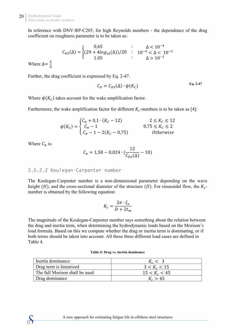
3.4.2 Wave loading
The inertia and drag load patterns are assigned as frame loads to the jacket legs as shown in Figure 3-11. Figure 3-12 shows the wave loading from the xz-plane. Notice how the load patterns are not applied onto the whole jacket leg. This is because hydrodynamic load calculations show that the inertia and drag forces are of very small values when approaching the seabed. Further, the load patterns represent three different waves with different wave amplitudes. The load patterns are therefore assigned in the global -x-direction from the mean wave amplitude to a depth of -40m.
Figure 3-11: Wave loading 3D-view Figure 3-12: Wave loading xz-plane view
3.5 Analysis

Structural analysis Analysis
37
A new approach for estimating fatigue life in offshore steel structures
The steel frame analysis is run based on the NORSOK N-004 design code, where the default preferences corresponding to this code are provided by the software. Therefore, it is not necessary to define or modify any preferences, unless the design is to be based on special criteria. The preferences are however reviewed to make sure they are acceptable. Figure 3-13 shows the load cases set to run in this analysis.
Figure 3-13: Load cases set to run
After running the analysis we check to verify the results obtained. The following verification steps are taken:
I. A design-check of the structure is performed in order to ensure that no member exceeds the capacity given by the design code.
II. Verification that the analysis and design section match for all steel frames III. Verification that the all steel frames pass the stress-capacity ratio
Verification step I is assessed in section 3.6. Figure 3-14 and Figure 3-15 confirm verification step II and III.
Figure 3-14: Analysis vs. design section verification
Figure 3-15: Member verification

38 Structural analysis Results
A new approach for estimating fatigue life in offshore steel structures
3.6 Results
3.6.1 Static design-check
Results show that design-check of the structure is sufficient and that no section is overstressed. Figure 3-16 shows the design-check of the structure and the capacity range on the right hand side. Figure 3-17 and Figure 3-18 show more detailed information about the utilization rate of the most utilized elements; element 31 and element 32, respectively.
Figure 3-16: Design-check of the structure and capacity range

Structural analysis Results
39
A new approach for estimating fatigue life in offshore steel structures
Figure 3-17: Element 31 – stress check information
Figure 3-18: Element 32 – stress check information
3.6.2 Static design overwrites
Further observations show that the FEM-based software is calculating the effective length factor for buckling, k, to be of values bigger than 1. NORSOK N-004 on the other hand suggests that the effective length factor, k, for jacket legs and piles is to be taken as 1 [7]. This deviation was observed when manually verifying the results. Further, SAP2000 offers the opportunity to overwrite the preferences for steel frame design. The modified preferences for effective length factor, k, are shown in Figure 3-19. Multiplying the frame element length with this factor gives the effective length of the frame element.
Figure 3-19: K-factor overwrites
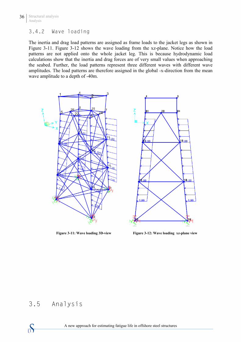
New design-check of the structure is shown in Figure 3-20. Results show that after modifying the k-factor values, each member has a lower utilization rate. The utilization rate for the lower part of the jacket legs are in the range of 0.7 – 0.9. Detailed information about the most utilized frame members is shown in Figure 3-21 and Figure 3-22. The results obtained are in correspondence with the manual verification performed for axial compression design-check. Based on the static design checks, we identify the axial stress components to be decisive when assessing the utilization rate.
40 Structural analysis Results
A new approach for estimating fatigue life in offshore steel structures
Figure 3-20: Modified design-check of the structure and capacity range
Figure 3-21: Element 31 – modified stress check information
Figure 3-22: Element 32 – modified stress check information

Structural analysis Results
41
A new approach for estimating fatigue life in offshore steel structures
3.6.3 Time-history analysis
A FEM dynamic time-history analysis is conducted. Figure 3-23 presents the envelope-stress diagram for the steel jacket, where the most critical joints are singled out (Figure 3-24 and Figure 3-25). Nominal stresses due to axial load, in-plane and out-of-plane bending moment for each frame element are plotted as time-history functions. These functions are the basis for stress history evaluation and fatigue life estimation conducted in Chapter 4 and Chapter 4.6.3.
Figure 3-23: Envelope-stress diagram
Figure 3-24: Joint 9 Figure 3-25: Joint 13

42 Conventional fatigue life estimation Introduction
A new approach for estimating fatigue life in offshore steel structures
4 Conventional fatigue life estimation
4.1 Introduction
This chapter covers basic fatigue mechanisms, characteristics and fatigue life estimation of a conventional steel jacket until crack initiation. Fatigue assessment of the steel jacket modelled in section 3.2 is based on the conventional S-N approach and damage accumulation rule (Palmgren-Miner Rule). Fatigue assessment is performed in accordance to DNV-RP-C203 and is valid for steel in air with yield strength less than 960 MPa, as well as steel materials in seawater with cathodic protection and yield strength up to 550 MPa [3]. The case under consideration consists of conventional steel material (steel grade S355) in seawater with cathodic protection.
4.2 Basic concepts of fatigue
One of the main characteristics of fatigue is that the load is not large enough to cause immediate failure [1]. Failure occurs after a number of load fluctuations, where the crack propagation has reached a critical phase, leading to failure at an arbitrary loading on a reduced cross section. It is therefore important to fully understand the factors affecting crack propagation, as well as quantify this propagation from parameters such as stress range and number of load cycles [11]. The most important load effect parameter in fatigue assessment is the stress or strain range, which is defined as the difference between a load peak and the following valley (Eq. 4-1). ∆𝜎 = 𝜎𝑚𝑎𝑥 − 𝜎𝑚𝑖𝑛 Eq. 4-1
A fatigue process is mainly considered to go through the following three stages:
I. Initiation of crack II. Crack growth
III. Final failure
4.2.1 Initiation of crack
Fatigue initiation is a process of cumulative plastic strain and is linked to the microscopic behaviour of the material. On the macroscopic level, the plastic deformation in each cycle is very likely to cancel out. However, defects will in the microscopic level accumulate by each cycle and lead to a progressive fatigue damage of the material. The crack growth will in this stage take place in a shear mode, implying that cracks are of subgrain size and oriented 45° to the maximum principal stress direction. The initiation phase will in general take place at the free surface of the material i.e. a weld toe. Only in rare cases is initiation observed taking place in the interior of the material and the material is in such cases considered to be hardened steel [1].

Conventional fatigue life estimation Basic concepts of fatigue
43
A new approach for estimating fatigue life in offshore steel structures
4.2.2 Crack growth
Assuming a material defect on the microscopic level as the starting point, further loading of the material will lead to initiation and crack growth on the macroscopic level. The crack growth is now characterized as a kinematic irreversible motion, where the crack is folded to a new position for each forthcoming load cycle. Further, fatigue cracking follows different laws depending on the level of the stress range. We distinguish between high-cycle fatigue (HCF), low-cycle fatigue (LCF) and ultra-low-cycle fatigue (ULCF). Fatigue that occurs after 104 − 105 cycles is defined as low-cycle fatigue. Ultra-low-cycle fatigue occurs in a cycle range that is less than the LCF’s. High-cycle fatigue on the other hand occurs after several millions cycles. Furthermore, the nature of crack growth on the macroscopic level is better described by fracture mechanics [11].
4.2.3 Final failure
If a fatigue crack is allowed to grow in load-carrying members, final failure is bound to take place. This failure represents the end of fatigue life and is usually defined as the maximum tolerable defect/crack size. Final fatigue failure is observed in three different mechanisms: brittle fracture, ductile fracture or plastic collapse, all depending on the material properties and size, environmental conditions, loading conditions and constraints [1].
4.2.4 Different approaches in fatigue assessment
Fatigue assessment is defined as the process where the fatigue demand on a structural element is established and compared to the predicted fatigue strength of that same element [14].The three main methods of fatigue assessment are listed in the following bullet points.
I. Simplified method II. Spectral method
III. Deterministic method There is a fourth option that is based on time domain analysis, which is preferred when assessing fatigue in structural systems subjected to non-linear loading. Fatigue assessment in this chapter is however based on the deterministic method, which is often considered to be a simplification of the spectral method. The deterministic method is applicable when there is a linear relationship between wave loads and the structural response due to these loads. The different wave heights and the corresponding periods are obtained from scatter-diagrams. A scatter diagram gives a description of the sea state, the probability of occurrence (usually expressed in the number of observations during a period of time), and the expected energy corresponding to each sea state for a specific site [14]. Having determined these parameters, the next step in fatigue life estimation is stress history evaluation and to establish the fatigue strength of the structural detail.

44 Conventional fatigue life estimation Fatigue strength based on S-N curves
A new approach for estimating fatigue life in offshore steel structures
4.3 Fatigue strength based on S-N curves
4.3.1 S-N curves
Nominal S-N curves are derived from fatigue tests of specimens mainly subjected to axial and bending loads [3]. The fatigue strength of a specimen is then presented either in the form of a table, equation or a curve. The output from the experimental data represents the number of cycles and a constant stress range that will cause fatigue failure. The basic design S-N curve is in reference with DNV-RP-C203 given as: log𝑁 = log 𝑎� − 𝑚 log∆𝜎 Eq. 4-2
Where ∆𝜎 is the stress range in MPa 𝑁 is the predicted number of cycles until failure for stress range ∆𝜎 𝑚 is the negative inverse slope of S-N curve 𝑙𝑜𝑔 𝑎� is the intercept of log N-axis It is previously mentioned that fatigue is governed by the local geometry of the structure. Given a slight change in the geometry due to material- or welding defects, high concentration of stress flow is very likely to occur. The plate thickness will have an effect on the fatigue strength of welded joints. To take account for this thickness effect, a modification is made on the “stress range” term. The modified design S-N is given by [3]:
log𝑁 = log𝑎� − 𝑚 log�∆𝜎 ∙ �𝑡𝑡𝑟𝑒𝑓
�𝑘
� Eq. 4-3
Where 𝑡 is the thickness through which a crack is most likely to grow 𝑡𝑟𝑒𝑓 = 32𝑚𝑚 is the reference thickness for tubular joints 𝑡 = 𝑡𝑟𝑒𝑓 for structural details where the thickness 𝑡 is less than the reference thickness 𝑘 is the thickness exponent for corresponding S-N curve, and is depending on the SCF Eq. 4-3 does however not take account for the thickness effect when assessing tubular joints shown in Figure 3-24Figure 3-23. This is because the cross-sectional thickness of each element (Table 7) is smaller than the reference thickness.
4.3.2 Nominal stress approach
Fatigue analysis based on S-N data is typically related to a nominal- or hot spot stress approach. Nominal stress range is defined as the stresses in a component that can be derived by simple beam theory [3]. When assessing other types of structural details (i.e. welding details), the nominal stress range should be modified in order to take account for the local conditions affecting the stresses at a specific location. The local stress at this location is expressed by a stress concentration factor multiplied with the nominal stress (Eq. 4-4). It is most common that the stress concentration factor results into an amplification of the nominal stress. However, there are cases where a stress concentration factor less than 1 can validly exist [14]. 𝜎𝑙𝑜𝑐𝑎𝑙 = 𝑆𝐶𝐹 ∙ 𝜎𝑛𝑜𝑚𝑖𝑛𝑎𝑙
Eq. 4-4

Conventional fatigue life estimation Fatigue strength based on S-N curves
45
A new approach for estimating fatigue life in offshore steel structures
4.3.3 Hot spot in tubular joints
Hot spot is in reference with DNV-RP-C203 defined as the maximum principal stress distributed instantly outside of the region affected by the geometry [3]. Stress concentration factors for tubular joints shall be applied in reference with the recommended practice, where a huge variety of equations are presented - defining stress concentration factors for different types of joints and loadings. Fatigue assessment of tubular joints is based on the hot spot approach, where corresponding S-N curves are applied. S-N curves representing tubular joints are assumed to be of class T. Fatigue life estimations which are to be covered during the course of the present chapter are based on T-curves with cathodic protection (Figure 4-1). 𝜎ℎ𝑜𝑡 𝑠𝑝𝑜𝑡 = 𝑆𝐶𝐹 ∙ 𝜎𝑛𝑜𝑚𝑖𝑛𝑎𝑙 Eq. 4-5
Figure 4-1: S-N curve for tubular joints in air and seawater [3]

46 Conventional fatigue life estimation Palmgren-Miner rule
A new approach for estimating fatigue life in offshore steel structures
4.4 Palmgren-Miner rule
The failure criteria when estimating fatigue life is based on the assumption of a linear cumulative damage commonly expressed by the Palmgren-Miner hypothesis and a fatigue design factor [3]:
𝐷 = �𝑛𝑖𝑁𝑖
𝑘
𝑖=1
=1𝑎��𝑛𝑖
𝑘𝑏
𝑖=1
∙ (∆𝜎𝑖)𝑚 ≤1
𝐹𝐷𝐹 Eq. 4-6
Where 𝑘𝑏 – number of stress blocks 𝐹𝐷𝐹 – fatigue design factor
4.4.1 Fatigue design factors
The number of load cycles is in reference with NORSOK N-004 [7] to be multiplied with a fatigue design factor before the fatigue analysis is concluded. Classification of fatigue design factors are depending on the significance of the structural component, with emphasis being put on structural integrity and availability for inspections/repair. The various fatigue design factors are presented in Table 10. First and foremost, one has to determine whether failure of the structural component will lead to danger of loss of human life, environmental pollution and financial consequences. Having identified the consequences and the accessibility, one is able to determine the fatigue design factor to be implemented into the fatigue analysis. Failure of the structural components that are to be assessed in this study are based on a conservative decision, identified to have substantial consequences and located below the splash zone. Based on this, we determine the fatigue design factor to be 3.
Table 10: Fatigue design factors [7]
Classification of structural component
Not accessible or in the splash zone
Accessible Below splash zone Above splash zone
Substantial consequences 10 3 2
Without substantial consequences 3 2 1

Conventional fatigue life estimation SCF and superposition of stresses
47
A new approach for estimating fatigue life in offshore steel structures
4.5 SCF and superposition of stresses
Stress concentration factors for the different frame elements and the different loading conditions are calculated in reference with DNV-RP-C203 [3]. The stress concentration factors for the chord are calculated at three different locations in order to identify the location where the concentration is at its highest (blue gradient adjacent to each brace in Figure 4-2). Further, the stress history output from section 3.6.3 is used for calculating and identifying the hot spot stress at the crown and saddle points. Furthermore, the hot spot stress is in reference with DNV to be evaluated at 8 spots around the circumference of the intersection, as shown in Figure 4-3. The highest value obtained identifies the hot spot stress for the element under consideration. Fatigue life estimation of the particular element is based on this hot spot.
Figure 4-2: Arbitrary KT-joint, ref.[3]
Figure 4-3: Hot spot around the circumference of the intersection, ref.[3]
CHORD

48 Conventional fatigue life estimation Stress-history evaluation of joint 9
A new approach for estimating fatigue life in offshore steel structures
4.6 Stress-history evaluation of joint 9
This section covers stress history evaluation of frame members in joint 9. Section 4.6.1 describes the approach for stress-history evaluation and hot-spot stress identification for the chord in joint 9. The same approach is used for joint 13 as well (section range 4.6.2 - 4.7.4).
4.6.1 Chord
Stress concentration factors for three different locations of the chord are presented in Table 11. The stresses are calculated at 8 spots in each location (i.e. location A, B, C). A summary of the hot spot stress evaluation is presented in Table 12. The table shows the maximum stress values observed in eight different spots for each location. The spot which gives the highest stress values is identified as the hot spot stress, which in this case is σ5. Note that each stress spot represents its unique stress history function. Samples of the stress-history functions for each wave height are presented in Figure 4-4-Figure 4-6.
Table 11: SCFs for the chord in joint 9
Location A B C
SCFs
SCFAC 3,878 10,918 12,909 SCFAS 3,878 10,918 12,909
SCFmip 1,854 3,715 4,302
SCFmop 14,084 18,922 21,414
Table 12: Hot spot stress evaluation of the chord in joint 9
σ1 σ2 σ3 σ4 σ5 σ6 σ7 σ8
Maximum Stress Observed [loc. A] 2,95 1,96 1,44 5,17 7,06 6,0 2,6 1,2 MPa Maximum Stress Observed [loc. B] 4,48 2,23 4,94 12,29 15,81 13,4 6,6 1,6
Maximum Stress Observed [loc. C] 5,06 2,50 5,89 14,39 18,45 15,68 7,71 1,83

Conventional fatigue life estimation Stress-history evaluation of joint 9
49
A new approach for estimating fatigue life in offshore steel structures
Figure 4-4: Stress-history sample for Hs 1.5m – Chord in joint 9
Figure 4-5: Stress-history sample for Hs 2.0m – Chord in joint 9

50 Conventional fatigue life estimation Stress-history evaluation of joint 9
A new approach for estimating fatigue life in offshore steel structures
Figure 4-6: Stress-history sample for Hs 2.5m – Chord in joint 9
4.6.2 Brace A
The stresses are calculated at eight different spots along the circumference of the intersection. σ5 represents the hot spot stress for brace A at the intersection adjacent to the chord.
Table 13: Stress concentration factors for brace A in joint 9
Brace A
SCFs
SCFAC 4,500 SCFAS 4,500
SCFmip 1,449
SCFmop 7,050
Table 14: Hot spot stress evaluation of brace A in joint 9
σ1 σ2 σ3 σ4 σ5 σ6 σ7 σ8 MPa
Maximum Stress Observed [Brace A] 3,056 3,092 3,144 3,182 3,183 3,147 3,095 3,057

Conventional fatigue life estimation Stress-history evaluation of joint 9
51
A new approach for estimating fatigue life in offshore steel structures
Figure 4-7: Stress-history sample for Hs 1.5m – Brace A in joint 9
Figure 4-8: Stress-history sample for Hs 2.0m – Brace A in joint 9

52 Conventional fatigue life estimation Stress-history evaluation of joint 9
A new approach for estimating fatigue life in offshore steel structures
Figure 4-9: Stress-history sample for Hs 2.5m – Brace A in joint 9
4.6.3 Brace B
The stresses are calculated at eight different spots along the circumference of the intersection. σ2 represents the hot spot stress for brace B at the intersection adjacent to the chord.
Table 15: Stress concentration factors for brace B in joint 9
Brace B
SCFs
SCFAC 14,921 SCFAS 14,921
SCFmip 2,667
SCFmop 10,180
Table 16: Hot spot stress evaluation of brace B in joint 9
σ1 σ2 σ3 σ4 σ5 σ6 σ7 σ8 MPa
Maximum Stress Observed [Brace B] 0,55 0,66 0,39 0,11 0,54 0,65 0,38 0,11

Conventional fatigue life estimation Stress-history evaluation of joint 9
53
A new approach for estimating fatigue life in offshore steel structures
Figure 4-10: Stress-history sample for Hs 1.5m – Brace B in joint 9
Figure 4-11: Stress-history sample for Hs 2.0m – Brace B in joint 9

54 Conventional fatigue life estimation Stress-history evaluation of joint 9
A new approach for estimating fatigue life in offshore steel structures
Figure 4-12: Stress-history sample for Hs 2.5m – Brace B in joint 9
4.6.4 Brace C
The stresses are calculated at eight different spots along the circumference of the intersection. σ1 represents the hot spot stress for brace C at the intersection adjacent to the chord.
Table 17: Stress concentration factors for brace C in joint 9
Brace C
SCFs
SCFAC 17,712 SCFAS 17,712
SCFmip 2,852
SCFmop 10,719
Table 18: Hot spot stress evaluation for brace C in joint 9
σ1 σ2 σ3 σ4 σ5 σ6 σ7 σ8 MPa
Maximum Stress Observed [Brace C] 10,12 10,09 10,03 9,98 9,96 9,98 10,04 10,10

Conventional fatigue life estimation Stress-history evaluation of joint 9
55
A new approach for estimating fatigue life in offshore steel structures
Figure 4-13: Stress-history sample for Hs 1.5m – Brace C in joint 9
Figure 4-14: Stress-history sample for Hs 2.0m – Brace C in joint 9

56 Conventional fatigue life estimation Stress-history evaluation of joint 9
A new approach for estimating fatigue life in offshore steel structures
Figure 4-15: Stress-history sample for Hs 2.5m – Brace C in joint 9

Conventional fatigue life estimation Stress-history evaluation of joint 13
57
A new approach for estimating fatigue life in offshore steel structures
4.7 Stress-history evaluation of joint 13
4.7.1 Chord
Stress concentration factors for three different locations of the chord are presented in Table 19. The stresses are calculated at 8 spots in each location (i.e. location A, B, C). A summary of the hot spot stress evaluation is presented in Table 20. The table shows the maximum stress values observed in eight different spots for each location. The spot which gives the highest stress values is identified as the hot spot stress, which in this case is σ5. Note that the values at location A are the same as the values at location B because of the symmetry of the diagonal braces (brace A and B)
Table 19: SCFs for the chord in joint 13
Location A B C
SCFs
SCFAC 8,999 7,611 8,999 SCFAS 8,999 7,611 8,999
SCFmip 4,302 3,715 4,302
SCFmop 22,719 24,524 22,719
Table 20: Hot spot stress evaluation of the chord in joint 13
σ1 σ2 σ3 σ4 σ5 σ6 σ7 σ8
Maximum Stress Observed [loc. A] 6,85 4,26 3,77 12,29 16,39 13,66 5,70 3,01
MPa Maximum Stress Observed [loc. B] 5,99 3,89 2,97 10,38 14,07 11,86 5,05 2,54
Maximum Stress Observed [loc. C] 6,85 4,26 3,77 12,29 16,39 13,66 5,70 3,01

58 Conventional fatigue life estimation Stress-history evaluation of joint 13
A new approach for estimating fatigue life in offshore steel structures
Figure 4-16: Stress-history sample for Hs 1.5m – Chord in joint 13
Figure 4-17: Stress-history sample for Hs 2.0m – Chord in joint 13

Conventional fatigue life estimation Stress-history evaluation of joint 13
59
A new approach for estimating fatigue life in offshore steel structures
Figure 4-18: Stress-history sample for Hs 2.5m – Chord in joint 13
4.7.2 Brace A
Table 21: SCFs for brace A in joint 13
Brace A
SCFs
SCFAC 12,348 SCFAS 12,348
SCFmip 2,852
SCFmop 11,372
Table 22: Hot spot stress evaluation of brace A in joint 13
σ1 σ2 σ3 σ4 σ5 σ6 σ7 σ8 MPa
Maximum Stress Observed [Brace A] 7,17 7,15 7,09 7,02 6,99 7,01 7,07 7,13

60 Conventional fatigue life estimation Stress-history evaluation of joint 13
A new approach for estimating fatigue life in offshore steel structures
Figure 4-19: Stress-history sample for Hs 1.5m – Brace A in joint 13
Figure 4-20: Stress-history sample for Hs 2.0m – Brace A in joint 13

Conventional fatigue life estimation Stress-history evaluation of joint 13
61
A new approach for estimating fatigue life in offshore steel structures
Figure 4-21: Stress-history sample for Hs 2.5m – Brace A in joint 13
4.7.3 Brace B
Table 23: SCFs for brace B in joint 13
Brace B
SCFs
SCFAC 10,402 SCFAS 10,402
SCFmip 2,667
SCFmop 13,194
Table 24: Hot spot stress evaluation of brace B in joint 13
σ1 σ2 σ3 σ4 σ5 σ6 σ7 σ8 MPa
Maximum Stress Observed [Brace B] 0,32 0,07 0,42 0,52 0,31 0,07 0,42 0,53

62 Conventional fatigue life estimation Stress-history evaluation of joint 13
A new approach for estimating fatigue life in offshore steel structures
Figure 4-22: Stress-history sample for Hs 1.5m – Brace B in joint 13
Figure 4-23: Stress-history sample for Hs 2.0m – Brace B in joint 13
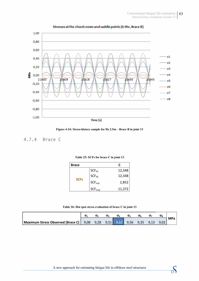
Conventional fatigue life estimation Stress-history evaluation of joint 13
63
A new approach for estimating fatigue life in offshore steel structures
Figure 4-24: Stress-history sample for Hs 2.5m – Brace B in joint 13
4.7.4 Brace C
Table 25: SCFs for brace C in joint 13
Brace C
SCFs
SCFAC 12,348 SCFAS 12,348
SCFmip 2,852
SCFmop 11,372
Table 26: Hot spot stress evaluation of brace C in joint 13
σ1 σ2 σ3 σ4 σ5 σ6 σ7 σ8 MPa
Maximum Stress Observed [Brace C] 9,08 9,28 9,51 9,62 9,56 9,35 9,13 9,02

64 Conventional fatigue life estimation Stress-history evaluation of joint 13
A new approach for estimating fatigue life in offshore steel structures
Figure 4-25: Stress-history sample for Hs 1.5m – Brace C in joint 13
Figure 4-26: Stress-history sample for Hs 2.0m – Brace C in joint 13

Conventional fatigue life estimation Stress-history evaluation of joint 13
65
A new approach for estimating fatigue life in offshore steel structures
Figure 4-27: Stress-history sample for Hs 2.5m – Brace C in joint 13

66 Conventional fatigue life estimation Fatigue life estimation
A new approach for estimating fatigue life in offshore steel structures
4.8 Fatigue life estimation
4.8.1 Joint 9
Table 27: Fatigue life estimation of joint 9 [in years]
Element nr. Member Fatigue Life [FDF: 3] Fatigue Life [FDF: 1]
Joint 9
32 Chord 17 50
63 Brace A ∞ ∞ 13 Brace B ∞ ∞ 56 Brace C 315 ∞
4.8.2 Joint 13
Table 28: Fatigue life estimation of joint 13 [in years]
Element nr. Member Fatigue Life [FDF: 3] Fatigue Life [FDF: 1]
Joint 13
32 Chord 30 90
55 Brace A ∞ ∞
19 Brace B ∞ ∞ 48 Brace C 369 ∞
4.8.3 Summary
Results show that the fatigue life of each joint is governed by the chord. The chord in joint 9 will be governing the fatigue life of the whole jacket platform. Fatigue life estimations are based on a fatigue design factor of 1 and 3. The “real” fatigue life of each structural component will be somewhere between these two parameters. Note that the structural components that are marked as infinite will not be subjected to fatigue.

Proposed approach for fatigue life estimation Introduction
67
A new approach for estimating fatigue life in offshore steel structures
5 Proposed approach for fatigue life estimation
5.1 Introduction
This chapter presents the application of the sequential law for fatigue life estimation of offshore steel structures and fatigue life estimation of the steel jacket presented in Chapter 3. Fatigue life estimation is based on the stress history evaluation already covered in Chapter 4.
5.2 Sequential Law
Engineers are constantly putting effort into the enhancement of structural health monitoring techniques, where emphasis is put on the different non-destructive field examinations and their efficiency. The modern day technology allows us to measure the loading history on most of the existing civil structures, whether they are at sea or onshore. The sequential law provides an algorithm for properly assessing the fatigue cumulative model – especially under variable loading conditions [16]. It was developed for the purpose of capturing the effect of the loading sequence more precisely [15]. This new approach consists mainly of three major steps:
Evaluation of the stress history
Transformation of the partially known S-N curve to a full range curve
Application of the sequential law

68 Proposed approach for fatigue life estimation Sequential Law
A new approach for estimating fatigue life in offshore steel structures
5.2.1 Full range S-N curve
It is previously mentioned that S-N curves are derived from fatigue tests of specimen and are often presented in the form of curves (Section 4.3.1). The curves are provided by recognized design codes. However, these S-N curves only describe the stress ranges corresponding to tens of thousands of failure cycles [15]. Hence, they are usually labelled as partially known S-N curves. Extension of the partially known S-N curve to a full range curve is therefore essential when assessing fatigue based on the sequential law. The method for this transformation is mainly based on Kohout and Vechet Wöhler curve modelling technique [17]. A schematic overview of this technique is presented in Figure 5-1.
Figure 5-1: Step-by-step graphical representation of the fully known S-N curve modelling technique, ref. [15]
The partially known curve provided by the design code is presented in a log-log plot as shown in Figure 5-1. The horizontal line 1 across the ultimate tensile strength is the asymptote 𝜎 = 𝜎𝑢for the low cycle fatigue region. The horizontal line 2 represents the stress for the high cycle fatigue region (𝜎 = 𝜎∞). Line 3 represents the tangent for the region of finite life described by the equation (or curve) of the partially known curve provided by the design code. Location B and C show the intersection points of the tangent line 3 with the horizontal lines 1 and 2. The full range curve is at any given point expressed by Eq. 5-1[17].
𝜎 = 𝜎∞ �𝑁 + 𝐵𝑁 + 𝐶
�𝑏
Eq. 5-1
Where 𝑏 is the slope of the tangent.

Proposed approach for fatigue life estimation Sequential Law
69
A new approach for estimating fatigue life in offshore steel structures
5.2.2 Full range T-curve in seawater with cathodic protection
A technique for defining the full range S-N curve was presented in the previous section (5.2.1). However, fatigue assessment for tubular members is to be based on T-curves. The design code T-curve provided by DNV-RP-C203 [3] consists of two different curve slopes. A point in question is how to obtain the full range T-curve. Two different approaches are presented in Figure 5-2. First and foremost, the design code given T-curve stretches along the black dotted line all the way to the purple triangle. It then stretches along the red curve all the way to interception point 𝜎∞ = 1. The purple triangle represents change in the negative inverse slope of the T-curve. The red curve represents the full range of a T-curve with tangent slope 𝑏 = 0.20. The green curve represents the full range of a T-curve with tangent slope 𝑏 = 0.33. Both full range curves are obtained from Eq. 5-1. A proposed approach is to base the fatigue assessment on the red colour curve. This is because stress history evaluation shows that the stress ranges for each structural component are in the high cycle region. Further, the stress ranges for each structural component are in the region where 𝑚 = 5 (Δ𝜎 ≤ ~83 𝑀𝑃𝑎). However, the fatigue testing data of the specimen and the application of the full range technique would allow us to plot a more accurate full range curve.
Figure 5-2: Full range T-curves
1
10
100
1000
10000
1,00E+01 1,00E+03 1,00E+05 1,00E+07 1,00E+09 1,00E+11 1,00E+13 1,00E+15 1,00E+17
Stre
ss R
ange
[MPa
]
Cycles N
B
SN-Curve (m=3)
SN-Curve (m=5)
Full Range SN-Curve(b=0,20)Full Range SN-Curve(b=0,33)

70 Proposed approach for fatigue life estimation Sequential Law
A new approach for estimating fatigue life in offshore steel structures
5.2.3 Application of the sequential law
The supposition of this fatigue criterion is that if the physical state of damage is the same, then fatigue life estimation should depend on the loading condition only [17]. Let us study Figure 5-3 and assume that a structural component is subjected to arbitrary stress amplitude 𝜎𝑖 for 𝑛𝑖 number of cycles at a load level 𝑖. 𝑁𝑖 would in this case denote the fatigue life corresponding to the stress amplitude or stress range 𝜎𝑖. The residual fatigue life at load level 𝑖 is obtained by (𝑁𝑖 − 𝑛𝑖). The equivalent stress amplitude corresponding to the residual fatigue life is denoted 𝜎(𝑖)𝑒𝑞, and is equal to 𝜎𝑖 at the first cycle. The new damage indicator 𝐷𝑖 is expressed by Eq. 5-2. It also follows that 𝐷𝑖 is equal to zero at the first cycle.
𝐷𝑖 =𝜎(𝑖)𝑒𝑞 − 𝜎𝑖𝜎𝑢 − 𝜎𝑖
Eq. 5-2
Where 𝜎𝑢is defined by “the intercept of the S-N curve with the ordinate at one-quarter of first fatigue cycle’’[15][17]. Furthermore, 𝜎𝑢is also commonly known as the ultimate tensile strength of the specimen in test-based design code S-N curves.
Figure 5-3: Schematic presentation of new damage indicator-based sequential law.
The same damage is transferred to the next load level (𝑖 + 1), thus the damage equivalent stress at the very same level is derived from the mathematical relation in Eq. 5-3.
𝐷𝑖 =𝜎(𝑖)𝑒𝑞 − 𝜎𝑖𝜎𝑢 − 𝜎𝑖
=𝜎(𝑖+1)𝑒𝑞′ − 𝜎𝑖+1𝜎𝑢 − 𝜎𝑖+1
Eq. 5-3
Where 𝜎(𝑖+1)𝑒𝑞
′ is the damage equivalent stress at load level (𝑖 + 1) and the corresponding number of cycles to failure is denoted 𝑁(𝑖+1)𝑅
′ . 𝜎(𝑖+1)𝑒𝑞
′ = 𝐷𝑖(𝜎𝑢 − 𝜎𝑖+1) + 𝜎𝑖+1 Eq. 5-4

Proposed approach for fatigue life estimation Sequential Law
71
A new approach for estimating fatigue life in offshore steel structures
The corresponding residual life at load level (𝑖 + 1) is defined by equation Eq. 5-5. 𝑁(𝑖+1)𝑅 = 𝑁(𝑖+1)𝑅
′ − 𝑛(𝑖+1) Eq. 5-5
This procedure leads to an iteration process (Figure 5-4) until the damage indicator becomes one. We are at this point dealing with fatigue failure of the structural component.
Figure 5-4 Flow chart for the proposed damage indicator based sequential law, ref.[17]
Ni failure number of cycles at σi stress level (from the S-N curve)
NiR=Ni-ni: Residual life
σ(i)eq: Damage stress for NiR number of cycles (from the S-N curve)
D=Di
A new damage indicator based sequential l
ni number of cycles at σi stress level
𝜎𝑖 > 𝜎∞ No
σ/(i +1)eq associated number of cycles N/
(i+1)R (from the S-N curve)
σ(i+1)eq: Damage stress for N(i+1)R number of cycles (from the S-N curve)
N (i+1) R =N/(i+1) R – ni+1: Residual life
i i+1
If No
Damage transformation from previous step to next step
ni+1 number of cycles atσi+1 stress level
No If D<1
Fatigue failure

72 Proposed approach for fatigue life estimation Sequential Law
A new approach for estimating fatigue life in offshore steel structures
5.2.4 Verification of the sequential law
Verification of the sequential law and the associated full range S-N curve was in previous research done by comparing theoretical results against experimental data. Experiments done on normalized 45C steel and 16Mn steel were the basis for this comparison [17]. The partially known S-N curves for each of these materials were transferred to fully known curves, and later on compared with the laboratory tests of the corresponding specimen. Results of each comparison are in good agreement with the experimental data (Figure 5-5 and Figure 5-6).
Figure 5-5: Predicted S-N curve for 16Mn steel vs. experimental data, ref. [17]
Figure 5-6: Predicted S-N curve for 45 C steel vs. experimental data, ref. [17]
Another form of verification was done by comparing the fatigue damage obtained by the sequential law against the Palmgren-Miner and the experimental data. Results show a good agreement between the sequential law and the experimental data. Palmgren-Miner on the other hand gives a linear-cumulative damage. Results are presented in Figure 5-7 and Figure 5-8.

Proposed approach for fatigue life estimation Sequential Law
73
A new approach for estimating fatigue life in offshore steel structures
Figure 5-7: Comparison of the predicted fatigue damage vs. experimental data for 16Mn steel, ref.[17]
Figure 5-8: Comparison of the predicted fatigue damage vs. experimental data for 45C steel, ref. [17]

74 Proposed approach for fatigue life estimation Fatigue life estimation
A new approach for estimating fatigue life in offshore steel structures
5.3 Fatigue life estimation
Results of the fatigue life estimation are presented in the following table. Fatigue life estimation based on the proposed damage indicator sequential law consists of big range of numerical iteration, till the damage indicator is equal to 1. Hence, structural components that were proven to not be subjected to fatigue (in section 4.8) are not attended for fatigue life estimations in this section. However, results presented in table 29 show that there is strong reason to believe that the proposed theoretical and technical approach for fatigue life estimation is giving more precise results.
Table 29: Sequential law vs. Miner’s fatigue life estimation

Discussion Fatigue life estimation
75
A new approach for estimating fatigue life in offshore steel structures
6 Discussion
The main focus of this thesis has been to develop and introduce a new approach for fatigue life estimation of offshore steel structures. S-N design curves and the Palmgren-Miner hypothesis are both acknowledged methods for fatigue assessment. However, previous research has shown that the Palmgren-Miner hypothesis is likely to provide different, possibly unreliable results for fatigue life estimation under variable amplitude loading. This has been the matter in question for this thesis. Different theoretical appraisals have been developed during the course of this thesis. Fatigue is a phenomenon that is a product of fluctuating loads, which cause time varying stresses in the structural detail. Fatigue in offshore structures is no exception. It is previously stated that waves and earthquakes stand for the majority of fluctuating loads acting on offshore structures. Further, earthquakes are only taken account for at locations close to or in tectonic fields. Hence, the starting point for fatigue assessment in this thesis was to describe the sea state, and further assess fatigue in offshore structures based on wave loads. The methodology for obtaining the hydrodynamic loads is presented step by step and with clarity. Calculations of the hydrodynamic loads are based on linear wave theory and the application of the Morrison’ equation. Definition of the sea state is based on a scatter diagram valid for the Northern North Sea. It is mentioned that one would like to avoid taking account for the drag force but this was not the case. However, this challenge was overcome and a step by step presentation of the linearization of the drag force was presented. Wave-structure interaction is modelled and a FEM-employed time history dynamic analysis is conducted. Design-check confirms that no frame member is overstressed. This is verified by an axial compression design-check conducted in reference with NORSOK N-004. Stress-history evaluation is based on output data from the axial force, in- and out-of-plane bending moments respectively. Further, fatigue assessment is based on the hot-spot stress and code provided stress concentration factors. Code given S-N curves and the Palmgren-Miner hypothesis is the basis for the conventional fatigue life estimation.
Application of the proposed damage indicator based sequential law is discussed in the view of fatigue life assessment of offshore steel structures. The modelling technique for the full range S-N curve is closely discussed. A big numerical stress-history evaluation is conducted and wide ranges of output data are presented, considering the fact that stress-history evaluation is essential when carrying out fatigue life estimations. Especially when emphasis is put on the loading sequence effect.

76 Conclusion Fatigue life estimation
A new approach for estimating fatigue life in offshore steel structures
7 Conclusion
A new damage indicator based fatigue model for offshore steel structures is proposed. This model is in previous research verified by comparing the theoretical approach against experimental data of different specimen. The compared results are in good agreement. Further, having proven this verification, the proposed model is compared to the conventional fatigue life estimation theory, which is based on code given S-N curves and the Palmgern-Miner hypothesis. Results presented show that the proposed model gives a more realistic fatigue life due to its ability to capture the loading sequence more precisely. However, only high cycle fatigue is assessed in this study. Comparisons of these two methods show reduction and deviation in the range of 17 to 23,5%.

Further studies Fatigue life estimation
77
A new approach for estimating fatigue life in offshore steel structures
8 Further studies
It is recommended that this same study is carried out by modelling the structural components (joint 9 and 13) in a FEM-employed software such as ABAQUS or ANSYS, to better capture the effect of the stress concentration. Another suggestion is that a more comprehensive, time-domain fatigue assessment is carried out. Non-linear effects would be included in this analysis and the Rainflow counting technique would have to be applied for estimating the number of cycles. The load case would in such analysis be varying more frequently and be of an irregular shape, leading to a higher deviation in the loading sequence.

78 References
A new approach for estimating fatigue life in offshore steel structures
9 References
[1] Almar-Næss, A., (1985), Fatigue Handbook - Offshore Steel Structures [2] Reddy, D.V., Arockiasamy, M., (1991), Offshore Structures Volume I [3] Det Norske Veritas, (2012), DNV-RP-C203: Fatigue Design of Offshore Steel Structures [4] Det Norske Veritas, (2010), DNV-RP-C205: Environmental Conditions and Environmental [5] NORSOK N-001, (2010), Integrity of Offshore Structures [6] NORSOK N-003 , (2007). Action and Action Effects [7] NORSOK N-004, (2004), Design of Steel Structures [8] Gudmestad, O.T., (2012), Marine Technology and Design,
University of Stavanger, Norway [9] Gudmestad, O.T., (2012), Marine Operations, University of Stavanger, Norway [10] Chakrabarti, Subrata K., (2005), Handbook of Offshore Engineering, Volume 1 [11] Larsen, Carl Martin., Lecture Notes for Special Topics - Dynamic Analysis of Marine
Structures, Norwegian University of Science and Technology, Accessed April 15th , 2013 (http://www.ivt.ntnu.no/imt/courses/tmr4305/del2/DRAG%20FORCE.pdf)
[12] ISSN 0902-7513 R8828 (1988), Structural Reliability Theory, Paper No. 50, Institute of Building Technology and Structural Engineering, University of Aalborg, Denmark
[13] Gudmestad, O.T., (1983), Linearization Methods and The Influence of Current on The Nonlinear Hydrodynamic Drag Force
[14] American Bureau of Shipping, (2003), Guide For The Fatigue Assessment of Offshore Structures, Updated November 2010
[15] Siriwardane, S.A.S.C., Ohga, M., Dissanayake, P.B.R., Kaita, T., (2010), Structural Appraisal-based Different Approach to Estimate the Remaining Fatigue Life of Railway Bridges
[16] Mesmacque, G., Garcia, S., Amrouche, A., Rubio-Gonzalez, C., (2005), Sequential Law in Multiaxial Fatigue, a New Damage Indicator
[17] Siriwardane, Sudath Chaminda., Ohga, M., Dissanayake, P.B.R., Kaita, T., (2009), Remaining Fatigue Life Estimation of Existing Railway Bridges
[18] Kajolli, R., (2012), On-Bottom Stability of Pipelines and Shore Approach (Unpublished), University of Stavanger, Norway
[19] SAP2000 v.15.1.0 Ultimate, User’s Manual

1
A new approach for estimating fatigue life in offshore steel structures
Appendix A
A.1 Structural Details
In reference with [12].
Joint 9 Joint 13

2
A new approach for estimating fatigue life in offshore steel structures
Appendix B
B.1 Hydrodynamic Loads Hs 1.5m
Ref. [4] DNV-RP-C205 Ref. [8] Marine Technology and Design
The surface profile: ω - Angular frequency t - Time k - Wave number (konstant) x - Position λ - Wave length ξ .o - Wave amplitude x 0 < x λ
ξ ξ x t, ( ) ξ0 sin ωt kx+( )⋅ Where:
Wave properties are evaluated by looking at the wave profile at a time t=0
ξλ
20,
0 ξ0 sin k−λ
2⋅
⋅ 0
ξ0 λ 0, ( ) 0 ξ0 sin k− λ⋅( )⋅ 0
Case Study:
Water depth: d 50m:=
3 Hours significant wave height: Hs 1.5m:=
Max wave height: Hmax 1.86 Hs⋅ 2.79m=:=
Wave period: Tp 9s:=
Classification of the water depth based on the dispersion relation ω 2 =gk tanh(kd) Where k is found through iteration:
ω 2π
Tp0.698
1s
=:= ω2 0.487
1
s2=
ξ0Hmax
21.395m=:=
Given
k 0:=
2π
Tp
2g k⋅ tanh k d⋅( )⋅
k Find k( ):=
k 0.051m
=

3
A new approach for estimating fatigue life in offshore steel structures
Given
2π
Tp
2g 2⋅
π
λtanh k d⋅( )
Wavelength : λg
2πTp
2⋅ tanh k d⋅( ):=
λ 124.789m=
Waterdepth "Shallow"dλ
120
<if
"Intermediate"120
dλ
<12
<if
"Deep" otherwise
:=
Waterdepth "Intermediate"=
t 0 1s, Tp..:= x 0 5m, λ..:= z ξ0 0, d−( )..
1.3950
-1.395
-2.79
-4.185
-5.58
-6.975
-8.37
-9.765
-11.16
-12.555
-13.95
-15.345
-16.74
...
m=:=
Surface Profile: ξ x t, ( ) ξ0 sin ω t⋅ k x⋅−( )⋅:=
Velocity Profile: t
ξ0 sin ω t⋅ k x⋅−( )⋅( )dd
Acceleration profile: 2t
ξ0 sin ω t⋅ k x⋅−( )⋅( )d
d
2

4
A new approach for estimating fatigue life in offshore steel structures
0 50 100
0.5−
0.5
1−
0.5−
0.5
1
tξ0 sin ω t⋅ k x⋅−( )⋅( )d
d 2tξ0 sin ω t⋅ k x⋅−( )⋅( )d
d
2
x
Figure B.1: Flow velocity vs. acceleration profile
Horisontal flow velocity:
uξ0 k⋅ g⋅
ω
cosh k z d+( )⋅[ ]cosh k d⋅( )
⋅
0
01
2
3
4
5
6
7
8
9
10
11
12
13
14
15
1.0580.987
0.921
0.859
0.802
0.749
0.699
0.653
0.61
0.57
0.533
0.498
0.466
0.437
0.409
...
ms
=:=
umaxξ0 k⋅ g⋅
ω
cosh k ξ0 d+( )⋅ cosh k d⋅( )
⋅ 1.058ms
=:=

5
A new approach for estimating fatigue life in offshore steel structures
0.1 0.2 0.3 0.4 0.5 0.6 0.7 0.8 0.9 1 1.150−
47.25−44.5−
41.75−39−
36.25−33.5−
30.75−28−
25.25−22.5−
19.75−17−
14.25−11.5−8.75−
6−3.25−0.5−
2.255
Particle velocity [m/s]
Wat
er d
epth
[m]
z
u
Figure B.2: Particle velocity vs. water depth
0.1 0.17 0.24 0.31 0.38 0.45 0.52 0.59 0.66 0.73 0.850−
47.25−44.5−
41.75−39−
36.25−33.5−
30.75−28−
25.25−22.5−
19.75−17−
14.25−11.5−8.75−
6−3.25−
0.5−2.25
5
Acceleration [m/s^2]
Wat
er d
epth
[m]
z
u'
Figure B.3: Particle acceleration vs. water depth

6
A new approach for estimating fatigue life in offshore steel structures
Water depth for member under consideration: dw 40−:=
Diameter of platform legs: Dst 1.2 m⋅:= Thickness : tleg 0.016 m⋅:=
tm 100 mm⋅ 40− dw≤ 2≤if
50 mm⋅ otherwise
:= tm 0.1m=
Marine growth density: ρm 1325kg
m3:=
Viscosity of seawater: ν 1.35 10⋅( ) 6− m2
s:=
Density of water: ρw 1025kg
m3:=
Outer diameter of platform legs: Do Dst tm+ 1.3m=:=
Inner diameter of platform legs: Di Do 2 tm⋅( )− 2 tleg⋅( )− 1.068m=:=
Cross-sectional area: Aπ Do
2⋅
41.327m2
=:=
Morrison "Appliccable" λ 5Do>if
"Not Applicable" otherwise
:= Morrison "Appliccable"=
Reynolds number: Reumax Do( )⋅
ν8.322 106
×=:=
Surface roughness: k1 5 10 2−⋅ m:= ...........................................for marine growth
Drag coeff. for roughness: ∆k1Do
0.038=:=
Keulegan Carpenter number for harmonic flow: KC2π ξ0⋅
Do6.742=:=
Drag Coefficients:
CDS ∆( ) 0.65 ∆ 10 4−<if
29 4 log ∆( )+( )20
10 4−∆≤ 10 2−
≤if
1.05 otherwise
:=
CDS ∆( ) 1.05=

7
A new approach for estimating fatigue life in offshore steel structures
Cπ 1.50 0.02412
CDS ∆( )10−
⋅− 1.466=:=
ψ KC( ) Cπ 0.1 KC 12−( )⋅+ 2 KC≤ 12<if
Cπ 1− 0.75 KC≤ 2<if
Cπ 1− 2 KC 0.75−( )⋅− otherwise
:= ψ KC( ) 0.94=
CD CDS ∆( ) ψ KC( )⋅ 0.987=:= Drag Coefficient:
Added mass coefficient:
CA 1.0 KC 3<if
max 1.0 0.044 KC 3−( )− 0.6 CDS ∆( ) 0.65−( )−, KC 3>if
"Drag Force Dominates" KC 25>if
:= CA 0.835=
CM 1 CA+ 1.835=:= Mass Coefficient:
Normal load on the jacket legs:
fn ρw 1 CA+( )⋅ A⋅ u'max⋅ 0.5Do
Hmax< 1.0<if
12
ρw⋅ CD⋅ Do⋅ umax⋅ umax⋅
DoHmax
0.1<if
"Take account for both drag and inertia term"( ) otherwise
:=
fn "Take account for both drag and inertia term"=
Maximum inertia load: fI.max ρw 1 CA+( )⋅ A⋅ u'max⋅ 1.844
kNm
⋅=:=
Maximum drag load: fD.max12
ρw⋅ CD⋅ Do⋅ umax⋅ umax⋅ 0.735kNm
⋅=:=
fD.maxfI.max
0.399= Drag to inertia ratio:

8
A new approach for estimating fatigue life in offshore steel structures
Morison's Load Formula The following calculations are valid for the members in a water depth of -40 to -50m
Water depth for member under consideration: dw.50 50−:=
tm.50 100 mm⋅ 40− dw.50≤ 2≤if
50 mm⋅ otherwise
:= tm.50 0.05m=
Outer diameter of platform legs: Do.50 Dst tm.50+ 1.25m=:=
Inner diameter of platform legs: Di.50 Do.50 2 tm.50⋅( )− 2 tleg⋅( )− 1.118m=:=
Cross-sectional area: A50π Do.50
2⋅
41.227m2
=:=
Morrison "Appliccable" λ 5Do.50>if
"Not Applicable" otherwise
:= Morrison "Appliccable"=
Reynolds number: Re.50umax Do.50( )⋅
ν8.002 106
×=:=
Surface roughness: k1.50 5 10 2−⋅ m:= ...........................................for marine growth
Drag coeff. for roughness: ∆ 50k1
Do.500.04=:=
Keulegan Carpenter number for harmonic flow: KC.502π ξ0⋅
Do.507.012=:=
Drag Coefficients:
CDS.50 ∆ 50( ) 0.65 ∆ 50 10 4−<if
29 4 log ∆ 50( )+( )20
10 4−∆ 50≤ 10 2−
≤if
1.05 otherwise
:=
CDS ∆( ) 1.05=
Given
Cπ.50 1.50 0.02412
CDS.50 ∆ 50( ) 10−
⋅− 1.466=:=

9
A new approach for estimating fatigue life in offshore steel structures
ψ50 KC.50( ) Cπ.50 0.1 KC.50 12−( )⋅+ 2 KC.50≤ 12<if
Cπ.50 1− 0.75 KC.50≤ 2<if
Cπ.50 1− 2 KC.50 0.75−( )⋅− otherwise
:= ψ50 KC.50( ) 0.967=
CD.50 CDS.50 ∆ 50( ) ψ50 KC.50( )⋅ 1.015=:= Drag Coefficient:
Added mass coefficient:
CA.50 1.0 KC.50 3<if
max 1.0 0.044 KC.50 3−( )− 0.6 CDS.50 ∆( ) 0.65−( )−, KC.50 3>if
"Drag Force Dominates" KC.50 25>if
:=
CA.50 0.823=
CM.50 1 CA.50+ 1.823=:= Mass Coefficient:
Normal load on the jacket legs:
fn.50 ρw 1 CA.50+( )⋅ A⋅ u'max⋅ 0.5Do.50Hmax
< 1.0<if
12
ρw⋅ CD.50⋅ Do.50⋅ umax⋅ umax⋅
Do.50Hmax
0.1<if
"Take account for both drag and inertia term"( ) otherwise
:=
fn.50 "Take account for both drag and inertia term"=
Maximum inertia load: fI.max.50 ρw 1 CA.50+( )⋅ A50⋅ u'max⋅ 1.693kNm
⋅=:=
fD.max.5012
ρw⋅ CD.50⋅ Do.50⋅ umax⋅ umax⋅ 0.727kNm
⋅=:= Maximum drag load:
Drag to inertia ratio: fD.max.50fI.max.50
0.43=

10
A new approach for estimating fatigue life in offshore steel structures
Total Load on the platform leg:
Fd.4040− m
ξ0
z12
ρw⋅ CD⋅ Do⋅ξ0 k⋅ g⋅
ω
cosh k z d+( )⋅[ ]cosh k d⋅( )
⋅ 1⋅
2
⌠⌡
d 7.464 kN⋅=:=
Fi.4040− m
0
zρw 1 CA+( )⋅ A⋅ ξ0 k⋅ g⋅cosh k z d+( )⋅[ ]
cosh k d⋅( )⋅
⌠⌡
d 30.843 kN⋅=:=
Fd.5050− m
40− m
z12
ρw⋅ CD.50⋅ Do.50⋅ξ0 k⋅ g⋅
ω
cosh k z d+( )⋅[ ]cosh k d⋅( )
⋅ 1⋅
2
⌠⌡
d 0.177 kN⋅=:=
Fi.5050− m
40− m
zρw 1 CA.50+( )⋅ A50⋅ ξ0 k⋅ g⋅cosh k z d+( )⋅[ ]
cosh k d⋅( )⋅
⌠⌡
d 2.641 kN⋅=:=
The total drag load on the platform leg is:
FD Fd.40 Fd.50+ 7.641 kN⋅=:=
The total inertia load on the platform leg is:
FI Fi.40 Fi.50+ 33.484 kN⋅=:=
If we were not to take account for the different amount of the marine growth in different depth levels, the total loads would be:
Fd50− m
0
z12
ρw⋅ CD⋅ Do⋅ξ0 k⋅ g⋅
ω
cosh k z d+( )⋅[ ]cosh k d⋅( )
⋅ 1⋅
2
⌠⌡
d 6.685 kN⋅=:=
Fi.50− m
0
zρw 1 CA+( )⋅ A⋅ ξ0 k⋅ g⋅cosh k z d+( )⋅[ ]
cosh k d⋅( )⋅
⌠⌡
d 33.718 kN⋅=:=
We observe that these loads are slightly bigger because of the bigger diameter of the member under consideration. This is as a result of the marine growth being of a higher value in depths up to -40m.

11
A new approach for estimating fatigue life in offshore steel structures
B.2 Hydrodynamic Loads Hs 2.0m
Ref. [4] DNV-RP-C205 Ref. [8] Marine Technology and Design
The surface profile: ω - Angular frequency t - Time k - Wave number (konstant) x - Position λ - Wave length ξ .o - Wave amplitude x 0 < x λ
ξ ξ x t, ( ) ξ0 sin ωt kx+( )⋅ Where:
Wave properties are evaluated by looking at the wave profile at a time t=0
ξλ
20,
0 ξ0 sin k−λ
2⋅
⋅ 0
ξ0 λ 0, ( ) 0 ξ0 sin k− λ⋅( )⋅ 0
Case Study:
Water depth: d 50m:=
3 Hours significant wave height: Hs 2.0m:=
Max wave height: Hmax 1.86 Hs⋅ 3.72m=:=
Wave period: Tp 9s:=
Classification of the water depth based on the dispersion relation ω 2 =gk tanh(kd) Where k is found through iteration:
ω 2π
Tp0.698
1s
=:= ω2 0.487
1
s2=
ξ0Hmax
21.86m=:=
Given
k 0:=
2π
Tp
2g k⋅ tanh k d⋅( )⋅
k Find k( ):=
k 0.051m
=

12
A new approach for estimating fatigue life in offshore steel structures
Given
2π
Tp
2g 2⋅
π
λtanh k d⋅( )
Wavelength : λg
2πTp
2⋅ tanh k d⋅( ):=
λ 124.789m=
Waterdepth "Shallow"dλ
120
<if
"Intermediate"120
dλ
<12
<if
"Deep" otherwise
:=
Waterdepth "Intermediate"=
t 0 1s, Tp..:= x 0 5m, λ..:= z ξ0 0, d−( )..
1.860
-1.86
-3.72
-5.58
-7.44
-9.3
-11.16
-13.02
-14.88
-16.74
-18.6
-20.46
-22.32
...
m=:=
Surface Profile: ξ x t, ( ) ξ0 sin ω t⋅ k x⋅−( )⋅:=
Velocity Profile: t
ξ0 sin ω t⋅ k x⋅−( )⋅( )dd
Acceleration profile: 2t
ξ0 sin ω t⋅ k x⋅−( )⋅( )d
d
2

13
A new approach for estimating fatigue life in offshore steel structures
0 50 100
1−
1
1−
0.5−
0.5
1
tξ0 sin ω t⋅ k x⋅−( )⋅( )d
d 2tξ0 sin ω t⋅ k x⋅−( )⋅( )d
d
2
x
Figure B.4: Flow velocity vs. acceleration profile
Horisontal flow velocity:
uξ0 k⋅ g⋅
ω
cosh k z d+( )⋅[ ]cosh k d⋅( )
⋅
0
01
2
3
4
5
6
7
8
9
10
11
12
13
14
15
1.4431.316
1.2
1.094
0.998
0.911
0.832
0.76
0.695
0.636
0.582
0.534
0.49
0.451
0.416
...
ms
=:=
umaxξ0 k⋅ g⋅
ω
cosh k ξ0 d+( )⋅ cosh k d⋅( )
⋅ 1.443ms
=:=

14
A new approach for estimating fatigue life in offshore steel structures
Horizontal particle accelerations: u' ξ0 k⋅ g⋅cosh k z d+( )⋅[ ]
cosh k d⋅( )⋅
0
01
2
3
4
5
6
7
8
9
10
11
12
13
14
15
1.0070.918
0.837
0.764
0.697
0.636
0.581
0.531
0.485
0.444
0.407
0.373
0.342
0.315
0.29
...
m
s2=:=
The acceleration term is at its minimum under the wave crest when cos ωt kx−( ) 0
The acceleration term is at its largest when the water particles cross the still water level z=0, hence:
cos ωt kx− 1(
ξ ξ0 sin ωt kx−( )⋅ 0
u'min ξ0 k⋅ g⋅cosh k 0 d+( )⋅[ ]
cosh k d⋅( )⋅ 0⋅ 0
m
s2⋅=:=
u'max ξ0 k⋅ g⋅cosh k ξ0 d+( )⋅
cosh k d⋅( )⋅ sin
π
2
⋅ 1.007m
s2=:=

15
A new approach for estimating fatigue life in offshore steel structures
0.2 0.34 0.48 0.62 0.76 0.9 1.04 1.18 1.32 1.46 1.650−
47.25−44.5−
41.75−39−
36.25−33.5−
30.75−28−
25.25−22.5−
19.75−17−
14.25−11.5−8.75−
6−3.25−
0.5−2.25
5
Particle velocity [m/s]
Wat
er d
epth
[m]
z
u
Figure B.5: Particle velocity vs. water depth
0.1 0.2 0.3 0.4 0.5 0.6 0.7 0.8 0.9 1 1.150−
47.25−44.5−
41.75−39−
36.25−33.5−
30.75−28−
25.25−22.5−
19.75−17−
14.25−11.5−8.75−
6−3.25−0.5−
2.255
Acceleration [m/s^2]
Wat
er d
epth
[m]
z
u'
Figure B.6: Particle acceleration vs. water depth

16
A new approach for estimating fatigue life in offshore steel structures
Morison's Load Formula
Water depth for member under consideration: dw 40−:=
Diameter of platform legs: Dst 1.2 m⋅:= Thickness : tleg 0.016 m⋅:=
tm 100 mm⋅ 40− dw≤ 2≤if
50 mm⋅ otherwise
:= tm 0.1m=
Marine growth density: ρm 1325kg
m3:=
Viscosity of seawater: ν 1.35 10⋅( ) 6− m2
s:=
Density of water: ρw 1025kg
m3:=
Outer diameter of platform legs: Do Dst tm+ 1.3m=:=
Inner diameter of platform legs: Di Do 2 tm⋅( )− 2 tleg⋅( )− 1.068m=:=
Cross-sectional area: Aπ Do
2⋅
41.327m2
=:=
Morrison "Appliccable" λ 5Do>if
"Not Applicable" otherwise
:= Morrison "Appliccable"=
Reynolds number: Reumax Do( )⋅
ν1.136 107
×=:=
Surface roughness: k1 5 10 2−⋅ m:= ...........................................for marine growth
Drag coeff. for roughness: ∆k1Do
0.038=:=
Keulegan Carpenter number for harmonic flow: KC2π ξ0⋅
Do8.99=:=
Drag Coefficients:
CDS ∆( ) 0.65 ∆ 10 4−<if
29 4 log ∆( )+( )20
10 4−∆≤ 10 2−
≤if
1.05 otherwise
:=
CDS ∆( ) 1.05=

17
A new approach for estimating fatigue life in offshore steel structures
Cπ 1.50 0.02412
CDS ∆( )10−
⋅− 1.466=:=
ψ KC( ) Cπ 0.1 KC 12−( )⋅+ 2 KC≤ 12<if
Cπ 1− 0.75 KC≤ 2<if
Cπ 1− 2 KC 0.75−( )⋅− otherwise
:= ψ KC( ) 1.165=
CD CDS ∆( ) ψ KC( )⋅ 1.223=:= Drag Coefficient:
Added mass coefficient:
CA 1.0 KC 3<if
max 1.0 0.044 KC 3−( )− 0.6 CDS ∆( ) 0.65−( )−, KC 3>if
"Drag Force Dominates" KC 25>if
:= CA 0.736=
CM 1 CA+ 1.736=:= Mass Coefficient:
Normal load on the jacket legs:
fn ρw 1 CA+( )⋅ A⋅ u'max⋅ 0.5Do
Hmax< 1.0<if
12
ρw⋅ CD⋅ Do⋅ umax⋅ umax⋅
DoHmax
0.1<if
"Take account for both drag and inertia term"( ) otherwise
:=
fn "Take account for both drag and inertia term"=
Maximum inertia load: fI.max ρw 1 CA+( )⋅ A⋅ u'max⋅ 2.38
kNm
⋅=:=
Maximum drag load: fD.max12
ρw⋅ CD⋅ Do⋅ umax⋅ umax⋅ 1.697kNm
⋅=:=
fD.maxfI.max
0.713= Drag to inertia ratio:

18
A new approach for estimating fatigue life in offshore steel structures
Morison's Load Formula The following calculations are valid for the members in a water depth of -40 to -50m
Water depth for member under consideration: dw.50 50−:=
tm.50 100 mm⋅ 40− dw.50≤ 2≤if
50 mm⋅ otherwise
:= tm.50 0.05m=
Outer diameter of platform legs: Do.50 Dst tm.50+ 1.25m=:=
Inner diameter of platform legs: Di.50 Do.50 2 tm.50⋅( )− 2 tleg⋅( )− 1.118m=:=
Cross-sectional area: A50π Do.50
2⋅
41.227m2
=:=
Morrison "Appliccable" λ 5Do.50>if
"Not Applicable" otherwise
:= Morrison "Appliccable"=
Reynolds number: Re.50umax Do.50( )⋅
ν1.092 107
×=:=
Surface roughness: k1.50 5 10 2−⋅ m:= ...........................................for marine growth
Drag coeff. for roughness: ∆ 50k1
Do.500.04=:=
Keulegan Carpenter number for harmonic flow: KC.502π ξ0⋅
Do.509.349=:=
Drag Coefficients:
CDS.50 ∆ 50( ) 0.65 ∆ 50 10 4−<if
29 4 log ∆ 50( )+( )20
10 4−∆ 50≤ 10 2−
≤if
1.05 otherwise
:=
CDS ∆( ) 1.05=
Given
Cπ.50 1.50 0.02412
CDS.50 ∆ 50( ) 10−
⋅− 1.466=:=

19
A new approach for estimating fatigue life in offshore steel structures
ψ50 KC.50( ) Cπ.50 0.1 KC.50 12−( )⋅+ 2 KC.50≤ 12<if
Cπ.50 1− 0.75 KC.50≤ 2<if
Cπ.50 1− 2 KC.50 0.75−( )⋅− otherwise
:= ψ50 KC.50( ) 1.201=
CD.50 CDS.50 ∆ 50( ) ψ50 KC.50( )⋅ 1.261=:= Drag Coefficient:
Added mass coefficient:
CA.50 1.0 KC.50 3<if
max 1.0 0.044 KC.50 3−( )− 0.6 CDS.50 ∆( ) 0.65−( )−, KC.50 3>if
"Drag Force Dominates" KC.50 25>if
:=
CA.50 0.721=
CM.50 1 CA.50+ 1.721=:= Mass Coefficient:
Normal load on the jacket legs:
fn.50 ρw 1 CA.50+( )⋅ A⋅ u'max⋅ 0.5Do.50Hmax
< 1.0<if
12
ρw⋅ CD.50⋅ Do.50⋅ umax⋅ umax⋅
Do.50Hmax
0.1<if
"Take account for both drag and inertia term"( ) otherwise
:=
fn.50 "Take account for both drag and inertia term"=
Maximum inertia load: fI.max.50 ρw 1 CA.50+( )⋅ A50⋅ u'max⋅ 2.18kNm
⋅=:=
fD.max.5012
ρw⋅ CD.50⋅ Do.50⋅ umax⋅ umax⋅ 1.682kNm
⋅=:= Maximum drag load:
Drag to inertia ratio: fD.max.50fI.max.50
0.771=

20
A new approach for estimating fatigue life in offshore steel structures
Total Load on the platform leg:
Fd.4040− m
ξ0
z12
ρw⋅ CD⋅ Do⋅ξ0 k⋅ g⋅
ω
cosh k z d+( )⋅[ ]cosh k d⋅( )
⋅ 1⋅
2
⌠⌡
d 17.214 kN⋅=:=
Fi.4040− m
0
zρw 1 CA+( )⋅ A⋅ ξ0 k⋅ g⋅cosh k z d+( )⋅[ ]
cosh k d⋅( )⋅
⌠⌡
d 38.909 kN⋅=:=
Fd.5050− m
40− m
z12
ρw⋅ CD.50⋅ Do.50⋅ξ0 k⋅ g⋅
ω
cosh k z d+( )⋅[ ]cosh k d⋅( )
⋅ 1⋅
2
⌠⌡
d 0.391 kN⋅=:=
Fi.5050− m
40− m
zρw 1 CA.50+( )⋅ A50⋅ ξ0 k⋅ g⋅cosh k z d+( )⋅[ ]
cosh k d⋅( )⋅
⌠⌡
d 3.322 kN⋅=:=
The total drag load on the platform leg is:
FD Fd.40 Fd.50+ 17.605 kN⋅=:=
The total inertia load on the platform leg is:
FI Fi.40 Fi.50+ 42.231 kN⋅=:=
If we were not to take account for the different amount of the marine growth in different depth levels, the total loads would be:
Fd50− m
0
z12
ρw⋅ CD⋅ Do⋅ξ0 k⋅ g⋅
ω
cosh k z d+( )⋅[ ]cosh k d⋅( )
⋅ 1⋅
2
⌠⌡
d 14.727 kN⋅=:=
Fi.50− m
0
zρw 1 CA+( )⋅ A⋅ ξ0 k⋅ g⋅cosh k z d+( )⋅[ ]
cosh k d⋅( )⋅
⌠⌡
d 42.535 kN⋅=:=
We observe that these loads are slightly bigger because of the bigger diameter of the member under consideration. This is as a result of the marine growth being of a higher value in depths up to -40m.

21
A new approach for estimating fatigue life in offshore steel structures
B.3 Hydrodynamic Loads Hs 2.5m
Ref. [4] DNV-RP-C205 Ref. [8] Marine Technology and Design
The surface profile: ω - Angular frequency t - Time k - Wave number (konstant) x - Position λ - Wave length ξ .o - Wave amplitude x 0 < x λ
ξ ξ x t, ( ) ξ0 sin ωt kx+( )⋅ Where:
Wave properties are evaluated by looking at the wave profile at a time t=0
ξλ
20,
0 ξ0 sin k−λ
2⋅
⋅ 0
ξ0 λ 0, ( ) 0 ξ0 sin k− λ⋅( )⋅ 0
Case Study:
Water depth: d 50m:=
3 Hours significant wave height: Hs 2.5m:=
Max wave height: Hmax 1.86 Hs⋅ 4.65m=:=
Wave period: Tp 9s:=
Classification of the water depth based on the dispersion relation ω 2 =gk tanh(kd) Where k is found through iteration:
ω 2π
Tp0.698
1s
=:= ω2 0.487
1
s2=
ξ0Hmax
22.325m=:=
Given
k 0:=
2π
Tp
2g k⋅ tanh k d⋅( )⋅
k Find k( ):=
k 0.051m
=

22
A new approach for estimating fatigue life in offshore steel structures
Given
2π
Tp
2g 2⋅
π
λtanh k d⋅( )
Wavelength : λg
2πTp
2⋅ tanh k d⋅( ):=
λ 124.789m=
Waterdepth "Shallow"dλ
120
<if
"Intermediate"120
dλ
<12
<if
"Deep" otherwise
:=
Waterdepth "Intermediate"=
t 0 1s, Tp..:= x 0 5m, λ..:= z ξ0 0, d−( )..
2.3250
-2.325
-4.65
-6.975
-9.3
-11.625
-13.95
-16.275
-18.6
-20.925
-23.25
-25.575
-27.9
...
m=:=
Surface Profile: ξ x t, ( ) ξ0 sin ω t⋅ k x⋅−( )⋅:=
Velocity Profile: t
ξ0 sin ω t⋅ k x⋅−( )⋅( )dd
Acceleration profile: 2t
ξ0 sin ω t⋅ k x⋅−( )⋅( )d
d
2

23
A new approach for estimating fatigue life in offshore steel structures
0 50 100
1−
1
2−
1−
1
2
tξ0 sin ω t⋅ k x⋅−( )⋅( )d
d 2tξ0 sin ω t⋅ k x⋅−( )⋅( )d
d
2
x
Figure B.7: Flow velocity vs. acceleration profile
Horisontal flow velocity:
uξ0 k⋅ g⋅
ω
cosh k z d+( )⋅[ ]cosh k d⋅( )
⋅
0
01
2
3
4
5
6
7
8
9
10
11
12
13
14
15
1.8461.644
1.465
1.306
1.165
1.04
0.929
0.831
0.744
0.668
0.6
0.541
0.489
0.444
0.405
...
ms
=:=
umaxξ0 k⋅ g⋅
ω
cosh k ξ0 d+( )⋅ cosh k d⋅( )
⋅ 1.846ms
=:=

24
A new approach for estimating fatigue life in offshore steel structures
Horizontal particle accelerations: u' ξ0 k⋅ g⋅cosh k z d+( )⋅[ ]
cosh k d⋅( )⋅
0
01
2
3
4
5
6
7
8
9
10
11
12
13
14
15
1.2891.148
1.023
0.912
0.813
0.726
0.649
0.58
0.519
0.466
0.419
0.378
0.342
0.31
0.283
...
m
s2=:=
The acceleration term is at its minimum under the wave crest when cos ωt kx−( ) 0
The acceleration term is at its largest when the water particles cross the still water level z=0, hence:
cos ωt kx− 1(
ξ ξ0 sin ωt kx−( )⋅ 0
u'min ξ0 k⋅ g⋅cosh k 0 d+( )⋅[ ]
cosh k d⋅( )⋅ 0⋅ 0
m
s2⋅=:=
u'max ξ0 k⋅ g⋅cosh k ξ0 d+( )⋅
cosh k d⋅( )⋅ sin
π
2
⋅ 1.289m
s2=:=

25
A new approach for estimating fatigue life in offshore steel structures
0.2 0.38 0.56 0.74 0.92 1.1 1.28 1.46 1.64 1.82 250−
47.25−44.5−
41.75−39−
36.25−33.5−
30.75−28−
25.25−22.5−
19.75−17−
14.25−11.5−8.75−
6−3.25−
0.5−2.25
5
Particle velocity [m/s]
Wat
er d
epth
[m]
z
u
Figure B.8: Particle velocity vs. water depth
0 0.14 0.28 0.42 0.56 0.7 0.84 0.98 1.12 1.26 1.450−
47.25−44.5−
41.75−39−
36.25−33.5−
30.75−28−
25.25−22.5−
19.75−17−
14.25−11.5−8.75−
6−3.25−
0.5−2.25
5
Acceleration [m/s^2]
Wat
er d
epth
[m]
z
u'
Figure B.9: Particle acceleration vs. water depth

26
A new approach for estimating fatigue life in offshore steel structures
Water depth for member under consideration: dw 40−:=
Diameter of platform legs: Dst 1.2 m⋅:= Thickness : tleg 0.016 m⋅:=
tm 100 mm⋅ 40− dw≤ 2≤if
50 mm⋅ otherwise
:= tm 0.1m=
Marine growth density: ρm 1325kg
m3:=
Viscosity of seawater: ν 1.35 10⋅( ) 6− m2
s:=
Density of water: ρw 1025kg
m3:=
Outer diameter of platform legs: Do Dst tm+ 1.3m=:=
Inner diameter of platform legs: Di Do 2 tm⋅( )− 2 tleg⋅( )− 1.068m=:=
Cross-sectional area: Aπ Do
2⋅
41.327m2
=:=
Morrison "Appliccable" λ 5Do>if
"Not Applicable" otherwise
:= Morrison "Appliccable"=
Reynolds number: Reumax Do( )⋅
ν1.453 107
×=:=
Surface roughness: k1 5 10 2−⋅ m:= ...........................................for marine growth
Drag coeff. for roughness: ∆k1Do
0.038=:=
Keulegan Carpenter number for harmonic flow: KC2π ξ0⋅
Do11.237=:=
Drag Coefficients:
CDS ∆( ) 0.65 ∆ 10 4−<if
29 4 log ∆( )+( )20
10 4−∆≤ 10 2−
≤if
1.05 otherwise
:=
CDS ∆( ) 1.05=

27
A new approach for estimating fatigue life in offshore steel structures
Cπ 1.50 0.02412
CDS ∆( )10−
⋅− 1.466=:=
ψ KC( ) Cπ 0.1 KC 12−( )⋅+ 2 KC≤ 12<if
Cπ 1− 0.75 KC≤ 2<if
Cπ 1− 2 KC 0.75−( )⋅− otherwise
:= ψ KC( ) 1.389=
CD CDS ∆( ) ψ KC( )⋅ 1.459=:= Drag Coefficient:
Added mass coefficient:
CA 1.0 KC 3<if
max 1.0 0.044 KC 3−( )− 0.6 CDS ∆( ) 0.65−( )−, KC 3>if
"Drag Force Dominates" KC 25>if
:= CA 0.638=
CM 1 CA+ 1.638=:= Mass Coefficient:
Normal load on the jacket legs:
fn ρw 1 CA+( )⋅ A⋅ u'max⋅ 0.5Do
Hmax< 1.0<if
12
ρw⋅ CD⋅ Do⋅ umax⋅ umax⋅
DoHmax
0.1<if
"Take account for both drag and inertia term"( ) otherwise
:=
fn "Take account for both drag and inertia term"=
Maximum inertia load: fI.max ρw 1 CA+( )⋅ A⋅ u'max⋅ 2.871
kNm
⋅=:=
Maximum drag load: fD.max12
ρw⋅ CD⋅ Do⋅ umax⋅ umax⋅ 3.313kNm
⋅=:=
fD.maxfI.max
1.154= Drag to inertia ratio:

28
A new approach for estimating fatigue life in offshore steel structures
Morison's Load Formula The following calculations are valid for the members in a water depth of -40 to -50m
Water depth for member under consideration: dw.50 50−:=
tm.50 100 mm⋅ 40− dw.50≤ 2≤if
50 mm⋅ otherwise
:= tm.50 0.05m=
Outer diameter of platform legs: Do.50 Dst tm.50+ 1.25m=:=
Inner diameter of platform legs: Di.50 Do.50 2 tm.50⋅( )− 2 tleg⋅( )− 1.118m=:=
Cross-sectional area: A50π Do.50
2⋅
41.227m2
=:=
Morrison "Appliccable" λ 5Do.50>if
"Not Applicable" otherwise
:= Morrison "Appliccable"=
Reynolds number: Re.50umax Do.50( )⋅
ν1.397 107
×=:=
Surface roughness: k1.50 5 10 2−⋅ m:= ...........................................for marine growth
Drag coeff. for roughness: ∆ 50k1
Do.500.04=:=
Keulegan Carpenter number for harmonic flow: KC.502π ξ0⋅
Do.5011.687=:=
Drag Coefficients:
CDS.50 ∆ 50( ) 0.65 ∆ 50 10 4−<if
29 4 log ∆ 50( )+( )20
10 4−∆ 50≤ 10 2−
≤if
1.05 otherwise
:=
CDS ∆( ) 1.05=
Given
Cπ.50 1.50 0.02412
CDS.50 ∆ 50( ) 10−
⋅− 1.466=:=

29
A new approach for estimating fatigue life in offshore steel structures
ψ50 KC.50( ) Cπ.50 0.1 KC.50 12−( )⋅+ 2 KC.50≤ 12<if
Cπ.50 1− 0.75 KC.50≤ 2<if
Cπ.50 1− 2 KC.50 0.75−( )⋅− otherwise
:= ψ50 KC.50( ) 1.434=
CD.50 CDS.50 ∆ 50( ) ψ50 KC.50( )⋅ 1.506=:= Drag Coefficient:
Added mass coefficient:
CA.50 1.0 KC.50 3<if
max 1.0 0.044 KC.50 3−( )− 0.6 CDS.50 ∆( ) 0.65−( )−, KC.50 3>if
"Drag Force Dominates" KC.50 25>if
:=
CA.50 0.618=
CM.50 1 CA.50+ 1.618=:= Mass Coefficient:
Normal load on the jacket legs:
fn.50 ρw 1 CA.50+( )⋅ A⋅ u'max⋅ 0.5Do.50Hmax
< 1.0<if
12
ρw⋅ CD.50⋅ Do.50⋅ umax⋅ umax⋅
Do.50Hmax
0.1<if
"Take account for both drag and inertia term"( ) otherwise
:=
fn.50 "Take account for both drag and inertia term"=
Maximum inertia load: fI.max.50 ρw 1 CA.50+( )⋅ A50⋅ u'max⋅ 2.623kNm
⋅=:=
fD.max.5012
ρw⋅ CD.50⋅ Do.50⋅ umax⋅ umax⋅ 3.288kNm
⋅=:= Maximum drag load:
Drag to inertia ratio: fD.max.50fI.max.50
1.254=

30
A new approach for estimating fatigue life in offshore steel structures
Total Load on the platform leg:
Fd.4040− m
ξ0
z12
ρw⋅ CD⋅ Do⋅ξ0 k⋅ g⋅
ω
cosh k z d+( )⋅[ ]cosh k d⋅( )
⋅ 1⋅
2
⌠⌡
d 33.592 kN⋅=:=
Fi.4040− m
0
zρw 1 CA+( )⋅ A⋅ ξ0 k⋅ g⋅cosh k z d+( )⋅[ ]
cosh k d⋅( )⋅
⌠⌡
d 45.866 kN⋅=:=
Fd.5050− m
40− m
z12
ρw⋅ CD.50⋅ Do.50⋅ξ0 k⋅ g⋅
ω
cosh k z d+( )⋅[ ]cosh k d⋅( )
⋅ 1⋅
2
⌠⌡
d 0.73 kN⋅=:=
Fi.5050− m
40− m
zρw 1 CA.50+( )⋅ A50⋅ ξ0 k⋅ g⋅cosh k z d+( )⋅[ ]
cosh k d⋅( )⋅
⌠⌡
d 3.904 kN⋅=:=
The total drag load on the platform leg is:
FD Fd.40 Fd.50+ 34.321 kN⋅=:=
The total inertia load on the platform leg is:
FI Fi.40 Fi.50+ 49.771 kN⋅=:=
If we were not to take account for the different amount of the marine growth in different depth levels, the total loads would be:
Fd50− m
0
z12
ρw⋅ CD⋅ Do⋅ξ0 k⋅ g⋅
ω
cosh k z d+( )⋅[ ]cosh k d⋅( )
⋅ 1⋅
2
⌠⌡
d 27.451 kN⋅=:=
Fi.50− m
0
zρw 1 CA+( )⋅ A⋅ ξ0 k⋅ g⋅cosh k z d+( )⋅[ ]
cosh k d⋅( )⋅
⌠⌡
d 50.141 kN⋅=:=
We observe that these loads are slightly bigger because of the bigger diameter of the member under consideration. This is as a result of the marine growth being of a higher value in depths up to -40m.

31
A new approach for estimating fatigue life in offshore steel structures
Appendix C
C.1 Stress Concentration Factors - Joint 9
In refrence with [3] DNV-RP-C203
Definition of geometrical parametrs:
βAdAD
βBdBD
βcdCD
τAtAT
τBtBT
τCtCD
γD2T
ξABgAB
D ξBC
gBCD
Case under consideration......................................................................... Joint 9
Where: T 0.016m:= D 1.2m:=
tA 0.016m:= dA 1.2m 1.2m=:=
tB 0.014m:= dB 1.2m 1.2m=:=
tC 0.016m:= dC 1.2m 1.2m=:=
gAB 0.4m:= ξAB
gABD
0.333=:= gBC 0.4m:=
ΘA 28:= ξBC
gBCD
0.333=:=
ΘB 89:=
ΘC 46:=

32
A new approach for estimating fatigue life in offshore steel structures
Θmax max ΘA ΘB, ΘC, ( ):=
γD2T
37.5=:= Θmin min ΘA ΘB, ΘC, ( ):=
βAdAD
1=:= βBdBD
1=:= βCdCD
1=:=
β βA βB βC β βA:=
βmax max βA βB, βC, ( ) 1=:=
βmin min βA βB, βC, ( ) 1=:=
τAtAT
1=:= τBtBT
0.875=:= τCtCT
1=:=
Balanced axial loading: Chord:
SCFcA τA0.9
γ0.5
⋅ 0.67 β2
− 1.16β+( ) sin ΘA( )sin Θmax( )sin Θmin( )
0.3
⋅βmaxβmin
0.3
⋅ 1.947=:=
SCFcB τB0.9
γ0.5
⋅ 0.67 β2
− 1.16β+( ) sin ΘB( )sin Θmax( )sin Θmin( )
0.3
⋅βmaxβmin
0.3
⋅ 5.482=:=
SCFcC τC0.9
γ0.5
⋅ 0.67 β2
− 1.16β+( ) sin ΘC( )sin Θmax( )sin Θmin( )
0.3
⋅βmaxβmin
0.3
⋅ 6.482=:=
SCFchordA SCFcA 1.64 0.29β0.38− atan 8ξAB( )+
⋅ 3.878=:=
SCFchordB SCFcB 1.64 0.29β0.38− atan 8ξBC( )+
⋅ 10.918=:=
SCFchordC SCFcC 1.64 0.29β0.38− atan 8ξAB( )+
⋅ 12.909=:=
Brace: For the diagonal braces A and C:
ξ ξAB ξBC+ βB+ 1.667=:=
For the central brace B:
ξB max ξAB ξBC, ( ) 0.333=:=
For gap joints: C 0:= Hence C β1.5
γ0.5
⋅⋅ τ1.22−
⋅ 0

33
A new approach for estimating fatigue life in offshore steel structures
SCFbraceA 1 1.97 1.57 β0.25
⋅−( ) τ0.14−
⋅ sin ΘA( )( )0.7⋅+
SCFcA⋅
sin1.8ΘA ΘB+( ) 0.131 0.084 atan 14ξ 4.2β+( ) rad⋅[ ]⋅−[ ]⋅ 0⋅+
...
SCFbraceA 1 1.97 1.57 β0.25
⋅−( ) τA0.14−
⋅ sin ΘA( )( )0.7⋅+
SCFchordA⋅ 4.5=:=
SCFbraceB 1 1.97 1.57 β0.25
⋅−( ) τB0.14−
⋅ sin ΘB( )( )0.7⋅+
SCFchordB⋅ 14.921=:=
SCFbraceC 1 1.97 1.57 β0.25
⋅−( ) τC0.14−
⋅ sin ΘC( )( )0.7⋅+
SCFchordC⋅ 17.712=:=
In plane bending for chord and brace at location A and B, respectively
SCFMIPchordA 1.45 β⋅ τA0.85
⋅ γ1 0.68β−( )
⋅ sin ΘA( )0.7⋅ 1.854=:=
SCFMIPchordB 1.45 β⋅ τB0.85
⋅ γ1 0.68β−( )
⋅ sin ΘB( )0.7⋅ 3.715=:=
SCFMIPchordC 1.45 β⋅ τC0.85
⋅ γ1 0.68β−( )
⋅ sin ΘC( )0.7⋅ 4.302=:=
SCFMIPbraceA 1 0.65 βA⋅ τA0.4
⋅ γ1.09 0.77βA−( )
⋅ sin ΘA( ) 0.06γ 1.16−( )⋅+ 1.499=:=
SCFMIPbraceB 1 0.65 βB⋅ τB0.4
⋅ γ1.09 0.77βB−( )
⋅ sin ΘB( ) 0.06γ 1.16−( )⋅+ 2.667=:=
SCFMIPbraceC 1 0.65 βC⋅ τC0.4
⋅ γ1.09 0.77βC−( )
⋅ sin ΘC( ) 0.06γ 1.16−( )⋅+ 2.852=:=
Out of plane bending for chord at locations A, B and C, respectively
SCFMOPA γ τA⋅ βA⋅ 1.7 1.05βA3
−
⋅ sin ΘA( )1.6
⋅ 3.016=:=
SCFMOPB γ τB⋅ βB⋅ 1.7 1.05βB3
−
⋅ sin ΘB( )1.6
⋅ 16.757=:=
SCFMOPC γ τC⋅ βC⋅ 1.7 1.05βC3
−
⋅ sin ΘC( )1.6
⋅ 20.659=:=

34
A new approach for estimating fatigue life in offshore steel structures
Unbalanced out of plane bending for KT-Kjoints: Where:
xAB 1ξAB sin ΘA( )⋅
βA+ 1.09=:= xAC 1
ξ sin ΘA( )⋅
βA+ 1.452=:=
Chord saddle SCF adjacent to diagonal brace A:
SCFMOPc.a SCFMOPA 1 0.08 βB γ⋅( )0.5⋅ e
0.8− xAB⋅( )⋅−
⋅ 1 0.08 βC γ⋅( )0.5
⋅ e0.8− xAC⋅( )
⋅−
⋅
SCFMOPB 1 0.08 βA γ⋅( )0.5⋅ e
0.8− xAB⋅( )⋅−
⋅ 2.05 βmax
0.5⋅ e
1.3− xAB⋅( )⋅
⋅+
...
SCFMOPC 1 0.08 βA γ⋅( )0.5⋅ e
0.8− xAC⋅( )⋅−
⋅ 2.05 βmax
0.5⋅ e
1.3− xAC⋅( )⋅
⋅+
...
:=
SCFMOP.chordA SCFMOPc.a 14.084=:=
Chord saddle SCF adjacent to diagonal brace C:
Where: xCB 1ξBC sin ΘC( )⋅
βC+ 1.301=:= xCA 1
ξ sin ΘC( )⋅
βC+ 2.503=:=
SCFMOPc.c SCFMOPC 1 0.08 βB γ⋅( )0.5⋅ e
0.8− xCB⋅( )⋅−
⋅ 1 0.08 βA γ⋅( )0.5
⋅ e0.8− xCA⋅( )
⋅−
⋅
SCFMOPB 1 0.08 βC γ⋅( )0.5⋅ e
0.8− xCB⋅( )⋅−
⋅ 2.05 βmax
0.5⋅ e
1.3− xCB⋅( )⋅
⋅+
...
SCFMOPA 1 0.08 βC γ⋅( )0.5⋅ e
0.8− xCA⋅( )⋅−
⋅ 2.05 βmax
0.5⋅ e
1.3− xCA⋅( )⋅
⋅+
...
:=
SCFMOP.chordC SCFMOPc.c 21.414=:=
Chord saddle SCF adjacent to central brace B:
Where:
xBC 1ξBC sin ΘB( )⋅
βB+ 1.287=:=
xAB.b 1ξAB sin ΘB( )⋅
βB+ 1.287=:=
P1βAβB
2
1=:= P2βCβB
2
1=:=

35
A new approach for estimating fatigue life in offshore steel structures
SCFMOPc.b SCFMOPB 1 0.08 βB γ⋅( )0.5⋅ e
0.8− xAB.b⋅( )⋅−
⋅ 1 0.08 βC γ⋅( )0.5
⋅ e0.8− xBC⋅( )
⋅−
⋅
SCFMOPA 1 0.08 βA γ⋅( )0.5⋅ e
0.8− xAB.b⋅( )⋅−
⋅ 2.05 βmax
0.5⋅ e
1.3− xAB.b⋅( )⋅
⋅+
...
SCFMOPC 1 0.08 βA γ⋅( )0.5⋅ e
0.8− xBC⋅( )⋅−
⋅ 2.05 βmax
0.5⋅ e
1.3− xBC⋅( )⋅
⋅+
...
:=
SCFMOP.chordB SCFMOPc.b 18.922=:=
Notice that the stress concentration factors for the chord are identified at two different locations (location A and location B). This is done in order to obtain the highest SCFs. Are the highest SFCs likely to occur at the chord adjacent to brace A or at the chord adjacent to brace B? Results are obtained in the excel sheet. Further, the fatigue analysis for the chord are based on the location with the highest SCFs.
Out of plane bending, brace SCFs:
SCFMOP.braceA τA0.54−
γ0.05− 0.99 0.47 βA⋅− 0.08βA
4+
SCFMOP.chordA⋅ 7.05=:=
SCFMOP.braceB τB0.54−
γ0.05− 0.99 0.47 βB⋅− 0.08βB
4+
SCFMOP.chordB⋅ 10.18=:=
SCFMOP.braceC τC0.54−
γ0.05− 0.99 0.47 βC⋅− 0.08βC
4+
SCFMOP.chordC⋅ 10.719=:=
The results obtained are summarised in Table C.2.
Location A 3,878 1,854 14,084Location B 10,918 3,715 18,922Location C 12,909 4,302 21,414
A 4,5 1,499 7,05B 14,921 2,667 10,18C 17,712 2,852 10,719Br
ace
Table C.2: Stress Concentration Factors
Chor
d
Axial MipSCF (JOINT 9) Mop

36
A new approach for estimating fatigue life in offshore steel structures
C.2 Stress Concentration Factors - Joint 13
In refrence with [3] DNV-RP-C203
Definition of geometrical parametrs:
βAdAD
βBdBD
βcdCD
τAtAT
τBtBT
τCtCD
γD2T
ξABgAB
D ξBC
gBCD
Case under consideration......................................................................... Joint 13
Where: T 0.016m:= D 1.2m:=
tA 0.016m:= dA 1.2m 1.2m=:=
tB 0.014m:= dB 1.2m 1.2m=:=
tC 0.016m:= dC 1.2m 1.2m=:=
gAB 0.4m:= ξAB
gABD
0.333=:= gBC 0.4m:=
ΘA 46:= ξBC
gBCD
0.333=:=
ΘB 89:=
ΘC 46:=

37
A new approach for estimating fatigue life in offshore steel structures
Θmax max ΘA ΘB, ΘC, ( ):=
γD2T
37.5=:= Θmin min ΘA ΘB, ΘC, ( ):=
βAdAD
1=:= βBdBD
1=:= βCdCD
1=:=
β βA βB βC β βA:=
βmax max βA βB, βC, ( ) 1=:=
βmin min βA βB, βC, ( ) 1=:=
τAtAT
1=:= τBtBT
0.875=:= τCtCT
1=:=
Balanced axial loading: Chord:
SCFcA τA0.9
γ0.5
⋅ 0.67 β2
− 1.16β+( ) sin ΘA( )sin Θmax( )sin Θmin( )
0.3
⋅βmaxβmin
0.3
⋅ 4.519=:=
SCFcB τB0.9
γ0.5
⋅ 0.67 β2
− 1.16β+( ) sin ΘB( )sin Θmax( )sin Θmin( )
0.3
⋅βmaxβmin
0.3
⋅ 3.822=:=
SCFcC τC0.9
γ0.5
⋅ 0.67 β2
− 1.16β+( ) sin ΘC( )sin Θmax( )sin Θmin( )
0.3
⋅βmaxβmin
0.3
⋅ 4.519=:=
SCFchordA SCFcA 1.64 0.29β0.38− atan 8ξAB( )+
⋅ 8.999=:=
SCFchordB SCFcB 1.64 0.29β0.38− atan 8ξBC( )+
⋅ 7.611=:=
SCFchordC SCFcC 1.64 0.29β0.38− atan 8ξAB( )+
⋅ 8.999=:=
Brace: For the diagonal braces A and C:
ξ ξAB ξBC+ βB+ 1.667=:=
For the central brace B:
ξB max ξAB ξBC, ( ) 0.333=:=
For gap joints: C 0:= Hence C β1.5
γ0.5
⋅⋅ τ1.22−
⋅ 0

38
A new approach for estimating fatigue life in offshore steel structures
SCFbraceA 1 1.97 1.57 β0.25
⋅−( ) τ0.14−
⋅ sin ΘA( )( )0.7⋅+
SCFcA⋅
sin1.8ΘA ΘB+( ) 0.131 0.084 atan 14ξ 4.2β+( ) rad⋅[ ]⋅−[ ]⋅ 0⋅+
...
SCFbraceA 1 1.97 1.57 β0.25
⋅−( ) τA0.14−
⋅ sin ΘA( )( )0.7⋅+
SCFchordA⋅ 12.348=:=
SCFbraceB 1 1.97 1.57 β0.25
⋅−( ) τB0.14−
⋅ sin ΘB( )( )0.7⋅+
SCFchordB⋅ 10.402=:=
SCFbraceC 1 1.97 1.57 β0.25
⋅−( ) τC0.14−
⋅ sin ΘC( )( )0.7⋅+
SCFchordC⋅ 12.348=:=
In plane bending for chord and brace at location A and B, respectively
SCFMIPchordA 1.45 β⋅ τA0.85
⋅ γ1 0.68β−( )
⋅ sin ΘA( )0.7⋅ 4.302=:=
SCFMIPchordB 1.45 β⋅ τB0.85
⋅ γ1 0.68β−( )
⋅ sin ΘB( )0.7⋅ 3.715=:=
SCFMIPchordC 1.45 β⋅ τC0.85
⋅ γ1 0.68β−( )
⋅ sin ΘC( )0.7⋅ 4.302=:=
SCFMIPbraceA 1 0.65 βA⋅ τA0.4
⋅ γ1.09 0.77βA−( )
⋅ sin ΘA( ) 0.06γ 1.16−( )⋅+ 2.852=:=
SCFMIPbraceB 1 0.65 βB⋅ τB0.4
⋅ γ1.09 0.77βB−( )
⋅ sin ΘB( ) 0.06γ 1.16−( )⋅+ 2.667=:=
SCFMIPbraceC 1 0.65 βC⋅ τC0.4
⋅ γ1.09 0.77βC−( )
⋅ sin ΘC( ) 0.06γ 1.16−( )⋅+ 2.852=:=
Out of plane bending for chord at locations A, B and C, respectively
SCFMOPA γ τA⋅ βA⋅ 1.7 1.05βA3
−
⋅ sin ΘA( )1.6
⋅ 20.659=:=
SCFMOPB γ τB⋅ βB⋅ 1.7 1.05βB3
−
⋅ sin ΘB( )1.6
⋅ 16.757=:=
SCFMOPC γ τC⋅ βC⋅ 1.7 1.05βC3
−
⋅ sin ΘC( )1.6
⋅ 20.659=:=

39
A new approach for estimating fatigue life in offshore steel structures
Unbalanced out of plane bending for KT-Kjoints: Where:
xAB 1ξAB sin ΘA( )⋅
βA+ 1.301=:= xAC 1
ξ sin ΘA( )⋅
βA+ 2.503=:=
Chord saddle SCF adjacent to diagonal brace A:
SCFMOPc.a SCFMOPA 1 0.08 βB γ⋅( )0.5⋅ e
0.8− xAB⋅( )⋅−
⋅ 1 0.08 βC γ⋅( )0.5
⋅ e0.8− xAC⋅( )
⋅−
⋅
SCFMOPB 1 0.08 βA γ⋅( )0.5⋅ e
0.8− xAB⋅( )⋅−
⋅ 2.05 βmax
0.5⋅ e
1.3− xAB⋅( )⋅
⋅+
...
SCFMOPC 1 0.08 βA γ⋅( )0.5⋅ e
0.8− xAC⋅( )⋅−
⋅ 2.05 βmax
0.5⋅ e
1.3− xAC⋅( )⋅
⋅+
...
:=
SCFMOP.chordA SCFMOPc.a 22.719=:=
Chord saddle SCF adjacent to diagonal brace C:
Where: xCB 1ξBC sin ΘC( )⋅
βC+ 1.301=:= xCA 1
ξ sin ΘC( )⋅
βC+ 2.503=:=
SCFMOPc.c SCFMOPC 1 0.08 βB γ⋅( )0.5⋅ e
0.8− xCB⋅( )⋅−
⋅ 1 0.08 βA γ⋅( )0.5
⋅ e0.8− xCA⋅( )
⋅−
⋅
SCFMOPB 1 0.08 βC γ⋅( )0.5⋅ e
0.8− xCB⋅( )⋅−
⋅ 2.05 βmax
0.5⋅ e
1.3− xCB⋅( )⋅
⋅+
...
SCFMOPA 1 0.08 βC γ⋅( )0.5⋅ e
0.8− xCA⋅( )⋅−
⋅ 2.05 βmax
0.5⋅ e
1.3− xCA⋅( )⋅
⋅+
...
:=
SCFMOP.chordC SCFMOPc.c 22.719=:=
Chord saddle SCF adjacent to central brace B:
Where:
xBC 1ξBC sin ΘB( )⋅
βB+ 1.287=:=
xAB.b 1ξAB sin ΘB( )⋅
βB+ 1.287=:=
P1βAβB
2
1=:= P2βCβB
2
1=:=

40
A new approach for estimating fatigue life in offshore steel structures
SCFMOPc.b SCFMOPB 1 0.08 βB γ⋅( )0.5⋅ e
0.8− xAB.b⋅( )⋅−
⋅ 1 0.08 βC γ⋅( )0.5
⋅ e0.8− xBC⋅( )
⋅−
⋅
SCFMOPA 1 0.08 βA γ⋅( )0.5⋅ e
0.8− xAB.b⋅( )⋅−
⋅ 2.05 βmax
0.5⋅ e
1.3− xAB.b⋅( )⋅
⋅+
...
SCFMOPC 1 0.08 βA γ⋅( )0.5⋅ e
0.8− xBC⋅( )⋅−
⋅ 2.05 βmax
0.5⋅ e
1.3− xBC⋅( )⋅
⋅+
...
:=
SCFMOP.chordB SCFMOPc.b 24.524=:=
Notice that the stress concentration factors for the chord are identified at two different locations (location A and location B). This is done in order to obtain the highest SCFs. Are the highest SFCs likely to occur at the chord adjacent to brace A or at the chord adjacent to brace B? Results are obtained in the excel sheet. Further, the fatigue analysis for the chord are based on the location with the highest SCFs.
Out of plane bending, brace SCFs:
SCFMOP.braceA τA0.54−
γ0.05− 0.99 0.47 βA⋅− 0.08βA
4+
SCFMOP.chordA⋅ 11.372=:=
SCFMOP.braceB τB0.54−
γ0.05− 0.99 0.47 βB⋅− 0.08βB
4+
SCFMOP.chordB⋅ 13.194=:=
SCFMOP.braceC τC0.54−
γ0.05− 0.99 0.47 βC⋅− 0.08βC
4+
SCFMOP.chordC⋅ 11.372=:=
The results obtained are summarised in Table C.1.
Location A 8,999 4,302 22,719Location B 7,611 3,715 24,524Location C 8,999 4,302 22,719
A 12,348 2,852 11,372B 10,402 2,667 13,194C 12,348 2,852 11,372Br
ace
Table C.1: Stress Concentration Factors
Chor
d
Axial MipSCF (JOINT 13) Mop

41
A new approach for estimating fatigue life in offshore steel structures
Appendix D
D.1 Axial Compression Design Check for Most Critical Member
In reference with Norsok N-004.
k 1:=
A 59514.33mm2:= E 210 103
⋅N
mm2:= D 1200mm:=
Nsd 12117.384kN:= t 16mm:=
Mysd 495.8252kN m⋅:=
Elastic section modulus: W 17384533mm3:=
σc.sdNsd
A
MysdW
+ 232.126 MPa⋅=:=
fy 355N
mm2:=
fc.e 2 0.3⋅ E⋅tD
⋅ 1.68 103× MPa⋅=:=
fyfc.e
0.211=
fcl fyfy
fc.e.0170≤if
1.047 0.274fy
fc.e⋅
−
fy⋅ 0.170fy
fc.e≤ 1.911≤if
fc.e otherwise
:=
fcl 351.131 MPa⋅=
λcfy
fc.e0.46=:=
λsσc.sd
fclλc⋅ 0.304=:=
i 418.6454mm:=
λk 20.199⋅ 1000⋅ mm
π i
fclE
⋅ 0.628=:=
fc 1 0.28 λ2
⋅−( ) fy⋅ 315.798 MPa⋅=:=
Nc.RD Afc
1.15⋅ 1.634 104
× kN⋅=:=
12117kNNc.RD
0.741= Utilization ratio..............................................................

42
A new approach for estimating fatigue life in offshore steel structures
Appendix E
E.1 Attached CD
Content: SAP2000 Model Input Data Conventional Fatigue Life Estimation in Excel Sheets Application of the New Damage Indicator-Based Equential Law Stress-History Function/Evaluation Full Range Excel Curve Appendices